Munich Personal RePEc Archive

An Assessment of the Italian 2007

Second Pillar Reform: a simulation

approach

Corsini, Lorenzo and Pacini, Pier Mario and Spataro, Luca

Univeristy of Pisa

2010

Online at https://mpra.ub.uni-muenchen.de/25922/

MPRA Paper No. 25922, posted 16 Oct 2010 11:22 UTC

An Assessment of the Italian 2007 Second Pillar

Reform: a simulation approach

Lorenzo Corsini∗, Pier Mario Pacini†, Luca Spataro‡

Abstract

In this paper we aim at assessing the outcomes of the 2007 Italianreform of the complementary social security and to identify the deter-minants behind them. The reform gave relevant incentives to workersto switch from investing about 7% of their gross wages into a com-pulsory defined benefit scheme inside the firm (which took the formof a termination indemnity payment, the TFR scheme) to an externalpension fund. We provide a theoretical framework to model workers’choice problem of switching between these pension schemes and wethen perform an agent-based simulation taking into account all thedetails of the reform. Our simulations are able to replicate the Italiandata in term of adhesion rates to complementary social security andalso to identify some of the key determinants of that outcome, like thefiscal incentives, the financial literacy and the expectations on the rateof returns of pension funds.

KEYWORDS: Pension Schemes; Second Pillar; Agent Based Sim-ulation.

JEL CLASSIFICATION: G23, J32, E27, C63

1 Introduction

The public Social Security System (SSS from now on) in Italy will hardlybe able to grant adequate pension benefits to the current generations ofyoung workers, in particular temporary workers: after the 1990’s reformsthat transformed the PAYG Italian SSS from a “defined benefit” (DB) into a

∗Corresponding Author: Dipartmento di Scienze Economiche, University of Pisa, ViaC. Ridolfi, 10, 56124 Pisa, Italy. Tel: +39 0502216220; E-mail: lcorsini@ec.unipi.it.

†Dipartmento di Scienze Economiche, University of Pisa, E-mail: pmpacini@ec.unipi.it.‡Dipartimento di Scienze Economiche, University of Pisa, and CHILD; E-mail:

l.spataro@ec.unipi.it.The authors would like to thank, for their useful comments, the partecipants of To SAVEor not to SAVE: Old-age provision in times of crisis held in Deidesheim, Germany andof the 8th International Workshop on Pension, Insurance and Saving held in Paris. Wealso thank the seminar participants at Mefop (Rome) and Department of Economics,University of Pisa.

1

“defined contribution” (DC) scheme, the replacement rate between pensionand last wage of private sector employees will decrease from current 70-80% to less favourable levels ranging between 55% and 79%, depending onboth the working career length and on the retirement age (see Table A.1,Appendix A).

In order to cope with this issue, since the first reform of SSS in 1993,the Parliament has voted several laws aiming at strengthening the secondPillar in Italy (or Complementary Social Security – CSS)1 which, however,is still undersized, both in absolute terms and when compared to the restof developed countries (3.5% of GDP, see Table A.2 in Appendix A). Giventhe relatively poor results of previous attempts, a new reform has been con-ceived in 2004 and implemented in 2007 in order to boost CSS for privatesector employees. This reform concern the possibility of investing future ter-mination indemnity payments2 (Trattamento di Fine Rapporto - TFR) intothe CSS (in particular into external Pension Funds, PF henceforth) throughthe principle of silent or implied consent and the provision of substantial fis-cal incentives. The switch from TFR to CSS is irreversible, while the choiceof remaining at the TFR scheme can be reconsidered in any future period.The reform outcomes appeared somehow puzzling in two aspects: first, ob-served adhesion rates to CSS have been low (only 26% of potential privatesector subscribers by the end of 2008 according to official data). Second, theadhesion rates are positively correlated with firms’ size. These results couldbe transitory, due to the recent negative performances of financial marketsand to the lack of information among employees; however, it might also bea consolidated phenomenon, casting doubts on the long run effectiveness ofthe reform. The results are also worrying if we consider that about 54% ofthe Italian labour force are employed in firms with less than 50 workers, sothat such an outcome implies a polarization in the choice of adhesion, withthe risk that a large share of employees could live their retirement periodwith insufficient economic resources. This paper wants to address the re-sults of this reform, shedding lights on the consequences for both workersand firms and trying to identify the determinants of its outcomes.

From a broader point of view, similar reforms have also been imple-mented in several other OECD and South America countries, where the DBscheme has usually been replaced, completely or partially, by other schemes,in some case run by the private sector (see Whiteford and Whitehouse 2006

1For example, D.lgs. 124/93, l. 335/95, D.M. 703/96, D.P.C.M. 20/12/1999 (modifiedby D.P.C.M. 26/02/2001), D.lgs. 47/2000, legge delega 243/2004, il D.lgs. 252/2005 e law296/2006.

2The current TFR italian system consists in an amount of money that is witheld bythe firm and given to the workers (revaluated at a certain rate) only at the moment of thejob termination. Some anticipation of these amounts are possible in special circumstances(for example during unemployment spells, to cover health expenditures, to buy a houseand so on).

2

for OECD countries and Mesa-Lago 2006 for South America). In some ofthose countries workers had to choose between different pension schemes,facing a decisional problem which shared some aspects with the Italian case.While in this paper we focus the analysis on the Italian case, the methodol-ogy we propose can be applied to analyse and evaluate the reforms of othercountries.

The heart of the issue we are tackling is the decisional process of work-ers facing different pension schemes. This aspect has not been studied indetails in the literature, even if some empirical analysis on partly similarissues exist: for example, Mitchell et alii (2008) try to assess the determi-nants of the choice between different private pension funds in Chile, stressingthe role of financial illiteracy and Butler and Teppa (2007), investigate thedeterminants behind the individual decisions to annuitize or to cash outaccumulated pension capital in Switzerland3.

As for the Italian case, the 2007 reform has been analyzed by some au-thors, though a full assessment is still to be done. On the individuals’ side,Cozzolino et al. (2006) in an empirical study show that only 21% of Ital-ian householders interviewed by Bank of Italy SHIW in 2004 considered thepublic sector pension adequate, although among these individuals only 23%regarded as useful the adhesion to a Pension Fund. Interestingly enough,on the basis of a survey carried out by ISAE in 2004 and 2005 on the CSSreform, the authors show that the share of individuals willing to maintainfuture TFR in the firm increased from 40% to 53% between 2004 and 2005.The authors impute such an increase to the irreversibility of the choiceof switching to CSS (introduced in 2005). Moreover, 56% of interviewedindividuals considered the fiscal rebates provided by the reform as unsatis-factory. Cesari et al. (2007) quantify the economic incentives provided bythe reform to adhere to CSS and unveil that such incentives are relevant notonly because of the fiscal rebates, but also for the presence of the “employercontribution”, the latter representing a “windfall gain” for the employee.

On the firms’ size, Bardazzi and Pazienza (2005) carry out simulationsaiming at estimating the cost of the reform for Italian firms. They concludethat such a cost would add up to 5% of total wages in ten years, and that,both taking into account the interest rate structure of loans and the size ofthe TFR stock currently held by the firms, such a cost is inversely relatedwith the firms’ size.

Calcagno et al. (2007) argue that the reform will reduce the aggregateinvestment by medium-small enterprises, since it will reduce the access tocredit for some of them. Their analysis follows the evidence provided byPazienza (1997) and Guiso (2003) according to which the size is a strong

3Of course there is a large literature that investigates on the characteristics of thedifferent pension schemes without focusing in particular on the choice problem; for anoverview of the latter subject see Barr (2006) and Barr and Diamond (2006). A moreanalytical treatment can be found in Blake (2006 and 2006a).

3

determinant of the success in obtaining credit from banks in Italy (see alsoPalermo and Valentini 2000 and Capitalia 2005 on the financial structureof Italian firms). In the light of these results much concern persists on theeffectiveness of the compensation measures conceived by the law for reducingthe negative impact of the foregone TFR on the financial costs for firms (seePammolli and Salerno 2006).

Although effective in highlighting the risk for SME’s financial healthbrought about by the reform, the literature up to now has overlooked therole that such a factor will exert on the workers’ incentives to adhere toCSS. A partial exception is represented by Garibaldi and Pacelli (2008),in which they work out a model entailing a positive relationship betweenTFR withdrawals and the risk of being fired by the firm. According totheir estimates, the authors argue that the 2007 reform will increase theprobability of job termination by 10% in the first year for an individualadhering to CSS. Moreover, their data show that withdrawing is more likelythe larger the firm employees work in. The paper, although interesting, doesnot take into account that such higher risk of unemployment is likely to bea key determinant in the choice of individuals as to whether adhering or notto CSS. However, in our opinion this aspect (the risk of unemployment) islikely to play a relevant role in the Italian economy, where the vast majorityof firms (more than 90%) are concentrated in the 1-20 dimensional class andthat neither the labour nor the financial market are perfectly competitive.

In our work we try to fill this gap in order to explain, on the one hand,the reasons for the partial failure of the reform and, on the other hand, thepositive correlation between the firms’ size and the adhesion rates. Firstwe describe a theoretical framework, based on Corsini et alii (2010), whichaddresses the role that the TFR stock has for the firm and the decisionproblem faced by workers after the introduction of the TFR reform. We thenuse this framework as the base for an agent-based simulation which aims toreplicate the outcomes of the reform and to understand which aspects areparticularly important in explaining those outcomes. Finally, we aim atperforming some forecasts on the possible future scenarios of reform at theregime phase.

The work is organized as follows: after presenting the institutional set-ting of the Italian CSS and the 2007 reform, we lay out the baseline the-oretical framework used to determine the economic incentives according towhich individuals decide whether adhering or not to CSS. On this basis wespecify a agent-based simulation model to replicate the main features of theItalian economy and to explain the outcomes of the reform as well as toprovide some future forecasts of them.

4

2 The situation of CSS in Italy after the recent

reforms

2.1 The institutional framework

As anticipated, the dimensions of the second pillar in Italy are very small.As Table A.2 in the appendix shows, the assets managed by CSS amountto 3% of GPD in 2006 (almost 3.5% in 2008). Given the worrying perspec-tives of the state pension scheme, the Italian Parliament has voted in pastyears several measures aimed at enhancing supplementary pensions, mea-sures which however have been scarcely effective. Thus, in 2004 the law243, and the subsequent implementing decrees 252/2005 and 296/2006 haveintroduced a new reform for private sector employees, which entails the pos-sibility of devolving future contributions for the severance fund (the TFR)to the CSS.

The TFR is regulated by the article 2120 of the Civil law Code (Codicecivile) which states that each firm has to put aside, for each tenured worker(hence, “atypical” workers are excluded), about 1/13th of gross salary peryear. Since such contributions are capitalized at 1.5% per year plus 75% ofthe inflation rate, until now from the firms’ point of view the TFR fund hasrepresented a cheap source of financing (consider that such a yield has beenlower than the risk-free rate of Treasury bonds in most of the past years).

Moreover, employees have the possibility to partially withdraw from sucha fund, although under very specific conditions: only once, after at least 8years of employment, up to 70% of the stock and given that withdrawingemployees in each year cannot exceed 10% of the entitled employees and4% of the workers of the firm as a whole. These withdrawals are allowed,for example, for the purchase of a house (either by the worker or by theworker’s children), for medical expenditures and so on. As for fiscal treat-ment, besides contributions being tax exempt for both firms and employees,the annual re-evaluation of the stock is taxed by 11% (lower than the 12.5%tax rate for the returns produced by other financial investments). Finally,upon worker’s dismissal, either voluntary or involuntary, the worker has theright of obtaining the whole stock of the TFR: such an amount of money (netof already taxed returns) is taxed at a fixed, favourable rate (the average oflast 5 years mean-tax rate on personal income, typically about 23%).

In order to make the switch from TFR to CSS less traumatic or, in anycase, more attractive for workers, the reform has, on the one hand, allowedthe possibility of withdrawing from the personal fund every 7 years and forspecific reasons (either partially or, in some cases completely, for exampleafter 4 years of unemployment), similar to the ones applying to TFR. Onthe other hand, a particularly favourable fiscal treatment for CSS has beenintroduced: more precisely, while contributions continue to be tax-exemptand returns taxed at 11%, the cumulated value of the investment obtained

5

upon retirement (at most 50% cash, while the other part must be convertedinto an annuity) is taxed at 15% rate, with a further 0.3% reduction pereach year beyond the 15th of contribution to CSS (and the minimum ratebeing 9%, granted after 35 years of adhesion to CSS). Finally, the law ex-plicitly allows for the possibility of receiving the “employer contribution”,provided that the employee adds a voluntary contribution on top of the6.91% (currently these contributions amount to 1.16% and 1.24% of grosswage respectively).

As far as firms are concerned, in order to partially offset the poten-tial harmfulness of the reform for the financial solidity of enterprises, thelegislator has, first of all, provided tax exemptions for contributions trans-ferred to CSS. Moreover, it has differentiated the regulation of contributionsmaintained inside the firm by the workers, according to the firm’s size. Inparticular, for “small firms” (that is, with less than 50 workers) these contri-butions will in fact remain inside the firm, while for “large firms” (employingmore than 50 workers) they will be transferred to a State fund (“Fondo diTesoreria” of INPS, the Institution managing Italian Social Security) and,hence, will be lost by the firm in any case, no matter the decision of theemployee.

The principle of “freedom of choice” explicitly stated by the law, has beensafeguarded through the mechanism of silent or implied consent. However,while the choice of switching to PF is irreversible, the option of maintainingthe contributions inside the firm can be reconsidered in any future period.Several authors argue that this asymmetry of treatment, together with othercritical aspects (such as the non-full portability of the “employer’s contri-bution”), are mostly responsible for the partial failure of the reform.

In fact, the adhesion rates, after two years, are clearly unsatisfactory.As shown by Table 1, from 2006 to 2007 the rate of subscription to CSS hasincreased from 16.28% to 25.11% and nearly became stable in 2008.

Adherents to any kind ofpension funds

2008 36030002007 34021352006 2161455

Potential adherents to pensionfunds

2008 138700002007 135488002006 13278100

Aggregate adhesion rates (%)2008 25.982007 25.112006 16.28

(a) Adhesion to PF for private sectoremployees (source: COVIP 2006, 2007and 2008)

Adherents to pension fundsthat contribute with their TFR(excluding pre-1993 adherents)

2008 24030422007 22742852006 1163501

Potential adherents to pensionfunds

(excluding pre-1993 adherents)2008 133860002007 131068002006 12861100

Aggregate adhesion rates (%)2008 17.952007 17.352006 9.05

(b) Adhesion to PF for private sectoremployees contributing with their TFR(source: our computations based onCOVIP data)

Table 1: Adhesion rates in italy

6

The situation is even worse if we consider that the above data refer toworkers that have adhered to any kind of PF. If we focus only on workersthat transferred their TFR to CSS and if we exclude those that had adheredto a PF before 1993, we obtain lower figures (see table 2). These latterdata are probably more suitable to describe the outcome of the 2007 reformwhich, as stated above, aimed at favouring the switch from TFR to CSS:for this reason, in the remainder of the paper we will use these data forour simulations. A second feature which is worth mentioning is that theadhesion rates are increasing with the size of the firm, as shown in the tablebelow.

Distribution of Distribution of adhesions Total adhesion rateemployees (%) (%) (%)

Size of thefirm 2006 2006 2007 2008 2006 2007 20081-19 40 10.70 14.10 12.50 2.43 6.15 5.6420-49 14 9.00 10.40 9.00 5.90 12.81 11.46

50 - 249 18 22.80 25.40 25.10 11.05 23.62 23.38250 + 28 57.50 50.10 53.40 18.76 31.36 33.42Total 100 100 100 100 9.05 17.35 17.95

Table 2: Adhesion rates by firm size (source: our computations based onCOVIP data)

In the remainder of the paper we will try to shed light on these featuresof the outcomes of the 2007 reform.

3 Modelling the choice process

We give here a brief theoretical foundation of the process underlying workers’choose on pension plans. We base our model on Corsini et alii (2010) wherefull details can be found. The basic idea behind this model is that workershave to choice between two different pension schemes: (i) a safe returnscheme inside the firm (called TFR or T henceforth) or (ii) a DC schemeexternal to it (called PF or F henceforth). In this choice, workers not onlyhave to weight out the rates of return and variability of the schemes, butthey also have to consider that investing their money inside or outside thefirm has relevant consequences on the very firm and, through it, on theworker career.

3.1 The basic framework and the role of the TFR stock

We imagine an economy populated by identical agents and firms. All firmsemploy N workers (N will be taken as a measure of the size of the firm),adopt an amount of capital H (with h being the ratio of capital over totalwage bill) and use the same technology for the production of a commodityY (the numeraire) in a regime of perfect long run competition. Workersare paid at gross wage w and capital is rewarded through the distribution ofdividends. Their production activity is subject to exogenous random shocks.

7

Workers can be in two possible states: they can be employed in oneof the above firms in which case they receive the wage w or they can beunemployed, in which case they receive a unemployment subsidy b; in eithercase they invest into a contribution scheme that is either a safe return schemedirectly managed by the firm (T ) or a F scheme external to the firm. Theamount contributed is the same (a fraction γ of income) for both schemes,but returns are different: a safe return r in the case of T and an uncertainreturn ρ in the case of F . If we define k the average number of periods thata worker has been contributed in the firm and s the share of worker thathas switched to the F scheme, then the T stock per worker in each firm isγ · w · k · (1− s).

Firms use their production to cover their costs: the total wage bill andthe remuneration of the capital stock4 and, given perfect competition, aver-age total production is equal to total costs. However, whenever the produc-tion value is below costs, firms do not immediately go bankruptcy; rather,there are some financial sources which they can use to cover the losses: first,they may not pay out dividends, second, they can access the credit marketwhere they receive credit within the limits of the collaterals that they canprovide to the bank (and we assume that the collaterals are the assets avail-able within the firm) and third, they can use the TFR stock present withinthe firm. These three sources make up the total amount of negative profitsthey can sustain before going bankrupt, in which case all the employeeslose their job. If we define Ψ (.) the cumulative distribution function of theaverage production, the firms’ probability of going bankrupt is given by:

λ = Ψ(w · [1− γ · k · (1− s) · (1 + r)− h]) (1)

The amount in the brackets represent the lowest average productivitythat a firm can stand without going bankrupt: it basically depends on thesize of the financing sources: the amount of capital w · h which can beused as guarantee to obtain credit and the TFR stock γ · k · (1− s). Theremuneration of capital does not enter the equation because it constituitesboth a cost and an indirect financing source (when divedends are not paidout) so that in the end it cancels out.

Equation (1) also determines the probability for a given worker of losinghis current job and it also shows the effect of the choice of the pension schemeon his current career: in fact his switching to the F scheme increases theshare s by 1/N , so that the new probability is

λ = Ψ

(

w ·

[

1− γ · k ·

(

1− s−1

N

)

· (1 + r)− h

])

(2)

4In truth also the remunaration of the TFR stock should be taken into account but, forsimplicity purposes and without loss of generality, we assume that this stock is investedby the firm, yielding the same remuneration as the T rate, so that the cost for the firm isactually null.

8

Accordingly, the quantity φ = λ − λ is the increase in the probability offailure of a firm induced by one more worker switching to the F scheme,i.e. it is the extra damage that a worker produces by switching to F anddepends among other things on N and s (that is φ = φ (N, s)) . Since theincrease in the starting share of adhesion is smaller the greater the size of Nis, it is easy to show that the damage is greater in smaller firms and becamenegligible when firms are large enough (see Corsini et alii (2010)).

3.2 Workers’ choice

As already stated, workers have to decide in which scheme (T or F ) toinvest the mandatory pension contribution γ · w. Since we assume that theadhesion to F is irreversible, we allow the possibility of switching only forthose workers that are currently enrolled in the T scheme (which can beconsidered the ”default” status). In their choice they have to weight out thedifferent average rates of return of the schemes (r for the T scheme and ρfor the F scheme), the variability of those returns (which is 0 in case of theT scheme) and the damage φ that they have from the switching, which, asshown above, is the increase in the probability of losing the job.

We can determine the lifetime utility of the two possibilities through theuse of a basic job searching model, augmented to take into account that aworkers might work under the T or F scheme. If he stays at the T schemehis expected lifetime utility VE(T ) can be written as:

VE(T ) =u(w, r) + λ · [VU (T )− VE(T )]

β(3)

where u(w, r) is the period utility (which increases in both w and r),β is the discount rate and VU (T ) is the expected lifetime utility for anunemployed worker which is still at the T scheme.

If he switches to the F scheme, his expected lifetime utility VE(TF−→) isgiven by:

VE(TF−→) =Eu(w, ρ) + λ ·

(

VU (TF−→)− VE(TF−→))

β(4)

where VU (TF−→) is the expected lifetime utility for an unemployed workerthat has switched to the F scheme.

The main difference between the two equations are the (expected) utilitythat they enjoy in each period and the probability of losing the job (whichis higher in the second case).

The two equations can be solved through recursive methods, and if wedefine as I the difference between the expected lifetime utility of switchingand that of not switching, we obtain5:

5Here we are somehow assuming that a worker is not considering the possibility of

9

I ≡ VE(TF−→)− VE(T ) =1

β · (q + λ)

q ·G− q ·1

q + λ

φ (N, s)+ 1

· P + λ ·B

(5)where q = β + δ, G = Eu(w, ρ) − u(w, r), P = Eu(w, ρ) − Eu(b, ρ) ,

B = Eu(b, ρ)−u(b, r), δ is the probability to find a new job when unemployedand b is a measure of the unemployment benefits.

The above gives us the incentive function of workers, and they will switchto the F scheme if and only if I > 0.

The sign of the incentive function (5) depends on the sign and the mag-nitude of the terms G, P and B and, under some given assumption, it ispossible to derive some general properties. Corsini et alii (2010) discusses indetails these properties and the underlying assumptions, here we just pointout two of the main results:first, the incentive is an increasing function offirms’ size; second, for large enough N , the incentive is positive wheneverEu(w, ρ) > u(w, r). In other words, in larger firms, workers will switch fromT to F scheme whenever the direct direct utility from the latter is higherthan from the former, while in smaller firms, this condition is not enough.

4 The simulation strategy

The model examined in the previous section sheds some light on the be-haviour of agents and the characteristics of the incentives they face whencontemplating the switch to the new F scheme and delivered an equationfor I whose value determined the choice of workers. However it has to beimproved in at least four aspects:

1. the incentive function crucially depends on the individual valuation ofthe different states in which an agent can find himself after a choice,i.e. incentives may differ depending on the specific form of the pref-erences of the worker and his degree of risk aversion, i.e. the explicitconsideration of heterogeneity in workers’ characteristics is called for.

2. the incentive function depends also on the specification of the failureprobability of the firms, and this latter, apart from the particular formof the probability of the shocks to productivity, is heavily affected by

(a) the size of the firm itself (N);

(b) the financial structure of the firm (k and h)

simply postponing the switch to a future period. However it can be shown that this thirdpossibility is always suboptimal, see (Corsini et alii (2010)).

10

whereas the theoretical analysis of Section 2 deals only with the sim-plified case in which all firms are of the same size and have an identicalfinancial structure. In other words, the consideration of heterogeneityin firms’ characteristics is called for.

3. workers’ incentives of course depend on the other workers’ decisionsthrough s, but, as shown in equation (5), the same value of s givesdifferent incentives in firms of different sizes and the system may be ina resting point with different adhesion rates in firms of different sizes.This fact may affect individual decisions through the expectations thatan agent, fired by a firm, has about the possibility to be hired in a firmof different size. The theoretical part did not take into account thiseffect since the analysis concentrated on firms of identical sizes, buta more realistic framework should tackle this point; in other words, amore explicit consideration of the interaction among workers’ decisionsand expectations is called for.

4. the scheme T and F do are not only different for their rate of returns,but also for several details, some of which were introduced with the2007 reform. The model above is too stylized to take into account thefull complexity of the different schemes, but if we want to fully assessthe role of the reforms, an explicit consideration of all the details iscalled for.

To deal with these aspects we set up a simulation framework to gainsome insights into the working of an economy stylized as in Section 2 withthe superimposition of explicit elements of heterogeneity and interactionthat would make a formal analysis intractable. To this purpose, we adopt astandard Agent Based Model approach modelling agents as follows.

4.1 Workers

We have a population ℑ of workers, each of them described by the followingvector of characteristics:

Wi = {ai, βi, ji, αi, Hi} ∀i ∈ ℑ (6)

where

ai is a parameter defining individual preferences;

βi is the individual discount rate;

ji identifies the firm which i works in;

11

αi is a parameter indicating the probability that an agent will actuallyswitch to F when he has positive incentive6;

Hi describes the information available to i and is made up by the knowledgeof the financial structure of the firm ji and the distribution of thefailure rates of firms across the economy.

4.1.1 Consumption levels and instant utilities

We assume worker’s preferences are represented by the following instantCRRA utility function:

ui (c) =cai

ai(7)

where c is instant consumption and a is the risk aversion coefficient (a < 1represents risk aversion, while a > 1 represents a risk prone attitude).

As described in Section 3, agents receive an income w when employedand b · w when unemployed and in either state an amount γ · w is forcedlyinvested in a pension plan (either T or F ); these latter payments cumulatesat a given rate and will be given back to him only at the end of the workingcareer. Since agents have infinite lives, we assume that they smooth thiswealth over the working life and approximate this pension with an annuitypτ , τ ∈ {T, F}, whose future value at a risk free rate (assumed equal to ι) isequal to the future value of periodical payments γ · w. Clearly pτ dependson the rate of return of the investment scheme7 and will be a single valuein the case of T (where accumulation occurs at the certain rate r) while itwill be a random variable in the case of F (when accumulation occurs atthe stochastic rate ρ).

By this token, we have the following utility levels

T case, employment state: ui(w, r) = ui((1− γ) · w + pT )

T case, unemployment state: ui(b, r) = ui((b− γ) · ·w + pT )

F case, employment state: Eui(w, ρ) =∫ +∞

−∞ui((1−γ)·w+pF )·f (pF ) d pF

where f (pF ) is the distribution function of the random variable pF8

F case, unemployment state: Eui(b, ρ) =∫ +∞

−∞ui((b − γ) · w + pF ) ·

f (pF ) d pF .

6This parameter is not necessarily, and indeed will not be, 1; by this we mean thatthere are some frictions in the process of switching and we can imagine that these are dueto misinformation, lack of financial literacy or a sort of aversion to changing: all theseaspects are measured by the parameter α. We imagine that the information is sharedamong workers belonging to the same firms so that α will be the same for all workers ofa given firm.

7It depends also on other factors such as the fiscal regime, fiscal rebates, possibleadditional contributions from firms and the age of retiring.

8Indeed this distribution function will be computed numerically as shown in the Ap-pendix B.

12

4.1.2 Expectations

We assume that every worker formulates expectations about the future prob-abilities of being employed in his own original firm (ǫ), or being unemployed(η) or being employed in another firm (θ). The expectation formation mech-anism follows a simple adaptive scheme represented by a dynamic system

ǫi (t+ 1) = ǫi (t) · (1− λji) (8)

ηi (t+ 1) = ηi (t) · (1− δ) + λji · ǫt + Λi · θi (t) (8a)

θi (t+ 1) = θi (t) · (1− Λi) + δ · ηi (t) (8b)

where λ is the probability of bankruptcy of the firm which i is working in,δ is the reabsorbing rate and Λ is the average probability of bankruptcy ofall other firms except ji, that is the one which agent i works in.

Imposing the obvious initial conditions ǫi (0) = 1, ηi (0) = 0 and θi (0) =0, the above dynamic system has a solution

ǫi (t) = (1− λji)t ∀t ≥ 0 (9)

ηi (t) =

0 for t = 0λji for t = 1((1−λji

)t−1)·(λji−Λi)·Λi+δ·((1−λji

)t·(λji−Λi)−λji

·(1−δ−Λi)t+Λi)

(δ+Λi)·(δ−λji+Λi)

for t ≥ 2

(9a)

θi(t) =

{

0 for t < 2

−δ·(−δ+λji

−λji·(1−δ−Λi)

t−Λi+(1−λji)t·(δ+Λi))

(δ+Λi)·(δ−λji+Λi)

for t ≥ 2(9b)

Clearly the expected probabilities of being employed or unemployed as aresult of a switch to the F scheme are the same as above simply replacing theprobability of default λji with λji and of default of other firms Λi with Λi,where the latter may differ from Λi because anyone knows that, switchingto F , he may contribute to the deterioration, of the financial conditions ofany firm in which he can happen to enter.

4.1.3 Lifetime utilities

In any period an agent expects to be employed or unemployed with theprobabilities given above and hence, with same probabilities, he will receivethe corresponding payoff.

The T case In this case the instant expected utility of an agent i ∈ ℑ ina generic period t is

Eui,t(T ) = (ǫi (t) + θi (t)) · ui(w, r) + ηi (t) · ui(b, r) (10)

13

Summing up over t and discounting at the rate βi gets the lifetime utility ofremaining at the T scheme, i.e.

VE,i(T ) =ui(b, r) · λji · (βi + Λi) + ui(w, r) ·

(

β2i + δ · λji + βi · (δ + Λi)

)

βi · (βi + λji) · (βi + δ + Λi)(11)

which simplifies to (3) when we assume Λi = λji = λ ∀i ∈ ℑ.

Switching to F In this case the instant expected utility of an agent i ∈ ℑin a generic period t is

Eui,t(F ) = (ǫi (t) + θi (t)) · Eui(w, ρ) + ηi (t) · Eui(b, ρ) (12)

Summing up over t and discounting at the rate βi gets the lifetime utility ofremaining at the T scheme, i.e.

VE,i(TF−→) =ui(b, r) · λji · (βi + Λi) + ui(w, r) ·

(

β2i + δ · λji + βi · (δ + Λi)

)

βi · (βi + λji) · (βi + δ + Λi)(13)

which simplifies to (4) when we assume Λi = λji = λ ∀i ∈ ℑ.

4.2 Firms

We have a population J of firms of different sizes from 1 to N . They allhave the same technology and each of them is described by the followingvector of characteristics:

Aj = {hj ,kj , θj} ∀j ∈ J (14)

where

kj measures the per worker amount of contributions kept within the firm;

hj measures the amount of social capital within the firm expressed as apercentage of the total wage bill;

θj is a dummy variable indicating whether the firm made an agreement withworkers to share the burden of an extra contribution to the pensionfund in the case they switch to F ;

4.3 Economy-wide parameters and state variables

There are some parameters that describe the structure of the economy andsome variables that are the result of individual actions and hence they maychange through time due to the evolution of the system. All of them arecommon knowledge and, in particular, they can be briefly described as:

14

r the certain capitalization rate of the funds contributed by agents enrolledin the T scheme.

f(ρ) the probability distribution of the uncertain capitalization rate ρ ofthe funds contributed by agents enrolled in the F scheme.

π the economy wide (assumed constant) inflation rate.

ι the certain return on private investments in capital. ι is also assumed tobe the risk free rate of interest.

(s1, . . . , sJ) the profile of the adhesion rates across firms. They in turndetermine the profile of failure probability of each firm (λ1, . . . , λJ).

τ a set of parameters describing the fiscal treatments of wages, contributionsand returns.

4.4 The mechanics of simulation

The simulation of the model works according to a simple mechanics. Ini-tially each worker is generated drawing his specific parameters from a givendistribution and is then assigned to a firm whose parameters have been ran-domly drawn as well. Then in any given period (t = 0, 1, 2, . . .) we computethe value of the incentive function for every worker and according to thatvalue we determine whether he switches to F or not. However a worker withpositive incentive will actually switch only with the probability αi.

Once the actual number of switching workers has been determined, anew period begins, in which a new s is determined in each firm accordingto what happened in the previous period. The new value of s determinesa new default probability (possibly different from firm to firm) and thesenew probabilities, due to the expectations formation mechanism, affects theindividual incentives for those workers that were still enrolled into the Tscheme within the firm. Workers with positive incentives and selected formaking the choice will switch to F thus changing the next period s withinthe firm, while the simultaneous choices of workers within the other firmswill modify the adhesion rate elsewhere. This procedure goes on for severalperiods until the incentives of all workers are non-positive or the adhesionrate is 1: at that point an equilibrium is reached and the value of s becomesstable. In order for the simulations to be statistically significant, we performthe simulation with a large number of firms and workers9.

9Indeed we perform sinulations with 4 millions firms and roughly 12 millions workers

15

5 An Assessment of the Italian 2007 Second Pillar

Reform

In this section we apply the methodology described in the previous sectionto give an assessment of the Italian 2007 reform. In order to pursue thisgoal, we have to fix proper values for the basic parameters of the model;thus we give below an account on the strategy we followed to set them.

5.1 The setting of base parameters

The parameters of the model define all the details concerning the agents,the system and the reform. Since it was not always possible to obtain exactmeasurements of them, we adopted the following empirical strategy:

1. we use existing data when available;

2. we resort to proxies for all other variables;

3. we set the standard deviations of the parameters, when their value isnot available, to one third of their mean.

The idea behind the last point is to allow the parameters to show somevariance without producing economically unreasonable values10.

To perform the simulation we also have to specify some further details,such as the tax regime and fiscal rebates, firms’ contribution and so on.From this point of view the simulation replicates both the pre and postreform scenarios in Italy. After replicating the pre and post reform periods,we push the analysis forward and try to make some predictions on the futureadhesions to the Italian CSS.

Workers As far as workers are concerned, they are basically defined by thedegree of risk aversion and by the rate at which they discount the future; weassume these parameters are drawn from normal distributions with meansand standard deviations described in the table below.

Workers’ parametersMean Standard Deviation

Discount rate 0.02 0.0066Risk aversion coefficient -2 1.5Share of risk averse workers 95%

Table 3: Workers’ parameters

We set the average risk aversion coefficient equal to -2 because thereis a wide consensus in the literature that this can be a realistic value, for

10In particular, most parameters are economically significant only for positive values:setting the standard deviation to one third, we confine the possibility of an unrealisticvalue to the extreme tail of the distribution.

16

instance Schlechter (2007); its variance was chosen to deliver a reasonableshare of risk averse population.

Firms The financial structure of the firms is basically determined by twoparameters: the amount of TFR payments that are kept within the firms(k) and the ratio of own capital over total wage bill (h), both measuring howmuch the firms can rely on these sources of credit before going bankrupt.Data from k were taken from Ministry of Labour and Social Policies (2002)and data for h were derived from Bardazzi and Pazienza (2005).

Each firm is also defined by the presence or absence of an agreementwith an occupational PF: the probability of this occurrence was proxied bythe ratio of potential adherents to occupational PF over total private sectoremployees, so that it measures the probability that a worker can effectivelysubscribe to an occupational PF which grants the extra contribution fromthe employer. Finally the value of the parameter representing the degree ofinformation α (that we assume to be firm specific), in the absence of exactdata, was chosen according to some proxies taken from two different surveys.More precisely, we set 1 − α = 0.5 (i.e. α = 0.5) in the pre-reform period,that is the percentage of workers interviewed in 2002 by Bank of Italy whodeclared either to be unable to predict their future pension or not to be inthe need of a supplementary pension. As for the post reform, we could relyon a more precise proxy and we set α = 0.7 because the ISAE (2005) surveyshowed that, at the end of 2005, 71% of workers were informed about theTFR reform and the possibility to switch to F . The values of the parametersfor the firms are summarized in the table below.

Firms’ parametersMean Standard Deviation

Amount of TFR payments keptwithin the firm

5.17 1.72

Capital share over total wage bill 0.339 0.113Degree of information (pre-reform) 0.5 0.16Degree of information (post-reform) 0.7 0.23Agreement probability (pre-reform) 0.69Agreement probability (post-reform)

0.78

Ratio of Standard error to averageproductivity

033

Table 4: Firms’ parameters

System parameters System parameters describe the economic systemand therefore are common across all firms and workers. These parametersdetermine aspects of the labour market (the hiring rate and the replacementrate), of the credit markets (interest rates on loans to firms and interest rateson consumer credit), and of the working of the F scheme (the contributionshare over gross wage, the tax rate on contributions and on interests, the realreturns in the F and T schemes). The data for the unemployment benefitsare obtained as the average of the replacement wage that was fixed by the

17

law during the period we are examining. The values of expected return inthe F scheme are another key issue. For the simulation of the pre-reformphase we used historical data and we adopted the average rate of return ofPF over the years 1999-2006, as given in Cesari et al. (2007). Things aremore complex for the post-reform period: first, long enough time series arenot available and second, the 2008 financial crisis is likely to have inducedlower expectations on returns for F investments. Hence we decided to varythe pre-reform expectations using as a proxy the reduction of the returns onlong term government bonds (10 years BTP in our case) in the second partof 2008, according to the data provided by Bank of Italy.

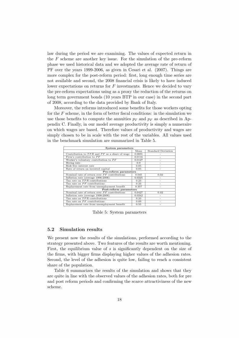
Moreover, the reforms introduced some benefits for those workers optingfor the F scheme, in the form of better fiscal conditions: in the simulation weuse those benefits to compute the annuities pT and pF as described in Ap-pendix C. Finally, in our model average productivity is simply a numeraireon which wages are based. Therefore values of productivity and wages aresimply chosen to be in scale with the rest of the variables. All values usedin the benchmark simulation are summarized in Table 5.

System parametersMean Standard Deviation

Contribution to TFR and PF as a share of wage 0.0691 -Firm’s contribution to PF 0.0116 -Worker’s voluntary contribution to PF 0.0127 -Hiring rate 0.9 -Risk free interest rate 0.05 -Rate of return on invested capital 0.05 -

Pre-reform parametersNominal rate of return over PF contributions 0.045 0.02Inflation rate (average 1996-2006) 0.0225 -Tax rate on TFR contributions 0.23 -Tax rate on PF contributions 0.23 -Replacement rate from unemployment benefit 0.357 -

Post-reform parametersNominal rate of return over PF contributions 0.0427 0.02Inflation rate (average 1998-2008) 0.0242 -Tax rate on TFR contributions 0.23 -Tax rate on PF contributions 0.09 -Replacement rate from unemployment benefit 0.55 -

Table 5: System parameters

5.2 Simulation results

We present now the results of the simulations, performed according to thestrategy presented above. Two features of the results are worth mentioning.First, the equilibrium value of s is significantly dependent on the size ofthe firms, with bigger firms displaying higher values of the adhesion rates.Second, the level of the adhesion is quite low, failing to reach a consistentshare of the population.

Table 6 summarizes the results of the simulation and shows that theyare quite in line with the observed values of the adhesion rates, both for preand post reform periods and confirming the scarce attractiviness of the newscheme.

18

5 10 15 20 25 30 35 40 450

0.02

0.04

0.06

0.08

0.1

0.12

0.14

0.16

0.18

0.2

Dimension

Sh

are

of

Ad

he

sio

ns t

o P

F

Pre−Reform

Post−Reform

Figure 1: Adhesion rates before and after the reform

Adhesion rates for class size (%)Class Real value Simulated value Real value Simulated valuesize 2006 2006 2008 20081-19 2.43 2.19 5.64 5.3520-49 5.90 6.49 11.47 13.521-49 3.32 3.16 7.16 7.16

Table 6: Simulation results: adhesion rates

Next, we present the results of the sensitivity analysis on the main pa-rameters of the model. The reason for such analysis is twofold: on the onehand, we want to check whether the results are robust to changes of theparameters (i.e. small changes of the latter do not produce unrealistic out-comes) and whether the simulated effects of such changes on the equilibriumvalues of s display the expected signs. On the other hand we aim at sheddingsome light on how adhesion rates react to different scenarios concerning theeconomic environment or the incentives to adhere to PF.

To accomplish the first goal we compute the adhesion rates of the post-reform period (years 2007-2008), for different values of the main parametersof the model. The results, presented in Figure 2, show that almost all pa-rameters have the expected effect on the adhesion rates and that the resultsare rather stable. In particular, although with few exceptions, when the pa-rameters are allowed to take the highest values explored in our simulations,the adhesion rates almost double (or are halved in the case of variation of thestandard deviation of the productivity shock), while in the case of changesof the share of firms’ own capital the participation to the PF scheme areeven higher. However, if we focus on the interval ±30% around the bench-mark values of the parameters under investigation, we can see that resultsare particularly sensitive to unemployment benefits, to the returns to PFand to the volatility of the productivity shocks.

On the contrary, neither the hiring probability nor the volatility of the

19

−4 −3.5 −3 −2.5 −2 −1.5 −1 −0.5 0 0.5 110

0.1

0.2

0.3

0.4

0.5

0.6

Risk Propensity (a)

Shareof

Adh

esionto

PF

1−19

20−49

1−49

0 0.02 0.04 0.060

0.1

0.2

0.3

0.4

0.5

0.6

Intertemporal Discount Rate (β)

Shareof

Adh

esionto

PF

0.7 0.8 0.9 1 1.1 1.20

0.1

0.2

0.3

0.4

0.5

0.6

Unemployment Benefits (b) - Ratio to Baseline Values

Shareof

Adh

esionto

PF

1−19

20−49

1−49

1−19

20−49

1−49

0.7 0.8 0.9 1 1.1 1.20

0.1

0.2

0.3

0.4

0.5

0.6

Average PF Returns (ρ) - Ratio to Baseline Values

Shareof

Adh

esionto

PF

1−19

20−49

1−49

0 0.04 0.08 0.12 0.16 0.20

0.1

0.2

0.3

0.4

0.5

0.6

Standard Deviation of PF Returns (σ)

Shareof

Adh

esionto

PF

0.7 0.75 0.8 0.85 0.9 0.950

0.1

0.2

0.3

0.4

0.5

0.6

Hiring Probability (δ)

Shareof

Adh

esionto

PF

1−19

20−49

1−49

1−19

20−49

1−49

0 1 2 3 4 5 6 7 80

0.1

0.2

0.3

0.4

0.5

0.6

0.7

0.8

0.9

1

Average TFR Payments per Worker (k)

Shareof

Adh

esionto

PF

1−19

20−49

1−49

0.2 0.3 0.4 0.50

0.1

0.2

0.3

0.4

0.5

0.6

0.7

0.8

0.9

1

Share of Own Capital of Firms (h)

Shareof

Adh

esionto

PF

0.25 0.3 0.35 0.40

0.1

0.2

0.3

0.4

0.5

0.6

0.7

0.8

0.9

1

Standard Deviation over Mean Value of Productivity

Shareof

Adh

esionto

PF

1−19

20−49

1−49

1−19

20−49

1−49

Figure 2: Sensitivity analysis for some key parameters

20

PF return rates appear to play a significant role. As for the former, thisoutcome may depend on the fact that the increase of the hiring probabilitymakes the individual better off in either states, i.e. T or F , moreover wecan add that according to our model, the gain from the higher reabsorbtionprobability is slightly more likely to occur in the F case, where the chanceof being unemployed is higher.

As for the volatility of PF return rate, the reason for the relatively lowsensitivity of the results stems from the fact that the contribution of the“lottery” (i.e. the F returns) to the overall utility is not particularly large(according to our parameters, the pension payments amount to 5-7% of thegross wage) and is generally outweighed by the loss in case of unemployment.

Finally, the role of k, the average number of yearly contributions tothe TFR scheme set aside by the firms, is worth to be commented. Asshown by the Figure 2, its effect on the adhesion rates is not monotonicand, more precisely, is U shaped. The reason is that, when k increases, twoopposite forces are at work. On the one hand, such an increase enhances therobustness of the firm, given that TFR contributions are an internal cheapsource of cash flow; on the other hand, it amplifies the damage that worker’swithdrawal of the TFR funds generates on the same financial solidity of thefirm. According to our simulations it turns out that the latter effect tendsto dominate the former for low levels of k, while it is offset for higher valuesof k.

We conclude this section by investigating the steady state (or long run)results of the reform; in particular, by exploring different scenarios con-cerning the economic performances of the PF scheme and the speed of theadhesion of workers (for example, due to enhanced information campaigns)we aim at assessing whether the current worrying scarce results of the 2007reform are temporary or permanent. To explore the former, we simulate themodel allowing for different PF nominal returns and we extend the simu-lation periods from 2 to 15 iterations, so that the reform has enough timeto display its full effect; for the latter, we allow for different degrees of in-formation, a more“normal” PF nominal returns (4.5%, in line with the lastdecade value) and extend the periods from 2 to 15 iterations. Figures 3 and4 show the results of such an exercise.

According to our simulations, and in line with what we expected, therate of return of the PF scheme has an important effect on the adhesion ratesbut only when the latter is above 6% (that is only for extremely optimisticrate of return), we observe a relevant value of the adhesion rate: from thispoint of view our results suggest that the current adhesion rates will stayquite stable even after the 2008 financial crisis is fully over. As for the roleof the α parameter, that is the share of those workers that, having a positiveincentive to switch from TFR to PF, effectively decide to do so, we observea weak effect on the final adhesion rate. In particular, in the absence offrictions in the adhesion process (e.g. α equal to 1), the adhesion rates

21

0.03 0.0325 0.035 0.0375 0.04 0.0425 0.045 0.0475 0.05 0.0525 0.055 0.0575 0.06 0.0625 0.065 0.0675 0.07

0

0.1

0.2

0.3

0.4

0.5

0.6

0.7

0.8

0.9

1

Pension Funds Expected Nominal Return

Ad

he

sio

n R

ate

s t

o P

F

1−49

20−49

1−19

Figure 3: Long run outcomes for different expected returns of PF

0.5 0.55 0.6 0.65 0.7 0.75 0.8 0.85 0.9 0.95 10

0.02

0.04

0.06

0.08

0.1

0.12

0.14

0.16

Degree of Information

Adhesio

n R

ate

s t

o P

F

Figure 4: Long run outcomes for different degree of information

22

would be boosted up to 13%, which shows that results are rather insensitiveto such a parameter. This latter result is interesting also because it maybe used to evaluate the effect of policies aimed at a greater diffusion of theknowledge of the reform or of financial literacy.

Finally, in the attempt of showing the potential of our simulation from apolicy point of view, we present the effects of a change in the fiscal treatmentof both returns and accrued value of contributions to the PF scheme (recallthat the current values of the tax rates are 11% and 9% respectively). Ac-cording to our simulations (see Figure 5) it emerges that, in order to boostadhesions to the PF scheme, the most effective measure would be a reduc-tion in the tax rate burdening the returns from PF: in fact, even increasingthe tax on the accrued value (in order to offset at least partly the loss intotal tax revenues), such a measure would deliver significantly higher ratesof adhesion to the pension funds.

00.05

0.10.15

0.2

0.05

0.1

0.15

0.2

0.25

0

0.05

0.1

0.15

0.2

0.25

0.3

Tax Rate on InterestsTax Rate on Contributions

Ad

he

sio

n R

ate

s

Figure 5: Adeshion rates for different levels of taxation

A possible reason for this outcome is that, although particularly favourablerelative to the TFR scheme, the fiscal treatment of the PF accrued capitalwill display its full effects only upon retirement, which can be very far inthe future in workers’ life and thus can be hardly perceived as relevant inthe choice of subscribing a pension plan, especially by young workers; onthe contrary the reduction of the tax rate on the PF returns affects currentflows of individuals’ wealth accruals, thus making more attractive the ad-hesion to a pension fund. However, one has to keep in mind that such apolicy (i.e. reduction of the interest rate tax and increase of the accrued

23

capital tax) can be rather costly for the State, given that the increase of thelatter tax rate would provide new resources only after several years, that iswhen individuals will start to retire or to withdraw from CSS (at least after7 years, according to the reform). Indeed, such a cost could be partly offsetby the increase in the adhesion rates to PF, given that the returns fromPF and thus tax revenues, ceteris paribus, are higher than those from TFR.Anyway, the analysis of the exact cost for the State of such a policy changeis beyond the scope of the present paper and is left for future research.

6 Conclusions

The aim of this work was to explain the results of the Italian 2007 reform interms of adhesion to CSS, providing an explanation of the mechanics behindit and identifying the key determinants of the scarce observed adhesion rates.We adopted a model representing the decisional process of workers whenchoosing between different pension schemes and we used it as the theoreticalbackground on which to build an agent-based simulation able to take intoaccount all the details of the reform and to replicate its outcome. The keyelement of the decisional process rests in the fact that workers have not onlyto consider the direct economic advantages and disadvantages (consisting inhigher but riskier returns) of the different schemes, but also the effects ofthis individual decision on the financial health of the firm in which he/sheis employed. In fact, the more workers switch to the PF scheme, the morethey indirectly induce the risk of default of the firm in which they workin, since they erode a (cheap) source of internal financing in the presenceof imperfect financial markets. However, the higher the number of workersemployed in a firm, the lower will be the effect of the individual decision onthe financial health of the firm.

The simulation of the model allows to examine the aggregate outcomesstemming from individual decisions, taking explicitly into account the het-erogeneity of firms’ and agents’ characteristics. Under some simplifyingassumptions on agents’ expectations formation process, we were able toreplicate quite well all the outcomes and in particular, we obtained the pos-itive significant relation between the rate of subscription to the PF schemeand the size of the firm that we observed from the empirical evidence. Thesensitivity analysis shows that adhesion rates are particularly sensitive tounemployment benefits, to returns from the PF and to the variability ofthe productivity shocks. We also used our simulation can also be used toperform exercises on the effect of policies aimed at boosting the adhesions.Indeed, our simulation suggests that more efficient distribution of the infor-mation about the PF scheme (financial literacy and information campaigns)seems to increase the speed of adoption but its effect on the long run ratesof adhesion is scarce. On the contrary, fiscal policy seems to be, through the

24

fiscal incentives, an important determinant of the final adhesion rates, andin particular reductions of the tax rate on the interests are more effectivethan reductions in the tax rate on the final capital in increasing the longrun adhesion rates.

Finally, we tried to assess whether the observed outcomes should beconsidered transitory and strictly dependant on the 2008 financial crisis: wethen allowed more optimistic scenarios regarding the returns from PF butthe results were not overthrown, so that the expected adhesion rates in theregime phase of the reform seem to still fail in reaching significant values.

25

A Data and Statistics

Tables is this section are taken from Covip (2008) and refers to the end ofthe years 2006 and 2007, unless otherwise specified.

Tab. A.1. Gross Replacement rates between public pension and last wage for private sector

employees and self-employed. Italian defined contribution scheme at the regime phase ( %).

Before reforms

After reforms (regime phase)

35-40 years of

contribution

Case 1: 35-40 years of

contribution

Case 2: 35-40 years of

contribution

Employees

Employees

Self-employed (or parasubordinati)

Employees

Self-employed (or parasubordinati)

60 58.46-66.82 35.43-40.49 54.18-61.47 32.83-37.25 62 70-80 62.23-71.11 37.71-43.09 57.76-65.53 35.00-39.71 65 69.85-79.83 42.33-48.38 64.86-73.59 39.30-44.6

Estimates obtained by using mortality tables of ISTAT 2004. Case 1: GDP rate of growth=1.5%, individual

wages rate of growth=1.5%. Case 2: GDP rate of growth =1.3%, Individual wages rate of growth=1.6%.

Contribution rates: 33% for employees and 20% for self-employed and “parasubordinati”.

Tab. A.2. PF in some OECD countries.(1) (2)

Value of assets as a percentage of GDP.

Paesi 2002 2003 2004 2005 2006 Australia 56.4 54.2 76.4 85.1 94.3 Austria 3.8 4.1 4.4 4.8 4.8 Belgium 4.9 3.9 4.0 4.5 4.3 Canada 48.5 47.3 48.1 50.3 53.4 Czech Republic 2.7 3.1 3.6 4.2 4.6 Denmark 26.0 28.5 30.9 33.6 32.4 Finland 49.2 53.9 61.8 68.7 71.3 France .. 1.3 1.2 1.2 1.1 Germany 3.5 3.6 3.8 4.0 4.2 Hungary 4.5 5.2 6.8 8.4 9.7 Iceland 84.3 98.5 106.9 120.1 132.7 Ireland 34.5 39.9 42.2 48.3 49.9 Italy 2.3 2.4 2.6 2.8 3.0 Japan 17.1 19.7 19.4 23.0 23.4 Korea 1.5 1.6 1.7 1.9 2.9 Mexico 5.2 5.8 6.3 9.9 11.5 Netherlands 85.5 101.2 108.4 122.5 130.0 New Zealand 13.0 11.3 11.3 11.3 12.4 Norway 5.5 6.5 6.6 6.7 6.8 Poland 3.8 5.3 6.8 8.7 11.1 Portugal 11.5 11.8 10.5 12.7 13.6 Slovak Republic 0.0 0.0 .. 0.6 2.8 Spain 5.7 6.2 6.6 7.2 7.6 Sweden 7.6 7.7 7.6 9.3 9.5 Switzerland 96.7 103.6 108.2 119.1 122.1 Turkey .. .. 0.5 0.9 1.0 United Kingdom 59.2 64.8 68.1 79.1 77.1 United States 63.3 72.6 73.8 72.4 73.7

Source: OCSE. Pension Markets in Focus. several years. (1) Data refers to autonomous PF whose gathered resources will generate only pension payments. Cfr. OECD, Private

Pensions: OECD Classification and Glossary, 2005. (2) With respect to previous data from OECD there are some revision to the time series of a few countries, due to the change in the classification criteria of PF.

B Determination of the pension annuities

We determine here the pension annuities py, with y = T, F , that a workeris entitled to depending on the pension scheme he chose.

In the case of TFR, we define the accrued value of contributions AVT :

26

AVT = wγT

S−1∑

t=0

(1 + r)S−1−t (B1)

where S is the number of years of contributions (35 years in the benchmarksimulation), γT = 6.91% and r is the real rate of return of the T scheme.

For the PF case, the rate of return is stochastic variable with distributionN(ρ, σ) and for a possible history of the returns rate ρ = {ρ0, ..., ρS} theaccrued value of contributions is

AVF (ρ) = wγF

S−1∑

t=0

(1− cF ) (1 + ρt)S−1−t (B1a)

where γF = 6.91% + γw + γe, that is the sum of the mandatory rate(6.91%) and the voluntary share by the worker –γw- and by the employer– γe; such values were set equal to the Italian average levels provided byCOVIP (2008): 1.16% and 1.22% respectively; cF is the administrative costof F , set equal to 0.44% per year, according to the estimates provided byCOVIP (2008). By sampling a huge number of such histories (1000000 inour case) we numerically determine the distribution of AVF , functional onthe distribution N(ρ, σ) of returns, call it (AVF p N(ρ, σ)).

Second, we compute the accrued value of the (gross of tax) annuity (py)the individual obtains by selling on the market, in each period, the accruedvalue of his/her contributions AV Py:

AV Py = py

S−1∑

t=0

(1 + ι)S−1−t (B2)

where ι is the real interest rate in the financial market.By imposing the equality AVy = AV Py and solving for py we get the

expression for the annuity. Finally, we compute the net of tax annuity:

py = pyqy(

1− τ cy)

+ py (1− qy)(

1− τ i)

(B3)

where qy and 1 − qy are the shares of contributions and of interests theaccrued capital and τ cy and τ i are the tax rates on these components, re-spectively. The τ cy is set to 23% for T both in the pre and post reform periodand, for F , at 23% in the pre-reform and at 9% in the post-reform; the τ i isfixed to 11% in all cases. Clearly, since AVF is a random variable with thenumerical distribution (AVF p N(ρ, σ)) we consequently the distributionfunction for pF and pF , with the latter being the distribution of the randomannuities that a worker gets when adhering at the F .

27

References

[1] Banca d’Italia (2004), “Indagine sui bilanci delle famiglie italianenell’anno 2002”, Supplemento al bollettino statistico, n. 12, marzo;

[2] Bardazzi, R. e Pazienza, M.G. (2005): “Il Tfr e il costo per le imp-rese minori: un contributo al dibattito in corso”, Cerp Argomenti di

discussione, n. 7;

[3] Barr, N. (2006), ”Pensions: Overview of the Issues”, Oxford Review ofEconomic Policy.

[4] Barr, N. and Diamond, P. (2006), ”The Economics of Pensions”, OxfordReview of Economic Policy.

[5] Blake (2006), Pension Economics, Chichester, England: John Wiley &Sons;

[6] Blake (2006a), Pension Finance, Chichester, England: John Wiley &Sons;

[7] Butler, M., Teppa, F. (2007), “The choice between an annuity anda lump sum: Results from Swiss pension funds”, Journal of Public

Economics, 91, 1944-1966.

[8] Cahuc, Pierre and Andre Zylberg (2004), Labor Economics, Cambridge,MA: MIT Press;

[9] Calcagno, R, Kraeussl R. and Monticone, C. 2007. ”An Analysis of theEffects of the Severance Pay Reform on Credit to Italian SMEs”, CeRPWorking Papers 59, Turin (Italy);

[10] Capitalia (2005), ”Indagine sulle imprese italiane”, Ottobre;

[11] Cesari R, Grande G. and Panetta F., (2007): “La Previdenza Comple-mentare in Italia: Caratteristiche, Sviluppo e Opportunita per i lavo-ratori”, CeRP Working Papers 60, Turin (Italy);

[12] Corsini, L., Pacini, P. M. and Spataro, L., (2010): “Workers Choice onPension Schemes: an Assesment of the Italian TFR reform throughTheory and Simulationsi”, Discussion Papers del Dipartimento di

Scienze Economiche 96, Pisa (Italy).

[13] COVIP (various years): “Relazione per l’anno. . . ”, Covip, Rome(Italy);

[14] Cozzolino, M., Di Nicola, F. (2006),”Il futuro dei fondi pensione: op-portunita e scelte sulla destinazione del TFR”, ISAE Working Papers

64, ISAE - Rome.

28

[15] Cozzolino, M., Di Nicola, F. and Raitano, M. (2006): “Il trasferimentodel Tfr ai Fondi Pensione: le preferenze dei lavoratori tra incentivi eincertezze”, Mefop Working Paper, n. 12;

[16] Garibaldi, P. and Pacelli, L., (2008). ”Do larger severance paymentsincrease individual job duration?”, Labour Economics, 15(2), 215-45;

[17] Guiso, L. (2003): “Small business finance in Italy”, EIB Papers Vo. 7,n. 2;

[18] ISAE (2005), Rapporto Trimestrale. Finanza pubblica e redistribuzione.Ottobre 2005;

[19] Mesa-Lago, C. 2006, Reassessing Pension Reform in Chile and OtherCountries in Latin America, Oxford Review of Economic Policy.

[20] Ministry of Labour and Social Policies (2002), Report on NationalStrategies for Future, Rome;

[21] Palermo G. and Valentini, M. (2000), Il fondo di Trattamento FineRapporto e la struttura finanziaria delle imprese, Economia Italiana,2/3, 513-40;

[22] Pammolli, F and Salerno, N.C. (2006): “Le imprese e il finanziamentodel pilastro previdenziale privato”, Quaderno CERM, n.2.

[23] Rauh, J. D. (2006), Investment and Financing Constraints: Evidencefrom the Funding of Corporate Pension Plans, The Journal of Finance,Vol. 61, No. 1, 33-71.

[24] Rauh, J. D. (2006), Risk Shifting versus Risk Management: InvestmentPolicy in Corporate Pension Plans, The Review of Financial Studies,Vol. 22, No. 7, 2687-2733

[25] Schlechter, L. (2007): ”Risk aversion and expected utility theory: Acalibration exercise”, Journal of Risk and Uncertainty 35, 67-76.

[26] Spataro, L. (2009): Leconomia dei Fondi Pensione: teorie ed appli-cazioni al caso italiano, in Ciocca G. (ed), Il trattamento di fine rapporto

e i fondi pensione, EUM, Macerata, 41-100;.

[27] Whiteford, P. and Whitehouse, E. (2006), ”Pension Challenges andPension Reforms in OECD Countries”, Oxford Review of EconomicPolicy.

29