AN APPROACH TO THE MULTIVECTORIAL APPARENT POWER IN TERMS OF A GENERALIZED POYNTING MULTIVECTOR

Progress In Electromagnetics Research B, Vol. 15, 401–422, 2009

AN APPROACH TO THE MULTIVECTORIAL APPAR-ENT POWER IN TERMS OF A GENERALIZED POYNT-ING MULTIVECTOR

M. Castilla and J. C. Bravo

Electrical Engineering DepartmentUniversity of SevillaEscuela Universitaria Politecnica, Virgen de Africa 7Sevilla 41011, Spain

M. Ordonez

Applied Mathematics DepartmentUniversity of SevillaEscuela Universitaria Politecnica, Virgen de Africa 7Sevilla 41011, Spain

J. C. Montano

Spanish Research Council (CSIC)Reina Mercedes 10, Sevilla 41012, Spain

Abstract—The purpose of this paper is to explain an exactderivation of apparent power in n-sinusoidal operation founded onelectromagnetic theory, until now unexplained by simple mathematicalmodels. The aim is to explore a new tool for a rigorous mathematicaland physical analysis of the power equation from the Poynting Vector(PV) concept. A powerful mathematical structure is necessary andGeometric Algebra offers such a characteristic. In this sense, PV hasbeen reformulated from a new Multivectorial Euclidean Vector Spacestructure (CGn-R3) to obtain a Generalized Poynting Multivector (S).Consequently, from S, a suitable multivectorial form (P and D) of thePoynting Vector corresponds to each component of apparent power.In particular, this framework is essential for the clarification of theconnection between a Complementary Poynting Multivector (D) andthe power contribution due to cross-frequency products. A simpleapplication example is presented as an illustration of the proposedpower multivector analysis.

Corresponding author: M. Castilla ([email protected]).

402 Castilla et al.

1. LIST OF SYMBOLS (NOMENCLATURE)

n-sinusoidal = non-sinusoidal or multi-sinusoidal.R = real numbersE3 = Euclidean vector spaceC = complex vector spaceVn = linear space over real numbersGn = Clifford algebra in n-dimensional real spaceCGn = complex Clifford AlgebraΦ = operatorΓ = time-domain frequency-domain transformCGt

n-R3 = time generalized Euclidean spaceCGn-R3 = frequency generalized Euclidean space~1X, ~1Y, ~1Z = Euclidean canonical basis~1X,Y,Z = generic unitary vector of E3

σ1,...,k = Clifford algebra canonical basisIdC = identity operationz(t) = instantaneous geometric vector (z ∈ CGt

n-R3)e(t) = instantaneous electric field geometric vectorh(t) = instantaneous magnetic field geometric vectord(t) = instantaneous displacement field geometric vectorb(t) = instantaneous magnetic induction field geometric vectorzX,Y,Z = components of z(t)zp = p-th harmonic component of z(t)ZX,Y,Z = spatial components of ZZ = spatial geometric phasor (Z ∈ CGn-R3)Zp = spatial p-th harmonic component of ZZ = geometric phasor (Z ∈ CGn)Zp = p-th harmonic component of Z

Zpq = bivector component of Z

E = electric field geometric phasorH = magnetic field geometric phasorD = displacement field geometric phasorB = magnetic induction field geometric phasorS = generalized Poynting multivector (GPM)P = Poynting multivector (PM)D = complementary Poynting multivector (CPM)Up = p-th harmonic voltage rms valueIp = p-th harmonic current rms value⊗ = classic geometric product¯ = generalized geometric product in CGn

Progress In Electromagnetics Research B, Vol. 15, 2009 403

= generalized geometric product in CGtn-R3

· = inner product∧ = outer product⊕ = direct sum+ = classic sum for scalars and also direct sum for multivectorsj = imaginary unit∗ = conjugated operation† = reverse operation〈〉0 = scalar part〈〉2 = bivector partS = apparent power multivector‖S‖ = norm, value or magnitude of multivector S

Ω· = complex scalarΩ∧ = complex bivectorωp, ωq = harmonic frequenciesαp = phase angle of p-th voltage geometric phasorαq = phase angle of q-th current geometric phasorϕq = phase angle between q-th voltage and q-th current geometricphasorsδ = relative quality index multivector (RQI )PF = power factor

2. INTRODUCTION

2.1. Motivation

One of the fundamental issues in power system analysis is related withthe electromagnetic theory in order to explain the energy transfer inan electric circuit. Hence, this paper establishes an electromagneticfoundation to the power equation representation. For this goal, a newGeneralized Poynting Multivector is proposed.

2.2. Literature Review

The electrical circuits in n-sinusoidal operation can be analyzed bymeans of mathematical tools that are much simpler to handle thanelectromagnetic theory based on Maxwell equations [1]. However, itis also true that these equations fully explain interactions betweenelectric and magnetic fields and therefore explain every electromagneticphenomenon, including the energy transfer in an electric system. Inn-sinusoidal operation, the distorted electromagnetic fields can berepresented as sums or series of harmonics. Each harmonic component

404 Castilla et al.

of the field is governed by Maxwell equations and satisfies the PoyntingTheorem.

It is relevant to classify the contribution of these equations to theelectric power theory into following lines of thought:

a) Circuit theory analysis: First, is the most commonly usedapproach. It analyzes currents, voltages and circuit element properties.In this sense, circuit theory, ruled by simple equations based on Ohm’slaw, can be regarded as a very particular case of electromagnetictheory, and power theory was developed mainly from circuit analysis.Electrical components of power systems are considered as elements ofcircuits and their electromagnetic behaviour is described by meansof voltages and currents of element terminals. Circuit theory canexplain only the power flows between components, and it is unableto reveal their spatial distribution. Nevertheless, no phenomena suchas hysteresis losses or skin effects can be explained by circuit theory.These are phenomena of the electromagnetic field characteristics.

For this first approach, Complex Algebra [2] provides an initialprocedure to solve the problem, despite its limitation to the purelysinusoidal case. The n-sinusoidal operation imposes the substitutionof the Complex Algebra approach with a new representation modeland the reformulation of the energy balance. Considerable researchefforts have been directed towards the representation of apparentpower in various ways [3–9]. Specifically, in [9], the authors useGeometric Algebra to define a multivector power based on thedecomposition of the instantaneous current into the active and reactivecomponents. It should be noted that their approach does notdistinguish between reactive and distortion power from a mathematicalviewpoint. Furthermore, none of the aforementioned papers leads to arepresentation that could be considered universally satisfactory.

b) Electromagnetic theory analysis: This second valid methodanalyzes the energy flow using the Poynting Theorem (PT), andtherefore the Poynting Vector (PV) should be considered, since itrepresents the bridge between electromagnetic theory and circuittheory [10]. These tools are fundamental concepts of electromagnetictheory with respect to energy flow. The goal is to investigate the natureof the non-active power and some progress has undeniably been made.Numerous valuable contributions have appeared in the literature [11–17], each shedding more light on some aspects of the problem. Fromamong them, [12, 13] masterfully explain the physical mechanism ofenergy propagation in electric power systems, [15] reconsiders thebases of electromagnetism in order to find a physical interpretationfor the power equation, and [16] uses the PV to illustrate the nature ofpower flow in electric circuits using electromagnetic fields. However,


critics of PV calculations [17] argue that electromagnetic theory isuseless for practical applications of electric power theory. Against thisreference, it is our view that the power equation can be based andinterpreted through a new formulation of the Poynting Vector andthat other aspects concerning the electromagnetic field in n-sinusoidaloperation and their direct relation with power theory have yet to bethoroughly investigated. Thus, the purpose of this paper is to advanceenergy flow analysis by using a new mathematical structure for therepresentation of the power equation in single-phase circuits under n-sinusoidal operation. In this way, a complete solution to the powerequation analysis problem for linear/non-linear circuits based on aGeneralized Poynting Multivector (S), is presented.

To this end, primarily our work introduces a CGtn-R3 mathematical

structure based on Clifford Algebra for the definition of the distortedelectric and magnetic field intensities (e, h), which are time geometricfields associated to an Euclidean direction. From these definitions itis possible to obtain the quantities called spatial geometric phasors(E, H) in the CGn-R3 structure in frequency domain. Consequently,our work is aimed at showing how an electric and magnetic field canbe associated with the elements of Clifford Algebras [21, 22] for a newformulation and interpretation of power theory in this framework.

This second approach is more general and fundamental that thefirst approach based on circuit theory, and it has the additionaladvantage of providing a physical insight into the spatial distributionof the power flow.

Finally, this paper addresses the need to understand themultidimensional character of electric power theory and its relationto the electromagnetic theory.

2.3. Contributions

The paper is concerned with a representation of the power equationunder non-sinusoidal conditions from electromagnetic theory. Theapparent power concept is better understood if a Clifford vector spaceis used for the representation of the distorted electric and magneticfield intensities. This generates a larger linear space called GeneralizedEuclidean Space CGt

n-R3, which will be utilized in this paper for a newrepresentation of the power equation. This objective cannot be reachedon the Complex Algebra framework.

406 Castilla et al.

3. MATHEMATICAL FOUNDATIONS: GEOMETRICEUCLIDEAN SPACES

3.1. Time Domain: Generalized Euclidean Space CGtn-R3

In order to introduce the instantaneous quantities of electric andmagnetic fields, in this section we define a new structure for thetime domain that we have named Generalized Euclidean Space, CGt

n-R3, whose coefficients belong to the Complex Geometric Algebra CGn

constructed in [18]. Let~1X , ~1Y , ~1Z

be the “canonic” basis of the

Euclidean space E3. A generic element of CGtn-R3 is given by

z(t) = zX~1X + zY

~1Y + zZ~1Z (1)

where each component in (1) is in the form z(t) = kej[α(t)+θ]σa ∈ CGtn,

k ≥ 0 and σa is a basis element of CGn structure [18].Thus, the CGt

n-R3 structure is a CGtn vector space whose inner

product is defined byz(t) · w(t) = 〈zX , w∗X〉0 + 〈zY , w∗Y 〉0 + 〈zZ , w∗Z〉0 (2)

where, z(t) = zX~1X + zY

~1Y + zZ~1Z , w(t) = wX

~1X + wY~1Y + wZ

~1Z .Moreover, from (D1) the norm of z(t) is given by

‖z(t)‖ =∑

i=X,Y,Z

〈zi, z∗i 〉0 (3)

Now we define the outer product in this structure as

z(t) ∧ (−w(t)) =

~1X~1Y

~1Z

zX zY zZ

−wX −wY −wZ

= (〈−zY , wZ〉2 + 〈zZ , wY 〉2)~1X

+ (〈zX , wZ〉2 + 〈−zZ , wX〉2)~1Y

+ (〈−zX , wY 〉2 + 〈zY , wX〉2)~1Z (4)Based on (3) and (4), the Geometric Algebra CGt

n-R3 is defined by thefollowing geometric product

z(t) w(t) = z(t) · w(t) + z(t) ∧ w(t) (5)

3.2. Frequency Domain: Generalized Euclidean SpaceCGn-R3

Let Φ : CGtn → CGn, Φ

(k ej[α(t)+θ]σa

)= k ejθσa, be the operator

that enables the transformation between time-domain and frequency-domain. We define CGn-R3 as

Φ(CGtn)~1X + Φ(CGt

n)~1Y + Φ(CGtn)~1Z (6)


where a generic element of this space is Φ(za) = Za. Note that CGn-R3 can also be seen as

CGn-R3 =

ZX~1X+ ZY

~1Y + ZZ~1Z : Z ∈ CGn

whereZ =

∑p

Zpσp, Zp ∈ C and σp ∈ Gn

Obviously, CGn-R3 is a CGn (complex-geometric) vector space and themultiplication rule for two vectors Z, W ∈ CGn-R3 is given by

Z W = Z · W + Z ∧(−W

)(7)

where (7) is the restriction from CGtn-R3 → CGn-R3.

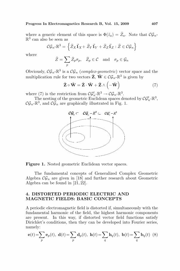
The nesting of the geometric Euclidean spaces denoted by CGtn-R3,

CGn-R3, and CGn are graphically illustrated in Fig. 1.

Figure 1. Nested geometric Euclidean vector spaces.

The fundamental concepts of Generalized Complex GeometricAlgebra CGn are given in [18] and further research about GeometricAlgebra can be found in [21, 22].

4. DISTORTED PERIODIC ELECTRIC ANDMAGNETIC FIELDS: BASIC CONCEPTS

A periodic electromagnetic field is distorted if, simultaneously with thefundamental harmonic of the field, the highest harmonic componentsare present. In this way, if distorted vector field functions satisfyDirichlet’s conditions, then they can be developed into Fourier series,namely:

e(t)=∑

p

ep(t), d(t)=∑

p

dp(t), h(t)=∑

q

hq(t), b(t)=∑

q

bq(t) (8)

408 Castilla et al.

where ep,dp,hq,bq, are harmonics of the field vectors. Each harmoniccomponent in the frequency domain of a periodic electromagnetic fieldsatisfies Maxwell’s equations

∇×Hp = Jp + jωpDp

∇×Ep = −jωpBp

∇ ·Dp = ρp

∇ ·Bp = 0

(9)

where Ep,Hp,Dp,Bp are complex phasors of the p-th harmonic of thefields.

One of the most important consequences of the first twoMaxwell equations is Poynting’s theorem, which describes the flowof electromagnetic energy in space and for a volume v enclosed bya surface s. This can be stated as∫∫

−(e× h)n ds =∫∫∫

e · jdv +∫∫∫ (

h · ∂b∂t

+ e · ∂d∂t

)dv (10)

where n is the unit vector orthogonal to the infinitesimal surface ds, eand h are the instantaneous intensity of the electric and magneticfields, d and b are the instantaneous flux densities of these fieldsrespectively, and j is the instantaneous current density. The theoremsimply means that the increase in stored energy in the fields plus theohmic losses within a volume, equal the inflow of a vector e×h acrossthe surface bounding that volume. The vector e × h is known as thePoynting Vector (PV), and gives the power density at a point on thesurface in terms of the electric and magnetic fields at that point. Itsphysical meaning is also known [23].

The equivalent complex Poynting theorem for a system in linearmedia is given by

−∫∫

(Ep×Hp)n ds =∫∫∫

EpJ∗pdv+jωp

∫∫∫[BpH∗

p−EpD∗p]dv (11)

The energetic interpretation of (11) is as follows

Sp = Pp + jQp (12)

where

• Sp is a complex apparent power of the p-th harmonic received bythe system enclosed in the surface “s”.

• Pp is the active power of the p-th harmonic received by the system.• Qp is the reactive power of the p-th harmonic received by the

system.


One can readily observe that

Pp =∫∫∫

EpJ∗pdv (13)

Qp = 2ωp

∫∫∫ [BpH∗

p

2− EpD∗

p

2

]dv (14)

where Pp represents harmonic losses in Joules and Qp is associated tothe average values of the p-th harmonic magnetic and electric energiesaccumulated in the volume v [15]. Another representation of (13)and (14) is given

Pp = Re[−

∮(Ep ×H∗

p)]n ds (15)

Qp = Im[−

∮(Ep ×H∗

p)]n ds (16)

5. POWER FLOWS IN DISTORTEDELECTROMAGNETIC FIELDS: GENERALIZEDPOYNTING MULTIVECTOR (S)

The following notation is adopted to define the electric and magneticfields in the CGt

n-R3 framework:

ep = |ep|ej(ωpt+θp)σp~1X,Y,Z , hq = |hq|ej(ωqt+γq)σq~1X,Y,Z (17)

where ep(t) and hq(t) are called instantaneous electric and magneticcomplex-geometric fields respectively.

Observe that the classic instantaneous fields can be derived fromthe real (or imaginary) part of the projections given by the scalarproduct (2) as follows:

ep(t) = Im(ep · σp) = Im|ep|ej(ωpt+θp)~1X,Y,Z (18)

hq(t) = Im(hq · σq) = Im|hq|ej(ωqt+γq)~1X,Y,Z (19)

In order to obtain the geometric phasors, it is necessary to apply theΦ operator on these quantities (see Section 3.2).

Φ(ep) = |ep|ejθpσp~1X,Y,Z = Ep (20)

Φ(hq) = |hq|ejγqσq~1X,Y,Z = Hq (21)

where Ep and Hq are called harmonic “spatial geometric phasors”of the electric and magnetic harmonic fields respectively and verify

410 Castilla et al.

Maxwell’s equations [20]. In this framework, a Generalized PoyntingMultivector (S) is defined as

S =∑p,q

(Ep ¯ H∗

q

)(22)

where H∗q is the conjugate of the q-th harmonic spatial geometric phasor

Hq and the symbol “¯” is the generalized complex geometric product(B7). Consequently, the Generalized Poynting Multivector (S) for avolume v enclosed by a surface s is given by∫∫

s

n · S ds =∫∫

s

∑p

n · P ds+∫∫

s

∑

p6=q

n · D ds

=∫∫

s

∑p

n·(Ep¯H∗p) ds+

∫∫

s

∑

p 6=q

n·(Ep¯H∗q+Eq¯H∗

p) ds (23)

where the unitary vector n is the unitary vector orthogonal to theinfinitesimal surface ds, P is the Poynting Multivector and D is theComplementary Poynting Multivector. Equation (23) expands the fluxof the S into two terms

• The first term∫∫s

∑p

n · P ds =∫∫s

∑p

n · (Ep ¯ H∗p) ds represents the power con-

tribution due to like-frequency products.• The second term∫∫

s

∑p6=q

n · D ds =∫∫s

∑p6=q

n · (Ep¯ H∗q + Eq¯ H∗

p) ds represents the

power contribution due to cross-frequency products.

6. POWER MULTIVECTOR APPROACH

6.1. Multivector Representation of Power in Terms ofGeneralized Poynting Multivector

The considerations stated in the above section have been derivedfrom an electric field e(t) and a magnetic field h(t). To understandenergy balance, one must touch base with electromagnetic fieldtheory and reformulate the classic Poynting Vector concept. In thisway, we consider an elementary single-phase transmission line (twoconductors), where an n-sinusoidal voltage source

u(t) =√

2 Im∑

p

Upej(ωpt+αp) (24)


is connected at the sending end in order to supply either a linear ornon-linear load. The same conductors carry a current responsible forthe generation of the magnetic field, given by

i(t) =√

2 Im∑

q

Iqej(ωqt+βq) (25)

where βq = αq−ϕq for linear operation, ϕq is the harmonic impedancephase angle and Up, Iq represent rms values of up(t) and iq(t)respectively.

The energy balance can thus be expressed as a multivector Sin CGn, generated by “¯” of the voltage and conjugate currentgeometric phasors (B2) given by the following set

S = U ¯ I∗ =

U · I∗︸︷︷︸

Ω·

⊕ U ∧ I∗︸︷︷︸Ω∧

(26)

This quantity consists of complex scalar (Ω·) and complex bivector(Ω∧) parts. Note from (26) that Ω· =

∑p∈N

UpIpejαpσ0. Clearly,

‖P‖ = ‖ReΩ·‖ = ‖ ∑p∈N

UpIp cosϕpσ0‖ is the active power or

average value of the instantaneous power in the time domain. ‖Q‖ =‖ImΩ·‖ = ‖ ∑

p∈N

UpIp sinϕpσ0‖ is called reactive power and is merely

the geometric complement of the active component. The complexbivector, deduced from (B7), is given by

Ω∧=∑

p6=qLinear

(UpIqe

jϕq − UqIpejϕp)ej(αp−αq)

σpq+∑

p 6=qNon Linear

UpIqej(αp−βq)σpq (27)

and it is associated to distortion power.The components ImΩ· and Ω∧ have a non-independent physical

nature: they constitute non-active power. Note that, consistentwith (D1), the squared value ‖S‖2 in (26), may be represented as‖S‖2 = ‖U ¯ I∗‖2 = |U |2|I|2 and ‖S‖2 = ‖Ω·‖2 + ‖Ω∧‖2. Thisexpression is identical to any classic squared value of the apparentpower.

From electromagnetic theory, (26) can be verified to have notonly a formal meaning, but also a physical meaning. For clarity ofpresentation and without loss of generality, it is possible to considerthat the electric field ep(t) vector is parallel with the X axis andassociate it with up(t). Similarly, the magnetic field hq(t) vector isparallel with the Y axis and associated to the harmonic current iq(t).

412 Castilla et al.

Since the harmonic electric and magnetic fields are supposed to varyin time and space, these quantities (18), (19) are given by

ep(t) = Im(ep · σp) = Im|ep|ej(ωpt+αp)~1X

= |ep| sin(ωpt + αp)~1X ⇒ e(t) =

[∑p

ep(t)

]~1X (28)

hq(t) = Im(hq · σq) = Im|hq|ej(ωqt+βq)~1Y

= |hq| sin(ωqt + βq)~1Y ⇒ h(t) =

[∑p

hp(t)

]~1Y (29)

By considering the conservation law of the electrical charge andmagnetic flux, iq(t) = −dqq

dt = hq(t) · lH and up(t) = −dφp

dt = ep(t) · lE ,then the harmonic vector phasors ep(t) and h∗q(t) of (28) and (29) canbe expressed as

ep(t) =√

2lE

[Upe

j(ωpt+αp)σp

]~1X (30)

h∗q(t) =√

2lH

[Iqe

−j(ωqt+βq)σq

]~1Y (31)

The corresponding harmonic spatial geometric phasors are thereforegiven by

Ep =(

l

lEUpe

jαpσp

)~1X (32)

H∗q =

(l

lHIqe

−jβqσq

)~1Y (33)

where lE and lH are average lengths of flux lines of the vector fields.Thus, returning to the Generalized Poynting Multivector (S)

concept (23), when n = ~1Z , this equation becomes∫∫

s

~1Z · S ds =∫∫

s

∑p

~1Z · P ds +∫∫

s

∑

p6=q

~1Z · D ds

=∫∫

s

∑p

~1Z ·(Ep¯H∗p) ds +

∫∫

s

∑

p6=q

~1Z ·(Ep¯H∗q+Eq¯H∗

p) ds (34)

and by combining (32), (33), and (34), two cases can be identified:


• First case: If p = q, then (34) can be written as∫∫

s

∑p

~1Z ·(Ep ¯ H∗p) ds =

∫∫

S

~1Z ·(

1lElH

∑p

UpIpejφpσ0

)ds

=∑

P

UpIpejφpσ0 = Ω· (35)

Hence, by virtue of (35), one obtains∫∫

s

∑p

~1Z · P ds =

∫∫

s

∑p

~1Z · (Ep ¯ H∗p) ds =

∑P

UpIpejφpσ0 (36)

The multivector P =∑p

Ep ¯ H∗p, (Poynting Multivector), is

associated to the power density at a point on the surface, interms of the harmonic spatial geometric phasor of electric andmagnetic fields at that point. The real part of (36) permits adirect interpretation in terms of average power flow, (i.e., activepower), P. Consequently, a net energy flow occurs in any linearor non-linear system when voltage and current components of thesame frequency exist.• Second case: If p 6= q then (34) yields∫∫

S

∑

p6=q

~1Z ·D ds =∫∫

S

∑

p6=q

~1Z ·(Ep¯H∗q +Eq¯H∗

p) ds = Ω∧ (37)

where D =∑p

(Ep¯H∗q +Eq¯H∗

p) is the Complementary Poynting

Multivector. Combining (32), (33) with (37) yields

Ω∧ =∑

p6=q

Linear

(UpIqe

jϕq − UqIpejϕp

)ej(αp−αq)

σpq

+∑

p6=q

UpIqej(αp−βq)σpq (38)

Equation (38) represents the power contribution due to the cross-frequency products. In this way, the power multivector thatoriginates from the surface of the source equals the power thatenters in the load surface. Finally, through (36) and (37), it canbe observed that∫∫

S

∑p

~1Z · (Ep ¯ H∗p)ds +

∫∫

S

∑

p6=q

~1Z · (Ep ¯ H∗q + Eq ¯ H∗

p)ds

= Ω· ⊕ Ω∧ (39)

414 Castilla et al.

Equation (39) coincides with (26) and represents to apparent powermultivector given by

S = Ω· ⊕ Ω∧ (40)

It is important to notice that in our framework, the ReΩ· andImΩ· components are associated to a scalar plane perpendicular tothe Z axis and each Ω∧pq is associated to a pq complex bivector planepertaining to the set of planes that contains the Z axis. Under theseconditions, is obvious that the average value of the second integral onthe right-hand side of (39) is zero. However, this component mustbe considered in order to understand the complete physical meaningof the power equation. Consequently, this new analysis demonstratesthat (39) not only justifies the net flow of energy, but also providespowerful information for the analysis of power theory. In short, thecomplex scalar in (35) and (36), is similar to the complex powerequation in sinusoidal operation. However, a new quantity, givenby (38), is identified with the Complementary Poynting Multivector(D).

6.2. Relative Quality Index and Power Factor

Regarding the power factor improvement, the suggested representationin (34) can be particularly useful. Thus, the multivectorial relativequality index (RQI) [18] expressed in terms of S, P and D is reducedto

δ =

∫∫s

~1Z · S ds

Re

∫∫s

∑p

~1Z · P ds

= 1 + j

Im

∫∫s

∑p

~1Z · P ds

Re

∫∫s

∑p

~1Z · P ds

+

∫∫s

∑p6=q

~1Z · D ds

Re

∫∫s

∑p

~1Z · P ds

(41)

and the power factor (PF) can be written as

PF =1‖δ‖ =

∥∥∥∥∥Re∫∫s

∑p

~1Z · P ds∥∥∥∥∥

∥∥∥∥∫∫s

~1Z · S ds

∥∥∥∥(42)


Equation (41) shows that on this index all its electromagneticquantities, with their direction and sense, are accessible for possiblecontrol of the power factor improvement.

7. NUMERICAL EXAMPLE

In this section, a numerical example is developed. Units of physicalquantities are the standard units of the MKSA system and thus areomitted.

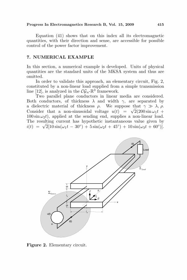
In order to validate this approach, an elementary circuit, Fig. 2,constituted by a non-linear load supplied from a simple transmissionline [12], is analyzed in the CGn-R3 framework.

Two parallel plane conductors in linear media are considered.Both conductors, of thickness λ and width γ, are separated bya dielectric material of thickness ρ. We suppose that γ À λ, ρ.Consider that a non-sinusoidal voltage u(t) =

√2(200 sinω1t +

100 sinω2t), applied at the sending end, supplies a non-linear load.The resulting current has hypothetic instantaneous value given byi(t) =

√2[10 sin(ω1t − 30) + 5 sin(ω2t + 45) + 10 sin(ω3t + 60)].

m

m

y

z

x

i ( t ) +

u ( t )

Load

i ( t )

H l

E l

Load Σ

Source Σ E

H S

~

~~

Figure 2. Elementary circuit.

416 Castilla et al.

By ignoring eddy currents, line impedance, fringing effects, then (32)and (33) can be expressed as

E =1lE

(200ej0σ1 + 100ej0σ2)~1X (43)

H∗ =1lH

(10ej30σ1 + 5e−j45σ2 + 10e−j60σ3)~1Y (44)

However, from (35) and (36), it follows that∫∫

s

∑p

~1Z · P ds = [(1732 + 353.5) + j(1000− 353.5)]σ0~1Z

= (2085.5 + j646.5)σ0~1Z (45)

Therefore, from (38),∫∫

S

∑

p6=q

1Z ·D ds=(−158.9−j1207.1)σ12+(1000−j1732)σ13+(500−j866)σ23 (46)

This example states that ReΩ·1 = 1732σ0, ReΩ·2 = 353.5σ0,ImΩ·1 = j1000σ0, ImΩ·2 = −j353.5σ0 and that the linear complexbivector component becomes Ω∧12 = (−158.9 − j1207.1)σ12, as well asthe nonlinear complex bivector components Ω∧13 = (1000− j1732)σ13,Ω∧23 = (500− j866)σ23 with their corresponding directions and senses.On the other hand, the rms values of voltage and current are givenby ‖U‖2 = 2002 + 1002 = 5 · 104 and ‖I‖2 = 102 + 52 + 102 = 225respectively. The values of P = ‖ReΩ·‖2, ‖ImΩ·‖2, ‖Ω∧‖2 arefound to add up to

‖S‖2 = P 2 + ‖ImΩ·‖2 + ‖Ω∧‖2 = 11.25 · 106 (47)

Therefore, apparent volt-amperes ‖S‖ at the terminals are found fromthe relation ‖S‖2 = ‖U‖2‖I‖2 = 11.25·106. Finally, from (41) and (42)we obtain the relative quality index and power factor respectively

δ = 1 +j646.5σ0

2085.5σ0

+(−158.9−j1207.1)σ12+(1000−j1732)σ13+(500−j866)σ23

2085.5σ0∥∥∥δ∥∥∥ = 1.608

PF =1∥∥∥δ∥∥∥

= 0.62 (48)


The methodology in the above example differs greatly to that of circuittheory. Furthermore, unlike the circuit theory approach, it can beapplied to solve and understand the operation of electric systemsdesigned to work in the frequency domain.

8. CONCLUSION

The suggestion that the power equation should be founded onelectromagnetic theory is analyzed in this paper. This goal remainsunexplained by simple mathematical models used in classical theory.To this end, we propose a Generalized Poynting Multivector (S)based on Clifford Algebras, which is decomposed into a PoyntingMultivector (P) and a Complementary Poynting Multivector (D).From Equations (34)–(40), both quantities are considered as thekeystone of the bridge between electromagnetic theory and circuittheory. Thus, the real part of the flow of Poynting Multivector (P)coincide with active power, and imaginary part of the complex scalarcoincides with the power contribution due to like-frequency products.The Complementary Poynting Multivector (D) is associated to thecomplex bivector or to the power contribution due to cross-frequencyproducts. This analysis demonstrates that the power equation canbe founded on the multivectorial concept of the Generalized PoyntingMultivector (S). Consequently, the apparent, active, and non-activepowers can be expressed and differentiated in terms of S. Theapplication of the proposed Generalized Poynting Multivector (S) topower theory should indicate important advances for any real futureresearch in this area.

ACKNOWLEDGMENT

We would like to thank the Ministry of Education and Science forsupporting this work as part of a research through project DPI-2006-17467-CO2-01.

APPENDIX A. GENERALIZED COMPLEXGEOMETRIC PRODUCT IN CGn

We define as C the complex-vector space, and Gn, the Clifford algebraon n-dimensional real space Vn. We define the set

CG=n

∑

k=1,2...n

Z1...kσ1...k

(A1)

418 Castilla et al.

where the coefficients Z1...k ∈ C and the basis σ1...k ∈ Gn. ObviouslyCGn is a vector space over R. According to (A1) definition, in the

complex-vector case, we obtain the vector subspace [CGn]1 =n∑

p=1Zpσp,

where Zp ∈ C and σp ∈ Gn. The generic element Zpσp, is a p-th complex-vector, and can be represented by the geometric phasorZp = (ap + jbp) σp. In the complex-bivector case, we obtain the vectorsubspace [CGn]2 =

∑p 6=q

Zpqσpq. The generic element Zpqσpq, is a pq-th

complex-bivector, and can be represented by Zpq = (apq + jbpq) σpq.In the most general form, complex-multivectors, we obtain the vectorsubspace [CGn]k =

∑Z12...kσ12...k. The element Z12...kσ12...k, is the

12 . . . k-th complex-multivector, and may be represented by Z12...k =(a12...k + j b12...k) σ12...k. Therefore, CGn (A1), also can be representedas

CGn = C︸︷︷︸complexscalar

⊕ [CGn]1︸︷︷︸complexvectors

⊕ [CGn]2︸︷︷︸complexbivectors

⊕ · · · ⊕ [CGn]n︸︷︷︸complex

pseudoscalar

The structure CGn,¯ is a complex geometric algebra since thefollowing properties are fulfilled: associative, distributive with respectto the sum and contraction.

APPENDIX B. PARTICULAR CASE: GENERALIZEDCOMPLEX GEOMETRIC PRODUCT FOR COMPLEXVECTORS (GEOMETRIC PHASORS)

Let σ1, . . . , σn be a vector basis of CGn. For two vectors Zp =Zpσp (p ∈ Ω) and Z ′q = Z ′qσq (q ∈ Ψ) where Ω,Ψ ⊆ 1, 2, . . . , n, andwhere complex numbers associated to each vector are

Zp = Zpejαp

Z ′q = Z ′qejβq = Z ′qe

j(αq−ϕq)(B1)

we define a new geometric product termed “generalized complexgeometric product”, ¯:

¯:(<αp,αq ,⊗

)(B2)

The symbol “⊗” represents the classic geometric product [21]and <αp,αq is an application in the complex planes associated to anymultivector product when αp 6= αq, and is given by

<αp,αq

(Z ′p, Z

′q

)=

e−2j(αq−αp) if p > q, p, q ∈ N1 otherwise, p and/or q /∈ N

(B3)


where N = Ω ∩Ψ.This new product for vectors Zp and Z ′q is given by

Zpσp ¯ Z ′qσq = ZpZ′qσpq (B4)

and the basis transposition states(Z ′qZpσqp

)= (−1)<αp,αq ZpZ

′qσpq (B5)

Note that the transposition operation is involutive.If αp = αq∀p, q ∈ N , then

<αp,αp = IdC (B6)

and “¯”, (B2), will then become the classic geometric product “⊗”. Itshould be noted that when C is restricted to real numbers, the classicClifford Algebra is obtained.

In particular, for two complex vectors

Z =∑

p

Zpejαpσp and Z ′ =

∑q

Z ′qej(−αq+ϕq)σq,

where the angles αp and (−αq + ϕq) identify the phase of the p-thand q-th harmonics respectively, the generalized complex geometricproduct in linear operation (p, q ∈ N), can be written

Z ¯ Z ′ =∑

p

ZpZ′pe

jϕp +∑p<q

ej(αp−αq)ZpZ′qe

jϕqσpq

+∑q<p

ej(αq−αp)ZqZ′pe

jϕpσqp =∑

p

ZpZ′pe

jϕp

+∑p<q

ej(αp−αq)ZpZ

′qe

jϕq−<αp,αqej(αq−αp)ZqZ

′pe

jϕp

σpq (B7)

where

<αp,αqej(αq−αp)ZqZ

′pe

jφpσq p = ej(αp−αq)ZqZ′pe

jφpσqp

APPENDIX C. REVERSE AND CONJUGATEDOPERATIONS

We define the bivector reverse element as(Zq pσq p

)† = (−1)Z pqσpq (C1)

where (†) is the “reverse” operation.The “conjugated” operation (∗) is given by

(Zpσp

)∗ = Z∗pσp (C2)

420 Castilla et al.

APPENDIX D. NORM DEFINITION

The norm, value or magnitude, of a multivector Z is the unique scalar∥∥∥Z∥∥∥, Z calculated by

∥∥∥Z∥∥∥

2= 〈Z(Z†)∗〉0 (D1)

where we apply (∗) in C, and (†) in Gn.

APPENDIX E. TIME-DOMAIN FREQUENCY-DOMAINTRANSFORM: Γ-TRANSFORM

Let fk : R → CGtn, fk(t) = Xke

j(ωkt+θk)σk be a continuous signal. TheΓ-transform of fk is given by

Γ fk(t) (ω) =1T

∫

T

fk(t)e−jωktdt = Xkejθkσk (E1)

where j2 = −1.Let f : R→ CGt

n be a real-valued multivector function. Thereforef(t) =

∑A∈P (1,...,n)∪0

fA(t) with fA(t) = kAej(ωAt+θA)σA, where

P (1, . . . , n) is the set of all the subsets of 1, . . . , n.According to the linearity of the Γ-transform:

Γ

f(t)

(ω) =∑

A∈P (1,...,n)∪0

Γ fA(t) (E2)

andΓ

f(t)

(ω) =

∑

A∈P (1,...,n)∪0

kAejθAσA = F (ω) (E3)

where F (ω) is a geometric phasor.

REFERENCES

1. Maxwell, J. C., “A dinamical theory of the electromagnetic field,”Phil. Trans. of the Royal Society, Vol. 155, 459–512, London, 1865.

2. Steinmetz, C. P., Theory and Calculation of Alternating CurrentPhenomena, Chaps. 15, 24, and 30, McGraw Publishing Company,New York, 1908.

3. Budeanu, C. I., “Puisances reactives et fictives,” Instytut Romainde l’Energie, Bucharest, Romania, 1927.


4. Fryze, S., “Wirk-, blind-, und scheinleistung in elektrischenstromkreisen mit nicht-sinusoidalen verlauf von strom undspannung,” Elekt. Z, Vol. 53, 596–599, 625–627, 700–702, 1932.

5. Sharon, D., “Reactive power definitions and power factorimprovement in non-linear systems,” Proc. IEE, Vol. 120, No. 6,June 1973.

6. Czarnecki, L. S., “Considerations on the reactive power in non-sinusoidal situations,” IEEE Trans. on Instrument. and Meas.,Vol. 36, No. 1, 399–404, 1985.

7. Emanuel, A. E., “Power in nonsinusoidal situations, a reviewof definitions and physical meaning,” IEEE Trans. on PowerDelivery, Vol. 5, No. 3, 1377–1389, 1990.

8. Sommariva, A. M., “Power analysis of one-port under periodicmulti-sinusoidal linear operation,” IEEE Trans. on Circuits andSystems I — Regular Papers, Vol. 53, No. 9, Sep. 2006.

9. Menti, A., T. Zacharias, and J. Milias-Argitis, “Geometric algebra:A powerful tool for representing power under nonsinusoidalconditions,” IEEE Trans. on Circuits and Systems I — RegularPapers, Vol. 54, No. 3, Mar. 2007.

10. Slepian, J., “Energy flow in electrical systems — the VI energypostulate,” AIEE Transactions, Vol. 61, 835–841, Dec. 1942.

11. Czarnecki, L. S., “Energy flow and power phenomena in electricalcircuits: Illusions and reality,” Electrical Engineering, Vol. 82,119–126, Springer-Verlag, 2000.

12. Emanuel, A. E., “Poynting vector and the physical meaningof nonactive powers,” IEEE Trans. on Instrument. and Meas.,Vol. 54, No. 4, Aug. 2005.

13. Emanuel, A. E., “About the rejection of poynting vector inpower systems analysis,” Electrical Power Quality and Utilization,Vol. 13, No. 1, 43–49, 2007.

14. Cakareski, Z. and A. E. Emanuel, “On the physical meaningof non-active power in three-phase systems,” IEEE PowerEngineering Review, Vol. 19, No. 7, 46–47, Jul. 1999.

15. Agunov, M. V. and A. V. Agunov, “On the power relationshipsin electrical circuits operating under nonsinusoidal conditions,”Elektricesvo, No. 4, 53–56, 2005.

16. Sutherland, P. E., “On the definition of power in an electricalcircuit,” IEEE Trans. on Power Delivery, Vol. 22, No. 2,Apr. 2007.

17. Czarnecki, L. S., “Considerations on the concept of poyntingvector contribution to power theory development,” Sixth

422 Castilla et al.

International Workshop on Power Definitions and Measurementunder Nonsinusoidal Conditions, Milano, Italy, 2003.

18. Castilla, M., J. C. Bravo, M. Ordonez, and J. C. Montano,“Clifford theory: A geometrical interpretation of multivectorialapparent power,” IEEE Trans. on Circuit and Systems I —Regular Papers, Vol. 55, No. 10, Nov. 2008.

19. Castilla, M., J. C. Bravo, and M. Ordonez, “Geometric algebra:A multivectorial proof of tellegen’s theorem in multiterminalnetworks,” IET Circuits, Devices and Systems, Vol. 2, No. 4,Aug. 2008.

20. Hestenes, D., “Oersted medal lecture 2002: Reforming themathematical language of physics,” American Journal of Physics,Vol. 71, No. 2, 104–121, 2003.

21. Doers, L., C. Doran, and J. Lasenby, Applications of GeometricalAlgebra in Computer Science and Engineering, Birkhauser,Boston, 2002.

22. Doran, Ch. and A. Lasenby, Geometric Algebra for Physicists,Cambridge University Press, 2005.

23. Demarest, K. R., Engineering Electromagnetics, Prentice Hall,1988.

AN APPROACH TO THE MULTIVECTORIAL APPARENT POWER IN TERMS OF A GENERALIZED POYNTING MULTIVECTOR

Documents

Transcript of AN APPROACH TO THE MULTIVECTORIAL APPARENT POWER IN TERMS OF A GENERALIZED POYNTING MULTIVECTOR