an application of the black litterman model in borsa

AN APPLICATION OF THE BLACK LITTERMAN MODEL IN BORSAISTANBUL USING ANALYSTS’ FORECASTS AS VIEWS

A THESIS SUBMITTED TOTHE GRADUATE SCHOOL OF APPLIED MATHEMATICS

OFMIDDLE EAST TECHNICAL UNIVERSITY

BY

CANSU ADAS

IN PARTIAL FULFILLMENT OF THE REQUIREMENTSFOR

THE DEGREE OF MASTER OF SCIENCEIN

FINANCIAL MATHEMATICS

JULY 2016

Approval of the thesis:


submitted by CANSU ADAS in partial fulfillment of the requirements for the de-gree of Master of Science in Department of Financial Mathematics, Middle EastTechnical University by,

Prof. Dr. Bulent KarasozenDirector, Graduate School of Applied Mathematics

Assoc. Prof. Dr. Yeliz Yolcu OkurHead of Department, Financial Mathematics

Prof. Dr. Zehra Nuray GunerSupervisor, Business Administration, METU

Assist. Prof. Dr. Seza DanısogluCo-supervisor, Business Administration, METU

Examining Committee Members:

Prof. Dr. Zehra Nuray GunerBusiness Administration, METU

Assist. Prof. Dr. Seza DanısogluBusiness Administration, METU

Prof. Dr. Gerhard Wilhelm WeberFinancial Mathematics, METU

Assoc. Prof. Dr. A. Sevtap KestelActuarial Sciences, METU

Assoc. Prof. Dr. Zeynep OnderBusiness Administration, BILKENT UNIVERSITY

Date:

I hereby declare that all information in this document has been obtained andpresented in accordance with academic rules and ethical conduct. I also declarethat, as required by these rules and conduct, I have fully cited and referenced allmaterial and results that are not original to this work.

Name, Last Name: CANSU ADAS

Signature :

v

ABSTRACT


Adas, Cansu

M.S., Department of Financial Mathematics

Supervisor : Prof. Dr. Zehra Nuray Guner

Co-Supervisor : Assist. Prof. Dr. Seza Danısoglu

July 2016, 114 pages

The optimal number of stocks to include in a portfolio in order to achieve the maximumdiversification benefit has been one of the issues in which investors have focused onsince Markowitz introduced fundamentals of the Modern Portfolio Theory. Each stockincluded in an investor’s portfolio decreases the portfolio risk, while increasing thetransaction costs incurred by the investor to create this portfolio. In this thesis, thesize of a well-diversified portfolio consisting of stocks included consistently in theBorsa Istanbul-50 (BIST-50) Index during every calendar year from 2005 to 2015 aredetermined. Due to the differences in the number of stocks consistently included inthe BIST-50 index and the correlation between these stocks from one year to another,the range for the optimal number of stocks varies between 8-10 to 16-18 stocks forthe years in the sample period analyzed. The results in this thesis indicate that theaverage size of the portfolio for the years examined in this thesis is between 11 and 13stocks. The same analysis is repeated by using posterior variance-covariance matrixderived from Black-Litterman (B-L) portfolio optimization model, which is anothersubject of this thesis. When the results derived from both the prior and the posteriorvariance-covariance matrices are compared, no remarkable differences are observed.

Another issue that investors have been interested in is the allocation of funds acrossstocks included in a portfolio to earn the maximum return. Although Markowitz madea significant contribution to portfolio optimization in theory, he was criticized in prac-tice for his model’s high sensitivity to inputs and disregard to investors’ views. To

vii

resolve some of the problems with Markowitz Model, B-L, developed a model whichuses the market returns derived from the Capital Asset Pricing Model (CAPM) as itsfirst estimate, and updates this first estimate with investors’ views. In this thesis, mar-ket returns of each stock included consistently in the BIST-50 Index during the wholeone year are combined with average return expectations of Bloomberg financial ana-lysts for the corresponding stock to incorporate investor views. It is observed that theweights of stocks on which Bloomberg analysts did not state any opinion do not changethat much from their market capitalization weights. It is observed that the posteriorweights of some stocks on which Bloomberg analysts specified views do not changein the same direction as the views expressed on them. For example, it is possible toobserve a negative change in the weight of a stock when the analysts express a positiveview on this stock or vice versa. Possible reasons for these counterintuitive changes inthe weights of stocks are the covariance structure of the stocks and the way the analystviews are defined. These explanations are shown to be instrumental by using an exam-ple of a portfolio with 3 stocks. Furthermore, first the budget constraint and then theshort selling constraint in addition to the budget constraint are imposed on B-L portfo-lio optimization, and the results are analyzed. Finally, optimal B-L portfolios obtainedby incorporating average views of Bloomberg analysts and the portfolios constructedfrom the CAPM are compared in terms of the Sharpe ratio and efficient frontier. As aresult of these comparisons, it is seen that under certain conditions the portfolios basedon the B-L Model perform better than the portfolios based on the CAPM. However,under some other conditions the portfolios based on the CAPM perform better than theportfolios based on the B-L Model.

Keywords : Portfolio diversification, Black-Litterman model, BIST-50

viii

OZ

YATIRIMCI GORUSU OLARAK ANALIST TAHMINLERINI KULLANANBLACK LITTERMAN MODELININ BORSA ISTANBUL UZERINE BIR

UYGULAMASI

Adas, Cansu

Yuksek Lisans, Finansal Matematik Bolumu

Tez Yoneticisi : Prof. Dr. Zehra Nuray Guner

Ortak Tez Yoneticisi : Yrd. Doc. Dr. Seza Danısoglu

Temmuz 2016, 114 sayfa

Markowitz’in Modern Portfoy Kuramı’nın temellerini ortaya koymasından itibaren,yatırımcıların odaklandıgı konulardan bir tanesi portfoy cesitlendirmesinden en iyiverimi alabilmek icin portfoye dahil edilmesi gereken en uygun hisse senedi sayısınıbelirlemek olmustur. Portfoye eklenen her bir hisse senedi portfoyun riskinde azalıssaglarken yatırımcının odemesi gereken toplam islem maliyetinde artısa sebep olmak-tadır. Bu yuksek lisans tezinde, 2005’ten 2015’e kadar olan surede her 1 yıl boyuncaBIST-50 endeksinde surekli olarak yer alan hisse senetlerinden olusturulan iyi cesitlen-dirilmis bir portfoyun buyuklugunun ne olması gerektigi belirlenmeye calısılmaktadır.Arastırma doneminde yer alan her bir yıllık donemde incelemeye dahil edilen hissesenedi sayısı ve hisse senetlerinin birbirleriyle olan korelasyonu degistigi icin iyi cesit-lendirilmis bir portfoyde yer alması gereken en uygun hisse senedi sayısının 8-10 ile16-18 arasında degiskenlik gosterdigi gorulmektedir. Gozlemlenen tum yıllar icin or-talama en uygun hisse senedi sayısı 11 ila 13 hisse senedi arasında seyretmektedir.Ayrıca, bu tezin bir diger konusu olan B-L portfoy optimizasyonundan elde edilenvaryans-kovaryans matrisi kullanılarak aynı calısma tekrarlanmakta ve elde edilen so-nuclar ilk calısmanın bulgularıyla karsılastırılmaktadır. Bu iki uygulamanın bulgularıarasında dikkate deger bir fark gozlenmemektedir.

Yatırımcıların ilgilendigi konulardan bir digeri de en yuksek getiriyi elde edebilmekicin bir potfoyde yer alan her bir hisse senedine ne kadar yatırım yapılması gerektiginin

ix

belirlenmesidir. Markowitz, portfoy optimizasyonu konusuna teorik olarak onemlikatkılar saglamıs olmakla birlikte, gelistirmis oldugu modelin yuksek girdi hassasiyetive yatırımcı goruslerinin dahil edilemesine imkan tanımaması nedeniyle pratikte elesti-rilere maruz kalmıstır. Markowitz modelinin sorunlarını cozmek amacıyla B-L, hissesenedi getirilerini hesaplamak icin ilk tahmin olarak Finansal Varlık FiyatlandırmaModeli’nden (FVFM) elde edilen piyasa getirilerini kullanan ve cıkan sonucları yatı-rımcının gorusleriyle guncelleyen bir model gelistirmislerdir. Bu calısmada, guncellen-mis getirileri elde etmek icin 1 yıl boyunca BIST-50 endeksinde surekli olarak islemgoren her bir hisse senedinin piyasa getirisi ile Bloomberg finans analistlerinin aynıhisse senedi icin ortalama getiri beklentisi birlestirilmektedir. Bloomberg finans ana-listlerinin gorus vermedigi hisse senetlerinin portfoy icindeki agırlıklarının hisse senet-lerinin piyasa agırlıklarına cok yakın kaldıgı gozlemlenmektedir. Bloomberg finansanalistlerinin gorus verdigi bazı hisse senetlerinin agırlıklarının ise analistlerin verdigigoruslerle uyumlu olarak degismedigi durumlar olmaktadır. Ornegin finansal analist-lerin olumlu gorus verdigi bir hisse senedinin portfoy icindeki agırlıgı dusebilmektedir.Sezgilere aykırı bu bulguların olası nedenlerinin hisse senetleri arasındaki kovaryansyapısı ve goruslerin tanımlanma sekli olabilecegi 3 hisse senedinden olusan bir portfoyornek gosterilerek acıklanmaktadır. Bunlara ek olarak, B-L portfoy optimizasyonunailk olarak butce kısıtı, daha sonra da butce kısıtına ilaveten acıga satıs yapılmamasıkısıtı getirilmekte ve cıkan sonuclar analiz edilmektedir. Son olarak, Bloomberg ana-listlerinin ortalama gorusleri ile elde edilen B-L portfoyleri FVFM’den elde edilenportfoylerle Sharpe oranı ve risk-getiri egrisi yaklasımı kullanılarak karsılastırılmaktadır.Bu karsılastırmalar sonucunda B-L Modeli’ne dayanan portfoyun bazı kosullarda FVFM’ye dayanan portfoyden daha iyi performans gosterirken bazılarında da daha kotu per-formans gosterdigi gorulmektedir.

Anahtar Kelimeler : Portfoy cesitliligi, Black-Litterman modeli, BIST-50

x

To My Beloved Parents

xi

ACKNOWLEDGMENTS

I would like to express my gratitude to all people who have helped me from the begin-ning to the end of this thesis. This thesis could have been not completed without theirpatience and support.

First of all, I would like to express my sincere appreciation to my thesis supervisorProf. Dr. Zehra Nuray Guner for her endless and patient guidance, emphasizing andvaluable advices during the development and preparation of this thesis. It has beenreally nice to working with her. She has broadened my horizon.

I would also thank to my co-supervisor Assist. Prof. Dr. Seza Danısoglu for her greatsupport.

I would like to thank the Scientific and Technological Research Council of Turkey(TUBITAK) for their financial help throughout this thesis.

I would like to thank Bilkent University for allowing us to use Bloomberg database.Most of the data used in this thesis were collected from Bloomberg database in thelibrary of Bilkent University.

Most importantly, I want to thank my dear parents and my dear friend Mustafa Ascıfor their endless love, patience, and supports.

xiii

TABLE OF CONTENTS

ABSTRACT . . . . . . . . . . . . . . . . . . . . . . . . . . . . . . . . . . . . vii

OZ . . . . . . . . . . . . . . . . . . . . . . . . . . . . . . . . . . . . . . . . . ix

ACKNOWLEDGMENTS . . . . . . . . . . . . . . . . . . . . . . . . . . . . . xiii

TABLE OF CONTENTS . . . . . . . . . . . . . . . . . . . . . . . . . . . . . xv

LIST OF FIGURES . . . . . . . . . . . . . . . . . . . . . . . . . . . . . . . . xix

LIST OF TABLES . . . . . . . . . . . . . . . . . . . . . . . . . . . . . . . . xxi

LIST OF ABBREVIATIONS . . . . . . . . . . . . . . . . . . . . . . . . . . . xxiii

CHAPTERS

1 INTRODUCTION . . . . . . . . . . . . . . . . . . . . . . . . . . . 1

2 LITERATURE REVIEW . . . . . . . . . . . . . . . . . . . . . . . . 5

2.1 Literature related to Optimal Number of Stocks for a Well-diversified Portfolio . . . . . . . . . . . . . . . . . . . . . . 6

2.1.1 Mathematical Preliminaries of Diversification . . . 10

2.1.2 Naive Diversification Strategy . . . . . . . . . . . 13

2.2 Literature related to Portfolio Theories . . . . . . . . . . . . 14

2.2.1 Markowitz Mean-Variance Optimization . . . . . . 16

2.2.2 The Capital Asset Pricing Model . . . . . . . . . . 19

2.3 Literature related to Black-Litterman Method . . . . . . . . . 21

xv

3 MATHEMATICAL DERIVATIONS FOR THE BLACK-LITTERMANMODEL . . . . . . . . . . . . . . . . . . . . . . . . . . . . . . . . . 27

3.1 Blending Prior and Posterior Returns with Bayes Theorem . . 30

3.2 Some Extensions of Black-Litterman Model . . . . . . . . . 35

3.3 Blending Prior and Posterior Returns with Theil’s Mixed Es-timation Approach . . . . . . . . . . . . . . . . . . . . . . . 42

4 DATA AND METHODOLOGY . . . . . . . . . . . . . . . . . . . . 45

4.1 Data . . . . . . . . . . . . . . . . . . . . . . . . . . . . . . 45

4.2 Methodology . . . . . . . . . . . . . . . . . . . . . . . . . . 48

4.2.1 Diversification . . . . . . . . . . . . . . . . . . . 48

4.2.2 Black-Litterman Method . . . . . . . . . . . . . . 50

4.2.2.1 Black-Litterman Method with BudgetConstraint . . . . . . . . . . . . . . . 55

4.2.2.2 Black-Litterman Method with Budgetand No Short Selling Constraint . . . . 55

5 EMPIRICAL FINDINGS . . . . . . . . . . . . . . . . . . . . . . . . 57

5.1 Optimal Number of Stocks Needed to Create a DiversifiedPortfolio of BIST-50 Securities . . . . . . . . . . . . . . . . 57

5.1.1 Comparison of Results with Prior and Posterior Variance-Covariance Matrix in terms of Diversification . . . 60

5.2 An Empirical Application of the Unconstrained Black-LittermanModel to the Stocks Included in the BIST-50 Index . . . . . . 64

5.2.1 An Empirical Application of the Black-LittermanModel with a Budget Constraint to the Stocks In-cluded in the BIST-50 Index . . . . . . . . . . . . 72

5.2.2 An Empirical Application of the Black-LittermanModel with a Budget and a No Short Selling Con-straints to the Stocks Included in the BIST-50 Index 73

xvi

5.2.3 Comparison of the CAPM and the Black-LittermanModels in terms of Sharpe Ratios . . . . . . . . . 75

5.2.4 Comparison of the CAPM and the Black-LittermanModel Using Efficient Frontier Technique . . . . . 76

6 CONCLUSION . . . . . . . . . . . . . . . . . . . . . . . . . . . . . 81

REFERENCES . . . . . . . . . . . . . . . . . . . . . . . . . . . . . . . . . . 85

APPENDICES

A Tables . . . . . . . . . . . . . . . . . . . . . . . . . . . . . . . . . . 87

B MATLAB Codes . . . . . . . . . . . . . . . . . . . . . . . . . . . . 111

xvii

LIST OF FIGURES

Figure 2.1 Portfolio Standard Deviation as a Function of the Weights of Stock A. 12

Figure 2.2 The Minimum-Variance Frontier. . . . . . . . . . . . . . . . . . . 17

Figure 2.3 Security Market Line. . . . . . . . . . . . . . . . . . . . . . . . . 21

Figure 4.1 Steps of the Black-Litterman Model. . . . . . . . . . . . . . . . . 51

Figure 5.1 Risk-Reduction versus Number of Stocks in the Portfolio for boththe Prior Variance Based on the CAPM and the Posterior Variance Basedon Black-Litterman Method. . . . . . . . . . . . . . . . . . . . . . . . . . 63

Figure 5.2 Comparison between Historical Average Returns and EquilibriumReturns. . . . . . . . . . . . . . . . . . . . . . . . . . . . . . . . . . . . 67

Figure 5.3 Efficient Frontiers for each Estimated Year. . . . . . . . . . . . . . 79

xix

LIST OF TABLES

Table 4.1 Stock Codes Used in This Thesis for the Period from 2005 through2015 . . . . . . . . . . . . . . . . . . . . . . . . . . . . . . . . . . . . . 46

Table 5.1 The Results of Jarque-Bera Test . . . . . . . . . . . . . . . . . . . 58

Table 5.2 The Range of Optimal Number of Stocks for each Year . . . . . . . 60

Table 5.3 Comparison between the Prior and the Posterior Variance-CovarianceMatrices in terms of Diversification Effect . . . . . . . . . . . . . . . . . 63

Table 5.4 The Range of Optimal Number of Stocks for Different Values of τfor 2015 . . . . . . . . . . . . . . . . . . . . . . . . . . . . . . . . . . . 64

Table 5.5 Risk Aversion Coefficients . . . . . . . . . . . . . . . . . . . . . . 66

Table 5.6 Market Capitalization Weights, Optimal Posterior Weights and Dif-ferences for the Estimation Year 2015 . . . . . . . . . . . . . . . . . . . . 68

Table 5.7 View and Equilibrium Return Differences and Market versus Poste-rior Weight Differences for the Estimation Year 2015 . . . . . . . . . . . 69

Table 5.8 Optimal Weights from only Budget constrained and Budget and NoShort Selling Constrained B-L Portfolio Optimizations for the EstimationYear 2015 . . . . . . . . . . . . . . . . . . . . . . . . . . . . . . . . . . 74

Table 5.9 Sharpe Ratios of CAPM and B-L Strategies for each Estimation Years 76

Table 5.10 Average Market Returns, Equilibrium Returns and Differences foreach Estimation Year . . . . . . . . . . . . . . . . . . . . . . . . . . . . 80

Table A.1 Estimated Average Standard Deviations of Monthly Logarithmic Ex-cess Portfolio Returns . . . . . . . . . . . . . . . . . . . . . . . . . . . . 87

Table A.2 The Results of T-test for each Year . . . . . . . . . . . . . . . . . . 90

Table A.3 Estimated Average Standard Deviations of the Combined MonthlyLogarithmic Excess Portfolio Returns with Investor Views . . . . . . . . . 96

Table A.4 The Results of T-test performed on Posterior Variance Matrices foreach Year . . . . . . . . . . . . . . . . . . . . . . . . . . . . . . . . . . . 100

xxi

Table A.5 Market Capitalization Weights, Optimal Posterior Weights and Dif-ferences for the Estimation Years from 2005 to 2014 . . . . . . . . . . . . 106

xxii

LIST OF ABBREVIATIONS

AEFES Anadolu Efes Biracılık ve Malt Sanayii A.S.

AKBNK Akbank T.A.S.

AKCNS Akcansa Cimento Sanayi ve Ticaret A.S.

AKENR Akenerji Elektrik Uretim A.S.

AKGRT Aksigorta A.S.

AKSA Aksa Akrilik Kimya Sanayii A.S.

ALARK Alarko Holding A.S.

ANSGR Anadolu Anonim Turk Sigorta Sirketi

APT Arbitrage pricing theory

AR(1) Autoregressive Model of order 1

ARCLK Arcelik A.S.

ASELS Aselsan Elektronik Sanayi ve Ticaret A.S.

ASYAB Asya Katılım Bankası A.S.

AYGAZ Aygaz A.S.

BAGFS Bagfas Bandırma Gubre Fabrikaları A.S.

BEKO Beko Elektronik A.S.

BIMAS Bim Birlesik Magazalar A.S.

BIST-30 Borsa Istanbul - 30



BJKAS Besiktas Futbol Yatırımları Sanayi ve Ticaret A.S.

B-L Black-Litterman

BRISA Bridgestone Sabancı Lastik Sanayi ve Ticaret A.S.

CAL Capital allocation line

CAPM Capital Asset Pricing Model

CCOLA Coca-Cola Icecek A.S.

CML Capital market line

DEVA Deva Holding A.S.

DISBA Dısbank Turk Dıs Ticaret Bankası A.S.

DOAS Dogus Otomotiv Servis ve Ticaret A.S.

xxiii

DOHOL Dogan Sirketler Grubu Holding A.S.

DYHOL Dogan Yayın Holding A.S.

ECILC Eczacıbası Ilac Sanayi ve Ticaret A.S.

EFES Efes Holding A.S.

EGARCH Exponential Generalized Autoregressive Conditional Heteroskedas-ticity

ENKAI Enka Insaat ve Sanayi A.S.

EREGL Eregli Demir ve Celik Fabrikaları T.A.S.

FENER Fenerbahce Futbol A.S.

FINBN Finansbank A.S.

FORTS Fortis Bank A.S.

FROTO Ford Otomotiv Sanayi A.S.

GARAN Turkiye Garanti Bankası A.S.

GDP Gross Domestic Product

GLYHO Global Yatırım Holding A.S.

GOLTS Goltas Goller Bolgesi Cimento Sanayi ve Ticaret A.S.

GOZDE Gozde Girisim Sermayesi Yatırım Ortaklıgı A.S.

GSDHO Gsd Holding A.S.

GSRAY Galatasaray Sportif Sınai ve Ticari Yatırımlar A.S.

GUBRF Gubre Fabrikaları T.A.S.

HALKB Turkiye Halk Bankası A.S.

HURGZ Hurriyet Gazetecilik ve Matbaacılık A.S.

IHLAS Ihlas Holding A.S.

IPEKE Ipek Dogal Enerji Uretim A.S.

ISCTR Turkiye Is Bankası A.S.

ISGYO Is Gayrimenkul Yatırım Ortaklıgı A.S.

IZMDC Izmir Demir Celik Sanayi A.S.

KARTN Kartonsan Karton Sanayi ve Ticaret A.S.

KCHOL Koc Holding A.S.

KONYA Konya Cimento Sanayii A.S.

KOZAA Koza Anadolu Metal Madencilik Isletmeleri A.S.

KRDMD Kardemir Karabuk Demir Celik Sanayi ve Ticaret A.S.

MGROS Migros Ticaret A.S.

MIGRS Migros Turk T.A.S.

MPT Modern Portfolio Theory

MV Mean-Variance

xxiv

NETAS Netas Telekomunikasyon A.S.

NTHOL Net Holding A.S.

OTKAR Otokar Otomotiv ve Savunma Sanayi A.S.

PETKM Petkim Petrokimya Holding A.S.

PRKTE Park Elektrik Uretim Madencilik Sanayi ve Ticaret A.S.

PRKME Park Elektrik Uretim Madencilik Sanayi ve Ticaret A.S.

PTOFS Omv Petrol Ofisi A.S.

SAHOL Hacı Omer Sabancı Holding A.S.

SISE Turkiye Sise ve Cam Fabrikaları A.S.

SKBNK Sekerbank T.A.S.

SML Security market line

SNGYO Sinpas Gayrimenkul Yatırım Ortaklıgı A.S.

TAVHL Tav Havalimanları Holding A.S.

TCELL Turkcell Iletisim Hizmetleri A.S.

TEBNK Turk Ekonomi Bankası A.S.

THYAO Turk Hava Yolları A.O.

TIRE Mondi Tire Kutsan Kagıt Ve Ambalaj Sanayi A.S.

TKFEN Tekfen Holding A.S.

TNSAS Tansas Perakende Magazacılık T.A.S.

TOASO Tofas Turk Otomobil Fabrikası A.S.

TRKCM Trakya Cam Sanayii A.S.

TSKB Turkiye Sınai Kalkınma Bankası A.S.

TTKOM Turk Telekomunikasyon A.S.

TTRAK Turk Traktor ve Ziraat Makineleri A.S.

TUPRS Tupras-Turkiye Petrol Rafineleri A.S.

ULKER Ulker Biskuvi Sanayi A.S.

U.S. United States

VAKBN Turkiye Vakıflar Bankası T.A.O.

VESTL Vestel Elektronik Sanayi ve Ticaret A.S.

YAZIC Yazıcılar Holding A.S.

YKBNK Yapı ve Kredi Bankası A.S.

ZOREN Zorlu Enerji Elektrik Uretim A.S.

xxv

CHAPTER 1

INTRODUCTION

Investors are concerned about the optimal number of securities to invest in from a widerange of securities. Diversification is a risk management approach that enables an in-vestor to reduce the effect of any one asset on the overall performance of a portfolioby including a wide variety of assets in the portfolio. In other words, diversificationlessens the risk of a portfolio without effecting its return. By increasing the number ofsecurities in the portfolio, an investor can achieve the maximum diversification benefitwhile incurring considerable amount of transaction costs. Therefore, an investor hasto set the balance between the reduction in the risk of the portfolio because of diversi-fication and the increase in the transaction costs due to the large number of securitiesincluded in the portfolio to achieve that diversification benefit [11].

The issue of the optimal number of securities needed to construct a well-diversifiedportfolio, which is one of the subjects of this thesis, has been debated among re-searchers since the middle of the nineteenth century. In the literature, the study ofEvans and Archer (1968, [12]) is one of the first attempts to determine the optimalnumber of stocks to have from New York Stock Exchange’s Standard and Poor’s (S&P)Index to construct a well-diversified portfolio. They start with a single stock portfo-lio and then increase the number of securities included in the portfolio iteratively. Bysimulating the risk of each of these portfolios that successively have more securitiesin them, they show that approximately 10 randomly selected stocks are needed to con-struct a well-diversified portfolio. Furthermore, they support their results by conduct-ing a t-test on the risks of portfolios that have successively more securities in them.Results of these tests reveal that no statistically significant decrease in the average riskof the portfolio is achieved by increasing the number of stocks included in it once thereare already 10 stocks in the portfolio. In this thesis, the simulation technique of Evansand Archer is used to demonstrate risk-reduction benefits of holding more than onestock in a portfolio for Borsa Istanbul (BIST). Following their methodology, a t-testis also used in order to determine the optimal portfolio size for BIST to achieve themaximum diversification benefit.

Another research on this subject belongs to Beck, Perfect and Peterson (1996, [1]).They focus on the effect of number of portfolio replications on the sensitivity of thestatistical test used. According to their research, portfolios should be replicated a sub-

1

stantial number of times in order to detect a significant change in the portfolio risk asthe number of securities in the portfolio increases. This is because the curve show-ing the relationship between the number of securities in the portfolio and the meanstandard deviation of the portfolio becomes flatter as the number of securities in theportfolio increases. They show that high number of replications also affects the sensi-tivity of statistical tests and hence probability of rejecting the null hypothesis. In thisthesis, number of replications is chosen to be 1000. In addition to this, successive port-folio sizes are determined by increasing the number of securities in the portfolio by 2.Then, the standard deviation of these successive portfolios are compared by using thet-test.

Besides these studies on stocks trading on the U.S. Stock Exchanges mentioned in theprevious paragraphs, there are some studies conducted on BIST as well. For example,Gokce and Cura (2003, [10]), Tosun and Oruc (2010, [28]) and Demirci and Keskinturk(2007) examine the stocks from BIST-30 index, and Atan and Duman (2007) study thestocks from the BIST-100 index. This thesis is the first study that analyzes stocks fromBIST-50 Index.

In this thesis, the optimal number of stocks from BIST-50 index to form a well-diversified portfolio for each year in the sample period from 2005 to 2015 are de-termined. The optimal number of stocks to have for a well-diversified portfolio areexamined by using the classical variance-covariance matrix obtained from historicalstock returns and the posterior variance-covariance matrix as defined in the Black-Litterman (B-L) Method.

In addition to determining the optimal number of stocks to form a well-diversified port-folio, researchers are also concerned about how to allocate money from their budgetacross stocks in a portfolio since Markowitz’s (1952, [19]) seminal paper on ModernPortfolio Theory. According to his approach, expected returns and variance of eachstock and covariance of each pair of stocks in the portfolio should be estimated.

In the early 1990s, Fisher Black and Robert Litterman, two researchers at GoldmanSachs Company, introduce a new model of asset allocation. This model, which isknown as the B-L model, is first introduced in the paper of B-L (1990, [4]), and ex-tended in following studies of B-L (1991, [17], 1992, [5]). The B-L method enablesinvestors to adjust equilibrium returns on stocks to reflect their views on these stocksby using the Bayesian approach. There are two key features of this model which differsfrom the classical mean-variance approach. One of them is that investors can defineviews on the expected returns of as many securities as they wish. In the classical mean-variance approach, expected returns on each asset in a portfolio must be forecast and alittle change in the estimation of return on a security results in large change in the port-folio weight allocated to that security. However, in the B-L method, this large changein the portfolio weight as a result of changes in estimated returns is not observed. Thesecond one is that the equilibrium market returns are taken as prior estimation of se-

2

curity returns and investor views are blended with this prior information set. Takinginto account investor views in determining optimal portfolio choices of investors is notpossible in the classical mean-variance approach.

In the first paper of B-L (1990, [4]), market views are mixed with the equilibriumreturns estimated by using the International Capital Asset Pricing Model (ICAPM) in-stead of CAPM since the data set includes currencies, bonds and forward contractsof different countries. In the second paper of B-L (1991, [17]), equity securities areincluded in the universe of assets that can be invested in a portfolio in addition to thecurrencies and the bonds from their first paper. In the third paper of B-L (1992, [5]),effectiveness of different investment strategies are analyzed for global portfolio opti-mizers. Their original papers do not provide an intuitive explanation of their modelin detail. However, the paper by He and Litterman (1999, [14]) reveal the intuitionbehind the B-L model. Similarly, details on mathematical aspects of the B-L modelare not provided in the original papers of B-L. However, Satchell and Scowcroft (2000,[23]) explain the Bayesian portfolio construction for incorporating the investors’ viewsinto prior information. In addition to this, Walters (2011, [29]) clarifies Theil’s MixedEstimation approach which is another method of blending prior returns with the views.

There is just one article applying the B-L method to stocks trading on the BIST byCalıskan (2012, [9]) and there are couple of master thesis written on this subject. Inthese studies, either the subjective opinion of researchers or the pseudo stock returnsestimated by using quantitative methods such as EGARCH and AR(1) are consideredas view returns. All of these studies acknowledge the difficulty in obtaining subjectiveviews on the stocks listed on BIST. In this thesis, the analysts’ average target price es-timates, available on Bloomberg database, on the stocks included in the BIST-50 Indexare taken as investors’ views. And these views are blended with the equilibrium re-turns of these stocks. Moreover, real world constraints such as budget and short sellingconstraints, are imposed iteratively on the optimization model while maximizing theutility of the investors. Finally, the CAPM and the B-L portfolios constructed for eachof the years in the sample period from 2005 to 2015 are compared by using the Sharperatios and the efficient frontiers. The results show that the B-L portfolios do not alwaysperform better than the CAPM portfolios in terms of these comparison methods.

The empirical findings in this thesis indicate that the range of the optimal number ofBIST-50 stocks needed to form a well-diversified portfolio varies between 8-10 and16-18 stocks from one estimation year to another. Moreover, there is not much differ-ence between the range of optimal number of stocks based on the classical variance-covariance matrix and the posterior variance-covariance matrix for each estimationyear. Furthermore, the results show that the B-L portfolios do not always performbetter than the CAPM portfolios in terms of Sharpe ratio and efficient frontier compar-isons.

The remaining parts of thesis is organized as follows. Chapter 2 describes literature

3

review on the subjects regarding the optimal number of stocks needed to form a well-diversified portfolio, portfolio theories before B-L model, their mathematical aspectsand an intuitive explanation of the B-L method. Chapter 3 has the mathematical deriva-tions of the B-L Model. Chapter 4 discusses the methodology used in the thesis andthe data sources. Chapter 5 summarizes the empirical findings of this thesis. Finally,Chapter 6 provides our conclusions.

4

CHAPTER 2

LITERATURE REVIEW

A key factor of the Modern Portfolio Theory (MPT) is the principle of diversifica-tion. The idiom “Do not put all your eggs in one basket” explains the concept ofdiversification very well. It gives the advice of investing one’s money in a variety offinancial securities instead of only one security. The portfolio’s total risk is composedof two parts: non-diversifiable (systematic) risk and diversifiable (firm-specific) risk.The macroeconomic factors such as the business cycle, inflation, interest rates and ex-change rates generate non-diversifiable risk which is an inherent risk regardless of theoperating activities of the firm. This risk thus remains even if one holds all the secu-rities in the market in his portfolio. On the other hand, diversifiable risk is the uniquerisk of an asset that comes from firm-specific effects such as personnel changes, and theachievements of a department like research and development or marketing. Since firmspecific effects are not correlated across firms, this risk can be eliminated by addingassets to a portfolio. In other words, diversification enables us to minimize the firm-specific risk [6].

Markowitz (1952, [19]) who is known as the father of the MPT, shows that one candecrease an individual asset’s risk to which investors are exposed to by holding a di-versified portfolio of assets. In his study, in order to indicate the risk-reduction benefitof holding more than one security, the mathematical formula for calculating the risk ofa portfolio of assets is constructed. Markowitz analyzes the expected portfolio return,portfolio risk, correlation of assets in the portfolio and the impact of diversificationon the portfolio risk. The expected return on the portfolio is calculated as the sum ofweighted average of the expected returns on the securities in the portfolio. On the otherhand, the portfolio risk, which is described as the variance or the standard deviation ofreturns on the portfolio, is shown to be not equal to a weighted average of variancesof assets in the portfolio. The variance of returns on the portfolio is shown to be theweighted sum of the terms in the variance-covariance matrix of securities included inthe portfolio. Markowitz demonstrates the benefits from diversification for portfoliosthat have less than perfectly positively correlated assets. Furthermore, it is shown thatthe lower the correlation between the assets in a portfolio, the higher the gains fromdiversification [6].

After the pioneering work of Markowitz, diversification is discussed in a variety of

5

papers. Researchers show that when the number of assets in a portfolio increases, theportfolio’s risk declines because of elimination of the firm-specific risk. However, theywonder how many randomly selected assets are required to create a well-diversifiedportfolio. Additional securities enhance the degree of diversification benefits at a de-creasing rate and bring more transaction costs at the same time. The optimal numberof stocks needed for a well-diversified portfolio has been debated among many re-searchers such as Evans and Archer (1968, [12]), Fisher and Lorie (1970, [13]), Eltonand Gruber (1977, [11]), Statman (1987, [25]), Beck, Perfect and Peterson (1996, [1]),Gokce and Cura (2003, [10]), Tosun and Oruc (2010, [28]) among others. The nextsection summarizes the findings of these studies.

2.1 Literature related to Optimal Number of Stocks for a Well-diversified Port-folio

First of all, Evans and Archer (1968, [12]) analyze the effect of additional number ofassets in the portfolio on the risk (the standard deviation) of the portfolios. The dataused in this study are coming from 470 securities included in the Standard and Poor’s(S&P) 500 index in 1958. The securities are selected randomly and for each securitysemi-annual observations are collected for the period from January 1958 to July 1967.The return of each security for each period and the geometric mean return of each se-curity as the average return for entire period is calculated and the standard deviation ofeach stock is calculated as the dispersion of the logarithms returns around the averagereturn. First, only one stock is selected randomly from 470 securities. This is the onestock portfolio and the average standard deviation of this portfolio is used to determinethe benefit of diversification from adding more stocks to a portfolio. Then equallyweighted two stock portfolios are formed without replacement which means that thefirst stock is selected from 470 securities, and the second stock is selected from theremaining 469 securities. This process is continued until the portfolio has randomlyselected 40 stocks in it. Each of these portfolios are formed 60 times. The portfolioreturn and the standard deviation of the portfolio return are calculated and recorded ina table. The average standard deviation of the portfolios are regressed on the inverse ofthe number of stocks in the portfolio to determine the optimal number of stocks neededto form a well-diversified portfolio. They show that the average standard deviation ofthe portfolio asymptote to the average non-diversifiable risk estimated by calculatingthe standard deviation of a portfolio containing all of 470 securities for the period theyexamined. Finally, by using a t-test and an F-test at the significance level of 0.05, theyshow that in order to achieve a statistically significant decrease in the average portfo-lio standard deviation, a substantial increase in the number of securities included in aportfolio is required once the portfolio already has 8 securities in it.

Evans and Archer (1968, [12]) deal with the change in the average standard deviationof a portfolio returns as the number of stocks in the portfolio increases, but Fisherand Lorie (1970, [13]) concentrate on the frequency distributions of returns on port-folios, and also on individual stocks. Furthermore, although Evans and Archer keepthe holding period of investments constant, Fisher and Lorie conduct their analysis for

6

different holding periods. They use the wealth ratio of the portfolio calculated as theratio of the ending value of the portfolio to the beginning value of the portfolio as theirreturn measure. Fisher and Lorie concentrate on three issues related to the variabilityof portfolio returns containing stocks from the New York Stock Exchange. First, theyanalyze the frequency distribution of returns over one to forty years during a sampleperiod from 1926 to 1965. Therefore, they provide a statistical view of diversificationeffects in the literature. Second, they analyze the aggregated distribution of stock re-turns in the portfolio for holding periods of 1, 5, 10, 20, and 40 years. Finally, thereturn distributions of portfolios having only one stock to 128 stocks are determined.They conclude that the frequency distribution of returns on portfolios with 8 stocksare almost same as the frequency distribution of returns on portfolios with more than8 stocks. According to the findings of their research, an investor can hold 8 stocks ina portfolio instead of dealing with a large number of stocks in a portfolio and have thesame frequency distribution of portfolio returns.

Contrary to simulation techniques used in studies such as Evans and Archer (1968,[12]), Elton and Gruber (1977, [11]) focus mostly on obtaining an analytical expressionfor the relationship between the number of securities in the portfolio and the portfoliorisk. Elton and Gruber (1977, [11]) use the total risk due to not only mean differencesbut also the second moment of the variance of returns as the portfolio risk, and sup-port the study of Fisher and Lorie (1970, [13]) in which the distribution of all possibleportfolio returns instead of dispersion of mean portfolio return is found. The exact for-mula for the expected variance of N -asset portfolio is first shown in the Markowitz’sstudy [19]. In addition to this exact formula, Elton and Gruber derive an approxima-tion to this formula by using simulated data. They use their approximation formulain their empirical analysis. The data used in the analysis consists of weekly returnsfrom 150 to 3,290 securities from the New York and the American Stock Exchangesfor the period from June 1971 to June 1974. They expect the parameter estimates likeportfolio return and variance of that return to differ across samples with different num-ber of stocks. However, values of the parameters estimated for the sample of 150 arevery close to those for the sample of 3,290. Securities are selected randomly withoutreplacement and they calculate the variance of an equally weighted portfolio of all se-curities in the population. They find that the expected annualized standard deviationis 23.701% for 1-stock portfolios, 11.506% for 10-stock portfolios and 9.211% for aportfolio including all 3,290 stocks. Therefore, they conclude that the majority of thepossible decrease in the portfolio risk is attained once there are 10 stocks in the port-folio. According to the results of previous papers mentioned in this article, most of therisk of an individual security is diversified away by holding portfolios with 10 to 20securities, whereas the risk-reduction benefits from adding stocks beyond 15 are stillsignificant.

Statman (1987, [25]) compares the risk of complete portfolios (passive portfolios) thatare on the Security Market Line constructed from the risk free asset and the S&P 500(taken as the market portfolio) to the risk of one constructed by randomly selecting 10to 50 stocks to form an active portfolio with the same return as the complete portfo-lio. While making this comparison between returns of actively and passively managed

7

portfolios, he also takes into account the transaction and administrative costs of anactively managed portfolio. These costs are estimated as the difference between thereturns of an actively and a passively managed portfolios. The passively managedportfolio is taken as the S&P 500index and the actively managed portfolio is prox-ied by the Vanguard Index Trust. Finally, the optimal number of stocks required fora well-diversified portfolio by taking into consideration pros and cons of diversifica-tion is found for both a borrowing and a lending investor. They allow for a differencebetween the borrowing (approximated by the Treasury bill rate) and the lending rates(approximated by the Call Money rate which is the interest rate charged on marginloans having the stock as a collateral by brokers). He demonstrates that at least 30stocks from the point of view of a borrowing investor, and 40 stocks from the pointof view of a lending investor are needed to form a well-diversified portfolio. The rea-son behind the difference between the optimal number of stocks for a lending and aborrowing investor is that a borrowing investor pays the spread between the borrowingrate and the lending rate which is estimated to be 2 percent per year.

Beck, Perfect and Peterson (1996, [1]) deliberate a different aspect of the analysis car-ried out to determine the required number of stocks for a well-diversified portfoliothan the previous studies. They state that in most of the diversification studies, numberof portfolio replications carried out to determine the portfolio expected return and therisk are not taken into account. When a high number of replications is used, the curverepresenting the relationship between the portfolio risk and the portfolio size becomesmore flat. However, the number of portfolio replications also affect the precision ofthe statistical tests conducted in these studies. Therefore, a large number of replica-tions leads to more sensitive test statistics so that statistically significant differencesbetween the variance of the sample portfolios and the market portfolio are always ob-served. Monthly returns of 1,221 securities from the New York Stock Exchange andthe American Stock Exchange with data available in the University of Chicago’s Cen-ter for Research in Securities Prices database are taken into account and an equallyweighted portfolio containing all of these stocks is considered as a proxy for marketportfolio. They conduct some hypothesis tests for portfolio replications ranging from50 to 2000 at the 5% level of significance. The null hypothesis states that the portfo-lio’s variance is equal to the market portfolio’s variance, and the alternative hypothesisstates that the portfolio’s variance is greater than the market portfolio’s variance. Ad-ditionally, they conduct the same test with different alternative hypothesis which statesthat the portfolio’s variance is equal to 1+ε (ε: the percentage away from the marketvariance) times the market portfolio’s variance. If an investor wants to hold a portfoliowithin 2% of the risk of the market portfolio, according to the power curves of chi-square test in their study, 200 replications and 48 securities are the optimal numbersin order to minimize the diversifiable risk by using this test. Increase in the numberof replication raised the precision of the test. They ask researchers to use more robuststatistical test and to be aware of the effect of the number of portfolio replications onthe sensitivity of the statistical test.

Gokce and Cura (2003, [10]) study stocks from the Borsa Istanbul-30 (BIST-30) In-dex in order to determine the optimal number of stocks to hold for a well-diversified

8

portfolio. They work with weekly returns for these stocks over a period from January1999 to June 2000. Their algorithm enables them to analyze all possible portfolios ofa specific size that can be created from a universe of certain number of securities. Forinstance, if one wants to analyze all portfolios of 2 stocks that can be created froma universe of 30 stocks, then one needs to look at 435 (30×29/2) different 2 stockportfolios. Then, the geometric and the arithmetic portfolio returns, and the minimumand the maximum portfolio standard deviation for both equally weighted and marketvalue weighted portfolios are calculated. To determine the optimal number of stocksfor a well-diversified portfolio, three different criteria are specified. The first one isthe ratio of average risk of the portfolio of a certain size to the market (BIST-30 in-dex) risk. As the number of stocks used to form the portfolio increases, this ratio isexpected to get closer to 1. However, after having certain number of securities in theportfolio, incremental decrease in the risk of the portfolio as a result of an incrementalincrease in the number of stocks included in the portfolio becomes negligible. Thenumber of stocks included in the portfolio at that point is taken as the optimal numberof stocks to have in order to form a well-diversified portfolio according to this crite-rion. The second criteria is the reduction in the diversifiable risk by comparison to1-stock portfolio’s diversifiable risk as the number of stocks in the portfolio increases.To calculate the second criteria, first the average non-systematic risk of N -stock port-folios is subtracted from the average non-systematic risk of 1-stock portfolios. Thenthis difference is divided by the average non-systematic risk of 1-stock portfolios andmultiplied by 100. When incremental percentage decrease in the non-systematic riskis less than 1%, the number of stocks included in the portfolio at that point is takento be necessary and sufficient number of stocks to form a well-diversified portfolioaccording to this criterion. The third and the last criteria is the reduction in the totalrisk by comparison to 1-stock portfolio’s total risk as the number of stocks in the port-folio increases. To calculate the last criteria, first, the ratio of the average total risk ofN -stock portfolio to the average total risk of 1-stock portfolio is calculated. Then, thisratio is subtracted from 1, and the resulting value is multiplied by 100. As the numberof stocks in the portfolio increases, the average total risk decreases due to decrease inthe non-systematic risk of the portfolio. When incremental percentage decrease in theaverage total risk is less than 1%, the number of stocks included in the portfolio at thatpoint is the required number of stocks for a well-diversified portfolio according to thiscriterion. The minimum and the maximum number of stocks indicated by these crite-ria are defined as the range of stocks needed to have a well-diversified portfolio. Fora well-diversified equally weighted portfolio, the optimal number of stocks needed isdetermined to be between 6 and 13 stocks, whereas for a well-diversified market valueweighted portfolio, it is determined to be between 7 and 14 stocks.

Tosun and Oruc (2010, [28]) analyze the monthly returns and the standard deviationof returns on 20 stocks that are consistently included in the BIST-30 Index during thewhole period from January 2001 to December 2008. Markowitz Mean-Variance (MV)model is used in this study. Three criteria proposed by Gokce and Cura (2003, [10])are also utilized to determine the optimal number of stocks to have in a well-diversifiedportfolio. Equally weighted portfolios consisting of 5 to 7 stocks are indicated to bewell-diversified portfolios. Some other studies on the BIST are cited in this paper aswell. However, author of this thesis can not find these studies electronically. The

9

work of Demirci and Keskinturk (2007) is one of those studies cited. Demirci andKeskinturk use weekly returns of the stocks included in the BIST-30 Index instead ofmonthly returns as in the study of Tosun and Oruc (2010), and determine the optimalportfolio size to be between 3 and 17 stocks. The work of Atan and Duman (2007)is also cited in Tosun and Oruc (2010). Atan and Duman (2007) use monthly returnsof the stocks included in the BIST-100 index instead of those included in the BIST-30index as in Tosun and Oruc (2010) and Gokce and Cura (2003), and they conclude that11 stocks are needed to form a well-diversified portfolio.

The number of stocks needed to have a diversified portfolio is different for the Amer-ican and the Turkish Stock Exchanges. The reason behind this difference is the cor-relation structure of returns on stocks in these markets. As the correlation betweensecurities decreases, the number of stocks needed to form a well-diversified portfolioshould also decrease. However, even though the correlation of the returns on Turkishstocks is higher than that for the American stocks, less number of securities are neededto form a well-diversified portfolio in Turkey. This finding is counterintuitive.

As pointed out above, diversification has been one of the main topics discussed in vari-ous papers. The effect of diversification on a portfolio variance is explained mathemat-ically in the following subsection. The remaining sections of this chapter are allocatedto the review of the literature on identification of assets to be included in a portfolioand the allocation of portfolio value across these assets, another debated issue in theportfolio theory literature.

2.1.1 Mathematical Preliminaries of Diversification

Markowitz (1952, [19]) defined the expected return on the portfolio as a weighted sumof average returns of each security in the portfolio. The expected return on the portfolioconsisting of N assets is described analytically as:

E(rp) =N∑i=1

wiE(ri), (2.1)

where

wi : the weight of the security i,

E(ri) : the expected return on the security i.

The variance of the portfolio is defined as a weighted sum of covariances, and is de-scribed analytically as:

σ2p =

N∑i=1

N∑j=1

wiwjCov(ri, rj), (2.2)

10

where

Cov(ri, rj) : the covariance between the returns of security i and j.

In order to investigate risk reduction, let us give a simple and clear example of a port-folio containing only stocks A and B. The variance of the portfolio can be shownas:

σ2p = wAwACov(rA, rA) + wBwBCov(rB, rB) + 2wAwBCov(rA, rB). (2.3)

Since the covariance of the return on an asset with itself is the variance of the returnon that asset, the Equation (2.3) can be rewritten as:

σ2p = w2

Aσ2A + w2

Bσ2B + 2wAwBCov(rA, rB). (2.4)

It can easily be deduced from the above Equation (2.4) of the portfolio variance thatthe risk is eliminated when the covariance term is negative. On the other hand, even ifthe covariance term is positive, some of the risk in individual securities is still elimi-nated when these securities are combined in a portfolio. Just under the circumstancethat returns of these two securities are perfectly positively correlated, there will be nodiversification of individual security risks when these two securities are combined in aportfolio.

To indicate this statement above, the covariance term can be rewritten in terms of thecorrelation coefficient. Correlation coefficient is the measure of the extent to which twosecurities move up and down together. It takes values between -1 and +1. If the corre-lation coefficient is equal to -1, then the securities are perfectly negatively correlated.If the correlation coefficient is equal to +1, then the securities are perfectly positivelycorrelated. Correlation coefficient is the normalized version of the covariance term:

ρAB =Cov(rA, rB)

σAσB. (2.5)

After substituting Equation (2.5) into the Equation (2.4), the portfolio variance equa-tion becomes:

σ2p = w2

Aσ2A + w2

Bσ2B + 2wAwBσAσBρAB. (2.6)

Consider the situation in which the correlation coefficient of the two stocks is equal to+1. In that case, the variance of the portfolio becomes the perfect square of a weightedsum of standard deviations of two securities:

σ2p = (wAσA + wBσB)2. (2.7)

After taking the square root of both sides of the Equation (2.7), it becomes:

σp = wAσA + wBσB. (2.8)

11

Thus, the standard deviation of the portfolio consisting of two perfectly positively cor-related securities is equal to the weighted sum of their standard deviations indicatingthat there is no diversification benefit from combining these two securities in a portfo-lio. Apart from the case in which the correlation coefficient of these two stocks is equalto +1, the standard deviation of the portfolio is smaller than the weighted average of thestandard deviations of two securities indicating that there is some diversification bene-fit from combining these two securities in a portfolio. In other words, portfolios, apartfrom the ones having all perfectly positively correlated securities, enable investors tobenefit from diversification to some extent. As the correlation between securities de-creases, an investor can gain more from diversification [6].

Now, consider the situation in which the correlation coefficient of these two stocks isequal to -1. In this instance, the variance of the portfolio becomes:

σ2p = (wAσA − wBσB)2. (2.9)

After taking the square root of both sides, the standard deviation is:

σp = |wAσA − wBσB| . (2.10)

Since the portfolio standard deviation can be equal to zero in this case, the maximumgain from diversification is obtained. Let us give a simple example of the portfolioconsisting of stock A with 20% standard deviation and stock B with 12% standarddeviation taken from [6]. For three cases, ρ = -1, ρ = 0, and ρ = +1, the relationshipbetween the standard deviation of the portfolio and the weight of stock A is representedin Figure 2.1:

Figure 2.1: Portfolio Standard Deviation as a Function of the Weights of Stock A.

This figure shows the standard deviation of the portfolio including stocks A and B againstthe weight of stock A. The standard deviation of stock A is 20% and the standard devi-ation of stock B is 12%. The straight line in this graph shows the relationship betweenthe standard deviation of the portfolio and the weight of stock A when the correlationbetween these two stocks equals to 1. The dotted curve represents this relation whenthe correlation between these stocks equals to 0. The dashed line illustrates this relationwhen the correlation between these stocks equals to -1.

12

This graph illustrates that the largest decrease in the standard deviation of the portfoliois captured when ρ = -1. Apart from the case of perfect positive correlation, as theweight of stock A rises from 0 to 1, firstly the portfolio standard deviation declines dueto the effect of diversification. However, as the weight of stock A increase, portfoliostandard deviation increases as well since stock A has a higher standard deviation thanstock B. Finally the portfolio is undiversified when an investor puts all of his money instock A or stock B [6].

2.1.2 Naive Diversification Strategy

First of all, let us remark the variance equation of the portfolio consisting of N stocks:

σ2p =

N∑i=1

N∑j=1

wiwjCov(ri, rj). (2.11)

Naive diversification strategy recommends constructing a portfolio of these N stocksby investing equal amounts in each of them. It is also known as 1/N strategy. When thestocks are equally weighted, the portfolio standard deviation Equation (2.11) becomes:

σ2p =

1

N

N∑i=1

1

Nσ2i +

N∑j=1j 6=i

N∑i=1

1

N2Cov(ri, rj). (2.12)

Markowitz (1976, [20]) described the portfolio variance as a function of average vari-ance and, the average covariance of the securities in that portfolio. This relationshipcan be written as:

σ2 =1

N

N∑i=1

σ2i , (2.13)

Cov =1

N(N − 1)

N∑j=1j 6=i

N∑i=1

Cov(ri, rj), (2.14)

σ2p =

1

Nσ2 +

N − 1

NCov. (2.15)

Markowitz (1976, [20]) also clarifies the effect of diversification. There are two mainfactors contributing to the decrease in the portfolio variance towards 0. As can be eas-ily seen from the formula, one of them is reducing the average covariance to 0, andthe other one is raising the number of stocks (N ) in a portfolio. As more securitiesadded to the portfolio, the risk (standard deviation) of the portfolio decreases towards

13

0. However, when N increases, the second term on the right-hand side of the equationconverges to Cov since the term N−1

Nconverges to 1. This part is called the undiversi-

fiable risk. As can be easily seen from the formula, this undiversifiable risk is due tothe covariance of the returns on securities, and is considered to be caused by macroe-conomic factors [6].

The relationship between undiversifiable risk and the correlations between securitiesis displayed clearly when an identical standard deviation, σ for all securities, and anidentical correlation coefficient, ρ, between returns on all securities, are assumed. Thenthe Equation (2.15) can be written as:

σ2p =

1

Nσ2 +

N − 1

Nρσ2. (2.16)

2.2 Literature related to Portfolio Theories

The pioneering work on this subject belongs to Markowitz. Markowitz (1952, [19])formulates the decision-making problem as a trade-off between portfolio’s expectedreturn and its variance. Markowitz’s Mean-Variance optimization model under cer-tain assumptions (i.e. rational and informed investors and efficient markets) allows usto construct portfolios which have the maximum possible expected return for a givenlevel of risk or the minimum possible risk for a given level of expected return. Theseportfolios form the efficient frontier. When a risk free asset is added to this environ-ment, combinations of this risk free asset and a risky asset creates a capital allocationline (CAL). The slope of a CAL is the ratio of excess return on the portfolio to therisk of that portfolio (standard deviation). The slope is also called as Sharpe ratio. Thecapital allocation line with the highest slope in a market is called as the capital marketline (CML) and it is the locus of all portfolios created from the risk free asset and abroad index of stocks in the market [6].

In Markowitz model, to determine the best possible portfolio, an investor should con-sider the expected returns of all stocks, the variances and the covariances of returns onthese stocks in the portfolio. Hence, when one’s portfolio includes a large number ofstocks, the large number of input data is needed for calculation and a larger variance-covariance matrix needs to be estimated. For instance, if one’s portfolio consists of Nsecurities, then N expected returns, N variance and N (N -1)/2 covariance terms, thatis, a total of N (N+3)/2 inputs will be required. If the security returns satisfy the as-sumptions of the Single-Index Model, then the number of parameters to be estimatedcan be reduced significantly. This model requires regressing the excess return of astock (return on a stock minus risk-free rate) on the excess return of the market index.Most observations reveal that stock prices move in the same direction with the market,that is, prices of the stocks increase when the market goes up and prices of the stocksdecrease when the market goes down. This suggests that the stock returns might becorrelated with the market returns, and this correlation might be estimated by the re-gression analysis of a stock’s returns on a stock market index returns (as a proxy for the

14

market). Therefore, using the Single-Index model, N market expected excess returns(called as alpha), N sensitivity coefficients (called as beta), N residual variances canbe estimated. The market risk premium and the variance of the returns on the marketindex can also be determined easily. Using these inputs the variance-covariance ma-trix of security returns can be constructed. Therefore, in this case, the total numberof variables to estimate is 3N+2 in order to construct the parameters needed for theMarkowitz optimization instead of N (N+3)/2.

The Capital Asset Pricing Model is developed by Sharpe (1964, [24]), Treynor (1962)and Lintner (1965). The CAPM is a single-index model. It is the pioneering equi-librium model (the model in which the demand for a stock is equal to the supply ofthat stock). It has a set of strict assumptions such as no transaction costs and taxes,investors with homogeneous expectations, mean-variance optimizing investors. Underthese assumptions, it is shown that all investors hold the same portfolio of risky assetswhich is the market portfolio. Each stock in this market portfolio has a weight equal tothe market value of that asset divided by the total market value of all risky assets in themarket. An investor can borrow and lend an unlimited amount at the risk-free rate inorder to adapt the risk of the market portfolio to her preferred risk level. All combina-tions of the risk-free and risky assets are located on the Security Market Line (SML).The Security Market Line is the same as the Capital Market Line with one difference.The relevant risk measure for the SML is the beta of a security whereas the relevant riskmeasure for the CML is the standard deviation of security returns. The CAPM definesthe relationship between the expected return and the beta, systematic risk, of a security.

Although the CAPM is an important equilibrium model, Stephen Ross (1976, [26])criticizes the CAPM on its assumption of a single factor determining the security re-turns. Arbitrage Pricing Theory (APT), a multifactor model, is first suggested by Ross(1976, [26]) as an alternative to the CAPM. In APT, unlike the CAPM, stock pricescan be affected from several macro factors such as anticipated growth or decline ingross domestic product (GDP), and changes in interest rates. Underlying principle ofthe APT is the law of one price, that is, two identical items can not be sold at differ-ent prices. It states that an arbitrage opportunity arises only if an investor can gain ariskless profit without spending any money out of his/her pocket [6].

Although Markowitz Mean-Variance approach has a significant effect on the portfoliotheory, most money managers believe that there are some shortcomings of this modelin practice [18]. The first one is that the model obliges investors to assign quite largeweights to stocks with large historical expected returns, or quite low weights to stockswith low historical returns. The second and the more important one is that the modeldoes not allow investors to embed their current views with respect to current conditionsinto the model. Here, the Black-Litterman (B-L) portfolio optimization model, whichis the fundamental subject of this thesis comes to rescue. Before the literature of theB-L model is reviewed, the mathematics behind the Markowitz portfolio optimizationand the Capital Asset Pricing Model is described in the following subsections.

15

2.2.1 Markowitz Mean-Variance Optimization

Markowitz (1952, [19]) describes the risk-return trade-off analytically as:

maximizeN∑i=1

wiE(ri)

subject to

N∑i=1

N∑j=1

wiwjCov(ri, rj) ≤ c1,

N∑i=1

wi = 1, wi ≥ 0 ∀i ∈ N.

where c1 is the specified level of portfolio risk.

In this optimization model, the portfolio expected return is maximized for a given levelof portfolio risk while satisfying the budget and no short-selling constraints. A budgetconstraint represents that investors must spend all of their money on the securitiesincluded in the portfolio. Short selling is the selling of a security that an investor doesnot own. To be able to sell this security, an investor needs to borrow that securityfrom another investor and, promise to deliver the security back to its original owneron demand. This type of trading is prevented by no short-selling constraint, i.e. byrequiring security weights to be positive.

The risk-return trade-off can also be modeled by minimizing the portfolio risk for agiven level of the portfolio expected return with similar constraints above:

minimizeN∑i=1

N∑j=1

wiwjCov(ri, rj)

subject to

N∑i=1

wiE(ri) ≥ c2,

N∑i=1

wi = 1, wi ≥ 0 ∀i ∈ N.

where c2 is the specified level of portfolio expected return.

16

Markowitz optimization generates the efficient frontier of investment opportunity set.The portfolios are formed by varying the proportion of each security in the portfo-lio, thus the portfolios’ expected returns and standard deviations are represented by agraph. The minimum-variance frontier is constructed from all points that satisfies theminimum variance for any given portfolio expected return. The point that lies on theminimum-variance frontier which has the lowest variance among all minimum vari-ance portfolios is defined as the global minimum-variance portfolio. The part of theminimum variance frontier that lies below the global minimum-variance portfolio isinefficient, since for any portfolio on the inefficient part of the frontier, there is an-other one on the efficient part that has the same standard deviation but higher expectedreturn. Therefore, risk averse utility maximizing investors will not be interested inholding these inefficient portfolios. When this inefficient part is removed from theminimum-variance frontier, the remaining part of this frontier is defined as the effi-cient frontier. In Figure 2.2 obtained from He and Litterman (1999, [14]), minimum-variance frontier, global minimum-variance portfolio and efficient frontier are markedclearly.

Figure 2.2: The Minimum-Variance Frontier.

This figure shows the minimum-variance frontier of the portfolio consisting of the assetsin the study of He and Litterman (1999, [14]). One can plot the expected portfolio returnson the Y axis and the standard deviations (risks) of the portfolio having these assets on theX axis of a graph. The minimum variance-frontier is the set of all possible portfolios withthe minimum risk for each portfolio expected return. The lowest risk portfolio amongall minimum risky portfolios is known as the global minimum-variance portfolio. Theefficient frontier represents all efficient portfolios above the global minimum-varianceportfolio.

One of the other expansions of the portfolio optimization is investing in the risk-freeasset along with the risky assets. Capital allocation line (CAL) indicates all combina-tions of the risk-free asset and a risky portfolio. The slope of the capital allocation line,which is known as Sharpe ratio, is equal to incremental expected return of the portfo-lio consisting of the risk-free asset and the risky portfolio per incremental standard

17

deviation of the portfolio. Sharpe ratio can be written as:

S =E(rp)− rf

σp,

where rf is the expected return of the risk-free asset.

Many capital allocation lines can be drawn by combining the risk-free asset and a dif-ferent risky portfolio on the efficient frontier. One of the lines, Capital Market Line(CML), is the combination of the risk-free asset and the market portfolio which con-tains all the assets in the market. This CAL has the highest Sharpe ratio. Therefore,all investors prefer the portfolios that lies on the CML when compared to portfolios onother CALs.

The choice of an optimal portfolio for each investor from the efficient portfolios isanother issue. The amount of the risk-free asset and the risky portfolio an investor iswilling to hold must be determined. At this point, the concept of risk aversion needsto be introduced. Investors are categorized into groups based on their level of riskaversion as risk lover, risk neutral and risk averse. Risk lover investors take a risk evenif there is no compensation for bearing that risk. Risk averse investors are willing toinvest in risky assets only if they offer a higher return than a safe alternative. Riskneutral investors care only about the return of their investments, and are indifferent tothe risk. Investors are assumed to be risk averse in optimization problems. However,there can be differences in their risk aversion levels. A less risk averse investor is will-ing to take more risk to gain higher return. A more risk averse investor on the otherhand, prefer less risky investments. To convince a more risk averse investor to holdhigher risk investments, we need to offer much higher return. For instance, among twoinvestments with the equal expected return, but different risks, a risk averse investorwill always choose the one with the lower risk.

In order to determine the optimal portfolio weights for a preferred level of risk aver-sion, the utility maximization can be used. Utility of an investor can be calculatedbased on a utility function. The most commonly used utility function by financialtheorists has the following form:

U = E(r)− 1

2λσ2,

U : utility value,λ : the investor’s risk aversion coefficient (λ < 0 for risk lovers, λ = 0 for risk neutrals,and λ > 0 for risk averse investors).

When the amount of w is invested in the risky portfolio, and the remaining part (1-w)is invested in the risk-free asset, the optimal weight of the risky portfolio can be foundby maximizing the utility function of the investor:

maximizew U = E(rp)−1

2λσ2

p = rf + w[E(rrp)− rf ]−1

2λw2σ2

rp,

18

E(rrp) : the expected return of the risky portfolio,σ2rp : the variance of the risky portfolio.

In order to solve this maximization problem, we need to take the first derivative of thisexpression and then equate it to 0. The optimal weight for the risky portfolio, w?, isobtained as follows:

w? =E(rrp)− rf

λσ2rp

.

2.2.2 The Capital Asset Pricing Model

The Capital Asset Pricing Model is one of the most important innovations in modernportfolio theory. It was developed by Sharpe (1964, [24]) and similar works wereobserved in the papers of Treynor (1962) and Lintner (1965). The concept of the risk-return trade-off is the main idea behind the modern portfolio theory. To put it moreexplicitly, the more risk an investor takes, the higher the expected return that will begained from that investment to compensate the investor for risk taken. The CapitalAsset Pricing Model is one way to determine the potential return that an investor willobtain by taking risk. Using the CAPM, the required rate of return on a security canbe calculated as a function of the systematic risk of that security. The model can berepresented as follows:

E(ri) = rf + βi[E(rM)− rf ], (2.17)

E(ri) : expected return on security i,rf : risk-free rate,βi : beta of security i,E(rM) : expected return on market portfolio.

Before analyzing the CAPM explicitly, we will give the assumptions of the model.Some of the assumptions are about an investor’s behavior and the others are about thestructure of the market. The main assumptions about the investors’ behaviors are, thatinvestors are rational, risk-averse and mean-variance optimizers. It means that all in-vestors behave judiciously in market transactions, their risk aversion coefficients aregreater than 0, they follow Markowitz mean-variance optimization model. Anotherassumption, which is related to market structure, is that investors are price-takers. Inother words, their own trading activities do not affect the stock prices, i.e. markets arecompetitive. The other assumption is that investors have homogeneous expectations;they have same input lists including identical expected returns, variances and covari-ances of the securities. Final assumption of this part is that investors focus on a singleinvestment period. The main assumption about the market structure is that, there is notaxes and transaction costs. Another one is that all information is publicly available,that means there is no private information that is kept secret. Final one is that all se-curities are publicly exchanged, short-selling is possible, and investors can lend and

19

borrow any amount at the certain risk-free rate [6].

By means of these assumptions, the nature of the equilibrium in security market can beexamined. This equilibrium market model states that the supply and the demand of thesecurities are equal to each other. When the demand exceeds the supply of a particularsecurity, the excess demand raises the price of the security, and decreases the expectedreturn of the security. Thus, the demand will decline and become equal to the supplyof the security, and the market will reach an equilibrium. In this market, each lendercan match with a corresponding borrower. Since all investors own the same input list,their investment horizon is identical and they all apply the Markowitz method on thesame securities, all investors will hold the same portfolio of risky assets, which is themarket portfolio, M . Market portfolio contains all tradable securities with proportionsequal to the market value of a security divided by the total market value of all securities.

According to the CAPM, the risk premium on the market portfolio equals to the mul-tiplication of its risk and the average degree of the risk aversion, it can be shown as:

E(rM)− rf = λσ2M .

The risk premium on a security is assessed by its contribution to the risk of the marketportfolio. The contribution of a security to the risk of the market portfolio, thus, canbe measured by the covariance of that security’s returns with returns on all the assetsthat form the market portfolio.

The Sharpe ratio for investments in security i is:security i’s contribution to risk premium

security i’s contribution to variance=

E(ri)− rfCov(ri, rM)

.

The Sharpe ratio for investment in the market portfolio is:Market risk premium

Market variance=E(rM)− rf

σ2M

.

The equilibrium approach states that the Sharpe ratios of all investments must be equal.If the Sharpe ratio for one investment is greater than the Sharpe ratio for another invest-ment, then investors’ portfolios would be rearranged toward the portfolio with greaterSharpe ratio. This would indicate that security prices would be pressured until the ra-tios would again be equal. In equilibrium, the Sharpe ratio of any security i and themarket portfolio must be equal:

E(ri)− rfCov(ri, rM)

=E(rM)− rf

σ2M

.

and the risk premium for security i is:

E(ri)− rf =Cov(ri, rM)

σ2M

[E(rM)− rf ].

20

The ratio Cov(ri,rM )

σ2M

is called as beta and it is the measure of the contribution of securityi to the variance of the market portfolio divided by the variance of the market portfolio.By putting the βi instead of this ratio, the Equation (2.17) is reached.

The expected return-beta relationship can be illustrated graphically as the security mar-ket line (SML). Since the contribution of the market portfolio to the variance of themarket portfolio is equal to the total variance of the portfolio, the market has a beta of1, and the slope of the SML is equal to the market risk premium. To demonstrate thisvisually, Figure 2.3 taken from [8] is drawn.

Figure 2.3: Security Market Line.

This figure shows the relation between the expected return and the risk measured by beta.The expected return on a security or a portfolio is shown on the Y axis and the risk (beta)is shown on the X axis. Beta measures the sensitivity of the asset to the market portfolio.The data was obtained from Financial Management [8]. The expected return of the riskfree asset is 8% and the expected return of the market portfolio is 15%. Since the marketportfolio is perfectly positively correlated with itself, it has a beta of 1.

Security Market Line can also be used to analyze whether securities are fairly priced ornot. SML provides investors the required rate of return necessary in order to compen-sate them for the risk that they are taking. If the expected return of a security is greaterthan the required rate of return on this security, in other words, this security lies abovethe SML, then the security will be defined as underpriced. On the other hand, if theexpected return of a security is less than the required rate of return on this security, thatmeans this security lies below the SML, then the security will be defined as overpriced.The securities that lies on the SML are described as fairly priced.

2.3 Literature related to Black-Litterman Method

The B-L model is first developed by Fisher Black who was a partner in Goldman SachsAsset Management group of companies and Robert Litterman who was a vice presi-dent in the Fixed-Income Research Department at Goldman Sachs Asset Managementgroup of companies [4]. The B-L method allows investors to update the equilibrium

21

expected returns based on their views. On the research of B-L (1990, [4]), the weightsfrom International Capital Asset Pricing Model (ICAPM) are used as a starting pointand these weights are adjusted to reflect their market views. Currencies, bonds andforward contracts of different countries are taken as the assets investors can have intheir portfolios. Their observation for the Markowitz model is that small changes inthe expected returns result in large changes in the optimal weights of securities in theportfolio. In their new model, views can be defined in a relative sense as well as in anabsolute sense and the level of confidence can be assigned to each view as well. On theother hand, in Mean-Variance approach the views should be assigned to all securitiesin the portfolio and the views have to be specified in an absolute sense. After definingtheir current views on bonds and currencies in a manner formulated mathematically,the optimal portfolio weights based on Mean-Variance approach are compared to theoptimal portfolio weights based on the B-L approach. Since the views are defined oneach security in an absolute sense, the optimal weights based on the Mean-Varianceapproach are shown to be quite extreme when compared to the optimal weights basedon the B-L approach. In the B-L model, the posterior weights are different from themarket weights to the extent of defined views. In order to demonstrate this, they use anexample. Views of investors on certain assets are expressed and then these views areused to update the market equilibrium excess returns. When investors are more con-fident about their views, a higher than 50% is assigned to their views in updating theequilibrium excess returns. The optimal weights of the portfolios created by assigning100% weight to the views are a little bit extreme than the optimal weights of the onesformed by assigning less weight to the views. Therefore, B-L state that because of theability of the model to assign different weights to the views, placing artificial limits oninvestment amounts in order to construct balanced portfolios becomes unnecessary.

Even though B-L (1990, [4]) create an innovative model for asset allocation problem,lots of question marks about their model are left in the minds of researchers. There-fore, the papers of B-L (1991, [17]) and B-L (1992, [5]) are published within 2 years toanswer some of these equations. On the paper of B-L (1991, [17]), investment universeis expanded to include equities as well as currencies and bonds. More details on thisnew model and its application are presented in this article. The data is the monthly ex-pected returns of stocks, currencies and bonds for the 7 countries (United States, Japan,Germany, France, the United Kingdom, Canada, and Australia) from January 1975 toAugust 1991. Calculation of currency hedged excess returns on an international bondor stock, the mean and the standard deviation of these returns are explained. Compar-isons similar to the ones in B-L (1990, [4]) are done by adding stocks. Lastly, howto mix the equilibrium excess returns with the investor’s views by using the Theil’smixed estimation method (1971, [27]), how to define the views as vectors, and the for-mula for the new combined return vector as a function of the excess equilibrium returnvector and the views are presented in details. In this new formulation, apart from theequilibrium returns and the views, τ , which is a constant and scaling factor, is seen asa multiplier of the variance. This scaling factor is assumed to have a value between 0and 1, since B-L assume that uncertainty of the expected equilibrium returns is smallerthan the uncertainty of equilibrium returns.

22

In addition to the work of B-L (1991, [17]), the work of B-L (1992, [5]) has anotherextension of the original model. This paper serves as a guide for global portfolio man-agers. They use the same data as B-L (1991, [17]). They take the considerable increasein expected portfolio returns as an indication of the benefit from global diversification.To show how their model performs in simulations, three strategies consisting of in-vesting in higher-yielding currencies, higher-yielding bonds of countries and stocks ofthe countries having higher dividend to bond yield ratios are tested by using rollingwindow approach. They conclude that the two strategies, which are investing in high-yielding currencies and stocks of the countries having higher dividend to bond yieldratios performed considerably better and the remaining strategy performed poorly.

He and Litterman (1999, [14]) clarify some issues of the B-L model known as a “blackbox” model. The posterior expected returns based on the equilibrium returns and theviews are defined as random variables, and just their probability distributions are de-rived. They clarify that in the B-L method the prior distribution is the equilibriumdistribution coming from the CAPM, and the additional information is the investorviews. In order to find the posterior distributions of expected returns, the CAPM equi-librium returns and the investor views are blended by using the Bayesian approach.Three intuitive features of the B-L model are verified analytically and numerically.First of all, they show that the optimal risky portfolio for an unconstrained problem isthe weighted sum of the equilibrium portfolio and portfolios representing the investor’sviews. Secondly, when a view return is more optimistic than the implied equilibriumreturn of that security and the view returns on other securities, a positive weight isassigned to the portfolio representing that view. Lastly, the weights increase not onlydue to the optimistic views, but also an increase in the level of confidence in the views.Moreover, how to change the optimal weight vector when one new view is added, isshown analytically.

Satchell and Scowcroft (2000, [23]) show each step needed to extract the posteriordistribution from the CAPM prior and the investor views by using Bayes’ theorem. InChapter 3 of this thesis, most of the derivations in this article are utilized and veri-fied. They develop an alternative reference model and prove that results similar to theoriginal model can be obtained with this alternative model as well. In their alterna-tive model, posterior returns follow a multivariate t distribution. Walters (2014, [29])explains that, in this reference model, there is no information on the precision of theestimate due to employing point estimates instead of distributions. Thus, the historicalcovariance matrix without the scaling factor (τ ) is in the formula. Moreover, there isno need to consider the posterior variance since the variance is not updated.

Application of the B-L method to different problems is explained in the article of Id-zorek (2004, [15]). In the literature, there are a few examples of preparing essentialinputs of the model in the form of a matrix. On the other hand, in Idzorek, comprehen-sive examples of constructing the vector of returns coming from the views, covariancematrix of the views and the pick matrix of the views are given in order to produce in-puts for the B-L model. Historical monthly returns for the eight assets including U.S.

23

Bonds, International Bonds, U.S. Large Growth, U.S. Large Value, U.S. Small Growth,U.S. Small Value, International Developed Equity, and International Emerging Equityover a 5 year period are used in these examples. The views expressed are formed inthe same way as in B-L (1990, [4]). He develops a new approach in order to integrateconfidence levels assigned by the investors to their views. For each view, the impliedconfidence in the view are calculated by using the B-L formula with 100% certainty ofthe view. In light of the structure of the implied confidence, the tilts due to the viewson the portfolio weights are found, and sum of the squared differences between theweights with tilts and without tilts is minimized. Hence, an investor can control theextent of the tilts by changing confidence level ranging from 0% to 100%. While B-Ltake a quantitative investor’s perspective, Idzorek (2004, [15]) provides information toa qualitative investor to utilize the B-L model via his new method.

Meucci (2006, [22]) develops a new method in order to determine posterior distribu-tion arising from the mixture of the equilibrium and the view distributions by usingthe principle of opinion pooling instead of Bayesian approach in the B-L model. Thus,unlike in B-L approach, the views are not needed to be normal and uncorrelated witheach other. The marginal distribution of each view is found out separately. However,the views can be jointly co-dependent. The copula directly comes up from the marketstructure. Finally, a joint distribution for the market can be extracted from the jointdistribution of the views by allowing an appropriate change in coordinates. In anotherarticle of Meucci (2010, [21]), the B-L model and its extensions are explained withrelated proofs.

Almost all derivations and transformations related to the B-L model are presented inthe article of Walters (2014, [29]). His work is like a literature survey of the B-Lmethod. By using Theil’s Mixed Estimation Model and Bayes’ Theory the deriva-tion of the posterior mean and variance arising from the blending of the equilibriummean with the views, variance with the view’s mean, and confidences in views areshown. Furthermore, differences between the canonical model which is proposed byB-L (1992, [5]) and the reference model which is proposed by Satchell and Scowcroft(2000, [23]), and Meucci (2006, [22]) are revealed. Some analysis are done by chang-ing the parameters of the model. Thanks to this paper, one can access the whole historyof the B-L model.

The B-L method is applied to several financial instruments and securities traded ondifferent stock exchanges. There is only one article which is an application of the B-Lmethod to securities of Turkish Stock Exchange Market. Calıskan (2012, [9]) usesthe data of daily returns of 17 stocks included in the BIST-30 Index over the periodfrom 2003 to 2009. Portfolios constructed from Mean-Variance method and the B-Lmethod are compared in terms of their unsystematic and total risks. In terms of system-atic risks, in each period the portfolios constructed from the B-L method have lowerbeta factors than the portfolios constructed from Mean-Variance method. With regardto unsystematic risk, in 11 periods over 13 periods analyzed, the portfolios constructedfrom the B-L method give better results than the portfolios constructed from Mean-

24

Variance method. From the point of total risks, in 9 periods over 13 periods analyzed,the portfolios formed from the B-L method have lower total risks than the portfoliosformed from Mean-Variance method.

Bozdemir (2011, [7]) has a master thesis on the application of B-L method to TurkishStock Market. He deals with returns on Turkish industrial price indexes for the periodfrom July 2000 to November 2010. Two information sets used in this thesis in orderto apply the B-L Model are the returns derived from the Capital Asset Pricing Modeland returns from an AR(1) Model used to represent investor views. These two infor-mation sets are blended by Theil’s Mixed Estimation Method. However, the posteriorweights obtained are not consistent with the expectations. By giving a simple 2 as-sets example he explains that the reason behind the unexpected relationship betweenthe expected return and the corresponding posterior weight is the covariance structure.Finally, performances of the B-L and the CAPM strategy returns are compared withregards to compounded returns, mean variance analysis, utility values and unpairedstudent-t test. In the end, he concludes that B-L portfolio derived from the combina-tion of CAPM and AR(1) returns is not superior to the market portfolio, because thereis not any statistically significant difference between the mean returns of the B-L andthe CAPM strategies.

25

CHAPTER 3

MATHEMATICAL DERIVATIONS FOR THEBLACK-LITTERMAN MODEL

It has been shown by Becker and Gurtler (2009, [2]) that Black and Litterman (B-L)(1991, [4]) assume return vector of N specified assets is normally distributed withN × 1 expected return vector µ and N ×N variance-covariance matrix Σ :

r ∼ N(µ,Σ).

It is also assumed that the variance-covariance matrix is known and is estimated fromhistorical return data of specified assets. Moreover, Becker and Gurtler (2009, [2])indicate that B-L (1991, [4]) determine the vector of expected returns as a randomvector which is distributed normally with known parameters Π, τ and Σ :

µ ∼ N(Π, τΣ).

Π is theN×1 equilibrium return vector and is supposed to be a neutral reference point.In the B-L model, “equilibrium” returns are considered as a starting point by Idzorek(2004, [15]). Equilibrium returns are derived from the Capital Asset Pricing Model(CAPM). These returns are the equilibrium returns that clear the market of all assets.The equilibrium returns are calculated via a reverse optimization method in which thevector of implied excess equilibrium returns is derived from the equation given as:

Π = λΣwMKT, (3.1)

where

Π is the implied excess equilibrium return vector (N × 1 column vector),

λ is the risk aversion coefficient,

Σ is the covariance matrix of excess returns (N ×N matrix), and

wMKT is the market capitalization weight (N × 1 column vector) of the assets.

27

The risk aversion coefficient of all investors in the market (λ) describes a trade-off be-tween the expected return and the risk. B-L assign 2.5 to λ which represents the worldaverage risk tolerance described in Black (1989, [3]). Idzorek (2004, [15]) assigns 3.07to λ which is derived from dividing excess returns by the variance of excess returns.The risk aversion coefficient serves as a scaling factor for the estimate of excess re-turns from the reverse optimization. These estimated excess returns get higher as therisk aversion coefficient increases.To obtain the Formula (3.1), the following utility function is maximized:

U = wTΠ−(λ

2

)wTΣw.

U is a concave function; therefore, it has a single global maximum. In order to find thisglobal maximum, the first derivative of the utility function with respect to w is taken.After setting this derivative equal to zero, equation presented below is obtained:

dU

dw= Π− λΣw = 0,

Π = λΣw.

The variance-covariance matrix of the expected return vector µ is supposed to be themultiplication of the variance-covariance matrix of returns with a scaling factor τ > 0.B-L (1992, [5]) assume that the uncertainty in the expected return is smaller than theuncertainty of returns themselves. Therefore they assign a quite small number to τ .

In the B-L model, investors’ views are expressed as either in absolute terms such as“asset A will have a return of X.” or in relative terms such as “asset A will outper-form asset B by X.” Idzorek (2004, [15]) uses 8 asset classes consisting of US Bonds(p1), International Bonds (p2), US Large Growth (p3), US Large Value (p4), US SmallGrowth (p5), US Small Value stocks (p6), International Developed Equity (p7) and In-ternational Emerging Equity (p8). Three sample views on these asset classes specifiedin the article of Idzorek (2004, [15]) are restated below in the format of B-L (1990):View 1: The excess return of International Developed Equity (p7) will be 5.25%.

View 2: The excess returns of International Bonds (p2) will be 25 basis points greaterthan the excess returns of U.S. Bonds (p1).

View 3: The excess returns of U.S. Large Growth (p3) and U.S. Small Growth (p5)will be 2% greater than the excess returns of U.S. Large Value (p4) and U.S. SmallValue (p6).1

1 Idzorek (2004, [15]) states that the portfolio including U.S. Large Growth and U.S. Small Growth assets isthe market-capitalization weighted portfolio and the portfolio including U.S. Large Value and U.S. Small Value isthe market-capitalization weighted portfolio as well.

28

View 1 is an absolute view; on the other hand, views 2 and 3 are relative views.

Incorporation of these views into the B-L model is tricky. It is stated in the model thatthere is no need to specify views on all assets. If we continue with Idzorek’s eightassets example, the number of views (k) is 3; therefore, the View vector (q) is a 3×1column vector. The uncertainty of views results in a random, unknown, independent,normally-distributed Error Term Vector (ε) with a mean of 0 and a covariance matrixΩ. Therefore, a view has the form of q + ε.

General Case: Idzorek’s Example:

q + ε =

q1...qk

+

ε1...εk

, q + ε =

5.250.25

2

+

ε1...εk

.The Error Term Vector (ε) itself is not part of the B-L formula directly. However, thevariance of each error term (ω), which is the absolute difference from the error terms(ε) expected value of 0, is incorporated into the formula by Idzorek (2004, [15]). Thevariances of error terms (ω) constitute Ω, where Ω is a diagonal variance-covariancematrix. Since views expressed on different assets are assumed to be independent of oneanother, the off-diagonal elements of Ω are 0. The variances of error terms ω indicatethe uncertainty associated with these views.

General case:

Ω =

ω1 0 0

0. . . 0

0 0 ωk

.Views stated in the column vector q are assigned to the related assets by a weight matrixP . Each stated view is shown as a 1×N row vector. Therefore, K views are shown ina K × N matrix. If we look at Idzorek’s example based on the work of Satchell andScowcrof (2000, [23]), in which there are 8 assets and 3 views, P is a 3×8 matrix.

General case: Idzorek’s Example (Equally Weighted Method)

P =

p1,1 . . . 0 p1,n... . . . ...pk,1 · · · pk,n

, P =

0 0 0 0 0 0 1 0−1 1 0 0 0 0 0 00 0 0.5 −0.5 0.5 −0.5 0 0

.The first row of Matrix P represents view 1, an absolute view. Views 2 and 3, relativeviews, are expressed by Rows 2 and 3, respectively.

In constructing the weight matrix depicted above, Satchell and Scowcroft (2000, [23])assign a weight of zero to any asset that is not mentioned in a view. On the otherhand, if there are more than one assets mentioned in a view, all of these assets areassigned equal weights. This is one of the methods of identifying the values of Matrix

29

P . Idzorek (2004, [15]), on the other hand, uses another method in order to constructpick or weight matrix, P . Idzorek (2004, [15]) assigns market value weights to all theassets mentioned in a view. Assets that are not mentioned in a view still have a weightof 0. More precisely, the relative weighting of each individual asset is calculated bydividing that asset’s market capitalization by the total market capitalization of eitherthe outperforming or underperforming assets in that specific view.

Matrix P (Market Capitalization Method)

P =

0 0 0 0 0 0 1 0−1 1 0 0 0 0 0 00 0 0.9 −0.9 0.1 −0.1 0 0

.When Matrix P is constructed, the variance of each individual view portfolio can becalculated. The variance of an individual view portfolio is pkΣpTk , where pk is a sin-gle 1 × N row vector from Matrix P that corresponds to the kth view and Σ is thecovariance matrix of excess returns.

3.1 Blending Prior and Posterior Returns with Bayes Theorem

Bayes Theorem allows investors to blend implied equilibrium returns with investors’views and states that:

f(E(r)|Π) =f(Π|E(r))f(E(r))

f(Π),

f(E(r)) is the prior density function that expresses the (prior) beliefs of the investor,

f(Π) represents the marginal probability density function (p.d.f.) of CAPM equilib-rium returns,

f(Π|E(r)) is the conditional p.d.f. of the CAPM equilibrium return, given the fore-casts declared by the investor.

Satchell and Scowcroft (2000, [23]) explain comprehensive mathematics behind theB-L model in detail. They make two normality assumptions:

Assumption 3.1.Let Υ = PE(r). Υ follows a normal distribution with mean matrix q and covariancematrix Ω:

Υ ∼ N(q,Ω).

As it is mentioned before in Idzorek’s example, Ω is a diagonal covariance matrixhaving elements of 0’s on off-diagonals. Each diagonal element ωii indicates the level

30

of certainty the investor has on that view. For example ωii = 0 indicates absolutecertainty. q and Ω are called as Bayesian hyper parameters.

Assumption 3.2.Π given E(r) follows a normal distribution with mean matrix E(r) and covariancematrix τΣ where τ is a scaling factor:

Π|E(r) ∼ N(E(r), τΣ).

One can deduce from this assumption that the equilibrium excess returns given theinvestor’s estimates equal to the investor’s estimates on average. On the other hand, inCAPM approach, where all investors have common beliefs and hold the same portfolio,then Π indicates the equilibrium returns given the investors’ common beliefs.

Theorem 3.1. The p.d.f. of E(r) given Π is distributed normally such that:

f(E(r)|Π) ∼ N([(τΣ)−1+P TΩ−1P ]−1[(τΣ)−1Π+P TΩ−1q], [(τΣ)−1+P TΩ−1P ]−1),

where

µBL = [(τΣ)−1 + P TΩ−1P ]−1[(τΣ)−1Π + P TΩ−1q,

ΣBL = [(τΣ)−1 + P TΩ−1P ]−1.

Proof. 2

By Assumption (3.2), we can write

f(Π|E(r)) =1√

(2π)N |τΣ|e−

12

(Π−E(r))T (τΣ)−1(Π−E(r)).

By Assumption (3.1), the p.d.f. of E(r)

f(E(r)) =1√

(2π)K |Ω|e−

12

(PE(r)−q)TΩ−1(PE(r)−q).

Let us define a constant c = 1√(2π)N+K |τΣ||Ω|

.

By Bayes Formula

f(E(r)|Π) =ce−

12

[(Π−E(r))T (τΣ)−1(Π−E(r))−(PE(r)−q)TΩ−1(PE(r)−q)]

f(Π). (3.2)

2 The major steps of the proof are obtained from the appendix of the paper by Satchell and Scowcroft (2000,[23]). All formulas of distributions, some matrix operations and multiplications are inserted between steps in orderto clarify the transition from one step to another.

31

Since p.d.f. of Π does not include any E(r) term, one can consider f(Π) as a nor-malizing factor. After realizing that, we just need to deal with the exponential term inEquation (3.2). By using some basic matrix operations and multiplications, this termcan be written in the following form:

−1

2(E(r))T (τΣ)−1E(r)− (E(r))T (τΣ)−1Π− ΠT (τΣ)−1E(r) + ΠT (τΣ)−1Π

+(E(r))TP TΩ−1PE(r)− qTΩ−1PE(r)− (E(r))TP TΩ−1q + qTΩ−1q.

Remark 3.1.(E(r))T (τΣ)−1Π = ΠT (τΣ)−1E(r),

(E(r))TP TΩ−1q = qTΩ−1PE(r).

By using Remark (3.1), the exponential term in Equation (3.2) becomes:

= −1

2(E(r))T (τΣ)−1E(r)− 2ΠT (τΣ)−1E(r) + ΠT (τΣ)−1Π + (E(r))TP TΩ−1PE(r)

−2qTΩ−1PE(r) + qTΩ−1q

= −1

2(E(r))T [((τΣ)−1 + P TΩP )((τΣ)−1 + P TΩP )−1((τΣ)−1 + P TΩ−1P )]E(r)

−2[(ΠT (τΣ)−1 + qTΩ−1P )((τΣ)−1 + P TΩ−1P )−1((τΣ)−1 + P TΩ−1P )]E(r)

+qTΩ−1q + ΠT (τΣ)−1Π.

Let

C = (τΣ)−1Π + P TΩ−1q,

H = (τΣ)−1 + P TΩ−1P , note that H is symmetric.

A = qTΩ−1q + ΠT (τΣ)−1Π.

Remark 3.2.H is symmetric which means H = HT .

Σ is an N × N covariance matrix. Therefore, it is a square matrix. If Σ is invert-ible, then ΣT is invertible and (Σ−1)T = (ΣT )−1. Furthermore, by the definition ofcovariance matrix, this is also a symmetric matrix which indicates that ΣT = Σ.

Ω is an K × K square matrix. If Ω is invertible, then ΩT is invertible and (Ω−1)T =(ΩT )−1. Furthermore, Ω is a diagonal matrix indicating that Ω = ΩT .

HT = [(τΣ)−1 +P TΩ−1P ]T = ((τΣ)T )−1 +P T (ΩT )−1P = (τΣ)−1 +P TΩ−1P = H.

32

Using the property of H, we can rewrite the exponential terms as follows:

−1

2(E(r))THTH−1HE(r)− 2CTH−1HE(r) + A

= −1

2(HE(r)− C)TH−1(HE(r)− C) + A− CTH−1C

= −1

2(E(r)−H−1C)TH(E(r)−H−1C) + A− CTH−1C.

Since there is noE(r) term inA−CTHC, terms likeA−CTHC appear to be constantin the equation above. Later, when this equation is integrated in terms of E(r), theseterms disappear. Hence,

f(E(r)|Π) ∼ e−12

[(E(r)−H−1C)TH(E(r)−H−1C)],

so that E(r)|Π has a mean of H−1C = [(τΣ)−1 + P TΩ−1P ]−1[(τΣ)−1Π + P TΩ−1q]

and the conditional variance of V ar(r|Π) = [(τΣ)−1 + P TΩ−1P ]−1.

Satchell and Scowcroft (2000, [23]) also explain an alternative formulation of the B-Lmodel in detail by making two more assumptions:

Assumption 3.3.f(Π|E(r), τ) ∼ N(E(r), τΣ),

f(E(r)|τ) ∼ N(q, τΩ).

Assumption 3.4.The marginal (prior) p.d.f. of ω = 1

τis given by the following

f(ω) =(λ

2)K/2ω(K/2)−1e(−λω

2)

Γ(K/2), 0 < ω <∞.

This p.d.f. has two hyper parameters K and λ, and these parameters are assumed to beindependent of f(Π).

Theorem 3.2. By Assumptions (3.3) and (3.4)

f(E(r)|Π) ∼ [K + (E(r)− θ)Tλ?V (E(r)− θ)]−N+K

2 ,

33

which is a multivariate t distribution. The vector θ is E(r|Π) given in Theorem (3.1),the matrix V is the V ar(r|Π) given in Theorem (3.1) while

λ? =K

λ+ A− CTH−1C,

where A, C, H are defined in the Proof of Theorem (3.1).

Proof. 3

By Bayes Formula

f(E(r), ω|Π) =f(Π|E(r), ω)f(E(r), ω)

f(Π)=f(Π|E(r), ω)f(E(r)|ω)f(ω)

f(Π)

f(Π|E(r), ω) =ωN/2√

(2π)N |Σ|e−

12

(Π−E(r))TωΣ−1(Π−E(r))

f(E(r)|ω) =1√

(2π)K |Ω|e−

12

(PE(r)−q)TωΩ−1(PE(r)−q).

If we define c = 1(2π)(N+K)/2|Σ|1/2|Ω|1/2

f(Π|E(r), ω)f(E(r)|ω) = cωN/2e−ω2G,

where G = (Π− E(r))TΣ−1(Π− E(r)) + (PE(r)− q)TΩ−1(PE(r)− q).

By Assumption (3.4)

f(E(r), ω|Π) =cωN/2e−

ω2G (λ

2

)K/2ω(K/2)−1e−

λω2

Γ(K2

)f(Π)

=cω(N+K

2)−1e−

ω2

(G+λ) (λ2

)K/2Γ(K

2)f(Π)

.

The probability distribution function shown above is integrated in terms of ω in orderto find f(E(r)|Π):

v = ω2(G+ λ), ω = 2v

(G+λ), dω = 2

(G+λ)dv,

3 The major steps of this proof are obtained from the appendix of the paper by Satchell and Scowcroft (2000,[23]). A few formulas of distributions are added in order to clarify the whole structure of the proof.

34

f(E(r)|Π) = c′(λ

2

)K/2 ∫ ∞0

e−v(

2v

G+ λ

)(N+K2 )−1(

2

G+ λ

)dv.

then

=c′(λ2 )

K/22(N+K)/2Γ(N+K

2 )Γ(K2 )(G+λ)(N+K)/2

.

A multivariate t distribution is defined for matrices θ(l×1) and V (l× l). Furthermore,a positive constant υ is defined:

f(x|θ, V, υ, l) =υυ/2Γ

(υ+l

2

)|V |1/2[υ + (x− θ)TV (x− θ)](υ+l)/2

π1/2Γ(υ2

) .

If G+ λ is rewritten in terms of A, C, and H as shown in the proof of Theorem (3.1),we can obtain:

G+ λ = (E(r)−H−1C)TH(E(r)−H−1C) + A− CTH−1C + λ

= (E(r)−H−1C)TKH

λ+ A− CTH−1C(E(r)−H−1C) +K.

This shows that f(E(r)|Π) is multivariate t ,

θ = H−1C (as before),

υ = Kλ+A−CTH−1C

H , l = N and υ = K.

3.2 Some Extensions of Black-Litterman Model

He and Litterman (1999, [14]) bring a new perspective to the B-L model. In theirmodel, uncertainties about investors’ views are defined as follows:

ωii = Pi(τΣ)P Ti .

Since τ is a quite small number, diagonal elements of Ω become much smaller thanthose in the case described above. As a result, weights assigned to securities withviews increase more.

They state that stock returns are distributed normally as follows:

35

r ∼ N(µ,Σ),

where

µ = [(τΣ)−1 + P TΩ−1P ]−1[(τΣ)−1Π + P TΩ−1q],

M−1

= [(τΣ)−1 + P TΩ−1P ]−1,

Σ = Σ +M−1.

Inputs of the standard mean-variance optimization method with security returns havingthe mean µ and the covariance matrix Σ are different from those in B-L method. Apartfrom this difference, following the same logic of B-L method, the utility function ofthe investor is being maximized in the optimization:

maximize wTµ− λ

2wTΣw.

Let us take the first derivative of this objective function with respect to w, and obtain

µ = λΣw?,

or, equivalently,

w? =1

λΣ−1µ,

where w? is the vector of optimal portfolio weights. These optimal portfolio weightscan be written in the form of

w? =1

λΣ−1M−1

[(τΣ)−1Π + P TΩ−1q].

Remark 3.3.(A+B)−1 = A−1 − A−1B(I + A−1B)−1A−1.

By Remark (3.3)

Σ−1

= (Σ +M−1

)−1 = M −M(M + Σ−1)−1M,

36

Σ−1M−1

=τ

1 + τ

(I − P TA−1P

Σ

1 + τ

),

A =Ω

τ+

PΣ

1 + τP T w? =

1

λΣ−1µ,

w? =1

1 + τ(weq + P T × Λ),

where weq = (λΣ)−1Π

Λ =1

λτΩ−1q − A−1P

Σ

1 + τweq −

1

λA−1P

Σ

1 + τP T τΩ−1q.

It can be easily understood from He and Litterman (1999, [14]) that Λ indicates tiltsof the posterior weights due to specified views. In other words, Λ is the measure ofimpact of the investors’ views on portfolio weights assigned to securities. It can beeasily seen from the first term in the formula of Λ that Λ moves in the same directionwith q, and moves in the opposite direction with Ω. More precisely, if the investor statebearish views, then Λ decreases. However, if the investor is less confident about thesebearish views, then Λ decreases less. The minus sign in front of the second term inthe equation indicates that the effect of investors views on security weights decreaseswhen the covariance between a view portfolio and the market equilibrium portfolio ishigh. The minus sign in front of the third term in the equation implies that the effect ofviews on security weights declines when the covariance between a view portfolio andother view portfolios is high.

Meucci (2010, [21]) assumes that µ is estimated without any estimation error. In otherwords, when τ ≡ 0, then B-L model boils down to the reference model, and

r ∼ N(Π,Σ).

B-L state that the investors assert the views on the parameter µ. In addition to this, theK × N “pick” matrix P indicates K views in the linear form, and this matrix’s k-throw determines the relative weight of each expected return in the corresponding view.To incorporate the level of uncertainty with the corresponding view, B-L assume theviews’ returns follows a normal distribution:

Pµ ∼ N(v,Ω), (3.3)

v is the vector of the views’ returns,

37

Ω is the matrix of the uncertainty of the views.

According to Meucci, if the investors have just qualitative views, they should set theentries of v in terms of the volatility of the market:

vk ≡ (PΠ)k + ηk

√(PΣP T )k,k (k = 1, ..., K),

ηk ∈ −β,−α,+α,+β.

Here, ηk allows investors to define views as “very bearish” (is indicated by−β), “bear-ish” (is indicated by−α, “bullish” (is indicated by +α, and “very bullish” (is indicatedby +β). α and β are two constants. Meucci states that the values of these parameterscan possibly be chosen as α ≡ 1 and β ≡ 2. However, it can also be defined as inMeucci (2005)

Ω =1

cPΣP T ,

where the part of PΣP T comes from the market volatilities and correlations and c ∈(0,∞) indicates an overall level of confidence in the views. Additionally, to specifya scale-independent and different relative uncertainty level to each view, the equationabove should be reconstructed as follows:

Ω =1

cdiag(u)PΣP Tdiag(u),

where u ∈ (0,∞)K

Meucci analyzes the uncertainty of the views in two ways. First, when the levels ofconfidence in the views are relatively low, i.e. Ω → ∞ in 3.3. Then, the posteriorbecomes the reference model:

X ∼ N(Π,Σ).

Second, when investors are quite sure of their views, i.e. Ω → 0. Then, the posteriorbecomes the reference model conditioned on the stated views. In that case, conditionaldistribution is still normal:

X|v ∼ N(µ|v,Σ|v),

µ|v ≡ Π + ΣP T (PΣP T )−1(v − PΠ),

38

Σ|v ≡ Σ− ΣP T (PΣP T )−1PΣ.

As it is mentioned before, in the B-L method, the investors assert their views on theparameter µ, not on the return r, and hence, the confidence in the views just affects theestimation risk part (τΣ) of the covariance ((1 + τ)Σ) , not its volatility-correlationcomponent Σ.

To start with the reference model, µ is not taken as a random variable. Thus, we setµ ≡ Π in order to obtain the reference model while not taking the estimation riskinto consideration. Investors can specify their views on linear functions of the marketV = PX , where P is a pick matrix. The views, V , which is defined by the referencemodel as a random variable given the market are distributed normally

V |x ∼ N(Px,Ω),

X ∼ N(Π,Σ) (no confidence: Ω→∞)

X ∼ N(µmBL,ΣmBL)

X ∼ N(µ|v,Σ|v) (full confidence: Ω→ 0)

Proof. 4

X ∼ N(Π,Σ),

f(x) =1√

(2π)N |Σ|e−

12

(x−Π)TΣ−1(x−Π),

v|x ∼ N(Px,Ω),

f(v|x) =1√

(2π)K |Ω|e−

12

(v−Πx)TΩ−1(v−Πx).

By Bayes’ Rule:

f(X|v; Ω) =f(v|x)f(x)

f(v).

4 The major steps of this proof are obtained from the technical appendix in the paper of Meucci (2010, [21]).Meucci also cites the study of Satchell and Scowcroft (2000, [23]) in this technical appendix. All formulas ofdistributions and some matrix operations and multiplications are inserted between steps in order to clarify thetransition from one step to another.

39

We can define c = 1√(2π)(N+K)|Σ||Ω|

,

f(x|v) =ce−

12 [(x−Π)TΣ−1(x−Π)+(v−Πx)TΩ−1(v−Πx)]

f(v),

f(v) can be considered as a normalizing factor. Then we just need to deal with theexponential term

(x− Π)TΣ−1(x− Π) + (v − Πx)TΩ−1(v − Πx)

= xTΣ−1x− ΠTΣ−1x− xTΣ−1Π + ΠTΣ−1Π + vTΩ−1v − vTΩ−1Px− xTP TΩ−1v

+xTP TΩ−1Px.

Remark 3.4.It should be stated that:

xTΣ−1Π = ΠTΣ−1x,

xTP TΩ−1v = vTΩ−1Px.

By Remark (3.4)

= xTΣ−1x− 2ΠTΣ−1x+ ΠTΣ−1Π + vTΩ−1v − 2vTΩ−1Px+ xTP TΩ−1Px

= xT [(Σ−1 + P TΩP )(Σ−1 + P TΩP )−1(Σ−1 + P TΩ−1P )]x

−2[(ΠTΣ−1 + vTΩ−1P )(Σ−1 + P TΩ−1P )−1(Σ−1 + P TΩ−1P )]x+ ΠTΣ−1Π

+vTΩ−1v,

C = Σ−1Π + P TΩ−1v,

H = Σ−1 + P TΩ−1P , note that H is symmetric.

A = ΠTΣ−1Π + vTΩ−1v.

Remark 3.5.H is symmetric which means H = HT .

Σ is an N × N covariance matrix. Therefore, it is a square matrix. If Σ is invertible,then ΣT is invertible and (Σ−1)T = (ΣT )−1. Furthermore, by definition of covariancematrix, this is also a symmetric matrix which indicates that ΣT = Σ.

Ω is an K × K square matrix. If Ω is invertible, then ΩT is invertible and (Ω−1)T =(ΩT )−1. Furthermore, Ω is diagonal indicating that Ω = ΩT .

40

HT = [Σ−1 + P TΩ−1P ]T = (ΣT )−1 + P T (ΩT )−1P = Σ−1 + P TΩ−1P = H

xTHTH−1Hx− 2CTH−1Hx+ A = (Hx− C)TH−1(Hx− C) + A− CTH−1C

= (x−H−1C)TH(x−H−1C) + A− CTH−1C.

Since there is no x term in A − CTH−1C, terms like A − CTH−1C appear to beconstant. Later when this equation is integrated in terms of x, these terms drop out ofthe equation. Hence,

f(x|v) ∼ e−12

(x−H−1C)TH(x−H−1C),

so that x|v has a mean of H−1C = [Σ−1 + P TΩ−1P ]−1[Σ−1Π + P TΩ−1v]

and a variance of V ar(x|v) = [Σ−1 + P TΩ−1P ]−1.

Remark 3.6.Using the matrix identity ( A and D invertible)

(A−BD−1C)−1 = A−1 − A−1B(CA−1B −D)−1CA−1,

µmBL = (Σ−1 + P TΩ−1P )−1(Σ−1Π + P TΩ−1v)

= (Σ− ΣP T (PΣP T + Ω)−1PΣ)(Σ−1Π + P TΩ−1v)

= Π− ΣP T (PΣP T + Ω)−1PΠ + ΣP TΩ−1v − ΣP T (PΣP TΩ)−1PΣP TΩ−1v

= Π + ΣP T (Ω−1 − (PΣP T + Ω)−1PΣ)(Σ−1Π + P TΩ−1v)

−ΣP T (PΣP T + Ω)−1PΠ.

Note that

Ω−1 − (PΣP T + Ω)−1PΣP TΩ−1 − (PΣP T + Ω)−1,

which can easily be checked. By left-multiplying both sides by (PΣP T + Ω), it canbe written as

µmBL = Π + ΣP T (PΣP T + Ω)−1(v − PΠ),

ΣmBL = (Σ−1 + P TΩ−1P )−1 = Σ− ΣP T (PΣP T + Ω)−1PΣ.

41

3.3 Blending Prior and Posterior Returns with Theil’s Mixed Estimation Ap-proach

Theil’s Mixed Estimation approach is another method used for blending prior returnswith the views. Walters (2011, [29]) explains the details of this approach in the ap-pendix of his paper. B-L (1992, [5]) assume that prior returns can be written as a linearmodel such as

Π = xβ + u,

Π is the equilibrium return vector,

β is the expected return vector,

u is the residual vector which follows a normal distribution with mean 0 and varianceΦ.

Walters also introduces views as a linear model such as:

q = Pβ + v,

where

q is the view vector,

v is residual vector which is normally distributed with mean 0 and variance Ω,

Walters assumes that both Ω and Σ are non-singular.

Prior returns and the returns coming from the views can be combined in the followingway:

[Πq

]=

[xP

]β +

[uv

],

where the expected value of the residual is 0, and the expected value of the variance is

E

([uv

] [uT vT

])=

[Φ 00 Ω

].

In order to estimate β, Walters uses the generalized least squares method:

β =

[[x P

] [ Φ 00 Ω

]−1 [xT

P T

]]−1 [xT P T

] [ Φ 00 Ω

]−1 [Πq

].

42

The above equation can be rewritten by using the matrix notation as follows:

β = [xΦ−1xT + PΩ−1P T ]−1[xTΦ−1Π + P TΩ−1q].

By substituting formula of combination vector of equilibrium returns and the returnscoming from the views into the β equation not written by using matrix notation, thefollowing equation can be obtained.

β = [xΦ−1xT + PΩ−1P T ]−1[xTΦ−1(xβ + u) + P TΩ−1(Pβ + v)]

= [xΦ−1xT + PΩ−1P T ]−1[xβΦ−1xT + P TΩ−1Pβ + xΦ−1u+ PΩ−1v]

= [xΦ−1xT + PΩ−1P T ]−1[xΦ−1xTβ + PΩ−1P Tβ] + [xΦ−1xT + PΩ−1P T ]−1

[xΦ−1u+ PΩ−1v],

β = β + [xΦ−1xT + PΩ−1P T ]−1[xΦ−1u+ PΩ−1v],

β − β = [xΦ−1xT + PΩ−1P T ]−1[xΦ−1u+ PΩ−1v],

The variance is the expectation of (β − β)2.

E((β − β)2) = ([xΦ−1xT + PΩ−1P T ]−1[xΦ−1uT + PΩ−1vT ])2

= [xΦ−1xT + PΩ−1P T ]−2[xΦ−1uTuΩ−1xT + PΩ−1vTvΩ−1P T

+xΦ−1uTvΩ−1P T + PΩ−1vTuΦ−1xT ].

By Walters’ assumptions, it can be easily deduced that E(uuT ) = Φ, E(vvT ) = Ω andE(uvT ) = 0 since u and v are independent variables.

E((β − β)2) = [xΦ−1xT + PΩ−1P T ]−2[(xΦ−1ΦΦ−1xT ) + (PΩ−1ΩΩ−1P T ) + 0 + 0]

= [xΦ−1xT + PΩ−1P T ]−2[xΦ−1xT + PΩ−1P T ].

In order to obtain the B-L model, x should be identity matrix and Φ = τΣ. Thereforeafter making these substitutions, Walters gets:

E((β − β)2) = [(τΣ)−1 + PΩ−1P T ]−1.

To sum up, the B-L model helps investors with two specific features while computingthe optimal weights for securities in their portfolios. The first one is that the marketportfolio based on Capital Asset Pricing Model is defined as the initial portfolio beforeincorporating investors’ views. Thus, the model has the substantial theoretical back-ground and quantitative investors can easily calculate the initial portfolio returns and

43

weights according to the CAPM framework. Moreover, in the B-L model the assets onwhich analysts do not specify any views still have their market-capitalization weights.In other studies in the literature, randomly weighted, equally weighted or global min-imum variance portfolios are taken as initial portfolios [29]. The second attribute ofthis model is that investors are able to express their views on the security returns ei-ther in an absolute or a relative form. In Markowitz model, investors should estimateeach asset’s expected return in a portfolio, and this indicates that extreme weights canbe assigned to each security in the portfolio due to the high sensitivity of model tosmall changes in inputs in the model. In the B-L model, the views can be expressed onthe returns of stocks for which investors have information or have conducted securityanalysis. Furthermore, the confidence in these views can also be stated. Therefore,final weights assigned to securities with views change from the initial market capital-ization weights in the direction of the views specified. These changes in weights arelarger when investors are more confident about their views. Final weights assigned tosecurities without views do not change by much from the initial market capitalizationweights.

44

CHAPTER 4

DATA AND METHODOLOGY

4.1 Data

In the analysis of this thesis, monthly continuously compounded returns on the stocksincluded in the Borsa Istanbul-50 (BIST-50) index are used. First, stocks that areconsistently included in BIST-50 index in any given year during the sample periodof this thesis are determined. Then monthly returns on these securities for the fiveyears prior to the year of analysis are used to estimate the expected excess returns andvariance-covariance matrix of these securities. For instance, for the year 2005, thestocks which are included in the BIST-50 index in the 1st, 2nd, 3rd, and 4th quartersof 2005 are identified. Then among those, the ones which have monthly return dataavailable from January 2000 to December 2004 are selected. Which stocks includedin the BIST-50 index for all periods in a particular year are found under the tab called“Constituent Equities of Indices” on the web site of BIST (www.borsaistanbul.com).Then, availability of monthly returns data for the prior 5 years are checked under thetab called “Monthly Price and Return of Equity Market Data” on the web site of BIST.List of the stocks analyzed for the periods from 2005 to 2015 are reported in the Table4.1 on the next page. For each of the years from 2005 to 2015, monthly return dataon these stocks for the prior 5 years, a total 60 observations, are downloaded. Thesereturns are calculated from closing prices of the stocks adjusted for stock splits anddividends.

The excess returns on sample stocks, is calculated by subtracting the monthly risk-freerate from corresponding monthly stock returns. The effective annual return on the 3-month Turkish government securities is taken as a proxy for the risk-free rate sincethe data for 1-month Turkish treasury bills is not consistently available for the sampleperiod analyzed in this thesis. Data for 3-month Turkish government securities areavailable under the tab called “Debt Securities Market Data” on the official websiteof the BIST. From the daily bulletins of government securities, effective annual yieldson securities that have remaining time to maturity closest to 90 days in each monthare selected as the proxy for the risk-free security. These effective annual returns areconverted to monthly returns by using the following formula:

rfmonthly = (1 + rfcompounded)1/12 − 1.

45

Table 4.1: Stock Codes Used in This Thesis for the Period from 2005 through 2015This table presents the sample stocks analyzed in each of the years between 2005 and 2015. To determine thissample, first stocks that are consistently included in the BIST-50 index in each year are determined. After that,the existence of the monthly return data for the prior 5 years is controlled for each of these securities on theofficial web site of BIST. The stocks meeting both of these conditions are shown in this table.

XXXXXXXXXXXXXXThe Codes ofcompany

The estimationyears20052006200720082009201020112012201320142015

AEFES X X X X X X X X X XAKBNK X X X X X X X X X X XAKCNS XAKENR X X X X X XAKGRT X X X X X XAKSA XALARK X X XANSGR X X X X XARCLK X X X X X X X X X X XASELS X X X X X XASYAB X XAYGAZ X X X X XBAGFS X X X X XBEKO XBIMAS X X X X XCCOLA X XDEVA XDISBA XDOAS X XDOHOL X X X X X X X X X X XDYHOL X X X X X X X X XECILC X X X X X X X X XENKAI X X X X X X X XEREGL X X X X X X X X X X XFENER X XFINBN X XFORTS X XFROTO X X X X X X XGARAN X X X X X X X X X X XGLYHO X X X XGOLTS X XGOZDE XGSDHO X X X XGSRAY XGUBRF X X X X XHALKB X X XHURGZ X X X X X XIHLAS X X X X X XIPEKE X X XISCTR X X X X X X X X X X XISGYO X X X XIZMDC XKARTN XKCHOL X X X X X X X X X X XKONYA XKOZAA X X X X X XKRDMD X X X X X X X X X X XMGROS X X X XMIGRS X X X XNETAS XNTHOL X X X X XOTKAR X XPETKM X X X X X X X X X X XPRKME XPRKTE X XPTOFS X X X X XSAHOL X X X X X X X X X X XSISE X X X X X X X X X X XSKBNK X X X X XSNGYO XTAVHL X X XTCELL X X X X X X X X X XTEBNK X X XTHYAO X X X X X X X X X XTIRE XTKFEN X XTNSAS XTOASO X X X X X X X X X X XTRKCM X X X X X XTSKB X X X X X X XTTKOM X XTTRAK X X XTUPRS X X X X X X X X X X XULKER X XVAKBN X X X X XVESTL X X X X X X XYAZIC XYKBNK X X X X X X X X X X XZOREN X

46

Finally, the natural logarithm of these excess returns are calculated by the formulaln(1 + R) in Excel. As a result, monthly logarithmic excess returns of BIST-50stocks are obtained to determine the optimal number of stocks needed to form a well-diversified portfolio from BIST-50 stocks.

For the application of the Markowitz and the Black-Litterman (B-L) models, a priorinformation set based on the CAPM approach is needed. Furthermore, for the B-Lmodel, a second information set consisting of investor views should be constructed.

Let us start with the prior information set based on the CAPM approach. For the priorreturn estimation, the data used in this application are composed of monthly logarith-mic excess returns on the stocks consistently included in the BIST-50 Index for theperiod from January 2000 to December 2014. The last data needed for the prior in-formation set is the market capitalization of stocks on the month before the beginningof each 1 year period. This data is also collected from the tab called “Equity MarketData” on the website of the BIST for the December of each year from 2004 to 2014.Market capitalization weight of each stock is calculated by dividing market value ofthis security by the total market value of all the stocks that are available for inclusionin the portfolio for that year.

Investor view, in this thesis, is taken as the analysts’ forecasts of target stock pricefor a company. This data is collected from the Bloomberg Analyst Recommendationsmodule. From the menu of analyst recommendations, one can reach the buy/sell rec-ommendations of analysts for a company, target price for that company shares anda time period over which this target price is expected to be observed. These recom-mendations and forecasts are made by Bloomberg analysts and analysts all around theworld.

On the menu of analyst recommendations in the Bloomberg database, there is a list oftarget prices which are expressed by several analysts for a selected stock, and also thereis an average target price for that stock. This average target stock price is used to rep-resent the views of analysts, hence investors, in this thesis. Analyst recommendationspage displays several analysts’ target price estimates over the next 12 months from aspecified date. Average target price is calculated by taking the mean of analysts’ targetprice estimates in the last 3 months from a specified date.

The average target prices available in the Bloomberg for the ith stock should be con-verted into an average target return for that stock by using the following equation:

ri =Average TargetPi − CurrentPi

CurrentPi.

These target returns are for a 12-month period. However, the prior information setof this thesis contains monthly returns. Therefore, these annual target stock returns

47

should be converted into monthly target returns as follows:

rmonthly = (1 + r12months)(1/12) − 1.

Since our prior information set has logarithmic monthly excess returns on stocks, andthe second information set should be consistent with the prior one, the views have toexpressed as monthly excess returns as well. First, the excess monthly target returns onstocks are calculated by subtracting the corresponding risk free-rate for the estimationyear from these returns. Second, the natural logarithms of these excess target returnsare calculated by using the formula ln(1 + R) in Excel. Thus, the second set of infor-mation needed to apply the B-L model is obtained.

4.2 Methodology

4.2.1 Diversification

The excess returns of BIST-50 stocks are expected to be normally distributed. First,the normality of excess returns is checked by the Jarque-Bera test on MATLAB. TheJarque-Bera test is one of the normality test based on skewness and kurtosis. Skewnessis a measure of how symmetric the returns are around their mean, and the sampleskewness is calculated as:

S =µ3

σ3=

1N

N∑i=1

(ri − r)3

(1N

N∑i=1

(ri − r)2

)3/2,

N : the number of observations (60 observations in our case).

Kurtosis is a measure of how thick the tails of the probability distribution of returns,and the sample kurtosis is defined as:

K =µ4

σ4=

1N

N∑i=1

(ri − r)4(1N

N∑i=1

(ri − r)2

)2 .

A normal distribution has the skewness of 0 and the kurtosis of 3. The Jarque-Beratest is now introduced. The null hypothesis states that the data follows a normal dis-tribution, and the alternative hypothesis states that the data does not follow a normaldistribution. The Jarque-Bera test statistic is:

48

JB = N

[S2

6+

(K − 3)2

24

],

which asymptotically follows a chi-squared distribution with two degrees of freedom.The test is proceeded as follows: when the calculated test statistic is greater than thecritical value obtained from the table of χ2

2 distribution at the particular significancelevel, the null hypothesis is rejected.

As mentioned in Subsection 2.1.2, a naive diversification strategy is performed. Foreach year, an Excel file is created with calculated logarithmic excess returns of thestocks. This Excel file is imported into MATLAB1. By means of the covariance func-tion available in MATLAB, the variance-covariance matrix of these returns is calcu-lated. After that, a random number ranging from 1 to total number of stocks to beanalyzed in a given year is generated for the 1-stock portfolio. By taking the squareroot of corresponding variance of the chosen stock, standard deviation of the selectedstock is calculated. This process is repeated 1000 times.

The standard deviation of each repeated 1-stock portfolio and the mean standard devi-ation of these portfolios are kept in the program of MATLAB. For 2 stock portfolios,a random number ranging from 1 to total number of stocks to be analyzed in a givenyear is generated. After that another random number ranging from 1 to total numberof stocks to be analyzed excluding the number of the first stock selected is generated.Hence, stocks are chosen without replacement. Corresponding variances and covari-ances of these two chosen stocks are extracted from the variance-covariance matrixvia the program in MATLAB. The standard deviations of each 2 stock portfolio andthe mean standard deviation of these portfolios are calculated by the Equation 2.12demonstrated in Subsection 2.1.2. This process is carried on with 3, 4, ..., total numberof stocks in a given year stock portfolios.

To determine the optimal range of stocks to form a well-diversified portfolio, a t-testis performed. A statistically significant change in the mean standard deviation of twoportfolios that have N (sample 1) and N + 2 (sample 2) stocks in them respectivelyare tested in this thesis by using a right tailed t-test at 5% significance level. Nullhypothesis states that mean of the two samples is equal, and the alternative hypothesisstates that mean of the first sample is greater than the mean of the second sample. T-teststatistic to compare the sample mean of portfolio standard deviations are calculated as:

t =µ1 − µ2√σ1N1

+ σ2N2

,

where1 All MATLAB codes used to run the analyses of this thesis are represented in the Appendix B.

49

µ1, and µ2 : sample means,σ1, and σ2 : sample variances,N1, and N2 : sample sizes.

When the calculated t statistic is greater than the critical t-value at 5% significancelevel, the null hypothesis is rejected. That range for which the null hypothesis is re-jected for the first time is defined as the optimal number of stocks to have in a well-diversified portfolio.

To conduct this hypothesis testing, the program which is available in the Appendix Bis written in MATLAB. First of all, the data of standard deviations of all repeated port-folios ranging from 1 to maximum number of stocks for a particular year is extractedfrom the excel file generated by the first program in the Appendix B. The sample con-sisting of standard deviations of 1 stock repeated portfolios and the sample includingstandard deviations of 2 stock repeated portfolios are tested in terms of means, and thisprocess is continued with the data for 2-4 stock repeated portfolios, 4-6 stock repeatedportfolios, and so on. The last range of stocks for which their mean standard deviationsare statistically different from each other before no statistically significant differenceis obtained for the first time is determined as the optimal range of stocks to construct awell-diversified portfolio.

4.2.2 Black-Litterman Method

In this Subsection, how the B-L model is constructed and applied in our study is ex-plained in detail. There are four main steps to apply B-L model. First, the impliedequilibrium returns based on the CAPM approach are found. Second, analyst viewsare formulated. Later, the posterior expected return and variance matrices are foundby inserting the calculated values in the first two steps into B-L formula. Finally, theoptimal posterior weight vector is found by the utility function optimization. Figure4.1 represents each step of the B-L model. The details of each step are discussed in thefollowing paragraphs.

Along with the collected data which is described in Section 4.1, the logarithmic excessequilibrium returns of stocks which are implied by the CAPM approach need to becalculated and used as prior returns of stocks in the B-L method. In order to obtainthese equilibrium returns, the following utility function is required to be maximized:

U = wTΠ−(λ

2

)wTΣw.

Here,

Π is the N× 1 logarithmic excess equilibrium return vector,

50

λ is the risk aversion coefficient (scalar),

Σ is the N ×N covariance matrix of logarithmic excess returns,

w is the N× 1 weight vector of the assets, and

N is the number of assets in the portfolio (For instance, for year 2015, N=39).

Figure 4.1: Steps of the Black-Litterman Model.

This figure shows each step of the B-L model taken from [16]. B-L model includes twoinformation sets which are the prior information set derived from the CAPM and thesecond information set coming from Bloomberg analysts’ views. Let us start explainingthe prior information set consisting of risk aversion coefficient, covariance matrix, marketcapitalization weights. In this thesis, the world average risk aversion coefficient is takenas 2.5 in accordance with the study of Black (1989, [3]). The covariance matrix is thevariance-covariance matrix of the 5-year historical returns. Each stock in the portfoliois weighted according to its market capitalization. After attaining the first informationset, the implied equilibrium return vector can be calculated by taking the first derivativeof the utility function of an investor with respect to the weight vector (w), then equatingthis to 0. The equilibrium returns are assumed to be distributed normally with mean Πand variance τΣ. τ is a scaling factor. It is determined as the inverse of the numberof observations in this thesis. Let us continue explaining the second information setinvolving analysts’ views. The weight vector q constitutes the stock returns derived fromBloomberg analysts’ average target stock prices. The variance matrix of the views Ω isdetermined as historical variances of the stocks scaled by τ as the study of Idzorek (2004,[15]). Hence, the view returns are assumed to be distributed normally with mean q andvariance Ω. Finally, an investor can blend the implied equilibrium returns with analystviews by Bayesian approach, and thus the posterior expected return and the posteriorvariance can be obtained.

Since U is a concave function, it has a single global maximum. To find this globalmaximum, the first derivative of this function with respect to w, has to be equated to 0.

51

The closed form of the solution is obtained as:

w = (λΣ)−1Π.

According to the CAPM approach, optimal weights are the market capitalization weightsof the stocks in the portfolio. Market capitalization weight of kth stock is calculatedby dividing the market value of this security by the total market value of the portfolioconstructed from all the securities available for investment:

wMKT(k) =Market Capitalization(k)N∑k=1

Market Capitalization(k)

.

Variance-covariance matrix, Σ, is estimated from 5-year historical logarithmic excessreturns of the stocks and is computed by using the covariance function in MATLAB.

In our study, the risk aversion coefficient is taken to be 2.5 which is estimated by Black(1989, [3]) as the world average risk aversion coefficient. Then using this constant riskaversion coefficient, the utility function of the investor with new expected returns (theCAPM returns combined with analysts’ views) and variances of these returns is maxi-mized.

Since the terms λ, Σ, and wMKT are estimated from market data, they are known. Theimplied logarithmic excess equilibrium returns are obtained via a reverse optimizationmethod from known information:

Π = λΣwMKT.

Thus, the prior expected returns derived from the CAPM approach are obtained. Nowit is time to formulate analyst views.

To construct the P “pick matrix”, for each stock available for investment in any yearanalyzed in this thesis, the average target price estimates of analyst are collected fromBloomberg. As it is mentioned in Chapter 3, the views can be expressed either in anabsolute or relative form. Since the Bloomberg database covers only absolute infor-mation about the stocks used in this thesis, we have just absolute views.

P is a K ×N matrix. K represents the number of stocks on which analysts expresseda target price, and thus an average target price is available. N represents the totalnumber of stocks available for investment in a portfolio for the given estimation year.For instance, for year 2015, the number of the stocks for which there is an average 12month target price for the period from January 2014 to January 2015 is determined as

52

37 out of 39 stocks that are available for investment in a portfolio. Therefore, P is a37×39 matrix for the year 2015. Each row of the matrix P represents one view. Sincewe have only absolute views, each view involves only one asset. In each row of thematrix P , there is only single 1 assigned to the stock on which a view is expressed,and all the other assets have 0s. Hence, the sum of the elements of each row equals to 1.

The view vector q is a K×1 column vector. In our study, q vector demonstrates the aver-age target returns for stocks. Therefore, average target price available in the Bloombergfor the ith stock is used to calculate the logarithmic monthly excess returns based onviews as explained before.

After defining the expected logarithmic excess returns on the stocks, the uncertainty ofthese expected returns needs to be estimated. These uncertainties are represented by aK×K matrix, Ω. Ω is a diagonal matrix since the views are assumed to be independentfrom each other. Because of the fact that some of analysts’ target prices are not reportedin the Bloomberg database to everyone but, when calculating the average 12-monthtarget price for a selected stock, these unreported estimates are also taken into accountby the Bloomberg, the exact variability of these expected target prices from the meantarget price can not be calculated. Hence, the historical variance of the actual returnson a selected stock is used to estimate the uncertainty of the expected return on thisstock. The matrix Ω is constructed as mentioned in Idzorek (2004, [15]) by using thefollowing formula:

Ω = diag(P (τΣ)P T ).

Thus, the second information set is also ready to put in the B-L formula.

The main motivation of the B-L method is to combine a quantitative data and a quali-tative view data into a joint framework. The equilibrium return vector (Π), the scalar(τ ) and the historical variance-covariance matrix (Σ) are the components of the firstinformation set. The pick matrix (P ), the view vector (q), and the covariance matrixof the views (Ω) are part of the second information set. All of these terms are esti-mated in order to incorporate into the B-L formula. Blending of the CAPM returnswith investor views using Bayesian as well as Theil’s Mixed Estimation approachesare shown in Chapter 3 of this thesis. Both methods give the same result shown below:

f(E(r)|Π) ∼ N([(τΣ)−1+P TΩ−1P ]−1[(τΣ)−1Π+P TΩ−1q], [(τΣ)−1+P TΩ−1P ]−1),

E(r) is a N×1 new combined logarithmic excess return vector,

Π is a N×1 logarithmic excess equilibrium return vector,

τ is a scaling factor of historical covariance matrix (τ is constant and equals to 0.0167in this thesis),

53

Σ is a N ×N covariance matrix of historical logarithmic excess returns,

P is a K ×N pick matrix of the stocks with views,

q is a K×1 logarithmic excess view returns vector,

Ω is a K×K the views’ covariance matrix ( Ω = diag(P (τΣ)P T ) in this thesis).

The result is that the new expected returns are normally distributed with a mean of µand a variance of M

−1, where

µ = [(τΣ)−1 + P TΩ−1P ]−1[(τΣ)−1Π + P TΩ−1q],

M−1

= [(τΣ)−1 + P TΩ−1P ]−1.

These updated mean returns, namely µ, can be rewritten as:

µ = Π + τΣP T [(PτΣP T ) + Ω]−1[q − PΠ].

This formula is derived by some matrix operations. Interested readers can refer to Wal-ters (2011, [29]) for the derivation of this formula.

As it is indicated in the beginning of the Chapter 3, the prior expected return vector isdistributed normally with a mean µ and a variance Σ:

r ∼ N(µ,Σ).

Later, the mean returns are updated as µ. However, the distribution of the returns is notN(µ,Σ). The posterior variance also needs to be updated. M

−1is the posterior vari-

ance, which is the variability of the posterior mean estimate around the actual mean.However, this, is not the variance of the posterior returns. In order to calculate thevariability of posterior returns, the variance of the posterior mean estimate around theactual mean has to be added to the variance of the distribution of returns around themean.

As He and Litterman (1999, [14]) states the expected returns are themselves randomvariables in the B-L model, therefore the distribution of the posterior returns becomes:

r ∼ N(µ,Σ),

Σ = Σ +M−1.

54

This new combined return vector and the posterior variance are computed via MAT-LAB for each estimation year, since most of the inputs such as Π, Σ, P , q, Ω, K and Nvary from one year to another.

In the final step, with the calculated µ and the calculated covariance matrix Σ, theoptimal posterior weights can be calculated by the mean-variance optimization model.The utility function being maximized is as follows:

maximizew

wTµ− λ

2wTΣw.

Let us take the first derivative of this utility function with respect to w, and obtain

w? =1

λΣ−1µ,

where w? is the vector of the optimal posterior weights.

This unconstrained optimization problem is solved using fminunc function in MAT-LAB. All codes are presented in the Appendix B.

4.2.2.1 Black-Litterman Method with Budget Constraint

In this case, the optimization problem to be solved can be formulated as follows:

maximizew

wTµ− λ

2wTΣw

subject toN∑k=1

wk = 1.

This optimization problem with a budget constraint is solved by using fminconmaxu-tility function in MATLAB. MATLAB codes of this program are presented in the Ap-pendix B.

4.2.2.2 Black-Litterman Method with Budget and No Short Selling Constraint

The mathematical formulation of the optimization problem in the case of budget andno short selling constrained B-L model can be shown as follows:

55

maximizew

wTµ− λ

2wTΣw

subject toN∑k=1

wk = 1,

wk ≥ 0 ∀k.

This budget and no short selling constrained optimization problem is solved usingfminconmaxutility2 function in MATLAB. MATLAB codes for this program are pre-sented in the Appendix B.

56

CHAPTER 5

EMPIRICAL FINDINGS

5.1 Optimal Number of Stocks Needed to Create a Diversified Portfolio of BIST-50 Securities

In this section, the optimal number of stocks to have in a well-diversified portfolio ofstocks included in the Borsa Istanbul-50 (BIST-50) Index are determined for the an-nual periods from 2005 to 2015 by using Markowitz optimization method. In additionto this, the same operation is performed for the posterior values of variance-covariancematrix in the Black-Litterman (B-L) model. The goal in this section is to analyze thechange in the required number of stocks to create a well-diversified portfolio wheninvestor views are taken into account.

The Jarque-Bera test described in Subsection 4.2.1 is performed on logarithmic andsimple stock returns, and the results are reported in Table 5.1 on the next page. Sincelogarithmic returns of more stocks are shown to be distributed normally by Jarque-Bera test compared to simple returns for the majority of the years analyzed in thisthesis, logarithmic excess returns are used in the analyses of this thesis.

As described in Section 4.1, for BIST-50 stocks listed in the Table 4.1 for each yearof analysis, logarithmic excess returns data for the prior five years are prepared. Afterthat, analyses are carried out by using the method explained in Subsection 4.2.1 foreach year. 1000 portfolio replications are conducted for each portfolio sizes. Accord-ing to the research of Beck, Perfect and Peterson (1996, [1]), as the number of portfolioreplications increases, more smoother curves are obtained and also the results reflectthe population much better. However, an increase in the number of replications alsoresults in an increase in the sensitivity of the test statistic. As mentioned in their study,increase in the number of replications affects the rejection level of the null hypothesisof equal mean standard deviations for two successive portfolio sizes. By defining asmaller change in the number of stocks included in two consecutive portfolios usedin the statistical test, the issue can be resolved. Therefore, statistical significance of achange in the mean standard deviation of two portfolios that have N (sample 1) andN + 2 (sample 2) stocks in them respectively are tested in this thesis by using a t-testto determine the optimal number of stocks needed to have well-diversified portfolio.

57

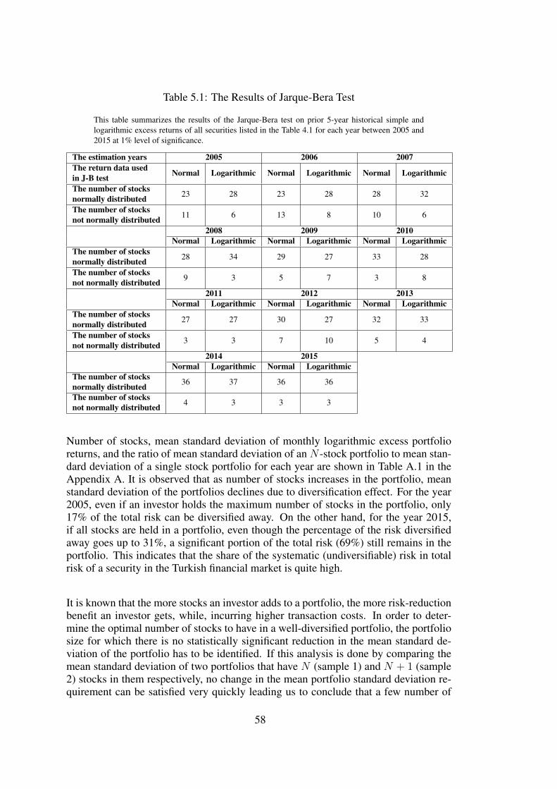
Table 5.1: The Results of Jarque-Bera Test

This table summarizes the results of the Jarque-Bera test on prior 5-year historical simple andlogarithmic excess returns of all securities listed in the Table 4.1 for each year between 2005 and2015 at 1% level of significance.

The estimation years 2005 2006 2007The return data usedin J-B test Normal Logarithmic Normal Logarithmic Normal Logarithmic

The number of stocksnormally distributed 23 28 23 28 28 32

The number of stocksnot normally distributed 11 6 13 8 10 6

2008 2009 2010Normal Logarithmic Normal Logarithmic Normal Logarithmic



2011 2012 2013Normal Logarithmic Normal Logarithmic Normal Logarithmic



2014 2015Normal Logarithmic Normal Logarithmic

The number of stocksnormally distributed 36 37 36 36

The number of stocksnot normally distributed 4 3 3 3

Number of stocks, mean standard deviation of monthly logarithmic excess portfolioreturns, and the ratio of mean standard deviation of an N -stock portfolio to mean stan-dard deviation of a single stock portfolio for each year are shown in Table A.1 in theAppendix A. It is observed that as number of stocks increases in the portfolio, meanstandard deviation of the portfolios declines due to diversification effect. For the year2005, even if an investor holds the maximum number of stocks in the portfolio, only17% of the total risk can be diversified away. On the other hand, for the year 2015,if all stocks are held in a portfolio, even though the percentage of the risk diversifiedaway goes up to 31%, a significant portion of the total risk (69%) still remains in theportfolio. This indicates that the share of the systematic (undiversifiable) risk in totalrisk of a security in the Turkish financial market is quite high.

It is known that the more stocks an investor adds to a portfolio, the more risk-reductionbenefit an investor gets, while, incurring higher transaction costs. In order to deter-mine the optimal number of stocks to have in a well-diversified portfolio, the portfoliosize for which there is no statistically significant reduction in the mean standard de-viation of the portfolio has to be identified. If this analysis is done by comparing themean standard deviation of two portfolios that have N (sample 1) and N + 1 (sample2) stocks in them respectively, no change in the mean portfolio standard deviation re-quirement can be satisfied very quickly leading us to conclude that a few number of

58

stocks are enough to create a diversified portfolio in Turkey. Thus, the statistically sig-nificant change in the mean standard deviation of two portfolios that have N (sample1) and N + 2 (sample 2) stocks in them respectively are tested in this thesis.

The results including t-test statistics and t critical values for each year are shown inTable A.2 in the Appendix A. When no statistically significant difference in standarddeviations of two portfolios with N and N + 2 securities is observed for the firsttime in a given year, the range of stocks prior to this, (N − 2 to N ) is taken as theoptimal number of stocks for that year. This range of optimal number of stocks foreach year analyzed in this thesis are shown in Table 5.2. In year 2005, by holding themaximum number of stocks available, which is 34, at most 17% of the total risk of anaverage security can be diversified away as seen in Table A.1 in the Appendix A. Byholding the optimal number of stocks which ranges from 10 to 12, approximately 16%of the total risk of an average security has already been diversified away. Therefore,a 1% reduction in the average standard deviation of the portfolio as we go from 10-12 stocks to 34 stocks is not considered as a statistically significant reduction in theportfolio risk. To gain a 1% risk-reduction benefit, high transaction costs may needto be paid. On the other hand, in year 2015, 29% of the total risk of an averagesecurity can be eliminated by holding 16 to 18 stocks in a portfolio. This reductionin portfolio risk increases to 31% of the total risk of an average security when themaximum number of stocks (39) available for investment are held in the portfolio.In the case of year 2015, the additional risk reduction of 2% in the average standarddeviation of the portfolio as we increase the number of stocks in the portfolio from 16-18 to 39 is not statistically significant. As for the other years, the reduction in the meanportfolio standard deviation is at most 3% as we go from holding the optimal numberof stocks to the maximum number of stocks available for investment. Again thesereductions are not statistically significant and they may not be economically significantto justify high transaction costs associated with larger portfolio sizes.

The results in Table 5.2 show that the optimal number of stocks to hold in a well-diversified portfolio differs from one year to another due to change in correlation be-tween the stocks. It is observed that an investor needs to hold more stocks in recentyears compared to earlier years to create a diversified portfolio. While 10-12 stocks areneeded to construct a well-diversified portfolio for the first observation year of 2005,the range of the optimal number of stocks needed for a well-diversified portfolio goesup to 16-18 for the last observation year of 2015.

Even though the sample stocks analyzed in this thesis are chosen from a different in-dex and data from a different time period is analyzed, findings of this thesis are quiteconsistent with the findings from earlier studies on Turkish stock market. For example,Gokce and Cura (2003, [10]) find the range for optimal number of stocks to be as 6-13for equally weighted portfolios created from stocks included in the BIST-30 Index overthe period from January 1999 to June 2000. Over the years analyzed in this thesis, theoptimal number of stocks to hold ranges from 8-10 to 16-18. Whereas, an averagerange of the optimal number of stocks over the observed periods is approximately 11-13 which is consistent with the work of Gokce and Cura (2003, [10]). Similarly, Atan

59

Table 5.2: The Range of Optimal Number of Stocks for each Year

This table presents ranges of the optimal number of stocks to create a well-diversifiedportfolio for each estimation year during the sample period from 2005 to 2015. Theanalyzed year is shown in the first column of this table and the second column reports thebeginning and the end of the periods of historical monthly return data used in the analysisfor that year.

Estimation yearThe period of historicalmonthly data used

The range of the optimalnumber of stocks

2005 Jan 2000-Dec 2004 10-122006 Jan 2001-Dec 2005 8-102007 Jan 2002-Dec 2006 10-122008 Jan 2003-Dec 2007 12-142009 Jan 2004-Dec 2008 12-142010 Jan 2005-Dec 2009 10-122011 Jan 2006-Dec 2010 16-182012 Jan 2007-Dec 2011 8-102013 Jan 2008-Dec 2012 12-142014 Jan 2009-Dec 2013 14-162015 Jan 2010-Dec 2014 16-18

and Duman (2007) analyze stocks that are constituents of BIST-100 Index, and find11, which is consistent with the findings in this thesis, as the optimal number of stocksto have in a well-diversified portfolio.

Even though the optimal number of stocks to have in a well-diversified portfolio changesfrom one year to another, according to the results reported in Table 5.2, over the periodanalyzed in this thesis on average, an investor needs to hold 11-13 stocks to gain mostof the risk-reduction benefits from diversification.

5.1.1 Comparison of Results with Prior and Posterior Variance-Covariance Ma-trix in terms of Diversification

In Section 5.1, when determining the optimal number of stocks for a well-diversifiedportfolio, only the variance-covariance matrix of 5-year historical monthly returns isused. B-L define this variance-covariance matrix as a prior matrix. In order to deter-mine the optimal weights for each stock in the portfolio while taking into account in-vestor views, they develop a new model which is explained in detail in Chapter 3 of thisthesis. In their model, the returns of stocks and the variances of these returns on stocksbased on the CAPM approach form the first information set and investor views on thereturns of stocks constitute the second information set. These two information sets areblended by Bayes’ Formula. The posterior variance-covariance matrix consisting ofthe combination of the prior one and the variances of stock returns based on investorviews is obtained. Mathematical background on the posterior variance-covariance ma-trix construction is also explained in Chapter 3. The prior one is denoted as Σ, and theformula for the posterior one as shown in the article of He and Litterman (1999, [14])

60

is as follows:Σ = Σ + ((τΣ)−1 + P TΩ−1P )−1,

where τ is a scaling factor, P is the pick matrix which indicates the stocks on whichinvestors express their views, and Ω is the matrix indicating the uncertainty associatedwith the views of investors.

τ is determined as inverse of the total number of observations. Since we use 60 monthlyhistorical returns for each year analyzed, τ equals to 0.0167 in this thesis. In additionto this, Ω is constructed as diag(P (τΣ)P T ) in this thesis.

Analysis conducted in the previous section on the prior variance-covariance matrix isrepeated here for the posterior variance-covariance matrix. The objective is to see howthe optimal number of stocks change when investor views and the uncertainty associ-ated with these views are taken into account. The posterior variance-covariance matrixbased on the B-L method is used as an input. Table A.3 in the Appendix A shows thenumber of stocks in the portfolio, average standard deviation of the combination oflogarithmic excess returns and investor views’ returns, and the ratio of average stan-dard deviation of the N -stock portfolio to average standard deviation of a single stockportfolio over the period analyzed in this thesis. The average standard deviation of thecombined returns decreases as the numbers of stocks in the portfolio increases due todiversification effect as it does with the prior variance-covariance matrix. For the year2005, the percentage of the risk diversified is just 17% by holding all of the stocksavailable for that period, whereas it increases to 31% for the year 2015. These resultsare quite similar to the ones obtained by using the prior variance-covariance matrix.

The relation between the average portfolio standard deviation and the number of stocksin the portfolio are shown in Figure 5.1 for each year in the sample when the priorvariance-covariance matrix based on the CAPM and the posterior variance-covariancematrix based on the B-L method are used. There is no noticeable difference betweenthese graphs for any of the years analyzed.

In order to find the optimal number of stocks for a well-diversified portfolio, a righttailed t-test at 5% significance level is also performed. The results are shown in TableA.4 in the Appendix A. Average variances, covariances, correlation coefficients andoptimal range of stocks for a well diversified portfolio by using variance matrices basedon both methods are summarized in Table 5.3. This table indicates that the averagevariances and covariances of the posterior matrix based on B-L approach are little bithigher than the average variances and covariances of the prior one. Moreover, for 2005,2006, 2011 and 2015, less number of stocks are needed to create a well-diversifiedportfolio when the posterior variance matrix is used. For the remaining years, therange for the optimal number of stocks is the same as in the case of prior variance.

61

Figure 5.1: Risk-Reduction versus Number of Stocks in the Portfolio for both the PriorVariance Based on the CAPM and the Posterior Variance Based on Black-LittermanMethod.

This figure shows the relation between the mean standard deviation of the portfolio andthe number of stocks included in the portfolio for each year from 2005 to 2015 byusing both the prior variance-covariance matrix (blue line) and the posterior variance-covariance matrix (red line). The prior matrix is the variance-covariance matrix of prior5-year historical monthly returns of stocks consistently included in the BIST-50 index.The beginning and the end of these 5-year periods are shown above the graphs. Aftertaking into account the investor views and the variance of these views, this prior matrixis converted into the posterior matrix by using the B-L formula.

Table 5.3: Comparison between the Prior and the Posterior Variance-Covariance Ma-trices in terms of Diversification Effect

This table presents the average variances, average covariances, average correlations and the ranges of the op-timal number of stocks when both prior variance-covariance matrix based on the CAPM and the posteriorvariance-covariance matrix based on the B-L method are used for each year from 2005 to 2015. First, for eachyear, the prior matrix is estimated by using prior 5 year historical monthly return data. Then, the average vari-ance and the average covariance of the stocks in the portfolio are calculated. Later, average correlation of thesestocks in the portfolio is calculated by dividing average covariance by average variance. The same process isrepeated for the posterior matrix derived from the B-L formula. For the purpose of attaining the range of theoptimal number of stocks, first, the simulation technique of Evans and Archer (1968, [12]) is performed. Byreplicating this procedure for 1000 times, the portfolios consisting of stocks ranging from 1 to total numberof stocks in any given year analyzed are generated and their mean standard deviations are found. In order todetermine whether any statistically significant decrease in the mean standard deviation of two portfolios thathave N and N + 2 stocks occurs or not, a t-test at 5% significance level is performed. Finally, the ideal rangeof stocks to create a diversified portfolio is selected as the last range of stocks whose mean standard deviationsare statistically different from each other before the first range of stocks whose mean standard deviations arestatistically indifferent from each other. The same process is repeated for posterior matrix based on the B-Lmethod to obtain the range of the optimal number of stocks.

Prior Variance(CAPM) Posterior Variance(Black Litterman)

AverageVariance

AverageCovariance

AverageCorrelation

The Range of theOptimal Number

of Stocks

AverageVariance

AverageCovariance

AverageCorrelation


of Stocks2005 491.53 321.12 0.65 10-12 494.03 321.46 0.65 8-102006 370.36 224.38 0.60 8-10 372.25 224.59 0.60 6-82007 236.73 131.28 0.55 10-12 238.00 131.38 0.55 10-122008 159.54 75.30 0.47 12-14 160.34 75.35 0.46 12-142009 196.14 93.32 0.47 12-14 197.07 93.39 0.47 12-142010 230.81 111.56 0.48 10-12 231.95 111.63 0.48 10-122011 210.45 95.03 0.45 16-18 211.56 95.11 0.44 14-162012 195.05 89.16 0.45 8-10 196.18 89.22 0.45 8-102013 197.18 106.75 0.54 12-14 198.04 106.81 0.53 12-142014 127.07 57.19 0.45 14-16 127.72 57.22 0.44 14-162015 102.72 45.99 0.44 16-18 103.26 46.02 0.44 14-16

63

As in the case of prior variance, the range of the optimal number of stocks differs fromone year to another. However, taking into account investor views does not affect therange of optimal number of stocks to hold, and the average portfolio standard devia-tions that much.

In addition to this comparison, we consider the effect of scaling factor τ used to de-termine the posterior variance on our results. To see this effect, a sensitivity analysisfor different τ value is conducted. The range of optimal number of stocks for a welldiversified portfolio by using posterior variance matrix for different τs for 2015 aresummarized in Table 5.4. Results in this table indicate that the range of the optimalnumber of stocks is not that sensitive to the value of τ chosen.

Table 5.4: The Range of Optimal Number of Stocks for Different Values of τ for 2015

This table presents the ranges of optimal number of stocks when the posterior matricesare constructed by using different values of the scaling factor τ for the estimation year2015. τ is taken as the inverse of the number of observations (5 years = 60 observations)in this thesis to determine the range of optimal number of stocks when the posteriormatrix is used. To study the sensitivity of our findings to τ values, a sensitivity analysisis conducted for τ values of 1/

√60, 0.25, 0.5 and 1.

The Values of τ τ = 160 τ = 1√

60τ = 0.25 τ = 0.5 τ = 1


of Stocks14-16 14-16 14-16 16-18 18-20

5.2 An Empirical Application of the Unconstrained Black-Litterman Model tothe Stocks Included in the BIST-50 Index

In the previous section, how many stocks from Borsa Istanbul-50 (BIST-50) Index areneeded to form a well-diversified portfolio is determined for every year in the sam-ple period analyzed. What portion of the portfolio should be invested in each stock isanother issue considered by investors. Markowitz Mean-Variance approach has beenused in determining optimal weights of each stock in the portfolio since the 1950’s.Although it is a breakthrough theory in finance, it has some drawbacks such as therequirement of estimating all stock returns in a portfolio and high level of sensitivityof optimal portfolio weights to inputs. These problems result in extremely low or highweights assigned to stocks included in the portfolio. In addition to this, investors cannot define their views about assets in a relative sense. After pointing out these prob-lems, Black and Litterman (B-L) proposed a new model in the 1990’s. Investors canspecify their views on the stocks of their choice and also define the confidence level ontheir views in this model.

In this section, B-L model is applied to the stocks included in the BIST-50 Index. Thedata used, the parameters selected, and each step of the model are explained in detail in

64

Subsection 4.2.2. Initial optimal weights for each stock in the portfolio is taken as mar-ket capitalization weights according to the CAPM approach. The stock return based onviews is calculated by using the financial analysts’ average expected stock price whichcan be accessed from the Bloomberg database. After combining prior information withanalysts’ views, the B-L model is estimated without imposing any constraints. It is ob-served that view returns of some assets do not affect posterior weights of these assetsin an expected way. First, reason behind this observation is explained. Secondly, B-Lmodel is re-estimated once by imposing a budget constraint alone, and then a budgetand no short selling constraints simultaneously on the model. Lastly, performances ofportfolios generated by the B-L method and by the CAPM approach are analyzed interms of two criteria: Sharpe ratio and efficient frontier.

The prior information set based on the CAPM approach is collected and prepared asdescribed in Section 4.1. The risk aversion coefficient, which is one of the inputs ofthe prior information set, is generally estimated from the historical data and calculatedas follows:

λ =E(rM)− rfσ2(rM)

,

where

E(rM)− rf is the estimated excess return of the market portfolio,

σ2(rM) is the variance of the market portfolio.

In our study, market portfolio is the portfolio consisting of all stocks whose codes arepresented in Table 4.1 for each estimation year. The excess return of this market port-folio is calculated as the market value weighted average of excess returns on the stocksincluded in the portfolio. The variance of the market portfolio is calculated by us-ing matrix multiplication. The transpose of the market capitalization weight vector ismultiplied by the estimated variance-covariance matrix, and the market capitalizationweight vector. Finally, the risk aversion coefficient is found by dividing the calculatedexcess return of the market portfolio by the calculated variance of the market portfolio.The results are presented in Table 5.5.

Risk aversion coefficients estimated by this method are quite low and even negativefor most of the estimated years. For only the years 2008 and 2014, the estimated riskaversion coefficients are consistent with expectations and the evidence from around theworld. However, risk aversion coefficients estimated for the remaining years are quitelow due to high variability of portfolio returns or negative average returns observed forthe majority of the stocks in some years. Since these negative or very low estimatesof risk aversion coefficients are not consistent with the expectations and the observedinvestor behavior, the risk aversion coefficient is taken to be 2.5 which is estimated byBlack (1989, [3]) as the world average risk aversion coefficient.

65

Table 5.5: Risk Aversion Coefficients

This table presents the average logarithmic excess return of the market portfolio, thevariance of the market portfolio and the risk aversion coefficient (λ) for each estimationyear during the sample period of this thesis. The market portfolio is constructed as themarket value weighted portfolio of all stocks shown in Table 4.1 for each estimation yearduring the sample period. The average 5-year historical logarithmic excess return and thevariance of the market portfolio are calculated for each estimation year. The risk aversioncoefficient is defined as excess return of the market portfolio per unit of the market risk(variance).

Average LogarithmicExcess Return of The Portfolio (%)

Variance ofThe Portfolio

Risk AversionCoefficient (λ)

2005 −2.58 % 291.00 −0.882006 −0.41 % 227.41 −0.182007 −0.23 % 127.07 −0.172008 1.47% 72.74 2.022009 −0.31 % 91.29 −0.332010 0.31% 108.85 0.282011 0.16% 111.03 0.142012 −0.12 % 98.77 −0.122013 0.1% 111.21 0.082014 1.45% 56.74 2.552015 0.66% 47.47 1.38

After the terms λ, Σ, and wMKT are estimated from market data, the implied logarith-mic excess equilibrium returns are computed for each year using MATLAB.

For year 2015, Figure 5.2 illustrates the historical average logarithmic returns and theimplied equilibrium average logarithmic excess returns on all the stocks available forinvestment over the 5-year period from January 2010 to December 2014. As can beseen in this figure, the implied equilibrium excess returns are all positive. Furthermore,they are more stable than historical returns. Therefore, they are more consistent withthe notion of expected excess returns. Hence, they can be good initial estimates ofexpected returns before taking investors’ views into account.

The variance-covariance matrix of this implied logarithmic excess equilibrium re-turns of the stocks is calculated as τΣ. τ is the scaling factor for historical variance-covariance matrix. B-L (1992, [5]) state that because the uncertainty in the mean is lessthan the uncertainty in the returns, τ is close to 0. In Figure 5.2, it is also observed thatthe logarithmic excess equilibrium returns are less volatile than the historical averagelogarithmic excess returns. Hence, in this thesis τ is defined as in Walters (2014, [29])as follows:

τ =1

T.

66

Figure 5.2: Comparison between Historical Average Returns and Equilibrium Returns.

This figure shows average 5-year historical and the implied equilibrium logarithmic ex-cess returns of the stocks consistently included in the BIST-50 index for 2015. The greenline indicates the average historical returns, whereas the purple line indicates the impliedequilibrium returns of these stocks. The beginning and the end of the 5-year period areshown above the graph.

Here, T is the total number of observations. Since 60 monthly historical returns areused for each year analyzed, τ is constant and equals to 0.0167 in this thesis.

After determining the prior information set, it is time to gather the second informationset including Bloomberg analysts’ views. How these target stock prices are collectedand converted into stock returns are explained in Section 4.1. Formulation of the pickmatrix (P ), the view vector (q), and the covariance matrix of the views (Ω) and blend-ing of this second information set with the first information set by using B-L formulaare explained step by step in Subsection 4.2.2. Finally, the posterior optimal weightsare found by using the calculated posterior expected return vector and the posteriorvariance matrix as inputs in the Markowitz Mean-Variance Optimization.

Table 5.6 on the next page displays market capitalization (equilibrium) weights, thecomputed posterior weights and the difference between equilibrium weights and newweights resulting from the B-L method for the estimation year 2015. The results forother estimation years are available in Table A.5 in the Appendix A. The stocks whosecodes are written in bold letters do not have a target stock price data available in theBloomberg database. All the others have the average target stock price information.

As seen in Table 5.6, the sum of the market capitalization weights of the stocks is equalto 1 by definition. On the other hand, the sum of the new optimal posterior weights ofthe stocks is equal to -0.3215 since the optimization problem does not have a budgetconstraint. Minus sign indicates that an investor invest his own money and the moneyobtained from shorting this portfolio of stocks in the risk-free asset.

67

For GOLTS and VESTL Bloomberg analysts did not estimate a target stock price,i.e. they did not express an opinion. These stocks’ optimal posterior weights slightlydifferent from their market capitalization weights, however differences are not evennoticeable. This is not surprising since the investor does not have any basis to changethe weights of these securities. On the other hand, optimal posterior weights of secu-rities for which analysts estimate a target stock price are significantly different fromtheir market capitalization weights.

Table 5.6: Market Capitalization Weights, Optimal Posterior Weights and Differencesfor the Estimation Year 2015

This table presents the market capitalization weights, the optimal posterior weights of the stocks that are consis-tently included in the BIST-50 index in 2015 and the differences between them. First column shows the codes ofthe stocks that are consistently included in BIST-50 index during the whole year and have monthly return datafrom January 2010 to December 2014. In the second and third columns, the market capitalization and posteriorweights of these securities are reported. The stock codes written in bold letters indicate the stocks for which theBloomberg analysts did not give a price estimate. The difference between the market capitalization weights andthe optimal posterior weights of both stocks with views and no views are shown in the last column of this table.Finally, in the last row of this table, the summation of both the market capitalization and the optimal posteriorweights are presented.

wMKT w? wMKT − w?

AEFES 0.0297 0.1840 −0.1544AKBNK 0.0764 −0.1293 0.2058ARCLK 0.0224 −0.1252 0.1475ASELS 0.0132 −0.0529 0.0661BAGFS 0.0014 −0.0748 0.0762BIMAS 0.0335 −0.2791 0.3126CCOLA 0.0283 0.1781 −0.1497DOAS 0.0058 −0.1466 0.1524DOHOL 0.0044 0.1329 −0.1286ENKAI 0.0419 0.1274 −0.0855EREGL 0.0344 −0.0658 0.1002FROTO 0.0252 −0.2714 0.2966GARAN 0.0873 −0.1276 0.2149GOLTS 0.0010 0.0010 0.0000GOZDE 0.0025 0.1229 −0.1205GUBRF 0.0037 −0.2605 0.2642HALKB 0.0383 0.4397 −0.4013ISCTR 0.0669 −0.2730 0.3399KCHOL 0.0694 −0.1678 0.2372KOZAA 0.0014 0.3505 −0.3490KRDMD 0.0035 0.3124 −0.3089MGROS 0.0089 0.0934 −0.0845OTKAR 0.0046 −0.3510 0.3556PETKM 0.0087 −0.0978 0.1065SAHOL 0.0457 0.4467 −0.4010SISE 0.0137 −0.2372 0.2508TAVHL 0.0153 0.0184 −0.0030TCELL 0.0694 −0.3127 0.3821THYAO 0.0293 −0.0475 0.0769TKFEN 0.0047 0.4442 −0.4394TOASO 0.0176 −0.0946 0.1122TRKCM 0.0056 0.0100 −0.0044TSKB 0.0067 0.4447 −0.4381TTKOM 0.0561 −0.1686 0.2248TUPRS 0.0305 −0.1821 0.2126ULKER 0.0140 −0.1423 0.1563VAKBN 0.0269 0.0388 −0.0119VESTL 0.0047 0.0046 0.0001YKBNK 0.0469 −0.0632 0.1101

SUM 1.000 −0.3215

68

Table 5.7: View and Equilibrium Return Differences and Market versus PosteriorWeight Differences for the Estimation Year 2015

This table presents the implied equilibrium returns, the view returns of the stocks calculated from Bloomberganalysts’ average target price and their difference for the year 2015. Also in this table the market capitalizationweights, the optimal posterior weights of these stocks and the difference between these two weights are reportedfor the same year.

Π q Π − q wMKT w? wMKT − w?

AEFES 0.0059 0.0068 −0.0009 0.0297 0.1840 −0.1544

AKBNK 0.0139 −0.0052 0.0191 0.0764 −0.1293 0.2058

ARCLK 0.0141 −0.0051 0.0192 0.0224 −0.1252 0.1475

ASELS 0.0114 −0.0043 0.0158 0.0132 −0.0529 0.0661

BAGFS 0.0090 −0.0029 0.0120 0.0014 −0.0748 0.0762

BIMAS 0.0048 −0.0030 0.0077 0.0335 −0.2791 0.3126

CCOLA 0.0076 0.0050 0.0027 0.0283 0.1781 −0.1497

DOAS 0.0169 −0.0072 0.0241 0.0058 −0.1466 0.1524

DOHOL 0.0098 0.0053 0.0045 0.0044 0.1329 −0.1286

ENKAI 0.0116 0.0053 0.0063 0.0419 0.1274 −0.0855

EREGL 0.0073 −0.0020 0.0094 0.0344 −0.0658 0.1002

FROTO 0.0112 −0.0129 0.0241 0.0252 −0.2714 0.2966

GARAN 0.0148 −0.0075 0.0223 0.0873 −0.1276 0.2149

GOZDE 0.0119 0.0072 0.0047 0.0025 0.1229 −0.1205

GUBRF 0.0106 −0.0130 0.0236 0.0037 −0.2605 0.2642

HALKB 0.0154 0.0143 0.0011 0.0383 0.4397 −0.4013

ISCTR 0.0148 −0.0105 0.0253 0.0669 −0.2730 0.3399

KCHOL 0.0143 −0.0067 0.0210 0.0694 −0.1678 0.2372

KOZAA 0.0159 0.0271 −0.0112 0.0014 0.3505 −0.3490

KRDMD 0.0122 0.0133 −0.0011 0.0035 0.3124 −0.3089

MGROS 0.0123 0.0028 0.0095 0.0089 0.0934 −0.0845

OTKAR 0.0106 −0.0213 0.0319 0.0046 −0.3510 0.3556

PETKM 0.0096 −0.0042 0.0138 0.0087 −0.0978 0.1065

SAHOL 0.0117 0.0071 0.0046 0.0457 0.4467 −0.4010

SISE 0.0111 −0.0088 0.0199 0.0137 −0.2372 0.2508

TAVHL 0.0075 −0.0034 0.0108 0.0153 0.0184 −0.0030

TCELL 0.0080 −0.0078 0.0158 0.0694 −0.3127 0.3821

THYAO 0.0132 −0.0041 0.0173 0.0293 −0.0475 0.0769

TKFEN 0.0108 0.0099 0.0008 0.0047 0.4442 −0.4394

TOASO 0.0155 −0.0065 0.0220 0.0176 −0.0946 0.1122

TRKCM 0.0135 −0.0034 0.0169 0.0056 0.0100 −0.0044

TSKB 0.0105 0.0072 0.0033 0.0067 0.4447 −0.4381

TTKOM 0.0067 −0.0055 0.0121 0.0561 −0.1686 0.2248

TUPRS 0.0127 −0.0079 0.0206 0.0305 −0.1821 0.2126

ULKER 0.0089 −0.0076 0.0165 0.0140 −0.1423 0.1563

VAKBN 0.0160 0.0008 0.0152 0.0269 0.0388 −0.0119

YKBNK 0.0167 −0.0043 0.0210 0.0469 −0.0632 0.1101

The posterior weights of the stocks are expected to change in the direction of the views.For example, if there is a positive view on a stock, its weight is expected to increaseor vice versa. Results of this investigation for 2015 are presented in Table 5.7. Theevidence is not consistent with this expectation for all the stock, however for about68% it is consistent. Therefore, evidence is in general but not completely consistentwith this expectation.

69

Bozdemir (2011, [7]) illustrates the nonexistence of a direct relationship between theviews on expected returns and corresponding posterior weights for the case of 2 assets.In his example, the expected return on one of the assets is raised and everything elseis kept constant. It is shown that an increase in the expected return of the asset resultsin a decrease in the posterior weight of the corresponding asset, a finding that is in-consistent with the expectation based on views. He concludes that the reason for thisunexpected relationship between the view on expected return and the correspondingposterior weight is the covariance structure.

To understand the relationship between specified views on returns and the B-L poste-rior weights, first the relationship between the view return and the expected return ofthat asset needs to be examined.

To see the effect of the relationship between the expected and the view returns of as-sets on this unexpected relationship between specified views and the posterior weights,let’s take a look at a simple example with 3 assets. Suppose that the equilibrium re-turn on the first asset is equal to 1%, the second one is 2% and the third one is 0.5%.Suppose the view 1 states that the return of first asset will be 2% and the view 2 statesthat the return on the second asset will be 3%. Hence, view returns of these two assetsare greater than their implied equilibrium returns. Let the covariance matrix of theseassets be

Σ =

1 −2 4−2 3 14 1 5

.

Scaling factor τ and the uncertainty of view matrix Ω are taken as defined in this thesisearlier.

τ =1

T=

1

60, T : total number of observations,

Ω = diag(P (τΣ)P T ).

Expected posterior return that combines the equilibrium returns and investor views iscalculated by the following formula:

E(r) = Π + τΣP T [(PτΣP T ) + Ω]−1[q − PΠ],

70

E(r) =

12

0.5

+1

60

1 −2 4−2 3 14 1 5

1 00 10 0

×

[ 1 0 0

0 1 0

]1

60

1 −2 4−2 3 14 1 5

1 00 10 0

+

[0.0167 0

0 0.05

]−1

×

[ 23

]−[

1 0 00 1 0

] 12

0.5

,

E(r) =

11.55

.

The equilibrium return of the first asset is given as 1%, and the view return of the firstasset is stated as 2% which is greater than the equilibrium return of this asset. Asshown by the calculations above, the expected posterior return of this asset remainsat 1%. Actually, given the view on this asset, its posterior return is expected to begreater than its equilibrium return. However, its posterior return is exactly equal to itsequilibrium return. When the second asset is concerned, its posterior return (1.5%) islower than its equilibrium (2%) and view (3%) returns. However, given the view onthis asset, its posterior return is also expected to be greater than its implied equilibriumreturn. Contrary to the expectations, its posterior return is declined.

As it can be seen in this example, higher view return than the implied equilibrium re-turn does not necessarily indicate higher posterior expected return than the equilibriumreturn. In other words, there is not a direct relationship between the view return of anasset and the posterior expected return of it. How the posterior expected return changesis determined by the covariance structure of the securities. In this example, there areonly 3 assets, therefore it is a lot easier to see the effect of covariance structure on theposterior expected return. In the case of this thesis, there are approximately 50 assetswith more than 30 views on these assets. Hence, analyzing the effect of covariancestructure of securities on the posterior return updating mechanism is a lot harder tounderstand.

Let’s continue work with this 3 assets example with different views on the assets. Sup-pose this time, there is only one relative view indicating that the return of the first assetis 1% higher than the return on the second asset. The rest of the data on these 3 assetsare the same as before.

Then the posterior expected returns are calculated as follows:

71

E(r) =

12

0.5

+1

60

1 −2 4−2 3 14 1 5

1−10

×

[ 1 −1 0

] 1

60

1 −2 4−2 3 14 1 5

1−10

+[

0.1333]−1

×

[ 1]−[

1 −1 0] 1

20.5

,

E(r) =

1.3751.3750.875

.Expected returns of the first two assets are changed in the direction of the view stated;that is, while the first asset’s expected return increases the second asset’s expected re-turn decreases. Thus, this example reveals that not only covariance structure but alsothe way views are defined affects the relation between view return and the posteriorexpected return of the corresponding asset.

Furthermore, confidence level of the view in addition to the covariance structure andthe way views are stated is another factor affecting the relationship between the viewreturns and the posterior expected returns of an asset. Since there is no information onthe confidence level of the views in Bloomberg database, this uncertainty of the viewvector is defined in terms of the covariance matrix of security returns, and the viewmatrix. Therefore, it is adequate to say that covariance structure of the securities andthe structure of the views defined might affect the relation between the view return andthe posterior expected return of an asset in our case too.

5.2.1 An Empirical Application of the Black-Litterman Model with a BudgetConstraint to the Stocks Included in the BIST-50 Index

In the empirical application of the unconstrained B-L Model, it is observed that thebudget required to create the optimal portfolios ranges from -1.8017 in the estimationyear of 2005 to 2.9325 in the estimation year of 2009 as reported in Table A.5 of theAppendix A. Since these budgets are quite extreme, putting a budget constraint on theB-L Model is considered. A budget constraint, which is a real world constraint, re-quires the sum of portfolio weights to be one.

The same data is used as in the application of the unconstrained B-L model up to thefinal Markowitz optimization step. In the final optimization model, the optimization

72

problem is formulated with the budget constraint.

Results reported in Table 5.8 for 2015 show that posterior weights of stocks with noassigned views differ much more from their equilibrium weights. However, the valueof the investor’s utility function is not affected that much from the addition of thisbudget constraint to the optimization problem. If an investor desires to invest all ofhis/her money into the optimal portfolio of all the stocks consistently included in theBIST-50 index, his utility loss compared to the unconstrained B-L strategy is not thatmuch from following this budget constrained B-L strategy.

5.2.2 An Empirical Application of the Black-Litterman Model with a Budgetand a No Short Selling Constraints to the Stocks Included in the BIST-50Index

In the application of both the unconstrained and the budget constrained B-L Models,there are several stocks that are sold short. However, there are restrictions on shortselling in financial markets. In order to examine the effect of a short selling constrainton the optimal portfolio of the investor, no short selling constraint is added to the op-timization problem with the budget constraint. No short selling constraint requires theweight of each security to be greater than or equal to 0.

The same data is used as in the application of both unconstrained and the budget con-strained B-L model. This application only differs from previous applications of theB-L model in the final Markowitz optimization step. In the optimization problem, theutility function of the investor is maximized while satisfying the budget and the noshort selling constraints simultaneously.

In Table 5.8, the maximum utility of the investor is achieved by investing in a smallnumber of stocks. However, this utility is significantly lower than the utility investorhas with either the unconstrained or only the budget constrained optimization. Thisfinding is not surprising given the nature of the constrained optimization and it indi-cates that the no short selling constraint is more binding that the budget constraint.Note that in these optimizations, transaction costs associated with trading are not takeninto account. Therefore, even though utility of the investor declines significantly afterimposing the no short selling constraint, an investor might still be interested in apply-ing this constrained optimization if the loss in utility because of short selling constraintis less than the loss in utility because of increased transaction costs. Furthermore, asin the case of budget constrained optimization, the optimal posterior weights of stockswith no assigned views deviate significantly from their equilibrium weights.

73

Table 5.8: Optimal Weights from only Budget constrained and Budget and No ShortSelling Constrained B-L Portfolio Optimizations for the Estimation Year 2015

This table presents the market capitalization weights, the optimal posterior weights of stocks obtained fromonly budget constrained and both budget and short selling constrained portfolio optimizations. The stocks thatare consistently included in the BIST-50 index throughout 2015 and have monthly return data from January2010 to December 2014 are shown in the first column of this table. The second, third and fourth columns ofthis table show the market capitalization weights, posterior weights with budget constraint only and posteriorweights with both budget and short selling constraints respectively. The stock for which Bloomberg analystdid not estimate a target price are shown in bold letters. Finally, the value of the utility function for both theunconstrained and the budget constrained portfolio optimization are shown in the last row of this table.

wMKT w? wOPT(budget)wOPT(budget&no short selling)AEFES 0.0297 0.1840 0.5497 0.6121AKBNK 0.0764 −0.1293 −0.1588 0.0000ARCLK 0.0224 −0.1252 −0.2357 0.0000ASELS 0.0132 −0.0529 −0.1674 0.0000BAGFS 0.0014 −0.0748 0.2495 0.0000BIMAS 0.0335 −0.2791 0.1745 0.2303CCOLA 0.0283 0.1781 0.2059 0.0070DOAS 0.0058 −0.1466 −0.2888 0.0000DOHOL 0.0044 0.1329 0.2865 0.0000ENKAI 0.0419 0.1274 0.2485 0.0787EREGL 0.0344 −0.0658 0.0589 0.0000FROTO 0.0252 −0.2714 −0.4726 0.0000GARAN 0.0873 −0.1276 0.1101 0.0000GOLTS 0.0010 0.0010 -0.1795 0.0000GOZDE 0.0025 0.1229 −0.0119 0.0000GUBRF 0.0037 −0.2605 −0.2843 0.0000HALKB 0.0383 0.4397 0.3426 0.0000ISCTR 0.0669 −0.2730 −0.6788 0.0000KCHOL 0.0694 −0.1678 −0.4000 0.0000KOZAA 0.0014 0.3505 0.2606 0.0720KRDMD 0.0035 0.3124 0.1798 0.0000MGROS 0.0089 0.0934 0.1540 0.0000OTKAR 0.0046 −0.3510 −0.1785 0.0000PETKM 0.0087 −0.0978 0.2206 0.0000SAHOL 0.0457 0.4467 0.6839 0.0000SISE 0.0137 −0.2372 −0.1434 0.0000TAVHL 0.0153 0.0184 −0.0588 0.0000TCELL 0.0694 −0.3127 0.0866 0.0000THYAO 0.0293 −0.0475 0.0067 0.0000TKFEN 0.0047 0.4442 0.3046 0.0000TOASO 0.0176 −0.0946 −0.2040 0.0000TRKCM 0.0056 0.0100 −0.2022 0.0000TSKB 0.0067 0.4447 0.5684 0.0000TTKOM 0.0561 −0.1686 0.1308 0.0000TUPRS 0.0305 −0.1821 −0.1081 0.0000ULKER 0.0140 −0.1423 0.0561 0.0000VAKBN 0.0269 0.0388 −0.1079 0.0000VESTL 0.0047 0.0046 -0.0838 0.0000YKBNK 0.0469 −0.0632 0.0859 0.0000

SUM −0.3215 1.0000 1.0000UTILITY 0.0097 0.0088 0.0001

74

5.2.3 Comparison of the CAPM and the Black-Litterman Models in terms ofSharpe Ratios

As described in Subsection 2.2.2 of this thesis, according to Capital Asset PricingModel, every investor holds the market portfolio because everyone has access to thesame information and uses the same decision rule in making their investment decisions.In other words, each investor holds a market value weighted portfolio of all the assetsin the market. Market value weight of each stock, i.e. weight vector of the assets, log-arithmic excess equilibrium return vector and covariance matrix of logarithmic excessreturns are estimated for each year in the sample period from 2005 to 2015. Then,by multiplying the weight vector of the assets with the logarithmic excess equilibriumreturn vector, the excess return of the equilibrium portfolio is computed. Similarly,by multiplying the transpose of weight vector of the assets and the covariance matrixof logarithmic excess returns and the weight vector of the assets, the variance of theequilibrium portfolio is determined.

As explained mathematically in Chapter 3 of this thesis, the B-L Model combinesthe equilibrium expected returns for assets with investors’ views using a Bayesian ap-proach. In this thesis, expected stock return calculated from the analysts’ average targetstock price in the Bloomberg database is taken as a proxy for investors’ views. Thevector of the optimal posterior weights, new combined logarithmic excess return vec-tor and the posterior covariance matrix of logarithmic excess returns are computed inMATLAB for each of the years in between 2005 and 2015. Therefore, by multiplyingthe vector of the optimal posterior weights with the new combined logarithmic excessreturn vector, the excess return on the B-L optimal portfolio is computed. Similarly, bymultiplying the transpose of the vector of the optimal posterior weights, the posteriorcovariance matrix of logarithmic excess returns and the vector of the optimal posteriorweights the variance of the optimal portfolios is calculated.

Performances of these two portfolios constructed from the CAPM and the B-L Modelare compared by using a Sharpe ratio. Sharpe ratio is a measure of excess return of theportfolio per unit of the total risk of the portfolio (standard deviation of the portfolio).The portfolio with the higher Sharpe ratio has a better risk-adjusted performance. Asgiven in the Subsection 2.2.1 of this thesis, the formula of the Sharpe ratio is:

S =E(rp)− rf

σp.

Sharpe ratios of the portfolios based on the CAPM and the B-L model for the 11 es-timated years from 2005 to 2015 are presented in Table 5.9 along with the portfolioexcess returns, the variance and the standard deviation of these returns.

75

Table 5.9: Sharpe Ratios of CAPM and B-L Strategies for each Estimation Years

This table presents the excess expected return, the variance, and the standard deviation of the portfolios calcu-lated with both the CAPM and the B-L methods for each estimation year between 2005 and 2015. Sharpe ratiomeasures the excess return of the portfolio per unit of the portfolio risk. This table is constructed to illustratethe portfolio which has better risk-adjusted performance.

2005 2006 2007 2008CAPM B-L CAPM B-L CAPM B-L CAPM B-L

E(R) 0.0727 1.9209 0.0569 0.0340 0.0318 0.0622 0.0182 0.0823Var 0.0291 0.7684 0.0228 0.0136 0.0127 0.0249 0.0073 0.0329

Std.Dev. 0.1706 0.8766 0.1510 0.1166 0.1127 0.1578 0.0854 0.1814Sharpe Ratio 0.4262 2.1913 0.3768 0.2915 0.2822 0.3942 0.2130 0.4537

2009 2010 2011 2012CAPM B-L CAPM B-L CAPM B-L CAPM B-L

E(R) 0.0228 0.1810 0.0272 0.0262 0.0278 0.0235 0.0247 0.0461Var 0.0091 0.0724 0.0109 0.0105 0.0111 0.0094 0.0099 0.0184

Std.Dev. 0.0954 0.2691 0.1044 0.1025 0.1054 0.0970 0.0995 0.1356Sharpe Ratio 0.2390 0.6727 0.2605 0.2557 0.2639 0.2424 0.2482 0.3399

2013 2014 2015CAPM B-L CAPM B-L CAPM B-L

E(R) 0.0278 0.0116 0.0142 0.0354 0.0119 0.0194Var 0.0111 0.0047 0.0057 0.0141 0.0047 0.0078

Std.Dev. 0.1054 0.0686 0.0755 0.1187 0.0686 0.0883Sharpe Ratio 0.2639 0.1692 0.1881 0.2981 0.1736 0.2197

For years 2005, 2007, 2008, 2009, 2012, 2014 and 2015 the B-L strategy is slightlysuperior to the CAPM strategy when the Sharpe ratios are used for comparison. How-ever, for the remaining years, the CAPM strategy slightly outperforms the B-L strategyaccording to this performance measure. Given these findings it is hard to conclude thatthe B-L strategy is always better than the CAPM strategy using this criteria.

5.2.4 Comparison of the CAPM and the Black-Litterman Model Using EfficientFrontier Technique

As presented in Subsection 2.2.1 of this thesis, the efficient frontier is a curve depictingthe portfolios that give investors the greatest possible rate of return for a given valueof risk they are willing to accept. The horizontal (X) axis of the efficient frontiergraph is usually the portfolio risk measured by the standard deviations of portfoliosand the vertical (Y) axis of this graph is the portfolio return. For the CAPM approach,the average of historical rate of returns for each stock and variances and covariancematrix of these average returns are calculated in MATLAB. For the B-L method, theposterior returns of each stock and the posterior variance-covariance matrix of thesereturns are calculated in MATLAB. By using plotEfficient function in MATLAB, theefficient frontiers of the portfolios according to the CAPM and the B-L approaches areestimated for each of the years in the sample period from 2005 to 2015 and displayedin Figure 5.3.

76

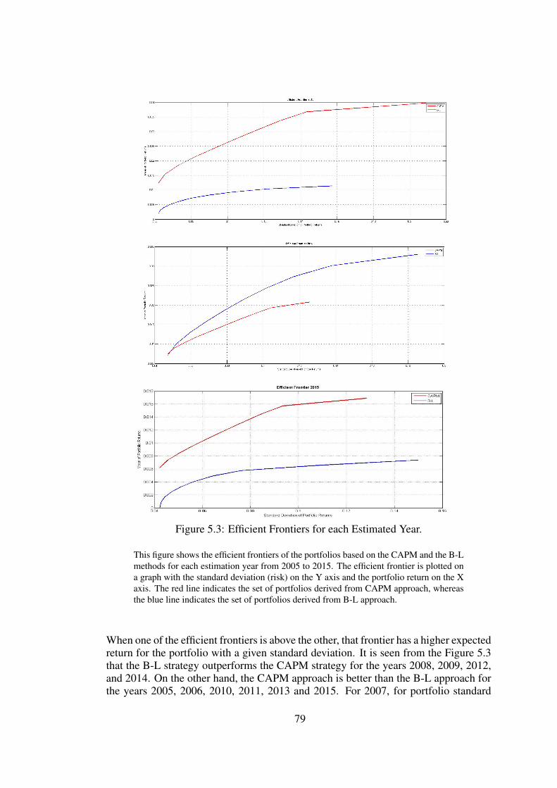
Figure 5.3: Efficient Frontiers for each Estimated Year.

This figure shows the efficient frontiers of the portfolios based on the CAPM and the B-Lmethods for each estimation year from 2005 to 2015. The efficient frontier is plotted ona graph with the standard deviation (risk) on the Y axis and the portfolio return on the Xaxis. The red line indicates the set of portfolios derived from CAPM approach, whereasthe blue line indicates the set of portfolios derived from B-L approach.

When one of the efficient frontiers is above the other, that frontier has a higher expectedreturn for the portfolio with a given standard deviation. It is seen from the Figure 5.3that the B-L strategy outperforms the CAPM strategy for the years 2008, 2009, 2012,and 2014. On the other hand, the CAPM approach is better than the B-L approach forthe years 2005, 2006, 2010, 2011, 2013 and 2015. For 2007, for portfolio standard

79

deviations between 0.085 and 0.13, the B-L strategy is superior to the CAPM strategy.However, when the portfolio standard deviation is lower than 0.085 or higher than 0.13,the CAPM strategy is superior to the B-L strategy.

To find a possible explanation for this domination by the CAPM or the B-L approach indifferent years during our sample period, the average equilibrium return, average pos-terior return and the difference between two is calculated and reported in Table 5.10.An analysis of this table, reveals that when the average equilibrium return exceeds theaverage posterior return by 1% or more in any estimation year, the efficient frontierderived from the CAPM approach lies above the efficient frontier derived from the B-L approach for that year. In other words, when stock returns estimated from analysts’target stock price forecasts are underestimating the future stock returns by more than1%, the efficient frontier of B-L is dominated by that of the CAPM. On the other hand,when the average equilibrium return exceeds the average posterior return by 0.01% orless, or the average posterior return exceeds the average equilibrium return regardlessof the size of the difference, the efficient frontier derived from the B-L strategy liesabove the efficient frontier derived from the CAPM strategy. In other words, whenanalysts are forecasting the future stock prices with small error or when they are over-estimating the future stock prices, the efficient frontier of B-L dominates that of theCAPM. In the case that the average equilibrium return exceeds the average posteriorreturn by more than 0.01% but less than 1%, which efficient frontier lies above theother is uncertain, because these two efficient frontiers intersect. For some levels ofthe portfolio standard deviation, efficient frontier derived from the B-L strategy can lieabove the one from the CAPM strategy. However, for some other levels of the portfo-lio standard deviation, the opposite is true. These findings can be observed from theefficient frontiers depicted in Figure 5.3.

Table 5.10: Average Market Returns, Equilibrium Returns and Differences for eachEstimation Year

This table presents the average view returns, the average implied equilibrium returns andthe difference between these two values for all the stocks that are consistently includedin the BIST-50 index and have target price estimated by the Bloomberg analysts.

2005 2006 2007 2008 2009 2010Avr. View Ret. −0.0168 0.0077 0.0249 0.0192 0.0429 0.0088

Equilibrium Ret. 0.0731 0.0562 0.0315 0.0180 0.0220 0.0274Difference −0.0899 −0.0485 −0.0065 0.0011 0.0208 −0.0186

2011 2012 2013 2014 2015Avr. View Ret. 0.0109 0.0242 0.0038 0.0132 −0.0014

Equilibrum Ret. 0.0251 0.0237 0.0263 0.0141 0.0116Difference −0.0142 0.0004 −0.0225 −0.0009 −0.0130

80

CHAPTER 6

CONCLUSION

The question of how many stocks are needed to effectively diversify a portfolio hasbeen burned in each investor’s mind for many years. While adding more stocks to aportfolio is beneficial from the point of view of diversification, it results in higher trans-action cost which is detrimental for an investor. This thesis reviews previous researchon this subject for both the U.S. Stock Exchanges and the Turkish Stock Exchange.The mathematical aspect of the concept of diversification is discussed as well. An-other question, an investor is concerned about is the allocation of his/her budget acrossstocks in a portfolio in order to achieve the maximum gain since the 1950s. Black andLitterman (B-L) (1990, [4]) brought a new perspective on Markowitz Mean-Varianceapproach. In their model, the returns of the securities in a portfolio obtained fromCAPM approach provide a base case, and later these returns can be combined with ananalyst or an investor’s views. This thesis deals with the literature related to some fi-nance theories starting from Markowitz Mean-Variance optimization to the B-L Modeland mathematics behind these theories as well as B-L Model.

The optimal number of stocks for a well-diversified portfolio of the Borsa Istanbul-50(BIST-50) Index constituents for the period from 2005 to 2015 is determined. In de-termining the optimal number of stocks, this thesis adopts the technique proposed byEvans and Archer (1968, [12]). The number of portfolio replication and the range ofnumber of stocks in a portfolio to test whether statistically significant difference canoccur are specified according to the study of Beck, Perfect and Peterson (1996, [1]).The optimal number of stocks is found to be as low as 8-10 for the years 2006 and 2012and as high as 16-18 for the years 2011 and 2015. For the remaining years during thesample, the optimal number of stocks is found to be in between these extreme values.The average range of the optimal number of stocks over the sample period analyzed inthis thesis is approximately 11-13. This finding is consistent with previous studies ofthe stocks included in the BIST-30 and the BIST-100. Moreover, for the year 2005, itis noticed that only 17% of the risk of a single stock portfolio is diversified by holdingall the stocks included in the BIST-50 index in the portfolio, while 16% of the risk ofa single stock portfolio is already diversified by holding the optimal number of stocks(10-12) for that year in the portfolio. In short, it can be concluded that a decrease of1% in the portfolio risk may not be enough to compensate transaction costs due toinvesting in additional stocks. Elton and Gruber (1977, [11]) document a decrease of51% in portfolio risk as the number of securities included in the portfolio increases

81

from 1 to 10 securities for the New York and American Stock Exchanges. On theother hand, for the Turkish Stock Market, the maximum decline in the portfolio risk isfound to be 31% in 2015. Comparison of these numbers might indicate the existence ofmuch higher nondiversifiable risk in the Turkish Stock Exchange compared to Amer-ican Stock Exchanges. Furthermore, the optimal number of stock for each year from2005 to 2015 is determined for both prior variance-covariance matrix and posteriorvariance-covariance matrix derived from B-L method. Comparison of these valuesshow that the optimal number of stocks obtained from the prior variance-covariancematrix does not differ significantly from the optimal number of stocks obtained fromthe posterior variance-covariance matrix. Moreover, for many years during the sampleperiod, no difference in the optimal number of stocks obtained from these two differentmethods is observed.

B-L portfolio optimization method is applied to the stocks included in the BIST-50 In-dex for the estimation years from 2005 to 2015. The previous research on the TurkishStock Exchange use either subjective views of authors or returns estimated by usingan econometric model such as AR(1) and EGARCH as view returns due to the factthat it is hard to reach subjective analyst views for Turkish stocks. However, in thisthesis, Bloomberg analysts’ average price estimates are used to construct view returnswhich are hand collected from the Bloomberg database. In the unconstrained B-Loptimization method, the optimal posterior weights of the stocks on which no viewsare expressed by a Bloomberg analyst are almost the same values as their equilibriummarket capitalization weights. Surprisingly, B-L posterior weight of a stock with aview may not move in the same direction with the view expressed on it. In a simpleexample with 3 asset, the way the views are expressed (either relative or absolute) andthe covariance structure of security returns are shown to be two of the reasons for theview return of a stock not being directly related to its B-L expected return and thusB-L posterior weight.

In addition to the unconstrained B-L portfolio optimization application mentioned inthe previous paragraph, a budget constrained and both a budget and a no short sellingconstrained B-L models are implemented for the same set of stocks. Contrary to thestudy of B-L (1991, [17]), more deviations from equilibrium weights for stocks withno assigned view are observed in both the budget constrained, and the budget and shortselling constrained optimizations. However, the value of the investor’s utility functionremains almost the same in the application of the budget constrained B-L optimization,whereas this value decreases significantly in the application of the budget and no shortselling constrained B-L optimization. It can be deduced from this that investors gainmore utility by short selling the stocks. Finally, whether the B-L strategy defeats theCAPM strategy or not is checked by using the Sharpe ratio and efficient frontier anal-ysis. The portfolios derived from the B-L strategy perform better than the portfoliosderived from the CAPM strategy based on the Sharpe ratio comparisons for most of theyears in the sample period but not for all the years. The B-L strategy may not alwaysbe superior to the CAPM strategy because of the quality of analysts views on returnsof the stocks used in this thesis. In contrast to the Sharpe ratio, the efficient frontiercriteria show that the CAPM strategy beats the B-L strategy for most of years in the

82

sample period analyzed in this thesis. According to the findings of this thesis, the ef-ficient frontier derived from CAPM dominates the efficient frontier derived from B-Lmodel when the average market return is 1% higher than or equal to the average viewreturn. On the other hand, the efficient frontier derived from the CAPM is dominatedby the one derived from the B-L model when the average market return is 0.01% lowerthan or equal to the average view return. However, it is impossible to determine whichfrontier dominates the other when the difference between the average market returnand the view return is higher than 0.01% but lower than 1%. It can be concluded thatwhen the average market return is sufficiently higher than the view return, the efficientfrontier of CAPM dominates that of B-L model. On the other hand, when the averageview return is sufficiently higher than the average market return, the efficient frontierof B-L Model dominates that of CAPM model.

This thesis can be extended in two different ways. First, the results of the optimal num-ber of stocks obtained from the traditional models to form a well-diversified portfoliocan potentially be added to the B-L model as a cardinality constraint. Such optimiza-tion problems can be solved by Heuristic methods as a future work. Second, the resultsof traditional portfolio optimization in the last step of the B-L model can be comparedto the results of robust or resampled portfolio optimization.

This thesis also has some limitations. Some of the Bloomberg analyst’s views are notavailable to users of this database. Therefore, it is impossible to calculate the varianceof analyst’s views. In this thesis, this variance is taken to be equal to the variance ofhistorical returns on the stock for which any Bloomberg analyst expresses a view. Thisassumption is a limitation of this thesis and it definitely have an effect on the findingsof this thesis. Another limitation of this thesis is that there does not exist any relativeview on the Bloomberg database, therefore only the absolute views are taken into con-sideration in this thesis.

83

REFERENCES

[1] K. L. Beck, S. B. Perfect, and P. P. Peterson, The Role of Alternative Method-ology on the Relation Between Portfolio Size and Diversification, The FinancialReview, 31(2), pp. 381–406.

[2] F. Becker and M. Gurtler, Quantitative Forecast Model for the Application of theBlack-Litterman Approach, in 2009 Paris Finance International Meeting, 2009.

[3] F. Black, Universal Hedging : How to Optimize Currency Risk and Reward inInternational Equity Portfolios, Financial Analysts Journal, pp. 16–22, August1989.

[4] F. Black and R. Litterman, Asset Allocation : Combining Investor View withMarket Equilibrium, Fixed Income Research, Goldman, Sachs & Co., 1990.

[5] F. Black and R. Litterman, Global Portfolio Optimization, Financial AnalystsJournal, 48(5), pp. 28–43, 1992, ISSN 0015-198X.

[6] Z. Bodie, A. Kane, and A. J. Marcus, Investments, McGraw-Hill Education, 10th global edition, 2014.

[7] M. B. Bozdemir, Portfolio Selection and Return Performance: An Application ofthe Black-Litterman Method in the Istanbul Stock Exchange, Ph.D. thesis, 2011.

[8] E. F. Brigham and M. C. Ehrhardt, Financial Management: Theory & Practice,Cengage Learning US, 14 th edition, 2014.

[9] T. Calıskan, Comparing Black Litterman Model and Markowitz Mean VarianceModel with Beta Factor, Unsystematic Risk and Total Risk, Business and Eco-nomics Research Journal, 3(4), 2012.

[10] T. Cura and A. G. Gokce, IMKB Hisse Senedi Piyasalarında Iyi CesitlendirilmisPortfoy Buyuklugunun Arastırılması, Yonetim Dergisi, 44(14), pp. 63–81, 2003.

[11] E. J. Elton and M. J. Gruber, Risk Reduction and Portfolio Size: An AnalyticalSolution, The Journal of Business, 50(4), p. 415, 1977, ISSN 0021-9398.

[12] J. L. Evans and S. H. Archer, Diversification and the Reduction of Dispersion:An Empirical Analysis, Journal of Finance, 23(5), pp. 761–767, 1968, ISSN00221082.

[13] L. Fisher and J. H. Lorie, Some Studies of Variability of Returns on Investmentsin Common Stocks, Journal of Business, 43, pp. 99–123, 1970.

[14] G. He and R. Litterman, The Intuition Behind Black-Litterman Model Portfolios,1999.

85

[15] T. M. Idzorek, A Step-by-Step Guide to the Black-Litterman Model IncorporatingUser-Specified Confidence Levels, 2004.

[16] B. Jiang, T. Panda, J. Lin, and Y. Zhang, Black-Litterman Asset AllocationModel, https://faculty.fuqua.duke.edu/.../MG.ppt, April 27,2005, final project.

[17] R. Litterman and F. Black, Global Asset Allocation With Equities, Bonds andCurrencies, Fixed Income Research, Goldman, Sachs & Co., October 1991.

[18] C. Mankert, The Black-Litterman Model: Towards its Use in Practice, Industrialeconomics and management, The Royal Institute of Technology, 2010.

[19] H. Markowitz, Portfolio selection, The Journal of Finance, 7(1), pp. 77–91, 1952,ISSN 00221082.

[20] H. M. Markowitz, Markowitz Revisited, 1976.

[21] A. Meucci, The Black-Litterman Approach: Original Model and Extensions, TheEncyclopedia of Quantitative Finance, pp. 1–17, 2010, ISSN 15565068.

[22] A. Meucci, Beyond Black-Litterman : Views on Non-Normal Markets, Invest-ment Management, pp. 87–92, February 2006.

[23] S. Satchell and A. Scowcroft, A Demystification of the Black-Litterman Model:Managing Quantitative and Traditional Portfolio Construction, Asset Manage-ment, 1, pp. 138–150, 2000, ISSN 1470-8272.

[24] W. F. Sharpe, Capital Asset Prices: A Theory of Market Equilibrium underConditions of Risk, The Journal of Finance, 19(3), pp. 425–442, 1964, ISSN00221082.

[25] M. Statman, How Many Stocks Make a Diversified Portfolio?, 1987.

[26] A. R. Stephen, The Arbitrage Theory of Capital Asset Pricing, Journal of Eco-nomic Theory, 13(3), pp. 341–360, 1976.

[27] H. Theil, Principles of Econometrics, Wiley and Sons, 1971.

[28] O. Tosun and E. Oruc, Portfoy Buyuklugunun Portfoy Riski Uzerine Etkileri:IMKB-30 uzerinde Test Edilmesi, Suleyman Demirel Universitesi Iktisadi veIdari Bilimler Fakultesi Dergisi, 15(2), pp. 479–493, 2010.

[29] J. Walters, The Black-Litterman Model in Detail, SSRN 1314585, pp. 1–65,February 2007, ISSN 1556-5068.

86

https://faculty.fuqua.duke.edu/.../MG.ppt

APPENDIX A

Tables

Table A.1: Estimated Average Standard Deviations of Monthly Logarithmic ExcessPortfolio Returns

This table presents the number of stocks in the portfolio, the mean standard deviation of these simulated port-folios and the ratio of mean standard deviation of the portfolio to mean standard deviation of a single stock foreach estimation year during the sample period in this thesis. The prior variance-covariance matrix used is es-timated from the prior 5-year historical return data. Initially, the replicated portfolios including stocks rangingfrom 1 to total number of stocks in the year analyzed are generated and their mean standard deviations are keptand shown in the second column of this table. In order to observe the percentage of risk which is distributed byholding large number of stocks in the portfolio the ratio is shown in the last column of this table.

2005

Number Of Stocksin the Portfoilo

Mean StandardDeviation of Returns

Ratio ofMean Standard Deviation

to Mean Standard Deviationof a Single Stock

1 21.8390 12 19.9393 0.91303 19.3732 0.88704 19.0139 0.87065 18.7270 0.85756 18.6538 0.85417 18.5521 0.84948 18.4704 0.84579 18.4661 0.845510 18.3895 0.842011 18.3471 0.840112 18.2799 0.837013 18.3250 0.839014 18.2533 0.835815 18.2304 0.834716 18.2468 0.835517 18.1932 0.833018 18.1970 0.833219 18.1905 0.832920 18.1484 0.831021 18.1599 0.831522 18.1594 0.831523 18.1530 0.831224 18.1557 0.831325 18.1083 0.829126 18.0857 0.828127 18.1118 0.829328 18.1076 0.829129 18.0850 0.828130 18.0815 0.827931 18.0912 0.828332 18.0701 0.827433 18.0696 0.827434 18.0593 0.8269

2006

Number of Stocksin the Portfolio


Ratio ofMean Standard Deviation to

Mean Standard Deviationof a Single Stock

1 18.7262 12 17.0503 0.91053 16.5168 0.88204 16.1095 0.86025 15.8705 0.84756 15.7247 0.83977 15.6763 0.83718 15.5994 0.83309 15.5181 0.828610 15.4456 0.824811 15.4571 0.825412 15.4256 0.823713 15.3428 0.819314 15.3444 0.819415 15.2912 0.816516 15.2833 0.816117 15.2580 0.814718 15.2431 0.813919 15.2333 0.813420 15.2366 0.813621 15.2580 0.814722 15.2152 0.812523 15.1994 0.811624 15.1945 0.811425 15.1932 0.811326 15.1847 0.810827 15.1857 0.810928 15.1729 0.810229 15.1793 0.810530 15.1707 0.810131 15.1663 0.809832 15.1683 0.810033 15.1369 0.808334 15.1404 0.808535 15.1298 0.807936 15.1142 0.8071

87

2007





1 15.0908 12 13.5741 0.89943 12.8681 0.85274 12.5656 0.83265 12.2877 0.81426 12.2064 0.80887 12.1337 0.80408 12.0179 0.79639 11.9767 0.7936

10 11.9282 0.790411 11.8766 0.787012 11.8011 0.782013 11.8412 0.784614 11.8349 0.784215 11.7787 0.780516 11.7823 0.780717 11.7444 0.778218 11.7434 0.778119 11.7308 0.777320 11.7103 0.775921 11.7185 0.776522 11.6965 0.775023 11.6973 0.775124 11.6951 0.774925 11.6781 0.773826 11.6642 0.772927 11.6510 0.772028 11.6597 0.772629 11.6452 0.771630 11.6495 0.771931 11.6278 0.770532 11.6329 0.770833 11.6218 0.770134 11.6093 0.769235 11.6169 0.769836 11.6038 0.768937 11.5930 0.768238 11.5785 0.7672

2008





1 12.4628 12 10.8187 0.86803 10.0672 0.80774 9.7424 0.78175 9.5147 0.76346 9.4595 0.75907 9.3274 0.74848 9.2843 0.74499 9.2045 0.7385

10 9.2015 0.738311 9.1146 0.731312 9.1234 0.732013 9.0794 0.728514 9.0412 0.725415 9.0379 0.725116 9.0139 0.723217 8.9753 0.720118 8.9828 0.720719 8.9675 0.719520 8.9597 0.718921 8.9230 0.715922 8.9479 0.717923 8.9038 0.714424 8.9127 0.715125 8.8968 0.713826 8.8932 0.713527 8.8832 0.712728 8.8868 0.713029 8.8761 0.712230 8.8633 0.711131 8.8503 0.710132 8.8550 0.710533 8.8492 0.710034 8.8375 0.709135 8.8298 0.708436 8.8197 0.707637 8.8078 0.7067

2009





1 13.8431 12 12.0105 0.86763 11.3038 0.81654 10.9585 0.79165 10.7038 0.77326 10.5449 0.76177 10.4677 0.75618 10.3529 0.74789 10.3162 0.7452

10 10.2043 0.737111 10.1771 0.735112 10.1396 0.732413 10.1097 0.730314 10.0860 0.728515 10.0594 0.726616 10.0576 0.726517 10.0299 0.724518 10.0017 0.722519 9.9973 0.722120 9.9757 0.720621 9.9647 0.719822 9.9605 0.719523 9.9523 0.718924 9.9586 0.719325 9.9012 0.715226 9.9026 0.715327 9.9005 0.715128 9.8986 0.715029 9.8916 0.714530 9.8741 0.713231 9.8705 0.713032 9.8595 0.712233 9.8374 0.710634 9.8159 0.7090

2010





1 15.0133 12 13.1390 0.87513 12.2590 0.81654 11.8560 0.78975 11.6220 0.77416 11.4713 0.76407 11.3620 0.75678 11.3155 0.75369 11.1849 0.7450

10 11.1360 0.741711 11.0948 0.73912 11.0511 0.736013 10.9921 0.732114 11.0145 0.733615 10.9515 0.729416 10.9386 0.728517 10.9109 0.726718 10.9150 0.727019 10.8802 0.724720 10.8920 0.725421 10.8506 0.722722 10.8523 0.722823 10.8633 0.723524 10.8402 0.722025 10.8180 0.720526 10.8086 0.719927 10.8028 0.719528 10.8063 0.719729 10.7886 0.718630 10.7793 0.717931 10.7795 0.717932 10.7584 0.716533 10.7531 0.716234 10.7428 0.715535 10.7331 0.714936 10.7180 0.7139

88

2011





1 14.3096 12 12.2796 0.85813 11.4936 0.80324 11.0981 0.77555 10.8186 0.75606 10.6691 0.74557 10.5049 0.73418 10.4417 0.72979 10.3564 0.723710 10.3291 0.721811 10.2602 0.717012 10.2104 0.713513 10.2169 0.713914 10.1405 0.708615 10.1182 0.707016 10.0870 0.704917 10.0817 0.704518 10.0537 0.702519 10.0497 0.702320 10.0288 0.700821 10.0193 0.700122 9.9916 0.698223 10.0097 0.699524 9.9785 0.697325 9.9906 0.698126 9.9753 0.697127 9.9716 0.696828 9.9564 0.695729 9.9503 0.695330 9.9441 0.6949

2012





1 13.9394 12 11.8672 0.85133 11.0712 0.79424 10.6545 0.76435 10.5208 0.75476 10.3258 0.74077 10.2530 0.73558 10.1446 0.72779 10.0541 0.721210 9.9613 0.714611 10.0042 0.717612 9.9206 0.711713 9.9114 0.711014 9.8516 0.706715 9.8437 0.706116 9.8232 0.704717 9.8142 0.704018 9.7839 0.701819 9.7588 0.700020 9.7543 0.699721 9.7299 0.698022 9.7418 0.698823 9.6938 0.695424 9.7196 0.697225 9.6904 0.695126 9.6896 0.695127 9.6887 0.695028 9.6714 0.693829 9.6666 0.693430 9.6564 0.692731 9.6531 0.692532 9.6434 0.691833 9.6321 0.691034 9.6348 0.691135 9.6201 0.690136 9.6056 0.689037 9.5928 0.6881

2013





1 13.8466 12 12.2056 0.88143 11.7484 0.84844 11.4172 0.82455 11.2043 0.80916 11.1106 0.80247 11.0072 0.79498 10.9142 0.78829 10.8142 0.781010 10.8563 0.784011 10.7797 0.778512 10.7551 0.776713 10.7204 0.774214 10.6720 0.770715 10.6632 0.770016 10.6454 0.768817 10.6550 0.769518 10.6457 0.768819 10.5917 0.764920 10.6054 0.765921 10.5763 0.763822 10.5631 0.762823 10.5667 0.763124 10.5618 0.762725 10.5376 0.761026 10.5343 0.760727 10.5437 0.761428 10.5140 0.759329 10.5333 0.760730 10.5191 0.759631 10.5126 0.759232 10.5007 0.758333 10.4890 0.757534 10.4866 0.757335 10.4818 0.757036 10.4670 0.755937 10.4497 0.7546

2014





1 11.1659 12 9.5173 0.85233 8.9355 0.80024 8.5658 0.76715 8.4128 0.75346 8.2965 0.74307 8.1974 0.73418 8.1120 0.72659 8.0800 0.723610 8.0072 0.717111 7.9569 0.712612 7.9590 0.712713 7.9013 0.707614 7.8852 0.706115 7.8613 0.704016 7.8381 0.701917 7.8489 0.702918 7.8385 0.702019 7.8343 0.701620 7.7993 0.698421 7.7897 0.697622 7.8009 0.698623 7.7770 0.696424 7.7616 0.695125 7.7717 0.696026 7.7496 0.694027 7.7454 0.693628 7.7434 0.693429 7.7341 0.692630 7.7317 0.692431 7.7111 0.690532 7.7233 0.691633 7.7135 0.690834 7.7082 0.690335 7.7027 0.689836 7.7019 0.689737 7.6964 0.689238 7.6953 0.689139 7.6865 0.688340 7.6770 0.6875

89

2015





1 9.9162 12 8.6147 0.86883 8.0327 0.81014 7.7318 0.77975 7.5384 0.76026 7.4808 0.75447 7.3374 0.73998 7.3149 0.73779 7.2104 0.7271

10 7.1910 0.725211 7.1707 0.723112 7.1129 0.717313 7.0979 0.715814 7.0791 0.713915 7.0692 0.712916 7.0476 0.710717 7.0230 0.708218 7.0219 0.708119 7.0019 0.706120 7.0108 0.707021 6.9887 0.704822 6.9799 0.703923 6.9754 0.703424 6.9572 0.701625 6.9597 0.701826 6.9523 0.701127 6.9442 0.700328 6.9367 0.699529 6.9308 0.698930 6.9209 0.697931 6.9344 0.699332 6.9186 0.697733 6.9206 0.697934 6.9098 0.696835 6.9083 0.696736 6.9017 0.696037 6.9030 0.696138 6.8948 0.695339 6.8883 0.6947

Table A.2: The Results of T-test for each Year

This table presents the results of the t-test at 5% significance level for each estimation years during the sample period. T-test is performed todetermine whether any change in the mean standard deviation of two portfolios that have N and N + 2 stocks occurs or not. The prior variance-covariance matrix used is estimated from the prior 5-year historical return data. Initially, the 1000 replicated portfolios including stocks rangingfrom 1 to total number of stocks in the year analyzed are generated and their mean standard deviations are kept. The statistical decrease in the meanstandard deviation of the portfolios that haveN andN + 2 stocks are tested. T-test statistic and the critical t values are shown in this table.

Estimation year The period of historical monthly data used2005 (Jan 2000-Dec 2004)Portfolio size T-test statistic Critical t value1 and 2 11.0577 1.64632 and 4 8.6463 1.64634 and 6 5.1252 1.64636 and 8 3.3184 1.64638 and 10 1.7105 1.646310 and 12 2.7862 1.646312 and 14 0.7410 1.646314 and 16 0.2088 1.646316 and 18 1.7218 1.646318 and 20 1.9371 1.646320 and 22 −0.5058 1.646322 and 24 0.1903 1.646324 and 26 4.1627 1.646326 and 28 −1.5591 1.646328 and 30 2.3176 1.646330 and 32 1.3302 1.646332 and 34 2.2397 1.6463

90

Estimation year The period of historical monthly data used2006 (Jan 2001-Dec 2005)Portfolio size T-test statistic Critical t value1 and 2 12.0661 1.64632 and 4 9.8776 1.64634 and 6 5.5598 1.64636 and 8 2.1795 1.64638 and 10 3.2723 1.646310 and 12 0.4854 1.646312 and 14 2.2558 1.646314 and 16 1.8541 1.646316 and 18 1.3587 1.646318 and 20 0.2438 1.646320 and 22 0.9029 1.646322 and 24 1.0231 1.646324 and 26 0.5334 1.646326 and 28 0.7244 1.646328 and 30 0.1560 1.646330 and 32 0.2151 1.646332 and 34 3.1963 1.646334 and 36 5.1311 1.6463

Estimation year The period of historical monthly data used2007 (Jan 2002-Dec 2006)Portfolio size T-test statistic Critical t value1 and 2 15.2200 1.64632 and 4 16.1687 1.64634 and 6 8.6698 1.64636 and 8 5.2866 1.64638 and 10 3.0659 1.646310 and 12 4.9719 1.646312 and 14 −1.4646 1.646314 and 16 2.5568 1.646316 and 18 2.1382 1.646318 and 20 2.0254 1.646320 and 22 0.9338 1.646322 and 24 0.1027 1.646324 and 26 2.5837 1.646326 and 28 0.4112 1.646328 and 30 1.0657 1.646330 and 32 2.0154 1.646332 and 34 3.5295 1.646334 and 36 1.0231 1.646336 and 38 7.9131 1.6463

91


Estimation year The period of historical monthly data used2009 (Jan 2004-Dec 2008)Portfolio size T-test statistic Critical t value1 and 2 21.3480 1.64632 and 4 17.7142 1.64634 and 6 9.0575 1.64636 and 8 5.0300 1.64638 and 10 4.4586 1.646310 and 12 2.1105 1.646312 and 14 1.9944 1.646314 and 16 1.2349 1.646316 and 18 2.7129 1.646318 and 20 1.3401 1.646320 and 22 0.9017 1.646322 and 24 0.1367 1.646324 and 26 4.3243 1.646326 and 28 0.3608 1.646328 and 30 2.7272 1.646330 and 32 2.1062 1.646332 and 34 10.9984 1.6463

92


Estimation year The period of historical monthly data used2011 (Jan 2006-Dec 2010)Portfolio size T-test statistic Critical t value1 and 2 20.4009 1.64632 and 4 18.6419 1.64634 and 6 8.7208 1.64636 and 8 5.6582 1.64638 and 10 3.2880 1.646310 and 12 3.8262 1.646312 and 14 2.6203 1.646314 and 16 2.3945 1.646316 and 18 1.6982 1.646318 and 20 1.4363 1.646320 and 22 2.4698 1.646322 and 24 1.0700 1.646324 and 26 0.3247 1.646326 and 28 2.6029 1.646328 and 30 3.1401 1.6463

93


Estimation year The period of historical monthly data used2013 (Jan 2008-Dec 2012)Portfolio size T-test statistic Critical t value1 and 2 17.5239 1.64632 and 4 12.0699 1.64634 and 6 6.1792 1.64636 and 8 4.9383 1.64638 and 10 1.7108 1.646310 and 12 3.4526 1.646312 and 14 3.0985 1.646314 and 16 1.1134 1.646316 and 18 −0.0164 1.646318 and 20 2.1828 1.646320 and 22 2.3893 1.646322 and 24 0.0814 1.646324 and 26 2.0245 1.646326 and 28 1.6947 1.646328 and 30 −0.4971 1.646330 and 32 2.0513 1.646332 and 34 1.9652 1.646334 and 37 8.5489 1.6463

94

Estimation year The period of historical monthly data used2014 (Jan 2009-Dec 2013)Portfolio size T-test statistic Critical t value1 and 2 18.3781 1.64632 and 4 16.8095 1.64634 and 6 6.8343 1.64636 and 8 5.7312 1.64638 and 10 4.0075 1.646310 and 12 2.0563 1.646312 and 14 3.5772 1.646314 and 16 2.5959 1.646316 and 18 −0.0276 1.646318 and 20 2.5679 1.646320 and 22 −0.1221 1.646322 and 24 3.2119 1.646324 and 26 1.0735 1.646326 and 28 0.6075 1.646328 and 30 1.3244 1.646330 and 32 1.0829 1.646332 and 34 2.2426 1.646334 and 36 1.1631 1.646336 and 38 1.5518 1.646338 and 40 7.2456 1.6463

Estimation year The period of historical monthly data used2015 (Jan 2010-Dec 2014)Portfolio size T-test statistic Critical t value1 and 2 19.0225 1.64632 and 4 20.5641 1.64634 and 6 8.2171 1.64636 and 8 6.7042 1.64638 and 10 5.9132 1.646310 and 12 4.1572 1.646312 and 14 1.9810 1.646314 and 16 2.1472 1.646316 and 18 1.8848 1.646318 and 20 0.8912 1.646320 and 22 2.7124 1.646322 and 24 2.2426 1.646324 and 26 0.5296 1.646326 and 28 1.9615 1.646328 and 30 2.1840 1.646330 and 32 0.3574 1.646332 and 34 1.6224 1.646334 and 36 1.8291 1.646336 and 39 4.9319 1.6463

95

Table A.3: Estimated Average Standard Deviations of the Combined Monthly Loga-rithmic Excess Portfolio Returns with Investor Views

This table presents the number of stocks in the portfolio, the mean standard deviation of these simulated port-folios and the ratio of mean standard deviation of the portfolio to mean standard deviation of a single stock foreach estimation year during the sample period in this thesis. The posterior variance-covariance matrix based onB-L model is used. Initially, the replicated portfolios including stocks ranging from 1 to total number of stocksin the year analyzed are generated and their mean standard deviations are kept and shown in the second columnof this table. In order to observe the percentage of risk which is diversified by holding large number of stocksin the portfolio the ratio is shown in the last column of this table.

2005





1 21.8241 12 19.9101 0.91223 19.2962 0.88414 18.9955 0.87035 18.8612 0.86426 18.6747 0.85567 18.5106 0.84818 18.5601 0.85049 18.4671 0.8461

10 18.3924 0.842711 18.4101 0.843512 18.3584 0.841213 18.3240 0.839614 18.2818 0.837615 18.2518 0.836316 18.1986 0.833817 18.2193 0.834818 18.2263 0.835119 18.1845 0.833220 18.1884 0.833421 18.1831 0.833122 18.1630 0.832223 18.1706 0.832524 18.1619 0.832125 18.1427 0.831326 18.1087 0.829727 18.1066 0.829628 18.1180 0.830129 18.0992 0.829330 18.1073 0.829631 18.0987 0.829232 18.0914 0.828933 18.0788 0.828334 18.0704 0.8280

2006





1 18.8776 12 17.2443 0.91343 16.5571 0.87704 16.1145 0.85365 15.9064 0.84266 15.7585 0.83477 15.6588 0.82948 15.4794 0.81999 15.5674 0.8246

10 15.4501 0.818411 15.4565 0.818712 15.4030 0.815913 15.3791 0.814614 15.3335 0.812215 15.2936 0.810116 15.3023 0.810617 15.2882 0.809818 15.2762 0.809219 15.2660 0.808620 15.2603 0.808321 15.2192 0.806222 15.2383 0.807223 15.2397 0.807224 15.1810 0.804125 15.2153 0.805926 15.1842 0.804327 15.2051 0.805428 15.2026 0.805329 15.1601 0.803030 15.1521 0.802631 15.1505 0.802532 15.1646 0.803333 15.1553 0.802834 15.1455 0.802335 15.1367 0.801836 15.1227 0.8010

96

2007





1 15.2868 12 13.5435 0.88593 12.8829 0.84274 12.5909 0.82365 12.3405 0.80726 12.2381 0.80057 12.1299 0.79348 12.0621 0.78909 11.9835 0.783910 11.9345 0.780711 11.9314 0.780512 11.8477 0.775013 11.8652 0.776114 11.8159 0.772915 11.8031 0.772116 11.7861 0.770917 11.7809 0.770618 11.7646 0.769519 11.7483 0.768520 11.7378 0.767821 11.7170 0.766422 11.7068 0.765823 11.6935 0.764924 11.7026 0.765525 11.7016 0.765426 11.6713 0.763427 11.6750 0.763728 11.6651 0.763029 11.6470 0.761830 11.6583 0.762631 11.6408 0.761432 11.6288 0.760733 11.6262 0.760534 11.6192 0.760035 11.6048 0.759136 11.6075 0.759337 11.5967 0.758638 11.5841 0.7577

2008





1 12.4085 12 10.8011 0.87043 10.1576 0.81864 9.8051 0.79025 9.6444 0.77726 9.4857 0.76447 9.3537 0.75388 9.2551 0.74589 9.2181 0.742810 9.1947 0.741011 9.1393 0.736512 9.1111 0.734213 9.0674 0.730714 9.0218 0.727015 9.0332 0.727916 9.0014 0.725417 8.9615 0.722218 8.9997 0.725219 8.9845 0.724020 8.9565 0.721821 8.9282 0.719522 8.9431 0.720723 8.9144 0.718424 8.9124 0.718225 8.9029 0.717426 8.8848 0.716027 8.8923 0.716628 8.8769 0.715329 8.8679 0.714630 8.8609 0.714131 8.8600 0.714032 8.8544 0.713533 8.8495 0.713134 8.8447 0.712735 8.8320 0.711736 8.8213 0.710937 8.8119 0.7101

2009





1 13.8532 12 12.0511 0.86993 11.3838 0.82174 10.9302 0.78905 10.7103 0.77316 10.5566 0.76207 10.4356 0.75328 10.3582 0.74779 10.2980 0.743310 10.2699 0.741311 10.2206 0.737712 10.1796 0.734813 10.1342 0.731514 10.0777 0.727415 10.0359 0.724416 10.0832 0.727817 10.0355 0.724418 10.0082 0.722419 10.0027 0.722020 9.9792 0.720321 9.9976 0.721622 9.9599 0.718923 9.9468 0.718024 9.9288 0.716725 9.9369 0.717326 9.9245 0.716427 9.8996 0.714628 9.9011 0.714729 9.8889 0.713830 9.8784 0.713031 9.8677 0.712332 9.8659 0.712133 9.8474 0.710834 9.8203 0.7088

2010





1 15.1070 12 13.0642 0.86473 12.2967 0.81394 11.9258 0.78945 11.6412 0.77056 11.4305 0.75667 11.3520 0.75148 11.2481 0.74459 11.1637 0.738910 11.1449 0.737711 11.0814 0.733512 11.0540 0.731713 11.0313 0.730214 11.0204 0.729415 10.9502 0.724816 10.9453 0.724517 10.9493 0.724718 10.9543 0.725119 10.8963 0.721220 10.8866 0.720621 10.8732 0.719722 10.8643 0.719123 10.8570 0.718624 10.8137 0.715825 10.8175 0.716026 10.7965 0.714627 10.8002 0.714928 10.8127 0.715729 10.7936 0.714430 10.7916 0.714331 10.7801 0.713532 10.7712 0.712933 10.7553 0.711934 10.7495 0.711535 10.7426 0.711136 10.7226 0.7097

97

2011





1 14.2133 12 12.2979 0.86523 11.5155 0.81014 11.0579 0.77805 10.8059 0.76026 10.6986 0.75277 10.5883 0.74498 10.4757 0.73709 10.3733 0.7298

10 10.3199 0.726011 10.2629 0.722012 10.2143 0.718613 10.1845 0.716514 10.1618 0.714915 10.1306 0.712716 10.1133 0.711517 10.1058 0.711018 10.0874 0.709719 10.0389 0.706320 10.0394 0.706321 10.0136 0.704522 10.0194 0.704923 10.0065 0.704024 10.0041 0.703825 9.9852 0.702526 9.9834 0.702427 9.9730 0.701628 9.9556 0.700429 9.9547 0.700330 9.9498 0.7000

2012



Ratio of MeanStandard Deviation to


1 13.9696 12 11.8206 0.84613 11.2194 0.80314 10.7136 0.76695 10.5055 0.75206 10.3382 0.74007 10.2150 0.73128 10.1452 0.72629 10.0565 0.7198

10 10.0136 0.716811 9.9674 0.713512 9.9732 0.713913 9.9017 0.708814 9.9186 0.710015 9.8662 0.706216 9.8593 0.705717 9.8034 0.701718 9.7963 0.701219 9.7789 0.700020 9.7622 0.698821 9.7610 0.698722 9.7396 0.697223 9.7451 0.697524 9.7105 0.695125 9.6895 0.693626 9.6891 0.693527 9.6782 0.692828 9.6681 0.692029 9.6627 0.691630 9.6611 0.691531 9.6730 0.692432 9.6490 0.690733 9.6417 0.690134 9.6271 0.689135 9.6221 0.688736 9.6138 0.688137 9.5978 0.6870

2013





1 13.8413 12 12.2761 0.88693 11.7309 0.84754 11.4105 0.82435 11.1560 0.80596 11.0826 0.80067 10.9684 0.79248 10.8864 0.78659 10.8269 0.7822

10 10.8216 0.781811 10.7645 0.777712 10.7502 0.776613 10.7478 0.776514 10.7000 0.773015 10.6723 0.771016 10.6649 0.770517 10.6460 0.769118 10.6217 0.767319 10.6303 0.768020 10.6078 0.766321 10.6179 0.767122 10.5728 0.763823 10.5823 0.764524 10.5611 0.763025 10.5645 0.763226 10.5479 0.762027 10.5463 0.761928 10.5346 0.761129 10.5206 0.760030 10.5153 0.759731 10.5191 0.759932 10.5014 0.758633 10.5008 0.758634 10.4943 0.758135 10.4798 0.757136 10.4731 0.756637 10.4538 0.7552

2014





1 11.1695 12 9.4589 0.84683 8.9748 0.80354 8.6047 0.77035 8.4523 0.75676 8.3341 0.74617 8.1892 0.73318 8.1223 0.72719 8.0881 0.7241

10 8.0432 0.720111 8.0118 0.717212 7.9586 0.712513 7.9505 0.711814 7.8892 0.706315 7.8842 0.705816 7.8396 0.701817 7.8718 0.704718 7.8518 0.702919 7.8109 0.699320 7.8213 0.700221 7.7951 0.697822 7.8015 0.698423 7.7720 0.695824 7.7793 0.696425 7.7553 0.694326 7.7574 0.694527 7.7537 0.694128 7.7450 0.693429 7.7375 0.692730 7.7243 0.691531 7.7273 0.691832 7.7164 0.690833 7.7142 0.690634 7.7129 0.690535 7.7119 0.690436 7.7014 0.689537 7.6994 0.689338 7.6898 0.688439 7.6854 0.688040 7.6804 0.6876

98

2015





1 9.9723 12 8.5912 0.86153 8.0280 0.80504 7.7517 0.77735 7.5704 0.75916 7.4175 0.74387 7.3534 0.73748 7.2752 0.72959 7.2267 0.7247

10 7.1873 0.720711 7.1704 0.719012 7.1321 0.715213 7.1209 0.714114 7.0779 0.709815 7.0665 0.708616 7.0308 0.705017 7.0473 0.706718 7.0285 0.704819 7.0050 0.702420 7.0054 0.702521 6.9913 0.701122 6.9937 0.701323 6.9792 0.699924 6.9760 0.699525 6.9568 0.697626 6.9519 0.697127 6.9526 0.697228 6.9403 0.696029 6.9363 0.695630 6.9292 0.694831 6.9194 0.693932 6.9298 0.694933 6.9173 0.693734 6.9160 0.693535 6.9118 0.693136 6.9073 0.692737 6.9042 0.692338 6.8980 0.691739 6.8915 0.6911

99

Table A.4: The Results of T-test performed on Posterior Variance Matrices for eachYear

This table presents the results of the t-test at 5% significance level for each estimation years during the sample period. T-test is performed todetermine whether any change in the mean standard deviation of two portfolios that have N and N + 2 stocks occurs or not. The posteriorvariance-covariance matrix based on B-L model is used. Initially, the 1000 replicated portfolios including stocks ranging from 1 to total number ofstocks in the year analyzed are generated and their mean standard deviations are kept. The statistical decrease in the mean standard deviation of theportfolios that haveN andN + 2 stocks are tested. T-test statistic and the critical t values are shown in this table.

Estimation year The period of historical monthly data used2005 (Jan 2000-Dec 2004)Portfolio size T-test statistic Critical t value1 and 2 11.7139 1.64632 and 4 8.8969 1.64634 and 6 4.5063 1.64636 and 8 2.0013 1.64638 and 10 3.5213 1.646310 and 12 0.8200 1.646312 and 14 2.2214 1.646314 and 16 2.6911 1.646316 and 18 −0.9894 1.646318 and 20 1.5667 1.646320 and 22 1.2002 1.646322 and 24 0.0568 1.646324 and 26 3.1969 1.646326 and 28 −0.6360 1.646328 and 30 0.9628 1.646330 and 32 1.8920 1.646332 and 34 4.4025 1.6463

Estimation year The period of historical monthly data used2006 (Jan 2001-Dec 2005)Portfolio size T-test statistic Critical t value1 and 2 11.7939 1.64632 and 4 12.1232 1.64634 and 6 5.4236 1.64636 and 8 5.0317 1.64638 and 10 0.6267 1.646310 and 12 1.1444 1.646312 and 14 1.9486 1.646314 and 16 0.9385 1.646316 and 18 0.8757 1.646318 and 20 0.6210 1.646320 and 22 0.9601 1.646322 and 24 2.7895 1.646324 and 26 −0.1709 1.646326 and 28 −1.1383 1.646328 and 30 3.5915 1.646330 and 32 −1.1087 1.646332 and 34 2.2295 1.646334 and 36 4.6152 1.6463

100

Estimation year The period of historical monthly data used2007 (Jan 2002-Dec 2006)Portfolio size T-test statistic Critical t value1 and 2 17.4608 1.64632 and 4 15.1451 1.64634 and 6 8.5874 1.64636 and 8 5.1089 1.64638 and 10 4.4163 1.646310 and 12 3.4191 1.646312 and 14 1.4068 1.646314 and 16 1.4814 1.646316 and 18 1.1873 1.646318 and 20 1.6370 1.646320 and 22 2.1046 1.646322 and 24 0.3151 1.646324 and 26 2.6004 1.646326 and 28 0.5572 1.646328 and 30 0.7318 1.646330 and 32 3.5571 1.646332 and 34 1.3690 1.646334 and 36 2.0767 1.646336 and 38 7.4008 1.6463


101

Estimation year The period of historical monthly data used2009 (Jan 2004-Dec 2008)Portfolio size T-test statistic Critical t value1 and 2 20.7922 1.64632 and 4 18.8026 1.64634 and 6 7.8394 1.64636 and 8 5.3122 1.64638 and 10 2.8109 1.646310 and 12 3.1407 1.646312 and 14 3.8802 1.646314 and 16 −0.2481 1.646316 and 18 3.6049 1.646318 and 20 1.5647 1.646320 and 22 1.1505 1.646322 and 24 2.1266 1.646324 and 26 0.3426 1.646326 and 28 2.0824 1.646328 and 30 2.4404 1.646330 and 32 1.8851 1.646332 and 34 11.413 1.6463

Estimation year The period of historical monthly data used2010 (Jan 2005-Dec 2009)Portfolio size T-test statistic Critical t value1 and 2 20.0641 1.64632 and 4 16.6292 1.64634 and 6 9.3226 1.64636 and 8 4.1521 1.64638 and 10 2.6907 1.646310 and 12 2.7069 1.646312 and 14 1.0685 1.646314 and 16 2.7680 1.646316 and 18 −0.3540 1.646318 and 20 3.0043 1.646320 and 22 1.1014 1.646322 and 24 2.7844 1.646324 and 26 1.0758 1.646326 and 28 −1.1753 1.646328 and 30 1.7471 1.646330 and 32 2.0203 1.646332 and 34 2.8310 1.646334 and 36 6.1885 1.646334 and 36 6.1885 1.6463

102

Estimation year The period of historical monthly data used2011 (Jan 2006-Dec 2010)Portfolio size T-test statistic Critical t value1 and 2 19.1147 1.64632 and 4 19.0495 1.64634 and 6 7.4948 1.64636 and 8 5.4274 1.64638 and 10 4.4428 1.646310 and 12 3.6531 1.646312 and 14 2.0740 1.646314 and 16 2.1442 1.646316 and 18 1.3185 1.646318 and 20 2.8161 1.646320 and 22 1.3949 1.646322 and 24 1.2453 1.646324 and 26 2.0446 1.646326 and 28 3.8377 1.646328 and 30 1.4264 1.6463


103


Estimation year The period of historical monthly data used2014 (Jan 2009-Dec 2013)Portfolio size T-test statistic Critical t value1 and 2 18.5598 1.64632 and 4 15.3562 1.64634 and 6 6.9359 1.64636 and 8 6.9304 1.64638 and 10 3.0242 1.646310 and 12 3.6215 1.646312 and 14 3.3675 1.646314 and 16 2.7684 1.646316 and 18 −0.7251 1.646318 and 20 2.0801 1.646320 and 22 1.5063 1.646322 and 24 1.8416 1.646324 and 26 1.9795 1.646326 and 28 1.2548 1.646328 and 30 2.2795 1.646330 and 32 1.0166 1.646332 and 34 0.5190 1.646334 and 36 2.0488 1.646336 and 38 2.6946 1.646338 and 40 3.6728 1.6463

104

Estimation year The period of historical monthly data used2015 (Jan 2010-Dec 2014)Portfolio size T-test statistic Critical t value1 and 2 19.4502 1.64632 and 4 19.3480 1.64634 and 6 10.6767 1.64636 and 8 5.6327 1.64638 and 10 3.9419 1.646310 and 12 2.9388 1.646312 and 14 3.2758 1.646314 and 16 3.1661 1.646316 and 18 0.1766 1.646318 and 20 1.8700 1.646320 and 22 1.0784 1.646322 and 24 1.7716 1.646324 and 26 2.6452 1.646326 and 28 1.4090 1.646328 and 30 1.5756 1.646330 and 32 −0.0958 1.646332 and 34 2.4989 1.646334 and 36 1.9604 1.646336 and 39 5.8677 1.6463

105

Table A.5: Market Capitalization Weights, Optimal Posterior Weights and Differencesfor the Estimation Years from 2005 to 2014

This table presents the market capitalization weights, the optimal posterior weights of the stocks that are consistently traded on BIST-50 index foreach year from 2005 to 2014 and the differences between them. First column shows the codes of the stocks that are consistently included in BIST-50index during whole the year and in addition to this monthly return data for former 5-year is available. Second column shows the weights of thesestocks according to market capitalization. By following each step of the B-L model described in Figure 4.1 the expected posterior returns and theposterior variances of these stocks can be calculated. The investor utility function is maximized by using these calculated values. By taking thederivative of this function with respect to weight vector the optimal posterior weights of these stocks are obtained and shown in the third column ofthis table. Bloomberg analysts did not estimate any target stock price for the stock codes written in bold letters. The difference between the marketcapitalization weights and the optimal posterior weights of both stocks with views and no views are shown in the last column of this table. Finally,the last row of this table shows the summation of both the market capitalization weights and the optimal posterior weights.

2005wMKT w? wMKT − w?

AKBNK 0.1563 0.1537 0.0026AKGRT 0.0103 0.5039 -0.4936AKSA 0.0052 -0.1996 0.2048ALARK 0.0080 0.3840 -0.3760ARCLK 0.0412 0.6378 -0.5966ASELS 0.0042 0.0041 0.0001BEKO 0.0067 -4.4986 4.5053DISBA 0.0115 0.0114 0.0001DOHOL 0.0262 0.0258 0.0004DYHOL 0.0228 -0.2696 0.2924ECILC 0.0055 0.0055 0.0000EFES 0.0024 0.0024 0.0000EREGL 0.0371 0.5624 -0.5253FINBN 0.0182 -0.2010 0.2192FROTO 0.0390 1.0287 -0.9897GARAN 0.0638 0.0627 0.0011GLYHO 0.0010 0.0010 0.0000HURGZ 0.0165 -0.2210 0.2375ISCTR 0.1525 0.1056 0.0469ISGYO 0.0079 0.0719 -0.0640KCHOL 0.0867 0.1575 -0.0708KRDMD 0.0028 0.0028 0.0000MIGRS 0.0192 -7.6724 7.6916NTHOL 0.0017 0.0016 0.0001PETKM 0.0167 0.0165 0.0002PRKTE 0.0040 0.0040 0.0000PTOFS 0.0193 0.0190 0.0003SAHOL 0.0786 0.8077 -0.7291SISE 0.0197 0.2033 -0.1836TNSAS 0.0064 0.1730 -0.1666TOASO 0.0154 0.2947 -0.2793TUPRS 0.0428 1.3425 -1.2997VESTL 0.0103 4.7412 -4.7309YKBNK 0.0398 -0.0642 0.1040

SUM 1.0000 -1.8017


AEFES 0.0288 -0.2137 0.2425AKBNK 0.1337 0.1584 -0.0247AKGRT 0.0106 0.2602 -0.2496ANSGR 0.0037 -0.1272 0.1309ARCLK 0.0254 0.2324 -0.2070DEVA 0.0030 0.0029 0.0001DOHOL 0.0218 0.0296 -0.0078DYHOL 0.0208 -0.1428 0.1636ECILC 0.0054 0.0053 0.0001EREGL 0.0295 -0.3625 0.3920FINBN 0.0389 -0.0490 0.0879FORTS 0.0173 -0.3416 0.3589FROTO 0.0280 0.7547 -0.7267GARAN 0.0695 0.0329 0.0366GLYHO 0.0014 0.0013 0.0001GSDHO 0.0018 0.0018 0.0000HURGZ 0.0149 -0.1916 0.2065ISCTR 0.1555 0.0014 0.1541ISGYO 0.0066 0.0065 0.0001KARTN 0.0025 0.0025 0.0000KCHOL 0.0493 -0.0874 0.1367KRDMD 0.0014 0.0014 0.0000MIGRS 0.0122 0.0758 -0.0636PETKM 0.0109 -0.4303 0.4412PRKTE 0.0023 0.0023 0.0000PTOFS 0.0176 -0.0795 0.0971SAHOL 0.0620 0.0862 -0.0242SISE 0.0134 -0.1268 0.1402SKBNK 0.0042 0.0041 0.0001TCELL 0.1027 0.1277 -0.0250THYAO 0.0100 -0.1788 0.1888TOASO 0.0096 0.1943 -0.1847TSKB 0.0062 0.0061 0.0001TUPRS 0.0419 0.9485 -0.9066VESTL 0.0054 0.0053 0.0001YKBNK 0.0320 -0.0428 0.0748

SUM 1.0000 0.5676

106


AEFES 0.0345 -0.2465 0.2810AKBNK 0.1323 -0.0603 0.1926AKCNS 0.0114 0.3299 -0.3185AKGRT 0.0114 0.3726 -0.3612ALARK 0.0044 -0.2422 0.2466ANSGR 0.0033 0.0563 -0.0530ARCLK 0.0234 0.0951 -0.0717AYGAZ 0.0067 0.2604 -0.2537DOHOL 0.0234 0.1129 -0.0895DYHOL 0.0212 -0.3033 0.3245ECILC 0.0070 0.2719 -0.2649EREGL 0.0307 -0.1615 0.1922FORTS 0.0144 0.0142 0.0002FROTO 0.0280 0.9262 -0.8982GARAN 0.0687 -0.1152 0.1839GLYHO 0.0011 -0.1100 0.1111GSDHO 0.0017 0.0016 0.0001HURGZ 0.0109 -0.1193 0.1302IHLAS 0.0014 0.0013 0.0001ISCTR 0.1253 0.1708 -0.0455ISGYO 0.0067 -0.0324 0.0391KCHOL 0.0487 -0.0412 0.0899KRDMD 0.0014 0.0013 0.0001MIGRS 0.0226 -0.5916 0.6142NTHOL 0.0015 0.0014 0.0001PETKM 0.0073 -0.1618 0.1691PTOFS 0.0134 -0.0235 0.0369SAHOL 0.0699 -0.0844 0.1543SISE 0.0148 -0.0917 0.1065SKBNK 0.0042 0.0041 0.0001TCELL 0.1100 -0.0203 0.1303THYAO 0.0075 -0.0753 0.0828TOASO 0.0171 0.1201 -0.1030TRKCM 0.0080 0.4007 -0.3927TSKB 0.0054 0.0381 -0.0327TUPRS 0.0424 0.7822 -0.7398VESTL 0.0041 -0.3522 0.3563YKBNK 0.0541 -0.1097 0.1638

SUM 1.000 1.0187


AEFES 0.0290 -0.6174 0.6464AKBNK 0.1209 0.0621 0.0588AKENR 0.0032 -0.2581 0.2613AKGRT 0.0098 0.7944 -0.7846ALARK 0.0037 -0.4089 0.4126ANSGR 0.0025 0.3541 -0.3516ARCLK 0.0151 0.2759 -0.2608AYGAZ 0.0061 0.3142 -0.3081DOHOL 0.0154 0.1491 -0.1337DYHOL 0.0136 -0.1846 0.1982ECILC 0.0044 0.6530 -0.6486ENKAI 0.0854 -0.7513 0.8367EREGL 0.0403 -0.0319 0.0722GARAN 0.1021 -0.2344 0.3365GLYHO 0.0019 -0.0619 0.0638GSDHO 0.0014 0.0514 -0.0500HURGZ 0.0071 -0.0883 0.0954IHLAS 0.0019 0.0019 0.0000ISCTR 0.0938 0.1750 -0.0812ISGYO 0.0036 0.2944 -0.2908KCHOL 0.0513 -0.1506 0.2019KRDMD 0.0024 -0.1027 0.1051MIGRS 0.0189 -0.5796 0.5985NTHOL 0.0018 0.0775 -0.0757PETKM 0.0082 -0.5130 0.5212PTOFS 0.0138 0.1855 -0.1717SAHOL 0.0538 0.0205 0.0333SISE 0.0104 -0.0260 0.0364SKBNK 0.0096 -0.2366 0.2462TCELL 0.1304 0.1841 -0.0537THYAO 0.0070 -0.0354 0.0424TOASO 0.0142 0.2066 -0.1924TRKCM 0.0062 0.1646 -0.1584TSKB 0.0036 -0.0050 0.0086TUPRS 0.0397 0.6776 -0.6379VESTL 0.0021 0.0021 0.0000YKBNK 0.0654 -0.1507 0.2161

SUM 1.000 0.2076

107


AEFES 0.0419 -0.0848 0.1267AKBNK 0.1297 -0.2821 0.4118AKENR 0.0036 0.1523 -0.1487AKGRT 0.0079 0.1306 -0.1227ANSGR 0.0029 0.0568 -0.0539ARCLK 0.0075 -0.1203 0.1278AYGAZ 0.0055 0.5542 -0.5487BAGFS 0.0017 0.2750 -0.2733DOHOL 0.0140 0.2698 -0.2558DYHOL 0.0037 -0.1530 0.1567ECILC 0.0044 0.6465 -0.6421ENKAI 0.0570 -0.1540 0.2110EREGL 0.0428 -0.3695 0.4123GARAN 0.0988 -0.2436 0.3424GUBRF 0.0046 0.3757 -0.3711HURGZ 0.0027 -0.0493 0.0520ISCTR 0.1022 -0.0059 0.1081KCHOL 0.0477 0.1014 -0.0537KRDMD 0.0017 0.2112 -0.2095NTHOL 0.0009 -0.0056 0.0065PETKM 0.0086 -0.5300 0.5386PTOFS 0.0137 0.0354 -0.0217SAHOL 0.0570 -0.1567 0.2137SISE 0.0099 -0.1283 0.1382SKBNK 0.0039 -0.1623 0.1662TCELL 0.1741 0.6965 -0.5224TEBNK 0.0082 -0.0856 0.0938THYAO 0.0090 0.0310 -0.0220TOASO 0.0052 0.5491 -0.5439TRKCM 0.0045 0.3598 -0.3553TSKB 0.0042 -0.1816 0.1858TUPRS 0.0367 1.2377 -1.2010VESTL 0.0013 0.2400 -0.2387YKBNK 0.0826 -0.2779 0.3605

SUM 1.0000 2.9325


AEFES 0.0370 -0.0143 0.0513AKBNK 0.1386 -0.1206 0.2592AKENR 0.0045 0.1567 -0.1522AKGRT 0.0078 0.5608 -0.5530ANSGR 0.0028 0.2348 -0.2320ARCLK 0.0193 0.0498 -0.0305AYGAZ 0.0083 0.3104 -0.3021BAGFS 0.0014 -0.1374 0.1388DOHOL 0.0123 0.0512 -0.0389DYHOL 0.0055 -0.3319 0.3374ECILC 0.0067 -0.1053 0.1120ENKAI 0.0607 -0.1566 0.2173EREGL 0.0352 0.0753 -0.0401GARAN 0.1304 0.0076 0.1228GSDHO 0.0012 0.0568 -0.0556HURGZ 0.0050 -0.0612 0.0662ISCTR 0.0949 0.2370 -0.1421KCHOL 0.0522 0.0157 0.0365KOZAA 0.0046 -0.1209 0.1255KRDMD 0.0019 -0.1055 0.1074NTHOL 0.0010 0.1087 -0.1077PETKM 0.0073 -0.1361 0.1434SAHOL 0.0534 -0.0262 0.0796SISE 0.0101 -0.1185 0.1286SKBNK 0.0063 -0.1485 0.1548TCELL 0.1140 0.1023 0.0117TEBNK 0.0151 -0.2602 0.2753THYAO 0.0244 -0.2333 0.2577TIRE 0.0021 0.0020 0.0001TOASO 0.0115 0.1809 -0.1694TSKB 0.0053 0.0991 -0.0938TUPRS 0.0364 0.5353 -0.4989ULKER 0.0046 0.1231 -0.1185VESTL 0.0043 -0.1528 0.1571YKBNK 0.0697 0.0422 0.0275ZOREN 0.0043 -0.1165 0.1208

SUM 1.0000 0.6039

108


AKBNK 0.1345 -0.0444 0.1789AKENR 0.0053 -0.0048 0.0101ARCLK 0.0207 0.0537 -0.0330ASELS 0.0076 -0.1287 0.1363BAGFS 0.0019 -0.0025 0.0044BIMAS 0.0312 -0.1683 0.1995DOHOL 0.0108 0.0362 -0.0254DYHOL 0.0077 -0.4614 0.4691ECILC 0.0054 0.3738 -0.3684ENKAI 0.0497 -0.0633 0.1130EREGL 0.0320 0.1548 -0.1228FENER 0.0052 0.0052 0.0000GARAN 0.1287 0.1314 -0.0027GUBRF 0.0056 0.0866 -0.0810IHLAS 0.0028 0.0028 0.0000IPEKE 0.0019 -0.0873 0.0892ISCTR 0.0970 0.3160 -0.2190KCHOL 0.0712 -0.0806 0.1518KOZAA 0.0035 0.0271 -0.0236KRDMD 0.0018 -0.1178 0.1196PETKM 0.0093 -0.0504 0.0597SAHOL 0.0576 0.0702 -0.0126SISE 0.0122 0.0172 -0.0050TCELL 0.0910 -0.0782 0.1692TEBNK 0.0096 -0.1206 0.1302THYAO 0.0212 0.1801 -0.1589TOASO 0.0156 0.1856 -0.1700TUPRS 0.0379 0.4009 -0.3630VAKBN 0.0383 -0.0105 0.0488YKBNK 0.0828 0.1740 -0.0912

SUM 1.0000 0.7968


AEFES 0.0486 -0.1896 0.2382AKBNK 0.1141 -0.1585 0.2726AKENR 0.0033 0.1900 -0.1867ARCLK 0.0196 -0.0172 0.0368ASELS 0.0091 -0.1347 0.1438ASYAB 0.0068 -0.2151 0.2219BAGFS 0.0022 0.0977 -0.0955BIMAS 0.0378 -0.2499 0.2877DOHOL 0.0062 0.3511 -0.3449DYHOL 0.0047 -0.1264 0.1311ECILC 0.0047 0.4485 -0.4438ENKAI 0.0486 -0.0965 0.1451EREGL 0.0334 0.0284 0.0050FENER 0.0047 0.0047 0.0000FROTO 0.0254 -0.3096 0.3350GARAN 0.1174 -0.0527 0.1701GSRAY 0.0022 0.0021 0.0001IHLAS 0.0029 0.0028 0.0001ISCTR 0.0706 0.1829 -0.1123IZMDC 0.0062 -0.2245 0.2307KCHOL 0.0650 -0.0910 0.1560KONYA 0.0071 0.0070 0.0001KOZAA 0.0024 0.3251 -0.3227KRDMD 0.0022 0.0315 -0.0293MGROS 0.0107 0.1839 -0.1732NETAS 0.0038 0.0037 0.0001PETKM 0.0093 0.1229 -0.1136PRKME 0.0024 0.2301 -0.2277SAHOL 0.0522 0.1726 -0.1204SISE 0.0176 -0.0717 0.0893TCELL 0.0925 -0.1830 0.2755THYAO 0.0121 0.2028 -0.1907TOASO 0.0140 0.1593 -0.1453TTRAK 0.0085 0.1111 -0.1026TUPRS 0.0475 -0.0513 0.0988VAKBN 0.0290 0.0048 0.0242YKBNK 0.0554 0.1389 -0.0835

SUM 1.0000 0.8302

109


AEFES 0.0422 0.1404 -0.0982AKBNK 0.0976 0.0040 0.0936AKENR 0.0033 -0.0861 0.0894ARCLK 0.0219 -0.0619 0.0838ASELS 0.0117 -0.2557 0.2674ASYAB 0.0055 -0.0850 0.0905AYGAZ 0.0079 0.3713 -0.3634BIMAS 0.0367 -0.3605 0.3972DOHOL 0.0063 0.1336 -0.1273DYHOL 0.0043 -0.0386 0.0429ECILC 0.0030 0.3361 -0.3331ENKAI 0.0412 -0.1644 0.2056EREGL 0.0210 0.0982 -0.0772FROTO 0.0208 -0.1878 0.2086GARAN 0.1079 -0.0238 0.1317GUBRF 0.0033 0.2167 -0.2134HALKB 0.0607 0.1545 -0.0938IHLAS 0.0027 0.0027 0.0000IPEKE 0.0043 -0.1138 0.1181ISCTR 0.0771 0.0590 0.0181KCHOL 0.0651 -0.1641 0.2292KOZAA 0.0061 0.1670 -0.1609KRDMD 0.0021 0.0345 -0.0324MGROS 0.0106 0.0655 -0.0549PETKM 0.0077 -0.4984 0.5061SAHOL 0.0555 0.0142 0.0413SISE 0.0123 -0.0532 0.0655SNGYO 0.0023 0.1301 -0.1278TAVHL 0.0092 0.3108 -0.3016TCELL 0.0705 0.1305 -0.0600THYAO 0.0208 -0.0960 0.1168TOASO 0.0145 0.0978 -0.0833TRKCM 0.0047 0.1400 -0.1353TTRAK 0.0086 -0.1064 0.1150TUPRS 0.0358 -0.1084 0.1442VAKBN 0.0320 -0.0481 0.0801YKBNK 0.0627 0.0422 0.0205

SUM 1.0000 0.1969


AEFES 0.0382 -0.4562 0.4944AKBNK 0.0743 -0.1105 0.1848ARCLK 0.0228 -0.1542 0.1770ASELS 0.0120 -0.2078 0.2198BIMAS 0.0365 -0.1808 0.2173CCOLA 0.0365 -0.0737 0.1102DOAS 0.0041 0.2944 -0.2903DOHOL 0.0049 0.3448 -0.3399ENKAI 0.0534 -0.3397 0.3931EREGL 0.0250 0.2811 -0.2561FROTO 0.0221 0.0720 -0.0499GARAN 0.0811 -0.0249 0.1060GOLTS 0.0010 0.0009 0.0001GUBRF 0.0026 0.2390 -0.2364HALKB 0.0421 0.4161 -0.3740IHLAS 0.0009 0.0009 0.0000IPEKE 0.0022 0.0294 -0.0272ISCTR 0.0580 0.0436 0.0144KCHOL 0.0619 -0.3068 0.3687KOZAA 0.0026 0.3535 -0.3509KRDMD 0.0021 0.3407 -0.3386MGROS 0.0079 0.0888 -0.0809OTKAR 0.0037 -0.5140 0.5177PETKM 0.0076 -0.1247 0.1323SAHOL 0.0489 0.1002 -0.0513SISE 0.0119 -0.0340 0.0459TAVHL 0.0156 -0.1704 0.1860TCELL 0.0693 0.3161 -0.2468THYAO 0.0247 0.1593 -0.1346TKFEN 0.0051 0.0459 -0.0408TOASO 0.0186 -0.2880 0.3066TRKCM 0.0050 0.1400 -0.1350TSKB 0.0066 0.1958 -0.1892TTKOM 0.0579 0.3926 -0.3347TTRAK 0.0091 0.0522 -0.0431TUPRS 0.0298 -0.1250 0.1548ULKER 0.0144 -0.1240 0.1384VAKBN 0.0265 -0.0464 0.0729YAZIC 0.0083 -0.2318 0.2401YKBNK 0.0449 0.0570 -0.0121

SUM 1.0000 0.4514

110

APPENDIX B

MATLAB Codes

• Diversification (ALL m.file)

% A= the matrix of monthly excess logarithmic returns% of the stocks% n= # of iterations% filename= name of the excel file will be created% (including average standard deviations% of the portfolios consisting of ranging% from 1 to maximum number of stocks% available on BIST-50 in particular year% for each iterations)function [] = ALL(A,n,filename)

ExcelData=zeros(size(A,2),n+3);% excel file includes first column consisting of% number of stocks, second column consisting of% average standard deviation of all iterative portolios,% third column consisting of -1’s in order to% distinguish between average standard deviation of% all portfolios and standard deviations of% each iterative portfoliostotalstdMatrix=zeros(size(A,2),n);for selectedrandomnumber=1:size(A,2)

warehouse=size(A,2); % # of stocks used for% particular period

selectedrandom=zeros(selectedrandomnumber,n);eachcolumn=zeros(1,selectedrandomnumber);rand1=0;if(warehouse>=selectedrandomnumber)

for i=1:nfor j=1:selectedrandomnumber

selectedrandom(j,i)=1+round((warehouse-1)...

*rand(1,1));rand1=selectedrandom(j,i);

% for without replacement ismember function is usedwhile (ismember(rand1, eachcolumn)...

== 1)rand1=1+round((warehouse-1)...

*rand(1,1));end

selectedrandom(j,i)=rand1;

111

eachcolumn(j)=rand1;endeachcolumn=zeros(1,selectedrandomnumber);rand1=0;

endend

B= cov ( A );totalstd=0;innertotal=0; %covariance totalselectedwarehouses=size(selectedrandom,1);% # of selected warehouseselection=zeros(1,selectedwarehouses);

for i=1: nfor j=1: selectedwarehouses

selection(j)=selectedrandom(j,i);% populate via random selected warehouses

end

allposibilities = combvec(selection,selection);%find all combinations of stocksallposibilitiesnumber =size(allposibilities,2);% # of combination

for k=1:allposibilitiesnumber% calculate variance of the portfolios for each% combinationsinnertotal=innertotal+ ...

((selectedwarehousesˆ2)ˆ-1) ...

*B(allposibilities(1,k),allposibilities(2,k));end

totalstdMatrix(selectedrandomnumber,i)=sqrt(innertotal);totalstd=totalstd+sqrt(innertotal);innertotal=0;selection=zeros(1,selectedwarehouses);endaveragestd=totalstd/n;

ExcelData(selectedrandomnumber,:)=[selectedrandomnumber ...[averagestd -1 totalstdMatrix(selectedrandomnumber,:)]];

endxlswrite(strcat(filename,’.xlsx’),ExcelData);% the excel file is created with the name specified before

end

• Ttest (hypothesisTtest m.file)

% filename= the name of the excel file% which was created by previous program% range= increase in the number of stocks% in order to compare average standard deviation% of the portfolios consisting these number of stocks% side = tail of t-test (both,left or right)

112

function [] = hyphothesisTtest(filename,range,side)Test=xlsread(strcat(filename,’.xlsx’));i=0;j=0;k=1;b=zeros(floor(size(Test,1)/range),8);while i<size(Test,1)

if(i==0)Test2=Test(i+1,:);Test3=Test(i+range,:);[h,p,ci,stats] =ttest(Test2(4:size(Test,2)), ...Test3(4:size(Test,2)),’Tail’,side);% h= hypothesis test result% p= p-value% ci= confidence interval% stats= test statistics containing the following% tstat |> Value of the test statistic% df |> Degrees of freedom of the test% sd |> Estimated population standard deviation

elseTest2=Test(i,:);Test3=Test(i+range,:);j=i+range;if (size(Test,1)-j)<range

Test3=Test(size(Test,1),:);[h,p,ci,stats] =ttest(Test2(4:size(Test,2)),...Test3(4:size(Test,2)),’Tail’,side);

else[h,p,ci,stats] =ttest(Test2(4:size(Test,2)),...

Test3(4:size(Test,2)),’Tail’,side);end

endb(k,:)=[i,h,p,ci,stats.tstat,stats.df,stats.sd];

i=i+range;k=k+1;if (size(Test,1)-j)<range

break;end

endbxlswrite(strcat(’Ttest-’,filename,’-’,side,’.xlsx’),b);

end

• Objective function (objfun2 m.file)

function f = objfun2(x)global er1 %the posterior return vectorglobal ps1 %the posterior covariance matrix

for i=1:39 % number of stocks in the portfolio for 2015c1(i)=x(i);end

f=[c1*er1-0.5*(2.5)*c1*ps1*c1’]; %max utilityf=-f; %to find maxend

113

• Unconstrained optimization (fminunc m.file)

options = optimoptions(@fminunc,’MaxFunEvals’,1000000, ...’MaxIter’,1000000,’TolFun’,1e-10);[x, fval] = fminunc(@objfun2,zeros(1,39),options)

• Budget constrained optimization (fminconmaxutility m.file)

function [] = fminconmaxutility(N,b)x0=zeros(1,N); %starting pointAeq=ones(1,N);beq=b; %b=1 budget constraintoptions = optimoptions(@fmincon,’MaxFunEvals’,1000000,...

’MaxIter’,1000000,’TolFun’,1e-10,’TolCon’,1e-10);[x, fval] = fmincon(@objfun2, x0, [], [],Aeq , beq,...

[],[],[],options)end

• Budget and no short selling constrained optimization (fminconmaxutility2 m.file)

function [] = fminconmaxutility2(N,b)

x0=zeros(1,N); %starting pointAeq=ones(1,N);beq=b; %b=1 budget constraintlb=zeros(1,N); %lower boundsoptions = optimoptions(@fmincon,’MaxFunEvals’,1000000,...

’MaxIter’,1000000,’TolFun’,1e-10,’TolCon’,1e-10);[x, fval] = fmincon(@objfun2, x0, [], [],Aeq , beq, ...

lb,[],[],options)end

114

an application of the black litterman model in borsa

Documents

Transcript of an application of the black litterman model in borsa