An Application of Hierarchical Linear Modeling: OKS-2006 Science Test Achievement

Eurasian Journal of Educational Research, Issue 37, Fall 2009, 1-16

1

An Application of Hierarchical Linear Modeling: OKS-2006 Science Test Achievement

Tülin Acar*

Suggested Citation: Acar, T. (2009). An application of hierarchical linear modeling: OKS–2006

sciences test achievement. Egitim Arastirmalari-Eurasian Journal of Educational Research, 37, 1–16.

Abstract Problem Statement: Recent research has commonly used hierarchical linear models (HLMs). Also known as multilevel models, HLMs can be used to analyze a variety of questions with either categorical or continuous dependent variables. With hierarchical linear models, each level (e.g., student, classroom, and school) is formally represented by its own sub-model. This study presents detailed descriptions of practical procedures to conduct nested data analysis using HLM.

Purpose of Study: The purpose of this study was to illustrate the use of HLMs to identify the effects of school districts and students’ gender on students’ science achievement.

Methods: A stratified random sampling method was used for the study, and the data was gathered from 10,727 students nested in 81 school districts. HLM 6.02 was used in order to build a two-level HLM model. In the analysis, a one-way ANOVA with random effects model was used first, followed by a Random-Coefficients Regression Model and finally the addition of a Level-1 and a Level-2 Predictor.

Results: According to the results of the one-way random effects ANOVA model, considerable variations were observed in the school means. 0.004 of the variability in science achievement was observed between school districts. According to the results of the Random-Coefficients Regression Model, a significant difference was observed in the gender slope (i.e., the effect of gender on science scores) across schools. According to the results of the contextual model with gender in level 1 and socio-economic status (SES) in level 2, SES had a significant effect on the means of school science achievement. The effect of gender on science achievement in schools with

* Ph.D., Measurement and Evaluation Specialist , Ankara – TURKEY, [email protected]

2 Tülin Acar

the average percentage of SES was statistically different from zero. Further, no significant effect by SES on the gender slope was observed.

Recommendations: Since the national exams show nested data structures, our recommendation is to use statistical models containing the hierarchies in which the student is classified, the characteristics belonging to these hierarchies, and the characteristics belonging to the student in the analyses concerning the factors that affect the success of the student.

Keywords: Hierarchical linear modeling, multilevel models, science achievement

Hierarchical linear models (HLMs) have been applied to nested structured data in the social sciences (Franks et al., 1996; Webster et al., 1996; Liu, 2004; Opdenakker & Van Damme, 1998; Tamada, 2002). HLMs are used for continuous outcomes, while hierarchical nonlinear models (HGLM) are used for dichotomous outcomes (Bryk & Raudenbush, 1992). Nested data structures are generally used in many research studies since individuals exist within organizational structures, such as families, schools, cities, countries. Students also exist within hierarchical structures, including classrooms, schools, school districts, cities, and countries (Osborne, 2000). The data has a structure that violates one of the first assumptions associated with the conventional linear model (i.e., observations in the data are sampled independently of the other observations) when data is nested. For example, education research is interested in the achievement (i.e., test scores) by the students. Students are nested within classrooms. Classrooms are nested within schools, and those schools are nested within school districts. Thus, students in the same classroom share a common teacher, a common teaching style, and learning experiences. Students’ scores can be correlated with scores of other students in the same classroom. If this correlation is ignored, statistical analysis can indicate differences that do not actually exist, thereby resulting in inflation of the type 1 error rate (Williams, 2003). Consequently, the use of traditional statistical approaches with most monitoring data yields biased estimates of the relationships among variables (Willms, 1999).

As shown in Figure 1, students are nested within school districts.

Figure 1. Hierarchical data structure.

Level 1

(Students)

J=81 1 2 3 4 Level 2

(School Districts)

Eurasian Journal of Educational Research 3

As seen in Figure 1, on level 1, each student can be assigned to one and only one unit on level 2. Generally, observations can be defined for each level (e.g., student level and school level). HLMs are used to analyze the effects of predictor variables from different levels on one outcome variable on level 1. According to the study by Novy and Francis (1989), common individual characteristics, such as gender and ethnicity, have occasionally been included as factors in group outcome studies. Wang (2000) showed the relevance of HLMs to the Trends in International Mathematics and Science Study (TIMSS) data analysis, and Zhang and Zhang (2000) modeled school and district effects on the mathematics scores of the Dekaware Student Testing Program (DSTP) using HLM. In HLM, variables can be modeled in many types. In this study, three types are explained, and the purpose of this study is to illustrate the use of HLMs.

1-Unconditional model or One-way ANOVA with Random Effects

The simplest HLM is a model with no predictors. It is also called the unconditional model or one-way ANOVA with random effects. When using such a model, the researcher is still interested in predicting an outcome variable but does not use any student level predictors or group level predictors. In HLM, the unconditional model is equivalent to a one-way ANOVA with random effects. Thus, a variance component is included for the group level or level-2, and another variance component is included for the student level or level-1 (Raudenbush & Bryk, 2002). For example, the level-1 (i.e., student level) equation for predicting Yij, i.e., science achievement, for student i associated with school district j, can be formulated as follows:

ijjij rBy 0

where ijy represents the science test score for student i in school district j, jB0 is

the mean science test score for school district j, and ijr is the student level random

deviation around school district j’s mean or the level-1 error. The level-2 (i.e., school district) model would then be:

jj uyB 0000

where jB0 is the mean science test score for school district j, 00y is the overall

grand mean science test score, and ju0 is school district j’s random deviation

around the grand mean ( 000 )( jBVar ). The full model can be represented as:

ijjij ruyy 000

The unconditional model is usually used in HLM analysis to determine whether partitioning the variance in science test scores into separate levels is necessary (Raudenbush & Bryk, 2002). The intraclass correlation coefficient offers a way to assess the proportion of variance in the science test scores (i.e., outcome variable) that

4 Tülin Acar

can be explained at the second level (i.e., between groups) of the model relative to the total variance in the model. The intraclass correlation can be represented as:

)(/ 20000

where 2 is the within-group variability and 00 is the between-group variability. A

high intraclass correlation indicates high dependency within groups; thus, the hierarchical structure of the data should be taken into consideration. If the intraclass correlation is zero, none of the variability in the outcome variable is due to between group differences; thus, the hierarchical structure of the data can be ignored. Even a low intraclass correlation indicates a dependency within groups; thus, HLM should be used.

2-Adding a Level-1 Predictor: Random-Coefficients Regression Model

Additionally, HLM is a regression technique. Indeed, HLM is similar to that of OLS regression. On level-1 (i.e., the student level), the analysis is similar to that of OLS regression. Hence, an outcome (i.e., a dependent) variable is predicted as a function of a linear combination of one or more level-1 variables plus an intercept (Raudenbush & Bryk, 2002). In this study, the outcome variable is science achievement test scores measured at the student level. In level-1, the independent variables are gender and school district. Note that the predictors added to the model may be either continuous variables or categorical variables (Williams, 2003). The level-1 model (i.e., the student level) could be defined as:

ijijjjij rXBBy 110

where ijy represents the science test score of i student in j school district,

jB0 represents the intercept in the j school district, jB1 represents the beta

coefficient for gender in the j school, and ijr is the error term for level-1. This error

term is assumed to be independent among students. The level-2 (i.e., school district level) equations can be modeled as follows:

jj uyB 0000

jj uyB 1101

jB0 and jB1 , the intercept values estimated at level 1, are used as outcome

variables (i.e., science test scores) in the level 2 equation. 00y is the overall grand

mean science test scores. 10y is the mean regression slope across the gender variable.

ju0 and ju1 are level 2 random effects. The full model can be represented as follows:

ijjjij rGenderuGenderyuyy 110000


This model allows the researcher to estimate the variation in the regression coefficients (i.e., intercepts and slopes) across different subgroups (Subedi, 2003; Koopmans, 1998). HLM has a better ability to contain regression effects, which remain a source of concern for the interpretation of basic skills evaluation data.

3-Adding a Level-1 and a Level-2 Predictor: Model in which the Constant and Slope Parameters are outputted

Plausibly, a HLM can include a level-2 predictor to help explain the variability between subgroups. In this model, a level-1 equation is the same as level-1 in the regression with random effects model. Level 1 regression parameters are modeled as outcome variables in the level 2 regression equation. The level-2 (i.e., school district level) equations can be modeled as follows:

jjj uWyyB 0101000

jjj uWyyB 1111101

jB0 and jB1 , the intercept values estimated at level 1, are used as outcome

variables (i.e., science test scores) in the level 2 equation. jB0 represents the intercept

in the jth school district. jB1 represents the beta coefficient for gender variable in the

jth school district. 00y is the mean intercept across the level 2 school districts. 10y is

the mean regression slope across the school districts. ju0 and ju1 are level 2

random effects. jW1 is a level 2 independent variable (e.g., socio-economic status

(SES)).

A two-level model in HLM consists of two sub-models at level 1 (i.e., the student level) and level 2 (i.e., the school level). In the level 1 model, science test scores are estimated as a function of the student’s gender. Also, in the level 2 model, science test scores are estimated as a function of school district’s SES (i.e., income).

Method Population and Sampling

The entire population for the this study was 798,307 students taking 2006 student selection and placement tests for secondary school-examination as conducted by the Ministry of National Education in Turkey. A stratified random sampling method was used, and the data was gathered from 10,727 students. Variables for the study were student answers for the science test, their gender, their school districts, and each school district’s SES.

6 Tülin Acar

Instruments

The OKS-2006 science test is a 25 item multiple choice test offering four options for each question. The Cronbach’s Alpha internal consistency coefficient was calculated as 0.792.

Data Analysis

The OKS data has a hierarchical structure with students nested within school districts. The data was gathered from 10,727 students nested in 81 school districts. HLM 6.02 was used to build a two-level HLM model. In the analysis, first, a one-way ANOVA with random effects model was built in order to partition the variance within groups and between groups. Then, in order to investigate the effects of school districts and student characteristics on the science achievement of students, a means as outcomes model with one level 1 covariate was built by adding different groups of variables successively at level 2. The independent variables for the level-1 model are gender, which was coded as 0 for boys and 1 for girls, and school districts. Cities in Turkey are defined as school districts. School districts, their SES, and school district student counts are presented in Table 1.

Table 1

Incomes of School District and the Number of Students School district code

School district SES (Income YTL)

Number of Students

School district code

School district

SES (Income YTL)

Number of Students

1 Adana 2834 670 42 Karabük 1919 22

2 Adıyaman 1112 171 43 Karaman 1923 33

3 Afyonkarahisar 1530 153 44 Kars 2438 40

4 Ağrı 688 114 45 Kastamonu 1073 32

5 Aksaray 1170 44 46 Kayseri 2158 178

6 Amasya 1743 80 47 Kırıkkale 2188 40

7 Ankara 3333 1838 48 Kırklareli 3301 27

8 Antalya 2657 392 49 Kırşehir 4349 29

9 Ardahan 1020 13 50 Kilis 1803 7

10 Artvin 2588 39 51 Kocaeli 2201 190

11 Aydın 2444 197 52 Konya 7468 211

12 Balıkesir 2429 196 53 Kütahya 1883 61

13 Bartın 1285 9 54 Malatya 2186 88

14 Batman 1473 41 55 Manisa 1716 134

15 Bayburt 1232 7 56 Mardin 2978 37

16 Bilecik 3131 45 57 Mersin 1191 220


17 Bingöl 963 53 58 Muğla 2970 79

18 Bitlis 782 65 59 Muş 4007 42

19 Bolu 5106 31 60 Nevşehir 700 29

20 Burdur 2364 51 61 Niğde 2564 24

21 Bursa 3037 419 62 Ordu 2158 68

22 Çanakkale 2829 64 63 Osmaniye 1289 45

23 Çankırı 1376 26 64 Rize 1401 34

24 Çorum 2003 93 65 Sakarya 2298 98

25 Denizli 2584 150 66 Samsun 2554 95

26 Diyarbakır 1591 204 67 Siirt 2035 31

27 Düzce 1384 37 68 Sinop 1346 24

28 Edirne 2911 49 69 Sivas 1767 74

29 Elazığ 2065 76 70 Şanlıurfa 1694 63

30 Erzincan 1403 32 71 Şırnak 1221 18

31 Eskişehir 1286 108 72 Tekirdağ 773 88

32 Gaziantep 3044 164 73 Tokat 3026 57

33 Giresun 1929 62 74 Trabzon 1660 78

34 Gümüşhane 1748 9 75 Tunceli 1824 12

35 Hakkâri 1303 37 76 Uşak 1919 27

36 Hatay 1012 151 77 Van 1739 73

37 Iğdır 2128 17 78 Yalova 1041 24

38 Isparta 1035 64 79 Yozgat 4195 58

39 İstanbul 1829 1457 80 Zonguldak 1032 50

40 İzmir 3711 512 81 Erzurum 3597 123

41 Kahraman 3894 124

Results and Comments First of all, by constructing the random influence one-way ANOVA model, the

total variability in the science test scores has been analyzed in two separate sections, i.e., between school districts and between students. The science test scores for the students and average science scores for the students in districts in which they receive their education has been brought into a model as a function of random error. Findings related to the parameter estimations made in HLM are shown in Table 2.

8 Tülin Acar

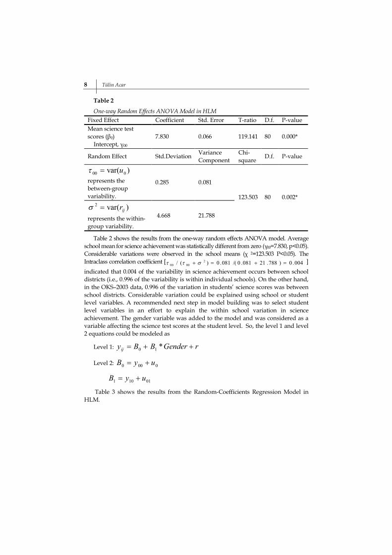
Table 2

One-way Random Effects ANOVA Model in HLM Fixed Effect Coefficient Std. Error T-ratio D.f. P-value Mean science test scores (β0) Intercept, γ00

7.830 0.066 119.141 80 0.000*

Random Effect Std.Deviation Variance Component

Chi-square D.f. P-value

)var( 000 u represents the between-group variability.

0.285 0.081

)var(2ijr

represents the within-group variability.

4.668 21.788

123.503 80 0.002*

Table 2 shows the results from the one-way random effects ANOVA model. Average school mean for science achievement was statistically different from zero (γ00=7.830, p<0.05). Considerable variations were observed in the school means (χ 2=123.503 P<0.05). The Intraclass correlation coefficient [ 004.0)788.21081.0/(081.0)(/ 2

0000 ] indicated that 0.004 of the variability in science achievement occurs between school districts (i.e., 0.996 of the variability is within individual schools). On the other hand, in the OKS–2003 data, 0.996 of the variation in students’ science scores was between school districts. Considerable variation could be explained using school or student level variables. A recommended next step in model building was to select student level variables in an effort to explain the within school variation in science achievement. The gender variable was added to the model and was considered as a variable affecting the science test scores at the student level. So, the level 1 and level 2 equations could be modeled as

Level 1: rGenderBByij *10

Level 2: 0000 uyB

01101 uyB

Table 3 shows the results from the Random-Coefficients Regression Model in HLM.


Table 3

Random-Coefficients Regression Model in HLM Fixed Effect Coefficient Std. Error T-ratio D.f. P-value Mean Science test scores γ00

7.702 0.084 92.214 80 0.000*

The average gender science regression slope across school districts γ10

0.261 0.092 2.842 80 0.006*

Random Effect Std. Deviation

Variance Component


)var( 000 u 0.325 0.106 115.537 80 0.006*

Gender effect, )var( 0111 u 0.093 0.009 69.804 80 >0.500

)var(2ijr 4.666 21.773

The overall mean science achievement across schools was significant from zero (γ00=7.702, p<0.05). Also, a significant difference was observed in gender slope (i.e., the effect of gender on science scores) across schools (γ10=0.261, p<0.05). For each unit increase in student gender, an average increase of 0.261 points occurs in student science scores across schools.

After including gender as a predictor of science achievement within schools, between school variability was reduced by 0.001 [(21.788-21.773)/21.788=0.001] relative to the one-way random effects ANOVA model. A statistically significant difference was observed in the remaining variance in school means (τ00=0.106, p<0.05). This suggests that highly significant differences exist among means from the 81 school districts, which is quite similar to the result from the one way ANOVA with random effects model. This between school variance might be explained after incorporating school level (i.e., level 2) variables. However, since τ11 was not found to be statistically different from zero, the between school variance related to the effect of gender seemed to be adequately explained (τ11=0.009, p>0.500). The relationship between gender and science achievement within schools did not vary significantly across the population of school districts. Additional level 2 (i.e., school-level) predictors were added in an effort to explain between school variance in the following models. Then, Table 4 shows the result of these analyses.

Level 1: rGenderBByij *10

Level 2: 001000 )(* uSESyyB

0111101 )(* uSESyyB

10 Tülin Acar

Table 4

Result of an Intercept and Slopes as Outcomes Model in HLM Fixed Effect Coefficient Std. Error T-ratio D.f. P-value Mean science test scores γ00

7.667 0.087029 88.092 79 0.000*

The main effect of SES γ01

0.0002 0.000059 2.478 79 0.016*

The average gender science regression slope across school districts γ10

0.317 0.091510 3.467 79 0.001*

The cross level interaction involving SES with student gender γ11

-0.0002 0.000062 -1.839 79 0.069

Random Effect Std.Deviation Variance Component


)var( 000 u 0.34101 0.11629 107.77740 79 0.017 Gender effect,

)var( 0111 u 0.18620 0.035 67.68107 79 >0.500

)var(2ijr 4.66546 21.767

Table 4 shows the results of the contextual model with gender in level 1 and SES in level 2. By including SES as a predictor in level 2, 0.001 of the variance [(21.788-21.767)/21.788=0.001] in the between school difference in mean science scores was accounted for by SES. Since τ00=0.116, p<0.05, considerable differences were still observed between schools. These differences might be explained by other level 2 variables. Because τ11=0.035, p>0.05, no significant variance remained in the effect of gender within schools once the adjustment for SES in the school was introduced.

Overall, the mean science achievement across schools was still significantly different from zero (γ00=7.667, p<0.05). Also, a significant effect of SES on mean school science achievement was observed (γ01=0.0002, p<0.05). In other words, students from the school districts where income is high scored on average 0.0002 units higher on the science tests.

The effect of gender on science achievement in schools with average percentage of SES was statistically different from zero (γ10=0.317, p<0.05). The female students’ science test scores are higher that the male students’ test scores. Further, no significant effect of SES on the gender slope was observed (γ11=-0.0002, p>0.05). Additionally, a 0.0002 unit decrease was observed in the science test scores of female students from the high income area.


Conclusions and Recommendations In this study, the science test success of the students who took the OKS (Middle

School Organization Student Selection and Placement Exam) -2003 science test were analyzed using analysis methods and HLM applied to the structure of the nested data. According to the random influence ANOVA model findings, a significant difference was found in the science test scores of the students who attended the examination from different school areas. Additionally, 0.996 of the variance in the test scores came from the variance within the students. Therefore, the gender variable from the student characteristics was added to the model, and the success on the science test was reanalyzed. According to the Random Coefficient Regression Model, the effect of gender on the science scores was significant. However, the between school district variance and the effect of gender seemed to be adequately explained because the relationship between gender and science achievement within school districts does not vary significantly across the population of school districts. By adding the SES variable for each school region to the model, the change in the science scores was analyzed. The science scores were affected by the SES variable for the region where the school is found, and the science scores are also affected by the gender of the students from different school regions. However, no significant effect was observed from both the gender and SES variables together in the science test success.

According to Park (2005), the effects of student engagement are consistent regardless of minority and gender. Among classroom level variables, such as teachers’ degree, experience, certification, authentic instruction, content coverage, and class size, no significant predictor of student math achievement growth has been identified. The findings suggest that student engagement and educational policy for student success should be emphasized in a school.

Acar (2005) indicated that a relationship of medium level significance was found between the OKS science test scores and the social studies test scores of 2001-2002 and 2003. Additionally, when the results from Park (2005) are considered, analyzing the variables belonging to the student (e.g., academic past) and variables belonging to the environment in which the student resides (e.g., experience of the instructor, study time at home, number of students in class, and school size) at a micro and macro level may render the research results more reliable in analyses concerning student success in later studies. Novy and Francis (1989) suggested that group research for statistical methods are better suited for the study of group processes than traditional analyses of variance and multiple regression.

12 Tülin Acar

References

Acar, T. (2005). OKÖSYS Sosyal Bilimler Test Başarı Puanlarının Diğer Alt Test Başarı Puanları ve Cinsiyet Değişkeni İle Karşılaştırılması. Egitim Arastirmalari-Eurasian Journal of educational Research,21.

Bryke, A. S. & Raudenbush, S.W. (1992). Hierarchical linear models. Thousand Oaks, CA: Sage.

Franks, M.E. and others (1996, April). An analysis of NEAP trial state assessment data concerning the effects of computers on Mathematics achievement. Paper presented at the annual meeting of the American Educational Research Association, New York.

Koopmans, M. (1998, April). Application of HLM to the evaluation of the effects of basic skills programs on Math achievement. Paper presented at the annual meeting of the American Educational Research Association, San Diego (ERIC Document Reproduction Service No. ED 419 843).

Liu, X. (2004, October). Applying HLM to estimate reading achievement. Paper presented at the 35th annual Conference of the Northheastern Educational Research Association, New York

Novy, D.M., & Francis, D.J. (1989, August). An application of hierarchical linear modeling to group research. Paper presented at the 1989 annual meeting of the American Psychological Association, New Orleans

Opdenakker, M.& Van Damme, J. (1998, April). The impotances of indentifinglevels in multilevel analysis. Paper presented at the annual meeting of the American Educational Research Association, San Diago. (ERIC Document Reproduction Service No. ED 422 400).

Osborne, J.W. (2000). Advantages of hierarchical linear modeling. Practical Assessment, Research, and Evaluation, 7(1). Retrieved 26 November 2007 from http://www4.ncsu.edu/~jwosbor2/otherfiles/MyResearch/PARE2000-HLM.pdf

Park, S. (2005). Student engagement and classroom variables in improving mathemetics achievement. Asia Pacific Education Review. Vol. 6, No. 1, 87-97.

Raudenbush, S. W., & Bryk, A. S. (2002). Hierarchical Linear Models: Applications and Data Analysis Methods. Sage Publications.

Subedi, B.R. (2005) Demonstratıon of the three-level hierarchical generalized linear model applied to educational research. Unpublished doctoral dissertation, The Florida State University (UMI No. 3183114).

Tamada, M. (2002, June). Predictors of graduation rates: Why they can be expected to have greater predictive value at the national level than at the intuitional research. Paper presented at the annual forum of the Association for intuitional Research, Toronto.(ERIC Document Reproduction Service No. ED 472 474).


Wang, J. (2000, April).Relevance of the hierarchical linear model to TIMSS data analysis. Paper presented at the annual meeting of the American Educational Research Association, New Orleans. (ERIC Document Reproduction Service No. ED 441 432).

Webster, W. J. and others (1996, April). The applicability of selected regression and hierarchical linear models to the estimation of school and teacher effects. Paper presented at the annual meeting of the National Council or Measurement in Education, New York. (ERIC Document Reproduction Service No. ED 400 320).

Williams, N. J. (2003). Item and Person Parameter Estimation using Hierarchical Generalized Linear Models and Polytomous Item Response Theory Models, Doctor of Philosophy: Unpublished doctoral dissertation, The University of Texas at Austin.(UMI No. 3116234).

Willms, J.D. (1999). Basic Concepts in Hierarchical Linear Modeling with Applications for Policy Analysis. In G. Cizek (Ed.), Handbook of educational policy. San Diego, CA: Academic Press. Retrieved 10 February 2008 from http://www.unb.ca/crisp/pdf/9806land.pdf

Zhang, Y.&Zhang, L. (2002, April). Modeling school and district effect in the Math achievenment of delaware students measured by DSTP: A preliminary application of hierarchical linear modeling in accountability study. Paper presented at the annual meeting of the American Educational Research Association, New Orleans. (ERIC Document Reproduction Service No. ED 468 962).

Aşamalı Doğrusal Modellemede Bir Uygulama:

OKS–2006 Fen Testi Başarısı

(Özet)

Problem Durumu: Son yıllarda iç içe geçmiş veri yapısı sergileyen verilerde aşamalı doğrusal modelleme (ADM) sıkça kullanılmaktadır. Veriler iç içe geçmiş veri yapıları sergiledikleri zaman, klasik doğrusal modellere ilişkin başlıca varsayımların (veri grubundaki gözlemlerin, veri grubundaki diğer gözlemlerle olan bağımsızlığı) ihlal edildiği bir yapıya sahip olurlar. Örneğin, eğitimde sıkça öğrencilerin çeşitli alanlardaki başarı puanları incelenir ve eğitim sisteminde öğrenciler sınıflardan (eğitim aldıkları ortamlardan), sınıflarda içinde bulundukları okullardan bağımsız olarak düşünülemez. Öğrenciler, aynı sınıfın içinde ortak bir öğretmeni, ortak bir öğretme sitilini ve ortak bir öğrenme deneyimlerini paylaşırlar. Bu ortak deneyimler nedeniyle, öğrenci başarı puanları, aynı sınıfın içindeki diğer öğrencilerin başarı puanlarıyla doğrudan ilişkilidir ve bağımsız olarak düşünülemez. Aşamalı ya da iç içe geçmiş verilere standart regresyon eşitlikleri uygulandığında da bazı problemlerle karşılaşılır. En temel

14 Tülin Acar

problem gözlemlerin bağımsızlığı sorunudur. Standart regresyon modellerinde değişkenlerin birbirinden bağımsız olma koşulu hiyerarşik verilerde bozulduğundan hiyerarşik yapılarda bulunan gözlemler, birbirlerine, tesadüfî yolla örneklenen gözlemlerden daha çok benzer olma eğilimindedirler. ADM’de değişkenler birkaç şekilde modellenebilir. Bu çalışmada ADM’de değişkenlerin 3 farklı şekilde modellemesi açıklanmıştır.

1-ADM’de Koşulsuz Modelleme Ya Da Tesadüfî Etkili ANOVA: ADM’nin en basiti, kestiricileri olmayan “koşulsuz modelleme” yöntemidir. Araştırmacılar, sonuç değişkeninin kestirimiyle ilgilenir fakat öğrenci veya sınıf düzeyinde her hangi bir kestirici değişken modelde kullanılmaz. Bu haliyle bu teknik, tek yönlü varyans analizi modeline eştir. Bu model genellikle, düzeylere ayrılmış sonuç değişkeni değerlerinde varyansın bölünüp bölünmediğini belirlemek için ADM’de birinci adım olarak kullanılır. Örneğin, birçok yerleşim yerinden sınava katılan öğrencilerin fen bilgisi test puanları sonuç değişkeni olarak tanımlandığında ADM’de en küçük düzey olan düzey 1(öğrenci düzeyi) şöyle tanımlanır:

ijjij rBy 0

Denklemdeki ijy , j. okul bölgesindeki i.öğrencinin fen bilgisi test

başarısıdır. jB0 , j.okul bölgesi için fen bilgisi test puanlarının ortalaması

ve ijr ortalaması sıfır, varyansı 2 olan bir normal dağılama yaklaşan

düzey 1 denkleminin hatası olarak düşünülür. 2. aşama olan düzey 2 (okul bölgesi modeli) denklemi,

jj uyB 0000 olarak kurulur. Bu denklemde, jB0 j. okul için fen

bilgisi test puanlarının ortalamasıdır. 00y , tüm verilerdeki gözlemlere ait

fen bilgisi test puanlarının genel ortalaması ve ju0 , j.okul bölgesine ait

ortalaması sıfır, varyansı 00 olarak değişen tesadüfî etkidir. Düzey 1 ve 2 model denklemleri birleştirildiğinde birleştirilmiş modelde şu şekilde oluşturulur:

ijjij ruyy 000

Sonuç değişkeni için toplam varyans, 2000 )()( ijjij ruVaryVar

olarak tanımlanır. Denklemdeki 2 gruplar içi değişkenliği (öğrenciler

arasındaki değişkenliği) ve 00 gruplar arası değişkenliği (okul bölgeleri arasındaki değişkenliği) temsil eder.


2- Düzey 1 Denklemine Kestiriciler Ekleme: Tesadüfî Katsayılı Regresyon Modeli ADM’de bu model, regresyon tekniğinin özel bir halini temsil eder. Koşullu modelleme koşulsuz modellemenin aksine, ilgili kestiriciler (örneğin öğrencilerin cinsiyeti) düzey 1 denklemine eklenir. Şöyle ki, Düzey 1 denklemi: ijijjjij rXBBy 110

ijy sonuç değişkenidir (fen bilgisi test puanları), jB0 j. okul bölgesi için

beklenen fen bigisi test puanları, X1 is kestirici değişken (öğrencilerin cinsiyeti değişkeni), jB1 cinsiyet değişkeni ile ilgili fen bilgisi test

puanlarında beklenen değişim ve ijr hata terimi. ADM’de Düzey 2

denklemi, düzey 1 denkleminin parametreleri düzey 2 denkleminin sonuç değişkeni olarak ele alınır. Düzey 2 denklemi,

jj uyB 0000

jj uyB 1101 olarak modellenir.

ADM’de düzey 2 denkleminde jB0 ve jB1 düzey 1 denkleminde

kestirilen kesim noktası değerleri bir sonuç değişkeni olarak modellenir.

00y fen bilgisi test puanlarının genel ortalaması, 10y cinsiyetler arasındaki

ortalama regresyon eğim değeri, ju0 ve ju1 düzey 2 denkleminin tesadüfi

etkileri olarak modellenir. Bu modelde kestirici değişken düzey 1 modeline eklenir fakat düzey 2 modeli için herhangi bir kestirici değişken eklenmemiştir. Düzey-2 modeline de kestirici değişken eklendiğinde kurulan model, tesadüfi etkili regresyon modelinden bir anlamda farklılaşır. 3- Düzey 1 ve 2 Denklemine Kestiriciler Ekleme: Sabit ve Eğim Parametrelerinin Çıktı Olduğu Modeller: ADM’de öğrenci düzeyindeki modele (düzey 1 modeline), sonuç değişkenini etkilediği düşünülen kestirici değişkenler eklenebildiği gibi öğrencilerin dahil olduğu gruplara ilişkin kestirici değişkenlerde eklenebilir. ADM’de oluşturulan düzey 2 denklemindeki kestiriciler alt gruplar arasındaki değişkenliği açıklamaya yardımcı olur. Düzey 1 denklemi, “tesadüfi katsayılı regresyon modelinin düzey 1 denklemi” ile aynı olurken düzey 2 denklemi şu şekildedir:

jjj uWyyB 0101000

jjj uWyyB 1111101

jB0 ve jB1 düzey 1 denkleminden kestirilen kesim noktası değerleridir.

Dikkat edilirse düzey 1 denkleminin kestirici değişkenleri, düzey 2 denkleminde sonuç değişkeni olarak kullanılır.

16 Tülin Acar

jB0 j. okul bölgesinin kesim noktası, jB1 j. okuldaki cinsiyet değişkeni

için beta katsayısı, 00y düzey 2 denklemindeki okul bölgeleri arasında

değişen ortalama kesim noktası, 10y okul bölgeleri arasında değişen

ortalama regresyon eğim noktası, ju0 ve ju1 düzey 2 denkleminin

tesadüfi etkileridir. jW1 j. okul bölgesindeki düzey 2 denkleminin kestirici

değişkenin (örneğin okul bölgelerinin gelir düzeyleri) göstergesidir.

Araştırmanın Yöntemi: Araştırma verileri 10727 öğrencinden elde edilmiştir. Araştırmanın değişkenleri öğrencilerin OKS-2006 Fen bilgisi alt testine vermiş oldukları yanıtlar, öğrencilerin cinsiyeti, öğrenim gördükleri okulun bulunduğu yerleşim yeri ve bu yerleşim yerine ait kişi başına düşen gayri safi yurt içi hasıla(YTL)’dır.

Araştırmanın Sonuçları ve Öneriler: Bu çalışmada iç içe geçmiş veri yapılarına uygulanan analiz yöntemlerinden ADM ile OKS–2003 Fen bilgisi testini cevaplayan öğrencilerin fen bilgisi test başarıları analiz edilmiştir. ADM’ de kurulan tesadüfî etkili ANOVA modelinin bulgularına göre farklı okul bölgelerinden sınava katılan öğrencilerin fen bilgisi test puanlarında anlamlı bir fark bulunmuştur. Bunun yanı sıra, test puanlarındaki değişkenliğin 0.996’sının öğrenciler içindeki değişkenlikten kaynakladığı görülmüştür. Bunun üzerine modele öğrenci özelliklerinden cinsiyet değişkeni eklenmiş ve fen bilgisi başarısı tekrar incelenmiştir. ADM’de tesadüfî katsayılı regresyon modeline göre öğrencilerin fen bilgisi test puanları üzerinde cinsiyetin etkisinin anlamlı olduğu bulunmuştur. Ancak, ADM’de okul düzeyinde kurulan modele, okul bölgelerine ilişkin sosyo-ekonomik düzey bilgisi eklenerek öğrencilerin fen bilgisi testi başarılarındaki değişim tekrar incelenmiştir. Fen bilgisi test puanlarının okulun bulunduğu yerleşim yerinin sosyo-ekonomik durumundan etkilendiği ve aynı zamanda farklı okul bölgelerinden gelen öğrencilerin cinsiyet değişkeninden fen bilgisi puanlarının etkilendiği görülmüştür. Ancak, öğrencilerin fen bilgisi test başarılarının hem cinsiyetinden hem de öğrenim gördükleri okullarının bulunduğu yerleşim yerinin sosyo-ekonomik durumundan etkilenmediği, fen bilgisi puanları üzerinde öğrencilerin cinsiyetlerinin ve öğrenim gördükleri okulların bulunduğu yerleşim yerinin sosyo-ekomnomik durumun anlamlı bir etkisinin olmadığı görülmüştür. Öğrenci başarısına ilişkin incelemelerde, öğreniciye ait değişkenler (akademik geçmişi) ve öğrencinin içinde bulunduğu çevreye ait değişkenler (öğretmenin tecrübesi, evde çalışma süresi, sınıftaki öğrenci sayısı, okulun büyüklüğü, okulun türü…v.b.) olmak üzere çoklu düzeyde incelenmesi, geleneksel istatistiksel yöntemlerin sonuçlarına göre araştırma sonuçlarının karşılaştırmalarının yapılması önerilmektedir.

Anahtar Sözcükler: Aşamalı doğrusal modelleme, çok düzeyli istatistikler, fen bilgisi başarısı

An Application of Hierarchical Linear Modeling: OKS-2006 Science Test Achievement

Documents

Transcript of An Application of Hierarchical Linear Modeling: OKS-2006 Science Test Achievement