
Incorporating Predictive Maintenance Practices into Marine ...
Upload
khangminh22Category
view
2download
0
FEDERAL UNIVERSITY OF SANTA CATARINAGRADUATE PROGRAM IN PRODUCTION ENGINEERING
Éder Vasco Pinheiro
AN APPLICATION OF DISTRIBUTED MODEL PREDICTIVECONTROL TO SUPPLY CHAIN MANAGEMENT
Florianópolis
2017

Éder Vasco Pinheiro
AN APPLICATION OF DISTRIBUTED MODEL PREDICTIVECONTROL TO SUPPLY CHAIN MANAGEMENT
Dissertation presented to the Grad-uate Program in Production Engi-neering in partial fulfillment of therequirements for the degree of Mas-ter in Production Engineering, areaLogistic and Transport.
Advisor: Prof. Enzo Morosini Frazzon, Dr.
Florianópolis
2017
Ficha de identificação da obra elaborada pelo autor, através do Programa de Geração Automática da Biblioteca Universitária da UFSC.
Pinheiro, Eder Vasco An Application of Distributed Model PredictiveControl to Supply Chain Management / Eder VascoPinheiro ; orientador, Enzo Morosini Frazzon, 2017. 122 p.
Dissertação (mestrado) - Universidade Federal deSanta Catarina, Centro Tecnológico, Programa de PósGraduação em Engenharia de Produção, Florianópolis,2017.
Inclui referências.
1. Engenharia de Produção. 2. Cadeias deSuprimento. 3. Controle Preditivo Distribuido. 4.Planejamento Logístico Operacional. I. Frazzon, EnzoMorosini. II. Universidade Federal de SantaCatarina. Programa de Pós-Graduação em Engenharia deProdução. III. Título.


I dedicate this work to my family.


ACKNOWLEDGEMENTS
I am grateful to the Federal University of Santa Catarina, its GraduateProgram in Production Engineering and my adviser Enzo Morosini Fraz-zon, for letting me achieving a Master degree. Through the course ofthese years, many people contributed somehow to this final dissertation,I thank them all, but especially Dr. Jürgen Pannek.This work should be dedicated to my family which deserves my thanksfor all the support they have given to me. I am especially grateful to mywife Vanessa who gave me diary support.


Time delays between taking a decision andits effects on the state of the system are com-mon and particularly troublesome.
(John D. Sterman, 2000)

RESUMO ESTENDIDO
Os produtos e servicos não apresentam valor até que eles literal-mente estejam no lugar e no instante que os consumidores precisam.O conjunto de princípios e técnicas que busca garantir esses valoresbaseados no tempo e na localizacão é atribuído a definicão de logística.Portanto, sempre que houver um processo incluem o planejamento, aimplementacão e o controle de fluxos de informacões e de bens ouservicos entre origem ofertantes e destinos consumidores, então trata-se de um processo logístico. A base para este trabalho é o planejamentooperacional, parte do processo logístico em uma cadeia de suprimentos.
Uma Cadeia de Suprimento é um conjunto de estruturas e pro-cessos que uma ou várias organizacões usam para atender a demandade um grupo de clientes. Entre as várias formas de visualizá-la, pode-se descrevê-la através de uma rede ou grafo cujos nós são os elos dacadeia e os arcos as conexões entre eles. Entre o conjunto de processosda cadeia de suprimentos, a logística tem seu papel de destaque ampli-ado ao longo da evolucão do seu conceito. Com isso, nas cadeias desuprimento, muitas vezes, a definicão do processo logístico ultrapassaas barreiras de uma única organizacão. Assim surge a Gestão da Cadeiade Suprimentos, que é composta por todas as atividades envolvidas naintegracão da cadeia de suprimentos e na coordenacão dos fluxos demateriais, os fluxos de informacões e os fluxos financeiros. A integracãoda cadeia de suprimentos visa promover a vantagem competitiva à ca-deia como um todo em detrimento de apenas um dos seus elos.
Os desafios da gestão da cadeia de suprimentos surgem de pro-blemas relacionados às mudancas no meio ambiente da cadeia, quenormalmente contêm várias incertezas, especialmente as relacionadasa demanda e tempos dos processos. O planejamento, em todos os seushorizontes, constituiu uma acão básica para este processo de busca pormelhoria da eficiência, a performance logística. Entre as etapas de pla-nejamento, estratégico, tática e operacional, o Planejamento Operacio-nal em logística é uma atividade que desempenha um papel importantena superacão de problemas de curto prazo na gestão da cadeia. Umdos problemas nesta atividade é a estabilizacão das variáveis de estado,especialmente a variável nível de estoque.
O problema de interesse da proposta deste trabalho de dissertacãoé a estabilizacão e otimizacão do nível de estoque contra a variacão dademanda, de forma a buscar a maior reducão possível do Efeito Chicote.Como consequência, este trabalho trata da ligacão entre a teoria de con-trole e gestão da cadeia de suprimentos através de Modelos de ControlePreditivo. A motivacão para apresentar um trabalho com essa aborda-
11
gem surgiu a partir da leitura do trabalho Supply Chain Optimizationvia Distributed Model Predictive Control (PANNEK; FRAZZON, 2014). Osbenefícios de aplicar a metodologia de controle preditivo à problemaslogísticos provêm do fato de que tal metodologia facilita o uso de váriostipos de modelos preditivos do sistema e, também, por ela utilizar valo-res atuais e passados do processo enquanto prevê o comportamento dosistema em um horizonte de planejamento. Usando essa capacidade deprevisão, os modelos de controle preditivo minimizam uma funcão ob-jetivo e calculam uma sequência de controles satisfazendo as restricõese o modelo do sistema.
A metodologia de controle preditivo para um modelo discreto dosistema segue uma idéia simples: a cada instante de tempo, usando oestado atual do sistema como estado inicial da sequência, a acão de con-trole é obtida através da solucão de um problema de controle ótimo emum horizonte finito de tempo. Com isso se obtém sequência finita devalores de controle e dela somente o primeiro elemento é aplicado aosistema. A simplicidade e qualidade desta metodologia mostra-se peloamplo uso que ela tem em processos industriais. Além disso, as refe-rência bibliográficas indicam a prevalência dela no controle de sistemascomplexos quando a solucão dadas por equacões de programacão dinâ-mica são computacionalmente intratáveis em problemas com grande di-mensionalidade. Mais ainda, os controles distribuídos preditivos podemviabilizar a solucão de problemas ainda maiores, dos quais a sociedadedepende fortemente, como redes de tráfego rodoviário, redes de água,redes eléctricas e redes de transporte intermodal.
Aliado a adequabilidade de um framework para otimizacão den-tro do planejamento operacional da logística de uma cadeia de supri-mentos, o cenário atual da introducão da tecnologia da informacão ecomunicacão como solucões à logística motiva ainda mais este tipo deestudo, o qual tem forte tendência a se desdobrar como ferramentapara solucão em tempo real às fortes mudancas das premissas usadaspara o planejamento operacional. De fato, as tecnologias da informacãotendem a facilitar a coleta de dados e a atuacão remota, fazendo comque os dados estejam disponíveis online e em tempo real. Portanto,os aperfeicoamentos dos modelos matemáticos e das metodologias queproporcionam apoio a tomada de decisão rápida são fundamentais.
As Cadeias de Suprimento têm a propriedade de serem sistemasdistribuídos que podem ou não ter uma gestão centralizada. Por isso,apesar deste trabalho destacar um modelo preditivo distribuído para acadeia logística de três estágios, o modelo com o controle centralizadotambém foi descrito e implementado. Assim, além deste trabalho apre-sentar um modelo conceitual baseado em Controle Preditivo Distribuído
para a Gestão da Cadeia de Suprimento, para efeitos de comparacãodo resultado, também apresenta um modelo com gestão centralizada.Por meio de experimentos desenvolvidos a partir da implementacão dosmodelos em Matlab, analisa-se algumas propriedades tais como estabi-lidade dos procedimentos, a influência do horizonte de planejamentono controle preditivo e o comportamento do Efeito-Chicote quando hávariacões da demanda final.
Como ferramenta de apoio a tomada de decisão, a abordagemapresentada busca dar maior entendimento da dinâmica do sistema,que se torna necessário aos gestores que participam de algum elo dacadeia e precisam considerar a dinâmica das rápidas mudancas da de-manda. No contexto de uso desta abordagem em um cenário real deve-se considerar possíveis restricões de acesso a informacão entre elos dacadeia de suprimentos. Além disso, pelo problema em questão possuiro fator humano da tomada de decisão pelos gestores do processo logís-tico a aplicacão das variáveis de controle não acontece como acontecenos processos industriais, em que a acão é executada instantaneamente.Todas essas questões teóricas ou experimentas são tratadas ao longo dadissertacão.
O primeiro capítulo apresenta detalhadamente o problema deinteresse que gerou os desenvolvimentos realizados nesta dissertacão.Além de tratar o contexto do estudo, esse capítulo destaca os objetivos,as contribuicões e as delimitacões do trabalho. O segundo capítulo con-tém toda a revisão de literatura estruturada, assim como a metodologiautilizada para reunir as bibliografias e as expor de forma organizada.Portanto, esse capítulo dedicado à exposicão das referências bibliográfi-cas foi organizado em quatro secões, uma para descrever a metodologia,duas para apresentar o entendimento dos conteúdos básicos do tema depesquisa e uma para apresentar o estado da arte do assunto específicodo trabalho. No terceiro capítulo é feita toda a descricão e deducão domodelo de controle preditivo formulado para o planejamento operaci-onal da cadeia de suprimentos com três elos. Como são apresentadoso modelo de gestores distribuídos e com gestor centralizado, cada umdeles possui sua própria secão. Ademais as duas secões, a terceira secãoapresenta uma breve visão sobre as restricões sobre usos práticos dosmodelos. O quarto capítulo apresenta o resultado dos experimentos re-alizados em Matlab. Esse capítulo contém uma secão para análise dosresultados do modelo distribuído e outra para uma análise comparativadele com o modelo centralizado. As conclusões são apresentadas noquinta capítulo assim com as observacões sobre pesquisas que podemsurgir como sequência ao que foi desenvolvido nesta dissertacão. Porfim, os códigos produzidos na implementacão dos modelos estão pre-

sentes após a lista das referências bibliográficas que foram citadas emtodo o texto.
Palavras-chave: Cadeias de Suprimento. Controle Preditivo Distri-buído. Planejamento Logístico Operacional.


ABSTRACT
A Supply Chain is a set of structures and processes an organiza-tion uses to deliver an output to group of customers. Among this set ofprocesses, the subset, defined as the logistics, is dedicated to providingvalues to customers making products or services available to them atthe appropriate location and time. The more quickly and completelythe demand can be met, the better the logistics process performance.Broadening the concept of logistic, the Supply Chain Management en-compasses all activities involved in integrating a Supply Chain and co-ordinating materials, information and financial flows in order to fulfillthe ultimate customer demands. This integration functionality aims toimprove the competitive advantage of the Supply Chain as a whole.
The challenges in Supply Chain Management arise from prob-lems related to changes in the Supply Chain environment, which nor-mally contain some degree of uncertainty. The Planning is the firstaction to evolve this process forward improving efficiency. This way,the Operational Planning plays a great role in overcoming Supply ChainManagement short-time problems. A problem in this step is stabilizationof states variables, especially the stock level. The problem of interestis the implementation of a controller for a set of dynamically coupledlinear subsystems called Three-Stage Supply Chain. Hence, the mainpurpose of this work is optimization and stabilization of stocks levelsagainst demand variation considering this entire Supply Chain with amodel predictive controller formulation.
The Model Predictive Control is one of the techniques which canbe applied to systems adaptation. Its advantages are particularly thebenefits relating the use of a system model, and both current and his-torical measurements of the process to predict the systems’ behaviourfor a planning horizon. Using this prediction ability, it minimizes anobjective function and calculates a control sequence satisfying the con-straints of the system. The Supply Chain (SC) has the property to bea distributed system, which can have centralized or even distributedmanagers. Therefore, this work presents a Distributed Model Predic-tive Control procedure to stabilize the stocks levels considering the dis-tributed view of the SC, and also a centralized Model Predictive Controlfor the purpose of comparability. Furthermore, it presents the resultsfrom a computational analysis of the application of both models.
Keywords: Supply Chain. Distributed Model Predictive Control. Op-erational Logistic Planning.
17

LIST OF FIGURES
1.1 Flows representation of a three-stage SC . . . . . . . . . 281.2 Venn diagram representing the two axes of research and
their intersection, which is the objective proposal research 32
2.1 Number of articles over time . . . . . . . . . . . . . . . . 362.2 Pareto Criterion or Rule 80-20 . . . . . . . . . . . . . . . 372.3 Supply Chain interconnected elements . . . . . . . . . . 412.4 Illustration of the Bullwhip Effect . . . . . . . . . . . . . 462.5 Model predictive control - rolling horizon illustration . . 492.6 Ilustration for network of the Beer Game . . . . . . . . . 57
3.1 Information and material flow for the three stage SC . . 653.2 Model predictive control - rolling horizon illustration . . 683.3 Procedure Flow: Decentralized Approach . . . . . . . . . 693.4 Information and material flow for the three stage SC . . 703.5 Procedure Flow: Centralized approach . . . . . . . . . . 72
4.1 E1-S1: Graphics of Stock, Unfulfilled order and Order . . 754.2 E1-S2: Graphics of Stock, Unfulfilled order and Order . . 764.3 E2-S1: Graphics of Stock, Unfulfilled order and Order . . 774.4 E2-S2: Graphics of Stock, Unfulfilled order and Order . . 784.5 E3-S1: Stock, Unfulfilled order and Order for distributed
model . . . . . . . . . . . . . . . . . . . . . . . . . . . . 794.6 E3-S1: Stock, Unfulfilled order and Order for centralized
model . . . . . . . . . . . . . . . . . . . . . . . . . . . . 794.7 E3-S2: Stock, Unfulfilled ordera and Order for distributed
model . . . . . . . . . . . . . . . . . . . . . . . . . . . . 804.8 E3-S2: Stock, Unfulfilled order and Order for centralized
model . . . . . . . . . . . . . . . . . . . . . . . . . . . . 80
19

LIST OF TABLES
2.1 Number of papers by source . . . . . . . . . . . . . . . . 38
3.1 Summary of variables’ notations for stage p and time tn . 65
4.1 Values for each experiments . . . . . . . . . . . . . . . . 74
21

LIST OF ABBREVIATIONS AND ACRONYMS
DMPC Distributed Model Predictive Control . 17, 30–33, 51, 52,56–59, 63, 72, 78, 81, 83, 84
ICT Information and Communication Technology . . . . . . . 30
M Manufacturer . . . . . . . . . . . . 27–29, 63, 64, 66, 75, 77
MPC Model Predictive Control 17, 29–33, 35, 38, 47–56, 59–61,63, 66, 67, 69–73, 78, 81, 83
QP Quadratic Programming . . . . . . . . . . . . . . . . . . . 52
R Retailer . . . . . . . . . . . . . . . . 27–29, 63, 64, 66, 69, 75
RH Receding Horizon . . . . . . . . . . . . . . . . . . . . . . 43
RHC Receding horizon control . . . . . . . . . . . . . . . . . 43
S Supplier . . . . . . . . . . . . . . 27–29, 63, 64, 66, 69, 75, 77
SC Supply Chain 17, 19, 27–33, 39–45, 53, 54, 56–60, 63, 65, 66,68, 70–72, 81, 83, 84
SCM Supply Chain Management 17, 27, 28, 30–33, 35, 38–42, 44,47, 53, 54, 56, 59, 72, 83, 84
SQP Sequential Quadratic Programming . . . . . . . . . . . . 52
SS Supply Chain Stages . . . . . . . . . . . . . . . 63, 68, 70, 71
23

CONTENTS
1 Introduction 271.1 Problem Context . . . . . . . . . . . . . . . . . . . . 271.2 Problem Statement . . . . . . . . . . . . . . . . . . . 301.3 Objective, Contributions and Delimitations . . . . . . 311.4 Research methodology . . . . . . . . . . . . . . . . . 321.5 Organization of the dissertation . . . . . . . . . . . . 33
2 Literature Review 352.1 Search Methodology . . . . . . . . . . . . . . . . . . 352.2 Supply Chain Management . . . . . . . . . . . . . . . 39
2.2.1 Logistics Management Concepts . . . . . . . . 392.2.2 Oscillation and the Bullwhip Effect . . . . . . 45
2.3 Model Predictive Control . . . . . . . . . . . . . . . . 472.4 Applications of MPC in SCM . . . . . . . . . . . . . . 53
2.4.1 Centralized models . . . . . . . . . . . . . . . 532.4.2 Decentralised or distributed models . . . . . . 56
3 A Model Predictive Control Framework for Supply ChainOperational Planning 633.1 A Distributed Managers Model . . . . . . . . . . . . . 633.2 A Centralized Manager Model . . . . . . . . . . . . . 693.3 Some restraints about using the model in a real system 72
4 Experiments 734.1 Distributed Model Results . . . . . . . . . . . . . . . 754.2 The Centralized against the Distributed Model . . . . 78
5 Conclusion 83
Bibliography 87
Appendix 93

1 INTRODUCTION
This document describes the work required to get a Master’sDegree in Production Engineering. In this chapter there is context,purpose, focus and significance for this study. Furthermore, it presentsa description of the methodology used to perform the work in ascientific context. The last chapter subject is the overview of thefollowing chapters.
1.1 PROBLEM CONTEXT
Products and services would not have value unless they arewith customers when and where they wish to consume them. Thereis a set of principles and techniques which seeks to achieve thisvalue and it is called the logistical process. The Logistic is the pro-cesses of "planning, implementation, and controls the efficiency, ofeffective forwards and reverses flows and storage of goods, servicesand related information between the origin and consumption pointsin order to meet customers’ requirements" (CSCMP, 2013). Thisway, the logistic process creates value by timing and positioning in-ventory. Then, the more quickly and completely the demand can bemet, the better the logistics process performance. This process is thecombination of a firm’s order management, inventory, transporta-tion, warehousing, materials handling, and packaging as integratedthroughout a facility network (BOWERSOX et al., 2002).
The SC, also called the value chain or demand chain, are thenetwork of organizations engaged in provide a product or servicefrom supplier to customer, or in the words of Chopra and Meindl(2010), it consists of all parties involved in fulfilling costumers’ re-quirements. That logistic definition given by (CSCMP, 2013), andreinforced by (BALLOU, 2006), implies that logistic is part of alarger process which consists in the management of SC. That is theunderstanding considered for this dissertation, which also meansto agree with Bowersox et al. (2002) who wrote that logistics, incontrast to Supply Chain Management (SCM), is the work requiredto move and position inventory throughout a supply chain. As such,logistics is a subset of and occurs within the broader framework ofa SC.
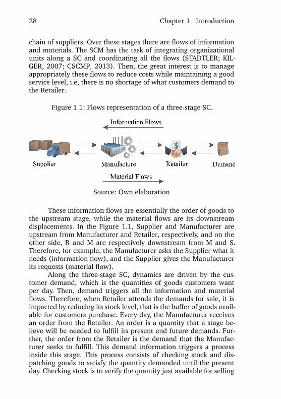
The Figure 1.1 shows a simplified representation of flows ina three stage SC consisting of a Supplier (S), a Manufacturer (M),and a Retailer (R). More specifically, this SC is a logistic chain,but throughout this work it is treated by its broad meaning, the
27
28 Chapter 1. Introduction
chain of suppliers. Over these stages there are flows of informationand materials. The SCM has the task of integrating organizationalunits along a SC and coordinating all the flows (STADTLER; KIL-GER, 2007; CSCMP, 2013). Then, the great interest is to manageappropriately these flows to reduce costs while maintaining a goodservice level, i.e, there is no shortage of what customers demand tothe Retailer.
Figure 1.1: Flows representation of a three-stage SC.
Source: Own elaboration
These information flows are essentially the order of goods tothe upstream stage, while the material flows are its downstreamdisplacements. In the Figure 1.1, Supplier and Manufacturer areupstream from Manufacturer and Retailer, respectively, and on theother side, R and M are respectively downstream from M and S.Therefore, for example, the Manufacturer asks the Supplier what itneeds (information flow), and the Supplier gives the Manufacturerits requests (material flow).
Along the three-stage SC, dynamics are driven by the cus-tomer demand, which is the quantities of goods customers wantper day. Then, demand triggers all the information and materialflows. Therefore, when Retailer attends the demands for sale, it isimpacted by reducing its stock level, that is the buffer of goods avail-able for customers purchase. Every day, the Manufacturer receivesan order from the Retailer. An order is a quantity that a stage be-lieve will be needed to fulfill its present end future demands. Fur-ther, the order from the Retailer is the demand that the Manufac-turer seeks to fulfill. This demand information triggers a processinside this stage. This process consists of checking stock and dis-patching goods to satisfy the quantity demanded until the presentday. Checking stock is to verify the quantity just available for selling
1.1. Problem Context 29
and the dispatching consists of delivering that quantity as soon aspossible. While delivering the products to the downstream stage, itis natural to exists a delay into that operation. Such delay should betaken into account because it can reduce performance in the logisticprocess.
The foregoing flows between Retailer and Manufacturer simi-larly exists for Manufacturer and Supplier. Then, every day the Man-ufacturer orders the quantity it needs for the Supplier, which shouldcheck stock and prepare for the delivery of goods downstream. Thiscontext assumes the Supplier does not order at any other stage andit is self-sufficient, however there is a delay between the Supplieridentifying its needs and having goods available.
The context of the Three-Stage SC is the same as the "BeerGame", which Sterman (1989) created to explain many phenomenonoccurring when flowing information and products between differ-ent agents. Although the name refers to beer, the product can be in-terpreted as any kind. For example, when used amongst high schoolstudents, this game is recast as the "apple juice game". When thisgame is applied in a company to explain what happens in SC, thenit is customized to represent the product of its industry. Here, forthe illustration purpose, it can be thought of as the Supplier offer-ing bottles to the Manufacturer, who brews and "bottles" the beer,and then ships it to the Retailer for sale to customers. Despite thesimplicity of the beer game, it is an example of a situation wherecyclical instability arises from the failure of decision makers to ac-count for time delays (STERMAN, 2000).
The dynamics of SC exists under an optimization process whichdepends on the demand over time. Then, its continuous necessityfor adaptation makes the Model Predictive Control (MPC) a naturalframework to deal with this class of problem (IVANOV et al., 2012).The MPC, or receding horizon control, has now become a standardcontrol methodology for industrial and process systems. Its wideadoption from the industry is largely based on the inherent abilityof the method to efficiently handle constraints and the non-linearityof multi-variable dynamic systems (SARIMVEIS et al., 2008).
The MPC methodology follows a simple idea: at each discrete-time instance, using the current state of the system as the initialstate, the control action is obtained by on-line solving a finite-horizonopen-loop optimal control problem. In this way, a finite-optimal con-trol sequence is obtained, from which only the first element is keptand applied to the system, that here is the SC illustrated by Fig-ure 1.1. The procedure is repeated after each state transition. The
30 Chapter 1. Introduction
MPC is prevalent in the control of complex systems where the off-line solution of the dynamic programming equations is computa-tionally intractable due to the high problem dimensionality (CAMA-CHO; BORDONS, 2007).
The planning is part of logistic process, and managing the in-formation and material flows between suppliers and customers intothe SC consider decisions, or planning, levels classified as strategic(long term), tactical (medium term), and operational (short term)(CHOPRA; MEINDL, 2010). These levels are defined by the timeperiod in which decisions are to be made and operational planningworks with the decisions which need more frequent to be taken. Thedaily decisions is the interest of this work besides the MPC which issuitable for models this problem, giving a solution to support oper-ational planning.
In addition to the suitability of the MPC framework for opti-mization on SC planning, the current logistic scenario which Infor-mation and Communication Technology (ICT) rapidly being intro-duced has also motivated this research. Indeed, this ICT facilitatesdata collection and remote actualization, making data more avail-able online. Then, improvements of math models and frameworksare even more important to better explain the dynamics of manydistributed systems. Special attention is given to the feasibility ofthe application of this rolling horizon framework, and also the im-pact of service level for the Bullwhip Effect, also called WhiplashEffect, or Forrest Effect (FORRESTER, 1961).
1.2 PROBLEM STATEMENT
The problem of interest is to implement a controller for thisset of dynamically coupled linear subsystems called Three-StageSC in order support operational planning decision-making of stocklevel, ordering rate and unfulfilled ordering. These subsystem couldhave a central or a distributed manager. Then a centralized anda distributed MPC are implemented. These model description arepresented in Chapter 3. The choice for both approaches is because,although decision centralization or a more available of customer de-mand information are better solutions proposed to reduce Bullwhip-Effect (CHEN; LEE, 2012), some industries cannot have it.
What first motivated this work was the propose to investigatethe suitability of the Distributed Model Predictive Control (DMPC)to the optimization in Supply Chain Management, as pointed by
1.3. Objective, Contributions and Delimitations 31
Pannek and Frazzon (2014). Furthermore, this paper has inducedthis work which intends to verified some of the theoretical pointsabout an implementation of a consolidated conceptual model and,then to study more about the application of the Distributed ModelPredictive Control (DMPC) to optimize the Supply Chain opera-tional planning. Stabilization and feasibility are seeking to providethat each subsystem does not deviate too far from the previouspolicy, consistent with traditional MPC move suppression penalties.This infeasibility could exist because, even though some degree ofcoordination is desired, the stockholders cannot divulge all the in-formation about their local states and objectives. For that reason, acentralized approach has also been implemented as a way to com-pare the distributed model against the centralization.
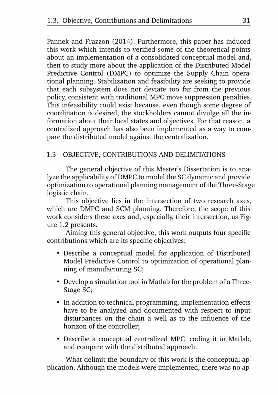
1.3 OBJECTIVE, CONTRIBUTIONS AND DELIMITATIONS
The general objective of this Master’s Dissertation is to ana-lyze the applicability of DMPC to model the SC dynamic and provideoptimization to operational planning management of the Three-Stagelogistic chain.
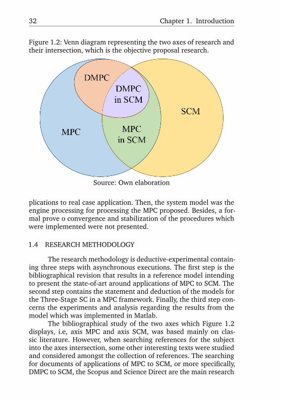
This objective lies in the intersection of two research axes,which are DMPC and SCM planning. Therefore, the scope of thiswork considers these axes and, especially, their intersection, as Fig-ure 1.2 presents.
Aiming this general objective, this work outputs four specificcontributions which are its specific objectives:
• Describe a conceptual model for application of DistributedModel Predictive Control to optimization of operational plan-ning of manufacturing SC;
• Develop a simulation tool in Matlab for the problem of a Three-Stage SC;
• In addition to technical programming, implementation effectshave to be analyzed and documented with respect to inputdisturbances on the chain a well as to the influence of thehorizon of the controller;
• Describe a conceptual centralized MPC, coding it in Matlab,and compare with the distributed approach.
What delimit the boundary of this work is the conceptual ap-plication. Although the models were implemented, there was no ap-
32 Chapter 1. Introduction
Figure 1.2: Venn diagram representing the two axes of research andtheir intersection, which is the objective proposal research.
Source: Own elaboration
plications to real case application. Then, the system model was theengine processing for processing the MPC proposed. Besides, a for-mal prove o convergence and stabilization of the procedures whichwere implemented were not presented.
1.4 RESEARCH METHODOLOGY
The research methodology is deductive-experimental contain-ing three steps with asynchronous executions. The first step is thebibliographical revision that results in a reference model intendingto present the state-of-art around applications of MPC to SCM. Thesecond step contains the statement and deduction of the models forthe Three-Stage SC in a MPC framework. Finally, the third step con-cerns the experiments and analysis regarding the results from themodel which was implemented in Matlab.
The bibliographical study of the two axes which Figure 1.2displays, i.e, axis MPC and axis SCM, was based mainly on clas-sic literature. However, when searching references for the subjectinto the axes intersection, some other interesting texts were studiedand considered amongst the collection of references. The searchingfor documents of applications of MPC to SCM, or more specifically,DMPC to SCM, the Scopus and Science Direct are the main research
1.5. Organization of the dissertation 33
databases. The keywords used in this searching were "Model pre-dictive control” and “Supply chain management”, both locally con-nected and restricted to the articles titles, keywords and abstract.Besides, the progress of the research also used some references ofthe bibliographies which resulted from the searching.
The construction of the general models, also called concep-tual model, starts from literature results and follows with a visualdesign to clear the steps. Finally, the conceptual model was imple-mented in Matlab, which were the tool to generate the data andgraphics for analyzing the results.
1.5 ORGANIZATION OF THE DISSERTATION
This dissertation contains five chapters. They were organizedin a sequence intending to present a constructive explanation of thedissertation subjects.
• Chapter 1 gives context, purpose, focus, significance and de-limitation for this study.
• Chapter 2 contains the literature review organized into twoparts: fundamental topics (Section 2.2 and Section 2.3, whichare important for understanding the developments describedin the following chapters; and the state of art related applica-tions of MPC and DMPC to SCM are in Section 2.4.
• Chapter 3 has the explanations and deduction of the equationsand procedures for the models which are objectives of thiswork. This chapter has two main section, each one describingone of the models, the distributed model (Section 3.1) andthe centralized model (Section 3.2). Following these two sec-tions, the last one delineate some issues concerning practicalimplementation of the methodology into a logistic system.
• Chapter 4 present the experiments which were performed forthe problem of a three-stage SC run in the Matlab environ-ment. There are two sections in this chapter, one section is ded-icated to the experiments concerning the distributed modeland another to a comparative analysis between the the dis-tributed and a centralized model.
• Chapter 5 has the conclusion of the dissertation. It commentsabout the results achieved and a perspective for further devel-opments relating this subject.

2 LITERATURE REVIEW
The review of literature concerning the subject of this disser-tation follows the axis presented at Figure 1.2 of Section 1.3 whichare components parts for this work. Therefore, the review startsfrom general to specific, i.e, the fundamental topics are presentedfirst, and then the applications, which were found in the literature.
The theory behind both general axes, Model Predictive Con-trol (MPC) and Supply Chain Management (SCM), are fundamen-tal for this work. They provide the theoretical grounding needed inunderstanding what following, applications of MPC to solve SCMsome planning problems. Furthermore the search for works alreadydealing with that kind of approach to SCM planning problems isvery important, because its a way to present what has been writtenon this topic of work.
2.1 SEARCH METHODOLOGY
The methodology of literature review is organized in twoparts. The first one is about the fundamental topics and second con-cerning the specific theme of the dissertation. Fundamental topicsreview were based only on books that could be accessible.
Aiming to capture what has already been done into the inter-section of the research’s axes showed by Figure 1.2, a more com-plete methodology is proposed. It follows four steps:
i. identifying the suitable set of keywords;
ii. searching for the collection of articles in the databases;
iii. selecting the Portfolio of articles to be analyzed;
iv. studying the articles.
The step i required a previous overview to got the keywordswhich best describe the subject. In order to get the keywords, thestudy of some works which could give a general vision about thetheme was necessary. This first group of articles for a general visionwere those which have simultaneously the expressions "Control The-ory" and "Supply Chain Management" Chain Management" in theirtitles, keywords or abstract. The chosen databases as sources forsearching the bibliographies in this study was Scopus and ScienceDirect. The reasons for this choice are flexibility for logical com-binations of keywords during the search and the great amount ofavailable articles.
35
36 Chapter 2. Literature Review
These articles has made possible identifying the suitable setof keywords necessary for the step ii. Hereby,the selected wordsfor the first subject were "model predictive control" and "recedinghorizon control", and for the second one were "supply chain" and"supply chain management". The step ii follows the rule: if at leastone of those keywords about the first subject and at least one ofthose about the second subject are in the article’s title, or abstract,or keywords, then the article is selected, i.e, at least one keywordof each subject should be mentioned. This search resulted in 104articles sourced just from journals and proceedings.
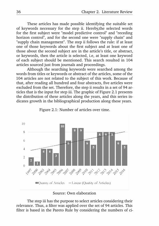
Although the searching keywords were searched among thewords from titles or keywords or abstract of the articles, some of the104 articles are not related to the subject of this work. Because ofthat, after reading all hundred and four abstracts, five articles wereexcluded from the set. Therefore, the step ii results in a set of 94 ar-ticles that is the input for step iii. The graphic of Figure 2.1 presentsthe distribution of these articles along the years, and this series in-dicates growth in the bibliographical production along these years.
Figure 2.1: Number of articles over time.
Source: Own elaboration
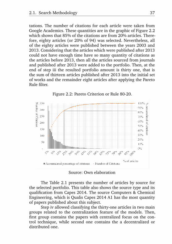
The step iii has the purpose to select articles considering theirrelevance. Thus, a filter was applied over the set of 94 articles. Thisfilter is based in the Pareto Rule by considering the numbers of ci-
2.1. Search Methodology 37
tations. The number of citations for each article were taken fromGoogle Academics. These quantities are in the graphic of Figure 2.2which shows that 85% of the citations are from 20% articles. There-fore, eighty articles (or 20% of 94) was selected. Nevertheless, allof the eighty articles were published between the years 2003 and2013. Considering that the articles which were published after 2013could not have enough time have so many quantity of citations asthe articles before 2013, then all the articles sourced from journalsand published after 2013 were added to the portfolio. Then, at theend of step iii the resulted portfolio amount is thirty one, that isthe sum of thirteen articles published after 2013 into the initial setof works and the remainder eight articles after applying the ParetoRule filter.
Figure 2.2: Pareto Criterion or Rule 80-20.
Source: Own elaboration
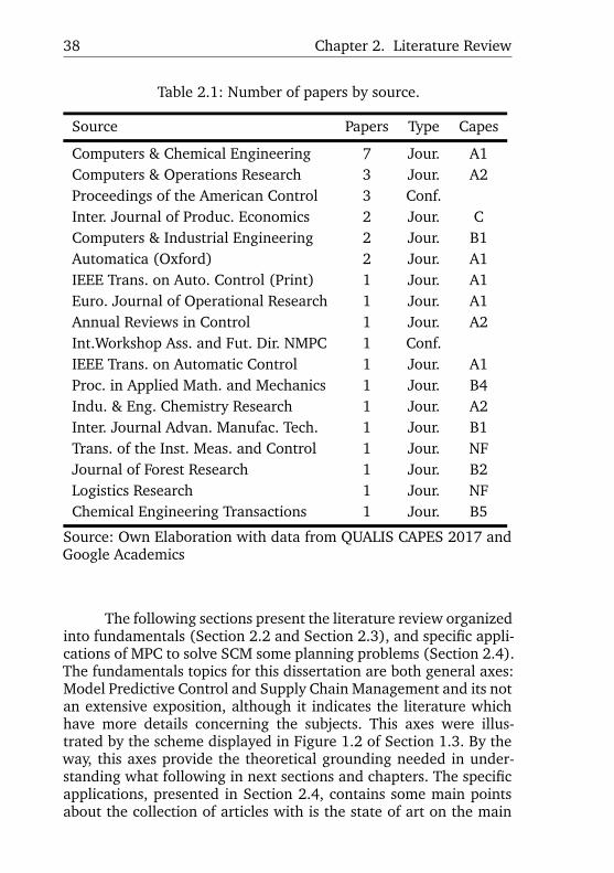
The Table 2.1 presents the number of articles by source forthe selected portfolio. This table also shows the source type and itsqualification from Capes 2014. The source Computers & ChemicalEngineering, which is Qualis Capes 2014 A1 has the most quantityof papers published about this subject.
Step iv allowed classifying the thirty-one articles in two maingroups related to the centralization feature of the models. Then,first group contains the papers with centralized focus on the con-trol technique, while second one contains the a decentralized ordistributed one.
38 Chapter 2. Literature Review
Table 2.1: Number of papers by source.
Source Papers Type Capes
Computers & Chemical Engineering 7 Jour. A1Computers & Operations Research 3 Jour. A2Proceedings of the American Control 3 Conf.Inter. Journal of Produc. Economics 2 Jour. CComputers & Industrial Engineering 2 Jour. B1Automatica (Oxford) 2 Jour. A1IEEE Trans. on Auto. Control (Print) 1 Jour. A1Euro. Journal of Operational Research 1 Jour. A1Annual Reviews in Control 1 Jour. A2Int.Workshop Ass. and Fut. Dir. NMPC 1 Conf.IEEE Trans. on Automatic Control 1 Jour. A1Proc. in Applied Math. and Mechanics 1 Jour. B4Indu. & Eng. Chemistry Research 1 Jour. A2Inter. Journal Advan. Manufac. Tech. 1 Jour. B1Trans. of the Inst. Meas. and Control 1 Jour. NFJournal of Forest Research 1 Jour. B2Logistics Research 1 Jour. NFChemical Engineering Transactions 1 Jour. B5
Source: Own Elaboration with data from QUALIS CAPES 2017 andGoogle Academics
The following sections present the literature review organizedinto fundamentals (Section 2.2 and Section 2.3), and specific appli-cations of MPC to solve SCM some planning problems (Section 2.4).The fundamentals topics for this dissertation are both general axes:Model Predictive Control and Supply Chain Management and its notan extensive exposition, although it indicates the literature whichhave more details concerning the subjects. This axes were illus-trated by the scheme displayed in Figure 1.2 of Section 1.3. By theway, this axes provide the theoretical grounding needed in under-standing what following in next sections and chapters. The specificapplications, presented in Section 2.4, contains some main pointsabout the collection of articles with is the state of art on the main
2.2. Supply Chain Management 39
subject of this dissertation.
2.2 SUPPLY CHAIN MANAGEMENT
Several authors tried to put the essence of SCM into a con-cise definition. During the nineties until present days many of themhave done it very well, but each definition has small differencescompared to other. Nevertheless, their mindset consists of a targetgroup to be managed, the objectives and the means for achievingthese objectives (STADTLER, 2005; CHRISTOPHER, 1992). In thiscontext, this chapter concern logistics concepts and issues, its evo-lution to SCM, and the values it produces to customers into a SC,which then is also called as value chain.
2.2.1 Logistics Management Concepts
The concept of logistics evolves from the beginning of civi-lization. Previously it was basically related to the transport of goodsamong productions and consumers centers (BALLOU, 2006). Thetechniques and worldwide markets evolution brought to light poten-tial gains that logistic alternatives could allow. Today the concept oflogistic is concerned with the effective and efficient availability ofgoods or services through a network of suppliers and customers.
The CSCMP (2013) defines logistics as the processes of "plan-ning, implementation, and controls the efficient, of effective for-ward and reverses flow and storage of goods, services and relatedinformation between the point of origin and the point of consump-tion in order to meet customers’ requirements". This way, the lo-gistic process creates value by timing and positioning inventory, itis the combination of a firm’s order management, inventory, trans-portation, warehousing, materials handling, and packaging as inte-grated throughout a facility network (BOWERSOX et al., 2002). Lo-gistics is important because it more the available goods or servicesit creates value for all stakeholders. Value in logistics is expressedin terms of time and place. Products and services would not havevalue unless they are in the with customers when and where theywish to consume them. To many firms throughout the world, logis-tics has become an increasingly important value-adding process fortime, space, and others consequent reasons (BALLOU, 1997).
The Supply Chain, also called the value chain or demandchain, are the network of organizations engaged in provide a prod-uct or service from supplier to customer, or in the words of Chopra
40 Chapter 2. Literature Review
and Meindl (2010), it consists of all parties involved in fulfilling cos-tumers’ requests. That logistic definition given by (CSCMP, 2013)and accepted by (BALLOU, 2006) implies that logistic is part of alarger process which consists in the management of SC. That is theunderstanding considered for this dissertation, which also meansto agree with Bowersox et al. (2002) who wrote that logistics, incontrast to supply chain management, is the work required to moveand position inventory throughout a supply chain. As such, logisticsis a subset of and occurs within the broader framework of a SC.
Supply Chain Management can be defined as the manage-ment of material, information and financial flows through a net-work of organizations that aim to produce and deliver products orservices to consumers (TANG, 2006). This broad concept has manyvariants and they rely on two main notions: a logistic framework,and the objective to achieve linkage and coordination between theprocesses of all involved entities, i.e, suppliers, customers and in-vestors (CHRISTOPHER, 1992). Then, a good understand of what isthe SCM must contemplate the relation between the work of agentsin the chain and the framework of logistics. Further, SCM consists offirms collaborating to leverage strategic positioning and to improveoperating efficiency. The evolution of logistics as integrated logisticsserves to link and synchronize the overall supply chain as a continu-ous process and it is essential for effective supply chain connectivity(BOWERSOX et al., 2002). While the purpose of logistical work hasremained essentially the same over the decades, the way the workis performed continues to radically change.
The object of SCM is obviously the SC (STADTLER, 2005).Each organization has a set of processes that makes it works. Aswritten by Sterman (2000), a Supply Chain is the set of structuresand processes an organization uses to deliver an output to a cus-tomer. Further, these organizations compound a system organizedin a network (JINGSHUANG et al., 2008). As discussed by Aitken(1998), this network consist of nodes, representing organizations,and links between them, manifesting the interactions within them.
The macro view of SC while creating values to all stakehold-ers consists of the stock and flow structures for acquisition, storage,conversion of inputs into outputs, and the management policies gov-erning the various flows. Due to the not clear barrier between logis-tic and SC, this work call SC as synonymous to logistic chain. Aitken(1998) has adapted the theoretical understanding of Supply Chainto the context of networks. Then, he considers the SC as a networkof connected and interdependent organizations mutually and co-
2.2. Supply Chain Management 41
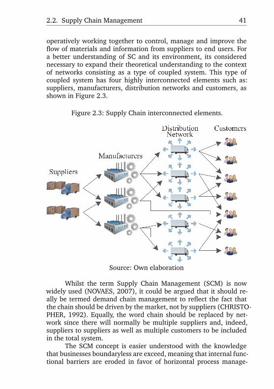
operatively working together to control, manage and improve theflow of materials and information from suppliers to end users. Fora better understanding of SC and its environment, its considerednecessary to expand their theoretical understanding to the contextof networks consisting as a type of coupled system. This type ofcoupled system has four highly interconnected elements such as:suppliers, manufacturers, distribution networks and customers, asshown in Figure 2.3.
Figure 2.3: Supply Chain interconnected elements.
Source: Own elaboration
Whilst the term Supply Chain Management (SCM) is nowwidely used (NOVAES, 2007), it could be argued that it should re-ally be termed demand chain management to reflect the fact thatthe chain should be driven by the market, not by suppliers (CHRISTO-PHER, 1992). Equally, the word chain should be replaced by net-work since there will normally be multiple suppliers and, indeed,suppliers to suppliers as well as multiple customers to be includedin the total system.
The SCM concept is easier understood with the knowledgethat businesses boundaryless are exceed, meaning that internal func-tional barriers are eroded in favor of horizontal process manage-
42 Chapter 2. Literature Review
ment; externally, the gap between vendors, distributors, customersand the firm close gradually (CHRISTOFIDES et al., 2013). Today’sturbulent business environment has caused a greater awarenessamong managers of the financial dimension of decision making,with business managers progressively becoming more driven by thegoal of enhancing shareholder value.
The suppliers in a chain are involved simultaneously in sev-eral other chains (CHRISTOPHER, 1992). For discussion purposesit is useful to outline the supply chain as a single and independententity but, in reality, it is contained within a network of organiza-tions. The aim of many SC studies has been to attempt to isolate andanalyse individual phenomena, instead of relating the issues to thebroader and more general processes and structures, of the networksin which they are embedded. The law of reductionism has been ap-plied to understanding supply chain integration and management.However, as observed, supply chains exist within the context of net-works, which must be able to compete in the market as the supplychains they contain. Perceiving the supply chain as a single line en-tity disguises the complexity in which it exists (STERMAN, 2000).
The decision for producing a product begins from the cus-tomers. A restrict concept to SCM system could be viewed as cus-tomers requesting a favourable commodity by visiting retailers in adistribution network, and this motive is transferred to manufactur-ers to meet the opportunity through a network of suppliers, manu-facturers, distributors, and retailers. This network is named a pro-duction/distribution/inventory system because it consists of an in-ventory management part, a logistic network, and production pro-gramming.
In a SC, a set of decision-maker facilities (suppliers, manufac-turers, warehouses, distributors, and retailers) cooperate for gettingthe demands or forecasting them, ordering, procuring materials oroutsourcing parts of the production procedure, manufacturing orassembling and finishing final products, stocking inventory, trans-porting, and finally, delivering the final products to customers. Sup-ply chains should be programmed by an efficient manager (or setof managers) who applies previous experiences with modern meth-ods. This combination is named a supply chain management systemand runs two processes of decisions and actions: as orders and ship-ments.
In some of the industries, such as industries that have a defi-nite customer or contract, changing in demand patterns across timerarely happen (CHRISTOPHER, 1992). In the supply chain of these
2.2. Supply Chain Management 43
products, in a specific time, such as at the beginning time of con-tract, or at the beginning time of production, a correct pattern ofcustomer demand is forecasted by famous methods, and productionplanning goes ahead for having suitable customer demand planning.The problem is solved offline in this time, as zero time, and its out-put is used for programming and scheduling shipments betweensupply chain entities, manufacturing planning, and holding or man-aging inventory volumes (AITKEN, 1998). Therefore, in this situ-ation, the optimization problem of the supply chain managementsystem, considering the required constraints, is just solved for zerotime and then production, warehousing, and distribution plans aregiven to related persons, managers, and employers of each division.
The programming and control of SC can be made by differ-ent methods, such as deterministic analytical models, stochastic an-alytical models, and simulation models coupled with desired opti-mization objectives and network performance measures. To employcontrol methods with prediction abilities is very suitable for supplychain management systems, because decision prediction by lookingto future demand exists inherently (IVANOV et al., 2012). Reced-ing horizon control (RHC) is one of them that uses the RecedingHorizon (RH) concept.
In general, supply chains operate as pull systems driven bythe orders that customers place to the retailers, and their generaloperation is as follows: retailers accumulate orders from customersand commit to satisfy them as long as they arrive before a certaindeadline. Orders arriving after the deadline will be logged for thenext period (STERMAN, 1989). At the end of the a some period,retailers start satisfying the accumulated orders upon product avail-ability, and if the products are in stock, the retailers pack and shipthem to the customer, otherwise, either those orders remain in thefile of orders to be fulfilled (if the company follows the policy ofbackorders), or the orders are lost.
Since product availability is the key factor to keep a goodlevel of customer satisfaction, retailers need to estimate their fu-ture demands and place the respective replacement orders to theirsupplying nodes to get the product. However, if they place moreorders than required they would pay extra storage and inventoryholding costs (CHRISTOFIDES et al., 2013). If they place fewer or-ders than needed, then their customer satisfaction level would drop.This process repeats itself throughout the distribution network untilthe orders reach the manufacturing site, where the plant managerhas to define a production and a raw material acquisition plan to
44 Chapter 2. Literature Review
satisfy them.The challenges in supply chain management arise from prob-
lems related to changes in the Supply Chain environment. Becausethe management of the upstream and downstream relationship, fromsuppliers to customers, aim to deliver superior customer value atless cost, this optimization problem tends to be multiobjective. Fur-ther challenges arise as the Supply Chain Management focuses onachieving a more profitable outcome for all parties within the chain(CSCMP, 2013). Then to achieve that focus, in SCM it is necessaryto plan and run the chain, to manage and review the results, and toreplan the process.
Solving the logistic problems, regarding their difficulties areactivities happening every day around the world, within each typeof supplying process. The difficulty is overcome by rationalizing theSupply Chain Management planning processes. Planning is some-times associated with optimization in SCM, i.e, it seek efficiencyas benefit. The planning process normally is organized into strate-gic, tactical and operational levels (STADTLER; KILGER, 2007). Thestrategic level deals with decisions that have a long-lasting effectson the firm. This includes decisions regarding the number, locationand capacities of warehouses and manufacturing plants, or the flowof materials through the logistics network. The tactical level typ-ically includes decisions that are updated anywhere between onceevery quarter and once every year. This includes purchasing and pro-duction decisions, inventory policies and transportation strategiesincluding the frequency with which customers are visited. Finally,operational level refers to day-to-day decisions such as scheduling,routing and loading trucks (CHOPRA; MEINDL, 2010).
All SCM complexities turn to challenges faced by SC man-agers who are seeking to enhance shareholder value is to identifystrategies that improve free cash flow generation (STADTLER; KIL-GER, 2007). Today, for competitive customer service to be main-tained the market requires environmentally friendly products, a goodportfolio mix, rapid development of new products, high quality andreliability, after-sales services, etc. Furthermore, SC managers needto consider the dynamics of a rapidly changing market environment,such as variability in demand, cancellations and returns, as well asthe dynamics of internal SC operations, such as processing times,production capacity pitfalls and the availability of materials. Theseoperational SC risks and disruptions can have severe long-term ef-fects on a firm’s financial performance.
2.2. Supply Chain Management 45
2.2.2 Oscillation and the Bullwhip Effect
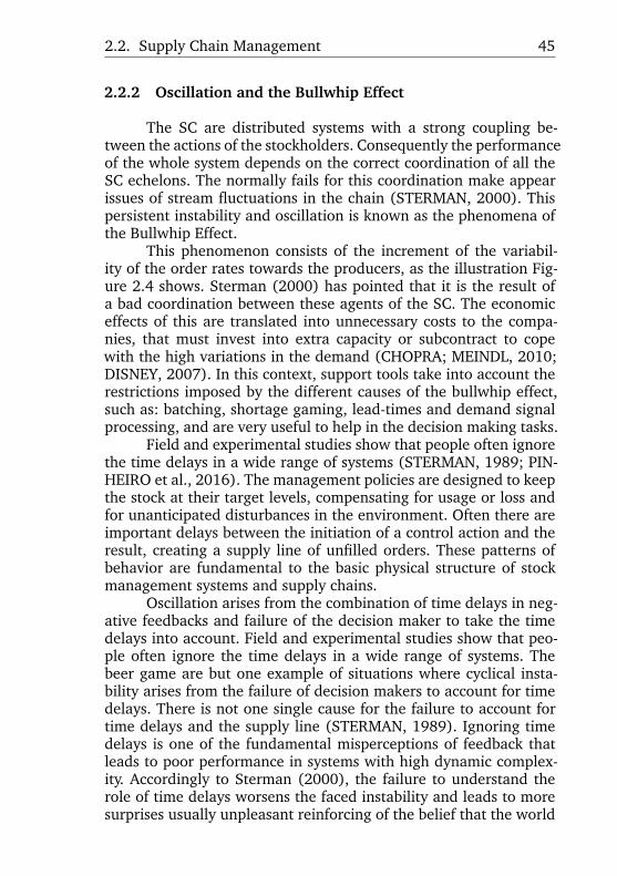
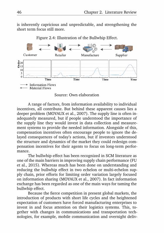
The SC are distributed systems with a strong coupling be-tween the actions of the stockholders. Consequently the performanceof the whole system depends on the correct coordination of all theSC echelons. The normally fails for this coordination make appearissues of stream fluctuations in the chain (STERMAN, 2000). Thispersistent instability and oscillation is known as the phenomena ofthe Bullwhip Effect.
This phenomenon consists of the increment of the variabil-ity of the order rates towards the producers, as the illustration Fig-ure 2.4 shows. Sterman (2000) has pointed that it is the result ofa bad coordination between these agents of the SC. The economiceffects of this are translated into unnecessary costs to the compa-nies, that must invest into extra capacity or subcontract to copewith the high variations in the demand (CHOPRA; MEINDL, 2010;DISNEY, 2007). In this context, support tools take into account therestrictions imposed by the different causes of the bullwhip effect,such as: batching, shortage gaming, lead-times and demand signalprocessing, and are very useful to help in the decision making tasks.
Field and experimental studies show that people often ignorethe time delays in a wide range of systems (STERMAN, 1989; PIN-HEIRO et al., 2016). The management policies are designed to keepthe stock at their target levels, compensating for usage or loss andfor unanticipated disturbances in the environment. Often there areimportant delays between the initiation of a control action and theresult, creating a supply line of unfilled orders. These patterns ofbehavior are fundamental to the basic physical structure of stockmanagement systems and supply chains.
Oscillation arises from the combination of time delays in neg-ative feedbacks and failure of the decision maker to take the timedelays into account. Field and experimental studies show that peo-ple often ignore the time delays in a wide range of systems. Thebeer game are but one example of situations where cyclical insta-bility arises from the failure of decision makers to account for timedelays. There is not one single cause for the failure to account fortime delays and the supply line (STERMAN, 1989). Ignoring timedelays is one of the fundamental misperceptions of feedback thatleads to poor performance in systems with high dynamic complex-ity. Accordingly to Sterman (2000), the failure to understand therole of time delays worsens the faced instability and leads to moresurprises usually unpleasant reinforcing of the belief that the world
46 Chapter 2. Literature Review
is inherently capricious and unpredictable, and strengthening theshort term focus still more.
Figure 2.4: Illustration of the Bullwhip Effect.
Source: Own elaboration
A range of factors, from information availability to individualincentives, all contribute. But behind these apparent causes lies adeeper problem (MOYAUX et al., 2007). The supply line is often in-adequately measured, but if people understood the importance ofthe supply line they would invest in data collection and measure-ment systems to provide the needed information. Alongside of this,compensation incentives often encourage people to ignore the de-layed consequences of today’s actions, but if investors understoodthe structure and dynamics of the market they could redesign com-pensation incentives for their agents to focus on long-term perfor-mance.
The bullwhip effect has been recognized in SCM literature asone of the main barriers in improving supply chain performance (FUet al., 2015). Whereas much has been done on understanding andreducing the bullwhip effect in two echelon or multi-echelon sup-ply chain, prior efforts for limiting order variation largely focusedon information sharing (MOYAUX et al., 2007). In fact informationexchange has been regarded as one of the main ways for taming thebullwhip effect.
Because the fierce competition in present global markets, theintroduction of products with short life cycles and the heightenedexpectation of customers have forced manufacturing enterprises toinvest in and focus attention on their logistics systems. This, to-gether with changes in communications and transportation tech-nologies, for example, mobile communication and overnight deliv-
2.3. Model Predictive Control 47
ery, has motivated continuous evolution of the management of lo-gistics systems. In these systems, items are produced at one or morefactories, shipped to warehouses for intermediate storage and thenshipped to retailers or customers. Consequently, to reduce cost andimprove service levels, logistics strategies must take into accountthe interactions of these various levels in this logistics network. Thisnetwork consists of suppliers,manufacturing centers,warehouses, dis-tribution centers and retailer outlets, as well as raw materials, work-in-process inventory and finished products that flow between thefacilities (BRAMEL; SIMCHI-LEVI, 1997).
The treatment of logistic as a strategic business lead it to anintegrating scenery. Novaes (2007) considers this scenery as an up-per stage of logistic evolution. Moreover, the supply chain manage-ment consists of the effective integration of the main entities of thesupply chain. This view, therefore, indicates the SCM as an evolu-tion of logistics pattern. Likewise, Aitken (1998) indicates supplychain management as "an integrative approach to dealing with theplanning and control of the material flow from suppliers to endusers".
2.3 MODEL PREDICTIVE CONTROL
The MPC is a process control methodology that is being in-creasingly employed across several industrial sectors (CAMACHO;BORDONS, 2007). The popularity of MPC in industry stems in partfrom its ability to tackle multivariable processes and handle pro-cess constraints. Furthermore, accordingly to Camacho and Bordons(2007) it perhaps is the most general way of posing the process con-trol problem in the time domain. The MPC is not a specific controlstrategy, but rather an ample range of control methods, a method-ology, to generate controllers. The main difference of MPC from an-other control strategy, such as stochastic dynamic programming andoptimal control, is that the control input is not computed a priori,as an explicit function of the state vector, but it is computed on-linethe rolling-horizon. Thus, MPC is prevalent in the control of com-plex systems where the off-line solution of the dynamic program-ming equations is computationally intractable due to high problemdimensionality (VENKAT, 2006).
The MPC methodology uses the model of the system and theconcept of open-loop optimal feedback. The system model is used topredict and optimize the future system behavior (PANNEK; GRüNE,
48 Chapter 2. Literature Review
2011). Moreover, past and current state measurements are the in-puts used to estimate the current state of the system at each timestep. Then, with the system model as constraint, an optimizationproblem is solved to determine an optimal open-loop policy fromthe present (estimated) state (MAYNE et al., 2000). The MPC trickis to inject only the first output move into the plant (the system).At the subsequent time step, the system state is re-estimated usingnew measurements. The optimization problem is resolved and theoptimal open-loop policy is recomputed.
A system is a set of things together, or parts of a mechanism,or an interconnecting network (OXFORD, 2016). It constitutes apart of the universe of interest to some study and it is characterizedby a relationship between its inputs and outputs. Specifically for thecontext of this dissertation, the system is the Three-Stage logisticchain presented in Figure 1.1. The model of a system mimics itsbehavior, but it is not the real world but merely a human constructto help us better understand the systems. In general all models havean information input, an information processor, and an output ofexpected results. The type of a model is the way in which the systemmodel is described mathematically: transfer function or state-space(NEGENBORN; MAESTRE, 2014).
The basic MPC elements are the prediction system model,the objective function, and obtaining the control law (CAMACHO;BORDONS, 2007). Although practically every possible form of mod-elling a process appears in a given MPC formulation, this chapterwill describe the issues related to the methodology in the contextof discrete time systems. The restricting of the exposure due to thefocus of the subject of this dissertation. Moreover, the expositionis restricted to quadratic objective function, and to only a few opti-mization methods to solve nonlinear models with that kind of objec-tive. Optimization is an important issue to MPC because to obtainthe control law it is necessary solving a minimization problem, andthis is going to be described in the following.
A discretization of the time is enumerated of time periods,that is, the time is counted in digital values tn in \BbbR whose the val-ues of n are from \BbbN . When a system or its model exists in the dis-crete time, it is called a discrete time system. This kind of system iscontrolled when from each time instant tn, its process state x(tn),taking values in \BbbR d, has is future behavior x(tn+1) influenced by acontrol input u(tn) from \BbbR m with the rule of a function
f : \BbbR d \times \BbbR m \rightarrow \BbbR m.
2.3. Model Predictive Control 49
This function is the law or dynamics of the system. Then, for all nin \BbbN and state value x(tn) in \BbbR d, the next state is
x(tn+1) = f(x(tn), u(tn)). (2.1)
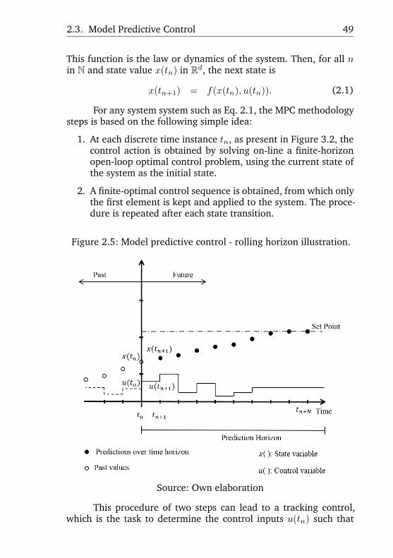
For any system system such as Eq. 2.1, the MPC methodologysteps is based on the following simple idea:
1. At each discrete time instance tn, as present in Figure 3.2, thecontrol action is obtained by solving on-line a finite-horizonopen-loop optimal control problem, using the current state ofthe system as the initial state.
2. A finite-optimal control sequence is obtained, from which onlythe first element is kept and applied to the system. The proce-dure is repeated after each state transition.
Figure 2.5: Model predictive control - rolling horizon illustration.
Source: Own elaboration
This procedure of two steps can lead to a tracking control,which is the task to determine the control inputs u(tn) such that

50 Chapter 2. Literature Review
x(tn) follows a given reference xref (tn) as good as possible. Thismeans that if the current state is far away from the reference, thenthe controller should want track the system towards the referenceand if the current state is already close to the reference, then itshould to keep it there. The stabilization problem exists when thereference is constant, that is, xref (tn) = x for all n \in \BbbN , and x isgiven a real number. Then, besides the full generality the trackingproblem, with such a constant reference it is reduced to a stabiliza-tion problem (PANNEK; GRüNE, 2011). Since it is necessary to beable to react to the current deviation of x(tn) from the referencevalue, the controller should have u(tn) in feedback form, i.e., in theform u(tn) = \mu (x(tn)) for some map between the state space andthe control space
\mu : \BbbR d \rightarrow \BbbR m.
In MPC the function \mu is not generate a priori, but it is build by theprocess of optimization in the rolling-horizon procedure.
The future outputs for a determined horizon N , a fixed inte-ger number which is called the prediction horizon, are predicted ateach instant tn using the process’ model from Eq. 2.1. These pre-dicted outputs x(tn+1) for n varying from 0 until N depend on theknown values up to instant tn and on the future control signalsu(tn). The set of future control signals is calculated by optimizinga determined criterion to keep the process as close as possible tothe reference trajectory, which can be the set-point itself or a closeapproximation of it. This criterion is a function
L : \BbbR d \times \BbbR m \rightarrow \BbbR
whose domain is Cartesian product of state and control spaces. Thisfunction usually takes the form of a quadratic function of the errorsbetween the predicted output signal and the predicted referencetrajectory, that is, for n natural number equal or less than N
L(x(tn), u(x(tn)) =d\sum
i=1
x2i (tn) +
m\sum i=1
u2i (tn). (2.2)
Furthermore, for some systems the state and control variables canonly take values into intervals. These are called resource constraintsand have form
lx \leq x(tn) \leq ux
lu \leq u(tn) \leq uu,(2.3)
2.3. Model Predictive Control 51
where the lower bounds lx and lu, and the upper bounds ux and uu
are constant real numbers.In order to generate the control values at each time instant
the optimization problem with objective function Eq. 2.5 and con-straints by Eq. 2.3, bounds for the stages, and by the system model,the equation Eq. 2.1. Therefore, the short notation for this optimiza-tion problem is
SPn : \mathrm{m}\mathrm{i}\mathrm{n} J(x(t0), u)
u
subject to (2.1)and (2.3)
(2.4)
where
J(x0, o) =N+n\sum k=n
L(x(tk), u(x(tk)). (2.5)
The control signal u(tn) is sent to the process whilst the nextcontrol signals calculated are rejected, because at the next samplinginstant x(tn+1) is already known. The process is repeated with thisnew value and all the sequences are brought up to date. Thus theu(tn+1) is calculated (which in principle will be different from theu(tn) because of the new information available) using the recedinghorizon concept.
In this formulation there is just one controller, and then it iscalled the a centralized MPC. When a series of static optimizationproblems the standard MPC formulation Eq. 2.4 then it is called adescentralized controller. Depending on the communication reulesamong the descentralized systems it is called a DMPC. The modelwhose fully description is presented in Section 3.1 is one exampleof DMPC formulation.
In general, the controllers can be classified depending on howmany of them participate in the solution of the control problem andthe relative importance between them (NEGENBORN; MAESTRE,2014). The control system is centralized if there is a single controllerthat solves the plant-wide problem. The control is decentralizedwhen there are local controllers in charge of the local subsystems ofthe plant that require no communication among them. When thereare different control layers coordinated to take care of the processthe control system is hierarchical. In this case, upper layers managethe global objectives of the process and provide references for thelower layers, which control directly the plant. Finally, if the local
52 Chapter 2. Literature Review
controllers communicate in order to find a solution for the overallcontrol problem the control system is distributed.
The MPC is usually implemented in a centralized controllerwhich has the full knowledge about the process and calculates thewhole control sequence for the system (SCHERER et al., 2015).Although, the size of the problems faced today by control engi-neers has grown enormously as the limitations imposed by the com-munication and computational capabilities decrease. In this sense,there are strong incentives to have decentralized or distributed con-trol schemes, such as DMPC. Indeed, accordingly to Negenbornand Maestre (2014), the society heavily depends on infrastructuresystems, such as power grids, water distribution networks, trafficsystems, road-traffic networks and intermodal transport networks.Nevertheless, these systems have also several drawbacks that haveto be taken into account, being the main one the loss of performancein comparison with a centralized controller. This loss depends onthe degree of interaction between the local subsystems and the coor-dination mechanisms between the agents (NEGENBORN; MAESTRE,2014).
The type of coordination mechanism that can be realized relyupon the information structure, i.e, the connectivity and capacityof the interagent communication MPC network (CAMPONOGARAet al., 2002). Therefore, the DMPC frameworks can be divided intocooperative and non-cooperative strategies. A cooperative strategyexists when the agents controlling the subsystems optimize over acommon overall objective considering only local variables. In a non-cooperative strategy, the agents exchange information but optimizetheir own objectives (SCHERER et al., 2015). Under some conditionabout coordination mechanism, it is possible that a DMPC has thesame performance as the centralized MPC, such as the case provedin Camponogara and Scherer (2011) for cooperative strategies.
This kind the optimization problem Eq. 2.4 is a quadraticprogram for which efficient algorithms exist for its solution suchas Trust Region Algorithms, Interior Point Algorithms, QuadraticProgramming (QP) and Sequential Quadratic Programming (SQP)(MARTINEZ; SANTS, 1995). Those are optimization methods andexplicit solutions can be obtained because the criterion is quadratic,the model is linear, and there are no constraints. In constrained opti-mization, the general aim is to transform the problem into an easiersubproblem that can then be solved and used as the basis of an it-erative process. A characteristic of a large class of early methods isthe translation of the constrained problem to a basic unconstrained
2.4. Applications of MPC in SCM 53
problem by using a penalty function for constraints that are near orbeyond the constraint boundary. In this way the constrained prob-lem is solved using a sequence of parameterized unconstrained op-timizations, which in the limit (of the sequence) converge to theconstrained problem
2.4 APPLICATIONS OF MPC IN SCM
The study of dynamics in supply chains can be referred toas both dynamics of process under optimization and as real-timedynamics (IVANOV et al., 2012). This distinguishing, however, isnot easy to understand. The connection between control theory andSCM can be due to an adaptation and real time control. Then, theMPC is one of the techniques which can be applied to model adap-tation in SC.
Described in Section 2.3, the broad concept of MPC is basedon a system model and both current and historical measurementsof the process to predict the systems’ behavior for a planning hori-zon. Using this prediction ability, it minimizes an objective functionand calculates a control sequence satisfying the constraints of thesystem.
2.4.1 Centralized models
Many of the works using MPC to SCM are dedicated to semi-conductor industry. It is the case of Wang et al. (2007), which intro-duces an upper level stochastic optimizer that provides constraintback-off parameters to the lower level MPC controller. This preventssignificantly the performance degradation caused by uncertainties.They treated demand as a load disturbance and they considered itas a stochastic signal driven by integrated white-noise (the discrete-time analog of Brownian motion). They applied a state estimation-based MPC in order to increase the system performance and robust-ness with respect to demand variability and erroneous forecasts. As-suming no information on disturbances, they employed a type offilter to estimate the state variables, where the filter gain is a tuningparameter based on the signal-to-noise ratio. Through simulationsthey concluded that when there is a large error between the averageof actual demands and the forecast, a larger filter gain can make thecontroller compensate for the error sufficiently fast.
Aiming to tune the parameter for a better performance MPCmodel of SCM, Schwartz et al. (2006) uses a simultaneous per-
54 Chapter 2. Literature Review
turbation stochastic approximation. They illustrate the benefits ofthis approach in enhancing the usefulness of the policies underconditions of uncertainty. In the first scenario, an internal modelcontrol decision policy for a single product and single echelon pro-duction–inventory system. The simultaneous perturbation stochas-tic approximation technique is applied to determine financially op-timal controller tuning parameters under conditions involving vary-ing magnitudes of forecast error. The second problem scenario in-volves the simultaneous selection of safety stock targets and MPCmove suppression parameters for the representative semiconduc-tor manufacturing problem described in circumstances involvingstochastic yield, variable throughout time, and uncertain, autocor-related demand.
Puigjaner and Laínez (2008) has addressed the dynamics man-agement of SC integrated solutions. The proposed approach uti-lizes a SC design and planning model that incorporates financialconcerns. Process operations decisions with finances considerationsare optimized in tandem by using mathematical mixed integer mod-elling techniques. The solution framework integrates an MPC strat-egy and a holistic stochastic model for SCM. A major disadvantageof discounted cash flow methods is that they do not account for un-certainties in commercial returns. In their work, to overcome thisproblem interest rates are regarded as random factors which havea direct effect upon cost of capital. The main advantages of thisjoint control approach have been highlighted through a motivatingcase study, in which a comparison with the traditional determinis-tic MPC is carried out. The control strategy presented in this workallows to handle uncertainty and incidences by combining reactiveand preventive approaches. A pro-active treatment of uncertaintyis included by means of stochastic programming. The review andupdate process that is required to tackle incidences and changes inrandom factors is performed by introducing the SC stochastic holis-tic model into a SCM. The novel control framework developed mayhelp to close the information loop for dynamic SCM by taking theform of a supervisory module.
Kempf (2004) used a control-oriented approach for this non-linear stochastic combinatorial optimization problem, an outer loopfor addressing the planning parts of the problem, and an inner loopto manage the execution aspects are proposed. The outer loop pro-vides a material release plan generated by a linear programmingformulation (LP) and inventory safety stock targets generated by adynamic programming formulation to the inner loop to guide ex-
2.4. Applications of MPC in SCM 55
ecution. Portions of the nonlinearity and stochasticity inherent inthe problem are addressed by the outer loop that requires iterativeconvergence between the LP and the DP. The inner loop is formu-lated from the perspective of MPC and integrates optimal controland stochastic control. Initial results are presented to demonstratethe ability of the inner loop to track material release and safetystock targets while improving delivery performance in the face ofboth supply and demand stochasticity. A simulation module is alsodescribed that supports the other components of the system by vali-dating their efficacy before application in the real world. This com-ponent has to address the integrated flows of materials, information,and decisions through the supply chain, and employs innovative ap-proaches combining a number of specialized models to do so quicklyand accurately.
Wang and Rivera (2008) presents a formulation of a modelpredictive control MPC-based decision algorithm that forms partof the tactical execution layer in a two-level hierarchical structurefor decision support in semiconductor manufacturing supply chainmanagement proposed by Kempf (2004). The standard strategicplanning and inventory planning modules form the outer loop. Theseplanning modules make the long timescale decisions, for instanceweekly decisions, on the starts of factories and inventory targetsby taking into account the capacities available in processes andthe forecast of future customer demand while maximizing a profit-based objective function. The decisions generated from these mod-ules are used as targets and passed to the tactical execution modulewhich relies on advanced control techniques to handle the stochas-ticity and nonlinearity on both supply side and demand side in semi-conductor manufacturing supply chain.
Wang et al. (2004) presents MPC as a tactical decision mod-ule for supply chain management in semiconductor manufactur-ing. A representative problem which includes distinguishing fea-tures of semiconductor manufacturing supply chains, such as mate-rial reconfiguration and stochastic product splits, is examined. Fluidanalogies are used to model the supply chain dynamics, with stochas-ticity and nonlinearity occurring on the throughput time, yield andcustomer demand. Given inventory targets and capacity limits, MPCusing linear time invariant models can make the system outputstrack the targets and improve customer service levels. The flexibil-ity provided by the choice of tuning parameters in MPC to achievebetter performance and robustness in semiconductor manufactur-ing supply chain management is demonstrated. Further Wang et al.
56 Chapter 2. Literature Review
(2005) apply a proper tuning parameter which helps the system toachieve both robustness and performance with the linear determin-istic nominal model despite the stochasticity and nonlinearity in theplant.
Schwartz and Rivera (2010) evaluated by simulations the ef-fectivenes of a series of control-oriented decision policies increasingsophistication based on the concepts of Internal Model Control andMPC. Its simulations involve changes in net stock targets, responseto forecasted demand and response to unforecasted demand. Theytuned MPC policies to minimize inventory deviation from setpoint,changes in factory starts, or a weighted combination. The paperpresented a comparison study which showed that MPC was ableto outperform the SRR with respect to both metrics. Optimal per-formance of the MPC decision policy hinges on the quality of itsexogenous signals, particularly demand forecasts. The detrimentaleffects of forecast error can be mitigated by applying a forecastingprocedure contextualized for the decision policy.
Hennet (2003) considers a multi-stage multi-item productionplant with its supply chain and customer environment. The produc-tion, supply and inventory plan is optimized on a dual-mode basis,under two different information patterns. The short-term plan re-lies on orders received from customers. On the contrary, the long-term plan is based on predicted demands represented by randomsequences. In this study, the role of the long-term plan is mainly toimpose a final condition set to the short-term plan.
Li and Marlin (2009) presents a robust MPC method that ad-dresses models with uncertainty in both the feedback process andthe disturbance forecast, with correlated uncertainty descriptions.The robust MPC handles hard bounds on decision variables througha heuristic, and it only requires solving a limited number of secondorder cone programs online. The simulation study shows its methodcan determine the optimal safety stock with the known informationon uncertainties, which is a key advantage over nominal MPC forSC optimization. The simulation study also shows the ability of therobust MPC to address both the model mismatch and disturbanceuncertainty for this supply chain optimization problem.
2.4.2 Decentralised or distributed models
This sections contains the main subject of this work, i.e, theintersection DMPC and SCM displaced in Figure 1.2.
Based on the found articles about this subject, it can be con-
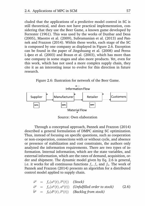
2.4. Applications of MPC in SCM 57
cluded that the applications of a predictive model control in SC isstill theoretical, and does not have practical implementation, con-sidering that they use the Beer Game, a known game developed byForrester (1961). This was used by the works of Dunbar and Desa(2005), Maestre et al. (2009), Subramanian et al. (2013) and Pan-nek and Frazzon (2014). Within these works, each stage of the SCis composed by one company as displayed in Figure 2.6. Exceptioncan be found in the paper of Jingshuang et al. (2008) and Perea-López et al. (2003) and Braun et al. (2003), which has more thanone company in some stages and also more products. Yet, even forthis work, which has not used a more complex supply chain, theycite it as an interesting issue to evolve for this direction in futureresearch.
Figure 2.6: Ilustration for network of the Beer Game.
Source: Own elaboration
Through a conceptual approach, Pannek and Frazzon (2014)described a general formulation of DMPC aiming SC optimization.Thus, instead of focusing on specific questions, such as cooperationor non-cooperation, connections with or without cycle, and absenceor presence of stabilization and cost constraints, the authors onlyanalyzed the information requirements. There are two types of in-formation. Internal information, which are the state variables, andexternal information, which are the rates of demand, acquisition, or-der and shipment. The dynamic model given by Eq. 2.6 is general,i.e. it works for all continuous functions fs, fo and fb. The work ofPannek and Frazzon (2014) presents an algorithm for a distributedcontrol model applied to supply chain.
\.sp = fs(ap(t), lp(t)) (Stock)
\.op = fo(op(t), ap(t)) (Unfulfilled order to stock)
\.bp = fb(dp(t), lp(t)) (Backlog from stock)
(2.6)
58 Chapter 2. Literature Review
The variables indicates the follow: sp - stock, opu - unfulfilled orderof stock, bp - backlog of stock ap - acquisition level, lp - shipmentrate, op: order rate, dp: demand rate, p - refer to the SC stages, i.e,p \in \{ S,M,R\} .
The application of Dunbar and Desa (2005) considers thatevery company in the chain optimizes its own objective. Then thecompanies make decisions that are sent to other companies, in theimmediate stages. The chain used by the authors contains threestages – one retailer, one manufacturer, one supplier and a markedcustomer. The flow of information to SC upstream has no delay, butthe information flow to downstream between coupled stages has aconstant delay. This work has used a dynamic model for each stage(2.7), which gives functions fp of (2.6). Then, this model has threestate variables – stock level, unfulfilled order to stock and backlogfrom stock. The instant variation of these states, depends on the rateof demand, acquisition, order and shipment. Every stage has its ownset of equations. These equations allow for distributed control of thestages, where the control variables are the stages orders. Therefore,the dynamic model can be used to predict the future development,which can be used to calculate optimal controls. Furthermore, thecustomers demand is regarded as a disturbance for the coupled sys-tem and the objective of each controller is to minimize the localcost, which includes to avoid unfulfilled order to stock while keep-ing backlog from stock and stock at desirable levels.
\.sp = ap(t) - lp(t) (Stock)\.op = op(t) - ap(t) (Unfulfilled order to stock)\.bp = dp(t) - lp(t) (Backlog from stock)
(2.7)
The results achieved by Dunbar and Desa (2005) show thatthe DMPC approach outperforms the nominal control shown bySterman (2000). This nominal control is a simple controller, in whichthe order rate is a function of stock level and unfulfilled order ofstock at each instant. Besides this advantage to DMPC approach,the authors highlights complications related to cycles of informa-tion. It means that in every sampling instant, the stages requiringinformation not available from upstream and downstream stages.The authors proposed that each stage sends its predictions of de-mand to stages immediately upstream.
In their model, Jingshuang et al. (2008) illustrated by sim-ulation that such an approach can be applied in real size supply
2.4. Applications of MPC in SCM 59
chain networks, which are subject to stochastic demand. The con-troller was implemented locally at each stage and aims at minimiz-ing the cost function. This function considers the inventory costs,transportation and unfulfilled demand. Moreover, the authors in-serted a weight for variation of batches of products. In fact, one ofthe results of this article is the comparison between what happenswhen using or not using this weight for the lots. The demands esti-mative is made using a time series model, autoregressive integratedmoving average (ARIMA).
Maestre et al. (2009) used the Beer Game to compare threeapproaches of MPC to model SCM. These approaches are relatedto the number of predictive controllers used in MPC and the typeof objective function that is used to estimate the control variables.The first approach used only one centralized controller to drive theoverall system. The second one exhibits distributed controllers andthe stages work cooperatively. Within the third one, the controllersare distributed but the cooperation property was removed. As ex-pected, the centralized version shows better performance, yet thedistributed approach represents the supreme strategy.
Subramanian et al. (2013) developed an DMPC based algo-rithm to accomplish the SCM with collaboration. The algorithm wasevaluated with a two stage supply chain. The properties and perfor-mance of this new approach were compared with classical distri-bution. The authors could verify that the cooperative distributionsetting performs better than the distribution approach without co-operation. Using developments in economic MPC Subramanian etal. (2014) proposed an economic model predictive control to guar-antee closed-loop properties for SC optimization. The controller ob-jective is a multi-objective cost function which intend to capture theeconomics as well as risk in the supply chain.
Mestan et al. (2006) compare several results of SC operationoptimization for several MPC configurations, that are centralized,decentralized, and semi-decentralized models. Centralized configu-ration results in better inventory management and production schedul-ing. Results also are compared in terms of total profit and customersatisfaction. In the fully decentralized and semi-decentralized mod-els, a lack of coordination is the key reason for obtaining inferiorresults, compared to the centralized model. This lack of coordina-tion causes the bullwhip effect, especially in the fully decentralizedmodel, which damages the optimal performance of the SC.
The work of Perea-López et al. (2003) has achieved a modelto support decisions based in the rolling horizon idea. This is an
60 Chapter 2. Literature Review
applications of MPC to multi-echelon production–inventory prob-lems. For that, they present a Mixed-Integer Linear Programmingmodel for the whole SC, i.e it analyzes the entire supply chainas a unit, considering suppliers, manufacturing, distribution andclients simultaneously. That model has the objective of finding theoptimal decision variables for maximizing profit in SCs with multi-product, single stage batch plants and multi-product, multiechelondistribution networks servicing multiple customers. However, thegreat result in this work is about when changes affecting the SCappear. In this situation they use Model Predictive Control. Theytested their formulation in quite a complex supply chain producingthree products and consisting of three factories, three warehouses,four distribution centers and 10 retailers servicing 20 customers.They compared their centralized approach against two decentral-ized approaches. The first decentralized approach optimizes distri-bution only and uses heuristic rules for production/inventory plan-ning. The second approach optimizes manufacturing while allowingthe distribution network to follow heuristic rules. Through simula-tions, they inferred that the centralized approach exhibits superiorperformance.
Braun et al. (2003) developed a linear MPC framework forlarge scale supply chain problems resulting from the semiconductorindustry. Through experiments, they showed that MPC can handleadequately uncertainty resulting from model mismatch (lead times)and demand forecasting errors. Due to the complexity of large scalesupply chains, they proposed a decentralized scheme where a modelpredictive controller is created for each node, i.e production facility,warehouse and retailers. Inventory levels are treated as state vari-ables for each node, the manipulated variables are orders and pro-duction rates, and demands are treated as disturbances. The goal ofthe MPC controller is to keep the inventory levels as close as possi-ble to the target values while satisfying constraints with respect toproduction and transportation capacities. Their simulations showedthat using move suppression, the term in the objective function thatpenalizes large deviations on control variables between two consec-utive time instants, then backorders can be eliminated. It is wellknown in the MPC community that the move suppression term hasthe effect of making the controller less sensitive to prediction inaccu-racies, although usually at the price of degrading set point trackingperformance.
Among all the observers studies, the stabilizing controllersstill remain a critical bottleneck in MPC as also pointed by Mayne
2.4. Applications of MPC in SCM 61
et al. (2000). That is, however, an expected result accourding Ca-macho and Bordons (2007), which point out stabilization in ModelPredictive Control is a difficult part in the Control Theory.

3 A MODEL PREDICTIVE CONTROL FRAMEWORK FOR SUPPLYCHAIN OPERATIONAL PLANNING
This chapter presents a framework for a SC operational plan-ning using MPC, both centralized and distributed controllers. Thecentralized controller is modeled for the sake of comparison withthe distributed controlling structure. This framework contains thegeneral schemes, the equations and the procedure steps. It also for-mally has some aspects of this SC for the purpose of understandingand communication rules. The meaning of frameworks in this con-text is synonymous of conceptual model in the meaning present byDavies et al. (2006), Mylopoulos (1992): it conveys the fundamen-tal principles and basic functionality of the system it represents.
The models of this chapter takes that an important objectivein the management and control of a SC is to rapidly fulfill customerdemand while keeping the inventory (stock) level in each stage aslow as possible. For example, considering the manufacturer stageM in the SC. The M must respond to a demand from the retailer Rfrom his current inventory and by ordering goods from the S. TheS attempts to fulfill the manufacturers order (from his inventoryor production), and ships the material to the manufacturer whoreceives (or acquires) them after a time delay that depends on themethod of shipment.
3.1 A DISTRIBUTED MANAGERS MODEL
The application of a DMPC in a three stage SC as displayedin Figure 1.1 is achieved by assigning a MPC controller for eachstage. Figure 3.1, supported by Table 3.1, shows this conceptualmodel and the flow of information and materials in that SC. Fromthis section, the set of these stages will be denoted by SS, i.e, theequality SS = {S, M, R}. Then, the state variables of each stagesuperscript by p \in SS at instant tn are
• the stock level: sp(tn),
• the unfulfilled order of stock: opu(tn), and
• the backlog of stock: bp(tn).
Stock level is the number of items currently available in stagep for shipment to the downstream stage. Unfulfilled order of stockis the number of items that stage p has yet to receive from the up-stream stage. Backlog of stock is the number of committed itemsthat stage p has yet to ship to the downstream stage.
63
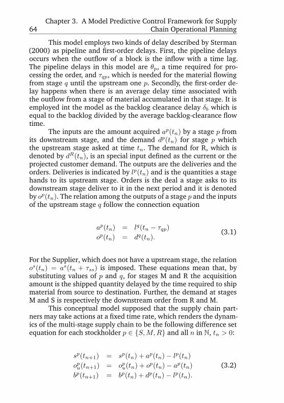
64Chapter 3. A Model Predictive Control Framework for Supply
Chain Operational Planning
This model employs two kinds of delay described by Sterman(2000) as pipeline and first-order delays. First, the pipeline delaysoccurs when the outflow of a block is the inflow with a time lag.The pipeline delays in this model are \theta p, a time required for pro-cessing the order, and \tau qp, which is needed for the material flowingfrom stage q until the upstream one p. Secondly, the first-order de-lay happens when there is an average delay time associated withthe outflow from a stage of material accumulated in that stage. It isemployed int the model as the backlog clearance delay \delta b which isequal to the backlog divided by the average backlog-clearance flowtime.
The inputs are the amount acquired ap(tn) by a stage p fromits downstream stage, and the demand dp(tn) for stage p whichthe upstream stage asked at time tn. The demand for R, which isdenoted by dR(tn), is an special input defined as the current or theprojected customer demand. The outputs are the deliveries and theorders. Deliveries is indicated by lp(tn) and is the quantities a stagehands to its upstream stage. Orders is the deal a stage asks to itsdownstream stage deliver to it in the next period and it is denotedby op(tn). The relation among the outputs of a stage p and the inputsof the upstream stage q follow the connection equation
ap(tn) = lq(tn - \tau qp)
op(tn) = dq(tn).(3.1)
For the Supplier, which does not have a upstream stage, the relationos(tn) = as(tn + \tau ss) is imposed. These equations mean that, bysubstituting values of p and q, for stages M and R the acquisitionamount is the shipped quantity delayed by the time required to shipmaterial from source to destination. Further, the demand at stagesM and S is respectively the downstream order from R and M.
This conceptual model supposed that the supply chain part-ners may take actions at a fixed time rate, which renders the dynam-ics of the multi-stage supply chain to be the following difference setequation for each stockholder p \in \{ S,M,R\} and all n in \BbbN , tn > 0:
sp(tn+1) = sp(tn) + ap(tn) - lp(tn)
opu(tn+1) = opu(tn) + op(tn) - ap(tn)
bp(tn+1) = bp(tn) + dp(tn) - lp(tn).
(3.2)
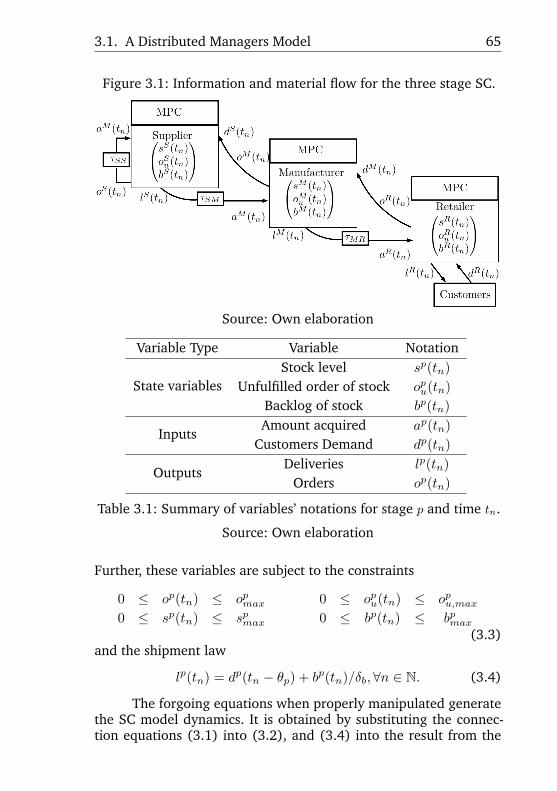
3.1. A Distributed Managers Model 65
Figure 3.1: Information and material flow for the three stage SC.
Source: Own elaboration
Variable Type Variable Notation
State variablesStock level sp(tn)
Unfulfilled order of stock opu(tn)
Backlog of stock bp(tn)
InputsAmount acquired ap(tn)
Customers Demand dp(tn)
OutputsDeliveries lp(tn)
Orders op(tn)
Table 3.1: Summary of variables’ notations for stage p and time tn.
Source: Own elaboration
Further, these variables are subject to the constraints
0 \leq op(tn) \leq opmax
0 \leq sp(tn) \leq spmax
0 \leq opu(tn) \leq opu,max
0 \leq bp(tn) \leq bpmax
(3.3)and the shipment law
lp(tn) = dp(tn - \theta p) + bp(tn)/\delta b,\forall n \in \BbbN . (3.4)
The forgoing equations when properly manipulated generatethe SC model dynamics. It is obtained by substituting the connec-tion equations (3.1) into (3.2), and (3.4) into the result from the
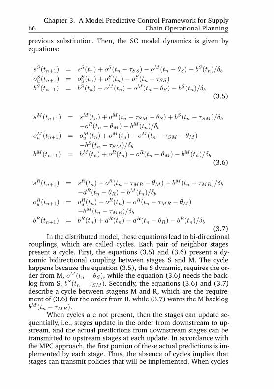
66Chapter 3. A Model Predictive Control Framework for Supply
Chain Operational Planning
previous substitution. Then, the SC model dynamics is given byequations:
sS(tn+1) = sS(tn) + oS(tn - \tau SS) - oM (tn - \theta S) - bS(tn)/\delta boSu(tn+1) = oSu(tn) + oS(tn) - oS(tn - \tau SS)
bS(tn+1) = bS(tn) + oM (tn) - oM (tn - \theta S) - bS(tn)/\delta b(3.5)
sM (tn+1) = sM (tn) + oM (tn - \tau SM - \theta S) + bS(tn - \tau SM )/\delta b - oR(tn - \theta M ) - bM (tn)/\delta b
oMu (tn+1) = oMu (tn) + oM (tn) - oM (tn - \tau SM - \theta M )
- bS(tn - \tau SM )/\delta bbM (tn+1) = bM (tn) + oR(tn) - oR(tn - \theta M ) - bM (tn)/\delta b
(3.6)
sR(tn+1) = sR(tn) + oR(tn - \tau MR - \theta M ) + bM (tn - \tau MR)/\delta b - dR(tn - \theta R) - bM (tn)/\delta b
oRu (tn+1) = oRu (tn) + oR(tn) - oR(tn - \tau MR - \theta M )
- bM (tn - \tau MR)/\delta bbR(tn+1) = bR(tn) + dR(tn) - dR(tn - \theta R) - bR(tn)/\delta b
(3.7)In the distributed model, these equations lead to bi-directional
couplings, which are called cycles. Each pair of neighbor stagespresent a cycle. First, the equations (3.5) and (3.6) present a dy-namic bidirectional coupling between stages S and M. The cyclehappens because the equation (3.5), the S dynamic, requires the or-der from M, oM (tn - \theta S), while the equation (3.6) needs the back-log from S, bS(tn - \tau SM ). Secondly, the equations (3.6) and (3.7)describe a cycle between stagens M and R, which are the require-ment of (3.6) for the order from R, while (3.7) wants the M backlogbM (tn - \tau MR).
When cycles are not present, then the stages can update se-quentially, i.e., stages update in the order from downstream to up-stream, and the actual predictions from downstream stages can betransmitted to upstream stages at each update. In accordance withthe MPC approach, the first portion of these actual predictions is im-plemented by each stage. Thus, the absence of cycles implies thatstages can transmit policies that will be implemented. When cycles
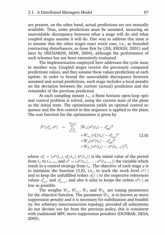
3.1. A Distributed Managers Model 67
are present, on the other hand, actual predictions are not mutuallyavailable. Thus, some predictions must be assumed, incurring anunavoidable discrepancy between what a stage will do and whatcoupled stages assume it will do. One way to address this issue isto assume that the other stages react worst case, i.e., as boundedcontracting disturbances, as done first by (JIA; KROGH, 2001) andlater by (RICHARDS; HOW, 2004), although the performance ofsuch schemes has not been extensively evaluated.
The implementation employed here addresses the cycle issuein another way. Coupled stages receive the previously computedpredictions values, and they assume these values predictions at eachupdate. In order to bound the unavoidable discrepancy betweenassumed and actual predictions, each stage includes a local penaltyon the deviation between the current (actual) prediction and theremainder of the previous prediction
At each sampling instant tn, a finite horizon open-loop opti-mal control problem is solved, using the current state of the plantas the initial state. The optimization yields an optimal control se-quence and the first control in this sequence is applied to the plant.The cost function for the optimization is given by
Jp(xpn, o
p) =N+n\sum k=n
[Ws(sp(tk) - spref)
2
+Wou(opu(tk) - opuref
)2
+Wo(op(tk) - opref)
2
+W\delta o(op(tk) - op(tk - 1))
2]
(3.8)
where xpn = (sp(tn), o
pu(tn), b
p(tn)) is the initial value of the periodfrom tn to tN+n, and op = (op(tn), . . . , o
p(tN+n)) the variable whichresult in a control strategy from tn. The objective of each stage p isto minimize the function (3.8), i.e., to track the stock level sp(\cdot )and to keep the unfulfilled orders opu(\cdot ) to the respective referencesvalues spref and opuref
, and also it aims to keeps the orders op(\cdot ) aslow as possible.
The weights Ws, Wou , Wo and W\delta o are tuning parametersfor the objective function. The parameter W\delta o is to known as movesuppression penalty and it is necessary for stabilization and feasibil-ity. For arbitrary interconnection topology, provided all subsystemsdo not deviate too far from the previous policy, this is consistentwith traditional MPC move suppression penalties (DUNBAR; DESA,2005).
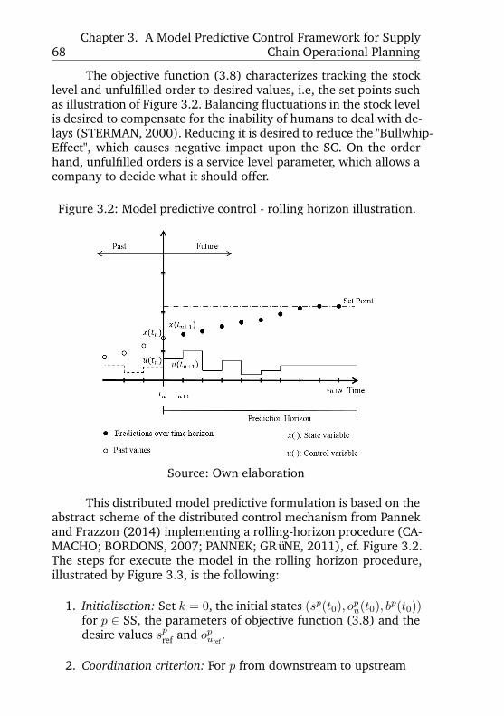
68Chapter 3. A Model Predictive Control Framework for Supply
Chain Operational Planning
The objective function (3.8) characterizes tracking the stocklevel and unfulfilled order to desired values, i.e, the set points suchas illustration of Figure 3.2. Balancing fluctuations in the stock levelis desired to compensate for the inability of humans to deal with de-lays (STERMAN, 2000). Reducing it is desired to reduce the "Bullwhip-Effect", which causes negative impact upon the SC. On the orderhand, unfulfilled orders is a service level parameter, which allows acompany to decide what it should offer.
Figure 3.2: Model predictive control - rolling horizon illustration.
Source: Own elaboration
This distributed model predictive formulation is based on theabstract scheme of the distributed control mechanism from Pannekand Frazzon (2014) implementing a rolling-horizon procedure (CA-MACHO; BORDONS, 2007; PANNEK; GRüNE, 2011), cf. Figure 3.2.The steps for execute the model in the rolling horizon procedure,illustrated by Figure 3.3, is the following:
1. Initialization: Set k = 0, the initial states (sp(t0), opu(t0), bp(t0))
for p \in SS, the parameters of objective function (3.8) and thedesire values spref and opuref
.
2. Coordination criterion: For p from downstream to upstream
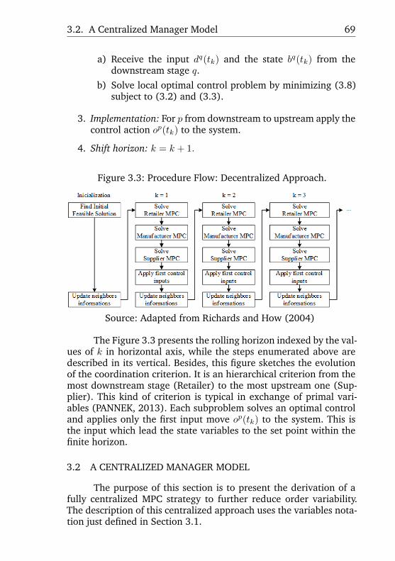
3.2. A Centralized Manager Model 69
a) Receive the input dq(tk) and the state bq(tk) from thedownstream stage q.
b) Solve local optimal control problem by minimizing (3.8)subject to (3.2) and (3.3).
3. Implementation: For p from downstream to upstream apply thecontrol action op(tk) to the system.
4. Shift horizon: k = k + 1.
Figure 3.3: Procedure Flow: Decentralized Approach.
Source: Adapted from Richards and How (2004)
The Figure 3.3 presents the rolling horizon indexed by the val-ues of k in horizontal axis, while the steps enumerated above aredescribed in its vertical. Besides, this figure sketches the evolutionof the coordination criterion. It is an hierarchical criterion from themost downstream stage (Retailer) to the most upstream one (Sup-plier). This kind of criterion is typical in exchange of primal vari-ables (PANNEK, 2013). Each subproblem solves an optimal controland applies only the first input move op(tk) to the system. This isthe input which lead the state variables to the set point within thefinite horizon.
3.2 A CENTRALIZED MANAGER MODEL
The purpose of this section is to present the derivation of afully centralized MPC strategy to further reduce order variability.The description of this centralized approach uses the variables nota-tion just defined in Section 3.1.
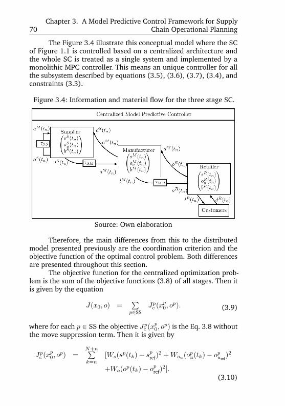
70Chapter 3. A Model Predictive Control Framework for Supply
Chain Operational Planning
The Figure 3.4 illustrate this conceptual model where the SCof Figure 1.1 is controlled based on a centralized architecture andthe whole SC is treated as a single system and implemented by amonolithic MPC controller. This means an unique controller for allthe subsystem described by equations (3.5), (3.6), (3.7), (3.4), andconstraints (3.3).
Figure 3.4: Information and material flow for the three stage SC.
Source: Own elaboration
Therefore, the main differences from this to the distributedmodel presented previously are the coordination criterion and theobjective function of the optimal control problem. Both differencesare presented throughout this section.
The objective function for the centralized optimization prob-lem is the sum of the objective functions (3.8) of all stages. Then itis given by the equation
J(x0, o) =\sum p\in SS
Jpc (x
p0, o
p). (3.9)
where for each p \in SS the objective Jpc (x
p0, o
p) is the Eq. 3.8 withoutthe move suppression term. Then it is given by
Jpc (x
p0, o
p) =N+n\sum k=n
[Ws(sp(tk) - spref)
2 +Wou(opu(tk) - opuref
)2
+Wo(op(tk) - opref)
2].(3.10)
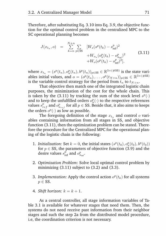
3.2. A Centralized Manager Model 71
Therefore, after substituting Eq. 3.10 into Eq. 3.9, the objective func-tion for the optimal control problem in the centralized MPC to theSC operational planning becomes
J(xtn , o) =N+n\sum k=n
\sum p\in SS
[Ws(sp(tk) - spref)
2
+Wou(opu(tk) - opuref
)2
+Wo(op(tk) - opref)
2],
(3.11)
where xtn = (sp(tn), opu(tn), b
p(tn))p\in SS \in \BbbR 3\times (\#SS) is the state vari-ables initial values, and o = (op(tn), . . . , o
p(tN+n))p\in SS \in \BbbR 3\times (\#SS)
is the variable control strategy for the period from tn to tN+n.That objective then match one of the integrated logistic chain
purposes, the minimization of the cost for the whole chain. Thisis taken by the (3.11) by tracking the sum of the stock level sp(\cdot )and to keep the unfulfilled orders opu(\cdot ) to the respective referencesvalues spref and opuref
for all p \in SS. Beside that, it also aims to keepsthe orders op(\cdot ) as low as possible.
The foregoing definition of the stage xtn and control o vari-ables containing information from all stages in SS, and objectivefunction (3.11), then the optimization problem can be stated. There-fore the procedure for the Centralized MPC for the operational plan-ing of the logistic chain is the following:
1. Initialization: Set k = 0, the initial states (sp(t0), opu(t0), bp(t0))
for p \in SS, the parameters of objective function (3.9) and thedesire values spref and opuref
.
2. Optimization Problem: Solve local optimal control problem byminimizing (3.11) subject to (3.2) and (3.3).
3. Implementation: Apply the control action op(tk) for all systemsp \in SS.
4. Shift horizon: k = k + 1.
As a central controller, all stage information variables of Ta-ble 3.1 is available for whatever stages that need them. Then, thesystems do not need receive past information from their neighborstages and such the step 2a from the distributed model procedure,i.e, the coordination criterion is not necessary.
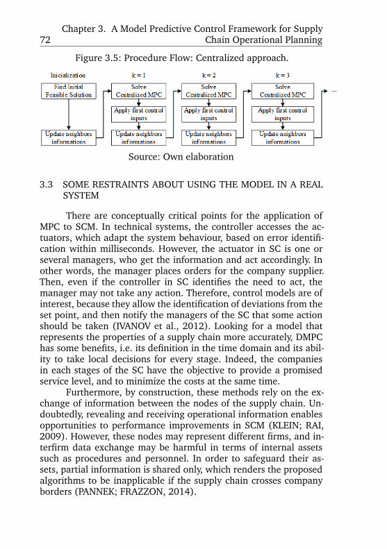
72Chapter 3. A Model Predictive Control Framework for Supply
Chain Operational Planning
Figure 3.5: Procedure Flow: Centralized approach.
Source: Own elaboration
3.3 SOME RESTRAINTS ABOUT USING THE MODEL IN A REALSYSTEM
There are conceptually critical points for the application ofMPC to SCM. In technical systems, the controller accesses the ac-tuators, which adapt the system behaviour, based on error identifi-cation within milliseconds. However, the actuator in SC is one orseveral managers, who get the information and act accordingly. Inother words, the manager places orders for the company supplier.Then, even if the controller in SC identifies the need to act, themanager may not take any action. Therefore, control models are ofinterest, because they allow the identification of deviations from theset point, and then notify the managers of the SC that some actionshould be taken (IVANOV et al., 2012). Looking for a model thatrepresents the properties of a supply chain more accurately, DMPChas some benefits, i.e. its definition in the time domain and its abil-ity to take local decisions for every stage. Indeed, the companiesin each stages of the SC have the objective to provide a promisedservice level, and to minimize the costs at the same time.
Furthermore, by construction, these methods rely on the ex-change of information between the nodes of the supply chain. Un-doubtedly, revealing and receiving operational information enablesopportunities to performance improvements in SCM (KLEIN; RAI,2009). However, these nodes may represent different firms, and in-terfirm data exchange may be harmful in terms of internal assetssuch as procedures and personnel. In order to safeguard their as-sets, partial information is shared only, which renders the proposedalgorithms to be inapplicable if the supply chain crosses companyborders (PANNEK; FRAZZON, 2014).
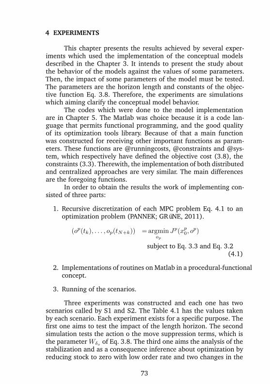
4 EXPERIMENTS
This chapter presents the results achieved by several exper-iments which used the implementation of the conceptual modelsdescribed in the Chapter 3. It intends to present the study aboutthe behavior of the models against the values of some parameters.Then, the impact of some parameters of the model must be tested.The parameters are the horizon length and constants of the objec-tive function Eq. 3.8. Therefore, the experiments are simulationswhich aiming clarify the conceptual model behavior.
The codes which were done to the model implementationare in Chapter 5. The Matlab was choice because it is a code lan-guage that permits functional programming, and the good qualityof its optimization tools library. Because of that a main functionwas constructed for receiving other important functions as param-eters. These functions are @runningcosts, @constraints and @sys-tem, which respectively have defined the objective cost (3.8), theconstraints (3.3). Therewith, the implementation of both distributedand centralized approaches are very similar. The main differencesare the foregoing functions.
In order to obtain the results the work of implementing con-sisted of three parts:
1. Recursive discretization of each MPC problem Eq. 4.1 to anoptimization problem (PANNEK; GRüNE, 2011).
(op(tk), . . . , op(tN+k)) = \mathrm{a}\mathrm{r}\mathrm{g}\mathrm{m}\mathrm{i}\mathrm{n}op
Jp(xp0, o
p)
subject to Eq. 3.3 and Eq. 3.2(4.1)
2. Implementations of routines on Matlab in a procedural-functionalconcept.
3. Running of the scenarios.
Three experiments was constructed and each one has twoscenarios called by S1 and S2. The Table 4.1 has the values takenby each scenario. Each experiment exists for a specific purpose. Thefirst one aims to test the impact of the length horizon. The secondsimulation tests the action o the move suppression terms, which isthe parameter W\delta o of Eq. 3.8. The third one aims the analysis of thestabilization and as a consequence inference about optimization byreducing stock to zero with low order rate and two changes in the
73
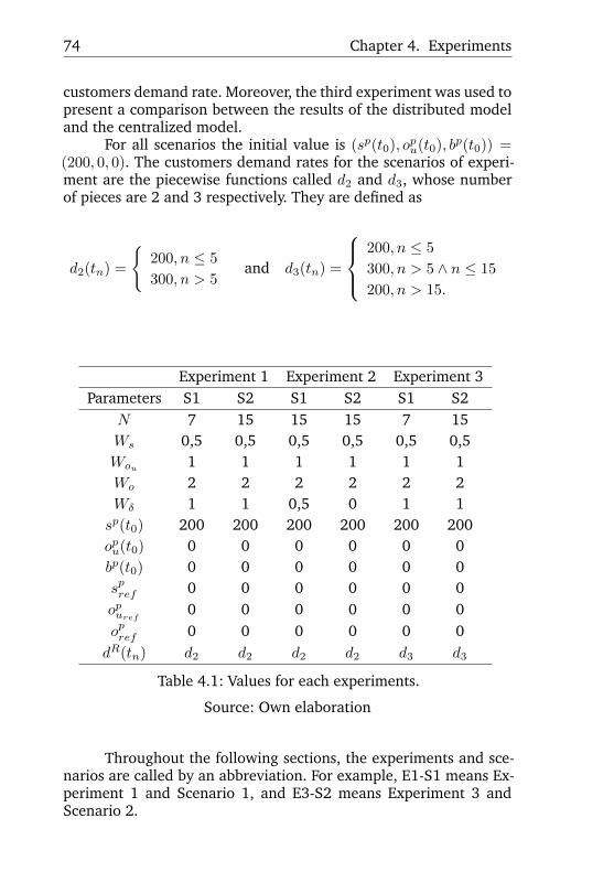
74 Chapter 4. Experiments
customers demand rate. Moreover, the third experiment was used topresent a comparison between the results of the distributed modeland the centralized model.
For all scenarios the initial value is (sp(t0), opu(t0), b
p(t0)) =(200, 0, 0). The customers demand rates for the scenarios of experi-ment are the piecewise functions called d2 and d3, whose numberof pieces are 2 and 3 respectively. They are defined as
d2(tn) =
\Biggl\{ 200, n \leq 5
300, n > 5and d3(tn) =
\left\{ 200, n \leq 5
300, n > 5 \wedge n \leq 15
200, n > 15.
Experiment 1 Experiment 2 Experiment 3Parameters S1 S2 S1 S2 S1 S2
N 7 15 15 15 7 15Ws 0,5 0,5 0,5 0,5 0,5 0,5Wou 1 1 1 1 1 1Wo 2 2 2 2 2 2W\delta 1 1 0,5 0 1 1
sp(t0) 200 200 200 200 200 200opu(t0) 0 0 0 0 0 0bp(t0) 0 0 0 0 0 0spref 0 0 0 0 0 0opuref
0 0 0 0 0 0opref 0 0 0 0 0 0
dR(tn) d2 d2 d2 d2 d3 d3
Table 4.1: Values for each experiments.
Source: Own elaboration
Throughout the following sections, the experiments and sce-narios are called by an abbreviation. For example, E1-S1 means Ex-periment 1 and Scenario 1, and E3-S2 means Experiment 3 andScenario 2.
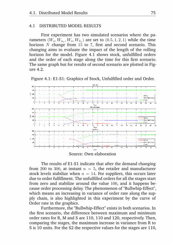
4.1. Distributed Model Results 75
4.1 DISTRIBUTED MODEL RESULTS
First experiment has two simulated scenarios where the pa-rameters (Ws,Wou ,Wo,W\delta o) are set to (0.5, 1, 2, 1) while the timehorizon N change from 15 to 7, first and second scenario. Thischanging aims to evaluate the impact of the length of the rollinghorizon for the model. Figure 4.1 shows stock, unfulfilled ordersand the order of each stage along the time for this first scenario.The same graph but for results of second scenario are plotted in Fig-ure 4.2.
Figure 4.1: E1-S1: Graphics of Stock, Unfulfilled order and Order.
Source: Own elaboration
The results of E1-S1 indicate that after the demand changingfrom 200 to 300, at instant n = 5, the retailer and manufacturerstock levels stabilize when n = 14. For suppliers, this occurs laterdue to order fulfillment. The unfulfilled orders for all the stages startfrom zero and stabilize around the value 100, and it happens be-cause order processing delay. The phenomenon of "Bullwhip-Effect",which means an increasing in variance of order rate along the sup-ply chain, is also highlighted in this experiment by the curve ofOrder rate in the graphics.
Furthermore, the "Bullwhip-Effect" exists in both scenarios. Inthe first scenario, the difference between maximum and minimumorder rates for R, M and S are 110, 110 and 120, respectively. Then,comparing the stages, the maximum increase in variance from R toS is 10 units. For the S2 the respective values for the stages are 110,
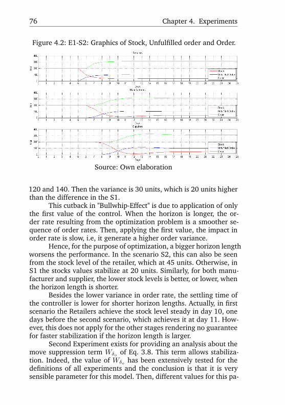
76 Chapter 4. Experiments
Figure 4.2: E1-S2: Graphics of Stock, Unfulfilled order and Order.
Source: Own elaboration
120 and 140. Then the variance is 30 units, which is 20 units higherthan the difference in the S1.
This cutback in "Bullwhip-Effect" is due to application of onlythe first value of the control. When the horizon is longer, the or-der rate resulting from the optimization problem is a smoother se-quence of order rates. Then, applying the first value, the impact inorder rate is slow, i.e, it generate a higher order variance.
Hence, for the purpose of optimization, a bigger horizon lengthworsens the performance. In the scenario S2, this can also be seenfrom the stock level of the retailer, which at 45 units. Otherwise, inS1 the stocks values stabilize at 20 units. Similarly, for both manu-facturer and supplier, the lower stock levels is better, or lower, whenthe horizon length is shorter.
Besides the lower variance in order rate, the settling time ofthe controller is lower for shorter horizon lengths. Actually, in firstscenario the Retailers achieve the stock level steady in day 10, onedays before the second scenario, which achieves it at day 11. How-ever, this does not apply for the other stages rendering no guaranteefor faster stabilization if the horizon length is larger.
Second Experiment exists for providing an analysis about themove suppression term W\delta o of Eq. 3.8. This term allows stabiliza-tion. Indeed, the value of W\delta o has been extensively tested for thedefinitions of all experiments and the conclusion is that it is verysensible parameter for this model. Then, different values for this pa-
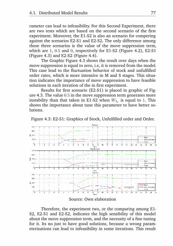
4.1. Distributed Model Results 77
rameter can lead to infeasibility. For this Second Experiment, thereare two tests which are based on the second scenario of the firstexperiment. Moreover, the E1-S2 is also an scenario for comperingagainst the scenarios E2-S1 and E2-S2. The only difference amongthese three scenarios is the value of the move suppression term,which are 1, 0.5 and 0, respectively for E1-S2 (Figure 4.2), E2-S1(Figure 4.3) and E2-S2 (Figure 4.4).
The Graphic Figure 4.3 shows the result over days when themove suppression is equal to zero, i.e, it is removed from the model.This case lead to the fluctuation behavior of stock and unfulfilledorder rates, which is more intensive in M and S stages. This situa-tion indicates the importance of move suppression to have feasiblesolutions in each iteration of the in first experiment.
Results for first scenario (E2-S1) is placed in graphic of Fig-ure 4.3. The value 0.5 in the move suppression term generates moreinstability than that taken in E1-S2 when W\delta o is equal to 1. Thisshows the importance about tune this parameter to have better so-lutions.
Figure 4.3: E2-S1: Graphics of Stock, Unfulfilled order and Order.
Source: Own elaboration
Therefore, the experiment two, or the comparing among E1-S2, E2-S1 and E2-S2, indicates the high sensibility of this modelabout the move suppression term, and the necessity of a fine tuningfor it. Its no just to have good solutions, because a wrong param-eterizations can lead to infeasibility in some iterations. This result
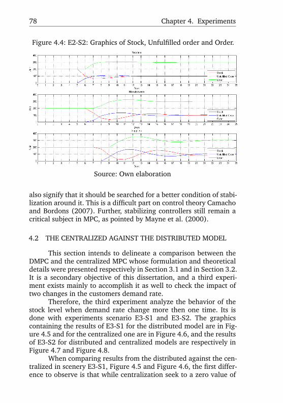
78 Chapter 4. Experiments
Figure 4.4: E2-S2: Graphics of Stock, Unfulfilled order and Order.
Source: Own elaboration
also signify that it should be searched for a better condition of stabi-lization around it. This is a difficult part on control theory Camachoand Bordons (2007). Further, stabilizing controllers still remain acritical subject in MPC, as pointed by Mayne et al. (2000).
4.2 THE CENTRALIZED AGAINST THE DISTRIBUTED MODEL
This section intends to delineate a comparison between theDMPC and the centralized MPC whose formulation and theoreticaldetails were presented respectively in Section 3.1 and in Section 3.2.It is a secondary objective of this dissertation, and a third experi-ment exists mainly to accomplish it as well to check the impact oftwo changes in the customers demand rate.
Therefore, the third experiment analyze the behavior of thestock level when demand rate change more then one time. Its isdone with experiments scenario E3-S1 and E3-S2. The graphicscontaining the results of E3-S1 for the distributed model are in Fig-ure 4.5 and for the centralized one are in Figure 4.6, and the resultsof E3-S2 for distributed and centralized models are respectively inFigure 4.7 and Figure 4.8.
When comparing results from the distributed against the cen-tralized in scenery E3-S1, Figure 4.5 and Figure 4.6, the first differ-ence to observe is that while centralization seek to a zero value of
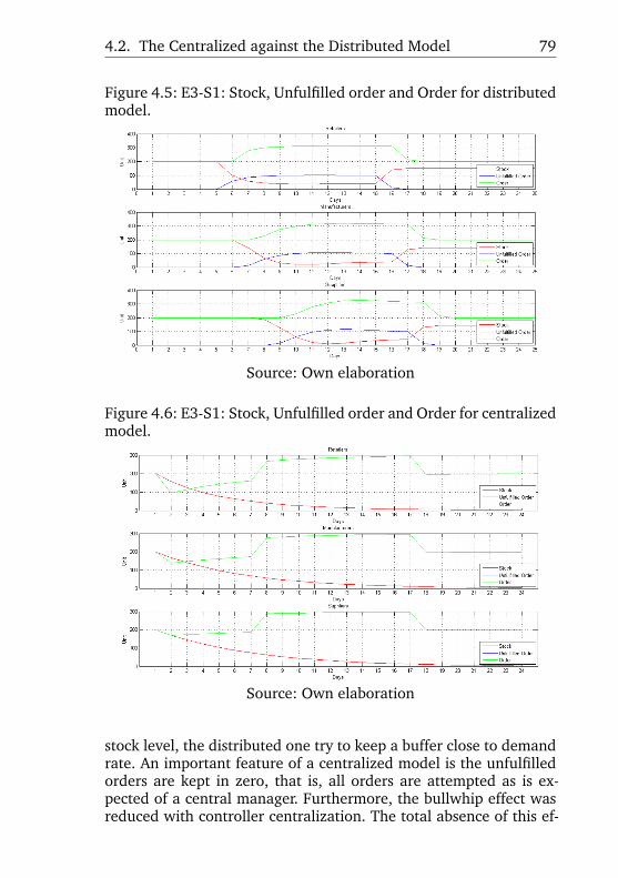
4.2. The Centralized against the Distributed Model 79
Figure 4.5: E3-S1: Stock, Unfulfilled order and Order for distributedmodel.
Source: Own elaboration
Figure 4.6: E3-S1: Stock, Unfulfilled order and Order for centralizedmodel.
Source: Own elaboration
stock level, the distributed one try to keep a buffer close to demandrate. An important feature of a centralized model is the unfulfilledorders are kept in zero, that is, all orders are attempted as is ex-pected of a central manager. Furthermore, the bullwhip effect wasreduced with controller centralization. The total absence of this ef-
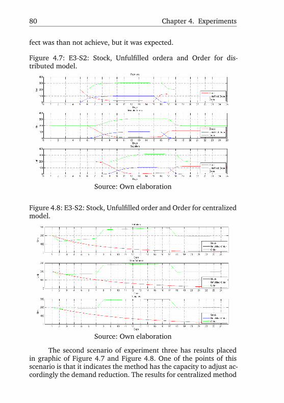
80 Chapter 4. Experiments
fect was than not achieve, but it was expected.
Figure 4.7: E3-S2: Stock, Unfulfilled ordera and Order for dis-tributed model.
Source: Own elaboration
Figure 4.8: E3-S2: Stock, Unfulfilled order and Order for centralizedmodel.
Source: Own elaboration
The second scenario of experiment three has results placedin graphic of Figure 4.7 and Figure 4.8. One of the points of thisscenario is that it indicates the method has the capacity to adjust ac-cordingly the demand reduction. The results for centralized method
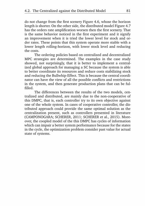
4.2. The Centralized against the Distributed Model 81
do not change from the first scenery Figure 4.6, whose the horizonlength is shorter. On the other side, the distributed model Figure 4.7has the orders rate amplification worsen then the first scenery. Thatis the same behavior noticed in the first experiment and it signifyan improvement when it is tried the lower level for stock and or-der rates. These points that this system operate more stable with alower length rolling-horizon, with lower stock level and reducingthe costs.
The ordering policies based on centralized and decentralizedMPC strategies are determined. The examples in the case studyshowed, not surprisingly, that it is better to implement a central-ized global approach for managing a SC because the system is ableto better coordinate its resources and reduce costs stabilizing stockand reducing the Bullwhip-Effect. This is because the central coordi-nator can have the view of all the possible conflicts and restrictionsin the system, and then generate production plans that can be ful-filled.
The differences between the results of the two models, cen-tralized and distributed, are mainly due to the non-cooperative ofthis DMPC, that is, each controller try to its own objective againstone of the whole system. In cases of cooperative controller, the dis-tributed approach could provide the same optimal solution as thecentralization present, such as controllers presented in literature(CAMPONOGARA; SCHERER, 2011; SCHERER et al., 2015). More-over, the coopled model of the this DMPC has cycles of informationwhich can impair a better system performance because for the statesin the cycle, the optimization problem consider past value for actualstate of systems.

5 CONCLUSION
The Supply Chain operational planning is a broad probleminto the Supply Chain Management or the logistics. This work hasmainly tacked the stabilization problem of stock level and the trade-off between it and the quantity of the orders. This is an optimizationproblem whose the expected solution benefit is to reduce the Bull-whip Effect. Then, the objective of this work was to study how isthe Model Predictive Control behavior as an optimization tool inlogistic operational planning. Indeed, the Model Predictive Controlis a control methodology which seems to be suitable for this kindof problem in logistics. Furthermore, as some bibliographical refer-ences are affirming, this methodology is already very popular in pro-cess control industry due to its explicitly form to deal with controlobjectives and operating constraints in the optimization problemthat is solved at each instant.
For accomplishing this objective, the conceptual model wasformally described, and computational routines were implementedto take results from the model. This aimed the understanding ofdifficulties associated with effects of an implementation. It was ob-served that the interconnected system model for the Supply Chainhas cycles of information, and that cycles bring problems about fea-sibility for optimization at each step of the procedure to execute themodel. The solution to that issue was using the state variable fromthe previous period, and the move suppression term calibration toprovide stability. Although the stability was achieved, it is very de-pendent of the move suppression term value. Then, in the progressthis research, it is necessary to study problem related to cycles andthe impact it have on feasibility and stability.
After implementing the model in Matlab it has become easyget results from some values of parameters and customer demandfunctions. Then, the behavior of Supply Chain operational optimiza-tion was analyzed against the variation on the move suppressionterm, the rolling-horizon length, and costumers demand. Besides,as the centralized model predictive control was also implemented,a comparative analysis become practicable.
The experiments show that although the move suppressionterms is not necessary in the centralized model, the DistributedModel Predictive Control approach is very sensible to them, andin this case the move suppression terms are essential. Without thisweight, the distributed models become unstable. However, whentuning the parameters, the optimization has presented a solution.When analyzing the effect of the time horizon, its impact on the per-
83
84 Chapter 5. Conclusion
formance shows that the longer the horizon, the solution tends tobe smoother, but it worsens the performance, that is, the Bullwhip-Effect is more intense.
The differences between the results of the two models, cen-tralized and distributed, are mainly due to the non-cooperative ofthis DMPC, that is, each controller try to its own objective againstone of the whole system. In cases of cooperative controller, the dis-tributed approach could provide the same optimal solution as thecentralization presents. Besides, the DMPC presented in this disser-tation has the cycles of information which worsen performance.
The literature review has shown that the academic status ofDistributed Model Predictive Control applications to Supply ChainManagement is still theoretical, i.e, the set of paper into this reviewhave not presented yet many implementations in real scenery. Fur-thermore, the studies are mainly using the Beer Game. However, thegrowing of good publications indicates this methodology as promi-nent to more studies and improvements.
In industrial process the controller traditionally accesses theactuators, which adapt the system behavior based on error identi-fication within milliseconds. However, in logistic the decisions aremade by managers and its time is counted at least in minutes, i.e,the Supply Chain actuator is one or several managers, who needmore then milliseconds to get the information and act accordingly,but together with theirs felling. In other words, the manager placesorders for the company supplier. Then, even if the controller in SCidentifies the need of acting, the manager may not take any actionimmediate. Therefore, control models are of interest, because theyallow the identification of the deviations from the set point, andthen notify the managers that some action should be taken.
Moreover, looking for a model that represents the propertiesof a Supply Chain more accurately, Distributed Model PredictiveControl has some benefits, i.e. its definition in the time domain andits ability to take local decisions for every stage. Indeed, the compa-nies in each stage of the Supply Chain have the objective to providea promised service level, and to minimize the costs at the same time.However, stability and feasibility are drawbacks to overcoming andmaking this application feasible in practice.
Finally, in addition to all conclusions from this work, some fu-ture developments can be pointed. First, a more detailed study onthe problem related to cycles and the impact it have on feasibilityand stability in the contexts the model presented. Secondly, otheralternatives to the move suppression or a set propositions on stabil-

85
ity guarantee for its use. Third an application in a real case sceneryof both centralized and decentralized models.

BIBLIOGRAPHY
AITKEN, J. M. Supply Chain Integration Within the Contextof a Supplier Association: Case Studies of Four SupplierAssociations. p. 392, 1998. Available from Internet: <http://onlinelibrary.wiley.com/doi/10.1002/cbdv.200490137/abstract>.
BALLOU, R. H. Business logistics – importance and some researchopportunities. Gestão e Producão, v. 4, n. 2, p. 117–129, 1997.
BALLOU, R. H. Gerenciamento da Cadeia de Suprimentos: LogísticaEmpresarial. 5ª. ed. [S.l.: s.n.], 2006.
BOWERSOX, D. J.; CLOSS, D. J.; COOPER, M. B. Supply chain logisticsmanagement. [S.l.: s.n.], 2002. 498 p.
BRAMEL, J.; SIMCHI-LEVI, D. The Logic of Logistics. New York, NY:Springer New York, 1997.
BRAUN, M. d. et al. A Model Predictive Control framework for robustmanagement of multi-product, multi-echelon demand networks.Annual Reviews in Control, v. 27 II, p. 229–245, 2003. ISSN 13675788.
CAMACHO, E. F.; BORDONS, C. Model Predictive Control. Second.[S.l.: s.n.], 2007. ISSN 15582531. ISBN 978-1-85233-694-3.
CAMPONOGARA, B. E. et al. Distributed Model Predictive Control.IEEE Control Syst. Mag., n. February, 2002.
CAMPONOGARA, E.; SCHERER, H. Distributed optimization for modelpredictive control of linear dynamic networks with control-input andoutput constraints. IEEE Transactions on Automation Science andEngineering, v. 8, p. 233–242, 2011.
CHEN, L. L.; LEE, H. L. H. Bullwhip effect measurement and itsimplications. Operations Research, v. 60, n. 4, p. 771–784, 2012.
CHOPRA, S.; MEINDL, P. Supply Chain Management: Strategy, Planningand Operations. New Jersey: Pearson Prentice Hall Press, 2010.
CHRISTOFIDES, P. D. et al. Distributed model predictive control: Atutorial review and future research directions. Comput. Chem. Eng.,v. 51, p. 21–41, apr 2013.
CHRISTOPHER, M. Logistics & supply chain management. [S.l.: s.n.],1992. 276 p. ISBN 9780273731122.
87
88 Bibliography
CSCMP, C. Supply Chain Management Terms and Glossary. 2013.Available from Internet: <www.cscmp.org>.
DAVIES, I. et al. How do practitioners use conceptual modeling inpractice? Data and Knowledge Engineering, v. 58, n. 3, p. 358 – 380,2006. ISSN 0169-023X.
DISNEY, S. M. The dynamics of material flows in supply chains. n.September, p. 1–22, 2007.
DUNBAR, W. B.; DESA, S. Distributed Model Predictive Control forDynamic Supply Chain Management. In: Int. Work. Assess. Futur. Dir.NMPC. Freudenstadt-Lauterbad, Germany: [s.n.], 2005. p. 26–30.
FORRESTER, J. W. Cambridge, MA: The M.I.T. Press, 1961. 484 p.
FU, D. et al. Quantifying and mitigating the bullwhip effect in abenchmark supply chain system by an extended prediction self-adaptivecontrol ordering policy. Computers and Industrial Engineering, ElsevierLtd, v. 81, p. 46–57, 2015. ISSN 03608352.
HENNET, J.-c. A bimodal scheme for multi-stage production andinventory control. v. 39, p. 793–805, 2003.
IVANOV, D.; DOLGUI, A.; SOKOLOV, B. Applicability of optimal controltheory to adaptive supply chain planning and scheduling. Annu. Rev.Control, Elsevier Ltd, v. 36, n. 1, p. 73–84, apr 2012. ISSN 13675788.
JIA, D.; KROGH, B. H. Distributed model predictive control. In:Proceedings of the American Control Conference. [S.l.: s.n.], 2001. p.2767–2772.
JINGSHUANG, F. et al. Applications of Distributed Model PredictiveControl in Supply Chain Management. In: International Conferenceon Information Management, Innovation Management and IndustrialEngineering. [S.l.]: IEEE, 2008. p. 63–67.
KEMPF, K. b. Control-oriented approaches to supply chain managementin semiconductor manufacturing. In: Proc. Am. Control Conf. Boston,MA: [s.n.], 2004. v. 5, p. 4563–4576. ISBN 0780383354. ISSN07431619.
KLEIN, R.; RAI, A. Interfirm Strategic Information Flows in LogisticsSupply Chain Relationships. Mis Quarterly, v. 33, n. 4, p. 735–762,2009.
Bibliography 89
LI, X.; MARLIN, T. E. Robust supply chain performance via ModelPredictive Control. Computers and Chemical Engineering, v. 33, n. 12, p.2134–2143, 2009. ISSN 00981354.
MAESTRE, J. M.; Muñoz De La Peña, D.; CAMACHO, E. F. Distributedmpc: A supply chain case study. In: Proc. IEEE Conf. Decis. Control.Shanghai: [s.n.], 2009. p. 7099–7104. ISBN 9781424438716. ISSN01912216.
MARTINEZ, J. M.; SANTS, S. A. Métodos Computacionais de Otimizacão.[S.l.]: IMPA, 1995.
MAYNE, D. Q. et al. Constrained model predictive control: Stabilityand optimality. Automatica, v. 36, n. 6, p. 789–814, 2000.
MESTAN, E.; TÜRKAY, M.; ARKUN, Y. Optimization of operationsin supply chain systems using hybrid systems approach and modelpredictive control. Industrial and Engineering Chemistry Research, v. 45,n. 19, p. 6493–6503, 2006. ISSN 08885885.
MOYAUX, T.; CHAIB-DRAA, B.; D’AMOURS, S. Information sharing asa coordination mechanism for reducing the bullwhip effect in a supplychain. IEEE Trans. Syst. Man Cybern. Part C Appl. Rev., v. 37, n. 3, p.396–409, 2007. ISSN 10946977.
MYLOPOULOS, J. Conceptual modeling, databases, and case anintegrated view of information systems development. Wiley, Wiley,1992.
NEGENBORN, R. R.; MAESTRE, J. M. Distributed Model PredictiveControl Made Easy. 1. ed. [S.l.]: Springer Netherlands, 2014.(Intelligent Systems, Control and Automation: Science and Engineering69).
NOVAES, A. G. Logística e gerenciamento da cadeia de suprimentos. Riode Janeiro: Elsevier, 2007.
OXFORD. Oxford Dictionaries. 2016.Http://www.oxforddictionaries.com/us/definition.
PANNEK, J. Parallelizing a state exchange strategy for noncooperativedistributed nmpc. Systems & Control Letters, Elsevier B.V., v. 62, p.29–36, 2013.
90 Bibliography
PANNEK, J.; FRAZZON, E. Supply Chain Optimization via DistributedModel Predictive Control. In: . [S.l.]: Proceedings in AppliedMathematics and Mechanics, 2014. p. 1–2.
PANNEK, J.; GRüNE, L. Nonlinear Model Predictive Control. [S.l.]:Springer, 2011. ISBN 9780857295002.
PEREA-LÓPEZ, E.; YDSTIE, B.; GROSSMANN, I. E. A model predictivecontrol strategy for supply chain optimization. Computers ChemicalEngineering, v. 27, p. 1201–1218, sep 2003.
PINHEIRO, É. V. et al. A beer game simulation model for studying theimpact of information sharing to diminish the bullwhip effect in supplychains: an educational support tool in supply chain management. Rev.Gestão da Producão Operacões e Sist., v. 11, n. 2, p. 53–66, 2016. ISSN19842430.
PUIGJANER, L.; LAÍNEZ, J. M. Capturing dynamics in integratedsupply chain management. Computers and Chemical Engineering, v. 32,n. 11, p. 2582–2605, 2008. ISSN 00981354.
RICHARDS, A.; HOW, J. A decentralized algorithm for robustconstrained model predictive control. In: . [S.l.]: Proc. 2004 Am.Control Conf., 2004. v. 5, p. 4261–4266. ISBN 0-7803-8335-4. ISSN0743-1619.
SARIMVEIS, H. et al. Dynamic modeling and control of supply chainsystems: A review. Comput. Oper. Res., v. 35, n. 11, p. 3530–3561, nov2008.
SCHERER, H. et al. Distributed mpc for resource-constrained controlsystems. Optimal Control Applications and Methods, v. 36, n. November2014, p. 272–291, 2015.
SCHWARTZ, J. D.; RIVERA, D. E. A process control approach to tacticalinventory management in production-inventory systems. InternationalJournal of Production Economics, Elsevier, v. 125, n. 1, p. 111–124,2010. ISSN 09255273.
SCHWARTZ, J. D.; WANG, W.; RIVERA, D. E. Simulation-basedoptimization of process control policies for inventory management insupply chains. Automatica, v. 42, n. 8, p. 1311–1320, 2006. ISSN00051098.
Bibliography 91
STADTLER, H. Supply chain management and advanced planning -Basics, overview and challenges. Eur. J. Oper. Res., v. 163, n. 3, p.575–588, 2005.
STADTLER, H.; KILGER, C. Supply chain management and advancedplanning - Basics, overview and challenges. 4. ed. Berlin: Springer,2007.
STERMAN, D. J. Business Dynamics - Systems Thinking and Modelingfor a Complex World. Boston: Irwin/McGraw-Hill, 2000. 982 p. ISBN007238915X.
STERMAN, J. D. Modeling managerial behavior: Misperceptions offeedback in a dynamic decision making experiment. ManagementScience, v. 35, n. 3, p. 321–339, 1989.
SUBRAMANIAN, K.; RAWLINGS, J. B.; MARAVELIAS, C. T. Economicmodel predictive control for inventory management in supply chains.Computers and Chemical Engineering, v. 64, p. 71–80, 2014. ISSN00981354.
SUBRAMANIAN, K. et al. Integration of control theory and schedulingmethods for supply chain management. Comput. Chem. Eng., ElsevierLtd, v. 51, p. 4–20, apr 2013.
TANG, C. S. Perspectives in supply chain risk management.International journal of production economics, v. 103, p. 431–488, 2006.
VENKAT, A. Distributed model predictive control: Theory andapplications. 352 p. Tese (Doutorado), 2006.
WANG, W.; RIVERA, D.; KEMPF, K. A novel model predictivecontrol algorithm for supply chain management in semiconductormanufacturing. In: Proc. Am. Control Conf. Portland, OR: [s.n.], 2005.v. 1, p. 208–213. ISSN 07431619.
WANG, W.; RIVERA, D.; KEMPF, K. Model predictive control strategiesfor supply chain management in semiconductor manufacturing.International Journal of Production Economics, v. 107, n. 1, p. 56–77,2007. ISSN 09255273.
WANG, W. et al. A model predictive control strategy for supply chainmanagement in semiconductor manufacturing under uncertainty. In:Proc. Am. Control Conf. Boston, MA: [s.n.], 2004. v. 5, p. 4577–4582.ISBN 0780383354. ISSN 07431619.

92 Bibliography
WANG, W. b.; RIVERA, D. Model predictive control for tacticaldecision-making in semiconductor manufacturing supply chainmanagement. IEEE Transactions on Control Systems Technology, v. 16,n. 5, p. 841–855, 2008. ISSN 10636536.
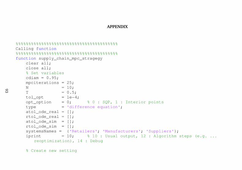
APPENDIX
%%%%%%%%%%%%%%%%%%%%%%%%%%%%%%%%%%%%%%%%Calling function%%%%%%%%%%%%%%%%%%%%%%%%%%%%%%%%%%%%%%%%function supply_chain_mpc_stragegy
clear all;close all;% Set variablescdiam = 0.95;mpciterations = 25;N = 10;T = 0.5;tol_opt = 1e - 4;opt_option = 0; % 0 : SQP, 1 : Interior pointstype = 'difference equation';atol_ode_real = [];rtol_ode_real = [];atol_ode_sim = [];rtol_ode_sim = [];systemsNames = {'Retailers'; 'Manufacturers'; 'Suppliers'};iprint = 10; % 10 : Usual output, 12 : Algorithm steps (e.g. ...
reoptimization), 14 : Debug
% Create new setting
93
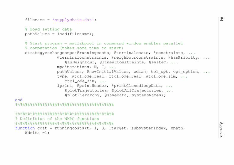
94A
ppendix
filename = 'supplychain.dat';
% Load setting datapathValues = load(filename);
% Start program - matlabpool in commmand window enables parallel% computation (takes some time to start)strategyexchangenmpc(@runningcosts, @terminalcosts, @constraints, ...
@terminalconstraints, @neighbourconstraints, @hasPriority, ...@isNeighbour, @linearConstraints, @system, ...
mpciterations, N, T, ...pathValues, @newInitialValues, cdiam, tol_opt, opt_option, ...type, atol_ode_real, rtol_ode_real, atol_ode_sim, ...
rtol_ode_sim, ...iprint, @printHeader, @printClosedloopData, ...
@plotTrajectories, @plotAllTrajectories, ...@plotHierarchy, @saveData, systemsNames);
end%%%%%%%%%%%%%%%%%%%%%%%%%%%%%%%%%%%%%%%%
%%%%%%%%%%%%%%%%%%%%%%%%%%%%%%%%%%%%%%%%% Definition of the NMPC functions%%%%%%%%%%%%%%%%%%%%%%%%%%%%%%%%%%%%%%%%function cost = runningcosts(t, l, u, ltarget, subsystemIndex, xpath)
Wdelta =1;
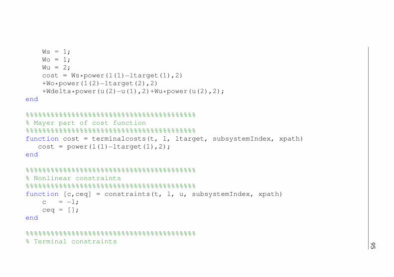
95
Ws = 1;Wo = 1;Wu = 2;cost = Ws*power(l(1) - ltarget(1),2)+Wo*power(l(2) - ltarget(2),2)+Wdelta*power(u(2) - u(1),2)+Wu*power(u(2),2);
end
%%%%%%%%%%%%%%%%%%%%%%%%%%%%%%%%%%%%%%%%%% Mayer part of cost function%%%%%%%%%%%%%%%%%%%%%%%%%%%%%%%%%%%%%%%%%function cost = terminalcosts(t, l, ltarget, subsystemIndex, xpath)
cost = power(l(1) - ltarget(1),2);end
%%%%%%%%%%%%%%%%%%%%%%%%%%%%%%%%%%%%%%%%%% Nonlinear constraints%%%%%%%%%%%%%%%%%%%%%%%%%%%%%%%%%%%%%%%%%function [c,ceq] = constraints(t, l, u, subsystemIndex, xpath)
c = - l;ceq = [];
end
%%%%%%%%%%%%%%%%%%%%%%%%%%%%%%%%%%%%%%%%%% Terminal constraints
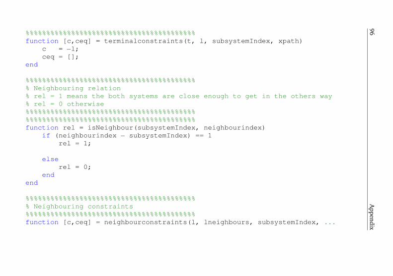
96A
ppendix
%%%%%%%%%%%%%%%%%%%%%%%%%%%%%%%%%%%%%%%%%function [c,ceq] = terminalconstraints(t, l, subsystemIndex, xpath)
c = - l;ceq = [];
end
%%%%%%%%%%%%%%%%%%%%%%%%%%%%%%%%%%%%%%%%%% Neighbouring relation% rel = 1 means the both systems are close enough to get in the others way% rel = 0 otherwise%%%%%%%%%%%%%%%%%%%%%%%%%%%%%%%%%%%%%%%%%%%%%%%%%%%%%%%%%%%%%%%%%%%%%%%%%%%%%%%%%%function rel = isNeighbour(subsystemIndex, neighbourindex)
if (neighbourindex - subsystemIndex) == 1rel = 1;
elserel = 0;
endend
%%%%%%%%%%%%%%%%%%%%%%%%%%%%%%%%%%%%%%%%%% Neighbouring constraints%%%%%%%%%%%%%%%%%%%%%%%%%%%%%%%%%%%%%%%%%function [c,ceq] = neighbourconstraints(l, lneighbours, subsystemIndex, ...
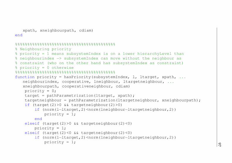
97
xpath, xneighbourpath, cdiam)end
%%%%%%%%%%%%%%%%%%%%%%%%%%%%%%%%%%%%%%%%%% Neighbouring priority% priority = 1 means subsystemIndex is on a lower hierarchyLevel than% neighbourindex - > subsystemIndex can move without the neighbour as% constraint (who on the other hand has subsystemIndex as constraint)% priority = 0 otherwise%%%%%%%%%%%%%%%%%%%%%%%%%%%%%%%%%%%%%%%%%function priority = hasPriority(subsystemIndex, l, ltarget, xpath, ...
neighbourindex, cooperative, lneighbour, ltargetneighbour, ...xneighbourpath, cooperativeneighbour, cdiam)priority = 0;target = pathParametrization(ltarget, xpath);targetneighbour = pathParametrization(ltargetneighbour, xneighbourpath);if (target(2)>0 && targetneighbour(2)>0)
if (norm(l - ltarget,2)<norm(lneighbour - ltargetneighbour,2))priority = 1;
endelseif (target(2)>0 && targetneighbour(2)<0)
priority = 1;elseif (target(2)<0 && targetneighbour(2)<0)
if (norm(l - ltarget,2)<norm(lneighbour - ltargetneighbour,2))priority = 1;
98A
ppendix
endend
end
%%%%%%%%%%%%%%%%%%%%%%%%%%%%%%%%%%%%%%%%%% Linear constraints%%%%%%%%%%%%%%%%%%%%%%%%%%%%%%%%%%%%%%%%%function [A, b, Aeq, beq, lb, ub] = linearConstraints(t, l, u, ...
subsystemIndex, maxOrder, xpath)A = [];b = [];Aeq = [];beq = [];lb = [];ub = [];lb = 0;ub = maxOrder;
end
%%%%%%%%%%%%%%%%%%%%%%%%%%%%%%%%%%%%%%%%%% System dynamics%%%%%%%%%%%%%%%%%%%%%%%%%%%%%%%%%%%%%%%%%function y = system(t, l, u, T, subsystemIndex, demand, lNeighbour)
tb = 5;if subsystemIndex == 3 %supplyer
99
y(1) = l(1) + u(1) - demand(2) - l(3)/tb;y(2) = l(2) + u(2) - u(1);y(3) = l(3) - l(3)/tb;
elseif subsystemIndex == 2 %Manufaturery(1) = l(1) + u(1) - demand(2) - l(3)/tb + lNeighbour(3)/tb;%bsy(2) = l(2) + u(2) - u(1) - lNeighbour(3);%bs(t - theta2)y(3) = l(3) - l(3)/tb;
elseif subsystemIndex == 1 %Retailery(1) = l(1) + u(1) - demand(2) - l(3)/tb + lNeighbour(3)/tb;%bm(t - theta2)y(2) = l(2) + u(2) - u(1) - lNeighbour(3)/tb;%bsy(3) = l(3) - l(3)/tb;
elsefprintf('Do not exist this susubsystemIndex %3d\n', subsystemIndex);
endend
%%%%%%%%%%%%%%%%%%%%%%%%%%%%%%%%%%%%%%%%%
%%%%%%%%%%%%%%%%%%%%%%%%%%%%%%%%%%%%%%%%%% Initial values%%%%%%%%%%%%%%%%%%%%%%%%%%%%%%%%%%%%%%%%%function [lstart, ltarget, maxOrder, firstDemand] = ...
newInitialValues(lastSystem, pathValues)
100A
ppendix
if(lastSystem == 1)firstDemand(1:2) = 200;
elsefirstDemand(1:2) = 200;
endlstart = pathValues(lastSystem,1:3);%300 0 0ltarget = pathValues(lastSystem,4:6);%300 200 0maxOrder = pathValues(lastSystem,7);
end%%%%%%%%%%%%%%%%%%%%%%%%%%%%%%%%%%%%%%%%%
%%%%%%%%%%%%%%%%%%%%%%%%%%%%%%%%%%%%%%%%%% Definition of output format%%%%%%%%%%%%%%%%%%%%%%%%%%%%%%%%%%%%%%%%%% Table header for Matlab output%%%%%%%%%%%%%%%%%%%%%%%%%%%%%%%%%%%%%%%%%function printHeader()
fprintf('k system| u1(k) x(1) x(2) x(3)\n');fprintf(' - - - - - - - - - - - - - - - - - - - - - - - - - - - - - - - - - - - - - - - - - - - - - - - - - - \n');
end
%%%%%%%%%%%%%%%%%%%%%%%%%%%%%%%%%%%%%%%%%% One line data for a single stage%%%%%%%%%%%%%%%%%%%%%%%%%%%%%%%%%%%%%%%%%
101
function printClosedloopData(mpciter, system, hierarchyLevel, ...neighbourcounter, u, l, xpath, tag)fprintf(' %3d %3d | %+11.6f %+11.6f %+11.6f %+11.6f\t', mpciter, ...
system, u(1), l(1), l(2), l(3));end
%%%%%%%%%%%%%%%%%%%%%%%%%%%%%%%%%%%%%%%%%% Plotting all trajectories simultaneously%%%%%%%%%%%%%%%%%%%%%%%%%%%%%%%%%%%%%%%%%function plotAllTrajectories(dynamic, system, N, T, t0, l0, u, mpciter, ...
ltarget, xpath, numberofsystems, cdiam, ...atol_ode, rtol_ode, type)
hold off;end
%%%%%%%%%%%%%%%%%%%%%%%%%%%%%%%%%%%%%%%%%% Plotting hierarchy%%%%%%%%%%%%%%%%%%%%%%%%%%%%%%%%%%%%%%%%%function plotHierarchy(numberOfSystems, hierarchyLevel)
maximalHierarchyLevel = max(hierarchyLevel);figure(1);hold on;for i=0:maximalHierarchyLevel
indexString = [];for j=1:numberOfSystems
102A
ppendix
if (hierarchyLevel(j) == i)indexString = strcat(indexString, ['p_{', int2str(j)], '} ');
endendtext(2,10 - (i+1),['Level ', int2str(i+1), ': ', ...
indexString],'HorizontalAlignment','left');endhold off;
end
function [t, x, u] = strategyexchangenmpc(runningcosts, terminalcosts, ...constraints, terminalconstraints, neighbourconstraints, hasPriority, ...
isNeighbour,...linearconstraints, system, ...mpciterations, N, T, ...pathvalues, newInitialValues, cdiam, varargin)
tPrint = [];xPrint = [];printindex = 1;
numberofsystems = 0;lastsystem = 1;removedsystem = 0;
maximalHierarchyLevel = 1;
103
%maxSpeed = 1.5;
% Start of the NMPC iterationmpciter = 1;while(mpciter <= mpciterations)while(lastsystem <= size(pathvalues, 1))
numberofsystems = numberofsystems + 1;[xmeasure{numberofsystems}, xtarget{numberofsystems}, ...
ubounds{numberofsystems}, demand{numberofsystems}{mpciter}] = ...newInitialValues(lastsystem, pathvalues);
tmeasure{numberofsystems} = mpciter * T;[t0{numberofsystems}, x0{numberofsystems}, removesystem] = ...
measureInitialValue ( tmeasure{numberofsystems}, ...xmeasure{numberofsystems}, xtarget{numberofsystems}, tol_opt );
u0{numberofsystems} = max(demand{numberofsystems}{mpciter}(1),0) * ...ones(N,1);
uApply{numberofsystems} = [0 u0{numberofsystems}(1)];hierarchyLevel(numberofsystems) = 0;xneighbours{numberofsystems} = [];xneighbourpaths{numberofsystems} = [];neighbourcounter(numberofsystems) = 0;neighboursindex{numberofsystems} = [];xopenloop{numberofsystems} = zeros(N+1,size(xmeasure{numberofsystems},2)+1);tPrint{numberofsystems} = [];
104A
ppendix
xPrint{numberofsystems} = [];for horizonindex=1:N+1xopenloop{numberofsystems}(horizonindex,1:size(xmeasure{numberofsystems},2)) = xmeasure{numberofsystems};
endfor subsystemindex=1:numberofsystems
for neighbourindex=1:numberofsystemsif (neighbourindex~=subsystemindex && hierarchyLevel(neighbourindex) ...
<= hierarchyLevel(subsystemindex))demand{neighbourindex}, cdiam) > 0)
if(isNeighbour(subsystemindex, neighbourindex))demand{neighbourindex}{mpciter}(1) = ...
demand{neighbourindex}{mpciter}(2);demand{neighbourindex}{mpciter}(2) = u0{subsystemindex}(1);
endend
endend
lastsystem = lastsystem + 1;end
% Step (1) of the NMPC algorithm:% Aggregate external dataif (mpciter>1)
for subsystemindex=1:numberofsystems
105
[t0{subsystemindex}, x0{subsystemindex}, removesystem] = ...measureInitialValue ( tmeasure{subsystemindex}, ...xmeasure{subsystemindex}, xtarget{subsystemindex}, tol_opt );
if (mpciter>0)tPrint{subsystemindex} = [tPrint{subsystemindex}; ...
t0{subsystemindex}];xPrint{subsystemindex} = [xPrint{subsystemindex}; ...
x0{subsystemindex}];end
end
if (mpciter <=5)demand{1}{mpciter}(1) = demand{1}{mpciter}(2);demand{1}{mpciter}(2) = 200;
endif (mpciter > 5)
demand{1}{mpciter}(1) = demand{1}{mpciter}(2);demand{1}{mpciter}(2) = 300;
endend
% Step (2) of the NMPC algorithm:% Solve the optimal control problemfor subsystemindex=1:numberofsystems
% Set neighbouring information
106A
ppendix
xneighbourpaths{subsystemindex} = [];neighboursindex{subsystemindex} = [];neighbourcounter(subsystemindex) = ...
neighbourcounter(subsystemindex) + 1;xneighbours{subsystemindex}{neighbourcounter(subsystemindex)} = [];
for neighbourindex=1:numberofsystemsif (neighbourindex~=subsystemindex && ...
hierarchyLevel(subsystemindex)>=hierarchyLevel(neighbourindex))if isNeighbour(subsystemindex, neighbourindex)
xneighbours{subsystemindex}{neighbourcounter(subsystemindex)} ...= xmeasure{neighbourindex};
endend
end
% Solve optimal control problem[u_new{subsystemindex}, V_current{subsystemindex}, ...
exitflag{subsystemindex}, output{subsystemindex}] = ...solveOptimalControlProblem ...(runningcosts, terminalcosts, constraints, ...terminalconstraints, neighbourconstraints, ...
linearconstraints, system, ...N, T, t0{subsystemindex}, x0{subsystemindex}, ...
u0{subsystemindex}, subsystemindex, ...
107
xtarget{subsystemindex}, ...neighbourcounter(subsystemindex), ...
xneighbours{subsystemindex}, ...demand{subsystemindex}{mpciter}, ...ubounds{subsystemindex}, ...xneighbourpaths{subsystemindex}, cdiam, ...
atol_ode_sim, rtol_ode_sim, tol_opt, options, type);end
% Update openloopfor subsystemindex=1:numberofsystems
xopenloop{subsystemindex} = computeOpenloopSolution(system, ...N, T, t0{subsystemindex}, x0{subsystemindex}, ...u_new{subsystemindex},uApply{subsystemindex}(2), ...
subsystemindex, demand{subsystemindex}{mpciter}, ...xneighbours{subsystemindex}{neighbourcounter(subsystemindex)}, ...atol_ode_sim, rtol_ode_sim, type);
end
% Update neighbouring informationfor subsystemindex=1:numberofsystems
for neighbourindex=1:numberofsystemsif (neighbourindex~=subsystemindex && ...
hierarchyLevel(neighbourindex) <= ...

108A
ppendix
hierarchyLevel(subsystemindex))if(isNeighbour(subsystemindex, neighbourindex))
demand{neighbourindex}{mpciter+1}(1) = ...demand{neighbourindex}{mpciter}(2);
demand{neighbourindex}{mpciter+1}(2) = ...u_new{subsystemindex}(1);
endend
end
if(subsystemindex == 1)demand{1}{mpciter+1} = demand{1}{mpciter};
endend
% Check violations / feasibility on same levelfor subsystemindex=1:numberofsystems
[c,ceq] = nonlinearconstraints(constraints, ...terminalconstraints, neighbourconstraints, system, ...N, T, t0{subsystemindex}, x0{subsystemindex}, ...
u_new{subsystemindex}, uApply{subsystemindex}(2), ...subsystemindex, demand{subsystemindex}{mpciter}, ...neighbourcounter(subsystemindex), ...xneighbours{subsystemindex}, ...xneighbourpaths{subsystemindex}, cdiam, ...
109
atol_ode_sim, rtol_ode_sim, type);
% If violated, shift to new levelviolated = find(c > tol_opt);if (size(violated,1) > 0)
if ( iprint >= 13 )fprintf('\tSystem %3d : %3d constraint violations ...
found\n', subsystemindex, size(violated,1));end
% Step (3) of the NMPC algorithm:% Apply control to processuApply{subsystemindex} = [uApply{subsystemindex}(2); ...
u_new{subsystemindex}(1)];[tmeasure{subsystemindex}, xmeasure{subsystemindex}] = ...
applyControl(system, T, t0{subsystemindex}, x0{subsystemindex}, ...uApply{subsystemindex}, removedsystem + subsystemindex, ...demand{subsystemindex}{mpciter}, ...xneighbours{subsystemindex}{neighbourcounter(subsystemindex)}, ...
atol_ode_real, rtol_ode_real, type);
xmeasureIter{subsystemindex}(mpciter) = xmeasure{subsystemindex}(1);
%printprintSolution(system, 0, printClosedloopData, ...
110A
ppendix
plotTrajectories, mpciter, N, T, ...tmeasure{subsystemindex}, xmeasure{subsystemindex}, ...u_new{subsystemindex}, xtarget{subsystemindex}, ...demand{subsystemindex}{mpciter}, subsystemindex, ...
hierarchyLevel(subsystemindex), ...neighbourcounter(subsystemindex), ...
atol_ode_sim, rtol_ode_sim, type, iprint, ...exitflag{subsystemindex}, output{subsystemindex}, ...
'actual');
% Prepare restartu0{subsystemindex} = shiftHorizon(u_new{subsystemindex}, ...
u0{subsystemindex}, ubounds{subsystemindex});xopenloop{subsystemindex} = ...
xopenloop{subsystemindex}(2:size(xopenloop{subsystemindex},1),:);xopenloop{subsystemindex}(N+1,:) = dynamic(system, T, ...
t0{subsystemindex}+N*T, ...xopenloop{subsystemindex}(N,1:size(xmeasure{numberofsystems},2)), ...uApply{subsystemindex}, removedsystem + subsystemindex, ...demand{subsystemindex}{mpciter}, ...xneighbours{subsystemindex}{neighbourcounter(subsystemindex)}, ...
atol_ode_sim, rtol_ode_sim, type);end
mpciter = mpciter+1;
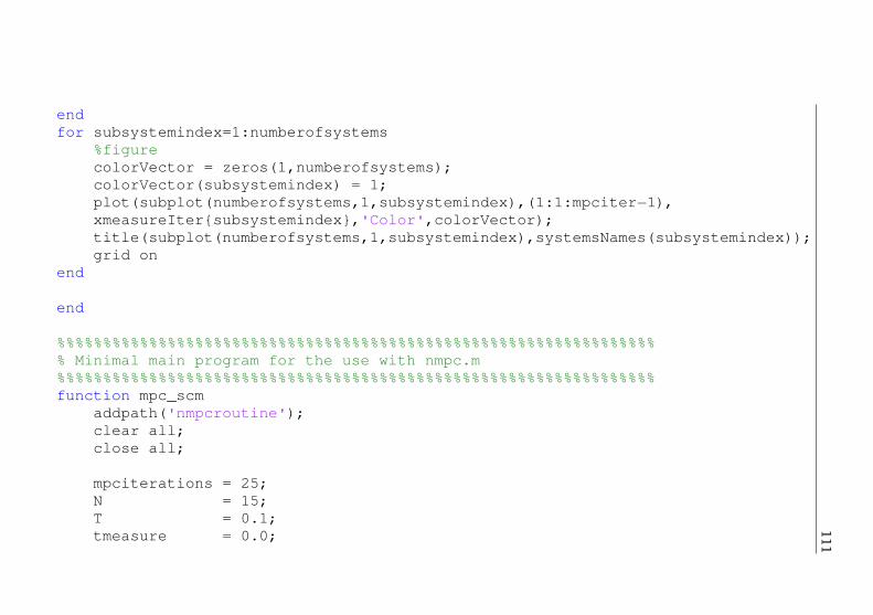
111
endfor subsystemindex=1:numberofsystems
%figurecolorVector = zeros(1,numberofsystems);colorVector(subsystemindex) = 1;plot(subplot(numberofsystems,1,subsystemindex),(1:1:mpciter - 1),xmeasureIter{subsystemindex},'Color',colorVector);title(subplot(numberofsystems,1,subsystemindex),systemsNames(subsystemindex));grid on
end
end
%%%%%%%%%%%%%%%%%%%%%%%%%%%%%%%%%%%%%%%%%%%%%%%%%%%%%%%%%%%%%%%%%% Minimal main program for the use with nmpc.m%%%%%%%%%%%%%%%%%%%%%%%%%%%%%%%%%%%%%%%%%%%%%%%%%%%%%%%%%%%%%%%%%function mpc_scm
addpath('nmpcroutine');clear all;close all;
mpciterations = 25;N = 15;T = 0.1;tmeasure = 0.0;
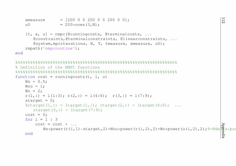
112A
ppendix
xmeasure = [200 0 0 200 0 0 200 0 0];u0 = 200*ones(3,N);
[t, x, u] = nmpc(@runningcosts, @terminalcosts, ...@constraints,@terminalconstraints, @linearconstraints, ...@system,mpciterations, N, T, tmeasure, xmeasure, u0);
rmpath('nmpcroutine');end
%%%%%%%%%%%%%%%%%%%%%%%%%%%%%%%%%%%%%%%%%%%%%%%%%%%%%%%%%%%%%%%%%% Definition of the NMPC functions%%%%%%%%%%%%%%%%%%%%%%%%%%%%%%%%%%%%%%%%%%%%%%%%%%%%%%%%%%%%%%%%%function cost = runningcosts(t, l, u)
Ws = 0.5;Wou = 1;Wo = 2;r(1,:) = l(1:3); r(2,:) = l(4:6); r(3,:) = l(7:9);starget = 0;%rtarget(1,:) = ltarget(1,:); rtarget(2,:) = ltarget(4:6); ...
rtarget(3,:) = ltarget(7:9);cost = 0;for i = 1 : 3
cost = cost + ...Ws*power(r(i,1) - starget,2)+Wou*power(r(i,2),2)+Wo*power(u(i,2),2);%+Wdelta*power(u(i,2) - u(i,1),2)
end
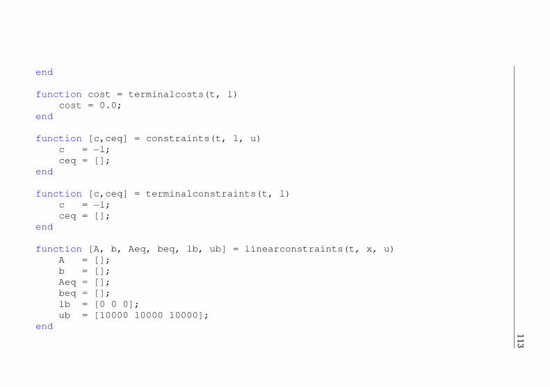
113
end
function cost = terminalcosts(t, l)cost = 0.0;
end
function [c,ceq] = constraints(t, l, u)c = - l;ceq = [];
end
function [c,ceq] = terminalconstraints(t, l)c = - l;ceq = [];
end
function [A, b, Aeq, beq, lb, ub] = linearconstraints(t, x, u)A = [];b = [];Aeq = [];beq = [];lb = [0 0 0];ub = [10000 10000 10000];
end
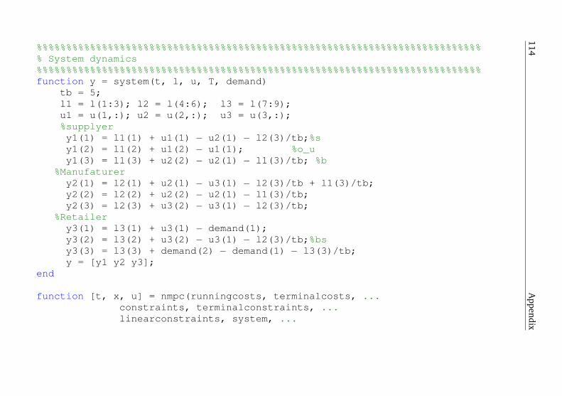
114A
ppendix
%%%%%%%%%%%%%%%%%%%%%%%%%%%%%%%%%%%%%%%%%%%%%%%%%%%%%%%%%%%%%%%%%%%%%%%%%%%% System dynamics%%%%%%%%%%%%%%%%%%%%%%%%%%%%%%%%%%%%%%%%%%%%%%%%%%%%%%%%%%%%%%%%%%%%%%%%%%%function y = system(t, l, u, T, demand)
tb = 5;l1 = l(1:3); l2 = l(4:6); l3 = l(7:9);u1 = u(1,:); u2 = u(2,:); u3 = u(3,:);%supplyery1(1) = l1(1) + u1(1) - u2(1) - l2(3)/tb;%sy1(2) = l1(2) + u1(2) - u1(1); %o_uy1(3) = l1(3) + u2(2) - u2(1) - l1(3)/tb; %b
%Manufaturery2(1) = l2(1) + u2(1) - u3(1) - l2(3)/tb + l1(3)/tb;y2(2) = l2(2) + u2(2) - u2(1) - l1(3)/tb;y2(3) = l2(3) + u3(2) - u3(1) - l2(3)/tb;
%Retailery3(1) = l3(1) + u3(1) - demand(1);y3(2) = l3(2) + u3(2) - u3(1) - l2(3)/tb;%bsy3(3) = l3(3) + demand(2) - demand(1) - l3(3)/tb;y = [y1 y2 y3];
end
function [t, x, u] = nmpc(runningcosts, terminalcosts, ...constraints, terminalconstraints, ...linearconstraints, system, ...
115
mpciterations, N, T, tmeasure, xmeasure, u0, ...varargin)
if (nargin>=13)tol_opt = varargin{1};
elsetol_opt = 1e - 6;
end;if (nargin>=14)
opt_option = varargin{2};else
opt_option = 0;end;if (nargin>=15)
if ( strcmp(varargin{3}, 'difference equation') | ...strcmp(varargin{3}, 'differential equation') )
type = varargin{3};else
fprintf([' Wrong input for type of dynamic: use either ', ...'"difference equation" or "differential equation".']);
endelse
type = 'difference equation';end;if (nargin>=16)
atol_ode_real = varargin{4};
116A
ppendix
elseatol_ode_real = 1e - 8;
end;if (nargin>=17)
rtol_ode_real = varargin{5};else
rtol_ode_real = 1e - 8;end;if (nargin>=18)
atol_ode_sim = varargin{6};else
atol_ode_sim = atol_ode_real;end;if (nargin>=19)
rtol_ode_sim = varargin{7};else
rtol_ode_sim = rtol_ode_real;end;if (nargin>=20)
iprint = varargin{8};else
iprint = 0;end;if (nargin>=21)
printHeader = varargin{9};
117
elseprintHeader = @printHeaderDummy;
end;if (nargin>=22)
printClosedloopData = varargin{10};else
printClosedloopData = @printClosedloopDataDummy;end;if (nargin>=23)
plotTrajectories = varargin{11};else
plotTrajectories = @plotTrajectoriesDummy;end;
% Determine MATLAB Version and% specify and configure optimization methodvs = version(' - date');vyear = str2num(vs(8:11))if (vyear <= 2007)
fprintf('MATLAB version R2007 or earlier detected\n');if ( opt_option == 0 )
options = optimset('Display','off',...'TolFun', tol_opt,...'MaxIter', 2000,...'LargeScale', 'off',...
118A
ppendix
'RelLineSrchBnd', [],...'RelLineSrchBndDuration', 1);
elseif ( opt_option == 1 )error('nmpc:WrongArgument', '%s\n%s', ...
'Interior point method not supported in MATLAB R2007', ...'Please use opt_option = 0 or opt_option = 2');
elseif ( opt_option == 2 )options = optimset('Display','off',...
'TolFun', tol_opt,...'MaxIter', 2000,...'LargeScale', 'on',...'Hessian', 'off',...'MaxPCGIter', max(1,floor(size(u0,1)*size(u0,2)/2)),...'PrecondBandWidth', 0,...'TolPCG', 1e - 1);
endelse
fprintf('MATLAB version R2008 or newer detected\n');if ( opt_option == 0 )
options = optimset('Display','off',...'TolFun', tol_opt,...'MaxIter', 10000,...'Algorithm', 'active - set',...'FinDiffType', 'forward',...'RelLineSrchBnd', [],...
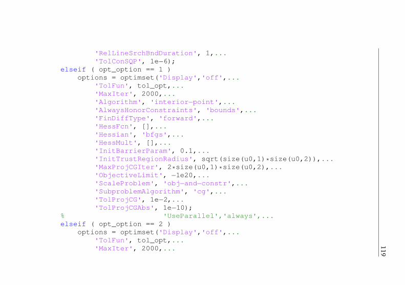
119
'RelLineSrchBndDuration', 1,...'TolConSQP', 1e - 6);
elseif ( opt_option == 1 )options = optimset('Display','off',...
'TolFun', tol_opt,...'MaxIter', 2000,...'Algorithm', 'interior - point',...'AlwaysHonorConstraints', 'bounds',...'FinDiffType', 'forward',...'HessFcn', [],...'Hessian', 'bfgs',...'HessMult', [],...'InitBarrierParam', 0.1,...'InitTrustRegionRadius', sqrt(size(u0,1)*size(u0,2)),...'MaxProjCGIter', 2*size(u0,1)*size(u0,2),...'ObjectiveLimit', - 1e20,...'ScaleProblem', 'obj - and - constr',...'SubproblemAlgorithm', 'cg',...'TolProjCG', 1e - 2,...'TolProjCGAbs', 1e - 10);
% 'UseParallel','always',...elseif ( opt_option == 2 )
options = optimset('Display','off',...'TolFun', tol_opt,...'MaxIter', 2000,...
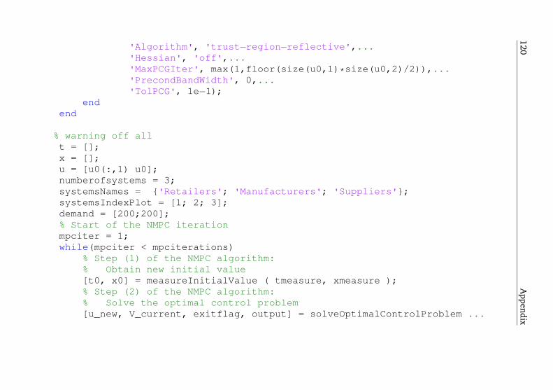
120A
ppendix
'Algorithm', 'trust - region - reflective',...'Hessian', 'off',...'MaxPCGIter', max(1,floor(size(u0,1)*size(u0,2)/2)),...'PrecondBandWidth', 0,...'TolPCG', 1e - 1);
endend
% warning off allt = [];x = [];u = [u0(:,1) u0];numberofsystems = 3;systemsNames = {'Retailers'; 'Manufacturers'; 'Suppliers'};systemsIndexPlot = [1; 2; 3];demand = [200;200];% Start of the NMPC iterationmpciter = 1;while(mpciter < mpciterations)
% Step (1) of the NMPC algorithm:% Obtain new initial value[t0, x0] = measureInitialValue ( tmeasure, xmeasure );% Step (2) of the NMPC algorithm:% Solve the optimal control problem[u_new, V_current, exitflag, output] = solveOptimalControlProblem ...
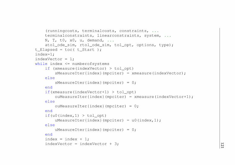
121
(runningcosts, terminalcosts, constraints, ...terminalconstraints, linearconstraints, system, ...N, T, t0, x0, u, demand, ...atol_ode_sim, rtol_ode_sim, tol_opt, options, type);
t_Elapsed = toc( t_Start );index=1;indexVector = 1;while index <= numberofsystems
if (xmeasure(indexVector) > tol_opt)sMeasureIter{index}(mpciter) = xmeasure(indexVector);
elsesMeasureIter{index}(mpciter) = 0;
endif(xmeasure(indexVector+1) > tol_opt)
ouMeasureIter{index}(mpciter) = xmeasure(indexVector+1);else
ouMeasureIter{index}(mpciter) = 0;endif(u0(index,1) > tol_opt)
uMeasureIter{index}(mpciter) = u0(index,1);else
uMeasureIter{index}(mpciter) = 0;endindex = index + 1;indexVector = indexVector + 3;
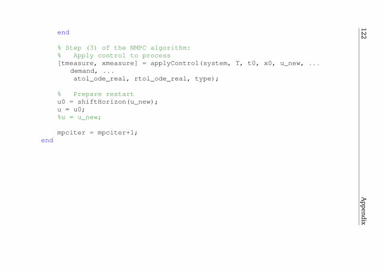
122A
ppendix
end
% Step (3) of the NMPC algorithm:% Apply control to process[tmeasure, xmeasure] = applyControl(system, T, t0, x0, u_new, ...
demand, ...atol_ode_real, rtol_ode_real, type);
% Prepare restartu0 = shiftHorizon(u_new);u = u0;%u = u_new;
mpciter = mpciter+1;end
Copyright © 2022 FDOKUMEN