- 1 -

CHAPTER 1 INTRODUCTION

1.1. BACKGROUND

In the fields of planning and urban design, spatial analysis is gaining an increasing emphasis.

Therefore various studies have been attempted to develop techniques to analyze space in a

comprehensive manner. Those attempts have focused on limited aspects of space due to the

complexity of urban system. ‘Nolli Map’ (Nolli, 1948), ‘Environmental image’ (Lynch,

1960) ‘Serial Vision’ (Cullen, 1961), analysis of different patterns that exists in built

environment (Alexander, 1977), generalized open spaces into basic geometric forms (Krier,

1979), and ‘Space Syntax’ (Hiller, 1996) are considered as benchmarks in those attempts in

spatial analysis history. Among them ‘Connectivity Analysis’ is a method derived from the

principal of ‘Graph theory’ (Erdos and Renyi, 1960). It is applied in spatial as well as non-

spatial analysis. Numerous studies have been carried out in this field with the understanding

of importance of connectivity. Those findings bring out a variety of perspectives and they

generate a range of analytical methods.

Although contemporary planning practices were increasingly oriented towards emerging

spatial analysis methods, applications of such methods are rare in Sri Lankan context

(Munasinghe, 2003). One of the underlying causes is inadequacy of studies on spatial

analysis methods. Although accessibility is a prime factor to identify urbanization potentials,

very few studies have been carried out to measure or evaluate the effect of accessibility in

planning. As a result, many plans and road development projects were implemented without

appropriate analysis on their implications on urbanization. On this landscape there is a need

to introduce effective spatial analysis methods and promote their application in decision

making process.

On such a situation, this study focused on the emerging spatial analysis methods called

connectivity analysis. Among its many applications, in this research, it is expected to use to

explain the pattern of urbanization. Urbanization is a phenomenon that concerned planning.

However, many urban development plans have not effectively accounted for the urbanizing

potentials. Despite the applications of rank-size rule and centrality matrix most of the urban

location decisions were arbitrary taken. Further, the existing methods have not well explained

the existing nature of urbanization. As a result of that, urbanization process has taken place

- 2 -

on some locations which were not envisaged in the plan. Further, most of the attributes used

in the above methods identifies the relationship between centres at one point in time but fail

to take into account the evolutionary process of spatial structure (Glasson, 1978). On the

other hand different ranking methods may lead to different results (MC Evay cited in

Glasson, 1978). Therefore, this study attempts to cater to that need by carrying out research

on applicability of connectivity analysis method to explain the pattern of urbanization in a

region.

1.2. OBJECTIVE

Despite several factors associated with the urbanization, connectivity (accessibility) is

considered as the prime factor on urbanization in this research. Accordingly the main

objective of this study is to test the applicability of connectivity analysis as a method to

explain the pattern of urbanization (in Locations) of a selected region in Sri Lanka.

1.3. METHOD OF STUDY

Figure-1.1: Method of study

- 3 -

This study evaluates the capability of connectivity analysis technique as a method to identify

the relationship between connectivity and urbanization. Therefore connectivity analysis

technique applied into a Kegalle district and the results correlated with current level of

urbanization of the nodes, to test the applicability of the technique to identify the pattern of

urbanization in a region. For the purpose of calculate the relative connectivity, the layout of

motorable road network of the study area reduced into a ‘node axial’ diagram by illustrating a

road intersection as a node and a link among two nodes as an axial line. Relative connectivity

of each node computed using an ‘interactive matrix’ which have prepared for each node by

indicating the number of axial lines that someone has to pass through to get into a node from

each of the other nodes in the most economic route. Level of urbanization of each node

computed using selected seventy two types of urban economic activities. Result of relative

connectivity pertaining to each node was correlated with the correspondent level of

urbanization of the node to examine the applicability of connectivity analysis to identify the

urbanizing nodes in a region.

1.4. SCOPE AND LIMITATION

Connectivity technique is a vast subject area, which include different type of methods (such

as simple connectivity analysis, weighted network analysis...etc.) and highly advanced

sophisticated mathematical operations used to compute and explain the results related to

connectivity. So analysis of connectivity among nodes located in road network can be done in

different methods and different levels. Since this is a very first attempt in Sri Lankan context,

study is only focused on the application of simple connectivity analysis to measure relative

connectivity among set of nodes.

Relative connectivity analyses have to be compute manually, due to unavailability of

accessible computer application. It seems to be consumed considerable time in this research.

Hence, study limited to one particular region (Kegalle District) in Sri Lanka.

Since the study expected to correlate the relative connectivity values with level of

urbanization of nodes, strong measurement need to measure the level of urbanization.

However, there was no any previous planning or economic study carried out in the region to

identify the level of urbanizing. Had there been the validity of the technique can be easily

tested and the extensive work involved in primary analysis could be minimized.

- 4 -

CHAPTER 2 LITERATURE REVIEW

2.1. INTRODUCTION TO LITERATURE REVIEW

Since connectivity is a vital factor in spatial analysis, variety of the analytical methods has

been evolved in the subject area. Accordingly, method of connectivity analysis was

developed and extended from non-spatial to spatial analysis studies. The objective of this

chapter is to review literature on the concept of connectivity analysis, method and its

application.

2.2. CONCEPT OF CONNECTIVITY ANALYSIS

‘Connectivity Analysis’ technique is one of methods developed in paradigm of ‘Graph

Theory’ which put forward by Erdos and Renyi (1960) with the ‘Random Graph’ model.

Despite the profound applications in computer network analysis recently connectivity

analysis applied in spatial analysis in the field of urban planning and design. This is mainly

because of its capability to model, forecast and explain the matters related to accessibility.

This technique can be defined as an analysis of the connectivity among systematically linked

points, lines and areas in terms of the degree of properties such as number, distance, travel

time, optimal path etc…

2.3. CONNECTIVITY ANALYSIS METHOD

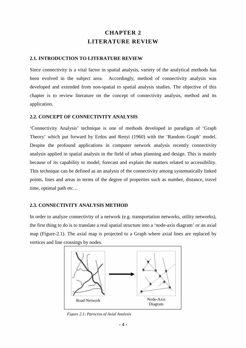
In order to analyze connectivity of a network (e.g. transportation networks, utility networks),

the first thing to do is to translate a real spatial structure into a ‘node-axis diagram’ or an axial

map (Figure-2.1). The axial map is projected to a Graph where axial lines are replaced by

vertices and line crossings by nodes.

Road Network Node-Axis

Diagram

Figure 2.1: Pprocess of Axial Analysis

- 5 -

Then compute the ‘relative connectivity’ of each node in terms of accessibility by an

‘interactive matrix’. The connectivity of each node represent by using following formula

developed by Hiller (1996).

Dj : relative connectivity of the node ‘j’ Aij: level of adjacency between node ‘i’ and ‘j’

The technique can be developed in to high level of accuracy by ‘weighted matrix’ indicating

the axial connection. It accounts the variables as distance between centers, travel difficulties,

natural environmental barriers etc…

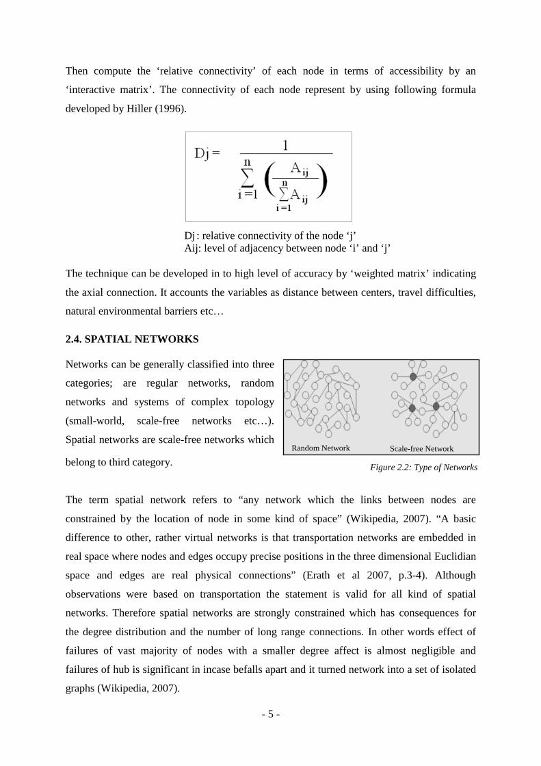
2.4. SPATIAL NETWORKS

Networks can be generally classified into three

categories; are regular networks, random

networks and systems of complex topology

(small-world, scale-free networks etc…).

Spatial networks are scale-free networks which

belong to third category.

The term spatial network refers to “any network which the links between nodes are

constrained by the location of node in some kind of space” (Wikipedia, 2007). “A basic

difference to other, rather virtual networks is that transportation networks are embedded in

real space where nodes and edges occupy precise positions in the three dimensional Euclidian

space and edges are real physical connections” (Erath et al 2007, p.3-4). Although

observations were based on transportation the statement is valid for all kind of spatial

networks. Therefore spatial networks are strongly constrained which has consequences for

the degree distribution and the number of long range connections. In other words effect of

failures of vast majority of nodes with a smaller degree affect is almost negligible and

failures of hub is significant in incase befalls apart and it turned network into a set of isolated

graphs (Wikipedia, 2007).

Figure 2.2: Type of Networks

Random Network Scale-free Network

- 6 -

2.5. EVOLUTION OF CONNECTIVITY ANALYSIS METHOD

In spite of Random Graph model “which rationalizes the small-world property of networks

by comparing the short distances with the number of links among nodes” (Montis et al 2007,

p.906) enormous efforts have associated with network analysis which contributed to the

development of the connectivity analysis technique. Some of are Barabasi and Albert (1999)

efforts on physical properties of networks like robustness, vulnerability; Studies of Batty and

Shiode (2000 and 2001) which promoted the development of this filed into quantitative

analysis with the twofold perspective with special reference to the World Wide Web, in terms

of geography, demography and economics. Salingaros article on ‘connectivity web are the

main source of urban life’ (Salingaros, 2001 cited in Montis et al 2007, p.906) also

significantly contributed to the development of connectivity analysis applications in relation

to urban planning and regional planning. Claremont and Jiang (2004) attempt to describe

transportation networks by revolving streets into nodes and intersections into edges, its called

as ‘Dual Graph’, Barrat’s (2004) studies focused on ‘Weighted Network’, the weighted graph

representation provided valuable elements that open the path to a series of questions of

fundamental importance to the understanding of the network. Among these are the issues of

how dynamics and structure affect each other and impact of traffic flow on the basic

properties of spreading and congestion phenomena (Montis et al 2007, p.906).

On the other hand there are several centrality measures developed in the this field to compute

the connectivity such as Accessibility Matrix (Shimbles, 1953), Dijkstra All-Pairs Distance

(Dijkstra, 1959), Circuits (Johnson, 1975), Closeness Centrality (Sabidussi, 1966), Degree

and Closeness Connectivity and Betweenness Centrality (Freeman, 1977), Connectivity

(Hillier, 1996), Local Efficiency / Clustering Coefficient (Latora, 2001)

Hiller (1996) and contemporary quantitative approaches on urban morphology provide initial

framework to develop connectivity analysis as application in urban spatial studies. Both

space syntax analysis and connectivity analysis study the patterns of connections, in terms of

the relationship of each spatial unit lines or field, to its immediate neighbors measured by

variables such as ‘connectivity’ and ‘integration’. However as a spatial analysis method

connectivity analysis is more reliable at regional level while space syntax is in urban level.

- 7 -

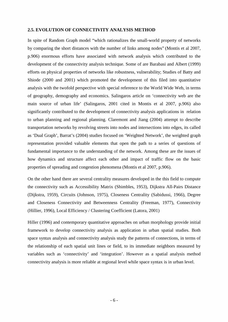
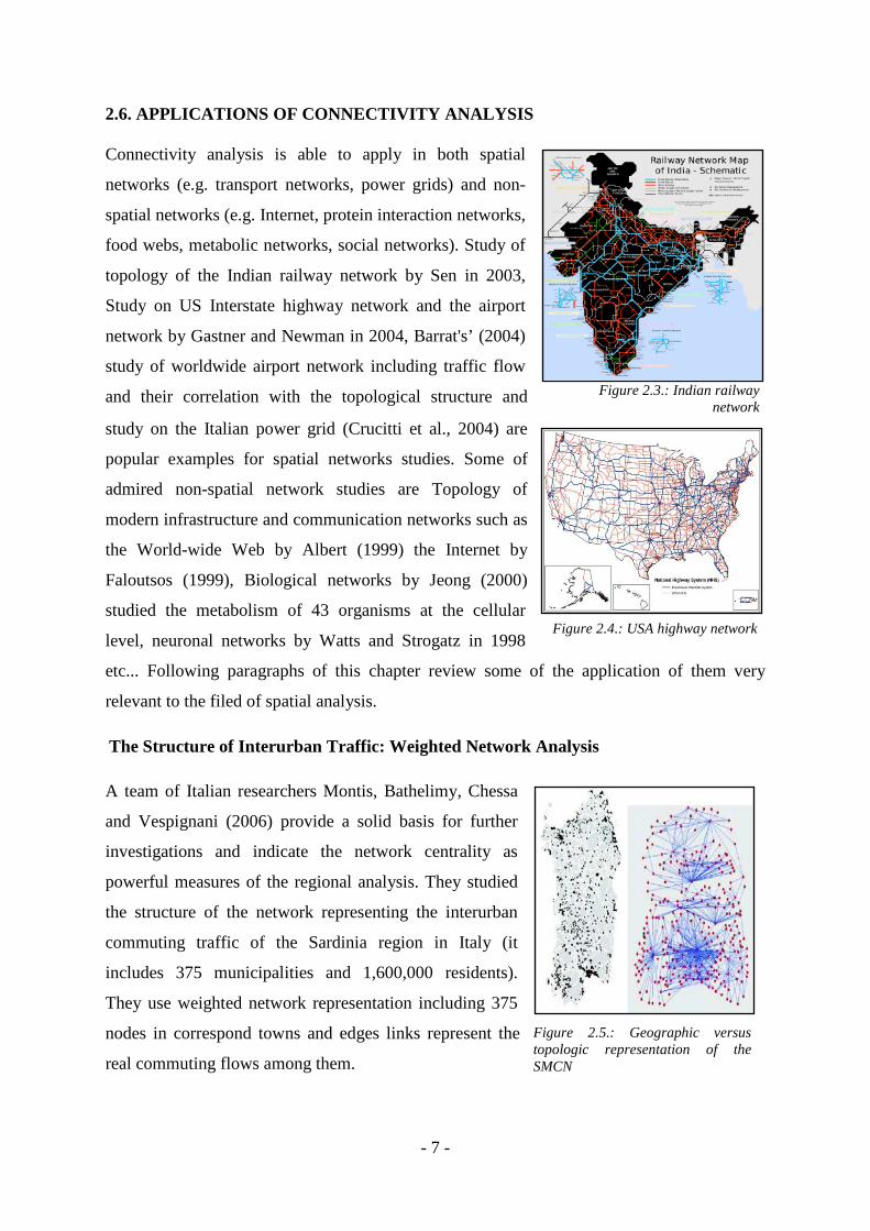
2.6. APPLICATIONS OF CONNECTIVITY ANALYSIS

Connectivity analysis is able to apply in both spatial

networks (e.g. transport networks, power grids) and non-

spatial networks (e.g. Internet, protein interaction networks,

food webs, metabolic networks, social networks). Study of

topology of the Indian railway network by Sen in 2003,

Study on US Interstate highway network and the airport

network by Gastner and Newman in 2004, Barrat's’ (2004)

study of worldwide airport network including traffic flow

and their correlation with the topological structure and

study on the Italian power grid (Crucitti et al., 2004) are

popular examples for spatial networks studies. Some of

admired non-spatial network studies are Topology of

modern infrastructure and communication networks such as

the World-wide Web by Albert (1999) the Internet by

Faloutsos (1999), Biological networks by Jeong (2000)

studied the metabolism of 43 organisms at the cellular

level, neuronal networks by Watts and Strogatz in 1998

etc... Following paragraphs of this chapter review some of the application of them very

relevant to the filed of spatial analysis.

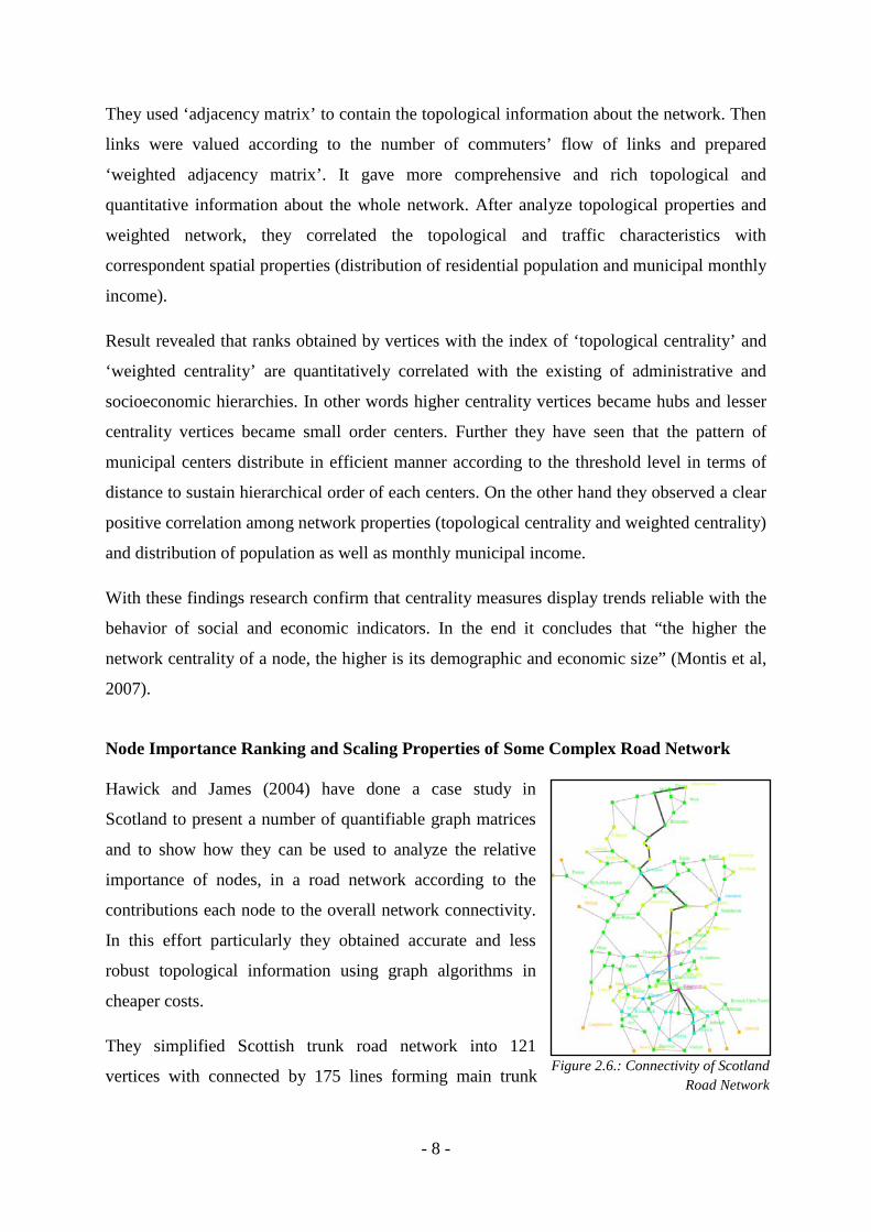
The Structure of Interurban Traffic: Weighted Network Analysis

A team of Italian researchers Montis, Bathelimy, Chessa

and Vespignani (2006) provide a solid basis for further

investigations and indicate the network centrality as

powerful measures of the regional analysis. They studied

the structure of the network representing the interurban

commuting traffic of the Sardinia region in Italy (it

includes 375 municipalities and 1,600,000 residents).

They use weighted network representation including 375

nodes in correspond towns and edges links represent the

real commuting flows among them.

Figure 2.3.: Indian railway network

Figure 2.4.: USA highway network

Figure 2.5.: Geographic versus topologic representation of the SMCN

- 8 -

They used ‘adjacency matrix’ to contain the topological information about the network. Then

links were valued according to the number of commuters’ flow of links and prepared

‘weighted adjacency matrix’. It gave more comprehensive and rich topological and

quantitative information about the whole network. After analyze topological properties and

weighted network, they correlated the topological and traffic characteristics with

correspondent spatial properties (distribution of residential population and municipal monthly

income).

Result revealed that ranks obtained by vertices with the index of ‘topological centrality’ and

‘weighted centrality’ are quantitatively correlated with the existing of administrative and

socioeconomic hierarchies. In other words higher centrality vertices became hubs and lesser

centrality vertices became small order centers. Further they have seen that the pattern of

municipal centers distribute in efficient manner according to the threshold level in terms of

distance to sustain hierarchical order of each centers. On the other hand they observed a clear

positive correlation among network properties (topological centrality and weighted centrality)

and distribution of population as well as monthly municipal income.

With these findings research confirm that centrality measures display trends reliable with the

behavior of social and economic indicators. In the end it concludes that “the higher the

network centrality of a node, the higher is its demographic and economic size” (Montis et al,

2007).

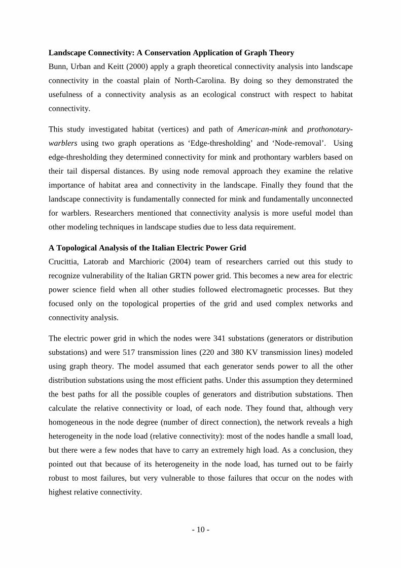
Node Importance Ranking and Scaling Properties of Some Complex Road Network

Hawick and James (2004) have done a case study in

Scotland to present a number of quantifiable graph matrices

and to show how they can be used to analyze the relative

importance of nodes, in a road network according to the

contributions each node to the overall network connectivity.

In this effort particularly they obtained accurate and less

robust topological information using graph algorithms in

cheaper costs.

They simplified Scottish trunk road network into 121

vertices with connected by 175 lines forming main trunk Figure 2.6.: Connectivity of Scotland Road Network

- 9 -

road network but not considered the detailed traffic flow and not developed to weighted

graphs. They only focused on robustness and vulnerability of particular location. That is, if it

removed what can happens to the network as a whole.

They measured the level of connectivity in terms of ‘Dijkstra all-pairs distance’ (which gives

a measure of how close nodes on the whole network are to one another) and the number of

elementary circuits in the graph to give measures regarding connectivity. Results indicated

that relatively flat landscaped area has high densities of well connected nodes whereas the

highlands have lower connectivity degree and node density. With that they conclude that the

method have capabilities to delineate geographical region (as using social and geographical

reasons). Further this analysis ranks importance of individual vertices in terms of their effect

on the rest of the network. It reveals that the highest degree (connectivity) nodes are the most

important nodes (hub cities like Perth, Inverness and Edinburgh) as well as have highest

disruptive effect on the all connectivity of the network, which is vulnerability or fragility of

vertices in the network.

Graph-Theoretical Analysis of the Swiss Road and Railway Networks

Erath, Lochl, Kay and Axhausen (2007) analyzed the development of the Swiss road and

railway networks by using well-established complex network measures (to measure

centrality) degree and closeness centrality, betweenness centrality, efficiency and straightness

centrality. Additionally they investigated new approaches to cover basic network

characteristics such as local clustering. The focus of this effort not only to classify the

transport network but also to provide the basis for further applications such as vulnerability

analysis and network development.

In this research, road and railway network data set have correlated with population data of

2896 Swiss municipalities’ from years 1950 to 2000. Research findings reveal that nodes

have higher degree of centrality or betweenness centrality is laid mostly in urbanized areas.

In other world it’s demonstrated that there is a correlation with the development and

centrality indicators. Furthermore, this work showed that the application of network measures

as used in the analysis of complex networks for transportation networks is challenging,

because of the complex weighting characteristics which involve capacity and spatial

restraints. However, this research anticipated the important measure of betweenness (link

load) as well as the concept of ‘closeness’ (accessibility).

- 10 -

Landscape Connectivity: A Conservation Application of Graph Theory

Bunn, Urban and Keitt (2000) apply a graph theoretical connectivity analysis into landscape

connectivity in the coastal plain of North-Carolina. By doing so they demonstrated the

usefulness of a connectivity analysis as an ecological construct with respect to habitat

connectivity.

This study investigated habitat (vertices) and path of American-mink and prothonotary-

warblers using two graph operations as ‘Edge-thresholding’ and ‘Node-removal’. Using

edge-thresholding they determined connectivity for mink and prothontary warblers based on

their tail dispersal distances. By using node removal approach they examine the relative

importance of habitat area and connectivity in the landscape. Finally they found that the

landscape connectivity is fundamentally connected for mink and fundamentally unconnected

for warblers. Researchers mentioned that connectivity analysis is more useful model than

other modeling techniques in landscape studies due to less data requirement.

A Topological Analysis of the Italian Electric Power Grid

Crucittia, Latorab and Marchioric (2004) team of researchers carried out this study to

recognize vulnerability of the Italian GRTN power grid. This becomes a new area for electric

power science field when all other studies followed electromagnetic processes. But they

focused only on the topological properties of the grid and used complex networks and

connectivity analysis.

The electric power grid in which the nodes were 341 substations (generators or distribution

substations) and were 517 transmission lines (220 and 380 KV transmission lines) modeled

using graph theory. The model assumed that each generator sends power to all the other

distribution substations using the most efficient paths. Under this assumption they determined

the best paths for all the possible couples of generators and distribution substations. Then

calculate the relative connectivity or load, of each node. They found that, although very

homogeneous in the node degree (number of direct connection), the network reveals a high

heterogeneity in the node load (relative connectivity): most of the nodes handle a small load,

but there were a few nodes that have to carry an extremely high load. As a conclusion, they

pointed out that because of its heterogeneity in the node load, has turned out to be fairly

robust to most failures, but very vulnerable to those failures that occur on the nodes with

highest relative connectivity.

- 11 -

2.7. CONCLUSION

‘Connectivity Analysis’ is one of the methods derived from the principal of ‘Graph theory’

which facilitate to evaluate the connectivity. As a result of numerous researches and studies,

the method evolved from simple connectivity analysis among nodes and developed into

advanced analysis such as weighted network method. Development of applications was

expanded and diversified the technique from non-spatial to spatial network spheres. Some of

the noticeable spatial analysis applications are Indian railway network (Sen, 2003), US

Interstate highway network and the airport network (Gastner and Newman, 2004), worldwide

airport network (Barrats, 2004) Italian power grid (Crucitti et al., 2004).

Spatial planners mainly focused on development promotion, concerning better distribution of

people and activities on land. Therefore, accessibility have recognized as a vital factor. So

there is a need of method to evaluate that factor. Above discussed examples confirms the

capability of connectivity analysis method to evaluate accessibility of a specific location or

node in the region. Accordingly it emphasizes that connectivity measures are versatile

enough to explain a fundamental quality required for the development of urban centers. At

the same time those studies provide a solid basis for the application of connectivity analysis

in the field of spatial analysis (particularly in regional context) to identify the socio-economic

and administrative hierarchy of the centers, delineate regions, assess vulnerability of

settlement, identify social interaction pattern…etc

Hence, the above literature indicates the capability of connectivity analysis to measure the

relative connectivity of nodes. Further relative connectivity can be used as an attribute to

measure many other related concepts too. Accordingly, this research made effort to apply

connectivity analysis to identify the level of urbanizing of nodes in a region.

- 12 -

2.8. REFERENCES

01. Montis, D.A.; Barthelimy, M.; Chessa, A. and Vespignani, A. (2007). The structure of interurban traffic – weighted network analysis. Environment and Planning B: Planning And Design, Vol. 34, pp. 905-924.

02. Wikipedia (2007). Erdős-Rényi model [online] Available from: http://en.wikipedia.org/ wiki/ Erd% C5%91s-R% C3%A 9nyi_model [Accessed 25th November 2007]

03. Wikipedia (2007). Small world networks [online] Available from: http://en.wikipedia. org/wiki/Small-world_network [Accessed 25th November 2007]

04. Wikipedia (No date). Spatial networks [online]. Available from: http://en.wikipedia.org/spatialnetwork[Accessed 25th November 2007]

05. Barrat, A. (2004). Weighted networks: analysis modeling [online], France, University Paris-Sud. Available from :http://www.th.u-psud.fr/page_person/Barrat[Accessed 20th November 2007]

06. Salingaros, N.A. (1998). Theory of the urban web. Journal of Urban Design [online]. Vol.3pp.53-71.Availableform:http://www.math.utsa.edu/ftp/salingar.old/urbanweb.html [Accessed 28nd November 2007]

07. Erath, A.; Löchl, M. and Axhausen, K.W. (2007). Graph-theoretical analysis of the Swiss road and railway networks over time [online], Conference paper Swiss Transport Research Conference. Available from: http://www.strc.ch/pdf_2007/erath.pdf [Accessed 25th November 2007].

08. Hawick, K.A. and James, H.A. (2005). Node importance ranking and scaling properties of some complex road network [online], Auckland, Massey University. Available from: http://www.massey.ac.nz [Accessed 25th November 2007].

09. Hillier, B. (1996a). The common language of space: a way of looking at the social economic and environmental functioning of cities on a common basis [online], London, University Collage London. Available from: http://www.spacesyntax.org/publications/ commomlamg.html [Accessed 13th November 2007].

10. Jiang, B. and Clarmunt, C. (2004).Topological analysis of urban street networks. Environment and Planning B: Planning And Design, Vol. 31, pp. 151-162

11. Bunn, A.G.; Urban, D.L. and Keitt; T.H. (2000). Landscape connectivity: A conservation application of graph theory. Journal of Environmental Management [online], 59, pp.265-278. Available from: http://www.idealibrary.com[Accessed 28th November 2007].

12. Crucittia, P.; Latorab, V.; and Marchioric, M. (2004). A Topological analysis of the Italian electric power grid [online], Italy, Universita di Venezia. Available from: http://www.sciencedirect.com[Accessed 10th January 2008].

13. Valdis Krebs (2007). Social network analysis [online]. Available from: http://www.orgnet.com/sna.html[Accessed 10th January 2008].

- 13 -

CHAPTER 3 RESEARCH DESIGN AND SURVEY

3.1. INTRODUCTION

This chapter explains the research design for application of connectivity analysis in a region.

Steps of research design including selection of study area, preparation of axial map,

connectivity analysis, preparation of level of urbanization index and correlation analysis.

Finally it discusses the limitations that were occurred in the study.

This study applies connectivity analysis technique in two levels are global level connectivity

and local level connectivity. In the global level connectivity analysis, relative connectivity of

each node was measured considering the level of connectivity of particular node with each of

the other nodes in the study area. But global connectivity does not accounts edge effects and

it does not measures the local connectivity. Hence local connectivity analysis carried out as

an extension to global connectivity analysis. Local connectivity of the each node was

measured considering the level of connectivity of particular node with each of the other nodes

within 15 km radius area.

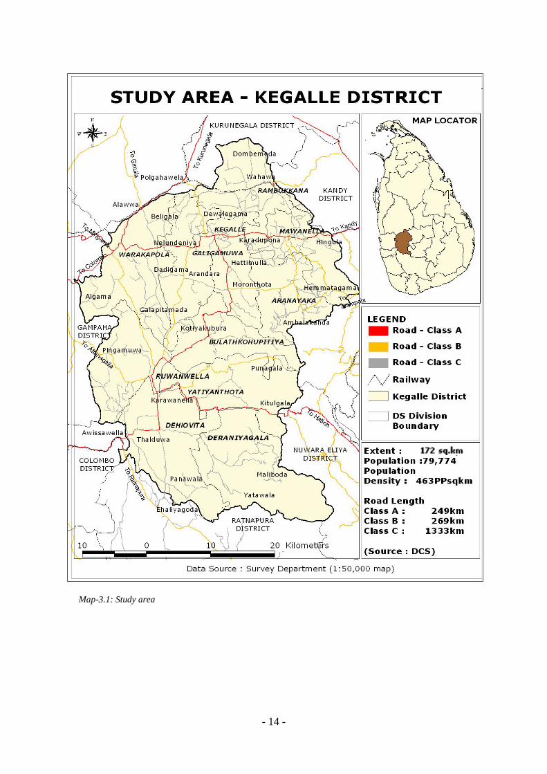
3.2. STUDY AREA

Kegalle district has been select as the study area (Map-3.1.), which comprises with well

spread road network to study the relative connectivity. Since this is a regional level analysis,

study area should have a reasonable extent. As mentioned in many regional planning studies,

extent of the region should be smaller than the national geographic unit and larger than local

geographic units (Glasson, 1978). Accordingly, the selected area was one of the twenty four

districts of the country consists of twelve local authorities. In addition to that, study area

apparent with a heterogeneous topographical profile which enables to analyze the effects of

topography. Because most of the theories and techniques related to geo-space are sensitive to

topographic variations. Further thorough understanding the author has of the region was also

contributed to select the area.

- 14 -

Map-3.1: Study area

- 15 -

3.2.1. Selection of Study Area for Global Connectivity Analysis

Since the district is an administrative unit, boundaries of it do not have accounted the

functional linkages with adjacent areas at the vicinity. This can be leading to error in

observation. Hence the boundary of the study area has to be adjusted; boundaries of the study

area decide to expand to Kandy-Kurunagala road-A10 from north and north-east,

Awissawella-Ehaliyagoda road-A4 from south, Ruwanwella-Nitambuwa road-B19 from

south-west and Ambepussa-Kurunagala road-A6 from north-west directions. Boundaries at

east and south-east directions were not expanded because Kadugannawa and Dolosbage

(Gampola) mountain range have physically divided the area.

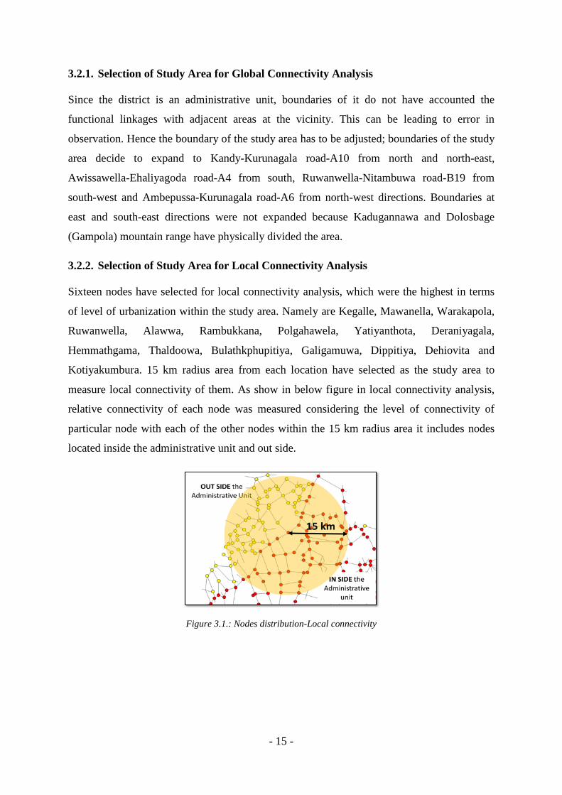
3.2.2. Selection of Study Area for Local Connectivity Analysis

Sixteen nodes have selected for local connectivity analysis, which were the highest in terms

of level of urbanization within the study area. Namely are Kegalle, Mawanella, Warakapola,

Ruwanwella, Alawwa, Rambukkana, Polgahawela, Yatiyanthota, Deraniyagala,

Hemmathgama, Thaldoowa, Bulathkphupitiya, Galigamuwa, Dippitiya, Dehiovita and

Kotiyakumbura. 15 km radius area from each location have selected as the study area to

measure local connectivity of them. As show in below figure in local connectivity analysis,

relative connectivity of each node was measured considering the level of connectivity of

particular node with each of the other nodes within the 15 km radius area it includes nodes

located inside the administrative unit and out side.

Figure 3.1.: Nodes distribution-Local connectivity

- 16 -

3.3. PREPARATION OF AXIAL LINE MAP

As the initial step of the method of connectivity analysis, the layout of real road network was

reduced into ‘node-axis’ diagram. This step was supported by Geographic Information

System (GIS) to obtain high accuracy.

First, a base map was prepared indicating the motorable road network. A digital format

1:50000 topographic map (survey department-1984) and updated road network using satellite

image (Google-earth) to prepare this map. Type A, B and C roads selected as motorable roads

considering the condition and volume of traffic flow.

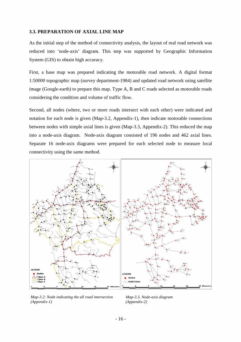
Second, all nodes (where, two or more roads intersect with each other) were indicated and

notation for each node is given (Map-3.2, Appendix-1), then indicate motorable connections

between nodes with simple axial lines is given (Map-3.3, Appendix-2). This reduced the map

into a node-axis diagram. Node-axis diagram consisted of 196 nodes and 462 axial lines.

Separate 16 node-axis diagrams were prepared for each selected node to measure local

connectivity using the same method.

Map-3.2: Node indicating the all road intersection (Appendix-1)

Map-3.3. Node-axis diagram (Appendix-2)

- 17 -

3.4. RELATIVE CONNECTIVITY ANALYSIS

This step calculated global connectivity and local connectivity in terms of relative

connectivity (both have similar steps). It includes the following steps. After preparation of

node-axis diagram, ‘interactive matrix’ was prepared with rows and columns dedicating for

each nodes. Then interactive cells of matrix filled up with number of axial line that someone

has to pass through to get into each node from each of the other nodes, in the most economic

route (adjacency-Aij). The cell value thus, represents the number of axils lines that connects

the respective node indicated in the row from the node indicated in the column (Table-3.1).

After the matrix is complete, cell values in the columns were summed up and all cell values

were normalized by dividing the sum value of the column. Inverse of the total value

represents the relative connectivity of each node represented in rows (Table-3.2).

Computation of relative connectivity is done separately for global and local level (Appendix-

3 and 4). After the connectivity values are obtained they were depicted in map using a range

of colour and scaled icons (Map-4.1 and 4.3.). MS-Excel spread sheet has been used for

above manipulations.

- 18 -

3.5. THE CORRELATION

Result obtained by connectivity analysis method need to be correlated with level of

urbanization. Therefore, the results of connectivity analysis pertaining to each node were

correlated with the correspondent level of urban economic activity values of the node. Level

of urbanizing measured under the assumption that the level of urbanizing is indicated by the

amount of existing urban activities. Because if there is a potential, then investors will be

invested harnessing the existing potential. Therefore 72 activity types were selected related to

urban economic activities (Appendix-5). In the next step data pertaining to each node (node

and vicinity) have been collected according to those activities through a field observation.

Since there were 72 activity types it was necessary to classify them into few categories for the

convenience of analysis. The attributes were broadly divided into two categories as goods

and services. Since there was a range of goods, they were further refined into five sub

categories according to the type. Similarly activity types were categorized into six as

convenience goods, services goods, shopping goods, luxury goods, entertainment goods and

services. Level of urbanization could be measured by the number of urban economic

activities as well as the scale of them. The scale of activities is changing from one location to

another depending on the functional magnitude. For the purpose of analysis, selected activity

types were classified according to the scale of location which supports to produce or sustain

the particular level of activity. This was a relative assessment among each activity types of

consecutive scales. Same scale of activities grouped into one cluster. Likewise total activity

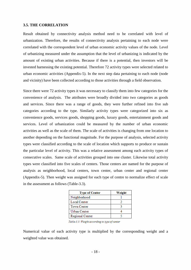
types were classified into five scales of centers. Those centers are named for the purpose of

analysis as neighborhood, local centers, town center, urban center and regional center

(Appendix-5). Then weight was assigned for each type of centre to normalize effect of scale

in the assessment as follows (Table-3.3).

Numerical value of each activity type is multiplied by the corresponding weight and a

weighted value was obtained.

- 19 -

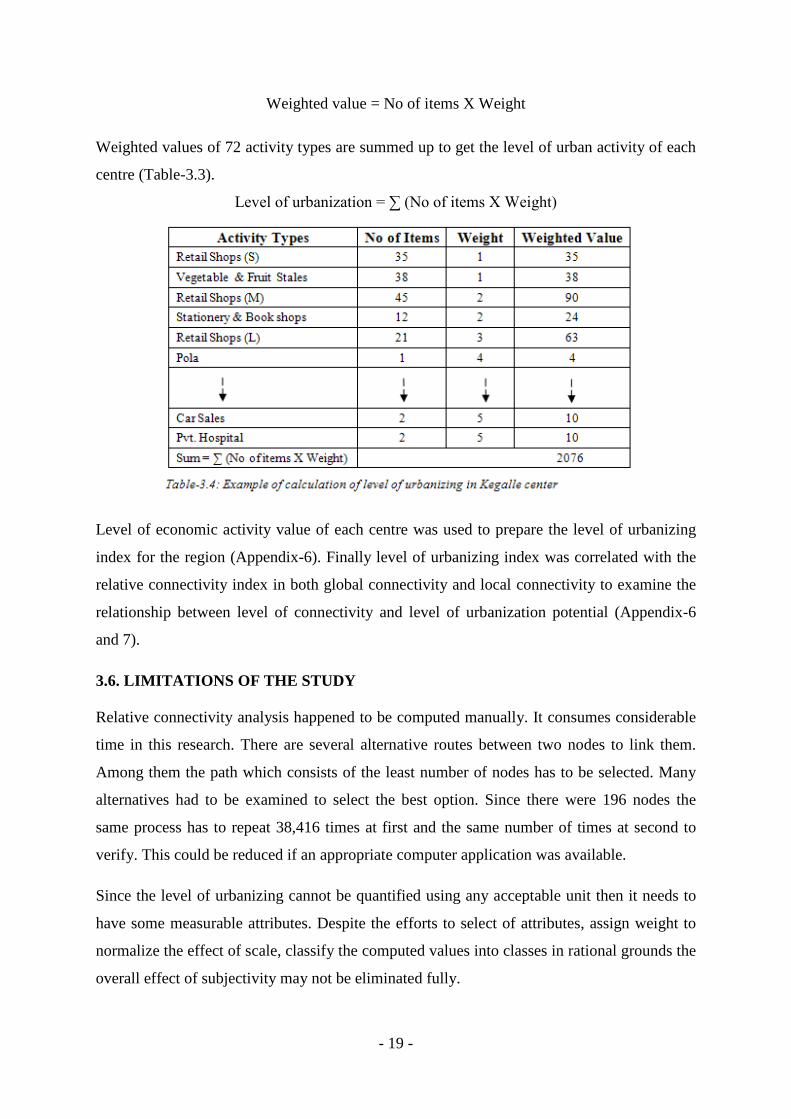
Weighted value = No of items X Weight

Weighted values of 72 activity types are summed up to get the level of urban activity of each

centre (Table-3.3).

Level of urbanization = ∑ (No of items X Weight)

Level of economic activity value of each centre was used to prepare the level of urbanizing

index for the region (Appendix-6). Finally level of urbanizing index was correlated with the

relative connectivity index in both global connectivity and local connectivity to examine the

relationship between level of connectivity and level of urbanization potential (Appendix-6

and 7).

3.6. LIMITATIONS OF THE STUDY

Relative connectivity analysis happened to be computed manually. It consumes considerable

time in this research. There are several alternative routes between two nodes to link them.

Among them the path which consists of the least number of nodes has to be selected. Many

alternatives had to be examined to select the best option. Since there were 196 nodes the

same process has to repeat 38,416 times at first and the same number of times at second to

verify. This could be reduced if an appropriate computer application was available.

Since the level of urbanizing cannot be quantified using any acceptable unit then it needs to

have some measurable attributes. Despite the efforts to select of attributes, assign weight to

normalize the effect of scale, classify the computed values into classes in rational grounds the

overall effect of subjectivity may not be eliminated fully.

- 20 -

At the same time there is no any previous study carried out in the region to identify the level

of urbanizing. Had there been the validity of the technique can be easily tested and the

extensive work involved in primary analysis could be minimized.

3.7. CONCLUSION

Kegalle district has been selected as the study area, to demonstrate applicability of

connectivity analysis as a method to identify pattern of urbanizing in the region. The region

was reasonable at extent and comprised with well distributed road network. Further thorough

understanding of the author on the region made more convenience to the study. Boundaries of

the region were adjusted outwards from administrative limits to account functional linkages

which reduce the edge effect.

For the purpose of calculate the relative connectivity, the layout of motorable road network of

the study area reduced into a ‘node-axial’ diagram by illustrating a road intersection as a node

and a link among two nodes as an axial line. Then ‘interactive matrix’ was prepared for each

node by indicating the number of axial lines that someone has to pass through to get into a

node from each of the other nodes in the most economic route. Relative connectivity of each

node computed using the matrix. This has done in two separate levels as global and local.

Local level connectivity measures used to minimize the errors occurred in the global level

connectivity measures due to the edge effect and measure local level connectivity

Result of relative connectivity pertaining to each node was need to be correlated with the

correspondent level of urbanization of the node. Therefore, data on selected seventy two

urban economic activity types pertaining to each node have been collected through field

observation. Level of urbanization of each node measured using that data on number and

scale of the economic activity. A weight assigned to normalize the effect of scale for each

type of activity. Level of urbanizing index was prepared using weighted values. Finally the

values of relative connectivity correlate with the values on the level of urbanizing to examine

the applicability of connectivity analysis to identify the level of urbanization of the nodes.

3.8.REFERENCES

01. Glasson, J. (1978). Introduction to regional planning. 2nd ed. London, Hutchnson and Co. (Publishers) Ltd.

- 21 -

CHAPTER 4 ANALYSIS

4.1. INTRODUCTION

This chapter discusses the analysis of the relative connectivity with level of urbanization

values in study area. First, briefly explain the results on level of connectivity and level of

urbanization of the region. Then discuss the correlation between them in detail. Finally this

chapter concludes the level of applicability to identify the level of urbanization in the nodes.

4.2. DISTRIBUTION OF NODE CONNECTIVITY

This network is being characterized by 196 nodes and 462 edges. The relative connectivity

‘c’ of nodes, which measure the connectivity of each node, range between 1.4971 (Kegalle)

and 0.4093(Ambalankanda) and exhibits an average value (c) = 1.0477. The relative

connectivity can be considered as an indication of topological centrality of a node: the

importance of the corresponding node as an attraction point for people in the network.

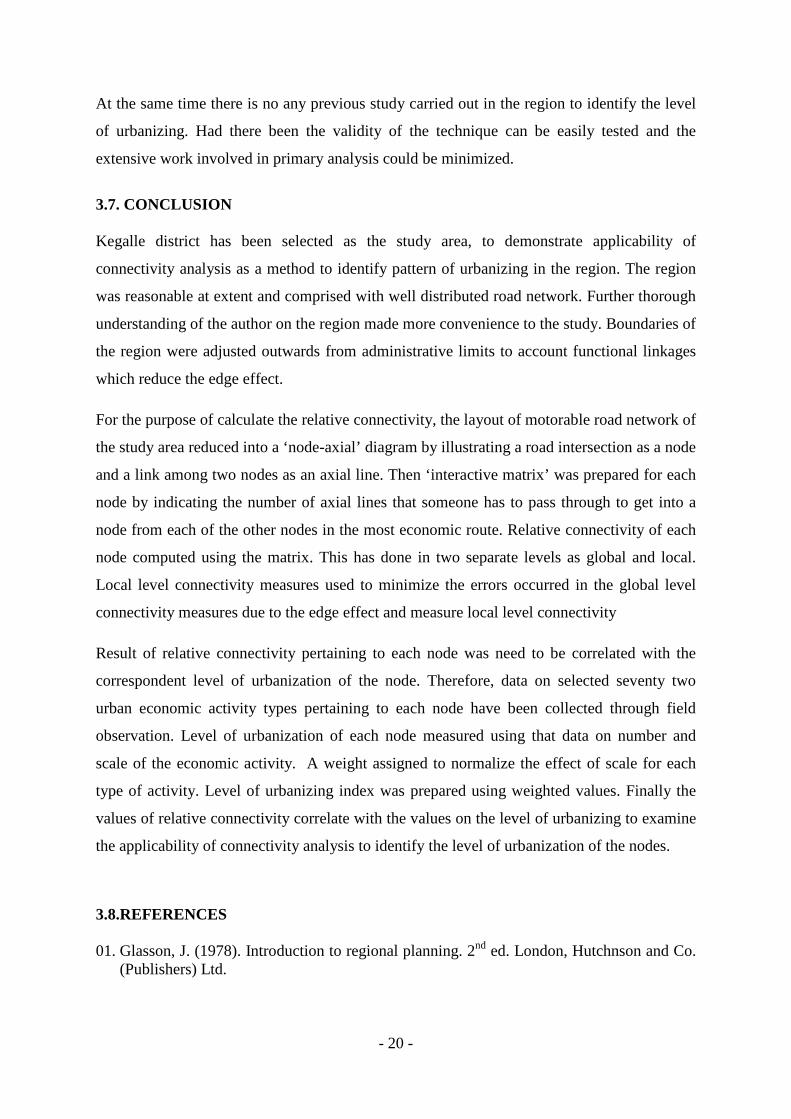
Further information on network connectivity is provided by the relative connectivity

distribution ‘P(c)’ defined as the probability that any given node has relative connectivity ‘c’.

In this case relative connectivity probability distribution is relatively peaked around a mean

value of 1.05 and is skewed by -0.48745 (Figure -4.1). The result implies that centres within

the region are well connected to each other.

- 22 -

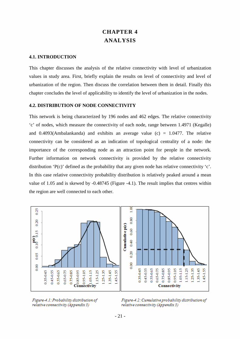
According to figure-4.2., (where x and y axes represent node connectivity and cumulative

probability respectively) most of the nodes have a lower connectivity (e.g. more than 75%

node out of total 196 nodes are with connectivity less than 1.15), while a few nodes have

higher connectivity (e.g. 25% node with connectivity more than 1.15) in particular only two

nodes with connectivity more than 1.45. This result implies that the topology of the Kegalle

district road network is close to the random graph with a quasi-absence of dominant hubs

(Barrat, 2004).

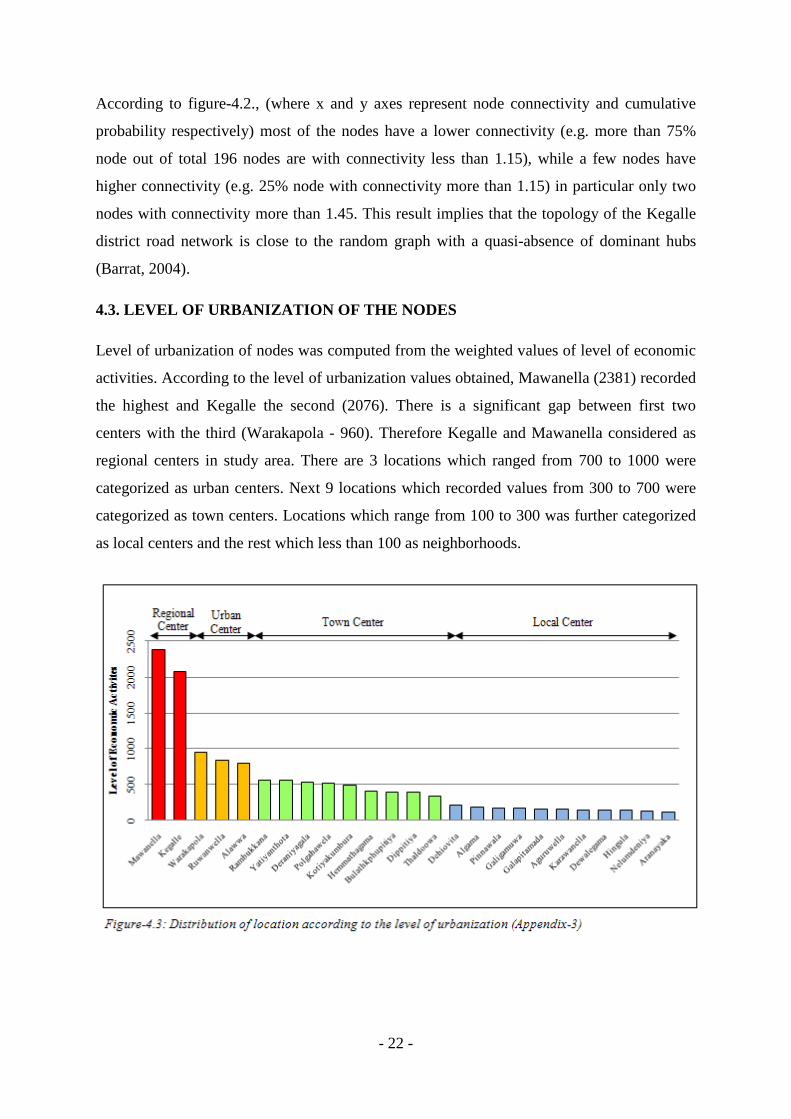
4.3. LEVEL OF URBANIZATION OF THE NODES

Level of urbanization of nodes was computed from the weighted values of level of economic

activities. According to the level of urbanization values obtained, Mawanella (2381) recorded

the highest and Kegalle the second (2076). There is a significant gap between first two

centers with the third (Warakapola - 960). Therefore Kegalle and Mawanella considered as

regional centers in study area. There are 3 locations which ranged from 700 to 1000 were

categorized as urban centers. Next 9 locations which recorded values from 300 to 700 were

categorized as town centers. Locations which range from 100 to 300 was further categorized

as local centers and the rest which less than 100 as neighborhoods.

- 23 -

4.4. THE ANALYSIS OF LEVEL OF URBANIZING - CONNECTIVITY CORRELATION

4.4.1. Global Connectivity

Correlation between relative connectivity value of each node and correspondent value of

level of urban activity recorded as 0.4208 (level of significant is 0.01). That reveals the

overall situation but in practice the need is inevitable to find the relationship at different

scales of the centres. In order to inspect in more detail relationship the results illustrated in

three different types of methods.

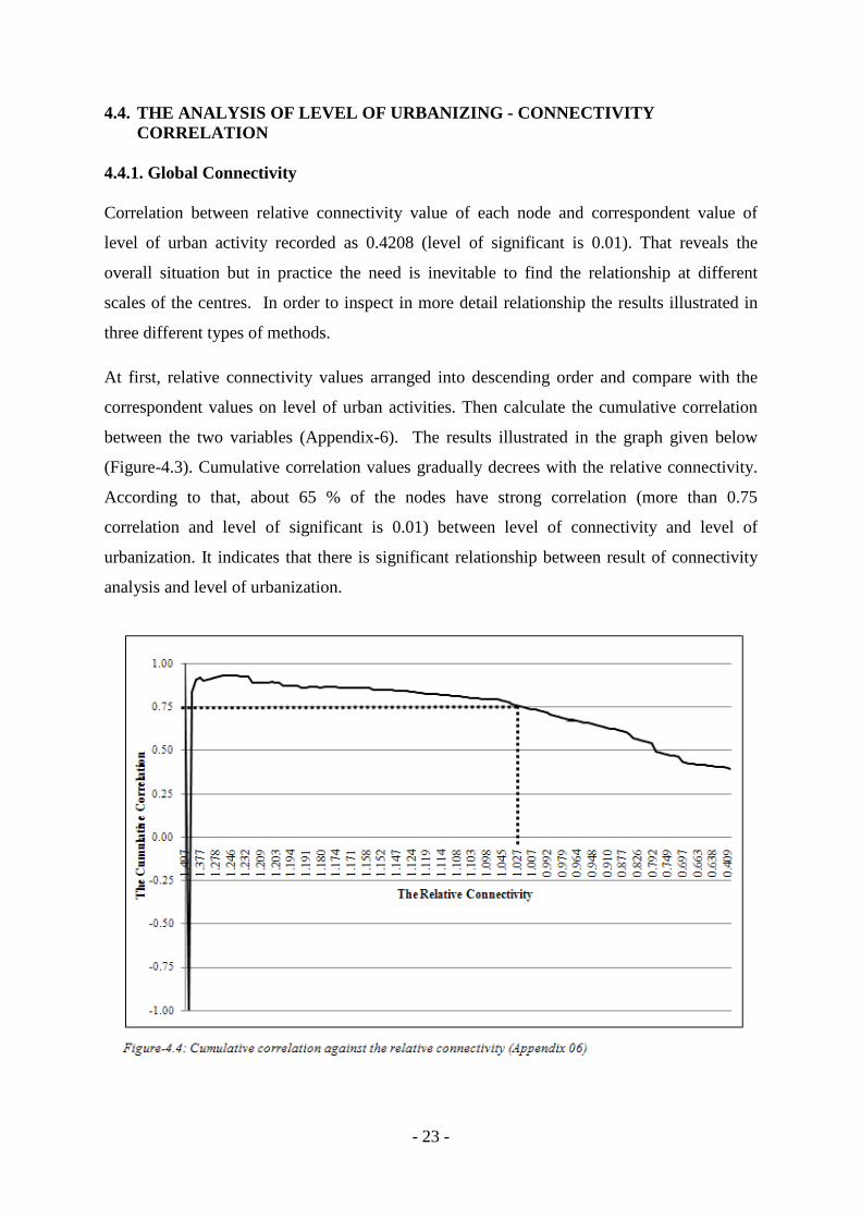
At first, relative connectivity values arranged into descending order and compare with the

correspondent values on level of urban activities. Then calculate the cumulative correlation

between the two variables (Appendix-6). The results illustrated in the graph given below

(Figure-4.3). Cumulative correlation values gradually decrees with the relative connectivity.

According to that, about 65 % of the nodes have strong correlation (more than 0.75

correlation and level of significant is 0.01) between level of connectivity and level of

urbanization. It indicates that there is significant relationship between result of connectivity

analysis and level of urbanization.

- 24 -

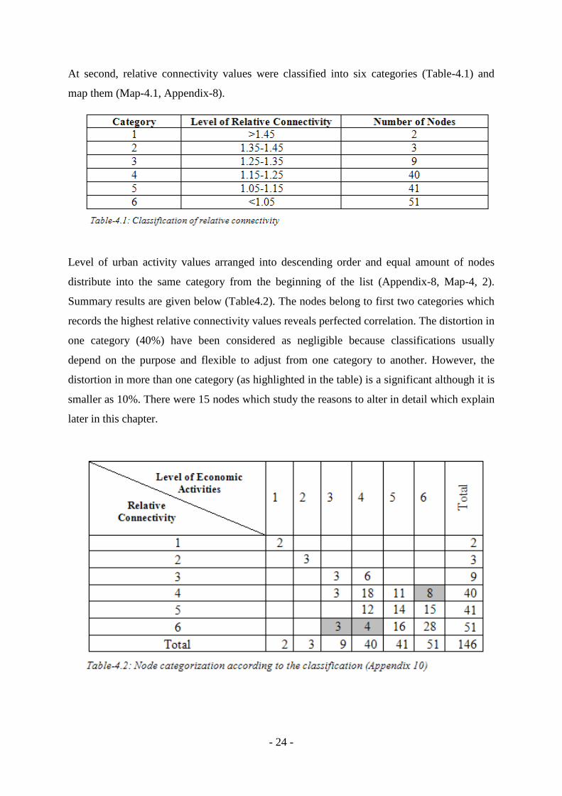
At second, relative connectivity values were classified into six categories (Table-4.1) and

map them (Map-4.1, Appendix-8).

Level of urban activity values arranged into descending order and equal amount of nodes

distribute into the same category from the beginning of the list (Appendix-8, Map-4, 2).

Summary results are given below (Table4.2). The nodes belong to first two categories which

records the highest relative connectivity values reveals perfected correlation. The distortion in

one category (40%) have been considered as negligible because classifications usually

depend on the purpose and flexible to adjust from one category to another. However, the

distortion in more than one category (as highlighted in the table) is a significant although it is

smaller as 10%. There were 15 nodes which study the reasons to alter in detail which explain

later in this chapter.

- 25 -

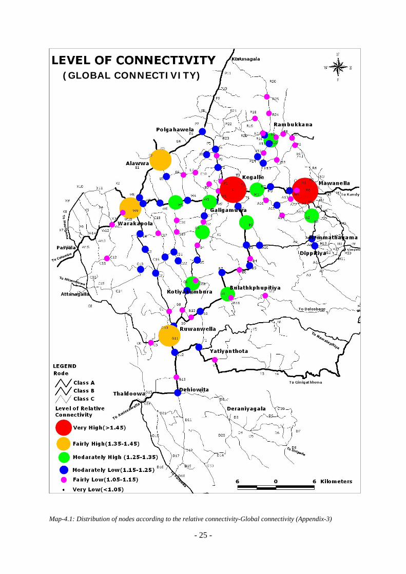
Map-4.1: Distribution of nodes according to the relative connectivity-Global connectivity (Appendix-3)

(GLOBAL CONNECTIVITY)

- 26 -

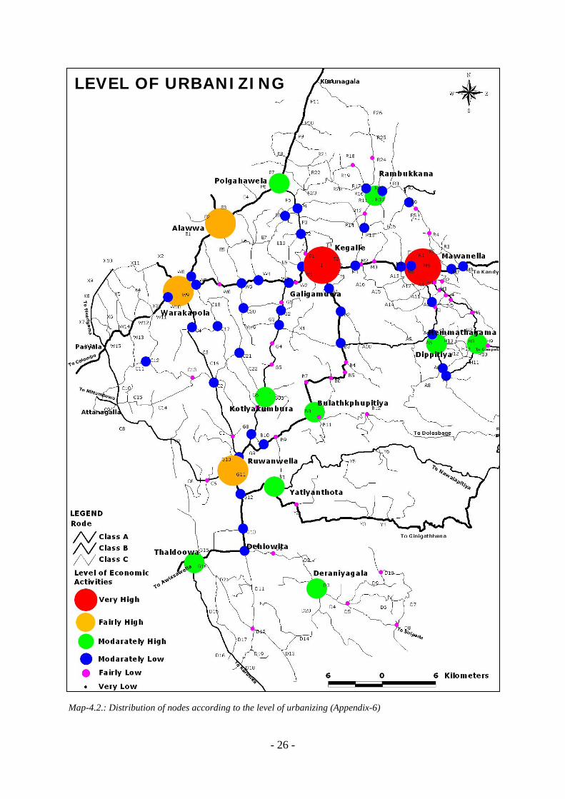
Map-4.2.: Distribution of nodes according to the level of urbanizing (Appendix-6)

LEVEL OF URBANIZING

- 27 -

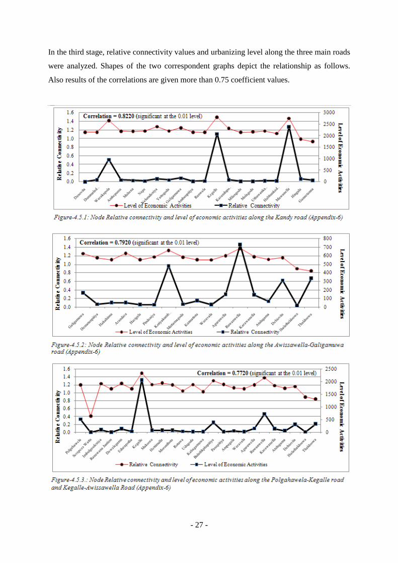
In the third stage, relative connectivity values and urbanizing level along the three main roads

were analyzed. Shapes of the two correspondent graphs depict the relationship as follows.

Also results of the correlations are given more than 0.75 coefficient values.

- 28 -

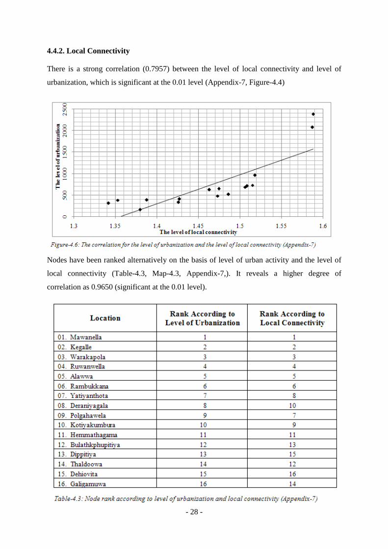
4.4.2. Local Connectivity

There is a strong correlation (0.7957) between the level of local connectivity and level of

urbanization, which is significant at the 0.01 level (Appendix-7, Figure-4.4)

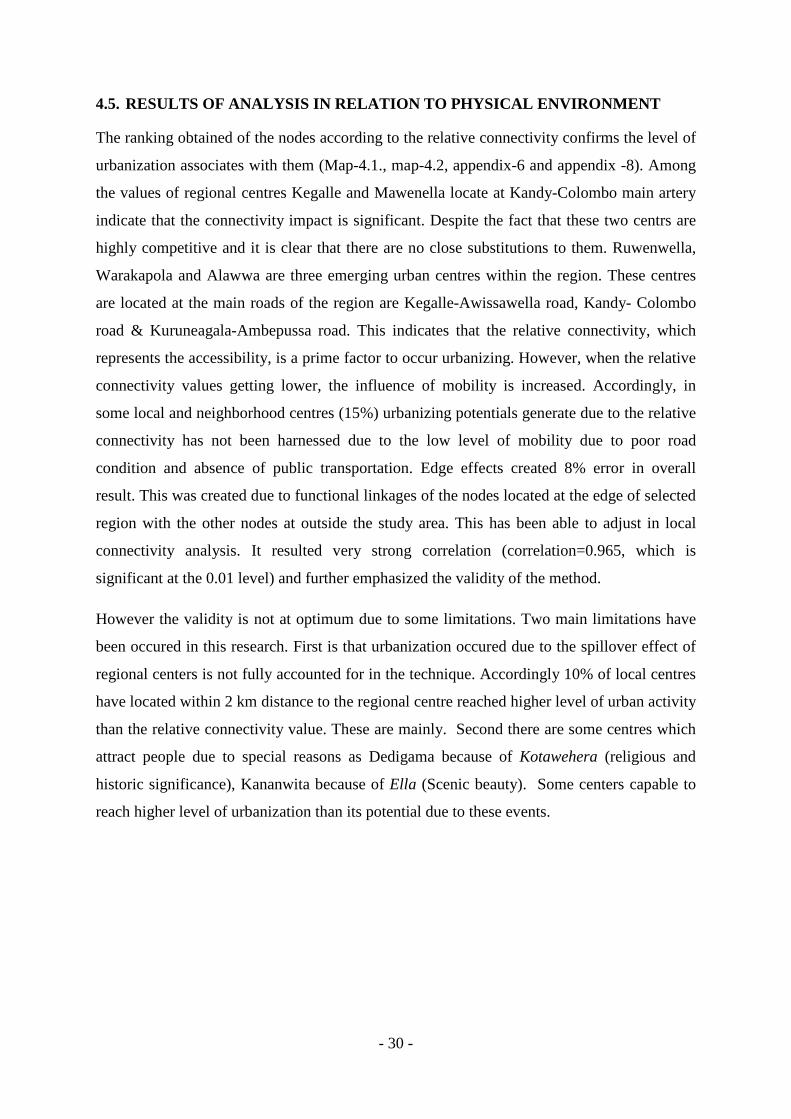
Nodes have been ranked alternatively on the basis of level of urban activity and the level of

local connectivity (Table-4.3, Map-4.3, Appendix-7,). It reveals a higher degree of

correlation as 0.9650 (significant at the 0.01 level).

- 29 -

Map-4.3: Distribution of nodes according to the relative connectivity-local connectivity (Appendix-7)

(LOCAL CONNECTIVITY)

- 30 -

4.5. RESULTS OF ANALYSIS IN RELATION TO PHYSICAL ENVIRONMENT

The ranking obtained of the nodes according to the relative connectivity confirms the level of

urbanization associates with them (Map-4.1., map-4.2, appendix-6 and appendix -8). Among

the values of regional centres Kegalle and Mawenella locate at Kandy-Colombo main artery

indicate that the connectivity impact is significant. Despite the fact that these two centrs are

highly competitive and it is clear that there are no close substitutions to them. Ruwenwella,

Warakapola and Alawwa are three emerging urban centres within the region. These centres

are located at the main roads of the region are Kegalle-Awissawella road, Kandy- Colombo

road & Kuruneagala-Ambepussa road. This indicates that the relative connectivity, which

represents the accessibility, is a prime factor to occur urbanizing. However, when the relative

connectivity values getting lower, the influence of mobility is increased. Accordingly, in

some local and neighborhood centres (15%) urbanizing potentials generate due to the relative

connectivity has not been harnessed due to the low level of mobility due to poor road

condition and absence of public transportation. Edge effects created 8% error in overall

result. This was created due to functional linkages of the nodes located at the edge of selected

region with the other nodes at outside the study area. This has been able to adjust in local

connectivity analysis. It resulted very strong correlation (correlation=0.965, which is

significant at the 0.01 level) and further emphasized the validity of the method.

However the validity is not at optimum due to some limitations. Two main limitations have

been occured in this research. First is that urbanization occured due to the spillover effect of

regional centers is not fully accounted for in the technique. Accordingly 10% of local centres

have located within 2 km distance to the regional centre reached higher level of urban activity

than the relative connectivity value. These are mainly. Second there are some centres which

attract people due to special reasons as Dedigama because of Kotawehera (religious and

historic significance), Kananwita because of Ella (Scenic beauty). Some centers capable to

reach higher level of urbanization than its potential due to these events.

- 31 -

4.6. CONCLUSION

This chapter discusses the analysis of the results of global connectivity and local connectivity

with the existing level of urbanization of the nodes. This has done in two stages; analysis of

the distribution of relative connectivity and level of urbanization values of nodes and analysis

of correlation values between relative connectivity and level of urbanization.

Relative connectivity values range between 1.4971 (Kegalle) and 0.4093(Ambalankanda). It

reveals an average value of 1.0477 is skewed by -0.4875. It is implies that nodes within the

region are well connected each other. On the other hand these values confirm that

connectivity web of the study area similar to a random graph. Because there are less number

of higher connected centers which act as a regional hubs and large number of node which

have obtained lower connectivity values (e.g. 25% node with connectivity more than 1.15 and

more than 75% node of total 195 nodes with connectivity less than 1.15).

According to the level of urbanization values obtained, Mawanella (2381) recorded the

highest and Kegalle the second (2076). There is a significant gap between first two centers

with the third (Warakapola - 960). Therefore Kegalle and Mawanella considered as regional

centers in study area. There are 3 locations which ranged from 700 to 1000 were categorized

as urban centers. Next 9 locations which recorded values from 300 to 700 were categorized as

town centers. Locations which range from 100 to 300 was further categorized as local centers

and the rest which less than 100 as neighborhoods.

Results of correlation analysis reveal some interesting points to be noted. First, about 65 % of

the nodes have strong correlation (more than 0.75) between the level of global connectivity

and level of urbanization although the overall correlation is 0.4028. Second, relative

connectivity values and urbanizing levels along the three main roads have significant

coefficient (0.822, 0.792 and 0.772) which was significant at the 0.01 level. Third, there is a

strong correlation between the level of local connectivity and level of urbanization is 0.7957

(significant at the 0.01 level). This indicates that the measure of relative connectivity which

represents the accessibility is capable enough to identify the level of urbanization.

However, when the relative connectivity values getting lower, the influence of mobility has

increased. Accordingly, in some local and neighborhood centres (15%) urbanizing levels

generate due to the relative connectivity has not been harnessed due to the low mobility as

poor road condition and absence of public transportation. Edge effects created 8% error in

- 32 -

overall result of global connectivity. This was created due to functional linkages of the

centres located at the edge of selected region with the locations outside the study area. This

has been able to be adjusted in local connectivity analysis. It resulted in very strong

correlation (correlation=0.965, significant at the 0.01 level) and further strength validity of

the method.

Two main limitations has identified in this research. First, the development potential created

due to the spillover effect of main urban centre is not fully accounted from the technique.

Second, there are some locations which attract people due to special reasons that are not fully

accounted from this technique.

4.7. REFERENCES

01. Barrat, A. (2004). Weighted networks: analysis modeling [online], France, University Paris-Sud. Available from :http://www.th.u-psud.fr/page_person/Barrat [Accessed 20th November 2007]

02. Watts, D.J. Strogatz, S.H. (1998). Collective dynamics of 'small-world' networks [online], Nature 393, 440-442 Available from : http://www.tam.cornell.edu /tam/cms/manage/upload/SS_nature_smallworld.pdf [Accessed 5th February 2007]

- 33 -

CHAPTER 5 CONCLUSION AND RECOMMENDATIONS

In the field of physical planning and urban design spatial analysis is gaining an increasing

emphasis. With that understanding there are numerous studies carried out in the field of

spatial analysis. Findings of them bring out a variety of perspectives and they generate a

range of analytical methods.

Connectivity analysis is one of the methods derived from the paradigm of graph theory.

Studies have tested the capabilities of this technique to measure relative connectivity of

location. On the other hand those studies were emphasized that this method has used to

identify urban hubs in a region, level of vulnerability of locations; to delineate functional

region…etc. Further connectivity analysis is useful dynamic tool to measure accessibility or

connectivity of transportation network.

In this background this study attempted to test the applicability of the technique to explain the

urbanizing locations in Sri Lankan context. Kegalle district was selected as the study area and

the study have correlated the level of relative connectivity values with existing level of

urbanization.

The results reveal that non-trivial correlation between the connectivity and the level of

urbanization. It indicates that connectivity analysis is capable of explaining the capacity of

urbanization of locations by comparing the level of economic activities in the location. That

could otherwise be very difficult to extract and to analyze from the conventional approaches.

Results of the current practices in Sri Lankan context to identify level of urbanization are

leading to many problems. One common practice is centrality matrix or rank size rule which

used to identify the functional hierarchy. But there are some locations which attract many

people than identified by the centrality matrix. Therefore the technique cannot apply

successfully to identify the level of urbanization. On other hand those technique are highly

critique due to its static nature. Further connectivity analysis does not consume that much of

data and provide precise information on a point. Therefore connectivity analysis could be use

to identify level of urbanization in locations illuminating many problems in current practice.

However it should be noted that the connectivity is only one aspect of promoting a location

for urbanizing, and there are many other causes to look into in the process of planning.

- 34 -

Though this study is conclude at this level, it opens a path for detailed studies on connectivity

analysis in Sri Lankan context. Further, study suggests that this approach might be useful in

other applications such as demarcating the functional hierarchy, delineate planning regions,

to identify the impact of proposed road development projects not only for road layout but also

hall region and to formulate strategies to achieve density policy which the connectivity can be

improved on where need to obtained high density, as well as to controlled the connectivity in

environmentally sensitive areas.

Further the research can be developed into used more advance analysis as weighted network

method and can be apply to other regions of the country to test the applicability.