European Journal of Operational Research 207 (2010) 110–120

Contents lists available at ScienceDirect

European Journal of Operational Research

journal homepage: www.elsevier .com/locate /e jor

Production, Manufacturing and Logistics

An ant colony system for enhanced loop-based aisle-network design

Ardavan Asef-Vaziri a,*, Morteza Kazemi b, Kourosh Eshghi b, Maher Lahmar c

a Systems and Operations Management, California State University, Northridge, United Statesb Industrial Engineering, Sharif University of Technology, Tehran, Iranc Industrial Engineering, University of Houston, United States

a r t i c l e i n f o a b s t r a c t

Article history:Received 4 August 2008Accepted 10 March 2010Available online 27 March 2010

Keywords:Facility logisticsFacility layoutMaterial handlingAutomated guided vehicle systemsVehicle based material transport systemsAnt colony optimization

0377-2217/$ - see front matter � 2010 Elsevier B.V. Adoi:10.1016/j.ejor.2010.03.024

* Corresponding author.E-mail address: ardavan.asef-vaziri@csun.edu (A. A

The purpose of this paper is to develop a global optimization model, simplification schemes, and a heu-ristic procedure for the design of a shortcut-enhanced unidirectional loop aisle-network with pick-up anddrop-off stations. The objective is to minimize the total loaded and empty trip distances. This objective isthe main determinant for the fleet size of the vehicles, which in turn is the driver of the total life-cyclecost of vehicle-based unit-load transport systems. The shortcut considerably reduces the length of thetrips while maintaining the simplicity of the system. The global model solves simultaneously for the loopdesign, stations’ locations and shortcut design. We then develop two simplifications each containing twoserial phases. Phase-1 of the first simplification step focuses on both loaded and empty trips, while that ofthe second simplification focuses only on loaded trips. In phase-2, both designs are enhanced with ashortcut to minimize both loaded and empty trip distances. The quality and efficiency of the three alter-native designs are tested for a set of problems with different layout size and product mix. While the solu-tion time of the second simplification procedure is a small percentage of the global formulation, itgenerates satisfactory solutions. On this foundation, we then develop a heuristic procedure to replacephase-1 of the second simplification. The heuristic procedure is using ant colony system to generate fea-sible solutions and then we implement a local search algorithm to improve the results. The heuristic algo-rithm quickly generates close to optimal solutions for phase-1 of the second simplification. By applyingphase-2 of the this second simplification on a set of loops generated by the heuristic, close to optimalsolutions are also quickly obtained for the global model.

� 2010 Elsevier B.V. All rights reserved.

1. Introduction

The facility layout problem involves three critical design deci-sions. (i) Design of the block layout representing work-centers(e.g. departments, production units, machining cells, assembly sta-tions, storage areas, etc.) as right-angle polygons, including dimen-sions and orientations. (ii) Design of aisle-network connecting thework-centers on the block layout, including topology of the net-work and directions of flow on its edges. (iii) Design of Pick-up(P) and Drop-off (D) stations on the aisle-network, including thenumber of stations and their potential locations. Since the imple-mentation of a facility layout design involves a significant initialinvestment, and further changes can incur a high reconfigurationcost, it is crucial to fully integrate the aisle-network and stationlocations into the block layout. A well-designed facility layoutcan smooth the material flow, reduce the Work-in-Process (WIP),decrease the cycle time, and contribute to the overall efficiencyof production systems (Heragu, 2008).

ll rights reserved.

sef-Vaziri).

The material handling devices in this study are unit-load auto-mated guided vehicles (AGVs) carrying a single load at a time.According to the Material Handling Industry of America (1999),unit-load vehicles represent the single largest segment of theAGV market. We address issues related to the design of the loop-based aisle-network, a type of guide-path that is often preferredto the operation of AGVs. However, the models and algorithms inthis paper can be applied to any system with discrete vehiclesnot just AGVs. The objective is to minimize the total loaded andempty trip distances. The loaded and empty trips in a loop aisle-network can be reduced by strategically adding shortcuts to theinitial network to provide the vehicle with alternative shorterroutes. The empty vehicle dispatching policy implemented in ourmodels is the shortest-trip-distance-first (STDF).

We focus on the integrated design of an aisle-network en-hanced with a shortcut and location of P&D stations. The arcs thatwill form the unidirectional loop network and the shortcut can beselected among the set of contour-lines on the boundaries of thework-centers in a block layout. The P&D stations can be locatedalong the contour-lines forming each work-center, and they arenot necessarily collocated.

A. Asef-Vaziri et al. / European Journal of Operational Research 207 (2010) 110–120 111

In the global model, Model (G), the loop, the shortcut, and thestations are designed concurrently. Given the complexity of theglobal model, we then develop two simplifications and a heuristicalgorithm, each being a two-phase sequential model. These algo-rithms are used to find a good solution in an acceptable time. Inthe first simplification scheme, Model (E), the objective functionin both phases is to minimize the total loaded and empty trip dis-tances. In phase 1, the loop and station locations are designed opti-mally, and then a shortcut is designed in phase-2. In the secondsimplification, Model (L), the loop is designed in phase-1 in orderto minimize the total loaded trip distances. In phase-2, the shortcutand final station locations are designed to minimize the totalloaded and empty trip distances. We test the quality of the solutionand the solution time of the obtained designs by each of the twosimplifications with those of the global model. The quality of Mod-el (L) is the same as Model (E), but its solution time is significantlyless than Model (E). While the solution time of Model (L) is a smallpercentage of the global formulation, it generates high qualitysolutions.

On this foundation, we then develop a heuristic algorithm,Model (H), which is similar to Model (L) but the optimization mod-el of phase-1 is replaced by an ant colony system heuristic algo-rithm. The heuristic algorithm generates close to optimalsolutions for phase-1 of Model (L), while its solution time is a smallpercentage of the optimization model. An interest of our work is toshow that the design obtained under loaded trip distance minimi-zation objective function, either optimally or heuristically, whenlater enhanced with a shortcut and final station locations, gener-ates a near-optimal solution for the total loaded and empty trip dis-tance objective function.

The remainder of this paper is organized as follows. Relevant lit-erature is reviewed in Section 2. The global model notation and for-mulation are described in Section 3. The two simplificationschemes are presented in Section 4. The heuristic procedure is pre-sented in Section 5. The quality and efficiency of the solution pro-cedures are tested and computational results are reported inSection 6. A summary of our work and future research directionsfollows in Section 7.

2. Literature review

There are several algorithms for the facility layout design. Twowell-known examples are BLOCPLAN (Donaghey, 1987) with lay-ered structure layouts, and the Kim and Goetschalckx (2005) algo-rithm with slicing structure layouts.

The design of a unidirectional loop aisle-network and P&D sta-tions on a fixed block layout was first modeled by Tanchoco andSinriech (1992) and Sinriech and Tanchoco (1993), who developeda five-phase serial optimization procedure. Asef-Vaziri et al. (2001)proposed an alternative formulation for the simultaneous design ofthe unidirectional loop and station locations. Caricato et al. (2007)put forward a branch-and-cut and a tabu search, and Zanjiraniet al. (2007) developed a genetic algorithm heuristic for the sameproblem. The objective function of all five models is to minimizethe total loaded trip distances. However, empty trips play a pro-found role in aisle-network and station location design process.

The empty travel modeling for AGVs is attributed to Egbelu(1987) when he designs four analytical models to link empty andloaded trips. Following first-come-first-served (FCFS) dispatching,Johnson (2001), by using simulation, and Benjaafar (2002) analyt-ically show that each loaded trip is usually followed by an emptytrip that varies in length with the nature of load-transport re-quests. Given a circular unidirectional configuration, Asef-Vaziriet al. (2008) numerically show that the optimal solution for loadedtrip distances is far from optimal when both loaded and empty

trips are taken into account. If the empty trips are not accountedfor, they can lead to the increase in the utilization of the allocatedmaterial transport devices and the surge in WIP all throughout theproduction facility (Benjaafar, 2002). Asef-Vaziri and Laporte(2009) argue that STDF, compared to FCFS, is a more effective dis-patching policy to be integrated into the design of a circular aisle-network. Under STDF policy, a vehicle is dispatched to a load at thework-center with the shortest-trip distance from the current work-center. Like the loaded travel calculation, the STDF empty vehicletrip consideration is a static calculation. It is essentially a lowerbound for the actual number of trips in the operations phase whichis highly stochastic. The STDF dispatching policy is a simple yetefficient policy that has been adopted by Malmborg and Shen(1994), Goetschalckx and Palliyil (1994), Sun and Tchernev(1996), Asef-Vaziri et al. (2007), Asef-Vaziri et al. (2008) andAsef-Vaziri and Goetschalckx (2008).

Sharp and Liu (1990) develop an optimization model to reducethe number of alternatives and a simulation model to make the fi-nal decision when a shortcut and off-line spurs are added to anexisting loop. Asef-Vaziri et al. (2007) developed global formula-tion, enumeration and a neighborhood search procedure for a sin-gle loop aisle-network design to minimize the loaded and emptytrip distances. They also introduced a set of flexible intermediatenodes as candidates for station locations. Our problem setting issimilar to that of Asef-Vaziri et al. (2007) with enhancement of ashortcut.

Eshghi and Kazemi (2006) develop an ant colony system (Dori-go and Gambardella, 1997) heuristic algorithm to design a shortestloop on a block layout. Ant colony system is one of the versions ofthe ant colony optimization algorithm, which was first introducedby Dorigo et al. (1991) to solve the traveling salesman problem(TSP). The essence of a part of our search process for finding feasi-ble loops benefits from the constructive algorithm of Eshghi andKazemi (2006). However, there are clear differences since theirprocedure aims to find the shortest loop in a block layout andmaterial flow has no effect on their problem. Furthermore, weimplement several improvements on their feasible loop identifica-tion process.

The reader is referred to Ganesharajah et al. (1998), VIS (2006),and Le-Anh and De Koster (2006) for a comprehensive review ofdesign and operational issues in AGV-based material transport sys-tems, to Johnson (2001) and Asef-Vaziri and Laporte (2009) for acomparison of empty vehicle dispatching policies, and to Asef-Vaz-iri and Laporte (2005) for a review on the loop-based facility plan-ning and material handling.

3. The global model: Model (G)

In this section, we describe the settings of the general problemand provide a global mathematical model that solves for the differ-ent components of the problem. We consider a block layout withpre-defined work-center locations and contour-lines defining theirboundaries. Our objective is to determine a loop-based aisle-net-work enhanced with a shortcut that allows the material transportvehicles to pick-up and drop-off loads from/at all work-centerssuch that the total loaded and empty trip distances is minimized.To preserve the contiguity of the work-centers, we let the aisle-network arcs overlap with the work-center boundaries.

We refer to the set of nodes at the intersection of the contour-lines defining the boundary of the work-centers as intersectionnodes. A new set of nodes determined at the mid-point of each pairof connected intersection nodes are defined as intermediate nodes.We position the P&D stations at intermediate nodes on the looparcs, which exclude the original intersection nodes as candidatestation locations. It is assumed that the cost of one unit of distance

ba

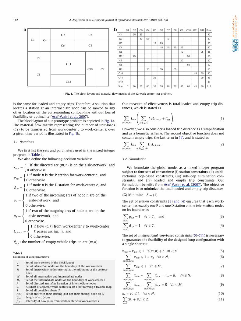
Fig. 1. The block layout and material flow matrix of the 12 work-center test problem.

112 A. Asef-Vaziri et al. / European Journal of Operational Research 207 (2010) 110–120

is the same for loaded and empty trips. Therefore, a solution thatlocates a station at an intermediate node can be moved to anyother location on the corresponding contour-line without loss offeasibility or optimality (Asef-Vaziri et al., 2007).

The block layout of our prototype problem is depicted in Fig. 1a.The material flow matrix representing the number of unit-loadsðfc;kÞ to be transferred from work-center c to work-center k overa given time period is illustrated in Fig. 1b.

3.1. Notations

We first list the sets and parameters used in the mixed-integerprogram in Table 1.

We also define the following decision variables:

xm;n ¼1 if the directed arc ðm;nÞ is on the aisle-network; and0 otherwise:

�

pc;n ¼1 if node n is the P station for work-center c; and0 otherwise:

�

dc;n ¼1 if node n is the D station for work-center c; and0 otherwise:

�

vn ¼1 if two of the incoming arcs of node n are on the

aisle-network; and0 otherwise:

8><>:

un ¼1 if two of the outgoing arcs of node n are on the

aisle-network; and0 otherwise:

8><>:

tc;k;m;n ¼1 if flow ðc; kÞ from work-center c to work-center

k passes arc ðm;nÞ; and0 otherwise:

8><>:

tem;n : the number of empty vehicle trips on arc ðm;nÞ:

Table 1Notations of used parameters.

C Set of work-centers in the block layoutN Set of intersection nodes on the boundary of the work-centersM Set of intermediate nodes inserted at the mid-point of the contour-

linesW Set of all intersection and intermediate nodesMc Set of the intermediate nodes on the boundary of work-center cA Set of directed arcs after insertion of intermediate nodesSi A subset of adjacent work-centers in set C not forming a feasible loopS Set of all possible subsets Si

AðSiÞ Set of arcs with their starting (but not their ending) node on Si

lm;n Length of arc ðm;nÞfc;k Intensity of flow ðc; kÞ from work-center c to work-center k

Our measure of effectiveness is total loaded and empty trip dis-tances, which is stated as

Xðm;nÞ2A

lm;n

Xc;k:fc;k>0

fc;ktc;k;m;n þ tem;n

0@

1A: ð1Þ

However, we also consider a loaded trip distance as a simplificationand as a heuristic scheme. The second objective function does notcontain empty trips, the last term in (1), and is stated asXðm;nÞ2A

lm;n

Xðc;kÞ:fc;k>0

fc;ktc;k;m;n: ð2Þ

3.2. Formulation

We formulate the global model as a mixed-integer programsubject to four sets of constraints: (i) station constraints, (ii) unidi-rectional loop-based constraints, (iii) sub-loop elimination con-straints, and (iv) loaded and empty trip constraints. Ourformulation benefits from Asef-Vaziri et al. (2007). The objectivefunction is to minimize the total loaded and empty trip distances

ðGÞ Minimize Z ¼ ð1Þ

The set of station constraints (3) and (4) ensures that each work-center has exactly one P and one D station on the intermediate nodeson its boundariesXn2Mc

pc;n ¼ 1 8c 2 C; and ð3ÞXn2Mc

dc;n ¼ 1 8c 2 C: ð4Þ

The set of unidirectional loop-based constraints (5)–(11) is necessaryto guarantee the feasibility of the designed loop configuration witha single shortcut

xm;n þ xn;m 6 1 8ðm;nÞ 2 A : m < n; ð5ÞXm:ðm;nÞ2A

xm;n 6 1þ vn 8n 2 N; ð6ÞX

m:ðm;nÞ2A

xm;n 6 1 8n 2 M; ð7ÞX

m:ðm;nÞ2A

xm;n �X

m:ðn;mÞ2A

xn;m ¼ vn � un 8n 2 N; ð8ÞX

m:ðm;nÞ2A

xm;n �X

m:ðn;mÞ2A

xn;m ¼ 0 8n 2 M; ð9Þ

un þ vn 6 1 8n 2 N; ð10ÞXn2N

ðun þ vnÞ 6 2: ð11Þ

A. Asef-Vaziri et al. / European Journal of Operational Research 207 (2010) 110–120 113

Constraints (5) state that a contour-line is either not on theaisle-network or it is unidirectional. For a loop with a single short-cut, all intersection and intermediate nodes have at most oneincoming arc, with the exception of one intersection node whichcould have two incoming arcs. Constraints (6) and (7), respectively,represent this condition for intersection and intermediate nodes.Constraints (8) state that the number of incoming arcs minus thenumber of outgoing arcs on intersection nodes is equal to 0, withthe exception of two such nodes when this difference is 1 and�1. Similarly, Constraints (9) represent the arc balance constrainton the intermediate nodes. Constraints (10) eliminate closed-loopshortcuts by ensuring that an intersection node has either one ex-tra incoming or outgoing arc. Constraint (11) allows a singleshortcut.

The third set of constraints is the sub-loop elimination con-straint. A sub-loop in a block layout is a set of contour-lines defin-ing the boundary of a (right-angle but not necessarily convex)polygon formed by a set of adjacent (having one contour-line incommon) work-centers. It becomes a feasible loop when coveringat least one contour-line of each work-center. A slight modificationof the sub-tour elimination constraints developed by Dantzig et al.(1954) for the TSP is used to eliminate the formation of sub-loopsXðm;nÞ2AðSiÞ

xm;n P 1 8Si � S: ð12Þ

This set of constraints ensures that at least one of the arcs that havetheir origin on the boundary of the polygon formed by Si and head-ing out of the polygon is on the aisle-network. Asef-Vaziri et al.(2001) show that the number of these inequalities in a block layoutcompared to TSP is small.

The fourth set of constraints is the loaded and empty vehicle con-straints. The loaded flow feasibility constraints (13) state thatloaded vehicles can only move along the aisle-network. The mul-ti-commodity loaded flow balance constraints (14) state that the to-tal incoming loads to a node plus loads picked up from that node isequal to the total outgoing loads plus loads dropped off at thatnode

tc;k;m;n 6 xm;n 8ðm;nÞ 2 A;8ðc; kÞ : fc;k > 0; ð13Þ

Xm:ðm;nÞ2A

tc;k;m;n þ pc;n ¼X

m:ðn;mÞ2A

tc;k;n;m þ dk;n 8n 2W ;8ðc;kÞ : fc;k > 0:

ð14Þ

The empty vehicle dispatching policy underlying our optimizationmodels is the STDF. Under this policy, if no material handling re-quest is placed, the vehicle stops at a spur at the last visitedwork-center and if multiple requests are placed, the vehicle is dis-patched to the work-center with the shortest-trip distance fromthe current work-center

tem;n 6

Xc;k

fc;k

!xm;n 8ðm;nÞ 2 A ð15Þ

Xm:ðm;nÞ2A

Xðc;kÞ:fc;k>0

fc;ktc;k;m;n þ tem;n

0@

1A

¼X

m:ðn;mÞ2A

Xðc;kÞ:fc;k>0

fc;ktc;k;n;m þ ten;m

0@

1A; 8n 2W ð16Þ

The empty flow feasibility constraints (15) ensure that empty vehi-cles can only move along the aisle-network. The first term on theright plays the role of a large number. The loaded and empty flowbalance constraints state that the total number of incoming and out-going vehicles on each node are equal.

4. Two simplification schemes: Model (E) and Model (L)

We now develop two simplified procedures, both based on atwo-phase method that sequentially solves for each phase. We re-fer to these models as Model (E) and Model (L), and to their firstphase as Model (E1) and Model (L1), respectively.

These two simplification are designed to obtain a good solutionin an acceptable time.

4.1. Phase-1

Model (E1): In Model (E1), the loop and station locations are de-signed under the total loaded and empty trip distance minimiza-tion objective function. The formulation of this model is similarto that of the global model without shortcut considerations

ðE1Þ Minimize Z ¼ ð1ÞConstraints ð3Þ—ð5Þ; ð7Þ; ð9Þ; ð12Þ—ð16Þ:Xðm;nÞ2A

xm;n 6 1 8n 2 N; ð17ÞXðm;nÞ2A

xm;n �Xðn;mÞ2A

xn;m ¼ 0 8n 2 N: ð18Þ

Constraints (17) and (18) replace constraints (6) and (8) of the glo-bal model, respectively.

Model (L1): In Model (L1), the loop and station locations are de-signed under the total loaded trip distance minimization objectivefunction. The formulation of this model is similar to that of Model(E1) without empty vehicle related variables and constraints.

ðL1Þ Minimize Z ¼ ð2ÞConstraints ð3Þ—ð5Þ; ð7Þ; ð9Þ; ð12Þ—ð14Þ; ð17Þ; ð18Þ:

4.2. Phase-2

At phase-2, the objective function for both models is to mini-mize the total loaded and empty trip distances. In Model (E), wefix the loop and the station locations and then design the shortcut,whereas in Model (L) we only fix the loop, and then design the sta-tion locations and the shortcut. Since the output of phase-1 is theinput to phase-2, we introduce a set of new notations which areused in formulating the new constraints of phase-2. Nl and Al,respectively, are defined as the set intersection nodes and directedarc on the loop. Pl and Dl, respectively, are defined as the set of Pand D stations on the loop.

Model (E): In this model, given a pre-determined loop aisle-net-work design and P&D station locations, the problem is to design ashortcut that minimizes the total loaded and empty trip distances.We fix the set of directed arcs on the loop aisle-network ðAlÞ by fix-ing the values of decision variables xm;n; 8ðm;nÞ 2 Al. We also fixthe P&D station locations by fixing the values of pc;n and dc;n vari-ables. The model identifies the directed arcs that will form theshortcut ðxm;n; 8ðm;nÞ 2 A n AlÞ and the total loaded and empty tripdistances

ðEÞ Minimize Z ¼ ð1ÞXðm;nÞ2Al

xm;n þX

c;n2Pl

pc;n þX

c;n2Dl

dc;n ¼ jAlj þ jPlj þ jDlj ð19Þ

Xðm;nÞ2A

ðxm;n � xn;mÞ ¼ vn � un 8n 2 Nl; ð20Þ

Xðm;nÞ2A

xm;n 6 1þ vn 8n 2 Nl; ð21Þ

un þ vn 6 1 8n 2 Nl; ð22Þxm;n þ xn;m 6 1; 8ðm;nÞ 2 A n Al ð23Þ

114 A. Asef-Vaziri et al. / European Journal of Operational Research 207 (2010) 110–120

Xðm;nÞ2A

xm;n 6 1 8n 2 N n Nl; ð24ÞXðm;nÞ2A

ðxm;n � xn;mÞ ¼ 0 8n 2 N n Nl; ð25ÞXn2Nl

ðun þ vnÞ 6 2; ð26Þ

Constraints ð13Þ—ð16Þ:

Constraints (19) fix the loop and stations of phase-1, where jRjstands for the cardinality of set R. Constraints (20)–(22) allow twointersection nodes on the loop to become starting and ending nodesfor the shortcut. Constraints (23)–(26) create a unidirectional short-cut on the nodes and arcs not on the loop.

Model (L): In this model, given a pre-determined loop, the prob-lem is to simultaneously design a shortcut, and to position the P&Dstations that minimize the total loaded and empty trip distances.Similar to Model (E), we fix the set of directed arcs on the loopaisle-network ðAlÞ by fixing the values of decision variablesxm;n; 8ðm;nÞ 2 Al.

ðLÞ Minimize Z ¼ ð1ÞXðm;nÞ2Al

xm;n ¼ jAlj; ð27Þ

Constraints ð3Þ; ð4Þ; ð13Þ—ð16Þ; ð20Þ—ð26Þ:

The above formulation identifies the directed arcs that will form theshortcut ðxm;n 8ðm; nÞ 2 A n AlÞ, the P&D station locations (pc;n anddc;n, respectively), as well as the rest of the consequence variables.

5. A heuristic algorithm

We now develop a heuristic (H), where its second phase is sim-ilar to Model (L), but the optimization Model (L1) is replaced by aheuristic (H1). The heuristic Model (H1) is based on the ant colonysystem (ACS) algorithm that is a version of the ant colony optimi-zation (ACO) algorithm to find feasible solutions. Then we apply alocal search to improve the algorithm efficiency. In order to im-prove the quality of the heuristic solution of Model (H), in additionto the best solution of Model (H1), we also send nine other bestsolutions to phase-2. In the remainder of this section, we limitour discussion to phase-1 of Model (H).

According to Dorigo et al. (2006), ACO is an iterative heuristicalgorithm in which a number of agents called ants build feasiblesolutions to an optimization problem. They exchange informationon the solution quality with a shared communication mechanismbased on pheromone. Pheromone is associated to each componentof the problem to indicate its desirability. Usually, another heuris-tic function is assigned to each component constituent to use localproperties of the problem. At each iteration, when ants find feasi-ble solutions, the pheromone of each component is changed basedon the generated solutions value.

We implement ACS algorithm, which is one of the most success-ful variants of ACO algorithms (Dorigo and Gambardella, 1997;Dorigo et al., 2006). ACS is designed based on three basic rules:(i) state transition, (ii) local pheromone update, and (iii) globalpheromone update. State transition rule is a probabilistic functionwhich is composed of the component pheromone and heuristicfunction. After generating a feasible solution by an ant, a local up-date rule is implemented. The main goal of the local update is todiversify the search performed by subsequent ants during an iter-ation. The effect of the local pheromone update is to decrease thepheromone values of the used components. Therefore, desirabilityof these components decrease for the ants that follow. Hence, it isless likely that several ants produce identical solutions during oneiteration. After all ants build their solution, then the global update

rule is applied. It aims to increase (decrease) the pheromone valuesassociated with promising (non-promising) solutions.

5.1. Feasible loops

A loop can be uniquely defined by the set work-centers itencompasses. Using the constructive algorithm of Eshghi and Kaz-emi (2006), at each step of our ACS algorithm, K ants are imple-mented to generate feasible loops. At each iteration of theconstructive algorithm, a new work-center among the set of thoseeligible is added to a partial solution generated by an ant. Thework-center is selected by using a state transition rule. This pro-cess is iterated until a feasible loop is obtained.

Let us define gm;n and sm;n, respectively, as heuristic function andpheromone function of contour-line ðm;nÞ in the block layout. Ateach step of constructing a feasible loop, ant k selects work-centeri by applying the following state transition rule:

Pki ¼

1 if q 6 q0 and i ¼ arg maxj2Jk

sj � ½gj�a

n o;

si �½gi �aP

j2Jksj �½gj �

a if q P q0 and i 2 Jk;

0 otherwise;

8>>>><>>>>:

ð28Þ

where Jk is the set of eligible work-centers, q 2 ½0;1� is a uniformrandom number, q0 2 ð0;1� is a specified threshold parameter, a isa parameter determining the relative importance of pheromoneversus heuristic function, and siðgiÞ is the sum of the counter-linespheromone (heuristic function) of the generated partial solutionafter adding the new work-center i.

To define a heuristic function for each counter-line, we considerintensity of the material flow. Each pair of adjacent work-centersðc; kÞ can uniquely be defined by their common edge ðm; nÞ. Theheuristic function of contour-line ðm; nÞ is defined as 1þ fc;k þ fk;c .

The state transition rule is used to pull a work-center from Jk. Ifa random number q is less than q0, the work-center with the max-imal si � ½gi�

a is selected. Otherwise, the work-center is selectedaccording to the probability given by the second part of the transi-tion rule.

After a feasible loop is constructed by one of the ants, the localpheromone update rule is implemented. The local update rulechanges the pheromone value of contour-line ðm; nÞ for a specifiedloop by

sðm;nÞ ð1�uÞ � sðm;nÞ þu � s0; ð29Þ

where u 2 ð0;1� is an adjusting parameter for the pheromone pre-viously deposited on contour-line ðm; nÞ, and s0 is a small positiveconstant equal to the initial value of pheromone laid on each con-tour-line.

At the end of each iteration, once all ants have generated theirown loop, the global pheromone is updated by the followingequation:

sðm;nÞ ð1� qÞ � sðm;nÞ þ q � Dsðm;nÞ; ð30Þ

where

Dsðm;nÞ ¼ðLgbÞ�1 if ðm;nÞ 2 global best loop;0 otherwise:

(

Lgb is the objective function value of the current best loop, andq 2 ð0;1� is the pheromone decay parameter.

5.2. Station locations

To evaluate the generated loops, we should identify the locationof the P&D stations and compute the total loaded trip distances. To

A. Asef-Vaziri et al. / European Journal of Operational Research 207 (2010) 110–120 115

reduce computation times, we first locate P&D stations using aheuristic algorithm. The promising loops identified by this heuris-tic procedure are then sent to an optimization model. Computa-tional results showed that the heuristic evaluation has strongrelation with the exact objective value.

5.2.1. The P&D location heuristicFor each case of clockwise and counterclockwise order, do com-

plete the following steps and select the one with the smaller totalloaded trip distance as the evaluation of loop value:

(1) Select the next-highest flow in the material flow matrix forwhich either the P station of the origin work-center or theD station of the destination work-center are not selected yet.

(2) Locate the P station of the origin work-center and the D sta-tion of the destination work-center at the nearest distancefrom each other.

(3) If the location of all P&D stations are not identified yet, go to(1).

(4) Fix the P stations of all work-centers. For each work-center,relocate the D station leading to the best improvement in theestimated objective function.

(5) Fix D stations of all work-centers. For each work-center,relocate the P station leading to the best improvement inthe estimated objective function.

(6) If in (4) or (5), the objective value is improved then go toStep (4). Otherwise, for the current order of a loop, computetotal loaded trip distance.

The optimal location of the P&D stations for each of the promisingloops can be obtained by using an optimization model. This IP modelis similar to that of Asef-Vaziri et al. (2007) but under the objectivefunction of minimization of the total loaded trip distances.

Given the directed loop l, the incoming and outgoing arcs foreach node n are known a priori. Assume that for any intermediateor intersection node n, the incoming flow enters from the adjacentnode m and the outgoing flow leaves to the adjacent node m0. GivenAl as the set of directed arcs on the loop, i.e. node m precedes nodesn, and node n precedes node m0 in the direction of the loop, Nl andMl as the set of intersection nodes and intermediate nodes on loopl, respectively, and Slc is the set of intermediate nodes on both loopl and work center c. The IP model is formulated as follows:

Minimize Z ¼ ð2Þ

subject toXn2Slc

pcn ¼ 1 8 c 2 C; ð31ÞXn2Slc

dcn ¼ 1 8 c 2 C; ð32ÞXfck>0

ðtckmn � tcknm0 Þ ¼ �pcn þ dkn 8 > n 2 Ml; ð33ÞXfck>0

ðtckmn � tcknm0 Þ ¼ 0 8 > n 2 Nl: ð34Þ

Constraints (31) and (32) locate P&D stations. Constraints (33) and(34), respectively, are multi-commodity flow balance constraint onintermediate and intersection nodes of a known directed loop.

5.3. Local improvement procedure

To improve the efficiency of ACO algorithms, they are often com-bined with a local search procedure. Local search is used to find abetter solution in a neighborhood of the generated solutions. Inour algorithm, the local improvement procedure consists of two

main phases of replacement and expansion. In the replacement phase,an inferior loop is replaced with a superior one, and in the expansionphase, the feasible region of the problem is deeply explored.

Replacement: This procedure checks if one loop is dominated byanother. If one or more of the work-centers in a loop has all fourconditions described below, the loop is replaced by those gener-ated by removing those work-centers.

Determine superior loop: Let S be a feasible loop and c be a work-center in S. If c has the following properties then S is removed andS� fcg is added to the list of generated loops:

(1) S� fcg is a feasible loop.(2) Work-center c is adjacent to the boundary of the block

layout.(3) Length of S� fcg loop is not greater than a length of S.(4) There is no flow between the work-center c and its adjacent

work-centers which are not in S.

Expansion: Two procedures are implemented to enrich thesearch space of the feasible loops. The first procedure explores aset of feasible suitable loops which cannot be generated by the con-struction algorithm. The second procedure generates a class of fea-sible loops that have a low probability to be reached by the ants.

It is possible to add a new work-center to a feasible loop andgenerate another one. However, a constructive algorithm cannotexplore these types of feasible loops. A constructive algorithmstops as soon as generating a feasible loop; it does not add anotherwork-center. To overcome this drawback, we may add one work-center to each generated feasible loops. Usually, there is more thanone candidate work-center, i.e. more than one additional loop. Theone with the best evaluation value is added to the list of generatedloops to reduce the number of potential feasible loops.

At each iteration of generating a feasible loop, a new work-center is added to the current partial solution (sub-loop). Given Sas the set of work-centers forming a loop, each work-center in Sis usually adjacent to more than one work-center in S. However,if for all c 2 S, the work-centers are adjacent to at most two otherwork-center in S, then we refer to the loop as a feasible path solu-tion (FPS). In general, at each step of the constructive algorithm,the new work-center i is adjacent to one or more already selectedwork-centers. However, in a FPS, the new work-center is adjacenteither to the first or the last work-center of the generated partialpath. The probability of generating FPS exponentially decreasesas the size of the problem increases. To include FPSs in the searchspace at each iteration, after all ants have constructed their feasiblesolutions, a set of FPSs are generated. At each step of generating aFPS, a feasible work-center is selected by uniform probability.

5.4. Model (H)

Our overall heuristic algorithm for Model (H), including itsphase-2, is given below.

Set parameters, initialize pheromonefor i ¼ 1 to iteration number do

for k ¼ 1 to ants number doConstruct a feasible loop by ant kApply local pheromone updating rule

end forApply local improvement procedureApply global updating rule

end forFind the optimal solution value for the best N loops.Identify the overall optimal solution for phase-1.Send the optimal solution and nine other best solutions to

phase-2.

Table 2Algorithm parameters.

Parameter Value Description

K 10 Number of antsp 10 Number of FPS generated in each iterationN 10 Number of selected loops to solve with IPa 0.5 Relative coefficientu 0.1 Local update coefficientq 0.1 Global update coefficientq0 0.9 Threshold parameterI 500 Iteration number

Table 3Problem instance with 12, 16, and 20 work-centers each with 5 products.

Product Productionvolume

Production routing

12 Work-center 1 25 1-3-6-2-4-9-8-10-122 5 1-2-7-9-6-10-11-123 10 1-2-3-5-9-6-10-124 25 1-2-4-8-10-11-5-125 15 1-2-4-7-9-4-6-10-11-12

16 Work-center 1 25 1-5-2-9-4-10-11-12-15-162 15 1-6-7-8-10-11-13-14-15-163 5 1-3-6-8-10-11-13-14-12-164 10 1-2-3-4-5-6-7-8-10-165 25 1-3-4-5-8-9-11-12-13-16

20 Work-center 1 25 1-3-4-5-6-9-11-12-14-16-18-20

116 A. Asef-Vaziri et al. / European Journal of Operational Research 207 (2010) 110–120

The initial value of pheromone associated to each contour-line,

2 15 1-5-6-7-8-10-12-15-16-18-203 5 1-3-8-5-6-7-8-9-10-11-13-15-

17-19-204 10 1-2-3-6-7-9-10-11-12-13-14-

16-17-18-205 25 1-2-3-5-6-8-9-11-12-14-15-16-

19-20

s0, is consider as a ðcell no� objÞ�1, where obj is an evaluation ofone randomly generated feasible loop. Other parameters of thealgorithm are summarized in Table 2.

6. Computational considerations

6.1. The test problems

To test the quality of our optimization and heuristic models, weconsider a variety of problem instances that range from 12 to 20work-centers. We also consider a variety of product mixes and pro-duction volumes. Figs. 1a, 2a and b illustrate a sample of three in-stances for 12, 16 and 20 work-center block layouts. Theseprototype problems are implemented as the seeds for test-bedproblem generation using the idea introduced by Nugent et al.(1968). Given a random permutation of integers 1;2; . . . ; jCj de-noted by P ¼ P1; P2; . . . ; Pi; . . . ; PjCj, a new test problem is generatedby assuming that the location of work-center i in the prototypeblock layout is now allocated to work-center Pi. Nine random per-mutations are generated for each layout to join the original proto-type problems and form 30 random test problems.

Production routings of the seed problems are shown in Table 3.This information can be used to generate flow matrices that repre-sent the frequency of loaded trips between different work-centerpairs. Below, we illustrate a compact representation of the flowmatrix, fðc; k; fc;kÞ : fc;k > 0g, for the 16 work-center seed problemwith its production routings presented in Table 3. The followingset represents the only 32 non-zero flows where the first two num-bers refer to the origin and destination work-centers (c and k,respectively) and the third number refers to the volume of the flowin unit-loads ðfc;kÞ.

{(1,2,10), (1,3,30), (1,5,25), (1,6,15), (2,3,10), (2,9,25), (3,4,35), (3,6,5), (4,5,35), (4,10,25), (5,2,25), (5,6,10), (5,8,25),(6,7,25), (6,8,5), (7,8,25), (8,9,25), (8,10,30), (9,4,25), (9,11,25),(10,11,45), (10,16,10), (11,12,50), (11,13,20), (12,13,25), (12,15,25), (12,16,5), (13,14,20), (13,16,25), (14,12,5), (14,15,15), (15,16,40)}

2

13 14 15 16

11109

1

56

78

43

12

a

Fig. 2. 16 Work-center and 20

The general purpose mixed-integer programming solver CPLEX7.1 was deployed to solve for the three Models (G), (E), and (L), aswell as the second phase of Model (H). All computations were car-ried out on a Sun Microsystems Ultra 10 work station with a440 MHz UltraSPARC-IIi processor and 128 Mbytes of RAM, run-ning the Solaris 8 operating system.

6.2. Comparison of Models (G), (E), and (L)

Tables 4–6 illustrate a summary of the solution and computa-tion results for 10 problem instances with 12, 16, and 20 work-cen-ters, respectively. Columns ZðGÞ and TðGÞ show the optimalobjective function and the CPU time (seconds), in this order, forthe global model.

To understand the value of adding a shortcut to the loop, wecompare the total loaded and empty trips on a single loop, ZðE1Þ,to that of one with a shortcut ZðGÞ. Our results show that integrat-ing a shortcut into the loop contributes an average of 25%, 28%, and32% in reducing the total loaded and empty trip distances for 12,16, and 20 work-center problems, respectively. Of course, thedesirability of the shortcut will largely depend on the trade-off be-tween the cost of incorporating a shortcut into the loop aisle-net-work and the savings due to shorter trip distances.

Columns ZðEÞ and TðEÞ show the optimal objective function andthe CPU time (seconds), respectively, for Model (E). On average, thevalue of the objective function of Model (E) is 12%, 15%, and 22%higher than that of the global Model (G) for the three problem sets,respectively. This implies that adding a shortcut to the aisle-net-work after deciding on the loop design and the stations’ locations

13

028171 19

15 1614

11

3

1 2

5

6

79

8

10

12

4

b

work-center test problems.

Table 4The solution time and quality of solutions for the three models applied on 10 instances of the 12 work-center problem.

Problem ZðGÞ TðGÞ ZðE1Þ ZðE1ÞZðGÞ

ZðEÞ TðEÞ ZðEÞZðGÞ

TðEÞTðGÞ

ZðLÞ TðLÞ ZðLÞZðGÞ

TðLÞTðGÞ

12.0 2700 1172 3200 1.19 2880 370 1.07 0.32 2860 30 1.06 0.0312.1 4210 800 5460 1.30 4800 784 1.14 0.98 4470 28 1.06 0.0312.2 3250 702 4600 1.42 4120 597 1.27 0.85 4300 63 1.32 0.0912.3 3710 1692 4810 1.30 4330 578 1.17 0.34 4310 37 1.16 0.0212.4 3720 1495 4680 1.26 4280 680 1.15 0.45 4200 50 1.13 0.0312.5 4260 2704 5060 1.19 4520 937 1.06 0.35 4730 61 1.11 0.0212.6 4240 2410 4700 1.11 4240 482 1.00 0.20 4240 45 1.00 0.0212.7 3450 1961 4700 1.36 4160 815 1.21 0.42 3960 44 1.15 0.0212.8 3980 3197 4560 1.15 4170 1015 1.05 0.32 4480 71 1.13 0.0212.9 3810 1140 4700 1.23 4240 632 1.11 0.55 4500 56 1.18 0.05

Mean 3733 1727 4647 1.25 4174 689 1.12 0.48 4205 49 1.13 0.03

Minimum 2700 702 3200 1.11 2880 370 1.00 0.20 2860 28 1.00 0.02

Maximum 4260 3197 5460 1.42 4800 1015 1.27 0.98 4730 71 1.32 0.09

Standard deviation 496 834 575 0.1 498 200 0.08 0.25 516 14 0.09 0.02

%95CI 307 517 356 0.06 309 124 0.05 0.16 320 9 0.05 0.01

Table 5The solution time and quality of solutions for the three models applied on 10 instances of the 16 work-center problem.

Problem ZðGÞ TðGÞ ZðE1Þ ZðE1ÞZðGÞ

ZðEÞ TðEÞ ZðEÞZðGÞ

TðEÞTðGÞ

ZðLÞ TðLÞ ZðLÞZðGÞ

TðLÞTðGÞ

16.0 4240 27,745 6400 1.51 5680 11,423 1.34 0.41 5950 1753 1.4 0.0616.1 7300 104,328 8550 1.17 7750 9474 1.06 0.09 7890 3505 1.08 0.0316.2 6030 16,884 7650 1.27 7010 6765 1.16 0.4 6530 1845 1.08 0.1116.3 7000 30,200 9540 1.36 8890 13,623 1.27 0.45 8610 2182 1.23 0.0716.4 6400 40,024 8820 1.38 7920 8345 1.24 0.21 7940 717 1.24 0.0216.5 5700 102,125 6860 1.20 5990 7349 1.05 0.07 7200 2055 1.26 0.0216.6 7520 74,611 9150 1.22 8250 12,987 1.1 0.17 8740 3748 1.16 0.0516.7 5790 22,113 7380 1.27 6630 6735 1.15 0.3 6460 579 1.12 0.0316.8 6680 45,536 8000 1.20 7040 10,626 1.05 0.23 7630 1848 1.14 0.0416.9 5840 33,694 7280 1.25 6500 15,008 1.11 0.45 6600 1575 1.13 0.05

Mean 6250 49,726 7963 1.28 7166 10,234 1.15 0.28 7355 1981 1.19 0.05

Minimum 4240 16,884 6400 1.17 5680 6735 1.05 0.07 5950 579 1.08 0.02

Maximum 7520 104,328 9540 1.51 8890 15,008 1.34 0.45 8740 3748 1.4 0.11

Standard deviation 958 32,353 1030 0.10 1023 2985 0.1 0.14 957 1017 0.1 0.03

%95CI 594 20,052 638 0.06 634 1850 0.06 0.09 593 630 0.06 0.02

Table 6The solution time and quality of solutions for the three models applied on 10 instances of the 20 work-center problem.

Problem ZðGÞ TðGÞ ZðE1Þ ZðE1ÞZðGÞ

ZðEÞ TðEÞ ZðEÞZðGÞ

TðEÞTðGÞ

ZðLÞ TðLÞ ZðLÞZðGÞ

TðLÞTðGÞ

20.0 24,840 204,827 36,000 1.45 28,800 82,502 1.16 0.40 34,180 5473 1.38 0.0320.1 57,000 11,26,402 64,260 1.13 62,640 89,399 1.10 0.08 57,000 17,594 1.00 0.0220.2 48,510 435,878 63,360 1.31 60,960 107,686 1.26 0.25 55,680 35,160 1.15 0.0820.3 51,420 350,093 68,340 1.33 65,580 159,484 1.28 0.46 56,040 36,362 1.09 0.1020.4 54,180 656,482 71,820 1.33 66,000 303,141 1.22 0.46 61,920 36,291 1.14 0.0620.5 56,580 119,384 74,520 1.32 69,600 163,179 1.23 1.37 67,920 12,198 1.20 0.1020.6 53,760 432,158 66,120 1.23 59,480 139,031 1.11 0.32 60,480 3941 1.13 0.0120.7 49,500 192,979 67,500 1.36 62,820 175,485 1.27 0.91 61,800 20,842 1.25 0.1120.8 48,240 684,885 60,480 1.25 56,580 104,485 1.17 0.15 51,600 61,015 1.07 0.0920.9 44,280 126,111 67,100 1.52 62,060 152,773 1.40 1.21 60,240 12,515 1.36 0.10

Mean 48,831 432,920 63,950 1.32 59,452 147,716 1.22 0.56 56,686 24,139 1.18 0.07

Minimum 24,840 119,384 36,000 1.13 28,800 82501.93 1.10 0.08 34,180 3941 1.00 0.01

Maximum 57,000 11,26,402 74,520 1.52 69,600 303141.15 1.40 1.37 67,920 61,015 1.38 0.11

Standard deviation 9331 316,805 10,614 0.11 11,362 63,711 0.09 0.45 9072 17,846 0.12 0.04

%95CI 5783 196,354 6578 0.07 7042 39,488 0.06 0.28 5623 11,061 0.08 0.02

A. Asef-Vaziri et al. / European Journal of Operational Research 207 (2010) 110–120 117

leads to only a fraction of the full potential savings that can beachieved by the shortcut. Nevertheless, the computation time to

solve Model (E) ranges between 28% and 56% of the time necessaryto solve for the global Model (G).

118 A. Asef-Vaziri et al. / European Journal of Operational Research 207 (2010) 110–120

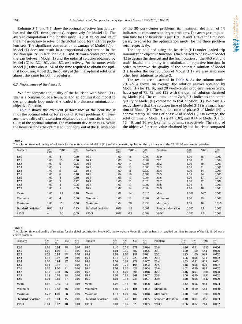
Columns ZðLÞ and TðLÞ show the optimal objective function va-lue and the CPU time (seconds), respectively for Model (L). Theaverage computation time for this model is just 3%, 5% and 7% ofthe time necessary to solve for the global model for the three prob-lem sets. The significant computation advantage of Model (L) onModel (E) does not result in a proportional deterioration in thesolution quality. In fact, for 12, 16, and 20 work-center problems,the gap between Model (L) and the optimal solution obtained byModel (G) is 13%, 19%, and 18%, respectively. Furthermore, whileModel (L) takes about 15% of the time required to obtain the opti-mal loop using Model (E), the quality of the final optimal solution isalmost the same for both procedures.

6.3. Performance of the heuristic

We first compare the quality of the heuristic with Model (L1).This is a comparison of a heuristic and an optimization model todesign a single loop under the loaded trip distance minimizationobjective function.

Table 7 shows the excellent performance of the heuristic. Itfinds the optimal solution for 23 out of 30 test problems. On aver-age, the quality of the solution obtained by the heuristic is within0–1% of the optimal solution. The maximum deviation is 4%. Whilethe heuristic finds the optimal solution for 8 out of the 10 instances

Table 7The solution time and quality of solutions for the optimization Model of (L1) and the heu

Problem ZðH1ÞZðL1Þ

TðH1Þ TðH1ÞTðL1Þ

Problem ZðH1ÞZðL1Þ

12.0 1.00 4 0.20 16.0 1.0012.1 1.00 15 0.56 16.1 1.0012.2 1.00 5 0.08 16.2 1.0012.3 1.00 5 0.16 16.3 1.0012.4 1.00 5 0.11 16.4 1.0012.5 1.00 6 0.10 16.5 1.0412.6 1.00 4 0.10 16.6 1.0312.7 1.00 5 0.12 16.7 1.0012.8 1.00 4 0.06 16.8 1.0312.9 1.00 5 0.09 16.9 1.02

Mean 1.00 5.8 0.16 Mean 1.01

Minimum 1.00 4 0.06 Minimum 1.00

Maximum 1.00 15 0.56 Maximum 1.04

Standard deviation 0.00 3.3 0.15 Standard deviation 0.02

%95CI – 2.0 0.09 %95CI 0.01

Table 8The solution time and quality of solutions for the global optimization Model (G), the two-center problem.

Problem ZðHÞZðGÞ

ZðHÞZðLÞ

TðHÞ TðHÞTðGÞ

Problem ZðHÞZðGÞ

12.0 1.00 0.94 78 0.07 16.0 1.1012.1 1.06 1.00 51 0.06 16.1 1.0412.2 1.22 0.93 48 0.07 16.2 1.0812.3 1.12 0.97 79 0.05 16.3 1.1712.4 1.06 0.94 47 0.03 16.4 1.0812.5 1.01 0.91 61 0.02 16.5 1.0012.6 1.00 1.00 71 0.03 16.6 1.0412.7 1.12 0.98 46 0.02 16.7 1.1212.8 1.11 0.98 88 0.03 16.8 1.0512.9 1.04 0.88 57 0.05 16.9 1.03

Mean 1.07 0.95 63 0.04 Mean 1.07

Minimum 1.00 0.88 46 0.02 Minimum 1.00

Maximum 1.22 1.00 88 0.07 Maximum 1.17

Standard deviation 0.07 0.04 15 0.02 Standard deviation 0.05

%95CI 0.04 0.02 10 0.01 %95CI 0.03

of the 20-work-center problems, its maximum deviation of 1%indicates its robustness on larger problems. The average computa-tion time for the heuristic is just 16%, 1% and 0.3% of the time nec-essary to solve for the optimization model for the three problemsets, respectively.

The loop obtained using the heuristic (H1) under loaded tripminimization objective function is then passed to phase-2 of Model(L) to design the shortcut and the final location of the P&D stationsunder loaded and empty trip minimization objective function. Inorder to improve the quality of the heuristic solution of Model(H), besides the best solution of Model (H1), we also send nineother best solutions to phase-2.

The results are illustrated in Table 8. As the column underZðHÞ=ZðGÞ shows, on average, the solution answer obtained byModel (H) for 12, 16, and 20 work-center problems, respectively,has a gap of 7%, 7%, and 12% with the optimal solution obtainedby Model (G). The columns under ZðHÞ=ZðLÞ indicates the betterquality of Model (H) compared to that of Model (L). We have al-ready shown that the solution time of Model (H1) is a small frac-tion of Model (H). The solution time of phase-2 of Model (H) isapproximately 10 times of phase-2 of Model (L). On average, thesolution time of Model (H) is 4%, 0.8%, and 0.4% of Model (G), for12, 16, and 20 work-center problems, respectively. The ratio ofthe objective function value obtained by the heuristic compared

ristic, applied on thirty instances of the 12, 16, 20 work-center problem.

TðH1Þ TðH1ÞTðL1Þ

Problem ZðH1ÞZðL1Þ

TðH1Þ TðH1ÞTðL1Þ

16 0.009 20.0 1.00 38 0.00714 0.004 20.1 1.00 31 0.00214 0.008 20.2 1.00 29 0.00113 0.006 20.3 1.00 31 0.00115 0.022 20.4 1.00 34 0.00116 0.008 20.5 1.01 34 0.00313 0.004 20.6 1.00 37 0.01013 0.023 20.7 1.00 37 0.00213 0.007 20.8 1.01 31 0.00114 0.009 20.9 1.00 40 0.003

14.1 0.010 Mean 1.002 34.2 0.003

13 0.004 Minimum 1.00 29 0.001

16 0.023 Maximum 1.01 40 0.010

1.2 0.007 Standard deviation 0.005 3.7 0.003

0.7 0.004 %95CI 0.003 2.3 0.002

phase Model (L) and the heuristic, applied on thirty instances of the 12, 16, 20 work-

ZðHÞZðLÞ

TðHÞ TðHÞTðGÞ

Problem ZðHÞZðGÞ

ZðHÞZðLÞ

TðHÞ TðHÞTðGÞ

0.79 378 0.014 20.0 1.26 0.91 1313 0.0060.96 487 0.005 20.1 1.00 1.00 544 0.0001.00 181 0.011 20.2 1.15 1.00 989 0.0020.95 223 0.007 20.3 1.06 0.98 564 0.0020.87 279 0.007 20.4 1.05 0.91 669 0.0010.79 198 0.002 20.5 1.18 0.98 828 0.0071.00 327 0.004 20.6 1.02 0.90 688 0.0021.00 406 0.018 20.7 1.16 0.93 1508 0.0080.92 341 0.007 20.8 1.06 0.99 1291 0.0020.92 235 0.007 20.9 1.30 0.96 1147 0.009

0.92 306 0.008 Mean 1.12 0.96 954 0.004

0.79 181 0.002 Minimum 1.00 0.90 544 0.0005

1.00 487 0.018 Maximum 1.30 1.00 1508 0.009

0.08 100 0.005 Standard deviation 0.10 0.04 346 0.003

0.05 62 0.003 %95CI 0.06 0.02 214 0.002

1

1.05

1.1

1.15

1.2

1.25

1.3

0 5 10 15 20 25 30

Qua

lity

of S

olut

ion

Number of Problems

Fig. 3. The quality of solutions obtained by the heuristic for 30 instances of the 12, 16, 20 work-center problem.

A. Asef-Vaziri et al. / European Journal of Operational Research 207 (2010) 110–120 119

to that of the global optimization model for thirty instances of the12, 16, 20 work-center problem are also illustrated in Fig. 3.

7. Conclusion and future directions

We considered the problem of simultaneously designing a loopaisle-network and a shortcut on a block layout, and locating P&Dstations such that the total loaded and empty trip distances areminimized. We formulated and solved for the integrated modeland developed two-phase simplified solution procedures. Webenchmarked our solutions to the optimal results and evaluatedthe computation efficiency of the three models. On the foundationsof these results, we replaced the second simplification procedurewith an ACS heuristic algorithm. The heuristic algorithm imple-ments an improved constructive algorithm to generate feasibleloops. Using a hybrid heuristic station location procedure and anexact IP model, we obtained high quality solutions in a short solu-tion time. The direction of our future research is to integrate theblock layout design with the circular aisle-network designproblem.

Acknowledgments

Thanks are due to Keivan Bozorgi for his help in computationalexperiments, and two anonymous referees for their valuablecomments.

References

Asef-Vaziri, A., Dessouky, M., Sriskandarajah, C., 2001. A loop material flow systemdesign for automated guided vehicles. International Journal of FlexibleManufacturing Systems 13, 33–48.

Asef-Vaziri, A., Goetschalckx, M., 2008. Dual track and segmented single trackbidirectional loop guidepath layout for AGV systems. European Journal ofOperational Research 186, 972–989.

Asef-Vaziri, A., Hall, N.G., George, R., 2008. The significance of deterministic emptyvehicle trips in the design of a unidirectional loop flow path. Computers andOperations Research 35, 1546–1561.

Asef-Vaziri, A., Laporte, G., 2005. Loop based facility planning and materialhandling. European Journal of Operational Research 164, 1–11.

Asef-Vaziri, A., Laporte, G., 2009. Integration of operational dispatching policies intothe design phase of a circular material handling network. International Journalof Advanced Operations Management 1, 108–134.

Asef-Vaziri, A., Laporte, G., Ortiz, R.A., 2007. Exact and heuristic procedures for thematerial handling circular flow path design problem. European Journal ofOperational Research 176, 707–726.

Benjaafar, S., 2002. Modeling and analysis of congestion in the design of facilitylayouts. Management Science 48, 679–704.

Caricato, P., Ghiani, G., Grieco, A., Musmanno, R., 2007. Improved formulation,branch-and-cut and tabu search heuristic for single loop material flow systemdesign. European Journal of Operational Research 178, 85–91.

Dantzig, G.B., Fulkerson, D.R., Johnson, S.M., 1954. Solution of a large-scale travelingsalesman problem. Operations Research 2, 393–410.

Donaghey, C.E., 1987. BLOCPLAN – An Integrated Tool for Developing andEvaluating Layouts, Recent Developments in Production Research. ElsevierPublication.

Dorigo, M., Birattari, M., Sttzle, T., 2006. Ant colony optimization: Artificial ants as acomputational intelligence technique. IEEE Computational IntelligenceMagazine 1, 28–39.

Dorigo, M., Gambardella, L.M., 1997. Ant colony system: A cooperative learningapproach to the traveling salesman problem. IEEE Transactions on EvolutionaryComputation 1, 53–66.

Dorigo, M., Maniezzo, V., Colorni, A., 1991. Positive feedback as a search strategy.Technical Report, 91-016, University of Milan, Italy.

Egbelu, P.J., 1987. The use of non-simulation approaches in estimating vehiclerequirements in an AGV based transport system. Material Flow 4, 17–32.

Eshghi, K., Kazemi, M., 2006. Ant colony algorithm for the shortest loop designproblem. Computers and Industrial Engineering 50, 358–366.

Ganesharajah, T., Hall, N.G., Sriskandarajah, C., 1998. Design and operational issuesin AGV-served manufacturing systems. Annals of Operations Research 76, 109–154.

Goetschalckx, M., Palliyil, G., 1994. A comprehensive model for the concurrentdetermination of aisle-based material handling systems. In: Graves, R. et al.(Eds.), Developments in Material Handling Research. Material HandlingInstitute of America, Charlotte, NC, pp. 161–188.

Heragu, S., 2008. Facilities Design, third ed. PWS Publishing, CRC Press, Boca Raton,FL.

Johnson, M.E., 2001. Modeling empty vehicle traffic in AGVS design. InternationalJournal of Production Research 39, 2615–2633.

Kim, J.-G., Goetschalckx, M., 2005. An integrated approach for the concurrentdetermination of the block layout and I/O point locations based on the contourdistance. International Journal of Production Research 43, 2027–2047.

Le-Anh, T., De Koster, M.B.M., 2006. A review of design and control ofautomated guided vehicle systems. European Journal of Operational Research171, 1–23.

Malmborg, C.J., Shen, Y.-C., 1994. Heuristic dispatching models for multi-vehiclematerial handling systems. Applied Mathematical Modeling 18, 124–133.

Material Handling Industry of America, 1999. A personal guide to automatic guidedvehicle systems. CD-Rom. Material Handling Industry of America, Charlotte, NC.

Nugent, C.E., Vollmann, T.E., Ruml, J., 1968. An experimental comparison oftechniques for the assignment of facilities to locations. Operations Research16, 150–173.

120 A. Asef-Vaziri et al. / European Journal of Operational Research 207 (2010) 110–120

Sharp, G.P., Liu, F.F., 1990. An analytical method for configuring fixed-path, closed-loop material handling systems. International Journal of Production Research28, 757–783.

Sinriech, D., Tanchoco, J.M.A., 1993. Solution methods for the mathematical modelsof single-loop AGV systems. International Journal of Production Research 31,705–725.

Sun, X.-C., Tchernev, N., 1996. Impact of empty vehicle flow on optimal flow pathdesign for unidirectional AGV systems. International Journal of ProductionResearch 34, 2827–2852.

Tanchoco, J.M.A., Sinriech, D., 1992. OSL-optimal single loop guide paths for AGVs.International Journal of Production Research 30, 665–681.

VIS, I.F.A., 2006. Survey of research in the design and control of automatedguided vehicle systems. European Journal of Operations Research 170,677–709.

Zanjirani, Farahani, Karimi, R.B., Tamadon, S., 2007. Designing an efficient methodfor simultaneously determining the loop and the location of the P/D stationsusing genetic algorithm. International Journal of Production Research 45, 1405–1427.