AN ANALYSIS OF PRICING AND RETURNS IN THE MARKET FOR FRENCHCANADIAN PAINTINGS

Douglas J. HodgsonUniversité du Québec à Montréal

hodgson.douglas-james@uqam.ca

ABSTRACTThe valuation of French Canadian paintings is analyzed empirically. Using a

sample of auction prices for major French Canadian painters for the period1968-2005, we run hedonic regressions to analyze the influence of various factors,including painter identity, on auction prices, as well as to construct a market priceindex. This index is used in a second stage analysis in which we analyze theproperties of this art viewed as an investment asset. We consider the extent towhich standard asset pricing theory, as incorporated in the capital asset pricingmodel (CAPM), can account for price movements in the market for FrenchCanadian paintings.

1. INTRODUCTION

The earliest history of European exploration and settlement of the St. Lawrencevalley - the territory originally called "Canada" - is predominantly French. Frenchexplorers sailed up the St. Lawrence River as early as 1534, and by the end of thesixteenth century colonization was under way, with the establishment of what wouldcome to be called New France, and - later - the predominantly francophoneprovince of Quebec. As the religion of the colony was Roman Catholic, it followedthat there would eventually be a need for painters to decorate churches andprovide devotional images. The first notable painters in Canada were in factFrench-born ecclesiatics come to Canada to satisfy the demand for this service,among others. A continuous tradition of painting by French speakers in Canadatherefore extends back well into the seventeenth century (Reid (1973, 1988)).

To this day, there is a strong consciousness among French Canadians,especially those living in Quebec, of a historical and cultural heritage that is uniqueand that can in some way be distinguished from the broader currents of Canadianhistory and culture. An important component of this heritage is represented by theart of painting. Many of the greatest and most influential Canadian painters havebeen francophone, and have belonged to what can be identified as a uniquelyFrench Canadian artistic filiation. In addition, some of these painters have assumedthe status of major cultural figures in Quebec. Just to give a couple of examples,consider first Ozias Leduc, mainly active in the first half of the twentieth century.He earned his living decorating churches in a time when the Church still wieldedgreat influence in Quebec society. Many of these decorations still exist and havebecome tourist attractions. His pupil, Paul-Émile Borduas, began his career as anapprentice of Leduc, working on many church projects, but later becominginterested in contemporary European trends in surrealism and abstract painting.Borduas would, in 1948, author the pamphlet "Refus Global", a broadside attack onthe stifling conservatism of Quebec society, with particular emphasis on thesuppressive role of the Church. This document is now considered to be one of themost influential and revolutionary texts ever published in Canada, and is seen asushering in the "Quiet Revolution" which would shake Quebec (and Canadian)society and politics in the ensuing decades. A group of students of Borduas, the"Automatists", would extend his influence in becoming a major force in Canadianpainting, with one of their number, Jean-Paul Riopelle, achieving majorinternational recognition and becoming a household name in Quebec (a square inthe heart of Montreal’s business district bears his name and predominantly featuresa fountain of his design).

These reflections suggest to us that it is appropriate and interesting to analyzethe art of French Canada and its market apart from Canadian art in general, andthe associated broader Canadian art market. In the growing economics literaturedevoted to studying the behaviour of art prices, most of the attention has beendevoted to markets for European and American art, but some authors have

analyzed various aspects of the market for Canadian art (Valsan (2002), Arvin andScigliano (2004), Hodgson and Vorkink (2004), Hodgson (2006)). The presentstudy extends this line of investigation in considering the factors influencing thepricing of French Canadian paintings. In addition, we build on the existing literatureon art as an investment in constructing a time series price index of FrenchCanadian paintings, and analyzing the return properties of these paintingsconsidered as risky financial investments, this being done within the context of thecapital asset pricing model (CAPM).

The empirical analysis reported below for the valuation of French Canadianpaintings considers prices of oil and acrylic paintings, over the period 1968-2005,for a set of major French Canadian painters. Preliminary to our analysis of theinvestment properties of this art, we estimate a price index and a return seriesusing hedonic methods, with the methodology presented in Section 2 and theresults reported in Section 3. The results of our hedonic regression also allow us togauge the influence on the auction prices of paintings of a number of separatefactors, including the identity of the artist, the auction house, the size of thepainting, and the medium and support. In Section 4, we compare the investmentproperties of Canadian art with those of Canadian government bonds andCanadian stocks, and estimate the CAPM for art returns.

2. HEDONIC REGRESSION - DATA ANDMETHODOLOGY

In this section, we describe the data and methodology used in our estimation ofa hedonic regression for French Canadian paintings using results of auctions from1968-2005. Among our objectives will be the computation of a time series priceindex for paintings. To accomplish this, we must address the fact that eachpainting is, to a certain extent, a unique object, and therefore the price at which agiven painting sells, whether at auction, in a gallery, or privately, cannot be takenas a general indicator of the level of the art market. In addition to reflecting thegeneral level of the market at the time of sale, the price will be affected by suchfactors as the identity of the artist, the size, medium, and support of the painting,the location of the sale (the auction house, gallery, city or country in which the saleoccurs), the condition and quality of the work itself, as well as a host ofidiosyncratic factors.

A few recent examples of the many instances where art prices have beenstudied within the context of a hedonic regression would be Chanel, Gérad-Varet,and Ginsburgh (1996), Czujack (1997), and Locatelli-Biey and Zanola (2002), aswell as the studies of Canadian art carried out by Arvin and Scigliano (2004),Hodgson and Vorkink (2004), and Hodgson (2006). Essentially, the logarithm ofthe price of each work sold at auction during a given time interval is regressed on

various available characteristics of the work, such as the artist, the size, themedium, the auction house, the time period, etc. Many of the regressors, such asthose associated with the time period, will take the form of a set of dummyvariables. For the time-period dummies, the estimated coefficients will form a timeseries representing time variation in the general market for the type of art workunder consideration.

2.1 Data

Records of sales of Canadian paintings at auction were used to constitute thedata set for our study. Data for auctions held between 1968 and 2005 werecollected from records published by Campbell (1970-75, 1980), Sotheby’s (1975,1980), and Westbridge (1981-2006). We chose to restrict our analysis to artistsconsidered to have made contributions of some lasting art historical importance, sothat we can claim to have assembled a sample of paintings by “major” artists. Ourcriterion for an artist to be “important” is that his or her work be mentioned in one ofthe standard surveys of Canadian art written by Harper (1977) or Reid (1973,1988). We only consider oil and acrylic paintings - the vast majority of ourobservations are for oils. We have only included sales for which the auctionhouse’s attribution is confident, and, for each painting, we recorded, in addition tothe identity of the artist, the height and width, the medium and support, the auctionhouse, the date of the sale, the genre of the picture, and an indicator of whether ornot the painting is dated. We use hammer prices as recorded in the publicationslisted above. No effort has been made to adjust or correct our numbers to accountfor such costs as auctioneers’ commissions, taxes, insurance premia, maintenanceand restoration costs, etc. These factors all act to reduce the monetary returns ofowning paintings below the levels recorded here. Factors acting to augment themonetary returns to art owners, such as reproduction fees and exhibition or lendingfees, are also omitted. A total of 56 painters are represented in our sample (theyare listed in the Appendix), and the total number of observed sales is 4135.

2.2 Econometric model

As mentioned above, one of our objectives is to obtain from our auction salesrecords a price index reflecting the evolution of the art market over time. We willconstruct an annual index, estimating a hedonic regression with time-perioddummy variables. The model to be estimated can be written

pi ∑t1

T

tzit ∑j1

J

jwij ui, i 1, . . . ,n, (1)

where pi is the logarithm of the price of sale i, the number of sales is n 4135, zit isthe value of a period−t dummy variable, equal to 1 if painting i was sold in period tand equal to zero otherwise, with the number of time periods T being 37. Weconsider an auction year in the same way as one would consider a school year or ahockey season, so that, for the purposes of forming an annual price series, theauction year is considered to run from July 1 of a given calendar year to June 30 ofthe following one. Our annual dummies thus start with the 1968-69 auction year,followed by 1969-70, and concluding with 2004-2005. Our estimates of the vectorof associated parameters tt1

T will therefore form our price index.The regressors wij in (1) represent the other characteristics of painting i.

These include 55 dummy variables for the painting’s artist, 8 for its genre,14medium/support dummies, and 27 auction house dummies (in all cases, onedummy was omitted to avoid collinearity with the time period dummies, hence 55painter dummies corresponds to a collection of 56 painters). Three additionalvariables reflecting a painting’s dimensions - height, width, and surface area - wereincluded, as was a dummy indicating whether or not the painting is dated. Equation(1) can be written more concisely as

pi xi′ ui, i 1, . . . ,n, (2)

where xi′ zi1, . . . , ziT,wi1, . . . ,wiJ and 1, . . . ,T,1, . . . ,J ′. Note that we have

J107 and T37, giving us a dimension K for the parameter vector of 144.A note should be added on the interpretation of the dummy parameters. In the

next section, we will analyze the rate of return on paintings, considered as financialassets. If we knew the time period dummies tt1

T , we could compute the rate ofreturn between, say, periods t and t 1 as follows:

rt1 expt1 − t − 1.We can proceed similarly for the characteristic-related dummies. We will see belowthat the dummy for Henri Masson was omitted from the regression (1), in otherwords it was arbitrarily set equal to zero. The dummy parameters j for each of theremaining painters can then be seen as reflecting their market values vis-à-visMasson. The percentage difference between the value of a work by painter j and aMasson, controlling for all the other factors in our analysis, will be

exp j − 1.

2.3 Estimation

The regression (1) and (2) can be, and usually is, estimated by ordinary leastsquares (OLS). Under the standard assumptions, OLS will be consistent andasymptotically normal, and will be asymptotically efficient if the disturbances uiare normally distributed. An application of the Jarque-Bera (1980) normality test toour OLS residuals yielded a highly significant statistic of 1389 (the test has a

chi-squared null distribution with two degrees of freedom), with an associated 21kurtosis statistic of 1347. Hence, there is reason to suppose that a substantialefficiency loss is borne when estimating the model by OLS, relative to maximumlikelihood or to a robust estimator such as least absolute deviations. For ourpurposes, efficiency is a major concern. This is because our estimates of thetime-period dummies tt1

T and, more specifically, of the associated returnsrtt2

T , will be treated in our analysis of Section 4 as being observed series ofprices and returns. Thus, it is essential that these parameters be estimated asprecisely as possible.

To achieve greater precision in our estimates of the time-period dummies, wehave chosen to estimate (2) adaptively, according to the procedure of Bickel(1982). This estimator is designed to deliver fully asymptotically efficient estimateswhen the distribution of the disturbances ui is of unknown functional form. Givenour strong evidence that the disturbances are not normally distributed, and in theabsence of any compelling economic argument favoring the adoption of some otherspecific functional form for the error distribution, we shall treat this distribution asunknown and proceed to compute a semiparametric analogue of the maximumlikelihood estimator (MLE). We will assume that the disturbances are independentand identically distributed (iid) with a density function fu. The version of the Bickel(1982) estimator we use incorporates a further assumption of symmetry of thisdistribution, so that fu f−u. Although it is quite possible that the apparentleptokurtosis in the errors is to some extent due to heteroskedasticity, Hodgson(2000) shows that Bickel’s (1982) estimator is robust to the presence ofheteroskedasticity in the errors, and will adapt for the non-normality induced in theunconditional density of the errors by this heteroskedasticity. Moreover, thestandard error estimates proposed by Bickel (1982) are also robust.

If the functional form of fu were known, computation of the maximumlikelihood estimator of would be a straightforward matter. With fu beingunknown, the basic approach to computing an efficient semiparametric analogue tothe MLE does not change much, with the principal complication being the necessityto use the data to compute a nonparametric estimate of f to use in lieu of theunknown function. We outline below the mechanics of computing a slightly modifiedversion of the Bickel (1982) adaptive estimator.

Using the OLS estimator, compute the associated residuals ui pi − xi

′,i 1, . . . ,n. For each residual ui, i 1, . . . ,n, one can use the remaining residuals tocompute a kernel estimate of the level of the density f evaluated at ui as follows:

f iui 1

2n − 1 ∑j1j≠i

n

Kui

uj

hn K

ui −uj

hn,

where K is a user-specified kernel weighting function and hn is a user-specifiedbandwidth parameter that satisfies the asymptotic condition hn → 0 as n → . Wewill also require the following estimate of the first derivative of f :

f i′ui 1

hn2n − 1 ∑j1j≠i

n

K′ui

uj

hn K′

ui −uj

hn.

We then have the estimated (negative of the) score of f, evaluated at ui:

iui

f i′ui

f iui

,

where some trimming conditions may need to be specified in the computation of i,depending on the kernel employed. In our empirical application, we will use anormal kernel with a bandwidth parameter specified using the rule-of-thumbapproach of Silverman (1986).

The sample score vector and information matrix of the likelihood function can beapproximated, respectively, by the following semiparametric estimators:

Sn n−1∑

i1

n

xiiui

and

In n−1∑i1

n

xixi′,

where n−1∑ i1n i

ui2. The adaptive estimator is then computed using the

following one-step Newton-style adjustment of the OLS estimator :

In−1Sn.

Under conditions specified by Bickel (1982), will be consistent and asymptotically

normal,

n −

d→ N0,I−1,

where the asymptotic covariance matrix I−1 is consistently estimated by In−1.

3. HEDONIC REGRESSION - RESULTS

The results of our estimation of the hedonic regression (1)-(2) are discussedhere and reported in Tables 1-6 and in the Appendix.

3.1 Time series price index and estimated returns

The time series dummy parameter estimates, along with the associatedestimates of nominal and real annual returns, are reported in Table 1, and plotted

in Figures 1 and 2. The real returns are obtained by deflating the nominal using theConsumer Price Index as obtained from the Statistics Canada website. Theaverage real return in the art market during the period 1968-2005 is 4.34%, with astandard deviation of 15.49%. The market is quite volatile, with a certain degree of"volatility clustering" seemingly evident. For example, there is a rapid increase inprice during the period 1976-1981, with increases in 1979 and 1980 of 27% and40%, respectively, followed by a sharp drop in the market in the early 80’s, withannual declines of over 20% in 1982 and 1983. A second boom occurs in thesecond half of the 1980’s, again followed by rapid price decreases in the early 90’s.A period of relative stability then set in during the mid- to late-90’s, with modest butsteady increases after 1997, with relatively large jumps of 27% in 2001 and 14% in2005. These phenomena are more or less in accord with those obtained byHodgson and Vorkink (2004) for the Canadian art market as a whole, especially aspertains to the depressions in the market in the early 80’s and 90’s, both of whichcan no doubt be at least partially attributed to macroeconomic recessions whichoccurred during these years.

3.2 Painters

The 56 painters included in the study are identified in the Appendix, along withinformation on the number of works sold for each painter, and the estimatedregression dummy parameter and standard error. As mentioned above, onedummy variable, that representing Henri Masson, was omitted to preventcollinearity with the time period dummies. Thus, each painter’s dummy estimatecan be interpreted as representing his/her market value vis-à-vis that of Masson.Although we cannot analyze these results in complete detail, we present in Table 2a list of the “Top 15” French-Canadian painters, i.e. those with the 15 highestdummy point estimates, ranked in descending order. For each of these painters,we report the percentage difference between the value of one of his/her works anda work of Masson, controlling for the other variables included in the regression.

In analyzing Table 2, a few considerations should be borne in mind. First, theranking is not necessarily statistically significant. The reported standard errorsallow us to infer the significance of the parameter estimate relative to HenriMasson, but not relative to any of the other artists on the list. Secondly, theprecision of these estimates varies widely by artist, depending on the number ofobservations available. Thirdly, the hedonic regression estimates a reduced formmodel in which no attempt is made to distinguish between supply and demandinfluences on price. It would be highly desirable to estimate a fully specified andidentified supply-demand model of this market, but we have not attempted to do sohere.

In general, no major surprises would be visited upon an amateur of Quebecoisart in perusing Table 2. The top two painters, Borduas and Riopelle, are the "twin

towers" of post-war abstract painting in Quebec, indeed in all of Canada, and havebeen discussed in the Introduction, along with Ozias Leduc, in eight place on ourlist. If we set aside the early colonial painter Roy-Audy, for whom only two salesare recorded in our sample, we then have four painters who interpreted andmodernized, in various ways, a traditional and nationalist vision of the Quebeclandscape and the people who inhabited it. Clarence Gagnon, Jean-Paul Lemieux,Marc-Aurèle Suzor-Coté, and Marc-Aurèle Fortin all painted in a representationalvein that was conservative by the standards of the most advanced art of their day,but was nevertheless distinctively individual and can be described as uniquelyFrench-Canadian. Five of the remaining seven painters were heavily involved intwentieth century avant-garde trends, with Pellan and Dallaire inspired byschool-of-Paris modernism and surrealism, and De Repentigny, Charles Gagnon,and Pierre Gauvreau being leading members of the post-war abstractionistmovements. Legaré and Hamel are among the most important francophonepainters of the nineteenth century.

3.3 Auction House

Paintings in our sample were sold at 28 different auction houses, and we havereported in Table 5 the dummy estimates for those 8 which are still active and forwhich we had at least 75 observations, with the Sotheby’s dummy being omittedfrom the regression. The estimates indicate a strong correlation between the houseat which the painting is sold and the price, with six houses showing devaluations ofover 20% compared to Sothby’s. The differences among the houses arepresumably due to geographical location or to segmentation of the market intohouses specializing in paintings of different levels of quality.

3.4 Medium and Support

The dummy estimates for selected medium/support combinations are reportedin Table 4. There were 15 different medium/support combinations included in theregression, but we have only reported estimates for those for which we had at least50 observations. The oil on canvas dummy was omitted, so the parameterestimates in Table 4 reflect the contribution to a painting’s value of a givenmedium/support in comparison to that of oil on canvas. Two things are particularlynoteworthy here: first, that medium and support are essential components of apainting’s value, and second, that oils painted on canvas command a substantialpremium compared to oils on panel, board, paper, and masonite.

3.5 Genre

Table 5 contains our dummy estimates for the genre of a picture, with that forlandscape being omitted from the regression. We can see that the subject of apicture can have an important influence on its price. Genre scenes and still lifessell, on average, for 23% and 12% more, respectively, than landscapes, while allother genres are generally less valuable than landscapes, with history paintingsand portraits being the cheapest.

3.6 Size and Dating Indicator

Our parameter estimates for the dimensions - height, width, and surface area -are given in Table 6. We can see that the height and width of a painting can havean appreciable impact on its price, with a one centimetre increase in either leadingto an augmentation in price of between 1.5 % and 2%. The parameter for surfacearea is of negligible magnitude. The indicator for whether or not a painting is datedis highly significant, with a point estimate indicating a gain in value of about 18%.

4. CAPITAL ASSET PRICING MODEL (CAPM)

4.1 Model

We conduct tests of the returns to our art index in the framework of the CapitalAsset Pricing Model (CAPM) of Sharpe (1964) and Lintner (1965). The followingequation demonstrates the main result of the CAPM, stating that the expectation ofthe return on asset i, denoted as Ri,t, in excess of the return on a risk-free security,Rf,t, is a linear function of the expected excess return on the market portfolio, Rm,t:

Et−1Ri,t − Rft Et−1Rm,t − Rf,t i,t, (3)

where i,t covt−1Rm,t,Ri,t

vart−1Rm,t is the conditional “beta” for asset i in period t, and the

subscripts on expectations and covariances indicate conditional moments.Assuming that no dynamics exist in the conditional expectations, (3) reduces to theunconditional CAPM

ERi,t − Rf,t ERm,t − Rf,t i. (4)There is an extensive empirical literature on the unconditional CAPM, most of

which has tested how well this model can explain stock returns, with importantearly work by Black, Jensen, and Scholes (1972) and Fama and MacBeth (1973)(see Campbell, Lo, and MacKinlay (1997) for a more comprehensive discussion of

empirical tests of the CAPM). However, the CAPM has been used as a model toexplain the returns on other assets. For example Bryan (1985) and Hodgson andVorkink (2004) use the CAPM to perform asset pricing tests of art, while Gyourkoand Nelling (1996) use the CAPM to analyze the performance of Real EstateInvestment Trusts (REIT). In a similar fashion to these and other studies of theCAPM, we use the following empirical version of the unconditional CAPM:

rt rM,t et, (5)where rt is the excess return on the art index in period t (return on the art indexminus the yield on a risk-free security), rM,t is the excess market return, et is adisturbance, and and are parameters. The CAPM suggests that measureshow much of the return to a particular asset (in our case art) is priced as systematicrisk, or the portion of returns that are generated by the asset’s correlation to that ofthe market. A simple t-test of the parameter will test if any portion of the asset’sreturn is systematic, i.e. if 0.

If there is some component of returns that is not due to market risk exposure, asmeasured by , but is persistent, it will appear in the intercept, . If the CAPM isthe true model describing returns, 0, whereas a finding that ≠ 0 would signalaverage returns that cannot be explained by market risk. A t-test of 0 will testthe CAPM’s ability to explain the returns of a particular asset. Hodgson and Vorkink(2004) concluded that is insignificantly different from zero in the overall Canadianart market.

4.2 Data and Results

The regression model (5) was estimated by ordinary least squares using ourreal return series of 36 obervations as reported in Table 1, with the risk-free ratebeing proxied by the Bank of Canada Bank Rate (obtained from the Bank’swebsite) and the market portfolio proxied by the TSX/S&P Composite Index, TotalReturns (i.e. with dividends included), this series provided by the Toronto StockExchange. Summary statistics for the data, along with results of the OLSestimation, are provided in Table 7.

Before commenting on the regression results, we make a few observations onthe returns’ descriptive statistics. First, we see that the average annual real returnon the art portfolio, at 4.34%, is about midway between the average real interestrate, 2.79%, and the average real return on the stock index, 5.69%. Nevertheless,the variability of the art return is very similar to that of the stock index, withrespective standard deviations of 15.49% and 16.55%, whereas the interest rateseries has a standard deviation of only 3.22%. Art returns and stock returns have amodest positive correlation coefficient of 0.277, while the art returns are negativelycorrelated with interest rates, the coefficient in this case being -0.345.

In the CAPM regression, which had an R2 of 0.105, and for which the errorsproduced an insiginificant Jarque-Bera (1980) normality test statistic of 0.642, we

find a significantly positive beta, with a point estimate of 0.335 (standard error:0.166), and an intercept very close to zero, with point estimate (standard error) of0.0058 (0.0274). These results are broadly in accord with what one finds in thegeneral literature in this area, with the beta estimate being higher than Hodgsonand Vorkink (2004) find for the overall Canadian market.

As pointed out by Hodgson and Vorkink (2004), a finding of 0 can have anumber of possible interpretations. The one posited above is that returns to the artmarket are adequately captured by the CAPM, and that only systematic risk isimportant for returns in this market. A second possibility is that there are returns notrelated to systematic risk, but that they are offset by the costs associated with artownership (costs referred to earlier but which we have not explicitly attempted tomeasure). Among the pecuniary and non-pecuniary returns associated with artownership that we have also not attempted to measure are the fees that may beobtainable through loans to gallery or museum exhibitions or through reproductionrights, and the direct utility afforded by a picture to its owner. Another way oflooking at it is in considering that, under the maintained hypothesis that the CAPMholds, then the unmeasured costs and benefits of holding art referred to herebalance one another exactly (since under the CAPM, any such imbalance wouldresult in a non-zero , positive if costs outweigh benefits and negative otherwise).

Acknowledgements

Financial support from SSHRC and FQRSC is acknowledged.

APPENDIX

The following is a list of all 152 painters included in our study, in alphabeticalorder. The three numbers given in parentheses for each artist represent,respectively, the number of observations, the dummy parameter estimate for thepainter (expressed as percentage difference with respect to Henri Masson), andthe associated standard error:

Edmund Alleyn (51, -71.67, 3.36); Marcel Barbeau (34, -69.34, 4.48); HenriBeau (100, -20.12, 6.55); Leon Bellefleur (135, 5.27, 9.60); Louis Belzile (20,-88.69, 2.02); Suzanne Bergeron (11, -86.93, 3.05); Andre Bieler (88, -27.99, 6.19);Paul-Emile Borduas (72, 887.87, 105.19); Joseph Bouchette (3, -88.89, 4.75);Napoleon Bourassa (4, -27.01, 26.86); Jean Dallaire (69, 173.91, 27.98); GeorgesDelfosse (142, -48.01, 3.66); Louis de Niverville (8, -68.80, 8.75); Rodolphe deRepentigny (8, 95.75, 52.14); Jacques De Tonnancour (56, 1.43, 10.75); RodolpheDuguay (73, -45.54, 5.08); Louis Dulongpre (1, -84.33, 11.42); Albert Dumouchel(18, -63.60, 6.48); A.S. Falardeau (13, -64.37, 7.52); Marcelle Ferron (73, -35.25,

7.35); Marc-Aurele Fortin (434, 220.60, 15.51); Joseph Franchere (147, -34.60,4.48); Louise Gadbois (122, -86.51, 1.19); Charles Gagnon (2, 75.62, 90.24);Clarence Gagnon (280, 509.22, 35.63); Yves Gaucher (3, 6.01, 45.67); PierreGauvreau (16, 54.97, 30.63); Jean Goguen (2, -46.07, 27.83); Theophile Hamel(13, 64.99, 35.25); Adrien Hebert (108, -45.39, 4.18); Charles Huot (55, -33.37,6.99); Jacques Hurtubise (11, -53.81, 11.10); Jean-Paul Jerome (30, -82.99, 2.54);Henri Julien (6, -5.39, 28.18); Denis Juneau (3, -38.18, 26.31); Ludger Larose (36,-45.39, 7.03); Fernand Leduc (7, 2.30, 28.89); Ozias Leduc (48, 204.73, 34.47);Joseph Legare (8, 95.02, 50.55); Jean-Paul Lemieux (180, 308.43, 26.11); RitaLetendre (59, -62.47, 4.57); Henri Masson (711, 0, 0); Jean McEwen (98, -31.24,7.53); Guy Monpetit (3, -77.89, 9.31); Jean-Paul Mousseau (9, -68.71, 7.73);0.2212); Alfred Pellan (83, 198.19, 28.53); Henri Perre (15, -50.41, 9.65); AntoinePlamondon (12, -15.67, 18.43); Jean-Paul Riopelle (249, 611.24, 62.88);Jean-Baptiste Roy-Audy (2, 502.19, 312.40); Joseph Saint-Charles (47, -65.03,3.97); Francoise Sullivan (1, -85.78, 10.27); Marc-Aurele de Foy Suzor-Cote (288,250.14, 18.64); Fernand Toupin (61, -73.66, 3.27); Claude Tousignant (6, -41.74,18.82); Zacharie Vincent (1, -95.16, 3.49)

REFERENCES

Arvin, B.M. and Scigliano, M.A. 2004. Hedonic prices in art and returns to artinvestment: Evidence from the Group of Seven at auction. ÉconomieAppliquée57:137-162.

Bickel, P. 1982. On adaptive estimation. Annals of Statistics 10:647-671.

Black, F., M. Jensen, and M. Scholes. 1972. The capital asset pricing model:some empirical tests. In Jensen, M. (ed), Studies in the theory of Capital Markets,New York, Praeger.

Bryan, M. 1985. Beauty and the Bulls: The Investment Characteristics ofPaintings, Economic Review of the Federal Reserve Bank of Cleveland, Q1, 2-10.

Campbell, J., W. Lo, and A. C. MacKinlay. 1997. The Econometrics of FinancialMarkets. Princeton: Princeton University Press.

Campbell, H. 1970-75. Canadian Art Auction Record, vol. 1-6, 1969-1974.Toronto, Canadian Antiques and Fine Arts; and Montreal, Bernard Amtmann, Inc.

Campbell, H. (ed.). 1980. Canadian Art Auctions, Sales and Prices, 1976-1978.Don Mills, Ont. General Publishing Co.

Chanel, O., Gérad-Varet, L.A., and Ginsburgh, V. 1996. The relevance ofhedonic price indexes: The case of paintings. Journal of Cultural Economics20:1-24.

Czujack, C. 1997. Picasso paintings at auction, 1963-1994. Journal of CulturalEconomics 21:229-247.

Fama, E., and J. MacBeth. 1973. Risk, return, and equilibrium: empirical tests.Journal of Political Economy 71:607-636.

Gyourko, J., and E. Nelling. 1996. Systematic Risk and Diversification in theEquity REIT Market,” AREUEA Journal, 24, 493-515.

Harper, J.R. 1977. Painting in Canada: A History (2nd ed.) Univ. of Toronto.

Hodgson, D.J. 2000. Unconditional pseudo-maximum likelihood estimation andadaptive estimation in the presence of conditional heterogeneity of unknown form.Econometric Reviews 19:175-206.

Hodgson, D.J. 2006. Age-price profiles for Canadian painters at auction.Université de Québec à Montréal.

Hodgson, D.J. and Vorkink, K. 2004. Asset pricing theory and the valuation ofCanadian paintings. Canadian Journal of Economics 37:629-655.

Jarque, C.M. and Bera, A.K. 1980. Efficient tests for normality,homoskedasticity, and serial independence of regression residuals. EconomicsLetters 6:255-259.

Lintner, J. 1965. The valuation of risky assets and the selection of riskyinvestments in stock portfolios and capital budgets. Review of Economics andStatistics 47: 13-37.

Locatelli-Biey, M. and Zanola, R. 2002. The sculpture market: An adjacent yearregression index. Journal of Cultural Economics 26:65-78.

Reid, D. 1973. A Concise History of Canadian Painting. Toronto; Oxford

University Press.

Reid, D. 1988. A Concise History of Canadian Painting (2nd ed.). Toronto;Oxford University Press.

Sharpe, W. 1964. Capital asset prices: A theory of market equilibrium underconditions of risk. Journal of Finance 19:425-442.

Silverman, B. 1986. Density Estimation for Statistics and Data Analysis.London; Chapman and Hill.

Sotheby’s. 1975. Canadian Art at Auction, 1968-1975. Toronto; Sotheby’s & Co.(Canada) Ltd.

Sotheby’s. 1980. Canadian Art at Auction, 1975-1980. Toronto; Sotheby’sParke Bernet (Canada) Inc.

Valsan, C. 2002. Canadian versus American art: What pays off and why.Journal of Cultural Economics 26: 203-216.

Westbridge, A.R. 1981-2006. Canadian Art Sales Index, 1977-2005.Vancouver, Westbridge Publications, Ltd.

Table 1– Time period dummies and estimated returns (annual) Time period

Number Of Obs.

Log-price dummy

Std. error

Estimated nominal return (%)

Std. error

Estimated real return (%)

68-69 23 4.45 .162 69-70 63 4.74 .129 34.62 25.91 30.19 70-71 143 4.73 .107 -1.71 11.13 -4.48 71-72 81 4.70 .120 -2.72 9.93 -7.17 72-73 78 4.77 .118 7.18 12.38 -0.49 73-74 61 5.03 .123 29.41 16.10 16.90 74-75 44 5.05 .130 1.95 14.79 -8.07 75-76 35 5.15 .147 10.01 18.67 2.33 76-77 53 5.41 .125 29.63 20.89 20.25 77-78 45 5.53 .133 13.06 16.63 3.72 78-79 78 5.86 .100 39.29 19.93 27.55 79-80 45 6.29 .121 54.44 21.48 40.27 80-81 90 6.52 .094 25.25 16.70 11.43 81-82 74 6.38 .103 -13.46 10.05 -21.97 82-83 53 6.15 .113 -20.39 10.54 -24.75 83-84 58 6.10 .111 -4.68 13.13 -8.61 84-85 73 6.14 .101 4.15 13.35 0.14 85-86 120 6.40 .088 30.22 14.12 25.09 86-87 158 6.65 .083 27.90 11.34 22.51 87-88 231 6.74 .080 9.56 8.80 5.35 88-89 224 6.99 .077 28.60 9.41 22.48 89-90 236 7.02 .077 2.97 6.99 -1.75 90-91 191 6.69 .080 -28.32 5.11 -32.12 91-92 123 6.76 .089 7.41 9.11 5.82 92-93 109 6.62 .093 -13.28 8.36 -14.81 93-94 105 6.56 .093 -5.89 9.50 -6.08 94-95 132 6.59 .086 3.21 9.89 0.99 95-96 100 6.56 .094 -3.10 9.42 -4.63 96-97 109 6.52 .093 -3.51 9.81 -5.03 97-98 146 6.55 .087 2.41 9.51 1.49 98-99 125 6.65 .088 11.08 9.91 9.22 99-00 130 6.71 .089 5.93 9.68 3.15 00-01 143 6.98 .086 30.60 11.63 27.29 01-02 146 7.02 .086 4.41 9.03 2.16 02-03 202 7.09 .082 7.82 8.70 4.88 03-04 157 7.15 .085 5.61 8.36 3.63 04-05 151 7.30 .087 16.32 9.67 13.82

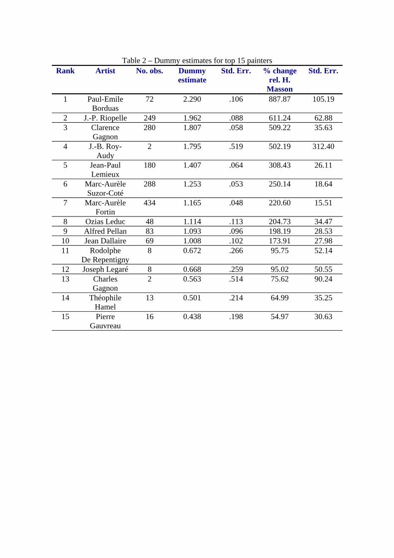
Table 2 – Dummy estimates for top 15 painters

Rank Artist No. obs. Dummy estimate

Std. Err. % change rel. H.

Masson

Std. Err.

1 Paul-Emile Borduas

72 2.290 .106 887.87 105.19

2 J.-P. Riopelle 249 1.962 .088 611.24 62.88 3 Clarence

Gagnon 280 1.807 .058 509.22 35.63

4 J.-B. Roy-Audy

2 1.795 .519 502.19 312.40

5 Jean-Paul Lemieux

180 1.407 .064 308.43 26.11

6 Marc-Aurèle Suzor-Coté

288 1.253 .053 250.14 18.64

7 Marc-Aurèle Fortin

434 1.165 .048 220.60 15.51

8 Ozias Leduc 48 1.114 .113 204.73 34.47 9 Alfred Pellan 83 1.093 .096 198.19 28.53 10 Jean Dallaire 69 1.008 .102 173.91 27.98 11 Rodolphe

De Repentigny 8 0.672 .266 95.75 52.14

12 Joseph Legaré 8 0.668 .259 95.02 50.55 13 Charles

Gagnon 2 0.563 .514 75.62 90.24

14 Théophile Hamel

13 0.501 .214 64.99 35.25

15 Pierre Gauvreau

16 0.438 .198 54.97 30.63

Table 3 – Dummy estimates for selected auction houses House No. obs. Dummy

estimate Std. Err. % change

rel. to Sothby’s

Std. Err.

Waddington 95 -0.410 .083 -33.61 5.53 Ritchie 111 -0.556 .076 -42.67 4.37 Fraser 423 -0.218 .055 -19.58 4.43 Pinney 244 -0.269 .059 -23.59 4.54 Empire 188 -0.344 .065 -29.12 4.60 Joyner 561 0.053 .044 5.45 4.64 Maison

d’encans 1045 -0.324 .043 -27.69 3.12

Heffel 96 -0.120 .083 -11.33 7.34

Table 4 – Dummy estimates for selected medium/support Medium/support No. obs. Dummy

estimate Std. Err. % change

rel. to oil/canvas

Std. Err.

Oil/panel 590 -0.141 .043 -13.18 3.72 Oil/board 646 -0.109 .038 -10.36 3.44 Oil/paper 71 -0.453 .091 -36.45 5.81

Oil/masonite 77 -0.120 .088 -11.27 7.76

Table 5 – Dummy estimates for selected genre Genre No. obs. Dummy

estimate Std. Err. % change

rel. to landscape

Std. Err.

Genre scene 472 0.208 .039 23.17 4.85 Still life 173 0.110 .063 11.66 7.00 Portrait 166 -0.237 .067 -21.11 5.30 Abstract 992 -0.010 .070 -9.50 6.31 Animal 21 -0.124 .162 -11.67 14.35 Figure 91 -0.119 .081 -11.19 7.21 History 43 -0.290 .120 -25.14 9.02

Table 6 – Dimension variables and dating indicator Variable Parameter

estimate Std. Err.

Height 0.0166 .0009 Width 0.0188 .0009 Area -1.04 410−× 6.78 610−×Dated 0.165 .028

Table 7 – Returns: descriptive statistics and CAPM regression Returns

Art Stocks Interest rate

Mean 0.0434 0.0569 0.0279 Standard dev. 0.1549 0.1655 0.0322

Correlation matrix Art Stocks Interest

rate Art 1 .277 -.345

Stocks 1 .184 Interest Rate 1

CAPM regression Parameter Estimate S.E.

α 0.00580 0.0274 β 0.335 0.166 =2R 0.105 JB = 0.642