An Analysis of Extreme Price Shocks and Illiquidity Among

Systematic Trend Followers

Bernard LeeSim Kee Boon Institute for Financial Economics

Singapore Management Universitybernardlee@smu.edu.sg

Shih-Fen ChengSchool of Information Systems

Singapore Management Universitysfcheng@smu.edu.sg

Annie KohLee Kong Chian School of BusinessSingapore Management University

anniekoh@smu.edu.sg

June 15, 2010

Abstract

We construct an agent-based model to study the interplay between extreme price shocksand illiquidity in the presence of systematic traders known as trend followers. The agent-basedapproach is particularly attractive in modeling commodity markets because the approach allowsfor the explicit modeling of production, capacities, and storage constraints. Our study beginsby using the price stream from a market simulation involving human participants and studiesthe behavior of various trend-following strategies, assuming initially that their participationwill not impact the market. We notice an incremental deterioration in strategy performanceas and when strategies deviate further and further from the theoretical strategy of lookbackstraddles (Fung and Hsieh [3]), due to the negative impacts of transaction costs and imperfectexecution. Next, the trend followers are allowed to participate in the market, trading againstzero intelligence computer traders making randomized bids and offers. We notice that marketprices begin to break down as the percentage of trend followers in the market reaches 80%.In addition, in a market dominated by smart traders, it becomes increasingly difficult for anyof them to generate profits using what is supposed to be a “long gamma” strategy. Afterall, trading is a zero-sum game: It is not feasible for any “long gamma” trader to generate aconsistent profit unless someone else is willing to be on the other side of his/her trades. In anysuch market dominated by smart traders with low liquidity and extreme price instability, oneproposed solution (as proposed earlier by the U.S. Commodity Futures Trading Commission) isto control position size limits, by either decreasing them (in the original proposal) or increasingthem (for completeness in our analysis). Based on our simulation results, we have found noevidence supporting that such a solution will be effective; in fact, doing so will only lead toerratic price behavior as well as a variety of practical issues when imposing such changes toposition size limits. An alternative proposal is to intervene in the market direct/indirectly, suchas by using a market maker to inject/reduce liquidity. Our simulation results show evidencethat injecting and reducing liquidity by the market maker can both be effective. However, amarket maker can accumulate a large negative P&L by buying in a one-sided, falling market inwhich it is the only bidder, or vice versa. Therefore, in practice, no market maker may volunteerto participate in any such market rescue efforts unless governments are willing to underwritesome of its large potential losses. In short, direct/indirect intervention by controlling liquidityis not a panacea, and there are practical limits to its effectiveness.

1

1 Background and Motivation

Commodity trading has been one of the backbones of economic activities since the dawn of thehuman civilization. Over the centuries, the trading of commodities has become more and morecomplex, evolving from primitive barter exchange (direct exchange of goods or services withoutmonetary instruments) to more sophisticated forward contracts between producers and consumers(agreements to buy or sell at a fixed price at a future time), and then, in recent years, to formalfutures exchanges with clearing houses guaranteeing transactions.

For most commodities, excessive volatility will hurt either producers or consumers (usually both)and this might have dire consequences: producers and consumers would react to volatile marketshocks, potentially making the market even more volatile and straining supplies and/or demands.Eventually, the market can break down completely and the whole supply chain that depends onthe commodity will be adversely impacted. Therefore, no matter how a particular commodity istraded, reining in excessive volatility of its price has always been an important policy objective forthe authority overseeing its trading. Roughly speaking, factors contributing to the volatility of thecommodity prices can be classified into three major categories: 1) natural/seasonal fluctuations insupply and demand, 2) disruptions along the commodity supply chain due to unexpected factorssuch as acts of nature, and 3) speculation.

For the first two sources of volatilities, while their occurrences are mostly inevitable (but pre-dictable to some degree), there are wide varieties of financial instruments (e.g., options and futures)and physical facilities (e.g., the construction of additional storage for strategic commodities likecrude oil and grains) that can be utilized to reduce the likely impact when struck by such unex-pected events. However, as commodities become more and more popular as an asset class, theinfluence of speculation on commodity prices has become increasingly more significant. The influxof hedge funds, commodity trading advisors, and institutional investors into commodity marketshas changed the dynamics of the market drastically. They are often seen by the public as convenientscapegoats behind the spectacular commodity booms and busts in the past two years.

Another danger that can be caused by speculative trades is potentially massive defaults dueto misplaced bets. This has occurred numerous times when rogue traders placed huge bets oncommodities, or when out-sized bets went wrong without sufficient cash available to cover marginrequirements. The high-profile failure of the hedge fund Amaranth in 2006 can be attributed toone single trader’s misplaced gamble on the natural gas market. Amaranth, with over $9 billion inassets, borrowed $8 for every $1 of its own fund in order to place its bets. The size of such betscould easily distort prices and destabilize markets both before and after the gambles went bad.

Not surprisingly, speculative activities at such order of magnitude have provoked public debateson how to best manage the market impact of speculators. For example, the U.S. Commodity FuturesTrading Commission (CFTC) (http://www.cftc.gov/) has recently engaged in the drafting ofregulations to curb speculation by imposing position size limits. The resulting policy debates focuson whether speculations might cause market instability; if so, whether imposing position limitswould be an effective policy solution.

There are two primary challenges in conducting a rigorous analytical study on the above twoissues: 1) to come up with proper models for speculative trading, and 2) to construct an environmentthat allows the analysis of how regulatory policies may impact different trading strategies. In thispaper, we adopt an agent-based framework to address these two challenges. Our ultimate goal inthis paper is to discuss the effectiveness of controlling position limits when the market is pushedto extreme conditions in which participants are dominated by speculators. The advantages of ouragent-based approach are:

2

• The agent-based framework allows us to build the market from the bottom up. We cantherefore take advantage of past research and implement well-known strategies for differentroles (e.g., traders trading for liquidity, speculators behaving like hedge funds, and marketmakers).

• Many different aspects of the trading simulation are easily configurable. We can easily testdifferent market compositions by changing the mix of agents. Also, different market scenarioscan be tested easily.

• An agent-based simulation approach allows us to observe the “complete” market evolution,not just a final analytical solution. This allows us to perform more in-depth time-seriesanalyses like the stability and volatility of price history. We can also obtain the profit-and-loss sequences for all agent types.

The rest of paper is structured as follows: Section 2 will go over a brief background on theagent-based approach that we adopt. Section 3 will provide the descriptions for all implementedagent strategies. Section 4 will highlight the theoretical upper bounds of our agent strategies.Section 5 will discuss how we set up our experiment and present our findings. Sections 6 and 7 willexamine the impacts of changing position limits and liquidity levels on market stabilities. Finally,Section 8 will discuss the potential implications of our results and conclude the paper.

2 The Agent-based Computational Approach

During the past decade, with advances in both hardware and software, significant progress wasmade in enabling large-scale study on computational economics. In particular, “Agent-based Com-putational Economics” (ACE) (see [6], [9], and [10] for comprehensive reviews) has become analternative approach in studying the behaviors of complex economical systems. The merit of ACEis probably best explained in Tesfatsion’s own words [10]:

The defining characteristic of ACE models is their constructive grounding in the inter-actions of agents... Starting from an initially specified system state, the motion of thestate through time is determined by endogenously generated agent interactions.

These features from ACE are exactly what we are looking for in our simulation platform.

2.1 Simulation Platform

The agent-based simulation platform that we have adopted for our study is derived from a genericmarket trading game server, AB3D [8]. The generic design of AB3D allows us to easily constructmarket mechanism, create agent strategies, and compose market scenarios.

To simplify the simulation design and focus on analyzing the primary issue that we care mostabout, we assume that all trades are handled by a standard Continuous Double Auction (CDA),and all participating agents can buy long or sell short at any given moment. Although we will bemodeling a commodity futures exchange, we assume for now that we ignore the daily settlementof futures contracts. This implies that margin calls will not be modeled and the cash flows will becomputed only when a transaction is made (to establish or close out a certain position). However,we do require that all agents should not exceed their pre-defined position limits at any time.

3

2.2 Agent Strategies

As stated earlier, one major goal of this paper is to assess the impact of the level of speculationon market stability. To achieve such a goal, we must clearly define what trading strategies eachagent may use. As highlighted in Section 1, coming up with a precise definition of the behavior ofa representative speculator is a key challenge. This is so because the term “speculation” is quitegeneral, and it can potentially refer to a wide spectrum of trading strategies.

To avoid unnecessary complications, we follow the argument of Fung and Hsieh [3], and adopta popular trading strategy: the trend-following strategy commonly used by “Commodity TradingAdvisors” (CTA) that replicates lookback options straddles as the speculative strategy. An optionsstraddle is constructed by acquiring both call (rights to buy) and put (rights to sell) options onthe same asset at the same time. The “lookback” option is a special type of option that allows itsholder to exercise it at its most favorable price from the point of purchase to the point of exercise.Therefore, a lookback call (put) option would allow its owner to buy (sell) the underlying asset atthe lowest (highest) price seen after the option is bought. By holding both lookback call and putoptions, the trader can pocket the difference between the highest and the lowest asset prices seenduring the lifespan of the options (after deducting the costs of the call and put options).

To construct controlled experiments with different levels of speculations, we must find a way torepeatedly generate scenarios that are mostly identical except for their different mixes of agents.This requirement is why we must rely on simulation and not historical data: at any given moment,only one specific market configuration exists and extrapolating on what might have happened forother configurations would not be credible. For this reason, we have adopted the agent-based sim-ulation framework described earlier in the section. This agent-based commodity market simulationis driven primarily by a pre-defined event stream, making it possible to construct a backgroundmarket trend that is qualitatively identical throughout all simulations (this event-driven frameworkis described in detail in [1]). Although the background market trends are identical, the resultingprice streams still have to be generated through agent interactions, and thus every instance will bea stochastic realization that is a function of the strategies of all market participants.

In our study, three types of agents are introduced. A brief description on their roles is providedhere. The implementation details of these agents will be discussed in Section 3.

1. Random agents that makes random bids/asks based on a normal distribution of bid-askspreads and therefore provides the majority of the liquidity.

2. Trend-following agents that executes certain type of trend following strategies by using optionsor by using the underlying to replicate such options.

3. A market maker agent that provides additional liquidity to the market. In typical cases,the market maker agent is allowed to make a small profit but is obligated to quote bothbuy and sell bids. When the market is extremely unstable or one-sided (e.g., during mar-ket crashes), the market maker agent might temporarily suspend either buy-side or sell-sidequoting, because it is restricted from running up large negative losses.

With these agent roles, we can then easily adjust the level of speculation by controlling theratio between the random agents and the trend-following agents.

3 Implementation of Agent Strategies

In our study, we are interested in the profit-and-loss dynamics of trend-following agents underdifferent levels of speculation (or equivalently, different levels of liquidity available), which will be

4

determined by the relative ratio of random agents to trend followers in the simulation.As noted earlier, we have included three types of agents in our experiments: 1) random agents,

2) trend-following agents, and 3) one market-maker agent. A specific trading strategy has beenimplemented for each agent type. The primary outputs of these strategies are the bids/asks that willbe sent by each agent to the market. A bid is simply a two-tuple that contains price and quantity,where positive quantity stands for buying (establishing long positions) and negative quantity standsfor selling (establishing short positions). In our experiments, all submitted bids/asks are handledin real time by a central continuous double auction (CDA). Through this CDA, transactions arematched continuously as new bids come in and price quotes (both bid and ask quotes) are generatedand sent back to all agents. Note that in a CDA, all active and valid bids that are not fullytransacted will be stored in an order book, and a transaction happens whenever a buy bid hasprice that is higher than the lowest sell price, or a sell bid has price that is lower than the highestbuy price. This implies that partial order matching is allowed as in real markets. The bid (or ask)quote of this CDA is simply defined as the highest (or lowest) price of all standing buy (or sell)bids.

Unlike most of the past research in market microstructure, there is no informed trader in ourexperiments. In our design, random agents resembling the behavior of retail investors create liquid-ity around current price quote, and trend-following agents resembling the behavior of professionalinvestors simply follow a fixed set of indicators and rules when generating their trades. As such,besides those trend-following agents who mechanically trade according to formulas, all other agentsbelieve that the initial market price is indicative of certain fair asset value consistent with themarginal cost of production of the traded commodity, and they will more or less demonstratemean-reverting behaviors.

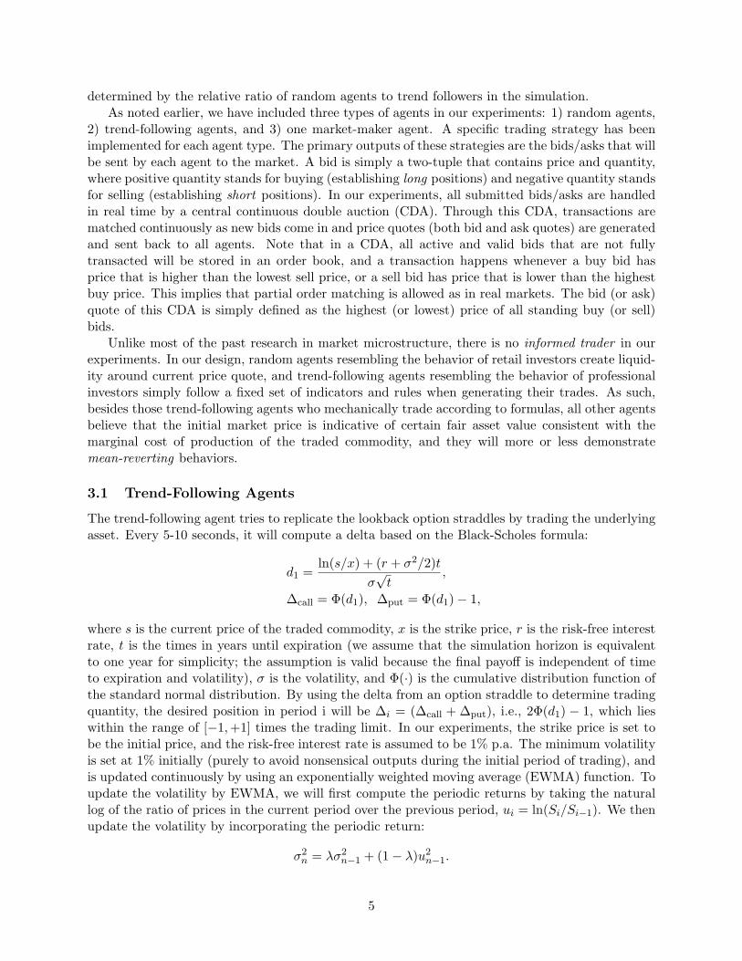
3.1 Trend-Following Agents

The trend-following agent tries to replicate the lookback option straddles by trading the underlyingasset. Every 5-10 seconds, it will compute a delta based on the Black-Scholes formula:

d1 =ln(s/x) + (r + σ2/2)t

σ√t

,

∆call = Φ(d1), ∆put = Φ(d1)− 1,

where s is the current price of the traded commodity, x is the strike price, r is the risk-free interestrate, t is the times in years until expiration (we assume that the simulation horizon is equivalentto one year for simplicity; the assumption is valid because the final payoff is independent of timeto expiration and volatility), σ is the volatility, and Φ(·) is the cumulative distribution function ofthe standard normal distribution. By using the delta from an option straddle to determine tradingquantity, the desired position in period i will be ∆i = (∆call + ∆put), i.e., 2Φ(d1) − 1, which lieswithin the range of [−1,+1] times the trading limit. In our experiments, the strike price is set tobe the initial price, and the risk-free interest rate is assumed to be 1% p.a. The minimum volatilityis set at 1% initially (purely to avoid nonsensical outputs during the initial period of trading), andis updated continuously by using an exponentially weighted moving average (EWMA) function. Toupdate the volatility by EWMA, we will first compute the periodic returns by taking the naturallog of the ratio of prices in the current period over the previous period, ui = ln(Si/Si−1). We thenupdate the volatility by incorporating the periodic return:

σ2n = λσ2

n−1 + (1− λ)u2n−1.

5

Throughout our experiments, we set λ to 0.9, which is a standard choice that can produce numer-ically stable outputs. With the formula above, we can obtain ∆i for every period i, and (∆i −Q),where Q stands for the current position, will be the differential quantity that this agent shouldadjust throughout trading (positive quantity stands for buying, negative quantity stands for sell-ing). However, the agent should not submit its bid unless the bid is consistent with recent markettrends, which is obtained by a simple linear regression with a minimum threshold of ±0.03 (in otherwords, the agent will do nothing if the absolute value of the slope of the price trend is less than0.03; this is necessary to avoid the agent “flip-flopping” based on insigificant trends). Our simpletrading rule states that the sign of the proposed bid should be the same as the sign of the slope ofthe recent market trend. If this rule is not satisfied, the agent will not submit any bid.

To avoid trend-following agents becoming artificially homogeneous (which may defeat the pur-pose of having an agent-based model), we introduce two additional features, as follows:

1. Each agent is given a randomly generated horizon on how far back into the past should it goin collecting market prices for the execution of the linear regression. The horizon parameteris uniformly distributed between 20 and 60 price observations.

2. The quantity differential, (∆i −Q), cannot be executed by the agent if its value is too large;In each time period, the agent will compute a quantity that is uniformly generated between50 and 250 and execute an order based on the smaller of (∆i −Q) and the random variable.Doing so ensures that orders are “broken up” into more manageable “lots”, which is consistentwith real-world market practice.

3.2 Random Agents

The random agent is designed to provide the bulk of liquidity to the market. Its bidding interval isevery 5-10 seconds, and it generates buy or sell bids according to a mean-reverting process: every10 ticks in positive (negative) price difference increase the selling (buying) probability by 0.1, untilreaching the upper bound at 0.8. The quantity of the bid is uniformly generated between 50 and 250and the prices of the bids follow a normal distribution. The mean of the normal distribution is theaverage of bid and ask quotes, and the standard deviation is the volatility of the price sequence,which is updated using the same EWMA updating procedure employed by the trend-followingagent.

3.3 Market Maker Agent

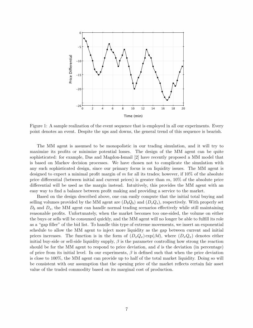
The market maker (MM) agent controls the underlying market movement and provides additionalliquidity when liquidity dries up in the market. It achieves this by maintaining a bid list containingmultiple bid points. For example, it can provide sell offers of Qs units for all prices up to Ds ticksabove a0 at an interval of δ, and buy offers of Qb units for all prices up to Db ticks below b0 at aninterval of δ (all mentioned variables are configurable parameters). If there are no other agents inthe system, this bid will result in ask and bid quotes of a0 and b0, respectively. To control this bidlist (i.e. list of bid points), we introduce an event-based mechanism that contains both bullish andbearish events. A bullish event will cause a positive shift of all bid points, resulting in an increasein both bid and ask quotes. On the other hand, a bearish event will cause a negative shift of allbid points, resulting in a decrease of both bid and ask quotes. For both bullish and bearish events,a strength parameter is provided so that the MM agent can determine how bullish (bearish) theresponse should be. The realization of the impact of event sequence in our experiments is plottedin Figure 1, where the general trend is bearish despite having ups and downs in the market.

6

200 2 4 6 8 10 12 14 16 18

0

-26

-20

-15

-10

-5

Time (min)

Pric

e D

iffer

entia

l

Figure 1: A sample realization of the event sequence that is employed in all our experiments. Everypoint denotes an event. Despite the ups and downs, the general trend of this sequence is bearish.

The MM agent is assumed to be monopolistic in our trading simulation, and it will try tomaximize its profits or minimize potential losses. The design of the MM agent can be quitesophisticated: for example, Das and Magdon-Ismail [2] have recently proposed a MM model thatis based on Markov decision processes. We have chosen not to complicate the simulation withany such sophisticated design, since our primary focus is on liquidity issues. The MM agent isdesigned to expect a minimal profit margin of m for all its trades; however, if 10% of the absoluteprice differential (between initial and current prices) is greater than m, 10% of the absolute pricedifferential will be used as the margin instead. Intuitively, this provides the MM agent with aneasy way to find a balance between profit making and providing a service to the market.

Based on the design described above, one can easily compute that the initial total buying andselling volumes provided by the MM agent are (DbQb) and (DsQs), respectively. With properly setDb and Ds, the MM agent can handle normal trading scenarios effectively while still maintainingreasonable profits. Unfortunately, when the market becomes too one-sided, the volume on eitherthe buys or sells will be consumed quickly, and the MM agent will no longer be able to fulfill its roleas a “gap filler” of the bid list. To handle this type of extreme movements, we insert an exponentialschedule to allow the MM agent to inject more liquidity as the gap between current and initialprices increases. The function is in the form of (DxQx) exp(βd), where (DxQx) denotes eitherinitial buy-side or sell-side liquidity supply, β is the parameter controlling how strong the reactionshould be for the MM agent to respond to price deviation, and d is the deviation (in percentage)of price from its initial level. In our experiments, β is defined such that when the price deviationis close to 100%, the MM agent can provide up to half of the total market liquidity. Doing so willbe consistent with our assumption that the opening price of the market reflects certain fair assetvalue of the traded commodity based on its marginal cost of production.

7

4 Deviation from Theoretical Assumptions

The theoretical trend-following strategy implemented by using lookback straddles has been de-scribed in considerable details by Fung and Hsieh [3]. Fung and Hsieh use such a strategy toconstruct the so-called “Primitive Trend Following Strategy” (PTFS). PTFS is a key factor inexplaining the returns of Commodity Trading Advisors (CTAs). However, PTFS is subject to anumber of practical limitations:

1. PTFS tends to work more effectively on commodities, currencies, interest rates and bonds,but has not worked particularly well with stocks.

2. The replication works only based on the assumption that the required Black-Scholes optionsexist, which may or may not be the case for exchange-traded options, while the bid-askspreads for over-the-counter options may be too expensive for any practical applications.

3. Many exchange-traded options are not European style options, or may have discrete strikepoints that do not match with the at-the-money strike that we intend to roll to.

4. The horizon of the options used is often determined by the availability of liquidity in theoption calendar. In our experiments, we have assumed that the option expiration will beone year, simply out of convenience because the payoffs are not dependent on the time toexpiration. Other “real-life” case studies tend to avoid options with expiration longer thanone quarter to avoid illiquid options.

5. PTFS assumes that the manager has no issue in coming up with any upfront cash outlay.That may or may not be the case.

To make our simulations more realistic when constructing trend followers in our simulations,we have relaxed the assumptions of Fung and Hsieh by:

1. Not constantly rolling the strikes of the straddles;

2. Using the underlying to replicate the options, thereby circumventing any issues related to theliquidity of the options; and

3. Using regression betas to “smooth” the trends to avoid transaction costs from excessive buyingand selling in violent markets with unclear directions.

The analyses in this section have taken reasonable steps to relax the original assumptionsof Fung and Hsieh. To ensure that the results obtained from the agent-based simulation arereasonable, we attempt five different implementations of the trend-following trading strategy. Forall these implementations, it is assumed that there will be sufficient market liquidity, and thatthe speculators’ actions have negligible effect on the market price. The differences among theseimplementations are based on how well the trader can replicate the theoretical lookback straddlestrategy. As expected, when market becomes more and more dominated by speculators, resultsfrom simulations with direct participation by trend-followers will become increasingly worse thanthese five theoretical bounds. Since we are assuming for now that these implementations haveno impact on market prices, we can use any “realized” price stream as inputs and construct therespective profit-and-loss curves for all five implementations. These off-line analyses can thus beused for comparison and calibration in the computational experiments that we plan to carry out.

8

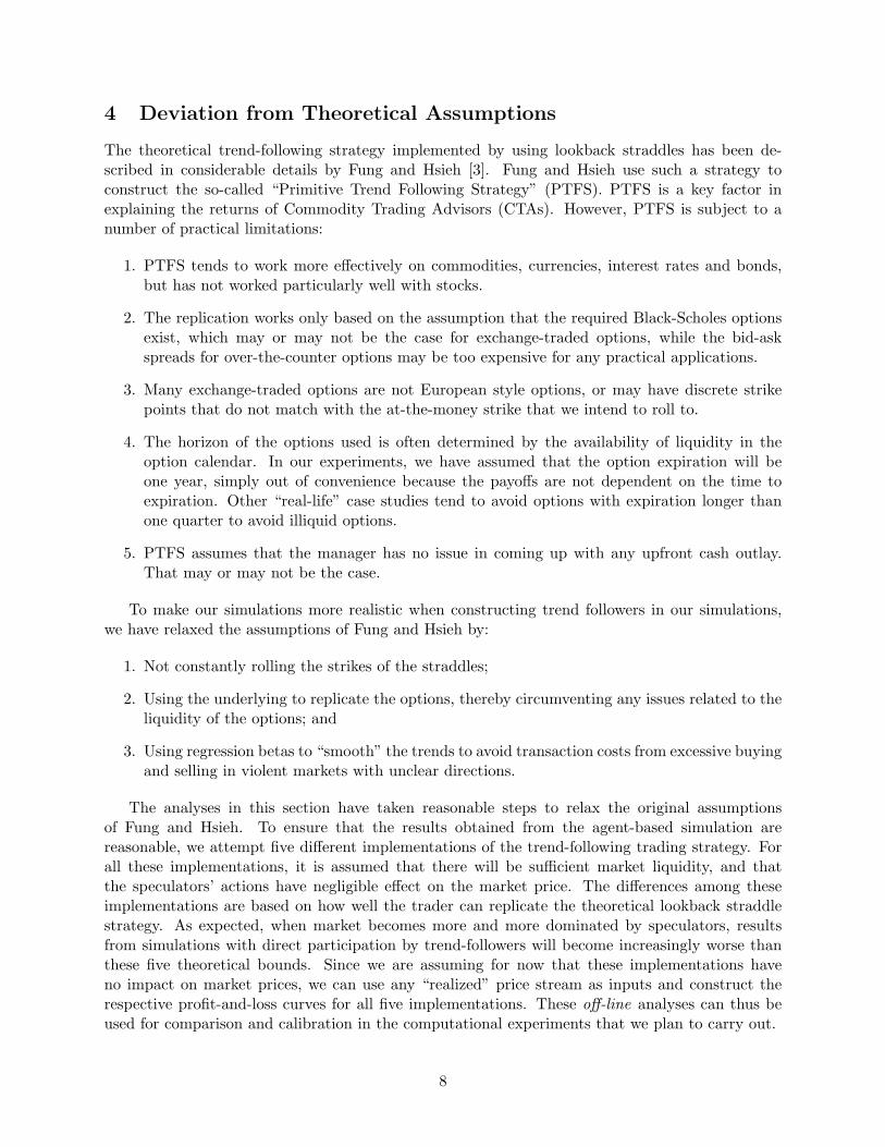
Type A – Trend-Followers Replicated by Lookback Straddles. As pointed out by Gold-man, Sosin and Gatto [4], the lookback straddle can be replicated by dynamically rolling thestrikes of standard Black-Scholes straddles over the life of the option. Fung and Hsieh [3]provides an in-depth discussion and analysis based on this classical methodology. We will notattempt to repeat those discussions, except to provide a basic summary for the convenienceof those readers who may be unfamiliar with the topic.

S(min), tracked by Straddle 1

S(max), tracked by Straddle 2

S(0)

S(T)

Figure 2: An illustration of the Type A strategy.

Generally speaking, lookback straddles can be thought of as the theoretical best-case scenario.In the perfect world, where there should be ample liquidity and no transaction cost, the TypeA strategy can be perfectly implemented with the following payoff (as depicted in Figure 2):

|Smax − Smin| −∑

Pop,

where Smax and Smin are the highest and the lowest observed prices during the investmenthorizon, and

∑Pop is the total cost spent on rolling options. This payoff is achieved by

continuously rolling the strike price of one straddle up whenever a new market high is achieved,and rolling the strike price of the other straddle down whenever a new market low is reached.1

The transaction costs involved in any such continuous rolling make it very difficult to achievethis type of theoretical payoff in practice, since the required out-of-the-money or in-the-moneyoptions may not exist or liquidly traded; even if they do, the bid-ask spreads on the optionsmay be too expensive to make this strategy practical. As we have explained in the footnote,we need to sell at the bid price and buy at the ask price continuously; a wide bid-ask spreadimplies an expensive “rolling” operation.

Type B – Stock Replication of Lookback Straddle. This is a variation of the Type A trader,in that the underlying commodity is bought/sold by delta hedging to replicate the lookbackstraddle. Given that such purchases/sales will not meet the continuous and frictionless marketassumption of Black-Scholes, we expect that a Type B trader will experience performancedeterioration as compared to a Type A trader.

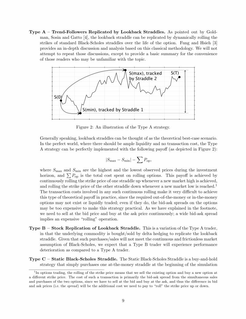
Type C – Static Black-Scholes Straddle. The Static Black-Scholes Straddle is a buy-and-holdstrategy that simply purchases one at-the-money straddle at the beginning of the simulation

1In options trading, the rolling of the strike price means that we sell the existing option and buy a new option ata different strike price. The cost of such a transaction is primarily the bid-ask spread from the simultaneous salesand purchases of the two options, since we have to sell at the bid and buy at the ask, and thus the difference in bidand ask prices (i.e. the spread) will be the additional cost we need to pay to “roll” the strike price up or down.

9

S(0)

S(T)

Figure 3: An illustration of the Type C strategy.

period. The payoff for the Type C implementation is (as depicted in Figure 3):

|St − S0| −∑

Pop,

where St is the price at option maturity, S0 is the initial price, and∑Pop is the premium paid

for options. The intuition is that, when traders do not have perfect foresights to pick the topsand the bottoms in any market, while the continuous rolling of Black-Scholes options may betoo expensive, one feasible alternative is to simply purchase a static straddle and hold it tomaturity. Such a trader’s belief is that the beginning and the end of the investment horizonwill provide a reasonable approximation of the predominant market trend during that period.

Type D – Stock Replication of Static Black-Scholes Straddle. This is a variation of theType C trader, in that the underlying commodity is bought/sold by delta hedging to replicatethe Black-Scholes straddle. Given that such purchases/sales will not meet the continuousand frictionless market assumption of Black-Scholes, we expect that a Type D trader willexperience performance deterioration as compared to a Type C trader. One can also thinkof Type D stock replication as a simplistic, tick-by-tick form of trend following, since a TypeD trader will be buying or selling based on a uptick or a downtick, respectively.

Type E – Simplistic Regression-Beta Trend Following. The final type of trader uses a sim-ple regression (say over 30 price observations) to determine whether the market is trendingupward or downward. If the regression beta is larger than a specific threshold, then thestrategy will purchase/sell the amount suggested by the delta in Type D trader.

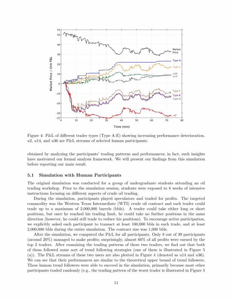
By applying practical tweaks to the theoretical strategy of a Type A trader, we expect to seedifferent levels of deterioration of trading performance from Type B to Type E. By feeding thesefive implementations with a price stream generated by human participants (detail of which will bediscussed in the next section), we can indeed observe such deterioration (see Figure 4).

5 Percentage of “Smart Traders” versus “Random Traders”

It should be noted that the simulation results from the previous section are hypothetical profits andlosses computed based on an already “realized” price stream, and that none of these hypotheticalagents participated in the trading simulation directly. The price stream as shown in Figure 4is taken from a simulation involving human participants. Unusually interesting insights can be

10

800 10 20 30 40 50 60 70

55

-35

-30

-20

-10

0

10

20

30

40

50

Time (min)

Mar

ket P

rice

/ Un

it P&

L

Type BType D

Type E

Type C

Type A

Market Price

u36u14

u2

Figure 4: P&L of different trader types (Type A-E) showing increasing performance deterioration.u2, u14, and u36 are P&L streams of selected human participants.

obtained by analyzing the participants’ trading patterns and performances; in fact, such insightshave motivated our formal analysis framework. We will present our findings from this simulationbefore reporting our main result.

5.1 Simulation with Human Participants

The original simulation was conducted for a group of undergraduate students attending an oiltrading workshop. Prior to the simulation session, students were exposed to 8 weeks of intensiveinstructions focusing on different aspects of crude oil trading.

During the simulation, participants played speculators and traded for profits. The targetedcommodity was the Western Texas Intermediate (WTI) crude oil contract and each trader couldtrade up to a maximum of 2,000,000 barrels (bbls). A trader could take either long or shortpositions, but once he reached his trading limit, he could take no further positions in the samedirection (however, he could still trade to reduce his positions). To encourage active participation,we explicitly asked each participant to transact at least 100,000 bbls in each trade, and at least2,000,000 bbls during the entire simulation. The contract size was 1,000 bbls.

After the simulation, we computed the P&L for all participants. Only 8 out of 39 participants(around 20%) managed to make profits; surprisingly, almost 60% of all profits were earned by thetop 2 traders. After examining the trading patterns of these two traders, we find out that bothof them followed some sort of trend following strategies (one of them is illustrated in Figure 5(a)). The P&L streams of these two users are also plotted in Figure 4 (denoted as u14 and u36).We can see that their performances are similar to the theoretical upper bound of trend followers.These human trend followers were able to succeed in the simulation, primarily because most otherparticipants traded randomly (e.g., the trading pattern of the worst trader is illustrated in Figure 5

11

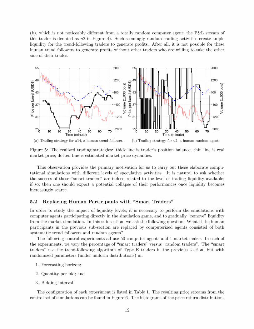
(b), which is not noticeably different from a totally random computer agent; the P&L stream ofthis trader is denoted as u2 in Figure 4). Such seemingly random trading activities create ampleliquidity for the trend-following traders to generate profits. After all, it is not possible for thesehuman trend followers to generate profits without other traders who are willing to take the otherside of their trades.

0 10 20 30 40 50 60 7025

31

37

43

49

55

Time (minute)

Pric

e pe

r ba

rrel

(U

SD

$)

0 10 20 30 40 50 60 70−2000

−1200

−400

400

1200

2000

Vol

ume

(1,0

00 b

bls)

(a) Trading strategy for u14, a human trend follower.

0 10 20 30 40 50 60 7025

31

37

43

49

55

Time (minute)P

rice

per

barr

el (

US

D$)

0 10 20 30 40 50 60 70−2000

−1200

−400

400

1200

2000

Vol

ume

(1,0

00 b

bls)

(b) Trading strategy for u2, a human random agent.

Figure 5: The realized trading strategies: thick line is trader’s position balance; thin line is realmarket price; dotted line is estimated market price dynamics.

This observation provides the primary motivation for us to carry out these elaborate compu-tational simulations with different levels of speculative activities. It is natural to ask whetherthe success of these “smart traders” are indeed related to the level of trading liquidity available;if so, then one should expect a potential collapse of their performances once liquidity becomesincreasingly scarce.

5.2 Replacing Human Participants with “Smart Traders”

In order to study the impact of liquidity levels, it is necessary to perform the simulations withcomputer agents participating directly in the simulation game, and to gradually “remove” liquidityfrom the market simulation. In this sub-section, we ask the following question: What if the humanparticipants in the previous sub-section are replaced by computerized agents consisted of bothsystematic trend followers and random agents?

The following control experiments all use 50 computer agents and 1 market maker. In each ofthe experiments, we vary the percentage of “smart traders” versus “random traders”. The “smarttraders” use the trend-following algorithm of Type E traders in the previous section, but withrandomized parameters (under uniform distributions) in:

1. Forecasting horizon;

2. Quantity per bid; and

3. Bidding interval.

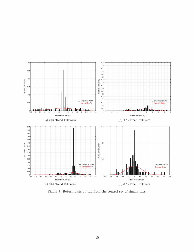
The configuration of each experiment is listed in Table 1. The resulting price streams from thecontrol set of simulations can be found in Figure 6. The histograms of the price return distributions

12

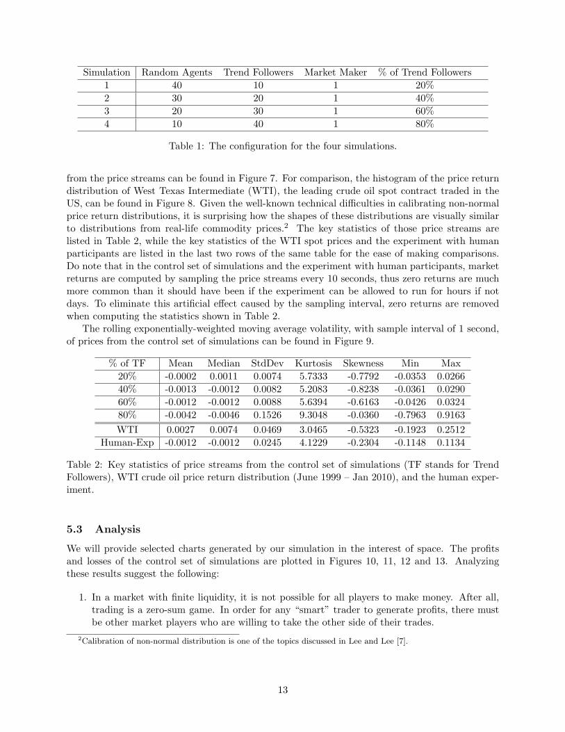
Simulation Random Agents Trend Followers Market Maker % of Trend Followers1 40 10 1 20%2 30 20 1 40%3 20 30 1 60%4 10 40 1 80%

Table 1: The configuration for the four simulations.

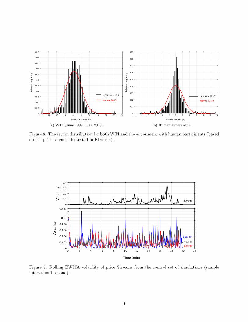
from the price streams can be found in Figure 7. For comparison, the histogram of the price returndistribution of West Texas Intermediate (WTI), the leading crude oil spot contract traded in theUS, can be found in Figure 8. Given the well-known technical difficulties in calibrating non-normalprice return distributions, it is surprising how the shapes of these distributions are visually similarto distributions from real-life commodity prices.2 The key statistics of those price streams arelisted in Table 2, while the key statistics of the WTI spot prices and the experiment with humanparticipants are listed in the last two rows of the same table for the ease of making comparisons.Do note that in the control set of simulations and the experiment with human participants, marketreturns are computed by sampling the price streams every 10 seconds, thus zero returns are muchmore common than it should have been if the experiment can be allowed to run for hours if notdays. To eliminate this artificial effect caused by the sampling interval, zero returns are removedwhen computing the statistics shown in Table 2.

The rolling exponentially-weighted moving average volatility, with sample interval of 1 second,of prices from the control set of simulations can be found in Figure 9.

% of TF Mean Median StdDev Kurtosis Skewness Min Max20% -0.0002 0.0011 0.0074 5.7333 -0.7792 -0.0353 0.026640% -0.0013 -0.0012 0.0082 5.2083 -0.8238 -0.0361 0.029060% -0.0012 -0.0012 0.0088 5.6394 -0.6163 -0.0426 0.032480% -0.0042 -0.0046 0.1526 9.3048 -0.0360 -0.7963 0.9163WTI 0.0027 0.0074 0.0469 3.0465 -0.5323 -0.1923 0.2512

Human-Exp -0.0012 -0.0012 0.0245 4.1229 -0.2304 -0.1148 0.1134

Table 2: Key statistics of price streams from the control set of simulations (TF stands for TrendFollowers), WTI crude oil price return distribution (June 1999 – Jan 2010), and the human exper-iment.

5.3 Analysis

We will provide selected charts generated by our simulation in the interest of space. The profitsand losses of the control set of simulations are plotted in Figures 10, 11, 12 and 13. Analyzingthese results suggest the following:

1. In a market with finite liquidity, it is not possible for all players to make money. After all,trading is a zero-sum game. In order for any “smart” trader to generate profits, there mustbe other market players who are willing to take the other side of their trades.

2Calibration of non-normal distribution is one of the topics discussed in Lee and Lee [7].

13

220 2 4 6 8 10 12 14 16 18 20

55

0

5

10

15

20

25

30

35

40

45

50

Time (min)

Mar

ket P

rice

20% TF60% TF

40% TF

80% TF

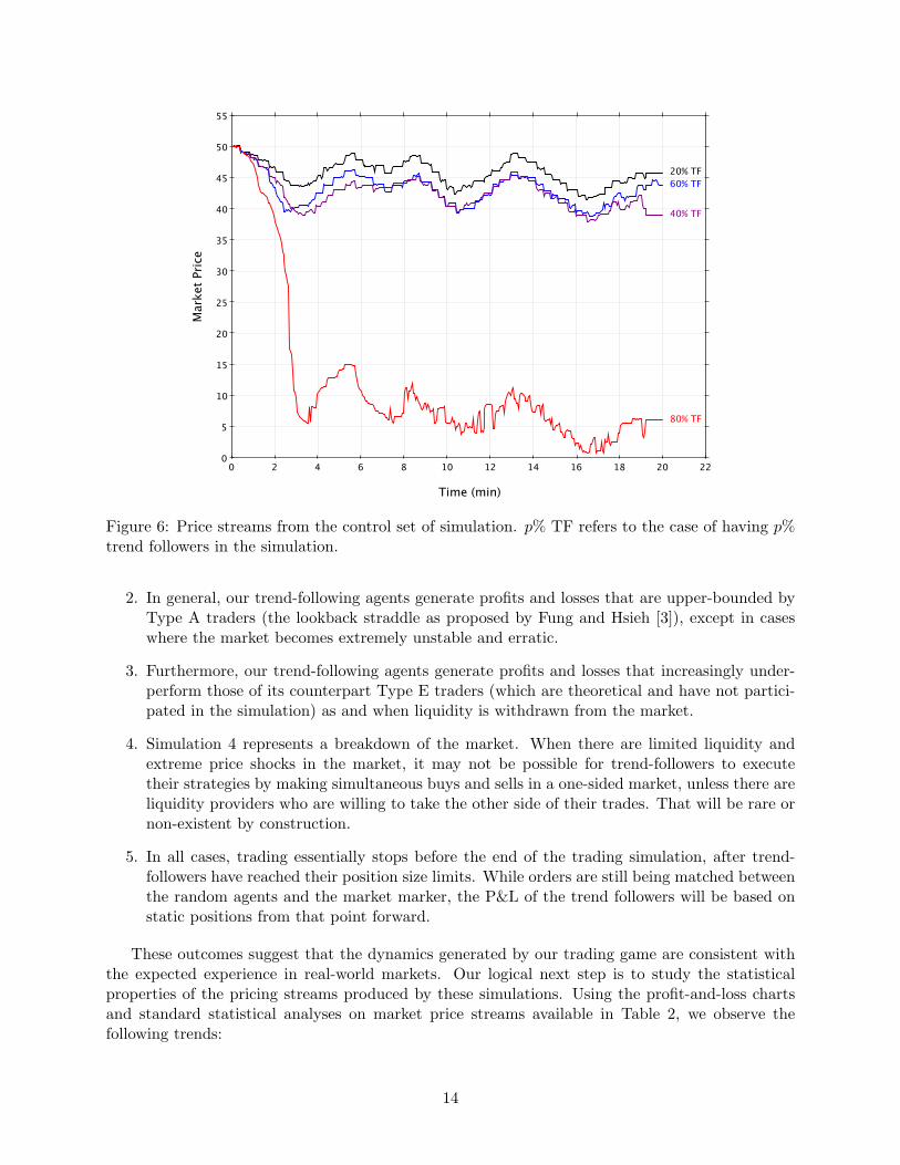
Figure 6: Price streams from the control set of simulation. p% TF refers to the case of having p%trend followers in the simulation.

2. In general, our trend-following agents generate profits and losses that are upper-bounded byType A traders (the lookback straddle as proposed by Fung and Hsieh [3]), except in caseswhere the market becomes extremely unstable and erratic.

3. Furthermore, our trend-following agents generate profits and losses that increasingly under-perform those of its counterpart Type E traders (which are theoretical and have not partici-pated in the simulation) as and when liquidity is withdrawn from the market.

4. Simulation 4 represents a breakdown of the market. When there are limited liquidity andextreme price shocks in the market, it may not be possible for trend-followers to executetheir strategies by making simultaneous buys and sells in a one-sided market, unless there areliquidity providers who are willing to take the other side of their trades. That will be rare ornon-existent by construction.

5. In all cases, trading essentially stops before the end of the trading simulation, after trend-followers have reached their position size limits. While orders are still being matched betweenthe random agents and the market marker, the P&L of the trend followers will be based onstatic positions from that point forward.

These outcomes suggest that the dynamics generated by our trading game are consistent withthe expected experience in real-world markets. Our logical next step is to study the statisticalproperties of the pricing streams produced by these simulations. Using the profit-and-loss chartsand standard statistical analyses on market price streams available in Table 2, we observe thefollowing trends:

14

3.5-3.5 -3 -2.5 -2 -1.5 -1 -0.5 0 0.5 1 1.5 2 2.5 3

0.3

0

0.05

0.1

0.15

0.2

0.25

Market Returns (%)

Rela

tive

Freq

uenc

y

Empirical Dist'nNormal Dist'n

(a) 20% Trend Followers

4-7 -6 -5 -4 -3 -2 -1 0 1 2 3

0.85

0

0.05

0.1

0.15

0.2

0.25

0.3

0.35

0.4

0.45

0.5

0.55

0.6

0.65

0.7

0.75

0.8

Market Returns (%)

Rela

tive

Freq

uenc

yEmpirical Dist'nNormal Dist'n

(b) 40% Trend Followers

4.5-8.5 -7.5 -6.5 -5.5 -4.5 -3.5 -2.5 -1.5 -0.5 0.5 1.5 2.5 3.5

0.75

0

0.05

0.1

0.15

0.2

0.25

0.3

0.35

0.4

0.45

0.5

0.55

0.6

0.65

0.7

Market Returns (%)

Rela

tive

Freq

uenc

y

Empirical Dist'nNormal Dist'n

(c) 60% Trend Followers

120-100 -80 -60 -40 -20 0 20 40 60 80 100

0.15

0

0.05

0.1

Market Returns (%)

Rela

tive

Freq

uenc

y

Empirical Dist'nNormal Dist'n

(d) 80% Trend Followers

Figure 7: Return distribution from the control set of simulations.

15

30-20 -15 -10 -5 0 5 10 15 20 25

0.055

0

0.005

0.01

0.015

0.02

0.025

0.03

0.035

0.04

0.045

0.05

Market Returns (%)

Rela

tive

Freq

uenc

y

Empirical Dist'n

Normal Dist'n

(a) WTI (June 1999 – Jan 2010).

12-12 -10 -8 -6 -4 -2 0 2 4 6 8 10

0.09

0

0.01

0.02

0.03

0.04

0.05

0.06

0.07

0.08

Market Returns (%)

Rela

tive

Freq

uenc

y

Empirical Dist'n

Normal Dist'n

(b) Human experiment.

Figure 8: The return distribution for both WTI and the experiment with human participants (basedon the price stream illustrated in Figure 4).

0.4

0

0.1

0.2

0.3

Vol

atili

ty

80% TF

220 2 4 6 8 10 12 14 16 18 20

0.013

0

0.002

0.004

0.006

0.008

0.01

Time (min)

Vol

atili

ty

60% TF

40% TF

20% TF

Figure 9: Rolling EWMA volatility of price Streams from the control set of simulations (sampleinterval = 1 second).

16

1. As and when liquidity is removed from the market, volatility will increase and extreme priceshocks become more prominent. This is consistent with empirical observations in the market,in that: 1) commodity futures markets that are increasingly dominated by speculative activ-ities as contracts “roll in” tend to exhibit increasing volatility; and 2) markets such as thatof convertible bonds, which is 95% dominated by professional speculators, (i.e. hedge fundsand proprietary trading desks, as opposed to long-term investors) show significantly highervolatility than other markets.

2. The kurtosis of the market actually decreases when the market is dominated by more andmore trend followers. Nonetheless, all simulation results show significant fat-tail behavior.More theoretical discussion on the modeling of fat-tail behavior in financial markets can befound in Lee and Lee [7].

3. Once the market has gone over a “tipping point” of destabilization (e.g. as in simulation 4),the instability usually does not become significantly worse by further withdrawal of liquidity.The key is that the market must find a new equilibrium of lower (or higher) prices whenthere is an overwhelming majority of sellers (or buyers). This is consistent with empiricalobservations by real-life practitioners.

Our next step is to look for evidence as to whether specific techniques of intervention may ormay not be effective in a market facing liquidity crises.

51

41

45

Mar

ket P

rice

MarketPrice

220 2 4 6 8 10 12 14 16 18 20

-2-101234567

Time (min)

Unit

P&L

Type A

Type CType EType B

TF

RA

MMType D

Figure 10: P&L of different strategies in simulation 1 with 40 random agents (denoted as RA), 10trend followers (20% trend followers, denoted as TF) and 1 market maker (denoted as MM).

17

220 2 4 6 8 10 12 14 16 18 20

-6

-4

-2

0

2

4

6

8

10

Time (min)

Unit

P&L

Type A

Type CType EType B

TF

RA

MM

Type D

51

37

40

45M

arke

t Pric

eMarketPrice

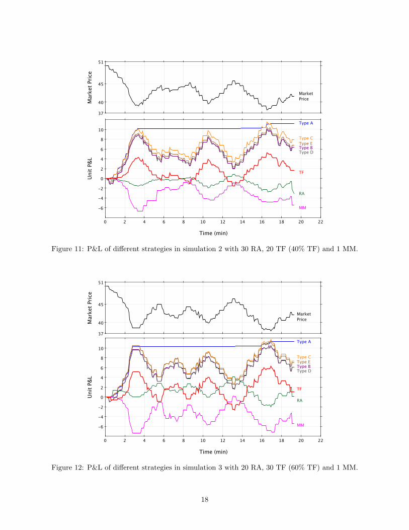
Figure 11: P&L of different strategies in simulation 2 with 30 RA, 20 TF (40% TF) and 1 MM.

220 2 4 6 8 10 12 14 16 18 20

-6

-4

-2

0

2

4

6

8

10

Time (min)

Unit

P&L

Type A

Type CType EType B

TF

RA

MM

Type D

51

37

40

45

Mar

ket P

rice

MarketPrice

Figure 12: P&L of different strategies in simulation 3 with 20 RA, 30 TF (60% TF) and 1 MM.

18

220 2 4 6 8 10 12 14 16 18 20

55

-15

-10

0

10

20

30

40

50

Time (min)

Mar

ket P

rice

/ Un

it P&

LType BType D

Type EType C

Type A

Market Price

TF

RAMM

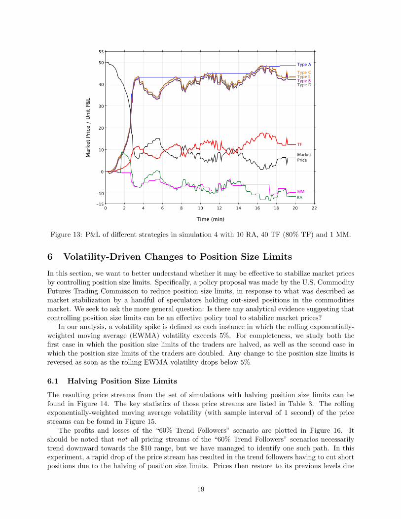
Figure 13: P&L of different strategies in simulation 4 with 10 RA, 40 TF (80% TF) and 1 MM.

6 Volatility-Driven Changes to Position Size Limits

In this section, we want to better understand whether it may be effective to stabilize market pricesby controlling position size limits. Specifically, a policy proposal was made by the U.S. CommodityFutures Trading Commission to reduce position size limits, in response to what was described asmarket stabilization by a handful of speculators holding out-sized positions in the commoditiesmarket. We seek to ask the more general question: Is there any analytical evidence suggesting thatcontrolling position size limits can be an effective policy tool to stabilize market prices?

In our analysis, a volatility spike is defined as each instance in which the rolling exponentially-weighted moving average (EWMA) volatility exceeds 5%. For completeness, we study both thefirst case in which the position size limits of the traders are halved, as well as the second case inwhich the position size limits of the traders are doubled. Any change to the position size limits isreversed as soon as the rolling EWMA volatility drops below 5%.

6.1 Halving Position Size Limits

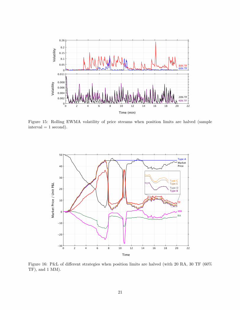
The resulting price streams from the set of simulations with halving position size limits can befound in Figure 14. The key statistics of those price streams are listed in Table 3. The rollingexponentially-weighted moving average volatility (with sample interval of 1 second) of the pricestreams can be found in Figure 15.

The profits and losses of the “60% Trend Followers” scenario are plotted in Figure 16. Itshould be noted that not all pricing streams of the “60% Trend Followers” scenarios necessarilytrend downward towards the $10 range, but we have managed to identify one such path. In thisexperiment, a rapid drop of the price stream has resulted in the trend followers having to cut shortpositions due to the halving of position size limits. Prices then restore to its previous levels due

19

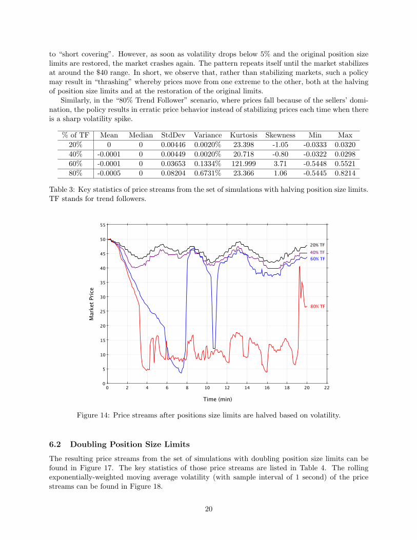
to “short covering”. However, as soon as volatility drops below 5% and the original position sizelimits are restored, the market crashes again. The pattern repeats itself until the market stabilizesat around the $40 range. In short, we observe that, rather than stabilizing markets, such a policymay result in “thrashing” whereby prices move from one extreme to the other, both at the halvingof position size limits and at the restoration of the original limits.

Similarly, in the “80% Trend Follower” scenario, where prices fall because of the sellers’ domi-nation, the policy results in erratic price behavior instead of stabilizing prices each time when thereis a sharp volatility spike.

% of TF Mean Median StdDev Variance Kurtosis Skewness Min Max20% 0 0 0.00446 0.0020% 23.398 -1.05 -0.0333 0.032040% -0.0001 0 0.00449 0.0020% 20.718 -0.80 -0.0322 0.029860% -0.0001 0 0.03653 0.1334% 121.999 3.71 -0.5448 0.552180% -0.0005 0 0.08204 0.6731% 23.366 1.06 -0.5445 0.8214

Table 3: Key statistics of price streams from the set of simulations with halving position size limits.TF stands for trend followers.

220 2 4 6 8 10 12 14 16 18 20

55

0

5

10

15

20

25

30

35

40

45

50

Time (min)

Mar

ket P

rice

20% TF

60% TF40% TF

80% TF

Figure 14: Price streams after positions size limits are halved based on volatility.

6.2 Doubling Position Size Limits

The resulting price streams from the set of simulations with doubling position size limits can befound in Figure 17. The key statistics of those price streams are listed in Table 4. The rollingexponentially-weighted moving average volatility (with sample interval of 1 second) of the pricestreams can be found in Figure 18.

20

0.26

0

0.05

0.1

0.15

0.2

Vol

atili

ty

60% TF80% TF

220 2 4 6 8 10 12 14 16 18 20

0.011

0

0.002

0.004

0.006

0.008

Time (min)

Vol

atili

ty

20% TF40% TF

Figure 15: Rolling EWMA volatility of price streams when position limits are halved (sampleinterval = 1 second).

220 2 4 6 8 10 12 14 16 18 20

50

-30

-20

-10

0

10

20

30

40

Time

Mar

ket P

rice

/ Uni

t P&L

Type AMarket Price

RAMM

TF

Type BType DType EType C

Figure 16: P&L of different strategies when position limits are halved (with 20 RA, 30 TF (60%TF), and 1 MM).

21

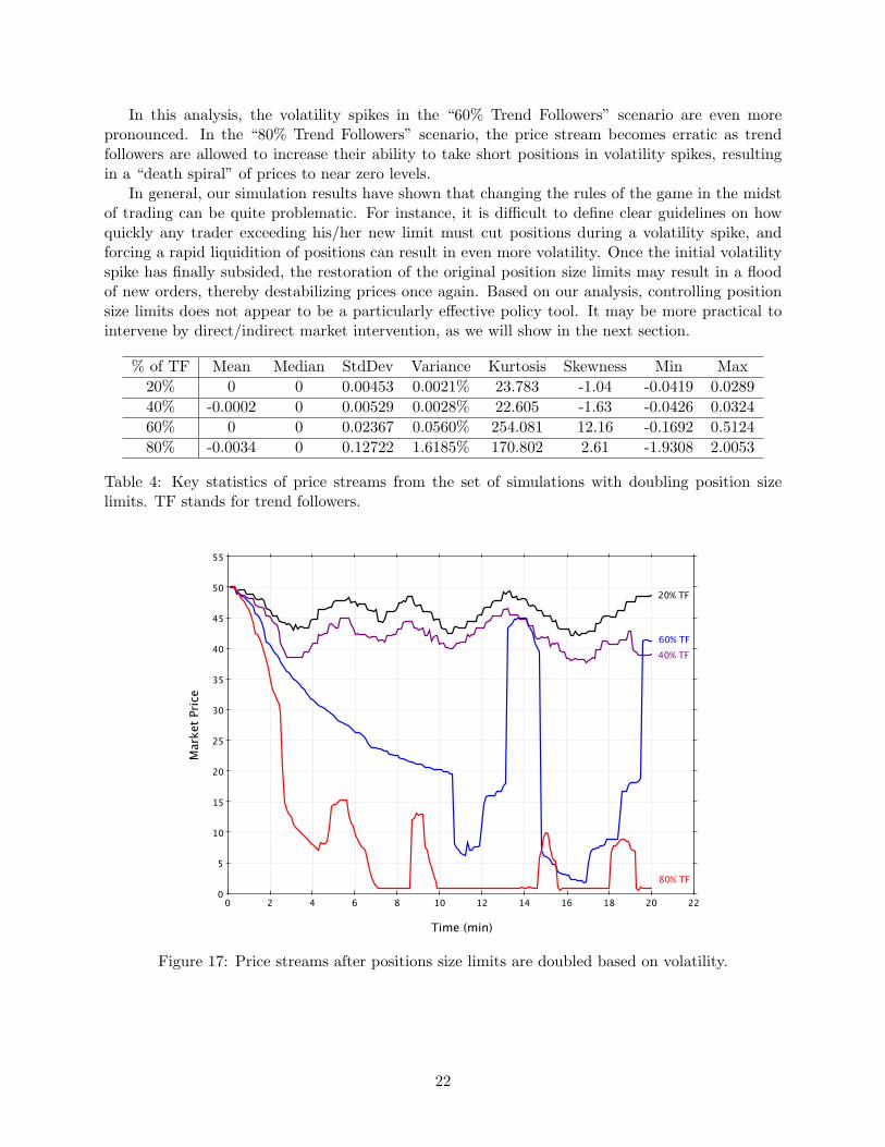
In this analysis, the volatility spikes in the “60% Trend Followers” scenario are even morepronounced. In the “80% Trend Followers” scenario, the price stream becomes erratic as trendfollowers are allowed to increase their ability to take short positions in volatility spikes, resultingin a “death spiral” of prices to near zero levels.

In general, our simulation results have shown that changing the rules of the game in the midstof trading can be quite problematic. For instance, it is difficult to define clear guidelines on howquickly any trader exceeding his/her new limit must cut positions during a volatility spike, andforcing a rapid liquidition of positions can result in even more volatility. Once the initial volatilityspike has finally subsided, the restoration of the original position size limits may result in a floodof new orders, thereby destabilizing prices once again. Based on our analysis, controlling positionsize limits does not appear to be a particularly effective policy tool. It may be more practical tointervene by direct/indirect market intervention, as we will show in the next section.

% of TF Mean Median StdDev Variance Kurtosis Skewness Min Max20% 0 0 0.00453 0.0021% 23.783 -1.04 -0.0419 0.028940% -0.0002 0 0.00529 0.0028% 22.605 -1.63 -0.0426 0.032460% 0 0 0.02367 0.0560% 254.081 12.16 -0.1692 0.512480% -0.0034 0 0.12722 1.6185% 170.802 2.61 -1.9308 2.0053

Table 4: Key statistics of price streams from the set of simulations with doubling position sizelimits. TF stands for trend followers.

220 2 4 6 8 10 12 14 16 18 20

55

0

5

10

15

20

25

30

35

40

45

50

Time (min)

Mar

ket P

rice

20% TF

60% TF40% TF

80% TF

Figure 17: Price streams after positions size limits are doubled based on volatility.

22

0.6

0

0.1

0.2

0.3

0.4

0.5

Vol

atili

ty60% TF80% TF

220 2 4 6 8 10 12 14 16 18 20

0.014

0

0.002

0.004

0.006

0.008

0.01

0.012

Time (min)

Vol

atili

ty

20% TF

40% TF

Figure 18: Rolling EWMA volatility of price streams when position limits are doubled (sampleinterval = 1 second).

7 Liquidity Reduction/Injection

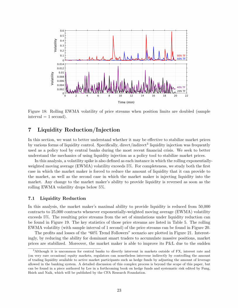
In this section, we want to better understand whether it may be effective to stabilize market pricesby various forms of liquidity control. Specifically, direct/indirect3 liquidity injection was frequentlyused as a policy tool by central banks during the most recent financial crisis. We seek to betterunderstand the mechanics of using liquidity injection as a policy tool to stabilize market prices.

In this analysis, a volatility spike is also defined as each instance in which the rolling exponentially-weighted moving average (EWMA) volatility exceeds 5%. For completeness, we study both the firstcase in which the market maker is forced to reduce the amount of liquidity that it can provide tothe market, as well as the second case in which the market maker is injecting liquidity into themarket. Any change to the market maker’s ability to provide liquidity is reversed as soon as therolling EWMA volatility drops below 5%.

7.1 Liquidity Reduction

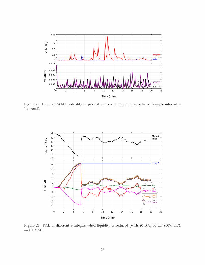
In this analysis, the market maker’s maximal ability to provide liquidity is reduced from 50,000contracts to 25,000 contracts whenever exponentially-weighted moving average (EWMA) volatilityexceeds 5%. The resulting price streams from the set of simulations under liquidity reduction canbe found in Figure 19. The key statistics of those price streams are listed in Table 5. The rollingEWMA volatility (with sample interval of 1 second) of the price streams can be found in Figure 20.

The profits and losses of the “60% Trend Followers” scenario are plotted in Figure 21. Interest-ingly, by reducing the ability for dominant smart traders to accumulate massive positions, marketprices are stabilized. Moreover, the market maker is able to improve its P&L due to the sudden

3Although it is uncommon for central banks to directly intervent in markets outside of FX, interest rate and(on very rare occasions) equity markets, regulators can nonetheless intervene indirectly by controlling the amountof trading liquidity available to active market participants such as hedge funds by adjusting the amount of leverageallowed in the banking system. A detailed discussion of this complex process is beyond the scope of this paper, butcan be found in a piece authored by Lee in a forthcoming book on hedge funds and systematic risk edited by Fung,Hsieh and Naik, which will be published by the CFA Research Foundation.

23

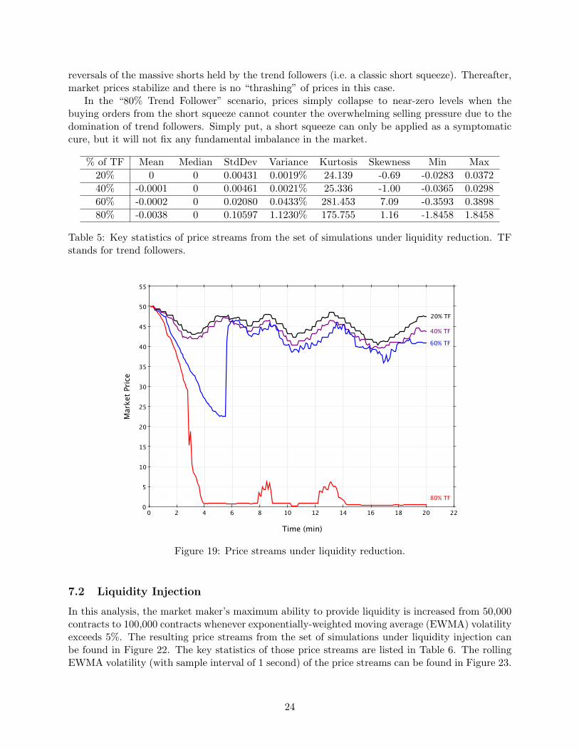
reversals of the massive shorts held by the trend followers (i.e. a classic short squeeze). Thereafter,market prices stabilize and there is no “thrashing” of prices in this case.

In the “80% Trend Follower” scenario, prices simply collapse to near-zero levels when thebuying orders from the short squeeze cannot counter the overwhelming selling pressure due to thedomination of trend followers. Simply put, a short squeeze can only be applied as a symptomaticcure, but it will not fix any fundamental imbalance in the market.

% of TF Mean Median StdDev Variance Kurtosis Skewness Min Max20% 0 0 0.00431 0.0019% 24.139 -0.69 -0.0283 0.037240% -0.0001 0 0.00461 0.0021% 25.336 -1.00 -0.0365 0.029860% -0.0002 0 0.02080 0.0433% 281.453 7.09 -0.3593 0.389880% -0.0038 0 0.10597 1.1230% 175.755 1.16 -1.8458 1.8458

Table 5: Key statistics of price streams from the set of simulations under liquidity reduction. TFstands for trend followers.

220 2 4 6 8 10 12 14 16 18 20

55

0

5

10

15

20

25

30

35

40

45

50

Time (min)

Mar

ket P

rice

20% TF

60% TF

40% TF

80% TF

Figure 19: Price streams under liquidity reduction.

7.2 Liquidity Injection

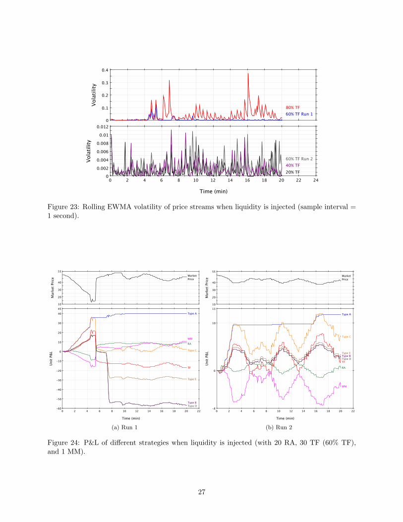
In this analysis, the market maker’s maximum ability to provide liquidity is increased from 50,000contracts to 100,000 contracts whenever exponentially-weighted moving average (EWMA) volatilityexceeds 5%. The resulting price streams from the set of simulations under liquidity injection canbe found in Figure 22. The key statistics of those price streams are listed in Table 6. The rollingEWMA volatility (with sample interval of 1 second) of the price streams can be found in Figure 23.

24

0.45

0

0.1

0.2

0.3V

olat

ility

60% TF

80% TF

220 2 4 6 8 10 12 14 16 18 20

0.011

0

0.002

0.004

0.006

0.008

Time (min)

Vol

atili

ty

20% TF

40% TF

Figure 20: Rolling EWMA volatility of price streams when liquidity is reduced (sample interval =1 second).

51

202530354045

Mar

ket P

rice Market

Price

220 2 4 6 8 10 12 14 16 18 20

-20-15-10-505

10152025

Time (min)

Unit

P&L

Type A

TFRA

MMType CType E

Type BType D

Figure 21: P&L of different strategies when liquidity is reduced (with 20 RA, 30 TF (60% TF),and 1 MM).

25

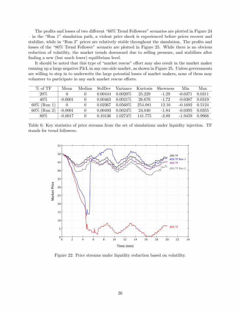
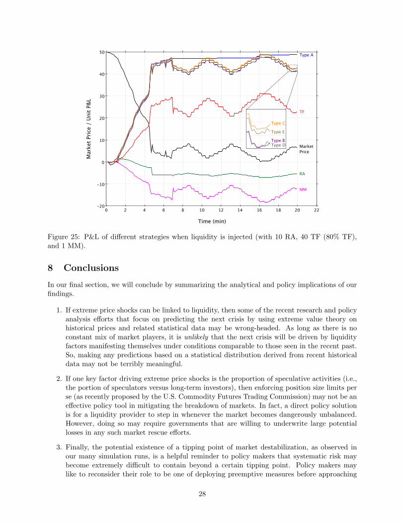
The profits and losses of two different “60% Trend Followers” scenarios are plotted in Figure 24– in the “Run 1” simulation path, a violent price shock is experienced before prices recover andstabilize, while in “Run 2” prices are relatively stable throughout the simulation. The profits andlosses of the “80% Trend Follower” scenario are plotted in Figure 25. While there is no obviousreduction of volatility, the market trends downward due to selling pressure, and stabilizes afterfinding a new (but much lower) equilibrium level.

It should be noted that this type of “market rescue” effort may also result in the market makerrunning up a large negative P&L in any one-side market, as shown in Figure 25. Unless governmentsare willing to step in to underwrite the large potential losses of market makers, none of them mayvolunteer to participate in any such market rescue efforts.

% of TF Mean Median StdDev Variance Kurtosis Skewness Min Max20% 0 0 0.00444 0.0020% 25.229 -1.29 -0.0371 0.031140% -0.0001 0 0.00463 0.0021% 26.676 -1.72 -0.0387 0.0319

60% (Run 1) 0 0 0.02367 0.0560% 254.081 12.16 -0.1692 0.512460% (Run 2) -0.0001 0 0.00493 0.0024% 24.040 -1.84 -0.0395 0.0355

80% -0.0017 0 0.10136 1.0274% 141.775 -3.89 -1.9459 0.9968

Table 6: Key statistics of price streams from the set of simulations under liquidity injection. TFstands for trend followers.

240 2 4 6 8 10 12 14 16 18 20 22

55

0

5

10

15

20

25

30

35

40

45

50

Time (min)

Mar

ket P

rice

20% TF60% TF Run 140% TF

80% TF

60% TF Run 2

Figure 22: Price streams under liquidity reduction based on volatility.

26

0.4

0

0.1

0.2

0.3

Vol

atili

ty

60% TF Run 1

80% TF

240 2 4 6 8 10 12 14 16 18 20 22

0.012

0

0.002

0.004

0.006

0.008

0.01

Time (min)

Vol

atili

ty

20% TF

40% TF

60% TF Run 2

Figure 23: Rolling EWMA volatility of price streams when liquidity is injected (sample interval =1 second).

55

10

20

30

40

Mar

ket P

rice Market

Price

220 2 4 6 8 10 12 14 16 18 20

45

-60

-50

-40

-30

-20

-10

0

10

20

30

40

Time (min)

Unit

P&L

Type BType D

Type E

Type C

Type A

TF

RAMM

(a) Run 1

55

10

20

30

40

Mar

ket P

rice Market

Price

220 2 4 6 8 10 12 14 16 18 20

13

-8

0

10

Time (min)

Unit

P&L

Type BType DType E

Type C

Type A

TFRA

MM

(b) Run 2

Figure 24: P&L of different strategies when liquidity is injected (with 20 RA, 30 TF (60% TF),and 1 MM).

27

220 2 4 6 8 10 12 14 16 18 20

50

-20

-10

0

10

20

30

40

Time (min)

Mar

ket P

rice

/ Uni

t P&L

Type A

TF

RA

MM

MarketPrice

Type CType EType BType D

Figure 25: P&L of different strategies when liquidity is injected (with 10 RA, 40 TF (80% TF),and 1 MM).

8 Conclusions

In our final section, we will conclude by summarizing the analytical and policy implications of ourfindings.

1. If extreme price shocks can be linked to liquidity, then some of the recent research and policyanalysis efforts that focus on predicting the next crisis by using extreme value theory onhistorical prices and related statistical data may be wrong-headed. As long as there is noconstant mix of market players, it is unlikely that the next crisis will be driven by liquidityfactors manifesting themselves under conditions comparable to those seen in the recent past.So, making any predictions based on a statistical distribution derived from recent historicaldata may not be terribly meaningful.

2. If one key factor driving extreme price shocks is the proportion of speculative activities (i.e.,the portion of speculators versus long-term investors), then enforcing position size limits perse (as recently proposed by the U.S. Commodity Futures Trading Commission) may not be aneffective policy tool in mitigating the breakdown of markets. In fact, a direct policy solutionis for a liquidity provider to step in whenever the market becomes dangerously unbalanced.However, doing so may require governments that are willing to underwrite large potentiallosses in any such market rescue efforts.

3. Finally, the potential existence of a tipping point of market destabilization, as observed inour many simulation runs, is a helpful reminder to policy makers that systematic risk maybecome extremely difficult to contain beyond a certain tipping point. Policy makers maylike to reconsider their role to be one of deploying preemptive measures before approaching

28

the tipping point, rather than looking for suitable corrective measures only after the tippingpoint has already been breached.

Any stylized model of market contagion should accommodate some or all of the characteristicsdescribed above. Such a framework will likely be an extension of the approach similar to that ofKyle and Xiong [5] by increasing the number of tradable assets, the policy options available to thecentral bank and the types of investors in the financial economy.

A flexible agent-based simulation platform will be a valuable tool to validate any follow-upresearch, since additional counterparties, such as central banks or additional investor types, canbe easily incorporated by introducing new agent types. All in all, this agent-based simulationtool has provided a flexible and easy-to-use suite of tools for policy makers to evaluate the possibleoutcomes of market policies. Although the tool is not meant to replace classical econometric models,it will supplement classical analyses with additional insights into agent-to-agent and agent-to-policyinteractions.

9 Acknowledgements

The authors want to thank Srikanthan Natarajan and Peter Zheng for their able research assis-tance, as well as Professor William Fung of the London Business School for his kind comments andsuggestions. Any errors and omissions remain the sole responsibility of the authors. This workwas supported in part by various academic units within the Singapore Management University,including the Provost’s Office, International Trading Institute, School of Information Systems, andWharton-SMU Research Centre under Grant C220/MSS7C008. In addition, the authors acknowl-edge generous financial support from International Enterprise Singapore as well as from the FinanceGraduate Immersion Programme run by the Monetary Authority of Singapore.

References

[1] S.-F. Cheng and Y. P. Lim. An agent-based commodity trading simulation. In Twenty-First Annual Conference on Innovative Applications of Artificial Intelligence, pages 72–78,Pasadena, CA, 2009.

[2] S. Das and S. Magdon-Ismail. Adapting to a market shock: Optimal sequential market-making.In Advances in Neural Information Processing Systems 21, pages 361–368. 2008.

[3] W. Fung and D. A. Hsieh. The risk in hedge fund strategies: theory and evidence from trendfollowers. Review of Financial Studies, 14(2):313–341, 2001.

[4] M. B. Goldman, H. B. Sosin, and M. A. Gatto. Path dependent options: “buy at the low, sellat the high”. The Journal of Finance, 34(5):1111–1127, 1979.

[5] A. S. Kyle and W. Xiong. Contagion as a wealth effect. The Journal of Finance, 56(4):1401–1440, 2001. 10.1111/0022-1082.00373.

[6] B. LeBaron. A builder’s guide to agent-based financial markets. Quantitative Finance, 1:254–261, 2001.

[7] Y. Lee and B. Lee. How “Sharpe” are funds of funds? In B. Schachter, editor, IntelligentHedge Fund Investing. Risk Books, 2004.

29

[8] K. M. Lochner, S.-F. Cheng, and M. P. Wellman. AB3D: A market game platform based onflexible specification of auction mechanisms. Technical report, University of Michigan, 2007.

[9] L. Tesfatsion. Agent-based computational economics: Growing economies from the bottomup. Artificial Life, 8(1):55–82, 2002.

[10] L. Tesfatsion. Agent-based computational economics: A constructive approach to economictheory. In T. Leigh and L. J. Kenneth, editors, Handbook of Computational Economics, Volume2: Agent-based Computational Economics. Elsevier, 2006.

30