An algorithm to find a perfect mapfor graphoid structures

Marco Baioletti1 Giuseppe Busanello2 Barbara Vantaggi2

1 Dip. Matematica e Informatica, Universita di Perugia, Italy,e-mail: baioletti@dipmat.unipg.it

2 Dip. Metodi e Modelli Matematici, Universita “La Sapienza” Roma, Italy,e-mail: {busanello, vantaggi}@dmmm.uniroma1.it

Abstract. We provide a necessary and sufficient condition for the ex-istence of a perfect map representing an independence model and wegive an algorithm for checking this condition and drawing a perfect map,when it exists.

Key words: Conditional independence models, Inferential rules, Acyclic di-rected graphs, Perfect map.

1 Introduction

Graphical models [11, 12, 14–16, 20] play a fundamental role in probability andmultivariate statistics and they have been deeply developed as a tool for rep-resenting conditional independence models. The usefulness of graphical modelsis not limited to the probabilistic setting, in fact they have been extended toother frameworks (see, e.g. [6–8, 13, 17]). Among graphical structures, we con-sider graphoids that are induced, for example, by a strictly positive probabilityunder the classical notion of independence [9].

A relevant problem is to represent a set J of conditional independence rela-tions, provided by an expert, by a directed acyclic graph (DAG), where inde-pendencies are encoded by d–separation. Such a graph is called perfect map forJ (see [14]). A DAG gives a very compact and human–readable representation,unfortunately it is known that there exist sets of independencies which admit noperfect maps. The problem of the existence of a perfect map has been studied bymany authors (see for instance [14]) by providing only partial answers in termsof necessary or sufficient conditions.

In [2] we have introduced a sufficient condition for the existence of a perfectmap in terms of existence of a certain ordering among the random variables,and we describe BN–draw procedure in order to build the corresponding inde-pendence map given an ordering. The sufficient condition, as well as BN–draw,uses the “fast” closure J∗ of J [1]. From J∗ it is possible to solve the implicationproblem for J and to extract independence maps with fast algorithms. The setJ∗ can be computed in a reasonable amount of time, as shown in [1, 3] and it

is extremely smaller than the complete closure J of J with respect to graphoidproperties, even if it gathers the same information of J .

A similar construction has been given in [15], essentially for the semi–graphoids,and used in [10] to describe a necessary condition for the existence of a perfectmap for semi–graphoid structures.

In this paper we provide a necessary and sufficient condition for the exis-tence of a perfect map for graphoid structures. This condition relies on someconstraints among the triples of the set J∗ and their components. Moreover, wegive an algorithm to check the existence of a perfect map based on the providedcondition1. In the positive case, the algorithm returns a relevant perfect map.

2 Graphoid

Let S = {Y1, . . . , Yn} be a finite not empty set of variables and S = {1, . . . , n}the set of indices associated to S. Furthermore, S(3) is the set of all (ordered)triples (A,B, C) of disjoint subsets of S, such that A and B are not empty.

A conditional independence model I is a suitable subset of S(3). We refer tographoid structure (S, I), with I ternary relation on the set S, satisfying thefollowing properties (where A,B, C, D are pairwise disjoint subsets of S):

G1 if (A,B,C) ∈ I, then (B, A,C) ∈ I (Symmetry);G2 if (A,B ∪ C, D) ∈ I, then (A,B, D) ∈ I (Decomposition);G3 if (A,B ∪ C, D) ∈ I, then (A,B, C ∪D) ∈ I (Weak Union);G4 if (A,B,C∪D) ∈ I and (A,C, D) ∈ I, then (A, B∪C, D) ∈ I (Contraction);G5 if (A,B, C ∪D) ∈ I and (A, C,B ∪D) ∈ I, then (A, B ∪ C, D) ∈ I (Inter-

section).

Given a triple θ = (A,B, C) we denote with θT (B,A, C) the transpose tripleobtained by applying G1 to θ.

Given a set J of conditional independence statements, a relevant problemabout graphoids is to find efficiently the closure of J with respect to G1–G5

J = {θ ∈ S(3) : θ is obtained from J by G1−G5} .

A related problem, called implication, concerns to establish whether a tripleθ ∈ S(3) can be derived from J .

This implication problem can be easily solved once the closure has beencomputed. But, the computation of the closure is infeasible because its size isexponentially larger than the size of J . In [1] we have described how it is possibleto compute a smaller set of triples having the same information as the closure.

Now we recall some definitions and properties introduced and studied in [1],which are used in the rest of the paper.

Given a pair of triples θ1, θ2 ∈ S(3), we say that θ1 is generalized–included inθ2 (briefly g–included), in symbol θ1 v θ2, if θ1 can be obtained from θ2 by afinite number of applications of G1, G2 and G3.1 An implementation of the proposed algorithms is available athttp://www.dmi.unipg.it/baioletti/graphoids

2

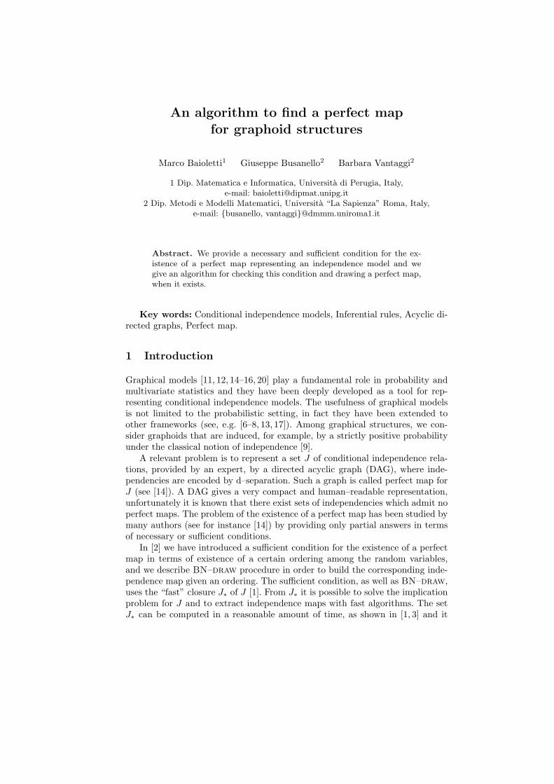
Proposition 1. Given θ1 = (A1, B1, C1) and θ2 = (A2, B2, C2), then θ1 v θ2 ifand only if the following conditions hold

(i) C2 ⊆ C1 ⊆ A2 ∪B2 ∪ C2;(ii) either A1 ⊆ A2 and B1 ⊆ B2 or A1 ⊆ B2 and B1 ⊆ A2.

Generalized inclusion is strictly related to the concept of dominance [15].In [1] we introduce a particular subset J∗ of J (called “fast closure”), which

can be computed from J by discarding the not “maximal” triples τ ∈ J , i.e.those g–included in some other triple of J . Moreover, in [1], we describe andcompare two different algorithms to compute J∗, called FC2 and FC1. In par-ticular, FC2 iteratively uses two inferential rules G4∗ and G5∗, related to G4and G5, introduced always in [1], and discards not maximal triples, until theset of independence relations is closed. FC1 has a similar structure, but uses asingle inference rule U, which corresponds to compute at once the fast closureof a couple of triples.

For some considerations and experimental results (see also [3]) FC1 appearsto be faster than FC2.

3 Graphs

In the following, we refer to the usual graph definitions (see [14]): we denote byG = (U , E) a graph with set U of nodes and oriented arcs E (ordered pairs ofnodes). In particular, we consider directed graphs having no cycles, i.e. acyclicdirected graphs (DAG). As usual, we denote by pa(u), for any u ∈ U , the parentset of u.

Definition 1. If A, B and C are three disjoint subsets of nodes in a DAG G,then C is said to d–separate A from B, denoted (A,B,C)G, if for each non–directed path between a node in A and a node in B, there exists a node x in thepath which satisfies one of these two conditions

1. x is a collider (i.e. both edges point to x), x 6∈ C and no descendant of x isin C;

2. x is not a collider and belongs to C.

In order to study the representation of a conditional independence model, weneed to distinguish between dependence map and independence map, since thereare conditional independence models that cannot be completely represented bya DAG (see e.g. [12, 14]).

In the following we denote with J (analogously for J , J∗) both a set of triplesand a set of conditional independence relations, obviously, the triples are definedon the set S and the independence relations on S.

Definition 2. Let J be a set of conditional independence relations on a set S.A DAG G = (S, E) is a dependence map (briefly a D–map) if for all triples(A,B, C) ∈ S(3)

(A, B,C) ∈ J ⇒ (A,B, C)G.

3

Moreover, G = (S, E) is an independence map (briefly an I–map) if for alltriples (A,B, C) ∈ S(3)

(A, B,C)G ⇒ (A,B,C) ∈ J .

G is a minimal I–map of J if deleting any arc, G is no more an I-map.G is said to be a perfect map (briefly a p–map) if it is both a I–map and a

D–map.

The next definition and theorem [14] provide a tool to build a DAG given anindependence model J .

Definition 3. Let J be an independence model defined on S and let π =<π1, . . . , πn > be an ordering of the elements of S. The boundary strata of J , rela-tive to π, is an ordered set of subsets < B(1), B(2), . . . , B(m) > of S (with m ≤ n),such that each B(i) is a minimal set satisfying B(i) ⊆ S(i) = {π1, . . . , πi−1} andγi = ({πi}, S(i)\B(i), B(i)) ∈ J . The DAG obtained by setting each B(i) as parentset of the node πi is called boundary DAG of J , relative to π.

The introduced triple γi is known as basic triple.The next theorem is an extension of Verma’s Theorem [18] stated for condi-

tional independence relations (see [14]).

Theorem 1. Let J be a independence model closed with respect to the semi–graphoid properties. If G is a boundary DAG of J , relative to any ordering π,then G is a minimal I–map of J .

Theorem 1 helps to build a DAG for an independence model J (induced bya probability P ) given an ordering π on indices of S. It is well known (see [14])that the boundary DAG of J relative to π is a minimal I–map. In the following,given an ordering π on S, Gπ is the corresponding I–map of J .

4 Perfect map

In [2] we have introduced some sufficient conditions for the existence of a perfectmap, given the fast closure J∗, and described the algorithm Backtrack whichchecks these conditions and, in the affirmative case, builds a perfect map. Sincethese conditions are only sufficient, this algorithm can fail also in the cases wherea perfect map exists.

In [4] we have improved the previous result by introducing conditions which,under a suitable hypothesis, are necessary and sufficient for the existence of aperfect map. This partial characterization relies on some constraints among thetriples of the set J∗ and their components.

In this paper we provide a necessary and sufficient condition valid also inthe case where the previously cited hypothesis fails (for the proof see [5]). Thesecondition fully characterizes the ordering from which a perfect map can be built.An algorithm able to check this condition and, in the positive case, to find aperfect map will be described in the next section.

4

In the following, we review the procedure BN–draw introduced in [2], whichbuilds the minimal I–map Gπ of J (see Definition 2) given the fast closure J∗ ofJ and an ordering π on S. This procedure is used by the algorithms describedin [2] and in this paper.

Note that, given the fast closure set J∗, it is not possible to apply the standardprocedure (see [11, 14]), described in Definition 3, to draw an I–map. In fact, thebasic triples, related to an arbitrary ordering π, might not be elements of J∗,but they could be just g–included in some triples of J∗ (see Example in [2]).

However, in [2] we have shown that it is easy to find the basic triples in thefast closure by using the following result, where, as in the rest of the paper,S(x) denotes the set of elements of S preceding x ∈ S, with respect to a givenordering π.

Proposition 2. Let J be a set of independence relations on S, J∗ its fast closureand π an ordering on S. For each x ∈ S, the set

Bx = {({x}, B, C) ∈ S(3) : B ∪ C = S(x), ∃ θ ∈ J∗ with ({x}, B,C) v θ}

is not empty if and only if the basic triple γx = ({x}, S(x) \ B(x), B(x)) exists,and coincides with the unique maximal triple γx of Bx.

In this paper, we describe a new version of BN–draw which uses the follow-ing operation. For each θ = (A,B, C) ∈ S(3), let X = (A ∪ B ∪ C) and for anyx ∈ S and P ⊆ S, define

Π(θ, P, x) =

P ∩ (A ∪ C) if C ⊆ P ⊆ X and x ∈ A

P ∩ (B ∪ C) if C ⊆ P ⊆ X and x ∈ B

P otherwise.

Algorithm 1 The set of parents of x

function PARENTS(x, P , K)pa ← Pfor all θ ∈ K do

p ← Π(θ, P, x)if |p| < |pa| then pa ← p

end forreturn pa

end function

The procedure BN–draw calls for each πi the function PARENTS and usesits results as parent set of πi.

Given π, BN–draw builds the minimal I–map Gπ in linear time with respectto the cardinality m of J∗ and the number of variables n. In fact, it is based on

5

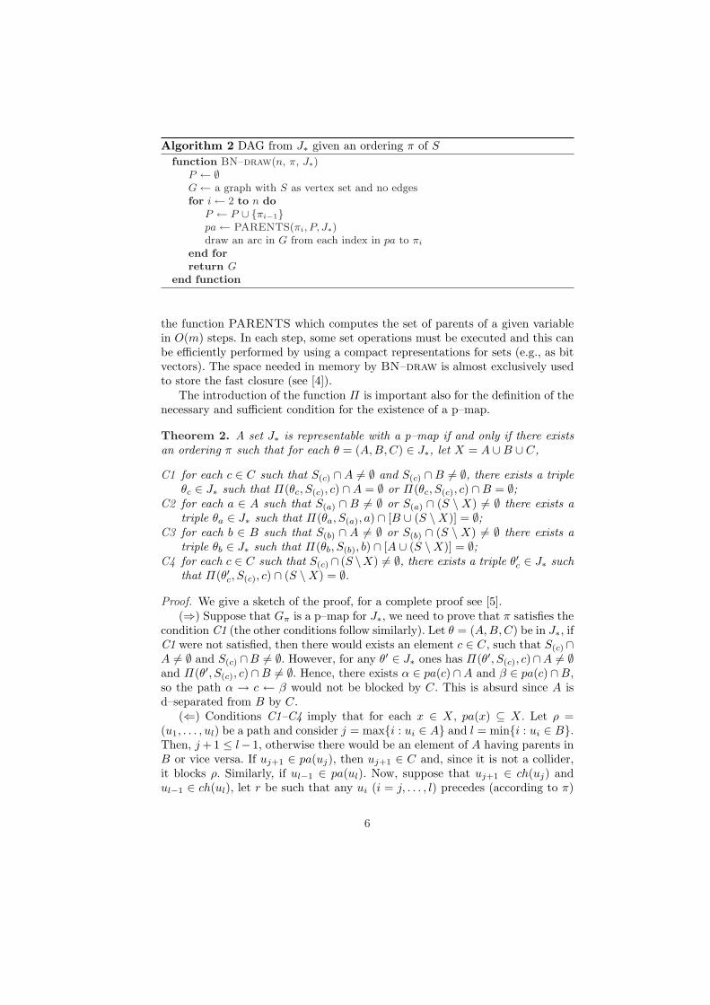
Algorithm 2 DAG from J∗ given an ordering π of S

function BN–draw(n, π, J∗)P ← ∅G ← a graph with S as vertex set and no edgesfor i ← 2 to n do

P ← P ∪ {πi−1}pa ← PARENTS(πi, P, J∗)draw an arc in G from each index in pa to πi

end forreturn G

end function

the function PARENTS which computes the set of parents of a given variablein O(m) steps. In each step, some set operations must be executed and this canbe efficiently performed by using a compact representations for sets (e.g., as bitvectors). The space needed in memory by BN–draw is almost exclusively usedto store the fast closure (see [4]).

The introduction of the function Π is important also for the definition of thenecessary and sufficient condition for the existence of a p–map.

Theorem 2. A set J∗ is representable with a p–map if and only if there existsan ordering π such that for each θ = (A,B, C) ∈ J∗, let X = A ∪B ∪ C,

C1 for each c ∈ C such that S(c) ∩A 6= ∅ and S(c) ∩B 6= ∅, there exists a tripleθc ∈ J∗ such that Π(θc, S(c), c) ∩A = ∅ or Π(θc, S(c), c) ∩B = ∅;

C2 for each a ∈ A such that S(a) ∩ B 6= ∅ or S(a) ∩ (S \X) 6= ∅ there exists atriple θa ∈ J∗ such that Π(θa, S(a), a) ∩ [B ∪ (S \X)] = ∅;

C3 for each b ∈ B such that S(b) ∩ A 6= ∅ or S(b) ∩ (S \ X) 6= ∅ there exists atriple θb ∈ J∗ such that Π(θb, S(b), b) ∩ [A ∪ (S \X)] = ∅;

C4 for each c ∈ C such that S(c) ∩ (S \X) 6= ∅, there exists a triple θ′c ∈ J∗ suchthat Π(θ′c, S(c), c) ∩ (S \X) = ∅.

Proof. We give a sketch of the proof, for a complete proof see [5].(⇒) Suppose that Gπ is a p–map for J∗, we need to prove that π satisfies the

condition C1 (the other conditions follow similarly). Let θ = (A,B, C) be in J∗, ifC1 were not satisfied, then there would exists an element c ∈ C, such that S(c)∩A 6= ∅ and S(c) ∩B 6= ∅. However, for any θ′ ∈ J∗ ones has Π(θ′, S(c), c)∩A 6= ∅and Π(θ′, S(c), c) ∩B 6= ∅. Hence, there exists α ∈ pa(c) ∩A and β ∈ pa(c) ∩B,so the path α → c ← β would not be blocked by C. This is absurd since A isd–separated from B by C.

(⇐) Conditions C1–C4 imply that for each x ∈ X, pa(x) ⊆ X. Let ρ =(u1, . . . , ul) be a path and consider j = max{i : ui ∈ A} and l = min{i : ui ∈ B}.Then, j + 1 ≤ l− 1, otherwise there would be an element of A having parents inB or vice versa. If uj+1 ∈ pa(uj), then uj+1 ∈ C and, since it is not a collider,it blocks ρ. Similarly, if ul−1 ∈ pa(ul). Now, suppose that uj+1 ∈ ch(uj) andul−1 ∈ ch(ul), let r be such that any ui (i = j, . . . , l) precedes (according to π)

6

ur. Thus, ur is a collider. If ur ∈ C, then j + 1 = r = l− 1 cannot be, otherwiseur would have parents both in A and in B. So, ur−1 or ur+1 is a parent of ur,belongs to C and blocks ρ. Otherwise, no descendent of ur belongs to C, so ur

blocks ρ. ut

The conditions C1–C4 are not so easy to check from the computational pointof view, because they require for each triple in J∗ and for x ∈ X to verify someconstraints and, when some of them do not hold, a suitable triple in J∗ needs tobe found. In the worst case, this process requires O(m2) steps, for each possibleordering. In the next section we will describe a more efficient way of achievingthe same result.

5 The algorithm

In this section we show how to use Theorem 2 to check whether J∗ is repre-sentable by a graph, and in the affirmative case to find a perfect map.

The main procedure is REPRESENT where [ ] denotes an empty sequence

Algorithm 3 Main function for representabilityfunction REPRESENT(J∗)

PREPROCESS(J∗)return SEARCH([ ], 1, S, J∗)

end function

of integers. The function PREPROCESS will be described in the following.The recursive function SEARCH incrementally tries to build an ordering π

satisfying conditions C1–C4 of Theorem 2. It returns the element ⊥ if it failsinto finding such an ordering. At the i–th recursive call it attempts to fix thei–th element in π, by selecting each of the remaining variables. For each possiblevariable x, the procedure CHECK–CONDS checks whether the conditions C1–C4 are not violated by setting πi as x. In the positive case, it calls itself until acomplete ordering is obtained. If no variable can be set at the i–th place of π,then the recursive call fails and a revision of the previously chosen variables isperformed (backtracking).

To check whether the choice of πi as x is correct we must verify whetherthe conditions C1–C4 are satisfied for all the triples in which x appears. Notethat we know all the variables preceding x, in fact S(x) is exactly the set{π1, π2, . . . , πi−1}. Hence, it is possible to compute the set of parents Q of xin the graph candidate to be a perfect map.

Let θ = (A,B,C) be a triple containing x. If x appears in C, then onlyconditions C1 and C4 must be checked. Let us see how to handle condition C1.It basically requires that if P intersects both A and B, there must exist a tripleτ ∈ K such that Π(τ, S(x), x) does not intersect both A and B.

7

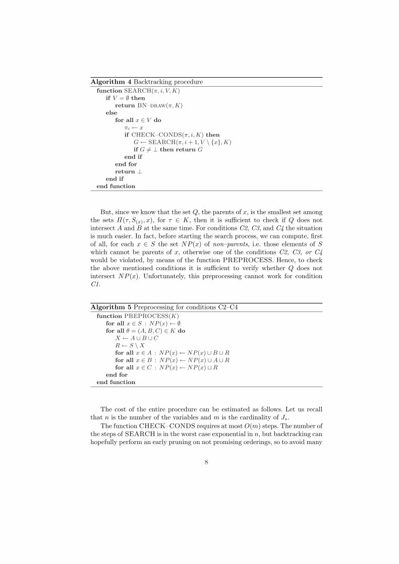
Algorithm 4 Backtracking procedurefunction SEARCH(π, i, V, K)

if V = ∅ thenreturn BN–draw(π, K)

elsefor all x ∈ V do

πi ← xif CHECK–CONDS(π, i, K) then

G ← SEARCH(π, i + 1, V \ {x}, K)if G 6= ⊥ then return G

end ifend forreturn ⊥

end ifend function

But, since we know that the set Q, the parents of x, is the smallest set amongthe sets Π(τ, S(x), x), for τ ∈ K, then it is sufficient to check if Q does notintersect A and B at the same time. For conditions C2, C3, and C4 the situationis much easier. In fact, before starting the search process, we can compute, firstof all, for each x ∈ S the set NP (x) of non–parents, i.e. those elements of Swhich cannot be parents of x, otherwise one of the conditions C2, C3, or C4would be violated, by means of the function PREPROCESS. Hence, to checkthe above mentioned conditions it is sufficient to verify whether Q does notintersect NP (x). Unfortunately, this preprocessing cannot work for conditionC1.

Algorithm 5 Preprocessing for conditions C2–C4function PREPROCESS(K)

for all x ∈ S : NP (x) ← ∅for all θ = (A, B, C) ∈ K do

X ← A ∪B ∪ CR ← S \Xfor all x ∈ A : NP (x) ← NP (x) ∪B ∪Rfor all x ∈ B : NP (x) ← NP (x) ∪A ∪Rfor all x ∈ C : NP (x) ← NP (x) ∪R

end forend function

The cost of the entire procedure can be estimated as follows. Let us recallthat n is the number of the variables and m is the cardinality of J∗.

The function CHECK–CONDS requires at most O(m) steps. The number ofthe steps of SEARCH is in the worst case exponential in n, but backtracking canhopefully perform an early pruning on not promising orderings, so to avoid many

8

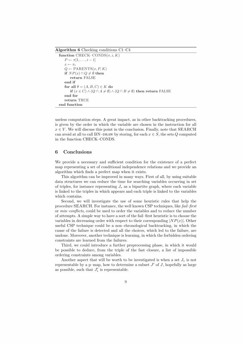
Algorithm 6 Checking conditions C1–C4function CHECK–CONDS(π, i, K)

P ← π[1, . . . , i− 1]x ← πi

Q ← PARENTS(x, P, K)if NP (x) ∩Q 6= ∅ then

return FALSEend iffor all θ = (A, B, C) ∈ K do

if (x ∈ C) ∧ (Q ∩A 6= ∅) ∧ (Q ∩B 6= ∅) then return FALSEend forreturn TRUE

end function

useless computation steps. A great impact, as in other backtracking procedures,is given by the order in which the variable are chosen in the instruction for allx ∈ V . We will discuss this point in the conclusion. Finally, note that SEARCHcan avoid at all to call BN–draw by storing, for each x ∈ S, the sets Q computedin the function CHECK–CONDS.

6 Conclusions

We provide a necessary and sufficient condition for the existence of a perfectmap representing a set of conditional independence relations and we provide analgorithm which finds a perfect map when it exists.

This algorithm can be improved in many ways. First of all, by using suitabledata structures we can reduce the time for searching variables occurring in setof triples, for instance representing J∗ as a bipartite graph, where each variableis linked to the triples in which appears and each triple is linked to the variableswhich contains.

Second, we will investigate the use of some heuristic rules that help theprocedure SEARCH. For instance, the well known CSP techniques, like fail–firstor min–conflicts, could be used to order the variables and to reduce the numberof attempts. A simple way to have a sort of the fail–first heuristic is to choose thevariables in decreasing order with respect to their corresponding |NP (x)|. Otheruseful CSP technique could be a non–chronological backtracking, in which thecause of the failure is detected and all the choices, which led to the failure, areundone. Moreover, another technique is learning, in which the forbidden orderingconstraints are learned from the failures.

Third, we could introduce a further preprocessing phase, in which it wouldbe possible to deduce, from the triple of the fast closure, a list of impossibleordering constraints among variables.

Another aspect that will be worth to be investigated is when a set J∗ is notrepresentable by a p–map, how to determine a subset J ′ of J , hopefully as largeas possible, such that J ′∗ is representable.

9

Finally, another possible way of enhancing this result is to find a new char-acterization for the existence of a p–map, which can generate a faster algorithm.

References

1. M. Baioletti, G. Busanello, B. Vantaggi (2009), Conditional independence structureand its closure: inferential rules and algorithms. Int. J. of Approx. Reason., 50, pp.1097 – 1114.

2. M. Baioletti, G. Busanello, B. Vantaggi (2009). Acyclic directed graphs to representconditional independence models. Lecture notes LNAI 5590, pp. 530–541.

3. M. Baioletti, G. Busanello, B. Vantaggi (2009). Closure of independencies undergraphoid properties: some experimental results. Proc. 6th Int. Symp. on ImpreciseProbability: Theories and Applications, pp. 11–19.

4. M. Baioletti, G. Busanello, B. Vantaggi (2009). Acyclic directed graphs represent-ing independence models. Int. J. of Approx. Reason. (submitted).

5. M. Baioletti, G. Busanello, B. Vantaggi (2010). Necessary and sufficient conditionsfor the existence of a perfect map. Tech. Rep. 01/2010. Univ. of Perugia.

6. G. Coletti, R. Scozzafava (2002). Probabilistic logic in a coherent setting. Dor-drecht/Boston/London: Kluwer (Trends in logic n.15).

7. F.G. Cozman, T. Seidenfeld (2007). Independence for full conditional measures,graphoids and Bayesian networks, Boletim BT/PMR/0711 Escola Politecnica daUniversidade de Sao Paulo, Sao Paulo, Brazil.

8. F. G. Cozman, P. Walley (2005). Graphoid properties of epistemic irrelevance andindependence. Ann. of Math. and Art. Intell., 45, pp. 173–195.

9. A.P. Dawid (1979). Conditional independence in statistical theory. J. Roy. Stat.Soc. B, 41, pp. 15–31.

10. P. R. de Waal, L. C. van der Gaag (2005). Stable Independence in Perfect Maps.Proc. 21st Conf. in Uncertainty in Artificial Intelligence, UAI ’05, Edinburgh, pp.161–168.

11. F.V. Jensen (1996). An introduction to Bayesian networks. UCL Press, Springer-Verlag.

12. S.L. Lauritzen (1996). Graphical models. Clarendon Press, Oxford.13. S. Moral, A. Cano (2002). Strong conditional independence for credal sets. Ann.

of Math. and Art. Intell., 35, pp. 295–321.14. J. Pearl (1988). Probabilistic reasoning in intelligent systems: networks of plausible

inference, Morgan Kaufmann, Los Altos, CA.15. M. Studeny (1997). Semigraphoids and structures of probabilistic conditional in-

dependence. Ann. of Math. Artif. Intell., 21, pp. 71–98.16. M. Studeny (2005). Probabilistic conditional independence structures, Springer-

Verlag, London.17. B. Vantaggi (2003). Conditional independence structures and graphical models.

Int. J. Uncertain. Fuzziness Knowledge-Based Systems, 11(5), pp. 545–571.18. T. S. Verma (1986). Causal networks: semantics and expressiveness. Tech. Rep.

R–65, Cognitive Systems Laboratory, University of California, Los Angeles.19. T. S. Verma, J. Pearl (1991). Equivalence and synthesis of causal models. Uncer-

tainty in Artificial Intelligence, 6, pp. 220–227.20. J. Witthaker (1990). Graphical models in applied multivariate statistic. Wiley &

Sons, New York.

10