An Algorithm for Finding the LargestApproximately Common Substructures of Two TreesJason T. L. Wang Bruce A. ShapiroDennis Shasha Kaizhong Zhang Kathleen M. Currey�Abstract | Ordered, labeled trees are trees in which each node has a label and the left-to-rightorder of its children (if it has any) is �xed. Such trees have many applications in vision, patternrecognition, molecular biology and natural language processing. We consider a substructure of anordered labeled tree T to be a connected subgraph of T . Given two ordered labeled trees T1 and T2and an integer d, the largest approximately common substructure problem is to �nd a substructureU1 of T1 and a substructure U2 of T2 such that U1 is within edit distance d of U2 and where theredoes not exist any other substructure V1 of T1 and V2 of T2 such that V1 and V2 satisfy the distanceconstraint and the sum of the sizes of V1 and V2 is greater than the sum of the sizes of U1 andU2. We present a dynamic programming algorithm to solve this problem, which runs as fast as thefastest known algorithm for computing the edit distance of two trees when the distance allowedin the common substructures is a constant independent of the input trees. To demonstrate theutility of our algorithm, we discuss its application to discovering motifs in multiple RNA secondarystructures (which are ordered labeled trees).Index Terms| Computational biology, dynamic programming, pattern matching, pattern recog-nition, trees.

�J. T. L. Wang is with the Department of Computer and Information Science, New Jersey Institute of Technology,University Heights, Newark, NJ 07102. E-mail: jason@cis.njit.edu. B. A. Shapiro is with the Image Processing Section,Laboratory of Experimental and Computational Biology, Division of Basic Sciences, National Cancer Institute, NationalInstitutes of Health, Frederick, MD 21702. E-mail: bshapiro@ncifcrf.gov. D. Shasha is with the Courant Institute ofMathematical Sciences, New York University, 251 Mercer Street, NY 10012. E-mail: shasha@cs.nyu.edu. K. Zhang is withthe Department of Computer Science, The University of Western Ontario, London, Ontario, Canada N6A 5B7. E-mail:kzhang@csd.uwo.ca. K. M. Currey is with the Image Processing Section, Laboratory of Experimental and ComputationalBiology, Division of Basic Sciences, National Cancer Institute, Frederick Cancer Research and Development Center, NationalInstitutes of Health, Frederick, MD 21702 and University of Maryland Medical Center, Department of Pediatrics, Baltimore,MD 21201. 1

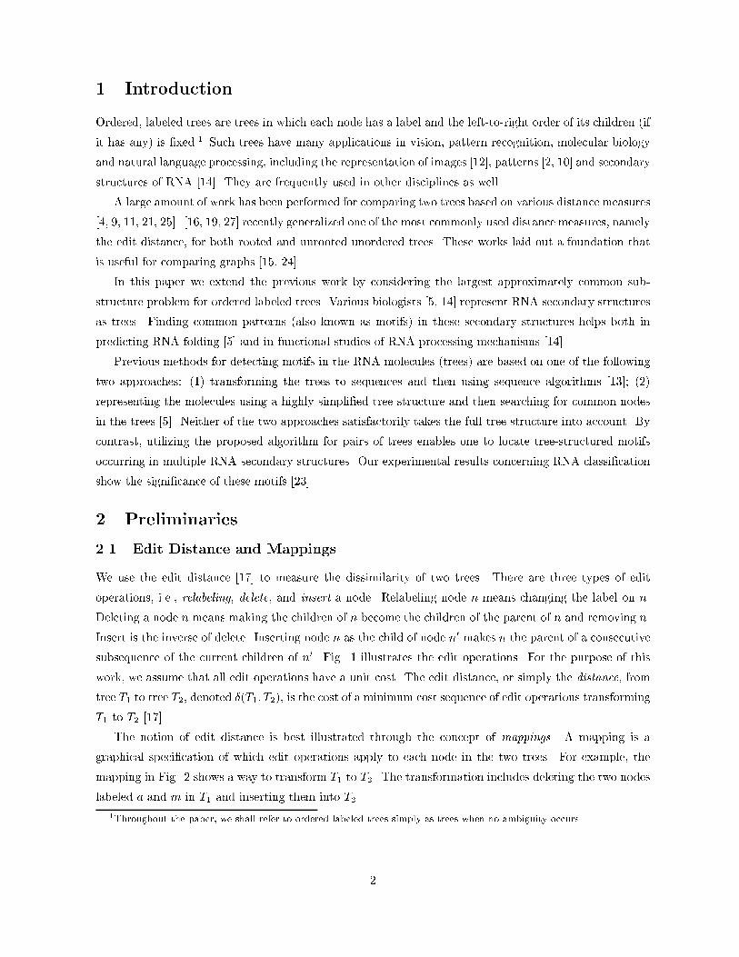
1 IntroductionOrdered, labeled trees are trees in which each node has a label and the left-to-right order of its children (ifit has any) is �xed.1 Such trees have many applications in vision, pattern recognition, molecular biologyand natural language processing, including the representation of images [12], patterns [2, 10] and secondarystructures of RNA [14]. They are frequently used in other disciplines as well.A large amount of work has been performed for comparing two trees based on various distance measures[4, 9, 11, 21, 25]. [16, 19, 27] recently generalized one of the most commonly used distance measures, namelythe edit distance, for both rooted and unrooted unordered trees. These works laid out a foundation thatis useful for comparing graphs [15, 24].In this paper we extend the previous work by considering the largest approximately common sub-structure problem for ordered labeled trees. Various biologists [5, 14] represent RNA secondary structuresas trees. Finding common patterns (also known as motifs) in these secondary structures helps both inpredicting RNA folding [5] and in functional studies of RNA processing mechanisms [14].Previous methods for detecting motifs in the RNA molecules (trees) are based on one of the followingtwo approaches: (1) transforming the trees to sequences and then using sequence algorithms [13]; (2)representing the molecules using a highly simpli�ed tree structure and then searching for common nodesin the trees [5]. Neither of the two approaches satisfactorily takes the full tree structure into account. Bycontrast, utilizing the proposed algorithm for pairs of trees enables one to locate tree-structured motifsoccurring in multiple RNA secondary structures. Our experimental results concerning RNA classi�cationshow the signi�cance of these motifs [23].2 Preliminaries2.1 Edit Distance and MappingsWe use the edit distance [17] to measure the dissimilarity of two trees. There are three types of editoperations, i.e., relabeling, delete, and insert a node. Relabeling node n means changing the label on n.Deleting a node n means making the children of n become the children of the parent of n and removing n.Insert is the inverse of delete. Inserting node n as the child of node n0 makes n the parent of a consecutivesubsequence of the current children of n0. Fig. 1 illustrates the edit operations. For the purpose of thiswork, we assume that all edit operations have a unit cost. The edit distance, or simply the distance, fromtree T1 to tree T2, denoted �(T1; T2), is the cost of a minimum cost sequence of edit operations transformingT1 to T2 [17].The notion of edit distance is best illustrated through the concept of mappings. A mapping is agraphical speci�cation of which edit operations apply to each node in the two trees. For example, themapping in Fig. 2 shows a way to transform T1 to T2. The transformation includes deleting the two nodeslabeled a and m in T1 and inserting them into T2.1Throughout the paper, we shall refer to ordered labeled trees simply as trees when no ambiguity occurs.2

1T T2

a cb

r

a b

r

rr

a f c

rr

e f

(i)

(ii)

(iii)

f

be

g h g h

f g

h h

f

f

g gg

Fig. 1. (i) Relabeling: To change one node label (a) to another (b). (ii) Delete: To delete a node;all children of the deleted node (labeled b) become children of the parent (labeled r). (iii) Insert:To insert a node; a consecutive sequence of siblings among the children of the node labeled r (here,f and the left g) become the children of the newly inserted node labeled b.r

a m

b c d e p

2T

r

a m

b c d e p

1T

Fig. 2. A mapping from tree T1 to tree T2.We use a postorder numbering of nodes in the trees. Let t[i] represent the node of T whose position inthe left-to-right postorder traversal of T is i. When there is no confusion, we also use t[i] to represent thelabel of node t[i]. Formally, a mapping from T1 to T2 is a triple (M;T1; T2) (or simply M if the context isclear), where M is any set of ordered pairs of integers (i; j) satisfying: (i) 1 � i � jT1j and 1 � j � jT2j;(ii) For any pair of (i1; j1) and (i2; j2) in M , (a) i1 = i2 i� j1 = j2 (one-to-one condition); (b) t1[i1] isto the left of t1[i2] i� t2[j1] is to the left of t2[j2] (sibling order preservation condition); (c) t1[i1] is an3

ancestor of t1[i2] i� t2[j1] is an ancestor of t2[j2] (ancestor order preservation condition). The cost of M isthe cost of deleting nodes of T1 not touched by a mapping line plus the cost of inserting nodes of T2 nottouched by a mapping line plus the cost of relabeling nodes in those pairs related by mapping lines withdi�erent labels. It can be proved [17] that �(T1; T2) equals the cost of a minimum cost mapping from treeT1 to tree T2.2.2 Cut OperationsWe de�ne a substructure U of tree T to be a connected subgraph of T . That is, U is rooted at a node nin T and is generated by cutting o� some subtrees in the subtree rooted at n. Formally, let T [i] representthe subtree rooted at t[i]. The operation of cutting at node t[i] means removing T [i]. A set S of nodes ofT [k] is said to be a set of consistent subtree cuts in T [k] if (i) t[i] 2 S implies that t[i] is a node in T [k],and (ii) t[i]; t[j] 2 S implies that neither is an ancestor of the other in T [k]. Intuitively, S is the set of allroots of the removed subtrees in T [k].We use Cut(T; S) to represent the tree T with subtree removals at all nodes in S. Let Subtrees(T )be the set of all possible sets of consistent subtree cuts in T . Given two trees T1 and T2 and an in-teger d, the size of the largest approximately common root-containing substructures within distancek, 0 � k � d, of T1[i] and T2[j], denoted �(T1[i]; T2[j]; k) (or simply �(i; j; k) when the context isclear), is maxfjCut(T1[i]; S1)j + jCut(T2[j]; S2)jg subject to �(Cut(T1[i]; S1); Cut(T2[j]; S2)) � k, S1 2Subtrees(T1[i]), S2 2 Subtrees(T2[j]). Finding the largest approximately common substructure (LACS),within distance d, of T1[i] and T2[j] amounts to calculating max1�u�i;1�v�j f�(T1[u]; T2[v]; d)g and locat-ing the Cut(T1[u]; Su) and Cut(T2[v]; Sv), Su 2 Subtrees(T1[u]), Sv 2 Subtrees(T2[v]) that achieve themaximum size. The size of LACS, within distance d, of T1 and T2 is max1�i�jT1j;1�j�jT2j f�(T1[i]; T2[j]; d)g.We shall focus on computing the maximum size. By memorizing the size information during the com-putation and by a simple backtracking technique, one can �nd both the maximum size and one of thecorresponding substructure pairs yielding the size in the same time and space complexity.3 Our Algorithm3.1 NotationWe use desc(i) to represent the set of postorder numbers of the descendants of the node t[i] and l(i)denotes the postorder number of the leftmost leaf of the subtree T [i]. When T [i] is a leaf, l(i) = i. T [i::j]is an ordered forest of tree T induced by the nodes numbered i to j inclusive (see Fig. 3). If i > j, thenT [i::j] = ;. The de�nition of mappings for ordered forests is the same as for trees. Let F1 and F2 be twoforests. The distance from F1 to F2, denoted �(F1; F2), equals the cost of a minimum cost mapping fromF1 to F2 [25].Let F = T [i::j]. A set S of nodes of F is said to be a set of consistent subtree cuts in F if (i) t[p] 2 Simplies that i � p � j, and (ii) t[p]; t[q] 2 S implies that neither is an ancestor of the other in F . Weuse Cut(F; S) to represent the sub-forest F with subtree removals at all nodes in S. Let Subtrees(F )4

be the set of all possible sets of consistent subtree cuts in F . De�ne the size of the largest approxi-mately common root-containing substructures, within distance k, of F1 and F2, denoted (F1; F2; k), tobe maxfjCut(F1; S1)j + jCut(F2; S2)jg subject to �(Cut(F1; S1); Cut(F2; S2)) � k, S1 2 Subtrees(F1),S2 2 Subtrees(F2). When F1 = T1[l(i)::s] and F2 = T2[l(j)::t], we also represent (F1; F2; k) by(l(i)::s; l(j)::t; k) if there is no confusion.T [2..8]T

[10]t

[4]t [9]t

[3][2][1]

[5] [6]

[8][7]t t t

t

t t

t

[4] [7] [8]

[6][5][3][2]

t t t

t t t t

Fig. 3. An induced ordered forest.3.2 Basic PropertiesLemma 3.1. Suppose s 2 desc(i) and t 2 desc(j). Then(i) (;; ;; 0) = 0;(ii) (T1[l(i)::s]; ;; 0) = 0;(iii) (;; T2[l(j)::t]; 0) = 0.Proof. Immediate from de�nitions.Lemma 3.2. Suppose s 2 desc(i) and t 2 desc(j). Then for all k, 1 � k � d,(i) (;; ;; k) = 0;(ii) (T1[l(i)::s]; ;; k) =max� (T1[l(i)::s� 1]; ;; k � 1) + 1;(T1[l(i)::l(s)� 1]; ;; k);(iii) (;; T2[l(j)::t]; k) =max� (;; T2[l(j)::t� 1]; k � 1) + 1;(;; T2[l(j)::l(t)� 1]; k):Proof. (i) follows from the de�nition. For (ii), suppose S1 2 Subtrees(T1[l(i)::s]) is a smallest set ofconsistent subtree cuts that maximizes jCut(T1[l(i)::s]; S1)j where �(Cut(T1[l(i)::s]; S1); ;) � k. Then oneof the following two cases must hold: (1) t1[s] 2 S1; (2) t1[s] 62 S1. If (1) is true, then (T1[l(i)::s]; ;; k)= (T1[l(i)::l(s)� 1]; ;; k); otherwise, (T1[l(i)::s], ;, k) = (T1[l(i)::s� 1], ;, k � 1) + 1. (iii) is provedsimilarly as for (ii). 5

Lemma 3.3. Suppose s 2 desc(i) and t 2 desc(j). If (l(s) 6= l(i) or l(t) 6= l(j)), then(l(i)::s; l(j)::t; 0) =max8<: (l(i)::l(s)� 1; l(j)::t; 0);(l(i)::s; l(j)::l(t)� 1; 0);(l(i)::l(s)� 1; l(j)::l(t)� 1; 0) + �(s; t; 0):Proof. Suppose S1 2 Subtrees(T1[l(i)::s]) and S2 2 Subtrees(T2[l(j)::t]) are two smallest sets of consis-tent subtree cuts that maximize jCut(T1[l(i)::s]; S1)j + jCut(T2[l(j)::t]; S2)j where �(Cut(T1[l(i)..s], S1),Cut(T2[l(j)::t], S2)) = 0. Then at least one of the following cases must hold:Case 1. t1[s] 2 S1 (i.e., the subtree T1[s] is removed). So, (l(i)::s; l(j)::t; 0) = (l(i)::l(s)�1, l(j)::t; 0).Case 2. t2[t] 2 S2 (i.e., the subtree T2[t] is removed). So, (l(i)::s; l(j)::t; 0) = (l(i)::s, l(j)::l(t)�1; 0).Case 3. t1[s] 62 S1 and t2[t] 62 S2 (i.e., neither T1[s] nor T2[t] is removed) (Fig. 4). Let M be themapping (with cost 0) from Cut(T1[l(i)::s]; S1) to Cut(T2[l(j)::t]; S2). In M , T1[s] must be mapped toT2[t] because otherwise we cannot have distance zero between Cut(T1[l(i)::s]; S1) and Cut(T2[l(j)::t]; S2).Therefore (l(i)::s; l(j)::t; 0) = (l(i)::l(s)� 1; l(j)::l(t)� 1; 0) + �(s; t; 0).Since these three cases exhaust all possible mappings yielding (l(i)::s; l(j)::t; 0), we take the maximumof the corresponding sizes, which gives the formula asserted by the lemma.[ l ( )... l (s)-1]i [s] [ l ( )... l ( )-1]j t t ]1 1 2 [2T T T TFig. 4. Illustration of the case in which one of T1[l(i)::s] and T2[l(j)::t] is a forest and neither T1[s]nor T2[t] is removed.Lemma 3.4. Suppose s 2 desc(i) and t 2 desc(j). Suppose both T1[l(i)::s] and T2[l(j)::t] are trees (i.e.,l(s) = l(i) and l(t) = l(j)). Then(l(i)::s; l(j)::t; 0) = � (l(i)::s� 1; l(j)::t� 1; 0) + 2 if t1[s] = t2[t];0 otherwise:Proof. Since l(s) = l(i) and l(t) = l(j), T1[l(i)::s] = T1[s] and T2[l(j)::t] = T2[t]. First, consider thecase where t1[s] = t2[t]. Suppose S1 2 Subtrees(T1[s]) and S2 2 Subtrees(T2[t]) are two smallest sets ofconsistent subtree cuts that maximize jCut(T1[s]; S1)j+ jCut(T2[t]; S2)j where �(Cut(T1[s]; S1), Cut(T2[t],S2)) = 0. Let M be the mapping (with cost 0) from Cut(T1[s]; S1) to Cut(T2[t]; S2) (see Fig. 5). Clearly,in M , t1[s] must be mapped to t2[t]. Furthermore, the largest common root-containing substructure ofT1[l(i)::s�1] and T2[l(j)::t�1] plus t1[s] (or t2[t]) must be the largest common root-containing substructure6

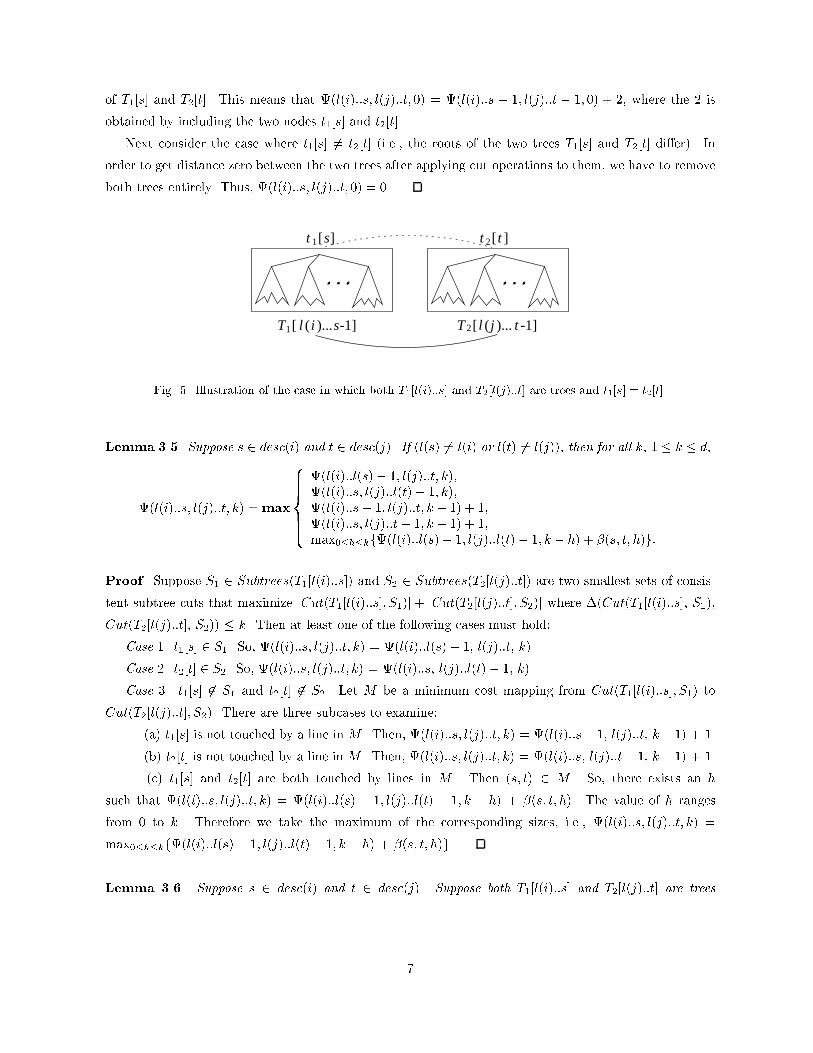
of T1[s] and T2[t]. This means that (l(i)::s; l(j)::t; 0) = (l(i)::s � 1; l(j)::t � 1; 0) + 2, where the 2 isobtained by including the two nodes t1[s] and t2[t].Next consider the case where t1[s] 6= t2[t] (i.e., the roots of the two trees T1[s] and T2[t] di�er). Inorder to get distance zero between the two trees after applying cut operations to them, we have to removeboth trees entirely. Thus, (l(i)::s; l(j)::t; 0) = 0.[ l ( )...i1 s-1]T [ l ( )...j2 t -1]T

s][1t [2 t ]t

Fig. 5. Illustration of the case in which both T1[l(i)::s] and T2[l(j)::t] are trees and t1[s] = t2[t].Lemma 3.5. Suppose s 2 desc(i) and t 2 desc(j). If (l(s) 6= l(i) or l(t) 6= l(j)), then for all k, 1 � k � d,(l(i)::s; l(j)::t; k) =max8>>>><>>>>: (l(i)::l(s)� 1; l(j)::t; k);(l(i)::s; l(j)::l(t)� 1; k);(l(i)::s� 1; l(j)::t; k � 1) + 1;(l(i)::s; l(j)::t� 1; k � 1) + 1;max0�h�kf(l(i)::l(s)� 1; l(j)::l(t)� 1; k � h) + �(s; t; h)g:Proof. Suppose S1 2 Subtrees(T1[l(i)::s]) and S2 2 Subtrees(T2[l(j)::t]) are two smallest sets of consis-tent subtree cuts that maximize jCut(T1[l(i)::s]; S1)j + jCut(T2[l(j)::t]; S2)j where �(Cut(T1[l(i)::s], S1),Cut(T2[l(j)::t], S2)) � k. Then at least one of the following cases must hold:Case 1. t1[s] 2 S1. So, (l(i)::s; l(j)::t; k) = (l(i)::l(s)� 1, l(j)::t, k).Case 2. t2[t] 2 S2. So, (l(i)::s; l(j)::t; k) = (l(i)::s, l(j)::l(t)� 1, k).Case 3. t1[s] 62 S1 and t2[t] 62 S2. Let M be a minimum cost mapping from Cut(T1[l(i)::s]; S1) toCut(T2[l(j)::t]; S2). There are three subcases to examine:(a) t1[s] is not touched by a line in M . Then, (l(i)::s; l(j)::t; k) = (l(i)::s� 1, l(j)::t, k� 1) + 1.(b) t2[t] is not touched by a line in M . Then, (l(i)::s; l(j)::t; k) = (l(i)::s, l(j)::t� 1, k� 1) + 1.(c) t1[s] and t2[t] are both touched by lines in M . Then (s; t) 2 M . So, there exists an hsuch that (l(i)::s; l(j)::t; k) = (l(i)::l(s) � 1; l(j)::l(t) � 1; k � h) + �(s; t; h). The value of h rangesfrom 0 to k. Therefore we take the maximum of the corresponding sizes, i.e., (l(i)::s; l(j)::t; k) =max0�h�kf(l(i)::l(s)� 1; l(j)::l(t)� 1; k � h) + �(s; t; h)g.Lemma 3.6. Suppose s 2 desc(i) and t 2 desc(j). Suppose both T1[l(i)::s] and T2[l(j)::t] are trees7

(i.e., l(s) = l(i) and l(t) = l(j)). Then for all k, 1 � k � d,(l(i)::s; l(j)::t; k) =max8<: (l(i)::s� 1; l(j)::t; k � 1) + 1;(l(i)::s; l(j)::t� 1; k � 1) + 1;(l(i)::s� 1; l(j)::t� 1; k � c) + 2;where c = � 0 if t1[s] = t2[t];1 otherwise:Proof. Since T1[l(i)::s] and T2[l(j)::t] are trees, T1[l(i)::s] = T1[s] and T2[l(j)::t] = T2[t]. We �rst show thatremoving either T1[s] or T2[t] would not yield the maximum size. There are three cases to be considered:Case 1. Both T1[s] and T2[t] are removed. Then, (l(i)::s; l(j)::t; k) = 0. However, since k � 1, cuttingat just the children of t1[s] and t2[t] would cause (l(i)::s; l(j)::t; k) � 2. Therefore removing both T1[s]and T2[t] cannot yield the maximum size.Case 2. Only T1[s] is removed. Then, (l(i)::s; l(j)::t; k) = �(;; T2[t]; k). Assume without loss ofgenerality that jT2[t]j � k. The above equation implies that we have to remove some subtrees from T2[t]so that there are no more than k nodes left in T2[t]. Thus, (l(i)::s; l(j)::t; k) = �(;; T2[t]; k) = k: On theother hand, if we just cut at the children of t1[s] and leave t1[s] in the tree, we would map t1[s] to t2[t].This would lead to (l(i)::s; l(j)::t; k) � (;; T2[l(j)::t� 1]; k� 1)+2 = k+1. Thus, removing T1[s] alonecannot yield the maximum size.Case 3. Only T2[t] is removed. The proof is similar to that in Case 2.The above arguments lead to the conclusion that in order to obtain the maximum size, neither T1[s]nor T2[t] can be removed. Now suppose S1 2 Subtrees(T1[s]) and S2 2 Subtrees(T2[t]) are two smallestsets of consistent subtree cuts that maximize jCut(T1[s]; S1)j + jCut(T2[t]; S2)j where �(Cut(T1[s]; S1),Cut(T2[t]; S2)) � k. Let M be a minimum cost mapping from Cut(T1[s]; S1) to Cut(T2[t]; S2). Then atleast one of the following cases must hold:Case 1. t1[s] is not touched by a line in M . So, (l(i)::s; l(j)::t; k) = (l(i)::s� 1, l(j)::t, k � 1) + 1.Case 2. t2[t] is not touched by a line in M . So, (l(i)::s; l(j)::t; k) = (l(i)::s, l(j)::t� 1, k � 1) + 1.Case 3. Both t1[s] and t2[t] are touched by lines in M . By the ancestor order preservation and siblingorder preservation conditions on mappings (cf. Section 2.1), (s; t) must be in M . Thus, if t1[s] = t2[t], wehave (l(i)::s; l(j)::t; k) = (l(i)::s � 1; l(j)::t � 1; k) + 2; otherwise, since mapping t1[s] to t2[t] costs 1,we have (l(i)::s; l(j)::t; k) = (l(i)::s� 1; l(j)::t� 1; k � 1) + 2.3.3 The AlgorithmFrom Lemma 3.4 and Lemma 3.6, we observe that when s is on the path from l(i) to i and t is onthe path from l(j) to j, we need not compute �(s; t; k), 0 � k � d, separately, since they can beobtained during the computation of �(i; j; k). Thus, we will only consider nodes that are either theroots of the trees or having a left sibling. Let keynodes(T ) contain all such nodes of a tree T , i.e.,keynodes(T ) = fkjthere exists no k0 > k such that l(k) = l(k0)g. For each i 2 keynodes(T1) and j 2keynodes(T2), Procedure Find-Largest-1 in Fig. 6 computes �(s; t; 0) for l(i) � s � i and l(j) � t � j and8

Procedure Find-Largest-2 in Fig. 6 computes �(s; t; k) for 1 � k � d. The main algorithm is summarizedin Fig. 6.Now, to calculate the size of the largest approximately common substructures (LACSs), within distanced, of T1[i] and T2[j], we build, in a bottom-up fashion, another array (i; j; d), 1 � i � jT1j, 1 � j � jT2j,using �(i; j; d) as follows. Let L = max1�u�s (iu; j; d) where i1 : : : is are the postorder numbers of thechildren of t1[i] or L = 0 if t1[i] is a leaf. Let R = max1�v�t (i; jv; d) where j1 : : : jt are the postordernumbers of the children of t2[j] or R = 0 if t2[j] is a leaf. Calculate (i; j; d) = maxf�(i; j; d); L;Rg. Thesize of LACSs, within distance d, of T1[i] and T2[j] is (i; j; d). The size of LACSs, within distance d, ofT1 and T2 is (jT1j; jT2j; d).Consider the complexity of the algorithm. We use an array to hold , � and , respectively. Thesearrays require O(d � jT1j � jT2j) space. Regarding the time complexity, given �(i; j; d), 1 � i � jT1j,1 � j � jT2j, calculating (i; j; d) requires O(jT1j� jT2j) time. For a �xed i and j, Procedure Find-Largest-1 requires O(jT1[i]j � jT2[j]j) time and Procedure Find-Largest-2 requires O(d2 � jT1[i]j � jT2[j]j) time. Sothe total time is bounded byXi2keynodes(T1) Xj2keynodes(T2)O(jT1[i]j � jT2[j]j) +O(d2 � jT1[i]j � jT2[j]j)� O( Xi2keynodes(T1) Xj2keynodes(T2) d2 � jT1[i]j � jT2[j]j)� O(d2 � Xi2keynodes(T1) jT1[i]j � Xj2keynodes(T2) jT2[j]j):From [25, Theorem 2], the last term above is bounded by O(d2 � jT1j � jT2j �min(H1; L1)�min(H2; L2))where Hi, i = 1; 2, is the height of Ti and Li is the number of leaves in Ti. When d is a constant, thisis the same as the complexity of the best current algorithm for tree matching based on the edit distance[11, 25], even though the problem at hand appears to be harder than tree matching.Note that to calculate max1�i�jT1j;1�j�jT2jf�(i; j; 0)g, one could use a faster algorithm that runs intime O(jT1j � jT2j). However, the reason for considering the keynodes and the formulas as speci�ed inLemmas 3.3 and 3.4 is to prepare the optimal sizes from forests to forests and store these size values in thearray to be used in calculating �(s; t; k) for k 6= 0. Even if one could incorporate the faster algorithm intothe Find-Largest algorithm, the overall time complexity would not be changed, because the calculation of�(s; t; k) for k 6= 0 dominates the cost.4 Implementation and DiscussionWe have applied our algorithm to �nd motifs in multiple RNA secondary structures. In this experiment, weexamined three phylogenetically related families of mRNA sequences chosen from GenBank [1] pertainingto the poliovirus, human rhinovirus and coxsackievirus. Each family contained two sequences, as shownin Table 1. 9

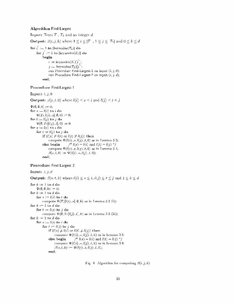
Algorithm Find-LargestInput: Trees T1, T2 and an integer d.Output: �(i; j; k) where 1 � i � jT1j, 1 � j � jT2j and 0 � k � d.for i0 := 1 to jkeynodes(T1)j dofor j0 := 1 to jkeynodes(T2)j dobegini := keynodes(T1)[i0 ];j := keynodes(T2)[j0 ];run Procedure Find-Largest-1 on input (i; j; 0);run Procedure Find-Largest-2 on input (i; j; d);end;Procedure Find-Largest-1Input: i; j; 0.Output: �(s; t; 0) where l(i) � s � i and l(j) � t � j.(;; ;; 0) := 0;for s := l(i) to i do(T1[l(i)::s]; ;; 0) := 0;for t := l(j) to j do(;; T2[l(j)::t]; 0) := 0;for s := l(i) to i dofor t := l(j) to j doif (l(s) 6= l(i) or l(t) 6= l(j)) thencompute (l(i)::s; l(j)::t; 0) as in Lemma 3.3;else begin /* l(s) = l(i) and l(t) = l(j) */compute (l(i)::s; l(j)::t; 0) as in Lemma 3.4;�(s; t; 0) := (l(i)::s; l(j)::t; 0);end;Procedure Find-Largest-2Input: i; j; d.Output: �(s; t; k) where l(i) � s � i, l(j) � t � j and 1 � k � d.for k := 1 to d do(;; ;; k) := 0;for k := 1 to d dofor s := l(i) to i docompute (T1[l(i)::s]; ;; k) as in Lemma 3.2 (ii);for k := 1 to d dofor t := l(j) to j docompute (;; T2[l(j)::t]; k) as in Lemma 3.2 (iii);for k := 1 to d dofor s := l(i) to i dofor t := l(j) to j doif (l(s) 6= l(i) or l(t) 6= l(j)) thencompute (l(i)::s; l(j)::t; k) as in Lemma 3.5;else begin /* l(s) = l(i) and l(t) = l(j) */compute (l(i)::s; l(j)::t; k) as in Lemma 3.6;�(s; t; k) := (l(i)::s; l(j)::t; k);end; Fig. 6. Algorithm for computing �(i; j; k).10

Family Sequence # of trees File #poliovirus polio3 sabin strain 3,026 �le 1pol3mut 3,000 �le 2human rhinovirus rhino 2 3,000 �le 3rhino 14 3,000 �le 4coxsackievirus cox5 3,000 �le 5cvb305pr 2,999 �le 6Table 1. Data used in the experiment.Under physiological conditions, i.e., at or above the room temperature, these RNA molecules do nottake on only a single structure. They may change their conformation between structures with similar freeenergies or be trapped in local minima. Thus, one has to consider not only the optimal structure but allstructures within a certain range of free energies. On the other hand, a loose rule of thumb is that the\real" structure of an RNA molecule appears in the top 5% - 10% of suboptimal structures of the sequencebased on the ranking of their energies with the minimum energy one (i.e. the optimal one) being at thetop. Therefore, we folded the 5' non-coding region of the selected mRNA sequences and collected (roughly)the top 3,000 suboptimal structures for each sequence. We then transformed these suboptimal structuresinto trees using the algorithms described in [13, 14]. Fig. 7 illustrates an RNA secondary structure andits tree representation.The structure is decomposed into �ve terms: stem, hairpin, bulge, internal loop and multi-branch loop[14]. In the tree, H represents hairpin nodes, I represents internal loops, B represents bulge loops, Mrepresents multi-branch loops, R represents helical stem regions (shown as connecting arcs) and N is aspecial node used to make sure the tree is connected. The tree is considered to be an ordered one wherethe ordering is imposed based upon the 5' to 3' nature of the molecule. The resulting trees for each mRNAsequence selected from GenBank were stored in a separate �le, where the trees had between 70 and 180nodes (cf. Table 1). Each tree is represented by a fully parenthesized notation where the root of everysubtree precedes all the nodes contained in the subtree. Thus, for example, the tree depicted in Fig. 7(ii)is represented as (N(R(I(R(M(R(B(R(M(R(H))(R(H))))))(R(H))))))).For each pair of trees T1, T2 in a �le, we ran the algorithm Find-Largest on T1, T2, �nding the size ofthe largest approximately common substructures, within distance 1, for each subtree pair T1[i] and T2[j],1 � i � jT1j and 1 � j � jT2j, and locating one of the corresponding substructure pairs yielding the size.These substructures constituted candidate motifs. Then we calculated the occurrence number2 of eachcandidate motif M by adding variable length don't cares (VLDCs) to M as the new root and leaves toform a VLDC pattern V and then comparing V with each tree T in the �le using the pattern matchingtechnique developed in [26]. (A VLDC (conventionally denoted by \�") can be matched, at no cost, witha path or portion of a path in T . The technique calculates the minimum distance between V and T afterimplicitly computing an optimal substitution for the VLDCs in V , allowing zero or more cuttings at nodesfrom T (see Fig. 8).) This way we can locate the motifs approximately occurring in all (or the majority2The occurrence number of a motif M with respect to distance k refers to the number of trees of the �le in which Mapproximately occurs (i.e. these trees approximately contain M) within distance k.11

of) the trees in the �le.3110

U AU

AA

A UG CC G

C

A

U

UA

CAUA

UGUAUAAAU

UA

GG

A

AGC

A

C

G

C

CG

GGU

CUGU

U

GC C

C

AC

CU

GC

GG

G

U

AG

AU A

CC

U

G

51

U

U

CG

AA

C

C

U

U

H

M

B H

M

H

I

N

A

(i)

(ii)

A A G C A A G U U C A U U U C G C C A U U A A G

1

Fig. 7. Illustration of a typical RNA secondary structure and its tree representation. (i)Normal polygonal representation of the structure. (ii) Tree representation of the structure.Table 2 summarizes the results where the motifs occur within distance 0 in at least 350 trees in thecorresponding �le. The table shows the number of motifs discovered for each sequence, the number ofdistinct motifs found in common between both sequences of each family, and the minimum and maximumsizes of these common motifs. Table 3 shows some big motifs found in common in all the three familiesand the number of each sequence's secondary structures that contain the motifs. These motifs serve as astarting point to conduct further study of common motif analysis [3, 22].3One can speed up this method by encoding the candidate motifs into a su�x tree and then using the statistical samplingand optimization techniques described in [23] to �nd the motifs.12

**

TV

a

b c

r

y x z

a

b d

h i m p

j n

*

Fig. 8. Matching a VLDC pattern V and a tree T (both the pattern and tree are hy-pothetical ones solely used for illustration purposes). The root � in V would be matchedwith nodes r; x in T , and the two leaves � in V would be matched with nodes i; j and m;nin T , respectively. Nodes y; z; h; p in T would be cut. The distance of V and T would be1 (representing the cost of changing c in V to d in T ).Family Sequence # of motifs found # of common motifs min size max sizepoliovirus polio3 sabin strain 836 347 3 101pol3mut 793rhinovirus rhino 2 287 70 3 10rhino 14 283coxsackievirus cox5 306 136 3 20cvb305pr 391Table 2. Statistics concerning motifs discovered from the secondary structures of the mRNA sequences used inthe experiment.Motifs found polio3 pol3mut rhino 2 rhino 14 cox 5 cvb305pr(R(M(R(I(R(H))))(R(B(R))))) 2,496 1,829 791 357 815 2,478(R(M(R(H))(R(I(R))))) 3,024 3,000 3,000 801 2,997 2,999(R(B(R(B(R(B(R))))))) 2,272 1,822 3,000 2,252 2,997 2,979(R(M(R)(R(I(R(H)))))) 2,074 1,712 3,000 702 2,997 2,999(R(M(R(I(R)))(R(H)))) 754 1,498 2,463 2,794 2,744 2,197Table 3. Motifs found in common in the secondary structures of the poliovirus, human rhinovirus and coxsack-ievirus sequences. The motifs are represented in a fully parenthesized notation where the root of every subtreeprecedes all the nodes contained in the subtree. For each motif, the table also shows the number of each sequence'ssuboptimal structures that contain the motif. 13

The proposed algorithm and the discovered motifs have also been applied to RNA classi�cation success-fully [23]. Our experimental results showed that one can get more intersections of motifs from sequencesof the same family. This indicates that closeness in motif corresponds to closeness in family. Anotherapplication of our algorithm is to apply it to a tree T and itself and calculate �(i; j; 0) for 1 � i; j � jT j.This allows one to �nd repeatedly occurring substructures (or repeats for short) in T . Finding repeats insecondary structures across di�erent RNA sequences may help understand the structures of RNA. Readersinterested in obtaining these programs may send a written request to any one of the authors.Our work is based on the edit distance originated in [17]. This metric is more permissive than otherworthy metrics (e.g. [18, 19, 20]) and therefore helps to locate subtle motifs existing in RNA secondarystructures. The algorithm presented here assumes a unit cost for all edit operations. In practice, a morere�ned non-unit cost function can re ect more subtle di�erences in the RNA secondary structures [14]. Itwould then be interesting to score the measures in detecting common substructures or repeats in trees.Another interesting problem is to �nd a largest consensus motif T3 in two input trees T1 and T2 where T3is a largest tree such that each of T1 and T2 has a substructure that is within a given distance to T3. Acomparison of the di�erent types of common substructures (see also [6, 7, 8]), probably based on di�erentmetrics (e.g. [18, 19, 20]), as well as their applications remains to be explored.AcknowledgmentsWe wish to thank the anonymous reviewers for their constructive suggestions and pointers to some rele-vant papers. We also thank Wojcieok Kasprzak (National Cancer Institute), Nat Goodman (WhiteheadInstitute of MIT) and Chia-Yo Chang for their useful comments and implementation e�orts. This workwas supported by the National Science Foundation under Grants IRI-9224601, IRI-9224602, IRI-9531548,IRI-9531554, and by the Natural Sciences and Engineering Research Council of Canada under GrantOGP0046373.References[1] C. Burks, M. Cassidy, M. J. Cinkosky, K. E. Cumella, P. Gilna, J. E.-D. Hayden, G. M. Keen, T. A.Kelley, M. Kelly, D. Kristo�erson, and J. Ryals. GenBank. Nucleic Acids Research, 19:2221{2225,1991.[2] Y. C. Cheng and S. Y. Lu. Waveform correlation by tree matching. IEEE Trans. Pattern Anal.Machine Intell., 7:299{305, May 1985.[3] K. M. Currey and B. A. Shapiro. Secondary structure computer prediction of the polio virus 5'non-coding region is improved with a genetic algorithm. Comput. Applic. Biosci., 13(1):1-12, 1997.[4] T. Jiang, L. Wang, and K. Zhang. Alignment of trees { An alternative to tree edit. In M. Crochemoreand D. Gus�eld, editors, Combinatorial Pattern Matching, Lecture Notes in Computer Science, 807,pages 75{86. Springer-Verlag, 1994. 14

[5] S.-Y. Le, J. Owens, R. Nussinov, J.-H. Chen, B. A. Shapiro, and J. V. Maizel. RNA secondary struc-tures: Comparison and determination of frequently recurring substructures by consensus. Comput.Applic. Biosci., 5(3):205{210, 1989.[6] S. Liu and E. Tanaka. A largest common similar substructure problem for trees embedded in a plane.Technical Report of the Institute of Electronics, Information and Communication Engineers, COMP95{74, Jan. 1996.[7] S. Liu and E. Tanaka. Largest common similar substructures of rooted and unordered trees. Mem.Grad. School Sci. & Technol., Kobe Univ., 14-A:107{119, 1996.[8] S. Liu and E. Tanaka. The largest common similar substructure problem. IEICE Trans. Fundamentals,E80-A:643{650, 1997.[9] S. Y. Lu. A tree-matching algorithm based on node splitting and merging. IEEE Trans. PatternAnal. Machine Intell., 6(2):249{256, Mar. 1984.[10] B. Moayer and K. S. Fu. A tree system approach for �ngerprint pattern recognition. IEEE Trans.Pattern Anal. Machine Intell., 8:376{387, May 1986.[11] K. Ohmori and E. Tanaka. A uni�ed view on tree metrics. In Preprint of the Workshop on Syntacticand Structural Pattern Recognition (Barcelona, 1986). Syntactic and Structural Pattern Recognition,Eds. G. Ferrate et al., Springer, 1988.[12] H. Samet. Distance transform for images represented by quadtrees. IEEE Trans. Pattern Anal.Machine Intell., 4(3):298{303, May 1982.[13] B. A. Shapiro. An algorithm for comparing multiple RNA secondary structures. Comput. Applic.Biosci., 4(3):387{393, 1988.[14] B. A. Shapiro and K. Zhang. Comparing multiple RNA secondary structures using tree comparisons.Comput. Applic. Biosci., 6(4):309{318, 1990.[15] L. G. Shapiro and R. M. Haralick. Structural descriptions and inexact matching. IEEE Trans. PatternAnal. Machine Intell., 3(5):504{519, Sep. 1981.[16] D. Shasha, J. T. L. Wang, K. Zhang, and F. Y. Shih. Exact and approximate algorithms for unorderedtree matching. IEEE Transactions on Systems, Man and Cybernetics, 24(4):668{678, April 1994.[17] K.-C. Tai. The tree-to-tree correction problem. J. ACM, 26(3):422{433, 1979.[18] E. Tanaka. The metric between rooted and ordered trees based on strongly structure preservingmapping and its computing method. IECE Trans., J67-D(6):722{723, 1984.[19] E. Tanaka. A metric between unrooted and unordered trees and its bottom-up computing method.IEEE Trans. Pattern Anal. Machine Intell., 16(12):1233{1238, Dec. 1994.15

[20] (a) E. Tanaka and K. Tanaka. A metric on trees and its computing method. IECE Trans., J65-D(5):511{518, 1982. (b) Correction to \A metric on trees and its computing method." IEICE Trans.,J76-D-I(11):635, 1993.[21] E. Tanaka and K. Tanaka. The tree-to-tree editing problem. International Journal of Pattern Recog-nition and Arti�cial Intelligence, 2(2):221{240, 1988.[22] Z. Tu, N. M. Chapman, G. Hufnagel, S. Tracy, B. A. Shapiro, J. R. Romero, W. H. Barry, L. Zhao,and K. M. Currey. The cardiovirulent phenotype of coxsackievirus B3 is determined at a single sitein the genomic 5' non-translated region. J. Virology, 69:4607{4618, 1995.[23] J. T. L. Wang, B. A. Shapiro, D. Shasha, K. Zhang, and C.-Y. Chang. Automated discovery of activemotifs in multiple RNA secondary structures. In Proceedings of the 2nd International Conference onKnowledge Discovery and Data Mining, pages 70{75, Portland, Oregon, August 1996.[24] A. K. Wong, M. You, and S. C. Chang. An algorithm for graph optimal monomorphism. IEEETransactions on Systems, Man and Cybernetics, 20:628{639, 1990.[25] K. Zhang and D. Shasha. Simple fast algorithms for the editing distance between trees and relatedproblems. SIAM Journal on Computing, 18(6):1245{1262, Dec. 1989.[26] K. Zhang, D. Shasha, and J. T. L. Wang. Approximate tree matching in the presence of variablelength don't cares. Journal of Algorithms, 16(1):33{66, Jan. 1994.[27] K. Zhang, J. T. L. Wang, and D. Shasha. On the editing distance between undirected acyclic graphs.International Journal of Foundations of Computer Science, 7(1):43{57, March 1996.

16