Study of degenerate parabolic system modeling the hydrogen ...
Upload
independentCategory
view
2download
0
International Journal of Physics
and Research (IJPR)
ISSN(P): 2250-0030; ISSN(E): 2319-4499
Vol. 4, Issue 1, Feb 2014, 5-14
© TJPRC Pvt. Ltd.
AMPLITUDE RESPONSE OF PSF WITH PARABOLIC APODIZATION FILTERS UNDER
DIFFERENT CONDITIONS OF TRANSMISSION
TIRUPATHI POTHU1 & SIVA PRASAD PEDDI
2
1Department of Mathematics, Osmania University, Hyderabad, Andhra Pradesh, India
2Professor, Department of Physics, College of Arts and Sciences,
Al Jouf University, Al Qurayat, Kingdom of Saudi Arabia
ABSTRACT
In all the branches of science, engineering and technology, it is known that the output due to an input impulse
function, spatial or temporal, is never an impulse. There is a spread of the input impulse function in the output due to the
noise introduced by the physical device. The expression for the distributions of the complex amplitude of the diffracted
light using circular apertures with Parabolic Apodization Filters(PAF) has been evaluated. The Amplitude Response of the
Point Spread Function (APSF) has been evaluated for various values of the apodisation parameter ( = 0.25, 0.5, 0.75, 1.0)
for different conditions of transmission ( ) where the system acts as an annular aperture with central obscuration (=0) to
a value of where the pupil transmission is circularly symmetric and reduces to Airy transmission for (=1). From the
evaluated results obtained Maximum Negative Value (MNV) has been analyzed and it was found that an adequate
explanation of the results obtained by large optical systems absolutely depends on this knowledge.
KEYWORDS: Amplitude Point Spread Function (APSF), Parabolic Filters, Apodization Parameter, Maximum Negative
Value
INTRODUCTION
The ideal point spread function (PSF) is the three-dimensional diffraction pattern of light emitted from an
infinitely small point source in the specimen and transmitted to the image plane through a high numerical aperture
objective. It is considered to be the fundamental unit of an image in theoretical models of image formation. When light is
emitted from such a point object, a fraction of it is collected by the objective and focused at a corresponding point in the
image plane. However, the objective lens does not focus the emitted light to an infinitely small point in the image plane.
Rather, light waves converge and interfere at the focal point to produce a diffraction pattern of concentric rings of light
surrounding a central, bright disk, when viewed in the x-y plane. The radius of disk is determined by the numerical
aperture, thus the resolving power of an objective lens can be evaluated by measuring the size of the Airy disk.
The problem was first studied by Airy in 1834 and then developed by Lord Rayleigh by investigating the light distributions
in the images of discs in the presence of spherical aberration. Rayleigh evaluated the central intensity by developing the
diffraction integrals into series and indicated that the outer intensities might be calculated by the method of mechanical
quadratures.
The mathematical theory of the light distributions in three dimensions at and near the focus of an optical system
with a circular pupil had been studied in a classical work by LOMMEL [1] who himself verified his calculations
experimentally. STRUVE [2] had published a similar but less comprehensive analysis of intensity distributions near the
edges of geometric shadows. SCHARTZCHILD [3] had also contributed to this subject for points far away from the focus.
These studies were almost dormant till 1909 when the problem was again taken up by DEBYE [4]. Thus, certain general
6 Tirupathi Pothu & Siva Prasad Peddi
features of the diffracted field near and far way from the Gaussian focal plane due to Airy type of pupils have already been
established. We shall follow the development of the mathematical formula for the complex amplitude of the diffracted light
at a point in a specified image plane, as discussed by BORN and WOLF [5], the original treatment of which has been duly
credited to DEBYE [4].
In what follows, we shall first establish the expression for the distributions of the complex amplitude of the
diffracted light using circular apertures with our apodization filters.
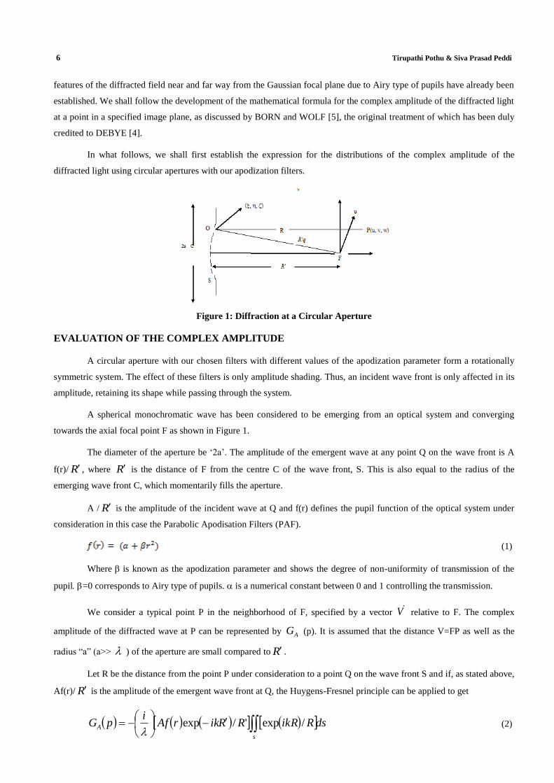
Figure 1: Diffraction at a Circular Aperture
EVALUATION OF THE COMPLEX AMPLITUDE
A circular aperture with our chosen filters with different values of the apodization parameter form a rotationally
symmetric system. The effect of these filters is only amplitude shading. Thus, an incident wave front is only affected in its
amplitude, retaining its shape while passing through the system.
A spherical monochromatic wave has been considered to be emerging from an optical system and converging
towards the axial focal point F as shown in Figure 1.
The diameter of the aperture be ‘2a’. The amplitude of the emergent wave at any point Q on the wave front is A
f(r)/ R , where R is the distance of F from the centre C of the wave front, S. This is also equal to the radius of the
emerging wave front C, which momentarily fills the aperture.
A / R is the amplitude of the incident wave at Q and f(r) defines the pupil function of the optical system under
consideration in this case the Parabolic Apodisation Filters (PAF).
(1)
Where is known as the apodization parameter and shows the degree of non-uniformity of transmission of the
pupil=0 corresponds to Airy type of pupils. is a numerical constant between 0 and 1 controlling the transmission.
We consider a typical point P in the neighborhood of F, specified by a vector V relative to F. The complex
amplitude of the diffracted wave at P can be represented by AG (p). It is assumed that the distance V=FP as well as the
radius “a” (a>> ) of the aperture are small compared to R .
Let R be the distance from the point P under consideration to a point Q on the wave front S and if, as stated above,
Af(r)/ R is the amplitude of the emergent wave front at Q, the Huygens-Fresnel principle can be applied to get
dsRikRRRikrAfi
pGs
A
/exp'/exp
(2)
Amplitude Response of PSF with Parabolic Apodization Filters Under Different Conditions of Transmission 7
if q denotes the unit vector in the direction of FQ, we can write to a good approximation,
vqRR (3)
The element ds of the wave front subtends a solid angle d at F and thus we can write,
dRds2
(4)
and, without any appreciable error, replacing R in the denominator of the integrand by R , we can rewrite
equation (1) as
dvqikrfiA
pGA
exp (5)
The integration extends over the solid angle subtended by the aperture at F. with ,1rf equation (2).
reduces to the well known Debye integral.
dvqikiA
pGAiry
exp (6)
Equation (5) expresses the field as a superposition of plane waves in different directions of propagation. Thus, it
represents a rigorous solution of the wave equation which in the limit R (aperture at infinite distance) is valid
throughout the whole of space. One can also include the contributions due to the waves propagated by each segment of the
wave front in all directions, but this does not appreciably add to the contributions considered in the direction of the incident
rays as long as the following conditions are satisfied (i) R>> a >> ,and (ii) R>> V.
To evaluate (5), we express the integrand in a more explicit form. We take the Cartesian axes at F above Figure
1.Let (u, v, w) be the coordinates of ,p and ,, are those of Q(r, ). r is the fractional coordinate of the point
Q. The direction is taken positive along axis of the system, to the right of F. We can now write
a.r. sin ( )
and
a.r. cos ( ) (7)
Also,
u sin
v = cos (8)
since Q is on the spherical wave front ‘S’
= - 1
2 2 2 2R a r
8 Tirupathi Pothu & Siva Prasad Peddi
=
..............
2
11
2
22
R
raR
(9)
then
q . u v wv
R
=
.........
2
11
cos2
22
R
raw
R
ra (10)
We introduce now two dimensionless variables y and z which, together with specify the position of P. Thus,
,2
2
wR
ay
21
222vu
R
az
(11)
The point P lies in the direct light beam or in the geometrical shadow according to .
y
z
1. From (9) and (10),
neglecting terms containing higher powers of
R
ra in comparison to unity,
k q . v
2
21cos
2
RZr y yr
a
(12)
the element of solid angle d is
rdraR
dsd 2
2
2R
d
(13)
Hence, (5) becomes
y
a
Ri
R
AaipGA
2
2
2
exp
rdrdiyrzrirf
2
1
0
2
02
1cosexp
(14)
The integral with respect to is easily recognized as one occurring in connection with Fraunhofer diffraction at a
circular aperture. It is well known to be equal to zrJ02 . Hence, equation (14) becomes
2
2
2
2
expa
yRi
R
AaipGA
( rdrzrJ
iyrrf 0
21
02
exp2
) (15)
now putting,
y
a
Ri
R
A2
2exp
, (16)
We get
rdrzrJiyr
rfaipGA 0
21
0
2
2exp2
(17)
Amplitude Response of PSF with Parabolic Apodization Filters Under Different Conditions of Transmission 9
This equation will be studied in terms of the dimensionless variables Y and Z in what follows and hence, we
express it conveniently by zyG , as
rdrzrJiyr
rfaizyG 0
1
0
22
2exp2,
(18)
In the above expression, zyG , is the finite Hankel transform of the pupil function multiplied by the factor
exp
2
2iyr
The factor outside the integral of (18) is a constant factor which depends only on the geometry of the
arrangement. This factor has no contribution to the diffraction pattern which depends only on the form of the pupil
function. Therefore, this factor is omitted for the purpose of calculating the effect of a particular pupil function on the
diffraction pattern and we can write (18) as;
1
0
2, rfzyG exp rdrzrJiyr
0
2
2
(19)
In the case of a clear aperture viz . , f (r ) = 1, we can write for the diffracted Amplitude
1
0
2, zyGA exp rdrzrJiyr
0
2
2
(20)
Or,
,AG y z = 1
0
02 zrJ cos rdryr
zrJirdryr
)2
sin(22
21
0
0
2
(21)
These integrals were evaluated by LOMMEL [1] in terms of the well known Lommel functions introduced by
LOMMEL himself. He expressed the complex amplitude in terms of convergent series of Bessel functions DURFEE [6]
expressible again in terms of simple trigonometric functions and LOMMEL functions. He studied the intensity
distributions in the geometrical focal plane. WOLF [7] has constructed the isophotes (the lines of equal intensity) near the
focus from Lommel’s data (BORN and WOLF [5].
RESULTS AND DISCUSSIONS
Field Charecteristics in the Gaussian Plane
In this section, we derive the expressions needed to investigate the various point image characteristics in the
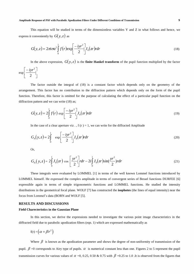
diffracted field due to parabolic apodization filters (eqn. 1) which are expressed mathematically as
f(r) = 2r
Where is known as the apodization parameter and shows the degree of non-uniformity of transmission of the
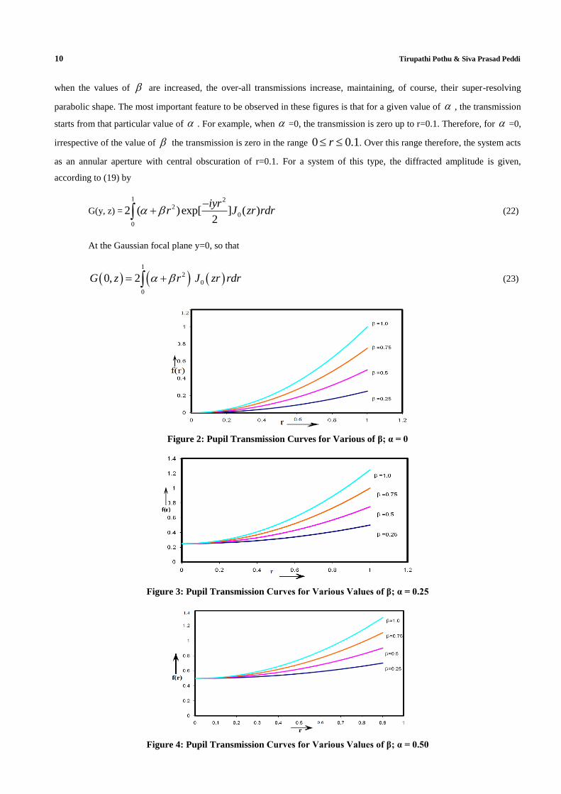
pupil. =0 corresponds to Airy type of pupils. is numerical constant less than one. Figures 2 to 5 represent the pupil
transmission curves for various values of =0, 0.25, 0.50 & 0.75 with =0.25 to 1.0 .It is observed from the figures that
10 Tirupathi Pothu & Siva Prasad Peddi
when the values of are increased, the over-all transmissions increase, maintaining, of course, their super-resolving
parabolic shape. The most important feature to be observed in these figures is that for a given value of , the transmission
starts from that particular value of . For example, when =0, the transmission is zero up to r=0.1. Therefore, for =0,
irrespective of the value of the transmission is zero in the range 0 0.1r . Over this range therefore, the system acts
as an annular aperture with central obscuration of r=0.1. For a system of this type, the diffracted amplitude is given,
according to (19) by
G(y, z) =
1 22
0
0
2 ( )exp[ ] ( )2
iyrr J zr rdr
(22)
At the Gaussian focal plane y=0, so that
1
2
0
0
0, 2G z r J zr rdr (23)
Figure 2: Pupil Transmission Curves for Various of β; α = 0
Figure 3: Pupil Transmission Curves for Various Values of β; α = 0.25
Figure 4: Pupil Transmission Curves for Various Values of β; α = 0.50
Amplitude Response of PSF with Parabolic Apodization Filters Under Different Conditions of Transmission
11
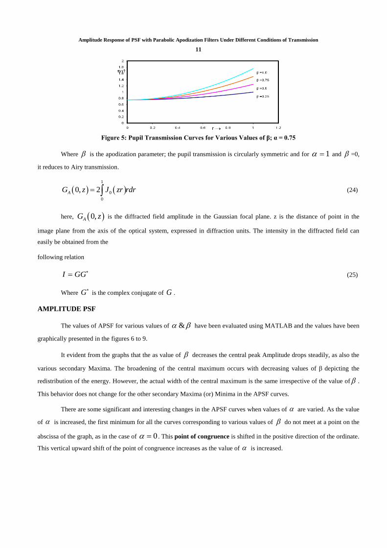
Figure 5: Pupil Transmission Curves for Various Values of β; α = 0.75
Where is the apodization parameter; the pupil transmission is circularly symmetric and for 1 and =0,
it reduces to Airy transmission.
1
0
0
0, 2AG z J zr rdr (24)
here, 0,AG z is the diffracted field amplitude in the Gaussian focal plane. z is the distance of point in the
image plane from the axis of the optical system, expressed in diffraction units. The intensity in the diffracted field can
easily be obtained from the
following relation
GGI (25)
Where G is the complex conjugate of G .
AMPLITUDE PSF
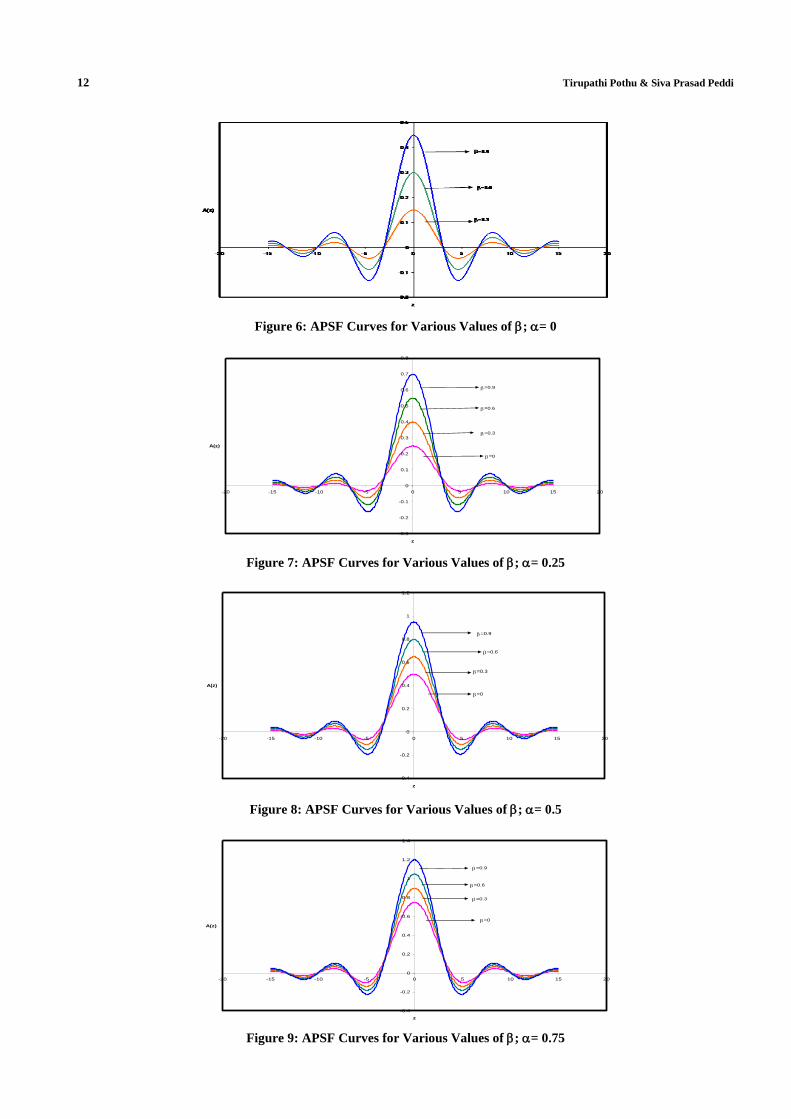
The values of APSF for various values of & have been evaluated using MATLAB and the values have been
graphically presented in the figures 6 to 9.
It evident from the graphs that the as value of decreases the central peak Amplitude drops steadily, as also the
various secondary Maxima. The broadening of the central maximum occurs with decreasing values of depicting the
redistribution of the energy. However, the actual width of the central maximum is the same irrespective of the value of .
This behavior does not change for the other secondary Maxima (or) Minima in the APSF curves.
There are some significant and interesting changes in the APSF curves when values of are varied. As the value
of is increased, the first minimum for all the curves corresponding to various values of do not meet at a point on the
abscissa of the graph, as in the case of 0 . This point of congruence is shifted in the positive direction of the ordinate.
This vertical upward shift of the point of congruence increases as the value of is increased.
12 Tirupathi Pothu & Siva Prasad Peddi
Figure 6: APSF Curves for Various Values of ; = 0
-0.3
-0.2
-0.1
0
0.1
0.2
0.3
0.4
0.5
0.6
0.7
0.8
-20 -15 -10 -5 0 5 10 15 20
z
A(z)
=0
=0.3
=0.6
=0.9
Fig.2.3 (b) APSF curves for various values of ; =0.25
Figure 7: APSF Curves for Various Values of ; = 0.25
-0.4
-0.2
0
0.2
0.4
0.6
0.8
1
1.2
-20 -15 -10 -5 0 5 10 15 20
z
A(z)
=0
=0.3
=0.6
=0.9
Fig.2.3 (c) APSF curves for various values of ; =0.50
Figure 8: APSF Curves for Various Values of ; = 0.5
-0.4
-0.2
0
0.2
0.4
0.6
0.8
1
1.2
1.4
-20 -15 -10 -5 0 5 10 15 20
z
A(z)
=0
=0.3
=0.6
=0.9
Fig.2.3 (d) APSF curves for various values of ; =0.75
Figure 9: APSF Curves for Various Values of ; = 0.75
Amplitude Response of PSF with Parabolic Apodization Filters Under Different Conditions of Transmission
13
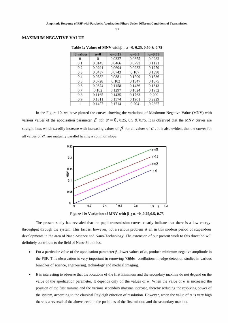
MAXIMUM NEGATIVE VALUE
Table 1: Values of MNV with =0, 0.25, 0.50 & 0.75
β values α=0 α=0.25 α=0.5 α=0.75
0 0 0.0327 0.0655 0.0982
0.1 0.0145 0.0466 0.0793 0.1121
0.2 0.0291 0.0604 0.0932 0.1259
0.3 0.0437 0.0743 0.107 0.1398
0.4 0.0582 0.0881 0.1209 0.1536
0.5 0.0728 0.102 0.1347 0.1675
0.6 0.0874 0.1158 0.1486 0.1813
0.7 0.102 0.1297 0.1624 0.1952
0.8 0.1165 0.1435 0.1763 0.209
0.9 0.1311 0.1574 0.1901 0.2229
1 0.1457 0.1714 0.204 0.2367
In the Figure 10, we have plotted the curves showing the variations of Maximum Negative Value (MNV) with
various values of the apodization parameter for 0 , 0.25, 0.5 & 0.75. It is observed that the MNV curves are
straight lines which steadily increase with increasing values of for all values of . It is also evident that the curves for
all values of are mutually parallel having a common slope.
Figure 10: Variation of MNV with =0 ,0.25,0.5, 0.75
The present study has revealed that the pupil transmission curves clearly indicate that there is a low energy-
throughput through the system. This fact is, however, not a serious problem at all in this modern period of stupendous
developments in the area of Nano-Science and Nano-Technology. The extension of our present work to this direction will
definitely contribute to the field of Nano-Photonics.
For a particular value of the apodization parameter , lower values of , produce minimum negative amplitude in
the PSF. This observation is very important in removing ‘Gibbs’ oscillations in edge-detection studies in various
branches of science, engineering, technology and medical imaging.
It is interesting to observe that the locations of the first minimum and the secondary maxima do not depend on the
value of the apodization parameter. It depends only on the values of . When the value of is increased the
position of the first minima and the various secondary maxima increase, thereby reducing the resolving power of
the system, according to the classical Rayleigh criterion of resolution. However, when the value of is very high
there is a reversal of the above trend in the positions of the first minima and the secondary maxima.
14 Tirupathi Pothu & Siva Prasad Peddi
ACKNOWLEDGEMENTS
One of the authors Dr. Siva Prasad Peddi thanks his employer M/S Al Jouf University, Kingdom of Saudi Arabia
where he is working as a Professor, Department of Physics, College of Arts and Sciences, Al Qurayat, KSA.
REFERENCES
1. LOMMEL, E., Abh.Bayer Akad., vol.15, Abth.2, 1885.
2. STRUVE, H., mem. Akad. Sci., st. peterburg, vol.34, 1886.
3. SCHWARTZSCHILD, Sitz, Munchen. Akd. Wiss., Math-Phys. K1.vol.28,1898.
4. DEBYE, P., Ann.d. physic., vol. 30, 1909.
5. BORN, M . and WOLF, E ., “ Principle of Optics”, 7 th
Ed., Pergaman Press, Newyork, 2007.
6. CHARLES G. DURFEE et al., Opt. Express 21, 15777-15786(2013)
7. WOLF, E ., Ref. Prog. Phy., (Physical Society Landon), vol.14, 1951.
Copyright © 2022 FDOKUMEN