Int. J. Intelligent Systems Technologies and Applications, Vol. 4, Nos. 1/2, 2008 123

Copyright © 2008 Inderscience Enterprises Ltd.

Allocation of work to the stations of an assembly line with buffers between stations and three general learning patterns

Yuval Cohen* Department of Management and Economics, The Open University of Israel, 108 Rabutzki street, P.O. Box 808, Raanana 43104, Israel E-mail: yuvalco@openu.ac.il *Corresponding author

Ezey M. Dar-El Technion (IIT), Kiryat Hatechnion, Haifa 32000, Israel E-mail: ezey@ie.technion.ac.il

Gad Vitner

Department of Industrial Engineering and Management, School of Engineering, The Ruppin Academic Centre, Emek-Hafer 40250, Israel E-mail: GadiV@ruppin.ac.il

Subhash C. Sarin Grado Department of Industrial and Systems Engineering, Virginia Tech, Blacksburg, VA 2061, USA E-mail: sarins@vt.edu

Abstract: This paper addresses the problem of allocating work to the stations of an assembly line for minimising the makespan required to process a lot of products with a low overall demand. This environment is characterised by different learning slopes in the various stations (due to the nature of work). We assume small (e.g. a laser pen) to medium size products (e.g. a pilot helmet) so buffer space, for temporary purposes, is typically not a problem. Three general patterns of stations’ learning are considered, namely, decreasing, increasing and constant. Methodologies are presented for the optimal allocation of work to the stations for each of these cases. Some numerical results are also presented to show a significant impact of buffer capacity on makespan reduction as well as to reveal significant improvement in the makespan value due to unequal (but optimal) work allocation.

124 Y. Cohen et al.

Keywords: batch assembly; learning; buffers; work-in-process; WIP; line balancing; optimisation.

Reference to this paper should be made as follows: Cohen, Y., Dar-El, E.M., Vitner, G. and Sarin, S.C. (2008) ‘Allocation of work to the stations of an assembly line with buffers between stations and three general learning patterns’, Int. J. Intelligent Systems Technologies and Applications, Vol. 4, Nos. 1/2, pp.123–140.

Biographical notes: Yuval Cohen is the Head of the Industrial Engineering programme at the Open University of Israel. His areas of speciality are production planning, industrial learning and logistics management. He has published several papers in these areas. He served as a senior operations planner at FedEx Ground (USA) for several years and received several awards for his contributions to the hub and terminal network planning. He received his PhD from the University of Pittsburgh (USA), his MSc from Technion – Israel Institute of Technology, and BSc from Ben-Gurion University. He is a Fellow of the Institute of Industrial Engineers (IIE), and a full Member of the Institute for Operations Research and Management Sciences (INFORMS).

Ezey M. Dar-El is the Harry Lebensfeld Chair in Industrial Engineering at the Faculty of Industrial Engineering and Management at Technion – Israel Institute of Technology. He has published extensively in several areas which include design and analysis of production/assembly systems, project and FMS scheduling; and productivity development. He also has authored two books in the areas of productivity improvement and industrial learning. He received BMechE, MEngSci and PhD from the University of Melbourne (Australia). He is a Fellow of the IIE, a Member of SME, ORSIS, HFS and IFPR and is on the Editorial Board of the IIE Transactions, International Journal of Production Research, Production Planning and Control, International journal of Engineering and Quality Observer. He is an internationally known Consultant having worked with over 70 companies located in Australia, UK, USA, the Netherlands, Antilles, Italy and Israel.

Gad Vitner is the Head of Industrial Engineering and Management Department at Ruppin Academic Centre in Israel. He received a PhD in Industrial and Systems Engineering from the University of Southern California in Los-Angeles (USA). He received a BSc and an MSc in Industrial Engineering and Management at Technion – Israel Institute of Technology. His research areas are project management, productivity, quality management, production planning and control and photo voltaic energy. He served for 15 years in various Senior Management positions in several organisations and supervised many projects in the areas of CIM, strategic planning, ERP, production planning and control and quality management.

Subhash C. Sarin is the Paul T. Norton Endowment Professor in the Grado Department of Industrial and Systems Engineering at Virginia Tech. His areas of speciality are production scheduling, applied mathematical programming and the design and analysis of manufacturing systems. He has published many papers in these areas. He is the recipient of several prestigious awards at the university, state and national levels. He has served as an Associate Editor of several journals. He is a Fellow of the Institute of Industrial Engineers and a Full Member of the Institute for Operations Research and Management Sciences.

Allocation of work to the stations of an assembly line 125

1 Introduction

In this paper, we address the problem of allocating work to the stations of an assembly line in order to minimise the makespan required to process a lot/batch of products with a low overall demand. The work stations on the assembly line involve different learning slopes as a result of the nature of work that is performed at the stations. Processing times are not random and could be computed for each cycle at each station. For the first time, buffer requirements due to different learning slopes in the different stations are investigated.

Assembly lines research had linked the need for buffers with randomness of the processing times (Gershwin and Schore 2000; Hillier 2000; Hillier and Hillier 2006; Shi and Men 2003; Smith and Cruz 2005; Spinellis and Papadopoulos, 2000) or with random failures (Enginarlar et al., 2002, 2005). In this paper, we assume deterministic processing times and no machine failures. Thus, buffer space between successive stations may only be required for temporarily bridging the gap between different processing rates at the different stations due to different learning curves.

We assume small to medium size products (say in the size range from a laser pen to a pilot helmet). Therefore, buffer capacity, for temporary purposes, is typically not a problem. We also assume that the number of stations, L, is known a priori, a method to compute optimal L is given in Cohen and Dar-El (1998).

The situation involving the processing of products with a low overall demand can, typically, be attributed to science-based products for which the total demands are likely to be between the mid-tens to the low hundreds. Ordinarily, minimal makespan is realised under equal station learning slopes (see Cohen and Dar-El, 1998). But, conditions may arise for which the learning slopes vary considerably across the stations. This may be due to a highly constrained network of tasks or segregated tasks with very dissimilar learning slopes, or due to the existence of a bottleneck.

The effect of learning on production scheduling has been analysed by several researchers. Adler and Nanda (1974) have studied the effects of learning on the determination of optimal lot sizes. Kroll (1989) incorporates the effects of learning in production planning models. The other studies have dealt with studying the impacts of the learning phenomenon in assembly line balancing. Dar-El and Rabinovitch (1988) and Cohen and Dar-El (1998) have considered the simple case in which the learning is identical for all the stations on the line. Chakravarty (1988) considered the case of no-buffer capacity in between the stations, and attributed the learning curve parameters to each station, depending upon the tasks in the precedence diagram. The minimisation of makespan in assembly lines under the constraint of a low total demand and in the presence of learning has been tackled by Globerson and Shtub (1984). They proposed the idea of balancing the line with the estimated task times of the mid-lot cycle. However, Cohen et al. (2006) have shown that even under homogeneous learning, allocating the same amount of work to each station is not optimal. The problem of allocating work to the stations of an assembly line in the presence of learning effects with buffer accumulation in between the stations has been dealt with by Globerson and Levin (1995), Cohen and Dar-El (1998), Brenner (1990), Dar-El (2000) and Ardity et al. (2001). However, they assume homogeneous learning phenomenon across the stations. In this paper, we address a general version of the problem by considering different learning slopes of the stations on the line and also allow buffers to temporarily accumulate in between the stations. In particular, we study the workload allocation behaviour under the

126 Y. Cohen et al.

increasing and decreasing trends of learning constants across the stations of a line along with the case of equal learning constants for all stations.

In what follows, we present some background information on the learning phenomenon and the impact of buffer capacity in between the stations in Section 2. Analyses of the cases pertaining to a trend in the magnitude of the station learning slopes, namely increasing, decreasing and constant, are presented in Section 3. A procedure to determine optimal workload allocation for each of these cases is also given. Some numerical results are presented to illustrate the impact of buffer capacity on makespan reduction as well as to reveal significant improvement in the makespan value due to unequal (but optimal) over equal allocation of work to the stations. Some concluding remarks are, then, made in Section 4.

2 Background information on the learning phenomenon and the impact of buffer capacity in between the stations

To capture the impact of learning, Wright (1936) proposed a model according to which the cycle time reduces by a constant percentage (φ) every time the quantity produced is doubled (φ is called the learning slope). Let t1 be the execution time of the first cycle, and tn be the execution time of the nth cycle, then the Wright’s learning model is given by Expression (1):

2log ( )1

nnt t φ= (1)

A more prevalent form of Equation (1) is based on the learning constant (b), as follows:

1b

nt t n−= (2)

A comparison of Equations (1) and (2) gives the following relationship between b and φ:

φ= − 2log ( )b (3)

By taking the integral of Equation 2, we obtain an approximation of the total time for n cycles given by:

( )11

1b

n

tT n

b−⎛ ⎞= ⎜ ⎟−⎝ ⎠

(4)

If STD designates the standard time of a task, Dar-El (2000) has shown that t1, the time for the first cycle, can be approximately expressed by:

1 STD(57 60 )t φ= − (5)

The standard time can be determined by using the Predetermined Motion Time Standards (PMTS), and the learning slope φ can be estimated by a method described in Dar-El (2000). Let

1( ) 57 60STD

tG φ φ= = − (6)

For example, substituting φ = 0.8 in Equation (6), yields: G(0.8) = 57 – (60)(0.8) = 57 – 48 = 9. So the ratio between the standard time (STD) and the first cycle (t1) is 9. Equation (6) enables determination of the first cycle time of any task or combination of tasks, given the estimation of their standard time and learning slope.

Allocation of work to the stations of an assembly line 127

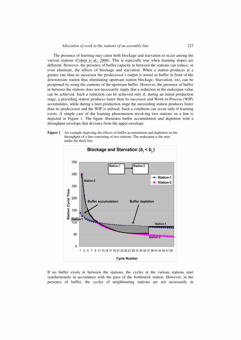
The presence of learning may cause both blockage and starvation to occur among the various stations (Cohen et al., 2006). This is especially true when learning slopes are different. However, the presence of buffer capacity in between the stations can reduce, or even eliminate, the effects of blockage and starvation. When a station produces at a greater rate than its successor the predecessor’s output is stored as buffer in front of the downstream station thus eliminating upstream station blockage. Starvation, too, can be postponed by using the contents of the upstream buffer. However, the presence of buffer in between the stations does not necessarily imply that a reduction in the makespan value can be achieved. Such a reduction can be achieved only if, during an initial production stage, a preceding station produces faster than its successor and Work-in-Process (WIP) accumulates, while during a later production stage the succeeding station produces faster than its predecessor and the WIP is utilised. Such a condition can occur only if learning exists. A simple case of the learning phenomenon involving two stations on a line is depicted in Figure 1. The figure illustrates buffer accumulation and depletion with a throughput envelope that deviates from the upper envelope.

Figure 1 An example depicting the effects of buffer accumulation and depletion on the throughput of a line consisting of two stations. The makespan is the area under the thick line

If no buffer exists in between the stations, the cycles at the various stations start synchronously in accordance with the pace of the bottleneck station. However, in the presence of buffer, the cycles of neighbouring stations are not necessarily in

128 Y. Cohen et al.

synchronism. We use the idea of cumulative learning curves to determine when a station is starved, blocked or is working continuously. This is presented in Section 3, where we analyse the situations in which different trends exist among the learning slopes of the stations on the line.

3 Analysis of the cases in which a trend exists in the learning constants of the stations on the line

Allowing temporary buffer accumulation in between the stations, this section presents analyses of the cases in which the following trends exist in the learning constants of the stations on the line:

1 Decreasing learning constants (along the line): bl ≥ b2 ≥... ≥ bL.

2 Increasing learning constants (along the line): bl ≤ b2 ≤ ... ≤ bL.

3 Homogeneous case: bl = b2 = ... = bL.

For each of these instances, a simple case is analysed first and, then, the analysis is generalised.

For the discussion below we define: ti,j as the jth cycle time on the ith station.

3.1 Case 1: decreasing learning constants – b1 ≥ b2 ≥ b3 ≥ …≥ bL

3.1.1 Special case for two stations: b1 ≥ b2

Following the concept of dominance (Cohen et al., 2006), the inequality t1, 2 > t2, 1 must hold in order to minimise makespan, because otherwise, the first station (which learn faster) will never be a bottleneck and we can improve the makespan value by transferring some workload from the bottleneck station to that station. Thus, the first station must be the first bottleneck station. Consequently, in the first period the second station starves and no products are accumulated in the buffer. Since the learning rate of the first station is larger, its cycle time shrinks faster and, after a while, the second station becomes the bottleneck. At that stage station two is working continuously and, if there were no buffer space, it would block station 1. Although items may accumulate in a buffer, it will never improve the rate at the bottleneck station and, therefore, it will not improve the makespan value. Thus, in this case, there is no advantage of having a buffer in between stations 1 and 2, and the problem reduces to that of the non-buffered lines and can be solved by using the method for that case (see Cohen and Dar-El, 1998; Cohen et al., 2006; Cohen et al., 2008).

3.1.2 A general case for L stations: b1 ≥ b2 ≥ b3 ≥ ... ≥ bL

If an assembly line consists of L stations with decreasing learning constants (i.e. b1 ≥ b2 ≥ ... ≥ bL), then the relationship between every pair of adjacent stations corresponds exactly to the two stations case discussed above. If the output of the first two stations were isolated, then their combined upper envelope can be looked upon as the learning curve of the two station system. On adding the third station curve to this combined learning curve, we return to the special case of two successive learning curves with the upper envelope representing the output rate of the three stations. In this way, it

Allocation of work to the stations of an assembly line 129

can be deduced that the upper envelope of any number of stations can represent the output rate of the assembly line having decreasing station learning constants. Since no total dominance is allowed it follows that in the optimal solution we must order tij as t1, 1 ≥ t2, 1 ≥ t3, 1 … ≥ tL, 1) so that each station remains ‘starved’ until it becomes a bottleneck for an appropriate length of time. The pace of transferred products, consequently, follows the pace of the bottleneck operations. The optimal solution in this case is, thus, identical to that for the case when no buffer is permitted in between the stations. There is no advantage in terms of the makespan or the output rate for having a buffer in between any two successive stations because it will never be used, as the cycle time of a preceding station will be longer than that of its succeeding station. The allocation of work to the stations can, therefore, be determined by using the procedure presented in Cohen et al. (2006); Cohen et al. (2008) which strictly forbid buffers.

3.2 Case 2: Increasing learning constants – b1≤ b2≤ b3 ≤ … ≤ bL

3.2.1 Special case for two stations: b1 ≤ b2

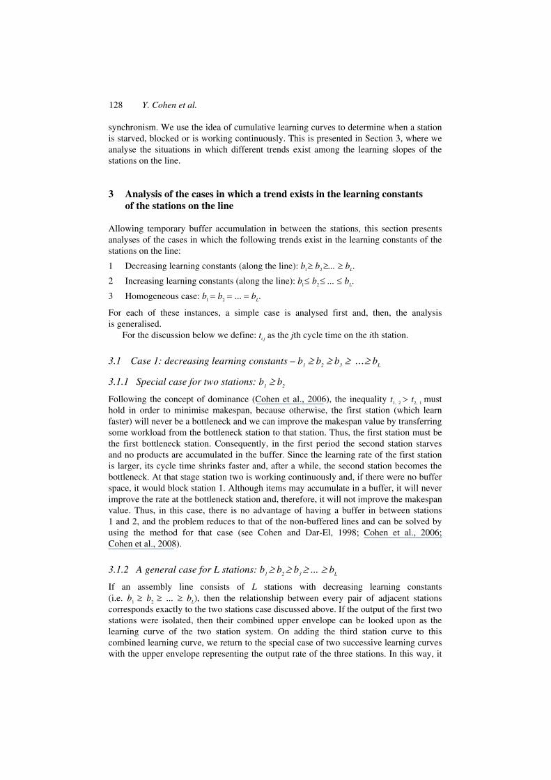
In order to avoid dominance of a station in this case, we must have t1, 2 ≤ t2, 1. This limits the domain of legitimate cumulative curves to three possibilities as depicted in Figures 2–4. Let M be the maximum number of cycles run on the line. The highest point of these curves at M represents the makespan for completing M cycles.

Figure 2 Cumulative time curve: suboptimal work allocation (too much work is allocated to station 2)

130 Y. Cohen et al.

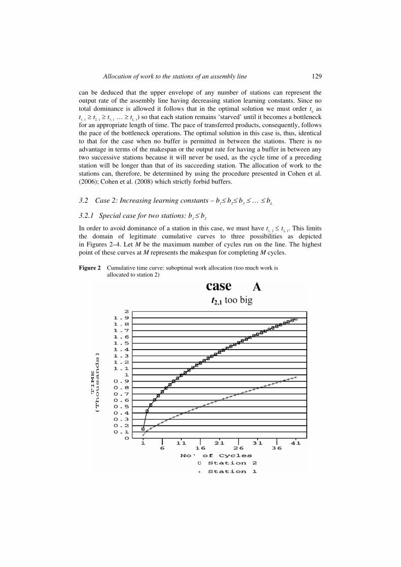
Figure 3 Cumulative time curve: suboptimal work allocation (station 2 becomes idle too fast)

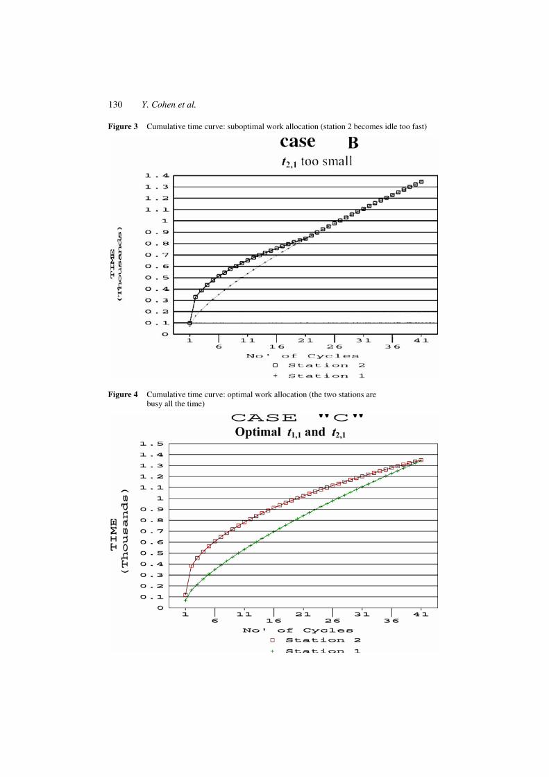
Figure 4 Cumulative time curve: optimal work allocation (the two stations are busy all the time)

Allocation of work to the stations of an assembly line 131

It is easy to show that in case A the makespan can be reduced by transferring work elements from stations 2 to 1, and thus case A is suboptimal. Reducing the makespan by gradually transferring work (from station 2 to station 1) culminates in reaching case C. If this work transfer is carried on further (from case C), case B is reached in which the makespan value increases. Case B reflects the situation in which a station has to wait for its predecessor to further process a product.

The above reasoning for case B implies that by transferring work elements from station 1 to station 2, we can reduce the makespan. Thus case B is suboptimal. Now any change in work allocation from case C brings about either case A or case B (depending on where the work is transferred to). It turns out that case C, where the two stations work continuously and simultaneously throughout, gives the optimal make span value.

Since, in the optimal solution, the two stations work continuously, the work allocation can be obtained analytically by solving the following two equations involving two variables (t1, 1, t2,1):

( ) 2111,1 2,11

1,11 2

11 1

bbt t

M t Mb b

−−⎛ ⎞ ⎛ ⎞− = −⎜ ⎟ ⎜ ⎟

− −⎝ ⎠ ⎝ ⎠ (7)

and

( ) ( )φ φ+ =1,1 2,1

1 2

STDt t

G G (8)

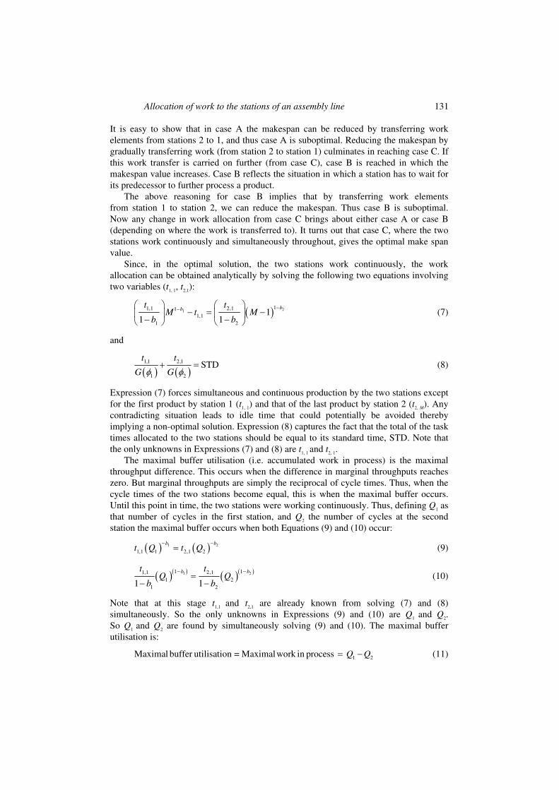
Expression (7) forces simultaneous and continuous production by the two stations except for the first product by station 1 (t1, 1) and that of the last product by station 2 (t2, M). Any contradicting situation leads to idle time that could potentially be avoided thereby implying a non-optimal solution. Expression (8) captures the fact that the total of the task times allocated to the two stations should be equal to its standard time, STD. Note that the only unknowns in Expressions (7) and (8) are t1, 1 and t2, 1.

The maximal buffer utilisation (i.e. accumulated work in process) is the maximal throughput difference. This occurs when the difference in marginal throughputs reaches zero. But marginal throughputs are simply the reciprocal of cycle times. Thus, when the cycle times of the two stations become equal, this is when the maximal buffer occurs. Until this point in time, the two stations were working continuously. Thus, defining Q1 as that number of cycles in the first station, and Q2 the number of cycles at the second station the maximal buffer occurs when both Equations (9) and (10) occur:

( ) ( )− −=1 2

1,1 1 2,1 2

b bt Q t Q (9)

( )( ) ( )( )− −=

− −1 21 11,1 2,1

1 21 21 1

b bt tQ Q

b b (10)

Note that at this stage t1,1 and t2,1 are already known from solving (7) and (8) simultaneously. So the only unknowns in Expressions (9) and (10) are Q1 and Q2. So Q1 and Q2 are found by simultaneously solving (9) and (10). The maximal buffer utilisation is:

1 2Maximal buffer utilisation = Maximalwork in process Q Q= − (11)

132 Y. Cohen et al.

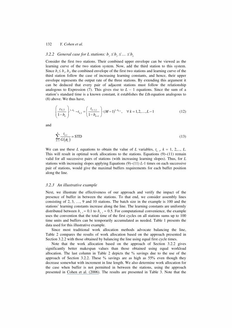
3.2.2 General case for L stations: b1 ≤ b2 ≤ … ≤ bL

Consider the first two stations. Their combined upper envelope can be viewed as the learning curve of the two station system. Now, add the third station to this system. Since b3 ≤ b1, b2, the combined envelope of the first two stations and learning curve of the third station follow the case of increasing learning constants, and hence, their upper envelope represents the output rate of the three stations. By extending this argument it can be deduced that every pair of adjacent stations must follow the relationship analogous to Expression (7). This gives rise to L – 1 equations. Since the sum of a station’s standard time is a known constant, it establishes the Lth equation analogous to (8) above. We thus have,

11,11 1,1

1

,1( 1) , 1,2, , 1

1 1k kkb b

kk k

k ttt M k L

b b++− −

+

⎛ ⎞ ⎛ ⎞⎜ ⎟ ⋅ − = ⋅ − ∀ = −⎜ ⎟⎜ ⎟− −⎝ ⎠⎝ ⎠

… (12)

and

( )φ=

=∑ ,1

1

STDL

k

k k

t

G (13)

We can use these L equations to obtain the value of L variables, tk, 1, k = 1, 2,..., L. This will result in optimal work allocations to the stations. Equations (9)–(11) remain valid for all successive pairs of stations (with increasing learning slopes). Thus, for L stations with increasing slopes applying Equations (9)–(11) L-1 times on each successive pair of stations, would give the maximal buffers requirements for each buffer position along the line.

3.2.3 An illustrative example

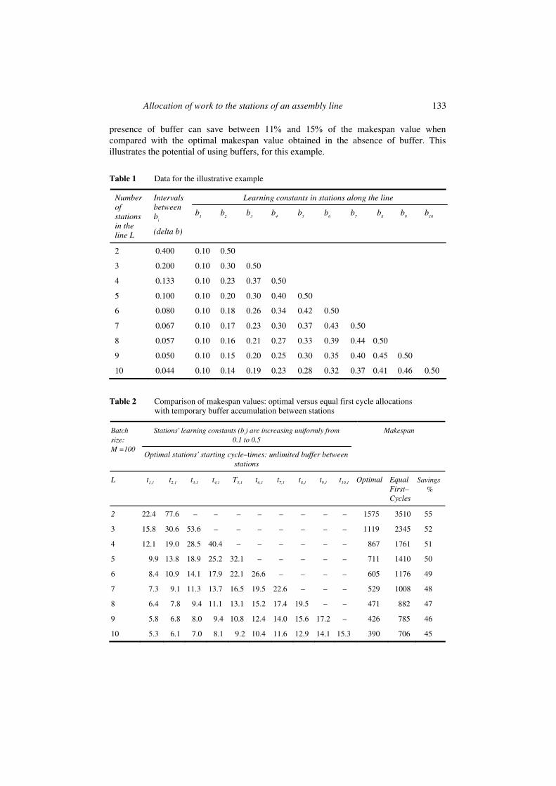
Next, we illustrate the effectiveness of our approach and verify the impact of the presence of buffer in between the stations. To that end, we consider assembly lines consisting of 2, 3, …, 9 and 10 stations. The batch size in the example is 100 and the stations’ learning constants increase along the line. The learning constants are uniformly distributed between b1, 1 = 0.1 to bL, 1 = 0.5. For computational convenience, the example uses the convention that the total time of the first cycles on all stations sums up to 100 time units and buffers can be temporarily accumulated as needed. Table 1 presents the data used for this illustrative example.

Since most traditional work allocation methods advocate balancing the line, Table 2 compares the results of work allocation based on the approach presented in Section 3.2.2 with those obtained by balancing the line using equal first cycle times.

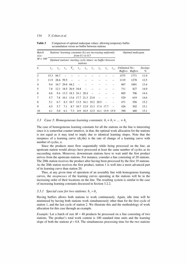
Note that the work allocation based on the approach of Section 3.2.2 gives significantly better makespan values than those obtained using equal workload allocation. The last column in Table 2 depicts the % savings due to the use of the approach of Section 3.2.2. These % savings are as high as 55% even though they decrease somewhat with increment in line length. We also determine work allocation for the case when buffer is not permitted in between the stations, using the approach presented in Cohen et al. (2006). The results are presented in Table 3. Note that the

Allocation of work to the stations of an assembly line 133

presence of buffer can save between 11% and 15% of the makespan value when compared with the optimal makespan value obtained in the absence of buffer. This illustrates the potential of using buffers, for this example.

Table 1 Data for the illustrative example

Learning constants in stations along the line Number of stations in the line L

Intervals between b

i

(delta b)

b1 b

2 b

3 b

4 b

5 b

6 b

7 b

8 b

9 b

10

2 0.400 0.10 0.50

3 0.200 0.10 0.30 0.50

4 0.133 0.10 0.23 0.37 0.50

5 0.100 0.10 0.20 0.30 0.40 0.50

6 0.080 0.10 0.18 0.26 0.34 0.42 0.50

7 0.067 0.10 0.17 0.23 0.30 0.37 0.43 0.50

8 0.057 0.10 0.16 0.21 0.27 0.33 0.39 0.44 0.50

9 0.050 0.10 0.15 0.20 0.25 0.30 0.35 0.40 0.45 0.50

10 0.044 0.10 0.14 0.19 0.23 0.28 0.32 0.37 0.41 0.46 0.50

Table 2 Comparison of makespan values: optimal versus equal first cycle allocations with temporary buffer accumulation between stations

Stations' learning constants (bi) are increasing uniformly from 0.1 to 0.5

Batch size: M =100

Optimal stations' starting cycle–times: unlimited buffer between stations

Makespan

L t1,1 t2,1 t3,1 t4,1 T5,1 t6,1 t7,1 t8,1 t9,1 t10,1 Optimal Equal First– Cycles

Savings%

2 22.4 77.6 – – – – – – – – 1575 3510 55

3 15.8 30.6 53.6 – – – – – – – 1119 2345 52

4 12.1 19.0 28.5 40.4 – – – – – – 867 1761 51

5 9.9 13.8 18.9 25.2 32.1 – – – – – 711 1410 50

6 8.4 10.9 14.1 17.9 22.1 26.6 – – – – 605 1176 49

7 7.3 9.1 11.3 13.7 16.5 19.5 22.6 – – – 529 1008 48

8 6.4 7.8 9.4 11.1 13.1 15.2 17.4 19.5 – – 471 882 47

9 5.8 6.8 8.0 9.4 10.8 12.4 14.0 15.6 17.2 – 426 785 46

10 5.3 6.1 7.0 8.1 9.2 10.4 11.6 12.9 14.1 15.3 390 706 45

134 Y. Cohen et al.

Table 3 Comparison of optimal makespan values: allowing temporary buffer accumulation versus no buffer between stations

Stations' learning constants (bi) are increasing uniformly

from 0.1 to 0.5 Batch size: M = 100 Optimal stations' starting cycle–times: no buffer between

stations

Optimal makespan

L t1,1

t2,1

t3,1

T4,1

t5,1

t6,1

t7,1

t8,1

t9,1

t10,1

Unlimited Buffers

No–Buffers

Savings %

2 15.3 84.7 – – – – – – – – 1575 1771 11.0

3 11.9 28.6 59.5 – – – – – – – 1119 1278 12.5

4 9.4 16.7 29.6 44.2 – – – – – – 867 1001 13.4

5 7.8 12.1 18.5 26.9 34.8 – – – – – 711 827 14.0

6 6.6 9.4 13.3 18.3 24.1 28.4 – – – – 605 706 14.4

7 5.7 7.8 10.1 13.6 17.7 21.3 23.8 – – – 529 619 14.6

8 5.1 6.7 8.3 10.7 13.5 16.1 19.2 20.5 – – 471 556 15.2

9 4.5 5.7 7.1 8.7 10.7 12.9 15.3 17.4 17.7 – 426 502 15.1

10 4.1 5.0 6.1 7.3 8.9 10.5 12.5 14.1 15.9 15.9 390 460 15.1

3.3 Case 3: Homogeneous learning constants: b1 = b2 = … = bL

The case of homogeneous learning constants for all the stations on the line is interesting since it is somewhat counter intuitive, in that, the optimal work allocation for the stations is not equal as it may tend to imply due to identical learning slopes. Note that the steepness of a learning curve (dtn/dn) is the rate of change of a learning curve with number of cycles, n.

Since the products must flow sequentially while being processed on the line, an upstream station would always have processed at least the same number of cycles as its succeeding station. Moreover, downstream stations have to wait until the first product arrives from the upstream stations. For instance, consider a line consisting of 20 stations. The 20th station receives the product after having been processed by the first 19 stations. As the 20th station receives the first product, station 1 is well into a more advanced part of its learning curve than station 20.

Thus, at any given time of operation of an assembly line with homogenous learning curves, the steepnesses of the learning curves operating at the stations will be in the increasing order of their locations on the line. The resulting system is similar to the case of increasing learning constants discussed in Section 3.2.2.

3.3.1 Special case for two stations: b1 = b2

Having buffers allows both stations to work continuously. Again, idle time will be minimised by having both stations work simultaneously other than for the first cycle of station 1, and the last cycle of station 2. We illustrate this and the methodology of work allocation for this case through an example.

Example: Let a batch of size M = 40 products be processed on a line consisting of two stations. The product’s total work content is 100 standard time units and the learning slope of both the stations φ = 0.8. The simultaneous processing time for the two stations

Allocation of work to the stations of an assembly line 135

exclude the first cycle of the first station and the last cycle of the second station. This time is computed is as follows:

( ) ( )1 11,1 2,1

1,1 2,1 1b b

M

t tt tM Mb b

− −− = −− −

(14)

After substituting for t2, M = t2, 1 M–b (by (2)), and simplifying, we get

( ) ( ) ( )( ) ( )

1

1, 1

12, 1

1

1

b b

b

M M bt

t M b

− −

−

⎡ ⎤− ⋅ −⎣ ⎦=⎡ ⎤− −⎣ ⎦

(15)

Under the condition that station 2 never starves, it implies that the cycle times on station 2 are larger than or equal to those on station 1, which further leads to the fact that, at any time, station 1 has processed more cycles than station 2. This translates into the following constraint:

( ) ( )1,1 2,11 11,1( 1) for 1,2, ,

1 1b b

t tk t k k M

b b− −+ − ≤ ∀ =

− −… (16)

which after manipulation becomes,

(1 )

1, 1 2, 11

1 1for 1,2, ,

b

b

k bt t k M

k k

−

−

⎛ ⎞+ −⎛ ⎞ ⎛ ⎞⋅ − ≤ ∀ =⎜ ⎟⎜ ⎟ ⎜ ⎟⎜ ⎟⎝ ⎠ ⎝ ⎠⎝ ⎠… (17)

Since the expression in brackets decreases with k, the effective constraint is when k = 1, that is,

( )−≥ − −2,1 1

1,1

(2) (1 )bt

bt

. (18)

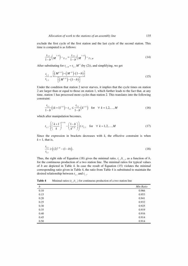
Thus, the right side of Equation (18) gives the minimal ratio, t2, 1/t1, 1, as a function of b, for the continuous production of a two station line. The minimal ratios for typical values of b are depicted in Table 4. In case the result of Equation (15) violates the minimal corresponding ratio given in Table 4, the ratio from Table 4 is substituted to maintain the desired relationship between t2, 1 and t1, 1.

Table 4 Minimal ratios (t2, 1

/t1, 1

) for continuous production of a two station line

b Min Ratio

0.10 0.966 0.15 0.953 0.20 0.941 0.25 0.932 0.30 0.925 0.35 0.919 0.40 0.916 0.45 0.914 0.50 0.914

136 Y. Cohen et al.

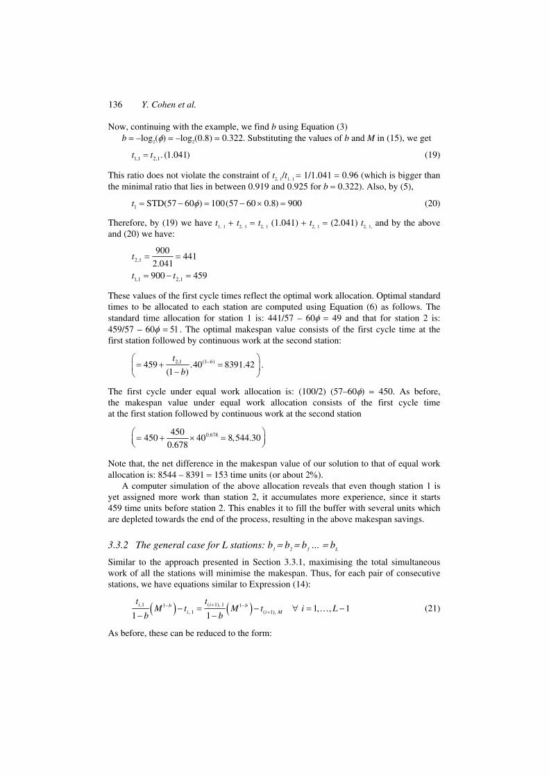
Now, continuing with the example, we find b using Equation (3) b = –log2(φ) = –log2(0.8) = 0.322. Substituting the values of b and M in (15), we get

1,1 2,1. (1.041)t t= (19)

This ratio does not violate the constraint of t2, 1/t1, 1 = 1/1.041 = 0.96 (which is bigger than the minimal ratio that lies in between 0.919 and 0.925 for b = 0.322). Also, by (5),

1 STD(57 60 ) 100(57 60 0.8) 900t φ= − = − × = (20)

Therefore, by (19) we have t1, 1 + t2, 1 = t2, 1 (1.041) + t2, 1 = (2.041) t2, 1, and by the above and (20) we have:

= =

= − =

2,1

1,1 2,1

900441

2.041900 459

t

t t

These values of the first cycle times reflect the optimal work allocation. Optimal standard times to be allocated to each station are computed using Equation (6) as follows. The standard time allocation for station 1 is: 441/57 – 60φ = 49 and that for station 2 is: 459/57 – 60φ = 51. The optimal makespan value consists of the first cycle time at the first station followed by continuous work at the second station:

2,1 (1 )459 .40 8391.42(1 )

bt

b−⎛ ⎞

= + =⎜ ⎟−⎝ ⎠.

The first cycle under equal work allocation is: (100/2) (57–60φ) = 450. As before, the makespan value under equal work allocation consists of the first cycle time at the first station followed by continuous work at the second station

0.678450450 40 8,544.30

0.678⎛ ⎞= + × =⎜ ⎟⎝ ⎠

Note that, the net difference in the makespan value of our solution to that of equal work allocation is: 8544 – 8391 = 153 time units (or about 2%).

A computer simulation of the above allocation reveals that even though station 1 is yet assigned more work than station 2, it accumulates more experience, since it starts 459 time units before station 2. This enables it to fill the buffer with several units which are depleted towards the end of the process, resulting in the above makespan savings.

3.3.2 The general case for L stations: b1 = b2 = b3 ... = bL

Similar to the approach presented in Section 3.3.1, maximising the total simultaneous work of all the stations will minimise the makespan. Thus, for each pair of consecutive stations, we have equations similar to Expression (14):

( ) ( ),1 ( 1), 11 1, 1 ( 1), 1, , 1

1 1i ib b

i i M

t tM t M t i L

b b+− −

+− = − ∀ = −− −

… (21)

As before, these can be reduced to the form:

Allocation of work to the stations of an assembly line 137

( ) ( )( ) ( ) ( )

1

( 1), 1

1, 1

11, , 1

1

b

i

b bi

M bti L

t M M b

−

+

− −

⎡ ⎤− −⎣ ⎦= ∀ = −⎡ ⎤− ⋅ −⎣ ⎦

… (22)

Expression (18) can be generalised to obtain the following constraint:

( )( 1),1 1

,1

(2) (1 ) for 1,2, ,i b

i

tb i L

t+ −≥ − − = … (23)

Thus, for a given b, the ratio of the first cycle times is a constant, ρ (1 > ρ > 0),

( ) ( )( ) ( )( )

( )1

( 1),1 (1 )

1, 1

1Max , (2) (1 )

1

b

i b

b bi

M btb

t M M bρ

−

+ −

− −

⎧ ⎫⎡ ⎤− −⎪ ⎪⎣ ⎦= = − −⎨ ⎬⎡ ⎤− −⎪ ⎪⎣ ⎦⎩ ⎭

(24)

Note that, since the expressions within the curly brackets are independent of i, Expression (24) can be written as,

( 1), 1 1, 1 1, ,i

it t i Lρ −= ⋅ ∀ = … (25)

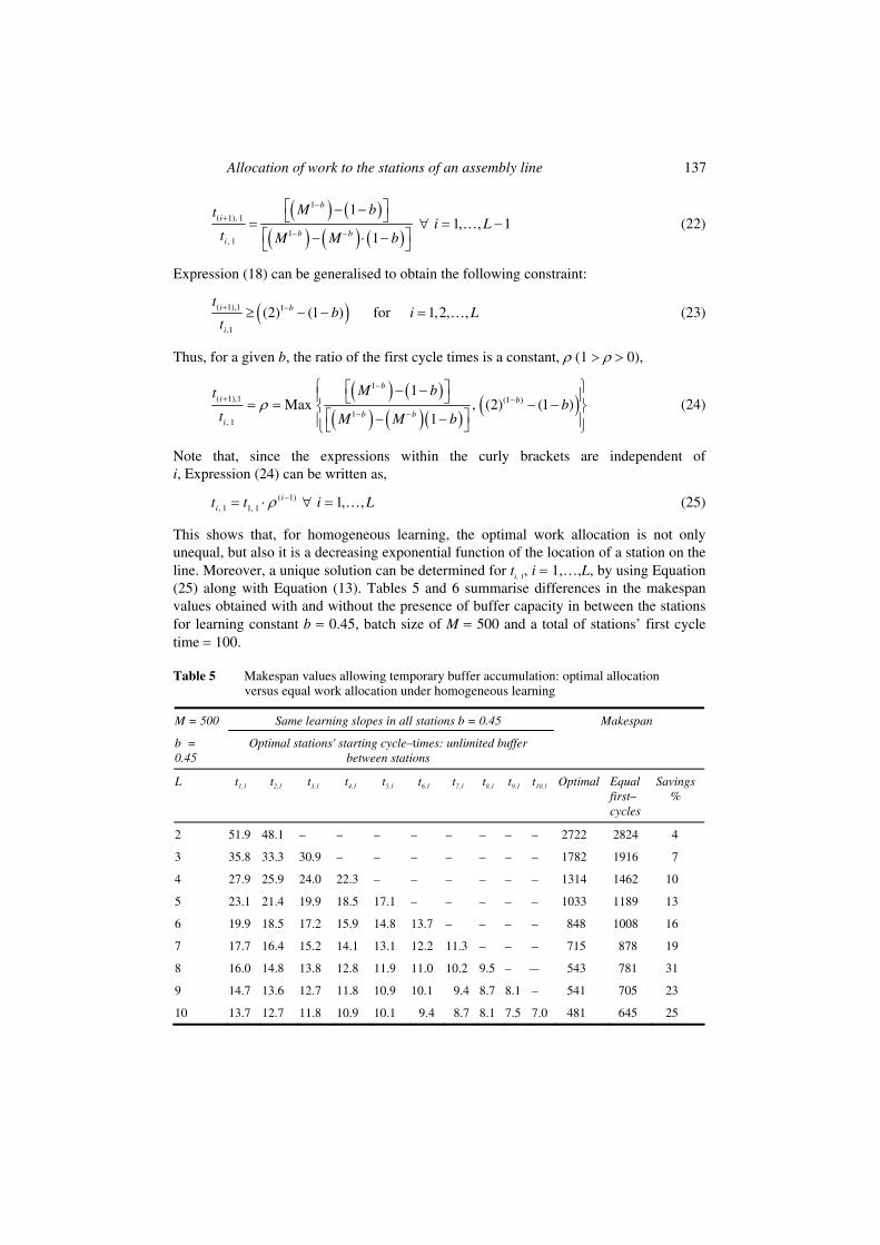
This shows that, for homogeneous learning, the optimal work allocation is not only unequal, but also it is a decreasing exponential function of the location of a station on the line. Moreover, a unique solution can be determined for ti, 1, i = 1,…,L, by using Equation (25) along with Equation (13). Tables 5 and 6 summarise differences in the makespan values obtained with and without the presence of buffer capacity in between the stations for learning constant b = 0.45, batch size of M = 500 and a total of stations’ first cycle time = 100.

Table 5 Makespan values allowing temporary buffer accumulation: optimal allocation versus equal work allocation under homogeneous learning

Same learning slopes in all stations b = 0.45 M = 500

b = 0.45

Optimal stations' starting cycle–times: unlimited buffer between stations

Makespan

L t1,1 t2,1 t3,1 t4,1 t5,1 t6,1 t7,1 t8,1 t9,1 t10,1 Optimal Equal first– cycles

Savings %

2 51.9 48.1 – – – – – – – – 2722 2824 4

3 35.8 33.3 30.9 – – – – – – – 1782 1916 7

4 27.9 25.9 24.0 22.3 – – – – – – 1314 1462 10

5 23.1 21.4 19.9 18.5 17.1 – – – – – 1033 1189 13

6 19.9 18.5 17.2 15.9 14.8 13.7 – – – – 848 1008 16

7 17.7 16.4 15.2 14.1 13.1 12.2 11.3 – – – 715 878 19

8 16.0 14.8 13.8 12.8 11.9 11.0 10.2 9.5 – –– 543 781 31

9 14.7 13.6 12.7 11.8 10.9 10.1 9.4 8.7 8.1 – 541 705 23

10 13.7 12.7 11.8 10.9 10.1 9.4 8.7 8.1 7.5 7.0 481 645 25

138 Y. Cohen et al.

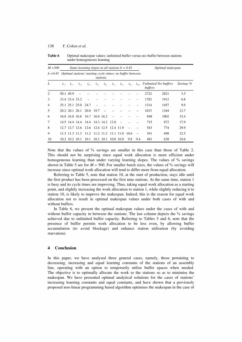
Table 6 Optimal makespan values: unlimited buffer versus no–buffer between stations under homogeneous learning

Same learning slopes in all stations b = 0.45 M =500

b =0.45 Optimal stations' starting cycle–times: no buffer between stations

Optimal makespan

L t1,1 t2,1 t3,1 t4,1 t5,1 t6,1 t7,1 t8,1 t9,1 t10,1 Unlimited buffers

No–buffers Savings %

2 50.1 49.9 – – – – – – – – 2722 2821 3.5

3 33.4 33.4 33.2 – – – – – – – 1782 1912 6.8

4 25.1 25.1 25.0 24.7 – – – – – – 1314 1457 9.9

5 20.2 20.1 20.1 20.0 19.7 – – – – – 1033 1184 12.7

6 16.8 16.8 16.8 16.7 16.6 16.2 – – – – 848 1002 15.4

7 14.5 14.4 14.4 14.4 14.3 14.2 13.8 – – – 715 872 17.9

8 12.7 12.7 12.6 12.6 12.6 12.5 12.4 11.9 – – 543 774 29.9

9 11.3 11.3 11.3 11.2 11.2 11.2 11.1 11.0 10.6 – 541 698 22.5

10 10.2 10.2 10.1 10.1 10.1 10.1 10.0 10.0 9.8 9.4 481 638 24.6

Note that the values of % savings are smaller in this case than those of Table 2. This should not be surprising since equal work allocation is more efficient under homogeneous learning than under varying learning slopes. The values of % savings shown in Table 5 are for M = 500. For smaller batch sizes, the values of % savings will increase since optimal work allocation will tend to differ more from equal allocation.

Referring to Table 5, note that station 10, at the start of production, stays idle until the first product has been processed on the first nine stations. At the same time, station 1 is busy and its cycle times are improving. Thus, taking equal work allocation as a starting point, and slightly increasing the work allocation to station 1, while slightly reducing it to station 10, is likely to improve the makespan. Indeed, this is the reason for equal work allocation not to result in optimal makespan values under both cases of with and without buffers.

In Table 6, we present the optimal makespan values under the cases of with and without buffer capacity in between the stations. The last column depicts the % savings achieved due to unlimited buffer capacity. Referring to Tables 5 and 6, note that the presence of buffer permits work allocation to be less even, by allowing buffer accumulation (to avoid blockage) and enhance station utilisation (by avoiding starvation).

4 Conclusion

In this paper, we have analysed three general cases, namely, those pertaining to decreasing, increasing and equal learning constants of the stations of an assembly line, operating with an option to temporarily utilise buffer spaces when needed. The objective is to optimally allocate the work to the stations so as to minimise the makespan. We have presented optimal analytical solutions for the cases of stations’ increasing learning constants and equal constants, and have shown that a previously proposed non-linear programming based algorithm optimises the makespan in the case of

Allocation of work to the stations of an assembly line 139

decreasing learning constants. Buffer requirements were investigated in all three cases. This is the first time buffer requirements due to difference in learning curves are investigated. The proposed methodologies are illustrated through example problems and numerical results are presented to compare the performances of optimal versus equal allocation of work to the stations. The equal work allocation policy is not expected to perform that well for the increasing and decreasing learning constants of the stations, as we show. However, even for the homogeneous learning constants of the stations, we show that the equal work allocation policy does not perform that well. Our numerical results also depict significant makespan reductions in the presence of available buffer capacity in between the stations of an assembly line as shown in Table 6.

References

Adler, G.L. and Nanada, R. (1974) ‘The effect of learning on optimal lot size determination the simple product case’, AIIE Transactions, Vol. 6, pp.14–20.

Ardity, D., Tokdemir, O.B. and Suh, K. (2001) ‘Effect of learning on line of balance scheduling’, International Journal of Project Management, Vol. 19, pp.265–277.

Brenner, M. (1990) Prediction of Learning Parameters for Short Cycle Tasks, Technion-IIT, Israel: Unpublished M.Sc. thesis.

Chakravarty, A.K. (1988) ‘Line balancing with task learning effects’, IIE Transactions, Vol. 20, No. 2, pp.186–193.

Cohen, Y. and Dar-El, E.M. (1998) ‘Optimizing the number of stations in assembly lines under learning’, Production Planning and Control, Vol. 9, No. 3, pp.230–240.

Cohen, Y., Vitner, G. and Sarin, S.C. (2006) ‘Optimal allocation of work in assembly lines for lots with homogeneous learning’, European Journal of Operational Research, Vol. 168, No. 3, pp.922–931.

Cohen, Y., Vitner, G. and Sarin, S.C. (2008) ‘Work allocation to stations with varying learning slopes and without buffers’, European Journal of Operational Research, Vol. 184, No. 3, pp.797–801.

Dar-El, E.M. (2000) Human Learning: From Learning Curves to Learning Organizations, Kluwer: Academic Publishers.

Dar-El, E.M. and Rabinovitch, M. (1988) ‘Optimal planning and scheduling of assembly lines’, International Journal of Production Research, Vol. 26, No. 9, pp.1433–1450.

Enginarlar, E., Li, J., Meerkov, S.M. and Zhang, R.Q. (2002) ‘Buffer capacity for accommodating machine downtime in serial production lines’, International Journal of Production Research, Vol. 40, No. 3, pp.601–624.

Enginarlar, E., Li, J. and Meerkov, S.M. (2005) ‘How lean can lean buffers be?, IIE Transactions, Vol. 37, No. 4, pp.333–342.

Gershwin, S.B. and Schore, S.G. (2000) ‘Efficient algorithm for buffer space allocation’, Annals of Operations Research, Vol. 93, pp.117–144.

Globerson, S. and Levin, N. (1995) ‘A learning curve model for an equivalent number of units’, IIE Transactions, Vol. 27, pp.716–721.

Globerson, S. and Shtub, A. (1984) ‘The impact of learning curves on the design of long cycle time lines’, Industrial Management, Vol. 26, No. 3, pp.5–10.

Hillier, M.S. (2000) ‘Characterizing the optimal allocation of storage space in production line systems, with variable processing times’, IIE Transactions, Vol. 32, pp.1–8.

Hillier, M. and Hillier, F. (2006) ‘Simultaneous optimization of work and buffer space in unpaced production lines with random processing times’, IIE Transactions, Vol. 38, pp.39–51.

140 Y. Cohen et al.

Kroll, D.E. (1989) ‘The incorporation of learning in production planning models’, Annals of O.R., Vol. 17, pp.291–304.

Shi, L. and Men, S. (2003) ‘Optimal buffer allocation in production lines’, IIE Transactions, Vol. 35, pp.1–10.

Smith, J.M. and Cruz, F.R.B. (2005) ‘The buffer allocation problem for the general finite buffer queueing networks’, IIE Transactions, Vol. 37, pp.343–365.

Spinellis, D.D. and Papadopoulos, C.T. (2000) ‘A simulated annealing approach for buffer allocation in reliable production lines’, Annals of Operations Research, Vol. 93, pp.373–384.

Wright, T.P. (1936) ‘Factors affecting the cost of airplanes’, Journal of Aeronautical Sciences, Vol. 3, No. 4, pp.122–128.