Ali Mohammad Khosravani Automatic Modeling of Building ...
134
Deutsche Geodätische Kommission der Bayerischen Akademie der Wissenschaften Reihe C Dissertationen Heft Nr. 767 Ali Mohammad Khosravani Automatic Modeling of Building Interiors Using Low-Cost Sensor Systems München 2016 Verlag der Bayerischen Akademie der Wissenschaften in Kommission beim Verlag C. H. Beck ISSN 0065-5325 ISBN 978-3-7696-5179-9
-
Upload
khangminh22 -
Category
Documents
-
view
3 -
download
0
Transcript of Ali Mohammad Khosravani Automatic Modeling of Building ...

Deutsche Geodätische Kommission
der Bayerischen Akademie der Wissenschaften
Reihe C Dissertationen Heft Nr. 767
Ali Mohammad Khosravani
Automatic Modeling of Building Interiors
Using Low-Cost Sensor Systems
München 2016
Verlag der Bayerischen Akademie der Wissenschaftenin Kommission beim Verlag C. H. Beck
ISSN 0065-5325 ISBN 978-3-7696-5179-9


Deutsche Geodätische Kommission
der Bayerischen Akademie der Wissenschaften
Reihe C Dissertationen Heft Nr. 767
Automatic Modeling of Building Interiors
Using Low-Cost Sensor Systems
Von der Fakultät Luft- und Raumfahrttechnik und Geodäsie
der Universität Stuttgart
zur Erlangung der Würde eines
Doktors der Ingenieurwissenschaften (Dr.-Ing.)
genehmigte Abhandlung
Vorgelegt von
M.Sc. Ali Mohammad Khosravani
aus Shiraz, Iran
München 2016
Verlag der Bayerischen Akademie der Wissenschaftenin Kommission beim Verlag C. H. Beck
ISSN 0065-5325 ISBN 978-3-7696-5179-9

Adresse der Deutschen Geodätischen Kommission:
Deutsche Geodätische KommissionAlfons-Goppel-Straße 11 ! D – 80 539 München
Telefon +49 – 89 – 23 031 1113 ! Telefax +49 – 89 – 23 031 - 1283 / - 1100e-mail [email protected] ! http://www.dgk.badw.de
Hauptberichter: Prof. Dr.-Ing. habil. Dieter FritschMitberichter: Prof. Dr.-Ing. habil. Volker Schwieger
Tag der mündlichen Prüfung: 09.12.2015
Diese Dissertation ist auf dem Server der Deutschen Geodätischen Kommission unter <http://dgk.badw.de/>sowie auf dem Server der Universität Stuttgart unter <http://elib.uni-stuttgart.de/opus/doku/e-diss.php>
elektronisch publiziert
© 2016 Deutsche Geodätische Kommission, München
Alle Rechte vorbehalten. Ohne Genehmigung der Herausgeber ist es auch nicht gestattet,die Veröffentlichung oder Teile daraus auf photomechanischem Wege (Photokopie, Mikrokopie) zu vervielfältigen.
ISSN 0065-5325 ISBN 978-3-7696-5179-9

This dissertation is gratefully dedicated to my beloved mother, for her endless love and
encouragements, and to my late father.

5
Kurzfassung
Die dreidimensionale Rekonstruktion von Innenraumszenen zielt darauf ab, die Form von
Gebäudeinnenräumen als Flächen oder Volumina abzubilden. Aufgrund von Fortschritten im Bereich
der Technologie entfernungsmessender Sensoren und Algorithmen der Computervision sowie
verursacht durch das gesteigerte Interesse vieler Anwendungsgebiete an Innenraummodellen hat
dieses Forschungsfeld in den letzten Jahren zunehmend an Aufmerksamkeit gewonnen. Die
Automatisierung des Rekonstruktionsprozesses ist weiterhin Forschungsgegenstand, verursacht durch
die Komplexität der Rekonstruktion, der geometrischen Modellierung beliebig geformter Räume und
besonders im Falle unvollständiger oder ungenauer Daten. Die hier vorgestellte Arbeit hat die
Erhöhung des Automatisierungsgrades dieser Aufgabe zum Ziel, unter der Verwendung einer geringen
Anzahl an Annahmen bzgl. der Form von Räumen und basierend auf Daten, welche mit Low-Cost-
Sensoren erfasst wurden und von geringer Qualität sind.
Diese Studie stellt einen automatisierten Arbeitsablauf vor, welcher sich aus zwei Hauptphasen
zusammensetzt. Die erste Phase beinhaltet die Datenerfassung mittels eines kostengünstigen und leicht
erhältlichen Sensorsystems, der Microsoft Kinect. Die Entfernungsdaten werden anhand von
Merkmalen, welche im Bildraum oder im 3D Objektraum beobachtet werden können, registriert. Ein
neuer komplementärer Ansatz für die Unterstützung der Registrierungsaufgabe wird präsentiert, da die
diese Ansätze zur Registrierung in manchen Fällen versagen können, wenn die Anzahl gefundener
visueller und geometrischer Merkmale nicht ausreicht. Der Ansatz basiert auf der Benutzerfußspur,
welche mittels einer Innenraumpositionierungsmethode erfasst wird, und auf einem vorhandenen
groben Stockwerksmodell.
In der zweiten Phase werden aus den registrierten Punktwolken mittels eines neuen Ansatzes
automatisiert hochdetaillierte 3D-Modelle abgeleitet. Hierzu werden die Daten im zweidimensionalen
Raum verarbeitet (indem die Punkte auf die Grundrissebene projiziert werden) und die Ergebnisse
werden durch eine Extrusion in den dreidimensionalen Raum zurückgewandelt (wobei die Raumhöhe
mittels einer Histogrammanalyse der in der Punktwolke enthaltenen Höhen erfasst wird). Die
Datenanalyse und -modellierung in 2D vereinfacht dabei nicht nur das Rekonstruktionsproblem,
sondern erlaubt auch eine topologische Analyse unter Verwendung der Graphentheorie. Die
Leistungsfähigkeit des Ansatzes wird dargestellt, indem Daten mehrerer Sensoren verwendet werden,
die unterschiedliche Genauigkeiten liefern, und anhand der Erfassung von Räumen unterschiedlicher
Form und Größe.
Abschließend zeigt die Studie, dass die rekonstruierten Modelle verwendbar sind, um vorhandene
grobe Innenraummodelle zu verfeinern, welche beispielsweise aus Architekturzeichnungen oder
Grundrissplänen abgeleitet werden können. Diese Verfeinerung wird durch die Fusion der detaillierten
Modelle einzelner Räume mit dem Grobmodell realisiert. Die Modellfusion beinhaltet dabei die
Überbrückung von Lücken im detaillierten Modell unter Verwendung eines neuen, auf maschinellem
Lernen basierenden Ansatzes. Darüber hinaus erlaubt der Verfeinerungsprozess die Detektion von
Änderungen oder Details, welche aufgrund der Generalisierung des Grobmodells oder
Renovierungsarbeiten im Gebäudeinnenraum fehlten.

6
Abstract
Indoor reconstruction or 3D modeling of indoor scenes aims at representing the 3D shape of building
interiors in terms of surfaces and volumes, using photographs, 3D point clouds or hypotheses. Due to
advances in the range measurement sensors technology and vision algorithms, and at the same time an
increased demand for indoor models by many applications, this topic of research has gained growing
attention during the last years. The automation of the reconstruction process is still a challenge, due to
the complexity of the data collection in indoor scenes, as well as geometrical modeling of arbitrary
room shapes, specially if the data is noisy or incomplete. Available reconstruction approaches rely on
either some level of user interaction, or making assumptions regarding the scene, in order to deal with
the challenges. The presented work aims at increasing the automation level of the reconstruction task,
while making fewer assumptions regarding the room shapes, even from the data collected by low-cost
sensor systems subject to a high level of noise or occlusions. This is realized by employing topological
corrections that assure a consistent and robust reconstruction.
This study presents an automatic workflow consisting of two main phases. In the first phase, range
data is collected using the affordable and accessible sensor system, Microsoft Kinect. The range data
is registered based on features observed in the image space or 3D object space. A new complementary
approach is presented to support the registration task in some cases where these registration
approaches fail, due to the existence of insufficient visual and geometrical features. The approach is
based on the user’s track information derived from an indoor positioning method, as well as an
available coarse floor plan.
In the second phase, 3D models are derived with a high level of details from the registered point
clouds. The data is processed in 2D space (by projecting the points onto the ground plane), and the
results are converted back to 3D by an extrusion (room height available from the point height
histogram analysis). Data processing and modeling in 2D does not only simplify the reconstruction
problem, but also allows for topological analysis using the graph theory. The performance of the
presented reconstruction approach is demonstrated for the data derived from different sensors having
different accuracies, as well as different room shapes and sizes.
Finally, the study shows that the reconstructed models can be used to refine available coarse indoor
models which are for instance derived from architectural drawings or floor plans. The refinement is
performed by the fusion of the detailed models of individual rooms (reconstructed in a higher level of
details by the new approach) to the coarse model. The model fusion also enables the reconstruction of
gaps in the detailed model using a new learning-based approach. Moreover, the refinement process
enables the detection of changes or details in the original plans, missing due to generalization
purposes, or later renovations in the building interiors.

7
Contents
Kurzfassung ............................................................................................................................................. 5
Abstract ....................................................................................................................................................6
1. Introduction ........................................................................................................................................11
1.1. Motivation .................................................................................................................................. 11
1.2. Objectives ................................................................................................................................... 13
1.3. Outline and Design of the Thesis ............................................................................................... 13
2. Overview of Indoor Data Collection Techniques...............................................................................15
2.1. State-of-the-Art Sensors for 3D Data Collection ........................................................................ 16
2.1.1. Laser Scanners .................................................................................................................. 17
2.1.2. 3D Range Cameras ........................................................................................................... 22
2.2. The Registration Problem ........................................................................................................... 31
2.2.1. Registration Using Point Correspondences in the Point Clouds ...................................... 31
2.2.2. Registration by the Estimation of the Sensor Pose ........................................................... 33
3. Data Collection using Microsoft Kinect for Xbox 360 ......................................................................36
3 .1. Point Cloud Collection by Kinect ............................................................................................... 36
3.1.1. System Interfaces and SDKs ............................................................................................ 36
3.1.2. System Calibration ........................................................................................................... 36
3.1.3. Generation of Colored Point Clouds ................................................................................ 39
3.2. Point Clouds Registration ........................................................................................................... 42
3.2.1. Point Clouds Registration Based on RGB and Depth Information .................................. 42
3.2.2. Point Clouds Registration Based on an Indoor Positioning Solution and Available Coarse
Indoor Models .......................................................................................................................... 43
3.3. Kinect SWOT Analysis .............................................................................................................. 49
4. Overview of Available Indoor Modeling Approaches .......................................................................50
4.1. Classification of Available Modeling Approaches ..................................................................... 51
4.2. Iconic Approaches ...................................................................................................................... 52
4.2.1. Image-Based Modeling .................................................................................................... 52
4.2.2. Range-Based Modeling .................................................................................................... 57
4.2.3. Modeling Based on Architectural Drawings .................................................................... 60
4.3. Symbolic Approaches ................................................................................................................. 63

8
5. Automatic Reconstruction of Indoor Spaces ......................................................................................65
5.1. Point Cloud Pre-Processing ........................................................................................................ 66
5.1.1. Outlier Removal ............................................................................................................... 66
5.1.2. Downsampling .................................................................................................................. 67
5.1.3. Noise Removal ................................................................................................................. 67
5.1.4. Leveling the Point Cloud .................................................................................................. 68
5.1.5. Height Estimation and Furniture Removal ....................................................................... 69
5.2. Reconstruction of Geometric Models ......................................................................................... 70
5.2.1. Generation of Orthographic Projected Image ................................................................... 70
5.2.2. Binarization ...................................................................................................................... 71
5.2.3. Morphological Image Processing ..................................................................................... 72
5.2.4. Estimation of the Lines Representing the Walls in 2D .................................................... 73
5.2.5. Topological Corrections ................................................................................................... 76
5.2.6. 2D to 3D Conversion of Reconstructed Models ............................................................... 81
6. Experimental Results and Analysis ....................................................................................................82
6.1. Kinect System Calibration and Accuracy Analysis .................................................................... 82
6.1.1. System Calibration ........................................................................................................... 82
6.1.2. Accuracy of Kinect Range Measurements ....................................................................... 85
6.2. Evaluation of the Reconstruction Approach ............................................................................... 88
6.2.1. Parameter Selection in Different Scenarios ...................................................................... 88
6.3. Quality of the Reconstructed Models ......................................................................................... 93
7. Application in the Refinement of Available Coarse Floor Models ....................................................95
7.1. Registration of Individual Detailed Models to an Available Coarse Floor Model ..................... 96
7.1.1. Approximate Registration ................................................................................................ 96
7.1.2. Fine Registration .............................................................................................................. 97
7.2. Fusion of Detailed Models to the Coarse Model ........................................................................ 99
8. Conclusion........................................................................................................................................103
8.1. Summary................................................................................................................................... 103
8.2. Contributions ............................................................................................................................ 103
8.3. Future Work .............................................................................................................................. 104
Appendix A. Point Cloud Registration – Fundamental Principles .......................................................106
A.1. Closed-Form Solution .............................................................................................................. 107
A.2. Iterative Solution (ICP) ........................................................................................................... 109
Appendix B. RANSAC ..........................................................................................................................112
Appendix C. SLAM Problem .................................................................................................................113

9
Appendix D. Hough Transform ...........................................................................................................115
D.1. Standard Hough Transform ..................................................................................................... 115
D.2. Progressive Probabilistic Hough Transform ............................................................................ 116
Appendix E. Reconstruction of Detailed Models – Case Studies ..........................................................117
References ............................................................................................................................................123
Relevant Publications ...........................................................................................................................130
Curriculum Vitae ..................................................................................................................................131
Acknowledgment .................................................................................................................................132

10

11
1. Introduction
1.1. Motivation
Indoor modeling addresses the reconstruction of 2D and 3D CAD models of building interiors by
means of surfaces or volumes. Such models can be derived from photographs by the extraction and
matching of features of interest, or from point clouds by the fitting geometric primitives.
Models of buildings interior structure are demanded by many applications to support a variety of
needs, from navigation to simulation. In robotics and computer vision, existence of a map or
simultaneous mapping is essential for localization of the user or a mobile robot. In virtual city models,
interior models constitute the levels-of-detail 4 (LOD4) models (according to OGC standard CityGML
(Kolbe et al., 2005)), to support many spatial-based applications such as GIS, urban planning, risk
management, emergency action planning, environmental simulation, navigation, etc.. In Building
Information Modeling (BIM), which is used for supporting construction, planning, design, and
maintaining infrastructures, interior models are the geometric basis of semantic information. In
architecture, virtual indoor models support interior designers to have a realistic and more precise
impression about spaces.
The most important challenge in the reconstruction of indoor models is the time and costs of data
collection and generating such models. In practice, this task is mainly performed using manual and
semi-automatic approaches, and therefore the user qualifications play an important role in the speed
and accuracy of the process. According to the comparison made by Panushev and Brandt (2007), the
reconstruction of average-sized building interiors takes several months, although modeling single
objects can be a fairly quick task. Therefore, the automation of this process is required. This
automation is still a challenge, due to the existence of clutter, complexity of the shape of the interior
and challenges in the data collection.
Indoor data collection is mostly performed from ground level viewpoints, and therefore is more
complex and challenging in comparison with airborne and remote data collection. Moreover, data
collection platforms delivering high accuracy data (e.g. Terrestrial Laser Scanners (TLS)) are usually
heavy and expensive, and therefore large-scale data collection is time consuming and costly. However,
development of low-cost range measurement sensors has recently increased the focus on range-based
indoor mapping. According to Luhmann et al. (2014), the mass market effect of the consumer-grade
3D sensing camera Microsoft Kinect (over 10 million units in circulation), had a significant impact on
the photogrammetric community where the number of 3D sensing systems is in the range of 1000s.
The registration of the point clouds collected by such low-cost and handheld systems is also an active
research area; as will be seen later, this task can be a challenge in scenarios having a poor texture or
insufficient geometrical features. Presented works by Henry et al. (2012), Newcombe et al. (2011),
Whelan et al. (2013) consider the Kinect a suitable platform for a fast and affordable data collection.
Google Project Tango, Structure Sensor and DPI-7/8 are examples of commercial solutions developed
so far, for the collection of 3D data from building interiors, as the user walks through space. For the
registration of the collected point clouds, the systems benefit from the geometric information extracted

12 1. Introduction
from the range images, or observations made in color image space, or a combination of both
information for an accurate pose estimation. Therefore, the systems turned to be fragile in scenarios
that the mentioned sources of information are not available or insufficient, such as scenes with low
visual or geometrical features (e.g. hallways). Therefore, other sources of information and new
strategies shall be considered to fill the gap in the available registration approaches.
Despite the fact that indoor data collection has already been studied by many researchers, and is
facilitated due to advances in sensor technology and vision algorithms, less attention is still paid to the
reconstruction of CAD models based on the collected data. Moreover, although some reconstruction
approaches are already available, the quality and density of the collected data by low-cost sensor
systems are not always consistent with the assumptions made by the approaches. In other words,
affordability comes with loss of quality and trade-offs; data collected by low-cost sensor systems are
subject to more noise, gaps and other artifacts that make the reconstruction process more challenging
than before. Due to the complexity of indoor scenes, existence of gap and clutter, and extreme
conditions for the registration of collected point clouds, still a general and fully automatic indoor
reconstruction approach does not exist. Available approaches rely either on some level of user
interaction, or make assumptions regarding the room shapes, quality of the collected data, etc.
Commercial software solutions such as Leica Cyclone and Leica CloudWorx are widely used for
modeling from the collected point clouds; however, they are based on a high level of user interaction.
A strategy for the automation of this process is proposed for instance by Budroni and Böhm (2009)
using a linear and rotational plane sweeping algorithm, however, under the assumption that the walls
are parallel or perpendicular to each other (Manhattan-world scenario). Moreover, the ceiling and floor
points have to be collected in this modeling approach (for the cell decomposition process), which is a
challenge for low-cost mobile mapping systems, due to the poor texture and 3D information required
for the registration of the point clouds captured from different viewpoints. Another example of
automatic reconstruction of indoor scenes is presented by Previtali et al. (2014), based on the
RANSAC algorithm for the extraction of planar features. Although this algorithm can model rooms
with more general shapes, still the collection of floor or ceiling points for the cell decomposition is
necessary. Another category of approaches converts the modeling problem from 3D to 2D, and extract
line segments corresponding to walls by processing images derived from the projection of points onto
the ground plane. Okorn et al. (2010) use the Hough transform for this purpose; however, the resulting
2D plan does not represent a topologically correct model. Adan and Huber (2011) use a similar
approach, but add more semantic information into the models and deal with occlusions using a ray-
tracing algorithm, assuming 3D data is collected from fixed and known locations. Valero et al. (2012)
further improve the results using a more robust line detection algorithm and considering some
topological analyses. However, this approach requires a dense and high quality input point cloud,
which is a challenge to fulfill using low-cost sensor systems.
Therefore, new approaches are required to fill the gap between the new data collection strategies and
available reconstruction approaches, by making fewer assumptions regarding the point cloud quality,
data collection strategy and different room shapes, and at the same time dealing with the gaps in the
data.
1.2. Objectives 13
1.2. Objectives
Regarding the mentioned gaps in the previous section, this work aims at increasing the automation
level, and at the same time the performance of the reconstruction process (i.e. modeling arbitrary
shapes with a higher level of detail), with a focus on the data collected by low-cost sensor systems. For
this purpose, the following objectives shall be fulfilled in this study:
Investigation on indoor data collection using low-cost sensor systems: In this part of the work, state-
of-the-art sensor systems used for the collection of 3D data in indoor scenes shall be investigated. A
suitable sensor system shall be selected as the case study, and the registration of the collected point
clouds by this sensor has to be studied in different scenarios.
Defining a robust and efficient reconstruction approach: In this part of the work, topologically correct
models have to be automatically reconstructed from the point clouds collected by the selected low-cost
sensor system in the previous part. Furniture and clutter have to be removed from the point cloud
automatically, or with a minimal user interaction. The reconstruction approach shall be capable of
dealing with the noise and occlusions contained in the collected data; strategies have to be defined to
compensate such effects. Moreover, the approach shall include modeling of more general shapes of the
building interiors (not only Manhattan-world scenarios). It is also required to reconstruct available
larger gaps (e.g. those caused by the existence of windows), using available sources of information,
such as architectural drawings and available floor plans.
Investigation on update and refinement of available coarse floor models: As-designed building models
and available floor plans do not necessarily represent the actual state of the building interiors (as-built
models). For many indoor applications, such models and plans have to be verified, updated or refined,
in order to fulfill the required accuracies. Low-cost data collection approaches have great potential for
a fast and efficient fulfillment of this task, if a suitable reconstruction and fusion algorithm is
available. This shall be investigated within the study as well.
1.3. Outline and Design of the Thesis
In order to fulfill the required tasks mentioned in the previous section, the thesis is structured within
the next seven chapters, as follows.
Chapter 2 presents state-of-the-art sensors used for 3D data acquisition in indoor scenes, together with
available approaches used for the registration of the data collected from different viewpoints.
In chapter 3, Microsoft Kinect is selected as the case study; the mathematical background for the
system calibration and generation of colored point clouds from disparity and color images is presented
in this chapter. Challenges regarding the data collection and registration are discussed in this chapter,
and a new complementary approach for the registration of the point clouds is proposed.
Chapter 4 presents state-of-the-art indoor reconstruction approaches, based on different sources of
input data. Iconic (bottom-up) approaches use real measurements, mainly derived from images and
range data. In contrast, symbolic (top-down) approaches support indoor reconstruction based on
hypotheses, in case of having incomplete or erroneous data.
Chapter 5 presents the proposed approach for the reconstruction of indoor spaces from the collected
point clouds using a pilot study.

14 1. Introduction
Experimental results are presented in chapter 6. The chapter starts with the system calibration and
accuracy analysis of the range measurements by Kinect, and then continues with the performance
evaluation of the reconstruction approach in different scenarios.
Chapter 7 aims at the refinement of available coarse floor models by the fusion of the detailed model
of individual rooms. Larger gaps in the detailed models (e.g. those caused by the existence of
windows) are reconstructed here, as a byproduct of the fusion process, using a proposed learning-
based approach.
Chapter 8 concludes the presented work with a summary of the achieved results and contributions. It
further suggests research areas, in which more investigation is required to increase the performance of
the proposed system and improve achieved results.
15
2. Overview of Indoor Data Collection Techniques
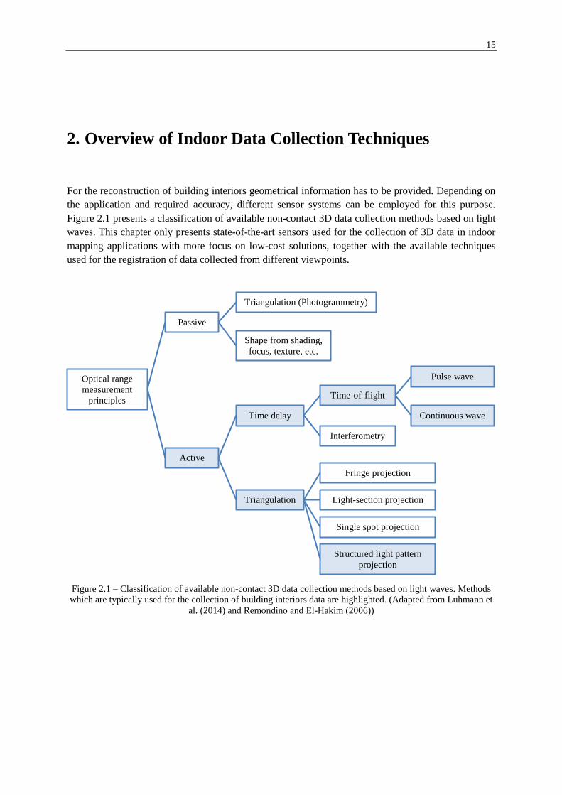
For the reconstruction of building interiors geometrical information has to be provided. Depending on
the application and required accuracy, different sensor systems can be employed for this purpose.
Figure 2.1 presents a classification of available non-contact 3D data collection methods based on light
waves. This chapter only presents state-of-the-art sensors used for the collection of 3D data in indoor
mapping applications with more focus on low-cost solutions, together with the available techniques
used for the registration of data collected from different viewpoints.
Figure 2.1 – Classification of available non-contact 3D data collection methods based on light waves. Methods
which are typically used for the collection of building interiors data are highlighted. (Adapted from Luhmann et
al. (2014) and Remondino and El-Hakim (2006))
Optical range
measurement
principles
Triangulation (Photogrammetry)
Active
Shape from shading,
focus, texture, etc.
Time delay
Triangulation
Time-of-flight
Passive
Interferometry
Pulse wave
Continuous wave
Fringe projection
Light-section projection
Single spot projection
Structured light pattern
projection

16 2. Overview of Indoor Data Collection Techniques
2.1. State-of-the-Art Sensors for 3D Data Collection
Sensor systems used for 3D data acquisition in indoor scenes are divided to two main categories,
based on their sensing principle: passive and active systems.
Passive Systems
Passive triangulation systems provide 3D information by measuring and analyzing the 2D image
coordinates of interest points, collected from multiple viewpoints (see figure 2.2). In close range
photogrammetry, solid state sensor cameras such as SLR-type cameras, high resolution cameras and
high speed cameras are certainly the most popular passive systems (Maas, 2008). Passive systems are
highly dependent on the ambient light conditions and the visual texture. The derivation of 3D
information requires post-processing efforts; however, the systems are low-cost, portable and flexible
to use.
The second type of passive systems rely on visual qualities such as texture, focus, shading and light
intensity to estimate surface normal vectors and therefore, the shape of the surface. For example,
shape-from-shading techniques recover the shape from the variation of shading in the image. This
requires recovering the light source in the image, which is a difficult task in real images, and requires
simplifications and making assumptions regarding the light conditions. Moreover, as also stated by
Zhang et al. (1999), even with such assumptions, finding a unique solution to the corresponding
geometrical problem is still difficult, since the surface is described in terms of its normal vectors, and
additional constraints are required. In general, this category of passive approaches is not suitable in
indoor modeling applications, and is mentioned here only for the completeness.
Figure 2.2 – Passive triangulation
principle.
Active Systems
Active systems rely on their own illumination and deliver 3D information (range images and point
clouds) without requiring post processing efforts by the user, and therefore are more suitable for
automation purposes. Since the systems do not rely on the visual appearance of the objects and
provide their own features to be measured, they are well suited for measuring textureless surfaces,
which is the case in many indoor spaces.
Advances in sensor design and technology as well as vision algorithms and computational capabilities
have resulted in portability, cost reduction and performance improvements of active range
measurement systems. In indoor reconstruction applications, not only terrestrial laser scanners have
become slightly less expensive and smaller than before, but also other solutions have been optimized
for the collection of 3D data, such as time-of-flight cameras and triangulation systems using projected
2.1. State-of-the-Art Sensors for 3D Data Collection 17
light patterns. In the following section, popular and state-of-the-art systems used for the 3D data
collection of indoor spaces are introduced.
2.1.1. Laser Scanners
2.1.1.1. Terrestrial Laser Scanners
Terrestrial laser scanners (TLS) are increasingly used to capture accurate and dense 3D data in many
applications, from the recording of building interiors to the documentation of heritage sites. They can
collect thousands to hundreds of thousands points per second with millimeters accuracy.
Distance measurements in terrestrial laser scanners are realized based on two methods: estimation of
light travel time and triangulation. The light travel time can be measured directly using pulse wave
time-of-flight (TOF) measurement, or indirectly by phase measurement in continuous wave lasers.
Short range laser scanners use triangulation principle for the range measurements, and are typically
used in industrial applications, where the object distance is less than 1m. Triangulation-based scanners
are not of interest in this study.
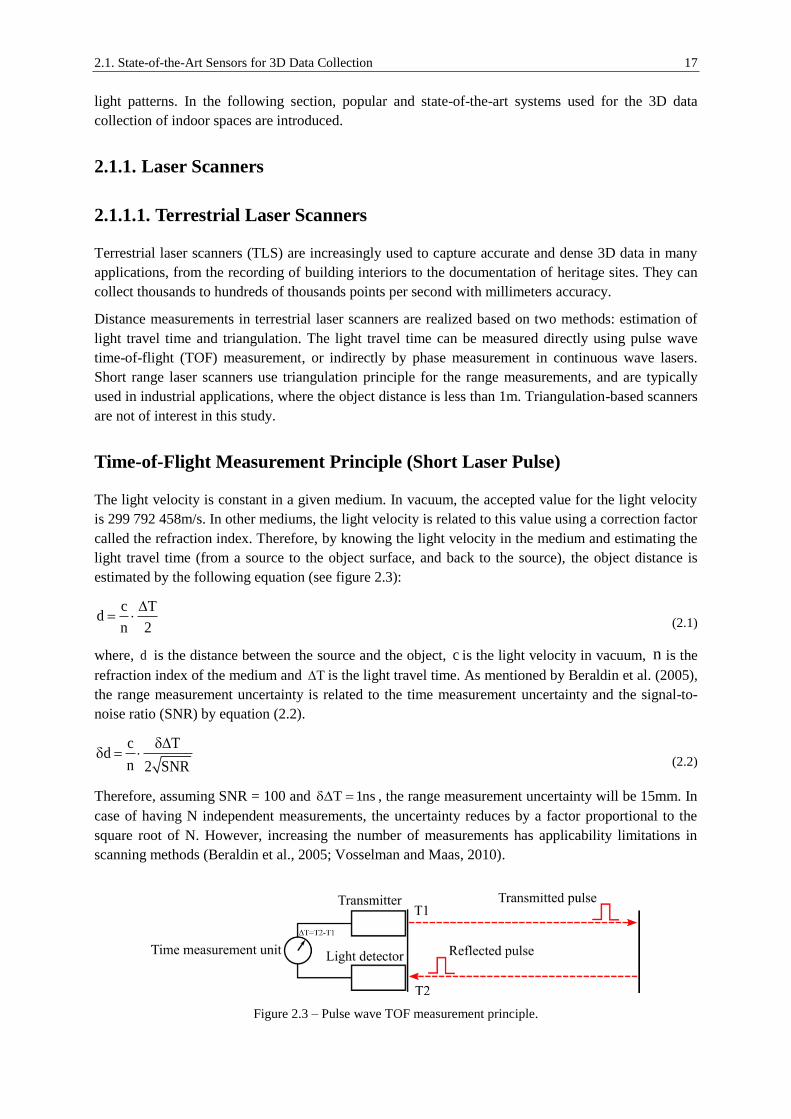
Time-of-Flight Measurement Principle (Short Laser Pulse)
The light velocity is constant in a given medium. In vacuum, the accepted value for the light velocity
is 299 792 458m/s. In other mediums, the light velocity is related to this value using a correction factor
called the refraction index. Therefore, by knowing the light velocity in the medium and estimating the
light travel time (from a source to the object surface, and back to the source), the object distance is
estimated by the following equation (see figure 2.3):
c Td
n 2
(2.1)
where, d is the distance between the source and the object, c is the light velocity in vacuum, n is the
refraction index of the medium and T is the light travel time. As mentioned by Beraldin et al. (2005),
the range measurement uncertainty is related to the time measurement uncertainty and the signal-to-
noise ratio (SNR) by equation (2.2).
c Td
n 2 SNR
(2.2)
Therefore, assuming SNR = 100 and T 1ns , the range measurement uncertainty will be 15mm. In
case of having N independent measurements, the uncertainty reduces by a factor proportional to the
square root of N. However, increasing the number of measurements has applicability limitations in
scanning methods (Beraldin et al., 2005; Vosselman and Maas, 2010).
Figure 2.3 – Pulse wave TOF measurement principle.

18 2. Overview of Indoor Data Collection Techniques
As mentioned by Beraldin et al. (2005) and Vosselman and Maas (2010), most of the pulse wave TOF
laser scanners provide an uncertainty of a few millimeters in the range measurements up to 50m, as
long as a high SNR is maintained. However, as mentioned by Beraldin et al. (2010), exact and
accurate measurement of the pulsed laser arrival time is a challenge, due to the difficulties in the
detection of the time trigger in the returned echo. For example, if the pulse is time-triggered at the
maximum amplitude, the detection of the time trigger will be difficult if the returned echo provides
more than one peak. The detection threshold can also be set to the leading edge of the echo, but on the
other hand the threshold will be strongly dependent on the echo’s amplitude, which is subject to
change due to the light attenuation nature in the atmosphere. Another method which is proven to be
more suitable is the constant fraction (Wagner et al., 2004), in which the trigger is typically set to 50%
of its maximum amplitude.
Phase Shift Measurement Principle (Continuous Wave)
Besides the direct measurement of the TOF, the estimation of the light travel time can also be realized
indirectly by the measurement of the phase difference between the original and returned waveforms
using amplitude modulation (AM) or frequency modulation (FM) techniques. The phase difference
between the two waveforms is related to the time delay and therefore to the corresponding distance by
equations (2.3) and (2.4) (see figure 2.4).
mnt
2 c
(2.3)
mmax
cd t, d
n 2
(2.4)
in which, d is the distance equivalent to the phase shift (the absolute distance is the summation of this
distance and a multiplication of the full wavelength), is the phase shift and m is the wavelength
of the modulated beam m(c / f ) . As mentioned by Beraldin et al. (2005), the distance uncertainty in
case of AM is given approximately by:
m1d
4 SNR
(2.5)
As it can be seen in the equation, a low frequency mf results in a less precise range measurement.
Therefore, using blue opposed to a near-infrared laser will decrease the range measurement
uncertainty. However, reducing the wavelength (increasing the frequency) will limit the operating
range of the system, due to the faster attenuation of high frequency waves.
Figure 2.4 – Continuous wave phase shift measurement principle.

2.1. State-of-the-Art Sensors for 3D Data Collection 19
Since the returned signal cannot be associated with a specific part of the original signal, the calculated
distance is not the absolute distance between the source and the object, but a fraction of the full
wavelength. The absolute distance is obtained by the summation of this value with a multiplication of
the full wavelength, also known as the ambiguity interval. The ambiguity interval cannot be purely
resolved by the phase shift measurement, and therefore, using multiple measurements with different
modulation frequencies is required. As mentioned by Guidi and Remondino (2012), continuous wave
solutions use two or three different modulation frequencies: a low modulation frequency for a large
ambiguity interval, and higher modulation frequencies for increasing the angular resolution and
therefore the resolution of the range measurements. By increasing the number of steps between the
low and high frequencies, the FM technique is realized. This has the advantage of reducing the
measurement uncertainty level, which is less than that of pulse wave devices (typically in range of 2-
3mm), as well as continuous wave devices with two or three modulation frequencies (typically 1mm at
a proper distance). Such devices are mostly used in industrial and cultural heritage applications.
According to Beraldin et al. (2005), The distance measurement uncertainty for such devices is
approximately given by:
3 c 1d
2 f SNR
(2.6)
where, f is the frequency excursion (Skolnik, 1980).
According to Guidi and Remondino (2012), continuous wave systems provide smaller distance
measurement uncertainties in comparison with pulse wave systems due to two reason: a) since the
light is sent to the target continuously, more energy is sent to the target and therefore a higher SNR is
provided; b) the low-path filtering used for the extraction of the signal further reduces the noise.
However, limitations caused by resolving the ambiguity interval make the operating range of such
systems smaller than pulse wave systems.
A large number of commercially available laser scanner operate based on pulse wave TOF
measurements. Such measurements operate at longer distances, but on the other hand are less sensitive
with respect to the object surface variations and small details. Moreover, the measurement rates are
usually about one order of magnitude slower than phase shift scanners. However, state-of-the-art pulse
wave TOF laser scanners such as Leica Scanstation P20/30/40 have overcome the speed limitation,
and can measure up to one million points per seconds even with TOF technology.
Regarding the application, range of operation, measurement principle, demanded accuracy and price,
different models of laser scanners are commercially available. Table 2.1 presents some of the popular
state-of-the-art models of available laser scanners used in surveying and photogrammetric tasks based
on TOF and phase shift measurement principles. Amongst the different models of the scanners,
RIEGL VZ series are made specially for long range measurements. Depending on the model, the
measurement range in RIEGL VZ series varies from 400m (VZ400, ca. 75K€) up to 6000m (VZ-6000,
ca. 150K€); this extended range is suitable for topographical, mining and archaeological applications.
Z+F and FARO laser scanners are based on phase shift measurements, and therefore provide a very
high measurement rate. Before the release of the Leica P20/30/40 series (TOF laser scanners), Z+F
laser scanner used to be the only TLS in the market which could measure about one million points per
second. FARO Focus3D
X130 and X330 models provide a similar measurement rate, however, with
smaller weight and price, which makes the scanners very popular for many indoor and outdoor
applications. Although the captured data by TLS is of high quality and density, the price of such
devices is usually too high to be accessible and used by public. In practice, the task of indoor data
collection along with 3D reconstruction, which is required for generating BIMs, is usually performed
by professional service providers (“U.S. General Services Administration,” 2009).

20 2. Overview of Indoor Data Collection Techniques
Laser scanner
Manufacturer Leica Geosystems RIEGL Zoller+Fröhlich FARO
Model Scanstation P40 VZ-400 Imager 5010C Focus3D
X330
Measurement Principle TOF (pulsed laser) TOF (pulsed laser) Phase shift Phase shift
Measurement rate (PPS) Up to 1Mio Up to 122K > 1Mio Up to 976K
Field of view (H×V) 360°×270° 360°×100° 360°×320° 360°×300°
Measurement range 0.4m - 270m 1.5m – 600m 0.3m - 187m 0.6m - 330m
Accuracy of single point
measurement ( 1 )
0.4mm @ 10m
0.5mm @ 50m 5mm @ 100m
0.3mm @ 25m
1.6mm @ 100m
(80% reflectivity,
127K points/sec)
Up to ± 2mm
0.3mm @ 10-25m
(90% reflectivity,
122K points/sec)
Weight of the scanner 12.5kg 9.6kg 11kg 5.2kg
Price of the scanner (€)* N. A. Ca. 75K Ca. 65K Ca. 50K
Table 2.1 – Examples of typical models of terrestrial laser scanners with their technical specifications from the
company product information (images adapted from the corresponding company website). *Non-official prices
in Germany, March 2015.
2.1.1.2. 2D Scanning Laser Range Finders (LRFs)
In robotic applications, the perception of the environment is required. This is usually fulfilled by the
use of inexpensive 2D scanning laser range finders (LRF), as an alternative to 3D laser scanners which
are not cost-effective for many applications. Such devices can provide accurate and high resolution
data in 2D, with a wide field of view and large measurement range, useful for mapping, obstacle
avoidance, feature detection and self-localization applications. Figure 2.5 depicts an exemplary 2D
range image derived by a 2D laser range finder. The range estimation in LRFs is realized based on
pulse wave TOF or phase shift measurements (technically simpler than TOF), although nowadays due
to advances in sensors technology, TOF measurements are accepted as the standard technique (Chli et
al., 2015).
In robotic applications, the most popular used LRFs are those offered by SICK and Hokuyo
companies. The price of the products ranges between a few hundred to a few thousand Euros,
depending on the detectable range, precision and resolution. Therefore, each type is preferred for a
special application. For instance, systems such as Hokuyo URG-04LX-UG01 and SICK TiM551 are
more suitable for obstacle detection and avoidance, but not optimal for mapping purposes, due to their
low angular and range resolution. For more detailed and high resolution mapping applications, more
accurate products such as Hokuyo UTM-30LX and SICK LMS511 (largest SICK LRF) are usually
preferred. The mentioned LRF models together with the corresponding technical specifications are
presented in table 2.2.

2.1. State-of-the-Art Sensors for 3D Data Collection 21
Laser range finder
Manufacturer SICK SICK Hokuyo Hokuyo
Model LMS511 TIM551 URG-04LX-UG01 UTM-30LX
Scan time 13msec/scan 67msec/scan 100msec/scan 25msec/scan
Angular field of view 190° 270° 240° 360°
Angular resolution 0.25° 1° 0.36° 0.25°
Operating range 0m - 80m 0.05m - 10m 0.02m - 4m 0.1m - 60m
Systematic error 25mm (1m - 10m)
35mm (10m - 20m) 60mm N. A. N. A.
Statistical error 7mm (1m - 10m)
9mm (10m - 20m) 20mm
30mm (0.02m - 1m)
3% (0.02m - 4m)
30mm (0.1m - 10m)
50mm (10m - 30m)
Dimensions
(W×D×H) [mm] 160×155×185 60×60×86 50×50×70 60×60×87
Weight 3.7kg 250gr 160gr 370gr
Price (€)* Ca. 6100 Ca. 1700 Ca. 1200 Ca. 4800
Table 2.2 – Examples of the most popular laser range finders (technical specifications and adapted images from
the corresponding company website). *Non-official prices in Germany, March 2015.
Figure 2.5 – An exemplary 2D range image derived by Hokuyo URG-04LX-UG01 laser range finder. Colors
indicate the intensity of the reflected beams. (adapted from “UrgBenri Information Page” (2015))
2.1.1.3. Indoor Mobile Mapping Systems Based on Laser Scanners
Indoor Mobile Mapping Systems (IMMS) have enabled a fast 3D data collection of large building
interiors using kinematic platforms. For the positioning purpose, opposed to the outdoor mobile
mapping systems that use GNSS solutions, these systems mostly use Simultaneous Localization and
Mapping (SLAM) methods. In most IMMS, in order to achieve a cost-effective solution, 3D maps are
created by a single tilted or multiple 2D laser scanners mounted on the system. Commercial solutions
such as i-MMS (by VIAMETRIS), ZEB1 (by CSIRO) and MID (supported by VIAMETRIS) are
examples of state-of-the-art IMMS based on 2D laser scanners.

22 2. Overview of Indoor Data Collection Techniques
i-MMS: This system consists of a mobile platform, 3 Hokuyo laser scanners (1 for positioning using
SLAM and 2 for the data collection), a Point Grey Ladybug spherical camera and batteries.
ZEB1: This system uses a handheld platform, 1 Hokuyo laser scanner, a low-cost IMU and a
computer. The performance of i-MMS and ZEB1 is investigated and compared by Thomson et al.
(2013). The comparison shows that i-MMS generates higher quality point clouds, although both
systems deliver results in centimeters accuracy, and therefore inadequate for surveying applications
requiring millimeters accuracy.
MID: This system features a Hokuyo laser scanner, a 5Mpx fisheye camera, an SBG-Systems AHRS
(Attitude and Heading Reference System, consists of set of three MEMS based gyroscopes,
accelerometers and magnetometers) and a tablet PC. The integrated positioning solution provides up to
1cm absolute accuracy, while the laser scanner delivers measurements with 3cm accuracy (0.1m -
10m) (“MID Brochure,” 2014).
To achieve millimeters accuracy, the use of more expensive laser scanners in IMMS is inevitable; an
example is the TIMMS system offered by Trimble-Applanix. The use of indoor mobile mapping
systems is the optimum solution for the data acquisition in large public buildings such as railway
stations and airports, in which the measurement range is usually too high for the low-cost systems, or
the data acquisition shall be performed faster than usual static laser scanning. The mentioned mobile
mapping systems are depicted in figure 2.6.
Figure 2.6 – Examples of commercial indoor mobile mapping systems. Left to right: Trimble-Applanix TIMMS,
VIAMETRIS i-MMS, CSIRO ZEB1 and VIAMETRIS MID. (images from the corresponding company website)
2.1.2. 3D Range Cameras
As an alternative solution to the abovementioned laser-based systems, one can use range cameras to
capture the scene 3D information using CMOS or CCD technologies at high frame rates, based on
TOF or triangulation principles.
2.1.2.1. Time-of-Flight (TOF) Cameras
TOF cameras measure the distance based on either timing of pulse, continues wave modulation or
signal gating, using the so called PMD (Photonic-Mixer-Device) sensors. Each PMD sensor has an

2.1. State-of-the-Art Sensors for 3D Data Collection 23
LED light emitter and a CMOS sensor. Each CMOS pixel, depending on the measurement principle,
estimates the time delay between the emission and arrival of the signal. This enables 3D imaging
without the need for scanning (Thorsten and Hagebeuker, 2007). Technical details regarding the
cameras’ components and the measurement principles are not of interest in this study; interested
readers may refer to Buxbaum et al. (2002), Kraft et al. (2004), as well as Sell and O’Connor (2014).
TOF cameras initially had very small resolutions; for instance the effector-PMD product introduced in
2005 has only 1 pixel resolution, used for the distance measurement in industrial applications.
However, advances in micro-optics and microelectronics caused the development of TOF cameras
with better performances and higher resolutions. According to Kolb et al. (2009), the development of
TOF cameras from 2006 to 2008 shows an increase by factor of 8 or 9. MESA SwissRanger 4000
introduced in 2008 is the first commercial-grade TOF camera which has a resolution of 176 by 144
pixels. Another popular TOF camera PMD CamCube introduced in 2009 has a resolution of 204 by
204 pixels. Some of the most widely used TOF camera models together with their technical
specifications are presented in table 2.3.
TOF cameras are not intended to be used in applications requiring high measurement accuracies. The
main advantage of the cameras is the ability of delivering frame-based real-time measurements. This is
required by applications dealing with object detection and recognition at very high frame rates, such as
industrial, automotive (car comfort and safety), robotics, gaming and security applications. The
cameras are also used in indoor localization and mapping applications requiring centimeters accuracy
(Hong et al., 2012; May et al., 2009). However, in general they are not an optimal solution for indoor
mapping applications, due to their high level of noise, small field of view and low resolution.
Different studies have investigated the calibration of TOF cameras by modeling the systematic errors
contained in the range data. For instance, the study presented by Lindner et al. (2008) shows that one
may expect a systematic error of 5-15cm and a noise of 5cm in the range data measure by the PMD
CamCube camera. However, the systematic errors can be modeled and removed by B-splines (Lindner
et al., 2008) or harmonic series (Pattinson, 2010).
Range camera
Manufacturer IEE MESA Imaging PMDTechnologies
Model and release date 3D-MLI Sensor (2008) SwissRanger 4000 (2008) CamCube 2.0 (2009)
Resolution 61×56 176×144 204×204
Operating range 7.5m 5m or 10m (optional) 7.5m
Scan rate 10 fps 10 - 30 fps 25 fps
Accuracy 2cm @ 1.5m 1cm or 1% 2cm @ 2m
Dimensions (W×D×H) [mm] 144×104×54 65×65×76 194×80×60 optics
Table 2.3 – Examples of TOF cameras. (adapted images and technical specifications from the corresponding
company website)

24 2. Overview of Indoor Data Collection Techniques
2.1.2.2. Active Triangulation Systems
The second type of the range cameras uses the fundamental trigonometric theorems to compute the
object distance, and has been widely used in close range photogrammetry. Triangulation systems can
be divided into two categories: passive and active. Passive triangulation systems extract and match
features across multiple images taken from different viewpoints (stereo photogrammetry, see ), while
active triangulation systems integrate a projector into the system in order to generate structured light
patterns (Maas, 2008). Figure 2.7 depicts the schematic setup of a systems based on the active
triangulation principle. In this method, the camera and projector must be calibrated and spatially
oriented to each other. The pattern is recorded by a CCD camera and analyzed by the integrating
computer in order to compute and , and therefore the dimensions of the triangle using the cosine
law. This yields the (X, Z) coordinates of the laser spot on the object surface using equations (2.7) and
(2.8).
Figure 2.7 – Single point triangulation principle. (adapted from Beraldin et al. (2010))
B X Ztan( ) Ztan( ) Ztan( ) (2.7)
B B fZ
tan( ) tan( ) f tan( ) p
(2.8)
In these equations Z (the perpendicular distance) is the unknown, p (the distance between the
projection of the point and the principal point of the censor), f (the effective focal length) and B (the
baseline) are known (estimated by the system calibration), and and are measurements. According
to Beraldin et al. (2010), the perpendicular distance uncertainty in this case is given by: 2
ZZ p
B f
(2.9)
where p depends on the type of the laser spot, peak detection algorithm, SNR (signal-to-noise ratio)
and the shape of the projected spot. Since p depends on the SNR which is proportional to the square
of the object distance, the distance uncertainty in theory is proportional to the fourth power of the
object distance. It makes the triangulation systems poor candidates for long-range applications, but
dominant in sub-meter ranges.
The projected patterns can be of different formats, for instance stationary and dynamic fringes, light
sections or speckle patterns. Figure 2.8 depicts two different types of active triangulation systems.
Figure 2.8 (a) presents a fringe coded-light projection system, in which a sequence of n binary stripe
patterns with 20
… 2n-1
vertical black and white stripes is projected onto the object surface, in order to
assign a binary code to each pixel of the CCD camera. In figure 2.8 (b), a known pattern is projected

2.1. State-of-the-Art Sensors for 3D Data Collection 25
on the object surface. The pattern is collected by the camera and the point correspondences are found
by matching the collected pattern with the reference pattern in the image, in order to recover the object
surface based on the disparity measurements.
Figure 2.8 – Active triangulation systems based on: a) fringe coded-light projection (from Luhmann et al.
(2014)); b) structured light pattern (from Remondino (2010)).
2.1.2.3. Low-Cost Consumer-Grade Range Cameras Based on Active
Triangulation and TOF Principles
Range cameras have been employed by the gaming industry for several years in order to provide
controllers based on the human gesture and natural user interactions. Companies such as 3DV System
Ltd. (Yahav et al., 2007) and Optrima NV (Van Nieuwenhove, 2011) provided range cameras for
game consoles based on the TOF principle. PrimeSense, the previous market leading company (now a
part of Apple Inc.) released range cameras originally applied to gaming, based on the active
triangulation principle. The company is best known for providing the technology to Microsoft for
producing the first Kinect, previously known as Project Natal. Figure 2.9 depicts the range cameras
based on the PrimeSense technology; some of them were licensed to ASUS and Microsoft. The
performance of some of these sensors (in terms of accuracy and repeatability) is analyzed and
compared by Böhm (2014).
Although the range imaging devices and technology have been available for several years, interest in
these sensors initially remained low; interest grew with the release of Microsoft Kinect. The most
important reason was the mass production of Microsoft Kinect (24 million units were sold as of
February 2013 (“Microsoft News,” 2013)), which had a great effect on the photogrammetric
community in which the number of traditional 3D sensing systems such as laser scanners is in the
range of 1000s. The low price of this system has made it one of the most affordable and accessible
systems for the collection of 3D data. (Böhm, 2014; Luhmann et al., 2014)
Figure 2.9 – Range cameras based on the PrimeSense technology.
Top to bottom: Microsoft Kinect, PrimeSense PSDK, ASUS Xtion
Pro Live and ASUS Xtion Pro. (from Böhm (2014))
a) b)
26 2. Overview of Indoor Data Collection Techniques
Microsoft Kinect for Xbox 360
The Microsoft Kinect was originally developed by the PrimeSense LTD as a human interface and a
hands-free game controller for Microsoft Xbox 360 game console in November 2010. Releasing the
non-official and later the official Software Development Kits (SDKs) for this device opened the way
for a wide range of new activities in which range cameras play an important role, such as Augmented
Reality, robotics (“MS Robotics Developer Studio,” 2014), security and surveillance (“Connecting
Kinects for Group Surveillance,” 2014), medicine and surgery (“GestSure,” 2014; Loriggio, 2011),
etc.
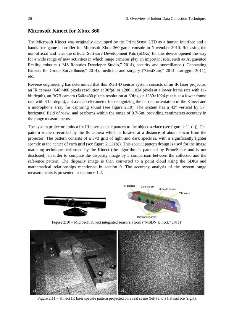
Reverse engineering has determined that this RGB-D sensor system consists of an IR laser projector,
an IR camera (640×480 pixels resolution at 30fps, or 1280×1024 pixels at a lower frame rate with 11-
bit depth), an RGB camera (640×480 pixels resolution at 30fps, or 1280×1024 pixels at a lower frame
rate with 8-bit depth), a 3-axis accelerometer for recognizing the current orientation of the Kinect and
a microphone array for capturing sound (see figure 2.10). The system has a 43° vertical by 57°
horizontal field of view, and performs within the range of 0.7-6m, providing centimeters accuracy in
the range measurements.
The system projector emits a fix IR laser speckle pattern to the object surface (see figure 2.11 (a)). The
pattern is then recorded by the IR camera which is located at a distance of about 7.5cm from the
projector. The pattern consists of a 3×3 grid of light and dark speckles, with a significantly lighter
speckle at the center of each grid (see figure 2.11 (b)). This special pattern design is used for the image
matching technique performed by the Kinect (the algorithm is patented by PrimeSense and is not
disclosed), in order to compute the disparity image by a comparison between the collected and the
reference pattern. The disparity image is then converted to a point cloud using the SDKs and
mathematical relationships mentioned in section 0. The accuracy analysis of the system range
measurements is presented in section 6.1.2.
Figure 2.10 – Microsoft Kinect integrated sensors. (from (“MSDN Kinect,” 2015))
Figure 2.11 – Kinect IR laser speckle pattern projected on a real scene (left) and a flat surface (right).
a) b)
2.1. State-of-the-Art Sensors for 3D Data Collection 27
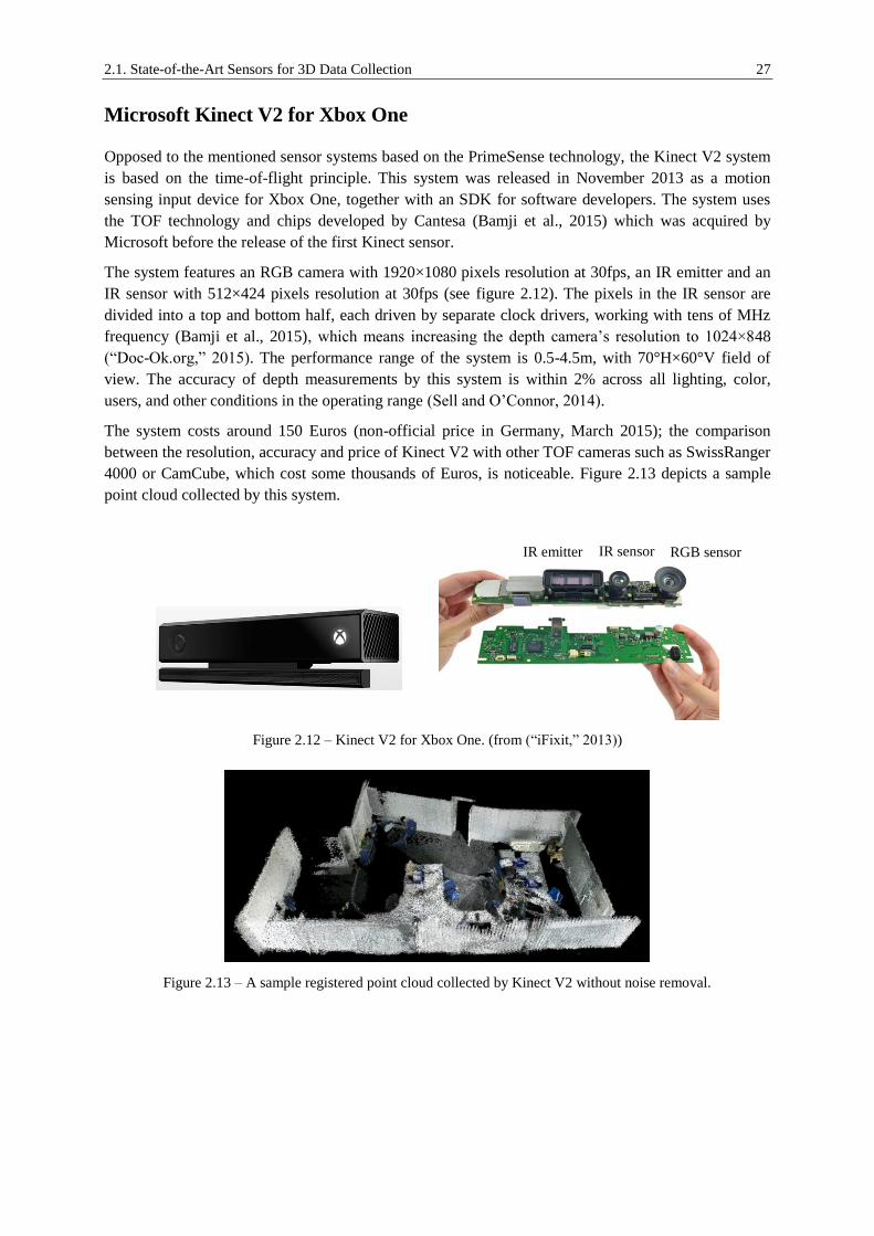
Microsoft Kinect V2 for Xbox One
Opposed to the mentioned sensor systems based on the PrimeSense technology, the Kinect V2 system
is based on the time-of-flight principle. This system was released in November 2013 as a motion
sensing input device for Xbox One, together with an SDK for software developers. The system uses
the TOF technology and chips developed by Cantesa (Bamji et al., 2015) which was acquired by
Microsoft before the release of the first Kinect sensor.
The system features an RGB camera with 1920×1080 pixels resolution at 30fps, an IR emitter and an
IR sensor with 512×424 pixels resolution at 30fps (see figure 2.12). The pixels in the IR sensor are
divided into a top and bottom half, each driven by separate clock drivers, working with tens of MHz
frequency (Bamji et al., 2015), which means increasing the depth camera’s resolution to 1024×848
(“Doc-Ok.org,” 2015). The performance range of the system is 0.5-4.5m, with 70°H×60°V field of
view. The accuracy of depth measurements by this system is within 2% across all lighting, color,
users, and other conditions in the operating range (Sell and O’Connor, 2014).
The system costs around 150 Euros (non-official price in Germany, March 2015); the comparison
between the resolution, accuracy and price of Kinect V2 with other TOF cameras such as SwissRanger
4000 or CamCube, which cost some thousands of Euros, is noticeable. Figure 2.13 depicts a sample
point cloud collected by this system.
Figure 2.12 – Kinect V2 for Xbox One. (from (“iFixit,” 2013))
Figure 2.13 – A sample registered point cloud collected by Kinect V2 without noise removal.
RGB sensor IR sensor IR emitter
28 2. Overview of Indoor Data Collection Techniques
2.1.2.4. Indoor Mobile Mapping Systems Based on Low-Cost Range
Cameras
Inspired by Microsoft Kinect, and based on the PrimeSense active triangulation and state-of-the-art
TOF technologies, low-cost commercial indoor mobile mapping systems are being developed
increasingly. Examples of such systems are presented in the following parts.
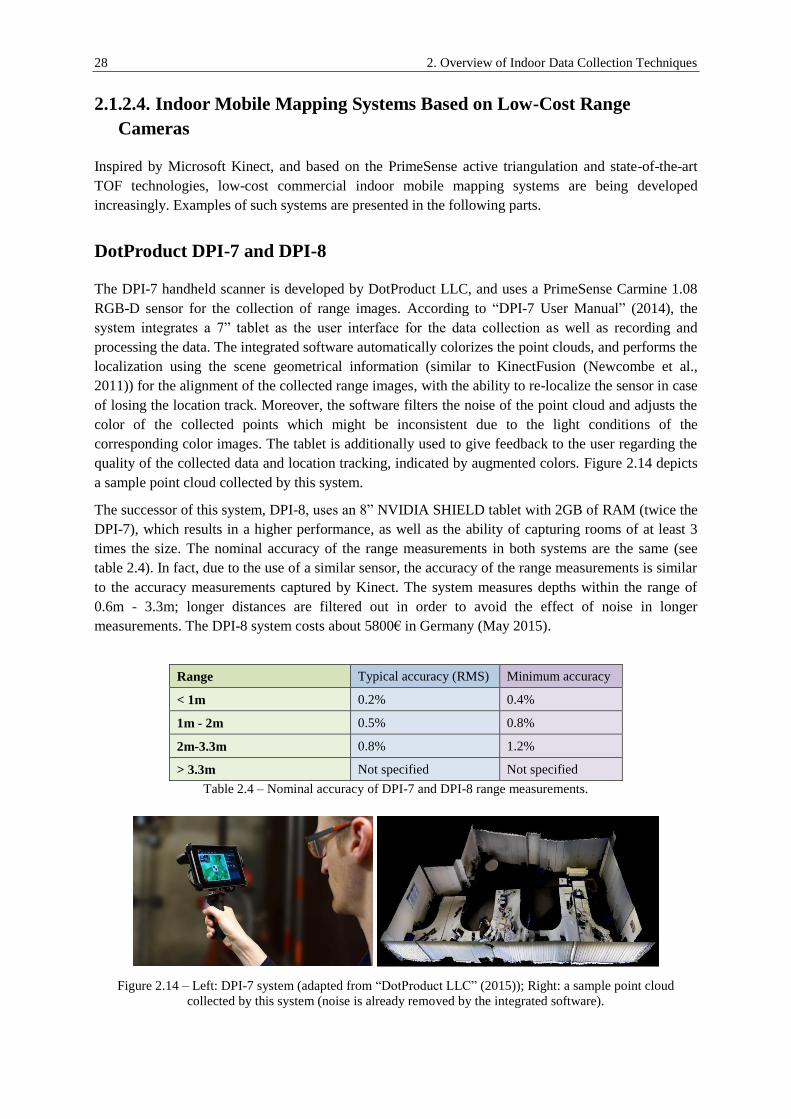
DotProduct DPI-7 and DPI-8
The DPI-7 handheld scanner is developed by DotProduct LLC, and uses a PrimeSense Carmine 1.08
RGB-D sensor for the collection of range images. According to “DPI-7 User Manual” (2014), the
system integrates a 7” tablet as the user interface for the data collection as well as recording and
processing the data. The integrated software automatically colorizes the point clouds, and performs the
localization using the scene geometrical information (similar to KinectFusion (Newcombe et al.,
2011)) for the alignment of the collected range images, with the ability to re-localize the sensor in case
of losing the location track. Moreover, the software filters the noise of the point cloud and adjusts the
color of the collected points which might be inconsistent due to the light conditions of the
corresponding color images. The tablet is additionally used to give feedback to the user regarding the
quality of the collected data and location tracking, indicated by augmented colors. Figure 2.14 depicts
a sample point cloud collected by this system.
The successor of this system, DPI-8, uses an 8” NVIDIA SHIELD tablet with 2GB of RAM (twice the
DPI-7), which results in a higher performance, as well as the ability of capturing rooms of at least 3
times the size. The nominal accuracy of the range measurements in both systems are the same (see
table 2.4). In fact, due to the use of a similar sensor, the accuracy of the range measurements is similar
to the accuracy measurements captured by Kinect. The system measures depths within the range of
0.6m - 3.3m; longer distances are filtered out in order to avoid the effect of noise in longer
measurements. The DPI-8 system costs about 5800€ in Germany (May 2015).
Range Typical accuracy (RMS) Minimum accuracy
< 1m 0.2% 0.4%
1m - 2m 0.5% 0.8%
2m-3.3m 0.8% 1.2%
> 3.3m Not specified Not specified
Table 2.4 – Nominal accuracy of DPI-7 and DPI-8 range measurements.
Figure 2.14 – Left: DPI-7 system (adapted from “DotProduct LLC” (2015)); Right: a sample point cloud
collected by this system (noise is already removed by the integrated software).

2.1. State-of-the-Art Sensors for 3D Data Collection 29
Structure Sensor
This sensor system is developed by Occipital, and captures the 3D map of indoor spaces using a range
measurement system developed by PrimeSense (active triangulation) and an integrating iPad
containing the software (figure 2.15 depicts the system). The software colorizes and aligns the range
images captured from different viewpoints, and creates meshes. A notable feature of this system is the
SDK provided for the developers in order to enable them to write mobile applications that interact
with the 3D maps, Augmented Reality, measurements on the objects, gaming, etc. Some of the
technical specifications of the system are summarized in Table 2.5. The range image alignment in this
system is based on the observations in the 3D object space (similar to KinectFusion (Newcombe et al.,
2011)); the sensor tracking is lost in case of dealing with flat surfaces.
Figure 2.15 – Structure Sensor mounted on an iPad. (from the company website)
Field of view (H×V) 58°×45°
Measurement rate 30fps & 60fps
Measurement range 0.4m - 3.5m
Precision 1% of the measured distance
Weight 99.2gr
Dimensions (W×D×H) [mm] 27.9×119.2×29
Price ($)* 379 and 499
Table 2.5 – Technical specifications of the Structure Sensor. *Official prices without iPad, in US, March 2015.
30 2. Overview of Indoor Data Collection Techniques
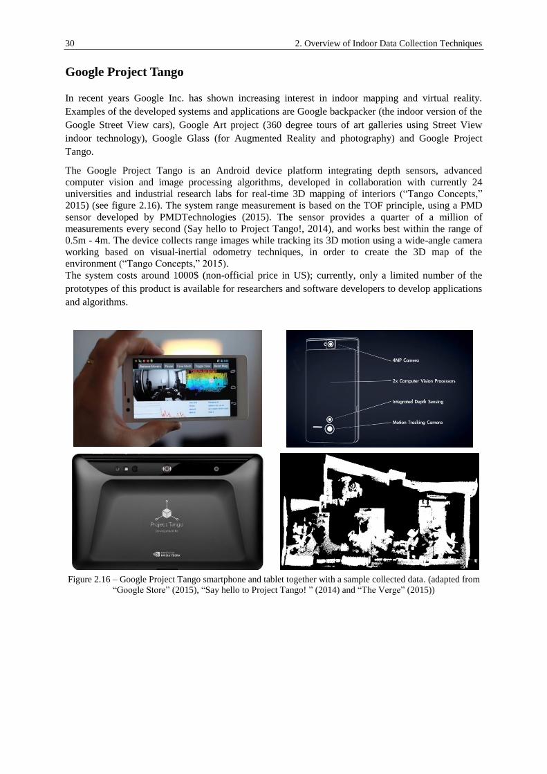
Google Project Tango
In recent years Google Inc. has shown increasing interest in indoor mapping and virtual reality.
Examples of the developed systems and applications are Google backpacker (the indoor version of the
Google Street View cars), Google Art project (360 degree tours of art galleries using Street View
indoor technology), Google Glass (for Augmented Reality and photography) and Google Project
Tango.
The Google Project Tango is an Android device platform integrating depth sensors, advanced
computer vision and image processing algorithms, developed in collaboration with currently 24
universities and industrial research labs for real-time 3D mapping of interiors (“Tango Concepts,”
2015) (see figure 2.16). The system range measurement is based on the TOF principle, using a PMD
sensor developed by PMDTechnologies (2015). The sensor provides a quarter of a million of
measurements every second (Say hello to Project Tango!, 2014), and works best within the range of
0.5m - 4m. The device collects range images while tracking its 3D motion using a wide-angle camera
working based on visual-inertial odometry techniques, in order to create the 3D map of the
environment (“Tango Concepts,” 2015).
The system costs around 1000$ (non-official price in US); currently, only a limited number of the
prototypes of this product is available for researchers and software developers to develop applications
and algorithms.
Figure 2.16 – Google Project Tango smartphone and tablet together with a sample collected data. (adapted from
“Google Store” (2015), “Say hello to Project Tango! ” (2014) and “The Verge” (2015))
2.2. The Registration Problem 31
2.2. The Registration Problem
Due to scene complexities and the scanners limited field of view, in many applications it is required to
collect point clouds from multiple viewpoints in order to cover the whole scene. Point clouds collected
from different viewpoints have their own local coordinate system; in order to align the coordinate
systems, the corresponding point clouds have to be registered together using a rigid-body
transformation, which is a special case of the 3D similarity (Helmert’s 7-parameters) transformation
by setting the scale factor to 1. The transformation can be estimated using point correspondences in
the point clouds, or by estimating the sensor pose in the reference coordinate system.
2.2.1. Registration Using Point Correspondences in the Point Clouds
The rigid-body transformation parameters can be estimated using point correspondences in the point
clouds. In case the point correspondences are already given in the form of 3D features in the scene
(artificial or natural) or 2D features in the corresponding intensity or color images, the transformation
parameters can be estimated for instance using a closed-form solution based on the unit quaternions
(Horn, 1987; Sanso, 1973). If the point correspondences are not provided, they can be estimated based
on the geometrical structure of the scene, using an iterative procedure called Iterative Closest Point
(ICP) algorithm (Besl and McKay, 1992). See appendix A for the mathematical background of the two
approaches.
2.2.1.1. Correspondences by Recognition of 3D Features
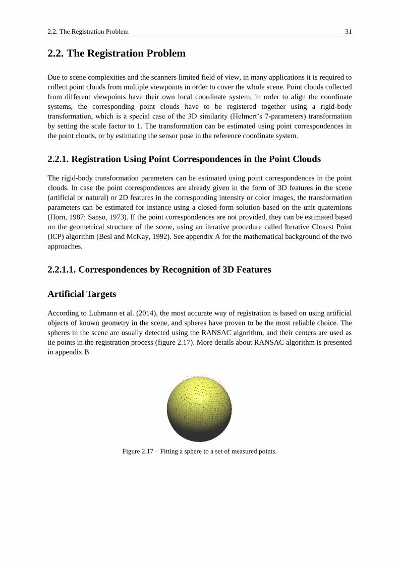
Artificial Targets
According to Luhmann et al. (2014), the most accurate way of registration is based on using artificial
objects of known geometry in the scene, and spheres have proven to be the most reliable choice. The
spheres in the scene are usually detected using the RANSAC algorithm, and their centers are used as
tie points in the registration process (figure 2.17). More details about RANSAC algorithm is presented
in appendix B.
Figure 2.17 – Fitting a sphere to a set of measured points.

32 2. Overview of Indoor Data Collection Techniques
Natural Targets
3D features can also be defined in the scene using well-defined sharp corners manually (figure 2.18
(a)), or automatically using feature extractors such as NARF (Normal Aligned Radial Feature) (Steder
et al., 2011) (figure 2.18 (b)). The NARF feature extractor works with the corresponding range
images. It first identifies the interest points on the objects border (outer shape of the object from a
certain perspective view), in locations where the surface is stable (robust estimation of normal vectors
is possible). Then it defines a descriptor for the interest points based on the amount and the main
direction of the surface changes (in terms of the surface curvature) in the vicinity of the point.
Figure 2.18 – Identification of 3D natural target points manually (left) and using NARF feature extractor
(adapted from “Documentation - Point Cloud Library (PCL)” (2015)) (right).
2.2.1.2. Correspondences by the Recognition of Features in 2D Images
3D point correspondences can be identified based on the information provided by the corresponding
color, intensity or reflectance image. However, as also mentioned by Luhmann et al. (2014), this
requires a perfect registration of the corresponding images, which means each pixel in the color,
intensity or reflectance image must correspond to the same point in the corresponding point cloud. In
this case, point candidates can be derived in the 2D image space using image processing techniques (to
recognize artificial targets) or 2D feature extractors such as SIFT (Lowe, 2004), SURF (Bay et al.,
2006), FAST (Rosten and Drummond, 2006, 2005), etc. The extracted features then have to be
matched against each other across different images. The matching process can be performed using the
RANSAC algorithm, based on the rigid-body transformation model in case of using intensity images,
or by the fundamental matrix in case of using color images. An example of the registration using this
method is presented by Böhm and Becker (2007). They extract and match SIFT features across the
corresponding reflectance images, and compute a pair-wise registration using a rigid-body
transformation (see figure 2.19).
Figure 2.19 – SIFT features extracted
and matched for a reflectance image.
(from Böhm and Becker (2007))
a) b)

2.2. The Registration Problem 33
2.2.1.3. Correspondences by the Analysis of the Scene Geometry – Iterative
Closest Point (ICP) Algorithm
In case no point correspondences are available, or the accuracy and distribution of the available
corresponding points are not sufficient for an accurate point cloud registration, one can alternatively
use the Iterative Closest Point (ICP) algorithm (Besl and McKay, 1992). For each point in the local
point cloud (scan world), the algorithm finds the closest points in the reference point cloud, and
estimates a rigid-body transformation. After applying the transformation, the algorithm is repeated
until the sum of the residuals of the distances between the point correspondences is smaller than a
threshold (see figure 2.20). This registration method requires initial values; bad initial values may
cause a wrong convergence of the solution. More details regarding the ICP algorithm are provided in
appendix A.
Figure 2.20 – Point cloud alignment using the ICP algorithm.
2.2.2. Registration by the Estimation of the Sensor Pose
Beside the abovementioned approaches, point clouds can be aligned if the sensor poses are estimated
in a common coordinate system. The sensor pose can be estimated by the integration of different
sensors such as low-cost MEMS-IMUs, LRFs and cameras into the range measurement system.
2.2.2.1. Registration Based on Structure from Motion Methods
The estimation of camera poses from two and three viewpoints has been focused for a long time by
photogrammetric and computer vision communities, and closed-form solutions have been developed
to solve this problem (Hartley and Zisserman, 2003). For multiple views, Structure from Motion
(SfM) methods estimate the sensor pose incrementally; image features are extracted and matched for
an initial image pair, the points are triangulated, and a new image is added. The solution is then
globally optimized using a bundle adjustment in a post processing step. There is a wide range of SfM
methods, each of which dealing differently with the large number of images, and pipelines for solving
the problem (Snavely, 2008). Famous commercial software solutions are available for solving the SfM
problem, such as Bundler (Snavely et al., 2006), VisualSfM (Wu, 2013), Agisoft PhotScan, etc.
SfM methods estimate the camera pose in a local coordinate system up to the scale factor. To register
the point clouds, camera locations have to be first scaled to a metric coordinate system. The scale
factor is estimated using a 3D similarity transformation, having point correspondences in the color and
range image channels. More details regarding this registration approach is presented in section 3.2.1.

34 2. Overview of Indoor Data Collection Techniques
2.2.2.2. Registration Based on SLAM Methods
In real-time and robotic applications, the sensor pose is estimated using SLAM approaches. In such
applications, the autonomous platform needs to localize itself within an unknown environment, while
simultaneously creating the map of the environment (see appendix C). Frese et al. (2010) present an
overview regarding available SLAM methods based on the application and different sensor inputs in
2D and 3D. According to this overview, in 3D applications, two general variants of SLAMs are
recognized: graph-based SLAM methods that rely on scan matching, and visual SLAM methods based
on point features extracted from images. Most of the graph-based SLAM methods use pair-wise
alignment of the consecutive scans and create constraints for the sensor 6 degree-of-freedom (DOF).
Nüchter et al. (2007) and Wurm et al. (2010) present localization and mapping methods using ICP
scan matching, supported by loop closure and pose graph for the global consistency and optimization.
The KinectFusion software implemented by the Microsoft Research Group (Newcombe et al., 2011)
besides presenting an optimized method or the sensor tracking, creates a dense and smooth 3D map by
the use of Kinect point clouds in real-time. Sensor tracking in this method is based on a GPU
implementation of a coarse-to-fine ICP algorithm. Open-source implementations of this method
(KinFu and KinFu Large Scale) are provided by the Point Cloud Library (PCL) (Rusu and Cousins,
2011) (see figure 2.21). Such methods, however require a suitable scene structure and enough
geometric information for the successful constraining of the sensor 6 DOF, and therefore fail in case
of dealing with flat surfaces.
Visual SLAM systems estimate the sensor pose by tracking sparse points of interest, extracted from
images, using vision algorithms. The offline version of this problem is studied as the bundle
adjustment problem in photogrammetry, and as SfM in computer vision community (Frese et al.,
2010; Hartley and Zisserman, 2003; Triggs et al., 2000). According to Newcombe et al. (2011),
research on SLAM has focused more on real-time marker-free tracking and mapping using monocular
RGB cameras. Systems such as Parallel Tracking and Mapping (PTAM) enable marker-free tracking
of the camera together with Augmented Reality applications using a single camera (Klein and Murray,
2007). This system emphasizes on the localization of the camera, and therefore performs mapping by
sparse point models.
Figure 2.21 – Creating an exemplary 3D map and sensor tracking using the KinFu software provided by the PCL
software library.
RGB-D sensors such as Microsoft Kinect provide range data together with corresponding color
images. This enables the combination of geometric and scale information with visual features to
localize the sensor and create the map of the environment. The combination of both information is
specially useful for Kinect which has a relatively small field of view (57°H×43°V), and therefore
vision-only and graph-based methods may easily fail due to finding insufficient visual or geometrical
features in the scene. Henry et al. (2012) present an RGBD-ICP mapping method that tightly uses

2.2. The Registration Problem 35
RGB and depth information for a robust frame-based matching and loop closure. This method first
extracts and matches sparse visual features (SIFT features) in two consecutive RGB images, and
associates them with depth values in the corresponding depth images to generate feature points in 3D.
Then it finds the best rigid-body transformation between the two sets using RANSAC algorithm. The
transformation is then refined using the ICP algorithm. The ICP algorithm, however, minimizes two
different Euclidean distances: the mean distance between visually associated points (sparse points) and
the mean distance between dense points (Kinect point clouds), by setting different weights for each of
the two distances in the error minimization process. This enables the method to benefit from the visual
information when the scene geometry cannot constrain the sensor 6 DOF, or to benefit from the scene
geometrical information in case of having poor visual features. The results then become globally
consistent using a graph optimization process. The process is summarized in figure 2.22. A sample
map created by this method is depicted in figure 2.23.
Figure 2.22 – Overview of the RGBD-ICP mapping system. The algorithm uses visually associated and dense
points for frame-to-frame alignment and loop closure detection in parallel threads. (from Henry et al. (2012))
Figure 2.23 – A sample map created by the RGBD-ICP mapping system. (from Henry et al. (2012))
36
3. Data Collection using Microsoft Kinect for Xbox 360
In the previous chapter, potential sensors and approaches for the collection of range data in indoor
scenes were introduced. In the presented work, the low-cost and accessible RGB-D camera Microsoft
Kinect for Xbox 360 is employed as the case study for the collection of 3D point cloud of interiors.
This chapter presents the mathematical background for the system calibration, derivation of point
clouds from disparity data and colorization of the point clouds. Moreover, in extreme cases where
vision-based and depth-matching-based registration approaches mentioned in the previous chapter fail,
due to the lack of visual features and appropriate geometrical scene structure, a registration approach
based on an indoor positioning solution is proposed as a complementary approach.
3.1. Point Cloud Collection by Kinect
3.1.1. System Interfaces and SDKs
For the collection of colored point clouds using Kinect, low level data streams such as color images
and disparity data have to be extracted using a Software Development Kit (SDK). SDKs enable the
interaction of the user with the system using specific programming languages (e.g. C, C++, C#, Java
and Python). In November 2010, when the Kinect system was first introduced as an interface for the
Xbox 360 game console, no official driver was introduced for developers. However, shortly after that,
open-source drivers such as libfreenect (OpenKinect project) and OpenNI (PrimeSense) were released
to support the data acquisition with Kinect. The official Kinect SDK for the Microsoft Windows
operating system was released in February 2011, which additionally supports gesture and face
recognition, voice recognition, alignment of the range data, etc.. In the present work, the libfreenect
driver was used for the interaction with the Kinect, as it supports programming under the free and
popular operating system Linux.
3.1.2. System Calibration
The Kinect system integrates a range measurement system (combination of an IR laser projector and
an IR camera) and an RGB camera (see figure 3.1). For the colorization of the Kinect point clouds,
and also registration of the point clouds using visual information, the Kinect range data have to be
registered with the color information. For a correct pixel-to-pixel registration of RGB and depth
values, besides the calibration of the IR and RGB cameras, the relative pose between the two cameras
has to be estimated precisely. The camera calibration refers to the determination of camera interior
orientation parameters (principal distance and the image coordinates of the principal point) together
with the parameters describing image errors (e.g. lens distortion parameters).

3.1. Point Cloud Collection by Kinect 37
Figure 3.1 – A disassembled Kinect; the system consists of an IR laser projector, an IR and an RGB camera.
According to Luhmann et al. (2014), three calibration techniques can be distinguished: laboratory
calibration, test-field calibration and self-calibration. Laboratory calibration was used in the past for
the calibration of metric cameras using optical alignment instruments. This method cannot be done by
the user, and therefore meets little applications in close range photogrammetry. State-of-the-art close
range techniques employ the analytical calibration methods in which the observation of the image
coordinates is used to derive the interior orientation parameters using a bundle block adjustment.
Moreover, by the inclusion of additional parameters, the position of the perspective center and the lens
distortion effects are modeled. The test-field calibration method employs a target field, photographed
using a suitable camera configuration, in order to ensure a suitable ray intersection, while filling the
maximum image format to assure a small correlation between the estimated parameters. In practice,
the test-field might be replaced by the actual object, only if a condition similar to the test-field
calibration can be fulfilled, to ensure a suitable ray intersection and small correlation between the
estimated parameters (self-calibration).
In the test-field calibration, measured image coordinates and approximate object coordinates are
processed using an unconstrained datum bundle adjustment technique (e.g. free net adjustment
technique), in order to avoid the effect of possible inconsistencies in the datum information on the
estimated unknowns. Moreover, to ensure the maximum accuracy in the estimation of the relative pose
between the two cameras, the exterior orientation together with the interior orientation parameters of
the IR and RGB images are estimated in one bundle adjustment process. It is necessary to mention that
the corresponding image pairs (IR and RGB) used in the bundle adjustment have to be taken
synchronously at multiple viewpoints, in order to avoid erroneous measurement of the stereo baseline.
The bundle adjustment is based on the well-known collinearity equations (equations (3.4)) which are
set for each target point. The collinearity equations are derived from the central projection equations
(equations (3.1), see figure 3.2) by solving the point dependent scale factor from the third row and
replacing it in the first and second rows.
Figure 3.2 – Central projection principle. (adapted from Cramer (2014))

38 3. Data Collection using Microsoft Kinect for Xbox 360
A O a p
A O A a p
A O
X X x x x
Y Y y y y
Z Z -c
R
(3.1)
1 1
a p A O
a p A A O
A O
x x x X X
y y y Y Y
-c Z Z
R
(3.2)
1
A
13 A O 23 A O 33 A O
c
r (X -X ) r (Y -Y ) r (Z -Z )
(3.3)
11 A O 21 A O 31 A Oa p a
13 A O 23 A O 33 A O
12 A O 22 A O 32 A Oa p a
13 A O 23 A O 33 A O
r (X -X ) r (Y -Y ) r (Z -Z )x x c x
r (X -X ) r (Y -Y ) r (Z -Z )
r (X -X ) r (Y -Y ) r (Z -Z )y y c y
r (X -X ) r (Y -Y ) r (Z -Z )
(3.4)
In these equations:
- A A AX , Y , Z are the coordinates of the point A in the world coordinate system;
- A is the scale factor corresponding to point A;
- R is the rotation matrix from the object to image coordinate system;
- ijr is the (i,j)R element;
- a ax , y are the measured image coordinates for the point A;
- p px , y are the coordinates of the principal point;
- a ax , y are the correction terms for image coordinates corresponding to point A;
- c is the calibrated focal length;
- O O OX , Y , Z are the coordinates of the camera projection center in the world coordinate system.
According to Guidi and Remondino (2012), for the estimation of the correction terms (additional
parameters) x, y , the model developed by Brown (1971) is proved to be the most effective, in
particular for close range sensors. The Brown calibration model which is a physical model, estimates
the lens distortion effect in the radial and decentering (tangential) directions by:
3 5 7
Radial 1 2 3
2 2
p p
r K r K r K r
r x x y y
(3.5)
2 4 6RadialRadial Radial d 1 2 3
2 4 6RadialRadial Radial d 1 2 3
rx = x x = x K r + K r + K r
r
ry = y y = y K r + K r + K r
r
(3.6)
2 2 2
Tangential 3 2 d 1 d d
2 2 2
Tangential 3 1 d 2 d d
x = 1 + P r P r + 2x + 2P x y
y = 1 + P r P r + 2y + 2P x y
(3.7)

3.1. Point Cloud Collection by Kinect 39
in which 1,2,3K are the distortion coefficients for the radial direction,
1,2P are the distortion coefficients
for the tangential direction, r is the radial distance reduced to the estimated principal point and d dx , y
are distorted image coordinates reduced to the principal point.
Besides the Brown’s physical model for the estimation of the additional parameters, Tang et al. (2012)
prove that there are rigorous and effective mathematical models based on the Legendre polynomials,
which are able to compensate distortions of very small magnitude (around 0.05 pixels). Equation (3.8)
presents an exemplary model of additional parameters derived based on the Legendre polynomials
with 34 unknowns (corresponding to degrees m=4 and n=3). The maximum order of the polynomial
should be chosen by the compromise between the optimal accuracy and reducing over-
parametrization.
1 1,0 2 0,1 3 2,0 4 1,1 5 0,2 6 3,0 7 2,1 8 1,2 9 0,3 10 4,0
11 3,1 12 2,2 13 1,3 14 4,1 15 3,2 16 2,3 17 4,2 18 3,3 19 4,3
2 1,0 1 0,1 20 2,0 3 1,1 4 0,2 21 3,0 22 2,1
x a p a p a p a p a p a p a p a p a p a p
a p a p a p a p a p a p a p a p a p
y a p a p a p a p a p a p a p
23 1,2 24 0,3 25 4,0
26 3,1 27 2,2 28 1,3 29 4,1 30 3,2 31 2,3 32 4,2 33 3,3 34 4,3
a p a p a p
a p a p a p a p a p a p a p a p a p
(3.8)
In these equations, ia coefficients are the additional parameters and m,np represent the series of
continuous orthogonal polynomials based on the Legendre polynomials. This family of additional
parameters is used where the Brown’s model is not sufficiently accurate and a very high accuracy is
required. However, this is not the case for the Kinect images, due to the high level of noise and blur
contained in image observations. Moreover, in practice, interest points are extracted and matched
based on the SIFT or other feature detectors, which deliver an accuracy of about 0.7 pixels
(Mikolajczyk and Schmid, 2004). Therefore, image measurements of around 0.5 pixels accuracy will
be sufficient in case of using Kinect. Numerical results and evaluations regarding the calibration of the
Kinect system are presented in section 6.1.1.
3.1.3. Generation of Colored Point Clouds
As already mentioned, the Kinect system calibration enables a correct registration of RGB and depth
values. In the first step, the disparity values have to be converted to depth values. Afterwards, through
some transformation steps which are described in this chapter, RGB values are transformed into the IR
image space for colorizing the point clouds.
3.1.3.1. From Disparity Image to 3D Point Clouds
In normal stereo photogrammetry, where two identical cameras have parallel axes perpendicular to the
baseline, disparity measurements are related to the object distance by the following equation:
H c
b d
(3.9)
whereby H is the depth or the object distance, b is the stereo baseline length, c is the focal length of
the IR camera and d is the measured disparity. This equation can be derived from the ratios indicated
in figure 3.3 or from the collinearity equations, by setting the rotation angles equal to zero. The
distance uncertainty with respect to the uncertainty in the disparity measurement is given by:
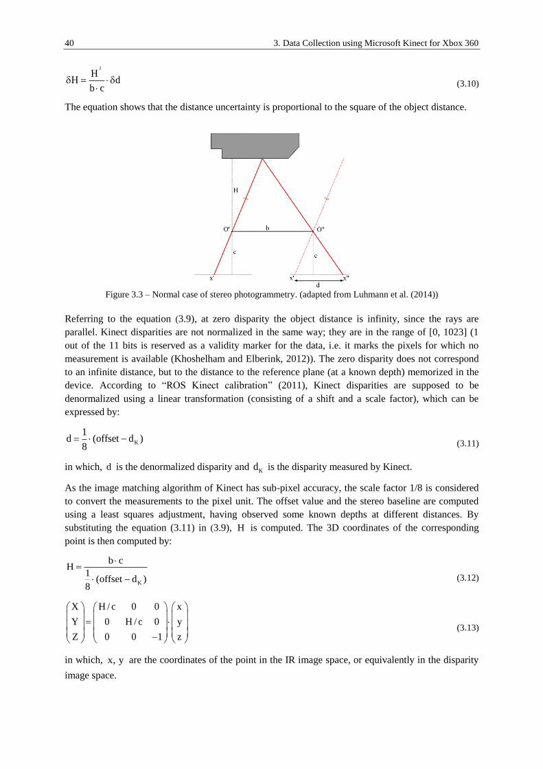
40 3. Data Collection using Microsoft Kinect for Xbox 360
2
HH d
b c
(3.10)
The equation shows that the distance uncertainty is proportional to the square of the object distance.
Figure 3.3 – Normal case of stereo photogrammetry. (adapted from Luhmann et al. (2014))
Referring to the equation (3.9), at zero disparity the object distance is infinity, since the rays are
parallel. Kinect disparities are not normalized in the same way; they are in the range of [0, 1023] (1
out of the 11 bits is reserved as a validity marker for the data, i.e. it marks the pixels for which no
measurement is available (Khoshelham and Elberink, 2012)). The zero disparity does not correspond
to an infinite distance, but to the distance to the reference plane (at a known depth) memorized in the
device. According to “ROS Kinect calibration” (2011), Kinect disparities are supposed to be
denormalized using a linear transformation (consisting of a shift and a scale factor), which can be
expressed by:
K
1d (offset d )
8
(3.11)
in which, d is the denormalized disparity and Kd is the disparity measured by Kinect.
As the image matching algorithm of Kinect has sub-pixel accuracy, the scale factor 1/8 is considered
to convert the measurements to the pixel unit. The offset value and the stereo baseline are computed
using a least squares adjustment, having observed some known depths at different distances. By
substituting the equation (3.11) in (3.9), H is computed. The 3D coordinates of the corresponding
point is then computed by:
K
b cH
1(offset d )
8
(3.12)
X H / c 0 0 x
Y 0 H / c 0 y
Z 0 0 1 z
(3.13)
in which, x, y are the coordinates of the point in the IR image space, or equivalently in the disparity
image space.
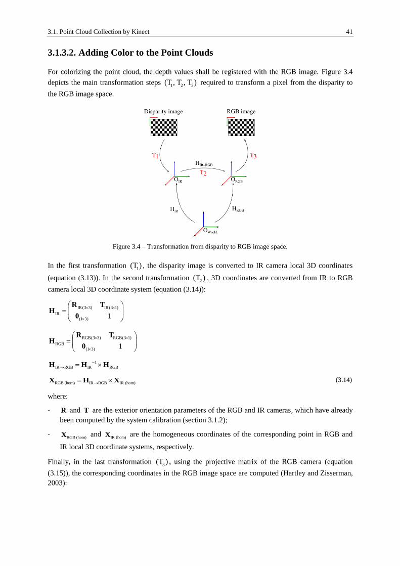
3.1. Point Cloud Collection by Kinect 41
3.1.3.2. Adding Color to the Point Clouds
For colorizing the point cloud, the depth values shall be registered with the RGB image. Figure 3.4
depicts the main transformation steps 1 2 3(T , T , T ) required to transform a pixel from the disparity to
the RGB image space.
Figure 3.4 – Transformation from disparity to RGB image space.
In the first transformation 1(T ) , the disparity image is converted to IR camera local 3D coordinates
(equation (3.13)). In the second transformation 2(T ) , 3D coordinates are converted from IR to RGB
camera local 3D coordinate system (equation (3.14)):
IR (3 3) IR(3 1)
IR
(1 3) 1
R TH
0
RGB(3 3) RGB(3 1)
RGB
(1 3) 1
R TH
0
1
IR RGB IR RGB
H H H
RGB (hom) IR RGB IR (hom) X H X (3.14)
where:
- R and T are the exterior orientation parameters of the RGB and IR cameras, which have already
been computed by the system calibration (section 3.1.2);
- RGB (hom)X and
IR (hom)X are the homogeneous coordinates of the corresponding point in RGB and
IR local 3D coordinate systems, respectively.
Finally, in the last transformation 3(T ) , using the projective matrix of the RGB camera (equation
(3.15)), the corresponding coordinates in the RGB image space are computed (Hartley and Zisserman,
2003):

42 3. Data Collection using Microsoft Kinect for Xbox 360
RGB p
RGB RGB p
c 0 x
0 c y
0 0 1
K
RGB IR RGB (3 3) IR RGB P K R I T
RGB (hom) RGB (hom).x P X
(3.15)
In the equations:
- RGBK is the calibration matrix of the RGB camera;
- P is the projection matrix of the RGB camera;
- RGB (hom)x and
RGB (hom)X are the homogeneous coordinates of the corresponding point in RGB
image and 3D local object coordinates, respectively.
The mentioned transformations enable the registration of each pixel in the disparity image, and
therefore a point in the corresponding 3D object coordinates to an RGB value.
3.2. Point Clouds Registration
In section 0, available approaches for the registration of the point clouds in indoor applications were
introduced. For the registration of the Kinect point clouds, as mentioned before, SfM and SLAM
approaches can be used. Commercial and open-source implementations of some of the solutions are
available. Software such as ReconstructMe (“ReconstructMe,” 2015), Skanect (“Skanect by
Occipital,” 2015), FARO SCENECT (“SCENECT,” 2015) and KinFu Large Scale (Rusu and Cousins,
2011) enable the user to easily scan the objects or scenes without requiring knowledge about
photogrammetry, computer vision and robotics. The user usually interacts with the software front-end,
and cannot manipulate parameters to deal with challenging scenes with poor texture or geometrical
information. To deal with such issues, one may use or customize available SfM or SLAM
implementations to adapt the localization method with the application.
3.2.1. Point Clouds Registration Based on RGB and Depth Information
This study uses the free software VisualSFM – the implementation of an SfM method to orient RGB
images captured by the Kinect system (Wu, 2013; Wu et al., 2011). Similar to all SfM methods,
VisualSFM uses point features to incrementally estimate the scene structure and camera poses. The
solution is then merged into a bundle adjustment for the global optimization of this estimation. As a
result of this process, 3D coordinates of point features are derived in a 3D local coordinate system up
to the scale factor. The scale factor is estimated by the best fitting of the 3D local coordinates with the
corresponding 3D object coordinates of matched point features at each range image frame, which is
then averaged over all frames. For the best fitting of the 3D point features at each range image frame,
having more than 3 points, a least squares adjustment can be performed based on the 3D similarity
(Helmert’s 7-parameters) transformation:
Object Local X R X T (3.16)
In this equation:

3.2. Point Clouds Registration 43
- ObjectX and LocalX are the 3D coordinates of point features in the object (metric) and local coordinate
systems;
- is the scale factor;
- R is the rotation matrix applied to the local coordinates;
- T is the translation vector from the centroid of rotated and scaled local to the centroid of the
object coordinates.
As the model is not linear regarding the unknown parameters , R and T , initial values and
iteration are required to estimate the unknown parameters. To avoid this issue, closed-form solutions
to the least squares problem is proposed by Horn (1987) and Sanso (1973), which are based on the unit
quaternions for the representation of rotations (see appendix A).
The RGB camera orientation parameters in the metric space can be used directly for the registration of
the corresponding point clouds, since the relative orientation of the RGB and IR camera is fixed.
Figure 3.5 depicts an example in which the point clouds collected from 10 viewpoints are aligned
using the mentioned approach.
Figure 3.5 – Oriented images and the sparse point cloud corresponding to point features (left); aligned point
clouds corresponding to the color images (right). Images are oriented using the VisualSFM software.
3.2.2. Point Clouds Registration Based on an Indoor Positioning Solution
and Available Coarse Indoor Models
Vision-based and depth-matching-based registration approaches for the estimation of the sensor pose
rely on the existence of sufficient well distributed features of interest, as well as suitable geometry of
the scene to constrain the sensor 6 DOF. Therefore, such approaches fail in scenarios with poor
texture, or scenes with insufficient geometric information. This issue can be handled for instance by
integrating inertial solutions into the system. For example, ZEB1 mobile mapping system (by CSIRO)
uses a 2D laser range finder supported by a low-cost MEMS IMU for the localization and mapping
purpose. In the robotics community, visual and inertial information are merged together for the
localization purpose using visual-inertial SLAM methods (for example see (Leutenegger et al., 2013)).
However, in order to avoid drift error, the existence of visual constraints in keyframes is inevitable.
This study presents a new complementary approach for the registration of collected point clouds in
extreme scenarios, in which the abovementioned methods fail, due to having poor texture and
symmetrical geometrical structure (e.g. hallways). For this purpose, the point cloud registration task is
supported by an indoor positioning method implemented at the Institute for Photogrammetry, together

44 3. Data Collection using Microsoft Kinect for Xbox 360
with information extracted from available coarse models. Figure 3.6 depicts the overview of this
approach, which is described in detail in following sections.
Figure 3.6 – Flowchart of the proposed approach for the registration of the point clouds: evacuation plans
support the indoor positioning by map matching, and at the same time, are used to generate coarse indoor
models. The user’s track and the information extracted from the coarse indoor model enable the registration of
point clouds.
3.2.2.1. Indoor Positioning Method Based on a Foot Mounted MEMS IMU
In recent years, indoor positioning has increasingly been focused by the robotics and computer vision
communities, and various approaches are proposed to solve this problem. As stated by Peter et al.
(2010), most of the approaches either use an extra infrastructure such as WLAN networks or RFID
beacons, or require a high quality indoor model. Therefore, low-cost sensor systems such as MEMS
IMUs have been focused to overcome the limitations. However, such systems suffer from large drifts
shortly after the data collection starts. To improve the accuracy, Godha and Lachapelle (2008) suggest
the use of zero-velocity updates algorithm (ZUPT) to reduce the problem of error accumulation over
time and to maintain the accuracy bounds for longer periods. In this approach, the MEMS IMU is
mounted on the user’s foot, and therefore the foot dynamics enable the use of frequent zero-velocity
updates.
Although zero-velocity updates significantly reduce the accumulation of the drift error, still this effect
is considerable in longer tracks. Therefore, Peter et al. (2011, 2010) further improve the accuracy of
navigation using the information extracted from the available coarse indoor models, assuming the
most parts of the user’s track is parallel or perpendicular to the main direction of the building. This
study uses their implemented software for the derivation of the user’s track.
3.2.2.2. Generation of Coarse Indoor Models
In Peter et al. (2010), a new approach for the extraction of course indoor models from available
evacuation plans is presented. In many countries, existence of such plans is compulsory for the public
buildings such as hospitals, universities, hotels, etc. The coarse models support the aforementioned
indoor positioning method, as well as point cloud registration, as will be shown in the following
sections. The procedure for the generation of such models is summarized in section 4.2.3.
3.2.2.3. Data Collection
For the data collection purpose, the user employs a foot mounted MEMS IMU and starts walking from
the position where the evacuation plan is photographed into the corridor, while holding a Kinect
system and capturing the range and MEMS IMU data, simultaneously. The user’s track as well as the
coarse indoor model is then derived using the aforementioned methods. Afterwards range images have
to be pre-processed and finally transformed into the world coordinate system using a rigid-body
transformation. The details are described in the following sections.
Evacuation plans Point clouds
registration
Indoor positioning
Coarse 3D models

3.2. Point Clouds Registration 45
3.2.2.4. Pre-Processing of the Point Clouds
In this step, point clouds are levelled in the horizontal plane (to compensate the sensor tilt) and the
heights are modified (using a shift in the vertical direction), so that the ground parts of the point clouds
lay at a same level. For this purpose, first the normal vectors of range images are analyzed in order to
find the ground points and to estimate the point clouds tilts regarding the horizontal plane. Points are
segmented as ground points, if the angular difference between their normal vector and the vertical axis
is less than a threshold (e.g. 45° which is a quite tolerant threshold). The segmentation is refined
iteratively by compensating the tilt and removing outliers. The point cloud of the walls can also be
grouped using a similar procedure, which is required by the next steps.
3.2.2.5. Extraction of 3D Rigid Transformation Parameters
In this step, the user’s track is analyzed in order to estimate the orientation of the point clouds
considering the captured timestamps (see figure 3.7). As the tilt of the system is already compensated
and the heights of the point clouds are equalized in the pre-processing step, the registration process
only consists of a rotation around the vertical axis as well as a translation in 2D space. The coordinates
of the track points are directly considered as 2D translations. Rotations are computed, assuming the
sensor is oriented towards the direction of the next track point. Equations (3.17) and (3.18) show the
rotation angle and translation components (XT, YT) for the registration of the point cloud
corresponding to the ith track point. Figure 3.7 depicts the registration of two exemplary point clouds
of the hallway using only position traces. As it is visible in this example, the point clouds are coarsely
aligned; the alignment will be refined in the next steps using the information extracted from the coarse
model.
Figure 3.7 – Initial point clouds alignment using position traces. Left to right: coarse model together with the
aligned user’s track, position traces and top view of two initially registered point clouds.
i 1 i
i 1 i
World World
i
World World
Y Yarctan
X X
(3.17)
i i
i i
T World
T World
X X
Y Y
(3.18)
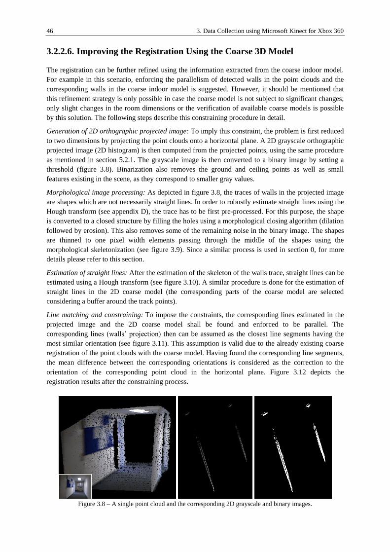
46 3. Data Collection using Microsoft Kinect for Xbox 360
3.2.2.6. Improving the Registration Using the Coarse 3D Model
The registration can be further refined using the information extracted from the coarse indoor model.
For example in this scenario, enforcing the parallelism of detected walls in the point clouds and the
corresponding walls in the coarse indoor model is suggested. However, it should be mentioned that
this refinement strategy is only possible in case the coarse model is not subject to significant changes;
only slight changes in the room dimensions or the verification of available coarse models is possible
by this solution. The following steps describe this constraining procedure in detail.
Generation of 2D orthographic projected image: To imply this constraint, the problem is first reduced
to two dimensions by projecting the point clouds onto a horizontal plane. A 2D grayscale orthographic
projected image (2D histogram) is then computed from the projected points, using the same procedure
as mentioned in section 5.2.1. The grayscale image is then converted to a binary image by setting a
threshold (figure 3.8). Binarization also removes the ground and ceiling points as well as small
features existing in the scene, as they correspond to smaller gray values.
Morphological image processing: As depicted in figure 3.8, the traces of walls in the projected image
are shapes which are not necessarily straight lines. In order to robustly estimate straight lines using the
Hough transform (see appendix D), the trace has to be first pre-processed. For this purpose, the shape
is converted to a closed structure by filling the holes using a morphological closing algorithm (dilation
followed by erosion). This also removes some of the remaining noise in the binary image. The shapes
are thinned to one pixel width elements passing through the middle of the shapes using the
morphological skeletonization (see figure 3.9). Since a similar process is used in section 0, for more
details please refer to this section.
Estimation of straight lines: After the estimation of the skeleton of the walls trace, straight lines can be
estimated using a Hough transform (see figure 3.10). A similar procedure is done for the estimation of
straight lines in the 2D coarse model (the corresponding parts of the coarse model are selected
considering a buffer around the track points).
Line matching and constraining: To impose the constraints, the corresponding lines estimated in the
projected image and the 2D coarse model shall be found and enforced to be parallel. The
corresponding lines (walls’ projection) then can be assumed as the closest line segments having the
most similar orientation (see figure 3.11). This assumption is valid due to the already existing coarse
registration of the point clouds with the coarse model. Having found the corresponding line segments,
the mean difference between the corresponding orientations is considered as the correction to the
orientation of the corresponding point cloud in the horizontal plane. Figure 3.12 depicts the
registration results after the constraining process.
Figure 3.8 – A single point cloud and the corresponding 2D grayscale and binary images.

3.2. Point Clouds Registration 47
Figure 3.9 – Polygon closing (left) and skeletonization (right).
Figure 3.10 – Estimated Hough lines in the orthographic projected image and the coarse model.
Figure 3.11 – Corresponding line segments in a point cloud and the coarse model.
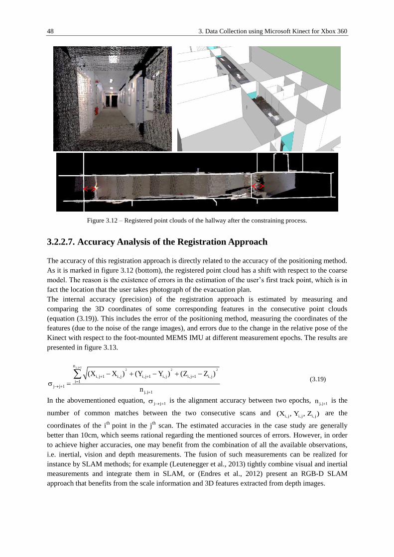
48 3. Data Collection using Microsoft Kinect for Xbox 360
Figure 3.12 – Registered point clouds of the hallway after the constraining process.
3.2.2.7. Accuracy Analysis of the Registration Approach
The accuracy of this registration approach is directly related to the accuracy of the positioning method.
As it is marked in figure 3.12 (bottom), the registered point cloud has a shift with respect to the coarse
model. The reason is the existence of errors in the estimation of the user’s first track point, which is in
fact the location that the user takes photograph of the evacuation plan.
The internal accuracy (precision) of the registration approach is estimated by measuring and
comparing the 3D coordinates of some corresponding features in the consecutive point clouds
(equation (3.19)). This includes the error of the positioning method, measuring the coordinates of the
features (due to the noise of the range images), and errors due to the change in the relative pose of the
Kinect with respect to the foot-mounted MEMS IMU at different measurement epochs. The results are
presented in figure 3.13.
j, j 12 2 2
n
i, j 1 i, j i, j 1 i, j i, j 1 i, j
i 1j j 1
j, j 1
(X X ) (Y Y ) (Z Z )
n
(3.19)
In the abovementioned equation, j j 1 is the alignment accuracy between two epochs,
j, j 1n is the
number of common matches between the two consecutive scans and i, j i, j i, j(X , Y , Z ) are the
coordinates of the ith
point in the jth scan. The estimated accuracies in the case study are generally
better than 10cm, which seems rational regarding the mentioned sources of errors. However, in order
to achieve higher accuracies, one may benefit from the combination of all the available observations,
i.e. inertial, vision and depth measurements. The fusion of such measurements can be realized for
instance by SLAM methods; for example (Leutenegger et al., 2013) tightly combine visual and inertial
measurements and integrate them in SLAM, or (Endres et al., 2012) present an RGB-D SLAM
approach that benefits from the scale information and 3D features extracted from depth images.
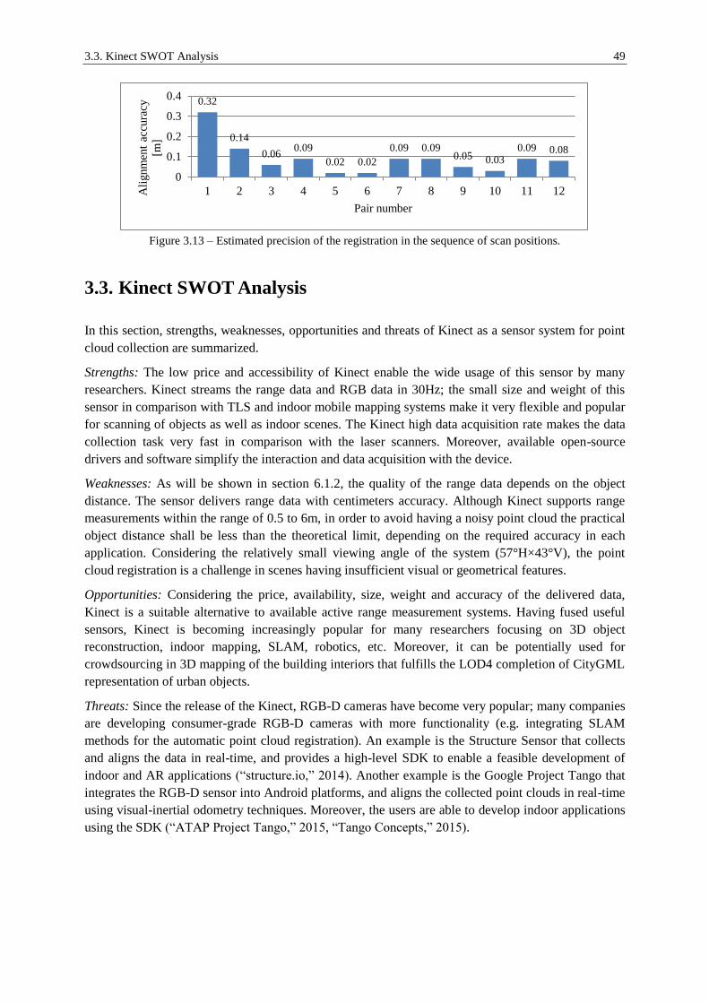
3.3. Kinect SWOT Analysis 49
Figure 3.13 – Estimated precision of the registration in the sequence of scan positions.
3.3. Kinect SWOT Analysis
In this section, strengths, weaknesses, opportunities and threats of Kinect as a sensor system for point
cloud collection are summarized.
Strengths: The low price and accessibility of Kinect enable the wide usage of this sensor by many
researchers. Kinect streams the range data and RGB data in 30Hz; the small size and weight of this
sensor in comparison with TLS and indoor mobile mapping systems make it very flexible and popular
for scanning of objects as well as indoor scenes. The Kinect high data acquisition rate makes the data
collection task very fast in comparison with the laser scanners. Moreover, available open-source
drivers and software simplify the interaction and data acquisition with the device.
Weaknesses: As will be shown in section 6.1.2, the quality of the range data depends on the object
distance. The sensor delivers range data with centimeters accuracy. Although Kinect supports range
measurements within the range of 0.5 to 6m, in order to avoid having a noisy point cloud the practical
object distance shall be less than the theoretical limit, depending on the required accuracy in each
application. Considering the relatively small viewing angle of the system (57°H×43°V), the point
cloud registration is a challenge in scenes having insufficient visual or geometrical features.
Opportunities: Considering the price, availability, size, weight and accuracy of the delivered data,
Kinect is a suitable alternative to available active range measurement systems. Having fused useful
sensors, Kinect is becoming increasingly popular for many researchers focusing on 3D object
reconstruction, indoor mapping, SLAM, robotics, etc. Moreover, it can be potentially used for
crowdsourcing in 3D mapping of the building interiors that fulfills the LOD4 completion of CityGML
representation of urban objects.
Threats: Since the release of the Kinect, RGB-D cameras have become very popular; many companies
are developing consumer-grade RGB-D cameras with more functionality (e.g. integrating SLAM
methods for the automatic point cloud registration). An example is the Structure Sensor that collects
and aligns the data in real-time, and provides a high-level SDK to enable a feasible development of
indoor and AR applications (“structure.io,” 2014). Another example is the Google Project Tango that
integrates the RGB-D sensor into Android platforms, and aligns the collected point clouds in real-time
using visual-inertial odometry techniques. Moreover, the users are able to develop indoor applications
using the SDK (“ATAP Project Tango,” 2015, “Tango Concepts,” 2015).
0.32
0.14
0.06 0.09
0.02 0.02
0.09 0.09 0.05 0.03
0.09 0.08
0
0.1
0.2
0.3
0.4
1 2 3 4 5 6 7 8 9 10 11 12Ali
gnm
ent
accu
racy
[m]
Pair number
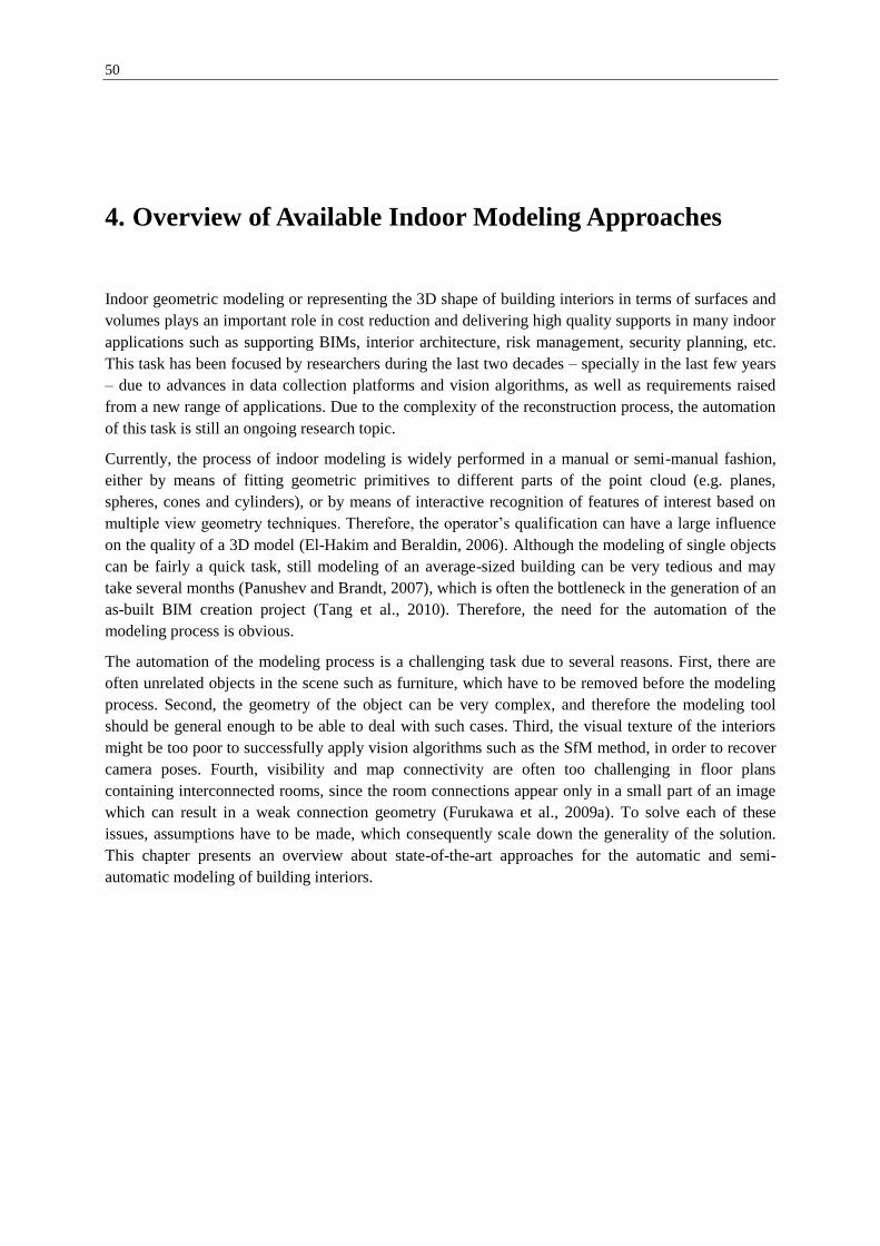
50
4. Overview of Available Indoor Modeling Approaches
Indoor geometric modeling or representing the 3D shape of building interiors in terms of surfaces and
volumes plays an important role in cost reduction and delivering high quality supports in many indoor
applications such as supporting BIMs, interior architecture, risk management, security planning, etc.
This task has been focused by researchers during the last two decades – specially in the last few years
– due to advances in data collection platforms and vision algorithms, as well as requirements raised
from a new range of applications. Due to the complexity of the reconstruction process, the automation
of this task is still an ongoing research topic.
Currently, the process of indoor modeling is widely performed in a manual or semi-manual fashion,
either by means of fitting geometric primitives to different parts of the point cloud (e.g. planes,
spheres, cones and cylinders), or by means of interactive recognition of features of interest based on
multiple view geometry techniques. Therefore, the operator’s qualification can have a large influence
on the quality of a 3D model (El-Hakim and Beraldin, 2006). Although the modeling of single objects
can be fairly a quick task, still modeling of an average-sized building can be very tedious and may
take several months (Panushev and Brandt, 2007), which is often the bottleneck in the generation of an
as-built BIM creation project (Tang et al., 2010). Therefore, the need for the automation of the
modeling process is obvious.
The automation of the modeling process is a challenging task due to several reasons. First, there are
often unrelated objects in the scene such as furniture, which have to be removed before the modeling
process. Second, the geometry of the object can be very complex, and therefore the modeling tool
should be general enough to be able to deal with such cases. Third, the visual texture of the interiors
might be too poor to successfully apply vision algorithms such as the SfM method, in order to recover
camera poses. Fourth, visibility and map connectivity are often too challenging in floor plans
containing interconnected rooms, since the room connections appear only in a small part of an image
which can result in a weak connection geometry (Furukawa et al., 2009a). To solve each of these
issues, assumptions have to be made, which consequently scale down the generality of the solution.
This chapter presents an overview about state-of-the-art approaches for the automatic and semi-
automatic modeling of building interiors.

4.1. Classification of Available Modeling Approaches 51
4.1. Classification of Available Modeling Approaches
Due to the availability of different data acquisition techniques, data processing algorithm and accuracy
requirements, the variety of reconstruction approaches is very large. According to comprehensive
reviews given by Remondino (2003), Remondino and El-Hakim (2006) and Tang et al. (2010), the
approaches can be classified based on many different criterions. The criterions can be for instance the
type of the input information, the type of the measurements, the spatial and mathematical
representation format of the outputs, used assumptions, or the level of automation.
Type of the input information: As the first and main classification criterion, the approaches based on
the source of input information can be divided into two main categories: iconic (bottom-up modeling)
and symbolic (top-down modeling). Iconic approaches generate models based on real measurements
and observations, while symbolic approaches rely on hypotheses derived from the indoor
reconstruction grammar, statistics and semantics.
Type of the measurements: Iconic reconstruction approaches rely on two main types of observations
and measurements. They either recover 3D models from 2D images based on single and multiple view
geometry (image-based), or from depth information derived from laser scanners, range cameras or
dense image matching techniques (range-based).
Spatial representation: Another classification can be done according to the spatial representation of
the output model. The output model can be represented either surface-based or volumetric. The
volumetric representation (including solid geometric primitives and voxel representation) is more
suitable for closed surfaces and objects. However, surface-based approaches (e.g. boundary-based
representation) do not distinguish between closed and open surfaces. Most of the modeling approaches
are categorized in this class. Moreover, it should be noted that some representations may belong to
both classes; for example a geometric primitive can be considered as a surface, or at the same time, as
a volume.
Mathematical representation: A further classification can be done according to the mathematical
representation of the output model. Parametric approaches use a small number of parameters to
represent a shape, and therefore require smaller storage volumes and computational complexities. In
contrast, despite the high storage requirements of non-parametric approaches (such as triangular
meshes), they are more flexible to represent complex geometries (Tang et al., 2010). However, the
complexity of the resulting model is reduced using region growing algorithms based on the surface
normal vectors (for example see (Hähnel et al., 2003)).
Used assumptions: The approaches can also be classified based on the assumptions regarding the
object geometry and topology. Assumptions such as Manhattan-world scenario in most of the man-
made scenes not only guarantee constructing a topologically correct model, but also make the
reconstruction procedure easier and more robust (Budroni and Böhm, 2009). Other assumptions
regarding the object geometry enable automatic fitting of geometric primitives to the segmented point
clouds.
Automation level: The final classification is based on the level of user interactions during the
reconstruction process.
Choosing the correct reconstruction approach depends on the application. For example, parametric
volumetric approaches are most relevant to BIMs, but surface-based approaches are more common
(Tang et al., 2010). In fact, although parametric volumetric approaches are more intuitive for the
manipulation by the user (Kemper and Wallrath, 1987), they are less flexible due to the limited size of
primitives libraries (Rottensteiner, 2000). Moreover, surface-based approaches enable efficient

52 4. Overview of Available Indoor Modeling Approaches
representation of partially occluded objects (Walker, 1989). This study deals with the representation of
the rooms main structures (walls); they can be simply represented by planar surfaces. Due to this and
aforementioned reasons, here, only parametric surface-based approaches are focused. Readers
interested in the field of automated reconstruction of volumetric model of indoor environments are
referred to the works presented by Jenke et al. (2009), Oesau et al. (2014), as well as Xiao and
Furukawa (2012).
The remainder of this chapter introduces state-of-the-art indoor reconstruction approaches, based on
the source of the input data, which is the most general criterion according to the abovementioned
classification scheme.
4.2. Iconic Approaches
Automatic and semi-automatic iconic (bottom-up) approaches for the reconstruction of geometric
models use different sources of data, such as photographs, point clouds (collected by laser scanners,
range cameras and dense image matching techniques) or available architectural plans to derive
geometric models.
4.2.1. Image-Based Modeling
Image-based modeling is the process of reconstructing 3D models of scenes from measurements made
on a single or multiple 2D images. According to Yu et al. (2011), the process includes detection,
grouping and extraction of nodes, edges or faces, and interpreting them as 3D clues.
4.2.1.1. Modeling Based on Single View Geometry
Besides multiple view geometry in which 3D information is extracted from motion and parallax, in
special cases, single view metrology can offer solutions to infer 3D information from single images
(Criminisi et al., 1999, 1998; Hartley and Zisserman, 2003). Recovering 3D information from a single
image is applicable, in cases where multiple views are not available, or the texture in images are too
poor in multiple views for a successful camera pose estimation using SfM methods, or the baseline in
multi-ocular systems is too short in comparison with the object distance. Such systems make use of
geometric properties invariant to perspective projection, such as vanishing points and lines, straight
lines, parallel lines and right angles (Criminisi et al., 1999). In practice, systems based on this
approach need some prior knowledge about the scene geometry to enable simplifications and therefore
automation of the modeling process. Figure 4.1 shows an example in which the 3D model is
reconstructed using a single perspective image, from a scene containing three dominant and mutually
perpendicular planes (building façades and the ground plane). The parallel lines in three main
directions determine three vanishing points. This together with the estimated camera calibration and
vanishing lines of planes which are not orthogonal, enable the reconstruction of 3D textured models
(Hartley and Zisserman, 2003).
Assumptions which are valid in most indoor scenarios (e.g. existence of constrained geometries such
as planes and straight lines, as well as relationships such as perpendicularity and parallelism) make the
automatic estimation of the geometric invariants more feasible. For example in Delage et al. (2006), it
is assumed that the scene is a “floor-wall” geometry. Their algorithm then recognizes the floor-wall
boundary in the image, and recovers 3D information based on Bayesian methods, in which visual cues
are combined with a prior knowledge about the scene geometry, such as main wall directions and the
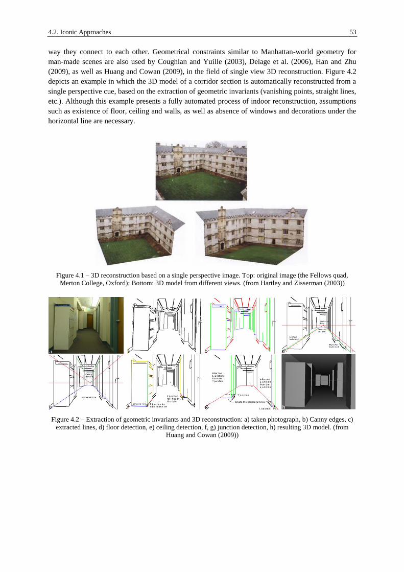
4.2. Iconic Approaches 53
way they connect to each other. Geometrical constraints similar to Manhattan-world geometry for
man-made scenes are also used by Coughlan and Yuille (2003), Delage et al. (2006), Han and Zhu
(2009), as well as Huang and Cowan (2009), in the field of single view 3D reconstruction. Figure 4.2
depicts an example in which the 3D model of a corridor section is automatically reconstructed from a
single perspective cue, based on the extraction of geometric invariants (vanishing points, straight lines,
etc.). Although this example presents a fully automated process of indoor reconstruction, assumptions
such as existence of floor, ceiling and walls, as well as absence of windows and decorations under the
horizontal line are necessary.
Figure 4.1 – 3D reconstruction based on a single perspective image. Top: original image (the Fellows quad,
Merton College, Oxford); Bottom: 3D model from different views. (from Hartley and Zisserman (2003))
Figure 4.2 – Extraction of geometric invariants and 3D reconstruction: a) taken photograph, b) Canny edges, c)
extracted lines, d) floor detection, e) ceiling detection, f, g) junction detection, h) resulting 3D model. (from
Huang and Cowan (2009))

54 4. Overview of Available Indoor Modeling Approaches
4.2.1.2. Modeling Based on Multiple View Geometry
3D reconstruction using photographs is more efficient and reliable using multiple view geometry, in
comparison with single view geometry. Promising outcomes have been resulting using computer
vision techniques during the last two decades in this field. In this modeling approach, the camera pose
is estimated using corresponding points or line features across images. In the next step, the 3D model
is generated either automatically having made some assumptions regarding the scene geometry, or in
an interactive way by the user drawings. In the latter case, vanishing points and lines are turned to be
powerful tools for 2D-to-3D applications that enable accurate sketching of polygonal faces in a single
image, without the need for refinement in another image to build up a globally consistent model
(Sinha et al., 2008).
The automation of the modeling process versus accuracy and generality trade-off is a challenge, and
the correct decision depends on the application. As mentioned by El-Hakim (2002), in traditional
modeling which is a widely used method, the focus is on the accuracy without a high level of
automation. In such approaches, data acquisition and registration by photogrammetric and computer
vision techniques are followed by an interactive drawing by the user. Although efforts are made for
the automation of the whole modeling process, the solutions still may fail in new environments, in
which the standard assumptions are not valid anymore, due to the scene complexity, or fragility of
algorithms and vision techniques (e.g. demanding accurate point or line correspondences) (Shum et
al., 1998). Therefore, the most impressive results are achieved by the semi-automated systems in
which the user is in the processing loop (El-Hakim, 2002). Currently, although improvements and
progresses are made in the automation of the modeling process, still user interaction is necessary to
achieve a robust and general solution. Recent works have shown that the interaction can be very
limited, simple and smart, by making some assumptions about the scene geometry, as well as making
use of geometric invariants.
The semi-automated approach presented in Shum et al. (1998) makes use of panoramic image mosaics
to efficiently cover the scene. It is one of the earliest works that uses regularities in man-made scenes
as constraints in the modeling process. The problem of image registration in this case is decoupled into
a zero baseline problem (for photos taken with a rotating camera) and a wide baseline stereo or SfM
problem. Therefore, the camera pose for each mosaic is computed under the assumption of having
some lines with known directions (e.g. horizontal or vertical lines). The baselines between the
panoramic images can be recovered having some known points and using robust computer vision
approaches. The modeling part of this system is an interactive process, in which the user draws the
lines and polygons in one panorama, and completes it by projecting the current model onto the new
panorama and recovering the new parts of the model subject to the constraints derived from the scene
regularities.
The approach presented by El-Hakim (2002), in contrast, uses a small number of perspective images
from widely separated views (e.g. photos taken by tourists), and automatically deals with occlusions
and unmarked surfaces. In this approach, image registration and segmentation are carried out by the
user in an interactive way. This is followed by an automatic corner detection and correspondence. In
this approach, in average, 80% of the points are generated automatically, by applying an edge detector
and sampling new points on the edges.
In the interactive solution proposed by Sinha et al. (2008), the 3D model is reconstructed from a
collection of unordered photographs. In this approach, camera poses are estimated using SfM methods.
This process also delivers a sparse 3D point cloud which is later used (together with vanishing
directions) in the modeling step for the estimation of plane normal vectors and depths. Vanishing
points are estimated automatically, by the automatic estimation of lines in the images. The system then

4.2. Iconic Approaches 55
uses this geometrical information for the upcoming interactive modeling steps. The modeling process
includes drawing the 2D outline of the planar sections over the photographs, which are automatically
converted to 3D polygons. By projecting the image onto the created 3D surfaces, the model not only
becomes photorealistic, but the user can also easily edit the sketches or draw lines which are observed
even in one image. Figure 4.3 shows the described system in use for generating photorealistic 3D
models.
Figure 4.3 – An interactive system interface for generating 3D photorealistic models from unordered
photographs. Top (from left to right): input photographs, 2D sketching of polygons, geometric model and
textured model. Bottom (example in an indoor scene, from left to right): input photograph, overlay of the model
on the photo and geometric model. (from Sinha et al. (2008))
Figure 4.4 – Exemplary data acquisition and the resulting 3D model using a smartphone application MagicPlan
(“Sensopia Inc.,” 2014), supported by Augmented Reality.

56 4. Overview of Available Indoor Modeling Approaches
In another form of user interactions, Augmented Reality systems are used to fulfil some constraints
during the data acquisition, as well as guiding the data acquisition task. Figure 4.4 illustrates an
exemplary data acquisition process and the resulting indoor model using a smartphone application
(“Sensopia Inc.,” 2014) supported by Augmented Reality. In this application, the user stands on a
single position inside the room, and takes photographs of only the room corners, while interactively
coincides the corners with markers indicated on the device screen. However, this application does not
rely only on photos, and also benefits from other device’s sensors such as compass and gyroscope to
recover a 2D plan.
User interactions are replaced by making assumptions about the scene geometry in Furukawa et al.
(2009a), in order to achieve a fully automated approach for indoor reconstruction based on state-of-
the-art computer vision algorithms. In this work, similar to the work presented by Sinha et al. (2008),
camera poses and image registration is performed based on the SfM method. The approach then
imposes Manhattan-world constraint on the scene, which is typical for many indoor scenes. Based on
this assumption, in the next step, a stereo algorithm specifically designed for Manhattan-world scenes
is used to derive axis-aligned depth maps from the images (Furukawa et al., 2009b). Afterwards, the
depth map and the sparse point cloud resulting by the SfM method are merged to extract a simplified
axis-aligned mesh model. After some refinement steps applying on the vertex positions up to sub-
voxel accuracy constrained with Manhattan-world assumption, the 2D plan is computed. Examples of
a floor plan and a 3D model generated by this approach are depicted in figure 4.5. In this example, a
simple and consistent model is generated from a sparse multi-view stereo point cloud and a noisy
depth model, thanks to the refinement steps and the Manhattan-world constraining.
Figure 4.5 – Input, interim and final results for indoor reconstruction from a sample dataset, using the approach
described by Furukawa et al. (2009a). From left to right and top to bottom: Input image, textured points,
Manhattan-world depth map, final 3D model and generated floor plan. (from Furukawa et al. (2009a))

4.2. Iconic Approaches 57
4.2.2. Range-Based Modeling
Range-based approaches for modeling of building interiors use geometrical information collected by
laser scanners, range cameras and dense image matching to represent the indoor space in terms of
surfaces and volumes. In general, this process consists of different phases, such as data acquisition,
data pre-processing (including registration, outlier and noise removal, furniture removal, etc.),
segmentation of the point clouds and geometric modeling (line or plane fitting, topological
corrections, possibly extraction of semantics such as openings, etc.). In this chapter, the special focus
is on the geometric modeling process.
Fitting planes and other geometric primitives to collected point clouds is the main approach developed
for the reconstruction of building interiors from measured point clouds. Although in commercial
solutions such as Cyclone (“Leica Cyclone,” 2014) the fitting is fulfilled in a semi-automatic manner,
there are researches pointing to the automation of this process. In Toldo and Fusiello (2008), a novel
and robust algorithm for fitting of geometric primitives to point clouds containing noise and outliers is
presented. The algorithm (so called J-Linkage) is based on a random sampling scheme (as in
RANSAC (Fischler and Bolles, 1981)) and Jaccard distance, and automatically groups the point cloud
into corresponding clusters considering the preference set of each point, i.e., the set of models to be
satisfied by the point within a tolerance. In other words, the models (characteristic functions) can be
considered as conceptual representations of the points; therefore, the points are clustered in a
conceptual space. Figure 4.6 shows an exemplary output of this algorithm applied on a room point
cloud, using the implementation provided by Toldo and Fusiello (2014). The algorithm is robust in
fitting applications, due to using powerful statistical tools; however, it still cannot be considered as a
sufficient solution for the geometric modeling of the building interiors, as it does not control the
topological correctness of the generated model. Another example of primitive shape detection using
RANSAC is given by Schnabel et al. (2007).
The plane fitting task is fulfilled by the linear and rotational plane sweeping algorithm in Budroni and
Böhm (2009). In their approach, the room is considered to be a Manhattan-world scenario, and
therefore, the main wall directions are perpendicular. A main direction in this approach is recovered
by the analysis of the number of points laid on the rotating sweep plane located at different random
positions. The walls are then identified based on a linear sweep along the main room direction,
followed by a cell decomposition process. This process, however, requires the acquisition of ceiling
and floor points. Floor and ceiling are identified by a linear plane sweep in the vertical direction, and
the analysis of the point height histogram. Existence of noise, outliers and clutter has no impact on the
output, as far as they do not gain the peaks in the resulting histograms. The proposed algorithm is
robust in applications satisfying the Manhattan-world constraint. Figure 4.7 shows the 3D model
reconstructed by this approach, for the same dataset used in the previous example.
The Manhattan-world assumption is ruled out, and therefore wall detection becomes more general in
the approach presented by Previtali et al. (2014). In this approach, besides the geometric
reconstruction, semantic information such as location of doors and windows are recovered, assuming a
known location of the laser scanner. For this purpose, the approach first detects and segments the
planes constituting the room outer shell, based on the RANSAC algorithm and some topological
measures. By recovering the ceiling and floor points based on the height histogram analysis of
horizontal plane segments, a first floor plan is inferred by projecting the ceiling or floor points onto a
horizontal plane, and a follow-up cell decomposition process. The floor plan then supports the
extraction of walls amongst all the vertical segments (including those produced by clutter), by finding
the vertical plane segments belonging to the boundary of the floor plan. To detect doors and windows,
openings inside the walls are looked for. Holes produced by clutter and occlusions are distinguished

58 4. Overview of Available Indoor Modeling Approaches
from doors or windows using a ray-tracing algorithm (similar to Adan and Huber (2011)), assuming
doors or windows are not occluded in the point clouds, as well as the scanner position is known. Doors
are distinguished from windows, if their corresponding holes intersect the ground. Figure 4.8 depicts
an example of a reconstructed 3D model based on the mentioned approach for a scenario with an
arbitrary shape. It should be noted that although this approach is compatible with more general room
shapes, the collection of ceiling or floor points is still necessary for the cell decomposition process.
While this is not an issue for data acquisition with TLS, indoor mobile mapping systems can face
problems regarding data acquisition of such featureless and broad surfaces.
Figure 4.6 – Plane fitting to a sample room point cloud using the algorithm presented by Toldo and Fusiello
(2008).
Figure 4.7 – 3D reconstruction using the plane sweep followed by a cell decomposition process. (from Budroni
(2013))
Figure 4.8 – Sample 3D model with semantic information automatically derived from a laser scanner point
cloud. From left to right: laser point cloud, binary occupancy map (cell decomposition) and 3D model with
distinguished door and window features. (adapted from Previtali et al. (2014))
There are also approaches that focus on the reconstruction of 2D floor plans which are then
convertible to 3D models by a simple extrusion. Besides that, in many applications, a 2D floor plan is
the required output. A related work in this field is presented by Okorn et al. (2010). This approach
recovers the 2D plan of the building interiors from a given 3D point cloud of the facility, based on the
projection of the points onto a horizontal 2D plane. The projection of the points forms a histogram

4.2. Iconic Approaches 59
from the point density, which is used for the extraction of line segments corresponding to walls using a
Hough transform. In this approach, clutter is removed based on the point height histogram. Moreover,
it is taken into account that walls have a higher intensity in the 2D point density histogram. Figure 4.9
shows an exemplary output of this algorithm for one floor of a building. Although many of the line
segments are correctly assigned by this approach, still the resulting 2D plan does not represent a
topologically correct model. Moreover, this approach does not deal with occlusions.
The aforementioned approach is semantically enriched in Adan and Huber (2011) by detection and
modeling of wall openings, and filling the occluded regions. In this approach, first, walls are detected
using a Hough transform just similar to that described in Okorn et al. (2010). Wall occlusions are then
classified into occupied, empty or occluded, using a ray-tracing algorithm, assuming that the 3D data
is obtained from fixed and known locations. In the next step, door and windows are detected using a
learning-based method that extracts and analyzes rectangular openings. Finally, occlusions not within
openings are reconstructed based on a hole-filling algorithm (see figure 4.10).
The approach presented by Valero et al. (2012) improves the geometric modeling of the works
presented by Okorn et al. (2010), as well as Adan and Huber (2011), using a more robust wall
detection algorithm supported by some topological analyses. They firstly use a similar algorithm to
derive the room’s boundary in 2D using the Hough transform. Due to the high density and low level of
noise in the input data collected by the laser scanner, each wall is represented by a corresponding edge
in the extracted room’s boundary, which is equivalent to a vertical plane in 3D. This supports the
segmentation of points into individual walls by the analysis of the point-to-plane distances. A
boundary representation model (planar surfaces) is then generated by the calculation of the best plane
fit to the segmented points. Finally, the intersections between the planes are computed, considering the
topological relationship between the already estimated boundary edges in the 2D projected image
(figure 4.11, top right). The process steps are depicted in figure 4.11 for a sample room point cloud. It
can be observed that for a successful process, having a dense point cloud of the room ceiling or floor is
necessary to robustly estimate the room’s boundary.
Figure 4.9 – 2D floor plan from point density histogram. From left to right: 2D point density histogram,
estimated Hough lines and overly with ground truth (labeling based on detected lines): green and blue line
segments are modeled by the algorithm, while red segments are missed. (adapted from Okorn et al. (2010))
Figure 4.10 – Opening detection. From left to right: opening detection using a machine learning model, openings
superimposed on a 2D projection image and final marked out openings. (from Adan and Huber (2011))

60 4. Overview of Available Indoor Modeling Approaches
Figure 4.11 – From point cloud to a boundary representation model. From left to right and top to bottom:
projection of the points onto a horizontal plane, detected edges, boundary detection using the Hough transform,
point cloud segmentation, estimation of best plane fits and the final boundary representation model. (adapted
from Valero et al. (2012))
4.2.3. Modeling Based on Architectural Drawings
Architectural drawings are essential for the design and construction of buildings. They are made
according to a set of conventions including symbols and annotations. Graphics recognition techniques
for the analysis of available 2D architectural floor plans can deliver geometric and semantic
information to reconstruct 3D models. Such approaches for 3D modeling can be classified as iconic, if
the underlying floor plan represents the as-built state, and therefore indirectly require the real
measurement of the building interiors. But on the other hand, they might be considered as symbolic, if
they are linked to an as-designed plan, which does not necessarily represent the as-built status.
The complexity of such modeling approaches depends on the provided input information, which can
be of different level-of-details, as well as very different formats, ranging from CAD documents to
scanned paper drawings. For instance the systems developed by Horna et al. (2007), Lewis and Séquin
(1998) and Lu et al. (2007, 2005) take the floor plans in digital version as input, and focus on
derivation of geometrical features, eventually semantic information and topological correction. But on
the other hand, many floor plans are recorded as paper documents or scanned images. Therefore, the
other category of approaches, such as those presented by Ah-Soon and Tombre (2001, 1997) and
Dosch et al. (2000), try to extract geometric and semantic information using a raster-to-vector
conversion process, supported by image processing and pattern recognition techniques. Another
challenge in this modeling approach is differences in drawing conventions, as well as the architects’
creative way of generalization and representation. Therefore, user interaction in the analysis of the
drawings becomes unavoidable, due to the limited size of the predefined symbols and libraries.
According to a survey study presented by Yin et al. (2009), most of the available approaches in this
field share a similar pipeline, however, they are different in terms of employed algorithms and
strategies dealing with different process steps. In general, the main pipeline consists of image parsing
(for the extraction of semantic information through text extraction and symbol detection), derivation of
geometrical information (including noise removal, image processing, template matching and detection
of architectural components such as walls, windows and the outer building shell), as well as
topological corrections.
This section describes in detail the approach presented by Peter et al. (2010), in which 3D indoor
models are extracted from photographed evacuation plans. The resulting 3D model will later serve as
the case study in demonstration of the capability of our reconstruction approach in the refinement of

4.2. Iconic Approaches 61
available coarse floor models (see chapter 7). The existence of evacuation plans is compulsory in
many countries for public buildings such as hospitals, universities, hotels, etc. Therefore, the
accessibility to these maps makes this approach more suitable for 3D modeling by the mass
(crowdsourcing). The approach first enhances the photograph to compensate for bad light condition to
increase the image quality using automatic white balancing and Wallis filtering (Wallis, 1976).
Afterwards, a binarization process is carried out using a single threshold so that the image can be
segmented into closed polygons for further topological analyses, such as distinction of rooms and
single stairs. The stair candidates are also used for the estimation of the floor height considering a
standard value for a single stair’s height. The main lines in the image are then estimated in order to
identify the building boundaries, using the Canny edge detector (Canny, 1986). Matching the
identified boundary of the building with the available outer shell contour extracted from city maps
further enables the derivation of geo-referenced metric models as well as computation of projective
transformation parameters to convert the image coordinates into the world coordinate system. It
additionally enables the removal of the perspective distortions caused by photography and cropping
the image. Since parts of the plan might be occluded by symbols, symbol areas have to be detected and
removed. Symbol areas are detected by template matching considering the image legend for the plan.
This technique is replaced in their follow-up work (Peter et al., 2013b) by a more general and efficient
method called Color Structure Code segmentation, in which symbols are detected based on their color
properties (“Color Structure Code,” 2014). The image is then vectorised by the estimation of the
skeleton of the cleaned binary image. The occluded lines (by symbol areas) then have to be bridged by
the prolongation of free end node edges identified in the vectorised image. The mentioned image
processing steps are depicted in figure 4.13. The resulting vectorised image, which is now the 2D floor
plan of the building, is further refined by detection of doors, using the indoor positioning system
described in section 3.2.2.1. Doors are detected by finding the intersection of the user’s track as well
as evacuation routes and existing walls within an appropriate intersection angular range. The 2D plan
is finally converted to a 3D model by an extrusion, having the floor height available (see figure 4.14).
The initial point of the user’s track, which is required for indoor positioning, can be computed by
detection of the “you are here” symbol using template matching. However, the distance between user
to the evacuation plan can be computed only by having the plan dimensions or by map matching of the
user’s route. Additionally, the user is able to collect geo-referenced semantic information in an
OpenStreetMap-like fashion, i.e. collection of geo-tagged photos which will be added to the map in a
post-processing step, e.g. location of fire extinguishers, doors, windows, room number, etc. The
mentioned steps are summarized and depicted in figure 4.12.

62 4. Overview of Available Indoor Modeling Approaches
Figure 4.12 – The main procedure to convert photographed evacuation plans to 3D models.
Figure 4.13 – Left: a photographed evacuation plan; Upper right: image processing steps (left to right): original
image, color enhancement, binarization, symbol detection using color segmentation or template matching,
symbol bridging and vectorization, and stair detection (green); Lower right: vectorized floor plan. (adapted from
Haala et al. (2011), Peter et al. (2013b) and Peter et al. (2013b))
Figure 4.14 – Generated 3D indoor
model corresponding to figure 4.13.
Photographing the
evacuation plan
Image enhancement
and white balance Binarization Stair detection
Height detection Edge detection
Vectorization Symbol detection and
removal
Estimation of the
building outer shell
Perspective removal
Transformation to
the world
coordinate system
Symbol bridging
Generation of the
final model
Estimation of the
user’s initial location Map matching

4.3. Symbolic Approaches 63
4.3. Symbolic Approaches
Symbolic (top-down) approaches can recover geometric models based on hypotheses, in case of
having incomplete or erroneous data, where the iconic modeling approaches fail or deliver invalid
results. The hypotheses are derived based on the knowledge inferred from the rules governing the
regularities and relationships in the arrangement of structure elements. It is similar to a language’s
grammar, in which words are put together according to grammar rules to construct a sentence. A shape
grammar rule governing a special design principle can be derived, for example, from the analysis of a
bottom-up modeling process, where the data is of sufficient accuracy and density to deliver valid
results.
Grammar-based approaches have successfully been used in the reconstruction of LOD3 models, by the
integration of façade models to available LOD2 building models (e.g. see (Becker, 2009; Müller et al.,
2006)), as well as in indoor applications that reconstruct LOD4 models, according to CityGML
representation standard (e.g. see (Becker et al., 2013; Gröger and Plümer, 2010; Khoshelham and
Díaz-Vilariño, 2014; Philipp et al., 2014)). This section shortly introduces available grammar-based
approaches used in indoor applications.
In grammar-based modeling, mainly spatial grammar rules (particularly split rules) are used to
reconstruct the more complex shapes from basic geometric primitives (e.g. splitting boxes and faces to
their constructive sub-spaces) (Müller et al., 2006; Wonka et al., 2003). However, it does not
guarantee the topological correctness of the models caused for instance by gap or overlap of the
constructive elements. This problem is addressed by Gröger and Plümer (2010), and a solution is
presented by explicit constraining based on topological concepts (such as adjacency, parallelism and
perpendicularity), setting up a rout graph as a benchmark for the consistency (coincidence of doors)
and use of semantics (such as distinction of rooms, hallways, staircases, as well as doors and ceilings
floors and walls). Such criterions define a limited number of rules to subdivide the space and
reconstruct the building interiors in more detail and rich semantics. The work is the first grammar-
based approach adapted for indoor applications, however, the grammar rules have to be defined
manually for every case study.
Grammar rules are derived automatically from observations in Becker et al. (2013), so that it becomes
flexible to support the reconstruction of more indoor scenarios with arbitrary shapes. Their grammar
design assumes building floors are composed of two parts: a hallway part which is designed for a
convenient access to rooms, and a non-hallway part consisting of individual rooms mostly arranged in
a linear sequence parallel to the hallway. Therefore, their grammar is a combination of two separate
rules: a simulation of plants growth pattern (a so-called Lindenmayer system) for the hallways part,
and split rules for the reconstruction of rooms.
To create an instance of an individual grammar which is able to reproduce a specific building interiors,
observations are required. A grammar instance can be generated for example from an available floor
plan or a collection of odometry data. In the example provided by Peter et al. (2013a), the indoor
model derived from a photographed evacuation plan yields a high level grammar instance using the
reverse modeling process. In Becker et al. (2013) and the corresponding extended work (Philipp et al.,
2014), the hypotheses about the indoor geometries are generated from the observation of 250
odometry traces collected by a foot mounted MEMS IMU (see figure 4.15). By means of constraints
derived from the trace data, door locations are estimated. It is assumed that each room has only one
door, which is the intersection of a trace with the corresponding wall. Therefore, it can also be
assumed that walls can be located only between the door locations. In their example, 116 rooms are
reconstructed from the trace data with an average width error of around 2 meters. Moreover, the room

64 4. Overview of Available Indoor Modeling Approaches
sizes are estimated based on the grammar and the probabilities assigned to them, together with
constraints, conjointly.
Figure 4.15 – Grammar-based reconstruction of an indoor scene based on the observation of 250 odometry
traces. From left to right: position traces, estimated door locations and hypothesized hallways (rooms are
reconstructed only from traces; without the use of hypotheses), complete model with hypothesized rooms and the
ground truth. (adapted from Becker et al. (2013))
In Khoshelham and Díaz-Vilariño (2014), the shape grammar is derived based on an architectural
indoor design concept known as Palladian grammar (Stiny et al., 1978). The grammar rules in their
work are automatically learnt from an available point cloud of the scene. The point cloud is first
aligned with the main axes of the coordinate system based on the analysis of normal vectors. Floors
are then distinguished based on the analysis of the point height histogram. Finally, grammar rules are
defined and adapted automatically to each case study, based on the analysis of the x- and y-
coordinates for each floor to find peaks corresponding to the location of walls and size of subspaces.
This grammar-based learning approach, however, is only valid for Manhattan-world scenarios.
Moreover, existence of ceiling points is necessary for the points-on-ceiling test that excludes invalid
subspaces made by the integrating cell decomposition step. Figure 4.16 depicts the results of this
reconstruction approach for a sample point cloud.
Figure 4.16 – Grammar-based reconstruction based on grammar rules derived from the point cloud. From left to
right: collected point cloud, cuboid placement (top-view) with points-on-ceiling constraining and cuboid
placement without points-on-ceiling constraining. (adapted from Khoshelham and Díaz-Vilariño (2014))
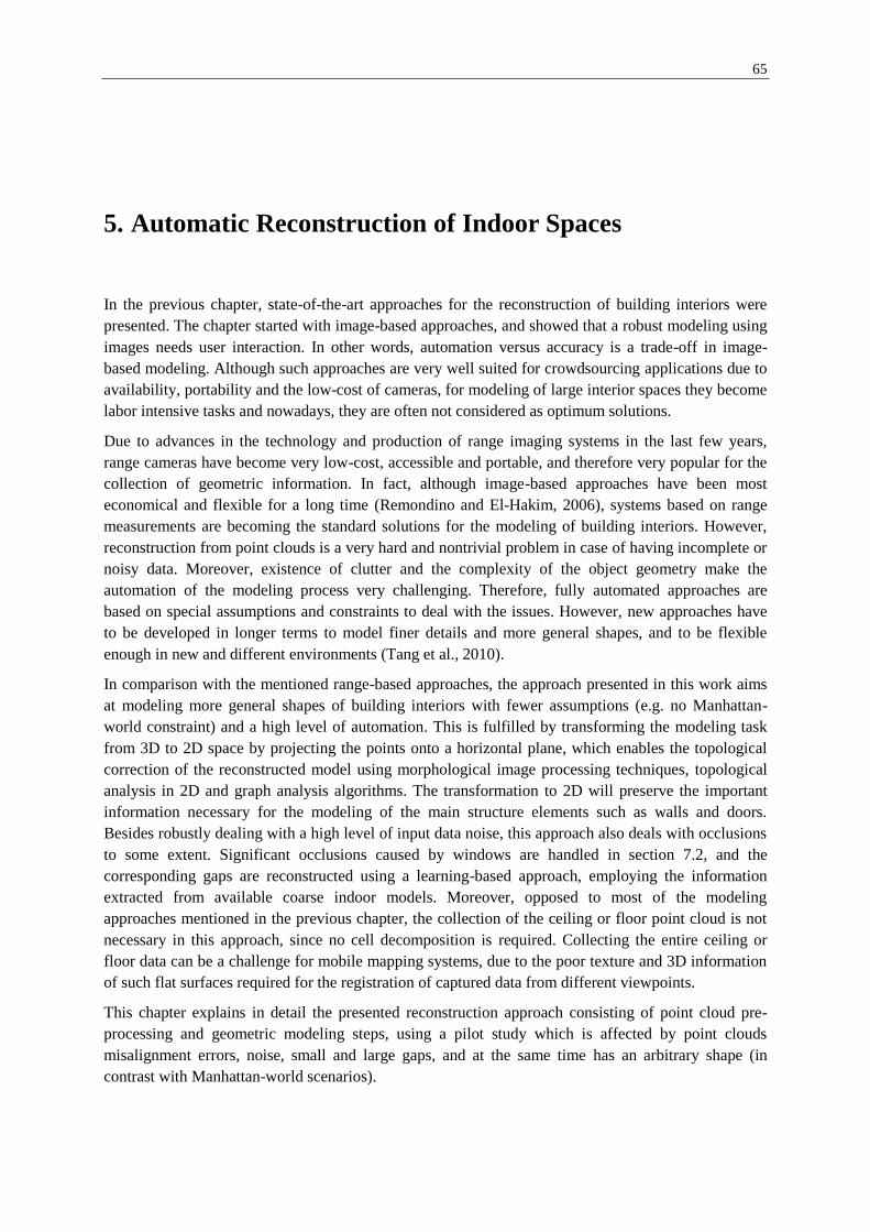
65
5. Automatic Reconstruction of Indoor Spaces
In the previous chapter, state-of-the-art approaches for the reconstruction of building interiors were
presented. The chapter started with image-based approaches, and showed that a robust modeling using
images needs user interaction. In other words, automation versus accuracy is a trade-off in image-
based modeling. Although such approaches are very well suited for crowdsourcing applications due to
availability, portability and the low-cost of cameras, for modeling of large interior spaces they become
labor intensive tasks and nowadays, they are often not considered as optimum solutions.
Due to advances in the technology and production of range imaging systems in the last few years,
range cameras have become very low-cost, accessible and portable, and therefore very popular for the
collection of geometric information. In fact, although image-based approaches have been most
economical and flexible for a long time (Remondino and El-Hakim, 2006), systems based on range
measurements are becoming the standard solutions for the modeling of building interiors. However,
reconstruction from point clouds is a very hard and nontrivial problem in case of having incomplete or
noisy data. Moreover, existence of clutter and the complexity of the object geometry make the
automation of the modeling process very challenging. Therefore, fully automated approaches are
based on special assumptions and constraints to deal with the issues. However, new approaches have
to be developed in longer terms to model finer details and more general shapes, and to be flexible
enough in new and different environments (Tang et al., 2010).
In comparison with the mentioned range-based approaches, the approach presented in this work aims
at modeling more general shapes of building interiors with fewer assumptions (e.g. no Manhattan-
world constraint) and a high level of automation. This is fulfilled by transforming the modeling task
from 3D to 2D space by projecting the points onto a horizontal plane, which enables the topological
correction of the reconstructed model using morphological image processing techniques, topological
analysis in 2D and graph analysis algorithms. The transformation to 2D will preserve the important
information necessary for the modeling of the main structure elements such as walls and doors.
Besides robustly dealing with a high level of input data noise, this approach also deals with occlusions
to some extent. Significant occlusions caused by windows are handled in section 7.2, and the
corresponding gaps are reconstructed using a learning-based approach, employing the information
extracted from available coarse indoor models. Moreover, opposed to most of the modeling
approaches mentioned in the previous chapter, the collection of the ceiling or floor point cloud is not
necessary in this approach, since no cell decomposition is required. Collecting the entire ceiling or
floor data can be a challenge for mobile mapping systems, due to the poor texture and 3D information
of such flat surfaces required for the registration of captured data from different viewpoints.
This chapter explains in detail the presented reconstruction approach consisting of point cloud pre-
processing and geometric modeling steps, using a pilot study which is affected by point clouds
misalignment errors, noise, small and large gaps, and at the same time has an arbitrary shape (in
contrast with Manhattan-world scenarios).

66 5. Automatic Reconstruction of Indoor Spaces
5.1. Point Cloud Pre-Processing
Pre-processing of the point cloud in this work includes outlier removal, downsampling, noise removal,
point cloud leveling and finally furniture and clutter removal.
5.1.1. Outlier Removal
In comparison with TLS, data collected by range cameras contain more noise as well as outliers due to
measurement errors. This affects the accuracy of further processing steps which include normal vector
estimation and estimation of walls. In the first pre-processing step, outliers are removed using a
statistical outlier removal filter implemented by the Point Cloud Library (PCL) (Rusu and Cousins,
2011). The filter works based on the distribution of the distances between the neighboring points. The
mean distance to K-nearest neighbors is computed at each point. Assuming a Gaussian distribution for
the distances, points corresponding to the mean distances outside of an interval defined by the global
mean and standard deviation are removed using a one-tailed normal distribution test. Figure 5.1
depicts the mean distances computed for an exemplary scene. In this example, outliers are removed
based on a 1 one-tailed normal distribution test:
2dist ~ N , P(dist ) 84.1% (5.1)
Figure 5.1 – Top: statistical outlier removal (9K out of 73K points are removed, equivalent to the 1 confidence
level normal distribution one-tailed test); Bottom: corresponding mean distance (in meters) to the 20 nearest
neighbors versus point index (mean: 0.011m, standard deviation: 0.005m).

5.1. Point Cloud Pre-Processing 67
5.1.2. Downsampling
Point clouds collected by range cameras are usually very dense. The number of points is increased
very fast soon after data acquisition starts; each range image frame captured by Kinect (for Xbox 360)
delivers 640 480 300K 3D points, or 1920 1080 2Mio points by Kinect V2. Reconstruction
programs therefore can face difficulties handling a large number of points collected from large spaces.
In order to efficiently manage the memory, as well as achieve a uniform point density, the registered
point cloud is downsampled by a voxel grid filter implemented by the PCL software library, in which
points are replaced by the centroid of the corresponding bounding voxel generated by an Octree data
structuring process (see figure 5.2). The voxel size can be set based on the overall noise of the
registered point cloud (e.g. 3-5cm in case of using Kinect), or for example the maximum allowed
tolerance specified by the adapted standard for building reconstruction (e.g. surface flatness tolerance
suggested by DIN 18202 standard).
Figure 5.2 – Voxel grid filtering: points inside
each voxel are replaced by the centroid of the
corresponding voxel (red points).
5.1.3. Noise Removal
Noise in the point cloud causes erroneous object fitting or feature extraction. Although the wall
estimation algorithm used in the following modeling process is capable of dealing with noise in the
point cloud to some extent, noise removal significantly improves the accuracy of feature detection in
modeling. The point cloud is smoothed using the moving least squares approximation algorithm,
originally introduced by Lancaster and Salkauskas (1981), and implemented by the PCL software
library. As described by Nealen (2004), the idea of the moving least squares algorithm is to start with a
weighted least squares surface estimator (a degree n polynomial) for an arbitrary fixed point, in
which weights are proportional to the neighboring points distance within a given radius. The point is
then moved over the entire parameter domain, where a weighted least squares fit is estimated for each
point individually, in order to estimate the overall surface. The global function f (x) is obtained from a
set local functions xf (x) that minimize the following cost function:
2
x i x i i
i I
f (x) f (x), x x f (x ) f min
(5.2)
in which is the weight function tending to zero at infinity distance. During the process, small holes
can be filled by resampling techniques, e.g. based on a higher order polynomial interpolation. This can
further remove the “double walls” artifacts caused by erroneous registration of multiple scans. Figure
5.3 depicts an example in which an overall noise of 34mm is reduced to 25mm by local plane fitting
using a moving least squares process within the search radius of 15cm.

68 5. Automatic Reconstruction of Indoor Spaces
Figure 5.3 – Before and after noise removal. In the cross section before the noise removal, the limited resolution
of Kinect disparity measurements is noticeable as a stripe pattern.
5.1.4. Leveling the Point Cloud
The resulting point cloud has to be leveled for the upcoming processing steps, i.e. generation of the
point height histogram and projection of points onto a horizontal plane. The leveling is performed by
the analysis of the point cloud normal vectors. Since most of the surfaces in man-made scenes are
aligned either horizontally or vertically, it is possible to cluster the normal vectors into two main
groups. Assuming the vertical axis of the point cloud’s local coordinate system is inclined less than
45° with respect to the vertical axis of the world coordinate system, the group of horizontal and
vertical surfaces can easily be distinguished, as they constitute a difference of 90°. The average of the
normal vectors corresponding to horizontal (or alternatively vertical) surface points is then used to find
the tilt, and thus level the point cloud. This procedure is an iterative process; in each step, after
leveling the point cloud based on the estimated tilt, the classification of horizontal and vertical surface
points is updated based on the new (recently transformed) normal vectors. Figure 5.4 depicts an
example of a normal vector histogram for a sample point cloud after leveling.
Figure 5.4 – Left: computed point normal vectors. Right: histogram of the inclination of the normal vectors with
respect to the vertical axis after leveling the point cloud.
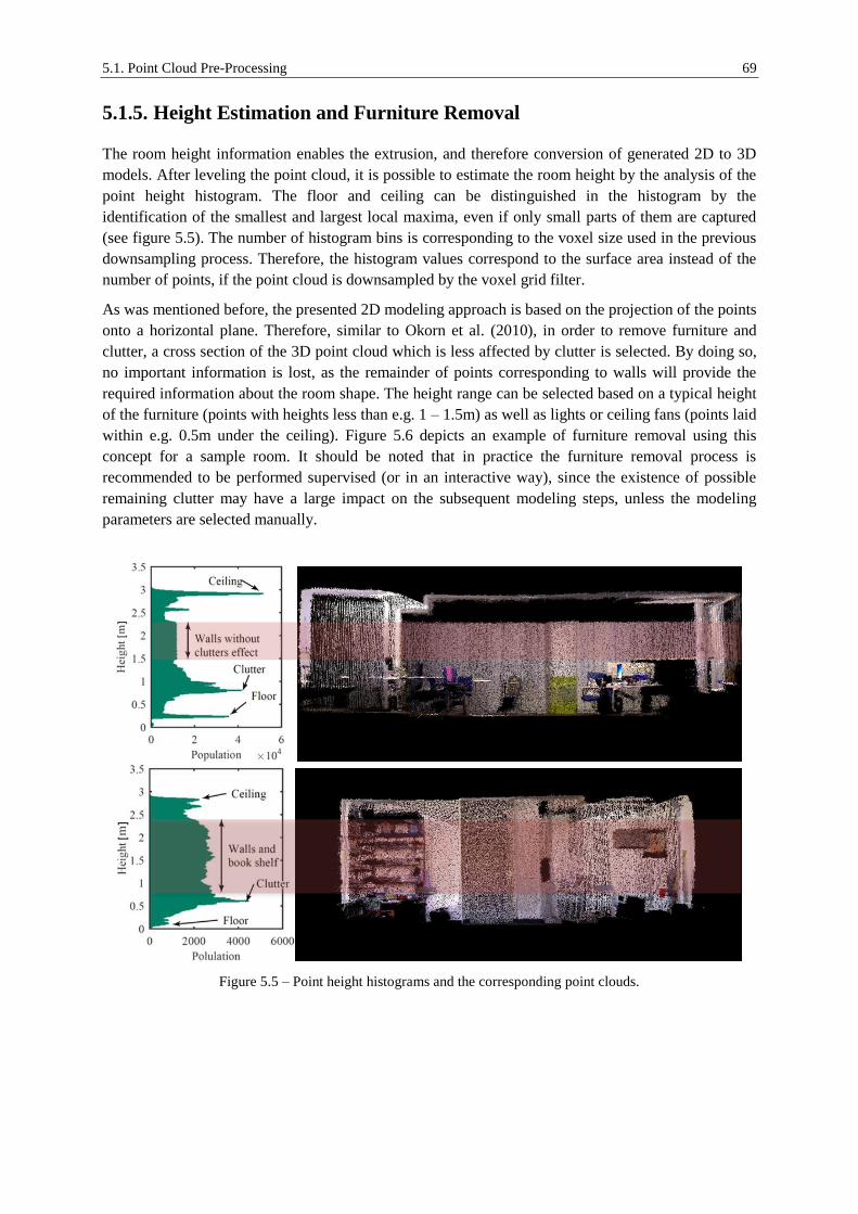
5.1. Point Cloud Pre-Processing 69
5.1.5. Height Estimation and Furniture Removal
The room height information enables the extrusion, and therefore conversion of generated 2D to 3D
models. After leveling the point cloud, it is possible to estimate the room height by the analysis of the
point height histogram. The floor and ceiling can be distinguished in the histogram by the
identification of the smallest and largest local maxima, even if only small parts of them are captured
(see figure 5.5). The number of histogram bins is corresponding to the voxel size used in the previous
downsampling process. Therefore, the histogram values correspond to the surface area instead of the
number of points, if the point cloud is downsampled by the voxel grid filter.
As was mentioned before, the presented 2D modeling approach is based on the projection of the points
onto a horizontal plane. Therefore, similar to Okorn et al. (2010), in order to remove furniture and
clutter, a cross section of the 3D point cloud which is less affected by clutter is selected. By doing so,
no important information is lost, as the remainder of points corresponding to walls will provide the
required information about the room shape. The height range can be selected based on a typical height
of the furniture (points with heights less than e.g. 1 – 1.5m) as well as lights or ceiling fans (points laid
within e.g. 0.5m under the ceiling). Figure 5.6 depicts an example of furniture removal using this
concept for a sample room. It should be noted that in practice the furniture removal process is
recommended to be performed supervised (or in an interactive way), since the existence of possible
remaining clutter may have a large impact on the subsequent modeling steps, unless the modeling
parameters are selected manually.
Figure 5.5 – Point height histograms and the corresponding point clouds.

70 5. Automatic Reconstruction of Indoor Spaces
Figure 5.6 – Furniture removal based on a selective height filter. The top view of the filtered points (bottom-right
figure) delivers information about the room shape geometry.
5.2. Reconstruction of Geometric Models
The mentioned pre-processing steps enable the 2D geometric modeling of individual rooms based on
the orthographic (top-down) projection of resulting points onto the ground plane. Further modeling
steps extract lines corresponding to walls and main structure elements within the 2D orthographic
projected image and apply topological corrections.
5.2.1. Generation of Orthographic Projected Image
For the orthographic projection of points onto a horizontal plane (e.g. the ground plane), one can
simply neglect the point heights in the corresponding leveled point cloud, generate a 2D grid with a
predefined resolution and finally count the number of the points falling inside each grid cell.
Alternatively, similar to Okorn et al. (2010), this task can be fulfilled more efficiently by counting the
number of voxels above each 2D grid cell (the voxel grid has been already generated in the previous
downsampling pre-processing step). The grid size has a direct effect on the accuracy of the final
model, and therefore shall not be larger than the overall noise of the point cloud. The 2D grayscale
orthographic projected image is computed based on the number of points inside (or alternatively the
number of voxels above) the grid cells, using the following equation:
max
N(m, n)I G
N(m,n)
(5.3)
in which, I(m,n) is the gray value of the grid cell at row m and column n , N(m,n) is the number
of the points inside (or voxels above) the corresponding cell, maxN is the maximum value of N(m,n)
over the entire grid and G is the number of gray levels.

5.2. Reconstruction of Geometric Models 71
5.2.2. Binarization
This study only deals with modeling of flat surfaces; curved surfaces are not considered here. The
modeling of such surfaces is fulfilled by the extraction of lines in the orthographic projected image
corresponding to walls and main structure elements in 3D, using the Hough transform. Line extraction
algorithms use binary images as input; therefore, the grayscale projected image has to be converted to
a binary image. The binarization process may also remove the noise and clutter remaining from the
pre-processing step, by choosing a correct threshold that removes lower gray values. The threshold can
be chosen based on probabilistic approaches, having the average and standard deviation of the gray
values. For example, assuming a Gaussian distribution for the gray values, a 95% confidence interval
is defined by pixels having gray values larger than the threshold TI equals to 1.65 .
2I ~ N , P( 1.65 I) 95% (5.4)
A more perceptible threshold can be defined based on the ratio between the maximum possible height
of remaining clutter and the height range of the selective height filter (equation (5.5)). The threshold
gives the optimum results in case of having a uniform distribution of points, which is already fulfilled
in the downsampling processing step.
noiseT
filter
HI G 1
H
(5.5)
In this equation, TI is the grayscale intensity threshold, noiseH is the maximum possible height of
remaining clutter, filterH is the height range of the selective height filter and G is the number of gray
levels. Figure 5.7 depicts the grayscale and binary orthographic projected images for an exemplary
dataset. In this example, the binarization threshold is computed from equation (5.5), assuming noiseH
being 5% of filterH .
Figure 5.7 – Grayscale and binary orthographic projected image for a sample point cloud.
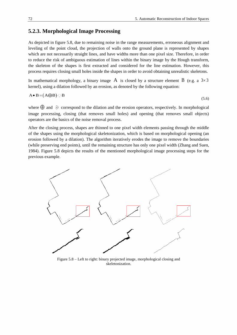
72 5. Automatic Reconstruction of Indoor Spaces
5.2.3. Morphological Image Processing
As depicted in figure 5.8, due to remaining noise in the range measurements, erroneous alignment and
leveling of the point cloud, the projection of walls onto the ground plane is represented by shapes
which are not necessarily straight lines, and have widths more than one pixel size. Therefore, in order
to reduce the risk of ambiguous estimation of lines within the binary image by the Hough transform,
the skeleton of the shapes is first extracted and considered for the line estimation. However, this
process requires closing small holes inside the shapes in order to avoid obtaining unrealistic skeletons.
In mathematical morphology, a binary image A is closed by a structure element B (e.g. a 3 3
kernel), using a dilation followed by an erosion, as denoted by the following equation:
A B A B B ⊕ (5.6)
where ⊕ and correspond to the dilation and the erosion operators, respectively. In morphological
image processing, closing (that removes small holes) and opening (that removes small objects)
operators are the basics of the noise removal process.
After the closing process, shapes are thinned to one pixel width elements passing through the middle
of the shapes using the morphological skeletonization, which is based on morphological opening (an
erosion followed by a dilation). The algorithm iteratively erodes the image to remove the boundaries
(while preserving end points), until the remaining structure has only one pixel width (Zhang and Suen,
1984). Figure 5.8 depicts the results of the mentioned morphological image processing steps for the
previous example.
Figure 5.8 – Left to right: binary projected image, morphological closing and
skeletonization.

5.2. Reconstruction of Geometric Models 73
5.2.4. Estimation of the Lines Representing the Walls in 2D
5.2.4.1. Line Extraction
The skeletonized image is appropriate for the extraction of straight line by means of the Hough
transform (Duda and Hart, 1972; Hough, 1962). The idea of the Hough transform is to find all
potential lines passing through each point, and select the candidates based on a voting procedure
carried out in a parameter space. This work uses a variant of the Hough transform called progressive
probabilistic Hough Transform (Matas et al., 2000), implemented by the OpenCV free software library
(Bradski, 2000). This variant is an optimization to the standard Hough transform in speed and
performance, by minimizing the number of points used in the voting process, while maintaining false
positive and false negatives detection rates at the same level of the standard Hough transform. More
details are provided in appendix D.
In the Hough transform process, parameters such as minimum allowed number of votes, minimum line
length and maximum allowed line gap between points on the same line can be set. However, the
parameters have to be suitable enough, so that small structures are not generalized during the line
extraction process. Figure 5.9 depicts an example, in which the Hough lines are extracted from the
skeletonized image in the previous example. In this example, parameters are selected as follows:
minimum votes of 15 pixels (equivalent to 15cm) on a line, minimum line length of 15 pixels and
maximum allowed line gap of 20 pixels (equivalent to 20cm). Although such kind of parameter
selection results in the extraction of multiple smaller line segments for each wall, it will preserve
almost all significant details and avoids the generalization. The effect of parameter selection on
modeling results, as well as the stability of the selected parameters from one example to another is
presented in the next chapter.
Figure 5.9 – Extraction of Hough line segments in a skeletonized image.
5.2.4.2. Clustering and Averaging the Line Segments
After the line extraction process, multiple smaller line segments corresponding to each wall have to be
identified and averaged. The suggested identification process consists of three hierarchial clustering
steps, in which line segments are grouped based on their orientation, distance to the centroid of the
image and connectivity, respectively.
The first clustering step groups the line segments based on their orientation. Since the modeling
approach is not limited to Manhattan-world scenarios, it takes into account all possible orientations

74 5. Automatic Reconstruction of Indoor Spaces
distinguished by a small threshold (angular resolution of the model). The threshold, however, shall be
able to tolerate the noise in the orientation of the extracted line segments. Various solutions are
proposed for clustering; here the K-means algorithm suggested by Lloyd (1982) is used, which is the
most common in the computer science community. The algorithm groups n observations
1 2 nx , x , , x into K sets 1 2 KS , S , , S , so that the sum of the squared Euclidean distances
between the observations and the nearest cluster centroid (mean) is minimized:
i
K2
i
i 1 x S
x x min
(5.7)
The solution to the abovementioned equation is an iterative refinement process, in which two steps are
repeatedly performed after each other. In the first step, each observation is assigned to the
corresponding cluster with the smallest distance to its mean, so that the equation is satisfied. In the
next step, a new centroid is computed and assigned to each cluster. The process is iterated until no
more change is observed. In this approach, the initial set of centroids is usually selected randomly, and
is updated during the process.
The number of clusters has to be pre-defined for the clustering algorithms. Estimation of the optimum
number of clusters depends on the noise, distribution, as well as the resolution of the data, and
therefore might be sometimes an ambiguous problem. However, in general there are different
criterions that suggest the optimum number of clusters based on statistical approaches, many of which
are summarized in Kodinariya and Makwana (2013). For instance, using the “elbow methods”
(Thorndike, 1953), one can start the algorithm with one cluster, and increase the number of clusters
until no more meaningful cluster is found (the corresponding chart has an elbow shape). This can be
measured by the sum of the squared errors within the groups, or by the percentage of the explained
variance (a goodness of fit index, equation (5.8)). In the previous example, as depicted in figure 5.10,
having more than 3 clusters does not reduce the sum of squared errors within the clusters dramatically,
nor does it increase the explained variance significantly. In this example, having 2 clusters results in a
Manhattan-world scenario (97.5% percentage of explained variance). However, adding the 3rd
cluster,
takes the line segment with 70° orientation (highlighted in the figure) into account as well (99.5%
percentage of explained variance). The percentage of explained variance is high in both cases, and
both results are acceptable, depending on the required details and the modeling accuracy.
k
K2
k k
k 1
NK2
k,i
k 1 i 1
1N (x x)
K 1Between groups varianceExplained variance
Total variance 1(x x)
N 1
(5.8)
In this equation, kx is the centroid (mean) of the kth cluster, x is the grand mean, kN is the number
of observations in the kth cluster, K is the total number of clusters, k ,ix is the i
th observation in the k
th
cluster and N is the total number of observations. The between groups variance measures the
variation of group means with respect to the grand mean; increasing the number of clusters, makes the
between groups variance closer to the total variance. The explained variance in fact measures how
good all the variances are explained, i.e. how good the predicted values fit the outcomes, in
multivariate statistics.
In the next step, using a similar clustering process, line segments within each orientation cluster are
grouped based on their distance to the origin of the projected image, so that the parallel line segments
are distinguished (see figure 5.11). The distance threshold will be set automatically based on the

5.2. Reconstruction of Geometric Models 75
number of estimated clusters, or alternatively one can set it to a fix value depending on the modeling
accuracy.
Line segments on the same direction are not necessarily adjacent; this can be caused by the situation
where simply walls are nonadjacent, or due to occlusions in the point cloud that represents the same
wall in multiple segments. The two cases are distinguished in the presented approach based on a
tolerance according to the maximum expected size of occlusions in the data (except for the large
occlusions caused by doors or windows). Therefore, a further clustering process is required to group
(distinguish) the line segments laid on the same direction, but separated with a distance larger than the
threshold. The threshold is set to 0.5m in the example depicted in figure 5.11.
Figure 5.10 – Clustering the orientation of lines by the K-means algorithm.
0
20
40
60
80
100
120
140
0 5 10 15 20 25 30 35 40 45
Ori
enta
tio
ns
[deg
]
Index of sorted line orientations
96342
2282 681 588
0
20000
40000
60000
80000
100000
120000
1 2 3 4
Sum
of
squar
ed e
rro
rs w
ithin
the
clust
ers
[deg
2]
Number of clusters
96.5
97.0
97.5
98.0
98.5
99.0
99.5
100.0
2 3 4
Per
centa
ge
of
exp
lain
ed
var
iance
(%
)
Number of clusters

76 5. Automatic Reconstruction of Indoor Spaces
Figure 5.11 – Clustering the line segments (groups are distinguished by colors). Left to right: clustering based on
the orientations, distinguishing parallel line segments laid on the same direction and finally distinguishing
nonadjacent line segments laid on the same direction.
Figure 5.12 – Averaging the line segments corresponding to individual walls.
After the assignment of the line segments to individual wall groups, they can be averaged within the
groups. Averaging is realized by sampling the line segments (converting them to points), calculating
the linear regression passing through the samples and cropping the resulting line according to the start
and end points in the samples. Figure 5.12 depicts the averaging results for the same example.
5.2.5. Topological Corrections
Due to the erroneous point cloud alignment and the remaining noise as well as occlusions in the
projected image of walls, the resulting model depicted in figure 5.12 does not necessarily fulfill a
topologically correct geometry. The line segments do not meet each other at the end points. Moreover,
the angles between the adjacent line segments (walls) are sometimes clearly inaccurate. Therefore, the
following topological corrections are proposed for a robust reconstruction from noisy or occluded data.
5.2.5.1. Refinement of the Orientation of Line Segments
Although the proposed approach is not limited to Manhattan-world scenarios, still in many man-made
scenes walls can be recognized that are aligned parallel or perpendicular to each other. Therefore, the
proposed reconstruction approach suggests the detection of such cases, and enforcing perpendicularity
or parallelism to the line segments whose orientations make a difference of 0 or 90 degrees within a
tolerance. This will correct most of the small orientation errors. For this purpose, the line segments are
first clustered based on their orientation, similar to the algorithm mentioned in section 5.2.4.2, and
with the same estimated number of clusters. An analysis of the angular differences is then performed

5.2. Reconstruction of Geometric Models 77
on the cluster means (rather than individual line segments). The orientation of the line segments within
the same groups are equated to the corresponding group mean, in order to fulfill parallelism. In the
next step, cluster means making a difference of 90 degrees within a tolerance are identified, and are
similarly corrected in order to make an exact difference of 90 degrees (see equations (5.9)). The
tolerance is defined by the maximum standard deviation within the groups, or the angular resolution of
the model. The cluster members are then updated by the same correction applied to their
corresponding mean. Figure 5.13 depicts the results of this process for the same example.
2 1
2 1
2 (corrected) 2
1 (corrected) 1
(parallelcase)2
90(perpendicular case)
2
(5.9)
Figure 5.13 – Top: overlaying the model states before (red) and after (green) the angular refinement (left); results
after the angular refinement (right). Bottom: orientations before (red) and after (green) the angular refinement,
annotated by the standard deviations corresponding to each of the 3 clusters.
1 2 3 4 5 6 7 8 9 10 11 12 13 14
Before 57.9 59.5 59.9 61.4 62.8 65.4 109.4 136.1 148.1 149.6 149.9 150.2 151.7 153.4
After 59.8 59.8 59.8 59.8 59.8 59.8 109.4 149.8 149.8 149.8 149.8 149.8 149.8 149.8
0.0
20.0
40.0
60.0
80.0
100.0
120.0
140.0
160.0
180.0
Ori
enta
tio
ns
[deg
]
78 5. Automatic Reconstruction of Indoor Spaces
5.2.5.2. Extension and Trimming
In this step, the intersections of line segments are analyzed. As depicted in figure 5.13, line segments
do not meet each other at the intersection points (walls junctures). This issue can be resolved by the
extension or trimming of the line segments within a given threshold. Similar to the last clustering step
in section 5.2.4.2, the threshold can be set to the maximum expected size of occlusions in the data
(except for the large occlusions caused by doors or windows). Figure 5.14 depicts the possible errors,
which may occur in the intersection of two line segments.
The extension and trimming is performed firstly in the original direction for all the line segments, in
order to find valid intersections (figure 5.14 a-c). In the next step, possible existing free end points are
detected, and line segments are additionally extended in the perpendicular direction at these points, in
order to be connected to available structure elements (figure 5.14 d). The latter step can be more
general in order to include the case depicted in figure 5.14 (e), if the perpendicular extension or
trimming is performed continuously, while the line segment is being extended gradually along its
original direction, until the first intersection is found. The proposed algorithm results in a model
whose components are connected, and at the same time, the connections fulfill a correct topology. It
should be mentioned that for the simplification of the analysis (e.g. finding free end points, etc.), and
also for further usages mentioned in chapter 7, the model is converted to a graph whose edges and
nodes are the line segments and the corresponding end points. Figure 5.15 depicts the result of the
presented algorithm applied to the output of the previous example. In this example, the maximum
expected size of occlusions (threshold for extension and trimming) is assumed to be 0.5m. More
experimental results are presented in the next chapter.
As it can be seen in figure 5.15, the extension process in the original direction may generate additional
invalid line segments (the extension in the perpendicular direction may not cause this problem, as it
connects the free end points to the available structure elements). Invalid line segments are detected by
analyzing the overlap of the line extensions with the range data. In more detail, a line segment is
marked as invalid if it is made by an extension in the original direction, and at the same time, has an
insufficient (e.g. less than 50%) overlap with the point cloud resulting from the pre-processing step. It
should be mentioned that for a valid overlap analysis, the angular refinement applied in the previous
step has to be taken into account, which means, inverse corrections regarding the equations (5.9) has
to be applied temporarily for this analysis step (see figure 5.16). Based on this approach, invalid line
segments are detected and removed in the presented example, as depicted in figure 5.17. This results
in the final 2D model fulfilling a topologically correct geometry.
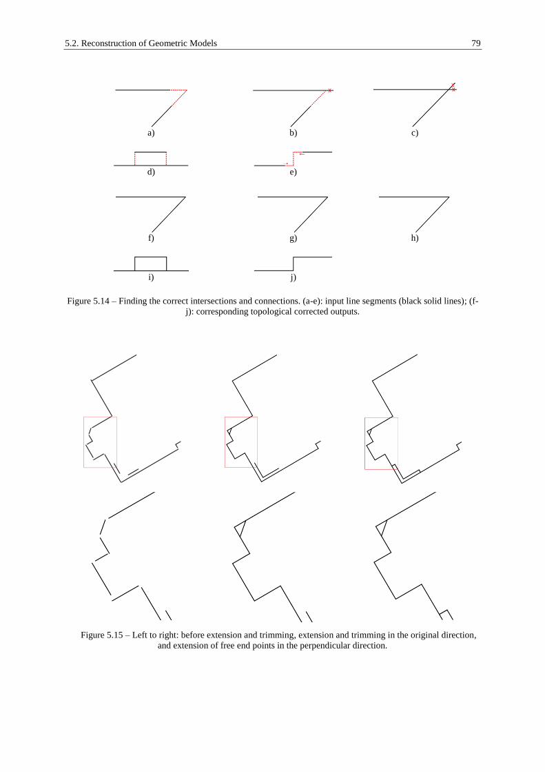
5.2. Reconstruction of Geometric Models 79
a)
b)
c)
d)
e)
f)
g)
h)
i)
j)
Figure 5.14 – Finding the correct intersections and connections. (a-e): input line segments (black solid lines); (f-
j): corresponding topological corrected outputs.
Figure 5.15 – Left to right: before extension and trimming, extension and trimming in the original direction,
and extension of free end points in the perpendicular direction.

80 5. Automatic Reconstruction of Indoor Spaces
Figure 5.16 – Analyzing the overlap of the line segments with the range data (the overlap percentage is annotated
for the zoomed-in parts).
Figure 5.17 – Left: line segments are marked as invalid (red), if they are made by an extension in the original
direction, and at the same time, have less than 50% overlap with the range data; Right: the topologically correct
2D model is generated after removing the invalid line segments.

5.2. Reconstruction of Geometric Models 81
5.2.6. 2D to 3D Conversion of Reconstructed Models
In the last step the reconstructed 2D model is converted to 3D by extruding the line segments in the
vertical direction, using the height of the room computed in section 0. Figure 5.18 depicts the 3D
model generated from the 2D model of the previous example, by an extrusion of 2.65m.
Evaluation of the reconstruction approach in different scenarios, accuracy analysis of the reconstructed
models, reconstruction of gaps caused by large occlusions such as doors and windows, and finally
fusion of the reconstructed 3D models with available coarse indoor models are presented in the next
chapters.
Figure 5.18 – Final 3D model resulting from the extrusion of the corresponding 2D model.

82
6. Experimental Results and Analysis
This chapter evaluates the performance and accuracy of the developed system for the automatic
reconstruction of indoor spaces, explained in the previous chapter. It starts with the system calibration
and accuracy analysis of the range measurements by Kinect, and then continues with the performance
evaluation of the modeling approach in different scenarios.
6.1. Kinect System Calibration and Accuracy Analysis
6.1.1. System Calibration
As already mentioned in section 3.1.2, for colorizing the point clouds derived by the Kinect range
measurement system, as well as making use of the information provided by the RGB camera for the
alignment of the point clouds, it is necessary to perform a pixel-to-pixel registration of the RGB and
depth values. The registration is possible having the system calibration parameters available.
The system calibration is composed of the optical calibration of the IR and RGB cameras together
with the estimation of their relative orientation, using a bundle block adjustment. In order to ensure the
maximum accuracy, a planar test-field with no control point was captured from eight positions by the
IR and RGB cameras synchronously, using a similar configuration recommended by Wester-
Ebbinghaus (1981) and Luhmann et al. (2014). In this configuration, corresponding images are taken
perpendicularly and obliquely with a relative orientation of 90° around the optical axis, as depicted in
figure 6.1. Measured image coordinates together with approximate object coordinates are processed
within a bundle adjustment in order to estimate the interior and exterior orientation parameters for
both cameras. In the test-field calibration, it is suggested to define the datum using an unconstrained
technique, e.g. using a free net bundle adjustment, in order to prevent the effect of possible
inconsistencies in the datum information on the estimated unknown parameters.
The target points in the test-field are usually circular, in order to provide a radial symmetry. Circular
targets are very suitable for the manual and automatic measurements and are invariant to rotation and
scale. Luhmann et al. (2014) suggest a minimum diameter of the targets to be at least 5 pixels in the
taken images. Moreover, considering the fact that the distortion parameters are dependent on the
object distance (Dold, 1997), the distance to the test-field shall be chosen as similar as possible to the
object distances in real applications. Therefore, the actual size of the targets can be computed having
the scale of the images and the pixel size. In this study, the approximate object distance in the practical
measurements is about 3m, which results in 5mm Ground Sampling Distance (GSD). Therefore, the
target diameter shall be at least 25mm. Centers of the targets are automatically detected based on
pattern matching techniques used by the Australis software (Photometrix) which is employed here for
the performance of the calibration task.
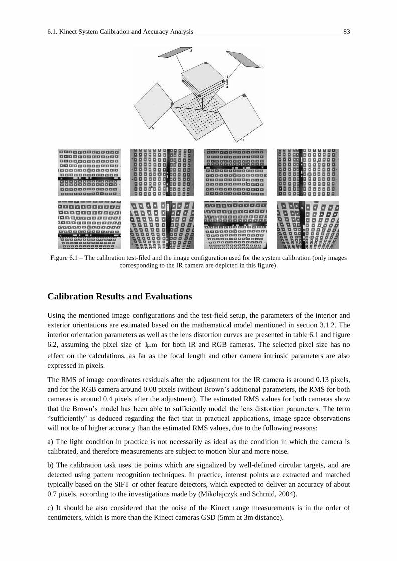
6.1. Kinect System Calibration and Accuracy Analysis 83
Figure 6.1 – The calibration test-filed and the image configuration used for the system calibration (only images
corresponding to the IR camera are depicted in this figure).
Calibration Results and Evaluations
Using the mentioned image configurations and the test-field setup, the parameters of the interior and
exterior orientations are estimated based on the mathematical model mentioned in section 3.1.2. The
interior orientation parameters as well as the lens distortion curves are presented in table 6.1 and figure
6.2, assuming the pixel size of 1 m for both IR and RGB cameras. The selected pixel size has no
effect on the calculations, as far as the focal length and other camera intrinsic parameters are also
expressed in pixels.
The RMS of image coordinates residuals after the adjustment for the IR camera is around 0.13 pixels,
and for the RGB camera around 0.08 pixels (without Brown’s additional parameters, the RMS for both
cameras is around 0.4 pixels after the adjustment). The estimated RMS values for both cameras show
that the Brown’s model has been able to sufficiently model the lens distortion parameters. The term
“sufficiently” is deduced regarding the fact that in practical applications, image space observations
will not be of higher accuracy than the estimated RMS values, due to the following reasons:
a) The light condition in practice is not necessarily as ideal as the condition in which the camera is
calibrated, and therefore measurements are subject to motion blur and more noise.
b) The calibration task uses tie points which are signalized by well-defined circular targets, and are
detected using pattern recognition techniques. In practice, interest points are extracted and matched
typically based on the SIFT or other feature detectors, which expected to deliver an accuracy of about
0.7 pixels, according to the investigations made by (Mikolajczyk and Schmid, 2004).
c) It should be also considered that the noise of the Kinect range measurements is in the order of
centimeters, which is more than the Kinect cameras GSD (5mm at 3m distance).

84 6. Experimental Results and Analysis
Therefore regarding the mentioned reason, in applications using Kinect, an accuracy of around 0.5
pixels for image space observations is already sufficient. For this reason, there is no need to use more
accurate and advanced calibration models, e.g. those introduced by Tang et al. (2012), as mentioned in
section 3.1.2.
The relative orientation of the IR and RGB sensors is computed using the exterior orientation of the
cameras estimated in the adjustment, by averaging the transformation matrices estimated at each
camera position (i.e. averaging the IR RGBH matrix in equation (3.14)). The resulting relative
orientation parameters are presented in table 6.2.
It should be mentioned that the actual size of the IR sensor is 1280×1024 pixels, but due to the
bandwidth limitation of the USB connection, the output of the IR camera as well as the disparity
image are cropped to 640×480 pixels. Moreover, the disparity image has a shift of 4 pixels with
respect to the IR image in the x direction, due to the application of a correlation window (9×9 pixels)
in the calculation of disparity values (Khoshelham and Elberink, 2012). This value has to be
considered in calculations in which RGB values have to be assigned to depth values.
IR Camera RGB Camera
Parameter Adjusted value Std. Dev. Adjusted value Std. Dev.
Focal length c 585.7 [pix] 6.6e-001 [pix] 521.9 [pix] 6.0e-001 [pix]
Principal point offset px
0.6 [pix] 1.2e-001 [pix] -0.3 [pix] 1.1e-001 [pix]
py
-9.1 [pix] 3.5e-001 [pix] -16.5 [pix] 3.2e-001 [pix]
Radial lens
distortion parameters
1K 3.75303e-001 6.7e-003 -6.63541e-001 7.401e-003
2K -3.94502e+000 8.612e-002 6.59073e+000 1.082e-001
3K 1.37589e+001 3.608e-001 -2.02217e+001 5.147e-001
Decentering lens
distortion parameters
1P 2.60056e-004 1.084e-004 5.79941e-004 1.191e-004
2P 2.51454e-003 1.041e-004 -1.13229e-003 1.141e-004
Image coordinates residuals
(RMS) 0.13 [pix] N. A. 0.08 [pix] N. A.
Table 6.1 – Adjusted parameters of the IR and RGB cameras, assuming a pixel size of 1 m for both sensors.
Radial and decentering distortion parameters are computed assuming the measurement unit is millimeters.
Parameter Value Std. Dev.
X [mm] 23.9 1.4
Y [mm] 1.2 1.4
Z [mm] 0.7 2.3
Heading [deg] -0.2 1.4
Elevation [deg] -0.1 1.5
Roll [deg] 0.1 0.6
Table 6.2 – Relative orientation of the RGB camera with respect to the IR local camera coordinate system. Only
X is significant.

6.1. Kinect System Calibration and Accuracy Analysis 85
Figure 6.2 – Radial and tangential distortion curves for the IR (top) and RGB (bottom) cameras, assuming a
pixel size of 1 m for both sensors.
6.1.2. Accuracy of Kinect Range Measurements
As already mentioned, Kinect range data is computed from disparity measurements. The IR laser
beamer projects a semi-random (but known) speckle pattern on the object surface. The reflection of
the pattern is then recorded by the IR camera in 30 frames per second. The disparity measurements are
realized by the cross-correlation of the reference and collected patterns. In practice, the accuracy of the
measurements is affected by factors such as:
Existence of other sources of light: Any interference in the infrared component (e.g. existence of sun
light) can significantly disturb the pattern matching, and therefore reduces the quality of range
measurements (figure 6.3).
Object properties: Smooth surfaces such as mirrors result in the specular diffusion of the incident
light, and therefore no speckle pattern can be observed by the IR camera. Moreover, black objects can
partly to entirely absorb the incident laser pattern.
Figure 6.3 – Range measurement with (left) and without (right) the existence of the sun light.

86 6. Experimental Results and Analysis
Object distance: Increasing the object distance increases the GSD of the IR camera pixels; this
consequently reduces the sensitivity of the detection of surface variations.
Moreover, since Kinect is a triangulation system with parallel axes and a fix baseline (the distance
between IR camera and laser projector is approximately 7.5cm), the precision of the range
measurements is decreased by increasing the object distance. In this case, as also mentioned by Menna
et al. (2011), the theoretical precision (as a measure of uncertainty) of the 3D coordinates of an object
point located on the xy plane (normal to the optical axis of the sensors at the distance H) is related to
the object distance by the following relationships (see figure 3.3):
XY
H
c (6.1)
2
H d
b c HH
d b c
(6.2)
where is the pixel size of the IR camera, c is the focal length of the IR camera, b is the baseline
between the IR camera and the laser projector and d is the precision of the measured parallax
(disparity). Equation (6.2) shows a quadratic relationship between object distance and the range
measurements precision (internal accuracy). Similar to Khoshelham and Elberink (2012), this effect is
verified by a plane fitting test for the data captured from a planar object located at different distances,
perpendicular to the optical axis of the sensor (see figure 6.4). In this test, the RMS of fitting errors is
considered as a measure for the precision of the range data at the measured distance, as the points have
approximately the same perpendicular distance to the sensor. However for this test, points are selected
from an area in the middle part of range images. The reason for this selection is the existence of a
radial error pattern in the range images, whose intensity is increased towards the image corners. The
intensity of this error pattern also depends on the object distance, which may imply the unmodeled
radial lens distortion of the IR camera as well as the IR laser projector in the image matching
algorithm. The reason for this assumption is that the radial lens distortion causes shifts within the
image plane that affects the computation of disparity values and therefore the range measurement
accuracies as a function of the squared object distance. The effect is visualized in figure 6.5 that
depicts the noise of range images acquired from a planar object (filling the whole image frame) at
three different distances. The figure further depicts the existence of a vertical stripe pattern. The
number of vertical stripes varies at different distances, which seems to be related to the image
matching algorithm used by Kinect (more details cannot be provided, since the algorithm used by
PrimeSense technology is not disclosed).
Figure 6.4 – RMS of plane fitting residuals at the central part of the range image at different distances with a
second order polynomial fit.

6.1. Kinect System Calibration and Accuracy Analysis 87
Figure 6.5 – Left to right: noise of the range data throughout the whole image format, at 1m (RMS: 3mm), 1.8m
(RMS: 7mm) and 2.6m (RMS: 15mm) distance, respectively.
Figure 6.6 – Depth resolution of Kinect at different object distances with a second order polynomial fit.
Equation (6.2) can also explain the depth quantization effect observed in Kinect range measurements.
As mentioned before, according to Khoshelham and Elberink (2012), Kinect disparity measurements
are stored as 11 bit integers, where 1 bit is reserved for marking the pixels for which no measurement
is available. Therefore, disparity values are quantified based on 1024 levels. The depth resolution is
then defined as the difference between the depth values corresponding to two consecutive disparity
levels, which is proportional to the squared object distance H ( d , b and c are constant). This effect is
visualized for the sample point cloud depicted in figure 6.6. The figure shows that at the distance of
5.5m, one can expect a depth resolution (quantization) of more than 8cm.
Side view Corresponding color image

88 6. Experimental Results and Analysis
6.2. Evaluation of the Reconstruction Approach
In chapter 5, an approach for the automatic reconstruction of indoor spaces was introduced, and
different steps were presented using an exemplary case study. This section aims at the evaluation of
the reconstruction approach by the assessment of the robustness and efficiency of the approach in
different scenarios. The robustness and efficiency can be described by the stability of the selected
parameters in different noise levels and different room shapes. It further continues with the accuracy
analysis of the reconstructed models, based on a comparison between resulting 3D models and the
point clouds collected by a highly accurate TLS.
6.2.1. Parameter Selection in Different Scenarios
The proposed reconstruction approach consists of several parameters and thresholds which have to be
set in different processing steps, from the point cloud pre-processing to final topological corrections.
Criterions for parameter selection were suggested during the presentation of the modeling process in
the previous chapter, which are summarized in table 6.3. The criteria mainly provide correct values for
the parameters; however, for some processing steps supervision (the user verification) might be
required, such as the furniture removal (section 0) and the binarization of the orthographic projected
images (section 5.2.2).
In the furniture removal process, although a selective height filter (see table 6.3) typically delivers
satisfactory results, the effect of remaining clutter cannot be compensated by the modeling process, if
a detailed modeling of indoor spaces is demanded. The remaining clutter can be removed manually,
however, it can be very time consuming and tedious in case of dealing with a large number of rooms.
Alternatively, one can remove the effect of the remaining clutter by setting a suitable threshold in the
binarization process. In this study, according to equation (5.5), the binarization threshold is defined
based on the ratio between the maximum possible height of remaining clutter and the height range of
the selective height filter. Figure 6.7 depicts an example, in which the effect of remaining clutter is
removed by changing the binarization threshold as a function of noise filterH / H . Selection of a
correct value for is verified by the user; the parameter is increased until no more clutter is observed
by the user. Moreover, as the core of the modeling process, the Hough transform parameters should be
noticed and selected correctly. The parameters are expressed as the minimum allowed number of votes
( 1 ), the minimum allowed length of the line ( 2 ) and the maximum allowed gap ( 3 ). In this
example, the parameters are set to the same values used by the pilot study in the previous chapter.

6.2. Evaluation of the Reconstruction Approach 89
Processing step Parameter/Threshold Selection criterion
Outlier removal Mean distance to K-
nearest neighbors Standard deviation of distances (1 or 2 normality test)
Downsampling Voxel size Noise of the point cloud (e.g. 3-5cm in case of using
Kinect) or flatness tolerance based on DIN 18202
Noise removal
Search radius and the
degree of the local
fitting polynomial
Noise of the point cloud (for Kinect, a local plane fitting
with a radius search of 10-15cm delivered the optimum
results in all of the examples)
Leveling the point
cloud
Clustering threshold
for finding horizontal
or vertical surface
points
45° tolerance, which is almost always fulfilled
Furniture removal Height range of the
selective height filter
Typically a range of [1.5m, 2.5m] gives the optimum
results. Supervision is recommended due to the possible
existence of large clutter such as plants, etc.
Generation of the
orthographic
projected image
Grid size Noise of the point cloud (e.g. 3-5cm in case of using
Kinect)
Binarization Grayscale intensity
threshold
Based on the ratio between the maximum possible height
of remaining clutter and the height range of the selective
height filter (case dependent, supervision is recommended)
Polygon closing Dilation and erosion
kernel size
Experience shows that a 3 3 kernel size delivers optimum
results. Larger kernel size may wrongly attach the adjacent
structures.
Line extraction using
the Hough transform
Minimum votes,
minimum length of the
line and maximum gap
Noise of the computed structure skeletons (expected
deviation from straight lines), grid (pixel) size of the
orthographic projected image and the modeling accuracy
Clustering and
averaging the line
segments
Maximum allowed gap
in the connectivity
clustering
Case dependent. In the presented examples, observed
occlusions and gaps are mostly up to 0.5-1m.
Parallelism and
perpendicularity
Maximum allowed
misalignment in the
line orientations
Maximum standard deviation within the orientation
clusters, or the required angular resolution in modeling
Line extension and
trimming
Extension and
trimming threshold Maximum allowed gap (see above)
Removing invalid
generated line
segments
Minimum allowed
overlap between the
candidate lines and the
point cloud
Noise of the point cloud and the modeling accuracy; an
overlap threshold of 50% (a preservative choice) was
qualified in all of the presented examples
Table 6.3 – Parameters and their selection criterion in different modeling steps.
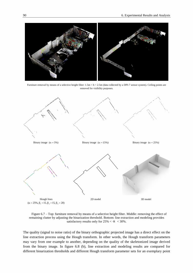
90 6. Experimental Results and Analysis
Furniture removal by means of a selective height filter: 1.5m < h < 2.5m (data collected by a DPI-7 sensor system). Ceiling points are
removed for visibility purposes.
Binary image ( 5%)
Binary image ( 15%)
Binary image ( 25%)
Hough lines
1 2 3( 25%, 15, 15, 20)
2D model
3D model
Figure 6.7 – Top: furniture removal by means of a selective height filter. Middle: removing the effect of
remaining clutter by adjusting the binarization threshold. Bottom: line extraction and modeling provides
satisfactory results only for 25% < < 30%.
The quality (signal to noise ratio) of the binary orthographic projected image has a direct effect on the
line extraction process using the Hough transform. In other words, the Hough transform parameters
may vary from one example to another, depending on the quality of the skeletonized image derived
from the binary image. In figure 6.8 (b), line extraction and modeling results are compared for
different binarization thresholds and different Hough transform parameter sets for an exemplary point
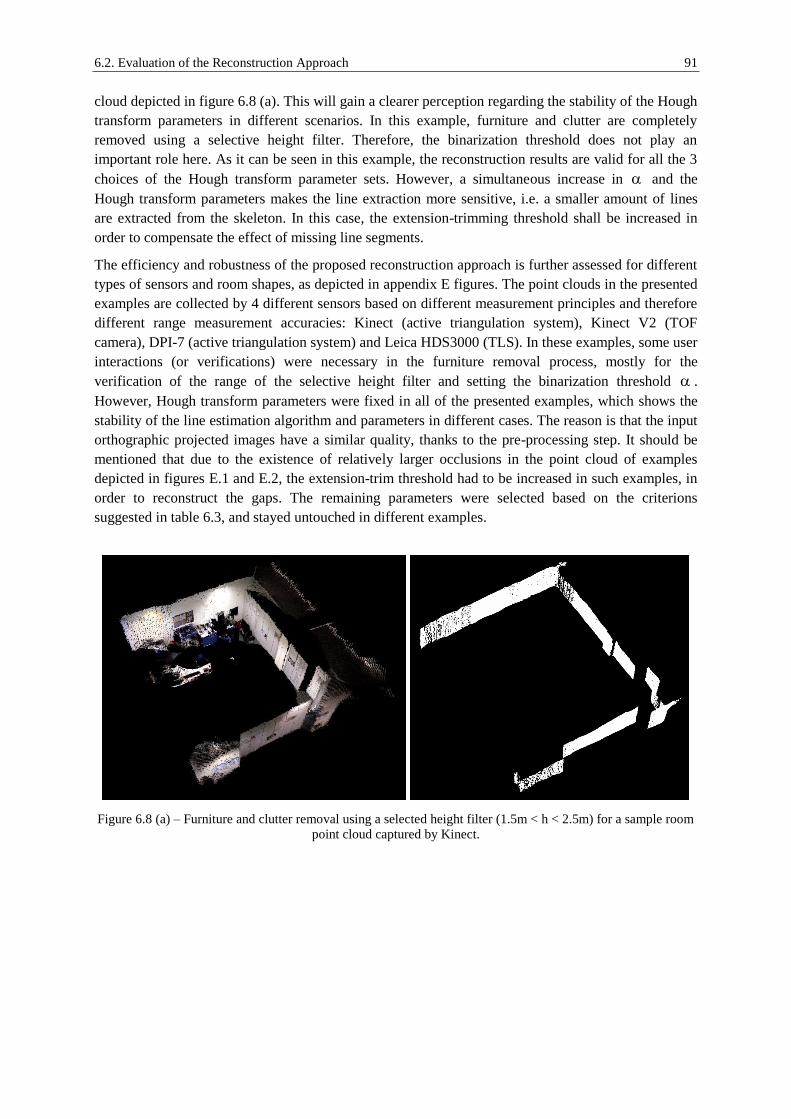
6.2. Evaluation of the Reconstruction Approach 91
cloud depicted in figure 6.8 (a). This will gain a clearer perception regarding the stability of the Hough
transform parameters in different scenarios. In this example, furniture and clutter are completely
removed using a selective height filter. Therefore, the binarization threshold does not play an
important role here. As it can be seen in this example, the reconstruction results are valid for all the 3
choices of the Hough transform parameter sets. However, a simultaneous increase in and the
Hough transform parameters makes the line extraction more sensitive, i.e. a smaller amount of lines
are extracted from the skeleton. In this case, the extension-trimming threshold shall be increased in
order to compensate the effect of missing line segments.
The efficiency and robustness of the proposed reconstruction approach is further assessed for different
types of sensors and room shapes, as depicted in appendix E figures. The point clouds in the presented
examples are collected by 4 different sensors based on different measurement principles and therefore
different range measurement accuracies: Kinect (active triangulation system), Kinect V2 (TOF
camera), DPI-7 (active triangulation system) and Leica HDS3000 (TLS). In these examples, some user
interactions (or verifications) were necessary in the furniture removal process, mostly for the
verification of the range of the selective height filter and setting the binarization threshold .
However, Hough transform parameters were fixed in all of the presented examples, which shows the
stability of the line estimation algorithm and parameters in different cases. The reason is that the input
orthographic projected images have a similar quality, thanks to the pre-processing step. It should be
mentioned that due to the existence of relatively larger occlusions in the point cloud of examples
depicted in figures E.1 and E.2, the extension-trim threshold had to be increased in such examples, in
order to reconstruct the gaps. The remaining parameters were selected based on the criterions
suggested in table 6.3, and stayed untouched in different examples.
Figure 6.8 (a) – Furniture and clutter removal using a selected height filter (1.5m < h < 2.5m) for a sample room
point cloud captured by Kinect.

92 6. Experimental Results and Analysis
Binary image ( 0%)
Skeletonized image
1 2 35, 5, 20
1 2 310, 10, 20
1 2 315, 15, 20
Binary image ( 5%)
Skeletonized image
1 2 35, 5, 20
1 2 310, 10, 20
1 2 315, 15, 20
Binary image ( 10%)
Skeletonized image
1 2 35, 5, 20
1 2 310, 10, 20
1 2 315, 15, 20
Figure 6.8 (b) – Line extraction and modeling results for different qualities of the binary image and different
Hough transform parameters for the example depicted in figure 6.8 (a).

6.3. Quality of the Reconstructed Models 93
6.3. Quality of the Reconstructed Models
After presenting the modeling approach and its performance evaluation, the accuracy of the
reconstructed models is investigated by comparing them with reference data. The comparison
represents errors in the range measurement and alignment, as well as the error committed in
representing interior structures by means of planar surfaces using the described modeling strategy. The
reference data is obtained by means of a high-accuracy laser scanner (Leica HDS3000), with 1cm
sampling distance, 4mm single point range measurement accuracy (1-50m distance, one sigma) and
2mm surface modeling accuracy (one sigma) (“Leica HDS3000 Product Specifications,” 2015). This
accuracy is one order of magnitude better than the noise of the registered point cloud obtained by low-
cost range cameras; therefore, the TLS data can be assumed accurate enough to serve as reference in
this comparison.
The results of comparison for an exemplary 3D model reconstructed from Kinect point clouds are
depicted in figure 6.9. In this example, the accuracy measure is the distance between the TLS point
cloud and the 3D model. Since the TLS point cloud is registered in a different local coordinate system,
the point cloud is registered to the 3D model using the ICP algorithm. The comparison shows an
overall mean difference of 0.030m with a standard deviation of 0.027m and a maximum of 0.137m.
However, as depicted in figure 6.9 (c), for different walls, different accuracies can be estimated (see
table 6.4). This effect can also be observed in figure 6.9 (d), in which 3 Gaussian fits can be
distinguished visually. Since the Kinect point cloud has a noise level of approximately 3cm at 3m
distance, the remaining error is assigned to the point cloud registration process. However, it should be
noted that the averaging concept, which is the basis of the modeling process, together with suggested
topological corrections to some extent have reduced the effect of range measurement and registration
errors on the final results.
In order to distinguish the data collection and modeling errors, a similar comparison is made between
the 3D model of the same room, reconstructed from the TLS point cloud, and the point cloud itself.
Figure 6.10 depicts the results of this comparison. The comparison shows an overall mean difference
of 0.007m with a standard deviation of 0.006m and a maximum of 0.040m. In this case, the modeling
accuracy is estimated from:
2 2 2
O D M
2 22 2 2
M O D
M
7mm 2mm
6.7mm
(6.3)
where, O is the overall accuracy, M is the modeling accuracy and D is the accuracy of the data
collected by the TLS. It should be noted that the modeling accuracy can be controlled by the
parameters presented in table 6.3. The most affective parameter in the modeling process is the voxel
size in the downsampling process (for the quantization of the input point cloud), as well as the pixel
size of the orthographic projected image. In this example, both of the parameters are set to 1cm, which
is consistent with the estimated overall mean difference (7mm).
It is necessary to mention that according to Tang et al. (2010), the modeling accuracy and level-of-
detail required for a particular application are still open questions, however, there exist guidelines for
the accuracy tolerances suggested e.g. by the U.S. GSA (“U.S. General Services Administration,”
2009). According to this guideline, the accuracy tolerance may range from 3mm to 51mm, and artifact
sizes may range from 13mm to 152mm.
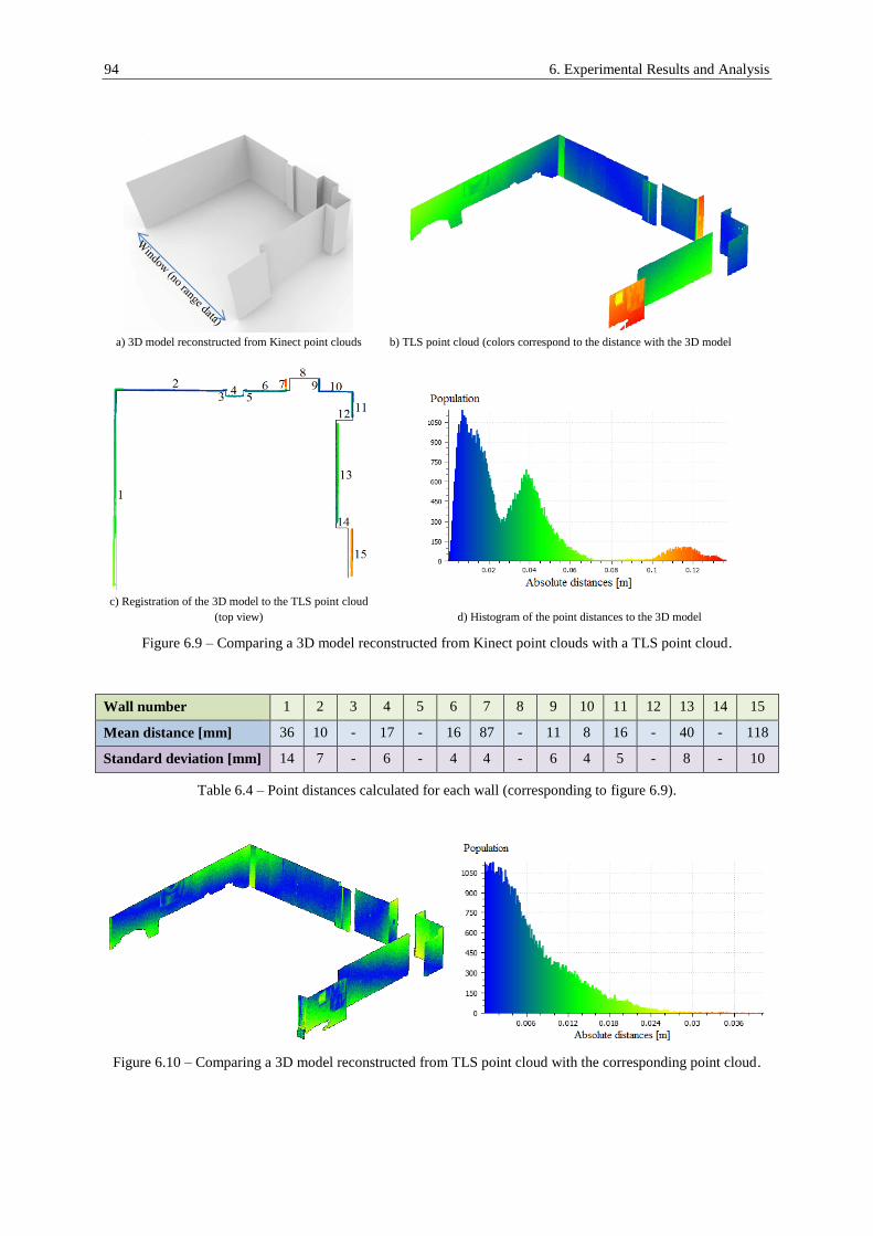
94 6. Experimental Results and Analysis
a) 3D model reconstructed from Kinect point clouds
b) TLS point cloud (colors correspond to the distance with the 3D model
c) Registration of the 3D model to the TLS point cloud
(top view)
d) Histogram of the point distances to the 3D model
Figure 6.9 – Comparing a 3D model reconstructed from Kinect point clouds with a TLS point cloud.
Wall number 1 2 3 4 5 6 7 8 9 10 11 12 13 14 15
Mean distance [mm] 36 10 - 17 - 16 87 - 11 8 16 - 40 - 118
Standard deviation [mm] 14 7 - 6 - 4 4 - 6 4 5 - 8 - 10
Table 6.4 – Point distances calculated for each wall (corresponding to figure 6.9).
Figure 6.10 – Comparing a 3D model reconstructed from TLS point cloud with the corresponding point cloud.

95
7. Application in the Refinement of Available Coarse Floor
Models
In the previous chapter, the performance of the presented approach for the automatic reconstruction of
individual room models was demonstrated. As an application, this chapter demonstrates how the
reconstructed room models can be used in the refinement of available coarse floor models. Available
floor models may need a refinement or an update due to generalizations in the reconstruction process,
or recent changes in the building interiors such as the addition of new elements (e.g. large cupboards,
partitions, etc.). The refinement is demanded by many applications, for instance interior design, safety
and security planning, indoor navigation, etc. Using low-cost sensor systems such as Kinect for the
data collection makes the performance of this task faster and more efficient.
The proposed refinement approach is presented using an example, in which a coarse floor model
(figure 7.1) is automatically derived from a photographed evacuation plan using the work of (Peter et
al., 2013b) (see section 4.2.3 for more details). The refinement approach firstly registers the detailed
model of individual rooms with the coarse model. The models are then merged together, and finally
possible gaps within the detailed models are automatically reconstructed using a new learning-based
approach employing the information inferred from the coarse model. Similar to the reconstruction
strategy mentioned in chapter 5, the algorithms of this process are designed for the 2D case; results are
converted to 3D in the very last step using a simple extrusion. The process is presented in the
following sections in more detail.
Assumption: While the approach deals with changes inside the room models, it excludes three special
scenarios in which a room is split, multiple rooms are merged, or a room is enlarged.
Figure 7.1 – The case study is a coarse floor plan automatically derived from a photographed evacuation plan
using the work of (Peter et al., 2013b).

96 7. Application in the Refinement of Available Coarse Floor Models
7.1. Registration of Individual Detailed Models to an Available
Coarse Floor Model
As already mentioned, in the first step of the update and refinement process, the reconstructed detailed
models have to be registered with an available coarse floor model. The registration consists of two
steps: approximate and fine registration. In fact, the approximate registration provides initial values
required for a fine registration, which is the optimal fitting of the detailed model to the coarse model
using a least squares adjustment.
7.1.1. Approximate Registration
For the approximate registration, the initial position and orientation of the detailed model with respect
to the coarse model is required. The translation is solved by the coincidence of the centroid of the
detailed model with the centroid of the corresponding room in the coarse model. Therefore, it is
sufficient to know the information about the room correspondences. This information can be provided
by the user in an interactive way, or alternatively, by means of an indoor positioning solution during
the data collection process. In the presented case study, the room correspondences are inferred by the
user’s track derived from the MEMS IMU positioning method, implemented and presented by (Peter
et al., 2013b). In this positioning method, the user track is registered to the coarse model based on the
initial position of the user and the building principal axes. The user initial position is assumed to be the
location of the evacuation plan, where the user photographs it. Therefore, the user employs a foot
mounted MEMS IMU and walks from the position of the evacuation plan into the room whose point
cloud has to be collected. The corresponding room is the one that contains the last track point.
Assuming the user starts capturing the point clouds while the sensor is oriented toward the door
location, the initial orientation of the detailed model with respect to the coarse model is approximately
known. According to Peter et al. (2013b), the door locations in the coarse model can be identified by
the intersection of the user’s track with this model. Figure 7.2 depicts the results of this registration for
an exemplary room.
Figure 7.2 – Approximate registration to the coarse model. The user’s track is identified in red, and the
corresponding room in the coarse model by green.

7.1. Registration of Individual Detailed Models to an Available Coarse Floor Model 97
7.1.2. Fine Registration
The approximate registration is further refined by the optimal fitting of the line segments in the
detailed model to the corresponding line segments in the coarse model.
Finding the corresponding line segments: To find the line correspondences, first the line segments
corresponding to the outer shell of the detailed model have to be derived by analyzing the convex hull
of the model (figure 7.3 (a)). Possible changes in the room geometry due to renovations or addition of
new structure elements cause the addition of new line segments only inside the room model.
Therefore, the room’s outer shell is assumed to be untouched, and consequently can be assigned to a
wall (line segment) in the coarse model. The correspondences in the coarse model are then found by
searching for the closest line segments having the most similar orientation. The search is performed
using a ray tracing process, in which the corresponding line segments are assumed to be intersected by
the same rays coming from the centroid of the model (figure 7.3 (b)). In order to deal with false
assignments in case of having multiple candidates, which is often the case if the initial orientation is
not accurate enough, candidates with the most similar orientations are selected. This assures a robust
correspondence of line segments, if the initial orientation is estimated within a tolerance of 45°.
a) b)
Figure 7.3 – Finding the corresponding line segments. a) Extracting the rooms outer shell using the convex hull
analysis (dashed lines); b) Ray tracing for finding the corresponding lines segments in the detailed and coarse
models.
Optimal fitting of the corresponding line segments: The corresponding line segments are optimally
fitted together using a least squares adjustment. The adjustment model does not simply minimize the
distance between the corresponding line segments (which is a “best fit”); instead, it firstly finds the
best rotation that minimizes the orientation differences, and then the best translation that minimizes
the distances between the corresponding line segments, in a separate process (here called an “optimal
(constrained) fit”). The “best fit” and the “optimal fit” deliver different results in case of the shape
asymmetry, as depicted in figure 7.4. The mathematical model of the “optimal fit” is presented as
follows.
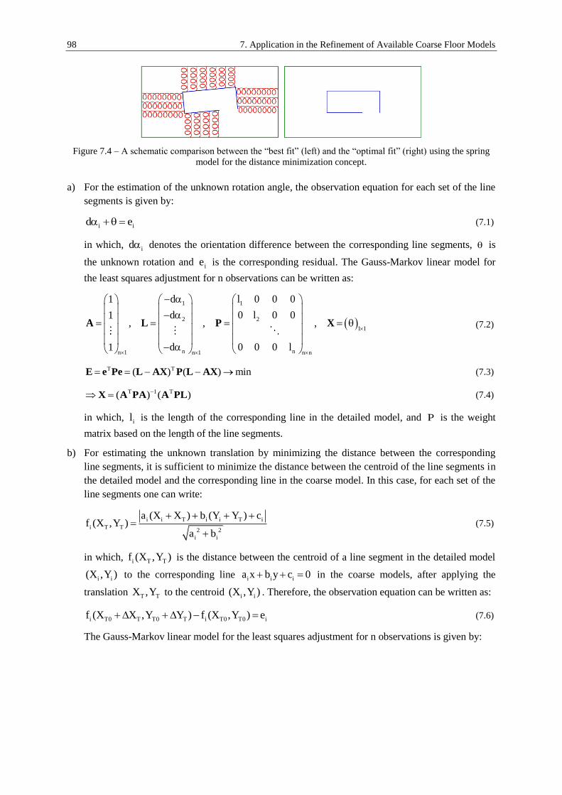
98 7. Application in the Refinement of Available Coarse Floor Models
Figure 7.4 – A schematic comparison between the “best fit” (left) and the “optimal fit” (right) using the spring
model for the distance minimization concept.
a) For the estimation of the unknown rotation angle, the observation equation for each set of the line
segments is given by:
i id e (7.1)
in which, id denotes the orientation difference between the corresponding line segments, is
the unknown rotation and ie is the corresponding residual. The Gauss-Markov linear model for
the least squares adjustment for n observations can be written as:
1 1
2 2
1 1
n nn 1 n 1 n n
d l 0 0 01
d 0 l 0 01, , ,
d 0 0 0 l1
A L P X (7.2)
T T( ) ( ) min E e Pe L AX P L AX (7.3)
T 1 T( ) ( ) X A PA A PL (7.4)
in which, il is the length of the corresponding line in the detailed model, and P is the weight
matrix based on the length of the line segments.
b) For estimating the unknown translation by minimizing the distance between the corresponding
line segments, it is sufficient to minimize the distance between the centroid of the line segments in
the detailed model and the corresponding line in the coarse model. In this case, for each set of the
line segments one can write:
i i T i i T i
i T T2 2
i i
a (X X ) b (Y Y ) cf (X ,Y )
a b
(7.5)
in which, i T Tf (X ,Y ) is the distance between the centroid of a line segment in the detailed model
i i(X ,Y ) to the corresponding line i i ia x b y c 0 in the coarse models, after applying the
translation T TX ,Y to the centroid i i(X ,Y ) . Therefore, the observation equation can be written as:
i T0 T T0 T i T0 T0 if (X X ,Y Y ) f (X ,Y ) e (7.6)
The Gauss-Markov linear model for the least squares adjustment for n observations is given by:

7.2. Fusion of Detailed Models to the Coarse Model 99
T 0 T 0
i ii i i T0 T0
X Y
1 1 1
2 2 2
T T 1 2
n n nn 2 n 1 n n
f f, f (X ,Y )
X Y
l 0 0 0
0 l 0 0, , , X Y
0 0 0 l
A L
A L
A LA L P δ
A L
(7.7)
T T( ) ( ) min E e Pe L Aδ P L Aδ (7.8)
T 1 T( ) ( ) δ A PA A PL (7.9)
Since the observation equation is non-linear with respect to the unknowns, the unknown
translation is estimated iteratively. In each iteration, the estimated translation is updated by:
T T0 T
T T0 T
X X X
Y Y Y
(7.10)
As the door thickness in comparison to the wall thickness is usually negligible, the coincident of the
line segments corresponding to the door serves as a constraint in the adjustment process. Figure 7.5
depicts the results of the constrained fit for the previous example.
Figure 7.5 – Optimal fitting of the detailed model to the coarse model. Fitting residuals close to a typical value
within a tolerance (e.g. 10-20cm) are considered as the wall thickness.
7.2. Fusion of Detailed Models to the Coarse Model
Computing the wall thickness: The actual value for the wall thickness is detectable after the
registration process, by analyzing the registration residuals (distance between the corresponding line
segments after the registration). In other words, residuals close to a typical value within a threshold
(e.g. 10-20cm) are considered as the actual wall thickness for the room (see figure 7.5). The
information about the wall thickness enables a correct fusion, and at the same time, a comparison
between the detailed and the coarse models for finding the changes in the building interiors and
updates to the coarse model.
Model fusion and gap filling: After the registration of the detailed models to the coarse model, they
have to be merged in a consistent way. Therefore, besides coincidence and merging of the doors in the
previous step, possible gaps in the detailed models have to be reconstructed based on the shape of the
coarse model. In other words, the gap parts are reconstructed by following the shape of the coarse

100 7. Application in the Refinement of Available Coarse Floor Models
model, considering the wall thickness. This is realized by generating a parallel buffer (equivalent to
the wall thickness) inside the corresponding rooms in the coarse model (figure 7.6 (a)), and filling the
gap parts using the buffer shell. For this purpose, the line segments in the detailed model are first
converted to graph edges (figure 7.6 (b)), and those containing a free end node (nodes of degree 1) will
be extended simultaneously in the original and perpendicular directions, in order to find their first
intersection with the offset shell (figure 7.6 (c)). Assuming the gap parts are less than 50% of the
corresponding detailed model, edges constituting the shortest path from the two most distant degree 1
nodes will be merged to the detailed model to fill the gaps (figure 7.6 (d)). Figure 7.7 depicts the
fusion of the detailed model of some exemplary rooms with the coarse model using this approach. As
already mentioned, the approach does not deal with the cases in which the detailed model is larger
than the coarse model (see the rooms number 1 and 7 in figure 7.7), or multiple rooms are merged
together (see the free space between rooms number 5 and 6). The main steps for the reconstruction of
the detailed models of this example are provided in appendix E.
Change detection: As already mentioned, computing the wall thickness enables the detection of the
changes to the coarse model; walls outside of a buffer equivalent to the wall thickness are considered
as updates to the coarse model. Updates in the mentioned example are distinguished in figure 7.8 using
a different color.
a) b)
c) d)
Figure 7.6 – a) Generating a parallel offset (black) inside the coarse model (green); b) Converting the line
segments into graph edges; c) Connecting the degree 1 nodes in the detailed model to the offset shell ; d)
Reconstructing the gaps by finding the shortest path between the two most distant degree 1 nodes in the detailed
model (red).
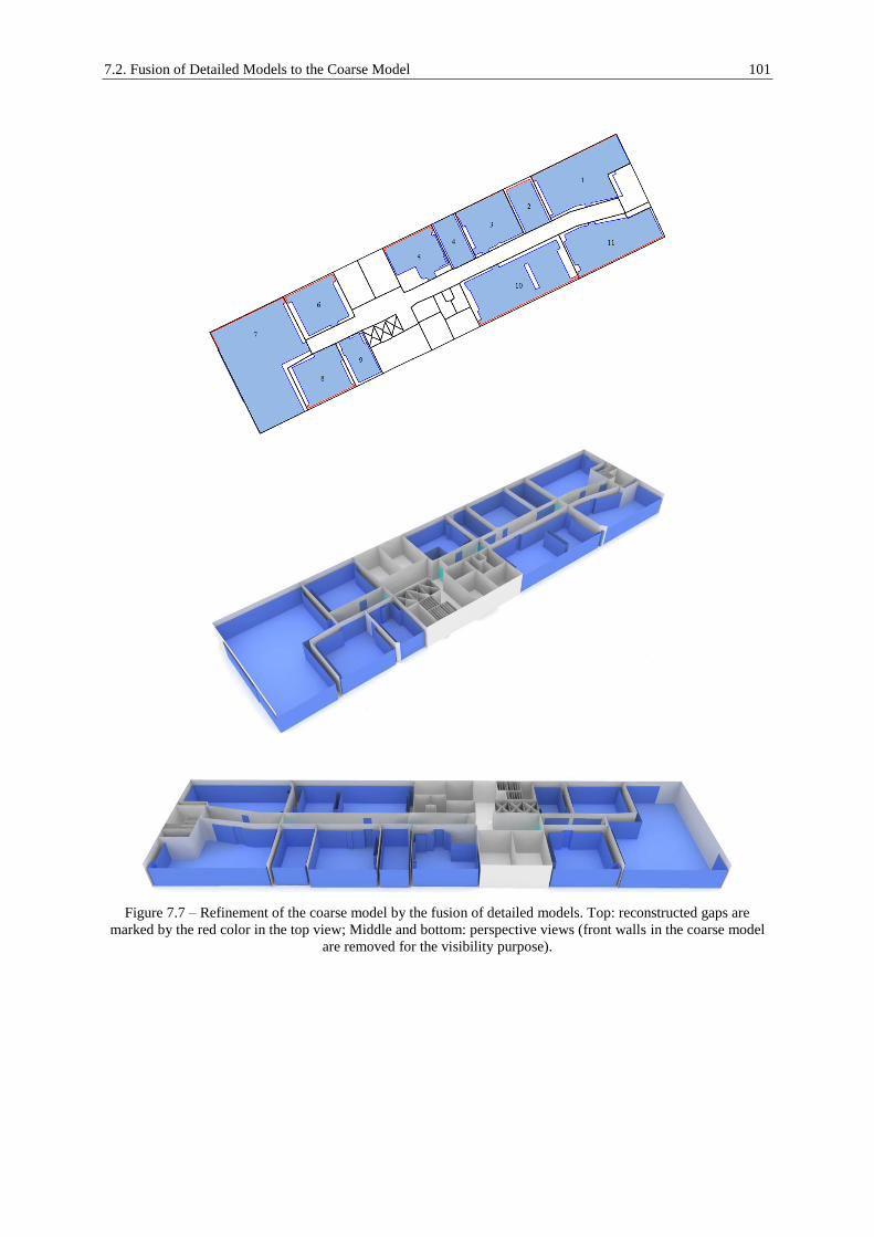
7.2. Fusion of Detailed Models to the Coarse Model 101
Figure 7.7 – Refinement of the coarse model by the fusion of detailed models. Top: reconstructed gaps are
marked by the red color in the top view; Middle and bottom: perspective views (front walls in the coarse model
are removed for the visibility purpose).
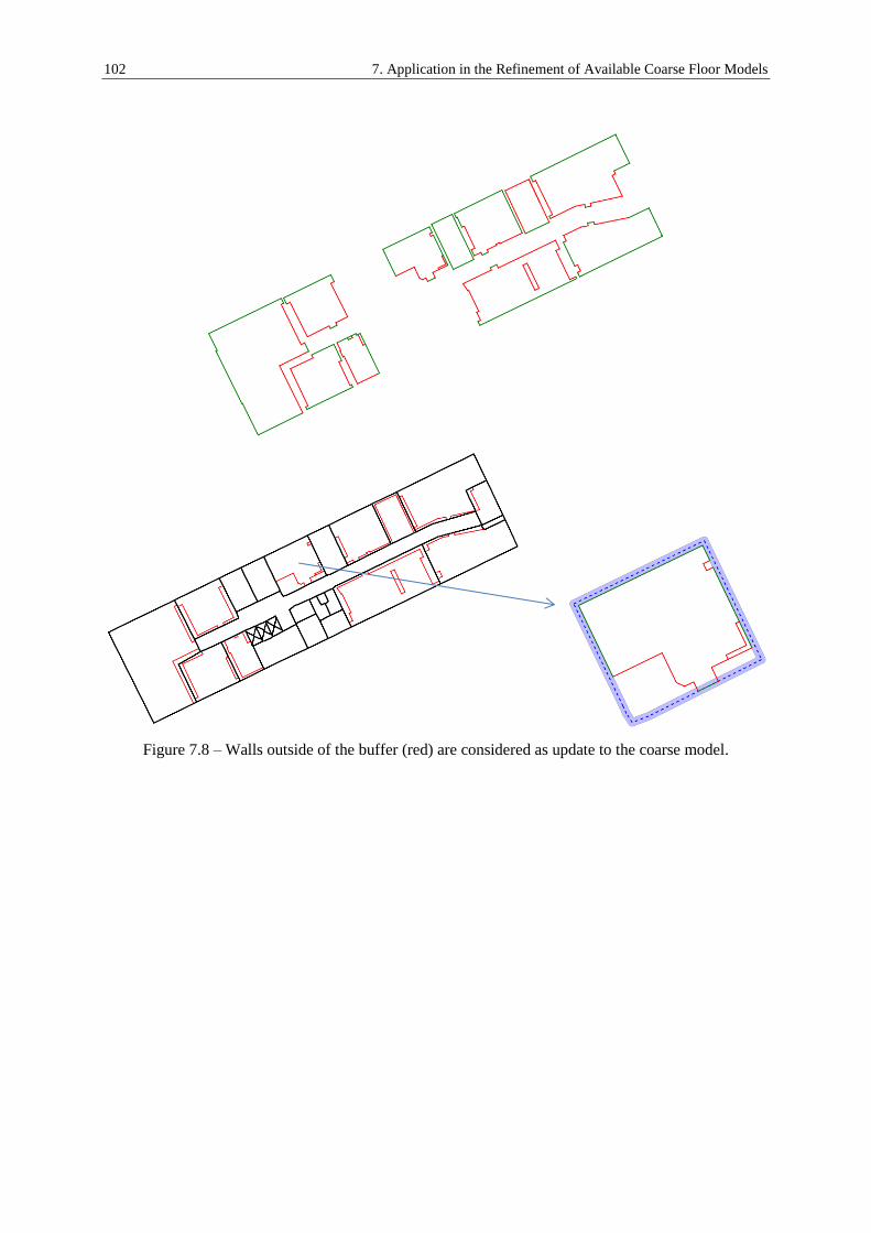
102 7. Application in the Refinement of Available Coarse Floor Models
Figure 7.8 – Walls outside of the buffer (red) are considered as update to the coarse model.

103
8. Conclusion
8.1. Summary
This work investigated the automatic reconstruction of building interiors using low-cost sensor
systems. The system developed for this purpose consists of two main parts: data acquisition and
2D/3D model reconstruction.
The data acquisition part focused on using state-of-the-art low-cost sensor systems for the collection of
range data in indoor scenes. Microsoft Kinect was selected as the case study, and the system
calibration together with the computation of 3D object coordinates were focused for this sensor
system. Afterwards, available approaches for the registration of Kinect point clouds were presented,
and a new complementary approach was proposed.
In the modeling part, the registered point clouds were first pre-processed in order to remove the
furniture and clutter, reduce the noise of the range measurements, level the point cloud and project the
points onto the ground plane. An orthographic projected image was then computed, in order to enable
the modeling process in 2D space. Converting the reconstruction problem from 3D to 2D, besides
simplification of the reconstruction task, enables efficient topological corrections using algebraic
relationships and graph theories. The modeling process consists of estimating the line segments
(corresponding to walls in 3D) together with some proposed topological corrections. The results were
converted back to 3D using an extrusion. The parameters used in the modeling algorithm were
discussed, and criterions for a correct parameter selection were presented. Experimental results
demonstrated the robustness of the reconstruction approach, as well as the stability of the selected
parameters in different scenarios, where different sensor types and different room shapes and sizes
were used.
Finally, as an application of the proposed reconstruction approach, it was shown how the resulted 3D
models with a higher level of details can be used to refine available coarse floor plans. During the
refinement process, existing gaps in the detailed models were automatically reconstructed using the
information derived from the coarse model.
8.2. Contributions
The contributions of this work can be summarized in the following parts:
Registration problem: Available approaches for the registration of point clouds collected from indoor
scenes mainly rely on visual features extracted from color images, as well as geometrical information
extracted from the rage data. Such approaches fail in scenarios, where not enough well-distributed
visual features can be observed, or geometrical constraints cannot fix the sensor 6 DOF. Therefore, a
new complementary approach is introduced, in order to support the registration task by employing the

104 8. Conclusion
user’s track information derived from an indoor positioning method, based on a foot mounted MEMS
IMU.
Line estimation, clustering and topological corrections: Available 2D reconstruction approaches
mostly directly deliver the output of the line estimation process (e.g. using the Hough transform) as the
final results. Therefore, the line estimation parameters play an important role in the final results, and a
suitable balance has to be made between the noise level, the required level of details and the expected
length of the line segments, in order to estimate each wall by a single line segment. In practice, the
problem is usually handled by estimating the parameters in a typical scenario, and using the same
parameters in similar cases. In the proposed approach, this problem is managed more efficiently.
Inputs for the modeling algorithm provided by different sensors (with different noise levels) are firstly
homogenized using a pre-processing step with minimal user interactions. Then the line estimation
parameters are set in a way that the smallest allowed features are taken into account. Although this
results in the estimation of each wall by multiple smaller line segments, the proposed hierarchical
clustering algorithm assigns the resulting line segments to the corresponding walls. It enables the
averaging and merging of multiple line segments, in order to estimate each wall by a single line
segment. The results are further improved using the proposed topological steps to correct small line
orientation errors (parallelism and perpendicularity check), and to assure a correct intersection
between the line segments (extension and trim algorithm). Moreover, small gaps in the model are
detected and filled by the extension of free end points (degree 1 nodes in the corresponding graph) in
the original and perpendicular directions. This results in the reconstruction of interiors with an
arbitrary level of details.
Reconstruction of larger gaps in the models and refinement of available coarse models: Available
coarse models (e.g. those derived from architectural drawings and floor plans) can be further refined
by the fusion of the reconstructed model with the coarse model. For this purpose, a fusion algorithm is
suggested, which also enables the reconstruction of remaining gaps in the detailed models using a
learning-based approach based on the information derived from the coarse model and the fusion
process. In other words, gaps are reconstructed by merging walls parallel to coarse model, considering
the wall thickness (the term “learning” refers to the prediction of gaps from the behavior of the coarse
model).
8.3. Future Work
The presented work has the potential of being used by the public for crowdsourcing, due to the
affordability and accessibility of range measurement systems in the recent years. For this purpose, the
following optimizations and extensions are suggested based on the experience gained in this work.
Visual user guides for the data acquisition task: The data acquisition task can be a challenge, if the
interior space is too complex and large, or the registration fails due to the weak estimation of the
sensor pose. Failures are revealed only after the data processing step. Therefore, it is required to make
use of SLAM and visual tracking techniques in order to develop an Augmented Reality system that is
able to guide the user in the data acquisition task, to assure a complete and faultless data acquisition.
This can be realized by the use of tablets or wearable devices such as Google Glass. Some of the
available business products have already integrated such features (e.g. DPI-7/8 handheld scanners),
however, the capability of capturing larger spaces and improving the tracking module by the fusion of
visual and geometrical features can still improve the performance of the systems.
Improving the pose estimation: As already mentioned, for an accurate registration of the range data,
one may benefit from the combination of visual and geometrical features. The GPU-based RGB-D

8.3. Future Work 105
odometry presented by (Whelan et al., 2013) is a successful example in this field. However, in public
buildings, indoor scenes usually have poor visual texture or geometrical features. In such scenarios,
one may benefit from the extraction and matching of line features instead of point features. Line-based
SLAM approaches are well-suited for this purpose. Therefore, replacing the method used in this work
(SfM) with such approaches can improve the registration results in challenging scenarios.
Extending the model fusion algorithm: In this work, a model fusion approach for the update or
refinement of coarse floor plan was introduced. The algorithm does not consider the case that a room
in the coarse model is split, or multiple rooms are merged together, or the room in the coarse model is
smaller than the corresponding detailed model. Therefore, including such cases in the algorithm is
required.
Extending the floor model reconstruction approach: The presented approach for the reconstruction of
a complete floor model is based on the reconstruction of individual rooms, and fusing the results with
an available coarse model. An extension to this work is the reconstruction of complete floor models
from point clouds, independent from the existence of coarse models. For this purpose, the proposed
topological concepts have to be extended, in order to assure a correct and consistent reconstruction and
combination of different rooms and hallways. The performance of grammar-based approaches in this
field is encouraging.
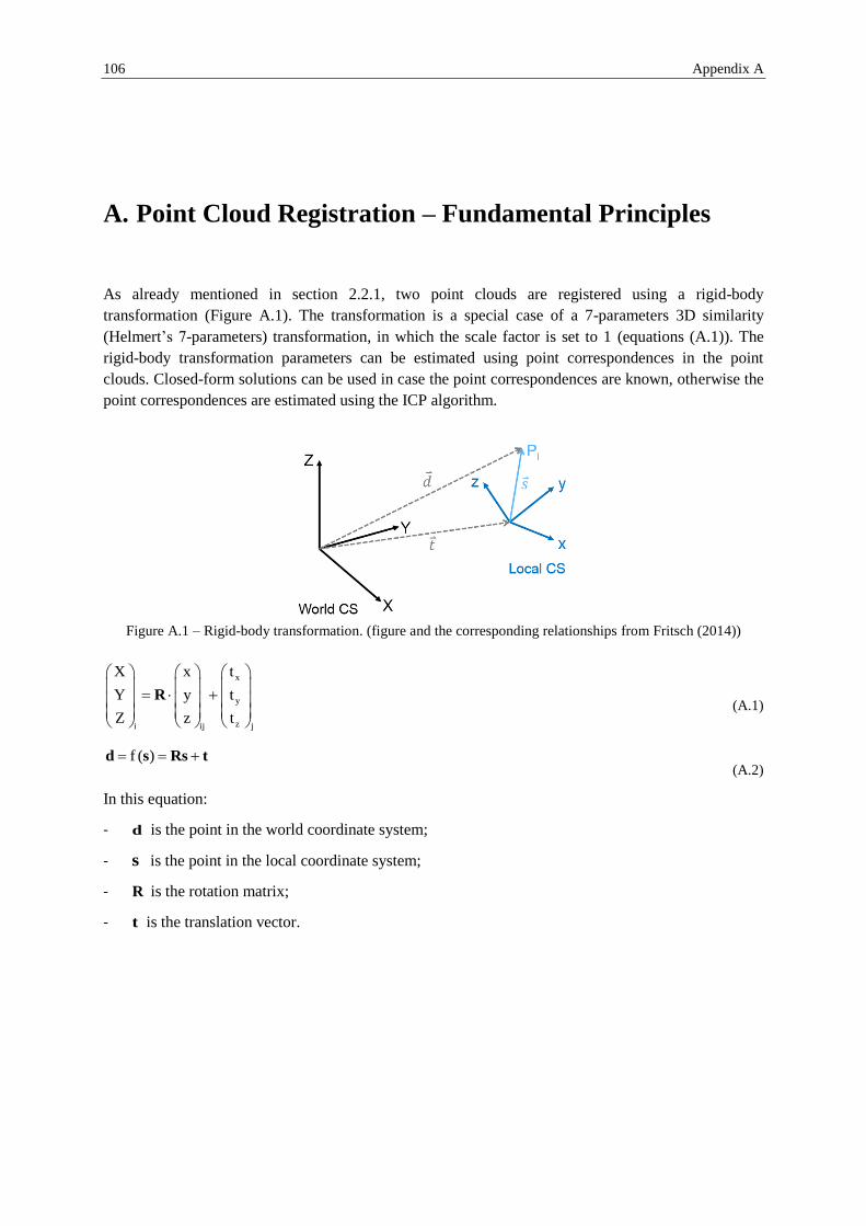
106 Appendix A
A. Point Cloud Registration – Fundamental Principles
As already mentioned in section 2.2.1, two point clouds are registered using a rigid-body
transformation (Figure A.1). The transformation is a special case of a 7-parameters 3D similarity
(Helmert’s 7-parameters) transformation, in which the scale factor is set to 1 (equations (A.1)). The
rigid-body transformation parameters can be estimated using point correspondences in the point
clouds. Closed-form solutions can be used in case the point correspondences are known, otherwise the
point correspondences are estimated using the ICP algorithm.
Figure A.1 – Rigid-body transformation. (figure and the corresponding relationships from Fritsch (2014))
x
y
zi ij j
X x t
Y y t
Z z t
R
(A.1)
f ( ) d s Rs t (A.2)
In this equation:
- d is the point in the world coordinate system;
- s is the point in the local coordinate system;
- R is the rotation matrix;
- t is the translation vector.
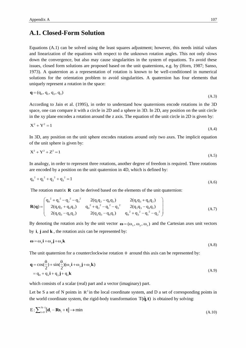
Appendix A 107
A.1. Closed-Form Solution
Equations (A.1) can be solved using the least squares adjustment; however, this needs initial values
and linearization of the equations with respect to the unknown rotation angles. This not only slows
down the convergence, but also may cause singularities in the system of equations. To avoid these
issues, closed form solutions are proposed based on the unit quaternions, e.g. by (Horn, 1987; Sanso,
1973). A quaternion as a representation of rotation is known to be well-conditioned in numerical
solutions for the orientation problem to avoid singularities. A quaternion has four elements that
uniquely represent a rotation in the space:
0 1 2 3(q , q , q , q )q (A.3)
According to Jain et al. (1995), in order to understand how quaternions encode rotations in the 3D
space, one can compare it with a circle in 2D and a sphere in 3D. In 2D, any position on the unit circle
in the xy plane encodes a rotation around the z axis. The equation of the unit circle in 2D is given by:
2 2X Y 1 (A.4)
In 3D, any position on the unit sphere encodes rotations around only two axes. The implicit equation
of the unit sphere is given by:
2 2 2X Y Z 1 (A.5)
In analogy, in order to represent three rotations, another degree of freedom is required. Three rotations
are encoded by a position on the unit quaternion in 4D, which is defined by:
2 2 2 2
0 1 2 3q q q q 1 (A.6)
The rotation matrix R can be derived based on the elements of the unit quaternion:
2 2 2 2
0 1 2 3 1 2 0 3 1 3 0 2
2 2 2 2
1 2 0 3 0 2 1 3 2 3 0 1
2 2 2 2
1 3 0 2 2 3 0 1 0 3 1 2
q q q q 2(q q q q ) 2(q q q q )
( ) 2(q q q q ) q q q q 2(q q q q )
2(q q q q ) 2(q q q q ) q q q q
R q
(A.7)
By denoting the rotation axis by the unit vector x y z( , , ) ω and the Cartesian axes unit vectors
by , andi j k , the rotation axis can be represented by:
x y z ω i j k (A.8)
The unit quaternion for a counterclockwise rotation around this axis can be represented by:
x y z
0 x y z
cos( ) sin( )( )2 2
q q q q
q i j k
i j k
(A.9)
which consists of a scalar (real) part and a vector (imaginary) part.
Let be S a set of N points in 3R in the local coordinate system, and D a set of corresponding points in
the world coordinate system, the rigid-body transformation ˆT( , )q t is obtained by solving:
N 1
i ii 0E : min
d Rs t
(A.10)

108 Appendix A
in which ˆ( )R R q and t are the rotation and translation matrices.
By computing the centroid of the points in the corresponding coordinate systems:
N 1 N 1
i i i ii 0 i 0
1 1; ; ' ; '
N N
d d s s d d d s s s
(A.11)
and constructing an auxiliary matrix :M
xx xy xzN 1 T
i i xy yy yzi 0
xz yz zz
S S S
' ' S S S
S S S
M d s
(A.12)
and a further auxiliary symmetric matrix :N
xx yy zz yz zy zx xz xy yx
yz zy xx yy zz zx xz
zx xz xy yx xx yy zz yz zy
xy yx zx xz yz zy xx yy zz
S S S S S S S S S
S S S S S S S S S
S S S S S S S S S
S S S S S S S S S
N
(A.13)
the singular value decomposition of N delivers singular values and the corresponding vectors; the
largest one represent the rotation matrix ˆ( )R R q .
The translation vector is finally given by:
t d Rs (A.14)

Appendix A 109
A.2. Iterative Solution (ICP)
If the point correspondences are not provided for the calculation of the rigid-body transformation, the
estimation of the transformation can be performed using common object surfaces in both point clouds.
However, as also stated by Luhmann et al. (2014), the common surfaces must have at least three
linearly independent normal vectors to achieve a unique solution. Moreover, if the common surfaces
contain only one symmetrical shape such as sphere or plane, the registration is not possible. The most
well-known registration algorithm based on common parts in the point cloud is the Iterative Closest
Point (ICP) algorithm (Besl and McKay, 1992). The algorithm is an iterative procedure. Assuming the
point cloud B has to be registered with the point cloud A, in each iteration, for every point in the point
cloud B, a point in the point cloud A with smallest Euclidean distance is assigned. Based on the
assigned correspondences, a rigid-body transformation is estimated, and is applied to the point cloud
B. The iteration is continued by finding a new set of point correspondences, estimating the
transformation and applying it, until the RMS of the distances is less than a given threshold (see
Figure A.2).
Figure A.2 – Flow diagram for the ICP algorithm. (adapted from Luhmann et al. (2014))
Distance Minimization
For the minimization of distances between the corresponding points in point clouds A and B,
parameters of the corresponding rigid-body transformation have to be estimated. The mathematical
model of the transformation is given by:
A 0B B 0B( ) X X R X X (A.15)
Assuming small (differential) rotation angles, the rotation matrix is given by:
Initial registration
Search for the closest points
Estimating the rigid-body transformation
RMS < ε
Apply the transformation and compute di
Stop
Yes
No

110 Appendix A
1 d d
(d , d , d ) d 1 d
d d 1
R R
(A.16)
Additionally, assuming small translation parameters, the transformation model can be replaced by the
following linear model:
A B 0B Bd X X X B X (A.17)
where:
t
B 0 0 0 Bd dX dY dZ d d d X
(A.18)
is the vector of unknowns containing 3 rotation angles and 3 translation elements, and:
0 0 0
iB iB
iB iB
iB iB
dX dY dZ d d d
1 0 0 0 Z Y
0 1 0 Z 0 X
0 0 1 Y X 0
... ...
B
(A.19)
is the coefficient matrix containing partial derivatives with respect to the unknowns, in which i denotes
the point index.
The unknowns are estimated by iteration, if appropriate initial values for the unknowns are provided.
In each iteration, after the estimation of the unknowns, the coordinates of the points in the point cloud
B are updated. The iteration is continued until the estimated unknowns (differential rotation and
translation elements) are smaller than a given threshold.
According to Fritsch (2014), the appropriate adjustment model for solving equation (A.17) is the
Gauß-Helmert model, since also the right side of the equation contains measured coordinates:
2 1; D( ) Av Bx w 0 l P (A.20)
In more detail, the update equations for every point correspondence are expressed by:
iA iB
iB iB
iA iB
iB iB
iA iB
iB
iA X iB X 00B 0B
iB Z 0 iB Y 0
iA Y iB Y 00B 0B
iB Z 0 iB X 0
iA Z iB X 00B 0B
iB Y
(X v ) (X v ) (X dX )
( Z v )( d ) ( Y v )( d ) 0
(Y v ) (Y v ) (Y dY )
( Z v )( d ) ( X v )( d ) 0
(Z v ) (Z Z ) (Z dZ )
( Y v )
iB0 iB X 0( d ) ( X v )( d ) 0
(A.21)
where, 00B 00B 00B 0 0 0X , Y , Z , , , are the initial (approximate) values of the unknown
parameters. Therefore, the coefficient matrices in the equation (A.20) are given by:
iA iA iA iB iB iB iB iB iBX Y Z X Y Z X Y Z
0 0
0 0
0 0
v v v v v v v v v
1 0 0 1 0 0 0
0 1 0 0 1 0 0
0 0 1 0 0 1 0
A
(A.22)

Appendix A 111
0 0 0
iB iB
iB iB
iB iB
dX dY dZ d d d
1 0 0 0 Z Y
0 1 0 Z 0 X
0 0 1 Y X 0
B
(A.23)
iA iB 00B iB 0 iB 0
iA iB 00B iB 0 iB 0
iA iB 00B iB 0 iB 0
X X X Z Y
Y Y Y Z X
Z Z Z Y X
w
(A.24)
Normal equations are given by:
1
t
ˆ
ˆ
wλAP A B
0B 0 X
(A.25)
which are solved by iteration to estimate the unknown vector X̂ containing the transformation
parameters.
This is the strict solution of the ICP algorithm. Although there are modifications and other variants for
this algorithm (e.g. different search algorithms or point-to-plane distance minimization instead of
point-to-point distance), the main steps which are described in Figure A.2 remain essentially the same.

112 Appendix B
B. RANSAC
Random Sample Consensus (RANSAC) is an adjustment algorithm presented by Fischler and Bolles
(1981), based on a voting scheme. The model is suitable for the estimation of any functional model
from a set of observations containing a significant number of gross errors, even up to 80% (Schnabel
et al., 2007). Opposed to many classical algorithms that fit the model to all of the presented data, this
algorithm estimate the model parameters from a minimum set of observations using an iterative
procedure.
In more detail, as described by Luhmann et al. (2014), the algorithm first randomly selects a minimum
required number of observations from the full set of the observations in order to estimate the model
parameters. Afterwards, all the remaining observations are tested against the estimated model, their
residuals are computed, and those which are consistent with the model within a certain tolerance are
regarded as valid observations and form a consensus set. The procedure is repeated using a new set of
random observations to create a new consensus set. After some iterations, the model corresponding to
the consensus set with the maximum number of valid observations is regarded as the best solution.
The success of the algorithm depends on the mentioned tolerance and the termination criterion which
can be the number of iterations, or the minimum size of the consensus set. Probabilistic criterions for
the minimum number of iterations or the minimum size of the consensus set are proposed by (Fischler
and Bolles, 1981). For instance, assuming w be the probability that any selected data is within the
error tolerance of the model, k the number of trials required to select a subset of n valid observations,
in order to ensure with probability of z that at least one of the random selections is an error-free set on
n observations, then the number of iterations is given by:
nb w
k(1 b) (1 z)
log(1 z)k
log(1 b)
(B.1)
According to Fischler and Bolles (1981), the algorithm is very well-suited for applications in
automated image analysis that rely on the data provided by error-prone feature detectors, such as
relative orientation. Other applications are for instance data association (e.g. 2D or 3D points in
different coordinate systems), feature detection and fitting of geometric primitive to a set of points
(e.g. line and circle in 2D or sphere and plane in 3D).

Appendix C 113
C. SLAM Problem
Simultaneous Localization And Mapping (SLAM) was originally introduced by Leonard and Durrant-
Whyte (1991) based on the work of Smith et al. (1990) for mobile robot navigation. SLAM aims at
creating a map of an unknown environment, while at the same time localizing the mobile robot within
the environment. In fact, the localization supports the mapping process, and the created map supports
the continuation of the localization process, similar to the well-known “chicken and egg” problem.
Figure C.1 illustrated this concept for a mobile robot using an example provided by (Frese et al.,
2010). In this example, the robot observes the environment (artificial features on the floor) relative to
its own unknown location using a camera mounted on the top of it. At the same time, the robot relative
motion is measured using odometry. If the environment was known, the robot’s pose could be
estimated using the provided observations (called localization). Conversely, if the robot’s pose was
known, measuring the feature points could lead the positioning of the points in a global reference
frame (called mapping). In general, neither the environment is known, nor the robot’s pose; they both
have to be estimated using the same data (called simultaneous localization and mapping).
Figure C.1 – A mobile robot observes the environment and measures its relative motion, in order to estimate its
pose and the scene geometry using a SLAM algorithm. (from Frese et al. (2010))
According to Riisgaard and Blas (2003), the standard SLAM process typically consists of following
steps:
a) Landmark extraction: Landmarks are the features that can be re-observed by the robot and be
distinguished in the environment for the localization purpose. Depending on the type of the
SLAM variant, landmarks can be extracted from different sources of data, e.g. laser scan data
or image features.
b) Data association: This problem deals with the searching and matching of the landmarks in an
uncertainty area, in order to realize if a landmark has been re-observed.
c) State estimation: In this step, it is assumed that the map is provided, and at least temporarily it
does not require any update. When the odometry data is changed, the robot pose is estimated

114 Appendix C
using the new data (e.g. laser scan data, IMU data and visual features). This can be performed
using different solutions, such as filtering methods (e.g. Extended Kalman Filter (EKF)) or
keyframe-based methods that optimizes the solution using a bundle adjustment.
d) State update: The robot’s state is updated, as soon as landmarks are re-observed, in order to
reduce errors in the pose estimation.
e) Landmark update: Extracted landmarks which have not been observed before are regarded as
new landmarks and added to the landmarks library.
Each of the mentioned steps of the SLAM process can be modified based on the application
requirements. In the overview presented by Frese et al. (2010), different types of applications are
distinguished, in which the standard SLAM algorithm is modified, in order to fulfil special
requirements of the application:
Offline-SLAM for mapping (map learning): In such applications, the robot is manually navigated
within the environment and sensor data is recorded. Then in a post-processing step, a map is computed
using the computed trajectory. The map is later used for the actual operation of the system, e.g.
localization, rout planning, etc.
Online-SLAM for localization: In this SLAM mode, both localization and mapping are performed in
real-time, but the application only uses the localization results, and the mapping is performed just to
support the localization. In this mode, the whole or parts of the map are known; therefore, the
localization error only grows when the map has to be extended.
Online-SLAM for continuously updating the map: This mode is the most complex way of using
SLAM, which is also the main motivation of SLAM research. In this mode, the map is generated and
extended and the robot is localized within the generated map. Both localization and mapping results
are further used for the robot navigation purpose.
The SLAM problem is a very active topic of research and still many problems have to be solved in
order to reach a fully automated approach for the robot navigation and exploration in real world
scenarios.

Appendix D 115
D. Hough Transform
D.1. Standard Hough Transform
Hough transform (Duda and Hart, 1972; Hough, 1962) extracts a certain class of shapes (most
commonly lines, circles or ellipses) in a binary image, based on a voting scheme. The voting process is
performed in a parameter space, which is defined by the parametric representation of the shape. For
instance for the extraction of straight lines or collinear points in an image, the parameter space is
defined by ( , ), [0, ] , corresponding to the slope-intercept representation of the line (equation
(D.1)). In this space, points in the (x, y) domain are represented by sinusoidal curves, and straight lines
by points which are the intersection of sinusoidal curves corresponding to collinear points (see Figure
D.1). Likewise, pointes lying on the same sinusoidal curves correspond to lines passing through a
common point in the (x, y) domain.
The Hough transform algorithm detects lines (collinear points) in the (x, y) domain using a two
dimensional array corresponding to ( , ) , called an accumulator. The size of the array depends on
the quantization error (step size) of and values. Each cell in the accumulator is incremented by
the number of curves passing through the corresponding point in the ( , ) domain. Therefore, the
count in a given cell i i( , ) determines how many points in the (x, y) domain lie along the line
whose parameters are i i( , ) . The algorithm afterwards searches for the cells having counts more
than a given threshold (counts are the number of collinear points for that line within the quantization
error).
x cos( ) ysin( ) (D.1)
Figure D.1 – Hough transform concept for the extraction of lines. (from “EBSD-Image, Hough Transform”
(2011))

116 Appendix D
D.2. Progressive Probabilistic Hough Transform
This variant of the Hough transform improves the speed and efficiency of the standard Hough
transform by minimizing the amount of computation needed for the detection of lines, which is
realized by reducing the number of candidates and votes needed to reliably detect lines with different
numbers of supporting points (Matas et al., 2000).
According to Matas et al. (2000), the algorithm repeatedly selects a random point for voting. After
casting a vote, the hypothesis that “could the count be due to random noise?” is tested, based on a
single comparison with a threshold per bin update (the threshold is also updated as votes are casted).
In other words, the algorithm checks if the highest pick in the accumulator that was updated by the
new point is higher than a threshold. After the detection of a line, the supporting points draw back
their votes. Additionally, the remaining points supporting the lines which are not yet participated in
the voting process are removed from the process. This reduces the amount of the remaining process, as
the new random point is selected from the remaining points, and therefore only a small fraction of
points are voted. This further reduces the number of false positives, where the assignment of points to
lines is ambiguous, i.e. points are located in the neighborhood of more than one line.

Appendix E 117
E. Reconstruction of Detailed Models – Case Studies
This appendix presents study cases used for the assessment of the efficiency and robustness of the
proposed reconstruction approach regarding parameter selection, different types of sensors (with
different accuracies) and different room shapes, as explained in section 6.2.1. Existing gaps in the
presented models are reconstructed in section 7.2, as a result of the fusion of these models to an
available coarse model.
Data collected by a Kinect sensor system Pre-processed point cloud. Clutter is removed by means of a selective
height filter (1.5m < h < 2.5m)
Binary image ( 5%)
Skeletonized image
Hough lines 1 2 3( 15, 15, 20)
2D model (extension-trim threshold: 0.6m)
3D model
Figure E.1 – Modeling of a sample room captured by a Kinect sensor system.
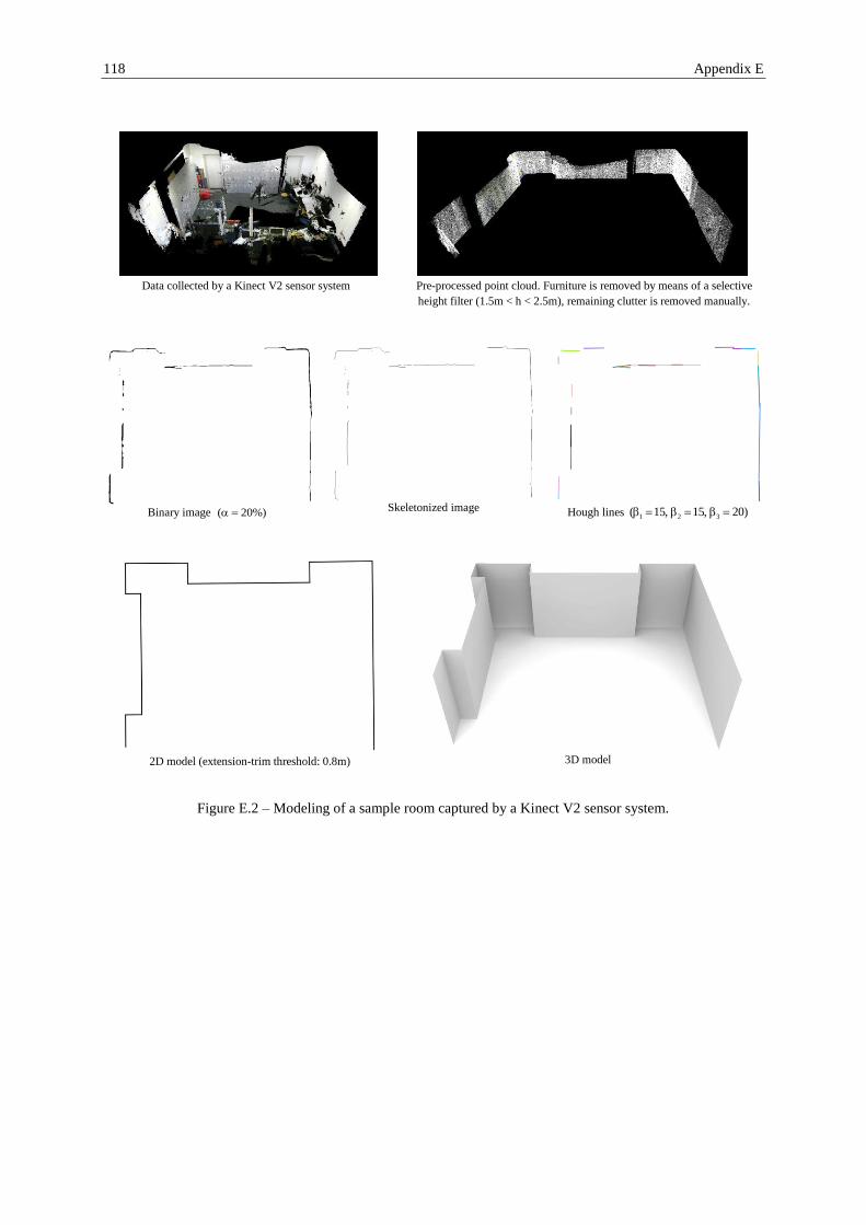
118 Appendix E
Data collected by a Kinect V2 sensor system Pre-processed point cloud. Furniture is removed by means of a selective
height filter (1.5m < h < 2.5m), remaining clutter is removed manually.
Binary image ( 20%)
Skeletonized image
Hough lines 1 2 3( 15, 15, 20)
2D model (extension-trim threshold: 0.8m)
3D model
Figure E.2 – Modeling of a sample room captured by a Kinect V2 sensor system.

Appendix E 119
Data collected by a DPI-7 sensor system (ceiling points are
removed for the visibility purpose) Pre-processed point cloud. Furniture is fully removed by means of a
selective height filter (1.5m < h < 2.5m). Remaining clutter is
removed in the binarization process.
Binary image ( 15%)
Skeletonized image
Hough lines 1 2 3( 15, 15, 20)
2D model (extension-trim threshold: 0.5m)
3D model
Figure E.3 – Modeling of a sample room captured by a DPI-7 sensor system.

120 Appendix E
Data collected by a DPI-7 sensor system Pre-processed point cloud. Furniture is fully removed by means of a
selective height filter (1.5m < h < 2.5m)
Binary image ( 5%)
Skeletonized image
Hough lines 1 2 3( 15, 15, 20)
2D model (extension-trim threshold: 0.5m)
3D model
Figure E.4 – Modeling of a sample room captured by a DPI-7 sensor system.

Appendix E 121
Data collected by a Leica HDS3000 laser scanner Pre-processed point cloud. Furniture is removed by means of a
selective height filter (1m < h < 1.5m), remaining clutter is
removed manually.
Binary image ( 5%)
Skeletonized image
Hough lines 1 2 3( 15, 15, 20)
2D model (extension-trim threshold: 0.5m)
3D model
Figure E.5 – Modeling of a sample room captured by a Leica HDS3000 laser scanner.
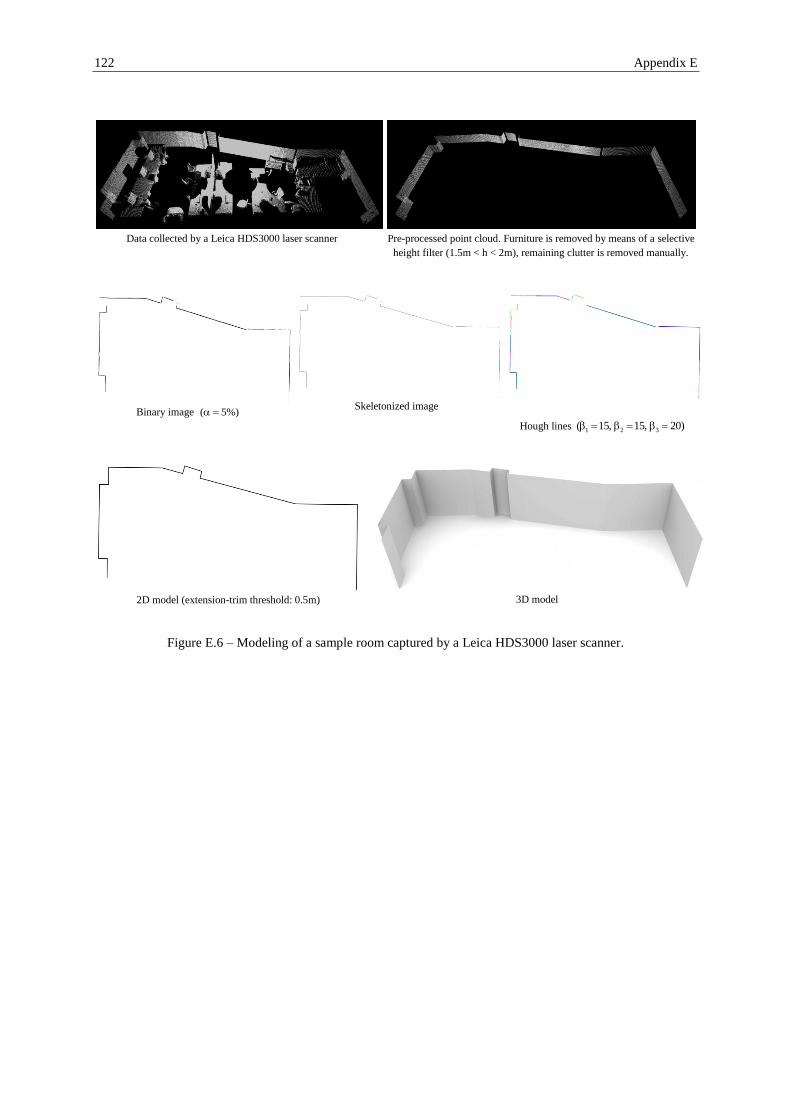
122 Appendix E
Data collected by a Leica HDS3000 laser scanner Pre-processed point cloud. Furniture is removed by means of a selective
height filter (1.5m < h < 2m), remaining clutter is removed manually.
Binary image ( 5%) Skeletonized image Hough lines 1 2 3( 15, 15, 20)
2D model (extension-trim threshold: 0.5m)
3D model
Figure E.6 – Modeling of a sample room captured by a Leica HDS3000 laser scanner.

123
References
Adan, A., Huber, D., 2011. 3D reconstruction of
interior wall surfaces under occlusion and
clutter, in: 3D Imaging, Modeling, Processing,
Visualization and Transmission (3DIMPVT),
2011 International Conference on. pp. 275–281.
Ah-Soon, C., Tombre, K., 2001. Architectural
symbol recognition using a network of
constraints. Pattern Recognition Letters 22,
231–248.
Ah-Soon, C., Tombre, K., 1997. Variations on the
analysis of architectural drawings, in: Document
Analysis and Recognition, 1997., Proceedings
of the Fourth International Conference on.
IEEE, pp. 347–351.
ATAP Project Tango [WWW Document], 2015. .
Google. URL
https://www.google.com/atap/projecttango/
(accessed 3.11.15).
Bamji, C.S., O’Connor, P., Elkhatib, T., Mehta, S.,
Thompson, B., Prather, L.A., Snow, D.,
Akkaya, O.C., Daniel, A., Payne, A.D., Perry,
T., Fenton, M., Chan, V.-H., 2015. A 0.13 um
CMOS System-on-Chip for a 512 x 424 Time-
of-Flight Image Sensor With Multi-Frequency
Photo-Demodulation up to 130 MHz and 2 GS/s
ADC. IEEE Journal of Solid-State Circuits 50,
303–319. doi:10.1109/JSSC.2014.2364270
Bay, H., Tuytelaars, T., Van Gool, L., 2006. Surf:
Speeded up robust features, in: Computer
vision–ECCV 2006. Springer, pp. 404–417.
Becker, S., 2009. Generation and application of
rules for quality dependent façade
reconstruction. ISPRS Journal of
Photogrammetry and Remote Sensing 64, 640–
653. doi:10.1016/j.isprsjprs.2009.06.002
Becker, S., Peter, M., Fritsch, D., Philipp, D., Baier,
P., Dibak, C., 2013. Combined Grammar for the
Modeling of Building Interiors. ISPRS Annals
of Photogrammetry, Remote Sensing and
Spatial Information Sciences II-4/W1, 1–6.
doi:10.5194/isprsannals-II-4-W1-1-2013
Beraldin, J.A., Blais, F., Lohr, U., 2010. Laser
scanning technology, in: Airborne and
Terrestrial Laser Scanning, Ed. Vosselman, G.
and Maas, H. G. Whittles Publishing, pp. 1–42.
Beraldin, J.-A., Picard, M., El-Hakim, S., Godin,
G., Borgeat, L., Blais, F., Paquet, E., Rioux, M.,
Valzano, V., Bandiera, A., 2005. Virtual
reconstruction of heritage sites: opportunities
and challenges created by 3D technologies.
NRC Publications Record.
Besl, P.J., McKay, N.D., 1992. Method for
registration of 3-D shapes, in: Robotics-DL
Tentative. pp. 586–606.
Böhm, J., 2014. Accuracy Investigation for
Structured-light Based Consumer 3D Sensors.
Photogrammetrie - Fernerkundung -
Geoinformation 2014, 117–127.
doi:10.1127/1432-8364/2014/0214
Böhm, J., Becker, S., 2007. Automatic marker-free
registration of terrestrial laser scans using
reflectance features, in: Proceedings of 8th
Conference on Optical 3D Measurement
Techniques. Zurich, Switzerland, pp. 338–344.
Bradski, G., 2000. The OpenCV Library (2000).
Dr. Dobb’s Journal of Software Tools.
Brown, D.C., 1971. Close-range camera calibration.
PHOTOGRAMMETRIC ENGINEERING 37,
855–866.
Budroni, A., 2013. Automatic Model
Reconstruction of Indoor Manhattan-world
Scenes from Dense Laser Range Data.
Dissertation at the Institute for Photogrammetry,
University of Stuttgart.
Budroni, A., Böhm, J., 2009. Toward automatic
reconstruction of interiors from laser data.
Proceedings of Virtual Reconstruction and
Visualization of Complex Architectures (3D-
Arch).
Buxbaum, B., Schwarte, R., Ringbeck, T., Grothof,
M., Luan, X., 2002. MSM-PMD as correlation
receiver in a new 3D-ranging system, in:
International Symposium on Remote Sensing.
International Society for Optics and Photonics,
pp. 145–153.
Canny, J., 1986. A computational approach to edge
detection. Pattern Analysis and Machine
Intelligence, IEEE Transactions on 679–698.

124 References
Chli, M., Furgale, P., Hutter, M., Siegwart, R.,
2015. Lecture notes in Autonomous Mobile
Robots, ASL (Master program), ETHZ.
Color Structure Code [WWW Document], 2014.
URL http://www.uni-koblenz-
landau.de/koblenz/fb4/icv//agpriese/research/Co
lorImgSeg/download/csc (accessed 6.30.14).
Connecting Kinects for Group Surveillance [WWW
Document], 2014. URL
http://actu.epfl.ch/news/connecting-kinects-for-
group-surveillance/ (accessed 2.19.14).
Coughlan, J.M., Yuille, A.L., 2003. Manhattan
world: Orientation and outlier detection by
bayesian inference. Neural Computation 15,
1063–1088.
Cramer, M., 2014. Lecture notes in
Photogrammetry, Institute for Photogrammetry,
University of Stuttgart.
Criminisi, A., Reid, I., Zisserman, A., 1999. Single
view metrology, in: The Proceedings of the
Seventh IEEE International Conference on
Computer Vision, 1999. pp. 434–441 vol.1.
doi:10.1109/ICCV.1999.791253
Criminisi, A., Reid, I., Zisserman, A., 1998.
Computing 3D euclidean distance from a single
view. Technical Report OUEL 2158/98, Dept.
Eng. Science, University of Oxford.
Delage, E., Lee, H., Ng, A.Y., 2006. A Dynamic
Bayesian Network Model for Autonomous 3D
Reconstruction from a Single Indoor Image, in:
2006 IEEE Computer Society Conference on
Computer Vision and Pattern Recognition. pp.
2418–2428. doi:10.1109/CVPR.2006.23
Doc-Ok.org [WWW Document], 2015. URL
http://doc-ok.org/?p=584 (accessed 3.11.15).
Documentation - Point Cloud Library (PCL)
[WWW Document], 2015. URL
http://pointclouds.org/documentation/tutorials/n
arf_feature_extraction.php (accessed 3.15.15).
Dold, J., 1997. Ein hybrides photogrammetrisches
Industriemesssystem höchster Genauigkeit und
seine Überprüfung (PhD thesis). Univ. der
Bundeswehr München, Fak. für Bauingenieur-
und Vermessungswesen, Studiengang
Vermessungswesen.
Dosch, P., Tombre, K., Ah-Soon, C., Masini, G.,
2000. A complete system for the analysis of
architectural drawings. International Journal on
Document Analysis and Recognition 3, 102–
116.
DotProduct LLC [WWW Document], 2015. URL
http://www.dotproduct3d.com (accessed
3.9.15).
DPI-7 User Manual, 2014.
Duda, R.O., Hart, P.E., 1972. Use of the Hough
transformation to detect lines and curves in
pictures. Communications of the ACM 15, 11–
15.
EBSD-Image [WWW Document], 2011. URL
http://www.ebsd-
image.org/documentation/reference/ops/hough/o
p/houghtransform.html (accessed 1.17.16).
El-Hakim, S., 2002. Semi-automatic 3D
reconstruction of occluded and unmarked
surfaces from widely separated views. Close
Range Visualization Techniques.
El-Hakim, S., Beraldin, J.-A., 2006. Sensor
integration and visualization. Chapter 10 of
Applications of 3D Measurement from Images.
Endres, F., Hess, J., Engelhard, N., Sturm, J.,
Cremers, D., Burgard, W., 2012. An evaluation
of the RGB-D SLAM system, in: Robotics and
Automation (ICRA), 2012 IEEE International
Conference on. IEEE, pp. 1691–1696.
Fischler, M.A., Bolles, R.C., 1981. Random sample
consensus: a paradigm for model fitting with
applications to image analysis and automated
cartography. Communications of the ACM 24,
381–395.
Frese, U., Wagner, R., Röfer, T., 2010. A SLAM
Overview from a User’s Perspective. KI -
Künstliche Intelligenz 24, 191–198.
doi:10.1007/s13218-010-0040-4
Fritsch, D., 2014. Lecture notes in Terrestrial Laser
Scanning (Terrestrisches Laserscanning),
Institute for Photogrammetry, University of
Stuttgart.
Furukawa, Y., Curless, B., Seitz, S.M., Szeliski, R.,
2009a. Reconstructing building interiors from
images, in: 2009 IEEE 12th International
Conference on Computer Vision. pp. 80–87.
doi:10.1109/ICCV.2009.5459145
Furukawa, Y., Curless, B., Seitz, S.M., Szeliski, R.,
2009b. Manhattan-world stereo, in: Computer
Vision and Pattern Recognition, 2009. IEEE
Conference on. pp. 1422–1429.
GestSure [WWW Document], 2014. URL
http://gestsure.com/ (accessed 2.19.14).
Godha, S., Lachapelle, G., 2008. Foot mounted
inertial system for pedestrian navigation.
Measurement Science and Technology 19,
075202. doi:10.1088/0957-0233/19/7/075202
Google Store [WWW Document], 2015. URL
https://store.google.com/product/project_tango_
tablet_black?playredirect=true
Gröger, G., Plümer, L., 2010. Derivation of 3D
indoor models by grammars for route planning.
Photogrammetrie-Fernerkundung-
Geoinformation 2010, 191–206.

References 125
Guidi, G., Remondino, F., 2012. 3D Modelling
from Real Data, in: Modelling and Simulation
in Engineering, Ed. Catalin , A. INTECH Open
Access Publisher.
Haala, N., Fritsch, D., Peter, M., Khosravani, A.M.,
2011. Pedestrian mobile mapping system for
indoor environments based on MEMS IMU and
range camera. Archives of Photogrammetry,
Cartography and Remote Sensing 22, 159–172.
Hähnel, D., Burgard, W., Thrun, S., 2003. Learning
compact 3D models of indoor and outdoor
environments with a mobile robot. Robotics and
Autonomous Systems 44, 15–27.
doi:10.1016/S0921-8890(03)00007-1
Han, F., Zhu, S.-C., 2009. Bottom-up/top-down
image parsing with attribute grammar. Pattern
Analysis and Machine Intelligence, IEEE
Transactions on 31, 59–73.
Hartley, R., Zisserman, A., 2003. Multiple view
geometry in computer vision. Cambridge
university press.
Henry, P., Krainin, M., Herbst, E., Ren, X., Fox, D.,
2012. RGB-D mapping: Using Kinect-style
depth cameras for dense 3D modeling of indoor
environments. The International Journal of
Robotics Research 31, 647–663.
Hong, S., Ye, C., Bruch, M., Halterman, R., 2012.
Performance evaluation of a Pose Estimation
method based on the SwissRanger SR4000, in:
Mechatronics and Automation (ICMA), 2012
International Conference on. IEEE, pp. 499–
504.
Horna, S., Damiand, G., Meneveaux, D., Bertrand,
Y., others, 2007. Building 3D indoor scenes
topology from 2D architectural plans., in: Proc.
of 2nd International Conference on Computer
Graphics Theory and Applications (GRAPP).
Barcelona, Spain, pp. 37–44.
Horn, B.K., 1987. Closed-form solution of absolute
orientation using unit quaternions. Optical
Society of America 4, 629–642.
Hough, P.V.C., 1962. Method and means for
recognizing complex patterns. US3069654 A.
Huang, J., Cowan, B., 2009. Simple 3D
Reconstruction of Single Indoor Image with
Perspective Cues. Presented at the Computer
and Robot Vision, 2009. CRV ’09. Canadian
Conference on, IEEE, Kelowna, BC, pp. 140–
147. doi:10.1109/CRV.2009.33
Jain, R., Kasturi, R., Schunck, B.G., 1995. Machine
Vision. McGraw-Hill.
Jenke, P., Huhle, B., Straßer, W., 2009. Statistical
reconstruction of indoor scenes, in: Proc.
WSCG ’09 (2009).
Kemper, A., Wallrath, M., 1987. An analysis of
geometric modeling in database systems. ACM
Computing Surveys (CSUR) 19, 47–91.
Khoshelham, K., Díaz-Vilariño, L., 2014. 3D
Modelling of Interior Spaces: Learning the
Language of Indoor Architecture. ISPRS -
International Archives of the Photogrammetry,
Remote Sensing and Spatial Information
Sciences XL-5, 321–326.
doi:10.5194/isprsarchives-XL-5-321-2014
Khoshelham, K., Elberink, S.O., 2012. Accuracy
and Resolution of Kinect Depth Data for Indoor
Mapping Applications. Sensors 12, 1437–1454.
doi:10.3390/s120201437
Klein, G., Murray, D., 2007. Parallel tracking and
mapping for small AR workspaces, in: Mixed
and Augmented Reality, 2007. ISMAR 2007.
6th IEEE and ACM International Symposium
on. pp. 225–234.
Kodinariya, T.M., Makwana, P.R., 2013. Review
on determining number of Cluster in K-Means
Clustering. nternational Journal of Advance
Research in Computer Science and Management
Studies 1.
Kolb, A., Barth, E., Koch, R., Larsen, R., 2009.
Time-of-flight sensors in computer graphics, in:
Proc. Eurographics (State-of-the-Art Report).
pp. 119–134.
Kolbe, T.H., Gröger, G., Plümer, L., 2005.
CityGML: Interoperable access to 3D city
models, in: Geo-Information for Disaster
Management. Springer, pp. 883–899.
Kraft, H., Frey, J., Moeller, T., Albrecht, M.,
Grothof, M., Schink, B., Hess, H., Buxbaum, B.,
2004. 3D-camera of high 3D-frame rate, depth-
resolution and background light elimination
based on improved PMD (photonic mixer
device)-technologies. OPTO, Nuernberg, May
2004.
Lancaster, P., Salkauskas, K., 1981. Surfaces
generated by moving least squares methods.
Mathematics of computation 37, 141–158.
Leica Cyclone [WWW Document], 2014. URL
http://hds.leica-geosystems.com/en/Leica-
Cyclone_6515.htm (accessed 12.9.14).
Leica HDS3000 Product Specifications [WWW
Document], 2015. URL http://hds.leica-
geosystems.com/hds/en/Leica_HDS3000.pdf
(accessed 2.14.15).
Leonard, J.J., Durrant-Whyte, H.F., 1991. Mobile
robot localization by tracking geometric
beacons. Robotics and Automation, IEEE
Transactions on 7, 376–382.
Leutenegger, S., Furgale, P.T., Rabaud, V., Chli,
M., Konolige, K., Siegwart, R., 2013.

126 References
Keyframe-Based Visual-Inertial SLAM using
Nonlinear Optimization., in: Robotics: Science
and Systems.
Lewis, R., Séquin, C., 1998. Generation of 3D
building models from 2D architectural plans.
Computer-Aided Design 30, 765–779.
Lindner, M., Kolb, A., Ringbeck, T., 2008. New
insights into the calibration of ToF-sensors, in:
Computer Vision and Pattern Recognition
Workshops, 2008. CVPRW’08. IEEE Computer
Society Conference on. IEEE, pp. 1–5.
Lloyd, S., 1982. Least squares quantization in
PCM. Information Theory, IEEE Transactions
on 28, 129–137.
Loriggio, P., 2011. Globe and Mail [WWW
Document]. Toronto: Globe and Mail. URL
http://www.theglobeandmail.com/technology/ga
dgets-and-gear/gadgets/toronto-doctors-try-
microsofts-kinect-in-or/article573347/
Lowe, D.G., 2004. Distinctive image features from
scale-invariant keypoints. International journal
of computer vision 60, 91–110.
Luhmann, T., Robson, S., Kyle, S., Boehm, J.,
2014. Close-range Photogrammetry and 3D
Imaging. De Gruyter.
Lu, T., Tai, C.-L., Bao, L., Su, F., Cai, S., 2005. 3D
Reconstruction of Detailed Buildings from
Architectural Drawings. Computer-Aided
Design and Applications 2, 527–536.
doi:10.1080/16864360.2005.10738402
Lu, T., Yang, H., Yang, R., Cai, S., 2007.
Automatic analysis and integration of
architectural drawings. International Journal of
Document Analysis and Recognition (IJDAR)
9, 31–47.
Maas, H.-G., 2008. Close-range photogrammetry
sensors, in: Advances in Photogrammetry,
Remote Sensing and Spatial Information
Science: 2008 ISPRS Congress Book. pp. 63–
72.
Matas, J., Galambos, C., Kittler, J., 2000. Robust
Detection of Lines Using the Progressive
Probabilistic Hough Transform. Computer
Vision and Image Understanding 78, 119–137.
doi:10.1006/cviu.1999.0831
May, S., Dröschel, D., Fuchs, S., Holz, D., Nuchter,
A., 2009. Robust 3D-mapping with time-of-
flight cameras, in: Intelligent Robots and
Systems, 2009. IROS 2009. IEEE/RSJ
International Conference on. IEEE, pp. 1673–
1678.
Menna, F., Remondino, F., Battisti, R., Nocerino,
E., 2011. Geometric investigation of a gaming
active device, in: Remondino, F., Shortis, M.R.
(Eds.), . p. 80850G–80850G–15.
doi:10.1117/12.890070
Microsoft news [WWW Document], 2013. .
Microsoft News. URL http://microsoft-
news.com/microsoft-76-million-xbox-360-
consoles-and-24-million-kinect-sensors-sold-
since-launch/ (accessed 1.17.16).
MID Brochure [WWW Document], 2014. URL
http://mapindoor.com/Brochure_MID.pdf
(accessed 3.9.15).
Mikolajczyk, K., Schmid, C., 2004. Scale & affine
invariant interest point detectors. International
journal of computer vision 60, 63–86.
MSDN Kinect [WWW Document], 2015. URL
https://msdn.microsoft.com/en-
us/library/jj131033.aspx (accessed 3.9.15).
MS Robotics Developer Studio [WWW
Document], 2014. URL
http://msdn.microsoft.com/en-
us/library/bb648760.aspx (accessed 12.31.14).
Müller, P., Wonka, P., Haegler, S., Ulmer, A., Van
Gool, L., 2006. Procedural modeling of
buildings. ACM.
Nealen, A., 2004. An as-short-as-possible
introduction to the least squares, weighted least
squares and moving least squares methods for
scattered data approximation and interpolation.
URL: http://www. nealen. com/projects 130,
150.
Newcombe, R.A., Davison, A.J., Izadi, S., Kohli,
P., Hilliges, O., Shotton, J., Molyneaux, D.,
Hodges, S., Kim, D., Fitzgibbon, A., 2011.
KinectFusion: Real-time dense surface mapping
and tracking, in: 2011 10th IEEE International
Symposium on Mixed and Augmented Reality
(ISMAR). Presented at the 2011 10th IEEE
International Symposium on Mixed and
Augmented Reality (ISMAR), pp. 127–136.
doi:10.1109/ISMAR.2011.6092378
Nüchter, A., Lingemann, K., Hertzberg, J.,
Surmann, H., 2007. 6D SLAM—3D mapping
outdoor environments. J. Field Robotics 24,
699–722. doi:10.1002/rob.20209
Oesau, S., Lafarge, F., Alliez, P., 2014. Indoor
scene reconstruction using feature sensitive
primitive extraction and graph-cut. ISPRS
Journal of Photogrammetry and Remote Sensing
90, 68–82. doi:10.1016/j.isprsjprs.2014.02.004
Okorn, B., Xiong, X., Akinci, B., Huber, D., 2010.
Toward automated modeling of floor plans, in:
Proceedings of the Symposium on 3D Data
Processing, Visualization and Transmission.
Panushev, I., Brandt, J., 2007. 3D Imaging Pilot
Projects: Three Case Studies (Research Report).
Harvard Design School, Boston, MA.

References 127
Pattinson, T., 2010. Quantification and Description
of Distance Measurement Errors of a Time-of-
Flight Camera. M. Sc. Thesis, University of
Stuttgart, Stuttgart, Germany.
Peter, M., Becker, S., Fritsch, D., 2013a. Grammar
Supported Indoor Mapping, in: Proceedings of
the 26th International Cartographic Conference
(ICC). Dresden, Germany, pp. 1–18.
Peter, M., Haala, N., Fritsch, D., 2011. Using
photographed evacuation plans to support
MEMS IMU navigation, in: Proceedings of the
2011 International Conference on Indoor
Positioning and Indoor Navigation (IPIN2011).
Guimaraes, Portugal.
Peter, M., Haala, N., Schenk, M., Otto, T., 2010.
Indoor Navigation and Modeling Using
Photographed Evacuation Plans and MEMS
IMU, in: ISPRS Archives, Vol. XXXVIII, Part
4, Commission IV Symposium. ISPRS,
Orlando, USA.
Peter, M., Khosravani, A.M., Fritsch, D., 2013b.
Refinement of Coarse Indoor Models using
Position Traces and a Low-Cost Range Camera,
in: International Conference on Indoor
Positioning and Indoor Navigation. p. 31.
Philipp, D., Baier, P., Dibak, C., Durr, F.,
Rothermel, K., Becker, S., Peter, M., Fritsch,
D., 2014. MapGENIE: Grammar-enhanced
indoor map construction from crowd-sourced
data, in: Pervasive Computing and
Communications (PerCom), 2014 IEEE
International Conference on. IEEE, pp. 139–
147.
PMDTechnologies [WWW Document], 2015. URL
http://pmdtec.com (accessed 3.12.15).
Previtali, M., Barazzetti, L., Brumana, R., Scaioni,
M., 2014. Towards automatic indoor
reconstruction of cluttered building rooms from
point clouds. ISPRS Annals of Photogrammetry,
Remote Sensing and Spatial Information
Sciences II-5, 281–288.
doi:10.5194/isprsannals-II-5-281-2014
ReconstructMe [WWW Document], 2015. URL
http://reconstructme.net/ (accessed 6.4.15).
Remondino, F., 2010. Terrestrial Optical Active
Sensors - Theory & Applications. Presented at
the International Summer School “3D Modeling
in Archaeology and Cultural Heritage, Durham,
UK.
Remondino, F., 2003. From point cloud to surface:
the modeling and visualization problem, in:
International Workshop on Visualization and
Animation of Reality-Based 3D Models. p. 5.
Remondino, F., El-Hakim, S., 2006. Image-based
3D Modelling: A Review. The Photogrammetric
Record 21, 269–291.
Riisgaard, S., Blas, M.R., 2003. SLAM for
Dummies - A Tutorial Approach to
Simultaneous Localization and Mapping.
ROS Kinect calibration [WWW Document], 2011.
URL
http://wiki.ros.org/kinect_calibration/technical
(accessed 1.28.11).
Rosten, E., Drummond, T., 2006. Machine learning
for high-speed corner detection, in: Computer
Vision–ECCV 2006. Springer, pp. 430–443.
Rosten, E., Drummond, T., 2005. Fusing points and
lines for high performance tracking, in:
Computer Vision, 2005. ICCV 2005. Tenth
IEEE International Conference on. IEEE, pp.
1508–1515.
Rottensteiner, F., 2000. Semi-automatic building
reconstruction integrated in strict bundle block
adjustment. International Archives of
Photogrammetry and Remote Sensing 33, 461–
468.
Rusu, R.B., Cousins, S., 2011. 3D is here: Point
Cloud Library (PCL), in: Robotics and
Automation (ICRA), 2011 IEEE International
Conference on. IEEE, pp. 1–4.
Sanso, F., 1973. An exact solution of the roto-
translation problem. Photogrammetria 29, 203–
216.
Say hello to Project Tango!, 2014.
SCENECT [WWW Document], 2015. URL
http://www.faro.com/de-de/scenect/scenect
(accessed 3.15.15).
Schnabel, R., Wahl, R., Klein, R., 2007. Efficient
RANSAC for Point-Cloud Shape Detection, in:
Computer Graphics Forum. Wiley Online
Library, pp. 214–226.
Sell, J., O’Connor, P., 2014. The Xbox One System
on a Chip and Kinect Sensor.
Sensopia Inc. [WWW Document], 2014. URL
http://www.sensopia.com/english/index.html
(accessed 12.12.14).
Shum, H.-Y., Han, M., Szeliski, R., 1998.
Interactive construction of 3D models from
panoramic mosaics, in: Computer Vision and
Pattern Recognition, 1998. Proceedings. 1998
IEEE Computer Society Conference on. IEEE,
pp. 427–433.
Sinha, S.N., Steedly, D., Szeliski, R., Agrawala, M.,
Pollefeys, M., 2008. Interactive 3D architectural
modeling from unordered photo collections, in:
ACM Transactions on Graphics (TOG). ACM,
p. 159.
Skanect by Occipital [WWW Document], 2015. .
Skanect 3D Scanning Software By Occipital.
128 References
URL http://skanect.occipital.com (accessed
3.15.15).
Skolnik, M.I., 1980. Introduction to radar systems,
2nd ed. McGraw-Hill, NY, USA.
Smith, R., Self, M., Cheeseman, P., 1990.
Estimating uncertain spatial relationships in
robotics, in: Autonomous Robot Vehicles.
Springer, pp. 167–193.
Snavely, K.N., 2008. Scene reconstruction and
visualization from internet photo collections.
University of Washington.
Snavely, N., Seitz, S.M., Szeliski, R., 2006. Photo
tourism: exploring photo collections in 3D.
ACM transactions on graphics (TOG) 25, 835–
846.
Steder, B., Rusu, R.B., Konolige, K., Burgard, W.,
2011. Point feature extraction on 3D range
scans taking into account object boundaries, in:
Robotics and Automation (icra), 2011 Ieee
International Conference on. IEEE, pp. 2601–
2608.
Stiny, G., Mitchell, W.J., others, 1978. The
palladian grammar. Environment and Planning
B 5, 5–18.
structure.io [WWW Document], 2014. URL
http://structure.io/ (accessed 5.23.14).
Tango Concepts [WWW Document], 2015. .
Google Developers. URL
https://developers.google.com/project-
tango/overview/concepts (accessed 3.12.15).
Tang, P., Huber, D., Akinci, B., Lipman, R., Lytle,
A., 2010. Automatic reconstruction of as-built
building information models from laser-scanned
point clouds: A review of related techniques.
Automation in Construction 19, 829–843.
doi:10.1016/j.autcon.2010.06.007
Tang, R., Fritsch, D., Cramer, M., 2012. A novel
family of mathematical self-calibration
additional parameters for airborne camera
systems. Castelldefels (Catalunya, Spain):
EuroCOW.
The Verge [WWW Document], 2015. . The Verge.
URL
http://www.theverge.com/2015/1/30/7952949/g
oogle-project-tango-graduates-from-atap
(accessed 3.11.15).
Thomson, C., Apostolopoulos, G., Backes, D.,
Boehm, J., 2013. Mobile Laser Scanning for
Indoor Modelling. ISPRS Annals of
Photogrammetry, Remote Sensing and Spatial
Information Sciences II-5/W2, 289–293.
doi:10.5194/isprsannals-II-5-W2-289-2013
Thorndike, R.L., 1953. Who belongs in the family?
Psychometrika 18, 267–276.
Thorsten, R., Hagebeuker, B., 2007. A 3D time of
flight camera for object detection. Optical 3-D
Measurement Techniques.
Toldo, R., Fusiello, A., 2014. J-linkage: Robust
fitting of multiple models [WWW Document].
URL
http://www.diegm.uniud.it/fusiello/demo/jlk/
(accessed 12.25.14).
Toldo, R., Fusiello, A., 2008. Robust multiple
structures estimation with j-linkage, in:
Computer Vision–ECCV 2008. Springer, pp.
537–547.
Triggs, B., Zisserman, A., Szeliski, R., 2000.
Vision Algorithms: Theory and Practice:
International Workshop on Vision Algorithms
Corfu, Greece, September 21-22, 1999
Proceedings. Springer Science & Business
Media.
UrgBenri Information Page [WWW Document],
2015. URL https://www.hokuyo-
aut.jp/02sensor/07scanner/download/products/ur
g-04lx-ug01/data/UrgBenri.htm (accessed
3.6.15).
U.S. General Services Administration [WWW
Document], 2009. . GSA BIM Guide for 3D
Imaging, ver. 1.0, vol. 3. URL
http://www.gsa.gov/graphics/pbs/GSA_BIM_G
uide_Series_03.pdf (accessed 12.4.14).
Valero, E., Adán, A., Cerrada, C., 2012. Automatic
Method for Building Indoor Boundary Models
from Dense Point Clouds Collected by Laser
Scanners. Sensors 12, 16099–16115.
doi:10.3390/s121216099
Van Nieuwenhove, D., 2011. Optrima Technology
Overview about DepthSense and OptriCam, in:
International Workshop on Range-Imaging
Sensors and Applications (RISA) 2011. Trento,
Italy.
Vosselman, G.V., Maas, H.-G., 2010. Airborne and
terrestrial laser scanning. Whittles.
Wagner, W., Ullrich, A., Melzer, T., Briese, C.,
Kraus, K., 2004. From single-pulse to full-
waveform airborne laser scanners: potential and
practical challenges. International Archives of
Photogrammetry, Remote Sensing and Spatial
Information Sciences 35, 201–206.
Walker, E.G.L., 1989. Frame-based geometric
reasoning for construction and maintenance of
three-dimensional world models.
Wallis, R., 1976. An approach to the space variant
restoration and enhancement of images, in:
Proc. of Symp. on Current Mathematical
Problems in Image Science, Naval Postgraduate
School, Monterey CA, USA, November. pp.
329–340.
References 129
Wester-Ebbinghaus, W., 1981. Zur
Verfahrensentwicklung in der
Nahbereichsphotogrammetrie.
Whelan, T., Johannsson, H., Kaess, M., Leonard,
J.J., McDonald, J., 2013. Robust real-time
visual odometry for dense RGB-D mapping, in:
Robotics and Automation (ICRA), 2013 IEEE
International Conference on. IEEE, pp. 5724–
5731.
Wonka, P., Wimmer, M., Sillion, F., Ribarsky, W.,
2003. Instant architecture. ACM.
Wu, C., 2013. Towards Linear-Time Incremental
Structure from Motion. IEEE, pp. 127–134.
doi:10.1109/3DV.2013.25
Wu, C., Agarwal, S., Curless, B., Seitz, S.M., 2011.
Multicore bundle adjustment, in: Computer
Vision and Pattern Recognition (CVPR), 2011
IEEE Conference on. IEEE, pp. 3057–3064.
Wurm, K.M., Hornung, A., Bennewitz, M.,
Stachniss, C., Burgard, W., 2010. OctoMap: A
probabilistic, flexible, and compact 3D map
representation for robotic systems, in: Proc. of
the ICRA 2010 Workshop on Best Practice in
3D Perception and Modeling for Mobile
Manipulation.
Xbox One Kinect Teardown [WWW Document],
2013. . iFixit. URL
https://www.ifixit.com/Teardown/Xbox+One+K
inect+Teardown/19725 (accessed 1.18.16).
Xiao, J., Furukawa, Y., 2012. Reconstructing the
world’s museums, in: Computer Vision–ECCV
2012. Springer, pp. 668–681.
Yahav, G., Iddan, G.J., Mandelboum, D., 2007. 3D
Imaging Camera for Gaming Application, in:
Consumer Electronics, 2007. ICCE 2007.
Digest of Technical Papers. International
Conference on.
Yin, X., Wonka, P., Razdan, A., 2009. Generating
3D building models from architectural
drawings: A survey. Computer Graphics and
Applications, IEEE 29, 20–30.
Yu, F., Lu, Z., Luo, H., Wang, P., 2011. Three-
dimensional model analysis and processing.
Springer.
Zhang, R., Tsai, P.-S., Cryer, J.E., Shah, M., 1999.
Shape-from-shading: a survey. Pattern Analysis
and Machine Intelligence, IEEE Transactions on
21, 690–706.
Zhang, T.Y., Suen, C.Y., 1984. A fast parallel
algorithm for thinning digital patterns.
Communications of the ACM 27, 236–239.

130
Relevant Publications
Most parts of the presented work have been published in:
Peter, M., Khosravani, A.M., Fritsch, D., 2013. Refinement of coarse indoor models using position
traces and a low-cost range camera, in: International Conference on Indoor Positioning and Indoor
Navigation. p. 31. (IEEE Conference Publications)
Khosravani, A.M., Peter, M., Fritsch, D., 2013. Alignment of range image data based on MEMS IMU
and coarse 3D models derived from evacuation plans, in: SPIE Optical Metrology. p. 87910F.
Khosravani, A.M., Lingenfelder, M., Wenzel, K., Fritsch, D., 2012. Co-registration of Kinect point
clouds based on image and object space observations. Presented at the LC3D workshop, Berlin.
Haala, N., Fritsch, D., Peter, M., Khosravani, A.M., 2011. Pedestrian mobile mapping system for
indoor environments based on MEMS IMU and range camera. Archives of Photogrammetry,
Cartography and Remote Sensing 22, 159–172.
Haala, N., Fritsch, D., Peter, M., Khosravani, A.M., 2011. Pedestrian navigation and modeling for
indoor environments, in: Proceeding of 7th International Symposium on Mobile Mapping
Technology, Cracow, Poland.
Fritsch, D., Khosravani, A.M., Cefalu, A., Wenzel, K., 2011. Multi-sensors and multiray
reconstruction for digital preservation, in: Photogrammetric Week, Ed. Fritsch, D., pp. 305–323.

131
Curriculum Vitae
Personal
Name Ali Mohammad Khosravani
Date and Place of
Birth
16.09.1984 in Shiraz, Iran
Education
2010 – 2015 Ph.D. candidate at the Institute for Photogrammetry, University of Stuttgart,
Germany
2008 – 2010 M.Sc. studies in Geomatics Engineering, University of Stuttgart, Germany
2002 – 2007 B.Sc. studies in Geomatics Engineering, University of Isfahan, Iran

132
Acknowledgment
First of all, I would like to express my profound gratitude to Prof. Dr.-Ing. Dieter Fritsch, for giving
me the opportunity to do my PhD research at the Institute for Photogrammetry (ifp), for his kind
supports during this time and the supervision of this work.
Also I would like to thank all my colleagues at ifp for their kind supports and cooperation. I specially
would like to appreciate Prof. Dr.-Ing. Norbert Haala, Dr.-Ing. Michael Peter and Dipl.-Ing.
Alessandro Cefalu for their invaluable advices and supports; without their help this work could not be
successfully finished. I would also like to thank Dipl.-Ing. Max Schneider for providing me with the
data collected by Kinect V2.
I also would like to thank the Ministry of Science, Research and the Arts of Baden-Württemberg for
funding this work for the duration of 3 years, through the “Landesgraduierten-förderung” scholarship.
Finally, I wish to express my heartily thanks and gratitude to my mother, Yasmin and Aryan for their
endless love and supports.