A Dynamic Window-Based Runlength Coding Algorithm Applied to Gray-Level Images
Upload
independentCategory
view
1download
0
Algorithm for air quality mapping using satellite images 283
Algorithm for air quality mapping using satellite images
H. S. Lim, M. Z. MatJafri and K. Abdulla
X
Algorithm for air quality mapping using satellite images
H. S. Lim, M. Z. MatJafri and K. Abdullah
School of Physics, Universiti Sains Malaysia,
11800 Penang, Malaysia. Tel: +604-6533888, Fax: +604-6579150
E-mail: [email protected], [email protected], [email protected]
1. Introduction
Nowadays, air quality is a major concern in many countries whether in the developed or the developing countries. Environmental pollution is the major concern nowadays because all our daily activities are related to the environmental. Due to the high cost and limited number of air pollutant stations in each area, they cannot provide a good spatial distribution of the air pollutant readings over a city. Satellite observations can give a high spatial distribution of air pollution. The present study is dealing with a new developed algorithm for the determination of the concentration of particulate matter of size less than 10-micron (PM10) over Penang Island, Malaysia. Air pollution in Asian cities has grown with the progressing industrialization and urbanization. This recent experience in Asia is predated by similar problems in the western countries at early stages of their economic development. Air quality in Chinese cities today is more closely resembles the London smog problem than the Los Angeles smog problem, although that could change as present problems with coal smoke are brought under control (UNEP Assessment Report). Air pollution causes a number of health problems and it has been linked with illnesses and deaths from heart or lung diseases. Nowadays, air quality is a major problem in many developed countries and they having build up their own network for measuring the air quality levels. Malaysia also has build up our network for monitoring our environment. A network is composed of static measuring stations, which allow continuous measurements of air pollution parameters. Data are collected hourly which include five types of the air pollution constituently such as particulate matter less than 10 micron (PM10), sulphur dioxide (SO2), nitrogen dioxide (NO2), carbon monoxide (CO), and ozone (O3). This network is managed by Alam Sekitar Malaysia Sdn. Bhd. (ASMA), agency contracted by the Department of Environment Malaysia to measure air quality in the country. Aerosols scatter incoming solar radiation and modify short-wave radiative properties of clouds by acting as cloud condensation nuclei (CCN) (Badarinath, et al.). Particulates matter
13
Air Quality284
(PM), or aerosol, is the general term used for a mixture of solid particles and liquid droplets found in the atmosphere. Monitoring natural (dust and volcanic ash) and anthopogenic aerosols (biomass burning smoke, industrial pollution) has gained renewed attention because they influence cloud properties, alter the radiation budget of the earth-atmosphere system, affect atmospheric circulation patterns and cause changes in surface temperature and precipitation (Wang and Cgristopher, 2003). The problem of particulate pollution in the atmosphere has attracted a new interest with the recent scientific evidence of the ill-health effects of small particles. Aerosol optical thickness in the visible (or atmospheric turbidity), which is defined as the linear integral of the extinction coefficient due to small airborne particles, can be considered as an overall air pollution indicator in urban areas. Several studies have shown the possible relationships between satellite data and air pollution. The monitoring of aerosol concentrations becomes a high environmental priority particularly in urban areas. Airborne particulate matter or aerosols, whether anthropogenic or of natural origin constitute a major environmental issue. At the regional level, aerosols are contributors to visibility degradation (haze) and to acid deposition; at the global level they play a role in climate change. At local level, epidemiological studies indicate that small sized aerosols are causal factors in mortality in urban areas. Therefore monitoring aerosol concentrations becomes a high priority at a variety of geographical scales. Remote sensing technique was wide used for environment pollutant application such as water quality [Dekker, et al., (2002), Tassan, (1993) and Doxaran, et al., (2002)] and air pollutant (Ung, et al., 2001b). Several studies have shown the possible relationships between satellite data and air pollution [Weber, et al., (2001) and Ung, et al, (2001a)]. Other researchers used satellite data for such environment atmospheric studies such as NOAA-14 AVHRR (Ahmad and Hashim, 1997) and Landsat TM (Ung, et al., 2001b). In fact, air quality can be measure using ground instrument such as air sample. But these instruments are quite expensive and the coverage is limited by the number of the air pollutant station in each area. So, they cannot provide a good spatial distribution of air pollutant readings over a city. Compared to ground measurements, satellite imagery, due to their large spatial coverage and reliable repeated measurements, provide another important tool to monitor aerosols and their transport patterns (Wang and Christopher, 2003). The atmosphere affects satellite images of the Earth’s surface in the solar spectrum. So, the signal observe by the satellite sensor was the sum of the effects from the ground and atmosphere. Tropospheric aerosols act to significantly alter the Earth’s radiation budget, but quantification of the change in radiation is difficult because atmospheric aerosol distributions vary greatly in type, size, space and time (Penner, et al. 2002). Surface reflectance is a key to the retrieval of atmospheric components from remotely sensed data. Optical atmospheric effects may influence the signal measured by a remote sensor in two ways: radiometrically and geometrically. This means that they can modify the signal’s intensity through scattering or absorption processes and its direction by refraction (Sifakis and Deschamps, 1992). The objective of this study was to evaluate the developed algorithm for PM10 mapping by using Landsat visible bands. The corresponding PM10 data were measured simultaneously with the acquisition satellite scene for algorithm regression analysis. The algorithm was developed based on the atmospheric optical model. An algorithm was developed for PM10 determination. The independent variables are the visible wavelengths reflectance signals.
2. Study Area
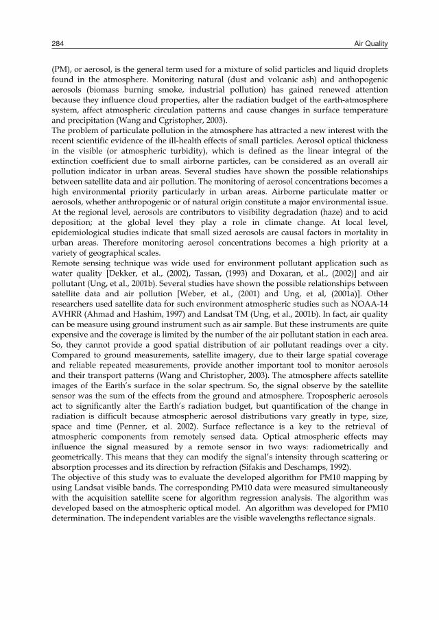
Fig. 1. Study area. The study area is the Penang Island, Malaysia, located within latitudes 5° 9’ N to 5° 33’ N and longitudes 100° 09’ E to 100° 30’ E (Figure 1). The map of the study area is shown in Figure 1. Penang Island is located in equatorial region and enjoys a warm equatorial weather the whole year. Therefore, it is impossible to get the 100 % cloud free satellite image over Penang Island. But, the satellite image chosen is less than 10 % of cloud coverage over the study area. Penang Island located on the northwest coast of Peninsular Malaysia.
Algorithm for air quality mapping using satellite images 285
(PM), or aerosol, is the general term used for a mixture of solid particles and liquid droplets found in the atmosphere. Monitoring natural (dust and volcanic ash) and anthopogenic aerosols (biomass burning smoke, industrial pollution) has gained renewed attention because they influence cloud properties, alter the radiation budget of the earth-atmosphere system, affect atmospheric circulation patterns and cause changes in surface temperature and precipitation (Wang and Cgristopher, 2003). The problem of particulate pollution in the atmosphere has attracted a new interest with the recent scientific evidence of the ill-health effects of small particles. Aerosol optical thickness in the visible (or atmospheric turbidity), which is defined as the linear integral of the extinction coefficient due to small airborne particles, can be considered as an overall air pollution indicator in urban areas. Several studies have shown the possible relationships between satellite data and air pollution. The monitoring of aerosol concentrations becomes a high environmental priority particularly in urban areas. Airborne particulate matter or aerosols, whether anthropogenic or of natural origin constitute a major environmental issue. At the regional level, aerosols are contributors to visibility degradation (haze) and to acid deposition; at the global level they play a role in climate change. At local level, epidemiological studies indicate that small sized aerosols are causal factors in mortality in urban areas. Therefore monitoring aerosol concentrations becomes a high priority at a variety of geographical scales. Remote sensing technique was wide used for environment pollutant application such as water quality [Dekker, et al., (2002), Tassan, (1993) and Doxaran, et al., (2002)] and air pollutant (Ung, et al., 2001b). Several studies have shown the possible relationships between satellite data and air pollution [Weber, et al., (2001) and Ung, et al, (2001a)]. Other researchers used satellite data for such environment atmospheric studies such as NOAA-14 AVHRR (Ahmad and Hashim, 1997) and Landsat TM (Ung, et al., 2001b). In fact, air quality can be measure using ground instrument such as air sample. But these instruments are quite expensive and the coverage is limited by the number of the air pollutant station in each area. So, they cannot provide a good spatial distribution of air pollutant readings over a city. Compared to ground measurements, satellite imagery, due to their large spatial coverage and reliable repeated measurements, provide another important tool to monitor aerosols and their transport patterns (Wang and Christopher, 2003). The atmosphere affects satellite images of the Earth’s surface in the solar spectrum. So, the signal observe by the satellite sensor was the sum of the effects from the ground and atmosphere. Tropospheric aerosols act to significantly alter the Earth’s radiation budget, but quantification of the change in radiation is difficult because atmospheric aerosol distributions vary greatly in type, size, space and time (Penner, et al. 2002). Surface reflectance is a key to the retrieval of atmospheric components from remotely sensed data. Optical atmospheric effects may influence the signal measured by a remote sensor in two ways: radiometrically and geometrically. This means that they can modify the signal’s intensity through scattering or absorption processes and its direction by refraction (Sifakis and Deschamps, 1992). The objective of this study was to evaluate the developed algorithm for PM10 mapping by using Landsat visible bands. The corresponding PM10 data were measured simultaneously with the acquisition satellite scene for algorithm regression analysis. The algorithm was developed based on the atmospheric optical model. An algorithm was developed for PM10 determination. The independent variables are the visible wavelengths reflectance signals.
2. Study Area
Fig. 1. Study area. The study area is the Penang Island, Malaysia, located within latitudes 5° 9’ N to 5° 33’ N and longitudes 100° 09’ E to 100° 30’ E (Figure 1). The map of the study area is shown in Figure 1. Penang Island is located in equatorial region and enjoys a warm equatorial weather the whole year. Therefore, it is impossible to get the 100 % cloud free satellite image over Penang Island. But, the satellite image chosen is less than 10 % of cloud coverage over the study area. Penang Island located on the northwest coast of Peninsular Malaysia.
Air Quality286
Penang is one of the 13 states of the Malaysia and the second smallest state in Malaysia after Perlis. The state is geographically divided into two different entities - Penang Island (or “Pulau Pinang” in Malay Language) and a portion of mainland called “Seberang Perai” in Malay Language. Penang Island is an island of 293 square kilometres located in the Straits of Malacca and “Seberang Perai” is a narrow hinterland of 753 square kilometres (Penang-Wikipedia, 2009). The island and the mainland are linked by the 13.5 km long Penang Bridge and ferry. Penang Island is predominantly hilly terrain, the highest point being Western Hill (part of Penang Hill) at 830 metres above sea level. The terrain consists of coastal plains, hills and mountains. The coastal plains are narrow, the most extensive of which is in the northeast which forms a triangular promontory where George Town, the state capital, is situated. The topography of “Seberang Perai” is mostly flat. Butterworth, the main town in “Seberang Perai”, lies along the “Perai” River estuary and faces George Town at a distance of 3 km (2 miles) across the channel to the east (Penang-Wikipedia, 2009). The Penang Island climate is tropical, and it is hot and humid throughout the year. with the average mean daily temperature of about 27oC and mean daily maximum and minimum temperature ranging between 31.4oC and 23.5oC respectively. However, the individual extremes are 35.7oC and 23.5oC respectively. The mean daily humidity varies between 60.9% and 96.8%. The average annual rainfall is about 267 cm and can be as high as 624 cm (Fauziah, et al, 2006).
3. Algorithm Model
The atmospheric reflectance due to molecule, Rr, is given by (Liu, et al., 1996)
vs
rrr
PR
4
)( (1)
where τr = Aerosol optical thickness (Molecule) Pr( ) = Rayleigh scattering phase function µv = Cosine of viewing angle µs = Cosine of solar zenith angle We assume that the atmospheric reflectance due to particle, Ra, is also linear with the τa
[King, et al., (1999) and Fukushima, et al., (2000)]. This assumption is reasonable because other researchers also found the linear relationship between both aerosol and molecule scattering (Liu, et al., 1996).
vs
aaa
PR
4
)( (2)
where τa = Aerosol optical thickness (aerosol) Pa( ) = Aerosol scattering phase function Atmospheric reflectance is the sum of the particle reflectance and molecule reflectance, Ratm, (Vermote, et al., (1997).
Ratm=Ra+Rr (3) where Ratm=atmospheric reflectance Rp=particle reflectance Rr=molecule reflectance
vs
rr
vs
aaatm
PKPR
4
)(4
)(1
)()(41
rraavs
atm PPR
(4)
The optical depth is given by other researcher as in equation (5) (Camagni and Sandroni, 1983). From the equation, we rewrite the optical depth for particle and molecule as s (5) where τ = optical depth σ = absorption s= finite path ra (Camagni and Sandroni, 1983)
srrr (6a)
sppp (6b)
Equations (6) are substituted into equation (4). The result was extended to a three bands algorithm as equation (8). Form the equation; we found that PM10 was linearly related to the reflectance for band 1 and band 2. This algorithm was generated based on the linear relationship between τ and reflectance. Other Researcher also found that the PM10 was linearly related to the τ and the correlation coefficient for linear was better that exponential in their study (overall) (Retalis et al., 2003). This means that reflectance was linear with the PM10. In order to simplify the data processing, the air quality concentration was used in our analysis instead of using density, ρ, values.
)()(41
rrraaavs
atm sPsPR
)()(4
rrraaavs
atm PPsR
Algorithm for air quality mapping using satellite images 287
Penang is one of the 13 states of the Malaysia and the second smallest state in Malaysia after Perlis. The state is geographically divided into two different entities - Penang Island (or “Pulau Pinang” in Malay Language) and a portion of mainland called “Seberang Perai” in Malay Language. Penang Island is an island of 293 square kilometres located in the Straits of Malacca and “Seberang Perai” is a narrow hinterland of 753 square kilometres (Penang-Wikipedia, 2009). The island and the mainland are linked by the 13.5 km long Penang Bridge and ferry. Penang Island is predominantly hilly terrain, the highest point being Western Hill (part of Penang Hill) at 830 metres above sea level. The terrain consists of coastal plains, hills and mountains. The coastal plains are narrow, the most extensive of which is in the northeast which forms a triangular promontory where George Town, the state capital, is situated. The topography of “Seberang Perai” is mostly flat. Butterworth, the main town in “Seberang Perai”, lies along the “Perai” River estuary and faces George Town at a distance of 3 km (2 miles) across the channel to the east (Penang-Wikipedia, 2009). The Penang Island climate is tropical, and it is hot and humid throughout the year. with the average mean daily temperature of about 27oC and mean daily maximum and minimum temperature ranging between 31.4oC and 23.5oC respectively. However, the individual extremes are 35.7oC and 23.5oC respectively. The mean daily humidity varies between 60.9% and 96.8%. The average annual rainfall is about 267 cm and can be as high as 624 cm (Fauziah, et al, 2006).
3. Algorithm Model
The atmospheric reflectance due to molecule, Rr, is given by (Liu, et al., 1996)
vs
rrr
PR
4
)( (1)
where τr = Aerosol optical thickness (Molecule) Pr( ) = Rayleigh scattering phase function µv = Cosine of viewing angle µs = Cosine of solar zenith angle We assume that the atmospheric reflectance due to particle, Ra, is also linear with the τa
[King, et al., (1999) and Fukushima, et al., (2000)]. This assumption is reasonable because other researchers also found the linear relationship between both aerosol and molecule scattering (Liu, et al., 1996).
vs
aaa
PR
4
)( (2)
where τa = Aerosol optical thickness (aerosol) Pa( ) = Aerosol scattering phase function Atmospheric reflectance is the sum of the particle reflectance and molecule reflectance, Ratm, (Vermote, et al., (1997).
Ratm=Ra+Rr (3) where Ratm=atmospheric reflectance Rp=particle reflectance Rr=molecule reflectance
vs
rr
vs
aaatm
PKPR
4
)(4
)(1
)()(41
rraavs
atm PPR
(4)
The optical depth is given by other researcher as in equation (5) (Camagni and Sandroni, 1983). From the equation, we rewrite the optical depth for particle and molecule as s (5) where τ = optical depth σ = absorption s= finite path ra (Camagni and Sandroni, 1983)
srrr (6a)
sppp (6b)
Equations (6) are substituted into equation (4). The result was extended to a three bands algorithm as equation (8). Form the equation; we found that PM10 was linearly related to the reflectance for band 1 and band 2. This algorithm was generated based on the linear relationship between τ and reflectance. Other Researcher also found that the PM10 was linearly related to the τ and the correlation coefficient for linear was better that exponential in their study (overall) (Retalis et al., 2003). This means that reflectance was linear with the PM10. In order to simplify the data processing, the air quality concentration was used in our analysis instead of using density, ρ, values.
)()(41
rrraaavs
atm sPsPR
)()(4
rrraaavs
atm PPsR
Air Quality288
),()(),()(4
)( 11111
rraavs
atm GPPPsR
),()(),()(4
)( 22222
rraavs
atm GPPPsR
)()( 2110 atmatm RaRaP (7) The equation (8) was for two bands, so we rewrite the PM10 equation in three bands as )()()( 322110 atmatmatm RaRaRaP (8) Where P = Particle concentration (PM10) G = Molecule concentration Ratmi= Atmospheric reflectance, i = 0, 1 and 3 are the number of the band ej= algorithm coefficient, j = 0, 1, 2, … (empirically determined).
4. Data Analysis and Results
Remote sensing satellite detectors exhibit linear response to incoming radiance, whether from the Earth’s surface radiance or internal calibration sources. This response is quantized into 8-bit values that represent brightness values commonly called Digital Numbers (DN). To convert the calibrated digital numbers to at-aperture radiance, rescaling gains and biases are created from the known dynamic range limits of the instrument. Radiance, L (λ) = Bias (λ) + [Gain (λ) x DN (λ)] (9) where λ = band number. L is the radiance expressed in Wm-2 sr-1m-1. The spectral radiance, as calculated above, can be converted to at sensor reflectance values.
2*
0
L( )( )cos
dE
(10)
Where ρ* = Sensor Reflectance values L () = Apparent At-Sensor Radiance (Wm-2 sr-1m-1) d = Earth-Sun distance in astronomical units
= {1.0-0.016729cos [0.9856(D-4)]} where (D = day of the year) E°() = mean solar exoatmospheric irradiance (Wm-2 sr-1m-1) θ = solar Zenith angle (degrees)
The retrieval of surface reflectance is important to obtain the atmospheric reflectance in remotely sensed data and later used for algorithm calibration. In this study, we retrieve the surface reflectance using the relationship between the two visible bands (blue and red) and the mid infrared data at 2.1 µm. We use the assumption that the mid infrared band data is not significantly affected by atmospheric haze. An algorithm was developed based on the aerosol properties to correlate the atmospheric reflectance and PM10. The surface reflectance can be obtained from mid-infrared band because the surface reflectances at various bands across the solar spectrum are correlated to each other to some extend. The surface reflectances of dark targets in the blue and red bands were estimated using the measurements in the mid-infrared band (Quaidrari and Vermote, 1999). Over a simple black target, the observed atmospheric reflectance is the sum of reflectance of aerosols and Rayleigh contributions (Equation 9). This simplification, however, is not valid at short wavelengths (less than 0.45 pm) or large sun and view zenith angles (Vermote and Roger, 1996). In this study, a simple form of the equation was used in this study (Equation 11). This equation also used by other research in their study (Popp, 2004). Rs – TRr = Ratm (11) Rs – Rr = Ratm (12) where: Rs = reflectance recorded by satellite sensor Rr = reflectance from surface references Ratm = reflectance from atmospheric components (aerosols and molecules) T = transmittance
The surface reflectance in mid-infrared band is related to those in the visible bands. The surface reflectances were measured using a handheld spectroradiometer in the wavelength range of visible wavelengths (red and blue bands). The surface reflectances of dark targets in the visible bands are as follows:
ρ (TM1) = ρ (TM7)/3.846
ρ (TM3) = ρ (TM7)/1.923 (13)
Algorithm for air quality mapping using satellite images 289
),()(),()(4
)( 11111
rraavs
atm GPPPsR
),()(),()(4
)( 22222
rraavs
atm GPPPsR
)()( 2110 atmatm RaRaP (7) The equation (8) was for two bands, so we rewrite the PM10 equation in three bands as )()()( 322110 atmatmatm RaRaRaP (8) Where P = Particle concentration (PM10) G = Molecule concentration Ratmi= Atmospheric reflectance, i = 0, 1 and 3 are the number of the band ej= algorithm coefficient, j = 0, 1, 2, … (empirically determined).
4. Data Analysis and Results
Remote sensing satellite detectors exhibit linear response to incoming radiance, whether from the Earth’s surface radiance or internal calibration sources. This response is quantized into 8-bit values that represent brightness values commonly called Digital Numbers (DN). To convert the calibrated digital numbers to at-aperture radiance, rescaling gains and biases are created from the known dynamic range limits of the instrument. Radiance, L (λ) = Bias (λ) + [Gain (λ) x DN (λ)] (9) where λ = band number. L is the radiance expressed in Wm-2 sr-1m-1. The spectral radiance, as calculated above, can be converted to at sensor reflectance values.
2*
0
L( )( )cos
dE
(10)
Where ρ* = Sensor Reflectance values L () = Apparent At-Sensor Radiance (Wm-2 sr-1m-1) d = Earth-Sun distance in astronomical units
= {1.0-0.016729cos [0.9856(D-4)]} where (D = day of the year) E°() = mean solar exoatmospheric irradiance (Wm-2 sr-1m-1) θ = solar Zenith angle (degrees)
The retrieval of surface reflectance is important to obtain the atmospheric reflectance in remotely sensed data and later used for algorithm calibration. In this study, we retrieve the surface reflectance using the relationship between the two visible bands (blue and red) and the mid infrared data at 2.1 µm. We use the assumption that the mid infrared band data is not significantly affected by atmospheric haze. An algorithm was developed based on the aerosol properties to correlate the atmospheric reflectance and PM10. The surface reflectance can be obtained from mid-infrared band because the surface reflectances at various bands across the solar spectrum are correlated to each other to some extend. The surface reflectances of dark targets in the blue and red bands were estimated using the measurements in the mid-infrared band (Quaidrari and Vermote, 1999). Over a simple black target, the observed atmospheric reflectance is the sum of reflectance of aerosols and Rayleigh contributions (Equation 9). This simplification, however, is not valid at short wavelengths (less than 0.45 pm) or large sun and view zenith angles (Vermote and Roger, 1996). In this study, a simple form of the equation was used in this study (Equation 11). This equation also used by other research in their study (Popp, 2004). Rs – TRr = Ratm (11) Rs – Rr = Ratm (12) where: Rs = reflectance recorded by satellite sensor Rr = reflectance from surface references Ratm = reflectance from atmospheric components (aerosols and molecules) T = transmittance
The surface reflectance in mid-infrared band is related to those in the visible bands. The surface reflectances were measured using a handheld spectroradiometer in the wavelength range of visible wavelengths (red and blue bands). The surface reflectances of dark targets in the visible bands are as follows:
ρ (TM1) = ρ (TM7)/3.846
ρ (TM3) = ρ (TM7)/1.923 (13)
Air Quality290
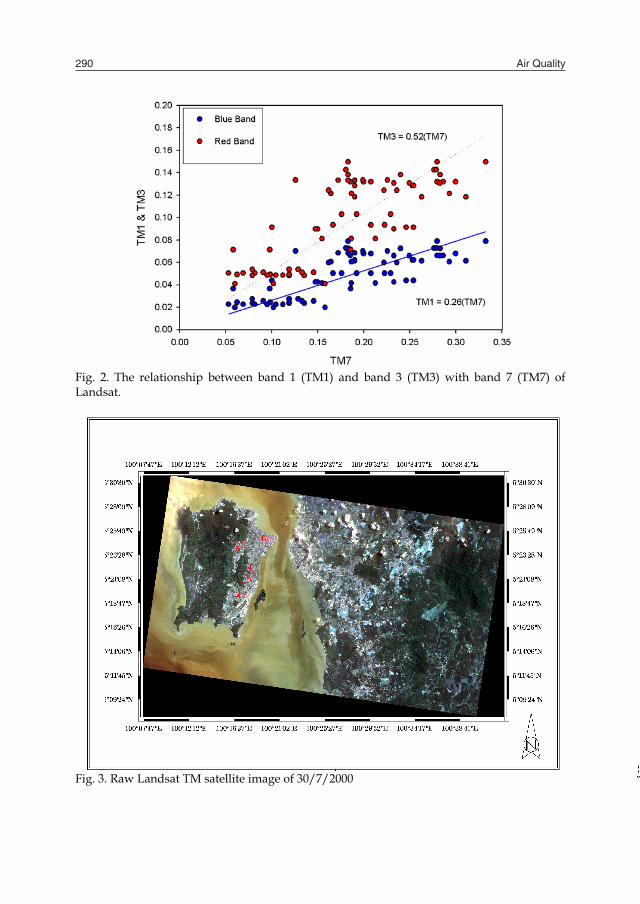
Fig. 2. The relationship between band 1 (TM1) and band 3 (TM3) with band 7 (TM7) of Landsat.
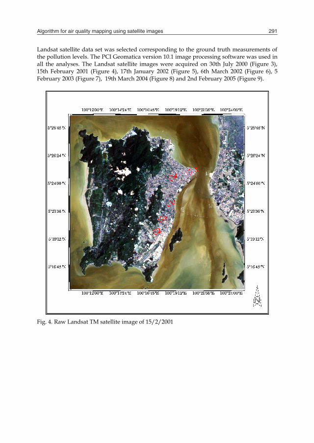
Fig. 3. Raw Landsat TM satellite image of 30/7/2000
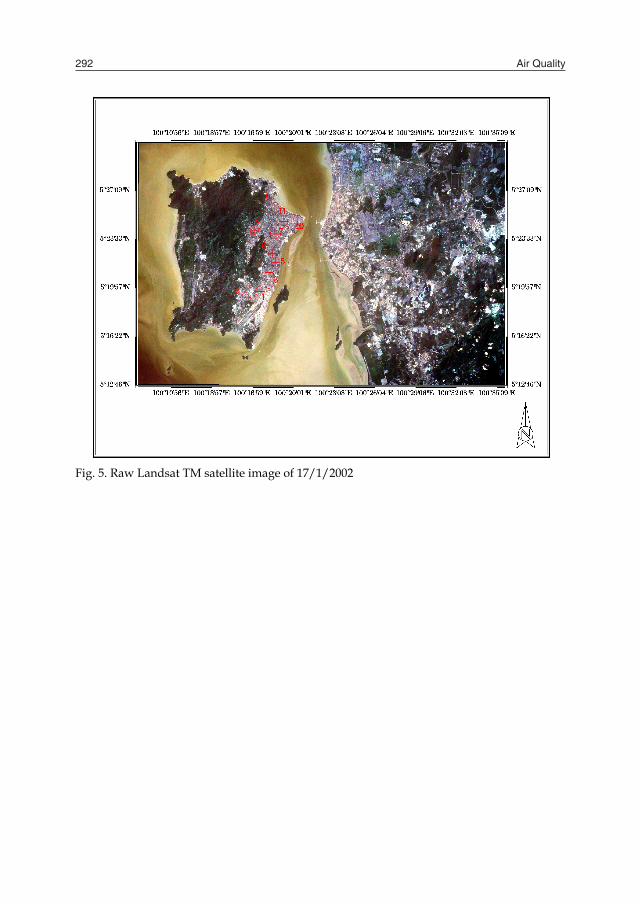
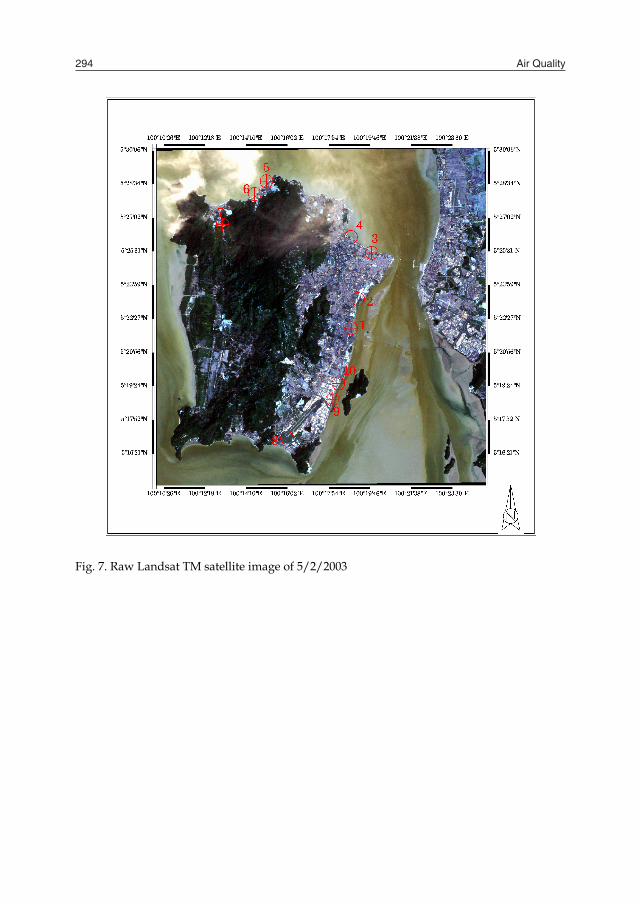
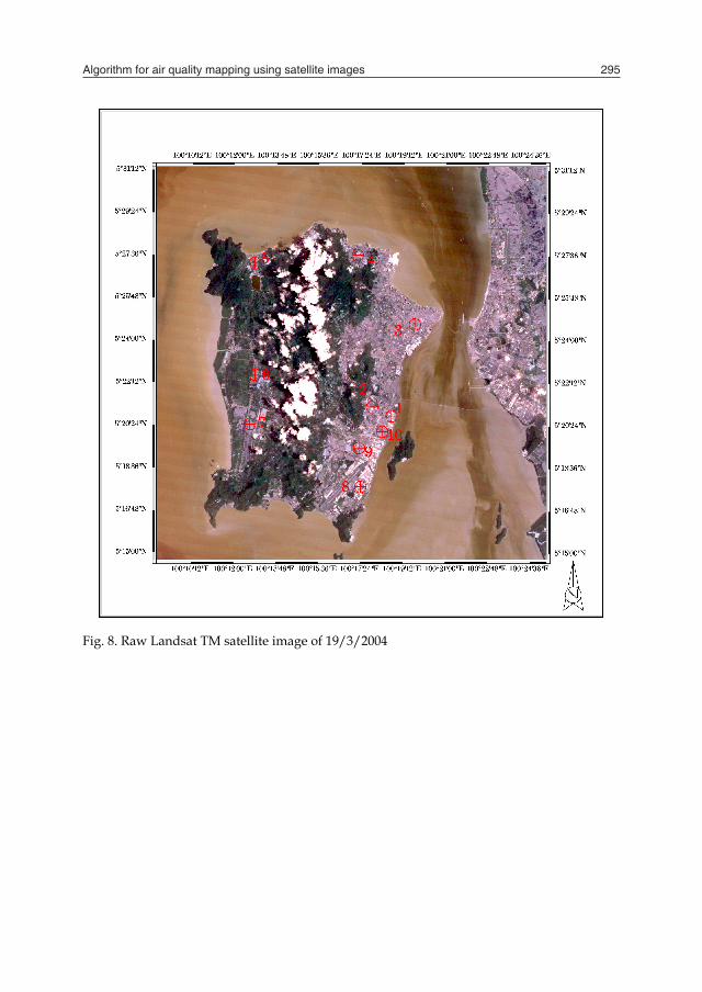
Landsat satellite data set was selected corresponding to the ground truth measurements of the pollution levels. The PCI Geomatica version 10.1 image processing software was used in all the analyses. The Landsat satellite images were acquired on 30th July 2000 (Figure 3), 15th February 2001 (Figure 4), 17th January 2002 (Figure 5), 6th March 2002 (Figure 6), 5 February 2003 (Figure 7), 19th March 2004 (Figure 8) and 2nd February 2005 (Figure 9).
Fig. 4. Raw Landsat TM satellite image of 15/2/2001
Algorithm for air quality mapping using satellite images 291
Fig. 2. The relationship between band 1 (TM1) and band 3 (TM3) with band 7 (TM7) of Landsat.
Fig. 3. Raw Landsat TM satellite image of 30/7/2000
Landsat satellite data set was selected corresponding to the ground truth measurements of the pollution levels. The PCI Geomatica version 10.1 image processing software was used in all the analyses. The Landsat satellite images were acquired on 30th July 2000 (Figure 3), 15th February 2001 (Figure 4), 17th January 2002 (Figure 5), 6th March 2002 (Figure 6), 5 February 2003 (Figure 7), 19th March 2004 (Figure 8) and 2nd February 2005 (Figure 9).
Fig. 4. Raw Landsat TM satellite image of 15/2/2001
Air Quality292
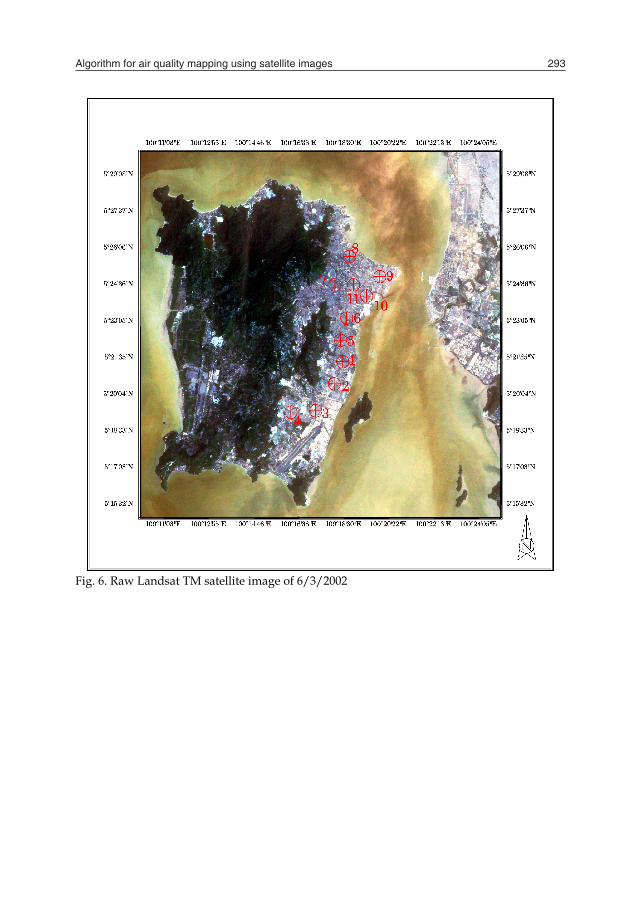
Fig. 5. Raw Landsat TM satellite image of 17/1/2002
Fig. 6. Raw Landsat TM satellite image of 6/3/2002
Algorithm for air quality mapping using satellite images 293
Fig. 5. Raw Landsat TM satellite image of 17/1/2002
Fig. 6. Raw Landsat TM satellite image of 6/3/2002
Air Quality294
Fig. 7. Raw Landsat TM satellite image of 5/2/2003
Fig. 8. Raw Landsat TM satellite image of 19/3/2004
Algorithm for air quality mapping using satellite images 295
Fig. 7. Raw Landsat TM satellite image of 5/2/2003
Fig. 8. Raw Landsat TM satellite image of 19/3/2004
Air Quality296
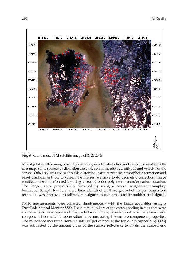
Fig. 9. Raw Landsat TM satellite image of 2/2/2005
Raw digital satellite images usually contain geometric distortion and cannot be used directly as a map. Some sources of distortion are variation in the altitude, attitude and velocity of the sensor. Other sources are panoramic distortion, earth curvature, atmospheric refraction and relief displacement. So, to correct the images, we have to do geometric correction. Image rectification was performed by using a second order polynomial transformation equation. The images were geometrically corrected by using a nearest neighbour resampling technique. Sample locations were then identified on these geocoded images. Regression technique was employed to calibrate the algorithm using the satellite multispectral signals. PM10 measurements were collected simultaneously with the image acquisition using a DustTrak Aerosol Monitor 8520. The digital numbers of the corresponding in situ data were converted into irradiance and then reflectance. Our approach to retrieve the atmospheric component from satellite observation is by measuring the surface component properties. The reflectance measured from the satellite [reflectance at the top of atmospheric, (TOA)] was subtracted by the amount given by the surface reflectance to obtain the atmospheric
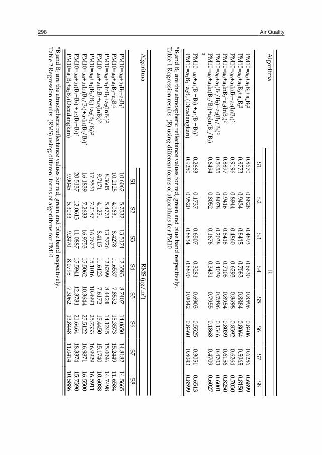
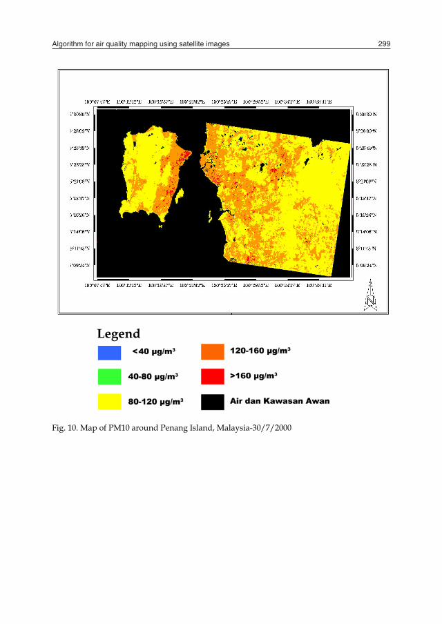
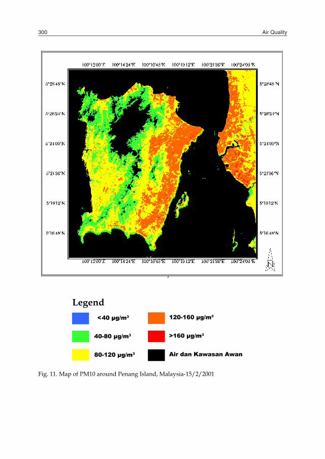
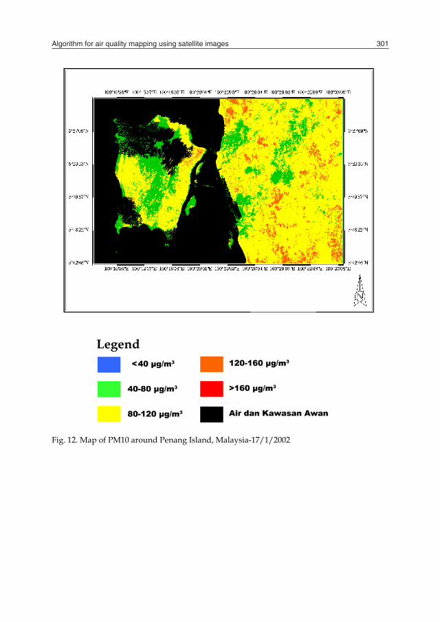
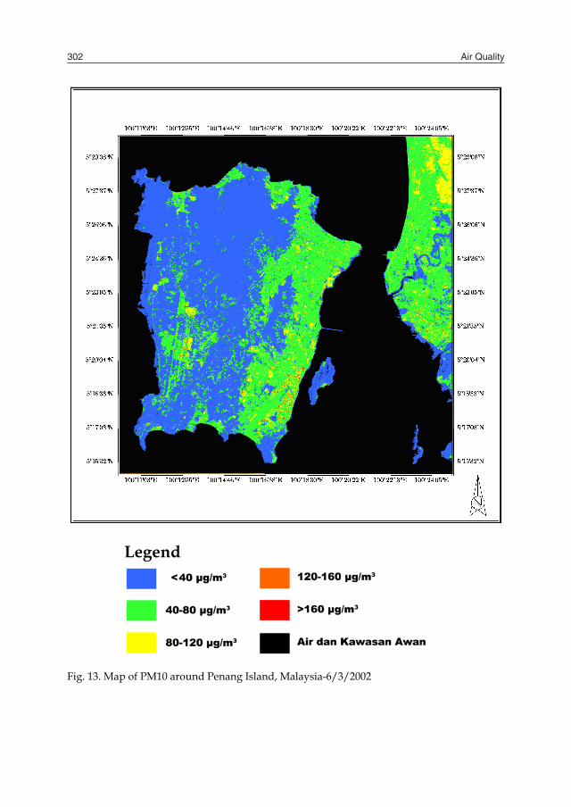
reflectance. And then the atmospheric reflectance was related to the PM10 using the regression algorithm analysis. For each visible band, the dark target surface reflectance was estimated from that of the mid-infrared band. The atmospheric reflectance values were extracted from the satellite observation reflectance values subtracted by the amount given by the surface reflectance. The atmospheric reflectance were determined for each band using different window sizes, such as, 1 by 1, 3 by 3, 5 by 5, 7 by 7, 9 by 9 and 11 by 11. In this study, the atmospheric reflectance values extracted using the window size of 3 by 3 was used due to the higher correlation coefficient (R) with the ground-truth data. The atmospheric reflectance values for the visible bands of TM1 and TM3 were extracted corresponding to the locations of in situ PM10 data. The relationship between the reflectance and the corresponding air quality data was determined using regression analysis. A new algorithm was developed for detecting air pollution from the digital images chosen based on the highest correlation coefficient, R and lowest root mean square error, RMS for PM10. The algorithm was used to correlate atmospheric reflectance and the PM10 values. The proposed algorithm produced high correlation coefficient (R) and low root-mean-square error (RMS) between the measured and estimated PM10 values. Finally, PM10 maps were generated using the proposed algorithm. This study indicates the potential of Landsat for PM10 mapping. The data points were then regressed to obtain all the coefficients of equation (8). Then the calibrated algorithm was used to estimate the PM10 concentrated values for each image. The proposed model produced the correlation coefficient of 0.83 and root-mean-square error 18 μg/m3. The PM10 maps were generated using the proposed calibrated algorithm. The generated PM10 map was colour-coded for visual interpretation [Figures 10 - 16]. Generally, the concentrations above industrial and urban areas were higher compared to other areas.
Algorithm for air quality mapping using satellite images 297
Fig. 9. Raw Landsat TM satellite image of 2/2/2005
Raw digital satellite images usually contain geometric distortion and cannot be used directly as a map. Some sources of distortion are variation in the altitude, attitude and velocity of the sensor. Other sources are panoramic distortion, earth curvature, atmospheric refraction and relief displacement. So, to correct the images, we have to do geometric correction. Image rectification was performed by using a second order polynomial transformation equation. The images were geometrically corrected by using a nearest neighbour resampling technique. Sample locations were then identified on these geocoded images. Regression technique was employed to calibrate the algorithm using the satellite multispectral signals. PM10 measurements were collected simultaneously with the image acquisition using a DustTrak Aerosol Monitor 8520. The digital numbers of the corresponding in situ data were converted into irradiance and then reflectance. Our approach to retrieve the atmospheric component from satellite observation is by measuring the surface component properties. The reflectance measured from the satellite [reflectance at the top of atmospheric, (TOA)] was subtracted by the amount given by the surface reflectance to obtain the atmospheric
reflectance. And then the atmospheric reflectance was related to the PM10 using the regression algorithm analysis. For each visible band, the dark target surface reflectance was estimated from that of the mid-infrared band. The atmospheric reflectance values were extracted from the satellite observation reflectance values subtracted by the amount given by the surface reflectance. The atmospheric reflectance were determined for each band using different window sizes, such as, 1 by 1, 3 by 3, 5 by 5, 7 by 7, 9 by 9 and 11 by 11. In this study, the atmospheric reflectance values extracted using the window size of 3 by 3 was used due to the higher correlation coefficient (R) with the ground-truth data. The atmospheric reflectance values for the visible bands of TM1 and TM3 were extracted corresponding to the locations of in situ PM10 data. The relationship between the reflectance and the corresponding air quality data was determined using regression analysis. A new algorithm was developed for detecting air pollution from the digital images chosen based on the highest correlation coefficient, R and lowest root mean square error, RMS for PM10. The algorithm was used to correlate atmospheric reflectance and the PM10 values. The proposed algorithm produced high correlation coefficient (R) and low root-mean-square error (RMS) between the measured and estimated PM10 values. Finally, PM10 maps were generated using the proposed algorithm. This study indicates the potential of Landsat for PM10 mapping. The data points were then regressed to obtain all the coefficients of equation (8). Then the calibrated algorithm was used to estimate the PM10 concentrated values for each image. The proposed model produced the correlation coefficient of 0.83 and root-mean-square error 18 μg/m3. The PM10 maps were generated using the proposed calibrated algorithm. The generated PM10 map was colour-coded for visual interpretation [Figures 10 - 16]. Generally, the concentrations above industrial and urban areas were higher compared to other areas.
Air Quality298
Algoritm
a R
S1 S2
S3 S4
S5 S6
S7 S8
PM10=a
0 +a1 B
1 +a2 B
1 2 0.8670
0.8828 0.4893
0.6630 0.8596
0.8406 0.6256
0.6899 PM
10=a0 +a
1 B3 +a
2 B3 2
0.8773 0.9434
0.8415 0.7083
0.8884 0.8064
0.5965 0.8150
PM10=a
0 +a1 lnB
1 +a2 (lnB
1 ) 2 0.9196
0.8944 0.4860
0.6293 0.8698
0.8392 0.6264
0.7030 PM
10=a0 +a
1 lnB3 +a
2 (lnB3 ) 2
0.8897 0.9416
0.8418 0.7108
0.8954 0.8039
0.6156 0.8250
PM10=a
0 +a1 (B
1 /B3 )+a
2 (B1 /B
3 ) 2 0.5655
0.8078 0.2038
0.4039 0.7896
0.1346 0.4703
0.6001 PM
10=a0 +a
1 ln(B1 /B
3 )+a2 ln(B
1 /B3 )
2 0.6494
0.8052 0.1676
0.3431 0.7955
0.1868 0.4709
0.6027
PM10=a
0 +a1 (B
1 −B3 ) +a
2 (B1 −B
3 ) 2 0.2663
0.1737 0.6507
0.3281 0.6903
0.5525 0.3051
0.6513 PM
10=a1 B
1 +a2 B
3 (Dicadangkan)
0.9250 0.9520
0.8834 0.8890
0.9042 0.8460
0.8043 0.8599
*B1 and B
3 are the atmospheric reflectance values for red, green and blue band respectively.
Table 1 Regression results (R) using different forms of algorithm
s for PM10
Algoritm
a RM
S (µg/m3)
S1 S2
S3 S4
S5 S6
S7 S8
PM10=a
0 +a1 B
1 +a2 B
1 2 10.6062
5.7532 13.5174
12.3583 8.7407
14.0650 14.8182
14.5665 PM
10=a0 +a
1 B3 +a
2 B3 2
10.2125 4.0631
8.4278 11.6537
7.8532 15.3573
15.2449 11.6584
PM10=a
0 +a1 lnB
1 +a2 (lnB
1 ) 2 8.3605
5.4773 13.5726
12.8299 8.4424
14.1245 15.0096
14.7498 PM
10=a0 +a
1 lnB3 +a
2 (lnB3 ) 2
9.7171 4.1251
8.4115 11.6123
7.6172 15.4450
15.1740 10.6088
PM10=a
0 +a1 (B
1 /B3 )+a
2 (B1 /B
3 ) 2 17.5531
7.2187 16.7673
15.1016 10.4991
25.7333 16.9929
16.5911 PM
10=a0 +a
1 ln(B1 /B
3 )+a2 ln(B
1 /B3 ) 2
16.1839 7.2633
16.9753 15.5062
10.3644 25.5122
16.9871 16.5500
PM10=a
0 +a1 (B
1 −B3 ) +a
2 (B1 −B
3 ) 2 20.5137
12.0613 11.0887
15.5941 12.3781
21.6464 18.3374
15.7390 PM
10=a1 B
1 +a2 B
3 (Dicadangkan)
9.9045 5.3033
9.2470 8.0795
7.3062 13.8448
11.0414 10.5886
*B1 and B
3 are the atmospheric reflectance values for red, green and blue band respectively.
Table 2 Regression results (RMS) using different form
s of algorithms for PM
10
Fig. 10. Map of PM10 around Penang Island, Malaysia-30/7/2000
Legend
Algorithm for air quality mapping using satellite images 299
Algoritm
a R
S1 S2
S3 S4
S5 S6
S7 S8
PM10=a
0 +a1 B
1 +a2 B
1 2 0.8670
0.8828 0.4893
0.6630 0.8596
0.8406 0.6256
0.6899 PM
10=a0 +a
1 B3 +a
2 B3 2
0.8773 0.9434
0.8415 0.7083
0.8884 0.8064
0.5965 0.8150
PM10=a
0 +a1 lnB
1 +a2 (lnB
1 ) 2 0.9196
0.8944 0.4860
0.6293 0.8698
0.8392 0.6264
0.7030 PM
10=a0 +a
1 lnB3 +a
2 (lnB3 ) 2
0.8897 0.9416
0.8418 0.7108
0.8954 0.8039
0.6156 0.8250
PM10=a
0 +a1 (B
1 /B3 )+a
2 (B1 /B
3 ) 2 0.5655
0.8078 0.2038
0.4039 0.7896
0.1346 0.4703
0.6001 PM
10=a0 +a
1 ln(B1 /B
3 )+a2 ln(B
1 /B3 )
2 0.6494
0.8052 0.1676
0.3431 0.7955
0.1868 0.4709
0.6027
PM10=a
0 +a1 (B
1 −B3 ) +a
2 (B1 −B
3 ) 2 0.2663
0.1737 0.6507
0.3281 0.6903
0.5525 0.3051
0.6513 PM
10=a1 B
1 +a2 B
3 (Dicadangkan)
0.9250 0.9520
0.8834 0.8890
0.9042 0.8460
0.8043 0.8599
*B1 and B
3 are the atmospheric reflectance values for red, green and blue band respectively.
Table 1 Regression results (R) using different forms of algorithm
s for PM10
Algoritm
a RM
S (µg/m3)
S1 S2
S3 S4
S5 S6
S7 S8
PM10=a
0 +a1 B
1 +a2 B
1 2 10.6062
5.7532 13.5174
12.3583 8.7407
14.0650 14.8182
14.5665 PM
10=a0 +a
1 B3 +a
2 B3 2
10.2125 4.0631
8.4278 11.6537
7.8532 15.3573
15.2449 11.6584
PM10=a
0 +a1 lnB
1 +a2 (lnB
1 ) 2 8.3605
5.4773 13.5726
12.8299 8.4424
14.1245 15.0096
14.7498 PM
10=a0 +a
1 lnB3 +a
2 (lnB3 ) 2
9.7171 4.1251
8.4115 11.6123
7.6172 15.4450
15.1740 10.6088
PM10=a
0 +a1 (B
1 /B3 )+a
2 (B1 /B
3 ) 2 17.5531
7.2187 16.7673
15.1016 10.4991
25.7333 16.9929
16.5911 PM
10=a0 +a
1 ln(B1 /B
3 )+a2 ln(B
1 /B3 ) 2
16.1839 7.2633
16.9753 15.5062
10.3644 25.5122
16.9871 16.5500
PM10=a
0 +a1 (B
1 −B3 ) +a
2 (B1 −B
3 ) 2 20.5137
12.0613 11.0887
15.5941 12.3781
21.6464 18.3374
15.7390 PM
10=a1 B
1 +a2 B
3 (Dicadangkan)
9.9045 5.3033
9.2470 8.0795
7.3062 13.8448
11.0414 10.5886
*B1 and B
3 are the atmospheric reflectance values for red, green and blue band respectively.
Table 2 Regression results (RMS) using different form
s of algorithms for PM
10
Fig. 10. Map of PM10 around Penang Island, Malaysia-30/7/2000
Legend
Air Quality300
Fig. 11. Map of PM10 around Penang Island, Malaysia-15/2/2001
Legend
Fig. 12. Map of PM10 around Penang Island, Malaysia-17/1/2002
Legend
Algorithm for air quality mapping using satellite images 301
Fig. 11. Map of PM10 around Penang Island, Malaysia-15/2/2001
Legend
Fig. 12. Map of PM10 around Penang Island, Malaysia-17/1/2002
Legend
Air Quality302
Fig. 13. Map of PM10 around Penang Island, Malaysia-6/3/2002
Legend
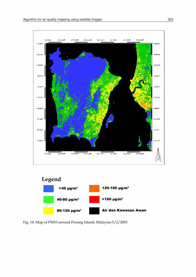
Fig. 14. Map of PM10 around Penang Island, Malaysia-5/2/2003
Legend
Algorithm for air quality mapping using satellite images 303
Fig. 13. Map of PM10 around Penang Island, Malaysia-6/3/2002
Legend
Fig. 14. Map of PM10 around Penang Island, Malaysia-5/2/2003
Legend
Air Quality304
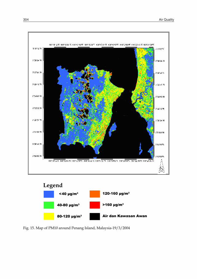
Fig. 15. Map of PM10 around Penang Island, Malaysia-19/3/2004
Legend
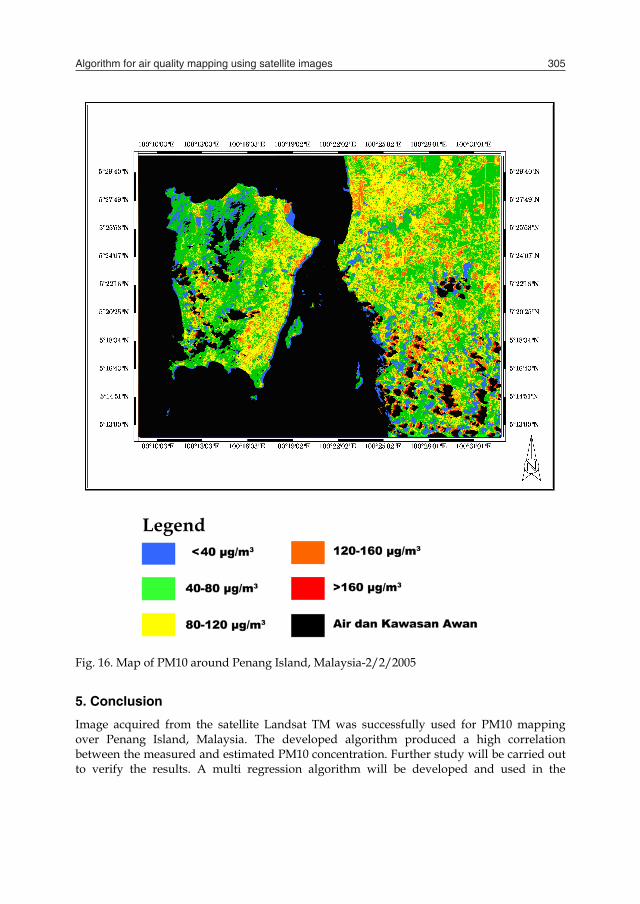
Fig. 16. Map of PM10 around Penang Island, Malaysia-2/2/2005
5. Conclusion
Image acquired from the satellite Landsat TM was successfully used for PM10 mapping over Penang Island, Malaysia. The developed algorithm produced a high correlation between the measured and estimated PM10 concentration. Further study will be carried out to verify the results. A multi regression algorithm will be developed and used in the
Legend
Algorithm for air quality mapping using satellite images 305
Fig. 15. Map of PM10 around Penang Island, Malaysia-19/3/2004
Legend
Fig. 16. Map of PM10 around Penang Island, Malaysia-2/2/2005
5. Conclusion
Image acquired from the satellite Landsat TM was successfully used for PM10 mapping over Penang Island, Malaysia. The developed algorithm produced a high correlation between the measured and estimated PM10 concentration. Further study will be carried out to verify the results. A multi regression algorithm will be developed and used in the
Legend
Air Quality306
analysis. This study had shown the feasibility of using Landsat TM imagery for air quality study.
6. Acknowledgements
This project was supported by the Ministry of Science, Technology and Innovation of Malaysia under Grant 06-01-05-SF0298 “ Environmental Mapping Using Digital Camera Imagery Taken From Autopilot Aircraft.“, supported by the Universiti Sains Malaysia under short term grant “ Digital Elevation Models (DEMs) studies for air quality retrieval from remote sensing data“. and also supported by the Ministry of Higher Education - Fundamental Research Grant Scheme (FRGS) "Simulation and Modeling of the Atmospheric Radiative Transfer of Aerosols in Penang". We would like to thank the technical staff who participated in this project. Thanks are also extended to USM for support and encouragement.
7. References
Asmala Ahmad and Mazlan Hashim, (2002). Determination of haze using NOAA-14 AVHRR satellite data, [Online] available:
http://www.gisdevelopment.net/aars/acrs/2002/czm/050.pdf Badarinath, K. V. S., Latha, K. M., Gupta, P. K., Christopher S. A. and Zhang, J., Biomass
burning aerosols characteristics and radiative forcing-a case study from eastern Ghats, India, [Online] available:
http://nsstc.uah.edu/~sundar/papers/conf/iasta_2002.pdf. Camagni. P. & Sandroni, S. (1983). Optical Remote sensing of air pollution, Joint Research
Centre, Ispra, Italy, Elsevier Science Publishing Company Inc Dekker, A. G., Vos, R. J. and Peters, S. W. M. (2002). Analytical algorithms for lakes water
TSM estimation for retrospective analyses of TM dan SPOT sensor data. International Journal of Remote Sensing, 23(1), 15−35.
Doxaran, D., Froidefond, J. M., Lavender, S. and Castaing, P. (2002). Spectral signature of highly turbid waters application with SPOT data to quantify suspended particulate matter concentrations. Remote Sensing of Environment, 81, 149−161.
Fauziah, Ahmad; Ahmad Shukri Yahaya & Mohd Ahmadullah Farooqi. (2006), Characterization and Geotechnical Properties of Penang Residual Soils with Emphasis on Landslides, American Journal of Environmental Sciences 2 (4): 121-128
Fukushima, H.; Toratani, M.; Yamamiya, S. & Mitomi, Y. (2000). Atmospheric correction algorithm for ADEOS/OCTS acean color data: performance comparison based on ship and buoy measurements. Adv. Space Res, Vol. 25, No. 5, 1015-1024
Liu, C. H.; Chen, A. J. ^ Liu, G. R. (1996). An image-based retrieval algorithm of aerosol characteristics and surface reflectance for satellite images, International Journal Of Remote Sensing, 17 (17), 3477-3500
King, M. D.; Kaufman, Y. J.; Tanre, D. & Nakajima, T. (1999). Remote sensing of tropospheric aerosold form space: past, present and future, Bulletin of the American Meteorological society, 2229-2259
Penang-Wikipedia, ( 2009). Penang, Available Online: http://en.wikipedia.org/wiki/Penang. Penner, J. E.; Zhang, S. Y.; Chin, M.; Chuang, C. C.; Feichter, J.; Feng, Y.; Geogdzhayev, I. V.;
Ginoux, P.; Herzog, M.; Higurashi, A.; Koch, D.; Land, C.; Lohmann, U.; Mishchenko, M.; Nakajima, T.; Pitari, G.; Soden, B.; Tegen, I. & Stowe, L. (2002). A Comparison of Model And Satellite-Derived Optical Depth And Reflectivity. [Online} available: http://data.engin.umich.edu/Penner/paper3.pdf
Popp, C.; Schläpfer, D.; Bojinski, S.; Schaepman, M. & Itten, K. I. (2004). Evaluation of Aerosol Mapping Methods using AVIRIS Imagery. R. Green (Editor), 13th Annual JPL Airborne Earth Science Workshop. JPL Publications, March 2004, Pasadena, CA, 10
Quaidrari, H. dan Vermote, E. F. (1999). Operational atmospheric correction of Landsat TM data, Remote Sensing Environment, 70: 4-15.
Retalis, A.; Sifakis, N.; Grosso, N.; Paronis, D. & Sarigiannis, D. (2003). Aerosol optical thickness retrieval from AVHRR images over the Athens urban area, [Online] available: http://sat2.space.noa.gr/rsensing/documents/IGARSS2003_AVHRR_ Retalisetal_web.pdf.
Sifakis, N. & Deschamps, P.Y. (1992). Mapping of air pollution using SPOT satellite data, Photogrammetric Engineering & Remote Sensing, 58(10), 1433 – 1437
Tassan, S. (1997). A numerical model for the detection of sediment concentration in stratified river plumes using Thematic Mapper data. International Journal of Remote Sensing, 18(12), 2699−2705.
UNEP Assessment Report, Part 1: The South Asian Haze: Air Pollution, Ozone And Aerosols, [Online] available:
http://www.rrcap.unep.org/issues/air/impactstudy/Part%20I.pdf. Ung, A., Weber, C., Perron, G., Hirsch, J., Kleinpeter, J., Wald, L. and Ranchin, T., 2001a. Air
Pollution Mapping Over A City – Virtual Stations And Morphological Indicators. Proceedings of 10th International Symposium “Transport and Air Pollution” September 17 - 19, 2001 – Boulder, Colorado USA. [Online] available: http://www-cenerg.cma.fr/Public/themes_de_recherche/teledetection/title_tele_air/title_tele_air_pub/air_pollution_mappin4043.
Ung, A., Wald, L., Ranchin, T., Weber, C., Hirsch, J., Perron, G. and Kleinpeter, J., 2001b. , Satellite data for Air Pollution Mapping Over A City- Virtual Stations, Proceeding of the 21th EARSeL Symposium, Observing Our Environment From Space: New Solutions For A New Millenium, Paris, France, 14 – 16 May 2001, Gerard Begni Editor, A., A., Balkema, Lisse, Abingdon, Exton (PA), Tokyo, pp. 147 – 151, [Online] available: http://www-cenerg.cma.fr/Public/themes_de_recherche/teledetection/ title_tele_air/title_tele_air_pub/satellite_data_for_t
Vermote, E. & Roger, J. C. (1996). Advances in the use of NOAA AVHRR data for land application: Radiative transfer modeling for calibration and atmospheric correction, Kluwer Academic Publishers, Dordrecht/Boston/London, 49-72
Vermote, E.; Tanre, D.; Deuze, J. L.; Herman, M. & Morcrette, J. J. (1997). 6S user guide Version 2, Second Simulation of the satellite signal in the solar spectrum (6S), [Online] available:
http://www.geog.tamu.edu/klein/geog661/handouts/6s/6smanv2.0_P1.pdf
Algorithm for air quality mapping using satellite images 307
analysis. This study had shown the feasibility of using Landsat TM imagery for air quality study.
6. Acknowledgements
This project was supported by the Ministry of Science, Technology and Innovation of Malaysia under Grant 06-01-05-SF0298 “ Environmental Mapping Using Digital Camera Imagery Taken From Autopilot Aircraft.“, supported by the Universiti Sains Malaysia under short term grant “ Digital Elevation Models (DEMs) studies for air quality retrieval from remote sensing data“. and also supported by the Ministry of Higher Education - Fundamental Research Grant Scheme (FRGS) "Simulation and Modeling of the Atmospheric Radiative Transfer of Aerosols in Penang". We would like to thank the technical staff who participated in this project. Thanks are also extended to USM for support and encouragement.
7. References
Asmala Ahmad and Mazlan Hashim, (2002). Determination of haze using NOAA-14 AVHRR satellite data, [Online] available:
http://www.gisdevelopment.net/aars/acrs/2002/czm/050.pdf Badarinath, K. V. S., Latha, K. M., Gupta, P. K., Christopher S. A. and Zhang, J., Biomass
burning aerosols characteristics and radiative forcing-a case study from eastern Ghats, India, [Online] available:
http://nsstc.uah.edu/~sundar/papers/conf/iasta_2002.pdf. Camagni. P. & Sandroni, S. (1983). Optical Remote sensing of air pollution, Joint Research
Centre, Ispra, Italy, Elsevier Science Publishing Company Inc Dekker, A. G., Vos, R. J. and Peters, S. W. M. (2002). Analytical algorithms for lakes water
TSM estimation for retrospective analyses of TM dan SPOT sensor data. International Journal of Remote Sensing, 23(1), 15−35.
Doxaran, D., Froidefond, J. M., Lavender, S. and Castaing, P. (2002). Spectral signature of highly turbid waters application with SPOT data to quantify suspended particulate matter concentrations. Remote Sensing of Environment, 81, 149−161.
Fauziah, Ahmad; Ahmad Shukri Yahaya & Mohd Ahmadullah Farooqi. (2006), Characterization and Geotechnical Properties of Penang Residual Soils with Emphasis on Landslides, American Journal of Environmental Sciences 2 (4): 121-128
Fukushima, H.; Toratani, M.; Yamamiya, S. & Mitomi, Y. (2000). Atmospheric correction algorithm for ADEOS/OCTS acean color data: performance comparison based on ship and buoy measurements. Adv. Space Res, Vol. 25, No. 5, 1015-1024
Liu, C. H.; Chen, A. J. ^ Liu, G. R. (1996). An image-based retrieval algorithm of aerosol characteristics and surface reflectance for satellite images, International Journal Of Remote Sensing, 17 (17), 3477-3500
King, M. D.; Kaufman, Y. J.; Tanre, D. & Nakajima, T. (1999). Remote sensing of tropospheric aerosold form space: past, present and future, Bulletin of the American Meteorological society, 2229-2259
Penang-Wikipedia, ( 2009). Penang, Available Online: http://en.wikipedia.org/wiki/Penang. Penner, J. E.; Zhang, S. Y.; Chin, M.; Chuang, C. C.; Feichter, J.; Feng, Y.; Geogdzhayev, I. V.;
Ginoux, P.; Herzog, M.; Higurashi, A.; Koch, D.; Land, C.; Lohmann, U.; Mishchenko, M.; Nakajima, T.; Pitari, G.; Soden, B.; Tegen, I. & Stowe, L. (2002). A Comparison of Model And Satellite-Derived Optical Depth And Reflectivity. [Online} available: http://data.engin.umich.edu/Penner/paper3.pdf
Popp, C.; Schläpfer, D.; Bojinski, S.; Schaepman, M. & Itten, K. I. (2004). Evaluation of Aerosol Mapping Methods using AVIRIS Imagery. R. Green (Editor), 13th Annual JPL Airborne Earth Science Workshop. JPL Publications, March 2004, Pasadena, CA, 10
Quaidrari, H. dan Vermote, E. F. (1999). Operational atmospheric correction of Landsat TM data, Remote Sensing Environment, 70: 4-15.
Retalis, A.; Sifakis, N.; Grosso, N.; Paronis, D. & Sarigiannis, D. (2003). Aerosol optical thickness retrieval from AVHRR images over the Athens urban area, [Online] available: http://sat2.space.noa.gr/rsensing/documents/IGARSS2003_AVHRR_ Retalisetal_web.pdf.
Sifakis, N. & Deschamps, P.Y. (1992). Mapping of air pollution using SPOT satellite data, Photogrammetric Engineering & Remote Sensing, 58(10), 1433 – 1437
Tassan, S. (1997). A numerical model for the detection of sediment concentration in stratified river plumes using Thematic Mapper data. International Journal of Remote Sensing, 18(12), 2699−2705.
UNEP Assessment Report, Part 1: The South Asian Haze: Air Pollution, Ozone And Aerosols, [Online] available:
http://www.rrcap.unep.org/issues/air/impactstudy/Part%20I.pdf. Ung, A., Weber, C., Perron, G., Hirsch, J., Kleinpeter, J., Wald, L. and Ranchin, T., 2001a. Air
Pollution Mapping Over A City – Virtual Stations And Morphological Indicators. Proceedings of 10th International Symposium “Transport and Air Pollution” September 17 - 19, 2001 – Boulder, Colorado USA. [Online] available: http://www-cenerg.cma.fr/Public/themes_de_recherche/teledetection/title_tele_air/title_tele_air_pub/air_pollution_mappin4043.
Ung, A., Wald, L., Ranchin, T., Weber, C., Hirsch, J., Perron, G. and Kleinpeter, J., 2001b. , Satellite data for Air Pollution Mapping Over A City- Virtual Stations, Proceeding of the 21th EARSeL Symposium, Observing Our Environment From Space: New Solutions For A New Millenium, Paris, France, 14 – 16 May 2001, Gerard Begni Editor, A., A., Balkema, Lisse, Abingdon, Exton (PA), Tokyo, pp. 147 – 151, [Online] available: http://www-cenerg.cma.fr/Public/themes_de_recherche/teledetection/ title_tele_air/title_tele_air_pub/satellite_data_for_t
Vermote, E. & Roger, J. C. (1996). Advances in the use of NOAA AVHRR data for land application: Radiative transfer modeling for calibration and atmospheric correction, Kluwer Academic Publishers, Dordrecht/Boston/London, 49-72
Vermote, E.; Tanre, D.; Deuze, J. L.; Herman, M. & Morcrette, J. J. (1997). 6S user guide Version 2, Second Simulation of the satellite signal in the solar spectrum (6S), [Online] available:
http://www.geog.tamu.edu/klein/geog661/handouts/6s/6smanv2.0_P1.pdf

Air Quality308
Weber, C., Hirsch, J., Perron, G., Kleinpeter, J., Ranchin, T., Ung, A. and Wald, L. 2001. Urban Morphology, Remote Sensing and Pollutants Distribution: An Application To The City of Strasbourg, France. International Union of Air Pollution Prevention and Environmental Protection Associations (IUAPPA) Symposium and Korean Society for Atmospheric Environment (KOSAE) Symposium, 12th World Clean Air & Environment Congress, Greening the New Millennium, 26 – 31 August 2001, Seoul, Korea. [Online] available: http://www-cenerg.cma.fr/Public/themes_de_recherche/ teledetection/title_tele_air/title_tele_air_pub/paper_urban_morpho.
Wang, J. and Christopher, S. A., (2003) Intercomparison between satellite-derived aerosol optical thickness and PM2.5 mass: Implications for air quality studies, Geophysics Research Letters, 30 (21).
Copyright © 2022 FDOKUMEN