1

GROWING AT THE PRODUCTION FRONTIER

EUROPEAN AGGREGATE GROWTH, 1870-19141

Albert Carreras (Universitat Pompeu Fabra) Camilla Josephson (Lund University)

INTRODUCTION: FROM MARX TO MARSHALL –AND LENIN. The dominant views on the performance of the British and European economy during the first half of the nineteenth century were quite pessimistic. Growth was considered difficult to achieve. The conflict over distribution was perceived as fundamental, be it between landowners and the rest of the society, or between factory owners and workers. In his famous Das Kapital as well as in many other writings Karl Marx insisted in the inevitable decline of real wages. The discussions about what was to be known as the Industrial Revolution and the decline or not in real wages were heated during those years, and have been so since then. They are, in many ways, the permanent appeal of the phenomenon across the disciplines and sensitivities –is economic growth worth the increase in inequality? Sometime during the 1860s there was a change in intellectual mood. Social conflict, polarization and the fight over income distribution were no more the only possible outcome of economic life. There were cases of countries –mostly all the developed world- that were able to provide increased incomes to all the population. There was economic growth without any single individual (or social group) paying a penalty for it. Growth was being diffused to the whole national economy. An increasing number of economies were enjoying this kind of growth. The world that Stanley Jevons, Karl Menger, Léon Walras and, a bit later on, Alfred Marshall were describing was the world whose economic performance we are now going to present. It was a growing world. For first time in history growth was being diffused almost all over Europe, and all over the world. At the commanding heights of the European system of nation states welfare considerations were mixed with –and many times secondary to- power goals.2 The period 1870 to 1914 starts with the Franco-Prussian war and finishes with the outbreak of the Great War –later on it came to be known as the First World War. Two major European wars define the period, and are not independent of what happens in between. The economic and social conflict view heralded by Marx was expanded to a view of conflict among imperial –i.e., European- nations by Lenin in his Imperialism, the highest

stage of capitalism. The switch from Marx to Lenin is still very present in the

1 We thank the participants of the RTN, especially those attending the meetings where first drafts of the book were discussed. Very special thanks to Xavier Tafunell (UPF), who provided us with his database and who should have been one of the co-authors, and to Steve Broadberry (U.Warwick) who assisted and supported us at all the stages of the writing of the manuscript. 2 See Paul Kennedy (1987)

2

historiography on the period. But what uses to be forgotten is the incredible amount of economic progress that happened during the period. The view of an expanding economy providing increasing welfare to everybody was very present among the contemporaries, but it is only starting to be accepted among our contemporaries. We will focus on the amazing growth that was experienced, its diffusion and its sources, in the context of the permanent competition among European nation states. A. EUROPEAN GROWTH PERFORMANCE: OVERALL ASSESSMENT The period 1870-1914 is the classical era of the European dominance. If we consider Europe in its wider definition (see infra), European GDP was the 46% of world GDP by 1870, and it will increase to 47% by 1913. European population jumped to 29% from 27%. Average per capita GDP was 171% world average by 1870, and it still was 165% by 1913. The only parts of the world that were challenging this hegemonic position were all of them mostly settled by Europeans –the Americas, Australia and New Zealand. They grew faster than Europe –from 13% to 26% of world GDP, from 6.8 to 10.7% of world population, and from 184 to 240% of world per capita GDP. There was a more successful Europe outside Europe. The United States of America epitomized it. In what follows we will focus in the European developments, but without loosing sight of what happened in the United States. The view of a continent made of nation-states fiercely competing among them for world supremacy has strong foundations. Countries compared their armed forces. Their strength depended both on the number of people that could be enrolled to the army, and on the industrial capacity that allowed for better armament. The combination of population and economic prosperity was starting to be assessed during those same years. What we now name Gross Domestic (or National) Product was a concept that started to be fully grasped at the turn of the century.3 Its first label was “wealth”, but we will refer to it as “product”, “output” or “income”.

3 Domestic if we only account for incomes obtained within the country. National if we account for incomes obtained by nationals all over the world and spent within the country. The largest empires, as the United Kingdom, had Gross National Products significantly higher than their Gross Domestic Products. Developing economies, like Spain or Sweden, with huge foreign direct investment and a lot of emigration had GDPs significantly higher than their GNPs. In the following we will only use GDP –we do not have a database of homogeneous GNPs for all the European countries.

3

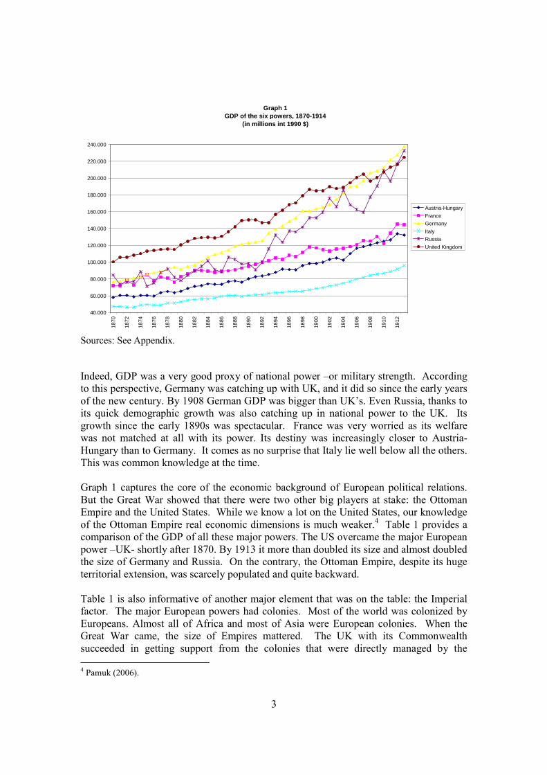
Graph 1GDP of the six powers, 1870-1914

(in millions int 1990 $)

40.000

60.000

80.000

100.000

120.000

140.000

160.000

180.000

200.000

220.000

240.000

1870

1872

1874

1876

1878

1880

1882

1884

1886

1888

1890

1892

1894

1896

1898

1900

1902

1904

1906

1908

1910

1912

Austria-Hungary

France

Germany

Italy

Russia

United Kingdom

Sources: See Appendix. Indeed, GDP was a very good proxy of national power –or military strength. According to this perspective, Germany was catching up with UK, and it did so since the early years of the new century. By 1908 German GDP was bigger than UK’s. Even Russia, thanks to its quick demographic growth was also catching up in national power to the UK. Its growth since the early 1890s was spectacular. France was very worried as its welfare was not matched at all with its power. Its destiny was increasingly closer to Austria-Hungary than to Germany. It comes as no surprise that Italy lie well below all the others. This was common knowledge at the time. Graph 1 captures the core of the economic background of European political relations. But the Great War showed that there were two other big players at stake: the Ottoman Empire and the United States. While we know a lot on the United States, our knowledge of the Ottoman Empire real economic dimensions is much weaker.4 Table 1 provides a comparison of the GDP of all these major powers. The US overcame the major European power –UK- shortly after 1870. By 1913 it more than doubled its size and almost doubled the size of Germany and Russia. On the contrary, the Ottoman Empire, despite its huge territorial extension, was scarcely populated and quite backward. Table 1 is also informative of another major element that was on the table: the Imperial factor. The major European powers had colonies. Most of the world was colonized by Europeans. Almost all of Africa and most of Asia were European colonies. When the Great War came, the size of Empires mattered. The UK with its Commonwealth succeeded in getting support from the colonies that were directly managed by the 4 Pamuk (2006).

4

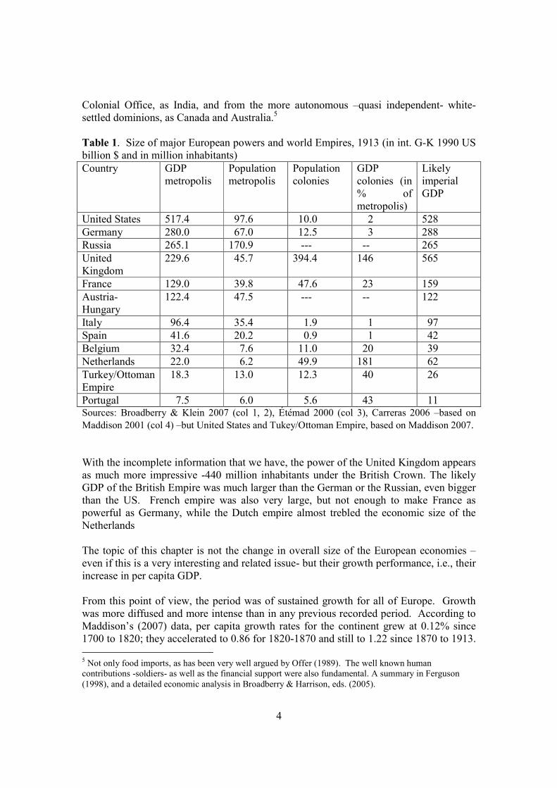
Colonial Office, as India, and from the more autonomous –quasi independent- white-settled dominions, as Canada and Australia.5 Table 1. Size of major European powers and world Empires, 1913 (in int. G-K 1990 US billion $ and in million inhabitants) Country GDP

metropolis Population metropolis

Population colonies

GDP colonies (in % of metropolis)

Likely imperial GDP

United States 517.4 97.6 10.0 2 528 Germany 280.0 67.0 12.5 3 288 Russia 265.1 170.9 --- -- 265 United Kingdom

229.6 45.7 394.4 146 565

France 129.0 39.8 47.6 23 159 Austria-Hungary

122.4 47.5 --- -- 122

Italy 96.4 35.4 1.9 1 97 Spain 41.6 20.2 0.9 1 42 Belgium 32.4 7.6 11.0 20 39 Netherlands 22.0 6.2 49.9 181 62 Turkey/Ottoman Empire

18.3 13.0 12.3 40 26

Portugal 7.5 6.0 5.6 43 11 Sources: Broadberry & Klein 2007 (col 1, 2), Étémad 2000 (col 3), Carreras 2006 –based on Maddison 2001 (col 4) –but United States and Tukey/Ottoman Empire, based on Maddison 2007. With the incomplete information that we have, the power of the United Kingdom appears as much more impressive -440 million inhabitants under the British Crown. The likely GDP of the British Empire was much larger than the German or the Russian, even bigger than the US. French empire was also very large, but not enough to make France as powerful as Germany, while the Dutch empire almost trebled the economic size of the Netherlands The topic of this chapter is not the change in overall size of the European economies –even if this is a very interesting and related issue- but their growth performance, i.e., their increase in per capita GDP. From this point of view, the period was of sustained growth for all of Europe. Growth was more diffused and more intense than in any previous recorded period. According to Maddison’s (2007) data, per capita growth rates for the continent grew at 0.12% since 1700 to 1820; they accelerated to 0.86 for 1820-1870 and still to 1.22 since 1870 to 1913. 5 Not only food imports, as has been very well argued by Offer (1989). The well known human contributions -soldiers- as well as the financial support were also fundamental. A summary in Ferguson (1998), and a detailed economic analysis in Broadberry & Harrison, eds. (2005).

5

On the contrary, the next period running through the two world wars performed worse, at a 0.96%. Indeed, it was between the end of the Napoleonic wars and the start of our period when Europe built most of its economic leadership over the rest of the world, but the 1870-1913 years displayed a sustained economic predominance that quickly expanded into political dominance –what was named imperialism. Broadberry and Klein (2007) propose a wide definition of Europe that includes the Russian Empire (i.e., including beyond the Urals) and present-day Turkey. According to them European GDP grew (at $ in 1990 international prices) at a 2.15%, while population at 1.06 and per capita GDP at 1.08. If we exclude Turkey because of having most of its territory in Asia (we are thinking in the actual borders), almost nothing changes in growth rates (0.01 in GDP and population, and nothing at all -0.00- in GDP per capita). Exactly the same happens if we exclude the Balkan countries with poor yearly data (Bulgaria, Romania and Serbia). But if we exclude Russia and Turkey, in order to focus on the countries that only have European territory, the changes are significant. GDP growth rate is reduced in 0.05, population growth rate in 0.25, and GDP per capita growth rate increases in 0.21. The conventions are only conventions, and we could argue about including the colonies of all European empires. In this case, the Russia beyond the Urals, the whole Ottoman Empire and the British, French, German, Dutch, Belgian, Italian, Portuguese, Spanish, and Danish colonies would qualify –it is our exercise in table 1. In what follows we will usually restrict, unless otherwise specified, the definition of Europe to the countries that provide us with yearly historical national accounts. This obliges us to put aside most of the Balkan countries: Turkey, Bulgaria, Romania and Serbia, as well as Bosnia-Herzegovina. This means that we have quite reliable figures for Austria-Hungary, Russia and Greece, but not for the countries South or East of these three. In order to get the exact feeling of the growth rates in all the countries that could qualify as European and the impact of putting a few of them aside, let us consider the following summary table:

6

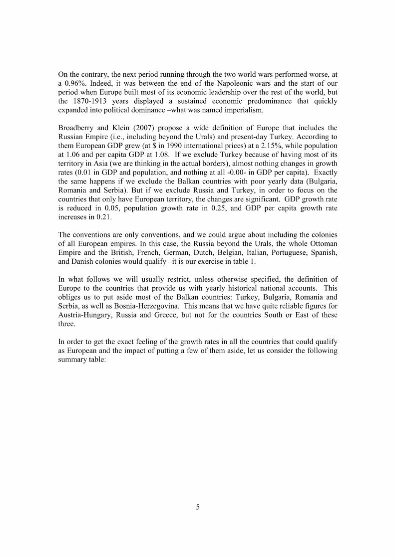
Table 2. Growth rates of GDP, Population and per capita GDP in Europe, 1870-1913 (%) Country GDP growth Population growth Per capita GDP growth Austria-Hungary 1.93 0.79 1.14 Belgium 2.01 0.95 1.05 Bulgaria 2.84 1.45 1.37 Denmark 2.66 1.07 1.57 Finland 2.66 1.30 1.34 France 1.63 0.18 1.45 Germany 2.90 1.16 1.72 Greece 2.32 1.40 0.91 Italy 1.66 0.73 0.92 Netherlands 2.16 1.26 0.89 Norway 2.19 0.81 1.36 Portugal 1.20 0.71 0.48 Romania 2.20 1.25 0.93 Russia 2.40 1.65 0.81 Serbia 3.34 1.99 1.34 Spain 1.81 0.51 1.28 Sweden 2.62 0.70 1.90 Switzerland 2.50 0.87 1.67 Turkey 1.48 0.56 0.91 United Kingdom 1.86 0.88 0.97 EUROPE 2.15 1.06 1.08 Standard deviation 0.54 0.43 0.36 Coefficient of variation 0.24 0.42 0.30 Source: Own calculations based on Broadberry and Klein (2007). The countries without yearly estimates between 1870 and 1913 are in italics. What we see is a quite narrow range of experience (the coefficient of variation is 0.24). The least growing economy is Portugal, at 1.20, and the fastest growing is Serbia at 3.34. The second least growing is Turkey at 1.48 and the second fastest is Germany at 2.90. Among the large economies it is worth to remind the 1.63 of France, the 1.86 of UK, the 1.93 of Austria-Hungary and the 2.40 of Russia. The changes, even if they seemed spectacular to the contemporaries, are not enormous. As expected, the major difference to be mentioned is the contrast between France and Germany. On population terms the range is also small (although the coefficient of variation is clearly bigger -0.42), although there is the exceptional French case with a 0.18 growth rate. On the other extreme, Serbia displays at 1.99. Far more important, Russia is growing at 1.60, i.e., nine times faster than France. The second least growing population is Spain, with 0.51. The other major powers share quite similar rates: Austria-Hungary, 0.79; UK, 0.88; Germany, 1.16.

7

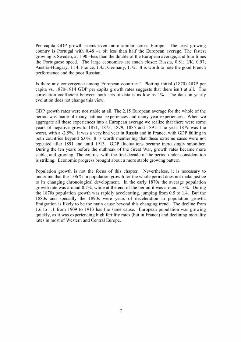
Per capita GDP growth seems even more similar across Europe. The least growing country is Portugal with 0.48 –a bit less than half the European average. The fastest growing is Sweden, at 1.90 –less than the double of the European average, and four times the Portuguese speed. The large economies are much closer: Russia, 0.81; UK, 0.97; Austria-Hungary, 1.14; France, 1.45; Germany, 1.72. It is worth to note the good French performance and the poor Russian. Is there any convergence among European countries? Plotting initial (1870) GDP per capita vs. 1870-1914 GDP per capita growth rates suggests that there isn’t at all. The correlation coefficient between both sets of data is as low as 4%. The data on yearly evolution does not change this view. GDP growth rates were not stable at all. The 2.15 European average for the whole of the period was made of many national experiences and many year experiences. When we aggregate all these experiences into a European average we realize that there were some years of negative growth: 1871, 1875, 1879, 1885 and 1891. The year 1879 was the worst, with a -2.5%. It was a very bad year in Russia and in France, with GDP falling in both countries beyond 6.0%. It is worth mentioning that these extreme cases were not repeated after 1891 and until 1913. GDP fluctuations became increasingly smoother. During the ten years before the outbreak of the Great War, growth rates became more stable, and growing. The contrast with the first decade of the period under consideration is striking. Economic progress brought about a more stable growing pattern. Population growth is not the focus of this chapter. Nevertheless, it is necessary to underline that the 1.06 % in population growth for the whole period does not make justice to its changing chronological development. In the early 1870s the average population growth rate was around 0.7%, while at the end of the period it was around 1.3%. During the 1870s population growth was rapidly accelerating, jumping from 0.5 to 1.4. But the 1880s and specially the 1890s were years of deceleration in population growth. Emigration is likely to be the main cause beyond this changing trend. The decline from 1.6 to 1.1 from 1909 to 1913 has the same cause. European population was growing quickly, as it was experiencing high fertility rates (but in France) and declining mortality rates in most of Western and Central Europe.

8

Graph 2.European per capita GDP gowth rate, 1871-1914 (%)

-5,00

-4,00

-3,00

-2,00

-1,00

0,00

1,00

2,00

3,00

4,00

5,00

1871

1873

1875

1877

1879

1881

1883

1885

1887

1889

1891

1893

1895

1897

1899

1901

1903

1905

1907

1909

1911

1913

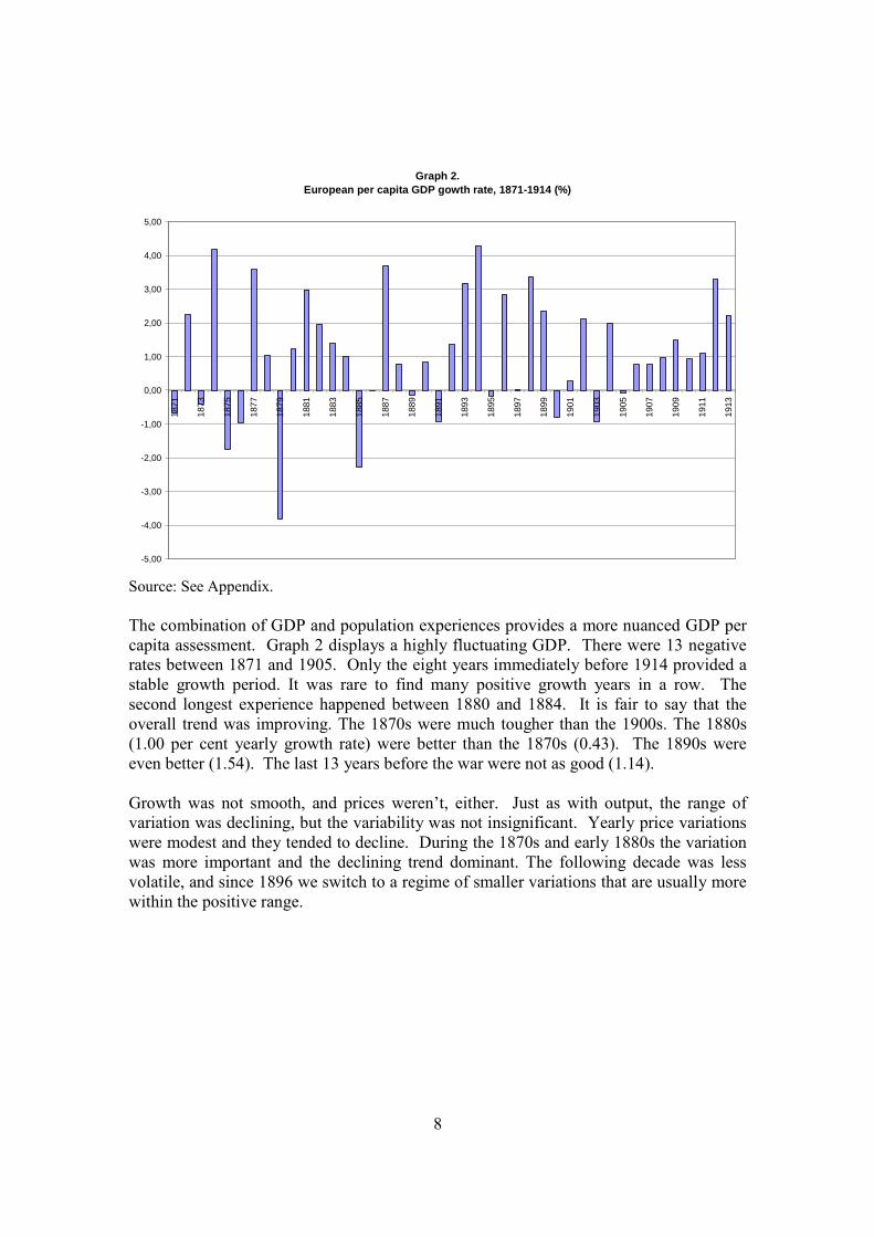
Source: See Appendix. The combination of GDP and population experiences provides a more nuanced GDP per capita assessment. Graph 2 displays a highly fluctuating GDP. There were 13 negative rates between 1871 and 1905. Only the eight years immediately before 1914 provided a stable growth period. It was rare to find many positive growth years in a row. The second longest experience happened between 1880 and 1884. It is fair to say that the overall trend was improving. The 1870s were much tougher than the 1900s. The 1880s (1.00 per cent yearly growth rate) were better than the 1870s (0.43). The 1890s were even better (1.54). The last 13 years before the war were not as good (1.14). Growth was not smooth, and prices weren’t, either. Just as with output, the range of variation was declining, but the variability was not insignificant. Yearly price variations were modest and they tended to decline. During the 1870s and early 1880s the variation was more important and the declining trend dominant. The following decade was less volatile, and since 1896 we switch to a regime of smaller variations that are usually more within the positive range.

9

Graph 3.Consumer Price Index yearly variation, Europe, 1871-1913 (%)

-6,00

-4,00

-2,00

0,00

2,00

4,00

6,00

1871

1873

1875

1877

1879

1881

1883

1885

1887

1889

1891

1893

1895

1897

1899

1901

1903

1905

1907

1909

1911

1913

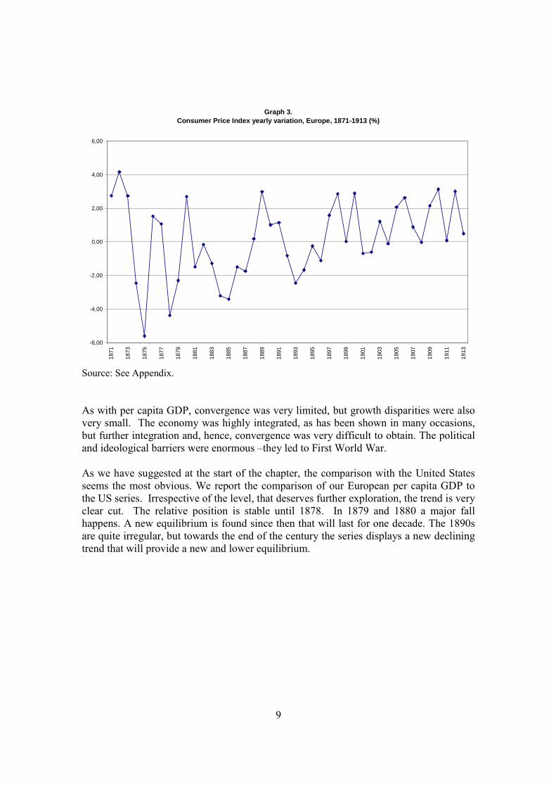
Source: See Appendix. As with per capita GDP, convergence was very limited, but growth disparities were also very small. The economy was highly integrated, as has been shown in many occasions, but further integration and, hence, convergence was very difficult to obtain. The political and ideological barriers were enormous –they led to First World War. As we have suggested at the start of the chapter, the comparison with the United States seems the most obvious. We report the comparison of our European per capita GDP to the US series. Irrespective of the level, that deserves further exploration, the trend is very clear cut. The relative position is stable until 1878. In 1879 and 1880 a major fall happens. A new equilibrium is found since then that will last for one decade. The 1890s are quite irregular, but towards the end of the century the series displays a new declining trend that will provide a new and lower equilibrium.

10

Graph 4.GDP per capita, Europe/United States, 1870-1913 (%)

40,00

45,00

50,00

55,00

60,00

65,00

70,00

75,00

1870

1872

1874

1876

1878

1880

1882

1884

1886

1888

1890

1892

1894

1896

1898

1900

1902

1904

1906

1908

1910

1912

US Maddison

Source: Europe: see Appendix. For the US, Maddison, 2007. The most important fact is the 1878-1880 divergence, when there is an economic crisis in Europe and a booming economy in the US. These are the years of the start of the agrarian depression, when poor harvests in Europe coincided with record highs in the US. What is called the agrarian crisis in the economic history literature appears in the transcontinental comparison as the major source of divergence. Europe, the dominant region of the world, was increasingly challenged by the Europeans overseas. While the European populated countries of the Southern cone, Oceania and Canada never reached the size to be real challengers, the United States managed to become a real one. Its huge economic size was only fully visible during First World War. But since 1880 it did matter a lot. Changing composition of expenditure When there is growth, there use to be changes in the composition of output. These changes are explored in detail in the chapter on structural change. There also uses to be increases in real wages and in the standards of living. Here, again, there is a chapter devoted to this fundamental issue. Because output produces incomes that are spent in all kinds of goods and services, the expenditure patterns are also very sensitive to economic growth. We will present here some evidence of the changing expenditure patterns of the European economies. The usual classification of expenditures starts with a distinction between consumption –private or public- and investment –private and public. Besides

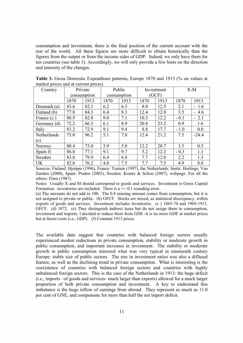
11

consumption and investment, there is the final position of the current account with the rest of the world. All these figures are more difficult to obtain historically than the figures from the output or from the income sides of GDP. Indeed, we only have them for ten countries (see table 3). Accordingly, we will only provide a few hints on the direction and intensity of the changes. Table 3. Gross Domestic Expenditure patterns, Europe 1870 and 1913 (% on values at market prices and at current prices)

Private consumption

Public consumption

Investment (GCF)

X-M Country

1870 1913 1870 1913 1870 1913 1870 1913 Denmark (a) 83.6 82.1 6.2 6.3 8.0 12.5 2.1 - 1.6 Finland (b) 77.8 84.3 6.4 8.3 12.4 12.0 3.5 - 4.6 France (c ) 80.9 82.8 9.0 7.1 10.3 12.2 - 0.1 - 2.1 Germany (d) 72.2 66.3 6.1 8.9 20.8 23.2 0.9 1.6 Italy 83.2 72.9 9.1 9.4 8.8 17.7 - 1.0 0.0 Netherlands (e)

75.0 96.2 5.1 7.0 12.4 21.2 7.5 -24.4

Norway 80.4 73.0 3.9 5.8 12.2 20.7 3.5 0.5 Spain f) 86.0 77.1 9.1 9.7 5.2 12.2 - 0,3 1.1 Sweden 83.8 79.9 6.4 6.8 7.7 12.0 2.2 1.3 UK 82.6 76.2 4.8 7.5 7.7 7.5 4.9 8.8 Sources: Finland: Hjerppe (1996), France: Toutain (1997), the Netherlands: Smits, Horlings, Van Zanden (2000), Spain: Prados (2003), Sweden: Krantz & Schon (2007), webpage. For all the others: Flora (1987). Notes: Usually X and M should correspond to goods and services. Investment is Gross Capital Formation –inventories are included. There is a +/- 0.1 rounding error. (a) The amounts do not add to 100. The 0.8 missing amount comes from consumption, but it is not assigned to private or public. (b) GFCF. Stocks are mixed, as statistical discrepancy, within exports of goods and services. Investment includes inventories. (c ) 1865-74 and 1905-1913. GFCF. (d) 1872. (e) They distinguish indirect taxes but do not assign them to consumption, investment and imports. I decided to reduce them from GDE -it is no more GDE at market prices but at factor costs (i.e., GDP). (f) Constant 1913 prices. The available data suggest that countries with balanced foreign sectors usually experienced modest reductions in private consumption, stability or moderate growth in public consumption, and important increases in investment. The stability or moderate growth in public consumption mirrored what was very typical in nineteenth century Europe: stable size of public sectors. The rise in investment ratios was also a diffused feature, as well as the declining trend in private consumption. What is interesting is the coexistence of countries with balanced foreign sectors and countries with highly unbalanced foreign sectors. This is the case of the Netherlands in 1913: the huge deficit (i.e., imports –of goods and services- much larger than exports) allowed for a much larger proportion of both private consumption and investment. A key to understand this imbalance is the huge inflow of earnings from abroad. They represent as much as 11.0 per cent of GNE, and compensate for more than half the net import deficit.

12

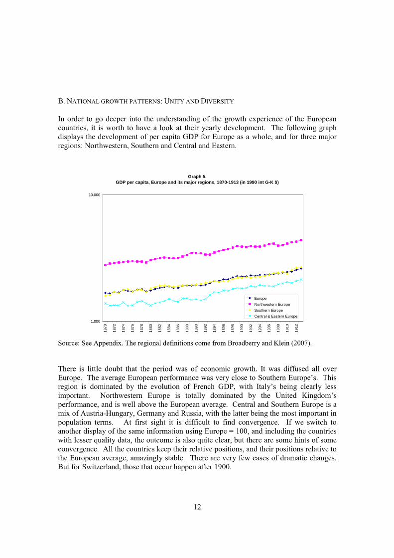
B. NATIONAL GROWTH PATTERNS: UNITY AND DIVERSITY In order to go deeper into the understanding of the growth experience of the European countries, it is worth to have a look at their yearly development. The following graph displays the development of per capita GDP for Europe as a whole, and for three major regions: Northwestern, Southern and Central and Eastern.

Graph 5.GDP per capita, Europe and its major regions, 1870-1913 (in 1990 int G-K $)

1.000

10.000

1870

1872

1874

1876

1878

1880

1882

1884

1886

1888

1890

1892

1894

1896

1898

1900

1902

1904

1906

1908

1910

1912

Europe

Northwestern Europe

Southern Europe

Central & Eastern Europe

Source: See Appendix. The regional definitions come from Broadberry and Klein (2007). There is little doubt that the period was of economic growth. It was diffused all over Europe. The average European performance was very close to Southern Europe’s. This region is dominated by the evolution of French GDP, with Italy’s being clearly less important. Northwestern Europe is totally dominated by the United Kingdom’s performance, and is well above the European average. Central and Southern Europe is a mix of Austria-Hungary, Germany and Russia, with the latter being the most important in population terms. At first sight it is difficult to find convergence. If we switch to another display of the same information using Europe = 100, and including the countries with lesser quality data, the outcome is also quite clear, but there are some hints of some convergence. All the countries keep their relative positions, and their positions relative to the European average, amazingly stable. There are very few cases of dramatic changes. But for Switzerland, those that occur happen after 1900.

13

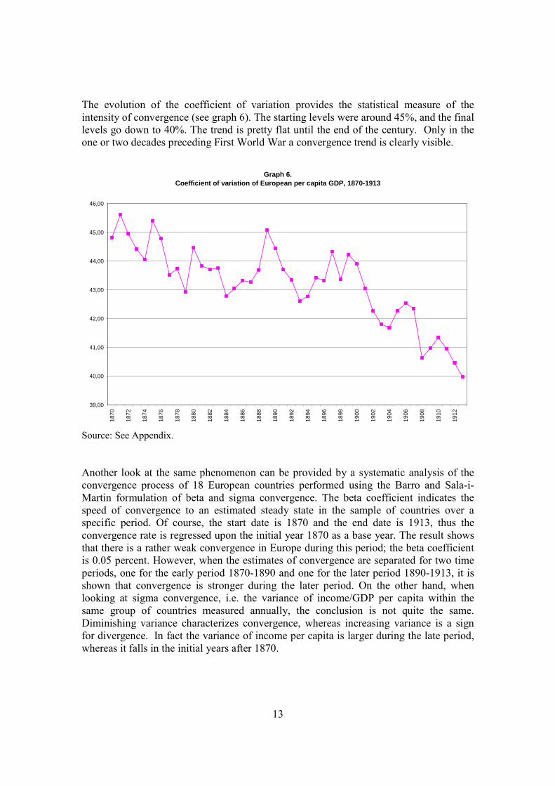
The evolution of the coefficient of variation provides the statistical measure of the intensity of convergence (see graph 6). The starting levels were around 45%, and the final levels go down to 40%. The trend is pretty flat until the end of the century. Only in the one or two decades preceding First World War a convergence trend is clearly visible.

Graph 6.Coefficient of variation of European per capita GDP, 1870-1913

39,00

40,00

41,00

42,00

43,00

44,00

45,00

46,00

1870

1872

1874

1876

1878

1880

1882

1884

1886

1888

1890

1892

1894

1896

1898

1900

1902

1904

1906

1908

1910

1912

Source: See Appendix. Another look at the same phenomenon can be provided by a systematic analysis of the convergence process of 18 European countries performed using the Barro and Sala-i-Martin formulation of beta and sigma convergence. The beta coefficient indicates the speed of convergence to an estimated steady state in the sample of countries over a specific period. Of course, the start date is 1870 and the end date is 1913, thus the convergence rate is regressed upon the initial year 1870 as a base year. The result shows that there is a rather weak convergence in Europe during this period; the beta coefficient is 0.05 percent. However, when the estimates of convergence are separated for two time periods, one for the early period 1870-1890 and one for the later period 1890-1913, it is shown that convergence is stronger during the later period. On the other hand, when looking at sigma convergence, i.e. the variance of income/GDP per capita within the same group of countries measured annually, the conclusion is not quite the same. Diminishing variance characterizes convergence, whereas increasing variance is a sign for divergence. In fact the variance of income per capita is larger during the late period, whereas it falls in the initial years after 1870.

14

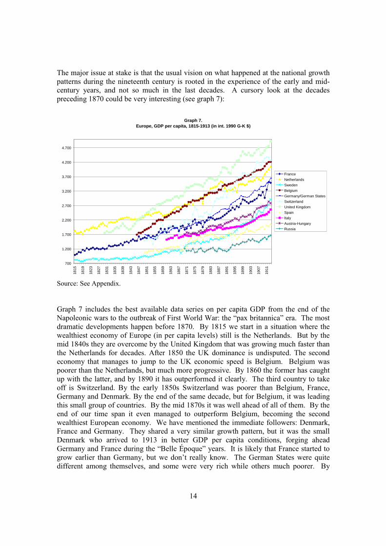
The major issue at stake is that the usual vision on what happened at the national growth patterns during the nineteenth century is rooted in the experience of the early and mid-century years, and not so much in the last decades. A cursory look at the decades preceding 1870 could be very interesting (see graph 7):

Graph 7.Europe, GDP per capita, 1815-1913 (in int. 1990 G-K $)

700

1.200

1.700

2.200

2.700

3.200

3.700

4.200

4.700

1815

1819

1823

1827

1831

1835

1839

1843

1847

1851

1855

1859

1863

1867

1871

1875

1879

1883

1887

1891

1895

1899

1903

1907

1911

France

Netherlands

Sweden

Belgium

Germany/German States

Switzerland

United Kingdom

Spain

Italy

Austria-Hungary

Russia

Source: See Appendix. Graph 7 includes the best available data series on per capita GDP from the end of the Napoleonic wars to the outbreak of First World War: the “pax britannica” era. The most dramatic developments happen before 1870. By 1815 we start in a situation where the wealthiest economy of Europe (in per capita levels) still is the Netherlands. But by the mid 1840s they are overcome by the United Kingdom that was growing much faster than the Netherlands for decades. After 1850 the UK dominance is undisputed. The second economy that manages to jump to the UK economic speed is Belgium. Belgium was poorer than the Netherlands, but much more progressive. By 1860 the former has caught up with the latter, and by 1890 it has outperformed it clearly. The third country to take off is Switzerland. By the early 1850s Switzerland was poorer than Belgium, France, Germany and Denmark. By the end of the same decade, but for Belgium, it was leading this small group of countries. By the mid 1870s it was well ahead of all of them. By the end of our time span it even managed to outperform Belgium, becoming the second wealthiest European economy. We have mentioned the immediate followers: Denmark, France and Germany. They shared a very similar growth pattern, but it was the small Denmark who arrived to 1913 in better GDP per capita conditions, forging ahead Germany and France during the “Belle Époque” years. It is likely that France started to grow earlier than Germany, but we don’t really know. The German States were quite different among themselves, and some were very rich while others much poorer. By

15

1850, the average German GDP per capita was very close to the French, and they remained so for one quarter of a century. Since the mid 1880s the German advantage was noticeable and remained so until 1913. Imperial Austria enjoyed similar income levels than France and Germany, but its growth rate was even smaller than the French one. By 1913 they were clearly below France. The quadrangle that includes France, Germany, Imperial Austria, and the smaller states of Belgium, the Netherlands, Switzerland and Denmark constituted the developing Europe of the early nineteenth century. All of them joined the United Kingdom as developed nations at some stage during the nineteenth century. They were the core of the early comers to industrialization. Italy, on the contrary, quite likely started the century among them but lost ground during the whole nineteenth century.6 After political unification in 1861 some growth impetus was achieved, but not enough to catch up with the quickly developing economies of Western and Central Europe. Only by 1900 there is acceleration in growth –a big spurt- that allowed Italy to start to catch up with the leader –the UK. The real European periphery of the early nineteenth century provided the classical case of a peripheral country able to take full advantage of its initial backwardness to enjoy very quick growth: Sweden. Its first rate performance during the thirty years prior to the First World War allowed it to be the most developed of the late comers. But by 1913 Sweden was not yet among the club of the successful economies. As late as 1880 the odds also seemed favorable to Spain. But after 1880 Spain did a much worse performance than Sweden7. Much more important than the Spanish failure to keep pace with the dynamic European peripheral countries –the Nordic group- is the Russian failure. Russia, by 1870 was a highly promising economy, fully embarked in major political, social and economic reforms. Its starting point was quite similar to Spain or Sweden. But Sweden did very well, Spain much less so, and Russia did very poorly –the least performing European economy of the nineteenth century among those of medium or large population size. Because of Russia’s sheer size and promise, the brakes on Russian late nineteenth century growth have been studied by generations of historians. They are, in a nutshell, a summary of the problems of today’s developing economies. As any reader with historiographical knowledge would have noticed, we have been using a number of concepts that were defined precisely to describe what happened in Europe during the long nineteenth century. Walt Rostow (1961) coined the concept of “take off”. Alexander Gerschenkron (1962) suggested a somewhat different concept, but he had to christen it as “big spurt” –not so far away from the Rostovian take off! The European diversity of national growth experiences is particularly appealing between 1815 and 1870. Growth is being diffused according to patterns that need some explanation. Was the driving force the availability of natural resources? Was it, more precisely, the availability of coal and iron, as so many authors as Pounds (1957), Pollard (1981) and Cameron (1985) have taught us? Or was the critical feature the availability of a wider set of institutions –the Gerschenkronian growth prerequisites? Is there room for a human capital based explanation? Many think that this is the case –as O’Rourke and Williamson

6 Malanima 2003, 2006 and 2007 argues forcefully for such a view. His data on income per capita suggests that Italy was as rich as the Netherlands by 1815. There is no consensus on this point, but his case for an overall stagnating Italy during most of the nineteenth century is convincing. 7 Carreras (2005)

16

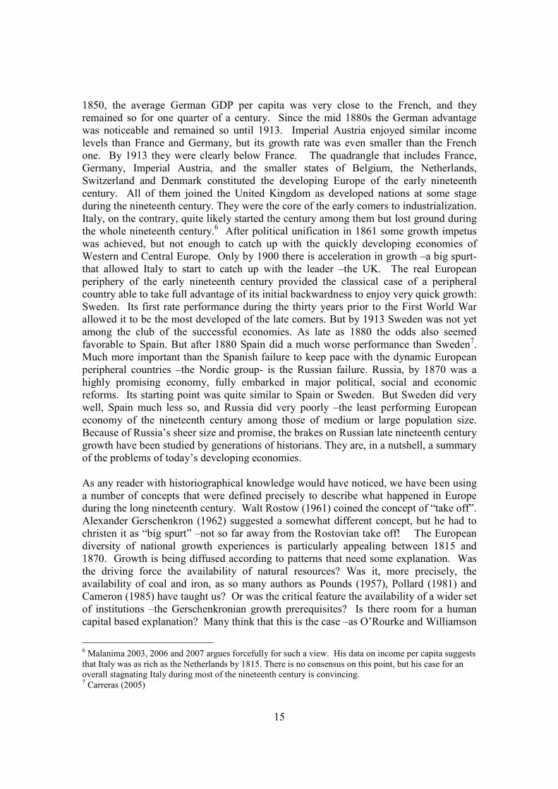
(1997) have argued. What role is left to economic policy? It is present in all the explanations –starting with Bairoch’s (1976) case for the importance of protectionist trade policies-, but no agreement has been reached on what would have been the best economic policy. Because growth was intrinsically mixed with national power, it is very difficult to disentangle growth promoting policies from power promoting policies as Landes (1969) and Trebilcock (1981) asserted. The dynamism of the small European economies is very telling for economics in general, and development economics in particular, but the contemporaries were much more worried about the race of the major economies. For all of them size mattered a lot –as we have been stressing earlier. The largest economies have usually been considered as competing among themselves. They were major “powers”, and their benchmarking was permanent –as happened most explicitly in 1914. Besides the major powers, Europe was made of a number of neighborhoods. Location mattered from many points of view: natural endowments, trade, language, institutions and technology, depended a lot on geographical closeness. A very good vicinity was that of Northwestern Europe, made of, mostly, the countries around the Northern Sea (see graph 8). Nobody challenged the economic superiority and welfare of the UK, even if Belgium and Netherlands were always close –but below- the UK. Only the small Denmark displayed the ability to grow at much faster rate and to converge. Danish convergence allowed for reaching the GDP per capita of the Netherlands and for coming close to the Belgian level. Out of the other Nordic countries, all of them much poorer than the rest of the Northwestern league, only Sweden was involved in successful catching up efforts during the quarter of a century prior to 1914.

Graph 8.Northwestern Europe GDP per capita, 1815-1913 (in int. 1990 G-K $)

700

1.200

1.700

2.200

2.700

3.200

3.700

4.200

4.700

1815

1818

1821

1824

1827

1830

1833

1836

1839

1842

1845

1848

1851

1854

1857

1860

1863

1866

1869

1872

1875

1878

1881

1884

1887

1890

1893

1896

1899

1902

1905

1908

1911

Netherlands

Sweden

Denmark

Belgium

Finland

Norway

United Kingdom

Source: See Appendix.

17

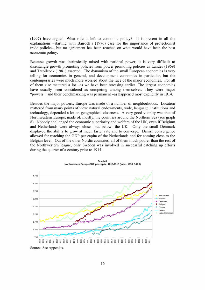
Central Europe was a prosperous European region. Switzerland built its economic leadership since the mid 1870s. It became closer in performance to Belgium and Netherlands than to its other neighbors. By 1870 the distance with Austria and Germany was negligible, just as it happened between Austria and Germany. It was only in the 1880s that Germany could forge ahead of Austria. Hungary was never at the par with the rest of Central Europe. Its position was lower, even if the progress made between 1876 and 1882 was so impressive.

Graph 9.Central and Eastern Europe per capita GDP, 1850-1913 (in 1990 int G_K $)

500

1.000

1.500

2.000

2.500

3.000

3.500

4.000

4.500

1850 1855 1860 1865 1870 1875 1880 1885 1890 1895 1900 1905 1910

Germany

Russia

Switzerland

Romania

Serbia

Austria

Hungary

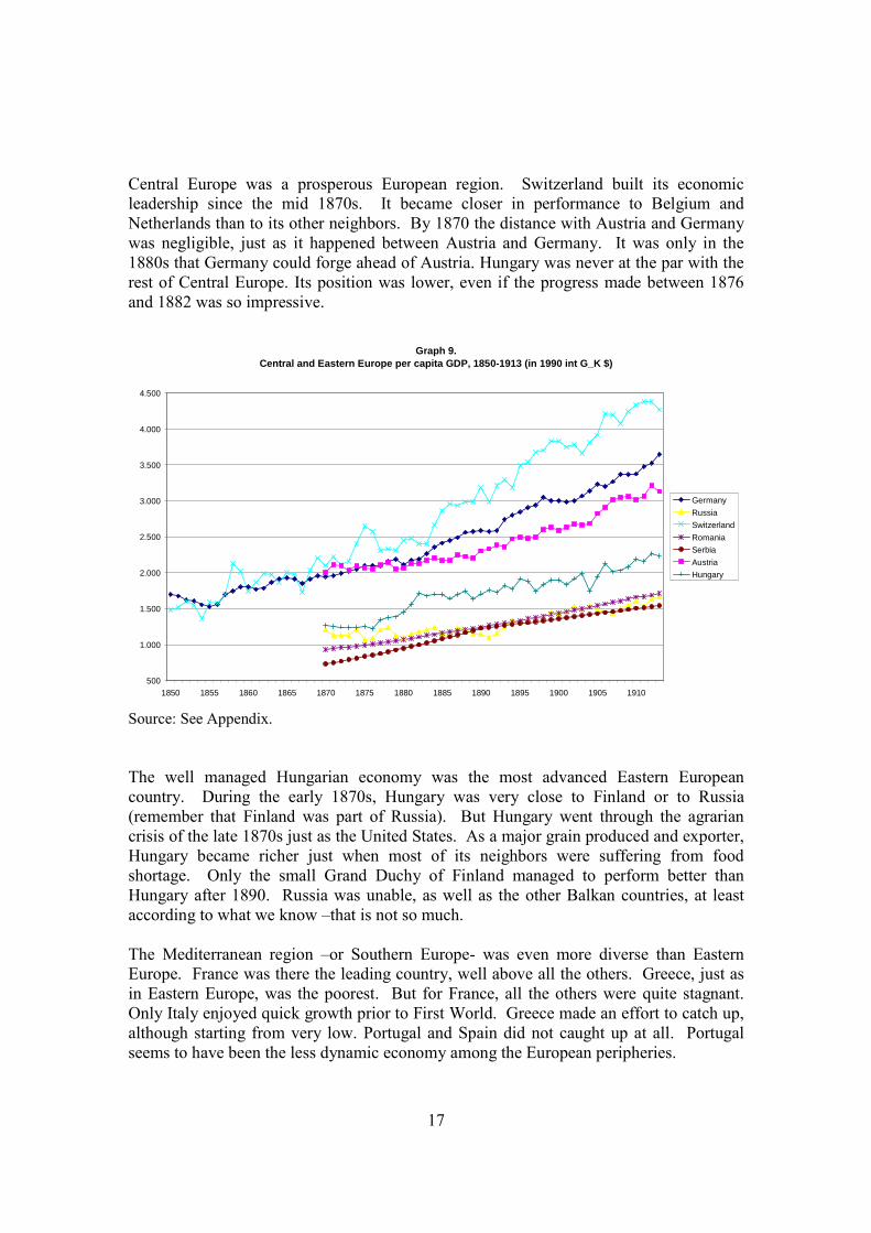
Source: See Appendix. The well managed Hungarian economy was the most advanced Eastern European country. During the early 1870s, Hungary was very close to Finland or to Russia (remember that Finland was part of Russia). But Hungary went through the agrarian crisis of the late 1870s just as the United States. As a major grain produced and exporter, Hungary became richer just when most of its neighbors were suffering from food shortage. Only the small Grand Duchy of Finland managed to perform better than Hungary after 1890. Russia was unable, as well as the other Balkan countries, at least according to what we know –that is not so much. The Mediterranean region –or Southern Europe- was even more diverse than Eastern Europe. France was there the leading country, well above all the others. Greece, just as in Eastern Europe, was the poorest. But for France, all the others were quite stagnant. Only Italy enjoyed quick growth prior to First World. Greece made an effort to catch up, although starting from very low. Portugal and Spain did not caught up at all. Portugal seems to have been the less dynamic economy among the European peripheries.

18

Graph 10.Europe, GDP per capita, 1815-1913 (in int. 1990 G-K $)

0

500

1.000

1.500

2.000

2.500

3.000

3.500

4.000

1815

1818

1821

1824

1827

1830

1833

1836

1839

1842

1845

1848

1851

1854

1857

1860

1863

1866

1869

1872

1875

1878

1881

1884

1887

1890

1893

1896

1899

1902

1905

1908

1911

France

Spain

Portugal

Italy

Greece

Source: See Appendix. Our knowledge of the poorest is, as can be expected, the most limited. The extreme peripheries were all of them poor, and it is quite likely that they were more or less around the same order of magnitude. In our “numéraire” -1990 international Geary-Khamis dollars- this means around 700 dollars. We are skeptical on the Greek figures because they are too much below this level. In a Europe that was growing at a similar pace, it is rare to find poor countries growing well below the average. This seems to have been the case with Portugal, and also of Greece for many decades. Both deserve the kind of attention that has been given to Russia.8

8 See Reis (1993) and Lains (2003) for interesting interpretations of the origins of Portuguese underperformance.

19

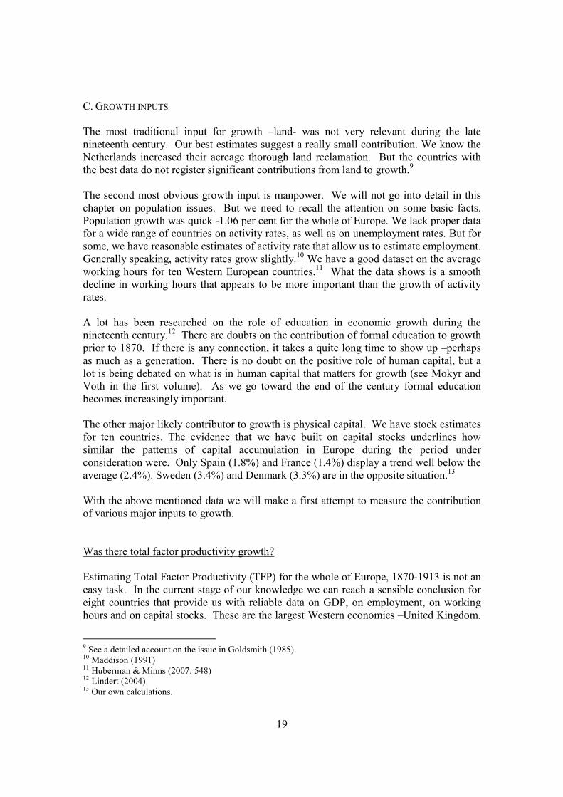
C. GROWTH INPUTS The most traditional input for growth –land- was not very relevant during the late nineteenth century. Our best estimates suggest a really small contribution. We know the Netherlands increased their acreage thorough land reclamation. But the countries with the best data do not register significant contributions from land to growth.9 The second most obvious growth input is manpower. We will not go into detail in this chapter on population issues. But we need to recall the attention on some basic facts. Population growth was quick -1.06 per cent for the whole of Europe. We lack proper data for a wide range of countries on activity rates, as well as on unemployment rates. But for some, we have reasonable estimates of activity rate that allow us to estimate employment. Generally speaking, activity rates grow slightly.10 We have a good dataset on the average working hours for ten Western European countries.11 What the data shows is a smooth decline in working hours that appears to be more important than the growth of activity rates. A lot has been researched on the role of education in economic growth during the nineteenth century.12 There are doubts on the contribution of formal education to growth prior to 1870. If there is any connection, it takes a quite long time to show up –perhaps as much as a generation. There is no doubt on the positive role of human capital, but a lot is being debated on what is in human capital that matters for growth (see Mokyr and Voth in the first volume). As we go toward the end of the century formal education becomes increasingly important. The other major likely contributor to growth is physical capital. We have stock estimates for ten countries. The evidence that we have built on capital stocks underlines how similar the patterns of capital accumulation in Europe during the period under consideration were. Only Spain (1.8%) and France (1.4%) display a trend well below the average (2.4%). Sweden (3.4%) and Denmark (3.3%) are in the opposite situation.13 With the above mentioned data we will make a first attempt to measure the contribution of various major inputs to growth. Was there total factor productivity growth? Estimating Total Factor Productivity (TFP) for the whole of Europe, 1870-1913 is not an easy task. In the current stage of our knowledge we can reach a sensible conclusion for eight countries that provide us with reliable data on GDP, on employment, on working hours and on capital stocks. These are the largest Western economies –United Kingdom,

9 See a detailed account on the issue in Goldsmith (1985). 10 Maddison (1991) 11 Huberman & Minns (2007: 548) 12 Lindert (2004) 13 Our own calculations.

20

France, Germany and Italy- and some of the middle and small sized economies –Spain, Netherlands, Sweden and Denmark. The following table summarizes the results for each of them and for all of them together, as if they were a unified entity. We also report the European values for each concept, in order to get a rough assessment of what could change with a broader European database. Table 4. TFP, 1870-1913 (growth rates or percentages, always in %) Country GDP Employment Hours

worked Capital stock

TFP GDP p.c.

TFP/ GDP p.c.

TFP/ GDP

Denmark 2.66 1.04 -0.53 3.29 1.32 1.57 84 49 France 1.63 0.20 -0.18 1.41 1.19 1.45 82 73 Germany 2.90 1.47 -0.43 3.12 1.24 1.72 72 43 Italy 1.66 0.58 -0.04 2.67 0.48 0.92 52 29 Netherlands

2.16 1.22 -0.25 3.14 0.54 0.89 61 25

Spain 1.81 0.52 -0.31 1.82 1.12 1.28 87 62 Sweden 2.62 0.71 -0.52 3.43 1.46 1.90 77 56 United Kingdom

1.86 1.15 -0.09 2.13 0.48 0.97 49 26

EUROPE-

8

2.04 0.85 -0.29 2.36 0.94 1.29 73 46

W.Europe (*)

2.05 0.86 -0.32 2.36 1.29

Europe Total

2.15 1.08

Sources: see text. Notes: TFP is calculated assuming a production function where labor contribution is 70 per cent and capital contribution is 30 per cent. (*) Western Europe stands for the Western European countries with data on capital stocks or on employment and working hours. On top of the 8 considered in the table, they are Belgium, Finland, Norway and Switzerland for employment; Belgium and Switzerland for working hours; Finland and Norway for capital stocks. GDP and GDP per capita data corresponds to the grouping of 12. The results in bold provide the best available synthetic view of the likely TFP for Western Europe.14 The following row providing data for Western Europe includes Belgium, Finland, Norway and Switzerland, and is almost identical even if we do not have all the necessary information for each of these countries. We can assume that the overall picture will not change if we include them. We cannot say the same for the whole of Europe. The last row reminds us that overall GDP growth was 0.1 per cent higher for the whole of Europe, and that overall per capita GDP growth was 0.2 per cent lower. European TFP could be different from the one that we have assessed –but not so much.

14 The TFP is pretty robust to the weighting assumptions. Although the most widely accepted is 70 and 30 for labor and capital, respectively, there are some cases where other assumptions have been made. In case of a 65/35 weighting, the resulting TFP would be 0.85. In case of a 75/25 weighting, 1.03.

21

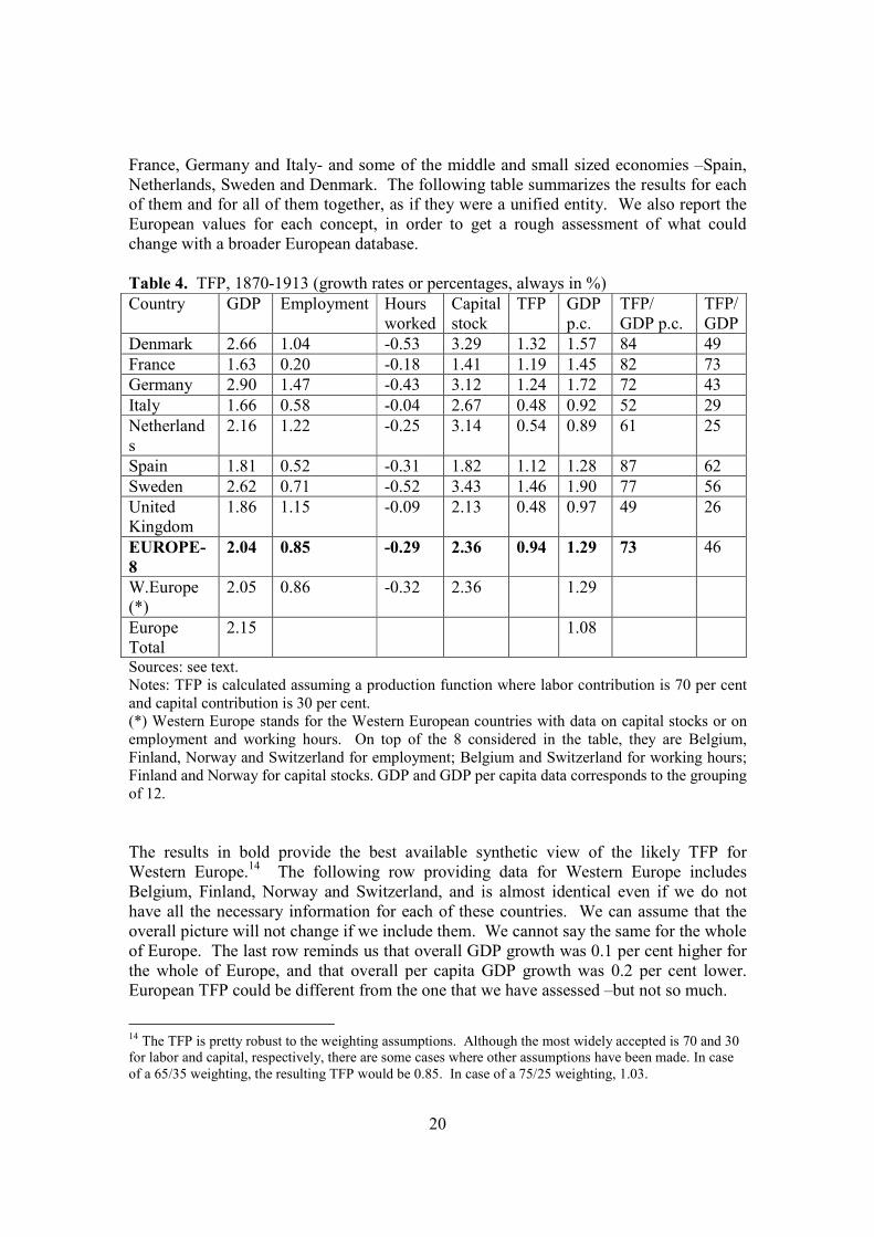
What we get is highly interesting. A 0.94 per cent TFP growth for the whole period is impressive. It is even more impressive to see that TFP growth accounts for almost three quarters of GDP per capita growth. The diversity of experience is limited. There are five countries with higher than average TFP growth rates, but all of them are within a close range (1.12 to 1.46). For these five countries –Denmark, France, Germany, Spain and Sweden-, TFP accounts for 72 to 87 per cent of GDP per capita growth. Three other countries –Italy, Netherlands and UK- share very similar TFP growth rates (0.48 to 0.54) and more modest ratios to per capita GDP (49 to 61 per cent). Even these last ratios are pretty high by current standards. The comparison with GDP growth rates can be checked in the last column. France appears as the country getting the most TFP out of its GDP growth, followed by Spain and Sweden, all of them well above the average. If we want to look for a parallel of very high TFP on GDP ratios or of TFP on GDP per capita, we have to look at the Golden Age of the Postwar era (see Crafts & Toniolo chapter). A significant portion of Europe was growing as fast as they could. We can say that they were growing at their full potential –at the production frontier. This happens both with countries that enjoyed relatively high GDP and per capita GDP growth rates like Germany, Sweden or Denmark, and with countries with much more modest GDP outcomes like France and Spain. This is highly suggestive that the economies were highly flexible, and allowed for a full exploitation of the economic opportunities at hand. We will quickly review these opportunities in what follows. Meanwhile we advance the hypothesis that a wide range of the European economies of the time managed to grow at its full potential –very close to the production frontier. Before this, let’s consider for a while the temporal pattern of TFP evolution. This is what is displayed in the next table. Table 5. TFP growth, 1870-1913, Europe at 8 (in %) Period GDP

growth Employment growth

Hours worked

Capital Stock

TFP growth

GDP p.c. growth

TFP on p.c. GDP

1870-1880

1.77 0.77 -0.32 2.15 0.81 1.08 75

1880-1890

2.00 0.75 -0.40 1.99 1.16 1.33 87

1890-1900

2.17 0.88 -0.27 2.47 1.00 1.38 72

1900-1913

2.17 0.98 -0.31 2.71 0.89 1.32 67

Sources: the same than previous table. The smooth acceleration of GDP growth rates was eroded by a similar trend in employment rates and in capital stock. The overall effect is of growing TFP from the

22

first to the second decades, and a declining trend afterwards. When TFP was most important in GDP and in per capita GDP growth was between 1880 and 1890 and when least, between 1900 and 1913. D. SOURCES OF GROWTH: PROXIMATE AND ULTIMATE CAUSES Following Maddison’s framework, we can distinguish between the proximate causes of growth that are easily accountable for (land, capital, labor, education, structural change…) from the ultimate causes, that are more difficult to capture in a figure (culture, institutions, values…). We start considering some of the most widely quoted proximate causes. We put aside the contribution of structural change that is properly considered in a specific chapter. Scientific and technological progress Science and technology have been posited by historians and economists as well as the deus ex machina of modern economic growth. The core of the explanation of the industrial revolution and of its diffusion, lies in technological change (Landes, 1969; Voth, 2006). Behind it what we have is scientific change (Mokyr, 2002). The determinants of scientific change are difficult to ascertain –Mokyr does a big effort into this direction. What we do know is that patenting had something to do with it. Patents provide the economic incentive to inventors, especially those more on the applied extreme. Patents provide the combination of a property rights and a technological change view of both the rise of modern economic growth and its sustainability over time. Because of its centrality in the explanations of the causal forces pushing for growth, we start having very good information on patenting. Scientific and technologic progress happened, in most countries, through patenting.15 A few small countries opted out of the system and went for an open, non-proprietary approach, most noticeable, the Netherlands. For all the others, patents did matter –and perhaps they mattered even more for the Netherlands, but for worse. By 1913, two small European countries had a clear lead in per capita patents granted per million inhabitants: Belgium and Switzerland (almost exactly the same: around 1455/1458). Denmark followed much behind with 528. Not surprisingly, the three were the most successful countries following the UK lead. The Netherlands, with a dismal 18 patents per million inhabitants in 1913 was not up to its GDP per capita –but its patenting failure shows perfectly well its inability to keep its past economic leadership and to enhance it. The Dutch failure in patenting mirrors its overall disappointing economic performance during the nineteenth century. The extreme Dutch position was exaggerated by its late return to a patent based system of protecting intellectual property rights. They abandoned it in 1869 and only returned to normal practice by 1912. The patenting ranking of the other European countries by 1913 was (in declining order): Norway (488), France (401), Great Britain (364), Sweden (341), Italy (298), Austria-Hungary (214), Germany (202), Finland (143), Spain (88), Portugal 15 See Petra Moser (2005) for a discussion of the exceptions.

23

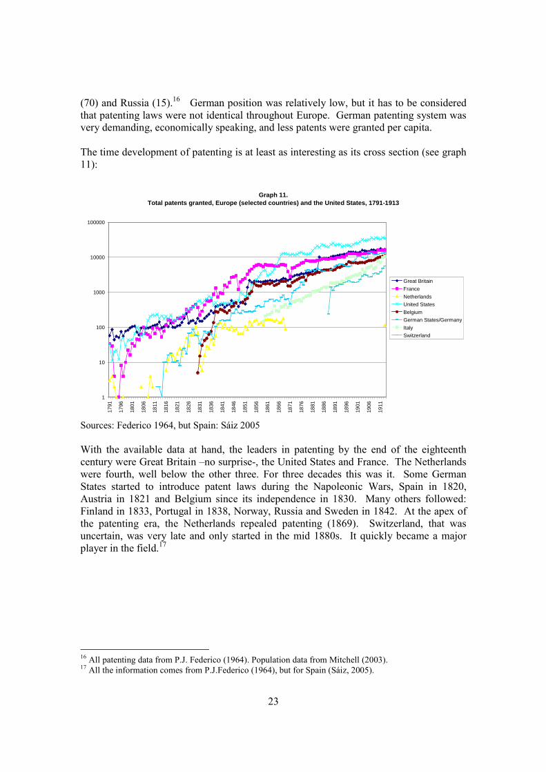
(70) and Russia (15).16 German position was relatively low, but it has to be considered that patenting laws were not identical throughout Europe. German patenting system was very demanding, economically speaking, and less patents were granted per capita. The time development of patenting is at least as interesting as its cross section (see graph 11):

Graph 11.Total patents granted, Europe (selected countries) and the United States, 1791-1913

1

10

100

1000

10000

100000

1791

1796

1801

1806

1811

1816

1821

1826

1831

1836

1841

1846

1851

1856

1861

1866

1871

1876

1881

1886

1891

1896

1901

1906

1911

Great Britain

France

Netherlands

United States

Belgium

German States/Germany

Italy

Switzerland

Sources: Federico 1964, but Spain: Sáiz 2005 With the available data at hand, the leaders in patenting by the end of the eighteenth century were Great Britain –no surprise-, the United States and France. The Netherlands were fourth, well below the other three. For three decades this was it. Some German States started to introduce patent laws during the Napoleonic Wars, Spain in 1820, Austria in 1821 and Belgium since its independence in 1830. Many others followed: Finland in 1833, Portugal in 1838, Norway, Russia and Sweden in 1842. At the apex of the patenting era, the Netherlands repealed patenting (1869). Switzerland, that was uncertain, was very late and only started in the mid 1880s. It quickly became a major player in the field.17

16 All patenting data from P.J. Federico (1964). Population data from Mitchell (2003). 17 All the information comes from P.J.Federico (1964), but for Spain (Sáiz, 2005).

24

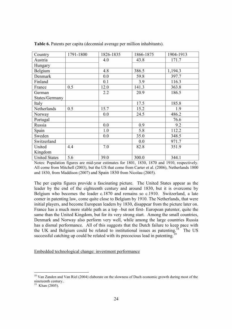
Table 6. Patents per capita (decennial average per million inhabitants). Country 1791-1800 1826-1835 1866-1875 1904-1913 Austria 43.8 171.7 Hungary

4.0

Belgium 4.8 386.5 1,194.3 Denmark 0.0 59.8 397.7 Finland 0.1 3.9 116.3 France 0.5 12.0 141.3 363.8 German States/Germany

2.2 20.9 186.5

Italy 17.5 185.8 Netherlands 0.5 15.7 15.2 1.9 Norway 0.0 24.5 486.2 Portugal 76.6 Russia 0.0 0.9 9.2 Spain 1.0 5.8 112.2 Sweden 0.0 35.0 348.5 Switzerland 0.0 971.7 United Kingdom

4.4 7.0 82.8 351.9

United States 5.6 39.0 300.0 344.1 Notes: Population figures are mid-year estimates for 1801, 1830, 1870 and 1910, respectively. All come from Mitchell (2003), but the US that come from Carter et al. (2006), Netherlands 1800 and 1830, from Maddison (2007) and Spain 1830 from Nicolau (2005). The per capita figures provide a fascinating picture. The United States appear as the leader by the end of the eighteenth century and around 1830, but it is overcome by Belgium who becomes the leader c.1870 and remains so c.1910. Switzerland, a late comer in patenting law, come quite close to Belgium by 1910. The Netherlands, that were initial players, and become European leaders by 1830, disappear from the picture later on. France has a much more stable path as a top –but not first- European patenter, quite the same than the United Kingdom, but for its very strong start. Among the small countries, Denmark and Norway also perform very well, while among the large countries Russia has a dismal performance. All of this suggests that the Dutch failure to keep pace with the UK and Belgium could be related to institutional issues as patenting.18 The US successful catching up could be related with its precocious lead in patenting.19 Embedded technological change: investment performance

18 Van Zanden and Van Riel (2004) elaborate on the slowness of Duch economic growth during most of the nineteenth century.. 19 Khan (2005).

25

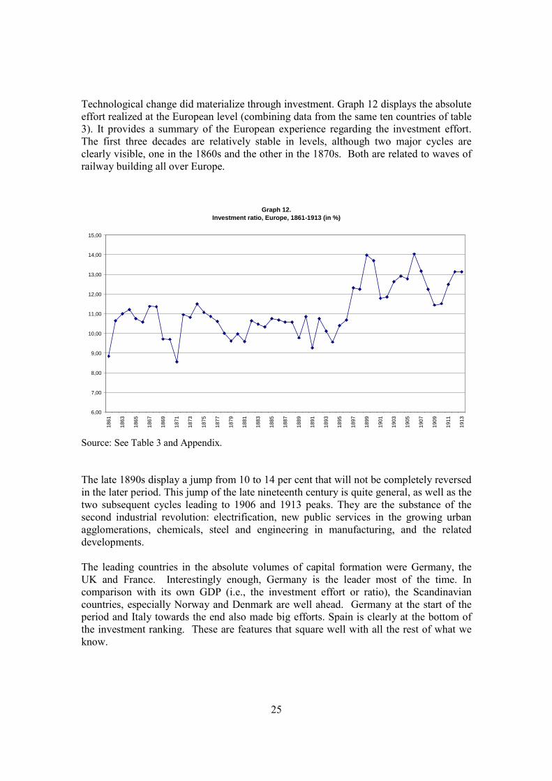
Technological change did materialize through investment. Graph 12 displays the absolute effort realized at the European level (combining data from the same ten countries of table 3). It provides a summary of the European experience regarding the investment effort. The first three decades are relatively stable in levels, although two major cycles are clearly visible, one in the 1860s and the other in the 1870s. Both are related to waves of railway building all over Europe.

Graph 12.Investment ratio, Europe, 1861-1913 (in %)

6,00

7,00

8,00

9,00

10,00

11,00

12,00

13,00

14,00

15,00

1861

1863

1865

1867

1869

1871

1873

1875

1877

1879

1881

1883

1885

1887

1889

1891

1893

1895

1897

1899

1901

1903

1905

1907

1909

1911

1913

Source: See Table 3 and Appendix. The late 1890s display a jump from 10 to 14 per cent that will not be completely reversed in the later period. This jump of the late nineteenth century is quite general, as well as the two subsequent cycles leading to 1906 and 1913 peaks. They are the substance of the second industrial revolution: electrification, new public services in the growing urban agglomerations, chemicals, steel and engineering in manufacturing, and the related developments. The leading countries in the absolute volumes of capital formation were Germany, the UK and France. Interestingly enough, Germany is the leader most of the time. In comparison with its own GDP (i.e., the investment effort or ratio), the Scandinavian countries, especially Norway and Denmark are well ahead. Germany at the start of the period and Italy towards the end also made big efforts. Spain is clearly at the bottom of the investment ranking. These are features that square well with all the rest of what we know.

26

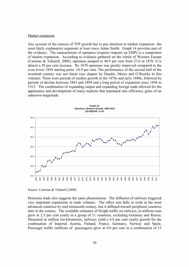
Market expansion Any account of the sources of TFP growth has to pay attention to market expansion –the most likely explanatory argument at least since Adam Smith. Graph 14 provides part of the evidence. The measurement of openness (exports+imports on GDP) is a component of market expansion. According to evidence gathered on the whole of Western Europe (Carreras & Tafunell, 2008), openness jumped to 40.9 per cent from 27.6 in 1870. It is almost a 50 per cent increase. By 1870 openness was greatly improved compared to the even lower 1850 starting point -16.9 per cent. The performance of the second half of the twentieth century was not linear (see chapter by Daudin, Morys and O’Rourke in this volume). There were periods of modest growth in the 1870s and early 1880s, followed by periods of decline between 1883 and 1894 and a long period of expansion since 1894 to 1913. The combination of expanding output and expanding foreign trade allowed for the appearance and development of many markets that translated into efficiency gains of an unknown magnitude.

Graph 14.Openness, Western Europe, 1850-1913

([X+M]/GDP, in %)

15,0

20,0

25,0

30,0

35,0

40,0

45,0

1850

1852

1854

1856

1858

1860

1862

1864

1866

1868

1870

1872

1874

1876

1878

1880

1882

1884

1886

1888

1890

1892

1894

1896

1898

1900

1902

1904

1906

1908

1910

1912

Source: Carreras & Tafunell (2008) Domestic trade also suggests the same phenomenon. The diffusion of railways triggered very important expansions in trade volumes. The effect was fully at work in the most advanced countries by mid nineteenth century, but it diffused toward peripheral countries later in the century. The available estimates of freight traffic on railways, in millions tons grew at 2.3 per cent yearly in a group of 11 countries, excluding Germany and Russia. Measured as million ton-kilometers, railways yield a 4.8 per cent yearly growth for the combination of Imperial Austria, Finland, France, Germany, Norway and Spain. Passenger traffic (millions of passengers) grew at 4.0 per cent in a combination of 13

27

countries, including all the big ones but Germany. Postal mail grew at 5.1 per cent in 13 European countries (but Russia and a few peripherals). Telegrams grew at 5.6 per cent in an almost comprehensive 17 European countries wide total –all but a few Balkans. All of these indices are proxies of market growth. All of them outperform by various points GDP growth and are suggestive of the importance of market expansion.20 Institutional developments We switch now to one of the typical ultimate causes of growth. Institutions do matter –no doubt about it. But: how much? Through what channels? These are much more difficult questions to answer. Late nineteenth century Europe provides some evidence of the role of political institutions. The database Polity IV provides a quantitative assessment of political development ranked along the continuum autocracy-democracy. The authors provide from 0 to 10 points to democratic features, and from 0 to 10 points to autocratic features. The “polity” index is the difference “Democracy less Autocracy”. By definition the highest value is +10 (democracy without autocracy features) and the minimum is -10 (autocracy without democratic elements). Of course, the polity index is about distribution of power, representative institutions, diffusion of the franchise, but not about property rights and rule of law. We may infer that in a country with proper democratic distribution of power, rule of law should be present as well. The countries that stand out as the most democratic by 1870 are Switzerland (Polity score: 10), Greece (9), Belgium (6) and UK (3). All the others (21) are in the negative range. The most autocratic are Russia and Turkey (-10). By 1913 there are 12 in the positive range and 8 in the negative side. The highest ranked are Switzerland, Greece and Norway (10), UK, France and Denmark (8). Belgium and Portugal (7), Spain (6), Sweden (5), Serbia (4), Germany (2). Bulgaria is the worst with a polity index of -9. While we may feel comfortable with Switzerland, Belgium and the UK having high marks by 1870, what can we say about Greece? Our data suggests that Greece was not doing well at all. It was in the poor range, and not growing quickly. We can say the same of the two Iberian countries, Spain and Portugal, that reach high marks in 1913 and improved a lot compared to 1870 (Portugal enjoys the second biggest improvement in Europe, just behind Norway). An alternative could be to obtain the average Polity index for the whole period. This is not an easy task as the authors of the index have failed to deal with the turmoil years. They have a range of values that does not add properly to the rest of values. The available data suggests that democratic regimes are usually prone to growth, but they can be even more prone to stability. Growth and stability might be complementary in advanced economies, but might be contradictory in backward economies.

20 All the data in the paragraph comes from Mitchell (2003).

28

CONCLUDING REMARKS: GROWING AT THE PRODUCTION FRONTIER What we know about the aggregate growth of the European economy between 1870 and 1913 is quite enough, even if we are still searching for better data for a number of Balkan economies. The globalized European economy reached a “silver age”. GDP growth was quite rapid (2.15% per annum) and diffused all over Europe. Even discounting the high rates of population growth (1.06%), per capita growth was left at a respectable 1.08%. Income per capita was rising in every country, and the rates of improvement were quite similar. This was a major achievement after two generations of highly localized growth, both geographically and socially. Indeed, the two first thirds of the century assisted at highly localized growth spurts and were not able to diffuse the benefits to most of the social fabric. On the contrary, since 1870 or even earlier, the whole of Europe, with very few exceptions, enjoyed the advantages of the industrial age, with new products, cheaper food, improved transport and communication facilities, and better access to markets. Growth was based in the increased use of labor and capital, but a good part of growth came out of what is called Total Factor Productivity –efficiency gains resulting from not well specified ultimate sources of growth. The proportion of increased income per capita coming from these sources suggests that the European economy was growing at full capacity –at its production frontier. It would have been very difficult to improve its performance. It is fair to say that the United States fared even better –but this was a truly exceptional achievement. Within Europe, convergence was limited, and it was mostly in motion after 1900. What happened was more the end of the era of big divergence rather than an era of big convergence. This did not seem enough to many –governments, elites and political and social movements- that very anxious to fully reap the abundant profits of the new capitalist world. The road to August 1914 was paved with the ambitions of many. The expanding European economy of 1870-1913 was growing quick enough to suggest to all the economic agents that all what was dreamt was at their immediate reach –only if they had the will to get it. Crowned heads, populist leaders, arm manufacturers as well as trade unions and minority political parties played the sorcerer’s apprentice. It is worth to remember that only Lenin fully reaped the opportunity –and we know the outcome. All the others failed. APPENDIX ON SOURCES: GDP, population and per capita GDP data for the whole of Western European and for each Western European country come from Carreras and Tafunell (2004) updated and expanded in Carreras and Tafunell (2008). More detailed information on sources and aggregation methods is available there. Austria-Hungary data comes from Schulze (2000). Russian data after 1885 comes from Gregory (1982), and earlier data comes from Goldsmith (1961). The limited data available on the Balkans presented by Maddison (2007) and the Ottoman Empire is reviewed by Avramov and Pamuk (2006). Pamuk (2007) provides new data for some benchmarks. We have adjusted our estimates to the frontiers of the time set of benchmarks defined by Broadberry and Klein (2007). GDP data is always presented in international US $ at 1990 prices. This accounting procedure has been widely accepted foir comparative purposes even if so many scholars are aware of its limitations (see L.Prados de la Escosura (2000) for an alternative measure). Western Europe consumer price index, openness and investment ratios come from Carreras and Tafunell (2008).

29

Bibliography Avramov, R. and S.Pamuk, eds. (2006), Monetary and fiscal policies in South-East

Europe. Historical and comparative perspective, Sofia, Bulgarian National Bank. Bairoch, Paul (1976), Commerce extérieur et développement économique de l’Europe au

XIXe siècle, Paris: Mouton / EHESS. Broadberry, Stephen, and Mark Harrison, eds. (2005), The Economics of World War I, Cambridge: Cambridge U.P. Broadberry, Stephen and Alexander Klein (2007), “Aggregate and per capita GDP in Europe, 1870-2000: Continental, Regional and National Data with changing boundaries”, manuscript, June 2007. Broadberry, S., G.Federico and A.Klein (2006), “Structural change, 1870-1913”, in S.Broadberry and K. O’Rourke, eds., The New Economic History of Europe. Cameron, R. (1985), “A New View of European Industrialization”, The Economic

History Review, XXXVIII, 1, pp. 1-23. Carreras, A. (2005), “Spanish industrialization in the Swedish mirror”, in Jerneck, Mörner, Tortella & Akerman, eds., Different Paths to Modernity. A Nordic and Spanish

Perspective, Nordic Academic Press, Lund, 2005, pp. 151-165. Carreras, Albert (2006), “The Twentieth Century” in A. Di Vittorio, ed., An economic

history of Europe: from expansion to development, London: Routledge. Carreras, Albert and Xavier Tafunell (2004), “The European Union economic growth experience, 1830-2000”, in S. Heikkinen & J.L. Van Zanden, eds., Explorations in

Economic Growth, Amsterdam, Aksant, pp.63-87. Carreras, Albert and Xavier Tafunell (2008), Western European Long Term Growth,

1830-2000: Facts and Issues, Barcelona: CREI (Opuscles del CREI, n.20). Carter, s. et al., eds. (2006), Historical Statistics of the United States. Millennial edition, Cambridge: Cambrdige University Press, vol. 1. Crafts, N.F.R., and G. Toniolo (2008), “Aggregate growth, 1950-2005”, in S.Broadberry and K. O’Rourke, eds., The New Economic History of Europe. Daudin, G., M.Morys and K.O’Rourke, “Europe and globalization, 1870-1914”, in S.Broadberry and K. O’Rourke, eds., The New Economic History of Europe. Étémad, Bouda (2000), La possession du monde. Poids et measures de la colonisation, Bruxelles: Éditions Complexe.

30

Federico, P.J. (1964), “Historical Patent Statistics, 1791-1961”, Journal of the Patent

Office Society, XLVI, 2, 89-171 Ferguson, N. (1998), The Pity of War, London: Allen Lane. Flora, Peter (1987), State, economy and society in Western Europe, 1815-1975. A data

handbook in two volumes, Frankfurt: Campus; London: Macmillan, New York: St James Press. Vol. II. Gerschenkron, A. (1962), Economic Backwardness in Historical Perspective, Cambridge Harvard U.P. Goldsmith, R. (1961), “The economic growth of Tsarist Russia, 1861-1913”, Economic

Development and Cultural Change, pp. 441-475. Goldsmith, R. (1985) Comparative national balance sheets: a study of twenty countries,

1688-1978, University of Chicago Press. Gregory, Paul (1982), Russian national income, 1885-1913, Cambridge: Cambridge U.P. Hjerppe, R. (1996). Finland’s Historical National Accounts 1860-1994. Calculation

Methods and Statistical Tables. Jyväskylä: Kivirauma. Huberman, M. and C. Minns (2007), “The times they are not changin’: Days and hours of work in Old and New worlds, 1870-2000”, Explorations in Economic History, 538-567 Kennedy, Paul (1987) The rise and fall of the great powers: economic change and

military conflict from 1500 to 2000, New York: Random House. Khan, Zorina (2005), The democratization of invention: patents and copyrights in

American economic development, 1790-1920, Cambridge: Cambridge University Press. Krantz, Olle & Lennart Schön (2007), Swedish Historical National Accounts 1800-2000, Lund. Checked at the webpage: http://www.ehl.lu.se/database/LU-MADD/National%20Accounts/default.htm. Lains, P. (2003). Os Progressos do Atraso. Uma Nova História Económica de Portugal. Lisboa: Imprensa de Ciências Sociais. Landes, David (1969), The Unbound Prometheus. Technological Change and Industrial

Development in Western Europe from 1750 to the Present, Cambridge U.P., Cambridge. Lindert, Peter (2004), Growing public: social spending and economic growth since the

eighteenth century, Cambridge: Cambridge University Press, 2 vols.

31

Maddison, A. (1982). Phases of Capitalist Development, Oxford, Oxford University Press. Maddison, A. (1987). “Growth and slowdown in advanced capitalist economies: techniques of quantitative assessment”, Journal of Economic Literature, 25, pp. 649-698. Maddison, A. (1991). Dynamic Forces in Capitalist Development. A Long-Run

Comparative View. Oxford: Oxford University Press. Maddison, A. (2001). The World Economy: A Millennial Perspective, Paris, OECD. Maddison, A. (2003). The World Economy. Historical Statistics, Paris, OECD. Maddison, A. (2007). http://www.ggdc.net/maddison/ Malanima, Paolo (2003), “Measuring the Italian Economy, 1300-1861”, Rivista di Storia

Economica, XIX, 3, 265-295. Malanima, Paolo (2006), Alle origini della crescita in Italia, 1820-1913, Rivista di Storia

Economica, XXII, 3, 307-330. Malanima, Paolo (2006), “An Age of Decline. Product and Income in Eighteenth-Nineteenth Century Italy”, Rivista di Storia Economica, XXII, 1, 91-133. Mitchell, B.R. (2003). International Historical Statistics. Europe, 1750-2000. New York: Stockton Press. Moser, P. (2005), “How do patent laws influence innovation? Evidence from nineteenth-century world fairs”, The American Economic Review, 95, 4, pp. 1214-1236. Mokyr, J. (2002), The gifts of Athena. The historical origins of the knowledge economy, Princeton: Princeton Uuniversity Press. Mokyr and Voth, “Understanding Growth in Early Modern Europe”, in S.Broadberry and K. O’Rourke, eds., The New Economic History of Europe. Nicolau, R. (2005), “Población, salud y actividad”, in A. Carreras and X. Tafunell, eds., Estadística históricas de España, siglos XIX-XX, Bilbao: Fundación BBVA, pp. 77-154. Offer, A. (1989), The First World War: an agrarian interpretation, Oxford: Clarendon. O’Rourke, K.H. and J.G.Williamson (1997), “Around the European periphery, 1870-1913: Globalization, schooling and growth”, European Review of Economic History, 1, pp.153-190.

32

Pamuk, S. (2006), “Estimating Economic Growth in the Middle Easzt Since 1820”, Journal of Economic History, 2006, 809-828. POLITY IV: http://www.systemicpeace.org/polity/polity4.htm Pollard, Sidney (1981), Peaceful Conquest. The Industrialization of Europe, 1760-1970, Oxford U.P., Oxford. Pounds (1957), Coal and steel in Western Europe: The influence of resources and

technique on production, Bloomington: Indiana U.P. Prados de la Escosura, L. (2000), “International comparisons of real product, 1820-1990: An alternative data set”, Explorations in Economic History, 7, pp. 1-41. Prados de la Escosura, L. (2003). El progreso económico de España, 1850-2000. Madrid: Fundación BBVA. Reis, Jaime (1993), O atraso económico Português, 1850-1930, Lisboa: Imprensa Nacional Casa da Moeda. Rostow, W.W. (1961). The Stages of Economic Growth. Cambridge: Cambridge University Press. Sáiz, J.P. (2005), “Investigación y desarrollo: Patentes”, in A. Carreras and X. Tafunell, eds., Estadística históricas de España, siglos XIX-XX, Bilbao: Fundación BBVA, pp. 835-872. Schulze, M.-S. (2000), “Patterns of growth and stagnation in the late nineteenth century Habsburg economy”, European Review of Economic History, 4, pp. 311-340. Smits, J.P., Horlings, E. y van Zanden, J.L. (2000). Dutch GNP and Its Components,

1800-1913, < http://nationalaccounts.niwi.knaw.nl > Toutain, J.C. (1997). “Le produit intérieur brut de la France, 1789-1990”. Economies et

Sociétes, Histoire économique quantitative, Série HEQ nº 1(11), pp.5-136. Trebilcock, Clive (1981), The Industrialization of the Continental Powers, 1780-1914, Longman, London. Van Zanden, J.L., and A. Van Riel (2004), The strictures of inheritance. The Dutch

economy in the nineteenth century, Princeton: Princeton University Press. Voth, H.-J. (2006), “La discontinuidad olvidada: provisión de trabajo, cambio tecnológico y nuevos bienes durante la Revolución Industrial”, Revista de Historia

Industrial, XV, 3, pp. 13-31.