Aircraft Thermal Management using Loop Heat Pipes - CORE

Wright State University Wright State University

CORE Scholar CORE Scholar

Browse all Theses and Dissertations Theses and Dissertations

2009

Aircraft Thermal Management using Loop Heat Pipes Aircraft Thermal Management using Loop Heat Pipes

Andrew J. Fleming Wright State University

Follow this and additional works at: https://corescholar.libraries.wright.edu/etd_all

Part of the Mechanical Engineering Commons

Repository Citation Repository Citation Fleming, Andrew J., "Aircraft Thermal Management using Loop Heat Pipes" (2009). Browse all Theses and Dissertations. 268. https://corescholar.libraries.wright.edu/etd_all/268

This Thesis is brought to you for free and open access by the Theses and Dissertations at CORE Scholar. It has been accepted for inclusion in Browse all Theses and Dissertations by an authorized administrator of CORE Scholar. For more information, please contact [email protected].

https://corescholar.libraries.wright.edu/

https://corescholar.libraries.wright.edu/etd_all

https://corescholar.libraries.wright.edu/etd_comm

https://corescholar.libraries.wright.edu/etd_all?utm_source=corescholar.libraries.wright.edu%2Fetd_all%2F268&utm_medium=PDF&utm_campaign=PDFCoverPages

http://network.bepress.com/hgg/discipline/293?utm_source=corescholar.libraries.wright.edu%2Fetd_all%2F268&utm_medium=PDF&utm_campaign=PDFCoverPages

https://corescholar.libraries.wright.edu/etd_all/268?utm_source=corescholar.libraries.wright.edu%2Fetd_all%2F268&utm_medium=PDF&utm_campaign=PDFCoverPages

mailto:[email protected]

AIRCRAFT THERMAL MANAGEMENT USING LOOP HEAT PIPES

A thesis submitted in partial fulfillment of the requirements for the degree of

Master of Science in Engineering

By

ANDREW JAMES FLEMING B.S., Wright State University, 2004

2009 Wright State University

WRIGHT STATE UNIVERSITY

SCHOOL OF GRADUATE STUDIES

March 20, 2009

I HEREBY RECOMMEND THAT THE THESIS PREPARED UNDER MY SUPERVISION BY Andrew James Fleming ENTITLED Aircraft Thermal Management Using Loop Heat Pipes BE ACCEPTED IN PARTIAL FULFILLMENT OF THE REQUIREMENTS FOR THE DEGREE OF Master of Science in Engineering.

____________________________________ Scott K. Thomas, Ph.D. Thesis Director

____________________________________

George P.G. Huang, P.E., Ph.D. Department Chair Committee on Final Examination ____________________________________ Scott K. Thomas, Ph.D.

____________________________________ Kirk L. Yerkes, Ph.D. ____________________________________ J. Mitch Wolff, Ph.D. ____________________________________ James A. Menart, Ph.D. ____________________________________ Joseph F. Thomas, Jr., Ph.D. Dean, School of Graduate Studies

iii

ABSTRACT

Fleming, Andrew James. M.S.Egr., Department of Mechanical and Materials Engineering, Wright State University, 2009. Aircraft Thermal Management using Loop Heat Pipes.

The objective of this thesis was to determine the feasibility of using loop heat

pipes to dissipate waste heat from power electronics to the skin of a fighter aircraft and

examine the performance characteristics of a titanium-water loop heat pipe under

stationary and elevated acceleration fields. In the past, it has been found that the

boundary condition at the condenser can be a controlling factor in the overall

performance of this type of thermal management scheme. Therefore, the heat transfer

removed from the aircraft skin has been determined by modeling the wing as a flat plate

at zero-incidence as a function of the following parameters: airspeed: 0.8 ≤ Ma∞ ≤ 1.4;

altitude: 0 ≤ H ≤ 22 km; wall temperature: 105 ≤ Tw ≤ 135°C. In addition, the effects of

the variable properties of air have been taken into account. Heat transfer due to thermal

radiation has been neglected in this analysis due to the low skin temperatures and high

airspeeds up to Ma∞ = 1.4. It was observed that flight speed and altitude have a

significant effect on the heat transfer abilities from the skin to ambient, with heat

rejection becoming more difficult with increasing Mach number or decreasing altitude.

An experiment has been developed to examine operating characteristics of a

titanium-water loop heat pipe (LHP) under stationary and elevated acceleration fields.

The LHP was mounted on a 2.44 m diameter centrifuge table on edge with heat applied

to the evaporator via a mica heater and heat rejected using a high-temperature

polyalphaolefin coolant loop. The LHP was tested under the following parametric

ranges: heat load at the evaporator: 100 ≤ Qin ≤ 600 W; heat load at the compensation

chamber: 0 ≤ Qcc ≤ 50 W; radial acceleration: 0 ≤ ar ≤ 10 g. For stationary operation (az

= 1.0 g, ar = 0 g), the LHP evaporative heat transfer coefficient decreased monotonically,

iv

thermal resistance decreased to a minimum then increased, and wall superheat increased

monotonically. Heat input to the compensation chamber was found to increase the

evaporative heat transfer coefficient and decrease thermal resistance for Qin = 500 W.

Flow reversal in the LHP was found for some cases, which was likely due to vapor

bubble formation in the primary wick. Operating the LHP in an elevated acceleration

environment (az = 1.0 g, ar > 0 g) revealed dry-out conditions from Qin = 100 to 400 W

and varying accelerations and the ability for the LHP to reprime after an acceleration

event that induced dry-out. Evaporative heat transfer coefficient and thermal resistance

was found not to be significantly dependent on radial acceleration. However, wall

superheat was found to increase slightly with radial acceleration.

v

TABLE OF CONTENTS

1. Convective Heat Transfer from High-Speed Aircraft Skin .................................... 1

1.1. Abstract ............................................................................................................ 1

1.2. Introduction ...................................................................................................... 1

1.3. Mathematical Model ........................................................................................ 3

1.4. Results and Discussion .................................................................................... 5

1.5. Conclusions ...................................................................................................... 6

2. Titanium-Water Loop Heat Pipe Characteristics Under Stationary and

Elevated Acceleration Fields .................................................................................... 14

2.1. Abstract .......................................................................................................... 14

2.2. Introduction .................................................................................................... 14

2.3. Experimental Setup ........................................................................................ 19

2.4. Results and Discussion .................................................................................. 27

2.5. Conclusions .................................................................................................... 39

2.6. Future Work ................................................................................................... 40

References ........................................................................................................................ 74

Appendix A. Operating Procedures .............................................................................. 77

A.1. Standard Operating Procedure ...................................................................... 77

A.2. Test Procedures ............................................................................................. 79

Appendix B. Uncertainty Analysis ................................................................................ 89

Appendix C. Calibration of Thermocouples and Flow Meter .................................... 92

C.1. Thermocouple Calibration ............................................................................. 92

vi

C.2. Flow Meter Calibration ................................................................................. 95

Appendix D. Loop Heat Pipe Mounting ..................................................................... 114

Appendix E. Brayco Micronic 889 Technical Data .................................................... 119

Appendix F. Centrifuge Table Upgrades .................................................................... 121

Appendix G. LabVIEW Programs .............................................................................. 130

Appendix H. Centrifuge Wiring Tables ...................................................................... 136

Appendix I. Sample Calculations ................................................................................ 139

vii

LIST OF FIGURES

Figure 1.1. Comparison of atmospheric properties versus altitude: (a) Temperature; (b) Density (DOD, 1997; Anderson, 2000). ........................................... 7

Figure 1.2. Adiabatic wall temperature versus altitude for various Mach numbers (1% hot day). ................................................................................................................. 8

Figure 1.3. Temperature difference )( aw ∞−TT versus altitude for various Mach numbers (1% hot day). .................................................................................................. 8

Figure 1.4. Temperature difference )( aww TT − versus altitude for various Mach numbers (Tw = 135ºC, 1% hot day). .............................................................................. 9

Figure 1.5. Maximum Mach number before heat is transferred from the air to the skin versus altitude for various wall temperatures (1% hot day). ................................. 9

Figure 1.6. Average convective heat transfer coefficient versus altitude for various Mach numbers (Tw = 135ºC, L = 1.0 m, 1% hot day). ................................... 10

Figure 1.7. Average heat flux dissipated over the plate versus altitude for various Mach numbers (Tw = 135ºC, L = 1.0 m, 1% hot day). ................................................ 10

Figure 1.8. Local heat flux dissipated over the plate versus plate length for various Mach numbers (Tw = 135ºC, 1% hot day): (a) H = 0 km; (b) H = 10 km; (c) H = 20 km. ...................................................................................................... 11

Figure 1.9. Average heat flux dissipated over the plate versus altitude for various atmospheric conditions (Tw = 135ºC, L = 1.0 m, Ma∞ = 0.98) (DOD, 1997; Anderson, 2000). ......................................................................................................... 12

Figure 1.10. Average heat flux dissipation versus altitude for various wall temperatures (Ma∞ = 0.98, L = 1.0 m, 1% hot day). ................................................... 12

Figure 2.1. Loop heat pipe operation. Adapted and reprinted with permission from AIAA (Hoang and Ku, 2003). ............................................................................ 42

Figure 2.2. Evaporator schematic: (a) Side view; (b) Cross-sectional view. Adapted and reprinted with permission from AIAA (Hoang and Ku, 2003). ............ 43

Figure 2.3. Schematic of Centrifuge Table Test Bed. ...................................................... 44

Figure 2.4. Titanium-water loop heat pipe test article as delivered. ................................ 45

Figure 2.5. Thermocouple locations on the LHP: (a) Locations of thermocouples TC04 through TC15 across the LHP; (b) Locations of TC04 through TC07 within the evaporator. ................................................................................................. 46

viii

Figure 2.6. Mounting of loop heat pipe to centrifuge table, front and top views: (a) Evaporator and compensation chamber: (b) Transport lines; (c) Condenser with cold plate; (d) Complete loop heat pipe. ............................................................. 47

Figure 2.7. High temperature fluid loop: (a) Schematic; (b) Reservoir, pump, filter, flowmeter, TC03, and liquid/liquid heat exchanger; (c) Cold plate, TC00, and TC01. ......................................................................................................... 48

Figure 2.8. Use of a cold-start test to determine when steady state occurred for the stationary LHP (Qin = 600 W, Qcc = 0 W, ar = 0 g, cpm& = 0.0077 kg/s, cpT = 67.7°C, Tamb = 38.1°C): (a) Transient temperature traces; (b) Transient rate of change of temperatures; (c) Transient thermal resistance and evaporative heat transfer coefficient. .............................................................................................. 49

Figure 2.9. Transient startup of the stationary LHP (Qin = 600 W, Qcc = 0 W, ar = 0 g, cpm& = 0.0077 kg/s, cpT = 67.7°C, Tamb = 38.1°C): (a) Initial startup; (b) Complete startup until steady state. ............................................................................ 50

Figure 2.10. Transient temperature profiles in the condenser and bayonet tube of the stationary LHP (Qcc = 0 W, ar = 0 g, cpm& = 0.0077 kg/s, 36.8 ≤ cpT ≤ 71.6°C, 31.7 ≤ Tamb ≤ 38.1°C): (a) Qin = 100 W; (b) Qin = 200 W; (c) Qin = 300 W; (d) Qin = 400 W; (e) Qin = 500 W; (f) Qin = 600 W. ...................................... 51

Figure 2.11. Transient temperature profiles of the stationary LHP for Qin = 200 W (Qcc = 0 W, ar = 0 g, cpm& = 0.0077 kg/s, cpT = 46.1°C, Tamb = 31.7°C): (a) Transient temperature profiles; (b) 2φ-1φ point oscillation in the condenser. ........... 52

Figure 2.12. Steady state temperature distribution versus transported heat for the stationary LHP (Qcc = 0 W, ar = 0 g, cpm& = 0.0077 kg/s, 36.8 ≤ cpT ≤ 71.6°C, 31.7 ≤ Tamb ≤ 38.1°C): (a) Evaporator section; (b) Condenser section. ..................... 53

Figure 2.13. Steady state performance characteristics of the stationary LHP versus transported heat (Qcc = 0 W, ar = 0 g, cpm& = 0.0077 kg/s, 36.8 ≤ cpT ≤ 67.7°C, 27.6 ≤ Tamb ≤ 38.7°C): (a) Evaporative heat transfer coefficient; (b) Thermal resistance; (c) Wall superheat ....................................................................... 54

Figure 2.14. Steady state performance characteristics of the stationary LHP versus compensation chamber heat input (Qin = 500 W, ar = 0 g, cpm& = 0.0077

kg/s, 63.4 ≤ cpT ≤ 64.8°C, 36.1 ≤ Tamb ≤ 38.1°C): (a) Evaporator temperatures; (b) Condenser temperatures; (c) Evaporative heat transfer coefficient and thermal resistance. .............................................................................. 55

Figure 2.15. Transient temperature profiles in the condenser and bayonet tube of the stationary LHP for Qcc = 25 to 50 W (Qin = 500 W, ar = 0 g, cpm& = 0.0077

kg/s, 63.4 ≤ cpT ≤ 64.8°C, 36.1 ≤ Tamb ≤ 38.1°C): (a) Qcc = 25 W; (b) Qcc = 30 W; (c) Qcc = 35 W; (d) Qcc = 40 W; (e) Qcc = 45 W; (f) Qcc = 50 W. ......................... 56

ix

Figure 2.16. Transient temperature traces of the LHP at elevated acceleration (Qin = 600 W, Qcc = 0 W, cpm& = 0.0077 kg/s, 55.2 ≤ cpT ≤ 59.7°C, 27.9 ≤ Tamb ≤ 30.1°C): (a) ar = 0.1 g startup phase; (b) Transition to and steady state at ar = 10.0 g; (c) Transient rate of change of temperatures. ................................................. 57

Figure 2.17. Effect of resultant acceleration vector direction on fluid distribution within the LHP: (a) Resultant acceleration vector orientation versus radial acceleration; (b) Liquid pooling in the evaporator, compensation chamber, and condenser under elevated acceleration (to scale, top view); (c) Liquid pooling in the condenser bends. ............................................................................................... 58

Figure 2.18. Steady state performance characteristics of the LHP versus transported heat at stationary and elevated acceleration (Qcc = 0 W, cpm& =

0.0077 kg/s, 37.2 ≤ cpT ≤ 67.7°C, 25.1 ≤ Tamb ≤ 38.7°C): (a) Evaporative heat transfer coefficient; (b) Thermal resistance; (c) Wall superheat. ............................... 59

Figure 2.19. Transient temperature traces of the LHP at elevated acceleration showing dry-out behavior (Qin = 400 W, Qcc = 0 W, cpm& = 0.0077 kg/s, 37.2 ≤

cpT ≤ 59.7°C, Tamb = 28.0°C): (a) Te,max = 150°C; (b) Te,max = 175°C; (c) Te,max = 200°C. ............................................................................................................ 60

Figure 2.20. Quasi-steady state temperature traces of the LHP and cold plate at elevated acceleration for Qin = 200 W (Qcc = 0 W, cpm& = 0.0077 kg/s, cpT = 41.9°C, Tamb = 26.4°C): (a) Transient temperature trace at ar = 0.1 g and t = 13834 s; (b) Transient temperature trace at ar = 4.0 g and t = 31240 s. ..................... 61

Figure 2.21. Steady state performance map of the LHP relating radial acceleration and heat transported (Qcc = 0 W, cpm& = 0.0077 kg/s, 37.2 ≤ cpT ≤ 59.7°C, 25.1 ≤ Tamb ≤ 30.2°C). ................................................................................... 62

Figure A.1. Centrifuge table main power breaker: (a) Electrical panel MCC-6; (b) Centrifuge table main power breaker. ................................................................... 81

Figure A.2. Centrifuge table control panel box. .............................................................. 82

Figure A.3. Sample LabVIEW control program. ............................................................. 83

Figure A.4. Centrifuge table power switch. ..................................................................... 84

Figure A.5. Neslab recirculating chiller. .......................................................................... 85

Figure A.6. Chill bath plumbing schematic. .................................................................... 86

Figure A.7. Booster pump control panel. ......................................................................... 87

Figure A.8. Centrifuge table motor control power switch. .............................................. 88

Figure C.1. LabVIEW sub-VI wire diagram for RTD read. .......................................... 100

Figure C.2. LabVIEW sub-VI wire diagram for calibration bath temperature set. ....... 100

Figure C.3. LabVIEW sub-VI wire diagram for calibration bath temperature read. ..... 101

x

Figure C.4. LabVIEW VI for controlling the automatic thermocouple calibration: (a) Front panel; (b) Wire diagram ............................................................................. 102

Figure C.5. LabVIEW VI for manual thermocouple calibration: (a) Front panel; (b) Wire diagram. ...................................................................................................... 103

Figure C.6. RTD temperature vs. time from the thermocouple calibration procedure. .................................................................................................................. 104

Figure C.7. Sample RTD vs. thermocouple plot for TC00. ........................................... 105

Figure C.8. LabVIEW VI for flow meter calibration program: (a) Front panel; (b) Wire diagram. ...................................................................................................... 106

Figure C.9. Schematic of flow meter calibration loop ................................................... 107

Figure C.10. Temperature and flow meter voltage versus mass flow rate calibration curve for the high-temperature fluid loop flow meter. ........................... 108

Figure C.11. Sample data collected during one time run for the flow meter calibration. (a) “Shotgun Blast” good data set; (b) “Trend” bad data set. ............... 109

Figure D.1. Mounting of LHP to minimize acceleration gradient. ................................ 116

Figure D.2. LHP survey locations.................................................................................. 117

Figure E.1. Brayco Micronic 889 properties vs. temperature. (a) ρ vs. T; (b) k vs. T; (c) Cp vs. T. ........................................................................................................... 120

Figure F.1. Updated wiring on the centrifuge table. ...................................................... 126

Figure F.2. Wiring panel from centrifuge table to the centrifuge table control room. ......................................................................................................................... 127

Figure F.3. Wiring panel for the new data acquisition system. ..................................... 128

Figure F.4. Centrifuge table voltage versus +ra . ........................................................ 129

Figure G.1. LabVIEW VI for the LHP experiment: (a) Front panel; (b) Wire diagram. .................................................................................................................... 131

Figure G.2. LabVIEW sub-VI wire diagram for voltage output control: (a) Output on; (b) Output off. ......................................................................................... 132

Figure G.3. LabVIEW sub-VI wire diagram for data acquisition communication. ...... 133

Figure G.4. LabVIEW sub-VI wire diagram for data analyzing. .................................. 134

Figure G.5. LabVIEW sub-VI wire diagram for data recording. ................................... 135

xi

LIST OF TABLES

Table 1.1. Regression equations for air properties versus altitude for 1% hot (DOD, 1997). .............................................................................................................. 13

Table 1.2. Regression equations for air properties versus temperature (Incropera and DeWitt, 2002). ...................................................................................................... 13

Table 2.1. AFRL/RZPS design requirements. ................................................................. 63

Table 2.2. ACT LHP geometric design parameters. ........................................................ 64

Table 2.3. Summary of LHP thermocouple locations ...................................................... 65

Table 2.4. Summary of uncertainties. .............................................................................. 66

Table 2.5. Steady state operating characteristics for the stationary LHP (Qcc = 0 W, ar = 0 g, cpm& = 0.0077 kg/s, 36.8 ≤ cpT ≤ 71.6°C, 27.6 ≤ Tamb ≤ 38.7°C) showing effect of startup path. .................................................................................... 67

Table 2.6. Steady state operating characteristics for the stationary LHP showing effect of heat input to the compensation chamber (Qin = 500 W, ar = 0 g, cpm&

= 0.0077 kg/s, 63.4 ≤ cpT ≤ 64.8°C, 36.1 ≤ Tamb ≤ 38.1°C). ....................................... 69

Table 2.7. The effect of compensation chamber temperature control on LHP operation (Qin = 500 W, ar = 0 g, cpm& = 0.0077 kg/s, cpT = 52.5°C, Tamb = 26.4°C) ........................................................................................................................ 70

Table 2.8. Steady state operating characteristics of the rotating LHP (Qcc = 0 W, cpm& = 0.0077 kg/s, 37.2 ≤ cpT ≤ 59.7°C, 25.1 ≤ Tamb ≤ 30.2°C). .............................. 71

Table 2.9. Comparison of quasi-steady states for Qin = 200 W (Qcc = 0 W, cpm& = 0.0077 kg/s)................................................................................................................. 73

Table C.1. Maximum deviation of calculated RTD and experimental RTD corresponding to each order of polynomial for thermocouple TC00. ...................... 110

Table C.2. Coefficients for the trend line of each thermocouple. .................................. 111

Table C.3. Maximum deviation and total error for each thermocouple. ........................ 112

Table C.4. 3-D paraboloid regression equation for high-temperature fluid loop flow meter. ................................................................................................................ 113

Table D.1. Loop heat pipe mounting survey data. ......................................................... 118

Table H.1. E1418A 8/16-CH D/A Converter wiring. .................................................... 137

xii

Table H.2. Data acqusition terminal board wiring. ........................................................ 138

xiii

NOMENCLATURE

a Speed of sound, m/s; acceleration, m/s2; flow meter calibration constant

b Flow meter calibration constant

B Experimental constant related to Eq. (F.2)

c Flow meter calibration constant

fC Skin friction coefficient, 2 /

Cp Specific heat, J/(kg-K)

d Flow meter calibration constant

D Diameter, m

f Frequency, Hz

g Acceleration due to standard gravity, 9.81 m/s2

h Heat transfer coefficient, W/(m2-K)

H Altitude, m

k Thermal conductivity, W/(m-K)

L Length, m

m Mass, kg

Ma Mach number, aU /

n Number of data points

Nu Nusselt number, /

Pr Prandtl number, /

Q Heat transfer rate, W

q Heat flux, W/m2

r Recovery factor; radial coordinate, m

R Particular gas constant, m2/(s2-K); thermal resistance, K/W

R2 Coefficient of determination

Ra Rayleigh number, /

xiv

Re Reynolds number, /

St Stanton number, /

t Time, s; t-distribution

T Temperature, K

U Velocity, m/s

V Voltage, V; volume, L

y0 Flow meter calibration constant

Greek Letters

α Thermal diffusivity, m2/s

β Inverse temperature, K-1

γ Ratio of specific heats

ΔT Temperature difference, K

ε Emissivity

θ Angle, degrees

μ Absolute or dynamic viscosity, (N-s)/m2

ν Kinematic viscosity, m2/s

ρ Density, kg/m3

σ Standard deviation; Stefan-Boltzmann constant, 5.67×10-8 W/(m2-K4)

φ Fluid phase

ω Angular velocity, rad/s

Superscripts

* Film condition

+ Normalized

1φ Single-phase

2φ Two-phase

Subscripts

1 Heat into vaporization of fluid

2 Heat leak to the compensation chamber

xv

∞ Freestream condition

a Actual

amb Ambient

aw Adiabatic wall

c Condenser

cc Compensation chamber

cl Centerline

cm Condenser midpoint

conv Convection

cp Cold plate

ct Centrifuge table

dev Deviation

D Diameter

e Evaporator

eg Ethylene glycol

e/cc Evaporator/compensation chamber junction

ie Inner edge

in Cold plate inlet; heat in to evaporator

L Local

max Maximum value

min Minimum value

m/t Mass/time

oe Outer edge

out Cold plate outlet; heat out of condenser

p Predicted

PAO Polyalphaolefin

r Radial

R Reference condition

rad Radiation

s Surface

sh Superheat

xvi

surr Surroundings

TC Thermocouple

tot Total

v Vapor

V/T Voltage/temperature

w Wall

z Axial

θ Azimuthal

xvii

ACKNOWLEDGEMENTS

This research effort was conducted as a part of the in-house program at the Air

Force Research Laboratory, Propulsion Directorate, Energy/Power/Thermal Division,

Thermal and Electrochemical Branch, AFRL/RZPS, Wright-Patterson Air Force Base,

Dayton, OH. I would like to thank Dr. Scott Thomas, Dr. Kirk Yerkes, and Dr. Quinn

Leland for the mentoring, wisdom, and knowledge you have given me over the past

several years. Thank you to Mr. Dave Courson for all of the technical assistance and

knowledge you have given to me throughout the duration of experimentation. Thank you

to the thermal crew for your guidance, help, and friendship: Mr. Travis Michalak, Mr.

Levi Elston, Dr. Larry Byrd, Ms. Cindy Obringer, and Ms. Bekah Puterbaugh. Thank

you to my parents, Ed and Judy, for your love, support, and guidance in helping me be

everything I am. Thank you to my wife and best friend, Jennifer, for your unfailing love

and support through our years together. Last, but most certainly not least, thank you to

my Lord and Savior Jesus Christ for all the blessings and gifts You have bestowed on me.

You are truly worth all my praise.

xviii

DEDICATION

To my beautiful wife, Jennifer, and son, Ethan. I love you.

1

1. CONVECTIVE HEAT TRANSFER FROM HIGH-SPEED AIRCRAFT SKIN

1.1. Abstract The objective of the present analysis was to determine the feasibility of using loop

heat pipes to dissipate waste heat from power electronics to the skin of a fighter aircraft.

In the past, it has been found that the boundary condition at the condenser can be a

controlling factor in the overall performance of this type of thermal management scheme.

Therefore, the heat transfer removed from the aircraft skin has been determined by

modeling the wing as a flat plate at zero-incidence as a function of the following

parameters: airspeed: 0.8 ≤ Ma∞ ≤ 1.4; altitude: 0 ≤ H ≤ 22 km; wall temperature: 105

≤ Tw ≤ 135°C. In addition, the effects of the variable properties of air have been taken

into account. Heat transfer due to thermal radiation has been neglected in this analysis

due to the low skin temperatures and high airspeeds up to Ma∞ = 1.4. It was observed

that flight speed and altitude have a significant effect on the heat transfer abilities from

the skin to ambient, with heat rejection becoming more difficult with increasing Mach

number or decreasing altitude.

1.2. Introduction The More Electric Aircraft initiative (MEA) is the concept for future aircraft

including warfighter, transport, helicopters, and commercial aircraft. This approach has

been adopted by the United States Air Force since the early 1990’s with the purpose of

reducing or removing as many of the hydraulic, mechanical, and pneumatic power

components and replacing them with electrically driven devices. This approach to

aircraft design was first envisioned during World War II. However, at that time, the

power generation capability and power conditioning equipment required was not feasible

due to volume requirements. As a result, hydraulic, pneumatic, and mechanical systems

became the norm for aircraft until this initiative. Under the MEA paradigm, power for

systems such as flight control actuation, anti-ice, braking, environmental control, engine

starting, and fuel pumping will be provided by a starter/generator driven by the gas

2

generator spool of the aircraft engine (Quigley, 1993). The MEA initiative has been

analytically proven to improve aircraft reliability, maintainability, support, and operations

cost as well as reduce weight, volume, and enhance battle damage reconfigurability

(Cloyd, 1997).

While the reduction of hydraulic, pneumatic, and mechanical systems in favor of

electrical systems is beneficial, it presents a problem in terms of thermal management.

Replacing the centralized hydraulic system with an electrical based system removes a

primary method of transporting and removing waste heat (Vrable and Yerkes, 1998). A

separate cooling fluid system for thermal management would be contrary to the goals of

the MEA initiative. Therefore, thermal management would need to be distributed over

the entire aircraft. As a result, a new approach to thermal management involves handling

heat loads on a local level. This means taking individual components in the aircraft and

locally handling their heat rejection requirements.

The operating envelope for military aircraft places stringent limitations on any

proposed thermal management system. The on-board electrical flight control actuation

system operates at altitudes from sea level to above 12 km, airspeeds from stationary to

supersonic speeds, transient body forces up to 9 g due to maneuvering, and ambient

temperatures from -68 to 58ºC. MEA has resulted in the development of high-

temperature, high-efficiency, and high-density power electronic component technologies.

The next-generation power electronics will be capable of operating at cold plate

temperature excursions up to 200ºC, which presents an opportunity to reject heat through

the aircraft skin to the ambient using passive cooling. In addition, the actuation system

rejects heat continuously at a rate of Q = 500 W (q = 3 W/cm2) and has transient heat

rejection rates of Q = 5000 W over a period of one second. Possible thermal

management scenarios include direct connection of the electronics package to the skin,

high-thermal conductivity graphite straps, or the use of a loop heat pipe between the

package and the skin to provide mounting flexibility. The objective of this analysis is to

determine the external heat transfer possibilities of the aircraft skin. The heat flux and

heat transfer coefficient have been found as functions of the skin and ambient

temperatures, the altitude, and airspeed.

3

1.3. Mathematical Model The temperature and density of air vary considerably with altitude and also vary

day-to-day depending on weather conditions. In order to be conservative in the

calculation of heat transfer coefficients, data for the highest temperature recorded with a

frequency-of-occurrence of 1% were used to generate equations for temperature and

density versus altitude (DOD, 1997) as shown in Figure 1.1 and Table 1.1. Also

presented are data for the lowest temperature recorded with a frequency-of-occurrence of

1% (DOD, 1997) and data for the “standard atmosphere” (Anderson, 2000).

The film temperature was used as the reference temperature to evaluate the air

properties (White, 1988)

∞ 0.5 0.039Ma 0.5 w (1.1)

The air density at the film temperature and at altitude was evaluated using the perfect gas

law

∞∞ (1.2)

The freestream speed of sound is

∞ ∞ (1.3)

The freestream velocity is

∞ Ma∞ ∞ (1.4)

The absolute viscosity of air is given by the following relation (NACA, 1953)

RR

.

(1.5)

where μR is a reference viscosity evaluated at a known reference temperature TR.

The Reynolds number for a plate of length L is determined by evaluating the

properties of air at the freestream condition.

ReL∞ ∞

∞ (1.6)

4

Regression equations for the specific heat and Prandtl number were determined as

functions of temperature using data from Incropera and DeWitt (2002), as shown in Table

1.2.

The adiabatic wall temperature is (White, 1988)

aw ∞ 11

2 Ma∞ (1.7)

where the recovery factor is

Pr1/2 for laminar flowPr1/3 for turbulent flow

(1.8)

For the purposes of this analysis, Reynolds numbers less than 500,000 were considered to

be laminar, greater than 500,000 were turbulent. The local skin friction coefficient at the

end of the plate was found by evaluating the air properties at the film temperature. For

laminar flow, the skin friction coefficient is given by (White, 1988)

f,L0.664

∞⁄ (1.9)

and for turbulent flow

f,L0.455

ln 0.06 ∞ (1.10)

The local Stanton number at the end of the plate for laminar flow is given by (White,

1988)

StL 0.332ReL/ Pr / (1.11)

and for turbulent flow

StLL

∞ p

f,L 2⁄

1 12.7 Pr / 1 f,L 2⁄ / (1.12)

The local heat transfer coefficient at the end of the plate is

L StL ∞ p (1.13)

5

The local heat transfer coefficient was calculated using the appropriate skin friction

coefficient and Stanton number based on laminar or turbulent flow. The average heat

transfer coefficient over the length of the plate is approximated by (White, 1988)

1.15 L (1.14)

The heat flux dissipated over the plate, both local and average, is defined in terms of the

adiabatic wall temperature (White, 1988)

w w aw (1.15)

Thermal radiation was neglected in this analysis as it contributed less than 1.6% to the

total heat rejected from the plate surface.

1.4. Results and Discussion The adiabatic wall temperature is shown in Figure 1.2 as a function of altitude and

Mach number. The overall trend of the adiabatic wall temperature with altitude follows

the freestream air temperature in Figure 1.1 and increases with Mach number as

expected. Figure 1.3 presents the temperature difference, ΔT = (Taw - T∞), versus altitude.

This temperature difference demonstrates the increase in the adiabatic wall temperature

over the freestream due to aerodynamic heating. The temperature difference ΔT = (Tw -

Taw) is given in Figure 1.4. Of interest is the portion of the curves in which this

difference is negative, which indicates that heat is transferred from the air to the aircraft

skin. The maximum Mach number achievable before heat is transferred from the air to

the skin is given by

Ma∞,max1 w

∞1

21

/

(1.16)

and is plotted in Figure 1.5 over a range of wall temperatures. The maximum Mach

number increases with altitude and wall temperature up to a maximum at approximately

18 km. In Figure 1.6, the average convective heat transfer coefficient decreases

monotonically with altitude due to the continual decrease in the air density. In general,

the convective heat transfer coefficient increases with Mach number, as expected. The

average heat flux dissipated from the plate is shown in Figure 1.7. For low Mach

numbers, the heat flux is positive for all values of altitude, which indicates that heat is

6

transferred from the aircraft skin to the air. At high Mach numbers, however, the heat

flux is negative at low altitudes due to the negative ΔT as shown in Figure 1.4. This

means that the adiabatic wall temperature is higher than the skin temperature due to

aerodynamic heating effects. The effect of heated plate length on the local heat flux for

H = 0, 10, and 20 km is shown in Figure 1.8. The local heat flux starts low and decreases

in the laminar region of the plate, and then increases as the flow transitions to turbulent

where it once again decreases. In general, the average heat flux follows the behavior of

the local heat transfer coefficient, where hL is high at the leading edge and at the

beginning of turbulent flow and decreases as the boundary layer grows. One item to note

is that Figure 1.9 shows the average heat flux dissipated over the plate versus altitude for

the 1% hot day, the 1% cold day, and the standard atmosphere data as presented in Figure

1.1. At low altitudes, wq is significantly higher for the 1% cold day due to the combined

effects of the lower atmospheric temperature and the higher air density. The effect of

wall temperature on average heat flux for a given airspeed is shown in Figure 1.10. The

heat flux increases dramatically with altitude and wall temperature for low altitudes.

1.5. Conclusions An analysis of the heat transfer from a heated plate has provided important

insights for the possible use of the aircraft skin to reject heat from electric actuator

systems. It was found that the altitude and speed of the aircraft significantly affected the

amount of heat that could be rejected from the skin. Aerodynamic heating of the skin

reduced the heat transfer, and if the Mach number was high enough, heat transfer from

the skin to the air went to zero. A performance map of this phenomenon was provided.

The altitude of the aircraft affected the freestream temperature and density, which in turn

affected the overall heat transfer coefficient. It was also shown that the assumption of a

“standard atmosphere” could result in significant errors in the prediction of the heat

dissipation as compared to the data for the 1% hot day or the 1% cold day. The analysis

showed that the aircraft skin temperature, which is directly influenced by the actuator

thermal management system, has a strong effect on the heat dissipation rate, especially at

low altitudes.

7

Figure 1.1. Comparison of atmospheric properties versus altitude: (a) Temperature; (b) Density (DOD, 1997; Anderson, 2000).

180

200

220

240

260

280

300

320

340

T∞

(K)

1% Hot Day

Standard Atmosphere

1% Cold Day

(a)

00.20.40.60.8

11.21.41.61.8

0 5 10 15 20

ρ ∞(k

g/m

3 )

H (km)

(b)

8

Figure 1.2. Adiabatic wall temperature versus altitude for various Mach numbers (1% hot day).

Figure 1.3. Temperature difference )( aw ∞−TT versus altitude for various Mach numbers (1% hot day).

050

100150200250300350400450

0 5 10 15 20H (km)

Taw

(K

)Ma = 0.8Ma = 0.98Ma = 1.2Ma = 1.4

0

20

40

60

80

100

120

140

0 5 10 15 20

ΔT =

[Taw

-T∞]

(K

)

H (km)

Ma = 0.8Ma = 0.98Ma = 1.2Ma = 1.4

9

Figure 1.4. Temperature difference )( aww TT − versus altitude for various Mach numbers (Tw = 135ºC, 1% hot day).

Figure 1.5. Maximum Mach number before heat is transferred from the air to the skin versus altitude for various wall temperatures (1% hot day).

0

20

40

60

80

100

120

140

0 5 10 15 20

ΔT =

[Taw

-T∞]

(K

)

H (km)

Ma = 0.8Ma = 0.98Ma = 1.2Ma = 1.4

0

0.5

1

1.5

2

2.5

0 5 10 15 20

Ma ∞

, m

ax

H (km)

Tw = 105 ºCTw = 115 ºCTw = 125 ºCTw = 135 ºC

10

Figure 1.6. Average convective heat transfer coefficient versus altitude for various Mach numbers (Tw = 135ºC, L = 1.0 m, 1% hot day).

Figure 1.7. Average heat flux dissipated over the plate versus altitude for various Mach numbers (Tw = 135ºC, L = 1.0 m, 1% hot day).

0

100

200

300

400

500

600

700

800

0 5 10 15 20

h

(W/m

2 -K

)

H (km)

Ma = 0.8Ma = 0.98Ma = 1.2Ma = 1.4

-2-1.5

-1-0.5

00.5

11.5

22.5

3

0 5 10 15 20q w(W

/cm

2 )

H (km)

Ma = 0.8Ma = 0.98Ma = 1.2Ma = 1.4

11

Figure 1.8. Local heat flux dissipated over the plate versus plate length for various Mach numbers (Tw = 135ºC, 1% hot day): (a) H = 0 km; (b) H = 10 km; (c) H = 20 km.

-4

-3

-2

-1

0

1

2

3

4

q w(W

/cm

2 )

Ma = 0.8Ma = 0.98Ma = 1.2Ma = 1.4

(a)

0

0.5

1

1.5

2

2.5

3

q w(W

/cm

2 )

(b)

0

0.2

0.4

0.6

0.8

1

1.2

0 0.5 1 1.5 2

q w(W

/cm

2 )

L (m)

(c)

12

Figure 1.9. Average heat flux dissipated over the plate versus altitude for various atmospheric conditions (Tw = 135ºC, L = 1.0 m, Ma∞ = 0.98) (DOD, 1997; Anderson, 2000).

Figure 1.10. Average heat flux dissipation versus altitude for various wall temperatures (Ma∞ = 0.98, L = 1.0 m, 1% hot day).

0

1

2

3

4

5

6

7

8

0 5 10 15 20

q w(W

/cm

2 )

H (km)

1% Hot DayStandard Atmosphere1% Cold Day

0

0.5

1

1.5

2

2.5

0 5 10 15 20

q w(W

/cm

2 )

H (km)

Tw = 105 ºCTw = 115 ºCTw = 125 ºCTw = 135 ºC

13

Table 1.1. Regression equations for air properties versus altitude for 1% hot (DOD, 1997).

y = a0 + a1H + a2H2 + a3H3 + a4H4

(H in km)

Property a0 a1 a2 a3 a4 R2 T∞ (ºC) 4.8507E+1 -9.5033E+0 5.3483E-1 -2.8994E-2 7.7664E-4 0.99779 ρ∞ (kg/m3) 1.0868E+0 -8.9917E-2 2.0898E-3 -4.9336E-6 — 0.99954

Table 1.2. Regression equations for air properties versus temperature (Incropera and DeWitt, 2002).

y = a0 + a1T + a2T2 + a3T3

(T in K)

Property a0 a1 a2 A3 R2 cp (J/kg-K) 1.0187E+3 -6.9921E-2 -3.3333E-5 4.4444E-7 0.99916

Pr 8.6418E-1 -9.4177E-4 1.7778E-6 -1.2593E-9 0.99725

14

2. TITANIUM-WATER LOOP HEAT PIPE CHARACTERISTICS UNDER STATIONARY AND ELEVATED ACCELERATION FIELDS

2.1. Abstract An experiment has been developed to examine operating characteristics of a

titanium-water loop heat pipe (LHP) under stationary and elevated acceleration fields.

The LHP was mounted on a 2.44 m diameter centrifuge table on edge with heat applied

to the evaporator via a mica heater and heat rejected using a high-temperature

polyalphaolefin coolant loop. The LHP was tested under the following parametric

ranges: heat load at the evaporator: 100 ≤ Qin ≤ 600 W; heat load at the compensation

chamber: 0 ≤ Qcc ≤ 50 W; radial acceleration: 0 ≤ ar ≤ 10 g. For stationary operation (az

= 1.0 g, ar = 0 g), the LHP evaporative heat transfer coefficient decreased monotonically,

thermal resistance decreased to a minimum then increased, and wall superheat increased

monotonically. Heat input to the compensation chamber was found to increase the

evaporative heat transfer coefficient and decrease thermal resistance for Qin = 500 W.

Flow reversal in the LHP was found for some cases, which was likely due to vapor

bubble formation in the primary wick. Operating the LHP in an elevated acceleration

environment revealed dry-out conditions from Qin = 100 to 400 W and varying

accelerations and the ability for the LHP to reprime after an acceleration event that

induced dry-out. Evaporative heat transfer coefficient and thermal resistance was found

not to be significantly dependent on radial acceleration. However, wall superheat was

found to increase slightly with radial acceleration.

2.2. Introduction Loop heat pipes (LHP's) are two-phase thermal transport devices that operate

passively using the latent heat of vaporization to transport heat from one location to

another. The LHP was invented in 1972 by Gerasimov and Maidanik (Maidanik, 2005)

in the former Soviet Union, and was later patented in the United States (Maidanik et al.,

1985). The LHP consists of an evaporator, compensation chamber, liquid and vapor

15

transport lines made of smooth tubing, and a condenser as shown in Figure 2.1. Heat is

applied directly to the exterior wall of the evaporator, which often has a circular cross-

section. The majority of the input heat is used to vaporize the working fluid within the

primary wick structure, which is an inverted meniscus wick in direct contact with the

exterior evaporator wall. The vapor is captured in the axial vapor grooves in the primary

wick and is directed via a manifold at the end of the evaporator to the vapor line due to

the increased pressure within the evaporator. Due to evaporation, menisci are developed

in the primary wick which establishes a capillary pressure head that returns liquid to the

evaporator from the condenser. This capillary head must be greater than the total system

pressure drop in order for the LHP to continue to operate without drying out.

The vapor from the evaporator section travels via the vapor line to the condenser

section, which is also made of smooth tubing. Heat is rejected from the condenser to the

ultimate heat sink. The working fluid enters the condenser as a superheated vapor. After

sufficient heat is rejected, the vapor becomes a saturated vapor, a two-phase mixture, a

saturated liquid, and, depending on the amount of heat rejection, it may or may not

become a subcooled liquid. The location of the point at which the working fluid becomes

a subcooled liquid (2φ-1φ) is dependent on the heat input at the evaporator, the heat

rejection at the condenser, and the saturation temperature in the compensation chamber.

After exiting the condenser section, the liquid will continue to lose heat due to convection

and/or thermal radiation to the ambient. The subcooled liquid returns to the evaporator

via the bayonet tube, which delivers the liquid to the end of the evaporator where the

vapor manifold resides.

As stated previously, most of the evaporator heat input evaporates liquid in the

primary wick. The rest of the heat is transferred by conduction through the primary wick,

where liquid is evaporated into vapor channels leading to the compensation chamber

(Figure 2.2). Part of this vapor stream condenses onto the secondary wick, which is in

intimate contact with the bayonet tube. This heat transfer to the bayonet tube raises the

temperature of the subcooled liquid entering the compensation chamber to the saturation

temperature as it travels to the end of the evaporator. The rest of the vapor condenses

onto the wick lining the compensation chamber. This latent heat is then rejected from the

compensation chamber to the ambient. The condensate in the compensation chamber is

16

drawn back to the evaporator section through the secondary wick by capillary action. In

this way, the secondary wick and the compensation chamber behave similar to a

conventional heat pipe.

The compensation chamber allows the LHP to automatically regulate itself during

transient situations like startup, shutdown, or a change in the operating conditions. The

compensation chamber provides for storage of excess liquid when the evaporator heat

input is high, where the majority of the condenser section is free of subcooled liquid. The

compensation chamber can also be used to control the location of the 2φ-1φ point in the

condenser. Controlling the heat transfer through the shell of the compensation chamber

can adjust the saturation point in the condenser, thereby changing the amount of

subcooling of the liquid returning to the evaporator.

There has been limited experimentation on the acceleration effects on loop heat

pipes and heat pipes. Ku et al. (2000a) performed experiments on a miniature

aluminum/anhydrous ammonia LHP by using a spin table to examine the effects of

varying acceleration on start-up. Four mounting configurations were examined: (1)

horizontally with the compensation chamber and liquid line outboard on the table, (2)

horizontally with the evaporator and vapor line outboard on the table, (3) vertically with

evaporator above the compensation chamber with no radial acceleration, and (4)

vertically with evaporator below the compensation chamber with no radial acceleration.

Several different experiments were conducted, including LHP startup before acceleration

was applied and vice versa, as well as varying heat load inputs up to Qin = 100 W.

Several acceleration profiles were examined, including ar = 0.0 g, constant ar = 1.2 g,

constant ar = 4.8 g, combination of constant ar = 1.2 and 4.8 g, constant ar = 1.2 g for 30

seconds followed by ar = 0.0 g for 300 seconds periodically, constant ar = 4.8 g for 30

seconds followed by ar = 0.0 g for 300 seconds periodically, and combinations of ar =1.2

and 4.8 g followed by ar = 0.0 g for 300 seconds periodically. Their experimental results

indicated that the wall superheat, defined as the difference between the evaporator and

compensation chamber wall temperatures, appeared to be independent of input heat load

and acceleration. When temperature overshoot in the evaporator was examined, for heat

loads greater than Qin = 50 W, there was essentially no overshoot. For smaller heat loads,

such as at Qin = 5 W, a temperature overshoot of a few degrees was always observed, but

17

at Qin = 25 W, the temperature overshoot ranged from 0 to 45°C. In every experiment,

the LHP started successfully.

Ku et al. (2000b), in an extension of the previous experimental study, examined

the temperature stability of the same miniature LHP under varying heat loads and

acceleration levels. Their experimental results showed that the radial acceleration caused

a redistribution of fluid in the evaporator, condenser, and compensation chamber. This in

turn changed the LHP operating temperature. The effect was not universal, in the sense

that all the operating conditions needed to be taken into account. With sufficient time,

constant acceleration could either increase or decrease the LHP operating temperature.

Periodic acceleration led to a quasi-steady operating temperature. Temperature hysteresis

could also be caused by the radial acceleration. In all of the experiments the LHP

continued to operate without problems.

Similar research has been conducted to examine body force effects on heat pipes.

Ponnappan et al. (1992) examined a flexible copper-water arterial wick heat pipe

subjected to transverse acceleration using a centrifuge table. Evaporator heat loads up to

Qin = 150 W and steady state radial accelerations up to ar = 10.0 g were investigated.

Transport capacity of the heat pipe dropped from Qout = 138 W at radial accelerations of

ar = 1.0 g to Qout = 60 W at ar = 10.0 g. The temperature difference between the

evaporator and condenser remained fairly constant up to ar = 4 g then decreased from ar =

4 to 10 g. This decrease was due to a more uniform distribution of fluid within the wick

at the higher radial acceleration.

Yerkes and Beam (1992) examined the same flexible copper-water arterial wick

heat pipe as Ponnappan et al. under transient transverse and axial acceleration forces with

periodic and burst transverse accelerations from f = 0.01 to 0.03 Hz and magnitudes from

ar = 1.1 to 9.8 g peak-to-peak and evaporator heat inputs up to Qin = 83 W. It was

observed that pooling of excess fluid had a significant effect on the heat transport of the

heat pipe at steady state transverse acceleration. Heat transport potential decreased with

increasing transverse acceleration causing partial dry-out of the artery and pooling in the

condenser. The heat pipe was able to reprime after dry-out events with subsequent

reduction of transverse acceleration. Under cyclic transverse acceleration, significant

fluid slosh was thought to create a cyclic variation in heat pipe temperature. Temperature

18

rise was lower at the onset of dry-out conditions when compared to steady state

transverse acceleration. Frequency of the steady periodic burst transverse acceleration

had no effect on the heat pipe temperature and tended to delay the onset of dry-out.

Thomas and Yerkes (1996) examined the same flexible copper-water arterial wick

heat pipe as Ponnappan et al. with evaporator heat loads from Qin = 75 to 150 W,

condenser temperatures of Tc = 3, 20, and 35°C, and sinusoidal acceleration frequencies

of f = 0, 0.01, 0.05, 0.1, 0.15, and 0.2 Hz. The amplitude of the radial acceleration ranged

from ar = 1.1 to 9.8 g. The effects of the previous dry-out history of the heat pipe were

also examined. It was discovered that the thermal resistance increased and then

decreased with respect to increasing acceleration frequency. The thermal resistance also

increased with increasing evaporator heat loads. The previous dry-out history adversely

affected the thermal resistance of the heat pipe when dry-out occurred prior to increasing

the acceleration frequency.

Thomas et al. (1998) examined a helically grooved copper-ethanol heat pipe as a

function of evaporator heat input and transverse radial acceleration. Heat loads ranging

from Qin = 20 to 250 W were applied to the evaporator. At Qin = 20 W the heat pipe did

not experience any dry-out conditions when the radial acceleration was increased and

then decreased stepwise from ar = 0 to 10 g. At Qin = 50 W, the heat pipe experienced

dry-out conditions at ar = 0 and 2 g, but quickly reprimed at the higher radial

accelerations. This indicated the elevated body forces actually aided the performance of

the heat pipe by increasing the capillary limit due to the forces generated from

acceleration gradients down the length of the helical groove. The thermal resistance of

the heat pipe was noted to decrease then increase with increasing heat transported when

dry-out started.

Zaghdoudi and Sarno (2001) examined the body force effects on a flat copper-

water heat pipe via a centrifuge setup. The heat pipe was mounted such that the

accelerating forces were opposite to the liquid flow, or in an “unfavorable” mounting

condition. Three types of accelerations were performed in this study: A parabolic profile

from ar = 0 to 10 to 0 g with a 5 second stabilization at ar = 10 g, a step increase from ar =

0 to 10 to 0 g with a 10 second stabilization at each step, and increasing then decreasing

the acceleration from ar = 0 to 10 g after thermal stabilization. Heat loads of Qin = 20, 40,

19

and 60 W were applied to examine the effect on evaporator and condenser temperature as

well as thermal resistance. For the first two types of acceleration profile, it was observed

there was a delayed increase in evaporator temperature and decrease in condenser

temperature. This was likely due to the pooling of fluid in the condenser. Thermal

resistance also experienced a delayed increase in onset and remained elevated even in the

absence of an accelerating force. For the third type of acceleration profile, there was a

much more gradual increase in evaporator temperature and nearly negligible decrease in

condenser temperature, quickly returning to normal in the absence of the accelerating

force. Thermal resistance had a similar trend, quickly returning to normal after the

acceleration burst. This suggested that the heat pipe quickly reprimed after the

acceleration event. These tests demonstrated the importance of prior operation history

when the heat pipe was subjected to elevated body forces.

The objective of the present experiment was to determine the operating

characteristics of a titanium-water loop heat pipe subjected to varying heat loads and

accelerations. Transient temperature distributions, the evaporative heat transfer

coefficient, and the thermal resistance have been found in terms of the heat input at the

evaporator, heat input at the compensation chamber, and radial acceleration field. In

addition, the transient behavior during startup and steady operation has been examined.

A performance map has been developed that relates dry-out to the heat load and radial

acceleration for the experimental conditions described. The experimental parametric

ranges were as follows: heat load at the evaporator: 100 ≤ Qin ≤ 600 W; heat load at the

compensation chamber: 0 ≤ Qcc ≤ 50 W; radial acceleration: 0 ≤ ar ≤ 10 g.

2.3. Experimental Setup The Centrifuge Table Test Bed at Wright-Patterson Air Force Base (AFRL/RZPS)

was used to determine the heat transfer characteristics of the titanium-water LHP under

stationary and elevated acceleration fields. A schematic of this test bed can be seen in

Figure 2.3. The test bed consisted of a 2.44 m diameter horizontal rotating table driven

by a 20 hp DC electric motor. The test bed was able to deliver the following to devices

mounted to the rotating table: Conditioned DC electrical power through three separate

power supplies, 120 VAC power, temperature-controlled ethylene glycol coolant, and

electrical signals for analog or digital control. In addition, electrical signals were

20

collected from instruments on the table and stored in a data acquisition computer. The

radial acceleration could exceed ar = 12 g, with a maximum onset of approximately ra& =

10 g/s, inducing a tangential acceleration. The acceleration field could be varied

manually using a potentiometer, or controlled digitally using a signal generator in the

data acquisition system. The acceleration field was measured using an orthogonal triaxial

accelerometer (Columbia SA-307HPTX) with an uncertainty of ± 0.01 g.

Power was supplied to heaters on the table by three precision power supplies

(Kepco ATE150-7M, Kepco ATE150-3.5M, and HP 6290A) through power slip rings.

These slip rings were separated from the instrumentation slip rings to reduce electrical

noise. The heater power was calculated by multiplying the voltage drop across the heater

by the current. The current was determined from the voltage drop across a precision

resistor in series with the heater. This type of measurement was required due to the

voltage drop between the control room and the table. The uncertainty in this

measurement was less than 2.0%

Heat was rejected from the centrifuge table using an ethylene-glycol/water

mixture that was delivered to the rotating centrifuge table via a double-pass hydraulic

rotary coupling (Deublin 1690-000-115). The temperature of the coolant was maintained

at a constant setting by a recirculating chiller (Neslab HX-300). The volumetric flow rate

of the coolant mixture was controlled using a high-pressure booster pump, which aided

the low-pressure pump in the recirculating chiller. Throughout experimentation the flow

rate was held constant at egV& = 2.4 L/min.

Instrumentation signals generated on the table were acquired through a custom-

built forty-channel instrumentation slip ring using a data acquisition system.

Temperatures, mass flow rates, accelerations, and voltages were all measured using a

data acquisition mainframe (Agilent VXI E8408A) with a command module (Agilent

E1406A), 5½ digit multimeter module (Agilent E1411B), and a 64-channel 3-wire

multiplexer module (Agilent E1476A). The rotational speed of the centrifuge table,

heater power, and other low voltage control devices on the table were controlled using an

8/16-channel D/A converter module (Agilent E1418A). Communication between the data

acquisition unit and the computer was established using a general purpose interface bus

(GPIB) coupled with a custom-designed LabVIEW virtual instrument.

21

Gathering temperature data from rotating machinery using slip rings presents

unique problems. First, when the thermocouple wires are connected to the wires leading

to a slip ring, at least one extra junction is created, depending on the materials of the

thermocouple wires. To avoid this problem, a Type E thermocouple amplifier was

installed on the centrifuge table (Omega OM7-47-E-07-2-C) with internal cold junction

compensation. This converted the millivoltage signals from the thermocouples to 0 to 10

V signals without the creation of extra junctions. Another problem that is present when

slip rings are used is electrical noise. This problem was reduced (not eliminated) by the

use of a low-pass filter for each of the thermocouple signals coming from the table before

the data acquisition system.

The test article, a titanium-water loop heat pipe, was developed for AFRL/RZPS

by Advanced Cooling Technologies (ACT), Inc., in Lancaster, PA, under contract

FA8601-06-P-0076. Initial design parameters set by AFRL/RZPS were to develop a loop

heat pipe capable of a minimum heat load of 500 W and minimum heat flux of 3 W/cm2.

The minimum transport line length was 2 m to simulate relevant aircraft geometries. An

evaporator operating temperature of 200°C and condenser operating temperature between

5 and 140°C were selected to match relevant acquisition and rejection temperatures

aboard aircraft. The evaporator and condenser dimensions were selected to be 20.32 ×

10.16 cm and 30.48 × 28.56 cm, respectively, to match commercial off-the-shelf heaters

and cold plates. A summary of the requested design parameters can be seen in Table 2.1.

After several design iterations, ACT delivered the loop heat pipe shown in Figure 2.4. A

summary of the loop heat pipe specifications can be seen in Table 2.2. The LHP was

instrumented with twelve type E exposed tip thermocouples as seen in Figure 2.5. A

summary of their locations can be seen in Table 2.3.

The loop heat pipe was mounted onto the centrifuge table such that the centerline

of the tubing coincided with the outer table radius as much as possible. Small deviations

existed since the condenser section and the evaporator/compensation chamber were both

straight. This induced a non-uniform radial acceleration field over the lengths of these

sections that needed to be quantified. Stands were designed using G-7 phenolic to mount

the loop heat pipe with support at the compensation chamber, evaporator, condenser, and

transport lines (Figure 2.6). The tops of these stands were anchored to the table to reduce

22

deflection when the table was rotating. A survey was taken at 22 locations on the loop

heat pipe to determine how far various portions of the loop heat pipe were from the

centerline radius. The loop heat pipe had a minimum radius to centerline of 119.2 cm

and a maximum radius to centerline of 123.3 cm. The entire loop heat pipe fitted within

4.6 cm for a percent acceleration difference of 3.8%. Complete survey data can be seen

in Appendix D. To minimize heat loss to the environment, the entire assembly was

thoroughly insulated using Kaowool blankets and aluminum foil. The assembly was

placed inside an aluminum frame (80/20, Inc.) for structural support and enclosed with

sheet metal sides to minimize convective heat losses.

During operation, heat was applied to the LHP at the evaporator while the heat

transfer to the compensation chamber was independently controlled. A mica heater

(Minco) was located between the evaporator body and a ceramic fiber insulative layer,

followed by the evaporator stand. A flexible electric heat tape (Thermolyne) was wound

around the compensation chamber and surrounded by Kaowool insulation and aluminum

foil to minimize heat losses. In normal operation, the compensation chamber is not

insulated and the temperature is closely controlled during operation. For these

experiments, insulating the LHP, including the compensation chamber, was selected to

mimic a typical configuration of a LHP in an aircraft environment where bay

temperatures could be higher than the LHP temperatures. This would minimize parasitic

heat gain, and reduce the use of external heaters or coolers on the compensation chamber.

As a result, the LHP compensation chamber was allowed to “float” into equilibrium with

the evaporator and condenser, rather than controlling the temperature of the evaporator

by controlling the compensation chamber temperature.

As previously mentioned, the centrifuge table was equipped with an on-board

fluid loop for dissipating heat from sources on the table, which used ethylene glycol as its

working fluid. In the present experiment, it was desired to have the option of operating

the LHP condenser section at elevated temperatures, so a high-temperature fluid loop was

constructed and mounted to the centrifuge table to act as an interface between the LHP

and the low-temperature fluid loop, as shown in Figure 2.7. The high-temperature

working fluid (Brayco Micronic 889 polyalphaolefin or PAO oil) flowed from the

custom-made copper reservoir into a positive displacement gear pump (Tuthill). After

23

passing through a filter and a flow-straightening section, the PAO was directed through

the turbine flow meter (Omega FTB-9506). An electrical tape heater was mounted to the

copper tubing after the flow meter to allow for preheating the PAO prior to reaching the

calorimeter on the condenser section, which consisted of three heat exchangers plumbed

in series and mounted to the condenser section. Type E thermocouple probes were

installed at the inlet and outlet of the three heat exchangers for calorimetry (TC00 and

TC01), and another was placed prior to the flow meter (TC03). This was needed due to

the dependence of the viscosity of PAO on temperature. After the PAO exited the three

heat exchangers on the condenser, it flowed to a liquid/liquid heat exchanger that

transferred heat from the high-temperature coolant loop to the low-temperature ethylene

glycol loop. The PAO then returned to the reservoir.

Four grounded probe thermocouples for the high temperature loop and twelve

exposed tip type E thermocouples mounted on the LHP were used in the experiment.

Thermocouple calibrations were conducted over two temperature ranges depending on

the anticipated operating temperatures. The grounded probe thermocouples were used for

calorimetry, coolant flow meter calibration and the measurement of the ambient

temperature, where the error needed to be minimized. These four thermocouples were

calibrated over the anticipated range of 20 to 145°C in 5°C intervals. The twelve

exposed tip thermocouples were mounted on the LHP in various locations and needed to

be calibrated over the full range of 20 to 230°C in 5°C increments. The calibration

procedure consisted of using two separate recirculating chiller baths (Brinkmann Lauda

RCS 20-D, T = 20 to 140°C; Hart Scientific 6330, T = 40 to 230°C) with PAO as the

working fluid to achieve the required temperature range. The temperature readings from

the sixteen thermocouples were compared to a NIST-traceable platinum resistance

temperature detector (Hart Scientific RTD 1502A) with a resolution of ± 0.009°C. To

ensure that the bath had reached steady state at a given temperature, the RTD temperature

was continuously monitored. When the standard deviation of 100 readings dropped

below the specified threshold of 0.005°C, 100 readings from the thermocouples were

sampled, stored in an array, and the bath temperature was changed. For repeatability, the

bath temperature was first incremented from the lowest temperature to the highest

temperature, and then decremented from highest to lowest, and the two sets of 100 data

24

points collected for each thermocouple at a given temperature were used to determine

two average readings. Plots of the RTD temperature versus each thermocouple

temperature were generated, and polynomial trend lines were fitted for each

thermocouple as can be seen in Appendix C. A fifth-order polynomial was selected since

it reduced the maximum deviation from the data by approximately a factor of four over a

first-order trend line. The uncertainty associated with each thermocouple was determined

by accounting for four sources of error: the stated uncertainty of the RTD, the confidence

interval of the RTD average reading at a confidence level of 0.95, the confidence interval

of the thermocouple average reading at a confidence level of 0.95, and the maximum

deviation of the temperature calculated using the polynomial curve fit from the actual

measured temperature.

The turbine flow meter used in the high-temperature fluid loop was calibrated to

achieve accurate results for the amount of heat extracted from the LHP. This was critical

for the calculation of the evaporative heat transfer coefficient and the thermal resistance

of the LHP. Since the viscosity of the PAO, used in the high-temperature fluid loop,

changes significantly with temperature, a “calibration surface” was generated that related

the output voltage of the flow meter and the temperature of the PAO at the entrance of

the flow meter to the mass flow rate. The calibration setup consisted of a recirculating

chiller bath (Brinkmann Lauda RCS 20-D) filled with PAO from the same source as used

in the high-temperature fluid loop. The gear pump, inline filter (Whitey SS56S6 140

micron) and a calibrated grounded thermocouple probe, from the high-temperature fluid

loop, were installed in a line from the bath to the turbine flow meter (Omega FTB-9506)

and signal conditioner (Omega FLSC-61). Flow straightening sections upstream and

downstream were placed according to the manufacturer's instructions. A three-way valve

was installed after the flow meter, which allowed the entire flow system to reach a steady

temperature. Once the temperature was steady, the flow was diverted to a catch basin for

a specified amount of time. The voltage from the flow meter and the temperature from

the thermocouple were recorded during this time, and when the basin was full, the flow

was again diverted to recirculating the PAO back to the chiller bath. All of the data was

collected through the instrumentation slip rings on the centrifuge table to the data

acquisition system to capture all errors inherent to the centrifuge table test bed. A lab

25

scale (Mettler PC4400) was used to determine the mass collected during a given test run

to within ± 0.3 gm. During each measurement, as many data points as possible were

collected across the time span with the limiting factor being the iteration time on the

LabVIEW software. The minimum number of data points collected for any given run

was 437. The voltages and temperatures were averaged and a confidence interval was

calculated based on a confidence level of 0.95 for each test run. The test was repeated for

a total of five averaged data points for each nominal temperature and flow rate. These

tests were completed over the range of T = 20 to 120°C in intervals of 25°C and flow

rates ranging from m& = 0.0064 to 0.025 kg/s in intervals of approximately 0.002 kg/s. A

3-D paraboloid regression equation was generated using SigmaPlot to relate temperature,

flow meter voltage, and mass flow rate, and was given by

cp (2.1)

where y0, a, b, c, and d are calibration constants (Appendix C). The general root-sum-

square uncertainty equation used for all uncertainties was given by

Δ Δ Δ

/

(2.2)

where y = f(x1, x2, …). The uncertainty of the mass flow rate measurement was affected

by the maximum deviation of the regression equation from the actual data, the confidence

interval for the temperature and flow meter voltage measurements, the root-sum-square

total error associated with the scale and stopwatch given by

Δ m/t1Δ Δ

/

(2.3)

and the root-sum-square error associated with the temperature and voltage measurements

given by

Δ V/T 2 Δ 2 Δ/ (2.4)

26

The percent error on the mass flow rate decreased with increasing flow rate. Since the

mass flow rate was kept constant at cpm& = 0.0077 kg/s, the uncertainty associated with

that setting was 4.0%.

The heat transferred from the LHP condenser to the cold plate, Qout, was defined

as

out cp p,PAO out in (2.5)

A linear fit equation for PAOp,C as a function of temperature was developed by Ghajar et

al. (1994) and used in equation (2.5) (Appendix E). The average evaporative heat

transfer coefficient was defined as

out

e v (2.6)

where D is the inside diameter of the evaporator shell, L is the length of the evaporator,

eT is the average evaporator temperature measured by the four thermocouples embedded

in the wall between the heater and the wick (Figure 2.5(b)), and Tv is the external

temperature of the vapor line at the outlet of the evaporator. The heat rejected to the cold

plate, Qout, was selected as it was the best estimate of heat actually transported by the

LHP. The thermal resistance of the loop heat pipe, R, was determined using the average

evaporator temperature and the average temperature of the cold plate, and was defined as

e cp

out (2.7)

where cpT is the average cold plate temperature. The root-sum-square uncertainty of Qout,

h , and R are given by

Δ out p,PAO out in Δ cp cp out in Δ p,PAO

cp p,PAOΔ out cp p,PAOΔ in/

(2.8)

27

Δ1e v

Δ oute v

Δ

out

e vΔ out

e vΔ e

out

e vΔ v

/

(2.9)

Δ e cp

outΔ out

1outΔ e

1outΔ cp

/

(2.10)

The uncertainty of PAOp,C was estimated by Ghajar et al. to be 0.5% of the value. For

each steady state condition, 151 data points were collected from each sensing device

representing five minutes of data. Measured values were averaged and uncertainties were

calculated based on the fixed error of each instrument and the confidence interval for the

average at a confidence level of 0.95. A summary of the uncertainties for this experiment

can be found in Table 2.4. Details of the uncertainty analysis can be found in Appendix

B.

2.4. Results and Discussion The purpose of this series of experiments was to determine the operating

characteristics of a titanium-water loop heat pipe subjected to changes in evaporator heat

input, compensation chamber heat input, and radial acceleration. Steady state and

transient temperature data were collected which provided insight into the fluid-thermal

behavior of the LHP. The raw data was reduced to obtain the evaporative heat transfer

coefficient, thermal resistance, and evaporator wall superheat in terms of the heat

transported and radial acceleration level. Quasi-steady phenomena and dry-out of the

LHP were observed and quantified in a performance map.

Figure 2.8 presents a typical stationary (az = 1.0 g, ar = 0.0 g) cold-start test of the

LHP, which consisted of the following: With the LHP at ambient conditions, the

recirculating chiller in the low-temperature fluid loop was set to Teg = 35°C. Heat was

applied as a step function to the evaporator section (in this case, Qin = 600 W) while the

pump for the high-temperature fluid loop was simultaneously turned on ( cpm& = 0.0077

28

kg/s). The mass flow rate of the high-temperature fluid loop was maintained constant at

this value throughout this series of experiments to minimize the uncertainty associated

with the calorimetry of the cold plate. Figure 2.8(a) shows the transient temperature

response of the evaporator, vapor line, and calorimeter inlet and outlet. The temperatures

appear to become steady after approximately 6000 s. However, in order to determine

when steady state occurred the time rate of change of the temperatures was averaged over

15 min. intervals and plotted with respect to time as shown in Figure 2.8(b). It was

observed that dT/dt approached zero shortly after 6000 s, but for times greater than 6000

s, significant oscillations occurred. The oscillations in dT/dt were not apparent in the raw

temperature traces, but steady state was found to occur at approximately 18,000 s. This

was further demonstrated by calculating the thermal resistance and heat transfer

coefficient for this test at different times, as shown in Figure 2.8(c). This methodology

was used throughout testing to ensure that a repeatable steady state was reached.

Figure 2.9 also shows transient temperature traces during the Qin = 600 W test

described in the previous paragraph. In Figure 2.9(a), the evaporator temperature

(TC04) increased very quickly while the rest of the LHP did not react. After

approximately 60 s, the thermocouple located on the vapor line nearest to the exit of the

evaporator (TC08) suddenly increased. This was followed in turn by increases in

temperature reflected by the thermocouples located throughout the condenser section.

This shows the progression of the saturated vapor clearing the condenser section of

liquid, which was subsequently displaced into the evaporator section and the

compensation chamber via the bayonet tube. Figure 2.9(b) shows that the evaporator

temperature was significantly higher than the condenser temperatures, which led to a

relatively high value of thermal resistance, which will be discussed in detail below.

Figure 2.10 shows temperature traces in the condenser (TC09 through TC13) and

at the bayonet inlet (TC14). Each figure shows the transient temperature after the

stationary LHP reached steady state conditions at heat inputs ranging from 100 ≤ Qin ≤

600 W. In Figure 2.10(a), with Qin = 100 W, the liquid entering the bayonet tube was

highly subcooled at approximately 40°C. At this heat input level, the majority of the

condenser was flooded with subcooled liquid. In fact, only TC09 (condenser inlet)

indicated two-phase flow. Figure 2.10(b), with Qin = 200 W, was a unique case that is

29

described further in the following paragraph (Figure 2.11). Figure 2.10(c) to Figure

2.10(f) shows that the 2φ-1φ point progressed through the liquid line as heat input

increased until it reached the bayonet inlet. If the heat input at the evaporator is high

enough, saturated vapor will pass through the bayonet tube and reach the evaporator

section. This point represents a performance limit to the LHP operation because if vapor

enters the evaporator, the wick will dry out and the LHP will overheat.

Figure 2.11 shows the oscillatory behavior of the LHP for the heat input of Qin =

200 W. Initially, at t = 0, the evaporator temperatures (TC04, TC05, TC06, and TC07)

ranged from 66 to 68°C. The evaporator temperature nearest to the bayonet tube outlet

(TC07) was the lowest, which indicated that the subcooled liquid that entered the

evaporator tended to reduce the evaporator temperature at this point. The vapor line and

condenser temperatures (TC08 through TC13) ranged from 46 to 58°C. The vapor line

(TC08) was the highest, with the first three thermocouples in the condenser (TC09,

TC10, TC11) decreasing slightly. The vapor became saturated within the condenser, and

condensation formed on the interior walls of the tubing. From the point at which the

quality of the working fluid was x = 1 (saturated vapor) to where it reached x = 0

(saturated liquid), the temperature should have been constant, except for the fact that the

pressure dropped slightly due to viscous losses. This drop in the saturation pressure in

turn decreased the saturation temperature. Past TC11, the other condenser temperatures

(TC12, TC13) dropped significantly. This showed that the 2φ-1φ point, where x = 0,

occurred between TC11 and TC12. The working fluid after this point became a

subcooled liquid, where the temperature drop was due to sensible heat extraction by the

cold plates. Interestingly, at t = 0, the temperature at the bayonet inlet (TC14) was higher

than the outlet of the condenser. Under typical operation, this was not the case due to

convective losses from the liquid lines.

As time progressed from t = 0 (Figure 2.11(a)), several things occurred nearly

simultaneously. The evaporator thermocouple nearest to the vapor manifold (TC07)

suddenly decreased, which indicated movement of subcooled liquid from the exit of the

bayonet tube into the evaporator. The junction between the evaporator and the

compensation chamber (TC15) increased and then decreased in temperature over a

relatively short period. This was due to warm liquid in the evaporator section being

30

pushed through the grooves into the compensation chamber, followed by cooler liquid

from the bayonet tube exit. The inlet of the bayonet tube (TC14) decreased, and the two

thermocouples measuring the subcooled liquid in the condenser increased (TC12 and

TC13). Again, this was indicative of movement of the slug of liquid that existed from the

2φ-1φ point in the condenser to the meniscus within the grooves of the secondary wick

inside the evaporator section, as shown in Figure 2.2(a). The dramatic increase in the

condenser section (TC12) shows that the 2φ-1φ point moved from between TC11 and

TC12, across the TC12 location, and then between TC12 and TC13 as shown

schematically in Figure 2.11(b). In fact, TC12 increased to the saturated vapor

temperature existing within the first half of the condenser.

At approximately t = 80 s, the temperatures in the evaporator and the bayonet tube

inlet (TC14) started to increase, while the condenser temperatures TC12 and TC13

decreased. This behavior indicated that the liquid slug had reversed direction; i.e. the 2φ-

1φ point re-crossed thermocouple location TC12 in the condenser. The significant rise in

the bayonet inlet temperature TC14 shows that warm liquid originally in the evaporator

was now flooding back through the bayonet tube into the liquid line. This movement of

liquid out of the evaporator may be due to the sudden appearance of a vapor bubble

within the wick structure of the evaporator section which would tend to drive the heated

liquid in the evaporator in the opposite direction. As can be seen in Figure 2.11(a), the

period of the oscillation was approximately 150 s. This type of percolation is not typical

of a fully operational LHP, but is actually closer to the behavior of a pulsating heat pipe.

Discussion of flow reversal within LHPs in the literature was limited to startup and

shutdown operation. Douglas et al. (1999) discussed flow reversal in LHPs as a

phenomenon that occurred during startup and continued until the capillary pressure in the

secondary wick could no longer maintain the system pressure drop. Cimbala et al. (2004)

used neutron radiography to visualize LHP operation and observed flow reversal only

occurred when the heat input was reduced to Qin = 0 W. It was concluded that with no

heat input, convective and radiative heat transfer from the LHP to the ambient caused the

flow reversal. In general, flow reversal was not discussed as part of normal operation.

However, in the present experiment, flow reversal was found at some operating points.

31

Figure 2.12 shows the various steady state LHP temperatures versus transported

heat for the stationary case. The four evaporator temperatures in Figure 2.12(a) increased

monotonically with heat transported, but diverged from the vapor outlet temperature.

The behavior of the condenser temperatures with heat transported was slightly different,

as shown in Figure 2.12(b). At the lowest heat input value (Qin = 100 W), a significant

temperature drop was present between the inlet of the condenser (TC09) and the

thermocouples within the condenser. This shows that the 2φ-1φ point resided between

TC09 and TC10, which means that very little of the available condenser was being used

for two-phase condensation. This condition also shows that the liquid returning to the

evaporator section (TC14) was highly subcooled. As the heat input increased to Qin =

200 W, the temperatures measured at TC10 and TC11 rose to match that at TC09, which

means that the time averaged location of the 2φ-1φ point moved farther into the

condenser (between TC11 and TC12). At a heat input of Qin = 300 W, the 2φ-1φ point

traveled past the end of the condenser into the liquid lines such that all of the condenser

temperatures matched the evaporator outlet temperature (TC08). As the heat input

increased, the condenser temperatures continued to rise. However, the evaporator outlet

temperature increased at a faster rate, which is indicative of an increased superheat

penalty.

Figure 2.13 shows the thermal performance of the stationary LHP for heat inputs

ranging from Qin = 100 to 600 W. The evaporative heat transfer coefficient, Figure

2.13(a), decreased monotonically with transported heat. This behavior was controlled by

the slope of the average evaporator temperature versus that of the evaporator outlet, as

shown in Figure 2.12(a). The temperature difference ( )ve TT − defined in equation (2.6)

increased more rapidly than Qout, which resulted in an overall decrease in h . As dry-out

was approached, more of the wick in the evaporator section was depleted of liquid, which

tended to increase the evaporator temperature. The thermal resistance of the stationary

LHP versus heat transported is presented in Figure 2.13(b), where it is seen to decrease,

reach a minimum, and then increase. At low power inputs, the relatively large

temperature drop defined by equation (2.7), ( )cpe TT − , drives the thermal resistance to a

high value. This temperature drop was a result of the fact that most of the condenser

32

section was flooded by subcooled liquid which was close to the cold plate temperature.

As the 2φ-1φ point moved through and then exited the condenser, the temperature drop

decreased with transported heat, which decreased the thermal resistance. The minimum

R corresponds to the point in Figure 2.12(b) where the 2φ-1φ point just exited the

condenser. Past this point, the evaporator section increased in temperature more rapidly

than the condenser section, which resulted in the thermal resistance increasing with

transported heat. The wall superheat, defined as the difference between the average

evaporator temperature and the temperature of the evaporator/compensation chamber

junction, was found to monotonically increase with an increasing amount of transported

heat. With respect to the evaporative heat transfer coefficient, thermal resistance, and

wall superheat, no notable difference was observed between starting the LHP while the

unit was at ambient temperature versus a step change in the evaporator heat input from a

lower to higher value or a higher to lower value. A summary of the stationary steady

state data points and the path to reach steady state can be seen in Table 2.5.

Figure 2.14 shows the operating characteristics and performance of the stationary

LHP for an evaporator heat input of Qin = 500 W while varying the compensation

chamber heat input from Qcc = 0 to 50 W. For this particular test, the LHP was allowed

to achieve steady state conditions for the given evaporator heat input, after which the

compensation chamber heat input was incremented in steps of 5 W. In Figure 2.14(a)

and Figure 2.14(b), for Qcc = 0 W, the evaporator temperatures were relatively uniform,

where the vapor exiting the evaporator was slightly superheated and the 2φ-1φ point was

out of the condenser. When a small amount of heat was input to the system through the

compensation chamber (Qcc = 5 W), the evaporator temperatures and the evaporator exit

temperature both decreased while the condenser temperatures remained constant. This

trend continued until approximately Qcc = 15 W, at which point the evaporator

temperature leveled off, the evaporator exit temperature decreased to the saturation

temperature within the condenser, and the condenser outlet temperature dropped below

the saturation temperature. The decrease in the average evaporator temperature

significantly affected the evaporative heat transfer coefficient and the thermal resistance,

as shown in Figure 2.14(c). In fact, h increased by 68% with an increase in the overall

heat input of only 3%. The drop in the condenser outlet temperature indicated that the

33

2φ-1φ point moved from the liquid line into the condenser section. For Qcc ≥ 20 W, the

evaporator temperatures increased and the 2φ-1φ point continued to move toward the

evaporator which resulted in an increase in the thermal resistance. Ku (1999) indicated

that operating the compensation chamber at a higher temperature by using an external

heater in effect increases the amount of subcooling in the condenser and liquid return

line. According to Ku (1999), this subcooling is necessary to balance the additional heat

input and results in underutilizing the condenser and a degradation of the thermal

conductance. In the present experiment, this conclusion held true for Qcc ≥ 20 W, as the

amount of subcooling increased the thermal resistance and decreased the evaporative heat

transfer coefficient by way of an increased superheat penalty. This did not hold true for

Qcc < 20 W. When the LHP operated at Qin = 500 W, the 2φ-1φ interface was located in

the liquid return line. Increasing the heat input to the compensation chamber moved the

2φ-1φ interface to the condenser outlet at Qcc = 15 W. Operation at this point maximized

the amount of heat transfer due to condensation with the added benefit of cooler liquid in

the compensation chamber and evaporator which decreased the thermal resistance and

increased the evaporative heat transfer coefficient.

Also of interest is the temperature increase at the bayonet inlet (TC14) starting

when Qcc = 35 W seen in Figure 2.14(b). Figure 2.15 shows the transient temperature

traces of the condenser, bayonet tube, and evaporator/compensation chamber junction for

Qcc = 25 to 50 W. In Figure 2.15(a) and Figure 2.15(b), with Qcc = 25 and 30 W,

subcooled liquid moved through the bayonet inlet as seen in typical operation. In Figure

2.15(c) through Figure 2.15(f), with Qcc = 35 through 50 W, a sudden increase in

temperature at the bayonet inlet (TC14) showed that flow reversal occurred in the

evaporator section. This was similar to the oscillating phenomena described for Qin =

200 W except that the liquid-vapor meniscus in the secondary wick was driven backward

by the elevated vapor pressure within the compensation chamber, which was due to the

heat input at the shell of the compensation chamber. In addition, the temperature of the

evaporator/compensation chamber interface (TC15) did not vary appreciably, which was

different than that seen at Qin = 200 W. The liquid-vapor meniscus moved backward due

to the increased pressure within the compensation chamber until a point at which the

pressure was balanced. Forward flow then resumed and heat was lost through the liquid

34

line, shown by the slow decrease in temperature at the bayonet inlet (TC14) to the

temperature of the subcooled liquid at the condenser outlet (TC13). A summary of the

steady state data points for Qcc = 0 to 50 W can be seen in Table 2.6.

To further explore compensation chamber heat input and heat loss to the ambient,

Table 2.7 shows the effect of operating the stationary LHP for Qin = 500 W with the

compensation chamber uninsulated, insulated, temperature controlled to Tcc = 72.8°C via

simultaneous heat input to the compensation chamber (Qcc = 20 W) and evaporator, and

preconditioning the temperature to Tcc = 72.8°C via heat input (Qcc = 100 W reduced to

Qcc = 20 W) prior to heat input to the evaporator. For this series of tests, thermocouple

TC15 was relocated to the top side of the compensation chamber to directly monitor its

operating temperature. It was observed that the average evaporator temperature

increased, the evaporative heat transfer coefficient decreased, and the thermal resistance

increased in the uninsulated state when compared to the insulated case. The uninsulated

compensation chamber operated at a temperature 3.6°C lower than the insulated case as

expected due to free convection and radiative heat loss. To estimate the amount of heat

loss to the ambient in the uninsulated case, the exposed compensation chamber was

modeled as a cylinder in free convection with radiation. The average Nusselt number for

free convection was given by (Incropera and DeWitt, 2002)

NuD 0.600.387RaD

/

1 0.559/Pr / / (2.11)

where

RaD (2.12)

with air properties evaluated at the average temperature of the freestream and the surface.

The average heat transfer coefficient was given by

NuD (2.13)

The total heat loss per unit length from the compensation chamber was given by

(2.14)

35

The emissivity of grade 2 titanium used in this calculation was ε = 0.3 (Boyer et al.,

1994). The heat loss from the compensation chamber for the uninsulated case was found

to be Qcc = -6.2 W. When the uninsulated case was included with the previous

compensation chamber heat input data, it was found that evaporative heat transfer

coefficient and thermal resistance followed the trends shown in Figure 2.14(c). These

results were expected since removing the insulation from the compensation chamber in

effect provided cooling, which moved the 2φ-1φ point away from the condenser. The

average evaporator and cold plate temperatures were significantly different which was

likely due a 10°C higher ambient temperature during the test involving the variation of

compensation chamber heat input from Qcc = 0 to 50 W. As a result, for this particular

case, it was advantageous to operate the LHP compensation chamber insulated for

improved performance. For controlling the temperature of the compensation chamber,

the evaporative heat transfer coefficient, thermal resistance, and operating temperatures

were nearly identical between simultaneous compensation chamber and evaporator heat

input startup and compensation chamber temperature preconditioning, demonstrating that

the startup procedure had no impact on steady state conditions. However,

preconditioning the compensation chamber required approximately one hour less time to

reach steady state conditions over the simultaneous heat input startup.

Figure 2.16 presents transient LHP temperatures for a typical test at elevated

acceleration (az = 1.0 g, ar > 0 g). With the LHP at ambient conditions, the recirculating

chiller in the low temperature loop was set to Teg = 35°C. Heat was applied as a step

function (in this case, Qin = 600 W) while simultaneously starting the pump for the high-

temperature loop ( cpm& = 0.0077 kg/s). In addition, the radial acceleration was increased

to ar = 0.1 g, which was a nominally small value to prevent damage to the power slip

rings (Figure 2.16(a)). The LHP was allowed to achieve steady state conditions at ar =

0.1 g, indicated by dT/dt (Figure 2.16(c)) decreasing to below the threshold of 0.01

K/min, then the acceleration was increased to the next desired radial acceleration value

(in this case, ar = 10.0 g). The LHP was again allowed to achieve steady state conditions

at the given acceleration (Figure 2.16(b)), then the acceleration was reduced back to ar =

0.1 g for a minimum of thirty min. If another elevated acceleration was desired, steady

state at ar = 0.1 g was reached before increasing the acceleration level. When the

36

acceleration was increased to ar = 10.0 g at t = 15,000 s in Figure 2.16(b), the average

evaporator temperature increased by 11°C. The 2φ-1φ point moved to the condenser

outlet from the liquid line with increasing acceleration, indicated by the small oscillations

in temperature at the TC13. The amount of subcooling increased overall as indicated by

the decrease in temperature at the bayonet inlet (TC14). These phenomena may be due in

part to fluid redistribution in the LHP and is discussed in the following paragraph.

As the rotational velocity of the centrifuge increased, the resultant acceleration

vector magnitude and direction changed (Figure 2.17(a)) which influenced the

distribution of fluid in the LHP. Subcooled liquid entering the primary wick of the

evaporator was forced to the outboard side of the evaporator body, opposite of the heat

source, and perhaps leading to a partial dry-out of the wick (Figure 2.17(b)). The

elevated acceleration also hindered the ability of the secondary wick in the compensation

chamber to supply the evaporator with liquid due to pooling. In the condenser, pooling

occurred in the bends of the condenser coil, again due to the acceleration gradient.

Depending on the acceleration vector direction, this pooling could either open or close

the passage to vapor flow (Figure 2.17(c)). All of these phenomena are a result of

centrifuge testing. Due to the short radius, strong acceleration gradients occur that could

have advantageous or adverse effects on the LHP operation. Operation in an aircraft

environment, with significantly larger radii during turns, will provide a more uniform

acceleration gradient across the LHP and potentially yield different temperature profiles,

evaporative heat transfer coefficients, and thermal resistances.

Figure 2.18 shows the thermal performance of the LHP for radial accelerations

ranging from ar = 0.1 to 10.0 g and heat inputs ranging from Qin = 100 to 600 W. The

evaporative heat transfer coefficient, Figure 2.18(a), again decreased with transported

heat, similar to the trend in Figure 2.13(a) for the stationary LHP. The thermal resistance

of the LHP (Figure 2.18(b)), was found to decrease to a minimum, then increase, again

similar to the stationary test results shown in Figure 2.13(b). In fact, when combining the

stationary and elevated acceleration test data, it was found that the evaporative heat

transfer coefficient and thermal resistance data were in close agreement with each other,

regardless of the radial acceleration. This indicated that bench top testing of the LHP was

a reliable method for determining the evaporative heat transfer coefficient and thermal

37

resistance of a LHP in an elevated acceleration environment. However, it will be shown

that this was not true with respect to finding the dry-out limit. The wall superheat (Figure

2.18(c)) was higher at elevated accelerations when compared to ar = 0 g. This was

possibly due to fluid redistribution in the evaporator forcing liquid away from the heater.

A summary of all elevated acceleration steady state data points can be seen in Table 2.8.

Ku et al. (2000a and 2000b) observed that radial acceleration changed the fluid

distribution throughout the LHP which changed operating temperatures and that

acceleration could either increase or decrease LHP operating temperatures. In addition,

temperature overshoots were observed for mid-range heat inputs and the wall superheat,

defined as the temperature difference between the evaporator and compensation chamber,

was independent of heat input and acceleration during startup. In the present elevated

acceleration tests, it was observed that the accelerating force changed the fluid

distribution within the LHP, causing the operating temperatures to change. However, in

all instances, it was observed that elevated acceleration forces increased operating

temperatures over those at ar = 0.1 g. Significant temperature overshoots were not

observed in any of the elevated acceleration tests.

Figure 2.19 shows the transient response of the LHP during a series of dry-out

events. Dry-out was indicated by a steady increase in the evaporator temperature and a

decrease in the heat extracted by the calorimeter Qout. In addition, the position of the 2φ-

1φ point in the condenser moved toward the evaporator as indicated by a sequential

decrease in the condenser temperatures. This occurred because the evaporator no longer

generated a sufficient flow of vapor which changed the operating point of the LHP. In

Figure 2.19(a), the LHP reached steady state while rotating slowly at ar = 0.1 g and Qin =

400 W. The rotational speed of the centrifuge table was increased until the radial

acceleration reached ar = 8.0 g at t = 300 s. After the evaporator temperature TC06

reached Te,max = 150°C, the radial acceleration was reduced back to ar = 0.1 g. At this

time, the evaporator temperature continued to increase, but then leveled off and then

decreased back to nearly the same temperature as the previous steady state. In fact, all of

the LHP temperatures returned to within 1°C of the original steady state except for TC13

(condenser outlet), which returned to within 4°C of the previous steady state. This larger

temperature difference in TC13 was attributable to a slight change in the location of the

38

2φ-1φ point in the condenser. This recovery behavior shows that the LHP was capable of

repriming at the end of an acceleration burst even if the heat input remained constant. In

Figure 2.19(b) and Figure 2.19(c), the radial acceleration was again increased from ar =

0.1 to 8.0 g with the same heat input (Qin = 400 W). In fact, all of the experiments

presented in Figure 2.19 were performed sequentially. In Figure 2.19(b), the evaporator

temperature TC06 was allowed to reach Te,max = 175°C before decreasing the radial

acceleration to ar = 0.1 g, and in Figure 2.19(c), the evaporator temperature TC06 reached

Te,max = 200°C before decelerating. In each instance, the evaporator temperature

continued to increase, reached a maximum, and then decreased to the original steady

state. However, the intensity of dry-out did seem to have an impact on the ability of the

LHP to reprime. In Figure 2.19(c), with a maximum evaporator temperature at

deceleration of Te,max = 200°C, the evaporator temperature reached two maximums before

finally decreasing back to the previous steady state, whereas in Figure 2.19(a) and Figure

2.19(b), the maximum evaporator temperatures reached a peak and then monotonically

decreased. This indicated that if the evaporator temperature were much higher than

200°C, the LHP may not have recovered, which would have required that the heat input

be reduced to zero.

Figure 2.20 shows the temperature traces associated with the test at Qin = 200 W

and ar = 0.1 and ar = 4.0 g. Following the previously mentioned startup procedures, the

LHP reached a quasi-steady state while the centrifuge table rotated slowly for ar = 0.1 g,

as shown in Figure 2.20(a). Similar to the stationary case at this heat input, the LHP

temperatures oscillated, showing that the heat pipe was operating during reversals in the

liquid flow due to the liquid-vapor meniscus in the secondary wick moving back and

forth. Overall, the temperatures shown in Figure 2.20(a) were quite close to the case

shown in Figure 2.11(b), as presented in Table 2.9. In addition, the period of the

oscillation of the ar = 0.1 g case was nearly identical to the ar = 0 g case (approximately

175 s). The only significant differences in the independent variables between the two

tests were the ambient temperature (ΔTamb = 5.3°C), and the relatively small value of the

radial acceleration. Of note, however, was the location of the 2φ-1φ point in the

condenser: For ar = 0 g, this point resided close to TC12, whereas for the case in which

ar = 0.1 g, the 2φ-1φ point was near TC10. The linear distance between these two points

39

was approximately 143 cm. While it was impossible to know the exact location of the

2φ-1φ point due to the coarse resolution of the thermocouples in the condenser, it was

obvious that the location had changed significantly between the two cases. In addition,

the evaporative heat transfer coefficient decreased and the thermal resistance increased

from ar = 0 to 0.1 g. It was believed that this small value of the radial acceleration

resulted in a significant change in location of the 2φ-1φ point due to the pooling of liquid.

After achieving the quasi-steady state at ar = 0.1 g, the radial acceleration was

increased to ar = 4.0 g, and the LHP again reached a quasi-steady state, as shown in

Figure 2.20(b). The average evaporator temperature increased by more than 30°C, and

the temperature in the bayonet inlet ranged from 37 ≤ Tbayonet inlet ≤ 70°C, which was a

much larger range than that for ar = 0.1 g. Oscillations were again seen at this

acceleration level, but the period of the oscillations increased to approximately 350 s.

This may be due to the distance that the meniscus travelled within the evaporator, which

resulted in wider swings in the evaporator temperatures and significant oscillations of the

cold plate outlet temperature, which was nearly steady in the ar = 0.1 g case.

Figure 2.21 shows the steady state performance map for the LHP relating radial

acceleration and heat transported for ar = 2.0 to 10.0 g and Qin = 100 to 600 W. It was

observed that dry-out conditions occurred at varying radial accelerations for Qin = 100 to

400 W. Dry-out conditions were not observed through ar = 10.0 g at Qin = 500 and 600

W. Quasi-steady state conditions were observed at Qin = 200 W and ar = 4.0 g. This

demonstrated that bench-top testing cannot be used to determine the dry-out limit with

respect to elevated acceleration.

2.5. Conclusions The effect of changes in evaporator heat input, compensation chamber heat input,

and radial acceleration on a titanium-water loop heat pipe were investigated for Qin = 100

to 600 W, Qcc = 0 to 50 W, and ar = 0.0 to 10.0 g. A transient temperature rate of change

method was developed to ensure steady state had been achieved. For evaporator heat

input Qin = 100 to 600 W, it was observed that the evaporative heat transfer coefficient

decreased monotonically, thermal resistance decreased to a minimum, then increased

over the same range, and wall superheat monotonically increased. Flow reversal was

observed at Qin = 200 W due to vapor bubble generation in the evaporator.

40

When examining the effect of compensation chamber heat input for Qin = 500 W,

it was found that the average evaporator temperatures dropped by 15°C and evaporative

heat transfer coefficient improved by 68% with only a 3% increase in heat load. These

results differ from Ku (1999) in that an improvement was observed for compensation

chamber heat input up to the point where subcooling was occurring in the condenser.

Flow reversal was observed starting at Qcc = 35 W due to the increased pressure in the

compensation chamber driving the liquid/vapor meniscus backwards. Operating the LHP

compensation chamber uninsulated at Qin = 500 W was found to degrade the LHP

performance for this particular case and preconditioning the compensation chamber

temperature prior to evaporator heat input shortened the time to steady state.

When examining the effect of radial acceleration, it was found that dry-out

conditions occurred more readily at lower heat inputs (Qin = 100 to 400 W) than at higher

heat inputs (Qin = 500 to 600 W). The LHP was found to be able to reprime after an

acceleration event that caused dry-out without the heat input being reduced to zero. It

was also observed that radial acceleration had little effect on the evaporative heat transfer

coefficient and thermal resistance of the LHP. Wall superheat was found to be higher at

steady state elevated accelerations when compared to ar = 0 g. This led to conclusion that

bench top testing of the LHP is a reliable method for determining the evaporative heat

transfer coefficient and thermal resistance of a LHP in an elevated acceleration

environment induced by a centrifuge table, but is not sufficient for determining the wall

superheat and dry-out limit. These results may or may not actually occur in an aircraft

environment as centrifuge operation can induce artifacts in the data due to the short

radius of operation.

2.6. Future Work Experimentation in this thesis has been conducted using strict regimented

procedures for repeatability and to allow comparisons across data sets. Typical operation

of LHPs is not along regimented schedules but in transient environments where heat

sources, heat sinks, and accelerating forces are varying with respect to time. As such,

experimentation should be conducted using transient profiles to more closely mimic

actual aircraft environments. Experimentation should also be conducted with tighter

41

control over the compensation chamber temperature to enhance repeatability and tailor

operation to specific heat sources and sinks.

42

Figure 2.1. Loop heat pipe operation. Adapted and reprinted with permission from AIAA (Hoang and Ku, 2003).

Liquid Line Vapor LineHeat Exchanger

CompensationChamber

Evaporator

Bayonet Tube

Liquid-Phase(Subcooler)

Vapor-Phase(Condenser)

Primary Wick

1φoutQ 2φ

outQ

inQccQ

2Q 1QLiquid

43

Figure 2.2. Evaporator schematic: (a) Side view; (b) Cross-sectional view. Adapted and reprinted with permission from AIAA (Hoang and Ku, 2003).

Liquid from CompensationChamber

Secondary Wick

Primary Wick

Vapor to Compensation Chamber

Liquid from Liquid Line

Non-wick Flow Path

Bayonet Tube

Q1

Q2

Liquid FlowBayonet Tube

Non-wick Flow Path

Secondary Wick

Primary Wick

Q1

Q2

(a)

(b)

Meniscus

44

Figure 2.3. Schematic of Centrifuge Table Test Bed.

Gear Box

Cool Bath

TVMonitor

DataAcquisition& Control

0 - 1 kWDC Power Supplies

Hydraulic RotaryCoupling

InstrumentationSlip Rings

TV Camera

CounterbalanceWeights

ThermocoupleSignal

ConditionerPower

Slip Rings

Centrifuge Table

20 HPDC Motor

IsolationTransformer

MotorController

Centrifuge Table Room Control Room

120 VAC Computer w/

LabVIEW

TriaxialAccelerometer

Test Article

45

Figure 2.4. Titanium-water loop heat pipe test article as delivered.

46

(a)

(b)

Figure 2.5. Thermocouple locations on the LHP: (a) Locations of thermocouples TC04 through TC15 across the LHP; (b) Locations of TC04 through TC07 within the evaporator.

4 5 6 7 81514 9 10 11 12 13

4 5 6 7 Qin

47

(a)

(b)

(c)

(d)

Figure 2.6. Mounting of loop heat pipe to centrifuge table, front and top views: (a) Evaporator and compensation chamber: (b) Transport lines; (c) Condenser with cold plate; (d) Complete loop heat pipe.

48

(a)

(b)

(c)

Figure 2.7. High temperature fluid loop: (a) Schematic; (b) Reservoir, pump, filter, flowmeter, TC03, and liquid/liquid heat exchanger; (c) Cold plate, TC00, and TC01.

Cold PlateTC00

TC01

Liquid-LiquidHeat Exchanger

Gear Pump

Flow meter

LHP Condenser

Reservoir

Recirculating chiller

TC03

LHP Evaporator

Electric HeaterPAO Heater

Filter

Reservoir

PumpFilter

TC03

L/L HX

Flow meter

Cold plate TC00

TC01

49

Figure 2.8. Use of a cold-start test to determine when steady state occurred for the stationary LHP (Qin = 600 W, Qcc = 0 W, ar = 0 g, cpm& = 0.0077 kg/s, cpT = 67.7°C, Tamb = 38.1°C): (a) Transient temperature traces; (b) Transient rate of change of temperatures; (c) Transient thermal resistance and evaporative heat transfer coefficient.

0

20

40

60

80

100

120

140

160

T (C

)TC00 - CP InTC01 - CP OutTC04 - Evap 1TC08 - Evap OutTC09 - Cond In

(a)

(TC00) (TC01)

(TC04)

(TC08) (TC09)

-0.5

0

0.5

1

1.5

2

2.5

3

3.5

dT/d

t (K

/min

)

TC00 - CP InTC01 - CP OutTC04 - Evap 1TC05 - Evap 2TC06 - Evap 3TC07 - Evap 4TC08 - Evap OutTC09 - Cond In

(b)

0

0.05

0.1

0.15

0.2

0.25

0.3

0

100

200

300

400

500

600

700

800

900

0 5000 10000 15000 20000 25000 30000

R (K

/W)

h (W

/m2 -

K)

t (s)

hR

(c)

50

Figure 2.9. Transient startup of the stationary LHP (Qin = 600 W, Qcc = 0 W, ar = 0 g,

cpm& = 0.0077 kg/s, cpT = 67.7°C, Tamb = 38.1°C): (a) Initial startup; (b) Complete startup until steady state.

0

20

40

60

80

100

120

0 200 400 600 800 1000 1200

T (C

)

t (s)

TC04 - Evap 1TC08 - Evap OutTC09 - Cond InTC10 - Cond 1TC11 - Cond 2TC12 - Cond 3TC13 - Cond OutTC14 - Bayonet InTC15 - Evap/CC

(a)

(TC04)

(TC08) (TC09) (TC10)

(TC11) (TC12)(TC13) (TC14)

(TC15)

0

20

40

60

80

100

120

140

160

0 5000 10000 15000 20000 25000 30000

T (C

)

t (s)

(b)

(TC04) (TC08) (TC09-TC15)

51

Figure 2.10. Transient temperature profiles in the condenser and bayonet tube of the stationary LHP (Qcc = 0 W, ar = 0 g, cpm& = 0.0077 kg/s, 36.8 ≤ cpT ≤ 71.6°C, 31.7 ≤ Tamb ≤ 38.1°C): (a) Qin = 100 W; (b) Qin = 200 W; (c) Qin = 300 W; (d) Qin = 400 W; (e) Qin = 500 W; (f) Qin = 600 W.

35404550556065

T (C

)

TC09 - Cond In TC10 - Cond 1TC11 - Cond 2 TC12 - Cond 3TC13 - Cond 4 TC14 - Bayonet In

(a)(TC09)

(TC10) (TC11) (TC12-TC14)

35404550556065

T (C

)

(b)(TC09- TC11)

(TC14)(TC12) (TC13)

45505560657075

T (C

)

(c)

(TC09- TC13) (TC14)

55606570758085

T (C

)

(d)

(TC09- TC13) (TC14)

707580859095

100

T (C

)

(e)

(TC09- TC13) (TC14)

80859095

100105110

T(C

)

(f)

(TC09- TC13) (TC14)

52

Figure 2.11. Transient temperature profiles of the stationary LHP for Qin = 200 W (Qcc = 0 W, ar = 0 g, cpm& = 0.0077 kg/s, cpT = 46.1°C, Tamb = 31.7°C): (a) Transient temperature profiles; (b) 2φ-1φ point oscillation in the condenser.

40

45

50

55

60

65

70

0 50 100 150 200 250 300

T (C

)

t (s)

(TC14)(TC12) (TC13) (TC15)

(TC04) (TC06) (TC07)(TC05)

(TC08) (TC10) (TC11)(TC09)Evaporator CondenserVapor Line Liquid LineEvap / CC Cold Plate

(TC00) (TC01)

(a)

9

10

11

12

13

0 ≤ t ≤ 30 30 ≤ t ≤ 80 t = 80 80 ≤ t ≤ 160 t = 160

1φ

2φ

Con

dens

er

(b)

53

Figure 2.12. Steady state temperature distribution versus transported heat for the stationary LHP (Qcc = 0 W, ar = 0 g, cpm& = 0.0077 kg/s, 36.8 ≤ cpT ≤ 71.6°C, 31.7 ≤ Tamb ≤ 38.1°C): (a) Evaporator section; (b) Condenser section.

0

20

40

60

80

100

120

140

160

T (C

)

TC04 Evap 1TC05 Evap 2TC06 Evap 3TC07 Evap 4TC08 Evap OutTC15 Evap/CC

(a)

0

20

40

60

80

100

120

0 100 200 300 400 500 600

T (C

)

Qout (W)

TC08 Evap OutTC09 Cond InTC10 Cond 1TC11 Cond 2TC12 Cond 3TC13 Cond OutTC14 Bayonet In

(b)

54

Figure 2.13. Steady state performance characteristics of the stationary LHP versus transported heat (Qcc = 0 W, ar = 0 g, cpm& = 0.0077 kg/s, 36.8 ≤ cpT ≤ 67.7°C, 27.6 ≤ Tamb ≤ 38.7°C): (a) Evaporative heat transfer coefficient; (b) Thermal resistance; (c) Wall superheat

0

500

1000

1500

2000

2500

h (W

/m2 -

K)

(a)

0

0.05

0.1

0.15

0.2

0.25

0.3

0.35

0.4

0.45

R (K

/W)

(b)

0

10

20

30

40

50

60

0 100 200 300 400 500 600

ΔTsh

(K)

Qout (W)

(c)

55

Figure 2.14. Steady state performance characteristics of the stationary LHP versus compensation chamber heat input (Qin = 500 W, ar = 0 g, cpm& = 0.0077 kg/s, 63.4 ≤ cpT ≤ 64.8°C, 36.1 ≤ Tamb ≤ 38.1°C): (a) Evaporator temperatures; (b) Condenser temperatures; (c) Evaporative heat transfer coefficient and thermal resistance.

80

90

100

110

120

130

140

T (C

)

TC04 - Evap 1TC05 - Evap 2TC06 - Evap 3TC07 - Evap 4TC08 - Evap OutTC15 - Evap/CC

(a)

60

70

80

90

100

110

T (C

)

TC08 - Evap OutTC09 - Cond InTC10 - Cond 1TC11 - Cond 2TC12 - Cond 3TC13 - Cond OutTC14 - Bayonet In

(b)

0

0.02

0.04

0.06

0.08

0.1

0.12

0.14

0.16

0200400600800

100012001400160018002000

-10 0 10 20 30 40 50 60

R (K

/W)

h (W

/m2 -

K)

Qcc (W)

hh - UninsulatedRR - Uninsulated

(c)

56

Figure 2.15. Transient temperature profiles in the condenser and bayonet tube of the stationary LHP for Qcc = 25 to 50 W (Qin = 500 W, ar = 0 g, cpm& = 0.0077 kg/s, 63.4 ≤

cpT ≤ 64.8°C, 36.1 ≤ Tamb ≤ 38.1°C): (a) Qcc = 25 W; (b) Qcc = 30 W; (c) Qcc = 35 W; (d) Qcc = 40 W; (e) Qcc = 45 W; (f) Qcc = 50 W.

60708090

100110

T (C

)

TC09 - Cond In TC10 - Cond 1TC11 - Cond 2 TC12 - Cond 3TC13 - Cond Out TC14 - Bayonet In

(TC09- TC12) (TC13)

(a)

(TC14) (TC15)

60708090

100110

T (C

)(TC09- TC12) (TC13) (b)(TC14) (TC15)

60708090

100110

T (C

)

(TC09- TC11) (TC13) (c)(TC14) (TC15)(TC12)

60708090

100110

T (C

)

(TC09- TC11) (TC13) (d)(TC14) (TC15)(TC12)

60708090

100110

T (C

) (TC09- TC10) (TC13) (e)(TC14) (TC15)(TC12)(TC11)

60708090

100110

0 50 100 150 200 250 300

T (C

)

t (s)

(TC09- TC10) (TC13) (f)(TC14) (TC15)(TC11) (TC12)

57

Figure 2.16. Transient temperature traces of the LHP at elevated acceleration (Qin = 600 W, Qcc = 0 W, cpm& = 0.0077 kg/s, 55.2 ≤ cpT ≤ 59.7°C, 27.9 ≤ Tamb ≤ 30.1°C): (a) ar = 0.1 g startup phase; (b) Transition to and steady state at ar = 10.0 g; (c) Transient rate of change of temperatures.

20

40

60

80

100

120

140

0 3000 6000 9000 12000 15000

T (C

)

t (s)

TC04 - Evap 1TC08 - Evap OutTC09 - Cond InTC10 - Cond 1TC11 - Cond 2TC12 - Cond 3TC13 - Cond OutTC14 - Bayonet InTC15 - Evap/CC

(a)

(TC04)(TC08) (TC09-TC13) (TC14)(TC15)

20

40

60

80

100

120

140

15000 18000 21000 24000 27000

T (C

)

t (s)

(b)

(TC04)

(TC13) (TC09-TC12) (TC14)(TC15)

-0.2

0

0.2

0.4

0.6

0.8

1

1.2

1.4

1.6

0 6000 12000 18000 24000

dT/d

t (K

/min

)

t (s)

TC00 - CP InTC01 - CP OutTC04 - Evap 1TC05 - Evap 2TC06 - Evap 3TC07 - Evap 4TC08 - Evap OutTC09 - Cond In

(c)

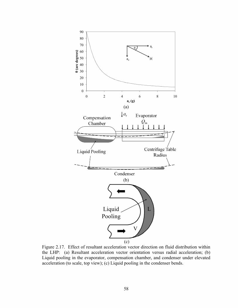
58

(a)

(b)

(c)

Figure 2.17. Effect of resultant acceleration vector direction on fluid distribution within the LHP: (a) Resultant acceleration vector orientation versus radial acceleration; (b) Liquid pooling in the evaporator, compensation chamber, and condenser under elevated acceleration (to scale, top view); (c) Liquid pooling in the condenser bends.

0

10

20

30

40

50

60

70

80

90

0 2 4 6 8 10

θ(a

rc d

egre

es)

ar (g)

θ

az

ar

|a|

V

LLiquidPooling

59

Figure 2.18. Steady state performance characteristics of the LHP versus transported heat at stationary and elevated acceleration (Qcc = 0 W, cpm& = 0.0077 kg/s, 37.2 ≤ cpT ≤ 67.7°C, 25.1 ≤ Tamb ≤ 38.7°C): (a) Evaporative heat transfer coefficient; (b) Thermal resistance; (c) Wall superheat.

0200400600800

100012001400160018002000

h (W

/m2 -

K)

(a)

00.050.1

0.150.2

0.250.3

0.350.4

0.450.5

R (K

/W)

(b)

0

10

20

30

40

50

60

70

80

90

0 100 200 300 400 500 600

ΔTsh

(K)

Qout (W)

a = 0 ga = 0.1 ga = 2.0 ga = 4.0 ga = 6.0 ga = 8.0 ga = 10.0 g

r

r

rrrr

(c)

r

60

Figure 2.19. Transient temperature traces of the LHP at elevated acceleration showing dry-out behavior (Qin = 400 W, Qcc = 0 W, cpm& = 0.0077 kg/s, 37.2 ≤ cpT ≤ 59.7°C, Tamb = 28.0°C): (a) Te,max = 150°C; (b) Te,max = 175°C; (c) Te,max = 200°C.

050100150200250300350400450500

25456585

105125145165185205225

0 1000 2000 3000 4000 5000 6000

Qou

t(W

)

T (C

)

t (s)

TC06 - Evap 3TC09 - Cond InTC10 - Cond 1TC11 - Cond 2TC12 - Cond 3TC13 - Cond OutQout

(TC11)(TC10) (TC12)(TC09) (TC13)

(Qout)

(TC06)

(a)8 g 0.1 g

050100150200250300350400450500

25456585

105125145165185205225

6000 7000 8000 9000 10000 11000 12000 13000Q

out(W

)

T (C

)

t (s)

(TC11)(TC10) (TC12)(TC09) (TC13)

(Qout)

(TC06)

(b)8 g 0.1 g0.1 g

050100150200250300350400450500

25456585

105125145165185205225

13000 15000 17000 19000 21000

Qou

t(W

)

T (C

)

t (s)

(TC11)(TC10) (TC12)(TC09) (TC13)

(Qout)

(TC06)

(c)8 g 0.1 g0.1 g

61

Figure 2.20. Quasi-steady state temperature traces of the LHP and cold plate at elevated acceleration for Qin = 200 W (Qcc = 0 W, cpm& = 0.0077 kg/s, cpT = 41.9°C, Tamb = 26.4°C): (a) Transient temperature trace at ar = 0.1 g and t = 13834 s; (b) Transient temperature trace at ar = 4.0 g and t = 31240 s.

35

40

45

50

55

60

65

70

75

0 50 100 150 200 250 300

T (C

)

t (s)

(TC14)(TC12) (TC13)

(TC15)(TC04)(TC06) (TC07)(TC05)

(TC08)

(TC10) (TC11)

(TC09)

Evaporator CondenserVapor Line Liquid LineEvap / CC Cold Plate

(TC00) (TC01)

(a)

30

40

50

60

70

80

90

100

110

0 100 200 300 400 500 600 700

T (C

)

t (s)

(TC14)(TC12) (TC13)

(TC15)

(TC04) (TC06) (TC07)(TC05)

(TC08)

(TC10) (TC11)

(TC09) Evaporator CondenserVapor Line Liquid LineEvap / CC Cold Plate

(TC00) (TC01)

(b)

62

Figure 2.21. Steady state performance map of the LHP relating radial acceleration and heat transported (Qcc = 0 W, cpm& = 0.0077 kg/s, 37.2 ≤ cpT ≤ 59.7°C, 25.1 ≤ Tamb ≤ 30.2°C).

0

2

4

6

8

10

12

0 100 200 300 400 500 600

a r(g

)

Qout (W)

Steady OperationQuasi-steady OperationDry-out

63

Table 2.1. AFRL/RZPS design requirements. Requirement Parameter

Thermal Minimum Heat Load 500 W Minimum Heat Flux 3 W/cm2

Operating Temperature 200°C Condenser Heat Sink Temperature 5 to 140°C

Tilt in One G ± 0 inches, horizontal Conductance 50°C/W

Proof of Pressure Test 3102 psi (200°C) Materials

Evaporator Envelope Material Titanium, CP Grade 2 Evaporator Wick Material Titanium, CP Grade 2 Transport Line Material Titanium, CP Grade 2

Working Fluid Water LHP Dimensions

Evaporator Configuration 2.54 cm OD up to 25.4 cm long Evaporator Footprint 20.32 × 10.16 cm Condenser Footprint 30.48 × 28.58 cm

Transport Line Lengths Approx. 243.8 cm

64

Table 2.2. ACT LHP geometric design parameters. Transport Lines

Vapor Line Length Approx. 243.8 cm Vapor Line Diameter 0.9525 OD × 0.0889 cm wall Liquid Line Length Approx. 335.3 cm

Liquid Line Diameter 0.6350 OD × 0.0889 cm wall Condenser Line Length Approx. 279.4 cm

Condenser Line Diameter 0.9525 OD × 0.0889 cm wall Compensation Chamber

Diameter 6.033 cm OD Length 11.43 cm

Chamber Location Coaxial with evaporator Wick Properties

Effective Pore Radius 9.1μm Permeability 1.2×10-12 m2

Outside Diameter 2.286 cm Length 20.32 cm

Inside Diameter 0.8001 cm Grooves 6

Groove Depth 0.1524 cm Groove Width 0.1524 cm

65

Table 2.3. Summary of LHP thermocouple locations Thermocouple Location

TC04 Evaporator 1 TC05 Evaporator 2 TC06 Evaporator 3 TC07 Evaporator 4 TC08 Evaporator Outlet TC09 Condenser Inlet TC10 Condenser 1 TC11 Condenser 2 TC12 Condenser 3 TC13 Condenser Outlet TC14 Bayonet Inlet TC15 Compensation Chamber / Evaporator

66

Table 2.4. Summary of uncertainties. Quantity Uncertainty

Measured Temperature ± (fixed value + confidence interval) °C Acceleration + (0.01 + confidence interval + (ar,oe – ar,cl)) g

- (0.01 + confidence interval + (ar,cl – ar,ie)) g Voltages ± (0.00025V + 0.005 + confidence interval) V

Constant Resistors ± 0.02%R Ω Wick D, L ± 0.0000254 m

Calculated cpT ± max(ΔTout, ΔTin)

eT ± max(Δ(TC04), Δ(TC05), Δ(TC06), Δ(TC07)) ΔTsh ± 1.28°C

Cp,PAO ± ( ) ( ) ( )( )cppcpcppcpp*%5.0 TCTTCTC −Δ++ Qout Equation (2.8) h Equation (2.9) R Equation (2.10)

67

Table 2.5. Steady state operating characteristics for the stationary LHP (Qcc = 0 W, ar = 0 g, cpm& = 0.0077 kg/s, 36.8 ≤ cpT ≤ 71.6°C, 27.6 ≤ Tamb ≤ 38.7°C) showing effect of startup path.

Final Qin (W)

Path to Final Qin eT (°C) Te/cc (°C) cpT (°C) Qout (W) h (W/m2-K) R (K/W)

100

0-100 66.6 ± 0.34 61.8 ± 0.86 39.5 ± 0.12 79.1 ± 4.3 1670 ± 390 0.342 ± 0.019 0-100 64.9 ± 0.34 59.9 ± 0.86 37.4 ± 0.12 78.4 ± 4.3 1660 ± 380 0.351 ± 0.020 0-100 64.8 ± 0.34 59.8 ± 0.86 37.6 ± 0.12 77.9 ± 4.3 1670 ± 390 0.348 ± 0.020 0-100 65.4 ± 0.34 60.1 ± 0.86 36.8 ± 0.12 79.0 ± 4.2 1540 ± 280 0.361 ± 0.020 0-100 65.4 ± 0.34 60.2 ± 0.86 38.2 ± 0.12 77.9 ± 4.3 1540 ± 300 0.350 ± 0.020 0-100-300-100 66.9 ± 0.34 62.2 ± 0.86 38.8 ± 0.12 79.1 ± 4.3 1730 ± 560 0.355 ± 0.020 0-100-500-100 67.4 ± 0.34 62.6 ± 0.86 39.0 ± 0.12 78.8 ± 4.3 1620 ± 500 0.361 ± 0.020

133 0-100-133 65.1 ± 0.34 59.0 ± 0.86 40.4 ± 0.12 114 ± 5.5 1770 ± 310 0.217 ± 0.011 166 0-100-133-166 65.6 ± 0.34 58.3 ± 0.86 43.0 ± 0.12 143 ± 6.5 1760 ± 250 0.158 ± 0.0076

200 0-200 66.3 ± 0.46 66.3 ± 0.86 46.1 ± 0.12 174 ± 7.7 1560 ± 230 0.116 ± 0.0058 0-200 66.4 ± 0.35 66.4 ± 0.86 45.7 ± 0.12 174 ± 7.7 1460 ± 140 0.119 ± 0.0057 0-200 65.5 ± 0.34 65.5 ± 0.86 45.4 ± 0.12 176 ± 7.8 1660 ± 250 0.114 ± 0.0055

68

Table 2.5, continued. Steady state operating characteristics for the stationary LHP (Qcc = 0 W, ar = 0 g, cpm& = 0.0077 kg/s, 36.8 ≤ cpT ≤ 71.6°C, 27.6 ≤ Tamb ≤ 38.7°C) showing effect of startup path.

Final Qin (W)

Path to Final Qin eT (°C) Te/cc (°C) cpT (°C) Qout (W) h (W/m2-K) R (K/W)

300

0-100-300 77.1 ± 0.39 62.4 ± 0.86 51.6 ± 0.12 260 ± 11 1660 ± 160 0.0985 ± 0.0045 0-100-300 75.8 ± 0.40 60.9 ± 0.86 50.2 ± 0.12 259 ± 11 1670 ± 170 0.0988 ± 0.0045 0-200-300 78.1 ± 0.38 63.1 ± 0.86 52.0 ± 0.12 258 ± 11 1580 ± 140 0.101 ± 0.0046 0-300 79.3 ± 0.40 64.4 ± 0.86 52.8 ± 0.12 258 ± 11 1550 ± 160 0.103 ± 0.0047

400 0-200-400 94.0 ± 0.34 73.6 ± 0.86 57.8 ± 0.12 345 ± 14 1400 ± 85 0.105 ± 0.0045 0-300-400 94.3 ± 0.35 75.0 ± 0.86 58.4 ± 0.12 345 ± 14 1470 ± 98 0.104 ± 0.0045 0-400 97.4 ± 0.34 72.6 ± 0.86 56.5 ± 0.12 344 ± 14 1190 ± 60 0.119 ± 0.0051

500

0-100-300-500 116 ± 0.34 82.4 ± 0.86 61.7 ± 0.12 430 ± 18 1050 ± 45 0.126 ± 0.0053 0-100-500 119 ± 0.34 83.8 ± 0.86 63.1 ± 0.12 429 ± 18 999 ± 41 0.131 ± 0.0055 0-400-500 117 ± 0.34 83.6 ± 0.86 62.4 ± 0.12 431 ± 18 1050 ± 47 0.127 ± 0.0053 0-500 122 ± 0.34 85.3 ± 0.86 63.7 ± 0.12 432 ± 18 956 ± 42 0.135 ± 0.0057

600 0-200-400-600 145 ± 0.36 93.1 ± 0.86 67.8 ± 0.12 515 ± 21 803 ± 33 0.149 ± 0.0062 0-400-500-600 141 ± 0.34 93.3 ± 0.86 67.5 ± 0.12 515 ± 21 867 ± 37 0.142 ± 0.0060 0-600 148 ± 0.36 93.7 ± 0.86 67.7 ± 0.12 513 ± 21 757 ± 33 0.157 ± 0.0066

69

Table 2.6. Steady state operating characteristics for the stationary LHP showing effect of heat input to the compensation chamber (Qin = 500 W, ar = 0 g, cpm& = 0.0077 kg/s, 63.4 ≤ cpT ≤ 64.8°C, 36.1 ≤ Tamb ≤ 38.1°C).

Qcc (W) eT (°C) Te/cc (°C) cpT (°C) Qout (W) h (W/m2-K) R (K/W) 0 122 ± 0.34 85.3 ± 0.86 63.7 ± 0.12 432 ± 18 956 ± 42 0.135 ± 0.0057 5 115 ± 0.35 85.3 ± 0.86 63.6 ± 0.12 438 ± 18 1130 ± 58 0.118 ± 0.0050

10 109 ± 0.35 85.6 ± 0.86 63.8 ± 0.12 444 ± 18 1420 ± 110 0.103 ± 0.0044 15 107 ± 0.35 85.1 ± 0.86 63.4 ± 0.12 449 ± 19 1610 ± 130 0.0970 ± 0.0041 20 108 ± 0.34 86.1 ± 0.86 64.0 ± 0.12 456 ± 19 1610 ± 130 0.0972 ± 0.0041 25 110 ± 0.34 87.7 ± 0.86 64.2 ± 0.12 461 ± 19 1620 ± 130 0.0991 ± 0.0042 30 112 ± 0.34 90.0 ± 0.86 64.5 ± 0.12 466 ± 19 1610 ± 130 0.103 ± 0.0044 35 118 ± 0.35 95.5 ± 0.86 64.6 ± 0.12 468 ± 19 1580 ± 120 0.114 ± 0.0048 40 120 ± 0.34 97.4 ± 0.86 64.8 ± 0.12 473 ± 20 1580 ± 120 0.117 ± 0.0049 45 127 ± 0.34 104 ± 0.86 64.5 ± 0.12 475 ± 20 1530 ± 110 0.132 ± 0.0055 50 129 ± 0.35 105 ± 0.86 64.5 ± 0.12 477 ± 20 1510 ± 110 0.134 ± 0.0056

70

Table 2.7. The effect of compensation chamber temperature control on LHP operation (Qin = 500 W, ar = 0 g, cpm& = 0.0077 kg/s, cpT = 52.5°C, Tamb = 26.4°C)

Compensation Chamber Conditions Qcc (W) eT (°C) cpT (°C) Tcc (°C) Qout (W) h (W/m2-K) R (K/W)

Time to Steady State

Uninsulated, no temperature control 0 115 52.4 59.3 442 ± 19 878 ± 37 0.142 ± 0.0060 300 min.

Insulated, no temperature control 0 107 52.6 62.9 447 ± 19 1050 ± 51 0.122 ± 0.0052 375 min.

Insulated, temperature controlled to Tcc = 72.8°C, simultaneous heat input startup

20 103 53.5 72.8 470 ± 20 1340 ± 77 0.106 ± 0.0045 310 min.

Insulated, temperature controlled to Tcc = 72.8°C, preconditioned CC

100 decreased

to 20 103 53.4 72.8 467 ± 19 1350 ± 77 0.106 ± 0.0045 250 min.

71

Table 2.8. Steady state operating characteristics of the rotating LHP (Qcc = 0 W, cpm& = 0.0077 kg/s, 37.2 ≤ cpT ≤ 59.7°C, 25.1 ≤ Tamb ≤ 30.2°C).

Qin (W) ar (g) eT (°C) Te/cc (°C) cpT (°C) Qout (W) h (W/m2-K) R (K/W) 100 0.1 ± 0.012 64.9 ± 0.34 59.8 ± 0.86 38.0 ± 0.12 74.2 ± 4.2 1620 ± 340 0.362 ± 0.021 100 0.1 ± 0.012 64.6 ± 0.34 59.8 ± 0.86 38.1 ± 0.12 74.6 ± 4.2 1810 ± 510 0.355 ± 0.020 100 2.0 ± 0.050 66.4 ± 0.34 61.2 ± 0.86 37.5 ± 0.12 79.9 ± 4.5 1770 ± 420 0.361 ± 0.021 100 4.1 ± 0.091 71.2 ± 0.44 64.3 ± 0.86 37.2 ± 0.16 76.1 ± 4.8 1130 ± 150 0.446 ± 0.029 200 0.1 ± 0.012 70.8 ± 0.41 59.3 ± 0.86 42.0 ± 0.13 174 ± 7.8 1400 ± 110 0.165 ± 0.0078 200 0.1 ± 0.012 71.1 ± 0.43 59.5 ± 0.86 41.9 ± 0.13 172 ± 7.8 1380 ± 110 0.169 ± 0.0081 200 0.1 ± 0.012 71.5 ± 0.38 60.3 ± 0.86 42.0 ± 0.12 174 ± 7.8 1360 ± 110 0.170 ± 0.0079 200 2.0 ± 0.050 75.8 ± 0.65 61.6 ± 0.86 41.7 ± 0.21 188 ± 9.2 1220 ± 86 0.181 ± 0.0096 300 0.1 ± 0.012 76.4 ± 0.48 57.2 ± 0.86 46.0 ± 0.12 275 ± 12 1390 ± 100 0.111 ± 0.0051 300 2.0 ± 0.050 81.7 ± 0.76 61.2 ± 0.86 45.6 ± 0.16 285 ± 13 1280 ± 80 0.126 ± 0.0063 400 0.1 ± 0.012 86.4 ± 0.39 60.6 ± 0.86 49.3 ± 0.12 360 ± 15 1300 ± 82 0.103 ± 0.0045 400 0.1 ± 0.012 86.6 ± 0.39 61.3 ± 0.86 49.3 ± 0.12 361 ± 15 1300 ± 81 0.103 ± 0.0045 400 0.1 ± 0.012 86.1 ± 0.39 61.1 ± 0.86 49.3 ± 0.12 361 ± 15 1330 ± 84 0.102 ± 0.0044 400 0.1 ± 0.012 85.8 ± 0.42 61.1 ± 0.86 49.3 ± 0.12 361 ± 15 1330 ± 89 0.101 ± 0.0044 400 2.0 ± 0.050 87.6 ± 0.42 59.7 ± 0.86 49.3 ± 0.12 372 ± 16 1280 ± 74 0.103 ± 0.0045 400 4.0 ± 0.089 91.5 ± 0.43 59.8 ± 0.86 49.3 ± 0.12 376 ± 16 1160 ± 56 0.112 ± 0.0051 400 4.1 ± 0.091 93.0 ± 0.63 60.0 ± 0.86 49.3 ± 0.15 376 ± 17 1130 ± 59 0.116 ± 0.0055 400 6.0 ± 0.13 94.8 ± 0.34 60.7 ± 0.86 49.9 ± 0.12 369 ± 16 1030 ± 46 0.122 ± 0.0053

72

Table 2.8, continued. Steady state operating characteristics of the rotating LHP (Qcc = 0 W, cpm& = 0.0077 kg/s, 37.2 ≤ cpT ≤ 59.7°C, 25.1 ≤ Tamb ≤ 30.2°C).

Qin (W) ar (g) eT (°C) Te/cc (°C) cpT (°C) Qout (W) h (W/m2-K) R (K/W) 500 0.1 ± 0.012 110 ± 0.36 69.3 ± 0.86 52.9 ± 0.12 440 ± 18 960 ± 43 0.131 ± 0.0055 500 0.1 ± 0.012 107 ± 0.35 69.0 ± 0.86 52.6 ± 0.12 446 ± 19 1030 ± 48 0.123 ± 0.0052 500 0.1 ± 0.012 107 ± 0.41 69.2 ± 0.86 52.7 ± 0.12 447 ± 19 1030 ± 50 0.122 ± 0.0052 500 0.1 ± 0.012 109 ± 0.42 69.5 ± 0.86 52.9 ± 0.12 447 ± 19 1000 ± 46 0.125 ± 0.0053 500 0.1 ± 0.012 108 ± 0.35 68.9 ± 0.86 52.6 ± 0.12 448 ± 19 1010 ± 47 0.123 ± 0.0052 500 2.0 ± 0.050 114 ± 0.42 65.5 ± 0.86 52.5 ± 0.12 452 ± 19 887 ± 37 0.136 ± 0.0058 500 4.0 ± 0.090 110 ± 0.34 64.4 ± 0.86 53.1 ± 0.13 459 ± 19 982 ± 43 0.123 ± 0.0053 500 6.0 ± 0.13 111 ± 0.34 64.6 ± 0.86 54.0 ± 0.13 460 ± 20 934 ± 42 0.125 ± 0.0055 500 8.0 ± 0.17 115 ± 0.34 65.1 ± 0.86 54.8 ± 0.12 463 ± 20 865 ± 38 0.131 ± 0.0058 500 10 ± 0.21 117 ± 0.34 64.7 ± 0.86 55.2 ± 0.12 452 ± 20 824 ± 35 0.136 ± 0.0060 600 0.1 ± 0.012 137 ± 0.36 76.6 ± 0.86 56.0 ± 0.12 533 ± 22 759 ± 32 0.152 ± 0.0063 600 0.1 ± 0.012 141 ± 0.43 76.6 ± 0.86 55.9 ± 0.12 533 ± 22 707 ± 29 0.160 ± 0.0067 600 0.1 ± 0.012 141 ± 0.43 76.3 ± 0.86 55.8 ± 0.12 533 ± 22 703 ± 29 0.160 ± 0.0067 600 0.1 ± 0.012 140 ± 0.42 76.2 ± 0.86 55.8 ± 0.12 531 ± 22 707 ± 30 0.159 ± 0.0067 600 0.1 ± 0.012 133 ± 0.34 76.2 ± 0.86 56.0 ± 0.12 539 ± 23 821 ± 35 0.143 ± 0.0060 600 2.0 ± 0.050 140 ± 0.34 72.9 ± 0.86 56.3 ± 0.12 547 ± 24 726 ± 31 0.152 ± 0.0066 600 4.0 ± 0.090 152 ± 0.50 71.7 ± 0.86 57.1 ± 0.12 546 ± 23 621 ± 26 0.173 ± 0.0075 600 6.0 ± 0.13 148 ± 0.34 71.5 ± 0.86 57.8 ± 0.12 545 ± 24 651 ± 27 0.165 ± 0.0072 600 8.1 ± 0.17 147 ± 0.34 71.8 ± 0.86 58.8 ± 0.12 546 ± 24 662 ± 28 0.162 ± 0.0072 600 10 ± 0.21 145 ± 0.34 72.2 ± 0.86 59.7 ± 0.13 538 ± 24 691 ± 29 0.158 ± 0.0070

73

Table 2.9. Comparison of quasi-steady states for Qin = 200 W (Qcc = 0 W, cpm& = 0.0077 kg/s).

ar (g) 0 0.1 Δ Tamb (°C) 31.7 26.4 -5.3 Tcp,in (°C) 41.1 36.9 -4.2 Tcp,out (°C) 51.1 47.0 -4.1

cpT (°C) 46.1 41.9 -4.2

eT (°C) 66.3 71.1 4.8 Tbayonet inlet,max (°C) 50.7 51.2 0.5 Tbayonet inlet,min (°C) 42.6 38.9 -3.7 Te/cc,max (°C) 56.8 60.9 4.1 Te/cc,min (°C) 54.0 57.1 3.1 h (W/m2-K) 1560 1380 -180 R (W/K) 0.116 0.169 0.053 ΔTsh (°C) 11.2 11.6 0.4

74

REFERENCES

Anderson, J. Introduction to Flight. Boston: McGraw-Hill, 2000.

Boyer, R., Welsch, G., Collings, E. Materials Properties Handbook: Titanium Alloys.

Materials Park, OH: ASM International, 1994.

Cimbala, J., Brenizer, J., Chuang, A., Hanna, S., Conroy, C., El-Ganayni, A., Riley, D.

"Study of a Loop Heat Pipe Using Neutron Radiography." Applied Radiation and

Isotopes 61, 2004: 701-705.

Cloyd, J. "A Status of the United States Air Force's More Electric Aircraft Initiative."

Energy Conversion Engineering Conference. Honolulu, HI: IEEE, 1997. 681-686.

DOD. MIL-HDBK-310: Global Climatic Data for Developing Military Products. 1997.

Douglas, D., Ku, J., Kaya, T. "Testing of the Geoscience Laser Altimeter System (GLAS)

Prototype Loop Heat Pipe." 37th AIAA Aerospace Sciences Meeting and Exhibit.

Reno, NV: AIAA, 1999. AIAA 99-0473.

Faghri, A. Heat Pipe Science and Technology. Washington D.C.: Taylor and Francis,

1995.

Ghajar, A., Tang, W., Beam, J. "Comparison of Hydraulic and Thermal Performance of

PAO and Coolanol 25R." 6th AIAA/ASME Joint Thermophysics and Heat Transfer

Conference. Colorado Springs, CO: AIAA, 1994. AIAA-94-1965.

Hoang, T., Ku, J. "Transient Modeling of Loop Heat Pipes." 1st International Energy

Conversion Engineering Conference. Portsmouth, VA: AIAA, 2003. AIAA 2003-

6082.

Incropera, F., DeWitt, D. Fundamentals of Heat and Mass Transfer. New York City:

Wiley, 2002.

75

Kaya, T., Hoang, T., Ku, J., Cheung, M. "Mathematical Modeling of Loop Heat Pipes."

37th AIAA Aerospace Sciences Meeting and Exhibit. Reno, NV: AIAA, 1999. A99-

16362.

Kaya, T., Ku, J. "Experimental Investigation of Performance Characteristics of Small

Loop Heat Pipes." Proceedings of 41st Aerospace Sciences Meeting and Exhibit.

Reno, NV: AIAA, 2003. AIAA 2003-1038.

Ku, J. "Operating Characteristics of Loop Heat Pipes." 29th International Conference on

Environmental System. Denver, CO: SAE, 1999. 1999-01-2007.

Ku, J., Ottenstein, L., Kaya, T., Rogers, P., Hoff, C. "Testing of a Loop Heat Pipe

Subjected to Variable Accelerating Forces, Part 1: Start-Up." SAE, 2000a: 2000-01-

2488.

Ku, J., Ottenstein, L., Kaya, T., Rogers, P., Hoff, C. "Testing of a Loop Heat Pipe

Subjected to Variable Accelerating Forces, Part 2: Temperature Stability." SAE,

2000b: 2000-01-2489.

Maidanik, J. "Review: Loop Heat Pipes." Applied Thermal Engineering 25, 2005: 635-

657.

Maidanik, J., Vershinin, S., Kholodov, V., Dolgirev, J. Heat Transfer Apparatus. United

States Patent 4,515,209. 1985.

Montgomery, D., Runger, G. Applied Statistics and Probability for Engineers. New York

City: Wiley, 2003.

NACA. Report 1135: Equations, Tables, and Charts for Compressible Flow.

Washington, D.C.: U.S. Government Printing Office, 1953.

Ponnappan, R., Yerkes, K., Chang, W., Beam, J. "Analysis and Testing of Heat Pipe in

Accelerating Environment." Proceedings of the 8th International Heat Pipe

Conference. Beijing, China, 1992. B-19-1 - B-19-6.

Quigley, R. "More Electric Aircraft." Applied Power Electronics Conference and

Exposition. San Diego, CA: IEEE, 1993. 906-911.

76

Thomas, S., Klasing, K., Yerkes, K. "The Effects of Transverse Acceleration-Induced

Body Forces on the Capillary Limit of Helically Grooved Heat Pipes." ASME Journal

of Heat Transfer, 120, 1998: 441-451.

Thomas, S., Yerkes, K. "Quasi-Steady-State Performace of a Heat Pipe Subjected to

Transient Acceleration Loadings." AIAA Journal of Thermophysics, Vol. 11, No. 2,

1996: 306-309.

Vrable, D., Yerkes, K. "A Thermal Management Concept for More Electric Aircraft

Power System Applications." Aerospace Power Systems Conference Proceedings.

Williamsburg, VA: SAE, 1998. P-322.

White, F. Heat and Mass Transfer. New York City: Addison-Wesley, 1988.

Yerkes, K., Beam, J. "Arterial Heat Pipe Performance in a Transient Heat Flux and Body

Force Environment." SAE, 1992: 921944.

Zaghdoudi, M., Sarno, C. "Investigation of the Effects of Body Force Environment on

Flat Heat Pipes." AIAA Journal of Thermophysics and Heat Transfer, Vol. 15, No. 4,

2001: 384-394.

77

APPENDIX A. OPERATING PROCEDURES

A.1. Standard Operating Procedure 0. Ensure the main power breaker is in the “OFF” position. The breaker is located

on the 71B H-bay second floor landing. See Figure A.1 for picture. Ensure the control

panel box is in “Man” mode, potentiometer is set to zero (turned completely counter-

clockwise), and the E-stop button has been depressed. The control panel box is located in

Control Room 2. See Figure A.2 for picture of control panel box.

1. Mount test payload with sufficient factor of safety to ensure a reliable mounting

configuration consistent with the generated forces. The retaining method will be

designed for a payload mass subjected to a maximum table capacity of 12 g.

2. Mount the appropriate counter balance weight at the appropriate location to place

the centroid in the center of the table and level each spoke to minimize vibrational noise

and table runout.

3. Ensure all centrifuge maintenance has been completed.

4. Software Startup Procedure

a. Open the LabVIEW VI file needed to control the data acquisition and

table voltage.

b. It is up to the experimentalist to write the program used to control data

acquisition and table voltage. Sample programs that perform these tasks

are available. See Figure A.3 for sample.

c. Press the ‘SYSTEM ENABLED’ button on the front panel so that it is

illuminated.

d. Press the ‘Run’ button located in the top-left of the LabVIEW toolbar.

This will cause the program to become functional.

5. Prior to each set of experimental testing:

a. Check all bolts to ensure all experimental apparatus are tightened

properly.

78

b. Clear the table of foreign objects, including removing all tools and placing

in the appropriate CTK. Ensure all free standing equipment and furniture

are securely placed along the perimeter of the room.

c. Turn table power switch on. This provides power to the instrumentation

and devices on the table. See Figure A.4 for location.

d. Check out instrumentation for proper operation.

e. Turn on recirculating chiller located on the east wall. See Figure A.5 for

picture. Check chill bath coolant flows and flow rates of any intermediate

flow loops. A booster pump for the chill bath coolant is available. Follow

the chill bath plumbing schematic in Figure A.6 to enable operation. The

booster pump control is remotely located in Control Room 2. See Figure

A.7 for picture.

f. Lock inter-connect door.

g. Check camera operation.

h. Make final check on the table for tools or loose objects.

6. Unlock main power breaker and flip to ‘ON’ position. See Figure A.1 for

location.

a. Ensure the emergency stop button is activated and the potentiometer is

turned completely counter-clockwise on the control panel box prior to

proceeding with powering the centrifuge table motor.

b. Turn on warning beacon and evacuate personnel. Warning beacon

switches are located outside Test Cell 4 and on the west wall of control

room 1.

c. Engage table motor control switch on the north wall (cooling motor will

be operational). See Figure A.8 for location.

d. Secure outer doors.

e. Place “Test in Progress Do Not Enter” sign on the outer door.

7. Controlling the System

a. To control the voltage supplied to the table, turn the mode switch from

‘MAN’ to ‘AUTO’ on the control panel box and flip the ‘Table Voltage’

switch to the ‘ON’ position. While the ‘Table Voltage’ switch is ‘ON’,

79

the voltage can be adjusted using the slider bar on the left side called

‘Table Voltage’. Table voltage can be turned on and off as often as

desired while the system is engaged.

8. Conduct test procedure. Test procedures are experiment dependent and up to the

experimentalist to develop.

9. Shutdown

a. Slowly reduce the table voltage to zero using the slider bar. Flip the

‘Table Voltage’ switch to the ‘OFF’ position on the LabVIEW VI.

b. On the control panel box, turn the switch from ‘AUTO’ to ‘MAN’ and

press the ‘STOP’ button. Wait for the table to stop rotating then press the

‘E-STOP’ button.

c. Press the ‘SYSTEM ENABLED’ button on the LabVIEW VI so that it is

no longer illuminated. The program will stop.

10. Emergency Shutdown

a. If for any reason an emergency should occur press the ‘E-STOP’ on the

control panel box. Should the table “run away” or suddenly accelerate the

motor will automatically shutdown. Contact the appropriate personnel

prior to a restart after an emergency shutdown.

• Andrew Fleming 58942

• Larry Byrd 53238

• Travis Michalak 64429

A.2. Test Procedures 1. Stationary Operation

a. Set chiller to Teg = 35°C. Allow to come to steady state.

b. Turn high temperature coolant loop on and set to m& = 0.0077 kg/s.

Simultaneously, apply desired heat load to evaporator.

c. Allow LHP to achieve steady state operation by examining dT/dt plot of

TC00, TC01, TC04, TC05, TC06, TC07, TC08, and TC09. Steady state is

achieved when all of these thermocouples are bracketed by -0.01 ≤ dT/dt ≤

0.01 K/min.

80

d. Remove heat load from the evaporator and turn off the high temperature

coolant loop or adjust to next desired heat load and repeat (c).

2. Rotational Operation

a. Set chiller to Teg = 35°C. Allow to come to steady state.

b. Increase radial acceleration to ar = 0.1 g.

c. Turn high temperature coolant loop on and set to m& = 0.0077 kg/s.

Simultaneously, apply desired heat load to evaporator.

d. Allow LHP to achieve steady state operation by examining dT/dt plot of

TC00, TC01, TC04, TC05, TC06, TC07, TC08, and TC09. Steady state is

achieved when all of these thermocouples are bracketed by -0.01 ≤ dT/dt ≤

0.01 K/min.

e. Increase radial acceleration to desired level.

f. Again, allow LHP to achieve steady state operation by examining dT/dt

plot of TC00, TC01, TC04, TC05, TC06, TC07, TC08, and TC09. Steady

state is achieved when all of these thermocouples are bracketed by -0.01 ≤

dT/dt ≤ 0.01 K/min.

g. Decrease radial acceleration to ar = 0.1 g.

h. If shutting down, allow LHP to operate for 30 min., then remove heat load

from the evaporator and turn off the high temperature coolant. Decrease

radial acceleration to ar = 0.0 g. If continuing testing, allow LHP to

achieve steady state operation by examining dT/dt plot of TC00, TC01,

TC04, TC05, TC06, TC07, TC08, and TC09. Steady state is achieved

when all of these thermocouples are bracketed by -0.01 ≤ dT/dt ≤ 0.01

K/min. Repeat (e)-(h).

81

(a)

(b)

Figure A.1. Centrifuge table main power breaker: (a) Electrical panel MCC-6; (b) Centrifuge table main power breaker.

82

Figure A.2. Centrifuge table control panel box.

83

Figure A.3. Sample LabVIEW control program.

84

Figure A.4. Centrifuge table power switch.

85

Figure A.5. Neslab recirculating chiller.

86

Figure A.6. Chill bath plumbing schematic.

Supply

RecirculatingChiller

F

P

F/M0-5LPM

F/M0-25LPM

F/M0-50LPM

To Centrifuge Table From Centrifuge Table

Return

Recirc

To Drain

BoosterPump

Filter1

2

3

4 5

6

87

Figure A.7. Booster pump control panel.

88

Figure A.8. Centrifuge table motor control power switch.

89

APPENDIX B. UNCERTAINTY ANALYSIS

The uncertainty analysis for this experiment was broken into the following three

different categories: measured, constant, and calculated quantities. For each steady state

condition, 151 data points were collected representing five minutes of data. Measured

values were averaged and uncertainties were calculated based on the fixed error of each

instrument plus the confidence interval for the average. The fixed error for

thermocouples and mass flow meter was determined via the calibration methods and can

be seen in Appendix C. The fixed error of the accelerometer was ±0.1 g and ±0.00025*V

+ 0.005 volts for voltage measurements. The confidence interval was based off a

statistical t-distribution with confidence level of 0.95 and was given by Montgomery

(Montgomery, 2003)

Confidence Interval√

(B.1)

where t is a tabulated value based on the confidence level and number of degrees of

freedom, σ is the sample standard deviation, and n is the number of data points in the

sample. Constant quantities included precision resistors used for current measurement

for heat input via evaporator, compensation chamber, and preheater with an uncertainty

of ±0.02% and wick diameter and length measurements, with an uncertainty of

±0.0000254 m. Calculated quantities used uncertainty methods that would be the most

conservative for the experiment. For averaged quantities including cpT , eT , and h , the

largest uncertainty of the individual measurements was used as the uncertainty of the

average value. For the specific heat of PAO, the uncertainty was 0.5% of the total value

plus difference between the specific heat using the upper limit of the temperature

measurement and the average specific heat. The calorimetry of the cold plate, Qout, was

given by

out p,PAO out in (B.2)

90

The uncertainty of Qout was determined to be

Δ outout Δ out

p,PAOΔ p,PAO

out

outΔ out

out

inΔ in

/

(B.3)

where

outp,PAO out in (B.4)

out

p,PAOout in (B.5)

out

outp,PAO (B.6)

out

inp,PAO (B.7)

The average evaporative heat transfer coefficient, h , was given by

out

e v (B.8)

The uncertainty of h was given by

ΔoutΔ out Δ

ΔeΔ e

vΔ v

/

(B.9)

where

out

1e v

(B.10)

91

e v

(B.11)

e v

(B.12)

e e v

(B.13)

v e v

(B.14)

The thermal resistance, R, was given by

e cp

out (B.15)

The uncertainty of the thermal resistance was given by

ΔoutΔ out

eΔ e

cpΔ cp

/

(B.16)

where

out

e cp

out (B.17)

e

1out

(B.18)

cp

1out

(B.19)

92

APPENDIX C. CALIBRATION OF THERMOCOUPLES AND FLOW METER

C.1. Thermocouple Calibration The calibrations of the thermocouples used on the centrifuge table required new

programming since the data acquisition system was upgraded for the centrifuge table.

Control of a calibration bath and RTD were integrated with the centrifuge table’s data

acquisition unit. A LabVIEW program was generated to simultaneously control all three

devices.

The thermocouples were calibrated using a Hart Scientific 6330 Calibration Bath

and Hart Scientific 1502A NIST-Traceable platinum resistance temperature detector

(RTD). The bath was capable of producing steady state temperatures from 40 to 280°C.

The calibration bath used Dow Corning 200.50 silicon oil. There were several steps

required before a thorough calibration of the thermocouples could be determined. First,

LabVIEW software needed to be written to interface with the calibration bath, RTD, and

data acquisition system. Second, the characteristics of the calibration bath and RTD

needed to be determined with respect to response times and temperature fluctuations.

Finally, complete calibration curves for each of the thermocouples needed to be

developed.

In the loop heat pipe experimental setup, there were four grounded probe

thermocouples and twelve exposed tip type E thermocouples. The grounded probe

thermocouples were used in the calorimetry of the cold plate, temperature measurement

for the flow meter calibration, and the ambient temperature inside the box, where the

error needed to be reduced as much as possible. As a result, it was decided to only

calibrate these four over the anticipated temperature range, from 20 to 145°C, in 5°C

intervals. The twelve exposed tip thermocouples were mounted on the loop heat pipe in

various locations. They needed to be calibrated over the full 20 to 230°C temperature

range. Thus, the calibration of the thermocouples needed a second calibration bath that

was capable of achieving the temperature range of 20 to 40°C. The Hart Scientific 6330

Calibration Bath was not capable of maintaining a steady temperature below 40°C for

93

Dow Corning 200.50 bath fluid. The bath used for this portion of the calibration was a

Brinkmann Lauda RCS 20-D calibration bath using Brayco Micronic 889

(polyalphaolefin or PAO) as the bath fluid. The same RTD was used as before, and the

temperature set point for the calibration bath was set manually rather than through the

data acquisition interface. After some examination, it was noticed that due to the limited

capability of the Brinkmann bath to heat and cool, it was difficult to maintain a fairly

constant temperature in the PAO. As a result, an insulated copper tube with a closed base

was placed in the bath, and the copper tube was filled with PAO. This significantly

reduced the temperature fluctuation in the bath temperature.

The first step in the development of the thermocouple calibrations was to write

the LabVIEW software to interface with the calibration bath, RTD, and data acquisition.

Initially, sub-VI’s were developed to interface directly with the calibration bath for

reading the current temperature and setting the bath temperature set point as well as for

reading the RTD. Wire diagrams of the RTD read, calibration bath temperature set point,

and calibration bath current temperature read can be found in Figure C.1 through Figure

C.3, respectively. Once these sub-VI’s were developed, they needed to be incorporated

into a larger framework. The front panel and wire diagram for the automatic calibration

program can be seen in Figure C.4 while the front panel and wire diagram for the manual

calibration program can be seen in Figure C.5.

Due to electrical noise in the centrifuge table test cell and fluctuations in the

calibration bath temperature, a method was devised to determine that the calibration bath

had reached a steady state. The previous 100 RTD temperature values were recorded into

an array, and the standard deviation of the sampling was calculated. This number of

RTD readings was selected for a 95% probability and a confidence interval of 0.95

(Montgomery, 2003). When the standard deviation dropped below the specified

threshold of 0.005°C, the program would indicate that the system had reached steady

state and the thermocouples were then read. The bath temperature would then be

incremented or decremented as necessary. First, the full calibration process began by

placing the thermocouples in the Hart Scientific calibration bath for the temperature

range 40 to 230°C in 5°C increments ramping up and down with a standard deviation

threshold of 0.005°C. Then, the thermocouples and RTD were cleaned and placed in the

94

Brinkmann bath for the temperature range 20 to 35°C. The data from each process was

combined to produce one composite data set constituting the entire temperature range.

For data reduction, all 100 data points constituting one nominal temperature value

were averaged and the confidence interval was calculated for the RTD. After this

process, due to the increment and decrement of the calibration process, there were two

data points for each nominal temperature value, as shown in Figure C.6. Plots of RTD

versus each thermocouple were generated, and polynomial trend lines were fit for each

thermocouple. A sample plot of TC00 is given in Figure C.7. Also, in an effort to reduce

maximum deviation of the actual versus calculated RTD values, higher-order polynomial

trend lines, from first to fifth order, were implemented to evaluate maximum deviation.

A fifth-order polynomial was selected since it reduced the maximum deviation by

approximately a factor of 4 over a first-order trend line. Results from this analysis can be

seen in Table C.1 for TC00. Table C.2 shows the trend line equations for each

thermocouple in tabular form.

The uncertainty associated with each thermocouple was determined by accounting

for four sources of error: maximum measured uncertainty inherent to the RTD, the

maximum confidence interval of the RTD temperature over the 100 readings used in the

calibration, the maximum deviation of the calculated temperature from the measured

temperature, and the confidence interval associated with the 100 data points in the sample

of the thermocouples. The error inherent to the RTD was ±0.009°C. The maximum

confidence interval of the RTD from the 100 readings was ±0.0055°C over the entire

temperature range. The maximum deviations of the calculated temperature and the

measured temperature are thermocouple specific, and can be seen in Table C.3 along with

the total error of each thermocouple.

C.1.1. Calibration Procedure 1. Mount all of the thermocouples to the RTD probe with the thermocouple and

RTD tips as close to each other as possible.

2. Place the thermocouple and RTD bundle vertically into the Hart Scientific 6330

Calibration Bath, with the probes not touching any of the bath surfaces.

3. Turn on the RTD and calibration bath, setting the bath to 40°C.

4. Turn on the centrifuge table power.

95

5. In the control room, turn on LabVIEW and open the thermocouple calibration

program.

6. Set the lower temperature set point to 40°C and the upper temperature set point to

230°C, with a temperature increment of 5°C.

7. Set the standard deviation threshold to 0.005°C.

8. Run the VI.

9. Current temperatures can be examined while the calibration is in progress on the

main screen.

10. After this calibration cycle has been completed, remove and clean the

thermocouples and RTD, rebundle, and place in the copper tube that is located in

the Brinkmann Lauda RCS 20-D calibration bath.

11. Turn the bath on and set to 20°C.

12. Open the manual thermocouple calibration VI.

13. Ensure the “Keep Running” button is depressed, then run the program.

14. Wait for the RTD standard deviation to reach below 0.005, the press the ‘Proceed

to TC Read’ button.

15. Increment the bath temperature by 5°C up to 35°C and back down to 20°C,

recording temperature values at each location an overall two times.

16. Take the two data files and combine to make one composite data file.

C.2. Flow Meter Calibration The calibration of the turbine flow meter for the high-temperature fluid loop

proved to be a difficult challenge. Due to the chemistry of PAO, there is a significant

difference in density and viscosity with respect to temperature. As a result, a calibration

surface that was dependent on flow meter output voltage and temperature was required to

determine the actual mass flow rate. An uncertainty analysis was also performed to fully

characterize the flow meter.

A calibration setup was developed using a Lauda RCS-20D calibration bath filled

with PAO, Tuthill pump from the high-temperature fluid loop, SS-56S6 Whitey inline

filter with a 140 micron filter, calibrated type-E thermocouple that was used for

measuring temperature entering the flow meter in the high temperature fluid loop, and an

Omega FTB-9506 turbine flow meter with FLSC-61 signal conditioner. A LabVIEW

96

code was developed to aid in the calibration of the flow meter (Figure C.8). This code

served as the stopwatch and data recording for the calibration. Temperature and flow

meter voltage were recorded, with raw data files generated. The pump was controlled via

a 0-10V input signal to a TECO FM50 motor controller. The flow meter required an

input voltage between 12-28VDC and output voltage between 0-10V. All data was

collected through the centrifuge table slip rings to the data acquisition to capture all error

inherent to the centrifuge table test bed. A calibrated Mettler PC4400 scale was used to

determine the mass collected during a given test run. Flow straightening sections

upstream and downstream were placed according to the manufacturer's instructions. A

three-way valve was installed after the flow meter, which allowed the entire flow system

to reach a steady temperature. A schematic of the setup is shown in Figure C.9. Once

the temperature was steady, the flow was diverted to a catch basin for a specified amount

of time. The voltage from the flow meter and the temperature from the thermocouple

were recorded during this time, and when the basin was full, the flow was again diverted

to recirculating the PAO back to the chiller. During each measurement, as many data

points as possible were collected across the time span with the limiting factor being the

iteration time on the LabVIEW software. The minimum number of data points collected

for any given run was 437. The voltages and temperatures were averaged and a

confidence interval of 0.95 was calculated based on a statistical t-distribution for each test

run. The test was repeated for a total of five averaged data points for each nominal

temperature and flow rate. These tests were completed over the range of T = 20 to 120°C

in intervals of 25°C and flow rates ranging from m& = 0.0064 to 0.025 kg/s in intervals of

approximately 0.002 kg/s. A 3-D paraboloid regression equation was generated using

SigmaPlot to relate temperature, flow meter voltage, and mass flow rate (Figure C.10).

The equation can be seen in Table C.4.

During the course of developing the calibration setup and testing, several issues

were encountered. Immediately from the start of working out the bugs in the system, it

was noticed that the flow meter would not output a voltage linearly as expected, but

rather responded in a quadratic fashion with a local maximum at approximately six volts.

It was discovered that the motor housing of the pump was not properly grounded, causing

electromagnetic interference to disrupt the operation of the flow meter. The output

97

voltage was extremely inconsistent, changing +/- 0.5 volts at apparently random times.

Initially an SS-56S6 Whitey inline filter with a 140 micron filter was placed in the flow

loop to catch any debris that may have been picked up by the pump. It was then noticed

that on the flow loop outlet, air bubbles were being rejected. All of the fittings were

retightened and the flow remained steady. At apparently random times the flow meter

would start outputting random voltage readings. It was discovered that screw terminal

was not tightened down on the wire connector, occasionally creating an open circuit loop.

During the course of data collection, the output voltage would develop a trend, as seen in

Figure C.11. When this was observed during data reduction, another data point would be

collected to replace it. This was likely due to fluctuations in the flow rate and was

observed more prevalently at higher flow rates.

With this type of calibration, it is critical to have a firm grasp on the uncertainty

associated with the mass flow rate. Three types of uncertainty were identified associated

with this calibration: error associated with the scale and time, error due to the voltage

confidence interval and thermocouple error and confidence interval, and deviation of the

fit equation from actual data. Each of these errors are described below.

The total error associated with this uncertainty analysis is given by

Δ tot Δ m/t Δ V/T Δ dev (C.1)

The error for m/tm&Δ was determined by

(C.2)

which yields the uncertainty

Δ m/tm/t Δ m/t Δ

/

(C.3)

where

m/t 1 (C.4)

and

98

m/t (C.5)

The error for V/Tm&Δ was determined by performing an error analysis on the fit equation

developed using SigmaPlot

(C.6)

which yields the uncertainty

Δ V/TV/T Δ V/T Δ

/

(C.7)

where

V/T 2 (C.8)

and

V/T 2 (C.9)

The error associated with the deviation of the fit equation from the actual data is given by

Δ dev a p (C.10)

Applying this uncertainty analysis to the data set, a maximum error of 4.0% was

calculated and imposed over the entire calibration range.

C.2.1. Calibration Procedure 1. Connect monitor, keyboard, and mouse to extensions in Test Cell 4.

2. Activate LabVIEW code entitled “Flow meter Calibration.”

3. Ensure three-way valve is in by-pass mode (flow diverting back to tank).

4. Turn on Lauda calibration bath and set to 20°C. Turn on the motor control unit.

5. Using the LabVIEW program, increase the motor control input voltage to the

desired setting (1.0).

6. Allow the flow meter to come to temperature using PAO from the calibration bath

that is by-passed back to the bath.

99

7. Take the empty 2 L flask and place on the scale. Tare the scale. Remove the

flask from the scale and place under the three-way valve.

8. When ready, quickly move the three-way valve into measurement mode while

simultaneously depressing the “Timer” button on the LabVIEW front panel.

9. Allow the flask to fill for 45 seconds for pump voltage settings one to five, and

for 30 seconds for pump voltages settings six to ten.

10. Quickly return the three-way valve to by-pass mode while simultaneously

depressing the “Timer” button on the LabVIEW front panel.

11. User will be prompted to enter the mass collected. Carefully place the filled flask

on the scale and record the mass in the program. Return the collected PAO to the

calibration bath.

12. Repeat steps 6 through 12, increasing the motor control input voltage by

increments of 1.0V up to 10.0V for a given temperature, then increasing the

temperature by 25°C up to 120°C.

100

Figure C.1. LabVIEW sub-VI wire diagram for RTD read.

Figure C.2. LabVIEW sub-VI wire diagram for calibration bath temperature set.

101

Figure C.3. LabVIEW sub-VI wire diagram for calibration bath temperature read.

102

(a)

(b)

Figure C.4. LabVIEW VI for controlling the automatic thermocouple calibration: (a) Front panel; (b) Wire diagram

103

(a)

(b)

Figure C.5. LabVIEW VI for manual thermocouple calibration: (a) Front panel; (b) Wire diagram.

104

Figure C.6. RTD temperature vs. time from the thermocouple calibration procedure.

0

50

100

150

200

250

0 20 40 60 80

Time (hrs)

RT

D T

empe

ratu

re (°

C)

105

Figure C.7. Sample RTD vs. thermocouple plot for TC00.

0

20

40

60

80

100

120

140

160

0 50 100 150

RT

D

TC00

106

(a)

(b)

Figure C.8. LabVIEW VI for flow meter calibration program: (a) Front panel; (b) Wire diagram.

107

Figure C.9. Schematic of flow meter calibration loop

108

Figure C.10. Temperature and flow meter voltage versus mass flow rate calibration curve for the high-temperature fluid loop flow meter.

2.84.4

67.6

9.200.0050.01

0.015

0.02

0.025

0.03

20 4570

95120

V (V)

(kg/

s)

T (C)

109

(a)

(b)

Figure C.11. Sample data collected during one time run for the flow meter calibration. (a) “Shotgun Blast” good data set; (b) “Trend” bad data set.

110

Table C.1. Maximum deviation of calculated RTD and experimental RTD corresponding to each order of polynomial for thermocouple TC00.

Polynomial Order First Second Third Fourth Fifth Maximum Deviation (°C) 0.48 0.45 0.16 0.15 0.11

111

Table C.2. Coefficients for the trend line of each thermocouple. 5

54

43

32

210 TCTCTCTCTCactual TaTaTaTaTaaT +++++=

Ther

moc

oupl

ea

0a

1a

2a

3a

4a

5

TC00

(CP

In)

4.57

0604

4542

8729

E-01

1.05

6528

3505

4604

E+0

0-3

.381

9052

0875

348E

-03

6.02

3022

0391

2097

E-05

-4.2

2250

8601

1407

3E-0

71.

0171

9370

7573

71E-

09TC

01 (C

P O

ut)

-6.7

1731

6702

4867

5E-0

21.

0916

2481

7233

44E

+00

-4.4

5690

7229

8098

8E-0

37.

4559

6958

2979

64E-

05-5

.127

5387

0618

840E

-07

1.23

5322

2794

1934

E-09

TC02

(Box

Am

bien

t)1.

6760

8851

8574

95E-

011.

0839

5588

4957

32E

+00

-4.1

8132

5747

9860

7E-0

37.

0711

1104

3933

85E-

05-4

.883

4439

9395

756E

-07

1.17

8417

6647

7268

E-09

TC03

(Flo

w M

eter

In)

3.41

5713

4882

4236

E-02

1.11

2715

8343

0979

E+0

0-5

.024

0418

3034

797E

-03

8.08

0825

8510

7749

E-05

-5.4

3858

6336

2882

3E-0

71.

2951

8294

7978

93E-

09TC

04 (E

vap

1)3.

8853

8977

2213

88E+

007.

9630

0850

2438

19E-

014.

2454

7606

7215

52E-

03-3

.886

7746

1307

058E

-05

1.58

2554

1601

5721

E-07

-2.3

4382

5480

3117

4E-1

0TC

05 (E

vap

2)3.

8466

6399

1577

82E+

007.

7938

9295

9126

49E-

014.

5878

1158

4270

47E-

03-4

.191

4748

3368

683E

-05

1.70

6073

6914

9700

E-07

-2.5

3272

1552

6254

5E-1

0TC

06 (E

vap

3)3.

4314

4596

5209

76E+

007.

8013

5796

6313

58E-

014.

5932

9657

8447

32E-

03-4

.205

1922

9310

971E

-05

1.71

4784

2467

0112

E-07

-2.5

4933

1997

0635

4E-1

0TC

07 (E

vap

4)3.

1397

9027

6326

99E+

007.

9083

6909

1055

68E-

014.

2855

6652

7232

63E-

03-3

.875

7318

3171

731E

-05

1.56

2715

2570

0294

E-07

-2.2

9581

1210

6140

1E-1

0TC

08 (E

vap

Out

)3.

6991

5288

5177

16E+

007.

8217

9382

1483

22E-

014.

5792

8286

2327

13E-

03-4

.216

7834

3228

003E

-05

1.72

7869

0506

7963

E-07

-2.5

8026

0570

4323

8E-1

0TC

09 (C

ond

In)

3.49

0992

1927

7048

E+00

7.70

7801

1860

8180

E-01

4.85

1096

0011

8292

E-03

-4.4

6693

7427

5309

4E-0

51.

8273

2284

3627

94E-

07-2

.724

1109

7504

291E

-10

TC10

(Con

d 1)

3.58

9749

6253

9873

E+00

7.83

4721

4901

6743

E-01

4.59

6303

1802

5552

E-03

-4.2

5067

8597

5508

8E-0

51.

7443

8732

8200

78E-

07-2

.605

0016

7972

660E

-10

TC11

(Con

d 2)

3.48

4733

2583

3062

E+00

7.81

2220

7906

8205

E-01

4.52

7023

1787

2843

E-03

-4.1

2552

0627

2201

7E-0

51.

6748

7608

2905

67E-

07-2

.478

2703

3736

023E

-10

TC12

(Con

d 3)

3.52

1215

6048

5026

E+00

7.65

7729

8971

9964

E-01

4.98

6014

7791

7870

E-03

-4.6

0604

8578

3087

5E-0

51.

8898

1194

0078

78E-

07-2

.825

2530

5173

107E

-10

TC13

(Con

d O

ut)

3.37

7585

2840

0691

E+00

7.75

6908

3372

5901

E-01

4.63

1743

4603

9307

E-03

-4.1

9508

1336

6553

7E-0

51.

6906

9414

3655

16E-

07-2

.483

4205

8180

827E

-10

TC14

(Bay

onet

In)

3.60

2336

4771

0038

E+00

7.75

8430

5206

6857

E-01

4.64

6888

5021

2116

E-03

-4.2

4299

7040

1279

3E-0

51.

7253

9813

4533

39E-

07-2

.558

4077

1155

446E

-10

TC15

(CC

/Eva

p)3.

4834

6921

5114

47E+

007.

7428

4360

4011

72E-

014.

6649

8637

7389

64E-

03-4

.244

1433

0959

761E

-05

1.72

0874

0259

5724

E-07

-2.5

4508

8695

5932

5E-1

0

112

Table C.3. Maximum deviation and total error for each thermocouple.

Thermocouple Maximum Deviation ±Total Error

TC00 (CP In) 0.106414 0.122388 TC01 (CP Out) 0.098267 0.111181

TC02 (Box Ambient) 0.097236 0.111085 TC03 (Flow Meter In) 0.098736 0.111083

TC04 (Evap 1) 0.295217 0.307238 TC05 (Evap 2) 0.280751 0.293427 TC06 (Evap 3) 0.280739 0.292962 TC07 (Evap 4) 0.322196 0.334702

TC08 (Evap Out) 0.315632 0.328080 TC09 (Cond In) 0.274506 0.288721 TC10 (Cond 1) 0.278507 0.291299 TC11 (Cond 2) 0.278103 0.290722 TC12 (Cond 3) 0.256994 0.269226

TC13 (Cond Out) 0.291867 0.304493 TC14 (Bayonet In) 0.285927 0.298477 TC15 (CC/Evap) 0.285186 0.297719

113

Table C.4. 3-D paraboloid regression equation for high-temperature fluid loop flow meter.

22

0 dVcTbVaTym ++++=& y0 2.07704738E-03 a -4.69012732E-05 b 2.35000226E-03 c 1.91650117E-07 d 1.49811559E-05

114

APPENDIX D. LOOP HEAT PIPE MOUNTING

The loop heat pipe was mounted onto the centrifuge table such that the centerline

of the tubing coincided with the outer table radius as much as possible. A small deviation

existed since the condenser section and the evaporator/compensation chamber were both

straight. This induced a non-uniform radial acceleration field over the lengths of these

sections that needed to be quantified. As shown in Figure D.1, the straight condenser

section, with length Lc, was geometrically aligned on the table so that the centerline was

as close to the table radius, Rct, as much as possible over its length. The radius of the

condenser midpoint, Rcm, was found as shown in Figure D.1 as well. The condenser

endpoints were first set to coincide with the centrifuge table radius. The half-angle is

given by

sin c

2 ct (D.1)

The length from the center of the centrifuge table to the midpoint of the condenser is

cm ct cos (D.2)

One-half of the change in radius from this point to the centrifuge table radius is used to

determine the radius of the midway point of the condenser section.

cm i12 ct cm (D.3)

The evaporator section and the compensation chamber were also straight and the method

to locate these components in relation to the outer table radius is similar to that described

above for the condenser section. However, the evaporator section is directly attached to

the compensation chamber and the length of the evaporator is different than that of the

compensation chamber. Therefore, further care was taken in determining the maximum

deviation of the centerline radius of these two components from the radius of the

centrifuge table.

115

Stands were designed using G-7 phenolic to mount the loop heat pipe vertically

with support at the compensation chamber, evaporator, condenser, and two on the

transport lines (Figure D.2). The tops of these stands were anchored to the table to

reduce deflection when the table was rotating. A survey was taken at 22 locations on the

loop heat pipe to determine how far various portions of the loop heat pipe were from the

centerline radius and at what distance that location was from the origin at point 1 (Figure

2.6(d)). The loop heat pipe had a minimum radius of 119.2 cm at locations 5 and 6 and

maximum radius of 123.3 cm at location 15 at the outside edge of the tubing at each

location. The entire loop heat pipe fitted within 4.6 cm for a percent radial difference of

3.7%. Complete survey data can be seen in Table D.1.

116

Figure D.1. Mounting of LHP to minimize acceleration gradient.

cL21

cmRR

cmL

1L-Rr =Δ

ctR

117

Figure D.2. LHP survey locations.

12

3

4 5

6

7

8

9

1011

12

13

14

15

16

1718

19

20 21 22

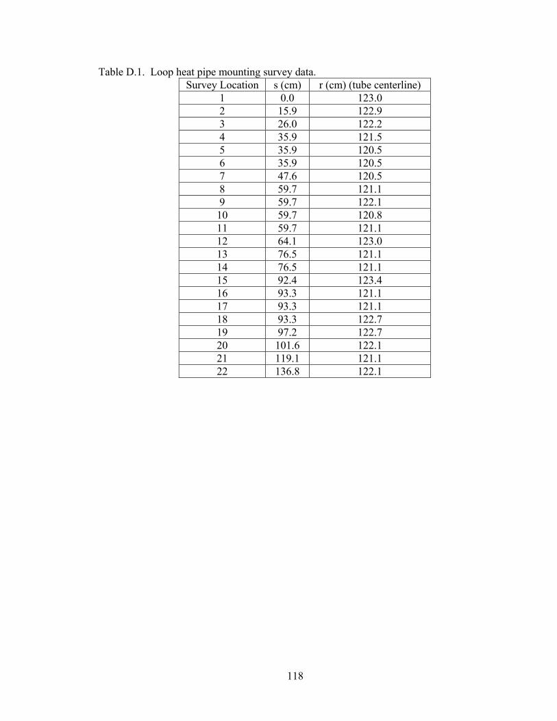
118

Table D.1. Loop heat pipe mounting survey data. Survey Location s (cm) r (cm) (tube centerline)

1 0.0 123.0 2 15.9 122.9 3 26.0 122.2 4 35.9 121.5 5 35.9 120.5 6 35.9 120.5 7 47.6 120.5 8 59.7 121.1 9 59.7 122.1 10 59.7 120.8 11 59.7 121.1 12 64.1 123.0 13 76.5 121.1 14 76.5 121.1 15 92.4 123.4 16 93.3 121.1 17 93.3 121.1 18 93.3 122.7 19 97.2 122.7 20 101.6 122.1 21 119.1 121.1 22 136.8 122.1

119

APPENDIX E. BRAYCO MICRONIC 889 TECHNICAL DATA

Technical data for various properties against temperature for Brayco Micronic

889, including density, specific heat at constant pressure, thermal conductivity, and

kinematic viscosity were provided by Ghajar et al (1994). Brayco Micronic 889 technical

data from Castrol was compiled and the data was curve-fitted using a least squares

approach and varying order polynomials. The equations are only valid on the

temperature range -54 ≤ T ≤ 135°C. The authors report that for ρ, Cp, and k a maximum

deviation of less than ±0.5% from the reported data for the property equations. For ν,

they reported a maximum deviation of +3.4%. The equations for these properties are

given as

1.36 10 4.56 0.0157 0.280 10

0.174 10 (E.1)

0.154 5.88 10 (E.2)

p 1.022 3.77 10 (E.3)

For all of these equations, T is in Kelvin, ρ is in kg/m3, Cp is in kJ/kg-K, and k is in W/m-

K.

120

(c)

Figure E.1. Brayco Micronic 889 properties vs. temperature. (a) ρ vs. T; (b) k vs. T; (c) Cp vs. T.

0100200300400500600700800900

1000

ρ(k

g/m

3 )

(a)

0.128

0.13

0.132

0.134

0.136

0.138

0.14

0.142

k (W

/m-k

)

(b)

0

500

1000

1500

2000

2500

3000

-100 -50 0 50 100 150

Cp

(J/k

g-k)

T (°C)

(c)

121

APPENDIX F. CENTRIFUGE TABLE UPGRADES

The previous centrifuge table data acquisition system dated back to the early

1990’s. The original computer was a Pentium 386 running ViewDAC for data collection

and reduction. At the start of this project, it was determined that the data acquisition

system needed to be upgraded, including the data acquisition unit and computer system.

Since all of this equipment was going to be upgraded, it was decided to completely

evaluate the existing data acquisition wiring and document this information.

The first step to updating the data acquisition system was to record the original

data acquisition wiring. All of the wiring on the centrifuge table was rewired and

documented so that it would be easier to trace wiring back to the centrifuge table control

room. The wiring scheme on the centrifuge table can be seen in Figure F.1. The terminal

strip at the bottom of this photo is located on the rotating table, while the terminal strips

at the top are on the stationary support. These are connected via a 40-ring slip ring. A

new wiring panel was developed for the wiring coming from the stationary terminal strips

above the centrifuge table back to the control room, as shown in Figure F.2. Wiring on

the centrifuge table terminal strip now matches the wiring coming into the centrifuge

table control room. This information was completely documented for future reference.

Each circuit from the centrifuge table to the slip ring wiring panel in the control room

was checked for continuity by hand.

After verifying the wiring configuration was in proper operating condition,

documentation for the new data acquisition hardware was reviewed so that the upgrades

could be started. Initially, a new wiring panel was developed for the new data acquisition

interface as shown in Figure F.3. This panel was designed to accommodate 64 channels

(three wires per channel) for data acquisition, as well as 16 channels (four wires per

channel) for voltage and current control. Each circuit from the data acquisition interface

panel to the two new data acquisition modules was checked for continuity by hand.

Jumper cables were created to transfer signals coming in from the slip rings to the data

acquisition wiring panel.

122

The new data acquisition system from Agilent Technologies has a mainframe

(E8408A) with four slots into which the following cards were installed: a command

module (E1406A), an 8/16 channel D/A converter (E1418A), a 5½-digit multimeter

(E1411B), and a sixty-four channel, 3-wire multiplexer (E1476A). The command

module serves as the main source of communication between all of the cards in the

mainframe. The command module also exchanges data and commands between the

computer and data acquisition system. The D/A converter is a control type module,

allowing the user to request a certain output voltage or current from up to sixteen

channels. The multimeter reads the voltages that the multiplexer collects from

thermocouples, pressure transducers, accelerometers, etc., as well as any externally

applied voltages, currents, and resistances. Communication between the data acquisition

system and the computer takes place via the general purpose interface bus (GPIB) or

IEEE-488 protocol. Essentially, text commands are sent from the computer to the data

acquisition system. Then, if the command requests a control signal, the proper output is

processed. If the command were for data acquisition, then ASCII data is returned to the

user for processing.

With the new data acquisition system and computer assembled, documentation for

the data acquisition system needed to be reviewed to determine the proper commands

necessary to use the computer to communicate with the data acquisition system. Initially,

single text lines were sent from the computer using Agilent’s VISA Assistant software.

Commands were sent to read thermocouple temperatures on one of the channels of the

multiplexer.

The software used for writing the data acquisition code was LabVIEW, a visual

computer language. Virtual instruments (VIs) for communicating with the data

acquisition system started fairly crudely. Virtual instruments are subprograms that are

written with certain inputs and calculated outputs, which can greatly simplify a

complicated code. First, the task of reading several voltage channels and outputting the

data to the screen was accomplished. Second, the reading of several voltage channels

was placed inside a timed loop such that data would be recorded at regular intervals and

written to a file that Microsoft Excel could read. Next, the proper conversions for voltage

123

to temperature, acceleration, and pressure were written into the code so that actual data

was recorded to a file.

The next task to be accomplished with this software was control communication.

What was desired was a system where a certain voltage could be applied to increase the

angular velocity of the centrifuge table, and to control a variety of other devices, such as

pumps, heaters, etc. Following a similar process to the development of the data

acquisition software, a virtual instrument was written that could control the output

voltage of several channels along with the capability of turning them on and off at any

time. This VI was then merged with the data acquisition program with appropriate

Boolean commands for control. This VI was tested and verified when data was collected

for a liquid-vapor separator experiment on the centrifuge table. A program was tailored

for this experiment, including the appropriate flow meter, pressure transducer,

accelerometer conversions, and data recording.

After control of the centrifuge table was accomplished using a voltage from the

D/A converter to control the angular velocity, it was decided to control the acceleration

directly. A relation was then developed between voltage and acceleration. Centrifugal

acceleration is given by

r (F.1)

Voltage is related to angular velocity by

(F.2)

where B is an experimental constant to be determined. Substituting this relation into the

expression for centrifugal acceleration yields

r (F.3)

Solving equation (F.3) for voltage yields the relation used for deriving a corresponding

voltage for a chosen centrifugal acceleration.

r (F.4)

124

Thus, voltage is linearly related to the square root of centrifugal acceleration. This

relation can be extended to relate voltage and the acceleration magnitude. The magnitude

of acceleration is given by

θ r z (F.5)

where +θa , +

ra , and +za are the accelerations normalized by gravity in the azimuthal,

radial, and axial directions on the centrifuge table. Solving for the radial acceleration

gives

r θ z (F.6)

When the centrifuge table is rotating with a constant velocity, +θa = 0 and +

za = −1. After

substituting these values in for equation (F.6) and solving for the square root of

centrifugal acceleration

r 1/

(F.7)

Substituting equation (F.7) into (F.4) yields the relation between table voltage and the

magnitude of the acceleration.

ct 1/

(F.8)

To calculate B, experimental data relating table voltage with centrifugal acceleration was

collected. Then, a plot of voltage versus the square root of centrifugal acceleration was

generated and a linear best fit regression was derived with the voltage intercept forced

through the origin. The corresponding slope is then rgB / . A sample plot can be seen

in Figure F.4. After the slope for this equation was found, an acceleration control slide

bar was added to the data acquisition program by deriving a corresponding voltage

output. It is important to note that the slope is experiment specific, and if the location of

the accelerometer is changed, a new slope needs to be found.

It was desired to have the capability of reading higher temperatures on the

centrifuge table. The current thermocouple amplifier on the centrifuge table is for Type

T thermocouples, which have an operating temperature range between -250 to 350°C. A

125

new Type E thermocouple amplifier (Omega OM7-47-E-07-2-C) has been installed on

the underside of the centrifuge table opposite of the existing thermocouple amplifier so

that either one can be used, depending on the experimental requirements specified,

providing operating temperatures between -200 to 900°C.

126

Figure F.1. Updated wiring on the centrifuge table.

127

Figure F.2. Wiring panel from centrifuge table to the centrifuge table control room.

128

Figure F.3. Wiring panel for the new data acquisition system.

129

Figure F.4. Centrifuge table voltage versus +

ra .

0

0.5

1

1.5

2

2.5

3

3.5

0 1 2 3 4

Out

put T

able

Vol

tage

(V)

130

APPENDIX G. LABVIEW PROGRAMS

131

(a)

(b)

Figure G.1. LabVIEW VI for the LHP experiment: (a) Front panel; (b) Wire diagram.

132

(a)

(b)

Figure G.2. LabVIEW sub-VI wire diagram for voltage output control: (a) Output on; (b) Output off.

133

Figure G.3. LabVIEW sub-VI wire diagram for data acquisition communication.

134

Figure G.4. LabVIEW sub-VI wire diagram for data analyzing.

135

Figure G.5. LabVIEW sub-VI wire diagram for data recording.

136

APPENDIX H. CENTRIFUGE WIRING TABLES

137

Table H.1. E1418A 8/16-CH D/A Converter wiring.

Module Terminal Number

Terminal Letter

Wire Bundle Number

Wire Color

Terminal Strip

Number

Terminal Number Function Slip Ring Wire Color

HS red 01HI white 02 Centrifuge Table Voltage (+) Green-Blue ShieldLO blue 03 Centrifuge Table Voltage (-) Black-Blue ShieldLS yellow 04HS green 05HI brown 06 Heater Power Voltage (+) Red-Red ShieldLO purple 07 Heater Power Voltage (-) Black-Red ShieldLS orange 08HS red 09HI white 10 Pump Voltage (+) 43 Red-Red ShieldLO blue 11 Pump Voltage (-) 44 Black-Red ShieldLS yellow 12HS green 13HI brown 14LO purple 15LS orange 16HS red 01HI white 02LO blue 03LS yellow 04HS green 05HI brown 06LO purple 07LS orange 08HS red 09HI white 10LO blue 11LS yellow 12HS green 13HI brown 14LO purple 15LS orange 16HS red 01HI white 02LO blue 03LS yellow 04HS green 05HI brown 06LO purple 07LS orange 08HS red 09HI white 10LO blue 11LS yellow 12HS green 13HI brown 14LO purple 15LS orange 16HS red 01HI white 02LO blue 03LS yellow 04HS green 05HI brown 06LO purple 07LS orange 08HS red 09HI white 10LO blue 11LS yellow 12HS green 13HI brown 14LO purple 15LS orange 16

GND red 01EXT TRIGn white 02

GND blue 03GND yellow 04

CAL HS green 05CAL HI brown 06CAL LO purple 07CAL LS orange 08

3

4

24

1

2

23

7

8

9

26

6

25

5

31

12

13

28

10

11

27

23

24

25

26

27

14

15

29

16

30

138

Table H.2. Data acqusition terminal board wiring. E1476A Module

Terminal Number

E1476A Terminal

Letter

Main Terminal

Strip Number

Main Terminal Number

Function Slip Ring Number Wire Color

Board Terminal Number

Location

H 01 TC00 3 red 01 CP InL 02 TC Ground 19 black GNDG 03H 04 TC01 4 white 02 CP OutL 05 TC Ground 19 black GNDG 06H 07 TC02 5 blue 03 Box AmbientL 08 TC Ground 19 black GNDG 09H 01 TC03 6 yellow 04 Flow meter InL 02 TC Ground 19 black GNDG 03H 04 TC04 7 green 05 Evap 1L 05 TC Ground 19 black GNDG 06H 07 TC05 8 brown 06 Evap 2L 08 TC Ground 19 black GNDG 09H 01 TC06 9 purple 07 Evap 3L 02 TC Ground 19 black GNDG 03H 04 TC07 10 orange 08 Evap 4L 05 TC Ground 19 black GNDG 06H 07 TC08 11 red 09 Evap OutL 08 TC Ground 19 black GNDG 09H 01 TC09 12 white 10 Cond InL 02 TC Ground 19 black GNDG 03H 04 TC10 13 blue 11 Cond 1L 05 TC Ground 19 black GNDG 06H 07 TC11 14 yellow 12 Cond 2L 08 TC Ground 19 black GNDG 09H 01 TC12 15 green 13 Cond 3L 02 TC Ground 19 black GNDG 03H 04 TC13 16 brown 14 Cond 4L 05 TC Ground 19 black GNDG 06H 07 TC14 17 purple 15 Bayonet InL 08 TC Ground 19 black GNDG 09H 01 TC15 18 orange 16 Evap/CCL 02 TC Ground 19 black GNDG 03H 04 Accel x-axis 21 red 2L 05 Accel GND 20 black 1G 06H 07 Accel y-axis 22 white 3L 08 Accel GND 20 black 1G 09H 01 Accel z-axis 23 blue 4L 02 Accel GND 20 black 1G 03H 04 Flowmeter 24 greenL 05 Flowmeter GND 25 blackG 06H 07 Evap Heater Resistor Voltage (+) 26 redL 08 Evap Heater Resistor Voltage (-) 27 orangeG 09H 01 Evap Heater Voltage (+) 28 whiteL 02 Evap Heater Voltage (-) 29 brownG 03H 04 Preheater Resistor Voltage (+) 30 yellowL 05 Preheater Resistor Voltage (-) 31 blueG 06H 07 Preheater Voltage (+) 32 redL 08 Preheater Voltage (-) 33 blackG 09H 01 CC Heater Resistor Voltage (+) 34 grayL 02 CC Heater Resistor Voltage (-) 35 purpleG 03H 04 CC Heater Voltage (+) 36 pinkL 05 CC Heater Voltage (-) 37 tanG 06H 07L 08G 09

03

0204

05

00

0101

02

09

0410

11

06

0307

08

15

0616

17

12

0513

14

21

0822

23

18

0719

20

24

0925

26

139

APPENDIX I. SAMPLE CALCULATIONS

Example Calculation of Average Heat Transfer Coefficient for Flat Plate Flow

Given: Altitude: H = 5 km Mach number: Ma∞ = 0.8 Wall temperature: Tw = 135 °C = 408.15 K Plate length: L = 1.0 m Calculations: Freestream temperature: T∞ = (7.7664E-4)H4 – (2.8994E-2)H3 + (5.3483E-1)H2 – (9.5033)H + (4.8507E+1) T∞ = 284.37 K Freestream density: ρ∞ = (-4.9336E-6)H3 + (2.0898E-3)H2 – (8.9917E-2)H + 1.0868 ρ∞ = 0.6870 kg/m3 Film temperature: T* = T∞(0.5 + 0.039 Ma∞2) + 0.5Tw = (284.37 K)(0.5+0.039(0. 8)2)+0.5(408.15 K) T* = 353.36 K Air density at the film temperature: ρ*= ρ ∞/(T∞/T*) = (0.6870 kg/m3)(284.37 K)/(353.36 K) = 0.5528 kg/m3 Freestream speed of sound: a∞ = √(γRT∞) = √((1.4)(286.9 m2/s2·K)( 284.37 K)) = 337.97 m/s Freestream velocity: U∞ = Ma∞a∞ = (0.8)(337.97 m/s) = 270.37 m/s Freestream absolute viscosity (Reference values from Incropera and DeWitt, 2002): μ∞ = μR(T∞/TR)0.76 = (184.6 × 10-7 N·s/m2)(284.37 K / 300 K)0.76 μ∞ = 1.772 × 10-5 N·s/m2 Reynolds number: ReL = (ρ∞U∞L)/μ∞ = (0.6870 kg/m3)(270.37 m/s)(1 m) / (1.772 × 10-5 N· s/m2) ReL = 1.05 × 107

[TURBULENT]

140

Prandtl number at the film temperature: Pr* = (-1.2593E-9)T3 + (1.7778E-6)T2 – (9.4177E-4)T + (8.6418E-1) Pr* = 0.6978 Specific heat at the film temperature: Cp

* = (4.4444E-7)T3 – (3.3333E-5)T2 – (6.9921E-2)T + (1.0187E+3) Cp

* = 1009.44 J/(kg·K) Recovery factor for turbulent flow: r = Pr*1/3 = (0.6978)1/3 = 0.8870 Adiabatic wall temperature: Taw = T∞[1+r((γ-1)/2)Ma∞2] = (284.37 K)(1+(0.8870)(0.4/2)(0.8)2) = 316.66 K Absolute viscosity at the film temperature: μ* = μR(T*/TR)0.76 = (184.6 × 10-7 N· s/m2)(353.36 K / 300 K)0.76 = 2.091 × 10-5 N·s/m2 Local skin friction coefficient at the end of the plate: Cf,L

* = 0.455/(ln2(0.06ρ*U∞L/ μ*)) = 0.455/(ln2(0.06(0.5528 kg/m3)(270.37 m/s)(1 m) / (2.091 × 10-5 N· s/m2)) = 0.002705 Local Stanton number at the end of the plate: StL

* = (Cf,L*/2) / (1+12.7(Pr*2/3-1)(Cf,L

*/2)1/2 = (0.002705/2) / (1+12.7((0.6978)2/3-1)(0.002705/2)1/2) = 0.001502 Local heat transfer coefficient at the end of the plate: hL = StL

*ρ*U∞Cp* = (0.001502)(0.5528 kg/m3)(270.37 m/s)(1009.44 J/kg·K)

= 226.7 W/m2·K

Average heat transfer coefficient over the length of the plate: h = 1.15 iL = 1.15(226.7 W/m2·K) = 260.7 W/m2·K Average heat flux dissipated over the plate: qw = h (Tw - Taw) = (260.7 W/m2·K)(408.15 K - 316.66 K) = 23847.7 W/m2

Aircraft Thermal Management using Loop Heat Pipes - CORE

Documents

Transcript of Aircraft Thermal Management using Loop Heat Pipes - CORE