Navy Ford (CVN-78) Class Aircraft Carrier Program: Background ...
Upload
khangminh22Category
view
1download
0
This report was prepared under Contract N00019-89-C-0259 which was competitively awarded for a total cost of $52,998.
Robert Heffley Engineering
349 First Street, Los Altos, CA 94022, USA Telephone: (650) 949-1747 FAX: (650) 949-1243
RHE-NAV-90-TR-1
OUTER-LOOP CONTROL FACTORS FOR CARRIER AIRCRAFT
Robert K. Heffley
1 December 1990
CONTRACT SUMMARY REPORT
Distribution authorized to U. S. Government agencies and their
contractors; (Critical technology). Other requests for this document
will be referred to the Naval Air Systems Command (AIR-5301).
Prepared for:
Naval Air Systems CommandDepartment of the NavyWashington DC 20361

THIS PAGE IS INTENTIONALLY BLANK

UNCLASSFIED/UNLIMITED
Outer-loop control factors are those qualities that affect the pilot's ability to regulate manually glideslope, angle of attack, and lineup during the final approach. This report concentrates on the first two, glideslope and angle of attack. The objective is to identify the crucial attributes that ensure effective outer-loop control, then to examine how well existing design requirements address such attributes. A combination of flying qualities and performance requirements applies to this area, including MIL-F-8785C, MIL-STD-1797A, and the Navy's approach-speed criteria. First, the report reviews the topic in terms of historical background, discusses the technical approach, and previews the analytical tools to be applied. Second, it gives the status of outer-loop control, including a description of the carrier landing task, existing aircraft characteristics, and some data describing in-flight simulated carrier approaches. A description follows that contains math model components of the task, the aircraft, and the pilot. The main section of the report presents a series of analyses that are useful in pinpointing crucial outer-loop control features. The final section gives conclusions and recommendations for implementing results. The technical approach applies
SECURITY CLASSIFICATION OF THIS PAGE
83 APR edition may be used until exhausted.All other editions are obsolete.
SECURITY CLASSIFICATION OF THIS PAGE
1a. REPORT SECURITY CLASSIFICATION
2a. SECURITY CLASSIFICATION AUTHORITY
2b. DECLASSIFICATION/DOWNGRADING SCHEDULE
4. PERFORMING ORGANIZATION REPORT NUMBER(S)
6c. ADDRESS (City, State, and ZIP Code)
6a. NAME OF PERFORMING ORGANIZATION
REPORT DOCUMENTATION PAGE
8c. ADDRESS (City, State, and ZIP Code)
6b. OFFICE SYMBOL (I f applicable)
8a. NAME OF FUNDING/SPONSORING ORGANIZATION
8b. OFFICE SYMBOL (If applicable)
11. TITLE (Include Security Classification)
12. PERSONAL AUTHOR(S)
13a. TYPE OF REPORT 13b. TIME COVERED
14. DATE OF REPORT (Year, Month, Day) 15. PAGE COUNT
16. SUPPLEMENTARY NOTATION
17. COSATI CODES
FIELD GROUP SUB-GROUP
18. SUBJECT TERMS (Continue on reverse if necessary and identify by block number)
19. ABSTRACT (Continue on reverse if necessary and identify by block number)
21. NAME OF RESPONSIBLE INDIVIDUAL
21. ABSTRACT SECURITY CLASSIFICATION
22b. TELEPHONE (include Area Code) 22c. OFFICE SYMBOL
DD FORM 1473, 84 MAR
10. SOURCE FUNDING NUMBERS
PROGRAMELEMENT NO.
PROJECT NO.
TASK NO.
WORK UNITACCESSION NO.
9. PROCUREMENT INSTRUMENT IDENTIFICATION NUMBER
7a. NAME OF MONITORING ORGANIZATION
7b. ADDRESS (City, State, and ZIP Code)
5. MONITORING ORGANIZATION REPORT NUMBER(S)
1b. RESTRICTIVE MARKINGS
3. DISTRIBUTION/AVAILABILITY OF REPORT
UNCLASSIFIED
Robert Heffley Engineering
349 First StreetLos Altos, CA 94022
OUTER-LOOP CONTROL FACTORS FOR CARRIER AIRCRAFT (U)
Heffley, Robert K.
Department of the NavyNaval Air Systems Command, AIR-5301
UNCLASSIFIED
RHE-NAV-90-TR-1
Washington, DC 20361
Distribution authorized to U. S. Government agencies and their contractors; (Critical technology). Other requests for this document will be referred to the Naval Air Systems Command (AIR-5301).
Contract N00019-89-C-0259
UNCLASSIFIED
UNCLASSIFIED
Page i
Contract Summary Report 90 Apr 90 Dec 90 Dec 1
STABILITY AND CONTROL, AIRCRAFT PERFORMANCE,FLYING QUALITIES, CARRIER AIRCRAFT, GLIDESLOPE CONTROL, PILOT-IN-THE-LOOP, MANUAL CONTROL
J. T. Lawrence (703) 692-3541 AIR-53011
20. DISTRIBUTION/AVAILABILITY OF ABSTRACTSAME AS RPT. DTIC USERS
196
Naval Air Systems Command AIR-5301
Washington, DC 20361
01 03 05
FROM _______ TO ________
X
(continued on next page)

SECURITY CLASSIFICATION OF THIS PAGE
SECURITY CLASSIFICATION OF THIS PAGE
UNCLASSIFIED
UNCLASSIFIED
Page ii
linear-systems analysis methods to low-order dynamics, mainly first- and second-order. The time domainis used to portray most results. The assumption of pitch-attitude constraints simplifies analysis bypartitioning away higher-order dynamics of the flight control system and aircraft pitching-momentequations. This permits full appreciation of the role of aircraft lift, drag, and control or engine laginfluences on outer-loop dynamics. Based on a system view of the pilot-vehicle-task combination, therelevant outer-loop control factors include: (i) Steady-state flightpath authority, (ii) short-term flightpathresponse, (iii) cue availability, (iv) safety margins, (v) commensurate amounts of pitch and thrust control,(vi) control quickness, (vii) established technique, and (viii) quality or shape of response. Current designrequirements do not address effectively short-term flightpath response, control quickness, establishedtechnique, and quality of response. Analysis of the Navy popup maneuver shows it to be mainlydependent upon the margin from stall. One device for examining multiple aspects of outer-loop control isthe “last significant glideslope correction.” It is an analytically-generated spatial envelope that bounds themaximum amplitude of a glideslope correction as a function of range from the ship. The method exploresvarious outer-loop control factors and underlines the importance of short-term response and controlquickness for glideslope control. Based on the analytical results, it is necessary to expand and betterquantify currently-used design requirements to include those factors crucial to the carrier landing task. Acombination of manned simulation and in-flight verification can do this best.
RHE-NAV-90-TR-1 Page iii
Robert Heffley Engineering 1 December 1990
TABLE OF CONTENTS
section page
1. INTRODUCTION…………………………………………………………………. 11.1 Purpose…………………………………………………………………………. 11.2 Background…………………………………………………………………….. 21.3 Technical Approach to Examining Outer-Loop Control Factors……………… 81.4 Introductory Technical Overview………………………………………………..11
2. THE CARRIER LANDING TASK AND EXISTING AIRCRAFT……………...…192.1 Carrier Landing Task Description……………………………………………… 192.2 Existing Carrier Aircraft………………………………………………………… 332.3 Examples of Simulated Carrier Landings (FCLP) ………………………………57
3. PILOT-VEHICLE-TASK MATH MODEL FOR CARRIER LANDING………… 653.1 Carrier Environment (Task) ……………………………………………………. 653.2 Aircraft and Flight Control Systems (Vehicle) ………………………………… 733.3 Pilot and Task Control Strategy (Pilot) ………………………………………… 863.4 Audit Trail of Outer-Loop Control Factors………………………………………96
4. ANALYSIS RESULTS BASED ON SYSTEM MATH MODEL…………………1014.1 Phase-Plane Analysis of Flight Data……………………………………………1014.2 Analysis of Navy VPA Criteria……………………………………………...… 116
4.3 Computation of the “Last Significant Glideslope Correction” ……………...…1334.4 Inner-Loop Control Lag Influence on Flightpath Response……………………1484.5 Effect of Engine Lag on Control of Thrust…………………………………..…152
5. CONCLUSIONS AND RECOMMENDATIONS……………………………….…1575.1 Conclusions Based on Analysis Results…………………………………..……1575.2 Need for Further Research…………………………………………………...…165
REFERENCES………………………………………………………………...……167
GLOSSARY………………………………………………………………..……… 173

RHE-NAV-90-TR-1 Page iv
Robert Heffley Engineering 1 December 1990
THIS PAGE IS INTENTIONALLY BLANK
RHE-NAV-90-TR-1 Page v
Robert Heffley Engineering 1 December 1990
LIST OF FIGURES
number title page
1-1 Scheme for Portraying the Pilot-Vehicle-TaskSystem…………………………….… 31-2 Topology of Carrier Landing Aircraft System…………………………………….…101-3 Range of Interest for CV Approach Task…………………………….……………... 111-4 Flight Path and Airspeed Response to Attitude Change……………………………. 141-5 Flight Path and Airspeed Response Due to Thrust Change………………………… 151-6 Summary of Key Aerodynamic Data……………………………………………..… 161-7 Summary of Geometric Data……………………………………………………...… 18
2-1 Carrier Landing Pattern as Described in NATOPS……………………………….… 202-2 LSO Range Descriptors…………………………….…………………………….…. 242-3 LSO Glideslope Descriptors………………………………………………………… 252-4 LSO Angle of Attack (Airspeed) Descriptors…………………………………….… 252-5 LSO Lineup Descriptors…………………………….……………………………… 262-6 Scale Drawing of Approach Flightpath Parameters………………………………… 282-7 Planview of Final Approach Leg…………………………….………………………292-8 Planview of Carrier Deck…………………………….………………………………302-9 Summary of F-4J Aero, Trim, and Response Parameters……………………………392-10 Summary of F-8C (no BLC) Aero, Trim, and Response Parameters………..… 402-11 Summary of F-8J (BLC) Aero, Trim, and Response Parameters……………… 412-12 Summary of F-14D Aero, Trim, and Response Parameters…………………….422-13 Summary of F/A-18A Aero, Trim, and Response Parameters……………….…432-14 Summary of F-111B Aero, Trim, and Response Parameters………………...… 442-15 Summary of A-3B Aero, Trim, and Response Parameters…………………….. 452-16 Summary of RA-5C Aero, Trim, and Response Parameters……………………462-17 Summary of A-6E Aero, Trim, and Response Parameters………………….…. 472-18 Summary of T-45A Aero, Trim, and Response Parameters…………………… 482-19 Thrust Lag Data for the J-85 Engine (T-2C) ………………………………..… 532-20 Thrust Lag Data for the J-52 Engine (TA-4J) ……………………………....… 542-21 Thrust Lag Data for the F405 Engine (T-45) ……………………………….… 552-22 Comparison of J79 and Spey Engines in F-4 Aircraft………………………… 562-23a FCLP Approach Example for A-6E…………………………………………… 582-23b FCLP Approach Example for A-6E…………………………………………… 582-23c FCLP Approach Example for A-6E…………………………….……………… 592-23d FCLP Approach Example for A-6E…………………………….……………… 59

RHE-NAV-90-TR-1 Page vi
Robert Heffley Engineering 1 December 1990
LIST OF FIGURES, Continued
number title page
2-23e FCLP Approach Example for A-6E…………………………….……………… 602-23f FCLP Approach Example for A-6E………………………………………….… 602-24a FCLP Approach Example for F-14A…………………………………………... 612-24b FCLP Approach Example for F-14A…………………………………………... 612-25a FCLP Approach Example for F-18A…………………………………………... 622-26a FCLP Approach Example for T-45A…………………………………………... 632-26b FCLP Approach Example for T-45A…………………………………………... 63
3-1 FLOLS Glideslope Display Geometry……………………………………………… 653-2 Effect of FLOLS Roll Angle on Light Plane…………………………………..…… 673-3 Sideview of FLOLS Geometry………………………………………………………683-4 Math Model of Glideslope Geometry………………………………………..………693-5 Angle-of-Attack Indexer Display………………………………………………….…703-6 Math Model of AOA Display……………………………………………………..… 713-7 Lineup Geometry………………………………………………………………….… 723-8 Comparison of Pilot-Vehicle Architectures………………………………………… 743-9 Dependence of Some Outer-Loop Features on Airframe Parameters…….………… 783-10 Dependence of Approach Speed Criteria on Airframe and Engine Parameters...793-11 High-Order System Response to a Pitch Step…………………………..……… 813-12 Reduced-Order System Response to a Pitch Step……………………………… 823-13 Longitudinal Position Effect on Flightpath…………………………………..… 833-14 Relationship Between Pitch Attitude and Flightpath Angle…………………… 843-15 Flightpath Response to Thrust……………………………………………….… 853-16 The Two Main Control Strategy Structures…………………………….……… 873-17 Diagram of Backside Technique………………………………………….…… 893-18 Response Survey for Backside Technique…………………………………..… 903-19 Diagram of Frontside Technique…………………………………………….… 913-20 Response Survey for Frontside Technique…………………………………….. 923-21 Diagram of Pursuit Technique………………………………………………… 933-22 Crossfeed Gains for Several Optimality Criteria……………………………… 943-23 Effective ∆ γ Rise Times for Several Optimality Criteria……………………… 943-24 Response Survey for Pursuit Technique……………………………………..… 95
4-1 Example of a Second-Order-System Phase-Plane Portrait………………….…1024-2 Appearance of Closed-Loop Attributes in the Phase Plane……………………1034-3 Glideslope Control Task Model…………………………………………….… 104
RHE-NAV-90-TR-1 Page vii
Robert Heffley Engineering 1 December 1990
LIST OF FIGURES, Continued
number title page
4-4 Phase-Plane Portrait of a Glideslope Correction………………………………1054-5a Phase-Plane Portrait of A-6 Glideslope Corrections…………………………..1064-5b Phase-Plane Portrait of A-6 Glideslope Corrections…………………………..1074-5c Phase-Plane Portrait of A-6 Glideslope Corrections…………………………..1084-5d Phase-Plane Portrait of A-6 Glideslope Corrections…………………………. 1084-5e Phase-Plane Portrait of A-6 Glideslope Corrections…………………………..1094-5f Phase-Plane Portrait of A-6 Glideslope Corrections………………….……… 1104-6a Phase-Plane Portrait of F-14 Glideslope Corrections………………….………1114-6b Phase-Plane Portrait of F-14 Glideslope Corrections………………………… 1114-7a Phase-Plane Portrait of F-18 Glideslope Corrections………………….………1124-7b Phase-Plane Portrait of F-18 Glideslope Corrections………………….………1134-7c Phase-Plane Portrait of F-18 Glideslope Corrections………………….………1134-7d Phase-Plane Portrait of F-18 Glideslope Corrections………………….………1144-8a Phase-Plane Portrait of T-45 Glideslope Corrections………………….………1154-8b Phase-Plane Portrait of T-45 Glideslope Corrections…………………….……1154-9 Acceleration Response to a Unit ∆ T/W Command…………………………...……1214-10 Nominal Aircraft Response in Popup Maneuver………………………………1244-11 Sensitivity of Popup Performance to nzα………………………………………1254-12 Sensitivity of Popup Performance to Approach Speed……………………..… 1264-13 Sensitivity of Popup Performance to Backsidedness…………………………. 1274-14 Sensitivity of Popup Performance to Pitch Attitude Response……………..… 1284-15 Sensitivity of Popup Performance to Margin from Stall………………………1294-16 Comparison of Popup for Two Diverse Pitch Maneuvers…………………..…1304-17 Simplified Representation of Pilot-Vehicle System………………………...…1334-18 Normalized Height Response as Pilot Aggressiveness Varied……………...…1344-19 Scheme for Measuring Performance of Glideslope Correction……………..…1364-20 Envelope of Permissible Correction Points for Nominal Aircraft Response…. 1384-21 Envelope of Permissible Correction Points in Terms of FLOLS Angular Error1394-22 Envelope of Peak Vertical Velocity Excursion for a Permissible Correction…1404-23 Envelope of Control-Required for Permissible Correction……………………1414-24 Closed-Loop Damping Ratio for the Terminal GS Correction……………..… 1424-25 Effect of Airframe Lag, T1, on Permissible Glideslope-Correction Boundary 1434-26 Effect of Airframe Lag, T1, on Vertical Velocity Excursion…………….…… 1444-27 Effect of Control Lag, T1, on Control Authority Required……………………1444-28 Effect of Control Lag, T2, on Permissible Glideslope-Correction Boundary... 1454-29 Effect of Control Lag, T2, on Vertical Velocity Excursion………………...… 146
RHE-NAV-90-TR-1 Page viii
Robert Heffley Engineering 1 December 1990
LIST OF FIGURES, Continued
number title page
4-30 Effect of Control Lag, T2, on Control Authority Required……………………1464-31 Relative Importance of Inner-Loop Lags for F-14…………………………….1494-32 Relative Importance of Inner-Loop Lags for F-4……………………………....1504-33 Relative Importance of Inner-Loop Lags for T-45…………………………….1514-34 Hess Structural Pilot Model…………………………….…………………….. 1534-35 Sample of HQ Sensitivity Factor Solutions…………………………...…….…1544-36 Max Acceptable Crossover Frequency vs Engine Lag……………………..….155
RHE-NAV-90-TR-1 Page ix
Robert Heffley Engineering 1 December 1990
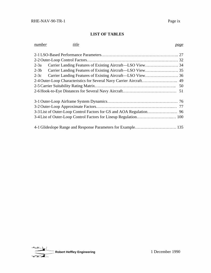
LIST OF TABLES
number title page
2-1 LSO-Based Performance Parameters……………………………………………….. 272-2 Outer-Loop Control Factors………………………………………………………… 322-3a Carrier Landing Features of Existing Aircraft—LSO View…………………… 342-3b Carrier Landing Features of Existing Aircraft—LSO View…………………… 352-3c Carrier Landing Features of Existing Aircraft—LSO View…………………… 362-4 Outer-Loop Characteristics for Several Navy Carrier Aircraft…………………….. 492-5 Carrier Suitability Rating Matrix………………………………………………….. 502-6 Hook-to-Eye Distances for Several Navy Aircraft………………………………… 51
3-1 Outer-Loop Airframe System Dynamics…………………………………………… 763-2 Outer-Loop Approximate Factors………………………………………………..… 773-3 List of Outer-Loop Control Factors for GS and AOA Regulation……………….… 963-4 List of Outer-Loop Control Factors for Lineup Regulation……………………..… 100
4-1 Glideslope Range and Response Parameters for Example………………………… 135

RHE-NAV-90-TR-1 Page x
Robert Heffley Engineering 1 December 1990
THIS PAGE IS INTENTIONALLY BLANK

RHE-NAV-90-TR-1 Page xi
Robert Heffley Engineering 1 December 1990
LIST OF SYMBOLS
symbol definition units
AOA angle of attack units,
degAOAcom angle of attack command units,
deg
AR wing aspect ratio, b2/S n/d
b wing span ftbAOA AOA indicator bias deg
c, cbar wing mean aerodynamic chord (MAC) ft
cg center of gravity (fraction of MAC) n/dCL lift coefficient, Lift/S/q n/dCLα lift curve slope, ∂ CL/∂ α 1/rad
CD drag coefficient, Drag/S/q n/dCDo minimum-drag coefficient n/d
CDi induced-drag coefficient n/d
CDCL∂CD/∂CL n/d
CDα ∂CD/∂ α = CDCL· CLα 1/rad
d glideslope error ftdcom glideslope command ft
d glideslope error rate ft/sec
e Oswald efficiency factor n/dfo effective frontal area, CDo · S ft2
g gravity constant ft/sec2
h altitude ftiT thrust incidence relative to FRL deg or
rad
K system gainKAOA AOA indicator proportionality factor units/deg
l distance ft
m mass slug
MAC mean aerodynamic chord, c ft

RHE-NAV-90-TR-1 Page xii
Robert Heffley Engineering 1 December 1990
LIST OF SYMBOLS, Continued
symbol definition units
Mα 1/Iy · ∂ M/∂ α 1/sec2
Mδe 1/Iy · ∂ M/∂ δe 1/sec2
n load factor gnxα ∂ nx/∂ α g/rad
nzα ∂ nz/∂ α g/rad
γNθ flightpath angle numerator for attitude control
γN
T/W flightpath numerator for thrust control
αNθ angle-of-attack numerator for attitude control
αNT/W angle-of-attack numerator for thrust control
Nθu
airpseed numerator for attitude control
NuT/W airspeed numerator for thrust control
q dynamic pressure pound/ft3
s Laplace operator rad/sec
S wing area ft2
t time sec
T thrust poundT1 effective first-order time constant used to lump airframe lag factors sec
T2 effective first-order time constant used to lump control lag factors sec
TW thrust-to-weight ratio, T/W n/dTθ1 long-term factor in θ/δe numerator sec
Tθ2 short-term factor in θ/δe numerator sec
Th1 long-term factor in γ/δe numerator sec
Th2,Th3 short-term factors in γ/δe numerator sec
Thθ factor in γ/∆ TW numerator sec
Tu1 short-term factor in u/δe numerator secTuθ short-term factor in u/∆ TW numerator sec
RHE-NAV-90-TR-1 Page xiii
Robert Heffley Engineering 1 December 1990
LIST OF SYMBOLS, Continued
symbol definition units
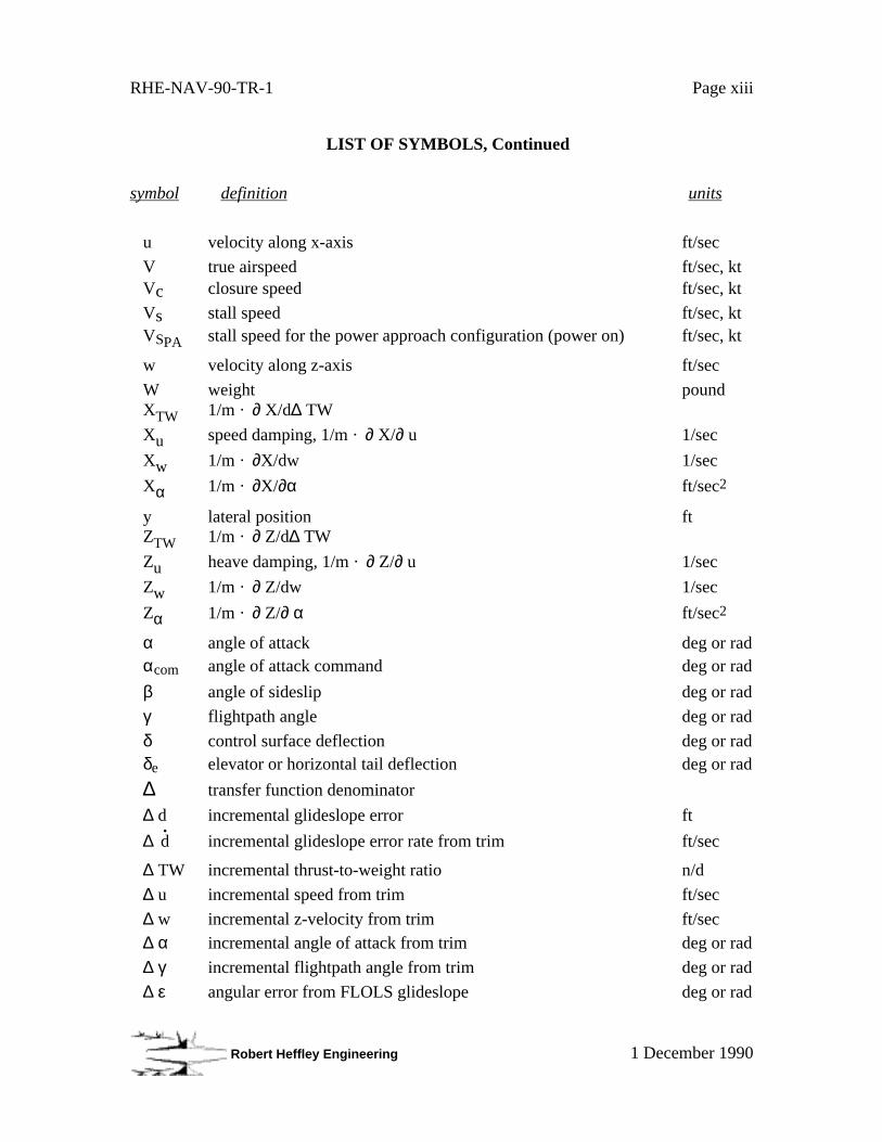
u velocity along x-axis ft/sec
V true airspeed ft/sec, ktVc closure speed ft/sec, kt
Vs stall speed ft/sec, ktVSPA stall speed for the power approach configuration (power on) ft/sec, kt
w velocity along z-axis ft/sec
W weight poundXTW 1/m · ∂ X/d∆ TW
Xu speed damping, 1/m · ∂ X/∂ u 1/sec
Xw 1/m · ∂X/dw 1/sec
Xα 1/m · ∂X/∂α ft/sec2
y lateral position ftZTW 1/m · ∂ Z/d∆ TW
Zu heave damping, 1/m · ∂ Z/∂ u 1/sec
Zw 1/m · ∂ Z/dw 1/sec
Zα 1/m · ∂ Z/∂ α ft/sec2
α angle of attack deg or radαcom angle of attack command deg or rad
β angle of sideslip deg or rad
γ flightpath angle deg or rad
δ control surface deflection deg or radδe elevator or horizontal tail deflection deg or rad
∆ transfer function denominator
∆ d incremental glideslope error ft
∆ d incremental glideslope error rate from trim ft/sec
∆ TW incremental thrust-to-weight ratio n/d
∆ u incremental speed from trim ft/sec
∆ w incremental z-velocity from trim ft/sec∆ α incremental angle of attack from trim deg or rad
∆ γ incremental flightpath angle from trim deg or rad
∆ ε angular error from FLOLS glideslope deg or rad
RHE-NAV-90-TR-1 Page xiv
Robert Heffley Engineering 1 December 1990
LIST OF SYMBOLS, Concluded
symbol definition units
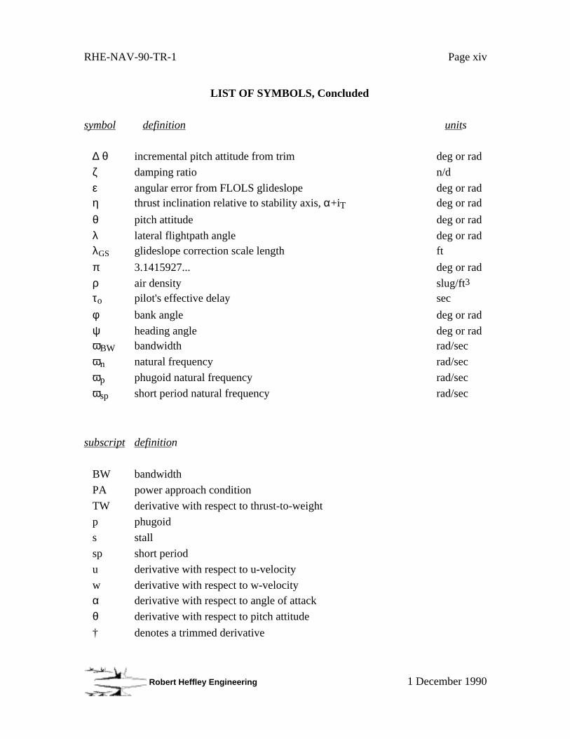
∆ θ incremental pitch attitude from trim deg or rad
ζ damping ratio n/d
ε angular error from FLOLS glideslope deg or radη thrust inclination relative to stability axis, α+iT deg or rad
θ pitch attitude deg or rad
λ lateral flightpath angle deg or radλGS glideslope correction scale length ft
π 3.1415927... deg or rad
ρ air density slug/ft3
τo pilot's effective delay sec
φ bank angle deg or rad
ψ heading angle deg or radωBW bandwidth rad/sec
ωn natural frequency rad/sec
ωp phugoid natural frequency rad/sec
ωsp short period natural frequency rad/sec
subscript definition
BW bandwidth
PA power approach condition
TW derivative with respect to thrust-to-weight
p phugoid
s stall
sp short period
u derivative with respect to u-velocity
w derivative with respect to w-velocityα derivative with respect to angle of attack
θ derivative with respect to pitch attitude
† denotes a trimmed derivative

RHE-NAV-90-TR-1 Page xv
Robert Heffley Engineering 1 December 1990
FOREWORD
This report was prepared under Contract N00019-89-C-0259 sponsored by theNaval Air Systems Command. The project is a Phase I study under the Small BusinessInnovation Research (SBIR) Program. The Contract Technical Monitor was Mr. J. T.Lawrence, AIR-53011, and the Contracting Officer was Mr. E. T. Ebner, AIR-21531E.Work commenced on 28 March 1990 and was completed 11 December 1990.
The author is grateful for the special assistance in obtaining data and backgroundinformation provided by the following individuals. From the Naval Air SystemsCommand Headquarters, AIR-5301: Ms. Jennifer Baliles, Ms. Marge Draper, Mr.Robert Hanley, Mr. J. T. Lawrence, and Mr. Melvin A. Luter; and from the U. S. NavalAir Test Center, NAS Patuxent River: LT Dan Canin, USN, Mr. Chris Clark, Mr.Bruce Feldman, and Ms. Kathleen Y. Fleming.
Professor Ronald A. Hess of the University of California, Davis, providedconsultant support in applying pilot model analysis techniques.

RHE-NAV-90-TR-1 Page xvi
Robert Heffley Engineering 1 December 1990
THIS PAGE IS INTENTIONALLY BLANK
RHE-NAV-90-TR-1 Page 1
Robert Heffley Engineering 1 December 1990
OUTER-LOOP CONTROL FACTORS FOR CARRIER AIRCRAFT
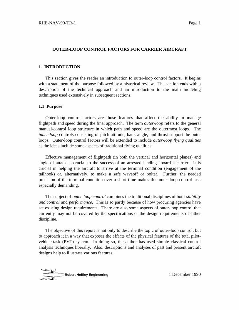
1. INTRODUCTION
This section gives the reader an introduction to outer-loop control factors. It beginswith a statement of the purpose followed by a historical review. The section ends with adescription of the technical approach and an introduction to the math modelingtechniques used extensively in subsequent sections.
1.1 Purpose
Outer-loop control factors are those features that affect the ability to manageflightpath and speed during the final approach. The term outer-loop refers to the generalmanual-control loop structure in which path and speed are the outermost loops. Theinner-loop controls consisting of pitch attitude, bank angle, and thrust support the outerloops. Outer-loop control factors will be extended to include outer-loop flying qualitiesas the ideas include some aspects of traditional flying qualities.
Effective management of flightpath (in both the vertical and horizontal planes) andangle of attack is crucial to the success of an arrested landing aboard a carrier. It iscrucial in helping the aircraft to arrive at the terminal condition (engagement of thetailhook) or, alternatively, to make a safe waveoff or bolter. Further, the neededprecision of the terminal condition over a short time makes this outer-loop control taskespecially demanding.
The subject of outer-loop control combines the traditional disciplines of both stabilityand control and performance. This is so partly because of how procuring agencies haveset existing design requirements. There are also some aspects of outer-loop control thatcurrently may not be covered by the specifications or the design requirements of eitherdiscipline.
The objective of this report is not only to describe the topic of outer-loop control, butto approach it in a way that exposes the effects of the physical features of the total pilot-vehicle-task (PVT) system. In doing so, the author has used simple classical controlanalysis techniques liberally. Also, descriptions and analyses of past and present aircraftdesigns help to illustrate various features.

RHE-NAV-90-TR-1 Page 2
Robert Heffley Engineering 1 December 1990
Ultimately, the analysis presented in this report leads to an assessment of designrequirements that affect outer-loop control, both directly and indirectly. Also it results incommentary on aspects not currently covered by such requirements and offerssuggestions for other analyses or experimentations that may be useful.
1.2 Background
The carrier landing is a major design issue for Navy aircraft. Precise control of flightpath and speed must be made within the narrow time and space bounds of the finalapproach leg. Simultaneously, the aircraft often requires high performance at otherextremes of the envelope. While these design factors can force the use of complexdisplays and flight control systems (FCS), there are some basic airframe and engineattributes still needed. In general, these airframe and engine factors relate to outer-loopcontrol. Moreover, they are not amenable to easy solution by clever FCS design becauseof the prevailing influence of basic lift, drag, and thrust characteristics.1 Outer-loopcontrol requires “muscle” because it deals with changes in flightpath and theaccompanying applied forces to make them.
It is convenient to establish a simple scheme for defining the relationship among thepilot, the aircraft, and the total flight task when viewing outer-loop control. This can beeffectively done using a feedback control system loop structure. Figure 1-1 diagramssuch a structuring of manual control as applied to an aircraft.
1This assumes that flight control systems are tied to basic control surfaces, i. e., they produce
roll, pitch, and yaw moments only. Outer-loop characteristics can be altered if flight controls
are extended to force-producing controls such as flaps, speedbrake, or engine thrust.

RHE-NAV-90-TR-1 Page 3
Robert Heffley Engineering 1 December 1990
+
-
+
-
cockpit controller
inner-loop command
vehicle(airframe,
engine,FCS)
inner-loop control
technique
outer-loop control
technique
pilot vehicle
task represented by total closed-loop system
inner-loop state
inner-loop
outer-loop
outer-loop stateouter-loop
command
Figure 1-1. Scheme for Portraying the Pilot-Vehicle-Task System.
The benefits of this kind of scheme are that all the components—pilot, aircraft, andtask—can be viewed in a common mathematical framework. The scheme induces theengineer to quantify some aspects not often viewed in strictly engineering terms, namely,those concerning the pilot and the task.
For the carrier landing task the outer-loop states are glideslope, angle of attack, andlineup. The inner-loop states are pitch attitude, thrust, and bank angle. Controls for theinner-loop states are the traditional set consisting of longitudinal-stick, lateral-stick andthrottle. Controls for the outer-loop states can be equated to the inner-loop statecommands (attitude command, thrust command, and bank angle command). Thisprovides a neat “partitioning” of the pilot and aircraft and simplifies many aspects of thetotal task (carrier landing) system.
Just as a practical consideration, outer-loop flying qualities need to be partitionedfrom inner-loop features. This would permit the handling of aircraft with advanced FCSconfigurations without dealing with their complexity. The analysis techniques used heremake this feasible, especially the use of pitch-constrained equations of motion to describethe aircraft and the inner-loop functions of the pilot.
Though the “outer-loop” control tasks of glideslope, angle-of-attack, and lineup arecrucial, existing flying qualities specifications or design standards only partially address
RHE-NAV-90-TR-1 Page 4
Robert Heffley Engineering 1 December 1990
them. One important objective of this report is to examine in detail the factors thatdetermine outer-loop flying qualities in order to set design requirements better.
1.2.1 Current Standards and Philosophies
There is not a clear structuring of inner- and outer-loop flying qualities characteristicsfor use in aircraft design. This is true both in MIL-F-8785C (Reference 1) and in thecurrent MIL-STD 1797A specification for flying qualities of piloted airplanes (Reference2). Sections that deal with inner-loop features, e. g., short-period dynamics, include someaspects of flightpath and speed control. The sections of MIL-STD 1797A that addressexplicitly outer-loop control contain only general background information and do notoffer much specific guidance for carrier aircraft, especially concerning speed (or angle-of-attack) control.
MIL-STD 1797A correctly identifies 1/Tθ22 as the primary influence in flightpath
response, but establishes values only indirectly.3 It does not give rationale for why 1/Tθ2,
a time response feature, should be scaled with nzα, an outer-loop control sensitivity
factor. Nor does it say why 135 kt should be used as the scale factor. It will be seen thatsome current carrier aircraft have values considerable lower than this limit.
MIL-STD 1797A and MIL-F-8785C address speed control only in terms of speedstability. Neither document recognizes that Navy aircraft (nor most current militaryaircraft) do not use a speed reference, but angle of attack instead. While thesespecifications bound the short-period dominant mode seen in angle-of-attack (α)response to elevator, this mode is not particularly relevant to the outer-loop controlsituation. It especially does not relate to loose regulation of angle of attack.
Speed damping is one aspect of speed control that current design requirements do notaddress in any way. This parameter, 1/Tθ1, can be characterized as the speed-damping
counterpart to heave damping, 1/Tθ2. One simulation experiment that focused on this
feature showed a high sensitivity of pilot rating (Reference 3). It will be shown that
21/Tθ2 is a parameter frequently referred to in this report. It and others are defined in the glossary at theend of the report as well as in the body of the report itself.
3Minimum 1/Tθ2 is computed based on a minimum nzα and an airspeed of 135 kt.(Min (1/Tθ2) = min(nzα)· g/V = 2.5 g/rad · 32ft/sec2 / 228ft/sec = 0.35 sec-1)
RHE-NAV-90-TR-1 Page 5
Robert Heffley Engineering 1 December 1990
1/Tθ1 relates to the speed-stability factor found in current specifications, ∂ γ/∂ V. Also
1/Tθ1 may have more fundamental effects on successful manual control of flightpath and
speed.
There is no requirement for an adequate level of flightpath control power or authorityin either of the flying-qualities specifications. Although it may be more correctly viewedas a performance feature. Yet, the design requirements that most effectively addressouter-loop control at this time fall under a performance classification, namely, the NavyVPA criteria. These criteria cover several factors that shall be introduced shortly and later
analyzed in depth.
No design requirement addresses explicitly outer-loop control factors for the lineuptask, although one should not necessarily view this as an oversight. Kinematicrelationships strongly constrain lineup control features (lateral flightpath response), atleast for coordinated turns. So long as the existing flying qualities requirementsadequately cover turn-coordination quality, there may not be a need for additionalrequirements. Unfortunately, those turn coordination requirements in both MIL-STD1797A and MIL-F-8785C are difficult to interpret in direct physical terms4. They mightbe better stated with respect to the relationship between turn initiation (bank angle) andresulting lateral flightpath (heading response or y-velocity response). But this will not bediscussed further in this report.
Because of limits imposed by the contract covering this study, the subject of outer-loop control in the horizontal-plane is not be addressed here other than to define its rolein the total carrier landing task. Also, for the longitudinal axes, there is no considerationof the use of auxiliary flightpath and speed controls such as direct lift control orspeedbrake modulation. Although, there will be some general conclusions drawn basedon the analyses that can be applied to these other controls.
1.2.2 Navy Approach Speed Criteria
The current criteria that define the approach speed, VPA, combine to set several flying
qualities and performance characteristics for Navy carrier aircraft (such as are given inReferences 4 and 5). The Navy approach speed criteria are closest to an explicit outer- 4Specifically, the roll rate oscillation limitations, bank angle oscillation limitations, and
sideslip excursion limitations as given in Section 3.3.2 of MIL-F-8785C.
RHE-NAV-90-TR-1 Page 6
Robert Heffley Engineering 1 December 1990
loop control requirement for carrier aircraft. These criteria address not only stability andcontrol and performance, but also flying qualities, visibility, safety margins, and engineresponse. Therefore they are worthy of scrutiny in this study.
The Navy VPA criteria combine in a synergistic way and appear to have worked
effectively for nearly 30 years. But, the variety of effects are sufficiently complex andinteractive to impede a clear understanding by engineers and pilots alike.
One purpose of this report is to present background for Navy approach speed criteriaand to analyze their effects on aircraft design, flying qualities, and performance. Theauthor presents a brief historical sketch followed by a discussion of each component ofthe criteria in basic engineering terms. This prepares the way for development of an audittrail between airplane design features and mission performance consequences for carrieraircraft. The analysis of approach speed criteria is finally tied to actual Navy aircraft sothat maximum use can be made of historical data.
Historical Sketch
The Navy approach speed criteria consist of several parts, the most notable of whichis the "popup" maneuver. The popup is a large-amplitude pitchup aimed at gaining agiven height change within a specified time. Other conditions support the popup,including visibility, safety, and the ability to sustain the altitude gain through use of theengine.
Most of the Navy approach speed criteria stem from a 1953 McDonnell AircraftCorporation report based on flight experience with both the USAF XF-88A and NavyXF3H-1 fighter aircraft (Reference 6). It was found that pilots needed to use higherapproach speeds than those previously based on 1.1 VS.5 This report proposed a set of
rational criteria to account for (i) speed loss due to potential energy increase, (ii) induceddrag, and (iii) thrust variation. It defined an analytical speed prediction method in termsof a fixed-throttle pitch up maneuver nearly identical with the current popup maneuver.
During the next few years the Navy, NACA, RAE, and the airframe contractorscollected operational and experimental data (References 7 through 15). Determination ofminimum acceptable approach speed was the objective of several research and flight test
5Stall speed with approach power setting.
RHE-NAV-90-TR-1 Page 7
Robert Heffley Engineering 1 December 1990
activities.In 1959 Mr. Jack Linden drafted a BuAer memo (Reference 16) discussing the need
for the Navy to consider a more realistic minimum speed criteria than simply 1.3 VS.6 He
recommended the McDonnell method described in the Shields report and cited flight testexperience from NASA Ames Research Center (Reference 10). Any method of approachspeed selection needed to consider a multitude of features, including altitude control,visibility, stall proximity, stability and control, engine response, and use of speedbrake.The 1961 VAX Request for Proposals, the design competition resulting in the A-7airplane, implemented recommendations from the Linden memo.
Beginning in 1964, NATC began a series of flight test evaluations applying the "step-up" or "popup" maneuver to several fleet aircraft. These included the F-4B, F-8C7, A-4E,RA-5C, and A-3B.8 These actions developed test methods evolved rules definingmaneuver performance. There were some notable interpretations of how the magnitudeof the pitch-up should b9e set and what should occur following the required altitudechange. References 17 through 22 reported this series of flight tests. NATCsubsequently tested the A-7, the first aircraft designed with these criteria (Reference 23).Several memoranda and papers concerning this testing documented and discussed thecriteria then being developed, applied, and refined (References 24 through 28).
The minimum approach speed issue became especially crucial around 1967 with twoaircraft, both having fan engines and the accompanying long lag in thrust response. Oneof these aircraft was the F-111B, a large and heavy carrier-based design with aguaranteed minimum approach speed of 113 kt at its maximum landing gross weight of56,000 lb. The other aircraft design with interesting properties was the Royal Navy F-4K, a Phantom airframe using Rolls Royce Spey engines instead of the original J79conventional turbojet engines (References 29 and 30). Neither design survived as acarrier-based aircraft, and the respective minimum approach speed issues of each passedfrom the scene.
6The current minimum speed criterion at that time, January 1959.
7With and without DLC.
8Standard wing version of the A-3 (i. e., without the cambered leading edge modification).
9One major issue was whether the peak angle of attack change was based on the maximum ∆g based on the static margin from CLmax or on the "available" margin which could beobtained in an actual pitchup maneuver. The former became the rule.

RHE-NAV-90-TR-1 Page 8
Robert Heffley Engineering 1 December 1990
The Navy maintained the VPA criteria through the 70's and 80's with designs that
were generally not lacking good carrier approach flying qualities. These included the F-14, S-3, and F/A-18 (Reference 31).
Summary of Approach Speed Criteria
The design criteria that most directly affect outer-loop flying qualities aresummarized below. (Section 4 states them fully and gives a detailed analysis.) Ingeneral, the approach speed must be fast enough to meet all the following minimumconditions:
(i) Longitudinal acceleration (waveoff): Level-flight acceleration of 5 ft/sec2 within2.5 seconds.10
(ii) Stall margin: Approach speed greater than 1.1 VSPA (power on).
(iii) Visibility over the nose: pilot can see stern waterline when intercepting 4° GS at600 ft altitude.
(iv) Handling qualities: Can satisfy MIL-F-8785C stability and control requirements.
(v) Time to make glidepath correction (popup maneuver): Using pitch attitude only,transition to a new glidepath 50 ft higher in 5 sec without exceeding half theavailable load factor.
(vi) Engine acceleration: For a step throttle commands equivalent to ± 3.86 ft/sec2,achieve 90% of the acceleration in 1.2 sec.
There have been several variations on the above requirements over their existence,beginning about 1960. For example, the popup maneuver once consisted of a 50 ftaltitude change starting and ending in level flight. Another variation allowed 7 secondsbut required a recapture of the glideslope within that time.11 Also, the available load
10Military thrust and speedbrake retraction are generally assumed.
11This procedure introduced a pilot-in-the-loop aspect to the criterion, something which
unfortunately is often viewed as being too subjective. The Navy eventually returned to the
RHE-NAV-90-TR-1 Page 9
Robert Heffley Engineering 1 December 1990
factor has been also interpreted as that obtainable in a dynamic maneuver rather thanbased on the static lift coefficient. The current requirements evolved, in part, toaccommodate flight test procedures.
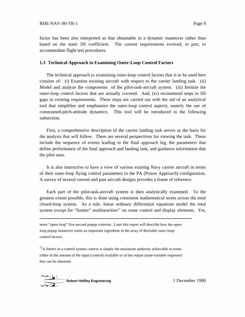
1.3 Technical Approach to Examining Outer-Loop Control Factors
The technical approach to examining outer-loop control factors that is to be used hereconsists of: (i) Examine existing aircraft with respect to the carrier landing task. (ii)Model and analyze the components of the pilot-task-aircraft system. (iii) Itemize theouter-loop control factors that are actually covered. And, (iv) recommend steps to fillgaps in existing requirements. These steps are carried out with the aid of an analyticaltool that simplifies and emphasizes the outer-loop control aspects, namely the use ofconstrained-pitch-attitude dynamics. This tool will be introduced in the followingsubsection.
First, a comprehensive description of the carrier landing task serves as the basis forthe analysis that will follow. There are several perspectives for viewing the task. Theseinclude the sequence of events leading to the final approach leg, the parameters thatdefine performance of the final approach and landing task, and guidance information thatthe pilot uses.
It is also instructive to have a view of various existing Navy carrier aircraft in termsof their outer-loop flying control parameters in the PA (Power Approach) configuration.A survey of several current and past aircraft designs provides a frame of reference.
Each part of the pilot-task-aircraft system is then analytically examined. To thegreatest extent possible, this is done using consistent mathematical terms across the totalclosed-loop system. As a rule, linear ordinary differential equations model the totalsystem except for “limiter” nonlinearities12 on some control and display elements. Yet,
more “open-loop” five-second popup criterion. Later this report will describe how the open-
loop popup maneuver omits an important ingredient in the array of desirable outer-loop
control factors.
12A limiter in a control system context is simply the maximum authority achievable in terms
either of the amount of the input (control) available or of the output (state-variable response)
that can be obtained.
RHE-NAV-90-TR-1 Page 10
Robert Heffley Engineering 1 December 1990
these nonlinearities do not invalidate the linear analysis technique.
Next the math model is analyzed to expose the primary features. The authordistinguishes between those features mainly related to the physical aircraft design andthose that describe the outer-loop state variable response. This is simply the difference inan engineer-centered point of view and a pilot-centered one.
Conclusions are summarized in terms of (i) outer-loop control factors and (ii) impli-cations for some supporting inner-loop characteristics. Recommendations forexperimental verification of the analysis results follow these conclusions.
Combined Pilot-Vehicle-Task System
As a first step to constructing an audit trail of outer-loop control factors, one mustconsider the combined PVT system. Several studies have analyzed the pilot-in-the-loop,References 32 through 37, for example. These studies have progressed from an emphasison inner-loop aspects to one on mainly the outer-loop. This report draws upon theseearlier approaches but tries to minimize the analytical complexity.
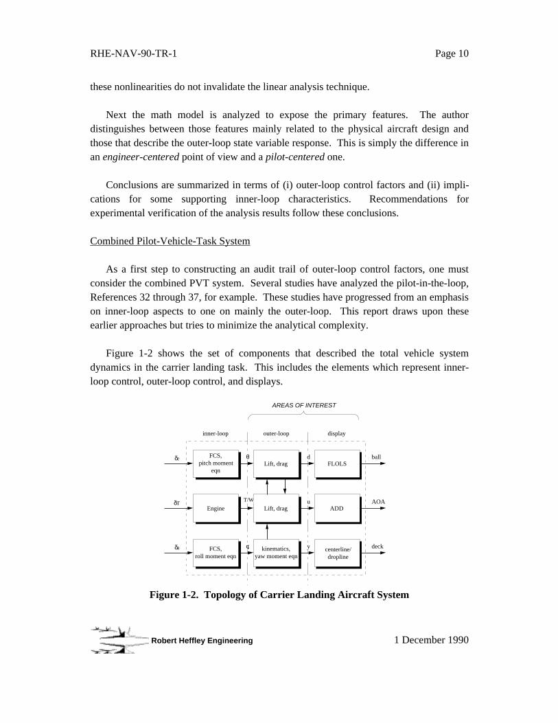
Figure 1-2 shows the set of components that described the total vehicle systemdynamics in the carrier landing task. This includes the elements which represent inner-loop control, outer-loop control, and displays.
inner-loop outer-loop display
δe ball
AOA
deck
δT
δa
θ
T/W
φ
d
u
y
FLOLS
ADD
centerline/dropline
FCS,pitch moment
eqn
Engine
FCS,roll moment eqn
Lift, drag
Lift, drag
kinematics,yaw moment eqn
AREAS OF INTEREST
Figure 1-2. Topology of Carrier Landing Aircraft System

RHE-NAV-90-TR-1 Page 11
Robert Heffley Engineering 1 December 1990
Some blocks in the above diagram will be described in explicit analytical terms in theshort introductory technical overview of the next subsection, namely the aircraft-relatedouter-loop components (aerodynamic lift and drag).
1.4 Introductory Technical Overview
The following is a brief overview of several fundamental ideas and physicalrelationships. It is an initial application of the technical approach that illustrates how thePVT system can be modeled with each component in consistent mathematical terms. Thepurpose is to present a simple statement of concepts that will be developed later in moredetail. A natural progression follows from (i) the task considerations, (ii) the impliedrelevant dynamic response features, and (iii) the contributing physical characteristics.
1.4.1 Implications of the CV Approach Task
The task of the pilot in a manual CV approach is to arrive at the deck at the desiredpoint, aircraft attitude, and speed. To do this, the pilot must follow a path prescribed bythe FLOLS glideslope at a speed indicated by the α display. The correct attitude is anatural result of good stabilization on flightpath and speed. The pilot performs the taskstarting at the roll-out onto final about 3/4 nm behind the ship (about 25 seconds beforetouchdown).
Figure 1-3. Range of Interest for CV Approach Task.
Therefore, this is a space- or time-bounded task with two primary controlledvariables. Flightpath error is proportional to the angular error indicated by one offive discrete Fresnel lens cells referenced to a row of datum lights. The pilot seesspeed error in terms of a head-up display of angle of attack relative to an on-speedreference.
3/4 nm25 sec

RHE-NAV-90-TR-1 Page 12
Robert Heffley Engineering 1 December 1990
1.4.2 Dominant Features of Aircraft Response
Equations of Motion
Given the above task considerations, the aircraft response can be viewed in simpleterms of two states and two controls. The relevant states are flightpath angle, ∆ γ, andangle of attack, ∆ α; and the controls are attitude, ∆ θ, and thrust-to-weight ratio, ∆ T/W.In order to avoid several complications involving range dependence and quantizationnonlinearities, ∆ γ and ∆ γ are selected in favor of the more explicit quantities of FLOLSmeatball error and indicated α error.
The math model used to describe the aircraft and FCS can typically vary greatly inform and degree of complexity.
The basic equations of motion consist of "trimmed" x-force and z-forces:
ax = ∆u·
= Σ X/m = Xu ∆ u + Xw ∆ w + g ∆ T/W (1)
az = - V ∆γ·
= Σ Z/m = Zu ∆ u + Zw ∆ w - ηg ∆ T/W (2)
and the auxiliary relationships:
∆ w/V = ∆ α = ∆ θ − ∆ γ (3)
or, combining these relationships in matrix form:
The determinant of the left side (characteristic) matrix, ∆ ,13 is:
∆ = (s - Zw) (s - Xu) - Xw Zu æ (s + 1 / Tθ1) (s + 1 / Tθ2)14 (5)
13The symbol ∆ is used both for the determinant of the characteristic equation (thedenominator of any transfer function) as well as to denote an incremental state variable orcontrol variable such as ∆ α or ∆ θ. The distinction should be self explanatory in all cases.
14The factors appearing here follow the conventions described in Reference 38 and usedwidely by the aircraft flying qualities community.
(s - Zw) Zu
Xw (s - Xu)
V ⋅ ∆∆u
= -Z g
X - g g
∆∆T/W
(4)

RHE-NAV-90-TR-1 Page 13
Robert Heffley Engineering 1 December 1990
Key numerators are similarly obtained and consist of:γ
Nθ = -Zw [s - Xu + Zu(Xα- g) / Zα] = g/V · nzα (s + 1 /Th1) (6)
γN
T/W = g/V (-Zu - Xu η + η s ) = 2 (g/V)2 · (1 + Thθ s) (7)
αNθ
= ∆ - γ
Nθ = s2 - Xu s - Zu g/V (8)
αNT/W
= - γ
NT/W
(9)
where ∆γ/∆θ(s) = γ
Nθ (s) /∆ (s) , or ∆α/∆T/W(s) = α
NT/W (s) /∆ (s) , etc.;
for example,
-Zw (s + 1/Th1)
(s + 1/Tθ1) (s + 1/Tθ2)
γ(s)
θ(s)=
(s + 1/Th1)
(s + 1/Tθ1) (Tθ2 s + 1)≈
≈ 0
washout lag
(10)
Reference 38 contains a comprehensive general treatment of the equations of motionand transfer functions for aircraft and flight control systems. However, the reader of thisreport will find that the above equations are uncomplicated and suffice for the purposesof the analysis performed here.
Response Shapes
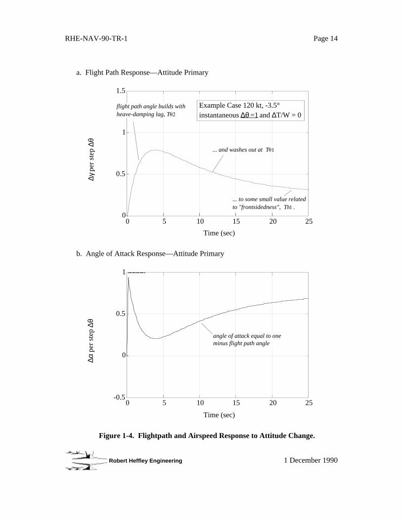
The following plots show two sets of flightpath and α responses, one set for a pitch-attitude step and the second for a thrust step.
Consider first the response of flightpath angle and angle of attack to an instantaneousstep pitch attitude change. Figure 1-4 shows that ∆ γ follows ∆ θ with a short-term lag,Tθ2, then washes out with a slower time constant, Tθ1. The short-term amplitude
approaches unity and the long-term amplitude is nearly zero, but depends upon thenumerator factor 1/Th1.
The angle of attack response is simply the mirror image of flightpath angle since ∆α = ∆ θ − ∆ γ. Angle of attack responds first with attitude, decays with Tθ2 and finallyincreases again more slowly with Tθ1.
RHE-NAV-90-TR-1 Page 14
Robert Heffley Engineering 1 December 1990
a. Flight Path Response—Attitude Primary
0.5
1
1.5
0 5 10 15 20 25
Time (sec)
∆γ p
er s
tep
∆θ
0
flight path angle builds with heave-damping lag, T
... and washes out at T
Example Case 120 kt, -3.5°instantaneous ∆θ =1 and ∆T/W = 0
... to some small value related to "frontsidedness", Th .
b. Angle of Attack Response—Attitude Primary
-0.5
0
0.5
1
0 5 10 15 20 25
Time (sec)
∆α p
er s
tep
∆θ
angle of attack equal to one minus flight path angle
Figure 1-4. Flightpath and Airspeed Response to Attitude Change.

RHE-NAV-90-TR-1 Page 15
Robert Heffley Engineering 1 December 1990
Next consider the use of thrust (normalized with aircraft weight), ∆ T/W, and note thevery different response shapes. Flightpath slowly increases without washout while αcorrespondingly decreases.
a. Flightpath Response—Thrust Primary
0.5
1.5
0 5 10 15 20 25
Time (sec)
∆γ p
er s
tep
∆T/W
0
1flight path angle builds with speed-damping lag, T
Example Case 120 kt, -3.5°instantaneous ∆θ = 0 and ∆T/W = 1
b. Angle of Attack Response—Thrust Primary
-0.5
0.5
1
0 5 10 15 20 25
Time (sec)
∆α p
er s
tep
∆T/W
0 angle of attack equal to negative of flight path angle
Figure 1-5. Flightpath and Airspeed Response Due to Thrust Change.
RHE-NAV-90-TR-1 Page 16
Robert Heffley Engineering 1 December 1990
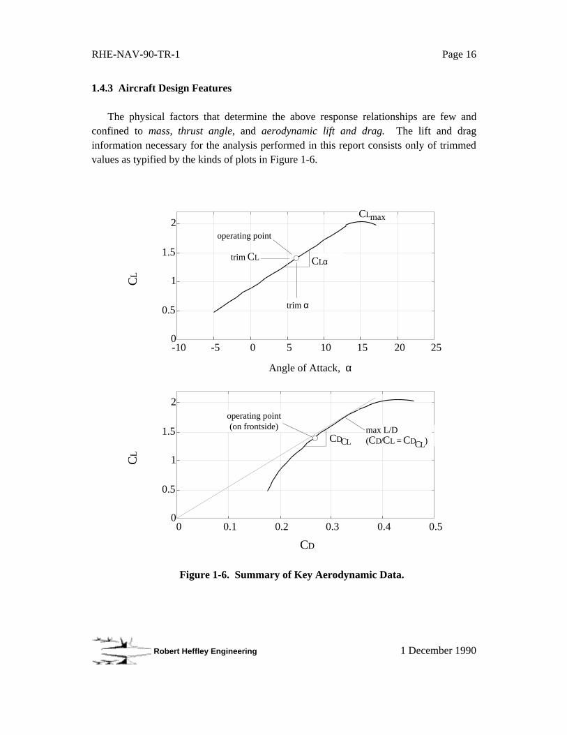
1.4.3 Aircraft Design Features
The physical factors that determine the above response relationships are few andconfined to mass, thrust angle, and aerodynamic lift and drag. The lift and draginformation necessary for the analysis performed in this report consists only of trimmedvalues as typified by the kinds of plots in Figure 1-6.
0
0.5
1
1.5
2
-10 -5 0 5 10 15 20 25
Angle of Attack, α
CL
0
0.5
1
1.5
2
0 0.1 0.2 0.3 0.4 0.5
CD
CL
CLα
CDCL
max L/D(CD/CL = CD )
operating point
operating point(on frontside)
trim α
trim CL
CL
CLmax
Figure 1-6. Summary of Key Aerodynamic Data.
RHE-NAV-90-TR-1 Page 17
Robert Heffley Engineering 1 December 1990
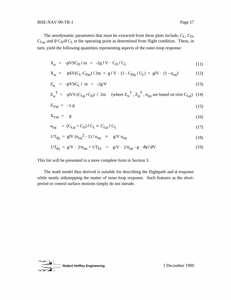
The aerodynamic parameters that must be extracted from these plots include, CL, CD,CLα, and ∂ CD/∂ CL at the operating point as determined from flight condition. These, in
turn, yield the following quantities representing aspects of the outer-loop response:
Xu = -ρVSCD / m = -2g / V · CD / CL (11)
Xw = ρSV(CL-CDα) / 2m = g / V · (1 - CDα / CL) = g/V · (1 - nxα) (12)
Zu = -ρVSCL / m = -2g/V (13)
Zw† = -ρVS (CLα+CD) / 2m (where Zw
† , Zα† , nzα are based on trim CLα) (14)
ZTW = - η g (15)
XTW = g (16)
nzα = (CLα + CD) / CL ≈ CLα / CL (17)
1/Tθ2 = g/V (nzα2 - 1) / nzα ≈ g/V nzα (18)
1/Tθ1 = g/V · 2/nzα + 1/Th1 = g/V · 2/nzα - g · ∂γ / ∂V (19)
This list will be presented in a more complete form in Section 3.
The math model thus derived is suitable for describing the flightpath and α responsewhile neatly sidestepping the matter of inner-loop response. Such features as the short-period or control surface motions simply do not intrude.

RHE-NAV-90-TR-1 Page 18
Robert Heffley Engineering 1 December 1990
THIS PAGE IS INTENTIONALLY BLANK

RHE-NAV-90-TR-1 Page 19
Robert Heffley Engineering 1 December 1990
2. THE CARRIER LANDING TASK AND EXISTING AIRCRAFT
The following is a description of both the carrier landing task and various aircraftdesigned to perform it. The math models and analyses in subsequent sections make useof this information. Thus the main purpose of this section is to provide backgroundinformation and a suitable context for the construction and use of mathematical models.
2.1 Carrier Landing Task Description
Navy pilots view the carrier landing as the most demanding of manual flight tasks formilitary aircraft. It must be performed under a wide range of visibility, weather, and sea-state conditions. Further, the pilot may be under substantial stress following combat orflight over an extended duration. If the carrier landing is part of a training mission, thepilot is likely to have only limited skill and experience.
There are several variations of the carrier landing task, including daytime VFR,nighttime VFR, and IFR. Pilots consider the nighttime carrier landing the mostdemanding. For its purposes, this study addresses the daytime VFR landing. Thisinvolves use of a racetrack pattern beginning with an upwind leg flown over the ship andending with the final approach leg and arrestment. Further, this study focuses on the finalapproach leg. Important features are that the turn-to-final and touchdown spatially boundthe task and the pilot is limited to visual guidance information from the deck.
Several sources serve as the basis for the task description, including interviews withNavy carrier pilots, LSO literature, carrier-qualification training manuals, and severalrelated carrier landing systems descriptions (References 39 through 46).15
2.1.1 General
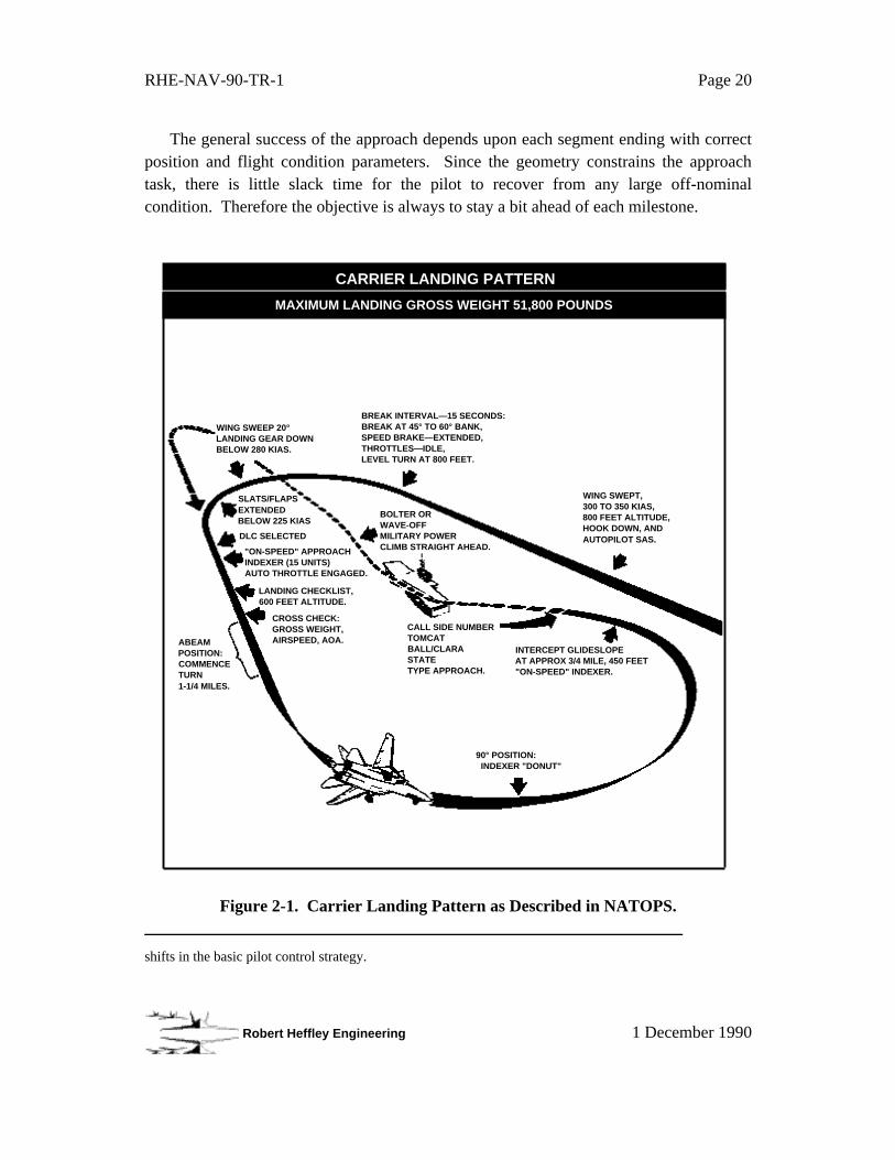
Four main segments comprise the VFR carrier landing pattern as Figure 2-1 shows(Reference 39). These segments consist of (i) the downwind leg overhead the carrier, (ii)the “break” maneuver and downwind leg, (iii) the turn to final, and (iv) the final approachleg. Each segment involves its own set of guidance information, pilot control technique,and aircraft flight condition and configuration.16
15The main source of information was a series of interviews with several active F-14 pilots at NAS
Miramar during 1982 and 1983.16This breakdown was made in Reference 29 on the basis of distinguishing where there were significant
RHE-NAV-90-TR-1 Page 20
Robert Heffley Engineering 1 December 1990
The general success of the approach depends upon each segment ending with correctposition and flight condition parameters. Since the geometry constrains the approachtask, there is little slack time for the pilot to recover from any large off-nominalcondition. Therefore the objective is always to stay a bit ahead of each milestone.
BREAK INTERVAL—15 SECONDS:BREAK AT 45° TO 60° BANK,SPEED BRAKE—EXTENDED,THROTTLES—IDLE,LEVEL TURN AT 800 FEET.
WING SWEPT,300 TO 350 KIAS,800 FEET ALTITUDE,HOOK DOWN, ANDAUTOPILOT SAS.
INTERCEPT GLIDESLOPEAT APPROX 3/4 MILE, 450 FEET"ON-SPEED" INDEXER.
CALL SIDE NUMBERTOMCATBALL/CLARASTATETYPE APPROACH.
WING SWEEP 20°LANDING GEAR DOWNBELOW 280 KIAS.
90° POSITION: INDEXER "DONUT"
ABEAMPOSITION:COMMENCETURN1-1/4 MILES.
SLATS/FLAPSEXTENDEDBELOW 225 KIAS
CROSS CHECK:GROSS WEIGHT,AIRSPEED, AOA.
LANDING CHECKLIST,600 FEET ALTITUDE.
DLC SELECTED
"ON-SPEED" APPROACHINDEXER (15 UNITS)AUTO THROTTLE ENGAGED.
BOLTER ORWAVE-OFFMILITARY POWERCLIMB STRAIGHT AHEAD.
CARRIER LANDING PATTERN
MAXIMUM LANDING GROSS WEIGHT 51,800 POUNDS
Figure 2-1. Carrier Landing Pattern as Described in NATOPS.
shifts in the basic pilot control strategy.
RHE-NAV-90-TR-1 Page 21
Robert Heffley Engineering 1 December 1990
Initial Leg
The pilot flies the initial leg to arrive overhead the carrier on a standard course,heading, and altitude in preparation for executing the racetrack pattern. This leg beginsnominally three miles astern the ship at 1200 ft and ends over or slightly beyond the bow.For the lead aircraft the main task during the initial leg are to arrive over the bow, on theBase Recover Course (BRC), and at 800 ft altitude. Maintaining formation is the maintask of aircraft flying formation on the lead aircraft. The lead aircraft sets the airspeed at300 to 400 kt.
The pilot control strategy involves compensatory management of course and altitudeusing pitch and roll attitude, supported by vertical velocity and heading, respectively.With thrust set at a nominal fuel flow, the pilot does not regulate airspeed tightly.
Aircraft dynamics during the initial leg are benign and typically “frontside.” Thehigh speed ensures small effective lags in pitch, roll, and flight path. The resultingmental effort required is therefore low. However, the large excess control capacity canbe absorbed by decisional tasks connected with deck spotting and planning for aminimum-interval approach.
Break Maneuver and Downwind Leg
The break starts the 360° racetrack course and includes crucial deceleration andreconfiguration events. The segment ends with the pilot flying the downwind leg at aconstant course and altitude. The objective of the break is to arrive at the turn-to-final(the next segment) in the landing configuration (PA) and trimmed for level flight at theapproach α.
Initially the pilot flies the break segment as a largely precognitive, high-g, level-turnmaneuver intended to reduce airspeed rapidly. The angle of bank during the break can bebetween 45° and 70° , depending upon the initial airspeed and the pilot's judgment of theresulting turn radius. No visual position cues relative to the ship are available until wellaround the 180° turn. At this point a minor heading change can be used to adjust thelateral distance from the ship.
The aircraft reconfiguration sequence effectively manages airspeed. The pilotdeploys the speedbrake upon initiating the break. For the F-14, the pilot may leave thewings unswept, but only to realize the induced-drag benefit. As quickly as airframe

RHE-NAV-90-TR-1 Page 22
Robert Heffley Engineering 1 December 1990
limits permit, the pilot lowers the landing gear and extends the flaps.
The interval is about 30 sec from initiation of the break until the roll-out to wings-level on the downwind leg. The pilot then has another 15 to 20 sec to reach a well-stabilized flight condition and complete required check list procedures.
Turn-to-Final
The turn-to-final begins when the pilot is abeam the LSO platform at an altitude of600 ft. Precisely at that point the pilot commands a constant-attitude bank angle tointercept the final approach leg down the deck centerline. For the F-14 a 27° bank isused.
The pilot targets an altitude of 450 ft at the 90° point in the turn, thus applying aloose regulation of vertical flightpath. Lateral path control during the turn is largelyopen-loop until the pilot begins to get lineup cues from the deck centerline.
At 45° from the BRC the Fresnel lens system begins to be visible thus permittingsome vertical flightpath regulation. At nearly the same time, lateral path informationbased on deck geometry may induce some adjustment of bank angle.
Because pilot trims to the approach condition during the turn, flying qualities aretypically “low-speed” with heave damping low, speed damping high, and adverse yaw apossible factor. For an aircraft such as the F-14, loss of lift due to lateral spoiler use canbe a problem. Therefore the pilot may use lateral control sparingly to avoid upsettingsink rate.
As in the previous leg, geometry spatially bounds the turn-to-final task. The totalperiod of the segment is about 30 sec at which point the pilot must begin intensiveclosed-loop control of glideslope, lineup, and angle-of-attack. If the turn-to-final endson-speed and with correct height and lineup position, it minimizes the difficulty of thefinal leg.
Final Approach Leg
The final approach leg begins as the pilot rolls out on the deck centerline and beginsprecise tracking of the vertical flightpath. The position of the FLOLS “meatball” relativeto the lighted datum bar gives vertical guidance information. The FLOLS assembly is
RHE-NAV-90-TR-1 Page 23
Robert Heffley Engineering 1 December 1990
positioned on the left edge of the deck about 500 ft ahead of the ramp. The pilot getsprecise lateral path information using the deck centerline angle relative either to thehorizon or to the vertical dropline at the stern. The latter is available even if the actualhorizon is obscured or if operating at night.17
This is the most crucial approach segment because it ends on the deck. Successfulrecovery depends upon the hook passing high enough to clear the ramp and low enoughto engage the furthest cross-deck pendant (#4 wire). However, the Landing SignalOfficer (LSO) will insist on much tighter bounds.
From the time of roll-out to wings-level, the pilot has about 25 sec before reachingthe deck. This period permits a limited number of corrections in Glideslope (GS), Lineup(LU), and angle-of-attack (AOA) such that all will be within acceptable bounds at thedeck. In addition, the pilot must null all velocity and attitude states the end. Thus thefinal approach leg is a classical terminal control problem and is distinct from acontinuous tracking control problem. Nevertheless, it is possible to employ somecontinuous-tracking analysis tools if the analyst adequately recognizes the role of theterminal constraints.
The pilot's success in managing the outer-loop states (GS, LU, and AOA) dependsupon each having a suitably short time-to-achieve. In general this can be lumped intosome effective first-order lag time constant. The respective control power is each case isimplicit in the effective lag time.
The pilot's strategy for controlling outer-loop states becomes crucial to the finalapproach in that aggressive closed-loop activity is required (in contrast to the more open-loop nature in the other segments). The combination of long response lags and limitedtime-available requires that the pilot try to optimize use of controls.
The LSO has a major role in helping the pilot to maintain the final approach legparameters should they begin to exceed prescribed LSO standards. The LSO has directvoice contact with the pilot and communicates using a standard vocabulary of about 50phrases having several degrees of urgency. The calls are classified as “informative,”“precautionary,” and “imperative.” Besides voice calls, the LSO ultimately cancommand a waveoff through light signals presented on the FLOLS assembly.
17Final approach guidance information is described in detail in Section 3.
RHE-NAV-90-TR-1 Page 24
Robert Heffley Engineering 1 December 1990
2.1.2 Details of Task Performance
Performance nomenclature and standards used by the LSO community are useful inquantifying the performance of the carrier approach task. While defined in terms of theLSO's viewing position, they also have a strong correspondence to the pilot's view of thetask. Also importantly, the LSO performance standards can be translated intoengineering terms.
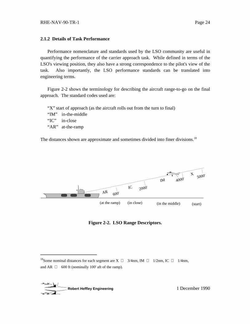
Figure 2-2 shows the terminology for describing the aircraft range-to-go on the finalapproach. The standard codes used are:
“X” start of approach (as the aircraft rolls out from the turn to final)“IM” in-the-middle“IC” in-close“AR” at-the-ramp
The distances shown are approximate and sometimes divided into finer divisions.18
Figure 2-2. LSO Range Descriptors.
18Some nominal distances for each segment are X ⇒ 3/4nm, IM ⇒ 1/2nm, IC ⇒ 1/4nm,
and AR ⇒ 600 ft (nominally 100' aft of the ramp).
600'2000'
4000' 5000'
ARIC
IM
X
(at the ramp) (in close) (in the middle) (start)
RHE-NAV-90-TR-1 Page 25
Robert Heffley Engineering 1 December 1990
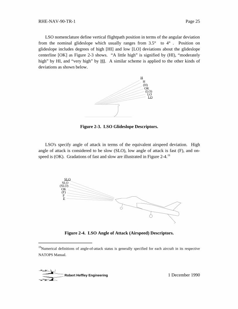
LSO nomenclature define vertical flightpath position in terms of the angular deviationfrom the nominal glideslope which usually ranges from 3.5° to 4° . Position onglideslope includes degrees of high [HI] and low [LO] deviations about the glideslopecenterline [OK] as Figure 2-3 shows. “A little high” is signified by (HI), “moderatelyhigh” by HI, and “very high” by HI. A similar scheme is applied to the other kinds ofdeviations as shown below.
HH(H)OK(LO)
LOLO
Figure 2-3. LSO Glideslope Descriptors.
LSO's specify angle of attack in terms of the equivalent airspeed deviation. Highangle of attack is considered to be slow (SLO), low angle of attack is fast (F), and on-speed is (OK). Gradations of fast and slow are illustrated in Figure 2-4.19
SLOSLO
(SLO)OK(F)FF
Figure 2-4. LSO Angle of Attack (Airspeed) Descriptors.
19Numerical definitions of angle-of-attack status is generally specified for each aircraft in its respective
NATOPS Manual.
RHE-NAV-90-TR-1 Page 26
Robert Heffley Engineering 1 December 1990
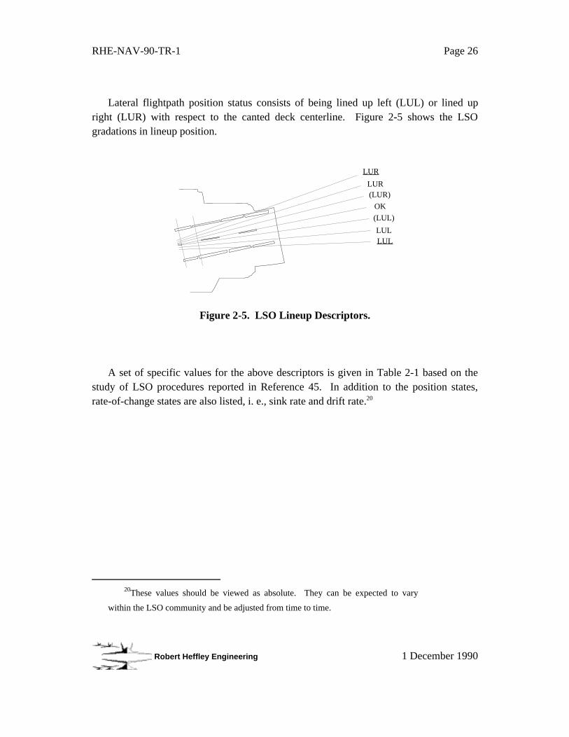
Lateral flightpath position status consists of being lined up left (LUL) or lined upright (LUR) with respect to the canted deck centerline. Figure 2-5 shows the LSOgradations in lineup position.
OK
LUL
LUR
LUL
(LUL)
LUR(LUR)
Figure 2-5. LSO Lineup Descriptors.
A set of specific values for the above descriptors is given in Table 2-1 based on thestudy of LSO procedures reported in Reference 45. In addition to the position states,rate-of-change states are also listed, i. e., sink rate and drift rate.20
20These values should be viewed as absolute. They can be expected to vary
within the LSO community and be adjusted from time to time.

RHE-NAV-90-TR-1 Page 27
Robert Heffley Engineering 1 December 1990
Table 2-1. LSO-Based Performance Parameters
Primary States (position, speed)
Range: verbal description symbol value at the ramp AR 100-600 ft from touchdown in close IC 600-2000 ft from touchdown in the middle IM 2000-4000 ft from touchdown at the start X 4000-5000 ft (~3/4 nm —beginning final leg)
Glideslope position: verbal description symbol value meaning very high H 1.3° well above FLOLS beam (~4 balls high) high H 0.8° at upper visible limit of FLOLS beam a little high (H) 0.3° in center of "one-ball-high" FLOLS indication OK OK 0 in center of "on-glideslope" FLOLS indication a little low (LO) -0.3° in center of "one-ball-low" FLOLS indication low LO -0.8° at lower visible limit of FLOLS beam very low LO -1.6° well below FLOLS beam (~5 balls low)
Angle of Attack (Speed): verbal description symbol value meaning very slow SLO +3 units nose-down chevron (green) slow SLO +2 units nose-down chevron (green) a little slow (SLO) +1 units donut + nose-down chevron (green) OK OK 0 donut, on-speed AOA a little fast (F) -1 unit donut + nose-up chevron (red) fast F -2 units nose-up chevron (red) very fast F -3 units nose-up chevron (red)
Lineup Position: verbal description symbol value meaning lined up very far rt LUR 3.5° right of deck centerline lined up right LUR 2.5° right of deck centerline lined up a little right (LUR) 1.5° right of deck centerline OK OK 0 on deck centerline lined up a little left (LUL) 1.5° left of deck centerline lined up left LUL 2.5° left of deck centerline lined up very far left LUL 3.5° left of deck centerline
Secondary States (rate of change of position)
Sink Rate: verbal description symbol value meaning not enough R/D NERD! 0.8 °/sec approx level flight @ 1000' range not enough R/D NERD 0.4 °/sec approx level flight @ 2000' range not enough R/D NERD 0.2 °/sec approx level flight @ 4000' range not enough R/D (NERD) 0.1 °/sec OK OK 0 descending on GS too much R/D (TMRD) -.1 °/sec too much R/D TMRD -.2 °/sec too much R/D TMRD -.4 °/sec
Drift Rate: verbal description symbol value meaning very fast right drift DR 1.0 °/sec ~10° heading error at 1/4 nm right drift DR 0.5 °/sec ~5° heading error at 1/4 nm a little right drift (DR) 0.2 °/sec ~2° heading error at 1/4 nm OK OK 0 a little left drift (DL) left drift DL very fast right drift DL

RHE-NAV-90-TR-1 Page 28
Robert Heffley Engineering 1 December 1990
Figure 2-6 shows a scale view of the glideslope and lineup ranges in terms of angulardeviations from the nominal flightpath. This is intended to present a frame of referencefor the magnitude of flightpath excursions (horizontal- and vertical-planes) as well as theprecision expected. Note the relative range of FLOLS information presented to the pilotas indicated by the scale at the left.
H
H
(H)
(L)
L
L
surface
OKLUL LURLUL LUR(LUR)(LUL)
Deck Centerline
FLOLS Centerline
+1.3°
+.8°
+.3°
-.3°-.8°
-1.6°
3.5°2.5° 1.5°
-4°
FLOLScells
Figure 2-6. Scale Drawing of Approach Flightpath Parameters.

RHE-NAV-90-TR-1 Page 29
Robert Heffley Engineering 1 December 1990
A corresponding planview of the approach geometry is given in Figure 2-7. Thisshows that the FLOLS becomes visible well before roll-out onto final, but the roll angleof the FLOLS light plane precludes valid glideslope information until on the centerline(which shall be explained shortly.)
Lin
ed U
p R
ight
"L
UR
"
Lin
ed U
p L
eft
"LU
L"
Start "X"
FLO
LS
fiel
d-of
-vie
w li
mit
FLO
LS
fiel
d-of
-vie
w li
mit
In the Middle "IM"
In Close "IC"
At the Ramp "AR"
ship
wak
e
600' (from #3 wire)
2000'
4000'
5000'
Figure 2-7. Planview of Final Approach Leg.
RHE-NAV-90-TR-1 Page 30
Robert Heffley Engineering 1 December 1990
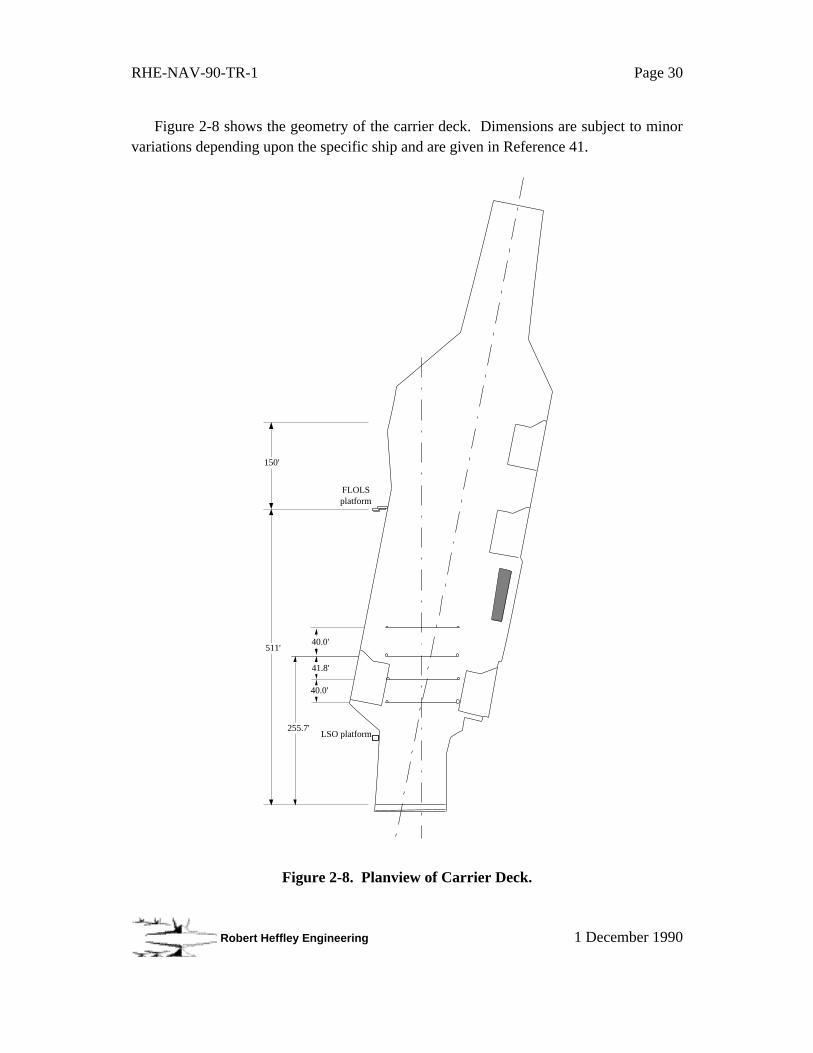
Figure 2-8 shows the geometry of the carrier deck. Dimensions are subject to minorvariations depending upon the specific ship and are given in Reference 41.
150'
511'
255.7'
40.0'
41.8'
40.0'
LSO platform
FLOLS platform
Figure 2-8. Planview of Carrier Deck.
RHE-NAV-90-TR-1 Page 31
Robert Heffley Engineering 1 December 1990
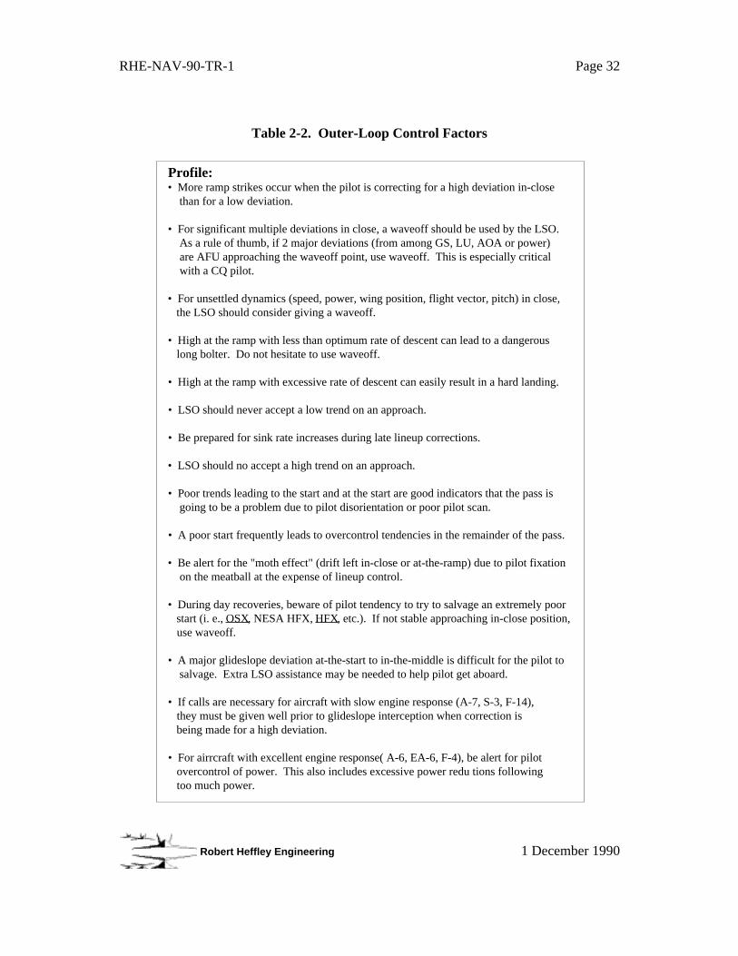
2.1.3 LSO View of Outer-Loop Control
Table 2-2 presents a list of outer-loop control factors from the LSO's vantage point(Reference 45). These are useful in evaluating aspects of the task and of the aircraftwhich may be crucial to success. A number of these items are concerned with where onthe final approach corrections can be made, especially when engine response is a factor.
According to this table, LSO's exercise may more caution with corrections from ahigh glideslope deviation than from low. Also, the aircraft should be stabilized on theapproach by the "in-close" position (about 1/4 nm range).
RHE-NAV-90-TR-1 Page 32
Robert Heffley Engineering 1 December 1990
Table 2-2. Outer-Loop Control Factors
Profile:• More ramp strikes occur when the pilot is correcting for a high deviation in-close than for a low deviation.
• For significant multiple deviations in close, a waveoff should be used by the LSO. As a rule of thumb, if 2 major deviations (from among GS, LU, AOA or power) are AFU approaching the waveoff point, use waveoff. This is especially critical with a CQ pilot.
• For unsettled dynamics (speed, power, wing position, flight vector, pitch) in close, the LSO should consider giving a waveoff.
• High at the ramp with less than optimum rate of descent can lead to a dangerous long bolter. Do not hesitate to use waveoff.
• High at the ramp with excessive rate of descent can easily result in a hard landing.
• LSO should never accept a low trend on an approach.
• Be prepared for sink rate increases during late lineup corrections.
• LSO should no accept a high trend on an approach.
• Poor trends leading to the start and at the start are good indicators that the pass is going to be a problem due to pilot disorientation or poor pilot scan.
• A poor start frequently leads to overcontrol tendencies in the remainder of the pass.
• Be alert for the "moth effect" (drift left in-close or at-the-ramp) due to pilot fixation on the meatball at the expense of lineup control.
• During day recoveries, beware of pilot tendency to try to salvage an extremely poor start (i. e., OSX, NESA HFX, HFX, etc.). If not stable approaching in-close position, use waveoff.
• A major glideslope deviation at-the-start to in-the-middle is difficult for the pilot to salvage. Extra LSO assistance may be needed to help pilot get aboard.
• If calls are necessary for aircraft with slow engine response (A-7, S-3, F-14), they must be given well prior to glideslope interception when correction is being made for a high deviation.
• For airrcraft with excellent engine response( A-6, EA-6, F-4), be alert for pilot overcontrol of power. This also includes excessive power redu tions following too much power.

RHE-NAV-90-TR-1 Page 33
Robert Heffley Engineering 1 December 1990
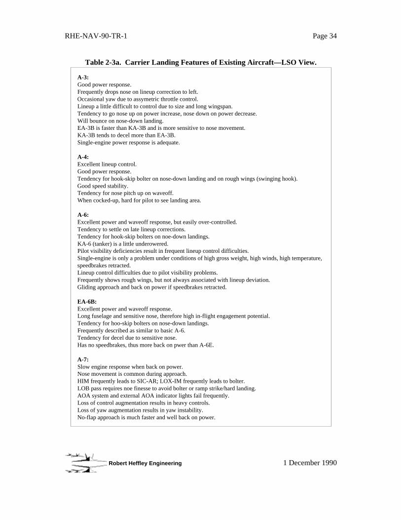
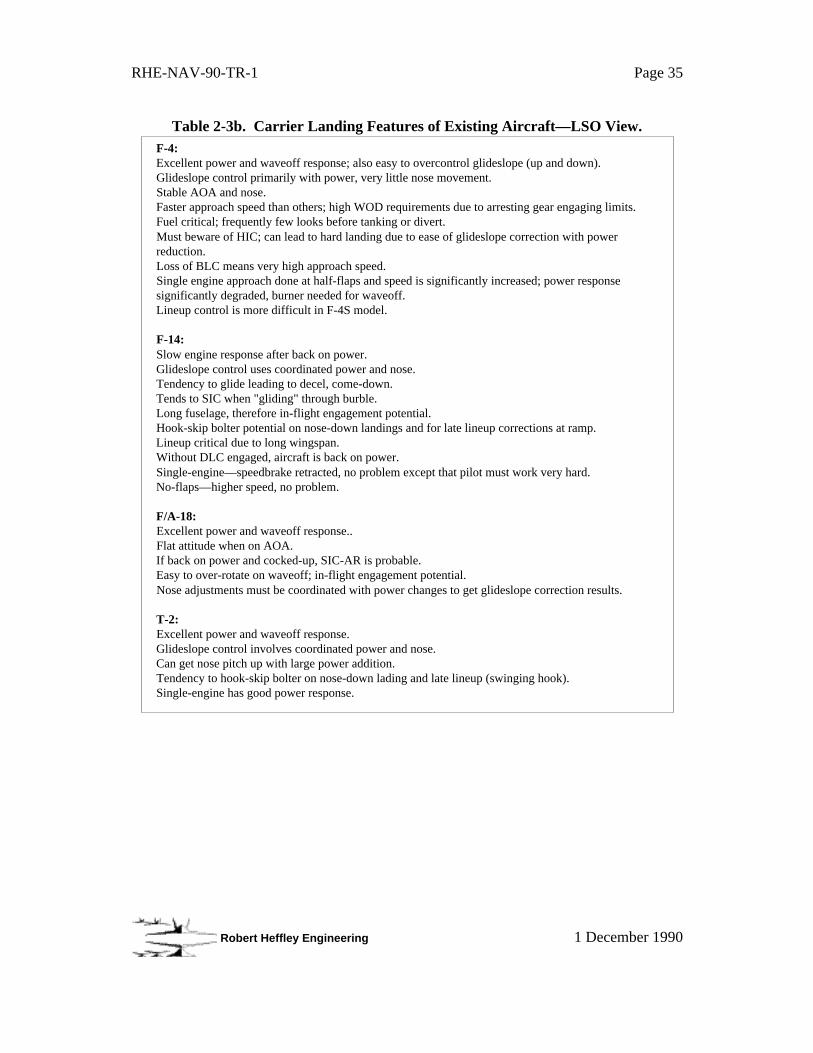
2.2 Aircraft Characteristics
A variety of fixed-wing aircraft types operate from carrier decks, including fighters,attack aircraft, trainers, anti-submarine aircraft, and transports. The purpose of thissection is to describe the characteristics of a number of existing carrier aircraft in order toprovide a feel for the values which may be of use in subsequent analysis.
Most of the aircraft which are represented in this section have successfully andsatisfactorily operated from carriers. One feature of this study is to examine andunderstand the characteristics of these existing aircraft. First, some characteristics fromthe LSO's view are listed. Next, an array of computed characteristics are given whichpermit a comparison of aerodynamic, trim, and response parameters. Finally, someexamples of engine response data are presented.
2.2.1 LSO View of Aircraft Characteristics
The Landing Signal Officer (LSO) is particularly sensitive to the outer-loop controlaspects of carrier aircraft. Glideslope, angle of attack, and lineup are the primaryconcerns of the LSO during the final 3/4 nm approach to the ship.
Table 2-3 gives a brief sketch of carrier landing characteristics of several Navyairplanes based on the Reference 45 study of the LSO's duties. While the itemsmentioned are qualitative, they portray an overview of the various control axes forspecific aircraft types.
RHE-NAV-90-TR-1 Page 34
Robert Heffley Engineering 1 December 1990
Table 2-3a. Carrier Landing Features of Existing Aircraft—LSO View.
A-3: Good power response.Frequently drops nose on lineup correction to left.Occasional yaw due to assymetric throttle control.Lineup a little difficult to control due to size and long wingspan.Tendency to go nose up on power increase, nose down on power decrease.Will bounce on nose-down landing.EA-3B is faster than KA-3B and is more sensitive to nose movement.KA-3B tends to decel more than EA-3B.Single-engine power response is adequate.
A-4: Excellent lineup control.Good power response.Tendency for hook-skip bolter on nose-down landing and on rough wings (swinging hook).Good speed stability.Tendency for nose pitch up on waveoff.When cocked-up, hard for pilot to see landing area.
A-6: Excellent power and waveoff response, but easily over-controlled.Tendency to settle on late lineup corrections.Tendency for hook-skip bolters on noe-down landings.KA-6 (tanker) is a little underowered.Pilot visibility deficiencies result in frequent lineup control difficulties.Single-engine is only a problem under conditions of high gross weight, high winds, high temperature, speedbrakes retracted.Lineup control difficulties due to pilot visibility problems.Frequently shows rough wings, but not always associated with lineup deviation.Gliding approach and back on power if speedbrakes retracted.
EA-6B: Excellent power and waveoff response.Long fuselage and sensitive nose, therefore high in-flight engagement potential.Tendency for hoo-skip bolters on nose-down landings.Frequently described as similar to basic A-6.Tendency for decel due to sensitive nose.Has no speedbrakes, thus more back on pwer than A-6E.
A-7: Slow engine response when back on power.Nose movement is common during approach.HIM frequently leads to SIC-AR; LOX-IM frequently leads to bolter.LOB pass requires noe finesse to avoid bolter or ramp strike/hard landing.AOA system and external AOA indicator lights fail frequently.Loss of control augmentation results in heavy controls.Loss of yaw augmentation results in yaw instability.No-flap approach is much faster and well back on power.
RHE-NAV-90-TR-1 Page 35
Robert Heffley Engineering 1 December 1990
Table 2-3b. Carrier Landing Features of Existing Aircraft—LSO View.F-4: Excellent power and waveoff response; also easy to overcontrol glideslope (up and down).Glideslope control primarily with power, very little nose movement.Stable AOA and nose.Faster approach speed than others; high WOD requirements due to arresting gear engaging limits.Fuel critical; frequently few looks before tanking or divert.Must beware of HIC; can lead to hard landing due to ease of glideslope correction with power reduction.Loss of BLC means very high approach speed.Single engine approach done at half-flaps and speed is significantly increased; power response significantly degraded, burner needed for waveoff.Lineup control is more difficult in F-4S model.
F-14: Slow engine response after back on power.Glideslope control uses coordinated power and nose.Tendency to glide leading to decel, come-down.Tends to SIC when "gliding" through burble.Long fuselage, therefore in-flight engagement potential.Hook-skip bolter potential on nose-down landings and for late lineup corrections at ramp.Lineup critical due to long wingspan.Without DLC engaged, aircraft is back on power.Single-engine—speedbrake retracted, no problem except that pilot must work very hard.No-flaps—higher speed, no problem.
F/A-18: Excellent power and waveoff response..Flat attitude when on AOA.If back on power and cocked-up, SIC-AR is probable.Easy to over-rotate on waveoff; in-flight engagement potential.Nose adjustments must be coordinated with power changes to get glideslope correction results.
T-2: Excellent power and waveoff response.Glideslope control involves coordinated power and nose.Can get nose pitch up with large power addition.Tendency to hook-skip bolter on nose-down lading and late lineup (swinging hook).Single-engine has good power response.

RHE-NAV-90-TR-1 Page 36
Robert Heffley Engineering 1 December 1990
Table 2-3c. Carrier Landing Features of Existing Aircraft—LSO View.
S-3: Slow engine response when back on power.Tendency to "glide" during approach.DLC is good for correcting high deviation and avoiding an undesired power reduction.Without DLC system, nose pitch is sensitive to power changes.Difficulties with burble under high WOD conditions.Burble causes glideslope control difficulties.Lineup control difficult, especially with shifting wind conditions.Nose pitch is sensitive to power changes, especially with DLC failure.No flap—very fast and well back on power.Single-engine—half-flaps, lineup control difficulties due to asymmetric thrust.
C-1: Nearly instantaneous power response.On the "cut" signal takes "high-dip" to land.Single-engine is faster, no flare on touchdown; no problem.
C-2: Like E-2, except thant when very light there is tendency to float during approach.
E-2: Excellent power and waveoff response.Excessive power reduction can "flatten" prop enough to cause a rapid settle.Lineup control difficult; also very critical due to long wing span.Long fuselage, therefore high in-flight engagement potential.Glideslope control very sensitive to nose movement.Fuselage alignment lights (when visible) and "popping sound" indicate need for right rudder.Tendency for hook-skip bolter on nose-down landing.On single engine approach, lineup control is difficult; also decel must be avoided.Lineup is extremely critical (±2.5 ft) on barricade recovery.On no-flap approach, very cocked-up and hook-to-ramp clearance is reduced.
RHE-NAV-90-TR-1 Page 37
Robert Heffley Engineering 1 December 1990
2.2.2 Characteristics of Existing Aircraft
This section provides a concise summary of characteristics for several existingaircraft which are central to outer-loop control. These characteristics correspond to thosewhich will be discussed in Section 3 and will be used for the analyses in Section 4.
The following figures employ a standard format to portray a range of aerodynamic,trim, and response parameters. This permits one to make direct comparisons easily.
The configuration of each aircraft consists of a single gross weight, usually themaximum carrier landing weight, a representative center of gravity, gear down, and flapsset for power approach. The flightpath angle is -3.5° in each case. Parameter variationsare shown for a range of speeds along with an indication of the nominal approach speed.
Aerodynamic data consist of the trimmed lift and drag coefficients for theconfiguration noted. These data are the basis for computing the trim thrust, pitch attitude,and angle of attack. Where information was available, the indicated angle of attack(AOA) is also shown. Finally, response-parameter plots show the transfer functionfactors 1/ Tθ1, 1/ Tθ2, 1/ Th1, and 1/Thθ. As Section 3 explains, these factors are fun-
damental to the response of flightpath and angle of attack.
Figures 2-9 to 2-18 present plotted data for the following aircraft:
• F-4J (equipped with BLC)• F-8C• F-8J (equipped with BLC)• F-14D (20° sweep)• F/A-18A• F-111B (16° sweep)• A-3B (standard-wing version)• RA-5C• A-6E• T-45A (based on initial aerodynamic data package)
These plots are based on manufacturers' data where available (References 47 through50 ). References 12 and 51 through 53 are used as secondary sources. These aircraftrepresent some of the standard fleet carrier aircraft which have operated over the pastthirty years and several of which are in current use. The F-111B was never operational

RHE-NAV-90-TR-1 Page 38
Robert Heffley Engineering 1 December 1990
but did make several carrier landings and underwent Navy Preliminary Evaluationtesting. The T-45A is still under development at this time and the aerodynamic data usedhere are in the process of revision.
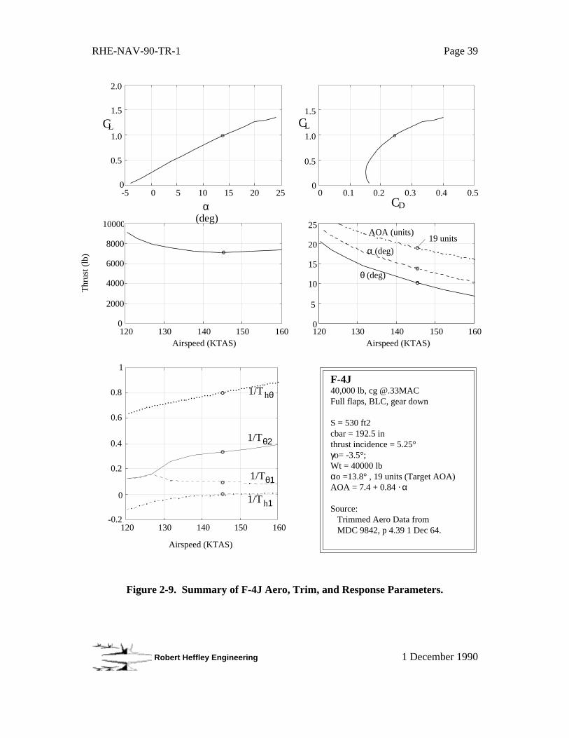
RHE-NAV-90-TR-1 Page 39
Robert Heffley Engineering 1 December 1990
-5 0 5 10 15 20 25
α (deg)
CL CL
CD
1.0
0
0.5
1.5
2.0
1.0
0
2000
4000
6000
8000
10000
120 130 140 150 160Airspeed (KTAS)
Thr
ust (
lb)
-0.2
0
0.2
0.4
0.6
0.8
1
120 130 140 150 160
Airspeed (KTAS)
F-4J 40,000 lb, cg @.33MACFull flaps, BLC, gear down
S = 530 ft2cbar = 192.5 inthrust incidence = 5.25°γo= -3.5°;Wt = 40000 lbαo =13.8° , 19 units (Target AOA)AOA = 7.4 + 0.84 · α
Source: Trimmed Aero Data from MDC 9842, p 4.39 1 Dec 64.
0
5
10
15
20
25
120 130 140 150Airspeed (KTAS)
α (deg)
θ (deg)
AOA (units)19 units
0 0.1 0.2 0.3 0.4 0.5
1.5
0.5
0
160
1/T θ1
1/T h1
1/T θ2
1/T hθ
Figure 2-9. Summary of F-4J Aero, Trim, and Response Parameters.
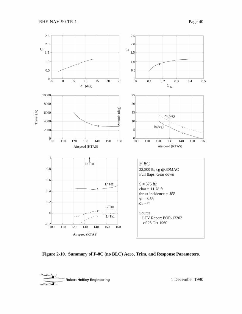
RHE-NAV-90-TR-1 Page 40
Robert Heffley Engineering 1 December 1990
C D
α (deg)
0
CL
0.5
2.0
1.0
2.5
1.5
θ (deg)
1 ⁄ Τhθ F-8C22,500 lb, cg @.30MACFull flaps, Gear down
S = 375 ft2cbar = 11.78 ftthrust incidence = .85°γo= -3.5°;αo =7°
Source: LTV Report EOR-13202 of 25 Oct 1960.-0.2
0
0.2
0.4
0.6
0.8
1
100 110 120 130 140 150 160
Airspeed (KTAS)
1 ⁄ Τθ1
1 ⁄ Τh1
1 ⁄ Τθ2
0
2000
4000
6000
8000
10000
100 110 120 130 140 150 160
Airspeed (KTAS)
Thr
ust (
lb)
0
5
10
15
20
25
100 110 120 130 140 150 160
Airspeed (KTAS)
Atti
tude
(de
g)
-5 0 5 10 15 20 25 0 0.1 0.2 0.3 0.4 0.50
CL
0.5
2.0
1.0
2.5
1.5
α (deg)
Figure 2-10. Summary of F-8C (no BLC) Aero, Trim, and Response Parameters.
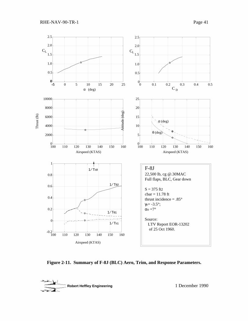
RHE-NAV-90-TR-1 Page 41
Robert Heffley Engineering 1 December 1990
α (deg) C D
0
F-8J22,500 lb, cg @.30MACFull flaps, BLC, Gear down
S = 375 ft2cbar = 11.78 ftthrust incidence = .85°γo= -3.5°;αo =7°
Source: LTV Report EOR-13202 of 25 Oct 1960.
α (deg)
-50
CL
0.5
2.0
1.0
2.5
0
CL
0.5
2.0
1.0
2.5
1.5 1.5
θ (deg)
1 ⁄ Τθ1
1 ⁄ Τθ2
1 ⁄ Τh1
1 ⁄ Τhθ
-5 0 5 10 15 20 25 0 0.1 0.2 0.3 0.4 0.5
0
2000
4000
6000
8000
10000
100 110 120 130 140 150 160
Airspeed (KTAS)
Thr
ust (
lb)
0
5
10
15
20
25
100 110 120 130 140 150 160
Airspeed (KTAS)
Atti
tude
(de
g)
-0.2
0
0.2
0.4
0.6
0.8
1
100 110 120 130 140 150 160
Airspeed (KTAS)
Figure 2-11. Summary of F-8J (BLC) Aero, Trim, and Response Parameters.
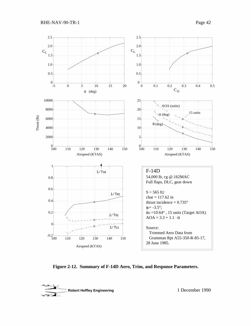
RHE-NAV-90-TR-1 Page 42
Robert Heffley Engineering 1 December 1990
α (deg) C D
0
CL
0.5
1.5
2.0
1.0
F-14D54,000 lb, cg @.162MACFull flaps, DLC, gear down
S = 565 ft2cbar = 117.62 inthrust incidence = 0.735°γo= -3.5°;αo =10.64° , 15 units (Target AOA)AOA = 3.3 + 1.1 · α
Source: Trimmed Aero Data from Grumman Rpt A55-350-R-85-17, 28 June 1985.
0
1 ⁄ Τθ1
1 ⁄ Τθ2
1 ⁄ Τhθ
1 ⁄ Τh1
-5 0 5 10 15 20 0 0.1 0.2 0.3 0.4 0.5
2.5
CL
2.0
1.0
2.5
0.5
1.5
0
2000
4000
6000
8000
10000
100 110 120 130 140 150
Airspeed (KTAS)
Thr
ust (
lb)
-0.2
0
0.2
0.4
0.6
0.8
1
100 110 120 130 140 150
Airspeed (KTAS)
0
10
15
20
25
100 110 120 130 140 150
Airspeed (KTAS)
5
15 unitsα (deg)
θ (deg)
AOA (units)
Figure 2-12. Summary of F-14D Aero, Trim, and Response Parameters.

RHE-NAV-90-TR-1 Page 43
Robert Heffley Engineering 1 December 1990
2.0
α (deg)
CL CL
C D
1.0
0
0.5
1.5
2.0
1.0
F/A-18A33,000 lb, cg @.25MACFull flaps, gear downFighter Escort--2 AIM-7, 2 AIM-9 δf/a, δh, δr toe-in, on AOA scheduleS = 400 ft2cbar = 11.52 ftthrust incidence = 0°γo= -3.5°;αo =8.1° , 8.1 units (Target AOA)AOA = 0 + 1.0 · α
Source: Trimmed Aero Data from MDC A8575 p 3-121 31 Mar 84.
1.5
0.5
0
1 ⁄ Τθ1
1 ⁄ Τθ2
1 ⁄ Τhθ
1 ⁄ Τh1
-5 0 5 10 15 20 25 0 0.1 0.2 0.3 0.4 0.5
0
2000
4000
6000
8000
10000
120 130 140 150 160
Airspeed (KTAS)
Thr
ust (
lb)
0
5
10
15
20
25
120 160
Airspeed (KTAS)
Atti
tude
(de
g)
-0.2
0
0.2
0.4
0.6
0.8
1
120 130 140 150 160
Airspeed (KTAS)
130 140 150
α (deg) or AOA (units)
8.1 units
θ (deg)
Figure 2-13. Summary of F/A-18A Aero, Trim, and Response Parameters.
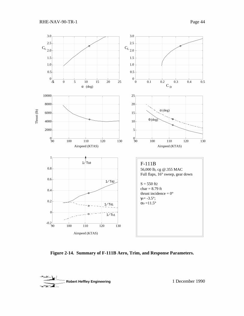
RHE-NAV-90-TR-1 Page 44
Robert Heffley Engineering 1 December 1990
α (deg) C D
0
α (deg)
-5
0.5
2.0
1.0
2.5
CL
1.5
θ (deg)
1 ⁄ Τθ1
1 ⁄ Τθ2
1 ⁄ Τh1
1 ⁄ Τhθ
-5 0 5 10 15 20 25 0 0.1 0.2 0.3 0.4 0.5
3.0
0
0.5
2.0
1.0
2.5
CL
1.5
3.0
F-111B 56,000 lb, cg @.355 MACFull flaps, 16° sweep, gear down
S = 550 ft2cbar = 8.79 ftthrust incidence = 0°γo= -3.5°;αo =11.5°
0
2000
4000
6000
8000
10000
90 100 110 120 130
Airspeed (KTAS)
Thr
ust (
lb)
0
5
10
15
20
25
90 100 110 120 130
Airspeed (KTAS)
-0.2
0
0.2
0.4
0.6
0.8
1
90 100 110 120 130
Airspeed (KTAS)
Figure 2-14. Summary of F-111B Aero, Trim, and Response Parameters.
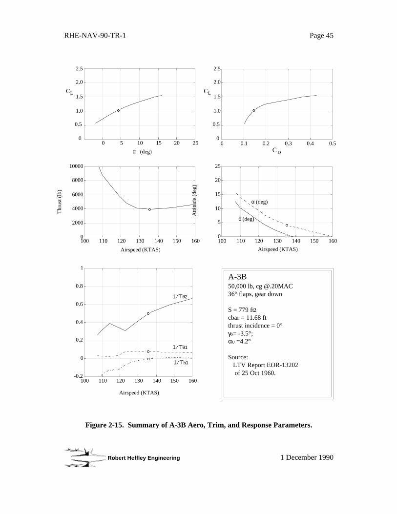
RHE-NAV-90-TR-1 Page 45
Robert Heffley Engineering 1 December 1990
α (deg) C D
α (deg)
2.0
1.0
2.5
1.5
θ (deg)
0
0.5
CL
0 5 10 15 20 25 0 0.1 0.2 0.3 0.4 0.5
2.0
1.0
2.5
1.5
0
0.5
CL
0
2000
4000
6000
8000
10000
100 110 120 130 140 150 160
Airspeed (KTAS)
Thr
ust (
lb)
0
5
10
15
20
25
100 110 120 130 140 150 160
Airspeed (KTAS)
Atti
tude
(de
g)
-0.2
0
0.2
0.4
0.6
0.8
1
100 110 120 130 140 150 160
Airspeed (KTAS)
A-3B50,000 lb, cg @.20MAC36° flaps, gear down
S = 779 ft2cbar = 11.68 ftthrust incidence = 0°γo= -3.5°;αo =4.2°
Source: LTV Report EOR-13202 of 25 Oct 1960.
1 ⁄ Τθ1
1 ⁄ Τθ2
1 ⁄ Τh1
Figure 2-15. Summary of A-3B Aero, Trim, and Response Parameters.

RHE-NAV-90-TR-1 Page 46
Robert Heffley Engineering 1 December 1990
α (deg)
0-5
CL
0.5
2.0
1.0
2.5
1.5
1 ⁄ Τθ1
1 ⁄ Τθ2
1 ⁄ Τh1
1 ⁄ Τhθ
-5 0 5 10 15 20 0.4 0.5
Airspeed (KTAS)
-0.2
0
0.2
0.4
0.6
0.8
1
120 130 140 150 160
0
2000
4000
6000
8000
10000
120 130 140 150
Airspeed (KTAS)
Thr
ust (
lb)
RA-5C 50,000 lb, Full flaps, Gear DownCD
25 0 0.1 0.2 0.3 0.4 0.50
CL
0.5
2.0
1.0
2.5
1.5
C D
RA-5C50,000 lb, cg @.31MACFull flaps, Gear down
S = 700 ft2cbar = 15.19 ftthrust incidence = 1.23°γo= -3.5°;αo =8°
1600
5
10
15
20
25
120 130 140 150 160
Airspeed (KTAS)
α (deg)
θ (deg)
Figure 2-16. Summary of RA-5C Aero, Trim, and Response Parameters.

RHE-NAV-90-TR-1 Page 47
Robert Heffley Engineering 1 December 1990
α (deg)
CL CL
C D
0
0.5
1.5
2.0
1.0
A-6E36,000 lb, cg @.28MAC30° flaps, tip brakes, gear down
S = 528.9 ft2cbar = 10.9 ftthrust incidence = 7°γo= -3.5°;αo =12° , 22 units (Target AOA)AOA = 8 + 1.15 · α1 ⁄ Τθ1
1 ⁄ Τθ2
1 ⁄ Τhθ
1 ⁄ Τh1
-5 0 5 10 15 20 25 0 0.1 0.2 0.3 0.4 0.5
2.5
0
0.5
1.5
2.0
1.0
2.5
-0.2
0
0.2
0.4
0.6
0.8
1
90 100 110 120 130 140
Airspeed (KTAS)
0
2000
4000
6000
8000
10000
90 100 110 120 130 140
Airspeed (KTAS)
Thr
ust (
lb)
0
5
10
15
20
25
90 100 110 120 130 140
Airspeed (KTAS)
Atti
tude
(de
g)
22 units
Figure 2-17. Summary of A-6E Aero, Trim, and Response Parameters.

RHE-NAV-90-TR-1 Page 48
Robert Heffley Engineering 1 December 1990
α (deg) C D
0
T-45A12,700 lb, cg @.25MACFull flaps, gear down
S = 179.64 ft2cbar = 69.96 inthrust incidence = 0°γo= -3.5°;αo =6° , 16 units (Target AOA)AOA =10.35 + 0.94 · α
Source: Trimmed Aero Data from MDC K2090 pp D23, D41 21 Nov 84.
α (deg)
0 0.1 0.2 0.3 0.4 0.5-5 0 5 10 15 20 250
CL
0.5
2.0
1.0
2.5
0
CL
0.5
2.0
1.0
2.5
1.5 1.5
0
1000
2000
3000
4000
5000
100 110 120 130 140 150
Airspeed (KTAS)
Thr
ust (
lb)
0
5
10
15
20
25
100 110 120 130 140 150
Airspeed (KTAS)
Atti
tude
(de
g)
16 unitsAOA (units)
θ (deg)
-0.2
0
0.2
0.4
0.6
0.8
1
100 110 120 130 140 150
Airspeed (KTAS)
1 ⁄ Τθ1
1 ⁄ Τθ2
1 ⁄ Τh1
1 ⁄ Τhθ
Figure 2-18. Summary of T-45A Aero, Trim, and Response Parameters.

RHE-NAV-90-TR-1 Page 49
Robert Heffley Engineering 1 December 1990
Other Aircraft Data
Table 2-4 provides additional characteristics for a variety of carrier aircraft at theirnominal approach speeds. These data have been refined with the assistance of NAVAIRpersonnel (Reference 54). Most cases represent the NATOPS-prescribed approach speed.
Table 2-4. Outer-Loop Characteristics for Several Navy Carrier Aircraft.
Aircraft Weight Speed Alpha CL CD CL CD/ CL Xu Xw Zu Zw nz† 1/T 2 1/T 1 1/Th1
___________________________________________________________________________________________
F-4J 40000 145 13.8 0.99 0.243 2.72 0.239 -0.064 0.045 -0.26 -0.39 3.0 0.35 0.11 0.01
F-8C 22500 141 7.0 0.87 0.174 2.65 0.362 -0.054 -0.014 -0.27 -0.44 3.2 0.45 0.04 -0.04
F-8J (BLC) 22500 128 7.0 1.06 0.213 2.86 0.200 -0.060 0.069 -0.30 -0.43 2.9 0.36 0.13 0.00
F-14D(DLC)54000 129 10.6 1.65 0.323 4.30 0.317 -0.058 0.026 -0.30 -0.41 2.8 0.39 0.08 -0.03
F/A-18 33000 137 8.1 1.26 0.334 2.84 0.269 -0.074 0.055 -0.28 -0.35 2.5 0.27 0.15 0.01
F-111B† † 56000 113 11.5 2.35 0.334 5.74 0.237 -0.048 0.071 -0.34 -0.44 2.6 0.36 0.12 -0.03
A-3B 50000 135 4.2 1.02 0.144 3.80 0.153 -0.040 0.061 -0.28 -0.55 3.9 0.51 0.08 0.00
A-4E 14500 130 13.0 0.98 0.230 3.30 0.250 -0.069 0.024 -0.29 -0.53 3.6 0.51 0.08 0.00
RA-5C 50000 149 8.0 0.93 0.216 3.47 0.252 -0.059 0.008 -0.26 -0.51 4.0 0.50 0.06 0.00
A-6E 36000 113 12.0 1.49 0.307 4.57 0.267 -0.069 0.031 -0.34 -0.55 3.3 0.53 0.09 -0.01
A-7E 22721 121 12.5 1.22 0.203 3.95 0.201 -0.052 0.055 -0.31 -0.54 3.4 0.50 0.09 -0.01
E-2C 42090 100 8.0 1.77 0.190 7.03 0.150 -0.041 0.077 -0.38 -0.78 4.1 0.73 0.08 -0.01
TF-9J 16500 125 10.0 0.92 0.184 3.27 0.210 -0.061 0.039 -0.30 -0.57 3.8 0.55 0.09 0.00
T-2C 12000 107 8.5 1.20 0.250 4.38 0.192 -0.074 0.053 -0.36 -0.69 3.9 0.65 0.11 0.01
TA-4J 14500 130 13.0 0.98 0.230 3.30 0.250 -0.069 0.024 -0.29 -0.53 3.6 0.51 0.08 0.00
T-45A 11253 123 5.0 1.22 0.270 4.13 0.160 -0.069 0.071 -0.31 -0.56 3.6 0.51 0.12 0.02
FJ-3 13678 112 11.5 1.06 0.188 3.44 0.152 -0.060 0.086 -0.34 -0.58 3.4 0.52 0.12 0.01
F4D-1 16870 121 18.0 0.56 0.107 1.80 0.342 -0.060 -0.016 -0.31 -0.54 3.4 0.55 0.05 -0.04
F7U-3 21030 133 16.0 0.69 0.140 2.55 0.165 -0.058 0.056 -0.29 -0.56 3.9 0.52 0.09 0.01
F9F-6 13440 114 9.8 1.02 0.198 3.95 0.260 -0.065 -0.001 -0.33 -0.68 4.1 0.68 0.06 -0.02
T-33A * 12000 125 3.9 0.96 0.130 5.07 0.120 -0.041 0.056 -0.30 -0.83 5.4 0.80 0.06 0.01
T-38A* 11761 180 5.8 0.63 0.137 2.87 0.260 -0.046 -0.020 -0.21 -0.51 4.8 0.51 0.04 -0.01
F-16* 18825 129 13.2 1.07 0.207 4.07 0.340 -0.057 -0.043 -0.30 -0.59 4.0 0.61 0.03 -0.04
_____________________
*USAF—not carrier aircraft.
† Trimmed values.† † VPAmin approach speed
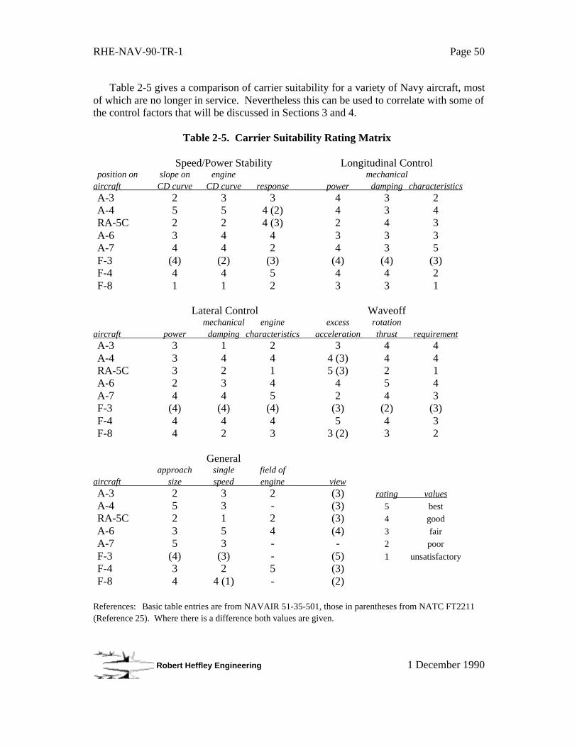
RHE-NAV-90-TR-1 Page 50
Robert Heffley Engineering 1 December 1990
Table 2-5 gives a comparison of carrier suitability for a variety of Navy aircraft, mostof which are no longer in service. Nevertheless this can be used to correlate with some ofthe control factors that will be discussed in Sections 3 and 4.
Table 2-5. Carrier Suitability Rating Matrix
Speed/Power Stability Longitudinal Controlposition on slope on engine mechanical
aircraft CD curve CD curve response power damping characteristicsA-3 2 3 3 4 3 2A-4 5 5 4 (2) 4 3 4RA-5C 2 2 4 (3) 2 4 3A-6 3 4 4 3 3 3A-7 4 4 2 4 3 5F-3 (4) (2) (3) (4) (4) (3)F-4 4 4 5 4 4 2F-8 1 1 2 3 3 1
Lateral Control Waveoffmechanical engine excess rotation
aircraft power damping characteristics acceleration thrust requirementA-3 3 1 2 3 4 4A-4 3 4 4 4 (3) 4 4RA-5C 3 2 1 5 (3) 2 1A-6 2 3 4 4 5 4A-7 4 4 5 2 4 3F-3 (4) (4) (4) (3) (2) (3)F-4 4 4 4 5 4 3F-8 4 2 3 3 (2) 3 2
Generalapproach single field of
aircraft size speed engine viewA-3 2 3 2 (3) rating values
A-4 5 3 - (3) 5 bestRA-5C 2 1 2 (3) 4 good
A-6 3 5 4 (4) 3 fairA-7 5 3 - - 2 poor
F-3 (4) (3) - (5) 1 unsatisfactoryF-4 3 2 5 (3)F-8 4 4 (1) - (2)
References: Basic table entries are from NAVAIR 51-35-501, those in parentheses from NATC FT2211(Reference 25). Where there is a difference both values are given.
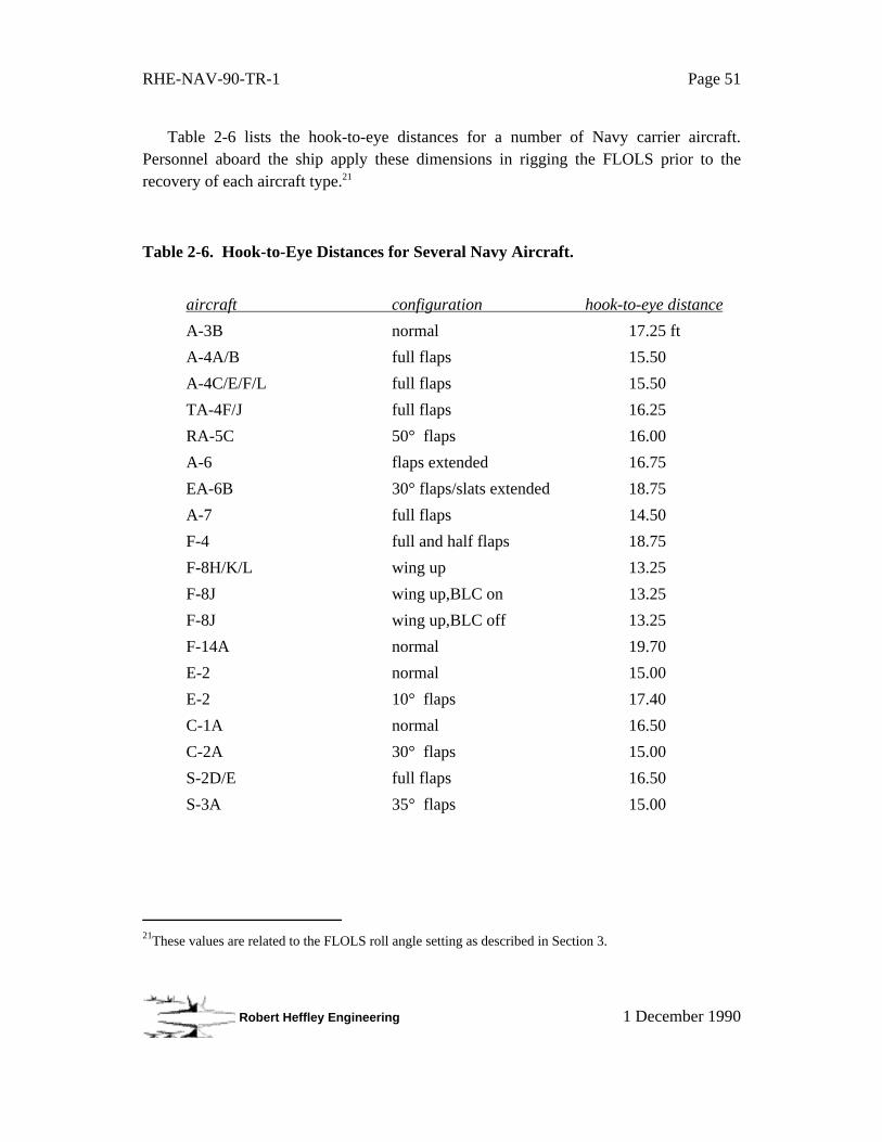
RHE-NAV-90-TR-1 Page 51
Robert Heffley Engineering 1 December 1990
Table 2-6 lists the hook-to-eye distances for a number of Navy carrier aircraft.Personnel aboard the ship apply these dimensions in rigging the FLOLS prior to therecovery of each aircraft type.21
Table 2-6. Hook-to-Eye Distances for Several Navy Aircraft.
aircraft configuration hook-to-eye distance
A-3B normal 17.25 ft
A-4A/B full flaps 15.50
A-4C/E/F/L full flaps 15.50
TA-4F/J full flaps 16.25
RA-5C 50° flaps 16.00
A-6 flaps extended 16.75
EA-6B 30° flaps/slats extended 18.75
A-7 full flaps 14.50
F-4 full and half flaps 18.75
F-8H/K/L wing up 13.25
F-8J wing up,BLC on 13.25
F-8J wing up,BLC off 13.25
F-14A normal 19.70
E-2 normal 15.00
E-2 10° flaps 17.40
C-1A normal 16.50
C-2A 30° flaps 15.00
S-2D/E full flaps 16.50
S-3A 35° flaps 15.00
21These values are related to the FLOLS roll angle setting as described in Section 3.
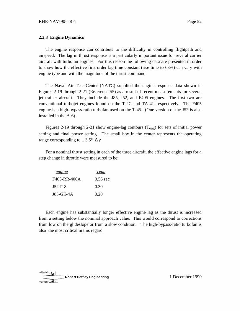
RHE-NAV-90-TR-1 Page 52
Robert Heffley Engineering 1 December 1990
2.2.3 Engine Dynamics
The engine response can contribute to the difficulty in controlling flightpath andairspeed. The lag in thrust response is a particularly important issue for several carrieraircraft with turbofan engines. For this reason the following data are presented in orderto show how the effective first-order lag time constant (rise-time-to-63%) can vary withengine type and with the magnitude of the thrust command.
The Naval Air Test Center (NATC) supplied the engine response data shown inFigures 2-19 through 2-21 (Reference 55) as a result of recent measurements for severaljet trainer aircraft. They include the J85, J52, and F405 engines. The first two areconventional turbojet engines found on the T-2C and TA-4J, respectively. The F405engine is a high-bypass-ratio turbofan used on the T-45. (One version of the J52 is alsoinstalled in the A-6).
Figures 2-19 through 2-21 show engine-lag contours (Teng) for sets of initial power
setting and final power setting. The small box in the center represents the operatingrange corresponding to ± 3.5° ∆ γ.
For a nominal thrust setting in each of the three aircraft, the effective engine lags for astep change in throttle were measured to be:
engine Teng
F405-RR-400A 0.56 sec
J52-P-8 0.30
J85-GE-4A 0.20
Each engine has substantially longer effective engine lag as the thrust is increasedfrom a setting below the nominal approach value. This would correspond to correctionsfrom low on the glideslope or from a slow condition. The high-bypass-ratio turbofan isalso the most critical in this regard.

RHE-NAV-90-TR-1 Page 53
Robert Heffley Engineering 1 December 1990
.6 .4
.2
.1
.2
high/fast correction
14
16
18
20
22
24
26
28
30
32
34
14 16 18 20 22 24 26 28 30 32 34Initial PT5 (psia)
Fina
l PT
5 (p
sia)
500 1000 1500 2000 2500 3000 3500 4000 4500 5000
Uncorrected Thrust (lb)
1.91.85
2.3
2.5
1.45
1
1.8
1.15
0.7
1
0.85
0.95
0.5
0.9
0.250.250.25
0.6
0.25
0.55
0.15
0.40.3
0.25
0.4
0.35
0.25
0.25
0.2
0.3
0.350.15
0.25
0.30.2
0.1
0.15
0.2
0.15
0.15
0.25
0.350.15
0.15
0.15
2.41.750.750.45
0.40.20.2
0.250.250.4
low/slow correction
Each data point indicates the value of Teng for the respective initial and final power settings.
MILIdle
.2
Figure 2-19. Thrust Lag Data for the J85 Engine (T-2C).
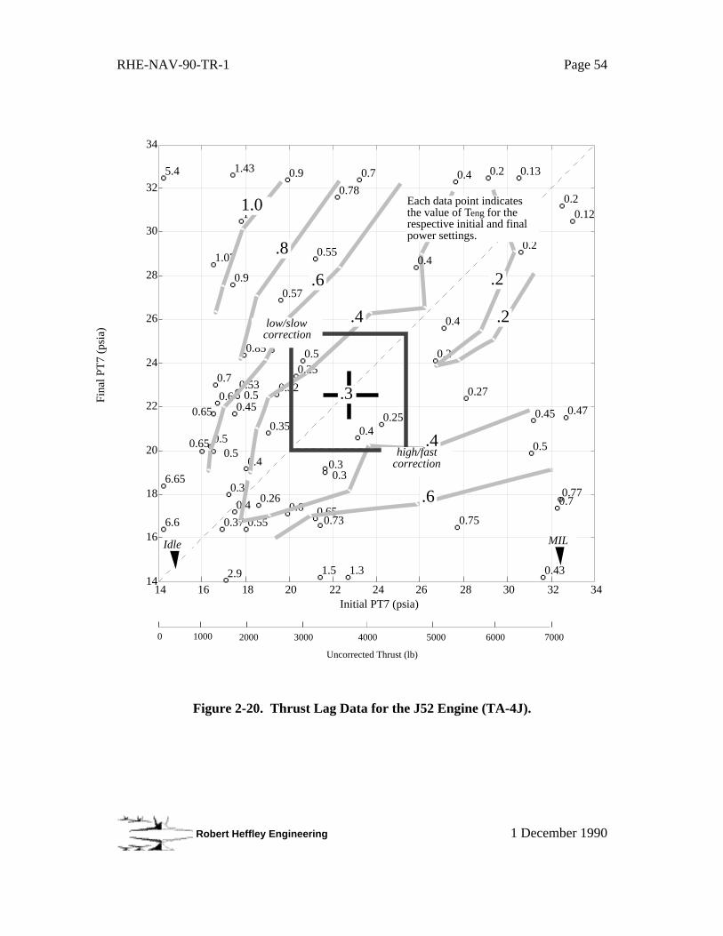
RHE-NAV-90-TR-1 Page 54
Robert Heffley Engineering 1 December 1990
0 1000 2000 3000 4000 5000 6000 7000
Uncorrected Thrust (lb)
14
34
16 18 20 22 24 26 28 30 32
0.12
Initial PT7 (psia)
Fina
l PT
7 (p
sia)
14 34
16
18
20
22
24
26
28
30
32
6.6
5.4
6.65
0.65 0.5
1.07
0.65
0.5
0.7
0.6
0.37
2.9
0.3
1.43
0.9
0.45
0.4
0.530.5
1
0.85
0.4
0.55
0.26
0.35
0.5
0.32
0.57
0.9
0.6
0.250.5
0.55
0.650.73
1.5
0.30.3
0.78
1.3
0.4
0.7
0.25
0.2
0.4
0.4
0.75
0.27
0.2 0.13
0.2
0.5
0.45
0.43
0.70.77
0.2
0.47
1.0
.8
.6
.4
.6
.4
.2
.2 low/slow correction
high/fast correction
.3
MILIdle
Each data point indicates the value of Teng for the respective initial and final power settings.
0.4
Figure 2-20. Thrust Lag Data for the J52 Engine (TA-4J).

RHE-NAV-90-TR-1 Page 55
Robert Heffley Engineering 1 December 1990
14
16
18
20
22
24
26
28
30
32
34
14 16 18 20 22 24 26 28 30 32 34Initial PS16 (psia)
Fina
l PS1
6 (p
sia)
50001000 2000 3000 4000
Uncorrected Thrust (lb)
0
4.9
3.2
4.1
4.4
4.42.2
1.75
1.51.4
1.2
1.5
1.75
1.351.3
1.5
1.5
1.2
1.2
1.45
1.55
1.2
1.35
1.5
0.9
1.050.91.8
0.8
0.80.8
0.70.8
0.55
0.6
0.55
0.8
1.05
1.1 0.85
0.8
0.6
0.7
0.6
0.5
0.5
0.50.55
0.5
0.45
1.3
0.45
0.2
0.55
1.5
.6
1.0 .8 .6
.6
low/slow correction
high/fast correction
Each data point indicates the value of Teng for the respective initial and final power settings.
Figure 2-21. Thrust Lag Data for the F405 Engine (T-45).
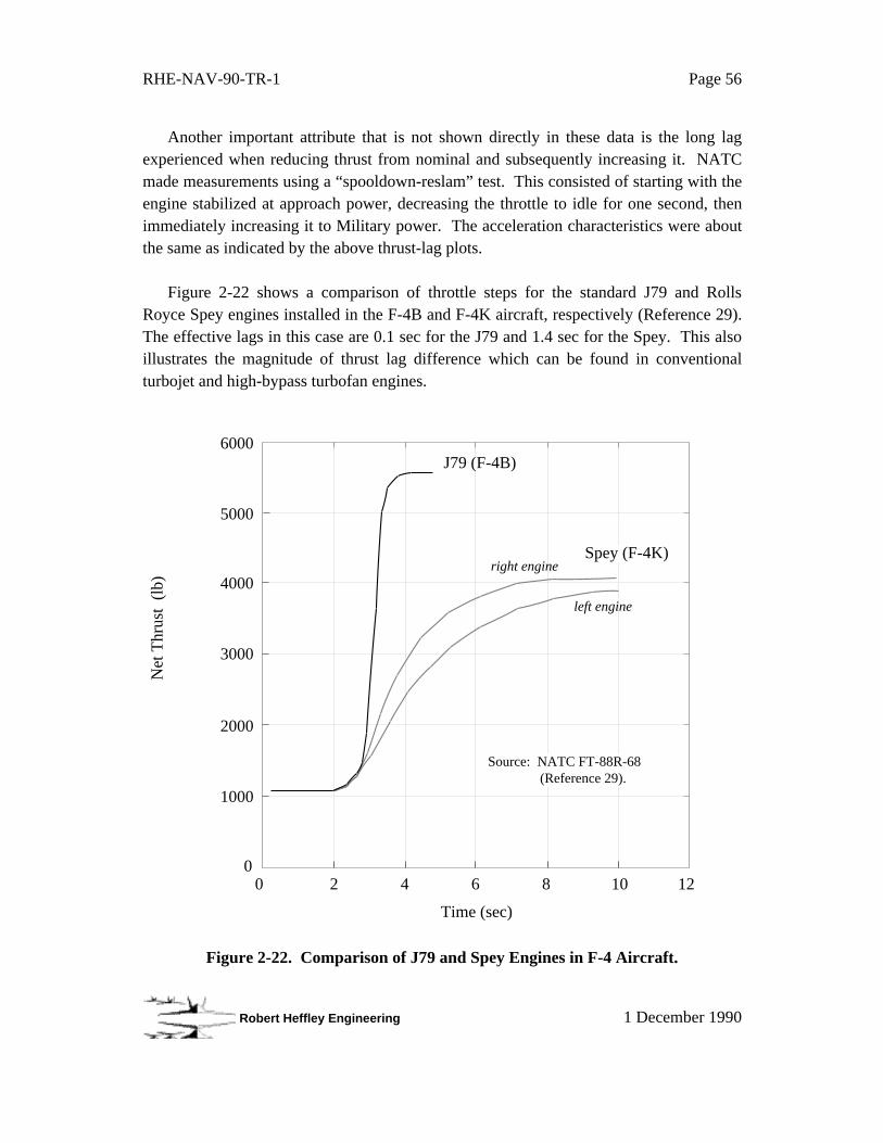
RHE-NAV-90-TR-1 Page 56
Robert Heffley Engineering 1 December 1990
Another important attribute that is not shown directly in these data is the long lagexperienced when reducing thrust from nominal and subsequently increasing it. NATCmade measurements using a “spooldown-reslam” test. This consisted of starting with theengine stabilized at approach power, decreasing the throttle to idle for one second, thenimmediately increasing it to Military power. The acceleration characteristics were aboutthe same as indicated by the above thrust-lag plots.
Figure 2-22 shows a comparison of throttle steps for the standard J79 and RollsRoyce Spey engines installed in the F-4B and F-4K aircraft, respectively (Reference 29).The effective lags in this case are 0.1 sec for the J79 and 1.4 sec for the Spey. This alsoillustrates the magnitude of thrust lag difference which can be found in conventionalturbojet and high-bypass turbofan engines.
00 2 4 6 8 10
1000
2000
3000
4000
5000
6000
12
J79 (F-4B)
right engine
left engine
Net
Thr
ust
(lb)
Time (sec)
Spey (F-4K)
Source: NATC FT-88R-68 (Reference 29).
Figure 2-22. Comparison of J79 and Spey Engines in F-4 Aircraft.
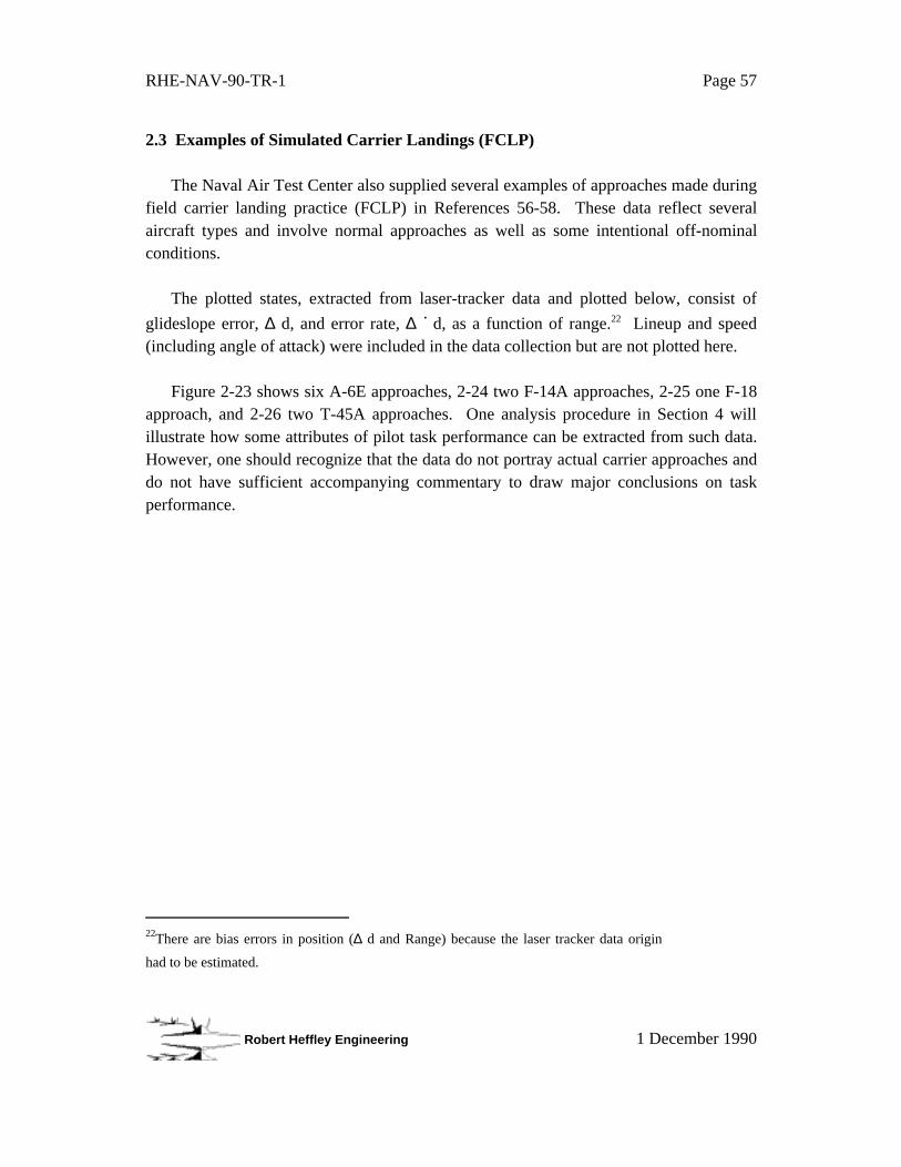
RHE-NAV-90-TR-1 Page 57
Robert Heffley Engineering 1 December 1990
2.3 Examples of Simulated Carrier Landings (FCLP)
The Naval Air Test Center also supplied several examples of approaches made duringfield carrier landing practice (FCLP) in References 56-58. These data reflect severalaircraft types and involve normal approaches as well as some intentional off-nominalconditions.
The plotted states, extracted from laser-tracker data and plotted below, consist of
glideslope error, ∆ d, and error rate, ∆ · d, as a function of range.22 Lineup and speed(including angle of attack) were included in the data collection but are not plotted here.
Figure 2-23 shows six A-6E approaches, 2-24 two F-14A approaches, 2-25 one F-18approach, and 2-26 two T-45A approaches. One analysis procedure in Section 4 willillustrate how some attributes of pilot task performance can be extracted from such data.However, one should recognize that the data do not portray actual carrier approaches anddo not have sufficient accompanying commentary to draw major conclusions on taskperformance.
22There are bias errors in position (∆ d and Range) because the laser tracker data origin
had to be estimated.

RHE-NAV-90-TR-1 Page 58
Robert Heffley Engineering 1 December 1990
-50
0
50
0 500 1000 1500 2000 2500 3000 3500 4000
Range (ft)
∆d (
ft)
-10
0
10
0 500 1000 1500 2000 2500 3000 3500 4000
Range (ft)
∆˙d
(ft/s
ec)
A-6E Run 4 Normal Approach
Figure 2-23a. FCLP Approach Example for A-6E.
-50
0
50
0 500 1000 1500 2000 2500 3000 3500 4000
Range (ft)
∆d (
ft)
-10
0
10
0 500 1000 1500 2000 2500 3000 3500 4000
Range (ft)
∆˙d
(ft/s
ec)
A-6E Run 5 Normal Approach
Figure 2-23b. FCLP Approach Example for A-6E.
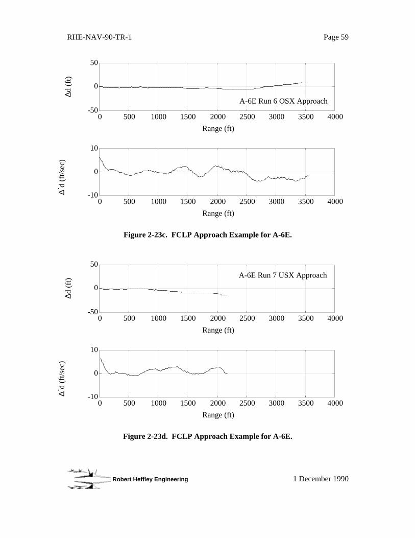
RHE-NAV-90-TR-1 Page 59
Robert Heffley Engineering 1 December 1990
-50
0
50
0 500 1000 1500 2000 2500 3000 3500 4000
Range (ft)
∆d (
ft)
-10
0
10
0 500 1000 1500 2000 2500 3000 3500 4000
Range (ft)
∆˙d
(ft/s
ec)
A-6E Run 6 OSX Approach
Figure 2-23c. FCLP Approach Example for A-6E.
-50
0
50
0 500 1000 1500 2000 2500 3000 3500 4000
Range (ft)
∆d (
ft)
-10
0
10
0 500 1000 1500 2000 2500 3000 3500 4000
Range (ft)
∆˙d
(ft/s
ec)
A-6E Run 7 USX Approach
Figure 2-23d. FCLP Approach Example for A-6E.
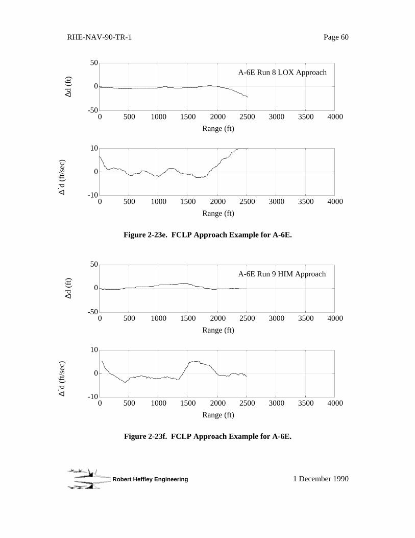
RHE-NAV-90-TR-1 Page 60
Robert Heffley Engineering 1 December 1990
-50
0
50
0 500 1000 1500 2000 2500 3000 3500 4000
Range (ft)
∆d (
ft)
-10
0
10
0 500 1000 1500 2000 2500 3000 3500 4000
Range (ft)
∆˙d
(ft/s
ec)
A-6E Run 8 LOX Approach
Figure 2-23e. FCLP Approach Example for A-6E.
-50
0
50
0 500 1000 1500 2000 2500 3000 3500 4000
Range (ft)
∆d (
ft)
-10
0
10
0 500 1000 1500 2000 2500 3000 3500 4000
Range (ft)
∆˙d
(ft/s
ec)
A-6E Run 9 HIM Approach
Figure 2-23f. FCLP Approach Example for A-6E.
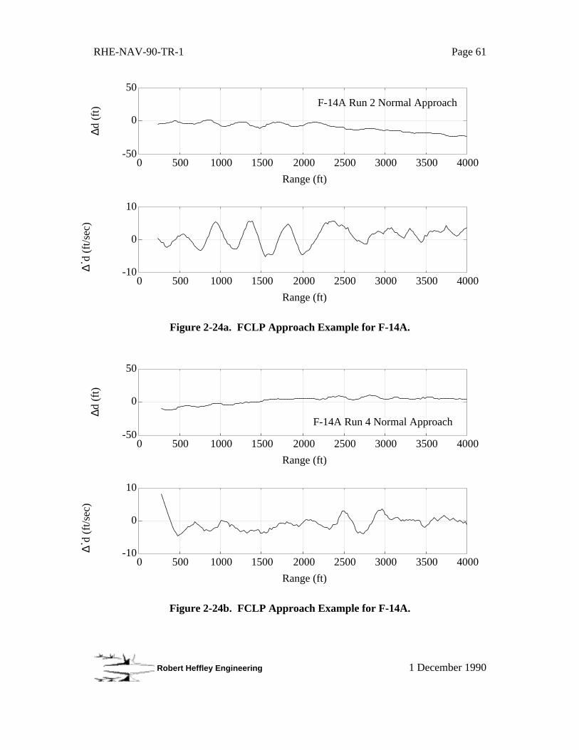
RHE-NAV-90-TR-1 Page 61
Robert Heffley Engineering 1 December 1990
-50
0
50
0 500 1000 1500 2000 2500 3000 3500 4000
F-14A Run 2 Normal Approach
Range (ft)
∆d (
ft)
-10
0
10
0 500 1000 1500 2000 2500 3000 3500 4000
Range (ft)
∆˙d
(ft/s
ec)
Figure 2-24a. FCLP Approach Example for F-14A.
-50
0
50
0 500 1000 1500 2000 2500 3000 3500 4000
Range (ft)
∆d (
ft)
-10
0
10
0 500 1000 1500 2000 2500 3000 3500 4000
Range (ft)
∆˙d
(ft/s
ec)
F-14A Run 4 Normal Approach
Figure 2-24b. FCLP Approach Example for F-14A.
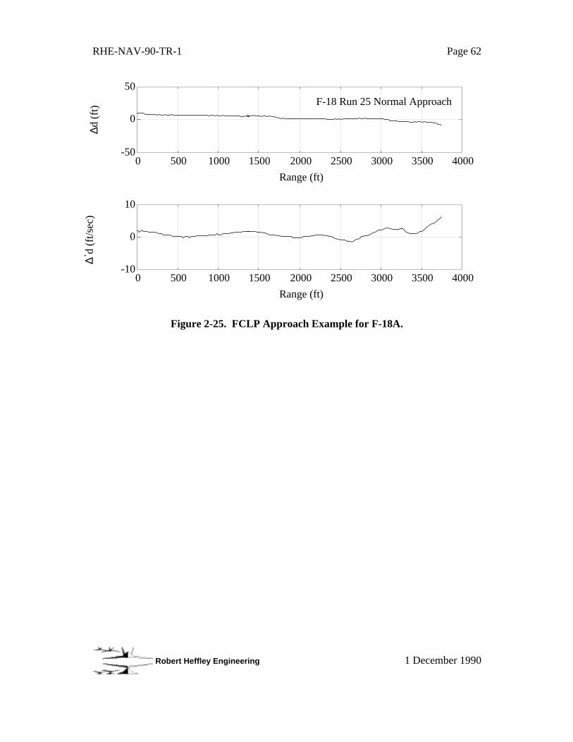
RHE-NAV-90-TR-1 Page 62
Robert Heffley Engineering 1 December 1990
-50
0
50
0 500 1000 1500 2000 2500 3000 3500 4000
Range (ft)
∆d (
ft)
-10
0
10
0 500 1000 1500 2000 2500 3000 3500 4000
Range (ft)
∆˙d
(ft/s
ec)
F-18 Run 25 Normal Approach
Figure 2-25. FCLP Approach Example for F-18A.
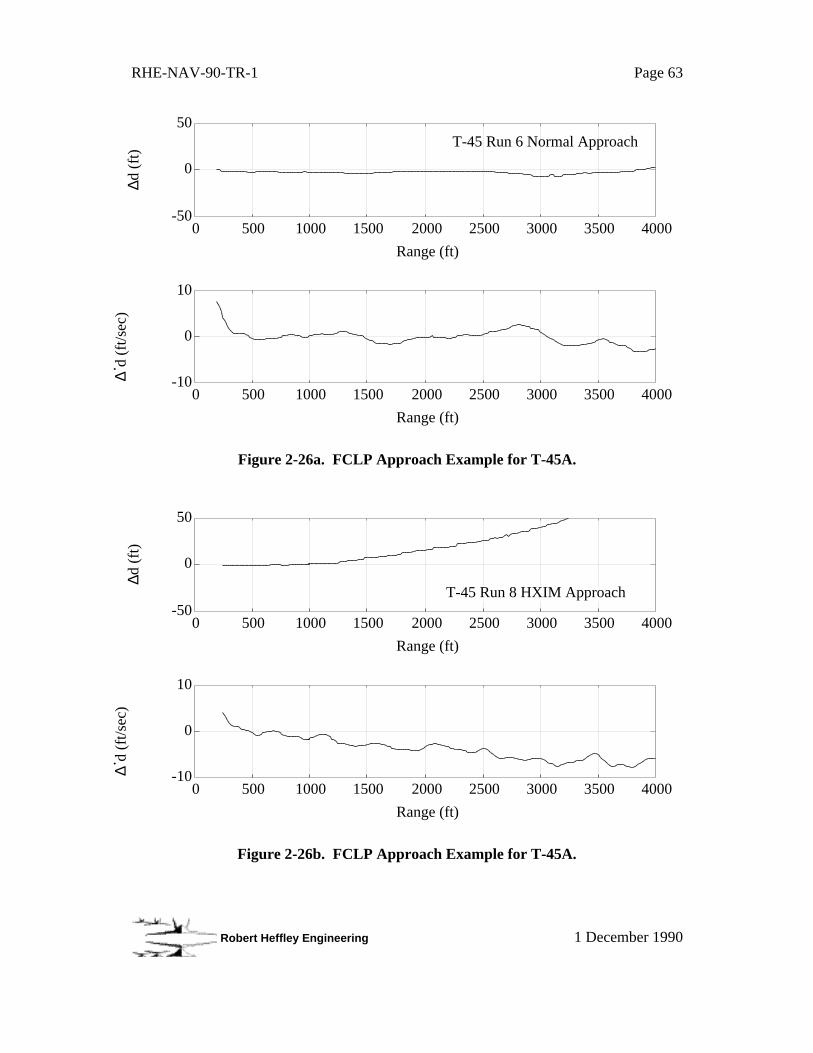
RHE-NAV-90-TR-1 Page 63
Robert Heffley Engineering 1 December 1990
-50
0
50
0 500 1000 1500 2000 2500 3000 3500 4000
Range (ft)
∆d (
ft)
-10
0
10
0 500 1000 1500 2000 2500 3000 3500 4000
Range (ft)
∆˙d
(ft/s
ec)
T-45 Run 6 Normal Approach
Figure 2-26a. FCLP Approach Example for T-45A.
-50
0
50
0 500 1000 1500 2000 2500 3000 3500 4000
Range (ft)
∆d (
ft)
-10
0
10
0 500 1000 1500 2000 2500 3000 3500 4000
Range (ft)
∆˙d
(ft/s
ec)
T-45 Run 8 HXIM Approach
Figure 2-26b. FCLP Approach Example for T-45A.

RHE-NAV-90-TR-1 Page 64
Robert Heffley Engineering 1 December 1990
THIS PAGE IS INTENTIONALLY BLANK
RHE-NAV-90-TR-1 Page 65
Robert Heffley Engineering 1 December 1990
3. CARRIER LANDING PILOT-VEHICLE-TASK MATH MODELS
The purpose of the math modeling process is to enable a systematic examination ofany or all the parts of the pilot-vehicle-task system. To do so, one must establish a validoperational context. That is, the dynamics must be viewed in the appropriate range ofinterest, whether in the time domain or frequency domain.
Since the focus is on the outer-loop dynamics it is possible to take advantage ofseveral simplifying assumptions. In fact, one can view the aircraft as a low-order systemin nearly all cases (first-, second-, or third-order). This makes it feasible to study the totalpilot-vehicle closed loop system without incurring undue complexity.
Following the form of previous sections, the author examines the carrier landing taskfirst, the aircraft next, and finally the total closed-loop system including the pilot.
3.1 Carrier Environment (Task)
Analytical study of the carrier landing task aids in the formulation math models in thecorrect context. Because the pilot receives outer-loop information primarily in the visualmodality, the aircraft motion needs to be computed at the pilot's station. Simultaneously,a crucial performance-related aspect is the position of the tailhook relative to the arrestingwires on the deck. Finally, one ordinarily solves the airplane equations of motion withrespect to the aircraft cg. The analyst may need to distinguish each of these referenceframes, depending upon the circumstances.
3.1.1 Glideslope Task
The Fresnel Lens Optical Landing System (FLOLS) is the most prominent guidancefeature in the carrier landing environment. A detailed description of the FLOLS systemcan be found in Reference 40.
The vertical array of five Fresnel lens provides a nearly-continuous23 display ofglideslope error over the 1.6° vertical beamwidth and 40° horizontal beamwidth. Figure
23Characteristics of the ball are sensitive to temperature changes in the internal Fresnel lens cell. If the lensassembly is not completely warmed-up there may not be a smooth transition of the ball between cells andthe ball may disappear as it tranverses the junction between adjacent cells. Under normal operatingconditions, however, the motion of the ball should be smooth and continuous.

RHE-NAV-90-TR-1 Page 66
Robert Heffley Engineering 1 December 1990
3-1 shows key glideslope features seen by the pilot. The glideslope light assembly hasfive Fresnel lens cells mounted vertically. Four of the lights are yellow in color and thebottommost (the extreme-low indication) is red. Personnel aboard the carrier can varyintensity depending upon ambient light and weather conditions.
Green Datum Lights
Glideslope Fresnel Lens Lights(top four cells are yellow)
"Meatball"
bottom cell is red and can be flashed if desired
glideslopeerror
Figure 3-1. FLOLS Glideslope Display Geometry.
Three fixed datum lights and four conditional datum lights are mounted horizontallyon each side of the lens. The fixed datums are illuminated continuously while theconditional datums go out when the waveoff lights are on.

RHE-NAV-90-TR-1 Page 67
Robert Heffley Engineering 1 December 1990
Four waveoff lights and three auxiliary waveoff lights are mounted vertically on eachside of the lens. When the LSO initiates a waveoff, the waveoff lights first flash at fullintensity then dim to the preset brightness.
The lens assembly can be tilted about two horizontal planes at right angles to eachother that equate roughly to the ship's pitch and roll axes. The tilt in pitch gives the basicglideslope angle and it seldom changes (3.5° to 4° ). Moving the lens about the roll axisrolls the glideslope and causes the glideslope at the landing area to be raised or loweredas Figure 3-2 shows. This compensates for the hook-to-eye distance of various aircraft toproduce a constant hook glide path for all aircraft.24 Roll angle can be varied from 0 to15 units. At 7.5 units all cells are vertical; 15 units cants the top of the cells outboardand provides for maximum ramp clearance, i. e., settings for the largest hook-to-eyedistance. One potential problem is that for large lens-assembly roll angles, extreme off-center approaches can result in hazardous ramp clearance.
15 units
7.5 units
zero roll setting
approach centerline
Light Plane
Figure 3-2. Effect of FLOLS Roll Angle on Light Plane.
24See Table 2-6 for hook-to-eye distances.
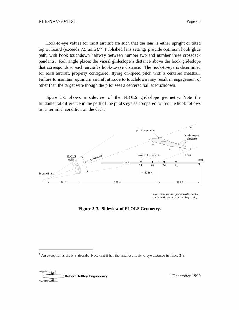
RHE-NAV-90-TR-1 Page 68
Robert Heffley Engineering 1 December 1990
Hook-to-eye values for most aircraft are such that the lens is either upright or tiltedtop outboard (exceeds 7.5 units).25 Published lens settings provide optimum hook glidepath, with hook touchdown halfway between number two and number three crossdeckpendants. Roll angle places the visual glideslope a distance above the hook glideslopethat corresponds to each aircraft's hook-to-eye distance. The hook-to-eye is determinedfor each aircraft, properly configured, flying on-speed pitch with a centered meatball.Failure to maintain optimum aircraft attitude to touchdown may result in engagement ofother than the target wire though the pilot sees a centered ball at touchdown.
Figure 3-3 shows a sideview of the FLOLS glideslope geometry. Note thefundamental difference in the path of the pilot's eye as compared to that the hook followsto its terminal condition on the deck.
deck
FLOLScells glideslope
pilot's eyepoint
hook
#1#2
focus of lens
hook-to-eye distance
150 ft 275 ft
#3#4
40 ft
crossdeck pendants
1.6°
note: dimensions approximate, not to scale, and can vary according to ship
ramp
235 ft
Figure 3-3. Sideview of FLOLS Geometry.
25An exception is the F-8 aircraft. Note that it has the smallest hook-to-eye distance in Table 2-6.
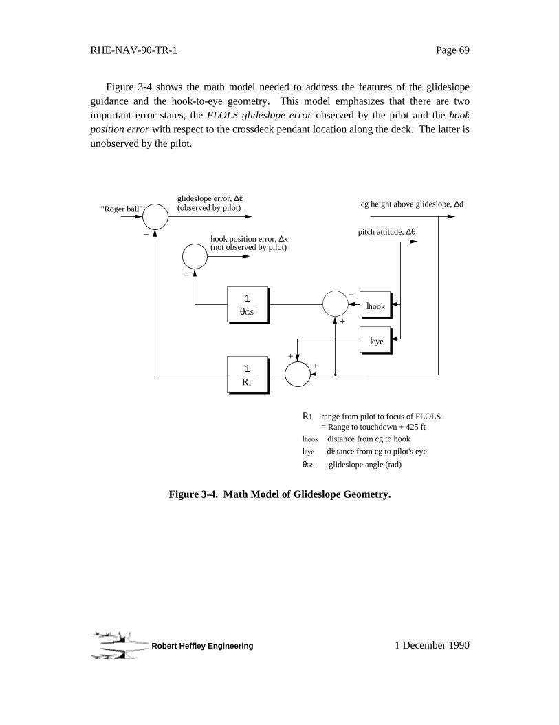
RHE-NAV-90-TR-1 Page 69
Robert Heffley Engineering 1 December 1990
Figure 3-4 shows the math model needed to address the features of the glideslopeguidance and the hook-to-eye geometry. This model emphasizes that there are twoimportant error states, the FLOLS glideslope error observed by the pilot and the hookposition error with respect to the crossdeck pendant location along the deck. The latter isunobserved by the pilot.
pitch attitude, ∆θ
cg height above glideslope, ∆d
hook position error, ∆x(not observed by pilot)
glideslope error, ∆ε(observed by pilot)
−
−
−1θGS
1R1
leye
lhook
+
++
•
"Roger ball"
R1 range from pilot to focus of FLOLS = Range to touchdown + 425 ft
lhook distance from cg to hook
leye distance from cg to pilot's eye
θGS glideslope angle (rad)
Figure 3-4. Math Model of Glideslope Geometry.
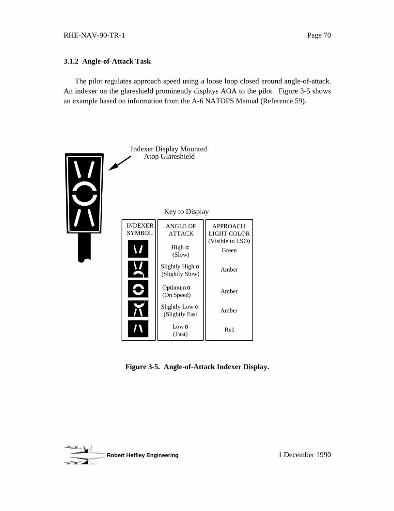
RHE-NAV-90-TR-1 Page 70
Robert Heffley Engineering 1 December 1990
3.1.2 Angle-of-Attack Task
The pilot regulates approach speed using a loose loop closed around angle-of-attack.An indexer on the glareshield prominently displays AOA to the pilot. Figure 3-5 showsan example based on information from the A-6 NATOPS Manual (Reference 59).
Figure 3-5. Angle-of-Attack Indexer Display.
Indexer Display MountedAtop Glareshield
INDEXERSYMBOL
ANGLE OF ATTACK
APPROACHLIGHT COLOR(Visible to LSO)
High α(Slow)
Slightly High α(Slightly Slow)
Optimum α(On Speed)
Slightly Low α(Slightly Fast
Low α(Fast)
Green
Amber
Amber
Amber
Red
Key to Display

RHE-NAV-90-TR-1 Page 71
Robert Heffley Engineering 1 December 1990
The angle of attack error observed by the pilot is essentially a linear function of thetrue α, and this is shown in Figure 3-6. It is important to note that the same aircraft statevariables are involved (∆ θ and the derivative of ∆ d). Figure 3-6 diagrams this only toemphasize the point. Its significance will be discussed in subsequent sections.
pitch attitude, ∆θ
cg vertical velocity, ∆d
AOA error observed on indexer
−
1V
+
V true airspeed
bΑΟΑ AOA system bias
KAOA AOA system proportionality factor
−
.
flightpath angle, ∆γ
+
ΚΑΟΑ+
bΑΟΑ
+
Figure 3-6. Math Model of AOA Display.

RHE-NAV-90-TR-1 Page 72
Robert Heffley Engineering 1 December 1990
3.1.3 Lineup Task
The pilot gets lateral flightpath information mainly through the perspective view ofthe landing area as in a normal field landing. The essential features shown in Figure 3-7are the canted deck centerline, dropline, and horizon (if visible). From the pilot'sviewpoint, the angle, λ, indicates the lateral offset between the deck centerline and eitherthe horizon or the vertical dropline extending off the stern of the ship. The former wouldbe more useful under normal daytime conditions, and the latter at night.
λ arctan(y/h) where y is lateral offset and h is altitude above deck.
dropline (vertical reference)
landing area
λ
horizon
Figure 3-7. Lineup Geometry.
RHE-NAV-90-TR-1 Page 73
Robert Heffley Engineering 1 December 1990
3.2 Aircraft and Flight Control Systems (Vehicle)
The math models used to describe the aircraft and its flight control systems typicallycan vary greatly both in form and complexity. The main requirement is that the dynamicsof the model are correct in the spectral range of interest and appropriate to the pilotingtask considered.
Traditional flying qualities are concerned with characteristics represented by thehigher-frequency classical response modes (short-period, Dutch-roll, and roll).Therefore, requirements address natural frequency, damping, response times, manipulatorsensitivity, and manipulator feel. Other lower-frequency-regime features are alsocovered by flying qualities. It is correct to associate items such as phugoid and spiralwith unattended operation than with closed-loop control.
One problem with the traditional way of viewing aircraft dynamics is that whenfocusing on the outer-loops, the high overhead in complexity associated with inner-loopfeatures distracts the analyst. This is true even when dealing with a basic unaugmentedaircraft, and complex flight control systems compound it.
There is a great practical advantage to partitioning inner- and outer-loop features.One benefit is the analyst's understanding of the physical system. Another is thatcalculations are simple and checkable with reasonable effort. Finally, it is usuallycheaper and faster to begin systems analysis with minimal simplicity and increasecomplexity as needed than it is to do the reverse. This, then, is the motivation for thetechnical approach introduced earlier in Section 1, namely, the use of pitch-constrainedequations of motion.
3.2.1 Pitch-Constrained Equations of Motion
The system analyst realizes considerable benefit by assuming the pilot is activelymanaging attitude. For examination of outer-loop features, one can rearrange the systemarchitecture as Figure 3-8 illustrates. The traditional architecture must lump airframe,engine, and flight control system into a complex, high-order system and include thepilot's regulation of the inner control loops around pitch attitude and, possibly, thrust(Figure 3-8a.). On the other hand, by the implicit assumption of good inner-loopregulation, the three major components (airframe, engine, and FCS) can be separated andeach modeled as low-order systems (Figure 3-8b). Another major benefit is the removalof explicit inner-loop feedback paths.
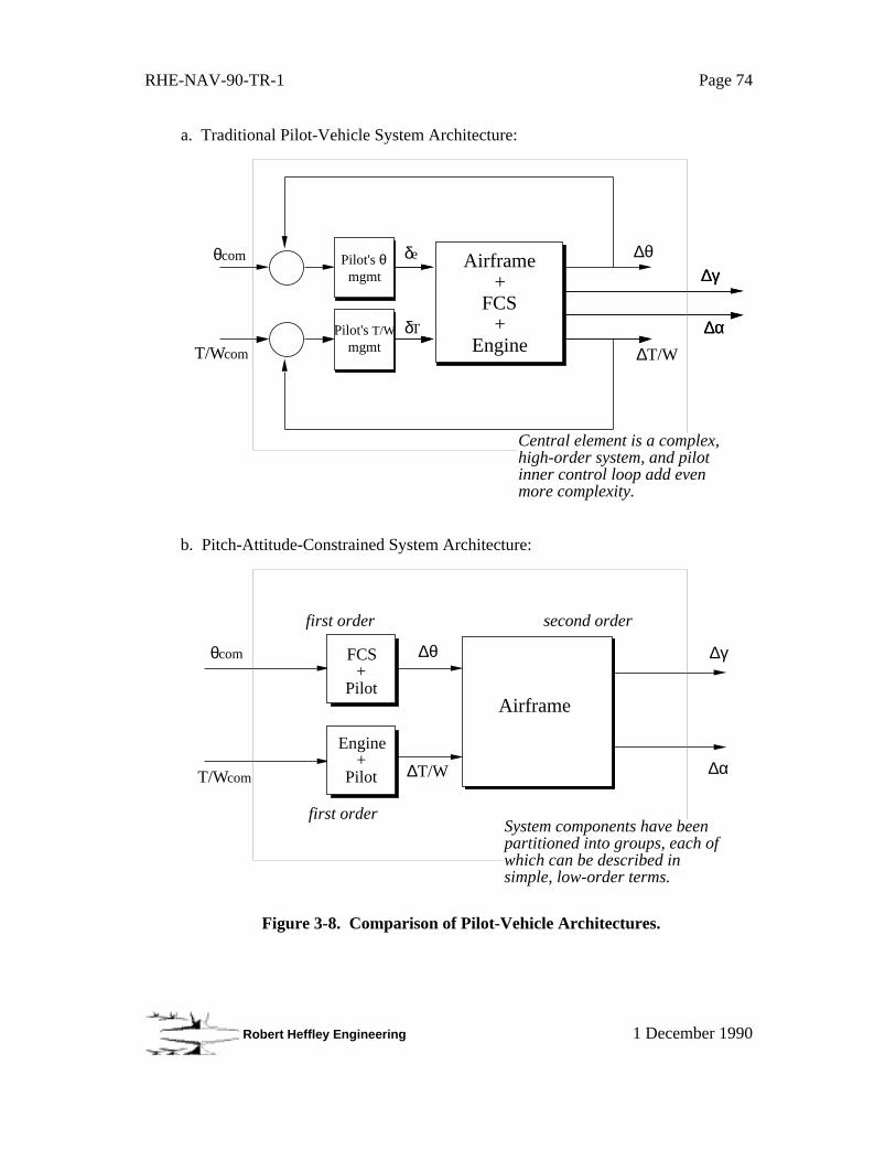
RHE-NAV-90-TR-1 Page 74
Robert Heffley Engineering 1 December 1990
δe
δT
∆θ∆γ
∆α∆T/W
Airframe+
FCS+
Engine
Pilot's θ mgmt
Pilot's T/W mgmt
θcom
T/Wcom
θcom
T/Wcom
∆γ
∆α
∆γ
∆α
∆θ
∆T/W
Airframe
FCS+
Pilot
Engine+
Pilot
a. Traditional Pilot-Vehicle System Architecture:
b. Pitch-Attitude-Constrained System Architecture:
System components have been partitioned into groups, each of which can be described in simple, low-order terms.
Central element is a complex, high-order system, and pilot inner control loop add even more complexity.
second orderfirst order
first order
Figure 3-8. Comparison of Pilot-Vehicle Architectures.

RHE-NAV-90-TR-1 Page 75
Robert Heffley Engineering 1 December 1990
The airframe component needs to be described only by “trimmed” lift and drag data.The FCS and engine blocks each can be represented by an effective lag or by the closed-loop pilot-engine or pilot-FCS bandwidth,26 whichever is considered more appropriate.Because of the spectral separation of engine and FCS from flightpath and speed, thespecific details of the engine and FCS blocks are generally not so influential as theairframe lift and drag. Therefore the main outer-loop system factors can be summarizedby the simple second-order system description given in Table 3-1.
The factors that comprise the Laplace-transform denominator and numerators listedabove are easy to compute. The data required are few and estimates are not difficultshould some data not be available. Table 3-2 gives a list of approximate factors.Approximate-factors relationships are useful for describing the primary audit trailbetween aircraft design features and control characteristics. Some approximate factorsare fairly accurate and imply ways for selecting specification parameters and criteria.
26This refers to the effective aggressiveness that the pilot exhibits when actively regulating pitch or thrust.
Normally it is sufficient to assume a simple first-order lag which is matched to the level of aggressiveness.
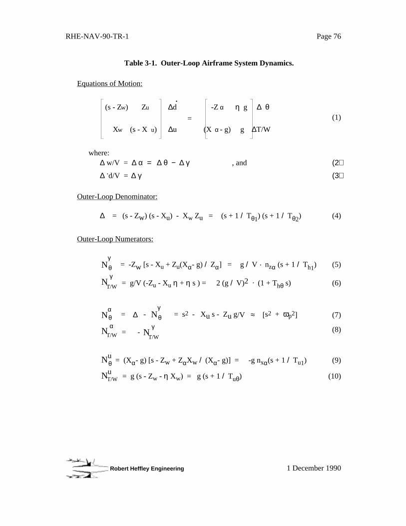
RHE-NAV-90-TR-1 Page 76
Robert Heffley Engineering 1 December 1990
Table 3-1. Outer-Loop Airframe System Dynamics.
Equations of Motion:
(s - Zw) Zu ∆d -Z α η g ∆ θ =
Xw (s - X u) ∆u (X α - g) g ∆T/W
˙(1)
where:∆ w/V = ∆ α = ∆ θ − ∆ γ , and (2)
∆ .d/V = ∆ γ (3)
Outer-Loop Denominator:
∆ = (s - Zw) (s - Xu) - Xw Zu = (s + 1 / Tθ1) (s + 1 / Tθ2) (4)
Outer-Loop Numerators:
γNθ = -Zw [s - Xu + Zu(Xα- g) / Zα] = g / V · nzα (s + 1 / Th1) (5)
γN
T/W = g/V (-Zu - Xu η + η s ) = 2 (g / V)2 · (1 + Thθ s) (6)
αNθ
= ∆ - γ
Nθ = s2 - Xu s - Zu g/V ≈ [s2 + ωp2] (7)
αNT/W
= - γ
NT/W
(8)
Nθu
= (Xα- g) [s - Zw + ZαXw / (Xα- g)] = -g nxα(s + 1 / Tu1) (9)
NuT/W = g (s - Zw -
η Xw) = g (s + 1 / Tuθ) (10)

RHE-NAV-90-TR-1 Page 77
Robert Heffley Engineering 1 December 1990
Table 3-2. Outer-Loop Approximate Factors.
Xu = -ρVSCD / m = -2g / V · CD / CL (11)
Xw = ρSV(CL-CDα) / 2m = g / V · (1 - CDα / CL) = g / V · (1 - nxα) (12)
Zu = -ρVSCL / m = -2g / V (13)
Zw† = -ρVS (CLα+CD) / 2m (where Zw
† , Zα† , nzα based on trim CLα) (14)
Zα† = V · Zw = -g nzα (15)
Xα - g = -g nxα (16)
ZTW = - η g (17)
XTW = g (18)
nzα = (CLα + CD) / CL ≈ CLα / CL (19)
nxα = CDα / CL ≈ 2CLα / (π · AR · e) (for a parabolic drag polar) (20)
1 / Tθ2 = g / V (nzα2 - 1) / nzα ≈ g / V nzα (21)
1 / Tθ1 = g / V · 2 / nzα + 1 / Th1 = g / V · 2 / nzα - g · ∂ γ / ∂ V (22)
1 / Th1 = -g · ∂ γ / ∂ V (23)
Thθ = η/2· V/g (24)
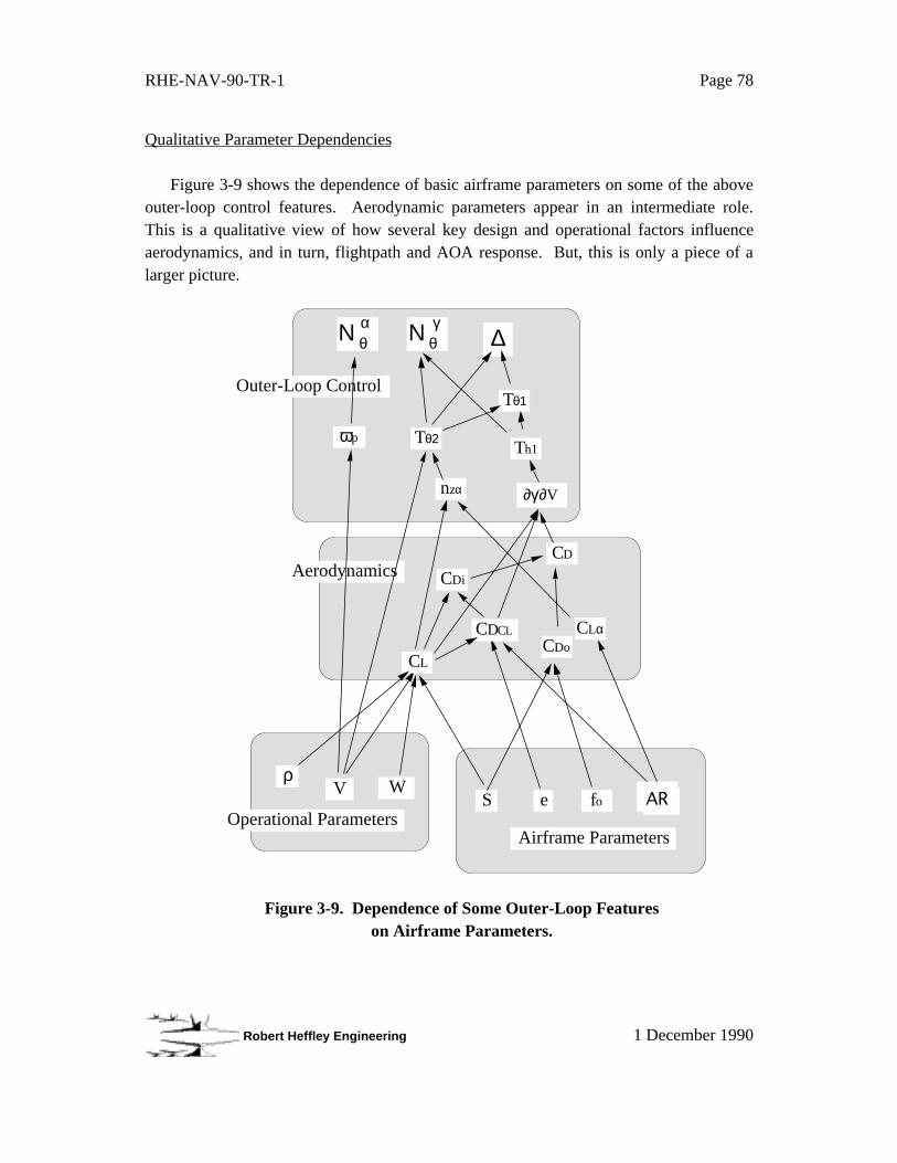
RHE-NAV-90-TR-1 Page 78
Robert Heffley Engineering 1 December 1990
Qualitative Parameter Dependencies
Figure 3-9 shows the dependence of basic airframe parameters on some of the aboveouter-loop control features. Aerodynamic parameters appear in an intermediate role.This is a qualitative view of how several key design and operational factors influenceaerodynamics, and in turn, flightpath and AOA response. But, this is only a piece of alarger picture.
Vρ
WS e fo
CL
CD
CDo
Tθ2
CLαCDCL
CDi
nzα
Tθ1
Th1
Aerodynamics
∂γ/∂V
Outer-Loop Control
Airframe Parameters Operational Parameters
Ν θγ
∆Ν θα
ωp
Figure 3-9. Dependence of Some Outer-Loop Featureson Airframe Parameters.

RHE-NAV-90-TR-1 Page 79
Robert Heffley Engineering 1 December 1990
One can construct a similar, more complete diagram to track other features such asthe thrust response numerators, speed margin, trim attitude, and other approach-speedcriteria. Figure 3-10 presents this view. Note the added role of engine parameters.
V W
S e fo δflaps
CL
CD
CDo
Tθ2
CLα
CDCL
CDi
nzα
Tθ1
Th1
Aerodynamic Factors
∂γ/∂V
iT
CLo
α
ηg/V
Thθ
Outer-Loop Control Factors
Airframe Parameters
Operational Parameters
T50'
CLmax
δslats
V/Vs
θfov
visibility
T/W
Ν θγ
∆Ν θα Ν γΝTW
αTW
ωp
αpk
∆ax
L/D
Teng
Engine Parameters
T90%
Approach Speed Criteria
To/W
ρ γο
-∆γ+∆γ
BPR
Figure 3-10. Dependence of Approach Speed Criteriaon Airframe and Engine Parameters.

RHE-NAV-90-TR-1 Page 80
Robert Heffley Engineering 1 December 1990
3.2.2 Outer-Loop Response Characteristics
The goodness of the reduced-order math model can be observed in the followingseries of plots. This is done for a set of typical response characteristics and can be easilyrepeated for any specific aircraft. The numerical values assumed are:
Tθ2 = 2 sec
Tθ1 = 10 sec
1 / Th1 = 0 (neutral backside)
The purpose of this section is to illustrate the general effect of various aircraftfeatures to justify the modeling assumptions made above. This begins with higher-orderfeatures included then progressively dropped.

RHE-NAV-90-TR-1 Page 81
Robert Heffley Engineering 1 December 1990
High-Order Model, Including Pitch Dynamics
First, consider the case for which there is no pitch-constrained assumption, that is,inclusion of all higher-order dynamics. Figure 3-11 shows the pitch attitude, flightpath,and angle of attack responses for a tight inner-loop regulation of pitch (damping ratio 0.7and closed-loop natural frequency of 3 rad/sec). The step command of pitch attitude hasa small overshoot but quickly settles to the commanded value (unity). There is evidenceof the initial downward motion of the cg, followed by a short-term rise, then eventualbleedoff with loss of airspeed.
-0.2
0
0.2
0.4
0.6
0.8
1.0
1.2
0 5 10 15 20
tightly-regulated pitch attitude step command
flightpath rises quickly (T ) then decays slowly (T )
angle of attack rises with pitch then immediately decays as flightpath builds and finally bleeds up as flightpath decays
Time (sec)
Res
pons
e R
elat
ive
to P
itch
Com
man
d
small initial reversal of flightpath at cg
∆γ
∆θ
∆α
Figure 3-11. High-Order System Response to a Pitch Step.
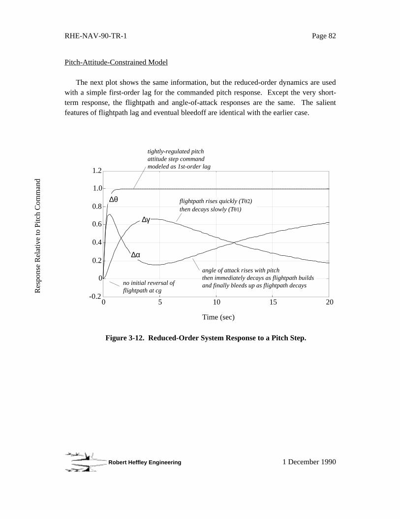
RHE-NAV-90-TR-1 Page 82
Robert Heffley Engineering 1 December 1990
Pitch-Attitude-Constrained Model
The next plot shows the same information, but the reduced-order dynamics are usedwith a simple first-order lag for the commanded pitch response. Except the very short-term response, the flightpath and angle-of-attack responses are the same. The salientfeatures of flightpath lag and eventual bleedoff are identical with the earlier case.
-0.2
0
0.2
0.4
0.6
0.8
1.0
1.2
0 5 10 15 20
no initial reversal of flightpath at cg
tightly-regulated pitch attitude step command modeled as 1st-order lag
flightpath rises quickly (T ) then decays slowly (T )
angle of attack rises with pitch then immediately decays as flightpath builds and finally bleeds up as flightpath decays
Time (sec)
Res
pons
e R
elat
ive
to P
itch
Com
man
d
∆γ
∆θ
∆α
Figure 3-12. Reduced-Order System Response to a Pitch Step.
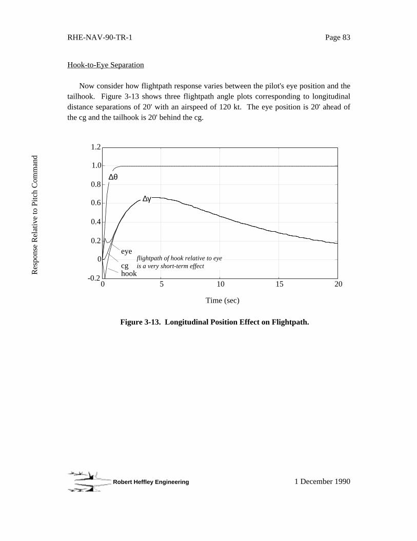
RHE-NAV-90-TR-1 Page 83
Robert Heffley Engineering 1 December 1990
Hook-to-Eye Separation
Now consider how flightpath response varies between the pilot's eye position and thetailhook. Figure 3-13 shows three flightpath angle plots corresponding to longitudinaldistance separations of 20' with an airspeed of 120 kt. The eye position is 20' ahead ofthe cg and the tailhook is 20' behind the cg.
-0.2
0
0.2
0.4
0.6
0.8
1.0
1.2
0 5 10 15 20
flightpath of hook relative to eye is a very short-term effect
Time (sec)
Res
pons
e R
elat
ive
to P
itch
Com
man
d
cg hook
eye
∆θ
∆γ
Figure 3-13. Longitudinal Position Effect on Flightpath.

RHE-NAV-90-TR-1 Page 84
Robert Heffley Engineering 1 December 1990
Short-Term Flightpath Response
Next, using a shorter time scale, Figure 3-14 shows the theoretical relationshipbetween pitch attitude and flightpath angle. This assumes that speed is maintained withthrust (and that angle of attack, in the long term, is held constant). Note that Tθ2represents the effective lag time constant. The essential parameters are simply trueairspeed, lift-curve-slope, and lift coefficient. These can be expressed in several waysand in terms of several other conventional parameters.
0
0.2
0.4
0.6
0.8
1.0
1.2
0 1 2 3 4 5
Time (sec)
Res
pons
e
θ
γ
ω = 1.5 rad/sec
ζ = 0.6n = 4 g/radV = 200 ft/sec
zαTa
sp
sp
attitude rise time
approximately T
flight path rise time
T ≈ 1.5θ2
Figure 3-14. Relationship Between Pitch Attitude and Flightpath Angle.

RHE-NAV-90-TR-1 Page 85
Robert Heffley Engineering 1 December 1990
Flightpath Response to Thrust
Inspection of the flightpath-to-thrust transfer function shows that the dominantresponse modes are both 1/Tθ1 and 1/Tθ2 (a double lag). Engine lag also adds to this.
Thrust inclination angle relative to the velocity vector, η, produces a lead effect that cancounter the thrust lag. Ten degrees thrust inclination produces about 0.5 sec lead if theapproach speed is about 120 kt.
-0.2
0
0.2
0.4
0.6
0.8
1.0
1.2
0 5 10 15 20
flightpath responds to thrust as a double lag (T + T ) plus the engine lage, Teng
Time (sec)
Res
pons
e R
elat
ive
to T
hrus
t Com
man
d
∆γ
∆T/W
η = 20° 10°0
thrust inclination produces a lead effect corresponding to the numerator factor Th
Figure 3-15. Flightpath Response to Thrust.
RHE-NAV-90-TR-1 Page 86
Robert Heffley Engineering 1 December 1990
3.3 Pilot and Task Control Strategy (Pilot)
The pilot and task control strategy models are the key elements that lead toidentifying the design factors which govern successful task execution. In their absenceonly an open-loop approach can be taken.
Several important analytical results relate to the effectiveness of competing pilotcontrol strategies. The pilot control strategy as interpreted in engineering terms is crucialto the efficient extraction of performance from the airframe/engine combination. It is atleast as important as the dynamics of the aircraft itself.
Outer-loop control strategy is not easily identified. Further, strategy as viewed inengineering terms, seems sometimes difficult to correlate with pilot-centered descriptions. Some more successful results have been obtained for discrete maneuvers such asthe landing flare (References 60 and 61) or helicopter accel/decel maneuvers (Reference62). In general, simpler analysis techniques seem to work as well or sometimes betterthan more sophisticated ones. Reference 63 contains some lessons learned in this regard.
Control strategy can be defined in terms of the incremental pitch attitude and thrustmade in proportion to the glideslope and angle-of-attack errors seen by the pilot. Further,this strategy can have levels of sophistication ranging from a simple one-control-per-stateto optimal blending of controls that tend to decouple the response. Figure 3-16 diagramsthe two primary general levels of control strategy, compensatory and pursuit, as they areapplied in this report.
The first and most profound feature of pilot control strategy or technique is itsclassification as either compensatory or pursuit (coordinated use of outer-loop controls).There is a fundamental difference in the structure of each, in the efficiency and ease ofmanual control, and in the nature of division-of-attention of the pilot.

RHE-NAV-90-TR-1 Page 87
Robert Heffley Engineering 1 December 1990
γ
αθ
T/Wroger ball
donut
Pilot Airframe/Engine
FLOLS
AOA
γ
αθ
T/Wroger ball
donut
Pilot Airframe/Engine
FLOLS
AOA
"COMPENSATORY" MODE OF CONTROL
"PURSUIT" MODE OF CONTROL
Figure 3-16. The Two Main Control Strategy Structures.
A compensatory level of control is the most elementary strategy and has a singlecontrol for each control variable. The case shown above is the backside case, i. e., thrustused to control glideslope and pitch attitude used to control angle of attack. Manyconsider this as the standard technique employed by navy pilots. It works even at speedsfar on the backside of the thrust-required curve, but it does have serious performancelimitations which shall be discussed.
Another version of the compensatory-level of control is the converse, or the frontsidetechnique. Pitch attitude is the glideslope control and thrust the angle of attack control.

RHE-NAV-90-TR-1 Page 88
Robert Heffley Engineering 1 December 1990
The choice between frontside and backside techniques is not necessarily tied to whetherthe aircraft is operating under the corresponding drag condition as values of either ∂ γ/∂ Vor 1/Th1 indicate.
The pursuit level includes crossfeed paths for the two controls which result indecoupling of responses. The technique is really just a coordination or blending of thrustand pitch attitude controls. For the investment in skill development, the benefit to thepilot is enhancement of performance, especially for glideslope control, and diminishedupset to angle of attack when making a glideslope adjustment.
Each above case is described in detail below.
3.3.1 Compensatory Backside Strategy (Thrust for Control of Flightpath)
The compensatory backside technique control law consists of making a thrustadjustment proportional to a flightpath or glideslope error, and a pitch attitude adjustmentproportional to a speed or angle of attack error. The benefit of this technique is that it issimple and it will always work, even when speeds are well on the frontside. Thedisadvantage is that the quickness of the closed-loop response is greatly limited,especially for a carrier landing. The potential for a highly aggressive last secondglideslope adjustment is much inferior to competing strategies.
One clear way to analyze the backside technique is to consider the response offlightpath to thrust with the angle of attack loop closed around pitch attitude. Theeffectiveness of the strategy can be judged by the quality of ∆ γ response to a step ∆ T/W.Figure 3-17 shows the block diagram of this scheme.

RHE-NAV-90-TR-1 Page 89
Robert Heffley Engineering 1 December 1990
Κα + ΚΙ s
∆T/W
∆θ
∆γ
∆α
airframe+
engineαcom
Figure 3-17. Diagram of Backside Technique.
The main factor in the backside technique is the limitation imposed in the angle-of-attack loop. Namely, as the pilot regulates α more and more aggressively, the dominantclosed-loop response (starting at 1/Tθ1 and 1/Tθ2) migrates to the phugoid and therefore
becomes a lightly-damped second-order response.
To obtain a good closed-loop response shape, the feedback must be an integral-plus-proportional blend, i. e.,
∆ θ = Kα · ∆ α + KI · ∫ ∆ α dt
The relative proportions of KI and Kα need to be set about equal to the phugoid
frequency in order to shape the closed-loop frequency response correctly:
KI /Kα ≈ ωp
Figure 3-18 shows a survey of the closed-loop response. The first two plots showflightpath and angle of attack, respectively, for a step in thrust with the angle-of-attackloop closed (according to the above block diagram). Note that flightpath responserequires 10 to 15 seconds during which time the angle of attack starts to bleed down.Only aggressive angle-of-attack regulation minimizes this, but the level of aggressivenessis limited to a crossover frequency less than the phugoid frequency (about 0.2 rad/sec).
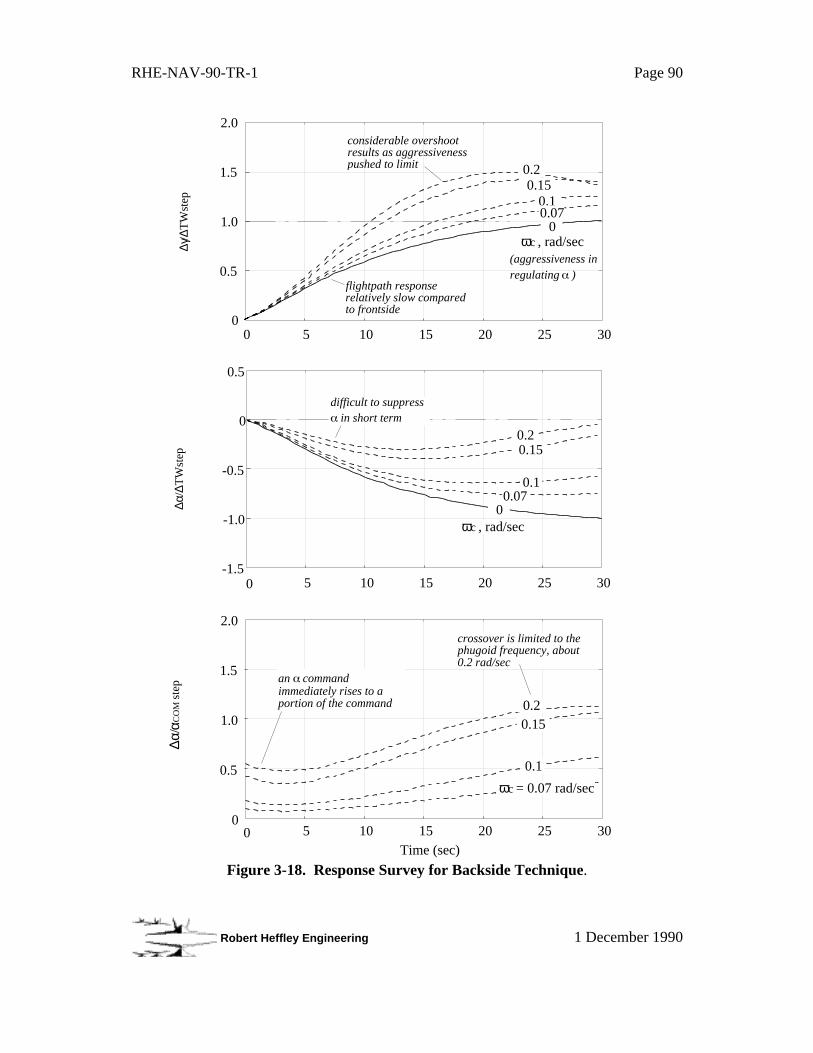
RHE-NAV-90-TR-1 Page 90
Robert Heffley Engineering 1 December 1990
0
0.5
1.0
1.5
2.0
0 5 10 15 20 25 30
∆γ/∆
TW
step
considerable overshoot results as aggressiveness pushed to limit
ωc , rad/sec
0.10.15
0.2
00.07
(aggressiveness in regulating )
flightpath response relatively slow compared to frontside
-1.5
-1.0
-0.5
0
0.5
∆α/∆
TW
step
ωc , rad/sec
5 10 15 20 25 30
difficult to suppress in short term
0
0.1
0.150.2
00.07
∆α/α
CO
M s
tep an command
immediately rises to a portion of the command
crossover is limited to the phugoid frequency, about 0.2 rad/sec
Time (sec)5 10 15 20 25 300
0
0.5
1.0
1.5
2.0
ωc = 0.07 rad/sec
0.1
0.150.2
Figure 3-18. Response Survey for Backside Technique.
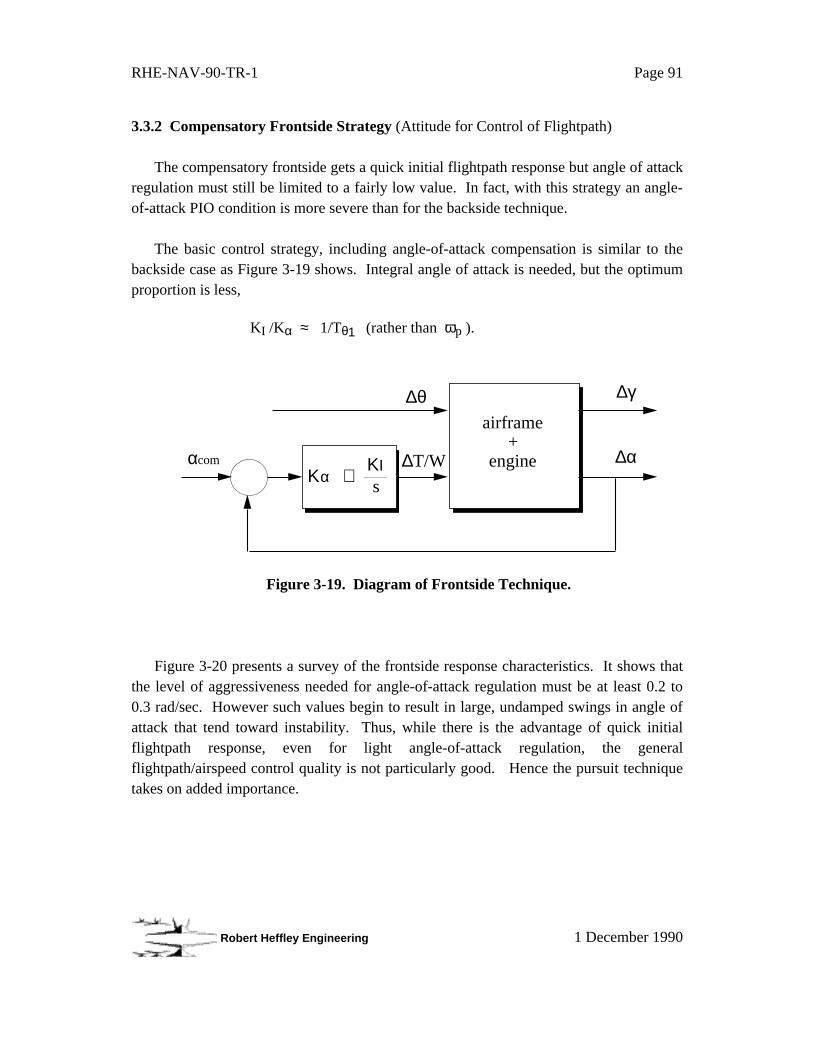
RHE-NAV-90-TR-1 Page 91
Robert Heffley Engineering 1 December 1990
3.3.2 Compensatory Frontside Strategy (Attitude for Control of Flightpath)
The compensatory frontside gets a quick initial flightpath response but angle of attackregulation must still be limited to a fairly low value. In fact, with this strategy an angle-of-attack PIO condition is more severe than for the backside technique.
The basic control strategy, including angle-of-attack compensation is similar to thebackside case as Figure 3-19 shows. Integral angle of attack is needed, but the optimumproportion is less,
KI /Kα ≈ 1/Tθ1 (rather than ωp ).
Κα + ΚΙ s
∆T/W
∆θ ∆γ
∆α
airframe+
engineαcom
Figure 3-19. Diagram of Frontside Technique.
Figure 3-20 presents a survey of the frontside response characteristics. It shows thatthe level of aggressiveness needed for angle-of-attack regulation must be at least 0.2 to0.3 rad/sec. However such values begin to result in large, undamped swings in angle ofattack that tend toward instability. Thus, while there is the advantage of quick initialflightpath response, even for light angle-of-attack regulation, the generalflightpath/airspeed control quality is not particularly good. Hence the pursuit techniquetakes on added importance.
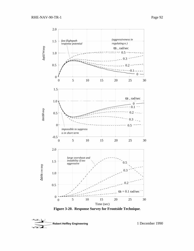
RHE-NAV-90-TR-1 Page 92
Robert Heffley Engineering 1 December 1990
0
0.5
1.0
1.5
2.0
0 5 10 15 20 25 30
∆γ/∆
TW
step ωc , rad/sec
(aggressiveness in regulating )
0.1
0.2
0
0.3
0.5
fast flightpath response potential
-0.5
0
0.5
1.0
1.5
∆α/∆
θ st
ep
ωc , rad/sec
5 10 15 20 25 30
impossible to suppress in short term
0
0.1
0.2
0
0.3
0.5
∆α/α
CO
M s
tep
Time (sec)5 10 15 20 25 300
0
0.5
1.0
1.5
2.0
ωc = 0.1 rad/sec
0.2
0.3
0.5
large overshoot and instability if too aggressive
Figure 3-20. Response Survey for Frontside Technique.
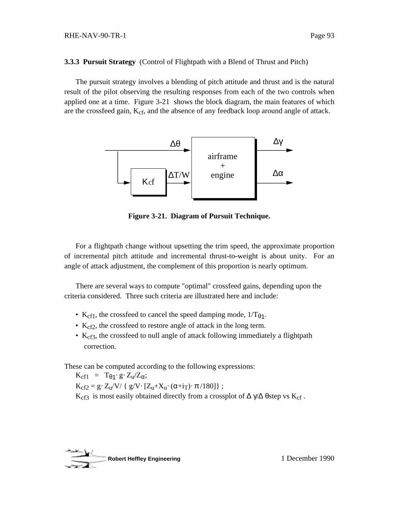
RHE-NAV-90-TR-1 Page 93
Robert Heffley Engineering 1 December 1990
3.3.3 Pursuit Strategy (Control of Flightpath with a Blend of Thrust and Pitch)
The pursuit strategy involves a blending of pitch attitude and thrust and is the naturalresult of the pilot observing the resulting responses from each of the two controls whenapplied one at a time. Figure 3-21 shows the block diagram, the main features of whichare the crossfeed gain, Kcf, and the absence of any feedback loop around angle of attack.
Κcf∆T/W
∆θ ∆γ
∆α
airframe+
engine
Figure 3-21. Diagram of Pursuit Technique.
For a flightpath change without upsetting the trim speed, the approximate proportionof incremental pitch attitude and incremental thrust-to-weight is about unity. For anangle of attack adjustment, the complement of this proportion is nearly optimum.
There are several ways to compute "optimal" crossfeed gains, depending upon thecriteria considered. Three such criteria are illustrated here and include:
• Kcf1, the crossfeed to cancel the speed damping mode, 1/Tθ1.
• Kcf2, the crossfeed to restore angle of attack in the long term.• Kcf3, the crossfeed to null angle of attack following immediately a flightpath
correction.
These can be computed according to the following expressions:Kcf1 = Tθ1· g· Zu/Zα;
Kcf2 = g· Zu/V/ { g/V· [Zu+Xu· (α+iT)· π /180]} ;Kcf3 is most easily obtained directly from a crossplot of ∆ γ/∆ θstep vs Kcf .
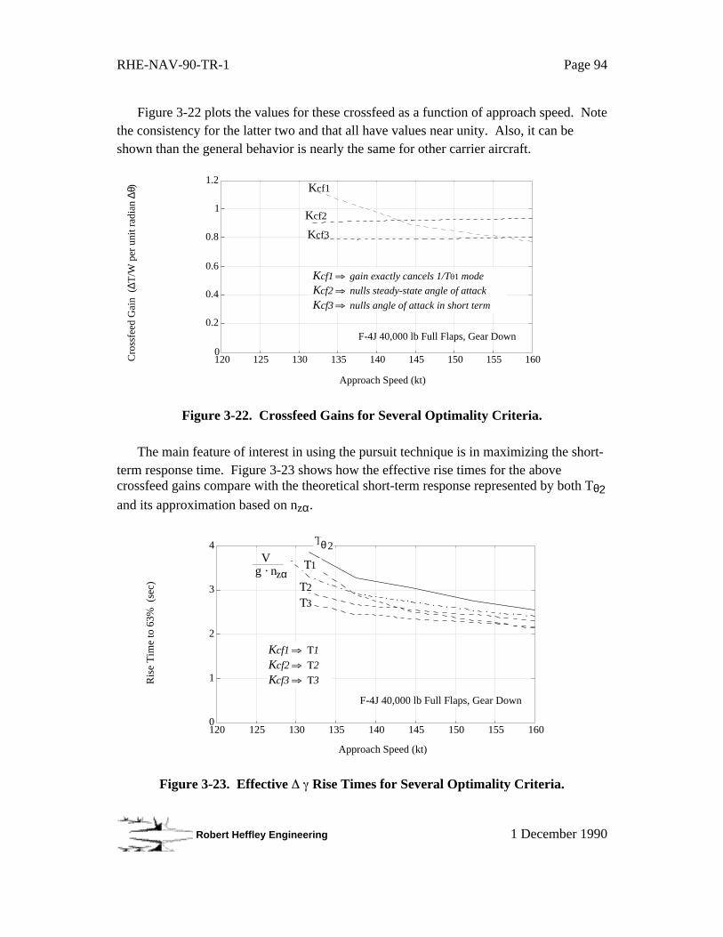
RHE-NAV-90-TR-1 Page 94
Robert Heffley Engineering 1 December 1990
Figure 3-22 plots the values for these crossfeed as a function of approach speed. Notethe consistency for the latter two and that all have values near unity. Also, it can beshown than the general behavior is nearly the same for other carrier aircraft.
0
0.2
0.4
0.6
0.8
1
1.2
120 125 130 135 140 145 150 155 160
F-4J 40,000 lb Full Flaps, Gear Down
Kcf1
Cro
ssfe
ed G
ain
(∆T
/W p
er u
nit r
adia
n ∆θ
)
Approach Speed (kt)
Kcf2
Kcf3
Kcf1 gain exactly cancels 1/T mode
Kcf2 nulls steady-state angle of attack
Kcf3 nulls angle of attack in short term
Figure 3-22. Crossfeed Gains for Several Optimality Criteria.
The main feature of interest in using the pursuit technique is in maximizing the short-term response time. Figure 3-23 shows how the effective rise times for the abovecrossfeed gains compare with the theoretical short-term response represented by both Tθ2and its approximation based on nzα.
0
1
2
3
4
120 125 130 135 140 145 150 155 160
T 2θV
g · nzαT1
T2
T3
Ris
e T
ime
to 6
3% (
sec)
F-4J 40,000 lb Full Flaps, Gear Down
Approach Speed (kt)
Kcf1 1
Kcf2 2
Kcf3 3
Figure 3-23. Effective Rise Times for Several Optimality Criteria.
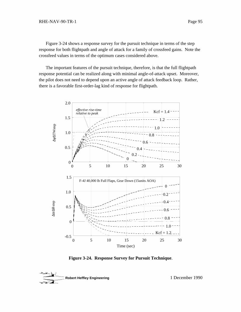
RHE-NAV-90-TR-1 Page 95
Robert Heffley Engineering 1 December 1990
Figure 3-24 shows a response survey for the pursuit technique in terms of the stepresponse for both flightpath and angle of attack for a family of crossfeed gains. Note thecrossfeed values in terms of the optimum cases considered above.
The important features of the pursuit technique, therefore, is that the full flightpathresponse potential can be realized along with minimal angle-of-attack upset. Moreover,the pilot does not need to depend upon an active angle of attack feedback loop. Rather,there is a favorable first-order-lag kind of response for flightpath.
0
0.5
1.0
1.5
2.0
∆γ/∆
TW
step
5 10 15 20 25 300
Kcf = 1.4
1.0
0.8
0.6
0.4
0.2 0
1.2
effective rise-time relative to peak
-0.5
0
0.5
1.0
1.5
∆α/∆
θ st
ep
5 10 15 20 25 300Time (sec)
F-4J 40,000 lb Full Flaps, Gear Down (15units AOA)
Kcf = 1.2
1.0
0.8
0.6
0.4
0.2
0
Figure 3-24. Response Survey for Pursuit Technique.
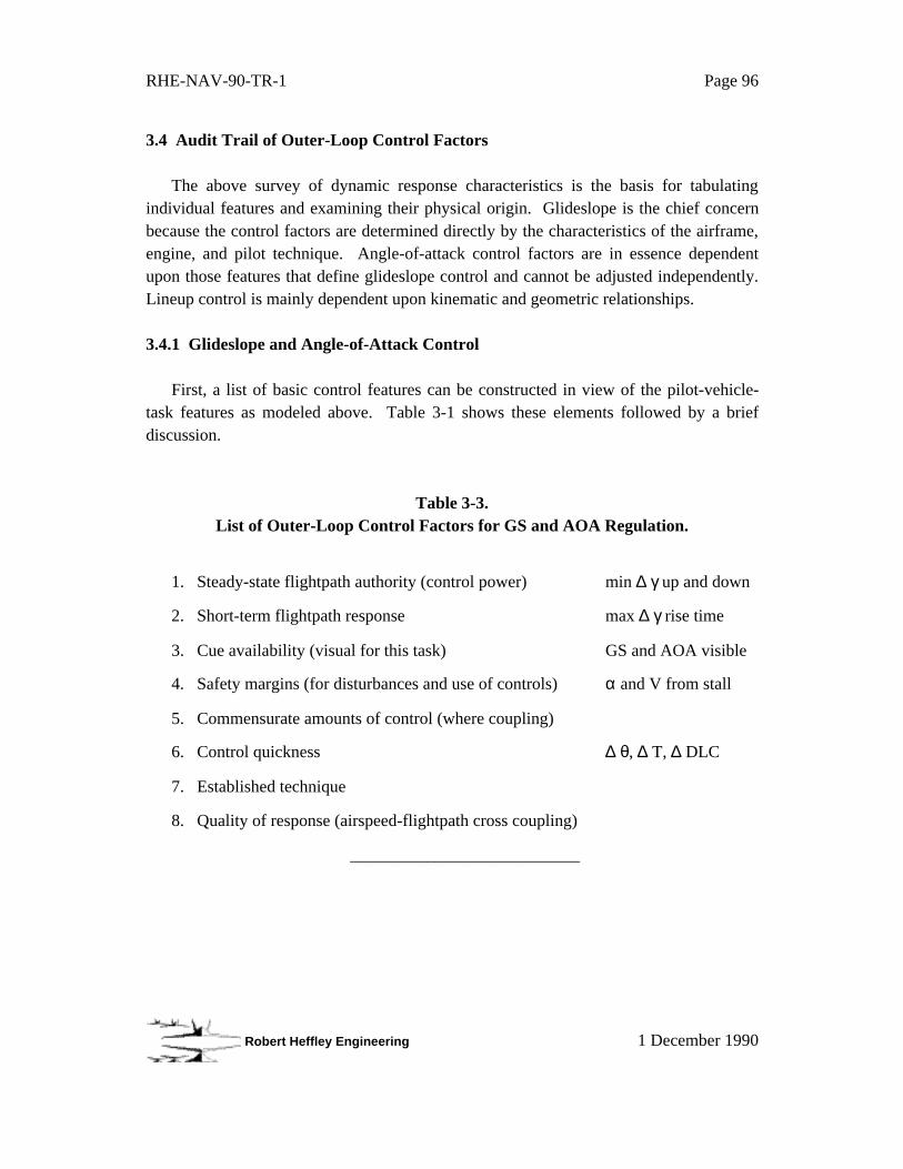
RHE-NAV-90-TR-1 Page 96
Robert Heffley Engineering 1 December 1990
3.4 Audit Trail of Outer-Loop Control Factors
The above survey of dynamic response characteristics is the basis for tabulatingindividual features and examining their physical origin. Glideslope is the chief concernbecause the control factors are determined directly by the characteristics of the airframe,engine, and pilot technique. Angle-of-attack control factors are in essence dependentupon those features that define glideslope control and cannot be adjusted independently.Lineup control is mainly dependent upon kinematic and geometric relationships.
3.4.1 Glideslope and Angle-of-Attack Control
First, a list of basic control features can be constructed in view of the pilot-vehicle-task features as modeled above. Table 3-1 shows these elements followed by a briefdiscussion.
Table 3-3.List of Outer-Loop Control Factors for GS and AOA Regulation.
1. Steady-state flightpath authority (control power) min ∆ γ up and down
2. Short-term flightpath response max ∆ γ rise time
3. Cue availability (visual for this task) GS and AOA visible
4. Safety margins (for disturbances and use of controls) α and V from stall
5. Commensurate amounts of control (where coupling)
6. Control quickness ∆ θ, ∆ T, ∆ DLC
7. Established technique
8. Quality of response (airspeed-flightpath cross coupling)
___________________________
RHE-NAV-90-TR-1 Page 97
Robert Heffley Engineering 1 December 1990
Steady-State Flightpath Authority
Steady-state flightpath authority is the ability to sustain an adjustment in flightpath. Itcan be represented either by the steady-state flightpath angle or vertical velocity. Itshould be taken with respect to the prescribed on-glideslope flightpath angle and mustinclude the ability to make both upward and downward corrections.
Because angle of attack is maintained in the long term, a sustained flightpath changecorresponds to a net change in thrust-to-weight from the on-glideslope condition.Therefore maximum thrust bounds one extreme and minimum thrust the other. Undersome conditions a speedbrake device might offer a means for modifying the thrust limits.
Short-Term Flightpath Response
The short-term flightpath response is a major limitation on the maximum-achievableaggressiveness in controlling flightpath. It can be a strong function of both the airframelift and drag and of the pilot technique used.
Short-term response can be defined in several ways. Its main feature is the timerequired to obtain a significant amount of the peak response. This can be expressed inboth the time and frequency domains. Perhaps the simplest and most useful metric is therise time to some given level of the peak or steady-state value. The rise-time-to 63% isparticularly popular because that factor can be viewed directly as the equivalent timeconstant for a first-order lag.
Cue Availability
Clear and timely cues are fundamental to any precise control situation. The carrierapproach task relies upon visual display of glideslope and lineup from the FLOLS anddeck geometry, respectively. The AOA indexer or HUD displays angle of attack directly.
Control cues also might be included under this item as they too are crucial to theouter-loop control task. Pitch and roll attitudes, both are implicit given that the ship isvisible. Engine cue quality is not clearly defined. In some aircraft the engine noise is sosubtle that unusual substitutes are sometimes used.27 Forcing the pilot to refer to cockpitgages is an unacceptable choice because of the delay introduced in the control loop.
27For example, in the A-7 without power indication displayed on the HUD, the pilot may use the change in
air conditioner flow as a substitute cue for thrust change.
RHE-NAV-90-TR-1 Page 98
Robert Heffley Engineering 1 December 1990
Safety Margins
Large-amplitude corrections must be made without encountering unsafe conditions.Normally aerodynamic stall is the main condition that is considered. There are at leasttwo main safety problems. One is the need to absorb both normal and tangential gustcomponents with minimal flightpath effects. The other is the ability to use the amount ofpitch control necessary without excessive α excursions.
There may be other safety margins that need to be defined. For example, it may beappropriate also to view a thrust setting resulting in excessive engine lag as a safety-margin situation. This would be crucial where the pilot reduces power to steepenflightpath then must quickly add power to regain the desired flightpath angle.
Commensurate Amounts of Control
Whenever more than one control is involved in the management of a state variable,there must be amounts of each control available that is commensurate with the desiredcontrol authority. For example, the pursuit-level technique requires use of both pitchattitude and thrust to make a given flightpath angle change. Neither pitch nor thrust canbe deficient.
The nature of control limits can vary. For example, a large upward flightpathcorrection might involve an excessive pitchup (too near stall) while more-than-adequatethrust is available. A large downward correction is more likely to encounter an aftthrottle limit while nose down pitch is limited only to the available pitching moment.
Control Quickness
The outer-loop controls (pitch, thrust, bank angle) must be sufficiently quick for thepilot to use them in controlling an outer-loop control state. As a general rule-of-thumb,the response of the outer-loop control must be about three times faster than the desiredclosed-loop response.28 For example, if a closed-loop bandwidth of 0.5 rad/sec is desired,the control should have a response of 1.5 rad/sec (or an effective lag of about 0.7seconds).
28This relationship can be shown analytically and has been observed empirically. It arises from thenecessary tradeoff in closed-loop bandwidth and damping when there is a substantial lag or delay in acontrol mechanism compared to the dominant lag in the system being controlled. Reference 37 provides anexplanation.
RHE-NAV-90-TR-1 Page 99
Robert Heffley Engineering 1 December 1990
The pitch-response bandwidth or short-period requirements of the current flyingqualities specifications represent a boundary on outer-loop control quickness for the pitchcontrol. Thrust response is similarly bounded by VPA criteria and will be discussed in
Section 4.2.
The experience in development of flying qualities criteria has shown that anyrequirement on control quickness needs to factor in the qualities of the manipulator andof the display. This seems particularly crucial for the engine for which the throttlemanipulator is a non-centering, high-friction device and the display ordinarily is subtleaural pitch and amplitude variations.
Established Technique
Several of the outer-loop control features depend upon the pilot technique. Forexample, Section 3.3 shows the dramatic difference in short-term response betweencompensatory frontside and backside techniques. Or, the use of DLC will generallyproduce different response features than pitch attitude. Therefore, the above outer-loopcontrol factors need to be defined in terms of some reasonable control techniqueassumption.
Quality of Response
This category includes two main features that may not be satisfactorily covered byany of the other categories. For glideslope control these are speed damping, Tθ1, and
backsidedness, ∂γ/∂V. These qualities show up as long-term degradations in the response,generally seen as washout of flightpath response following a pitch control input.
The speed damping effect is a true washout effect and reflects how quickly theaircraft is convected axially due to aerodynamic and inertial forces. For an aircraft in theapproach configuration, the response mode, 1/Tθ1, covaries with the dominant glideslopemode, 1/Tθ2. Therefore it is not particularly feasible to set independent standards.Nevertheless Reference 3 indicates that 1/Tθ1, when varied, strongly influences pilot
opinion.
The degree of backsidedness, as defined by ∂ γ/∂ V (or 1/Th1), is another aspect of the
quality of response. The effect on the flightpath response is a faster decay, but moreimportantly perhaps, there is a destabilizing effect on flightpath and airspeed for a pathcontrol loop involving the pitch attitude control.

RHE-NAV-90-TR-1 Page 100
Robert Heffley Engineering 1 December 1990
3.4.2 Lineup Control
The following is a tentative list of lineup control factors. The number of items is fewbecause lineup control depends mainly upon coordinated-turn kinematics.
Table 3-4. List of Outer-Loop Control Factors for Lineup Regulation.
1. Short-term lateral flightpath response ∆ ψ, ∆ λ or ∆ y rise time
2. Cue availability (visual for this task) deck LU information
3. Control quickness ∆ φ
___________________________
Short-Term Lateral Flightpath Response
For a coordinated-turn regulation of lateral flightpath there is no direct analogy toheave damping in the short-term response. Instead there is only the net time for lateralflightpath to follow bank angle, given general amount of adverse yaw present. Most ofthe factors involved in this are a complex result of the roll and yaw moments produced byaerodynamics and the FCS. Use of a direct sideforce device would be a special case.
Cue Availability
Control of lineup requires visibility of the landing area and deck centerline relative toeither the horizon or vertical dropline. In general, satisfaction of the FLOLS visibilityrequirement would be sufficient for lineup cues also.
Control Quickness
Control quickness for lineup equates to the inner-loop bank angle responsecharacteristics. This will be a strong function of the natural roll damping or, ifaugmented in the roll axis, the artificial roll damping. Flying qualities requirementscurrently prescribe this characteristic.
RHE-NAV-90-TR-1 Page 101
Robert Heffley Engineering 1 December 1990
4. ANALYSIS RESULTS BASED ON SYSTEM MATH MODEL
This section presents several analysis topics that provide insight into the carrierlanding task and implications for design requirements not presently in effect. The topicsinclude:
• Phase-plane analysis of flight data from simulated approaches
• Analysis of current Navy VPA criteria
• Computation of the “last significant glideslope correction”
• Inner-loop control lag influence on flightpath response
• Effect of engine lag on control of thrust
The analysis approach in each above case is simple yet yields substantial informationabout several aspects of outer-loop flying qualities. The phase-plane analysis permits adirect view of the closed-loop activity in glideslope control during actual landings. Next,the analysis of current approach speed criteria shows which design features areinfluenced—several important ones are not. The last significant glideslope correction isan approach for relating crucial features of the carrier landing task to pilot-vehicle systemparameters. Then, the analysis of inner-loop control influence shows the relativeimportance of pitch attitude lag and thrust lag on the path-response potential. Finally,based on findings from the previous topic, engine lag is examined as an inner-loopproblem based on the previous analysis topic. These analysis results combine to providesome direction for reexamination of existing design requirements and the need foradditional research to fill gaps.
4.1 Phase-Plane Analysis of Flight Data
As a starting point, it is useful to examine the flight data examples of the simulatedcarrier approaches supplied by the Naval Air Test Center (presented earlier in Section 2).This illustrates how to extract easily information on pilot aggressiveness and maneuveramplitude, among other closed-loop features.
Background
A phase plane is an alternative way to show time-history data for a dynamic system.The plot generally consists of rate-of-change of a state plotted versus the state itself.Time can be still be indicated. Figure 4-1 gives an example of how the step response of asecond-order system can be shown in terms of both a time history and a phase plane.
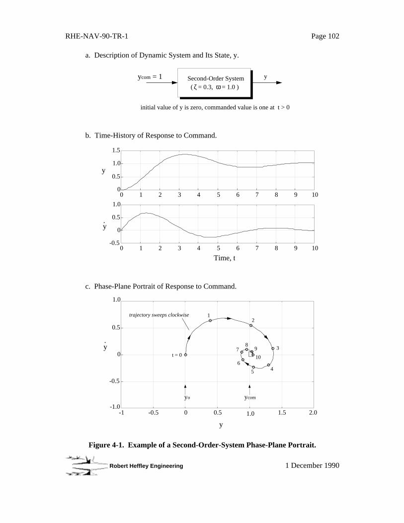
RHE-NAV-90-TR-1 Page 102
Robert Heffley Engineering 1 December 1990
0
0.5
1.0
1.5
0 1 2 3 4 5 6 7 8 9 10
-0.5
0
0.5
1.0
0 1 2 3 4 5 6 7 8 9 10
-1.0
-0.5
0
0.5
1.0
-1 -0.5 0 0.5 1.0 1.5 2.0
Second-Order System( ζ = 0.3, ω = 1.0 )
initial value of y is zero, commanded value is one at t > 0
y ycom = 1
a. Description of Dynamic System and Its State, y.
b. Time-History of Response to Command.
c. Phase-Plane Portrait of Response to Command.
Time, t
y
y
y ·
ycomyo
t = 0
12
3
45
6
78
9
10
trajectory sweeps clockwise
y ·
+
Figure 4-1. Example of a Second-Order-System Phase-Plane Portrait.
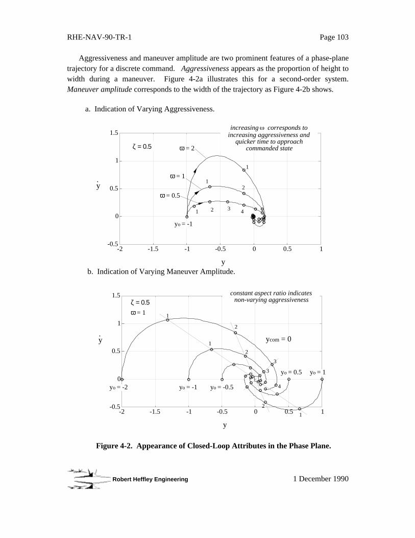
RHE-NAV-90-TR-1 Page 103
Robert Heffley Engineering 1 December 1990
Aggressiveness and maneuver amplitude are two prominent features of a phase-planetrajectory for a discrete command. Aggressiveness appears as the proportion of height towidth during a maneuver. Figure 4-2a illustrates this for a second-order system.Maneuver amplitude corresponds to the width of the trajectory as Figure 4-2b shows.
-0.5
0.5
1.5
-1 -0.5 0 0.5 1
1 2 3 4
12
1
0
1
ω = 2
ω = 1
ω = 0.5
ζ = 0.5
increasing corresponds to increasing aggressiveness and
quicker time to approach commanded state
y
y·
-2 -1.5
a. Indication of Varying Aggressiveness.
yo = -1
-0.5
0.5
1.5
-1 -0.5 0 0.5 1
1
0
1
ω = 1
ζ = 0.5
constant aspect ratio indicates non-varying aggressiveness
y
-2 -1.5
yo = -2 yo = -0.5yo = -2
yo = 0.5 yo = 1
yo = -1
ycom = 0
+
2
3
4
1
2
3
1
2
b. Indication of Varying Maneuver Amplitude.
y·
Figure 4-2. Appearance of Closed-Loop Attributes in the Phase Plane.

RHE-NAV-90-TR-1 Page 104
Robert Heffley Engineering 1 December 1990
A phase-plane view of glideslope control is merely the crossplot of vertical velocity,∆˙d, with glideslope displacement, ∆ d. One can show time, range, or any discrete eventson the phase-plane trajectory, if desired.
A short sample of a glideslope correction was computed using the simple modelshown in Figure 4-3. One can lump the dominant response modes as an integration inseries with a lag. The integration represents the transfer function between verticalvelocity and glideslope error; the lag lumps the heave damping and control lag with theimplicit assumption of good pitch/thrust coordination. Two nonlinearities are included,one representing the amount of vertical velocity available (or tolerable to the pilot) andthe other the limit of the FLOLS display range.
Ks (1 + T s)
a
a
Ks (1 + T s)
aa
judgmentof GS error
aircraftflight pathlimits (±)
pilot aggressiveness,aircraft response
FLOLSlinear
with/limitsFLOLS
indication"roger ball"
+-
∆d
Figure 4-3. Glideslope Control Task Model.

RHE-NAV-90-TR-1 Page 105
Robert Heffley Engineering 1 December 1990
Figure 4-4 shows the resulting phase-plane portrait of a correction based on the abovemodel. Starting at 1000 ft from touchdown, the math-model pilot makes a six-secondcorrection ending on-glideslope, but with slightly less than the nominal rate of descent
(probably resulting in a long landing). The proportion of ∆ · d to net ∆ d (indicating theaggressiveness of the maneuver) is about 0.35.
-10
-5
0
5
10
-20 -10 0 10 20
∆d (ft)
∆d (
ft/s
ec)
Ka=1 Ta=2 Ro=1000' V=100kt
.0x
5
1 sec
23
4
6
∆d limit.
start
end (at deck)
Figure 4-4. Phase-Plane Portrait of a Glideslope Correction.
Application to Flight Data
Several analysts have used this technique to examine the closed-loop control ofaircraft. One notable study (Reference 60) compared airliner landings on simulators withactual landings to assess training effectiveness. Phase-plane analysis showed cleardifferences between flight and simulator in terms of aggressiveness, settling, amplitude,and consistency in the closed-loop landing flare.
Another study of Navy aircraft flying qualities applied the phase-plane analysis to alimited set of F-14 approach flight data describing a lineup maneuver(Reference 64).This was also reported in References 37 and 65. However, the lack of direct lineupposition measurements detracted from the validity of the results.
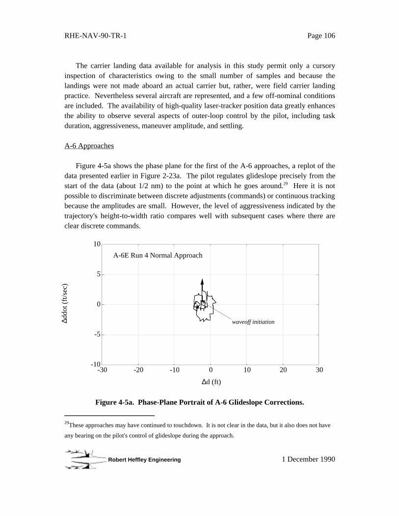
RHE-NAV-90-TR-1 Page 106
Robert Heffley Engineering 1 December 1990
The carrier landing data available for analysis in this study permit only a cursoryinspection of characteristics owing to the small number of samples and because thelandings were not made aboard an actual carrier but, rather, were field carrier landingpractice. Nevertheless several aircraft are represented, and a few off-nominal conditionsare included. The availability of high-quality laser-tracker position data greatly enhancesthe ability to observe several aspects of outer-loop control by the pilot, including taskduration, aggressiveness, maneuver amplitude, and settling.
A-6 Approaches
Figure 4-5a shows the phase plane for the first of the A-6 approaches, a replot of thedata presented earlier in Figure 2-23a. The pilot regulates glideslope precisely from thestart of the data (about 1/2 nm) to the point at which he goes around.29 Here it is notpossible to discriminate between discrete adjustments (commands) or continuous trackingbecause the amplitudes are small. However, the level of aggressiveness indicated by thetrajectory's height-to-width ratio compares well with subsequent cases where there areclear discrete commands.
-10
-5
0
5
10
-30 -20 -10 0 10 20 30
∆d (ft)
∆ddo
t (ft
/sec
)
A-6E Run 4 Normal Approach
waveoff initiation
Figure 4-5a. Phase-Plane Portrait of A-6 Glideslope Corrections.
29These approaches may have continued to touchdown. It is not clear in the data, but it also does not have
any bearing on the pilot's control of glideslope during the approach.
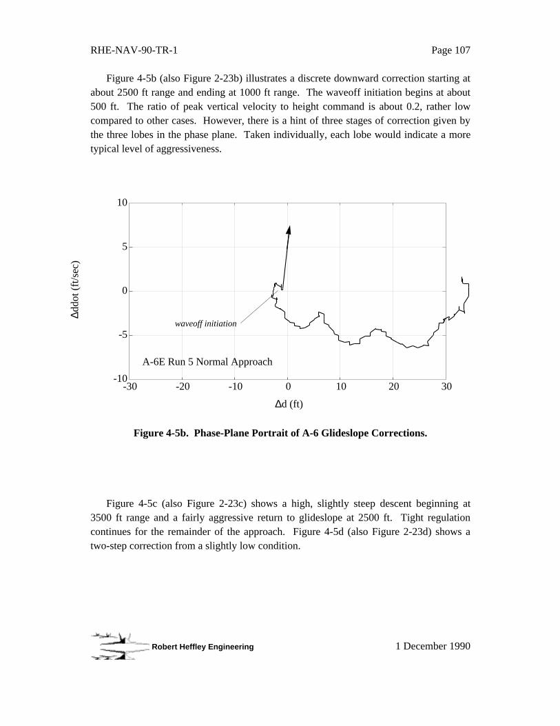
RHE-NAV-90-TR-1 Page 107
Robert Heffley Engineering 1 December 1990
Figure 4-5b (also Figure 2-23b) illustrates a discrete downward correction starting atabout 2500 ft range and ending at 1000 ft range. The waveoff initiation begins at about500 ft. The ratio of peak vertical velocity to height command is about 0.2, rather lowcompared to other cases. However, there is a hint of three stages of correction given bythe three lobes in the phase plane. Taken individually, each lobe would indicate a moretypical level of aggressiveness.
-10
-5
0
5
10
-30 -20 -10 0 10 20 30
∆d (ft)
∆ddo
t (ft
/sec
)
A-6E Run 5 Normal Approach
waveoff initiation
Figure 4-5b. Phase-Plane Portrait of A-6 Glideslope Corrections.
Figure 4-5c (also Figure 2-23c) shows a high, slightly steep descent beginning at3500 ft range and a fairly aggressive return to glideslope at 2500 ft. Tight regulationcontinues for the remainder of the approach. Figure 4-5d (also Figure 2-23d) shows atwo-step correction from a slightly low condition.

RHE-NAV-90-TR-1 Page 108
Robert Heffley Engineering 1 December 1990
-10
-5
0
5
10
-30 -20 -10 0 10 20 30
∆d (ft)
∆ddo
t (ft
/sec
)A-6E Run 6 OSX Approach
Figure 4-5c. Phase-Plane Portrait of A-6 Glideslope Corrections.
-10
-5
0
5
10
-30 -20 -10 0 10 20 30
∆d (ft)
∆ddo
t (ft
/sec
)
A-6E Run 7 USX Approach
waveoff initiation
Figure 4-4d. Phase-Plane Portrait of A-6 Glideslope Corrections.

RHE-NAV-90-TR-1 Page 109
Robert Heffley Engineering 1 December 1990
Figure 4-5e (also Figure 2-23e) illustrates a large correction from a low conditionfollowed by tight tracking about the glideslope.
-10
10
-30 -20 -10 0 10 20 30
∆d (ft)
∆ddo
t (ft
/sec
)
A-6E Run 8 LOX Approach
-5
0
5
Figure 4-5e. Phase-Plane Portrait of A-6 Glideslope Corrections.

RHE-NAV-90-TR-1 Page 110
Robert Heffley Engineering 1 December 1990
Figure 4-5f (also Figure 2-23f) shows a large intentional transition to a high positionin the middle followed by fine corrections back to the glideslope.
-10
-5
10
-30 -20 -10 0 10 20 30
∆d (ft)
∆ddo
t (ft
/sec
)
A-6E Run 9 HIM Approach
0
5
Figure 4-5f. Phase-Plane Portrait of A-6 Glideslope Corrections.
F-14 Approaches
The next set of phase planes represents two F-14 approaches. Figure 4-6a is a slowrecovery from a low position followed by an oscillatory regulation of glideslope. Thefirst part has some higher-frequency content yet three discrete corrections are visible.The second part is oscillatory and suggests some PIO yet damps at the end. Figure 4-6bportrays a continuing downward set of corrections.
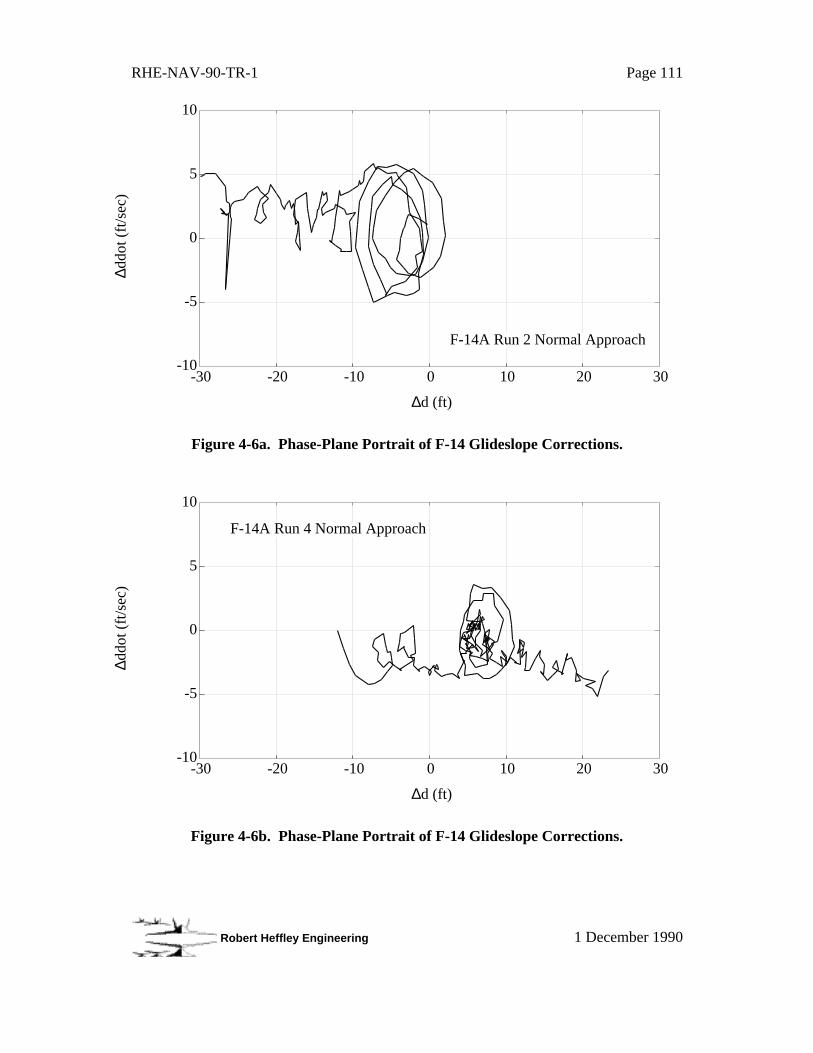
RHE-NAV-90-TR-1 Page 111
Robert Heffley Engineering 1 December 1990
-10
-5
0
5
10
-30 -20 -10 0 10 20 30
∆d (ft)
∆ddo
t (ft
/sec
)
F-14A Run 2 Normal Approach
Figure 4-6a. Phase-Plane Portrait of F-14 Glideslope Corrections.
-10
-5
0
5
10
-30 -20 -10 0 10 20 30
∆d (ft)
∆ddo
t (ft
/sec
)
F-14A Run 4 Normal Approach
Figure 4-6b. Phase-Plane Portrait of F-14 Glideslope Corrections.
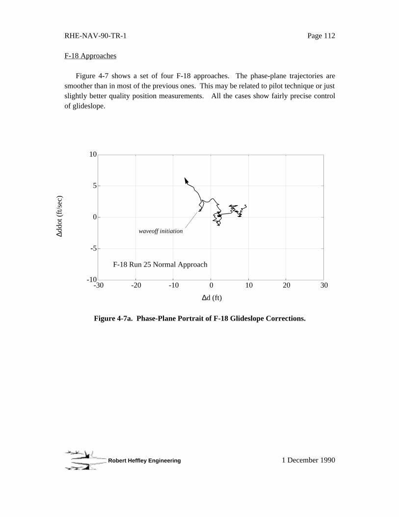
RHE-NAV-90-TR-1 Page 112
Robert Heffley Engineering 1 December 1990
F-18 Approaches
Figure 4-7 shows a set of four F-18 approaches. The phase-plane trajectories aresmoother than in most of the previous ones. This may be related to pilot technique or justslightly better quality position measurements. All the cases show fairly precise controlof glideslope.
-10
-5
0
5
10
-30 -20 -10 0 10 20 30
∆d (ft)
∆ddo
t (ft
/sec
)
F-18 Run 25 Normal Approach
waveoff initiation
Figure 4-7a. Phase-Plane Portrait of F-18 Glideslope Corrections.
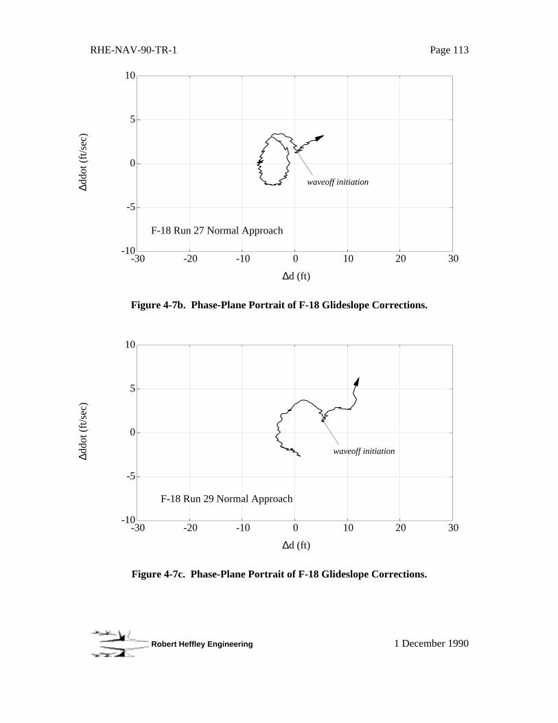
RHE-NAV-90-TR-1 Page 113
Robert Heffley Engineering 1 December 1990
-10
10
-30 -20 -10 0 10 20 30
∆d (ft)
∆ddo
t (ft
/sec
)
-5
0
5
F-18 Run 27 Normal Approach
waveoff initiation
Figure 4-7b. Phase-Plane Portrait of F-18 Glideslope Corrections.
-10
-5
0
5
10
-30 -20 -10 0 10 20 30
∆d (ft)
∆ddo
t (ft
/sec
)
F-18 Run 29 Normal Approach
waveoff initiation
Figure 4-7c. Phase-Plane Portrait of F-18 Glideslope Corrections.
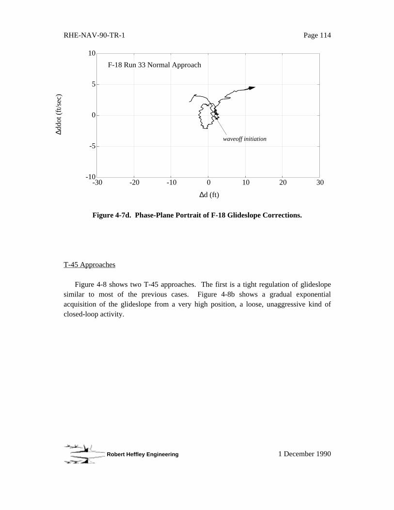
RHE-NAV-90-TR-1 Page 114
Robert Heffley Engineering 1 December 1990
-10
-5
0
5
10
-30 -20 -10 0 10 20 30
∆d (ft)
∆ddo
t (ft
/sec
)
waveoff initiation
F-18 Run 33 Normal Approach
Figure 4-7d. Phase-Plane Portrait of F-18 Glideslope Corrections.
T-45 Approaches
Figure 4-8 shows two T-45 approaches. The first is a tight regulation of glideslopesimilar to most of the previous cases. Figure 4-8b shows a gradual exponentialacquisition of the glideslope from a very high position, a loose, unaggressive kind ofclosed-loop activity.

RHE-NAV-90-TR-1 Page 115
Robert Heffley Engineering 1 December 1990
-10
-5
0
5
10
-30 -20 -10 0 10 20 30
∆d (ft)
∆ddo
t (ft
/sec
)T-45 Run 6 Normal Approach
Figure 4-8a. Phase-Plane Portrait of T-45 Glideslope Corrections.
-10
-5
0
5
10
-20 -10 0 10 20 30 40
∆d (ft)
∆ddo
t (ft
/sec
)
T-45 Run 8 HXIM Approach
Figure 4-8b. Phase-Plane Portrait of T-45 Glideslope Corrections.
RHE-NAV-90-TR-1 Page 116
Robert Heffley Engineering 1 December 1990
The foregoing examples indicate similar closed-loop activity among all the aircraftand over the magnitude of corrections. Further detailed analysis of these data could beperformed following the procedures described in Reference 60, but this would notprovide any additional insight for two reasons. One is that there is no detailed pilotcommentary available for the above approaches, therefore some analysis of controlbehavior would only be speculative. The second reason for not doing further analysis isthat these were only simulated carrier approaches to a field. Actual carrier landingswould provide far more credibility of analytical results. Nevertheless, the above data doprovide a starting point for assessing the true nature of actual outer-loop control forcurrent Navy aircraft for the landing task.
Further, more detailed analyses of carrier approach data are needed, though, to obtaingood quantification of task performance for setting rational design requirements. Allthree outer-loop control tasks need to be addressed. For approach data being gathered,the pilot and the LSO need to assess and discuss individual corrections in each axis,particularly their criticality with respect to the terminal condition. Inner-loop data alsomust be monitored to establish pilot technique.
4.2 Analysis of VPA Criteria
The VPA criteria, including the popup maneuver, are the main requirements set by the
Navy to ensure adequate glideslope and angle-of-attack control characteristics for carrieraircraft. It is worthwhile, therefore, to review these criteria and their effect on shapingouter-loop response features.
Section 1 gave an introductory discussion of the Navy approach speed criteria.Below is a more detailed statement of them followed by an analysis of each of theirimplications for outer-loop control. The objective is to identify what outer-loop controlfactors are effectively guaranteed and where there are gaps. The list of necessary factorspresented earlier in Section 3.4 is useful in making this determination.
RHE-NAV-90-TR-1 Page 117
Robert Heffley Engineering 1 December 1990
4.2.1 Statement of Criteria
The Navy approach speed criteria are stated below from Reference 5, the F/A-18system specification. It is a reasonably recent version of the various sets of requirementsused by the Navy since the early 1960's.
Navy Approach Speed Criteria
With the aircraft in the landing configuration and on a 4° glideslope on a 89.8° F day, the approachspeed, VPA , shall be the highest of the airspeeds defined by the following:
a. The lowest speed at which it is possible to achieve a level flight longitudinal acceleration of 5ft/sec2 within 2.5 sec after initiation of throttle movement (to MIL thrust) and speedbrakeretraction.
b. VSPA x 1.1 where VSPA is the power-on stall speed using the thrust required for level flight at
1.15 VSL, the power-off stall speed.
c. The lowest level-flight speed at which the pilot, at the design eye position, can see the stern of thecarrier at the waterline when intercepting a 4° glideslope at an altitude of 600 ft. The origin of theglideslope is 500 ft forward of the stern and 63 ft above the waterline.
d. The lowest speed at which all stability and control requirements are satisfied (MIL-F-8785C).
e. The lowest speed at which the aircraft is capable of making a glide path correction from stabilizedflight at VPA to a new glide path 50 ft above the original glide path within 5 sec after initiation ofthe maneuver. The maneuver shall be performed without change in thrust settings, and the aircraftangle of attack during the maneuver shall not exceed that necessary to achieve 50% of themaximum positive delta load factor available, based on static lift coefficient, at the initiation of themaneuver. Control rate input for simulation of VPA shall not exceed control system limits. Themaneuver shall be considered complete when a glide path correction of 50 ft has been reached.After completion of this maneuver, the aircraft shall be capable of maintaining a new glide path atleast 50 ft above and parallel to the initial glide path, with the pilot permitted to change thrustsetting as required.
f. To ensure rapid aircraft response to step throttle commands corresponding to ± 3.86 ft/sec2 (± 0.12g) longitudinal acceleration, such throttle inputs shall result in achieving 90% of the commandedacceleration within 1.2 sec. This requirement shall apply in the approach configuration throughoutthe range of all throttle settings required for operations over the usable approach configurationweight/drag levels while trimmed on a 4° glideslope.
Each item listed above is more or less significant to the general specification of anacceptable approach speed because of the collective constraint and limitation of a varietyof outer-loop control features. This is demonstrated in the analysis of each itempresented next.
RHE-NAV-90-TR-1 Page 118
Robert Heffley Engineering 1 December 1990
4.2.2 Implications of Requirements on Airframe/Engine Characteristics
The VPA requirements imply several characteristics for the outer-loop dynamics of
the airframe/engine system. This is shown by rearranging the order of items thenillustrating the implied constraints and limitations by analysis based on the math modelspresented in the previous sections.
Analysis of the approach speed criteria shows that they restrict several outer-loopcontrol factors, but sometimes in indirect ways. One criterion, the popup maneuver, maynot set the strong constraint on flightpath response that the requirement seems to suggest.Also, the short-term axial acceleration criterion may suffer from ambiguity in its wordingthus compromising its important implication for the quickness of thrust response.
Satisfaction of Stability and Control Requirements in MIL-F-8785C
There are several requirements in both of the existing flying qualities specifications,MIL-F-8785C (Reference 2) and, the more recent MIL-STD 1797A (Reference 1),30 thatsupport the Navy approach speed criteria. Most of these supporting requirementsinfluence inner-loop pitch attitude control. There are some which address outer-loopflightpath and speed control, but may not be particularly effective, especially for thecarrier landing task. There are no requirements that ensure the quality of thrust control.
Both the above specifications cover the basic inner-loop pitch axis flying qualities indepth. This includes pitch-attitude response to the control stick and the stick feelcharacteristics. Attitude response includes control bandwidth, damping, control power,and control forces. There are provisions for complex high-gain stability and controlaugmentation systems as well as for a basic unaugmented airframe.
Beyond such inner-loop requirements there are some that appear to have outer-loopimplications but are still open to question. Section 1.2.1 described these. The one outer-loop weakness that should be stressed is the minimum allowable short-term flightpathresponse. It is not defined in MIL-F-8785C and done in MIL-STD 1797A withinsufficient justification by its lower bound on 1/Tθ2.
There is some belief that the ωsp versus nzα boundaries, common to both of thespecifications, address outer-loop flightpath control. The allowable band of ωsp that is
30MIL-STD-1797A is addressed here in order to anticipate its future application to Navy carrier aircraft.
RHE-NAV-90-TR-1 Page 119
Robert Heffley Engineering 1 December 1990
expressed as a function of nzα is based on the Bihrle Control Anticipation Parameter
(CAP) criterion originally proposed in Reference 66. CAP, strictly interpreted, is theratio of the instantaneous angular pitching acceleration per unit of the eventual steady-state load factor. Therefore, it is a kind of inner-loop/outer-loop control-harmony metric,and therefore is a beneficial feature supporting the approach speed criteria. But it doesnot determine how quickly flightpath responds to an attitude change, nor does the lowerlimit on nzα as one can see from inspection of the approximate factors in Section 3.
One additional, and general, shortcoming of the traditional flying qualitiesrequirements is their lack of any accompanying conditions on piloting technique. Prioranalysis has already shown how outer-loop control performance depends upon thespecific technique used. For example, there should be an expectation that pitch attituderesponse criteria may depend upon the role of attitude in controlling flightpath.
In summary, the current role of flying qualities specifications is simply to provide asuitable pitch attitude control capability. There is, however, a potential for effectivecoverage of outer-loop response characteristics, particularly short-term flightpathresponse.
Longitudinal Acceleration of 90% of ± 3.86 ft/sec2 Within 1.2 Seconds
This requirement affects two crucial outer-loop control factors. First, it sets amaximum engine response time constant over the range of flightpath angle excursionslikely to be used during an approach. Second, it sets the level of flightpath controlauthority (∆ γ), both upward and downward.
The implication for engine response, unfortunately, is subject to two possibleinterpretations depending upon the definition of “commanded acceleration.” If this refersto the virtual acceleration without airframe speed damping, then the commandedacceleration simply is equal to the ∆ T/W ratio. On the other hand, if the commandedacceleration includes airframe speed damping then there is no near-term, steady-stateacceleration. Instead there is a peak acceleration followed by a washout as drag forcebuilds against the thrust force. Consider each of these cases.
The first case is simple. Only the net thrust force is considered and the 1.2 secrequirement applies to the point at which thrust increases (or decreases) to 90% of thenew steady-state value. Assuming a first-order lag response shape (i. e., exponential),
RHE-NAV-90-TR-1 Page 120
Robert Heffley Engineering 1 December 1990
this requirement equates to an engine lag time constant, Teng, of 0.52 sec.31 Further, it
applies for net ∆ T/W changes spanning ± 0.12.
The second case is more complex and requires the computation of axial acceleration.The ∆ ax response transfer function, using the nomenclature presented in Sections 1 and
3, is given by:
∆ ax(s) =
s N ∆
uT/W
· ∆ T/W(s)
where ∆ T/W is a step throttle command applied to an engine having an effective first-order lag time constant of Teng.
By inspection, the approximate factors yield:
∆ ax(s) = g s (s -Zw - η Xw)
( s+ 1/T ) (s + 1/T ) θ1 θ2
washout
1 ( Teng s + 1 )
cancellation lag
· ∆ T/W(s)
Thus, the airframe response component essentially is a slow washout of ax with atime constant of Tθ1 , and the dominant response mode is the engine lag, Teng. Figure 4-
9 shows an example for an airframe with a typical 10 sec speed-damping time constant(Tθ1) and an engine with a 0.5 sec lag (Teng). For a unit thrust command, the airframe
acceleration builds to a peak then begins to decay.
31Neglecting the airframe contribution, the thrust rise-time-to-90% can be converted to an effective first-
order time constant by dividing by a factor of -ln(.1), or 2.3. Thus the 1.2 sec rise time is equivalent to a
first-order time constant of 0.52 sec.
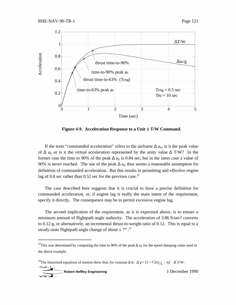
RHE-NAV-90-TR-1 Page 121
Robert Heffley Engineering 1 December 1990
0
0.2
0.4
0.6
0.8
1.2
0 1 2 3 4 5
1
Time (sec)
Teng = 0.5 sec Tθ1 = 10 sec
Acc
eler
atio
n∆T/W
∆ax/gthrust time-to-90%
time-to-90% peak ax
time-to-63% peak ax
thrust time-to-63% (Teng)
Figure 4-9. Acceleration Response to a Unit T/W Command.
If the term “commanded acceleration” refers to the airframe ∆ ax, is it the peak valueof ∆ ax or is it the virtual acceleration represented by the unity value ∆ T/W? In theformer case the time to 90% of the peak ∆ ax is 0.84 sec, but in the latter case a value of90% is never reached. The use of the peak ∆ ax thus seems a reasonable assumption for
definition of commanded acceleration. But this results in permitting and effective enginelag of 0.8 sec rather than 0.52 sec for the previous case.32
The case described here suggests that it is crucial to have a precise definition forcommanded acceleration, or, if engine lag is really the main intent of the requirement,specify it directly. The consequence may be to permit excessive engine lag.
The second implication of the requirement, as it is expressed above, is to ensure aminimum amount of flightpath angle authority. The acceleration of 3.86 ft/sec2 convertsto 0.12 g, or alternatively, an incremental thrust-to-weight ratio of 0.12. This is equal to asteady-state flightpath angle change of about ± 7° .33
32This was determined by computing the time to 90% of the peak ∆ ax for the speed damping value used in
the above example.
33The linearized equations of motion show that, for constant ∆ α: ∆ γ = [1 + CD/CL · η] · ∆ T/W.
RHE-NAV-90-TR-1 Page 122
Robert Heffley Engineering 1 December 1990
One should note that the basic requirement applies only to thrust changes maderelative to the nominal glideslope flightpath angle, however. It does not require that theengine thrust lag be as fast when making an upward correction from steeper descentconditions. This could result in an excessively slow flightpath response back to thenominal flightpath angle in view of the tendency for longer engine lag at low thrustsettings shown in Section 2, especially for turbofan engines.
Level-Flight Acceleration of 5 ft/sec2 Within 2.5 Seconds
The 5 ft/sec2 longitudinal acceleration within 2.5 sec provides an upward flightpathcontrol power capability, but sets no additional constraint on the thrust lag time constant.The requirement generally permits use of military thrust and retraction of speedbrakes,thus it applies to a waveoff condition. The ∆ ax time history given in the previous
example shows that at 2.5 sec the axial acceleration has probably peaked and isbeginning to washout due to airframe speed damping. There do not appear to be criticalimplications with respect to approach flightpath control factors.
Correction in Glidepath of 50ft Within 5 Seconds (Popup Maneuver)
One is tempted to regard the popup maneuver to have direct implications for airframeflightpath response. For example, it would be natural to expect that the popup maneuverreflects explicitly a short-term response capability. However, careful analysis of theeffect of various design parameters on popup maneuver performance reveals a generalinsensitivity to most of the parameters in the ∆ γ/∆ θ response function. The main factorin performing the popup maneuver is the ratio of approach speed to stall speed, V/VSPA.
The following paragraphs demonstrate this.
All the main features of the popup maneuver are contained in the linear transferfunction for height, ∆ d, due to a change in attitude, ∆ θ:
∆ d = V· N s ∆
γθ · ∆ θ
Careful inspection using the approximate factors listed in Sections 1 and 3 proves thatall the factors in this transfer function can be determined from the parameters V, nzα, and
∂ γ/∂ V. Next, the pitchup maneuver, ∆ θ, is defined by the stall margin, V/VSPA, nzα,
and the way in which the pilot applies the pitchup to the maximum allowable α (abruptly,
RHE-NAV-90-TR-1 Page 123
Robert Heffley Engineering 1 December 1990
slowly, etc.).34 The peak incremental α excursion permitted during the popup maneuvercorresponds to one-half the remaining aerodynamic lift and is given by:
( )[ ]PA
2 nzα
VV
- 12
Speak ∆α =
Any pitch-control time history sequence (elevator or longitudinal control input) ispermitted so long as the peak ∆ α limit is satisfied.
The following is an analysis of how the basic design parameters named aboveinfluence the popup maneuver performance. First, Figure 4-10 shows the popupmaneuver response for a nominal set of conditions typical of existing carrier aircraft:
• normal-acceleration sensitivity to angle of attack, nzα = 3.5 g/rad
• neutral backsidedness, ∂ γ/∂ V = 0• power-on stall margin, V/VSPA = 1.2
• rapid attitude step with a min-bandwidth control system, 0.4 sec lag pitch step35
• approach speed, V = 125 kt
The resulting height response is predominantly ramp-like with an initial lag. For thenominal values chosen, the time to 50 ft is about 5 sec (4.8 sec). Hence this would satisfythe VPA criterion.
34There is a broad spectrum of ways for the pilot to pitch the aircraft while staying within the peak angle of
attack limit. One example is to make an abrupt pitch step wherein the α quickly peaks then washes out.
Another way is to establish a fairly constant pitch rate with α rising to the allowable peak value then
holding. Or there can be any number of variations in between these cases.
35This is based on a step input into a minimum-bandwidth flight control system where ωBW = 2.5 rad/sec.
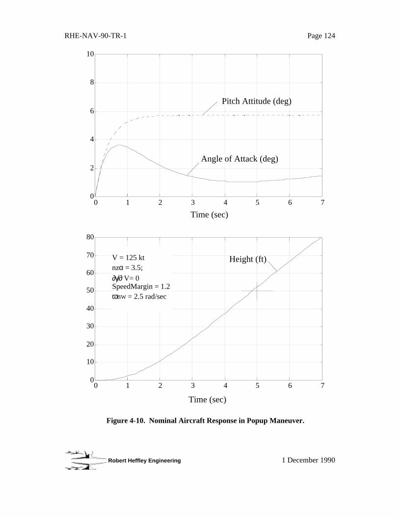
RHE-NAV-90-TR-1 Page 124
Robert Heffley Engineering 1 December 1990
0
2
4
6
8
10
0 1 2 3 4 5 6 7
0
10
20
30
40
50
60
70
80
0 1 2 3 4 5 6 7
Height (ft)
Pitch Attitude (deg)
Angle of Attack (deg)
V = 125 ktnzα = 3.5;
∂γ/∂ V= 0SpeedMargin = 1.2ωBW = 2.5 rad/sec
Time (sec)
Time (sec)
Figure 4-10. Nominal Aircraft Response in Popup Maneuver.
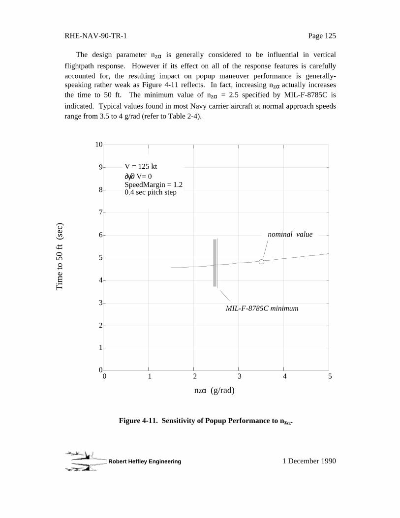
RHE-NAV-90-TR-1 Page 125
Robert Heffley Engineering 1 December 1990
The design parameter nzα is generally considered to be influential in vertical
flightpath response. However if its effect on all of the response features is carefullyaccounted for, the resulting impact on popup maneuver performance is generally-speaking rather weak as Figure 4-11 reflects. In fact, increasing nzα actually increasesthe time to 50 ft. The minimum value of nzα = 2.5 specified by MIL-F-8785C is
indicated. Typical values found in most Navy carrier aircraft at normal approach speedsrange from 3.5 to 4 g/rad (refer to Table 2-4).
0
10
0 1 2 3 4 5
1
2
3
4
5
6
7
8
9
Tim
e to
50
ft (
sec)
nzα (g/rad)
V = 125 kt∂γ/∂ V= 0SpeedMargin = 1.20.4 sec pitch step
MIL-F-8785C minimum
nominal value
Figure 4-11. Sensitivity of Popup Performance to nz .

RHE-NAV-90-TR-1 Page 126
Robert Heffley Engineering 1 December 1990
Approach speed also affects the time-to-50 ft only slightly, even for a very largerange of speeds. As Figure 4-12 shows, higher speeds yield a slightly shorter time-to-50ft.
100 110 120 130 140 1500
1
2
3
4
5
6
7
8
9
10
Tim
e to
50
ft (
sec)
Approach Speed, V (kt)
nzα = 3.5;
∂γ/∂ V= 0SpeedMargin = 1.20.4 sec pitch step
nominal value
Figure 4-12. Sensitivity of Popup Performance to Approach Speed.

RHE-NAV-90-TR-1 Page 127
Robert Heffley Engineering 1 December 1990
Figure 4-13 shows that the backsidedness parameter also has a rather weak effect ontime-to-50 ft. Even the largest permissible ∂ γ/∂ V of +0.06 (on the backside) does notchange the popup maneuver performance much.
0
1
2
3
4
5
6
7
8
9
10
-0.06 -0.04 -0.02 0 0.02 0.04 0.06 0.08 0.1 0.12
Tim
e to
50
ft (
sec)
∂γ/∂V (deg/kt)
backsidefrontside
V = 125 ktnzα = 3.5;SpeedMargin = 1.20.4 sec pitch step
nominal value
MIL-F-8785C limit
Figure 4-13. Sensitivity of Popup Performance to Backsidedness.

RHE-NAV-90-TR-1 Page 128
Robert Heffley Engineering 1 December 1990
Even the abruptness of the pitch response has surprisingly small effect on the time-to-50 ft. A first-order time constant has been used to vary the profile of the pitchupmaneuver. A value of zero for this time constant would correspond to an instantaneouspitch step while larger values would yield more ramp-shaped pitch responses. The limitshown in the plot corresponds to the quickest pitchup obtainable with a minimumbandwidth flight control system as specified by the STI bandwidth criterion (ωBW = 2.5
rad/sec). Longer time constants would be obtainable with increasingly gradual pilot pitchcommands. This feature is illustrated further shortly.
Tim
e to
50
ft (
sec)
Pitch Response Time Constant (sec)
0
1
2
3
4
5
6
7
8
9
10
0 1 2 3 4 5
MIL-STD-1797A bandwidth limit
V = 125 ktnzα = 3.5;
∂γ/∂ V= 0SpeedMargin = 1.2
Figure 4-14. Sensitivity of Popup Performance to Pitch Attitude Response.

RHE-NAV-90-TR-1 Page 129
Robert Heffley Engineering 1 December 1990
The one design parameter that does have a large effect on popup maneuverperformance is the speed margin, i. e., ratio of approach speed to power-on stall speed.According to Figure 4-15, a speed margin of about 20% is required in order to satisfy thepopup maneuver criterion.
0
1
2
3
4
5
6
7
8
9
10
1 1.05 1.1 1.15 1.2 1.25 1.3 1.35 1.4
Speed Margin
Tim
e to
50
ft (
sec)
V = 125 ktnzα = 3.5;
∂γ/∂ V= 00.4 sec pitch step
nominal value
Figure 4-15. Sensitivity of Popup Performance to Margin from Stall.

RHE-NAV-90-TR-1 Page 130
Robert Heffley Engineering 1 December 1990
As indicated previously, the pitch attitude bandwidth does not have much effect. Infact, there is a penalty for pitching up too quickly. In order to obtain a more effectiveangle-of-attack change, it is advantageous to slow down the pitch maneuver. As shownbelow, for a very long pitch time constant (5 sec) the maneuver resembles a constantpitch rate. The same peak angle of attack is obtained, but it is sustained rather thandecaying. Figure 4-16 shows the comparison the nominal case shown above with thesustained pitch up. Both cases result in about the same time to 50 ft height gain.
0
2
4
6
8
10
0 1 2 3 4 5 6 7
0
10
20
30
40
50
60
70
80
0 1 2 3 4 5 6 7
Height (ft)
Pitch Attitude (deg)
Angle of Attack (deg)
V = 125 ktnzα = 3.5;
∂γ/∂V= 0SpeedMargin = 1.2ωBW = 2.5 rad/sec
Time (sec)
Time (sec)
0
10
20
30
40
50
60
70
80
0 1 2 3 4 5 6 7
Height (ft)
V = 125 ktnzα = 3.5;
∂γ/∂V= 0SpeedMargin = 1.2ωBW = 0.2 rad/sec
Time (sec)
0
2
4
6
8
10
0 1 2 3 4 5 6 7
Pitch Attitude (deg)
Angle of Attack (deg)
Time (sec)
Figure 4-16. Comparison of Popup for Two Diverse Pitch Maneuvers.
In summary, only the stall speed margin appears to have a significant influence on thetime to 50 ft. Each of the other parameters can be varied over a wide range withoutaffecting popup maneuver performance by more than a few percent. Given the nominalvalues of these other parameters, a speed margin of about 20% appears sufficient toguarantee popup maneuver performance.
RHE-NAV-90-TR-1 Page 131
Robert Heffley Engineering 1 December 1990
Variations of the Popup Maneuver
Some variations in the popup maneuver have been mentioned. One concerns thedefinition of the allowable ∆ α, another the terminal condition of the popup.
The angle-of-attack limit defined above is based on the static incremental normalacceleration available. Another definition used during initial flight testing of the popupmaneuver based the α limit on the actual ∆ g available for an abrupt pullup. This resultedin a far smaller amplitude pitchup maneuver for the popup, generally about one-half thatbased on the static ∆ g-available.
Another important variation that was used by the Navy for a period of time put anadditional constraint on the end of the maneuver. Instead of the 5 sec time-to-50ft limit,the aircraft was given 7 sec to step-up through 50 ft and to pass back through 50 ft. Thiswas a significant additional contstraint because it introduced a closed-loop aspect to themaneuver. The important benefit in terms of outer-loop control is that short-termresponse of the airframe is crucial to the maneuver and is therefore implicit in the popupcriterion. The difficulty, because of the necessary closed-loop pilot actions, is that such amaneuver is more dependent on the technique of an individual pilot than the simple time-to-50ft criterion.
Operation at or Above 1.1 VSPA
The 10% margin above stall speed provides a safety factor in terms both of an angleof attack and of airspeed. If, indeed, the popup maneuver requires a stall-speed margin ofabout 20%, then the 1.1 VSPA requirement may be unnecessary except for unusual
circumstances. If there is a desire to guarantee a specific stall-speed margin, say 20%,then the direct wording of this requirement is better, perhaps, and should replace thepopup maneuver in its current form. At the same time, the popup maneuver might berestated to ensure an effective limit on short-term flightpath response.
Visibility over the Nose Upon Intercepting the Glideslope
This requirement directly addresses visual cueing for the pilot. It recognizes that theprimary vertical and horizontal flightpath information originates at the deck of the carrier(FLOLS and dropline). The geometry specified implies a downward field of view limitover the nose. The visibility requirement to see the stern at an altitude of 600 ft whileflying level implies that the visibility over the nose be equal to the approach angle ofattack plus 4.8°. For example, if the F-18 uses a true angle of attack of 8.1 deg, then
RHE-NAV-90-TR-1 Page 132
Robert Heffley Engineering 1 December 1990
over-the-nose visibility must be at least 12.9° below the FRL.
Inner-loop cueing is not covered in this requirement, however. It is crucial for thepilot to have both pitch attitude and thrust cues in order to effectively control outer-loopstates. Pitch attitude is usually implicit in the requirement for visibility over the nose.There can be a problem if there is no distinct nose reference, though.36 The other crucialinner-loop cue is thrust level. Pilots ordinarily depend upon engine sound, but in someaircraft such as the A-7 and F-14, the sound level is well insulated from the pilot. HUDdisplay of thrust level can provide a good substitute, particularly if the commanded levelis shown. This has the benefit of eliminating the problem of thrust lag in making throttleadjustments.
4.2.3 Summary of VPAmin Criteria
The VPAmin criteria effectively set the following features:
(i) Engine thrust lag less than 0.52 sec (depending upon interpretation)(ii) Upward and downward steady-state flightpath angle correction of at least 7°(iii)Margin from power-on stall speed of about 20% (10% explicitly)(iv)Downward field-of-view adequate for the final approach leg(v) Various pitch-attitude response requirements of 8785C
Notably absent from this list are:(i) Short-term flightpath response (such as Tθ2)(ii) Quality of the flightpath response (such as speed damping, Tθ1)
(iii)Engine thrust-level cueing
36This might be the case if the downward field of view were taken to an extreme, say, 90° from the
horizontal.

RHE-NAV-90-TR-1 Page 133
Robert Heffley Engineering 1 December 1990
4.3 Computation of the “Last Significant Glideslope Correction”
4.3.1 General
It is crucial to understand how the aircraft characteristics examined previously fit intothe total context of the final approach to the carrier. The following simple time-domainanalysis accomplishes this by showing how basic aircraft response affects successfulcompletion of the carrier landing task. Factors include those relating to the pilot, aircraft,task geometry, and LSO.
This analysis considers a “final significant glideslope correction,” i. e., a discretemaneuver. It has already been demonstrated that any discrete pilot correction requires atime interval, the length of which depends on how aggressively the pilot operates. Onecan also interpret this time interval as a distance-traveled if multiplied by the averagevelocity. Thus, it is possible to work backward from the ship in order to compute thepoint in space at which the pilot must initiate the final correction maneuver.
4.3.2 Math Model Description
One can use the following basic system math model to explore the relationshipbetween pilot-vehicle and flight task. It is composed of a single loop around altitude withthree open-loop response modes: a free-s (representing the integration of verticalvelocity), an airframe lag, T1 (representing the effective heave response given pilotcoordination of pitch and thrust), and a control lag, T2 (representing some combination of
pitch and thrust control lag).
K(T s + 1) (T s + 1) s2 1
+
-
∆dd com
Lumped Pilot-Vehicle
Figure 4-17. Simplified Representation of Pilot-Vehicle System.

RHE-NAV-90-TR-1 Page 134
Robert Heffley Engineering 1 December 1990
K ≈ k · V (approximate "crossover frequency" or "bandwidth")T1 ≈ -1/Zw (heave damping, i. e., limit of vertical response)T2 ≈ Teng and/or 1/ωBW or 0.7/ωsp (effective control response)
Using the above math model framework, one can first explore the effect of pilotaggressiveness by simply varying the gain, K. The resulting set of height responses tostep commands is shown in Figure 4-18.
0
0.5
1
1.5
2
0 5 10 15 20
∆d/dcom
0.1 = K
0.2
0.5
1.0
Time (sec)
T1 = 2.0 secT2 = 0.5 sec
Figure 4-18. Normalized Height Response as Pilot Aggressiveness Varied.
Note that as aggressiveness is increased, rise time decreases and overshoot increases.The following table contains solutions for the three gain selections shown above:
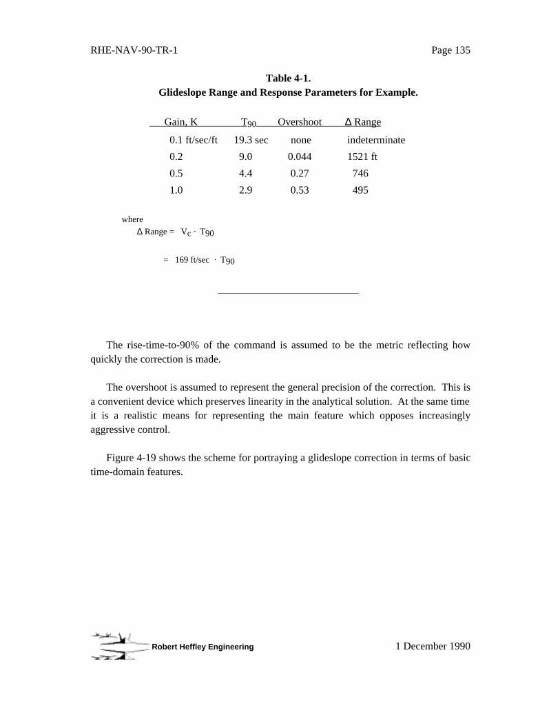
RHE-NAV-90-TR-1 Page 135
Robert Heffley Engineering 1 December 1990
Table 4-1.Glideslope Range and Response Parameters for Example.
Gain, K T90 Overshoot ∆ Range
0.1 ft/sec/ft 19.3 sec none indeterminate
0.2 9.0 0.044 1521 ft
0.5 4.4 0.27 746
1.0 2.9 0.53 495
where
∆ Range = Vc · T90
= 169 ft/sec · T90
________________________________
The rise-time-to-90% of the command is assumed to be the metric reflecting howquickly the correction is made.
The overshoot is assumed to represent the general precision of the correction. This isa convenient device which preserves linearity in the analytical solution. At the same timeit is a realistic means for representing the main feature which opposes increasinglyaggressive control.
Figure 4-19 shows the scheme for portraying a glideslope correction in terms of basictime-domain features.
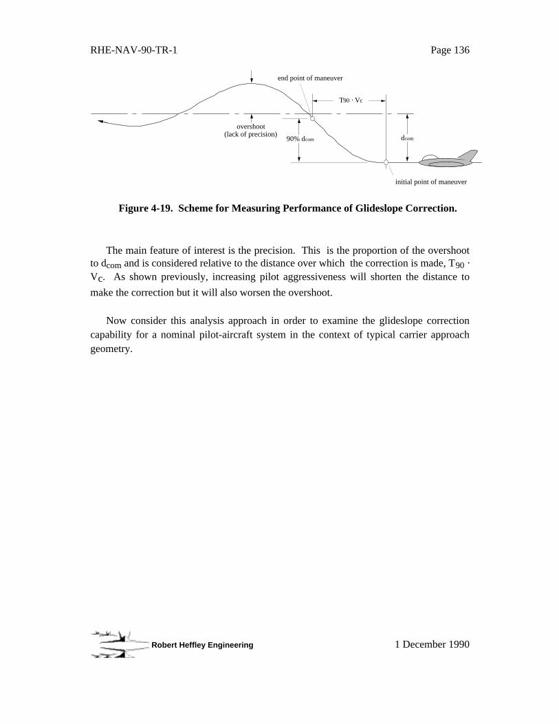
RHE-NAV-90-TR-1 Page 136
Robert Heffley Engineering 1 December 1990
initial point of maneuver
end point of maneuver
T90 · Vc
dcom
overshoot(lack of precision)
90% dcom
Figure 4-19. Scheme for Measuring Performance of Glideslope Correction.
The main feature of interest is the precision. This is the proportion of the overshootto dcom and is considered relative to the distance over which the correction is made, T90 ·Vc. As shown previously, increasing pilot aggressiveness will shorten the distance to
make the correction but it will also worsen the overshoot.
Now consider this analysis approach in order to examine the glideslope correctioncapability for a nominal pilot-aircraft system in the context of typical carrier approachgeometry.

RHE-NAV-90-TR-1 Page 137
Robert Heffley Engineering 1 December 1990
4.3.3 Analysis Results for a Nominal Pilot-Aircraft Combination
The family of time-response curves can next be applied to the carrier approachscenario with the following interpretations on time-of-response and precision-of-response. First, consider the basic task assumptions used for this analysis:
(i) The last significant correction should be completed no closer to the touchdownpoint than at-the-ramp ("AR"), i. e., about 600 ft from the nominal touchdownpoint (which is the #3 wire).
(ii) The vertical flightpath precision should be related to the ability to catch a givenwire. Since the wire spacing is about 40 ft and the nominal glideslope angle is4°, the equivalent vertical flightpath precision would be about 33 in.
(iii)The rise-time-to-90%, T90, is the time to do the task. Using the closure speedwith the ship, Vc, this establishes the point at which the last significantcorrection is begun. Thus the corresponding range would be 600' plus T90 · Vc.
(iv)This scheme assumes that the pilot uses an optimal coordination of thrust andpitch in order to minimize AOA upsets while maximizing flightpath response.This is reflected by the basic math model form used.
(v) Also limit the maximum correction rate-of-descent to correspond to the LSO'sperception of too much or too little glideslope excursion rate, i. e., 0.2° /sec.
From the above assumptions a boundary can be computed which represents the locusof points in the vertical plane from which the aircraft will reach an on-glideslopecondition at the ramp (OK GS and OK rate-of-descent). This allows for the LSO to makea final judgement of the approach and for the aircraft to continue on a trajectory to thedesired arresting wire. Inherent in the method is that pilot aggressiveness is left to varyin order to make whatever tradeoff is necessary between response quickness andprecision.
Some aspects are neglected in the interest of simplicity. First, the effects ofatmospheric disturbances (burble, gusts) on precision are assumed to be smaller than themaneuver-induced upset. This is reasonable for at least the larger-amplitude corrections.Second, the effect of AOA corrections is ignored, but this is consistent with use of acoordinated pitch/thrust control strategy. Finally, no nonlinear effects are taken intoaccount. This will be found acceptable upon seeing that relatively small measures of
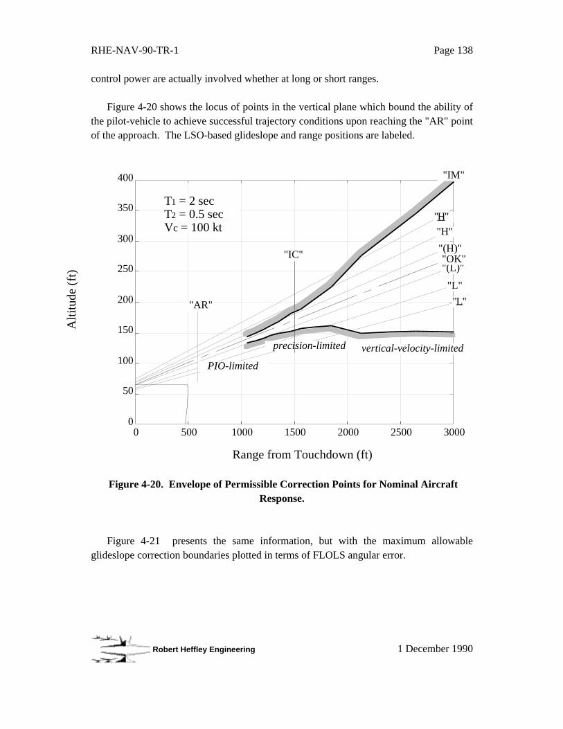
RHE-NAV-90-TR-1 Page 138
Robert Heffley Engineering 1 December 1990
control power are actually involved whether at long or short ranges.
Figure 4-20 shows the locus of points in the vertical plane which bound the ability ofthe pilot-vehicle to achieve successful trajectory conditions upon reaching the "AR" pointof the approach. The LSO-based glideslope and range positions are labeled.
0
50
100
150
200
250
300
350
400
0 500 1000 1500 2000 2500 3000
Alti
tude
(ft
)
Range from Touchdown (ft)
vertical-velocity-limited precision-limited
"AR"
"IC"
"H"
"H"
"(H)"
"L"
"L"
"(L)""OK"
"IM"
PIO-limited
T1 = 2 secT2 = 0.5 secVc = 100 kt
Figure 4-20. Envelope of Permissible Correction Points for Nominal AircraftResponse.
Figure 4-21 presents the same information, but with the maximum allowableglideslope correction boundaries plotted in terms of FLOLS angular error.

RHE-NAV-90-TR-1 Page 139
Robert Heffley Engineering 1 December 1990
-1.5
-1
-0.5
0
0.5
1
1.5
0 500 1000 1500 2000 2500 3000
Range from Touchdown (ft)
FLO
LS
Err
or (
deg)
"H"
"H"
"(H)"
"L"
"L"
"(L)"
"OK"
T1 = 2 secT2 = 0.5 secVc = 100 kt
"AR" "IC" "IM"
33 in
"TD"
Figure 4-21. Envelope of Permissible Correction Points in Terms of FLOLSAngular Error.
Note that for ranges beyond about 2100 ft (0.35 nm) the pilot-aircraft system canachieve an "OK-AR" (on glideslope at the ramp) from any point ranging from "L" (verylow, -1.3° ) to "H" (very high, +1.3° ). From 1800 ft this also can be accomplished, butonly from "L" (0.8° low) to "H" (0.8° high). Increasingly smaller corrections are possibleas the final correction range is moved closer to the ship. At about 1000 ft any correctionapproaching the necessary precision would result in a flightpath PIO (the closed-loopdamping ratio is divergent).

RHE-NAV-90-TR-1 Page 140
Robert Heffley Engineering 1 December 1990
Figure 4-22 shows the corresponding maximum vertical velocity excursions formaneuvers which begin at the glideslope deviation boundaries plotted above in Figure 4-21. The segments on the far left (labeled NERD and TMRD) reflect the ± 0.2° /secglideslope rate of change limit found in the LSO standard in Table 2-1.
Ver
tical
Vel
ocity
Exc
ursi
on, ∆
d (
ft/s
ec)
•
Range from Touchdown (ft)
-20
-15
-10
-5
0
5
10
15
20
0 500 1000 1500 2000 2500 3000
Level flight
"TMRD"
"NERD" "AR"
T1 = 2 secT2 = 0.5 secVc = 100 kt
Figure 4-22. Envelope of Peak Vertical Velocity Excursion for a PermissibleCorrection.
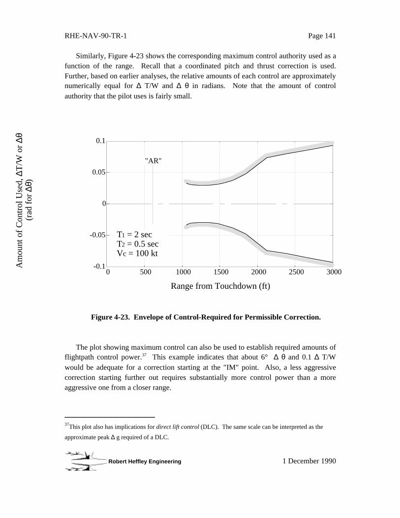
RHE-NAV-90-TR-1 Page 141
Robert Heffley Engineering 1 December 1990
Similarly, Figure 4-23 shows the corresponding maximum control authority used as afunction of the range. Recall that a coordinated pitch and thrust correction is used.Further, based on earlier analyses, the relative amounts of each control are approximatelynumerically equal for ∆ T/W and ∆ θ in radians. Note that the amount of controlauthority that the pilot uses is fairly small.
-0.1
-0.05
0
0.05
0.1
0 500 1000 1500 2000 2500 3000
Range from Touchdown (ft)
Am
ount
of
Con
trol
Use
d, ∆
T/W
or
∆θ
(rad
for
∆θ)
T1 = 2 secT2 = 0.5 secVc = 100 kt
"AR"
Figure 4-23. Envelope of Control-Required for Permissible Correction.
The plot showing maximum control can also be used to establish required amounts offlightpath control power.37 This example indicates that about 6° ∆ θ and 0.1 ∆ T/Wwould be adequate for a correction starting at the "IM" point. Also, a less aggressivecorrection starting further out requires substantially more control power than a moreaggressive one from a closer range.
37This plot also has implications for direct lift control (DLC). The same scale can be interpreted as the
approximate peak ∆ g required of a DLC.
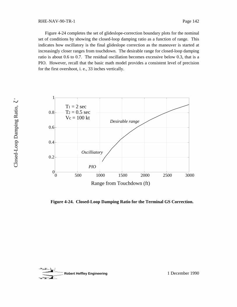
RHE-NAV-90-TR-1 Page 142
Robert Heffley Engineering 1 December 1990
Figure 4-24 completes the set of glideslope-correction boundary plots for the nominalset of conditions by showing the closed-loop damping ratio as a function of range. Thisindicates how oscillatory is the final glideslope correction as the maneuver is started atincreasingly closer ranges from touchdown. The desirable range for closed-loop dampingratio is about 0.6 to 0.7. The residual oscillation becomes excessive below 0.3, that is aPIO. However, recall that the basic math model provides a consistent level of precisionfor the first overshoot, i. e., 33 inches vertically.
0
0.2
0.4
0.6
0.8
1
0 500 1000 1500 2000 2500 3000
Clo
sed-
Loo
p D
ampi
ng R
atio
, ζ
'
Range from Touchdown (ft)
Desirable range
Oscilliatory
PIO
T1 = 2 secT2 = 0.5 secVc = 100 kt
Figure 4-24. Closed-Loop Damping Ratio for the Terminal GS Correction.

RHE-NAV-90-TR-1 Page 143
Robert Heffley Engineering 1 December 1990
4.3.4 Effect of Outer-Loop Control Features on Task Performance
The analysis approach described above and illustrated for a nominal set of conditionsis next used to explore the effects of lumped outer-loop control features, T1, and T2. Theparameter T1 represents the airframe effective lag and is most closely associated withTθ2. T2, the effective control lag, would usually represent the effective pitch-attitude lag
as determined by the FCS, but could also include engine lag in some cases.
Effect of T1, Airframe-Related Time Constant
If the airframe lag, T1, is varied the impact on glideslope control is profound as
Figure 4-25 shows. The last significant glideslope correction must be made progressivelyfurther out as T1 increases. This follows the fact that the scale length of the response,λGS = T1· Vc, gets correspondingly longer. For example, a correction from "H" mustbegin at about 1800 ft if T1 is 2 sec, and 2500 ft for 3 sec.
-1.5
-1
-0.5
0
0.5
1
1.5
0 500 1000 1500 2000 2500 3000
Range from Touchdown (ft)
FLO
LS
Err
or (
deg)
"H"
"H"
"(H)"
"L"
"L"
"(L)"
"OK"
T2 = 0.5 secVc = 100 kt
"AR" "IC" "IM"
33 in
"TD"
32
4
T1 = 1 sec
resulting precision
Figure 4-25. Effect of Airframe Lag, T1, on Permissible
Glideslope-Correction Boundary.
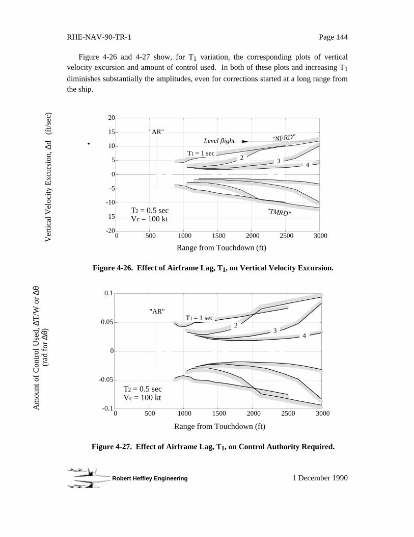
RHE-NAV-90-TR-1 Page 144
Robert Heffley Engineering 1 December 1990
Figure 4-26 and 4-27 show, for T1 variation, the corresponding plots of verticalvelocity excursion and amount of control used. In both of these plots and increasing T1
diminishes substantially the amplitudes, even for corrections started at a long range fromthe ship.
Ver
tical
Vel
ocity
Exc
ursi
on, ∆
d (
ft/s
ec)
•
Range from Touchdown (ft)
-20
-15
-10
-5
0
5
10
15
20
0 500 1000 1500 2000 2500 3000
Level flight
"TMRD"
"NERD" "AR"
T2 = 0.5 secVc = 100 kt
324
T1 = 1 sec
Figure 4-26. Effect of Airframe Lag, T1, on Vertical Velocity Excursion.
-0.1
-0.05
0
0.05
0.1
0 500 1000 1500 2000 2500 3000
Range from Touchdown (ft)
Am
ount
of
Con
trol
Use
d, ∆
T/W
or
∆θ
(rad
for
∆θ)
T2 = 0.5 secVc = 100 kt
"AR"
32
4
T1 = 1 sec
Figure 4-27. Effect of Airframe Lag, T1, on Control Authority Required.
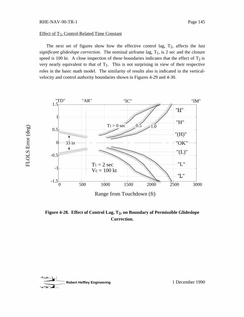
RHE-NAV-90-TR-1 Page 145
Robert Heffley Engineering 1 December 1990
Effect of T2, Control-Related Time Constant
The next set of figures show how the effective control lag, T2, affects the lastsignificant glideslope correction. The nominal airframe lag, T1, is 2 sec and the closurespeed is 100 kt. A close inspection of these boundaries indicates that the effect of T2 isvery nearly equivalent to that of T1. This is not surprising in view of their respective
roles in the basic math model. The similarity of results also is indicated in the vertical-velocity and control authority boundaries shown in Figures 4-29 and 4-30.
-1.5
-1
-0.5
0
0.5
1
1.5
0 500 1000 1500 2000 2500 3000
Range from Touchdown (ft)
FLO
LS
Err
or (
deg)
"H"
"H"
"(H)"
"L"
"L"
"(L)"
"OK"
T1 = 2 secVc = 100 kt
"AR" "IC" "IM"
33 in
"TD"
1.00.5T1 = 0 sec
Figure 4-28. Effect of Control Lag, T2, on Boundary of Permissible Glideslope
Correction.
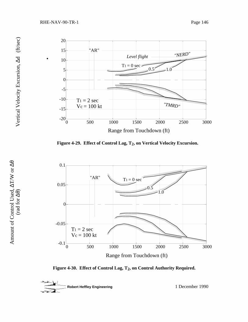
RHE-NAV-90-TR-1 Page 146
Robert Heffley Engineering 1 December 1990
Ver
tical
Vel
ocity
Exc
ursi
on, ∆
d (
ft/s
ec)
•
Range from Touchdown (ft)
-20
-15
-10
-5
0
5
10
15
20
0 500 1000 1500 2000 2500 3000
Level flight
"TMRD"
"NERD" "AR"
T1 = 2 secVc = 100 kt
1.00.5T1 = 0 sec
Figure 4-29. Effect of Control Lag, T2, on Vertical Velocity Excursion.
-0.1
-0.05
0
0.05
0.1
0 500 1000 1500 2000 2500 3000
Range from Touchdown (ft)
Am
ount
of
Con
trol
Use
d, ∆
T/W
or
∆θ
(rad
for
∆θ)
T1 = 2 secVc = 100 kt
"AR"
1.00.5
T1 = 0 sec
Figure 4-30. Effect of Control Lag, T2, on Control Authority Required.
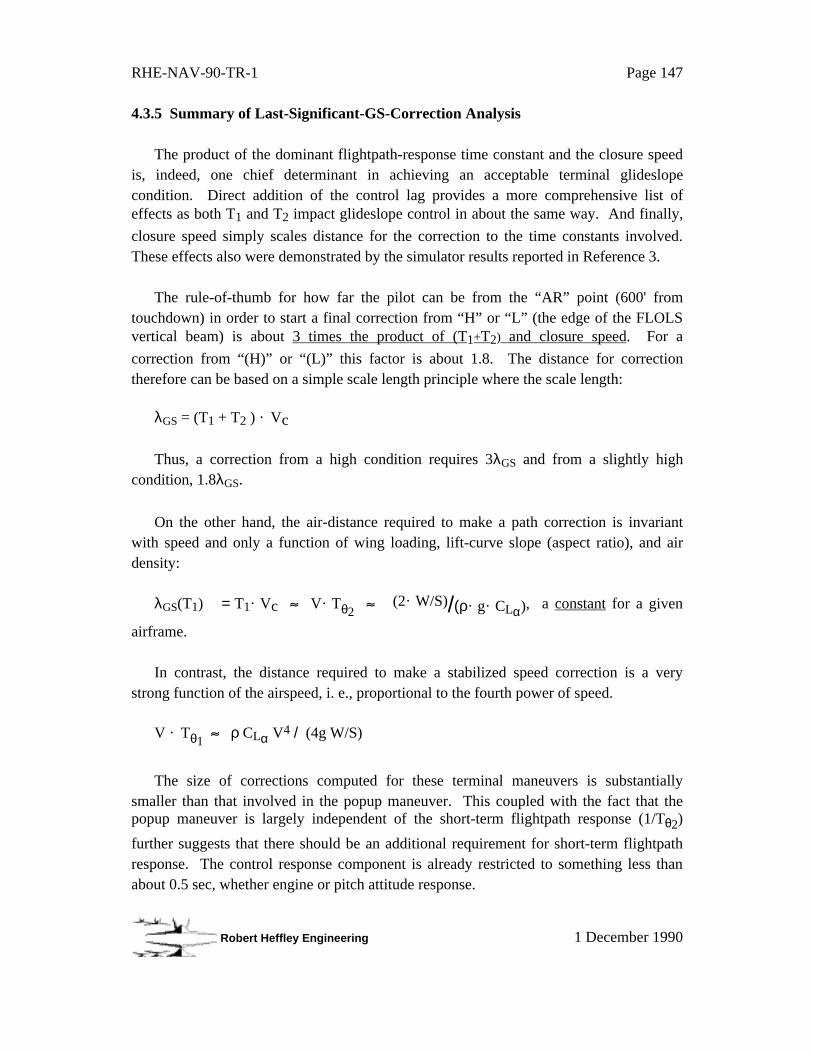
RHE-NAV-90-TR-1 Page 147
Robert Heffley Engineering 1 December 1990
4.3.5 Summary of Last-Significant-GS-Correction Analysis
The product of the dominant flightpath-response time constant and the closure speedis, indeed, one chief determinant in achieving an acceptable terminal glideslopecondition. Direct addition of the control lag provides a more comprehensive list ofeffects as both T1 and T2 impact glideslope control in about the same way. And finally,
closure speed simply scales distance for the correction to the time constants involved.These effects also were demonstrated by the simulator results reported in Reference 3.
The rule-of-thumb for how far the pilot can be from the “AR” point (600' fromtouchdown) in order to start a final correction from “H” or “L” (the edge of the FLOLSvertical beam) is about 3 times the product of (T1+T2) and closure speed. For a
correction from “(H)” or “(L)” this factor is about 1.8. The distance for correctiontherefore can be based on a simple scale length principle where the scale length:
λGS = (T1 + T2 ) · Vc
Thus, a correction from a high condition requires 3λGS and from a slightly highcondition, 1.8λGS.
On the other hand, the air-distance required to make a path correction is invariantwith speed and only a function of wing loading, lift-curve slope (aspect ratio), and airdensity:
λGS(T1) = T1· Vc V· Tθ2 (2· W/S)/(ρ· g· CLα), a constant for a given
airframe.
In contrast, the distance required to make a stabilized speed correction is a verystrong function of the airspeed, i. e., proportional to the fourth power of speed.
V · Tθ1 ρ CLα V4 / (4g W/S)
The size of corrections computed for these terminal maneuvers is substantiallysmaller than that involved in the popup maneuver. This coupled with the fact that thepopup maneuver is largely independent of the short-term flightpath response (1/Tθ2)
further suggests that there should be an additional requirement for short-term flightpathresponse. The control response component is already restricted to something less thanabout 0.5 sec, whether engine or pitch attitude response.
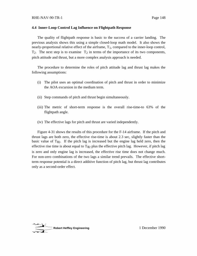
RHE-NAV-90-TR-1 Page 148
Robert Heffley Engineering 1 December 1990
4.4 Inner-Loop Control Lag Influence on Flightpath Response
The quality of flightpath response is basic to the success of a carrier landing. Theprevious analysis shows this using a simple closed-loop math model. It also shows thenearly-proportional relative effect of the airframe, T1, compared to the inner-loop control,T2. The next step is to examine T2 in terms of the importance of its two components,
pitch attitude and thrust, but a more complex analysis approach is needed.
The procedure to determine the roles of pitch attitude lag and thrust lag makes thefollowing assumptions:
(i) The pilot uses an optimal coordination of pitch and thrust in order to minimizethe AOA excursion in the medium term.
(ii) Step commands of pitch and thrust begin simultaneously.
(iii) The metric of short-term response is the overall rise-time-to 63% of theflightpath angle.
(iv) The effective lags for pitch and thrust are varied independently.
Figure 4-31 shows the results of this procedure for the F-14 airframe. If the pitch andthrust lags are both zero, the effective rise-time is about 2.3 sec, slightly faster than thebasic value of Tθ2. If the pitch lag is increased but the engine lag held zero, then theeffective rise time is about equal to Tθ2 plus the effective pitch lag. However, if pitch lag
is zero and only engine lag is increased, the effective rise time does not change much.For non-zero combinations of the two lags a similar trend prevails. The effective short-term response potential is a direct additive function of pitch lag, but thrust lag contributesonly as a second-order effect.
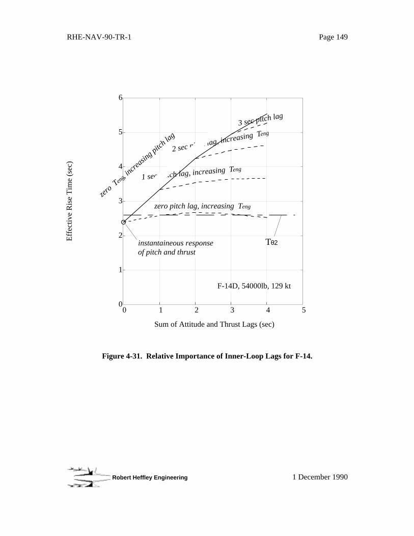
RHE-NAV-90-TR-1 Page 149
Robert Heffley Engineering 1 December 1990
0
1
2
3
4
5
6
0 1 2 3 4 5
F-14D, 54000lb, 129 kt
Sum of Attitude and Thrust Lags (sec)
Eff
ectiv
e R
ise
Tim
e (s
ec)
Tθ2instantaineous response of pitch and thrust
zero pitch lag, increasing Teng
1 sec pitch lag, increasing Teng
2 sec pitch lag, increasing Teng
zero T
eng, i
ncreasin
g pitch la
g 3 sec pitch lag
Figure 4-31. Relative Importance of Inner-Loop Lags for F-14.
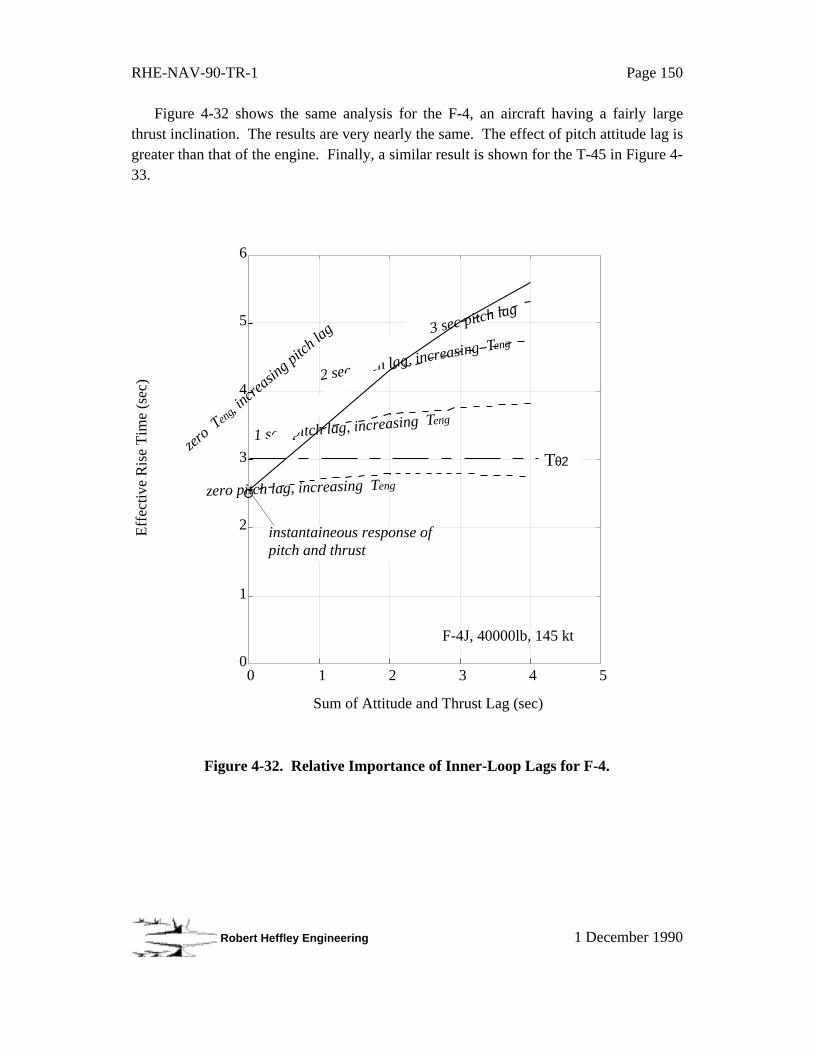
RHE-NAV-90-TR-1 Page 150
Robert Heffley Engineering 1 December 1990
Figure 4-32 shows the same analysis for the F-4, an aircraft having a fairly largethrust inclination. The results are very nearly the same. The effect of pitch attitude lag isgreater than that of the engine. Finally, a similar result is shown for the T-45 in Figure 4-33.
0
1
2
3
4
5
6
0 1 2 3 4 5
F-4J, 40000lb, 145 kt
Sum of Attitude and Thrust Lag (sec)
Eff
ectiv
e R
ise
Tim
e (s
ec)
Tθ2
instantaineous response of pitch and thrust
zero pitch lag, increasing Teng
1 sec pitch lag, increasing Teng
2 sec pitch lag, increasing Teng
zero T
eng, i
ncreasin
g pitch la
g 3 sec pitch lag
Figure 4-32. Relative Importance of Inner-Loop Lags for F-4.
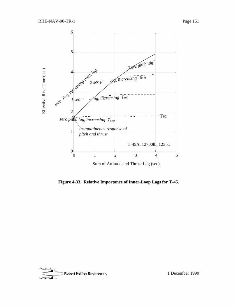
RHE-NAV-90-TR-1 Page 151
Robert Heffley Engineering 1 December 1990
0
1
2
3
4
5
6
0 1 2 3 4 5
T-45A, 12700lb, 125 kt
Sum of Attitude and Thrust Lag (sec)
Eff
ectiv
e R
ise
Tim
e (s
ec)
Tθ2
instantaineous response of pitch and thrust
zero pitch lag, increasing Teng
1 sec pitch lag, increasing Teng
2 sec pitch lag, increasing Teng
zero T
eng, i
ncreasin
g pitch la
g 3 sec pitch lag
Figure 4-33. Relative Importance of Inner-Loop Lags for T-45.
RHE-NAV-90-TR-1 Page 152
Robert Heffley Engineering 1 December 1990
4.5 Effect of Engine Lag on Control of Thrust
The previous analysis shows that thrust lag does not limit directly the short-termglideslope response-potential. Therefore, one needs to explore the effect of thrust lagfrom a different point of view.
Informal interviews were conducted with pilots who have operated aircraft with slow-responding engines (high-bypass-ratio turbofans). The main complaint appeared to be insimply making thrust adjustments, a basic inner-loop task. As described, the pilot hasdifficulty in predicting the eventual thrust level following the initial throttle change whenmade without reference to engine gages. There is simply no reliable initial cue whichcorrelates with the steady-state thrust. The problem is most acute when restoring thrustfrom a near-idle condition. (Recall from Section 2 that thrust lags are greatest at lowpower settings.)
A review of the outer-loop control structures for the likely control strategies indicatesthat thrust control is really an inner-loop control function, similar to pitch attitude control.Further, the essential response features of thrust are that (i) it is a proportional control(the steady-state thrust level follows throttle position) and (ii) the status is usuallymonitored aurally, at least during the latter stages of the approach where use of cockpitgauges is inadvisable.
Thus the maximum thrust lag should be a function of inner-loop control activity. Thethrust lag, Teng, should influence how quickly the pilot can make a simple thrust
adjustment using only the feedback of engine noise.38 One analytical method which hasbeen demonstrated valid for similar inner-loop applications is the Hess Structural PilotModel.
Hess Structural Pilot Model
R. Hess has developed a theoretical approach to predict the effect of various designfeatures on aircraft handing qualities (Reference 67). He has applied it successfully tothe effects of motion cueing (Reference 68), and has succeeded in correlating severalexperiments in which pilot ratings were collected for a wide range of system types(Reference 69). This includes the broad class investigated by J. McDonnell in Reference
38One assumes that engine noise is a direct function of the actual thrust level as opposed to the commanded
thrust level.
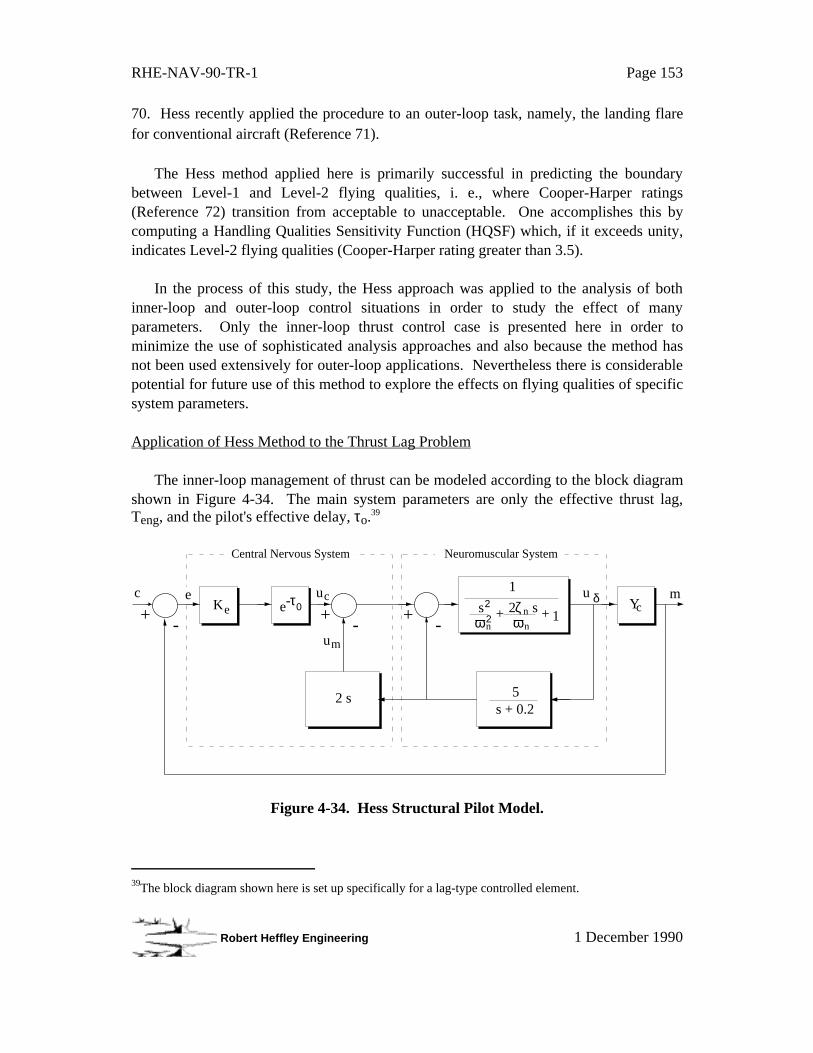
RHE-NAV-90-TR-1 Page 153
Robert Heffley Engineering 1 December 1990
70. Hess recently applied the procedure to an outer-loop task, namely, the landing flarefor conventional aircraft (Reference 71).
The Hess method applied here is primarily successful in predicting the boundarybetween Level-1 and Level-2 flying qualities, i. e., where Cooper-Harper ratings(Reference 72) transition from acceptable to unacceptable. One accomplishes this bycomputing a Handling Qualities Sensitivity Function (HQSF) which, if it exceeds unity,indicates Level-2 flying qualities (Cooper-Harper rating greater than 3.5).
In the process of this study, the Hess approach was applied to the analysis of bothinner-loop and outer-loop control situations in order to study the effect of manyparameters. Only the inner-loop thrust control case is presented here in order tominimize the use of sophisticated analysis approaches and also because the method hasnot been used extensively for outer-loop applications. Nevertheless there is considerablepotential for future use of this method to explore the effects on flying qualities of specificsystem parameters.
Application of Hess Method to the Thrust Lag Problem
The inner-loop management of thrust can be modeled according to the block diagramshown in Figure 4-34. The main system parameters are only the effective thrust lag,Teng, and the pilot's effective delay, τo.39
Ke Yce-τ 0e uc
um
u δ mc
Central Nervous System Neuromuscular System
+-
+-
+-
s 2ζ sω ω
22n n
n+ + 1
1
2 s 5s + 0.2
Figure 4-34. Hess Structural Pilot Model.
39The block diagram shown here is set up specifically for a lag-type controlled element.

RHE-NAV-90-TR-1 Page 154
Robert Heffley Engineering 1 December 1990
If the effective delay is assumed to be 0.15 sec, we can compute the maximum pilotcrossover frequency at which the Hess HQSF exceeds unity. Figure 4-35 shows this forthree crossover frequencies (levels of pilot aggressiveness) and an engine lag of 0.3 sec.A crossplot of the results yields a crossover of 2.44 rad/sec as the maximumaggressiveness for Level-1 flying qualities.
0
1
2
3
4
5
0 1 2 3 4 5
Engine Sound Cue Only T = 0.3 sec
max = 2.44 rad/sec
Frequency (rad/sec)
HQ
Sen
sitiv
ity F
acto
r
eng
ω = 3.0 rad/sec
2.5
2.0
c
c
For HQSF < 1
Figure 4-35. Sample of HQ Sensitivity Factor Solutions.
This process is repeated for several values of Teng in order to map the Level-1 flying
qualities boundary (HQSF = 1). The results are presented in Figure 4-36 in terms of themaximum pilot aggressiveness as a function of engine lag.
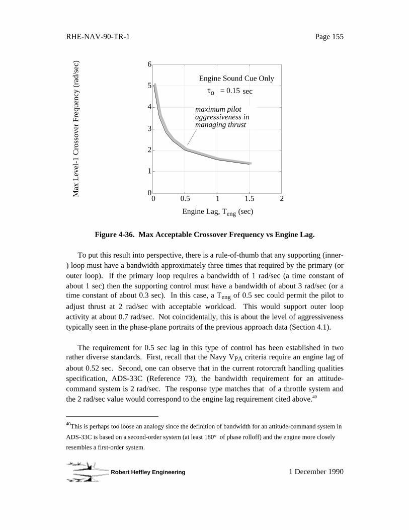
RHE-NAV-90-TR-1 Page 155
Robert Heffley Engineering 1 December 1990
0
1
2
3
4
5
6
0 0.5 1 1.5 2
Engine Sound Cue Only
Engine Lag, T (sec)
Max
Lev
el-1
Cro
ssov
er F
requ
ency
(ra
d/se
c)
eng
τ = 0.15ο sec
maximum pilot aggressiveness in managing thrust
Figure 4-36. Max Acceptable Crossover Frequency vs Engine Lag.
To put this result into perspective, there is a rule-of-thumb that any supporting (inner-) loop must have a bandwidth approximately three times that required by the primary (orouter loop). If the primary loop requires a bandwidth of 1 rad/sec (a time constant ofabout 1 sec) then the supporting control must have a bandwidth of about 3 rad/sec (or atime constant of about 0.3 sec). In this case, a Teng of 0.5 sec could permit the pilot to
adjust thrust at 2 rad/sec with acceptable workload. This would support outer loopactivity at about 0.7 rad/sec. Not coincidentally, this is about the level of aggressivenesstypically seen in the phase-plane portraits of the previous approach data (Section 4.1).
The requirement for 0.5 sec lag in this type of control has been established in tworather diverse standards. First, recall that the Navy VPA criteria require an engine lag of
about 0.52 sec. Second, one can observe that in the current rotorcraft handling qualitiesspecification, ADS-33C (Reference 73), the bandwidth requirement for an attitude-command system is 2 rad/sec. The response type matches that of a throttle system andthe 2 rad/sec value would correspond to the engine lag requirement cited above.40
40This is perhaps too loose an analogy since the definition of bandwidth for an attitude-command system in
ADS-33C is based on a second-order system (at least 180° of phase rolloff) and the engine more closely
resembles a first-order system.

RHE-NAV-90-TR-1 Page 156
Robert Heffley Engineering 1 December 1990
The Navy approach speed criterion which now limits thrust lag appears to have somejustification. However, given the need for the pilot to make quick thrust adjustmentswithout head-down reference, this may be a matter which properly should be addressed inthe flying qualities specifications. Further, this issue may be particularly acute forturbofan engine installations in a number of critical flight phases, including airbornerefueling and close-formation flight.
RHE-NAV-90-TR-1 Page 157
Robert Heffley Engineering 1 December 1990
5. CONCLUSIONS AND RECOMMENDATIONS
The analytical study of outer-loop control factors for carrier aircraft has led to severalconclusions regarding aircraft design and testing processes. These conclusions aresummarized below, and recommendations are given for additional analysis and experi-mentation.
5.1 Conclusions Based on Analysis Results
The paragraphs below summarize, with a brief discussion, the important results ofthis study. General conclusions are followed by several more specific ones.
5.1.1 General
• A candidate list of outer-loop control factors serves as a starting point.
Section 3 of this report presents, without quantification, a systematic list of outer-loopcontrol factors based on a general assessment of the carrier approach task and existingcontrol criteria. This is a useful tool for examining the effectiveness of existing criteria,identifying weaknesses, and recommending modifications and additional criteria.
_____________________________
• Outer-loop control factors presently are covered only partially.
The combination of existing flying qualities requirements and the Navy approach-speed criteria presently provides a degree of coverage of outer-loop control factors forcarrier aircraft. However, there is no systematic identification of those factors andcorresponding design criteria. The MIL-STD-1797A flying qualities specificationfurnishes a general framework but fails to back it up quantitatively, particularly for outer-loop features of the carrier landing task. Overall, the existing requirements address manyouter-loop control factors, but not directly and explicitly. Specific cases are detailed inseveral of the following items.
_____________________________
RHE-NAV-90-TR-1 Page 158
Robert Heffley Engineering 1 December 1990
• The carrier-landing task lacks quantitative definition.
Presently there is no quantitative definition of the carrier landing task that describesthe minimum requirements for pilot aggressiveness, amplitude of maneuvers, precisionof terminal conditions, and settling of corrections. The only explicit task feature is theduration of the approach given by the distance from the roll-out into the final leg and theclosure speed with the ship. LSO performance criteria furnish useful backgroundinformation but are not sufficient for an engineering definition of the task.
The main benefit of a comprehensive task definition is that one could computedirectly most of the necessary for outer-loop control factors. This would promote adegree of consistency among the individual control factors and economy when imposingthem as design requirements. The failure to have a comprehensive task definition forcesreliance on subjective assessment of task performance and of the effectiveness of designrequirements.
_____________________________
• Pilot technique for the carrier landing task is defined only subjectively.
Pilot technique or control strategy for the carrier landing is not well understood ordefined in clear quantitative terms. The classical "backside" technique attributed to Navyuse, if rigidly interpreted, severely limits pilot aggressiveness in controlling flightpath.There is some danger that this might lead to inappropriate design assumptions. Carefulmeasurement and analysis of data obtained from flight could yield an accurate assessmentof the technique, or variety of techniques, that Navy carrier pilots actually use. In turn,this would be an important component in the quantification of task performance.
_____________________________
• Pitch-constrained equations offer the analyst a powerful tool.
Pitch-attitude-constrained equations of motion provide a simple but powerfulanalytical tool for examining outer-loop stability and control features.
(i) They embrace fundamental, easily-estimated, parameters.(ii) They permit inner-loop control features to be partitioned and treated separately.(iii) They emphasize the strong, fundamental influence of lift and drag on flightpath
and airspeed dynamics.

RHE-NAV-90-TR-1 Page 159
Robert Heffley Engineering 1 December 1990
This tool is particularly useful for examining the bridge between the disciplines ofstability and control and of performance, at least where the effects of nonlinearities donot prevail. Although, even where there are significant nonlinearities, say in lift or drag,many of the basic pitch-constrained principles remain valid and useful.
_____________________________
• The Navy's use of AOA as a speed reference has special implications.
Given that pitch attitude is actively regulated by the pilot, angle-of-attack responsemathematically is the complement of flightpath angle. This implies that any constraint onflightpath control features also governs AOA control features. Attitude-constrainedequations show directly that dynamics of angle-of-attack and flightpath are closelyrelated. Further, this relationship effectively minimizes the number of system parametersnecessary to describe dynamic response of the outer-loop control states involved in thecarrier approach.
_____________________________
RHE-NAV-90-TR-1 Page 160
Robert Heffley Engineering 1 December 1990
5.1.2 Specific Conclusions
• Current Navy approach-speed criteria are necessary but not sufficient.
Each component of the Navy approach speed criteria implies certain constraints onthe outer-loop control, but these constraints are not sufficiently comprehensive to coverall aspects crucial to performing the carrier landing task.
Features which are covered include:• Flightpath control-power upward, applicable to the waveoff task• Flightpath control-power upward and downward, applicable to the approach task• Engine thrust lag for the nominal flightpath-angle power setting• Pitch attitude response lag, control power, and manipulator characteristics• Margin from power-on stall (implicit in popup and explicit in 1.1VSPA req’t)
• Visibility of deck-centered glideslope and lineup cues (downward field of view)
Features which are not covered include:• Short-term flightpath response• Engine thrust lag for off-nominal power settings• Quality of flightpath response (such as speed damping effects)• Engine thrust-level cueing in the absence of a HUD
Other observations made:• Popup maneuver defines "safe" pitchup amplitude• Criteria assume a "conventional" non powered-lift airplane
_____________________________
• Flying-qualities specifications mainly address inner-loop pitch response.
The Navy approach-speed criteria requirement for compliance with MIL-F-8785Caffects mainly inner-loop control of pitch attitude due to the traditional emphasis ofaircraft flying qualities. Outer-loop control benefits are minor and indirect. MIL-STD-1797A furnishes a more systematic framework that includes outer-loop control but doesnot contain well-supported outer-loop backup data. Its main strength also is inner-looppitch control criteria. Neither specification addresses inner-loop control of thrust.
_____________________________

RHE-NAV-90-TR-1 Page 161
Robert Heffley Engineering 1 December 1990
• The thrust acceleration-response requirement covers both engine lag andflightpath control power but is subject to misinterpretation.
The criterion requiring not more than 1.2 sec rise-time-to-90% for a ± 3.86 ft/sec2
longitudinal acceleration command can limit two important control features. First, it canindirectly provide for a level of flightpath control authority equivalent to about ± 7°incremental flightpath angle. Second, the rise time, if expressed as an equivalent first-order lag, limit the maximum thrust lag to 0.52 sec. Both are key factors for outer-loopcontrol, but there is a potential difficulty.
The favorable control constraints described above are really based on interpreting thecommand as the incremental thrust-to-weight ratio rather than longitudinal acceleration.The latter quantity does not approach a commanded value, but instead washes out as thespeed-damping takes effect. Use of the longitudinal acceleration state can result inunclear and unfavorable interpretations of the effective thrust lag and flightpath controlpower.
_____________________________
• Primary outer-loop design parameters have been identified.
The lowest-common-denominator set of design parameters for any pitch-inducedflightpath maneuver, including the popup, consists of:
• Airspeed, V• nzα• Margin from stall, V/VSPA
• Pitchup abruptness (time-constant of pitch command)• Backsidedness, ∂ γ/∂ V
This set recognizes certain interdependencies among the response factors (including Tθ1,Tθ2, and Th1) defined by pitch-constrained equations of motion.
The main effects of individual parameters are:nzα ⇒ in combination with airspeed, a key element in flightpath response modes
V ⇒ primary determinant of time-available to make corrections∂ γ/∂ V ⇒ strong modifier of basic speed damping, speed-stability a secondary roleV/VSPA ⇒ affects the available maneuvering amplitude using pitch control
∆ T/W margins (± ) ⇒ permit sustained changes in flightpath, i. e., controlauthority
RHE-NAV-90-TR-1 Page 162
Robert Heffley Engineering 1 December 1990
ωBW or ωsp ⇒ effective pitch control short-term response
Teng ⇒ effective thrust control short-term response
(There are few corresponding parameters for the horizontal-plane outer-loop responsecharacteristics. The main ones of interest would be inner-loop response in the roll axisand the turn coordination quality.)
_____________________________
• The 5 sec-to-50 ft popup maneuver mainly reflects stall margin.
The popup maneuver 5-sec-to-50ft criterion, represents mainly a level of power-onstall margin. Generally speaking, the popup maneuver can be performed only if theV/VSPA ratio is about 1.2. Hence, the existing 1.1 VSPA minimum-speed criterion is not
likely to be critical and its necessity is open to question.
Also, the 5-sec-to-50ft criterion is an open-loop maneuver in which the short-termresponse factor is only weakly represented. A modification of the maneuver that includesmaintenance of glideslope (such as the “7-sec-to-50ft-and-back-to-50ft” version used atone time) would strengthen the short-term response attribute implicit in the maneuver.
_____________________________
• The “minimum potential flightpath lag” is a useful short-term response metric.
The minimum potential flightpath lag is the rise-time-to 63% for a well-coordinatedstep input of pitch attitude and thrust. It is a short-term response metric that embodies theairframe and control system features in the context of a well-refined pilot technique.Also it is directly computable for the open-loop aircraft system. Competing but moresimplistic metrics include, Zw, Tθ2, and V· nzα.
_____________________________
RHE-NAV-90-TR-1 Page 163
Robert Heffley Engineering 1 December 1990
• Thrust-lag is mainly an “inner-loop” control problem.
The effect of thrust lag on the total short-term response (minimum potential flightpathlag) is small compared to the effects of basic heave damping (Tθ2) and the effective pitch
attitude response. Therefore one can deduce that thrust lag is an inner-loop controlproblem under some conditions. This would be true for aircraft having quick airframeand pitch response but receiving engine-response complaints.
One can relate thrust lag to the pilot's ability to adjust thrust, given that engine soundis the only status cue. Using the Hess analytical approach, the boundary for pilotacceptance was estimated. The current 1.2 sec rise-time-to-90% criterion coincides withthe knee in the Hess criterion estimate, and it agrees numerically with the bandwidthcriterion for inner-loop pitch response.
_____________________________
• “Last significant glideslope correction” is an extension of the popup criterion.
The main requirements for effective flightpath control rest upon answeringsimultaneously how quick, how large, and how precise can the pilot perform a terminalflightpath maneuver. The last significant glideslope correction is a math modelformulation aimed at obtaining such an answer for the carrier landing task.
Airframe and control features are lumped into a low-order math model and afeedback loop closed around them. It is used here to explore the effects of several designparameters. This analysis method is a sophistication of the popup maneuver thatpotentially incorporates multiple aspects of the pilot-vehicle-task system.
This method demonstrates the influences of several control factors, particularlyshort-term response. Tentative conclusions were made based on LSO task performanceassumptions, but only to demonstrate the method. Firmer results depend upon analysis ofactual carrier landing data involving large, close-in terminal maneuvers along with pilotand LSO assessments of acceptability.
_____________________________
RHE-NAV-90-TR-1 Page 164
Robert Heffley Engineering 1 December 1990
• Carrier landing task-performance can be defined using existing facilities.
The main objective of quantifying task performance in the carrier approach is to assistin setting design and test criteria. Given the heavy reliance on computer-aided designand simulation in the design process, task performance standards can be factored-in at theearliest stages.
It is desirable to determine the quantitative nature of each task-performance featurethrough direct measurement, including:
(i) how aggressively the pilot needs and desires to make flightpath corrections,(ii) how large they might be (presumably as a function of range),(iii) what degree of closed-loop damping or settling is needed, and(iv) how precise in order to meet terminal conditions with high likelihood of success.
Each of these can be quantified, measured, and reduced to basic design factors.
Existing analysis techniques and flight-test measurement facilities are fully capable ofcollecting and organizing these specific task-performance data. The main requirementsare to obtain precise position data and to obtain it in the context of an actual carrierenviron ment. Both presently are feasible.
While an analysis of some laser-tracker data was performed, it was not possible toarrive at any definitive assessment of how the carrier landing task is carried out in usefulengineering terms. An initial phase-plane analysis was done to examine pilotaggressiveness and maneuver amplitude for the FCLP data available, and this showed ageneral degree of consistency from run to run and from one aircraft to another. Butwithout accompanying pilot commentary and a full knowledge of the circumstances ofeach approach, there is some danger in over-analyzing such data. Also, they did not fullyrepresent an actual carrier environment and therefore lack credibility.
_____________________________

RHE-NAV-90-TR-1 Page 165
Robert Heffley Engineering 1 December 1990
5.2 Need for Further Research
Based on this study, primarily an analytical effort, there are several gaps in existingdesign requirements as indicated above. Also there is reasonable doubt of theeffectiveness of some requirements now in use. Future research should address severalitems, both experimentally and by non-intrusive in-flight measurements. This workshould focus on the carrier landing task but also should include, where possible, othertasks and mission elements for which manual control is crucial. The following itemsdescribe briefly the logical steps in any future program to achieve these goals.
• Analyze quantitatively examples of carrier-landing task performance.
First, there is a need to make a comprehensive survey parameters which describe thecarrier landing task. One main objective should be to quantify for several aircraft typesthe maximum desired level of aggressiveness in control of flightpath as a function ofrange from the ship. This must be done with highly skilled and experienced carrierpilots. It should include both glideslope and lineup tasks. Aircraft instrumented forlaser-tracker position measurement should be used in all cases. The last significantglideslope correction is a model about which task performance data can be gathered andorganized.
• Develop a simulator experimental test program.
The second step should be to design a flight-simulator experiment that systematicallyexplores the design parameters identified in this study. It is necessary to confirm theirimportance and structure a comprehensive framework for outer-loop-control designrequirements. The design of an experiment needs to be based partly on the analysespresented in this report and on some subsequent, more detailed analyses.
• Conduct a simulator experiment.
Following the experimental design, a simulator experiment should be carried out togather the needed data. This should be done using facilities and pilot subjects that aresuited to examining the Navy carrier landing mission. Objective data should include alltask performance measurements gathered for in-flight carrier landing examples.Subjective data should contain pilot commentary and Cooper-Harper ratings.
RHE-NAV-90-TR-1 Page 166
Robert Heffley Engineering 1 December 1990
• Verify simulator results with flight tests.
The simulator results must be verified by selected in-flight testing. This is possibleusing non-intrusive test pilot evaluations made during routine carrier-suitability flighttesting. This needs to be done either during the simulator program or shortly following itand with some of the same pilots who participate in the simulations.
• Propose outer-loop-control requirements.
The final step is to prepare a comprehensive report documenting all analytical,experimental, and flight verification work along with a proposal for outer-loop controlrequirements. This needs to be done with the cooperation and participation ofrepresentatives from several disciplines, including stability and control, aircraftperformance, and carrier suitability testing. This team-effort report thus would serve asthe basis for any needed revision of existing design requirements.

RHE-NAV-90-TR-1 167
Robert Heffley Engineering 1 December 1990
REFERENCES
1 Anon., Military Standard, Flying Qualities of Piloted Aircraft, MIL-STD-1797A, 30January 1990.
2 Anon., Military Specification, Flying Qualities of Piloted Airplanes, MIL-F-8785C, 5November 1980.
3 Heffley, R. K., Terminal Control Factors for the Carrier Landing Task, AIAA-86-2251-CP, August 1986.
4 Anon., Detail Specification for Model T-45A Aircraft Weapons System (U), Full ScaleDevelopment, SD-570-1 R2, 1 October 1984.
5 Anon., Detail Specification for Model F-18A Aircraft Weapons System (U), SD-565-1(C), 25 November 1975.
6 Shields, E. R. and D. J. Phelan, The Minimum Landing Approach Speed of HighPerformance Aircraft, McDonnell Report 3232, October 1953.
7 Bihrle, William, Jr., and Ralph W. Stone, Jr., Analytical Studies of the Response toLongitudinal Control of Three Airplane Configurations in Landing Approaches,NACA RM L53B10 (also IAS preprint 404), 1953.
8 Lina, Lindsay J., Garland J. Morris, and Robert A. Champine, Flight Investigation ofFactors Affecting the Choice of Minimum Approach Speed for Carrier-Type Landingsof a Swept-Wing Jet Fighter Airplane, NACA RM L57F13, 1957.
9 Lean, D. and R. Eaton, The Influence of Drag Characteristics on the Choice ofLanding Approach Speeds, R. A. E TN Aero. 2503, April 1957.
10 White, Maurice D., Bernard A. Schlaff, and Fred J. Drinkwater, III, A Comparison ofFlight Measured Carrier Approach Speeds with Values Predicted by SeveralDifferent Criteria for 41 Fighter Type Airplane Configurations, NACA RM A57L11,1958.
11 Drinkwater, Fred J., III, and George E. Cooper, A Flight Evaluation of the Factorswhich Influence the Selection of Landing Approach Speeds, NASA Memo 10-6-58A,1958.
RHE-NAV-90-TR-1 168
Robert Heffley Engineering 1 December 1990
12 Eberle, R. B., D. B. Schoelerman, and N. A. Smykacz, Six New Criteria forPredicting Landing Approach Speed Based on an Analog Computer Analysis of 21Jet-Propelled Aircraft, Chance Vought Report AER-EOR-13202, 25 October 1960.
13 Whitehead, D. J., “The Low Speed Approach and Catapult Launch Problems in HighPerformance Naval Aircraft,” Journal of the Royal Aeronautical Society, Volume 64,Number 592, April 1960.
14 Bezanson, A. F., Effects of Pilot Technique on Minimum Approach Speed, NATCReport FT2222-56, 17 February 1961.
15 Rapp, Fred L., LCDR, USN, “Determination of Optimum Approach Speeds forCarrier Landings,” Naval Weapons Bulletin No. 3-61, 1961.
16 Linden, J. E., A Discussion of the Carrier Landing Approach Speed Problem, Bureauof Aeronautics, Aerodynamics and Hydrodynamics Branch Technical Memo 1-59, 15January 1959.
17 Miller, W. H., LCDR, USN, and B. J. Brockhagen, Evaluation of Revised DroopedAileron Installation in Model F-4B Aircraft, Final Report, NATC Report No.FT2123-51R-64, 27 July 1964.
18 Mickle, Don A., MAJ, USMC, and B. J. Brockhagen, Investigation of Feasibility ofPerformance Demonstration of Landing Approach Speed, F-8 Phase, First InterimReport, NATC Report No. FT2123-67R-64, 2 December 1964.
19 Leuschner, R L., LT, USN, and B. J. Brockhagen, Investigation of Feasibility ofPerformance Demonstration of Landing Approach Speed, A-4 Phase, NATC ReportNo. FT2123-26R-65, 28 April 1965.
20 Gralow, R. T., LT, USN, et al, Evaluation of the Direct Lift Control System Installedin the F-8C Airplane, NATC Report FT-51R-65, 13 August 1965.
21 Read, J. A, CAPT, USMCR, and B. J. Brockhagen, Investigation of Feasibility ofPerformance Demonstration of Landing Approach Speed, RA-5C Phase, NATCReport No. FT71R-65, 15 October 1965.
22 Dewey, R. T., LT, USN, and B. J. Brockhagen, Investigation of Feasibility ofPerformance Demonstration of Landing Approach Speed, A-3B Phase, NATC ReportNo. FT27R-66, 16 March 1966.
RHE-NAV-90-TR-1 169
Robert Heffley Engineering 1 December 1990
23 Birtwistle, R., Jr., LT, USN, Performance Guarantees Evaluation of the Model A-7AAirplane, First Interim Report, NATC Report No. FT-016R-66, 7 December 1966.
24 Tinajero, Anibal Alfredo, The Prediction of Landing Approach Speed of Aircraft,BuAer internal working paper, circa 1965.
25 Anon., Comments on the Carrier Suitability of Various Airplanes, NATC Memo F-11B FT2211, 3 May 1966.
26 Anon., BUWEPS Approach Speed Criteria as of February 1966, BUWEPS Memo,February 1966.
27 Anon., A Brief Discussion of Causes of Carrier Landing Accidents as related to theA-6 Airplane, NAVAIR Memo, circa 1967.
28 Patterson, G. A., Jr., Criteria for Determination of Minimum Usable Approach Speed,AIAA Paper 67-578, August 1967.
29 Schroeder, LT K. C., USN, et al, Preliminary Carrier Evaluation of Model F-4KAirplane, First Interim Report, NATC Report No. FT-88R-68, 2 December 1968.
30 Schroeder, LT K. C., USN, and LCDR P. E. H. Banfield, USN, Carrier Evaluation ofthe Model F-4K Airplane, Final Report, NATC Report No. FT-49R-69, 12 June1969.
31 Anon., Determination of the Maximum Recommended Approach Angle of Attack ofthe F/A-18A Roll Mod Airplane, NATC Report No. SA-92R-80, 4 November 1980.
32 Cromwell, C. H. and I. L. Ashkenas, A Systems Analysis of Longitudinal PilotedControl in Carrier Approach, STI Report No. 124-1, June 1962.
33 Durand, Tulvio S., Theory and Simulation of Piloted Longitudinal Control in CarrierApproach, STI TR 130-1, March 1965.
34 Clement, Warren F. and Lee Gregor Hofmann, A Systems Analysis of Manual ControlTechniques and Display Arrangements for Instrument Landing Approaches inHelicopters, STI TR 183-1 (JANAIR Report 690718), July 1969.
RHE-NAV-90-TR-1 170
Robert Heffley Engineering 1 December 1990
35 Stapleford, R. L., D. T. McRuer, R. H. Hoh, D. E. Johnston, and R. K. Heffley,Outsmarting MIL-F-8785B(ASG), The Military Flying Qualities Specification, STITR-190-1, August 1971.
36 Craig, S. J., R. F. Ringland, and I. L. Ashkenas, An Analysis of Navy Approach PowerCompensator Problems and Requirements, STI TR 197-1, March 1971.
37 Heffley, R. K., Pilot Workload Modeling for Aircraft Flying Qualities Analysis,NADC Report No. NADC-82094-60, 1 May 1984.
38 McRuer, Duane, Irving Ashkenas, and Dunstan Graham, “Aircraft Dynamics andAutomatic Control,” Princeton University Press, Princeton, NJ, 1973.
39 Anon., NATOPS Manual, Navy Model F-14A Aircraft, NAVAIR 01-F14AAA-1, 1October 1980.
40 Anon., NATOPS Manual, Landing Signal Officer, Department of the Navy, 15November 1975.
41 Anon., Aircraft Carrier Reference Data Manual, Naval Air Engineering Center,NAEC 06900, 1 January 1984.
42 Smith, Ralph H., The Landing Signal Officer: A Preliminary Dynamic Model forAnalyses of System Dynamics, Report No. NADC-720278-VT, 23 April 1973.
43 Smith, Ralph H., LSO-Pilot Interviews on Carrier Approach Phase Report, ReportNo. NADC-VT-TM-1681, 24 April 1973.
44 McCauley, Michael E. and Gail J. Borden, Computer Based Landing Signal OfficerCarrier Aircraft Recovery Model, Technical Report NAVTRAEQUIPCEN 77-C-0110-1, September 1983.
45 Hooks, J. Thel and William S. McMurry, Pilot Behavior Models for LSO TrainingSystems, Technical Report NAVTRAEQUIPCEN 80-C-0063-2, October 1983.
46 Anon., Flight Training Instruction, TA-4J, Volume 1, Parts 1 and II, FAM StageStrike, CNAT P-1531 (Ref. 3-80), 2 April 1980.
47 Peters, G. E., S. L. Parker, C. M. Pulley, and B. R. Williams, F/A-18 BasicAerodynamic Data, MDC A8575, 1 August 1985.
RHE-NAV-90-TR-1 171
Robert Heffley Engineering 1 December 1990
48 Merritt, F. D., T-45A Aerodynamic Stability, Control, and Flying Qualities, MDCK2090, 28 March 1985.
49 Abzug, M. J., and R. L. Faith, Aerodynamic Data for Model A4D-1 OperationalFlight Trainer, Douglas Report ES 26104, 24 November 1958.
50 Bonine, W. J., C. R. Niemann, A. H. Sonntag, and W. B. Weber, Model F/RF-4B-CAerodynamic Derivatives, McDonnell Report 9842, 22 September 1965.
51 Schuetz, A. J., and R. L. Fortenbaugh, An Aerodynamic Stability and Control DataSummary for Several Selected Military Aircraft, Volume I: Conventional Aircraft,NADC-AM-7106, 28 September 1971.
52 Teper, Gary L., Aircraft Stability and Control Data, NASA CR-96008, April 1969.
53 Heffley, Robert K., and Wayne F. Jewell, Aircraft Handling Qualities Data, NASACR-2144, May 1972.
54 Draper, Marge, Transmittal of refined approach data for various aircraft, 14 August1987.
55 Feldman, Bruce, Transmittal of engine response data for F405, J52, and J85 engines,28 March 1990.
56 Fleming, K. Y., Transmittal of A-6E Laser-Tracker data for five approaches, 20 July1990.
57 Fleming, K. Y., Transmittal of T-45 Laser-Tracker data for five approaches, 11September 1990.
58 Fleming, K. Y., Transmittal of F-14 and F-18 Laser-Tracker data for nine approaches,15 October 1990.
59 Anon., NATOPS Flight Manual, Navy Model A-6A Aircraft, NAVAIR 01-85ADA-1,15 April 1968.
RHE-NAV-90-TR-1 172
Robert Heffley Engineering 1 December 1990
60 Heffley, R. K., Ted M. Schulman, R. J. Randle, Jr., and W. F. Clement, An Analysisof Airline Landing Flare Data Based on Flight and Training SimulatorMeasurements, NASA CR 166404, August 1982.
61 Heffley, Robert K., Pilot Models for Discrete Maneuvers, AIAA 82-1519-CP, August1982.
62 Heffley, Robert K., “A Pilot-in-the-Loop Analysis of Several Kinds of HelicopterAcceleration/Deceleration Maneuvers,” Helicopter Handling Qualities, NASA CP2219, April 1982.
63 Heffley, Robert K., Gregory D. Hanson, Wayne F. Jewell, and Warren F. Clement,Analysis of Pilot Control Strategy, NASA CR-170399, April 1983.
64 Anon., Phase I NPE, F-14A, Naval Air Test Center Report FT-03R-72, May 1972.
65 Heffley, R. K., Extended Pilot-Vehicle-Task Models for Navy Missions, AIAA-83-2233, August 1983.
66 Bihrle, William, Jr., A Handling Qualities Theory for Precise Flight Path Control,AFFDL-TR-65-198, June, 1966.
67 Hess, Ronald A., Theory for Aircraft Handling Qualities Based Upon a StructuralPilot Model, AIAA 87-2537, August 1987.
68 Hess, Ronald A., “Model for Human Use of Motion Cues in Vehicular Control,”AIAA Journal of Guidance, Vol. 13, No. 3, May-June 1990.
69 Hess, Ronald A., “Methodology for the Analytical Assessment of Aircraft HandlingQualities,” Control and Dynamic Systems, Vol. 33, 1990.
70 McDonnell, J. D., Pilot Rating Techniques for the Estimation and Evaluation ofHandling Qualities, AFFDL-TR-68-76, 1968.
71 Hess, Ronald A., and Marduke Yousefpor, Analyzing the Flared Landing Task withPitch-Rate Flight Control Systems, forthcoming AIAA paper, 1990.
72 Cooper, G. E, and R. P. Harper, The Use of Pilot Rating in the Evaluation of AircraftHandling Qualities, NASA TN D-5153, 1969.
73 Anon., Handling Qualities Requirements for Miliary Rotorcraft, United States ArmyAviation Systems Command, ADS-33C, August 1989.
RHE-NAV-90-TR-1 173
Robert Heffley Engineering 1 December 1990
GLOSSARY
This glossary defines several technical terms as they are used in this report. Theseterms describe aspects of the Navy carrier aircraft environment, airplane flight dynamics,and manual control theory.
airspeed A general term that can include true airspeed, calibrated airspeed, indicatedairspeed, or equivalent airspeed. For Navy aircraft it can refer toangle of attack as it is viewed as a speed indication. Thesedistinctions are neglected here although angle of attack is generallyspecified when it is involved explicitly.
angle of attack The angle between the fuselage reference line and the relativewind. It is the primary speed reference for Navy aircraft in low-speed or approach conditions.
AOA An acronym for angle of attack.
backsidedness The general quality describing the thrust-required operating pointwith respect to airspeed. It can be defined as the partial derivative∂ γ/∂ V taken from a plot of trimmed flightpath angle versusairspeed, or alternatively, as the value of the numerator coefficient1/Th1. It has several interpretations, including “speed stability” for
a single-loop closure on flightpath with pitch-attitude or elevatorcontrol. Backsidedness specifically occurs when the proportion ofinduced drag exceeds the profile drag (CDi > CDo).
backside technique A “compensatory” control technique in which thrust is used tocontrol flightpath and pitch attitude is used to control speed (orangle of attack). It is commonly viewed as the appropriatetechnique for Navy aircraft, but there are fundamental and seriouslimitations on the closed-loop response if applied rigorously. Thebackside technique can also be applied to a trimmed condition onthe frontside of the thrust-required curve. (See frontside technique,compensatory.)

RHE-NAV-90-TR-1 174
Robert Heffley Engineering 1 December 1990
bolter Touching down on the deck but not engaging the tailhook with thearresting gear. In anticipation of a bolter the pilot always appliesmilitary thrust at touchdown to guarantee becoming airborne afterpassing over the deck. Thus the consequences of a bolter aresimilar to a waveoff.
BRC The "base recovery course" or direction of the ship. It differsfrom the final-approach-leg heading by the deck cant angle and asmall function of the wind.
break The decelerating-turn maneuver used to transition from the initialupwind leg to the downwind leg of the approach.
chevrons The AOA indexer lights above and below the doughnut thatindicate a fast or slow condition. The upper chevron indicates aslow condition and points toward a nose-down correction. Thelower chevron is the reverse. (See doughnut, indexer.)
closure speed The relative speed between the aircraft and ship as set by the speedof the ship and the wind speed.
compensatory A general manual control-loop structure in which the pilot uses onecontrol to regulate one state and a second control for a secondstate. The amount of control used is in strict proportion to theperceived error weighted with error rate (lead) and error standoff(time-integral). “Compensatory” loop structure is simpler than“pursuit” but is likely to yield inferior performance. The“backside” technique is an example of a compensatory structure:If a glideslope error is detected, the pilot applies thrust inproportion to the error but leaves pitch attitude unchanged; when aspeed error is detected, the pitch attitude is adjusted and thrust ismaintained.
control power The maximum sustainable size of change for a state variable orcontrol. Here the term is used mainly in conjunction withflightpath angle or vertical velocity. It normally is used to describemaximum available angular rates or accelerations. It can beapplied to translational accelerations.
RHE-NAV-90-TR-1 175
Robert Heffley Engineering 1 December 1990
denominator Refers to the component of a transfer function that contains themodal response factors. A first-order denominator rootcorresponds to an exponential mode and a second-order root adamped sinusoidal mode. For traditional longitudinal equations ofmotion the denominator consists of the phugoid (ζp, ωp) and short-period (ζsp, ωsp) modes. For attitude-constrained equations ofmotion there are two first-order modes, heave damping (1/Tθ2) andspeed damping (1/Tθ1).
doughnut The round light on the AOA indexer that indicates an on-speedcondition when illuminated. (See chevrons, indexer.)
flightpath A general term describing the translational motion in either thevertical or horizontal plane. In the vertical plane it can includeflightpath angle, glideslope error or error rate, altitude, or verticalvelocity; in the horizontal plane it can include lateral displacement,lateral velocity, or lateral flightpath angle.
flightpath angle The instantaneous direction of flight as given by the differencebetween pitch attitude and angle of attack. Symbols are γ(absolute) or ∆ γ (incremental).
FLOLS The acronym for the Fresnel Lens Optical Landing System, adevice that gives a continuous visual indication of glideslope error.It is physically situated on the portside about midway along thedeck, but the focus of the glideslope is 150 ft forward of thephysical system.
frontside technique A “compensatory” control technique in which the pilot adjustspitch attitude control flightpath and thrust to control speed (orangle of attack). It is commonly viewed as being appropriate onlyfor "frontside" operating conditions but this is not entirely correct,it can be used by the pilot even though the aircraft is trimmed onthe “backside” of the thrust-required curve. The frontsidetechnique has fundamental benefits with respect to bandwidthpotential over that of the backside technique. (See backsidetechnique, compensatory.)
RHE-NAV-90-TR-1 176
Robert Heffley Engineering 1 December 1990
FRL Aircraft fuselage reference line, the primary x-axis referencedesignated by the manufacturer. In this report angle of attack istaken with respect to the FRL.
glideslope The nominal vertical-plane path leading to the touchdown point.The origin is at the focus of the FLOLS (about 150 ft beyond thephysical assembly) and the nominal angle is set at 3.5° to 4° . Thebeam centerline also can be adjusted vertically by rolling the planeof the beam off-axis from the centerline. This is done to adjust the"hook-to-eye" distance that is peculiar to each aircraft type.
glideslope error The angular error between the actual aircraft position and thenominal glideslope. The error is displayed to the pilot via theFLOLS.
heave damping The proportion of aerodynamic to inertial forces in the verticalaxis. It is normally represented by the dimensional stabilityderivative Zw but is also often equated to the response coefficient1/Tθ2. The main aerodynamic component is the non-dimensionalderivative CLα. (Speed damping its counterpart in the longitudinal
axis.)
hook-to-eye distance The nominal vertical distance between the paths of the pilot's eyeand the tailhook when the aircraft is at its prescribed approachspeed. This dimension is factored into the FLOLS setup for eachaircraft type and, sometimes, for different flap positions.
HUD Acronym for Head-Up Display.
indexer The glareshield-mounted AOA light display containing doughnutand chevron symbols.
LSO The Landing Signal Officer assigned to assist the pilot during thefinal approach from a vantage point adjacent to the landing area.The LSO maintains voice contact with the pilot and uses aprescribed set of oral commands. In addition, the LSO can signal awaveoff with lights mounted on the FLOLS assembly.
RHE-NAV-90-TR-1 177
Robert Heffley Engineering 1 December 1990
meatball The Fresnel lens presentation of glideslope error. It is a yellowlight (red for the lowest cell) which moves relative to a horizontalrow of datum lights. The sense of the meatball is “fly-from.”
NATOPS Manuals issued in conjunction with the Naval Air Training andOperating Procedures Standardization Program. Each aircraftmodel has a NATOPS flight manual, and there is an LSONATOPS manual.
numerator The transfer function component that contains the “gain” and the“zeros,” factors that are peculiar to the particular transfer functionstate and control combination and modify the degree of excitation
of each response mode. For example, the αθN numerator applies
to the response of angle of attack to a pitch attitude change. Theroots of this numerator are very nearly coincident with the phugoidmode. Therefore, any modal response near the phugoid tends to bediminished. Also, should angle of attack be constrained with pitchinputs, the resulting dominant response will be a phugoid motion.(See denominator).
nz A partial derivative, ∂ nz/∂ α, which describes the instantaneous
sensitivity of normal acceleration to angle of attack or,alternatively, to pitch attitude. It is a fundamental designparameter that enters several factors, including 1/Tθ1, 1/Tθ2, and
the magnitude of pitchup in the popup maneuver. It is computedeasily by taking the ratio of trimmed CLα/CL.
pitch attitude The angle between the FRL and the horizontal plane.
pitch-attitude-constrainedThe assumption that pitch attitude is effectively an independent orcontrol variable, but not that pitch attitude is necessarily heldconstant. It is a condition used to gain simplification of theequations of motion when flightpath and speed are the main statevariables of interest.
RHE-NAV-90-TR-1 178
Robert Heffley Engineering 1 December 1990
pursuit A more sophisticated level of pilot control structure than“compensatory” and recognizes that the pilot can coordinate(crossfeed) two controls to enhance response of one state whileminimizing the disturbance of others. It reflects the pilot's abilityto apply his knowledge of the vehicle response to his controltechnique. Normally there is a combined benefit of enhancedresponse and lower workload over the more basic “compensatory”level of control. An example of a pursuit technique is the pilot'sblending of pitchup and increased thrust when making and upwardflightpath correction. Another example would be the converse foran increased speed correction, namely, pitching up whiledecreasing thrust. A pilot typically develops a pursuit controlstructure as a natural result of experience.
ramp The aft edge of the deck landing area on an aircraft carrier. A“ramp-strike” accident occurs when an aircraft undershoots thelanding area and impacts the aft portion of the deck. During anormal approach, the aircraft is “at the ramp” when about 600 ft aftof the touchdown point.
speed damping The proportion of aerodynamic force to inertial force along thelongitudinal (x-) axis. It is represented normally by thedimensional stability derivative Xu but is more correctly equated tothe response coefficient 1/Tθ1 (in contrast to heave damping).
Th A transfer function factor found in the γ/θ, d/θ, γ/δe, or
d/δe numerators that represents the degree of “backsidedness” or“frontsidedness.” Normally it is expressed as the inverse, 1/Th1.For 1/Th1 > 0 the aircraft is on the frontside of the thrust-required
curve (the slope of ∂ γ/∂ V is negative).
T A transfer function factor that represents a surge-motion (speed-
damping) exponential-response mode for pitch-attitude-constrainedconditions. If an axial force is applied the airspeed increasesexponentially with a time constant of Tθ1.

RHE-NAV-90-TR-1 179
Robert Heffley Engineering 1 December 1990
T A transfer function factor that represents a heave-motion (heave-
damping) exponential-response mode for pitch-attitude-constrainedconditions. The value of Tθ2 is approximately -1/Zw. 1/Tθ2 is
essentially the limiting bandwidth for flightpath response with themost favorable piloting technique.
wire A general term that refers to the cross-deck pendant portion of theship's arresting cable system. Normally there are four wires withthe #1 wire closest to the ramp.

RHE-NAV-90-TR-1 180
Robert Heffley Engineering 1 December 1990
THIS PAGE IS INTENTIONALLY BLANK
Copyright © 2022 FDOKUMEN