Aircraft Design Driven by Climate Change
173
TECHNISCHE UNIVERSITÄT MÜNCHEN Institut für Luft- und Raumfahrt Aircraft Design Driven by Climate Change Regina Egelhofer Vollständiger Abdruck der von der Fakultät für Maschinenwesen der Technischen Universität München zur Erlangung des akademischen Grades eines Doktor-Ingenieurs (Dr.-Ing.) genehmigten Dissertation. Vorsitzender: Univ.-Prof. Dr.-Ing. Nikolaus Adams Prüfer der Dissertation: 1. Univ.-Prof. Dr.-Ing. Horst Baier 2. Hon.-Prof. Dr.-Ing. Dieter Schmitt 3. Prof. Keith P. Shine, Ph.D., University of Reading/UK Die Dissertation wurde am 14.07.2008 bei der Technischen Universität München eingereicht und durch die Fakultät für Maschinenwesen am 08.12.2008 angenom- men.
-
Upload
khangminh22 -
Category
Documents
-
view
2 -
download
0
Transcript of Aircraft Design Driven by Climate Change

TECHNISCHE UNIVERSITÄT MÜNCHEN
Institut für Luft- und Raumfahrt
Aircraft Design Driven by Climate Change
Regina Egelhofer
Vollständiger Abdruck der von der Fakultät für Maschinenwesen der Technischen Universität München zur Erlangung des akademischen Grades eines
Doktor-Ingenieurs (Dr.-Ing.)
genehmigten Dissertation.
Vorsitzender: Univ.-Prof. Dr.-Ing. Nikolaus Adams
Prüfer der Dissertation: 1. Univ.-Prof. Dr.-Ing. Horst Baier
2. Hon.-Prof. Dr.-Ing. Dieter Schmitt
3. Prof. Keith P. Shine, Ph.D., University of Reading/UK
Die Dissertation wurde am 14.07.2008 bei der Technischen Universität München eingereicht und durch die Fakultät für Maschinenwesen am 08.12.2008 angenom-men.

Bibliografische Information der Deutschen NationalbibliothekDie Deutsche Nationalbibliothek verzeichnet diese Publikation in der Deutschen Nationalbibliografie; detaillierte bibliografische Daten sind im Internet überhttp://dnb.d-nb.de abrufbar.
ISBN 978-3-86853-072-8
© Verlag Dr. Hut, München 2009Sternstr. 18, 80538 MünchenTel.: 089/66060798www.dr.hut-verlag.de
Die Informationen in diesem Buch wurden mit großer Sorgfalt erarbeitet. Dennoch können Fehler nicht vollständig ausgeschlossen werden. Verlag, Autoren und ggf. Übersetzer übernehmen keine juristische Verantwortung oder irgendeine Haftung für eventuell verbliebene fehlerhafte Angaben und deren Folgen.
Alle Rechte, auch die des auszugsweisen Nachdrucks, der Vervielfältigung und Verbreitung in besonderen Verfahren wie fotomechanischer Nachdruck, Fotokopie, Mikrokopie, elektronische Datenaufzeichnung einschließlich Speicherung und Übertragung auf weitere Datenträger sowie Übersetzung in andere Sprachen, behält sich der Autor vor.
1. Auflage 2009

If man is to survive, he will have learned to take a delight in the essential differences between men and between cultures. He will learn that differences in ideas and attitudes are a de-light, part of life's exciting variety, not something to fear.
Gene Roddenberry

- page intentionally left blank -

Acknowledgements
This thesis arose from my research work at Lehrstuhl für Luftfahrttechnik of Tech-nische Universität München and at Airbus’ Future Projects Office between 2004 and 2008.
I would like to thank my thesis adviser Prof. Dieter Schmitt for supporting this challenging subject and always being approachable for questions. Equally, I would like to thank my supervisor at university, Prof. Horst Baier, for his constructive criticism and at the same time continuous commitment to my research work. Special thanks to Prof. Keith Shine for fruitful discussions on climate metrics and for making his way from Reading to the viva voce as part of the jury. I would also like to thank Prof. Nikolaus Adams for chairing the jury.
Moreover, I would like to acknowledge Airbus for funding this research. More particu-larly, I would like to express my gratitude to Yvon Vigneron, Philippe Escarnot and Jacques Genty de la Sagne for accepting me in the Future Projects team. Without Serge Bonnet, the team leader in St. Martin, this project would never have come to life. I am greatly indebted to Christophe Cros, who was not only the responsible pro-ject manager, but also a good friend. He helped in hard times, when I felt stuck due to administrative or political issues. Thanks also to Corinne Marizy for contributing to the subject definition and continuous competent support during the thesis, and to Thierry Druot for creative technical and moral help and a great modelling environ-ment. Special thanks also to Chris Hume and Christine Bickerstaff for many fresh discussions and great support for my publications.
Even though I was not full-time at university, my LLT colleagues always made me feel being part of the team, when I came back. I would like to thank Dr. Tilman Rich-ter, Stephan Eelman, Ralf Gaffal, Stefan Schwanke, Björn Brückner, Dr. Ralf Metzger and Angelika Heininger and all “younger” colleagues for a great and inspiring time in Garching. Thanks also to Prof. Gottfried Sachs and Prof. Florian Holzapfel for gener-ously offering me a quiet office for the final phase of the thesis.
I would like to thank the Institut für Physik der Atmosphäre of DLR, more particularly Prof. Ulrich Schumann, Prof. Robert Sausen, Prof. Michael Ponater, Dr. Volker Grewe and Christine Fichter for interesting discussions and constructive feedback.
There are many more people, that I have in mind while writing these lines. Citing all people who had their part in this research will not be feasible – I hope, that our rela-tion is sincere enough that they still feel included in my warm-felt gratitude.
I would finally like to thank my family, more particularly my mother, for endless and unconditional support, and my fiancé François, for accepting this challenge during the last years.
München, December 2008
Regina Egelhofer

- page intentionally left blank -

Aircraft Design Driven by Climate Change
- vii -
Abstract
A methodology for the integration of climate change criteria in preliminary aircraft de-sign is developed. Operational aspects such as route networks and aircraft fleets are represented by using global emissions scenarios. Climate metrics similar to the Global Warming Potential used in the Kyoto protocol are also integrated in the design loop. Non-CO2 effects such as nitrogen oxides and condensation trails can therefore be taken into account in the design process. Variations of design range, cruise alti-tude and speed identify potential for the reduction of fuel consumption and climate impact. Prioritising either fuel consumption or climate impact leads to different aircraft configurations. Despite uncertainties in the evaluation of climate impact, the method-ology provides a basis for a future optimisation of aircraft for minimum impact on cli-mate.
Zusammenfassung
Es wird eine Methodik zur Berücksichtigung des Klimawandels im Flugzeugvorent-wurf entwickelt. Operationelle Aspekte wie Streckennetzwerke und Flugzeugflotten werden in globalen Emissionsszenarien abgebildet. Als Maßzahl werden Klimametri-ken ähnlich dem im Kyoto-Protokoll eingeführten Global Warming Potential in die Entwurfsschleife integriert. Damit können auch Nicht-CO2-Effekte wie Stickoxide und Kondensstreifen berücksichtigt werden. Variationen der Reichweite, Flughöhe und Fluggeschwindigkeit zeigen Potentiale zur Reduktion des Treibstoffverbrauchs und der Klimawirkung auf. Je nach Priorisierung des Treibstoffverbrauchs oder der Kli-mawirkung ergeben sich unterschiedliche Flugzeugkonfigurationen. Trotz Unsicher-heiten in der Klimaeinflussbewertung schafft die Methodik eine Basis für die zukünfti-ge Optimierung von Flugzeugen für minimalen Einfluss auf das Klima.

Aircraft Design Driven by Climate Change
- viii -

Aircraft Design Driven by Climate Change
- ix -
Content
Acknowledgements .....................................................................................................v Abstract ..................................................................................................................... vii Zusammenfassung .................................................................................................... vii
CHAPTER 1: INTRODUCTION..................................................................................1
1.1 Interference of aviation with the environment....................................................1 1.1.1 Engine exhaust gas emissions.................................................................2 1.1.2 Environmental impact...............................................................................3 1.1.3 Related regulations ..................................................................................4
1.2 Previous work in the field ..................................................................................5 1.3 Objectives .........................................................................................................9 1.4 Organisation of thesis .......................................................................................9
CHAPTER 2: EARTH’S ATMOSPHERE AND CLIMATE CHANGE .............. .........11
2.1 Structure, composition and chemistry of the atmosphere ...............................11 2.1.1 Vertical structure and temperature profiles ............................................11 2.1.2 Horizontal structure and atmospheric general circulation.......................13 2.1.3 Relevant atmospheric constituents ........................................................14 2.1.4 Chemical processes in the atmosphere .................................................18 2.1.5 Formation of condensation trails (contrails)............................................20
2.2 Greenhouse effect and global warming...........................................................21 2.2.1 Climatic feedbacks .................................................................................24 2.2.2 Anthropogenic greenhouse effect ..........................................................24 2.2.3 Consequences of global warming ..........................................................25 2.2.4 International agreements on mitigating climate change .........................27
2.3 Ozone chemistry and ozone hole....................................................................27 2.3.1 Stratospheric ozone chemistry ...............................................................27 2.3.2 Current status and mitigation .................................................................29
2.4 Impact of aviation on the atmosphere .............................................................29 2.4.1 Aviation and climate change ..................................................................29 2.4.2 Aviation and ozone depletion .................................................................31
CHAPTER 3: COMPREHENSIVE METHODOLOGY TO INTEGRATE CLIMATE CHANGE INTO THE AIRCRAFT DESIGN PROCESS............ ..........33
3.1 The air transport system under environmental review ....................................33 3.2 Current aircraft preliminary design process.....................................................36 3.3 Development of a comprehensive design methodology..................................38
3.3.1 Aircraft preliminary design loop employing global traffic scenarios – Macro approach .....................................................................................40
3.3.2 Aircraft preliminary design loop – Micro approach .................................42 3.3.3 Evaluation at different precision levels ...................................................42
CHAPTER 4: GLOBAL EMISSION SCENARIOS .......................... .........................45
4.1 Air transport market and forecasts ..................................................................46 4.1.1 Market segments in civil air transport.....................................................46

Aircraft Design Driven by Climate Change
- x -
4.1.2 Market forecasts.....................................................................................47 4.1.3 Type of data, collection and format ........................................................49
4.2 Mission calculation..........................................................................................53 4.2.1 Standard mission profile.........................................................................53 4.2.2 Comparison of calculated and real flight profiles....................................54
4.3 Emissions calculation......................................................................................57 4.3.1 ICAO Aircraft Engine Emissions Databank and LTO cycle ....................57 4.3.2 T3-p3 Methods (p3-T3 Methods) ..............................................................58 4.3.3 Fuel Flow Methods (Boeing 1 and 2, DLR) ............................................58 4.3.4 Estimation of particles and contrails.......................................................60
4.4 Example results for global emission scenarios using the ELISA tool – Plausibility check.............................................................................................60
CHAPTER 5: ATMOSPHERIC MODELS AND METRICS..................... ..................65
5.1 Atmospheric modelling....................................................................................65 5.1.1 Model types............................................................................................66 5.1.2 Reliability of atmospheric modelling, uncertainties, comparability..........67
5.2 Climate metrics ...............................................................................................68 5.2.1 Radiative Forcing (RF) ...........................................................................69 5.2.2 Global Warming Potential.......................................................................73 5.2.3 Global Temperature Change Potential...................................................76 5.2.4 Summary of RF-based metrics...............................................................78
5.3 Opportunities and limits of designing climate metrics to the aircraft design process ...........................................................................................................79 5.3.1 LEEA – approach and metrics................................................................80 5.3.2 AirClim linearised atmospheric model for application in aircraft design..86
CHAPTER 6: ATMOSPHERIC IMPACT OF AIRCRAFT TECHNOLOGY AND DESIGN CHANGES...........................................................................89
6.1 General approach ...........................................................................................89 6.1.1 Emission scenario setup ........................................................................89 6.1.2 Replacement of aircraft types.................................................................91
6.2 Results of the scenario calculations................................................................92 6.2.1 Difference in fuel consumption and NOx emissions................................92 6.2.2 Vertical emission distribution and impact on climate change .................93
CHAPTER 7: AIRCRAFT DESIGN WITH A VIEW TO ITS IMPACT ON CLIMAT E 99
7.1 Conclusions from the explicit approach: starting points for the implicit approach .........................................................................................................99
7.2 Design platform ODIP and aircraft model SMAC/USMAC ............................100 7.2.1 ODIP ....................................................................................................100 7.2.2 SMAC/USMAC.....................................................................................100
7.3 Applied aircraft design and evaluation process.............................................101 7.3.1 Basic weight-performance design loop ................................................101 7.3.2 Operational constraints ........................................................................102 7.3.3 Model tuning and reference aircraft......................................................104 7.3.4 Estimation of emissions and climate impact.........................................106
7.4 Parameter variations.....................................................................................106 7.4.1 Design range........................................................................................106

Aircraft Design Driven by Climate Change
- xi -
7.4.2 Cruise altitude ......................................................................................112 7.4.3 Cruise Mach .........................................................................................116 7.4.4 Aspect ratio – wing span ......................................................................118 7.4.5 Parallel variation of Mach number and cruise altitude..........................120
7.5 Clues for a “green” aircraft ............................................................................124 7.5.1 Example “green” configurations ...........................................................124 7.5.2 Summary of aircraft design options to reduce climate impact ..............126
CHAPTER 8: DISCUSSION OF THE METHODOLOGY AND SCOPE FOR IMPROVEMENT...............................................................................129
8.1 Synthesis of simplifications and assumptions ...............................................129 8.1.1 Aircraft Design......................................................................................129 8.1.2 Emission scenarios ..............................................................................130 8.1.3 Climate impact estimation ....................................................................131
8.2 Improvement potentials of the methodology .................................................131
CHAPTER 9: SUMMARY AND CONCLUSION............................. ........................135
Abbreviations and Acronyms...................................................................................137 Symbols...................................................................................................................138 Glossary ..................................................................................................................139 References ..............................................................................................................142 Appendices..............................................................................................................155
A 1 Mission segment rules ..................................................................................155 A 2 Definitions for interpretation of emission scenarios in chapter 6 ...................156 A 3 Details on atmospheric metrics calculations .................................................157 A 4 Configurations with varying Mach numbers and cruise altitudes...................160
Publications and conference contributions within this research...............................161

Aircraft Design Driven by Climate Change
- xii -

- 1 -
CHAPTER 1: Introduction
Aviation has often been subject to particular public attention concerning its detrimen-tal effects on the environment. Whereas noise has been a source of complaints for a very long time, concerns about the effect of gaseous emissions are more recent. This is mainly due to the fact that noise is easily perceived and immediately annoying, whereas aircraft engine exhaust gases have more long-term effects and do not ap-pear to be directly disturbing, except where their concentration is strong enough to be smelled. Since levels of pollutant gases have been regulated in most parts of the world, technical measures are now undertaken to control the actual immission levels to preserve local air quality. The most long-term and probably most challenging envi-ronmental issue of aviation, however, is its impact on climate change. The unique place of its emissions at cruise altitude requires very particular scientific knowledge in terms of their impact on the atmosphere. With the high growth rates of commercial aviation, such scientific competences are vital to assure a minimum impact of air traf-fic on the climate. Amongst many other domains with considerable emission-saving potentials, the aircraft itself is a starting point for mitigation.
This thesis thus deals with how to evaluate and consecutively minimise aviation’s contribution to climate change by taking into account climate impact of aircraft, from the very beginning of the design and configuration process.
1.1 Interference of aviation with the environment
Like all means of transport, commercial aviation affects the environment significantly through operations in terms of noise and gaseous emissions. Noise affects the com-munity health on and around airports; emissions may act locally or globally. Local emissions decrease air quality beneath the atmospheric mixing height, i.e. ~3000 ft, which is also the reference for the ICAO landing and takeoff (LTO) cycle (ICAO, 1993). Global emissions act on Earth’s atmosphere and contribute to climate change. This definition of “local” and “global” emissions is commonly used and shall be ap-plied throughout this thesis. Condensation trails (contrails) are included in the con-sideration of global emissions, even if, strictly speaking, they are not gaseous emis-sions themselves, but induced by them.

Aircraft Design Driven by Climate Change
- 2 -
Community noise
Local gaseous emissions
Global gaseous emissions
Pollution
Gases Noise
Sphere of impact
AirportsPlanet
Fig. 1: Environmental interference of the operation of civil aircraft
Even if this thesis concentrates on the effects of global emissions, references to noise and local emissions are given in the text when convenient, especially in terms of tradeoffs for maximum overall environmental efficiency.
1.1.1 Engine exhaust gas emissions
Combustion in aircraft engines ideally burns hydrocarbons (jet fuel) and air to water and carbon dioxide. In reality, hydrocarbons are not entirely converted; some rests are emitted (unburned hydrocarbons: UHC or HC). Products of incomplete combus-tion are carbon monoxide CO and soot. By-products of complete combustion, built at high temperatures, are nitrogen oxides NO and NO2, commonly called NOx. Two principal mechanisms lead to high temperature formation of NOx:
• Zeldovich mechanism: so-called “thermic NOx” is set off by dissociation of oxygen at temperatures above 1800 K. As the reaction is slow and requires high tempera-ture and pressure, it mainly occurs near the stoichiometric fuel/air ratio (HENNECKE
and WÖRRLEIN, 2000, p. 124).
• Fenimore mechanism: so-called “prompt NOx” (very quick reaction) is formed by CH• radicals attacking molecular nitrogen N2. The necessary CH• radicals occur in significant concentration in the flame zone (rich fuel / air ratio) (PETERS, 2006, p. 89).
Another process of NOx formation is the oxidation of nitrogen that is bound organi-cally in the fuel. As aviation uses light fuel with a nitrogen mass fraction of 0.06 % only, this type of NOx formation is secondary in aircraft engines (HENNECKE and
WÖRRLEIN, 2000, p. 124). Similarly, sulphur oxides SOx can form, the quantity de-pending directly on the sulphur impurity of the fuel used. The real combustion proc-ess in aircraft engines is summarised in the following simplified equation:
CxHy + S + N2 + O2 → CO2 + H2O + N2 + O2 + NOx + UHC + CO + SOx + soot + traces of other substances
(1)

1. Introduction
- 3 -
1.1.2 Environmental impact
Carbon dioxides and water from aviation do not have a relevant impact on local air quality, but on the climate. CO2 and water form the biggest part of the natural green-house effect. The quantity of water emissions from aviation is small compared to its natural concentration in the atmosphere (SCHUMANN, 2002, his Table 1); its direct radiative forcing (see glossary or section 5.2.1) is worth mentioning (SAUSEN et al., 2005), as some of the emissions occur in the stratosphere, where the natural humid-ity is low.
Anthropogenic CO2 emissions, however, have increased its global concentration from a preindustrial level of 280 ppm (GFZ, 2005) to 380 ppm in 2006 (TANS, 2007). It is difficult to estimate the percentage of aviation’s role in this increase. According to IPCC (1999), aviation caused around two percent of all anthropogenic carbon dioxide emissions in 1992. This percentage has probably increased since, assuming that aviation traditionally has higher growth rates than other industries and the saving po-tentials through technological advances are smaller. Aviation is already very efficient; other industry branches may have more possibilities for improvement. Carbon diox-ide stays in the atmosphere for fifty to two hundred years and is thus “well-mixed” through all atmospheric layers. For this reason, the impact on climate change per kg CO2 emitted is constant after a certain time, no matter where and by what the carbon dioxide was emitted. The fact that aircraft emit the CO2 at altitude does not therefore influence its radiative (climate change) impact.
Nitrogen oxides affect both local air quality and climate change. In the troposphere and the low stratosphere, they trigger the formation of ozone, which is a greenhouse gas and toxic to humans. In the high stratosphere (~above 15 km), i.e. at flight alti-tudes of supersonic aircraft, they destroy ozone and thus contribute to the depletion of the ozone layer. Together with carbon monoxide, they interact with methane, an-other greenhouse gas. The overall radiative forcing of NOx from aviation is positive, i.e. warming, considering the altitude of the emissions, and almost half as high as that of aviation’s CO2 emissions (SAUSEN et al., 2005).
Unburned hydrocarbons and carbon monoxide are carcinogenic and toxic respec-tively. Their emissions from aviation play a significant role in the air quality at airports, but not beyond, as the quantity of UHC and CO from aviation is much smaller than that of other anthropogenic sources (SCHUMANN, 2002).
Sulphur oxides SOx cause acid rain. At altitude, they can change cloud properties, and more specifically, they have an influence on the size of ice droplets in contrails. Their direct effect on climate change, however, is cooling. At about the same order of magnitude, soot is estimated to contribute to global warming (SAUSEN et al., 2005). For local air quality, however, such particles are relevant, as they are carcinogenic and may carry toxins. Other substances in aircraft emissions such as N2O or OH do

Aircraft Design Driven by Climate Change
- 4 -
occur (SCHMITT, 2004), but at quantities that are negligible concerning both local air quality and climate change.
1.1.3 Related regulations
Since 1981, aircraft engine exhaust gas emissions have been certified according to Annex 16, Vol. II (Volume I concerns noise) of the Convention on International Civil Aviation through the International Civil Aviation Organization ICAO (ICAO, 1993). This certification limits the emissions of NOx, CO, HC and indirectly soot (“smoke number”) and was initiated following the United Nations Conference on the Human Environment in 1972 in Stockholm (ICAO, 1993, p. V). It is based on a reference landing and takeoff cycle and thus principally represents the local impact of gaseous emissions. There is no specific certification taking into account global effects, but ar-guably, the current “local” values allow the comparison of engines also in view of global effects. When it comes to comparing aircraft as to their contribution to global effects, the evaluation is much more complicated and requires more parameters (see chapter 3) than those certified within Annex 16.
Since the initial introduction of Volume II of Annex 16, the limits for gaseous emis-sions have become more and more restrictive. However, the principal method of evaluation has not been revised. Its overall validity for engine certification has not really been challenged. Basing local emission estimations on the LTO cycle should be critically assessed in general, as operational conditions may differ significantly from the standard values in the cycle for different aircraft types and airports (e.g. times in mode and thrust settings required by specific operational requirements). This deviation from the certification standards needs to be brought up even more for the estimation of global emissions, as they are strongly linked to operational performance of an aircraft as a whole and not only the aircraft engine. Still the ICAO emissions databank (ICAO, 2005) is widely used for this purpose and methods have been de-veloped to account for operational effects (e.g. Boeing and DLR Fuel Flow Methods, see chapter 4.3).
Apart from certification, aviation emissions have been limited by the introduction of emission-related landing charges at some European airports. Pioneered by the air-port of Zurich, other Swiss and Swedish airports, London’s Heathrow and Gatwick airports, as well as Munich and Frankfurt have introduced such charges. German authorities consider them to account for local air quality improvement, but also to mitigate climate change (TAGESSCHAU, 2007).
Recent developments in climate policy have favoured a reduction of aviation’s impact on climate change by regulatory means. Most prominently, the European Union plans to integrate aircraft CO2 emissions into the European Emissions Trading Scheme (ETS). As not only CO2, but also other aircraft engine exhaust gas components (NOx, SOx, contrails) contribute to climate change, a more sophisticated system is under consideration, which also includes the non-CO2 effects (WIT et al., 2005). Alterna-

1. Introduction
- 5 -
tively, taxes on kerosene remain a subject of public discussion. As a comparison, road traffic is already charged a supplementary ecotax in some European countries. Again, such taxes would only tackle consumption, and thus CO2 emissions, but not the other exhaust gas constituents that are responsible for a considerable part of aviation’s climate impact1. Besides, there are also significant doubts whether the full environmental efficiency of such a measure can be reached as long as it is only in-troduced regionally: companies might simply refuel their aircraft in countries with low ecotaxes, still accepting higher fuel consumption, and therefore higher climate im-pact. Network carriers with a hub in a country with ecotaxes would have a competi-tive disadvantage compared to those in countries without taxes. In its resolution A35-5 adopted at the assembly session in 2004, ICAO traditionally favours technical limi-tations, but still considers market-based options for mitigation. However, it “recom-mends inter alia the reciprocal exemption from all taxes levied on fuel taken on board by aircraft in connection with international air services” (ICAO, 2004). The European Parliament is “concerned at the large and rapid increase in air transport and polluting emissions in that sector” and proposes “to supplement the traditional regulatory in-struments with market instruments such as cost internalisation, ecotaxes, subsidies and the emission quota exchange system” (EUROPEAN PARLIAMENT, 2005). Provided that an international consensus can be reached, kerosene taxation may remain an option to reduce aviation’s impact on climate change by regulatory means.
Today (as of July 2008), however, there are no direct global emissions restrictions for aviation.
1.2 Previous work in the field
This section gives a very brief overview on current research on aviation’s impact on climate change and its mitigation. Further detailed references will be given in the re-spective background chapters (mainly 2, 3 and 5).
Research on the contribution of aviation to climate change dates back to the 1990s, after ICAO, together with the Parties to the Montreal Protocol (1989), had requested an assessment of aviation’s impact on climate change from the Intergovernmental Panel of Climate Change (IPCC). At that time, the depletion of the ozone layer was at the centre of concerns. When the IPCC published its “Special Report on Aviation and the Global Atmosphere” (IPCC, 1999) nine years later, global warming had proved to be the more prominent issue. Since then, the report has served as definitive scientific reference on the issue. According to the report, aviation is responsible for approxi-mately 3.5 % of anthropogenic radiative forcing, referenced to the 1992 traffic.
In the same period of time, the US framework programme “Atmospheric Effects of Aviation [Project]” (THOMPSON et al., 1996) aimed at covering atmospheric sciences
1 According to IPPC (1999), the total RF of aviation is between two and four times the RF of its CO2
emissions.

Aircraft Design Driven by Climate Change
- 6 -
including observation and modelling, and aviation-specific emission characterisation including operational scenarios. The atmospheric effects of subsonic aircraft were specifically dealt with in FRIEDL (1999). According to the study, aircraft emissions con-tributed 5 to 10 % to the globally averaged NOx in the upper tropospheric region be-tween 7 and 13 km (20 % between 30°N and 60°N), wit h a subsequent increase of 1 % of the upper tropospheric ozone concentration (3 % between 30°N and 60°N) (FRIEDL, 1999, p.vi). Carbon dioxide emissions from aircraft were estimated to repre-sent 2.5 % of the world total from fossil fuel use. “Over the last 30 years”, i.e., from 1969 to 1999, aircraft CO2 emissions would lead to an increase of 0.5 ppmv (parts per million per volume) and to an equilibrium temperature change of 0.007°C.
In atmospheric sciences, research continues to reduce uncertainties and develop new metrics for the evaluation of climate change. The European project TRADEOFF (ISAKSEN et al., 2003) has explicitly corrected the findings of the IPCC (1999) report: the radiative forcing of aviation was then estimated at around 50 mW/m² for the traffic of the year 2000. As a comparison, the radiative forcing value for the 1992’s traffic (IPPC, 1999) was almost the same, because the increase of air traffic between 1992 and 2000 was counteracted by a downsizing of the radiative forcing of line-shaped contrails, which had previously been overestimated. Both estimations do not incorpo-rate the effect of aviation-induced cirrus cloud, of which the radiative forcing might be as high as that of all other contributing substances together (SAUSEN et al., 2005).
The availability of detailed emission scenarios is a prerequisite for atmospheric mod-elling and enables a view into the future. Within the AERO2K project (EYERS et al., 2004), an emission scenario including real flight data records was made available to the public for subsequent research. For the evaluation of aircraft technologies, adaptable scenarios are needed. Within the European SCENIC project, Airbus de-veloped such a methodology, provided different emissions scenarios (varying design parameters of supersonic aircraft) and the project partners from scientific institutions made comparative atmospheric assessments. A current attempt to develop emission scenarios is the PARTNER consortium’s SAGE2 tool. The tool calculates annual global aircraft-related emission inventories and may be used to analyse changes in operations, policy and technology of aviation with regard to their benefit in emissions (WAITZ et al., 2006). The tool has been developed by the FAA and has not yet been made available to the public.
Following the assessment of aviation’s contribution to climate change, IPCC’s and other reports also explored mitigation options. Significant reduction of fuel consump-tion and thus emissions can be obtained through operational measures such as op-timised flight planning or traffic control (IATA, 2004). On the part of the aircraft, im-proved aerodynamics (reduction of drag) and structures (lower weights) have brought substantial improvements to fuel efficiency. Engine design to reduce aviation’s im-pact on local air quality has also brought benefits in terms of global emissions. Spe-
2 SAGE: System for assessing Aviation’s Global Emissions (WAITZ et al., 2006)

1. Introduction
- 7 -
cific exhaust gases such as NOx are being reduced by innovative combustor con-cepts (e.g. CFM 56 double annular combustor, ICAO (2005)). All of these mitigation options aim at reducing the quantity of emissions, either of CO2 (fuel consumption) or of NOx, but their actual impact on climate change is not necessarily fully assessed in these reports. Such an evaluation would require considering the operational condi-tions of the aircraft, in which the respective technology is installed, i.e. where (later-ally), at which altitudes and when exactly the aircraft flies. The SCENIC project represents one of the rare examples of research where aircraft design options were explicitly evaluated regarding their impact on climate change. Still very few parame-ters were assessed in this regard and the project has not yet elaborated a systemic approach to enable such an assessment within a standard aircraft design process. Following SCENIC, the European HISAC project now investigates the climate impact of supersonic business jets.
A broader view on the link between aircraft design and climate change was pre-sented in several theses. In 2002, Marco Volders from TU Delft defended his Mas-ter’s thesis “Aircraft emission analysis – ‘A parameter study for minimum environ-mental harm, applied on the Airbus A380-800’”. Volders supposes ozone depletion to be zero when flying beneath the stratosphere (limiting the cruise altitude as a bound-ary condition). The global warming impact is evaluated by applying a Global Warming Potential GWP such as defined in KLUG et al. (1996), which is the metric used in the Kyoto protocol, but strongly criticised for application in aviation today (SHINE et al., 2005; SVENSSON et al., 2004; see detailed discussion in chapter 5). As an example, wing area, aspect ratio and cruise altitude were varied in optimisation runs. Later on, wing loading’s and thrust loading’s influence on emissions are evaluated. In a trade-off study, Volders has shown that a design with an eight percent decrease of GWP would cause a four percent increase of direct operating cost (DOC). (VOLDERS, 2002).
A more comprehensive doctoral thesis with a similar subject to the present thesis was presented by Nicolas Antoine in 2004. His “aircraft optimization for minimum en-vironmental impact” (ANTOINE, 2004) included both noise and emissions, and evalu-ated their link to operating costs. The optimisation then parallelly minimised certifica-tion noise, trip CO2, LTO NOx and DOC, using 14 variables and eleven constraints. The conclusion of his study was to make aircraft “slower, lower, greener”. The pa-rameters to be minimised (trip CO2, LTO NOx and certification noise), however, do not reflect the actual environmental impact, but are based on the current regulatory basis. The impact on climate change, in particular, is reduced to the quantity of CO2 emitted, without taking into account nitrogen oxides or contrails, not to mention the application of an atmospheric metric such as the GWP. However, even if simplified, the thesis provides a system-wide methodology for the environmental optimisation of aircraft with genetic algorithms at preliminary design stage.

Aircraft Design Driven by Climate Change
- 8 -
Fredrik Svensson carried out a more directed study and assessed the “Potential of Reducing the Environmental Impact of Civil Subsonic Aviation by Using Liquid Hy-drogen” in his doctoral thesis (SVENSSON, 2005). He was closely involved with the European Cryoplane project. Apart from aircraft design issues, he dealt with the op-erational introduction and viability of cryoplanes in Swedish domestic air traffic. For the climate impact evaluation of his aircraft concept, Svensson also based his as-sessment on the GWP developed by KLUG et al. (1996), however, slightly adapted compared to the one used by VOLDERS (2002). Svensson finds that lowering the flight altitudes of conventional aircraft increases the impact on climate, lowering the flight altitudes of cryoplanes reduces the impact on climate. This finding will be challenged in chapter 7.
In the United Kingdom, the Royal Aeronautical Society’s “Greener by Design Initia-tive” (GbD) has achieved great notoriety, since its advisory group is composed of both academic and industrial members. The group aims at reducing the environ-mental impact of the air transport system by appropriate operational and technologi-cal design choices. They consider noise, local air quality and global emissions in their work, but clearly put their strongest focus on climate change, which they consider the “most serious threat to the continued growth of air travel” (GREEN, 2005, p. ) and therefore the issue meriting the most important research effort in the long term. Their 2005 report “Air Travel – Greener by Design” (GREEN, 2005) summarises key topics where further research should be performed according to the group: noise reduction of open rotors, natural and hybrid laminar flow control, unconventional configurations such as blended wing-bodies, system-level assessments including multi-stage opera-tions, are just a few examples. The GbD report itself issues several results on design studies dealing with the issues mentioned above. The report will be referred to again later on in the thesis, when concrete examples will be calculated. For aircraft design, the key questions identified are that of the role of cirrus and NOx versus CO2, their respective dependence on the altitude, and the “appropriate measure of climate im-pact”. In this thesis, some indications to answer these questions will be elaborated.
In the United States, the PARTNER (Partnership for Air Transportation Noise and Emissions Reduction) research programme aims at fostering “breakthrough techno-logical, operational, policy, and workforce advances for the betterment of mobility, economy, national security, and the environment”3. Within 23 separate projects per-formed by ten universities, PARTNER covers inter alia all environmental aspects of air transport operations, i.e., noise, local air quality and global emissions. The project “Environmental Design Space” will link aircraft design, emission (noise and gas) es-timation to policy options and market scenarios. Considering the resources of PARTNER, one may expect interesting results in the near future.
The public awareness of climate change, especially with regard to aviation, has in-creased during the last years. So have the research efforts. Whereas in 2004 it was
3 PARTNER website: http://web.mit.edu/aeroastro/partner/about/index.html, accessed on 8 May 2008.

1. Introduction
- 9 -
difficult to find appropriate scientific fora to discuss the role of aviation, and even more aircraft design, in climate change, most of the reputed aeronautical organisa-tions, conferences and public institutions now make the subject a headliner. The in-creasing scientific effort promises reliable figures in the near future.
1.3 Objectives
Climate change is to be introduced as a criterion into the aircraft design process. Aviation’s effects on global warming depend on many aspects of the aviation system. Its consideration from the beginning, i.e. at conceptual design level, is therefore necessary.
Within this thesis, interdependencies between the different domains of the aviation system will be identified, which are relevant to climate change and influenced by the aircraft. Further on, a simple, but comprehensive methodology for the assessment of the effect of aircraft parameter variations in terms of climate change will be devel-oped. Several example applications of the methodology will elaborate the potential of the approach, give indications as to the level of complexity that is necessary to achieve reliable results, and highlight shortcomings of the overall methodology and gaps in scientific research. Its overall readiness for industrial application can then be evaluated.
From these thoughts, several high level requirements arise:
• The method must be applicable at conceptual design level.
• It must stay flexible for further improvements expected in atmospheric sciences and computing. The method shall be modular in order to allow replacement of parts.
• It must be applicable to any commercial aircraft type, and may not be restricted to the classic tube and wing configuration.
• Implications for the international air traffic market and operational issues shall be taken into account.
• In the long run, the methodology shall be used for optimisation of aircraft design parameters with regard to climate impact.
• The methodology shall constitute a platform for the subsequent development of the competence of aircraft design for minimum impact on climate change.
1.4 Organisation of thesis
In order to identify key aspects of interaction of aviation and climate change, chapter 2 will synthesise the fundamentals of atmospheric sciences including the physico-chemical properties of Earth’s atmosphere, and of basic mechanisms of global warm-ing and the ozone hole.

Aircraft Design Driven by Climate Change
- 10 -
Chapter 3 will analyse the aviation system with regard to its implications for climate change. Interfaces with aircraft design will be identified. Aiming at a systemic ap-proach, the principal methodology for aircraft design for minimum climate impact will be deducted. The following two chapters will detail two essential bricks of the meth-odology. Chapter 4 will explain how global emission inventories or “scenarios” are developed. Chapter 5 will give a short overview of atmospheric modelling and pre-sent metrics derived from these models that are available for application today.
Following the elaboration of the methodology, concrete example studies will be con-ducted. As “explicit” approach (chapter 6), the climate change benefit of the global aircraft fleet renewal between 1995 and 2005 will be assessed. The design loop will be closed in chapter 7 (“implicit approach”). Aircraft parameter variations will be per-formed and their respective impact on climate change will be evaluated.
Chapter 8 will discuss potentials and shortcomings of the methodology and identify further research needs. The thesis will be summarised and conclusions will be pre-sented in chapter 9.

- 11 -
CHAPTER 2: Earth’s Atmosphere and Climate Change
From outer space, a thin bluish layer around the Earth can be perceived in the twi-light: the atmosphere. 99.9 % of its mass is concentrated within the lowermost 50 km, corresponding to less than 1 % of the Earth’s radius (WALLACE and HOBBS, 2006, p. 4). And yet, the atmosphere assures life on Earth by providing oxygen, filtering harm-ful UV radiation and last, but not least, by keeping the temperature on the Earth’s surface at liveable level.
This chapter gives an overview of the fundamentals of atmospheric science including the structure, composition, chemistry, dynamics and radiation phenomena in the at-mosphere. The role of aviation in anthropogenic climate change in terms of global warming and ozone depletion is also explained. These aspects are important for the understanding of this thesis, but admittedly they do not usually belong to the knowl-edge of aircraft engineers.
The following fundamentals were compiled from GRAEDEL and CRUTZEN (1994), GAIA
(1995), IPCC (2001), KRAUS (2004) and WALLACE and HOBBS (2006) and are thus supposed to reflect the current state of scientific knowledge of the atmosphere. Within the frame of this work, this overview must remain very basic; the interested reader may refer to the documents quoted above.
2.1 Structure, composition and chemistry of the atm osphere
Earth’s atmosphere has a heterogeneous structure that is mapped by state variables, e.g. temperature and humidity, and controlled by chemical, dynamic and radiative processes. Depending on the direction, these descriptives enable the definition of layers (altitude) and zones (latitude and longitude). The chemical composition and processes in the atmosphere depend on this classification.
2.1.1 Vertical structure and temperature profiles
The vertical structure of Earth’s atmosphere can be distinguished clearly. Several criteria for this distinction are possible; however, temperature is the most commonly used.
The lowermost layer is called Troposphere . It reaches up to around eight km at the poles and to around 17 km in the tropics, where temperatures are higher and more

Aircraft Design Driven by Climate Change
- 12 -
water vapour is available to cause strong vertical motions, leading to effective mixing over a deeper layer. For similar reasons, its height also varies with the season: it is higher in the summer than in the winter. As the troposphere is mainly warmed by Earth’s surface, its air temperature decreases with altitude (GRAEDEL and CRUTZEN, 1994, p. 0).
a)
Stratosphere
Troposhere
8 km11 km
17 km
50 km
b)
0
10
20
30
40
50
60
70
80
90
100
160 180 200 220 240 260 280 300
Temperature (K)
Hei
ght (
km)
Troposphere
Stratosphere
Mesosphere
Thermosphere
Mesopause
Stratopause
Tropopause
Fig. 2: a) Scheme of atmospheric layers and mean fl ight level of civil subsonic aircraft, not to scale. b) Atmospheric layers according to US Standa rd Atmosphere, figure according to Fig. 1.9 in W ALLACE and HOBBS (2002).
The troposphere features strong vertical and horizontal air movements. Together with high quantities of water vapour, these dynamics enable weather patterns such as winds, clouds, precipitation and thunderstorms. Man-made pollutant gases are mixed through the troposphere and can be washed out fairly quickly by cloud droplets and ice particles that fall to ground as precipitation (WALLACE, 2006, p. 1). The tropo-sphere contains ~80 % of the atmospheric air mass. Its upper boundary is the Tro-popause , an atmospheric transition layer that is characterised by the fact that tem-perature stops decreasing with altitude.
The layer above is called Stratosphere . The temperature in the lower stratosphere (below 20 km) increases only slightly with altitude (constant in standard atmosphere), above 20 km it increases more steeply (see Fig. 2 b)). The layering of air masses is thus stable and only weak vertical air movements occur. However, there can be strong horizontal winds. Humidity is very low in the stratosphere. For these reasons, gaseous contaminations need more time to be washed out than in the troposphere. Their “residence” or lifetime is higher. On the other hand, emissions from the Earth’s surface generally do not reach the stratosphere, except if there are intense vertical air movements such as thunderstorms or volcanic eruptions that allow a penetration into the inversion of the stratosphere, which normally inhibits vertical mixing. The stratosphere contains the so-called ozone layer. In fact, there is no actual layer, but just a very significant increase of ozone concentration at around 20 km altitude above

2. Earth’s Atmosphere and Climate Change
- 13 -
the poles and at around 25 km above the tropics. The stratospheric ozone absorbs high-energy radiation (UV) from the sun, which heats the air. Ozone is also an effi-cient greenhouse gas.
The maximum temperature of the stratosphere is reached at its upper limit, the Stra-topause , at around 50 km altitude. Temperature then decreases again in the meso-sphere and increases in the thermosphere. The latter two layers as well as even higher atmospheric layers are not relevant in this thesis and will consequently be omitted in the following.
The layers described above constitute a pronounced structure of the atmospheric temperature profiles. Further parameters that define the actual temperature at a given place and altitude are the latitude, the season and the daytime. Temperature generally decreases at locations with lower solar irradiation: at high latitudes, in the winter, at night.
Air traffic occurs in both the troposphere and the stratosphere. Due to the large dif-ferences of both layers with regard to their physical and chemical properties, the cli-mate impact of aircraft emissions can only be assessed if their location (altitude, lati-tude and to a lesser extent longitude) as well as the time of the day is taken into ac-count in the evaluation.
2.1.2 Horizontal structure and atmospheric general circulation
In contrast to the vertical structure, which is determined by the temperature profile, horizontal large-scale patterns are identified by regarding air pressure and conse-quently wind speeds and direction. Winds on a wide range of scales are caused by the differential heating of low and high latitudes (WALLACE and HOBBS, 2006, p. 2, KRAUS, 2004, p. 17), i.e. by the horizontal temperature gradient. Three circulation cells between the equator and each of the poles determine the large-scale air move-ments in the troposphere. Air masses ascend at the equator and at around 60° lati-tude (north and south), they descend at 30° latitud e (north and south) and at the poles (GRAEDEL and CRUTZEN, 1994, p. 61). The subsequent cyclones (low-pressure area) and anticyclones (high-pressure area) cause winds in north-south or south-north direction. Due to Coriolis forces, these winds are diverted to the right on the northern hemisphere, to the left on the southern hemisphere. That is why winds around anticyclones turn clockwise in the northern hemisphere and anti-clockwise in the southern hemisphere. Winds around cyclones turn in the opposite direction (GRAEDEL and CRUTZEN, 1994, p. 61). Prominent features of the general circulation include the trade winds in the intertropical convergence zone or the westerly mid-latitude tropospheric jet streams that occur just beneath the tropopause and enhance flight speeds on north-Atlantic routes to the east.
Apart from the general circulation features, land-sea contrasts and topographic dif-ferences largely impact on the local wind and weather patterns at the Earth’s surface, but also throughout the troposphere.

Aircraft Design Driven by Climate Change
- 14 -
2.1.3 Relevant atmospheric constituents
The current state of the atmosphere is the result of a development lasting over three billion years to date. The primal atmosphere originated from volcanic exhalation and consisted mainly of water vapour (80%), carbon dioxide (10%) and sulphuric compo-nents. Nowadays, its main chemical component is nitrogen (78%) that was built by exhalation of the Earth’s crust and chemical processes. Nitrogen is chemically inac-tive and has therefore been strongly enriched in the atmosphere. (GAIA, 1995, B.I)
The second gas is oxygen (21%). Initially only a trace atmospheric constituent, the rise of oxygen in the atmosphere has enabled the development of an ozone layer. Today, oxygen is mainly built by the photosynthesis4 reaction (WALLACE and HOBBS, p. 2-50). Almost one percent of the atmosphere consists of argon, an inert gas, built by radioactive fission of potassium. Most of the CO2 had dissolved in the primal oceans, converted to calcium and magnesium carbonate and dumped in sediments, so CO2 accounted for only 0.03 % of the air volume before industrialisation (GAIA, 1995, B.I.). Due to anthropogenic CO2 emissions, this percentage has since in-creased by a third (GLOBALVIEW-CO2, 2006).
Fig. 3: Three-dimensional representation of the lat itudinal distribution of atmospheric carbon dioxide in the marine boundary layer. The surface r epresents data smoothed in time and lati-tude (NOAA, 2004)
In contrast to these well-mixed gases, whose concentration is approximately constant up to 20 km altitude, the concentration of particles and short-lived trace gases may vary greatly depending on the location of their emission or formation. Even though 4 Photosynthesis is the energy production process of green plants: CO2 and water are transformed to
oxygen and sugar with the help of sunlight and chlorophyll (green leaf colouring).

2. Earth’s Atmosphere and Climate Change
- 15 -
their concentrations are smaller by several orders of magnitude compared to the main constituents (N2, O2, Ar and CO2), they often take a decisive part in chemical or physical processes in the atmosphere. Water vapour and the most important trace gases will be described shortly regarding their occurrence and major effects, empha-sizing those related to aviation. Some of the most important related chemical interac-tions are set out in the following chapter.
The most important greenhouse gas is water (H2O), responsible for two thirds of the natural greenhouse effect. In liquid or solid state, it constitutes clouds that store three quarters of the solar energy absorbed by the oceans in latent warmth. Clouds are mainly situated in the troposphere. Stratospheric clouds occur in regions with strong vertical movements and a low tropopause, such as in the Scandinavian mountains.
Carbon dioxide (CO2) is mainly produced by combustion. Large portions of CO2 are transported in the deep sea. However, the capacity of oceans to store CO2 largely depends on their temperature. Without human interception, gains and losses of CO2 compensate each other. The rate of exchange between the biosphere and the at-mosphere is estimated at around 0.1 to 0.2 kg C per square metre per year (WAL-
LACE, 2006, p. 3), which corresponds to 200-400 billion tons of CO2 (Earth’s surface
is 5.1⋅1014 m² and 1 kg C corresponds to 3.7 kg CO2). As a comparison, anthropo-genic CO2 emissions were estimated to reach approximately 30 billion tons in 2005 (SCHUMANN, 2002). Man-made CO2 emissions thus amount to roughly one tenth of the natural turnover. Humans are causing an increase in the CO2 concentration of currently 2 ppm (parts per million) per year (GLOBALVIEW-CO2, 2006), which will probably result in a doubling of the natural concentration in the second half of this century (IPCC, 2001, chapter 3). As carbon dioxide is chemically fairly inert, the at-mosphere needs a long time to take additional CO2 away, although the residence time of a single CO2 molecule in the atmosphere is only a few years. The carbon di-oxide that we emit today will stay in the atmosphere for 50 to 200 years on average (WALLACE and HOBBS, 2006, p. 55), even if single molecules are exchanged in the natural turnover process. This is why the location of the emission of carbon dioxides is irrelevant for global warming. Consequently, one kg of CO2 emitted from aviation has the same effect on climate as any other land-based source such as industry and land-based transport.
Carbon monoxide (CO) is a product of incomplete combustion and mainly emitted by anthropogenic sources. Its residence time is a few months, which still allows variable concentrations. CO is toxic to humans, as it blocks oxygen intake by combining with haemoglobin. (DEHART and DAVIS, 2003, p. 3).
NO and NO2 are considered together as nitrogen oxides (NOx). They are very reac-tive gases, so that their relative concentration is driven by a photochemical equilib-rium. NO changes to NO2 and vice versa within a day (WALLACE and HOBBS, 2006, p. 63). When dealing with masses of NOx, either kg N (atomic weight: 14) or kg NOx

Aircraft Design Driven by Climate Change
- 16 -
are given, which then refers to the mass of NO2 (molecular weight: 46). The following conversion can be applied:
N conversion: 1 kg N ≙ 3.2857 kg NOx or NO2 (2)
Tropospheric NOx are emitted as NO or built by lightning. They are washed out after transformation into nitric acid (HNO3). Their short lifetime leads to high variations in concentration. Meanwhile, anthropogenic NOx emissions exceed natural deposit (GAIA, 1995, B.I-20). Nitrogen oxides are very relevant to local air quality as they produce ozone. In the higher stratosphere, roughly above 15 km, NOx contribute to the depletion of the ozone layer (BAUGHCUM et al., 2003).
Ozone (O3) is a chemically reactive gas with variable lifetimes in the atmosphere (days to weeks in the troposphere (WALLACE and HOBBS, 2006, p. 53)). 90 % of the global ozone is contained in the stratosphere, formed by O2 photolysis and recombi-nation. Its highest concentration of 10 ppm occurs at 30 km altitude, its highest den-sity at 20 km (air density decreases with altitude) (GAIA, 1995, p.B.I-26).
Methane (CH4) is mainly emitted by farm animals5, termites, rice cultivation and wet-lands (WALLACE and HOBBS, 2006, p. 157). Its concentration has more than doubled since 1750 (IPCC, 2001, Table 6.1.). Its tropospheric lifetime is about ten years (IPCC, 2001, p. 386), which makes it well-mixed over the atmosphere. Methane is an efficient greenhouse gas and its oxidation a major source of water vapour in the stratosphere. Its concentration is reduced by the presence of NOx.
Tiny liquid or solid particles in the atmosphere are called aerosols. PM10, i.e. parti-cles (“Particulate Matter”) with a size smaller than 10 µm, play an important role in local air quality. Higher in the atmosphere, particles serve as condensation nuclei and thus trigger the formation of clouds. Natural sources of aerosols are wind ero-sion, sea spray and volcanism. Anthropogenic sources are soot from combustion, construction, agriculture and indirectly gases that are converted to liquid state at-mospheric constituents. Variable residence times in the troposphere lead to a large temporal and spatial variation of the aerosol concentration. The stratospheric resi-dence time is several years.
Volatile organic compounds (VOC) such as aliphatic and aromatic hydrocarbons, al-cohols, aldehydes, fatty acids etc. are emitted by biota in the oceanic surface water and by motor vehicles including aviation, mainly in the form of hydrocarbons. They are ozone precursors with very different ozone formation potentials. (GAIA, 1995, p.BI-31)
The atmosphere also contains halogen compounds such as chlorine (Cl), fluorine (Fl), bromine (Br) and iodine (I) (GRAEDEL and CRUTZEN, 1994). Halogens play an important role for catalytic processes in the stratosphere and are a major factor in the depletion of the ozone layer. Anthropogenic emissions of chlorine via CFCs6 have a 5 One cow emits 120 l methane a day. 6 CFC: chlorofluorocarbons

2. Earth’s Atmosphere and Climate Change
- 17 -
three magnitudes higher warming impact than CO2 and take five to ten years to as-cend into the stratosphere. CFCs have been identified as a major cause for ozone depletion and were consequently largely prohibited in the Montreal Protocol (UNEP, 2004b). So-called halons, i.e. the bromine pendants of CFCs have even higher im-pacts on the ozone hole (GAIA, 1995, p. B.I-27-29).
Laughing gas (Nitrous Oxide, N2O) is naturally produced by bacteria. Anthropogenic sources are nitrogen fertilisers and the production of nylon and HNO3. A residence time of around 170 years explains its consideration concerning climate change de-spite fairly low increases of concentration by 0.2 to 0.3 % per year.
The hydroxyl radical OH occurs at very low concentrations (0.1-0.04 ppt), but is es-sential for the chemical composition of the atmosphere. It acts as an “atmospheric cleaning agent”. Reactions of contaminants with hydroxyl increase their reactivity, solubility and wash-out rate. (GAIA, 1995, B.I-34)
Sulphuric trace gases mainly result from volcanic activity and biological productivity in the oceans (WALLACE, 2006, p. 157). The annual increase of 5 % in concentration of SO2 in the stratosphere during times with no significant volcanic activity is sup-posed to be caused by aviation though (GAIA, 1995, p.B.I-30). In the troposphere, they cause acid rain.
SO2 N2O CH4 CO NOx NMHC
Unit yearTg(S)
yearTg(N)
year)Tg(CH4
yearTg(CO)
yearTg(N)
yearTg(C)
Natural 42.5 9 160 150 13.5 450 Anthropo-genic
78 5.7 360 1000 30.5 110
fossil fuel 75a 85 500 22.5b 70
Total 120.5 14.7 520 1150 44 660
a: including other industrial sources b: thereof ~0.5 Tg(N)/year from aviation (see EGELHOFER, MARIZY and CROS, 2006)
Table 1: Estimate of natural and anthropogenic sour ces of traces gases to which aviation con-tributes, for the year 2000. Based on Table 5.2 in WALLACE and HOBBS (2006).
Table 1 gives an overview of natural and anthropogenic sources of some trace gases that are relevant for climate change, and of which the concentration is impacted by aviation. Anthropogenic emissions of N2O and non-methane hydrocarbons (NMHC) are less than those of natural sources. Man-made SO2, CH4 and NOx, however, are emitted at quantities that are roughly twice as high as natural sources. Anthropogenic CO emissions finally exceed natural sources by a factor of almost seven.
As estimated above in summary, a similar comparison for carbon dioxide would show that man-made CO2 emissions correspond to only about one tenth of natural emis-sions. However, it is unreasonable to conclude from this that anthropogenic CO2

Aircraft Design Driven by Climate Change
- 18 -
emissions play a minor role in climate change. Natural CO2 emissions are part of a sensitive equilibrium that is strongly disturbed by anthropogenic CO2, even though their quantities seem low in comparison to the natural turnover. Not only is the at-mospheric adjustment time of CO2 very long, but also a subsequent adaptation of the global mean temperature causes significant changes in the world as we know it to-day.
2.1.4 Chemical processes in the atmosphere
Atmospheric chemistry includes innumerable chemical reactions. For the sake of the subject presented in this thesis, only reactants caused by aviation with the highest impact on climate are outlined. Stratospheric ozone chemistry will be addressed in chapter 2.3.1.
2.1.4.1 Carbon monoxide
Apart from combustion, CO is produced by the oxidation of hydrocarbons, e.g. meth-ane. The dominant sink of CO is oxidation by OH. (WALLACE and HOBBS, 2006, p. 65)
CO + OH → H + CO2 (3)
Reaction (3) is also the major sink for OH in non-urban regions, so that concentra-tions of OH and CO are often closely linked, although other atmospheric constituents may also play an important role (WALLACE et al, 2006, p. 65). Thus, the “self-cleaning capacity” of the atmosphere is impacted by CO emissions.
2.1.4.2 Nitrogen oxides and tropospheric ozone
Most of the ozone is contained in the stratosphere. In the troposphere, ozone is built by photochemical reactions employing NO, CO and organic compounds, which result from human activity or natural processes (WALLACE and HOBBS, 2006, pp. 65-168).
NO2 + hν → NO + O (4)
O + O2 + M → O3 + M (5)
O3 + NO → NO2 + O2 (6)
where M represents an inert molecule. hν designates the light energy that is neces-sary for the reaction (see symbols). The resulting ozone concentration depends on the rate coefficients (reaction velocity) of reactions (4) and (6), and the concentra-tions of NO and NO2.
A second mechanism involves HOx (OH and HO2), which, similarly to NOx, establish
a photostationary steady state. If the NO mixing ratio is high enough (≥ 10 pptv), HO2 converts NO to NO2, which then forms O3. This pathway requires the presence of CO and is described in WALLACE and HOBBS (2006, p. 167):
2. Earth’s Atmosphere and Climate Change
- 19 -
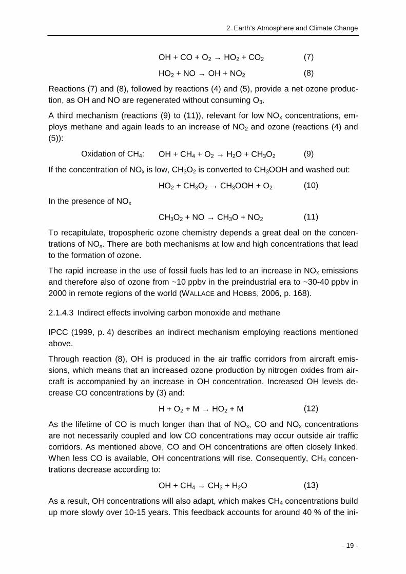
OH + CO + O2 → HO2 + CO2 (7)
HO2 + NO → OH + NO2 (8)
Reactions (7) and (8), followed by reactions (4) and (5), provide a net ozone produc-tion, as OH and NO are regenerated without consuming O3.
A third mechanism (reactions (9) to (11)), relevant for low NOx concentrations, em-ploys methane and again leads to an increase of NO2 and ozone (reactions (4) and (5)):
Oxidation of CH4: OH + CH4 + O2 → H2O + CH3O2 (9)
If the concentration of NOx is low, CH3O2 is converted to CH3OOH and washed out:
HO2 + CH3O2 → CH3OOH + O2 (10)
In the presence of NOx
CH3O2 + NO → CH3O + NO2 (11)
To recapitulate, tropospheric ozone chemistry depends a great deal on the concen-trations of NOx. There are both mechanisms at low and high concentrations that lead to the formation of ozone.
The rapid increase in the use of fossil fuels has led to an increase in NOx emissions and therefore also of ozone from ~10 ppbv in the preindustrial era to ~30-40 ppbv in 2000 in remote regions of the world (WALLACE and HOBBS, 2006, p. 168).
2.1.4.3 Indirect effects involving carbon monoxide and methane
IPCC (1999, p. 4) describes an indirect mechanism employing reactions mentioned above.
Through reaction (8), OH is produced in the air traffic corridors from aircraft emis-sions, which means that an increased ozone production by nitrogen oxides from air-craft is accompanied by an increase in OH concentration. Increased OH levels de-crease CO concentrations by (3) and:
H + O2 + M → HO2 + M (12)
As the lifetime of CO is much longer than that of NOx, CO and NOx concentrations are not necessarily coupled and low CO concentrations may occur outside air traffic corridors. As mentioned above, CO and OH concentrations are often closely linked. When less CO is available, OH concentrations will rise. Consequently, CH4 concen-trations decrease according to:
OH + CH4 → CH3 + H2O (13)
As a result, OH concentrations will also adapt, which makes CH4 concentrations build up more slowly over 10-15 years. This feedback accounts for around 40 % of the ini-

Aircraft Design Driven by Climate Change
- 20 -
tial CH4 decrease due to enhanced HO concentrations from aviation NOx. (IPCC, 1999, p. 4)
2.1.5 Formation of condensation trails (contrails)
Water vapour has an impact on climate not only as a gaseous atmospheric constitu-ent, but also by forming clouds through condensation. The quantity of water emitted by aircraft (138 Mt/year for the 2005 commercial fleet above 100 seats, based on EGELHOFER et al., 2006) seems insignificant in comparison to the natural evaporation from Earth’s surface (525000 Mt/year) (SCHUMANN, 2002). Indeed, the direct climatic impact of water vapour emitted by aircraft is fairly low (see chapter 2.4). Aviation, however, features visible line clouds that are called condensation trails or contrails, and cirrus clouds of which the formation is triggered by contrails. The latter are not necessarily visible to the naked eye and are yet supposed to contribute significantly to global warming (IPCC, 2007, Table 2.9).
Contrails form as aircraft fly through sufficiently cold and humid air. The water vapour in the engine exhaust locally increases the relative humidity by mixing the hot and humid exhaust plume with the colder ambient air. When reaching saturation, the wa-ter condenses on small particles in the exhaust plume, or on particles already exist-ing in the atmosphere. At typical flight altitudes, temperatures of around -50°C make the water freeze quickly.
Natural condensation nuclei in the upper troposphere and lower stratosphere result mainly from volcanic eruptions, as dust and sea salt seldom reach these altitudes. Also, most industrial aerosols are washed out before reaching typical flight altitudes, so that the background concentration of aerosols at altitude between such events is fairly low. Apart from the fact that water vapour in the engine exhaust provides a source of humidity, soot and sulphur oxides are suspected to be even more important for contrail formation, as they provide condensation nuclei. This is why the pure con-sideration of the mass of engine exhaust gases does not allow an estimation of the potential to form contrails. In currently available rough estimations, it is rather the amount of kilometres flown that is taken as a basis for quantification (e.g., LEEA, 2007).
Ice particles in young contrails are typically 10-30 microns in diameter – smaller than those of natural cirrus clouds (> 30 micron). Hence for the same ice water paths (ice water content), there are more, but smaller particles, which leads to a higher optical density and thus a higher specific climatic impact than that of natural clouds (see chapters 2.2 and 2.4). The average coverage of natural clouds, however, is much larger of course. Contrails vanish quickly in dry and windy regions, but may persist for hours where the humidity is above ice saturation and few air movements occur. In this case, they can form contrail-induced cirrus. These clouds are hard to distinguish from natural cirrus once air movements have blurred their initially clear line-shape. In

2. Earth’s Atmosphere and Climate Change
- 21 -
comparison to short-lived contrails, contrail cirrus today is estimated to have an im-pact on climate larger by up to one order of magnitude (SAUSEN et al., 2005).
A very uncommon form of contrails is induced by aircraft aerodynamics (GIERENS et al, 2006). The negative pressure over the wing (lift) decreases air temperature abruptly. Even if air passes by this negative pressure in several milliseconds, this time can, depending on the ambient air humidity, suffice to allow ice crystals to grow and thus form condensation trails.
Knowledge on both the formation and the effect of contrails is still poor (IPCC, 2007, Table 2.11). This is why large research efforts are being made and many ongoing projects deal with contrails.
2.2 Greenhouse effect and global warming
The main drivers of atmospheric dynamics (and related tracer transports) are radia-tive processes and the resulting differential heating of the various regions. Earth re-ceives a radiation of 1368 W/m² from its sun (WALLACE and HOBBS, p. 119). If a radia-tive equilibrium is to be maintained, i.e. temperatures on Earth stay constant, as much radiation as enters must leave the system. Some of the solar radiation is ab-sorbed in the atmosphere before reaching Earth’s surface. Upper atmospheric layers are heated and photochemical reactions enabled. When radiation is reflected, the wavelength of the radiation changes to higher values, as temperatures both in Earth’s atmosphere and on ground are lower than that of the Sun’s surface. Accord-ing to the law of Stefan-Boltzmann (HAMMER and HAMMER, p. 52) blackbody tempera-tures of 5770 K and 255 K for Sun and Earth can be derived. Applying Planck’s law (HAMMER and HAMMER, p. 2), Earth and Sun radiate in completely different wave-lengths with negligible overlapping (see Fig. 4).
0.1 1 10 100Wavelength (µm)
Rad
iatio
n po
wer
nor
mal
ised
Fig. 4: Radiation intensity as a function of the wa velength for Earth and Sun
The Earth’s atmosphere absorbs and emits radiation at specific wavelengths. It is fairly transparent for Sun’s radiation, but absorbs a significant amount of Earth’s ra-diation (see Fig. 5). If the concentration of constituents that absorb Earth’s radiation
Sun Earth

Aircraft Design Driven by Climate Change
- 22 -
is increased, the radiative equilibrium is disturbed and a new (higher) equilibrium temperature is elaborated. Such gases are called greenhouse gases, and the phe-nomenon greenhouse effect.
Fig. 5: Atmospheric absorption: the ordinate gives the percentage of the radiation that is ab-sorbed by the respective atmospheric components (CH 4, N2O, O2, O3, CO2, H2O) and the entire atmosphere, as a function of the wavelength. In con trast to Fig. 4, wavelengths decrease from the left to the right. Figure based on Fig. 2.11 in A HRENS (2000, p. 8), provided by Katherine Klink (Univers ity of Minnesota).
Fig. 5 shows the absorption of atmospheric constituents as a function of the wave-length of radiation. The prominent role of water and carbon dioxide for the overall absorption can be clearly distinguished. Ozone is clearly marked as a peak in a re-gion, where H2O and CO2 do not absorb. Methane and nitrous oxide complete the water’s absorption at wavelengths of around 9 µm. Altogether, the atmosphere clearly absorbs more radiation in the domain of radiation of the Earth than in that of the Sun.

2. Earth’s Atmosphere and Climate Change
- 23 -
Fig. 6: Earth’s annual and global radiation energy balance. From IPCC (2001), p. 90, Fig. 1-2.
Fig. 6 gives an overview of annually and globally averaged radiation fluxes in Earth’s atmosphere including reflections on Earth’s surface, clouds and aerosols. Supple-mentary greenhouse gases and clouds “trap” radiation in the atmosphere, i.e., more energy enters the atmosphere than it can radiate out in space. This difference be-tween ingoing and outgoing radiation is called Radiative Forcing (RF) and is meas-ured in mW/m². Without external perturbation (e.g., anthropogenic emissions), the radiative forcing is zero. Positive RF causes a warming, negative RF a cooling of the atmosphere.
Without greenhouse gases, the Earth’s average temperature at mean sea level would be around -18°C. The natural greenhouse effec t raises this average to around 15°C. Two thirds of the natural effect is due to wa ter vapour; carbon dioxide and trace gases cause the rest of the warming (see also Fig. 5).
Standard mean temperature without greenhouse effect:
-18°C
Water vapour H2O + 21°C
Carbon dioxide CO2 + 7°C
Gre
en-
hous
e ef
-fe
ct
Trace gases Tem
pera
-tu
re in
-cr
ease
by
+ 5°C
Standard mean temperature with greenhouse effect
+15°C
Table 2: Effect of greenhouse gases on the standard mean temperature
The thermal equilibrium depends strongly on the single gases’ concentration and is therefore vulnerable to anthropogenic perturbations. A sudden change of the stan-dard mean temperature, i.e. over some decades, might cause severe environmental problems, such as floods or droughts.

Aircraft Design Driven by Climate Change
- 24 -
2.2.1 Climatic feedbacks
In addition to direct effects of global warming, climatic feedbacks may occur that may amplify or compensate primary effects. GRAEDEL and CRUTZEN (1994, p. 420 f.) give some examples (T = temperature):
• Ice-Albedo: Ice melting causes less reflection of sunlight, more heat is absorbed. (T↑).
• Water vapour: Higher temperatures lead to more water being vaporised, which extends the greenhouse effect. (T↑).
• Chemical feedbacks: CH4 ↑ → HO ↓ → CH4 ↑↑ → HO ↓↓. (T↑).
• Cloud feedbacks: Low clouds decrease Earth’s albedo and do not absorb much of Earth’s warmth. High clouds do not change the albedo appreciably, but they ab-sorb warmth from the surface (T↑↓).
• Biotic feedbacks: e.g. T↑ → CO2 ↑ by ground respiration → T↑ or plants fertilising → CO2↓ (T↑↓).
These feedbacks are taken into account in complex atmospheric modelling. They should also be kept in mind when evaluating climate change qualitatively, when non-specialists, e.g. aircraft engineers discuss how aviation impacts Earth’s atmosphere.
2.2.2 Anthropogenic greenhouse effect
Humans impact on the greenhouse effect by emitting greenhouse gases: mainly car-bon dioxide, methane, laughing gas and ozone. Indirectly, greenhouse gas precur-sors (e.g. NOx) contribute further to anthropogenic global warming.
According to the most recent IPCC report (2007, SPM, p. ), “global atmospheric con-centrations of carbon dioxide, methane and nitrous oxide [laughing gas] have in-creased markedly as a result of human activities since 1750 and now far exceed pre-industrial values determined from ice cores spanning many thousands of years. (…) The global increases in carbon dioxide concentration are due primarily to fossil fuel use and land use change, while those of methane and nitrous oxide are primarily due to agriculture.”
In its assessments, the IPCC uses the radiative forcing as a metric for climate change. On this basis, the most important contribution to climate change comes from carbon dioxide. This is partly due to its long atmospheric lifetime (see 2.1.3).

2. Earth’s Atmosphere and Climate Change
- 25 -
LOSU
CO2 1.66 High
CH4 0.48 High
N2O 0.16 High
Halocarbons 0.34 High
Ozone 0.30 Med
Stratospheric water vapour from CH4 0.07 Low
Surface albedo -0.10 Med-Low
Aerosols (direct and cloud albedo effect) -1.20 Med-Low
Linear contrails 0.01 Low
Solar irradiance 0.12 Low
Total net anthropogenic 1.60
Average overall RF [W/m²]
Table 3: Average overall radiative forcing in 2005 due to human interception and respective level of scientific understanding (LOSU). For compa rison, the impact of solar irradiance varia-
tion is given. Data from IPCC (2007, SPM, p. 4).
Table 5 summarises radiative forcings from anthropogenic origin in 2005 according to IPCC (2007). In addition to greenhouse gases, effects of aerosols and albedo (reflec-tivity) are included. Whereas for long-lived gases (CO2, CH4, N2O and halocarbons) values are estimated fairly reliably, the level of scientific understanding of the other contributors is medium to low. Consequently, the potential effect of aviation-induced cirrus clouds is not included in this table. It could account for 0.03 [0.01; 0.08] mW/m² (IPCC, 2007, Table 2.9).
2.2.3 Consequences of global warming
2.2.3.1 Impact on nature and human environment
Global warming has multiple repercussions that do not only affect animals and plants, but also the human environment. IPCC’s working group II published the cur-rent scientific knowledge on “Impacts, Adaptation and Vulnerability” in their contribu-tion to the Fourth Assessment Report (IPCC, 2007b). “Observational evidence from all continents and most oceans shows that many natural systems are being affected by regional climate changes, particularly temperature increases”.
Whereas no globally valid conclusions can be drawn as to the total extent of negative or positive impacts, a broad number of local analyses show that, in general, the negative consequences of climate change outweigh potential benefits. The IPCC re-port gives details on each region on the planet. The following list gives a few exam-ples of consequences for Europe (based on IPCC, 2007b, SPM):
• “Retreating glaciers, longer growing seasons, shift of species ranges, and health impacts due to a heat wave of unprecedented magnitude” have been documented in the current climate and are said to represent future climate consequences.

Aircraft Design Driven by Climate Change
- 26 -
• Europe will face “increased risk of inland flash floods, (…) more frequent coastal flooding and increased erosion” with a great majority of the ecosystems having finding it difficult to adapt.
• Heat and droughts will occur more often in Southern Europe and reduce “water availability, hydropower potential, (…) tourism and (…) crop productivity”.
• Decreasing summer precipitation in central and Eastern Europe will cause higher water stress with declined forest productivity and higher frequency of peatland fires.
• Northern Europe might initially benefit from climate change with less necessity for heating, higher crop yields and increased forest growth. However, more frequent winter floods, endangered ecosystems and decreasing ground stability “are likely to outweigh” such benefits.
The capability of both ecosystems and humans to adapt to climate change depends on many factors that are not yet fully understood. It is stated though, that “there are formidable environmental, economic, informational, social, attitudinal and behavioural barriers to implementation of adaptation.” Developing countries tend to be affected more heavily by climate change, but have less capability to cope with it. In general, “vulnerability to climate change can be exacerbated by the presence of other stresses”. However, sustainable development as defined by the Brundtland Commis-sion (UN, 1987) is estimated to be able to reduce this vulnerability and “many im-pacts can be avoided, reduced or delayed by mitigation”.
2.2.3.2 Economic damage
The IPCC report (2007b) also gives an estimation of the economic damage of climate change: a loss of 1-5 % GDP for 4°C warming. “In so me locations and amongst some groups of people with high exposure, high sensitivity, and/or low adaptive ca-pacity, net costs will be significantly larger than the global aggregate.”
In autumn 2006, the former chief economist of the World Bank, Sir Nicholas Stern published a report on the economic consequences of climate change (Stern, 2006). Even if reactions to the report appear to be both very positive and negative, the re-port has appreciably impacted the public and political perception of climate change as an economic and not merely ideological issue. According to the report, a 5-6°C warming, considered possible for the next century with “business as usual” increase of greenhouse gas emissions, would cause an “average 5-10 % loss in global GDP, with poor countries suffering costs in excess of 10 % of GDP”. Including some indi-rect factors, this percentage could even grow to 20 % according to the report. Stern compares these numbers with the two World Wars and the economic crisis in the first half of the 20th century.
The report explores mitigation actions that would result in a stabilisation of the CO2 (equivalent) concentration at 450 or 550 ppm. The latter concentration would “require

2. Earth’s Atmosphere and Climate Change
- 27 -
global emissions to peak in the next 10 - 20 years, and then fall at a rate of at least 1 - 3 % per year. (…) By 2050, global emissions would need to be around 25 % be-low current levels.” Costs for this stabilisation were estimated to be around 1% of the GDP. Consequently, according to the report, the “benefits of strong, early action on climate change outweigh the costs”, and this clearly when comparing to the costs of a business-as-usual attitude mentioned above.
The correctness of Stern’s results is the subject of on-going discussion. However, even if the numbers of the report prove to be over- or underestimated, the report has brought climate change to the centre stage of public discussion. Politics has dealt with the issue incomparably more seriously ever since (e.g., G8 summit in June 2007, German EU presidency 2007 etc.).
2.2.4 International agreements on mitigating climat e change
Climate change was identified as a global problem many years ago. The first interna-tional agreement on climate dates back to 1979, when World Climate Conference brought up the “Geneva Convention on Long-Range Transboundary Air Pollution (CLRTAP)”. Since then, several protocols (Helsinki 1985, Sofia 1988, Geneva 1991, Oslo 1994 and Gothenburg 1999) have completed the initial stipulations. Far more famous is the 1997 Kyoto Protocol, which gave the UN Framework Convention on Climate Change (UNFCCC) of 1992 a legal binding. The protocol entered into force in February 2005 and includes reduction commitments for CO2, CH4, N2O, perfluoro-carbons, hydrofluorocarbons and SF6 (UNITED NATIONS, 2007). International aviation is excluded from the greenhouse gas reduction committed in the protocol, as states are supposed to limit aviation bunker fuels through ICAO. Domestic aviation, how-ever, is principally included in the reduction measures adopted by each country. Consequently, the European Union is about to discuss the integration of aviation in its Emissions Trading Scheme (e.g., WIT et al., 2005).
2.3 Ozone chemistry and ozone hole
A second publicly discussed phenomenon of human impact on Earth’s atmosphere is the depletion of the ozone layer. This chapter sets out very briefly relevant chemistry, current status and mitigation by regulation.
2.3.1 Stratospheric ozone chemistry
There are mainly two chemical cycles that determine the ozone concentration in the stratosphere. The first was found by Chapman in 1930 and is an “oxygen-only” cycle (WALLACE and HOBBS, 2006, p. 88 ff., GRAEDEL and CRUTZEN, 1994, p. 150 ff., KRAUS, 2004, p. 40):

Aircraft Design Driven by Climate Change
- 28 -
Ozone formation: O2 + hν (λ ≤ 242 nm) → O + O (14)
O + O2 + M → O3 + M (M: N2 / O2) (15)
Ozone depletion: O3 + hν (λ ≤ 366 nm7) → O + O2 (16)
O + O3 → 2 O2 (17)
Ozone is formed with high energetic radiation of a wavelength of less than 242 nm, which is in the invisible part of the light spectrum (UV-C radiation). Such radiation is thus filtered by the ozone layer and cannot reach Earth’s surface. Reactions (15) and (16) are fast, (14) and (17) slow. The final concentration depends on the reaction ve-locities of all four reactions. However, they are not able to fully represent the real concentrations of ozone in the stratosphere. Catalytic cycles that involve nitrogen compounds (NOx!), H, OH, Cl and Br cause the depletion of ozone:
Catalytic O3 depl.: X + O3 → XO + O2 (X: catalyst) (18)
XO + O → X + O2 (19)
where O is built by reaction (16). If (18) and (19) are fast, they can proceed much faster than reaction (17) and the catalytic cycle is much more important than the “oxygen only” depletion. Since the catalyst X is recycled, small concentrations of X may cause significant depletion of ozone and atomic oxygen. X can be HO, NO, Br and Cl (produced by fission of CFCs), for example. Ozone depletion is naturally lim-ited by the mutual extinction of such catalysts. Such reactions, however, are only temporary as they may be reversed by photo-dissociation (GRAEDEL and CRUTZEN, 1994, p. 154).
Concerning the ozone layer, the polar region merits special attention owing to the extreme physical conditions such as temperature, sunshine duration, magnetic field and the altitudes of the respective atmospheric layers (GRAEDEL and CRUTZEN, 1994, p. 155-159). The production of chlorine, the most important “ozone killer”, is linked to reactions on icy surfaces as they occur in polar stratospheric clouds (PSC). HCl and chlorine nitrate contained in these clouds produce Cl2 and HNO3, which is a slow re-action in a gaseous environment, but very fast on icy surfaces such as in PSC. HNO3 would normally split to HO and NO2, which could react with chlorine (“natural limita-tion of ozone depletion”, see above). But due to the low temperatures, it is bound in ice. The situation in Antarctica is aggravated by the fact that the chlorine is kept in the region by the “polar vortex” during winter. Furthermore, the polar region is pene-trated by solar protons that move along the magnetic streamlines and collide with atoms and molecules to produce electrons, which lead to the production of NO and thus deplete ozone.
Finally, atmospheric dynamics transport ozone from “its primary source in the tropical stratosphere poleward and downward into the extratropical lower stratosphere” (WAL-
7 Wavelength λ from WALLACE and HOBBS (2002). GRAEDEL and CRUTZEN (1994) give 1140 nm,
KRAUS (2004) gives 0.3 µm.

2. Earth’s Atmosphere and Climate Change
- 29 -
LACE and HOBBS, 2006, p. 89). Stratospheric ozone concentrations and also the ozone hole thus depend on many different factors and phenomena.
2.3.2 Current status and mitigation
In 1985, the United Nations adopted the “Vienna Convention for the Protection of the Ozone Layer”, although its effects were neither felt nor scientifically proven (UNEP, 2004). It was only shortly after that British scientists published an article about severe ozone depletion in Antarctica (FARMAN et al., 1985). Their results were confirmed by American satellite data, and in 1987, the “Montreal Protocol on Substances that De-plete the Ozone Layer” was signed and amended since. The protocol prohibits the production and consumption of certain CFCs and halons.
Fig. 7: Antarctic ozone hole on the 24th of September 2006. Lowest O 3 concentrations in purple and blue (NASA, 2006)
Today’s ozone hole, i.e., the temporary deple-tion of ozone in spring, is mainly due to chlorine from CFCs that were widely used as refriger-ants in the 20th century (WALLACE and HOBBS, 2006, p. 91). Thanks to the rigorous reduction of emissions of CFCs, their concentration in the lower atmosphere does not continue to rise. However, they keep on growing in the strato-sphere due to their long lifetimes. The hitherto largest ozone hole was measured on the 24th of September 2006. Depending on the estimation, the ozone hole will recover fully by the middle or late 21st century thanks to the application of the Montreal Protocol. (WALLACE and HOBBS, 2006, p. 96, NASA, 2006).
2.4 Impact of aviation on the atmosphere
From the preceding sections, it becomes clear that emissions from aviation contrib-ute to both global warming and the ozone hole. This subchapter gives an overview in which cases and to which extent commercial aviation is concerned.
2.4.1 Aviation and climate change
The most up-to-date estimation of aviation’s contribution to climate change was pre-sented in a paper by SAUSEN et al. in 2005. Fig. 8 (SAUSEN et al., 2005) shows the radiative forcing of aviation for the years 1992 (from IPCC, 1999) and for 2000 as it was estimated in the TRADEOFF project (ISAKSEN et al., 2003). In order to compare the two estimations, values from 1992 were scaled linearly to 2000, based on traffic growth (white bars). The whiskers denote the 2/3 confidence intervals of the IPCC (1999) value.

Aircraft Design Driven by Climate Change
- 30 -
The level of scientific understanding (LOSU) is also given below the graph. The LOSU being good for CO2, the estimation of its radiative forcing is virtually un-changed (25.0 mW/m² from IPCC, 25.3 mW/m² from TRADEOFF). Positive and negative effects of nitrogen oxides have been downsized appreciably, their sum, however, has slightly increased (IPCC: 10.4 mW/m², TRADEOFF: 11.5 mW/m²). Val-ues for water vapour were not corrected. Direct sulphate and soot were considered less impacting than before, but their contribution is minimal anyway. The major dif-ference between the total sums (last bars, IPCC: 71.3 mW/m2, TRADEOFF: 47.8 mW/m²), however, comes from contrails. The best estimate of their impact in the IPCC (1999) report gave 33.9 mW/m² (scaled to 2000), in the TRADEOFF project, the RF was estimated to be 10 mW/m². Contrail-induced cirrus, however, is now con-sidered to be far more important than line-shaped contrails. As the LOSU for cirrus cloud is still poor (though improving), a best estimate is not included in the total bars. Potentially, they could have a radiative forcing that is as high as all the other con-stituents together.
The estimation of radiative forcing from aviation alone does not allow a conclusion on its contribution to global warming in future. This is why the two effects of NOx, on ozone and on methane, should not just be summed up. To combine several values, atmospheric lifetimes would need to be taken into account. Section 5.2 will set out more details on possible alternative metrics that include the temporal aspects.
Fig. 8: Radiative Forcing RF [mW/m²] from aviation until 1992 and 2000 based on IPCC (1999) and TRADEOFF results (from S AUSEN et al., 2005). The whiskers denote the 2/3 confide nce in-tervals of the IPCC (1999) value.

2. Earth’s Atmosphere and Climate Change
- 31 -
Based on the RF, aviation was estimated to be responsible for 3.5 % of global warm-ing in 1992 (IPCC, 1999). Since then, no similar number has been published. Taking into account the downsizing of the importance of contrails, the TRADEOFF estima-
tion could result in a percentage of 2.35 % of RF (= (47.8/71.3) ⋅ 3.5 %) for the year 2000, if greenhouse gas emissions from other industries grew at the same rates as those from aviation. Including an estimate for contrail-induced cirrus (30 mW/m², see IPCC, 2007a, their table 2.9) would then result in 3.8 % of RF for the year 2000
(= (77.8/47.8) ⋅ 2.35 %). The statement that commercial aviation today is the “climate killer number 1” (e.g., STAUD, 2006, SCHLEICH and DOBROWOLSKI, 1998), is thus not confirmed by these numbers. However, the large growth rates of aviation in the past and predictions for the future (AIRBUS, 2005, BOEING, 2006), and simultaneous reduc-tion of greenhouse gas emissions in other industries, which probably have higher and easier reduction potentials, make a growth of this percentage probable in the future. Efforts in research and industrial application of low-emission technologies must thus be pursued and reinforced.
2.4.2 Aviation and ozone depletion
The 1999 IPCC Special Report on Aviation and the Global Atmosphere was prepared following a request from ICAO and the Parties to the Montreal Protocol (IPCC, 1999, SPM) and thus initially focused on aviation’s impact on the ozone layer. According to the report, subsonic aircraft tend to increase the total ozone column and so decrease the erythemal dose rate8 by 0.5 % at 45°N in July 1992. “The net effect of subsonic aircraft appears to be an increase in column ozone and a decrease in UV radiation, which is mainly due to aircraft NOx emissions” (IPCC, 1999, SPM).
More recent publications from WUEBBLES et al. (2003) and BAUGHCUM et al. (2003), show that aviation contributes to ozone depletion above a flight altitude of around 15 km. Using the HSCT scenarios (BAUGHCUM and HENDERSON, 1998), their study says, a fleet of supersonic aircraft could cause a decrease in total column ozone of 1.5 % or even 2.5 % in the northern hemisphere at an EINOx of 15 g/kg, i.e. 15 g of NOx emitted for each kilogramme of fuel burned. “The major impact on ozone column occurs at altitudes above the cruise altitudes with the ozone impact increasing with higher cruise altitudes” (BAUGHCUM et al., 2003). Their results also depend on the atmospheric chemistry model used. Unfortunately, the studies do not give details on the dependence of ozone depletion on latitude. But from the explanations given in section 2.3 and the shape of the ozone hole (see Fig. 7, biggest depletion of ozone at high latitudes), it can be concluded that the impact on the “ozone hole” itself is higher than the percentages given here, which were averaged over the whole hemisphere.
In the following sections, the ozone hole will be largely omitted, as the focus of the thesis lies on subsonic commercial air transport that today does not use cruise alti-
8 Measure for radiation that affects the skin

Aircraft Design Driven by Climate Change
- 32 -
tudes higher than 15 km (typical cruise altitudes are around 10-12 km). However, the issue should be kept in mind when deliberating on higher cruise altitudes.

- 33 -
CHAPTER 3: Comprehensive methodology to integrate c limate change into the aircraft design process
Aircraft enable the fast transport of people and goods over long distances. In order to assure a smooth and efficient provision of this service, not only are aspects that have a direct impact on flying itself such as aerodynamics and flight mechanics considered in their design process, but also operational aspects such as flight routing, air traffic control, airline fleet management and so on. The impact on the environment is a fur-ther criterion that must be taken into account, and is strongly interlinked to the opera-tional issues raised above. Logically, embedding climate change into aircraft design presumes allowance for operational issues from the first steps of the design process.
This chapter describes a superstructure for the integration of climate change into the preliminary aircraft design process. After an analysis of the air transport system with regard to its impact on the environment, the classic aircraft preliminary design proc-ess is presented. On this basis, a comprehensive design methodology is developed that integrates operations and a metric for climate change into the process.
The subsequent sections 4 and 5 then set out in detail how emission scenarios are elaborated, and how the actual impact on the atmosphere is measured.
3.1 The air transport system under environmental re view
The air transport system includes a broad variety of stakeholders, each of which has innate needs. When trying to simplify the complex system in a scheme, several do-mains could be placed at the centre. POMPL (2002, p. 3), e.g., puts airlines and pas-sengers at the centre stage, which reflects the view of consumers of aviation as a transport service provider. From a more technical point of view, aircraft represent a node in the system. Most of the stakeholders of aviation express certain require-ments on the design of aircraft. For the purpose of this thesis, the “operation of air-craft” shall be put at centre stage, being the key for aviation’s impact on the environ-ment.
Fig. 9 gives an overview of stakeholders of the air transport system, which influence the operation and thus the design of aircraft with regard to their impact on climate change:

Aircraft Design Driven by Climate Change
- 34 -
AircraftOperations
Airlines
Airports
Certification
Passengers
ATM/ATCMilitary
ATM/ATCMilitary
Weather
Fig. 9: Simplified scheme of the aviation system: a ircraft operations take the centre stage.
Aircraft engine emissions have been certified since 1981, when Volume II of Annex 16 to the Chicago Convention was first issued (ICAO, 1993). The certification is based on the “ICAO Landing and Takeoff (LTO) Cycle”, a theoretic procedure em-ploying fixed thrust settings and fixed times in each mode. NOx, HC, CO and smoke are regulated and the limits are downsized regularly by ICAO’s Committee on Avia-tion Environmental Protection (CAEP). The standard for engines, of which the first individual production model was produced after 1 January 2008, is called CAEP/6 and represents a decrease of the limits for NOx hitherto valid by 12 %. Evaluation parameter is the total quantity of a gas (e.g., NOx) emitted during the LTO cycle di-vided by the engine maximum rate thrust at sea level (F00). This system of certifica-tion is limited to the engine and does thus not incorporate aircraft-specific or opera-tional aspects, e.g., real thrust settings and times in mode, that would have an impact on the quantity of gases emitted.
Airports are often in the front line for discussing environmental issues of aviation with the public. Whereas aircraft noise was initially the major concern of airport resi-dents, the number of complaints regarding air pollution is increasing (personal com-munication: Ralf Gaffal, 2007). Today, airports even face inquiries concerning climate change, which is eventually beyond their scope of interference. Airport authorities tend to react by elaborating measurements of trace gases, by informing the public, e.g., with extensive internet presence, and some by introducing emission-related landing charges. ICAO still “urges Contracting States to refrain from unilateral imple-mentation of greenhouse gas emissions charges prior to the next regular session of the Assembly in 2007 (…)” (ICAO, A35-5, 2004), which means not to introduce any charges, until ICAO has clearly developed schemes to do so. Following European airports’ initiatives in introducing emission-related landing charges, the European Civil Aviation Conference (ECAC) has published its recommendation 27-4 (ECAC, 2003) giving a “NOx Emission Classification Scheme” that has since been adopted in Sweden, Switzerland and Germany. Emanating from the development of noise-related charges, the number of emission-related restrictions or charges and thus the importance of emissions for the aircraft design process will increase soon.
Airlines provide the most important contact surface of aviation to the public. Apart from the political interest, they also have an economic interest in environmental is-

3. Comprehensive Methodology to Integrate Climate Change …
- 35 -
sues in view of increasing fuel prices, and of existing and future environmental charges and taxes (costs). Under the growing concern of the public with regard to the impact of aviation on climate change, minimisation of its contribution to global warm-ing becomes a sales argument. Consequently, the fuel efficiency of aircraft is crucial. But airlines also enhance their environmental performance by optimising their fleet planning, flight plans and operational procedures. SAS Scandinavian Airlines, e.g., has developed an approach system that minimises fuel consumption and also pro-vides benefits in terms of noise. They report savings of up to 200 kg of fuel on each of these “green landings” by setting the “aircraft’s landing time and exact runway specifications within minutes after takeoff”, so that the landing sequence can be de-termined at an early stage and the aircraft can descend with reduced revolutions (SAS, 2007). Lufthansa German Airlines also amplify their communication regarding climate change. Apart from their Environmental Reports (LUFTHANSA, 2001-2006), they recently referred to their advances in the reduction of fuel consumption by opti-mised flight routing and more exact fuel and fresh water loading in advertisements (LUFTHANSA, 2007b). The potential reduction by “optimization of these operational measures is in the range of 2-6 %” (IPCC, 1999).
“Ryanair warns on CO2 ‘hysteria’” as a reaction to the media coverage of aviation’s contribution on global carbon dioxide emissions, which contributed to the “softening in demand the airline has experienced” in mid 2007 (MASSY-BERESFORD, 2007). Fur-thermore, Easyjet even announce an “easyjet ecojet”, an aircraft concept that re-duces fuel consumption by 50 % compared to current aircraft (HANDELSBLATT, 2007). In IATA’s Environmental Review of 2004, “the reduction of fuel use (and hence CO2 and water vapour) through improvements in fuel efficiency [was identified as] a key priority for the entire aviation industry” (IATA, 2004, p. 9). Hence, pressure from air-lines with regard to environmental performance of aircraft is increasing (HOLLMEIER, 2007, p. 3) and therewith their demand for new aircraft with less environmental im-pact.
For passengers , it is mainly the ticket price that makes them choose one airline or another (HOLLMEIER, 2007, p. 9). Fuel prices are increasing and environmental charges may one day contribute appreciably to operating costs, which could increase ticket prices. Furthermore, several non-governmental institutions encourage people to refrain from flying and use other means of transport, said to be less harmful to Earth’s atmosphere, or to abandon the trips. The image of airlines in terms of their environmental compatibility, and also of aviation as a whole with regard to its impact on climate change may potentially be decisive for passenger demand in future (see paragraph on airlines above).
Air traffic management and control bears large potentials for the reduction of fuel consumption and thus of the impact on climate change. According to IPCC (1999, p. 73), “improvements in air traffic management could help to improve overall fuel efficiency by 6-12 %”. These measures include the reduction of delays, the develop-

Aircraft Design Driven by Climate Change
- 36 -
ment of infrastructure (to avoid congestion) and the improvement of operational effi-ciency. Lufthansa German Airlines blame military airspaces for causing appreciable amounts of fuel burn of civil aircraft, as they often hinder direct routing (LUFTHANSA, 2006, p. 1). Furthermore, the complex European air traffic control system with na-tional service providers proves to be inefficient and expensive (LUFTHANSA, 2006, p. 5). The “Single European Sky” initiative launched by the European Commission aims at increasing the overall efficiency of the ATM system by restructuring Euro-pean airspace as a function of air traffic flows and not of national borders (EUROCON-
TROL, 2007). The project is expected to “reduce greenhouse gas emissions by 4 % to 6 % per flight” (EU, 2005), which is a more conservative estimation than that of IPCC. According to these reports, the potentials for fuel reduction by operational means seem enormous compared to fuel reduction by weight or drag reduction through ad-vanced materials and optimised aerodynamics, unless radically new concepts are considered (GREEN, 2005). However, the actual impact of such operational measures on the environment including non-CO2 effects has not yet been estimated systemati-cally.
Envisaging the adaptation of flight routing to climate change-related constraints, stra-tegic ATM and tactical ATC must be fully included in the development of such sys-tems to ensure operational applicability. Most prominent features of this approach are a decrease or increase of cruise flight altitudes on the short run or in general.
Current design cruise altitudes are chosen to minimise fuel consumption at a given design Mach, but also to make the flight comfortable for passengers and avoid struc-tural fatigue. Disturbing weather patterns such as strong gusts at lower altitudes may be critical for the safety of the aircraft and are thus included in current regulations for structural stiffness. Extreme weather events such as thunderstorms or heavy precipi-tation may cause delays, deviations and cancellation of flights. Meteorological condi-tions are locally heterogeneous. Adaptations of the flight profile for minimum impact on climate thus need to take the weather into account. Vice versa, meteorological constraints may require adaptation of the flight path to non-optimised routing.
This short overview aims at giving an idea of how complex interactions in the air transport system affect the operation of aircraft and in which way these effects may also interfere with the environment. Without any claim to completeness, the compila-tion presented shall be considered in the following development of a more compre-hensive design methodology.
3.2 Current aircraft preliminary design process
Today many analyses of the environmental impact of aviation exist, but they are done downstream and their results are not fed back into the standard aircraft design process.

3. Comprehensive Methodology to Integrate Climate Change …
- 37 -
Integrated Aircraft Designtoday
tomorrow
Weights
Lift
Drag
Thrust
Consumption
Emissions
Env. Impact
Aerodynamics
EngineTechnology
Configuration
Structures
Parameter ?
Design Loop
Fig. 10: Current and potential future aircraft desi gn process with regard to the environment (Egelhofer, 2006). Up to now, emissions and their i mpact on the environment are evaluated after the actual design process, but they are not d irectly included in the aircraft optimisation loop except CO 2 that is directly addressed by reducing fuel consum ption.
The standard aircraft design process (Fig. 10) starts from the expression of three principal criteria: range, payload and usually speed. Preliminary studies check sev-eral alternative configurations with regard to all top level requirements. The scheme presented in Fig. 10 does not necessarily reflect the chronological flow of design steps, but illustrates the technical or computational logic: principal baseline of the development of an aircraft is its configuration. Once structural solutions have been defined, its design weights can be estimated. Together with configurative aspects, the required lift is determined. The aerodynamics of the chosen configuration defines the aircraft’s drag polar, which allows the elaboration of requirements for engine thrust. The consumption of the engine, respectively the aircraft, will depend on the technology level used and on design choices that are specific to the engine and its integration into the aircraft. The combustion technology employed will finally deter-mine how much trace gas emissions (HC, CO, NOx, smoke) are produced. To date, aircraft design loops fully integrate steps until the consumption of fuel, as it has a significant impact on weights and thus the entire configuration. The design process is iterative and parameters are varied until the initial design requirements are met. The final optimisation of the design regards quite specific objective functions, often oper-ating cost or the maximum takeoff weight.
As previously mentioned, emissions are certified for an engine and aircraft-specific parameters are not taken into account. Apart from CO2 and water, of which the emis-

Aircraft Design Driven by Climate Change
- 38 -
sion quantities are directly proportional to fuel consumption, they are omitted in the optimisation loop of the aircraft design process. As a first step, it would thus be rea-sonable to include an estimation of the quantity of emissions in the design process. A tradeoff between the different species of exhaust gases in terms of their environ-mental impact and also with other design requirements could be performed by the more or less objective “expert view” of the design engineer. Overall formal optimisa-tion of the aircraft concept would call for an objective criterion. For the reliable appli-cation within the design process, an environmental impact parameter for global emis-sions would need to be developed. Confident weighting in comparison to other re-quirements or constraints would even call for a common monetary metric. A mone-tary evaluation of impacts on the environment could logically use the external costs approach (EGELHOFER et al., 2006), if no regulations for global emissions exist. As soon as such operative constraints or charges and taxes are established, classic op-erating cost calculation would then account for the effect of global emissions. How-ever, there is no regulatory basis for costs of climate change and the reliability of ex-ternal costs approach for climate change is not sufficient to justify its introduction into the aircraft design process today.
Therefore, the aircraft design loop shall be enlarged up to a real evaluation of the impact of aircraft operations on global temperature change. A monetary evaluation of climate change will not be considered in this thesis, but could be the subject of future research.
3.3 Development of a comprehensive design methodolo gy
Coupling aircraft design and climate change is not trivial, because the two domains refer to completely different system levels. Aircraft design and options for mitigation tackle global warming from the bottom. Atmospheric chemistry and physics, including climate research, address global warming on a global scale, always dealing with the whole atmosphere and thus global anthropogenic influences. In order to align both domains, a structured system scheme departing from the Earth’s atmosphere is elaborated in Fig. 11, inspired by Iberall’s definition of Systems engineering (ICH, 2007). In contrast to Fig. 9, which is a small “bottom up” extract, this scheme is aimed at displaying “top down”, how global warming is influenced by commercial aviation and finally aircraft. The lifetime of the air transport system should be taken into account for the evaluation of its impact on climate (see Atmospheric metrics in chapter 5).
In order to establish a link between the Earth’s atmosphere and the aircraft design process, either the aircraft has to be scaled up to the global level or the atmosphere’s properties need to be simplified down to the level of one single aircraft. The first ap-proach is easier from an engineering point of view, as there is better availability of necessary data (air traffic market, aircraft operations etc.). Atmospheric scientists would probably try to simplify their models in order to fit in the aircraft design process,

3. Comprehensive Methodology to Integrate Climate Change …
- 39 -
as they do not necessarily have data and expertise at their disposal to illustrate avia-tion properly. For a realistic assessment, both approaches require knowledge from both scientific domains. Hypotheses and simplifications will increase the uncertainty of results in either case. In this sense, the parallel view of a system “top down” and “bottom up” may provide some control of the results and enable a simple validation. Real validation is possible to some extent for the past: atmospheric models are vali-dated using climate data records from ice cores. Aircraft performance and emission estimations can be measured during flight-testing or when the aircraft is in service. During the design process of the aircraft, such recorded data and the experience of the design engineers may constitute a valuable aid to estimate the future tentatively, when no empiric validation can be provided.
Earth’s Atmosphere
Chemistry / Physics Natural variability Natural emissions Anthropogenic emissions …
Anthropogenic emissions
Agriculture Transport Other industry
Transport
Sea AirLand …
Air Transport
MilitaryGeneral Aviation Commercial
Top
Dow
n “The application of engineering to solutions of a complete problem in its full environment by systematic assembly and matching of parts in the context of the lifetime use of the system.” (ICH, 2007)
Aircraft operations (Fig. 9)
Aircraft Design
Heating, energy …Systems engineering
Fig. 11: System scheme: Link of atmospheric environ ment to commercial aircraft design with several intermediate levels.
In order to structure possible calculation procedures, three scales were attributed to the air transport system: “micro”, “meso” and “macro”. The micro scale refers to one single aircraft operation on a certain – possibly generic – route. Macro includes the global traffic, i.e. all operations of commercial aircraft worldwide. The meso scale may concern one aircraft type on a certain route network, e.g. the regional traffic of a flag carrier. Alternatively, one could refer to the annual traffic on a specific route in-cluding all aircraft types. This definition is arbitrary, but proved to be reasonable within the scope of this thesis.

Aircraft Design Driven by Climate Change
- 40 -
3.3.1 Aircraft preliminary design loop employing gl obal traffic scenarios – Macro approach
In order to reflect the effective benefit of micro design choices in terms of climate change reasonably, it would be beneficial to employ global traffic scenarios, so that the new aircraft concept is embedded realistically in the global air transport market. A similar approach was pursued in the EU-funded SCENIC project, but was not formal-ised at that time. For the integration of an evaluation of the climate change impact into the preliminary aircraft design loop the following “macro” process of evaluation was developed (Fig. 12).
Market research
Aircraft sizing
Market SCENARIOS
• New A/C requirements• A/C fleet for any year including
new A/C penetration
A/C fleet in 20XX
Existing A/C types
Route network
A/C requirements
Fleet composition
EMISSION SCENARIOS
Geographically determined (altitude, latitude, longitude) and quantified emissions over one year
Future A/Cconcept(s)
INVESTIGATED SCENARIOEmission scenario
including new A/C type(s)
REFERENCE SCENARIOReference emission scenario
without new A/C type(s)
Atmospheric models / metrics to enable
ESTIMATE OF CLIMATE IMPACT
Fee
dbac
k to
Des
ign
OP
ER
AT
ION
S
Fig. 12: Aircraft design loop including an estimate of climate impact
A first / provisional aircraft concept is elaborated based on classic top-level require-ments such as capacity, range, cruise speed (Mach number) etc. It is then embedded in a commercial aircraft fleet at one point in time of its estimated service life. With the help of market scenarios, a reasonable penetration of the concept in the future air transport market of the given time horizon is estimated. The choice on the time hori-zon will essentially depend on the market forecast. It seems reasonable to use a time horizon with the largest market penetration of the assessed concept in order to make the climate effects of aircraft parameter variations clearly distinguishable.

3. Comprehensive Methodology to Integrate Climate Change …
- 41 -
Market research does not only provide data on the new aircraft concept, but also in-formation on the rest of the fleet, including aircraft from competitors or even concur-rence from other means of transport, e.g. high-speed trains for short-haul flights on highly congested routes. For near-future scenarios, detailed information on the struc-ture of the route network is available. Data of all scheduled flights can be obtained for past years, which allows some projection in the future. The later the time horizon chosen, the less precise the operational scenario becomes. Publicly available market research thus generally displays air transport activity in available seat kilometres (ASK) or revenue passenger kilometres (RPK), but not in the exact number of flights, and certainly not detailed down to a specific aircraft type. To build up global emission scenarios from the bottom, these data are necessary, however, and can be roughly generated with estimations based on the past distribution of aircraft (more details in chapter 4).
Once a global traffic scenario is established, aircraft performance data of existing and future aircraft are needed to calculate the mission profiles and the quantities of ex-haust gas emissions on each route. As an alternative to mission profiles optimised for minimum operating costs, real operational data such as flight data records from the air traffic control institutions can be used for past years. For the future, some correc-tion factor can be applied to the quantity of exhaust gases. However, it is difficult to account for the differences of cruise flight altitudes between optimised and real-world missions, which play, however, a role for the impact on climate (see chapters 2 and 5). The emissions thus calculated are then allocated to atmospheric “cubes” of a variable volume. The dataset serves as input for atmospheric models.
In order to reflect parameter variations of the investigated aircraft concept, two sce-narios are created: one with the new aircraft and one without, replacing the respec-tive market segment by a comparable existing aircraft. Alternatively, two design choices are compared with each other. This process has the advantage that uncer-tainties and errors of absolute results are less important, as the study is only com-parative.
The subsequent application of an atmospheric model attributes a metric of climate change, e.g., global temperature change or sea level rise, to the investigated sce-nario or to the respective varied parameter, if a comparative study (as shown in Fig. 12) is performed. By default, such models are not yet available in the aviation com-munity, but are developed and run by specialised scientific institutions (e.g., ECHAM model at DLR, Cambridge University’s TOMCAT and SLIMCAT models, University of Oslo’s model and many others). At the moment, it is thus not possible to close the design loop completely, including an atmospheric impact parameter. Even if not fully automated, the calculation and design process presented here enables a view on aircraft emissions beyond their pure quantity, i.e., with a perspective on their real ef-fect on Earth’s climate. This information gives the aircraft designer a valuable feed-back at an early stage of the process.

Aircraft Design Driven by Climate Change
- 42 -
The methodology presented in this subsection provides a systemic link between air-craft design, market research, aircraft operations and Earth’s atmosphere. As the full calculation loop as presented in Fig. 12 cannot be performed within a standard air-craft design process owing to the high complexity of atmospheric evaluation and a lack of necessary knowledge of the atmosphere in the aviation community (or the lack of engineering knowledge in the meteorological environment), a simplified proc-ess must be developed. Such a loop would then also enable optimisation runs, which are too sumptuous in calculation time with the process proposed here, even if the necessary knowledge were available at once.
3.3.2 Aircraft preliminary design loop – Micro appr oach
A micro aircraft design loop including an estimation of its environmental performance concerning climate change requires some suitable atmospheric metric. A minimal definition of the operational environment, e.g., via one or several generic routes is necessary to transfer the aircraft design parameters in a quantity of emissions. The choice of these routes is arbitrary, but should reflect the operational reality of the considered aircraft concept. The atmospheric metric then gives an estimation of the climate impact based on the quantity of emissions calculated.
The crucial link in the process is the availability of a reliable atmospheric metric. KLUG et al. (1996) and SVENSSON et al. (2004) proposed a Global Warming Potential (GWP) metric in the style of the Kyoto protocol, of which the application for aviation was heavily criticised. In the Airbus- and DTI (Department of Trade and Industry, UK)- sponsored “Low Emissions Effect Aircraft (LEEA)” project, more advanced met-rics were developed based on calculations for the full annual cycle using 3D atmos-pheric models (more details in section 5). The project perfectly reflects the “top down” approach mentioned above: using a full-scale atmospheric model, a reduced atmos-pheric metric was derived based on very simple assumptions for the operation of the aircraft.
3.3.3 Evaluation at different precision levels
The micro loop presented above cannot replace modelling the effects of the global air traffic on climate change. It should be used for fast estimations or in optimisation runs. Its results, however, should be validated by macro control runs. Following the different system levels of aircraft design and Earth’s climate, a parallel use of both loops is preferable. Both approaches are summarised in Fig. 13.

3. Comprehensive Methodology to Integrate Climate Change …
- 43 -
Emissions of 1 A/C
Climatic Impact
A/C Design
Simplified “micro” loopDetailed “macro” loop
Feedback into design
Fig. 13: Parallel aircraft evaluation and design lo ops with high and low system levels.
The level of detail of the aircraft concept always refers to preliminary design, whether or not it is embedded in a global traffic scenario. It is important to adapt the calcula-tion of the emissions and the evaluation in terms of climate change to the precision of the available aircraft data in order to establish a homogeneous calculation process. For example, there is no advantage in calculating emission scenarios in three dimen-sions, if the subsequent atmospheric model can only handle two dimensions in its input data.
To conclude, even the best modelling can only provide some help to the design engi-neer, who will supply the last arbitration in the process. He will need to decide when it is most appropriate to use one aircraft on a single route or the global traffic, and on the level of precision of the atmospheric modelling.

Aircraft Design Driven by Climate Change
- 44 -

- 45 -
CHAPTER 4: Global emission scenarios
Emission scenarios play a decisive role in the aircraft design methodology presented in the previous chapter. Therefore, their elaboration is to be explained a little more in detail here.
Emission “scenarios” or “inventories” display the quantity of relevant exhaust gas emissions on a global level, often in three dimensions and over one year. In scientific literature, the term “inventory” tends to refer to the past; “scenarios” allude to as-sessments of the future. In this thesis, the term “scenario” is employed for all applica-tions because the emissions are calculated and not deducted from real fuel con-sumption or similar.
To create global scenarios, well-established mission and emission calculation meth-ods were employed. The difficulty in providing valuable results arises from the huge amount of available data. Assuring consistency is of utmost importance and requires rigorous treatment of all input data. Moreover, it is almost impossible to validate emission scenarios. Control measures would need to be taken at many investigated points of Earth’s atmosphere. Even if this was feasible, the part of aviation in increas-ing the concentrations of pollutant gases could not be unambiguously assigned, as the sources of these gases cannot be traced back. Lastly, chemical processes and transport phenomena continuously change the composition of the atmosphere. Com-paring measurements with emission calculations thus automatically employs some atmospheric modelling. Nevertheless, measures of the atmosphere, such as per-formed in the European MOZAIC, CARIBIC and IAGOS projects, help to understand the processes in the atmosphere and to improve the models. In some places, the effects of aviation can be isolated, where few or no other polluting sources exist (e.g., North-Atlantic flight corridor).
Emission scenarios are built “bottom up”. Market forecasts can be established both “bottom up” or “top down” or even as a mixture of both approaches. Depending on the market information available, input data have to be adapted to fit in the scenario calculation process.
In the following subsections, each type of input data is presented. The difficulty of producing data consistency is highlighted. On top of this, the calculation of missions and finally of each pollutant gas is explained. An overview of previous emission stud-

Aircraft Design Driven by Climate Change
- 46 -
ies with Airbus’ ELISA tool, but also from other sources, and a summary of common hypotheses and uncertainties in such scenarios close the chapter.
4.1 Air transport market and forecasts
Air transport is a highly dynamic market with growth rates that are twice as high as those from other industries on average (SCHMITT, 2004; AIRBUS, 2002a, p. 5). How-ever, profit margins of airlines are small: DOGANIS (2002, p. ) shows that air traffic is subject to economic cycles and that between 1970 and 2000, ICAO member airlines produced an average of three percent net profit in good years (almost the same as loss in bad years). Events such as 9/11 or the Asian SARS crisis in 2003 have a great impact on demand. Due to profit margins, already small in “good” years, vul-nerable airlines have difficulty in coping with such crises and may go bankrupt. On the other hand, completely new forms of air transport were generated from the liber-alisation of the market. Low-fare airlines started in the 1980s and now constitute an appreciable amount of air traffic. Ryanair, for example, transported more passengers in Europe than Lufthansa in 2006 (RYANAIR, 2007, LUFTHANSA, 2007a, p. 31). Air transport services have actually diversified extensively in the last decades. The de-mand for aircraft has increased.
4.1.1 Market segments in civil air transport
Civil air transport can be qualified and structured in several ways:
• Type of payload: passengers or freight • Purpose of travelling: business or leisure • Airline model: flag carrier, low cost, charter, private / corporate • Frontier crossing: domestic or international • Regional traffic flows: Intra-European, US, Asia, Africa, North-Atlantic etc. • Distances flown: short range, middle range, long range, ultra-long range, with
definitions depending on the source. • Capacity segments or number of seats
The terms “regional aircraft” and “regional traffic” are often used to designate air transport that is provided by aircraft with less than one hundred seats. In order not to confuse such traffic with traffic in larger-scale regions, e.g., Europe or Asia, the terms “small aircraft” including small jets and turboprops, and “traffic generated by small aircraft” are used in this thesis. Consequently, the term “large aircraft” applies to air-craft with more than one hundred seats.
General Aviation and military traffic are sometimes included in global emission inven-tories. This must be taken into consideration when validating emission scenarios by comparison with other scenarios. In this study, only civil commercial air traffic is re-garded. Generally, caution is to be exercised on the traffic data used to avoid com-paring apples and oranges. In investigations based on the past (e.g., 1975), it should

4. Global Emission Scenarios
- 47 -
also be noted that traffic data in those times might be incomplete. In fact, databases such as OAG have included more and more data over the past years. Traffic in-crease calculated just on the data available in their records might therefore lead to too high growth rates. Worldwide kerosene production may provide further clues to the growth of aviation. However, the latter depends on fuel efficiency, and does not necessarily allow conclusions on who has consumed the fuel. Worldwide fuel produc-tion thus provides supplementary information, but cannot provide an objective meas-ure for traffic growth as important measures of air traffic “available seat kilometres (ASK)” or “revenue seat kilometres (RPK)” must be consulted when different scenar-ios are compared. Strictly speaking, global emission scenarios cannot be validated, but their plausibility can be checked by such means of comparison.
4.1.2 Market forecasts
The global development of air traffic depends on various aspects, therefore its de-tailed forecast is very difficult. However, based on the experience over the last dec-ades, some principal developments can be identified: 1. Very stable global growth, that recovers quickly (within two or three years) from crises (see Fig. 14); 2. Strong linkage to the economic development of a region, which may allow some specula-tions of extremely high growth rates in emerging markets such as in India or China. Consequently, different sources of global forecasts quote similar overall results, even if specific data vary appreciably, depending on the varying prioritisation of influence factors (e.g. world economy, crises), and also on the communication strategy of the one or the other.
Fig. 14: World annual traffic in 10 12 revenue passenger kilometres. Even if air traffic is sensible to global effects and crises, it recovers well and quickly. Whereas 9/11 was initially thought to cause a permanent delay of aviation growth of aroun d two years (such as after the Gulf Crisis in 1990), air transport has actually regained value s that are almost in line with projections from before 9/11, after around three years. Figure from Airbus Global Market Forecast 2006 (A IRBUS, 2006, p. 31).

Aircraft Design Driven by Climate Change
- 48 -
Both Airbus and Boeing forecast an average growth in passenger demand of around five percent for the next twenty years in their respective analyses. The growth rates for cargo range at around six percent (Fig. 15).
Air traffic forecast for the next 20 years
4.0%
4.5%
5.0%
5.5%
6.0%
6.5%
7.0%
1998 2000 2002 2004 2006
Gro
wth
in R
PK
/ R
TK
[%]
Boeing CMO Pax
Airbus GMF Pax
Boeing CMO Cargo
Airbus GMF Cargo
Fig. 15: Passenger (Pax) and cargo traffic forecast according to Airbus and Boeing, each value referring to the given year and the 19 years after, i.e. the value at “2000” refers to the period from 2000 to 2019. Data collected from “Airbus Glob al Market Forecast” brochures and “Boe-ing Current Market Outlook” news releases.
Rolls Royce’s Market Outlook of 2006 (RR, 2006) foresees an average traffic growth of 4.8 % between 2005 and 2025, well in line with Airbus and Boeing estimates. Their cargo growth adds up to 6.8 % for the same time horizon, which distinctly exceeds the aircraft manufacturers’ expectations. They acknowledge that the cargo market grew by only three to four percent in 2005, which was “partly due to fuel price in-creases being passed on to customers” (RR, 2006, p. 4). This means that, compared to passenger traffic, in which higher ticket prices do not necessarily reduce demand in the same proportion, the price elasticity of cargo traffic is important. As a second reason, the increase in available shipping tonnage was identified to have beaten down cargo growth rates in 2005. Rolls Royce’s confidence for the future relies on the fact that the “global economy remains strong, with international trade growing at roughly twice the pace of the world GDP” (RR, 2006, p. 4).
The US Federal Aviation Administration’s (FAA) Market Forecast uses a “blended methodology. It relies on published schedule information and current monthly trends to drive the short-term (one year out) forecasts and then bases the medium and long-term (2008-2020) forecasts on the results of econometric models. The starting point for developing the commercial aviation forecasts (air carriers and regionals [i.e., air-lines employing small aircraft]) continues to be the future schedules published in the Official Airline Guide (OAG). Using monthly schedules allows FAA forecasters to de-velop monthly capacity and demand forecasts for both mainline and regional carriers for fiscal and calendar year 2007” (FAA, 2007, p. 5). The FAA forecast concentrates on US airlines so that no direct comparison to the globally averaged RPK growths from Boeing and Airbus is possible. FAA states, however, clearly that optimistic

4. Global Emission Scenarios
- 49 -
growth rates of aviation will only be attained if no major crises such as terrorist at-tacks or pandemics occur and the industry is not further contracted (FAA, 2007, p. 5-26).
The aforementioned market forecasts all employ different methods and input data to assess the future growth of air traffic. Methodically, the largest difference is between a sumptuous bottom-up approach employing estimations for each single airline and top-down estimates based on worldwide economics. A direct comparison of their re-sults is only possible to a certain extent. Nevertheless, they all agree with a continu-ously strong growth in the industry of around five percent within the next twenty years.
Market forecasts are demand-driven and do not necessarily account for growth con-straints such as lacking infrastructure developments or environmental regulations in detail. Emission scenarios that are built on such forecasts may provide a view on a “business as usual” future. Within the work of IPCC, the consideration of other factors has enabled market and also emission scenarios that vary significantly from the trend line (IPCC, 1999, their chapter 9). If such macro trends, i.e., global restrictions, were to be reflected in detailed emission scenarios, corrective factors on each traffic flow would have to be applied. Assuming a restriction of the market, the composition of the global fleet might vary appreciably. Older aircraft would probably be grounded earlier if new regulations entered into force. Depending on the regulations, demand for new aircraft could either decrease due to a lower demand of air transport ser-vices, or increase, if new technology aircraft are required. Intelligent regulations can then be a driver for innovation in the industry and can make technological improve-ments and even step changes economically viable.
4.1.3 Type of data, collection and format
Air traffic data are available in several formats. They may be detailed down to a sin-gle aircraft operation in the past. In this case, even the tail number, and thus the ex-act aircraft and engine type is known. Fleet data in such detail can be obtained from Airclaims (CASE database). The Official Airline Guide (OAG) offers traffic raw data and analyses of the air traffic market for past years. These are based on flight schedules of almost all airlines in the world. They give a good representation of the actual operations flown, even if there are slight changes due to unforeseen events, such as cancellations or delays of flights.
Often air traffic databases are established for market research. Technical details are of lesser consequence. In forecasts, the market is measured in available seat kilome-tres (ASK) and revenue passenger kilometres (RPK). These metrics allow the provi-sion of service to be quantified. In order to trace these numbers back to operations, capacity segments are attributed to each of the routes considered in the global net-work. Based on statistics over the past years, the actual distribution of aircraft within a capacity segment can be estimated.

Aircraft Design Driven by Climate Change
- 50 -
T O
P
D O
W N
Global market (ASK / RPK)
MUC-CDGMUC-LAX MUC-TLS …Routes MUC-CDGMUC-LAX MUC-TLS …Routes
125 seats 200 seats150 seats …Capacities 125 seats 200 seats150 seats …Capacities
737-300 A320-200 …Aircraft 737-300 A320-200 …Aircraft
DLH AFR …Airline DLH AFR …Airline
Fig. 16: Top down air transport market analysis. Ex ample operation in bold characters.
Fig. 16 displays a scheme for a “top down” market analysis. As an example, the op-eration of an Airbus A320-200 of Air France in the capacity segment of 150 seats on the route Munich – Paris (Charles de Gaulle Airport) is highlighted. Depending on the level of detail of the available information, missing items may need to be recon-structed. For an estimation of the future, the demand of transport between Munich and Paris may be known in the capacity segment of 150 seats, but possibly not which airline or even aircraft will be used. In this case, today’s market share of Luf-thansa (DLH) and Air France (AFR) can be applied to the traffic volume forecast for the future. Current market shares can be obtained in OAG, for example. In order to allow suggesting which aircraft type will actually fly, the airline’s strategy, develop-ment, the age of existing aircraft, regional economy etc. must be known and consid-ered. Again, the current repartition of aircraft types on each route may be used as a first approach for the repartition in future.
Market forecasts are generally established by manufacturers in order to estimate how many new aircraft and how much supplementary infrastructure is necessary to serve the demand increase. Creating emission scenarios requires supplementary informa-tion apart from the pure amount of traffic per capacity segment: exact aircraft types and engine types determining the pollutant gases’ quantities.
Market researchers of aircraft manufacturers use the “top down” analysis displayed in Fig. 16 to determine the need for aircraft in future. Factors other than the market, such as the replacement policy, play a role in the buying activities of an airline. A very sumptuous “bottom up” process may complete the information obtained in the top down process and may then allow the future demand for new aircraft to be rea-sonably well estimated.
An accurate representation of all emissions from aviation (past years) would also re-quire flight data records. Such data can principally be obtained from air traffic control organisations or airlines. Practically, confidentiality concerns make provision of these data extremely difficult. Furthermore, global commercial air traffic includes an order

4. Global Emission Scenarios
- 51 -
of magnitude of several million flights per month or ~ 26 million flights per year (in 2005, increasing). Retracing each of the flights operationally would explode the cal-culation effort that is necessary to create such scenarios.
For the purpose of evaluating aircraft design solutions embedded in the global traffic, emission scenarios should be easy to modify. Simplifying market data is convenient.
Within this thesis, two principal sources of market data were used, which led to two different calculation procedures:
1. Aircraft types on city pairs, number of flights per month / year
2. Amount of traffic (ASK) per capacity segment on city pairs. The number of flights can be derived. The repartition of this traffic on an aircraft type, how-ever, must be estimated by
a. today’s fleet distribution
b. estimations of the fleet distribution of future years, e.g., with “Global De-livery Forecasts”
The repartition of traffic based on a global fleet composition means that all types of aircraft fly everywhere in the world, e.g., Tupolevs flying in the United States. This issue was improved by excluding certain aircraft from geographical regions and traffic flows explicitly, where they clearly do not fly at all.
On small routes (little traffic), distributing ASK uniformly on the aircraft per capacity segment leads to fractions of flights per aircraft. The total number of calculations to represent the global traffic consequently increases.
1. Route A Route B Route C Flights per A/CA320 27% 19 - - 19737-700 26% - 18 - 18737-800 24% 15 2 - 17A319 23% 6 - 10 16
Total flights per route 40 20 10 70
2. Route A Route B Route C Flights per A/CA320 27% 10.8 5.4 2.7 18.9737-700 26% 10.4 5.2 2.6 18.2737-800 24% 9.6 4.8 2.4 16.8A319 23% 9.2 4.6 2.3 16.1
Total flights per route 40 20 10 70
Calculated flights on
Actual flights on
Share in cap. segment
Share in cap. segment
Table 4: Aircraft type distribution on routes: 1. r eal distribution based on scheduled traffic data; 2. calculated distribution based on aircraft shares in each capacity segment.
The two approaches described above are illustrated with the sample traffic distribu-tion in Table 4. The capacity segment considered contains four different aircraft that operate on three routes. Summing up all flights per aircraft and dividing them by the

Aircraft Design Driven by Climate Change
- 52 -
total number of flights (70) attributes a share of traffic per aircraft type within the segment. If all aircraft were utilised uniformly, their share in the fleet would be the same as their share in operations (Table 4 a)). If the actual flights are unknown, these percentages may be applied to the total number of flights per route (Table 4 b)). This number is a measure for traffic and may be available from traffic forecasts. As a result, each aircraft flies the same number of flights in total as in the real distri-bution (Table 4 a)), but the single share on routes may be completely different. In terms of the total quantity of fuel consumed and emissions produced, both calcula-tions may not differ from each other significantly, especially if the considered routes have similar stage lengths. The climate impact, however, may display larger differ-ences. It depends not only on the total quantity of emissions, but also on where these emissions occur. If the considered aircraft have different emission performances (alti-tude and quantity) and if the geographical position (mainly latitude) of the considered routes varies appreciably, the climate impact may not be represented accurately by using the second approach (Table 4 b)). Furthermore, the total number of mission calculations would increase from six to twelve in the example presented here. When calculating global traffic, this effect amounted to a tenfold increase of mission calcula-tions in the studies conducted during this work. The approach is still valuable if no better data are available, which is generally the case for future estimations. For past years, data on aircraft types per route should be used. Comparing scenarios with dif-ferent aircraft distribution methods requires special attention. It may prove to be nec-essary to deteriorate the “real” scenario (Approach 1) to allow comparing emission data to be resolved geographically.
The number of calculations is also reduced by regrouping similar aircraft types (air-craft / engine combinations). This was done where their market penetration was small, or where no appropriate aircraft performance data were available. The two conditions generally entailed each other.
Aircraft with less than one hundred seats were excluded from scenario calculations, as this work focuses on large aircraft9. Furthermore, the calculation of emissions for these aircraft is somehow “standardised”: for civil jet engines, publicly available certi-fication data (see chapter 4.3) can be used to interpolate emission quantities at all thrust settings. Small aircraft are powered by propeller engines to a large extent. Their emission calculation methods are less widespread and data are more difficult to obtain.
Routes with less than one hundred kilometres were eliminated. OAG issues several city pairs with such a short stage length. This results from nearby airports, between which a connection with a flight number exists, but this is often serviced by ground transport means. In this case, these routes are sometimes attributed to an aircraft type that is used for a connection on one of these airports. Secondly, flights between
9 Traffic generated by small aircraft represents roughly 6 % of the global commercial air traffic
(measured in ASK)

4. Global Emission Scenarios
- 53 -
very near islands may be shorter than 100 km. These routes occur very sporadically for aircraft larger than one hundred seats and are thus negligible in the global scenar-ios.
Charter traffic was not specifically taken into account, as OAG includes more and more charter flights in its scheduled flight data basis. Cargo flights were included, when corresponding data were available. In this case, they were attributed to pas-senger flights on the same routes.
This subchapter gave an overview of major difficulties and necessary simplifications of market data within this work. Depending on the source chosen, new difficulties may occur; and some of the ones presented might turn out to be irrelevant. The task of creating emission scenarios cannot be standardised in general. Rather the person in charge should evaluate the benefits and drawbacks of simplification individually each time that an emission scenario is created in order to assure a consistent setup of input data.
4.2 Mission calculation
Market data specify the horizontal position of aircraft emissions. The vertical profile of these emissions must be evaluated by calculating each mission with standard per-formance estimation. The term “mission” hereby refers to one flight, i.e., a certain aircraft flying a certain distance. In principle, the geographical position of each flight should be considered in order to integrate known deviating effects such as winds, fixed flight routes or congestions, which could have an effect on flight altitudes, hori-zontal positions or effective stage lengths. For integration of the scenarios in the air-craft preliminary design process, calculating fuel-optimised flight profiles without con-sidering these effects appears sufficient, as the scenarios are only used for compari-son with each other and not in absolute terms. When validating scenarios by com-parison to other scenarios, these aspects must be taken into account and may ex-plain considerable differences between the various sources. Real flight data illustrate this difference in section 4.2.2.
4.2.1 Standard mission profile
A typical mission profile such as used in aircraft performance evaluations could be similar to the one presented in Fig. 17: Each of the flight phases - takeoff, climb, cruise, descent, approach and landing - is specified by certain rules (see Appendix A 1). The parameters fixed may be the fuel consumed, the duration of the phase, the respective altitudes (beginning and end), and the speed (either as Mach or as VCAS). Ideally, the cruise altitude would increase continually with decreasing aircraft weight. Airspace organisation requires aircraft to fly at distinct altitudes, so that cruise flight is performed in constant altitude steps of 2000 ft in “Reduced Vertical Separa-tion Minima” (RVSM) regions.

Aircraft Design Driven by Climate Change
- 54 -
Step 1 Step 2 Step 3 ...
Taxi Out
Takeoff Climb Cruise Descent Landing
Taxi In
Alti
tude
Fig. 17: Standard mission profile
Fuel reserves for holdings and flight deviations reduce the maximum range of an air-craft configuration. These effects are taken into account in mission calculations dur-ing aircraft design and for flight planning, as the take-off weight for each mission con-sequently increases. The mission fuel consumption is slightly increased by respect-ing these safety measures, even if - in the end - the actual reserves remain in the tank. Still, civil aircraft have to prepare for such incidents and fuel estimations of nor-mal operations must take this effect into account.
Detailed mission calculations require information on fuel consumption, time, aircraft weight and distance of each flight segment, which makes the calculation process la-borious. This is why rapid calculations often rely on the “Overhead-Overhead method”. It consists of calculating cruise flight segments from the departure to the arrival airport. The fuel for takeoff, climb, descent and landing is accounted for by fixed values or simple estimations, e.g., depending on the Takeoff Weight (see BRÜN-
ING et al., 1993, p. 08 f.). Alternatively, interpolating in precalculated result networks provide a fair compromise between precision and calculation time. Such networks can cope with both low (takeoff and landing) and high (cruise flight) speed parts of a mission.
In this work, performance data of roughly 60 aircraft-engine combinations were avail-able. Consequently, traffic of similar aircraft was merged into the available aircraft types.
4.2.2 Comparison of calculated and real flight prof iles
Due to airspace congestion, bad weather or other constraints related to air traffic management, flights are rarely operated in optimal conditions. As an example, Fig. 18 a) shows an A340-313 mission from Hong Kong to Zurich, both the calculated op-timal flight profile (assuming RVSM and three cruise steps) and a sample operational flight profile. The green curve (triangles) gives the geometrical altitude measured by GPS, the red curve (squares) gives the respective chosen flight levels. At the begin-ning of cruise flight, the green curve is roughly 2000 ft higher than the red curve. This means that temperature and pressure did not correspond to standard conditions (ISA) on this flight. More specifically, these differences are larger on the first few thousands of kilometres, i.e., at low latitudes with high temperatures. As the differ-

4. Global Emission Scenarios
- 55 -
ence in the real (GPS) altitude to the pressure altitude (Flight Level) is small com-pared to its distance to optimum altitude, at least later on in the flight and on other routes, the variance between pressure and GPS will not be considered any further at the moment. It is important to note that flights are often operated at lower cruise alti-tudes than their optimum owing to constraints from air traffic control. In certain rarer cases, ATC also asks for higher than optimum altitudes.
Hong Kong HKG - Zurich ZRH
0
5000
10000
15000
20000
25000
30000
35000
40000
45000
0 1000 2000 3000 4000 5000 6000 7000 8000 9000 10000
Ground track distance (km)
0
50
100
150
200
250
300
350
400
450
Optimised mission A340-313 GPS altitude A340-313 Pressure altitude
Altitude (ft) Flight Level
Los Angeles LAX - Zurich ZRH
0
5000
10000
15000
20000
25000
30000
35000
40000
45000
0 1000 2000 3000 4000 5000 6000 7000 8000 9000 10000
Ground track distance (km)
0
50
100
150
200
250
300
350
400
450
Optimised mission A340-313 GPS altitude A340-313 Pressure altitude
Altitude (ft) Flight Level
Fig. 18: Comparison of calculated and real flight a ltitudes of A340-313 missions, real mis-sion data normalised to great circle stage length o f routes a) Hong Kong to Zurich (above) b) Los Angeles to Zurich (below)

Aircraft Design Driven by Climate Change
- 56 -
Fig. 18 b) features a more remarkable event: the pilot flew 10000 ft below optimum altitude in the second half of the flight, probably to catch a jet stream. As explained in chapter 2, the impact of emissions on climate strongly depends on the altitude at which they are emitted. For precise assessment of current aviation’s impact on cli-mate, real operational data, e.g. from flight data records or radar data from air traffic control should be used to create emission scenarios. For the purpose of aircraft de-sign, dealt with in this thesis, optimum flight altitudes provide good comparability be-tween one concept and the other. Still these effects should be kept in mind when analysing and interpreting the results.
The last paragraphs mainly dealt with vertical deviations, but civil flights also deviate from their calculated horizontal flight paths. This work uses great circle routes, i.e., the shortest possible distance between departure and arrival airports. On top of the constraints mentioned above, operational flight routing requires considering alternate airports in case of emergency (ETOPS), high mountains (especially Himalaya), weather conditions and so on. In contrast to flight altitude deviations, horizontal de-viations from the optimum path influence climate impact assessment less, especially if they are in longitude direction. Changes in latitude direction may have a similar ef-fect to deviations in the altitude, because the tropopause sinks with the latitude, as does the most sensitive altitude. However, this effect is clearly less important than direct changes to the cruise altitude.
Lee et al. (2005) show in their table 11 that Eurocontrol-recorded flown kilometres of Intra EU25 flights differ by around one third to an OAG-based estimation in 2000. The larger part of this deviation is due to traffic data missing in OAG. OAG does not retain charter traffic in its database, for example. On the other hand, as an annual mean of 2000, 13 % of flown kilometres are flown on top of pure great circle dis-tances according to Lee et al. (2005), which corresponds to roughly one third of the difference between Eurocontrol and OAG data.
Intra EU25 flights are short or medium-range flights. On long-range flights, aircraft do not necessarily fly many supplementary kilometres. But, on some routes, the “still air distance” is higher by up to around 20 %, when cruising with headwind (DAGGETT et al., 2005, p. 3-57). Consequently, fuel consumption is higher than if calculating a mission on the great circle distance, even if the aircraft did not really fly significantly more kilometres. Such an increase is not recognized by air traffic control. On some routes, the wind effect may also bring benefits: from New York to London, for exam-ple, the still air distance is between 10 % and 15 % shorter than the great circle (Daggett et al., 2005, p. 4).
The emissions impact of vertical and horizontal flight path deviations is fairly well covered by estimating related fuel and emission consumption increments or benefits. When it comes to assessing the climate impact, caution should be exercised.

4. Global Emission Scenarios
- 57 -
4.3 Emissions calculation
The emission quantities of the two greenhouse gases carbon dioxides and water as well as of SOx can be derived directly from fuel consumption. Their “emission index” (EI), i.e. the quantity of the gas emitted per kilogramme of fuel burned, is constant. It only depends on the percentage of carbon, hydrogen and sulphur respectively con-tained in the fuel. In contrast to this, CO, HC and NOx emission indices depend on the combustor technology and also on the thrust setting of an engine. In order to ob-tain precise results on these variable pollutant gases, detailed data about the engine and its operational conditions are required. Whereas turboprop engines have not yet been regulated by ICAO, jet engine emissions have to be certified and their emission characteristics are published. The following subchapter will deal with jet engines only, as they power current civil aircraft above 100 seats. Emission estimation methods for turboprops can be found in KALIVODA and KUDRNA (1997, MEET project).
4.3.1 ICAO Aircraft Engine Emissions Databank and L TO cycle
The ICAO publishes pollutant gas emissions of aircraft engines during the landing and takeoff (LTO) cycle. These data are obtained during the certification process ac-cording to Annex 16 of the Chicago Convention (ICAO, 1993). The database is avail-able to anyone with no registration required (ICAO, 2005). Apart from typical engine characteristics such as bypass ratio, overall pressure ratio or sea level static thrust, it contains the fuel flows and emission indices of CO, HC and NOx at four “certification points”, i.e. thrust settings. In order to specify reference overall LTO emission quanti-ties for each pollutant and each engine, corresponding times in mode are defined (see Table 5).
Thrust setting EI HC EICO EINOX Fuel Flow[% of F00] [kg/sec]
Take-off 100% 0.7 0.05 0.05 26.55 2.453Climb-out 85% 2.2 0.05 0.04 20.45 1.989Approach 30% 4.0 0.12 2.05 12.43 0.651Idle 7% 26.0 1.59 19.76 4.68 0.201
[g/kg fuel]Time in Mode
[min]
Table 5: Example of ICAO LTO cycle for engine certi fication: CF6-80C2A1 engine (ICAO, 2005). Thrust setting, respective times in mode, fuel flow s and emission indices at ISA conditions. A detailed description of the cycle can be found in F LEUTI and POLYMÉRIS (2004).
The quantity of a pollutant gas emission during one LTO cycle can be determined easily by summing up all four parts of the LTO cycle:

Aircraft Design Driven by Climate Change
- 58 -
Total emissions during LTO:
FF EI TIM M IiGas,i
iGas ⋅⋅=∑
(20)
MGas: Mass of pollutant gas during LTO cycle TIM: Time in Mode EI: Emission Index FF: Fuel Flow
The engine certification concerning emissions was designed for local air quality is-sues and thus concentrated on the landing and takeoff cycle. For global emission inventories information on cruise flight emissions is required. Typical thrust settings in cruise range around 50 to 70 %, so that emission quantities must be interpolated from the data published in the ICAO database. Furthermore, ambient pressure and temperature, i.e. the flight altitude, and flight speed and humidity influence emission indices. Several methods were developed to calculate them for all thrust settings and ambient conditions. They provide estimations of HC, CO and NOx. Since HC and CO emissions from aircraft are not relevant for climate change, this resume concentrates on the NOx estimation methods.
4.3.2 T3-p3 Methods (p 3-T3 Methods)
“T3-p3 Methods” correlate emission characteristics to the combustor inlet temperature T3 and pressure p3. They model the thermodynamic cycle of an engine. The engine simulation also accounts for altitude, ambient temperature, power setting and flight speed. Integrating engine emission information from the ICAO databank allows HC, CO and NOx emissions to be calculated. This process is laborious and requires pro-prietary data that are not necessarily available at all times. MARTIN et al. (1996) and OTTEN et al. (2006) describe this type of correlation method briefly. MARTIN et al. (1996) then introduce a simplified method that does not require knowledge of T3 and P3, but employs only data that are available in the ICAO datasheet, and the actual fuel flow. With the help of such a “fuel flow method” aircraft manufacturers or other interested stakeholders are able to estimate aircraft emissions without exact knowl-edge of the engine.
4.3.3 Fuel Flow Methods (Boeing 1 and 2, DLR)
The first fuel flow method described in MARTIN et al. (1996) was called “Boeing Method 1”. The improved version “Boeing Method 2” (in the following: “Bg2”) “allows for non-standard temperature conditions and expands the previous method’s (…) altitude capacity” (BAUGHCUM et al., 1996, Appendix D). The DLR (Deutsches Zent-rum für Luft- und Raumfahrt, German Aerospace Centre) proposes a similar fuel flow method in DEIDEWIG et al. (1996). It is based on the same idea, to correlate emission indices with the fuel flow including a temperature and pressure correction without

4. Global Emission Scenarios
- 59 -
needing proprietary data, but uses different correlation functions. Eurocontrol’s Ex-perimental Centre corrected a slight error in both methods’ humidity calculation (JELINEK et al., 2005, Appendix 1). In practical terms, this correction affects the third decimal digit of the resulting EINOx.
In comparison with the more sophisticated p3-T3 method, Bg2 tends to calculate slightly higher NOx emission indices, especially at high thrust settings, DLR slightly lower NOx emission indices, especially at low thrust settings (see Fig. 19).
Fig. 19: Comparison of prediction methods for cruis e EINOx. CFM56-5B1 (SAC) engine at 35000 ft and M=0.8. Figure taken from the NEPAIR report ( NORMAN et al., 2003, p. 31).
The two methods were also validated with in situ measurements on long-range air-craft during cruise flight. SCHULTE et al. (1997) report “that the DLR fuel flow method values are lower by 11.7% ± 13.6%, and the Boeing method 2 values by 11.5% ± 10.7% than the measured values”. A high level of concordance was found for one measurement, where the actual fuel flow was known precisely. SCHULTE et al. (1997) concluded that low precision of the predicted EINOx could result from low precision of the reported fuel rates to a large extent. They also found that the age and mainte-nance standard of an engine could play a role: their measurements indicated that older engines tended to produce significantly more NOx (e.g. 20% difference between 24 and 19 year old engines of the same type). All things considered, SCHULTE et al. (1997) found that the fuel flow methods underestimate the NOx emission indices by about 11 % on average compared to in situ measurements. NEPAIR results do not show a general underestimation, but differences of prediction methods to the ther-modynamic cycle modelling are in the same order of magnitude as the measured data in SCHULTE et al. (1997), albeit negatively for DLR and positively for Bg2 (see

Aircraft Design Driven by Climate Change
- 60 -
Fig. 19). To conclude, both methods seem to reproduce real NOx emission indices with similar precision, but they cannot account for engine-specific maintenance or ageing characteristics. When evaluating air transport’s impact on climate, this age and maintenance-related underestimation should be taken into account. When com-paring one new aircraft concept to another, the effect is less relevant, but might still shift the importance of NOx emissions in comparison to other climate-relevant effects (CO2, contrails, e.g.).
Within this work, both Bg2 and DLR methods were used.
4.3.4 Estimation of particles and contrails
Particles and soot were not investigated in this work, because the reliability of esti-mation methods was deemed insufficient. Furthermore, the direct impact of particles on climate is one order of magnitude smaller than the other effects (see also section 2.4.1). SAUSEN et al. (2005) found in the TRADEOFF project that direct soot from aviation accounted for a RF of 2.5 mW/m² compared to 25.3 mW/m² for CO2. To-gether with an atmospheric lifetime of days to weeks (WALLACE and HOBBS, p. 76-177), the importance of soot from aviation is concentrated on local effects. For local air quality issues, however, particles from aviation are important, particularly owing to their small size compared to other polluters.
Particles have an indirect effect on climate change as they trigger the formation of contrails and contrail-induced cirrus (see section 2.1.5). The quantity of contrails is estimated by kilometres flown (also see section 5.2), a value, which is available in global traffic and emission scenarios in any case. In contrast to all other pollutant gases, where masses of the respective gases are issued in the emission scenarios, the number of kilometres flown is given to allow an estimation of the climate impact of contrails and contrail-induced cirrus. It is important to note that consequently the type of aircraft or engine is not taken into account in the estimation of contrails and con-trail-induced cirrus with this approach.
4.4 Example results for global emission scenarios u sing the ELISA tool – Plausibility check
Emission scenarios in this work were elaborated using Airbus’ ELISA (Estimation of gLobal emISsions of Aviation) tool. The tool was created to build emission scenarios for the European SCENIC project and has since been improved in this work. It calcu-lates optimised mission profiles on great circles. Fuel consumptions and emissions from the tool are thus always significantly lower than realistic studies that include constraints from weather, air traffic control and so on. The tool calculates fuel con-sumption, flown kilometres, CO, HC and NOx emissions based on the Bg2 or DLR method. Results are issued on a grid of 1° latitude x 1° longitude x 1000 ft up to 50000 ft (15.24 km) altitude.

4. Global Emission Scenarios
- 61 -
The calculation process is fully integrated, including a module for traffic repartition, mission calculation, emission estimation and geographic distribution. Scenarios can be adapted conveniently and run again. The calculation time is moderate (from half an hour to half a day on a current standard PC, depending on the market database). These features are particularly interesting when it comes to investigating different design options of aircraft or their engines, where many different scenarios have to be calculated. Even if the tool presents some shortcomings when producing scenarios as a basis for overall aviation climate assessments, its simple and efficient structure make it a sound compromise for comparative aircraft design studies.
In an Airbus-internal study called EMVAL (EGELHOFER, 2005), reference emission scenarios for the years 2002, 2012 and 2022 were created, based on Airbus’ Global Market Forecast for aircraft larger than one hundred seats (AIRBUS, 2003). In the forecast data, part of the traffic was not attributed to specific routes, but it was as-sumed to be generated on new routes. Consequently, calculated flown kilometres did not cover the traffic forecast entirely. Results in Table 6 take this effect into account and are scaled up linearly (2002: 8.4%, 2012: 9%. 2022: 8.8%) to represent the en-tire civil passenger traffic with large aircraft. Traffic from small aircraft was included in the investigation, if large aircraft competed on the same route and in the same ca-pacity segment. Consequently, only large members of small aircraft families (e.g. BAE146-300) appeared in the data used in this study. All traffic data were issued as flights per route for a certain capacity segment. The repartition of traffic on aircraft types was estimated based on global fleet data (Approach 2, see section 4.1.3).
The attribution of traffic was more explicit in EGELHOFER et al. (2006b), where emis-sion scenarios were elaborated based on OAG data. Scheduled flights of aircraft with more than one hundred seats were simulated based on an aircraft database of around 50 types. In this case, aircraft types were already attributed to routes (Ap-proach 1, see section 4.1.3). The aircraft database was refined in this study com-pared to the EMVAL project (more details in chapter 6).
Table 6 compares the main results of the aforementioned studies performed with the ELISA tool (bold) with examples of the respective scientific literature (regular font).

Aircraft Design Driven by Climate Change
- 62 -
Scenario / year ASK FuelRelative fuel consumption CO2 NOx EINOx Source
[109] [Tg] [l/100ASK]* [Tg]** [Tg] [g/kg]
NASA 1992 95 300 1.23 12.9 Baughcum et al. (1996, p.16)Reference 1995 3394 86 3.23 271 1.04 12.1 Own study (Egelhofer et al., 2006b)NASA 1999 128 404 1.69 13.2 Sutkus et al. (2001, p. 29)TRADEOFF-2000(base) 152 480 1.95 12.8 Gauss et al. (2006)CONSAVE 2000 168 530 2.23 13.3 N.N. (2005)FAST-2000(OAG) 152 480 2.03 13.4 Lee et al. (2005, p. 43)EMVAL 2002*** 4512 127 3.58 400 1.62 12.8 Own study (Egelhofer, 2005, p. 33)Aero2K 2002 4787 156 4.15 492 2.06 13.2 Eyers et al. (2004, p. 49, p. 90)Reference 2005 4851 112 2.95 354 1.49 13.3 Own study (Egelhofer et al., 2006b)EMVAL 2012*** 7461 214 3.66 676 2.97 13.8 Own study (Egelhofer, 2005, p. 33)NASA 2015 250 789 3.53 14.1 Baughcum et al. (1998, p. 10)NASA 2020 347 1095 4.89 14.1 Sutkus et al. (2003, p. 20)EMVAL 2022*** 11417 329 3.67 1038 4.79 14.6 Own study (Egelhofer, 2005, p. 33)SCENIC 2025 355 1119 4.69 13.2 Vandenbroucke (2004, p. 79)Aero2K 2025 12430 327 3.35 1032 3.31 10.1 Eyers et al. (2004, p. 49, p. 90)
*calculated with fuel density: 0.785 kg/l**calculated with EICO2: 3.155 g/kg
***values scaled linearly to integrate new routes
Table 6: Comparison of emission scenarios for civil aviation: scenario name and reference year, ASK (Available Seat Kilometres), Fuel consump tion per year, Relative Fuel Consumption (to ASK), CO 2 and NO x emissions per year, average EINO x. Bold scenarios were calculated with the ELISA tool from Airbus. Differences result main ly from the different choice of market bases and related hypotheses (see text).
ELISA emission scenarios generally display smaller total values for fuel consumption and NOx emissions compared to the other studies. One reason is that these scenar-ios did not include as much traffic as the other scenarios. The NASA studies, for ex-ample, use the global scheduled traffic. EMVAL scenarios disregard small aircraft; the two “Reference scenarios” of 1995 and 2005 do not take cargo traffic into ac-count either. Compared to the fuel consumption of NASA (interpolated between 1992 and 1999), the Reference Scenario 1995 displays roughly 20 % less fuel consump-tion. Based on the number of aircraft in service in 1999, cargo operations were able to account for more than 15 % of kerosene consumption of all scheduled flights (Passenger fleet: 10349 aircraft (27 % widebody), freighter fleet: 1510 aircraft (35 % widebody), AIRBUS, 2000, p. and p. 6). According to a study performed during this work, small aircraft account for 6 % of civil aviation’s fuel consumption (EGELHOFER, 2006b, p. ). An order of magnitude of 20 % difference in fuel consumption between NASA and ELISA “Reference” scenarios is thus perfectly plausible.

4. Global Emission Scenarios
- 63 -
In terms of the average NOx emission indices, values of both types of scenarios are similar (NASA: 13 g/kg, Reference 1995: 12.1 g/kg). The difference may result from several effects:
1. “Reference 1995” relies on the DLR method, the NASA scenarios use Bg2. 2. The scenarios use significantly different “representative” aircraft/engine com-
binations. 3. NASA scenarios include small and cargo aircraft, which use older combustion
technology than modern large aircraft. Their EINOx is thus lower than modern aircraft with high combustion temperatures.
Compared to the NASA scenarios, far less aircraft engine combinations were used in the ELISA scenarios. Sutkus et al. (2001) calculated “effective”, i.e. operational, global emission indices for 1999 aircraft (p. 3ff.): Effective EINOx of different engines of one aircraft type varied typically by around 20 %. Furthermore, variations and ab-solute EINOx were lower for older aircraft in their study, so that an overall difference of 10 % of EINOx between NASA and ELISA scenarios is in the same order of magni-tude and plausible.
Fuel consumption varies more for later reference years, especially when studies were based on forecasting and not on flight schedules. The global EINOx, however, match fairly well with the studies listed in Table 6 (variation of 10 %) except the Aero2K study for 2025. This work relies on very ambitious future NOx regulations and anticipates corresponding technology advances, which would result in both a very low EINOx (10.1 g/kg) and low fuel consumption, compared to their 2002 scenario. Both took into account some operational fuel increases relative to optimum profiles and flight paths.
This section gave some indication of possible sources for differences of fuel con-sumption and NOx emission amongst several emission scenario studies. A validation of scenarios referring to reality is even more diffuse. For example, estimated overall fuel consumption can be put into relation to kerosene sold. Schumann (2002) gives a fuel consumption of 130 Mt from calculated estimations and of 170 Mt from its re-corded production for the traffic of the year 1992, which corresponds to an underes-timation of 24 %. SUTKUS et al. (2001, p. 8) found an underestimation of 21 % for the ten largest US carriers.
To conclude, the high number of hypotheses and simplifications to be drawn to set up global emission scenarios makes a comparison between these scenarios, and also to measured data, very difficult. Even if absolute results vary significantly from the real world, relative studies, for example, comparing aircraft design options to each other, are sufficiently supported using scenarios of the quality described in this thesis (see chapter 6 for an example), if these assumptions are kept constant. Table 7 gives an overview of the most important characteristics of emission scenarios with examples. The congruence of different models concerning these characteristics de-termines whether their results can reasonably be compared.

Aircraft Design Driven by Climate Change
- 64 -
ExampleMarket Civil scheduled: large jets/small jets
CargoCharterGeneral AviationMilitaryScheduled, e.g. OAGA/C per route, tail numberNumber of flights per segment of capacityGeographical resolution: per route, per region
Mission Great circleStrategic routing - considering waypoints etc.Tactical routing - temporary ATC constraintsMeteorological conditions, windsIndividual pilot choicesAvailable performance data - number of represented A/CCalculation method: empirical ./.flight-mechanicalAirline specific operational practicesTactical ATC constraintsMeteorological conditions, windsIndividual pilot choices
Emissions Number of considered engine typesPrecision of data: ICAO certification points ./. detailed information on thermodynamic cyclesT3p3
Bg2DLR
Resolution 3D atmospheric cubes2D altitude and latitude resolved2D latitude and longitude resolved1D altitude resolvedper yearper monthper dayper hour
temporal
Horizontal flight path
Vertical mission profile
Databasis
Type of traffic
Databasis
Calculation method
spatial
Table 7: Summary of characteristics and sources of uncertainty of emission scenarios

- 65 -
CHAPTER 5: Atmospheric models and metrics
The previous chapter dealt with how to place single aircraft missions in the global traffic context in order to evaluate the fuel efficiency and emission characteristics of an aircraft type, depending on its real operational use (stage lengths). Up to now, the results of such investigations were thus quantities of emissions, which also lend themselves as a metric for environmental impact. Aviation emits different types of exhaust products that are relevant for climate change and therefore their relative im-portance has to be assessed. Aircraft and engines can then be designed to minimise the overall operational impact on climate.
As no experimental studies can be performed at the spatial and temporal level of cli-mate – i.e. globally and over hundreds or even thousands of years – computer-modelling has gained special importance in atmospheric sciences. Thanks to rapidly increasing computer performance, more and more complex models with increasing resolution can be run today and the quality of their results increases. Still, reliable calculations require large computing resources and profound knowledge of atmos-pheric physics and chemistry. Consequently, aircraft design engineers are not able to run and interpret such models at the moment. To minimise climate impact by means of improved design, simpler evaluation methods are required. Atmospheric scientists have devised several metrics on climate change in general, some of which have been specially adapted for use in aircraft design.
This chapter briefly summarises the most essential background of atmospheric mod-elling, based on chapter 8 of the Fourth Assessment Report of IPCC (IPCC, 2007a). A general introduction to climate metrics is given. For aviation, the climate evaluation process in this work relies on the results of the recent “Low Emissions Effect Aircraft” (LEEA) project and is explained in detail. An alternative approach from DLR, the Air-Clim assessment model, is also shortly summarised for comparison.
5.1 Atmospheric modelling
The climate system is controlled by numerous physical and chemical processes in the atmosphere, in the oceans and on land. Atmospheric models aim at representing these processes numerically. They rely on fundamental physical laws such as New-ton’s laws of motion (IPCC, 2007a, p. 96), but use parameterised functions for com-

Aircraft Design Driven by Climate Change
- 66 -
plex processes, which are mathematically discretised for the calculation with com-puters. Characteristics of the models reflect those of the climate system.
The physical and chemical processes of the climate system and in the models inter-act with each other on many temporal and spatial scales (IPCC, 2007a, p. 02): for example, weather forecasts need to be performed on a spatial scale of tenths of kilometres while extending over a temporal scale of only hours to days. Predicting climate assumes at least regional, if not continental or global observation spaces and time scales of years to millennia. Due to computing time, but also to the nature of respective observation data used for validation, these entirely different applications call for specific models. Numerical weather forecasting methods cannot be used for climate change prediction and vice versa. Nevertheless, process understanding is improved in both cases with profit to either application, and both model types require the evaluation of observational data.
5.1.1 Model types
Different levels of complexity exist in climate modelling; they are called “model spec-tra” or “hierarchies” (IPCC, 2007a, p. 96): Atmosphere-Ocean General Circulation Models (AOGCM), Earth System Models of Intermediate Complexity (EMIC) and simple climate models.
AOGCM provide the most comprehensive representation of the climate system and its dynamics. Especially on large scales, they produce credible quantitative estima-tions of temperature changes and even, albeit less, of sea level rises (IPCC, 2007a, p. 91). However, their computation costs are high, so that they are not suitable for studies with many calculation runs. A great number of calculation runs are necessary for parameter studies, e.g. with different emission scenarios or for the estimation of model uncertainty. High spatial and temporal resolution further burden the calculation time and make the application of AOGCM costly. The maximum complexity of this model type makes the identification of specific cause-and-effect relationships very difficult.
EMIC employ simplified atmospheric components and sometimes also a simplified oceanic model. That means that they use reduced resolution and processes that are even more parameterised than in the AOGCM. Some EMIC allow simulating over several thousands of years. The uncertainty of the model can be assessed by explor-ing the parameter space with some completeness through numerous model runs, which is impossible with AOGCM. Furthermore, especially interesting time slices can be identified for further investigation with AOGCM. The difficulty of applying EMIC is to be able to assess their validity limits. It has been shown that EMIC represent large scale processes quite well compared to AOGCM or observational data. But this is not a general proof of their validity. For each specific application, the appropriate model type must be identified. (IPCC, 2007a, p. 43-644)

5. Atmospheric models and metrics
- 67 -
The spectrum of climate models ends with so-called “simple climate models”. Their climate sensitivity must be specified using a priori knowledge from AOGCM or obser-vations. Consequently, they will feature similar properties as their reference AOGCM or observation and may then be used as a quick and simple emulator of them. In sec-tion 5.3.2 is an example of this approach. The most advanced simple climate models are able to calculate
1. The future development of greenhouse gases’ concentration
2. The radiative forcing (see section 5.2.1) from emissions and aerosol precur-sors
3. The global mean surface temperature response to the calculated RF
4. The global mean sea-level rise due to thermal extension of water and re-sponse of glaciers and sea ice.
Extremely low calculation times of such models allow expressing climate and sea-level results as probabilistic distributions, as many calculations can be run. Also, they are specially suited for studies on a global scale, consequently with a very low reso-lution. (IPCC, 2007a, p. 43)
It is important to mention that no best model or spectrum of models exists. On the contrary, it has proved useful to have many different models available in order to be able to choose the best fit for each problem or study. In IPCC’s Fourth Assessment Report, 23 AOGCM were used as well as 8 EMIC. Their properties are summarised in tables 8.1 and 8.3 of the report respectively. (IPCC, 2007a)
5.1.2 Reliability of atmospheric modelling, uncerta inties, comparability
Complex modelling brings about large uncertainties and potentially large differences between the models themselves and compared to observations, too. IPCC tradition-ally addresses this question clearly and issues concrete probabilities of events. For example, in the Third Assessment Report (TAR), higher temperatures were esti-mated to occur at a probability of 90-99 % in the 21st century (IPCC, 2001, p. 15). The Fourth Assessment Report (AR4) qualifies the occurrence of higher tempera-tures as “virtually certain”, which corresponds to a probability of more than 99 % (IPCC, 2007a, p. 8). Since the TAR, significant advances in atmospheric modelling have been achieved, which serve to reduce uncertainties. A summary of these im-provements is given in chapter 8 of AR4 (IPCC, 2007a, pp. 589 ff.).
As climate models incorporate a great number of parameterised processes, each adding uncertainties on its own, the estimation of overall uncertainties or occurrence probabilities is complex. The overall uncertainty of the model is composed of each of the component’s uncertainties. Their consequence on the reliability of climate predic-tions in general is the subject of a number of on going research studies, for example within the ACCENT European Network of Excellence. Within this network, STEVEN-

Aircraft Design Driven by Climate Change
- 68 -
SON et al. (2006) compared 26 different “state-of-the-art atmospheric chemistry mod-els” concerning the representation of ozone effects today (2000) and in the future (2030). Some of these models use numerical weather forecasts as underlying mete-orology, others outputs from global circulation models. Resolutions are considerably different, varying, e.g., from 1° x 1° to 22.5° x 1 0° horizontally. Tropospheric chemis-tries include from 31 to one hundred species. Some of the models fully couple chem-istry and radiation, others do not. Despite these considerable differences, the “inter-model uncertainty (±1 standard deviation)” is calculated at about ±25 % for the global tropospheric ozone burden of several scenarios between 2000 and 2030 in this study. STEVENSON et al. (2006) see the sources of uncertainties in “many processes, including emissions, transport (…), chemistry (…), mixing, deposition, and also [in] (…) upper and lower boundary conditions”. Many differences can be explained in de-tail, while others are assumed, but have not been proven yet.
The mentioned paper is just one example to show that science is making a great ef-fort to reduce uncertainties further and that it takes respective concerns seriously. But the reliability of atmospheric modelling has attained a level where doubts about the principal findings (such as the fact that man is responsible for global warming) are no longer appropriate. IPCC addresses the question explicitly on pages 600-601 in IPCC (2007a):
There is considerable confidence that climate models provide credible quantita-tive estimates of future climate change, particularly at continental scales and above. This confidence comes from the foundation of the models in accepted physical principles and from their ability to reproduce observed features of cur-rent climate and past climate changes. Confidence in model estimates is higher for some climate variables (e.g., temperature) than for others (e.g., precipita-tion). Over several decades of development, models have consistently provided a robust and unambiguous picture of significant climate warming in response to increasing greenhouse gases.
5.2 Climate metrics
Running atmospheric general circulation models requires profound knowledge of at-mospheric science and causes high computation costs. To enable technological or political choices without the necessity of analysing a myriad of processes and data, atmospheric scientists have come up with several “climate change metrics”. These measures aim at attributing a certain amount of climate impact to particular green-house gas emission quantities / events.

5. Atmospheric models and metrics
- 69 -
Temperature
Impact on Biosphere Societal ConsequencesMan
Radiation BudgetConcentrationEmissions
Fig. 20: Simplified causes-effect chain for global warming due to anthropogenic emissions. For a more comprehensive diagram, refer to IPCC (1999), p. 89.
Fig. 20 shows the principal cause-effect chain of emissions. Often climate change is referred to as “global warming”, which implies temperature change as a metric. An alternative could be the rise in sea level, which is obviously not suitable for land sur-faces, or precipitation, which is not as well modelled. For regionally resolved as-sessments, the change of surface temperature appears to be the best comparable and globally applicable metric, in the chain immediately before the societal conse-quences.
Fundamental for the climate state and the temperatures that we have today are the Sun’s radiation and the composition of the atmosphere. Earth’s surface receives about 240 W/m² in average (solar constant of 1360 W/m² gives 340 W/m² on Earth in average, but 100 W/m² are reflected back into space), which results in an average surface temperature of 15°C. Greenhouse gases enhan ce the energy retained near the Earth’s surface. The atmosphere adjusts to a new radiative equilibrium by in-creasing tropospheric temperatures. Physically, this difference in the radiation budget suggests itself as a possible climate metric. Indeed, this so-called Radiative Forcing (RF), previously mentioned several times in this thesis, has become a central meas-ure of climate change. However, there is still a long way to go from RF to societal consequences of climate change. Scientists have got ahead in developing RF-based metrics that allude to emissions’ actual effect on Earth’s surface temperature. The idea behind these metrics will be explained in the following. However, a metric does not yet exist that allows the effect of one emission on mankind to be quantified. The loop in Fig. 20 has not yet been fully captured by metrics, since the impact on the biosphere and societal consequences are of course very complex and insufficiently explored.
However, the possibility of calculating temperature changes caused by an aircraft operation provides enough information to compare and consequently optimise air-craft with regard to climate change. Even if the reliability of currently available metrics is yet to be consolidated, this method discloses completely new insights on the ques-tion of how to make air transport less climate-effective.
5.2.1 Radiative Forcing (RF)
Empirical model studies on the climate effect of CO2 emissions and a change in the solar constant showed that resulting temperature changes are approximately equal

Aircraft Design Driven by Climate Change
- 70 -
for the same RF of both perturbations (STUBER, 2003, p. -9). It was even found that
the link between both is linear, with a climate sensitivity parameter λ:
Surface temperature change:
RFTsurf ⋅λ=∆ (21)
λ is ~0.8 K/(Wm-²) [0.5K/(Wm-²) - 1.2K/(Wm-²)] (SCHUMANN, 2008). Unfortunately, not
only does the value of λ depend on the atmospheric model used, but also on the species. In particular, heterogeneously (horizontally, but even more vertically) distrib-uted emissions bring about significantly different climate sensitivity parameters and, consequently, a different impact on climate.
0
2
4
6
8
10
12
14
16
18
20
0 0.5 1 1.5 2 2.5
Temperature Change (K) / climate sensitivity (K/(W/m²))
Alti
tude
(km
)
0
20
40
60
80
100
120
140
160
180
200
0 1 2 3 4RF adjusted (W/m²)
Pre
ssur
e (h
Pa)
Temp. change
climate sens.
RF adjusted
60
83
114
156
214
264
356
472
616
795
1013
Fig. 21: Effects from 100 Dobson Units additional o zone as a function of the altitude, at which the ozone was added: adjusted 10 RF (dark-grey line, on secondary abscissa), global mean sur-face temperature change ∆∆∆∆Ts including all internal feedback processes (black l ine), and climate sensitivity parameter λλλλ (light-grey line). The plot is based on table 3 in HANSEN et al. (1997). See Figure 6-10 in IPCC (1999, p. 07) for values of hig her altitudes.
Fig. 21 shows the effect of an increase of 100 Dobson Units (DU) of ozone on the
Adjusted RF, λ and ∆Ts as a function of the altitude at which the ozone was added to the atmosphere. The figure points out clearly that the altitude of emissions may play a very important part in their impact on climate. Both RF and related climate sensitiv-ity strongly depend on the altitude, and so does the temperature response (equation (21)). In that case, the RF alone does not represent the actual temperature change clearly. The temperature response is highest when the ozone is emitted between two and six kilometres or between 800 and 460hPa. Other short-lived greenhouse gases or radiative effects (e.g., contrails) may also have strongly altitude-dependent climate impact. Long-lived greenhouse gases, such as CO2, have enough time to be distrib-
10 Adjusted RF means the RF of a gas after adjustment of the stratospheric temperature (however
before adjustment of tropospheric temperature); see glossary.
∆Ts
λ
RFa

5. Atmospheric models and metrics
- 71 -
uted uniformly (both vertically and horizontally) in the atmosphere. The homogeneity in concentration and radiative impact are the probable reason why their RF has a similar effect on climate as an increase of the solar constant (HANSEN et al., 1997; STUBER, 2003).
RF from aviation up to 2000
-20
-10
0
10
20
30
40
50
60
70
80
CO2 O3 CH4 H2O Contrails Cirrus Sum w/ocirrus
Sum withcirrus
Rad
iativ
e F
orci
ng (
mW
/m²)
Based on - TRADEOFF project (Sausen et al., 2005)- IPCC (2007a, Table 2.9) for cirrus estimation
~50-200 years
several weeks - 1 year
~12 years
several days -
1 month
minutes - hours
Atmospheric lifetimes
hours -days
Fig. 22: Radiative Forcing from aviation up to 2000 , based on results of the TRADEOFF project (Sausen et al., 2005). Direct sulphate (-3.5 mW/m²) and direct soot (2.5 mW/m²) are not shown, but are included in the total sums. The RF of contr ail-induced cirrus is given as a best estimate of 30 mW/m² (shaded bar) with 10mW/m² as minimum, 8 0 mW/m² as maximum value (IPCC, 2007a, Table 2.9). The total sum is given without c irrus as in IPCC reports, and including cirrus (shaded bar). As an order of magnitude, the lifetim es (blue italic font) of each contributor are given in italic font above the RF bars.
Now focusing on aviation-related climate change contributors, it is essential to keep in mind their different atmospheric lifetimes (see Fig. 22 and Fig. 8) in an appropriate metric. The results of the TRADEOFF project (SAUSEN et al., 2005) could be inter-preted in the following way: if CO2 stays in the atmosphere for such a long period, we should focus on reducing it without compromise at the benefit of other agents (NOx, contrails). But the numbers given do not relate to emissions in 2000, but to concen-tration changes accumulated up to the year 2000. This means that the RF from CO2 includes practically the whole air transport since its beginnings in the early 20th cen-tury, whereas the ozone effect represents only up to about one year of emissions and had a similar effect in the year 2000 to the CO2 accumulated over more than 50 years. This consideration is even more appropriate for contrails and contrail-induced cirrus that may only have an atmospheric lifetime of a few hours or days, but whose combined influence could potentially affect the climate in the year 2000 as much as, or even more than, CO2 from aviation (see Fig. 22). Reducing air transpor-tation significantly from one year to the next would reduce RF from ozone and con-trails quickly. Reductions in CO2 would play a bigger role in the longer term. In the

Aircraft Design Driven by Climate Change
- 72 -
discussion of how to integrate aviation into the European Emissions Trading Scheme, a Radiative Forcing Index (RFI) was discussed to represent non-CO2 ef-fects. It is defined as the ratio of the overall RF to the RF of CO2. The relative impor-tance of non-CO2 effects (expressed by use of the RFI), depends essentially on the growth of aviation. Low growth rates or stagnation will increase the relative impor-tance of CO2. High growth rates such as those projected lead to a greater importance of short-lived effects. RF alone does not provide sufficient information on the future climate impact of gases and is called a “backward-looking metric”. It is therefore not suitable for aircraft design purposes.
The effects mentioned here shall be illustrated by a thought experiment: we assume one hundred years of CO2 and O3 concentration changes (from whatever source) with an average growth rate of 3% per year. The RF after this time taken as “year 0” is assumed to be the same for both gases. Afterwards, growth rates of both emis-sions vary from 1% to 5% per year. Fig. 23 shows the development of the RF of both CO2 (solid lines) and O3 (dashed lines) relative to year “0”. Fig. 24 shows the ratio of the RF of O3 to the RF of CO2 based on their concentration changes (see next sec-tion and Appendix A 3 for formulas). Depending on the growth rate of air transport, RF from O3 varies between roughly 40% more (5% growth) or 45% less (1% growth) than that of CO2.
0 20 40 60 80 1000
5
10
15
20
RF of CO2 and O3 depending on air traffic growth
Years
Rat
io o
f RF
to R
F(y
ear
0)
Emission Growth Rate after year “0”
5 % CO24 % O33 %2 %1 %
Emission Growth Rate after year “0”
5 % CO24 % O33 %2 %1 %
Fig. 23: Thought experiment on the importance of sh ort-lived or long-lived effects of aviation on climate, depending on the growth rate of air tra ffic. Example calculation based on CO 2 cycle from S HINE et al. (2005) and a hypothetical lifetime of O 3 of one year. This assumption reflects the fact that ozone (caused by NO x from aviation) has higher atmospheric lifetimes th an the global average. RF is supposed to scale linearly wi th the concentration change. The simulation is based on an average growth rate of 3% over one h undred years up to year “0”; afterwards, variable growth rates are assumed. No altitude effe cts are taken into account, nor the possibil-ity of decoupled evolutions of CO 2 and NO x emissions from aviation.

5. Atmospheric models and metrics
- 73 -
0 10 20 30 40 50 60 70 80 90 1000.50.60.70.80.91.01.11.21.31.41.5
Relative importance of O3 to CO2
Years
RF
O3
/ RF
CO
2 (~
conc
entr
atio
ns)
Emission Growth Rate after year “0”
5 %4 %3 %2 %1 %
Emission Growth Rate after year “0”
5 %4 %3 %2 %1 %
Fig. 24: Relative importance of O 3 compared to CO 2, with RF as metric, based on the thought experiment described in the caption of Fig. 23. Col our codes are the same as in Fig. 23.
The same example could be conducted with contrails, methane and so on. The ap-proach does not provide exact numbers, as it simplifies atmospheric dynamics strongly. Still it gives an idea of the order of magnitude of such effects.
To summarise, it appears that short-lived effects of aviation have a significant effect on global warming compared to CO2, if the considered time horizon is in the order of magnitude of their lifetimes. If the time horizon is nearer to the principal life-times/modes of CO2, the relative impact of short-lived effects is smaller. Since CO2 accumulates over the years, but its immediate effect is low, the growth rate of avia-tion has an impact on the importance of non-CO2 effects compared to CO2. These thoughts affect the requirements for future aircraft designs or operational solutions, e.g., if NOx reduction is aimed at, while accepting a penalty in fuel consumption (CO2).
Despite the difficulties in using RF to compare species with different lifetimes and
different climate sensitivity parameters (λ), the IPCC still considers RF a suitable metric to compare different contributing effects on climate. “However, for aircraft-induced climate perturbations, the additivity of RFs across all perturbations cannot be taken for granted and adds further uncertainty” (IPCC, 1999, p. 208) to that inherent to the modelling.
5.2.2 Global Warming Potential
As we saw in the previous section, the atmospheric lifetime plays a central role in the evaluation of the impact of greenhouse gases on climate. Figuratively speaking, the RF corresponds to a heating (energy gain per time) of the climate system. The actual total energy supply further depends on the duration of this radiation. It would make sense to integrate the RF over the time, including a model of decay of the respective

Aircraft Design Driven by Climate Change
- 74 -
greenhouse gas’ concentration. This integral is called (Absolute) Global Warming Potential or Parameter and can be expressed by the following equation:
∫=H
H dt)t(RFAGWP (22)
H is the time horizon, over which the RF is integrated, i.e. the time period considered meaningful for a certain investigation. If the RF of the gas at the starting point is known, the equation (22) can also be expressed using the concentration change of the gas following an emission event:
∫ ∆⋅=H
H dt)t(CRFAGWP 0 (23)
with τ−
=∆t
edt)t(C (24)
gives )e(RFAGWPH
Hτ
−
−⋅τ⋅= 10 (25)
if the gas has an exponential decay with τ as atmospheric lifetime. CO2 behaves in a more complicated manner, as it has different temporal modes. The concentration change must be expressed as a sum of several exponential decays with different time constants (e.g. SAUSEN and SCHUMANN, 2000; SHINE et al., 2005). Parts of the CO2 are removed very quickly from the atmosphere, parts do not decompose at all, but remain in the atmosphere. See Appendix A 3 for details on the CO2 cycle.
The GWP can be used as absolute values in [J/m²] referring to a certain quantity of emissions (as above) or without dimension, i.e., relative to the radiative effect of the same quantity of CO2, once a value for CO2 has been established. This is the most common definition:
∫
∫=
HCO
Hgas
gas,Hdt)t(RF
dt)t(RF
GWP2
(26)
The integral is calculated over a certain time horizon H, which is arbitrarily chosen, but ought to have a reasonable climatological timescale, e.g., one hundred years. CH4, e.g., has a GWP100 of 25 (IPCC, 2007a, their Table 2.14), which means that one kilogramme of methane causes 25 times more warming than one kilogramme of CO2, over a time horizon of one hundred years. The Kyoto Protocol uses the relative GWP with this time horizon, so that one hundred years have somehow become a standard value and the significance is rarely discussed outside the scientific community. How-ever, the use of other time horizons would significantly affect the importance of each gas. The GWP20 of methane is 72, the GWP500 7.1 (IPCC, 2007a, their Table 2.14), representing a factor of roughly three up- or downwards respectively. The choice of the time horizon is a political and ethical question, since the application of these met-rics in regulations would set priorities to limiting global warming rather in the near or far future. Scientifically, no best value can be given. For the evaluation of air trans-

5. Atmospheric models and metrics
- 75 -
port in particular, this issue needs special consideration, when it comes to techno-logical tradeoffs of CO2 and NOx or contrails during the design process (see chapter 7).
Another specification of the GWP can be made concerning the underlying type of emission: as a pulse at the beginning of the period under observation or as emis-sions sustained during the whole period. BERNTSEN et al. (2005) explain the “sus-tained global warming potential” in detail in their appendix. Again, the equation (23) can be used, but the concentration change must be expressed differently (assuming constant emissions, 0% growth):
)e(dt)t(Ct
sustainedτ
−
−⋅τ=∆ 1 (27)
gives ))e(H(RFAGWPH
sustained,sustained,Hτ
−
−τ−⋅τ⋅= 10 (28)
RF0,sustained is the RF of the respective species emitted per time unit, e.g. year. To illustrate the different models of concentration change, Fig. 25 shows the develop-ment of the concentration of a gas due to a pulse and a sustained emission. The ex-ample employs an atmospheric lifetime of 15 years. Whereas the pulse emission in-serts 100 % at once into the atmosphere (black line), the sustained emission distrib-utes the same quantity over one hundred years (lightgrey line). The pulse emission and the shaded sustained emission with 1 % of the total quantity emitted per year burden the atmosphere with the same emissions in total, but the development over time is completely different.
0
20
40
60
80
100
0 20 40 60 80 100
Time (years)
Con
cent
ratio
n ch
ange
C
(%
)
Pulse
Sustained: 1% per year
Atmospheric lifetime: 15 years
Fig. 25: Concentration change of a gas with an atmo spheric lifetime of 15 years. Pulse emis-sion (black line); sustained emission with 1% per y ear over one hundred years, i.e.; emitting the same quantity as the pulse emission (lightgrey line).
Fig. 26 shows both the pulse GWP and the sustained GWP for a fictitious gas with an
atmospheric lifetime of 15 years and a RF of 1.3⋅10-13 W/m²/kg (similar to methane). The relative importance of this gas compared to CO2 strongly depends on the chosen

Aircraft Design Driven by Climate Change
- 76 -
time horizon, but also on the type of metric. In the end, the choice of both parameters is political, i.e. it depends on the time scale thought to be relevant for future planning. In practice, decision-makers are not aware of this fact and generally rely on the pulse GWP100.
6.7
21.5
53.9
60.0
11.2
32.0
0
10
20
30
40
50
60
70
0 100 200 300 400 500
Time horizon (years)
GW
P (
rela
tive
to C
O2 ) Pulse
Sustained
20
Fig. 26: Global warming potential: absolute and rel ative to CO 2, of a fictitious greenhouse gas with an atmospheric lifetime of 15 years and a RF o f 1.3 ⋅⋅⋅⋅10-13 W/m²/kg (similar to methane). The atmospheric cycle of CO 2 is based on Shine et al. (2005) with a RF of 1.98 ⋅⋅⋅⋅10-15 W/m²/kg. Blue numbers indicate the values of the following time h orizons: 20, 100 and 500 years.
This means that the choice of the emission model (pulse or sustained) and the time horizon essentially changes the assessed relative importance of a certain gas. The first (pulse/sustained emissions) may be chosen in order to best represent the actual emission source; the latter (time horizon) depends basically on ethical or political choices, thus no "scientifically best value" can be given. It is important to point this out clearly, since consequent design choices vary accordingly: the aim to reduce overall aircraft climate impact over a 50-year time scale may call for other design choices than if a reduction is to be achieved on a much longer time scale.
5.2.3 Global Temperature Change Potential
The GWP represents the “heating” of the atmosphere. A thermodynamic system re-acts to a heating with an increase in temperature, of which the amount depends on the heat capacity of the system. The heat capacity of Earth’s atmosphere is fairly small compared to linked systems, i.e. land surface and oceans. If a value of their combined heat capacity can be given, it is fairly easy to derive the temperature change based on the calculated “heating”. The consequent metric is called Global Temperature Change Potential (GTP). Well in line with the GWP, the GTP can be calculated for pulse or sustained emission changes, and in absolute terms or relative to CO2. (SHINE et al., 2005; BERNTSEN et al., 2005)

5. Atmospheric models and metrics
- 77 -
Equations (29)-(31) summarise this train of thoughts according to SHINE et al. (2005). The temperature change due to a RF can be represented by
λ
∆−=∆ )t(T)t(RF
dtTd
C (29)
with C: heat capacity of the system
λ: climate sensitivity parameter
The general solution of (29) is
'dte)'t(RFC
)t(Tt
Ct't
∫
λ−
⋅=∆0
1 (30)
Assuming a pulse emission at t=0 defines the absolute GTP over a time horizon H with
−⋅
τ⋅−λ= λ
−τ
−
−−CHH
H eeC
RFAGTP
110 (31)
Similarly to the GWP, a sustained metric can be devised:
−⋅
λ−τλτ
−
−⋅λ⋅τ⋅= λ
−τ
−λ
−C
HH
C
H
sustained,H eeC
eRFAGTP 10 (32)
For more details on how the GTP is formulated, please refer to SHINE et al. (2005). Both pulse and sustained GTP of a greenhouse gas can be put into relation to the respective values of the same amount of CO2 emitted and so provide an alternative to the commonly used GWP100. Note that, in contrast to the GWP, the GTP includes the climate sensitivity parameter (see section 5.2.1) and thus may take into account
the differential climate sensitivities (λ) of different radiative forcings.
Fig. 27 summarises all four metrics presented here: relative pulse and sustained GWPs (PGWP and SGWP) and GTPs (PGTP and SGTP) of a fictitious gas with an atmospheric lifetime of 15 years. PGWP and SGTP behave very similarly for time horizons larger than one hundred years, which makes the SGTP an interesting alter-native to the “Kyoto metric” PGWP. This effect is explained in detail in SHINE et al. (2005). For gases with shorter lifetimes (not shown), e.g., one year, the SGTP gives similar values as the SGWP for short time horizons. In the long run, both sustained metrics join the PGWP values. The PGTP of long-lived gases is higher than the other metrics for short time horizons. In the long run, the PGTP is lower than the other met-rics, if lifetimes are shorter than that of CO2.
A major advantage of the temperature change metrics compared to the warming po-tentials is that they directly devise a temperature change, which is far more demon-strative for non-specialists.

Aircraft Design Driven by Climate Change
- 78 -
For the application in aircraft design presented in this thesis, all four metrics will be used with special attention to the SGTP, because it resembles the commonly known PGWP and is easier to grasp.
0
10
20
30
40
50
60
70
0 100 200 300 400 500
Time horizon (years)
Rel
ativ
e m
etric
s
PGWPSGWPPGTPSGTP
SGWP
PGTPPGWP
SGTP
Fig. 27: Comparison of relative climate metrics for a fictitious gas (as described in Fig. 26 cap-tion): pulse and sustained GWPs and GTPs.
5.2.4 Summary of RF-based metrics
Fig. 28 gives an overview of RF-based metrics and their interdependencies.
Radiative Forcing RF: mW/m²/kg
Global Warming Potential: mJ/m²/kg
Global Temp. Change Pot.: K/kg
Global Temperature Change: K
∫=Horizon
Absolute dtRF(t)GWP Time integration:
Heat capacity of Earth’s atmosphere considered
Evaluation of emissions
Fig. 28: Overview of metrics of climate change: Rad iative Forcing, Global Warming Potential, Global Temperature Change Potential and Temperature Change. Metrics can be used either as absolute metrics or in relation to the respective v alues for CO 2.
The RF is the net radiation that hits Earth in excess of the natural long-term radiative equilibrium of the Earth. Integrating the RF over time, the GWP can be calculated as a measure of received energy in total. If the heat capacity of the system (atmosphere and linked biosphere) is known, the resulting temperature change (potential) can be calculated. Thus, a measure for the impact on climate as a change in temperature can be attributed to each greenhouse gas.

5. Atmospheric models and metrics
- 79 -
5.3 Opportunities and limits of designing climate m etrics to the aircraft de-sign process
Globally averaged metrics do not differentiate between the locations, where green-house gas emissions occur. Altitude, latitude and, to a lesser extent, longitude have an impact on atmospheric lifetimes, climatic feedbacks, and consequently on the net climate impact. If emission events with a distinct spatial structure are to be com-pared, the climate metric used should be devised as a function of the location of the emission. Furthermore, a general critique of the metrics described in the section above is that they misjudge the atmospheric impact of species that have a lifetime differing appreciably from the chosen reference period (e.g. one hundred years). Thus, the GWP published for surface-based emissions in the Kyoto protocol was rated not applicable to aviation.
The altitude is the most important factor for the climate impact of aviation’s emis-sions. KLUG et al. (1996) and SVENSSON et al. (2004) thus developed a GWP depend-ing on the altitude to evaluate the climate impact of a hydrogen-fuelled aircraft com-pared to a conventional one (CRYOPLANE, 2003). The idea was to develop a simpli-fied metric for its integration into the evaluation of aircraft. Their methods used infor-mation available at the time; more recent work indicates some shortcomings (accord-ing to LEEA, 2007): KLUG et al. (1996) limit O3 perturbation to the altitude at which NOx is emitted. Furthermore, they do not account for the non-linearity of O3 produc-tion due to NOx (see Fig. 2.1 of IPCC, 1999). “In summary the ozone production rate is dependent on several factors, including background NOx and H2O, UV, tempera-ture and pressure – (…) [KLUG et al. (1996)] have only considered one effect, that of NOx.” SVENSSON et al. (2004) broadly rely on KLUG et al. (1996), but develop the method further. As an example of their simplifications, they calculate the GWP based on an absolute GWP of CO2 assuming a lifetime of 150 years instead of using a more complex cycle such as described in IPCC (2007, p. 13), SHINE et al. (2005) or SAUSEN and SCHUMANN (2000). Consequently, they underestimate their GWP100 by 25 to 55% (depending on the CO2 cycle compared). If they calculated a GWP500, it would be overestimated by almost an order of magnitude just because of this simpli-fication.
If a simplified metric is to be devised, the question is whether to derive it from simpli-fied modelling or to use complex models to create some reliable results that are then carried over into a parameterised metric. Pioneering the idea of an climate metric for aircraft design, KLUG et al. (1996) and SVENSSON et al. (2004) attempted the first ap-proach, which needs to be revised based on more recent scientific knowledge. The application of their GWPs for aircraft design is therefore not recommended today (LEEA, 2007). A detailed discussion of KLUG et al. (1996) and SVENSSON et al. (2004) was at the beginning of the LEEA project (see next section) and was included in the project final report (LEEA, 2007, Appendix I). LEEA pursued the second approach and used complex atmospheric models to derive a parameterised metric. Similarly,

Aircraft Design Driven by Climate Change
- 80 -
DLR’s AirClim model linearises their complex atmospheric model for use in aircraft design studies (GREWE and STENKE, 2008; see section 5.3.2).
5.3.1 LEEA – approach and metrics
LEEA (“Low Emissions Effect Aircraft”) was a project funded by UK’s Department of Trade and Industry and Airbus, running from 2004 to 2006. The study was performed by the universities of Cambridge and Reading. Its results have been published in KÖHLER et al. (2008) and RÄDEL and SHINE (2008), further information on the meth-odology can also be found in KÖHLER et al. (2007) and RÄDEL and SHINE (2006).
5.3.1.1 Methodology
The principal idea of LEEA is to perform sensitivity studies based on a global emis-sion scenario in order to calculate the change of RF due to a change in emissions from the introduction of a new aircraft into the fleet. LEEA employs the AERO2K sce-nario (EYERS et al., 2004), which contains civil and military flights for the year 2002. 16 levels of investigation were introduced (Fig. 29) in order to include two flight levels per investigation level (alluding to globally reduced vertical separation minima - RVSM). This implies that each LEEA level sums up one eastbound and one west-bound flight level.
0
50
100
150
200
250
300
350
400
450
500
0 0.5 1 Tg (fuel)
Flig
ht L
evel
16
14
12
10
8
6
4
2
15
13
11
9
7
5
3
1
LEE
A L
evel
Fuel consumption from AERO2K for September 2002
Fig. 29: LEEA levels: 16 levels between FL 165 and FL 485, each comprising two flight levels utilised by aircraft (RVSM standard). Fuel consumpt ion data from the AERO2K (EU FP5 project) website 11. In 2002, RVSM was not yet introduced in the US ai rspace, so that FL 340 and 360 show significantly lower fuel consumption than thei r neighbouring levels.
11 http://www.cate.mmu.ac.uk/aero2k.asp

5. Atmospheric models and metrics
- 81 -
In each of the 16 levels, emissions and the number of flown kilometres were in-creased by 5% and the effect on atmospheric chemistry was estimated by running Cambridge’s p-TOMCAT and SLIMCAT chemical transport models (KÖHLER et al., 2008) for each of the perturbations. Reading’s contribution was to estimate the for-mation of contrails and to calculate their RF and that of the ozone and methane changes. This process yielded at devising a value for
)altitude(ftrafficimpact =∂
∂ (33)
for each constituent considered, i.e. the RF of NOx-induced O3 and contrails, and the NOx-induced CH4 change (see IPCC, 2001, table 6.2 for derivation of RF). The feed-back of the CH4 change on O3 is taken into account by assuming an additional RF that equals 0.42 times the (negative) CH4 forcing, with the same lifetime as for CH4 (LEEA, 2007, their chapter 6.5.2.4)12. The RF of CO2 is constant over all altitudes due to its long lifetimes and is given at
1.98⋅10-15 W/m²/kg (SHINE et al., 2005, their table A1).
For each of the constituents, a lifetime must be devised. Default values in the LEEA project were one year for O3, 14 years (adjustment time) for CH4 and 0.0002 years (~2 hours) for contrails (LEEA, 2007, their chapter 6). With the help of these RF, life-times and formulas (25), (28), (31) and (32), the four metrics described in sections 5.2.2 and 5.2.3 can be calculated. Data of the RFs found in LEEA have been pub-lished in KÖHLER et al. (2008, their table 1) and RÄDEL and SHINE (2008, their table 1). Contrail-induced cirrus was roughly taken into account by applying a multiplier on the effect of line-shaped contrails, e.g., “5”.
LEEA results rely on observations of current aircraft. Significant changes in engine technology might significantly impact the contrail RF (RÄDEL and SHINE, 2008), since the properties of contrails also depend on the exhaust gas temperatures. It is impor-tant to note that the estimation of contrails is currently based on the flown distance (number of kilometres) and it is not related to a certain amount of water emissions. Putting the climate impact of contrails in reference to the other constituents based on emission quantities requires a ratio of emissions to distances (kg/km), i.e. some op-erational baseline is needed: either a concrete mission, for which the flown distance, fuel used and NOx emissions are known, or a generic mission representative for one aircraft type, one fleet, one airline, the global traffic and so on. The meaningfulness of applying atmospheric metrics of this type thus depends on the choice of the opera-tional reference. This approach has been further developed in EGELHOFER et al. (2006a). Since there is a large variety of possibilities of devising the climate impact, it is very important to clearly state the operational references and assumptions chosen to enable meaningful comparisons and conclusions.
12 Put differently, the absolute value of the negative methane forcing is increased by a feedback on
ozone (decrease in methane leads to decrease in ozone on the same timescale).

Aircraft Design Driven by Climate Change
- 82 -
5.3.1.2 LEEA results
Fig. 30 displays, as an example, the absolute pulse GWP100 per km flown of a hypo-thetical long-range aircraft on a mission of 8000 km length, with a fuel consumption of 60 t in total and an average EINOx of 15g/kg, that was introduced at each of the 16 altitudes. The figure illustrates how sensitively the Earth’s climate system reacts to aircraft emissions as a function of the altitude. This illustration does not reflect any operational or aircraft design-related issues, only the response of the atmosphere to a certain amount of emissions (and contrails) according to the LEEA method.
100
150
200
250
300
350
400
450
500
-2 -1 0 1 2 3 4 5 6 7
Absolute PGWP100 (10-9 mW/m2 per flown km)
Flig
ht L
evel
CO2NOx - OzoneNOx - MethaneMethane-ozoneContrailsTotal
Time horizon: 100 years
Fig. 30: Absolute Pulse GWP 100 (10-9 mW/m² per km) for operationally meaningful ratios of emission components derived with LEEA results. Base d on an exemplary long-range mission: 60 t of fuel consumed, average EINO x 15g/kg, 8000 km (4320 NM) stage length (relevant f or con-trail estimation); one flight per year at each alti tude. Contrails included line-shaped contrails and roughly contrail-induced cirrus (multiplying th e contrail value by 5, see text).
According to the results presented in Fig. 30, the total climate impact is highest for the altitude band between FL 330 and 380. This is due to both a high level of the PGWP of contrails in LEEA level 9 (FL 325 – FL 345) and high levels of that of ozone from NOx at LEEA levels 9 to 11 (FL 325 – FL 385). If the cirrus-multiplier is smaller, the peak is more clearly focused on LEEA level 11 (FL 365 – FL 385), if it is higher, the PGWP peaks at LEEA level 9.
In this example, an average EINOx of 15g/kg was assumed, which is reasonable for today’s long-range aircraft in cruise flight. If a higher EINOx is considered (e.g., more efficient engines with higher combustor temperatures, see sections 1.1.1 and 3.2), the maximum peak from NOx-ozone is even more pronounced. If significantly less NOx were emitted, the maximum peak would only depend on the contrails’ impor-tance; overall climate impact without contrails would grow slightly, but steadily with altitude.

5. Atmospheric models and metrics
- 83 -
The extremely high values of the ozone impact at flight levels above 450 appear to result from an artefact of the experiment setup: NOx emissions at those altitudes oc-curred mainly in the Middle East in the AERO2K database. Relative to the global av-erage, this region yields at a higher ozone RF from aircraft NOx (KÖHLER et al., 2008; GREWE and STENKE, 2008). As there are few emissions at those altitudes elsewhere, the average “global” value is overestimated.
The latter example highlights the importance of the geographical distribution of global emission scenarios that are used as reference case for a LEEA-type empirical parameterisation. If, for example, an emission scenario with uniformly distributed emissions (over latitudes and longitudes) had been used, globally averaged RF would differ from those derived in LEEA. Such an approach would describe the at-mosphere’s reaction to emissions directly. But LEEA metrics are designed as globally and annually averaged metrics for air transport. Consequently, the bias of the distri-bution of air transport must be taken into account in some way, if the metrics are to represent the effects of aviation accurately.
-2 0 2 4 6
Absolute SGWP100 (10-7 mW/m2 per km/year)
Flig
ht L
evel
ASGWP100
-2 0 2 4 6
Absolute SGTP100 (10-9 mK per km/year)
Flig
ht L
evel
ASGTP100
100
150
200
250
300
350
400
450
500
-2 0 2 4 6
Absolute PGWP100 (10-9 mW/m2 per flown km)
Flig
ht L
evel
APGWP100
100
150
200
250
300
350
400
450
500
-4 0 4 8 12
Absolute PGTP100 (10-12 mK per flown km)
Flig
ht L
evel
APGTP100
Fig. 31: LEEA metrics: absolute pulse and sustained GWPs and GTPs based on operational reference such as described in the caption of Fig. 30. Legend as in Fig. 30.
Fig. 31 gives an overview of all four climate metrics for the example described in Fig. 30. The diagrams on the left refer to pulse metrics, the ones on the right to sustained emissions metrics. On the top, the warming potentials are drawn, on the bottom the temperature change potentials. Interestingly, PGWP (Kyoto metric) and SGTP dis-play very similar behaviour for all time horizons (only one hundred years shown). SHINE et al. (2005, their section 4.2) explain a general similarity of those two metrics by the analogy of their mathematic formulations (see equations (25) and (32)), al-though they are drawn from different concepts.

Aircraft Design Driven by Climate Change
- 84 -
The SGWP increases the relative importance of non-CO2 effects compared to the PGWP. In this example, the ratio of the total PGWP to the PGWP of CO2 is 2.1 (SGTP: 2.2) at FL 350, the one of SGWP mounts to 3.2. In contrast to this, the PGTP almost neglects all non-CO2, i.e. short-lived, effects over a one hundred years’ time horizon, reflecting the fact that a pulse emission of a short-lived component has al-most no impact on the slowly responding temperature. Only for very short time hori-zons (e.g. shorter than ten years), do the PGTP attributes to short-lived effects dis-play a similar relative effect as the other three metrics. It appears that this metric is not able to evaluate long-term effects of short-lived emissions, but its use should be restricted to the assessment of the temperature impact of realistic pulse emissions (see SHINE et al., 2005). For the sake of completeness and for comparison, the PGTP will still be included in the following text, even though for the reasons explained above it is not recommended as a single metric in aviation. Aviation concerns longer time horizons (longer than ten years), and their emissions are sustained and not a single pulse. A special focus will be put on the SGTP, because it gives similar (rela-tive) results to the widely known PGWP, but is further down the cause-effect chain; its unit (Kelvin) is easier for non-specialists to understand and is also a sustained metric.
5.3.1.3 Principal LEEA limitations
LEEA’s experiment setup has some intrinsic limitations. The atmospheric modelling was based on a background atmosphere from 2002. This means that for devising a metric over a time horizon of one hundred years, the evolution of the atmosphere between 2002 and 2102 is not taken into account. Furthermore, the expected signifi-cant increase of emissions from aviation due to high demand growth rates might bring the overall emission scenario outside of linearity quite quickly, even if KÖHLER et al. (2008) are confident that the atmospheric response is linear well beyond the tested 20 % increase of emissions. They conducted an experiment, increasing the emissions at LEEA level 11 (FL 365 - 385) by 200 %, which resulted “in a global ozone burden increase that is only 5.3 % smaller than the expected burden increase applying a linear scaling”. For comparison, if fuel consumption from aviation grows at 4% per year (e.g. 5% traffic growth, 1% efficiency gain), emissions will largely double in 20 years. In a time horizon typical for aviation, e.g., a fourty years’ lifetime of an aircraft, linearity might be impacted more seriously. Calculating climate metrics over a, e.g., hundred years’ time horizon will thus not properly issue temperature changes at that point of time. The LEEA metrics should be used for comparison of technology improvements in air transport or aircraft design, but not as an overall estimation of the climate impact of air traffic in future years.
Other difficulties in LEEA result from the use of the AERO2K emission scenario (EY-
ERS et al., 2004). For an illustration, see Fig. 32 and Fig. 33, displaying NOx emis-sions from civil and military operations in AERO2K respectively. The artefact at very high altitudes, already mentioned in the previous section, is only one example. De-

5. Atmospheric models and metrics
- 85 -
tailed analyses of the AERO2K emission data would be necessary to assess where the reference scenario leads to such surprising results and where they reflect real atmospheric response.
150 120 90 60 30 0 30 60 90 120 150West East150 120 90 60 30 0 30 60 90 120 150West East
60
30
0
30
60
South
North
60
30
0
30
60
South
North
g NOx per km²0 102 1051041030 102 105104103
Fig. 32: NO x emissions from civil operations such as included i n AERO2K 11.
150 120 90 60 30 0 30 60 90 120 150West East150 120 90 60 30 0 30 60 90 120 150West East
60
30
0
30
60
South
North
60
30
0
30
60
South
North
g NOx per km²0 101 1041031020 101 104103102
Fig. 33: NO x emissions from military operations such as include d in AERO2K 11, in g per km². Please note that the colour scale is different by a factor of 10 compared to Fig. 32.
For example, a kink in the atmospheric response to air transport around the UTLS (Upper troposphere – lower stratosphere) region was expected, since many proc-

Aircraft Design Driven by Climate Change
- 86 -
esses change at this level. However, the zigzag of the NOx-induced effects in LEEA levels 11 to 14 (FL 375 – FL 435) is not evident to explain just by analysing one-dimensional (altitude) effects. A trace to explain this behaviour might be to look at AERO2K’s military NOx emissions that were included for LEEA: over large surfaces they are estimated with an average value per km², summed over all altitudes. No clear horizontal distribution is noticeable (see Fig. 33). Over the North of Europe, a rectangle of military emissions is included between 10°W and 30°E. Over the United States, emissions are given with similar values incl. Alaska, which certainly does not reflect real military operations. In average, these military operations occur at higher latitudes than those from civil transport, which will influence their climate impact. They also display vertical patterns, which might have led to additional artefacts in LEEA. For obvious reasons, it is difficult to obtain reliable information on military op-erations. For LEEA, the exactness of these emissions is not immediately important, but special features in the geographical distribution of emissions might lead to results that do not reflect the atmosphere’s response accurately.
For future studies, the reference emission scenario should be harmonised as much as possible in order to increase data consistency and to avoid artefacts such as men-tioned above. This might include abandoning military emissions and creating a purely civil reference. Furthermore, the vertical resolution of the scenario should reflect standards in air transport, i.e. one thousand feet spacing instead of 500 ft spacing, and cell borders between and not on the standard flight altitudes in order to have a clearer attribution of emissions to the altitudes.
To conclude, the difficulty of devising climate metrics for aviation consists in choosing the right “moment” to simplify: from the very beginning in the modelling concept (such as in KLUG et al., 1996, and SVENSSON et al., 2004), or later on in parameterising re-sults of a complex tool (such as in LEEA). Since atmospheric processes are com-plex, the second approach has proved more appropriate.
5.3.2 AirClim linearised atmospheric model for appl ication in aircraft design
For comparison to the LEEA methodology, this section gives a very brief overview of DLR’s AirClim model, based on its publication by GREWE and STENKE (2008). AirClim goes somewhat further than LEEA in the direction of real atmospheric modelling. In-stead of parameterising the final result of a model, the model itself is linearised. The intrinsic shortcoming of linearisations is, of course, their restricted validity. From the experience with LEEA (previous section), we expect that the evaluation of changes in aircraft emissions within several tens of percent to give fair results. GREWE and STENKE (2008) address this issue directly and conclude that “the values agree within the uncertainty ranges evaluated in IPCC (1999)” between the original complex cli-mate model and its linearised version.
Instead of using 16 altitude layers over all latitudes and longitudes as reference emission region, AirClim uses 24 atmospheric boxes, each representative of a cer-

5. Atmospheric models and metrics
- 87 -
tain altitude and latitude combination. Since the model was initially developed for the evaluation of supersonic transport within the EU HISAC project, three potential su-personic cruise levels were chosen as well as three subsonic levels to represent takeoff, climb and cruise phases (GREWE and STENKE, 2008). Horizontally, four lati-tude bands are defined: the polar region (from 60°N ) and mid-latitudes (30-60°N) on the northern hemisphere, the “Tropic” region between 30° South and North, and a “South” region, which covers 30°-45°S, since no air craft emissions occur more southerly. AirClim thus resolves altitude and latitude, whereas LEEA issues results based on the altitude only and averages over latitudes (and longitudes like AirClim).
Similarly to LEEA, a complex atmospheric model (“E39/C”, detailed references in GREWE and STENKE, 2008) is run in these “emission regions” in order to assess the atmospheric sensitivity with regard to specific emissions (here: air transport), as a function of the location (altitude and latitude resolved). Reference sensitivity calcula-tions issue concentration changes and radiative forcings due to the perturbation in the respective box. For the evaluation of technological options, the emissions to be
investigated are then multiplied by the ratio of effect (∆C, RF) to perturbation (e.g., kg NOx) and summed up over the flight path(s). Therefore, the respective uncertainties of the concentration change and the subsequent supplementary RF do not add up, since they are issued independently (personal communication: Volker Grewe, 2008). The temperature change is calculated in a second step from the temporal develop-ment of RF. As a climate metric, the ratio of the temperature change due to the background scenario in 2100 and one of the perturbed scenario is proposed, based on the following emission scenario: background conditions in 2050 from IPCC’s sce-nario A1B (IPCC, 2001), background aircraft emissions from the database of the SCENIC project; then emissions are kept constant until 2100. AirClim potentially pro-vides far more results than this specific temperature change; moreover, the existing results could be completed in future in order to form a more comprehensive climate assessment tool for air transport.
In contrast to LEEA, the sensitivity studies employ the same amount of emissions for each box and not a percentage of the background emissions. The pattern of emis-sion distribution is thus not reproduced, neither vertically nor horizontally. If atmos-pheric effects within the considered ranges of perturbation (supplementary emis-sions) are really linear, this does not change the results compared to the approach conducted in LEEA. The perturbations used to calculate the atmospheric sensitivity differ, however, considerably: AirClim uses the highest background emission values of the globe in 2050 (emissions at 50°N, ~12 km alt itude) as perturbation in all emis-sion regions, whereas LEEA takes 5 % of the background emissions in 2002. This means, that there is at least a factor of eighty (100/5 times the traffic growth between 2000 and 2050). Detailed comparative studies should be conducted to quantify the effect of these methodological differences.

Aircraft Design Driven by Climate Change
- 88 -
Based on the experience of this work, it is meaningful to include operational patterns to represent the utilisation of aircraft realistically. Whether the use of a representative background scenario suffices or the perturbations also have to reproduce the global distribution of air traffic, needs to be assessed.
Table 8 summarises the most important features of the LEEA and AirClim climate metrics for use in aircraft evaluation and design.
LEEA AirClim
Input CO2, NOx, distance, f(alt) resolution: 2000 ft, 16 lev-els between FL 165 and FL 485
2 D emissions, f(alt, lat) resolution: 24 atmospheric boxes - 6 vertical levels, 4 latitudinal re-gions
Output PGWPH, PGTPH, SGWPH, SGTPH for any H
∆T2100: “equilibrium” temp. change, emissions kept constant after 2050
Underlying back-ground emissions
AERO2K, 2002 civil and military
IPCC 2050 Scenario A1B + SCE-NIC 2050, constant emissions until 2100
Underlying perturbations
5% per level, perturbation emissions’ quantity de-pends on background emis-sions
fixed quantity per box (~max. of 2050 scenario from SCENIC), same values for all boxes
Table 8: Comparison of input, output and underlying background emissions and perturbations of the LEEA metrics and the AirClim linearised atmo spheric model

- 89 -
CHAPTER 6: Atmospheric impact of aircraft technolog y and design changes
In this chapter, the methodology elaborated in this thesis shall be applied on a “macro” example, such as defined in chapter 3 (see Fig. 13): global civil air traffic is investigated with regard to the climate change benefit of the fleet renewal between 1995 and 2005. The objective is to work out the effects of the new aircraft only, leav-ing aside changing operational conditions such as more congestion due to an in-crease of traffic or – on the other hand – improved ATM and ATC processes that might have had a significant contribution to the overall climate effect of air transport in this period.
This example refers to the past, which makes validating the results possible by com-paring them to other studies. At the same time, the design loop is not closed, but the results indicate first parameters of A/C design, that play a role in air transport’s im-pact on climate.
6.1 General approach
Two reference emission scenarios were calculated, one for 1995 and one for 2005. Subsequently, aircraft from 2005 were replaced by aircraft from the 1995 global fleet in order to establish a “1995-type” aircraft fleet serving the traffic of 2005. The result-ing scenarios were compared in terms of fuel consumption (CO2 emissions) and NOx emissions. Later on, they were evaluated using LEEA metrics, also including flown kilometres for estimation of contrails.
6.1.1 Emission scenario setup
The emission scenarios were created with Airbus’ ELISA tool. Traffic data for all sce-narios were taken from the OAG database. The huge amount of data was simplified in several ways:
• Focus on aircraft with more than one hundred seats in order to have sufficient availability of performance data for both years under consideration.
• Use of the actual flight schedules for September of each year; the number of flights was multiplied by eleven, assuming that the traffic in September corre-sponds to one eleventh of the annual traffic, which is a common marketing as-

Aircraft Design Driven by Climate Change
- 90 -
sumption (personal communication: Corinne Marizy, 2004). For comparison, BAUGHCUM et al. (1996) use the month of May as the average month. Based on the data in AERO2K for the year 2002, our approach slightly underestimates, Baughcum’s approach would overestimate, the annual traffic in 2002.
• Grouping of several aircraft types, e.g., MD-80, all series
• Only one representative engine per aircraft type is considered.
No operational data, but optimised flight profiles and great circle routes without con-sideration of the wind were used. Each mission (“mission” = one aircraft flying on a certain distance) of the global network was calculated. Emissions were attributed to each mission segment using the DLR Fuel Flow Method (DEIDEWIG et al., 1996, see section 4.3.3). The emissions of each route were distributed in three dimensions over the globe.
150 120 90 60 30 0 30 60 90 120 150West East150 120 90 60 30 0 30 60 90 120 150West East
60
30
0
30
60
South
North
60
30
0
30
60
South
North
kg fuel per km²0 >0 <4⋅103101 102 103
Fig. 34: Fuel consumption of civil aircraft with mo re than 100 seats in 2005, calculated with ELISA, optimised flight profiles on great circles.
Fig. 34 shows the fuel consumption of the scenario simplified in the above-referred manner, i.e., aircraft above 100 seats, in 2005. Compared to Fig. 32, routes are more clearly distinguishable, since great circle routes were used and operational diversions from the great circle routes are not reflected in this figure.

6. Atmospheric impact of aircraft technology and design changes
- 91 -
6.1.2 Replacement of aircraft types
Within the study, two aircraft replacement approaches were pursued:
Study 1: Common sense replacements
The first virtual scenario was created by replacing aircraft from 2005 arbitrarily with aircraft types that were typical in the year 1995. The objective was to attain about the same percentage of flights per aircraft in the 2005 virtual scenario, i.e. with the 1995-type aircraft, as in the 2005 reference scenario. The main replacement criterion was the number of seats in order to keep the same transport capacity, measured in avail-able seat kilometres per year (ASK). The second criterion was the range of an air-craft in order to avoid a replacing aircraft unable to fly a route. To give an example, the A318s flying in 2005 were replaced by Fokker 100, A319 by Boeing 727. A320 were partly replaced by Boeing 727, 737 and MD 80. The respective repartitions were chosen so as to attain a reasonable representation of the aircraft distribution within the fleet of the year 1995.
The manual replacement of aircraft incorporates a great uncertainty of the setup quality. In terms of ASK, the resulting delta between the 2005 Reference Scenario 1 and the 2005 Virtual Scenario 1 added up to 2 % in total. But the breakdown in the number of flights per aircraft type differed significantly for some aircraft, even if ex-actly the same number of flights were used. This is why a second approach was pur-sued.
Study 2: Analytical replacements with reduced traffic volume
The reference scenarios for 1995 and 2005 were reduced to the routes that are common to both years. Even if the number of routes was reduced by almost half compared to the complete traffic in 2005, 75 % of the global ASK were included in the study. In terms of fuel consumption, the common routes account for 86 % in 1995 and 75 % in 2005 (see Table 9).
The number of flights per route was summed up for each year and a growth coeffi-cient was calculated for each route. This coefficient was applied to the number of flights per aircraft in 1995. The resulting 2005 Virtual Scenario 2 contains exactly the same number of flights per route as the 2005 Reference Scenario 2, but the aircraft are distributed according to the 1995 breakdown on each route. This approach seemed consistent within the considered market segment and still easy to establish.

Aircraft Design Driven by Climate Change
- 92 -
1995 2005
Number of routes 16868 22016ASK (1012) 3.5 5Fuel consumption (Tg) 85.8 112.2
Common routes 11425 11425ASK (1012) on common routes 3 3.7Fuel consumption on common routes (Tg) 73.5 84.4
Study 1
Study 2
Table 9: Comparison of methods of aircraft replacem ent to create virtual scenarios with traffic from 2005 and aircraft from 1995.
6.2 Results of the scenario calculations
6.2.1 Difference in fuel consumption and NO x emissions
Detailed results of both comparative studies are displayed in Table 10. A detailed explanation of the used variables is given in A 2.
1995a) Study 1 Ref. 1 Ref. 1 Virtual 1 Delta
Available Seat Kilometres (ASK) [1012] 3.5 4.99 4.91 -1.7%Estimated Load Factor [-] 69% 75% 75%Total flown distance from OAG [109 km] 16.32 22.31 22.31Considered number of flights in OAG [million] 12.5 14.5 14.5Total flown distance calculated [109 km] 15.84 21.69 21.65 -0.2%Fuel consumption [Tg] 85.8 112.2 116.9 4.1%NOx emissions [Tg] 1.04 1.49 1.49 0.1%Global NOx emissions index [g/kg] 12.15 13.26 12.76 -3.8%Average seat capacity [-] 214 224 220Average sector length [km] 1308 1539 1539Consumption/100ASK [kg] 2.45 2.25 2.38Consumption/100RPK [kg] 3.56 3 3.18Consumption/100RPK [l] 4.45 3.75 3.97 5.9%
1995b) Study 2 Ref. 2 Ref. 2 Virtual 2 Delta
Available Seat Kilometres (ASK) [1012] 3 3.72 3.75 0.8%Estimated Load Factor [-] 69% 75% 75%Total flown distance from OAG [109 km] 13.97 16.55 16.55Considered number of flights in OAG [million] 10.5 11.2 11.2Total flown distance calculated [109 km] 13.58 16.09 16.11 0.1%Fuel consumption [Tg] 73.5 84.4 91.2 8.1%NOx emissions [Tg] 0.9 1.12 1.14 1.2%Global NOx emissions index [g/kg] 12.21 13.33 12.48 -6.4%Average seat capacity [-] 215 225 227Average sector length [km] 1329 1479 1479Consumption/100ASK [kg] 2.45 2.27 2.43Consumption/100RPK [kg] 3.55 3.02 3.24Consumption/100RPK [l] 4.44 3.78 4.05 7.3%
2005
2005
Table 10: Results of study of fleet renewal between 1995 and 2005: ASK, total distance flown, number of flights, fuel consumption, NO x emissions, efficiency. Furthermore, the respective benefits (“Delta”) thanks to the fleet renewal is g iven, (Virtual - 2005) divided by 2005.

6. Atmospheric impact of aircraft technology and design changes
- 93 -
The Virtual Scenarios presented a higher fuel consumption per ASK/RPK of 5.9 % and 7.3 % for study 1 and 2 respectively.
The slight difference between the “Total flown distance calculated” and the “Total flown distance from OAG” is due to simplification of the input data. By grouping sev-eral aircraft types into one, it may happen that an aircraft is not able to fly certain routes, which are too long. These routes are consequently omitted in the scenario calculation. The calculated flown kilometres of the virtual scenarios differ slightly from those of the reference scenarios for the same reason. This means that due to the different maximum range of the new replacing and old replaced aircraft, the replacing aircraft from 1995 had a lower maximum range in Virtual Scenario 1 and a higher maximum range in Virtual Scenario 2 on average.
If the relative fuel consumption is calculated using the “Total flown distance calcu-lated” and the average seat capacity, the delta in fuel consumption between the Ref-erence and the Virtual Scenarios would be 6.1 % in Study 1 and 7.1 % in Study 2.
Logically, the absolute quantity of NOx emissions would decrease along with the fuel consumption. However, the introduction of more fuel-efficient engines also brought about higher combustion temperatures with higher NOx emission indices, which led to higher relative NOx emissions. As a third effect, NOx reduction technologies were introduced during this period. These three effects are difficult to separate in examin-ing the final results. However, the overall average increase of the NOx emission index was estimated at 4 % or 6 %, which is associated with nil or 1% reduction of the global NOx emissions for study 1 and 2 respectively (the fuel efficiency having a dominant effect). Consequently, if calculating the total NOx emissions index, there is a clear penalty on the fleet renewal between 1995 and 2005. Considering the high effort on low NOx technologies, it can be assumed that the subsequent renewal of the fleet will decrease NOx emissions per passenger-kilometre in the following years.
Even if neither approach is conclusive, their results give an order of magnitude for the reduction in fuel consumption and the status of NOx emissions resulting from the introduction of new aircraft between 1995 and 2005.
6.2.2 Vertical emission distribution and impact on climate change
The replacement of old aircraft by more recent aircraft has an impact on the vertical distribution of emissions produced by the commercial fleet. Flight profiles are opti-mised with regard to fuel consumption, i.e., the aircraft reach their optimum cruise altitude as early as possible. Most modern aircraft have better climb performance and a higher maximal ceiling than older generations. Consequently, the peak correspond-ing to the fleet cruise altitude is increasing slightly (by approximately 2000 to 3000 ft, see Fig. 35). In the airport environment (0-3000 ft), fuel consumption is reduced for the same reasons: climb performance makes the aircraft leave the lower levels more quickly. NOx emissions tend to increase: recent engines have higher overall pressure

Aircraft Design Driven by Climate Change
- 94 -
ratios and combustion temperatures for better fuel efficiency, but their relative NOx emissions are higher.
0 2 4 6 8 10 12 14
0
40
80
120
160
200
240
280
320
360
400
440
480
Flig
ht L
evel
Fuel (109 tons)
2005 with '95 aircraft fleet
2005 Reference
Fig. 35: Vertical distribution of fuel consumption of 2005 Reference 2 and 2005 Virtual 2 scenar-ios
0 20 40 60 80 100 120 140 160 180
0
40
80
120
160
200
240
280
320
360
400
440
480
Flig
ht L
evel
NOx (106 tons)
2005 with '95 aircraft fleet
2005 Reference
Fig. 36: Vertical distribution of NO x emissions of 2005 Reference 2 and 2005 Virtual 2 s cenarios
Following the results in terms of emissions and their vertical distribution, some pre-liminary conclusions can be drawn on the potential environmental effects of these fleets. The reduction in fuel consumption and thus CO2 emissions achieved by 2005 can definitely be considered beneficial for the climate. However, the maximum level of NOx emissions at cruise altitude is rising, which could slightly increase the regional
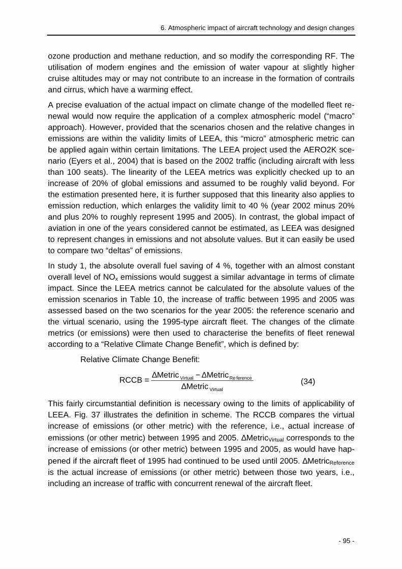
6. Atmospheric impact of aircraft technology and design changes
- 95 -
ozone production and methane reduction, and so modify the corresponding RF. The utilisation of modern engines and the emission of water vapour at slightly higher cruise altitudes may or may not contribute to an increase in the formation of contrails and cirrus, which have a warming effect.
A precise evaluation of the actual impact on climate change of the modelled fleet re-newal would now require the application of a complex atmospheric model (“macro” approach). However, provided that the scenarios chosen and the relative changes in emissions are within the validity limits of LEEA, this “micro” atmospheric metric can be applied again within certain limitations. The LEEA project used the AERO2K sce-nario (Eyers et al., 2004) that is based on the 2002 traffic (including aircraft with less than 100 seats). The linearity of the LEEA metrics was explicitly checked up to an increase of 20% of global emissions and assumed to be roughly valid beyond. For the estimation presented here, it is further supposed that this linearity also applies to emission reduction, which enlarges the validity limit to 40 % (year 2002 minus 20% and plus 20% to roughly represent 1995 and 2005). In contrast, the global impact of aviation in one of the years considered cannot be estimated, as LEEA was designed to represent changes in emissions and not absolute values. But it can easily be used to compare two “deltas” of emissions.
In study 1, the absolute overall fuel saving of 4 %, together with an almost constant overall level of NOx emissions would suggest a similar advantage in terms of climate impact. Since the LEEA metrics cannot be calculated for the absolute values of the emission scenarios in Table 10, the increase of traffic between 1995 and 2005 was assessed based on the two scenarios for the year 2005: the reference scenario and the virtual scenario, using the 1995-type aircraft fleet. The changes of the climate metrics (or emissions) were then used to characterise the benefits of fleet renewal according to a “Relative Climate Change Benefit”, which is defined by:
Relative Climate Change Benefit:
Virtual
ferenceReVirtual
MetricMetricMetric
RCCB∆
∆−∆= (34)
This fairly circumstantial definition is necessary owing to the limits of applicability of LEEA. Fig. 37 illustrates the definition in scheme. The RCCB compares the virtual increase of emissions (or other metric) with the reference, i.e., actual increase of
emissions (or other metric) between 1995 and 2005. ∆MetricVirtual corresponds to the increase of emissions (or other metric) between 1995 and 2005, as would have hap-
pened if the aircraft fleet of 1995 had continued to be used until 2005. ∆MetricReference is the actual increase of emissions (or other metric) between those two years, i.e., including an increase of traffic with concurrent renewal of the aircraft fleet.

Aircraft Design Driven by Climate Change
- 96 -
Virtual 1995 aircraft
1995 2005Traffic
Emissions
Climate metric ∆MetricRef.
∆MetricVirtual
Fig. 37: Scheme illustrating the definition of the “Relative Climate Change Benefit”.
Taking CO2 as a metric, this relative benefit would account for 15 % or 38 %. Using LEEA metrics (PGWP, SGWP, SGTP), i.e., including effects other than CO2, gives “Relative Climate Change Benefit” values between 13 % and 14 % for approach 1, between 23 % and 28 % for approach 2, in total (using the PGTP as a metric logically gives almost the same results as CO2). This means that the climate change benefit of the fleet renewal between 1995 and 2005 appears to be smaller by around a tenth or a third compared to the pure consideration of CO2. The RCCBs of the two studies presented here are displayed in Table 11.
RCCB CO2 PGWP SGWP PGTP SGTPStudy 1 15% 14% 13% 15% 14%Study 2 38% 28% 24% 39% 28%
LEEA metrics
Table 11: Relative Climate Change Benefit based on CO2 and on LEEA metrics: PGWP, SGWP, PGTP, SGTP, over a time horizon of one hundred year s.
These results, however, are summed over all flight altitudes. Calculating the climate change benefits for each of the flight levels with the help of the formula given above enables a more detailed interpretation of the results: even if NOx emission indices might be increased in some cases associated with more fuel-efficient combustion, these benefits (fuel) and drawbacks (NOx) are not necessarily produced at the same altitudes. It turns out that high NOx emission indices are particularly important at high thrust settings, which are used during take-off and climb phases, i.e. at low altitudes. As we have seen before, the overall effect of NOx-induced gases below a certain alti-tude is cooling. Since the effect of NOx below 16500 ft was neglected in this study owing to the lack of data, this effect is probably even underestimated in the total val-ues given above. The overall benefit of the fleet renewal might therefore be as high as or even higher than the benefit estimated based on CO2.
These considerations do not allow the conclusion that NOx emissions are beneficial. On the contrary, their interactions with the atmosphere are multiple, which makes a general statement difficult whether they contribute to or reduce global warming. In this work, we suggest that NOx emissions contribute to global warming at high alti-

6. Atmospheric impact of aircraft technology and design changes
- 97 -
tudes, which is specifically relevant to long-range traffic with long periods at altitude. This effect is aggravated by the fact that there are many long-range routes at high latitudes, where the climate impact pattern illustrated in Fig. 30 and Fig. 31 is down-shifted; thus, a larger part of emissions occurs in regions where NOx tend to contrib-ute to global warming. Regionally, NOx emissions can thus increase or reduce global warming significantly.
Going one step of interpretation further, the results presented above mean that mini-mising the NOx emissions of aircraft that operate a considerable amount of time at low altitudes (short range aircraft), might be less important with regard to their impact on climate than hitherto assumed. Obviously, this is no reason to abandon efforts to reduce NOx of engines for short range aircraft, since the initial motivation of NOx regulations for the purpose of ameliorating local air quality remains valid and has even increased in importance. However, if one imagines future engine design con-sidering NOx emission indices specifically at each thrust setting, these findings might prove very helpful: combustion stages of engines for short-range aircraft could be chosen so as to minimise takeoff-NOx, but not necessarily to trade off fuel consump-tion with NOx production in cruise flight conditions.

Aircraft Design Driven by Climate Change
- 98 -

- 99 -
CHAPTER 7: Aircraft design with a view to its impac t on climate
Step by step, the previous chapters have set up step by step a methodology for the consideration and consequent minimisation of aviation’s impact on climate in aircraft design. Chapter 6 linked operational issues and climate metrics into the evaluation loop. However, the link back to the design of an aircraft has not yet been completed. This chapter aims at closing the design loop and relate climate impact to single air-craft design parameters. Acknowledging the considerable uncertainties at several levels of the design process, and the complexity of this subject, the results presented in this chapter have to be considered as preliminary for the time being. Interpreting them and looking for plausible explanations reveals, however, several coherences that will be useful for further investigations.
After a short summary of conclusions drawn from the “explicit” approach in chapter 6, the overall aircraft design process applied in this thesis will be presented. The tool, in which the calculations were implemented, and the choice of fixed design parameters will be explained. Concrete examples of application with parameter variations will illustrate the potentials of the methodology. Feeding back the climate impact to the aircraft design process closes the investigations as an “implicit” approach.
The chapter will close with an outlook on how “green” aircraft should be according to the results presented here.
7.1 Conclusions from the explicit approach: startin g points for the implicit approach
As detailed in chapter 3, capacity (size), range and speed are the main requirements of a new aircraft concept, and consequently are varied only within tight parameter ranges in the design process (see also Fig. 10). The configuration is chosen to re-spond as well as possible to these demands, but also to ensure reasonable risk. Air-craft designers therefore maintained well-known solutions in recent programmes, since unconventional aircraft concepts may bear unforeseeable difficulties that the industry is not necessarily able to manage, given the high cost pressure today. To-gether with the performance of available engines at the planned time horizon of the new concept, these configurational aspects result in a compromise of other aircraft parameters, one of the most important of which for climate change is the cruise alti-tude. The latter is also linked to the chosen cruise speed (cruise Mach) of the aircraft.

Aircraft Design Driven by Climate Change
- 100 -
Consequently, reconsidering the cruise speed for future aircraft may well have a sig-nificant influence on its climate impact, since the cruise altitude could be adapted ac-cordingly.
Engine parameters such as the specific fuel consumption (SFC), certified NOx levels (see section 4.3.1) directly influence the quantity of an aircraft’s emissions. NOx emissions also depend on the operational thrust setting and thus on the overall air-craft configuration, including the number and position of engines.
The preliminary aircraft design process is a heavily coupled calculation process, so that tradeoffs between the parameters mentioned above cannot easily be deducted and a computational tool is needed to evaluate parameter sensitivities.
7.2 Design platform ODIP and aircraft model SMAC/US MAC
Design trade-off studies in this thesis were conducted with an Airbus internal re-search tool, which is based on the GNU software SCILAB13: “Odisa14 Integration Plat-form” (ODIP). The aircraft model used is called SMAC/USMAC – (Ultra-) Simplified Model of Aircraft. The overall design process, such as performed in Airbus’ Future Projects Office is described in more detail in BADUFLE (2007, her chapter 1). The same logic is pursued here.
7.2.1 ODIP
ODIP provides a graphical user interface to define variables and functions in a simpli-fied programming language (SCILAB). It further provides several data drawing and viewing tools as well as devices for scanning larger number of parameters. The graphical display allows understanding and simple adaptation of existing calculation structures and variables. Supplementary codes may be integrated easily. For this thesis work, two modules were added to the existing aircraft model: one for the cli-mate impact estimation according to LEEA (see chapter 5); and one to produce per-formance input data for subsequent use in the ELISA emission scenario tool (see chapter 4). ODIP thus provides the necessary computational basis for both the macro and the micro aircraft design loop presented in chapter 3.
7.2.2 SMAC/USMAC
The USMAC was initially created to support a study on uncertainty propagation within the aircraft preliminary design process (MAY, 2005). It contains roughly one hundred, often simple, functions that describe an aircraft’s geometry, weights and perform-ance. Some are derived from physical models (e.g., standard atmosphere); others
13 SCILAB: Open source platform for numerical computation initiated by the French National Insitute
for Research in Computer Science and Control (INRIA). More information on http://www.scilab.org (accessed on 24 June 2008).
14 Object Driven Integrated Sizing and Analysis, Airbus internal project for the development of an en-hanced aircraft conceptual design environment (BADUFLE, 2007, p. 41).

7. Aircraft design with a view to its impact on climate
- 101 -
refer to statistic regressions from conventional aircraft in service (e.g., weight estima-tions). Whereas the Breguet range equation is used in this sizing loop to calculate a mission, a reasonably exact calculation of emissions and the subsequent climate metrics requires more precise mission estimation techniques. This more sophisti-cated evaluation is integrated in the SMAC. It contains all typical mission elements such as initial climb, acceleration, step climbs, takeoff and landing, holding (cf. sec-tion 4.2). In the following, the USMAC is used for initial sizing purposes; the SMAC provides a sufficiently precise mission calculation for further application in the macro or micro loop (see chapter 3), i.e. for emissions and climate impact estimation. Since the aircraft model used here is tuned with the help of statistical regressions, the reli-ability of configurations differing a great deal from the reference configuration is lim-ited. This should be considered when analysing the extreme solutions in the follow-ing.
7.3 Applied aircraft design and evaluation process
The aircraft design and evaluation process consists of a basic weight-performance loop, the choice of a configuration with regard to operational constraints and a mis-sion calculation with estimation of emissions and climate impact.
7.3.1 Basic weight-performance design loop
The weight-performance design loop calculates the solution of a system of three equations with OWE, MTOW and fuel consumption unknown, payload and range given as requirements (see Fig. 38).
,...),( RangeMTOWfOWE Structure= (35)
FUELLPOWEMTOW ++= / (36)
Breguet: ,...),( FUELMTOWgRA Missioneff = (37)
MTOW
OWE
gMission
fStructure
Fig. 38: Weights and performances calculation loop: Determination of OWE and MTOW

Aircraft Design Driven by Climate Change
- 102 -
The process results in a compromise between the mission (green line in Fig. 38) and the structural weight (red line in Fig. 38). The mission line is steeper, since it includes a feedback on the structure requirements from the higher fuel weight of a longer de-sign range. If the structure weight is increased, this effect is smaller at constant range, thus the slope of the structure line is flatter. The intersection of both curves represents the solution of the sizing problem. This process is explained in detail in BADUFLE (2007, pp. 30, 52-53).
The reference wing surface (Sref) and the sea-level static thrust of the engine (FNslst) are chosen as main variables of the design process and only Sref and FNslst are varied in all sizing exercises. This process is comparable to the parametric aircraft design that varies the Wing loading (MTOW/Sref) and the Thrust to Weight Ratio (FNslst/MTOW). Parametric aircraft design has been described, e.g., in SCHMITT (2002), STINTON (2001), HOWE (2000), TORENBEEK (1982), and many others.
Within the basic design loop, several operational constraints are calculated. For each set of requirements (range, payload), several solutions are possible, which all satisfy the chosen operational constraints. Several possible combinations of Sref and FNslst are evaluated and a results surface is represented, from which an aircraft configura-tion can be chosen (see section 7.3.3). The chosen configuration is entered in a more complete mission calculation incl. takeoff, climb, descent, landing, holding and diversion (SMAC model) and the resulting emissions and climate impact are evalu-ated.
Subsequently, several central aircraft parameters such as cruise Mach, cruise alti-tude and range are varied, and the calculation procedure of choosing a configuration, calculating mission, emissions and climate impact is performed.
The size of the aircraft, i.e. the number of passengers, is kept constant throughout the study. The geometry stays constant with the exception of the wing size and sweep. The size of the aircraft is another potential central parameter, for the minimi-sation of both the fuel consumption and the climate impact of an aircraft configuration (see GREEN, 2005, p. 25).
7.3.2 Operational constraints
Several operational constraints determine the design space, in which parameter variations can be performed. Within this study, five operational constraints are moni-tored:
1. tofl: The take-off field length represents a regulatory field length, i.e. a maxi-mum of take-off distances and accelerate-stop-distances in “all engines oper-ating” and “one engine inoperative” cases (see FAR/JAR 25.113 regulations or AIRBUS, 2002b, p. 49 ff.). It is calculated based on a temperature of 15° above ISA (denoted as “disa 15”), as proposed in AIRBUS (1996, p. 04-04). As a typi-

7. Aircraft design with a view to its impact on climate
- 103 -
cal maximum value for this type of aircraft, 9500 ft are chosen in this study, which is 2896 m.
2. kcz_buf: Buffeting margin. Buffeting occurs at either low Mach number and high angle of attack, when the airflow separates on the back upper wing, or at high Mach number and consequently relatively low angle of attack, when compressibility effects lead to shock waves on the upper wing and conse-quently also to a separation of the airflow (AIRBUS, 2002b, p. 144). Both effects induce buffeting, but for commercial aircraft only the high speed buffeting is relevant. In operations, it is necessary to maintain a margin of the actual flown load factor (acceleration in z-direction divided by aircraft weight) to the maxi-mum load factor during a turn or other manoeuvre, until which no buffeting oc-curs. Since the buffeting limits of an aircraft depend on the altitude (pressure) at which it flies, a “buffet ceiling” can be devised depending on the Mach num-ber. kcz_buf stands for the chosen margin of the load factor and alternatively of the current lift coefficient. This parameter is not defined by regulations, but at least 1.3 is recommended in AIRBUS (2002b, p. 145).
3. vz_clb: Vertical speed at top of climb, i.e. at the initial cruise altitude. In order to provide reasonable (= short) climb times and sufficient manoeuvring capa-bility in cruise, a minimum climb capability is required. Again, no strict regula-tion is available, however 300 ft/min have become a minimum value, which must be exceeded, 500 ft/min is desirable and has thus been chosen for this study (corresponding to 2.54 m/s).
4. v_app: approach speed. Current landing procedures require fairly similar ap-proach speeds of arriving aircraft. Otherwise, keeping the required minimum tactical distances between aircraft would result in reduced runway landing ca-pacity. Related FAA codes classify aircraft for the purpose of designing air-ports according to their approach speed (e.g., category C: 121-141 kt, cate-gory D: 141-166 kt; DE NEUFVILLE and ODONI, 2003, p. 301). In daily airport operations at busy airports, controllers rely, however, on empirical values (ex-perience) of the approach speed of each aircraft (personal communication: Philipp Böck, 2008). The mentioned categories are thus important, but do not strictly limit the design of an aircraft. A second reason for limiting the approach speed is that landing at high speeds will require better braking performance (higher weight). A lower limit is given by FAR/JAR regulations: the approach speed must be higher than 1.23 times the stalling speed, which is the value calculated in this study. An often used maximum value for the approach speed is 140 kt (category C mentioned above). However, increasing the approach speed to 145 kt is easily conceivable, 150 kt somehow present an absolute limit for reasonable operations. In this study, v_app was limited to 145 kt (269 km/h or 74.6 m/s).

Aircraft Design Driven by Climate Change
- 104 -
5. kfn_cth is the ratio between the actual cruise thrust setting versus the maxi-mum cruise thrust setting. There is more power available for manoeuvres, even if kfn_cth takes “1” as value, however, not for continuous use. Airlines tend to prefer to have some thrust margin available for their continuous cruise, too. kfn_cth should thus be smaller than 0.9, for example. Often, it is not cruise thrust, but climb thrust, which limits the aircraft first.
These constraints can be defined by regulations. In this case, no adaptation is possi-ble in principle, except if the regulatory bodies can be convinced to modify them, which is difficult. But constraints may also refer to requirements defined by the cus-tomer, e.g., the climb speed, approach speed and the cruise thrust setting, which may be negotiated depending on an airline’s network and operating habits. Con-straints such as the Takeoff field length (tofl) and the buffet margin concern aircraft safety and are thus strict limits. Whereas the required tofl is not a physical limit as it depends on the available runway lengths in the airline’s route network, the buffet margin is fixed and may not be compromised under any circumstances.
Table 12 summarises the operational constraints chosen for this study:
Usual units SI unitstofl < 9500 ft 2896 mkcz_buf > 1.3 1.3kfn_cth < 0.9 0.9vz_clb > 500 ft/min 2.54 m/sv_app < 145 kt 74.6 m/s
Table 12: Chosen operational constraints for aircra ft design exercises
7.3.3 Model tuning and reference aircraft
For this study, a generic aircraft was created that resembles the A330-200 with CF6-80E1A4 engines. The absolute values given here are results from a very simplified model and should thus not be confused with aircraft data from the real A330-200. Wherever feasible, the model was tuned to this reference, however, to represent the operational performance of the A330-200 as well as possible.

7. Aircraft design with a view to its impact on climate
- 105 -
250000 260000 270000 280000 290000 300000 310000 320000 330000 340000 350000300
310
320
330
340
350
360
370
380
390
400
FNslst()
Aw
ing(
)
2.1e+005
2.2e+005
2.3e+005
2.4e+005
2.5e+005
tofl<2896
vapp<74.6
vz_clb>2.54
kfn_cth<0.9
kcz_buf>1.3
2.1e+005
2.2e+005
2.3e+005
2.4e+005
2.5e+005
2.1e+005
2.2e+005
2.3e+005
2.4e+005
2.5e+005
tofl < 2896 m
vapp < 74.6 m/s
vz_clb > 2.54 m/s
kfn_cth < 0.9
kcz_buf > 1.3Referenceaircraft
Reference aircraft:FNslst = 294 kNAwing = 363 m²MTOW = 230 ttofl = 2571 mvapp = 69.4 m/svz_clb = 4.12 m/skfn_cth = 0.86kcz_buf = 1.34
FNslst (N)
Sre
f (m
²)
Operational constraints
MTOW (kg)
kcz_bufmargin
kfn_cthmargin
vappmargin
toflmargin
vz_clbmargin
Fig. 39: Design point of reference aircraft with ma rgins to chosen operational constraints (red arrows). The colour shading in the back indicates t he respective MTOW of the chosen aircraft. Hatchings direct to forbidden solutions (constraint violated).
Fig. 39 shows the design space opened by variation of Sref and FNslst. The hatched lines represent the operational constraints with the hatching pointing to the solutions where operational constraints are not satisfied. The background gives an indication of the MTOW of the respective design points. Since the MTOW provides a good indi-cation of the overall efficiency of an aircraft with regard to fuel consumption and op-erational costs in general, an optimum solution for this aircraft could be found in the lower left corner of the allowed space, at the intersection of the tofl (black) and the kcz_buf (yellow) margin lines. This optimum would yield a Sref of 326.4 m² and a FNslst of 264 kN. The reference aircraft is, however, placed at 363 m² and 293 kN. It has margins to tofl, kcz_buf and kfn_cth. vapp and vz_clb are not relevant for this design, since they limit the design less than the other constraints. vapp and vz_clb are inactive constraints, tofl, kcz_buf and kfn_cth are active.
Thus, the reference aircraft has margins vs. the operational constraints chosen in section 7.3.2. If the same margins were required for an alternative solution, the new concept would be penalised at the slightest change of the shape of these margins with regard to Sref and FNslst variations, even though it would still meet the absolute constraints set. Therefore, the constraint margins shall be kept flexible for future de-signs. An aircraft concept is chosen visually in the design space, if one is aiming for a similar overall operational flexibility to the reference aircraft, which allows some shifts

Aircraft Design Driven by Climate Change
- 106 -
from one margin to another. In order to be able to compare operational performance between different aircraft types more rigorously, minimum MTOW design solutions are considered in parallel to the visually chosen design points with margins. The min. MTOW solutions are generally limited by two constraints, even if more than two are active.
7.3.4 Estimation of emissions and climate impact
Emissions were calculated according to the Boeing Fuel Flow Method 2 or the DLR method, such as mentioned in section 4.3.3. If not stated explicitly, the Boeing 2 method was used. As standard parameters, a relative humidity of 0.6 was assumed, as recommended in the method description. The coding was verified by comparing the results within ODIP to those of the ELISA tool and a separate spreadsheet.
The climate metrics were calculated as described in chapter 5. The SGTP100 (100 years’ time horizon) was chosen as a reference climate metric, because it resembles the GWP used in the Kyoto protocol, but is easier to understand (given in Kelvin). Furthermore, a metric employing sustained emissions reflects the reality of emissions from aviation better than one employing a pulse emission. A summary of the formu-las used as well as the atmospheric parameters chosen is given in Appendix A 3. The coding was verified by comparing the results to a spreadsheet delivered in the LEEA project.
7.4 Parameter variations
Essential parameters of aircraft design, design range, cruise altitude, cruise Mach (incl. wing sweep), and wing span (aspect ratio) were varied to reveal potential air-craft configurations with significantly lower climate impact based on the SGTP100 from LEEA.
7.4.1 Design range
In steady flight, the thrust of an aircraft is equivalent to its drag, much of which is di-rectly linked to the aerodynamic lift of the aircraft. Consequently, an increased aircraft weight demands more thrust and leads to higher fuel consumption. On long-range flights, aircraft use a great deal of fuel just to transport fuel, which leads to a high relative fuel consumption on very long distance flights. On the other hand, the takeoff procedure is very fuel-consuming, which leads to high consumption on short routes. Furthermore, the fuel reserves that do not depend on the mission length (holding) become more noticeable in the overall evaluation of short ranges. For each aircraft, a distance for minimum fuel consumption per flown kilometre can be determined. The Specific Air Range (SAR, ratio of mission length to block fuel) and, to a smaller ex-tent, the mission length at which it occurs, vary with the length of the design range and consequent aircraft weights (assuming constant aerodynamics and engine effi-

7. Aircraft design with a view to its impact on climate
- 107 -
ciency). Therefore, a parameter variation on design ranges of the generic aircraft was performed. The reference aircraft had a range of 6463 nm.
Table 13 gives an overview of the principal properties of the aircraft configurations discussed in this section.
Range Sref FNslst MTOW tofl kcz_buf vz_clb v_app kfn_cth[NM] [m²] [kN] [t] [m] [-] [ft/min] [kt] [-]
2000 266 187 144 2118 1.491 700 145 0.903000 271 197 156 2352 1.420 674 145 0.904000 278 208 170 2591 1.363 654 145 0.905000 284 221 185 2836 1.318 639 145 0.906000 308 249 206 2895 1.300 692 142 0.886463 326 264 219 2894 1.300 684 140 0.89
2000 295 219 149 1764 1.576 1069 140 0.823000 300 220 162 2031 1.492 890 140 0.854000 306 238 177 2214 1.415 930 140 0.835000 310 248 192 2480 1.353 861 141 0.846000 338 276 215 2573 1.333 846 138 0.856463 363 294 230 2571 1.336 811 135 0.86
Min. MTOW conf.
Conf. with op. margins
Table 13: Aircraft configurations derived from rang e variation: Sref, FNslst, MTOW and opera-tional constraints
7.4.1.1 Influence on fuel consumption
Fig. 40 shows the Specific Air Ranges (SAR) of several aircraft configurations with different design ranges as a function of the flown distance. The first line of the legend concerns visually chosen configurations with some margins to the operational con-straints (see section 7.3.2). For direct comparison, the configurations minimising the MTOW, i.e. with no margin to the operational constraints, are represented with full symbols and a line between the single points. According to the results presented in the figure, the SAR increases by roughly 14 % between the original configuration (red) with a design range of 6463 NM and one with a design range of 3000 NM. Be-tween a 6000 NM design and a 3000 NM design, the difference is still 11 % on aver-age. Furthermore, even an aircraft that is not redesigned will have an SAR that is 8 % higher on a 3000 NM mission than on a 6000 NM mission. Combining both effects, i.e. flying two equal stages of 3000 NM with a redesigned aircraft compared to one stage with an aircraft designed for 6000 NM would result in a fuel reduction of 15 % in total (18 % higher SAR). Of course, this investigation does not consider opera-tional implications such as the availability of airports around the mid-point etc. EGEL-
HOFER et al. (2008) give more details on the fuel efficiency of so-called Two-Stage-Operations and indications of operational entanglements.

Aircraft Design Driven by Climate Change
- 108 -
0.07
0.08
0.09
0.1
0.11
0.12
0 1000 2000 3000 4000 5000 6000 7000
Flown Distance (NM)
SA
R (N
M/k
g)
6463 6000 5000 4000 3000 20006463 6000 5000 4000 3000 2000
Conf. with margins: Conf. at min. MTOW:
Fig. 40: Specific Air Range (SAR) as a function of the Design Range and the actual distance flown. Empty symbols concern “common-sense” configu rations (with margins), full symbols refer to min. MTOW solutions without margin to oper ational constraints.
0.090
0.095
0.100
0.105
0.110
0.115
1000 2000 3000 4000 5000 6000 7000
Design Range (NM)
SA
R (N
M/k
g)
Conf. at min. MTOW
Conf. with margins
Distance flown: 2000 NM
kcz_buf, tofl and kfn_cth active
vapp and kfn_cth active
Fig. 41: SAR (NM/kg) for a 2000 NM mission, as a fu nction of the design range.
Fig. 41 shows the Specific Air Range as a function of the design range for a distance flown of 2000 NM. The configurations can be split in two groups: the reference and the 6000 NM design range configuration are constrained by kcz_buf and tofl with kfn_cth active. At a design range of 5000 NM and below, vapp and kfn_cth are ac-tive. vapp strongly depends on the landing weight of the aircraft and its wing surface. tofl is a parameter for the takeoff performance of an aircraft. A longer design range incorporates both a higher structural weight (relevant for landing weight) and higher fuel weight for the mission (relevant for both takeoff and landing). Therefore, the function displayed shows a greater negative slope for the aircraft configurations lim-ited by tofl than those limited by vapp. This observation is consistent with the graph shown in Fig. 38.

7. Aircraft design with a view to its impact on climate
- 109 -
kcz_buf increases with decreasing design range (1.49 for the min. MTOW solution at 2000 NM design range). Due to the vapp limit, the low design range configurations still have quite high wing surfaces, despite their very low thrust levels (due to low thrust requirements at takeoff with low weight). Buffeting occurs at high altitudes, when speed or angle of attack need to be high owing to the low air pressure. The third parameter defining the lift is the wing surface. Since it is fairly big, the two pa-rameters causing buffeting (Mach, angle of attack) do not need to be as high to cause the effect. Consequently, the kcz_buf loses in importance compared to vapp for the smaller design ranges.
The marginal fuel benefit (slope of function in Fig. 41) of reducing the design range thus depends on the operational constraints chosen. For example, if a higher ap-proach speed (vapp) or a lower cruise thrust excess (kfn_cth) was negotiated with clients, reducing the design range to below 5000 NM would bring about even higher fuel benefits. Put differently, reducing the design range with the current operational constraints would bring larger benefits until 5240 NM than below.
0.0800.085
0.0900.0950.1000.105
0.1100.115
1000 2000 3000 4000 5000 6000 7000
Design Range and Mission Distance (NM)
SA
R (N
M/k
g)
Conf. at min. MTOW
Conf. with margins
kcz_buf, tofl and kfn_cth active
vapp and kfn_cth active
Distance flown: Design Range
Fig. 42: SAR (NM/kg) as a function of the design ra nge, for mission distance equal to design range.
Fig. 42 shows the SAR if the flown distance is equal to the design range, which en-ables conclusions with regard to two-stage operations. GREEN (2005, p. 25) cites a study according to which an aircraft designed for 4000 NM “operating in stages over current real routes compared with direct flights by a different design with a range of 8000 NM” would show a fuel burn benefit of 10 %, compared to 15 % by halving the design range and the distance flown from 6000 NM to 3000 NM in this study (see Fig. 42). The fuel burn benefit is considerably higher than that from GREEN’s study since it is theoretical and not restricted to operational routes. Based on these results, one could argue that operational entanglements would offset roughly a third of the fuel benefit attained by operating in two stages on long-range routes.

Aircraft Design Driven by Climate Change
- 110 -
0
5
10
15
20
25
500 1000 1500 2000 2500 3000 3500 4000 4500 5000 5500
Distances (NM)
Num
ber o
f flig
hts
(10
3 )
0
10
20
30
40
50
60
Flo
wn
Dis
tanc
es (1
06 N
M)
Number of flights
Flown Distance
Fig. 43: Percentage of flights and flown distance o f the A330-200 depending on the mission length. The categories given represent distances un til the given value, i.e. “1500” means all routes from 1001 to 1500 NM. Data from OAG for 2005 (data for September multiplied by 11).
In order to evaluate the operational importance of the design range in a global con-text, OAG traffic data of the year 2005 were analysed. Best comparing to the generic aircraft used in this study, Fig. 43 shows the percentage of flights and flown distance of the A330-200. Low distance missions (up to 2000 NM) account for more than half of the flights. In terms of km flown, they represent only 24 % of the A330-200 mis-sions. The largest numbers of flown kilometres occur between 2500 and 3500 NM (39 %) with still considerable amounts between 3500 NM and 4500 NM (24 %). Routes above 4500 NM make up 6.5 % of the total flown kilometres and 2.7 % of the flights. Since the fuel efficiency is considered per NM (1/SAR), the percentage of flown distance is more relevant for the choice of a reasonable design range than the number of flights. According to the results presented here, choosing 5000 NM as de-sign range would serve 99% of the kilometres flown by an A330-200 in 2005, at a fuel benefit of 9 % on average.
These considerations disregard any freight that might be transported in the aircraft. The payload assumed for all calculations in this thesis is the maximum passenger payload, i.e. no supplementary freight can be carried if the mission distance equals the design range. This is probably the reason why no distances above 5500 NM oc-cur in the OAG traffic analysis: Operational A330-200 seem to transport a consider-able amount of freight with the consequence that the actual maximum passenger payload design range may not be exploited.
7.4.1.2 Influence on climate impact
The climate impact is driven by the fuel consumption (CO2) and by the fact that NOx and contrails act mainly at certain flight altitudes (see chapter 5, especially Fig. 30 and Fig. 31). Consequently, issuing the analyses of the previous section for the SGTP100 gives different findings.

7. Aircraft design with a view to its impact on climate
- 111 -
Fig. 44 shows the SGTP100 per NM of different design ranges and distances flown. Consistently with the former consideration, designing the aircraft to lower ranges has a positive effect on its impact on climate measured by the SGTP100. A min. MTOW design for a range of 3000 NM decreases the SGTP100 per flown NM by 8 % on a flown distance of 3000 NM compared to a design for 6000 NM range. The benefit of designing to lower ranges is thus less expressed when taking the SGTP100 as a met-ric compared to when the fuel consumption is taken as a metric (difference is 10 %). This is due to the fact, that an aircraft designed for low range spends more time at higher altitudes (lower weight) than an aircraft designed for high range, both operat-ing over the same distance15. The STGP100 includes NOx and contrail effects, which have a higher warming effect at higher altitudes. Therefore, the climate benefit of lower ranges is reduced compared to a mere consideration of CO2.
2.9E-12
3.4E-12
3.9E-12
4.4E-12
4.9E-12
5.4E-12
0 1000 2000 3000 4000 5000 6000 7000
Flown Distance (NM)
SG
TP
100
(K /
(NM
/yea
r))
6463 6000 5000 4000 3000 20006463 6000 5000 4000 3000 2000
Conf. with margins: Conf. at min. MTOW:
Fig. 44: Sustained Global Temperature Change Potent ial (SGTP) on a time horizon of 100 years as a function of the Design Range and the actual di stance flown. Empty symbols concern “common-sense” configurations (with margins), full symbols refer to min. MTOW solutions without margin to operational constraints.
On the other hand, the actual flown distance has a far larger impact based on the
SGTP100: the 6000 NM design range aircraft produces an SGTP100 of 4.2⋅10-12 K/NM
on the 3000 NM mission, of 4.93⋅10-12 K/NM on the 6000 NM mission, i.e. 18 % more. This is again due to the higher portion of high altitudes in the entire mission, and of course, to the higher fuel consumption already revealed in the SAR compari-son study.
15 This is the case for optimised mission profiles. In the operational reality, short-range aircraft are
often flown at lower altitudes in order to optimise their true air speed, which increases at a given Mach due to a higher temperature at lower altitudes.

Aircraft Design Driven by Climate Change
- 112 -
Summing both effects, a two-stage operation on 6000 NM in total with an aircraft de-signed for 3000 NM has 22 % less impact on warming than a single stage with an aircraft designed for 6000 NM (17 % if considering CO2 only). Considering the route analysis in Fig. 43, a 5000 NM aircraft design would bring a climate impact benefit of a mere 3 to 4 % compared to the reference aircraft (6463 NM design range).
To conclude, reducing the climate impact would imply flying shorter stages in general (operational measure), lower design ranges would further contribute to the reduction in both the climate impact and fuel consumption (and fuel costs), but to a lower ex-tent than reducing the stage lengths.
7.4.2 Cruise altitude
Since the climate impact of aircraft emissions depends heavily on the altitude at which they are emitted, the cruise altitude is varied in this section. In order to assure reasonable comparability and facilitate reading, some graphs in the following show only the configurations for minimum MTOW. The given altitudes represent a maxi-mum cruise altitude with the initial cruise altitude being 2000 ft lower. This maximum cruise altitude limits the optimisation of a mission for minimum fuel: in this section, the reference generic aircraft (FL 350) has a higher fuel consumption than before, because it is also constrained to fly at its reference flight level for comparability rea-sons, and not able to use step climbs higher than FL 350.
The following configurations were generated:
Cr. FL Sref FNslst MTOW tofl kcz_buf vz_clb v_app kfn_cth[-] [m²] [kN] [t] [m] [-] [ft/min] [kt] [-]
370 386 312 236 2386 1.299 629 132 0.90360 352 281 225 2667 1.299 627 136 0.90350 326 264 219 2894 1.300 684 140 0.89330 304 288 220 2894 1.310 1263 145 0.76310 307 300 225 2895 1.364 1556 145 0.72290 311 316 233 2896 1.430 1868 145 0.70
370 412 342 246 2205 1.314 751 130 0.87360 377 310 235 2431 1.317 780 133 0.86350 363 294 230 2571 1.336 811 135 0.86330 332 304 228 2671 1.347 1300 140 0.75310 332 314 233 2706 1.407 1578 141 0.72290 339 324 240 2736 1.495 1794 140 0.71
Min. MTOW conf.
Conf. with op. margins
Table 14: Aircraft configurations derived from alti tude variation: Sref, FNslst, MTOW and opera-tional constraints

7. Aircraft design with a view to its impact on climate
- 113 -
7.4.2.1 Influence on fuel consumption
0.070
0.075
0.080
0.085
0.090
0.095
0 1000 2000 3000 4000 5000 6000 7000
Flown Distance (NM)
SA
R (N
M/k
g)
370 360 350 330 310 290Cruise Flight Level (min. MTOW):
Fig. 45: Specific Air Range (SAR) as a function of the reference cruise flight level and the actual distance flown.
According to the results presented in Fig. 45, both increasing and decreasing the flight altitude decreases the SAR, if no other aircraft parameter is changed at the same time. The effect is more clearly pronounced for higher altitudes. For a flown distance of 3000 NM, an aircraft designed for FL 350 consumes 8 % less than the one for FL 370, 14 % less than one for FL 290.
Fig. 46 summarises these effects for a 3000 NM mission. By way of comparison, the rose points give an indication where operationally reasonable configurations could be placed, i.e. aircraft that have some margins to the operational constraints chosen.
0.075
0.080
0.085
0.090
0.095
270 290 310 330 350 370
Cruise Flight Level
SA
R (N
M/k
g)
Conf. at min. MTOW
Conf. with margins
Distance flown: 3000 NM
Fig. 46: SAR (NM/kg) for a 3000 NM mission, dependi ng on the maximum cruise altitude for both minimum MTOW configurations and configurations with margins to operational con-straints.
Since the engine cycle was not adapted to the changing cruise altitude, except the rubberising to yield at a new FNslst, its performance and fuel consumption properties as a function of the altitude and the Mach number are the same for all configurations.

Aircraft Design Driven by Climate Change
- 114 -
They must be taken into account to understand fully the effects of an altitude varia-tion.
0 2000 4000 6000 8000 10000 12000
3000
4000
5000
6000
7000
8000
9000
Fuel consumption for different altitudes at Mach 0.80 ALT(ft)
Cruise Thrust (daN)
Fue
l con
sum
ptio
n (k
g/h)
30007000
110001500019000
2300027000
3100033000
350003700039000
41000
1000
2000
Fig. 47: Fuel consumption of reference engine (FNsl st = 29400 daN) at Mach 0.8 (DISA=0) as a function of the thrust, for different flight altitu des
Fig. 47 shows the fuel consumption of the reference engine as a function of the thrust for several altitudes. An aircraft weight of 200 t and an L/D of 20 would require a thrust of 100 kN with both engines, i.e. 50 kN for each engine. In principle, the en-gine’s specific fuel consumption decreases with the altitude. There is, however, a thrust (just before maximum available cruise thrust), where this behaviour is inverted. For 50 kN, the consumption of the engine is higher at FL 390 than at FL 370 (flight levels around the tropopause, where the decrease of air pressure with increasing altitude is slowed down). Engine performance and aerodynamics are well optimised to fit together for the reference aircraft: the minimum SFC therefore coincides more or less with the maximum L/D for each aircraft weight and altitude. For the changed aircraft configurations considered (see Table 14), these SFC optima do not necessar-ily coincide with the chosen cruise flight altitudes for each aircraft (the L/D optima do not necessarily coincide either), since they are limited by operational constraints or by definition like in this section.
Therefore, a real fuel benefit from changing the cruise altitude only, without redesign-ing the engine or other aircraft parameters such as the aerodynamics of the wing, cannot be attained.

7. Aircraft design with a view to its impact on climate
- 115 -
7.4.2.2 Influence on climate impact
Since the altitude of aircraft emissions is a major parameter for their climate impact, varying the reference cruise altitude directly affects the SGTP100 values of the con-sidered configurations.
3.5E-12
4.0E-12
4.5E-12
5.0E-12
5.5E-12
6.0E-12
0 1000 2000 3000 4000 5000 6000 7000
Flown Distance (NM)
SG
TP
100
(K /
(NM
/kg)
)
370 360 350 330 310 290Cruise Flight Level (min. MTOW):
Fig. 48: Sustained Global Temperature Change Potent ial (SGTP) on a time horizon of 100 years as a function of the cruise altitude and the actual distance flown (minimum MTOW configura-tions shown).
Despite the higher fuel consumption of aircraft with changed fuel altitudes, their cli-mate impact generally decreases with decreasing altitude (see Fig. 48). For a mis-sion of 3000 NM, the SGTP100 increases by 4 % for the A/C flying at FL 370 and de-creases by 20 % for a FL 290 aircraft, compared to the reference aircraft flying at FL 350. This 20 % reduction in climate impact is attained despite the increase in fuel consumption of 14 % with a consequent increase of SGTP100 from CO2 of 14 %. This results from a reduction in the NOx-related impacts (O3, CH4, O3-CH4) of 75 % and of that of the contrails of 40 %. If the contrails are not taken into account, reducing the cruise altitude to FL 290 would yield a reduction in climate impact of only 3 %: the benefit from the NOx effects would largely be offset by the increase in fuel consump-tion.
An exception to the benefits of reducing the cruise altitude is the aircraft designed for FL 330. Its overall climate impact is slightly higher than that of the reference aircraft. The benefit of NOx effects is largely offset by an increase in the contrail effect. To-gether with higher fuel consumption, the overall benefit of designing to FL 330 is null.
The increase of SGTP100 results from the increase of fuel consumption and an even higher portion from NOx-related impacts, which is, however, largely offset by a reduc-tion of the contrails’ effect.

Aircraft Design Driven by Climate Change
- 116 -
To conclude, a decrease in the cruise altitude of more than 2000 ft (with all other air-craft parameters constant) results in a decreased climate impact measured by SGTP100 from LEEA, even if the fuel consumption increases.
7.4.3 Cruise Mach
The last section showed that changing the flight altitude would result in higher fuel consumption, because aerodynamics and engine performance are not adapted ac-cordingly. For lower altitudes, the fuel consumption increases inter alia because the aircraft flies at a lower angle of attack due to a higher air pressure, but with lower L/D. A reduction in the Mach number capitalises on this effect in order to return to the optimum angle of attack and then optimum L/D. Therefore, a Mach variation study was performed. In this section, only the Mach numbers are varied, later on, Mach and cruise altitude are varied together (see section 7.4.5).
Directly linked to the cruise Mach of an aircraft, the wing sweep has to be adapted accordingly. STINTON (2001, p. 152) states that the Mach number normal to the wing (leading edge) should not exceed 0.7. In this study, the 25% sweep of the reference aircraft was chosen and the ratio (0.71278) of the reference aircraft was applied to the configurations with changed Mach. This resulted in the following correspondence:
Mach Sweep25% (degrees)
0.74 15.730.76 20.410.78 24.050.80 27.080.82 29.700.84 32.010.86 34.08
Table 15: Mach – sweep correspondence for con-stant normal Mach num-ber (normal to 25% line)
Applying these numbers in sizing loops led to the configurations listed in Table 16.
Mach Sref FNslst MTOW tofl kcz_buf vz_clb v_app kfn_cth[-] [m²] [kN] [t] [m] [-] [ft/min] [kt] [-]
0.74 287 274 212 2894 1.346 898 145 0.780.76 291 274 212 2893 1.427 926 145 0.780.78 294 275 213 2894 1.474 937 145 0.790.80 298 277 214 2893 1.423 947 145 0.800.82 326 264 219 2894 1.300 684 140 0.890.83 445 328 254 2268 1.300 711 126 0.900.84 306 287 219 2894 1.035 955 145 0.830.86 311 295 224 2896 0.783 943 145 0.85
Min. MTOW conf.
Table 16: Aircraft configurations with minimum MTOW derived from Mach variation: Sref, FNslst, MTOW and operational constraints. Configura tions with M 0.84 and 0.86 do not respect the buffeting constraint.
By simply analysing the resulting MTOW, it turns out that reducing the Mach by 0.02 could lead to significant fuel benefit, a further decrease would have less effect. A slight increase in the Mach number by 0.01 leads to a minimum MTOW of 253 t (Sref

7. Aircraft design with a view to its impact on climate
- 117 -
= 445 m², FNslst = 328 kN) owing to the buffeting constraint. For Mach numbers higher than 0.83, releasing the buffeting constraint may allow configurations to be retrieved that satisfy all other constraints (see Table 16). Whereas the 0.84 configu-ration still has a minimum margin to buffeting, the 0.86 configuration has a kcz_buf strictly lower than 1. Moreover, both configurations have poor fuel efficiency com-pared to the reference case. Configurations with Mach numbers higher than 0.83 are thus disregarded in the following.
Analysing the respective SAR for the minimum MTOW configurations allows more detailed conclusions:
0.075
0.080
0.085
0.090
0.095
0.100
0.105
0 1000 2000 3000 4000 5000 6000 7000
Flown Distance (NM)
SA
R (N
M/k
g)
0.83 0.82 0.80 0.78 0.76 0.74Cruise Mach (min. MTOW):
Fig. 49: Specific Air Range (SAR) as a function of the cruise Mach and the actual distance flown
According to the results presented in Fig. 49, reducing the cruise Mach reduces fuel consumption within some limits, which confirms the short conclusions from above. Compared to the reference cruise Mach of 0.82, a reduction to 0.80 yields significant improvements (3%), whereas the next step to 0.78 is only half a percent better than 0.8. Increasing the Mach, even to only 0.83, clearly costs fuel even if the wing sweep is adapted accordingly. This is partly due to a higher SFC of the engine.
The SGTP100 reacts in a more complicated way to Mach changes (see Fig. 50), which is due to subsequent changes in the actual proportion of step flight altitudes. Note that, in this section, aircraft are allowed to use step climbs. As expected from the analysis of the SAR, reducing Mach has less impact on climate compared to in-creasing Mach. Whereas the CO2 effect and the NOx-related effects reduce the SGTP100 for lower speeds, the impact from contrails increases and offsets these benefits. For long distances, the overall effect of reducing the cruise Mach is small regarding the climate impact. For higher Mach numbers, CO2-, NOx- and contrail ef-fects increase, which results in a distinct overall increase of the SGTP100.

Aircraft Design Driven by Climate Change
- 118 -
3.5E-12
4.0E-12
4.5E-12
5.0E-12
5.5E-12
0 1000 2000 3000 4000 5000 6000 7000
Flown Distance (NM)
SG
TP
100
(K /
(NM
/yea
r))
0.83 0.82 0.8 0.78 0.76 0.74Cruise Mach (min. MTOW):
Fig. 50: Sustained Global Temperature Change Potent ial (SGTP) on a time horizon of 100 years as a function of the cruise Mach and the actual dis tance flown.
7.4.4 Aspect ratio – wing span
The aspect ratio of the wing is an important parameter for the aerodynamic efficiency (L/D) of an aircraft. From an aerodynamic point of view, large aspect ratios reduce induced drag. They go hand in hand with high structural weight, however. This effect is taken into account in the simplified aircraft model in this study, but the validity of extreme solutions (aspect ratio higher than 16 for min. MTOW configuration) is ques-tionable. The simple aerodynamic and weights models (empiric) used do not neces-sarily represent them accurately. Supplementary concerns such as fluttering or the availability of enough space to house the landing gear would need to be investigated in detail, before large span solutions can be fully evaluated. Also, airport handling limits the scope of reasonable wing spans, and so indirectly of aspect ratios.
Varying the wing span led to the theoretical configurations listed in Table 17.
Span Sref Aspect r. FNslst MTOW tofl kcz_buf vz_clb v_app kfn_cth[m] [m²] [-] [kN] [t] [m] [-] [ft/min] [kt] [-]
50 378 6.6 350 253 2519 1.300 740 135 0.9054 343 8.5 290 230 2765 1.300 675 138 0.9058 326 10.3 264 219 2894 1.300 684 140 0.8962 318 12.1 257 213 2893 1.300 789 141 0.8566 307 14.2 248 206 2894 1.300 928 143 0.8070 302 16.2 245 203 2893 1.300 977 143 0.7874 299 18.3 242 200 2894 1.300 1013 144 0.77
Min. MTOW conf.
Table 17: Aircraft configurations derived from span variation: Sref, aspect ratio, FNslst, MTOW and operational constraints.

7. Aircraft design with a view to its impact on climate
- 119 -
ICAO defines four classes of commercial aircraft for airport handling purposes, of which two are relevant for this study: “Code E” for a wing span between 52 m and 65 m, “Code F” for a wing span between 65 m and 80 m (DENEUFVILLE and ODONI, 2003, p. 301). The wing span of the reference aircraft is 58 m. Roughly 2.5 m should be added on top to allow the use of wing tip devices such as tip fences and winglets. Since the ICAO codes represent a clear geometric constraint, not the aspect ratio, the wing span is varied here: the configurations with reference wing spans between 50 m and 62 m enter the “Code E” category, the configurations with 66 m to 74 m would place at an aircraft in “Code F”.
Larger wing spans have a clear advantage both in terms of fuel consumption and climate impact, smaller wing spans increase both (see Fig. 51 and Fig. 52). The del-tas are more pronounced for small wing spans than for large wing spans: an increase of the wing span from 58 m to 62 m results in a fuel reduction of 6 % (9 % SGTP100). An increase from 70 m to 74 m yields only 3 % (5 % SGTP100) supplementary reduc-tion. These results are consistent with the consideration of a higher structural weight of high span wings. Reducing the wing span to 54 m, on the other hand, increases fuel consumption by 9 % (SGTP100 12 %). (All numbers for 3000 NM mission)
The altitudes during the mission calculation are not constrained here. Larger span configurations attain higher cruise levels faster, so that the SGTP100 reacts stronger to the wing span variation than the fuel consumption. Longer high altitude portions bring about slightly higher NOx effects, but significantly lower impact from contrails. Therefore, the overall SGTP100 benefits even more from a larger wing span than the bare fuel consumption.
0.06
0.07
0.08
0.09
0.10
0.11
0.12
0 1000 2000 3000 4000 5000 6000 7000
Flown Distance (NM)
SA
R (N
M/k
g)
50
54
58
62
66
70
74
Wing span (m)
Fig. 51: SAR for wing span variation as function of the distance flown

Aircraft Design Driven by Climate Change
- 120 -
3.0E-12
3.5E-12
4.0E-12
4.5E-12
5.0E-12
5.5E-12
6.0E-12
6.5E-12
7.0E-12
0 1000 2000 3000 4000 5000 6000 7000
Flown Distance (NM)
SG
TP
100
(K /
(NM
/yea
r))
50
54
58
62
66
70
74
Wing span (m)
Fig. 52: SGTP 100 for wing span variation as function of the distanc e flown
7.4.5 Parallel variation of Mach number and cruise altitude
Whereas a reduction in the design range or an increase in the span led to significant benefits for both fuel consumption and climate impact, reducing the Mach number decreased fuel consumption, but increased climate impact; lowering the cruise alti-tude increased fuel consumption, but decreased climate impact. Mach number and cruise altitude are connected and are therefore varied together in this section. Again, the engine is not changed except the rubberising of its thrust just as in the previous sections.
As mentioned previously, the chosen lift coefficient and consequent lift to drag ratio (L/D) essentially influences the overall efficiency of an aircraft. Fig. 53 shows the L/D of the generic aircraft as a function of the lift coefficient and the Mach number. The maximum L/D decreases with increasing Mach, and occurs at lower lift coefficients. Consequently, designing to lower altitudes, where the air pressure is higher, would imply lower lift coefficients at iso-Mach (and thus lower L/D, since the reference con-figuration flies near the optimum L/D), or lower Mach numbers with consequently higher lift coefficient to maintain a maximum L/D. This could decrease the needed wing surface if it is not constrained by the approach speed or buffeting.

7. Aircraft design with a view to its impact on climate
- 121 -
10
12
14
16
18
20
22
0.2 0.3 0.4 0.5 0.6
lift coefficient
L/D
0.74
0.78
0.80
0.81
0.82
0.83
0.84
0.86
0.88
0.90
Mach:
Fig. 53: Lift to drag ratio of generic aircraft for different Mach as a function of the lift coeffi-cient.
In this section, all other aircraft parameters were kept constant, but Mach (incl. wing sweep) and altitude were varied together. Since two dimensions were changed, a total of 47 configurations were calculated, of which the complete list is attached in appendix A 4.
Fig. 54 shows the fuel efficiency and climate impact of all these configurations as a function of the reference flight level and the cruise Mach for a distance flown of 3000 NM. This distance reflects the overall effects distinctly. In Fig. 54 a), it can be clearly seen that flying fast comes at some cost of fuel consumption at all flight lev-els: flying more slowly would incorporate savings in the order of several percent (less for high altitudes).
The red and violet curves for Mach numbers 0.82 and 0.83 respectively form a fairly sharp bend due to the buffeting constraint (see section 7.4.3 on Mach variation). The aircraft configurations for higher Mach number and / or higher altitude thus need a larger wing and consequently have significantly higher structural weight, which pays dividends on fuel consumption. Therefore, no configuration above Mach 0.83 was examined in this study. Aiming at higher Mach numbers would imply adapting the wing geometry (profile, thickness etc.).
Fig. 54 b) issues the SGTP100 including all effects (NOx-related: O3, CH4, O3-CH4; contrails; CO2). Fig. 54 c) sums the SGTP100 of CO2 and NOx effects only.
In contrast to section 7.4.3, the SGTP100 decreases with decreasing Mach number. This results from the constrained altitude in the mission calculation (see section 7.4.2): instead of freely choosing the step climbs that minimise the mission fuel, the cruise altitude is limited to the given flight levels. Consequently, the disadvantage in SGTP100 from longer mission portions at high altitude is very small. Actually the air-craft attain the maximum flight altitude just several minutes earlier. The fuel con-sumption is thus the predominating effect for the SGTP100.

Aircraft Design Driven by Climate Change
- 122 -
0.070
0.075
0.080
0.085
0.090
0.095
0.100
250 270 290 310 330 350 370 390
Reference Cruise Flight Level
SA
R (N
M/k
g)
M0.74
M0.76
M0.78
M0.79
M0.80
M0.81
M0.82
M0.83
Buffetingconstraint!
3.0E-12
3.5E-12
4.0E-12
4.5E-12
5.0E-12
5.5E-12
250 270 290 310 330 350 370 390
Reference Cruise Flight Level
SG
TP
100
(K /
(NM
/yea
r))
M0.74
M0.76
M0.78
M0.79
M0.80
M0.81
M0.82
M0.83
Distance Flown: 3000 NM
Distance Flown: 3000 NM
2.0E-12
2.5E-12
3.0E-12
3.5E-12
250 270 290 310 330 350 370 390
Reference Cruise Flight Level
SG
TP
100
(K /
(NM
/yea
r))
M0.74
M0.76
M0.78
M0.79
M0.80
M0.81
M0.82
M0.83
Distance Flown: 3000 NM
without consideration of contrails
including all effects (CO2, NOx, contrails)
a)
b)
c)
Fig. 54: Fuel efficiency / climate impact of parall el Mach number and cruise altitude variation: a) SAR; b) SGTP 100 including all effects; c) SGTP 100 without contrails effect; for a flown distance of 3000 NM
The comparison of Fig. 54 b) and c) allows the role of contrails to be highlighted: If they are taken into account and if their relative effect is accurately represented by the LEEA results, changing the flight altitude results in a very significant advantage for the climate impact of an aircraft: reducing the cruise altitude would be beneficial for

7. Aircraft design with a view to its impact on climate
- 123 -
all Mach numbers considered here. Increasing the flight altitude would bring benefits, if the Mach is slightly reduced.
If contrails are not considered or if their impact is significantly lower than that esti-mated in LEEA, changing the cruise altitude has far less impact on climate. A reduc-tion of the Mach number remains beneficial at all altitudes. For all Mach higher than 0.74, FL 330 represents a local minimum of SGTP100; a further decrease could only be attained by lowering the cruise altitude to FL 270 or probably below (not calcu-lated).
To conclude, a fuel consumption increase due to a deliberate decrease in the flight altitude can be offset, at least partly, by a lower cruise Mach. Reducing the cruise altitude from FL 350 to FL 330, e.g., would require a Mach of 0.80 to attain the same fuel efficiency. FL 310 would require M 0.74. Since the temperature increases at lower altitudes, the actual cruise speed (true air speed) would be higher than indi-cated by the change of Mach. At the same time, increasing the flight altitude would reduce the air speed on top of the Mach reduction, but at a significant advantage for both fuel consumption and SGTP100. These considerations are summarised in the Table 18.
Mach Temp Sound vel. TAS SAR SGTP100 SGTP100 without contrails
[-] [K] [m/s] [kt] [NM/kg] [10-12K/NM/a] [10-12K/NM/a]
FL 310 0.74 227 302 434 0.092 4.57 2.47FL 330 0.80 223 299 465 0.092 5.18 2.61FL 350 0.82 219 297 473 0.092 5.21 2.83FL 370 0.81 217 295 464 0.097 4.83 2.83
Table 18: Effects on true airspeed (TAS), SAR and S GTP100 of changing Mach and altitude at the same time. Example configurations that aim at m aintaining the fuel consumption similar to that of the ref. aircraft (bold font).
• Flying at FL 310 and M 0.74 would reduce climate impact by 12 % (13 %, if con-trails are not considered), while consuming half a percent more and with a true airspeed (TAS) reduced by 8 %.
• Flying at FL 330 and M 0.80 would reduce climate impact by 0.7 % (8 %, if con-trails are not considered), while consuming 0.2 % more and with a true airspeed (TAS) reduced by 1.7 %.
• Flying at FL 370 and M 0.81 would reduce climate impact by 7 % (null, if contrails are not considered), while consuming 6 % more and with a true airspeed (TAS) reduced by 2 %.
These analyses highlight the importance of the respective weighting of NOx-related effects and contrails, and their development as a function of the altitude.

Aircraft Design Driven by Climate Change
- 124 -
7.5 Clues for a “green” aircraft
This chapter explored options in the aircraft design process to reduce the climate im-pact of future commercial aircraft. While far from complete, the study has revealed several starting points for “green” aircraft, i.e. aircraft that reduce the impact on cli-mate significantly compared to today’s configurations.
7.5.1 Example “green” configurations
To illustrate the findings further, five example configurations were chosen based on the results of the parameter variations in the previous sections. Table 19 gives an overview of their basic design parameters, resulting MTOW, operational constraints, fuel consumption on a distance of 3000 NM and related SGTP100. The difference in fuel consumption and climate impact of the “green” aircraft versus the reference air-craft is also given. As in sections 7.4.2 and 7.4.5, the mission altitudes are con-strained to the flight levels given in the table.
All configurations have a larger span than the reference aircraft. Green 1, 2 and 3 still fit in the same ICAO aircraft compatibility category (“Code E”), even if wing tip de-vices were attached. As shown in section 7.4.4, an increase in the wing span by 4 m results in a fuel reduction of roughly 6 %, if the mission altitude is not constrained. If it is constrained, as in this section, the fuel consumption is reduced by 4 % (7 % for a wing span of 66 m).
Reference Green 1 Green 2 Green 3 Green 4 Ultragreen
Range [NM] 6463 6463 6463 5000 5000 4000Cr. FL [-] 350 370 330 330 330 290Mach [-] 0.82 0.81 0.78 0.78 0.80 0.76Span [m] 58 62 62 62 66 66Sref [m²] 326 297 294 277 281 267Asprect r. [-] 10.3 12.9 13.1 13.9 15.5 16.3FNslst [kN] 264 264 269 210 209 184MTOW [t] 219 209 211 181 182 168tofl [m] 2894 2895 2895 2896 2894 2894kcz_buf [-] 1.300 1.325 1.594 1.707 1.636 2.115vz_clb [ft/min] 684 708 1274 881 898 1003v_app [kt] 140 145 145 145 145 145kfn_cth [-] 0.89 0.86 0.71 0.81 0.81 0.81SAR [NM/kg] 0.092 0.102 0.097 0.105 0.106 0.104Fuel cons. [kg/NM] 10.8 9.8 10.3 9.5 9.5 9.7SGTP100 5.21 4.65 5.00 4.75 4.75 3.45 Fuel cons. [-] -10.0% -5.3% -12.5% -12.7% -11.0% SGTP100 [-] -10.7% -4.0% -8.8% -8.9% -33.8%
[10-12K/NM/a]
Table 19: “Green” aircraft configurations (min. MTO W solutions) compared to reference air-craft: design parameters and operational constraint s. Fuel consumption and SGTP 100 are given for a flown distance of 3000 NM
Fig. 55 shows the SAR and SGTP100 as a function of the flown distance for the mini-mum MTOW configurations of the reference and all green aircraft.
∆ ∆

7. Aircraft design with a view to its impact on climate
- 125 -
0.080
0.085
0.090
0.095
0.100
0.105
0.110
0 1000 2000 3000 4000 5000 6000 7000
Flown Distance (NM)
SA
R (N
M/k
g)
ReferenceGreen 1Green 2Green 3Green 4Ultragreen
3.0E-12
3.5E-12
4.0E-12
4.5E-12
5.0E-12
5.5E-12
6.0E-12
6.5E-12
0 1000 2000 3000 4000 5000 6000 7000
Flown Distance (NM)
SG
TP
100
(K /
(NM
/yea
r))
ReferenceGreen 1Green 2Green 3Green 4Ultragreen
Min. MTOW configurations
Min. MTOW configurations
Two stage operations
Two stage operations
a)
b)
Fig. 55: a) SAR and b) SGTP100 for “Green” aircraft and reference configuration as a function of the distance flown
Green 1 is the only concept that flies at a cruise altitude higher than the reference aircraft. As indicated in section 7.4.5, the higher flight altitude results in significant fuel and climate impact reduction if the Mach number is decreased to 0.81. Together with an increase in the wing span by 4 m, the total reduction of climate impact is 10 %, while retaining the same design range as the reference configuration.
Green 2 also keeps the initial design range and increases the wing span by 4 m. But it flies at FL 330, with a Mach of 0.78 that counteracts the increase in fuel consump-tion that would occur owing to the lower altitude. Compared to Green 1, the reduction in both fuel consumption and climate impact is smaller, 5 % and 4 % respectively, since all effects are included. If the contrails were disregarded or if their effect was significantly lower than assumed in LEEA, Green 2 could yield to a SGTP100 reduc-

Aircraft Design Driven by Climate Change
- 126 -
tion of 8 % compared to the reference aircraft (without any impact of contrails). Green 3 is similar to Green 2, except that it has a design range reduced to 5000 NM. Con-sequently, savings in fuel consumption and the reduction of climate impact is signifi-cantly higher than that of Green 2.
Green 4 finally trades off a higher Mach number compared to Green 3 with a higher wing span. The aircraft would thus be classified as “Code F”, but would still clearly be smaller than the very large aircraft (Airbus A380 and Boeing 747). Its fuel consump-tion and climate impact would be the same as that of Green 3.
Ultragreen finally combines all climate impact-reducing parameter changes: the de-sign range is reduced to 4000 NM, if it flies at FL 290 at a Mach of 0.76 and has the large wing span of Green 4. Despite the fuel consumption-increasing altitude, it yields an 11 % fuel reduction in total, and a reduction in the climate impact of 34 %.
It is interesting to note that all green configurations were constrained by the approach speed and the takeoff field length in this study. This result may not be generalised for all aircraft sizing exercises. It depends on the values of these constraints and on the aerodynamic design of the wing, which may otherwise well lead to a limit by engine power (vz_clb/kfn_cth).
Margins to the other operational constraints depend on the configuration. Green 2, for example, has an excess of engine power in cruise flight, which is expressed by a low kfn_cth and high vz_clb. Green 4 and Ultragreen are conspicuous for their very high buffeting margin. They both have low thrust-to-weight ratios and wing loadings.
Since range-reduced configurations (Green 3, 4 and Ultragreen) are not able to ser-vice the longer distances, the empty bullets indicate a theoretical SAR and SGTP100 if these distances were operated in two stages with optimum stage lengths, i.e. with an intermediate landing right in the middle of the route.
7.5.2 Summary of aircraft design options to reduce climate impact
Straightforward, continuous advances in lightweight structures and aerodynamics will reduce fuel consumption, as does a further improvement in engine fuel efficiency.
Almost equally obvious is the benefit of reducing the design range of aircraft. The operational route network of airlines should therefore be checked in detail, and adapted, if aiming at a lower impact of civil aviation on climate. Depending on the cost of fuel and climate impact (assuming regulations in the future), operating in two stages could be an alternative on certain routes. It is important to note that there are in general very few ultra-long-range routes in an airline’s network; the design penalty from allowing direct operations on these routes affects, however, every route on which the aircraft operates.
Increasing the aspect ratio also leads to significant benefits in fuel consumption within reasonable limits. New longrange aircraft (Airbus A350 and Boeing 787) ex-

7. Aircraft design with a view to its impact on climate
- 127 -
ploit the limits of Code E more rigorously. If regulatory constraints or fuel prices be-come more stringent, adaptation of existent airport infrastructure for wider aircraft may be worthwhile.
The reduction in fuel consumption from the mitigation options mentioned directly re-duces climate impact. Specific mitigation of the climate impact itself on top of or even against fuel consumption involves the composition of exhaust gases and the location of their emission. Obviously, modern engine design aims at reducing pollutant emis-sions and fuel consumption. However, tradeoffs between the different gases are not necessarily performed to reduce climate impact, but to comply with regulations. Also, the airframe has significant impact on the thrust setting (relevant for EINOx) and, of course, on the flight altitude. Minimising the climate impact of aircraft exhaust gases is thus a task that requires the consideration of the aircraft as a whole and not only the engines.
Design range, cruise altitude, Mach number and wing span were identified as essen-tial parameters for an aircraft’s impact on climate. For industrial application and even more important improvements in climate efficiency, engines and aerodynamics would have to be optimised for the new operational conditions (e.g., lower cruise altitude). This could also include more flexible design, which would allow operational adapta-tion of the flight altitude: when shortterm meteorological conditions or the time of day require aircraft to fly lower or higher for minimum impact on climate (e.g., contrail formation): the aircraft would then be able to fly off-design with lower performance degradation.

Aircraft Design Driven by Climate Change
- 128 -

- 129 -
CHAPTER 8: Discussion of the methodology and scope for im-provement
This chapter summarises the major simplifications, hypotheses and drawbacks of the methodology developed in this thesis and gives indications on how to improve it in future.
8.1 Synthesis of simplifications and assumptions
As a combination of several methods or calculation steps, the methodology incorpo-rates a large number of assumptions. Moreover, the employed models are largely simplified in order to make the entire process controllable with regard to the calcula-tion time and complexity for interpretation. As presented in chapter 3, the bricks of the methodology are aircraft design, operational integration – emission scenarios, and climate impact estimation.
8.1.1 Aircraft Design
The aircraft design process was simplified at several levels:
• Formulation of design parameters according to statistic laws ⇒ Extreme parame-ter variations cannot ensure reliable results
• Use of a reference generic aircraft ⇒ Results obtained by using another aircraft will probably differ significantly from the ones presented here. Quantitative find-ings may be transferred to other design exercises with limited reliability.
• Limited coupling of parameters in the design tool: for example, the size of the ver-
tical tail plane is not changed when FNslst is varied ⇒ Benefits and disadvan-tages of adapting FNslst are not fully represented.
Several simplifications in the design process used here merit special attention with regard to climate impact: as explained in more detail in chapter 7, limiting the cruise altitude of an aircraft automatically implies a significant increase of fuel consumption, if no other aircraft parameters are changed in parallel. This is also the case if the ref-erence aircraft is limited to its “design cruise altitude” with no step climbs allowed in a mission. Limiting the altitude in this way refers more to a regulatory or operational measure than actually touches the design of an aircraft. By nature, comparing cruise

Aircraft Design Driven by Climate Change
- 130 -
altitude variations defined by such a limitation to other aircraft parameter variations is therefore difficult. The methodology is thus not self-explanatory here, but needs to be used with caution and with a clear definition of the process.
Another simplification that significantly influences the climate impact evaluation is due to the lack of redesigned engines and aerodynamics, and also of the size (num-ber of passengers) of the aircraft. “Engine design” alludes to both its performance and fuel consumption, and to more climate-specific features such as its NOx emis-sions. For industrial application, all these aspects would need to be looked at in de-tail.
8.1.2 Emission scenarios
For the full consideration of operational implications, emission scenarios are used in the macro design loop (see chapter 3). Emission scenarios rely on a very large num-ber of data. Even if a single element of global aviation (i.e., one mission) is fairly sim-ple to evaluate, the sheer number of operations and the variety of data types make the setup of emission scenarios difficult and ambiguous. At the end of chapter 4, ma-jor sources of uncertainties for emission scenarios in general were summarised. At this point, only the key aspects relevant to the emission scenarios in this thesis shall be mentioned:
• Use of optimum flight profiles on great circles with no consideration of winds or
any other tactical flight routing ⇒ On average, emissions are calculated to occur at higher altitude compared to the operational reality, and on a far smaller scale.
• Fuel flow methods for NOx estimation based on the ICAO-certified engine data yields an underestimation of an order of magnitude of 11 % for used engines
(Norman et al., 2003, p. 29) ⇒ Since this underestimation is systematic, it does however have no significant influence on comparative studies such as performed here.
• Reliability of market forecasts for the future ⇒ As mentioned in chapter 5, the growth rate of aviation influences the relative effort, at which each constituent of exhaust gases (CO2, NOx, contrails) should be tackled in future aircraft design. High growth rates put a relatively higher weight on the reduction of short-lived ef-fects; low growth rates make the reduction of CO2, i.e., fuel consumption relatively more important. Also, the size of future aircraft, clients’ need for speed and others play an important role in climate impact and would be reflected in the global emis-sion scenarios.
In order to design an aircraft with minimum climate impact in the future requires de-tailed knowledge on future air traffic. Different traffic scenarios were not investigated in this study, but the methodology provides the necessary computational basis to do so.

8. Discussion of the methodology and scope of improvement
- 131 -
8.1.3 Climate impact estimation
Even though science has made large progress in the last years, more specifically since the 1999 IPCC Report, the estimation of climate impact still includes high un-certainties. On top of this, LEEA contains several specific simplifications.
• Reliability of contrail estimation ⇒ still most unsure element, estimation based on kilometres flown only without taking into account engine properties such as the exhaust gas temperature or the quantity of soot particles. Furthermore, the whole estimation is based on line-shaped contrails; cirrus clouds are included by apply-ing a factor on the RF of line-shaped contrails, with “5” as a default value.
• Time of day, seasonal or regional effects are not taken into account ⇒ These would affect the relative importance of NOx- related effects and contrails.
• The effect of water vapour itself is not taken into account in this thesis ⇒ It is of small importance for the evaluation of current civil air traffic, since its impact on climate increases with altitude (longer lifetime at altitude). It should be accounted for if high altitudes are considered, e.g., for supersonic aircraft.
• LEEA did not provide atmospheric response data below 16500 ft, so that only CO2
effects can be taken into account below this altitude ⇒ For the aircraft design ex-ample studies in chapter 7, this effect was minor, since the aircraft used was a long-range aircraft, which operates only small portions of a mission at low altitude. For evaluation of short-range aircraft or global air traffic studies (see chapter 6), missing these numbers may well have an impact on the results.
• LEEA results depend on the underlying reference scenario AERO2K ⇒ They re-quire validation by different approaches and different base emission scenarios.
• Last, not least, the choice of several input parameters has an impact on results ⇒ Most importantly, the time horizon, for which the investigations are conducted, has an impact on the relative importance of exhaust constituents. No “true” nor “best” time horizon can, however, be calculated by scientists, but the factor must be de-vised based on political or ethical considerations. In this thesis, 100 years were chosen following the Kyoto Protocol.
8.2 Improvement potentials of the methodology
The methodology could be improved at several levels in the short (~ one year) and in the long (~several years) term.
In the very near term, the precision of the aircraft design brick of the methodology could be improved by employing analytical or more comprehensive semi-empirical design tools such as those available in aircraft manufacturer design offices. Further-more, it would be interesting to investigate on several other aircraft design parame-ters, e.g., wing thickness over chord ratio, aircraft size, and aerodynamic design. In

Aircraft Design Driven by Climate Change
- 132 -
the longer term, using more comprehensive tools would allow the application of the methodology to unconventional aircraft designs, which might yield more significant reductions than with the conventional designs presented in this thesis.
In order to account for strategic and tactical air traffic control and meteorological con-ditions, estimated optimised profiles could be rubberised with a factor derived from fuel sold, e.g., affecting fuel consumption, emissions and flight altitudes. A first esti-mation of such factors could be achieved with reasonable effort in the near term. A precise evaluation of operational effects is, however, cumbersome and would need to be actualised frequently in order to represent actual flight operations. Mission calcu-lations adapted in this way could be employed in both the aircraft design environment and for emission scenarios.
Furthermore, the lateral bias of employing great circles instead of operational routing should be evaluated and reduced, too, even if less important than the altitude. Again, this would be a cumbersome endeavour, since international cooperation at high level would be needed to provide sufficient air traffic control data: a long-term effort.
For a more precise estimation of emissions with atmospheric models, emission sce-narios could also be issued in four dimensions, i.e. including the time: month of emis-sion or even time of day, which is an essential parameter for the estimation of the impact of contrails. Such a comprehensive setup of emission scenarios requires, however, very large resources for computation and even more for consistent data handling. Scenarios of this type could, however, be used for the calibration of results of the macro design loop (long-term effort).
For the estimation of emissions in future, new methods have to be developed, since the Fuel Flow Methods interpolate in a strictly continuous curve. New concepts em-ploying staged combustion, by definition, have unsteady EINOx vs. fuel flow curves. If further NOx reduction is aimed at, the discontinuities of EINOx as a function of the fuel flow of future engine concepts will probably be even more numerous (see OTTEN et al., 2006).
Finally, the entire methodology depends on the reliability of the applied atmospheric metrics or models. In order to decrease uncertainties and improve scientific credibility and comparability, atmospheric models and metrics should be coordinated. Models of various complexity levels could then be employed such as needed in the evalua-tion process of both new aircraft designs and of the climate impact of the global air transport. Table 20 proposes domains of application for each level of complexity of atmospheric models.

8. Discussion of the methodology and scope of improvement
- 133 -
Model / metric Application domain
1-dim. Parameter Optimisation 2-dim. simplified model Design evaluation 3-dim. complex model Calibration of simpler models and validation
Table 20: Atmospheric models and metrics for differ ent levels of application in aircraft design
Example runs with large AOGCMs could be performed for the most interesting emis-sion scenarios to validate the results obtained with two-dimensional or linearised models or climate metrics (such as LEEA), which substantially simplify the processes in the atmosphere. Simple models or metrics can be used in design evaluation. One-dimensional parameters such as the LEEA metrics could even support optimisations. For the application in aircraft design, climate metrics have to be further developed and validated with regard to results from atmospheric models (long-term effort).

Aircraft Design Driven by Climate Change
- 134 -

- 135 -
CHAPTER 9: Summary and conclusion
In this thesis, a methodology is proposed to include the impact of aviation on climate in the preliminary aircraft design process. The methodology consists of modules for aircraft design, for operational integration by global emission scenarios, and for the evaluation of climate impact by climate metrics. These modules were coupled on two scales: globally in the so-called “macro design loop”, for one single aircraft or aircraft operation in the so-called “micro design loop”. The approach makes allowance for the need to consider both operational aspects and an atmospheric evaluation of aircraft emissions in the preliminary design process in order to reduce and ultimately mini-mise a future aircraft’s impact on climate.
Both loops of the methodology were applied to example studies: the macro study consisted of estimating the climate benefit of the global fleet renewal between 1995 and 2005. Within the micro loop, aircraft design parameters were identified on the basis of a long-range generic aircraft that are particularly important with regard to the climate impact. Both studies revealed based on simplified climate metrics from the LEEA project that the choice of design and operational cruise altitudes is of the ut-most importance to climate impact. Strongly affecting fuel consumption, design range, aspect ratio and cruise Mach were confirmed as further central parameters. The studies also showed that designing an aircraft to have a minimum impact on cli-mate would not yield the same configurations as if it were designed for minimum fuel consumption. Consequently, future design choices will not only be driven by the cost of fuel, but also by the cost caused by eventual climate impact-related regulations.
Table 21 summarises the first order effects on fuel consumption and climate impact, of varying ceteris paribus design range, cruise altitude, Mach number or span (aspect ratio) of a given aircraft configuration.
Fuel consumption Climate impact based on SGTP100
Design Range ↓ ↓ ↓Cruise altitude ↓ ↑ ↓Mach number ↓ ↓ ↓Span ↑ ↓ ↓
Table 21: First order effects of ceteris paribus ai rcraft parameter variations on fuel consump-tion and climate impact

Aircraft Design Driven by Climate Change
- 136 -
The high complexity of the subject required large simplifications at several levels, which were presented in the thesis. The reliability of climate metrics and models ap-pears as the principal obstacle to a full industrial application of the methodology. However, the results obtained in this thesis provide a sound basis for further re-search, both in the industry and in academia.
The methodology provides a systemic superstructure and first indication of quantita-tive results of aircraft design for minimum impact on climate. Depending on the fur-ther development of each of the bricks of the methodology, these results might change in the future. Allegedly optimising for minimum impact on climate might lead to an adverse effect, if the methodology, and more particularly the LEEA metrics, are not used with great caution. As soon as it is available, new knowledge in atmospheric sciences and actualised traffic data can be easily plugged into the methodology. Al-ready now, the methodology may sensitise aircraft design engineers, aviation indus-try stakeholders and the interested public for the effects of aircraft design parameters on climate change. Also, other research groups might find it useful to have compara-tive results to their investigations. The work may thus serve as a basis for more tech-nical discussions instead of subjective emotional disputes in this often politically per-ceived subject.
Summing up, this thesis highlights the importance of re-opening the design space for future aircraft. Aircraft parameters such as cruise speed and operational habits do not refer to physical laws, but have evolved over decades of civil air transport as function of the operational and regulatory constraints. Climate impact has now been acknowledged as one of the most important aspects for future air transport. Aircraft design has to take this new requirement into account from the very beginning of the development process, if civil aviation is to be made sustainable for the future.

Abbreviations, Acronyms, Symbols, Glossary
- 137 -
Abbreviations and Acronyms
ACARE Advisory Council for Aeronautics Research in Europe
ACCENT Atmospheric Composition Change - The European Network of Excel-lence
ANCAT ECAC Group of Experts on the Abatement of Nuisances Caused by Air Transport
AOGCM Atmosphere-Ocean General Circulation Model
AR4 Fourth Assessment Report
ASK Available Seat Kilometres
ATC Air Traffic Control
Bg2 Boeing Fuel Flow Method 2
CARIBIC Civil Aircraft for the Regular Investigation of the atmosphere Based on an Instrument Container
CFC Chlorofluorocarbons
CH4 Methane
CO Carbon monoxide
CO2 Carbon dioxide
DISA Delta of temperature to standard atmosphere
DLR Deutsches Zentrum für Luft- und Raumfahrt
DOC Direct Operating Cost
DU Dobson Unit (see glossary)
ECAC European Civil Aviation Conference
EI Emission index
EINOX Emission Index (EI) of NOx
EMIC Earth System Model of Intermediate Complexity
ERLIG ANCAT Subgroup on Emissions Related Landing Charges Investigation
ETOPS Extended Twin-Engine Operations
FAA Federal Aviation Administration
FNslst Sea level static thrust
GbD Greener by Design (see glossary)
HC Hydrocarbons (unburned)
HISAC Environmentally Friendly High Speed Aircraft
HOx OH and HO2 Radicals
HSCT High Speed Civil Transport
IAGOS Integration of routine Aircraft measurements into a Global Observing System

Aircraft Design Driven by Climate Change
- 138 -
IATA International Air Transport Association
ICAO International Civil Aviation Organization
INRIA Institut National de Recherche en Informatique et en Automatique
IPCC Intergovernmental Panel on Climate Change
ISA International Standard Atmosphere
LEEA Low Emissions Effect Aircraft
LTO Landing and Takeoff
MOZAIC Measurement of ozone, water vapour, carbon monoxide and nitrogen oxides by Airbus in-service aircraft
NEPAIR New Emissions Parameter for all Aircraft operation
NMHC Non-methane hydrocarbons
NOx Nitrogen oxides (see glossary)
PARTNER Partnership for Air Transportation, Noise and Emissions Reduction, an FAA/NASA/Transport Canada-sponsored Center of Excellence
RF Radiative Forcing
RFI Radiative Forcing Index
RVSM Reduced Vertical Separation Minimum
SAR Specific Air Range
SFC Specific Fuel Consumption (see glossary)
SOx Sulphur oxides
SPM Summary for Policymakers
TAR Third Assessment Report
TAS True Air Speed
UHC Unburned hydrocarbons
UNFCCC United Nations Framework Convention on Climate Change
UTLS Upper Troposphere Lower Stratosphere
UV Ultra-violet (radiation)
VCAS Calibrated Air Speed
Symbols
νννν s-1 frequency (of light)
h J s Planck constant
λλλλ m wavelength
λλλλ K / Wm-2 climate sensitivity parameter

Abbreviations, Acronyms, Symbols, Glossary
- 139 -
Glossary
Adjusted Radiative Forcing
RF taking into account the fairly rapid adaptation of strato-spheric temperature (in contrast to the tropospheric tempera-ture, which adjusts only after many years due to high thermal inertia)
Adjustment time “Time scale characterising the decay of an instantaneous pulse input into the reservoir (…), also used to characterise the ad-justment of the mass of a reservoir following a step change in the source strength” (IPCC, 2007a, p. 948)
Aerosols Small solid particles or liquid droplets that are suspended in a gas
Albedo “The fraction of solar radiation reflected by a surface or object” (IPCC, 2007b, p. 869)
AR4 Fourth Assessment Report of the IPCC in 2007
Climate change A “change of climate which is attributed directly or indirectly to human activity that alters the composition of the global atmos-phere and which is in addition to natural climate variability ob-served over comparable time periods” (UNFCCC, Article 1.2), used here.
For comparison, IPCC (2007b, SPM p. 22) takes climate change as “any change in climate over time, whether due to natural variability or as a result of human activity”.
Climate Variability Natural variability of climate without human interference
CO2 Equivalent Term used to quantify climate impact of non-CO2 gases as a ratio of the impact of CO2. Generally, the impact is measured by a GWP over a 100 years time horizon (STERN et al., 2006, p. 198)
Contrail Condensation trail behind aircraft engines, formed by conden-sation of exhaust water vapour in cold and humid air
Dobson Unit Unit to measure ozone levels: height of total ozone column in hundredths of mm, if the complete ozone in the atmosphere was brought to 0°C and 1013.25 hPa (W ALLACE and HOBBS, 2006, p. 159)
Emission Index (EI)
Quantity of exhaust gas emissions per kg fuel burned
Erythemal dose rate
Measure of radiation with regard to a temporal reddening of the skin

Aircraft Design Driven by Climate Change
- 140 -
Flight Level Pressure-altitude attributed to commercial flights, expressed in hundreds of feet, i.e. FL 300 is 30000f t, based on a sea-level pressure of 1013.25 hPa
Global emissions Emissions from aviation and condensation trails that affect the global atmosphere with regard to global warming
Global Tempera-ture Change Po-tential (GTP)
Metric for climate change: similar to GWP, but considering the heat capacity of Earth’s atmosphere and therefore issuing a temperature response
Global warming Long-term rise of global mean temperature
Global Warming Potential (GWP)
Metric for climate change: Integral over Radiative Forcing over a certain time period, often 100 years.
Greener by Design Technology Subgroup of the Royal Aeronautical Society focus-ing on sustainable aviation
Greenhouse effect Warming of the atmosphere caused by substances that are transparent for solar radiation and opaque for infrared radiation from Earth. Similarly to a greenhouse, warmth is “trapped” in the atmosphere
Greenhouse gas Gas contributing to the greenhouse effect
Halocarbons Carbonic substances that contain halogen atoms (fluorine, chlorine, bromine, iodine), e.g. CFC
Immission Gases that enter in a certain zone, opposite of emission, delta of concentration
Lifetime “General term used for various time scales characterising the rate of processes affecting the concentration of trace gases” (IPCC, 2007a, p. 948)
Local emissions Emissions below the atmospheric mixing height, generally as-sumed at 3000 ft, that affect local air quality
LTO cycle ICAO Landing and Takeoff Cycle for engine emission certifica-tion, detailed in four modes determining the duration and thrust setting at each measuring point (mode)
Marine boundary layer
Atmospheric layer directly over the oceans, with high humidity (WALLACE and HOBBS, 2006, p. 401)
Montreal Protocol International treaty from 1987 with the objective to protect the ozone layer
NOx Term for nitrogen oxides, i.d. NO (nitric oxide) and NO2 (nitro-gen dioxide), mass given as if both were in the form of NO2

Abbreviations, Acronyms, Symbols, Glossary
- 141 -
Optical Density Transmittance of a substance to light, potentially varying with the wavelength
Photochemical Reaction
Chemical reaction depending on energy from light
Polar Vortex “In the stratosphere, a strong belt of winds that encircles the South Pole at mean latitudes of approximately 60°S to 70°S. A weaker and considerably more variable belt of stratospheric winds also encircles the North Pole at high latitudes during the colder months of the year” (IPCC, 1999, p. 364).
Radiative Forcing (RF)
“A change in average net radiation (in W m-²) at the top of the troposphere (…); perturbance in the balance between incoming solar radiation and outgoing infrared radiation” (IPCC, 1999, p. 364)
Residence time “Ratio of burden over sinks” (IPCC, 2007a, p. 160)
RVSM Reduction of minimum vertical separation between flight routes between Flight Levels 290 and 410 from 2000 ft to 1000 ft
Specific Fuel Consumption (SFC)
Fuel consumption per thrust and time, i.e. measured in kg/Ns, e.g.
Sustainable Development
“meeting the needs of the present without compromising the ability of future generations to meet their own needs” (UN General Assembly Resolution 42/187, also known as Brundtland Commission)
TAR Third Assessment Report of the IPCC in 2001
Vulnerability The “degree to which a system is susceptible to, or unable to cope with, adverse effects of climate change, including climate variability and extremes” (IPCC, 2007b, SPM p. 22)

Aircraft Design Driven by Climate Change
- 142 -
References
AHRENS, D. (2000): Meteorology Today: An Introduction to Weather, Climate, and the Environment, 6th ed., Thompson, Brooks/Cole, Pacific Grove, California, 2000.
ANTOINE, N. (2004): Aircraft Optimization for Minimal Environmental Impact, Doctoral Thesis, Stanford University, Palo Alto, California, 2004.
AIRBUS (1996): A330 Technical Description, Volume I General, Issue 4, Ref. AI/ED-N 433.084/89Airbus, Blagnac, France, 1996.
AIRBUS (2000): Global Market Forecast. 2000-2019, Company report, Airbus, Blag-nac, France, 2000.
AIRBUS (2002a): Global Market Forecast. 2001-2020, Company report, Airbus, Blag-nac, France, 2002.
AIRBUS (2002b): Getting to Grips with Aircraft Performance, Company report, Airbus – Flight Operations Support & Line Assistance, Blagnac, France, 2002.
AIRBUS (2003): Global Market Forecast. 2003-2022, Company report, Airbus, Blag-nac, France, 2003.
AIRBUS (2006): Global Market Forecast. The future of flying. 2006-2025, Company report, Airbus, Blagnac, France, 2006.
BADUFLE, C. (2007): Conceptual aircraft design: towards multiobjective, robust and uncertain optimisation, Doctoral Thesis, Université Paul Sabatier, Toulouse, France, 2007.
BAUGHCUM, S.L., G.T. TRITZ, S.C. HENDERSON AND D.C. PICKET (1996): Scheduled Civil Aircraft Emissions Inventories for 1992: Database Development and Analysis, NASA contract report 4700, Langley Research Center, 1996.
BAUGHCUM, S.L. and S.C. HENDERSON (1998): Aircraft Emission Scenarios Projected in Year 2015 for the NASA Technology Concept Aircraft (TCA) High Speed Civil Transport, NASA report CR-1998-207635, Langley Research Center, 1998.
BAUGHCUM, S.L., I.C. PLUMB and P.F. VOHRALIK (2003): “Stratospheric Ozone Sensitiv-ity to Aircraft Cruise Altitudes and NOx Emissions”, In: Sausen, R., C. Fichter und G. Amanatidis (Eds.): Proceedings of European Conference on Aviation, Atmosphere and Climate (AAC), Friedrichshafen, 2003, Air pollution research report 83 of the European Commission, 2003, pp. 145-150.

References
- 143 -
BERNTSEN, T.K., J.S. FUGLESTVEDT, M.M. JOSHI, K.P. SHINE, N. STUBER, M. PONATER, R. SAUSEN, D.A. HAUGLUSTAINE and L. LI (2005): “Response of climate to re-gional emissions of ozone precursors: sensitivities and warming potentials”. Tellus, Vol. 57B, (2005), pp. 283-304.
BOEING (2006): Current Market Outlook 2006, Company report, Boeing, Seattle, USA, 2006.
BOEING (2006): Boeing: Bis 2026 Bedarf an neuen Verkehrsflugzeugen für 2,6 Bil-lionen US-Dollar, Press release, 12 July 2006, URL: http://www.boeing.com/global/german/ 2006/060712.html (accessed on 16 July 2007).
BOEING (2007): Boeing sieht Bedarf an neuen Verkehrsflugzeugen für 2,8 Billionen US-Dollar, Press release, 13 June 2007, URL: http://www.boeing.de/2007/070613.html (accessed on 16 July 2007).
BRÜNING G., HAFER X. AND SACHS, G. (1993): Flugleistungen. Grundlagen, Flugzu-stände, Flugabschnitte, 3rd edition, Springer, Berlin, Heidelberg, 1993.
CRYOPLANE (2003): Liquid Hydrogen Fuelled Aircraft - System Analysis (CRYO-PLANE), Final Technical Report (publishable version), European Commission contract G4RD-CT-2000-00192, 2003, URL: http://www.aero-net.org (ac-cessed on 12 February 2008).
DAGGETT, D.L., D.J. SUTKUS, D.P. DUBOIS and S.L. BAUGHCUM (1999): An Evaluation of Aircraft Emissions Inventory Methodology by Comparisons With Reported Airline Data, NASA/CR-1999-209480 contract report, Goddard Space Flight Center, Greenbelt, Maryland, 1999.
DEHART, R.L. and J.R. DAVIS (eds.) (2002): Fundamentals of Aerospace Medicine, 3rd edition, Lippincott Williams & Wilkins, Philadelphia, 2002.
DEIDEWIG, F.A., A. DÖPELHEUER and M. LECHT: “Methods to assess aircraft engine emissions in flight”, 20th Congress of the International Council of Aeronautical Sciences, Sorrento, Italy, 1996.
DE NEUFVILLE, R. and A. ODONI (2003): Airport Systems. Planning, Design and Man-agement, McGraw-Hill, New York et al., 2003.
DOGANIS, R. (2002): Flying Off Course. The Economics of International Airlines, 3rd edition, Routhledge / Taylor & Francis, London and New York, 2002.
EGELHOFER, R. (2005): Emission scenario calculation with the SCENIC tool, Techni-cal Report, LLT project ID LT-IP05/1, Garching, Germany, 2005.

Aircraft Design Driven by Climate Change
- 144 -
EGELHOFER, R. (2006a): “Reduzierung des durch Luftverkehr verursachten Atmo-sphärenschadens durch ganzheitliche Betrachtung im Flugzeugvorentwurf”. In: Deutscher Luft- und Raumfahrtkongress, Friedrichshafen, Germany, 2005, Proceedings, Vol. III, DGLR-2005-016, Deutsche Gesellschaft für Luft- und Raumfahrt, 2006.
EGELHOFER, R. (2006b): Replacing Jets by Turboprops – Contribution to ACARE vi-sion 2020, Internal presentation, Airbus/Technische Universität München, Tou-louse, France, and Garching, Germany, 2006.
EGELHOFER, R., S. SCHWANKE and R. GAFFAL (2006a): “Holistic Approach for Envi-ronmentally Friendly Aircraft Design”. In: 25th Congress of the International Council of the Aeronautical Sciences, Hamburg, 2006, Paper 503.
EGELHOFER, R., C. MARIZY and C. CROS (2006b): “Atmospheric Impact of Aircraft Technology and Design Changes”, In: 10th Annual World Conference of the Air Transport Research Society (ATRS), Nagoya, 2006, paper 122.
EGELHOFER R., C. BICKERSTAFF and S. BONNET (2007): “Minimizing Impact on Climate in Aircraft Design”, SAE AeroTech Conference and Exhibition, Los Angeles, California, 2007, paper SAE-2007-01-3807.
EUROPEAN CIVIL AVIATION CONFERENCE (ECAC) (2003): NOx Emission Classification Scheme, Recommendation ECAC/27-4, 2003.
EUROPEAN PARLIAMENT (2005): see FERREIRA (2005).
EUROPEAN UNION (EU) (2005): SESAR: Europe modernises air traffic control, Internet article, Brussels, 16 Nov 2005, URL: http://europa.eu/rapid/pressReleasesAction.do? refer-ence=IP/05/1435&format=HTML&aged=0&language=EN&guiLanguage=en (accessed on 14 June 2007).
EYERS, C.J., P. NORMAN, J. MIDDLE, M. PLOHR, S. MICHOT, K. ATKINSON and R.A. CHRISTOU (2004): AERO2K Global aviation emissions inventories for 2002 and 2025, Final report, EC project G4RD-CT-2000-00382, 2004.
FAHRION, H. (2007): Development of an Environmental Footprint for Commercial Airc-raft, Diploma Thesis, Universität der Bundeswehr München, Technische Uni-versität München, Airbus, LLT report number LT-DA 07/02-Ex, 2007.
FARMAN, J., B.D. GARDNER and J.D. SHANKLIN (1985): “Large Losses of Total Ozone in Antarctica Reveal Seasonal ClOx/NOx Interaction”, Nature, Vol. 315, (1985), pp. 207-210.

References
- 145 -
FEDERAL AVIATION ADMINISTRATION (FAA) (2007): FAA Aerospace Forecasts. Fiscal Years 2007-2020, URL: http://www.faa.gov/data_statistics/aviation/aerospace_forecasts/ (accessed on 9 Aug 07).
FERREIRA, A. (2005): Report on the environmental aspects of sustainable develop-ment, European Parliament Session document A6-0383/2005, Committee on the Environment, Public Health and Food Safety, 2005.
FIELDING, J. (1999): Introduction to Aircraft Design, Cambridge University Press, Cambridge, UK, 1999.
FLEUTI, E. and J. POLYMÉRIS (2004): Aircraft NOx-Emissions within the Operational LTO Cycle, Unique (Flughafen Zürich AG) Company Publication, in coopera-tion with Swiss Flight Data Monitoring, Zurich, 2004, URL: http://www.aero-net.org/pdf-docs/Operational%20Aircraft%20Emissions.pdf (accessed on 15 January 2008).
FRIEDL, R.R. (ed.) (1999): Atmospheric Effects of Subsonic Aircraft: Interim Assess-ment Report of the Advanced Subsonic Technology Program, NASA Refer-ence Publication 1400, Goddard Space Flight Center, Greenbelt, Maryland, 1997.
GAIA (1995): see. KEILHOFER (1995).
GAUSS, M., I.S.A. ISAKSEN, D.S. LEE and O.A. SØVDE (2006): “Impact of aircraft NOx emissions on the atmosphere, tradeoffs to reduce the impact”, Atmospheric Chemistry and Physics, Vol.6, (2006), pp. 1529-1548.
GEOFORSCHUNGSZENTRUM POTSDAM (GFZ) (2005): Biologische Aktivität der Meere und Klima-Änderung, Press release, 13 May 2005, URL: http://www.gfz-potsdam.de/news/20050513-OzeanCO2.html (accessed on 10 April 2007).
GIERENS, K., B. KÄRCHER, H. MANNSTEIN and B. MAYER (2006): “Aerodynamic Forma-tion of Condensation Trails”, In: International Conference on Transport, At-mosphere and Climate (TAC), Oxford, United Kingdom, 26th to 29th June 2006, poster.
GLOBALVIEW-CO2 (2006): Cooperative Atmospheric Data Integration Project - Car-bon Dioxide, CD-ROM, NOAA/CMDL, Boulder, Colorado, also available on Internet via anonymous FTP to ftp.cmdl.noaa.gov, path: ccg/co2/GLOBALVIEW, 2006 (accessed on 10 April 2007).

Aircraft Design Driven by Climate Change
- 146 -
GRAEDEL, T.E. and P.J. CRUTZEN (1994): Chemie der Atmosphäre. Bedeutung für Klima und Umwelt, Spektrum Akademischer Verlag, Heidelberg, Berlin and Oxford, 1994.
GREEN, J. (2005): Air Travel – Greener by Design. Mitigating the Environmental Im-pact of Aviation: Opportunities and Priorities, Report of the Greener by Design Science and Technology Sub-Group, Royal Aeronautical Society, London, United Kingdom, 2005.
GREEN, J. (2006): “Küchemann’s weight model as applied in the first Greener by De-sign Technology Sub Group Report: a correction, adaptation and commen-tary”, The Aeronautical Journal, 110, (2006), pp. 11-516.
GREWE, V. and A. STENKE (2008): “AirClim: An efficient tool for climate evaluation of aircraft technology”, Atmos. Chem. Phys. Discuss., submitted, 2008.
HAMMER, A. and K. HAMMER (1988): Physikalische Formeln und Tabellen, 5th edition, Lindauer Verlag (Schaefer), Munich, 1988.
HANDELSBLATT (2007): “Easyjet präsentiert Spar-Flugzeug”, In: Handelsblatt, Internet article, 14 June 2007, URL: http://www.handelsblatt.com/news/Technologie/Zukunfts-Konzepte/_pv/_p/302640/_t/ft/_b/1281388/default.aspx/easyjet-praesentiert-spar-flugzeug.html (accessed on 14 June 2007).
HANSEN, J., M. SATO and R. RUEDY (1997): “Radiative Forcing and Climate Re-sponse”. Journal of Geophysical Research, Vol. 102, (1997), pp. 831-6864.
HENNECKE, D.K. and K. WÖRRLEIN (2000): Flugantriebe und Gasturbinen, Second Edi-tion, lecture notes, Technische Universität Darmstadt, Fachgebiet Gasturbinen und Flugantriebe, Darmstadt, 2000.
HOLLMEIER, S. (2007): Wirtschaftliche und strategische Grundlagen einer Fluggesell-schaft, Lecture at Technische Universität München, 26th of January 2007.
HOUGHTON, J.T., Y. DING, D.J. GRIGGS, M. NOGUER, P.J. VAN DER LINDEN, X. DAI, K. MASKELL and C.A. JOHNSON (eds.) (2001): Climate Change 2001: The Scien-tific Basis, Contribution of Working Group I to the Third Assessment Report of the Intergovernmental Panel on Climate Change, Cambridge University Press, Cambridge and New York, 2001.
HOWE, D. (2001): Aircraft Conceptual Design Synthesis, Professional Engineering Publishing Limited, Surfolk, UK, 2001.

References
- 147 -
INTERNATIONAL AIR TRANSPORT ASSOCIATION (IATA) (2004): Environmental Review 2004, IATA, 2004.
INTERNATIONAL CIVIL AVIATION ORGANIZATION (ICAO) (2004): Consolidated statement of continuing ICAO policies and practices related to environmental protection, Assembly resolution A35-5, Montreal, 2004.
INTERNATIONAL CIVIL AVIATION ORGANIZATION (ICAO) (2005): ICAO Aircraft Engine Emissions Databank, 14th Edition, ICAO, 2005, published on the website of the British Civil Aviation Authority, URL: http://www.caa.co.uk.
INTERNATIONAL CIVIL AVIATION ORGANIZATION (ICAO) (1993): International Standards and Recommended Practices. Environmental Protection. Annex 16 to the Convention on International Civil Aviation. Volume II: Aircraft Engine Emis-sions, Second Edition, ICAO, Montreal, 1993.
INTERNATIONAL AIR TRANSPORT ASSOCIATION (IATA) (2007): “Fast facts”, In: Airlines International, IATA magazine, issue 06, p. 1, Feb/Mar 2007.
INTEROPERABILITY CLEARINGHOUSE (ICH) (2007): Interoperability Clearinghouse Glos-sary of Terms, URL: http://www.ichnet.org/glossary.htm (accessed on 9 Aug 07).
IPCC (1999): see PENNER et al. (1999).
IPCC (2000): see NAKICENOVIC and SWART (2000).
IPCC (2001): see HOUGHTON et al. (2001).
IPCC (2007a): see SOLOMON et al. (2007).
IPCC (2007b): see PARRY et al. (2007).
ISAKSEN, I.S.A., R. SAUSEN, J.A. PYLE et al. (2003): The EU project TRADEOFF – Air-craft emissions: Contributions of various climate compounds to changes in composition and radiative forcing – tradeoff to reduce atmospheric impact, Project Final report, Contract No. EVK2-CT-1999-0030, 2003.
JELINEK, F., S. CARLIER, J.-C. HUSTACHE and J. SMITH (2005): Aircraft Retrofit action to comply to the 8.33kHz Vertical Expansion Programme (above FL195). Envi-ronmental Assessment Including meteorological, safety and economics as-pects, Eurocontrol Experimental Centre, report EEC/SEE/2005/001, Paris, France, 2005.

Aircraft Design Driven by Climate Change
- 148 -
KALIVODA, M.T. and M. KUDRNA (1997): Methodologies for Estimating Emissions from Air Traffic. MEET project, Task 3.1, contract number ST-96-SC.204, deliver-able number 18, Perchtoldsdorf, Austria, 1997.
KEILHOFER, F. (1995): GAIA - Die Auswirkungen der Luftfahrt auf die Umwelt, Study by order of the Daimler-Benz Aerospace Airbus GmbH and produced by GFAS-Gesellschaft für angewandte Systemtechnik mbH & Co. Beratungs KG. Immenstaad, 1995.
KLUG, H.G., S. BAKAN and H. GRAßL (1996): “Cryoplane – quantitative comparison of contribution to anthropogenic greenhouse effect of liquid hydrogen aircraft versus conventional kerosene aircraft”, EGS XXI General Assembly, Den Haag, 1996, cited in N.N. (2007).
KÖHLER, M.O., O. DESSENS, H.L. ROGERS, O.WILD and J.A. PYLE (2007): “Response in ozone and methane to small emission changes and dependence on cruise alti-tude”, In: R. SAUSEN, A. BLUM, D. LEE and C. BRÜNING (eds.): Proceedings of an International Conference on Transport, Atmosphere and Climate (TAC), Oxford, United Kingdom,26th to 29th June 2006, Proceedings, Oberpfaffen-hofen, 2007.
KÖHLER, M. O., G. RÄDEL, O. DESSENS, K. P. SHINE, H. L. ROGERS, O. WILD, and J. A. PYLE (2008): “Impact of perturbations to nitrogen oxide emissions from global aviation”. Journal of Geophysical Research, (2008), doi:10.1029/2007JD009140, in press.
KRAUS, H. (2004): Die Atmosphäre der Erde. Eine Einführung in die Meteorologie, 3rd edition, Springer, Berlin, Heidelberg, 2004.
LEE, D., B. OWEN, A. GRAHAM, C. FICHTER, L.L. LIM and D. DIMITRIU: Allocation of Inter-national Aviation Emissions from Scheduled Air Traffic – Present day and His-torical (Report 2 of 3), Final Report to DEFRA Global Atmosphere Division, Manchester Metropolitan University, Manchester, UK, 2005.
LEEA (2007): see N.N. (2007).
LUFTHANSA (2001-2005): Balance Facts and Figures 2001/2002, 2002/2003, 2003/2004, 2004/2005, Lufthansa Sustainability Reports, 2001-2005, all ac-cessible through website, URL: http://konzern.lufthansa.com/en/html/presse/downloads/publikationen/index.html (accessed on 14 June 2007).
LUFTHANSA (2006): Sustainability Report Balance, company report, 2006, URL: http://konzern.lufthansa.com/en/html/presse/downloads/publikationen/index.html (accessed on 14 June 2007).

References
- 149 -
LUFTHANSA (2007a): Sustainability Report Balance, company report, 2007, URL: http://konzern.lufthansa.com/en/html/presse/downloads/publikationen/index.html (accessed on 21 July 2008).
LUFTHANSA (2007b): “Wir arbeiten daran, CO2-Emissionen weiter zu reduzieren. Täg-lich”, In: Süddeutsche Zeitung, 11 June 2007, p. .
MARTIN, R.L., C.A. ONCINA and J.P. ZEEBEN: “A Simplified Method for Estimating Airc-raft Engine Emissions”. In: BAUGHCUM et al. (1996), Appendix C.
MASSY-BERESFORD, H. (2007): “Ryanair warns on CO2 ‘hysteria’”, In: Flight Interna-tional, 5-11 June 2007, p. .
MAY, N. (2005): Quantifying Uncertainty in Aircraft Conceptual Design, Stage de fin d’études, Airbus France, 2005.
N.N. (2005): Quantification of Constrained Scenarios on Aviation and Emissions, CONSAVE 2050, Results (Excerpt), Website, DLR, URL: http://www.dlr.de/consave/library.htm (accessed on 22 Jan 2008).
N.N. (2007): LEEA – ‘Low Emissions Effect Aircraft’, project final report, Department of Trade and Industry - Ref. CHAD/11/55, CHAD/11/54, Airbus - Ref. EDXN RP0706783_v1.0, 2007.
NAKICENOVIC, N. and R. SWART (eds.) (2000): Special Report on Emissions Scenar-ios: A Special Report of Working Group III of the International Panel on Cli-mate Change, Cambridge University Press, Cambridge and New York, 2000.
NATIONAL AERONAUTICS AND SPACE ADMINISTRATION (NASA) (2006): NASA and NOAA Announce Ozone Hole is a Double Record Breaker, Internet article, 19 oct 2006, URL: http://www.nasa.gov/vision/earth/lookingatearth/ozone_record.html (accessed on 6 June 2007).
NATIONAL OCEANIC AND ATMOSPHERIC ADMINISTRATION (NOAA) (2004): CMDL/CCGG Photo Album, Climate Monitoring and Diagnostics Laboratory (CMDL) / Car-bon Cycle Greenhouse Gases, January 2004, URL: http://www.cmdl.noaa.gov/gallery/ ccgg_figures (accessed on 26 Aug 2004).
NORMAN, P.D., D.H. LISTER, M. LECHT, P. MADDEN, K. PARK, O. PENANHOAT, C. PLAI-
SANCE and K. RENGER (2003): Development of the technical basis for a New Emissions Parameter covering the whole AIRcraft operation: NEPAIR, Final Technical Report, EC Contract Number G4RD-CT-2000-00182, 2003.

Aircraft Design Driven by Climate Change
- 150 -
OBERPRILLER, Q. (2005): Wolkenrückkopplung und variable Klimasensitivität, Diploma Thesis, Technische Universität München, Lehrstuhl für Luftfahrttechnik, Mün-chen, 2005.
OTTEN, T., M. PLOHR and R. VON DER BANK (2006): “Gegenüberstellung des Emissi-onsverbesserungspotentials von Brennkammertechnologien und anderen Wei-terentwicklungen am Lufttransportsystem”, In: Deutscher Luft- und Raumfahrt-kongress 2006, Braunschweig, Germany, 2006, paper DGLR-2006-131.
PARRY, M., O. CANZIANI, J. PALUTIKOF, P. VAN DER LINDEN and C. HANSON (eds.) (2007): Climate Change 2007: Impacts, Adaptation and Vulnerability. Contribution of Working Group II to the Fourth Assessment Report of the Intergovernmental Panel on Climate Change, Cambridge University Press, Cambridge, UK, 2007.
PENNER, J.E., D.H. LISTER, D.J. GRIGGS, D.J. DOKKEN and M. MCFARLAND (eds.) (1999): Aviation and the global atmosphere. A special report of IPCC working groups I and III, Intergovernmental Panel of Climate Change (IPCC), Cam-bridge University Press, Cambridge and New York, 1999.
PETERS, N.: Technische Verbrennung, lecture notes, RWTH Aachen, Institut für Technische Mechanik, 2006.
POMPL, W. (2002): Luftverkehr: eine ökonomische und politische Einführung, 4th edi-tion, Springer, Berlin, Heidelberg, New York et al., 2002.
RÄDEL, G., and K.P. SHINE (2006): “Sensitivity of radiative forcing due to aircraft alti-tude”. In: International Conference on Transport, Atmosphere and Climate (TAC), Oxford, United Kingdom, 26th to 29th June 2006, presentation.
RÄDEL, G., and K. P. SHINE (2008): “Radiative Forcing by Persistent Contrails and its Dependence on Cruise Altitudes”. Journal of Geophysical Research, (2008), doi:10.1029/2007JD009117, in press.
ROLLS-ROYCE (RR) (2006): Market Outlook 2006-2025, Company Report, Rolls-Royce plc, Derby (UK), 2006.
RYANAIR (2007): History of Ryanair, Internet article, URL: http://www.ryanair.com/site/DE/about.php?page=About (accessed on 4 July 2007).
SAS SCANDINAVIAN AIRLINES (SAS) (2007): Scandinavian Airlines Sets World First For Greener Aviation, internet press report, 12 Feb 2007, URL: http://www.flysas.com/en/uk/Press-center/Scandinavian_Airlines_Sets_World_First_For_Greener_Aviation/ (ac-cessed on 14 June 2007).

References
- 151 -
SAUSEN, R. and U. SCHUMANN (2000): “Estimates of the Climate Response to Aircraft CO2 and NOx Emission Scenarios”. Climatic Change, Vol. 44, (2000), pp. 27-58.
SAUSEN, R., I. ISAKSEN, V. GREWE, D. HAUGLUSTAINE, D.S. LEE, G. MYHRE, M.O. KÖHLER, G. PITARI, U. SCHUMANN, F. STORDAL, and C. ZEREFOS (2005): “Avia-tion radiative forcing in 2000: An update on IPCC (1999)”, Meteorol. Z., Vol. 14, (2005), pp. 555-561.
SCHLEICH, U. and P. DOBROWOLSKI (1998): “Klimakiller Nummer 1. Ein Plädoyer ge-gen den Flugtourismus”, In: Wiener Zeitung, 20 May 1998, URL: http://www.wienerzeitung.at/ Desktopde-fault.aspx?TabID=3946&Alias=wzo&lexikon=W&letter=W&cob=7567 (acces-sed on 8 June 2007).
SCHMITT, D. (2002): Flugzeugentwurf, lecture notes, Technische Universität Mün-chen, Lehrstuhl für Luftfahrttechnik, Garching, 2002.
SCHMITT, D. (2004): Luftfahrtsysteme, lecture notes, Technische Universität Mün-chen, Lehrstuhl für Luftfahrttechnik, Garching, 2004.
SCHULTE, P., H. SCHLAGER, H. ZIEREIS, U. SCHUMANN, S.L. BAUGHCUM AND F. DEIDEWIG
(1997): “NOx emission indices of subsonic long-range jet aircraft at cruise alti-tude: In situ measurements and predictions”. Journal of Geophysical Re-search, Vol. 102, (1997), pp. 21431-21442.
SCHUMANN, U. (2002): “Aircraft Emissions”. In: T. Munn (Editor-in-chief): Encyclope-dia of Global Environmental Change, John Wiley & Sons, Chichester, 2002, pp. 178-186.
SCHUMANN, U. (2008): Luftfahrt und Atmosphäre, Lecture at the Technische Universi-tät München, Garching, 31 Jan 2008.
SHINE, K.P., J.S. FUGLESTVEDT, K. HAILEMARIAM and N. STUBER (2005): “Alternatives to the Global Warming Potential for comparing climate impacts of emissions of greenhouse gases”, Climatic Change, Vol. 68, (2005), pp. 281-302.
SOLOMON, S., D. QIN, M. MANNING, M. MARQUIS, K. AVERYT, M.M.B. TIGNOR, H. LEROY
MILLER and Z. CHEN (eds.) (2007): Climate Change 2007. The Physical Sci-ence Basis. Contribution of Working Group I to the Fourth Assessment Report of the Intergovernmental Panel on Climate Change, Cambridge University Press, Cambridge, UK, New York, USA, 2007.

Aircraft Design Driven by Climate Change
- 152 -
STAUD, T. (2006): Der Kerosin-Skandal: “Flugzeuge sind Klimakiller – Trotzdem flie-gen viele steuerfrei. Der Staat verschenkt Milliarden”, In: Greenpeace Maga-zin, Issue 5, 2006, p. 2 ff.
STERN, N., S. PETERS, V. BAKHSHI et al. (2006): Stern Review: The Economics of Cli-mate Change. Executive Summary, HM Treasury, London, Great Britiain, 2006, URL: www.hm-treasury.gov.uk/independent_reviews/stern_review_economics_climate _change/sternreview_index.cfm (accessed on 6 June 2007).
STEVENSON, D.S., F.J. DENTENER, M.G. SCHULTZ, K. ELLINGSEN, T.P.C. VAN NOIJE, O. WILD, G. ZENG, M. AMANN, C.S. ATHERTON, N. BELL, D.J. BERGMANN, I. BEY, T. BUTLER, J. COFALA, W.J. COLLINS, R.G. DERWENT, R.M. DOHERTY, J. DREVET, H. J. ESKES, A.M. FIORE, M. GAUSS, D.A. HAUGLUSTAINE, L.W. HOROWITZ, I.S.A. ISAKSEN, M.C. KROL, J.-F. LAMARQUE, M.G. LAWRENCE, V. MONTANARO, J.-F. MÜLLER, G. PITARI, M.J. PRATHER, J.A. PYLE, S. RAST, J.M. RODRIGUEZ, M. G. SANDERSON, N.H. SAVAGE, D.T. SHINDELL, S.E. STRAHAN, K. SUDO and S. SZOPA1 (2006): “Multimodel ensemble simulations of present-day and near-future tropospheric ozone”, Journal of Geophysical Research, Vol. 111, (2006), doi:10.1029/2005JD006338.
STINTON, D. (2001): The Design of the Airplane, 2nd edition, American Institute of Aeronautics and Astronautics, Reston (VA), 2001.
STUBER, N. (2003): Ursachen der Variabilität des Klimasensitivitätsparameters für räumlich inhomogene Ozonstörungen, Doctoral Thesis, Universität Hamburg, DLR-Forschungsbericht 2003-03, Oberpfaffenhofen, 2003.
SUTKUS, D.J., S.L. BAUGHCUM and D.P. DUBOIS (2001): Scheduled Civil Aircraft Emis-sion Inventories for 1999: Database Development and Analysis, NASA/CR-2001-211216 contract report, Glenn Research Center, Cleveland, Ohio, 2001.
SVENSSON, F., A. HASSLROF and J. MOLDANOVA (2004): “Reduced environmental im-pact by lowered cruise altitude for liquid hydrogen-fuelled aircraft”. Aerospace Science and Technology, Vol. 8, (2004), pp. 307-320.
SVENSSON, F. (2005): Potential of Reducing the Environmental Impact of Civil Sub-sonic Aviation by Using Liquid Hydrogen, Doctoral Thesis, Cranfield Univer-sity, UK, FOI Stockholm, Sweden, 2005.
TAGESSCHAU (2007): “Tiefensee-Vorschlag zum Klimaschutz. Landen könnte teurer werden”, Tagesschau, 5 March 2007, URL: www.tagesschau.de (accessed on 19 March 2007).

References
- 153 -
TANS, P. (2007): Trends in Atmospheric Carbon Dioxide – Global, Internet Article, NOAA/ESRL, URL: http://www.esrl.noaa.gov/gmd/ccgg/trends/#global (ac-cessed on 10 April 2007).
THOMPSON, A.M., R.R. FRIEDL and H.L. WESOKY (eds.) (1996): Atmospheric Effects of Aviation: First Report of the Subsonic Assessment Project, NASA Reference Publication 1385, Goddard Space Flight Center, Greenbelt, Maryland, 1996.
TORENBEEK, E. (1982): Synthesis of Subsonic Airplane Design, Kluwer Academic Publishers, Dordrecht, Boston, London, 1982.
UNITED NATIONS (UN) (1987): Report of the World Commission on Environment and Development, General Assembly Resolution 42/187, 1987.
UNITED NATIONS (UN) (2007): United Nations Framework Convention on Climate Change, website, URL: http://unfccc.int (accessed on 6 June 2007).
UNITED NATIONS ENVIRONMENTAL PROGRAM (UNEP) (2004a): The Vienna Convention, Internet article, 2004, URL: http://ozone.unep.org/Treaties_and_Ratification/ 2A_vienna_convention.shtml (accessed on 6 June 2007).
UNITED NATIONS ENVIRONMENTAL PROGRAM (UNEP) (2004b): The Montreal Protocol, Internet article, 2004, URL: http://ozone.unep.org/Treaties_and_Ratification/ 2B_montreal_protocol.shtml (accessed on 10 June 2007).
VANDENBROUCKE, B. (2004): SCENIC Tool, Airbus Technical Report, Toulouse, France, 2004.
VOLDERS, M. (2002): Aircraft emission analysis – ‘A parameter study for minimum environmental harm, applied on the Airbus A380-800’, Master thesis, Delft University of Technology, Delft, Netherlands, 2002.
WAITZ I., S. LUKACHKO, K. WILLCOX, P. BELOBABA, E. GARCIA, P. HOLLINGSWORTH, D. MAVRIS, K. HARBACK, F. MORSER and M. STEINBACH (2006): Architecture Study for the Aviation Environmental Portfolio Management Tool, Report No. PART-NER-COE-2006-002, Massachusetts Institute of Technology, Cambridge (MA), 2006.
WALLACE, J. and P.V. HOBBS (2006): Atmospheric Science. An Introductory Survey, 2nd edition, Academic Press, Amsterdam, Boston, Heidelberg et al., 2006.
WARWICK, G. (2007): “GE checks pulse for hybrid engine”. Flight International, 18-24 September, 2007.

Aircraft Design Driven by Climate Change
- 154 -
WIT, R.C.N., B.H. BOON, A. VAN VELZEN, M. CAMES, O. DEUBER and D.S. LEE (2005): Giving wings to emission trading. Inclusion of aviation under the European emission trading system (ETS): design and impacts, CE, Delft, 2005.
WUEBBLES, D.J., M. DUTTA, K.O. PATTEN and S.L. BAUGHCUM (2003): “Parametric Study of Potential Effects of Aircraft Emissions on Stratospheric Ozone”, In: Sausen, R., C. Fichter und G. Amanatidis (Eds.): Proceedings of European Conference on Aviation, Atmosphere and Climate (AAC), Friedrichshafen, 2003, Air pollution research report 83 of the European Commission, 2003, pp. 140-144.

Appendices
- 155 -
Appendices
A 1 Mission segment rules
A typical mission calculation consists of the regular flight profile (see figure below) with two climb and two descent segments, a reserve fuel allowance as a percentage of the block fuel, and a holding and diversion pattern (not shown). The following pa-rameters can be considered representative for the example aircraft dealt with in chapter 7 or an A330-200.
Step 1 Step 2 Step 3
Taxi OutTakeoff
Climb Cruise DescentLanding
Taxi In
Alti
tude
1500 ft
10000 ft
cruisealtitude
Taxi-out time 9 min Takeoff time 2 min Climb 1 VCAS = 250 kt (speed limit below FL 100 in airspace Charlie) Climb 2 VCAS = 300 kt (330 kt) until Mach 0.80 (Mach 0.82) Cruise step climbs for minimum fuel consumption respecting semi-circular
rules with max. cruise Mach = 0.82
Descent 1 Mach 0.8 (Mach 0.82), then VCAS = 300 kt (330 kt) Descent 2 VCAS = 250 kt (speed limit below FL 100 in airspace Charlie) Approach-landing
5 min
Taxi-in time 5 min Reserve fuel 5 % of block fuel Holding time 30 min Altitudeholding 1500 ft VCASholding minimum drag speed (~240 kt) Diversion leg 200 NM VCASclimb,div. 250 kt Altitudediv. 25000 ft Machdiversion 0.65 VCASdescent, div. 250 kt

Aircraft Design Driven by Climate Change
- 156 -
A 2 Definitions for interpretation of emission scen arios in chapter 6
The following definitions and formulas were used in the results interpretation:
x: route (city pair) a: aircraft type n: number of annual flights
c: seat capacity r: flown distance LF: load factor
Available Seat Kilometres (ASK): available transport capacity per year
r(x)c(a)x)n(a, ASKx a∑∑ ⋅⋅= (A1)
Total flown distance…:
r(x)x)n(a, distance flown Totalx a∑∑ ⋅= (A2)
… from OAG: calculated based on OAG input data … calculated: routes that were considered in the scenario calculation
Considered number of flights in OAG: Total number of considered flights
x)n(a, nx a∑∑=total (A3)
Fuel consumption: Annual fuel consumption in Tg of the global considered traffic
NOx emissions: Annual emissions of nitrogen oxides by the global considered traffic
Global NOx emissions index: nconsumptio Fuel
emissionsNOx EI global NOx, = (A4)
Average seat capacity: averaged by ASK, i.e. taking into account the flown distances and flight frequencies, based on input data
OAG from distance flown Total
ASK c =average (A5)
Average sector length: average distance of a city pair, based on input data
OAG in flights of number Considered
OAG from distance flown Total r =average (A6)
Consumption/100ASK: Relative consumption in kg/100ASK
capacity Transport
nconsumptio Fuel consASK = (A7)
Consumption/100RPK: Relative consumption in kg/100RPK16 and l/100RPK (for comparison with other means of transport), assuming a fuel density of 0.8 kg/l.
LFcapacity Transport
nconsumptio Fuel consRPK ⋅
= (A8)
16 RPK: Revenue Passenger Kilometres, i.e. “sold” ASK.

Appendices
- 157 -
A 3 Details on atmospheric metrics calculations
This appendix presents the methods and parameters necessary to perform atmos-pheric calculations as presented in chapter 5 and used in chapter 6 and 7.
CO2 cycles
CO2 has n temporal modes. Several sources give the percentage in the entire CO2 and the lifetime of each of these modes as follows:
modei τi ai τi ai τi ai
0 ∞ 0.1756 ∞ 0.1424 ∞ 0.2171 421.093 0.1375 313.8 0.2412 172.9 0.2592 70.5965 0.1858 79.8 0.3231 18.51 0.3383 21.4216 0.2423 18.8 0.2062 1.186 0.1864 3.4154 0.2589 1.7 0.0871
Shine et al., 2005 Sausen and Schumann, 2000
IPCC, 2007, p.213
The CO2 concentration as a function of the time following a pulse of CO2 is then:
∑ τ−
⋅+=n t
i ieaaC
)t(C
10
0
For illustration, the following figure represents the decay of a CO2 pulse according to the different CO2 cycles presented:
Decay of a CO 2 pulse
0
0.2
0.4
0.6
0.8
1
0 200 400 600 800 1000
Years
CO
2 co
ncen
tratio
n
Shine et al., 2005 IPCC, 2007a, p. 213Sausen and Schumann, 2000 Exponential with lifetime of 150 years

Aircraft Design Driven by Climate Change
- 158 -
Calculation of LEEA metrics
Metrics were calculated with the formulas introduced in chapter 5, i.e. based on SHINE et al. (2005) and BERNTSEN et al. (2005). They are absolute metrics, i.e. not referenced to CO2:
)e(RFPGWPHτ
−−⋅τ⋅= 1
−⋅τ−⋅τ⋅= τ
−)e(HRFSGWP
H
1
)ee(C
RFPGTP CHH
λ−
τ−
−λ−τ
λτ⋅=
−
λ−τλτ−−⋅λ⋅τ⋅= λ
−τ
−λ
−)ee(
C)e1(RFSGTP C
HHC
H
Cλ is the timescale of the climate response.
Since the CO2 cycle is more complicated than a generic gas with only one lifetime, the atmospheric metrics are calculated in the following way:
−⋅τ⋅+⋅⋅= τ
−
∑ )e1(aHaRFPGWP i
22
Hn
iii0COCO
τ−⋅τ+⋅τ⋅+⋅⋅⋅= τ
−
∑ )eH(aHa5.0RFSGWP i
H
i
n
iii
20COCO
i
22
−
λ−τ+−⋅λ⋅⋅= ∑ τ
−λ
−
−−λ
− n
i
H
CH
11i
iCH
0CO
CO )ee()C(
a)e1(Ca
C
RFPGTP i2
2
−
λ−τ−−⋅λ⋅τ⋅+
+
−⋅λ−λ⋅⋅⋅=
τ−
λ−
−−λ
−
λ−
∑ )ee()C(
1)e1(Ca
)e1()C(aCHaC
RFSGTP
i
2
2
H
CH
11i
CHn
iii
CH
200
COCO
According to HANSEN et al. (1997) (see also Fig. 21), value of the climate sensitivity
parameter λ varies with the altitude. This is not taken into account here. Instead, a constant value of 0.8 K/Wm-2 is used.
with H time horizon
τ lifetime C heat capacity of the climate sys-tem
λ climate sensitivity parameter

Appendices
- 159 -
Parameters in LEEA metrics
The calculation of climate metrics from LEEA requires several parameters:
ozone stratospheric adjustment 0.9
CH4 concentration 1740 ppbv
N2O 319 ppbv
RFCO2 1.98⋅10-15 W/m²/kg
O3 lifetime 1 year
CH4 lifetime 14 years
contrails’ lifetime 0.0002 years ≈ 2 hours
C heat capacity of the climate system 4.22⋅108 J/(K m²)

Aircraft Design Driven by Climate Change
- 160 -
A 4 Configurations with varying Mach numbers and cr uise altitudes
The following table lists the major properties of the aircraft configurations with mini-mum MTOW retrieved by varying cruise altitude and Mach number, see section 7.4.57.4.5. The bold numbers refer to constraints that limit the configuration.
Mach ALT Sref FNslst MTOW tofl kcz_buf vz_clb v_app kfn_cth[-] [FL] [m²] [kN] [t] [m] [-] [m/s] [m/s] [-]
0.74 270 295 309 228 2892 1.831 10.61 74.6 0.600.74 290 292 295 221 2891 1.712 9.01 74.6 0.630.74 310 289 284 216 2895 1.589 7.54 74.6 0.660.74 330 287 277 213 2890 1.468 6.14 74.6 0.710.74 350 287 274 212 2894 1.346 4.56 74.6 0.780.76 270 300 314 231 2900 1.902 10.75 74.6 0.620.76 290 297 299 224 2892 1.786 9.17 74.6 0.640.76 310 294 287 218 2892 1.665 7.67 74.6 0.680.76 330 292 278 214 2893 1.545 6.25 74.6 0.710.76 350 291 274 212 2893 1.427 4.70 74.6 0.780.76 370 293 278 214 2893 1.301 3.11 74.5 0.870.78 270 306 321 234 2894 1.872 10.88 74.6 0.640.78 290 301 303 226 2894 1.767 9.26 74.6 0.660.78 310 298 290 220 2893 1.669 7.74 74.6 0.690.78 330 296 280 215 2894 1.575 6.31 74.6 0.730.78 350 294 275 213 2894 1.474 4.76 74.6 0.790.78 370 295 277 214 2890 1.361 3.27 74.6 0.870.79 270 308 324 236 2897 1.830 10.96 74.6 0.650.79 290 304 306 228 2891 1.730 9.33 74.6 0.670.79 310 300 292 221 2893 1.632 7.81 74.6 0.700.79 330 297 281 216 2893 1.542 6.36 74.6 0.730.79 350 296 275 213 2895 1.460 4.78 74.6 0.800.79 370 297 277 214 2892 1.374 3.28 74.5 0.870.80 270 311 328 238 2895 1.763 11.00 74.6 0.660.80 290 307 309 229 2892 1.678 9.34 74.5 0.680.80 310 302 294 222 2893 1.593 7.83 74.6 0.700.80 330 300 283 217 2892 1.504 6.38 74.6 0.740.80 350 298 277 214 2893 1.423 4.81 74.6 0.800.80 370 298 277 214 2895 1.351 3.31 74.6 0.880.81 270 314 333 240 2894 1.638 11.09 74.6 0.670.81 290 309 312 231 2894 1.557 9.42 74.6 0.690.81 310 305 297 224 2895 1.484 7.86 74.6 0.710.81 330 302 285 218 2893 1.425 6.39 74.6 0.750.81 350 300 278 215 2897 1.379 4.82 74.6 0.810.81 370 300 278 215 2894 1.312 3.31 74.6 0.880.82 270 318 339 243 2885 1.507 11.24 74.5 0.670.82 290 311 316 233 2896 1.430 9.49 74.6 0.700.82 310 307 300 225 2895 1.364 7.90 74.6 0.720.82 330 304 288 220 2894 1.310 6.42 74.6 0.760.82 350 326 264 219 2894 1.300 3.47 71.9 0.890.82 360 352 281 225 2667 1.299 3.19 70.1 0.900.82 370 386 312 236 2386 1.299 3.19 68.1 0.900.83 270 320 344 245 2895 1.366 11.28 74.6 0.680.83 290 314 321 235 2895 1.300 9.51 74.5 0.710.83 310 336 284 230 2892 1.301 6.07 71.8 0.810.83 330 372 271 232 2780 1.300 3.67 68.6 0.900.83 350 445 328 253 2268 1.300 3.62 64.9 0.90

Aircraft Design Driven by Climate Change
- 161 -
Publications and conference contributions within th is research
Reviewed Papers
Egelhofer R., Marizy C., Bickerstaff C.: “On how to Consider Climate Change in Air-craft Design”, Meteorologische Zeitschrift, Vol. 17, No. 2, 2008.
Egelhofer R., Marizy C., Cros C.: “Climate Impact of Aircraft Technology and Design Changes”, Journal of Air Transportation, Vol. 12, No. 2, 2007.
Egelhofer R., Bickerstaff C., Bonnet S.: “Minimizing Impact on Climate in Aircraft De-sign”, SAE AeroTech Conference and Exhibition, Los Angeles, 2007, paper SAE-2007-01-3807.
Conference participations and lectures
Egelhofer R.: Aircraft for Reduced Impact on Climate – “How Aircraft Design can Contribute to Mitigating Global Warming”, First CEAS European Air and Space Conference, Berlin, 2007. Invited lecture .
Egelhofer R., Schwanke S., Gaffal R.: “Green Aircraft - Definition and Implications", 1st NACRE Workshop, Garching, 12th of October 2006.
Egelhofer R., Schwanke S., Gaffal R.: “Holistic Approach for Environmentally Friendly Aircraft Design”. In: 25th Congress of the International Council of the Aeronautical Sciences (ICAS), Hamburg, 2006. Paper 503.
Egelhofer R., Marizy C., Bickerstaff C.: “On how to consider the Earth’s Atmosphere in Aircraft Design”. In: Proceedings of the International Conference on Transport, Atmosphere and Climate, Oxford, 2006.
Egelhofer R., Marizy C., Cros C.: “Atmospheric Impact of Aircraft Technology and Design Changes”, 10th Annual World Conference of the Air Transport Research Society (ATRS), Nagoya, 2006. Paper number 122.
Egelhofer R.: “Reduzierung des durch Luftverkehr verursachten Atmosphärenscha-dens durch ganzheitliche Betrachtung im Flugzeugvorentwurf“, Internes Seminar des DLR-Instituts für Physik der Atmosphäre, 23. November 2005. Invited lectu-re.
Egelhofer R.: “Reduzierung des durch Luftverkehr verursachten Atmosphärenscha-dens durch ganzheitliche Betrachtung im Flugzeugvorentwurf”, Jahrestagung der Deutschen Gesellschaft für Luft- und Raumfahrt, Friedrichshafen, 2005. DGLR-2005-016, Jahrbuch 2005 der Deutschen Gesellschaft für Luft- und Raumfahrt, Vol. 3, 2006. Presentation awarded with “DGLR Lectureship Award” .