Agriculture, livelihoods and climate change in Bosnia and ...
184
Philosophiae Doctor (PhD) Thesis 2018:29 Ognjen Žurovec Agriculture, livelihoods and climate change in Bosnia and Herzegovina – Impacts, vulnerability and adaptation Landbruk, levevilkår og klimaendring i Bosnia-Hercegovina –Effekter, sårbarhet og tilpasning Norwegian University of Life Sciences Faculty of Landscape and Society
-
Upload
khangminh22 -
Category
Documents
-
view
3 -
download
0
Transcript of Agriculture, livelihoods and climate change in Bosnia and ...

Philosophiae Doctor (PhD)Thesis 2018:29
Ognjen Žurovec
Agriculture, livelihoods and climate change in Bosnia and Herzegovina – Impacts, vulnerability and adaptation
Landbruk, levevilkår og klimaendring i Bosnia-Hercegovina –Effekter, sårbarhet og tilpasning
Norwegian University of Life Sciences Faculty of Landscape and Society

������������� ������������������������������������������� �������������� ������������������������
�
����������� ����������������������������� ����� �������!""�������������������������
#�����������$�����%#�$&�'�����
(��)��*��� ��
$�������"������������!� �����������$ ������+�����,�������"��������������+�����
-��.�����/�� ������"���"�+������
0���1234�
�
�
�
�'����������5�1234516
�++-5�3467 8721��+�-5�694 41 :9: 374: ;�

ii

iii
Table of contents
Summary ............................................................................................................................ vii�
Sammendrag ........................................................................................................................ ix�
Acknowledgements .............................................................................................................. xi�
List of abbreviations ........................................................................................................... xiii�
PART ONE: Synthesising Chapter .................................................................................... 1�
1.� Introduction ...................................................................................................................... 3�
1.1� Background ............................................................................................................... 3�
1.2� Context of Bosnia and Herzegovina ........................................................................... 5�
1.3� Impacts of climate change in Bosnia and Herzegovina ............................................... 7�
2.� Objectives and research questions ................................................................................... 11�
3.� Theoretical and conceptual framework ........................................................................... 13�
3.1� Vulnerability ............................................................................................................ 14�
3.2� Sustainable livelihoods approach ............................................................................. 16�
3.3� Conservation tillage as an adaptation option for sustainable agriculture and
climate change ......................................................................................................... 19�
3.4� Biogeochemistry of Nitrogen and its link to climate change ..................................... 21�
4.� Materials and methods .................................................................................................... 25�
4.1� Study area ................................................................................................................ 25�
4.2� Research design ....................................................................................................... 27�
4.3� Primary data collection ............................................................................................ 28�

iv
4.3.1� Household questionnaire ................................................................................ 28�
4.3.2� Field experiment ............................................................................................ 29�
4.4� Secondary data collection ........................................................................................ 32�
4.5� Statistical analysis .................................................................................................... 33�
4.6� Research challenges ................................................................................................. 35�
5.� Results and discussion .................................................................................................... 37�
5.1� Agricultural sector of Bosnia and Herzegovina and climate change - challenges and
opportunities (Paper I) ............................................................................................. 37�
5.2� Quantitative assessment of vulnerability to climate change in rural municipalities of
Bosnia and Herzegovina (Paper II) .......................................................................... 38�
5.3� A case study of rural livelihoods and climate change adaptation in different regions of
Bosnia and Herzegovina (Paper III) ......................................................................... 40�
5.4� Effects of tillage practice on soil structure, N2O emissions and economics in cereal
production under current socio-economic conditions in central Bosnia and Herzegovina
(Paper IV) ................................................................................................................ 42�
6.� Synthesis and conclusions............................................................................................... 45�
6.1� Concluding remarks ................................................................................................. 48�
References .......................................................................................................................... 51�
Appendix 1. Household questionnaire ................................................................................. 61�
PART Two: Compilation of Papers .................................................................................. 71�
Paper 1. Žurovec, O., Vedeld, P.O., Sitaula, B.K. (2015): Agricultural Sector of Bosnia and
Herzegovina and Climate Change – Challenges and Opportunities. Agriculture, 5(2),
245-266

v
Paper 2. Žurovec, O., �adro, S., Sitaula, B.K. (2017): Quantitative assessment of vulnerability
to climate change in rural municipalities of Bosnia and Herzegovina. Sustainability,
9(7): 1208
Paper 3. Žurovec, O., Vedeld, P.O. A case study of rural livelihoods and climate change
adaptation in different regions of Bosnia and Herzegovina (manuscript)
Paper 4. Žurovec, O., Sitaula, B.K., �ustovi�, H., Žurovec, J., Dörsch, P. (2017): Effects of
tillage practice on soil structure, N2O emissions and economics in cereal production
under current socio-economic conditions in central Bosnia and Herzegovina. PLoS
ONE, 12(11): e0187681

vi

vii
Summary
Bosnia and Herzegovina is still recovering from the shocks caused by armed conflict during
the nineties, while being faced with a long and difficult path of institutional and economic
reforms of transition from central to market economy at the same time. Nearly a third of the
households in this predominantly rural country resorted to agriculture as a livelihood strategy
to cope with the effects of the multiple shocks caused by these events, resulting in limited
income opportunities, especially in rural areas. Agricultural sector of Bosnia and Herzegovina
is facing many challenges, which are expected to be further exacerbated by climate change and
variability.
This thesis analyses the impact of climate change on the agricultural sector; on the vulnerability
and livelihoods of the rural population in Bosnia and Herzegovina; as well the different
adaptation strategies, with the focus on conservation tillage. A multidisciplinary approach,
using different conceptual and methodological approaches depending on the objectives of the
individual papers, was used to define and discuss the research outcomes from different
perspectives and scale. Research findings indicate that the agricultural sector in Bosnia and
Herzegovina suffers from low general productivity, a weak and inefficient agrarian policy, low
budget allocations for agriculture, imperfect markets and a general lack of information and
knowledge. At the same time, the negative impacts of climate change are already being felt and
will continue to increase according to the currently available climate projections.
The rural population is vulnerable to climate change due to present significant dependence on
agricultural incomes as a particularly climate sensitive livelihood option. Quantitative analysis
of vulnerability indicates that low adaptive capacity to cope with the negative effects of climate
change and high sensitivity of the current human and environmental systems to climate impacts
are currently the main sources of vulnerability in the most vulnerable rural municipalities,
rather than the degree to which they are exposed to climatic variations. This finding is
consistent with the results obtained at the micro-level, where rural households were found to
be relatively asset poor, dependent on agriculture irrespective of location or total income, with
their access to assets further constrained by the ongoing structures and processes. The studied
households were found to be aware about the recent climate trends and did report to adopt a
wide range of more long term adaptation strategies. In the context of agricultural production,
the level of adoption of different agricultural practices and technologies shows the signs of the
overall intensification of agricultural production in BH, as well as adaptation to the perceived
changes in climate. Further adoption and adaptation at a farm level is constrained by a lack of
asset access, most notably financial capital, as well by a lack of knowledge and labour.
Conservation agriculture was one of the least adopted agricultural practices in this study,
despite its documented potential to offer both environmental and economic benefits for
farmers. The results of the field experiments carried out in this study indicate that the reduced
number of tillage operations has a potential to achieve high net returns due to decreased
production costs, while maintaining the same level of crop productivity, when compared to
conventional tillage. Reduced tillage cropping system was also less susceptible to weather
extremes under differing weather conditions and was more Nitrogen efficient when expressed
in yield-scaled N2O emissions. The application of no-till, however, led to reduced yields and
resulted in economically inacceptable returns.

viii
The general conclusion derived from this thesis is that the rural dwellers and the agricultural
sector in the current state are unlikely to cope with the consequences of climate change and
undergo the process of successful adaptation without the support of other political, institutional,
economic and social actors and policies.

ix
Sammendrag
I Bosnia-Hercegovina (BH) arbeides det fortsatt med å gjenreise landet etter den langvarige
væpnede konflikten på nittitallet. Samtidig står landet overfor en lang og vanskelig prosess
med institusjonell og økonomisk reformer i en overgang fra planøkonomi til markedsøkonomi.
For nær en tredjedel av husholdene i dette primært bygde- og landbruksbaserte landet har jord-
bruk vært brukt som en overlevelsesstrategi for å håndtere effektene av både eksterne hendelser
og indre konflikter. Disse konfliktene har også ført til lavere inntektsmuligheter, spesielt på
landsbygda. Jordbrukssektoren i Bosnia-Hercegovina har fortsatt store utfordringer på mange
plan og disse kan bli ytterligere forsterket av økte klimavariasjoner og endringer.
Denne avhandlingen analyserer hvordan klimaendringer påvirker jordbrukssektoren i BH gjen-
nom økt sårbarhet og mer marginale levevilkår. Den ser videre på ulike tilpasningsstrategier,
med vekt på redusert jordbearbeiding. En bred tverrfaglig tilnærming med vekt på ulike be-
grepsmessige og metodiske tilnærminger er benyttet for å definere og diskutere ulike funn i de
forskjellige artiklene. Forskningen viser at jordbruket i Bosnia-Hercegovina har lav generell
produktivitet, delvis som følge av en svak og ineffektiv jordbrukspolitikk, et lavt nivå på bud-
sjettoverføringer til sektoren, mange ikke-fungerende markeder, samt mangel på informasjon
og kunnskap blant ulike aktører. Samtidig påvirker klimaendringer allerede i dag landbruket
negativt, noe som vil fortsette og bli forsterket i følge nåværende framskrivninger for klima-
endringer.
Landsbygd-befolkningen er svært utsatt i forbindelse med klimaendringer, både på grunn av
stor avhengighet av inntekter fra jordbruket, og på grunn av landbrukets agro-økologiske sår-
barhet for klimaendringer. En kvalitativ analyse av sårbarhet indikerer lav tilpasningsevne når
det gjelder å håndtere negative effekter av klimaendringer. I tillegg viser analysen høy rappor-
tert følsomhet for klimaendringer gitt dagens menneskeskapte og økologiske systemer. Kom-
binasjonen av lav tilpasningsevne og høy følsomhet er hovedkilden til sårbarhet i de mest ut-
satte landbrukskommunene; mer enn i hvilken grad de utsettes for klimatiske variasjoner. Dette
funnet er i tråd med andre resultater på mikro-nivå, hvor husholdene viser seg å ha lite tilgang
på kapital i ulike former. De er svært avhengige av jordbruk, uavhengig av beliggenhet eller
total inntekt. Tilgang til kapital er ytterligere begrenset både av pågående politiske og økono-
miske prosesser og av ytre strukturer og drivkrefter. Husholdene i denne studien har god infor-
masjon om og forståelse for nylige klimatiske endringer, og de rapporterer at de benytter en
rekke forskjellige langsiktige strategier for tilpasning. Innenfor jordbruket i BH viser tilpas-
ningsnivået gjennom valg av forskjellige metoder/praksiser og teknologibruk tegn på en inten-
sifisering av produksjonen, samt at valgene reflekterer en tilpasning til det man oppfatter som
klimaendringer. Ytterligere tilpasning og endring på gårdsnivå hindres av mangel på egenka-
pital, primært finansiell kapital, i tillegg til mangel på kunnskap og arbeidskraft.
Miljøvennlige eller bærekraftige jordbruksteknikker (Conservation agriculture) var lite rappor-
tert og brukt av bønder i dette utvalget, på tross av dokumenterte potensialer til å gi både mil-
jømessige og økonomiske fordeler for bønder. Resultatet av felteksperimentene indikerer at
redusert jordbearbeiding har et potensiale for høy netto avkastning grunnet reduserte produk-
sjonskostnader samtidig som nåværende avlingsnivå og areal-produktivitet opprettholdes sam-

x
menlignet med konvensjonell jordbearbeiding. Landbrukssystemer med redusert jordbearbei-
ding viste seg også å være mindre sårbare for ekstremvær under forskjellige værforhold, og var
mer nitrogeneffektive uttrykt som "avlingskorrigert N2O utslipp". Innføring av tiltaket "ingen
pløying" førte derimot til reduserte avlinger og en økonomisk uakseptabel avkastning.
Hovedkonklusjonene i denne avhandlingen er at hushold på landsbygda og jordbrukssektoren
i sin nåværende situasjon i liten grad vil evne å håndtere konsekvensene av økte klima-
endringer i BH, eller være i stand til på egen hånd å gjennomføre nødvendige tilpasningspro-
sesser. De vil være avhengige av økonomisk og politisk støtte fra andre aktører og av en om-
fattende omlegging av dagens politikk.
xi
Acknowledgements
Firstly, I would like to express my appreciation and gratitude to my supervisor, Prof. Bishal
Sitaula, for his knowledge, patience, and the words of wisdom. Thank you for giving me flex-
ibility to carry out my research as I saw fit and supporting me all the way to this final product
of our fruitful labour. A special thanks goes to my co-supervisors, Prof. Pål Vedeld and Dr.
Peter Dörsch – I could have not asked for better scholars and people to guide me throughout
the process, always been there when I needed them, to encourage and challenge me, and to be
full of insightful comments and suggestions.
This thesis would not be possible without the help and contribution of many brilliant people
and scientists, both in Norway and Bosnia and Herzegovina. From the people from University
of Sarajevo, Faculty of Agriculture and Food Sciences, special thanks goes to my everlasting
supervisor, mentor and colleague, Prof. Hamid �ustovi�, who has supported me since my stu-
dent days and later collaboration, including his support as a partner in the project from which
my research was funded. From the same institution, special mention goes to my mother, Prof.
Jasminka Žurovec, to whom I will come back below, Dr. Melisa Ljuša for all the useful infor-
mation and support she selflessly provided, my great friend and colleague Sabrija �adro for all
the technical work he has done to help me in multiple occasions, and Merima Makaš for her
immense help during the household survey. I also extend this thanks to Prof. Mirha �iki�,
Džemila Dizdarevi�, Dino Mujanovi�, Dr. Adnan Mali�evi�, Dr. Teofil Gavri� and the former
and the current Dean – Prof. Mirsad Kurtovi� and Prof. Zlatan Sari�. From Bosnia and Herze-
govina, I am also grateful to the personnel of the Federal Institute of Agropedology, �or�e
Gruj�i�, Prof. Mihajlo Markovi�, Ibrahim He�imovi�, Zerina Zaklan and Admir Hodži�.
Living in a bubble called Ås was a great experience and I have grown and developed immensely
as a human being and a scientist in its peace and tranquillity, but also had great fun occasion-
ally. What I value as much as my PhD experience, is the amount of great and interesting people
I met throughout my 5 years of living in Norway – a great deal of them, coming from every
corner of the world. It would be a really ungrateful task to remember all of them who came and
left my life in these 5 years. In fear to exclude somebody from this list and in order to keep this
section short, I just want to thank all the wonderful (and bad) people I met since I moved to
Norway, I really cherish every good (and bad) moment I spent with you. To those who spent
more time with me than others, I hope you know by now that you hold a special place in my
heart, without your explicit mention here. I would also like to thank both the administrative
and scientific personnel at Noragric, and later LANDSAM, for always making me feel as a
valuable member of a group and welcome. Special thanks goes to Josie Teurlings for all the
help (and reminders!) since my arrival, Per Stokstad for his kind and selfless help during my
bureaucratic troubles when initially settling in, and Prof. Poul Wisborg for his kindness and
support during some other bureaucratic problems I had closer to the end of my study. Speaking
of bureaucratic troubles, I also have to mention Vilma Bischof, who helped me a great deal in
many different occasions. I am thankful to the academic staff and fellow PhD students at Nor-
agric for the insightful and valuable comments and discussions, which helped in framing my
research proposal and refine my research findings. Most notable of them include Prof. Jens
Aune, Dr. Andrei Marin, Prof. Bill Derman, Prof. Ola Westengen, Dr. Lutgart Lenaerts and
Prof. Espen Sjaastad. I extend my thanks to the NMBU Nitrogen group, which provided me

xii
with an opportunity to join their team and gave me access to the laboratory and research facil-
ities. I also thank Ellen Stenslie for her help with the Norwegian translation of the thesis sum-
mary (as well as her friendship!) and mo chuisle Dr. Maria Hayes for proofreading my manu-
scripts and thesis, not to mention all your support, encouragement, motivation and love.
I am extremely grateful to the Norwegian Ministry of Foreign Affairs, and their project funded
via HERD programme titled “Agricultural Adaptation to Climate Change—Networking, Edu-
cation, Research and Extension in the West Balkans”, for giving me the opportunity to carry
out my doctoral research and for their financial support. I am also very grateful to Statens
Lånekassen and their Quota scheme for covering my living costs while doing this study.
Last, but not by any means the least, a special thanks goes to my family: my parents Josip and
Jasminka, my brother Boris, and Olgica Gmaz, who is like a second mother to me. I will never
be able to express how much I am grateful for all your support, love and sacrifices in life. I was
very happy to be able to include you in parts of my research. I am especially proud that a part
of my thesis is a result of our joint family effort. While I designed the field experiment, my
mother was coordinating the activities on the field, while I trained my brother, an agronomy
student, to be in charge of weekly soil greenhouse gas flux sampling. I could not wish for more
reliable people to step in and cover for me during my necessary extended stays in Norway,
while the experiment was running. I know you are proud of my accomplishments even more
than I am and I am very lucky to have you.

xiii
List of abbreviations
BD – Bulk density (soil)
BH – Bosnia and Herzegovina
EU – European Union
FAO – Food and Agriculture Organization of the United Nations
FBiH – Federation of Bosnia and Herzegovina
GDP – Gross domestic product
GHG – Greenhouse gas(es)
HDI - Human Development Index
IPCC – Intergovernmental Panel on Climate Change
IPCC SRES - IPCC Special Report Emissions Scenarios
MDG – Millennium Development Goals
N – Nitrogen
N2O – Nitrous oxide
NT – No-till
PD – Particle density (soil)
RS – Republic of Srpska
RT – Reduced tillage
SOC – Soil organic carbon
VSWC – Volumetric soil water content
WFPS – Water filled pore space

xiv

1
PART ONE: Synthesising Chapter

2

3
1. Introduction
1.1 Background
Climate change is widely considered as one of the main environmental challenges of the 21st
century. According to the IPCC 5th Assessment Report, the globally averaged combined surface
temperature data as calculated by a linear trend show a warming of 0.85 (±0.20) °C over the
period 1880 to 2012 (Stocker 2014). The natural greenhouse effect, which was a blessing for
us for millions of years and without which our planet would have been a cold, lifeless place, is
turning into a serious threat caused mainly by anthropogenic activities. The increased global
human population, growth and industrialisation along with the emission of greenhouse gases
(GHG) caused by burning of fossil fuels, deforestation, clearing of land for agriculture and
agricultural intensification have caused these increased temperatures and further warming, and
changes in all components of the climate system are likely if this trend continues. The increase
of global mean surface temperature by the end of this century is predicted to be 1.5-4°C under
most scenarios (Pachauri et al. 2014). In addition, it is expected that the incidence and duration
of heat waves, droughts, floods, hail, storms, cyclones and wildfires, intensified melting of
glaciers and other ice, sea level increases and soil erosion, will increase during this century.
This may pose a significant threat to ecosystems and the vulnerability of many human systems
is likely to increase (Pachauri et al. 2014).
Agricultural land covers 38.4% of the world's land area (FAOSTAT 2017) and is exposed to
increased climate variability and change. Climate change and agriculture are interrelated
processes, both occurring at a global scale. Agriculture is extremely vulnerable to climate
change. Higher temperatures can reduce crop yields and can lead to increases in and the
emergence, growth and frequency of weeds and pests (Rosenzweig et al. 2001). Heat waves
can cause extreme heat stress in crops, which may limit yields if they occur during certain
growth period, like pollination and ripening. Increased incidence and duration of droughts can
cause yield reduction or crop failure, especially if the crops are not irrigated. Moreover, climate
change is likely to increase irrigation water demands in agriculture subsequently increasing
demand for water resources (Fischer et al. 2007). Furthermore, heavy rains can result in
waterlogging and flooding, causing damage to farm infrastructure, crops and soil structure
(Rosenzweig et al. 2002). Many plants do not survive for long in flooded, anoxic conditions. It

4
is likely that cropping seasons will be extended in some regions of the world due to the increase
in temperatures and one positive result may be the increase in opportunity to grow wider
varieties of crops in certain areas (Porter 2005). However, the overall impacts of climate change
on agriculture will be negative, threatening global food security (Rosenzweig et al. 2001).
The year 2015 was the end of the monitoring period for the first Millennium development goals
(MDG) targets. The first target of MDG was to eradicate extreme hunger and reduce poverty
by half in 2015 in relation to 1990 figures. While there are 216 million less undernourished
people globally, despite significant population growth, there are still about 795 million people
who are deemed undernourished currently (FAO et al. 2015). Most of these people are located
in South Asia and sub-Saharan Africa. The main characteristics of these regions are large rural
populations, widespread poverty and extensive areas of low agricultural productivity due to
steadily degrading resource bases, weak markets and high climatic risks (Vermeulen et al.
2012). Climate change is expected to further exacerbate the risks that farmers face. It affects
food production directly through changes in agro-ecological conditions and indirectly by
affecting growth and distribution of incomes, and thus demand for agricultural produce
(Schmidhuber & Tubiello 2007). Favourable macro-economic and trade policies, good
infrastructure, and access to credit, land and markets are required for fast rates of economic
growth (Gregory et al. 2005) in addition to the key pillars of food security, namely food
availability, access, utilization and stability (FAO 2009). However, increased agricultural
productivity is a key step in reducing rural poverty. Smallholder farmers constitute 85% of the
world’s farmers and are estimated to represent half of the undernourished people worldwide
(Harvey et al. 2014). Most of them rely directly on agriculture for their livelihoods for survival
and have limited resources and capacity to cope with the shocks/impact of climate change. Any
reductions in agricultural productivity can have significant impacts on their food security,
nutrition, income and well-being (Hertel & Rosch 2010).
Today's world is faced with the challenge of how to produce enough food to meet growing
consumer demands and that is accessible for the hungry. In addition, food should be produced
using environmentally and socially sustainable methods. The solution to both challenges lies
partly in changing the way land is managed. Agriculture is both a victim and one of the main
culprits of climate change. It is estimated that 24% of the global anthropogenic GHG emissions
are derived from agriculture and deforestation (IPCC 2014). The most important GHG

5
emissions from the agricultural sector are related to direct nitrous oxide (N2O) emissions from
soils, as a consequence of increased fertilization with synthetic nitrogen (N) or manures.
Following the industrial N fixation to produce bioavailable ammonia at a large scale, an era of
widespread use of synthetic fertilizers in agriculture began and which has increased
dramatically over the past 50 years (Erisman et al. 2008; Galloway et al. 2004). Synthetic N
has contributed significantly to boost agricultural and industrial production, and to secure
nutrition and food security. However, in order to achieve expected yields of today’s high-
yielding crop varieties, additional fertilization is needed, making N a nutrient on which the
production of all crops depends. About 75% of the total amount of industrially fixed N is used
in agriculture, creating severe environmental down-stream effects in the atmosphere and the
hydrosphere (Galloway et al. 2003). Although the absolute quantities are small, increasing N2O
emissions play an important role in global climate change. N2O is a potent GHG and the most
important agent of ozone stratospheric destruction (Sutton et al. 2011). Improving the overall
N efficiency in agricultural systems plays a key role for accomplishing this goal. The global
potential of N availability through recycling and N fixation is far bigger than the current
production of synthetic N. Therefore, changes should be made in agricultural practices, which
could improve the efficiency of N use.
1.2 Context of Bosnia and Herzegovina
Bosnia and Herzegovina is faced with a major challenge of rebuilding the war-torn country and
reviving the economy. The war in Bosnia and Herzegovina (1992-1995) resulted in
devastation, emigration of more than two million people and massive internal displacements
and migration, with significant and lasting consequences on the demographics and economy of
its local communities. In addition to post-war reconstruction of the economy and infrastructure,
the country is also faced with a long and difficult path of political and economic reforms in the
transition from a centrally planned to a free market economy. The Dayton peace agreement,
which ended the war, created a unique and very complex decentralized political and
administrative structure in the country. This unique constitutional order includes two state
entities - Federation of BH (FBiH) and Republic of Srpska (RS), and Br�ko as a district
municipality, forming three separate administrative units (Figure 1). In addition, FBiH is
divided into 10 cantons. The lowest administrative units are municipalities, each of 143 of them
with its own government and public services, which are under jurisdiction of the cantons (in

6
FBiH) or the entity (in RS). This unique structure profoundly affects every aspect of
development, implementation and enforcement of every policy. The psychological effects of
war still occasionally emerge on the surface and each political decision is carefully reviewed
for its potential impacts on the existing three ethnic groups, as well as the balance of power
and resources between the state, entities, cantons and municipalities. Consequently, it lead to
“politicization” of public administration, election of politicians and public officials based on
their ethnical belonging and political aspirations, rather than competence. There is a
multiplication of horizontal and vertical levels of government, legislative overlaps, limited
capacities and communication channels, as well as a lack of clear vision and failure to
implement necessary reforms. This resulted in unsustainable level of public spending to sustain
the bloated and inefficient bureaucracy, staggering amount of corruption and economic
stagnation (Donais 2003).
Figure 1. Administrative map of Bosnia and Herzegovina

7
Former centrally planned economy in BH economy was mainly based on heavy industry, which
employed more than half of the total population and was a main driver of development in many
rural areas. Agriculture was often seen as a cause of poverty, not a solution (Christoplos 2007).
State farms were established to supply food, and the production of the remaining farmers was
purchased under disadvantaged terms. Furthermore, the maximum private farm size was
restricted to 10 ha. Coupled with the inheritance law, demanding the subdivision of farm
holdings into equal parts among all heirs, resulted in further fragmentation of land. In the post-
conflict period, many lost their jobs due to devastation, migration, privatization, bankruptcy
and restructuring of the companies they worked in. This created big differences between rural
and urban areas and increasing migration to urban areas. Still, a large proportion of smallholder
farmers in BH today are former industrial and public sector employees, which have returned to
farms owned by their families in the absence of other income opportunities. The renewed
interest in agricultural development and its potential for economic growth and development in
rural areas and post-conflict agricultural programmes have helped farmers to begin
commercialising their products. However, the major proportion of smallholders is still
producing food for subsistence, with the sales of surpluses. Agricultural sector in BH therefore
has multiple roles - it provides income and food security to a large part of population, it
mitigates a social burden of economic reforms and restructuring, and has a role in reduction of
rural poverty (Bojnec 2005). The importance of agricultural sector in rural areas in BH also
makes it one of the most vulnerable economic sectors, given its climate-sensitivity and the
ongoing negative impacts of climate change (UNFCCC 2013).
1.3 Impacts of climate change in Bosnia and Herzegovina
The impacts of climate change are already observable in BH. Most notable is an increase in
average temperatures. For the last hundred years, the average temperature in BH has increased
by 0.8°C, with a tendency to accelerate - the decade of 2000-2010 was the warmest in the last
120 years (UNFCCC 2013). Although the amount of annual precipitation has not changed
significantly, the number of days in which precipitation is recorded was reduced and the
number of days with more intense precipitation was increased. Results of these changes are the
increasing frequency and magnitude of droughts, as well as the increased occurrence of floods
and other extreme weather events. Bosnia and Herzegovina has been experiencing serious
incidences of extreme weather events over the past two decades, causing severe economic
consequences. Six extreme drought periods were registered in the past 15 years, which resulted

8
in an enormous economic damage in agriculture. In 2004, flooding affected over 300.000
people in 48 municipalities, destroyed 20.000 ha of farmland, washed away several bridges,
and contaminated drinking water. In 2010, BH experienced the largest amount of precipitation
recorded to that moment, which resulted in massive floods in many territories (IFAD 2012).
The flooding situation culminated with an extraordinary rainfall in May 2014, surpassing even
the amount from 2010, which led to severe flood and landslides. This led to temporary
displacement of 90,000 people and more than 40,000 took extended refuge in public or private
shelters. According to EC (2014), the floods in 2014 caused a damage equivalent to nearly 15
percent of GDP (ca 2.6 billion USD). Increased occurrence of other extreme weather events,
such as hail, and increased maximum wind speeds in central parts of the country have also been
recorded (UNFCCC 2013).
Based on available data and currently available climate projections, exposure to threats from
climate change will continue to increase in BH (UNFCCC 2009). According to IPCC SRES
scenario based on SINTEX-G and ECHAM5 climate models, the mean seasonal temperature
changes for the period 2001-2030 are expected to range from +0.8°C to +1.0°C above previous
average temperatures (UNFCCC 2013). Winters are predicted to become warmer (from 0.5°C
to 0.8°C), while the biggest changes will be during the months of June, July and August, with
predicted changes of +1.4°C in the north and +1.1°C in southern areas. Precipitation is
predicted to decrease by 10% in the west of the country and increase by 5% in the east. The
autumn and winter seasons are expected to have the highest reduction in precipitation. Further
significant temperature increases are expected during the period 2071-2100, with a predicted
average rise in temperature up to 4°C and precipitation decrease up to 50%. It is expected that
the duration of droughts, the incidence of torrential flooding and intensity of soil erosion will
increase during this century. In addition, a higher incidence of hail, storms and increased
maximum wind speed may pose a threat to all forms of human activity in BH (�ustovi� et al.
2012). This will significantly affect the water balance in soil and groundwater, as the increased
intensity of rainfall and frequent episodes of rapid melting of snow increases the amount of
water flowing over the surface and steep slopes of the mountains (UNFCCC 2013). The likely
result of this will be yield reduction due to reduced precipitation and increased evaporation;
potentially reducing the productivity of livestock; increased incidence of pests and diseases of
agricultural crops.
9
Addressing climate change in a meaningful way requires efforts on every level of governance.
Being a Non-Annex I Party of UNFCCC, with net GHG emissions beyond more developed
countries, BH as a country has to focus their efforts on adaptation to climate change. In order
to do so effectively, the country needs to have the political and scientific knowledge, and public
support system to do so, i.e. capacity to address climate change. Agriculture is a significant
economic activity for the country, employing 20% of the total population and it is often a main
source of income in rural communities. It is a well-known that investments made by this part
of population are critical to overall improvements in agricultural productivity and adaptation.
Yet investment in agricultural research and development has been declining, or stagnating at
best, thus creating a knowledge gap between low and high-income countries (Beddington et al.
2012).
It is crucial to take a long-term, strategic view and to conduct research in order to meet future
climate challenges and to develop approaches to facilitate transfer of new knowledge and
technologies into practical application in BH. A critical review and analysis of challenges and
opportunities is required. There is a paucity of information in this regard, particularly in the
agricultural sector in terms of vulnerability to climate change and the related implications for
rural livelihoods and adaptation strategies, which should be the important topic to explore in
this early stage of climate change related research in BH. Furthermore, agricultural
development in BH will depend on farmers adopting the appropriate technologies and
management practices in the specific ago-ecological environment.

10

11
2. Objectives and research questions
The general objective of this thesis is to assess the impact of climate change on the agricultural
sector, vulnerability and livelihoods of the rural population in Bosnia and Herzegovina, as well
as to explore the effects of alternative tillage systems as one of the potentially sustainable
adaptation options. In order to achieve this objective, the specific objectives and research
questions were outlined as follows:
1. To present the current state of the agricultural sector and the impact of climate change on
agricultural systems in BH
- What are the main milestones in the history of agricultural development in BH and how
are they reflected in the main characteristics of the agricultural sector today?
- What characterizes agricultural sector of BH and what are the main challenges and pos-
sible opportunities?
- How does climate change impact agricultural sector of BH based on both current con-
ditions and future predictions?
- What policy options could be derived based on the international literature to optimize
opportunities and mitigate consequences of climate change in the agricultural sector of
BH?
2. To quantitatively assess the current state of vulnerability of the rural population to climate
change at the local level in BH
- Based on the chosen vulnerability framework and list of indicators, what is the vulner-
ability index of rural municipalities in BH?
- What is the influence of different components of vulnerability on the overall vulnera-
bility index?
- What is the difference between the chosen summarising and weighting methods? How
much do they influence the overall vulnerability score?
3. To assess the structure of livelihoods of rural households and their livelihood strategies, the
influence of geographical location and different agro-ecological conditions, to determine
perceptions of climate change by rural households, choice of adaptation measures and fac-
tors influencing adaptation

12
- What is the structure of rural livelihoods in the different regions?
- What are the main factors and processes which influence rural livelihoods and house-
hold decision making?
- How do rural households perceive climate change? Is it identified as one of the main
threats?
- What is the relationship between livelihoods and agricultural adaptation to climate
change?
4. To investigate short-term effects of alternative tillage systems on N2O emissions, soil prop-
erties, Nitrogen use efficiency and economics under current socio-economic conditions in
cereal production system of central Bosnia and Herzegovina
- What are the effects of reduced tillage (RT) and no-tillage (NT) on N2O emissions and
soil properties?
- What is the difference in Nitrogen use efficiency between tillage systems?
- What is the economics of different tillage systems and what is the likelihood for small-
scale farmers to adopt alternative tillage systems under the current socio-economic con-
ditions in BH?
13
3. Theoretical and conceptual framework
The core entry point for defining research framework in this thesis is impact of climate change
on agricultural production in BH. Climate change affects agricultural production because
climate is one of the key factors of production, providing essential inputs (water, solar
radiation, and temperature) needed for plant and animal growth. The increased intensity and
frequency of the adverse weather conditions is negatively affecting both crop and livestock
systems, leading to production declines and losses. BH is a highly rural country and nearly a
third of the total households in BH are engaged in agriculture. Thus, climate change directly
affects the livelihoods of many who depend on agriculture as a source of income or food
security. Changes in climatic conditions will require different adaptation strategies, in terms of
both livelihood strategies and adjustments in agricultural production in order to alleviate the
severity of climate change impacts. Adaptations can be either planned or autonomous (private)
with the latter being carried out depending on how the perceptions of climate change are
translated into agricultural decision-making processes (Smithers & Smit 2009). Currently,
adaptation responses to climate change in BH have been reactive and an example of
autonomous adaptation. However, the extent of autonomous adaptations likely will not be
enough to cope with the negative effects of climate change. Thus, the “mainstreaming” of
climate change adaptation into policies would be necessary to enable and facilitate effective
planning and capacity building for adaptation to climate change (IPCC 2007).
Adaptation, whether analysed for purposes of assessment or practice, is closely associated with
vulnerability, since the extent of sustainable adaptation depends on the magnitude of climate
change and its variability, as well as the capacity to adapt to these changes (Smit & Wandel
2006). The limited access to livelihood assets and capabilities often shapes poverty and
consequently the lack of adaptive capacity. If enhancing the adaptive capacity is a starting point
of adaptation and reduction of vulnerability on the household level, it is essential to understand
how the local livelihoods are composed, accessed and sustained. Therefore, based on the
objectives and research questions of the individual papers, vulnerability and livelihoods
approaches were used in this thesis to investigate the impact of climate change on agricultural
systems in BH, with the focus on rural population, their adaptation and coping strategies.

14
Adaptation to climate change in agriculture can be achieved through a broad range of
management practices and adoption of new technologies. However, there is no “one-size-fits-
all” framework for adaptation and adoption of new practices and technologies. Successful
adaptation should be based on adequate, local scientific knowledge and continuously updated
based on new research findings. In this context, the application of conservation tillage was
chosen as an example in this thesis. The documented ability of conservation tillage practices to
minimize the risks associated with climate change and variability, as well as to improve
resource-use efficiency were investigated when applied in the local conditions of BH.
3.1 Vulnerability
The ordinary use of the word ‘vulnerability’ refers to the capacity to be wounded, i.e. the degree
to which a system is likely to experience harm due to exposure to a hazard (Turner et al. 2003).
The scientific use of vulnerability has its roots in geography and natural hazards research, but
this term is now a central concept in a variety of other research contexts, including climate
impacts and adaptation (Füssel 2007). There are many different definitions of vulnerability,
but the focus in this study is on use of vulnerability in climate change research.
Approaches to conceptualize vulnerability in the literature concerning climate change tend to
fall into two categories. The end point approach views vulnerability in terms of the amount of
(potential) damage caused to a system by a particular climate-related event or hazard (Brooks
2003; Kelly & Adger 2000). This approach, based on assessments of hazards and their impacts
and in which the role of human systems in mediating the outcomes of hazard events is
downplayed or neglected, may be referred to as physical or biophysical vulnerability (Brooks
2003). These are indicators of outcome rather than indicators of the state of a system prior to
the occurrence of a hazard event. The starting point approach views vulnerability as a state
determined by the internal properties of a system that exist within a system before the
occurrence of a hazard event. Vulnerability viewed as an inherent property of a system arising
from its internal social and economic characteristics is known as social vulnerability (Adger
1999; Brooks 2003).
Füssel and Klein (2006) distinguish three main models for conceptualizing and assessing
vulnerability. The first model is known as the risk – hazard framework and has been cited in
the technical literature on risk and disaster management (Dilley & Boudreau 2001; Downing
et al. 2005; UNDHA 1992). It conceptualizes vulnerability as the “dose – response relationship
15
between an exogenous hazard to a system and its adverse effects” (Füssel & Klein 2006). Since
vulnerability is described in terms of the potential hazard damage to a system, this model can
be related to biophysical vulnerability. The second model, the social constructivist framework,
regards vulnerability as “an a priori condition of a household or a community that is determined
by socio-economic and political factors” (Füssel & Klein 2006) and is common in political
economy and human geography (Adger & Kelly 1999; Blaikie et al. 2014; Dow 1992).
Therefore, vulnerability is conceptualized the same way as social vulnerability using this
model. The third model of vulnerability assessment, which is most prominent in global change
and climate change research, is based on the IPCC definition of vulnerability. The IPCC Third
Assessment Report (TAR) describes vulnerability as “The degree to which a system is
susceptible to, or unable to cope with, adverse effects of climate change, including climate
variability and extremes. Vulnerability is a function of the character, magnitude, and rate of
climate variation to which a system is exposed, its sensitivity, and its adaptive capacity.” (IPCC
2001). Such an integrated approach includes an external biophysical dimension, represented
through exposure to climate variations, as well as an internal social dimension of a system,
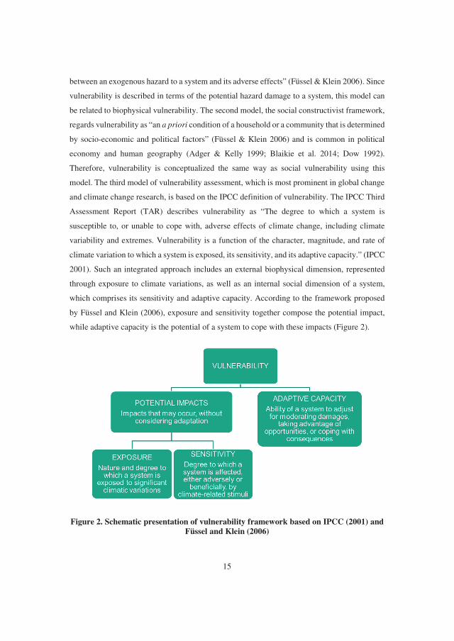
which comprises its sensitivity and adaptive capacity. According to the framework proposed
by Füssel and Klein (2006), exposure and sensitivity together compose the potential impact,
while adaptive capacity is the potential of a system to cope with these impacts (Figure 2).
Figure 2. Schematic presentation of vulnerability framework based on IPCC (2001) and
Füssel and Klein (2006)
16
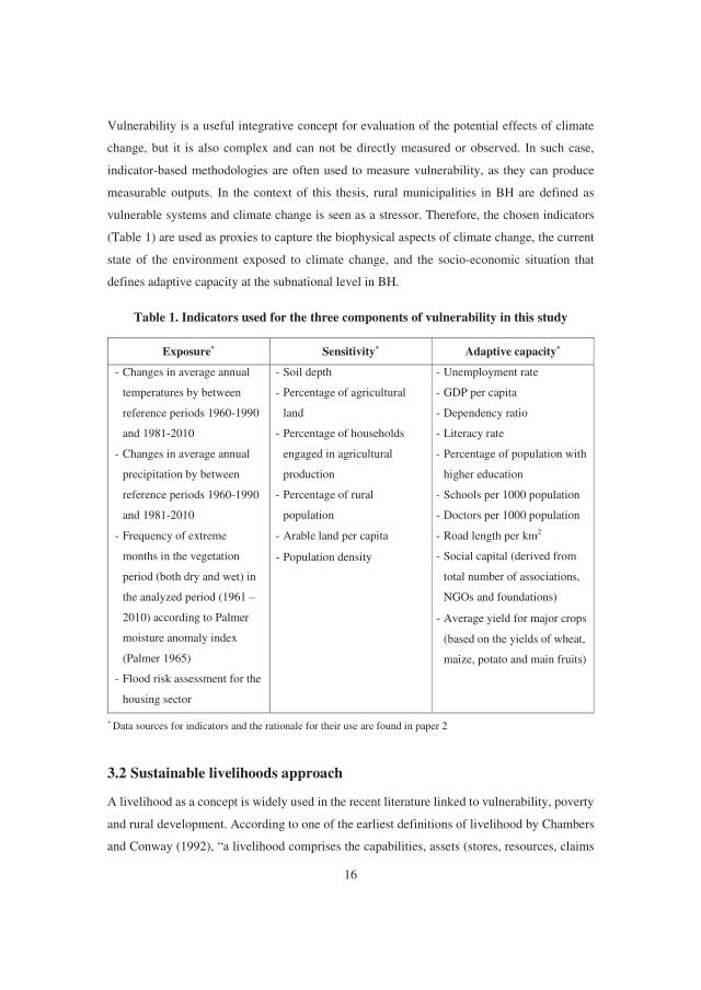
Vulnerability is a useful integrative concept for evaluation of the potential effects of climate
change, but it is also complex and can not be directly measured or observed. In such case,
indicator-based methodologies are often used to measure vulnerability, as they can produce
measurable outputs. In the context of this thesis, rural municipalities in BH are defined as
vulnerable systems and climate change is seen as a stressor. Therefore, the chosen indicators
(Table 1) are used as proxies to capture the biophysical aspects of climate change, the current
state of the environment exposed to climate change, and the socio-economic situation that
defines adaptive capacity at the subnational level in BH.
Table 1. Indicators used for the three components of vulnerability in this study
Exposure* Sensitivity* Adaptive capacity*
- Changes in average annual
temperatures by between
reference periods 1960-1990
and 1981-2010
- Changes in average annual
precipitation by between
reference periods 1960-1990
and 1981-2010
- Frequency of extreme
months in the vegetation
period (both dry and wet) in
the analyzed period (1961 –
2010) according to Palmer
moisture anomaly index
(Palmer 1965)
- Flood risk assessment for the
housing sector
- Soil depth
- Percentage of agricultural
land
- Percentage of households
engaged in agricultural
production
- Percentage of rural
population
- Arable land per capita
- Population density
- Unemployment rate
- GDP per capita
- Dependency ratio
- Literacy rate
- Percentage of population with
higher education
- Schools per 1000 population
- Doctors per 1000 population
- Road length per km2
- Social capital (derived from
total number of associations,
NGOs and foundations)
- Average yield for major crops
(based on the yields of wheat,
maize, potato and main fruits)
* Data sources for indicators and the rationale for their use are found in paper 2
3.2 Sustainable livelihoods approach
A livelihood as a concept is widely used in the recent literature linked to vulnerability, poverty
and rural development. According to one of the earliest definitions of livelihood by Chambers
and Conway (1992), “a livelihood comprises the capabilities, assets (stores, resources, claims

17
and access) and activities required for a means of living. A livelihood is sustainable which can
cope with and recover from stress and shocks, maintain or enhance its capabilities and assets,
and provide sustainable livelihood opportunities for the next generation; and which contributes
net benefits to other livelihoods at the local and global levels and in the short and long term”.
In this definition, capabilities are the options one possesses to pursue different activities to
generate income required for survival and to realise its potential as a human being. Capabilities
are determined based on the portfolio of assets one possesses, based upon which one makes
decisions and construct the living. Five main categories of capital contribute to livelihood
assets: natural, physical, human, financial and social capital (Scoones 1998).
While this economic asset-centred approach captures the essentials of what constitutes
livelihoods, it has been criticised for the use of limited set of indicators (such as income and
productivity) to define poverty. This led to development of more integrated approaches to
assess livelihoods, with the focus on various factors and processes which either constrain or
enhance poor people’s ability to make a living in an economically, ecologically, and socially
sustainable manner (Krantz 2001). Based on the proposed sustainable livelihoods framework
by Scoones (1998), which views a livelihood as not just a question of assets and activities, but
also composed and accessed within the certain institutional processes and social structures,
Ellis (2000) proposed the following definition of livelihood: “A livelihood comprises the assets
(natural, physical, human, financial and social capital), the activities, and the access to these
(mediated by institutions and social relations that together determine the living gained by the
individual or household.”
The schematic representation of sustainable livelihoods framework developed by DFID (1999)
(Figure 3) acknowledges the importance of assets and the activities engaged by individuals and
households using the assets available for them, as it is defined in the original definition of
livelihoods. The difference is that how the livelihoods are accessed and mediated by the
ongoing institutional and social processes has the same importance and is viewed as a separate
component. Such framework for livelihood analysis also has a vulnerability context, viewed in
terms of shocks, seasonality and trends, which have a direct impact upon people’s assets and
over which they have limited or no control (DFID 1999). Therefore, the ability of a livelihood
to be able to cope with and recover from stresses and shocks is central to the definition of
sustainable livelihoods (Scoones 1998). Furthermore, the range and combination of activities
and choices that individuals and households undertake, depending on the range and the degree
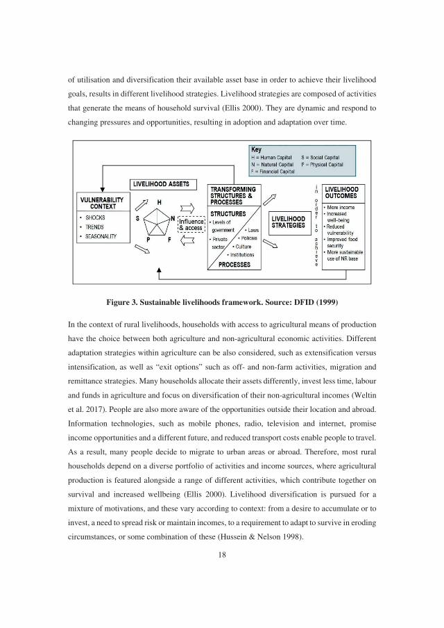
18
of utilisation and diversification their available asset base in order to achieve their livelihood
goals, results in different livelihood strategies. Livelihood strategies are composed of activities
that generate the means of household survival (Ellis 2000). They are dynamic and respond to
changing pressures and opportunities, resulting in adoption and adaptation over time.
Figure 3. Sustainable livelihoods framework. Source: DFID (1999)
In the context of rural livelihoods, households with access to agricultural means of production
have the choice between both agriculture and non-agricultural economic activities. Different
adaptation strategies within agriculture can be also considered, such as extensification versus
intensification, as well as “exit options” such as off- and non-farm activities, migration and
remittance strategies. Many households allocate their assets differently, invest less time, labour
and funds in agriculture and focus on diversification of their non-agricultural incomes (Weltin
et al. 2017). People are also more aware of the opportunities outside their location and abroad.
Information technologies, such as mobile phones, radio, television and internet, promise
income opportunities and a different future, and reduced transport costs enable people to travel.
As a result, many people decide to migrate to urban areas or abroad. Therefore, most rural
households depend on a diverse portfolio of activities and income sources, where agricultural
production is featured alongside a range of different activities, which contribute together on
survival and increased wellbeing (Ellis 2000). Livelihood diversification is pursued for a
mixture of motivations, and these vary according to context: from a desire to accumulate or to
invest, a need to spread risk or maintain incomes, to a requirement to adapt to survive in eroding
circumstances, or some combination of these (Hussein & Nelson 1998).

19
The sustainable livelihoods approach was used in the thesis to better understand the dynamic
nature of livelihoods and what influences different livelihood strategies carried out by rural
households in BH. Poverty in BH is mostly a rural phenomenon, as close to 80 % of the total
poor live in rural areas. By understanding the livelihoods of rural households in terms of assets,
activities and outcomes, as well as the main factors and processes influencing rural livelihoods
and household decision-making, we can gain a better insight on the underlying causes of
poverty. Furthermore, we can assess the impacts of climate change on rural households and
how they response to experienced climate shocks with the available assets and how these
conditions can be reflected and built upon for successful adaptation strategies and reduction of
vulnerability.
3.3 Conservation tillage as an adaptation option for sustainable agriculture
and climate change
Soils are living, complex systems, and in many ways the fundamental foundation of our food
security (Reicosky 2015). As the world’s population increases and food production demands
rise, agricultural systems will have to produce more food from less land by making more
efficient use of natural resources. Such production increases must also be sustainable, i.e. by
minimizing negative environmental effects and providing increased income to help improve
the livelihoods of those employed in agricultural production (Hobbs 2007).
At present, conventional tillage is almost exclusively applied in the cultivation of crops in BH.
This traditionally adopted tillage method in BH and worldwide has its significant advantages,
such as the incorporation of crop residues and weeds, optimum conditions for seed
establishment and root growth, incorporation of organic and mineral fertilizers, accumulation
of soil moisture in the autumn-winter period, disease and pest control. However, with all its
benefits, conventional tillage also has its negative effects. Aggressive mechanical inversion of
soil leads to unintended consequences of soil erosion, high rates of soil organic carbon (C) loss,
compaction and loss of stable soil structure and disruption of the soil biology (Reicosky 2015).
These processes can cause a wide range of environmental problems and lead to soil
degradation, with the “Dust Bowl” of the 1930s in the US Great Plains as one of the most
notable examples. In order to combat soil loss and preserve soil moisture, soil conservation
techniques known as “conservation tillage” have been developed.

20
Conservation tillage includes a broad set of practices with a goal to minimise the disruption of
the soil structure and to maintain the surface soil cover through retention of crop residues, what
is achievable by practicing zero tillage and minimal mechanical soil disturbance (Baker &
Saxton 2007). While the term conservation tillage encompasses different practices, the focus
of this thesis were the experimental application no-tillage and reduced tillage under typical
pedo-climatic conditions of continental BH. No tillage (NT) was carried out by direct drilling
into the untilled, chemically mulched soil. Reduced tillage (RT) in this thesis was defined as a
reduced number of operations and passages, without autumn ploughing, but disking to 15 cm
depth in spring before seedbed preparation. Typically, conservation tillage is associated with
improved water infiltration and conservation, reduced erosion, improved soil structure and
reduced labour and fuel costs (Franzluebbers 2002; Hobbs et al. 2008). Therefore, the
documented abilities of conservation tillage could have a potential to stabilise crop yields and
improve soil conditions, while being less labour intensive and more cost-efficient, thus
improving rural livelihoods in a country with prevailing low-input smallholder agriculture,
such as BH.
It is likely that climate change will have a significant impact on soils, and therefore on the
existing cropping systems. Increased temperatures, frequency and severity of droughts could
potentially lead to yield reduction and crop failure and may increase mineralization and loss of
the soil organic carbon (Choudhary et al. 2016). Climate change may also exacerbate the
problem of soil erosion, as rainfall events become more erratic with a greater frequency of
storms (Holland 2004). Conservation tillage could thus provide both sustainability in crop
production systems and offer potential adaptation option to mitigate the effects of climate
change and variability.
Recently, conservation tillage practices have been advocated as a measure to mitigate climate
change through enhanced soil carbon (C) sequestration (Lal 2004). While the benefits of
increased soil organic C (SOC) on soil structure, water-nutrient relationships and soil biota are
well established (Johnston et al. 2009), the question whether or not agricultural soils lend
themselves to sequester relevant amounts of C is currently under debate (Minasny et al. 2017;
Powlson et al. 2011). One drawback of increased C sequestration into soils may be increased
nitrous oxide (N2O) emissions, offsetting the “cooling effect” of CO2 draw down (Tian et al.
2016). Variable effects of conservation tillage on N2O emissions have been reported (van
21
Kessel et al. 2013), varying from decreased to increased N2O emissions, especially shortly after
shifting from conventional tillage to NT (Rochette 2008; Six et al. 2002).
3.4 Biogeochemistry of Nitrogen and its link to climate change
Terrestrial N can be categorised in different compartments, namely soil and standing biomass
(plants and animals), and is it relatively small compared to the abundant pool of inert N in the
atmosphere. Notwithstanding, terrestrial N has an immense significance for the global
biogeochemistry of N. Soils are the major reservoir of terrestrial N. According to Batjes (1996),
global soil N in the upper 100 cm of the soil profile amounts to 133 – 140 Pg N (1 Pg = 1015
g). Compared to soils, only about 10 Pg N is held in the plant biomass and about 2 Pg in the
microbial biomass (Davidson 1994). The transformations involved in N mineralization are
entirely driven by soil microorganisms. A fraction of the mineralized N is lost from the system
by NO3- leaching or by NH3 volatilization. Furthermore, denitrifiers, a specialized group of
microorganisms, have the capacity to use NO3- as terminal electron acceptor instead of oxygen,
thus reducing NO3- to N2 via the gaseous intermediates nitric oxide (NO) and nitrous oxide
(N2O). Gaseous N diffuses to the soil surface and is emitted to the atmosphere, thus closing the
N cycle (Mosier et al. 2004). In non-cultivated soil-plant systems, the size of the organic and
inorganic N pools often reach a steady-state or change very slowly, since N inputs from
biological N2 fixation, atmospheric deposition and N losses through leaching and
denitrification are relatively constant (Vitousek et al. 2002). In agricultural systems, the amount
of N circulating between the atmosphere, soil organic matter and living organisms is too small
to satisfy the N required for high yields. In addition, a large quantity of N is removed from the
system through harvest. Thus, the extra demand for N has to be satisfied by applying N-rich
manures or synthetic N fertilizers to the soil. The additional N is either taken up by the crop,
immobilized by the microbial biomass, stabilized as humus, or lost to water or atmosphere as
nitrate or gaseous N. Therefore, understanding the cycling of N in soil-plant systems is pivotal
for both sustainable agriculture and climate change mitigation.
As a consequence of anthropogenic inputs, the global N cycle has been significantly altered
over the past century (Figure 4). Although the absolute quantities are small, increasing N2O
emissions play an important role for global climate change. Human activities account for over
one-third of N2O emissions, most of which are from the agricultural sector. Since the industrial
revolution, an additional source of anthropogenic N input has been fossil fuel combustion,

22
during which the high temperatures and pressures provide energy to produce NOx from N2
oxidation. Activities such as agriculture, fossil fuel combustion and industrial processes are the
primary cause of the increased nitrous oxide concentrations in the atmosphere. Together these
sources are responsible for 77% of all human nitrous oxide emissions (Bernstein et al. 2007).
N2O emissions from the agricultural sector are mainly related to direct N2O emissions from
soils as a consequence of increased fertilization with synthetic N or manures. Livestock
production is also a significant contributor to the global N2O emissions, specifically during
manure storage, livestock grazing or from paddocks. It is estimated that approximately 40% of
the 270 Tg N yr−1 globally added to terrestrial ecosystems is removed via soil denitrification
(Seitzinger et al. 2006).
Figure 4. N cycle in terrestrial ecosystems. Source: Pidwirny (2006)
Nitrous oxide (N2O) is a GHG with a 100-year global warming potential 298 times that of
carbon dioxide (CO2), contributing 6.24 % to the overall global radiative forcing and is the
single most important depleting substance of stratospheric ozone (Butterbach-Bahl et al. 2013).
According the same authors, atmospheric N2O concentrations have increased by 19 % since
pre-industrial times, with an average increase of 0.77 ppbv yr−1 for the period 2000–2009. N2O
is a product of denitrification, but it is also produced during nitrification and during the

23
dissimilatory reduction of NO3- to NH4
+ (Ward et al. 2011). Denitrification in soil produces
both N2O and N2, hence this bacterial process may serve either as source or sink for N2O. The
rate of denitrification in soil is dependent on various factors such as the pH, temperature and
soil moisture content (Maag & Vinther 1996). Most soil microbial processes are strongly
influenced by temperature. Studies show that denitrification is most rapid at temperatures
between 20 and 30°C, which is warmer than most soils in the temperate climates (Saad &
Conrad 1993). The presence or absence of oxygen is one of the largest factors determining the
extent and duration of denitrification. Denitrification can occur in aerobic conditions, but to a
relatively insignificant degree. Soil moisture, especially during saturation, is generally the
trigger for denitrification and the products of denitrification appear almost instantly after soil
saturation (Bateman & Baggs 2005). However, the ratio of N2 to N2O tends to increase in
favour of N2 under higher soil moisture conditions (Weier et al. 1993). Denitrification in
anaerobic soils is largely controlled by the supply of readily decomposable organic matter,
from which the denitrifying bacteria obtain carbon as their energy source (Burford & Bremner
1975; Weier et al. 1993). Denitrification potential is greatest in the topsoil where microbial
activity is highest and it decreases rapidly with depth. It is important to note that denitrification
of NO3- does not occur only in soils. NO3
- leached from the soils is transported to freshwater
ecosystems and may enhance the biogenic production of N2O through the same microbial
processes, which occur ubiquitously in terrestrial and aquatic ecosystems (Burgin & Hamilton
2007).
In order to better understand the soil GHG fluxes, and to increase SOC and nutrient efficiency
in the particular regions, it is necessary to conduct research on soils depending on their type
and use, to identify natural and anthropogenic parameters and the corresponding relations
between them. In relation to the natural factors, it is necessary to consider climatic elements
(such as temperature and precipitation) and type of vegetation, while the most important
anthropogenic factor to be considered is land management (tillage type, fertilization, irrigation,
etc.). In this thesis, this was accomplished by setting up an experimental field in Sarajevo,
where N2O emissions and accompanying ancillary variables were monitored over two cropping
seasons on the soil type and climatic conditions typical for humid continental climate of BH.

24

25
4. Materials and methods
4.1 Study area
Bosnia and Herzegovina is a country in South-eastern Europe, located in the Western Balkan
region, with a total surface area of 51,209.2 km2, composed of 51,197 km2 of land and 12.2
km2 of sea. The land is mainly hilly to mountainous, with an average altitude of 500 meters.
Of the total land area, 5% is lowlands, 24% hills, 42% mountains, and 29% karst region.
According to the most recent population census in 2013, the population is 3.53 million (AFSBH
2016a). It is estimated that 60% of the total population lives in rural areas, which makes it one
of the most rural countries in Europe (UNDP 2013).
Figure 5. Geographical position and the digital elevation model of Bosnia and
Herzegovina
26
Agricultural land covers 2.1 million hectares, 50.1% of which is arable land (MOFTER 2016).
Fertile lowlands comprise about 20% of agricultural land in Bosnia and Herzegovina, most of
it in the northern lowlands and river valleys across the country. These areas are suitable for
intensive agricultural production of wide range of crops. Moderately to less fertile hilly and
mountainous areas comprise 80% of the agricultural land, of which more than a half is
relatively suitable for agricultural production, especially livestock production with the
complementary pastures and fodder production. The harsh alpine environment (mountainous
areas), steep slopes or aridity (especially in karst areas) usually limit agricultural production in
the remaining areas. About 53% of the total area is covered by forests. Although the share of
agriculture in GDP is relatively low (6.4% in 2016), agricultural production is still a backbone
of rural economy, employing 20% of workforce (AFSBH 2016b).
The general atmospheric circulation and air mass flow, the dynamic relief, the orientation of
mountain ranges, the hydrographical network and the vicinity of the Adriatic Sea have all
created conditions for a wide spectrum of climate types in BH (Baji� & Trbi� 2016). These
include humid continental climate, represented mostly in the northern and lowland central parts
of the territory; sub-alpine and alpine climate of the mountainous region of central BH, and
semi-arid mediterranean climate represented in the coastal area and in the lowlands of
Herzegovina (southern BH). This means that the effects of climate change and variability will
be highly dependent on the geographical location and each region is facing specific challenges.
For example, the mediterranean region, characterized with scarce and shallow soils, with the
significant areas under karst, and northern BH with deep and mostly heavy soils, which has the
same climate as most of central Europe, are both faced with the negative effects of increased
temperatures and unfavourable rainfall distribution. At the same time, the hilly and
mountainous regions of central BH might even benefit from the increased temperatures due to
the increased vegetation season, allowing wider range of crops and higher productivity of
grasslands.
When it comes to the territorial scope of research within this thesis, it covers different research
units, depending on the objectives and focus of the individual papers. Paper 1 deals with the
state of the agricultural sector and effects of climate change at the national level. The main
focus of the research in paper 2 was the impact of climate change on rural municipalities, which

27
form 136 of the total 142 municipalities in BH1. Paper 3 focuses research at the household
level, more specifically on households within the different climatic regions, while paper 4
focuses on the field experiment conducted in a single field in central BH as a case study.
4.2 Research design
In order to gain more comprehensive and valid answers to the broad range of research questions
posed in this thesis, a variety of methods were employed. While most of the methods were
quantitative, they were in many instances supported with qualitative methods and observations.
Therefore, the methodological approach in this study can be classified as a mixed methods
approach. This approach has emerged over the last decades and is described as “increasingly
articulated, attached to research practice, and recognized as the third major research approach
or research paradigm along with qualitative and quantitative research” (Johnson et al. 2007).
Climate change is a complex phenomenon and utilisation of hybrid research methods enables
us to capture biophysical aspects of climate change, but also help us to define how this change
impacts local communities in their socio-political and environmental conditions (Batterbury et
al. 1997). The main rationale behind this approach is that when both qualitative and quantitative
methods are used in combination, they tend to complement each other on the basis of
pragmatism and a practice-driven need to mix methods and hence allow for analysis that is
more comprehensive and can help to better understand the research problem (Denscombe 2008;
Tashakkori & Teddlie 1998). Thus mixed methods research can also help bridge the schism
between quantitative and qualitative research purists (Johnson et al. 2007). Due to the strong
reliance on the quantitative data, this study could be more specifically classified as
“quantitative dominant mixed methods”, which is defined by Johnson et al. (2007) as “the type
of mixed research in which one relies on a quantitative, postpositivist view of the research
process, while concurrently recognizing that the addition of qualitative data and approaches are
likely to benefit most research projects”.
The quantitative methods in this study encompassed assessment of vulnerability using
quantitative biophysical and socio-economic indicators (paper 2); analysis of household
questionnaire data and micro-economic model to identify the major determinants of adaptation
(paper 3); measurements of soil GHG emissions and the accompanying ancillary variables, soil
1 A 143th municipality (Stanari) was established in 2014, but was not included in the study, since the statistical
data from 2013 were used as a base for paper 2.

28
chemical and physical properties, crop yields, as well as economic indicators, such as total
income from crop and variable productions costs (paper 4). Qualitative methods used in this
study were key informant interviews and semi-structured interviews. Some of them were used
to validate the obtained quantitative data, e.g. the indicators of vulnerability in paper 2 were
discussed with key informants, or to gain more knowledge and to support some statements in
the papers. The conducted rural household survey (paper 3) is also defined as a semi-structured
interview, because it contained open-ended questions on farmers’ perceptions and
understandings of climate change, livelihoods, agricultural practices, coping and adaptation
strategies.
4.3 Primary data collection
4.3.1 Household questionnaire
The main objective of the household questionnaire was to determine the access to livelihood
assets and the main factors and processes that influence rural livelihoods and livelihood
strategies, as well as perceptions of climate change and the responses carried out through
various adaptation options. The questionnaire was mainly, but not exclusively, directed to the
head of the households, which were mostly men and usually the main decision makers at the
household level. In some cases, the questionnaire was conducted with multiple household
members jointly, in case they showed interest to participate. Other household members (e.g.
wives, sons/daughters, siblings) were interviewed in the physical absence or lack of will of the
household head to participate, provided they were well informed about the household assets
and on-farm activities. The questionnaire was drafted according to the research questions
outlined in paper 3, tested in practice on some farmers and amended after every session if
necessary, before its implementation in the field.
The household questionnaire was divided into four sections (Appendix 1). Section 1 focused
on the basic details of the household, such as the duration of farm ownership and basic values
and norms about being the farmer. Section 2 was concerned with the assets of the surveyed
household, which were structured as natural, physical, human, financial and social capital.
Section 3 was divided into two parts – the first one contained questions related to perceptions
and personal observations about of climate change and its nature and extent, as well as
questions about the damage caused by the selected extreme weather events in the past. The
second part was focused on the awareness and implementation of the selected adaptation
29
measures. Section 4 encompassed the questions related to various determinants of livelihood
diversification and adaptation, recent investments and the biggest perceived challenges and
obstacles for wellbeing.
The questionnaire contained mainly closed-ended questions, but some of the questions were
open ended and allowed the respondent to elaborate some key issues in more detail. Therefore,
this questionnaire may be considered as a semi-structured interview as well (Jamshed 2014).
Closed end questions included dichotomous, multiple choice, Likert scale and fill-in-the-blank
questions depending on the suitability and expected output (Burgess 2001). The questionnaire
was designed and tested in a way that the duration of an interview with the single respondent
does not last more than one hour. I personally administered a third of interviews with the
respondents, and allowed field assistants to help me complete the required number of
households after each of them spent some time with me on the field, in order for them to
become familiar with the questions asked and the research objectives. The chosen field
assistants were experienced and highly educated agricultural scientists and agro-economists.
The choice of households, depending on the region, tended to be as randomized as possible.
The only condition was that agriculture should be one of the income sources of the household.
In order to overcome the issue of distrust, households were selected based on the
recommendation of key informants in the field in the selected regions. In order to reduce the
amount of bias, multiple key informants were selected and each of them selected no more than
five households. Informed consent was obtained before the start of every interview and it was
clarified that the questionnaire is anonymous and the information will be used for research
purposes only. In total, 104 households from three different agro-climatic regions in BH were
interviewed.
4.3.2 Field experiment
In order to accomplish the objectives of paper 4, a field experiment was set up in the chosen
climatic and soil conditions of continental BH and weekly N2O measurements were conducted
in Maize-Barley rotation over two growing seasons, with the accompanying measurements of
ancillary variables, soil, agronomic and economic parameters. This study was carried out on
the research farm Butmir of the Faculty of Agricultural and Food Sciences in Sarajevo, Bosnia
and Herzegovina (43°49'N, 18°19'E, 547 m a.s.l.) from December 2013 to December 2015 and
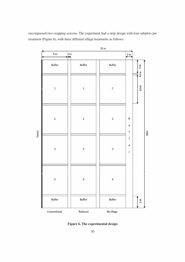
30
encompassed two cropping seasons. The experiment had a strip design with four subplots per
treatment (Figure 6), with three different tillage treatments as follows:
Figure 6. The experimental design
31
- Conventional tillage (CT): autumn ploughing to a 30 cm depth, secondary tillage with
a roto-tiller in spring to 15 cm depth before seedbed preparation and sowing
- Reduced tillage (RT): spring disk harrowing to 15 cm depth and seedbed preparation
before sowing
- No tillage (NT): direct drilling into the untilled soil. In the absence of the specialised
NT seed drill, we used the traditional mechanical drill with an added ballast for in-
creased penetration strength
Periodic measurements of N2O emissions were carried out from December 2013 to December
2014 and from March 2015 to December 2015. The fluxes were measured following the
methodology described by Nadeem et al. (2015), using static aluminium chambers. Gas
samples were taken every 7-10 days throughout the entire research period and every 3 - 5 days
in the month after fertilization in 2015. The gas samples were shipped to Norway and analysed
at the Faculty of Environmental Sciences and Natural Resource Management (MINA), using a
gas chromatograph (GC, Model 7890 A, Agilant, Santa Clara, CA, USA).
Cumulative flux in 2014 represents area-scaled emissions for the entire year, while in 2015 it
represents the cumulative flux for 226 days of the year (flux measurements started on 20th of
March) plus linearly interpolated values for the missing period, assuming low emissions like
in the previous year. Emission factors were calculated as the fraction of applied fertilizer N
emitted as N2O-N (minus background N2O emission of 1 kg N ha−1 year−1) as a percentage
(IPCC 2006). Alfalfa residue N in the first year was estimated based on the results from Kelner
et al. (1997) adjusted for alfalfa yields from our studied field (see Junuzovic 2005). Yield-
scaled N2O emission was calculated as emission intensity, which is a function of fertilization
rate and expressed as N2O-N (g) emitted per ton of grain yield (Mosier et al. 2006).
Soil moisture and temperature at 5 cm depth were measured automatically every day using data
loggers (Decagon EM50, Pullman, WA, USA) in three replicates for every treatment. ECH2O
sensors (Decagon) were used to monitor volumetric soil water content (VSWC) and
temperature.
Soil physical properties were analysed in undisturbed soil cores (100 cm3 stainless steel
cylinders) collected in July 2015 in four replicates per treatment. Particle density (PD) was
determined using an air pycnometer according to Langer. Bulk density (PD) was determined
gravimetrically. BD and PD were used to calculate total porosity, which was used to convert
VSWC to water filled pore space (WFPS) by using the following equation:

32
���� � ���� ��
��
Soil water retention curves between pF 1.8 and 4.2 were determined using ceramic pressure
plate extractors (Klute & Dirksen 1986). These results were then used to determine soil pore
size distributions in different tillage treatments.
In 2015, soil samples were taken from 0 to 15 cm depth at each gas sampling date. Multiple
cores from each treatment (4 per subplot) were homogenized, bulked and frozen. Immediately
after thawing the samples, 45 g fresh weight soil was extracted by 30 minutes of horizontal
shaking in a 50 ml 2M KCl solution. The extracts were filtered and soil mineral N (NH4+, NO3
−)
analysed by colorimetry according to Keeney (1982).
Yields were measured as dry grain corn in 2014 and barley in 2015. Samples were taken from
every subplot and standardized to 14% moisture content. Production costs were estimated for
each of the three tillage systems. Input items such as seed, fertilizer and chemicals applied were
purchased from local retailers and the exact prices were recorded. Average purchase market
prices for the crops used in the experiment are taken from Agency for Statistics of Bosnia and
Herzegovina (AFSBH 2015; AFSBH 2016c) for the respective years. For an approximation of
labour and tillage operation costs, we used data from the local agricultural extension service,
which was cross-validated with farmers in the same area. An economical comparison between
tillage systems was shown as a difference in net return per hectare, which was calculated from
net income for crop after deducting all variable costs. We refrained to estimate fixed costs for
production systems in this study due to high variability in possession of tractors and other
necessary mechanisation and assets, which often have a long depreciation life and the general
tendency to become obsolete (MAWFFBH 2015).
4.4 Secondary data collection
Various secondary data sources were used in this thesis and the first two papers were mainly
based on them. Paper 1 collated information from journal articles, conference papers, national
reports, official statistical data, strategic and policy documents. These documents were mainly
related to the history of agricultural development, main characteristics of agricultural sector
today and impact of climate change on agricultural systems in BH. In the case of significant

33
knowledge gaps at some stages of research, some statements and conclusions were derived
from the international literature or the statements from key informants combined with my
personal observations. Both biophysical and socioeconomic secondary data for the purposes of
paper 2 were obtained from various sources, such as statistical yearbooks, census data, climate
data from hydrometeorological institutes and other public databases and archives. Based on
these datasets, the sets of indicators at the local level (municipality) were chosen as proxies for
exposure, sensitivity and adaptive capacity, in order to compose an overall vulnerability index
and quantitatively assess vulnerability to climate change.
4.5 Statistical analysis
The chosen method in paper 2 was to use a quantitative approach to assess vulnerability by
constructing a vulnerability index based on specific sets or combinations of indicators, which
serve as proxies. Each indicator is measured in different scales and units. Therefore, they had
to be normalized to ensure that they were comparable. The values of all indicators were
normalized based on the calculation of Human Development Index (HDI) (UNDP 1990) to
values between 0 and 1, depending on the functional relationship between the indicators and
vulnerability. Two different weighting methods were used to analyse and present the results.
Using equal weights as a method, normalized indicators were integrated in two calculated
composite sub-indices in accordance with their belonging to particular components of
vulnerability (O’Brien et al. 2004). The final value of the vulnerability index for every
municipality was obtained from the arithmetic sum of these two sub-indices. In the second
weighting method, Principal components analysis (PCA) was used to extract the linear
combinations that best capture the information from a large group of variables. One of the
methods was to use PCA to generate composite indices is by using “eigenvalue-greater-than-
one” rule proposed by Kaiser (1960). After retaining all the components with eigenvalues
greater than one, factor analysis was used to generate factor loadings for all indicators, which
were used as weights. In order to summarize all weighted indicators into the single composite
index, the following equation proposed by Gbetibouo et al. (2010) was used:
� ������� ���
������������������ � ��� ��� � � �
Where V is a vulnerability index, w is the weight, i is the indicator, x is the indicator value, j is
a specific municipality, � is the mean indicator value and s is the standard deviation.

34
Due to the dichotomous outcome of the variables regarding individual adoptions of agricultural
practices and technologies (1 – adopted; 0 - not adopted) in paper 3, binary logit model was
used to analyse the determinants for their adoption. This model considers the relationship
between a binary dependent variable and a set of independent variables, whether binary or
continuous. The model in its simple form can be presented as:
� � ! " #��$� " %��
���
where Yi is the dichotomous dependent variable for an individual adaptation option (1 =
adapted; 0 = not adapted), ! is the Y-intercept, ���are a set of regression coefficients, Xi denotes
the set of explanatory independent variables and �i is an error term.
For the purposes of paper 4, rates of N2O emission were estimated by fitting either linear (R2
� 0.85) or polynomial functions to the observed N2O accumulation over time. N2O flux was
calculated according to the following equation:
�&'( � )*+,)- . /0
1 .2*/3 . 45
where FN2O is the N2O emission flux (�g N2O-N m−2 h−1), dN2O/dt is the relative change in N2O
concentration in the chamber headspace (ppmv min−1), Vc is the chamber volume (L), A is the
area covered by the chamber (m2), MN is the molecular mass of N in N2O (g mol−1) and Vm is
the molecular volume of gas at chamber temperature (L mol−1).
Furthermore, cumulative N2O fluxes were calculated by plotting daily average N2O fluxes
against time, interpolating linearly between them, and integrating the area under the curve
(Dobbie & Smith 2003). To test the effects of treatment and year, repeated measures two-way
ANOVA followed by Bonferroni post-test was performed for N2O flux data, soil temperature
and WFPS. One-way ANOVA followed by a Tukey’s multiple comparison post test was
performed for soil NH4+ and NO3
−, cumulative N2O emissions and yield-scaled N2O emissions.
Prior to these analyses, N2O emission rates and ancillary variables were log-transformed to
ensure normal Gaussian distribution.
The data in every paper were analysed using SPSS ver. 24 (IBM Corp, USA).

35
4.6 Research challenges
Most of the challenges in this study were a consequence of the very complex, decentralized
political and administrative structure in BH. There is limited coordination and an insufficient
level of cooperation between institutions at different levels (especially between two state
entities) in a context of distribution and acquisition of data, which leads to inability to establish
an efficient data collection, monitoring and reporting system. As a result, there were difficulties
collecting significant quantity of necessary data. It was challenging and a time consuming
process to summarise the certain datasets at the national and local level. The members from
each institution were more or less reluctant to share the requested datasets, even though such
data was publicly available. Many publicly or donor funded studies were carried out in the last
two decades, but there is a problem with their accessibility or even knowledge of their
existence. The institutions or researchers involved in such studies are usually reluctant to share
their main project outputs or datasets, unless it is in their self-interest. Luckily, I managed to
overcome most of these challenges with the immense help of my network, which I developed
during my previous work experiences in BH and during this research project.
While I was designing my research proposal in 2012/13, preparations for the first post-war
census in BH and the first one since 1991 were under way. Therefore, the data analysis and
writing of paper 2 relied on some indicators available only from the results of this census.
However, the publication and processing of census results in 2013 was followed by a series of
problems, irregularities and the lack of political consensus, which delayed publication of the
results until June 2016. After many postponements, uncertainty about the future of the
mentioned paper and many alternative considerations, I did finally succeed and finished the
paper using the limited BH census datasets available to me and published to the present time.
Another problem, or more of an anecdote, happened shortly after establishment of the field
experiment in Sarajevo. A pack of stray dogs, which have taken residence nearby, took an
interest in the installed soil moisture and temperature sensors, which were connected to the
data logger via network of cables. They decided to play and chew through most of the cables,
which resulted in absence of soil measurements for nearly three months. Luckily, new sensors
were ordered and installed as soon as possible and the experiment continued.

36

37
5. Results and discussion
5.1 Agricultural sector of Bosnia and Herzegovina and climate change -
challenges and opportunities (Paper I)
There is a striking lack of knowledge regarding climate change and its impacts on the most
vulnerable sectors in BH. Local scientific studies concerning the impact of climate change on
agriculture have been modest at least for the past two decades. Some previous attempts were
made to summarise the impact of climate change on agricultural production, either through
scientific papers as a part of the regional initiatives in the Western Balkan area (�ustovi� et al.
2012; Kova�evi� et al. 2013), or as a part of the National Communications under the United
Nations Framework Convention on Climate Change (UNFCCC 2009; UNFCCC 2013). After
an extensive review of the existing literature concerning the impacts of climate change on the
agricultural sector of BH, I reached the conclusion that a comprehensive review paper was
necessary as a starting point, with the main objective being to present the current state of the
agricultural sector in BH and the impact of climate change on agricultural systems there, based
on local scientific knowledge and supplemented with the most recent findings from the global
literature.
The first sections gives an overview of the agricultural sector in BH, history of its development
and significance, as well as the most important current features and challenges faced. The
general conclusion is that the challenges in the agricultural sector are mainly derived from the
legacy of the past socio-political system and further exacerbated in the present by inefficient
and complex governance. This has led to low productivity in both livestock and crop
production, small and fragmented farms, low budget allocations for agriculture and farm
investments, imperfect markets and a lack of knowledge and technology transfer.
The first part of the second section of this review paper assesses the impact of climate change
on the agricultural sector of BH based on current conditions and future predictions. Based on
the findings in this chapter, the agricultural sector in BH is found to be vulnerable to climate
change. It is reflected in the serious incidences of extreme weather events over the past two
decades, which caused severe economic losses. Higher incidences of droughts, floods, hail,
storms and increased maximum wind speed may subsequently lead to yield reduction and the

38
emergence of new pathogens and diseases, crop failures and long-term production declines.
According to available data and currently available climate projections, the exposure to such
threats will continue to increase. The second part of this section gives a brief overview of the
main climate institutions in the country. Research findings show that there is a political will to
build the necessary capacities and policies in order to promote low-emission and climate
resilient development, as witnessed by the recent reports and development strategies. However,
climate change has yet to be mainstreamed into national and regional development policies.
The third section is concerned with policy implications and proposes some socio-political and
technological options that could form the basis for further strategic planning and development
of necessary institutions in BH, and which should address adequately the problem of climate
change in agriculture. These processes are roughly grouped into two groups – 1) policy and
research capacity and 2) technological development. It is pointed out that the main priorities
concerning policy and research capacities should be the formation of a national Ministry of
Agriculture, harmonised policies, vulnerability assessments on every level, investments in
agricultural research and development, capacity building and strengthening of public
agricultural extension services. Technological development should be focused on developing
local crop varieties, weather and climate information systems (including early warning
systems) and investments in irrigation systems.
5.2 Quantitative assessment of vulnerability to climate change in rural
municipalities of Bosnia and Herzegovina (Paper II)
It was concluded in the previous paper that the agricultural sector in BH is vulnerable to climate
change and that the exposure to threats from climate change will continue to increase,
according to the available data and projections. Assessment of vulnerability was also pointed
out as one of the priorities for future development in this sector. Vulnerability assessment is an
important tool for the analysis and presentation of data at different scales, where the current
and potential consequences of climate change are presented to stakeholders in a convenient
way and where it serves as a base for further adaptation policy decisions (Füssel & Klein 2006).
Paper 2 builds upon these conclusions and recommendations, with the main objective to
quantitatively assess the current state of vulnerability of the rural population to climate change
at the local level in BH, with rural municipalities chosen as the main units for this study. A
combination of both biophysical and socio-economic indicators as proxies was used to

39
construct composite vulnerability indices for rural municipalities. Given the lack of scientific
consensus on the different approaches and indicators used to assess vulnerability in the
literature (Adger 2006; Hinkel 2011), the chosen set of indicators in this study was analysed
using two summarizing and weighting methods for increased validity and demonstration of the
differences between them.
Based on the results obtained using the different summarizing and weighting methods to
generate the overall vulnerability indices, the most vulnerable municipalities are found to be
mostly located across the north of BH, with a gradual decrease in vulnerability towards the
central, eastern and western parts of the country. In the south, most of municipalities in the
lowland region of Herzegovina are classified as highly vulnerable, while municipalities in the
surrounding regions are mostly classified as low or moderately vulnerable. Least vulnerable
municipalities are those with larger cities and towns within their territory and those located in
central-south and south-east. Although half of municipalities were classified differently based
on the weighting method, the differences were not fundamentally different and the general
geographical distribution of vulnerability indicators did not change notably for the different
regions of BH. Compared to the first method, the use of weighted indicators led to differences
in the classification of vulnerability in case of half of the studied municipalities (53.7%). Most
notable was the increase in number of highly vulnerable municipalities, and the decrease in
number of municipalities with low vulnerability index.
While representing vulnerability with the single index might bring an insight about the degree
of vulnerability on a sub-national level and identify the most vulnerable regions, this approach
may also be too simplistic and misleading as it does not explain the main sources of
vulnerability (Gbetibouo et al. 2010; Saisana & Tarantola 2002). Therefore, the overall
vulnerability index was decomposed into the components that generate vulnerability and these
components are discussed separately. When the results were analysed and discussed in this
way, it was shown that the most vulnerable rural municipalities are those with the highest
degree of potential impact (PI), as well as low adaptive capacity (AC) to cope with this impact.
Furthermore, when the two components that generate PI (exposure and sensitivity) were
analysed separately, the sensitivity index was the main determinant of PI in almost every highly
vulnerable municipality. This indicates that the current socio-economic conditions and the
increased environmental pressure as a result of the present human-environment interactions are
the main determinant of vulnerability in the most vulnerable municipalities, rather than the

40
degree to which these municipalities are exposed to significant climatic variations, i.e. social
vulnerability is the main determinant of vulnerability to climate change in BH.
5.3 A case study of rural livelihoods and climate change adaptation in
different regions of Bosnia and Herzegovina (Paper III)
This paper is linked to the previous one in a sense that it continues to explore vulnerability, but
this time in the context of livelihoods at the micro level, exploring rural households from the
three agricultural regions in BH. It was concluded in paper 2 that vulnerability to climate
change depends on the potential impact, which is composed of exposure and sensitivity, and
adaptive capacity of an affected system to cope with the impacts and risks of climate change,
which is mainly determined by socioeconomic characteristics. In the context of rural
households, low adaptive capacity is mainly related to poverty, which is reflected in limited
access to capital assets and capabilities that comprise livelihoods (Scoones 1998). Poverty
reduction requires an understanding of how local livelihoods are constructed, accessed and
sustained, as the assets and capabilities that comprise livelihoods often shape poverty and the
ability to reduce it (IISD 2003). The studied households were grouped based on their belonging
to one of the three agro-climatic regions in BH, as well by income level, in order to explore the
difference in access to assets, livelihood strategies, impacts and perceptions of climate change
and adaptation strategies.
Generally, people were found to be asset poor. This is most notable in the limited access to
natural and financial capital. Access to different types of assets significantly differed by region
and income level. Most notable difference was found in total household income, which was
much higher in the southern region.
A striking feature in the overall sample was a very high dependence on agricultural incomes,
constituting 72.4 % of the total average income. Relative agricultural income in the central
region, which was somewhat lower (55.9 %), compared to the northern (78.1 %) and southern
region (83.2 %). There was no significant difference in the relative contribution of different
income sources to the total household income. However, the total income from agriculture in
the south is more than twice that of the other regions, as well as being a significantly higher
contributor to total household income. The wealthiest group also had more than 5 times higher
agricultural income than the poorest group.

41
The substantial difference in total incomes by region and wealth group, as well as high
dependence on agricultural incomes irrespective of region and income, lead to the conclusion
that the total household income mainly depends on how the available assets are used in
agriculture. The less poor own more land and are able to produce more. However, the example
of the southern region shows that significantly higher agricultural incomes can be achieved
with significantly lower access to land. This is mainly attributed to more favourable climatic
conditions in this region, which enables the farmers to time their production in order to exploit
the opportunities on the market and to produce more lucrative crops. Furthermore, households
in the southern region have better access to technology (e.g. irrigation, greenhouses) and are
more often part of agricultural associations. Lastly, less poor households show a higher degree
of entrepreneurship, reflected in more variable market outlet choices.
This difference in livelihood outcomes however, can not only be attributed to asset structure
and activities. High dependence on agriculture in rural areas is mainly driven by a lack of
alternative income sources. The main constraints to improved rural livelihoods result from the
shocks brought by war devastation and post-conflict transition from the centrally planned to
market economy. This resulted in poor and inefficient governance and policies, imperfect
markets and number of other derived from the aforementioned.
High dependence on agriculture makes rural households more vulnerable to negative effects of
climate change, some of them already affecting the studied households. The negative effect of
droughts were most common and more stressed in the humid continental climate of the northern
and central region than in the south, which is traditionally more resilient due to the prevalent
semi-arid climatic conditions that present production systems are designed for. The negative
effects of other adverse weather conditions were less common and more region-specific.
Studied households were well aware of the recent climate trends. Most respondents in our study
perceive an increase in average temperature in line with the actual climate data. The way
changes in precipitation are perceived, in terms of both amount and distribution, varied
depending on the region. This inconsistency between perceived and actual precipitation is
likely influenced by a decrease in water availability under the increased frequency and intensity
of droughts and higher temperatures.
Respondents reported a wide range of adaptation strategies. While it is hard to differentiate
whether it is climate change, agricultural intensification, or some other factor that are the main

42
motives behind certain adaptation options, especially within agriculture, the number of adopted
measures shows that there are signs of an overall intensification strategy of agricultural
production in BH, as well as marked adaptations to climate change. Most notable were the
application of both organic and mineral fertilizers, changes in crops and crop varieties, and a
surprisingly high degree of irrigation. Other common agricultural practices were those that
require no or little investments. Conservation agriculture practices were found to be less
common and only a small part of the respondents was familiar with their existence and
implementation. The main reported constraints for further adoption and long-term adaptation
within agriculture were lack of funds, knowledge and labour. Certain agricultural practices
carried out were in some cases more region-specific, but overall were similar in relation to
income level. The results also indicate that increased access to different types of assets in most
cases influence the likelihood of adaptations in agriculture, most notably social capital and
access to technology (tractors).
5.4 Effects of tillage practice on soil structure, N2O emissions and
economics in cereal production under current socio-economic
conditions in central Bosnia and Herzegovina (Paper IV)
This paper explores the application of conservation tillage, a widely recognised
environmentally sound and sustainable management practice, and one of the measures of
agricultural adaptation to climate change, in agro-environmental and socio-economic
conditions of BH. It was concluded in paper 1 that low agricultural productivity is often a
consequence of the absence of clear specialization, inferior technical equipment and high
dependence on weather conditions. Another finding was a significant technological and
knowledge gap in the agricultural sector compared to the rest of Europe, as a consequence of,
among other things, inefficient agrarian policy, low budget allocations for agriculture and
underdeveloped agricultural extension services. While the results from paper 3 show that there
are some signs of an overall intensification strategy of agricultural production in BH, as well
as adaptations in response to changing climatic conditions, the adoption of conservation tillage
is very limited and negligible in size to date and so is the knowledge and awareness about it.
This can be also clearly seen from the survey results in paper 3, where only 10% of the surveyed
households adopted the different types of reduced tillage (RT), while only 3% of them adopted
no-till (NT). Not that only the adoption of conservation tillage is low, but so is the knowledge

43
about the existence of such practices, with only 35% and 23% of surveyed households being
aware of the existence of RT and NT, respectively. Considering a significant knowledge gap
when it comes to the implementation of sustainable farming practices in BH, the objective of
this study was to examine the effects of the alternative tillage systems on crop productivity and
soil properties in the pedo-climatic conditions of central BH. Agricultural soils are also the
largest anthropogenic source of N2O, associated with the use of synthetic nitrogen (N) and
manures. Given the fact that N2O emissions and its underlying variables have never been
studied before in BH or the Western Balkan region, another objective was to study the impact
of different tillage systems on soil N2O emissions and to assess the Nitrogen use efficiency in
these systems. Lastly, while the agronomic benefits of alternative tillage methods are easy to
recognize, the likelihood of their adoption is also constrained due to uncertainties about the
economic benefits, given that a majority of farmers is also strongly motivated by profits.
Therefore, the economics of the different tillage systems was evaluated in order to assess the
likelihood of their adoption by farmers under the current socio-economic conditions. In order
to accomplish these objectives, a field experiment was set up in Sarajevo, on the experimental
farm of the Faculty of Agriculture and Food Science, where the measurements of N2O in
Maize-Barley rotation over two cropping seasons were carried out (2014 and 2015), with the
accompanying measurements of ancillary variables, soil, agronomic and economic parameters.
Fertilization was found to be the main driver of N2O emissions irrespective of tillage treatment.
However, clear treatment effects outside the period directly affected by fertilization were noted,
indicating the importance of crop residue management and tillage on soil structure, temperature
and moisture. In the much wetter 2014, N2O emissions were in the order of CT > RT > NT,
while in the drier 2015, the order was RT > CT > NT. The emission factors were within or
slightly above the uncertainty range of the IPCC Tier 1 factor, if taking account for the N input
from the cover crop (alfalfa) preceding the first experimental year. Saturated soils in the spring,
formation of soil crusts and occasional droughts adversely affected yields, particularly in the
second year. In 2014, yield-scaled N2O emissions ranged from 83.2 to 161.7 g N Mg-1 grain
(corn) but were much greater in the second year due to crop failure (barley). RT had the smallest
yield-scaled N2O emission in both years. Reduction in variable costs associated with NT was
small due to the increased costs of weed control. Moreover, low yields in NT in both years
resulted in economically inacceptable returns. On the other hand, the reduced number of
operations in case of RT generated higher net returns due to reduced production costs.
44
The results of this study indicate that a wider adoption of NT in BH would likely not be realistic
at this moment, especially by smallholder farmers who lack knowledge and financial capital.
However, the results also show that reduced number of tillage operations can be both N
efficient, economically acceptable and less susceptible to weather extremes in the differing
weather conditions, compared to conventional tillage system. While some of these findings
were discussed for the first time in the region, it is important to note, however, that these were
just short-term effects of tillage in the markedly different weather conditions compared to the
average values of the reference weather parameters in the studied area. Further research,
especially long-term, in the same and other agroclimatic zones of BH would be needed in to
infer overall effects on a national level, with the objective to mitigate N2O and other greenhouse
gas emissions and improve N use efficiency from agricultural systems. Integration of the
different agronomical and agroecological approaches through the experimental work is needed
in order to develop the optimal production system in BH, which is both environmentally and
economically sound and likely to be adopted by farmers.

45
6. Synthesis and conclusions
The general objective of this thesis was to assess the impact of climate change on the
agricultural sector of BH and the rural population as one of the most vulnerable parts of the
population. Different concepts and approaches, depending on the scope and the objectives of
the individual papers, have been applied in order to understand the impact of climate change
from multiple perspectives. Every paper deals with different aspects of climate change and its
impact at various scales, starting from the overall impact at the national level and policy
implications, vulnerability at the local level, to livelihoods and adaptation at the micro-level.
In addition, the objectives of this thesis go beyond just generation of new knowledge about the
impacts of climate change. Another objective was to apply the latest global knowledge and
experiences related to agronomical practices through experimental work in the agro-
environmental and socio-economic conditions of BH. As such, this thesis also contributes to
the global and local knowledge about the agro-ecological practices, conservation agriculture
and the importance of Nitrogen use efficiency, as practices that could potentially increase the
production while being environmentally and socially sustainable, as well as being the measures
of climate change adaptation and mitigation.
The agricultural sector of BH, while rich in natural resources, biodiversity and with climatic
conditions that are mostly favourable for agricultural production, is also faced with many
challenges. Some of these challenges are partly inherited from the past socialist state, where
agriculture was marginalized in favour of industrial development, but are further exacerbated
by massive demographic, economic, social and political changes caused by armed conflict and
the slow process of post-conflict transition from a centrally planned to a market-oriented
economy. The main challenge in the agricultural sector is low productivity, resulting from
extensive farming practices and obsolete technologies, carried out on small and fragmented
farms. Furthermore, agricultural development is constrained by inefficient asymmetrical
administrative structure and policies, low budget allocations for agriculture, imperfect markets
and a general lack of information and knowledge.
BH is a predominantly rural country. A significant part of that population previously employed
in industry and other sectors became unemployed after the war that led mass migration,
devastation and economic decline in rural areas. In the absence of income options, a significant

46
part of that population resorted to agriculture as a main or additional source of income. Thus,
the already weak agricultural sector has received an additional role - as a social buffer in terms
of food security, mitigating a social burden of economic reforms and restructuring, as well as
rural poverty reduction. This significant dependence on agriculture as a climate-sensitive
livelihood option also means that the livelihoods of many are vulnerable to present and
expected impacts of climate change and climatic variability.
The negative impacts of climate change are already felt in BH. Serious incidences of extreme
weather events in the past two decades and the severe economic losses have been reported by
many studies and reports. The impacts of climate change on agriculture are primarily reflected
in increased average temperature and frequency of extreme weather events, which
subsequently lead to yield reduction, crop failure and the consequent reduction in livestock
productivity. Based on available data and currently available climate projections, exposure to
threats from climate change will continue to increase in future. Therefore, climate change is
increasing vulnerability for many rural dwellers in BH, already exposed to multiple stressors.
Another feature of BH as a country is its pronounced heterogeneity in terms of geographical,
agro-ecological and climatic conditions, all of them modifying the extent of climate impacts
and the access to different types of assets. Therefore, certain regions and certain communities
within each region are more vulnerable to climate change than others. Their vulnerability is
determined by exposure to climate variation, sensitivity to climatic stresses and adaptive
capacity moderate potential damages, to take advantage of opportunities, or to cope with the
consequences.
Based on the quantitative assessment of vulnerability to climate change, carried out for 136
rural and semi-rural municipalities in this thesis, the most vulnerable municipalities are mostly
found across the lowlands in the north and south, while the municipalities located in the hilly
central, eastern and western regions are in most cases less vulnerable to climate change. Least
vulnerable municipalities are those with bigger cities within their territory, which provide more
diverse livelihood options and non-agricultural income opportunities. There was a considerable
degree of variability in terms of the main determinants of vulnerability, depending on the
geographical location. Some regions, most notably in the continental humid northern region of
BH, experience a higher degree of exposure to climate variations, most notably higher
temperatures and increased incidence of floods. However, the main determinants of

47
vulnerability for the most vulnerable municipalities and their population results from low
adaptive capacity arising from low level of economic development, less developed
infrastructure and weak access to assets, and the increased sensitivity of present livelihood
activities under climatic variations.
The most important factor shaping the adaptive capacity of rural households is their access to
capital assets and the resulting livelihood activities and outcomes. Rural households in this
study were highly dependent on agriculture as a source of income, irrespective of their location
in the country and total income. Livelihood assets, activities and outcomes of rural households
in BH are generally constrained by inefficient institutions and policies, inadequate
infrastructure, services and imperfect markets and access. The observed differences in both
total and agricultural income of studied households mainly result from how the available assets
are used in agricultural production. Clearly, wealthier households have better access to assets.
However, access to certain types of assets in three studied agricultural regions is also modified
with the prevailing variations in terms of landforms, climate, and natural resources.
The studied households were well aware of the recent climate trends and the number of adopted
agricultural practices indicate that there are signs of an overall intensification of agricultural
production in BH, as well as marked adaptations to perceived changes in climatic conditions.
Most notable were the application of both organic and mineral fertilizers, changes in crops and
crop varieties, and a surprisingly high degree of irrigation. The main reported constraints for
further adaptation in agriculture are lack of funds, knowledge and labour. It was also shown
that increased access to different types of assets in most cases has a positive influence on the
likelihood of adaptations in agriculture.
Conservation tillage was one of the least adopted agricultural practices by rural households in
BH and the awareness about such practices is still very limited. Nonetheless, the results from
this study indicate that conservation tillage has a potential to improve productivity and
sustainability of cropping systems relative to conventional tillage practices. There is a serious
need to gain more knowledge about the potential effect of conservation tillage and other
agroecological practices on crop productivity, Nitrogen efficiency and the potential of
conservation tillage as an adaptation strategy to cope with the extreme weather conditions,
whose severity and frequency will be further increased by climate change. The experimental
results in this study showed that the reduced number of tillage operations under the current

48
climatic and socio-economic conditions of central BH has a potential to achieve high net
returns due to decreased production costs, while maintaining the same level of productivity,
expressed in crop yields, relative to conventional tillage. Cereal production in reduced tillage
cropping system was also less susceptible to weather extremes in the differing weather
conditions and was more Nitrogen efficient when expressed as yield-scaled N2O emissions. It
was concluded that wider acceptance of no-till would not be realistic at this moment in BH,
especially by smallholder farmers who lack knowledge and financial capital and are risk averse.
However, these results should not be discouraging, but rather encourage further research in the
same and other agroclimatic zones of BH, especially the long term studies, since the results of
the study and the conclusions were drawn from the short-term effects.
6.1 Concluding remarks
This thesis employed some contemporary research methods and approaches for the first time
in BH, promoting mixed methods, interdisciplinary and multidisciplinary approaches to
generate new knowledge, to assess the situation and tackle the issues in a more integrated,
holistic way. However, it has only scratched the surface of the many discussed issues and
challenges and established a baseline for future research. The ultimate goal of this thesis was
to popularize common, internationally used research approaches in BH and the Western Balkan
region. This, it is hoped, will ultimately lead to improved data collection and implementation
of resultant knowledge in BH.
Agricultural development in BH faces many challenges. The challenges are largely a result of
poor governance, imperfect markets and a general lack of information and knowledge, which,
has led to slow agricultural and rural development processes. The high degree of vulnerability
and constrained livelihoods in rural areas are mainly a reflection of the economic recession in
the country and a lack of income generating possibilities, resulting from the shocks suffered
over the last three decades. Climate change enters this stage as an additional stressor, which
could potentially further threaten the vulnerability and livelihoods of the rural communities in
BH. Extreme weather events have always occurred in the region. However, increased
incidences of such events are reported and they are expected to further increase in the coming
decades. Therefore, the inappropriate response and adaptation to climate change may further
undermine the development efforts and entrench poverty.

49
Given the current conditions, agriculture may still be the main driver of rural development in
BH. Potential increased incomes from agriculture can lead to investments here and in other
sectors in rural areas. However, there are constraints for such developments, in terms of
production, markets and institutions. There is a general lack of investments, in terms of on-
farm infrastructure and technologies, as well as overall rural infrastructure. Therefore, future
policies and public investments should shift away from being dominantly agriculture-focused
and viewing agriculture as a social buffer in the overall rural development, and be more focused
towards rural infrastructure, availability and accessibility to technologies and inputs, easier
land transactions, accessibility to markets, farming associations, better extension and
accessible and favourable credits.
Lastly, as a country that is a potential candidate to the EU-membership, BH has the strategic
goal to implement the necessary reforms in agriculture and other sectors. There is a potential
in such a situation to facilitate development and implementation of future policies. One of the
future priorities should be the strengthening of institutional and professional capacities for
agricultural development and implementation of development-related policies, as well as
mainstreaming adaptation and mitigation to climate change. The effective use of EU pre-
accession funds could significantly alleviate the financial burden associated with agricultural
and rural development. This should be accompanied concurrently by adequate scientific and
technological advances, which, can aim to meet future challenges and develop regional and
context-specific approaches to facilitate transfer of new knowledge and technologies into
practical application and successful adaptation strategies.

50

51
References
Adger, W. N. (1999). Social vulnerability to climate change and extremes in coastal Vietnam.
World Development, 27 (2): 249-269.
Adger, W. N. & Kelly, P. M. (1999). Social Vulnerability to Climate Change and the
Architecture of Entitlements. Mitigation and Adaptation Strategies for Global Change,
4 (3-4): 253-266.
Adger, W. N. (2006). Vulnerability. Global Environmental Change, 16 (3): 268-281.
AFSBH, Agency for Statistics of Bosnia And Herzegovina (2015). Purchase and direct
sale/realization of agricultural products, 2014 Available at:
http://www.bhas.ba/saopstenja/2015/AGR_2014_006_01-bos.pdf (accessed: 25
November 2016).
AFSBH, Agency for Statistics of Bosnia And Herzegovina. (2016a). Census 2013 data.
Available at: http://popis2013.ba/ (accessed: 3 July 2016).
AFSBH, Agency for Statistics of Bosnia And Herzegovina. (2016b). Gross domestic product
of Bosnia and Herzegovina 2015. Available at:
http://www.bhas.ba/saopstenja/2016/GDP%20Proizvodni2015.pdf (accessed: 10 April
2017).
AFSBH, Agency for Statistics of Bosnia And Herzegovina. (2016c). Purchase and direct
sale/realization of agricultural products, III quarter of 2015. Available at:
http://www.bhas.ba/saopstenja/2015/AGR_2015Q3_006_01_bh.pdf (accessed: 25
November 2016).
Baji�, D. & Trbi�, G. (2016). Climate Atlas of Bosnia and Herzegovina. Faculty of Science,
Banja Luka, Bosnia and Herzegovina.
Baker, C. J. & Saxton, K. E. (2007). No-tillage seeding in conservation agriculture. 2 ed.
Oxford, UK: CABI and FAO.
Bateman, E. J. & Baggs, E. M. (2005). Contributions of nitrification and denitrification to N2O
emissions from soils at different water-filled pore space. Biology and Fertility of Soils,
41 (6): 379-388.
Batjes, N. H. (1996). Total carbon and nitrogen in the soils of the world. European journal of
soil science, 47 (2): 151-163.
Batterbury, S., Forsyth, T. & Thomson, K. (1997). Environmental Transformations in
Developing Countries: Hybrid Research and Democratic Policy. The Geographical
Journal, 163 (2): 126-132.
Beddington, J., Asaduzzaman, M., Clark, M., Bremauntz, A., Guillou, M., Jahn, M., Lin, E.,
Mamo, T., Negra, C., Nobre, C., et al. (2012). The role for scientists in tackling food
insecurity and climate change. Agriculture & Food Security, 1 (1): 10.

52
Bernstein, L., Bosch, P., Canziani, O., Chen, Z., Christ, R., Davidson, O., Hare, W., Huq, S.,
Karoly, D. & Kattsov, V. (2007). IPCC, 2007: climate change 2007: synthesis report.
Contribution of working groups I. II and III to the Fourth Assessment Report of the
Intergovernmental Panel on Climate Change. Intergovernmental Panel on Climate
Change, Geneva.
Blaikie, P., Cannon, T., Davis, I. & Wisner, B. (2014). At Risk: Natural Hazards, People's
Vulnerability and Disasters. London: Routledge.
Bojnec, S. (2005). Agriculture in post-war Bosnia and Herzegovina: Social buffer vs.
development. XI European Association of Agricultural Economists Congress,
Copenhagen, Denmark, August. 24-27 pp.
Brooks, N. (2003). Vulnerability, risk and adaptation: A conceptual framework. Tyndall Centre
for Climate Change Research Working Paper, 38: 1-16.
Burford, J. R. & Bremner, J. M. (1975). Relationships between the denitrification capacities of
soils and total, water-soluble and readily decomposable soil organic matter. Soil
Biology and Biochemistry, 7 (6): 389-394.
Burgess, T. F. (2001). Guide to the Design of Questionnaires. A general introduction to the
design of questionnaires for survey research: University of Leeds, UK. 1-27 pp.
Burgin, A. J. & Hamilton, S. K. (2007). Have We Overemphasized the Role of Denitrification
in Aquatic Ecosystems? A Review of Nitrate Removal Pathways. Frontiers in Ecology
and the Environment, 5 (2): 89-96.
Butterbach-Bahl, K., Baggs, E. M., Dannenmann, M., Kiese, R. & Zechmeister-Boltenstern, S.
(2013). Nitrous oxide emissions from soils: how well do we understand the processes
and their controls? Philosophical Transactions of the Royal Society B: Biological
Sciences, 368 (1621).
Chambers, R. & Conway, G. (1992). Sustainable rural livelihoods: practical concepts for the
21st century: Institute of Development Studies (UK).
Choudhary, M., Ghasal, P. C., Kumar, S., Yadav, R. P., Singh, S., Meena, V. S. & Bisht, J. K.
(2016). Conservation Agriculture and Climate Change: An Overview. In Bisht, J. K.,
Meena, V. S., Mishra, P. K. & Pattanayak, A. (eds) Conservation Agriculture: An
Approach to Combat Climate Change in Indian Himalaya, pp. 1-37. Singapore:
Springer Singapore.
Christoplos, I. (2007). Between the CAPs: Agricultural policies, programming and the market
in Bosnia and Herzegovina. Humanitarian Policy Group Background Paper. Overseas
Development Institute, London, UK.
�ustovi�, H., �ikic, M., Ljuša, M. & Žurovec, O. (2012). Effect of Climate Changes on
Agriculture of The Western Balkan Countries and Adaptation Policies. Agriculture &
Forestry, 58 (2): 127-141.

53
Davidson, E. (1994). Climate change and soil microbial processes: secondary effects are
hypothesised from better known interacting primary effects. In Soil responses to
climate change, pp. 155-168: Springer.
Denscombe, M. (2008). Communities of Practice. Journal of Mixed Methods Research, 2 (3):
270-283.
DFID, Department For International Development. (1999). Sustainable livelihoods guidance
sheets. DFID, London, UK.
Dilley, M. & Boudreau, T. E. (2001). Coming to terms with vulnerability: a critique of the food
security definition. Food Policy, 26 (3): 229-247.
Dobbie, K. E. & Smith, K. A. (2003). Nitrous oxide emission factors for agricultural soils in
Great Britain: the impact of soil water-filled pore space and other controlling variables.
Global Change Biology, 9 (2): 204-218.
Donais, T. (2003). The political economy of stalemate: organised crime, corruption and
economic deformation in post-Dayton Bosnia. Conflict, Security & Development, 3 (3):
359-382.
Dow, K. (1992). Exploring differences in our common future(s): the meaning of vulnerability
to global environmental change. Geoforum, 23 (3): 417-436.
Downing, T. E., Patwardhan, A., Klein, R. J. & Mukhala, E. (2005). Assessing vulnerability
for climate adaptation. In Lim, B., Spanger-Siegfried, E., Burton, I., Malone, E. & Huq,
S. (eds) Adaptation Policy Frameworks for Climate Change: Developing Strategies,
Policies and Measures, pp. 67-90: Cambridge University Press.
EC, European Commission. (2014). Bosnia and Herzegovina Recovery Needs Assessment,
Floods 14 – 19 May - Executive Summary. Available at:
http://ec.europa.eu/enlargement/pdf/press_corner/floods/rna-executive-summary.pdf
(accessed: 11 September 2014)
Ellis, F. (2000). Rural livelihoods and diversity in developing countries: Oxford university
press.
Erisman, J. W., Sutton, M. A., Galloway, J., Klimont, Z. & Winiwarter, W. (2008). How a
century of ammonia synthesis changed the world. Nature Geoscience, 1 (10): 636-639.
FAO, Food and Agriculture Organization of the United Nations. (2009). Declaration on world
food security. Rome: World Summit on Food Security, FAO.
FAO (Food and Agriculture Organization of the United Nations), IFAD (International Fund
for Agricultural Development) & WFP (World Food Programme). (2015). The State of
Food Insecurity in the World 2015. Meeting the 2015 international hunger targets:
taking stock of uneven progress.: FAO, Rome.
FAOSTAT, Food and Agriculture Organization Corporate Statistical Database. (2017). Agri-
Environmental Indicators: Land. Available at: http://www.fao.org/faostat/en/#data/EL
(accessed: 26 April 2017).

54
Fischer, G., Tubiello, F. N., van Velthuizen, H. & Wiberg, D. A. (2007). Climate change
impacts on irrigation water requirements: Effects of mitigation, 1990–2080.
Technological Forecasting and Social Change, 74 (7): 1083-1107.
Franzluebbers, A. J. (2002). Water infiltration and soil structure related to organic matter and
its stratification with depth. Soil and Tillage Research, 66 (2): 197-205.
Füssel, H.-M. & Klein, R. J. T. (2006). Climate Change Vulnerability Assessments: An
Evolution of Conceptual Thinking. Climatic Change, 75 (3): 301-329.
Füssel, H.-M. (2007). Vulnerability: A generally applicable conceptual framework for climate
change research. Global Environmental Change, 17 (2): 155-167.
Galloway, J. N., Aber, J. D., Erisman, J. W., Seitzinger, S. P., Howarth, R. W., Cowling, E. B.
& Cosby, B. J. (2003). The nitrogen cascade. Bioscience, 53 (4): 341-356.
Galloway, J. N., Dentener, F. J., Capone, D. G., Boyer, E. W., Howarth, R. W., Seitzinger, S.
P., Asner, G. P., Cleveland, C., Green, P. & Holland, E. (2004). Nitrogen cycles: past,
present, and future. Biogeochemistry, 70 (2): 153-226.
Gbetibouo, G. A., Ringler, C. & Hassan, R. (2010). Vulnerability of the South African farming
sector to climate change and variability: An indicator approach. Nat Resour Forum, 34
(3): 175-187.
Gregory, P. J., Ingram, J. S. I. & Brklacich, M. (2005). Climate change and food security.
Philosophical Transactions of the Royal Society B: Biological Sciences, 360 (1463):
2139-2148.
Harvey, C. A., Rakotobe, Z. L., Rao, N. S., Dave, R., Razafimahatratra, H., Rabarijohn, R. H.,
Rajaofara, H. & MacKinnon, J. L. (2014). Extreme vulnerability of smallholder farmers
to agricultural risks and climate change in Madagascar. Philosophical Transactions of
the Royal Society B: Biological Sciences, 369 (1639).
Hertel, T. W. & Rosch, S. D. (2010). Climate change, agriculture, and poverty. Applied
Economic Perspectives and Policy, 32 (3): 355-385.
Hinkel, J. (2011). “Indicators of vulnerability and adaptive capacity”: Towards a clarification
of the science–policy interface. Global Environmental Change, 21 (1): 198-208.
Hobbs, P. R. (2007). Conservation agriculture: what is it and why is it important for future
sustainable food production? The Journal of Agricultural Science, 145 (2): 127-137.
Hobbs, P. R., Sayre, K. & Gupta, R. (2008). The role of conservation agriculture in sustainable
agriculture. Philosophical Transactions of the Royal Society B: Biological Sciences,
363 (1491): 543-555.
Holland, J. M. (2004). The environmental consequences of adopting conservation tillage in
Europe: reviewing the evidence. Agriculture, Ecosystems & Environment, 103 (1): 1-
25.

55
Hussein, K. & Nelson, J. (1998). Sustainable livelihoods and livelihood diversification. IDS
Working Paper 69, Brighton: IDS.
IFAD, International Fund for Agricultural Development. (2012). Environmental and Climate
Change Assessment - Bosnia and Herzegovina. Available online:
https://operations.ifad.org/documents/654016/0/bosnia.pdf/b9a05c73-e0b2-46c6-
b04a-5640a9ecff86 (accessed on 7 September 2014)
IISD, International Institute for Sustainable Development. (2003). Combining disaster risk
reduction, natural resource management and climate change adaptation in a new
approach to the reduction of vulnerability and poverty. A conceptual framework paper
prepared by the task force on climate change, vulnerable communities and adaptation:
International Institute for Sustainable Development, Winnepeg, Canada.
IPCC, Intergovernmental Panel on Climate Change. (2001). Climate Change 2001: Synthesis
Report. A Contribution of Working Groups I, II and III to the Third Assessment Report
of the Intergovernmental Panel on Climate Change. Cambridge, UK.
IPCC, Intergovernmental Panel on Climate Change. (2006). IPCC Guidelines For National
Greenhouse Gas Inventories, IPCC NGGIP Programme, IPCC-TSU/IGES. Institute for
Global Environmental Strategies (IGES) on behalf of the IPCC. Hayama, Japan.
IPCC, Intergovernmental Panel on Climate Change. (2007). Climate Change 2007: Synthesis
Report. Contribution of Working Groups I, II and III to the Fourth Assessment Report
of the Intergovernmental Panel on Climate Change [Core Writing Team, Pachauri, R.K
and Reisinger, A. (eds.)]. Geneva, Switzerland. 104 pp.
IPCC, Intergovernmental Panel on Climate Change. (2014). Climate Change 2014: Synthesis
Report. Contribution of Working Groups I, II and III to the Fifth Assessment Report of
the Intergovernmental Panel on Climate Change. In Core Writing Team, Pachauri, R.
K. & Meyer, L. A. (eds). IPCC, Geneva, Switzerland. 151 pp.
Jamshed, S. (2014). Qualitative research method-interviewing and observation. Journal of
Basic and Clinical Pharmacy, 5 (4): 87-88.
Johnson, R. B., Onwuegbuzie, A. J. & Turner, L. A. (2007). Toward a Definition of Mixed
Methods Research. Journal of Mixed Methods Research, 1 (2): 112-133.
Johnston, A. E., Poulton, P. R. & Coleman, K. (2009). Chapter 1 Soil Organic Matter: Its
Importance in Sustainable Agriculture and Carbon Dioxide Fluxes. In Donald, L. S.
(ed.) vol. Volume 101 Advances in Agronomy, pp. 1-57: Academic Press.
Junuzovic, D. (2005). Productivity of Alfalfa (Medicago Sativa) Cultivars. Works of the
Faculty of Agriculture, University of Sarajevo, L (55): 61-73.
Keeney, D. R. (1982). Nitrogen—Availability Indices. In Page, A. L. (ed.) Agronomy
Monograph, Methods of Soil Analysis. Part 2. Chemical and Microbiological
Properties, pp. 711-733. Madison, WI: American Society of Agronomy, Soil Science
Society of America.
56
Kelly, P. M. & Adger, W. N. (2000). Theory and Practice in Assessing Vulnerability to Climate
Change andFacilitating Adaptation. Climatic Change, 47 (4): 325-352.
Kelner, D. J., Vessey, J. K. & Entz, M. H. (1997). The nitrogen dynamics of 1-, 2- and 3-year
stands of alfalfa in a cropping system. Agriculture, Ecosystems & Environment, 64 (1):
1-10.
Klute, A. & Dirksen, C. (1986). Hydraulic conductivity and diffusivity: laboratory methods. In
Klute, A. (ed.) Methods of soil analysis: part 1—physical and mineralogical methods,
pp. 687-734. USA: SSSA Book Series 5.1.
Kova�evi�, V., Kova�evi�, D., Pepo, P. & Markovi�, M. (2013). Climate change in Croatia,
Serbia, Hungary and Bosnia and Herzegovina: comparison the 2010 and 2012 maize
growing seasons. Poljoprivreda, 19 (2): 16-22.
Krantz, L. (2001). The sustainable livelihood approach to poverty reduction. SIDA. Division
for Policy and Socio-Economic Analysis.
Lal, R. (2004). Soil Carbon Sequestration Impacts on Global Climate Change and Food
Security. Science, 304 (5677): 1623-1627.
Maag, M. & Vinther, F. P. (1996). Nitrous oxide emission by nitrification and denitrification
in different soil types and at different soil moisture contents and temperatures. Applied
Soil Ecology, 4 (1): 5-14.
MAWFFBH, Ministry of Agriculture, Water Management and Forestry of the Federation of
BiH. (2015). Srednjoro�na strategija razvoja poljoprivrednog sektora u Federaciji
Bosne i Hercegovine za period 2015–2019 godina (Medium-term Strategy of
agricultural sector development in Federation of Bosnia and Herzegovina for the
period 2015-2019) Available at:
http://www.parlamentfbih.gov.ba/dom_naroda/bos/parlament/propisi/usvojeni_p_14_
18/Prijedlog%20Srednjorocne%20strategije%20razvoja%20poljoprivrednog%20sekto
ra.pdf (accessed: 6 May 2016).
Minasny, B., Malone, B. P., McBratney, A. B., Angers, D. A., Arrouays, D., Chambers, A.,
Chaplot, V., Chen, Z.-S., Cheng, K., Das, B. S., et al. (2017). Soil carbon 4 per mille.
Geoderma, 292: 59-86.
MOFTER, Ministry of Foreign Trade and Economic Relations of Bosnia and Herzegovina.
(2016). Agriculture, nutrition and rural development report for Bosnia and
Herzegovina in 2015. Available at:
http://www.mvteo.gov.ba/izvjestaji_publikacije/izvjestaji/?id=8246 (accessed: 10
April 2017).
Mosier, A., Syers, J. & Freney, J. (2004). Agriculture and the nitrogen cycle. SCOPE 65: Island
Press, Washington, DC.
Mosier, A. R., Halvorson, A. D., Reule, C. A. & Liu, X. J. (2006). Net Global Warming
Potential and Greenhouse Gas Intensity in Irrigated Cropping Systems in Northeastern
Colorado. Journal of Environmental Quality, 35 (4): 1584-1598.

57
Nadeem, S., Børresen, T. & Dörsch, P. (2015). Effect of fertilization rate and ploughing time
on nitrous oxide emissions in a long-term cereal trail in south east Norway. Biology and
Fertility of Soils, 51 (3): 353-365.
O’Brien, K., Leichenko, R., Kelkar, U., Venema, H., Aandahl, G., Tompkins, H., Javed, A.,
Bhadwal, S., Barg, S., Nygaard, L., et al. (2004). Mapping vulnerability to multiple
stressors: climate change and globalization in India. Global Environ Chang, 14 (4):
303-313.
Pachauri, R. K., Allen, M. R., Barros, V. R., Broome, J., Cramer, W., Christ, R., Church, J. A.,
Clarke, L., Dahe, Q. & Dasgupta, P. (2014). Climate change 2014: synthesis report.
Contribution of Working Groups I, II and III to the fifth assessment report of the
Intergovernmental Panel on Climate Change: IPCC.
Palmer, W. C. (1965). Meteorological drought, vol. 30: US Department of Commerce, Weather
Bureau Washington, DC.
Pidwirny, M. (2006). Fundamentals of physical geography. The Nitrogen Cycle. Available at:
http://www.physicalgeography.net/fundamentals/9s.html.
Porter, J. R. (2005). Rising temperatures are likely to reduce crop yields. Nature, 436: 174.
Powlson, D. S., Whitmore, A. P. & Goulding, K. W. T. (2011). Soil carbon sequestration to
mitigate climate change: a critical re-examination to identify the true and the false.
European Journal of Soil Science, 62 (1): 42-55.
Reicosky, D. C. (2015). Conservation tillage is not conservation agriculture. Journal of Soil
and Water Conservation, 70 (5): 103A-108A.
Rochette, P. (2008). No-till only increases N2O emissions in poorly-aerated soils. Soil and
Tillage Research, 101 (1–2): 97-100.
Rosenzweig, C., Iglesias, A., Yang, X. B., Epstein, P. R. & Chivian, E. (2001). Climate Change
and Extreme Weather Events; Implications for Food Production, Plant Diseases, and
Pests. Global Change and Human Health, 2 (2): 90-104.
Rosenzweig, C., Tubiello, F. N., Goldberg, R., Mills, E. & Bloomfield, J. (2002). Increased
crop damage in the US from excess precipitation under climate change. Global
Environmental Change, 12 (3): 197-202.
Saad, O. A. L. O. & Conrad, R. (1993). Temperature dependence of nitrification,
denitrification, and turnover of nitric oxide in different soils. Biology and Fertility of
Soils, 15 (1): 21-27.
Saisana, M. & Tarantola, S. (2002). State-of-the-art report on current methodologies and
practices for composite indicator development. European Commission, Joint Research
Centre, Ispra, Italy.
Schmidhuber, J. & Tubiello, F. N. (2007). Global food security under climate change.
Proceedings of the National Academy of Sciences, 104 (50): 19703-19708.
58
Scoones, I. (1998). Sustainable rural livelihoods: a framework for analysis. IDS Working
Paper 72. Brighton, UK.
Seitzinger, S., Harrison, J. A., Böhlke, J., Bouwman, A., Lowrance, R., Peterson, B., Tobias,
C. & Drecht, G. V. (2006). Denitrification across landscapes and waterscapes: a
synthesis. Ecological Applications, 16 (6): 2064-2090.
Six, J., Feller, C., Denef, K., Ogle, S., Joao Carlos De Moraes Sa & Albrecht, A. (2002). Soil
organic matter, biota and aggregation in temperate and tropical soils - Effects of no-
tillage. Agronomie, 22 (7-8): 755-775.
Smit, B. & Wandel, J. (2006). Adaptation, adaptive capacity and vulnerability. Global
Environmental Change, 16 (3): 282-292.
Stocker, T. (2014). Climate change 2013: the physical science basis: Working Group I
contribution to the Fifth assessment report of the Intergovernmental Panel on Climate
Change: Cambridge University Press.
Sutton, M. A., Howard, C. M., Erisman, J. W., Billen, G., Bleeker, A., Grennfelt, P., Van
Grinsven, H. & Grizzetti, B. (2011). The European nitrogen assessment: sources,
effects and policy perspectives: Cambridge University Press.
Tashakkori, A. & Teddlie, C. (1998). Mixed methodology: Combining qualitative and
quantitative approaches, vol. 46: Sage.
Tian, H., Lu, C., Ciais, P., Michalak, A. M., Canadell, J. G., Saikawa, E., Huntzinger, D. N.,
Gurney, K. R., Sitch, S., Zhang, B., et al. (2016). The terrestrial biosphere as a net
source of greenhouse gases to the atmosphere. Nature, 531 (7593): 225-228.
Turner, B. L., Kasperson, R. E., Matson, P. A., McCarthy, J. J., Corell, R. W., Christensen, L.,
Eckley, N., Kasperson, J. X., Luers, A., Martello, M. L., et al. (2003). A framework for
vulnerability analysis in sustainability science. Proceedings of the National Academy
of Sciences, 100 (14): 8074-8079.
UNDHA, United Nations Department of Humanitarian Affairs. (1992). Internationally agreed
glossary of basic terms related to disaster management. UNDHA, Geneva.
UNDP, United Nations Development Programme. (1990). Human development report:
Concept and measurement of human development. UNDP, New York.
UNDP, United Nations Development Programme. (2013). Rural Development in Bosnia and
Herzegovina: Myth and Reality. National Human Development Report 2013. United
Nations Development Programme, Sarajevo, Bosnia and Herzegovina. Available at:
http://hdr.undp.org/en/content/rural-development-bosnia-and-herzegovina-myth-and-
reality (accessed: April 10).
UNFCCC, United Nation Framework Convention on Climate Change. (2009). Initial National
Communication of Bosnia and Herzegovina Under the United Nation Framework
Convention on Climate Change (INCBiH): Ministry for Spatial Planning, Construction
and Ecology of Republic of Srpska.
59
UNFCCC, United Nation Framework Convention on Climate Change. (2013). Second
National Communication of Bosnia and Herzegovina Under the United Nation
Framework Convention on Climate Change (SNCBiH): Ministry for Spatial Planning,
Construction and Ecology of Republic of Srpska.
van Kessel, C., Venterea, R., Six, J., Adviento-Borbe, M. A., Linquist, B. & van Groenigen,
K. J. (2013). Climate, duration, and N placement determine N2O emissions in reduced
tillage systems: a meta-analysis. Global Change Biology, 19 (1): 33-44.
Vermeulen, S. J., Aggarwal, P. K., Ainslie, A., Angelone, C., Campbell, B. M., Challinor, A.
J., Hansen, J. W., Ingram, J. S. I., Jarvis, A., Kristjanson, P., et al. (2012). Options for
support to agriculture and food security under climate change. Environmental Science
& Policy, 15 (1): 136-144.
Vitousek, P. M., Hättenschwiler, S., Olander, L. & Allison, S. (2002). Nitrogen and Nature.
AMBIO: A Journal of the Human Environment, 31 (2): 97-101.
Ward, B. B., Arp, D. J. & Klotz, M. G. (2011). Nitrification: American Society for
Microbiology Press.
Weier, K. L., Doran, J. W., Power, J. F. & Walters, D. T. (1993). Denitrification and the
Dinitrogen/Nitrous Oxide Ratio as Affected by Soil Water, Available Carbon, and
Nitrate. Soil Science Society of America Journal, 57 (1): 66-72.
Weltin, M., Zasada, I., Franke, C., Piorr, A., Raggi, M. & Viaggi, D. (2017). Analysing
behavioural differences of farm households: An example of income diversification
strategies based on European farm survey data. Land Use Policy, 62: 172-184.

60
��

61
Appendix 1. Household questionnaire
Interviewer: Region/Place: Number:
VALUES AND NORMS
1. How long do you own this farm? ______ years
2. How have you acquired it? Bought Inherited
3. If inherited, how long is the farm owned by your family/kin? ____ years
4. Are you happy with the independence and self-reliance which you achieve by working on
your farm, or would you rather change it for a stable and equally/better paid work as an em-
ployee somewhere else?
a) Yes, I am happy b) I would be happier somewhere else c) Not sure
5. Are you planning one of your children to be the successor of your farm? Would you be happy
if one of your children/close relatives continue the farm tradition? Yes No
ASSETS
Natural capital
1. Farm size:__________________, under lease____________
2. Area under crops:___________
3. Meadows, pastures: ________________
4. Other (forest, lake, unproductive, etc.):______________________
5. Is the farm land fragmented a) Yes b) No
6. Soil fertility (in general): a) Low b) Medium c) High
7. Access to irrigation water: a) No b) Yes - River/lake, Well
8. Crop yields (t/ha):
Crop This year Last year Max yield
1.
2.
3.
4.
5.
9. Agricultural practice: Monoculture Crop rotation_____________________________
10. Percentage (area) of fallows ________
11. How long the fallows haven’t been used _______ years
12. What is present on fallows _________________________
13. Are they used for grazing? __________________________
14. Reason why under fallow ___________________________

62
Physical capital
1. Access to drinking water: Yes No
1. Access to electricity: Yes No
2. Road access to other areas: No Yes, road quality (1- lowest – 5 highest)
3. Ownership of the house: Yes No
4. Other available and owned objects (e.g. barn, storage…): _____________________________
5. Agricultural mechanization (and
age):______________________________________________
6. Irrigation system: No Yes (which
one):_____________________________________________
7. Irrigated area (% of total arable land): __________________
8. Tools for other on-farm or off-farm activities (if applicable):
__________________________________________________
Human capital
1. Number of household members:
2. Age of the household head:
3. Age (all):
4. Gender (all):
5. Level of education of HH members (0-no education, 8-9-elementary, 11-12-skilled worker,
15-16-university, 16+ higher): 1____2___ 3____ 4___ 5____6____7____
6. Work capable HH members/incapable (low health, other): ___/___
7. Where did you/other HH members work before the war?
___________________________________________________________________________
___________________________________________________________________________
___________________________________________________________________________
Financial capital
1. Main source of income: Agriculture Other:_____________
2. Area utilized for agricultural production (crops, meadows, pastures):___________
3. Number of livestock: Cattle ______; Sheep_______; Pig________; Poultry________;
Other__________
4. Where does your livestock graze? a) own pastures b) own homestead c) communal pastures
d) other:______________________
5. Do you receive any subsidies for your production?__________________________________
___________________________________________________________________________
6. Does any household member has a job outside agriculture?:
If yes, it it: On farm (and what)______________________________________________
Off farm_______________________________________________________
7. Any HH member(s) that lives in other area or abroad which contributes to the household?
If yes, are they living: a) in other rural area b) urban area c) abroad
8. Average yearly household income (approx.): _______________
1 2 3 4 5

63
9. How would you roughly distribute your income per these categories:
Agriculture _____%
Job on farm outside agriculture_____%
Job outside of farm_____%
Remittances_____%
Other (pension, aid, etc.)______%
Social capital
1. Access to information: TV, Internet, Phone, Radio
2. Are you a member of any social organization (political, business, cooperative, trade, religious,
cultural):
If yes, do you have any benefit from this organization (knowledge, income, friendship, spir-
itual,
other):______________________________________________________________________
___________________________________________________________________________
___________________________________________________________________________
3. Do you have access to any agricultural extension service (public extension, NGO, coopera-
tive, other)?
4. Are you using agricultural extension services? How often are you using their services?
5. Do you have trust in the national government? (1- lowest – 5 highest)
6. What about the local government? (1- lowest – 5 highest)
7. How do you get on with your neighbors?
8. If some local problem or issue arises, do you think you and your neigh-
bors would join your forces in order to overcome it?
9. Do you think your community could bring change and improve their lives if they all group
together and try to do something?
1 2 3 4 5
1 2 3 4 5
1 2 3 4 5

64
CLIMATE CHANGE AND ADAPTATION
1. Do you believe the climate is changing? Yes No
2. Do you think climate change is mainly human induced? Yes No
3. Have you noticed any change in annual air temperatures since you started with agricultural
production?
Yes No
If yes, is it becoming: Warmer Colder
4. Have you noticed any change in annual precipitation since you started with working in agri-
culture?
Yes No
If yes, is it: Higher Lower
5. Have you noticed the change in the seasonal rainfall patterns (during the vegetation season)
Yes No
Describe____________________________________________________________________
6. Have you experienced a loss of yield, income, or total crop failure caused by any of these
events?
Event Very often often sometimes rarely Never
Drought
Waterlogging
Flood
Early autumn
frost
Late spring frost
Hail
Other_________
7. Have you taken any changes on the farm in order to avoid damage caused by these events?
Yes No (if yes, state
them)___________________________________________________________

65
8. Have you considered or implemented any of these measures?
Mea
sure
Have
yo
u
heard
ab
out
this
mea
s-
ure
?
1-
Yes
2-
No
Have
you
im
-
ple
-
men
ted
this
mea
s-
ure
?
1-
Yes
2-
No
Sou
rce o
f in
-
form
ati
on
1-
Exte
n-
sion
2-
Ra-
dio
/TV
3-
NG
O
4-
Neig
h-
bor
5-
Rel
ati
ve
6-
Lit
era
-
ture
7-
oth
er
Has
an
y
neig
hbor
or
rela
-
tive i
n-
vest
ed i
n
this
meas
-
ure
?
1-
Yes
2-
No
Have
you
in-
ves
ted i
n
this
measu
re
1-
Yes
2-
No
If n
o, w
hy?
1-
Lack o
f
kn
ow
led
ge
2-
Lack o
f fi
-
nances
3-
Lack o
f la
-
bor
4-
To
o r
isk
y
5-
Not
co
n-
vin
ced
in
benefi
ts
6-
oth
er
If y
es,
what
are
the
out-
com
es?
1-
In-
cre
ase
d
incom
e
2-
No b
en-
efi
t
3-
Wors
e
than
be-
fore
1.
Chan
ge o
f cro
p
2.
Chan
ge o
f cro
p v
arie
ty
3.
Dro
ugh
t re
sist
ant
cro
ps
4.
Red
uce
d t
illa
ge
5.
No-t
ill
6.
Chan
ge i
n s
ow
ing/p
lanti
ng d
ate
s
7.
Fert
iliz
atio
n (
syn
theti
c +
man
ure
s)
8.
Incorp
ora
tion o
f cro
p r
esi
dues
9.
Use
of
cover
cro
ps
10.
Irri
gati
on
11.
Dra
inage
12.
Ero
sion p
reventi
on
13.
Anti
-hail
nets
14.
Gre
enhouse
15.
Cro
p i
nsu
rance

66
9. Have you considered or implemented any of these measures?
Measure 1- Yes
2- No
If no, why
1- Lack of
knowledge
2- Lack of finances
3- Lack of labor
4- Too risky
5- Not convinced
in benefits
6- other
If yes, what are the out-
comes
1- Increased in-
come
2- No benefit
3- Worse than be-
fore
1. Reduce the number of live-
stock (if engaged in livestock
production)
2. Change from crop production
to livestock (if not engaged in
livestock production)
3. Buy crop insurance
4. Rent out your land
5. Work on another farm
6. Find off-farm job
7. Migrate to urban area in
search for job
8. Migrate to another country
Others
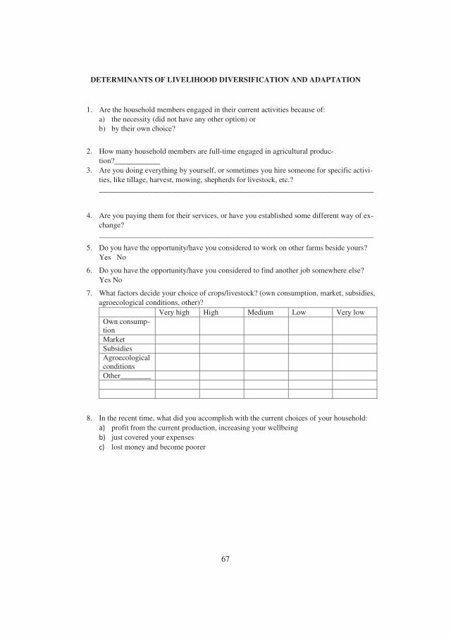
67
DETERMINANTS OF LIVELIHOOD DIVERSIFICATION AND ADAPTATION
1. Are the household members engaged in their current activities because of:
a) the necessity (did not have any other option) or
b) by their own choice?
2. How many household members are full-time engaged in agricultural produc-
tion?____________
3. Are you doing everything by yourself, or sometimes you hire someone for specific activi-
ties, like tillage, harvest, mowing, shepherds for livestock, etc.?
________________________________________________________________________
4. Are you paying them for their services, or have you established some different way of ex-
change?
________________________________________________________________________
5. Do you have the opportunity/have you considered to work on other farms beside yours?
Yes No
6. Do you have the opportunity/have you considered to find another job somewhere else?
Yes No
7. What factors decide your choice of crops/livestock? (own consumption, market, subsidies,
agroecological conditions, other)?
Very high High Medium Low Very low
Own consump-
tion
Market
Subsidies
Agroecological
conditions
Other________
8. In the recent time, what did you accomplish with the current choices of your household:
�� profit from the current production, increasing your wellbeing
�� just covered your expenses
�� lost money and become poorer

68
9. How do you use your eventual incomes? Have you invested in something, like
Significant Some None
purchasing more land
investment in the current or new production
infrastructure
education
memberships in some organizations
personal comfort
leisure and hobbies
other
10. Have you (considered) to purchase more land to increase your production? Yes No
Explain the reason for
both_______________________________________________________
11. In case you would like to purchase more land in your community, do you think it would be
easy to find someone to sell it? Yes No, explain why
________________________________________________________________________
12. If you were faced with some event which lead you to the loss of your capital (drought,
flood, loss of job, market failure, etc.), how did you cope with it?
�� Used the savings to recover
�� Sold the assets (land, livestock, house, other material valuables) to recover
� Received aid from the local/regional government
� Other_______________________________________________________________
13. How would you rate the subsidies you are receiving for agricultural production?
How would you characterize them in one sentence?
14. Do you have access to loans? Yes No
15. How well informed are you about such possibilities?
16. Did you ever take a loan, or have you considered taking a loan in order to invest in your
current production or start with the new one? Yes No
In both cases, state
why__________________________________________________________
17. Do you have access to local/distant markets? How satisfied are you with them (access and
prices)?
Access
Prices
1 2 3 4 5
1 2 3 4 5
1 2 3 4 5
1 2 3 4 5

69
18. What are your farm products and how do you use them
Products Min
price
Avg
price
Max
price
Consumed
on farm
(%)
Sold to
market (%)
Sold di-
rectly(%)
19. How satisfied are you with the infrastructure in your community
20. Where do you buy your seeding materials, fertilizers and pesticides?
In your community In the nearby town Not available
nearby
Seed material
Fertilizers
Pesticides
21. How satisfied are you with the services provided to you by the state/local government
22. What do you think is the biggest obstacle when it comes to your wellbeing and future?
High-
est
High Me-
dium
Low Low-
est
1. Political instability in the country
2. Weak and inadequate agrarian policy
3. Market access and purchase prices
4. Weak infrastructure in your community
5. Climate change and its effect on agricul-
ture
What is the main challenge (presented 1-5,
6-other, explain)
23. What do you think might help you, in addition to what is mentioned here, to achieve your
goals and increase your wellbeing?
1 2 3 4 5
1 2 3 4 5

70

71
PART TWO: Compilation of Papers

�

PAPER 1
Žurovec, O., Vedeld, P.O., Sitaula, B.K. (2015)
Agricultural Sector of Bosnia and Herzegovina and Climate Change – Challenges
and Opportunities.
Agriculture, 5(2), 245-266
�
� �

�

������������ �� ����������������������� !��" �����
��������������������
###�$�%����$�&���'� ������� !��"
�������
������������������������������������������ ��!��� "����# "�����������$%%����������
$��&��'������()*+�$���,�����������"��-�!���������
("%��!$"'!�)*'!"�'�!��'� +',���'$"'!�'�("," �%$"'!-!���"./0�������1
0��#"���'2'�,"�.�!3�)4�)"-��"'�"/056212'�,"�.�!"!.!�'"!�����7.0��#�3�
+�5�� .�%� �,"�" �8'$9��'�/:�;�<�1�9�.=� �.�!�� �8'$9��'�/6�>�-�1
( ?�!=��!�#=�$����".%�'�"'�".=�� �9"����".."��+�5�� ���'&"'�@���,"�8'$9��'��
A" ��B�C��C��������
?���"$��+��!���A"�"'�"D"'!'"�
����������������������� ������������ �������� ������ !�������������� �
.������/E� )�)6�.'���'�E"�@"��,�'�F./6E1%�%� �!��' �,".�'���� ��"�.�?����� !���
%�����!��'�.�9��G9�'"�)!="���� "��'�$3�'��"'"��!"..��'�)���'!"��'�$��,� �")��
!=" ���'!�3� 6E �. =��= 3 ,� '"��9 " !� � �$�!" �=�'�" #=��= %�.". � .��'�)���'!
�"," �%$"'!�=� "'�"��,"'!="� �$�!"�."'.�!�,�!3�)!="������ !��� ."�!��!=".=��"�)
������ !��" �' !=" !�!� "��'�$3 !=" '�$9"� �) %"�% " "$% �3"� �' !=" ."�!�� �'� !="
� �." 3 �" �!"� .�����"��'�$�� �..�". �) )��� ."����!3� 6E =�. "H%"��"'�"� ."����.
�'���"'�".�)"H!�"$"#"�!="�","'!.�,"�!="%�.!!#��"���".���.�'�.","�""��'�$��
�..".� 6�."� �' �,�� �9 " ��!� �'� ����"'! 3 �,�� �9 " � �$�!" %��&"�!��'. "H%�.��" !�
!=�"�!.)��$� �$�!"�=�'�"#� ��'!�'�"!��'��"�."�A="�",�"#%�%"�%�"."'!.!="����"'!
.!�!"�)!="6E������ !��� ."�!���'�!="�$%��!�)%�!"'!�� � �$�!"�=�'�"�'������ !���
.3.!"$.�*!%��%�.".%� ��3�%!��'.!��%!�$�@"�%%��!�'�!�".�'�$�!���!"��'."I�"'�".�)
%�..�9 " � �$�!" �=�'�" �' !=" ������ !��� ."�!��� ("," �%$"'! �) %� ��3 �'� �"."���=
��%���!3.=�� ��'� ��"=��$�'�.�!��'�'��"'!�� �.�!��'�)��$".!�������� !��� %� ���".
����3�'���!�,� '"��9� �!3�.."..$"'!�'�.!�"'�!="'�'�!="%�9 ���'�%��,�!""H!"'.��'
.3.!"$.�J��!="�!"�='� ����� �"," �%$"'!.=�� ��'� ��"�$%��,"$"'!.�'#"�!="��'�
� �$�!"�')��$�!��'.3.!"$.���%�"," �%$"'!������!��'�'�#�!"�$�'��"$"'!�
-�01����/6�.'���'�E"�@"��,�'�������� !��"�� �$�!"�=�'�"����%!�!��'
$*2� 2��

������������� � ��3
�4������������
6�.'�� �'� E"�@"��,�'� /6E1 9" �'�. !� � ����% �) ���'!��". ��'.��"�"� =��= 3 ,� '"��9 " !�
� �$�!" �=�'�" K��L� ?����� !��" �. �' �$%��!�'! �'� ,� '"��9 " "��'�$�� ."�!�� �' 6E ��,"' !="
� �$�!"�."'.�!�,�!3�)!="."�!��!=".=��"�)������ !��"�'!=""��'�$3/CM�)!="N(:1!="'�$9"�
�)%"�% ""$% �3"��'!="."�!���'�!="� �." 3�" �!"�.�����"��'�$���..�".�))���."����!3K�L�
D �$�!" �=�'�" "��. !� ���%!�!��' �$�'� )��$"�. �'� !="�� ������ !��� %�����!��' �' !="
�))"�!"���"�.�E�#","����%!�!��'��".'�!������'�"%"'�"'! 39�!��!="��.�%���"..�') �"'�"�93
.�����"��'�$�� %� �!��� �� !��� �"����%=��� "�� ����� �'� �'.!�!�!��'� )��!��. K� L� ?�"I��!"
�".%�'.".#� �"%"'��'!="�9� �!3�)�"��.��'$�G"�.)��$!=")��$ "," !�!="'�!��'� %� ��3 ","
!�%"��"�,"� �$�!"�=�'�"�'�!�!�G"�" ",�'!��!��'�A="����"'!.!�!"�)%� �!��.�'O".!"�'6� G�'
���'!��"./O6D1#="�"!="%�9 ��."�!���.$�.! 3.� "'!�'�'�'�!��'.%��"'!�'�#="�"!=".��"'!�)��
��'!��9�!��'.�'� �$�!"�=�'�"�'� 3.".��".����"=�. "�!� �$�!"��"," �%$"'!�)��!�,�!�".�'!=�.
)�" ��*!!="�")��"��$".�.'�.��%��."!=�!� �$�!"�=�'�"%� ��3�..�".��"'�!,�.�9 "�!�'3 "," �)
!="%� ��3�$�G�'���"'���'!="."���'!��".�?.��".� !� �$�!"�=�'�"�.'�!!�"�!"�."����. 3�'����"'!
%�9 �.="�G"3.!��!"�������$"'!.�;'"�)!="$��'%��9 "$.��$".)��$�'��"I��!".���� �'�=�$�'
��%�!� #="'�!��$".!�!="�'!�����!��'�'��$% "$"'!�!��'�)$"�.��".�'�%� ���".�E�#","�!="�"
�.������� ��."�)�#��"'"..�'O6D�9��!� �$�!"�=�'�"�!.�$%��!�'�"�'��$%��!�'� .%="�".�)
�)"K��PQL�
A="�"'"�� �9&"�!�,"�)!=�.�",�"#%�%"��.!�%�"."'!!="����"'!.!�!"�)!="������ !��� ."�!���'
6E�'�!="�$%��!�)� �$�!"�=�'�"�'������ !��� .3.!"$.�'6E�A=")��.!."�!��'�)!=�.%�%"���,".
�'�,"�,�"#�)6EF.������ !��� ."�!���'��!..��'�)���'�"!��"!="�#�!=!="�=� "'�".�'�%�..�9 "
�%%��!�'�!�".�A="."��'�."�!��'�.."..".!="�$%��!�)� �$�!"�=�'�"!�6EF.������ !��� ."�!��9�."�
�'9�!=����"'!��'��!��'.�'�)�!��"%�"���!��'.�A=")��.!!#�."�!��'.��"9�."��'��!��"��,"�)��$
�))���� .!�!�.!��� �" "�.".'�!��'� �'� �'!"�'�!��'� �"%��!. �'��!="� �" ",�'! �!"��!��"� *' !=" �.!
."�!��'#"%��%�."%� ��3�%!��'.9�."��'!="�'!"�'�!��'� �!"��!��"!��%!�$�@"�%%��!�'�!�".�'�
$�!���!"��'."I�"'�".�)� �$�!"�=�'�"�'!="������ !��� ."�!���'���"�!��'��"�."%�����!�,�!3�'�
���%!������ !��"�'6E!��=�'��'�� �$�!"�
�4$������1�� ���������������������������������������
6E#�.��'.��"�"��.���#$�!"��� �"'"��3%��,���'��"���'�)!=")��$"�R���. �,��!=����=��!
!="$�&��%��!�) !=" �.! �"'!��3 K�L� *' !="��'.!�!�!��'� ���"��)R���. �,��6E#�.%��!�) !="
)"�"��!��'�).�H��!�'�$��.�"%�9 ��.�� "�93�.!��'��"'!�� ��,"�'$"'!�'�"�!="��'!�� �)!="
D�$$�'�.! :��!3� A="�")��" !=" �"," �%$"'! %�!= �'� %� ���". ��''�! 9" �!!��9�!"� !� �'��,����
�"%�9 ��. �' 3 9�! "H!"�'� �"��.��'. !�G"' �! =��="� "," . #"�" ������ �' %� ��3 )��$� �!��' �'�
��!��$"%���"..".K��L�A="'�!��� �".����".�)6E��"!="���'!�3F.��"�!)��!�'"�'�$�.)��!�'"�!
!=" .�$" !�$" #=��= #�. =�.!����� 3 �"���'�."� 93 � ���" '�$9"� �) ����%�"� "H% ��!�'� !="."
�".����". !=����=��! !=" ����." �) =�.!��3� :���� !� !=" -"��'� O�� � O�� 6E #�. � %��!��� �� 3
�'�"," �%"��������'���'!�3��$%��"�!��!.#".!"�''"��=9���.�?����� !��"#�.!="$��'."�!���)
!=""��'�$3����'�%�.!�#���"��'.!���!��'�E�#","��!!=".�$"!�$"!=")��'��!��'.�)!="�'��.!���

������������� � ��
�"," �%$"'!"H� �.�," 3�" �!"�!�%�!"'!�� �'��#$�!"��� .#"�"".!�9 �.="��*'��.!�3"$% �3"��' 3
�M�)!="!�!� %�%� �!��'%����!�!=�.%"����K��L�
A="$��'�=����!"��.!��.�)!=")��$"�6E"��'�$3�'�'�!��'� % �''�'��."��'�$���"," �%$"'!
9�."��'!=""H�$% "�)%�.!��",� �!��'��3-�,�"!S�..��K���L#=��=%�")"��"��"," �%$"'!�)="�,3
�'��.!�3 �. � %�"�"I��.�!" )�� !=" �"," �%$"'! �) ��=! �'��.!�3 !��'.%��! �'� ������ !��" K��L� A="
"���'��'��.!��".#"�"�'$"!� ���3�'��="$��� �'��.!�3�A="�'��.!�3"$% �3"� ���M�)!=""'!��"
%�%� �!��'�'�����"��="��!.%"�G�'��Q�/ Q��M1�'�#�.��M�'�����)!"�#=��=��$".�'"#
%"�����)#���*'��.!��� �@�!��'#�.!="G"3���."�)�"��������'%���"..".#=��= ")!�""%�$%��!.�'
.���� .!���!��". �' ���� ��"�.�A=".=��"�)������ !��� %�%� �!��'=�.�"��"�."�C�M �'����3"��
%"���� /���QP��Q�1 K��L� 6E "H%"��"'�"� �'��.!��� �@�!��' !=�! �'�!��!"� �' ��9�' �"," �%$"'! �'�
$����!��'!���9�'��"�.�"�%�%� �!�'����� ��"�.�?����� !��� �".����".�.�%�9 ������=�,"'�!
9""'.""'�'�������'�"#�!=�"'"�� .���� �'!"�".!T ���"��"�.�)���9 " �'�=�,"9""' ")!�9�'��'"�
�'��'�� !�,�!"�K� L�A=�.�$�'��!="�)��!��. "�!��.�!��!��'#="�"!="���'!�3��� �$""!9��" 3
�M�)�!.'""�.)��)���K��L�
;'" �) !=" $��' �",� �!��'��3 ��',��!��'. �) !=" '"# 3 ".!�9 �.="� .���� �.! .!�!" #�. !=�! !="
�'="��!"���%�!� �.!$��" �)�#'"�.=�%�'�%��%"�!3���=!.#�..""'�.����."�).���� �'&�.!��"�'�
�'"I�� �!3�A="'"#��,"�'$"'!�!!"$%!"�!���=�","!="��,�.��'�).���� "I�� �!3�'�&�.!��"!=����=
!=" �'!�����!��' �) ��$$�' �#'"�.=�% K�CL� A=�. #�. ����$% �.="� !=����= ���%!��' �) �#. �'�
�"�� �!��'.!=�!�9� �.="�%��,�!"%��%"�!�".�.!="%�"��$�'�'!)��$�?!!=�.!�$"�$%��!�'!"��'�$��
�'��'��.!��� )��� �!�".#"�"��',"�!"�!�.!�!"%��%"�!3 !=����=��')�.��!��'."I�".!��!��'�������'
�")��$.�'�'�!��'� �@�!��'�4�'��.���$$�'�#'"�.=�%#�.��I���"�%��$��� 393��')�.��!��'�)
�.."!.)��$%"�.�'.��',��!"��.U"'"$�".�)!=".!�!"V�'�!="'.��'�)���'! 3�'��"�."�!=����=�������'
�")��$.�'��� �'��� ��?������'�")��$.�9� �.="� ���"%��,�!" �'�=� ��'�.�'� �$�!"�!="$!��
$�H�$�$�)��=�%"�%��,�!""'!�!3K�C�QL�A="��')�.��!"� �'�#�.�#���"�!� �'� "..%"�.�'!.�'�
)��$"�.#�!=�'.�))���"'! �'��A=�. "�!�!=""$"��"'�"�)� ���"'�$9"��).$� �'�$"���$.�@"�
)��$.#�!=�!"'�"'�3�))��!="�)���$"'!�!��'�A="�������'�")��$.."!9��G������ !��� %�����!��'
� $�.! !� � .�"'���� �) '�!��� �� .�9.�.!"'�" "��'�$3 K�L� *' ����!��' !=" �"$��'�'� ������ !���
%�����!��'#�.% ���"�93#"�G��%�!� "I��%$"'!�))�$� 3)��$.K��L�'��9.� "!"!"�='� ���".K��L�
? .=�)! �' ������ !��� %� ���". #�. �"����"� �' !=" C�. #="�" $��= �!!"'!��' #�. %��� !� !="
�"," �%$"'!�)������ !��"�'����� ��"�.�A="% �'#�.!��'��"�."!="�'!"'.�!3�)%�����!��'!=����=
=��="� 3�" �. �'� �"'"�� �'��"�."� %�����!�,�!3� *',".!$"'! �' �'� �$" ����!��' #�. �'"
�)!=")���.��"�.�)!=�.$�.!"�% �'�*'!="Q�.R���. �,��#�.% �'�"��'!���""%"��'�$�����.�.
#=��= =�. �))"�!"� �',".!$"'!. �' ������ !��" �'� !=" "))"�!�," �$% "$"'!�!��' �) !=" % �''"�
�',".!$"'!%�����$.�
4�G"� �!="�."�!��.!="������ !��� ."�!��=�..�))"�"�"'��$��.��$��"����'�!="#��%"����
/����P��� 1�A="%�����$.�)�"��'.!���!��'�'��".!���!��'�)�'!"�'�!��'� ��'��.)���."��'9�.��
���� �')��.!���!��"�'�=��.�'�%���=�."�)������ !��� $��=�'"�3�'��'%�!..""�.�'�)"�!� �@"�.)��
!="�"��'.!���!��'�'��"=�9� �!�!��'�)���%%�����!��'�*!#�.$��"�)�.���� ���!� ��� %"�% "!=�'
� ."����. �',".!$"'! �' !=" �",�!� �@�!��' �) ������ !��"#�!= !="$��' �9&"�!�," !� �"!��' ��.% ��"�
%�%� �!��'�'���� ��"�.K��L�
A���36E�..!� �%�"��$�'�'! 3���� ���'!�3�*!�.".!�$�!"�!=�!�9��!��M�)!="%�%� �!��' �,"
�'���� ��"�.K��L�? !=���=!=".=��"�)������ !��"�'N(:�.��'.!�'! 3�"��"�.�'�/��M�'����!�

������������� � ��5
CM�'����1������ !��� %�����!��'�.�9��G9�'"�)!="���� "��'�$3"$% �3�'���M�)#��G)���"�
A=""��'�$3�)6E�"$�'.!��!"���'.��"��9 ",�!� �!393��=�",�'�=��=���#!=��!".".%"��� 3�'
����9�!�!#�.'�!"'���=!�.��'�)���'! 3�%%����=!=" "," �)$"���$�"," �%"����'!��".�?�!��
N(:%"���%�!��'����#�.�' 3��M�)!="+2�C�,"���"�'��"��="��' 3Q�M�)N(:�)#=��=�!
=���'��Q�K��L�6EF.�"�"'!�� �@"�%� �!��� �'���$�'�.!��!�,".!���!��"�.,"�3��$% "H�A=�.�'�I�"
��'.!�!�!��'� ���"��',� ,".!#�"'!�!�".�J"�"��!��'�)6E/J6�E1�'�S"%�9 �G�-�%.G�/S-1�.#" �.
!=" 6��G� (�.!���! �) 6E /6(1 �. ."%���!" ��$�'�.!��!�," �'�!.� *' ����!��' J6�E �. ��,��"� �'!�
��D�'!�'.�A=�.��$% "H��,"�'�'�".!���!��"� .�=�.���"�!�$%��!�'$�'��"$"'!��$%"!"'�"�'�
��%���!3�'!="������ !��� ."�!���A=".�!��!��'�'!="������ !��� ."�!���'6E�.)"�!��"�93��))"�"'!
�"�� �!��'.�!��))"�"'! "," . "��. �!�,"�,"� �%. �$�!"���%���!�".�'���$$�'���!��'�=�''" .�.
#" �. � ��G �) � "�� ,�.��' �'� )�� ��" !� �$% "$"'! '"�"..��3 �")��$.� A=" "���3 �) !=" %�.!
.�����%� �!��� .3.!"$ ���% "� #�!= !=" ����"'! ��$% "H %� �!��� .!���!��" =�," .��'�)���'!
��'."I�"'�".)�������� !��� �"," �%$"'!)���'�$�'3�=� "'�".�
�"�"������������#��������
A="$��'%��9 "$�)!="������ !��� ."�!���. �#%�����!�,�!39�!=%"��'�!�)%�����!��'�'�%"�
)��$KQL�A="$��')"�!��"�..$� �.�� ".�9.�.!"'�"������ !��"���"'!"�%�����!��'��!="�!=�'�$��"
��$$"���� ��$��G"!���"'!"������)���.3.!"$�*!�.�$��'���."�) �#��$%"!�!�,"'"..%��!��� �� 3
�'!="��$".!��$��G"!�4�#������ !��� %�����!�,�!3�.�)!"'���'."I�"'�"�) !="�9."'�"�)� "��
.%"��� �@�!��'%��$��� 3�'���%%�����!��' �#!"�='� ��3 "," .�))��$.�'�"H!�"$"�"%"'�"'�"�'
#"�!="���'��!��'.�-=�)!.�'!"�$.�)�$%��,�'�%�����!�,�!3��"�%%��"'!=�#","�!="."%���"..".��"
,"�3. �#K��L�A="$��'�"�.�'.)���. �#%���"..�)�$%��,�'�%�����!�,�!3��"��))��� !�'���.G3
$��G"!���"..�'��'.�))���"'!��%���!3)��.!���'��'�%���"..�'�".%"��� 3,"�"!�9 ".�*'����!��'
%�����!��'�).""�$�!"��� '��."��".�'�.""� �'�.�.�'�"��"," �%"��'�!="%�����!��'�"%"'�.�'
�$%��!"� .""�. �)!"' #�!= I�".!��'�9 " I�� �!3 �'� #�!=��! ��"I��!" ��'!�� KQL� A=" "," �)
!"�='� ����� �'�$��G"!�'�G'�# "��"�$�'�%�����"�.�. �##=��=�"�!��' 3=�.�'"��!�,""))"�!
�'!="%�����!�,�!3�)!="."�!���A="$��'���.")�� �#%�����!��'�)9�.�������� !��� %�����!.�.!=�!
�'!="%�",���.3"��."H�.!�'������� !��� ��%���!�".=�,"'�!9""'�."��'!"'.�," 3�?����� !��� �'�
��,"�.���$� ��'="�!��".�)#=��=��� M�.���9 "/A�9 "�1�'��.$��=�.=� )�)���9 " �'��"$��'.
�'�."�/J����"�1�
6�.���4-!���!��"�)������ !��� �'��'6�.'���'�E"�@"��,�'��-����"�K� L�
������0 ���7���"�8 9?��9 " �'� ������ ����;��=���. ���� ���<�'"3���. �� ���5"���#. ����� ���:�.!��". QQ�� ���
6���� �����������:��� ���54; ��4�J��".!. �C� �� ���;!="� ����� ���6���� ���<4 ���4�

������������� � ��<
=������4-!���!��"�)���9 "�'��� !�,�!"����9 " �'��-����"�K��L�
�"�"�$��� �#�%���#����#&
4�,".!��G%�����!��'=�.���"�!.��'�)���'�")��6E������ !��"��'.��"��'� !="�,�� �9 "'�!���
�".����".�'�!="'�$9"��)%"�% ""'���"��'!=�.%�����!��'�A="G"3%�����!.)��$ �,".!��G�',� ,"
$� G�'�����3%�����!.$"�!�'�$"�!%�����!.�-�'�"!="'�$9"��) �,".!��G.!��'�!"����"� �'"�
�' �"�"'! 3"��. "H�"%! �' !=" ��." �) %�� !�3 /J����" �1 ���#!= �' %�����!��' �) $"�! �'� $� G �.
"H% ��'"�93�$%��,"$"'!.�'3�" �.�'�9�""���$%�.�!��'9�!%�����!�,�!3�..!� �#��$%��"�#�!=
���'!��".�'!="�"���'K��L�4�#%�����!�,�!3�.�"�!��' 3%��! 3��"!�.!� �'��"I��!"9�""�.!���!��"
�'"))���"'!9�""��'��'�." "�!��'#��G9�!$�.! 39"���."�)!="��� �!3�'%�����!��'KQL�+H!"'.�,"
%�����!��'�'.$� )��$.�.%�",�� �'��' �,".!��G%�����!��'#=� "�'!="�!="�=�'��.$� %��!�)
!="%�����!��'�.����'�@"��'!="$��"�'!"�='� ����� 3#" �"I��%%"�)��$.�O=� "!="�"=�.9""'
.�$" %����".. �' "H%��!. �'� %�����!�,�!3 �' �"�"'! 3"��. !=" �,"�� ��$%"!�!�,"'".. �) �,".!��G
%�����!��'�'!="�'!"�'�!��'� $��G"!.�..!� #"�G�6E����"'! 3��=�",".�' 3�.$� .=��"�)�$%��!.
�'�!.$�&��"H%��!�".!�'�!��'.$��' 3!="O".!"�'6� G�'���'!��".K�CL�;'"�)!=" ���".!%��9 "$.
�' �,".!��G%�����!��'�.!="9�''"��'"H%��!�):�����!.�)?'�$� ;����'!�+2�J��$�'33"��.
+2=�.9""'�"I�".!�'�!="".!�9 �.=$"'!�'��"����'�.�!��'�)��'!�� .3.!"$)��)����'��'�$� .!��G
)""�9�."��'!="%��'��% "UJ��$J��$!�J��GV�E�#","�!=�.�..�"=�.'�!9""'�".� ,"���"!�
��.���""$"'!.�'� ��G�)������'�!��'�'����%"��!��'9"!#""'!=".!�!"�'�"'!�!3 "," �'.!�!�!��'.�'
!=")���.�)"!3.3.!"$�'��!�"$��'.�'� "��#="'�!#� 9"����".."�K�QL�
������������� ��������
���� �� �����������������
����������
���� ������� ����
!�"� #���$���
%��"����� �����
��� �� ��������
&�#�����

������������� � ���
=������45"�!�'�$� G%�����!��'�'6�.'���'�E"�@"��,�'��-����"�K��L�
�"'"�(�#����#����#&
(".%�!"�" �!�," 3)�,����9 "'�!��� ��'��!��'.���%%�����!��'�.)���'�$�'3�=� "'�".�J�"I�"'!
��,"�."#"�!="���'��!��'.�'G"3.!��".�)���%���#!=/=��=�� �#!"$%"��!��". �!".%��'���"�� 3
��!�$')��.!.�")���!��.��% �.���')� 1��")��!="������,�!"�93 ��G�))��$�',".!$"'!=��=%���".
�'� %��� I�� �!3 �) �'%�!. /.��= �. .""�. )"�!� �@"�. �'� %".!����".1 .�9.�.!"'�" ������ !��" �'�
!����!��'� "H!"'.�," )��$�'� %���!��".�A=" �".� ! �. �#%�����!�,�!3 �'� .��'�)���'! 3 �#"� 3�" �.
��$%��"�#�!=!="�".!�)!="�"���'/J����"�1�
=�����;4R�" ���$%���.�')��$�.!�$%��!�'!���%.�'6�.'���'�E"�@"��,�'�#�!=!="
�"���'� %�����!��'�-����"�K��L�
D"�"� .��$�'�!"������ !��� ���%%�����!��'��"�./J����"�1#�!=$��@"�.!="$��'���%/$��"
!=�'��M�)!�!� �"�"� %�����!��'1�(�$".!��%�����!��'�)�"�"� .�'6E�.'�!.�))���"'!!�$""!!="
!�!� ��'.�$%!��' �"$�'�. K��L� A=" 3�" �. �) )����" ���%. ��" �# �'� #" 9" �# !="�� �"'"!��
%�!"'!�� �S".� !�'� )""�=�. � �#%��!"�' �'�=��= �" � �."%"��"'!��" �".%�!" !="�.��"�) =��=
�
�����
����
�����
�����
�����
�����
���� ���� ���� ��� ��� �� ��� ��� ��� ��� ��� ��� ��� ��� ��� ��
������������� ��������������� ������������ ������������ ���� ��!������!��"����������!�
�
�����
������
������
�����
�����
#���� ���$� %��!�� &!'(��� ��!���
)"'����*�!��!� �
&������� +�����!��&"�(�",
-�� ���� ��.�"$��/� � 0�'���" �1'"��� 1'"���
2��!����3���

������������� � ���
I�� �!3 "��$".�'�!="��$�H!��".K��L�E�33�" �.�'���.. �'�.��"","' �#"�.�'�"$�.!�)!="$��"
'�!$�'��"��!� �<"�"!�9 "%�����!��'�.$��' 3)���."��' ��� $��G"!.�'�!�G".% ��"�'$�H"�
)��$�'�.3.!"$.�)!"'�.�.�%% "$"'!��3.����"�)�'��$"�;��=���.�'�,�'"3���.�'6E.�))"�"�
"'��$��. ��$��" ����'� !=" #�� �'� ��" ����"'! 3 ���'� !=����= � %=�." �) ��'.� ���!��' �'�
�"�"'"��!��'�: �$.�%% ".�'�%"��.��$�'�!"!="%�����!��'K��L�
�")"����*�+�������
A=""H��!'�$9"��)������ !��� =� ��'�.%��!��� �� 3)�$� 3)��$.�.'�!G'�#'.�'�"��"'.�.�)
������ !��"!=�!#�� �%��,��"���$%�"="'.�,"%��!��"�)!=".!���!��"�)������ !��� =� ��'�.=�.'�!
9""'��'���!"�.�'�"�����A=�.�'� ��".�"!"�$�'�'��'�!3%� ����� 3��!"����.�'�)��$.�'�" �!��'
!�!="�!� �@"������� !��� ��"�/2??1�'��"!"�$�'�'�!=".�@"�))��$.�������'�!�2??�A="�"'"��
�=����!"��.!���)!="O".!"�'6� G�'.F������ !��"�.!=�!!="$�&���!3�)!="%�����"�.��".$� =� �"�.�
A=" $��' �"�.�' )�� !=�. .�!��!��' �. !=" )��$"� R���. �,��' ������ !��� %� ��3 /)��$ .�@" �$�!
��="�!��".1K�C�QL�6".��"�!. �#.�@"/��C=��)��$1�'$�.!��.".)��$.��")��$"�)��$.$� %���" .
�)!"'��. ���!"� )��$"��=�!="�#=��=$�G". !="%�����!��'$��"��.! 3�'� ".. "))���"'!�-�$"
� �����)��$./ �M1��" "..!=�'�="�!��".�'����������Q�M��" "..!=�' ="�!��".#=� "�' 3
�M=�,"��"�.9"3�'���="�!��".K��L�
�" "��������&��#���
A=" 9���"! � ���!��' !� ������ !��" �. I��!" �# ��$%��"� !� �"," �%"� �'� ","' �"," �%�'�
���'!��".�$��'!�'�!��9��!�M�)!�!� %�9 ��.%"'��'��'���CK��L�63 ��G�'��!!=".!���!��"�)
������ !��� .�%%��!93����%.�)$"�.��".�!�.'�!��"�9 "!=�!!=" ���".!�$��'!�).�%%��!����'�!="
�'� 3."�%"����#�.#�!=�'!=")��$"#��G�)���"�!%�3$"'!.!�%�����"�.#=��=�")"�.!�%�3$"'!.
9�."��'��!%�!�'�!="%�3$"'!%"��'�!��"����!! "�A="����"'!6E%� ��3�"."$9 ".!="+2%� ��3�'
!=" $���Q�. #=��= #� '�! ���"�! 3 %��$�!" %�����!�,�!3 �'��"�.". �' 6EF. ������ !��"� 6���"!��3
!��'.)"�.�" �!"�!����"�!.�%%��!!�%�����"�.�'�%�3$"'!.9�."��'��!%�!)��$$��"!=�'��M�)
!="!�!� ������ !��� 9���"!KQL�A=�.$"�'.!=�!!="��$%�.�!��'�).�9.���".�'6E�.="�,� 3���"'!"�
!�#��� ���"�! %�����!��' ��!="� !=�' �',".!$"'!.� A�G�'� �'!� �����'! !=�! $�.! �) !=" .$� =� �"�
)��$"�. ���"'! !="�� %�����!��' !�#���. .�9.���@"� ���%. �� �,".!��G �' ���"� !� =�," ���".. !� �'
����!��'� .����" �) �'��$" !=�. )��$ �) .�%%��! =�. !=" )�'�!��' �) � .���� !��'.)"� ��!="� !=�'
%��,���'�%�����!�,".�%%��!!�!="������ !��"."�!��K��L�A="9���".!��))"�"'�"9"!#""'!="�������'
%� ��3�)6E�'� !="+2F.D�$$�'?����� !��� :� ��3 /D?:1 �. !=�!D?:=�.$�,"��#�3 )��$
.�9.���". !�"� !� %�����!��'��'9��'� %�3$"'!. %"� �'�! ��"����!! "��","'�"��'��$" �'� �. ������ 3
$�,�'�!�#����',".!$"'!���'!./!=����=:� ��**1�
�","�������������%��
*'��"I��!" $��G"! ���".. �"���". !=" $�!�,�!��' �) )��$"�. !� .%"��� �@" �'� �$%��," !="��
%"�)��$�'�"�'�!��'��"�."%�����!��'�6"���."�)!=")���$"'!"������� !��� %�����!��'�'"�)!="
$�.! �$%��!�'!�=�''" . )�������� !��� ��!%�!. !=" )��� �'��.!�3 �.'�!$�!�,�!"� !� �'G�%#�!=
������ !��� %�����"�.�' �'��!"�$��'!���!.K��L�*'����!��'!="����"'!#"�G)����'��.!�3�.'�!�9 "

������������� � ���
!�!�G"!="�� "�)9"�'�!="$��'���,"���,"=�� "�),"�!��� ��''"�!�,�!3)���'"))���"'!,� �"�=��'�
D�'."I�"'! 3!="�'��.!�3�.'�!�'!"�".!"��'�$%��,�'�!="%�"."'!,� �"�=��'��!�.".�!.'"��!��!�'�
%�#"�. �'��)!"'��".'�! �".%"�! ���""$"'!.$��"�;' !="�!="�=�'�=���@�'!� 3��.&��'!"� �'�
��.����'�@"�%�����"�.#=�.�'�"!="!�$"�).���� �.$=�,""H%"�!�!��'.!=�!!=")����'��.!�3=�.�'
����!��'� .���� !�.GT!="%���=�."�)%�����"�)���.T��'�!�))"���".%"�!��'!���!I��'!�!�".�'�
�)!"'��'�!�" �,"���"I��!"I�� �!3KQL�A="%�����"�.��'�!�."!="�%%��!�'�!3!��"," �%�!.�"���'�
��"'!�!3!=����=!="%�����!��'�)%�����!.#�!=�"����%=��� �����'�����'� �!3��!����!��'� %�����!.�
*'�!="�#���.!="%�����!��'�"�.,"�3'����#�'�� ��$%�'�".�%"��!"#�!=�'�'����#."�$"'!�)
!="$��G"!#=� "!="�".!�)!="'��="$��G"!.��" ")!!��$%��!��$%�'�".�A=�!�.#=3!=")����'��.!�3
��$%�'�".��")��"�#�!=.!�))��$%"!�!��'#�!=�'!="��$".!��$��G"!�'�� ���"'�$9"��)��$%�'�".
��"'�!�9 "!��'�"%"'�"'! 3���%!!=".!�'����.�"I���"�)��)��"��'$��G"!.�
�"-"����������./��& �#&�
A="'"!#��G.�)%�9 ���'�%��,�!"�'.!�!�!��'.����'�@�!��'.�'��"."���=�'.!�!�!��'.#=��=�" 3�'
�.3.!"$�) �)"� �'�"����!��'"))���"'! !��'.)"��)G'�# "��" !"�='� ��3�'� �')��$�!��' )��$�
%�!"'!�� 9�." )�� �''�,�!��' �'� $��"�'�@�!��' 9�! !="3 ��" '�! ".!�9 �.="� �� ��" .","�" 3
�'�"��"," �%"��A="�')��$� ."�!���'�0N;.��!�,�!�".#=��=��"�$% "$"'!�'���))"�"'!�.�� 3
�'!"�'�!��'� 3)�'�"��"," �%$"'!%��&"�!.=���.��'�)���'!�� "�'!="!��'.)"��)!"�='� ��3�'!="
%�",���. %"����� A="." %��&"�!. =�," ��'�="� �'�!��!�,". )�� !=" ".!�9 �.=$"'! �) %��,�!" ��,�.��3
."�,��".�.#" �.9�� ��'��%��!� )��!=""H�=�'�"�'���.."$�'�!��'�),�����.!3%".�)�')��$�!��'
#=��=�%�'��$% "!��'�)!="%��&"�!��""�!="�)����!!"'���'.�.!��'�9 "9"���."!=".3.!"$��''�!
9"��$" %��! �) !=" !"�='� ��3 !��'.)"� .3.!"$ KQL� A=" ���" �) G'�# "��" �'� !"�='� ��3 !��'.)"�
."�,��".�.$"�'!!���!=����=!="%�9 ��"H!"'.��'."�,��"�A="%�9 ��"H!"'.��'."�,��".#=��=��"
���!"��!!="�"���'� ����'!�'� $�'�.!��".�"%"'��'��'!=""'!�!3$��' 3%"�)��$��$�'�.!��!�,"
#��G�'��",�!","�3 �!! "!�$"!�)�" ��" �!"�#��G�D�����'�!��'9"!#""'�"���'� "H!"'.��'."�,��".
��'�!"H�.!'����".�.3.!"$���%%����=!�!="��.!�"'�!="'�'�/".%"��� 3"����!��'1�'�"I��%%�'��
A=�.�".� !.�'�,"�3. �#!"�='� ����� %����"..�'!="."�!����$%��"�!�!="������ !��� ."�!��.�'
'"��=9����'����'!��".#=��=� !�$�!" 3 "��.!���""%"'�'��)!="!"�='� ����� �'�G'�# "��"��%�
�"0"�1�����2*���&���
N"'"�� 3�" �!�," 3'"��!�,"$����"��'�$��!�"'�.��"!="�".� !�)=��=)��"��'!���"�$9� �'�"
�'�=��=!���"�")���!.#=��=��"!="$��'���.".�)!="'"��!�,"����"'!�����'!9� �'�"�? !=���=!="
�" �!�," .=��" �) !=" '"��!�," !���" 9� �'�" �' N(: �. �"��"�.�'�T)��$ ����M /����1 !� �Q��M
/����1T�!�..!� �'.�.!��'�9 3=��=KQL�-��=�=��='"��!�,"!���"9� �'�"�..��'�)���'! 3�))"�!"�93
�$%��!�)�����)���%�����!./�Q��M�'����1�(".%�!"!=�!6E=�..��'"�� ���"'�$9"��)9� �!"��
�'�$� !� �!"�� ���""$"'!.#�!='"��=9����'����'!��"."H�.!�'��'"))���"'!!���"%� ��3$"�=�'�.$.
=�,"'�! "��!��.��'�)���'!�'��"�."�'"H%��!.�)������ !��"�'�)���%�����!.K��L�?!!=".�$"!�$"
!="������ !��� ."�!��)��".$�'3�!="��=� "'�".".%"��� 3�'!="%��!�)!=")� )� $"'!�)�9 ���!��'.
!�#���.!="+���%"�'2'��'.�'�"&��'�'��'",�!�9 3�"I���".��&�.!$"'!�'��")��$�)!="������ !���
."�!���' �'"#�!=+2�"I���"$"'!.�

������������� � ��;
;4����������������������� ��!��� "����
6E�.�$��'!��'��.���'!�3#�!= �# �'�.� �'�!="9�'G.�)$�&����,"�.�5�,�'�)��$'��!=!�
.��!=!=") �! �'�.��%"������ 39"��$".#��")��!=� .���.�'�)��$��� ���$�9�,"."� "," �'�
������ 3!��'.�'!��$��'!��'��.�"���'�A="�".!�)!="��"��.��$�'�!"�93!="(�'����? %.#=��=
"H!"'� ����.. !=" #=� " ���'!�3 )��$ !=" #".!"�' 9���"� #�!= D���!�� !�#���. !=" .��!="�.!�
A="�"'!�� %��!��'.�.!�)=� .�$�'�#=��=��"�" �!�," 39������,"�,� "3.�'�9�.�'.�>��.!/9���"'
���G31!"����'.��,"�$�.!�)!=".��!=�#".!"�'!"���!���".�)6E�
?.%��!�)!="�"'"�� ����� �!��'�)!="�!$�.%="�"�,"�!="6� G�'.�'�!=�.�,"�6E!="�"��"
)�"I�"'!.=�)!.�)!��%��� ���$�..".����'�.�$$"��'�!="�') �#�)�� ����!���������'�#�'!"��?
!="."%���"..".��" ���" 3$���)�"�93�" �")!=�!�����.�.�$�&��� �$�!"$���)�"��J��!=�.�"�.�'!="
!"���!��3�)6E�..% �!9"!#""'!=�""$��'!3%".�)� �$�!"�/�1D�'!�'"'!� �'�$��"��!"���'!�'"'!� /�1
5��'!��'�'�$��'!��'��"%�"..��'��'�/�15"��!"���'"�'�'�$���)�"�5"��!"���'"�'� �$�!"K���L�
D�'!�'"'!� � �$�!"�����.�'!="'��!=!="5"��!"���'"�'!�!=".��!=�'�!=" �'"!=�!."%���!".!="."
!#��"���'.�.��$�'�!"�93=��=$��'!��'.% �!"��.�'�� �)).#=��=��"�"%"'��'��'!="� !�!��"
�))"�!"�93!="$��'!��'� �$�!"�
'"�"������(�*����(!�&���+��&���# �
6E=�."H%"��"'�"�."����.�'���"'�".�)"H!�"$"#"�!="�","'!.�'!="%�.!!#��"���".���.�'�
.","�""��'�$�� �..".�6�."��'�,�� �9 "��!��'�����"'! 3�,�� �9 "� �$�!"%��&"�!��'."H%�.��"
!�!=�"�!.)��$� �$�!"�=�'�"#� ��'!�'�"!��'��"�."K��L�;9."�,"�� �$�!"�=�'�".��"�") "�!"�
!=����=�'�'��"�."�'�,"���"!"$%"��!��".�'6E�J��!=" �.!=�'��"�3"��.!="�,"���"!"$%"��!��"
=�.�'��"�."�93��QWD/#=��=�.�' �'"#�!=� �9� !�"'�.1#�!=�!"'�"'�3!����" "��!"T!="�"���"�)
����P�����.#��$".!�'!=" �.!���3"��.�?������'�!�*:DD-S+-F..�"'����.9�."��'-*0A+X�N
�'� +DE?5 � �$�!" $��" . /J����" �1 !=" $"�' ."�.�'� !"$%"��!��" �=�'�". )�� !=" %"����
����P������""H%"�!"� !���'�")��$B��QWD!�B���WD�9�,"%�",���.�,"���" !"$%"��!��".K�L�
O�'!"�.��"%�"���!"�!�9"��$"#��$"�/)��$�� WDP��QWD1#=� "!="9���".!�=�'�".#� 9"����'�
!="$�'!=.�)Y�'"Y� 3�'�?���.!#�!=%�"���!"��=�'�".�)B���WD�'!="'��!=�'�B���WD�'
.��!="�'��"�.�:�"��%�!�!��'�.%�"���!"�!��"��"�."93��M�'!="#".!�)!="���'!�3�'��'��"�."93
M�'!=""�.!�A="��!�$'�'�#�'!"�."�.�'.��""H%"�!"�!�=�,"!="=��=".!�"���!��'�'%�"��%�!�!��'�
J��!="�.��'�)���'!!"$%"��!��"�'��"�.".��""H%"�!"�����'�!="%"������C�P����#�!=�%�"���!"�
�,"���"��."�'!"$%"��!��"�%!��WD�'�%�"��%�!�!��'�"��"�."�%!� �M�
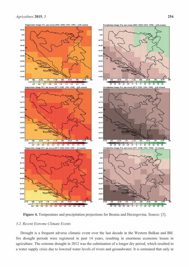
������������� � ���
=������4A"$%"��!��"�'�%�"��%�!�!��'%��&"�!��'.)��6�.'���'�E"�@"��,�'��-����"�K�L�
'"�"�����&��./���*��(�*����.��&� �
(����=! �.� )�"I�"'!��,"�."� �$�!��","'!�,"� !=" �.!�"���"�' !="O".!"�'6� G�'�'�6E�
-�H �����=! %"����. #"�" �"��.!"�"� �' %�.! �� 3"��. �".� !�'� �' "'��$��. "��'�$�� �..". �'
������ !��"�A=""H!�"$"�����=!�'����#�.!="�� $�'�!��'�)� �'�"���3%"����#=��=�".� !"��'
�#�!"�.�%% 3���.�.��"!� �#"�"�#�!"� "," .�)��,"�.�'�����'�#�!"��*!�.".!�$�!"�!=�!�' 3�'

������������� � ���
���� !=" �����=! %"����. ���."� �..". �) �,"� 2-( � 9� ��' �' ������ !��� %�����!��' �'� 3�" �
�"���!��'�%!�C�MK��L�A="$�.!�))"�!"�#�.$��@"%�����!��'#=��=�.!="$��'��#$�!"��� �'
%�����!��'�)�'�$� )""��-�$� �� �..".#"�")��'��'%�����!��'�)9�� "3.�39"�'.� )� )�� �,"�
9"�'.$"���#.�'�%�.!��".#=��= "�!�� ��G�))���"��4��G�))���"��') �"'�"�!="�"���!��'�'!="
'�$9"� �) �,".!��G �'� �,".!��G %�����!��' %�����!��' �) $� G �'� $"�! .�%% 3 !� !=" ��$".!��
$��G"!�?!!=".�$"!�$"!=""))"�!.�)!="�����=!=�,"�))"�!"���.".�')���%���".�'��"���"�!="
"H%��!�)%�����!.�D���"'!%��&"�!��'.�)�����=!�$%��!�'���%3�" �.�"$��'�'�"�!��'��"!� ��G�)
�"."���=�'!=�.��"��E�#","��!�.�"�!��'!=�!!=�.�..�".=�� �'�!9"��'��"�!�G�'��'!������'!!="
"H�.!�'��"."���=�S"."���=��'���!"��''��!="�.!6�.'���'����!".!=".","��!3�)!="%��9 "$.)���'�
!="���'!�3#="'�!��$".!�!=""H!"'.��'�)�����=!%"����.�'��=�'�".�'%�"��%�!�!��'��.!��9�!��'�
2.�'�� �$�!".�� �'����%��!�!="".!�$�!"��,"���"3�" ��"���!��'�'���'�)"������� !��")��!="
.�H$�.!��$$�'���%.�'!="�"���')��%�.!)�,"�"���".#�.��QMP����M�'����MP�C�CM�' ��$3
�'�="�,3.�� �".%"�!�," 3K� L�A="�"�.�9����))"�"'�"#="'!="3�" ��"���!��')��$!=" �.!�"���"
�.��$%��"�!�!="�".!�)!="�"."���=%"������"!��'��"�."����!"$%"��!��"%�"��%�!�!��'#�'�.%""�
�'� �#"��" �!�,"���=�$���!3�5�.!'�!�9 3!="$��@"3�" ��"���!��'�'!="%�.!�"���"#�.�Q�M
=��="���$%��"�!�!=""�� �"�%"�����
J ����.!="�!="�)�"I�"'!$�&��'�!��� =�@����" �!"�!�#"�!="��'�� �$�!"�=�'�"�'6E�*'����
) ����'��))"�!"��,"�������%"�% "�'�Q$�'���%� �!�".�".!��3"������=��))��$ �'�#�.="�
�#�3.","�� 9����".�'���'!�$�'�!"����'G�'�#�!"��*'����6E"H%"��"'�"�!=" ���".!�$��'!�)
%�"��%�!�!��'�"����"�!�!=�!$�$"'!#=��=�".� !"��'$�..�,") ���.�'!=""'!��"!"���!��3K��L�A="
) ����'� .�!��!��'�� $�'�!"�#�!=�' "H!������'��3 ���')� �'5�3���� .��%�..�'� ","' !=" ) ���
"," .)��$�����))"�!�'�6E�'�!=".�����'��'����'!��".�A="#=� "#�!"�.="��)��,"�-�,�!="
���".!#�!"�.="��'6E/�CM�)!="!�!� !"���!��31#�.�,"�) ���"�#�!=!="����$� �!"���#'.!�"�$
) �# �) #�!"� $�� �'� �"9��. ���.�'� #��".%�"�� ) ���. �' !=" % ��'� 6�"��=". �) "$9�'G$"'!.
�".� !"� �' ) �.= ) ���. �'� !=" ��,"�. ����3�'��"9��. ��#'.!�"�$��"�!"� � %�!=�) �".!���!��' �'�
�".� �!��'K�CL�+�� 3".!�$�!".�'����!"!=�!Q� ��� ��,"�'$"'!�'�!..�))"�"���$��". �..".�.#"
�..���� ��"',���'$"'!� �$%��!.!�,��3�'��"��"".�?���'������%"�% "#"�"!"$%����� 3��.% ��"�
)��$!="��=�$".�'�$��"!=�'�����!��G"H!"'�"��")��"�'%�9 ����%��,�!".=" !"�.�A=") ���.�'
�������."�!="��$��""I��,� "'!!�'"�� 3� M�)N(:/������9� ��'2-(1�
'"'"�2*�����#3�(�*����(!�&���#&����������+� ��* �
A="�""H�.!'��"!�� "��')��$�!��'��'�"�'�'��$%��!�)� �$�!"�=�'�"�'6E�E�#","��!�.#"
����$"'!"�!=�!� �$�!"�=�'�"�'��'��"�."�,����9� �!3#� "��!��=�'�".�' �'��'�#�!"��"��$".
�'�!=�.=�,"����"�!�$%��!�'������ !��"�'!="�"���'K�QL/A�9 "�1�A="�$%��!.�)� �$�!"�=�'�"
�' ������ !��" ��" %��$��� 3 �") "�!"� �' �=�'�". �' $"�' !"$%"��!��". �'� %�"��%�!�!��' #=��=
.�9."I�"'! 3 "��!�3�" ��"���!��'�'�!=""$"��"'�"�)'"#%�!=��"'.�'���."�.".���%)�� ��".
�'��!"�$%�����!��'�"� �'".K��L�D �$�!"�=�'�"#� =�,"��))"�"'!"))"�!.�'������ !��� .3.!"$.
�'+���%"#�!= �G" 3�'��"�.".�'���%3�" �.�'���'�".�)���#'���%.�'!="'��!=#=� "�.��'�)���'!
�"��"�."�'3�" �.��""H%"�!"��'!="-��!=K��L�A="��!�� �$%��!.�)� �$�!"�=�'�"�"%"'���"�! 3
�'!="���%!�,"��%���!3�)�'�))"�!"�.3.!"$�"���'����$$�'�!3!���%"#�!=!="�$%��!.�'���.G.
�)� �$�!"�=�'�"#=��=�.����'�"!"�$�'"�93�!..����"��'�$���=����!"��.!��.K��L�A="�".%�'."�)
������������� � ��3
���%3�" �.!�� �$�!"�=�'�",���".#��" 3�"%"'��'��'����� �$�!��@�'"..%"��".�� !�,��.��
��'��!��'.D;� "," �'��!="� ���!��')��!��.K��L�<� '"��9� �!3�)!="������ !��� ."�!���'6E�.
�=����!"��."�!=����=�%%"���'�"�'�)�"I�"'�3�)�����=!.�'�) ���.#=��=��'���."�.��'�)���'!
3�" � �..���"���!��'�
*!�."H%"�!"�!=�!!="����!��'�)��3%"����.!="�'���"'�"�)!���"'!�� ) ����'��'��'!"'.�!3�).��
"��.��'#� �'��"�."����'�!=�.�"'!��3�*'����!��'�=��="��'���"'�"�)=�� .!��$.�'��'��"�."�
$�H�$�$#�'�.%""�$�3%�."�!=�"�!!�� )��$.�)=�$�'��!�,�!3KCL�A=�.#� .��'�)���'! 3�))"�!
!="#�!"�9� �'�"�'.�� �'��'�"�����'��.!="�'��"�."��'!"'.�!3�)���')� �'�)�"I�"'!"%�.��".�)
��%��$" !�'��).'�#�'��"�.".!="�$��'!�)#�!"�) �#�'��,"�!=".��)��"�'�.!""%. �%".�)!="
$��'!��'. K�L�A=" �".� !�) !=�.#� 9"3�" � �"���!��'.��" !� �"���"�%�"��%�!�!��'�'� �'��"�."�
",�%���!��' %�!"'!�� 3 �"����'� !=" %�����!�,�!3 �) �,".!��G �'� �'��"�."� �'���"'�" �) %".!. �'�
��."�.".�)������ !��� ���%.K��L�E�#","���"!�!=""H!"'�"�,"�"!�!��'%"�������#�'�."�.�'.
#� 9""H!"'�"�#�!=�'��"�.�'�%�!"'!�� )�����#�'��#��"���'�"�)���%.�
'")"�(�*����2& �����#& �
?.�.��'�!��3!�20JDDD�'�!=">3�!�:��!��� 6E�.�9 ��"�!��"," �%.!��!"��".)��� �$�!"
�=�'�"$�!���!��'�'����%!�!��'!��=�'��'�� �$�!����'��!��'.!����%"��!"�'� �$�!"�9."�,�!��'.
�"."���=�'�!"�='� ��3!��'.)"�.�'�!����."%�9 ���#��"'"..�*!#�.I��"!�'!="� �$�!"�=�'�")��'!
�% �'!� ���� #="' !=" *'�!�� 0�!��'� D�$$�'���!��' �) 6E /*0D6�E1 �'�"� 20JDDD #"�"
%�9 �.="��A="$��'�9&"�!�,"�)!="*0D6�E#�.!�$�G"�'�',"'!��3�)��""'=��."��."$�..��'.�'
�'"#�!=20JDDD�"%��!�'�����" �'".#=��=#"�"�,�� �9 "�' 3)�������!!="!�$"�6".��".!="
NEN�',"'!��3!="����$"'!� .�%��%�."�.�$"%�" �$�'��3)�'��'�.�'� �$�!"�=�'�".�"'����.�'�
!="���$%��!�'��))"�"'!."�!��.K��L�A="-"��'�0�!��'� D�$$�'���!��'/-0D6�E1)� �#"��'����
#=��= �%��!"� NEN �',"'!��3 %"���� /����P����1 �. #" �. ,� '"��9� �!3 �) $��' ."�!��. �'�
".!�$�!"�%�!"'!�� . )��$�!���!�'�� �$�!"�=�'�" K�L�O=�! �.$��" �$%��!�'! !="D �$�!"D=�'�"
?��%!�!��'�'�4�#�+$�..��'("," �%$"'!-!��!"�3)��6E=�.9""'�"," �%"�� �'�.��"-0D6�E�
? !=���=�")�'"��.!="�'�!�� .!��!"�3�"I����'�$��"�" ��9 "��!��'�����!��'� �"," �%$"'!����'�
!="����."�)�!.�$% "$"'!�!��'�!.=�#.!="%� �!��� #� !�#���.9�� ��'�'"�"..��3��%���!�".�'�
%� ���". !�#���. �#�"$�..��' �'� � �$�!" �".� �"'! �"," �%$"'! K��L� A=" .!��!"�3 �"����. #�!"�
�".����".�'������� !��"�. !="$�&��%�����!�".#=��=�))"�! !="�!="�."�!��. !����"�!"��� ".."�
"H!"'!�'�%�"."'!.�$"��'��"!"��!�,�!�".�'���!%�!.!��"!="�#�!=�'����!��.�'����!�,"9���"!�'�
!�$")��$"�(")�'�'������� !��"�.�%�����!3."�!��� �'�#�!=!=")�!��"�'!"���!��'�)���%!�!��'�'�
$�!���!��'$"�.��". �' !=" ������ !��� .!��!"�������$"'!. �'� !=" ��"I��!" )�'��'� ��"�!". )"�!� "
����'�)��!="�"� �@�!��'�)��!�,�!�".�" �!"�!����%!�!��'!�� �$�!"�=�'�"�'������ !��"%��%�."��'
!="'"H!."�!��'�
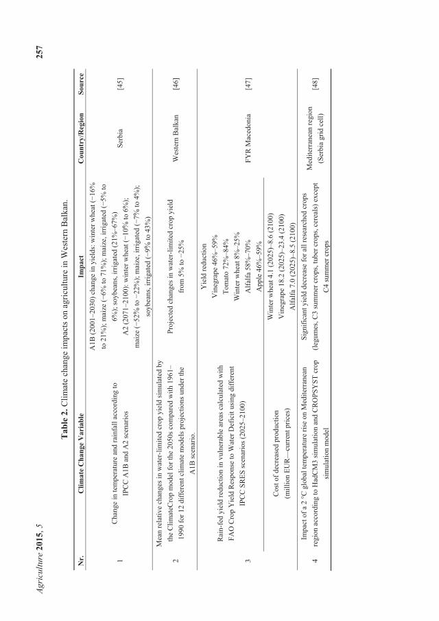
�����
���
�����
�
��
6�.���4D
�$
�!"
�=�'
�"�$
%��!
.�'
���
���
!��"
�'O
".!"
�'6
� G�
'�
��4
��!��� "����,����.��
�!%���
�����0>?�����
������
�D
=�'�
"�'
!"$
%"��
!��"
�'�
���
')�
���
����
'�!�
*:D
D?
�6�
'�?
�.�
"'��
��.
?�6
/��
��P�
���1
�=�
'�"
�'3
�" �
.�#
�'!"
�#
="�!
/��
M
!��
�M1�
$��
@"/
�M!�
C�M
1�$
��@"
���
���!
"�/
M!�
�M1�
.�3
9"�'
.��
����
!"�
/��M
P�CM
1
?�
/��C
�P��
��1�
#�'
!"�
#="
�!/
��M
!��
M1�
$��
@"/
�M
!�
��M
1�$
��@"
���
���!
"�/
CM!�
�M
1�
.�39
"�'.
���
���!
"�/
� M!�
��M
1
-"�
9��
K� L
�
5"�
'�"
�!�,"
�=�
'�".
�'#
�!"�
� �$
�!"�
���
%3�
" �
.�$
� �!
"�9
3
!="
D �
$�!
"D��
%$
��"
)��
!="
�� �
.��
$%�
�"�
#�!=
����
P
����
)��
��
��))
"�"'
!� �$
�!"
$��
" .
%��&
"�!�
�'.
�'�"
�!=
"
?�6
.�"
'���
��
:��
&"�!
"��
=�'�
".�'
#�!
"��
�$�!"�
���
%3�
" �
)��$
M
!�
� M
O
".!"
�'6
� G�
'K�
�L
�
S��
'�)"
�3�
" �
�"��
�!��
'�'
,�
'"��
9 "
��"�
.��
��
�!"�
#�!=
J?
;D
��%
R�"
�S
".%�
'."
!�O
�!"�
(")
���!�
.�'�
��)
)"�"
'!
*:D
D-
S+
-.
�"'�
���.
/��
� P�
���1
R�"
��
"���
!��'
<�'
"���
%"�
�MP
�M
A�$
�!�
C�M
PQ�M
O�'
!"�
#="
�!Q
MP�
M
? )
� )�
QM
PC�M
?%%
"�
�MP
�M
JR
S5
��"�
�'��
K�
CL
D�.
!�)
�"��
"�."
�%�
����
!��'
/$�
��'
+2
ST
����
"'!%
���"
.1
O�'
!"�
#="
�!�
��/
���
1PQ�
�/�
���1
<�'
"���
%"�
Q��
/���
1P�
���
/���
�1
? )
� )�
C��
/��
� 1P
Q�
/���
�1
�
*$%�
�!�
)�
�WD
� �
9� !
"$%"
��!�
�"�
�."
�'5
"��!
"���
'"�'
�"��
�'�
����
��'�
!�E
��D
5�
.�$
� �!
��'
�'�
DS
;:
-R
-A
���
%
.�$
� �!
��'
$��
"
-��
'�)�
��'!
3�"
��
"��"
�."
)��
� �
"."�
��="
���
�%.
/ "�
�$".
D�
.�$
$"�
���
%.!
�9"�
���
%.�
"�"�
.1
"H�"
%!
D�
.�$
$"�
���
%.
5"�
�!"�
��'"
�'�
"���
'
/-"�
9��
����
�"
1
K�QL

������������� � ��5
�4*����0�!%����������� ��!��� "����
A="� �9� �=� "'�".�)���%!�!��'!�� �$�!"�=�'�"�'������ !��"��"$�'3�A="���"�=� "'�"�.
!� %�����" $��" )��� 93 �.�'� ".. �".����". �'�"� �=�'��'� %�����!��' ��'��!��'. �'� #�!= '"!
�"���!��'�'��""'=��."��."$�..��'.K��L�A=""H!"'!�).�.!��'�9 "���%!�!��'�"%"'�.�'!="���%!�,"
��%���!3 G'�# "��" .G� . ��9�.!'".. �) �," �=���. �'� � !"�'�!�,". �".����". �'� �'.!�!�!��'.
���"..�9 "!�"'�9 "�'�"�!�G�'�"))"�!�,"���%!�!��'K �L�+H!�"$"#"�!="�","'!..��=�.�'��"�."�
�'!"'.�!3�)�����=!.)�"I�"'�3�)="�!#�,".="�,3%�"��%�!�!��'","'!.�".� !�'��'!=") ���.�'�
�'�. ��".��"9"��$�'��'��"�.�'� 3$��")�"I�"'!K �L�A="."","'!.=�,".��'�)���'!�$%��!.�'9�!=
=�$�' �,".�'�'�!��'� "��'�$�".�'���""H%"�!"�!���'!�'�"!��'��"�."�'!=")�!��"�)#"��'�!
!�G".�))���"'!��!��'.�+H!�"$"#"�!="�","'!.=�,"!="%�!"'!�� !��","�."�"," �%$"'!%����"..�'�
"'!�"'�=%�,"�!3".%"��� 3�'�"," �%�'����'!��". �G"6E�=����!"��@"�93 �$�!"�.���� .�)"!3'"!.
��G�)���"..!�$��G"!.��%�!� �.."!.���'.���'�"$"�=�'�.$.K �L�6" �##"=��= ��=!�" ",�'!
.�����%� �!��� �'�!"�='� ����� %���"..".!=�!.=�� �9"!="9�.�.)��)��!="�.!��!"���% �''�'��'�
�"," �%$"'!�)'"�"..��3�'.!�!�!��'.�'6E�A="."%���".."..=�� �����"..��"I��!" 3!="%��9 "$�)
� �$�!"�=�'�"�'������ !��"�
)"�"��#�����&���� ����!�(��������
-��'�)���'!��))��� !�".)�� !="������ !��� ."�!�� �'6E���.")��$!=".!�!"F.��'.!�!�!��'� ���"�
�������'� !� #=��= � ".!�9 �.="� "," . �) ��,"�'$"'!T)��$ '�!��'� !� $�'���%� T=�," !="
��!=���!3)��% �''�'��'�$�'��"$"'!�'������ !��"�A=�..��!�)����'�@�!��'�'!="�'"=�'���".
'�!� �#)��!="".!�9 �.=$"'!�))�'�!��'� ������'�!"�'"!#��G.�)�'.!�!�!��'.�'��'!="�!="�=�'�
�! "��. !��''"�"..��3�'���.! 3$� !�% ���!��'.�) �'.!�!�!��'.�) !=" .�$"�� .�$� ����$��'. KQL�
A="�'�'�$��.�!!�!��"�)$�.!."�!��� �'!"�".!����%.�'�'�'���,"�'$"'!� ����'�@�!��'.�.!=�!6E
'""�.�'�!��'� 5�'�.!�3�)?����� !��")��$�!��'�)#=��=#�� ��"%�"."'!�%�..�9 "#�3!�9"!!"�
������'�!"������ !��� %� ���".�'���'.�.!"'!��!��� �!��'�)!="�'!"�".!.�)!="."�!���'�'!"�'�!��'�
�" �!��'. /".%"��� 3 �' !="%���"..�) &��'�'�#�!=+21 �.#" �. "�.�"� ".!�9 �.=�'� !="'"�"..��3
�')��$�!��'.3.!"$.�'��"��.!"�.K�QL�A="������ !��� ."�!���.� �"��3)���'�$�'3�=� "'�".#=��=
#� 9")��!="�"H��"�9�!"�93�'��"�."�)�"I�"'�3�'�.","��!3�)"H!�"$"#"�!="�","'!.","'!�� 3
"���'�!��'��"�."�,� '"��9� �!3�D �$�!"�=�'�"�.�� �9� �=� "'�"#=�.""',���'$"'!� �$%��!.
G'�#. '� 9��'����". �� 9���"�.�;' 3 !=" �'�)�"� .!�'�" �'� ��$$�' %� ��3#� "�� !� "))"�!�,"
������'�!��'�'�=��$�'�.�!��'�'!"�$.�)�$% "$"'!�!��'�)���%!�!��'�'�$�!���!��'$"�.��".�'
������ !��"�'�� �!="�,� '"��9 "."�!��.�
?.."..$"'!�),� '"��9� �!3!�� �$�!"�=�'�"�.�'�$%��!�'!!�� )��!="�'� 3.�.�'�%�"."'!�!��'
�)��!��!�'�!��'� "," #="�"!="����"'!�'�%�!"'!�� ��'."I�"'�".�)� �$�!"�=�'�"��"%�"."'!"�
!�.!�G"=� �"�.�'���',"'�"'!#�3�'�."�,"�.�9�.")��)��!="����%!�!��'%� ��3�"��.��'.K �L�A="
%���"..�)���%!�!��'9"��'.#�!=�'�.."..$"'!�) !="��))"�"'!��$"'.��'.�),� '"��9� �!3�'� !="
��'�"�)%�!"'!�� �%!��'.)����!��'�'� ���'�!="��&�.!�)���!��'�?!�%���#'�%%����=�.�"��,"�)��$
� �9� � �$�!"%��&"�!��'.#=��=�.)��!="���#'.�� "��'��%% �"�!��.."..�"���'� �$%��!.�)� �$�!"
�=�'�"#=� "!="9�!!�$��%�%%����=".�'� ��"!="�',� ,"$"'!�)!="%�%� �!��'�'�.!�G"=� �"�.�)
!=" .3.!"$ �' ��"'!�)3�'� � �$�!"��=�'�" .!�"..". �$%��!. �'� ���%!�," .!��!"��". K �L� *' !"�$. �)

������������� � ��<
������ !��"�.."..$"'!�)������ !��� ,� '"��9� �!3!�� �$�!"�=�'�".=�� � "��!���"'!�)���!��'�)
%��!��� �� 3,� '"��9 "�"���'.�'������� !��� %�����!��'.3.!"$.#=��=.=�� �)��!="� "��!��=���"
�).%"��)�����%!�!��'$"�.��".�'��".����"� ���!��')�����%!�!��'�
6E'""�.!�=�,"!="%� �!��� �'�.��"'!�)��G'�# "��"�'�%�9 ��.�%%��!!����%!!�� �$�!"�=�'�"�
*',".!$"'! �' ������ !��� �"."���= �'� �"," �%$"'! =�. 9""' �"� �'�'� �� .!��'�!�'� �! 9".! !=�.
��"�!�'��G'�# "��"��%9"!#""' �#�'�=��=��'��$"���'!��".K L�*!�.������ !�!�G"� �'��!"�$
.!��!"��� ,�"# �'� !� ��'���! �"."���= �' ���"� !� $""! )�!��" � �$�!" �=� "'�". �'� !� �"," �%
�%%����=".!�)��� �!�!"!��'.)"��)'"#G'�# "��"�'�!"�='� ���".�'!�%���!��� �%% ���!��'�+H!"'.��'
."�,��".=�,"% �3"��G"3�� "�'%��$�!�'������� !��� %�����!�,�!3�'���.."$�'�!��'�)G'�# "��"
�'� !="�� �� " �' %��$�!�'� ���%!�!��' $"�.��". !� � �$�!" �=�'�" #� �"�!��' 3 =�," !=" .�$"
�$%��!�'�" K � CL� A="�")��" �! �. '"�"..��3 !� .!�"'�!="' !=" ��%���!3 �) �'�"��"," �%"� %�9 ��
������ !��� "H!"'.��'."�,��"."'�9 �'�!="$!�!�G" "���'��� "�'!"�$.�).!�"'�!="'�'��''�,�!��'
%���"..9�� ��'� �'G��".9"!#""')��$"�.�'��!="���"'��".�'��'.!�!�!��'� �"," �%$"'!�S"."���=
�'.!�!�!". �'������� !��� �'�,"�.�!�". �. � ���'!�3F. "��"�. �'G'�# "��"�"'"��!��''""� !���"�!"
�'G��". �'� %��,��" ���"�! !��'.)"� �) �')��$�!��' 93 "����!�'� "H!"'.��' #��G"�. �"�����'� !="
��,�'!��".�'�%�!"'!�� !"�='� ���".�'�%���!��".�A=�.��'9"����$% �.="��'��))"�"'!#�3..��=
�.�"$�'.!��!��')�" �.&��'!�"."���=%��&"�!.)�" �!��� .!���'�'�."$�'��.����"K QL�
)"�"�1��!&##�����4���#�*�&��
+))��!.!��"���",� '"��9� �!3!�� �$�!"�=�'�"$�.!�'� ��".!�"'�!="'�'��)���%!�,"��%���!3�'�
�".� �"'�" �) ���� ��$$�'�!�".� -��= .!��!"��". #� "'�9 " )��$"�. !� ��=�"," )��� ."����!3 �'�
�'��"�."�#" �9"�'��'�"�����"'!� �$�!����'��!��'.�'�#� ���"�! 3��'!��9�!"!��'��"�.�'�!="��
�9� �!3!���%"#�!=)�!��"�'�"�!��'!3�5��"%�����!�,"�'��".� �"'!������ !��"�"I���".�$�&��.=�)!
�'!="#�3 �'�#�!"�.�� '�!��"'!.�'��"'"!���".����".��"$�'��"�!�"'.��"!=�!!="."�".����".
��"�."�$��""))���"'! 3�'�.�.!��'�9 3K �L�5�G�'�!=�..=�)!#� �"I���"��'.��"��9 "�=�'�".�'
'�!��'� �'� ��� ��,"�'�'�" "��. �!��' %� ���". �'� )�'�'��� $"�=�'�.$.� A=" " "$"'!. �) !=�.
��!"����@�!��'�'� ��"$"�=�'��� 9�� ����� �="$��� ����'�$��9��!"�='� ����� �'��')��$�!��'�
�''�,�!��'.K��L�:�����!��'!=�!�.$��""))���"'!�'���"�!".$��"�%%��!�'�!�".�'����"..!�9����"�
$��G"!. ��' 9��.! .$� =� �"�.F �".� �"'�" �'� ��"�!" .�.!��'�9 " �," �=���. #=� " =" %�'� !� $""!
���#�'��"$�'�)��)����
("," �%$"'!�)'"#=��=3�" ��'� �'%�!�."�"))���"'! �9��!���'�9��!�� .!�"..��".�.!�'!,���"!�".
#�!= "'=�'�"� !���!.9"!!"� .��!"� !� ���%! !� � �$�!" �=�'�" �. ������ )�� ������ !��� ���%!�!��' !�
� �$�!"�=�'�"�?�!�,�!�".�'��"."���=�'% �'!�"'"!���".����".�'6E.!��!"�����'�"��=!�".�) �.!
�"'!��3#�!=�'�%��&"�!�� "�!="UN"'"6�'G�)R���. �,��V�2')��!�'�!" 3$�.!�)!="����$"'!.
)��$ !=�! %"����#"'!$�..�'���#"�"�".!��3"�����'� !=" �.!#���?�!�,�!�". .��= �.�/� �� �'����&� ���',"'!��3�'���'."�,�!��'�)% �'!�"'"!���".����".)�������� !��"=�,"9""'�".!��!"�����'�
!=" 9"��''�'� �) !=�. �"'!��3 #�!= !=" =" % �) �'!"�'�!��'� ��'��. K��L� ?)!"� !=" �',"'!��3 �'�
��"'!�)���!��'�) ��� �"'�!3%". !="'"H!.!"%.=�� �9" �'G�'�!="." "�!��'%���"..#�!=!="�!="�
.!�G"=� �"�.93"$% �3�'�%��!���%�!��3!"�='�I�".�'���"�!��$%��,"!=""))"�!�,"'"..�'��$%��!�)
������ !��� �"."���=�E�,�'�)��$"�.�'��!="�.!�G"=� �"�.�',� ,"��'!="�"," �%$"'!�),���"!�".
������������� � �3�
!=����=%��!���%�!��3% �'!9�""��'�K����L$�3 "��I���G�'���.!�"))"�!�,"%�����!��'�)'"#9�""�.
�'�,���"!�".�)���%.���%!"�!� ��� '""�.�
O"�!="� �'� � �$�!" �')��$�!��' .3.!"$. �'� ���'� "�� 3 #��'�'� .3.!"$. ��$ !� �"���"
,� '"��9� �!3 �'� �$%��," �".%�'."��%���!�".�) !=�." �! ��.G93 �'��"�.�'� !="�� %�"%��"�'".. K��L�
:��$%!��"'!�)���!��'�)���.G�'���$$�'���!��'��'"'�9 "!�$" 3�".%�'.".�'��..�.!�')��$ ","
���%!�!��'� J��$"�. .=�� � �." %�"."'! �'� )�!��" � �$�!"��" �!"� �')��$�!��' !� % �' �'� $�'��"
#"�!="� ��.G.$�H�$�@"%�����!�,�!3�'�$�'�$�@" !=""',���'$"'!� �$%��!.�) )��$�'�%���!��".�
*')��$�!��')��$!="'"!#��G�)�����$�'�!���'�.!�!��'.��$9�'"�#�!=�"$�!" 3."'."��')��$�!��'
"'�9 " !="�"," �%$"'!�)9��%=3.��� $��" .�."� !�".!�$�!"#"�!="���'��!��'..�� �'�'�!��"'!
.!�!�.���%#�!"�'""�..�� "��.��'%".!�'���."�.""$"��"'�"�=���"�)���%,���"!39".!.��!"�)��
��� ��'��!��'.����"K� L�A="�")��".!�"'�!="'�'��)!"�='� ���".=�$�'�".����".�'��"," �%$"'!
�)$�'�!���'�#��'�'��'�)��"��.!�'�'"!#��G.�" �!"�!�=3��� ����� $"!"��� ����� � �$�!���'�
"',���'$"'!� ��.G..=�� �9"��'.��"�"��.�'"�)!="%�����!�".�
N �9� � �$�!" �=�'�" #� ��'!�'�" !� "�� !�#���. .��'�)���'! �=�'�". �' �''�� %�"��%�!�!��'
%�!!"�'. �' .��!=�"�.!"�' +���%"� *' .��= �����$.!�'�". ������!��' ��' �"�!��' 3 9" �'" �) !=" G"3
$"�=�'�.$.�)���%!�!��'�'������ !��"�A="�""H�.!.'��,�� �9 "��!��'������!"���"�.�����%.�'6E�
A="!�!� ������!"���"��������'�!��'�))���� ��!��.�' 3���M�)���9 " �'�#=��=�.��'.��"��9 3
"..!=�'�''"��=9����'����'!��".".%"��� 3+2K��L�*'!=�..�!��!��'������!��'�.�$"�.��"!=�!��'
�"���" !=" %��9 "$. �) ���!��� �����=! %"����. 93 �$%��,�'� �'� .!�9� �@�'� 3�" �.� (�" !� !="
����$"'!"�#�!"��")���!.�'�!="���#�'��'���"'�".�)�����=!������!��'.=�� �."!! "����'���M
�''�� #�!"�'""�.)��% �'!.�'.��!=��M�''��!=�'�QM�'�"'!�� 6EK�CL�A="."'""�.#� �'��"�."
)��!="��������'�!�)�!��"� �$�!"%��&"�!��'.)��6E#=��=�'� ��""H!"'.��'�),"�"!�!��'%"����
�'��"�."�)�"I�"'�3�)"H!�"$"!"$%"��!��".�'� �'�"�)��.!�)�""%"����. "���'�!�����!��'� �'��"�."
�'",�%�!��'.%���!��'�'��"���"�.�� $��.!��"��'!"'!K���QL�A="������ !��� ."�!��'""�.!=".�%%��!
�'����%"��!��'�)�!="�."�!��.�'���"�!��%"��!"�'�.�.!��'�9 "$�''"��'�)� �#!="%��'��% ".�)
�'!"���!"�#�!"�$�'��"$"'!�:�9 ���'�%��,�!"�',".!$"'!.�'������!��'#�� �"'�9 "!=""H%�'.��'
�) ������!"� ��"�. �'� ������!��'�." �. � .�%% "$"'! !� ���'�)"� ������ !��" �' ���"� !� .!�9� �@" �'�
�'��"�."3�" �.�
�4 ����������
O"=�,"�",�"#"�!="������ !��� ."�!���'6�.'���'�E"�@"��,�'��'�!=" �G" 3�$%��!.�)� �$�!"
�=�'�" �%�' �!� O" =�," � .� %��%�."� %� ��3 �%!��'. !� �%!�$�@" �%%��!�'�!�". �'� $�!���!"
��'."I�"'�". �) � �$�!" �=�'�"� O" ��'� ��" !=�! 6E �. � ���'!�3 ���= �' '�!��� �".����". �'�
9����,"�.�!3 �'� ���"%��!.�) !=" ���'!�3%�..".. � )�,����9 " � �$�!" )�� ������ !��� %�����!��'�
E�#","��".%�!".��="'��#$"'!.!="������ !��� ."�!���.=�$%"�"�93 �#%�����!�,�!3"H!"'.�,"
)��$�'� %���!��". �'� !"�='� ���". �����"� ��! �' .$� �'� )���$"'!"� )��$.� A=�. �. )��!="�
"H��"�9�!"� 93 � #"�G �'� �'"))���"'! �������' %� ��3 �'� "��. �!��' �# 9���"! � ���!��'. )��
������ !��"�'��"I��!"$��G"!���"..�'���"'"�� ��G�)�')��$�!��'�'�G'�# "��"�
A=" "���3 �) !=" %�.! .�����%� �!��� .3.!"$ �'� !=" ����"'! ��$% "H %� �!��� .!���!��" =�,"
.��'�)���'!��'."I�"'�".)��!="������ !��� �"," �%$"'!�?����� !��"�.=��= 3,� '"��9 "!�� �$�!"
�=�'�"�E��="�!"$%"��!��".�'��=�'�".�'%�"��%�!�!��'��"�"����'����%3�" �.�'��'��"�.�'�!="

������������� � �3�
�G" �=����).=��!�!"�$���%)�� ��".�'� �'��!"�$%�����!��'�"� �'".�6�.'���'�E"�@"��,�'��.#"
�. �!="� 5"��!"���'"�' ���'!��". �' .��!="�' �'� .��!=�"�.!"�' +���%" ��" "H%"�!"� !� "H%"��"'�"
.��'�)���'!������ !��� %�����!��' �..".�?.����'!�3!=�!�.�%�!"'!�� ��'����!")��!="+2�$"$9"�.=�%
6E'""�.!��$% "$"'!�")��$.�'!="������ !��� �'����� �"," �%$"'!."�!��.�'���"�!��"���"!="
.��'�)���'!%� ��3��%��$%��"�!��!="�+���%"�'���'!��".�*'���"�!���%"#�!=!="�=� "'�".�)
� �$�!" �=�'�" �'� � �$�!" ,����9� �!3 �! �. �$%"��!�," !� ���." !=" %� �!��� �#��"'".. �'� �'��"�."
�"���'�!��'�'� ��,"�'$"'!� "," .�9��!!="�$%"��'�!=�"�!.�)� �$�!"�=�'�"�'!="������ !���
."�!���A=" �!"��!��"�'� �$�!"�=�'�"�$%��!.�'�,� '"��9� �!3�'!="������ !��� ."�!��.!�"..".!="
�$%��!�'�"�)���%!�!��'�'����"'�3!��$% "$"'!���%!�!��'�'�$�!���!��'$"�.��".�A="�"�"'! 3
%�9 �.="�D �$�!"D=�'�"?��%!�!��' �'�4�#�+$�..��'("," �%$"'! -!��!"�3 )��6E .=�#. !=�!
!="�" �. � %� �!��� #� !� 9�� �'"�"..��3 ��%���!�". �'�%� ���". !�#���. �#�"$�..��' �'� � �$�!"
�".� �"'!�"," �%$"'!�O"����".."�.�$"�)!="�" ",�'!.�����%� �!��� �'�!"�='� ����� %���"..".
!=�! .=�� � 9" !=" 9�.�. )�� )��!="� .!��!"��� % �''�'� �'� �'.!�!�!��'. !=�! ��" '""�"� !� ��"�!" !="
��%���!3 !� ����".. � �$�!" �=�'�" �' ������ !��" ������ !��� �"," �%$"'! G'�# "��" !��'.)"� �'�
�$% "$"'!�!��'�5�.!�)!="$�"I���".��'�)���'!)�'�.�'�!�$")��!="���$% "$"'!�!��'�E�#","��!
�.�' �G" 3!=�!!="������ !��� ."�!��� �'"#� 9"�9 "!���%"#�!=!="%���"..�)���%!�!��'�;' 3!="
�"," �%$"'!�)�)�,���9 ""',���'$"'!!��"!="�#�!=%� �!��� �'.!�!�!��'� "��'�$��.���� �'��!="�
��!��.#� "��!��.���"..)� ������ !��� ���%!�!��'!�� �$�!"�=�'�"�
�@��1����!����
A=�..!��3 �..�%%��!"�93 !="%��&"�!U?����� !��� ?��%!�!��' !�D �$�!"D=�'�"T0"!#��G�'�
+����!��'S"."���=�'�+H!"'.��'�'!="O".!6� G�'.V)�'�"�93E+S(T:�����$$")��E��="�
+����!��'S"."���=�'�("," �%$"'!����P�����
-%"��� !=�'G. !� 5" �.� 4&�.� )��$ !=" J��� !3 �) ?����� !��" �'� J��� -��"'�". 2'�,"�.�!3
�) -���&",� )�� %��,���'� ,� ��9 " �'.��=!. �' !=" =�.!��3 �) ������ !��� �"," �%$"'! �' 6�.'��
�'�E"�@"��,�'��
A="��!=��.#�� � �G"!�!=�'G!="�'�'3$��.�",�"#"�.)��!="��=" %)� �'���'.!���!�,"��$$"'!.�
������������������
A="��!=��.�"� ��"'���') ��!�)�'!"�".!�
?���������
��� 6���G.0��?��"�O�0��>" 3:�5�A="�"!"�$�'�'!.�),� '"��9� �!3�'����%!�,"��%���!3�!
!="'�!��'� "," �'�!="�$% ���!��'.)�����%!�!��'�5#�"�.&���#&"�(!�&�"������ � �P����
��� >�")!-��+�G.!"�'(�5#���(�*������ %�2&��/����)�N"�$�'#�!�=�6�''N"�$�'3�����
��� 20JDDD�-"��'�0�!��'� D�$$�'���!��'�)6�.'���'�E"�@"��,�'��'�"�!="2'�!"�0�!��'
J��$"#��GD�',"'!��'�'D �$�!"D=�'�"/-0D6*E1�?,�� �9 "�' �'"�=!!%���###�9���'�%�����
��'!"'!�9�.'��Z�'�Z="�@"��,�'��"'�=�$"� �9���3�"',���'$"'!Z"'"��3�.'�9�=������=!$
/���".."��'�Y� 3����1�

������������� � �3�
��� -$�!6��-G�''"�5�O�?��%!�!��'�%!��'.�'������ !��"!�� �$�!"�=�'�"�?!3%� ��3������"������"�+������"�5#�"�(!�&�"�����-Q P����
�� +��G."' -�� ? ��'�" :�� 6�=�'�%�!� D�-�� 5��!�'. S�(�?�� 5� ")" Y�*�� 0="$��="'� D��
; 6��"'>��; ���')"$�J��:��GY��-3�'�4�������"O="''�!","�3�".%�'."!�� �$�!"�=�'�"
�.������'"�*�"'!�)3�'�%��'��% ".)��.�.!��'�9 "���%!�!��'�(�*"�4��"�����'CP���
34� -��!=+�.!+���%"�'J���$�'D �$�!"D=�'�"?��%!�!��'/-++JDD?1�(�*����6&���������� � *�&���+������-++JDD?�6" ����"-"�9�������
C�� D�.!�,��E��(&�G��5��4&�.�5��[���,"�;�+))"�!�)� �$�!"�=�'�".�'������ !��"�)!="
#".!"�'6� G�'���'!��".�'����%!�!��'%� ���".������"��#�"����� 0��CP����
Q�� J"�"�� 5�'�.!�3 �) ?����� !��" O�!"� 5�'��"$"'! �'� J��".!�3� ����*� ���*� ����#�*�&�� ��������#3���������� ���#���&���������#&�#3�7# &����&��8��9��#��&��3#�����):���0�J"�"��
5�'�.!�3�)?����� !��"O�!"�5�'��"$"'!�'�J��".!�3�-���&",�6�.'���'�E"�@"��,�'������
��� >�$9"��,� E�;.'�,'��9� &"\&���@,�&����]!,��6�.'��E"��"��,�'������ ���� �� � #�� �+���*"��#��;� ���<<5'�� �P�C��
���� N� � 6�6�.�'.G�="��"��,� G�"G�'�$�&���[?<0;6*E����(�3!�'�������*��#3�+���&�� ��&����� �#3�7# &����&��8��9��#��&�<�+���"���"�����'-���P�CC�
���� >�$9"��,� E�>���G!"��.!�G"���]!,��6�.'��E"��"��,�'�'"%�.�"�'�'�G�'������.,&"!.G��
��!�������*��#3�+���&�� ��&����� �#3�7# &����&��8��9��#��&�<�+���"���"����'-���P��C�
���� >�!@ <� (��]!,"'� � "G�'�$.G� ��@,�& 6�.'" � E"��"��,�'" /��� P�� �1� *'.!�!�! @� �.!���&��
-���&",�6�.'���'�E"�@"��,�'���������� -�$�'(�("," �%$"'!�",�.�!"��A=�'G�'��9��!%���!���'��'�!"��=�'��"," �%$"'!�)!"�!="
D� � O��� *'4���#�*�&�� � � 1!�#��� �&������������(���&�� ��� ������� � #&�4���#�*�&�� �&��4���#�*�&�� (##������#&� -�$�' (� 0��$�' ?� +�.�� S��! "��"� 4�'��' 2> ����
%%��CP ��
���� 0��G�,� S�(�.!��9�!��' �) �'��.!�3 �'6�.'�� �'�E"�@"��,�'��5� &�%�=�+�>#�������50
�CP���
� �� 5��&�'� -� :� &�%��,�"�'� ["$ &�]!" � (��]!,"'�$ : �'� S"%�9 �G" +��;��#��&;�� #� 1�*��=�*;�?��� � ��# �#�&#*� ��&� +�� 7�8� :� &�%��,�"�'� J�G� !"!� -���&",� 6�.'�� �'�
E"�@"��,�'���Q��
���� -" �G<�:�!��\'&�=��'"�@"$ &�]'�%��.!���-S6�E<�+��;��#��&;��#�1�*��=�*;�?������# �#�&#*���&�+��7�8�:� &�%��,�"�'�J�G� !"!�-���&",�6�.'���'�E"�@"��,�'���Q��
�C�� 5���'G�,� N� -!,���'&" ��\�,'" � ���]!,"'" .,�&�'" '� %���� &� -�9�&" � 9�,]" Y���. �,�&"�
=�#�&�%����#���5�� ��"���%������������� P��C�
�Q�� 5�@�G A� ? .'�%.=�! �) #".!"�' 6� G�'F. ������ !��" )��$ !=" %"�.%"�!�," �) +2 ���"..��'�
+��"������"�.�#&"�������)��P�Q�
���� :� &�@ <� .% #� � �#;#�������&�%�� D"'!�� @� .���� ���&� ." � ����� � %��.!��� *'.!�!�!� @�
���]!,"'��.!��\�,�'&�-,"� � �]!��[���"9��[���"9R���. �,����CC�
���� ^�$9�"GA������&���#���%�@�9����&���������&;��?���'�$.G� )�G� !"!-,"� � �]!��[���"9��
[���"9D���!�����Q�
���� *,�'G�,��5��6�&'"�-��>� "��?��-" �G<�+��'�$���'�.���� �� "�)������ !��" �' !="
J"�"��!��'�)6�.'���'�E"�@"��,�'��A"�5�&"�+#�"�2 � ����3� �Q�PQ �
������������� � �3;
���� 5�'�.!�3�)J��"��'A���"�'�+��'�$��S" �!��'./5�JA+S1�������������#���3#��7# &����&��8��9��#��&��3#�������5�'�.!�3�)J��"��'A���"�'�+��'�$��S" �!��'./5�JA+S1�-���&",�
6�.'���'�E"�@"��,�'������
�;4� +���%"�'6�'G)��S"��'.!���!��'�'�("," �%$"'!/+6S(1�1��& ���#&����#������'�?,�� �9 "
�' �'"� =!!%���###�"9�����$�'"#.�%�9 ���!��'.�!��'.�!��'��"%��!�!��'.�!��'��"%��!������=!$
/���".."��'C;�!�9"�����1���� ?�"'�3 )�� -!�!�.!��. �) 6�.'�� �'� E"�@"��,�'� /6E?-1� 7# &��� �&�� 8��9��#��&�� �&��
3���� B+���� �����7���&�?�"'�3)��-!�!�.!��.�)6�.'���'�E"�@"��,�'�/6E?-1�-���&",�
6�.'���'�E"�@"��,�'������
� �� ?�"'�3)��-!�!�.!��.�)6�.'���'�E"�@"��,�'�/6E?-1�-!���!��"�)������ !��� �'��'6�.'��
�'�E"�@"��,�'�"�2'%�9 �.="���!��,�� �9 "�'�"I�".!�-���&",�6�.'���'�E"�@"��,�'���������� ?�"'�3)��-!�!�.!��.�)6�.'���'�E"�@"��,�'�/6E?-1�8���� ��������<��#�����#����#&��&��
�����#3�*��&���#� <�+���� �����7���&�?�"'�3)��-!�!�.!��.�)6�.'���'�E"�@"��,�'�/6E?-1�
-���&",�6�.'���'�E"�@"��,�'������
�C�� 5�'�.!�3 �) J��"��' A���" �'� +��'�$�� S" �!��'. /5�JA+S1�(#*��������&� � � � *�&�� #3��!���� ����� �&� � ���@�!��& � �&� 7# &��� �&�� 8��9��#��&�� ?'!"&� +DN� 4&�9 &�'�
- �,"'�������
�Q�� N�""'D��'�� �. ���� !*�&��#3��!��7�8���&� ����#3���������<�3##���&������4���#�*�&���&��#�!���+������ �� �������#3���!����&����#&#*�����#��� �3#��7�8��&��!��.C��&�������#&���#�� �N�""'D��'�� �-���&",�6�.'���'�E"�@"��,�'������
���� J?;-A?A�D�$%��" ��!� !�� T:�����!��'�?,�� �9 " �' �'"� =!!%���)��.!�!��)���������$%��"�+
/���".."��'Q("�"$9"�����1�
���� ? �9"��,���N�9��-��D�,��E��D"'���-��5���!�,��-��(@�$9�+�+))"�!�)#"�!="���'��!��'.
.!��"�)% �'!���#!=�'�0�%% ���!��'�'3�" ��'�I�� �!3�)���.. �'��'6�.'���'�E"�@"��,�'��
*'$�&�� �� � ��* ��&���� �&���#*�&���������#& "���#�����&� �#3��!�����!�5�&���������&��#3��!��.�#���&�5�� �&����������#&4�@"�'-#�!@"� �'���P��Y�'"����%%�Q�CPQ���
���� +���%"�' D�$�..��' /+D1� 7# &��� �&�� 8��9��#��&�� �#&���� ���#��� ?���!��.. N$9E�
N"�$�'3�����
���� O�� �6�'G���������� ���#���#����&#���3#��7# &����&��8��9��#��&�B1������&���&�������#&��#����&#�� �O�� �6�'G�O�.=�'�!�'(D2-?�����
���� 20JDDD�2&�����D���#&��(#**&�����#&�#3�7# &����&��8��9��#��&��&�����!��C&�����D���#&����*��#�%�(#&��&��#&�#&�(�*����(!�&���E2D(728F�5�'�.!�3)��-%�!�� : �''�'�D�'.!���!��'
�'�+�� ��3�)S"%�9 ���)-�%.G��6�'&�4�G�6�.'���'�E"�@"��,�'������
���� E��@��-��5��G�,��5��D�.!�,��E�(����=!��'��!��'.�'�$�'��"$"'!.!��!"��".�'6�.'��
�'� E"�@"��,�'�TD�'��." ���'!�3 �"%��!� ?,�� �9 " �' �'"� =!!%���###���.��'#�!"��������.�
% ���')� "�%=%� �Q�$��Z%��"���'!"'!�C��6�.'��ZE"�@"��,�'�ZD��'!�3S"%��!�%�)/���".."��'��
-"%!"$9"�����1
� �� [���,"�Y��D����-�D �$�!"�=�'�".!="'""��'��$%��!�'�"�)���%������!��'�''��!="�.!"�'
6�.'���'�E"�@"��,�'��*':���""��'�.�)!="��.!-��"'!�)���+H%"�!D�')"�"'�"�'?����� !��"
�'� J��� *'��.!�3 0"�$ 6�.'�� �'� E"�@"��,�'� �� -"%!"$9"� ����T� ;�!�9"� � �����
%%�C� PC���
������������� � �3�
���� *'!"�'�!��'� J�'� )�� ?����� !��� ("," �%$"'! /*J?(1� +',���'$"'!� �'� � �$�!" �=�'�"
�.."..$"'!T6�.'�� �'� E"�@"��,�'�� ?,�� �9 " �' �'"� =!!%���###��)�������� �$�!"��".����".�
=!$/���".."��'C-"%!"$9"�����1
�C�� +���%"�' D�$�..��' /+D1� 6�.'�� �'� E"�@"��,�'� �"��,"�3 '""�. �.."..$"'! ) ���. ��P��
5�3T+H"��!�," .�$$��3� ?,�� �9 " �' �'"� =!!%���"��"���%��"��"' ���"$"'!�%�)�%�"..Z���'"��
) ���.��'��"H"��!�,"�.�$$��3�%�)/���".."��'��-"%!"$9"�����1�
�Q�� >���G� �.���3� :�� S�."'!=� -� D �$�!" D=�'�" �'� ?����� !��"� ? S",�"# �) *$%��!. �'�
?��%!�!��'.� (�*���� (!�&��� +���� � ��"� .&���#&*�&�� 4�����*�&�� ����� �� O�� � 6�'G�
O�.=�'�!�'(D2-?����;����� 0" .�' N�D�� S�."���'! 5�O�� >�� Y�� S�9"�!.�' S�� -� ."� A�� [=� A�� S�'� "� D��
5.�'��-��:� �@@�?��6�!G�5�D �$�!"D=�'�"�*$%��!�'������ !��"�'���.!.�)���%!�!��'�
*'!"�'�!��'� J���:� ��3S"."���=*'.!�!�!"O�.=�'�!�'(D2-?�����
���� ? ��$�Y��5��"'�Y�5��0�,_G36��6�'��5��D���9�,S��(",�3S�Y�0��N��''�G�%�� �.D��
5��!�'+��; "."'Y�+��-=,��"'G�?�+���%"�*'(�*����(!�&������-��2*���� <���������#&��&��6&��������"� (#&������#&� #3� G#�%�&�� 5�#�� 22� �#� �!�� �#��!� � � *�&�� ���#��� #3� �!��2&����#���&*�&��� ��&�� #&� (�*���� (!�&��� :���3 5�4� D�'@��'� ;�J� :� �!�G�) Y�:�
,�' �"� 4�'�"' :�Y� E�'.�' D�+� +�.�� D�$9����" 2'�,"�.�!3 :�"..� D�$9����" 2> ���C�
%%� ��P Q��
���� -$�!6��:� �)�.�,�;�?��%!�!��'!�� �$�!"�=�'�"�'!="��'!"H!�).�.!��'�9 "�"," �%$"'!�'�
"I��!3�+ ���&"�4��"����;0��
���� A=��'!�':�>��Y�'".:�N��? ����.#�$3N��?'��"."'Y�-%�!�� ,����!��'�)���%3�" ��".%�'."
!�� �$�!"�=�'�"�'"�.!?)�����5#�"�.&���#&"�(!�&�"����<�� �P� �
���� 6`� S�� S��=� �='"&�� +�� S�=$�' >�� ?99�.%��� >�D�� 4"=$�'' ?� D �$�!" �=�'�" �'�
������ !��� #�!"��".����".�?,� '"��9� �!3�.."..$"'!�)!="6 ��G-"���!�=$"'!�.&���#&"�+��"��#��������), CP���
���� D��'�� �)5�'�.!"�.�)6�E�D �$�!"�=�'�"���%!�!��'�'� �#�"$�..��'�"," �%$"'!.!��!"�3
)�� 6�.'�� �'� E"�@"��,�'�� ?,�� �9 " �' �'"� =!!%���###�9���'�%�������'!"'!�9�.'��Z�'�Z
="�@"��,�'��"'�=�$"� �9���3�"',���'$"'!Z"'"��3�� �$�!"��=�'�"����%!�!��'��'�� �#�"$�..��'�
�"," �%$"'!�.!��!"�3��/���".."��'�?���.!����1�
� �� 5�=�� �,� (�A��4� � 6��(�"]G�,� 0��5�$� N��(&���&",� <��Y�' � 5�D �$�!"�=�'�"
"))"�!.�'���%3�" �.�'-"�9���'��" �!"�.=�)!.�)>a%%"'� �$�!"@�'".�'�"�!="-S+-�?�6
�'� -S+-�?�� ?,�� �9 " �' �'"� =!!%����' �'" �9���3�#� "3���$�������������&���������9.!���!
/���".."��'��-"%!"$9"�����1�
���� *� ".��. ?�� b������ -�� (�@ ?� 4��G�'� �'!� !=" )�!��" �) ������ !��" �' � �=�'��'� � �$�!"�
.�"����"������"�.�#&"�����'0��CP��C�
�C�� A="S"���'� +',���'$"'!� D"'!"�)��D"'!�� �'�+��!"�'+���%"/S+D1�A="�$%��!.�)� �$�!"
�=�'�" �' )��� %�����!��' �' !=" #".!"�' 6� G�' �"���'� ?,�� �9 " �' �'"�
=!!%�������$"'!.��"������!�%�����"�.�*$%��!.�� �$��"��=�'�"�)����%�����!��'�%�)/���".."��'��
-"%!"$9"�����1
�Q�� N��''�G�%�� �.D��6�'��5��5����'��5��4"-��"�:��A�'A�D �$�!"�=�'�"�$%��!.�'!="
$"��!"���'"�'�".� !�'�)��$��WD� �9� !"$%"��!��"��."�OOJ�N �'�-#�!@"� �'���� �

������������� � �3�
���� 4399"�!A�Y��-�$'"�(�?�?����� !��� !"�='� ���".)��� �$�!"�=�'�"�'�"," �%�'����'!��".�
:� ��3�%!��'.)���''�,�!��'�'�!"�='� ��3��))�.��'��##���#��������'-���P����
��� *:DD�(�*����(!�&������-��+�&�!� � ����#��"�(#&������#&�#3�G#�%�&��5�#� �2<�22��&��222��#��!���#��!�� � *�&�����#���#3��!��2&����#���&*�&�����&��#&�(�*����(!�&��<�(#���G����&��1��*�
:��=����S�>�S"�.�'�"�?�+�.��*:DD�N"'",�-#�!@"� �'����C�%�����
��� *:DD�-%"��� S"%��!T5�'���'�!="S�.G.�)+H!�"$"+,"'!.�'�(�.�.!"�.!�?�,�'�"D �$�!"
D=�'�"?��%!�!��'�D�$9����"2'�,"�.�!3:�"..�0"#R��G0R2-?�����
��� -="%="��?��5�!�=" A��4"#�.>��4"'=���!?��Y�'".4��-��!!4�5����O���S������#����5�#����!��#3�4� � ��� <��#�������&��(�*����./���*� ��&���'��;(*�4�'��'2>�����
��� Jc.." E��5��> "�'S�Y�A�D �$�!"�=�'�",� '"��9� �!3�.."..$"'!.�?'",� �!��'�)��'�"%!��
!=�'G�'��(�*"�(!�&�"����3- ���P����
��� ("..��-��E� $"5�(�".� �$�!"���%!�!��'%� ��3'""�%��9�9� �!�".d(�*"��#��������)
��CP��Q�
�� 6"���'�!�' Y�� ?.���@@�$�' 5�� D ��G 5�� 6�"$��'!@ ?�� N�� �� 5�� Y�=' 5�� 4�' +��
5�$�A��0"���D��0�9�"D�������"A="�� ")��.��"'!�.!.�'!��G �'�)����'."����!3�'�� �$�!"
�=�'�"������"��##��+���"���������
��� 5�%�'3�:��5%�'�" �-�A="�� "�)"H!"'.��'."�,��".�'� �$�!"�=�'�"���%!�!��'�'4�$%�%�
%��,�'�"-��!=?)�����A"������"�./�"����"�4��"����; ��CP����
C�� 6�3�'+��("�"..�A�A��N9"!�9���N�?��S�'� "�D�?��%!�!��'!�� �$�!"�=�'�"�'+!=��%��
�'�-��!=?)�����;%!��'.�'���'.!���'!.�.&���#&"�+��"��#�������<�����P����
Q�� J?;���&���*�&��#3������������ ����!����1���&�&����&�"��#���0���� ����!@./��& �#&�$�&%����J?;�S�$"*!� 3�<<�
��� J?;�D �$�!"�.$��!������ !��".����"9��G�?,�� �9 "�' �'"�=!!%���###�)�������� �$�!"�=�'�"�
� �$�!".$��!�"'�/���".."��'��0�,"$9"�����1�
���� -�'��'�(��[� 9"�$�'(�A="������ !��� �''�,�!��'%���"..�S"."���=�'�!"�='� ��3���%!��'
�'��=�'��'������� !��� ."�!���8�&��"������"�.�#&"��������CP����
���� J?;�(#&�������#���#&��!��+�����#3���&��5�&������� #��� �3#���##���&����������B7# &����&��8��9��#��&��J?;�S�$"*!� 3�����
���� O�!��$9" Y�S�� Y�.=�>�(��N3�#� � -��5�.�?�5�� Y�=�'."'D��<��G(�-�� -!=�%�!6�S�
:��!���%�!��3 % �'! 9�""��'� �. 9"!!"� �".���9"� �. =��= 3 � �"'!����"'!"� % �'! 9�""��'�� *� J���
�'����!��.�)� �"'!����"'!�!��'�'% �'!9�""��'��./�"������"�����)����P����
���� 59� D�� N��$���". +�� N=�.= >� S"����"'!�'� ���% �$%��,"$"'! )�� !=" �=�'��'� � �$�!��
��'��!��'.�)!="��.!�"'!��3������"��##��+���"�������C�
���� E����!=Y�S��D�$%9" (��O�'�" Y�?.."..�'�=�$�',� '"��9� �!3!�� �$�!"�=�'�")��$�'
",� �!��'��3%"�.%"�!�,"�*'�����&��4� � �����.����G��&�&��+� ��* �3#��(�*����(!�&���-�'�=
?�[�$$"�.[�+�.��-%��'�"��0"!="� �'�.�����%%���PQC�
� �� O"�.. ?�� <�' D��#�"� 4�� 6"�'���� 5� D�$$�'���!�'� ����$"!"��� ����� �')��$�!��' !�
)��$�'���$$�'�!�".������"��#�"�����#�#"�������'�Q P����
���� -�"9"�! -�� (a :�� E���",""' Y�� J���". Y�5�� J�"'G"' >�� J"��G -� ("," �%$"'! �'�
,� ���!��'�)!="� �9� $�%�)������!��'��"�.�8���#"�.���!�+� �"�+��"������ � P �C�
�C�� < �=�'�� 5� E3��� ����$� �!��' ������ !��" �'� �'� �'� #�!"� $�'��"$"'! �' 6�.'�� �'�
E"�@"��,�'��6#�����*�������-��P�C�

������������� � �33
�Q�� 6�@@�@J��-�$9��"GO�N �9� � �$�!"�=�'�"�'������� !��� %�����!��'�(��"�!�'��'���"�!
"))"�!.�) �=�'��'�=3��� ����� %"�� ����� �'�% �'!%=3.�� ����� %���"..".�J?;�'� Y�='
O� "3e-�'.�4�'��'2>�����
f ��� 93 !=" ��!=��.� ��"'."" 5(:* 6�." -#�!@"� �'�� A=�. ��!�� " �. �' �%"' ���".. ��!�� "
��.!��9�!"� �'�"� !=" !"�$. �'� ��'��!��'. �) !=" D�"�!�," D�$$�'. ?!!��9�!��' ��"'."
/=!!%�����"�!�,"��$$�'.����� ��"'.".�93�����1�

PAPER 2
Žurovec, O., �adro, S., Sitaula, B.K. (2017)
Quantitative assessment of vulnerability to climate change in rural municipalities of
Bosnia and Herzegovina.
Sustainability, 9(7): 1208
� �

sustainability
Article
Quantitative Assessment of Vulnerability to ClimateChange in Rural Municipalities of Bosniaand Herzegovina
Ognjen Žurovec 1,*, Sabrija Cadro 2 and Bishal Kumar Sitaula 1
1 Department of International Environment and Development Studies, Norwegian University of LifeSciences (NMBU), Universitetstunet 3, 1433 Ås, Norway; [email protected]
2 Faculty of Agriculture and Food Sciences, University of Sarajevo, Zmaja od Bosne 8, 71000 Sarajevo, Bosniaand Herzegovina; [email protected]
* Correspondence: [email protected]; Tel.: +47-67-231-344
Received: 6 June 2017; Accepted: 8 July 2017; Published: 10 July 2017
Abstract: The rural population in Bosnia and Herzegovina (BH), which constitutes more than halfof the total population, experienced serious incidences of extreme weather events in the past twodecades. This part of the population is vulnerable to climate change due to significant dependence onagriculture as a climate-sensitive livelihood option. However, the source of their vulnerability is duenot only to the extent and magnitude of these extreme climate events, but also to the internal statuswithin the vulnerable systems before the occurrence of such events. In order to explore the differentdimensions of vulnerability, we used a set of 20 indicators to quantitatively assess the vulnerability ofthe rural population to climate change at the local level in BH. Two summarizing and two weightingmethods were applied to assess vulnerability—Equal weights (EW) and principal component analysis(PCA). Based on the results obtained, we concluded that the current socio-economic conditions andthe increased environmental pressure as a result of the present human-environment interactionsare the main determinants of vulnerability in most vulnerable municipalities, rather than thedegree to which these municipalities are exposed to significant climatic variations. Most vulnerablemunicipalities are located across the north, with a gradual decrease in vulnerability towards thecentral, north, and east of the country. Vulnerability increases again from here towards the south ofthe country. The number of municipalities classified as the highest and highly vulnerable increasedwhen the second summarizing method and weighted indicators were used. However, the generalgeographic distribution of vulnerability did not change substantially compared to the first method.The approaches used in this study provide some valuable results at the local level, and are presentedin a way that is practical for decision-making processes and may serve as a base for further researchwhen designing effective adaptation and mitigation strategies, especially in the regions with similarclimatic and socio-economic conditions.
Keywords: vulnerability; climate change; rural areas; agriculture; Bosnia and Herzegovina
1. Introduction
Bosnia and Herzegovina (BH) has experienced serious incidences of extreme weather eventsin the past two decades, causing severe economic losses. Based on available data and current,available climate projections, exposure to threats from climate change will continue to increase [1,2].BH is a predominantly rural country. It is estimated that nearly two thirds of the population live inrural areas [2]. The rural population in these regions is vulnerable to climate change due to heavydependence on climate sensitive livelihood options (agriculture in particular) and limited adaptivecapacity to cope with changes, similar to what is described in the case of the developing countries [3,4].
Sustainability 2017, 9, 1208; doi:10.3390/su9071208 www.mdpi.com/journal/sustainability

Sustainability 2017, 9, 1208 2 of 18
Understanding climate change, and its effects and interactions with other global challenges, is a crucialstep in designing effective adaptation and mitigation measures. Therefore, vulnerability assessment isone of the key tools used to learn more about the degree of impact of climate hazards within humanand ecological systems and how these systems respond and cope with this potential threat [5]. In orderto provide the best possible outcome in terms of adaptation and mitigation strategies, vulnerabilityassessment has to be holistic, at the appropriate scale, and must integrate a wide range of relevantfactors [6].
In the last decade, there has been a gradual rise of awareness about climate change, and itsimportance and impact in BH and the Western Balkan region in general. This is primarily reflectedin the growing number of national reports and strategic documents in which climate change isincreasingly recognized as an issue of key strategic importance [7,8]. Preliminary findings are basedon the existing climate change scenarios and their impact on different sectors, as well as identificationof the most vulnerable sectors and estimated potentials for mitigating climate change. Although thebasic foundations for building the necessary capacities and policies towards more climate resilientdevelopment have been set on the national level, more detailed studies and scientific contributionregarding climate change impacts and vulnerability, especially at the local level, are still modest andinsufficient. Local governments and communities have a critical role in adaptation to climate changeby structuring responses to local impacts, mediating between individual and collective responses tovulnerability, and governing the delivery of resources to facilitate adaptation [9]. Spatial vulnerabilityassessment carried out at a local level can thus be a useful tool, which allows for engagement betweenresearchers and local stakeholders through the visualization of climate vulnerability and the integrationof its biophysical and socio-economic determinants [10]. Therefore, the objective of our study wasto quantitatively assess the current state of vulnerability of the rural population to climate changeat the local level in BH and to present it in a way that will facilitate further discussion betweenresearchers, local governments, and stakeholders, ultimately leading to more detailed assessments andadaptation strategies.
2. Choice of Framework and Indicators
2.1. Choice of Framework
Many different methods and approaches have been developed and applied to quantitativelyassess vulnerability on different scales [11]. While not without their constraints, these approaches arepractical for decision-making processes, since they give a clear picture about the geographical locationof the most vulnerable populations and allows the implementation of measures for their protectionand adaptation policies [12].
Approaches to conceptualizing vulnerability in the literature concerning climate change tendto fall into three categories. The first one, the end point approach, views vulnerability in termsof the amount of (potential) damage caused to a system by a particular climate-related event orhazard [13,14]. This approach is based on assessments of hazards and their impact, in which therole of human systems in mediating the outcomes of hazard events is downplayed or neglected and,as such, may be referred to as a physical or biophysical vulnerability [13]. This approach is focusedon indicators of outcome rather than indicators of the state of a system prior to the occurrence ofa hazard event. The second one, the starting point approach, views vulnerability as a state determinedby the internal properties of a system that exist within a system before the occurrence of a hazardevent. Vulnerability viewed as an inherent property of a system arising from its internal social andeconomic characteristics is known as social vulnerability [13,15]. Lastly, the third approach is basedon the IPCC Third Assessment Report (TAR), in which vulnerability to climate change is defined as:“the degree to which a system is susceptible to, or unable to cope with, adverse effects of climate change,including climate variability and extremes. Vulnerability is a function of the character, magnitude,and rate of climate variation to which a system is exposed, its sensitivity, and its adaptive capacity” [16]
Sustainability 2017, 9, 1208 3 of 18
(p. 21). Such an integrated approach includes an external biophysical dimension, represented throughexposure to climate variations, as well as an internal social dimension of a system, which comprises itssensitivity and adaptive capacity [17].
Acknowledging that vulnerability of a certain area or system has an exogenous, biophysicaldimension, as well as an internal, socio-economic dimension, we opted to construct a vulnerabilityindex based on the IPCC definition of vulnerability using the indicators approach to assesssocio-economic and biophysical factors contributing to vulnerability. According to the IPCC definitionof vulnerability, vulnerability to climate change and variability is represented by three elements:exposure, sensitivity, and adaptive capacity [16]. According to the framework proposed by Füssel andKlein [17], exposure and sensitivity together compose the potential impact, while adaptive capacity isthe potential of a system to cope with these impacts. Thus, vulnerability can be expressed with thefollowing mathematical equation (Equation (1)):
V = f (PI, AC) (1)
where V is vulnerability, PI is potential impact, and AC is adaptive capacity. Therefore, vulnerabilitycan be defined as a function of biophysical and social indicators, which constitute the three componentsof vulnerability.
2.2. Choice of Indicators
A commonly used quantitative approach to assess vulnerability is the construction ofa vulnerability index based on specific sets or combinations of indicators, which serve as proxies [18].Our study views population in rural municipalities as a vulnerable system and climate change andvariability as a stressor. It is based on the assumption that the large number of rural households inBH are dependent on agriculture either as a main source of income or as a significant part of theirlivelihoods [19]. Agriculture is highly sensitive to variations in climate, which will be further increasedwith the ongoing climate change. Therefore, the chosen indicators should capture the biophysicalaspects of climate change, the current state of the environment exposed to climate change, and thesocio-economic situation which defines adaptive capacity in rural areas. In order to accomplishgreater validity and cross-comparison, we picked most of our indicators based on past peer-reviewedstudies, which dealt with quantitative assessment of agricultural vulnerability on a sub-national level,e.g., [12,20–23]. However, some of the indicators, most notably financial indicators in the case ofadaptive capacity, were not available at the time of writing this study. In order to address the absenceof such indicators, we chose some alternative, existing indicators, which were used as the same orsimilar proxies in previous peer-reviewed studies. Finally, the indicators were integrated into thesub-indices, in accordance with their belonging to particular components of vulnerability, togetherwith the rationale why certain indicators were used, as shown in Table 1.
Table 1. Indicators used for the three components of vulnerability.
Component IndicatorFunctional
Relationship *Source
Exposure
Changes in average annual temperatures between referenceperiods 1960–1990 and 1981–2010 1 + [8]
Changes in average annual precipitation between referenceperiods 1960–1990 and 1981–2010 1 + [8]
Frequency of extreme months in the vegetation period (both dryand wet) in the analyzed period (1961–2010) according to the
Palmer moisture anomaly index (Z Index) [24]+ Authors *
Flood risk assessment for the housing sector 1,a + [25]

Sustainability 2017, 9, 1208 4 of 18
Table 1. Cont.
Component IndicatorFunctional
Relationship *Source
Sensitivity
Soil depth 2 - [26]
Percentage of agricultural land 4 + [27]
Percentage of households engaged in agricultural production 2,a + [28]
Percentage of rural population b + [29,30]
Arable land per capita c - [27,28]
Population density 1,3 + [28]
Adaptivecapacity
Unemployment rate 1 + [29,30]
GDP per capita 5 - [29,30]
Dependency ratio 4 - [28]
Literacy rate 1 - [28]
Percentage of population with higher education d - [28]
Schools per 1000 population 1 - [29,30]
Doctors per 1000 population 1 - [29,30]
Road length per sq. km 2 [29,30]
Social capital (derived from total number of associations, NGOs,and foundations) 1,a - [31,32]
Average yield for major crops (based on the yields of wheat,maize, potato, and main fruits) 3,4 - [29,30]
* We calculated the frequency of extreme dry and wet months of the vegetation period for every weather station inBH which has measured the required data from 1961 to 2010. The extreme months were considered as those thathad the index value lower than −3 (severe and extreme drought) and higher than 3 (very and extremely wet), basedon the classification according to Wells and Goddard [33]. Positive relationship with vulnerability is assumed, sincethe higher frequency of extreme months increases vulnerability. 1 Indicator used in [12]; 2 Indicator used in [21];3 Indicator used in [22]; 4 Indicator used in [23]; 5 Indicator used in [20]; a Not identical to indicator used in the citedsource; b Population in rural areas is more dependent on natural resources, has less developed infrastructure andservices, as well as limited income sources compared to population in urban areas. Therefore, highly rural regionsare more vulnerable [34,35]. c Used as a proxy for population pressure on available agroecosystems in the absenceof any more reliable indicator. A negative correlation with vulnerability is assumed, since higher area per capitareduces the population pressure on arable land and therefore reduces vulnerability [34]. d Proxy for human capital.It is assumed that the higher percentage of the population with higher education reduces vulnerability, thereforea negative correlation with vulnerability is assumed [36].
3. Study Area
Bosnia and Herzegovina is a country in south-eastern Europe, located in the Western Balkanregion, with a total surface area of 51,209.2 km2, composed of 51,197 km2 of land and 12.2 km2 of sea.According to the most recent census in 2013, the population number is 3.53 million [28]. It is estimatedthat 61% of the total population lives in rural areas, which makes it one of the most rural countriesin Europe [37]. The land is mainly hilly to mountainous, with an average altitude of 500 m. Of thetotal land area, 5% is lowlands, 24% hills, 42% mountains, and 29% karst region. The topographyof the country and the location of the major cities are shown in Figure 1. Fertile flatlands compriseabout 20% of agricultural land in BH, most of it in the northern lowlands and river valleys acrossthe country. These areas are suitable for intensive agricultural production of a wide range of crops.Moderately to less fertile hilly and mountainous areas comprise 80% of the agricultural land, of whichmore than a half is relatively suitable for agricultural production, especially livestock production withits complementary grasslands and fodder production. The harsh Alpine environment (mountainousareas), steep slopes, or aridity in the vegetation period (especially in southern BH) usually limitagricultural production in the remaining areas.

Sustainability 2017, 9, 1208 5 of 18
�
Figure 1. Geographical location, cities, and a digital elevation map of Bosnia and Herzegovina.
The general atmospheric circulation and air mass flow, the dynamic topography, the orientationof mountain ranges, the hydrographical network, and the vicinity of the Adriatic Sea have all createdconditions for a wide spectrum of climate types in BH [38], as shown in Supplementary Figure S2.These include a humid continental climate, represented mostly in the northern and lowland centralparts of the territory; the sub-alpine and alpine climate of the mountainous region of central, eastern andwestern BH; and the Mediterranean climate represented in the coastal area and the lowlands of southernBH. This means that the effects of climate change and variability will depend on geographical location,and each region is facing specific challenges. For example, the Mediterranean region, characterizedby scarce and shallow soils and significant areas under karst, and northern BH, which has the sameclimate as most of central Europe, are faced with the negative effects of increased temperatures andunfavorable rainfall distribution [39]. At the same time, the hilly and mountainous regions of centralBH might even benefit from increased temperatures due to the increased vegetation season, allowinga wider range of crops and a higher productivity of grasslands.
BH, as a country in transition, is faced with numerous political, social, economic, and otherproblems in the post-war period. At the same time, it has been experiencing serious incidences ofextreme weather events in the past two decades, causing severe economic consequences. Six extremedrought periods and three excessive floods in BH have been registered in the past 15 years, which haveaffected hundreds of thousands of people and resulted in enormous economic damage in agricultureand other sectors [2].
4. Methods
This study is focused on rural municipalities. Therefore, six municipalities, which are classified asurban based on the OECD criteria [40], were excluded from this study. These urban municipalitieswere excluded due to insignificant agricultural production and, secondly, because demographic and
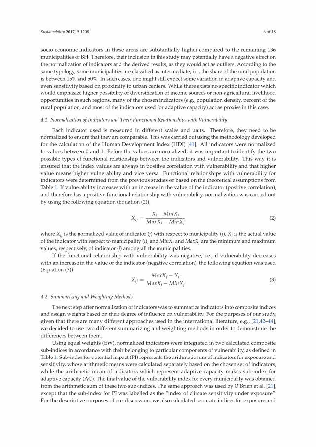
Sustainability 2017, 9, 1208 6 of 18
socio-economic indicators in these areas are substantially higher compared to the remaining 136municipalities of BH. Therefore, their inclusion in this study may potentially have a negative effect onthe normalization of indicators and the derived results, as they would act as outliers. According to thesame typology, some municipalities are classified as intermediate, i.e., the share of the rural populationis between 15% and 50%. In such cases, one might still expect some variation in adaptive capacity andeven sensitivity based on proximity to urban centers. While there exists no specific indicator whichwould emphasize higher possibility of diversification of income sources or non-agricultural livelihoodopportunities in such regions, many of the chosen indicators (e.g., population density, percent of therural population, and most of the indicators used for adaptive capacity) act as proxies in this case.
4.1. Normalization of Indicators and Their Functional Relationships with Vulnerability
Each indicator used is measured in different scales and units. Therefore, they need to benormalized to ensure that they are comparable. This was carried out using the methodology developedfor the calculation of the Human Development Index (HDI) [41]. All indicators were normalizedto values between 0 and 1. Before the values are normalized, it was important to identify the twopossible types of functional relationship between the indicators and vulnerability. This way it isensured that the index values are always in positive correlation with vulnerability and that highervalue means higher vulnerability and vice versa. Functional relationships with vulnerability forindicators were determined from the previous studies or based on the theoretical assumptions fromTable 1. If vulnerability increases with an increase in the value of the indicator (positive correlation),and therefore has a positive functional relationship with vulnerability, normalization was carried outby using the following equation (Equation (2)),
Xij =Xi − MinXj
MaxXj −MinXj(2)
where Xij is the normalized value of indicator (j) with respect to municipality (i), Xi is the actual valueof the indicator with respect to municipality (i), and MinXj and MaxXj are the minimum and maximumvalues, respectively, of indicator (j) among all the municipalities.
If the functional relationship with vulnerability was negative, i.e., if vulnerability decreaseswith an increase in the value of the indicator (negative correlation), the following equation was used(Equation (3)):
Xij =MaxXj − Xi
MaxXj −MinXj(3)
4.2. Summarizing and Weighting Methods
The next step after normalization of indicators was to summarize indicators into composite indicesand assign weights based on their degree of influence on vulnerability. For the purposes of our study,given that there are many different approaches used in the international literature, e.g., [21,42–44],we decided to use two different summarizing and weighting methods in order to demonstrate thedifferences between them.
Using equal weights (EW), normalized indicators were integrated in two calculated compositesub-indices in accordance with their belonging to particular components of vulnerability, as defined inTable 1. Sub-index for potential impact (PI) represents the arithmetic sum of indicators for exposure andsensitivity, whose arithmetic means were calculated separately based on the chosen set of indicators,while the arithmetic mean of indicators which represent adaptive capacity makes sub-index foradaptive capacity (AC). The final value of the vulnerability index for every municipality was obtainedfrom the arithmetic sum of these two sub-indices. The same approach was used by O’Brien et al. [21],except that the sub-index for PI was labelled as the “index of climate sensitivity under exposure”.For the descriptive purposes of our discussion, we also calculated separate indices for exposure and
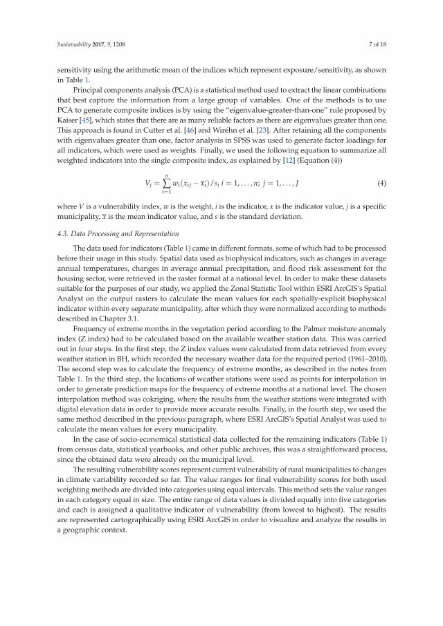
Sustainability 2017, 9, 1208 7 of 18
sensitivity using the arithmetic mean of the indices which represent exposure/sensitivity, as shownin Table 1.
Principal components analysis (PCA) is a statistical method used to extract the linear combinationsthat best capture the information from a large group of variables. One of the methods is to usePCA to generate composite indices is by using the “eigenvalue-greater-than-one” rule proposed byKaiser [45], which states that there are as many reliable factors as there are eigenvalues greater than one.This approach is found in Cutter et al. [46] and Wiréhn et al. [23]. After retaining all the componentswith eigenvalues greater than one, factor analysis in SPSS was used to generate factor loadings forall indicators, which were used as weights. Finally, we used the following equation to summarize allweighted indicators into the single composite index, as explained by [12] (Equation (4))
Vj =n
∑i=1
wi(xij − xi)/si i = 1, . . . , n; j = 1, . . . , J (4)
where V is a vulnerability index, w is the weight, i is the indicator, x is the indicator value, j is a specificmunicipality, x is the mean indicator value, and s is the standard deviation.
4.3. Data Processing and Representation
The data used for indicators (Table 1) came in different formats, some of which had to be processedbefore their usage in this study. Spatial data used as biophysical indicators, such as changes in averageannual temperatures, changes in average annual precipitation, and flood risk assessment for thehousing sector, were retrieved in the raster format at a national level. In order to make these datasetssuitable for the purposes of our study, we applied the Zonal Statistic Tool within ESRI ArcGIS’s SpatialAnalyst on the output rasters to calculate the mean values for each spatially-explicit biophysicalindicator within every separate municipality, after which they were normalized according to methodsdescribed in Chapter 3.1.
Frequency of extreme months in the vegetation period according to the Palmer moisture anomalyindex (Z index) had to be calculated based on the available weather station data. This was carriedout in four steps. In the first step, the Z index values were calculated from data retrieved from everyweather station in BH, which recorded the necessary weather data for the required period (1961–2010).The second step was to calculate the frequency of extreme months, as described in the notes fromTable 1. In the third step, the locations of weather stations were used as points for interpolation inorder to generate prediction maps for the frequency of extreme months at a national level. The choseninterpolation method was cokriging, where the results from the weather stations were integrated withdigital elevation data in order to provide more accurate results. Finally, in the fourth step, we used thesame method described in the previous paragraph, where ESRI ArcGIS’s Spatial Analyst was used tocalculate the mean values for every municipality.
In the case of socio-economical statistical data collected for the remaining indicators (Table 1)from census data, statistical yearbooks, and other public archives, this was a straightforward process,since the obtained data were already on the municipal level.
The resulting vulnerability scores represent current vulnerability of rural municipalities to changesin climate variability recorded so far. The value ranges for final vulnerability scores for both usedweighting methods are divided into categories using equal intervals. This method sets the value rangesin each category equal in size. The entire range of data values is divided equally into five categoriesand each is assigned a qualitative indicator of vulnerability (from lowest to highest). The resultsare represented cartographically using ESRI ArcGIS in order to visualize and analyze the results ina geographic context.

Sustainability 2017, 9, 1208 8 of 18
5. Results and Discussion
5.1. The Overall Vulnerability Index
To obtain the overall index of vulnerability using EW, we summed the composite sub-indices forPI and AC. The results are shown in Figure 2. According to this method, nine municipalities (6.6%)had the highest vulnerability index, while only four municipalities (2.9%) had the lowest vulnerabilityindex. The largest number of municipalities had high (51) or moderate (47) vulnerability (37.5%and 34.6%, respectively). 18.4% of the total number of municipalities (25) had a low vulnerabilityindex. Geographically, the most vulnerable municipalities are located across the north, with a gradualdecrease in vulnerability towards the central, eastern, and western parts of the country. In the south,most of municipalities in the lowland region of Herzegovina are classified as highly vulnerable, whilemunicipalities in the surrounding region are mostly classified as low or moderately vulnerable.
�
Figure 2. Vulnerability index across municipalities using equal weights.
According to Filmer and Pritchett, the absolute value of the loading of the first single componentis valid for assigning weights. This method was used in Gbetibouo et al. [12] to assign weights andconstruct an overall vulnerability index. In the case of our study, we decided to retain all componentswith eigenvalues greater than one, as recommended by Kaiser [45], in order to avoid a higher degreeof uncertainty in our results caused by significant dimension reduction, since the first componentdescribes only 23% of variance. In this study, six components had an eigenvalue greater than one andtogether they explained 71.1% of the variance observed. Using factor analysis, we assigned weightsfor all variables (indicators). The value of the Kaiser-Meyer-Olkin measure of sampling adequacywas 0.719, which is acceptable for factor analysis, as well as the significance level of Bartlett’s test ofsphericity (p < 0.001). The sum of weighted variables for every municipality represents an overallvulnerability index as shown in Figure 3.

Sustainability 2017, 9, 1208 9 of 18
�
Figure 3. Vulnerability index across municipalities using PCA as weighting method.
Compared to EW, nearly half of the municipalities retained the same class of vulnerability (46.3%),while 41.9% and 8.1% of the municipalities had increased or decreased vulnerability class, respectively.More substantial changes in vulnerability class occurred in the case of five municipalities, which hadtheir class increased by two. Although the apparent increase in the number of vulnerable municipalitiesis evident, the general geographic distribution of vulnerability using weighted indicators did notmarkedly change compared to equally weighted indicators. Most vulnerable municipalities are stilllocated in the north, and the least vulnerable ones in the east and southeast of BH. However, therewas an increase in the number of highly vulnerable municipalities in central and western BH, as wellas an overall increase in vulnerability in the south. Overall, most notable is the decrease in thenumber of municipalities with low vulnerability indices, while there was an increase in the number ofmunicipalities with the highest and high classes of vulnerability.
The difference in results between the two selected methods results from participation of individualindicators in the formation of the composite indices. This is conditioned by (1) summarizing methodand (2) contribution of individual indicators in generation of composite indices determined by weights.The final value of the vulnerability index for our first method (EW) was obtained from the arithmeticsum of two sub-indices (PI and AC), while in the second method (PCA) a single composite indexwas generated from the arithmetic sum of all weighted indicators. The weighting method hada significant impact on our results. When using EW, every indicator had an equal impact on the finalsub-index value, depending on whether or not it belonged to one of the three groups of indicators,while the weights used for some indicators in our study were so low they did not substantially affectthe vulnerability index in the case of PCA as a weighting method. Only four indicators (averageyields, road length, changes in temperature, and precipitation) had weights (loadings) above 0.3 andwere therefore the main determinants of vulnerability, while nine indicators had weights below 0.1(Supplementary Table S1). The difference in results between two weighting methods used in this study

Sustainability 2017, 9, 1208 10 of 18
was expected, since only six components were extracted from PCA and they account for 71.1% ofvariance. Similar differences between these two summarizing and weighting methods were reportedby Wiréhn et al. [23].
While EW and PCA are some of the common weighting methods found in the relevant literature,other methods are used, such as inverse of variance and expert opinion [44]. Each of these methodshas its own constraints and the scientific debate about the optimal approach is as old as the firstattempts to quantitatively assess vulnerability. The arbitrary strategy of assigning equal weightsto indicators might mislead the calculations, since not all indicators can have equal influence onvulnerability or may lead to difficulties in reaching a consensus among expert panel members, similarto cases where assigning weights using expert judgment is carried out arbitrarily [12]. Assigninghigher weights to indicators showing lower variance may ensure that large variations among theindicators would not unduly dominate the contribution of the rest of the indicators and distort interregional comparisons. However, a downside to this approach is the suppression of the pronouncementof relevant indicators [43]. Using PCA, it is not guaranteed that correlations necessarily represent thereal, or even statistical, influence of used sub-indicators on the phenomenon the composite indicator ismeasuring [47].
Representation of vulnerability with the single index might bring an insight about the degreeof vulnerability on a sub-national level and identify the most vulnerable regions. However, such anapproach may also be misleading and lead to simplistic policy conclusions [12,47]. In order to fullyassess the “big picture”, composite indicators should be used in combination with the sub-indicators.Therefore, we used the results of our first summarizing method, which was composed of sub-indictorsusing EW, in order to better explain the main sources of vulnerability and the influence of differentcomponents of vulnerability in the development of the overall vulnerability index in the next section.
5.2. Influence of Different Components of Vulnerability on the Overall Vulnerability Index
According to the PI index shown in Figure 4a, it is notable that the municipalities experiencinga high degree of PI from current climate variability are located in the northern part of BH, with theexception of four municipalities located on the south-western edge of the country. However, PI iscomposed of exposure and sensitivity [17] and therefore we have further decomposed the PI indexinto these two sub-indices in order to better understand the main sources contributing to PI index,as well as the degree and interaction between the components which form PI, as shown in Figure 4b,c.
Figure 4b shows the evident difference in degree of exposure between the hilly-mountainousparts of BH, which stretch from the north-west to the south-east, and the rest of the country(Figure 1). The main cause of high exposure in the northern part of BH is the highest differencein average yearly temperatures and the higher incidence of months with extreme weather conditions,while the south-western region has experienced the highest difference in the amount of precipitation.Two municipalities on the northern border of the country with the highest degree of PI are also highlyvulnerable to flooding. These municipalities are in the plain region and located next to the river Sava,the biggest river in BH, which constitutes the northern border of BH and the tributaries in the territoryof which BH forms the second largest sub-basin of the Danube river basin. The southern part ofthe country is the warmest, with a prevailing Mediterranean climate (unlike the rest of the country,which has different forms of the continental and alpine climates). The degree of exposure to climatechange in these regions will continue to increase according to regional projections, with an expectedaverage temperature increase of 4 ◦C in the coming decades, especially in the northern part of thecountry [8]. According to the same model, an additional unfavorable factor, which will affect thesouthern part of the country, is the further reduction in annual precipitation, especially during summer,while no significant changes in the amount of precipitation are expected in the rest of the country.
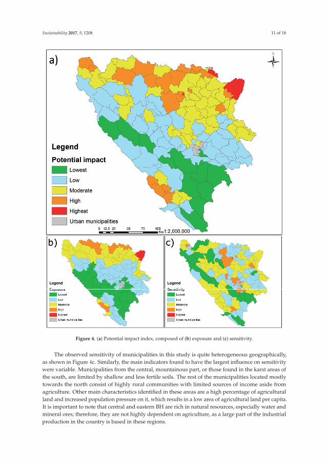
Sustainability 2017, 9, 1208 11 of 18
Figure 4. (a) Potential impact index, composed of (b) exposure and (c) sensitivity.
The observed sensitivity of municipalities in this study is quite heterogeneous geographically,as shown in Figure 4c. Similarly, the main indicators found to have the largest influence on sensitivitywere variable. Municipalities from the central, mountainous part, or those found in the karst areas ofthe south, are limited by shallow and less fertile soils. The rest of the municipalities located mostlytowards the north consist of highly rural communities with limited sources of income aside fromagriculture. Other main characteristics identified in these areas are a high percentage of agriculturalland and increased population pressure on it, which results in a low area of agricultural land per capita.It is important to note that central and eastern BH are rich in natural resources, especially water andmineral ores; therefore, they are not highly dependent on agriculture, as a large part of the industrialproduction in the country is based in these regions.

Sustainability 2017, 9, 1208 12 of 18
The situation is diverse when it comes to the adaptive capacity of municipalities, shown inFigure 5. However, some common characteristics are found between the municipalities with low andhigh adaptive capacity. Municipalities with the highest adaptive capacity have a larger GDP and lowerunemployment rates. This is mainly due to the presence of larger towns or cities located within theirborders, which likely creates more business opportunities for the local population. Some municipalitieshave developed into industrial and entrepreneurial centers in the past two decades, with a multitudeof varying business activities varying from small to large in size and in outputs/activities [48]. On theother hand, municipalities with low adaptive capacity were found to have a high dependency ratio,underdeveloped infrastructure, public and social services, and high unemployment rates. A significantpercentage of the population in these municipalities are smallholder farmers engaged in extensive,often subsistence, agriculture [2].
Figure 5. Adaptive capacity index.
The example from Table 2 is used to gain a more detailed insight into the main determinants ofvulnerability in the nine most vulnerable municipalities in BH. Looking at the overall results based onthe vulnerability index and two sub-indices from which the overall vulnerability index is composed,it is clear that the most vulnerable rural municipalities in BH are those with the high degree of PI,as well as low AC to cope with this impact. Furthermore, when the two components which generatePI (exposure and sensitivity) are analyzed separately, there is a difference as to which componentdetermines the higher degree of PI. Apart from the most vulnerable municipality of Bijeljina, which ismuch more vulnerable to flooding than the rest of the municipalities of BH, it is evident that thesensitivity index is the main determinant of PI, rather than the exposure index. Therefore, it canbe concluded that the current socio-economic conditions (social vulnerability) and the increasedenvironmental pressure as a result of the present human-environment interactions are usually themain determinant of vulnerability in the most vulnerable municipalities, rather than the degree towhich these municipalities are exposed to significant climatic variations (biophysical vulnerability).

Sustainability 2017, 9, 1208 13 of 18
Table 2. The most vulnerable municipalities in BH and their rankings according to different componentsof vulnerability.
MunicipalityPotential impact
Adaptive CapacityExposure Sensitivity Overall
Bijeljina highest moderate highest moderateDoboj-Jug moderate highest highest moderate
Doboj-Istok moderate high high lowOrašje moderate high highest moderateUsora moderate high high lowTešanj moderate high high moderate
Kalesija low high high lowBužim moderate high high low
Vukosavlje moderate moderate high low
5.3. Future Considerations for Quantitative Assessment of Vulnerability to Climate Change with Special Focuson Choice of Biophysical Indicators
The results indicate variability between the chosen summarizing and weighting methods, whichwould certainly increase even more if additional methods from recent studies were used for furthercomparison, as shown by Wiréhn et al. [23]. Development of the vulnerability index involves sequentialstages, including the selection of indicators, their normalization, and summation to a final value.There is a significant degree of uncertainty in vulnerability assessments and data transformationin these stages, as described in more detail by Tate [49]. Also, while a number of indicators havebeen used and developed for assessing vulnerability, the choice of indicators should be context andregion-specific, as there is no “one size fits all” blueprint that can be used regardless of the context [50].Based on these arguments and the experiences which we obtained during the preparation of this study,as well as reviewing literature related to vulnerability assessment in the context of agriculture andclimate change, we would like to emphasize the importance of the right choice of biophysical datawhen doing local vulnerability assessments to climate change. We believe that the indicators used tomeasure exposure, such as frequency of extreme weather events (such as drought and floods) andvariation of temperature and rainfall, might be misleading depending on the climate zone in which thestudy is conducted, as they may not fully capture the magnitude and the extent of such events.
Drought is a normal, recurring feature of climate, which occurs in all climatic regimes (in contrastto aridity, which is a permanent feature of the climate and is restricted to low rainfall areas [51]).Like vulnerability, drought has both a natural and social component, i.e., the risk associated withdrought is a product of both the region’s exposure to the drought, as well as the resilience of theecosystem or adaptive capacity of that region [52]. Impacts also differ spatially and temporally, as wellas depending on the type of drought. Drought has been grouped by type as follows: meteorological,hydrological, agricultural, and socioeconomic [53]. Meteorological droughts result from precipitationdeficiencies, while agricultural droughts are largely the result of soil moisture deficiencies. Agricultureis usually the first economic sector to be affected by drought because soil moisture supplies are oftenquickly depleted, especially if the period of moisture deficiency is associated with high temperaturesand windy conditions [51].
Similar to drought, waterlogging is another phenomenon which limits agricultural productivity.Unlike floods, which are in a more conventional sense defined as an overflow of water from waterbodies, waterlogging occurs when the soil becomes saturated in cases when the amount of precipitationexceeds the ability of the soil to infiltrate or evaporate the excessive moisture. Like in the case ofdrought, the extent and duration of waterlogging is mainly related to climatic and soil water-physicalproperties [54]. Waterlogging causes anaerobic conditions in the crop-root zone and leads to reducedcrop growth and yields; it also delays agricultural field operations, such as tillage and harvesting,and can lead to abundant surface runoff, inducing soil erosion and the loss of nutrients [55–57].

Sustainability 2017, 9, 1208 14 of 18
Based on the above definitions, we believe that agricultural drought should be the starting pointwhen using drought as an indicator of agricultural vulnerability to climate change, and that theimpact of drought should be based on soil moisture, not meteorological data. We also believe thatwaterlogging of heavy soils in humid, and in some cases sub-humid, areas, especially flatlands andvalleys, can cause the same amount of damage as drought, and therefore we recommend it as animportant indicator when assessing exposure to climate change in such conditions. For the purposesof this study, the approach developed by Wells and Goddard [33] was used to classify Palmer Z-indexvalues and calculate the frequency of extreme months (both dry and wet) in the last 50 years, whichwas used as an indicator for exposure in our study. Most studies related to climate hazard analysesand monitoring systems have been conducted using either: (1) The Palmer Drought Severity Index(PDSI) or Palmer moisture anomaly index (Z Index) [24], based on a soil water balance equation;or (2) The Standardized Precipitation Index (SPI) [58], based on a precipitation probabilistic approach.They are called drought indices, but they have ability to measure dryness (negative values) and wetness(positive values) at the same time. The Palmer drought indices show how monthly moisture conditionsdiffer from normal conditions for the specific area based on available soil water content, referenceevapotranspiration, and precipitation, and they are sensitive to unusual dry (and wet) months even inextended dry (or wet) spells. While PDSI is used to quantify the long-term changes in soil moisture,the Z-index is usually used for detection of short-term deviations from normal moisture conditions,which are important for agriculture and were therefore included as an indicator in our study [59].
SPI can also be calculated at different time scales to monitor droughts with respect to differentusable water resources. However, it might not be suitable for climate change analysis, since it doesnot take temperature or evapotranspiration as input parameters [60]. A new climatic drought indexsimilar to SPI, the Standardized Precipitation Evapotranspiration Index (SPEI), has been proposedrecently by Vicente-Serrano et al. [61]. SPEI is similar to SPI, but includes temperature as a parameterof calculation, which makes it closer to PDSI. As such, it has been already used in studies concerningagriculture and climate change, e.g., [62,63], and with its multiscalar character is suitable to use indrought-related vulnerability assessments.
6. Conclusions
This study was a first assessment of vulnerability to climate change at the sub-national level inBH. Quantitative assessment of vulnerability to climate change in rural municipalities was carried outfor 136 rural and semi-rural municipalities in BH. The chosen conceptual framework for this research,based on the IPCC definition of vulnerability, views vulnerability as a function of biophysical and socialindicators, which constitute the three components of vulnerability: exposure, sensitivity, and adaptivecapacity. 20 biophysical and socio-economic indicators were used to reflect these three components.For the purposes of our study, we decided to use two different summarizing and weighting methods(EW and PCA) to assess vulnerability to demonstrate the differences between them.
Based on the results obtained for the overall vulnerability index using the first summarizingmethod and EW, the most vulnerable municipalities are mostly located across the north, with thegradual decrease in vulnerability towards the central, northern and eastern parts of the country.Less vulnerable municipalities are those with larger towns and cities within their territory and theones located in hilly-mountainous central-south, central-west and south-eastern regions. From there,towards the south of BH, most of the municipalities in the Mediterranean lowland region of southernBH are classified as highly vulnerable, while municipalities in the surrounding region are mostlyclassified as low or moderately vulnerable. General geographic distribution of vulnerability usingthe second summarizing method and weighted indicators did not change substantially comparedto the first method. However, there was an overall increase in the number of highly vulnerablemunicipalities, most notably in the central, east, and south of BH, while the number of municipalitieswith low vulnerability index decreased.
Sustainability 2017, 9, 1208 15 of 18
We used the results of our first summarizing method using EW to better explain the mainsources of vulnerability and the influence of different components of vulnerability on the developmentof the overall vulnerability index. Based on these results, it was concluded that the currentsocio-economic conditions (adaptive capacity) and increased environmental pressure as a resultof present human-environment interactions (sensitivity) are the usually the main determinants ofvulnerability in the most vulnerable municipalities, rather than the degree to which these municipalitiesare exposed to significant climatic variations.
The results of this study provided valuable knowledge about the current state of vulnerability ofthe rural population of BH to climate change and the main determinants of vulnerability. They alsoestablish a baseline, which can be further updated at regular intervals, and they represent the firststep towards further local assessments and improvements, as new indicators become available andare discussed by the main stakeholders and the local communities. The same or similar approachescan also be applied in regions with similar climatic and socio-economic conditions, particularly thecountries of the Western Balkan region and South-eastern Europe.
Supplementary Materials: The following are available online at www.mdpi.com/2071-1050/9/7/1208/s1,Figure S1: Administrative structure and municipalities of Bosnia and Herzegovina, Figure S2: Climate zones ofBosnia and Herzegovina according to Köppen-Geiger climate classification, Table S1: Factor loadings for extractedprincipal components.
Acknowledgments: This study was supported by the project “Agricultural Adaptation to ClimateChange—Networking, Education, Research, and Extension in the West Balkans”, funded by HERD, the Programmefor Higher Education, Research and Development 2010–2014. The authors are very grateful to Espen Sjaastadand the anonymous reviewers for valuable comments and suggestions during the earlier versions of themanuscript. We would also like to thank Hamid Custovic, Goran Trbic, Davorin Bajic, Sretenka Srdic, and thehydrometeorological institutes in BH for providing some of the datasets used in this study, and Maria Hayesfor proofreading the manuscript. The open access publishing costs were covered by the publishing fund of theNorwegian University of Life Sciences (NMBU).
Author Contributions: Ognjen Žurovec conceived the study, chose the framework and methods, analyzed thedata and wrote the paper; Sabrija Cadro analyzed the weather data and drought indices; Bishal Kumar Sitaulacontributed significantly with writing and feedback during every stage of the manuscript.
Conflicts of Interest: The authors declare no conflict of interest.
References
1. United Nations Framework Convention on Climate Change (UNFCCC). Initial National Communication of
Bosnia and Herzegovina under the United Nation Framework Convention on Climate Change (INCBiH); Ministry forSpatial Planning, Construction and Ecology of Republic of Srpska: Banja Luka, Bosnia and Herzegovina, 2009.
2. Zurovec, O.; Vedeld, P.O.; Sitaula, B.K. Agricultural sector of Bosnia and Herzegovina and climatechange—Challenges and opportunities. Agriculture 2015, 5, 245–266. [CrossRef]
3. Sharma, V.; Reddy, B.; Sahu, N. Sustainable rural livelihoods approach for climate change adaptation inwestern Odisha, Eastern India. Dev. Pract. 2014, 24, 591–604. [CrossRef]
4. Thompson, H.E.; Berrang-Ford, L.; Ford, J.D. Climate change and food security in Sub-saharan Africa:A systematic literature review. Sustainability 2010, 2, 2719. [CrossRef]
5. Adger, W.N.; Agrawala, S.; Mirza, M.M.Q.; Conde, C.; O’Brien, K.; Pulhin, J.; Pulwarty, R.; Smit, B.;Takahashi, K. Assessment of adaptation practices, options, constraints and capacity. In Climate Change
2007: Impacts, Adaptation and Vulnerability (Contribution of Working Group II to the Fourth Assessment Report
of the Intergovernmental Panel On Climate Change); Parry, M., Canziani, O., Palutikof, J., van der Linden, P.,Hanson, C., Eds.; Cambridge University Press: Cambridge, UK, 2007.
6. Sullivan, C.; Meigh, J. Targeting attention on local vulnerabilities using an integrated index approach:The example of the climate vulnerability index. Water. Sci. Technol. 2005, 51, 69–78. [PubMed]
7. Council of Ministers of Bosnia and Herzegovina. Climate Change Adaptation and Low-EmissionDevelopment Strategy for Bosnia and Herzegovina. Available online: http://www.ba.undp.org/content/bosnia_and_herzegovina/en/home/library/environment_energy/climate-change-adaptation-and-low-emission-development-strategy-/ (accessed on 4 August 2016).

Sustainability 2017, 9, 1208 16 of 18
8. United Nations Framework Convention on Climate Change (UNFCCC). Second National Communication of
Bosnia and Herzegovina under the United Nation Framework Convention on Climate Change (SNCBIH); Ministry forSpatial Planning, Construction and Ecology of Republic of Srpska: Banja Luka, Bosnia and Herzegovina, 2013.
9. Agrawal, A. Local institutions and adaptation to climate change. In Social Dimensions of Climate Change:
Equity and Vulnerability in a Warming World; Mearns, R., Ed.; The World Bank: Washington, DC, USA, 2010;pp. 173–198.
10. Preston, B.L.; Brooke, C.; Measham, T.G.; Smith, T.F.; Gorddard, R. Igniting change in local government:Lessons learned from a bushfire vulnerability assessment. Mitig. Adapt. Strateg. Glob. Chang. 2009,14, 251–283. [CrossRef]
11. Füssel, H.-M. Vulnerability: A generally applicable conceptual framework for climate change research.Glob. Environ. Chang. 2007, 17, 155–167. [CrossRef]
12. Gbetibouo, G.A.; Ringler, C.; Hassan, R. Vulnerability of the South African farming sector to climate changeand variability: An indicator approach. Nat. Resour. Forum 2010, 34, 175–187. [CrossRef]
13. Brooks, N. Vulnerability, Risk and Adaptation: A Conceptual Framework; Tyndall Centre for Climate ChangeResearch and Centre for Social and Economic Research on the Global Environment (CSERGE), School ofEnvironmental Sciences University of East Anglia: Norwich, UK, 2003; pp. 1–16.
14. Kelly, P.M.; Adger, W.N. Theory and practice in assessing vulnerability to climate change and facilitatingadaptation. Clim. Chang. 2000, 47, 325–352. [CrossRef]
15. Adger, W.N. Social vulnerability to climate change and extremes in coastal vietnam. World Dev. 1999,27, 249–269. [CrossRef]
16. Intergovernmental Panel on Climate Change (IPCC). Climate Change 2001: Synthesis Report. A Contribution
of Working Groups I, II, and III to the Third Assessment Report of the Integovernmental Panel on Climate Change;Watson, R.T., Core Writing Team, Eds.; Cambridge University Press: Cambridge, UK; New York, NY, USA,2001; p. 398.
17. Füssel, H.-M.; Klein, R.J.T. Climate change vulnerability assessments: An evolution of conceptual thinking.Clim. Chang. 2006, 75, 301–329. [CrossRef]
18. Adger, W.N.; Brooks, N.; Bentham, G.; Agnew, M.; Eriksen, S. New Indicators of Vulnerability and Adaptive
Capacity; Tyndall Centre for Climate Change Research: Norwich, UK, 2004.19. Berjan, S.; Jovanovic, M.; Mrdalj, V.; Paspalj, M.; Matovic, F.; Driouech, N.; El Bilali, H.; Abouabdillah, A.
Rural livelihood diversification in south-eastern Bosnia: Influence of household financial management. Int. J.
Environ. Rural Dev. 2014, 5, 17–22.20. Monterroso, A.; Conde, C.; Gay, C.; Gómez, D.; López, J. Two methods to assess vulnerability to climate
change in the Mexican agricultural sector. Mitig. Adapt. Strateg. Glob. Chang. 2014, 19, 445–461. [CrossRef]21. O’Brien, K.; Leichenko, R.; Kelkar, U.; Venema, H.; Aandahl, G.; Tompkins, H.; Javed, A.; Bhadwal, S.;
Barg, S.; Nygaard, L.; et al. Mapping vulnerability to multiple stressors: Climate change and globalization inIndia. Glob. Environ. Chang. 2004, 14, 303–313. [CrossRef]
22. Ravindranath, N.; Rao, S.; Sharma, N.; Nair, M.; Gopalakrishnan, R.; Rao, A.S.; Malaviya, S.; Tiwari, R.;Sagadevan, A.; Munsi, M. Climate change vulnerability profiles for north east India. Curr. Sci. India 2011, 101.
23. Wiréhn, L.; Danielsson, Å.; Neset, T.-S.S. Assessment of composite index methods for agriculturalvulnerability to climate change. J. Environ. Manag. 2015, 156, 70–80. [CrossRef] [PubMed]
24. Palmer, W.C. Meteorological Drought; US Department of Commerce, Weather Bureau Washington: Washington,DC, USA, 1965; Volume 30.
25. Hydro-Engineering Institute Sarajevo (HEIS). Assessment on Floods and Landslides Risk for the Housing Sector in
Bosnia and Herzegovina; Hydro-Engineering Institute: Sarajevo, Bosnia and Herzegovina, 2015.26. Federal Institute for Agropedology. FAO Soil and Terrain Database (SOTER) for Bosnia and Herzegovina: Dominant
Soil Types, Scale 1:1000000; Federal Institute for Agropedology: Sarajevo, Bosnia and Herzegovina, 2000.27. European Environment Agency (EEA). Corine Land Cover Database—Bosnia and Herzegovina. Available
online: http://cdr.eionet.europa.eu/ba/eea/clc/envvu5ofg (accessed on 16 August 2015).28. Agency for Statistics of Bosnia and Herzegovina—Census 2013 Data. Available online: http://popis2013.ba/
(accessed on 3 July 2016).29. Institute for Statistics of Federation of Bosnia and Herzegovina—Kantoni U Brojkama (Cantons in Numbers).
Available online: http://www.fzs.ba/kantoniubrojkama.htm (accessed on 22 April 2016).

Sustainability 2017, 9, 1208 17 of 18
30. Institute for Statistics of Republic of Srpska—Statistical Yearbook of Republic of Srpska 2014: Reviewby Municipalities. Available online: http://www.rzs.rs.ba/front/article/1331/?left_mi=287&add=287(accessed on 22 April 2015).
31. Ministry of Justice of Bosnia and Herzegovina—Registry of Associations. Available online: http://www.mpr.gov.ba/web_dokumenti/RU_23_03_12.pdf (accessed on 13 July 2015).
32. NGO Members of the Portal. Available online: http://www.ngo.ba/index.php/nvo-clanice-portala(accessed on 16 July 2015).
33. Wells, N.; Goddard, S. A self-calibrating Palmer drought severity index. J. Clim. 2004, 17, 2335–2351.[CrossRef]
34. Bruinsma, J. World Agriculture: Towards 2015/2030: An FAO Perspective; Earthscan: London, UK, 2003.35. Houghton, A.; Austin, J.; Beerman, A.; Horton, C. An approach to developing local climate change
environmental public health indicators in a rural district. J. Environ. Public Health 2017, 2017, 1–16. [CrossRef][PubMed]
36. Muttarak, R.; Lutz, W. Is education a key to reducing vulnerability to natural disasters and hence unavoidableclimate change? Ecol. Soc. 2014, 19, 42. [CrossRef]
37. United Nations Development Programme (UNDP). Rural Development in Bosnia and Herzegovina:Myth and Reality. Available online: http://hdr.undp.org/en/content/rural-development-bosnia-and-herzegovina-myth-and-reality (accessed on 10 April 2017).
38. Bajic, D.; Trbic, G. Climate Atlas of Bosnia and Herzegovina; Faculty of Science: Banja Luka, Bosnia andHerzegovina, 2016.
39. European Environment Agency (EEA). Climate Change, Impacts and Vulnerability in Europe 2016;
An Indicator-Based Report; EEA Report No 1/2017; European Environment Agency: Luxembourg, 2017.40. Brezzi, M.; Dijkstra, L.; Ruiz, V. OECD Extended Regional Typology: The Economic Performance of Remote Rural
Regions; OECD Publishing: Paris, France, 2011.41. United Nations Development Programme (UNDP). Human Development Report: Concept and Measurement of
Human Development; United Nations Development Programme: New York, NY, USA, 1990.42. Palanisami, K.; Paramasivam, P.; Ranganathan, C.; Aggarwal, P.; Senthilnathan, S. Quantifying vulnerability
and impact of climate change on production of major crops in Tamil Nadu, India. In From Headwaters to the
Ocean: Hydrological Change and Water Management-Hydrochange; Taniguchi, M., Burnett, W.C., Fukushima, Y.,Haigh, M., Umezawa, Y., Eds.; CRC Press/Balkema: Boca Raton, FL, USA, 2008.
43. Varadan, R.J.; Kumar, P. Mapping agricultural vulnerability of Tamil Nadu, India to climate change:A dynamic approach to take forward the vulnerability assessment methodology. Clim. Chang. 2015,129, 159–181. [CrossRef]
44. Yusuf, A.A.; Francisco, H. Climate Change Vulnerability Mapping for Southeast Asia; Economy and EnvironmentProgram for Southeast Asia (EEPSEA): Singapore, 2009; pp. 10–15.
45. Kaiser, H.F. The application of electronic computers to factor analysis. Educ. Psychol. Meas. 1960, 20, 141–151.[CrossRef]
46. Cutter, S.L.; Boruff, B.J.; Shirley, W.L. Social vulnerability to environmental hazards. Soc. Sci. Q. 2003,84, 242–261. [CrossRef]
47. Saisana, M.; Tarantola, S. State-of-the-Art Report on Current Methodologies and Practices for Composite Indicator
Development; European Commission, Joint Research Centre: Ispra, Italy, 2002.48. Alagic, I.; Petkovic, D. Economic Development of Small Areas Based on Own Resources as Opposed to
Existence/Nonexistence of the Support of the Capital City. In Special editions of The Academy of Sciences
and Arts of Bosnia and Herzegovina, Department of Social Science, Book 6; Osmankovic, J., Pejanovic, M., Eds.;The Academy of Sciences and Arts of Bosnia and Herzegovina: Sarajevo, Bosnia and Herzegovina, 2016;pp. 179–194.
49. Tate, E. Uncertainty analysis for a social vulnerability index. Ann. Assoc. Am. Geogr. 2013, 103, 526–543.[CrossRef]
50. Vincent, K.; Cull, T. Using indicators to assess climate change vulnerabilities: Are there lessons to learn foremerging loss and damage debates? Geogr. Compass 2014, 8, 1–12. [CrossRef]
51. Wilhite, D.A. Drought as a natural hazard: Concepts and definitions. In Drought: A Global Assessment;Wilhite, D.A., Ed.; Routledge: London, UK, 2000; Volume 2, pp. 3–18.

Sustainability 2017, 9, 1208 18 of 18
52. Zarafshani, K.; Sharafi, L.; Azadi, H.; Van Passel, S. Vulnerability assessment models to drought: Toward aconceptual framework. Sustainability 2016, 8, 588. [CrossRef]
53. Wilhite, D.A.; Glantz, M.H. Understanding: The drought phenomenon: The role of definitions. Water Int.
1985, 10, 111–120. [CrossRef]54. Moore, G.A. Soilguide. In A Handbook for Understanding and Managing Agricultural Soils; Department of
Agriculture and Food, Bulletin No. 4343; Department of Agriculture and Food: Perth, Australia, 2001;Chapter 3.
55. Dickin, E.; Wright, D. The effects of winter waterlogging and summer drought on the growth and yield ofwinter wheat (Triticum Aestivum L.). Eur. J. Agron. 2008, 28, 234–244. [CrossRef]
56. Drew, M.C.; Lynch, J.M. Soil anaerobiosis, microorganisms, and root function. Annu. Rev. Phytopathol. 1980,18, 37–66. [CrossRef]
57. Turtola, E.; Paajanen, A. Influence of improved subsurface drainage on phosphorus losses and nitrogenleaching from a heavy clay soil. Agric. Water Manag. 1995, 28, 295–310. [CrossRef]
58. McKee, T.B.; Doesken, N.J.; Kleist, J. The relationship of drought frequency and duration to time scales.In Proceedings of the 8th Conference on Applied Climatology, American Meteorological Society, Anaheim,CA, USA, 17–22 January 1993; Volume 17, pp. 179–183.
59. Vicente-Serrano, S.M.; Beguería, S.; Lorenzo-Lacruz, J.; Camarero, J.J.; López-Moreno, J.I.; Azorin-Molina, C.;Revuelto, J.; Morán-Tejeda, E.; Sanchez-Lorenzo, A. Performance of drought indices for ecological,agricultural, and hydrological applications. Earth Interact. 2012, 16, 1–27. [CrossRef]
60. World Meteorological Organization (WMO). Standardized Precipitation Index User Guide; World MeteorologicalOrganization: Geneva, Switzerland, 2012.
61. Vicente-Serrano, S.M.; Beguería, S.; López-Moreno, J.I. A multiscalar drought index sensitive to globalwarming: The standardized precipitation evapotranspiration index. J. Clim. 2010, 23, 1696–1718. [CrossRef]
62. Potop, V.; Možný, M.; Soukup, J. Drought evolution at various time scales in the lowland regions and theirimpact on vegetable crops in the Czech Republic. Agric. For. Meteorol. 2012, 156, 121–133. [CrossRef]
63. Yu, M.; Li, Q.; Hayes, M.J.; Svoboda, M.D.; Heim, R.R. Are droughts becoming more frequent or severe inChina based on the standardized precipitation evapotranspiration index: 1951–2010? Int. J. Climatol. 2014,34, 545–558. [CrossRef]
© 2017 by the authors. Licensee MDPI, Basel, Switzerland. This article is an open accessarticle distributed under the terms and conditions of the Creative Commons Attribution(CC BY) license (http://creativecommons.org/licenses/by/4.0/).
PAPER 3
Žurovec, O., Vedeld, P.O.
A case study of rural livelihoods and climate change adaptation in different regions
of Bosnia and Herzegovina
- Manuscript -
� �


���
A case study of rural livelihoods and climate change adaptation in different regions of
Bosnia and Herzegovina
Ognjen Žurovec, Pål Olav Vedeld
Abstract
Nearly a third of the households in Bosnia and Herzegovina (BH) are engaged in agriculture as a livelihood
strategy to cope with the effects of the multiple shocks suffered over the past three decades, resulting in
economic decline and the absence of income opportunities. A significant dependence on agricultural
incomes makes this part of population particularly vulnerable to climate change. Based on the data collected
using a household questionnaire, this study investigates the livelihoods of rural households in three
agricultural regions in BH, how they are affected by climate change and their perceptions of changes in
climatic conditions, as well as household adaptation strategies and the main determinants of climate change
adaptation in agriculture. The results were discussed in the context of sustainable livelihoods approach and
a binary logit model was used to analyse the determinants of adoption of agricultural practices and
technologies in the context of assets. The results show that rural households are relatively asset poor and
dependent on agriculture irrespective of location or total income. Their access to assets is further
constrained by the ongoing structures and processes. Negative effects of climate change were reported in
terms of yield declines and the reduced quality of products. The studied households were found to be aware
about the recent climate trends and reported to adopt a wide range of more long-term adaptation strategies.
In the context of agricultural production, the level of adoption of different agricultural practices and
technologies shows the signs of the overall intensification of agricultural production in BH, as well as
adaptation to the perceived changes in climate. Increased access to different types of assets was shown to
positively influence the likelihood of adoptions of agricultural practices and technologies, most notably
social capital, access to technologies (tractors) and human capital.
1. Introduction
Bosnia and Herzegovina (BH) is predominantly rural, with 61% of the population living in rural areas
(MOFTER 2012). Although the share of agriculture in GDP is decreasing, it is still a backbone of the rural
economy, employing 20% of the workforce and constituting 6.4 % of total GDP. The potential for
agriculture in BH is substantial. Of the total 2.1 million hectares of agricultural land, 46.5% is arable, while
only 50% is currently utilised in agricultural production. Favourable climatic conditions and its geopolitical
position, abundant freshwater supplies and relatively cheap labour costs gives the agricultural sector in BH
a clear, comparative advantage over many other European countries and potentially gives BH an advantage
in terms of labour-intensive products. Livestock production has the highest economic value in the present
agricultural production system in BH, with great potential for further expansion and intensification due to
the high availability of grasslands and pastures in areas less favourable for intensive crop production.
However, agriculture in BH suffers from low general productivity, with rather extensive farming practices
and technologies, carried out on small and fragmented farms. This is a problem partly inherited from the
past socio-political system, where agriculture was marginalized in favour of industrial development, but
further exacerbated in the post-war period by poor governance in the ongoing process of transition (Žurovec
et al. 2015). A large proportion of the population, most of them employed in industry, have become
unemployed in the aftermath of the war in the nineties, which led to devastation, mass migration and

��
economic decline in rural areas. In the absence of income options, a significant part of that population
resorted to agriculture as a main or additional source of income. As a result, more than 31% of the total
households in BH are engaged in agriculture, but only 5% of them are considered commercial farmers
(AFSBH 2013). This shows the significant role that the agricultural sector in BH provides in terms of food
security, mitigating a social burden of economic reforms and restructuring, as well as rural poverty
reduction (Bojnec 2005). However, as agriculture remains one of the main sources of income for most rural
households in BH, this means that the livelihoods of many become increasingly vulnerable to present and
expected climate pressures.
BH is considered highly vulnerable to climate change (Brooks et al. 2005; Kreft and Eckstein 2013).
Extreme weather events, such as increased intensity of droughts, frequency of heat waves, heavy
precipitation resulting in floods and landslides and other extreme weather events, are becoming increasingly
more frequent in the region and have and can cause significant economic losses (IPCC 2011; Žurovec et
al. 2015). There is a limited adaptive capacity to cope with both climate and other shocks in BH, and the
situation is similar to that found in developing countries. This inherently low adaptive capacity is the main
determinant of vulnerability to climate change in most rural areas of BH, even more so than the degree to
which these areas are de facto exposed to significant climatic variations (Žurovec et al. 2017a). Poverty in
BH is mostly a rural phenomenon - close to 80 % of the total poor live in rural areas. Non-farm employment
opportunities in rural areas are limited. Many rural areas have poorly developed transport, social and
economic infrastructure, all of which are basic preconditions for social and economic development. These
conditions preceded the massive changes through the recent war events, but were also exacerbated by the
economic crisis and poor governance in the country. This is especially pronounced in remote areas, where
a continuous process of desertion through migration results in the closure and degradation of the existing
infrastructure including schools, shops and local clinics.
Adaptation is crucial both in order to enhance the resilience of the agricultural sector and for individuals to
secure their livelihoods by increasing their adaptive capacity. Adequate responses in terms of adaptation to
climate change depend on; the adaptive capacity, knowledge and skills, robustness of livelihoods and
alternatives, resources and access to institutions in order to undertake effective adaptation (IPCC 2007).
While technological development, government programs and insurance schemes require greater
investments from the public sector and industry to be subsequently adopted by farmers (Smit and Skinner
2002), adaptation to climate change at the farm level includes many possible responses. This could
encompass changes in crop management practices, livestock management practices, land use and land
management and a variety of both on-farm and off-/non-farm livelihood strategies (Bryan et al. 2013).
While climate change has yet to be mainstreamed into national and regional development policies in BH,
individuals and communities are already adapting to changing climatic conditions. Such adaptation
strategies are mostly reactive and carried out privately by individuals or communities in response to
perceived and experienced adverse impacts of climate change and variability (Smit et al. 2000). Perceptions
are key components in the on-farm decision-making process. Observations and experiences over time shape
farmers’ climate change perceptions and influence their choices of appropriate adaptation strategies.
However, adaptations in agriculture are not only carried out with respect to climatic stimuli alone, but rather
as a “joint effects of multiple forces” (Smit and Skinner 2002). People adapt to changes in their external
frame conditions in different ways and it can be difficult to assess complex changes in institutional
arrangements and explore what can be reasonably linked to climate change in addition to how other frame
conditions can interact with climate change in relation to how people adapt in both the short- and long-
term.

���
Rural households with access to agricultural means of production have the choice between both agriculture
and non-agricultural economic activities. Different adaptation strategies within agriculture can also be
considered, such as extensification versus intensification, as well as “exit options” such as off- and non-
farm activities, migration and remittance strategies. In as much as climate change is one driver for particular
courses of action, other frame conditions such as agricultural policies and market conditions, alternative
economic options and other factors situate households with different asset access in different positions
concerning such choices. There is no single profitable or desired option for all households or individuals;
but diversification patterns in terms of adaptation must be understood as a broad spectre of opportunities.
It is also useful to see this as a combination of (“free”) choice versus necessity (Ellis 2000) and or as a
structure-agency dichotomy. Choices are made but under such strong preconditions or bearings that the
choice is “given”.
Another feature of BH as a country is its pronounced heterogeneity in terms of geographical, agro-
ecological and climatic conditions, as well as a unique, and rather asymmetric constitutional, political and
institutional arrangements and governance. This means that households under different socioeconomic and
agro-ecological conditions will obviously have different realities to relate to and also different perceptions
of climate change and accompanying consequences for agricultural and other income generating potential.
Such perceptions are both individual and social, where kinship and the existing social environment often
play important roles in the evolution of perceptions and understandings of various issues.
The objectives of this study were to: i) assess the livelihoods of rural households, their access to assets and
livelihood diversification strategies; ii) investigate how the households are affected by climate change and
how they perceive these ongoing changes and iii) to analyse household adaptation strategies in different
regions of BH and the main determinants of climate change adaptation. The results were analysed and
discussed in the context of three different agricultural regions and three wealth groups according to total
income level of the households.
2. Study area
BH is a country in South-eastern Europe, located in the Western Balkan region, with a total surface area of
51,209.2 km2, composed of 51,197 km2 of land and 12.2 km2 of sea. The land is mainly hilly to
mountainous, with an average altitude of 500 meters. Of the total land area, 5% is lowlands, 24% hills, 42%
mountains, and 29% is the karst region. The general atmospheric circulation and air mass flow, the dynamic
relief, the orientation of mountain ranges, the hydrographical network and the vicinity of the Adriatic Sea
have all created conditions for a wide spectrum of climate types and subtypes in BH (Baji� and Trbi� 2016).
Generally, these include a humid continental climate, represented mostly in the northern and lowland
central parts of the territory; a sub-alpine and alpine climate in the mountainous region of central, east and
western BH, and a semi-arid mediterranean climate represented in the coastal areas and in lowlands of
Herzegovina (southern BH). Areas above 800 m asl are mostly unsuitable for crop production due to harsh
climatic conditions.
The country is divided into six agricultural regions, differing by altitude, share of certain types of crops and
livestock and the degree of economic development. These can be roughly grouped into three main
agricultural regions: lowlands, hilly-mountainous and Mediterranean region (FMAWF 2013). The sites
used in this study are situated in these three regions (Figure 1), referred to as the northern (lowland), central
(hilly-mountainous) and southern region (meditteranean).
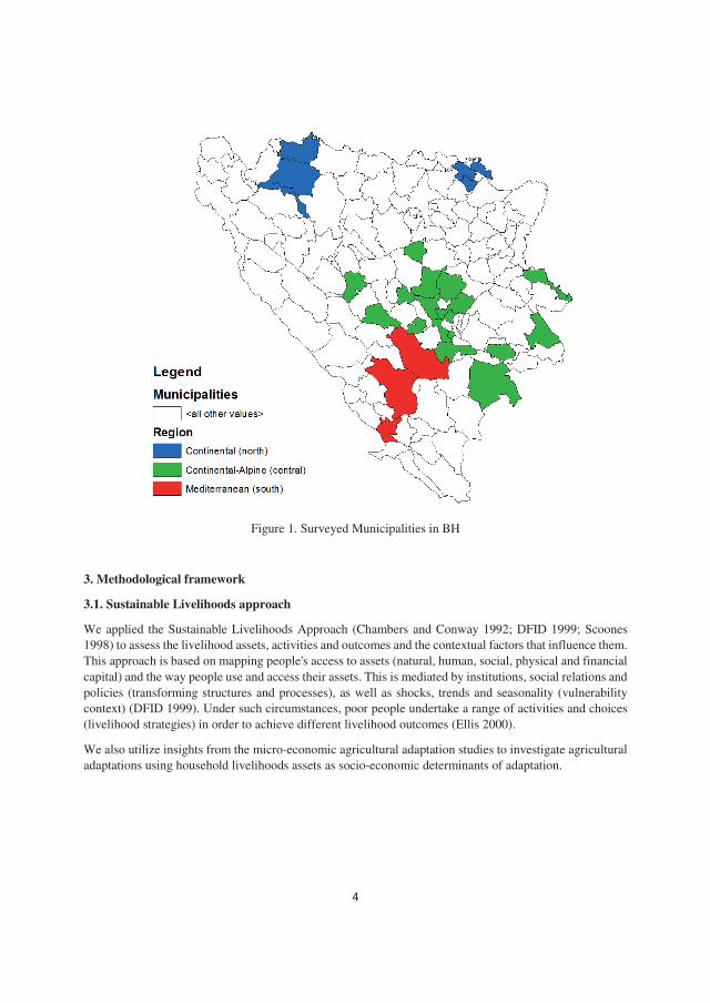
���
Figure 1. Surveyed Municipalities in BH
3. Methodological framework
3.1. Sustainable Livelihoods approach
We applied the Sustainable Livelihoods Approach (Chambers and Conway 1992; DFID 1999; Scoones
1998) to assess the livelihood assets, activities and outcomes and the contextual factors that influence them.
This approach is based on mapping people's access to assets (natural, human, social, physical and financial
capital) and the way people use and access their assets. This is mediated by institutions, social relations and
policies (transforming structures and processes), as well as shocks, trends and seasonality (vulnerability
context) (DFID 1999). Under such circumstances, poor people undertake a range of activities and choices
(livelihood strategies) in order to achieve different livelihood outcomes (Ellis 2000).
We also utilize insights from the micro-economic agricultural adaptation studies to investigate agricultural
adaptations using household livelihoods assets as socio-economic determinants of adaptation.
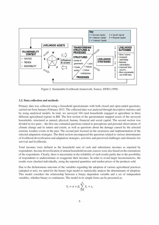
���
Figure 2. Sustainable livelihoods framework, Source: DFID (1999)
3.2. Data collection and methods
Primary data was collected using a household questionnaire with both closed and open-ended questions,
carried out from January-February 2015. The collected data was analysed through descriptive statistics and
by using analytical models. In total, we surveyed 104 rural households engaged in agriculture in three
different agricultural regions in BH. The first section of the questionnaire mapped assets of the surveyed
households, structured as natural, physical, human, financial and social capital. The second section was
divided in two parts – the first one contained questions related to perceptions and personal observations of
climate change and its nature and extent, as well as questions about the damage caused by the selected
extreme weather events in the past. The second part focused on the awareness and implementation of the
selected adaptation strategies. The third section encompassed the questions related to various determinants
of livelihood diversification and adaptation strategies, activities and perceived challenges and obstacles for
survival and livelihoods.
Total incomes were defined as the household sum of cash and subsistence incomes as reported by
respondents. Income diversification of annual household income sources were also based on the estimations
of the respondents. Clearly, there is uncertainty in the reliability of such results partly due to the possibility
of respondents to underestimate or exaggerate their incomes. In order to avoid larger inconsistencies, the
results were checked individually, using the reported quantities and market prices of the products sold.
Due to the dichotomous outcome of the variables regarding the adoption of various agricultural practices
(adopted or not), we opted for the binary logit model to statistically analyse the determinants of adoption.
This model considers the relationship between a binary dependent variable and a set of independent
variables, whether binary or continuous. The model in its simple form can be presented as:
� � ! " #��$� " %��
���

���
Where, Yi is the dichotomous dependent variable for individual agricultural practices (1 = adopted; 0 = not
adopted), ! is the Y-intercept, Hi are a set of regression coefficients, Xi denotes the set of explanatory
independent variables and �i is an error term.
4. Results and discussion
4.1 Livelihood assets
Five main categories of capital contribute to livelihood assets: natural, physical, human, financial and social
capital (Ellis 2000; Scoones 1998). Generally, people were found to be relatively asset poor. This is most
notable in the limited access to natural and financial capital. The average farm size in our survey was 5 ha,
which is small but still larger than the estimated farm size in BH (80% farms are smaller than 5 ha (World
Bank 2010)). The average annual income per capita was 7,576.8 BAM (= USD 4,536.80), meaning that the
average person lives on USD 12.43 a day. Access to basic infrastructure is satisfactory and most of the
households had access to electricity, drinking water and a decent road access. The average dependency ratio
inside the household was relatively high (34.2%) due to the fact that he majority households in BH that
were surveyed had a three generation family household structure. Most of the people had basic access to
information and physical access to public and financial services, but the level of their development was
low, which constrains their wider use (e.g. underdeveloped extension services, unfavourable credit lines for
rural population). In the next subsections, we present the general asset access for the sample and the
differences by location and by income of households.
The access to natural capital in terms of arable land is larger the northern region of BH than in the two other
regions. The size of land under lease and areas used to cultivate crops are significantly bigger. Rural
households have higher and easier access to land. By comparison, agriculture in the central and southern
regions is limited by lack of arable land. Most of the people in these two regions live in fertile plains and
valleys, creating a pressure on limited land resources, while the remaining areas are generally less suitable
and accessible due to rugged terrain, slopes, forests and karst. In the northern region we find that there is a
significantly larger area of leased land, as a significant amount of land in this area is owned by the state,
who rents land to farmers through various concession agreements. A smaller part of the leased areas in the
northern region are privately owned. Unlike in the north, private land makes the most of the leased areas in
the other two regions. The number of crops produced on farms varies by region. Farmers from the northern
region had the lowest range of crops grown. The most frequent crops found in the northern region were
wheat, maize and tobacco. Potato, raspberries and apple were the most common crops found in the central
region, while potatoes, onions and tomatoes were most frequently found in the southern region. The
dominant type of farming in the northern and the central region was mixed crop and livestock production,
where livestock feed and fodder is produced on grassland areas in addition to maize, wheat and barley. The
main reasons stated why some parts of the land were left as fallows are frequent flooding, lack of labour,
low fertility and remoteness of certain plots.
Certain differences were found related to physical capital in the researched regions. While they are less
emphasized in terms of infrastructure, the differences are primarily reflected in the possession and
utilization of on-farm technologies, including mechanization, irrigation systems and greenhouses. Most
farmers in the north and south have their own agricultural machinery. However, the age of the tractors and
other machinery is worrying, especially in the southern region. Agricultural mechanization in BH often has
a long depreciation life and there is a general tendency for such assets to become obsolete (FMAWF 2015).
The percentage of households that own some type of the irrigation system in this study is surprisingly high,
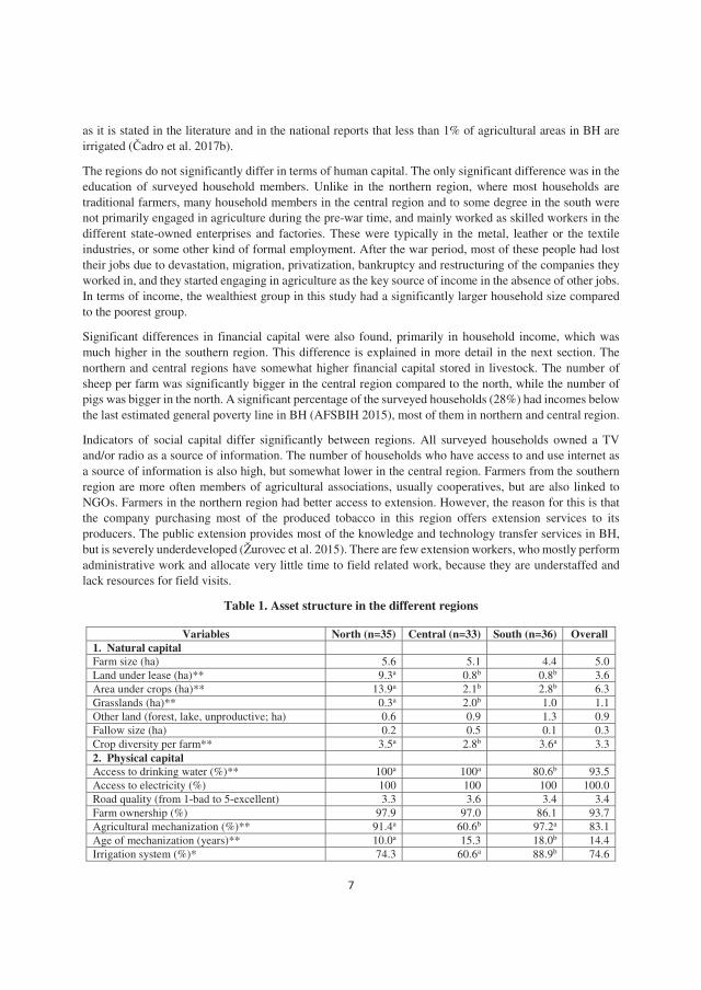
���
as it is stated in the literature and in the national reports that less than 1% of agricultural areas in BH are
irrigated (�adro et al. 2017b).
The regions do not significantly differ in terms of human capital. The only significant difference was in the
education of surveyed household members. Unlike in the northern region, where most households are
traditional farmers, many household members in the central region and to some degree in the south were
not primarily engaged in agriculture during the pre-war time, and mainly worked as skilled workers in the
different state-owned enterprises and factories. These were typically in the metal, leather or the textile
industries, or some other kind of formal employment. After the war period, most of these people had lost
their jobs due to devastation, migration, privatization, bankruptcy and restructuring of the companies they
worked in, and they started engaging in agriculture as the key source of income in the absence of other jobs.
In terms of income, the wealthiest group in this study had a significantly larger household size compared
to the poorest group.
Significant differences in financial capital were also found, primarily in household income, which was
much higher in the southern region. This difference is explained in more detail in the next section. The
northern and central regions have somewhat higher financial capital stored in livestock. The number of
sheep per farm was significantly bigger in the central region compared to the north, while the number of
pigs was bigger in the north. A significant percentage of the surveyed households (28%) had incomes below
the last estimated general poverty line in BH (AFSBIH 2015), most of them in northern and central region.
Indicators of social capital differ significantly between regions. All surveyed households owned a TV
and/or radio as a source of information. The number of households who have access to and use internet as
a source of information is also high, but somewhat lower in the central region. Farmers from the southern
region are more often members of agricultural associations, usually cooperatives, but are also linked to
NGOs. Farmers in the northern region had better access to extension. However, the reason for this is that
the company purchasing most of the produced tobacco in this region offers extension services to its
producers. The public extension provides most of the knowledge and technology transfer services in BH,
but is severely underdeveloped (Žurovec et al. 2015). There are few extension workers, who mostly perform
administrative work and allocate very little time to field related work, because they are understaffed and
lack resources for field visits.
Table 1. Asset structure in the different regions
Variables North (n=35) Central (n=33) South (n=36) Overall
1. Natural capital
Farm size (ha) 5.6 5.1 4.4 5.0
Land under lease (ha)** 9.3a 0.8b 0.8b 3.6
Area under crops (ha)** 13.9a 2.1b 2.8b 6.3
Grasslands (ha)** 0.3a 2.0b 1.0 1.1
Other land (forest, lake, unproductive; ha) 0.6 0.9 1.3 0.9
Fallow size (ha) 0.2 0.5 0.1 0.3
Crop diversity per farm** 3.5a 2.8b 3.6a 3.3
2. Physical capital
Access to drinking water (%)** 100a 100a 80.6b 93.5
Access to electricity (%) 100 100 100 100.0
Road quality (from 1-bad to 5-excellent) 3.3 3.6 3.4 3.4
Farm ownership (%) 97.9 97.0 86.1 93.7
Agricultural mechanization (%)** 91.4a 60.6b 97.2a 83.1
Age of mechanization (years)** 10.0a 15.3 18.0b 14.4
Irrigation system (%)* 74.3 60.6a 88.9b 74.6

���
Irrigated land (%) 59.2 46.4 59.1 54.9
Greenhouse (%) 11.4a 18.2a 47.2b 26.0
3. Human capital
Household size 4.2 4.5 5.0 4.6
Age of the head of household 54.3 53.8 59.5 55.9
Education – head of household (years) 10.1 12.3 11.2 11.2
Education – highest in household (years)** 12.3a 14.0b 12.9a 13.1
Dependency ratio (%) 32.4 23.1 47.2 34.2
4. Financial capital
Number of cows/cattle 2.8 3.6 0.5 2.3
Number of sheep* 0.5a 19.2b 2.3 7.3
Number of goats 0.0 4.0 0.1 1.4
Number of pigs** 3.4a 0.1b 0.0b 1.2
Number of poultry 128.3 5.1 3.4 45.6
Number of beehives 0.0 3.1 3.3 2.1
Household annual income (BAM)** 22,302.9a 27,381.8a 48,233.3b 32,639.3
Annual income per household member (BAM)** 5,554.3a 5,949.7a 11,226.3b 7,576.8
5. Social capital
Access to information (Radio, TV) 100.0 100.0 100.0 100.0
Internet access (%)** 94.3a 66.6b 94.4a 85.1
Membership in associations (%)** 37.1a 45.4a 88.9b 57.1
Access to extension (%)** 88.6a 57.6b 58.3b 68.2
Access to credit (%)** 100a 81.8b 97.2a 93.0
* p<0.05
** p<0.01 a,b Tukey test; groups with different letters are significantly different from each other (p<0.05)
The biggest differences between income groups, apart from income, were found in access to natural capital,
with the wealthiest group of households having significantly bigger farms, areas under crops and higher
diversity of crops produced on farms. Wealthier households also had a bigger household size and therefore
more access to family labour, and more agricultural machinery. Lastly, the poorest households had
significantly lower access to social capital, with significant differences found in membership in associations
and access to credit. Clearly, higher access to natural capital and farm labour enables increased on-farm
production. Increased participation in farming associations of households with higher incomes indicates the
importance of these associations in improving livelihood opportunities and security. They also allow
farmers, especially smallholders, improved access to markets in terms of both inputs and outputs, and access
to information and technologies through a wide range of services (Stockbridge et al. 2003). Based on these
results, it can be concluded that the rural households who are able to specialize in agriculture have higher
income levels. We return to this under a discussion of livelihood activities and outcomes.
Table 2. Asset structure in relation to total household income
Variables Poorest (n=35) Poor (n=34) Less poor (n=35) Overall
1. Natural capital
Farm size (ha)** 2.4a 4.0a 8.8b 5.0
Land under lease (ha) 1.3 5.1 4.7 3.6
Area under crops (ha)* 2.8a 7.2 9.1b 6.3
Grasslands (ha) 0.5 1.3 1.5 1.1
Other land (forest, lake, unproductive; ha)* 0.3a 0.6 1.8b 0.9
Fallow size (ha) 0.1 0.2 0.5 0.3
Crop diversity per farm* 2.6a 3.4 3.4b 3.3
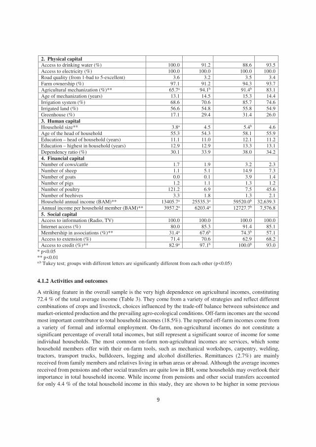
���
2. Physical capital
Access to drinking water (%) 100.0 91.2 88.6 93.5
Access to electricity (%) 100.0 100.0 100.0 100.0
Road quality (from 1-bad to 5-excellent) 3.6 3.2 3.5 3.4
Farm ownership (%) 97.1 91.2 94.3 93.7
Agricultural mechanization (%)** 65.7a 94.1b 91.4b 83.1
Age of mechanization (years) 13.1 14.5 15.3 14.4
Irrigation system (%) 68.6 70.6 85.7 74.6
Irrigated land (%) 56.6 54.8 55.8 54.9
Greenhouse (%) 17.1 29.4 31.4 26.0
3. Human capital
Household size** 3.8a 4.5 5.4b 4.6
Age of the head of household 55.3 54.3 58.1 55.9
Education – head of household (years) 11.1 11.0 12.1 11.2
Education – highest in household (years) 12.9 12.9 13.3 13.1
Dependency ratio (%) 30.1 33.9 38.0 34.2
4. Financial capital
Number of cows/cattle 1.7 1.9 3.2 2.3
Number of sheep 1.1 5.1 14.9 7.3
Number of goats 0.0 0.1 3.9 1.4
Number of pigs 1.2 1.1 1.3 1.2
Number of poultry 121.2 6.9 7.5 45.6
Number of beehives 3.3 1.8 1.3 2.1
Household annual income (BAM)** 13405.7a 25535.3a 59520.0b 32,639.3
Annual income per household member (BAM)** 3957.2a 6203.4a 12727.7b 7,576.8
5. Social capital
Access to information (Radio, TV) 100.0 100.0 100.0 100.0
Internet access (%) 80.0 85.3 91.4 85.1
Membership in associations (%)** 31.4a 67.6b 74.3b 57.1
Access to extension (%) 71.4 70.6 62.9 68.2
Access to credit (%)** 82.9a 97.1b 100.0b 93.0
* p<0.05
** p<0.01 a,b Tukey test; groups with different letters are significantly different from each other (p<0.05)
4.1.2 Activities and outcomes
A striking feature in the overall sample is the very high dependence on agricultural incomes, constituting
72.4 % of the total average income (Table 3). They come from a variety of strategies and reflect different
combinations of crops and livestock, choices influenced by the trade-off balance between subsistence and
market-oriented production and the prevailing agro-ecological conditions. Off-farm incomes are the second
most important contributor to total household incomes (18.5%). The reported off-farm incomes come from
a variety of formal and informal employment. On-farm, non-agricultural incomes do not constitute a
significant percentage of overall total incomes, but still represent a significant source of income for some
individual households. The most common on-farm non-agricultural incomes are services, which some
household members offer with their on-farm tools, such as mechanical workshops, carpentry, welding,
tractors, transport trucks, bulldozers, logging and alcohol distilleries. Remittances (2.7%) are mainly
received from family members and relatives living in urban areas or abroad. Although the average incomes
received from pensions and other social transfers are quite low in BH, some households may overlook their
importance in total household income. While income from pensions and other social transfers accounted
for only 4.4 % of the total household income in this study, they are shown to be higher in some previous

����
studies (e.g. (Berjan et al. 2014b; UNDP 2013). Here, we analyse and discuss the differences in income
sources by region and income level, as well as diversification in agricultural production and on-farm
products.
Table 3. Diversification of income sources by region
Income source North (n=35) Central (n=33) South (n=36) Total (n=104)
Agriculture**++ 17,877a 78.1b 16,356a 55.9a 41,198b 83.2b 25,467 72.8
On-farm non-agricultural*+ 309a 1.1 1,590b 3.9a 150a 0.1b 660 1.7
Off-farm+ 3,158 15.9 7,068 28.2a 5,298 12.1b 5,140 18.5
Remittances 549 3.7 927 4.4 13 0.1 483 2.7
Pension, other social transfers*+ 411 1.1a 1,440 7.6b 1,573 4.6 1,140 4.4
Total** 22,303 100 27,382a 100 48,233b 100 32,891 100 * significant difference between some of the three categories (Anova). * P<0.05; ** P<0.01.
+ = significant difference between some of the three relative income categories + P<0.05; ++ P<0.01.
a,b = Tukey test; groups with different letters are significantly different from each other (p<0.05).
There was a significant difference between relative agricultural income in the central region, which was
lower (55.9 %), compared to the northern (78.1 %) and southern region (83.2 %). Interestingly, the total
income from agriculture in the south is more than twice that of the other regions, as well as being a
significantly higher contributor to total household income. This is not explained by the regional differences
in asset access, since higher agricultural income in the south is achieved with access to the same, or even
lower amounts of natural capital compared to the other regions. The main difference rather derives from
the structure of the agricultural production unit and the on-farm products sold, which are determined by
how the assets are used in agricultural production, as well as agricultural potential in the researched regions
in terms of climatic conditions. We come back to this later in this section.
From Table 4 we see that the total income is more than four times higher for the less poor than for the poor
household group. They have more land, livestock, labour, and general capital access. Regarding the
diversification of income sources, a statistically significant difference was found in the case of total
agricultural and off-farm incomes between the poor and the less poor group. Interestingly, there was no
statistically significant difference in the relative contribution of different income sources to the total
household income. Households in the three income groups thus have a similar structure of income sources
in terms of their relative incomes, but they differ in their total amounts. The poorest group of households
had lower total incomes from every source, except remittances. Less poor households had much higher total
agricultural income. This is in line with the higher access to natural (most notably land), physical
(agricultural machinery) and human capital (more family labour) these households have as discussed
earlier. Another interesting finding is that the wealthiest households in this study (less poor group) tend to
be either those who acquired their farms in the last 15 years on average (50% of the total sample) or have
a long tradition of farming, spanning three or more generations (46% of the total sample).
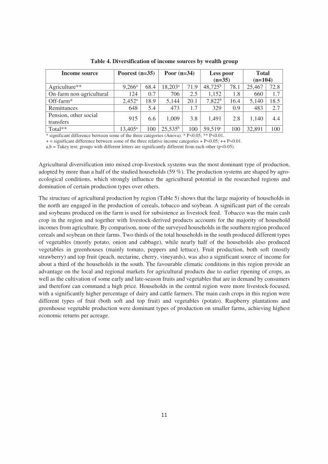
����
Table 4. Diversification of income sources by wealth group
Income source Poorest (n=35) Poor (n=34) Less poor
(n=35)
Total
(n=104)
Agriculture** 9,266a 68.4 18,203a 71.9 48,725b 78.1 25,467 72.8
On-farm non-agricultural 124 0.7 706 2.5 1,152 1.8 660 1.7
Off-farm* 2,452a 18.9 5,144 20.1 7,822b 16.4 5,140 18.5
Remittances 648 5.4 473 1.7 329 0.9 483 2.7
Pension, other social
transfers 915 6.6 1,009 3.8 1,491 2.8 1,140 4.4
Total** 13,405a 100 25,535b 100 59,519c 100 32,891 100 * significant difference between some of the three categories (Anova). * P<0.05; ** P<0.01.
+ = significant difference between some of the three relative income categories + P<0.05; ++ P<0.01.
a,b = Tukey test; groups with different letters are significantly different from each other (p<0.05).
Agricultural diversification into mixed crop-livestock systems was the most dominant type of production,
adopted by more than a half of the studied households (59 %). The production systems are shaped by agro-
ecological conditions, which strongly influence the agricultural potential in the researched regions and
domination of certain production types over others.
The structure of agricultural production by region (Table 5) shows that the large majority of households in
the north are engaged in the production of cereals, tobacco and soybean. A significant part of the cereals
and soybeans produced on the farm is used for subsistence as livestock feed. Tobacco was the main cash
crop in the region and together with livestock-derived products accounts for the majority of household
incomes from agriculture. By comparison, none of the surveyed households in the southern region produced
cereals and soybean on their farms. Two thirds of the total households in the south produced different types
of vegetables (mostly potato, onion and cabbage), while nearly half of the households also produced
vegetables in greenhouses (mainly tomato, peppers and lettuce). Fruit production, both soft (mostly
strawberry) and top fruit (peach, nectarine, cherry, vineyards), was also a significant source of income for
about a third of the households in the south. The favourable climatic conditions in this region provide an
advantage on the local and regional markets for agricultural products due to earlier ripening of crops, as
well as the cultivation of some early and late-season fruits and vegetables that are in demand by consumers
and therefore can command a high price. Households in the central region were more livestock-focused,
with a significantly higher percentage of dairy and cattle farmers. The main cash crops in this region were
different types of fruit (both soft and top fruit) and vegetables (potato). Raspberry plantations and
greenhouse vegetable production were dominant types of production on smaller farms, achieving highest
economic returns per acreage.
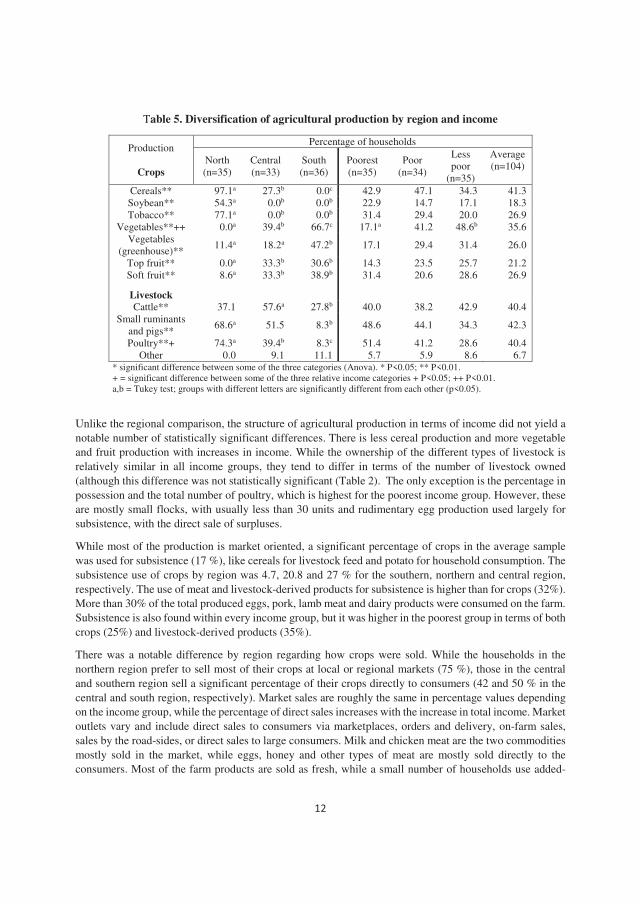
� ��
Table 5. Diversification of agricultural production by region and income
Production
Crops
Percentage of households
North
(n=35)
Central
(n=33)
South
(n=36)
Poorest
(n=35)
Poor
(n=34)
Less
poor
(n=35)
Average
(n=104)
Cereals** 97.1a 27.3b 0.0c 42.9 47.1 34.3 41.3
Soybean** 54.3a 0.0b 0.0b 22.9 14.7 17.1 18.3
Tobacco** 77.1a 0.0b 0.0b 31.4 29.4 20.0 26.9
Vegetables**++ 0.0a 39.4b 66.7c 17.1a 41.2 48.6b 35.6
Vegetables
(greenhouse)** 11.4a 18.2a 47.2b 17.1 29.4 31.4 26.0
Top fruit** 0.0a 33.3b 30.6b 14.3 23.5 25.7 21.2
Soft fruit** 8.6a 33.3b 38.9b 31.4 20.6 28.6 26.9
Livestock
Cattle** 37.1 57.6a 27.8b 40.0 38.2 42.9 40.4
Small ruminants
and pigs** 68.6a 51.5 8.3b 48.6 44.1 34.3 42.3
Poultry**+ 74.3a 39.4b 8.3c 51.4 41.2 28.6 40.4
Other 0.0 9.1 11.1 5.7 5.9 8.6 6.7
* significant difference between some of the three categories (Anova). * P<0.05; ** P<0.01.
+ = significant difference between some of the three relative income categories + P<0.05; ++ P<0.01.
a,b = Tukey test; groups with different letters are significantly different from each other (p<0.05).
Unlike the regional comparison, the structure of agricultural production in terms of income did not yield a
notable number of statistically significant differences. There is less cereal production and more vegetable
and fruit production with increases in income. While the ownership of the different types of livestock is
relatively similar in all income groups, they tend to differ in terms of the number of livestock owned
(although this difference was not statistically significant (Table 2). The only exception is the percentage in
possession and the total number of poultry, which is highest for the poorest income group. However, these
are mostly small flocks, with usually less than 30 units and rudimentary egg production used largely for
subsistence, with the direct sale of surpluses.
While most of the production is market oriented, a significant percentage of crops in the average sample
was used for subsistence (17 %), like cereals for livestock feed and potato for household consumption. The
subsistence use of crops by region was 4.7, 20.8 and 27 % for the southern, northern and central region,
respectively. The use of meat and livestock-derived products for subsistence is higher than for crops (32%).
More than 30% of the total produced eggs, pork, lamb meat and dairy products were consumed on the farm.
Subsistence is also found within every income group, but it was higher in the poorest group in terms of both
crops (25%) and livestock-derived products (35%).
There was a notable difference by region regarding how crops were sold. While the households in the
northern region prefer to sell most of their crops at local or regional markets (75 %), those in the central
and southern region sell a significant percentage of their crops directly to consumers (42 and 50 % in the
central and south region, respectively). Market sales are roughly the same in percentage values depending
on the income group, while the percentage of direct sales increases with the increase in total income. Market
outlets vary and include direct sales to consumers via marketplaces, orders and delivery, on-farm sales,
sales by the road-sides, or direct sales to large consumers. Milk and chicken meat are the two commodities
mostly sold in the market, while eggs, honey and other types of meat are mostly sold directly to the
consumers. Most of the farm products are sold as fresh, while a small number of households use added-

����
value processing as a strategy to increase the net profitability of their products. The common value-added
products found in this study were apple and pear juice, jam, cheese and other dairy products.
The results show a very high relative dependence on agriculture, especially in the north and south, and
irrespective of income group. Higher incomes from agriculture is driving the wealthiest group, most of
them from the southern region. Low agricultural incomes and a significant degree of subsistence, coupled
with low incomes from off-farm activities constrain the livelihoods and income from the poorest group –
most of them from the northern region. The situation in the central region resembles that found in the north,
with one difference; that low incomes from agriculture are partly mitigated by income from non-agricultural
on- and off-farm activities. Wealthier households also show a higher degree of entrepreneurship, reflected
in more variable market outlet choices.
Higher agricultural incomes in the southern region can be mainly attributed to more favourable climatic
conditions in this region, which enables the farmers to time their production in order to exploit the
opportunities on the market and also to produce more lucrative crops. In addition, households in the
southern region have better access technologies (e.g. irrigation, greenhouses) and are more often part of
agricultural associations. Access to technologies enables a higher degree of agricultural intensification,
while participation in associations allows for increased and improved access to markets, information and
technologies.
This difference in livelihood outcomes however, can not only be attributed to asset structure and activities.
Rural households are situated within institutional and organisational conditions partly beyond their direct
control. These institutional processes and organisational structures influence both access to livelihood assets
and the composition of livelihood portfolios and therefore have an impact on peoples’ ability to secure
livelihood outcomes (Ellis 2000).
4.1.3 Institutional constraints to improved livelihoods
In the context of rural households in BH, main constraints found to hinder improved livelihoods result from
the shocks brought about by war devastation and post-conflict transition from the centrally planned to
market economy, which resulted in the creation of fundamentally different governmental institutions. Such
conditions led to a rise in unemployment and informal economy, inflation, high rates of migration and other
longer-term constraints on development which are often found in all transition economies (Davis 2006).
These reforms have affected rural households in BH in many ways. High dependence on agriculture in rural
areas is mainly driven by a lack of alternative income sources. The dependence on agriculture for both
subsistence and as a source of income can be seen as an effective strategy to cope with risks and
uncertainty. However, simple technologies, lack of entrepreneurship, absence of specialisation and capital
farm investments keep agricultural and labour productivity low. We focus on some key constraints
identified by the rural households in our study.
The decentralized political and administrative structure of BH is both very complex and quite unique. A
tripartite government structure, established to ensure that the interests of the three major ethnic groups are
represented, resulted in an asymmetrical and complex governance structure. BH comprises two state entities
- Federation of BH (FBiH) and Republika Srpska (RS), as well as the municipality of Br�ko District of BH
(BD), which are all politically autonomous to an extent. In addition, FBiH is divided into 10 Cantons, each
with its own government. The lowest administrative units are municipalities. There are 143 of them and
each one has its own government and public services, which are under the jurisdiction of the cantons (in
FBiH) or the entity (in RS). This has led to different policies at different levels, legislative overlaps, limited

����
capacities and communication channels, as well as lack of a clear vision and failure to implement necessary
reforms. Consequently, this affects every aspect of development, implementation and enforcement of
policies and results in an unsustainable level of government spending, a staggering amount of corruption,
economic stagnation and economic inefficiency. The difficult and complicated political situation is one of
the main obstacles for foreign investments, without which there is no significant economic progress
(Borensztein et al. 1998). According to the most recent official survey in 2017, the unemployment rate in
BH was 20.5 % (AFSBIH 2017), which is among the highest in the world (WB 2017). This creates a
pessimistic environment and leads to both migration to urban areas and abroad, leaving the ever aging
population in rural areas.
The main feature of agricultural policies in BH is a low budget allocation for agriculture. The public
spending for agriculture accounted for about 3 % of the total public spending in 2015 (MOFTER 2016).
The largest amount of support (90 %) was classified as direct payments to farmers, which refers to payments
based on output and the payment per unit area/cattle. This means that the composition of subsidies in BH
is heavily oriented toward direct production rather than investments, thus having a social safety net function
rather than providing productive support to the agricultural sector. Of the total number of surveyed
households, 65.4 % were subsidized for different types of production. Not only are the budget allocations
low, but the payments are usually not paid within the allocated budget year. Some of the surveyed
households reported not having been paid the agreed subsidies since 2014. In the absence of investment
grants, the farm function is on the level of simple reproduction, using outdated and obsolete fixed assets
under the lack of financial resources to invest in expanded production (Bernstein 2010).
Domestic agricultural production suffers from low competitiveness caused by poor governance and a lack
of public investments. The problem partly lies in an insufficiently developed food industry, discrepancy
with quality standards and legislation, low levels of market-oriented production to create the critical mass
needed for export, as well as the problems of inconsistent product quality and increased transport costs due
to fragmentation of smallholders and supply chains (Bajramovi� et al. 2008). In addition, the disconnected
smallholders and the lack of association in cooperatives with the aim of improving production and joint
appearance on the market has, to date, deprived smallholder farmers of better negotiating opportunities and
favourable purchases of both their products and the necessary inputs. The lack of competitiveness in the
agricultural sector makes it difficult to enter export markets, and to compete with imported products in the
domestic market. A general unsustainably high negative trade balance in BH and low domestic
competitiveness is significantly affected by import of agricultural products. The most recent ratio of import
coverage by export for agricultural products was only 31.7% (MOFTER 2017).
Although there is a large number of banks and credit organizations in BH, which enables sufficient physical
access to loans, the conditions posed to obtain the credit for agricultural producers are highly demanding
and discouraging for farmers, especially smallholders. An unstable political situation in the country and a
dysfunctional market further create a large degree of uncertainty and discourage investments in agriculture,
which is consequently stagnating (see Berjan et al. (2014a)).
Furthermore, important obstacles to development of the agricultural sector in BH include the large
fragmentation of agricultural land and an inefficient land market. Regulated maximum private farm size in
a former socialist state (10 ha), coupled with the still existing inheritance law, demanding the subdivision
of farm holdings into equal parts among all heirs, resulted in severe fragmentation of private holdings and
farms. A staggering 88.5% of households in our total sample had farms formed from small parcels, often
dislocated from each other, which makes agricultural production less efficient and hampers investment in
technologies. Those who are interested in investing in expansion or consolidation of their farms are often

����
faced with an incomplete land registry and rigid land transaction processes, making land registration and
land transactions costly and time consuming (World Bank 2010).
4.2 Impact of climate change on livelihoods and adaptation strategies
4.2.1 Reported damage from adverse weather effects
The reported damages in terms of adverse weather effects were almost exclusively related to agricultural
production and the associated damage to crops in terms of yield declines and the reduced quality of
products. Negative effects of drought were seen as the most serious and the most frequent cause leading to
production declines and were more frequent in the northern and central region. In the same regions,
occasional waterlogging is associated with reduced crop growth and consequently yields, as well as delays
in agricultural field operations. More significant damage to crops and infrastructure due to floods was
reported only in the northern region. Damage to crops caused by hail is found in every region, but it was
more frequent in the north. Similarly, damage caused by frost is found in all regions. Negative effects of
early spring frost are similar in all regions, while the increased presence of late crops (most notably fruits)
in the central and southern region is the main reason for the damage caused by late autumn frosts.
Figure 3. Reported frequency of damage caused by adverse weather conditions
The reported negative impacts of adverse weather conditions correspond well with the prevalent climatic
conditions in the studied regions, as well as with previous scientific findings. The southern region is semi-
arid while the other two regions are humid. The agricultural systems in the semi-arid south are traditionally
and inherently more drought resilient in design and function. Thus, drought in the south is perceived as
something which occurs regularly, unlike in the other regions that have been recently exposed to the
increasing frequency of droughts (�adro et al. 2017a). The mostly plain landscape and the dominant heavy
soils with limited infiltration capacity makes the northern region more vulnerable to negative effects caused
by heavy precipitation events, such as waterlogging and floods (Žurovec et al. 2017a). Increased incidences
of hail have also been recorded (UNFCCC 2013). Frosts occur regularly in the studied climate zones, further
modified by topography of the studied regions and therefore cannot be attributed to climate change.
However, it is not known if the ongoing climate trends have any influence on the occurrence of frosts in
the region.
�
�
�
�
4"�'�� #���"!�� )!��� .��! 0�"� �"��� %'�'( �"���5�"�� 6� �"�! 0�'��
�� 7� �/�"8� �7�"�"�!,8���7���(���(��8���7���� 8���7�/�",���� �

����
4.2.2 Perceptions of climate change
Rural households report awareness of recent trends in climate change. The overwhelming majority of the
respondents in our study perceive an increase in average temperature (92 %). This in line with the actual
climate data for the period from 1961 to 2015, where, an increase in temperatures was recorded in every
region (Figure 4a). Average annual temperature has increased by 1.6 oC in all regions for the observed 55-
year period. The increase was even bigger if only the months of the cropping season are observed (March-
September) and range from 1.7 oC in the north, 1.8 oC in the central to 2.1 oC in the southern region. The
average temperature in BH has increased by 0.8°C in the last 100 years, while the last two decades are the
warmest ever recorded (UNFCCC 2013).
The perception of long-term precipitation change varied by region in this study. While most of the
respondents in the northern region perceive a decrease in the total amount of precipitation, most of the
respondents in the southern and central region report different distribution of the precipitation over the year.
However, there has been a slight factual increasing trend in the total annual precipitation in the northern
and central region, while a significant decrease has been observed only in the south, where the total annual
precipitation has decreased 120 mm in the last 55 years (Figure 4b). Minimum changes in precipitation
were recorded within the cropping season (March-September) in all regions, with a very low increase in
precipitation trends in the observed period.
Figure 4. a Temperature trends and b precipitation trends from the weather stations in the studied regions
One reason why some respondents perceive a decreased amount of precipitation, even though it is not in
line with the actual long-term climate observations, may be based on a measured decrease in water
availability under the prolonged and severe droughts and higher temperatures experienced in recent years,
as previously reported by Bryan et al. (2013). While the level of annual precipitation did not significantly

����
change, a decrease in number of days with precipitation and an increase in number of days with more
intense precipitation resulted in the increased frequency of droughts (UNFCCC 2013).
We found little differences between perceptions of climate changes by income groups. The only notable
difference was that part of the respondents (18 %) from the wealthiest group did not attribute the increased
incidence of extreme weather events to climate change.
4.2.3 Adaptation strategies
Respondents reported different adaptation strategies, in terms of both non-agricultural activities and the
adoption of agricultural practices and technologies (Table 5). Overall, off-farm employment was the most
common non-agricultural strategy and 57.7% of the total researched households had one or more family
members employed off the farm. The central region had the highest level of off-farm activities. Other non-
agricultural activities were adopted to a lesser extent, and with some variation by region and by income
levels. A third of the households in the north decided to lease out parts of their land, partly due to lack of
labour access and partly due to remoteness of some of the parcels of land relative to their farm. Household
members in the central region, especially the younger and educated ones, tend to migrate more to urban
areas. Migration to urban areas was also significantly more expressed in the poorest group of households.
Table 5. Reported adaptation strategies by region and income.
Adaptation strategies
Percentage of households
North
(n=35)
Central
(n=33)
South
(n=36)
Poorest
(n=35)
Poor
(n=34)
Less
poor
(n=35)
Average
(n=104)
Non-agricultural
Lease out land** 31.4a 3.1b 0.0b 11.4 12.1 11.1 11.8
Work on other farm 17.1 3.1 19.4 20.0 14.7 5.6 13.6
Finding employment* 62.9 72.7a 38.9b 60.0 55.9 54.1 57.7
Moving to urban area*+ 14.3 21.2a 0.0b 22.9a 5.9 5.4b 11.5
Moving abroad 5.7 6.1 5.6 8.6 2.9 5.4 5.8
Agricultural
Change of crop** 88.6a 43.3b 70.6a 61.8 84.4 58.8 68.7
Change of crop variety** 91.4a 54.8b 85.3a 70.6 81.3 85.7 78.0
Drought resistant crops* 2.9a 26.7b 14.7 5.9 21.9 14.7 14.1
Reduced tillage 5.7 16.1 8.8 5.9 12.5 11.4 10.0
No-till 0.0 3.2 5.9 2.9 3.1 2.9 3.0
Change in sowing/planting dates 54.3 46.7 58.8 52.9 53.1 58.8 53.5
Fertilization (synthetic + manures) 94.3 90.0 100.0 88.2 100.0 100.0 94.9
Incorporation of crop residues** 88.6a 50.0b 15.2c 47.1 61.3 47.1 52.0
Use of cover crops* 5.7a 26.7b 8.8 14.7 15.6 8.8 13.1
Irrigation** 85.7a 60.0b 97.1a 82.4 75.0 91.2 81.8
Drainage** 54.3a 20.0b 0.0b 26.5 28.1 20.6 25.3
Erosion prevention** 2.9a 23.3b 0.0a 8.8 6.3 8.8 8.1
Anti-hail nets 0.0 10.0 5.9 5.9 6.3 2.9 5.1
Greenhouse** 11.4a 18.2a 47.2b 17.1 29.4 32.4 26.0
Crop insurance** 51.4a 0.0b 0.0b 14.3 18.2 19.4 17.3
Agricultural adaptations (average
per household) 6.4a 4.5b 4.9 4.9 5.6 5.3 5.3
* significant difference between some of the three categories (Anova). * P<0.05; ** P<0.01.
+ = significant difference between some of the three relative income categories + P<0.05; ++ P<0.01.
a,b = Tukey test; groups with different letters are significantly different from each other (p<0.05).

����
We also looked into the adoption of various agricultural practices and technologies. There are indications
in our material for an overall intensification strategy for agricultural production in BH, as well as adaptation
to the perceived changes in climatic conditions. Most notable is the application of both organic and mineral
fertilizers, adopted by 94.9 % of the households in this study. While we did not measure the total amounts
applied, increased fertilization is likely one of the main reasons for an overall increase in yields of the main
crops, such as maize, wheat and potato (Vaško and Mirjani� 2013). However, the yields of most crops are
still significantly lower compared to the more developed parts of Europe (Žurovec et al. 2015).
We also found a high degree of adoption of irrigation, where 82.7% of the surveyed households reported
investing in some type of irrigation system, irrigating an average of 55.7% of their utilized arable land. Drip
irrigation is mainly used for cash crops and greenhouses, although the irrigation of cereals and other crops
using typhons was also found in the northern region. Public investments in irrigation and related agricultural
and water management projects in the post-war period in BH has been low, thus the adoption of irrigation
is carried out privately by individual households. Therefore, the adoption of irrigation can be seen as a
reactive adaptation to intensify production and as a response to the perceived increased incidence of
droughts. Most of the irrigation systems are simple, not requiring significant investments. They are usually
drip-irrigation systems using water from private wells or adjacent watercourses, mostly manually operated
and without much regard to water consumption. Most of those who irrigate generally avoid paying water
usage fees due to the lack of farm registers and other means of water monitoring. This makes irrigation
cost-effective from the individual farmers point of view, but less so from a social profitability point of view.
While subsistence needs still are an important determinant in the selection of crops and livestock, an
increasing number of cash crops on farms and more market-oriented production are noticeable. A
significant number of households report to change their crops according to market demands (68.7 %), or
report to use more productive crop varieties (78 %), in order to achieve higher yields. Some households,
most notably in the central region, have adopted crops that are more drought tolerant.
Other agricultural adaptation strategies include those requiring low implementation investments. Most
notable adopted agricultural practices are changes in sowing/planting dates (53.5 %) and incorporation of
crop residues (52%). The degree of adoption of certain agricultural practices varied significantly by region,
while no significant differences were observed in terms of different income groups. Some adoptions are
more suited for particular regions, such as drainage (northern region) or erosion prevention (central region).
Conservation agriculture practices were found to be less common, such as use of cover crops (13.3%),
reduced tillage (10.1%) and no-till (3.0%). Only a small part of the respondents were familiar with the
existence and implementation of such measures, most notably no-till (23.2%), and reduced tillage (35.4%).
There is a general lack of knowledge in the Western Balkan region regarding the effects of conservation
tillage practices. However, recent short-term results show that reduced tillage is potentially more climate
resilient in central BH (Žurovec et al. 2017b). The reported 17.3% of households who insured their crops
might lead to the conclusion that a significant number of households opted for crop insurance as a strategy
to protect themselves against the risk of crop failure. However, crop insurance is an isolated phenomenon
related to tobacco producers in the northern region, who are offered crop insurance by the company
purchasing the majority of produced tobacco in the region. Although some insurance companies in BH
offer crop insurance services, the wider application of these services were not reported.
Fifteen different agronomic practices were reported in this study. Households adopted 5.3 on average. The
results varied by researched region, while no statistical difference was found in terms of income.
Households in the northern region adopted 6.4 of them on average, compared to 4.9 and 4.5 in the southern
and central region, respectively. A large majority of respondents reported both agronomic and economic

����
benefits upon adoption of the reported practices. The main reported constraints for altered adoption were
lack of financial capital, knowledge and labour.
The differences in adopted agricultural practices further demonstrate that location plays an important role
in climate change adaptation in BH, both in the number and type of adoptions. Furthermore, adoption of
agricultural practices was less dependent on income group, despite the significant differences in total
income among them. In the context of the livelihoods approach, adaptations are seen as the outcome of
different livelihood strategies, which are not necessarily seen as a way to only maximize profits, but rather
as development and diversification of a portfolio of assets pursuing different motives, such as increased
well-being, reduced vulnerability, improved food security and a more sustainable use of natural
resources (DFID 1999; Ellis 2000). Climate change can directly affect livelihoods and the capacity to adapt
to shocks will be determined how assets are accessed and used in different ways. Furthermore, it has been
reported by a significant body of literature that access to capital assets has an important role in facilitating
adaptation and adoption of technologies in agriculture. Below we analyse the agricultural practices as a
function of access to various assets at the individual household level.
4.2.4 Determinants of agricultural practices and technology adoption
We used bivariate logistics regression to assess the important determinants of the various adopted
agricultural practices and technologies in terms of access to different types of assets. In total, 10 out of 15
agricultural practices were found to have an adequate sample size for the analysis. Based on the overall
results (Table 6), it is evident that the factors influencing the decision to adopt a particular agricultural
practice vary and it is difficult to draw generalized conclusions. However, it is notable that increased access
to different types of assets in most cases influence the likelihood of adoption. Factors influencing adoption
in our study correspond well to empirical research findings in relation to farmers’ general adaptation to
climate change. Social capital was found to be the most significant determinant of adoption. Membership
in agricultural associations, internet access, access and utilisation of public extension and the frequency of
extension visits increase the likelihood for adoption of most practices. Participation in different social
groups provides one means for exposure to knowledge, innovations and technologies that can be used to
adapt to changes in climatic conditions (Bryan et al. 2013; Deressa et al. 2009).
Access to physical capital, which includes farm machinery, buildings, other facilities and equipment, is a
primary factor of production in agriculture. We could not draw conclusions related to infrastructure because
most of the households in this study owned their farms and nearly all of them had access to basic
infrastructure, such as electricity and water. However, possession of tractors and its highly positive
influence on adoption in our study shows the importance of access to technologies in terms of different
management options and labour they provide (Nhemachena et al. 2014). Investment in physical capital can
be also seen as a more long term adaptation strategy, like investments in greenhouses or irrigation systems.
Human capital also had a positive impact on adoption. While an increase in household size can be seen as
an increase in total labour available, which increases the likelihood to adopt certain agricultural practices,
education can also influence adaptation through increased awareness and knowledge, better access to social
networks, off-farm work and a general increased adaptive capacity (Wamsler 2011; Yohe and Tol 2002).
Younger farmers are also more innovative and less risk-averse compared to their older counterparts (Ali
and Erenstein 2017).
Natural capital, viewed through farm size, had a mixed effect on long term adaptation in our study. While
an increase in the farm size was shown to increase the likelihood of adoption of some agricultural practices

���
(e.g. incorporation of crop residues, crop insurance), the opposite effect was found in case of larger on-farm
investments, such as irrigation, drainage or greenhouse. This may be due to the fact that farmers on larger
farms prefer to adapt by diversifying their crops and/or grasslands and pastures (if they have livestock),
rather than to invest in infrastructure or technologies.
Increase in total household income generally had an overall positive effect on adoption. Interestingly,
however, non-agricultural income is mostly negatively associated with adoption. This could be explained
by the household motives for diversification of their income generating activities, described as “push” and
“pull” factors (Haggblade et al. 2007). Households may be pushed into agriculture by necessity and may
be pulled by non–agricultural opportunities. Such households would be less likely to invest in agriculture
and focus more on non-agricultural opportunities.

��
�
Table
3. D
ete
rmin
ants
of
adap
tati
on
, o
dd
rat
ios,
BH
20
1x
x (
<1
mean
s n
egati
ve a
sso
ciati
on
, >
1 p
osi
tive)
Cap
ital
ass
ets
C
han
ge
of
cro
p
Ch
an
ge
of
cro
p
vari
ety
Dro
ugh
t
resi
stan
t
cro
ps
Ch
an
ge i
n
sow
ing/p
lan
tin
g
date
s
Inco
rpo
rati
on
of
cro
p
resi
du
es
Co
ver
cro
ps
Irri
gati
on
Dra
inage
Gre
en
ho
use
C
rop
insu
ran
ce
Farm
siz
e
1.0
7
1.0
9
0.9
5
1.0
6
1.0
0
0.9
9
0.9
8
0.8
7*
1.0
9
0.9
8
Farm
siz
e (
incl.
lease
d l
an
d)
1.0
0
1.0
2
1.0
7
0.9
9
1.2
7**
1.0
1
0.9
1**
1.2
4
0.9
0**
1.3
3**
Po
ssess
ion
of
tracto
r 3
.89
*
5.1
3*
10
5.5
1
3.5
5*
4.1
6*
0.0
7
7.9
8*
2.3
2
6.5
3*
66
2.8
4
Farm
ing
exp
eri
en
ce
1.0
1
1.0
2
1.0
0
1.0
4*
0.9
9
0.9
2
1.0
0
0.9
8
0.9
8
1.1
0
Age (
head
of
HH
) 0
.96
0.9
1***
0.9
6
0.9
9
0.9
8
0.9
8
0.9
9
1.0
0
0.9
9
0.9
9
Ed
ucati
on
(h
ead
of
HH
) 1
.09
0.8
7
1.8
9*
1.1
7*
1.0
4
0.6
8
0.9
3
0.9
7
0.9
1
0.9
5
Ed
ucati
on
(hig
hest
in H
H)
0.6
0
1.2
0
1.2
9
0.8
7
1.1
6
1.5
4
1.3
4
1.6
9**
0.8
1
0.7
7
Ho
use
hold
siz
e 1
.01
0.8
3
0.2
8
1.4
7*
0.8
4
0.6
6
1.7
1
0.4
0
1.4
7**
1.1
2
Ass
ocia
tio
n
mem
bers
hip
2
.19
4.0
3*
23
.10
*
1.4
4
0.3
0
9.3
2**
0.2
6
0.3
9
2.0
9
1.3
6
Exte
nsi
on
vis
its
2.9
1
1.0
7
0.0
0
0.3
5
5.3
3*
0.2
3
1.4
1
6.7
3**
0.8
9
25
85
.99
Fre
qu
en
cy o
f
exte
nsi
on
vis
its
0.7
9
0.7
9
4.5
7**
1.0
9
1.0
2
2.0
6**
2.7
4*
1.0
1
1.1
0
0.2
6
Inte
rnet
access
1
.97
2.1
3
0.4
7
2.4
0*
0.5
7
0.6
9
10
.42
***
3.8
8
0.3
6
11
61
.70
To
tal
inco
me
1.0
0
1.0
0
1.0
0**
1.0
0
1.0
0
1.0
0
1.0
0
1.0
0*
1.0
0
1.0
0
Inco
me p
er
cap
ita
1.0
0
1.0
0
1.0
0
1.0
0
1.0
0
1.0
0
1.0
0
1.0
0
1.0
0
1.0
0
Agri
cu
ltu
ral
inco
me
0.1
5
0.2
8
0.0
0*
0.1
0
4.3
2
4.0
4
0.0
9
0.0
1
2.0
7
46
.29
No
n-a
gri
cu
ltu
ral
inco
me
0.7
8
0.6
6*
0.6
0
0.7
0*
1.5
2
3.3
0
0.8
6
0.8
3*
0.8
8
1.9
4*
* p
<0
.1
** p
<0.0
5
*** p
<0
.01

��
5. Conclusions
The studied rural households in BH are exposed to multiple stressors that increase vulnerability and
constrain their livelihood options. Many stressors are typical for economies in transition, and include factors
such as inefficient institutions and policies, inadequate infrastructure, services and imperfect markets and
access. Under such conditions, continued high dependence on agriculture in rural areas is more driven by a
lack of alternative income sources.
The results of this study indicate a very high relative dependence on agriculture in the study areas (72.8%).
There are some variations by location (56-83%) and by income level (68-78%). The total income from
agriculture is around 25000 USD per year for the whole sample, while the difference in total income is 2-3
times larger for the southern region than the other two and more than 5 times higher agricultural income
for the least poor group than for the poorest group. The substantial difference in incomes observed mainly
depends on how the available assets are used in agriculture. The less poor own more land and are able to
produce more. However, the example of the southern region shows that significantly higher agricultural
incomes can be achieved also with significantly lower access to land. This is mainly attributed to more
favourable climatic conditions in this region, which enables the farmers to time their production in order to
exploit the opportunities on the market and to produce more lucrative crops. Furthermore, households in
the southern region have better access to technology (e.g. irrigation, greenhouses) and are more often part
of agricultural associations. Lastly, less poor households show a higher degree of entrepreneurship,
reflected in more variable market outlet choices.
Combing these insights, we see a group of less poor households with higher incomes and more specialised
in agriculture, while we observe a group of low-income households depending somewhat more on off-farm
activities. Half of the less poor income group was composed of the households from the southern region,
while the poorest group was mainly composed from the households from the northern region. The
households in the central region are more similar to those in the north in terms of income, with the difference
that low incomes from agriculture are partly mitigated by income from non-agricultural on- and off-farm
activities.
The observed high dependence on agriculture makes rural households more vulnerable to negative effects
of climate change, some of them already affecting the studied households. The negative effect of droughts
were most common and more stressed in the humid continental climate of the northern and central region
than in the south, which is traditionally more resilient due to the prevalent semi-arid climatic conditions
that present production systems are designed for. The northern region experienced occasional incidences
of heavy precipitation events, leading to waterlogging and floods. Damage from hail is found all regions,
but was more frequent in the north. It is not known if the ongoing climate trends have any influence on the
occurrence of early spring and late autumn frosts, which occur regularly in the studied climate zones and
cause significant damage to crops.
Studied households express their awareness of the recent climate trends. Most respondents in our study
perceive an increase in average temperature in line with the actual climate data. The way changes in
precipitation are perceived, both in terms of amount and distribution, varied depending on the region.
However, actual climate data showed a significant decrease in precipitation only in the south (-120 mm).
We attribute this inconsistency between perceived and actual precipitation to a decrease in water availability
under the increased frequency and intensity of droughts and higher temperatures.
While it is hard to differentiate whether it is climate change, agricultural intensification, or some other
factor that are the main motives behind certain adaptation options, especially within agriculture, the number
of adopted measures shows that there are signs of an overall intensification strategy of agricultural

���
production in BH, as well as marked adaptations to (perceived) climate changes. Most notable were the
application of both organic and mineral fertilizers, changes in crops and crop varieties, and a surprisingly
high degree of irrigation. Other common agricultural practices were those that require no or little
investments. The main reported constraints for further adoption and long-term adaptation within agriculture
were lack of funds, knowledge and labour. Certain agricultural practices carried out were in some cases
more region-specific, but overall were similar in relation to income level.
The results indicate that increased access to different types of assets in most cases influence the likelihood
of adaptations in agriculture. Higher access to social capital was found to have a positive influence on
adoption of significant number of agricultural practices, along with higher access to technologies (tractors)
and human capital. Higher access to natural capital (land) had a mixed effect, increasing the likelihood of
adoption of some practices, but the opposite effect was found in the case of larger on-farm investments,
such as irrigation, drainage or greenhouses. Similar results were found in the case of financial capital - the
increase in total household income generally had an overall positive effect on adaptation, while non-
agricultural income is mostly negatively associated with adaptation. This is likely because many household
members in rural households are looking to exit agriculture and allocate more labour to non-farm activities.
Climate change in BH enters a scene of economic recession and lack of income generating possibilities,
especially outside agriculture. Nevertheless, the main resource at hand for the rural dwellers in the sample
is still land and agriculture for both cash and subsistence incomes. Climate change does not change the
heavy dependence on agriculture, but has created additional hardship for most households. The increased
incidence of adverse weather events leads to lower incomes from agriculture due to production declines,
and as the alternative employment options are limited, climate change may lead to increased poverty for
those who lack the capacity to adapt.
It is difficult to predict what has and what will happen over time based on the results of this survey alone.
It may seem reasonable to assume more migration of rural people, especially younger and more educated.
On the other hand, it does also seem as if there are groups of people looking to increase investment and
specialise in agriculture. Some of them are established farmers and have a long tradition of farming in their
family, while there are also some groups of new farmers moving into the rural landscape, bringing their
investments. Given the current conditions, agriculture may be the main driver of rural development in BH.
Potential increased incomes from agriculture can lead to investments also in other sectors in rural areas.
However, there are constraints for such developments, in terms of production, markets and institutional
constraints. Therefore, future rural development policies should be focused on rural infrastructure,
availability and accessibility to technologies and inputs, easier purchases of land, accessibility to markets,
farming associations, better extension and accessible and favourable credits. In general, more investments
in rural and agricultural development to support the ability of households to make strategic long-term
decisions are necessary, in order to secure and improve their livelihoods.
References
AFSBH, Agency for Statistics of Bosnia and Herzegovina (2013) Results of the 2013 Census.
http://popis2013.ba/. Accessed 3 July 2016
AFSBIH, Agency for Statistics of Bosnia and Herzegovina (2015) Household budget survey 2015.
http://www.bhas.ba/ankete/HBS_saopstenje_juli_BS_www.pdf. Accessed 08 November 2017
AFSBIH, Agency for Statistics of Bosnia and Herzegovina (2017) Labour Force Survey 2017 -
Preliminary data. http://www.bhas.ba/saopstenja/2017/ARS_2017G12_001_01_bos.pdf.
Accessed 05 September 2017

���
Ali A, Erenstein O (2017) Assessing farmer use of climate change adaptation practices and impacts on
food security and poverty in Pakistan. Climate Risk Management 16:183-194
doi:http://dx.doi.org/10.1016/j.crm.2016.12.001
Baji� D, Trbi� G (2016) Climate Atlas of Bosnia and Herzegovina. Faculty of Science, Banja Luka,
Bosnia and Herzegovina
Bajramovi� S, Ognjenovi� D, Nikoli� A (2008) Challenges Faced by the Agro-food sector in Bosnia and
Herzegovina as Regards to its Integration with the EU. Agriculture in Western Balkans and EU
Integration, Slovene Association of Agricultural Economists, Ljubljana, Slovenia
Berjan S, El Bilali H, Soraji� B, Le TMC, Driouech N, Milutinovi� H (2014a) Rural finance and credit
access in south-eastern Bosnia and Herzegovina. Agriculture & Forestry 60:119
Berjan S et al. (2014b) Rural Livelihood Diversification in South-Eastern Bosnia: Influence of Household
Financial Management. International Journal of Environmental and Rural Development 5:17-22
Bernstein H (2010) Class dynamics of agrarian change. Fernwood Publishing, Halifax
Bojnec S Agriculture in post-war Bosnia and Herzegovina: Social buffer vs. development. In: XI
European Association of Agricultural Economists Congress, Copenhagen, Denmark, August,
2005. pp 24-27
Borensztein E, De Gregorio J, Lee JW (1998) How does foreign direct investment affect economic
growth? Journal of International Economics 45:115-135 doi:https://doi.org/10.1016/S0022-
1996(97)00033-0
Brooks N, Adger WN, Kelly PM (2005) The determinants of vulnerability and adaptive capacity at the
national level and the implications for adaptation. Global Environ Chang 15:151-163 doi:DOI
10.1016/j.gloenvcha.2004.12.006
Bryan E, Ringler C, Okoba B, Roncoli C, Silvestri S, Herrero M (2013) Adapting agriculture to climate
change in Kenya: Household strategies and determinants. Journal of Environmental Management
114:26-35 doi:http://dx.doi.org/10.1016/j.jenvman.2012.10.036
�adro S, Žurovec J, Cherni-�adro S (2017a) Severity, magnitude and duration of droughts in Bosnia and
Herzegovina using standardized precipitation evapotranspiration index (SPEI). Agriculture &
Forestry 63:199-206 doi:10.17707/AgricultForest.63.3.20
�adro S, Žurovec J, Husi� S (2017b) Chart for real time potato irrigation based on actual weather
conditions in Herzegovina. Works of the Faculty of Agriculture and Food Sciencies, University
of Sarajevo 67:101-111
Chambers R, Conway G (1992) Sustainable rural livelihoods: practical concepts for the 21st century. IDS
Discussion Paper 296, Brighton: IDS
Davis J (2006) Rural Non-farm Livelihoods in Transition Economies: Emerging Issues and Policies.
eJADE: electronic Journal of Agricultural and Development Economics 03
Deressa TT, Hassan RM, Ringler C, Alemu T, Yesuf M (2009) Determinants of farmers’ choice of
adaptation methods to climate change in the Nile Basin of Ethiopia. Global Environmental
Change 19:248-255 doi:http://dx.doi.org/10.1016/j.gloenvcha.2009.01.002
DFID, Department For International Development. (1999) Sustainable livelihoods guidance sheets.
DFID, London, UK
Ellis F (2000) Rural livelihoods and diversity in developing countries. Oxford university press, USA
FMAWF, Federal Ministry of Agriculture, Water Management and Forestry (2013) Orchard zoning of
Federation of Bosnia and Herzegovina. http://fmpvs.gov.ba/upload_files/1440616881-
361_1201_1813_b.pdf. Accessed 8 November 2017
FMAWF, Federal Ministry of Agriculture, Water Management and Forestry (2015) Medium-term
Strategy of agricultural sector development in Federation of Bosnia and Herzegovina for the
period 2015-2019 (in Bosnian)
http://www.parlamentfbih.gov.ba/dom_naroda/bos/parlament/propisi/usvojeni_p_14_18/Prijedlog
%20Srednjorocne%20strategije%20razvoja%20poljoprivrednog%20sektora.pdf. Accessed 6 May
2017
���
Haggblade S, Hazell PB, Reardon T (2007) Transforming the rural nonfarm economy: Opportunities and
threats in the developing world. The Johns Hopkins University Press, Baltimore, USA
IPCC, Intergovernmental Panel on Climate Change (2007) Climate Change 2007: Synthesis Report.
Contribution of Working Groups I, II and III to the Fourth Assessment Report of the
Intergovernmental Panel on Climate Change [Core Writing Team, Pachauri, R.K and Reisinger,
A. (eds.)]. IPCC Geneva, Switzerland
IPCC, Intergovernmental Panel on Climate Change (2011) Special Report - Managing the Risks of
Extreme Events and Disasters to Advance Climate Change Adaptation. Cambridge University
Press, NY, USA
Kreft S, Eckstein D (2013) Global Climate Risk Index 2014. Germanwatch: Bonn, Germany,
MOFTER, Ministry of Foreign Trade and Economic Relationships (2012) Agriculture Report for Bosnia
and Herzegovina for 2012.
MOFTER, Ministry of Foreign Trade and Economic Relationships (2016) The annual report from
agricultural, food and rural developments sectors in Bosnia and Herzegovina in 2015 (in
Bosnian).http://www.mvteo.gov.ba/izvjestaji_publikacije/izvjestaji/default.aspx?id=8246&langT
ag=bs-BA.
MOFTER, Ministry of Foreign Trade and Economic Relationships (2017) Analysis of foreign trade of
Bosnia and Herzegovina - 2016 (in Bosnian).
http://www.mvteo.gov.ba/izvjestaji_publikacije/izvjestaji/default.aspx?id=8622&langTag=bs-
BA.
Nhemachena C, Hassan R, Chakwizira J (2014) Analysis of determinants of farm-level adaptation
measures to climate change in Southern Africa. Journal of Development and Agricultural
Economics 6:232-241
Scoones I (1998) Sustainable rural livelihoods: a framework for analysis. IDS Working Paper 72.
Brighton, UK
Smit B, Burton I, Klein RJT, Wandel J (2000) An Anatomy of Adaptation to Climate Change and
Variability. Climatic Change 45:223-251 doi:10.1023/a:1005661622966
Smit B, Skinner MW (2002) Adaptation options in agriculture to climate change: a typology. Mitigation
and Adaptation Strategies for Global Change 7:85-114 doi:10.1023/A:1015862228270
Stockbridge M, Dorward A, Kydd J (2003) Farmer organizations for market access: A briefing paper.
Wye Campus, Kent, England: Imperial College, London
UNDP (2013) Rural Development in Bosnia and Herzegovina: Myth and Reality. National Human
Development Report 2013. http://hdr.undp.org/en/content/rural-development-bosnia-and-
herzegovina-myth-and-reality. Accessed April 10 2017
UNFCCC (2013) Second National Communication of Bosnia and Herzegovina Under the United Nation
Framework Convention on Climate Change (SNCBiH). Ministry for Spatial Planning,
Construction and Ecology of Republic of Srpska, Bosnia and Herzegovina
Vaško Ž, Mirjani� S (2013) Key indicators of agricultural development in Bosnia and Herzegovina –
Retrospective from 1950 to 2010. Agroznanje 14:575-589
Wamsler C (2011) Climate Change, Adaptation and Formal Education: The Role of Schooling for
Increasing Societies' Adaptive Capacities.�IIASA Interim Report. IIASA, Laxenburg, Austria
WB TWB (2017) Unemployment, total (% of total labor force). International Labour Organization,
ILOSTAT database. https://data.worldbank.org/indicator/SL.UEM.TOTL.ZS. Accessed 05
September 2017
World Bank (2010) Agricultural Sector Policy Note for Bosnia and Herzegovina - Trade and Integration
Policy Notes. Washington, DC.
Yohe G, Tol RSJ (2002) Indicators for social and economic coping capacity—moving toward a working
definition of adaptive capacity. Global Environmental Change 12:25-40
doi:https://doi.org/10.1016/S0959-3780(01)00026-7
Žurovec O, �adro S, Sitaula BK (2017a) Quantitative Assessment of Vulnerability to Climate Change in
Rural Municipalities of Bosnia and Herzegovina. Sustainability 9:1208

���
Žurovec O, Sitaula BK, �ustovi� H, Žurovec J, Dörsch P (2017b) Effects of tillage practice on soil
structure, N2O emissions and economics in cereal production under current socio-economic
conditions in central Bosnia and Herzegovina. PLOS ONE 12:e0187681
doi:10.1371/journal.pone.0187681
Žurovec O, Vedeld PO, Sitaula BK (2015) Agricultural sector of Bosnia and Herzegovina and climate
change—Challenges and opportunities. Agriculture 5: 245-266 doi:10.3390/agriculture5020245
PAPER 4
Žurovec, O., Sitaula, B.K., �ustovi�, H., Žurovec, J., Dörsch, P. (2017)
Effects of tillage practice on soil structure, N2O emissions and economics in cereal
production under current socio-economic conditions in central Bosnia and
Herzegovina.
PLoS ONE, 12(11): e0187681
� �


RESEARCH ARTICLE
Effects of tillage practice on soil structure, N2Oemissions and economics in cerealproduction under current socio-economicconditions in central Bosnia and Herzegovina
Ognjen Zurovec1 , Bishal Kumar Sitaula1, Hamid ustovi 2, Jasminka Zurovec2,
Peter Dorsch3
1 Department of International Environment and Development Studies, Norwegian University of Life Sciences(NMBU), s, Norway, 2 Faculty of Agriculture and Food Sciences, University of Sarajevo, Sarajevo, Bosnia
and Herzegovina, 3 Faculty of Environmental Sciences and Natural Resource Management, NorwegianUniversity of Life Sciences (NMBU), s, Norway
Abstract
Conservation tillage is expected to have a positive effect on soil physical properties, soil
Carbon (C) storage, while reducing fuel, labour and machinery costs. However, reduced till-
age could increase soil nitrous oxide (N2O) emissions and offset the expected gains from
increased C sequestration. To date, conservation tillage is barely practiced or studied in
Bosnia and Herzegovina (BH). Here, we report a field study on the short-term effects of
reduced (RT) and no tillage (NT) on N2O emission dynamics, yield-scaled N2O emissions,
soil structure and the economics of cereal production, as compared with conventional tillage
(CT). The field experiment was conducted in the Sarajevo region on a clayey loam under
typical climatic conditions for humid, continental BH. N2O emissions were monitored in a
Maize-Barley rotation over two cropping seasons. Soil structure was studied at the end of
the second season. In the much wetter 2014, N2O emission were in the order of CT RT
NT, while in the drier 2015, the order was RT CT NT. The emission factors were within
or slightly above the uncertainty range of the IPCC Tier 1 factor, if taking account for the N
input from the cover crop (alfalfa) preceding the first experimental year. Saturated soils in
spring, formation of soil crusts and occasional droughts adversely affected yields, particu-
larly in the second year (barley). In 2014, yield-scaled N2O emissions ranged from 83.2 to
161.7 g N Mg-1 grain (corn) but were much greater in the second year due to crop failure
(barley). RT had the smallest yield-scaled N2O emission in both years. NT resulted in eco-
nomically inacceptable returns, due to the increased costs of weed control and low yields in
both years. The reduced number of operations in RT reduced production costs and gener-
ated positive net returns. Therefore, RT could potentially provide agronomic and environ-
mental benefits in crop production in BH.
PLOSONE | https://doi.org/10.1371/journal.pone.0187681 November 8, 2017 1 / 22
a1111111111a1111111111a1111111111a1111111111a1111111111
Citation: Zurovec O, Sitaula BK, ustovi H,
Zurovec J, Dorsch P (2017) Effects of tillage
practice on soil structure, N2O emissions and
economics in cereal production under current
socio-economic conditions in central Bosnia and
Herzegovina. PLoS ONE 12(11): e0187681. https://
doi.org/10.1371/journal.pone.0187681
Editor: Dafeng Hui, Tennessee State University,
UNITED STATES
Received: July 11, 2017
Accepted:October 24, 2017
Published: November 8, 2017
Copyright: 2017 Zurovec et al. This is an open
access article distributed under the terms of the
Creative Commons Attribution License, which
permits unrestricted use, distribution, and
reproduction in any medium, provided the original
author and source are credited.
Data Availability Statement: All relevant data are
within the paper.
Funding: This study was supported by the project
“Agricultural Adaptation to Climate Change—
Networking, Education, Research, and Extension in
theWest Balkans”, funded by HERD, the
Programme for Higher Education, Research and
Development 2010–2014. The funders had no role
in study design, data collection and analysis,

Introduction
It is widely believed that conservation tillage practices such as no-till (NT), minimum or
reduced tillage (RT) have beneficial effects on cropping systems relative to conventional tillage
(CT). Typically, conservation tillage is associated with improved water infiltration and conser-
vation, reduced erosion and improved soil structure [1, 2] and is perceived as an environmen-
tally sound and sustainable management practice [3]. Recently, conservation tillage practices
have been advocated as a measure to mitigate climate change through enhanced soil carbon
(C) sequestration [4]. However, C accumulation in soils is finite and the question whether or
not agricultural soils lend themselves to sequester relevant amounts of C is currently under
debate [5, 6]. One drawback of increased C sequestration into soils may be increased nitrous
oxide (N2O) emissions, offsetting the “cooling effect” of CO2 draw down [7]. Variable effects
of NT/RT on N2O emissions have been reported [8], varying from decreased to increased N2O
emissions, especially shortly after shifting from CT to NT [9, 10]. Nevertheless, the benefits of
increased soil organic C (SOC) on soil structure, water-nutrient relationships and soil biota
are well established [11].
Nitrous oxide (N2O) is a greenhouse gas (GHG) with a radiative forcing 298 times that of
CO2 in a 100-year perspective [12] and currently the most important agent for stratospheric
ozone destruction [13]. Agricultural soils are the largest anthropogenic source of N2O, associ-
ated with the ever-increasing use of synthetic nitrogen (N) and manures [14]. It is estimated
that soil-borne N2O emissions contribute around 60% to the total anthropogenic climate foot-
print of agriculture [15]. N2O is a product of the microbial N transformations denitrification
and nitrifier denitrification in soil, but it is also produced as a by-product during nitrification
and during dissimilatory reduction of NO3- to NH4
+ [16]. Soil denitrification produces both
N2O and N2, hence this process may serve either as a source or a sink for N2O [17]. The rate
and product ratio (N2O/N2) of denitrification in soil depends on various factors such as the
amount and availability of mineral N, the C:N ratio of the soil organic matter, the pH as well
as temperature and soil moisture content [18]. According to Seitzinger et al. [19], approxi-
mately 40% of the 270 Tg N yr −1 globally added to terrestrial ecosystems are removed by soil
denitrification.
Soil management can lead to degradation of soil structure [20]. Increase in bulk density due
to compaction leads to decreased porosity and changes in pore size distribution, which may
give rise to decreased soil aeration, reduced water infiltration, formation of crusts, reduced
plant root growth, changes in biological processes and delayed germination and emergence of
seedlings [21–23]. Conservation tillage, combined with permanent soil cover, has been shown
to result in a build-up of SOC in soil surface layers and has a potential to improve soil structure
and to increase infiltration of water, thus reducing water runoff and erosion [20, 24].
Minimum soil disturbance is one of its three main pillars of conservation agriculture [3]. So
far, conservation agriculture has been adopted mainly in countries in which highly mecha-
nized and high-input agricultural production prevails [25]. The reason for this is CA’s docu-
mented ability to reduce land degradation, soil erosion and to reduce fuel costs [26].
Implementing CA in a country with prevailing low-input smallholder agriculture, such as
Bosnia and Herzegovina (BH), could thus have a potential to stabilise crop yields and improve
soil conditions, while being less labour intensive and more cost-efficient, especially in rain-
fed agriculture. However, a number of obstacles challenges implementation of CA in BH.
Agriculture in BH today is characterized by smallholder farmers with low financial capital and
high risk aversion, pursuing subsistence farming in mixed crop/livestock systems on limited
land resources [27]. This has resulted in decreased productivity due to inadequate technical
equipment and mechanisation and lack of education, similar to what has been described for
Tillage effect on soil structure, N2O emissions and economics of cereal production in Bosnia and Herzegovina
PLOSONE | https://doi.org/10.1371/journal.pone.0187681 November 8, 2017 2 / 22
decision to publish, or preparation of the
manuscript.
Competing interests: The authors have declared
that no competing interests exist.

developing countries [28]. Smallholders have become risk averse in applying costly inputs,
such as fertilizers and pesticides, which has resulted in significant yield reductions. In addition,
the existence of counterfeits and low quality products, such as seed material, fertilizers and pes-
ticides, reduces trust in the effectiveness of agricultural inputs [29]. Due to the lack of invest-
ment in modern agricultural machinery, smallholder farmers in BH andWestern Balkan are
forced to apply conventional tilling methods using existing machinery with small working
width, which increases the production costs due to the increased number of passages and
increased fuel consumption [30].
First attempts to investigate the benefits of conservation tillage in the Western Balkan
region were made in former Yugoslavia in the 1960ies and 70ies [31]. Yet, conservation tillage
is very little applied to date. Despite a renewed interest in tillage research in BH and the neigh-
bouring countries in the past decade [32, 33], long-term effects of alternative tillage methods
on soil structure, crop yields and N2O emissions under the current agro-ecological conditions
are largely unknown. In fact, while much is known about the impact of fertilizer N on different
agricultural crops, N2O emissions and its underlying variables have never been studied in BH
or the western Balkan region.
The objectives of the present study were i) to examine the effects of CT, RT and NT on soil
structure, crop yields and N2O emissions, ii) to compare yield-scaled emissions in the three
tillage systems and iii) to evaluate the economics of RT and NT with respect to the likelihood
of its adoption by small-scale farmers under the current socio-economic conditions. For this,
we set up a field experiment under typical pedo- climatic conditions of continental BH and
conducted weekly N2O measurements in a Maize-Barley rotation over two growing seasons.
Soil structure was measured at the end of the second year.
Materials andmethods
Experimental site
This study was carried out on the research farm Butmir of the Faculty of Agricultural and
Food Sciences in Sarajevo, Bosnia and Herzegovina (43˚49’N, 18˚19’E, 547 m a.s.l.) from
December 2013 to December 2015. The study site has a continental humid climate with a
mean annual temperature of 9.6 oC and a mean annual precipitation of 899 mm. The soil is
classified as a Fluvisol, with a pH of 6.40 and a total C and N content of 1.34% and 0.14%,
respectively. The texture class is a clayey loam, with 41.5, 24.6 and 33.9% of sand, silt and clay,
respectively. The experiment included three tillage treatments laid out in a strip design with
four subplots per treatment.
• Conventional tillage (CT): autumn ploughing to 30 cm depth and secondary tillage with a
roto-tiller in spring to 15 cm depth before seedbed preparation
• Reduced tillage (RT): no autumn ploughing but disking to 15 cm depth in spring before
seedbed preparation
• No tillage (NT): direct sowing into the untilled soil. Since no specialised NT seed drill was
available, we used a traditional mechanical drill with an added ballast for increased penetra-
tion strength
The treatments were established in three 50 m long and 5 m wide stripes. Each strip was
divided in four 50 m2 subplots for GHG exchange and yield measurements. The crop rotation
consisted of Corn (Zea mays L.) in 2014 and spring Barley (Hordeum vulgare L.) in 2015. At
the time establishing the experiment in autumn 2013, the field was uniformly grown to Alfalfa,
which was either autumn ploughed (CT) in 2013 and tilled in spring 2014, chemically mulched
Tillage effect on soil structure, N2O emissions and economics of cereal production in Bosnia and Herzegovina
PLOSONE | https://doi.org/10.1371/journal.pone.0187681 November 8, 2017 3 / 22
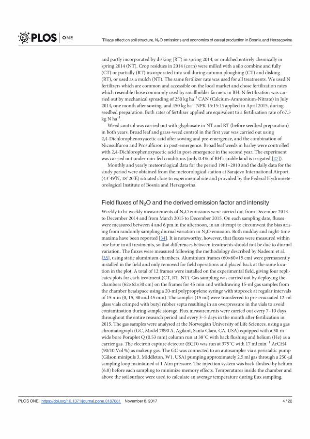
and partly incorporated by disking (RT) in spring 2014, or mulched entirely chemically in
spring 2014 (NT). Crop residues in 2014 (corn) were milled with a silo combine and fully
(CT) or partially (RT) incorporated into soil during autumn ploughing (CT) and disking
(RT), or used as a mulch (NT). The same fertilizer rate was used for all treatments. We used N
fertilizers which are common and accessible on the local market and chose fertilization rates
which resemble those commonly used by smallholder farmers in BH. N fertilization was car-
ried out by mechanical spreading of 250 kg ha-1 CAN (Calcium-Ammonium-Nitrate) in July
2014, one month after sowing, and 450 kg ha-1 NPK 15:15:15 applied in April 2015, during
seedbed preparation. Both rates of fertilizer applied are equivalent to a fertilization rate of 67.5
kg N ha-1.
Weed control was carried out with glyphosate in NT and RT (before seedbed preparation)
in both years. Broad leaf and grass-weed control in the first year was carried out using
2,4-Dichlorophenoxyacetic acid after sowing and pre-emergence, and the combination of
Nicosulfuron and Prosulfuron in post-emergence. Broad leaf weeds in barley were controlled
with 2,4-Dichlorophenoxyacetic acid in post-emergence in the second year. The experiment
was carried out under rain-fed conditions (only 0.4% of BH’s arable land is irrigated [27]).
Monthly and yearly meteorological data for the period 1961–2010 and the daily data for the
study period were obtained from the meteorological station at Sarajevo International Airport
(43˚49’N, 18˚20’E) situated close to experimental site and provided by the Federal Hydromete-
orological Institute of Bosnia and Herzegovina.
Field fluxes of N2O and the derived emission factor and intensity
Weekly to bi-weekly measurements of N2O emissions were carried out from December 2013
to December 2014 and fromMarch 2015 to December 2015. On each sampling date, fluxes
were measured between 4 and 6 pm in the afternoon, in an attempt to circumvent the bias aris-
ing from randomly sampling diurnal variation in N2O emission. Both midday and night-time
maxima have been reported [34]. It is noteworthy, however, that fluxes were measured within
one hour in all treatments, so that differences between treatments should not be due to diurnal
variation. The fluxes were measured following the methodology described by Nadeem et al.
[35], using static aluminium chambers. Aluminium frames (60×60×15 cm) were permanently
installed in the field and only removed for field operations and placed back at the same loca-
tion in the plot. A total of 12 frames were installed on the experimental field, giving four repli-
cates plots for each treatment (CT, RT, NT). Gas sampling was carried out by deploying the
chambers (62×62×30 cm) on the frames for 45 min and withdrawing 15-ml gas samples from
the chamber headspace using a 20-ml polypropylene syringe with stopcock at regular intervals
of 15 min (0, 15, 30 and 45 min). The samples (15 ml) were transferred to pre-evacuated 12-ml
glass vials crimped with butyl rubber septa resulting in an overpressure in the vials to avoid
contamination during sample storage. Flux measurements were carried out every 7–10 days
throughout the entire research period and every 3–5 days in the month after fertilization in
2015. The gas samples were analysed at the Norwegian University of Life Sciences, using a gas
chromatograph (GC, Model 7890 A, Agilant, Santa Clara, CA, USA) equipped with a 30-m-
wide bore Poraplot Q (0.53 mm) column run at 38˚C with back flushing and helium (He) as a
carrier gas. The electron capture detector (ECD) was run at 375˚C with 17 ml min−1 ArCH4
(90/10 Vol %) as makeup gas. The GC was connected to an autosampler via a peristaltic pump
(Gilson minipuls 3, Middleton, W1, USA) pumping approximately 2.5 ml gas through a 250-μlsampling loop maintained at 1 Atm pressure. The injection system was back-flushed by helium
(6.0) before each sampling to minimize memory effects. Temperatures inside the chamber and
above the soil surface were used to calculate an average temperature during flux sampling.
Tillage effect on soil structure, N2O emissions and economics of cereal production in Bosnia and Herzegovina
PLOSONE | https://doi.org/10.1371/journal.pone.0187681 November 8, 2017 4 / 22

Rates of N2O emission were estimated by fitting either a linear (R2 � 0.85) or a quadratic func-
tion to the observed N2O accumulation over time. For this, all fluxes were inspected graphi-
cally and fluxes with a R2< 0.85 and a flux density of< 5 mg Nm-2 h-1 were set to zero. N2O
flux was calculated according to Eq 1:
FN2O ¼dN2O
dt�Vc
A�MN
Vm
� 60 ð1Þ
where FN2O is the N2O emission flux (μg N2O-N m−2 h−1), dN2O/dt is the relative change in
N2O concentration in the chamber headspace (ppmv min−1), Vc is the chamber volume (L), A
is the area covered by the chamber (m2),MN is the molecular mass of N in N2O (g mol−1) and
Vm is the molecular volume of gas at chamber temperature (L mol−1).
Cumulative fluxes were calculated by plotting daily average N2O fluxes against time,
interpolating linearly between them, and integrating the area under the curve [36]. Cumula-
tive flux in 2014 represents area-scaled emissions for the entire year, while in 2015 it repre-
sents the cumulative flux for 226 days of the year (flux measurements started on 20th of
March) plus linearly interpolated values for the missing period, assuming small off-season
emissions like observed in the previous year. Emission factors were calculated as the fraction
of applied fertilizer N emitted as N2O-N, assuming background N2O emission of 1 kg N
ha−1 year−1 [37]. Yield-scaled N2O emission was calculated as emission intensity, which is a
function of N fertilization rate and expressed as N2O-N (g) emitted per ton of grain yield
[38]. To account for the N-input by preceding alfalfa in the first cropping year, we estimated
the N returned to soil with the crowns and roots based in literature values. According to
Kelner et al. [39], this amount is 107 kg N ha-1 for a 1-year stand of alfalfa. However, when
the yields of the first cut from that study are compared with results reported by Junuzović[40] for our field, we reduced the N yield by roughly 50% to a more realistic N input of 53.5
kg N ha-1.
Soil measurements
Soil moisture and temperature at 5 cm depth were measured daily using data loggers (Decagon
EM50, Pullman, WA, USA) together with ECH2O sensors (Decagon) for volumetric soil water
content (VSWC) and temperature in three replicates per treatment. No measurements are
available for the period between 2 April and 24 June 2014, due to equipment failure.
Soil physical properties were analysed in undisturbed soil cores (100 cm3 stainless steel cyl-
inders) collected in July 2015 in four replicates per treatment. Particle density (PD) was deter-
mined using an air pycnometer according to Langer. Bulk density (PD) was determined
gravimetrically. BD and PD were used to calculate total porosity, which was used to convert
VSWC to water filled pore space (WFPS) by Eq 2:
WFPS ¼VSWC
1� BDPD
ð2Þ
Soil water retention curves between pF 1.8 and 4.2 were determined using ceramic pressure
plate extractors [41]. These results were then used to determine soil pore size distributions in
different tillage treatments.
In 2015, soil samples were taken from 0 to 15 cm depth at each gas sampling date. Multiple
cores from each treatment (4 per subplot) were homogenized, bulked and frozen. Immediately
after thawing, 45 g fresh weight soil was extracted by 30 minutes of horizontal shaking in a 50
ml 2M KCl solution. The extracts were filtered and soil mineral N (NH4+, NO3
−) was analysed
by colorimetry as described by Keeney [42].
Tillage effect on soil structure, N2O emissions and economics of cereal production in Bosnia and Herzegovina
PLOSONE | https://doi.org/10.1371/journal.pone.0187681 November 8, 2017 5 / 22

Yield and economic parameters
Yields were measured on each subplot as dry grain corn in 2014 and barley in 2015 standardized
to 14%moisture content. Production costs were estimated for each of the three tillage systems.
Input items such as seed, fertilizer and chemicals applied were purchased from local retailers
and the exact prices were recorded. Average purchase market prices for the crops used in the
experiment are taken from Agency for Statistics of Bosnia and Herzegovina [43, 44] for the
respective years. For an approximation of labour and tillage operation costs, we used data from
the local agricultural extension service, which were cross-validated with farmers in the same
area. The results were calculated and discussed as the difference in net return per hectare in the
three tillage systems, which was calculated from net income for crop after deducting all variable
costs. We refrained to estimate fixed costs for production systems in this study due to high vari-
ability in possession of tractors and other necessary mechanisation and assets, which often have
a long depreciation life and the general tendency to become obsolete [45].
Statistical analysis
N2O emission rates were log-transformed to approach normal Gaussian distribution. To test
the effects of treatment and year, repeated measures two-way ANOVA followed by Bonferroni
post-test was performed for N2O flux data, soil temperature andWFPS. One-way ANOVA fol-
lowed by a Tukey’s multiple comparison post test was performed for soil NH4+ and NO3
−,
cumulative N2O emissions and yield-scaled N2O emissions. All data were analysed using SPSS
ver. 24 (IBM Corp, USA).
Results
Weather conditions
The average temperature in 2014 and 2015 was 11.2 and 10.2 oC, respectively, which is warmer
than the long-term reference temperature (9.6 oC). The year 2014 had an exceptionally warm
winter (Jan-March, 2015, Fig 1), while monthly temperatures for the rest of the year were simi-
lar to the long-term average values. Monthly average temperatures in summer 2015 were
clearly higher than the reference temperatures. (Fig 1).
Both the amount of annual precipitation and the seasonal distribution varied greatly
between the two years. Cumulative precipitation was larger (1020 mm) in 2014, while it was
smaller in 2015 (719 mm) compared with the reference precipitation (899 mm). The annual
rain distribution in 2014 showed excessive amounts of precipitation in April, May and Sep-
tember and the amount of precipitation was larger than the monthly reference precipitation
throughout most of the cropping season. By contrast, 2015 was a dry year, with extremely low
precipitation in the cropping season, especially May and July, with monthly precipitation sums
of only 24 and 6 mm, respectively.
N2O emission dynamics and ancillary variables
All treatments had similar N2O emission dynamics, although peak values differed during cer-
tain periods, most notably after fertilization (Figs 2A and 3A). Two-way repeated measures
ANOVA showed that tillage and experimental year had a significant effect on N2O flux
(P< 0.05), while the interaction between tillage and experimental year was not significant.
According to Bonferroni pairwise comparison, the difference in N2O emissions between CT
and NT was significant only for the 90% confidence interval in the first year, while there was a
significant difference between RT and NT (P< 0.05) in the second year. All peak emissions
coincided with high WFPS values and elevated soil temperatures (Figs 2B and 3B). In contrast,
Tillage effect on soil structure, N2O emissions and economics of cereal production in Bosnia and Herzegovina
PLOSONE | https://doi.org/10.1371/journal.pone.0187681 November 8, 2017 6 / 22

winter emissions in 2014 (January–April) were small, despite large WFPS values in non-tilled
soil. The first N2O emission peak occurred at the beginning of April, at the time of rototillage
in CT; Emission rates in CT and RT increased, whereas they remained small in NT. The largest
N2O emission rates were recorded, regardless of treatment, in August 2014, one month after
fertilization, when soil moisture started to fluctuate (Fig 2A and 2B). Maximum observed
Fig 1. Averagemonthly temperatures and precipitation close to the sampling site.
https://doi.org/10.1371/journal.pone.0187681.g001
Tillage effect on soil structure, N2O emissions and economics of cereal production in Bosnia and Herzegovina
PLOSONE | https://doi.org/10.1371/journal.pone.0187681 November 8, 2017 7 / 22

fluxes (treatment means per date) were 587.1 μg N2O-N m-2 h-1 for CT, 373.7 for NT and
301.0 for RT. Emission rates remained slightly elevated for the remainder of the cropping
period in all treatments, before decreasing gradually with decreasing soil temperature to low
background values one month before harvest (first week of November).
In 2015, N2Omeasurements started right before tillage operations in March (Fig 3A). Emis-
sion rates remained small during seedbed preparation and herbicide treatment until fertiliza-
tion and sowing of barley in the beginning of April. N2O emission rates increased strongly in
all treatments immediately after fertilization and remained large throughout April, while the
soil was still wet (>60%WFPS; Fig 3B). Maximum emission rates were measured three weeks
after fertilization, with treatment means of 434.4 μg N2O-N m-2 h-1 for RT, 306.2 for NT and
234.0 μg N2O-N m-2 h-1 for CT. WhenWFPS values dropped below 60% in the middle of
May, N2O emission rates receded. A smaller, transient emission peak was observed in NT and
Fig 2. aMean N2O emissions per treatment (n = 4) and b daily precipitation, and mean soil temperature and moisture in 5 cmdepth in CT, NT and RT treatments in 2014. Error bars are omitted to maintain readability.
https://doi.org/10.1371/journal.pone.0187681.g002
Tillage effect on soil structure, N2O emissions and economics of cereal production in Bosnia and Herzegovina
PLOSONE | https://doi.org/10.1371/journal.pone.0187681 November 8, 2017 8 / 22

RT, but not in CT plots, in the middle of June, which coincided with rewetting of dry soil by
rain. Pronounced drying-rewetting later in 2015 did not induce measurable N2O emission
response, nor did harvest and ploughing, which is in line with small mineral N concentrations
during this period (Fig 3C and 3D).
Fig 3. aMean N2O emissions (n = 4), b daily precipitation, mean soil temperature and moisture in 5 cmdepth, c Soil NO3
- and d soil NH4+ concentrations in 0–15 cm depth CT, NT and RT treatments in 2015. Error
bars are omitted to maintain readability.
https://doi.org/10.1371/journal.pone.0187681.g003
Tillage effect on soil structure, N2O emissions and economics of cereal production in Bosnia and Herzegovina
PLOSONE | https://doi.org/10.1371/journal.pone.0187681 November 8, 2017 9 / 22

To find out whether tillage treatments had any effect on known drivers for N2O emission,
we tested for differences in soil temperatures and WFPS in both years and for differences in
extractable NH4+ or NO3
− in 2015 across treatments. Mean daily soil temperature showed little
difference between treatments (Figs 2B and 3B), but annual average soil temperature was
slightly higher in NT plots in both years (12.8 and 13.2 oC) than in CT (12.6 and 12.8) and RT
plots (12.5 and 12.8) and statistically significant (P< 0.001).
In both years, CT soils had consistently smaller WFPS values than RT or NT soil. This con-
trast was most pronounced after ploughing (CT) and secondary tillage (CT and RT). During
the wet summer of 2014, WFPS values of NT soil were almost constantly within the range of
80–90%WFPS, often exceeding 90%. On average, WFPS of NT soil exceeded that of CT and
RT soil by 22.1% and 4.6%, respectively. Also in the dry summer of 2015, NT soil had the high-
est average WFPS values, although the difference between the treatments was less pronounced
than in 2014 (6.4% and 3.7% higher than in CT and RT soils, respectively). Both tillage, experi-
mental year and their interaction had a highly significant effect onWFPS and the difference
was significant between every treatment (P< 0.0001).
No significant difference between treatments was found for extractable NH4+ or NO3
− at
0–15 cm depth in 2015. The mineral N content increased rapidly after fertilization (Fig 3C and
3D), before levelling off to low background values by the end of June. The increase in NH4+
was somewhat delayed in NT soil, reflecting the difference between surface applied (NT) and
incorporated (during seedbed preparation in CT and RT) fertilizer. Concentrations of NO3−
declined to below 10 μg g-1 one month after fertilization and remained at very low levels for
the remainder of the growing season. Similar to NO3−, NH4
+ concentrations declined to values
lower than 10 μg g dw soil-1 two months after fertilization and remained low until the end of
the year. The only difference was that NT showed occasionally elevated concentrations of
NH4+, likely reflecting drying-rewetting induced mineralization pulses.
Soil properties and crop yields
By August 2015, i.e. in the second experimental year, two months after seedbed preparation,
tillage regime had resulted in clear differences in soil bulk density, total porosity and pore size
distribution (Table 1). CT soil had the smallest bulk density among all treatments, which was
significantly different from that of NT (P< 0.05). Accordingly, CT soil had a larger porosity
and a larger share of medium and macro pores. Increased bulk density in NT combined with
reduced infiltration resulted in soil crusting and occasional waterlogging during both growing
seasons.
Next to soil properties, weather conditions had a major impact on crop yields in both crop-
ping seasons. Excessive rainfall during spring 2014 delayed most of agricultural operations,
including rototilling, disking, seedbed preparation and sowing of corn for more than one
Table 1. Soil physical properties 20months after the establishment of contrasting tillage regimes (August 2015).
Treatment Bulk density(g cm-3)
Total porosity(%)
Pore size distribution (%)
Micro( 0.2 m)
Meso(0.2–10 m)
Macro( 10 m)
CT 1.36 ( 0.03)a 53.56a 13.85a 27.03a 12.68a
RT 1.42 ( 0.04) 51.07a 12.57a 26.53a 11.97a
NT 1.55 ( 0.04)b 45.40b 15.72b 21.47b 8.22b
* SE shown in bracketsa,b Different letters indicate significant differences across treatments (Bonferroni, P 0.05)
https://doi.org/10.1371/journal.pone.0187681.t001
Tillage effect on soil structure, N2O emissions and economics of cereal production in Bosnia and Herzegovina
PLOSONE | https://doi.org/10.1371/journal.pone.0187681 November 8, 2017 10 / 22

month, which led to late harvest and yield decrease. The same weather conditions occurred in
the following year, resulting in late sowing of barley. This delay, coupled with two drought
periods in May and July, led to crop failure. Average crop yields per treatment and year are
shown in Table 2.
Cumulative N2O emissions and emission factors
In 2014, cumulative N2O emission was largest in CT and significantly different from RT and
NT only at P< 0.1 (Table 3). Cumulative N2O emissions in 2015 were significantly smaller
(P< 0.005) than in 2014 for all treatments and RT had the highest emission, followed by CT
and NT, with the difference between RT and NT treatments being significant (P< 0.05).
Annual N2O emission factors, assuming a background emission of 1 kg N2O-N ha-1 y-1 [37],
are shown in Fig 4. Extraordinary large apparent emission factors were found in 2014 with 4.8%
for CT, 2.9% for RT and 2.6% for NT, which likely reflect the extra N from alfalfa incorporated
in autumn 2013 (CT) and spring 2014 (RT), or mulched in spring 2014 (RT, NT). We therefore
estimated the amount of N from alfalfa residues based on N content and crown-root ratios
reported in the literature as well as measured yields and added this N to the fertilizer N. Esti-
mated N input by alfalfa crop residues was 53.5 kg N ha-1 for all three treatments. This resulted
in more realistic emission factors of 1.5, 1.6 and 2.7% for NT, RT and CT, respectively, in the
year of establishing the three tillage treatments. Irrespective of the amount of N input estimated,
CT hat the largest emission factor in 2014. Emission factors in the dry year 2015 were much
smaller and in the order of 0.7, 1.0 and 1.5% for NT, CT and RT, respectively.
Yield-scaled N2O emission (Fig 5) was smallest for RT plots in both cropping seasons, rang-
ing from 83.2 (2014) to 413.5 g N2O-NMg-1 (2015). NT had the largest yield-scaled N2O emis-
sion in 2014 (161.7), while it was largest for CT in 2015 (736.1). Very high values in 2015 are
the result of crop failure caused by drought. Analysis by one-way ANOVA followed by a
Table 2. Average crop yields corrected for 14%moisture in CT, RT and NT.
Year—crop Treatment Average yield(kg ha-1) SD (n = 4)
CT 6561.9 678.7a
2014—corn RT 6165.8 790.3a
NT 4314.2 1118.2b
CT 1508.1 139.7a
2015—barley RT 2185.0 254.3b
NT 1571.5 135.2a
a,b Different letters indicate significant differences across treatments (Bonferroni, P 0.05)
https://doi.org/10.1371/journal.pone.0187681.t002
Table 3. Cumulative N2O emissions.
Season Cumulative N2O emission (kg N2O-N ha-1)
CT RT NT
2014 4.3 ( 0.6)a 3.0 ( 0.2)b 2.8 ( 0.4)b
2015 1.7 ( 0.1) 1.9 ( 0.1)a 1.4 ( 0.05)b
* SE shown in bracketsa,b Different letters indicate significant differences across treatments (Bonferroni, P 0.1 in 2014 and
P 0.05 in 2015)
https://doi.org/10.1371/journal.pone.0187681.t003
Tillage effect on soil structure, N2O emissions and economics of cereal production in Bosnia and Herzegovina
PLOSONE | https://doi.org/10.1371/journal.pone.0187681 November 8, 2017 11 / 22

Tukey’s multiple comparison post-test showed statistically significant differences between RT
and NT (P< 0.05) in 2014 and between CT and RT (P< 0.005) in 2015
Economic comparison between tillage methods
Based on estimated net return per hectare in the different tillage systems (Table 4), it is evident
that the reduced number of cultivation steps in NT decreased production costs as compared to
CT. However, this reduction was zeroed by increased costs for weed control. With an overall
smaller yield in NT, this resulted in markedly smaller net return in NT than in RT or CT in
2014. There was a notable difference in net return between the two years among the tillage
treatments. The differences in yield between the two cropping seasons can be mainly attributed
to different weather conditions, which lead to yield reduction in the first year and crop failure
in the second year. Notably, RT had large net return, close to that of CT, in the first year and
the least negative net return in the second year. CT had largest net return in the first year and
smallest in the second year. NT achieved a small net return in the first year in comparison to
CT and RT, while it had less negative net return than CT in the second year.
Discussion
Tillage effects on N2O fluxes and soil variables
N2O emissions showed a similar N fertilization response in all treatments and consequently
similar N2O emission rates in both years. Between 35% (NT) and 57% (CT) of the cumulative
Fig 4. N2O emission factors.Different letters indicate significant differences across treatments at P 0.05.
https://doi.org/10.1371/journal.pone.0187681.g004
Tillage effect on soil structure, N2O emissions and economics of cereal production in Bosnia and Herzegovina
PLOSONE | https://doi.org/10.1371/journal.pone.0187681 November 8, 2017 12 / 22
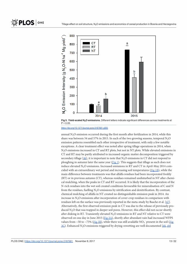
annual N2O emission occurred during the first month after fertilization in 2014, while this
share was between 54 and 57% in 2015. In each of the two growing seasons, temporal N2O
emission patterns resembled each other irrespective of treatment, with only a few notable
exceptions. A clear treatment effect was noted after spring tillage operations in 2014, when
N2O emissions increased in CT and RT plots, but not in NT plots. While elevated emissions in
CT and RT may be partly attributed to increased organic matter decomposition triggered by
secondary tillage [46], it is important to note that N2O emissions in CT did not respond to
ploughing in autumn later the same year (Fig 1). This suggests that tillage as such does not
induce elevated N2O emissions. Increased emissions in RT and CT in April-May 2014 coin-
cided with an extraordinary wet period and increasing soil temperatures (Fig 1B), while the
main difference between treatments was that alfalfa residues had been incorporated freshly
(RT) or in previous autumn (CT), whereas residues remained undisturbed in NT after chemi-
cal mulching, when the peaks in CT and RT occurred. It is likely that the incorporation of the
N-rich residues into the wet soil created conditions favourable for mineralisation of C and N
from the residues, fuelling N2O emissions by nitrification and denitrification. By contrast,
chemical mulching of alfalfa in NT created no distinguishable emission peak in 2014. An
increase in N2O emissions after incorporation of cover crop residues in comparison with
residues left on the surface was previously reported in the meta-study by Basche et al. [47].
Alternatively, the first observed emission peak in CT was due to the release of previously pro-
duced N2O that was trapped in deeper soil pores. However, this effect did not occur shortly
after disking in RT. Transiently elevated N2O emissions in RT and NT relative to CT were
observed on one day in June 2015 (Fig 3A), shortly after abundant rain had increased WFPS
values from ~50 to ~75% (Fig 3B), while there was still available NO3- present in the soil (Fig
3C). Enhanced N2O emissions triggered by drying-rewetting are well documented [48, 49]
Fig 5. Yield-scaled N2O emissions.Different letters indicate significant differences across treatments atP 0.05.
https://doi.org/10.1371/journal.pone.0187681.g005
Tillage effect on soil structure, N2O emissions and economics of cereal production in Bosnia and Herzegovina
PLOSONE | https://doi.org/10.1371/journal.pone.0187681 November 8, 2017 13 / 22
and are most likely due to denitrification. Interestingly, WFPS increase in CT was smaller than
in RT and NT, probably explaining the lack of N2O emission response in this treatment. Peri-
ods of repeated drought and rewetting later in 2015 did not induce measurable N2O emissions,
apparently because small concentrations of NH4+ and NO3
− limited nitrification and denitrifi-
cation activity. All peak emissions outside the period directly affected by fertilization coincided
with large WFPS (70–90%) and high soil temperatures (>10˚C), illustrating the importance of
crop residue management (April 2014) and tillage regime (June 2015) for N2O emissions out-
side the period directly affected by fertilization. The greatest differences between treatment
means of N2O emissions were seen after fertilizer application. In 2014, post-fertilization emis-
sions were greatest in CT, followed by NT and RT (Fig 2A), despite lowest WFPS values in CT
(Fig 2B). The likely reason for this is that incorporation of the preceding crop (alfalfa) in
autumn 2013 had resulted in a more active microbial community in CT than in RT and NT,
which was further stimulated by rototilling in spring 2014. Thus, CT plots responded stronger
to N addition than RT or NT plots. In 2015, no N-rich residues were present, and RT responded
strongest to N-fertilization (Fig 3A), providing the most favourable conditions for nitrification
and denitrification in terms of soil structure and substrate availability.
Despite the relatively short periods of distinct N2O flux, we found differences in annual
emissions between treatments (Table 3). Since annual emissions were dominated by post-fer-
tilization fluxes, largest annual emissions were found in CT in 2014 and in RT in 2015. NT had
Table 4. Net income per hectare under different tillage systems based on the difference of crop netincome and variable costs of production.
Season/Crop Price (BAM)
2014 Corn CT RT NT
Seed cost 240 240 240
Fertilizer and application 265 265 265
Tillage operations, fuel, maintenance, labour 272 146 80
Herbicide and application 99 188 233
Harvesting (hired machinery and labour) 300 300 300
Total variable costs 1176 1139 1118
Yield (t)
6.56 6.17 4.31
Price (BAM per t) 268.4
Net income 1761.3 1655.0 1158.0
Net return 585.3 516.0 40.0
2015 Barley CT RT NT
Seed cost 200 200 200
Fertilizer and application 475 475 475
Tillage, fuel, maintenance, labour 265 142 70
Herbicide and application 54 143 188
Harvesting (hired machinery and labour) 300 300 300
Total variable costs 1294 1260 1233
Yield (t)
1.51 2.18 1.57
Price (BAM per t) 388.63
Net income 586.1 849.1 610.7
Net return -707.9 -410.9 -622.3
* 1 BAM = 0.51 EUR
https://doi.org/10.1371/journal.pone.0187681.t004
Tillage effect on soil structure, N2O emissions and economics of cereal production in Bosnia and Herzegovina
PLOSONE | https://doi.org/10.1371/journal.pone.0187681 November 8, 2017 14 / 22

the smallest emission in both years, although this difference was not significant in 2014. A
meta-analysis of reported N2O emissions in 239 paired field trials with conventional tillage
(CT) and NT/RT showed no consistent short-term (�10 years) tillage effect on area-scaled
N2O emissions when land was converted from CT to NT/RT [8]. Smaller N2O emissions from
NT soils in a newly established tillage experiment, like the case in our study, were previously
reported by Chatskikh and Olesen [50] in a loamy sand soil with barley as a crop, while long-
term reduction in N2O emission by NT on loams are reported by Gregorich et al. [51] and
Mosier et al. [38] for corn-soybean crop rotation. By contrast, larger N2O emissions in newly
established NT systems than in CT have been reported by Ball et al. [52] and Baggs et al. [53]
on loamy soils in humid areas. This indicates that tillage effects on N2O emissions are highly
variable, both spatially and temporally, and influenced by a wide spectrum of biotic and abiotic
factors and their interactions in the specific region. It should be also mentioned, that the sam-
pling frequency used in our study was low and that contrasts in annual N2O emission probably
underestimated treatment effects, since the resolution was not high enough to capture every
N2O emission peak.
In our experiment, tillage regime had a clear effect on every measured soil variable. Soil
temperatures in NT were on average 0.3–0.4 oC higher and had up to 22.1% larger average
WPFS values as compared with CT. Lower bulk density and more medium and macro pores
in CT suggested that the ploughed soil was better aerated than RT or NT. Overall, warmer,
wetter and less aerated soil in NT would be expected to favour denitrification and hence
increased N2O emissions, especially in case of heavy soils in humid climates [9]. Interestingly,
this effect was not found in our study, which may have a number of management-specific rea-
sons. Firstly, while no cover crops were planned in our study, all fields were uniformly cropped
to alfalfa, an N-fixing legume, in the year prior to establishing the experiment. Using alfalfa or
some other legume as a cover crop is not common in BH, but is sometimes practiced by farm-
ers who do not have access to manure (which was the case on our field) or want to decrease
the production costs with the application of green manures. Even though we did not measure
mineral N in the first year, it is obvious from the N2O emissions that ploughing the cover crop
in autumn prior to the first experimental year and rototilling it in spring released more C and
N than in RT and NT, likely because alfalfa residues had a longer contact time with the soil. A
similar finding was reported by [54] for a Mediterranean cover crop system. Secondly, 2014
was an extraordinary wet year (Fig 1), with WFPS values around 70–80% in CT and exceeding
90% in NT in the period after fertilization (Fig 2). It is well known that N2O emissions from
denitrification are greatest at WFPS values around 80%, (e.g. [55]), whereas larger WFPS val-
ues favour reduction of N2O to N2 [56]. For instance, larger N2O emissions at 80% compared
to 100%WFPS have been reported by Ciarlo et al. [57], who observed decreasing N2O emis-
sion in saturated soil. In the wet summer of 2014, we observed several occasions of waterlog-
ging during sampling in NT plots. RT plots hadWFPS values intermediate to RT and NT,
which resulted in intermediate post-fertilization N2O emissions. In contrast, the second year
was quite dry (Fig 1), and the differences in WFPS between treatments were less pronounced.
Post-fertilization emissions occurred during a period with decreasing WFPS, and were largest
in RT. We have no explanation for this finding other than that NH4+ and NO3- values were
largest in RT during this period, pointing at enhanced mineralisation and nitrification in this
treatment at 60–80%WFPS.
Soil properties
Our experiment was conducted on a clayey loam low in SOC (1.34%). The soil had been under
intensive arable cropping for the past decade with limited application of manure. Arable
Tillage effect on soil structure, N2O emissions and economics of cereal production in Bosnia and Herzegovina
PLOSONE | https://doi.org/10.1371/journal.pone.0187681 November 8, 2017 15 / 22
cultivation without manures decreases the SOM content over time and consequently weakens
the structural stability of the soil [58]. Twenty months into our experimental trial, NT soil had
the largest bulk density and may have experienced soil compaction [59], which is known to be
a problem in soils with low aggregate stability [60]. Negative effects of soil compaction on crop
yields are well documented [61]. In our study, NT soil had 8.2% less total porosity than CT soil
and smaller proportion of meso and macro pores (Table 1). This led to reduced water infiltra-
tion and occasional waterlogging during more intense and prolonged rainfall events, especially
in 2014. In both years, large rainfalls after sowing led to soil crusting, even in the presence of
mulched crop residues in RT and NT, delaying the emergence of seedlings relative to CT. This
effect was especially pronounced in NT, which led to significant reduction (approx. 25%) in
the abundance of corn plants relative to CT and RT in 2014. Another notable observation was
that both corn and barley plants in CT and RT were taller irrespective of their phenological
stage and that the phenological development was 10–15 days ahead this of NT. Among the
positive effects of NT and RT in 2015 was a larger proportion of soil micro- and macro-pores,
respectively (Table 1), resulting in larger soil water retention during drought periods, which
probably contributed to equal (NT) or larger (RT) barley yields compared with CT in 2015,
despite later phenological development and general crop failure.
N2O emission factor and intensity
Assuming a background emission of 1 kg N2O-N ha-1 y-1 [37], we obtained mean N2O emis-
sion factors (EF) ranging from 2.7 to 4.8% of fertilizer N applied. Since these emission factors
are markedly larger than the IPCC Tier 1 EF (1% of applied fertilizer N), we tried to estimate
the additional N input from alfalfa residues during the first year (Fig 4), based on the results
from Kelner et al. [39] and adjusted for alfalfa yields from our study field [40]. Adding this
amount of N to the fertilizer N, reduced N2O emission factors in 2014 to 1.5, 1.6 and 2.7% for
NT, RT and CT respectively, which is closer, but still above the IPCC Tier 1 EF of 1% [37]. In
2015, emission factors were 0.7, 1.0 and 1.5% for NT, CT and RT respectively, which is close to
the IPCC Tier 1 EF, despite the general crop failure in this year. Given the uncertain estimate
of extra N input in 2014, and the insignificant differences in the EF across tillage treatments in
2015, we conclude that tillage regime had no measurable effect on the N2O emission factors in
our experiment.
To assess the N2O footprint of cropping methods, yield-scaled approaches are increasing
employed [38, 62]. Calculated as N2O intensity (g N2O-NMg grain-1), RT had the lowest
intensity in both years. We used the results from 2014 for further comparison, since the high
values in 2015 essentially reflected crop failure. Yield-scaled N2O emissions in 2014 ranged
from 83.2 (RT) to 161.7 g N2O-NMg-1 (NT) and this difference was statistically significant.
These results are within range of 77.1–391.8 g N2O-NMg−1 as reported by Guo et al. [63], but
larger than those reported by Halvorson et al. [64] (31–67 g N2O-NMg−1) and Venterea et al.
[65] (46–100 g N2O-NMg−1) for the same crop (corn). Our intensities are smaller than those
reported by Burzaco et al. [66] for similar fertilization rates (211–285 g N2O-NMg−1) and
markedly smaller than the 1.3–2.0 kg N2O-NMg−1 reported by Gagnon et al. [67].
Environmental vs. economic benefits
It has been widely recognised that conservation tillage practices have a beneficial effect on soil
properties in cropping systems compared to conventional practices [68]. However, the adop-
tion of NT in Europe is still limited in comparison with the Americas, despite extensive
research in this area [69]. The relative advantages of NT and CT depend on a number of
aspects, grouped roughly into agronomic and environmental factors [70]. According to Soane
Tillage effect on soil structure, N2O emissions and economics of cereal production in Bosnia and Herzegovina
PLOSONE | https://doi.org/10.1371/journal.pone.0187681 November 8, 2017 16 / 22

et al. [69], the opinions and choices of farmers related to tillage will be dictated primarily by
agronomic factors, whereas environmental factors are of a more general concern for soil and
landscape protection and climate change. While the agronomic benefits of alternative tillage
methods are easy to recognize, the likelihood for their adoption is constrained due to relative
uncertainty about the economic benefits [71, 72].
Summarizing stipulated costs and revenues over the two cropping seasons, including one
year of crop failure, it is notable that RT had smaller yield-scaled N2O emissions than CT and
NT, while generating the largest net returns per ha. These findings are in agreement with and
support the current situation in Europe, where intermediate forms of tillage have been adopted
much more widely than NT [69]. While only a small reduction of variable costs in NT could
be achieved in our experiment due to the increased costs for weed control, the main reason for
small net returns and large yield-scaled N2O emissions in NT were lower crop yields compared
to CT and RT. Conservation tillage initially leads to yield reduction of varying degree depend-
ing on crop type, tillage, soil properties, climate and crop rotation [73, 74]. However, it is
expected that the yield gap between reduced and conventional tillage will level out over time,
as the soil structure, water infiltration and root growth improve in the surface soil under con-
tinuous NT systems [75].
Based on our findings and the current socio-economic conditions in BH, we conclude that
a wider acceptance of NT is not realistic at the moment, especially among risk-averse small-
holder farmers who lack knowledge and financial capital. However, our result also show that
RT could be a compromise between CT and NT, given the current conditions, because it can
be both N efficient and economically acceptable. RT appeared to be more resilient to weather
extremes, particularly during the dry year of 2015. Our study was conducted in “continental”
BH, characteristic for the northern lowlands and river valleys of central, eastern and western
BH, which is central for BH’s intensive agricultural production of a wide range of crops. Yet,
further research is needed in other agroclimatic zones and soil types of BH to assess tillage
effects at the national level. In addition, longer-term studies are needed to make more reliable
projections of yield levels and environmental savings.
Conclusion
Fertilization was found to be the main driver of N2O emissions irrespective of tillage treat-
ment. However, clear treatment effects outside the period directly affected by fertilization were
noted, indicating the importance of crop residue management and tillage on soil structure,
temperature and moisture. Annual emissions were different between tillage treatments, but
this depended on the year. NT had the smallest N2O emission in both years, while CT had the
largest emission in the first year and RT the largest emission in the second year. When normal-
ized for yield, RT had the smallest N2O intensity in both years. The emission factors were
within or slightly above the uncertainty range of the IPCC Tier 1 EF. Reduction in variable
costs associated with NT was small due to the increased costs of weed control. Moreover, low
yields in NT in both years resulted in economically inacceptable returns. On the other hand,
the reduced number of operations in case of RT generated higher net returns due to reduced
production costs. Based on our results, we conclude that RT could be a feasible way to improve
N yields and net returns, while reducing yield-scaled N2O emissions under the given agro-eco-
logical and socio-economic conditions of BH. Future studies with the objective to mitigate
N2O and other greenhouse gas emissions, improve crop yields and N use efficiency from agri-
cultural systems in the region are needed, including long-term observation, that can integrate
over the large interannual weather variability in central BH. Studies on the effect of CA princi-
ples other than reduced tillage (e.g. cover crops, crop rotation) are needed if region-specific
Tillage effect on soil structure, N2O emissions and economics of cereal production in Bosnia and Herzegovina
PLOSONE | https://doi.org/10.1371/journal.pone.0187681 November 8, 2017 17 / 22

production system are to be designed to optimize crop production both environmentally and
economically.
Acknowledgments
The authors are very grateful to Boris Zurovec for his help during weekly N2O sampling, and
the scientific and technical personnel of the Institute for Agricultural Machinery from Faculty
of Agriculture and Food Sciences, University of Sarajevo, for their help during tillage opera-
tions. We also thank the Federal Institute of Agropedology Sarajevo for providing their labora-
tory for physical soil measurements and Sabrija Čadro, Trygve Fredriksen and Shahid Nadeem
for their technical assistance.
Author Contributions
Conceptualization: Ognjen Zurovec.
Formal analysis:Ognjen Zurovec, Peter Dorsch.
Funding acquisition: Bishal Kumar Sitaula.
Investigation: Ognjen Zurovec, Jasminka Zurovec, Peter Dorsch.
Methodology:Ognjen Zurovec, Peter Dorsch.
Project administration: Ognjen Zurovec, Jasminka Zurovec.
Resources:Hamid Čustović, Peter Dorsch.
Supervision: Bishal Kumar Sitaula, Hamid Čustović, Peter Dorsch.
Validation: Ognjen Zurovec, Peter Dorsch.
Visualization: Ognjen Zurovec.
Writing – original draft:Ognjen Zurovec, Bishal Kumar Sitaula, Peter Dorsch.
Writing – review & editing: Ognjen Zurovec, Bishal Kumar Sitaula, Peter Dorsch.
References1. Hobbs PR, Sayre K, Gupta R. The role of conservation agriculture in sustainable agriculture. Philosoph-
ical Transactions of the Royal Society B: Biological Sciences. 2008; 363(1491):543–55. https://doi.org/10.1098/rstb.2007.2169. PMID: 17720669
2. Franzluebbers AJ. Water infiltration and soil structure related to organic matter and its stratification withdepth. Soil and Tillage Research. 2002; 66(2):197–205. https://doi.org/10.1016/S0167-1987(02)00027-2.
3. Hobbs PR. Conservation agriculture: what is it and why is it important for future sustainable food produc-tion? The Journal of Agricultural Science. 2007; 145(2):127–37. https://doi.org/10.1017/S0021859607006892.
4. Lal R. Soil Carbon Sequestration Impacts on Global Climate Change and Food Security. Science.2004; 304(5677):1623–7. https://doi.org/10.1126/science.1097396. PMID: 15192216
5. Powlson DS,Whitmore AP, Goulding KWT. Soil carbon sequestration to mitigate climate change: a crit-ical re-examination to identify the true and the false. European Journal of Soil Science. 2011; 62(1):42–55. https://doi.org/10.1111/j.1365-2389.2010.01342.x.
6. Minasny B, Malone BP, McBratney AB, Angers DA, Arrouays D, Chambers A, et al. Soil carbon 4 permille. Geoderma. 2017; 292:59–86. https://doi.org/10.1016/j.geoderma.2017.01.002.
7. Tian H, Lu C, Ciais P, Michalak AM, Canadell JG, Saikawa E, et al. The terrestrial biosphere as a netsource of greenhouse gases to the atmosphere. Nature. 2016; 531(7593):225–8. https://doi.org/10.1038/nature16946. PMID: 26961656
Tillage effect on soil structure, N2O emissions and economics of cereal production in Bosnia and Herzegovina
PLOSONE | https://doi.org/10.1371/journal.pone.0187681 November 8, 2017 18 / 22
8. van Kessel C, Venterea R, Six J, Adviento-Borbe MA, Linquist B, van Groenigen KJ. Climate, duration,and N placement determine N2O emissions in reduced tillage systems: a meta-analysis. Global ChangeBiology. 2013; 19(1):33–44. https://doi.org/10.1111/j.1365-2486.2012.02779.x. PMID: 23504719
9. Rochette P. No-till only increases N2O emissions in poorly-aerated soils. Soil and Tillage Research.2008; 101(1–2):97–100. https://doi.org/10.1016/j.still.2008.07.011.
10. Six J, Feller C, Denef K, Ogle S, Joao Carlos DeMoraes Sa, Albrecht A. Soil organic matter, biota andaggregation in temperate and tropical soils—Effects of no-tillage. Agronomie. 2002; 22(7–8):755–75.https://doi.org/10.1051/agro:2002043.
11. Johnston AE, Poulton PR, Coleman K. Chapter 1 Soil Organic Matter: Its Importance in SustainableAgriculture and Carbon Dioxide Fluxes. In: Donald LS, editor. Advances in Agronomy. Volume 101:Academic Press; 2009. p. 1–57.
12. Myhre G, Shindell D, Breon F, CollinsW, Fuglestvedt J, Huang J, et al. Anthropogenic and NaturalRadiative Forcing. In: Stocker TF, Qin D, Plattner G-K, Tignor M, Allen SK, Boschung J, et al., editors.Climate change 2013: The physical science basis Intergovernmental Panel on Climate Change,Work-ing Group I Contribution to the IPCC Fifth Assessment Report (AR5). New York: Cambridge UnivPress; 2013.
13. Ravishankara AR, Daniel JS, Portmann RW. Nitrous Oxide (N2O): The Dominant Ozone-DepletingSubstance Emitted in the 21st Century. Science. 2009; 326(5949):123–5. https://doi.org/10.1126/science.1176985 PMID: 19713491
14. Smith P, Martino D, Cai Z, Gwary D, Janzen H, Kumar P, et al. Agriculture. In: Metz B, Davidson O,Bosch P, Dave R, Meyer L, editors. Climate Change 2007: Mitigation Contribution of Working Group IIIto the Fourth Assessment Report of the Intergovernmental Panel on Climate Change. Cambridge, UK:Cambridge Univ Press; 2007.
15. Syakila A, Kroeze C. The global nitrous oxide budget revisited. Greenhouse Gas Measurement andManagement. 2011; 1(1):17–26. https://doi.org/10.3763/ghgmm.2010.0007.
16. Ward BB, Arp DJ, Klotz MG. Nitrification. Washington, DC: American Society for Microbiology Press;2011.
17. Chapuis-Lardy L, Wrage N, Metay A, Chotte J-L, Bernoux M. Soils, a sink for N2O? A review. GlobalChange Biology. 2007; 13(1):1–17. https://doi.org/10.1111/j.1365-2486.2006.01280.x.
18. MaagM, Vinther FP. Nitrous oxide emission by nitrification and denitrification in different soil types andat different soil moisture contents and temperatures. Applied Soil Ecology. 1996; 4(1):5–14. https://doi.org/10.1016/0929-1393(96)00106-0.
19. Seitzinger S, Harrison JA, Bohlke J, Bouwman A, Lowrance R, Peterson B, et al. Denitrification acrosslandscapes and waterscapes: a synthesis. Ecological Applications. 2006; 16(6):2064–90. https://doi.org/10.1890/1051-0761(2006)016[2064:DALAWA]2.0.CO;2. PMID: 17205890
20. Bronick CJ, Lal R. Soil structure and management: a review. Geoderma. 2005; 124(1–2):3–22. https://doi.org/10.1016/j.geoderma.2004.03.005.
21. DamRF, Mehdi BB, Burgess MSE, Madramootoo CA, Mehuys GR, Callum IR. Soil bulk density andcrop yield under eleven consecutive years of corn with different tillage and residue practices in a sandyloam soil in central Canada. Soil and Tillage Research. 2005; 84(1):41–53. https://doi.org/10.1016/j.still.2004.08.006.
22. Pagliai M, Vignozzi N, Pellegrini S. Soil structure and the effect of management practices. Soil and Till-age Research. 2004; 79(2):131–43. https://doi.org/10.1016/j.still.2004.07.002.
23. Logsdon SD, Karlen DL. Bulk density as a soil quality indicator during conversion to no-tillage. Soil andTillage Research. 2004; 78(2):143–9. https://doi.org/10.1016/j.still.2004.02.003.
24. Shaver TM, Peterson GA, Ahuja LR, Westfall DG, Sherrod LA, Dunn G. Surface Soil Physical Proper-ties After Twelve Years of Dryland No-Till Management. Soil Science Society of America Journal. 2002;66(4):1296–303. https://doi.org/10.2136/sssaj2002.1296.
25. Friedrich T, Derpsch R, Kassam A. Chapter 3 Overview of the Global Spread of Conservation Agricul-ture. Sustainable Development of Organic Agriculture: Historical Perspectives: Apple Academic Press;2017. p. 53–68.
26. Holland JM. The environmental consequences of adopting conservation tillage in Europe: reviewing theevidence. Agriculture, Ecosystems & Environment. 2004; 103(1):1–25. https://doi.org/10.1016/j.agee.2003.12.018.
27. Zurovec O, Vedeld PO, Sitaula BK. Agricultural sector of Bosnia and Herzegovina and climate change—Challenges and opportunities. Agriculture. 2015; 5(2): 245–66. https://doi.org/10.3390/agriculture5020245.
28. Wall PC. Tailoring Conservation Agriculture to the Needs of Small Farmers in Developing Countries.Journal of Crop Improvement. 2007; 19(1–2):137–55. https://doi.org/10.1300/J411v19n01_07.
Tillage effect on soil structure, N2O emissions and economics of cereal production in Bosnia and Herzegovina
PLOSONE | https://doi.org/10.1371/journal.pone.0187681 November 8, 2017 19 / 22

29. International Finance Corporation (IFC). Working with Smallholders. A Handbook for Firms BuildingSustainable Supply Chains. Washington, D.C.: IFC Sustainable Business Advisory; 2013.
30. Zimmer R, Kosuti S, Jurisi M, Duvnjak V. Comparasion of energy consumption and machinery workwith various soil tillage practices at soybean production. In: Mihailov N, editor. Energy Efficiency andAgricultural Engineering; Rousse, Bulgaria, 3–5 june, 2004: Association of agricultural engineering insoutheastern Europe; 2004.
31. Kisi I, Basi F, Mesi M, Butorac A, Saboli M. Influence of different tillage systems on yield of maizeon stagnic Luvisols of Central Croatia. Agriculturae Conspectus Scientificus. 2002; 67(2):81–9.
32. Jug D, Stipesevi B, Jug I, Stosi M, KopasG. Yield of Maize (ZeaMays L.) on Different Soil Tillage Var-iants. Poljoprivreda. 2006; 12(2):5–10.
33. Komljenovi I, Jug D, Markovi M, Kova evi V, Misi M. Reduced tillage as the agricultural techniquesin agricultural productivity and to mitigate climate change in Croatia and Bosnia and Herzegovina. Pro-ceedings of the Scientific-technical conference "Environment protection between science and practice–status and perspectives"; 13 December 2013; Banja Luka, Bosnia and Herzegovina 2013. p. 401–12.
34. Shurpali NJ, Rannik U, Jokinen S, Lind S, Biasi C, Mammarella I, et al. Neglecting diurnal variationsleads to uncertainties in terrestrial nitrous oxide emissions. Scientific Reports. 2016; 6:25739. https://doi.org/10.1038/srep25739. PMID: 27158119
35. Nadeem S, B rresen T, Dorsch P. Effect of fertilization rate and ploughing time on nitrous oxide emis-sions in a long-term cereal trail in south east Norway. Biology and Fertility of Soils. 2015; 51(3):353–65.https://doi.org/10.1007/s00374-014-0979-7.
36. Dobbie KE, Smith KA. Nitrous oxide emission factors for agricultural soils in Great Britain: the impact ofsoil water-filled pore space and other controlling variables. Global Change Biology. 2003; 9(2):204–18.https://doi.org/10.1046/j.1365-2486.2003.00563.x
37. Intergovernmental Panel on Climate Change (IPCC). IPCCGuidelines For National Greenhouse GasInventories, IPCC NGGIP Programme, IPCC-TSU/IGES. Hayama, Japan: Institute for Global Environ-mental Strategies (IGES) on behalf of the IPCC: 2006.
38. Mosier AR, Halvorson AD, Reule CA, Liu XJ. Net Global Warming Potential and Greenhouse Gas Inten-sity in Irrigated Cropping Systems in Northeastern Colorado. Journal of Environmental Quality. 2006;35(4):1584–98. https://doi.org/10.2134/jeq2005.0232. PMID: 16825479
39. Kelner DJ, Vessey JK, Entz MH. The nitrogen dynamics of 1-, 2- and 3-year stands of alfalfa in a crop-ping system. Agriculture, Ecosystems & Environment. 1997; 64(1):1–10. https://doi.org/10.1016/S0167-8809(97)00019-4.
40. Junuzovic D. Productivity of Alfalfa (Medicago Sativa) Cultivars. Works of the Faculty of Agriculture,University of Sarajevo. 2005; L(55):61–73.
41. Klute A, Dirksen C. Hydraulic conductivity and diffusivity: laboratory methods. In: Klute A, editor. Meth-ods of soil analysis: part 1—physical and mineralogical methods. USA: SSSA Book Series 5.1; 1986.p. 687–734.
42. Keeney DR. Nitrogen—Availability Indices. In: Page AL, editor. Methods of Soil Analysis Part 2 Chemi-cal and Microbiological Properties. AgronomyMonograph. Madison, WI: American Society of Agron-omy, Soil Science Society of America; 1982. p. 711–33.
43. Agency for Statistics of Bosnia and Herzegovina (BHAS). Purchase and direct sale/realization of agri-cultural products, 2014; 2015 [cited 2016 25 November]. Available from: http://www.bhas.ba/saopstenja/2015/AGR_2014_006_01-bos.pdf.
44. Agency for Statistics of Bosnia and Herzegovina (BHAS). Purchase and direct sale/realization of agri-cultural products, III quarter of 2015; 2016 [cited 2016 25 November]. Available from: http://www.bhas.ba/saopstenja/2015/AGR_2015Q3_006_01_bh.pdf.
45. Ministry of Agriculture, Water Management and Forestry of the Federation of BiH. Srednjoro na strate-gija razvoja poljoprivrednog sektora u Federaciji Bosne i Hercegovine za period 2015–2019 godina(Medium-term Strategy of agricultural sector development in Federation of Bosnia and Herzegovina forthe period 2015–2019) 2015 [cited 2017 6 May]. Available from: http://www.parlamentfbih.gov.ba/dom_naroda/bos/parlament/propisi/usvojeni_p_14_18/Prijedlog%20Srednjorocne%20strategije%20razvoja%20poljoprivrednog%20sektora.pdf.
46. Balesdent J, Chenu C, Balabane M. Relationship of soil organic matter dynamics to physical protectionand tillage. Soil and Tillage Research. 2000; 53(3–4):215–30. https://doi.org/10.1016/S0167-1987(99)00107-5.
47. Basche AD, Miguez FE, Kaspar TC, Castellano MJ. Do cover crops increase or decrease nitrous oxideemissions? A meta-analysis. Journal of Soil andWater Conservation. 2014; 69(6):471–82. 10.2489/jswc.69.6.471.
Tillage effect on soil structure, N2O emissions and economics of cereal production in Bosnia and Herzegovina
PLOSONE | https://doi.org/10.1371/journal.pone.0187681 November 8, 2017 20 / 22

48. Groffman PM, Tiedje JM. Denitrification Hysteresis DuringWetting and Drying Cycles in Soil. Soil Sci-ence Society of America Journal. 1988; 52(6):1626–9. https://doi.org/10.2136/sssaj1988.03615995005200060022x.
49. Kim DG, Vargas R, Bond-Lamberty B, Turetsky MR. Effects of soil rewetting and thawing on soil gasfluxes: a review of current literature and suggestions for future research. Biogeosciences. 2012; 9(7):2459–83. https://doi.org/10.5194/bg-9-2459-2012.
50. Chatskikh D, Olesen JE. Soil tillage enhanced CO2 and N2O emissions from loamy sand soil underspring barley. Soil and Tillage Research. 2007; 97(1):5–18. https://doi.org/10.1016/j.still.2007.08.004.
51. Gregorich EG, Rochette P, St-Georges P, McKim UF, Chan C. Tillage effects on N2O emission fromsoils under corn and soybeans in Eastern Canada. Canadian Journal of Soil Science. 2008; 88(2):153–61. https://doi.org/10.4141/CJSS06041.
52. Ball BC, Scott A, Parker JP. Field N2O, CO2 and CH4 fluxes in relation to tillage, compaction and soilquality in Scotland. Soil and Tillage Research. 1999; 53(1):29–39. https://doi.org/10.1016/S0167-1987(99)00074-4.
53. Baggs EM, StevensonM, Pihlatie M, Regar A, Cook H, Cadisch G. Nitrous oxide emissions followingapplication of residues and fertiliser under zero and conventional tillage. Plant and Soil. 2003; 254(2):361–70. https://doi.org/10.1023/a:1025593121839.
54. Guardia G, Abalos D, Garcıa-Marco S, Quemada M, Alonso-AyusoM, Cardenas LM, et al. Effect ofcover crops on greenhouse gas emissions in an irrigated field under integrated soil fertility manage-ment. Biogeosciences. 2016; 13(18):5245–57. https://doi.org/10.5194/bg-13-5245-2016.
55. Skiba U, Smith KA. The control of nitrous oxide emissions from agricultural and natural soils. Chemo-sphere—Global Change Science. 2000; 2(3–4):379–86. https://doi.org/10.1016/S1465-9972(00)00016-7.
56. Weier KL, Doran JW, Power JF, Walters DT. Denitrification and the Dinitrogen/Nitrous Oxide Ratio asAffected by Soil Water, Available Carbon, and Nitrate. Soil Science Society of America Journal. 1993;57(1):66–72. https://doi.org/10.2136/sssaj1993.03615995005700010013x.
57. Ciarlo E, Conti M, Bartoloni N, Rubio G. The effect of moisture on nitrous oxide emissions from soil andthe N2O/(N2O+N2) ratio under laboratory conditions. Biology and Fertility of Soils. 2007; 43(6):675–81.https://doi.org/10.1007/s00374-006-0147-9.
58. Lal R, Mahboubi AA, Fausey NR. Long-Term Tillage and Rotation Effects on Properties of a CentralOhio Soil. Soil Science Society of America Journal. 1994; 58(2):517–22. https://doi.org/10.2136/sssaj1994.03615995005800020038x.
59. Raper R, Reeves D, Burmester C, Schwab E. Tillage depth, tillage timing, and cover crop effects on cot-ton yield, soil strength, and tillage energy requirements. Applied Engineering in Agriculture. 2000; 16(4):379–86.
60. EhlersW, Kopke U, Hesse F, BohmW. Penetration resistance and root growth of oats in tilled anduntilled loess soil. Soil and Tillage Research. 1983; 3(3):261–75. https://doi.org/10.1016/0167-1987(83)90027-2.
61. Soane BD, van Ouwerkerk C. Soil compaction in crop production: Elsevier; 2013.
62. van Groenigen JW, Velthof GL, Oenema O, van Groenigen KJ, van Kessel C. Towards an agronomicassessment of N2O emissions: a case study for arable crops. European Journal of Soil Science. 2010;61(6):903–13. https://doi.org/10.1111/j.1365-2389.2009.01217.x.
63. Guo Y, Luo L, Chen G, Kou Y, Xu H. Mitigating nitrous oxide emissions from amaize-cropping blacksoil in northeast China by a combination of reducing chemical N fertilizer application and applyingmanure in autumn. Soil Science and Plant Nutrition. 2013; 59(3):392–402. https://doi.org/10.1080/00380768.2013.775006.
64. Halvorson AD, Del Grosso SJ, Alluvione F. Nitrogen Source Effects on Nitrous Oxide Emissions fromIrrigated No-Till Corn. Journal of Environmental Quality. 2010; 39(5):1554–62. https://doi.org/10.2134/jeq2010.0041. PMID: 21043261
65. Venterea RT, Bijesh M, Dolan MS. Fertilizer Source and Tillage Effects on Yield-Scaled Nitrous OxideEmissions in a Corn Cropping System. Journal of Environmental Quality. 2011; 40(5):1521–31. https://doi.org/10.2134/jeq2011.0039. PMID: 21869514
66. Burzaco J P., Smith D R., Vyn T J. Nitrous oxide emissions in Midwest USmaize production vary widelywith band-injected N fertilizer rates, timing and nitrapyrin presence. Environmental Research Letters.2013; 8(3):035031. https://doi.org/10.1088/1748-9326/8/3/035031.
67. Gagnon B, Ziadi N, Rochette P, ChantignyMH, Angers DA. Fertilizer Source Influenced Nitrous OxideEmissions from a Clay Soil under Corn. Soil Science Society of America Journal. 2011; 75(2):595–604.https://doi.org/10.2136/sssaj2010.0212.
Tillage effect on soil structure, N2O emissions and economics of cereal production in Bosnia and Herzegovina
PLOSONE | https://doi.org/10.1371/journal.pone.0187681 November 8, 2017 21 / 22

68. Derpsch R, Friedrich T, Kassam A, Li H. Current status of adoption of no-till farming in the world andsome of its main benefits. Int J Agric & Biol Eng. 2010; 3(1):1–25. https://doi.org/10.3965/j.issn.1934-6344.2010.01.0-0.
69. Soane BD, Ball BC, Arvidsson J, Basch G, Moreno F, Roger-Estrade J. No-till in northern, western andsouth-western Europe: A review of problems and opportunities for crop production and the environment.Soil and Tillage Research. 2012; 118:66–87. https://doi.org/10.1016/j.still.2011.10.015.
70. Tebrugge F. No-Tillage Visions- Protection of Soil, Water and Climate and Influence on Managementand Farm Income. In: Garcıa-Torres L, Benites J, Martınez-Vilela A, Holgado-Cabrera A, editors. Con-servation Agriculture: Environment, Farmers Experiences, Innovations, Socio-economy, Policy. Dor-drecht: Springer Netherlands; 2003. p. 327–40.
71. Stonehouse DP. Socio-economics of alternative tillage systems. Soil and Tillage Research. 1997; 43(1):109–30. https://doi.org/10.1016/S0167-1987(97)00037-8.
72. Ribera LA, Hons FM, Richardson JW. An Economic Comparison between Conventional and No-TillageFarming Systems in Burleson County, Texas. Agronomy Journal. 2004; 96(2):415–24. https://doi.org/10.2134/agronj2004.4150.
73. van den Putte A, Govers G, Diels J, Gillijns K, Demuzere M. Assessing the effect of soil tillage on cropgrowth: A meta-regression analysis on European crop yields under conservation agriculture. EuropeanJournal of Agronomy. 2010; 33(3):231–41. https://doi.org/10.1016/j.eja.2010.05.008.
74. Pittelkow CM, Linquist BA, Lundy ME, Liang X, van Groenigen KJ, Lee J, et al. When does no-till yieldmore? A global meta-analysis. Field Crops Research. 2015; 183:156–68. https://dx.doi.org/10.1016/j.fcr.2015.07.020.
75. Dıaz-Zorita M, Grove JH, Murdock L, Herbeck J, Perfect E. Soil Structural Disturbance Effects on CropYields and Soil Properties in a No-Till Production System. Agronomy Journal. 2004; 96(6):1651–9.https://doi.org/10.2134/agronj2004.1651.
Tillage effect on soil structure, N2O emissions and economics of cereal production in Bosnia and Herzegovina
PLOSONE | https://doi.org/10.1371/journal.pone.0187681 November 8, 2017 22 / 22

97433 / AN
DVO
RD
GR
AFISK
.NO
ISBN: 978-82-575-1485-3 ISSN: 1894-6402
Postboks 5003 NO-1432 Ås, Norway+47 67 23 00 00www.nmbu.no