Inter-American Development BankBanco Interamericano de Desarrollo

Office of the Chief EconomistWorking paper #405

Aging and Economic Opportunities: Major World Regions around

the Turn of the Century

by

Jere R. Behrman, Suzanne Duryea and Miguel Székely∗

September 7, 1999

Background paper for the Economic and Social Progress Report 2000

∗ Behrman is the William R. Kenan, Jr. Professor of Economics and Director of the PopulationStudies Center at the University of Pennsylvania and can be contacted at Economics, McNeil 160,3718 Locust Walk, University of Pennsylvania, Philadelphia, PA 19104-6297, USA; telephone215 898 7704, fax 215 898 2124, e-mail jbehrman@econ.sas.upenn.edu. Duryea and Székely areEconomists in the Office of the Chief Economist, Inter-American Development Bank, 1300 NewYork Ave. NW, Washington, DC 20577; telephone 1 202 623 3589 and 1 202 623 2907; fax 1202 623 2481; e-mail suzanned@iadb.org and miguels@iadb.org. Behrman collaborated withDuryea and Székely on this paper as a consultant to the Inter-American Development Bank. Wethank participants at a seminar at the IDB, as well as Alejandro Gaviria, David Lam, CarmenPages, Ugo Panizza and Paul Schultz for helpful discussions.

2

Abstract: This paper presents new evidence for major world regions and for the mostpopulous countries in each region on associations between the average ages of populationsand three groups of economic outcomes: (1) macroeconomic aggregates (domestic saving asa share of GDP, GDP per capita, capital per worker and tax revenue as a share of GDP); (2)governmental expenditures on education and health; and (3) social indicators (inequality,unemployment, homicide rates, and schooling progression rates). The results suggest that thevariables considered follow clear age-related patterns, that the patterns differ by regions, andthat the patterns differ with different policy regimes related to trade openness, domesticfinancial market deepening and macroeconomic volatility. The evidence is consistent withthe possibility that some age structure shifts can provide favorable conditions fordevelopment. Apparently regions such as East Asia in recent decades have been able tobenefit from this demographic opportunity. However, in others such as Latin America andthe Caribbean -which is at the verge of experiencing the largest age structure shifts in thecoming decades- creating an adequate economic environment to translate the opportunityinto higher living standards for its population is a major challenge.

Key Words: demographic transition, aging, age structure, economic development,life-cycle savings, social sectors, dependency ratios, working-age population, unemployment

JEL classification: J11, J14, and O111

© 1999Inter-American Development Bank1300 New York Avenue, N.W.Washington, D.C. 20577

The views and interpretations in this document are those of the authors and should not beattributed to the Inter-American Development Bank, or to any individual acting on its behalf.

The Office of the Chief Economist (OCE) also publishes the Latin American Economic PoliciesNewsletter, as well as working paper series and books, on diverse economic issues. Visit ourHome Page at: http://www.iadb.org/oce. To obtain a complete list of OCE publications,and to read or download them, please visit our Web Site at:http://www.iadb.org/oce/32.htm

3

Introduction

The emphasis on demographic factors in economic development has varied considerably

over time. In some eras demographic factors have been viewed by many as strongly shaping

development prospects, often with dire concerns about overpopulation in a Mathusian tradition.

At other times -- including most of the 1970s, 1980s and early 1990s -- demographic factors

have been considered by economists as one of many aspects of the development process, in part

responding endogenously to that process, but without any particular centrality. More recently,

there has been a revival of emphasis on demographic factors as importantly shaping development

options with this revisionist emphasis being on implications of the changing age structure in the

latter part of the demographic transition.

Before the onset of the stereotypic demographic transition, crude birth rates and death

rates are both relatively high and young and old dependency ratios are stable. In the first phase of

the transition mortality falls, particularly infant and child mortality, as a result of improvements

in clean water, nutrition, and sanitation methods, so that the young dependency ratio increases. In

the second phase of the transition, fertility typically falls after infant mortality has declined,

perhaps because couples can achieve a desired family size with lower fertility. With a lag the

young dependency ratio falls due to the lowered fertility rates. With a much greater lag (perhaps

after fertility and mortality rates have stabilized in the third stage), as the population bulge due to

the first phase of the transition ages and becomes old, the old dependency ratio increases. In the

third phase of the transition fertility rates and mortality rates are moderate. So, the demographic

transition leads to changes in the age structure of the population that may be rapid if the

demographic transition is rapid.

A central question in this new perspective has been whether there is a “window of

demographic opportunity” through which East and Southeast Asian have passed and Latin

America and the Caribbean (LAC) is passing because of transitory low dependency ratios (due to

falling youth dependency ratios with lesser fertility and more slowly increasing old dependency

ratios and associated life cycle patterns in savings, human resource investments, health demands,

work patterns, etc.). ADB (1997, p. 158), for example, claims that Asia’s recent “demographic

gift” has accounted for 0.5 to 1.3 percentage points of the annual GDP per capita growth rate, or

from 15 to 40 percent of the average annual growth rate of 3.3 percent between 1965 and 1990.

4

Because of this and other studies, increasingly conventional wisdom has become that the age

structure changes that occur as part of the demographic transition may affect substantially

economic options in the medium run. The empirical explorations related to such possibilities to

date, however, have been limited and have not considered many of the channels through which

these effects might be manifested.

This paper presents some new empirical evidence on associations between age structures

of populations, as summarized by their average ages, and selected economic outcomes. We start

in Section 1 by briefly documenting differences in age structures across major regions in the

world and selected countries including the most populous ones for each region. In Section 2 we

present our strategy for estimating the age pattern of a series of variables and discuss the

advantages and disadvantages of using the country average age as a summary indicator of age

structure. Section 3 presents the country average age patterns, net of country fixed effects and

year fixed effects, for four aggregate macroeconomic variables (domestic saving, GDP per

capita, capital per worker and tax revenue), three variables related to the provision of public

education and health, and four socioeconomic indicators (the Gini coefficient, unemployment

rates, homicide rates and schooling progression rates). Section 4 explores if the country average

age patterns differ between low and high levels of trade openness, financial market deepening

and macroeconomic stability. Section 5 concludes.

1. Age Structures in Major World Regions and Subregions in 1995 and 2020

Table 1 presents data on the population age structures in major world regions and

subregions in 1995 and on those estimated for 2020 using the moderate UN (1998) population

projections and definitions of regions and subregions. The population shares for three age groups

are given: “young” (0-14 years old), “working age” (15-64 years old), and “old” (65 and older).1

All six African subregions are in the initial stage of the demographic transition, with

large proportions of the population in the young age group (42% in 1995) due to recent high

fertility rates. The relative size of the working age population is lower than in any other region in

1 For convenience as a shorthand terminology we use “young,”, “working-age” and “old” to refer to these three agegroups throughout this paper. These designations are meant only to capture the age structures of populations, notnecessarily to describe behavioral choices (e.g., whether the majority of persons at various ages are working) orhealth, both of which vary substantially across populations and over time in the same population.

5

the world (54%), while the share of population in the old age group is negligible (3%). The

average population age ranged from 21.0 to 24.2 years in 1995 (with Eastern Africa the lowest).

Central and South America and South-central, Southeastern and Western Asia also are relatively

young (with average ages in the 24.4 to 27.0 range), but are well into the second stage of the

transition. These subregions have on average around 35% of their population in the young age

group, around 61% in the working age group and not more than 5% in the old group. In contrast,

Eastern Asia and the countries in Europe and North America are well into the final stage of the

transition. Around 20% of their populations is in the young age group, two thirds of their

populations is of working age, and with the exception of Eastern Asia, more than 12% of their

populations is old. The average ages in 1995 were 30.5 years for Eastern Asia, 35.2 for Northern

American, and between 35.8 and 38.3 years for the European subregions (with Western Europe

the highest). Thus there is considerable current variation in age structures among regions and

subregions, with average ages by subregions in 1995 ranging from 21.0 in Eastern Africa to 38.3

years in Western Europe. The regions/subregions that are relatively “younger” include all those

in Africa, Latin American and the Caribbean (LA), and Asia (excluding Eastern Asia). Those in

Eastern Asia and Europe and North America are relatively “older.”

Due to the speed of the demographic transition in the developing world, there is a

tendency for the “younger” regions to catch up with the “older” ones. By the year 2020, the

proportions of populations in working age across all subregions (with the exceptions only of

Western, Eastern and Middle Africa) will be fairly similar – between 0.63 and 0.69 -- according

to the UN medium projections. The main difference among regions will be that the proportion of

the old will be much larger in the “older” countries (0.12 in Eastern Asia and from 0.16 to 0.21

in the subregions of Europe and North America but less than 0.10 in the “younger” subregions),

while the younger ones will still have substantial proportions of the young (from 0.24 to 0.41 in

Africa, Asia (excluding Eastern Asia), and LAC, but under 0.20 in the “older” subregions). The

young dependency ratios are projected to decline significantly between 1995 and 2020 in the

younger subregions, but only marginally in the older ones. The old dependency ratios are

projected to increase quite dramatically in the older subregions, but only marginally in the

younger subregions.

The average ages across subregions are also slowly tending to convergence, though with

considerable lags for three of the African subregions. Between 1995 and 2020, the UN medium

6

projections are that in LAC and Asia the average age will increase by 6.1 and 5.5 years, while it

will rise by 4.4 years in Europe and North America. The average in Africa is expected to

increase by only 3.3 years, reflecting that young dependency will still be very high in this region.

However for Western Sahara and Northern Africa, the projected increases in average ages are 5.5

and 5.6 years respectively, so the lag in convergence in Africa basically is for the other four

African subregions.

Table 1 shows that of all the regions that for 1995 we classify as “younger”, Central

America and South America are the ones that are predicted to experience the greatest changes in

age structure in the following 25 years.2 Southeastern Asia will also experience a relatively fast

demographic transition, but it will be somewhat slower than the average in LAC.

2. Methodological Considerations

General Strategy: In the following sections we explore the relations between changing age

structures and a series of aggregate variables across regions and over time. To look at the

relations between changing age structures and aggregate economic variables we draw on the

literature on the dynamic analysis of individual decision making using time series of cross-

sectional data. In this literature, the average behavior of cohorts of individuals are followed

through in the absence of data that tracks the same individual as he/she ages time (Browning,

Deaton and Irish 1985). In a similar fashion, we follow the average behavior of a set of variables

as countries go from a stage at which large proportions of their population are young to later

stages at which the relative shares of older groups increases. The main difference between our

approach and the micro life-cycle analysis is that when individuals are followed, there is a

natural and inevitable steady aging process. But an older country can become younger or age at a

reduced rate due to a surge in fertility. Therefore countries do not necessarily follow a natural

monotomic linear progression from young to old. In fact in the initial stages of the demographic

transition the average age of a population tends to fall and only subsequently does it tend to rise.

2 In Behrman, Duryea and Székely (1999) we take a closer look at the Latin American and Caribbean countries.Specifically, we look at the demographic structure in each country, and we also discuss in detail where each countryfits into the picture presented in the following sections of this paper.

7

In the context of the literature on individual decision making, a change in any aggregate

variable can be traced back to three factors. First, individuals may behave differently at each

stage of their life cycles, and therefore a change in the age composition of the population shifts

the value of aggregate variables even though for any individual conditional on life-cycle stage or

age there is no change in behavior. Second, there can be factors that are common to all cohorts

and stages of the life cycle within a country, or country effects, such as a common culture.

Third, there can be factors that are common to all cohorts and stages of the life cycle across

countries at a point of time, such as a shock in international markets, or period (year) effects. Our

interest here is in the first of these three effects – i.e., how life cycle effects are revealed as the

population shares of different birth cohorts change due to the demographic transition.

Representation of Country Age Structures: There are many ways of summarizing

information on the age structure of a country. We use the mean age. The mean has the

disadvantage of not summarizing all relevant information about the age structure of a country,

but it simplifies the interpretation of our results and conveys almost the same information as

would alternatives such as the tripartite division among young, working-age adults, and old.3 The

mean age is in fact highly correlated with the population shares of these broad groups. The

correlation coefficients between the country average age and the share of the population in the 0-

14, 15-64, 65 and over groups, are -.97, .89, and .96, respectively, for 1950-1995. 4

To give a better idea about the relation between mean country ages and the population

shares in the young, working-age and old age groups, we use panel data for the period 1950 to

1995 to estimate three regressions in which the dependent variables are the three population

shares for the young, working-age and old age groups, respectively, and the right-side variables

are average country ages, country fixed effects and year fixed effects. The coefficient estimates

for the age dummies are shown in Figure 1. The figure therefore shows the typical distribution of

population in the three broad age groups corresponding to each country average age (while

abstracting from country and year fixed effects). A region which has an average age of about 27,

3 Regressions using the shares of different population subgroups rather than country mean ages (not presented) arenot significantly more consistent with variations in the dependent variables that are discussed in the next twosections.4 Correlations for finer disaggregations of the age groups to the age ranges 20-24, 25-29, 30-34, 35-39, 40-44, 45-49,50-54, 55-60 and 60-64 are .36, .30, .41, .65, .81, .88, .91, .93, .94, .77, .6, .50, .51 and .54, respectively. Note thatthe correlations between the average and the division of the population into young, working age and over 65 arequite strong, but the correlations decline if the working age population is split in finer partitions. Therefore, ourresults mainly capture shifts among the three broad age groups mentioned in the text.

8

as for Asia and LAC in 1995, for example, has about 34% of its population in the young group,

62% in the working-age group, and 4% in the old group. Africa is younger, with a larger share

of young and a smaller share of working-age population (and slightly smaller share of old). The

four rapidly growing East Asian countries (Hong Kong, Korea, Taiwan, and Singapore –

indicated by “4 East Asia”) are much older, and the developed countries are older still, with

much smaller shares of young and larger shares of both working-age and old groups in their

populations.

To test whether these patterns differ by regions, we estimate the same relations separately

by regions. Figure 2 plots the coefficient estimates for the average age variables obtained with

the working-age population share as the dependent variable. This figure suggests that the average

East Asian country has a slightly larger proportion of its population in the working age at each

country average age than do LAC, Eastern Europe and developed countries. The largest

difference is observed at 30 years of age, where the average East Asian country typically has

69% of its population in the 15-64 group, while the average developed country has around 63%.

However, the only significant differences are those between the averages for developed and East

Asian countries for the average age range of 27 to 31, where the latter systematically has a

significantly larger proportion of population in working age, at the same average age. These

results and similar results for the young and old age groups suggest that the interpretation of

what average country age means in terms of the age structure of a population will be very similar

irrespectively of the region in which each country is located, with but a few exceptions.

Table 2 presents summary statistics for the average country ages, by major regions. The

mean average age for the period 1950-1995 for all 164 countries included in the analysis is 25.2

years. The minimum is 19 years and the maximum is 39 years. There is a large difference

between developed and developing countries. For the former, there are no observations for the

country average age in the 19-25 year range while developing country average ages cover the

whole spectrum. Among the developing country regions, East Asia has the broadest range (from

21.5 to 39.2), followed by Eastern Europe (22-38), Asia (excluding East Asia, 20 to 34), the

Middle East (19-34) and LAC (20-34). Among the developing country regions, Africa has the

shortest coverage, from 19 to 29 years of age. Among all the regions, moreover, Africa has the

smallest standard deviation because most countries in this region have average country ages

close to the mean of 22 years.

9

A possible concern is that because the panel that we are using is unbalanced, the patterns

that emerge from the data could be reflecting differences in composition of the sample across

different country average ages. Regression results might only be identified by developing

countries at younger ages and mainly by developed countries at old ages. Table 3 gives the

number of observations (that is, country-year observations) for every country average age, by

region. The first column shows that there are many more observations in the 21-25 year range

than in any other, and that the number declines considerably after age 25. All of the observations

up to age 24 are from developing countries. At the other extreme, there are relatively few

observations in the oldest country average age ranges. In this case, the sample of countries is

quite balanced in terms of developed and developing countries, but among the developing

countries there are no observations for Africa, LAC, Asia and the Middle East after age 36. For

the country average ages of 37, 38 and 39, the developing countries that identify regressions

based on the full sample are from East Asia and Eastern Europe.

While the unbalanced sample is not a cause of alarm per se, because the sample size is

lower at older ages, the degree of precision of the estimates for the 36-38 range will be lower

than for the rest of the country average ages. A smaller balanced panel (in terms of number of

observations) could be used instead of the full panel, but the loss of information would be

substantial.

Basic Specification for Estimates: The regressions in the next two sections that

characterize the relations between a number of aggregate variables and country age structures are

parallel to those used to obtain the estimates in Figures 1 and 2, using the same panel of

countries for the period 1950 to 1995 and including the same right-side variables: average age of

the population of each country in each time period, country fixed effects, and year fixed effects: 5

(1) Xi,t = αADi,t + βyear,t + γcountryi + εi,t

5 This procedure is similar to a smoothing technique used and discussed by Deaton and Paxson (1994), Attanasioand Banks (1998), Attanasio (1998) and Jappelli (1999) on household survey data, in which a dependent variable isregressed on a series of age and cohort dummies, while time effects are normalized and assumed to be zero. In ourcase, we regress the dependent variable on country average age dummy variables and control for year and countryfixed effects (including time effects also helps to de-trend the dependent variables). For most of our dependentvariables, statistical tests indicate that the country fixed effects and year fixed effects are statistically significant.

10

where X is a one of a set of aggregate variables for country ‘i’ and year ‘t’; AD is a vector of 19

dummy variables indicating the average age of the country in that particular year (the dummy for

average age 19 is always the excluded category), the variable year indicates the year of each

observation, the variable country indicates the country of each observation and ε is the error

term. The coefficient estimates for the elements in the AD vector reveal whether, after

controlling for country fixed characteristics and time effects, the X variable shifts as the average

age of the country changes.6 In most of the graphs shown in the following sections we plot the

coefficient estimates for the average country age dummy variables after controlling for country

and year fixed effects. We interpret the graphs to represent the pattern of an aggregate variable as

the average age of a country changes, net of country and year effects. We also estimate two

alternative specifications with interactive differences by region or by decade to see whether there

are differences among regions or over time in the extent to which age structure changes are

associated with changes in the aggregate variables of interest.

3. Estimates of Associations between Country Average Ages and

Socioeconomic Outcomes

This section presents the country average age patterns for eleven different variables,

classified into three groups: (1) four macro variables: domestic saving, GDP per capita, capital

per worker and tax revenue; (2) three indicators of governmental expenditures on education and

health; and (3) four indicators of social conditions: the Gini index of inequality, unemployment

rates, homicides per 1000 individuals, and schooling progression rates. The estimates are

summarized in figures that give the age coefficient estimates, net of country and year fixed

effects. Each figure indicates along the horizontal axis the average ages in 1995 for the major

world regions and for the most populous country in each region, as well as for the countries with

the lowest and highest average ages in the world -- Uganda and Germany, respectively. The

6 Miles (1999) presents a calibrated general equilibrium model that explicitly considers the connection betweendemography and savings and then simulates the effect of future demographic changes on savings. Our approach issimilar in spirit to Miles’ in the sense that we try to identify the pattern that a variable follows as a country ages, butthere are two important differences. First, our intention is not to develop a full behavioral model as Miles does, butrather to flesh out the association between X and the average country age. Second, we obtain our patterns fromhistorical data, while Miles’ main focus is to simulate the behavior of a specific variable in the future as a result ofexpected demographic changes.

11

average age for 1950, 1995 and that estimated for 2025, for all the countries for which

information is available, is presented in Appendix C.7

3.1 Macro Savings/Capital/Tax/Product Variables

Domestic savings as a share of GNP: Simple versions of life-cycle savings theories predict that

individuals save little or dis-save at young ages when their income-generating capacities are

lower than their desired consumption, then the same individuals save at high rates when they are

in their prime working ages because their annual income flows exceed their average annual

permanent income, and then, when the same individuals reach old age and are no longer

generating as much income as when they were in their prime working ages, they use past savings

for maintaining consumption above their current income. We expect that aggregate domestic

savings follow a similar pattern. Countries with high young dependency ratios are expected to

have relatively low savings shares in GNP because large shares of their population have

relatively low productivities and are at a stage of the life cycle in which they are “investing” in

human capital for increasing future income-earning capacities. Countries that have reached a

stage of the demographic transition in which their working-age populations are relatively large

so that overall dependency ratios are low are expected to save relatively more in order to shift

resources for their anticipated desired consumption greater than current income when they

become older. Countries with high old dependency ratios are expected to save relatively less

because the old are using resources accumulated in the past through individual savings, pension

schemes, or other social benefits to maintain their consumption above their current income

levels.

Figure 3 plots the coefficient estimates for the country average age dummies from

estimating equation (1) with domestic savings as a share of GNP as the dependent variable for

the whole sample (the solid line labeled “general pattern”). The figure shows the expected

inverted “U” shape for savings along the average-age pattern. As the country average ages

increase from the low 20s, the savings rate increases sharply and reaches a peak at around an

average of 33 years of age and declines somewhat for higher country average ages. The increase 7 The appendices provide substantial related information underlying the figures presented in the text. Appendix Agives the central underlying point estimates for these figures, with the basic estimates in Table A1, those withregional interactions for LAC in Table A2 and for East Asia in Table A3, and those with decade interactions for

12

in the value of the coefficient estimates between ages 20 and 33, the decline between the age 33

dummy and the dummy for ages 37 and 38 and the decline between ages 35 and 36 and 36 and

37 are all significant and are all consistent with the life-cycle savings theory.8

Figure 3 also indicates on the horizontal axis regional average ages, the average ages in

the most populous country in each region, and the average ages for the two countries with the

lowest and highest average ages (Uganda and Germany, respectively), all for 1995. Countries

with young populations, such as Uganda, Nigeria, India and most other countries in the African

and South Asian regions, have mean ages associated with relatively low savings rates. LAC has

populations that are five years older on average than Africa, which implies a larger proportion of

the population in the prime-working ages and higher savings rates, as indicated for Brazil. LAC

has a slightly older population on average than all of Asia, but a much younger population on

average than the four East Asian countries that have undergone the fastest recent demographic

transition. It is well known that the East Asian economies have much larger domestic savings

rates than the average Latin American and Caribbean country. An important part of the

difference may be that the average individual in East Asia is at a later stage of his/her life cycle,

which is characterised by higher savings rates. Indeed at the averages for the two regions in the

figure the savings rate is twice as high for the average age of the four fast-growing East Asian

economies (about 28%) as for the average age for LAC (about 14%). Developed countries such

as the United States and Germany are the oldest group. They have somewhat less average

savings rates than the four fast-growing East Asian economies perhaps in part because their

country average ages are greater than the peak levels in the figure, presumably associated with

the increase in the relative weight of older population subgroups that are approaching or have

reached retirement ages.

However, the general pattern may be an oversimplification if the nature of the relation

varies by region. Figure 3 also plots the country average age dummies for four different groups

of countries. Perhaps surprisingly, developing countries have a much more pronounced inverted

“U” country average age pattern (with a statistically significant decline after age 339) than does

LAC in Table A4. Appendix B gives F tests for the significance of differences between coefficients, with one tablefor each of the 11 dependent variables considered in this section.. Appendix D gives data sources.8 In his simulations, Miles (1999) finds a similar pattern for the United Kingdom although the turning point occursin the future at around age 42.9 The ‘p’ tests for the significance of the difference between all the coefficient estimates of each of the regions byregion is not presented here for brevity, but are available upon request.

13

the whole sample. Thus the general pattern is not driven only by the experience of developed

countries, as might be expected given the slowdown and decline in savings that occur at the

country average ages for which developed countries have more observations. Actually, the

pattern for developed countries is quite flat, with small declines at the highest country average

ages.

The pattern for East Asia is much more pronounced and closer to the life-cycle

hypothesis prediction than is the pattern for LAC. The increase for East Asia is sharper than

average between ages 23 and 29. There is also a sharper (and significant) decline between ages

32 and 35. In contrast, the country average age pattern of domestic savings in LAC is flat

between ages 21 and 27, increases (although much less than in East Asia) between ages 27 and

30, and is flat thereafter. For LAC, only the country average age pattern between ages 24 and 27

is significantly different from the patterns for other regions. For East Asia the portion between

ages 22 and 28 (where the sharp increase is observed) is significantly different from the rest, but

the pattern from age 29 on, is not.

If we consider the worldwide pattern as the generalized relation between age structure

and savings, the steeper pattern for East Asia suggests that the region took great advantage of the

early part of the demographic transition to boost savings while aging at the end of the transition

is associated with greater rates of disavings in the region. In contrast, the early stage of the

demographic transition in LAC is associated with no increase in savings. While the expansion of

savings between the mean ages of 27 and 30 is as steep as the world average, savings again

flattens out after the age of 30. One possibility is that right when the region was provided with

the demographic boost, it was hit by the negative shock of the debt crisis. The third of the

specifications we have estimated, with decade interactions (in this case together with LAC

dummy interactions in Table A4), is intended to address this possibility. These results suggest

that, after controlling for the country average age, LAC seems to have been savings less in the

1990s than in the 1960s, but the difference is not statistically significant. Therefore, the

slowdown in the country average age pattern should not be attributed to a shock in any specific

decade, but must be reflecting structural differences between this and other regions.

GDP per capita: When the country average age increases from low levels there is an initial shift

in the age structure of the population toward people in working ages. If the rate of employment

14

generation were sufficiently large we would expect this process to be associated with an increase

in GDP per capita. One way of illustrating this point is by comparing the GDP per capita to the

GDP per worker for countries with different age structures. If there were no differences in

average worker productivity between two countries, their GDPs per capita would differ if one

had a larger share of its population in the working ages than did the other. In Figure 4 we

compare Hong Kong (one of the fastest growing economies with one of the oldest populations)

with Mexico (which has a relatively young population) and Argentina (which has one of the

oldest populations in LAC, but still a young population in comparison with developed countries).

The first panel in the figure plots GDP per capita for Mexico and Hong Kong. This panel

indicates that GDP per capita in Hong Kong has been greater than that in Mexico since 1960.

However, in Hong Kong a larger proportion of the population has been of working age.

Therefore if we plot the GDP per worker, the differences narrow considerably. Panel B still

indicates that Hong Kong has grown at a much faster pace, but it only seems to have surpassed

Mexico in terms of GDP per worker in about 1990. So, our ranking of these two countries for the

period 1960-1990 after “adjusting” for differences in population structure would be modified. A

similar story applies for the difference between Argentina and Hong Kong in Panels C and D.

Figure 5 plots the coefficient estimates for the country average age dummies from

estimating equation (1) with PPP adjusted GDP per capita as the dependent variable. When we

use the whole sample of countries we find that GDP per capita is quite flat and stable at young

ages, and starts increasing as the population ages (with statistically significant increases after age

27). When comparing the position of specific regions and countries on the horizontal axis, it

seems that East Asia (and, more so the four fast-growing East Asian economies) is already

benefiting from the demographic effect of reducing young dependency rates, while LAC on

average is still at the initial stages of this process and Africa on average has a population much

younger than that at which the upturn has occurred historically.

When the regressions are estimated separately for each region, we find that East Asia has

a much steeper slope with respect to age than does LAC, all developing countries as a group (the

pattern for all developing countries overlaps considerably with the LAC pattern and therefore is

not included in Figure 5) or all developed countries. In East Asia the demographic transition was

accompanied by a sharp and significant increase in GDP per capita, while for the other regions

GDP per capita does not seem to follow a distinguishable average-age pattern. The East Asian

15

pattern is significantly different from the rest of the world up to age 31 and from ages 37 on.

The specification with decade-region interactions suggest that LAC experienced a severe

negative shock right at the moment when demographics might start “paying off,” with

significantly negative effects for the 1980s and 1990s.

Capital per worker: When a country has a relatively young population, the rate at which its

working age population is expanding tends to outpace the rate of capital accumulation. But after

some point, when the size of the cohorts entering working ages declines, capital per worker tends

to increase. Thus, we would expect that capital per worker would follow a similar pattern as

GDP per capita, though with country-average-age associated increases commencing at higher

ages. Figure 6 presents the country average age pattern that emerges from estimating equation

(1) using capital per worker as the dependent variable. As anticipated, the curve is flat at young

ages and has a strong positive slope at older ones, with statistically significant increases after age

31.

Regional differences are also apparent in Figure 6. For East Asia, surprisingly there is a

negative (and significant) decline between ages 22 and 31, but after this age, there is an increase,

which is statistically significant between ages 30 and 33. The patterns for all developing

countries and for LAC are quite flat, and significantly less than the average pattern at the oldest

ages for LAC. Part of the reason why LAC has a flatter pattern at older ages is that the 1990s

decade was characterised by a negative effect on capital per worker for this region. Developed

countries have a significant increase at older ages. Therefore mainly East Asian and developed

countries determine the general pattern for this variable.

Tax revenue as a share of GDP: Figure 7 presents the coefficient estimates from regressing tax

revenue as a share of GDP on the country average age dummies and country and time fixed

effects. The pattern for the whole sample indicates that tax revenue as a proportion of GDP

declines somewhat with increasing average age of populations until the country average age

reaches about 31 years, but increases as the average age of the population increases from 31

years on. This reflects that in the transition from a young to an older population, the relative

weight of the potential tax base increases. We expect that at some point, with the increase in the

relative size of the population that is retired, there will be reductions in the rate of increase of the

16

tax share as the average age of the population increases further. Eventually a turning-point in the

average-age pattern of tax revenues due to the increased old-age dependency rate will be

observed. But apparently, once there is control for country and year fixed effects, the experience

for 1950-1995 does not lead to identifying this turning point. All in all, the associations between

country average ages and tax revenue shares in GDP are not all that strong (certainly much

weaker than for savings shares). The only changes that are actually statistically significant are

those between ages 30 and 32 and between ages 34 and 39.

However, the shape of the country average age pattern for tax revenues as a share of GDP

differs markedly by region. The increase after age 30 that is observed in the general pattern

seems to be determined exclusively by developing countries, where the raise at the second half of

the age-spectrum is statistically significant, while the pattern for developed countries is quite flat.

The pattern for East Asia is significantly flatter than the general one. The LAC pattern is similar

to the general one, but from age 27 is significantly different from those for other regions. For the

1980s and 1990s, moreover, LAC has significantly greater tax revenue as a share of GDP even

after controlling for the demographic effect of changing age structures and country and year

fixed effects.

3.2 Governmental Expenditures on Education and Health

Public expenditures on education as a share of GDP: We expect that countries with young

populations, where the proportion of children is large, face greater demand for educational

expenditures, which would be reflected in a larger share of these in GDP. Figure 8 presents the

age coefficient patterns for public expenditures on education as a share of GDP.10 Perhaps

surprisingly, the average-age pattern for public expenditures on education is basically flat, with a

slight reduction as country average ages increase up to the early 30s and then a slight increase

(but practically none of the coefficient estimates differ significantly from each other). 11

10 There also may be changes in demands for private services and substitution between public and privateeducational and health services. We have not been able to find data to explore such possibilities.11 The curves in this figure (and in some others below) go below zero even though the underlying dependentvariables are nonnegative by definition. This reflects the positive impact of country and/or year effects, which havebeen purged in the estimates used to obtain these figures. What is of primary interest for this paper is not whethersuch estimates are positive but what are the slopes as the country average age changes.

17

However, the relation seems to differ considerably by region. While the pattern from developed

countries and all developing countries taken together do not seem to be very different from the

general one, East Asia and LAC present stark contrasts. East Asia appears to have a pattern that

is not in line with the general one, but the differences are not statistically significant. In LAC,

public expenditures in education as a share of GDP falls significantly between ages 20 and 30

and increases between ages 30 and 33 (the pattern between ages 20 and 26 is significantly

different from other regions). The decline observed in LAC cannot be attributed to “decade”

effects; the interaction between the LAC region dummy and the decade dummies is insignificant

after controlling for average age effects and the LAC country average age dummy interaction

(see Appendix Table A4).

Public expenditure on primary education per primary school-age child as a proportion of GNP:

Figure 9 plots the coefficient estimates from estimating equation (1) for public expenditure on

primary education per primary school-age child as a proportion of GNP. This curve indicates that

as the country average age increases, public expenditure on primary education per school-age

child as a proportion of GNP increases -- with fairly large slopes both for country average ages

in the 20 to 25 year range and above 30 years that generally are statistically significant. This

pattern is consistent with the fact that if the share of education expenditures for primary

education in GDP remains constant as the country average age changes, as suggested by Figure

8, the expenditure per child is relatively small in countries with young populations but public

expenditures per primary-age child tend to increase as the relative size of this group falls with the

demographic transition. If more public expenditures per primary-school-age child increase the

quality of basic public schooling (about which there is some controversy; see, e.g., Hanushek

1995 and Kremer 1995), then this pattern may have an important impact on productivity and

other outcomes for these children in their post-schooling years.

Figure 9 suggests that East Asia on average has benefited from the average-age related

increases in expenditure per school age child for some time already, though with considerable

potential for further benefits as the country average age approaches that of current developed

countries. On average LAC is just entering the stage of the average-age profile where this

variable increases, with the overall Asian average slightly behind the LAC region. Developed

countries as a group have been on the positive-sloping section of the curve for quite some time,

18

while on the average African countries are still far away from being at the stage where constant

public expenditure GDP shares in education imply greater resources per school-age child.

For developing countries, the country average age pattern is steeper than the pattern

observed for the whole sample, while the pattern for developed countries is much flatter. This

may seem surprising because educational expenditures tend to be higher in developed countries.

However, the graph is not inconsistent with that possibility because it is showing that, after

controlling for country characteristics such as the preference to spend more on education in

general and year effects, there is no evidence that developed countries have spent more per

primary school age child as their populations have been aging.

It may be surprising that the pattern for East Asia in Figure 9 is flatter than the pattern for

developing countries, and does not show an increase after age 30. This suggests that if East

Asian countries spend on average more in education than countries in other developing country

regions, as the available evidence seems to indicate, they do so regardless of their age structure.

The LAC pattern is much more in line with the one for the whole sample (and is not significantly

different from the general pattern), indicating that expenditures in primary education per child

increase with country average age, although the increase starts at a later age than the world

average.

Health expenditures as a share of GDP: We expect that in very young and very old countries,

the demands for health services are larger than if most of the population is of working age.

Figure 10 presents the coefficient estimates from the base regression applied to health

expenditures as a share of GDP. As expected, the average-age profile for health expenditures is

“U” shaped. If countries have low average age (and high young dependency ratios), health

expenditures as a share of GDP tend to be high, reflecting the demand for public health services

that is typical of the initial stages of the demographic transition that are characterized by high

fertility and high infant mortality.12 As the average age (and the population share of the working

age population) increases, the shares of health expenditures in GDP decline. They reach a

minimum at age 33 and then start rising for higher average ages, apparently in response to

12 As shown by Savedoff and Piras (1999), data from LAC reveal that at young country average ages, the proportionof deaths by communicable diseases (that tend to affect infants and small children more than older individuals) isabout 90%, but the proportion decreases to about 30% at older ages. At the other end of the life cycle the proportionof deaths due to circulatory diseases and external causes increases substantially at older country average ages.

19

increased demand by older individuals, who are increasing their population share. The decline up

to age 33 is statistically significant, but the coefficient estimates for the country average age

dummy from this age on do not differ significantly from one another.

The average age in Africa is associated with a high share of health expenditure, while the

typical Asian and LAC countries are at the stage of the demographic transition where the aging

process is associated with declining health expenditures as a share of GDP. East Asia is close to

the turning point of the health expenditure-age relationship (with the four fast-growing East

Asian countries past it), while developed countries have an average age at which expenditures in

health tend to increase.

The pattern for all developing countries mirrors the general pattern, while developed

countries taken alone suggest a slight reduction in health expenditure shares as countries age.

The East Asian pattern is quite flat, but not significantly different from the average. In contrast,

LAC follows an inverted “U” pattern, with health expenditures increasing as countries age, and

then declining between ages 28 and 32 similarly to the whole.

3.3 Social Indicators

Gini coefficient of inequality: Figure 11 presents the estimated average-age pattern for inequality,

using the Gini coefficient as the dependent variable.13 We obtain an upward sloping curve and

the increases observed after age 27 are statistically significant (the only coefficient estimates in

the right portion of the figure that are not consistently different from the rest are those for ages

28 and 29). Prima facie the result may seem surprising because it is well known that the oldest

and most developed countries tend to have less unequal distributions than do the younger and

less developed ones, and developed countries are well represented at older ages. However, the

results in Figure 11 are not inconsistent with this well-known fact. The coefficient estimates of

the dummy variables are capturing the average-age profile of the Gini coefficient with controls

13 Dummy variables indicating that the index comes from a household rather than an individual distribution and thatthe welfare indicator is consumption rather than income also were introduced into the specification, but with nosignificant implications for the coefficient estimates of the age dummy variables. The coefficient estimates for theseinequality data indicators (i.e., household versus individual, consumption versus income) are not presented in TableA1 for brevity but are available upon request. The income distribution data was “cleaned” to assure that within thesame country the welfare indicator (income or expenditure) and the unit of observation (households or individuals)remains unchanged.

20

for country effects. The country effects control for characteristics such as the degree of

homogeneity and the general level of development over the sample period.

The estimates imply that abstracting from such differences among countries, as a

population ages there is an age structure effect that generates pressures toward increasing

inequality. This evidence is in line with results from several studies using micro data that have

found that inequality within cohorts tends to increase with age in part because of the persistent

effects of good and bad shocks experienced early in the life cycle (e.g., good or bad luck in

initial job match, bad luck in experiencing chronic illnesses or disabilities).14 The regression

results suggest that these effects are reflected in the Gini inequality index for the whole

distribution of income. When the population weight of older (and more unequal) age groups

increases, inequality tends to rise. This does not imply that a country will necessarily become

more unequal as it ages, but simply that there are unequalizing age structure factors that will

predominate unless there are other stronger effects in the opposite direction.

On average, Africa, Asia and LAC are close to the lowest part of the curve for the whole

sample. In contrast East Asia and even more the developed countries on average have larger

current unequalizing effects due to their age structures. This is striking because LAC has been

the most unequal region in the world in recent decades. If inequality within cohorts continues to

increase with country average age in LAC, there will be intensified age-structure inequality-

increasing pressures in much of the region in the initial decades of the 21st century. In fact,

according to Figure 11, the country average age pattern for the Gini coefficient is steeper in Latin

America than in any other region in the 27-31 age range, although the difference is only

statistically significant for the change observed by age 28. East Asia has the steepest pattern for

average ages 27 and under, a pattern that is significantly different from those for other regions.

The pattern for all developing countries mirrors the general pattern. The pattern for the

developed countries does not deviate from the general pattern in contrast to what might have

been expected by some because of the relatively low inequality in the developed countries.

Unemployment rates: Changes in the age structure are also expected to have strong effects on

unemployment rates because different age groups usually have very different probabilities of

14 See, for instance Attanasio and Székely (1998), Deaton (1997), Deaton and Paxson (1994), Duryea and Székely(1998) and Lam (1997).

21

becoming unemployed. Unemployment rates tend to be higher among younger workers because

when individuals enter the labor market for the first time they spend more time searching for the

best match for their skills, they are less costly to release, they tend to have less information about

labor markets, and they and potential employers tend to have less knowledge about their own

comparative advantages and preferences than do older workers.15 Thus, we would expect that

when the working age population of a country is relatively young, unemployment rates will tend

to be higher, but unemployment will be lessened as the age structure shifts toward older ages.

Figure 12 presents estimates that are consistent with these expectations. Unemployment rates are

relatively high and even increasing when the country average age is very young, and decline

continuously between the ages of 22 and 33. For ages higher than 33, unemployment rates start

increasing again. One interpretation of the increase at older country average ages is that there

may be increasing difficulty in finding employment at older ages due to the specificity of human

capital and experience. The increase between ages 20 and 21 and the decline between ages 26

and 33 both are statistically significant, as is the difference between the coefficient estimate for

age 31 and the coefficient estimates for most higher country average ages.

Figure 12 also allows comparisons across regions in the horizontal axis. Africa, Asia and

LAC are on average in the downward sloping section of the average-age pattern, implying that as

the country average age increases there may be further declines in unemployment rates ceteris

paribus. East Asia, in contrast, already is near the lowest point of the average-age- related

unemployment pattern and the developed countries are on the upward-sloping segment.

The unemployment rate is the only variable considered so far for which the general

pattern is very similar to the patterns observed in the smaller samples of developing, developed,

Latin American and Caribbean and East Asian countries. In all of these regions there is a

declining trend at relatively younger ages, and an increase at older ages. In statistical terms, the

LAC pattern is different from the rest of the regions only for ages 25 to 28 and for age 32 and

there do not seem to be any decade effects for this region. The East Asian pattern is only

significantly different at some of the youngest ages and at age 36.

15 Duryea and Székely (1998) discuss these arguments and explore some of their implications for several LACcountries. Another argument, developed in Pages and Montenegro (1999) is that severance payments that increasewith tenure provide dis-incentives to hire young workers and create incentives for their displacement if there arenegative shocks.

22

Homicide rates: There is evidence that crime rates tend to be higher among juveniles16 so we

would expect that with a surge in the relative importance of the crime-prone age groups total

crime rates would raise and that they would tend to fall as the population shifts to older ages.17

As noted by Morrison, Pages and Fuentes (1999), information on crime rates is usually plagued

by problems of under-reporting, but generally homicide rates tend to be subject to less

measurement error than other crime indicators. Thus, Figure 13 uses homicide rates. The form of

the curve for the whole sample supports the argument that there is an inverted “U” relation

between homicide rates and age structure with a peak at country average age of 26, although

there is a slight increase at the oldest ages. However, the only cases where the coefficient

estimates are statistically significantly different from each other are in the increase observed

between ages 22-24 and age 28, close to where the peak is observed. So, there is evidence of a

positive relationship between shifts of population from young to juvenile, and increases in

homicide rates, but the expected reduction from shifts to older ages is not statistically significant.

On average LAC and Asia are close to the country average age at which homicide rates

peak, while Africa is on the verge of entering the age range with the positive relation between

age structure shifts from young to juvenile ages and homicide rates. East Asia is on the

downward slope of the general curve, where age structure shifts are expected to result in

reductions in homicides.

The pattern observed in developing countries mirrors the general pattern for the whole

sample, while in developed countries there seems to be a reduction at older ages rather than a

slight increase. In LAC, the country average age pattern of homicide rates is significantly

different at ages 24 to 28, where rather than registering a turning point, homicide rates increase.

In fact, from age 26 on, homicide rates remain much more stable. There is also is a significant

and negative decade effect in the 1990s in LAC. For East Asia the pattern also differs from the

one that emerges for the whole sample. In the case of this region, homicide rates increase

consistently with country average age, and the differences from the overall pattern are

statistically significant

16 Some of the best evidence comes from the United States. See Levitt (1998).17 Easterlin (1978, 1987) argues that this effect is reinforced in the case of individuals born in relatively largecohorts. Morrison, Pages and Fuentes (1999) present some empirical evidence for LAC that supports this argument.Levitt (1998) argues that the demographic effect is observed but not very large in the United States.

23

Schooling progression: Figure 14 plots the country average age coefficient estimates for

schooling progression -- the probability that a student belonging to the cohort that is of school

age in the year of reference, progresses to grade 4. We choose this variable because we would

like to capture the crowding out effect that would be expected to occur when large proportions of

a population demand a service. The probability of progression to grade 4 is low at young country

average ages, and then increases as country average age increases, with relatively steep slopes

for the country average age ranges of 23-27 and 31-35. The difference between the coefficient

estimates for ages 20 to 34 and those for ages 36-39 are significant in most cases. This pattern is

consistent with the crowding out argument, and is also consistent with the results in Figure 9 that

suggests that public education expenditures per child (which presumably have an effect on the

quality of education) are initially low, and start increasing when a country ages.

It would appear that on average the LAC region has already benefited from this positive

effect for the 23-27 age range, though with potential in the future for the gains from the 31-35

age range. East Asia on the average is poised to benefit from the gains for the 31-35 age range.

The four fast-growing East Asian economies on the average apparently already have benefited

from most of the latter age range

The nature of the relationship seems to be different in LAC than in other regions. While

the pattern for developing countries, East Asia and developed countries is in line with the general

pattern, the relation between country average age and the probability of progressing to grade 4 in

LAC is much flatter (although the differences are only statistically significant in few cases). The

reason why LAC diverges from the other regions does not seem to be that the region was subject

to a shock in a specific decade. In fact, the decade effects for the 1990s and 1980s are

significantly higher than those observed in the 1960s, even after controlling for country and year

fixed effects and country average age. This suggests that on average, the region has not been able

to benefit from the demographic opportunity to improve its education prospects.

4. Age Patterns and Policy Variables

The evidence presented so far indicates that a number of key variables for the

development process have clear average-age-related patterns. LAC is entering the stage where

some of the strongest (mostly positive) age structure effects will start to be perceived, while East

24

Asia has already for a while been at a stage in which their population age structures have

provided favorable conditions for development. Africa has much younger populations, which

means that most of these potential gains are further in the future.

We also find that for some regions the average-age pattern significantly differs from the

general pattern. One reason might be that some regions have been more able to translate the

demographic opportunity into better economic performance by implementing specific

complementary policies. Consider, for instance, Figures 5 that shows that clearly East Asia has

followed a country average age pattern for GDP per capita that is very different from the LAC

experience, even after controlling for country specific effects and year effects.

This leads to the question of which are the policies associated with more desirable age

patterns. If in fact, demography provides a boost for GDP per capita, as Figure 5 suggests, why

have the LAC and East Asian experiences been so different? In this section we try to shed light

on this question by including some policy variables in the analysis. We explore whether the

demographic opportunities for increasing GDP per capita, increasing savings and improving

education attainment are associated with trade policy, financial market development,

macroeconomic stability and governmental expenditures on education.

Our econometric strategy is similar to the one used in the previous section to identify age

patterns by region; we divide the sample in different ways to check whether an age pattern is

different among subsamples. We re-estimate equation (1) for GDP per capita, unemployment

rates, domestic savings as a share of GDP and the probability of progressing to grade 4,

respectively; but rather than using the whole sample as we did to derive the general patterns in

Section 3, we subdivide the sample depending on whether the value of the policy indicator of

interest for country ‘i’ at time ‘t’ is below or above the median for that variable. In addition we

run a regression for the full sample in which we include interactions between a dummy variable

that indicates whether or not each observation is associated with a value above or below the

relevant policy indicator mean and the country average age dummies (Appendix Table A5). This

last regression permits testing whether there are statistically significant differences between

coefficient estimates of the country average age variables if the policy indicator is above versus

below the median. 18

18 Two additional regressions were estimated to check for the robustness of the patterns in all the figures presentedbelow. First we estimate equation (1) by including the observations where the value of the policy variable of interestis above the median, and also include the policy variable of interest as control. Second we regress the dependent

25

The four policy variables on which we focus are: (i) exports plus imports over GDP as a

proxy for trade openness19; (ii) the value of credit to the private sector as a share of GDP as a

measure of financial market development; (iii) the absolute value of the coefficient of variation

of the GDP per capita growth rate for ‘t’, ‘t-1’, ‘t-2’, and ‘t-3’ as a proxy for macroeconomic

volatility; and (iv) in the case of the probability of progressing to grade 4, the proportion of

governmental expenditures on education relative to GDP. Table 4 presents some summary

statistics for these variables, all of which have substantial variation in the sample. Because, as in

Section 3, in all our regressions here we continue to include country and year fixed effects, again

all of the age patterns that we report are net of country specific characteristics and year effects.

Domestic savings rates: One of the most emphasized aspects of changing age structures, as noted

above, is the change in savings that occurs under the life-cycle savings models. The extent to

which the tendencies to change savings patterns as age structure changes, however, may depend

importantly on aspects of the economy that are related to major policy choices, several of which

we now investigate.

Domestic savings as a proportion of GDP and trade openness: In the full sample there is

evidence of a somewhat inverted “U” pattern between country average age and domestic savings

(Figure 3). Figure 15a plots the coefficient estimates for the average country age for the two

subsamples defined by being above or below the median trade openness. The interaction terms in

the lower part of Table A5 indicate that the average age pattern of domestic savings is

statistically significantly different for countries with trade openness above the median than for

those with openness below the median. The coefficient estimates for the average age pattern of

domestic savings for the countries with openness above the median is very similar to the overall

variable on the age dummies and country and time effects for the cases where the value of the policy variable ofinterest is below the median, and also include the policy variable of interest as a control. We only present below thecases where the country average age patterns that result from the regression are not modified by the inclusion of thiscontrol.19 One drawback of this particular indicator of trade openness is that small economies may be inherently more openthan large ones due to scale economies, and that countries with certain mixes of factor endowments also tend totrade more. Spilimbergo, Londoño and Székely (1999) construct a measure of trade openness that controls forcountry size (in terms of both, geographic size and GDP), geographic location in terms of distance to the majorworld markets, and factor endowments. We use this measure of trade openness as an alternative to exports plusimports over GDP in the regressions described below, but in all cases, the coefficients of interest were insignificantin statistical terms. Therefore, the conclusions derived from the use of the proxy for trade openness described in thetext should be taken with caution, since they are not robust to other indicators of openness.

26

general pattern in Figure 3. It increases fairly sharply with country average age until age 33, and

then declines somewhat thereafter. In contrast, the estimates for the subsample for which trade

openness is below the median have a much flatter pattern with a peak at a country average age of

31. This difference suggests that in the countries that are relatively more open to trade, the shift

in age structure toward older ages is more likely to be translated into higher saving.

Domestic savings as a proportion of GDP and financial market development: The extent to

which age structure changes due to the demographic transition can provide an opportunity for

savings also a priori depends on the development of financial markets. If individuals are credit

constrained and are subject to uncertainty, savings will be of much higher frequency and

individuals will be less able to save with long-term objectives such as accumulating assets for

retirement and will find it more difficult to shift between current and future consumption.20

Figure 15b explores if in fact the country average age pattern of domestic savings differs at

higher or lower levels of financial market development. The average difference in the age

patterns for the subsamples below and above the median is statistically significant. Figure 15b

shows that the age pattern for observations above the median is similar to the general pattern for

the overall sample in Figure 3, while the pattern for observations below the median deviates

substantially after age 28, with a sharp decline in domestic savings after this age rather than a

further increase and a leveling off at older ages. This result is consistent with the idea that if

financial markets are more developed, individuals have more opportunities to save, and the

financial system is more efficient in allocating credit. Therefore, it is more plausible that

individuals are able to behave as the life-cycle theory predicts.

Domestic savings as a proportion of GDP and macro economic volatility: The methodology

employed for Figure 15a and 15b was also applied to the relation between domestic savings and

macroeconomic volatility. But the difference between the two age patterns of coefficient

estimates is not statistically significant so we do not present a figure for this case.21

20 Deaton (1991) discusses this argument in detail.21 The results are available upon request.

27

GDP per capita: Although the demographic transition from a young to an older population

initially can boost the prospects for economic growth due to the reduction in the young-

dependency ratio, the shift to larger proportions of the population in working ages can also

constitute a potential threat if the right policies are not in place. Figure 5 suggests that in East

Asia this shift was accompanied by substantial increases in GDP per capita, but this would have

not been the case if the population moving to working age did not have employment

opportunities. We here consider types of policies that a priori would be expected to affect the

likelihood of translating the demographic shift into an opportunity rather than a burden.

GDP per capita and trade openness: If a country is open to trade and the size of the working age

population is increasing quickly, it would seem to be more able to exploit the comparative

advantage of having more labor. However when we split the sample according to levels of

exports plus imports as a share of GDP above and below the median, we find no significant

differences so we do not present a figure for this case.

GDP per capita and financial market development: Better financial markets improve the

allocation of financial resources, which would be expected to be associated with more

employment generation. Figure 16a plots the coefficient estimates from estimating relation (1)

for subsamples for which the level of private credit as a share of GDP are above and below the

median, respectively. The differences are statistically significant. For the cases where financial

markets are relatively more developed, the country average age pattern of GDP has a positive

slope from age 27 on, and is much steeper. For those with relatively low financial development,

the country average age pattern is practically flat. This suggests that financial markets may play

an important role in assuring that the expansion of the working age population is translated into

greater economic activity.

GDP per capita and macroeconomic volatility: We expect that countries that are subject to lower

macroeconomic volatility would benefit from lower uncertainty. A more stable environment

during the period of expansion of the working age population will make it more likely to attract

investment, which is needed to create enough jobs for the new entrants into the labor market.

Figure 16b plots the coefficient estimates that result from estimating relation (1) with GDP per

28

capita as the dependent variable for the two subsamples in which, respectively, our measure of

macro volatility is above and below the median. Although the curves do not seem to differ

markedly at very young and old ages, for several cases between ages 25 and 34 the observations

with relatively low volatility present significantly sharper increases in GDP per capita than the

cases below the median. This provides some support for the argument that a more stable

macroeconomic environment provides more favorable conditions in which to take advantage of

the demographic opportunity presented by the enlarged working-age population.

Unemployment rates: For reasons similar to those articulated above for savings rates and GDP

per capita, a priori it would seem that the coefficient estimates for the country average age

patterns in unemployment rates also might be associated with policy alternatives.

Unemployment rates and trade openness: Figure 17 plots the coefficient estimates for the

unemployment rates when we divide the sample into cases for which our proxy for trade

openness is above and below the median, respectively. The hump-shape in the country average

age pattern for unemployment rates observed in Figure 12 is present in the cases of low trade

openness, but absent in those of relatively high openness. In fact, consistent with the results

discussed in Section 3, unemployment rates appear to be relatively high at young ages and

relatively low at older ones, but the decline in unemployment along the country average age

profile is much steeper in the cases where openness is above the median. This suggests that in

fact, trade policy might help to release some pressure from the labor markets at the time when

large shares of the population are entering working-age even if such effects are not reflected in

GDP per capita.

Unemployment rates and (a) financial market development and (b) macroeconomic volatility:

While a priori arguments are easy to make about why financial market development and

macroeconomic volatility both may be related to the estimated coefficients for the country

average age patterns, in fact we find no significant differences so we do not present these figures.

Probability of progressing to grade 4: Finally, we estimate four sets of regressions using the

probability of progressing to grade 4 as the dependent variable. As subsample classification

29

criteria, we use the three indicators that we examined for the other dependent variables in this

section -- trade openness, financial market development, and macroeconomic volatility -- and the

proportion of governmental expenditures on education as a share of GDP. A priori there are

arguments that each of these policy-related indicators might affect schooling success both

through changing the expected rates of return from investing in schooling and through changing

the costs of schooling directly and through the opportunity costs of time spend in school. But we

do not find evidence of significant differences in the age patterns of estimates for subsamples

defined by any of these four policy-related indicators. We find this a surprising result (or

nonresult). Perhaps schooling is affected through other channels such as changing the quality of

education, but – if so – micro estimates suggest that even in this case there should be induced

changes in the quantity of schooling as well (e.g., Birdsall 1985).

5. Conclusions

The economic literature has varied considerably over time regarding the importance that

it has given to demographic factors in the process of economic development. At times those who

perceive that Mathusian factors severely limit human options have considered population growth

a major determinant of economic options, perhaps the major determinant. At other times,

including in most of the mainstream economic literature of the last half century, demographic

considerations have been treated as but one of many factors that might shape aggregate options

in part because they respond to, as well as affect, the development process. A number of studies

of empirical associations between population characteristics and economic aggregates in the

1950s through the early 1990s revealed very little that supported those that thought that

demographic factors played major conditioning roles in the development process.

In the 1990s, however, there has been a rebirth of emphasis on the importance that

demographic factors may play in conditioning economic development. This emphasis has not

been on traditional Mathusian population pressures, but instead on how the shifting age structure

during the demographic transition may offer medium-term economic opportunities. This recent

aggregate evidence, perhaps supported by very recent micro analysis of life cycle savings, raises

again the question of whether there is an inverse relation between population growth and per

capita income growth, particularly through transitory effects on the age structure of population

30

(which, although transitory, may last for decades). Thus, there has been a recent shift from

emphasis on the negative long-run effects of population growth on economic outcomes to focus

on medium-run effects of changes in the age structure on economic outcomes, with increasing

emphasis on the opportunities that transitory reductions in dependency ratios may afford. The

empirical explorations related to such possibilities to date, however, have been limited and have

not considered many of the channels through which these effects might be manifested.

This paper presents new evidence on the association between the average age of a

population and three groups of economic outcomes: (1) macroeconomic aggregates (domestic

savings as a share of GDP, GDP per capita, capital per worker and tax revenue as a share of

GDP); (2) governmental expenditures in education and health; and (3) social indicators

(inequality, unemployment, homicide rates, and schooling progression rates). This evidence is

based on analysis of panel data for 164 countries for 1950-1995. The results suggest that the

variables considered follow clear age-related patterns, that the patterns differ by regions, and that

the patterns differ with different policy regimes related to trade openness, domestic financial

market deepening and macroeconomic volatility. The evidence is consistent with the possibility

that some age structure shifts can provide favorable conditions for development. Apparently

regions such as East Asia in recent decades have been able to benefit from this demographic

opportunity. However, in others such as LAC and South Asia (which are at the verge of

experiencing the largest age structure shifts in the coming decades) and with further lag, Africa --

creating an adequate economic environment to translate the opportunity into higher living

standards for its population is a major challenge.

31

Figure 1

Figure 2

0

0.1

0.2

0.3

0.4

0.5

0.6

0.7

% o

f Tot

al p

opul

atio

n in

age

gro

up

19 20 21 22 23 24 25 26 27 28 29 30 31 32 33 34 35 36 37 38

Population share of Age GroupsCorresponding to each Average Age

% in 15-64 age group

% in 0-14 age group

% in 65 and overage group

Africa Asia LAC East Asia Developed

0.45

0.47

0.49

0.51

0.53

0.55

0.57

0.59

0.61

0.63

0.65

0.67

0.69

0.71

0.73

0.75

% o

f Tot

al p

opul

atio

n in

wor

king

age

19 20 21 22 23 24 25 26 27 28 29 30 31 32 33 34 35 36 37 38

Population Share of 15-64 Age GroupCorresponding to Each Average Age

LAC

East Asia

Africa

Developed

EasternEurope

32

Figure 3

Figure 4Panel A

pc

GDP per capita in Mexico and Hong Kongyear

1950 1955 1960 1965 1970 1975 1980 1985 19901991

7.37.5

8

8.5

9

9.5

10

Panel B

lpw

GDP per worker in Mexico and Hong Kongyear

1950 1955 1960 1965 1970 1975 1980 1985 19901991

7.37.5

8

8.5

9

9.5

10

Panel C

pc

GDP per capita in Argentina and Hong Kongyear

1950 1955 1960 1965 1970 1975 1980 1985 19901991

7.37.5

8

8.5

9

9.5

10

Panel D

lpw

GDP per worker in Argentina and Hong Kongyear

1950 1955 1960 1965 1970 1975 1980 1985 19901991

7.37.5

8

8.5

9

9.5

10

Hong Kong

Mexi

Hong Kong

Argenti

Argentin

Mexico

-10

0

10

20

30

Coe

ffici

ent o

f dum

my

for a

vera

ge a

ge

20 21 22 23 24 25 26 27 28 29 30 31 32 33 34 35 36 37 38 39

Average Age Pattern of Domestic Saving

AfricaAsia

LAC Developed

General pattern

East Asian pattern

Developed pattern

LAC pattern

All Developing

4 EastAsian

EastAsia

Nigeria GermanyIndia Brazil China KoreaUnitedStates

Uganda

33

Figure 5

Figure 6

-16000

-13500

-11000

-8500

-6000

-3500

-1000

1500

4000

6500

9000

11500

14000

Coe

ffici

ent o

f dum

my

for a

vera

ge a

ge

20 21 22 23 24 25 26 27 28 29 30 31 32 33 34 35 36 37 38 39

Average Age Pattern of GDP per Capita

Africa AsiaLAC Developed

General pattern

East Asian pattern

Developed pattern

LAC pattern

4 EastAsian

EastAsia

Nigeria India Brazil China Korea GermanyUnitedStates

Uganda

-12000

-7000

-2000

3000

8000

13000

18000

23000

Coe

ffici

ent o

f dum

my

for a

vera

ge a

ge

20 21 22 23 24 25 26 27 28 29 30 31 32 33 34 35 36 37 38 39

Age Pattern of Capital per Worker

Africa AsiaLAC Developed

General pattern

East Asian pattern

Developed pattern

LAC pattern

Developing countries

4 EastAsian

EastAsia

Nigeria India BrazilChina Korea Germany

UnitedStates

Uganda

34

Figure 7

Figure 8

-15

-10

-5

0

5

10

15

20

25

30

Coe

ffici

ent o

f dum

my

for a

vera

ge a

ge

20 21 22 23 24 25 26 27 28 29 30 31 32 33 34 35 36 37 38 39

Age Pattern of Tax Revenue as % of GDP

Africa AsiaLAC 4 East

Asian

Developed

General pattern

East Asian pattern Developed countries

LAC pattern

Developing countries

EastAsia

Nigeria India Brazil China Korea GermanyUnitedStates

Uganda

-2

-1.5

-1

-0.5

0

0.5

1

1.5

2

2.5

3

3.5

4

4.5

5

5.5

6

6.5

Coe

ffici

ent o

f dum

my

for a

vera

ge a

ge

20 21 22 23 24 25 26 27 28 29 30 31 32 33 34 35 36 37 38 39

Age Pattern of Public Education Exp.

Africa AsiaLAC Developed

General pattern

East Asian pattern

Developed countries

LAC pattern

Developing countries

4 EastAsian

EastAsia

Nigeria India Brazil China Korea GermanyUnitedStates

Uganda

35

Figure 9

Figure 10

-12

-7

-2

3

8

13

18

23

28

Coe

ffici

ent o

f dum

my

for a

vera

ge a

ge

20 21 22 23 24 25 26 27 28 29 30 31 32 33 34 35 36 37 38 39

Age Pattern of Education Exp per child

Africa AsiaLAC Developed

General pattern

East Asian pattern

Developed countries

LAC pattern

Developing countries

4 EastAsian

EastAsia

Nigeria India Brazil China Korea GermanyUnitedStates

Uganda

-5.5

-4.5

-3.5

-2.5

-1.5

-0.5

0.5

1.5

2.5

Coe

ffici

ent o

f dum

my

for a

vera

ge a

ge

20 21 22 23 24 25 26 27 28 29 30 31 32 33 34 35 36 37 38 39

Age Pattern of Public Health Expend.

Africa AsiaLAC Developed

General pattern

East Asian pattern

Developed countries

LAC pattern

Developing countries

4 EastAsian

EastAsia

Nigeria India Brazil China Korea GermanyUnitedStates

Uganda

36

Figure 11

Figure 12

-15 -14 -13 -12 -11 -10 -9 -8 -7 -6 -5 -4 -3 -2 -1 0 1 2 3 4 5 6 7 8 9

10 11

Coe

ffici

ent o

f dum

my

for a

vera

ge a

ge

20 21 22 23 24 25 26 27 28 29 30 31 32 33 34 35 36 37 38

Age Pattern of Gini Coefficient

Africa AsiaLAC Developed

General pattern

East Asian pattern

Developed countries

LAC pattern

Developing countries

4 EastAsian

EastAsia

Nigeria India Brazil China Korea GermanyUnitedStates

Uganda

-5

-4

-3

-2

-1

0

1

2

3

4

5

6

7

8

9

10

11

Coe

ffici

ent o

f dum

my

for a

vera

ge a

ge

20 21 22 23 24 25 26 27 28 29 30 31 32 33 34 35 36 37 38 39

Age Pattern of Unemployment Rate

Africa AsiaLAC Developed

Generalpattern

East Asian pattern

Developed countries

LAC pattern

Developing countries

4 EastAsian

EastAsia

Nigeria India Brazil China Korea GermanyUnitedStates

Uganda

37

Figure 13

Figure 14

-5

-4

-3

-2

-1

0

1

2

3

4

5

6

7

8

9

10

11

12

13 C

oeffi

cien

t of d

umm

y fo

r ave

rage

age

20 21 22 23 24 25 26 27 28 29 30 31 32 33 34 35 36 37 38 39

Age Pattern of Homicide Rates

Africa AsiaLAC Developed

General pattern

East Asian pattern

Developed countries

LAC pattern

Developing countries

4 EastAsian

EastAsia

Nigeria India Brazil China KoreaGermany

UnitedStates

Uganda

-1

0

1

2

3

4

5

6

7

8

9

10

11

12

13

14

15

Coe

ffici

ent o

f dum

my

for a

vera

ge a

ge

20 21 22 23 24 25 26 27 28 29 30 31 32 33 34 35 36 37 38 39

Age Pattern of Progression to Grade 4

Africa AsiaLAC Developed

Generalpattern

East Asianpattern

Developedcountries

LAC pattern

Developing countries

4 EastAsian

EastAsia

Nigeria India Brazil China Korea GermanyUnitedStates

Uganda

38

Figure 15a

Figure 15b

5

10

15

20

25

30

35

40

Nor

mal

ized

coe

ffici

ent f

or a

ge d

umm

y

20 21 22 23 24 25 26 27 28 29 30 31 32 33 34 35 36 37 38 39Average Age

Average Age Pattern of Domestic Savingfor High and Low Levels of Openness

Openness above the median

Opennessbelow the median

-20

-15

-10

-5

0

5

Nor

mal

ized

coe

ffici

ent f

or a

ge d

umm

y

20 21 22 23 24 25 26 27 28 29 30 31 32 33 34 35 36 37 38 39Average Age

Average Age Pattern of Domestic Saving for High and Low Private Credit/GDP

Private credit above themedian

Private credit below themedian

39

Figure 16a

Figure 16b

-1000 0

1000 2000 3000 4000 5000 6000 7000 8000 9000

10000 11000 12000 13000 14000 15000

Nor

mal

ized

coe

ffici

ent f

or a

ge d

umm

y

20 21 22 23 24 25 26 27 28 29 30 31 32 33 34 35 36 37 38 39Average Age

Average Age Pattern of GDP per capita for High and Low Private Credit

Credit above the median

Credit below the median

-1000

1000

3000

5000

7000

9000

11000

13000

15000

Nor

mal

ized

coe

ffici

ent f

or a

ge d

umm

y

20 21 22 23 24 25 26 27 28 29 30 31 32 33 34 35 36 37 38Average Age

Average Age Pattern of GDP per capita for High and Low Volatility

Volatility above the median

Volatility below the median

40

Figure 17

-1

4

9

14

19

24

Nor

mal

ized

coe

ffici

ent f

or a

ge d

umm

y

20 21 22 23 24 25 26 27 28 29 30 31 32 33 34 35 36 37 38 39Average Age

Average Age Pattern of Unemployment Rates for High and Low Openness

Openness above the median

Openness below the median

41

Table 1

Demographic Structure of the PopulationAverage AgeOld dependency Young dep. (%) of Pop. (%) of Pop. (%) of Pop.of Population Ratio Ratio 65 and over15-64 Age grp.0-14 Age grp.Region

20201995202019952020199520201995202019952020199532.628.30.140.100.380.500.090.070.660.620.250.31World total

Africa28.224.70.090.070.490.660.060.040.630.580.310.38Southern Africa28.923.40.070.060.410.680.050.030.670.570.280.39Western Sahara23.621.40.060.050.690.890.030.030.570.510.390.46Western Africa23.121.00.050.050.700.900.030.030.570.510.400.46Eastern Africa22.721.50.060.060.750.910.030.030.550.510.410.46Middle Africa29.824.20.090.070.410.670.060.040.670.580.270.39Northern Africa26.0322.700.070.060.570.790.040.030.610.540.340.42Average Africa

Latin America and Caribbean31.024.40.110.070.400.630.070.040.660.590.260.37Central America32.827.00.130.080.360.530.090.050.670.620.240.33South America31.9125.700.120.080.380.580.080.050.670.610.250.35Average LAC

Asia30.425.20.100.070.400.630.060.040.670.590.270.37South-central Asia31.825.70.100.070.350.560.070.040.690.610.240.34South-eastern Asia29.025.10.100.080.480.630.060.040.630.590.300.37Western Asia37.330.50.170.100.280.370.120.070.690.680.190.25Eastern Asia32.1126.610.120.080.380.550.080.050.670.620.250.33Average Asia

Europe and North America39.035.20.260.190.300.340.160.120.640.660.190.22Northern America40.937.70.300.240.280.300.190.150.630.650.180.19Northern Europe43.038.30.310.220.230.260.200.150.650.670.150.18Western Europe43.737.80.310.210.210.250.210.150.660.680.140.17Southern Europe40.335.80.230.180.240.310.160.120.680.670.160.21Eastern Europe41.3836.970.280.210.250.290.180.140.650.670.160.19Average Europe and NA

Source: Calculated from United Nations Population Statistics, 1996 revision.

42

Table 2

Table 3Observations by Region

Average All Middle East 4 East Eastern WesternAge regions Industrial LDC's Africa LAC Asia East Asia Asian European Europe19 20 20 11 720 236 236 106 28 8 5021 1,080 1,080 595 165 60 164 4722 1,580 1,580 645 187 223 216 33 5 3223 1,555 1,555 413 283 270 208 44 28 10024 1,139 1,139 210 229 211 129 34 15 8325 655 3 655 89 160 90 64 59 27 6026 393 14 390 26 84 33 27 36 9 9127 292 8 278 23 50 24 34 19 7 75 1028 236 43 228 32 42 15 35 18 7 56 529 239 66 196 12 33 6 15 19 11 75 2631 263 123 197 52 23 10 16 10 82 3432 383 127 260 42 9 7 15 10 124 6733 352 78 225 29 6 12 10 5 123 9334 254 122 176 19 5 8 6 3 104 5235 303 137 181 7 4 1 6 3 122 9436 336 182 199 3 1 118 11837 296 102 114 3 82 17738 163 88 61 3 32 9939 107 34 19 3 4 85

Summary statistics for average age by regionRegion Mean Standard Max Min

DeviationAll regions 25.2 6.57 19 40Industrial 34.0 2.84 26 40LDC's 24.1 6.06 19 38Africa 22.3 1.62 19 29LAC 24.4 3.06 20 34Asia 23.8 2.42 20 35Middle East 23.3 2.61 19 34East Asia 23.2 9.45 0 394 East Asian 26.5 3.31 22 35Eastern Europe 30.0 4.29 22 38Western Europe 34.5 2.71 27 40Source: Authors' calculations.

43

Table 4

Summary statistics for policy-related variablesvariable Median Median Mean Standard Max Min

DeviationExports+Imports/GDP 53.3 62.3 42.11 423.4 4.67Private Credit/GDP 22.9 32.1 28.44 209.068 0.08681Volatility 1.3 6.0 69.60 659.152 0.01134Exp. in Education/GDP 12.5 14.8 9.80 71.8132 0.54539Source: Authors' calculations from various sources.

44

Appendix ATable A1

Dummy Coefficient EstimatesAge DummiesDependent

38373635343332313029282726252423222120Variable26.124.527.127.526.530.128.227.926.125.223.614.416.912.510.66.38.57.93.3Dom. Saving (%GDP)

6.326.146.907.096.978.027.597.617.227.126.754.155.003.783.251.932.662.501.05

11374100698080696759465469434735602575904281-422-961-849-998-1194-1150-1185-1346GDP per capita

26.0823.4219.0416.5214.2113.1510.578.686.272.210.69-1.05-2.43-2.18-2.58-3.10-3.00-3.13-3.63

234581824913253114576030534624511362-948166-1055-976-1237-566-19-27605785192Cap. per Wker

13.3510.718.007.043.773.411.600.89-0.630.12-0.78-0.72-0.98-0.47-0.02-0.020.540.730.19

5.695.734.163.422.451.29-0.070.60-0.482.041.812.653.093.003.392.743.174.593.55Tax Rev. (%GDP)

2.973.092.301.921.380.74-0.040.36-0.301.281.171.732.122.122.441.992.363.542.70

-1.19-0.46-1.10-1.02-0.81-1.28-1.25-1.11-1.79-1.12-1.20-0.65-0.60-0.63-0.47-0.21-0.130.29Exp. Educ. (%GDP)

-0.89-0.36-0.87-0.84-0.69-1.14-1.13-1.13-1.97-1.37-1.56-0.88-0.87-0.97-0.74-0.35-0.240.80

14.2914.4110.689.576.877.387.176.751.391.060.330.94-0.220.50-0.04-0.66-2.41-3.86-4.67Exp. p/child prim.

3.303.442.622.381.741.911.891.860.420.330.110.32-0.080.18-0.02-0.26-0.97-1.63-2.01

-3.55-3.25-3.83-4.48-4.53-4.59-5.47-4.01-3.99-2.83-2.40-1.62-1.55-1.14-1.12-0.22-0.32Health Exp. (%GDP)

-2.09-1.96-2.36-2.88-3.05-3.19-4.17-3.24-3.59-2.90-2.71-2.00-2.12-1.74-1.89-0.45-1.15

0.66-0.56-2.55-1.65-1.56-2.72-3.44-4.29-4.32-2.69-4.70-7.85-7.31-7.51-8.00-8.34-8.56-8.14-5.55Gini coefficient

0.43-0.37-1.62-1.01-0.91-1.53-1.86-2.24-2.11-1.25-1.94-3.30-2.94-2.99-3.00-3.03-3.00-2.64-1.53

0.280.40-0.60-0.75-0.81-0.91-2.47-0.650.230.551.402.773.645.686.146.226.357.234.40Unemployment Rate

0.110.16-0.24-0.29-0.31-0.35-0.93-0.240.080.190.480.951.221.871.971.941.902.081.25

10.3010.039.368.318.229.459.7010.199.2110.0512.2912.6411.009.014.976.187.072.37Homicides per 1000

1.121.141.111.031.041.251.341.481.421.642.092.222.071.801.031.371.630.79

13.8712.4113.1513.9413.7112.8411.039.148.569.398.248.509.486.533.060.03-0.532.171.12Progression to Grade 4

2.802.622.792.972.972.862.512.202.162.452.292.382.721.930.920.01-0.170.720.37

Source: Authors' calculations. 't' Statistics presented in italics below the coefficients.

45

Table A2Estimation of Average Age Patterns for Aggregate Variables with Regional Interactions(Coefficients for Interaction of Latin American Dummy with Avg. Age Dummy)

ConstantYearInteracted Age DummiesDependentTrend3332313029282726252423222120Variable

216.0-0.1-0.91.31.43.6-3.9-10.9-4.8-14.5-13.3-10.5-7.0-7.2-9.48.2Dom. Saving (%GDP)

6.39-6.12-0.220.320.330.72-0.76-2.01-0.86-2.56-2.37-1.86-1.24-1.26-1.611.27

-101383532851920286034334731420140634663306328073378389144365209GDP per capita

-34.1935.580.583.906.236.117.996.936.677.204.794.425.296.036.767.31

-4695832435235-3985-4193-3441-3369-1643-1516-3350-3987-2515Cap. per Wker

-21.1521.262.07-1.15-1.64-1.40-1.60-0.81-0.79-1.84-2.33-1.63

-160.470.0916.0310.8712.177.547.63-5.83-5.321.662.782.141.963.962.831.74Tax Rev. (%GDP)

-5.606.133.702.563.092.182.34-2.20-2.200.721.441.181.132.361.831.36

-56.110.030.621.07-0.29-0.890.890.592.572.512.843.574.335.217.24Pub. Exp. Educ. (%GDP)

-2.582.740.740.86-0.21-0.500.830.532.222.102.322.823.113.344.03

76.33-0.030.600.014.971.36-1.73-1.42-0.041.90-1.42-4.78-5.77-4.09-2.13-0.59Pub. Exp. p/child prim.

1.42-1.130.060.000.620.18-0.25-0.23-0.010.38-0.34-1.24-1.57-1.17-0.65-0.23

-107.250.060.355.010.961.290.801.120.620.41-2.25Pub. Health Exp. (%GDP)

-2.792.880.332.780.500.790.590.970.650.52-2.51

126.52-0.042.569.926.748.68-1.551.981.48-0.63-0.71-2.17Gini coefficient

3.06-2.100.411.391.072.02-0.370.510.38-0.16-0.17-0.46

-251.150.136.138.055.826.654.156.888.338.356.713.933.823.556.405.80Unemployment Rate

-4.174.411.371.921.421.651.051.832.232.722.211.341.341.262.412.47

180.39-0.097.575.25-3.04-1.7322.4541.0121.5827.8714.3410.407.63-0.44Homicides per 1000

1.17-1.170.880.80-0.49-0.262.284.602.523.461.881.351.03-0.06

85.82-1.19-33.7926.09-0.893.136.080.99-8.56-13.23-27.75Progression to Grade 4

24.78-0.34-4.252.71-0.120.400.770.13-1.06-1.45-2.94

Source: Authors' calculations. 't' Statistics presented in italics below the coefficients.

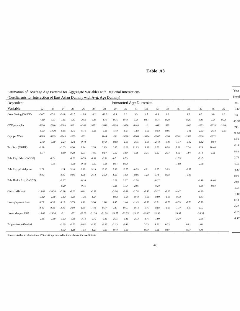
46

Table A3

Year

Trend

-0.1

-6.12

53

35.58

243

21.26

0.09

6.13

0.03

2.74

-0.03

-1.13

0.06

2.88

-0.04

-2.10

0.13

4.41

-0.09

-1.17

Estimation of Average Age Patterns for Aggregate Variables with Regional Interactions(Coefficients for Interaction of East Asian Dummy with Avg. Age Dummy)

Interacted Age DummiesDependent393837363534333231302928272625242322Variable1.83.86.21.81.2-1.94.73.32.3-2.1-10.8-3.2-16.8-21.5-24.8-35.6-30.7Dom. Saving (%GDP)

0.180.540.890.260.20-0.310.810.580.40-0.36-1.75-0.49-2.62-3.47-3.85-5.53-4.68

-2246-2270-1923-667685-418-2-1183-3066-2959-3919-3831-4263-5971-7088-7210-6656GDP per capita

-2.37-2.74-2.33-0.810.96-0.58-0.00-1.82-4.67-4.49-5.80-5.65-6.10-8.73-9.96-10.23-9.33

-3272-2336-2337-3501-398-6267-5094-7765-5226-2111044-753-1255-3845-6339-4385Cap. per Wker

-0.94-0.82-0.82-1.17-0.14-2.48-2.04-3.15-2.09-0.090.48-0.44-0.76-2.27-3.50-2.48

10.468.297.347.618.968.7811.1211.0510.620.052.052.552.240.50-1.33-1.68Tax Rev. (%GDP)

2.612.181.941.902.372.323.263.683.690.020.841.050.970.22-0.60-0.74

-2.45-1.350.73-0.71-0.64-1.41-0.74-1.02-1.04Pub. Exp. Educ. (%GDP)

-2.08-1.030.52-0.51-0.38-0.87-0.43-0.60-0.55

-0.573.093.054.81-0.2910.758.8810.009.196.963.181.242.78Pub. Exp. p/child prim.

-0.150.730.781.22-0.061.921.692.132.141.980.960.390.80

-0.46-1.18-0.17-2.502.270.22-0.14-0.27Pub. Health Exp. (%GDP)

-0.58-1.36-0.28-2.951.730.26-0.15-0.29

-4.99-4.47-6.08-5.17-5.46-2.78-3.69-3.06-6.37-6.01-2.66-7.68-10.53-13.89Gini coefficient

-0.87-0.73-1.04-0.90-0.95-0.48-0.64-0.53-1.64-1.39-0.65-1.83-2.48-3.02

-5.79-6.76-6.33-3.73-2.91-2.56-1.451.461.451.083.904.903.754.120.560.76Unemployment Rate

-1.51-1.87-1.77-1.05-0.83-0.77-0.440.450.470.371.401.802.042.230.330.46

-26.35-24.47-21.46-19.07-21.00-22.35-21.57-21.28-21.34-23.02-27-21-15.56-16.66Homicides per 1000

-2.36-2.24-1.99-1.77-2.13-2.41-2.35-2.41-2.72-3.18-3.60-3.13-2.40-2.05

1.610.810.331.563.73-3.46-2.13-3.35-6.85-8.62-6.75-1.99Progression to Grade 4

0.340.170.070.310.79-0.63-0.40-0.63-1.27-1.51-1.18-0.33

Source: Authors' calculations. 't' Statistics presented in italics below the coefficients.

47

Table A4

Estimation of Average Age Patterns for Aggregate Variables with Regional and Decade Interactions(Coefficients for Interaction of Latin American Dummy-Decade Dummy)

F TestR-squareT-barNo.No.ConstantYearDecade InteractionDependentWithinCountriesObs.Trend1990198019701960Variable

50.190.105.70164934213.5-0.1-0.50.01.8Dom. Saving (%GDP)

5.88-5.84-0.390.032.16

200.190.688.101391,123-10887656-1265-342142-2GDP per capita

-31.9032.59-8.44-2.941.34-0.02

209.240.755.9063374-486816251-2015-229473Cap. per Wker

-19.5019.63-2.94-0.491.26

72.760.163.80134503-153.580.090.971.16Tax Rev. (%GDP)

-5.195.681.392.70

17.460.122.40141338-66.080.04-1.41-0.94Pub. Exp. Educ. (%GDP)

-2.993.18-1.69-1.20

39.070.093.2012640593.79-0.040.211.21Pub. Exp. p/child prim.

1.67-1.420.171.74

Pub. Health Exp. (%GDP)

26.690.112.4052126149.27-0.050.681.441.643.45Gini coefficient

3.37-2.510.300.730.841.61

34.730.253.0075226-355.660.181.312.941.94Unemployment Rate

-5.966.140.661.591.09

11.190.403.30115374-4.220.00-5.66-2.76Homicides per 1000

-0.030.04-1.86-1.43

36.470.182.1012326483.3711.135.68Progression to Grade 4

24.936.575.84

Source: Authors' calculations. 't' Statistics presented in italics below the coefficients.

48

Table A5

Estimation of Average Age Patterns for Aggregate VariablesWith Interactions Between Age Patterns and Policy Dummies

Dependent Variable: PPP Adjusted Dependent Dependent Variable: Domestic GDP per capita Variable: Saving/GDPAverage

Unemployment Policy Variabes Policy Variabe Policy Variabes

Volatility of GDP Private CreditTrade OpennessPrivate CreditTrade OpennessAge Growth

t stat.Coeff.t stat.Coeff.t stat.Coeff.t stat.Coeff.t stat.Coeff.Dummy0.242580.02250.747.1-0.40-3.6-3.16-21.5 a200.394050.11153-0.39-3.5-3.18-19.4 a210.626520.152081.9116.3-0.29-2.6-3.32-19.8 a220.414320.233161.7614.5-0.50-4.6-3.66-21.8 a230.535690.608271.9315.8-0.45-4.2-3.15-18.8 a240.596450.608481.9915.6-0.08-0.8-2.82-16.5 a250.677400.466962.0415.70.080.8-1.94-13.6 a261.231,4030.609391.6813.00.080.8-1.67-13.6 a271.912,1940.871,3221.4611.50.858.6 a282.192,5161.702,7200.964.50.374.0-0.08-0.7 a293.634,1622.804,2721.074.8-0.49-5.20.131.0 a304.915,6542.564,0291.024.30.455.20.403.0 a315.716,5713.826,0220.703.30.374.0-0.27-2.1 a326.107,1963.696,1441.125.10.577.70.251.9 a336.827,9892.595,2691.034.7-0.03-0.60.503.9 a347.769,1955.919,5351.175.10.9310.80.030.2 a358.5810,1085.549,1641.044.80.576.20.080.6 a3610.5012,6434.849,6240.813.60.131.50.090.7 a3711.8815,1835.0210,2121.376.6-0.18-2.5-0.09-0.9 a388.9912,221 a3911.454111.51422.400.2-2.49-0.1-2.57-0.1 year

1.992,046-0.17(300)1.415.1-1.68-19.7-2.56-23.4Policy Variable

Age-Policy Interactions-1.88(2,124)0.213740.8610.42.4424.0age20*policy-1.97(2,076)0.294981.5711.01.3616.02.6124.4age21*policy-2.16(2,267)0.31537-1.02-4.51.5117.82.9627.6age22*policy-1.97(2,069)0.12213-1.07-4.21.4417.02.8626.7age23*policy-1.71(1,806)-0.08(132)-1.62-6.71.8321.72.7025.3age24*policy-1.60(1,742)0.06112-1.39-5.81.5618.72.6024.5age25*policy-2.15(2,480)-0.01(19)-2.21-9.31.6620.82.4024.6age26*policy-1.69(1,961)0.37712-1.25-5.61.6321.12.2024.6age27*policy-2.67(3,164)0.28526-1.07-5.61.6320.62.3618.2age28*policy-1.24(1,453)0.112132.1327.82.0022.5age29*policy-1.72(1,936)0.03562.8336.31.4216.0age30*policy-2.74(3,052)0.731,3681.9526.51.8019.3age31*policy-3.04(3,396)0.09167-0.73-2.22.2528.62.4926.6age32*policy-1.68(1,951)0.651,277-1.19-3.71.6424.72.3224.1age33*policy-2.48(2,807)1.152,614-1.27-4.51.6829.91.6216.4age34*policy-2.46(2,753)-0.40(755)-1.16-4.71.4919.52.4124.2age35*policy-1.44(1,626)0.591,132-1.27-5.51.8523.52.1522.1age36*policy-2.61(3,112)1.252,749-0.40-1.62.0526.71.8019.0age37*policy-3.57(4,268)1.603,629-0.63-2.82.1032.31.9723.1age38*policy

8.5513,3092.6630.32.2723.8age39*policy-11.2(79,788)-11(82,159)-2.37-381.62.76178.33.01207.8Constant

1,1231,123226934934No. Obs.13913975164164Countries8.088.083.015.705.70T-bar 0.650.640.340.110.08R-sq within 42.9641.341.702.141.67F( 40, 730) 0.000.000.020.000.01Prob > F

Source: Author's calculations

49

Appendix B

Table B1: F Tests for significance of differences between coefficients Dependent variable: Domestic Saving

38373635343332313029282726252423222120Age dummy

20

0.00021

0.3160.00022

0.0000.0400.01423

0.0000.0060.0020.00024

0.0140.0000.0000.0000.00025

0.0000.0000.0000.0000.0000.00026

0.0500.1210.0030.0000.0000.0000.00027

0.0000.0000.0000.0000.0000.0000.0000.00028

0.2470.0000.0000.0000.0000.0000.0000.0000.00029

0.5080.1070.0000.0000.0000.0000.0000.0000.0000.00030

0.2450.0730.0110.0000.0000.0000.0000.0000.0000.0000.00031

0.7830.1880.0550.0090.0000.0000.0000.0000.0000.0000.0000.00032

0.1480.1040.0140.0020.0000.0000.0000.0000.0000.0000.0000.0000.00033

0.0050.1980.3340.8460.4540.1250.0000.0000.0000.0000.0000.0000.0000.00034

0.4580.0750.6120.8000.4700.2170.0550.0000.0000.0000.0000.0000.0000.0000.00035

0.7910.6380.0640.5080.6760.6010.3160.0930.0000.0000.0000.0000.0000.0000.0000.00036

0.0200.0220.2060.0010.0320.0640.4200.7300.6700.0000.0010.0000.0000.0000.0000.0000.00037

0.3090.4860.3990.8360.0400.2810.3890.9810.6970.3010.0000.0000.0000.0000.0000.0000.0000.00038

0.9690.6370.8000.7350.9490.3050.5960.6690.9820.7960.5110.0030.0220.0010.0000.0000.0000.0000.00039

Table B2: F Tests for significance of differences between coefficients Dependent variable: PPP-Adjusted GDP per capita

38373635343332313029282726252423222120Age dummy

20

0.15821

0.6040.12022

0.5070.9180.26623

0.0060.0560.0510.01324

0.0820.0000.0010.0020.00025

0.3500.7480.0510.1290.0930.02126

0.0000.0020.0000.0000.0000.0000.00027

0.0000.0000.0000.0000.0000.0000.0000.00028

0.0000.0000.0000.0000.0000.0000.0000.0000.00029

0.0000.0000.0000.0000.0000.0000.0000.0000.0000.00030

0.0000.0000.0000.0000.0000.0000.0000.0000.0000.0000.00031

0.0000.0000.0000.0000.0000.0000.0000.0000.0000.0000.0000.00032

0.0000.0000.0000.0000.0000.0000.0000.0000.0000.0000.0000.0000.00033

0.0000.0000.0000.0000.0000.0000.0000.0000.0000.0000.0000.0000.0000.00034

0.0000.0000.0000.0000.0000.0000.0000.0000.0000.0000.0000.0000.0000.0000.00035

0.0000.0000.0000.0000.0000.0000.0000.0000.0000.0000.0000.0000.0000.0000.0000.00036

0.0000.0000.0000.0000.0000.0000.0000.0000.0000.0000.0000.0000.0000.0000.0000.0000.00037

0.0000.0000.0000.0000.0000.0000.0000.0000.0000.0000.0000.0000.0000.0000.0000.0000.0000.00038

0.3310.0000.0000.0000.0000.0000.0000.0000.0000.0000.0000.0000.0000.0000.0000.0000.0000.0000.00039

Table B3: F Tests for significance of differences between coefficients Dependent variable: Capital Per Worker

38373635343332313029282726252423222120Age dummy

20

0.18521

0.6080.44022

0.0820.0800.72123

0.9830.1410.1150.74224

0.1750.2630.0260.0240.28125

0.1790.0130.0340.0020.0020.06226

0.7140.5480.1710.2050.0430.0340.19627

0.9220.8000.4780.1490.1780.0380.0300.17528

0.0890.2070.0880.3610.8260.8280.6360.5230.98029

0.1220.9000.9770.7530.6730.3260.3530.1320.1050.30830

0.0000.0980.0050.0190.0050.0350.1510.1700.4720.5960.30331

0.0100.0000.0010.0000.0000.0000.0010.0110.0150.0840.1320.04932

0.0000.0000.0000.0000.0000.0000.0000.0000.0000.0000.0000.0000.00033

0.1240.0000.0000.0000.0000.0000.0000.0000.0000.0000.0000.0000.0000.00034

0.0000.0000.0000.0000.0000.0000.0000.0000.0000.0000.0000.0000.0000.0000.00035

0.0000.0000.0000.0000.0000.0000.0000.0000.0000.0000.0000.0000.0000.0000.0000.00036

0.0000.0000.0000.0000.0000.0000.0000.0000.0000.0000.0000.0000.0000.0000.0000.0000.00037

0.0000.0000.0000.0000.0000.0000.0000.0000.0000.0000.0000.0000.0000.0000.0000.0000.0000.00038

0.0000.0000.0000.0000.0000.0000.0000.0000.0000.0000.0000.0000.0000.0000.0000.0000.0000.0000.00039

50

Table B4: F Tests for significance of differences between coefficients Dependent variable: Tax Revenue as Share of GDP

38373635343332313029282726252423222120Age dummy

20

0.042821

0.0008 0.567222

0.2541 0.0004 0.262023

0.0856 0.6336 0.0387 0.837824

0.3076 0.5656 0.7517 0.0140 0.502925

0.8556 0.5507 0.5409 0.8989 0.0424 0.606726

0.5172 0.6019 0.2854 0.9089 0.5211 0.0292 0.376927

0.2621 0.0677 0.0893 0.0289 0.2379 0.1035 0.0022 0.092428

0.7666 0.4738 0.1882 0.2283 0.1011 0.4320 0.2265 0.0108 0.175129

0.0029 0.0134 0.0014 0.0001 0.0002 0.0000 0.0014 0.0005 0.0000 0.000830

0.1354 0.1274 0.2323 0.0511 0.0132 0.0167 0.0067 0.0499 0.0228 0.0007 0.020431

0.2959 0.6139 0.0405 0.0860 0.0163 0.0038 0.0049 0.0020 0.0168 0.0075 0.0002 0.007032

0.0114 0.3054 0.0346 0.4771 0.6432 0.2399 0.1086 0.1280 0.0692 0.2344 0.1339 0.0110 0.102033

0.0292 0.0000 0.0111 0.0010 0.7081 0.5815 0.8657 0.5816 0.6362 0.4346 0.8198 0.5802 0.1132 0.441734

0.0903 0.0003 0.0000 0.0003 0.0000 0.2198 0.1761 0.5298 0.7822 0.7278 0.9802 0.5999 0.8527 0.4005 0.931635

0.1518 0.0065 0.0000 0.0000 0.0000 0.0000 0.0694 0.0566 0.2340 0.3896 0.3548 0.5513 0.2929 0.4783 0.7661 0.683836

0.0006 0.0000 0.0000 0.0000 0.0000 0.0000 0.0000 0.0021 0.0020 0.0183 0.0399 0.0353 0.0809 0.0333 0.0773 0.4401 0.160637

0.9426 0.0050 0.0003 0.0000 0.0000 0.0000 0.0000 0.0000 0.0040 0.0037 0.0266 0.0551 0.0496 0.1046 0.0468 0.0992 0.4782 0.188338

0.0009 0.0009 0.0000 0.0000 0.0000 0.0000 0.0000 0.0000 0.0000 0.0000 0.0000 0.0001 0.0003 0.0002 0.0008 0.0003 0.0010 0.0137 0.003339

Table B5: F Tests for significance of differences between coefficients Dependent variable: Public Expenditure in Education as % of GDP

38373635343332313029282726252423222120Age dummy

20

0.42321

0.2660.80722

0.7880.2820.72623

0.2740.350.1380.45924

0.4780.1170.1970.0840.33225

0.890.6630.2490.2930.1250.38726

0.8740.9620.640.2940.3120.1390.38127

0.1160.0850.1330.0870.0310.0520.0250.11828

0.8420.2330.2250.280.1920.0860.1060.050.1729

0.1410.2940.0330.0380.0490.0370.0160.0230.0110.04930

0.1320.9840.8870.4560.4380.4810.3720.2270.2270.1190.25931

0.7820.3860.8570.9510.440.4230.4570.3670.2430.2380.1330.25732

0.9290.740.4230.8260.920.4250.4110.4440.360.240.2360.1340.25433

0.1210.2830.6070.1590.6930.650.8490.8110.8440.7160.5330.5060.3170.4934

0.4770.4950.6210.8910.2990.9070.8440.6730.6460.680.5740.4220.4050.2520.40135

0.8320.4970.6910.7730.9850.380.9780.9120.6330.610.6420.5450.4040.3880.2450.38536

0.0150.0840.4050.0770.140.350.0980.4590.4420.8440.890.8660.9970.8130.7690.5350.71837

0.0140.7840.6830.4460.8760.930.910.4910.9370.9950.590.5710.6020.5170.3920.3780.2450.37538

0.8970.3240.9780.8980.6940.8370.8750.9950.5210.9960.9420.6940.6720.6980.6140.4890.4690.3240.45439

Table B6: F Tests for significance of differences between coefficients Dependent variable: Public Expenditure in primary education per child

38373635343332313029282726252423222120Age dummy

20

0.31121

0.0560.03822

0.0160.0010.00123

0.3540.0090.0000.00024

0.4670.1970.0080.0000.00025

0.4460.8600.6930.0900.0120.00726

0.3060.7290.4490.2600.0320.0040.00227

0.6290.6710.9010.7970.5280.1080.0220.01228

0.5820.9410.4100.7360.5170.3430.0740.0170.00929

0.8330.5080.8060.3710.6380.4590.3150.0780.0200.01130

0.0010.0040.0010.0090.0020.0070.0040.0020.0000.0000.00031

0.7350.0010.0050.0020.0100.0020.0080.0050.0030.0000.0000.00032

0.8130.6170.0010.0040.0020.0090.0020.0070.0050.0030.0000.0000.00033

0.5580.7730.9330.0060.0120.0060.0210.0060.0170.0110.0080.0010.0000.00034

0.0030.0310.0380.0620.0000.0000.0000.0010.0000.0010.0000.0000.0000.0000.00035

0.1410.0000.0020.0030.0120.0000.0000.0000.0000.0000.0000.0000.0000.0000.0000.00036

0.0000.0000.0000.0000.0000.0000.0000.0000.0000.0000.0000.0000.0000.0000.0000.0000.00037

0.9130.0000.0000.0000.0000.0000.0000.0000.0000.0000.0000.0000.0000.0000.0000.0000.0000.00038

0.0000.0000.0000.0000.0000.0000.0000.0000.0000.0000.0000.0000.0000.0000.0000.0000.0000.0000.00039

51

Table B7: F Tests for significance of differences between coefficients Dependent variable: Public expenditures in Health as % of GDP

38373635343332313029282726252423222120Age dummy

20

21

0.2520.25222

0.8150.6520.65223

0.0040.1220.0590.05924

0.9230.0240.1590.0810.08125

0.1610.2700.0100.0650.0340.03426

0.8340.2740.3290.0230.0830.0460.04627

0.0120.0590.0210.0370.0020.0120.0070.00728

0.2420.0130.0300.0110.0190.0010.0060.0030.00329

0.0220.0110.0000.0020.0000.0010.0000.0000.0000.00030

0.9700.0990.0470.0060.0090.0040.0050.0000.0020.0010.00131

0.0000.0180.0010.0000.0000.0000.0000.0000.0000.0000.0000.00032

0.0960.3910.4680.0710.0380.0070.0090.0040.0060.0010.0020.0010.00133

0.8110.1120.4770.5380.0960.0520.0120.0140.0070.0090.0010.0030.0020.00234

0.8850.8020.1590.5720.6130.1330.0760.0200.0220.0120.0150.0030.0060.0040.00435

0.0950.1940.2100.0450.8490.8800.3950.2530.0910.0930.0570.0630.0170.0270.0180.01836

0.0030.0050.0290.0400.0090.4350.4990.7250.5060.2230.2210.1440.1520.0500.0710.0500.05037

0.2010.3520.0660.1240.1390.0330.6490.6960.5640.3850.1620.1630.1050.1130.0360.0520.0370.03738

0.6790.7150.3520.0820.1240.1350.0340.5750.6230.6610.4680.2150.2140.1430.1510.0540.0730.0530.05339

Table B8: F Tests for significance of differences between coefficients Dependent variable: Gini Coefficient

38373635343332313029282726252423222120Age dummy

20

0.17621

0.7120.17622

0.7750.8810.22823

0.5700.4830.9110.29124

0.4570.3000.2890.6640.41525

0.8170.4340.2970.2750.5960.47826

0.5860.7280.8870.6660.5780.8610.36527

0.0050.0430.0250.0130.0090.0120.0660.74928

0.1390.0000.0000.0000.0000.0000.0000.0060.30029

0.1370.7950.0070.0400.0280.0170.0130.0150.0640.66230

0.9710.1350.7820.0090.0450.0330.0220.0170.0180.0700.65931

0.2100.3480.4890.4040.0010.0120.0080.0060.0050.0060.0300.46532

0.2670.0330.0960.9760.2000.0000.0030.0020.0020.0020.0020.0150.33733

0.0660.0070.0000.0070.3340.0490.0000.0000.0000.0000.0000.0000.0040.18534

0.8940.1370.0220.0030.0160.4030.0650.0000.0010.0000.0000.0000.0010.0060.20235

0.1150.1880.8310.3190.0820.1420.9150.2150.0010.0080.0060.0050.0050.0060.0230.33636

0.0010.0970.2250.0180.0040.0000.0040.1380.0230.0000.0000.0000.0000.0000.0000.0030.12037

0.1870.0000.0230.0550.0060.0010.0000.0010.0470.0080.0000.0000.0000.0000.0000.0000.0010.06438

0.6700.7140.1060.3140.3650.1270.0630.0250.0350.2100.0530.0010.0030.0020.0020.0020.0020.0080.12739

Table B9: F Tests for significance of differences between coefficients Dependent variable: Unemployment rate

38373635343332313029282726252423222120Age dummy

20

0.01121

0.2720.12222

0.8330.2760.17823

0.8680.7650.2750.20624

0.2500.3270.4050.1590.37325

0.0000.0000.0000.0020.0020.60826

0.0660.0000.0000.0000.0000.0000.28927

0.0140.0000.0000.0000.0000.0000.0000.06128

0.1360.0000.0000.0000.0000.0000.0000.0000.02229

0.6050.0910.0000.0000.0000.0000.0000.0000.0000.01830

0.1710.0670.0060.0000.0000.0000.0000.0000.0000.0000.00531

0.0020.0000.0000.0000.0000.0000.0000.0000.0000.0000.0000.00032

0.0050.6810.1430.0760.0140.0000.0000.0000.0000.0000.0000.0000.00733

0.8330.0070.8320.2320.1390.0330.0000.0000.0000.0000.0000.0000.0000.01234

0.9130.7840.0130.9080.3080.2020.0600.0030.0000.0000.0000.0000.0000.0000.01835

0.7840.7350.6450.0170.9480.4280.2980.1030.0080.0010.0000.0000.0000.0000.0000.02636

0.0620.0570.0780.0870.0010.2870.8740.9060.4540.0870.0280.0000.0000.0010.0030.0020.08937

0.8250.1950.1620.1820.1840.0050.4020.9660.8380.4380.0960.0340.0010.0010.0020.0040.0030.09238

0.3300.2600.9530.9270.8890.8240.1440.9990.5460.4310.2120.0430.0150.0000.0000.0010.0020.0010.05139

52

Table B10: F Tests for significance of differences between coefficients Dependent variable: Homicide Rates

38373635343332313029282726252423222120Age dummy

20

0.43021

0.1320.10422

0.6600.2470.17223

0.5110.3980.4790.30624

0.0130.1600.4750.0830.07325

0.2940.0030.0560.2180.0410.04026

0.4770.1350.0040.0380.1340.0270.02727

0.9040.6360.2380.0150.0710.1890.0410.03728

0.4790.3550.7440.7350.1250.2980.4910.1350.10329

0.7850.4050.3120.6010.9560.2630.4710.6540.2160.15630

0.7310.9660.6020.5110.8320.7700.2230.3940.5550.1910.14131

0.8510.8740.9270.5510.4700.7560.8750.3130.4910.6430.2480.18132

0.9080.7860.9430.8810.5360.4640.7300.9270.3740.5500.6940.2890.21333

0.5800.5770.5270.7930.6760.4110.3510.5700.8760.5510.7290.8590.4070.30034

0.9670.6230.5900.5570.8160.6970.4300.3720.5930.8930.5520.7250.8520.4110.30535

0.5450.6620.9740.9070.8160.9710.8860.5840.5260.7600.9500.4630.6200.7440.3560.26736

0.6900.4020.5300.8460.9200.9680.8570.9970.6900.6360.8650.8650.4270.5720.6900.3360.25437

0.8870.6560.4140.5190.8000.8700.9780.8260.9620.7400.6900.9080.8410.4330.5700.6810.3440.26338

0.9870.9090.7380.5290.5830.8230.8810.9740.8370.9600.7640.7180.9200.8470.4610.5910.6950.3670.28339

Table B11: F Tests for significance of differences between coefficients Dependent variable: % of school age cohort progressing to grade 4

38373635343332313029282726252423222120Age dummy

20

0.96221

0.0630.19722

0.1990.0180.06923

0.2040.9660.2010.31124

0.3000.0570.3980.6700.73825

0.2740.0600.0140.1220.6970.71926

0.1040.4860.9820.5030.9660.3910.45727

0.8220.0830.3770.8530.6430.8940.3170.38128

0.9120.7820.1530.4360.8040.7900.8410.3570.40529

0.3240.2690.1960.0230.0940.2410.5050.2970.0950.12330

0.7050.2050.1720.1180.0180.0680.1660.3520.2080.0690.08931

0.8120.6130.2040.1770.1300.0260.0800.1720.3310.2080.0780.09532

0.3990.5230.4260.1310.1140.0820.0170.0520.1160.2320.1450.0530.06733

0.6800.3040.4240.3550.1100.0970.0710.0150.0460.1000.1980.1260.0470.05834

0.8850.6330.3080.4010.3370.1080.0960.0710.0160.0470.0990.1910.1230.0470.05835

0.0080.0660.0350.0100.0620.0720.0150.0130.0080.0010.0060.0160.0410.0240.0070.01036

0.0010.0000.0000.0000.0000.0030.0070.0010.0010.0000.0000.0000.0010.0050.0030.0000.00137

0.8820.0420.0000.0040.0020.0000.0080.0120.0020.0020.0010.0000.0010.0020.0080.0050.0010.00238

0.6490.6050.2100.0560.0600.0460.0290.0380.0350.0120.0110.0090.0030.0060.0120.0230.0160.0070.00839

53

Appendix C

Average AgeCountryAverage AgeCountry20251995195020251995195032.8624.9325.22Ecuador5125.1522.8120.61Afghanistan132.1924.8923.64Egypt5225.6522.1322.70Africa231.5823.9822.24El Salvador5335.1227.7125.92Albania324.8823.2127.35Equatorial Guinea5431.3623.4124.27Algeria425.6422.1021.73Eritrea5522.8720.9123.11Angola542.5536.5233.01Estonia5635.1130.8327.79Argentina622.7921.3021.98Ethiopia5737.7430.2828.22Armenia742.5637.0631.71Europe5834.1227.4525.44Asia833.4725.7420.64Fiji5939.2634.8731.84Australia941.7837.7029.72Finland6043.9237.7835.08Austria1042.8737.4334.82France6135.0927.7128.24Azerbaijan1133.2125.8721.58French Polynesia6236.4827.9424.28Bahamas, The1226.1526.2129.43Gabon6336.3526.6322.17Bahrain1326.3723.2724.25Gambia, The6430.8923.1925.16Bangladesh1438.2834.2131.79Georgia6539.4333.1227.64Barbados1544.4839.2534.71Germany6641.2835.6931.19Belarus1625.7521.7821.39Ghana6742.7838.4635.47Belgium1744.6038.7629.37Greece6830.8522.2424.32Belize1837.2230.7924.59Guadeloupe6924.0820.6428.77Benin1934.7027.5222.44Guam7025.2222.8323.86Bhutan2026.8721.9821.57Guatemala7128.8723.5423.35Bolivia2123.0420.7922.39Guinea7242.3433.3024.46Bosnia and Herzegovina2224.8323.7924.86Guinea-Bissau7326.8621.4221.61Botswana2334.6125.8823.72Guyana7434.8027.0022.96Brazil2425.5023.6726.31Haiti7535.4225.4325.37Brunei2528.9821.8521.30Honduras7642.2237.7929.99Bulgaria2644.9834.4224.81Hong Kong7722.6820.6822.23Burkina Faso2741.7537.4431.89Hungary7824.7321.0223.23Burundi2838.8233.5729.35Iceland7928.6423.1422.55Cambodia2933.1226.1224.07India8024.8422.2824.01Cameroon3033.5426.1824.14Indonesia8141.4635.5729.98Canada3128.5522.1825.35Iran, I.R. of8229.9122.3725.66Cape Verde3227.2622.2421.28Iraq8334.2828.5125.14Caribbean3339.9433.3232.02Ireland8425.7023.2526.10Central African Republic3435.9130.5326.99Israel8524.7322.6825.15Chad3547.2639.3831.58Italy8635.7229.1025.73Chile3634.8927.1125.34Jamaica8737.7129.6526.89China3745.4738.8326.14Japan8833.5525.7322.88Colombia3826.4821.4522.94Jordan8925.1320.6722.65Comoros3935.2329.3427.96Kazakstan9023.4921.5623.78Congo4027.4020.7324.17Kenya9132.7625.9422.65Costa Rica4139.5930.6723.36Korea9226.7221.7121.99Cote d'Ivoire4236.4128.3223.38Korea, North9341.3737.2231.00Croatia4334.3223.4323.31Kuwait9441.7332.6526.49Cuba4432.1625.8230.24Kyrgyz Republic9538.1433.4627.20Cyprus4541.4036.8133.41Latvia9642.0836.3233.03Czech Republic4633.2526.0627.63Lebanon9741.0138.2432.70Denmark4726.2723.3024.23Lesotho9826.6822.9820.63Djibouti4824.1122.9123.08Liberia9933.7525.2322.10Dominican Republic4924.8821.5923.77Libya10029.8722.8723.29East Timor50

Source: Authors'calculations from UN (1998)

54

Appendix C

Average AgeCountryAverage AgeCountry20251995195020251995195041.1731.7522.99Singapore15140.8135.5231.59Lithuania10140.1333.8429.89Slovak Republic15241.2037.7435.01Luxembourg10243.9536.9930.66Slovenia15340.9130.7326.67Macau10326.4521.5322.44Solomon Islands15438.4332.2927.28Macedonia10422.6120.6723.14Somalia15524.2920.8422.79Madagascar10529.7925.0624.52South Africa15623.1720.8521.50Malawi10645.6137.7030.42Spain15732.6124.8324.23Malaysia10735.7828.5523.47Sri Lanka15823.1920.5621.74Mali10828.0022.9122.35Sudan15939.4434.8027.39Malta10933.5425.5024.96Suriname16038.0632.4625.48Martinique11027.5621.5322.11Swaziland16126.1422.3522.90Mauritania11141.5438.9334.50Sweden16235.7128.8921.66Mauritius11244.1738.1733.85Switzerland16328.7823.6423.53Melanesia11329.2521.2923.77Syrian Arab Republic16433.7424.9324.01Mexico114

Taiwan16536.8932.1930.03Moldova11530.1223.2126.59Tajikistan16631.3223.5323.19Mongolia11624.5420.9720.94Tanzania16732.8324.5821.84Morocco11737.4128.0322.35Thailand16823.9522.0022.84Mozambique11823.8721.5823.80Togo16931.8125.2524.57Myanmar11936.0228.4524.27Trinidad & Tobago17025.9323.0223.64Namibia12033.4225.4625.17Tunisia17127.1622.7924.55Nepal12134.7727.1424.28Turkey17243.5437.0130.36Netherlands12231.2023.8827.82Turkmenistan17337.9131.7626.40Netherlands Antilles12322.0019.8921.70Uganda17434.9827.6828.57New Caledonia12441.8136.9930.79Ukraine17538.0433.9131.18New Zealand12536.7828.1223.09United Arab Emirates17629.1421.6321.41Nicaragua12641.5037.9734.86United Kingdom17722.3820.2821.71Niger12739.3735.2131.60United States17824.6121.5121.13Nigeria12836.4133.9630.69Uruguay17940.5737.5233.54Norway12931.1223.9528.55Uzbekistan18036.1532.0430.03Oceania13027.4622.5520.83Vanuatu18122.5321.1422.65Oman13132.7525.1121.91Venezuela18227.9222.3725.43Pakistan13232.8524.8126.24Viet Nam18334.7326.5824.33Panama13321.2118.8323.07West Bank and Gaza18428.1623.2823.98Papua New Guinea13422.9019.9923.24Yemen, Republic of18528.5823.0526.12Paraguay13539.3435.2729.65Yugoslavia18632.9925.2023.44Peru13622.8720.9122.55Zaire18731.3623.9622.73Philippines13723.9519.9121.47Zambia18839.4734.3728.63Poland13826.9021.3022.08Zimbabwe18932.5125.0421.19Polynesia139

42.9437.5029.41Portugal14036.5529.5323.25Qatar14241.4935.3729.14Romania14441.4235.7428.97Russian Federation14524.8320.5121.02Rwanda14631.5623.9120.45Samoa14725.2121.7523.15Senegal14923.9422.1223.91Sierra Leone150

Source: Authors'calculations from UN (1998)

55

Appendix Table D: Data Sources

Variables Source

all age structure variables United Nations (1998)

domestic savings as a share of GNP World Bank World Development Indicators (1998)

PPP adjusted GDP per capita For 1950-1992, Penn World Tables. The World BankDevelopment Indicators (1998) provide a series of PPPadjusted GDP per capita for the period 1980-1997. Weuse the growth rates from the World Bank (using thesame definition as in the Penn World Tables) to extendthe Penn World Tables series through 1995.

capital per worker Penn World Tables

tax revenue as a share of GDP World Bank World Development Indicators (1998)

public expenditures on education as a share of GDP World Bank World Development Indicators (1998)

public expenditure on primary education per primaryschool-age child as a proportion of GNP

World Bank World Development Indicators (1998)

health expenditures as a share of GDP World Bank World Development Indicators (1998)

Gini coefficients “good quality” distribution data from Deininger andSquire (1996)

Unemployment rates ILO (1998)

homicide rates Fajnzylber, Lederman and Loayza (1998), whocombine homicide rates from the United NationsSurveys of Criminal Trends and Operations of CriminalJustice Systems, and data from the World HealthOrganization.

Probability that a student belonging to the cohort that isof school age in the year of reference, progresses tograde 4

World Bank World Development Indicators (1998)

trade openness ((imports plus exports))/GDP Penn World Tables.

private credit as a share of GDP World Bank World Development Indicators (1998)

macro volatility constructed from the Penn World tables and WorldBank data

expenditures in education as a share of GDP World Bank World Development Indicators (1998)

56

REFERENCES

Ahmad, Sultan, 1994, "Improving Inter-Spatial and Inter-Temporal Comparability of NationalAccounts," Journal of Development Economics 44:1 (June), 53-76.

Asian Development Bank (ADB), 1997, Emerging Asia: Changes and Challenges, Manila: AsianDevelopment Bank.

Attanasio, Orazio P., 1998, “Cohort Analysis of Saving Behavior by U.S. Households,” Journalof Human Resources 33:3 (Summer), 575-609.

Attanasio, Orazio P. and Miguel Székely, 1998 “Household Saving and Income Distribution inMexico" OCE working paper No. 390, Inter American Development Bank, 1998.

Behrman, Jere R., 1996a, Human Resources in Latin America and the Caribbean, Baltimore: TheJohns Hopkins University Press for the Inter-American Development Bank

Behrman, Jere R., 1999a, “Education, Health and Demography in Latin America around the Endof the Century: What Do We Know? What Questions Should be Explored?” Philadelphia, PA:University of Pennsylvania, Background Paper for IPES 2000 for IDB mimeo.

Behrman, Jere R., 1999b “Why Micro Matters: Why a Micro Perspective on Population Changeand Economic Development is Essential for Good Conditional Predictions and Policy Formationand Evaluation,” in Nancy Birdsall and Steven Sinding, eds. Population Change and EconomicDevelopment (Papers Presented at a Conference Co-Sponsored by Rockefeller Foundation,Packard Foundation and the United Nations Population Fund UNFPA at the RockefellerFoundation’s Bellagio Center, Lake Como, Italy, November 2-6, 1998) Oxford, UK: OxfordUniversity Press, 1999.

Behrman, Jere R. and Nancy Birdsall, 1983, "The Quality of Schooling: Quantity Alone isMisleading," American Economic Review 73, 928-946.

Behrman, Jere R., Suzanne Duryea and Miguel Székely, 1999, "Aging and Economic Options:Latin America in a World Perspective" Office of the Chief Economist, Inter AmericanDevelopment Bank, mimeo.

Behrman, Jere R. and Mark R. Rosenzweig, 1994, "Caveat Emptor: Cross-Country Data onEducation and the Labor Force," Journal of Development Economics 44:1 (June), 147-172.

Birdsall, Nancy, 1985, "Public Inputs and Child Schooling in Brazil," Journal of DevelopmentEconomics 18:1 (May-June), 67-86.

Birdsall, Nancy and Richard H. Sabot, 1994, "Virtuous Circles: Human Capital, Growth andEquity in East Asia," Washington, D.C.: World Bank, mimeo.

Birdsall, Nancy and Steven Sinding, eds., 1999,Population Change and Economic Development(Papers Presented at a Conference Co-Sponsored by Rockefeller Foundation, Packard Foundationand the United Nations Population Fund UNFPA at the Rockefeller Foundation? s BellagioCenter, Lake Como, Italy, November 2-6, 1998) Oxford, UK: Oxford University Press.

57

Bloom, David E. and Jeffrey G. Williamson, 1999, “Demographic Transitions and EconomicMiracles in Emerging Asia,” The World Bank Economic Review 12:3 (September), 419-456.

Bouis, Howarth E., 1994, "The Effect of Income on Demand for Food in Poor Countries: Are OurDatabases Giving Us Reliable Estimates?" Journal of Development Economics 44:1 (June),199-226.

Browning, Martin, Angus Deaton, Margaret Irish, 1985, “A Profitable Approach to Labor Supplyand Commodity Demands over the Life Cycle,” Econometrica 53:3 (May), 503-544.

Chamie, Joseph, 1994, "Population Databases in Development Analysis," Journal ofDevelopment Economics 44:1 (June), 131-146.

Coale, Ansley J. and Edgar M. Hoover, 1958, Population Growth and Economic Development inLow-Income Countries: A Case Study of India's Prospects, Princeton, NJ: Princeton UniversityPress.

Deaton, Angus, 1991 “Saving and Liquidity Constraints”, Econometrica 59:5 (September), 1221-1248.

Deaton, Angus, 1997, The Analysis of Household Surveys: A Microeconometric Approach toDevelopment Policy, Johns Hopkins University Press, Baltimore.

Deaton, Angus and Christina Paxson, 1994, "Intertemporal Choice and Inequality," Journal ofPolitical Economy 102:3 (June), 437-467.

Deaton, Angus and Christina Paxson, 1997, “The Effects of Economic and Population Growth onNational Saving and Inequality,” Demography 34:1 (February), 97-114.

Deaton, Angus and Christina Paxson, 1998, “Saving and Growth: Another Look at the CohortEvidence,” Princeton, NJ: Princeton University, mimeo.

Deininger, Klaus and Lynn Squire, 1996, “A New Data Set Measuring Income Inequality,”World Bank Economic Review 10:3 (September), 565-591.

Duryea, Suzanne and Miguel Székely, 1998, “Labor Markets in Latin America: A Supply-SideStory,” Washington, DC: Inter-American Development Bank, Office of the Chief Economist,Working Paper Series 374.

Ehrlich, Paul R., 1968, The Population Bomb, New York: Ballentine Books.

Easterlin, Richard, 1978, “What will 1984 be like? Socioeconomic Implications of Recent Twistsin Age Structure,” Demography 15:397-432.

Easterlin, Richard, 1987, Birth and Fortune: The Impact of Numbers on Personal Welfare,Chicago University Press, Chicago.

Fajnzylber, Pablo, D. Lederman and N. Loayza, 1998, “Determinants of Crime rates in LatinAmerica and the World; an empirical assessment”, World Bank Latin American and CaribbeanStudies, The World Bank, Washington.

58

Hanushek, Eric A., 1995, "Interpreting Recent Research On Schooling in Developing Countries,"The World Bank Research Observer 10:2 (August), 227-246.

Heston, Alan, 1994, "A Brief Review of Some Problems in Using National Accounts Data inLevel Comparisons and Growth Studies," Journal of Development Economics 44:1 (June), 29-52.

Inter-American Development Bank (IDB), 1998, Economic and Social Progress in LatinAmerica: 1998-1999 Report, Special Section - Facing Up to Inequality in Latin America,Baltimore, MD: Distributed by the Johns Hopkins University Press for the Inter-AmericanDevelopment Bank.

International Labor Organization (ILO), 1998, Labor Market Indicators, Geneva.

Jappelli, Tullio, 1999, “The Age-Wealth Profile and the Life-Cycle Hypothesis: A CohortAnalysis with a Time Series of Italian Households”, The Review of Income and Wealth 45:1, 57-75.

Kelley, Allen C. and William Paul McGreevey, 1994, "Population and Development in HistoricalPerspective," in Robert Cassen, ed., Population and Development: Old Debates, newConclusions, Washington, D.C.: Overseas Development Council.

Kelley, Allen C. and Robert M. Schmidt, 1994, “Population and Income Change: RecentEvidence,” Washington: World Bank Discussion Paper No. 249.

Kelley, Allen C. and Robert M. Schmidt, 1998, “Economic and Demographic Change: ASynthesis of Models, Findings, and Perspectives,” revision in Birdsall and Sinding, 1999.

Kremer, Michael R., 1995, “Research on Schooling: What We Know and What We Don? t: AComment on Hanushek,” World Bank Research Observer 10:2 (August), 247-254.

Kuznets, Simon, 1958, "Long Swings in the Growth of Population and in Related EconomicVariables," Proceedings of the American Philosophical Society 102 (February), 25-52.

Kuznets, Simon, 1967, "Population and Economic Growth," Proceedings of the AmericanPhilosophical Society 111:3 (June), 170-193.

Lam, David, 1997, "Demographic Variables and Income Inequality," in Mark R. Rosenzweig andOded Stark, eds., Handbook of Population and Family Economics, Amsterdam: North-HollandPublishing Company.

Levitt, Steven, 1998, “The Limited Role of Changing Age Structure in Explaining AggregateCrime Changes,” Chicago: University of Chicago, mimeo.

Loayza, Norman, Klaus Schmidt-Heggel and Luis Servén’, 1998, “What Drives Saving Acrossthe World?” Washington, DC: The World Bank, mimeo.

Miles, David, 1999, “Modeling the Impact of Demographic Change Upon the Economy,” TheEconomic Journal 109 (January) 1-36.

59

Morrison, Andrew, Carmen Pagés, and Ricardo Fuentes, 1999, “The Demographics of ViolentCrime in Latin America,” Washington, DC: Office of the Chief Economist, Inter AmericanDevelopment Bank, mimeo.

National Research Council, 1986, Population Growth and Economic Development: PolicyQuestions, Washington, D.C.: National Academy Press.

Page, John, et al., 1993, The East Asian Miracle: Economic Growth and Public Policy,Washington, D.C.: The World Bank.

Phelps, Edmund S., 1968, "Population Increase," Canadian Journal of Economics 1:3 (August),497-518.

Republic of China, 1997, “Statistical Yearbook”, Director General of Budget, Accounting andStatistics, Republic of China.

Savedoff, William and Claudia Piras, 1999 “Does Growth Lead to Growth?: Income Effects opnAdults Height, IDB Mimeo, Washington DC.

Solow, Robert M., 1956, "A Contribution to the Theory of Economic Growth," Quarterly Journalof Economics 70:1 (February), 65-94.

Srinivasan, T. N., 1994, "Data Base for Development Analysis: An Overview," Journal ofDevelopment Economics 44:1 (June), 3-26.

United Nations, 1996, The Sex and Age Distribution of the World Populations: The 1996Revision, New York: United Nations.