Aggregation of stochastic automata networks with replicas

Linear Algebra and its Applications 386 (2004) 111–136www.elsevier.com/locate/laa

Aggregation of stochastic automata networkswith replicas�

Anne Benoit a,∗, L. Brenner b,1, P. Fernandes b,1, B. Plateau a

aLaboratoire ID-IMAG, CNRS-INRIA-INPG-UJF, 51 Av. Jean Kuntzmann, 38330 Montbonnot,Saint-Martin, France

bPUCRS, Faculdade de Informática, Av. Ipiranga, 6681 90619-900 Porto Alegre, Brazil

Received 12 August 2003; accepted 24 February 2004

Submitted by W. Stewart

Abstract

We present techniques for computing the solution of large Markov chain models whosegenerators can be represented in the form of a generalized tensor algebra, such as StochasticAutomata Networks (SAN). Many large systems include a number of replications of identicalcomponents. This paper exploits replication by aggregating similar components. This leads toa state space reduction, based on lumpability. We define SAN with replicas, and we show howsuch SAN models can be strongly aggregated, taking functional rates into account. A tensorrepresentation of the matrix of the aggregated Markov chain is proposed, allowing to storethis chain in a compact manner and to handle larger models with replicas more efficiently.Examples and numerical results are presented to illustrate the reduction in state space and,consequently, the memory and processing time gains.© 2004 Elsevier Inc. All rights reserved.

Keywords: Large Markov chains; Stochastic automata networks; Generalized tensor algebra; Replication;Lumpability; Strong aggregation; PEPS software tool

�Contract/grant sponsor: Authors partially supported by CNPq-INRIA agreement PAGE II project,HP/Brasil-PUCRS agreement CASCO project and DECORE-IMAG project.∗ Corresponding author. Tel.: +33-0-476612088; fax: +33-0-476612099.

E-mail addresses: [email protected] (A. Benoit), [email protected] (L. Brenner),[email protected] (P. Fernandes), [email protected] (B. Plateau).

1 Tel.: +55-51-320-36-11; fax: +55-51-320-36-21.

0024-3795/$ - see front matter � 2004 Elsevier Inc. All rights reserved.doi:10.1016/j.laa.2004.02.015

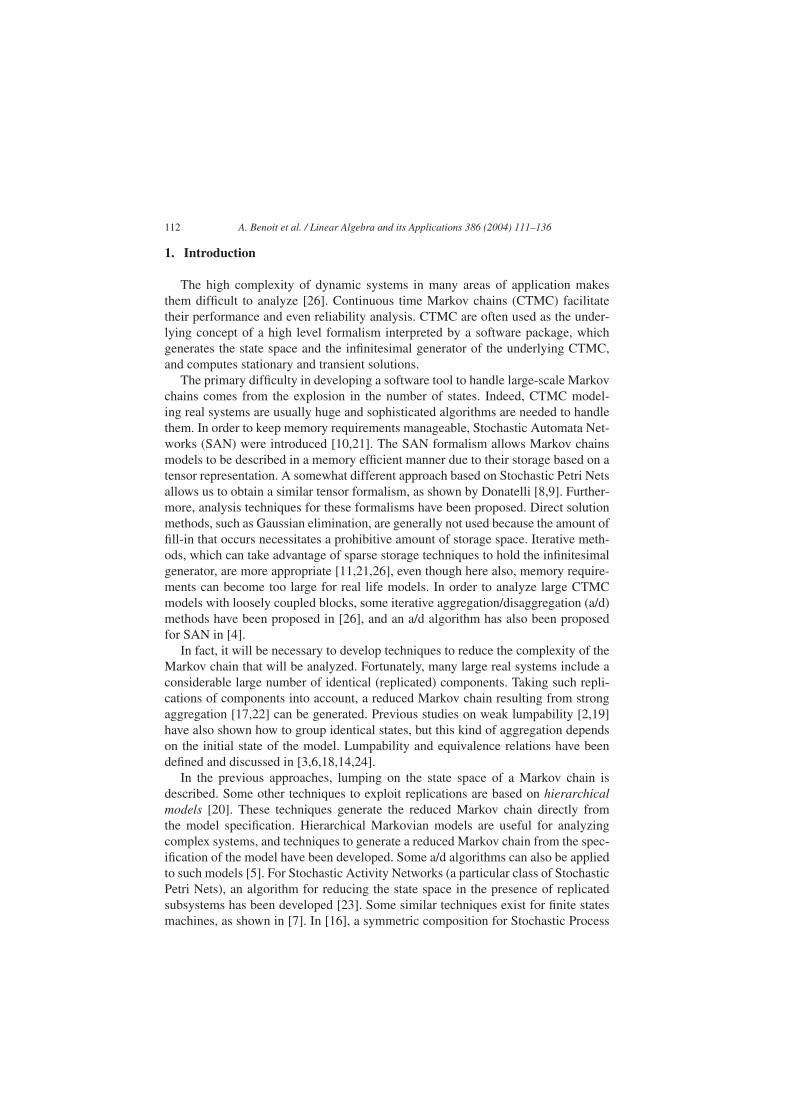
112 A. Benoit et al. / Linear Algebra and its Applications 386 (2004) 111–136

1. Introduction

The high complexity of dynamic systems in many areas of application makesthem difficult to analyze [26]. Continuous time Markov chains (CTMC) facilitatetheir performance and even reliability analysis. CTMC are often used as the under-lying concept of a high level formalism interpreted by a software package, whichgenerates the state space and the infinitesimal generator of the underlying CTMC,and computes stationary and transient solutions.

The primary difficulty in developing a software tool to handle large-scale Markovchains comes from the explosion in the number of states. Indeed, CTMC model-ing real systems are usually huge and sophisticated algorithms are needed to handlethem. In order to keep memory requirements manageable, Stochastic Automata Net-works (SAN) were introduced [10,21]. The SAN formalism allows Markov chainsmodels to be described in a memory efficient manner due to their storage based on atensor representation. A somewhat different approach based on Stochastic Petri Netsallows us to obtain a similar tensor formalism, as shown by Donatelli [8,9]. Further-more, analysis techniques for these formalisms have been proposed. Direct solutionmethods, such as Gaussian elimination, are generally not used because the amount offill-in that occurs necessitates a prohibitive amount of storage space. Iterative meth-ods, which can take advantage of sparse storage techniques to hold the infinitesimalgenerator, are more appropriate [11,21,26], even though here also, memory require-ments can become too large for real life models. In order to analyze large CTMCmodels with loosely coupled blocks, some iterative aggregation/disaggregation (a/d)methods have been proposed in [26], and an a/d algorithm has also been proposedfor SAN in [4].

In fact, it will be necessary to develop techniques to reduce the complexity of theMarkov chain that will be analyzed. Fortunately, many large real systems include aconsiderable large number of identical (replicated) components. Taking such repli-cations of components into account, a reduced Markov chain resulting from strongaggregation [17,22] can be generated. Previous studies on weak lumpability [2,19]have also shown how to group identical states, but this kind of aggregation dependson the initial state of the model. Lumpability and equivalence relations have beendefined and discussed in [3,6,18,14,24].

In the previous approaches, lumping on the state space of a Markov chain isdescribed. Some other techniques to exploit replications are based on hierarchicalmodels [20]. These techniques generate the reduced Markov chain directly fromthe model specification. Hierarchical Markovian models are useful for analyzingcomplex systems, and techniques to generate a reduced Markov chain from the spec-ification of the model have been developed. Some a/d algorithms can also be appliedto such models [5]. For Stochastic Activity Networks (a particular class of StochasticPetri Nets), an algorithm for reducing the state space in the presence of replicatedsubsystems has been developed [23]. Some similar techniques exist for finite statesmachines, as shown in [7]. In [16], a symmetric composition for Stochastic Process

A. Benoit et al. / Linear Algebra and its Applications 386 (2004) 111–136 113

Algebras is proposed. Its operational semantics is compact and intuitive, and it allowsa compact description of systems with replicas.

All these approaches present lumpability conditions for various modeling tech-niques in order to reduce the state space. The goal of this paper is to present anequivalent technique that can be used to efficiently aggregate SAN models. The lum-pability conditions, as shown earlier in [17,22], are described and used in order todemonstrate that a SAN with replicas can be strongly aggregated. Identical automatawithin the model are detected and they can be automatically grouped and aggregatedin order to generate the reduced Markov chain. A similar approach is described bySiegle [25], but it does not take functional rates, one of the major components of SANmodels, into account. In his work [3], Buchholz defines the equivalence relations forStochastic Automata Networks, and particularly equivalent representations for a Sto-chastic Automata. Gusak et al. [14,15] have provided relatively general lumpabilityconditions for continuous-time and discrete-time SAN; these conditions are checkedon automata matrices and they do not require exact replication of components. Allthese approaches emphasis on equivalence relations, but they do not give any formaldefinition of replicas for SAN. Moreover they do not give a tensorial expression ofthe matrix of the aggregated Markov chain.

In the next section, we briefly recall the concept of SAN, and then we formallydefine SAN with replicas in Section 3. The strong aggregation of such SAN isdescribed in Section 4, and a tensorial expression of the matrix of the aggregatedMarkov chain is proposed. The final section shows the benefits of aggregation andsome numerical results of practical examples.

2. Stochastic Automata Networks (SAN)

Continuous-time Stochastic Automata Networks [10,11,21] describe a system asa set of subsystems that interact. Each subsystem is modeled by a stochastic autom-aton, and some rules between the states of each automaton describe the interactionsbetween subsystems.

Each automaton is composed of states, called local states, and transitions amongthem. Transitions on each automaton are labeled with the list of the events that maytrigger it. An event is triggered after a delay which is exponentially distributed andthe exponentially distributed variables corresponding to each event are independent.Each event is defined by its name and its rate.

When the occurrence of the same event can lead to different target states, a proba-bility of occurrence is assigned to each possible transition. The label on the transitionis evt(prob), where evt is the event name, and prob is the probability of occurrenceof each possible transition. When only one transition is possible, the probability canbe omitted.

There are basically two ways in which stochastic automata interact. Firstly, therate at which an event may occur can be a function of the state of other automata.


Such rates are called functional rates. Rates that are not functional are said to beconstant rates. The probabilities of occurrence can also be functional. Secondly, anevent may involve more than one automaton: the occurrence of such event triggerstransitions in two or more automata at the same time. Such events are called syn-chronizing events, in opposition to events involving only one automaton, called localevents. As local events, synchronizing events may have constant or functional ratesand probabilities.

Consider a SAN model with N automata and E events. It is a N-component Mar-kov chain whose components are not necessarily independent (due to the possiblepresence of functional rates and synchronizing events). A local state of ith autom-aton (A(i) | i = 1, . . . , N) is denoted x(i) while the complete set of states for thisautomaton is denoted S(i), and the cardinality of S(i) is denoted by ni . S = S(1) ×· · · × S(N) is called the product state space, and its cardinality is equal to

∏Ni=1 ni . A

global state for the model is a vector x = (x(1), . . . , x(N)) ∈ S. The reachable statespace of the model is denoted by S; it is generally smaller than the product statespace, most of the time because of synchronizing events and functional rates whichprevent some states in S from occurring.

An automaton is involved by an event if it has at least one transition labeled bythis event. The set of automata involved by an event e is denoted by Oe. The event e

can occur if, and only if, all the automata in Oe are in a local state from which one ofthose transitions can be triggered. When it occurs, all the corresponding transitionsare triggered. Notice that for a local event e, Oe is reduced to the automaton involvedby this event, and that only one transition occurs.

For i = 1, . . . , N , the behavior of continuous-time automaton A(i) is describedby a set of square matrices, all of order ni . We shall denote the set of synchronizingevents by ES. Let us denote, for i = 1, . . . , N , and for e ∈ ES:

• Q(i)l the matrix consisting only of the transitions that are local to automaton A(i);

• Q(i)e+ the positive synchronization matrix of A(i), which represents the occurrence

of the synchronizing event e and its rates;• Q

(i)e− the negative synchronization matrix of A(i), which corresponds to an updat-

ing of the diagonal elements for event e; it is defined by Q(i)e+ and its elements are

not necessarily negative as suggested by the name.

Notice that if A(i) is not in Oe, then Q(i)e+ and Q

(i)e− are identity matrices.

Then, it has been shown in [10,11] that the transition matrix can be expressed as:

Q =N⊕

gi=1

Q(i)l +

∑e∈ES

N⊗

gi=1

Q(i)e+ +

N⊗g

i=1

Q(i)e−

. (1)

The tensor sum corresponds to the analysis of the local events, while the tensorproducts correspond to the analysis of the synchronizing events. Notice the use of


generalized tensor algebra [10,21], i.e., the use of operators⊕

g and⊗

g , instead of⊕and

⊗.

3. SAN models with replicas

Although large systems often contain identical components, we turn our attentionto two different cases: systems where all subsystems are equal, and systems where onlysome sets of subsystems are equal among themselves. The first case is modeled by aSAN composed of one replica, and the second case is modeled by a SAN with multiplereplicas. In this section we formally define SAN models composed of one replica andSAN models with multiple replicas with an illustrating example for each case.

3.1. SAN models composed of one replica

Informally, a SAN composed of one replica consists of a set of N identical auto-mata, i.e., the states of each automaton are identical, and the transitions are labeledwith identical synchronizing events or replicated local events (for a given transition,the local events have the same rate in each automaton). This implies that the syn-chronizing events involve all replicated automata. Moreover, we have a replica onlyif the functions are not changed by a permutation of the parameters. For example,if N = 2, for all functional rate f and for all x(1) ∈ S(1) and x(2) ∈ S(2), we musthave f (x(1), x(2)) = f (x(2), x(1)) (remember that S(i) is the state space of automa-ton A(i)). Formalizing the definition of such SAN:

Definition 1. A SAN composed of one replica is a SAN model with N automata,such that, for i = 1, . . . , N , we have:

• all local matrices Q(i)l are identical (equal to Ql);

• for every synchronizing event e ∈ ES, all matrices Q(i)e+ and all matrices Q

(i)e− are

identical and respectively equal to Qe+ and Qe−; only one automaton hold thetransition rate fe of the event (matrices feQe+ and feQe−);

• for all functional rates f , for all permutations σ of [1, . . . , N], and for each globalstate x = (x(1), . . . , x(N)), f (x) = f (σ (x)), where σ(x) = (xσ(1), . . . , xσ(N))

(the functions are not changed by a permutation of the parameters).

The concept of a SAN composed of one replica is now illustrated through a smallexample.

3.2. The basic resource sharing model––RS1

In this model, Np distinguishable processes share Nr identical units of a com-mon resource. Each of these processes alternates between a sleeping state and aresource using state. Notice that when Nr = 1 this model reduces to the usual mutual


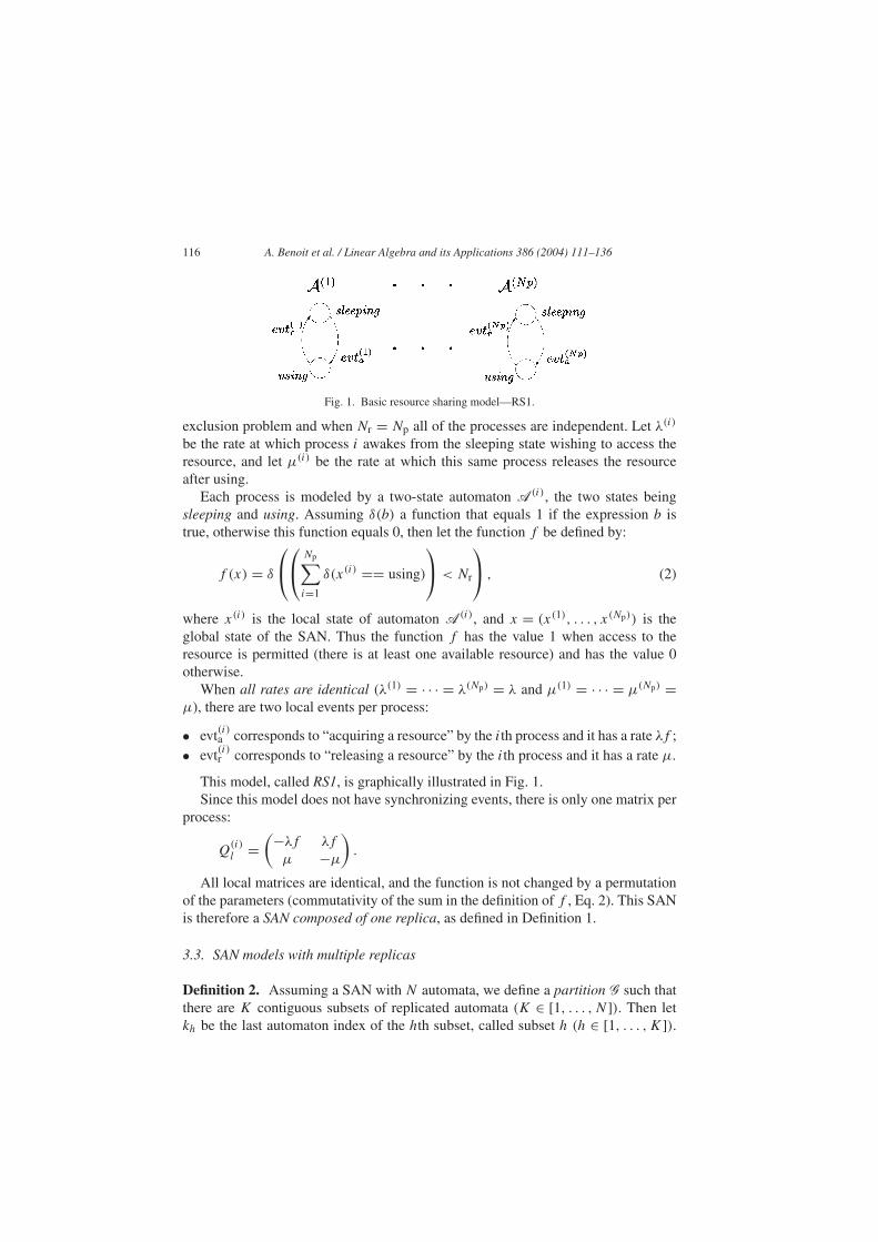
Fig. 1. Basic resource sharing model––RS1.

exclusion problem and when Nr = Np all of the processes are independent. Let λ(i)

be the rate at which process i awakes from the sleeping state wishing to access theresource, and let µ(i) be the rate at which this same process releases the resourceafter using.

Each process is modeled by a two-state automaton A(i), the two states beingsleeping and using. Assuming δ(b) a function that equals 1 if the expression b istrue, otherwise this function equals 0, then let the function f be defined by:

f (x) = δ

Np∑

i=1

δ(x(i) == using)

< Nr

, (2)

where x(i) is the local state of automaton A(i), and x = (x(1), . . . , x(Np)) is theglobal state of the SAN. Thus the function f has the value 1 when access to theresource is permitted (there is at least one available resource) and has the value 0otherwise.

When all rates are identical (λ(1) = · · · = λ(Np) = λ and µ(1) = · · · = µ(Np) =µ), there are two local events per process:

• evt(i)a corresponds to “acquiring a resource” by the ith process and it has a rate λf ;• evt(i)r corresponds to “releasing a resource” by the ith process and it has a rate µ.

This model, called RS1, is graphically illustrated in Fig. 1.Since this model does not have synchronizing events, there is only one matrix per

process:

Q(i)l =

(−λf λf

µ −µ

).

All local matrices are identical, and the function is not changed by a permutationof the parameters (commutativity of the sum in the definition of f , Eq. 2). This SANis therefore a SAN composed of one replica, as defined in Definition 1.

3.3. SAN models with multiple replicas

Definition 2. Assuming a SAN with N automata, we define a partition G such thatthere are K contiguous subsets of replicated automata (K ∈ [1, . . . , N]). Then letkh be the last automaton index of the hth subset, called subset h (h ∈ [1, . . . , K]).


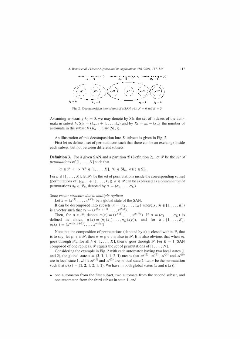
Fig. 2. Decomposition into subsets of a SAN with N = 6 and K = 3.

Assuming arbitrarily k0 = 0, we may denote by SIh the set of indexes of the auto-mata in subset h: SIh = (kh−1 + 1, . . . , kh) and by Rh = kh − kh−1 the number ofautomata in the subset h (Rh = Card(SIh)).

An illustration of this decomposition into K subsets is given in Fig. 2.First let us define a set of permutations such that there can be an exchange inside

each subset, but not between different subsets:

Definition 3. For a given SAN and a partition G (Definition 2), let P be the set ofpermutations of [1, . . . , N] such that

σ ∈ P ⇐⇒ ∀h ∈ [1, . . . , K], ∀i ∈ SIh, σ (i) ∈ SIh.

For h ∈ [1, . . . , K], let Ph be the set of permutations inside the corresponding subset(permutations of [(kh−1 + 1), . . . , kh]). σ ∈ P can be expressed as a combination ofpermutations σh ∈ Ph, denoted by σ = (σ1, . . . , σK).

State vector structure due to multiple replicasLet x = (x(1), . . . , x(N)) be a global state of the SAN.It can be decomposed into subsets, x = (x1, . . . , xK) where xh(h ∈ [1, . . . , K])

is a vector such that xh = (x(kh−1+1), . . . , x(kh)).Then, for σ ∈ P, denote σ(x) = (xσ(1), . . . , xσ(N)). If σ = (σ1, . . . , σK) is

defined as above, σ(x) = (σ1(x1), . . . , σK(xK)), and for h ∈ [1, . . . , K],σh(xl) = (xσ(kh−1+1), . . . , xσ(kh)).

Note that the composition of permutations (denoted by ◦) is closed within P, thatis to say: let ϕ, τ ∈ P, then σ = ϕ ◦ τ is also in P. It is also obvious that when σh

goes through Ph, for all h ∈ [1, . . . , K], then σ goes through P. For K = 1 (SANcomposed of one replica), P equals the set of permutations of [1, . . . , N].

Considering the example in Fig. 2 with each automaton having two local states (1and 2), the global state x = (2, 1, 1, 1, 2, 1) means that A(2), A(3), A(4) and A(6)

are in local state 1, while A(1) and A(5) are in local state 2. Let σ be the permutationsuch that σ(x) = (1, 2, 1, 2, 1, 1). We have in both global states (x and σ(x)):

• one automaton from the first subset, two automata from the second subset, andone automaton from the third subset in state 1; and


• one automaton from the first subset, one automaton from the second subset, andno automata from the third subset in state 2.

Having the same number of automata in all local states means that we can exchangeglobal states with a permutation of P (Definition 3).

A formal definition of SAN models with multiple replicas can be as follows:

Definition 4. A SAN with multiple replicas is a SAN model with N automata anda partition G (Definition 2), such that, for h = 1, . . . , K , we have:

• for all j ∈ SIh, the local matrices Q(j)l are identical (equal to Q(l,h));

• for every synchronizing event e ∈ ES, for almost all j ∈ SIh, all matrices Q(j)e+

and Q(j)e− are identical and respectively equal to Q(e+,h) and Q(e−,h). Only one

automaton in the whole SAN holds the transition rate fe of the event and thereforethis automaton has different matrices. When this automaton is in subset h, itsmatrices are respectively equal to feQ(e+,h) and feQ(e−,h);

• for all functional rates f , for all permutations σ ∈ P (Definition 3), and for eachglobal state x, f (x) = f (σ (x)) (for each subset h, the function is not changed bya permutation of the parameters “state of A(kh−1+1)” to “state of A(kh)”).

A SAN is said to be without replica if there are N subsets with only one automatonin each subset (K = N and kh = h for h = 1, . . . , N). On the other hand, a SANcomposed of one replica is a SAN for which all automata are in the same subset(K = 1), as for the RS1 example presented in Section 3.2. A SAN with multiplereplicas is therefore a SAN for which 1 < K < N .

Note also that synchronizing events may affect several subsets (as well as onlyone subset). The conditions in the above definitions expresses that automata in thesame replica have the same behavior with respect to all synchronizing events.

3.4. The resource sharing model with different rates––RS2

In this model (Fig. 3), we consider Np processes partitioned in K groups withdifferent rates for acquiring and releasing Nr units of a common resource (the Nrunits of resource can be used by any process of any group). For each process of eachgroup (h ∈ [1, . . . , K], i ∈ SIh), we have two local events:

• evt(i)a,h is the local event corresponding to “acquiring a resource” by process i

of group h. It has rate λhf (f has the definition given in Eq. 2 for the exampleRS1);

• evt(i)r,h is the local event corresponding to “releasing a resource” by process i ofgroup h. It has rate µh.

There are no synchronizing events, so we have only local matrices. For h =1, . . . , K and i ∈ SIh,


Fig. 3. Resource sharing model, different rates––RS2.

Q(i)l,h =

(−λhf λhf

µh −µh

).

Inside each subset, the local matrices are identical, and the function f (Eq. 2) isnot changed by a permutation of the parameters. Following Definition 4, this SAN istherefore a SAN with multiple replicas.

3.5. How to detect replicas in a SAN model

Since large systems are often described with identical components, it is usualto describe these identical components as replicas during the model specification.So the partition G of replicated automata is usually given by the user during themodel specification phase. In fact, we just have to be sure that the properties of SANwith multiple replicas (or with one replica) are checked for the user defined model.Therefore we do not have to detect the subsets, because they are given by the modelitself.

The current implementation of replica detection in the PEPS software tool [1]is based on the verification of properties for automata informed as identical duringthe model specification. Specifically, to each set of automata informed as a replica(using brackets []) any functional rates and probabilities are verified to comply withDefinition 4. Such verification is quite simple and its computational cost is irrelevant.

4. Aggregation of replicas

Now that we have introduced the notion of replicas in SAN, we can proceed tomodel aggregation. In this following, we assume that we have an initial SAN anda decomposition into subsets, as defined in Definition 2. Our goal is to obtain areduced Markov chain resulting from strong aggregation (the formal definition ofstrong aggregation will be given in Section 4.2). Firstly, it is shown how aggrega-tion intuitively works on a small example. After that, we prove that a SAN withmultiple replicas can be strongly aggregated. Finally, it is shown that the matrix ofthe aggregated Markov chain can still be written as a tensor expression.


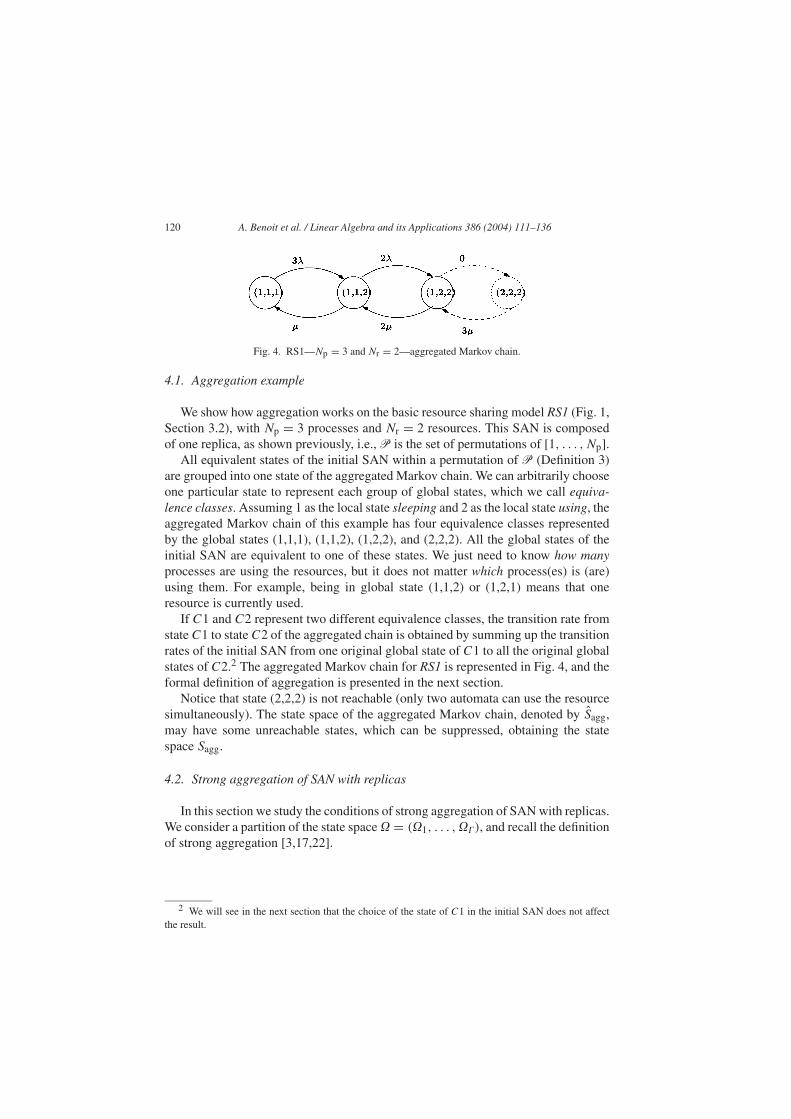
Fig. 4. RS1––Np = 3 and Nr = 2––aggregated Markov chain.

4.1. Aggregation example

We show how aggregation works on the basic resource sharing model RS1 (Fig. 1,Section 3.2), with Np = 3 processes and Nr = 2 resources. This SAN is composedof one replica, as shown previously, i.e., P is the set of permutations of [1, . . . , Np].

All equivalent states of the initial SAN within a permutation of P (Definition 3)are grouped into one state of the aggregated Markov chain. We can arbitrarily chooseone particular state to represent each group of global states, which we call equiva-lence classes. Assuming 1 as the local state sleeping and 2 as the local state using, theaggregated Markov chain of this example has four equivalence classes representedby the global states (1,1,1), (1,1,2), (1,2,2), and (2,2,2). All the global states of theinitial SAN are equivalent to one of these states. We just need to know how manyprocesses are using the resources, but it does not matter which process(es) is (are)using them. For example, being in global state (1,1,2) or (1,2,1) means that oneresource is currently used.

If C1 and C2 represent two different equivalence classes, the transition rate fromstate C1 to state C2 of the aggregated chain is obtained by summing up the transitionrates of the initial SAN from one original global state of C1 to all the original globalstates of C2.2 The aggregated Markov chain for RS1 is represented in Fig. 4, and theformal definition of aggregation is presented in the next section.

Notice that state (2,2,2) is not reachable (only two automata can use the resourcesimultaneously). The state space of the aggregated Markov chain, denoted by Sagg,may have some unreachable states, which can be suppressed, obtaining the statespace Sagg.

4.2. Strong aggregation of SAN with replicas

In this section we study the conditions of strong aggregation of SAN with replicas.We consider a partition of the state space � = (�1, . . . , ��), and recall the definitionof strong aggregation [3,17,22].

2 We will see in the next section that the choice of the state of C1 in the initial SAN does not affectthe result.


Definition 5 (Strong aggregation). A Markov chain can be strongly aggregated onthe partition � if for any initial vector, the aggregated chain (whose states are �γ ,for γ ∈ [1, . . . , �]) is a Markov chain and the transition rates of this chain do notdepend on the initial vector.

Finally, a condition of strong aggregation is given by the following theorem ofRosenblatt. A proof of this theorem can be found in [17].

Theorem 1 (Rosenblatt). Consider a continuous time Markov chain with state space�, and a partition of the state space � = (�1, . . . , ��). If, for all β, γ ∈ [1, . . . , �],the probability of passing from a state x ∈ �β to �γ always has the same value foreach state x from �β, then the Markov chain can be strongly aggregated on thepartition �.

The transition rate from a state �β of the aggregated chain to another state �γ

(β, γ ∈ [1, . . . , �]) is the sum of transition rates in the initial SAN from one stateof �β to all the states of �γ . Due to the condition of Rosenblatt, we can arbitrarilychoose any of the states of �β , and the result will not be affected.

We have seen the conditions needed to aggregate a Markov chain. We now inves-tigate whether a SAN with multiple replicas can be aggregated, and prove that aSAN with multiple replicas can be strongly aggregated. To do this, we first definethe partition of the state space that we want to consider in the theorem of Rosenblatt(Definition 6), then introduce some notation, and finally prove that the condition ofRosenblatt is satisfied for the considered partition (Lemma 1).

Definition 6 (State space partition). Two global states x and y (x, y ∈ S) are equiv-alent if ∃σ ∈ P σ(x) = y. For both global states, there is in each subset the samenumber of automata in a given local state.The partition that we consider is � = (�1, . . . , ��), where each �γ (γ ∈ [1, . . . , �])corresponds to a class of equivalent states.All the states in �γ are equivalent, so we can choose for each �γ one particular staterγ ∈ �γ , called the reference state, and for all other states x ∈ �γ , we can find apermutation τ ∈ P such that τ(x) = rγ .

Notation• If x is a global state of the SAN, x(i) is the local state of A(i), for i = 1, . . . , N .

Notice that if τ ∈ P, then τ(x)(i) = x(τ(i)).• If A is a matrix, i and j two indexes, then aij represents the element of A on row

i and column j . It may be functional, and aij (x) is the function evaluated for theglobal state x.

• The descriptor Q described in Eq. (1) can be decomposed into three parts: Q =L + ∑

e∈ES(P e + Ne) where the matrix L corresponds to the local part of the


descriptor, Pe to the positive synchronization part for event e, and Ne to thenegative synchronization part for event e.

• If x and y are two global states of the SAN, qxy = lxy + ∑e∈ES(pexy + nexy) is

the rate of passing from state x to state y.• If x is a global state of the SAN and γ ∈ [1, . . . , �], then qx�γ is the cumulative

rate of passing from state x to one of the states of �γ : qx�γ = ∑y∈�γ

qxy .

This can also be defined for the matrix L, and for Pe and Ne (where e ∈ ES):lx�γ = ∑

y∈�γlxy , pex�γ = ∑

y∈�γpexy , nex�γ = ∑

y∈�γnexy .

Notice that all states in �γ are equivalent within a permutation of P, so we havelx�γ = ∑

y∈�γlxy = ∑

σ∈P lxσ (rγ ). The same can be written for pe and ne.

Lemma 1. The Rosenblatt condition (Theorem 1) is satisfied for the SAN on the par-tition � = (�1, . . . , ��) (Definition 6). In other words, for all β, γ ∈ [1, . . . , �], theprobability of passing from a state x ∈ �β to �γ always has the same value for eachstate x in �β : ∀x ∈ �β qx�γ = qrβ�γ (where rβ ∈ �β is the reference state of �β).

The proof of this Lemma is in the Appendix. With the application of the Theo-rem 1 (Rosenblatt), the Markov chain underlying the SAN can therefore be stronglyaggregated on the partition �.

The aggregated Markov chain is defined on the set of equivalence classes definedby the permutations of P (Definition 6). These equivalence classes are built fromthe product state space of the initial SAN which may contain unreachable states.As a consequence, some of these equivalence classes may also be unreachable. Letus denote by Sagg this state space of equivalence classes (product state space of theaggregated Markov chain).

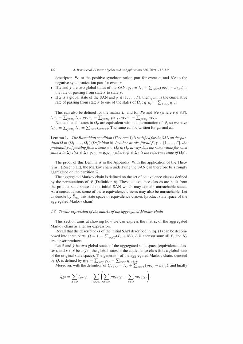
4.3. Tensor expression of the matrix of the aggregated Markov chain

This section aims at showing how we can express the matrix of the aggregatedMarkov chain as a tensor expression.

Recall that the descriptor Q of the initial SAN described in Eq. (1) can be decom-posed into three parts: Q = L + ∑

e∈ES(Pe + Ne). L is a tensor sum; all Pe and Ne

are tensor products.Let x and y be two global states of the aggregated state space (equivalence clas-

ses), and x ∈ x be any of the global states of the equivalence class (it is a global stateof the original state space). The generator of the aggregated Markov chain, denotedby Q, is defined by qxy = ∑

y∈y qxy = ∑σ∈P qxσ(y).

Moreover, with the definition of Q, qxy = lxy + ∑e∈ES(pexy + nexy), and finally

qxy =∑σ∈P

lxσ (y) +∑e∈ES

(∑σ∈P

pexσ(y) +∑σ∈P

nexσ(y)

).


Therefore, the matrix Q can be expressed as a sum of matrices: Q = L+∑e∈ES(Pe +

Ne), where, for each global state x and y, and for a = l, a = pe or a = ne (e ∈ ES),

axy =∑σ∈P

axσ(y).

Now we consider a lumped version of each matrix A (A can be any of the matrixL, Pe and Ne, where e ∈ ES), denoted by A. This lumped matrix (defined in thefollowing) is a tensor expression, obtained by the aggregation of each subset of rep-licated automaton. The equivalent SAN obtained is not defined there, we work onlyon the matrix expression of this SAN.

We want to prove that Q = L + ∑e∈ES(Pe + Ne), where Q is the matrix of the

aggregated Markov chain. So, we will have a tensor expression of Q.To prove this, we work on each term a, where a can be l, pe or ne (e ∈ ES), and

we show that axy = axy .We consider first the tensor products Pe and Ne, for e ∈ ES. Then we explore the

case of the tensor sum L.

• Let A be one of the tensor products Pe or Ne, e ∈ ES: A =N⊗

gi=1

Q(i).

Let x and y be two global states. With the definition of generalized tensor product,we haveaxy = ∏N

i=1 q(i)

x(i)y(i) (x). So axy = ∑σ∈P axσ(y) = ∑

σ∈P∏N

i=1 q(i)

x(i)σ (y(i))(x).

Recall that σ can be expressed as a combination σ = (σ1, . . . , σK) (Definition 3).So we have

axy =∑

σ1∈P1

, . . . ,∑

σK∈PK

N∏i=1

q(i)

x(i)σ (y(i))(x).

If we decompose the product into subsets, we can replace in the product term, σ

by the corresponding σh, where h ∈ [1, . . . , K], and factorize the independent terms:

axy =K∏

h=1

∑

σh∈Ph

∏i∈SIh

q(i)

x(i)σh(y(i))(x)

. (3)

Then let us define the lumped matrix A.

Definition 7. Let us consider a SAN with N automata and a partition G (Defini-tion 2). Then, let A be one of the tensor products of the generator of the SAN, A =N⊗

gi=1

Q(i).

The lumped matrix A is defined as a tensor product of K matrices:

A =⊗

gh∈[1,...,K]

Ah,


where Ah, h ∈ [1, . . . , K], is defined by

ahxhyh

(x) =∑

σh∈Ph

∏i∈SIh

q(i)

x(i)σh(y(i))(x).

Recall that x = (x1, . . . , xK) = (x(1), . . . , x(N)).Then we have

axy =K∏

h=1

ahxhyh

(x) =K∏

h=1

∑σh∈Ph

∏i∈SIh

q(i)

x(i)σh(y(i))(x). (4)

Due to the properties of the functions, when we evaluate them with all x ∈ x, wealways have the same result, so formula (3) and (4) are equal, which prove the resultaxy = axy .

• Now, let A be the tensor sum L: A =N⊕

gi=1

Q(i).

Let x and y be two global states. With the definition of generalized tensor sum,we have

axy = ∑Ni=1 q

(i)

x(i)y(i) (x)�(x(i),y(i)), where3 �(x(i),y(i)) = ∏j=1,...,N,j /=i δx(j)y(j) .

So axy = ∑σ∈P axσ(y) = ∑

σ∈P∑N

i=1 q(i)

x(i)σ (y(i))(x)�(x(i),σ (y(i))).

Notice that the only σ = (σ1, . . . , σK) giving a non-zero result for �(x(i),σ (y(i)))

are such that only one of the σh, h = 1, . . . , K , is not the identity (denoted by id).Let σh = (id, . . . , σh, . . . , id) be such a permutation. Then we have:

axy =K∑

h=1

∑

σh∈Ph

N∑i=1

q(i)

x(i)σh(y(i))(x)�(x(i),σh(y(i)))

.

�(x(i),σh(y(i))) can be non-null only for i ∈ SIh, so finally,

axy =K∑

h=1

∑

σh∈Ph

∑i∈SIh

q(i)

x(i)σh(y(i))(x)�(x(i),σh(y(i)))

. (5)

Then let us define the lumped matrix A.

Definition 8. Let us consider a SAN with N automata and a partition G (Defini-tion 2). Then, let A be the tensor sum of the generator of the SAN,

A =N⊕

gi=1

Q(i).

3 δuv = 1 if u = v, and 0 otherwise.


The lumped matrix A is defined as a tensor sum of K matrices:

A =⊕

gh∈[1,...,K]

Ah,

where Ah, h ∈ [1, . . . , K], is defined by

ahxhyh

(x) =∑

σh∈Ph

∑i∈SIh

q(i)

x(i)σh(y(i))(x)�h

(x(i),σh(y(i)))

and �h(x(i),y(i))

= ∏j∈SIh,j /=i δx(j)y(j) .

Then we have

axy =K∑

h=1

ahxhyh

(x)

=K∑

h=1

∑

σh∈Ph

∑i∈SIh

q(i)

x(i)σh(y(i))(x)�h

(x(i),σh(y(i)))

∏

k∈[1,...,K],k /=h

δxkyk. (6)

In Eq. (6), the product∏

k∈[1,...,K],k /=h δxkykmultiplied by the �h

(x(i),σh(y(i)))is

equivalent to the �(x(i),σh(y(i))) defined for Eq. (5).The two formula are therefore identical, and axy = axy .

Tensor expression of Q

We have proved that Q = L + ∑e∈ES(Pe + Ne), and with the expression of the

different lumped matrix, we have

Q =⊕

gh∈[1,...,K]

Lh +∑e∈ES

⊗

gh∈[1,...,K]

Peh +

⊗g

h∈[1,...,K]Ne

h

and all the matrices Ah have been defined above (Definitions 7 and 8).Thus, we obtain a compact representation of the aggregated Markov chain, as if

each subset has been aggregated in an independent way.

5. The benefits of aggregation

We have seen that we can strongly aggregate a SAN with multiple replicas, butwe still need to see what benefits it brings in order to justify this aggregation. Wepresent at first some theoretical results, then we show the benefits of aggregation onpractical examples.


5.1. Theoretical results

Consider a SAN composed of one replica with N automata, and let M be the num-ber of states per automaton (it is the same for all automata because of the replication).The total number of states of the SAN is then MN . We wish to calculate the numberof states of the reduced Markov chain. Notice that we do not take unreachable statesinto account, and some states of the aggregated Markov chain can be removed (asseen in the examples).

For a given global state of the initial SAN, let us denote by nam (m ∈ [1, . . . , M])the number of automata that are in state m. the number of integer solutions of theequation

∑Mm=1 nam = N , which is [18](

N + M − 1

M − 1

)= (N + M − 1)!

N !(M − 1)! .

Aggregation is beneficial only when there are several automata. For example, if weaggregate a SAN with N = 2 and M = 5, we have initially 52 = 25 states and we ob-tain 15 states after aggregation. For large values of N , it becomes much more interest-ing. For example, when N = 100 and M = 5, we obtain an order of 4.6 million statesafter aggregation, instead of the 5100 ≈ 1070 initial states. If we have N automata with2 states each, we have initially 2N states, and only N + 1 after aggregation.

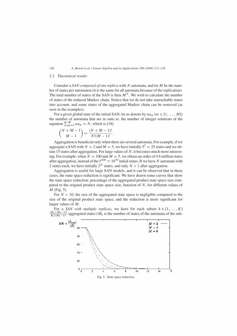
Aggregation is useful for large SAN models, and it can be observed that in thesecases, the state space reduction is significant. We have drawn some curves that showthe state space reduction: percentage of the aggregated product state space size com-pared to the original product state space size, function of N , for different values ofM (Fig. 5).

For N > 10, the size of the aggregated state space is negligible compared to thesize of the original product state space, and the reduction is more significant forlarger values of M .

For a SAN with multiple replicas, we have for each subset h ∈ [1, . . . , K](Rh+Mh−1)!Rh!(Mh−1)! aggregated states (Mh is the number of states of the automata of the sub-

Fig. 5. State space reduction.


Fig. 6. RS1––aggregated Markov chain.

set h, and Rh the number of replicas), what makes a total of∏K

h=1(Rh+Mh−1)!Rh!(Mh−1)! states.

For example, if we have 2 subsets of R automaton, each having 2 states, and K

other subsets containing only one automaton with M states each, we have initially2R × 2R × MK states, and only (R + 1) × (R + 1) × MK states after aggregation.

5.2. Numerical results

This section aims at showing the practical benefits of aggregation through a fewexamples. At first, we introduce some examples, and then we summarize the results.

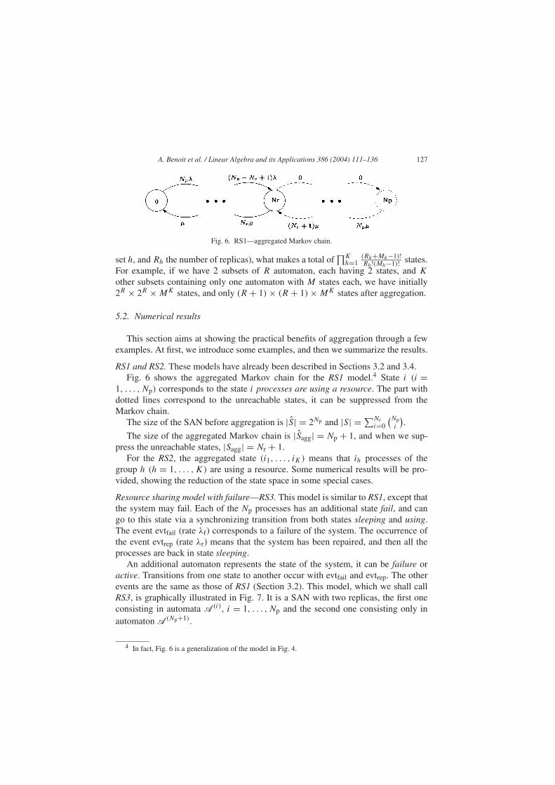
RS1 and RS2. These models have already been described in Sections 3.2 and 3.4.Fig. 6 shows the aggregated Markov chain for the RS1 model.4 State i (i =

1, . . . , Np) corresponds to the state i processes are using a resource. The part withdotted lines correspond to the unreachable states, it can be suppressed from theMarkov chain.

The size of the SAN before aggregation is |S| = 2Np and |S| = ∑Nri=0

(Npi

).

The size of the aggregated Markov chain is |Sagg| = Np + 1, and when we sup-press the unreachable states, |Sagg| = Nr + 1.

For the RS2, the aggregated state (i1, . . . , iK) means that ih processes of thegroup h (h = 1, . . . , K) are using a resource. Some numerical results will be pro-vided, showing the reduction of the state space in some special cases.

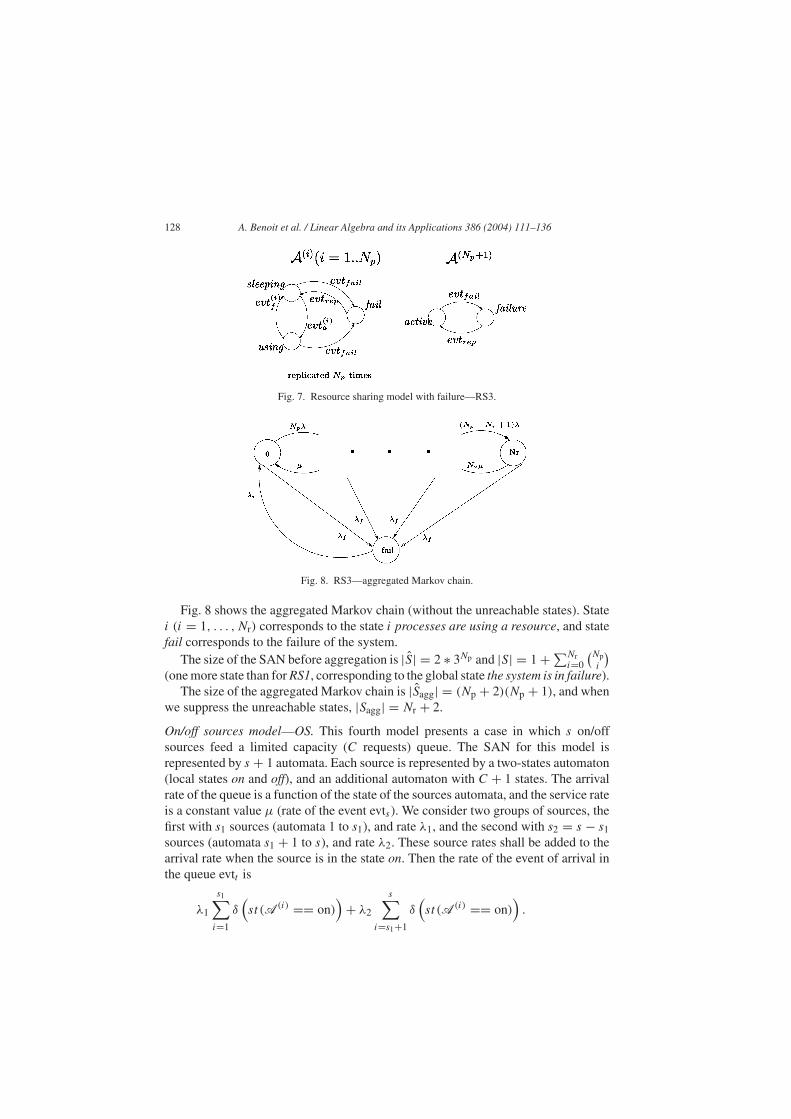
Resource sharing model with failure––RS3. This model is similar to RS1, except thatthe system may fail. Each of the Np processes has an additional state fail, and cango to this state via a synchronizing transition from both states sleeping and using.The event evtfail (rate λf) corresponds to a failure of the system. The occurrence ofthe event evtrep (rate λr) means that the system has been repaired, and then all theprocesses are back in state sleeping.

An additional automaton represents the state of the system, it can be failure oractive. Transitions from one state to another occur with evtfail and evtrep. The otherevents are the same as those of RS1 (Section 3.2). This model, which we shall callRS3, is graphically illustrated in Fig. 7. It is a SAN with two replicas, the first oneconsisting in automata A(i), i = 1, . . . , Np and the second one consisting only inautomaton A(Np+1).

4 In fact, Fig. 6 is a generalization of the model in Fig. 4.


Fig. 7. Resource sharing model with failure––RS3.

Fig. 8. RS3––aggregated Markov chain.

Fig. 8 shows the aggregated Markov chain (without the unreachable states). Statei (i = 1, . . . , Nr) corresponds to the state i processes are using a resource, and statefail corresponds to the failure of the system.

The size of the SAN before aggregation is |S| = 2 ∗ 3Np and |S| = 1 + ∑Nri=0

(Npi

)(one more state than for RS1, corresponding to the global state the system is in failure).

The size of the aggregated Markov chain is |Sagg| = (Np + 2)(Np + 1), and whenwe suppress the unreachable states, |Sagg| = Nr + 2.

On/off sources model––OS. This fourth model presents a case in which s on/offsources feed a limited capacity (C requests) queue. The SAN for this model isrepresented by s + 1 automata. Each source is represented by a two-states automaton(local states on and off), and an additional automaton with C + 1 states. The arrivalrate of the queue is a function of the state of the sources automata, and the service rateis a constant value µ (rate of the event evts). We consider two groups of sources, thefirst with s1 sources (automata 1 to s1), and rate λ1, and the second with s2 = s − s1sources (automata s1 + 1 to s), and rate λ2. These source rates shall be added to thearrival rate when the source is in the state on. Then the rate of the event of arrival inthe queue evtt is

λ1

s1∑i=1

δ(st (A(i) == on)

)+ λ2

s∑i=s1+1

δ(st (A(i) == on)

).


Fig. 9. On/off sources model––OS.

Fig. 9 illustrates this SAN model. The events evt(i)a and evt(i)f have constant rates,depending only of the type of source (group 1 or group 2).

This model has three subsets (K = 3), and the first and second subsets can beaggregated. The first subset aggregation results in an automaton with s1 + 1 states,and the second subset aggregation results in an automaton with s2 + 1 states. Thereduced state space is then |Sagg| = (s1 + 1) × (s2 + 1) × (C + 1), instead of theoriginal state space |S| = 2s × (C + 1).

Cluster with Bus Communication––CB. This fifth model represents a cluster with Npprocessing nodes with a simple behavior:

• each node i alternates from idle (Id(i)) to processing (Pr(i)) state;• being in the idle state a node can pass to transmission (T x(i)) state if no other

node is already transmitting; or it can pass to reception (Rx(i)) state if there isanother node transmitting;

• after transmitting or receiving each node returns to idle state regardless of thestate of the other nodes.5

Such model could be seen as a simple description of UDP protocol over a sharedbus, or other communication protocol in which there is no need of commitmentbetween send/receive connections. Despite the application of such model, our inter-est in this paper is the description of a SAN with Np automata with four states each.This replicated automata model is represented in Fig. 10. All events in this SAN arelocal, but events l

(i)3 and l

(i)5 must be defined with functional rates (the other events

have constant rates), respectively:

5 According to such behavior it is not necessary to synchronize nor the beginning, neither the end oftransmissions.


Fig. 10. Cluster with bus communication replicated automaton––CB.

•(∑Np

i=1 δ(st (A(i) == T x(i))))

= 1 in order to grant access to reception state if

there is one node transmitting; and

•(∑Np

i=1 δ(st (A(i) == T x(i))))

= 0 in order to grant access to transmission state

if no node is already transmitting.

When all nodes have the same rates this model is a SAN composed of one replica.Only the global states in which only one node, at most, is transmitting are reachable,i.e.:

reachability = Np∑

i=1

δ(st (A(i) == T x(i)))

� 1.

Numerical results. We present here some numerical results obtained with thesoftware package PEPS [1] aggregating and solving the presented examples. Theaggregation of replicas was automatically performed by PEPS using the model spec-ification information (see Section 3.5), and the lumped SAN models were stored inthe tensor format (see Section 4.3). The computer used to run the examples was anIBM-PC running Linux OS (Mandrake distribution, version 8.0), with 1.5 Gbytesof RAM and with 2.0 GHz Pentium IV processor. The indicated processing timesdo not take system time into account, i.e., they refer only to the user time spent toperform one iteration,6 in order to compute the steady-state probabilities.7 A timeof 0 s means that the time is negligible (less than 10−4 s). An indication – means

6 The number of iterations may vary according to the chosen numerical input parameters. However,the time to perform one iteration is not affected by the choice of numerical parameters. The solutionmethod used to compute results was power iteration, but the other methods available in PEPS (Arnoldi andGMRES) have a quite similar time costs per iteration that depends on the cost of one vector-descriptionmultiplication [12].

7 The technique presented in this paper is probably also useful for transient analysis. However, ourinterest here is limited to stationary solution, since this is the only solution formally defined for SANmodels and implemented in the PEPS software tool.


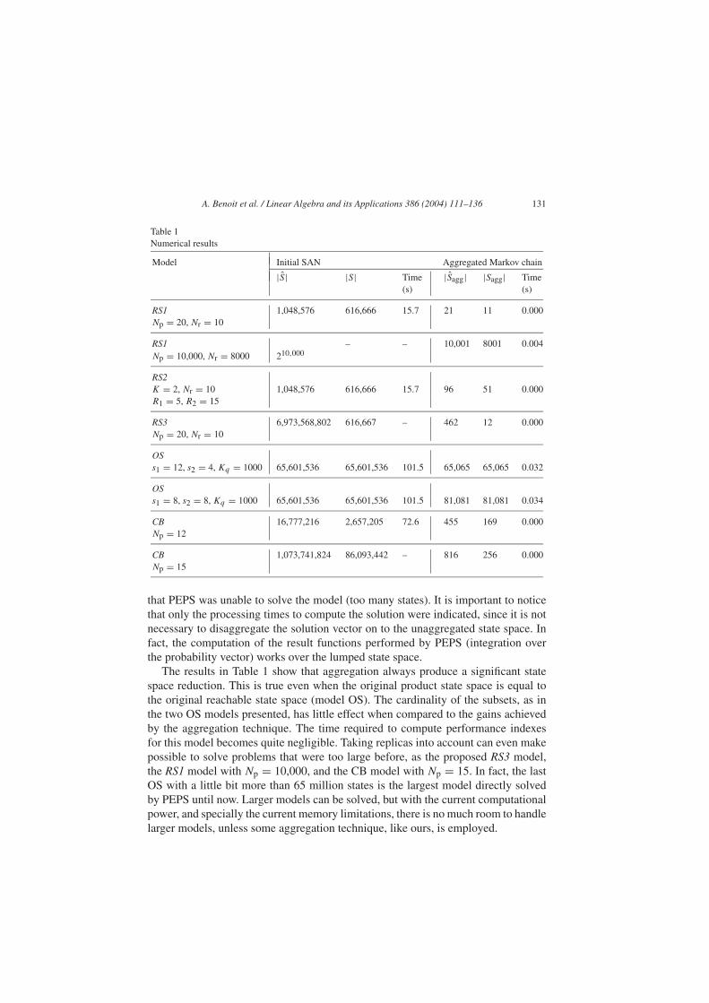
Table 1Numerical results

Model Initial SAN Aggregated Markov chain

|S| |S| Time |Sagg| |Sagg| Time(s) (s)

RS1 1,048,576 616,666 15.7 21 11 0.000Np = 20, Nr = 10

RS1 – – 10,001 8001 0.004Np = 10,000, Nr = 8000 210,000

RS2K = 2, Nr = 10 1,048,576 616,666 15.7 96 51 0.000R1 = 5, R2 = 15

RS3 6,973,568,802 616,667 – 462 12 0.000Np = 20, Nr = 10

OSs1 = 12, s2 = 4, Kq = 1000 65,601,536 65,601,536 101.5 65,065 65,065 0.032

OSs1 = 8, s2 = 8, Kq = 1000 65,601,536 65,601,536 101.5 81,081 81,081 0.034

CB 16,777,216 2,657,205 72.6 455 169 0.000Np = 12

CB 1,073,741,824 86,093,442 – 816 256 0.000Np = 15

that PEPS was unable to solve the model (too many states). It is important to noticethat only the processing times to compute the solution were indicated, since it is notnecessary to disaggregate the solution vector on to the unaggregated state space. Infact, the computation of the result functions performed by PEPS (integration overthe probability vector) works over the lumped state space.

The results in Table 1 show that aggregation always produce a significant statespace reduction. This is true even when the original product state space is equal tothe original reachable state space (model OS). The cardinality of the subsets, as inthe two OS models presented, has little effect when compared to the gains achievedby the aggregation technique. The time required to compute performance indexesfor this model becomes quite negligible. Taking replicas into account can even makepossible to solve problems that were too large before, as the proposed RS3 model,the RS1 model with Np = 10,000, and the CB model with Np = 15. In fact, the lastOS with a little bit more than 65 million states is the largest model directly solvedby PEPS until now. Larger models can be solved, but with the current computationalpower, and specially the current memory limitations, there is no much room to handlelarger models, unless some aggregation technique, like ours, is employed.


6. Conclusions

In this paper, we have defined SAN models with replicas, and have exposed a tech-nique to aggregate such models. We proved a theorem showing how strong aggrega-tion can be performed, and how the matrix of the aggregated Markov chain can beexpressed as a tensor expression. The theoretical benefits of such an aggregation arealso presented and verified by the numerical achievements of the implementation inthe PEPS software tool.

It can be shown that a SAN with replicas is also exactly lumpable over the samepartition [2]. The proof is very similar to the proof of Lemma 1 (Section 4). Thisproperty (exactly lumpable) allows to compute the probabilities of the initial modelknowing the probabilities of the aggregated system.

Notice that the subsets of replicated automata have to be defined at the high levelspecification. This is often a fake problem since the replicas are usually known whenmodeling a particular system.

The implementation of the automatic generation of the aggregated Markov Chainin PEPS proved the efficiency of the proposed technique. The implemented algorithmgenerates the tensor expression of the matrix very quickly (much faster than the timespent by one single iteration). The resulting tensor expression is usually much morecompact, so we can compute the numerical solution with an impressive reduction ofCPU costs.

In this paper, we work only on the matrices describing such SAN to prove thatthe matrix of the aggregated Markov chain can be expressed as a tensor expres-sion. We could as future work define formally an equivalent SAN resulting from theaggregation of each subset.

Finally, we plan to work on applications, e.g., communication protocols, to exper-iment those new techniques on real and large systems with a significant numberof replicas. Many models in communication could not be solved by SAN due tothe limitation of the product state space size, but we do believe that the proposedtechnique can boost the use of SAN to such practical cases.

Acknowledgements

The authors wish to thank Cyril Guilloud for his preliminary work on SAN aggre-gation.

Appendix: Proof of Lemma 1

To prove Lemma 1, we decompose the problem into two parts, correspondingrespectively to the local part of the descriptor (Lemma 2) and the synchronizing part(Lemma 3).


Lemma 2. For all β, γ ∈ [1, . . . , �], the probability of passing from a state x ∈ �β

to �γ with a local transition always has the same value for each state x in �β :∀x ∈ �β lx�γ = lrβ�γ .

• Proof of Lemma 2Let β, γ ∈ [1, . . . , �], x ∈ �β and let τ ∈ P be the permutation such that x =

τ(rβ).With the definition of a generalized tensor sum [10,26], for y ∈ �γ , we have

lxy =N∑

i=1

q

(i)

l x(i)y(i) (x)

N∏j=1,j /=i

δx(j)y(j)

,

where Q(i)l is the local transition matrix of automaton A(i), and δuv = 1 if u = v,

and 0 otherwise.In order to simplify the notation, let us define �x(i)y(i) = ∏N

j=1,j /=i δx(j)y(j) . Thenwe have

lx�γ =∑y∈�γ

lxy =∑σ∈P

lxσ (rγ ) =∑σ∈P

N∑i=1

q(i)

l x(i)rγ (σ(i)) (x) �x(i)rγ (σ(i)) .

Moreover, we have x = τ(rβ), so

lx�γ =∑σ∈P

N∑i=1

q(i)

l rβ(τ(i)) rγ (σ(i)) (τ (rβ)) �rβ(τ(i)) rγ (σ(i)) .

Now decompose the equation for each subset of the SAN. Recall that the matricesof a subset h ∈ [1, . . . , K] are all identical to Q(l,h). Moreover, for σ ∈ P, let ϕ ∈ Pbe the permutation ϕ = σ ◦ τ−1. Then σ = ϕ ◦ τ and when σ goes through P, ϕ

does the same (in a different order). Because of the commutativity of the sum, wecan replace

∑σ∈P with

∑ϕ∈P. Then we have:

lx�γ =∑ϕ∈P

K∑h=1

∑i∈SIh

q(l,h) rβ(τ(i)) rγ (ϕ◦τ(i)) (τ (rβ)) �rβ(τ(i)) rγ (ϕ◦τ(i)) .

The functions are not changed by a permutation of P, and τ ∈ P, so we canreplace τ(rβ) by rβ in the above equation. Moreover, for each subset h, when i goesthrough SIh, τ(i) does the same but in a different order (it is a permutation inside thesubset). Because of the commutativity of a sum, we can change the order and replaceτ(i) by i in the equation:

lx�γ =∑ϕ∈P

K∑h=1

∑i∈SIh

q(l,h) rβ(i) rγ (ϕ(i)) (rβ) �rβ(i) rγ (ϕ(i))

=∑ϕ∈P

N∑i=1

q(i)

l rβ(i) rγ (ϕ(i)) (rβ) �rβ(i) rγ (ϕ(i)) .

Finally, lx�γ = ∑ϕ∈P lrβ ϕ(rγ ) = lrβ �γ . �


Lemma 3. For all β, γ ∈ [1, . . . , �], the probability of passing from a state x ∈�β to �γ with a synchronizing transition always has the same value for each state x

in �β : ∀x ∈ �β

∑e∈ES(pex�γ + nex�γ ) = ∑

e∈ES(perβ�γ + nerβ�γ ).

• Proof of Lemma 3Let e ∈ ES, β, γ ∈ [1, . . . , �], x ∈ �β and let τ ∈ P be the permutation such

that x = τ(rβ). We prove first that pex�γ = perβ�γ . The proof for ne is similar.With the definition of a generalized tensor product [10,26], for y ∈ �γ , we have

pexy = ∏Ni=1 q

(i)

e+ x(i)y(i) (x), where Q(i)e+ is the positive synchronization transition

matrix of automaton A(i).Moreover, x = τ(rβ), so we have

pex�γ =∑y∈�γ

pexy =∑σ∈P

pexσ(rγ ) =∑σ∈P

N∏i=1

q(i)

e+ rβ(τ(i)) rγ (σ(i)) (τ (rβ)).

Now decompose the equation for each subset of the SAN. Recall that almost allthe matrices are identical inside a subset g ∈ [1, . . . , K]; we denote them by Q(e+,g).There is only one particular matrix in one of the subsets equal to feQ(e+,g), wherefe is the transition rate of the event (definition of SAN models with replicas).

For σ ∈ P, let ϕ ∈ P be the permutation ϕ = σ ◦ τ−1. Then σ = ϕ ◦ τ and whenσ goes through P, ϕ does the same (in a different order). Because of the commuta-tivity of the sum, we can replace

∑σ∈P with

∑ϕ∈P. Then we have:

pex�γ =∑ϕ∈P

K∏h=1

fe(τ (rβ))

∏i∈SIh

q(e+,h) rβ(τ(i)) rγ (ϕ◦τ(i)) (τ (rβ))

.

The functions are not changed by a permutation of P, and τ ∈ P, so we canreplace τ(rβ) by rβ in the above equation. Moreover, for each subset h, when i goesthrough SIh, τ(i) does the same but in a different order (it is a permutation insidethe subset). Because of the commutativity of a product, we can change the order andreplace τ(i) by i in the equation:

pex�γ =∑ϕ∈P

K∏h=1

fe(rβ)

∏i∈SIh

q(e+,h) rβ(i) rγ (ϕ(i)) (rβ)

=∑ϕ∈P

N∏i=1

q(i)

e+ rβ(i) rγ (ϕ(i)) (rβ).

Finally, pex�γ = ∑ϕ∈P perβ ϕ(rγ ) = perβ �γ .

In a similar way, we can prove that nex�γ = nerβ �γ . This is true for all events e ∈ES, so we finally have

∑e∈ES(pex�γ + nex�γ ) = ∑

e∈ES(perβ�γ + nerβ�γ ). �


• Proof of Lemma 1Let β, γ ∈ [1, . . . , �], x ∈ �β and let τ ∈ P be the permutation such that x =

τ(rβ).With the decomposition of Q, we have

qx�γ =∑y∈�γ

qxy =∑y∈�γ

(lxy +

∑e∈ES

(pexy + nexy)

)

=∑y∈�γ

lxy +∑e∈ES

∑

y∈�γ

pexy +∑y∈�γ

nexy

= lx�γ +∑e∈ES

(pex�γ + nex�γ ).

With the application of Lemmas 2 and 3, we finally have

qx�γ = lrβ�γ +∑e∈ES

(perβ�γ + nerβ�γ ) = qrβ�γ . �

References

[1] A. Benoit, L. Brenner, P. Fernandes, B. Plateau, W. J. Stewart, The PEPS software tool, in: P. Kem-per, W.H. Sanders (Eds.), 13th International Conference on Modelling Techniques and Tools forComputer Performance Evaluation, LNCS, Urbana-Champaign, Illinois, USA, 2003.

[2] P. Buchholz, Exact and ordinary lumpability in finite Markov chains, J. Appl. Prob. 31 (1994) 59–75.[3] P. Buchholz, Equivalence relations for stochastic automata networks, in: Proc. 2nd Int. Workshop

on the Numerical Solution of Markov Chains, Kluwer, Boston, Masachussetts, 1995.[4] P. Buchholz, An aggregation–disaggregation algorithm for stochastic automata networks, Prob. Eng.

Inf. Sci. 11 (1997) 229–253.[5] P. Buchholz, An adaptative aggregation–disaggregation algorithm for hierarchical Markovian mod-

els, Euro. J. Oper. Res. 116 (1999) 545–564.[6] P. Buchholz, Exact performance equivalence––an equivalence relation for stochastic automata,

Theor. Comput. Sci. 215 (1/2) (1999) 239–261.[7] J. Campos, M. Silva, S. Donatelli, Structured solution of stochastic DSSP systems, in: Proc. 7th Int.

Workshop on Petri Nets and Performance Models (PNPM’97), Saint Malo, France, IEEE Comp.Soc. Press, June 1997, pp. 91–100.

[8] S. Donatelli, Superposed stochastic automata: a class of stochastic Petri nets with parallel solutionand distributed state space, Perform. Evaluat. 18 (1) (1993) 21–36.

[9] S. Donatelli, Superposed generalized stochastic Petri nets: definition and efficient solution, in: R.Valette (Ed.), 15th International Conference on Application and Theory of Petri Nets, LNCS 815,Zaragoza, Spain, 1994, pp. 258–277.

[10] P. Fernandes, Méthodes Numériques pour la Solution de Systémes Markoviens à Grand Espaced’États, PhD thesis, Institut National Polytechnique de Grenoble, France, 1998.

[11] P. Fernandes, B. Plateau, W.J. Stewart, Efficient descriptor-vector multiplications in stochastic auto-mata networks, JACM 45 (3) (1998) 381–414.

[12] P. Fernandes, B. Plateau, W.J. Stewart, Optimizing tensor product computations in stochastic auto-mata networks, RAIRO, Oper. Res. 32 (3) (1998) 325–351.


[13] O. Gusak, T. Dayar, J.-M. Fourneau, Stochastic automata networks and near complete decompos-ability, SIAM J. Matrix Anal. Appl. 23 (2001) 581–599.

[14] O. Gusak, T. Dayar, J.-M. Fourneau, Lumpable continuous-time stochastic automata networks,Euro. J. Oper. Res. 148 (2003) 436–451.

[15] O. Gusak, T. Dayar, J.-M. Fourneau, Iterative disaggregation for a class of lumpable discrete-timestochastic automata networks, Perform. Evaluat. 53 (2003) 43–69.

[16] H. Hermanns, M. Ribaudo, Exploiting symmetries in stochastic process algebras, in: Proc. of 12thEuropean Simulation Multiconference, Manchester, UK, 1998.

[17] J.G. Kemeny, J.L. Snell, Finite Markov Chains, Van Nostrand Reinhold, New York, 1960.[18] D.E. Knuth, The Art of Computer Programming, Volume 1 (Fundamental Algorithms), Addi-

son-Wesley, 1967.[19] J. Ledoux, Weak lumpability of finite Markov chains and positive invariance of cones, Technical

report, Rapport de recherche INRIA n. 2801, France, 1996.[20] A.S. Miner, G. Ciardo, S. Donatelli, Using the exact state space of a Markov model to compute

approximate stationary measures, Measure. Model. Comput. Syst. (2000) 207–216.[21] B. Plateau, On the stochastic structure of parallelism and synchronization models for distributed

algorithms, in: Proc. ACM Sigmetrics Conference on Measurement and Modelling of ComputerSystems, Austin, Texas, August 1985.

[22] M. Rosenblatt, Functions of a Markov process that are Markovian, J. Math. Mech. 8 (4) (1959)585–596.

[23] W.H. Sanders, J.F. Meyer, Reduced base model construction methods for stochastic activity net-works, IEEE J. Select. Areas Commun. 9 (1) (1991) 25–36.

[24] M. Siegle, Structured Markovian performance modelling with automatic symmetry exploitation, in:Proc. 11th Conf. Computer Performance Evaluation: Modelling Techniques and Tools, LNCS 794,1994.

[25] M. Siegle, Using structured modelling for efficient performance prediction of parallel systems,in: G.R. Joubert et al. (Eds.), Parallel Computing: Trends and Applications, NorthHolland, 1994,pp. 453–460.

[26] W.J. Stewart, Introduction to the Numerical Solution of Markov Chains, Princeton University Press,Princeton, 1994.

Aggregation of stochastic automata networks with replicas

Documents

Transcript of Aggregation of stochastic automata networks with replicas