Advanced solutions for neonatal sleep analysis and the effects ...
248
ARENBERG DOCTORAL SCHOOL Faculty of Engineering Science Advanced solutions for neonatal sleep analysis and the effects of maturation Ofelie De Wel Dissertation presented in partial fulfillment of the requirements for the degree of Doctor of Engineering Science (PhD): Electrical Engineering February 2020 Supervisor: Prof. dr. ir. S. Van Huffel Co-supervisor: Prof. dr. G. Naulaers
-
Upload
khangminh22 -
Category
Documents
-
view
1 -
download
0
Transcript of Advanced solutions for neonatal sleep analysis and the effects ...

ARENBERG DOCTORAL SCHOOLFaculty of Engineering Science
Advanced solutions forneonatal sleep analysis andthe effects of maturation
Ofelie De Wel
Dissertation presented in partialfulfillment of the requirements for the
degree of Doctor of EngineeringScience (PhD): Electrical Engineering
February 2020
Supervisor:Prof. dr. ir. S. Van HuffelCo-supervisor:Prof. dr. G. Naulaers


Advanced solutions for neonatal sleep analysis andthe effects of maturation
Ofelie DE WEL
Examination committee:Prof. dr. ir. H. Hens, chairProf. dr. ir. S. Van Huffel, supervisorProf. dr. G. Naulaers, co-supervisorProf. dr. ir. L. De LathauwerProf. dr. ir. M. De VosProf. dr. K. JansenProf. dr. ir. B. PuersProf. dr. ir. J. SuykensProf. dr. J. Dudink(University Medical Center Utrecht)
Dissertation presented in partialfulfillment of the requirements forthe degree of Doctor of EngineeringScience (PhD): Electrical Engineer-ing
February 2020

© 2020 KU Leuven – Faculty of Engineering ScienceUitgegeven in eigen beheer, Ofelie De Wel, Kasteelpark Arenberg 10 box 2446, B-3001 Leuven (Belgium)
Alle rechten voorbehouden. Niets uit deze uitgave mag worden vermenigvuldigd en/of openbaar gemaakt wordendoor middel van druk, fotokopie, microfilm, elektronisch of op welke andere wijze ook zonder voorafgaandeschriftelijke toestemming van de uitgever.
All rights reserved. No part of the publication may be reproduced in any form by print, photoprint, microfilm,electronic or any other means without written permission from the publisher.

Abstract
Worldwide approximately 11% of the babies are born before 37 weeks ofgestation. The survival rates of these prematurely born infants have steadilyincreased during the last decades as a result of the technical and medical progressin the neonatal intensive care units (NICUs). The focus of the NICUs hastherefore gradually evolved from increasing life chances to improving quality oflife. In this respect, promoting and supporting optimal brain development iscrucial. Because these neonates are born during a period of rapid growth anddevelopment of the brain, they are susceptible to brain damage and thereforevulnerable to adverse neurodevelopmental outcome. In order to identify patientsat risk of long-term disabilities, close monitoring of the neurological functionduring the first critical weeks is a primary concern in the current NICUs.Electroencephalography (EEG) is a valuable tool for continuous noninvasivebrain monitoring at the bedside. The brain waves and patterns in theneonatal EEG provide interesting information about the newborn brain function.However, visual interpretation is a time-consuming and tedious task requiringexpert knowledge. This indicates a need for automated analysis of the neonatalEEG characteristics. The work presented in this thesis aims at contributing tothis.
The first part of this thesis focuses on the development of algorithms toautomatically classify sleep stages in preterm babies. In total three differentstrategies are proposed. In the first method, the problem is traditionallyapproached and a new set of EEG complexity features is combined with aclassification algorithm. This analysis demonstrates that the complexity ofthe EEG signal is fundamentally different dependent on the vigilance stateof the infant. Building on this finding, a novel tensor-based approach thatdetects quiet sleep in an unsupervised manner is presented. Finally, a deepconvolutional neural network to classify neonatal sleep stages is implemented.This end-to-end model optimizes the feature extraction and classification modelsimultaneously, avoiding the challenging task of feature engineering.
i

ii ABSTRACT
The second part concentrates on the quantification of functional brainmaturation in preterm infants. We establish that the complexity of the EEGtime series is significantly positively correlated with the postmenstrual ageof the neonate. Moreover, these promising biomarkers of brain maturity areused to develop a brain-age model. This model can accurately estimate theinfant’s age and thereby assess the functional brain maturation. In addition, therelationship between the early functional and structural brain development isinvestigated based on two complementary neuromonitoring modalities, EEG andMRI. Regression models show that the brain activity during the first postnataldays is related to the size and growth of the cerebellum in the subsequent weeks.At last, the influence of the thyroid function on the developing brain is examinedin extremely premature infants. No significant association was observed betweenthe change in free thyroxine concentrations during the first week of life andmaturational features extracted from the EEG at term equivalent age. Toshed more light on the precise relationship between thyroid function and brainmaturation, prospective studies with a more homogeneous dataset are neededin the future.

Beknopte samenvatting
Wereldwijd wordt ongeveer 11% van de baby’s vóór 37 weken zwangerschapgeboren. De overlevingskansen van deze premature baby’s zijn de laatstedecennia gestaag toegenomen als gevolg van de technische en medischevooruitgang op de dienst neonatale intensieve zorgen (NIC). De focus vande medische zorg bij vroeggeboren kinderen is daarom geleidelijk geëvolueerdvan het verhogen van levenskansen naar het verbeteren van de levenskwaliteit. Indit opzicht is het bevorderen en ondersteunen van optimale hersenontwikkelingvan cruciaal belang. Omdat deze baby’s geboren worden tijdens een periode vansnelle groei en ontwikkeling van de hersenen, zijn ze gevoelig voor hersenletsels enbijgevolg kwetsbaar voor neurologische ontwikkelingsachterstand. Om patiëntenmet verhoogd risico op beperkingen te identificeren, is nauwgezet toezicht opde neurologische functie tijdens de eerste kritieke weken van primair belang inde huidige NICs.Elektro-encefalografie (EEG) is een nuttig instrument voor continue niet-invasieve hersenmonitoring tijdens het verblijf in de couveuse. De hersengolvenen patronen in het neonatale EEG verschaffen interessante informatie over dehersenfunctie van pasgeborenen. Visuele interpretatie is echter een tijdrovendeen eentonige taak die bovendien kennis van experts vereist. Er is dus behoefteaan geautomatiseerde analyse van de neonatale EEG kenmerken. Het werk datin dit proefschrift wordt gepresenteerd wil hiertoe bijdragen.
Het eerste deel van deze thesis richt zich op de ontwikkeling van algoritmes omslaapstadia bij premature baby’s automatisch te classificeren. Drie verschillendemethodes worden uitgewerkt. In de eerste methode wordt het probleemtraditioneel benaderd en wordt een reeks complexiteitskenmerken van hetEEG gecombineerd met een classificatiemodel. Deze analyse toont aan dat decomplexiteit van het EEG-signaal fundamenteel verschillend is afhankelijk vande slaapfase waarin de baby zich bevindt. Voortbouwend op deze vaststelling,wordt een nieuwe, tensor-gebaseerde aanpak voorgesteld die diepe slaap op eenongesuperviseerde manier detecteert. Tot slot wordt een diep convolutioneel
iii

iv BEKNOPTE SAMENVATTING
neuraal netwerk geïmplementeerd om neonatale slaapstadia van elkaar teonderscheiden. Dit model optimaliseert tegelijkertijd de extractie van deattributen en het classificatiemodel, waardoor de moeilijke taak van featureengineering overbodig wordt.
Het kwantificeren van de hersenontwikkeling bij premature baby’s maakt hetonderwerp uit van het tweede deel. We stellen vast dat de complexiteit van deEEG signalen significant positief gecorreleerd is met de postmenstruele leeftijdvan de baby. Bovendien worden deze veelbelovende kenmerken gebruikt omeen hersenleeftijdsmodel te ontwikkelen. Hiermee kan de leeftijd van de babynauwkeurig geschat worden en is het dus mogelijk om de functionele hersenrijpingte beoordelen. Daarnaast wordt de relatie tussen vroege functionele enstructurele hersenontwikkeling onderzocht aan de hand van twee complementairebeeldvormingstechnieken, EEG en MRI. Regressiemodellen tonen aan datde hersenactiviteit tijdens de eerste postnatale dagen verband houdt metde grootte en groei van het cerebellum in de daaropvolgende weken. Tenslotte wordt de invloed van de schildklierfunctie op de ontwikkelende hersenenbij extreem premature baby’s onderzocht. Er werd geen significant verbandwaargenomen tussen de verandering in vrije thyroxine concentraties tijdens deeerste levensweek en de maturiteit van corticale activiteit op a terme leeftijd.Om meer licht te werpen op de precieze relatie tussen schildklierwerking ende hersenmaturatie, zijn er in de toekomst prospectieve studies nodig met eenmeer homogene dataset.

List of Abbreviations
ACF Autocorrelation functionaEEG Amplitude-integrated electroencephalographyALS Alternating least squaresApEn Approximate entropyAS Active sleepAUC Area under the curve
CFM Cerebral function monitorCLASS Cluster-based Adaptive Sleep StagingCNN Convolutional neural networkConv ConvolutionalCORCONDIA Core consistency diagnosticCPD Canonical polyadic decompositionCSF Cerebrospinal fluidcUS Cranial ultrasound
DIFFIT Difference of fitDIO2 Type 2 deiodinaseDTI Diffusion tensor imagingDWI Diffusion weighted imaging
ECG ElectrocardiogramECL ElectroChemiLuminescenceEEG ElectroencephalographyELGAN Extremely low gestational age neonateEMG Electromyogram
FIR Finite impulse responsefT4 Free thyroxine
v

vi List of Abbreviations
GA Gestational ageGM Grey matter
HIE Hypoxic ischaemic encephalopathyHVS High-voltage slow pattern
IBI Interburst intervalICA Independent component analysisIHF Interhemispheric fissureIS Indeterminate sleepISI Inter-SAT interval
LASSO Least absolute shrinkage and selection operatorLME Linear mixed-effectsLS-SVM Least squares support vector machinesLSTM Long-short term memory
MR Magnetic resonanceMRI Magnetic resonance imagingMSE Multiscale entropyMy Myelinated white matter
NIC Dienst neonatale intensieve zorgenNICU Neonatal intensive care unitNIRS Near-infrared spectroscopyNLEO Nonlinear energy operatorNLS Nonlinear least squaresNQS Non-quiet sleepNREM Non-rapid eye movement
PARAFAC Parallel factor analysisPCA Principal component analysisPD Polyadic decompositionPMA Postmenstrual agePSD Power spectral densityPVL Periventricular leukomalacia
QS Quiet sleep
RBF Radial basis functionReLU Rectified linear unitREM Rapid eye movement

LIST OF ABBREVIATIONS vii
RMSE Root mean square errorROC Receiver operating characteristic
SAT Spontaneous activity transientSEF Spectral edge frequencySGD Stochastic gradient descentSGM Subcortical grey matterSVD Singular value decompositionSVM Support vector machine
T3 TriiodothyronineT4 ThyroxineTA Tracé alternantTBV Total brain volumeTD Tracé discontinuTEA Term equivalent ageTH Thyroid hormoneTHOP Transient hypothyroxinemia of prematurityTHRA Thyroid hormone receptor alphaTHRB Thyroid hormone receptor betaTS Transitional sleepTSH Thyroid-stimulating hormone
UWM Unmyelinated white matter
WKZ Wilhelmina Children’s Hospital


List of Symbols
α EEG frequency band: 8-12 Hzβ EEG frequency band: 12-30 Hzδ EEG frequency band: 0.5-4 Hzκ Cohen’s Kappa score‖.‖F Frobenius normρ Pearson’s correlation coefficientτ Scale factorθ EEG frequency band: 4-8 Hza,b,. . . Scalarm Embedding dimensionr Tolerance for sample entropy computationA,B,. . . MatrixA,B,. . . Tensora,b,. . . VectorR2 Coefficient of determination
ix


Contents
Abstract i
Beknopte samenvatting iii
List of Abbreviations vii
List of Symbols ix
Contents xi
List of Figures xix
List of Tables xxv
I Introduction 1
1 Introduction 3
1.1 Problem statement . . . . . . . . . . . . . . . . . . . . . . . . . 3
1.2 Outline of the thesis . . . . . . . . . . . . . . . . . . . . . . . . 4
1.2.1 Part I: Introduction . . . . . . . . . . . . . . . . . . . . 5
1.2.2 Part II: Automated neonatal EEG sleep staging . . . . . 5
1.2.3 Part III: Automated brain maturation quantification . . 6
xi

xii CONTENTS
1.2.4 Part IV: Conclusion . . . . . . . . . . . . . . . . . . . . 7
1.3 Collaborations . . . . . . . . . . . . . . . . . . . . . . . . . . . 7
1.4 Conclusion . . . . . . . . . . . . . . . . . . . . . . . . . . . . . 9
2 Physiological interpretation of the neonatal EEG 11
2.1 Preterm birth . . . . . . . . . . . . . . . . . . . . . . . . . . . . 11
2.1.1 Motivation . . . . . . . . . . . . . . . . . . . . . . . . . 11
2.1.2 Age terminology . . . . . . . . . . . . . . . . . . . . . . 12
2.2 The neonatal brain . . . . . . . . . . . . . . . . . . . . . . . . . 13
2.2.1 Building blocks of the brain . . . . . . . . . . . . . . . . 13
2.2.2 Early structural brain development . . . . . . . . . . . . 13
2.2.3 Monitoring of the developing brain in the NICU . . . . 16
2.3 The electroencephalogram of the newborn . . . . . . . . . . . . 18
2.3.1 Recording technique . . . . . . . . . . . . . . . . . . . . 18
2.3.2 aEEG . . . . . . . . . . . . . . . . . . . . . . . . . . . . 20
2.3.3 Patterns in the neonatal EEG . . . . . . . . . . . . . . . 20
2.3.4 Artifacts . . . . . . . . . . . . . . . . . . . . . . . . . . . 29
2.4 Conclusion . . . . . . . . . . . . . . . . . . . . . . . . . . . . . 31
3 Mathematical background 33
3.1 EEG features . . . . . . . . . . . . . . . . . . . . . . . . . . . . 33
3.1.1 EEG continuity . . . . . . . . . . . . . . . . . . . . . . . 33
3.1.2 Entropy of the EEG . . . . . . . . . . . . . . . . . . . . 34
3.1.3 Spectral features . . . . . . . . . . . . . . . . . . . . . . 39
3.2 Tensors . . . . . . . . . . . . . . . . . . . . . . . . . . . . . . . 40
3.2.1 Multiway data . . . . . . . . . . . . . . . . . . . . . . . 40
3.2.2 Notations and definitions . . . . . . . . . . . . . . . . . 41
3.2.3 Canonical polyadic decomposition . . . . . . . . . . . . 42

CONTENTS xiii
3.3 Supervised learning . . . . . . . . . . . . . . . . . . . . . . . . . 46
3.3.1 Support vector machines . . . . . . . . . . . . . . . . . . 47
3.3.2 Least squares support vector machines . . . . . . . . . . 51
3.3.3 Deep learning . . . . . . . . . . . . . . . . . . . . . . . . 52
3.3.4 Linear regression . . . . . . . . . . . . . . . . . . . . . . 55
3.4 Performance metrics . . . . . . . . . . . . . . . . . . . . . . . . 57
3.4.1 Classification . . . . . . . . . . . . . . . . . . . . . . . . 57
3.4.2 Regression . . . . . . . . . . . . . . . . . . . . . . . . . . 60
3.5 Conclusion . . . . . . . . . . . . . . . . . . . . . . . . . . . . . 60
II Automated neonatal EEG sleep staging 61
4 Neonatal sleep stage classification based on EEG complexity features 63
4.1 Introduction . . . . . . . . . . . . . . . . . . . . . . . . . . . . . 64
4.2 Materials and methods . . . . . . . . . . . . . . . . . . . . . . . 65
4.2.1 Database . . . . . . . . . . . . . . . . . . . . . . . . . . 65
4.2.2 Preprocessing . . . . . . . . . . . . . . . . . . . . . . . . 67
4.2.3 Multiscale entropy computation . . . . . . . . . . . . . . 67
4.2.4 Feature extraction . . . . . . . . . . . . . . . . . . . . . 68
4.2.5 Classification model and training procedure . . . . . . . 68
4.3 Results . . . . . . . . . . . . . . . . . . . . . . . . . . . . . . . . 70
4.4 Discussion . . . . . . . . . . . . . . . . . . . . . . . . . . . . . . 70
4.5 Conclusion . . . . . . . . . . . . . . . . . . . . . . . . . . . . . 72
5 CPD of a multiscale tensor for neonatal sleep stage identification 73
5.1 Introduction . . . . . . . . . . . . . . . . . . . . . . . . . . . . . 74
5.2 Database . . . . . . . . . . . . . . . . . . . . . . . . . . . . . . 75

xiv CONTENTS
5.3 The proposed tensor-based sleep stage identification method . . 75
5.3.1 EEG preprocessing . . . . . . . . . . . . . . . . . . . . . 76
5.3.2 Multiscale entropy computation . . . . . . . . . . . . . . 76
5.3.3 Tensorization . . . . . . . . . . . . . . . . . . . . . . . . 76
5.3.4 Tensor decomposition . . . . . . . . . . . . . . . . . . . 77
5.3.5 Selection of the component of interest . . . . . . . . . . 80
5.3.6 Postprocessing and clustering . . . . . . . . . . . . . . . 80
5.3.7 Classification Performance . . . . . . . . . . . . . . . . . 82
5.3.8 Statistical Analysis . . . . . . . . . . . . . . . . . . . . . 82
5.4 Results . . . . . . . . . . . . . . . . . . . . . . . . . . . . . . . . 84
5.5 Discussion . . . . . . . . . . . . . . . . . . . . . . . . . . . . . . 87
5.6 Conclusion . . . . . . . . . . . . . . . . . . . . . . . . . . . . . 90
6 Quiet sleep detection in preterm infants using deep CNN 91
6.1 Introduction . . . . . . . . . . . . . . . . . . . . . . . . . . . . . 92
6.2 Materials and methods . . . . . . . . . . . . . . . . . . . . . . . 94
6.2.1 Database . . . . . . . . . . . . . . . . . . . . . . . . . . 94
6.2.2 The proposed CNN for sleep stage classification . . . . . 94
6.2.3 Spectral feature based neonatal sleep stage classifier . . 96
6.2.4 Cluster-based Adaptive Sleep Staging (CLASS) . . . . . 97
6.2.5 Classification performance . . . . . . . . . . . . . . . . . 97
6.2.6 Error correlation . . . . . . . . . . . . . . . . . . . . . . 98
6.2.7 Computational time . . . . . . . . . . . . . . . . . . . . 98
6.3 Results . . . . . . . . . . . . . . . . . . . . . . . . . . . . . . . . 98
6.3.1 Feature evolution during sleep-wake cycling . . . . . . . 98
6.3.2 Classification performance . . . . . . . . . . . . . . . . . 99
6.3.3 Error correlation . . . . . . . . . . . . . . . . . . . . . . 100

CONTENTS xv
6.3.4 Computational Time . . . . . . . . . . . . . . . . . . . . 102
6.4 Discussion . . . . . . . . . . . . . . . . . . . . . . . . . . . . . . 103
6.5 Conclusion . . . . . . . . . . . . . . . . . . . . . . . . . . . . . 105
7 Comparison of neonatal sleep stage classification algorithms 107
7.1 Performance comparison . . . . . . . . . . . . . . . . . . . . . . 108
7.1.1 Database and performance evaluation . . . . . . . . . . 108
7.1.2 Results . . . . . . . . . . . . . . . . . . . . . . . . . . . 109
7.1.3 Statistical analysis . . . . . . . . . . . . . . . . . . . . . 109
7.1.4 Discussion . . . . . . . . . . . . . . . . . . . . . . . . . . 110
7.2 Maturational effect . . . . . . . . . . . . . . . . . . . . . . . . . 110
7.3 Generalizability . . . . . . . . . . . . . . . . . . . . . . . . . . . 112
7.4 Computational time . . . . . . . . . . . . . . . . . . . . . . . . 114
7.5 Conclusion . . . . . . . . . . . . . . . . . . . . . . . . . . . . . 115
III Automated brain maturation quantification 117
8 Assessing brain maturation in preterm infants using EEG complex-ity features 119
8.1 Introduction . . . . . . . . . . . . . . . . . . . . . . . . . . . . . 120
8.2 Materials and methods . . . . . . . . . . . . . . . . . . . . . . . 121
8.2.1 Database . . . . . . . . . . . . . . . . . . . . . . . . . . 121
8.2.2 EEG preprocessing . . . . . . . . . . . . . . . . . . . . . 121
8.2.3 Multiscale entropy . . . . . . . . . . . . . . . . . . . . . 122
8.2.4 Feature extraction . . . . . . . . . . . . . . . . . . . . . 122
8.2.5 Correlation and linear regression analysis . . . . . . . . 123
8.2.6 Topological analysis . . . . . . . . . . . . . . . . . . . . 124
8.3 Results . . . . . . . . . . . . . . . . . . . . . . . . . . . . . . . . 126

xvi CONTENTS
8.3.1 Correlation and linear regression analysis . . . . . . . . 126
8.3.2 Topological analysis . . . . . . . . . . . . . . . . . . . . 126
8.4 Discussion . . . . . . . . . . . . . . . . . . . . . . . . . . . . . . 128
8.5 Conclusion . . . . . . . . . . . . . . . . . . . . . . . . . . . . . 130
9 Relationship between early functional and structural brain devel-opment in preterm infants 131
9.1 Introduction . . . . . . . . . . . . . . . . . . . . . . . . . . . . . 132
9.2 Materials and methods . . . . . . . . . . . . . . . . . . . . . . . 134
9.2.1 Database . . . . . . . . . . . . . . . . . . . . . . . . . . 134
9.2.2 Preprocessing and feature extraction . . . . . . . . . . . 135
9.2.3 Brain maturation quantification using EEG features . . 140
9.2.4 Relationship between early brain function and structure 141
9.3 Results . . . . . . . . . . . . . . . . . . . . . . . . . . . . . . . . 143
9.3.1 Brain maturation quantification using EEG features . . 143
9.3.2 Relationship between early brain function and structure 145
9.4 Discussion . . . . . . . . . . . . . . . . . . . . . . . . . . . . . . 148
9.5 Conclusion . . . . . . . . . . . . . . . . . . . . . . . . . . . . . 151
10 Measurement of thyroid hormone action in the preterm infants’brain using EEG 153
10.1 Introduction . . . . . . . . . . . . . . . . . . . . . . . . . . . . . 154
10.2 Materials and Methods . . . . . . . . . . . . . . . . . . . . . . . 155
10.2.1 Database . . . . . . . . . . . . . . . . . . . . . . . . . . 155
10.2.2 Thyroid hormone function . . . . . . . . . . . . . . . . . 157
10.2.3 Automated EEG analysis . . . . . . . . . . . . . . . . . 158
10.3 Results . . . . . . . . . . . . . . . . . . . . . . . . . . . . . . . . 160
10.3.1 Thyroid hormone function . . . . . . . . . . . . . . . . . 160

CONTENTS xvii
10.3.2 Automated EEG analysis . . . . . . . . . . . . . . . . . 161
10.4 Discussion . . . . . . . . . . . . . . . . . . . . . . . . . . . . . . 162
10.5 Conclusion . . . . . . . . . . . . . . . . . . . . . . . . . . . . . 166
IV Conclusion 167
11 Conclusions and Future directions 169
11.1 Conclusions . . . . . . . . . . . . . . . . . . . . . . . . . . . . . 170
11.1.1 Automated EEG sleep staging . . . . . . . . . . . . . . 170
11.1.2 Automated brain maturation quantification . . . . . . . 171
11.2 Future directions . . . . . . . . . . . . . . . . . . . . . . . . . . 172
11.2.1 Automated EEG sleep staging . . . . . . . . . . . . . . 172
11.2.2 Automated brain maturation quantification . . . . . . . 178
A Performance of algorithms for automated EEG sleep staging inpreterm infants 181
Bibliography 189
Curriculum vitae 211
List of publications 213


List of Figures
1.1 Schematic overview of the structure of the thesis. . . . . . . . . 8
2.1 Age terminology in preterm infants. . . . . . . . . . . . . . . . 12
2.2 Schematic diagram of a neuron and synapse [145]. . . . . . . . 14
2.3 Early structural brain development [145]. . . . . . . . . . . . . 15
2.4 Electrode placement according to the international 10-20 system[126]. . . . . . . . . . . . . . . . . . . . . . . . . . . . . . . . . . 19
2.5 Schematic overview of maturational EEG features. . . . . . . . 22
2.6 Example of the EEG, ECG, respiration (Resp) and electroocu-logram (EOG) during quiet sleep and active sleep in a preterminfant (PMA: 32 weeks). . . . . . . . . . . . . . . . . . . . . . . 24
2.7 Examples of the EEG, ECG, respiration (Resp) and electroocu-logram (EOG) during quiet sleep in a term infant. . . . . . . . 25
2.8 Examples of the EEG, ECG, respiration (Resp) and electroocu-logram (EOG) during active sleep in a term infant. . . . . . . . 26
2.9 Illustration of the most common EEG graphoelements [183]. . . 28
3.1 Example of a discontinuous EEG segment with indicated burstsand interburst intervals. . . . . . . . . . . . . . . . . . . . . . . 34
3.2 (a) Entropy and complexity versus randomness of the time series[216]. (b) Multiscale entropy curves for white gaussian noise,pink noise, a sine wave and a neonatal EEG segment. . . . . . 37
xix

xx LIST OF FIGURES
3.3 Illustration of the computation of multiscale entropy. (a) Coarse-graining procedure. (b) Sample entropy computation. . . . . . 38
3.4 Power spectral density of a 30 s EEG segment with indicateddelta, theta, alpha and beta frequency band. . . . . . . . . . . 40
3.5 A scalar x, vector x, matrix X and tensor X . . . . . . . . . . . 40
3.6 The canonical polyadic decomposition of a third-order tensor. . 43
3.7 Illustration of (a) underfitting, (b) appropriate fitting and (c)overfitting. . . . . . . . . . . . . . . . . . . . . . . . . . . . . . . 47
3.8 Optimal hyperplane of a support vector machine. . . . . . . . . 48
3.9 Schematic illustration of the convolution operation in CNN. . . 54
3.10 Illustration of a simple linear regression. . . . . . . . . . . . . . 57
4.1 Example of a labelled non-quiet sleep and quiet sleep segment. 66
4.2 (a) Window length optimization for multiscale entropy computa-tion. (b) Multiscale entropy of original EEG time series and itsrandomly shuffled surrogate. . . . . . . . . . . . . . . . . . . . . 69
4.3 (a) The ROC curve of the neonatal sleep stage classifier based oncomplexity features assessed on the complete test set. (b) TheROC curves showing the performance for the three age groupsseparately. . . . . . . . . . . . . . . . . . . . . . . . . . . . . . . . 71
5.1 Multiscale entropy of quiet sleep versus non-quiet sleep. . . . . 77
5.2 The rank-R polyadic decomposition of a multiscale entropy tensorT . . . . . . . . . . . . . . . . . . . . . . . . . . . . . . . . . . . 78
5.3 Illustration of the automated selection of the temporal signatureof interest. . . . . . . . . . . . . . . . . . . . . . . . . . . . . . . . 81
5.4 Illustration of the postprocessing and clustering of the temporalsignature for a rank-1 (a) and rank-2 (b) decomposition of themultiscale entropy tensor. . . . . . . . . . . . . . . . . . . . . . 83
5.5 The area under the ROC curve as a function of the postmenstrualage at the moment of the recording. . . . . . . . . . . . . . . . 86

LIST OF FIGURES xxi
5.6 Boxplots of the area under absolute value of autocorrelation ofthe temporal signatures after sorting them in descending orderaccording to their Kappa score. . . . . . . . . . . . . . . . . . . 88
6.1 Architecture of the convolutional neural network. . . . . . . . . 94
6.2 Features derived by the CNN during sleep cycling. . . . . . . . 99
6.3 ROC curves for the CNN sleep stage classifier. . . . . . . . . . 100
6.4 The histogram of the training data segments is displayed inlight grey (left y-axis). The blue circles show the AUC for eachrecording from the test set (right y-axis). . . . . . . . . . . . . . 101
6.5 The error correlation between the CNN and two existing sleepstage classifiers. . . . . . . . . . . . . . . . . . . . . . . . . . . . 102
6.6 The average computational time for 2 h multichannel EEGsegments for the CNN, the CLASS algorithm and the feature-based approach. . . . . . . . . . . . . . . . . . . . . . . . . . . . 103
7.1 The AUC for each test recording using the three proposedalgorithms for neonatal sleep stage classification. . . . . . . . . . 111
7.2 Performance of the CNN sleep stage classifier on the completetest set for one missing electrode. . . . . . . . . . . . . . . . . . 113
7.3 Performance of the CNN sleep stage classifier on the completetest set for a reduced montage. . . . . . . . . . . . . . . . . . . 113
8.1 Multiscale entropy curves of EEG recordings measured between29 and 39 weeks postmenstrual age. The multiscale entropy curveshifts upwards with increasing PMA. . . . . . . . . . . . . . . . 123
8.2 (a) The relationship between the complexity index of channelT3 and the postmenstrual age (PMA) fitted by simple linearregression. (b) Boxplots of the complexity index averaged over allchannels for both quiet sleep and non-quiet sleep. A clear increaseof electroencephalogram (EEG) complexity can be observed inboth sleep stages. . . . . . . . . . . . . . . . . . . . . . . . . . . 127
8.3 The topoplot of the grand average of the complexity index during(a) quiet sleep (QS) and (b) non-quiet sleep (NQS). . . . . . . . 129

xxii LIST OF FIGURES
9.1 Visualization of the dataset used to investigate the relationshipbetween early functional and structural brain development inpreterm infants. . . . . . . . . . . . . . . . . . . . . . . . . . . . 134
9.2 Illustration of detection of spontaneous activity transient andinterburst intervals in the preterm EEG. . . . . . . . . . . . . . 139
9.3 Examples of an automatically segmented MRI at (a) 30 weeksPMA and (b) 40 weeks PMA. . . . . . . . . . . . . . . . . . . . 140
9.4 The fixed effects of the regression model fitting the relationshipbetween SAT% and PMA are shown on the left. The regressionmodel on the right shows the association between the complexityindex and the PMA. . . . . . . . . . . . . . . . . . . . . . . . . 143
10.1 Fetal brain development in relation to maternal thyroid hormonesupply and fetal thyroid hormone metabolism. . . . . . . . . . 156
10.2 (a) Boxplot of the gestational age of infants with positive ∆fT4and negative ∆fT4. (b) Comparison of fT4 levels at day of birth,at the end of the first week of life and the difference betweenthe two measurements for the patients with positive ∆fT4 versuspatients with negative ∆fT4. . . . . . . . . . . . . . . . . . . . 162
10.3 Postmenstrual age at which EEG time series were measuredversus the change in free thyroxine concentration during the firstweek of life. . . . . . . . . . . . . . . . . . . . . . . . . . . . . . 165
11.1 Temporal signature obtained by the rank-1 CPD brain connec-tivity tensor showing increased functional connectivity duringquiet sleep. . . . . . . . . . . . . . . . . . . . . . . . . . . . . . 175
11.2 Temporal signature obtained by the rank-1 CPD brain connec-tivity tensor not showing a clear relation to the neonatal sleepstages. . . . . . . . . . . . . . . . . . . . . . . . . . . . . . . . . 176
11.3 Regularity of the respiration signal versus clinically labelled quietsleep segments. . . . . . . . . . . . . . . . . . . . . . . . . . . . 177
11.4 The area under the ROC curves constructed based on therespiration regularity and the clinical sleep labels as a functionof PMA. . . . . . . . . . . . . . . . . . . . . . . . . . . . . . . . 177

LIST OF FIGURES xxiii
11.5 (a) The boxplot shows the average complexity index among thecomplete recording length and all channels for HIE neonateswith good and poor outcome. (b) The boxplots illustrate thedifference in complexity index across different severity grades ofbackground activity. . . . . . . . . . . . . . . . . . . . . . . . . 180


List of Tables
5.1 The classification performance of the proposed tensor-basedmethod for different values of the rank R. . . . . . . . . . . . . 85
6.1 Layers of the designed network. . . . . . . . . . . . . . . . . . . 95
6.2 Overview of the classification performance of the proposed CNN,the CLASS algorithm and the feature-based approach with andwithout postprocessing step. . . . . . . . . . . . . . . . . . . . . . 101
7.1 Performance comparison of various algorithms for automatedsleep stage classification in preterm infants. . . . . . . . . . . . 109
7.2 Overview of the pros and cons of the proposed preterm sleepstage classification algorithms. . . . . . . . . . . . . . . . . . . . 115
8.1 Results of correlation and regression analysis investigating theassociation between EEG complexity features and postmenstrualage. . . . . . . . . . . . . . . . . . . . . . . . . . . . . . . . . . 125
9.1 Overview of maturational features extracted from EEG recordingsand developmental and injury measures extracted from magneticresonance images. . . . . . . . . . . . . . . . . . . . . . . . . . . 136
9.2 Results of the correlation and regression analysis performed toassess the relationship between the maturational EEG featuresand the postmenstrual age at the moment of the recording. . . 144
xxv

xxvi LIST OF TABLES
9.3 The relationship between the change in maturational EEG featureand the significantly correlated MRI metrics at term equivalentage. . . . . . . . . . . . . . . . . . . . . . . . . . . . . . . . . . 146
9.4 The relationship between early brain activity and featuresextracted from subsequent MRI recordings. . . . . . . . . . . . 147
10.1 Patient characteristics . . . . . . . . . . . . . . . . . . . . . . . . 161
10.2 Results of the mixed-effects model. For each maturationalEEG feature, the regression coefficient indicating the associationbetween the EEG feature and delta fT4 is set out. Moreover, theconfidence interval of the regression coefficient and its p-value ispresented. . . . . . . . . . . . . . . . . . . . . . . . . . . . . . . 163
A.1 Performance of the complexity feature-based algorithm on eachof the test recordings. . . . . . . . . . . . . . . . . . . . . . . . 182
A.2 Performance of the tensor-based algorithm on each of the testrecordings. . . . . . . . . . . . . . . . . . . . . . . . . . . . . . . 183
A.3 Performance of the CNN sleep stage classifier on each of the testrecordings. . . . . . . . . . . . . . . . . . . . . . . . . . . . . . . 184
A.4 Performance of the cluster-based adaptive sleep staging (CLASS)algorithm on each of the test recordings. . . . . . . . . . . . . . 185
A.5 Performance of the spectral feature-based algorithm withoutpostprocessing on each of the test recordings. . . . . . . . . . . 186
A.6 Performance of the spectral feature-based algorithm withpostprocessing on each of the test recordings. . . . . . . . . . . 187

Part I
Introduction
1


Chapter 1
Introduction
1.1 Problem statement
The human brain is a complex system composed of 86 billion interacting neurons[81]. A vast amount of its growth and development takes place before birth.However, when a baby is born too early, this natural process of rapid fetal braindevelopment is suddenly interrupted. Hence, these neonates are born with animmature central nervous system. Therefore, an important part of their braindevelopment has to take place in the noisy neonatal intensive care unit insteadof the safe environment of the mother’s womb. As a consequence, it comes as nosurprise that early birth can result in far-reaching consequences. Preterm infantsoften face serious neurodevelopmental challenges and their long-term healthprospects are strongly dependent on the perinatal care provided in neonatalintensive care unit (NICU). Therefore, close monitoring of these vulnerablenewborns, especially their brains, during the first critical weeks is of utmostimportance.
The electroencephalogram (EEG) is a non-invasive and cheap tool to monitor theelectrical activity of the brain. Continuous electroencephalography is commonlyused to monitor the brain function of newborns in need of intensive care at thecot-side. It provides valuable information about the neonate’s brain developmentand can assist in early detection and assessment of cerebral abnormalities.Moreover, continuous neuromonitoring can guide optimal neurological care andcan be used to predict the infant’s prognosis.
Ideally, the electrocortical activity of these vulnerable neonates is continuouslymonitored. However, visual interpretation of the complex patterns in the
3

4 INTRODUCTION
neonatal EEG is challenging and requires expertise. Moreover, reading long-term EEG recordings is a tedious and time-consuming task for the neonatalelectrophysiologist, who is not always available in the NICU. Therefore, thereis an urgent need for reliable automated analysis of the EEG to monitor thedeveloping preterm brain.
A considerable amount of literature has focused on the development of algorithmsfor automated neonatal seizure detection or assessment of the backgroundpatterns in patients with hypoxic ischaemic encephalopathy (HIE). However,as mentioned above, also in patients without severe pathologies continuousbrain monitoring is of added value. During the last decades, there is anincreased interest in objective methods to quantify brain maturation in preterminfants [54, 142]. Similar to the existing growth charts used to track theweight and height of newborns, models to monitor the brain maturation ofpreterm neonates have been developed [150, 179]. In addition to giving anestimation of the maturational age of the infant, these models attempt togain insight in the physiological processes taking place during early brainmaturation. Previous studies performing automated quantification of brainmaturation have mainly focussed on the increase of EEG continuity duringageing [54, 150, 179]. Moreover, features characterizing the spectral content ofthe EEG time series are often assessed to evaluate the early brain development.In addition to characteristics of specific waves and patterns observed in theEEG, the organization of the sleep-wake cycling of preterm infants also carriesimportant information about the functional brain integrity [56].
In this dissertation, fully automated algorithms to monitor the early braindevelopment in preterm infants are proposed. Briefly, the aim of this thesisis two-fold. On the one hand, different methodologies to classify EEG sleepstages in preterm infants have been investigated. On the other hand, we havelooked at other aspects of the EEG, more specifically the complexity of theelectrocortical recordings, to quantify the maturity of the neonatal brain. It ishoped that these automated algorithms will further improve the monitoring ofthese vulnerable infants, allowing early therapeutic intervention and in this wayimprove their clinical outcome.
1.2 Outline of the thesis
The overall structure of this manuscript takes the form of four main parts. Thefirst part is composed of two introductory chapters, dealing respectively withthe physiological and mathematical background necessary to understand thefollowing chapters. The second part of the thesis comprises four chapters, each of

OUTLINE OF THE THESIS 5
the first three propose a different approach to perform automated sleep stagingin preterm infants, while the fourth one compares and discusses the presentedalgorithms. The third part focuses on quantification of brain maturation inneonates. At last, the findings of the research are presented and suggestions forfurther studies are given. A more detailed description of each chapter can befound below. Moreover, Figure 1.1 presents a graphical representation of thestructure of the thesis.
1.2.1 Part I: Introduction
Chapter 1 is the current chapter, introducing the problem statement and theresearch objectives of the thesis. Moreover, the collaborations that led to thefindings presented in this thesis are described.
Chapter 2 provides an overview of the neurophysiological background of theneonatal EEG. First, the building blocks and the early structural developmentof the brain is set out. Next, the most commonly used neuroimaging andneuromonitoring techniques are described. Finally, the recording techniqueand the maturational patterns observed in the neonatal EEG are thoroughlydiscussed.
Chapter 3 is concerned with a comprehensive background of the mathematicalmethodologies and signal processing tools used in the remainder of the thesis.First, the maturational features typically extracted from the EEG are described.Second, tensors and their decompositions are briefly introduced. Third,different strategies for supervised learning, including support vector machines,convolutional neural networks and regression models, are described. At last,metrics to assess the algorithm’s performance are listed.
1.2.2 Part II: Automated neonatal EEG sleep staging
Chapter 4 presents an automated algorithm for sleep stage classification ina preterm cohort based on EEG complexity. A fixed-size LS-SVM classifiertrained using features reflecting the complexity of the EEG signal is able todiscriminate quiet sleep from non-quiet sleep in a wide PMA range.
Chapter 5 exploits tensor algebra to identify neonatal EEG sleep stages. Basedon the findings of Chapter 4, the EEG complexity is used to tensorize the EEG

6 INTRODUCTION
time series. By decomposing a multiscale entropy tensor, a reliable estimate ofthe sleep cycling can be obtained. This data-driven approach avoids the needto train a machine learning algorithm. Hence, this unsupervised approach canbe easily applied in other clinical centers.
Chapter 6 adopts deep learning to construct a robust automated algorithm todetect quiet sleep in preterm infants. This end-to-end learning approach reachesa high performance and has a low computational time, making it suitable forreal-time sleep staging in clinical practice.
Chaper 7 compares the performance and properties of the three aforemen-tioned algorithms for neonatal sleep stage identification on the same test set.Moreover, the advantages and disadvantages of each of the methods are set out.
1.2.3 Part III: Automated brain maturation quantification
Chapter 8 proposes a brain-age model, estimating the age of the neonatebased on complexity features extracted from the EEG signal. This model canbe used to assess the brain maturation of the infant by computing the deviationfrom the real postmenstrual age.
Chapter 9 presents an exploratory study investigating the relationship betweenthe function and structure of the developing premature brain. In orderto examine this association, maturational features are extracted from EEGrecordings measured immediately after birth and during the first postnatalweeks. A correlation and regression analysis is then used to evaluate therelationship between EEG features assessing the brain function and structuralmetrics extracted from MRI recordings measured around 30 weeks and 40 weekspostmenstrual age.
Chapter 10 investigates whether poor thyroid function in preterm infants isreflected by abnormal brain maturation in EEG recordings measured at termequivalent age. The change in the free thyroxine concentration during the firstweek of life is measured to assess the thyroid function of the neonate, while thebrain function is assessed via a set of maturational features extracted from theEEG.

COLLABORATIONS 7
1.2.4 Part IV: Conclusion
Chapter 11 summarizes the main findings of the research presented in thisthesis. Moreover, it includes a discussion of the implication of the findings tofuture research into this area.
1.3 Collaborations
The research presented in this thesis was carried out in the Biomed researchgroup1 under the supervision of Prof. Sabine Van Huffel. However, collaborationswith several people played an important role in the development of the algorithmsproposed in the following chapters. An overview of the different collaborationsset up during my PhD will be given below.
First of all, the idea of the complexity analysis of the neonatal EEG withapplications in both sleep stage classification (Chapter 4) and brain maturationquantification (Chapter 8) resulted from discussions with Mario Lavanga. Ingeneral, together with Prof. Alexander Caicedo, he provided essential suggestionsand feedback during numerous brainstorming sessions.
The work presented in Chapter 5 contributes to the ERC Advanced GrantBIOTENSORS (no. 339804). During the last decade, several studies have proventhat tensor decompositions are useful in neonatal brain function monitoring.A novel tensor-based approach to localize neonatal seizures was proposed byDeburchgraeve et al. [53]. Moreover, an objective algorithm to automaticallyassess the EEG background pattern in neonates with hypoxic ischaemicencephalopathy based on higher order discriminant analysis has been presentedin [129]. Our group has also adopted a canonical polyadic decomposition (CPD)updating algorithm for the monitoring of brain haemodynamics in neonates[26]. This thesis continues this promising research line and illustrates how thepolyadic decomposition of a multiscale entropy tensor can be used to identifyneonatal sleep stages (Chapter 5).
The deep learning approach for neonatal sleep stage classification presented inChapter 6 is the result of a close collaboration with Dr. Amir Hossein Ansari.We thoroughly discussed the decisions on the network architecture and thesetup of the study. Moreover, we both contributed to the implementation ofthe algorithms, the data analysis and the interpretation of the results.
1Biomedical data processing research team, division of STADIUS, center of dynamicalsystems, signal processing and data analytics, Department of Electrical Engineering (ESAT),KU Leuven, Belgium

8 INTRODUCTION
Part I
Problem statementChapter 1
Physiological backgroundChapter 2
Mathematical backgroundChapter 3
Introduction
Part IV
Discussion & future directionsChapter 11
Conclusion
Part II Part III
Thyroid functionChapter 10
Functional brain development
EEG – brain functionChapter 9
MRI – brain structure
Sleep staging
Convolutional neural networkChapter 6
Comparison & discussionChapter 7
Low rank tensor decompositionChapter 5
EEG complexity – maturationChapter 8
Brain-age model
Brain maturation
EEG complexity + LS-SVMChapter 4
Figure 1.1: Chapter-by-chapter overview of the structure of the thesis. Theblue and green boxes represent the contributions of this thesis in the domain ofautomated EEG sleep staging and brain maturation quantification, respectively.

CONCLUSION 9
The research was conducted in strong collaboration with the Department ofNeonatalogy from the University Hospitals Leuven (Prof. Gunnar Naulaers,Prof. Katrien Jansen, Dr. Anneleen Dereymaeker, Dr. An Eerdekens and JanVervisch). The database of high quality multichannel EEG used to develop thesleep staging algorithms (Chapter 4 – 6) and to build the regression model inChapter 8 was recorded in UZ Leuven. Prof. Katrien Jansen and Dr. AnneleenDereymaeker visually annotated the quiet sleep periods in this database. Dr. AnEerdekens provided the patient characteristics, change in free thyroxine levelsduring the first week of life and the EEG data of the database used in Chapter10. Moreover, all clinicians helped with the clinical interpretation of the resultsand gave important feedback during the biweekly neonatal meetings.
Finally, an international collaboration was established with Dr. MariaLuisa Tataranno associated to the Department of Neonatalogy, UMCUtrecht/Wilhelmina Children’s Hospital, the Netherlands. She provided thedatabase of EEG recordings and the MRI metrics used to study the relationshipbetween early functional and structural brain development as described inChapter 9.
1.4 Conclusion
This chapter introduced the problem statement and presented the two mainresearch objectives of the thesis: automated neonatal EEG sleep staging andassessment of brain maturation. Moreover, a chapter-by-chapter overview ofthe structure of the dissertation is presented. At last, the collaborations leadingto the results presented in this thesis are described.


Chapter 2
Physiological interpretation ofthe neonatal EEG
This chapter provides a brief overview of the physiological background andterminology required to follow the remainder of the thesis. It begins by explainingthe physiology and early structural development of the neonatal brain. It willthen go on to the most common neuroimaging and neuromonitoring techniquesused in the current neonatal intensive care units. At last, EEG, the modalityanalysed in this thesis, will be described in more detail. The acquisition andinterpretation of neonatal EEG will be thoroughly discussed.
2.1 Preterm birth
2.1.1 Motivation
Preterm birth is defined as a delivery before 37 completed weeks of gestation.Worldwide approximately 11% of all babies are born too early, accounting foraround 15 million babies every year [20]. The rates of prematurity are risingand its complications are among the leading causes of mortality in childrenbelow the age of 5 [122]. Although the remarkable medical advancements andthe sophisticated neonatal intensive care units (NICUs) have lead to increasedsurvival rates of these neonates, they are still at an increased risk of brain injuryand neurodevelopmental problems [36, 166]. The most common long-termneurodisabilities associated with preterm birth are cerebral palsy, hearing and
11

12 PHYSIOLOGICAL INTERPRETATION OF THE NEONATAL EEG
visual impairments, learning difficulties and psychological problems. Theseneurobehavioural sequelae of premature birth have a major impact on the livesof these patients and their families, and are one of the major public health issuesin the current society. Therefore, during the last decades the focus has shiftedfrom improving survival towards cot-side brain monitoring and neuroprotectionof these vulnerable infants [146].
2.1.2 Age terminology
Specific terminology is used to refer to the age of preterm infants as shown inFigure 2.1 [64]. Gestational age (GA) is defined as the age from the first day ofthe last menstrual period of the mother until the delivery, while the chronologicalage refers to the time elapsed from birth onwards. The postmenstrual age (PMA)is the sum of the gestational and chronological age. The corrected age is thechronological age taken into account the time period born before 40 weeksgestation [64].Based on the gestational age of the neonate, they can be classified into differentgroups. This is also indicated by the colours in Figure 2.1. Extremely preterminfants are born before 28 weeks of gestation, very preterm between 28 to 32weeks of gestation and moderate to late preterm neonates from 32 to 37 weeks ofpregnancy. The gestational age is a major determinant of the clinical outcome.The earlier the baby is born, the higher the risk for severe disabilities.
First day of thelast menstrual period
Estimateddelivery dateBirth Today
Very pretermModerate to late pretermTerm
28 4037 weeks32
Extremely preterm
Postmenstrual age (PMA)
Chronological age (CA)
Corrected age
Gestational age (GA)
0
Embryo/Fetus
Figure 2.1: Age terminology in preterm infants.

THE NEONATAL BRAIN 13
2.2 The neonatal brain
2.2.1 Building blocks of the brain
Neurons are the information processing units of the brain. They consist ofa cell body and are able to connect with each other via dendrites and axons.The former are short tree-like structures, which receive information from otherneurons. While the latter is a longer nerve fiber conducting electrical impulses,called action potentials, away from the cell body. Axons are covered in a fattysubstance called myelin, which enhances its conduction velocity. The axonof a neuron can connect to the dendrites of another neuron via a specializedconnection known as the synapse. At the synapse, an action potential will triggerthe presynaptic neuron to release chemical neurotransmitters which will bind tothe receptors of the target postsynaptic neuron [145]. During development, avast amount of interconnections between neurons are made resulting in extensive,well-connected neural networks [182]. A schematic diagram of a neuron and itssynapse is shown in Figure 2.2.
2.2.2 Early structural brain development
The human brain is the most complex organ and grows enormously duringgestation. The development of the human brain is a highly ordered andprotracted process starting shortly after conception and continuing well intoadolescence [82].The first step of brain development is taken, when gastrulation occurs andepiblast cells differentiate into different type of stem cells which play a majorrole in embryonic development. Among these stems cells are the neural stemcells, also called the neural progenitor cells, which are able to produce all cellspart of the central nervous system [182]. The region of the embryo containingthe neural progenitor cells, the neural plate, is the basis of the nervous system.During a process called neurulation, this flat plate will fold and close to forma cylindrical neural tube (formed during the third week of gestation). Thishollow tube is the first neural structure and the precursor of the central nervoussystem [182]. The neural stem cells in the anterior part of the neural tube willgive rise to the brain, while the posterior part of this tube will later-on form thespinal cord and the hindbrain. As the neural tube closes, it will develop bulgesand bends and will undergo segmentation. By the fourth week of gestation, theneural tube will have formed three primary brain vesicles: the prosencephalon(forebrain), mesencephalon (midbrain) and rhombencephalon (hindbrain). Asthe brain develops, two regions will further subdivide, finally resulting in fivesecondary brain vesicles which will develop into specialized brain structures

14 PHYSIOLOGICAL INTERPRETATION OF THE NEONATAL EEG
neuron 2
neuroncell body dendrites
neurondendrite
synapse
axon
receptor
neurotransmittermolecule
axonterminal
synapticcleft
Figure 2.2: Schematic diagram of a neuron and synapse. Adapted from [145].
[182, 188]. By the end of the embryonic period, gradients of signalling moleculesalong the anterior-posterior and dorso-ventral axes of the neural tube initiateneural patterning of the neocortex. As a consequence, a primitive organisationof sensorimotor regions in the neocortex is already established after 8 weeks ofgestation [182].
During the fetal period, so from 9 weeks of gestation up to birth, four importantprocesses occur in the brain development: neural proliferation, migration anddifferentiation and cell death. The mature brain consists of around 86 billionneurons and the majority of them are produced prenatally. After neurulation thenumber of neurons starts to increase drastically. Up to day 42 of gestation, theneural progenitor cells divide symmetrically resulting in two neural progenitorcells. From day 42 until midgestation, the division of the neural stem cellbecomes asymmetric and results in one neural progenitor cell and one neuron.

THE NEONATAL BRAIN 15
actual size
5 months 6 months 7 months
100 days100 days
50 days40 days35 days25 days
forebrainrudiment
midbrainrudiment
hindbrainrudiment
9 months8 months
Figure 2.3: Early structural brain development. Adapted from [145].

16 PHYSIOLOGICAL INTERPRETATION OF THE NEONATAL EEG
At the peak of neurogenesis, neurons are produced at a rate of 250,000 neuronsper minute [145]. These newly produced neurons will migrate outwardly to theirfinal positions in the cortex and differentiate into a specific type of neuron. Oncethe neurons have arrived at their target position, they will extend dendrites andaxons and form new synaptic connections with other neurons (synaptogenesis).In this way, information-processing neural networks are formed [182]. Next toneural proliferation, part of the neuron population will also be eliminated dueto (programmed) cell death.
In addition to the microscopic changes in the fetal brain, the morphology alsoalters quickly. The most striking macroscopic change is the rapid increase ofthe brain’s volume and mass. MRI studies have demonstrated that the volumeof the premature brain even triples during the last trimester of the pregnancy[34]. Concurrently, the smooth cerebral surface progressively changes into ahighly convoluted structure consisting of gyri and sulci. This cortical folding isan ordered and complex process, leading to a drastic increase of the corticalsurface.
As mentioned before, brain development is not finished by the time of birth andcontinues postnatally. Myelination and synaptic pruning (selective eliminationof neural connections) are the two main events that continue in the postnatalperiod.
2.2.3 Monitoring of the developing brain in the NICU
From the section above, it is clear that the early development of the neonatalbrain is a highly regulated sequence of events. It is obvious that a disturbanceof this process can have catastrophic consequences. Depending on the timing,different brain dysfunctions can arise. Therefore, the measurement of vital signs,such as heart rate, breathing pattern, and blood pressure, is often accompaniedby brain monitoring tools in the current NICU setting. Various techniques tomonitor the neonatal brain have been developed. Dependent on the conditionof the patient or suspected injury another technique might be recommended.In the next sections, the brain imaging modalities most commonly used in theNICU will be briefly explained.
Structural neuroimaging
Cranial ultrasound (cUS) is part of the routine neurological monitoring in theNICU due to the fact that it is a safe, portable, relatively low-cost and fastprocedure which can be performed at the bedside [77, 146, 199]. As a result, it is

THE NEONATAL BRAIN 17
the initial diagnostic modality used in the NICU. This tool is traditionally usedto detect and track the evolution of peri- and intraventricular haemorrhages,hydrocephalus and periventricular leukomalacia (PVL, a common white matterbrain injury in preterm infants caused by a shortage of oxygen and blood supply)[199].Magnetic resonance imaging (MRI) can also be used to visualize structurallesions and has a higher spatial resolution, and thus greater sensitivity forinjury detection compared to cUS. Therefore, this complementary imagingtechnique is often used to confirm the presence, exact location and extent ofthe lesions found using cUS [199]. Even though MRI also does not employionising radiation, it is a more expensive and challenging imaging techniqueoften requiring transportation and sedation of the neonate. Due to these safetyissues, it is only suitable for medically stable infants. Recently, more advanced,diffusion-based MRI techniques have emerged in the NICU. Diffusion-weightedimaging (DWI), including diffusion tensor imaging (DTI), can be used toevaluate the microstructure, integrity and fiber orientation of the white mattertracts [163]. Nevertheless, these advanced tools are not widely adopted inclinical practice and remain mainly experimental in the preterm population.
Functional neuromonitoring
While cUS and MRI are used to quantify the structure of the developing brain,near-infrared spectroscopy (NIRS) and the electroencephalogram (EEG) arefunctional neuromonitoring techniques. In contrast to the structural imagingtechniques explained before, these tools also allow continuous monitoring of thebrain function.Near-infrared spectroscopy can noninvasively measure the cerebral tissueoxygenation. The technique relies on two basic physical principles: 1) therelative transparency of biological tissue (especially neonatal brain tissue) tolight in the near-infrared range, and 2) the oxygen-dependent light absorptionproperties of haemoglobin [58, 215]. This harmless and painless procedure is ofgreat clinical value since many neonatal brain pathologies are associated withpoor cerebral oxygenation or haemodynamics. NIRS monitoring is indicatedin patients with hypoxic ischaemic encephalopathy (HIE), haemodynamicallyrelevant patent ductus arteriosis, unstable or low blood pressure, neonatesreceiving respiratory support and infants at risk of impaired autoregulation[58, 215].At last, the electroencephalogram (EEG) provides a multichannel recordingof the electrocortical activity. Due to the ease of electrode application andinterpretation, amplitude-integrated electroencephalography (aEEG), ratherthan conventional EEG, is utilized in many centers. aEEG is a filtered andtime-compressed version of the EEG measured by only two up to four scalp

18 PHYSIOLOGICAL INTERPRETATION OF THE NEONATAL EEG
electrodes. Continuous registration of the EEG or aEEG is the gold standardin diagnosis of (subclinical) seizure activity, the assessment of the backgroundactivity (e.g. after a hypoxic ischaemic insult) and evaluation of the sleep-wake cycling [30, 79, 80]. Like NIRS, EEG/aEEG is an affordable noninvasiveneuromonitoring tool, feasible at the bedside of the patient.
2.3 The electroencephalogram of the newborn
The electroencephalogram provides a measurement of the electrical activityof the cerebral cortex via electrodes attached to the scalp. More specifically,it records postsynaptic potentials generated by large populations of similarlyoriented active cortical pyramidal neurons close to the scalp electrode [21]. Thesignal is severely attenuated because it has to propagate through different braintissue layers, such as the cerebrospinal fluid, the scalp and the skull. As aconsequence, it has to be strongly amplified for display purposes. Moreover,this volume conduction together with the limited number of scalp electrodesdeteriorates the spatial resolution of the EEG. In contrast to the poor spatialresolution, the temporal resolution of the EEG is excellent and even rapidlychanging patterns can be captured.
2.3.1 Recording technique
Electrode setup
The conventional EEG is a multichannel recording, where each EEG channelrepresents the potential difference between two electrode recording sites. Ingeneral, two distinct types of montages can be distinguished. On the one hand,a bipolar montage where the voltage difference between two scalp electrodesis measured. On the other hand, a referential montage where one commonreference is used. This reference can be either a scalp electrode, typically thevertex electrode (Cz), nose tip, linked mastoids or ears, or the average activityamong all leads [21]. The scalp electrodes are placed according to the standardinternational 10-20 system, which is illustrated in Figure 2.4. The "10-20" refersto distance between neighbouring electrodes which equals either 10% or 20%of the total distance from nasion (bridge of the nose) to inion (bump at theback of the skull). This system based on anatomical landmarks leads to aconsistent placement of the electrodes, ensures that all brain regions are coveredand allows comparison of different EEG measurements (e.g. from differentsubjects or at different recording times). Besides, every electrode position is

THE ELECTROENCEPHALOGRAM OF THE NEWBORN 19
Figure 2.4: Electrode placement according to the international 10-20 system.Reprinted from [126].
represented by a letter and a number. The letter refers to the brain area itoverlies, i.e. F is frontal, C is central, T is temporal, P is parietal and O isoccipital. Odd-numbered electrodes correspond to the left hemisphere, whereaseven numbers record from the right hemisphere and "z" refers to the midline[21].
Because of the smaller head size and vulnerable skin of the newborn, oftenfewer electrodes are used compared to adult EEG [118]. A restricted 10-20electrode system consisting of nine electrodes: Fp1,2, C3,4, Cz, T3,4 and O1,2 isused in many clinical centers. Since most clinical indications for EEG at thisage do not require an excellent spatial resolution, this reduced montage doesnot compromise the diagnostic capabilities [30].The electrodes used to record the EEG in these compromised neonates should besterile. Moreover, the change of the head size with gestational age complicatesthe use of predesigned electrode caps in the neonatal population. Therefore,adhesive disposable electrodes are commonly used in the NICU. The skin ofneonates has a high electrical impedance, so adequate preparation of the scalpis required to obtain good quality tracings. The scalp is typically cleaned usingan abrasive gel and a conducting paste is used to lower the impedance. In orderto acquire good quality EEG, the impedance should not exceed 10kΩ duringthe recording [7, 30, 123].

20 PHYSIOLOGICAL INTERPRETATION OF THE NEONATAL EEG
Clinical information
When recording and interpreting the EEG of a newborn, important patientinformation has to be taken into account. First, the age of the baby shouldbe considered in order to properly interpret the signal. Second, the clinicianassessing the EEG should be familiar with the clinical state of the patientand potential medication use. Furthermore, the recording time should be longenough to cover the complete sleep-wake cycling and the vigilance states haveto be taken into account during interpretation [30]. At last, the electrodeplacement and acquisition of the EEG should disturb the neonate as little aspossible [7] .
2.3.2 aEEG
As briefly mentioned before, in many clinical centers aEEG is monitored. Atthe end of the 1960s, Maynard et al. introduced the cerebral function monitor(CFM) with the aim of quickly scanning the brain function of adults at theintensive care unit [130]. Nowadays, it is commonly used in the NICU andis often called amplitude-integrated EEG (aEEG). It is based on an EEGrecording with limited electrodes, typically the central electrodes C3, C4 and/orthe parietal electrodes P3, P4. The signals measured from these electrodesare then passed through a bandpass filter enhancing frequencies from 2 to 15Hz. After filtering, a semi-logarithmic amplitude compression, rectification andsmoothing is performed. Moreover, the recording is time-compressed such thateach 6 cm on display corresponds to a recording of 1 hour. The key benefits ofaEEG are the simple electrode application and the relatively easy interpretationrequiring little training. As a result, it is a feasible tool for continuous long-termbrain monitoring in the NICU. However, due to the limited spatial coverageand compression important information might be missed [79, 80].
2.3.3 Patterns in the neonatal EEG
Not only the brain, but also the electroencephalogram of a newborn, especiallya preterm newborn, is drastically different compared to that of an older childor adult. Moreover, the appearance of the preterm EEG changes rapidly inparallel with the fast physiological maturation of the central nervous systemas described in section 2.2.2 [118]. As a result, a pattern that is common ata certain postmenstrual age, might indicate brain abnormalities at anotherstage in development. For this reason, the most important characteristics ofthe neonatal EEG for specific ages will be presented in the following sections.

THE ELECTROENCEPHALOGRAM OF THE NEWBORN 21
The EEG of a neonate is usually assessed in terms of background continuity,interhemispheric synchrony, the appearance of specific waveforms and theorganization of behavioural states [7, 207]. In the next paragraphs, thesedifferent maturational effects will be explained in more detail. The mostimportant developmental changes in the EEG are visualized in Figure 2.5.
Organization of behavioural states
In preterm infants only two main sleep stages, active sleep (AS or rapid-eye movement (REM)) and quiet sleep (QS or non REM sleep (NREM)),and wakefulness can be distinguished [56, 118]. Periods with discordantcharacteristics, which cannot explicitly be assigned to either quiet sleep ornon-quiet sleep, are labelled as indeterminate sleep (IS). These often occur atthe transition between two well-defined sleep stages and are then labelled astransitional sleep (TS) [7].
Appearance In neonates, the first signs of sleep staging can be observed ataround 28 weeks PMA in the EEG. However, it is only at about 30 weeksPMA that the differentiation of sleep states is well established [30, 56]. TheEEG pattern typically observed in very young infants, before 30 weeks PMA,is tracé discontinu (TD). This is a highly discontinuous pattern with burstsof high-voltage mixed activity (50 – 300 µV) alternated by long periods ofelectrographic quiescence (< 25 µV) [56, 118]. The duration of these flatperiods, also called interburst intervals (IBI), progressively decreases duringmaturation while its amplitude increases. Simultaneously, the duration of thebursts increases and their voltage decreases. From 32 weeks onwards, the EEGtrace during wakefulness and active sleep becomes more continuous and evolvesgradually in a tracé continu [30]. Quiet sleep is consistently more discontinuouscompared to active sleep and evolves slower towards a continuous trace. Anexample of an EEG segment during quiet sleep and active sleep in a preterminfant at 32 weeks PMA is shown in Figure 2.6.Around 36 weeks PMA, a more complex sleep state organization consisting offour sleep stages and wakefulness is established [56]. Mixed frequency pattern(M) and low voltage irregular pattern (LVI) mainly occur during active sleep,while tracé alternant (TA) and high voltage slow wave (HVS) are most oftenseen during quiet sleep. An example of the EEG during quiet sleep stages ina term infant can be seen in Figure 2.7, while Figure 2.8 shows an exampleof the EEG in the two term active sleep stages. As the name suggests, thelow voltage irregular pattern is composed of low-voltage (15 – 35 µV) irregularwaves of mixed frequencies with dominance of delta and theta activity. Themixed frequency activity M has a similar appearance compared to the LVI,

22 PHYSIOLOGICAL INTERPRETATION OF THE NEONATAL EEG
26 28 36343230 38 40 42
Slee
por
gani
zati
onE
EG
grap
hoel
emen
ts
Postmenstrual age (weeks)
Gen
eral
tren
ds
Delta brushes Central OccipitalTemporal-Occipital
Anterior slowdysrhythmia
Amplitude300 µV 50 µV200 µV 100 µV
Frequency
Synchrony 100%70%100%
Discontinuity<30s <10sIBI<60s
Quiet sleepTD TA HVS or TA
Active sleepLVI or M
Temporalsawtooth
Frontaltransients
Indeterminatesleep
Figure 2.5: Schematic overview of maturational EEG features based on findingsby [7, 21, 30, 118, 155, 208]. The top part visualizes how the proportion ofthe sleep stages evolves during maturation. The middle part illustrates thegeneral changes, related to continuity, amplitude, frequency and synchrony ofthe signal. The bottom part shows when specific EEG graphoelements appearon the neonatal EEG.

THE ELECTROENCEPHALOGRAM OF THE NEWBORN 23
despite the fact that it has higher amplitudes and more slow waves [118]. Thetracé discontinu pattern typically observed during quiet sleep changes graduallyinto the tracé alternant (TA) pattern [56]. This pattern consists of high voltagebursts with interspersed flatter periods. Although this is still a discontinuouspattern, the bursts and IBIs now have approximately the same length (4 – 8 s),while during tracé discontinu the bursts are much shorter compared to the IBIs[96]. Moreover, the bursts are less pronounced, whereas the flat periods have ahigher amplitude. Besides, high voltage slow wave (HVS) emerges during quietsleep and will gradually replace tracé alternant. The HVS pattern consists ofcontinuous diffuse slow wave activity at high voltage (50 – 150 µV) [96, 118].With the advent of HVS, the EEG trace is becoming more continuous duringquiet sleep as well. As a result, there is only a slight difference in discontinuitybetween quiet sleep and active sleep [56].
Since the electroencephalographic features alone are not enough to distinguishthe sleep stages at every postmenstrual age, the golden standard forsleep stage identification is visual analysis of the EEG in combinationwith noncerebral physiological criteria (e.g. cardiorespiratory patterns, limbmovements, electrooculogram). Quiet sleep is characterized by a more deepand regular breathing, and less body and eye movements compared to activesleep or awake. Because the non-cerebral physiological parameters (more bodymovements, irregular breathing) are similar during wakefulness and active sleep,information about the eye closure is crucial to differentiate these two states.
Sleep organization Not only the appearance of the EEG patterns during sleep,but also the proportion of the different sleep stages evolves at a fast rate duringdevelopment. Initially, the preterm infant spends up to 90% of the time asleep.During maturation, the percentage of time spent asleep gradually decreasesand is around 70% at term equivalent age [12]. In the young preterm infantactive sleep is the predominant sleep stage, taking up to even 70% of the totalsleep time before 30 weeks PMA. The sleep development is characterized byan increase of relative proportion of quiet sleep, while the time spent in activesleep decreases. At term age, the neonate spends approximately half of thesleep time in quiet sleep and half in active sleep. In addition, with maturationmore distinct sleep stages occur and the sleep time labelled as indeterminatesleep reduces progressively [69, 74].

24 PHYSIOLOGICAL INTERPRETATION OF THE NEONATAL EEG
Cz
T4
T3
O2
O1
C4
C3
Fp2
Fp1100 uV
0 5 10 15 20 25 30
Time (sec)
EOG
Resp
ECG
(a) Quiet sleep
Cz
T4
T3
O2
O1
C4
C3
Fp2
Fp1
100 uV
0 5 10 15 20 25 30
Time (sec)
EOG
Resp
ECG
(b) Active sleep
Figure 2.6: Example of the EEG, ECG, respiration (Resp) and electrooculogram(EOG) during (a) quiet sleep and (b) active sleep in a preterm infant (PMA:32 weeks). The sensitivity of 100 µV corresponds to the distance between thedashed lines.

THE ELECTROENCEPHALOGRAM OF THE NEWBORN 25
(a) High voltage slow wave
(b) Tracé alternant
Figure 2.7: Example of the EEG, ECG, respiration (Resp) and electrooculogram(EOG) during (a) high voltage slow wave and (b) tracé alternant in a terminfant.

26 PHYSIOLOGICAL INTERPRETATION OF THE NEONATAL EEG
(a) Low voltage irregular pattern
(b) Mixed frequency pattern
Figure 2.8: Example of the EEG, ECG, respiration (Resp) and electrooculogram(EOG) during (a) low voltage irregular pattern and (b) mixed frequency patternin a term infant.

THE ELECTROENCEPHALOGRAM OF THE NEWBORN 27
Continuity
As was mentioned in the previous section, the key maturational feature ofneonatal EEG is the increase of continuity. The background pattern graduallychanges from a discontinuous pattern, consisting of high bursts of activity thatalternate with periods of electrographic quiescence, towards a continuous tracewith a relatively steady amplitude [21]. A pattern is considered discontinuousif more than 50% of a one minute analysis window is taken up by interburstintervals [7]. Since the continuity increase is one of the prominent electrographicfeatures of brain maturation in preterm infants, the duration of these interburstintervals are often one of the first parameters to assess. The length of thesuppressed EEG segments can go up to even 60 s in the very young infants andis less than 10 s long in neonates at 36 weeks [155]. Next to this shortening of theinterburst intervals, their amplitude also increases with PMA. In addition, theamplitude of the delta-theta bursts decreases while their length and complexityincreases.The continuous pattern appears first during active sleep, then during the awakestate and at last during quiet sleep. The discontinuity is consistently morepresent during quiet sleep, but near term age the EEG will have continuousactivity in all vigilance states.
Synchrony
The synchrony of the EEG refers to the timing of background waves duringdiscontinuous periods at homologous regions of the two hemispheres. It providesinformation about the development of the corpus callosum and the formation ofinterhemispheric connections. The EEG is labelled as asynchronous if the onsetof the burst is more than 1.5 s apart between the right and left hemisphere [7, 21].The initial severely discontinuous tracé discontinu pattern is accompanied byhypersynchrony of the EEG. This high degree of synchronization persists upto 30 weeks PMA, from then on interhemispheric asynchrony appears. Thisasynchrony is physiological and lasts up to 36 weeks, after which the EEGgradually evolves into a synchronous signal again [155]. The degree of synchronyis dependent on the sleep state, a higher degree of synchrony is observed duringquiet sleep compared to non-quiet sleep.
EEG grahpoelements
In addition to these general EEG maturational trends described above, theappearance of EEG features at a specific postmenstrual age and with a particularspatial organization is of interest as well. These are called EEG graphoelements

28 PHYSIOLOGICAL INTERPRETATION OF THE NEONATAL EEG
Frontal sharp transients Anterior slow dysrhythmia
F1-C3C3-O1F1-T3T3-O1F2-C4C4-O2F2-T4T4-O2C3-CzCz-C4
F1-C3C3-O1F1-T3T3-O1F2-C4C4-O2F2-T4T4-O2C3-CzCz-C4
Delta brushTemporal sawtooth
Figure 2.9: Illustration of the most common EEG graphoelements. Adaptedfrom [183].
and the most common ones are delta brushes, temporal sawtooth waves, frontalsharp transients and anterior slow dysrhythmia. Figure 2.9 provides an exampleof each EEG graphoelement.
Delta brushes Delta brushes are the hallmark of premature EEG. These slowwaves (0.3 – 1.5 Hz) with superimposed fast activity (> 8 Hz) can be seenfor the first time at around 28 weeks. From then on their number increasesand they reach their peak expression at 32 to 34 weeks. From then on theirincidence decreases and they disappear around 38 weeks [7, 155]. These deltabrushes have a strong spatial organization and are initially diffuse, then theyare predominant in the central regions, subsequently they start to occur in

THE ELECTROENCEPHALOGRAM OF THE NEWBORN 29
the temporal-occipital regions and near term age they are mainly observedoccipitally [7]. The amplitude of the brushes peaks between 30 and 31 weeks ataround 300 µV and decreases with age up to 50 to 100 µV at term equivalentage [155, 211]. Aside from the amplitude, the frequency also changes withmaturation. The frequency of the slow component shifts from the lower (0.3– 1 Hz) to the higher (2 – 3.5 Hz) border of the delta frequency range. Thefrequency of the superimposed fast activity increases up to 36 weeks, but reducesfrom then onwards [211].
Temporal sawtooth waves Temporal sawtooth waves, also called prematuretemporal theta, consists of bursts of theta activity (4 to 6 Hz) in the temporalareas [118]. They can be seen for the first time at 24 weeks PMA. They areexpressed maximally between 29 to 31 weeks after which its occurrence declines.Whereas the length and number of theta bursts increases up to 31 weeks, theamplitude decreases. Temporal sawtooth waves can typically be observed onhomologous EEG channels, but are not synchronous. Although the sleep statesare not that well established yet at this age, they are more frequent duringactive sleep [7].
Frontal sharp transients or encoches frontales As the name implies theseare high-voltage sharp waves that can be observed on the frontal channels of theEEG. Immature frontal transients can already be seen at 33 weeks PMA and arehigh-voltage, polymorphic, asymmetric discharges [7, 155]. The mature encochesfrontales emerge at 35 weeks and have a diphasic morphology. Typically, asmall negative deflection is followed by a wider, and sometimes larger, positivedeflection. These EEG transients can be unilateral, but when bilateral they aresymmetrical and synchronous among the two hemispheres. Their amplitudeand duration is in the range of 50 – 200 µV and 0.5 – 0.75 s, respectively [7].They persist up to term age and should disappear completely by 48 weeks PMA[155].
Anterior slow dysrhythmia These short mono- or polymorphic delta waves (1to 3 Hz) appear in the frontal regions. They have an amplitude in the range of50 to 100 µV and appear between 36 and 37 weeks during active sleep [7].
2.3.4 Artifacts
In addition to the typical preterm EEG patterns described above, artifactsare omnipresent in neonatal EEG recordings. Based on their source they can

30 PHYSIOLOGICAL INTERPRETATION OF THE NEONATAL EEG
be divided into two types: physiological or extra-physiological. Since artifactscan heavily distort the analysis, artifact detection and removal is a crucial andnecessary step prior to performing automated EEG analysis. The most commonartifacts in neonatal EEG will be briefly discussed below [7, 109].
Extra-physiological artifacts
• Powerline interference: this is the most common nonbiological source ofartifacts and is characterized by interference at 50 or 60 Hz (with possiblyadditional harmonics). The presence of the artifact can be easily detectedby investigating the power spectrum of the signal. Since it is a narrowbandartifact, it can be removed using a notch filter [7].
• Electrode artifacts: these can be different types of artifacts related to thescalp electrodes (e.g. poor contact, lead movement, salt bridge artifact,etc.). However, the most common electrode artifacts on the EEG areelectrode "pops". These are spontaneous discharges that appear as asudden spike discharge followed by a more gradual return to baseline.These are seen focally in a single or a few electrodes, which typically havea poor contact and high impedance [7, 109]. They can be easily visuallydetected due to their specific morphology.
• High frequency ventilators: these ventilators induce a diffuse, rhythmicartifact on all electrodes at a constant frequency between 10 and 15 Hz[7, 109].
• Rocking or patting artifact: these are a diffuse, repetitive artifacts. Theseartifacts can have a varying frequency over time and can be confused withictal activity [21, 109].
Physiological artifacts
• Muscular artifacts: different types of artifacts caused by muscle activityexist. EMG is an important source of noise in neonatal EEG and canbe recognized by its higher frequency content (>50 Hz) [7]. In additionto EMG artifacts, glossokinetic artifacts, such as chewing and sucking,can also appear. Logically, these muscular artifacts are more frequentlyobserved during wake periods [30].
• Ocular artifacts: these slow waves are due to the movement of the eyeball, which acts as a dipole. These can be observed in the frontal regions,but are less common in neonates compared to adults [7].

CONCLUSION 31
• Cardiac artifacts: these artifacts can be divided into electrical (ECG) andmechanical (pulse) artifacts. The electrical artifact is due to the ECGsignal picked up by the scalp electrodes. This interference is observedas sharp peaks coinciding with the QRS complex. Hence, the artifactcan be identified by comparing the EEG tracing with the ECG signal.Independent component analysis (ICA) is typically used to discard thissource of interference. The mechanical artifact is caused by the movementof EEG electrodes on top of a pulsating blood vessel. This artifact canbe recognized as a slow rhythmic wave. This occurs mainly in the frontaland temporal leads [109].
• Respiratory artifacts: these mechanical artifacts are caused by respiratorymovement and appear as slow activity synchronous to the breathingpattern of the neonate.
2.4 Conclusion
The human brain undergoes a series of complex developmental processes duringgestation. Various techniques have been proposed to monitor the structureand function of the developing brain. The EEG measures the electrocorticalactivity and is a useful modality to assess the brain function in prematurelyborn neonates. Brain maturation is characterized by a gradual increase of theEEG continuity, the appearance of specific EEG graphoelements and changesin the sleep state organization.


Chapter 3
Mathematical background
This chapter provides background information on the mathematical techniquesused in this thesis. First, commonly used maturational or sleep-state relatedfeatures will be described. Afterwards, we will give a brief introduction totensors and the canonical polyadic decomposition. Then, the supervised learningtechniques adopted in this thesis, namely support vector machines, deep learningand regression, will be explained in more detail. In the last section, the metricsto assess the performance of classification or regression models will be presented.
3.1 EEG features
This section provides an overview of the features extracted from the EEG inthis research. These features characterize different aspects of the EEG signaland are used as a biomarker for brain maturation or can discriminate neonatalsleep stages. Some of these features are generally used in the analysis of EEG,while some features are tailored to the specific properties of the preterm EEG.First, features related to the continuity of the EEG time series will be discussed.Then measures of the signal entropy are explained. At last, features capturingthe spectral content of the EEG signal are presented.
3.1.1 EEG continuity
As described in the previous chapter, the neonatal EEG evolves froma discontinuous towards a continuous tracing during maturation. As a
33

34 MATHEMATICAL BACKGROUND
Burst BurstIBIIBI IBI
Figure 3.1: Example of a discontinuous EEG segment with indicated burstsand interburst intervals.
consequence, the continuity of the preterm EEG is commonly assessed inorder to evaluate the background pattern. A straightforward way to quantifythe continuity of the signal is to investigate the occurrence of high-activitybursts, also called spontaneous activity transients (SAT), or measures related tothe duration of interburst intervals (IBIs). Therefore, various methods to detectthese SATs have been developed [102, 150, 153]. In Figure 3.1 an example ofa discontinuous EEG segment with labelled bursts and interburst intervals isprovided. After automated identification of the bursts, the most commonlyderived features are the burst percentage or SAT%, computed as the proportionof recording time labelled as burst, and the median or maximum length of theinterburst intervals.
3.1.2 Entropy of the EEG
Approximate entropy
The term "entropy" is generally used to assess the order or disorder of asystem. In signal processing, entropy is adopted to measure the irregularity orunpredictability of a time series.Approximate entropy (ApEn) was introduced by Pincus et al. [160, 161] asa statistic to robustly quantify the regularity of a time series. In order tocompute the approximate entropy of the time series x(1), x(2), . . . , x(N) oflength N, the signal is divided into segments of m consecutive data points. Thedistance d from the ith segment or template u(i) = [x(i) . . . x(i+m− 1)] to allother segments is then computed to determine the number of segments close tothe template. A segment u(j) is similar to the template u(i) if the Chebyshev

EEG FEATURES 35
distance between the two segments d[u(i),u(j)]= max[x(i + k) − x(j + k)],0 6 k 6 m− 1 is smaller than the defined tolerance r. The probability thatany segment u(j) is similar to the template u(i) is computed as:
Cmi (r) = number of u(j) such that d[u(i), u(j)] 6 r
N −m+ 1 . (3.1)
The approximate entropy is then defined as:
ApEn(m, r,N) = φm(r)− φm+1(r) (3.2)
(3.3)
where
φm(r) = 1N −m+ 1
N−m+1∑i=1
lnCmi (r). (3.4)
In layman’s terms, approximate entropy measures the likelihood that sequencesof m consecutive data points close to each other will still be close to each otherwhen an extra data point is added to the sequence. A regular time series willbe characterized by a lower ApEn compared to an irregular, less predictabletime series [39].
Sample entropy
Richmann and Moorman proposed sample entropy as an improvement toapproximate entropy, being less sensitive to the signal length N [165]. Incontrast to approximate entropy, self-matches are not taken into account insample entropy resulting in a reduction of the bias. The second difference isthat only the first N −m segments of length m are selected to ensure that thecorresponding segment of length m+1 is also defined. Thus, the probability oftwo matching sequences of length m, Bm(r), is then equal to
Bm(r) = 1N −m
N−m∑i=1
Bmi (r) (3.5)
where Bmi (r) is (N −m − 1)−1 times the number of segments u(j) within adistance r from u(i) with 1 6 j 6 N −m and j 6= i. Similarly for the segmentsof length m +1, Am(r) is the probability of two matching sequences of lengthm +1:
Am(r) = 1N −m
N−m∑i=1
Ami (r) (3.6)

36 MATHEMATICAL BACKGROUND
where Ami (r) is (N −m − 1)−1 times the number of segments u(j) within adistance r from u(i) with j going from 1 to N −m and excluding self-matches.Sample entropy is then computed as:
SampEn(m, r,N) = − ln Am(r)
Bm(r) , (3.7)
which can be reduced to
SampEn(m, r,N) = − ln AB, (3.8)
where B and A represents the number of template matches at length m andm + 1, respectively. This ratio of A
B is the conditional probability that twosequences of length m matching within a tolerance r will still be matching forlength m +1. The tolerance is typically set as a percentage of the standarddeviation of the original time series. This normalization prevents the resultfrom being affected by the variance of the signal [39, 165].
Multiscale entropy
The conventional entropy measures explained in the previous paragraphs assessthe regularity of a signal. A regular signal will be assigned a low entropy value,and the entropy will increase monotonically with the degree of randomness [38].Consequently, entropy reaches its maximum for completely random processes[216]. This is illustrated in the left plot of Figure 3.2. However, complex signalscontain "meaningful structural richness", hence they incorporate non-randomfluctuations at multiple scales [38, 127]. So, neither a completely random signal(large entropy value) nor a completely regular signal (small entropy value)are truly complex. Therefore, entropy is not a suitable statistic to quantifythe complexity of a time series. To address this problem, Costa et al. haveproposed multiscale entropy (MSE) [38, 39]. This quantitative measurementof complexity measures the sample entropy over a range of time scales. Asa consequence, it can distinguish truly complex dynamics from uncorrelatedrandom or deterministic processes [38].
The procedure to compute the multiscale entropy of a signal consists of twosteps (Figure 3.3). The signal is first coarse-grained according to the scale factorτ . In order to do this, the time series x(1), x(2), . . . , x(N) is segmented intononoverlapping windows of length τ and the mean of the data points in eachof these windows is computed. Thus, each element of the coarse-grained timeseries is computed as:
yτj = 1τ
jτ∑i=(j−1)τ+1
xi, 1 6 j 6N
τ(3.9)

EEG FEATURES 37
0 5 10 15 20Scale factor τ
0
1
2
Sampleentrop
y
Sine wave
White Gaussian noise
Pink noise
EEG
RandomnessRegularity
Entrop
yCom
plexity
(a) (b)
Figure 3.2: (a) The convential entropy metrics increase monotonically withincreasing randomness of the signal. However, the complexity of both acompletely regular and a completely random signal is low [216]. (b) Themultiscale entropy curves of white Gaussian noise (green squares) decreaseswith increasing scale factor. The sample entropy of pink noise (yellow circles) isconstant and for most scale factors higher than for white Gaussian noise. Thesample entropy of a regular sine wave (pink diamonds) is low across all scales.The sample entropy of a neonatal EEG segment (blue triangles) increases forlow scales after which it levels off.
resulting in a new time series yτ = yτj , j = 1, ..., Nτ . This coarse-grainingprocedure corresponds to applying a moving average filter
yτj = 1τ
τ−1∑k=0
x(j − k), 1 6 j 6 N (3.10)
followed by downsampling with a factor τ [83, 195]. The length of the coarse-grained time series is equal to the length of the original signal divided by thescale factor τ . At scale 1, the original time series will be obtained. The next stepis to calculate the sample entropy for each coarse-grained time series. Finally,these sample entropy values can be plotted as a function of the scale τ whichwill be referred to as the multiscale entropy curve. This curve can then be usedto assess and compare the complexity of different time series [39].

38 MATHEMATICAL BACKGROUND
y23
yn1 = 1n
n∑i=1
xi
Scale 1
Scale 2
Scale n
x1 x2 x3 x4 x6x5
x1 x2 x3 x4 x6x5
x1 x2 x3 x4 x6
.
.
.
y21 y2
2
x5
(a) Coarse-graining (b) Sample entropy computation
Time (samples)Amplitu
de(a.u.)
tolerance r
Figure 3.3: Illustration of the computation of the multiscale entropy. (a)The coarse-graining procedure consists of averaging consecutive samples innonoverlapping windows of length τ . (b) Next, the sample entropy of eachcoarse-grained time series is computed.
The multiscale entropy of a regular signal is expected to be low at all temporalscales, while an uncorrelated random signal will have a high entropy at lowscale factors but it declines for increasing values of the scale factor τ [39, 216].At last, a complex signal typically has consistent entropy value over multiplescales. In order to illustrate this, we have computed the multiscale entropy ofwhite Gaussian noise, pink noise, a sine wave and a segment of neonatal EEG.All signals were equally long and normalized to unit standard deviation. Theresulting MSE curves are presented in Figure 3.2. From the graphs in Figure 3.2it can be seen that the sample entropy of the white Gaussian noise monotonicallydecreases for increasing scale. The 1/f noise contains long-range correlationsand is thus more complex than white Gaussian noise. This is confirmed by thefact that the MSE curve of the pink noise is higher compared to the one ofGaussian noise for most of the scales. Note that the sample entropy at scale oneis higher for white Gaussian noise compared to the pink noise. This illustratesthat the conventional entropy metric can be misleading and is not capable ofquantifying the real complexity of the data. Moreover, the regular sine wavehas a low entropy value across all scales. Finally, the MSE curve of the EEGsegment increases first in the small scales after which it levels off, representinghealthy complexity.

TENSORS 39
3.1.3 Spectral features
Relative power in frequency subbands
The EEG signal is often subdivided and analysed in different frequency bands:delta (0.5 – 4 Hz), theta (4 – 8 Hz), alpha (8 – 12 Hz) and beta (12 – 30 Hz)band. In preterm infants, the delta band is sometimes subdivided in two bands:delta 1 (0.5 – 1 Hz) and delta 2 (1 – 4 Hz) [142]. A commonly used featurein automated EEG analysis is the (relative) power in these different frequencysubbands. In order to compute these features, the power spectral density is firstestimated using Welch’s method. The relative spectral power is then calculatedas the proportion of power in the specific frequency band compared to the powerin the complete frequency band of interest (delta - beta). So, the relative powerin the frequency band from f1 to f2 can be computed as:
relative power(f1, f2) =∫ f2f1P (f)df∫ fmax
fminP (f)df
, (3.11)
where P(f) represents the power of the signal as a function of the frequency andfmin and fmax denote the lower and upper boundary of the frequency range ofinterest, 0.5 and 30 Hz, respectively.An example of the power spectral density of a 30 s EEG segment is plottedin Figure 3.4. The delta, theta, alpha and beta band are indicated in blue,red, yellow and purple, respectively. Computation of the relative power in aspecific subband corresponds to the ratio of the area under the power spectraldensity (PSD) in that frequency band to the area under the PSD in the completefrequency band of interest.
Spectral edge frequency
Another feature extracted from the power spectral density is the spectral edgefrequency. The spectral edge frequency x or SEF x is the frequency below whichx% of the power of the signal is located and is typically computed for x equalto 75% or 90%.

40 MATHEMATICAL BACKGROUND
80.5 4 12 30Frequency (Hz)
-25-20-15-10-505101520
Power
spectral
density
(dB/H
z)
δ θ α β
Figure 3.4: Power spectral density of a 30 s EEG segment with delta, theta, alphaand beta frequency band indicated in blue, red, yellow and purple, respectively.
3.2 Tensors
3.2.1 Multiway data
While vectors and matrices are respectively one-way and two-way arrays ofnumerical values, three-way or generally higher-way arrays are called tensors[174]. Hence, tensors are multidimensional arrays and can be seen as ageneralization of vectors and matrices to a higher dimension. This is illustrated inFigure 3.5 where a scalar, vector, matrix and third-order tensor are represented.These higher-way arrays do not only appear in theoretical textbooks, but canactually be seen anywhere around you in daily life. For example, an RGBimage is naturally represented by a third-order tensor where every slice contains
X Xx
x
Figure 3.5: A scalar x, vector x, matrix X and tensor X .

TENSORS 41
the intensity of each pixel for one of the three specific colours. Video is evena fourth-order tensor due to the additional mode for temporal information.Furthermore, the recommender system of Netflix is based on a third-ordertensor containing the ratings of customers for different movies dependent onthe time they watched them. Or a company can store their sales in a three-wayarray with a mode for the products, the time and the location, etc.
Many physiological signals, including the EEG, are recorded using multiple leads.These multichannel data are typically represented as two-way arrays showing theamplitude of the signal as a function of time for each spatial location. However,in many (biomedical) applications more than two modes (space and time)naturally arise. Data can for example be collected from multiple subjects or formultiple trials of a specific experiment. As a result, the data will fit in a multi-way array with modes channels× time× subjects or channels× time× trials,respectively. In this way, common patterns among different subjects or trialscan be detected [87]. Even when the collected data is not naturally representedas a higher order tensor, several expansions can be performed on the time series.These transformations allow to capture additional information about the signaland will also yield a multi-way array [87]. Time-frequency analysis of the EEGis commonly used, because it is generally known that the frequency of neuraloscillations carries important information for various applications. Performinga frequency transformation of the EEG time series, such as a wavelet transformor short-time Fourier transform, will result in a third-order tensor with modeschannels, time and frequency. In addition, other tensorization techniques suchas hankelization, segmentation or löwnerization can be useful in biomedicalapplications [85, 151]. The appropriate tensorization technique depends on theapplication and available data.
In order to analyse these higher order tensors, the multi-way array could beunfolded into a matrix, which can then be investigated using well-establishedmatrix tools. However, it is obvious that reshaping the tensor into amatrix destroys the interactions among the different modes. By using tensoralgebra rather than reshaping the tensor, the data structure can be optimallyexploited [37]. In addition to the fact that the structural information is bettercaptured, there are also mathematical uniqueness properties which make tensordecompositions attractive. The fact is, in contrast with matrix operations,tensor decompositions are easily unique under mild conditions.
3.2.2 Notations and definitions
In the remainder of this thesis, scalars will be denoted by lowercase letters (x),vectors by bold lowercase letters (x), matrices by bold uppercase letters (X)

42 MATHEMATICAL BACKGROUND
and higher-order tensors by calligraphic letters (X ).The order of a tensor X refers to the number of dimensions, and is also knownas modes or ways [32]. So, a scalar is a tensor of order zero, a vector is a tensorof order one, a matrix is a tensor of order two, and generally a tensor of orderN is denoted by X ∈ RI1×I2×...×IN .By fixing only a subset of a tensor’s indices, subarrays of the original data tensorare selected [31]. A mode-n fiber is obtained by fixing all indices except for thenth. The mode-1, mode-2 and mode-3 fibers are referred to as column, row andtube fibers, respectively. Similarly, a tensor slice is a two-way subarray of theoriginal tensor obtained by fixing all but 2 indices. For third order tensors, thehorizontal (Xi::), lateral (X:j:) and frontal (X::k) slices are obtained by fixingonly the first, second and third index, respectively.The Frobenius norm of a tensor X ∈ RI1×I2×...×IN is computed as [101]:
‖X‖F =
√√√√ I1∑i1=1
I2∑i2=1
...
IN∑iN=1
x2i1i2...iN
. (3.12)
The outer product or tensor product of the N-way tensor A ∈ RI1×I2×...×IN andthe M-way tensor B ∈ RJ1×J2×...×JM yields the (N+M)-way tensor C = AB ∈RI1×I2×...×IN×J1×J2×...×JM with entries
ci1i2...iN j1j2...jM = ai1i2...iN bj1j2...jM . (3.13)
Note that the entries of C consists of all possible pairwise products of theelements of A and B [32]. So, the outer product of the vectors a ∈ RI1 andb ∈ RI2 will result in a rank-1 matrix C = abT = a b ∈ RI1×I2 . Generally,the tensor product of N vectors a(n) ∈ RIn (n = 1, 2,..., N) yields a rank-1tensor:
X = a(1) a(2) ... a(N) ∈ RI1×I2×...×IN . (3.14)
Each entry of the tensor X is computed as the product of the correspondingvector elements [101]:
xi1i2...iN = a(1)i1a
(2)i2...a
(N)iN
. (3.15)
3.2.3 Canonical polyadic decomposition
Various tensor decompositions and factorizations have been proposed during thepast decades. Although the foundation of many of these tensor decompositionswas laid a long time ago, these techniques have recently received increasedattention from researchers in a variety of fields such as signal processing,mathematics, bioinformatics, computer vision and data mining [32]. Nowadays,

TENSORS 43
X =
c1
a1
b1 + · · · +
cR
aR
bR = AB
C
Figure 3.6: The canonical polyadic decomposition of a third-order tensor.
the use of tensor data mining tools is rapidly increasing, due to the ever-increasing amount of available data.Two of the most commonly used tensor decompositions are the canonical polyadicdecomposition (CPD) and the Tucker decomposition. Next to the CPD and theTucker decomposition, other more advanced decompositions, for example theblock term decomposition [46] and the tensor train decomposition [147], exist.Dependent on the specific application and the properties of the data, a differenttensor decomposition might be appropriate. In the remainder of this section,we will focus on the CPD, because that is the decomposition used in Chapter 5.For more details about tensor decompositions and their application in signalprocessing, the reader is referred to [31, 174].
A polyadic decomposition (PD) approximates a tensor by a linear combination ofR rank-1 tensors. If the number of rank-1 terms R is minimal, the decompositionis called canonical polyadic decomposition (CPD) and R is the tensor rank. Fora third-order tensor X ∈ RI1×I2×I3 this can be written as:
X =R∑r=1
ar br cr = JA,B,CK, (3.16)
where R represents the number of components and ar ∈ RI1 , br ∈ RI2 andcr ∈ RI3 are the factor vectors. These factor vectors ar,br and cr are therth (1 6 r 6 R) column of the factor matrices A ∈ RI1×R, B ∈ RI2×R andC ∈ RI3×R, respectively. A visual representation of this decomposition for athird-order tensor is given in Figure 3.6.
Stability
In order to find the components of the CPD for a given rank R, the least squaresoptimization problem:
minA,B,C
f = 12 ‖X − JA,B,CK‖2F . (3.17)

44 MATHEMATICAL BACKGROUND
has to be solved [174]. Different approaches, such as the well-known alternatingleast squares (ALS) [101], algebraic methods [45] and nonlinear least squares(NLS) methods [177], have been proposed to minimize this objective function.Because the optimization problem in (3.17) is non-convex, these algorithmsmight converge to a local minimum. As a result, when decomposing the tensormultiple times using different initializations of the factor matrices, other solutionsmight be obtained even though the residual between the original data tensorand its CPD is similar. Therefore, it is recommended to run the decompositionmultiple times using different initializations and assess the stability of thesolution [197]. The initialization of the factor matrices can be done randomly orbased on generalized eigenvalue decompositions, however when specific patternsare expected in one or multiple modes, this prior knowledge can be taken intoaccount during the initialization. Note that stability issues might not only occurdue to convergence to a local minimum, but it is also possible that the costfunction does not have a minimum and as a consequence the optimal CPDsolution is non-existent (diverging terms) [107].
The number of components
It is generally known that the column rank of a matrix corresponds to its rowrank, and these are equal to the rank of the matrix. The rank of matrix canbe computed by means of its singular value decomposition (SVD). Moreover,according to the Eckart-Young theorem, the best low-rank approximation ofa matrix can be obtained by truncation of its SVD (only retaining the largestsingular values) [60].
However, determining the rank of higher-order tensors is less straightforward.As mentioned before, the rank of a higher-order tensor X is the smallest numberof rank-1 terms that sum to X . The mode-n rank of a tensor corresponds to thedimension of the vector space spanned by the mode-n fibers [31]. Hence, themode-n rank is computed by estimating the rank of the mode-n unfolding ofthe original tensor, which can be done using established matrix techniques. TheN-tuple of mode-n ranks (R1, R2, ..., RN ) is then referred to as the multilinearrank of the tensor [47]. In contrast to the matrix case, these mode-n ranks donot necessarily have to be the same. Moreover, the rank of the tensor does nothave to be the same as one of the mode-n ranks, not even if they are equal [47].In fact, the rank of a tensor can even be greater than its largest dimension andis per definition greater than or equal to the largest mode-n rank.
In practice, the rank of a tensor is not known a priori and defining the rank isan NP-hard problem. Therefore, different tools to assess the proper numberof components have been proposed. First of all, the multilinear singular value

TENSORS 45
spectrum can give an indication of the appropriate number of components[31]. Moreover, Bro et al. have introduced the core consistency diagnostic(CORCONDIA) to determine the rank [23]. CORCONDIA relies on the factthat the CPD model can also be written as multilinear product with a diagonalcore [31] and assesses the degree of superdiagonality of the core tensor forincreasing values of the rank R (starting at R = 1). For a tensor X with coretensor G, the core consistency is computed as:
core consistency = 100(
1−‖G − I‖2F
R
), (3.18)
where I is a superdiagonal tensor of size R × R × R with R the number ofcomponents. The last model, so the one with the highest number of components,for which the CORCONDIA is still close to 100% will be selected. This metricwas introduced in the field of chemometrics, but has also been used to estimatethe number of components for EEG applications [86, 135]. Besides, diagnosticsbased on the fitting error have been developed. For example, difference of fit(DIFFIT) uses the change in fitting error with increasing number of componentsto estimate the rank [190]. The fitting/reconstruction error is computed as thesquared Frobenius norm of the residual between a tensor X and its rank-r CPDapproximation JA,B,CK:
e(r) = ‖X − JA,B,CK‖2F (3.19)
DIFFIT is then defining the optimal rank R by maximizing the ratio of thedifference in fitting error between consecutive models [121]:
DIFFIT(r) = e(r − 1)− e(r)e(r)− e(r + 1) . (3.20)
Although several metrics to estimate the rank (e.g. core consistency andDIFFIT) have been proven successful in several applications, the determinationof the optimal number of components is still a frequently occurring challenge.Therefore, it is good practice to compute multiple diagnostic tools and investigatethe obtained factor matrices for different ranks [2]. Prior knowledge can often aidin assessing the model. Moreover the occurrence of cancelling diverging termsis an indication of a poor selection of the rank. This problem is referred to asdegeneracy and can be overcome by imposing constraints such as nonnegativity,smoothness, sparsity, etc. These additional constraints on the factor matricescan also facilitate interpretation of the obtained signatures [31].

46 MATHEMATICAL BACKGROUND
Uniqueness
In matrix decompositions constraints are required to ensure uniqueness, e.g.orthogonality for principal component analysis (PCA) and independence forindependent component analysis (ICA). However, for many applications theseconstraints are too stringent and hamper interpretability of the components.Unlike low-rank matrix decompositions, low-rank tensor decompositions areunique, up to scaling and permutation ambiguity, under relatively mildconditions [59]. This property is one of the main strengths of low-rank tensordecompositions and plays an important role in various applications [31, 174].
3.3 Supervised learning
In supervised learning a training dataset, consisting of N training examplesor inputs with their corresponding outputs: (x1, y1), (x2, y2), ..., (xN , yN ),is used to infer a mapping function y = f(x) [67]. The inputs are usuallyD-dimensional feature vectors: xi = [xi,1 xi,2 ... xi,D] ∈ RD(1 6 i 6 N). Inclassification problems the output is a discrete value (e.g. binary classification:y ∈ −1, 1), while the output is continuous in a regression problem.The goal in supervised learning is to train the model such that the inferredmapping function f can predict the output of new, unseen data points. Therefore,the trained model should have good generalization capabilities, which is mostlydetermined by the model’s complexity. On the one hand, if the learned functionis too simple, it will not be flexible enough to capture the relationship betweenthe input and output of the training data. As a consequence, unreliablepredictions will be obtained for a new unseen test set. This phenomenon iscalled underfitting. On the other hand, a too complex model will tend to fitirrelevant noise in the particular training dataset, known as overfitting, therebyrisking low generalization and poor predictions. The concepts underfitting andoverfitting in the context of classification models are illustrated in Figure 3.7.
We will start by introducing the supervised classification models used in thismanuscript. First, the most important concepts of support vector machines(SVMs) will be explained. This will be followed by a brief discussion onleast squares SVMs (LS-SVMs) and fixed-size LS-SVMs. Afterwards, theconcept of deep learning, more specifically the building blocks and propertiesof convolutional neural networks, will be presented. At last, linear regressionmodels will be discussed.

SUPERVISED LEARNING 47
(a) Underfitting (b) Good fit (c) Overfitting
Figure 3.7: (a) An underfitted model is too simple to capture the input-outputinteraction of the training data. Hence, it performs poorly on both trainingand test set. (b) Appropriate fitting will lead to a generalizable classificationmodel. (c) Overfitting occurs when the model learns the noise in the trainingdata, resulting in poor performance on unseen test samples.
3.3.1 Support vector machines
Support vector machines or SVMs have been introduced by Vapnik et al. in 1995[202] and are nowadays among the most commonly used supervised learningmethods for solving both classification and regression problems.
Let us consider a binary classification problem with training dataset:(x1, y1), (x2, y2), ..., (xN , yN ) composed of N feature vectors xn ∈ RD andtheir class label yn ∈ −1, 1 for n = 1, 2, ..., N . The SVM will use this labelledtraining data to find the optimal hyperplane which separates the classes whilemaximizing the margin between the decision boundary and the closest samples.Actually, only a small subset of the training samples, called support vectors,define the decision boundary. This decision function can subsequently be usedto define the class of new, unknown test samples [19]. Figure 3.8 illustrates howthe SVM finds the optimal hyperplane.
If the classes are not linearly separable, the feature space can be mapped to ahigher-dimensional space where a linear classification of the training dataset ispossible. This feature-space transformation of input vectors x is denoted as φ(x).

48 MATHEMATICAL BACKGROUND
yn=+1
yn=−1 Margin
wT
x+b=
−1
Optimal
w
wT
x+b=
0wT
x+b=
+1
Support
ξ>1
ξ<1
ξ=0vectors
hyperplane
yn=−1
yn=+1Which hyperplane?
x1 x1x
2
x2
Figure 3.8: An SVM finds the optimal hyperplane by maximizing the margin.The closest data points to the decision boundary, called support vectors, definethe position and orientation of the separating hyperplane.
Hard margin
A possible decision function for the binary classification problem in this higher-dimensional feature space can be written as:
wTφ(x) + b = 0 (3.21)
where w is the weight vector normal to the hyperplane and b is the bias [15].We want to find the two parallel hyperplanes (defining the boundary of themargin) with maximal margin such that for all training data points [185]:
wTφ(xn) + b > +1, if yn = +1wTφ(xn) + b 6 −1, if yn = −1
(3.22)
which is equivalent to:
yn(wTφ(xn) + b) > 1 n = 1, ..., N. (3.23)
As a result, the distance from the support vectors to the hyperplane is equal to:
d = |wTφ(x) + b|‖w‖ = 1
‖w‖ . (3.24)
In order to find the optimal separating hyperplane, the margin equal to 2× d =2‖w‖ has to be maximized, which is equivalent to minimizing ‖w‖
2
2 . Therefore,

SUPERVISED LEARNING 49
the optimal weight vector and bias parameter for a linearly separable trainingdataset can be found by solving the following optimization problem [15]:
minw,b
J1(w) = 12w
Tw
s.t. yn(wTφ(xn) + b) > 1 n = 1, ..., N.(3.25)
Soft margin
Because in practice the data is usually not linearly separable in the featurespace φ(x), misclassification of some data points is tolerated. Slack variablesξn > 0, n = 1, ..., N are introduced to penalize mislabelled training data points[19]. Training data points on the correct side of the decision boundary or onthe margin are correctly classified and will get a slack variable ξn equal to zero.A slack variable penalty 0 < ξn 6 1 is given to data points at the correct sideof the hyperplane which lie within the margin. At last, data points at thewrong side of the decision boundary are misclassified and receive ξn > 1, with apenalty proportional to the distance from the hyperplane [19]. The sum of allslack variables
∑Nn=1 ξn can be seen as a measure of how many training samples
are misclassified [15].The optimization problem of this soft margin method is then equal to:
minw,b,ξn
J2(w, ξn) = 12w
Tw + c
N∑n=1
ξn
s.t. yn(wTφ(xn) + b) > 1− ξn
ξn > 0, n = 1, ..., N.
(3.26)
As can be seen from Equation (3.26) the goal of the objective function is dual.On the one hand the margin is maximized, on the other hand the numberof misclassifications should be kept as low as possible. The parameter c > 0controls the trade-off between the penalty for misclassification and the width ofthe margin [15, 19].

50 MATHEMATICAL BACKGROUND
The Lagrange multipliers αn > 0 and µn > 0 (n = 1, ..., N) are introduced tosolve the optimization problem in (3.26):
L2(w, b, ξn, αn, µn) = J2(w, ξn)−N∑n=1
αn[yn(wTφ(xn) + b)
−1 + ξn]−N∑n=1
µnξn.
(3.27)
If the partial derivatives of L2(w, b, ξn, αn, µn) with respect to w, b and ξn areset equal to 0 and the results are substituted in equation (3.27), the Lagrangianin (3.27) can be reduced to the dual quadratic programming problem [19, 185]:
maxαn
L2(αn) =N∑n=1
αn −12
N∑n,m=1
αnαmynymK(xn,xm)
s.t.N∑n=1
αnyn = 0
0 6 αn 6 C, n = 1, ..., N
(3.28)
with K(xn,xm) = φ(xn)Tφ(xm) a kernel function. This kernel trick avoidsthe explicit computation of the mapping to the high-dimensional feature spaceφ(.), since this is done implicitly using the positive definite kernel function K[65]. Various kernel functions exist, two commonly used functions are the linearkernel
K(xn,xm) = xTnxm (3.29)
and the radial basis function (RBF) kernel
K(xn,xm) = exp(−‖xn − xm‖2
σ2
), (3.30)
where σ is a tuning parameter.
The dual optimization problem in (3.28) represents a quadratic programmingproblem in which a quadratic function is optimized with a set of inequalityconstraints [19]. Only data points with αn different from zero, the supportvectors, are contributing to the predictive model. In this way sparsity is addedand only the distance between this subset of data points and the hyperplaneare maximized. By solving the Lagrangian and finding the optimal values for

SUPERVISED LEARNING 51
αn, the weight vectors can be found as:
w =N∑n=1
αnynφ(xn). (3.31)
and the bias term can be determined using the Karush-Kuhn-Tucker (KKT)conditions [19].The SVM decision function is then equal to:
y(x) = sign[wTφ(x) + b
]= sign
[N∑n=1
αnynK(x,xn) + b
] (3.32)
3.3.2 Least squares support vector machines
Least squares SVMs have been proposed by Suykens et al. [185]. In the LS-SVMthe objective function of the optimization problem in (3.26) is formulated asa least squares problem. Moreover, equality constraints instead of inequalityconstraints are imposed:
minw,b,en
J3(w, en) = 12w
Tw + γ12
N∑n=1
e2n
s.t. yn(wTφ(xn) + b) = 1− en n = 1, ..., N,
(3.33)
where γ is a regularization parameter. The Lagrangian is then defined as:
L3(w, b, en, αn) = J3(w, en)−N∑n=1
αn[yn(wTφ(xn) + b)− 1 + en
](3.34)
with Lagrange multipliers αn. After solving for the conditions of optimality,this can be written as a system of linear equations [185]:
[0 yTy Ω + γ−1I
] [bα
]=[
01N
],
where α = [α1 α2 ... αN ]T are the Lagrange multipliers, y = [y1 y2 ... yN ]T ,1N = [1 1 ... 1]T and Ωn,m = ynymφ(xn)Tφ(xm) = ynymK(xn,xm) for n,m =1,..., N.As a consequence , the formulation of the LS-SVM classifier can be found by

52 MATHEMATICAL BACKGROUND
solving a system of linear equations instead of a quadratic programming problem[185]. Moreover, in contrast with SVMs, there is no sparsity since all supportvalues αn are different from zero. As a result, all training data points contributeto the model.
Fixed-size LS-SVM
For very large training datasets, evaluation of the kernel function for eachtraining example can be computationally expensive. Therefore, a numberof methods to deal with these large scale datasets have been suggested (e.g.Nyström method) [186]. Here we will focus on the fixed-size LS-SVM, wherea representative subset of the training set (M N) is selected ensuring thatthe underlying distribution of the original data is retained. So, a predefinednumber of training examples are iteratively selected by maximization of thequadratic Renyi entropy [65, 186]:
HR = − log∫p(x)2dx (3.35)
which can be approximated by∫p(x)2dx = 1
N2 1TNΩ1TN , (3.36)
where Ω and N denotes the kernel matrix and the total number of trainingsamples, respectively.
3.3.3 Deep learning
Finding an appropriate set of useful discriminative features to represent theinput data is an important step in the traditional machine learning pipeline.This feature engineering is a time-consuming, problem-specific and challengingtask, which heavily relies on prior domain knowledge [117]. Deep learning,by contrast, can learn the relevant features directly from the raw input data,making manual feature engineering redundant [117].Various types of deep neural networks exist (e.g. autoencoders, deepbelief networks, recurrent neural networks, convolutional neural networks).Convolutional neural networks or CNNs are among the most commonly usedones and are biologically inspired by the structure and function of the mammalianvisual cortex [170]. As a result, they have been abundantly applied for imagerecognition [108, 116], but also in other domains such as speech processing tasks[1], recommender systems [42] and biomedical signal processing [3, 184]. The

SUPERVISED LEARNING 53
building blocks and properties of CNNs will be explained in more detail in thenext section.
Convolutional neural networks
The architecture of a convolutional neural network consists of a sequence ofdifferent types of layers: convolutional layers, nonlinear activation layers andpooling layers. These stacked layers automatically extract descriptive featuresfrom the input. The input is usually a three-dimensional volume with modes:width, height and depth. The final layers of the network are fully connectedand use the extracted features to perform the classification. The output of thenetwork is a class score, representing the probability of belonging to one of theoutput classes.
Convolutional layer Convolutional (Conv) layers are the core building blocksof a CNN and are characterized by some specific properties. A first importantproperty of the convolutional layer is that, unlike traditional artificial neuralnetworks, the neurons are not fully connected. This local or sparse connectivitymeans that each neuron is only connected to a small region of the input volume,called the receptive field. The spatial extent of this subregion is defined by thefilter size. It is important to note that this local connectivity only holds in thespatial mode (width and height) and the neuron is fully connected along thedepth of the input volume [72].A second property of CNN is the use of parameter sharing. Due to the sharedparameters, the CNN has shift invariance properties.Moreover, these propertieslead to a drastic reduction in the number of parameters, resulting in a substantialincrease of the computational efficiency.
In the convolutional layer a dot product between the filter weights and theentries in the subregion of the input volume is computed. This operation isperformed in a sliding window fashion, where the stride defines how much thekernel or filter moves in each direction. The output of this layer is called anactivation or feature map. This operation is represented schematically in Figure3.9. Mathematically, this computation corresponds to a convolution, hence thename [117].
For a three-dimensional input I(i,j,p), this convolution operation can be writtenas:
O(i, j, k) =P∑p=1
N∑n=1
M∑m=1Fk(m,n, p)I(i−m+ 1, j − n+ 1, p) + bk

54 MATHEMATICAL BACKGROUND
k feature maps
k
Input volume
h
wd
k filters
d
w’
h’
Figure 3.9: During the convolution operation dot product of the input volumeand the filter is computed in a sliding window fashion resulting in a singlefeature map. Hence, the application of k filters will result in k feature maps.
where k is the index of the filter, O(i,j,k) is the output of the convolutionallayer, bk is the bias of the kth filter and Fk is the filter that is convolved withthe input in the first and second mode. This filter consists of M × N × Pcoefficients, where M and N represent the size of the filter, while P representsthe number of feature maps in the previous layer. O(i,j,k) is the output ofconvolutional layer and subsequently the input of the next layer.
The hyperparameters of the convolutional layer that have to be selected whendesigning the network are the number of filters (defining the depth of theoutput volume), the filter size, the stride and the amount of zero-padding.The dimension of the third mode of the output is defined by the number offilters, while the dimensionality in the first spatial modes depend on thesehyperparameters according to the following formula:
O = I − F + 2ZS
+ 1 (3.37)
where O and I are the size (width/height) of the output and input, F is thefilter size and Z and S correspond to the zero padding and stride, respectively.
Nonlinear activation layer Nonlinear activation layers are implemented inorder to introduce nonlinearity into the network. The most popular activationfunction in CNNs is a rectified linear unit or ReLU. This activation functionreplaces each negative element by zero, which can be written as: g(z) =

SUPERVISED LEARNING 55
max(z, 0). This layer works element-wise and hence does not change thedimension of the input.
Pooling layer The pooling layer performs a nonlinear downsampling. Differentfunctions can be used to progressively reduce the size of the input, the mostcommon ones are averaging (avg pooling) and taking the maximum (maxpooling) in a small subregion of the input volume. Pooling is performed onevery depth slice independently, so it only affects the size of the input volume inthe spatial modes [72]. The pooling layers enhance the translational invarianceof the network [73]. This operation does not need any parameters, however thespatial extent and stride have to be set during the design of the network.
Fully connected layer The last layers of the CNN are usually fully connected,so each neuron is connected to each neuron of the previous layer. These fullyconnected layers use the extracted high level features to perform the classification.The activation function typically used in the final layer is a softmax function.Finally, the output of the network is a score with dimensions [1 × 1 × N]reflecting the probability of belonging to one of the N classes [72].
Training procedure Before the network is ready for use, the internalparameters of the machine have to be optimized using backpropagation duringthe training phase. This means that training examples are presented to thenetwork (during the forward pass) and the loss function, a measure of the errorbetween the class score of the network and the real class labels, is computed.Afterwards, the gradients are backpropagated via the chain rule during thebackward pass. Eventually, the filter weights are adjusted via gradient descent inorder to minimize loss across the training data set [72, 117]. Different variationsof gradient descent exist. Optimization algorithms where the complete trainingset is used to update the weights is called batch gradient descent. In stochasticgradient descent (SGD) only a single training example is used to adjust theweights. Mini batch stochastic gradient descent is an in-between solution using abatch of training examples [73]. The learning rate defines how much the weightsare adjusted during each optimization step. This is one of the hyperparametersthat has to be chosen by the designer of the network [72].
3.3.4 Linear regression
Regression models are used to examine the relationship between a dependentvariable and one or more independent variables. The most simple linear

56 MATHEMATICAL BACKGROUND
regression model is a univariable regression, where the linear relationship betweena single independent variable or predictor and the continuous dependent variableor response variable is fitted. Multiple regression refers to models with multipleindependent variables [164, 171]. Note that these independent variables can beeither continuous or categorical.Generally, the multiple regression model describing the relation between thedependent variable y and the p independent variables x can be written as:
yi = β0 + β1xi1 + β2xi2 + . . . βpxip + εi, (3.38)
where i indicates the observation, i = 1, 2, . . . n. There are p independentvariables with a corresponding regression coefficient β. These regressioncoefficients or slopes describe the rate of change of the dependent variableper unit change of its corresponding independent variable, while holding allother predictors constant. β0 is the intercept and ε represents the error term[164]. If y are the regression model’s estimated values, then the residual for theith observation ei is computed as:
ei = yi − yi. (3.39)
These residuals measure the deviation of the observed data from the fittedregression line, as illustrated in Figure 3.10 [164]. The parameters of theregression model, the intercept and regression coefficients, are estimated ina least squares sense by minimizing the sum of squares of the residualsSSres =
∑ni=1(yi − yi)2 = e2
i .
The coefficient of determination or R2 is a measure to assess how well the modelcan explain and predict the response variable. It describes the proportion ofvariation in the dependent variable explained by the best-fit regression line andis computed as:
R2 = explained variationtotal variation = SSreg
SStot= 1− SSres
SStot(3.40)
with the explained sum of squares SSreg and the total sum of squares SStotequal to
SSreg =n∑i=1
(yi − y)2 (3.41)
SStot =n∑i=1
(yi − y)2, (3.42)

PERFORMANCE METRICS 57
0 10 20 30 40 50x
20
40
60y
β0
Totalvariation
y
Residual
Explainedvariation
Figure 3.10: Illustration of a simple linear regression. The blue circles representthe data points and the solid black line the least squares regression line. Thedashed line indicates the mean of the dependent variable Y. For one particulardata point, the residual, variation explained by the model and total variationare indicated.
where y denotes the mean of the dependent variable among all observations.
The multiple linear regression described above assumes that all observationsare independent. However, in case of repeated measurements, for examplewhen multiple recordings are measured from the same subject, this assumptionis violated. Therefore, a linear mixed-effects (LME) model containing bothfixed and random effects should be used to account for this patient-to-patientvariability [164].
3.4 Performance metrics
3.4.1 Classification
After feature extraction, selection and training a classification model, we needperformance measures to evaluate how well the model can predict the class ofnew, unseen samples. Various metrics to assess the performance of a classifierhave been developed. The performance measures used in this thesis will be

58 MATHEMATICAL BACKGROUND
briefly discussed for binary classification problems, however they can be easilyextended to multiclass problems.
Confusion matrix
Typically, the first step in evaluating the classification performance is toconstruct a confusion matrix. This matrix consists of four values: the numberof true positives/negatives and false positives/negatives:
• True Positives (TP)/True Negatives (TN): these are samples that arecorrectly predicted as positive/negative by the model.
• False Positives (FP)/False Negatives (FN): these are samples that areincorrectly predicted as positive/negative by the model.
Sensitivity, specificity and accuracy
Based on these metrics the accuracy, sensitivity and specificity are usuallycomputed:
• Accuracy is the ratio of the number of correctly predicted samples to allpredicted samples:
Accuracy = TP + TN
TP + FP + TN + FN. (3.43)
However, it is not a reliable performance metric in case of imbalanceddatasets (e.g. 99 percent of the dataset belongs to class 1 and 1 percentof the dataset belongs to class 2 results in an accuracy of 99 percent if allsamples are classified as class 1).
• Sensitivity or recall is the fraction of positive samples that are correctlyclassified by the model:
Sensitivity = TP
TP + FN. (3.44)
• Specificity is the fraction of negative samples that are correctly classifiedby the model
Specificity = TN
FP + TN. (3.45)

PERFORMANCE METRICS 59
Cohen’s Kappa
As mentioned above, in case of imbalanced datasets the accuracy will be biasedand is not a reliable performance metric. In contrast to accuracy, Cohen’sKappa coefficient is a performance measure that can handle imbalanced datasets.Cohen’s Kappa score (κ) was originally proposed as a metric to assess the inter-rater agreement, but can also be employed to assess the agreement between thepredicted labels of the model and the ground truth. This statistical measuretakes the agreement occurring by chance into account, hence it is a more robustand more conservative measure compared to accuracy [35, 131]. It is computedaccording to the following formula:
κ = po − pe1− pe
= 1− 1− po1− pe
(3.46)
where po and pe represent the observed agreement and expected agreement,respectively. The observed agreement is computed as the accuracy in (3.43),while the expected agreement due to chance pe is obtained as [175]
pe =f1×g1n + f2×g2
n
n= f1 × g1 + f2 × g2
n2 , (3.47)
where n denotes the total number of samples. f1/2 and g1/2 represent thenumber of times rater 1 (f) and rater 2 (g) predicted class 1/2, respectively.So, Cohen’s Kappa is indicating the classification model’s performance correctedfor chance agreement. Contrary to the previously described performance metrics,Cohen’s Kappa is not a value between 0 and 1, but can range from -1 to 1. AKappa statistic equal to 1 indicates a perfect agreement and 0 represents theagreement expected by chance. Therefore, an agreement worse than randomchance is reflected in a negative Kappa value [131].
Receiver operating characteristic
However, the above mentioned performance criteria depend on the chosendecision threshold. To account for this, the receiver operating characteristic(ROC) curve can be computed. The ROC curve displays the true positive rateversus the false positive rate of the classification model for all classificationthresholds. The higher the true positive rate and the smaller the false positiverate, the better the classifier. Therefore, the performance of the classificationmodel is often measured as the area under the curve (AUC) of the ROC. Itis a measure of the discrimination power of the classifier across all decisionthresholds and its value is bounded between zero (worthless classifier) and one(perfect classifier).

60 MATHEMATICAL BACKGROUND
3.4.2 Regression
Coefficient of determination
Various metrics exist to assess the fit of regression model. As proposed in theprevious section, the goodness-of-fit of the regression line can be quantified usingR-squared statistic computed as in (3.40). The coefficient of determination is inthe range from 0 to 1. A model that fits the data well will have an R-squaredclose to 1, while an invalid model is characterized by an R-squared close to 0.
Root mean square error
Another commonly used performance metric is the root mean square error(RMSE). This metric evaluates how close the data points are to the leastsquares regression line by computing the standard deviation of the residuals:
RMSE =
√√√√ 1n
n∑i=1
(yi − yi)2, (3.48)
where n represents the number of observations, yi is the ith observation ofthe response variable and yi its estimate. In contrast to the coefficient ofdetermination this is an absolute measure of fit and is expressed in the sameunit as the response variable. The lower the RMSE, the better the model canpredict the response variable.
3.5 Conclusion
This chapter provided the necessary technical background of the methodsused throughout the thesis. Time domain features assessing the continuityand the complexity of the EEG signal were described. Moreover, frequencydomain features commonly used to classify neonatal sleep stages and to assessbrain maturation are presented. Generalizations of vectors and matrices tohigher dimensions, tensors, are introduced. Moreover, the canonical polyadicdecomposition and its properties are discussed. Afterwards, different approachesfor supervised classification and the basics of linear regression models arepresented. At last, the metrics used to assess the performance of classificationand regression models are introduced.

Part II
Automated neonatal EEGsleep staging
61


Chapter 4
Neonatal sleep stageclassification based on EEGcomplexity features
As described in section 2.2.2, the sleep architecture of preterm infants changesgradually during early brain development. Therefore, automated classificationof the neonatal sleep stages can provide information about the brain maturationof the infant. This chapter presents the first automated method for neonatalsleep stage classification proposed in this thesis. This algorithm follows theclassical machine learning pipeline for classification problems. So, first a setof discriminative features is extracted from the preprocessed EEG time series.These features are then used to train a supervised learning model. Finally, thetrained model can predict the labels of new, unseen test samples.In this study, a novel set of features quantifying the complexity of the EEGsignal is explored to discriminate quiet sleep from non-quiet sleep. This analysisis performed on a large database consisting of 97 EEG recordings from 26prematurely born infants, measured between 27 and 42 weeks postmenstrualage. The results suggest that the complexity of the brain dynamics is differentdependent on the neonate’s vigilance state, that’s why it is a highly usefulfeature to perform automated sleep stage classification. Chapter 5 builds onthese findings and exploits the complexity of the EEG time series in a tensorframework to identify quiet sleep segments. A deep learning approach forneonatal sleep stage classification is presented in Chapter 6. The current sleepstage classifier based on EEG complexity features is thoroughly compared tothe other proposed algorithms in Chapter 7. This work has been published in
63

64 NEONATAL SLEEP STAGE CLASSIFICATION BASED ON EEG COMPLEXITY FEATURES
modified form as part of [50].
4.1 Introduction
The sleep state organization of preterm infants undergoes fast developmentduring their stay in the neonatal intensive care unit (NICU) and providesinformation about their functional brain maturation. For that reason, severalalgorithms have been developed for automated sleep stage classification inpreterm neonates [56, 103, 162]. These algorithms typically rely on the differencein continuity or spectral content of the EEG time series to distinguish quietsleep from non-quiet sleep. More recently, attention has focused on nonlineardynamical analysis of neonatal EEG as well. Few studies have carried out adimensional analysis of the neonatal EEG during sleep [88, 169]. According toJanjarasjitt et al. [89], the dimensional complexity tends to be higher duringactive sleep than during quiet sleep. In addition, the sample entropy of theneonatal sleep EEG has been explored by Zhang et al. [218]. They reporteda higher sample entropy during active sleep compared to quiet sleep, whichsupports the findings of Janjarasjitt et al. [89].
The studies presented thus far provide evidence that the EEG complexityin neonates is dependent on the vigilance state. More specifically, that thecomplexity of the EEG is higher during active sleep compared to quiet sleep.In this study, another metric, multiscale entropy, will be employed to quantifythe complexity of the EEG time series. This method calculates the sampleentropy over multiple time scales, exploiting the fact that complex systems arecharacterized by dynamics at multiple scales.The purpose of this study is to investigate whether the EEG complexityquantified using multiscale entropy is indeed different depending on thesleep state of the neonate and can thus be used for automated sleep stagediscrimination. Therefore, a sleep stage classifier based on complexity featuresderived from the multiscale entropy curve is developed.
The remainder of this chapter has been organised as follows. First, an overviewof the database and the preprocessing of the EEG is given. Secondly, theextraction of EEG complexity features is described. In the following section,the classification model will be thoroughly explained. Finally, the findings ofthis research will be presented and discussed.

MATERIALS AND METHODS 65
4.2 Materials and methods
4.2.1 Database
The dataset used in this study consists of 97 multichannel EEG recordings from26 preterm neonates with a postmenstrual age (PMA) ranging from 27 weeks to42 weeks (33.96 ± 3.33 weeks). The neonates included in this study were bornprematurely before 32 weeks of gestation (28.74 ± 2.33 weeks). On average,the first EEG recording of each patient was measured 2 weeks after birth (2days – 5 weeks plus 3 days), and serial recordings were performed with at leasttwo recordings per subject. All babies recruited for this study had a normalneurodevelopmental outcome score at 9 and 24 months corrected age (BayleyScales of Infant Development-II, mental and motor score > 85). Moreover, noneof the subjects were under sedative or anti-epileptic medication during the EEGregistration or had severe cerebral lesions (normal cerebral ultrasonography orintraventricular haemorrhage grade 6 II, no periventricular leukomalacia orventricular dilatation > p97).
The EEG signals were recorded between 2012 and 2014 at the Neonatal IntensiveCare Unit of the University Hospitals Leuven, Belgium. Informed parentalconsent was obtained for each recruited patient and the study was approvedby the Ethics Committee of the University Hospitals of Leuven. The EEGwas recorded using nine electrodes: F1, F2, C3, C4, T3, T4, O1, O2 andreference electrode Cz, according to the modified international 10-20 system[30]. The monopolar EEG set up was used and the reference electrode Cz wasdisregarded during the analysis phase. All EEG time series were acquired usingBrainRT equipment (OSG bvba, Rumst, Belgium). The data were initiallyfiltered between 0.3 and 70 Hz and sampled at 250 Hz. Neither preselection ofdata segments, nor artifact rejection has been applied.
The duration of the EEG recordings ranged from 2 h to 25 h 57 min, withan average recording length of 6 h 57 min. Two independent expert clinicianscarried out annotation of quiet sleep segments upon consensus based on visualanalysis of video EEG. Other vigilance states, such as active sleep and awake,are considered non-quiet sleep. An example of a labelled non-quiet sleep andquiet sleep EEG segment at a postmenstrual age of 32 weeks are presented inFigure 4.1. In some recordings (mainly in the long EEG measurements from 36weeks PMA onwards), the quiet sleep (QS) labelling was stopped before the endof the recording. As a result, the average length of the labelled EEG recordingsis 5 h 4 min (1 h 33 min – 10 h 9 min).

66 NEONATAL SLEEP STAGE CLASSIFICATION BASED ON EEG COMPLEXITY FEATURES
(a) Non-quiet sleep
(b) Quiet sleep
Figure 4.1: Example of a non-quiet sleep and quiet sleep EEG segment at 32weeks and 2 days PMA. (a) Continuous tracing during active sleep. Deltabrushes in temporal and occipital regions, irregular breathing pattern. (b)Discontinuous tracing during quiet sleep. IBI shorter than 15 s, temporal thetaactivity and occipital delta brushes, more regular breathing pattern.

MATERIALS AND METHODS 67
4.2.2 Preprocessing
The first preprocessing step consisted of resampling all time series to 125 Hz toreduce the computational time. Next, the EEG signals were bandpass filteredbetween 1 and 20 Hz, in order to avoid distortion by artifacts while retainingmost of the neural activity. The filter was applied twice, once forwards andonce reversed, resulting in zero phase filtering.
4.2.3 Multiscale entropy computation
A well-known method to assess the complexity of physiological signals ismultiscale entropy. Multiscale entropy, developed by Costa et al. [39], quantifiesthe degree of irregularity of the time series across multiple scales. In contrast withthe traditional single-scale entropy measures, multiscale entropy can accountfor structures with long-range correlations on multiple time scales present incomplex systems. As a consequence, it will not assign a high complexity tocompletely random signals which are not truly complex [38, 39].
The procedure to compute the multiscale entropy (MSE) of a signal consistsof two steps. The signal is first coarse-grained according to the scale factor τ .This coarse-graining consists of averaging all data points within nonoverlappingwindows of length τ . Next, the sample entropy of each coarse-grained timeseries is computed. In this study, the multiscale entropy is computed for scalesfrom 1 to 20. The parameters used to compute the sample entropy were set asfollows: the embedding dimension m was chosen equal to 2 and tolerance r wasset as 0.2 × standard deviation of the EEG segment [125, 218]. Eventually, theoutput of the multiscale entropy analysis is a curve showing sample entropy infunction of the scale factor τ , referred to as the multiscale entropy curve. For amore elaborate description of the MSE computation, the reader is referred tosection 3.1.2.
Prior to computing the multiscale entropy of the neonatal EEG time series, thesignals were segmented into epochs of length N. There are multiple factors totake into account when optimizing the window length. To acquire a reliableentropy estimate, the number of data points should be large enough [39]. Ifthe window length is too short, it is possible that no template matches will befound, hence the entropy will be undefined. An important consideration in thechoice of the window length N is that the length of the coarse-grained sequencereduces progressively with increasing scale τ . In this study, the largest analysedscale is equal to 20, thus the shortest sequence will have length N
20 . Figure 4.2ashows the multiscale entropy of a neonatal EEG recording (channel C3) duringquiet sleep evaluated at three different window lengths: 10 s (1250 samples),

68 NEONATAL SLEEP STAGE CLASSIFICATION BASED ON EEG COMPLEXITY FEATURES
100 s (12,500 samples), and 200 s (25,000 samples). The graph shows that froma certain window length on, the mean is no longer affected, while the standarddeviation slightly reduces for longer epochs. However, the computational time isinversely proportional to the window length. As a result, the choice of windowlength is a trade-off between accuracy, robustness, and computational time.Since the reduction in standard deviation for 200 s versus 100 s is negligibleand the computational time is reasonable, the window length is chosen equal to100 s. As a consequence, the shortest coarse-grained time series (at τ = 20) willconsist of 625 samples, which complies with the rule that at least 10m − 20mdata points are required to obtain a robust estimate of the sample entropy [165].
Moreover, a surrogate time series was constructed by randomly shuffling thetime order of the data points within each 100 s segment of an EEG recording.In this way, the temporal correlations of the signal are destroyed, while thestatistical properties of the distribution are preserved [40]. The symbols anderror bars in Figure 4.2b show the mean and standard deviation of the multiscaleentropy for both the original EEG recording and its surrogate. The multiscaleentropy curve of the surrogate time series resembles that of white Gaussiannoise, having a high sample entropy at small scales, but quickly decreasing withincreasing scale factor. Although the sample entropy of the surrogate is greaterthan that of the original time series at small scales, the physiologic time seriesis more complex than the surrogate as can be seen from the greater entropyvalues at larger scales [40].
4.2.4 Feature extraction
After quantifying the multiscale entropy of each multichannel 100 s EEG segment,four features were extracted from the multiscale entropy curve: (1) the areaunder the multiscale curve (this will be referred to as the complexity index), (2)the average slope of the multiscale entropy curve in the small scales (scale 1 – 5),(3) the average slope of the curve in the large scales (scale 6 – 20), and (4) themaximum value of the multiscale entropy curve. Thus, in total, a set of 32 (8channels × 4) features are extracted. These EEG complexity features are thenused to train a classification model to discriminate quiet sleep from non-quietsleep. The model and training procedure will be described in detail in the nextsection.
4.2.5 Classification model and training procedure
To investigate how powerful the complexity features are in identifying neonatalsleep stages, a sleep stage classifier was developed using LS-SVMlab [43, 186].

MATERIALS AND METHODS 69
0.55 10 15 20
Scale τ
1
1.5
2
Surrogate
EEG
SampleEn
trop
y
5 10 15 20Scale τ
0.4
0.8
1.2
1.6
10 s100 s200 s
(a) Window length optimization (b) Surrogate testing
Figure 4.2: (a) The multiscale entropy computed using three different windowlengths: 10 s (blue triangles), 100 s (red stars), and 200 s (green squares).The symbols represent the mean and the error bars the standard deviation. Theconsistency of the entropy estimation is lost if the window length is too short.The sample entropy is even undefined at scale 20 for a window length of 10 s.(b) The blue triangles and error bars represent the mean and standard deviationof the multiscale entropy of all 100 s segments of an EEG recording, respectively.The red circles and error bars show the mean and standard deviation of therandomly shuffled surrogate of this EEG time series. The entropy of the originaltime series is greater than that of the surrogate at large scales, indicating morecomplex dynamics.
The complete feature matrix X ∈ IRN×d consists of N = 17,600 data points(NQS = 4356, NNQS = 13,244) and d = 32 features. To cope with the largenumber of data points, a fixed-size least squares support vector machine (LS-SVM) was adopted. This method selects a (small) fixed number of trainingdata points M (M N ) representing the underlying distribution of the datasetthrough maximization of the quadratic Renyi entropy [65]. A Radial BasisFunction (RBF) kernel was used during this active selection of the supportvectors, and its bandwidth parameter was computed according to the rule ofthumb: σ2 = factor × d × mean[var(X)], where d is equal to the number offeatures, and var(X) = [var(x1) var(x2) ... var(xd)] with xi ∈ IRN [203]. Thefactor was tuned experimentally and set equal to 0.1. The number of supportvectors M that are selected in an iterative way was set equal to 1500.
As the data are recorded in a wide range of age and we expect the maturationaleffect to play a role during sleep stage classification, the observations were

70 NEONATAL SLEEP STAGE CLASSIFICATION BASED ON EEG COMPLEXITY FEATURES
divided into three groups according to their PMA: brain activity measuredbefore 31 weeks (N<31 = 2395), in the range from 31 to 37 weeks (N31−37 =10,901), and EEGs recorded beyond 37 weeks PMA (N>37 = 4304) [111]. Toassure that not all training data points were drawn from 1 sleep state, the numberof training datapoints selected from a specific sleep state was proportional toits representation in the complete dataset. Similarly, the ratio of the number ofobservations for a specific age group was preserved.
The hyperparameters of the LS-SVM model with Gaussian RBF kernel werethen tuned using 10-fold cross-validation, resulting in a regularization parameterγ = 52.02 and a squared bandwidth σ2 = 283.88.
After training the LS-SVM classifier, the classification performance was testedon all remaining samples. As the complexity of the appearance of the EEG isexpected to evolve throughout age as well, we are interested in both the overallclassification performance and in the classification power for each of the agegroups separately. The receiver operating characteristic (ROC) curves will beconstructed for the four test sets (PMA < 31 weeks, PMA: 31 – 37 weeks, PMA> 37 weeks, complete test set) and the performance will be measured as thearea under the ROC curve (AUC).
4.3 Results
The performance of the LS-SVM classifier is shown by means of ROC curves inFigure 4.3. The left panel shows the ROC curve when the classifier is evaluatedon the complete test set consisting of all EEG segments not used for training themodel. The area under the ROC curve is 90%, indicating a good classificationperformance. Figure 4.3b illustrates how the classifier performs on the differentage groups. The best performance is reached for the oldest group (PMA > 37weeks) with an AUC of 94%, the middle group (PMA: 31 - 37 weeks) has anAUC of 91%, and the classifier performed worst at the youngest age (PMA <31 weeks) with an AUC of only 76%.
4.4 Discussion
In this study the complexity of the neonatal EEG is quantified by means ofmultiscale entropy. Features extracted from the multiscale entropy curves werethen used to build a neonatal sleep stage classifier. The performance of thetrained fixed-size LS-SVM classifier was assessed on a large test set of EEGrecordings measured in a wide range of PMA.

DISCUSSION 71
0 0.25 0.5 0.75 11 - Specificity
0
0.25
0.5
0.75
1
Sensitivity
0 0.25 0.5 0.75 11 - Specificity
0
0.25
0.5
0.75
1
< 31 wks PMA31-37 wks PMA>37 wks PMA
(a) Complete test set (b) Different age groups
Figure 4.3: (a) The receiver operating characteristic (ROC) curve, with an areaunder the curve (AUC) of 90%, showing the performance of the sleep stageclassifier on the complete test set. (b) The ROC curves when the least squaressupport vector machine (LS-SVM) classifier was applied on recordings from thedifferent age groups. The red curve is the ROC curve of the recordings below31 weeks PMA and has an AUC of 76%. The blue curve represents the ROC ofthe recordings between 31 and 37 weeks PMA. For this age group the AUC is91%. The green curve shows the ROC for all recordings of the oldest group.The classifier performed best on this age group with an AUC of 94%.
The high performance of the proposed sleep stage classifier indicates that thecomplexity of brain dynamics exhibit fundamental differences between vigilancestates in preterm infants. These results corroborate the findings of previous work[89, 218] and contribute additional evidence suggesting that brain dynamics aredifferent in quiet sleep compared to non-quiet sleep.
It is interesting to note that the performance of the proposed sleep stage classifierdepends on the PMA. The classifier reaches the highest performance (AUC= 0.94) on neonates near term age and has the lowest performance on EEGrecordings of very young neonates (AUC = 0.76). Note that the performanceon the complete test set is biased as the majority of the EEG recordings aremeasured between 31 and 37 weeks PMA. Therefore, it is no surprise that theclassifier on the complete test set (AUC = 0.90) has approximately the sameperformance as the classifier tested on the middle group (AUC = 0.91).Even though sleep state organization starts at around 27 weeks, sleep–wakecycles can only be reliably differentiated from the EEG at around 31 weeks PMA[30]. Therefore, sleep stage discrimination below 31 weeks is challenging both forclinicians and for the algorithm. This might explain why the worst performance

72 NEONATAL SLEEP STAGE CLASSIFICATION BASED ON EEG COMPLEXITY FEATURES
is obtained for EEG signals recorded before 31 weeks PMA. Another factor thatmay explain the low performance in the young neonates is the imbalance of theage groups. With only 14% of the training data coming from recordings of theyoungest age group, this group is underrepresented in the training set. As aconsequence, the classifier might be biased towards other, more represented,age groups. In future studies this problem can be tackled by balancing the agegroups in the training data. Moreover, the use of weighted LS-SVM classifierscould be explored in order to deal with this data imbalance problem. In contrastwith the approach taken here, it is also possible to train a separate classifierfor the different age groups. As the models can learn age-specific patterns,they will probably outperform the presented classifier. However, since thesemodels will then be tailored to a specific PMA range, they will be less useful inclinical practice. Besides, the current study was limited by the fact that theperformance was evaluated on all data points not used for training. This meansthat some EEG segments of a particular recording are used for training andothers for testing. As a result, the classifier might be able to learn patient specificpatterns during the training procedure. To get an idea of the performanceon completely unseen data, the algorithm should be evaluated on a patientindependent division of the dataset into training and test set. This analysis willbe carried out and discussed in Chapter 7.Future research should also be undertaken to investigate the influence of thenumber of selected support vectors in the fixed-size LS-SVM on the performance.At last, only EEG complexity features were considered to develop the proposedalgorithm. Yet, previous studies have demonstrated that other EEG features,such as the (relative) power in specific frequency bands or measures of thecontinuity of the EEG, are suitable to perform sleep stage classification.Therefore, future studies should focus on combining all established discriminativefeatures to design a robust and reliable neonatal sleep stage classifier.
4.5 Conclusion
In this chapter, we investigate how the complexity of the EEG can be used toclassify sleep stages in preterm infants. An LS-SVM classifier relying on solelyEEG complexity features could identify neonatal sleep stages with an AUC of90%. The performance has also been evaluated on three different age groups.The highest performance was obtained for the oldest neonates (AUC = 94%),followed by the measurements between 31 and 37 weeks PMA (AUC = 91%)and the lowest performance was observed for the very young infants (AUC =76%).

Chapter 5
Decomposition of amultiscale entropy tensor forsleep stage identification inpreterm infants
In the previous chapter we presented an algorithm for automated classification ofneonatal sleep stages based on EEG complexity features. The high performanceof the classifier indicated that the EEG complexity of preterm neonates dependson the infant’s behavioural state. This chapter relies on these results and exploitstensor algebra to perform neonatal sleep stage identification. The multiscaleentropy of each EEG recording is computed to represent the EEG signal as atensor. The decomposition of this multiscale entropy tensor will then be used toextract the sleep-cycling of the infant. In contrast to the previous chapter, thistensor-based algorithm is unsupervised, which allows to apply it in other clinicalcenters using different EEG acquisition setups. The performance of this noveltensor-based algorithm will be assessed for different ranks on a database of 97neonatal EEG recordings. This chapter is based on [51].
73

74 CPD OF A MULTISCALE TENSOR FOR NEONATAL SLEEP STAGE IDENTIFICATION
5.1 Introduction
In human infants, the emergence of sleep cycles occurs at approximately 26 to28 weeks postmenstrual age (PMA) [75]. During maturation of the sleeparchitecture, the distribution and duration of specific sleep states changegradually. Very young preterm infants have an abundant amount of sleep,and active sleep is the dominant sleep stage. From then on, the proportion oftime spent asleep decreases, while the relative amount of quiet sleep increases.Near term age, both active sleep and quiet sleep constitute approximately halfof the total sleep time [27, 74]. Existing research recognises the importanceof sleep in early brain development [27, 56, 75]. Sleep and established sleepcycling play a vital role in normal neurosensory development, learning processes,memory consolidation and in the protection of the infant’s brain plasticity [75].Moreover, studies such as that conducted by Shellhaas et al [172] have shownthat the presence of sleep cycling and the quantity and quality of each sleepstate are associated with neurodevelopmental outcomes [12, 97, 148].
Most prematurely born infants stay in the neonatal intensive care unit (NICU)during the first critical weeks of rapid growth and development of the brain.In the NICU, neonates are exposed to a myriad of noxious environmental stimuli,such as high noise and light levels and painful procedures, which might disrupttheir sleep state organization. In recent years, there has been an increasinginterest in strategies to promote sleep in the NICU environment (e.g., kangaroocare, massage therapy, cycle lighting, etc.) [12, 196].Real-time automated identification of behavioural states can be used to optimizethe planning of NICU caregiving in order to reduce disturbance of sleep-wakecyclicity [210]. Moreover, an automated sleep staging algorithm can be usedto assess the sleep architecture and by that the functional brain maturation.In view of all that has been mentioned so far, one may suppose that there is aneed to assess the sleep staging of neonates in order to provide developmentallyappropriate care.
A number of algorithms for sleep stage classification in preterm neonates havebeen developed. The majority of these approaches are supervised and combine aset of electroencephalography (EEG) features (e.g., temporal features, spectralfeatures, spatial features, complexity features) with a classification algorithm [50,103].This chapter proposes a novel unsupervised method to discriminate quiet sleepfrom non-quiet sleep in preterm infants. In this study, a tensor-based methodexploiting the differences in EEG complexity between different vigilance stateswill be used. Due to the increasing amount of data being collected, and thespecific properties of tensor decompositions, multiway analysis has receivedincreasing attention during recent decades. Tensor algebra has been used in

DATABASE 75
a broad range of applications, such as image and video processing, machinelearning and biomedical applications [31, 220]. To the best of our knowledge,this is the first study where tensor decompositions are used to discriminatesleep stages in preterm neonates. Therefore, this research can serve as aproof of concept and illustrate how tensor decompositions can be used inbiomedical applications, and more specifically in a classification problem basedon neonatal EEG.
The remaining part of this chapter proceeds as follows. The first section willdescribe the dataset. It will then go on to the explanation of the differentsteps of the proposed method. Afterwards the results of the algorithm will bereported and discussed.
5.2 Database
The proposed method is evaluated on the same dataset as used in Chapter 4.A brief overview of the database will be given here, more details can be foundin section 4.2.1. All neonates included in the study were born at a gestationalage below 32 weeks and had multiple EEG measurements at a postmenstrualage (PMA) between 27 and 42 weeks. In total 97 EEG measurements witha monopolar setup of eight EEG channels (Fp1, Fp2, C3, C4, T3, T4, O1,O2) were used in the analysis. Quiet sleep periods were annotated by twoindependent expert clinicians upon agreement. All other sleep states are mergedand will be referred to as non-quiet sleep. The goal of the proposed algorithmis to automatically label EEG segments as either quiet sleep (QS) or non-quietsleep (NQS). The analysis of the data was carried out in Matlab 2017b (TheMathWorks, Inc., Natick, MA, USA), and the tensor decompositions wereperformed using Tensorlab [205].
5.3 The proposed tensor-based sleep stage identi-fication method
The pipeline of the proposed algorithm consists of the following six steps:(1) Preprocessing of the EEG; (2) Assessment of the EEG complexity viacomputation of the multiscale entropy; (3) Tensorization of each EEG recording,(4) Decomposition of the multiscale entropy tensor; (5) Selecting the componentof interest; and (6) Postprocessing and clustering of the temporal signature.Each step of the algorithm will be extensively described in the next paragraphs.

76 CPD OF A MULTISCALE TENSOR FOR NEONATAL SLEEP STAGE IDENTIFICATION
Finally, the metrics to assess the classification performance and the statisticaltesting will be explained.
5.3.1 EEG preprocessing
In order to avoid distortion of the EEG time series by high or low frequencyartifacts, a finite impulse response bandpass filter between 1 and 40 Hz wasapplied on each EEG channel. Moreover, an additional notch filter at 50 Hz isused to remove any remaining powerline interference. The EEG signal is thendownsampled by a factor of two to reduce the computational complexity.
5.3.2 Multiscale entropy computation
After filtering the data, the complexity of the EEG signal is assessed by meansof multiscale entropy. Therefore, the multichannel EEG is segmented intononoverlapping windows of 100 s as decided in section 4.2.3. Per channel, themultiscale entropy of each 100 s EEG segment is then computed for scales τfrom 1 to 20. For the computation of the sample entropy, the template lengthm is set equal to 2 and the tolerance is defined as 0.2 × the standard deviationof the original time series. Once the sample entropy is computed for each of thecoarse-grained time series, a multiscale entropy (MSE) curve can be constructed.This curve shows the sample entropy in function of the scale factor τ . Hence, itreflects the regularity of the signal across multiple scales.Figure 5.1 presents an example of the average multiscale entropy curve of allquiet sleep and non-quiet sleep segments within a single EEG recording in greenand pink, respectively. At all scales the sample entropy is lower during quietsleep compared to non-quiet sleep, which indicates a reduced EEG complexityduring quiet sleep. The algorithm will rely on this property to discriminatequiet sleep from non-quiet sleep segments.
5.3.3 Tensorization
The entropy values of each EEG recording are then organized in a third ordertensor with modes: channels, scales and time segments. So, the multiscaleentropy curves of consecutive time segments are stacked in the third mode ofthe tensor X ∈ RN×S×T . Using this tensorization, the structural informationamong the leads is preserved. In this study, the number of EEG channels N isequal to 8, the number of scales S for which the sample entropy is computedis equal to 20 and the number of time segments T is variable depending on

THE PROPOSED TENSOR-BASED SLEEP STAGE IDENTIFICATION METHOD 77
Quiet Sleep
Non-quiet Sleep
1 20
0.5
1
1.5
SampleEn
trop
y
Scale τ
Figure 5.1: The pink curve represents the average multiscale entropy curve ofall non-quiet sleep segments of an EEG recording measured at 32 weeks and 5days PMA. The green curve shows the average multiscale entropy curve of allquiet sleep segments within the same recording. The multiscale entropy curve islower during quiet sleep compared to non-quiet sleep, indicating reduced EEGcomplexity during quiet sleep.
the length of the EEG recording. Thus, the data of each EEG recording istransformed into a third order tensor X ∈ R8×20×T , where each row fiber(mode-2 fiber) of the tensor represents a multiscale entropy curve from a specificEEG channel and time segment. In the remainder of this paper, this tensor willbe referred to as the multiscale entropy tensor.
5.3.4 Tensor decomposition
The canonical polyadic decomposition (CPD) or parallel factor analysis(PARAFAC) of a rank-R tensor T factorizes the tensor in a sum of R rank-1tensors [101]. This can be written as:
T =R∑r=1
ar br cr = JA,B,CK (5.1)
where the factor vectors ar,br and cr are the r th (1 6 r 6 R) column of thefactor matrices A,B and C, respectively. The factor matrices A,B and Care obtained by solving the least-squares optimization problem with objectivefunction:
minA,B,C
12 ‖T − JA,B,CK‖2F . (5.2)
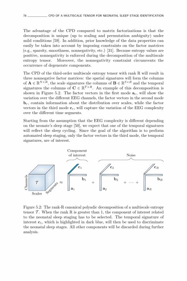
78 CPD OF A MULTISCALE TENSOR FOR NEONATAL SLEEP STAGE IDENTIFICATION
The advantage of the CPD compared to matrix factorizations is that thedecomposition is unique (up to scaling and permutation ambiguity) undermild conditions [59]. In addition, prior knowledge of the data properties caneasily be taken into account by imposing constraints on the factor matrices(e.g., sparsity, smoothness, nonnegativity, etc.) [31]. Because entropy values arepositive, nonnegativity is enforced during the decomposition of the multiscaleentropy tensor. Moreover, the nonnegativity constraint circumvents theoccurrence of degenerate components.
The CPD of the third-order multiscale entropy tensor with rank R will result inthree nonnegative factor matrices: the spatial signatures will form the columnsof A ∈ RN×R, the scale signatures the columns of B ∈ RS×R and the temporalsignatures the columns of C ∈ RT×R. An example of this decomposition isshown in Figure 5.2. The factor vectors in the first mode ar, will show thevariation over the different EEG channels, the factor vectors in the second modebr, contain information about the distribution over scales, while the factorvectors in the third mode cr, will capture the variation of the EEG complexityover the different time segments.
Starting from the assumption that the EEG complexity is different dependingon the neonate’s sleep stage [50], we expect that one of the temporal signatureswill reflect the sleep cycling. Since the goal of the algorithm is to performautomated sleep staging, only the factor vectors in the third mode, the temporalsignatures, are of interest.
T ≈
c1
a1
b1 +
c2
a2
b2 + · · · +
cR
aR
bR
Cha
nnels
Scales Segments
Componentof interest Noise
Figure 5.2: The rank-R canonical polyadic decomposition of a multiscale entropytensor T . When the rank R is greater than 1, the component of interest relatedto the neonatal sleep staging has to be selected. The temporal signature ofinterest c1, which is highlighted in dark blue, will then be used to discriminatethe neonatal sleep stages. All other components will be discarded during furtheranalysis.

THE PROPOSED TENSOR-BASED SLEEP STAGE IDENTIFICATION METHOD 79
Detection of stable solution
Due to the fact that (5.2) is a non-convex optimization problem, we may endup in a local minimum rather than a global minimum. Thus, different factormatrices can be obtained depending on their initialization [197]. To ensurethat a reliable solution is found, the decomposition is repeated 50 times withdifferent random initializations. Next, we want to detect and select the mostoccurring, stable solution among these 50 repetitions. To this end, the similaritybetween all possible combinations of components is assessed by means of cosinesimilarity. In this study we assume that each component should match in all itsmodes, so the triple cosine product or congruence is computed. To assess thesimilarity of two rank 1 tensors X = k l m and Y = p q r this can bewritten as [22, 124, 193]:
cong(X ,Y) = cos(k,p) cos(l,q) cos(m, r) = kTp‖k‖ ‖p‖
lTq‖l‖ ‖q‖
mT r‖m‖ ‖r‖ . (5.3)
The R components of each repetition are sorted based on (5.3) to account for thepermutation indeterminacy of the decomposition. Subsequently, the similaritybetween the corresponding components of different repetitions is investigated.On the assumption that all R components should match, the congruence of theR components is multiplied. This can be organized in a symmetric similaritymatrix S ∈ Rit×it, where it represents the number of iterations (in this case 50).So, sij represents how similar the factor matrices of the ith and jth iterationare. Finally, the solution of the iteration with the highest similarity to the otherrepetitions is selected as the stable and reproducible solution.
Number of components
One of the principal challenges when applying tensor decompositions isselecting an appropriate number of components for the problem at hand [174].A multitude of strategies to define the rank have been proposed. First of all, weinvestigated the multilinear singular value spectrum in order to get an initialestimate of the rank. Then, we performed the decomposition for rank R goingfrom 1 to 5. To compare the different ranks, we investigated the core consistencydiagnostic (CORCONDIA), which assesses how close the core tensor is to beingsuperdiagonal. In addition, a diagnostic based on the relative reduction of thefitting error for an increase of the rank, called the difference of fit (DIFFIT) [190],was computed to assist in determining the appropriate number of components.

80 CPD OF A MULTISCALE TENSOR FOR NEONATAL SLEEP STAGE IDENTIFICATION
5.3.5 Selection of the component of interest
When decomposing the multiscale entropy tensor, we expect that one componentwill reflect the sleep staging of the neonate. However, if the number ofcomponents R is greater than one, an automatic selection of the component ofinterest is required. So, the goal is to find the temporal signature related tosleep staging. In Figure 5.2 this is the temporal signature of the first component,c1, which is marked in blue.
We expect that the component related to sleep staging will have a moreregular, cyclic pattern compared to the other (noise) components. Therefore,the autocorrelation function of the temporal signatures are computed. Sincethe temporal signature reflecting the sleep staging has a stronger correlation intime, we expect that its area under the absolute value of the autocorrelationfunction (ACF) will be larger [52, 100]. Therefore, the component whosearea is the largest will be selected as the component of interest and used forfurther processing.
Figure 5.3 shows an example of this procedure for a rank-2 CPD of a multiscaleentropy tensor. The autocorrelation of the two temporal signatures is plottedon top. The area under the absolute value of the autocorrelation is equal to31.85 and 13.82 for the temporal signature of the first (blue) and second (red)component, respectively. Therefore, the first component will be selected asthe component of interest. The temporal signatures of the two componentsare plotted at the bottom with highlighted periods of quiet sleep in light grey.From these graphs we can see that the first component is indeed reduced duringquiet sleep segments compared to non-quiet sleep segments, whereas the secondcomponent is not related to the sleep stages.
5.3.6 Postprocessing and clustering
Once the nonnegative polyadic decomposition of the multiscale entropy tensoris performed, the temporal signature of the selected component is used to definethe neonate’s sleep stage. This temporal signature shows a (slow) cyclic patternreflecting the sleep staging of the infant. However, there are high frequencyoscillations superimposed on this pattern, which could lead to incorrect sleepstage identification. Therefore, a postprocessing step consisting of smoothingthe temporal signature using a moving average filter with length L equal to 5 isapplied. This moving average filter is applied in both directions (to avoid phasedistortion), so actually a weighted moving average filter is used with triangularshape and length 2 × L. This smoothing operation accounts for the fact that asleep stage does not change instantly. More specifically, sleep periods were only

THE PROPOSED TENSOR-BASED SLEEP STAGE IDENTIFICATION METHOD 81
0 100 200 300Lag (samples)
-0.5
0
0.5
1
Autocorrelatio
n
Area |ACF| = 31.85Area |ACF| = 13.82
0 2 4 6 8Time (h)
0
1 Component 1
0 2 4 6 8Time (h)
Component 2
Tempo
rals
igna
ture
Figure 5.3: Illustration of the component selection procedure. On top,the autocorrelations of the temporal signatures of a rank-2 canonical polyadicdecomposition (CPD) of a multiscale entropy tensor are shown. The area underthe absolute value of the autocorrelation (ACF) is equal to 31.85 and 13.82 forthe first component (in blue) and the second component (in red), respectively.Hence, the first component will be selected as the component of interest. At thebottom, the corresponding temporal signatures are plotted with the quiet sleepperiods annotated by the clinicians highlighted in light grey. The temporalsignature of the first component shows a clear reduction during quiet sleep,while the second component is not correlated with the sleep cycling.
82 CPD OF A MULTISCALE TENSOR FOR NEONATAL SLEEP STAGE IDENTIFICATION
visually labelled as quiet sleep if 3 consecutive minutes or 3 out 4 min wereclinically detected as quiet sleep.
In order to divide the data then into two distinct clusters, k-means clustering(k = 2) is performed using the smoothed temporal loading. So, each datapoint of the smoothed temporal signature of interest c ∈ RT×1 will be assignedto one of the two clusters. Thus, the result of the clustering is a vector oflength T containing a cluster label for each of the 100 s EEG segments. Sincek-means clustering is heavily dependent on its initialization, k-means clusteringis repeated 100 times with different initial cluster centroids and the clusteringwith the lowest sum of within-cluster point-to-centroid distances is selected.The cluster with the lowest EEG complexity will be assigned the label of quietsleep, while the other cluster is labelled as non-quiet sleep [50, 89].
The effect of the smoothing and the result of the clustering is illustratedin Figure 5.4. In this example, the multiscale entropy tensor of an EEGrecording is decomposed for rank R equal to 1 and 2. The raw temporalsignatures of the rank-1 and rank-2 decomposition (only the temporal signatureof interest) are shown on the left, while their smoothed versions are plotted onthe right. The smoothing clearly removes the unwanted variations. The sleeplabels obtained by the algorithm based on k-means clustering are marked byyellow squares (cluster 1 corresponding to quiet sleep) and red dots (cluster2 corresponding to non-quiet sleep). The rank-1 CPD does not correlate wellwith the clinical annotations of quiet sleep highlighted in light grey, whilethe smoothed temporal signature of the rank-2 CPD is clearly reduced duringquiet sleep.
5.3.7 Classification Performance
The performance of the algorithm is evaluated using the annotations by expertclinicians. The sensitivity, specificity, accuracy and Cohen’s Kappa will becomputed for each EEG recording and the mean and standard deviation willbe reported. Moreover, to investigate the performance without the k-meansclustering step, receiver operating characteristic (ROC) curves are constructedbased on the smoothed temporal signatures and the clinical labels. The mean andstandard deviation of the area under the ROC curve (AUC) will be presented.
5.3.8 Statistical Analysis
Statistical analysis is performed to gain insight in the choice of the parameters. Astatistical test is used to investigate whether the area under the absolute value of

THE PROPOSED TENSOR-BASED SLEEP STAGE IDENTIFICATION METHOD 83
0 2 4 6 8Time (h)
0
1
Tempo
ralS
igna
ture
0 2 4 6 8Time (h)
Temporal signatureCluster 1: QSCluster 2: NQS
Quiet sleep
(a) Rank-1 CPD.
0 2 4 6 8Time (h)
0
1
0 2 4 6 8Time (h)
Tempo
ralS
igna
ture
(b) Rank-2 CPD.
Figure 5.4: Illustration of the postprocessing and clustering of the temporalsignature for a rank-1 (a) and rank-2 (b) decomposition of the multiscaleentropy tensor (PMA = 40 weeks 5 days). On the left half of the figure,the temporal signature of interest is plotted in blue. The right half of thefigure shows the smoothed temporal signature after applying the weightedmoving average filter. Moreover, the quiet sleep and non-quiet sleep segmentsestimated by the algorithm are marked by the yellow squares and red dots,respectively. The clinically labelled quiet sleep periods are highlighted in lightgrey. The rank-1 CPD does not give a good indication of the sleep stages, whilethe (smoothed) temporal signature of the rank-2 CPD is clearly reduced duringthe quiet sleep periods.

84 CPD OF A MULTISCALE TENSOR FOR NEONATAL SLEEP STAGE IDENTIFICATION
the autocorrelation function is a good feature to detect the component of interest.In order to do this, the agreement between each of the R temporal signaturesobtained from a rank-R CPD and the clinical sleep labels are evaluated usingthe Kappa score. The temporal signatures are then sorted in descending orderbased on their Kappa statistic. As a result, the first component is the mostrelated to sleep staging and should have the largest area under the absolutevalue of its autocorrelation function (ACF). A statistical test is then performedto assess whether the area under the ACF of the component of interest issignificantly different from the other components.In addition, a statistical test is carried out to investigate the influence of the rankR on the performance. More specifically, we compared Cohen’s Kappa betweenmodels with different values of the rank R. In all analyses, the Shapiro-Wilktest is used to test for normality. If the data is normally distributed, one-wayANOVA is used, otherwise a Kruskal-Wallis test is performed. The significancelevel is always set equal to 0.05.
5.4 Results
Comparison of the factor matrices obtained using the rank indicated byCORCONDIA or DIFFIT with the ones for other ranks revealed that thediagnostics were often not suitable to define the appropriate number ofcomponents in this application. Therefore, the rank has not been fixed for eachrecording, instead the results are reported for different values of the rank R.Table 5.1 presents the mean and standard deviation of the performance measuresamong the 97 EEG recordings. The first five rows show the performance fora fixed rank R for all recordings with R going from 1 to 5. From these data,we can see that the average performance is slightly higher for rank 2 comparedto rank 1 (higher AUC and kappa). Moreover, Table 5.1 also shows that theperformance decreases gradually for an increasing rank beyond 2. However,a Kruskal-Wallis test with multiple comparisons revealed that this performancedifference between the rank-1 and rank-2 model is not significant, while Cohen’skappa of the rank-1 and rank-2 model are both significantly better comparedto the rank-5 model. In order to get more insight in the performance differencebetween a rank-1 and rank-2 CPD, the performance of each recording is plottedas a function of the postmenstrual age in Figure 5.5. In this figure each greencircle and pink square represents the area under the ROC curve of an EEGrecording for a rank-1 and rank-2 decomposition, respectively. The dashedline indicates 37 weeks postmenstrual age. The most interesting aspect of thisgraph is that when a rank-1 decomposition is used, a high performance is onlyobtained up to around 36 to 37 weeks PMA. From that age onwards a clear dropin the AUC can be observed in Figure 5.5. The rank-2 CPD on the other hand,

RESULT
S85
Table 5.1: The classification performance of the proposed tensor-based method for different values of the rank R. Themean (standard deviation) of the sensitivity, specificity, accuracy, area under the ROC curve (AUC) and Cohen’sKappa are presented.
Sensitivity Specificity Accuracy AUC KappaFixed rank
R = 1 0.73(0.29) 0.79(0.16) 0.78(0.15) 0.84(0.19) 0.47(0.34)R = 2 0.82(0.27) 0.74(0.23) 0.76(0.18) 0.87(0.19) 0.49(0.33)R = 3 0.74 (0.34) 0.71(0.2) 0.72(0.17) 0.80(0.24) 0.38(0.36)R = 4 0.75(0.33) 0.67(0.22) 0.70(0.18) 0.80(0.24) 0.35(0.36)R = 5 0.73(0.35) 0.64(0.24) 0.67(0.21) 0.75(0.27) 0.31(0.38)
Age-dependent rankPreterm: R = 1, term: R = 2 0.80(0.23) 0.79(0.17) 0.79(0.14) 0.87(0.16) 0.53(0.28)
Optimal rankAutomatic component selection 0.76(0.32) 0.78(0.18) 0.79(0.17) 0.85(0.21) 0.50(0.38)Optimal component 0.86(0.32) 0.81(0.18) 0.82(0.17) 0.91(0.21) 0.60(0.38)

86 CPD OF A MULTISCALE TENSOR FOR NEONATAL SLEEP STAGE IDENTIFICATION
has a high performance for most recordings at term equivalent age, but has alower performance for some measurements recorded at a younger age.
28 30 32 34 36 38 40 42Postmenstrual Age (weeks)
0
0.5
1
AUC
Rank = 1Rank = 2
37
Figure 5.5: The area under the ROC curve as a function of the postmenstrualage at the moment of the recording. Each green circle shows the performancefor one of the EEG recordings for a rank-1 CPD, whereas the pink squaresrepresent the performance for a rank-2 CPD.
Based on these findings we decided to also report the results for an age-dependentrank, where the rank is chosen equal to 1 for preterm recordings and equal to2 for EEGs recorded from 37 weeks PMA onwards. The performance of thisapproach is set out in the sixth row of Table 5.1. It is clear that the averageperformance of using an age-dependent rank is better compared to a fixed rankfor all recordings, however this performance difference is not significant.
Finally, the last two rows of the table show the classification performance whenthe optimal rank (between 1 and 5) for each recording was selected basedon Cohen’s Kappa computed with the ground truth annotations. Specifically,the last row corresponds to the highest attainable performance (optimal rankand best component), while in the penultimate row the optimal rank was usedbut the component of interest was automatically selected using the strategybased on the autocorrelation explained above. As a consequence, the differencebetween these two rows is caused by failures of the automatic componentselection procedure.
As explained in section 5.3.8, a statistical analysis is performed to examinewhether the area under the ACF is a suitable feature to rely on for the automaticcomponent selection. The boxplots in Figure 5.6 show the area under theabsolute value of the ACF after sorting the temporal signatures based on theiragreement with the clinical annotations. The component of interest, with the

DISCUSSION 87
largest Kappa score, is the first component and is marked in blue. A Mann-Whitney U test and Kruskal-Wallis test with multiple comparisons determinedthat the first component is significantly different from all other componentsfor the rank-2 and rank-3 CPD, respectively (Figure 5.6 a,b). For the rank-4and rank-5 CPD the area under the ACF of the sleep staging component issignificantly different compared to all other components except the second one.This is also indicated on the boxplots in Figures 5.6 (c,d).
5.5 Discussion
This study aimed to discriminate quiet sleep (QS) from non-quiet sleep(NQS) using the nonlinear dynamics of the EEG signal in a data-driven way.The proposed algorithm relies on the fact that the EEG complexity is differentdepending on the sleep state. In order to quantify the complexity of theEEG signal, multiscale entropy is computed for consecutive segments of themultichannel EEG recording. These multiscale entropy values are then usedto construct a third-order tensor with modes channels, scales and segments.Subsequently, the rank-R nonnegative CPD of the multiscale entropy tensoris computed. The temporal signature of interest is detected based on the areaunder the absolute value of its autocorrelation function. After smoothing, thistemporal signature shows a cyclic pattern reflecting the neonatal sleep staging.Clustering is then performed to discriminate quiet sleep from non-quiet sleep.
The performance of the algorithm is reported for different ranks. The averageKappa is equal to 0.47 and 0.49, for a rank-1 and rank-2 CPD, respectively.However, if a rank-1 decomposition is used for EEGs recorded at a postmenstrualage below 37 weeks and a rank-2 decomposition is used for EEGs recordedat an older age, a Kappa of 0.53 is obtained. This indicates that a higherrank is preferred for neonates at term equivalent age, while rank 1 is suitablefor most of the preterm recordings. The fact that for some recordings rank1 is not sufficient, is demonstrated by the example in Figure 5.4. An evenhigher performance could be obtained if the optimal rank is used and thecomponent of interest is detected correctly. However, as can be seen fromTable 5.1, the performance when the optimal rank is used and the component ofinterest is selected automatically is slightly lower compared to an age-dependentrank. This reduction in performance is due to the fact that the procedureto select the component of interest is more likely to fail for a higher numberof components. From the data presented in Table 5.1 we can see that theperformance gradually decreases if a rank higher than two is used. This findingsuggests that for the majority of the recordings in the current database a lower

88 CPD OF A MULTISCALE TENSOR FOR NEONATAL SLEEP STAGE IDENTIFICATION
1 2Component
0
10
20
30
40
50Areaun
der|A
CF|
*
(a) Rank = 2
1 2 3Component
0
10
20
30
40
50
Areaun
der|A
CF|
**
(b) Rank = 3
1 2 3 4Component
0
10
20
30
40
50
Areaun
der|A
CF|
**
(c) Rank = 4
1 2 3 4 5Component
0
10
20
30
40
50
Areaun
der|A
CF|
* * *
(d) Rank = 5
Figure 5.6: Boxplots of the area under absolute value of autocorrelation of thetemporal signatures after sorting them in descending order according to theirKappa score. The component with the largest Kappa score and therefore mostrelated to sleep staging is the first one and is marked in blue, while the other(noise) components are marked in red. ’*’ indicates a statistically significantdifference with p < 0.05. For the rank-2 CPD (a) and the rank-3 CPD (b) thereis a significant difference between the area under the ACF of the sleep stagingcomponent and the noise component(s). For a rank-4 (c) and rank-5 CPD (d)the component most related to sleep staging is significantly different from allother components except one.

DISCUSSION 89
rank is more appropriate. Nevertheless, this performance reduction can also bepartly attributed to the more difficult component selection for higher ranks.
There are various possible explanations for the need for a higher rank forrecordings at term-equivalent age. First of all, it is likely that this is due to theincreased amount of artifacts in near term EEG recordings. It is expected thatan older neonate will move more, which could lead to more severe distortionsand lower quality of the EEG signal. The higher performance for higher ranks innoisy preterm EEG recordings confirms this reasoning. Secondly, the emergenceof four distinct sleep states around 36 weeks PMA might also play a role in thisphenomenon [56].
The performance of the described algorithm is lower compared to state-of-the-art algorithms [9, 57, 162]. However, there are multiple advantages of theproposed method. The major advantage of the algorithm is that it is data-drivenand unsupervised. As a consequence, the method can be easily applied on acompletely new dataset and used in new centers, where there is little expertiseabout EEG sleep labelling. Moreover, in this study the algorithm is assessedon eight channel EEG recordings measured using the restricted 10–20 systemfor neonates. However, as long as the data is of appropriate quality, the sameapproach can also be applied on datasets with fewer or more electrodes withoutadjustments. Finally, the tensor decomposition can be updated in an efficientway whenever a new batch of EEG data is available [200]. This allows real timetracking of neonatal sleep states.
The main weakness of this study is the lack of a method to define the rankfor each new EEG recording automatically in a data-driven way. This is ageneral issue in tensor applications, therefore it is suggested to combine differenttools to asses the rank [2, 37]. We tested several diagnostics, but none of themresulted in a reliable estimate of the number of components. More researchis needed to determine the optimal number of components for this specificapplication. An additional drawback of the proposed algorithm is the procedurefor selecting the component of interest. The temporal signature of interest doesnot always have the largest area under the absolute value of the autocorrelationfunction. For that reason more advanced strategies for component selectionshould be investigated in future studies. Another limitation of the study is thatartifacts commonly lead to misclassification of the segment. More specifically,EEG segments distorted by artifacts are often classified as quiet sleep becausethey have a reduced EEG complexity. The cause of this is two-fold. Firstof all, artifacts are more predictable and less complex compared to noise-freeEEG [128]. Secondly, a high amplitude artifact will drastically increase thestandard deviation of the segment, resulting in a much higher tolerance r andthus more template matches and consequently lower entropy. Detecting artifactsas quiet sleep periods will lead to a reduced performance, since the majority of

90 CPD OF A MULTISCALE TENSOR FOR NEONATAL SLEEP STAGE IDENTIFICATION
the (motion) artifacts occur during non-quiet sleep. The smoothing operationis implemented to reduce the influence of artifacts and can deal with shortduration artifacts (sudden drop in EEG complexity). Yet, the postprocessingcannot avoid false detections caused by longer artifacts (on multiple channels).Further research might explore incorporating information about the noise inthe algorithm to make it more robust to artifacts. Besides, an estimation of theamount of noise could be used to get an initial estimate of the proper numberof components. Notwithstanding these limitations, the study suggests thata decomposition of a multiscale entropy tensor can be used to discriminateneonatal sleep stages.
This study is an exploratory analysis on the use of tensor decompositionsfor sleep stage identification in preterm infants. Only the differences incomplexity between different sleep stages are used. However, in future work thetemporal signature could be combined with other discriminating features (e.g.,spectral edge frequency, power in specific EEG frequency bands, etc.) to boostthe performance. Moreover, the heart rate variability, respiration and bodymovements of the infant are also dependent on the sleep state. Hence, in futureresearch the combination of these complementary modalities can be studied.Finally, other tensorization techniques can be examined in future investigations.
5.6 Conclusion
This study confirmed that the EEG complexity is significantly lower duringquiet sleep compared to non-quiet sleep. This property is exploited to developan unsupervised algorithm that can detect quiet sleep in preterm infants basedon the data-driven factorization of the multiscale entropy tensor.

Chapter 6
Quiet sleep detection inpreterm infants using deepconvolutional neural networks
So far, two algorithms for automated sleep staging in preterm infants have beenproposed in this thesis. The first algorithm, explained in Chapter 4, followed thetypical machine learning approach with the extraction of complexity features fromthe EEG which are then used to train an LS-SVM classifier. The second method,presented in Chapter 5, proposes a new pipeline based on tensor decompositionsto identify the neonatal sleep stages in an unsupervised manner. While thetensor-based approach is not fully exploiting the data and available clinicalannotations to achieve the optimal performance, the first algorithm is limited bythe set of handcrafted features which only assess the complexity of the EEG. Inthis chapter, we will address these problems by introducing a new algorithm forautomated EEG sleep staging based on deep learning.The proposed 17-layer convolutional neural network is fed with raw multichannelEEG data and gives a sleep stage label, quiet sleep or non-quiet sleep, as output.The network is trained on 54 recordings from 13 prematurely born neonates andthe performance is assessed on 43 recordings from 13 independent patients. Thisresearch was performed in close collaboration with Dr. Amir Hossein Ansariand led to a joint publication [9].
91

92 QUIET SLEEP DETECTION IN PRETERM INFANTS USING DEEP CNN
6.1 Introduction
Preterm infants are born during a critical period of rapid growth anddevelopment of the brain and central nervous system. In these newborns, thefast neural growth that normally occurs in the womb during the third trimesterof gestation is interrupted and has to take place in the neonatal intensive careunit (NICU). Therefore, a primary concern of NICUs is to support optimalbrain development of these vulnerable infants, who are at increased risk ofneurodevelopmental disorders [144, 158]. Continuous electroencephalography(EEG) monitoring is considered a valuable noninvasive tool to assess and trackbrain maturation of newborns in the NICU. Sleep wake cycling (SWC) undergoesfast changes and is one of the main hallmarks of neurodevelopment in preterminfants. Since sleep state organization reflects the level of functional braindevelopment, a first step towards automated analysis of cerebral function is toidentify the different sleep stages [56, 168].Moreover, evidence suggests that sleep is of utmost importance in thedevelopment and maturation of neural pathways. As a consequence, theneonate’s sleep should be protected and promoted during their stay in the NICU[6, 196]. Automated algorithms for real-time neonatal sleep state identificationcould optimise the scheduling of neonatal interventions and care procedures inthe NICU. Up to now, the gold standard for the assessment of sleep EEG isvisual analysis by an expert clinician. However, visual interpretation of neonatalEEG is a tedious and time consuming task for the clinician and requires expertisethat might not always be available in the NICU [56]. This can be overcome bydeveloping automated algorithms to discriminate neonatal vigilance states.
A growing body of literature has investigated algorithms for neonatal EEGsleep scoring [28, 103, 159], which typically rely on the difference in continuity[56, 103] and frequency content [162] between neonatal sleep states. Palmuet al. [152] compared the proportional duration of bursts, called SpontaneousActivity Transients (SAT%), in the EEG between neonatal sleep states. Theyconfirmed the existence of genuine vigilance states in early preterm infantsand found that the fluctuation of the SAT% signal corresponds to sleep stagecycling. Stevenson et al. [181] continued this work and derived quantitativemeasures of brain activity cycling from the frequency domain representation ofthe SAT% time series. Besides analysis of the SAT% signal, EEG time profileshave been used for automated sleep stage detection as well [57, 105, 106]. TheEEG time profiles are constructed by adaptive segmentation of the EEG andsubsequent clustering of features extracted from each segment. Thresholdingof the processed time profile, which shows the class membership of the EEGsegments over time, will then lead to labels of the sleep states. This concept ofEEG time profiles for sleep stage modelling was explored by Barlow et al. [13],

INTRODUCTION 93
extended by Krajca et al. [105, 106] and further improved by Dereymaeker et al.[57]. In addition to the approaches described above, a number of studies havedeveloped a neonatal sleep stage classifier based on a set of discriminative EEGfeatures in combination with a machine learning classifier [50, 71, 103, 111].
While a wide range of features have been used to develop neonatal sleep stageclassifiers, there is still no consensus on the optimal combination of features.Moreover, those handcrafted features are based on prior human knowledge aboutEEG sleep patterns, hence only a limited set of features have been examined.In general, the process of selecting the optimal feature set and classifier is achallenging task.
This study will address these problems by adopting a deep convolutional neuralnetwork (CNN) to detect quiet sleep in preterm infants. Deep neural networkslearn the features directly from the data, which eliminates the need for manualfeature extraction. CNNs have been extensively used in the field of imageand speech processing [1, 33, 108, 115, 116, 176]. Only recently, deep neuralnetworks have been attracting a lot of interest for biomedical applications,such as medical image analysis [173], detection of myocardial infarction [3]and (neonatal) seizure detection [4, 8]. CNNs have been applied for sleepstage scoring in adults [29, 134, 156, 178, 184, 194], however to the best ofour knowledge this is the first study adopting CNNs for neonatal sleep stageclassification.
The aim of this paper is to design and train a deep convolutional neuralnetwork to identify sleep stages in preterm infants. The performance of thisnovel classifier will be compared to two reference algorithms described in theliterature: (1) a support vector machine (SVM) classifier using a set of spectralfeatures [162] and (2) CLuster-based Adaptive Sleep Staging (CLASS) developedby Dereymaeker et al. [57].
The remaining part of the paper proceeds as follows. We start by describing thedatabase that has been used to develop, train and test the classifier. We willthen go on to a thorough description of the architecture and training procedureof the network developed for sleep scoring. The pipeline of the two referencealgorithms described in the literature will be briefly explained as well. Thefollowing sections are concerned with the comparison of the proposed algorithmand the two reference algorithms from the literature in the sense of performance,error correlation and computational time. Next, the performance of the proposedCNN and two reference algorithms will be reported and compared. At last, theadvantages and disadvantages of the proposed method and future directionswill be discussed.

94 QUIET SLEEP DETECTION IN PRETERM INFANTS USING DEEP CNN
Time (30s = 900)
Ch
ann
els
(8
)
Features
NQs
QS
Convolution+ ReLU + Pooling
Convolution+ ReLU + Pooling Convolution
+ ReLU + Pooling
Fully Connected
Feature Extraction ClassifierInput Prediction
Figure 6.1: Architecture of the convolutional neural network.
6.2 Materials and methods
6.2.1 Database
The same dataset as described in section 4.2.1 is used to train and test theconvolutional neural network. The database consisting of 8-channel EEGrecordings from 26 prematurely born infants was split into a training set and atest set. The training set containing 54 recordings from 13 patients was usedto develop and train the convolutional neural network. The total duration oftraining data is equal to 269 h, with 69 h of quiet sleep, and 200 h of non-quietsleep. The test set consisting of 43 recordings from 13 independent patientswas used to assess the classification performance. The test set consists of 223 hof EEG with 53 h during quiet sleep and 170 h during non-quiet sleep. Thisinterpatient data splitting avoids that the model is tested on data from a patientthat is also used to train the model. In this way, we expect that patient specificcharacteristics cannot bias the classification performance.
6.2.2 The proposed CNN for sleep stage classification
Preprocessing
Prior to using the EEG data as input for the CNN, some preprocessing steps areperformed. First of all, the EEG is bandpass filtered between 1 and 15 Hz. Thefiltered EEG is then downsampled to 30 Hz in order to reduce the complexityof the network. The training data is normalized so that the mean and standarddeviation of each EEG channel across the whole dataset is equal to zero andone, respectively. The parameters from the training data are then used tonormalize the test data. At last, the EEG is segmented into windows of length30 s, resulting in EEG segments of size 8 (channels) × 900 (samples).

MATERIALS AND METHODS 95
Table 6.1: Layers of the designed network.
Layer Type Size No. No. Stride Padding Outputfilters parameters dimension
FeatureExtraction
0 Input (8,900,1)1 Conv (1,10) 3 33 (1,1) (0,9) (8,900,3)2 ReLU (8,900,3)3 Conv (3,1) 3 30 (1,1) (6,900,3)4 ReLU (6,900,3)5 Mpool (2,3) (2,2) (0,2) (3,450,3)6 Conv (1,5) 5 80 (1,1) (0,4) (3,450,5)7 ReLU (3,450,5)8 Conv (3,1) 5 80 (1,1) (1,450,5)9 ReLU (1,450,5)10 Mpool (1,5) (1,3) (0,2) (1,150,5)11 Conv (1,5) 7 182 (1,1) (0,7) (1,150,7)12 ReLU (1,150,7)13 Mpool (1,6) (1,4) (1,37,7)14 Conv (1,37) 10 2600 (1,1) (1,1,10)
FC
15 Sigmoid (1,1,10)16 Conv (1,1) 2 22 (1,1) (1,1,2)17 Softmax (1,1,2)
Total Number of Parameters: 3027Conv: Convolutional layerReLU: Rectified linear unitMPool: Pooling by maximum operatorFC: Fully connected classifier
CNN architecture
These preprocessed multichannel EEG segments are then fed into a 17-layerconvolutional neural network, whose architecture is shown in Figure 6.1 andTable 6.1. The architecture of the network was designed based on our previousexperience for neonatal seizure detection [8], and trial and error using thetraining and validation data. The CNN is designed and implemented in Matlabusing the MatConvNet toolbox [204]. The first 14 layers perform featureextraction and the last 3 layers including the fully connected layers performclassification. The mask (kernel) size, stride, padding, and the number of featuremaps used in the conv and/or pooling layers are also mentioned in the table.In order to train the CNN using the backpropagation algorithm, 20% of the

96 QUIET SLEEP DETECTION IN PRETERM INFANTS USING DEEP CNN
training data was selected as validation set and the remaining 80% of thetraining data was used to train the network’s parameters. During this splittingof training data into training and validation set, the ratio of quiet sleep tonon-quiet sleep segments is retained. The learning rate changes from 10−2 to10−4 dependent on the training epoch and the layer. The weight decay wasequal to 10−6. For initializing the network, all bias terms were initiated withzero and the filter coefficients were set with Gaussian random noise with meanand standard deviation equal to 0 and 0.4 respectively. Batch learning wasadopted with the batch size equal to 20 EEG segments and the maximumnumber of training epochs equal to 1000. Early stopping was used in order toavoid overfitting and ensure network generalization. So, the validation set errorwas monitored during the training phase, and training was stopped at epoch493 which has the lowest validation set error.
Postprocessing
According to the literature a sleep stage should last at least three consecutiveminutes or three out of four consecutive minutes [104]. Relying on this fact, amoving average filter with length 6 (6 segments of 30 s = 3 min) is used as apostprocessing step.
6.2.3 Spectral feature based neonatal sleep stage classifier
This neonatal sleep stage classifier is based on a set of spectral features describedby Piryatinska et al. [162]. These features are fed into a support vector machine(SVM) classifier.
After bandpass filtering between 1 and 20 Hz and segmenting the multichannelEEG in epochs of 30 s, 9 spectral features are extracted from each EEG segment:(1-4) relative power in 4 EEG frequency bands (δ: 0.5 - 4 Hz, θ: 4 - 8 Hz, α: 8 -12 Hz, β: 12 - 15 Hz), (5-6) spectral edge frequency (75% and 90%), (7) spectralmoment, (8) spectral entropy and (9) amplitude entropy. Each multichannelEEG segment is then characterized by a total of 72 (9 × 8 channels) featuresand is marked as quiet sleep or non-quiet sleep according to the clinical label.The hyperparameters of the SVM with radial basis function (RBF) kernel areset using 5-fold cross validation on the training data. This SVM classifier isthen trained using the training set and the performance is evaluated on the testset. As in the proposed CNN, a moving average filter with length 6 is added toremove the transient discontinuities.

MATERIALS AND METHODS 97
6.2.4 Cluster-based Adaptive Sleep Staging (CLASS)
This algorithm is based on the relatively higher discontinuity in quiet sleepcompared to non-quiet sleep and has been developed by Dereymaeker et al. [56].Briefly, the pipeline of the algorithm is as follows. First, a preprocessing stepconsisting of a bandpass filter from 1 to 40 Hz and a notch filter at 50 Hz isperformed. Artefact subspace reconstruction is then adopted to reject remainingartefacts, which could otherwise be wrongly detected as EEG discontinuities.After artefact removal, the cleaned EEG is downsampled with a factor three(sampling frequency = 83 Hz) to reduce the computational time during thesubsequent steps. To deal with the nonstationarity of the EEG signal, therecordings are adaptively segmented resulting in quasi-stationary segments ofvariable length. Features extracted from these segments are then used to clustersegments with similar characteristics. A cluster time profile is obtained byrepresenting each sample by its cluster label. Once the cluster time profile isextracted for each EEG channel, some processing steps are performed to obtaina single smooth envelope which can then be thresholded to detect quiet sleepsegments. This threshold is calculated as the mean of the envelope plus a factormultiplied with the standard deviation of the signal envelope. In the final stageof the algorithm, quiet sleep detections shorter than three minutes are removed[104].
6.2.5 Classification performance
In order to assess the performance of the sleep stage classifier, the sensitivity,specificity and Cohen’s Kappa coefficient κ have been computed. All of theabove mentioned evaluation metrics are measured for each recording of the testset, and the median and interquartile range are reported. The computation ofthese measures require a fixed decision threshold. In this study, the optimalthreshold was defined so that the sensitivity equals the specificity on the trainingset. Since the threshold used in the CLASS algorithm is computed as threshold= mean(y) + factor × std(y), where y denotes the smooth envelope, the factorinstead of the complete threshold is optimized on the training set.
In addition, the receiver operating characteristic (ROC) curve is computed foreach recording of the test set. This allows to analyse the effectiveness of theclassification without defining a fixed threshold. The mean and median ROCcurve over all recordings are then obtained by taking the mean and median ofthe true positive rate and the false positive rate at a specific threshold. Thesemean and median ROC curves are plotted and the area under the curve (AUC)is computed.

98 QUIET SLEEP DETECTION IN PRETERM INFANTS USING DEEP CNN
6.2.6 Error correlation
In order to investigate the error correlation between the three sleep stageclassifiers, the percentage of test segments correctly classified by all threealgorithms, by only two or one of the algorithms, or by none of the algorithmsare computed. In addition, Cohen’s Kappa is computed among each of the sleepclassification algorithms and the clinical sleep labels in order to investigate theagreement between the different algorithms.
6.2.7 Computational time
It is generally known that deep neural networks are highly complex andcomputationally expensive to train. However, when using a sleep stage classifierin clinical practice, it is not the training time, but the time required to classifya new incoming EEG segment that is of interest.
In order to compare the computational evaluation time of the three algorithms,sleep stage classification of the complete test set in blocks of 2 h of EEGis performed with each of the algorithms. The three algorithms were runchronologically and the mean and standard deviation of the computationaltime are reported to avoid variable CPU loading. Since the complete test setis classified, more than 100 iterations are performed. This experiment wasconducted on a workstation with an Intel(R) Core(TM) i7 3.6 GHz processorand 16 GB RAM, implemented in MATLAB R2016a software (The MathWorks,Natick, MA, USA).
6.3 Results
6.3.1 Feature evolution during sleep-wake cycling
To illustrate how each of the 10 features extracted by the convolutional neuralnetwork behave during each of the sleep states, boxplots of the features duringsleep-wake cycling are shown in Figure 6.2. The top of Figure 6.2 illustrates theamplitude integrated electroencephalography (aEEG) derived from the bicentralchannels C3/C4 from a test recording at 31 weeks and 3 days postmenstrualage. aEEG is commonly used in the NICU to monitor the functional brainintegrity and is a suitable tool to assess sleep-wake cycling of the infant [49].More discontinuous activity during quiet sleep is recognized by a wideningof the aEEG trace, while the more continuous activity during active sleep orwakefulness is characterized by a narrow trace [12, 49]. The aEEG of the quiet

RESULTS 99
f1 f3 f5 f7 f9 f10 f1 f3 f5 f7 f9 f10 f1 f3 f5 f7 f9 f10
f2 f4 f6 f8 f2 f4 f6 f8 f2 f4 f6 f8
NQS QS NQS
10050
10
25
5
Figure 6.2: The aEEG trace derived from the bicentral channels C3 and C4 froma recording of the test set at 31 weeks and 3 days PMA is shown on top. Theselected quiet sleep (QS) segment and preceding and subsequent non-quiet sleep(NQS) segments are indicated on the aEEG. The boxplots show the featuresduring each of these selected segments. The top half of the boxplots show thesix features that reduce during quiet sleep (f1, f3, f5, f7, f9, f10), the bottomhalf shows the four features that increase during quiet sleep (f2, f4, f6, f8). Mostof the features are significantly different for the two sleep stages.
sleep segment selected in Figure 6.2 has a clearly wider bandwidth compared tothe non-quiet sleep segments before and after. The top row of boxplots showsfeatures 1, 3, 5, 7, 9 and 10, which are reduced during quiet sleep (the middlebox) compared to non-quiet sleep (left and right box). The bottom row providesthe boxplots of features 2, 4, 6 and 8, which increase during quiet sleep. Fromthe boxplots in Figure 6.2, it can be seen that most of the features are welldiscriminating quiet sleep from non-quiet sleep.
6.3.2 Classification performance
The classification performance of the proposed CNN is illustrated in Figure 6.3,which presents the ROC curves for each of the test recordings separately, andthe mean and median ROC curve. The area under the mean and median ROC

100 QUIET SLEEP DETECTION IN PRETERM INFANTS USING DEEP CNN
curve are equal to 92% and 98%, respectively. The histogram of the trainingdata segments and the AUC for each recording of the test set as function ofpostmenstrual age are plotted in Figure 6.4. It can be seen from the histogramthat training data is available at all ages. From the AUC in function of PMA,it is apparent that most of the test recordings are measured between 30 and 38weeks of PMA. Moreover, the figure shows that the algorithm performs wellover a wide range of PMA. It is notable that in Figure 6.3 as well as in Figure6.4 two outliers with a low AUC (6 0.65) can be observed.Table 6.2 compares the AUC, sensitivity, specificity and Cohen’s Kappa acrossthe 3 methods. It can be seen from the table that the proposed CNN has similarperformance compared to the CLASS and feature-based algorithm. In addition,it is clear that the postprocessing step significantly improves the performanceof the feature-based sleep stage classifier.
0 50 1001-Specificity
0
50
100
Sensitivity
Mean ROCMedian ROCEach Recording
Figure 6.3: The ROC curves for the proposed CNN sleep stage classifier. Thelight grey ROC curves show the performance of the classifier for each recordingof the test set. The black dashed and full line represent the mean ROC andmedian ROC curve, respectively.
6.3.3 Error correlation
Figure 6.5a illustrates the percentage of segments correctly labelled by allthe algorithms, by only two or one of the algorithms, or misclassified by allmethods. The complete bars represent the complete test set, the dark grey part

RESULTS 101
28 30 32 34 36 38 40 420
2000
4000
6000
No.
oftr
aini
ngse
gmen
ts
0
0.2
0.4
0.6
0.8
1
AUC
PMA (weeks)
Figure 6.4: The histogram of the training data segments is displayed in lightgrey (left y-axis). The blue circles show the AUC for each recording from thetest set (right y-axis).
Table 6.2: The classification performance for the proposed CNN, the CLASSalgorithm and the feature-based approach without (NP) and with (PP)postprocessing respectively. The area under the mean ROC curve (AUC)and median(IQR) of the sensitivity, specificity and Cohen’s Kappa are set out.
AUC Sensitivity Specificity KappaCNN 0.92 0.88(0.26) 0.93(0.13) 0.74(0.17)CLASS 0.92 0.72(0.19) 0.97(0.06) 0.75(0.19)Feature-based NP 0.83 0.74(0.21) 0.87(0.13) 0.59(0.25)Feature-based PP 0.93 0.83(0.28) 0.97(0.07) 0.77(0.23)
corresponds to the segments of the two outliers in Figure 6.4, while the lightgrey part of the bars correspond to the remaining segments. From this bargraph, it is clear that most of the segments (nearly 80%) are correctly classifiedby all algorithms. Approximately 14% of the segments are correctly identifiedby two of the algorithms, and only 8% of the segments were only correctlyclassified by one of the described methods. Less than 3% of the segments werewrongly classified by all the algorithms. However, a considerable amount of thesegments that were misclassified by all algorithms are part of the two recordingswith a low AUC. More specifically, from all segments of the outliers, almost 25%is not identified by any of the algorithms. This illustrates the high agreementamong the three algorithms, which is also confirmed by the Kappa values shownin Figure 6.5b.

102 QUIET SLEEP DETECTION IN PRETERM INFANTS USING DEEP CNN
0
20
40
60
80
100
Percentage
ofsegm
ents
All
FB&CN
N
CLASS &
CNN
CLASSCN
N FB None
CLASS &
FB
FB
LABEL
0.720.680.67
0.67
0.650.59
CNN
CLASS
(a) (b)
Figure 6.5: The error correlation between the three sleep stage classifiers.(a) The bar graph shows the percentage of EEG segments correctly classifiedby all, two, only one or none of the algorithms. The dark grey part of thebars correspond to the segments of the two outliers, while the light grey partcorresponds to the remaining test segments. (b) This graph represents theagreement among the three algorithms (CNN, FB, CLASS) and the clinicallabels (LABEL) computed using Cohen’s Kappa coefficient.
6.3.4 Computational Time
The bar graph in Figure 6.6 illustrates the mean evaluation time for 2 hEEG segments. The dark blue box represents the average total time forloading, preprocessing and classifying 2 h EEG data. The light blue boxshows the time required for classification. In case of CLASS, the classificationconsists of performing CLASS, starting from the artefact subspace reconstructionup to defining the quiet sleep periods. For the feature-based approach, thecomputational time for feature extraction, classification using the SVM andthe postprocessing are merged in the classification time. Finally, the time forclassification and postprocessing are combined and marked as classification timefor the CNN.From this chart, it can be seen that overall the CNN (10 ± 1.0 s) is 9 timesfaster than CLASS (92 ± 3.8 s) and slightly faster than the feature-based (12± 1.3 s) approach. The most remarkable difference is the classification time,

DISCUSSION 103
which is significantly lower for the CNN (0.16 ± 0.04 s) compared to CLASS(85 ± 3.74 s) and the feature-based classification (2.5 ± 0.28 s).
Total
10.43 s
12.22 s
92.29 s
Classification
0.16 s
2.51 s
84.70 s
CNN
FB
CLASS
Figure 6.6: The average computational time for 2 h multichannel EEG segmentsfor each of the three algorithms. The total computational time (left) and thetime for only classification (right) are shown.
6.4 Discussion
The aim of the current study was to implement a convolutional neural networkfor neonatal sleep stage classification. By adopting convolutional neural networkswhich are able to learn relevant features automatically from the raw EEG data,the difficult and time-consuming process of selecting the proper feature set,which requires domain knowledge from experts, can be avoided. Moreover, theCNN optimizes the feature extraction and classification simultaneously. Thisnovel data-driven approach successfully identified quiet sleep in preterm infantswith an average and median AUC of 92% and 98% respectively.
While this performance is comparable to the CLASS algorithm developed byDereymaeker et al. [56], the CNN has some advantages compared to the clustertime profiles approach. First of all, except for bandpass filtering the proposedmethod does not use any advanced artefact removal, whereas the CLASSalgorithm uses artefact subspace reconstruction as additional artefact rejection.Secondly, the proposed CNN can be retrained if additional data collection isperformed, while this is not straightforward for the CLASS algorithm. Assleep patterns will be better represented in a larger training database, theclassification performance will further improve. At last, it must be pointedout that the threshold used in the CLASS algorithm is based on the meanand the standard deviation of the signal envelope. Therefore, the complete

104 QUIET SLEEP DETECTION IN PRETERM INFANTS USING DEEP CNN
or at least a representative part of the recording should be available beforethe classification can be performed. In contrast to CLASS, the proposed CNNuses a fixed threshold which can be decided based on the training set and doesnot need to be adjusted to the new recording. This facilitates real time sleepscoring. Although the proposed CNN uses only 10 features as input for thefully connected classification stage, it reaches the same performance as thefeature-based approach which is based on 72 features [162]. To conclude, it canbe seen in Figure 6.6 that the presented CNN is considerably faster comparedto the current state-of-the-art.
One of the key challenges of neonatal sleep stage classification is to deal with thefast alterations in the EEG patterns during sleep ontogenesis. It is apparent fromFigure 6.4 that the network is able to train the age specific EEG characteristics,resulting in a good performance over a wide PMA range (30 - 38 weeks PMA).Due to the small number of recordings below 30 weeks and beyond 38 weeksPMA, we cannot make any statements about the performance in those ageranges. Both in Figure 6.3 and 6.4, two outliers can be observed. Theserecordings also had a low AUC in the CLASS and feature-based approach.According to an expert clinician, the outlier at 28 weeks and 5 days (AUC equalto 65%) is due to poor EEG quality probably as a result of electrode impedanceproblems, while the low performance of the recording at 30 weeks and 6 days(AUC equal to 36%) is caused by an intravenous infusion motor artifact.
In this study, the overall AUC is computed as the area under the mean or medianROC curve. As explained above, this mean ROC curve is obtained by averagingthe sensitivity and specificity at an incremental threshold between zero andone, which is called threshold averaging [66]. It is important to note that thisprocedure of first computing the average ROC and then the AUC is not thesame as computing the AUC for each recording separately and then taking theaverage. Computing the mean of individual AUCs is called vertical averaging,which corresponds to taking the average of the true positive rates at a fixed falsepositive rate [66]. In this application we opted for threshold averaging ratherthan vertical averaging, because implementation of the algorithm in a brainmonitor for use in clinical practice requires the choice of one fixed threshold.
The present study has relevance for clinical practice. First of all, the proposedCNN has a low computational time, hence it is suitable for real time sleepstage monitoring. Real time sleep scoring is important in the NICU as it canaid in making the neonatal care more patient-driven and avoid disruption ofthe infant’s sleep. In addition to implementation of the algorithm in a brainfunction monitor to promote neonatal sleep in the NICU, this algorithm isof great interest in maturation studies as we have to account for the cyclicnature of EEG during brain maturation analysis. Furthermore, the sleep EEGundergoes fast maturational changes during early brain development.

CONCLUSION 105
The main limitation lies in the fact that the training phase is computationallyexpensive and requires a large database. However, training time is secondarysince the network only has to be trained once. After training, the recallcomputational time is the important parameter, which is much smaller forCNN compared to the existing algorithms. A weakness of this study was thepaucity of EEG recordings below 30 weeks and beyond 38 weeks postmenstrualage. Another drawback of CNNs is the lack of interpretability of the features.Further work needs to be done to establish which features are extracted by thenetwork.
The results of the current study suggest that convolutional neural networks area promising approach for sleep stage classification in preterm infants. However,several steps can be explored to further improve the performance of the sleepstage classification. A number of recommendations for future research are given.First of all, as mentioned before, the current architecture of the network has beendefined based on trial and error. As a result, there is abundant room for furtherprogress in designing the network, especially with the aid of the high-speedgraphics processing unit (GPU). Some of the model design parameters (e.g.number of layers) could for instance be considered as hyperparameters and couldbe systematically tuned in order to obtain a more optimal and reproduciblenetwork architecture. In addition, the proposed method uses a postprocessingstep to take into account that the sleep state cannot change instantly. Infuture investigations, it might be possible to incorporate this in the networkby including information of the preceding and subsequent segments by usinganother deep learning algorithm such as Long Short Term Memory networks(LSTM). Moreover, clinicians do not rely only on EEG characteristics, butassess other non-cerebral criteria as well during visual sleep scoring [56, 157].Behavioural correlates that are essential to distinguish quiet sleep and non-quietsleep are body movements, eye movements and cardiorespiratory regularity.Therefore, we expect that the performance can be improved by includingadditional modalities such as EMG, respiration and EOG. Our results indicatethat the proposed network can reliably classify sleep in preterm infants with aPMA from 30 to 38 weeks. Future studies should aim to replicate the resultsfor a larger age range, by retraining the network using data from an older, termneonates population. At last, interpretation of the features extracted by thenetwork is an important issue for future research.
6.5 Conclusion
In this study, we designed and implemented a deep convolutional neural networkwhich automatically extracts optimal features to discriminate quiet sleep from

106 QUIET SLEEP DETECTION IN PRETERM INFANTS USING DEEP CNN
non-quiet sleep in preterm infants. The proposed network achieved the state-of-the-art performance over a wide range of PMA without using domain-specific knowledge. Furthermore, the presented sleep stage classifier has alow computational time, which makes the CNN based sleep stage classificationattractive for real time sleep scoring in the NICU.

Chapter 7
Comparison of neonatal sleepstage classification algorithms
In this chapter, the sleep stage classification models developed and explainedin the previous chapters (Chapter 4-6) will be compared. For the sake ofcompleteness, two algorithms proposed in the literature, the CLASS algorithmand an approach based on spectral features in combination with an SVM, havealso been included in this comparative analysis. Both algorithms are brieflydiscussed in Chapter 6, for a more elaborate explanation the reader is referredto [56, 162].This chapter begins by explaining which division into training and test setwas considered and how each of the algorithms was adjusted to evaluate theperformance on this particular test set. Section 7.1 will then go on to presentand discuss the performance of each classifier on the same test set. In section7.2 the effect of brain maturation and the concomitant changing EEG patternson the performance of the sleep stage classifier will be explored. At last, thegeneralizability and computational time of the proposed methods will be comparedin section 7.3 and 7.4
107

108 COMPARISON OF NEONATAL SLEEP STAGE CLASSIFICATION ALGORITHMS
7.1 Performance comparison
7.1.1 Database and performance evaluation
To allow a proper comparison of the different algorithms, they all have to betrained and evaluated on the same training and test set, respectively. Sinceretraining the deep learning algorithm is not that straightforward and a patientindependent splitting of the dataset was used to develop the network, thisdivision into training and test set has also been used for this comparativeanalysis. As a consequence, the performance of the CNN and the two referencealgorithms is the same as presented in Chapter 6, but now the mean and standarddeviation instead of the median and interquartile range will be presented.Given that the tensor-based sleep stage identification is unsupervised, no extracomputations were required. However, the rank for the decomposition of eachof the multiscale entropy tensors has to be defined. We opted to present theresults with an age-dependent rank, meaning that a rank equal to 1 is used inEEG signals recorded before 37 weeks PMA and a rank equal to 2 for olderneonates.At last, the sleep stage classifier based on complexity features derived from themultiscale entropy curve was trained on a different training set, so a new LS-SVMclassifier has to be trained using the current training set for proper comparison.As in the proposed algorithm (Chapter 5) 1500 data points representing theunderlying distribution of the dataset are selected from the original trainingdataset to train a fixed-size LS-SVM. The set of support vectors is found bymaximizing the Renyi-entropy and k-medoids is used for the initialization inorder to reduce the number of iterations [203]. After training the fixed-sizeLS-SVM classifier, the algorithm is evaluated on the same test set. Similarly tothe other algorithms, the decision threshold is fixed and defined based on thetraining dataset in order to report realistic performance measures. The decisionthreshold is selected so that the average sensitivity equals the average specificityon the training set. Based on this decision threshold, the sensitivity, specificity,accuracy and Cohen’s Kappa are then computed for each EEG recording andthe average and standard deviation among the different test recordings will bepresented. Moreover, the area under the average ROC curve is extracted.

PERFORMANCE COMPARISON 109
Table 7.1: Performance comparison of various algorithms for automatedsleep stage classification in preterm infants. The top three algorithmshave been proposed in the previous chapters, while the bottom three arereference algorithms from the literature. The mean (standard deviation) of theperformance metric among the different test recordings is presented for each ofthe considered algorithms.
Sensitivity Specificity Accuracy AUC KappaProposed algorithms
CNN 0.80(0.22) 0.90(0.12) 0.88(0.10) 0.92 0.68(0.24)CPD-MSE 0.75(0.25) 0.81(0.17) 0.79(0.14) 0.87(0.15) 0.50(0.29)Complexity features 0.66(0.24) 0.87(0.13) 0.83(0.10) 0.85 0.52(0.23)
Reference algorithmsCLASS 0.69(0.20) 0.95(0.06) 0.88(0.09) 0.92 0.66(0.24)Feature-based NP 0.73(0.16) 0.84(0.11) 0.82(0.09) 0.83 0.53(0.17)Feature-based PP 0.77(0.20) 0.92(0.11) 0.89(0.09) 0.93 0.70(0.21)
7.1.2 Results
Table 7.1 provides an overview of the performance of each of the proposedclassification models on the same test set consisting of 43 EEG recordingsfrom 13 prematurely born neonates. Note that for the algorithm based onthe decomposition of the multiscale entropy tensor both average and standarddeviation of the AUC are reported. This has to do with the fact that the finalclassification decision is based on clustering of the temporal signature of interestrather than applying a fixed decision threshold. As a result, the ROC curve andthe corresponding AUC can be computed for each recording separately withoutloss of generalizability. A detailed overview list the performance for each of thetest recordings for the different algorithms is presented in Tables A.1 – A.6 inAppendix A.
7.1.3 Statistical analysis
Statistical testing is used to compare the performance of the different methodsfor neonatal sleep stage classification. We selected Cohen’s Kappa as theperformance measure of interest, since it uses a fixed decision threshold, as wouldbe the case in clinical practice. Moreover, it is a comprehensive performancemetric which is also reliable in unbalanced datasets. The normality of thedistribution of the Kappa scores is tested using a Shapiro-Wilk test. Sincethe null-hypothesis of normal distribution was rejected, statistical significance

110 COMPARISON OF NEONATAL SLEEP STAGE CLASSIFICATION ALGORITHMS
was analysed using the Kruskal-Wallis test with multiple comparisons. Thesignificance level was set at 0.05.This statistical testing revealed that Cohen’s Kappa of the CNN, the spectralfeature-based approach with postprocessing and the CLASS algorithm aresignificantly higher compared to the tensor-based method or the algorithmsrelying on either complexity or spectral features without postprocessing step.No significant difference within each of these three algorithms could be observed.
7.1.4 Discussion
From this analysis, it is apparent that the convolutional neural networkoutperforms the algorithms proposed in the previous chapters. This comesas no surprise, as this approach fully exploits the training data to learn theEEG patterns corresponding to the different sleep stages, while the two otheralgorithms only consider information about the signal’s complexity. However,the performance of the deep learning algorithm is comparable to the CLASSalgorithm and the feature-based algorithm with an additional postprocessingstep. From the data in Table 7.1 and the statistical test, it can be seen thatthis postprocessing step is of key importance and leads to a significant increaseof the classification performance. The sleep stage classifier based on solelyEEG complexity features attains approximately the same performance as thefeature-based algorithm without postprocessing step. Hence, both complexityand spectral content of the EEG contain a considerable amount of informationabout the sleep-wake cycling of neonates. Note that a similar postprocessingstep, consisting of a smoothing operation using on moving average filter, couldalso be applied on the output of the LS-SVM classifier using complexity features.This might boost the performance of the approach based on complexity features.However, the complexity features are computed for 100 s segments instead of theconventional 30 s segments. As a result, less segments can be considered duringsmoothing, hence a smaller rise in classification performance is expected. Theselonger epochs, which are required to obtain a reliable estimate of the multiscaleentropy, also hamper the accurate localization of sleep stage transitions anddetection of short duration sleep cycles.
7.2 Maturational effect
The challenge of developing a sleep stage classifier for preterm infants is toensure that the algorithm performs well on a wide range of PMA. In order toillustrate that all of the proposed methods are able to deal with the maturational

MATURATIONAL EFFECT 111
trend of the neonatal sleep-wake cycling, the AUC of each test recording isplotted as function of the PMA at the moment of recording in Figure 7.1.It is clear that the majority of the recordings of the test set are measured between30 and 38 weeks PMA. Only few younger and older neonates are included inthe test set. Overall, it can be seen that the classifiers work well throughoutthe complete age range. The data in Figure 7.1 show that both CNN andthe complexity feature based algorithm perform poorly on two recordings, onemeasured at 28 weeks and 5 days and one at 30 weeks and 6 days. As mentionedin Chapter 6, this is probably due to inadequate recording quality and infusionmotor artifacts, respectively. Remarkably, the CPD-based algorithm is ableto deal with these distortions of the EEG and attains a higher performancefor these recordings. However, the tensor-based approach has difficulties toclassify other recordings correctly, especially the ones near 37 weeks PMA. Thisis probably caused by a poor choice of the rank, which is the main drawback ofthe CPD-based algorithm. For example, the recording at 36 weeks and 6 dayshas AUC of 0.22 for a rank-1 decomposition, while an AUC of 0.84 would beobtained when a rank-3 decomposition is performed. Hence, automated decisionof the optimal rank is an important issue for improvement of this algorithm.
28 30 32 34 36 38 40 42PMA (weeks)
0
0.5
1
AUC
CPDComplexity
CNN
Figure 7.1: The AUC for each test recording using the three proposed algorithmsfor neonatal sleep stage classification.

112 COMPARISON OF NEONATAL SLEEP STAGE CLASSIFICATION ALGORITHMS
7.3 Generalizability
The ultimate goal of algorithm development in the setting of biomedical signalprocessing is to develop an algorithm that can be used in clinical practice at thebenefit of the patient. Hence, we want to build a sleep stage classification modelthat does not only perform well on the dataset used to develop and evaluatethe model, but that can also be applied in other clinical centers where littleexpertise is available (hence no clinical sleep annotations are at disposal).In the sense of generalizability, the aspects that have to be taken into accountfor neonatal EEG sleep staging is that many centers measure aEEG rather thanfull montage conventional EEG. As a result, only two up to four EEG channelswill be available for analysis. Moreover, different EEG monitors, each with theirown characteristics (e.g. amplifier, sample rate, filter settings, etc.), are beingused. This will affect the appearance of the EEG time series.
All supervised algorithms suffer from the fact that they have been explicitlytrained on the characteristics of this specific training dataset. As a result, it islikely that the performance will drop when the same model is tested on a newdatabase acquired in a different center. Moreover, when fewer electrodes areused to record the EEG or an electrode detaches during the measurement, theclassifier’s performance will be affected.In order to illustrate this, we have performed a channel analysis on the sleepstaging algorithm based on deep learning. At first, we simulated the detachmentof a single electrode by replacing the time series of the corresponding channelby zeros. The performance for the case of one missing electrode obtained onthe complete test set is visualized in Figure 7.2. It can be seen that for mostelectrodes the performance is similar to the performance reported in Table 7.1using all EEG channels. Only removal of the T3 electrode induces a larger dropof the classifier’s performance.
Secondly, we have also explored different electrode setups. As the aEEG iscommonly measured using two or four electrodes in the C3, P3, C4 and P4positions, we have evaluated the algorithm for the electrode pair C3 – C4and for all 4 electrodes. However, the parietal electrodes are not availablein the current dataset, so they are replaced by occipital channels O1 – O2.The results for these two montages are shown in Figure 7.3. The reduction ofthe number of electrodes to four electrodes, covering the central and occipitalregions, resulted in a clear drop in performance. However, the AUC is stillabove chance level. The reduction from four to two EEG channels only leadsto a small performance decline. A similar decrease in performance is expectedin the supervised algorithms based on either complexity or spectral features.In these methods a reduced number of electrodes will lead to missing features,which on their turn will not be considered by the classifier. In future studies,

GENERALIZABILITY 113
F1 F2 C3 C4 T3 T4 O1 O2Missing electrode
0
0.5
1
Accuracy
Sensitivity
Specificity
Kappa
Mean AUC
Figure 7.2: Performance of the CNN sleep stage classifier on the complete testset for one missing electrode.
Mean AUC Accuracy Sensitivity Specificity Kappa0
0.5
1
C3-C4 C3-C4-O1-O2 All electrodes
Figure 7.3: Performance of the CNN sleep stage classifier on the completetest set for a reduced montage. The green bars represent the performance for2-channel EEG measured using the central electrodes C3-C4. The pink barsillustrate the performance for EEG measured using C3-C4-O1-O2. The bluebars show the performance using the full-montage including all 8 electrodes.

114 COMPARISON OF NEONATAL SLEEP STAGE CLASSIFICATION ALGORITHMS
this problem could be tackled by training a separate classifier for each EEGchannel and merge the outputs of these classifiers. This late integration ensuresthat the algorithm can also be used with fewer electrodes, but requires trainingof multiple models and is hence more complex compared to early integrationapproaches.
In contrast to the algorithms using a supervised classifier (i.e. the CNN andthe algorithms based on complexity or spectral features), the tensor-basedapproach and the CLASS algorithm are expected to be more easily transferableto different centers. First of all, the decision threshold is either determinedbased on k-means clustering or set using the statistics of the envelope of thecluster time profile (with an additional scaling factor). Therefore, we expectthat even when the EEG time series is measured with a different machine, thealgorithm will work reasonably well. Some recalibration of the scale factor todefine the threshold for the CLASS algorithm might be required though.In addition, these algorithms are expected to be less sensitive to the number ofelectrodes. The tensor-based algorithm does not necessarily need an 8-channelrecording. The same pipeline can also be used using less electrodes and propersleep stage identification is expected as long as some of the retained channels areof decent quality. Likewise, the cluster time profile used to define the sleep stagein the CLASS algorithm can also be computed based on fewer EEG channels.To conclude, the major advantage of the unsupervised learning methods is theirgeneralizability properties.
7.4 Computational time
The computational time of the CNN, the CLASS algorithm and the spectralfeature-based algorithm have been compared in Chapter 6. This revealed thatthe CNN approach is computationally faster that the CLASS and feature-basedalgorithm, especially for the classification time. While the classification step ofthe tensor- and complexity feature-based algorithms are reasonably fast, theycannot compete with the algorithms mentioned above due to the computationallyexpensive feature extraction. In order to compute the multiscale entropy, thesample entropy has to be computed at multiple scales, which is the bottleneckin the computational time of these algorithms.

CONCLUSION 115
Table 7.2: Overview of the pros and cons of the proposed preterm sleep stageclassification algorithms.
Algorithm Pros ConsCNN • Optimal use of training dataset • Poor interpretability
• High performance • Tailored to 8-channel EEG• Low computational time • Requires large training dataset
CPD-MSE • Unsupervised • Decision of the rank• Generalizability • Suboptimal performance• Interpretability
Complexity • Interpretability • Tailored to 8-channel EEGfeatures • Can be easily extended
7.5 Conclusion
To conclude, three methods for automated EEG sleep staging in preterm infantshave been proposed. Each has its advantages and drawbacks, an overviewis given in Table 7.2. Dependent on the properties of the dataset and theperformance requirements, another algorithm might be optimal. Therefore, weare convinced that the best approach to perform automated sleep staging on acompletely new, unlabelled dataset is to run multiple algorithms and comparethe obtained sleep labels. A high agreement among the different algorithmsindicates that it is likely that the sleep stages are correctly identified, whilecaution is advised when poor agreement is observed.


Part III
Automated brain maturationquantification
117


Chapter 8
Assessing brain maturation inpreterm infants using EEGcomplexity features
In premature babies, especially those born very early, many organs areunderdeveloped at birth. These immature organs are particularly susceptible toabnormal structural and functional development, which can lead to long-termhealth issues. Especially the early development of the neonatal brain has alarge impact on the neurodevelopmental outcome of these vulnerable neonates.Therefore, careful monitoring of the neurological function is a primary concernin the current NICU setting.Automated analysis of the electroencephalographic (EEG) data has been provenuseful in tracking the evolution of the brain maturation during the first postnatalweeks. In this chapter, we will investigate whether the complexity of the EEGsignal can provide information about the brain function of preterm neonates.First, we examine how the complexity of the neonatal EEG signal evolves withincreasing postmenstrual age. In addition to this correlation analysis, a brain-age regression model is developed to estimate the postmenstrual age (PMA),and thus the neonate’s electrocortical maturation, based on a combination ofcomplexity features. The study is also described as part of [50].
119

120 ASSESSING BRAIN MATURATION IN PRETERM INFANTS USING EEG COMPLEXITY FEATURES
8.1 Introduction
According to the World Health Organization (WHO), approximately 15 millionbabies are born prematurely every year, and the number of births before 37completed weeks of gestation is still rising [20]. Due to the advancements inthe neonatal intensive care units (NICUs), the survival rates of these infantshave increased over the course of several decades. However, these babies aremore susceptible to brain damage and are prone to neurological impairment.As a result, focus has shifted towards close monitoring of the brain developmentduring the first critical weeks of life [166]. Assessment of brain maturationby automated analysis of the neonatal EEG can assist clinicians in startingtimely treatment, monitoring the evolution of the baby, and predicting theneurodevelopmental outcome. As a result, a great deal of literature has focusedon the extraction of features from the EEG that reflect electrocortical maturationof the neonate. The vast majority of these studies explored features related tothe developmental increase of continuity of the EEG [54, 141], the shift towardshigher frequencies [142, 150] and the changes in functional brain connectivity[114, 133]. Moreover, previous studies have investigated how the correlationdimension of a single EEG channel evolves at increasing age [88, 169]. Theyreported a positive correlation between the dimensional complexity and theneonate’s age. Furthermore, they observed a significant difference in EEGcomplexity between the preterm and full term population assessed at the samepostmenstrual age [88].
In this chapter, multiscale entropy will be employed to quantify the complexityof the EEG time series. This method has been successfully applied to a widerange of biological signals, such as heart rate variability [209], EEG [136], andelectromyography (EMG) [219]. During ageing or disease, a reduction of thecomplexity of the physiological system is generally observed due the reducedcapacity of the system to adapt to stress [120]. The underlying idea for this studyis that—in contrast with the loss of the complexity during ageing—the rapidchanges in the developing brain will result in more complex brain dynamics. Weexpect that this increase of complexity of the brain dynamics will be reflectedin the EEG.The specific objective of this study was to examine whether EEG complexitymeasured by multiscale entropy is related to the postmenstrual age. If thesecomplexity features can be used to accurately estimate the infant’s postmenstrualage, the discrepancy between the estimated age and the real postmenstrualage of the infant can serve as an indication of the neonate’s brain maturity[150]. A large deviation from the real age (typically more than two weeks)might indicate a maturational delay, while an accurate estimation indicatesnormal brain development [150, 154]. In this study, a correlation analysis is

MATERIALS AND METHODS 121
performed to examine the relationship between the EEG complexity and thepostmenstrual age. Afterwards, a linear regression model is trained to estimatethe neonate’s postmenstrual age based on a set of EEG complexity features.The performance has been tested on a large database of preterm patients withgood outcome to prove that the extracted complexity features can serve as abrain maturation index.
The chapter first gives a brief overview of the database and the procedureto compute multiscale entropy. The correlation and regression analysis usedto examine the relationship between the EEG complexity features and thepostmenstrual age are then thoroughly explained. The last section of themethodology is concerned with the topological changes of the complexity featuresduring maturation. Afterwards, the results of the correlation, regression andtopological analysis are presented. Finally, the findings of the study will bediscussed and suggestions for further work will be given.
8.2 Materials and methods
The same database and feature set is used as in Chapter 4, so we will onlyprovide a brief overview here. More detailed information can be found in section4.2.1 and 4.2.3, respectively.
8.2.1 Database
The dataset used to investigate the EEG complexity in relation to thepostmenstrual age consists of serial EEG measurements from 26 infants bornbefore 32 weeks of gestation. Their electrical brain activity was measured atleast twice during their stay in the NICU at a postmenstrual age between 27and 42 weeks. The 8-channel EEG (Fp1, Fp2, C3, C4, T3, T4, O1, O2) wasregistered at a sampling rate of 250 Hz. Quiet sleep periods were annotated bytwo expert clinicians upon agreement.
8.2.2 EEG preprocessing
First, the EEG was downsampled, with an anti-aliasing low pass filtering, to125 Hz. The resampled EEG signals were then bandpass filtered between 1 and20 Hz to reduce the contamination by artefacts.

122 ASSESSING BRAIN MATURATION IN PRETERM INFANTS USING EEG COMPLEXITY FEATURES
8.2.3 Multiscale entropy
The multiscale entropy of each preprocessed EEG recording is then computedin order to assess its complexity. For this purpose, the EEG time series wassegmented into nonoverlapping windows of 100 s. Per channel, the 100 sEEG segments are coarse-grained for scales τ from 1 to 20. Next, the sampleentropy of each coarse-grained time series is computed to assess the regularityor predictability of the signal. The embedding dimension m was chosen equalto 2, while the tolerance r is set at 0.2 × the standard deviation of the EEGsegment. Eventually, this results in a measure of the regularity of the signal at20 scales, which can be represented by a multiscale entropy curve.
Figure 8.1 illustrates how the multiscale entropy curve of an EEG recording(channel C4) changes with increasing postmenstrual age. Five differentmultiscale entropy curves are plotted, corresponding to 5 serial EEG recordingsmeasured between 29 and 39 weeks PMA from a neonate born at 24 weeks ofgestation. Each multiscale entropy curve is computed as the average acrossall quiet sleep segments within that particular EEG recording. In Figure 8.1there is a clear trend of increasing entropy values for increasing postmenstrualage. This shift indicates that the EEG recordings increase in complexity withdevelopment of the brain.
8.2.4 Feature extraction
Four features are then extracted from each multiscale entropy curve. First, thecomplexity index which is computed as the area under the multiscale entropycurve. Second, the average slope of the multiscale entropy curve between scales1 and 5. Third, the average slope in the large scales (scale factor τ : 6 - 20). Atlast, the maximum value of the multiscale entropy curve. As all features arecomputed for each EEG channel separately, this will result in 32 features (8channels × 4 features).Based on the example in Figure 8.1, an increase of the complexity index, theslope in the small scales and the maximum value is expected. However, thetrend for the average slope in the large scales is less clear. In order to investigatethe relationship between the complexity features and the patient’s age properly,a correlation and regression analysis will be performed. The findings of Chapter4 indicate that the EEG complexity of the EEG is different depending on thesleep state, therefore it is important to account for them during the maturationalanalysis. Since quiet sleep is less prone to artefacts and shows more subtlealterations of brain function [57], only quiet sleep periods are considered duringthe correlation and regression analysis.

MATERIALS AND METHODS 123
0 5 10 15 20Scale factor τ
PMA
PMA = 29 weeksPMA = 31 weeks
PMA = 37 weeksPMA = 34 weeks
PMA = 39 weeks0.5
1
1.5Sa
mpleentrop
y
Figure 8.1: Multiscale entropy curves of EEG recordings measured between 29and 39 weeks postmenstrual age. The multiscale entropy curve shifts upwardswith increasing PMA, indicating an increase of EEG complexity with brainmaturation.
8.2.5 Correlation and linear regression analysis
To prepare the feature matrix for the correlation and linear regression analysis,all data points during quiet sleep within a recording were averaged, resulting inone data point for each recording (97 in total). Thus, the feature matrix can bewritten as X ∈ RN×d, with N = 97 recordings and d = 32 features.
The Pearson correlation coefficient ρ between each of the EEG complexityfeatures and the response variable, the PMA, was computed. Moreover, thep-value corresponding to the null hypothesis stating that there is no relationshipbetween the complexity feature and the PMA is stored. Significance level wasset at 0.05.
To increase the robustness and reliability of the results, the regression analysiswas repeated 100 times, and in each iteration the dataset was randomly split intoa training and test set with a 70 – 30 ratio. The training set was used to build themodel, while the prediction error of the model was assessed on the independenttest set. The median and interquartile range of the performance measures arereported. For each complexity feature, a linear regression model explainingthe relationship between the EEG feature and the PMA was estimated on the

124 ASSESSING BRAIN MATURATION IN PRETERM INFANTS USING EEG COMPLEXITY FEATURES
training set. The coefficient of determination, R2, was then assessed on the testset as:
R2 = 1−∑
(ytest − ytest)2∑(ytest − ytest)2 , (8.1)
where ytest denotes the observed response variable, ytest is its mean, and ytest isthe corresponding predicted value [5]. Finally, the PMA estimation is evaluatedon the test set using the root mean square error (RMSE):
RMSE =√
1n
∑(ytest − ytest)2. (8.2)
In the second step, several complexity features were combined in a multiplelinear regression model. First, features that did not have a significant correlationwith the response variable were removed. Afterwards, selection of the mostrelevant features was carried out using the least absolute shrinkage and selectionoperator (LASSO) algorithm. This method adds a regularization term to theloss function of the regression. This penalty term forces regression coefficientsto zero and tends to avoid collinear predictors [189]. The LASSO regularizationwas performed 100 times, and the features that were selected more than 80times were retained to build the multiple linear regression model. To assess theperformance of this age-prediction model, the coefficient of determination andthe RMSE are evaluated on the test set during 100 iterations. Their medianand interquartile range will be reported.
8.2.6 Topological analysis
In addition to the evolution of EEG complexity with age, topological differencesare of great interest as well. Since the complexity features were computedfor each of the EEG channels, it is possible to investigate how the complexitychanges are dependent on the brain region. For this analysis we focused on thecomplexity index (area under the multiscale entropy curve) and we divided therecordings into four age groups: postmenstrual age below 31 weeks, from 31 to34 weeks, from 34 to 37 weeks, and above 37 weeks. The spatial map was thenconstructed by computing the grand average of the complexity index during aspecific sleep stage (quiet sleep, non-quiet sleep) for a specific age group. Inaddition, we explored whether there is a difference in EEG complexity betweenthe two brain hemispheres.

RESULT
S125
Table 8.1: The top of the table provides the results of the correlation and regression analysis for each feature that hasbeen selected by the least absolute shrinkage and selection operator (LASSO) algorithm. At the bottom of the tablethe performance of the multiple regression model combining all 16 features is presented. The correlation coefficient ρfor the complete dataset, and the median (interquartile range) of the R2 and root mean squared error (RMSE) for thetest set are set out. The last column indicates how many times each feature was selected by LASSO.
Feature(s) ρ R2test RMSE (weeks) # selected LASSO
Complexity Index C3 0.76 0.54 (0.19) 2.17 (0.52) 99T3 0.81 0.66 (0.14) 1.93 (0.42) 100
Average slope in small scales Fp1 0.76 0.56 (0.19) 2.17 (0.49) 99Fp2 0.75 0.53 (0.19) 2.19 (0.39) 99C3 0.78 0.55 (0.19) 2.16 (0.45) 99C4 0.80 0.64 (0.14) 1.96 (0.40) 100T4 0.80 0.61 (0.15) 2.01 (0.56) 100O1 0.78 0.61 (0.17) 2.03 (0.38) 99O2 0.77 0.56 (0.16) 2.15 (0.36) 100
Maximum of MSE curve Fp1 0.77 0.59 (0.15) 2.12 (0.30) 99Fp2 0.76 0.52 (0.19) 2.25 (0.52) 99C4 0.79 0.60 (0.18) 2.03 (0.39) 96T3 0.8 0.61 (0.15) 1.98 (0.49) 99T4 0.79 0.61 (0.17) 2.00 (0.44) 100O1 0.75 0.55 (0.18) 2.19 (0.38) 99O2 0.74 0.52 (0.11) 2.31 (0.29) 99
Combination of 16 selected features 0.69 (0.13) 1.88 (0.36)

126 ASSESSING BRAIN MATURATION IN PRETERM INFANTS USING EEG COMPLEXITY FEATURES
8.3 Results
8.3.1 Correlation and linear regression analysis
The significance of the correlation between each EEG complexity feature andthe PMA at the recording time was examined. The eight features representingthe average slope in the large scales were removed during further analysis,since for the majority of the channels this feature did not have a significantcorrelation with age. All the remaining EEG complexity features had asignificant correlation coefficient in the range from 0.74 to 0.81, indicatinga strong positive correlation with PMA.Out of the remaining 24 complexity features, the LASSO algorithm selecteda subset of 16 features. These features are represented in the first column ofTable 8.1. As can be seen from the last column of Table 8.1, these featureswere selected at least 96 times. The results of the correlation and simple linearregression models for each of the chosen complexity features are presented inthe top part of Table 8.1. Each of the single predictors could estimate the ageof the neonate with an RMSE between 1.93 and 2.31 weeks. The performanceof the multiple regression model, where all 16 features selected by LASSO arecombined, is presented in the last row of Table 8.1. Using this model, the ageof the neonate could be estimated with a root mean square error of 1.88 weeksand a coefficient of determination equal to 0.69.
Figure 8.2 visualizes how the EEG complexity changes during maturation.Figure 8.2a illustrates the fitted linear regression model for the complexityindex of electrode T3. The boxplots in Figure 8.2b show the complexity indexaveraged among all EEG channels for both sleep stages grouped according toPMA. It is apparent from these boxplots that the average complexity indexincreases with age in both sleep states. Moreover, there is a clear differencebetween the two sleep stages, confirming the results of Chapter 4.
8.3.2 Topological analysis
The topoplots of the grand average of the complexity index during quiet sleepand non-quiet sleep are presented in Figure 8.3a and 8.3b, respectively. Thecolor indicates the value of the complexity index at the different brain areas,and the black dots represent the position of the eight EEG electrodes.To begin with, the colorbars show a rise of the complexity index withpostmenstrual age within each sleep state. On top of that, comparison ofthe colorbars between the vigilance states for the same age group reveals thatcomplexity index is generally higher during non-quiet sleep compared to quiet

RESULTS 127
10 15 20 25 30T3 Complexity Index
26
30
34
38
42Po
stmen
strual
age(w
eeks)
26 - 31 31 - 34 34 - 37 37 - 42
15
20
25
30
Com
plexity
Inde
xPMA (weeks)
(a) (b)
Non-quiet sleepQuiet sleep
Figure 8.2: (a) The relationship between the complexity index of channel T3and the postmenstrual age (PMA) fitted by simple linear regression. Eachblue circle represents a data point (corresponding to 1 EEG recording), whilethe black solid line shows the regression line. The 95% confidence boundsare indicated by the dashed lines and the corresponding confidence interval ishighlighted in light grey. (b) Boxplots of the complexity index averaged over allchannels for both quiet sleep (blue) and non-quiet sleep (red). A clear increaseof electroencephalogram (EEG) complexity can be observed in both sleep stages.Moreover, the complexity index is higher during non-quiet sleep compared toquiet sleep.
sleep. These findings confirm the results of the correlation analysis describedabove and is in line with the trends that can be seen in the boxplots in Figure8.2b.From Figure 8.3a, it can be seen that the central derivation is dominant below31 weeks PMA during quiet sleep. In the second age group, from 31 to 34weeks PMA, the EEG complexity exhibits the highest value in the central andoccipital regions. From 34 weeks PMA onwards, the temporal electrodes gainimportance as well. Beyond 37 weeks PMA, the spatial maps remain static,with highest EEG complexity in the central, temporal, and occipital regions.During non-quiet sleep, the topological changes in brain complexity are lesspronounced. As during quiet sleep, central complexity predominates at theyoungest age. Between 31 and 34 weeks PMA, a spread towards the frontocentralregion can be observed. In the oldest age groups, the frontotemporal areasexhibit the highest complexity index. However, conclusions drawn from thesetopoplots should be interpreted with caution, as only the group average wasinvestigated and the variability among the recordings was disregarded. Finally,

128 ASSESSING BRAIN MATURATION IN PRETERM INFANTS USING EEG COMPLEXITY FEATURES
we also compared the complexity of left hemisphere to the complexity of theright hemisphere, but could not observe significant differences.
8.4 Discussion
This study was set out with the aim of assessing the brain maturity in preterminfants based on the neural complexity of multichannel EEG recordings. Thefirst part of the analysis demonstrated that there was a significant positivecorrelation between the features derived from the multiscale entropy curve ofthe EEG signals and the PMA. Moreover, we proposed a multiple regressionmodel which can accurately estimate the neonate’s age using a set of EEGcomplexity features. To conclude, the spatiotemporal plots of the complexitysuggest that the central area is most complex below 31 weeks in both sleepstates. During quiet sleep, the predominance of the central area shifts towardsthe occipital and temporal regions with increasing age.
The maturational trend observed in the complexity features confirms thehypothesis and is in line with the results of prior studies [88, 169]. Thisincrease in EEG complexity can be attributed to changes in the dynamics ofthe underlying neural networks during cortical maturation [89]. In this papera regression model, relying solely on complexity features, is used to predictthe patient’s PMA. The best estimate of the PMA has a RMSE of 1.88 weeks,which is comparable to the results reported in [113, 150]. In addition, this issimilar to an expert electroencephalographer who can estimate the neonate’sPMA within approximately 2 weeks based on the EEG appearance [118, 154].
As the complexity was assessed for each EEG channel separately, spatiotemporalinformation could be extracted. This topological analysis can shed more light onthe electrophysiological aspects of the study. One of the hallmarks of pretermEEG are delta brushes. At first these complexes tend to appear in the centralbrain regions; from around 31 weeks onwards they become more predominantin the temporal-occipital regions [7]. Eventually, they are mainly observedin the occipital regions (Figure 2.5). This pattern, with the dominant areaevolving from the central towards temporal-occipital and occipital regions,corresponds to what is observed in the topoplots of the complexity duringquiet sleep. The patterns in the spatial maps during non-quiet sleep are moredifficult to interpret. The dominance of the central regions at the youngest agecorresponds to what has been found during quiet sleep, but we could not find aclinical explanation for the spread towards the frontal and temporal areas withincreasing age. This might be due to the fact that non-quiet sleep incorporatesboth active sleep and being awake. Moreover, artifacts are more likely to occur

DISCU
SSION
129
QS: PMA < 31 wks
T4C4
Fp2
02
FP1
O1
C3T3
16
17
18
19QS: 31 wks ≤ PMA < 34 wks
T4C4
Fp2
02
FP1
O1
C3T3
18
19
20
21
QS: 34 wks ≤ PMA ≤ 37 wks
T4C4
Fp2
02
FP1
O1
C3T3
21
22
23
24
QS: PMA > 37 wks
T4C4
Fp2
02
FP1
O1
C3T3
26
28
30
(a) Quiet sleep
NQS: PMA < 31 wks
T4C4
Fp2
02
FP1
O1
C3T3
19
20
21
NQS: 31 wks ≤ PMA < 34 wks
T4C4
Fp2
02
FP1
O1
C3T3
23
24
25
NQS: 34 wks ≤ PMA ≤ 37 wks
T4C4
Fp2
02
FP1
O1
C3T3
24
26
28
30
NQS: PMA > 37 wks
T4C4
Fp2
02
FP1
O1
C3T3
26
28
30
32
(b) Non-quiet sleep
Figure 8.3: The topoplot of the grand average of the complexity index during (a) quiet sleep (QS) and (b) non-quietsleep (NQS). During quiet sleep the predominant region shifts from the central lobe towards the temporal-occipitalregions. During non-quiet sleep, the central regions are initially predominant. Afterwards, the frontotemporal areasexhibit the largest complexity index.

130 ASSESSING BRAIN MATURATION IN PRETERM INFANTS USING EEG COMPLEXITY FEATURES
during non-quiet sleep and might have affected the spatial maps.The presented research has important clinical implications. To begin with, theresults of the analysis show that the neonatal EEG complexity is a biomarkerof brain maturation and can assist clinicians in evaluating the neurologicalfunction of the infant. Moreover, aberrations in the complexity features canplay a major role in identifying neonates at increased risk for neurodevelopmentaldelay which need close cot-side EEG monitoring. In this way, neuroprotectiveinterventions can be started early after diagnosis and the efficacy of the therapycan be monitored. In the present study, promising results were obtained usingmultiscale entropy to analyse the complexity of the neonatal EEG. However,extensions of multiscale entropy or other advanced methods to assess signalcomplexity can be adopted in future investigations [137, 217]. One of thelimitations of the current study is that the EEG was only recorded in neonateswith normal neurodevelopmental outcome up to 42 weeks PMA. Accordingto the existing literature and the well-known “loss of complexity”, a reducedcomplexity of the brain dynamics is expected in preterm infants with pooroutcome [120, 125]. As a result, we expect that the brain-age regression modelwould underestimate the postmenstrual age of neonates with poor outcome. Inorder to confirm this hypothesis, further research in a cohort with unfavourableprognosis must be carried out. Moreover, to develop a full picture of the EEGcomplexity, future investigations must establish the behaviour of the EEGcomplexity beyond 42 weeks PMA. On top of that, an important issue forfuture research is to reveal how the observed complexity changes are relatedto structural changes in the underlying brain structure. For this purpose, asimultaneous neuroimaging study would be of great interest. Since the resultspresented in this paper strengthen the idea that the EEG complexity is highlyuseful in tracking brain maturation, and linear and nonlinear features canprovide complementary information, a natural progression of this work is tocombine the presented nonlinear complexity features with previously developedfeatures to quantify neurodevelopment.
8.5 Conclusion
This study has identified a significant positive correlation between the complexityof the EEG signal and the postmenstrual age in preterm neonates. A multipleregression model based on a combination of EEG complexity features derivedfrom the multiscale entropy curves could estimate the age of the neonatesaccurately with a RMSE of 1.88 weeks. These findings indicate that EEGcomplexity is able to quantify and track the early functional development ofthe brain. In summary, these results show that EEG complexity is a valuablefeature in the neuromonitoring of preterm infants.

Chapter 9
Relationship between earlyfunctional and structuralbrain development in preterminfants
The previous chapter established that EEG complexity features are highly usefulto track the brain maturation in preterm infants. This chapter starts with amulticenter validation of these results on a dataset consisting of 115 aEEGrecordings from 52 neonates measured between 24 and 31 weeks postmenstrualage. In addition, this chapter aims to provide insight into the relationship betweenearly functional and structural brain development in preterm infants. For thispurpose, the association between features extracted from two complementarymodalities, the EEG and MRI, is inspected. The relationship between a set ofmaturational EEG features quantifying early brain function and MRI metrics,characterizing the structural brain development and injury, is examined.
131

132 RELATIONSHIP BETWEEN EARLY FUNCTIONAL AND STRUCTURAL BRAIN DEVELOPMENT INPRETERM INFANTS
9.1 Introduction
The immature brain of extremely preterm infants is prone to brain injuries,therefore monitoring and promoting optimal structural and functional braindevelopment is key in the current neonatal intensive care units (NICUs).Electroencephalography is a cheap and non-invasive tool widely used to performlong-term brain monitoring of preterm infants in the NICU. A great deal ofprevious research has focused on how the patterns and characteristics of the EEGevolve during maturation. Various studies have shown that these maturationalfeatures extracted from serial EEG recordings can be used to construct a brain-age model and thereby assess the neonate’s brain function [50, 54, 150, 179].Moreover, there is growing evidence that these maturational features are usefulin the prognosis of long-term neurodevelopmental outcome [78, 99, 172, 212].In addition to this, magnetic resonance imaging (MRI) is a valuableneuroimaging modality to detect and assess pathologies in the preterm brain,such as white matter injury and cerebellar haemorrhages, which are difficult todetect using cranial ultrasound [41, 84]. Moreover, sequential magnetic resonanceimaging allows longitudinal assessment of the structural brain development,such as integrity and growth of brain structures [14].
Although extensive research has focused on evaluating the preterm brain functionusing (automated) analysis of the EEG and many studies have investigatedMR images to examine the structural development of the brain, little is knownabout the relationship between the function and structure of the developingbrain in preterm infants. Only a relatively small body of recent literatureexplores the relationship between early brain function assessed via EEG, andbrain morphology evaluated using MRI in the preterm population. Benders etal. have investigated the correlation between early brain activity and structuralbrain development [16]. On the one hand, early brain activity was assessedby quantifying the EEG amplitude and the occurrence of spontaneous activitytransients (SATs) during the first postnatal days. On the other hand, thestructural metrics were measured based on segmentation of two sequential MRIrecordings, one performed as early as possible after birth (around 30 weekspostmenstrual age) and one at term equivalent age (TEA). This study revealedthat patients with increased level of early brain activity have a greater volumetricbrain growth during the following weeks. Similarly, Tataranno et al. studied theassociation between early cortical network activity and the subsequent growthof cerebellar and cortical volumes and microstructural brain development [187].A significant positive correlation between early brain activity, quantified usingSAT rate and the inter-SAT interval (ISI) duration, and cerebellar and corticalgrey matter growth between 30 and 40 weeks PMA was found. Moreover, ahigher SAT rate was accompanied by increased fractional anisotropy in the

INTRODUCTION 133
corpus callosum. These results are supported by a recent study by Hüning etal., which explores the relationship between aEEG and MRI features, and theirpower to predict the neurodevelopmental outcome at corrected age of 24 months[84]. The patterns of the aEEG recordings measured during the first 72 hafter birth were assessed by means of the Burdjalov score [24]. The Burdjalovscoring system is based on visual evaluation of the continuity, sleep-wake cycling,bandwidth and amplitude depression of the aEEG in order to objectively assessthe cerebral maturity [24]. Volumetric brain measurements were extractedfrom the MRI recordings and a Bayley Scales of Infant Development II wasused to assess the neurodevelopmental outcome at 2 years corrected age. Theyconfirmed the strong relationship between early brain activity and subsequentbrain growth and observed that the combination of functional and structuralbrain parameters can aid in outcome prognosis [84].
So, few studies have investigated and confirmed the relationship between earlybrain function and structure in a systematic way. However, none of thesestudies have investigated EEG parameters beyond the first three days afterbirth. Moreover, the automated extraction of features from the EEG is limitedto the computation of SAT-related parameters, while many other maturationalEEG features have proven useful in the quantification of early brain function[50, 142]. At last, all previous studies were evaluated on a relatively smallcohort of preterm infants.
The current study has two primary aims. First, the main goal of this study isto investigate the relationship between maturational features extracted fromserial aEEG measurements during the first weeks after extremely prematurebirth and features derived from MRI recordings measured around 30 weeksPMA and at TEA. In contrast with the previously described studies, the brainfunction is not only assessed during the perinatal adaptation period the first72 h after birth, but with serial aEEG recordings up to five weeks after birth.Moreover, in this study different aspects of the aEEG trace will be quantified(e.g. complexity, spectral content, etc.). A secondary objective is a multicentervalidation of the maturational EEG features. More specifically, we want toverify whether previously developed maturational EEG features also show astrong relationship with postmenstrual age on 2-channel EEG measurements ofa younger patient population acquired using a different monitor.
The remaining part of this chapter proceeds as follows. First, the acquisitionand characteristics of the dataset consisting of both aEEG and MRI recordingsare described. Afterwards, the preprocessing and feature extraction of bothmodalities are discussed. The next section is concerned with the methodologyused for this study. On the one hand, it explains how the relationship betweenthe postmenstrual age and the maturational features is assessed. On the otherhand, the correlation and regression analysis used to investigate the relationship

134 RELATIONSHIP BETWEEN EARLY FUNCTIONAL AND STRUCTURAL BRAIN DEVELOPMENT INPRETERM INFANTS
<28 40 PMA (weeks)
Birth aEEG MRI946 26 17 16 1 4952
1
Recordings
30
28week
Figure 9.1: Visualization of the dataset used for the analysis. All babies areborn before 28 weeks of gestation. A first 72h aEEG recording is measuredimmediately after birth, followed by weekly sequential recordings. Note that notall neonates are born at the same GA, hence the first recording of one patientcan be measured at the same PMA of the third recording of another patient. In28 patients, an MRI is recorded as soon as possible after birth, around 30 weeksPMA. Additionally, an MRI is performed at term equivalent age (40 weeks).
between the EEG and MRI features are described. Finally, the results of thestudy are presented and discussed.
9.2 Materials and methods
9.2.1 Database
The analysis was performed on aEEG and MRI recordings measured aspart of the NEOBRAIN study between May 2008 and October 2010 at theNeonatal Intensive Care Unit of the Wilhelmina Children Hospital (Utrecht,The Netherlands). In total 106 infants were enrolled in this study, all bornextremely preterm, at a gestational age below 28 weeks. Patients with congenitaldisorders or syndromes were excluded from the study. The medical ethicalreview committee approved the use of these data for research purposes. Aschematic overview of the different aspects of the dataset is given in Figure 9.1.
aEEG acquisition
Bedside aEEG monitoring of each infant was started as soon as possible afterbirth for the first three days of life (72 hours). In addition, a sequential aEEGrecording with a duration between 2 and 4 hours is performed each week forthe first 4 up to even 5 consecutive weeks after birth. However, some weeklyaEEG registrations could not be performed due to the unstable condition ofthe neonate.The aEEG time series were measured using four subcutaneous needle electrodes

MATERIALS AND METHODS 135
positioned on the parietal and frontal lobes (F3-P3 and F4-P4) according tothe international 10–20 system. Additionally, a reference electrode measuringthe impedance is placed on the central lobe. The aEEG was acquired at asampling frequency of 256 Hz using either the BRM2 or BRM3 BrainZ monitor(BRM2/BRM3, BrainZ; Natus, Seattle, WA). The BRM2 and BRM3 monitorapply a highpass filter with a cutoff frequency at 2 Hz and 0.5 Hz, respectively.Note that aEEG was monitored because it requires fewer electrodes (easierplacement and less invasive for the infant) and allows interpretation at thebedside, however the acquired raw EEG signals will be used in further analysis.
MRI acquisition
MRI was performed at term equivalent age (PMA: 40 - 44 weeks) in all infantsborn below 28 weeks of gestation as standard of care at the Wilhelmina Children’sHospital (WKZ). Moreover, some patients also had an MRI around 30 weeksPMA. The MRI was performed on a 3T MR system (Achieva, Philips MedicalSystems, Best, the Netherlands) using a SENSE head coil. In order to reducemovement artifacts, the infants were positioned in a vacuum pillow. Moreover,all infants received double-layer hearing protection using Minimuffs (NatusMedical Incorporated, San Carlos, CA) and Earmuffs (EM’s 4 Kids, Brisbane,Australia) to reduce noise exposure.
The scanning protocol included coronal T2-weighted imaging (turbo spin echo,at 30 weeks: repetition time 10085 ms; echo time 120ms; slice thickness 2 mm,in-plane spatial resolution 0.35 x 0.35 mm2; at TEA: repetition time 4847-6293ms; echo time 120-150 ms; slice thickness 1.2 mm, in-plane spatial resolution0.35 x 0.35 mm2, full brain coverage) for the calculation of brain volumes. Aneonatologist or physician assistant, with experience in neonatal neurology,was present during the whole examination to check the patient’s condition andquality of the MRI images. Oxygen saturation, respiratory and heart rate ofthe infants were continuously monitored. All infants were sedated using oralchloral hydrate 50 – 60 mg/kg.
9.2.2 Preprocessing and feature extraction
This section describes the preprocessing performed on the EEG and MRIrecordings. The maturational features extracted from the preprocessed EEGepochs and metrics related to brain development or injury derived from thesegmented MR images are then discussed. An overview of all the featurescomputed from on the one hand the EEG recordings, and on the other handthe MR images is given in Table 9.1.

136 RELATIONSHIP BETWEEN EARLY FUNCTIONAL AND STRUCTURAL BRAIN DEVELOPMENT INPRETERM INFANTS
Table 9.1: Overview of maturational features extracted from EEG recordingsand developmental and injury measures extracted from MR images. The tworightmost columns indicate which features were extracted from the first (PMA:30 weeks) and/or the second (PMA: 40 weeks) MRI recording.
Modality Feature Rec 1 Rec 2EEG • Relative power in frequency subbands
(delta, theta, alpha, beta)• Spectral edge frequency 75%/90%• SAT rate complete recording/5min• Median IBI duration• Complexity index• Mean slope small scales (1-5)• Maximum value MSE curve
MRI
Develop
ment • Cerebellar volume X
• Cortical grey matter volume X• Total brain volume X• Cerebellar height (mid-sagittal) X X• Cerebellar width (mid-sagittal) X X• Cerebellar width (coronal) X X
Injury
• Total white matter injury score X• White matter classes X• Grey matter classes X• Ventricle left X X• Ventricle right X X• Interhemispheric fissure X X
EEG preprocessing
Automated artifact detection based on features proposed by Stevenson et al.[180], i.e. the amplitude, standard deviation, peak frequency and spectraldistortion of the EEG, was applied on each 2-channel EEG recording. Thisanalysis revealed that many EEG recordings are heavily distorted by artifacts.Therefore, the quality of the EEG recordings was visually evaluated in order toexclude severe abnormalities, artifacts or caretaking events. During this manualdata preselection a representative one hour EEG epoch is selected taking intoaccount the sleep-wake cycling of the infant.From each of the three consecutive days of the first 72 hour EEG recording, thebest quality EEG epoch is selected. In four patients, the first EEG recordingdid not span the complete period of three days and only two 1h EEG epochs

MATERIALS AND METHODS 137
could be chosen. If the quality of the subsequent weekly recording allowed it,a 1 hour epoch of clean EEG was visually selected. Thus, some poor qualityEEG recordings were discarded from the database and all further processingis performed on EEG epochs with a duration of one hour. In total 115 EEGrecordings from 52 neonates are retained after visual assessment of the quality.In 46 of these neonates the first recording of 72 h as soon as possible after birthis available, 26 recordings are measured approximately one week after birth, 17were recorded around two weeks after birth, 16 recordings are measured in thesubsequent week and respectively 9 and 1 recording are registered at 4 and 5weeks after birth. Figure 9.1 illustrates how many EEG recordings are retainedfor further analyis at each time point.
Each of the manually preselected 1h EEG epochs are then bandpass filtered topreserve the electrocortical activity of interest, while reducing the contributionof low- and high frequency artifacts. The bandwidth of a normal preterm EEGsignal ranges from around 0.5 Hz up to 40 Hz. However, the BRM2 BrainZmonitor has a built-in highpass filter with cutoff frequency 2 Hz. Therefore,all signals had to be filtered with a highpass filter with 2 Hz cutoff frequencyin order to compose a homogeneous database. Thus, all EEG time series arefiltered between 2 and 40 Hz using a FIR highpass filter with cutoff frequency 2Hz followed by FIR lowpass filter with cutoff frequency 40 Hz. In addition, anotch filter at 50 Hz is used to remove any remaining powerline interference.
EEG feature extraction
After preprocessing, a set of features are extracted from the EEG time series.These features assess three characteristics of the changing EEG patterns duringmaturation: 1) the spectral content, 2) the continuity and 3) the complexity ofthe EEG time series.First of all, a set of commonly used spectral features, the relative power in thedelta (δ: 2 – 4 Hz), theta (θ: 4 – 8 Hz), alpha (α: 8 – 12 Hz) and beta (β: 12 –30 Hz) frequency band, are extracted. Moreover, the spectral edge frequency(SEF) with the edge at 75% and 90% are computed. These spectral featuresare derived from the power spectral density estimated using Welch’s method,computed in nonoverlapping 25 s EEG segments for each channel.The second type of EEG features, are event-based EEG measures related tothe continuity of the signal: the burst percentage or SAT% and the medianinterburst interval (IBI) duration. The bursts are detected using the algorithmproposed by Palmu et al. [153]. This algorithm applies the nonlinear energyoperator (NLEO) to the bandpass filtered EEG time series. The smoothedabsolute value of the output of NLEO is then thresholded to identify the locationof the SATs. Subsequently, the SAT percentage among the complete recording,

138 RELATIONSHIP BETWEEN EARLY FUNCTIONAL AND STRUCTURAL BRAIN DEVELOPMENT INPRETERM INFANTS
the average SAT percentage in nonoverlapping windows of 5 minutes and themedian IBI length among the complete EEG recording are computed. Figure9.2 illustrates the NLEO-based detection of SAT events and interburst intervalson a 5 min EEG segment.At last, the complexity of each nonoverlapping 100 s EEG segment is quantifiedusing multiscale entropy [38, 50]. The multiscale entropy curve, representingthe sample entropy as a function of the scale τ , is constructed per channel forscales ranging from 1 to 20. Three features are derived from this multiscaleentropy curve: the complexity index which is computed as the area under thecurve, the average slope in the small scales (τ : 1 – 5) and the maximum valueof the curve.
For all above-mentioned maturational features, the grand average among allEEG segments within the 1 hour selected clean EEG epoch is computed inorder to obtain one feature value per recording (for each channel). In case ofthe first long recording, the average among the three clean 1 hour EEG epochsis computed. Moreover, all features are averaged across the two channels. Thisaveraging procedure relies on the fact that similar characteristics are expectedin both hemispheres and will reduce the impact of short-duration distortions ofthe signal. As a result, one robust feature is obtained for each 2-channel EEGrecording.
MRI preprocessing
MR image quality was checked by two neonatologists with more than 20 yearsexperience in neonatal neuroimaging. Only in 58 out of 106 infants the MRIwas considered of appropriate quality to perform image postprocessing andcompute brain volume measures.
MRI feature extraction
In all images of appropriate quality, automatic MR image segmentationwas performed with the atlas-free method of Gui et al. [76]. This yieldssegmentations of the following regions: cortical grey matter, unmyelinatedwhite matter, myelinated white matter, subcortical grey matter, cerebrospinalfluid (CSF), cerebellum and brain stem. These segmentations are used toextract the following tissue volumes: cortical grey matter (GM), unmyelinatedwhite matter (UWM), myelinated white matter (My), subcortical grey matter(SGM), cerebral spinal fluid (CSF), brain stem and cerebellar volumes. Totalbrain volume (TBV) was calculated as the sum of all brain region volumes,including the CSF. An example of a segmented MRI is presented in Figure 9.3,

MATERIALS AND METHODS 139
IBI
SAT
Time (min)
10 20 30
SAT
0
SAT SAT
IBI IBI IBI IBI
Time (s)
EEG
EEG
0 1 2 3 4 5
Figure 9.2: Illustration of detection of spontaneous activity transient andinterburst intervals in the preterm EEG. At the bottom, a 5 min EEG segmentand the output of the NLEO-based SAT detection algorithm are presented. Ontop, a 30 s excerpt of the 5 min EEG segment is shown with labelled SAT eventsand IBI periods.

140 RELATIONSHIP BETWEEN EARLY FUNCTIONAL AND STRUCTURAL BRAIN DEVELOPMENT INPRETERM INFANTS
(a) MRI at 30 weeks PMA (b) MRI at 40 weeks PMA
Figure 9.3: Examples of an automatically segmented MRI at (a) 30 weeks PMAand (b) 40 weeks PMA. Volumes are indicated according to the following colourscheme: red: deep grey matter; light purple: unmyelinated white matter; darkpurple: ventricles; yellow: cortical grey matter; orange: cerebral spinal fluid;white: myelinated white matter; green: brain stem.
where the colours indicate different tissue volumes. Because the MRI recordingswere not all measured at the same postmenstrual age, brain volumes wereadjusted for postmenstrual age at the moment of the scan according to [93].The brain volumes expected to be the most associated to early brain function(cerebellar volume, cortical grey matter volume, total brain volume) are retainedfor analysis as listed in Table 9.1.In addition to volumetric measurements, the MRIs were also scored for braininjury by two experienced neonatologists according to Kidokoro et al. [98]. TheKidokoro MRI score assesses both brain injury and impaired brain growth. TheMRI metrics derived from this assessment are the linear measurements of thecerebellar size in the coronal and mid-sagittal plane and all the brain injurymetrics mentioned in Table 9.1.
9.2.3 Brain maturation quantification using EEG features
A number of EEG features have been developed to track brain maturationin preterm infants. Many researchers have utilised characteristics related tothe continuity of the EEG, because this is one of the main criteria in thevisual assessment of neonatal EEG. However, more recently also spectral and

MATERIALS AND METHODS 141
complexity features have been proposed. Since these features have not all beendeveloped or validated on 2-channel EEG recordings of such a young pretermcohort, the first step in the analysis consists of investigating the relationshipbetween each of the extracted maturational EEG feature and the infant’spostmenstrual age (PMA) at the moment of the recording.In total 115 EEG recordings from 52 neonates measured at a postmenstrualage ranging from 24 weeks and 5 days to 31 weeks and 6 days are used forthe analysis. The Pearson correlation coefficient ρ is computed between eachof the EEG metrics and the PMA. Subsequently, a regression model is builtto investigate the relationship between these two variables. As multiple EEGrecordings are measured from the same neonate, these recordings cannot beregarded as independent from each other. Therefore, a linear mixed-effectsmodel accounting for the repeated measurements is implemented. A randomintercept and slope were introduced to correct for inter-patient variability withthe subject as grouping variable. For all statistical tests, the significance levelwas set at p < 0.05.
9.2.4 Relationship between early brain function and structure
Early EEG metrics versus structural brain development and brain injury
After establishing which EEG features are suitable to track brain maturationin this group of preterm neonates, the relationship between the maturationalEEG features and each of the MRI measures is investigated. In this first step,a similar approach to the existing literature [16] is taken. This means that theEEG features extracted from the first aEEG recording, during the first 72 hoursafter birth, are associated to MRI recordings performed at 30 and/or 40 weeksPMA. This analysis can be performed on all 43 infants for which a clean firstEEG recording and a high quality MRI recording is available.In addition, we will examine whether neonates with increased early brain activityare characterized by increased brain growth between approximately 30 and 40weeks PMA [187]. This relationship can only be explored for the subset of 25patients that underwent two serial MRI recordings and for the 3 developmentalbrain metrics that have been extracted from both MRI recordings. Therefore,only the change in size of the cerebellum in the mid-sagittal and coronal planecan be studied (see Table 9.1). The structural brain growth (increase/decreaseper week) is computed as the difference between the feature at the second andfirst MRI recording divided by the number of weeks in between the recordings.
In the same way as described in the previous section 9.2.3, the relationshipbetween the early brain function and structure is evaluated using a correlationand regression analysis. The neonates included in this analysis are born at

142 RELATIONSHIP BETWEEN EARLY FUNCTIONAL AND STRUCTURAL BRAIN DEVELOPMENT INPRETERM INFANTS
different gestational ages (GA: 24 weeks 5 days - 27 weeks 6 days). Moreover, 26out of 43 infants received morphine as sedation on mechanical ventilation. Thesevariables might affect the found association. Therefore, the partial correlationbetween each of the EEG features and each of the MRI parameters, controllingfor the gestational age and morphine administration, are computed. Since onlythe first EEG measurement is used, all observations are independent and there isno need to include random effects in the regression model. However, gestationalage and morphine administration are included as additional independentvariables in the model in order to control for confounding factors [132]. Thisresults in a multiple regression model with an EEG feature, gestational ageand morphine administration as independent variables, and the MRI metricas dependent variable. Thus, for each possible combination of EEG and MRI(growth) metrics, the partial correlation is computed and a multiple regressionmodel is built.
Change in EEG metrics versus structural brain development and injury atterm equivalent age
In the second part of exploring the relationship between brain function andstructure, the serial EEG recordings will be exploited. As most of the neonates’electrocortical activity is recorded at multiple time points, namely immediatelyafter birth and in the subsequent weeks, a trajectory of the maturational EEGfeature can be constructed per neonate. For the purpose of this analysis, allpatients with multiple EEG recordings are selected and the slope of thesepatient-specific maturation trajectories are estimated using a linear regressionmodel. The hypothesis that will be tested is that faster increase of earlybrain activity, a greater slope of the maturation trajectory, will be reflected inincreased structural brain development on the MRI recording.In total 32 neonates had multiple EEG measurements and an MRI recordingat term equivalent age, but for only 17 of these patients the early MRI wasalso available. Because of this small sample size, the relationship with featuresextracted from the early MRI measurements were not investigated.For each of these 32 patients a linear regression model is used to estimatethe slope of the maturational feature as a function of PMA, expressed asincrease/decrease per week. The association between the change in early brainactivity and each of the MRI metrics derived from the term recording is thenexplored by means of partial correlation and multiple linear regression accountingfor the confounding factors GA and morphine administration.

RESULTS 143
9.3 Results
9.3.1 Brain maturation quantification using EEG features
5 10 15 20Complexity index
24
26
28
30
32
PMA
(weeks)
10 20 30 40 50SAT% complete recording
24
26
28
30
32
PMA
(weeks)
Figure 9.4: The fixed effects of the regression model fitting the relationshipbetween SAT% and PMA are shown on the left. The regression model onthe right shows the association between the complexity index and the PMA.Each blue circle represents a data point (corresponding to 1 EEG recording),while the black solid line shows the regression line. The 95% confidence boundsare indicated by the dashed lines and the corresponding confidence interval ishighlighted in light grey.
The results of the correlational analysis, in particular the correlation coefficientρ and the corresponding p-value, between each of the maturational EEG featuresand the PMA are presented in the left half of Table 9.2. The right half of thetable shows the characteristics of the mixed-effects regression model, consistingof the coefficient of determination or R2, the regression coefficient b and its 95%confidence interval and p-value.Among the spectral features, the relative power in the beta band and thespectral edge frequency 90% are significantly correlated with the postmenstrualage of the neonate. Moreover, the regression coefficients of these predictors aresignificantly different from zero. However, the coefficient of determination isfor both models equal to 0.07. This low R-squared value indicates that thesemodels are not reliable in predicting the age of the infant.As expected the SAT percentage computed in the complete recording or averagedwithin 5 minute windows has a significant positive correlation with PMA, whilethe median IBI duration decreases with increasing age. These trends reflect

144 RELATIONSHIP BETWEEN EARLY FUNCTIONAL AND STRUCTURAL BRAIN DEVELOPMENT INPRETERM INFANTS
the gradual increase of EEG continuity with maturation. The null-hypothesisthat the regression coefficient is equal to zero was rejected and the R-squaredvalue is equal to 0.27, 0.26 and 0.20, respectively. The left graph in Figure 9.4shows the fixed effects of the regression model fitting the relationship betweenthe SAT% and the PMA.Finally, all maturational features related to the complexity of the EEG signalare strongly correlated with PMA with a correlation coefficient between 0.70and 0.73. Moreover, the fitted regression models have a significant positiveslope and a coefficient of determination equal to 0.71 or 0.72. This strongpositive correlation is also illustrated in Figure 9.4 where the fixed effects ofthe regression between the complexity index and the PMA are visualized. It isapparent from Table 9.2 that the complexity features derived from the multiscaleentropy curve are the most associated with the age of the baby, followed by theSAT-related features. Based on these results, we expect that these features willshow the strongest relationship with the brain structure metrics derived fromthe MRI.
Table 9.2: The results of the correlation and regression analysis performedto assess the relationship between the maturational EEG features and thepostmenstrual age at the moment of the recording. The table reports thePearson correlation coefficient ρ and its p-value. Moreover, the coefficient ofdetermination R2, the regression coefficient b and its 95% confidence interval(cilower,ciupper) and p-value are set out.
EEG Feature Correlation Regressionρ p(ρ) R2 b(cilower,ciupper) p(b)
Relative power δ band -0.12 0.21 0.04 -3.29(-9.2;2.62) 0.27Relative power θ band -0.02 0.82 0.05 -2.6(-10.45;5.24) 0.51Relative power α band 0.15 0.12 0.08 13.57(-3.85;30.98) 0.13Relative power β band 0.19 0.04 0.07 13.17(0.52;25.83) 0.04Spectral edge frequency 75% 0.13 0.15 0.05 0.29(-0.11;0.69) 0.15Spectral edge frequency 90% 0.26 0.00 0.07 0.34(0.11;0.57) 0.00
SAT% complete recording 0.52 0.00 0.27 0.08(0.06;0.10) 0.00Mean SAT% 5 min 0.51 0.00 0.26 0.08(0.05;0.10) 0.00Median IBI duration -0.29 0.00 0.20 -0.24(-0.36;-0.12) 0.00
Complexity index 0.73 0.00 0.72 0.28(0.24;0.33) 0.00Mean slope small scales (1-5) 0.70 0.00 0.71 35.43(29.59;41.26) 0.00Maximum value MSE curve 0.72 0.00 0.71 4.52(3.79;5.24) 0.00

RESULTS 145
9.3.2 Relationship between early brain function and structure
Early EEG metrics versus structural brain development and brain injury
Since there are a tremendous amount of possible combinations of EEG andMRI features, only the EEG and MRI metrics which were significantly relatedwill be presented. The results of the correlation and regression analysis forsignificantly correlated features are set out in Table 9.4. It can be seen thatmainly features related to the size of the cerebellum at either 30 weeks or 40weeks PMA, or the cerebellar growth are strongly associated with early brainactivity. The complexity features are positively correlated with the height of thecerebellum early after birth, while the SAT-related features are more associatedto the cerebellar size measured at term age. The relative power in the higherfrequency bands and the spectral edge frequency 90 are negatively related tothe size of the cerebellum at TEA. In addition, the relative power in the betaband is also inversely correlated with the volume of the cortical grey matterand the total brain volume.The last three rows of Table 9.4 show the metrics for brain injury that weresignificantly correlated with early brain activity. The relative power of the EEGin the beta band is positively correlated with the total white matter injuryscore, while two complexity features are negatively correlated with the size ofthe right ventricle on the early MRI.
Change in EEG metrics versus structural brain development and injury atterm equivalent age
The results of the exploration of the association between the change in EEGmetrics and the term MRI recording are presented in Table 9.3. Among the MRImetrics, mainly the brain injury metrics, especially the size of the ventricles,are closely related to the change in EEG metrics. A greater increase of themaximum value of the multiscale entropy curve is associated with a smaller leftand right ventricle size. Surprisingly, the slope of spectral features in the lowerfrequency ranges showed significant trends with the interhemispheric fissure(IHF), ventricular sizes and the cerebellar volume. The change in the relativepower in the delta and theta frequency band is respectively negatively andpositively associated with the ventricular size.

146 RELATIONSHIP BETWEEN EARLY FUNCTIONAL AND STRUCTURAL BRAIN DEVELOPMENT INPRETERM INFANTS
Table 9.3: The relationship between the change in maturational EEG featureand the significantly correlated MRI metrics at term equivalent age. The twoleftmost columns show the MRI and EEG features of interest, respectively. Theresults of the correlation and regression analysis are presented at the right.
MRI Feature EEG Feature Correlation Regressionρ p(ρ) R2 b(cilower,ciupper) p(b)
Cerebellar volume Relative power delta band -0.4 0.04 0.18 -73.43(-142.34;-4.51) 0.04
IHF Relative power theta band 0.39 0.03 0.2 21.92(1.75;42.1) 0.03Ventricle left Relative power delta band -0.4 0.04 0.15 -25.84(-49.99;-1.7) 0.04
Relative power theta band 0.45 0.01 0.2 41.6(9.8;73.41) 0.01Maximum value MSE curve -0.4 0.04 0.14 -5.64(-11.13;-0.14) 0.04
Ventricle right Relative power delta band -0.4 0.01 0.21 -33.03(-58.92;-7.15) 0.01Relative power theta band 0.68 0 0.47 69.06(40.14;97.98) 0Maximum value MSE curve -0.4 0.03 0.17 -6.65(-12.66;-0.65) 0.03

DISCU
SSION
147
Table 9.4: The relationship between early brain activity and features extracted from subsequent MRI recordings.The left column shows the MRI feature and the recording it was derived from (recording 1: around 30 weeks PMA,recording 2: around 40 weeks PMA). The next column lists the significantly associated EEG features and the right partrepresents the results of the correlational and regression analysis. The correlation coefficient ρ and its correspondingp-value p(ρ), the coefficient of determination R2 and the regression coefficient b, expressing the change in the MRIfeature per unit increase of the EEG feature, and its p-value p(b) are provided.
MRI Feature Rec EEG Feature Correlation Regression1 2 ρ p(ρ) R2 b(cilower,ciupper) p(b)
Cerebellar height (mid-sagittal) X Complexity index 0.44 0.04 0.31 0.27(0.01;0.54) 0.04X Mean slope small scales 0.47 0.03 0.34 37.08(4.35;69.8) 0.03
Cerebellar width (mid-sagittal) X Relative power alpha band -0.45 0 0.23 -50.34(-82.75;-17.92) 0X SAT% 0.55 0 0.33 0.13(0.07;0.19) 0X Mean SAT% 5min 0.55 0 0.33 0.13(0.06;0.19) 0X Median IBI duration -0.42 0.01 0.2 -0.23(-0.38;-0.07) 0.01
Growth cerebellar width (mid-sagittal) X X SAT% 0.49 0.02 0.25 0.01(0;0.02) 0.02X X Mean SAT% 5min 0.49 0.02 0.25 0.01(0;0.02) 0.02
Cerebellar width (coronal) X Relative power beta band -0.56 0 0.43 -115.08(-171.7;-58.47) 0X SEF90 -0.37 0.02 0.29 -1.27(-2.31;-0.23) 0.02
Cerebellar volume X SAT% 0.34 0.03 0.13 0.22(0.02;0.42) 0.03X Mean SAT% 5min 0.34 0.03 0.13 0.22(0.02;0.42) 0.03X Median IBI duration -0.48 0 0.25 -0.73(-1.16;-0.3) 0
Cortical grey matter volume X Relative power beta band -0.37 0.02 0.15 -550.68(-1004.25;-97.11) 0.02Total brain volume X Relative power beta band -0.32 0.05 0.12 -1065.85(-2131.15;-0.55) 0.05
Total white matter injury score X Relative power beta band 0.31 0.05 0.12 32.8(0.1;65.49) 0.05Ventricle right X Complexity index -0.43 0.05 0.22 -0.41(-0.82;-0.01) 0.05
X Mean slope small scales -0.47 0.03 0.25 -57.42(-107.8;-7.04) 0.03

148 RELATIONSHIP BETWEEN EARLY FUNCTIONAL AND STRUCTURAL BRAIN DEVELOPMENT INPRETERM INFANTS
9.4 Discussion
In this study, the relationship between the function and structure of thedeveloping brain of preterm infants is investigated. It was hypothesized thatincreased brain function during the first weeks after birth will be reflected ingreater structural brain development. The link between brain function andstructure was evaluated by quantifying the relationship between maturationalfeatures extracted from serial EEG recordings and the structural metricsextracted from MRI recordings at 30 and 40 weeks postmenstrual age. Ifthe maturational features extracted from the EEG during the first couple ofweeks after birth could provide information about the subsequent structuraldevelopment of the brain, earlier intervention would be possible and neonatesat risk of abnormal brain growth or brain injury can be monitored more closely.
The first research question, however, was to validate the EEG features previouslyproposed to track early brain maturation in this patient group. For this purposea correlation analysis and linear mixed-effects model, assessing the directionand strength of the relationship between each of the EEG features and thepostmenstrual age of the patient, are used. Consistent with the literature, thisstudy has found that the continuity of the neonatal EEG increases progressivelyduring brain maturation. This is characterized by an increase of the burstpercentage and a concomitant decrease of the median interburst interval duration.The SAT% computed over the complete 1 hour epoch of EEG and the averagefor consecutive 5 minute segments are very similar, which is an indication ofclean brain activity with little distortion due to artifacts.In contrast to earlier findings [142, 149], no maturational trend in the relativepower of the delta, theta, alpha frequency band or spectral edge frequency 75could be observed. This result may be explained by the preprocessing of theEEG signals. Due to the different filter settings of the two BrainZ monitors(BRM2 and BRM3), all EEG time series had to be filtered with a highpassfilter with a cutoff frequency of 2 Hz, removing an important part of the deltafrequency band. Consequently, all very low frequency information of the EEG(0.5 – 2Hz), which contains essential information in the early preterm infant, islost. Only the relative power in the beta band (12 – 30 Hz) and spectral edgefrequency 90 show a significant positive correlation with PMA. However, thecoefficient of determination of the corresponding regression models is only equalto 0.07, indicating a poor fit.The last set of EEG metrics assessed the complexity of the time series usingfeatures extracted from the multiscale entropy curve. These complexity featuresshow the strongest relationship with PMA, with a correlation coefficient around72% and a coefficient of determination of approximately 71%. These resultsare consistent with the findings of Chapter 8, hence they serve as multicenter

DISCUSSION 149
validation on a younger patient group with only 2-channel EEG recordings. Asthe continuity and complexity features are the strongest related to the PMA ofthe neonate, we expect the evolution of these features to be the most related tothe structural development of the brain.
The main objective of the study was to determine whether early functional andstructural development are intertwined. First, the association between brainfunction during the first three days after birth was compared to measures ofboth MRI recordings as well as to the growth of the cerebellum between thetwo measurements.Two out of three complexity features are strongly positively correlated withthe height of the cerebellum measured in the mid-sagittal plane at 30 weeksPMA. These complexity features are also negatively correlated with the size ofthe right ventricle on the early MRI. Hence, more complex early EEG patternsseem to be related to the size of the cerebellum, while reduced EEG complexityis related to ventricular enlargement, indicating brain injury.The width of the cerebellum in the mid-sagittal plane at 40 weeks PMAis strongly associated with the decrease of EEG discontinuity. Moreover,increased burst percentage and shorter interburst intervals shortly after birth areassociated to greater cerebellar volume at TEA. At last, a higher SAT percentageis also positively correlated with the subsequent increase of the cerebellar widthin the mid-sagittal plane. This finding is in line with the results of Tatarannoet al. [187] who found that the number of SATs correlated with the cerebellargrowth between 30 and 40 weeks PMA. SATs are the main hallmark of thepreterm EEG and previous studies have suggested their pivotal role in structuralbrain development [16, 201] and in the development of cortical circuits. Thecerebellar volume almost triples during the last trimester of gestation, being oneof the structures with the largest relative growth during this period. Moreover,Limperopoulos et al. demonstrated that injury to the cerebellum is associatedwith long-term cognitive impairment in extremely preterm infants [119].Interestingly, these significant relationships between the complexity andcontinuity of the early EEG and the cerebellar size are observed in the mid-sagittal plane, but not in the coronal plane. Moreover, the EEG complexityfeatures are related to the early MRI, while the EEG continuity features havesignificant associations with the MRI recording at TEA.The most striking result to emerge from the data in Table 9.4 are the trendsfound for the spectral features. During maturation, the frequency of the pretermEEG increases slowly, which is captured by an increase of the spectral edgefrequency and the relative power of the higher frequency bands, while therelative power in the low frequency bands decreases. However, the cerebellarwidth, cortical grey matter volume and total brain volume at term age areinversely correlated with the relative power in the higher frequency bands (alphaand beta band). Moreover, the relative power in the beta band is related to the

150 RELATIONSHIP BETWEEN EARLY FUNCTIONAL AND STRUCTURAL BRAIN DEVELOPMENT INPRETERM INFANTS
total white matter injury score. These unexpected findings indicate that higherrelative power in the beta band might be associated with worse structural braindevelopment.
Second, the increase/decrease of the EEG feature per week PMA are comparedto the features of the term MRI recordings. A greater increase of the complexityduring the first weeks after birth is related to smaller left and right ventricles.This demonstrates that EEG complexity might be suitable to predict braininjury. The change in the relative power in the delta and theta band are alsoassociated to the ventricular size at TEA.
The key strength of the current study is that different aspects of the EEGtime series are characterized. In contrast to earlier studies, we have not onlylooked at EEG features related to burst activity, but also assessed the spectralcontent and complexity of the time series. Moreover, a broad range of MRImetrics quantifying either the development or the injury of the brain have beenconsidered. On top of that, the relation between the function and structure ofthe developing brain is extensively analysed in a systematic way. All possibleinteractions between EEG and MRI features have been examined. Furthermore,both early and term MRI measures, and the growth between the two recordings,have been explored. In addition, the brain function is not only quantified duringthe first postnatal days of the neonate. This is the first research where thematurational trend computed over serial EEG recordings is compared to thestructural brain development.However, a number of important limitations should be considered. Even thoughthe current database consists of a larger patient group compared to previousresearch, there are some important drawbacks related to the dataset. Visualpreselection of 1h EEG epochs was required because many of the EEG recordingsare highly contaminated by artifacts. Due to this, a large proportion of each EEGrecording was discarded and the processing is not completely automated, makingit infeasible for use in clinical practice. Many of the weekly recordings were noteven considered for analysis, as the poor quality did not allow the selection of 1hour of clean data. As a result of the small sample size of subsequent weeklyrecordings, these recordings could not be separately related to each of the MRIfeatures and the estimation of the slope of the maturation trajectory is lessreliable. In addition, the fact that different BrainZ monitors were used to recordthe signals, led to the loss of important spectral information from the deltafrequency band. Besides, the study is limited by the lack of clinical annotationsof sleep-wake cycling. Because of this, the analysis had to be performed for thecomplete EEG epoch, rather than on each sleep stage separately. At last, thenumber of early MR images and the number of volumetric measures computedfrom these images is limited (e.g. total brain volume, cerebellar volume andcortical grey matter volume are only extracted at TEA). Future studies on the

CONCLUSION 151
current topic are therefore recommended.
9.5 Conclusion
In this study, the relationship between two complementary modalities EEG andMRI, providing information about the brain function and structure respectively,is investigated. First of all, we investigated which EEG features can be usedto predict the postmenstrual age of the neonate, and in this way quantify thebrain maturation. Both SAT percentage and EEG complexity were significantlypositively correlated with PMA, while the median IBI duration was inverselyassociated with the age. This provides further support for the fact that withageing of the infant, the continuity and complexity of the preterm EEG steadilyincreases.A correlational analysis and multiple regression models are used to explore therelationship between early brain function and structural brain development.This analysis revealed that complexity features extracted from an EEG recordingduring the first three days after birth have a significant positive correlation withthe cerebellar size around 30 weeks PMA, while the event-based measures arerelated to the cerebellar size at term equivalent age.The current study provided additional insight into the early brain development,however further studies are needed to unravel the dynamics between the earlyfunctional and structural development of the brain in preterm infants.


Chapter 10
Measurement of thyroidhormone action in thepreterm infants’ brain usingEEG
The previous chapters have proven that automated analysis of the EEG isan objective method to assess brain maturation in preterm infants. In thischapter, established maturational EEG features will be used to study the effect ofthyroid hormone levels on early brain development in prematurely born infants.Thyroid hormones are indispensable for brain development and neonates bornat an extremely low gestational age (ELGAN) often suffer from transienthypothyroxinemia of prematurity (THOP). The effect of this condition is acontroversial and much disputed topic. In this chapter we hypothesized that incase of low circulating thyroid hormone levels, brain maturation will be affected,which will be reflected by the maturational EEG features. In order to assessthe thyroid function, circulating free thyroxine (fT4) levels on day 0 (time 1)and at the end of the first week of life (time 2) were collected and delta (∆)fT4 (= fT4time2 − fT4time1) was calculated in 63 ELGANs. Brain maturationwas quantified using complexity and spectral features extracted from the EEGaround term equivalent age (TEA). Linear regression models are then used toinvestigate the relationship between the change in fT4 level during the first weekof life and the brain maturation assessed via EEG features at TEA.
153

154 MEASUREMENT OF THYROID HORMONE ACTION IN THE PRETERM INFANTS’ BRAIN USINGEEG
10.1 Introduction
Thyroid hormones (THs) are important developmental hormones in differentkind of species [110]. In humans, they play a vital role in fetal and neonataldevelopmental processes in general, and in particular in the developing brain[44, 70]. This is illustrated in Figure 10.1. By activation of numerous thyroidresponsive genes, they regulate several neurodevelopmental processes, such asneurogenesis, myelination, dendrite proliferation and synapse formation [18].These actions occur in specific time windows and are initiated by binding ofthe active hormone T3 to nuclear receptors encoded by the thyroid hormonereceptor genes (THRA, THRB). Most T3 is produced by deiodination of T4in peripheral tissues [206]. Also in the human fetus, cerebral T3 availability isprimarily generated by local T4 deiodination [94]. Fetal TH metabolism startsprogressively from mid-gestation. Up to that point, the fetus is completelydependent of trans-placental maternal TH supply, which remains presentuntil birth. Only then, the infant’s thyroid hormone system acts completelyautonomously [68]. However, in preterm birth, the trans-placental maternalTH supply is suddenly interrupted while the infant’s thyroid system is stillimmature. These elements are contributing to the development of transienthypothyroxinemia of prematurity (THOP). THOP is characterized by lowcirculating total and free T4 concentrations, without the expected increase inpituitary thyroid-stimulating hormone (TSH) secretion. This phenomenon ismore severe in patients born at lower gestational age (GA) [68]. For more thanthree decades, THOP has been a debatable research topic. Heterogeneity inTHOP definitions, difficulties with TH assessment, identifying patients at riskand a lack of sufficiently powered studies add to the controversy [62]. Studyingthe trends in circulating TH levels in the first week of life has been proposedrecently as a new approach to THOP. The difference between TH levels at theend of the first week of life (time 2) and cord blood (time 1) is calculated, theso called ∆, and it has been shown that immaturity is the most importantcontributing factor to a negative ∆ [63].Since THs play a critical role in the early development of the brain, we expectalterations in the brain maturation of ELGANs with THOP. The EEG is themost common tool for continuous bedside monitoring of the cerebral functionof infants in the neonatal intensive care unit. The fast brain developmentduring the first weeks after birth is reflected in a continuously changing EEG.Automated analysis of these rapidly changing EEG patterns can be used toquantify the brain maturation in order to monitor the brain development and topredict the neurodevelopmental outcome of the infant. Various characteristicsof the neonatal EEG have been investigated, such as the continuity of the EEG[54, 141] the (relative) power in specific frequency bands [91, 142, 150], thespatial organization of the EEG [112, 133] and its complexity [50]. To the

MATERIALS AND METHODS 155
best of our knowledge, the impact of THOP on brain maturation quantifiedusing EEG features has never been assessed before. Nevertheless, diffuseslowing of background activity on EEGs in adults with hypothyroidism hasbeen demonstrated [95]. In pediatric patients with congenital hypothyroidism,altered sleep state organization on polysomnographic studies at toddler agehas been shown [167]. Finally, in a chicken-model of brain development, mildhypothyroidism was associated with a delay in developmental changes in basalEEG patterns [11]. Therefore, we hypothesized that temporary low circulatingfT4 levels in preterm infants on a critical moment of their brain developmentmight affect brain maturation, which might be reflected by alterations in electro-cortical maturation on the EEG.Previous research has established that spectral features and the complexityof the EEG are powerful characteristics to track brain maturation in preterminfants [50, 91]. Therefore, we decided to assess the brain maturation in thisstudy by means of EEG complexity and frequency domain features. Featuresrelated to the continuity of the EEG were considered less appropriate since theEEG is recorded around term equivalent age. The aim of this study was toinvestigate whether a delayed brain maturation could be observed in ELGANswith lower TH levels in the first week of life.
10.2 Materials and Methods
10.2.1 Database
Patient selection
In this single-center retrospective study, quantitative EEG maturation at (near)term age (PMA: 35 weeks 2 days - 46 weeks 5 days) in 65 preterm infantsborn before 28 weeks of gestation (GA: 23 weeks and 6 days - 27 weeks 5days), was analysed in relation to the evolution of their fT4 levels in thefirst week of life. The EEG signals were collected in the framework of theNeoGuard [57] and Resilience study (June 2012 – May 2017) at UniversityHospitals Leuven. Relevant clinical data were collected: gestational age (GA),birth weight, presence of intrauterine growth restriction (IUGR), CRIB score,moderate or severe bronchopulmonary dysplasia (BPD, need for supplementaloxygen/ventilation at 36 weeks GA), retinopathy of prematurity (ROP)with need for laser therapy, persistent ductus arteriosus (PDA), necrotizingenterocolitis (NEC, defined as Bell’s stage II & III), sepsis with positive bloodculture, cranial ultrasound abnormalities (grade II-IV IVH and localized infarct),levothyroxine treatment after the first week of life. TH supplementation

156 MEASUREMENT OF THYROID HORMONE ACTION IN THE PRETERM INFANTS’ BRAIN USINGEEG
Increasing DiO2 and T3 in cerebral cortex
T3 binding to brain nuclear receptors
Nuclear receptors in brain, liver, lung, kidney and other organs
Myelination
Glial cell proliferation
Synapse formation
Axon and dendrite migration and branching
Neuronal migration
Neuronal proliferation
Cerebellum
Hippocampus
Cochlea
Cortex
(a)
Hypothalamus
Pituitary gland
Thyroid gland
Maturation of hypothalamopituitary axis(b)
1st trimester 2nd trimester 3rd trimester Postnatal
Term birth28/4014/40
Fetal thyroid hormone secretionMaternal thyroid hormone transfer
(c)
Figure 10.1: Fetal brain development in relation to maternal thyroid hormonesupply and fetal thyroid hormone metabolism. (a) Embryological and fetaldevelopment of brain structures; (b) Embryological and fetal formation andmaturation of thyroid hormone system structures; (c) Until mid-gestation, thefetus is completely dependent on maternal thyroid hormone supply. Thereafter,the fetal thyroid system starts to work, but it is only after birth that the infants’thyroid system functions completely autonomously. DIO2: type 2 deiodinase,T3: triiodothyronine. Adapted from [18].

MATERIALS AND METHODS 157
(levothyroxine 10 µg/kg) for 14 days was initiated when fT4 levels were below0.8 ng/dL at the end of the first week of life, according to the treatment regimenof the unit. Parental informed consent was obtained. The study was approvedby the local ethical committee of the University Hospitals Leuven (S61028).
EEG monitoring
All infants had an overnight polysomnography recording with multichannel EEG,electrocardiogram, oxygen saturation, chin electromyogram, 2 electrooculograms,piezo-electric belts to measure abdominal and thoracic respiratory effort, anda nasal thermistor for airflow monitoring at a PMA between 35 weeks 2 daysand 46 weeks 5 days. The EEG recordings were measured using 9 electrodes:Fp1, Fp2, C3, C4, T3, T4, O1, O2 and reference Cz, placed according tothe international 10 – 20 EEG recording system (BrainRT, OSG equipment,Mechelen, Belgium). A monopolar EEG setup was used and the referenceelectrode Cz was not considered during the analysis. The EEG time series weresampled at 250 or 256 Hz. The duration of the EEG recording is in the rangefrom 3 h 27 min to 15 h 24 min. The average recording length is equal to 9 h55 min with a standard deviation of 1 h 15 min, which is sufficient to cover allsleep stages. No visual preselection of the data was performed.
10.2.2 Thyroid hormone function
As part of the clinical standard care protocol, fT4 levels on the first day of life(preferably cord blood) and at the end of the first week of life were determined bycompetitive immunoassay with ECL, Hitachi/Roche-Modular E. Blood sampleswere primarily taken through an arterial line, or by vena puncture, when noarterial line was available. The evolution of the fT4 levels through the firstweek of life was calculated as:
∆fT4 = fT4 (at the end of the first week of life) - fT4 (at the day of birth).
Statistical analysis
Statistical analyses were done using IBM SPSS Statistics. Shapiro-Wilk wasused for normality testing. Normally distributed data were analysed using theindependent-samples t-test. The nonparametric Mann-Whitney U test was usedwhen data were not normally distributed. Chi-square test of independence andFisher’s exact test were used for categorical variables. Data are expressed as

158 MEASUREMENT OF THYROID HORMONE ACTION IN THE PRETERM INFANTS’ BRAIN USINGEEG
mean +/- SD or median with interquartile range. Statistical significance wasassumed for a two-sided p-value < 0.05.
10.2.3 Automated EEG analysis
Preprocessing
The first step in the automated analysis of EEG is preprocessing of the data.The EEG time series is bandpass filtered between 0.5 and 40 Hz in order toremove low and high frequency noise. In addition, a notch filter at 50 Hz isapplied to avoid distortion by powerline interference. After filtering the EEG,the signal is downsampled with a factor two in order to reduce the computationalcomplexity during further analysis. Afterwards, an automated artifact detectionstep is used to identify the segments in the filtered EEG which could containartifacts. For this automated artifact detection, the EEG is segmented intononoverlapping windows of 100 s. If more than 5% of an EEG segment consistsof missing values or has an absolute value of the amplitude higher than 150 µV,the segment is annotated as potential artifact and is not taken into account infurther analysis. In addition, segments with a standard deviation above 50 µVor below 0.001 µV are discarded. This analysis is performed per channel and ifan artifact is identified on more than half of the EEG channels, the segment isexcluded from all channels. At last, the complete recording is considered to beof poor quality if for more than half of the channels (> 4) more than 50% ofthe segments are indicated as potential artifact. Because of this, two recordingswere excluded from the analysis.
Feature extraction
After preprocessing the EEG time series, the maturational features are extractedfrom the EEG. On the one hand, spectral features are computed, on the otherhand the complexity of the EEG is assessed.
Spectral features In order to compute the spectral features, the power spectraldensity of each nonoverlapping 25 s EEG segment is estimated. Welch’s methodwas adopted using a 4 s Hamming windows with 50 % overlap. The relativepower in the delta 1 (δ1: 0.5 – 1 Hz), delta 2 (δ2: 1 – 4 Hz), theta (θ: 4 – 8Hz), alpha (α: 8 – 12 Hz) and beta (β: 12 – 30 Hz) band is then computed byintegrating the modified periodograms in these frequency bands and dividingby the total power in the band from 0.5 to 30 Hz. In addition to the relativebandpower, the spectral edge frequency (SEF) 75 and 90 are also computed.

MATERIALS AND METHODS 159
This corresponds to the frequency below which respectively 75% and 90% of thetotal power of the signal is located. In total 7 spectral features are extractedfrom each clean 25 s EEG segment, resulting in 56 (7 features × 8 channels)features per multichannel EEG segment. The average of each feature acrossall EEG segments within the recording is then computed, so that one value foreach feature is obtained per EEG recording.
Complexity features Similarly to the previous studies, the complexity ofeach clean multichannel EEG segment of 100 s is assessed by computing themultiscale entropy. A multiscale entropy curve is then constructed for eachEEG segment. Three features are extracted from the multiscale entropy curve.First of all, the complexity index (CI), estimated by computing the area underthe multiscale entropy curve [25, 92, 125]. This feature provides insight in theregularity of the signal over all considered scales. Second, the average slopeof the multiscale entropy in the small scales, τ : 1 – 5, is computed. The lastfeature is the maximum value of the multiscale entropy curve. Thus, for eachmultichannel EEG segment three complexity features are extracted, resulting in24 values for each 100 s segment (three for each EEG channel). Similarly to thefrequency domain features, each of the complexity features is averaged amongall 100 s segments within the EEG recording. Therefore, each EEG recording ischaracterized by 24 complexity features.
Regression analysis
A regression analysis is performed in order to investigate whether poor thyroidfunction is related to abnormal brain maturation reflected in EEG featuresaround term equivalent age. First, the relationship between the delta fT4 andeach of the maturational EEG features is investigated per channel. As the EEGrecordings took place at different postmenstrual ages and an increase/decreaseof the extracted maturational features with PMA is expected, this might leadto biased results. To account for this confounding variable, the postmenstrualage is included in the multiple regression model. Moreover, only a subset of thecohort was treated with levothyroxine and some of the neonates suffered from anintraventricular haemorrhage (IVH) as presented in Table 10.1. Both factors areexpected to influence the subsequent brain development, and as a consequencealso the appearance of the EEG around term equivalent age. That is why thesevariables are included as additional independent variables. The independentvariables can be represented in a matrix X ∈ RN×d, with N the number ofobservations, corresponding to 63 EEG recordings, and d = 4 representing thenumber of independent variables (delta fT4, postmenstrual age, treatment andIVH). Note that ∆fT4 and postmenstrual age are continuous variables, while

160 MEASUREMENT OF THYROID HORMONE ACTION IN THE PRETERM INFANTS’ BRAIN USINGEEG
treatment and IVH are dummy variables (either 0 or 1). Eventually, for eachchannel a multiple linear regression model is fitted between the independentvariables and each of the maturational EEG features. Then, the significance ofthe regression coefficient of interest, the one indicating the relationship between∆fT4 and the EEG feature holding all confounding variables constant, wastested. The significance level was set at 0.05.While the multiple regression model described above can indicate which featuresare significantly related to the fT4 level evolution for a particular EEG channel,it suffers from the multiple comparisons problem as the significance for eachfeature for all 8 channels is tested separately [17]. In order to reduce the risk ofincorrectly rejecting the null hypothesis, we have also developed a regressionmodel in which all EEG channels are considered simultaneously. Since thedifferent observations are no longer independent (8 channels from the sameneonate), a mixed-effects model with a random intercept using the patientas grouping variable is adopted. Moreover, the EEG channel is included asadditional independent variable, because channel-dependent differences areexpected relying on the fact that not all brain regions develop equally fast. Thiswill result in a mixed-effects regression model investigating the relationshipbetween the change in delta fT4 and each EEG maturational feature considering504 observations (63 EEG recordings × 8 channels). In the same way as thechannel-wise analysis, the significance of the regression coefficient reflecting theassociation between ∆fT4 and the EEG feature is tested.
10.3 Results
10.3.1 Thyroid hormone function
Both EEG recordings at term equivalent age and fT4 levels at birth andduring the first week of life were available in 65 ELGANs, but 2 patients wereremoved from the analysis during the preprocessing phase because of poor EEGquality. 27 (43 %) neonates had a positive ∆fT4 level in the first week of life,whereas 36 (57%) neonates had a negative ∆fT4 level. Patient characteristicsare summarized in Table 10.1. Gestational age was significantly lower inthe negative ∆fT4 group (p < 0.01), (Figure 10.2a). Moreover, infants withnegative ∆fT4 had a significant higher rate of supplementation therapy withlevothyroxine (p < 0.01). Although the number of patients with intracranialultrasound abnormalities were not significantly different between both groups,we included IVH as a confounding factor in the analysis since these brain lesionscan theoretically also affect the EEG appearance. Figure 10.2b shows the fT4levels at day of birth, at the end of the first week of life and the change between

RESULTS 161
Table 10.1: Patient characteristics
Positive ∆fT4 Negative ∆fT4 p-value(n=27) (n=36)
Median GA (w) (+/- IQR) 26 (1) 26 (2) 0.007Mean birth weight (g) (+/- SD) 910 (213) 834 (170) 0.2IUGR (n) (%) 4 (14) 3 (8) 0.4Median CRIB score (range) 4 (1-15) 5 (1-12) 0.1Treatment with levothyroxine(n) (%)
4 (14) 20 (55) 0.001
BPD (n) (%) 7 (25) 18 (50) 0.07ROP (n) (%) 8 (28) 15 (41) 0.4PDA (n) (%) 11 (40) 25 (69) 0.04Sepsis (n) (%) 9 (32) 20 (55) 0.1NEC (n) (%) 1(3) 5 (14) 0.2Cerebral lesions (n) (%) 5 (18) 16 (43) 0.04IVH & infarcts (n) (%) 4 (14) 9 (24) 0.4Persistent flaring (n) (%) 1 (3) 7 (19) 0.1GA: gestational age; w: weeks; IQR: interquartile range; g: gram; SD: standarddeviation; n: number; IUGR: intrauterine growth restriction; CRIB score:Clinical Risk Index for Babies (birth weight 6 1500 g and or gestational age< 31 weeks), range 0-23; BPD: bronchopulmonary dysplasia, defined as O2and/or ventilation need at 36 weeks postmenstrual age; ROP: retinopathy ofprematurity with need for lasertherapy; PDA: persistent ductus arteriosus;sepsis: positive blood culture; NEC: necrotizing enterocolitis, defined as Bell’sstage II & III; cerebral lesions: grade II-IV intraventricular haemorrhage (IVH),persistent flaring > 2 weeks and cerebral infarcts.
the measurements in patients with a positive and a negative ∆fT4. It can beseen that the difference in fT4 level at the end of the first week of life and thechange in fT4 is significantly different between the group with positive ∆fT4and negative ∆fT4.
10.3.2 Automated EEG analysis
Regression analysis was used to examine whether thyroid hormone evolutionduring the first week of life is associated with maturational features extractedfrom the EEG. First, this relationship is evaluated for each EEG channelseparately. Only for one of the maturational EEG features, more specifically thespectral edge frequency 75 in EEG channel T4, a significant inverse relationshipwith the delta fT4 was found.Second, a mixed-effects model, fitting the relationship between delta fT4 and a

162 MEASUREMENT OF THYROID HORMONE ACTION IN THE PRETERM INFANTS’ BRAIN USINGEEG
Positive ∆fT4 Negative ∆fT423
24
25
26
27
28Gestatio
nala
ge(w
eeks)
**
(a)fT4 day 0 fT4 day 7 ∆fT4
-10
0
10
20
(∆)fT4(ng/dL
)(b)
**
**
Positive ∆fT4Negative ∆fT4
Figure 10.2: (a) Boxplot of the gestational age of infants with positive ∆fT4and negative ∆fT4. The gestational age is significantly lower in patients withnegative ∆fT4 as indicated by ’**’ (p < 0.01). (b) Comparison of fT4 levels atday of birth, at the end of the first week of life and the difference between thetwo measurements for the patients with positive ∆fT4 (blue) versus patientswith negative ∆fT4 (red). Both fT4 level at day 7 and the change in the firstweek is significantly lower in patients with negative ∆fT4 (p < 0.01, marked as’**’).
specific maturational EEG feature (including all channels), was also considered.The results of this analysis are presented in Table 10.2. As can be seen from thetable, none of the maturational EEG features are significantly related to thechange in free thyroxine concentrations during the first week of life (p>0.05).
10.4 Discussion
In this retrospective, observational study the relationship between changes infT4 hormone during the first week of life and a set of maturational featuresextracted from the EEG is explored by means of a regression analysis. Only forthe relationship between the delta fT4 and the spectral edge frequency 75 in theT4 channel a significant inverse association was observed. However, the p-valuewas close to significance level (p=0.048) and due to the many statistical tests,it is likely that this corresponds to a false positive. Actually, we would evenexpect a positive association between ∆fT4 and SEF, given that the dominant

DISCUSSION 163
Table 10.2: Results of the mixed-effects model. For each maturational EEGfeature, the regression coefficient indicating the association between the EEGfeature and delta fT4 is set out (b∆fT4). Moreover, the lower and upper boundsof the confidence interval of the regression coefficient (CI(lower;upper)) and itsp-value are presented.
EEG feature b∆fT4 CI(lower;upper) p–valueComplexity index 0.0423 (-0.0649;0.1495) 0.44Average slope small scales 0.0001 (-0.0009;0.0012) 0.80Maximum MSE curve 0.0001 (-0.0002;0.0003) 0.55Relative power delta1 0.0029 (-0.0031;0.0088) 0.35Relative power delta2 0.0008 (-0.0018;0.0033) 0.56Relative power theta 0.0009 (-0.0018;0.0035) 0.52Relative power alpha 0.0002 (-0.0019;0.0022) 0.88Relative power beta -0.0007 (-0.002;0.0005) 0.25SEF75 -0.0003 (-0.0007;0.0001) 0.13SEF90 0 (-0.0004;0.0005) 0.98
frequency of the EEG increases with ageing. Generally, the multiple linearregression model and mixed effects model, corrected for possible confoundingby postmenstrual age, treatment or IVH, did not demonstrate a significantassociation between disturbed thyroid function and EEG features at term age.
As far as we know, this is the first study that investigates THOP in relationto functional brain maturation assessed via EEG. In contrast to our study,De Vries et al. described a relationship between hypothyroxinemia and neuralmaturation in very low birth weight preterm infants [48]. They demonstratedthat low thyroxine concentrations are associated with a delay in progressionof peripheral nerve conduction velocity in preterm infants at term equivalentage, possibly due to decreased central and peripheral myelin formation. Inthe TIPIT-trial, a randomized placebo-controlled trial investigating the role ofprophylactic levothyroxine therapy in ELGANs, no advantage of prophylacticsupplementation therapy could be demonstrated [140]. However, in a sub-studywith MRI, the lowest fT4 levels were associated with markers of poorly organizedbrain microstructure [139]. The association between EEG and MRI findingsin very preterm infants has already been demonstrated and contributed to theoutcome prediction at 24 months [84]. It would therefore be of further interestto study THOP in relation to both EEG and MRI findings and in relation tothe long term neurodevelopmental outcome.
Several limitations of the current study need to be considered. First of all, thiswas a retrospective study. Although fT4 levels at day 0 were usually obtained

164 MEASUREMENT OF THYROID HORMONE ACTION IN THE PRETERM INFANTS’ BRAIN USINGEEG
in cord blood, to exclude the effect of the TH surge during the first hours oflife [68], there is uncertainty whether this was the case in all infants. Albeitthe TH surge in ELGANs is usually limited compared to term infants [68],increased TH levels in the first hours of life may have influenced the ∆fT4results. An additional issue is related to the equipment used to measure the freethyroxine concentrations. Commercial kits, as used in this study, are knownto underestimate the fT4 levels when there is low TH protein binding capacity.The golden standard for fT4 measurement is the expensive and labour-intensiveequilibrium dialysis, nevertheless this is rarely used in the clinical setting. Withthis technique, depression of T4 levels and maintenance of fT4 levels at 2 weeksof age in ELGANs were described [214]. Information about whether bloodsamples were collected from an arterial line or by venipuncture was also notavailable. Heparin is used for patency of the arterial line. Heparin releasesplasma lipases, leading to increased plasma free fatty acids. These competewith T4 for binding to plasma binding proteins, causing an increase in fT4 levels[90]. Therefore, these alterations might have influenced the obtained ∆fT4.Besides, there are important differences in patient characteristics between thegroups with negative and positive ∆fT4 levels. The group with negative ∆fT4levels had a significantly lower GA. This is in accordance with the fact thatimmaturity is an important contributing factor to the development of THOP[198]. Although the infants in the negative ∆fT4 group were significantly youngerthan the infants in the positive ∆fT4 group, their CRIB scores, reflecting theseverity of disease, were comparable. Moreover, as illustrated in Figure 10.3, theEEG signals are generally recorded at a higher age for neonates with a disturbedthyroid function. EEG recordings at a higher PMA are expected to reflectincreased brain maturation. As a result, patients with a negative ∆fT4 evolutionare biased towards better maturational EEG features. Therefore, correction forthe postmenstrual age was deemed necessary. Although current evidence forTHOP treatment is lacking, as is the case in several topics in neonatal medicine[213], infants with the lowest fT4 levels received levothyroxine treatment. Asthis might affect the patterns observed in the EEG, this is also consideredas a confounding variable in the regression analysis. It is important to notethat correction for confounding variables can affect the obtained results. In aprevious analysis described in [61] a more strict age correction was used anda significant difference in EEG complexity between the patients with positiveversus negative delta fT4 was observed in some EEG channels.The current investigation was also limited by the lack of information on thesleep-wake cycling during the EEG recording. In this study the EEG complexityof the complete recording was considered, however it is generally known thatthe EEG complexity is dependent on the sleep state of the infant [50]. Hence, adifferent proportion of the sleep might have affected the average value of thematurational EEG feature. An additional uncontrolled factor is that part of the

DISCUSSION 165
-15 -10 -5 0 5 10∆fT4 (ng/dL)
34
36
38
40
42
44
46
48
Postmen
strual
age(w
eeks)
Figure 10.3: Postmenstrual age at which EEG time series were measured versusthe change in free thyroxine concentration during the first week of life. It isclear that the electrocortical activity of patients with a decrease in fT4 levelare measured at a later age, compared to neonates with a positive trend in fT4.
artifacts might not have been removed from the EEG during the preprocessingphase and influenced the subsequent analysis. Finally, the regression modelsused in this study assumed a linear relationship between the ∆fT4 levels andmetrics to quantify brain maturation extracted from the EEG. However, theevolution of the maturational EEG features have been extensively studied upto around 40 weeks PMA, but little is known about the trends beyond termequivalent age. Therefore, it is suggested that further research investigatesthyroid function in relation to functional brain maturation assessed at the samepostmenstrual age.Despite these limitations, this study is the first step towards a new,neurophysiological approach to obtain a better understanding of THOP. Asmany of the aforementioned limitations are related to the dataset, furtherprospective studies accounting for these weaknesses are recommended. Theseprospective studies exploring the impact of THOP on EEG maturation, inrelation to the neurodevelopmental outcome are required to improve insights inthe development and impact of THOP.

166 MEASUREMENT OF THYROID HORMONE ACTION IN THE PRETERM INFANTS’ BRAIN USINGEEG
10.5 Conclusion
This study was set out to determine the relationship between the evolution offree thyroxine levels during the first week of life and functional brain maturationassessed via EEG features at term equivalent age. For this purpose, linearregression analyses accounting for possible confounding by PMA, levothyroxinetreatment and IVH has been performed. No significant correlations betweenthyroid function and maturational EEG features were found.

Part IV
Conclusion
167


Chapter 11
Conclusions and Futuredirections
In this thesis, we focused on two important topics for automated monitoringof the brain development of preterm infants: automated EEG sleep stagingand automated quantification of brain maturation. On the one hand, weproposed algorithms for automated sleep staging based on various machinelearning approaches. On the other hand, we investigated biomarkers for brainmaturation in preterm infants for different clinical applications. The mostimportant findings and contributions of the work presented in this thesis willbe summarized in this final chapter. To conclude, some open problems andrecommendations for future work will be discussed.
169

170 CONCLUSIONS AND FUTURE DIRECTIONS
11.1 Conclusions
In the introduction, the two main goals of this thesis have been defined as:
1. Development of algorithms for automated sleep stage classification
2. Automated analysis of the EEG to quantify brain maturation
In the next sections, we will summarize the findings of the presented researchin relation to these objectives.
11.1.1 Automated EEG sleep staging
The first objective of this thesis was the development of algorithms for automatedEEG sleep staging. In this thesis three different approaches to performautomated sleep stage classification in preterm infants have been proposed.
The first algorithm, proposed in Chapter 4, uses a set of EEG complexity featuresin combination with a fixed-size LS-SVM classifier to discriminate quiet sleepfrom non-quiet sleep. Performance evaluated on a large database of labelledpreterm EEG recordings revealed that this method works well in neonatesbetween 31 and 42 weeks PMA, but has a poor performance in neonates below31 weeks postmenstrual age. This analysis confirmed that the EEG complexityis different depending on the behavioural state, therefore it is a highly usefulfeature in the context of neonatal sleep stage classification.
Chapter 5 aimed at identifying neonatal sleep stages in an unsupervised manner.The proposed algorithm uses tensor algebra, relying on the sleep state-dependentdifference in EEG complexity described in the previous chapter. This novelapproach based on the CPD of the multiscale entropy tensor allows to retrievethe sleep cycling of the infant in a data-driven way. However, the decision ofthe rank of the decomposition is still an open problem. As the postmenstrualage and/or the amount of artifacts increases, the optimal rank increases. As aconsequence, a logical choice is to choose the rank dependent on the age of theneonate. Nevertheless, approaches estimating the amount of noise to define theoptimal number of components could also be considered.
The last algorithm for automated sleep staging (Chapter 6) makes use ofdeep learning, a special field within machine learning which is omnipresent in(biomedical) signal processing nowadays. The implemented deep convolutionalneural network outperforms the previously developed algorithms, while itsperformance is comparable to existing algorithms from the literature. The

CONCLUSIONS 171
presented CNN is considerably faster in terms of recall time, which is animportant consideration for implementation in a neonatal brain monitor.
Finally, all proposed algorithms have been evaluated on the same test recordingsand their performance and properties are thoroughly compared. The advantagesand disadvantages of each of the proposed methods for sleep stage classificationare listed and discussed in Chapter 7.
11.1.2 Automated brain maturation quantification
The second objective of this thesis is related to automated analysis of theneonatal EEG to quantify functional brain maturation. In Chapter 8 a setof EEG complexity features are proposed to track the evolution of braindevelopment. Chapters 9 and 10 combine these complexity features withother maturational EEG features for two clinical applications.
While the complexity of the EEG was studied in relation to the vigilancestates in Chapter 4, Chapter 8 examined whether features characterizing thecomplexity of the neonatal EEG signal can be used to track the maturity of thepreterm brain. A significant positive correlation between the EEG complexityand the postmenstrual age of the infant was established. Moreover, a brain-agemodel based on complexity features could reliably estimate the age of the infant.As a consequence, the EEG complexity can be used as a biomarker for brainmaturation.
Chapter 9 validated the results of Chapter 8 on a large dataset of aEEGrecordings from a younger patient group. Moreover, the relationship betweenearly brain function and structural brain development is investigated by meansof regression models. This study revealed that the continuity and the complexityof the EEG during the first postnatal days is associated with the cerebellar sizein the subsequent weeks. However, unexpected results regarding the relationshipbetween the bandpower in frequency subbands and structural brain developmentwere observed.
The aim of Chapter 10 is to gain insight into the effect of the thyroid functionon early brain development in ELGANs. Multiple linear regression models wereused to assess the relationship between the change in free thyroxine concentrationduring the first week of life and maturational features extracted from the EEGat TEA. These models could not identify a significant association between earlythyroid hormone action and functional brain maturation at TEA.

172 CONCLUSIONS AND FUTURE DIRECTIONS
11.2 Future directions
In this research important steps towards automated EEG sleep stagingand quantification of brain maturation in preterm infants have been taken.Nevertheless, there is abundant room for further progress. In the next sections,possible refinements and extensions of the proposed algorithms will be discussed.Moreover, some interesting preliminary results which can initiate further researchwill be presented.
11.2.1 Automated EEG sleep staging
Neonatology is a relatively small field within medicine, hence monitoring of theneurological function in prematurely born infants is still heavily relying on visualinterpretation of the EEG. Only in the last decades, there has been an increasinginterest in algorithms which analyse the EEG patterns automatically. As a result,a wide variety of algorithms to perform automated sleep stage classification inadults exist, while only a handful of methods are capable of discriminating sleepstages in preterm infants, dealing with the changing patterns of the neonatalEEG. The sleep stage classifiers presented in this dissertation can successfullydiscriminate quiet sleep from non-quiet sleep in a wide PMA range. However,the proposed algorithms can be further improved by extending the dataset,by exploiting the temporal dependencies or by incorporating additional EEGfeatures or other modalities. These different aspects, which can be investigatedin future studies, will be thoroughly discussed in the next sections.
Dataset
All algorithms were developed using the same dataset consisting of 97 EEGrecordings from prematurely born infants. Only quiet sleep periods wereclinically annotated in this database, as this is the only neonatal sleep stage thatcan be reliably discriminated in very young neonates. As a result, our algorithmscould only be trained on the detection of quiet sleep periods. However, not onlyquiet sleep, but also active sleep, are believed to be crucial during early braindevelopment in preterm infants (e.g. during memory consolidation processesand synaptic remodelling). To develop a clinically relevant sleep stage classifier,future studies should focus on further differentiation of the sleep stages withinnon-quiet sleep (wake, active sleep and indeterminate sleep).The 97 EEG recordings were acquired between 27 and 42 weeks postmenstrualage. However, most of the EEG registrations took place between 30 and 38weeks PMA. As a result the presented methods could not be properly trained

FUTURE DIRECTIONS 173
and tested for neonates below 30 or above 42 weeks PMA. Therefore, additionaldata from very young preemies would be useful to validate the sleep stageclassifiers. Besides, if a considerable amount of EEG recordings measuredabove 38 weeks PMA are available, we could further examine whether theproposed algorithms are able to deal with the changing sleep architecture andthe transition towards four distinct sleep stages. The extension of the proposedmethods to the classification of four sleep stages in term neonates can bean interesting topic for further research. This has already been done for theCNN-based method, where the network architecture was further improved andsuccessfully applied for two- and four-stage sleep stage classification in bothpreterm and term infants [10]. At last, the methods should also be validated ondatasets from other clinical centers in order to test the generalizability of thepresented sleep stage classifiers.
Temporal dependencies
Based on the characteristics of sleep-wake cycling in preterm infants, theproposed algorithms can be further refined. First of all, sleep states do notchange instantly (in the current database the minimal length of quiet sleepperiods is set at 3 consecutive minutes). Moreover, the state of the currentEEG segment provides information about the state probability of the nextEEG segment. For example, the longer the neonate has spent in a quiet sleep,the higher the probability of transition to non-quiet sleep. Likewise, shortlyafter the sleep state transition, the sleep stage of the next EEG segment ismost probable the same as the current EEG segment. In term infants, wherefour distinct sleep stages can be identified, specific sleep-state transitions arephysiologically more likely. A typical sleep cycle of a term neonate consists of thefollowing transitions: AS1/M →HVS →TA →AS2/LVI →wake [56]. Pillay etal. adopted hidden markov models to incorporate these transition probabilitiesin a four-state sleep classifier for term infants [159].Two of the proposed algorithms accounted for these temporal patternsby adopting a moving average filter to smooth the obtained sleep stateprobabilities. Although this simple postprocessing step reduced the number ofmisclassifications, more advanced strategies could be used to further improvethe results. In the case of deep learning approaches, this could be accomplishedby using recurrent neural networks, especially long-short term memory (LSTM)seem promising to incorporate these temporal dependencies in the network [156].For the tensor-based approach, we have explored the usage of an additionalregularization term to the objective function of the CPD. In this way, thesmoothing operation is imposed during the tensor decomposition. However, theresulting smoothed temporal signature was very similar to the one obtainedusing a simple postprocessing step, while the regularization parameter was more

174 CONCLUSIONS AND FUTURE DIRECTIONS
difficult to tune. Therefore, further research to other approaches fully exploitingthe temporal dependencies in tensor decompositions should be carried out.
Other characteristics of the EEG patterns
The algorithms presented in Chapter 4 and 5 are solely based on the sleepstate-dependent difference in EEG complexity to identify neonatal sleep stages.However, previous research has identified a wide range of EEG features withhigh discriminative power (e.g. spectral features, features related to EEGdiscontinuity, nonlinear features, etc.) [103, 162, 169]. Therefore, a logicalextension of the fixed-size LS-SVM classifier is to combine all sleep state-relatedfeatures, perform feature selection and use the selected, most discriminativefeatures to develop the final classifier. In case of the tensor-based sleep stageclassifier, the temporal signature of interest can be combined with other featuresto perform either clustering or to train a supervised classifier. Moreover, othertensorizations of the EEG time series can be explored to retrieve informationabout the sleep cycling. In the next paragraph we will present preliminaryresults on the use of tensor decompositions to extract sleep stage informationfrom the brain connectivity of EEG signals.
Brain connectivity for sleep staging Recent research has suggested that thefunctional brain connectivity is fundamentally different depending on the sleepstate [191, 192]. As the interactions between different brain regions can naturallybe represented in a tensor, we have explored decompositions of brain connectivitytensors to obtain information about the neonate’s sleep cycling. First of all, theEEG time series is bandpass filtered in order to remove the most severe artifacts.Each filtered 8-channel EEG recording is then segmented into windows of 30seconds. For each of these windows the coherency between every possible channelcombination is computed. By using the imaginary part of the coherency, weavoid false interactions due to volume conduction which is a common problem inbrain connectivity studies [143]. Finally, each EEG recording can be tensorizedinto a fourth-order tensor with modes: channels, channels, frequency andsegments. So each frontal slice will reflect how strongly each EEG channel isinteracting with any other channel (in graph theory this is referred to as theadjacency matrix) at a specific frequency in a specific time segment. As theimaginary part of the coherency is a measure of functional brain connectivityand is therefore undirected, each frontal slice will be symmetric. This priorinformation can be incorporated during the tensor decomposition. Similarlyto the approach proposed in Chapter 5, the nonnegative rank-1 CPD of thebrain connectivity tensor is computed. Assuming that the brain connectivityis significantly different in quiet sleep compared to non-quiet sleep, we expect

FUTURE DIRECTIONS 175
1 2 3 4Time (h)
0
1
Tem
pora
lSig
natu
re
0 2 4 6 8Time (h)
0
Figure 11.1: Example of two smoothed temporal signatures obtained by therank-1 CPD of the brain connectivity tensor of two EEG recordings (left: PMA= 32 weeks, right: PMA = 39 weeks). The temporal signatures are clearlyincreased during quiet sleep periods highlighted in light grey.
that the factor vector in the fourth mode (temporal signature) will provideinformation about the neonate’s sleep cycles. The smoothed temporal signatureof two EEG recordings are shown in blue, while the clinically labelled quietsleep periods are highlighted in light grey in Figure 11.1. From these plots it canbe seen that the temporal signature is clearly increased during quiet sleep. Theleft graph is obtained from the EEG recording measured at 32 weeks, while theright plot corresponds to a measurement at 39 weeks PMA. This illustrates thatthe brain connectivity can also be a useful feature for sleep stage classificationat different postmenstrual ages.
These preliminary results seem promising to perform neonatal sleep staging,however in some EEG recordings the obtained temporal signature was notrelated to the sleep cycling. This is illustrated in the example in Figure 11.2,where the smoothed temporal signature obtained from the rank-1 CPD of aEEG recording at 36 weeks (left) and 40 weeks (right) PMA is represented.Consequently, further studies on this novel approach are recommended. As inthe proposed method for sleep stage identification based on the CPD of themultiscale entropy tensor, the main challenge in this approach will be reliablyestimating the number of components. So far, we have only considered a rank-1CPD of the brain connectivity tensor. However, in future work higher ranks andother tensor decompositions, allowing more flexibility, should be considered.
Other modalities
In this thesis, we focused on the use of EEG in order to classify the sleep stagesin preterm infants. However, when a newborn is admitted to the NICU it is

176 CONCLUSIONS AND FUTURE DIRECTIONS
1 2Time (h)
0
1
Tem
pora
lSig
natu
re
0 1 2 3 4 5 6 7Time (h)
0
Figure 11.2: Example of two smoothed temporal signatures obtained by therank-1 CPD of the brain connectivity tensor of two EEG recordings (left: PMA= 36 weeks, right: PMA = 40 weeks). The temporal signatures do not showa clear correlation with the clinically labelled quiet sleep periods indicated inlight grey.
common to also monitor other vital parameters, such as ECG, respiration, chinmuscle EMG activity in addition to the EEG. During visual labelling of thesleep-wake cycling, these other modalities are also considered by the clinician.As has been mentioned before, quiet sleep is characterized by more regularcardiorespiratory patterns and less body movements [56]. As a consequence, infuture studies these additional modalities can be incorporated in the sleep stageclassifiers to further improve the performance. In the next paragraph, we willbriefly demonstrate that the respiration signal can provide information aboutthe sleep cycling in preterm neonates.
Regularity of respiration for sleep staging Based on a proposal of W. De-burchgraeve [52], we have investigated whether the regularity of the respirationis a discriminative feature to distinguish quiet sleep from non-quiet sleep inpreterm infants. The regularity of the respiration signal was assessed in slidingwindows of 30 s by computing the area under its normalized autocorrelation.The regularity of each of the 97 EEG recordings measured between 27 and42 weeks was assessed and compared to clinically labelled quiet sleep periods.As stated above, the regularity of the respiration is expected to be higherduring quiet sleep compared to non-quiet sleep segments. Figure 11.3 shows theregularity of the respiration of two EEG recordings in blue, while the quiet sleepperiods are highlighted in light grey. In the left graph, the quiet sleep periodsare characterized by an increase of the respiration regularity. However, thisexpected pattern is not observed in the EEG recording visualized on the right.To evaluate how well the regularity of the respiration is related to the sleepstages across the complete dataset, ROC curves are constructed based on the

FUTURE DIRECTIONS 177
1 2 3 4Time (h)
1 2 3 4 5 6 7 8Time (h)
0
1
Res
pira
tion
regu
lari
ty
00
Figure 11.3: The regularity of the respiration of two EEG recordings. Theclinically labelled quiet sleep periods are highlighted in light grey. In the leftgraph, the quiet sleep periods are characterized by an increased regularity ofthe respiration. In the EEG recording shown on the right, no clear trend in therespiration regularity with regard to the sleep staging can be observed.
28 30 32 34 36 38 40 42Postmenstrual age (weeks)
0
0.25
0.5
0.75
1
AUC
Figure 11.4: The area under the ROC curves constructed based on the regularityof the respiration and the clinical sleep labels as a function of PMA. A nearlyperfect sleep state identification is observed near term age, while the respirationregularity is less discriminating in the very young neonates.
respiration regularity and the annotated quiet sleep segments. The AUC of eachof the 97 recordings is represented in function of PMA in Figure 11.4. It can beseen from Figure 11.4 that a nearly perfect AUC is obtained for EEG signalsrecorded near term age, while the performance is significantly lower in veryyoung neonates. It is likely that these younger neonates received respiratorysupport which diminishes the difference in respiration regularity between thesleep stages. Therefore, we can conclude that this modality can mainly add tothe classification performance in older neonates without ventilation.

178 CONCLUSIONS AND FUTURE DIRECTIONS
11.2.2 Automated brain maturation quantification
The second problem dealt with in this thesis, is the automated quantification ofbrain maturation in preterm infants. EEG complexity features are proposed asa biomarker of brain maturation in preterm infants. Based on these complexityfeatures, a brain-age model which can accurately estimate the postmenstrualage of the neonate has been developed. Similarly to the sleep stage algorithms, anatural progression of this work is to include other state-of-the-art maturationalEEG features in this regression model. The most important limitation of thisresearch lies in the fact that the proposed model was only evaluated on neonateswith good neurodevelopmental outcome.The studies presented in Chapter 8 and Chapter 9 investigated a set ofmaturational EEG features (including the above-mentioned complexity features)in relation to structural brain development and thyroid hormone function duringthe first week of life, respectively. The main weakness of these studies is thequality of the EEG recordings and the heterogeneity of the dataset.In the next sections, suggestions for further research will be given starting fromthese limitations.
Dataset
One of the main struggles in biomedical data processing, especially in automatedprocessing of EEG signals, are data-related. EEG is characterized by a poorsignal-to-noise ratio and is known to be sensitive to artifacts. As a result,preprocessing of the data is an important step in the algorithmic pipeline.Especially in Chapter 9 and 10 EEG recordings were of poor quality andautomated or visual preselection of data was deemed necessary. However, thispreselection of clean EEG segments leads to a drastic reduction of the sample size.Therefore, automated methods to remove the source of the artifacts without lossof data (e.g. independent component analysis) should be considered in furtherwork. Another major issue encountered in these studies is the heterogeneityof the dataset. In Chapter 9 two EEG monitors with different filter settingswere used, some of the patients received morphine, the neonates included in thestudy were not all born at the same gestational age and there is variation in thepostmenstrual age at which the EEGs and MRIs were recorded. Although wehave tried to correct for the most important confounding variables, the variabilitywithin the dataset hampers the analysis. In Chapter 10 similar problems arose asthe patients with low ∆fT4 levels were born at a lower gestational age and theirEEG was recorded at a higher PMA. Moreover, levothyroxine was administeredto a subset of the patients and some infants suffered from IVH. Therefore,

FUTURE DIRECTIONS 179
prospective studies with more homogeneous datasets should be carried out toconfirm the findings reported in these studies.
Automated prognosis of neurodevelopmental outcome
The idea behind the brain-age model based on multiscale entropy featuresis that a large deviation between the estimated and the real postmenstrualage of the neonate might indicate abnormal brain development. However,as the database of serial EEG recordings only contained patients with goodneurodevelopmental outcome, we could not confirm that neonates with pooroutcome are characterized by a different maturational trajectory. Hence, this isan interesting research line for future studies. An exploratory analysis performedin neonates with HIE will be described below.
Complexity index to assess severity of EEG background and outcome inneonates with HIE In order to explore whether the complexity of theneonatal EEG is reduced in patients with poor outcome, we have computed themultiscale entropy on EEG recordings of 19 neonates with hypoxic ischaemicencephalopathy (HIE) (GA: 36 – 41 weeks) [55]. The multichannel EEGrecordings were measured during therapeutic hypothermia and rewarming, andthe background activity of each epoch of six hours of EEG was labelled fromgrade 0 (normal EEG) to 4 (inactive EEG) according to Murphy et al. [138].Neurodevelopmental outcome was assessed based on the Bayley Scales of InfantDevelopment cognitive and motor score at 12 and 24 months. Ten patientshad poor outcome and nine of them died following redirection of care. Theremaining nine patients had good neurodevelopmental outcome assessed at 24months of age.The complexity index was computed for each EEG recording in windows of100 s. The average complexity index for each patient is then computed by takingthe mean across all EEG segments and channels. The boxplot in Figure 11.5acompares this average complexity index between the neonates with favourableoutcome and adverse outcome. Even though it is a very small sample size, aclear difference between the two patient groups can be observed. As expected,the EEG activity of the patients with good outcome is more complex comparedto infants with poor outcome.To establish whether the EEG complexity is different depending on the gradeof background abnormality, the average complexity index is also computed foreach 6 h epoch of EEG. The average complexity index for each of the EEGgrades is compared in the boxplots of Figure 11.5b. The complexity index isclearly higher for EEG windows labelled as mild or moderate compared to the

180 CONCLUSIONS AND FUTURE DIRECTIONS
Mild Moderate Severe Inactive(b) EEG background grade
10
20
30
Good Poor
22
23
24
25
Com
plexity
inde
x
(a) Outcome
Figure 11.5: (a) The boxplot shows the average complexity index among thecomplete recording length and all channels for HIE neonates with good andpoor outcome. It is clear that the complexity index is greater in patient withgood neurodevelopmental outcome. (b) The boxplots illustrate the differencein complexity index across different severity grades of background activity[138]. EEG segments with mild and moderate abnormalities have a highercomplexity index averaged among the channels compared to segments withsevere abnormalities or inactive EEG.
segments with severe abnormalities or even inactive EEG. Note that none ofthe EEG segments were scored as normal.
These findings, while preliminary, suggest that the proposed complexity featurescan also be useful in the automated prognosis of the neurodevelopmental outcomeof neonates with HIE. Moreover, based on the observations in Figure 11.5b, itis probable that the complexity index can be used to track the evolution of theEEG background activity in HIE patients. However, discrimination betweenmild and moderate abnormalities or severe abnormalities and inactive EEGseems challenging.The results of this small study support the idea that the complexity featurescan also be used to track recovery or deterioration of a neonate’s brain activityand detect patients at risk of adverse neurodevelopmental outcome. Therefore,future studies evaluating the proposed brain-age model using complexity featureson serial EEG recordings of patients with poor neurodevelopmental outcomeare recommended.

Appendix A
Performance of algorithms forautomated EEG sleep stagingin preterm infants
This chapter gives a detailed overview of the performance of each proposedalgorithm for automated sleep staging and two algorithms described in theliterature. Tables A.1 – A.6 list the performance for each EEG recording of thetest set separately.
181

182 PERFORMANCE OF ALGORITHMS FOR AUTOMATED EEG SLEEP STAGING IN PRETERMINFANTS
Table A.1: Performance of the complexity feature-based algorithm on each ofthe test recordings.
Patient GA PMA Acc Sens Spec Kappa AUC(wks;days) (wks;days)
19 30;0 32;0 0.72 0.98 0.58 0.47 0.919 30;0 34;4 0.91 0.87 0.92 0.74 0.9722 25;3 28;5 0.7 0.38 0.79 0.16 0.5922 25;3 34;2 0.85 0.83 0.85 0.53 0.9222 25;3 37;5 0.91 0.59 0.96 0.57 0.9135 30;3 31;1 0.73 0.96 0.61 0.49 0.9235 30;3 34;1 0.85 0.81 0.87 0.63 0.9235 30;3 35;5 0.93 0.78 0.97 0.77 0.9835 30;3 36;4 0.93 0.73 0.99 0.77 0.9640 30;2 31;3 0.89 0.88 0.9 0.67 0.9340 30;2 36;0 0.91 0.74 0.96 0.74 0.9656 30;4 30;6 0.43 0.44 0.43 -0.11 0.4556 30;4 33;1 0.92 0.87 0.94 0.8 0.9656 30;4 36;6 0.88 0.55 0.96 0.56 0.9457 30;4 30;6 0.74 0.84 0.71 0.45 0.8557 30;4 33;1 0.8 0.94 0.75 0.57 0.9657 30;4 36;6 0.8 0.37 0.91 0.31 0.8260 31;6 32;2 0.85 0.9 0.82 0.69 0.9360 31;6 34;0 0.87 0.7 0.93 0.64 0.9260 31;6 36;2 0.93 0.93 0.93 0.8 0.9872 30;0 30;5 0.64 0.72 0.58 0.29 0.6872 30;0 32;2 0.88 0.46 0.98 0.54 0.8572 30;0 34;0 0.87 0.05 1 0.08 0.7372 30;0 36;0 0.84 0.22 1 0.31 0.9372 30;0 37;3 0.84 0.23 0.98 0.29 0.8475 28;6 31;2 0.85 0.81 0.86 0.66 0.8975 28;6 33;2 0.93 0.97 0.91 0.81 0.9975 28;6 36;2 0.83 0.57 0.9 0.48 0.8278 29;6 30;2 0.75 0.67 0.8 0.47 0.8278 29;6 32;5 0.74 0.86 0.68 0.47 0.8678 29;6 34;4 0.89 0.55 0.99 0.63 0.9678 29;6 36;5 0.84 0.38 0.95 0.39 0.84106 26;2 31;5 0.88 0.72 0.93 0.68 0.93106 26;2 33;4 0.89 0.69 0.97 0.71 0.97106 26;2 36;5 0.94 0.89 0.95 0.78 0.97159 29;4 32;4 0.86 0.7 0.95 0.68 0.92159 29;4 34;3 0.8 0.73 0.81 0.33 0.88159 29;4 36;4 0.78 0.38 0.94 0.38 0.83159 29;4 37;3 0.89 0.62 0.96 0.64 0.93159 29;4 41;5 0.83 0.79 0.85 0.59 0.88160 29;4 32;5 0.72 0.42 0.78 0.17 0.64160 29;4 36;5 0.87 0.63 1 0.69 0.96160 29;4 40;6 0.9 0.87 0.91 0.75 0.95

PERFORMANCE OF ALGORITHMS FOR AUTOMATED EEG SLEEP STAGING IN PRETERM INFANTS183
Table A.2: Performance of the tensor-based algorithm on each of the testrecordings.
Patient GA PMA Acc Sens Spec Kappa AUC(wks;days) (wks;days)
19 30;0 32;0 0.59 0.85 0.45 0.25 0.7619 30;0 34;4 0.91 0.97 0.9 0.75 0.9722 25;3 28;5 0.66 0.82 0.61 0.3 0.822 25;3 34;2 0.83 0.89 0.83 0.51 0.9122 25;3 37;5 0.78 1 0.75 0.42 0.9735 30;3 31;1 0.83 0.81 0.85 0.64 0.9435 30;3 34;1 0.89 0.97 0.86 0.72 0.9935 30;3 35;5 0.93 0.72 0.98 0.76 0.8935 30;3 36;4 0.91 0.87 0.93 0.77 0.9740 30;2 31;3 0.85 0.79 0.86 0.55 0.9140 30;2 36;0 0.83 0.81 0.83 0.58 0.956 30;4 30;6 0.62 0.81 0.53 0.28 0.6756 30;4 33;1 0.94 0.87 0.97 0.86 0.9956 30;4 36;6 0.41 0.02 0.49 -0.33 0.2257 30;4 30;6 0.75 0.58 0.81 0.38 0.7957 30;4 33;1 0.94 0.9 0.96 0.85 0.9857 30;4 36;6 0.6 0.25 0.68 -0.05 0.5860 31;6 32;2 0.82 0.84 0.81 0.63 0.9160 31;6 34;0 0.87 0.61 0.97 0.64 0.9460 31;6 36;2 0.56 0.81 0.5 0.18 0.7972 30;0 30;5 0.73 0.43 0.99 0.44 0.8172 30;0 32;2 0.81 0.77 0.81 0.48 0.9172 30;0 34;0 0.56 1 0.5 0.21 0.8472 30;0 36;0 0.9 0.67 0.96 0.67 0.9372 30;0 37;3 0.47 1 0.34 0.17 0.9275 28;6 31;2 0.9 0.95 0.87 0.77 0.9875 28;6 33;2 0.97 0.92 0.98 0.91 0.9975 28;6 36;2 0.58 0.3 0.66 -0.04 0.5778 29;6 30;2 0.83 0.89 0.79 0.65 0.8878 29;6 32;5 0.88 0.79 0.92 0.72 0.9278 29;6 34;4 0.93 0.73 0.99 0.78 0.9578 29;6 36;5 0.75 0.57 0.79 0.31 0.72106 26;2 31;5 0.93 0.8 0.98 0.81 0.94106 26;2 33;4 0.9 0.75 0.96 0.74 0.96106 26;2 36;5 0.94 0.86 0.95 0.77 0.96159 29;4 32;4 0.93 0.83 0.99 0.85 0.99159 29;4 34;3 0.84 0.87 0.84 0.45 0.94159 29;4 36;4 0.69 0 0.97 -0.04 0.74159 29;4 37;3 0.87 0.83 0.88 0.64 0.9159 29;4 41;5 0.73 1 0.64 0.48 0.97160 29;4 32;5 0.75 0.3 0.84 0.14 0.78160 29;4 36;5 0.8 0.74 0.83 0.56 0.83160 29;4 40;6 0.68 1 0.57 0.41 0.95

184 PERFORMANCE OF ALGORITHMS FOR AUTOMATED EEG SLEEP STAGING IN PRETERMINFANTS
Table A.3: Performance of the CNN sleep stage classifier on each of the testrecordings.
Patient GA PMA Acc Sens Spec Kappa AUC(wks;days) (wks;days)
19 30;0 32;0 0.85 0.98 0.79 0.7 0.9319 30;0 34;4 0.91 0.97 0.89 0.74 0.9822 25;3 28;5 0.77 0.34 0.88 0.24 0.6422 25;3 34;2 0.94 0.91 0.94 0.77 0.9922 25;3 37;5 0.89 0.28 0.97 0.31 0.7935 30;3 31;1 0.89 1 0.83 0.76 0.9835 30;3 34;1 0.89 0.76 0.93 0.69 0.9535 30;3 35;5 0.96 0.88 0.98 0.88 0.9935 30;3 36;4 0.96 0.83 1 0.88 0.9940 30;2 31;3 0.97 0.82 1 0.88 0.9940 30;2 36;0 0.92 0.69 0.99 0.75 0.9656 30;4 30;6 0.54 0.24 0.68 -0.08 0.3656 30;4 33;1 0.95 0.9 0.97 0.88 0.9956 30;4 36;6 0.88 0.4 0.99 0.5 0.9657 30;4 30;6 0.88 0.78 0.91 0.68 0.9557 30;4 33;1 0.87 0.99 0.82 0.7 0.9957 30;4 36;6 0.9 0.54 0.99 0.64 0.9560 31;6 32;2 0.89 0.96 0.84 0.77 0.9860 31;6 34;0 0.86 0.97 0.82 0.69 0.9860 31;6 36;2 0.92 0.9 0.92 0.75 0.9872 30;0 30;5 0.62 0.83 0.44 0.27 0.7472 30;0 32;2 0.58 0.9 0.51 0.22 0.8772 30;0 34;0 0.81 0.5 0.86 0.3 0.8172 30;0 36;0 0.92 0.7 0.98 0.74 0.972 30;0 37;3 0.92 0.6 0.99 0.69 0.9175 28;6 31;2 0.79 1 0.69 0.59 0.9875 28;6 33;2 0.92 0.97 0.9 0.79 0.9975 28;6 36;2 0.89 0.98 0.86 0.72 0.9878 29;6 30;2 0.9 0.99 0.85 0.8 0.9678 29;6 32;5 0.89 0.68 0.99 0.73 0.9678 29;6 34;4 0.93 0.96 0.91 0.81 0.9978 29;6 36;5 0.86 0.27 1 0.37 0.93106 26;2 31;5 0.93 0.92 0.94 0.83 0.98106 26;2 33;4 0.94 1 0.92 0.86 0.99106 26;2 36;5 0.95 0.88 0.97 0.83 0.98159 29;4 32;4 0.96 0.93 0.97 0.9 0.99159 29;4 34;3 0.98 0.87 0.99 0.89 1159 29;4 36;4 0.96 0.9 0.98 0.9 0.99159 29;4 37;3 0.94 0.77 0.98 0.8 0.98159 29;4 41;5 0.92 0.73 0.98 0.76 0.93160 29;4 32;5 0.87 0.81 0.88 0.59 0.87160 29;4 36;5 0.95 0.91 0.97 0.89 0.99160 29;4 40;6 0.86 1 0.81 0.69 0.96

PERFORMANCE OF ALGORITHMS FOR AUTOMATED EEG SLEEP STAGING IN PRETERM INFANTS185
Table A.4: Performance of the cluster-based adaptive sleep staging (CLASS)algorithm on each of the test recordings.
Patient GA PMA Acc Sens Spec Kappa AUC(wks;days) (wks;days)
19 30;0 32;0 0.81 0.58 0.93 0.54 0.8419 30;0 34;4 0.89 0.83 0.91 0.69 0.9622 25;3 28;5 0.72 0.18 0.86 0.05 0.4922 25;3 34;2 0.95 0.98 0.94 0.8 0.9922 25;3 37;5 0.93 0.82 0.94 0.68 0.9735 30;3 31;1 0.87 0.65 0.98 0.69 0.9735 30;3 34;1 0.91 0.71 0.97 0.73 0.9535 30;3 35;5 0.97 0.85 1 0.89 0.9835 30;3 36;4 0.95 0.8 0.99 0.85 0.9940 30;2 31;3 0.9 0.84 0.91 0.68 0.9740 30;2 36;0 0.93 0.73 0.99 0.78 0.9956 30;4 30;6 0.54 0.12 0.73 -0.16 0.356 30;4 33;1 0.91 0.72 0.98 0.76 0.9856 30;4 36;6 0.94 0.77 0.98 0.79 0.9757 30;4 30;6 0.86 0.59 0.95 0.59 0.9457 30;4 33;1 0.92 0.78 0.97 0.79 0.9857 30;4 36;6 0.93 0.67 0.99 0.75 0.9860 31;6 32;2 0.73 0.39 0.95 0.37 0.7660 31;6 34;0 0.89 0.62 0.99 0.69 0.9860 31;6 36;2 0.94 0.79 0.97 0.8 0.9772 30;0 30;5 0.72 0.42 0.97 0.41 0.8572 30;0 32;2 0.81 0.58 0.86 0.42 0.8772 30;0 34;0 0.87 0.92 0.86 0.59 0.9472 30;0 36;0 0.94 0.72 0.99 0.79 0.9972 30;0 37;3 0.9 0.74 0.94 0.67 0.9575 28;6 31;2 0.91 0.72 1 0.78 0.9875 28;6 33;2 0.98 0.92 1 0.94 175 28;6 36;2 0.75 0.3 0.88 0.2 0.7978 29;6 30;2 0.62 0.24 0.83 0.08 0.6178 29;6 32;5 0.91 0.73 0.99 0.78 0.9478 29;6 34;4 0.96 0.85 1 0.89 0.9978 29;6 36;5 0.96 0.93 0.97 0.88 1106 26;2 31;5 0.93 0.78 0.98 0.81 0.99106 26;2 33;4 0.9 0.7 0.98 0.73 0.99106 26;2 36;5 0.97 0.95 0.98 0.9 1159 29;4 32;4 0.9 0.71 0.99 0.75 0.99159 29;4 34;3 0.96 0.89 0.97 0.8 1159 29;4 36;4 0.82 0.62 0.9 0.54 0.94159 29;4 37;3 0.95 0.82 0.98 0.84 0.99159 29;4 41;5 0.92 0.73 0.98 0.76 0.96160 29;4 32;5 0.9 0.71 0.93 0.64 0.94160 29;4 36;5 0.89 0.7 1 0.75 1160 29;4 40;6 0.87 0.65 0.96 0.65 0.96

186 PERFORMANCE OF ALGORITHMS FOR AUTOMATED EEG SLEEP STAGING IN PRETERMINFANTS
Table A.5: Performance of the spectral feature-based algorithm withoutpostprocessing on each of the test recordings.
Patient GA PMA Acc Sens Spec Kappa AUC(wks;days) (wks;days)
19 30;0 32;0 0.77 0.82 0.75 0.53 0.8619 30;0 34;4 0.86 0.95 0.84 0.64 0.9522 25;3 28;5 0.76 0.3 0.88 0.2 0.622 25;3 34;2 0.9 0.71 0.93 0.61 0.9322 25;3 37;5 0.85 0.63 0.88 0.42 0.8635 30;3 31;1 0.68 0.85 0.6 0.39 0.8235 30;3 34;1 0.71 0.85 0.66 0.39 0.8235 30;3 35;5 0.86 0.89 0.86 0.65 0.9535 30;3 36;4 0.92 0.92 0.92 0.78 0.9740 30;2 31;3 0.85 0.76 0.87 0.54 0.8640 30;2 36;0 0.92 0.78 0.96 0.77 0.9456 30;4 30;6 0.52 0.45 0.54 0 0.556 30;4 33;1 0.88 0.7 0.96 0.69 0.8956 30;4 36;6 0.86 0.84 0.87 0.61 0.9257 30;4 30;6 0.7 0.71 0.7 0.34 0.7457 30;4 33;1 0.78 0.81 0.77 0.5 0.8657 30;4 36;6 0.86 0.84 0.86 0.61 0.9260 31;6 32;2 0.71 0.43 0.88 0.33 0.7760 31;6 34;0 0.85 0.71 0.9 0.61 0.8860 31;6 36;2 0.92 0.87 0.93 0.76 0.9672 30;0 30;5 0.67 0.57 0.75 0.32 0.7272 30;0 32;2 0.73 0.51 0.78 0.24 0.7372 30;0 34;0 0.87 0.61 0.91 0.49 0.8372 30;0 36;0 0.87 0.57 0.95 0.57 0.8972 30;0 37;3 0.9 0.66 0.95 0.64 0.975 28;6 31;2 0.81 0.68 0.87 0.55 0.8675 28;6 33;2 0.89 0.87 0.89 0.71 0.9375 28;6 36;2 0.84 0.88 0.83 0.61 0.9278 29;6 30;2 0.66 0.84 0.55 0.35 0.7478 29;6 32;5 0.66 0.87 0.57 0.35 0.8378 29;6 34;4 0.85 0.64 0.92 0.57 0.8478 29;6 36;5 0.88 0.75 0.91 0.62 0.91106 26;2 31;5 0.83 0.72 0.86 0.55 0.85106 26;2 33;4 0.81 0.45 0.95 0.46 0.84106 26;2 36;5 0.89 0.67 0.93 0.59 0.9159 29;4 32;4 0.82 0.74 0.86 0.6 0.88159 29;4 34;3 0.93 0.74 0.95 0.66 0.94159 29;4 36;4 0.85 0.73 0.9 0.64 0.89159 29;4 37;3 0.88 0.86 0.88 0.67 0.94159 29;4 41;5 0.83 0.95 0.79 0.63 0.96160 29;4 32;5 0.8 0.54 0.85 0.35 0.77160 29;4 36;5 0.82 0.79 0.83 0.61 0.9160 29;4 40;6 0.84 0.97 0.79 0.65 0.96

PERFORMANCE OF ALGORITHMS FOR AUTOMATED EEG SLEEP STAGING IN PRETERM INFANTS187
Table A.6: Performance of the spectral feature-based algorithm withpostprocessing on each of the test recordings.
Patient GA PMA Acc Sens Spec Kappa AUC(wks;days) (wks;days)
19 30;0 32;0 0.88 0.91 0.87 0.74 0.9519 30;0 34;4 0.92 0.99 0.9 0.77 0.9922 25;3 28;5 0.79 0.3 0.92 0.25 0.6322 25;3 34;2 0.93 0.78 0.96 0.72 0.9822 25;3 37;5 0.93 0.65 0.97 0.64 0.9435 30;3 31;1 0.8 0.99 0.71 0.62 0.9535 30;3 34;1 0.8 0.92 0.76 0.55 0.9535 30;3 35;5 0.95 0.95 0.95 0.85 0.9935 30;3 36;4 0.98 0.97 0.98 0.93 0.9940 30;2 31;3 0.93 0.78 0.96 0.75 0.9740 30;2 36;0 0.96 0.87 0.99 0.89 0.9856 30;4 30;6 0.54 0.29 0.64 -0.06 0.4856 30;4 33;1 0.92 0.76 0.99 0.81 0.9756 30;4 36;6 0.96 0.92 0.97 0.87 0.9957 30;4 30;6 0.85 0.83 0.86 0.63 0.957 30;4 33;1 0.87 0.86 0.87 0.68 0.9657 30;4 36;6 0.96 0.88 0.98 0.86 0.9960 31;6 32;2 0.75 0.37 0.99 0.41 0.9360 31;6 34;0 0.93 0.78 0.98 0.81 0.9760 31;6 36;2 0.98 0.94 0.99 0.94 172 30;0 30;5 0.73 0.49 0.93 0.43 0.8772 30;0 32;2 0.9 0.55 0.98 0.62 0.972 30;0 34;0 0.93 0.61 0.98 0.66 0.9272 30;0 36;0 0.9 0.51 1 0.62 0.9972 30;0 37;3 0.92 0.66 0.99 0.72 0.9875 28;6 31;2 0.92 0.8 0.99 0.82 0.9875 28;6 33;2 0.97 0.88 0.99 0.9 0.9875 28;6 36;2 0.93 0.96 0.92 0.81 0.9978 29;6 30;2 0.65 0.98 0.47 0.38 0.9178 29;6 32;5 0.75 0.97 0.65 0.51 0.9778 29;6 34;4 0.92 0.65 1 0.74 0.9378 29;6 36;5 0.95 0.85 0.97 0.83 0.98106 26;2 31;5 0.93 0.82 0.97 0.81 0.96106 26;2 33;4 0.82 0.37 0.99 0.45 0.95106 26;2 36;5 0.95 0.75 0.98 0.79 0.98159 29;4 32;4 0.93 0.87 0.96 0.84 0.98159 29;4 34;3 0.98 0.8 1 0.86 1159 29;4 36;4 0.91 0.77 0.96 0.77 0.97159 29;4 37;3 0.95 0.98 0.94 0.87 0.99159 29;4 41;5 0.95 1 0.94 0.88 1160 29;4 32;5 0.85 0.46 0.93 0.42 0.84160 29;4 36;5 0.93 0.87 0.97 0.86 0.98160 29;4 40;6 0.91 1 0.88 0.79 0.99


Bibliography
[1] Abdel-Hamid, O., Mohamed, A.-r., Jiang, H., and Penn, G.Applying convolutional neural networks concepts to hybrid NN-HMMmodel for speech recognition. In IEEE International Conference onAcoustics, Speech and Signal Processing (ICASSP) (2012), IEEE, pp. 4277–4280.
[2] Acar, E., and Yener, B. Unsupervised Multiway Data Analysis: ALiterature Survey. IEEE Transactions on Knowledge and Data Engineering21, 1 (2009), 6–20.
[3] Acharya, U. R., Fujita, H., Oh, S. L., Hagiwara, Y., Tan,J. H., and Adam, M. Application of deep convolutional neural networkfor automated detection of myocardial infarction using ECG signals.Information Sciences 415-416 (2017), 190–198.
[4] Acharya, U. R., Oh, S. L., Hagiwara, Y., Tan, J. H., and Adeli,H. Deep convolutional neural network for the automated detection anddiagnosis of seizure using EEG signals. Computers in Biology and Medicine100 (2017), 270–278.
[5] Alexander, D. L., Tropsha, A., and Winkler, D. A. Beware of R2:Simple, Unambiguous Assessment of the Prediction Accuracy of QSARand QSPR Models. Journal of Chemical Information and Modeling 55, 7(2015), 1316–1322.
[6] Allen, K. A. Promoting and Protecting Infant Sleep. Advances inneonatal care 12, 5 (2012), 288–291.
[7] André, M., Lamblin, M.-D., D’Allest, A., Curzi-Dascalova, L.,Moussalli-Salefranque, F., Nguyen The Tich, S., Vecchierini-Blineau, M.-F., Wallois, F., Walls-Esquivel, E., and Plouin,P. Electroencephalography in premature and full-term infants.Developmental features and glossary. Neurophysiologie Clinique/ClinicalNeurophysiology 40, 2 (2010), 59–124.
189

190 BIBLIOGRAPHY
[8] Ansari, A. H., Cherian, P. J., Caicedo, A., Naulaers, G., DeVos, M., and Van Huffel, S. Neonatal Seizure Detection Using DeepConvolutional Neural Networks. International Journal of Neural Systems29, 4 (2019), 1850011.
[9] Ansari, A. H., De Wel, O., Lavanga, M., Caicedo, A.,Dereymaeker, A., Jansen, K., Vervisch, J., De Vos, M.,Naulaers, G., and Van Huffel, S. Quiet sleep detection in preterminfants using deep convolutional neural networks. Journal of NeuralEngineering 15, 6 (2018), 066006.
[10] Ansari, A. H., De Wel, O., Pillay, K., Dereymaeker, A., Jansen,K., Van Huffel, S., Naulaers, G., and De Vos, M. A convolutionalneural network outperforming state-of-the-art sleep staging algorithmsfor both preterm and term infants. Accepted for publication in Journal ofNeural Engineering (2019).
[11] Atkinson, R., Migues, P. V., Cammarota, M., Kavanagh, J.,Hunter, M., and Rostas, J. A. P. Biochemical, behavioural andelectrophysiological investigations of brain maturation in chickens. BrainResearch Bulletin 76, 3 (2008), 217–223.
[12] Barbeau, D. Y., and Weiss, M. D. Sleep Disturbances in Newborns.Children 4, 10 (2017), 90.
[13] Barlow, J. S. Computer characterization of tracé alternant andREM sleep patterns in the neonatal EEG by adaptive segmentation–an exploratory study. Electroencephalography and clinical neurophysiology60, 2 (1985), 163–173.
[14] Battin, M., and Rutherford, M. A. Magnetic resonance imaging ofthe brain in preterm infants: 24 weeks’ gestation to term. In MRI of theneonatal brain, M. A. Rutherford, Ed. W.B. Saunders Ltd., 2001, ch. 3.
[15] Batuwita, R., and Palade, V. Class Imbalance Learning Methodsfor Support Vector Machines. In Imbalanced Learning: Foundations,Algorithms, Applications, H. He and Y. Ma, Eds. Wiley-IEEE Press, 2013,ch. 6, pp. 101–150.
[16] Benders, M. J., Palmu, K., Menache, C., Borradori-Tolsa, C.,Lazeyras, F., Sizonenko, S., Dubois, J., Vanhatalo, S., andHüppi, P. S. Early brain activity relates to subsequent brain growth inpremature infants. Cerebral Cortex 25, 9 (2014), 3014–3024.
[17] Benjamini, Y. Simultaneous and selective inference: Current successesand future challenges. Biometrical journal. Biometrische Zeitschrift 52, 6(2010), 708–21.

BIBLIOGRAPHY 191
[18] Bernal, J. Thyroid hormone receptors in brain development and function.Nature Clinical Practice Endocrinology & Metabolism 3, 3 (2007), 249–259.
[19] Bishop, C. M. Sparse Kernel Machines. In Pattern Recognition andMachine Learning, M. Jordan, J. Kleinberg, and B. Schölkopf, Eds.Springer, 2006, ch. 7, pp. 325–358.
[20] Blencowe, H., Cousens, S., Oestergaard, M. Z., Chou, D.,Moller, A.-B., Narwal, R., Adler, A., Vera Garcia, C., Rohde,S., Say, L., and Lawn, J. E. National, regional, and worldwideestimates of preterm birth rates in the year 2010 with time trends since1990 for selected countries: a systematic analysis and implications. TheLancet 379, 9832 (2012), 2162–2172.
[21] Britton, J. W., Frey, L. C., Hopp, J. L., Korb, P., Koubeissi,M. Z., Lievens, W. E., Pestana-Knight, E. M., and Louis, E. K. S.Electroencephalography (EEG): An Introductory Text and Atlas of Normaland Abnormal Findings in Adults, Children, and Infants. AmericanEpilepsy Society, 2016.
[22] Bro, R. PARAFAC. Tutorial and applications. Chemometrics andIntelligent Laboratory Systems 38, 2 (1997), 149–171.
[23] Bro, R., and Kiers, H. A. L. A new efficient method for determiningthe number of components in PARAFAC models. Journal of Chemometrics17, 5 (2003), 274–286.
[24] Burdjalov, V. F., Baumgart, S., and Spitzer, A. R. Cerebralfunction monitoring: a new scoring system for the evaluation of brainmaturation in neonates. Pediatrics 112, 4 (2003), 855–861.
[25] Busa, M. A., and van Emmerik, R. E. Multiscale entropy: A tool forunderstanding the complexity of postural control. Journal of Sport andHealth Science 5, 1 (2016), 44–51.
[26] Caicedo, A., Wel, O. D., Vandecappelle, M., Thewissen, L.,Smits, A., Allegaert, K., Lathauwer, L. D., Naulaers, G., andHuffel, S. V. Monitoring of Brain Hemodynamics Coupling in Neonatesusing Updated Tensor Decompositions. In 41st Annual InternationalConference of the IEEE Engineering in Medicine and Biology Society(EMBC) (Berlin, Germany, 2019), IEEE, pp. 660–663.
[27] Calciolari, G., and Montirosso, R. The sleep protection in thepreterm infants. The Journal of Maternal-Fetal & Neonatal Medicine 24,suppl. 1 (2011), 12–14.

192 BIBLIOGRAPHY
[28] Carrozzi, M., Accardo, A., and Bouquet, F. Analysis of sleep-stagecharacteristics in full-term newborns by means of spectral and fractalparameters. Sleep 27, 7 (2004), 1384–1393.
[29] Chambon, S., Galtier, M., Arnal, P., Wainrib, G., andGramfort, A. A deep learning architecture for temporal sleep stageclassification using multivariate and multimodal time series. IEEETransactions on Neural Systems and Rehabilitation Engineering 26, 4(2018), 758–769.
[30] Cherian, P. J., Swarte, R. M., and Visser, G. H. Technical stan-dards for recording and interpretation of neonatal electroencephalogramin clinical practice. Annals of Indian Academy of Neurology 12, 1 (2009),58–70.
[31] Cichocki, A., Mandic, D., De Lathauwer, L., Zhou, G., Zhao,Q., Caiafa, C., and Phan, H. A. Tensor decompositions for signalprocessing applications: From two-way to multiway component analysis.IEEE Signal Processing Magazine 32, 2 (2015), 145–163.
[32] Cichocki, A., Zdunek, R., Phan, A. H., and Amari, S. I.Nonnegative Matrix and Tensor Factorizations: Applications toExploratory Multi-Way Data Analysis and Blind Source Separation. JohnWiley and Sons, Ltd, 2009.
[33] Ciresan, D. C., Meier, U., Masci, J., Maria Gambardella, L.,and Schmidhuber, J. Flexible, high performance convolutional neuralnetworks for image classification. In IJCAI Proceedings of the Twenty-Second International Joint Conference on Artificial Intelligence (2011),vol. 2, Barcelona, Spain, pp. 1237–1242.
[34] Clouchoux, C., Guizard, N., Evans, A. C., du Plessis, A. J., andLimperopoulos, C. Normative fetal brain growth by quantitative invivo magnetic resonance imaging. American Journal of Obstetrics andGynecology 206 (2012), 173.e1–173.e8.
[35] Cohen, J. A coefficient of agreement for nominal scales. Educationaland Psychological Measurement 20, 1 (1960), 37–46.
[36] Colvin, M., McGuire, W., and Fowlie, P. W. Neurodevelopmentaloutcomes after preterm birth. BMJ 329, 7479 (2004), 1390–1393.
[37] Cong, F., Lin, Q. H., Kuang, L. D., Gong, X. F., Astikainen,P., and Ristaniemi, T. Tensor decomposition of EEG signals: A briefreview. Journal of Neuroscience Methods 248 (2015), 59–69.

BIBLIOGRAPHY 193
[38] Costa, M., Goldberger, A. L., and Peng, C.-K. Multiscale EntropyAnalysis of Complex Physiologic Time Series. Physical Review Letters 89,6 (2002), 068102.
[39] Costa, M., Goldberger, A. L., and Peng, C.-K. Multiscale entropyanalysis of biological signals. Physical Review E 71 (2005), 021906.
[40] Costa, M., Peng, C.-K., Goldberger, A. L., and Hausdorff,J. M. Multiscale entropy analysis of human gait dynamics. Physica A330 (2003), 53–60.
[41] Counsell, S. J. Magnetic resonance imaging of preterm brain injury.Archives of Disease in Childhood - Fetal and Neonatal Edition 88, 4 (2003),F269–F274.
[42] Covington, P., and Adams, J. Deep Neural Networks for YouTubeRecommendations. In Proceedings of the 10th ACM Conference onRecommender Systems (Boston, USA, 2016), pp. 191–198.
[43] De Brabanter, K., Karsmakers, P., Ojeda, F., Alzate, C., DeBrabanter, J., Pelckmans, K., De Moor, B., Vandewalle, J.,and Suykens, J. LS-SVM Toolbox User’s Guide version 1.8. Tech. rep.,ESAT-SISTA, KU Leuven, 2010.
[44] De Groot, L. J., Chrousos, G., Dungan, K., Feingold, K. R.,Grossman, A., Hershman, J. M., Koch, C., Korbonits, M.,McLachlan, R., New, M., and Others. Thyroid Hormones in BrainDevelopment and Function–Endotext. In Endotext. MDText. com, Inc.,2000.
[45] De Lathauwer, L. A link between the canonical decomposition inmultilinear algebra and simultaneous matrix diagonalization. SIAMJournal on Matrix Analysis and Applications 28, 3 (2006), 642–666.
[46] De Lathauwer, L. Decompositions of a Higher-Order Tensor in BlockTerms—Part I: Lemmas for Partitioned Matrices. SIAM Journal onMatrix Analysis and Applications 30, 3 (2008), 1022–1032.
[47] De Lathauwer, L., De Moor, B., and Vandewalle, J. A multilinearsingular value decomposition. SIAM Journal on Matrix Analysis andApplications 21, 4 (2000), 1253–1278.
[48] De Vries, L. S., Heckmatt, J. Z., Burrin, J. M., Dubowitz, L. M.,and Dubowitz, V. Low serum thyroxine concentrations and neuralmaturation in preterm infants. Archives of Disease in Childhood 61, 9(1986), 862–866.

194 BIBLIOGRAPHY
[49] De Vries, L. S., and Hellström-Westas, L. Role of cerebral functionmonitoring in the newborn. Archives of Disease in Childhood: Fetal andNeonatal Edition 90, 3 (2005), 201–207.
[50] De Wel, O., Lavanga, M., Caicedo, A., Jansen, K.,Dereymaeker, A., Naulaers, G., and Van Huffel, S. ComplexityAnalysis of Neonatal EEG Using Multiscale Entropy : Applications inBrain Maturation and Sleep Stage Classification. Entropy 19, 10 (2017),516.
[51] De Wel, O., Lavanga, M., Caicedo, A., Jansen, K., Naulaers,G., and Van Huffel, S. Decomposition of a Multiscale Entropy Tensorfor Sleep Stage Identification in Preterm Infants. Entropy 21, 10 (2019),936.
[52] Deburchgraeve, W. Development of an automated neonatal EEGseizure monitor. PhD thesis, KU Leuven, 2010.
[53] Deburchgraeve, W., Cherian, P. J., De Vos, M., Swarte, R. M.,Blok, J. H., Visser, G. H., Govaert, P., and Van Huffel, S.Neonatal seizure localization using PARAFAC decomposition. ClinicalNeurophysiology 120, 10 (2009), 1787–1796.
[54] Dereymaeker, A., Koolen, N., Jansen, K., Vervisch, J., Ortibus,E., De Vos, M., Van Huffel, S., and Naulaers, G. The suppressioncurve as a quantitative approach for measuring brain maturation inpreterm infants. Clinical Neurophysiology 127, 8 (2016), 2760–2765.
[55] Dereymaeker, A., Matic, V., Vervisch, J., Cherian, P. J.,Ansari, A. H., De Wel, O., Govaert, P., De Vos, M., Van Huffel,S., Naulaers, G., and Jansen, K. Automated EEG backgroundanalysis to identify neonates with hypoxic-ischemic encephalopathy treatedwith hypothermia at risk for adverse outcome: A pilot study. Pediatricsand Neonatology 60, 1 (2019), 50–58.
[56] Dereymaeker, A., Pillay, K., Vervisch, J., De Vos, M., VanHuffel, S., Jansen, K., and Naulaers, G. Review of sleep-EEGin preterm and term neonates. Early Human Development 113 (2017),87–103.
[57] Dereymaeker, A., Pillay, K., Vervisch, J., Van Huffel, S.,Naulaers, G., Jansen, K., and De Vos, M. An Automated QuietSleep Detection Approach in Preterm Infants as a Gateway to AssessBrain Maturation. International Journal of Neural Systems 27, 6 (2017),1750023.

BIBLIOGRAPHY 195
[58] Dix, L. M. L., van Bel, F., and Lemmers, P. M. A. MonitoringCerebral Oxygenation in Neonates: An Update. Frontiers in pediatrics 5,46 (2017).
[59] Domanov, I., and De Lathauwer, L. On the Uniqueness of theCanonical Polyadic Decomposition of Third-Order Tensors—Part I: Basicresults and uniquensess of one factor matrix and part II: Uniquenessof the overall decomposition. SIAM Journal on Matrix Analysis andApplications 34, 3 (2013), 855–903.
[60] Eckart, C., and Young, G. The approximation of one matrix byanother of lower rank. Psychometrika 1, 3 (1936), 211–218.
[61] Eerdekens, A. New Insights in Thyroid Function in Preterm Infants.PhD thesis, KU Leuven, 2019.
[62] Eerdekens, A., Langouche, L., den Berghe, G. V., Verhaeghe,J., Naulaers, G., and Vanhole, C. Review shows that thyroidhormone substitution could benefit transient hypothyroxinaemia ofprematurity but treatment strategies need to be clarified. Acta Paediatrica108, 5 (2019), 792–805.
[63] Eerdekens, A., Naulaers, G., Ortibus, E., Verhaeghe, J.,Langouche, L., and Vanhole, C. Evolution of circulating thyroidhormone levels in preterm infants during the first week of life: Perinatalinfluences and impact on neurodevelopment. Journal of PediatricEndocrinology and Metabolism 32, 6 (2019), 597–606.
[64] Engle, W. Age Terminology During the Perinatal Period. PEDIATRICS114, 5 (2004), 1362–1364.
[65] Espinoza, M., Suykens, J., and Moor, B. Fixed-size Least SquaresSupport Vector Machines: A Large Scale Application in Electrical LoadForecasting. Computational Management Science 3, 2 (2006), 113–129.
[66] Fawcett, T. An introduction to ROC analysis. Pattern RecognitionLetters 27, 8 (2006), 861–874.
[67] Figueiredo, M. A. Adaptive sparseness for supervised learning. IEEETransactions on Pattern Analysis and Machine Intelligence 25, 9 (2003),1150–1159.
[68] Fisher, D. A. Thyroid System Immaturities in Very Low Birth WeightPremature Infants. Seminars in Perinatology 32, 6 (2008), 387–397.

196 BIBLIOGRAPHY
[69] Foreman, S. W., Thomas, K. A., and Blackburn, S. T. PretermInfant State Development: Individual and Gender Differences Matter.Journal of obstetric, gynecologic, and neonatal nursing 37, 6 (2008), 657–665.
[70] Forhead, A. J., and Fowden, A. L. Thyroid hormones in fetal growthand prepartum maturation. Journal of Endocrinology 221, 3 (2014),R87—-R103.
[71] Fraiwan, L., Lweesy, K., Khasawneh, N., Fraiwan, M., Wenz,H., and Dickhaus, H. Time frequency analysis for automated sleepstage identification in fullterm and preterm neonates. Journal of MedicalSystems 35, 4 (2011), 693–702.
[72] Gibson, A., and Patterson, J. Deep Learning. O’Reilly Media, Inc.,2017.
[73] Goodfellow, I., Bengio, Y., and Courville, A. Deep Learning.MIT Press, 2016.
[74] Graven, S. Sleep and Brain Development. Clinics in Perinatology 33, 3(2006), 693–706.
[75] Graven, S. N., and Browne, J. V. Sleep and Brain Development. TheCritical Role of Sleep in Fetal and Early Neonatal Brain Development.Newborn and Infant Nursing Reviews 8, 4 (2008), 173–179.
[76] Gui, L., Lisowski, R., Faundez, T., Hüppi, P. S., Lazeyras, F., andKocher, M. Morphology-driven automatic segmentation of MR imagesof the neonatal brain. Medical image analysis 16, 8 (2012), 1565–1579.
[77] Gupta, P., Sodhi, K. S., Saxena, A. K., Khandelwal, N., andSinghi, P. Neonatal cranial sonography: A concise review for clinicians.Journal of Pediatric Neurosciences 11, 1 (2016), 7–13.
[78] Hellström-Westas, L., Klette, H., Thorngren-Jerneck, K.,and Rosén, I. Early prediction of outcome with aEEG in preterminfants with large intraventricular hemorrhages. Neuropediatrics 32, 6(2001), 319–24.
[79] Hellström-Westas, L., and Rosén, I. Continuous brain-functionmonitoring: State of the art in clinical practice. Seminars in Fetal andNeonatal Medicine 11, 6 (2006), 503–511.
[80] Hellström-Westas, L., Rosén, I., de Vries, L. S., and Greisen, G.Amplitude-integrated EEG Classification and Interpretation in Pretermand Term Infants. NeoReviews 7, 2 (2006), e76–e87.

BIBLIOGRAPHY 197
[81] Herculano-Houzel, S. The human brain in numbers: a linearly scaled-up primate brain. Frontiers in human neuroscience 3, 31 (2009), 1–11.
[82] Houston, S. M., Herting, M. M., and Sowell, E. R. Theneurobiology of childhood structural brain development: conceptionthrough adulthood. Current topics in behavioral neurosciences 16 (2014),3–17.
[83] Humeau-Heurtier, A. The Multiscale Entropy Algorithm and ItsVariants: A Review. Entropy 17, 5 (2015), 3110–3123.
[84] Hüning, B., Storbeck, T., Bruns, N., Dransfeld, F., Hobrecht,J., Karpienski, J., Sirin, S., Schweiger, B., Weiss, C.,Felderhoff-Müser, U., and Müller, H. Relationship between brainfunction (aEEG) and brain structure (MRI) and their predictive valuefor neurodevelopmental outcome of preterm infants. European Journal ofPediatrics 177, 8 (2018), 1181–1189.
[85] Hunyadi, B., Camps, D., Sorber, L., Paesschen, W. V., Vos,M. D., Huffel, S. V., and Lathauwer, L. D. Block termdecomposition for modelling epileptic seizures. EURASIP Journal onAdvances in Signal Processing, 139 (2014), 1–19.
[86] Hunyadi, B., Dupont, P., Van Paesschen, W., and Van Huffel, S.Tensor decompositions and data fusion in epileptic electroencephalographyand functional magnetic resonance imaging data. WIREs Data Miningand Knowledge Discovery 7, e1197 (2017), 1–15.
[87] Hunyadi, B. H., Van Huffel, S. V. H., and De Vos, M. D. V. Thepower of tensor decompositions in biomedical applications. In MachineLearning for Healthcare Technologies. Institution of Engineering andTechnology, 2016, ch. 5, pp. 83–109.
[88] Janjarasjitt, S., Scher, M. S., and Loparo, K. A. Nonlineardynamical analysis of the neonatal EEG time series : The relationshipbetween neurodevelopment and complexity. Clinical Neurophysiology 119,4 (2008), 822–836.
[89] Janjarasjitt, S., Scher, M. S., and Loparo, K. A. Nonlineardynamical analysis of the neonatal EEG time series : The relationshipbetween sleep state and complexity. Clinical Neurophysiology 119, 8(2008), 1812–1823.
[90] Jaume, J. C., Mendel, C. M., Frost, P. H., Greenspan, F. S.,and Laughton, C. W. Extremely Low Doses of Heparin Release LipaseActivity into the Plasma and Can Thereby Cause Artifactual Elevations

198 BIBLIOGRAPHY
in the Serum-Free Thyroxine Concentration as Measured by EquilibriumDialysis. Thyroid 6, 2 (1996), 79–83.
[91] Jennekens, W., Niemarkt, H. J., Engels, M., Pasman, J. W., vanPul, C., and Andriessen, P. Topography of maturational changes inEEG burst spectral power of the preterm infant with a normal follow-upat 2 years of age. Clinical Neurophysiology 123, 11 (2012), 2130–2138.
[92] Kang, H. G., and Dingwell, J. B. Differential Changes with Age inMultiscale Entropy of Electromyography Signals from Leg Muscles duringTreadmill Walking. PLOS ONE 11, 8 (2016), e0162034.
[93] Kersbergen, K. J., Makropoulos, A., Aljabar, P., Groenendaal,F., De Vries, L. S., Counsell, S. J., and Benders, M. J. N. L.Longitudinal Regional Brain Development and Clinical Risk Factors inExtremely Preterm Infants. The Journal of Pediatrics 178 (2016), 93–100.e6.
[94] Kester, M. H. A., de Mena, R. M., Obregon, M. J., Marinkovic,D., Howatson, A., Visser, T. J., Hume, R., and de Escobar, G. M.Iodothyronine Levels in the Human Developing Brain: Major RegulatoryRoles of Iodothyronine Deiodinases in Different Areas. The Journal ofClinical Endocrinology & Metabolism 89, 7 (2004), 3117–3128.
[95] Khedr, E. M., Toony, L. F. E., Tarkhan, M. N., and Abdella, G.Peripheral and Central Nervous System Alterations in Hypothyroidism:Electrophysiological Findings. Neuropsychobiology 41, 2 (2000), 88–94.
[96] Kidokoro, H., Inder, T., Okumura, A., and Watanabe, K. Whatdoes cyclicity on amplitude-integrated EEG mean. Journal of Perinatology32, 8 (2012), 565–569.
[97] Kidokoro, H., Kubota, T., Hayashi, N., Hayakawa, M.,Takemoto, K., Kato, Y., and Okumura, A. Absent cyclicity onaEEG within the first 24 h is associated with brain damage in preterminfants. Neuropediatrics 41, 6 (2010), 241–245.
[98] Kidokoro, H., Neil, J. J., and Inder, T. E. New MR imagingassessment tool to define brain abnormalities in very preterm infants atterm. American Journal of Neuroradiology 34, 11 (2013), 2208–2214.
[99] Klebermass, K., Olischar, M., Waldhoer, T., Fuiko, R., Pollak,A., and Weninger, M. Amplitude-integrated EEG pattern predictsfurther outcome in preterm infants. Pediatric research 70, 1 (2011),102–108.

BIBLIOGRAPHY 199
[100] Kobayashi, H., Kakihana, W., and Kimura, T. Combinedeffects of age and gender on gait symmetry and regularity assessed byautocorrelation of trunk acceleration. Journal of Neuroengineering andRehabilitation 11, 109 (2014).
[101] Kolda, T. G., and Bader, B. W. Tensor Decompositions andApplications. SIAM Review 51, 3 (2009), 455–500.
[102] Koolen, N., Jansen, K., Vervisch, J., Matic, V., De Vos, M.,Naulaers, G., and Van Huffel, S. Line length as a robust methodto detect high-activity events: automated burst detection in prematureEEG recordings. Clinical neurophysiology 125, 10 (2014), 1985–1994.
[103] Koolen, N., Oberdorfer, L., Rona, Z., Giordano, V., Werther,T., Klebermass-Schrehof, K., Stevenson, N., and Vanhatalo,S. Automated classification of neonatal sleep states using EEG. ClinicalNeurophysiology 128, 6 (2017), 1100–1108.
[104] Korotchikova, I., Stevenson, N. J., Livingstone, V., Ryan, C. A.,and Boylan, G. B. Sleep-wake cycle of the healthy term newborn infantin the immediate postnatal period. Clinical neurophysiology 127, 4 (2016),2095–2101.
[105] Krajča, V., Petránek, S., Mohylová, J., Paul, K., Gerla, V.,and Lhotská, L. Neonatal EEG Sleep Stages Modelling by TemporalProfiles. In Moreno Díaz R., Pichler F., Quesada Arencibia A. (eds)Computer Aided Systems Theory – EUROCAST 2007. EUROCAST 2007.Lecture Notes in Computer Science (Berlin, 2007), vol. 4739, Springer,Berlin, Heidelberg, pp. 195–201.
[106] Krajča, V., Petránek, S., Paul, K., Matousek, M., Mohylová,J., and Lhotská, L. Automatic Detection of Sleep Stages in NeonatalEEG Using the Structural Time Profiles. In 2005 IEEE Engineering inMedicine and Biology 27th Annual Conference (Shanghai, China, 2005),IEEE, pp. 6014–6016.
[107] Krijnen, W. P., Dijkstra, T. K., and Stegeman, A. On the non-existence of optimal solutions and the occurrence of "degeneracy" in theCANDECOMP/PARAFAC model. Psychometrika 73, 3 (2008), 431–439.
[108] Krizhevsky, A., Sutskever, I., and Hinton, G. E. Imagenetclassification with deep convolutional neural networks. In Advancesin neural information processing systems (Lake Tahoe, Nevada, 2012),pp. 1097–1105.

200 BIBLIOGRAPHY
[109] Laoprasert, P. Artifacts. In Atlas of pediatric eeg. The McGraw-HillCompanies, Inc., 2011, ch. 2, pp. 125–200.
[110] Laudet, V. The Origins and Evolution of Vertebrate Metamorphosis.Current Biology 21, 18 (2011), R726–R737.
[111] Lavanga, M., De Wel, O., Caicedo, A., Heremans, E., Jansen, K.,Dereymaeker, A., Naulaers, G., and Van Huffel, S. Automaticquiet sleep detection based on multifractality in preterm neonates: effectsof maturation. In Proc. 39th Annual International Conference of theIEEE Engineering in Medicine & Biology Society (Seogwipo, South Korea,2017).
[112] Lavanga, M., De Wel, O., Caicedo, A., Jansen, K.,Dereymaeker, A., Naulaers, G., and Huffel, S. V. A brain-agemodel for preterm infants based on functional connectivity. PhysiologicalMeasurement 39, 4 (2018), 44006.
[113] Lavanga, M., De Wel, O., Caicedo, A., Jansen, K.,Dereymaeker, A., Naulaers, G., and Van Huffel, S. Linear andnonlinear functional connectivity methods to predict brain maturation inpreterm babies. In Proc. of the 8th international workshop on biosignalinterpretation. (2016), pp. 1–4.
[114] Lavanga, M., De Wel, O., Caicedo, A., Jansen, K.,Dereymaeker, A., Naulaers, G., and Van Huffel, S. Monitoringeffective connectivity in the preterm brain: a graph approach to studymaturation. Complexity (2017), 1–13.
[115] Lawrence, S., Giles, C. L., Tsoi, A. C., and Back, A. D. Facerecognition: A convolutional neural-network approach. IEEE transactionson neural networks 8, 1 (1997), 98–113.
[116] LeCun, Y., and Bengio, Y. Convolutional networks for images, speech,and time series. The handbook of brain theory and neural networks 3361,10 (1995).
[117] LeCun, Y., Bengio, Y., and Hinton, G. Deep learning. Nature 521,7553 (2015), 436–444.
[118] Libenson, M. H. The electroencephalogram of the newborn. In PracticalApproach to Electroencephalography. Elsevier Health Sciences, 2010, ch. 13,pp. 301–328.
[119] Limperopoulos, C., Bassan, H., Gauvreau, K., Robertson, R. L.,Sullivan, N. R., Benson, C. B., Avery, L., Stewart, J., Soul,

BIBLIOGRAPHY 201
J. S., Ringer, S. A., Volpe, J. J., and DuPlessis, A. J. Doescerebellar injury in premature infants contribute to the high prevalenceof long-term cognitive, learning, and behavioral disability in survivors?Pediatrics 120, 3 (2007), 584–593.
[120] Lipsitz, L. A., and Goldberger, A. L. Loss of ’Complexity’ andAging. Jama 267, 13 (1992), 1806–1809.
[121] Liu, K., da Costa, J. P. C., So, H. C., Huang, L., and Ye, J.Detection of number of components in CANDECOMP/PARAFAC modelsvia minimum description length. Digital Signal Processing 51 (2016),110–123.
[122] Liu, L., Oza, S., Hogan, D., Chu, Y., Perin, J., Zhu, J., Lawn,J. E., Cousens, S., Mathers, C., and Black, R. E. Global, regional,and national causes of under-5 mortality in 2000-15: an updated systematicanalysis with implications for the Sustainable Development Goals. Lancet388 (2016), 3027–3035.
[123] Lloyd, R., Goulding, R., Filan, P., and Boylan, G. Overcomingthe practical challenges of electroencephalography for very preterm infantsin the neonatal intensive care unit. Acta paediatrica 104, 2 (2015), 152–157.
[124] Lorenzo-Seva, U., and Ten Berge, J. M. F. Tucker’s CongruenceCoefficient as a Meaningful Index of Factor Similarity. Methodology 2, 2(2006), 57–64.
[125] Lu, W. Y., Chen, J. Y., Chang, C. F., Weng, W. C., Lee, W. T.,and Shieh, J. S. Multiscale entropy of electroencephalogram as apotential predictor for the prognosis of neonatal seizures. PLoS ONE 10,12 (2015), e0144732.
[126] Malmivuo, J., and Plonsey, R. Bioelectromagnetism Principles andApplications of Bioelectric and Biomagnetic Fields. Oxford UniversityPress, New York, 1995.
[127] Manor, B., and Lipsitz, L. A. Physiologic complexity and aging:Implications for physical function and rehabilitation. Progress in Neuro-Psychopharmacology and Biological Psychiatry 45 (2013), 287–293.
[128] Mariani, S., Borges, A. F. T., Henriques, T., Goldberger, A. L.,and Costa, M. D. Use of multiscale entropy to facilitate artifactdetection in electroencephalographic signals. In Annual InternationalConference of the IEEE Engineering in Medicine and Biology Society(2015), NIH Public Access, pp. 7869–7872.

202 BIBLIOGRAPHY
[129] Matic, V., Cherian, P. J., Koolen, N., Naulaers, G., Swarte,R. M., Govaert, P., Van Huffel, S., and De Vos, M. Holisticapproach for automated background EEG assessment in asphyxiatedfull-term infants. Journal of Neural Engineering 11 (2014), 066007.
[130] Maynard, D., Prior, P. F., and Scott, D. F. Device for continuousmonitoring of cerebral activity in resuscitated patients. British medicaljournal 4, 5682 (1969), 545–6.
[131] McHugh, M. L. Interrater reliability: The kappa statistic. BiochemiaMedica 22, 3 (2012), 276–282.
[132] McNamee, R. Regression modelling and other methods to controlconfounding. Occupational and Environmental Medicine 62, 7 (2005),500–506.
[133] Meijer, E. J., Hermans, K. H. M., Zwanenburg, A., Jennekens,W., Niemarkt, H. J., Cluitmans, P. J. M., Van Pul, C., Wijn, P.F. F., and Andriessen, P. Functional connectivity in preterm infantsderived from EEG coherence analysis. European Journal of PaediatricNeurology 18, 6 (2014), 780–789.
[134] Mikkelsen, K., and De Vos, M. Personalizing deep learning modelsfor automatic sleep staging. arXiv:1801.02645. (2018).
[135] Miwakeichi, F., Martínez-Montes, E., Valdés-Sosa, P. A.,Nishiyama, N., Mizuhara, H., and Yamaguchi, Y. DecomposingEEG data into space-time-frequency components using Parallel FactorAnalysis. NeuroImage 22, 3 (2004), 1035–1045.
[136] Mizuno, T., Takahashi, T., Cho, R. Y., Kikuchi, M., Murata,T., Takahashi, K., and Wada, Y. Assessment of EEG dynamicalcomplexity in Alzheimer’s disease using multiscale entropy. ClinicalNeurophysiology 121, 9 (2010), 1438–1446.
[137] Morabito, F. C., Labate, D., La Foresta, F., Bramanti, A.,Morabito, G., and Palamara, I. Multivariate multi-scale permutationentropy for complexity analysis of Alzheimer’s disease EEG. Entropy 14,7 (2012), 1186–1202.
[138] Murray, D. M., Boylan, G. B., Ryan, C. A., and Connolly, S.Early EEG findings in hypoxic-ischemic encephalopathy predict outcomesat 2 years. Pediatrics 124, 3 (2009).
[139] Ng, S. M., Turner, M. A., Gamble, C., Didi, M., Victor, S.,Atkinson, J., Sluming, V., Parkes, L. M., Tietze, A., Abernethy,

BIBLIOGRAPHY 203
L. J., and Weindling, A. M. Effect of thyroxine on brain microstructurein extremely premature babies: magnetic resonance imaging findings inthe TIPIT study. Pediatric Radiology 44, 8 (2014), 987–996.
[140] Ng, S. M., Turner, M. A., Gamble, C., Didi, M., Victor,S., Manning, D., Settle, P., Gupta, R., Newland, P., andWeindling, A. M. An explanatory randomised placebo controlledtrial of levothyroxine supplementation for babies born. Trials 14, 1 (2013),211.
[141] Niemarkt, H. J., Andriessen, P., Peters, C. H. L., Pasman, J. W.,Zimmermann, L. J., and Bambang Oetomo, S. Quantitative analysisof maturational changes in EEG background activity in very preterminfants with a normal neurodevelopment at 1year of age. Early HumanDevelopment 86, 4 (2010), 219–224.
[142] Niemarkt, H. J., Jennekens, W., Pasman, J. W., Katgert, T.,van Pul, C., Gavilanes, A. W. D., Kramer, B. W., Zimmermann,L. J., Bambang Oetomo, S., and Andriessen, P. MaturationalChanges in Automated EEG Spectral Power Analysis in Preterm Infants.Pediatric Research 70, 5 (2011), 529–534.
[143] Nolte, G., Bai, O., Wheaton, L., Mari, Z., Vorbach, S., andHallett, M. Identifying true brain interaction from EEG data usingthe imaginary part of coherency. Clinical Neurophysiology 115, 10 (2004),2292–2307.
[144] Nosarti, C., Nam, K. W., Walshe, M., Murray, R. M., Cuddy,M., Rifkin, L., and Allin, M. P. G. Preterm birth and structuralbrain alterations in early adulthood. NeuroImage: Clinical 13, 6 (2014),180–191.
[145] Oates, J., Karmiloff-Smith, A., and Johnson, M. DevelopingBrains. Early Childhood in Focus 7 (2012).
[146] Ortinau, C., and Neil, J. The neuroanatomy of prematurity: Normalbrain development and the impact of preterm birth. Clinical Anatomy 28,2 (2015), 168–183.
[147] Oseledets, I. V. Tensor-Train Decomposition. SIAM Journal onScientific Computing 33, 5 (2011), 2295–2317.
[148] Osredkar, D., Toet, M. C., van Rooij, L. G. M., van Huffelen,A. C., Groenendaal, F., and de Vries, L. S. Sleep-Wake Cycling onAmplitude-Integrated Electroencephalography in Term Newborns WithHypoxic-Ischemic Encephalopathy. Pediactrics 115, 2 (2005), 327–332.

204 BIBLIOGRAPHY
[149] O’Toole, J. M., and Boylan, G. B. Quantitative Preterm EEGAnalysis: The Need for Caution in Using Modern Data Science Techniques.Frontiers in Pediatrics 7, 174 (2019).
[150] O’Toole, J. M., Boylan, G. B., Vanhatalo, S., and Stevenson,N. J. Estimating functional brain maturity in very and extremely pretermneonates using automated analysis of the electroencephalogram. ClinicalNeurophysiology 127, 8 (2016), 2910–2918.
[151] Padhy, S., Goovaerts, G., Boussé, M., De Lathauwer, L., andVan Huffel, S. The power of tensor-based approaches in cardiacapplications. In Biomedical Signal Processing - Advances in Theory,Algorithms and Applications. Springer, 2019.
[152] Palmu, K., Kirjavainen, T., Stjerna, S., Salokivi, T., andVanhatalo, S. Sleep wake cycling in early preterm infants: Comparisonof polysomnographic recordings with a novel EEG-based index. ClinicalNeurophysiology 124, 9 (2013), 1807–1814.
[153] Palmu, K., Stevenson, N., Wikström, S., Hellström-Westas, L.,Vanhatalo, S., and Palva, J. M. Optimization of an NLEO-basedalgorithm for automated detection of spontaneous activity transients inearly preterm EEG. Physiological Measurement 31, 11 (2010), N85–N93.
[154] Parmelee, A. H., Schulte, F. J., Akiyama, Y., Wenner, W. H.,Schultz, M. A., And, E., and Stern, M. A. Maturation of EEGactivity during sleep in premature infants. Electroencephalography andclinical neurophysiology 24, 4 (1968), 319–329.
[155] Pavlidis, E., Lloyd, R. O., Mathieson, S., and Boylan, G. B. Areview of important electroencephalogram features for the assessment ofbrain maturation in premature infants. Acta Paediatrica, InternationalJournal of Paediatrics 106, 9 (2017), 1394–1408.
[156] Phan, H., Andreotti, F., Cooray, N., Chén, O. Y., and De Vos,M. SeqSleepNet: End-to-End Hierarchical Recurrent Neural Network forSequence-to-Sequence Automatic Sleep Staging. IEEE Transactions onNeural Systems and Rehabilitation Engineering 27, 3 (2019), 400–410.
[157] Picchietti, D. L., Sheldon, S. H., and Iber, C. The Visual Scoringof Sleep and Arousal in Infants and Children. Journal of Clinical SleepMedicine 3, 1 (2007), 201–240.
[158] Pickler, R. H., McGrath, J. M., Reyna, B. A., McCain, N.,Lewis, M., Cone, S., Wetzel, P., and Best, A. A Model ofNeurodevelopmental Risk and Protection for Preterm Infants. The Journalof Perinatal & Neonatal Nursing 24, 4 (2010), 356–365.

BIBLIOGRAPHY 205
[159] Pillay, K., Dereymaeker, A., Jansen, K., Naulaers, G., VanHuffel, S., and De Vos, M. Automated EEG sleep staging in theterm-age baby using a generative modelling approach. Journal of NeuralEngineering 15, 3 (2018), 036004.
[160] Pincus, S. M. Approximate entropy as a measure of system complexity.Proc. Nati. Acad. Sci. USA 88, 6 (1991), 2297–2301.
[161] Pincus, S. M., Gladstone, I. M., and Ehrenkranz, R. A.A regularity statistic for medical data analysis. Journal of ClinicalMonitoring 7, 4 (1991), 335–345.
[162] Piryatinska, A., Terdik, G., Woyczynskic, W. A., Loparo, K. A.,Scher, M. S., and Zlotnikf, A. Automated detection of neonateEEG sleep stages. Computer Methods and Programs in Biomedicine 95, 1(2009), 31–46.
[163] Ramenghi, L. A., Rutherford, M., Fumagalli, M., Bassi, L.,Messner, H., Counsell, S., and Mosca, F. Neonatal neuroimaging:Going beyond the pictures. Early Human Development 85, 10 (2009),S75–S77.
[164] Rawlings, J. O., Pantula, S. G., and Dickey, D. A. AppliedRegression Analysis: A Research Tool. Springer Science & Business Media,2001.
[165] Richman, J. S., and Moorman, J. R. Physiological time-series analysisusing approximate entropy and sample entropy. American Journal ofPhysiology: Heart and Circulatory Physiology 278, 6 (2000), H2039–H2049.
[166] Saigal, S., and Doyle, L. W. An overview of mortality and sequelaeof preterm birth from infancy to adulthood. The Lancet 371, 9608 (2008),261–269.
[167] Santana-Miranda, R., Murata, C., Bruni, O., Rosa, A., Ruiz,G. A. A., Montoya, C. R. C., Rojas-Zamorano, J. Á., Esqueda-León, E., Dominguez-Salazar, E., Poblano, A., and Velazquez-Moctezuma, J. Cyclic alternating pattern in infants with congenitalhypothyroidism. Brain and Development 41, 1 (2019), 66–71.
[168] Scher, M. S. Ontogeny of EEG-sleep from neonatal through infancyperiods. Sleep Medicine 9, 6 (2008), 615–636.
[169] Scher, M. S., Waisanen, H., Loparo, K. A., and Johnson, M. W.Prediction of Neonatal State and Maturational Change Using DimensionalAnalysis. Journal of Clinical Neurophysiology 22, 3 (2005), 159–165.

206 BIBLIOGRAPHY
[170] Schmidhuber, J. Deep learning in neural networks: An overview. NeuralNetworks 61 (2015), 85–117.
[171] Schneider, A., Hommel, G., and Blettner, M. Linear RegressionAnalysis - Part 14 of a Series on Evaluation of Scientific Publications.Dtsch Arztebl Int 107, 44 (2010), 776–82.
[172] Shellhaas, R. A., Burns, J. W., Hassan, F., Carlson, M. D.,Barks, J. D. E., and Chervin, R. D. Neonatal Sleep–Wake AnalysesPredict 18-month Neurodevelopmental Outcomes. Sleep 40, 11 (2017).
[173] Shen, D., Wu, G., and Suk, H.-I. Deep Learning in Medical ImageAnalysis. Annual review of biomedical engineering 19 (2017), 221–248.
[174] Sidiropoulos, N. D., De Lathauwer, L., Fu, X., Huang, K.,Papalexakis, E. E., and Faloutsos, C. Tensor Decomposition forSignal Processing and Machine Learning. IEEE Transactions on SignalProcessing 65, 13 (2017), 3551–3582.
[175] Sim, J., and Wright, C. C. The Kappa Statistic in Reliability Studies:Use, Interpretation, and Sample Size Requirements. Physical Therapy 85,3 (2005), 257–268.
[176] Simonyan, K., and Zisserman, A. Very deep convolutional networksfor large-scale image recognition. arXiv preprint arXiv:1409.1556 (2014).
[177] Sorber, L., Van Barel, M., and De Lathauwer, L. Optimization-based algorithms for tensor decompositions: Canonical polyadicdecomposition, decomposition in rank-(Lr, Lr, 1) terms, and a newgeneralization. SIAM Journal on Optimization 23, 2 (2013), 695–720.
[178] Sors, A., Bonnet, S., Mirek, S., Vercueil, L., and Payen, J. F.A convolutional neural network for sleep stage scoring from raw single-channel EEG. Biomedical Signal Processing and Control 42 (2018),107–114.
[179] Stevenson, N. J., Oberdorfer, L., Koolen, N., O’Toole, J. M.,Werther, T., Klebermass-Schrehof, K., and Vanhatalo, S.Functional maturation in preterm infants measured by serial recording ofcortical activity. Scientific Reports 7, 1 (2017), 12969.
[180] Stevenson, N. J., O’Toole, J. M., Korotchikova, I., and Boylan,G. B. Artefact detection in neonatal EEG. In 2014 36th AnnualInternational Conference of the IEEE Engineering in Medicine and BiologySociety (2014), IEEE, pp. 926–929.

BIBLIOGRAPHY 207
[181] Stevenson, N. J., Palmu, K., Wikström, S., Hellström-Westas,L., and Vanhatalo, S. Measuring brain activity cycling (BAC) in longterm EEG monitoring of preterm babies. Physiological Measurement 35,7 (2014), 1493–1508.
[182] Stiles, J., and Jernigan, T. L. The Basics of Brain Development.Neuropsychology review 20, 4 (2010), 327–48.
[183] Stockart-Pope, J., Werner, S., and Bickford, R. Atlas of NeonatalElectroencephalography, 2 ed. New York: Raven Press, 1992.
[184] Supratak, A., Dong, H., Wu, C., and Guo, Y. DeepSleepNet:a Model for Automatic Sleep Stage Scoring based on Raw Single-Channel EEG. IEEE Transactions on Neural Systems and RehabilitationEngineering 25, 11 (2017), 1998–2008.
[185] Suykens, J. A., and Vandewalle, J. Least squares support vectormachine classifiers. Neural Processing Letters 9, 3 (1999), 293–300.
[186] Suykens, J. A. K., Van Gestel, T., De Brabanter, J., De Moor,B., and Vandewalle, J. Least Squares Support Vector Machines. WorldScientific, 2002.
[187] Tataranno, M. L., Claessens, N. H. P., Moeskops, P., Toet,M. C., Kersbergen, K. J., Buonocore, G., Išgum, I., Leemans,A., Counsell, S., Groenendaal, F., de Vries, L. S., and Benders,M. J. N. L. Changes in brain morphology and microstructure in relationto early brain activity in extremely preterm infants. Pediatric Research83, 4 (2017), 834–842.
[188] Tau, G. Z., and Peterson, B. S. Normal Development of BrainCircuits. Neuropsychopharmacology 35, 1 (2010), 147–168.
[189] Tibshirani, R. Regression Selection and Shrinkage via the Lasso. Journalof the Royal Statistical Society B 58, 1 (1996), 267–288.
[190] Timmerman, M. E., and Kiers, H. A. L. Three-mode principalcomponents analysis: Choosing the numbers of components and sensitivityto local optima. British Journal of Mathematical and Statistical Psychology53, 1 (2000), 1–16.
[191] Tokariev, A., Roberts, J. A., Zalesky, A., Zhao, X., Vanhatalo,S., Breakspear, M., and Cocchi, L. Large-scale brain modesreorganize between infant sleep states and carry prognostic informationfor preterms. Nature Communications 10, 1 (2019), 2619.

208 BIBLIOGRAPHY
[192] Tokariev, A., Videman, M., Palva, J. M., and Vanhatalo, S.Functional Brain Connectivity Develops Rapidly Around Term Age andChanges Between Vigilance States in the Human Newborn. CerebralCortex 26, 12 (2016), 4540–4550.
[193] Tomasi, G., and Bro, R. A comparison of algorithms for fitting thePARAFAC model. Computational Statistics & Data Analysis 50, 7 (2006),1700–1734.
[194] Tsinalis, O., Matthews, P. M., Guo, Y., and Zafeiriou,S. Automatic Sleep Stage Scoring with Single-Channel EEG UsingConvolutional Neural Networks. arXiv preprint arXiv:1610.01683 (2016).
[195] Valencia, F. J., Porta, A., Vallverdù, M., Clarià, F.,Baranowski, R., Orłowska-Baranowska, E., and Caminal, P.Refined Multiscale Entropy : Application to 24-h Holter Recordings ofHeart Period Variability in Healthy and Aortic Stenosis Subjects. IEEETransactions on Biomedical Engineering 56, 9 (2009), 2202–2213.
[196] van den Hoogen, A., Teunis, C. J., Shellhaas, R. A., Pillen, S.,Benders, M., and Dudink, J. How to improve sleep in a neonatalintensive care unit: A systematic review. Early Human Development 113(2017), 78–86.
[197] Van Eyndhoven, S., Vervliet, N., De Lathauwer, L., andVan Huffel, S. Identifying Stable Components of Matrix/TensorFactorizations via Low-Rank Approximation of Inter-FactorizationSimilarity. In Proc. of the 27th European Signal Processing Conference(EUSIPCO) (A Coruna, Spain, 2019), pp. 2–6.
[198] van Wassenaer, A. G., Kok, J. H., de Vijlder, J. J. M., Briët,J. M., Smit, B. J., Tamminga, P., van Baar, A., Dekker, F. W.,and Vulsma, T. Effects of Thyroxine Supplementation on NeurologicDevelopment in Infants Born at Less Than 30 Weeks’ Gestation. NewEngland Journal of Medicine 336, 1 (1997), 21–26.
[199] van Wezel-Meijler, G., Steggerda, S. J., and Leijser, L. M.Cranial Ultrasonography in Neonates: Role and Limitations. Seminars inPerinatology 34, 1 (2010), 28–38.
[200] Vandecappelle, M., Vervliet, N., and De Lathauwer, L.Nonlinear least squares updating of the canonical polyadic decomposition.In 2017 25th European Signal Processing Conference (EUSIPCO) (2017),IEEE, pp. 663–667.

BIBLIOGRAPHY 209
[201] Vanhatalo, S., and Kaila, K. Development of neonatal EEG activity:from phenomenology to physiology. Seminars in fetal & neonatal medicine11, 6 (2006), 471–8.
[202] Vapnik, V. The nature of statistical learning theory. Springer Science &Business Media, New York, 1995.
[203] Varon, C., Alzate, C., Suykens, J. a. K., and Member, S. NoiseLevel Estimation for Model Selection in Kernel PCA Denoising. IEEETransactions on Neural Networks and Learning Systems 26, 11 (2015),2650–2663.
[204] Vedaldi, A., and Lenc, K. MatConvNet: Convolutional NeuralNetworks for MATLAB. In Proceedings of the 23rd ACM internationalconference on Multimedia (2015), ACM, pp. 689–692.
[205] Vervliet, N., Debals, O., Sorber, L., Van Barel, M., and DeLathauwer, L. Tensorlab 3.0, 2016.
[206] Visser, T. J. Thyroid hormone transport across the placenta. Annalesd’Endocrinologie 77, 6 (2016), 680–683.
[207] Volpe, J. J. Neurology of the Newborn, 5 ed. Saunders, 2008.
[208] Wallois, F. Synopsis of maturation of specific features in EEG ofpremature neonates. Neurophysiology 40, 2 (2010), 125–126.
[209] Watanabe, E., Kiyono, K., Hayano, J., Yamamoto, Y., Inamasu,J., Yamamoto, M., Ichikawa, T., Sobue, Y., Harada, M., andOzaki, Y. Multiscale entropy of the heart rate variability for theprediction of an ischemic stroke in patients with permanent atrialfibrillation. PLoS ONE 10, 9 (2015), e0137144.
[210] Werth, J., Atallah, L., Andriessen, P., Long, X., Zwartkruis-Pelgrim, E., and Aarts, R. M. Unobtrusive sleep state measurementsin preterm infants–A review. Sleep medicine reviews 32 (2017), 109–122.
[211] Whitehead, K., Pressler, R., and Fabrizi, L. Characteristics andclinical significance of delta brushes in the EEG of premature infants.Clinical neurophysiology practice 2 (2017), 12–18.
[212] Wikström, S., Pupp, I. H., Rosén, I., Norman, E., Fellman, V.,Ley, D., and Hellström-Westas, L. Early single-channel aEEG/EEGpredicts outcome in very preterm infants. Acta paediatrica 101, 7 (2012),719–726.

210 BIBLIOGRAPHY
[213] Willhelm, C., Girisch, W., Gottschling, S., Gräber, S., Wahl,H., and Meyer, S. Systematic Cochrane Reviews in Neonatology: ACritical Appraisal. Pediatrics & Neonatology 54, 4 (2013), 261–266.
[214] Williams, F. L. R., Simpson, J., Delahunty, C., Ogston, S. A.,Bongers-Schokking, J. J., Murphy, N., van Toor, H., Wu, S.-Y.,Visser, T. J., and Hume, R. Developmental Trends in Cord andPostpartum Serum Thyroid Hormones in Preterm Infants. The Journalof Clinical Endocrinology & Metabolism 89, 11 (2004), 5314–5320.
[215] Wolf, M., Naulaers, G., Van Bel, F., Kleiser, S., and Greisen,G. A review of near infrared spectroscopy for term and preterm newborns.Journal of Near Infrared Spectroscopy 20, 1 (2012), 43–55.
[216] Yang, A. C., Hong, C.-J., Liou, Y.-J., Huang, K.-L., Huang,C.-C., Liu, M.-E., Lo, M.-T., Huang, N. E., Peng, C.-K.,Lin, C.-P., and Tsai, S.-J. Decreased Resting-State Brain ActivityComplexity in Schizophrenia Characterized by Both Increased Regularityand Randomness. Human Brain Mapping 36, 6 (2015), 2174–2186.
[217] Zanin, M., Zunino, L., Rosso, O. A., and Papo, D. Permutationentropy and its main biomedical and econophysics applications: A review.Entropy 14, 8 (2012), 1553–1577.
[218] Zhang, D., Ding, H., Liu, Y., Zhou, C., Ding, H., and Ye,D. Neurodevelopment in newborns: a sample entropy analysis ofelectroencephalogram. Physiological measurement 30, 5 (2009), 491–504.
[219] Zhang, X., Chen, X., Barkhaus, P. E., and Zhou, P. MultiscaleEntropy Analysis of Different Spontaneous Motor Unit Discharge Patterns.IEEE Journal of Biomedical and Health Informatics 17, 2 (2013), 470–476.
[220] Zhou, G., Zhao, Q., Zhang, Y., Adali, T., Xie, S., and Cichocki,A. Linked Component Analysis From Matrices to High-Order Tensors:Applications to Biomedical Data. Proceedings of the IEEE 104, 2 (2016),310–331.

Curriculum vitae
Ofelie De Wel was born in Bruges, Belgium on October 13, 1992.In September 2010 she started studying engineering at KU Leuven. During thefirst year of the master "Biomedical Engineering" she studied abroad at TrinityCollege Dublin in the framework of an Erasmus programme. During her masterthesis entitled ’Tensor-based classification of irregular heartbeats’ she exploredmultilinear discriminant analysis to perform irregular heartbeat classification.She received a M.Sc. degree in Biomedical Engineering (magna cum laude) atKU Leuven, Belgium, in June 2015.In October 2015 she joined STADIUS, Department of Electrical Engi-neering (ESAT), KU Leuven as a PhD student under the supervision ofProf. dr. ir. Sabine Van Huffel and Prof. dr. Gunnar Naulaers. She incorporatedtensor approaches in neonatal EEG signal processing as part of the Biotensorsproject. In close collaboration with the University Hospitals Leuven, shedeveloped automated algorithms to track the sleep-wake cycling and brainmaturation of preterm infants.
211


List of publications
Articles in internationally reviewed journals
1. Ansari A. H., De Wel O., Pillay K., Dereymaeker A., Jansen K., VanHuffel S., De Vos M. (2019). A convolutional neural network outperformingstate-of-the-art sleep staging algorithms for both preterm and term infants.Accepted for publication in Journal of Neural Engineering.
2. De Wel O., Lavanga M., Caicedo A., Jansen K., Naulaers G., Van HuffelS. (2019). Decomposition of a Multiscale Entropy Tensor for Sleep StageIdentification in Preterm Infants. Entropy, 21(10), 936.
3. Hendrikx D., Smits A., Lavanga M., De Wel O., Thewissen L., Jansen K.,Naulaers G. (2019). Measurement of neurovascular coupling in neonates.Frontiers in Physiology, 10(65).
4. Dereymaeker A., Matic V., Vervisch J., Cherian P. J., Ansari A. H.,De Wel O., Jansen K. (2019). Automated EEG background analysisto identify neonates with hypoxic-ischemic encephalopathy treated withhypothermia at risk for adverse outcome: A pilot study. Pediatrics andNeonatology, 60(1), 50–58.
5. (Ansari A. H., De Wel O.)*, Lavanga M., Caicedo A., Dereymaeker A.,Jansen K., Vervisch J., De Vos M., Naulaers G., Van Huffel S. (2018).Quiet sleep detection in preterm infants using deep convolutional neuralnetworks. Journal of Neural Engineering, 15 (6), 066006.(*: joint first author)
6. Lavanga M., De Wel O., Caicedo A., Jansen K., Dereymaeker A.,Naulaers G., Van Huffel S. (2018). A brain-age model for preterm infantsbased on functional connectivity. Physiological Measurement, 39(4), 44006.
213

214 LIST OF PUBLICATIONS
7. Lavanga M., De Wel O., Caicedo A., Jansen K., Dereymaeker A.,Naulaers G., Van Huffel S. (2017). Monitoring effective connectivityin the preterm brain: a graph approach to study maturation. Complexity.
8. De Wel O., Lavanga M., Caicedo A., Jansen K., Dereymaeker A.,Naulaers G., Van Huffel S. (2017). Complexity Analysis of NeonatalEEG Using Multiscale Entropy: Applications in Brain Maturation andSleep Stage Classification. Entropy, 19 (10), 516.
Articles in preparation
1. De Wel O., Van Huffel S., Lavanga M., Isgum I., Dudink J., GroenendaalF., de Vries L., Dereymaeker A., Jansen K., Naulaers G., BendersM., Tataranno M.L. (2020). Relationship between early functional andstructural brain development in preterm infants.
2. (DeWel O., Eerdekens A.)*, Lavanga M., Caicedo A., Jansen K., VanholeC., Van Huffel S., Naulaers G. (2020). Measurement of thyroid hormoneaction in the preterm infants’ brain using EEG.(*: joint first author)
Papers in proceedings of international conferences
1. Lavanga M., De Wel O., Caicedo A., Deviaene M., Moeyersons J., VaronC., Bollen B., Jansen K., Ortibus E., Naulaers G., Van Huffel S. (2019).The implementation of an apnea-based perinatal stress calculator. In 41stAnnual International Conference of the IEEE Engineering in Medicineand Biology Society (EMBC) (pp. 6000-6003). Berlin, Germany.
2. Caicedo A., De Wel O., Vandecappelle M., Thewissen L., Smits A.,Allegaert K., Van Huffel S. (2019). Monitoring of Brain HemodynamicsCoupling in Neonates using Updated Tensor Decompositions. In 41stAnnual International Conference of the IEEE Engineering in Medicineand Biology Society (EMBC) (pp. 660–663). Berlin, Germany.
3. Lavanga M., De Wel O., Caicedo A., Heremans E., Jansen K.,Dereymaeker A., Van Huffel S. (2017). Automatic quiet sleep detectionbased on multifractality in preterm neonates: effects of maturation. InProc. 39th Annual International Conference of the IEEE Engineering inMedicine & Biology Society. Seogwipo, South Korea.

LIST OF PUBLICATIONS 215
4. Lavanga M., De Wel O., Caicedo A., Jansen K., Dereymaeker A.,Naulaers G., Van Huffel S. (2016). Linear and nonlinear functionalconnectivity methods to predict brain maturation in preterm babies. InProc. of the 8th international workshop on biosignal interpretation. (pp.1–4). Osaka, Japan.
Abstracts in proceedings of (inter)national confer-ences
1. De Wel O., Lavanga M., Caicedo A., Jansen K., Naulaers G., Van HuffelS. (2019). Sleep stage identification in preterm infants based on thedecomposition of a multiscale entropy tensor. In The 11th InternationalConference on Brain Monitoring and Neuroprotection in the Newborn.Clearwater Beach, Florida, USA.
2. De Wel O., Lavanga M., Caicedo A., Jansen K., Naulaers G., Van HuffelS. (2019). Decomposition of a multiscale entropy tensor for sleep stageidentification in preterm neonates. In 7th Dutch Bio-Medical EngineeringConference. Egmond aan Zee, The Netherlands.
3. De Wel O., Ansari A. H., Lavanga M., Caicedo A., Dereymaeker A.,Jansen K., De Vos M., Naulaers G., Van Huffel S. (2018). Automated EEGsleep staging in preterm infants using deep learning. In 17th NationalDay on Biomedical Engineering. Brussels, Belgium.
4. De Wel O., Lavanga M., Caicedo A., Jansen K., Naulaers G., VanHuffel S. (2019). Decomposition of a multiscale entropy tensor for sleepstage identification in preterm neonates. In EURASIP Summer School,Tensor-Based Signal Processing. Leuven, Belgium.
5. De Wel O., Lavanga M., Caicedo A., Jansen K., Dereymaeker A.,Naulaers G., Van Huffel S. (2017). The Evolution of EEG Complexityduring Brain Maturation in Preterm Infants using Multiscale Entropy. In16th National Day on Biomedical Engineering. Brussels, Belgium.
6. De Wel O., Lavanga M., Caicedo A., Jansen K., DereymaekerA., Naulaers G., Van Huffel S. (2017). The Evolution of EEGComplexity during Brain Maturation in Preterm Infants using MultiscaleEntropy. In The 10th International Conference on Brain Monitoring andNeuroprotection in the Newborn. Killarney, Ireland.
7. De Wel O., Lavanga M., Caicedo A., Jansen K., Naulaers G., Van HuffelS. (2017) Canonical Polyadic Decomposition of a Multiscale Entropy

216 LIST OF PUBLICATIONS
Tensor for Sleep Stage Identification in Preterm Neonates. In Couplingand Causality in Complex Systems. Cologne, Germany.


FACULTY OF ENGINEERING SCIENCEDEPARTMENT OF ELECTRICAL ENGINEERING
STADIUS CENTER FOR DYNAMICAL SYSTEMS, SIGNAL PROCESSING AND DATA ANALYTICSKasteelpark Arenberg 10 box 2446
B-3001 [email protected]
http://www.esat.kuleuven.be/stadius/