ADS and Circuit Simulation Fundamentals

1

ADS and Circuit Simulation Fundamentals

Topic 1:

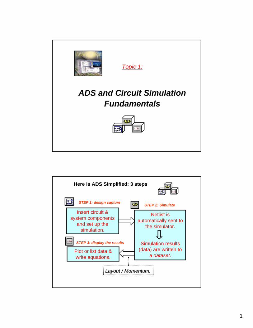
Here is ADS Simplified: 3 steps

Plot or list data & write equations.

Insert circuit & system components

and set up the simulation.

Layout / Momentum.Layout / Momentum.

Simulation results (data) are written to

a dataset.

Netlist is automatically sent to

the simulator.

STEP 1: design captureSTEP 2: Simulate

STEP 3: display the results

2

User Variables, Licenses, Directories

$HOME (UNIX variable) or %HOME% (PC variable) is usually where you run and use ADS.

$HPEESOF_DIR (UNIX variable) or %HPEESOF_DIR% (PC variable) points to where you get ADS.

LM_LICENSE_FILE points to the license file(default is: LM_LICENSE_FILE = $HPEESOF_DIR/licenses/license.dat.).

NOTE: When you install ADS, you will be prompted where to load ADS

(HPEESOF_DIR) and where you want to run ADS (PC: C:\users\default).

For this class (US laptops), you should be working in either:D:\user\ads15

or on the HP 3000- C:\user\ads15

Just in case you need to know:

ADS Windows: Main, Schematic, Status, Data Display

Main window: manage projects and open other windows...

Data Display window:plots, lists, equations

Schematic window:create / refine circuits & run simulations...

Simulation Controller

Project Directory

Default Dataset

Sim

ulat

e

Display opens

Open a schematic

Status window:simulation info: messages, errors, etc...

3

How to Start ADS...

Toolbar icons

Menu commands

Help = online manuals using internet explorer.

Project with lower level directories

You can also create an ADS shortcut.

Note the ADS tools:

To create a project, click: File > New Project and name it: lab_1

First step:

ADS Project Directory Structure and Files

filename.ds

filename .dds

data

networks

synthesis (used for E-Syn & DSP)verification (used for DRC)

mom_dsn (Momentum only)

filename.dsn Schematic & Layout files

Dataset files (simulation data)

Not required for most simulations(can be removed)

Project

Data Display files (windows to display data)

preferences & ADS netlist.log

filename. ael (application extension language)filename. atf (compiled ael)

Aut

omat

ical

ly c

reat

ed b

y A

DS

for example: lab_1_prj

4

Main window: File , View, and more...

Use icons or commands. However, not all commands have icons. But all icons have commands.

File commands:

View commands:

Zap your files :more on this later

Spice or IFF

Examples directory

Click + box to expand or -box to collapse.

Main window: Options

Main window preferences are global, they apply to all projects. The Schematic window has its own preferences.

Sets the initial palettes and simulations. For now, use: Analog/RF design.

AEL

5

Main window: Window commands...

So, let’s open the Schematic window...

If you are in a project, you can open one of these windows:

Notice the default Hot Keys

Schematic window

A new schematic becomes a.dsn file in the networks directory only after you save it.

Save your work often... All icons have labels (balloon help).

Also – use Window > Open Designs

6

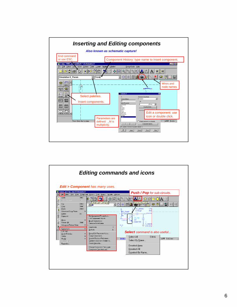
Inserting and Editing components

End command or use ESC.

Select palettes.

Insert components.

Component History: type name to insert component.

Edit a component: use icon or double click.

Parameters are defined: _M is multiplicity.

Wires and node names.

Also known as schematic capture!

Editing commands and icons

Edit > Component has many uses.

Select command is also useful...

Push / Pop for sub-circuits.

7

Library vendor parts + all your circuits

Click the + Click the + or or -- to to expand or expand or collapse.collapse.

FIND any part or search the WWW for parts.

Schematic...Click:

Select the part and it is attached to your cursor, ready to insert.

Wiring and Moving components

•• Use the wire or connect pins = wired • Point and click to snap to grid • Drag a wired component and it stays wired..•• Wire colors are in Options > Layers

Two rotation icons:

Tips for wiring!

Red pin = not connected

Click to wire:

Edit wired components:

8

Check Representation for errors

Click: Options > Check Representation

Use this if your simulation results look wrong!

Node Names in Schematics

To remove a node name:Edit > Component > Remove Node Nameor use the icon with a blank name.

• Node names result in simulation data (node voltage) in the dataset.• Node names can also connect two points without using a wire.• Global nodes can connect node names in sub-circuits:

Click the icon:

Insert > Global Node

9

Variable Equations: VAR

VAR is a declaration (initialization).Component parameters can be assigned a value using a variable equation.

Variables can be used with optimization, parameter sweeps, and many ...

Click:TIP: Add dummy (X,Y,Z) variables and then edit on-screen.

Symbols, units, and names

Circle for mutual inductance:

C (component name): changes the componentC1 (instance name): rename it: c_shuntC= (parameter): a number (unit) or valid variable.

Ccoupling_cC = x

Example of on-screen control:

QUIZ: Is this valid? Answer: _______

Slash for pin# 1 (layout):

10

Units and case sensitivity

m = milli, M = Mega, V = volts

• General Rule #1: UNIX is always case sensitive.

–– Inserting some components: R or r is OK,because after the first insert, PC will recognize either one.

• General Rule #2: PCs are case sensitive, except for:

However, some rules apply to both, for example:

& variable names are always case sensitive!

And now, let’s Simulate...

By the way, right mouse button has some commands:

First, select the Simulation Controller

Choose from PaletteChoose from Palette

HB

DC

S-Parameter

NOTE: all palettes have many of the same components (Prm Swp) and specific Meas Eqns.

Click the gear to insert the controller.

11

Set up the Simulation

Simulation requires setting the simulation controller.

Some simulations, like HB, require more setup.

DC requires no setup in most cases.

S-param requires Terms.

Edit on-screen or double click for dialog box.

*NOTE asterisk means schematic is not yet saved.

Example dialog for Controller

Edit on-screen if the parameter is displayed or use the dialog box.

Display the parameters:Display tab lists all the settings you can show on-screen.

You will get lots of practice in the

labs.

12

Templates for simulation

Insert & setup circuit, nodes and variables.

ADS 1.5 has many new templates.

Specifying a Dataset and Data Display

Before you simulate: you can name the dataset. If not, the default dataset = schematic name or the last dataset named.

Uncheck this box if desired.

Click: Simulate > Setup:

To run the simulation, click F7 key or click the gear...

NOTE: Dataset files (.ds) are in the DATA directory. Data Displays (.dds) are in the PROJECT directory & read datasets.

13

When finished, theData Display opens...

During Simulation: Status Window appears!

One way to stop a simulation, click:

Simulation/Synthesis > Stop Simulation

A successful simulation results in a dataset:

Or click: Window > Simulation Status

To stop a simulation from the schematic window.

For more sim info, set simulation controller:

Data Display window

Also, open Data Displays from schematic or the Main window:

Data displays open empty the first time, unless you use a template. Also, the default dataset shows here. If you change the dataset, the data changes, but not the format of plots or equations.

You insert plots, lists, equations.

14

STEPS: 1) Select the type: plot or list. 2) Select the data or equations. 3) Options - edit data or plot.4) Save/name the DDS window.

List or plot your simulation data

Edit the data trace or equation here.

Other datasets and DDS equations, click here!

Measurement equations from schematics will also appear here.

Def

ault

data

set

Data Displays are powerful...

Write equations to manipulate data to be listed or plotted.

Markers have readout properties you can edit. Use cursor or arrow keys to move a marker.

Scroll through lists.

Explicit dataset..path if not default.

Traces can be edited for color and thickness.

View and zoom data.

Insert Templates.

15

Tune mode is simulation!

Simulate > Tuning...

Tuning allows you to “tweak” values and see the results!

You will do this in the lab in just a few minutes...

Printing data or schematics

File >File >For Data, you can print selected plots, lists, equations.

Print Setup - select the printer, style, etc.

16

NOTE on ending ADS processes

UNIX users kill processes - PC users end processes

PC task manager -NT: ctrl-alt-delete

In a UNIX window,use: ps -ef | tailand you can kill (xxx)a processes.

hpeesofde.exe - closes the ADS program (same as exit) Hpeesofsim.exe - stops the simulation hpeesofdds.exe - end to stop the data display serverhpeesofdss.exe - end to stop the dataset server

If your computer is locked up or if there is any other problem (Data Display), you can safely stop some processes:

AVOID killing these:

hpeesofsess.exehpeesofbrowser.exehpeesofemx.exe

Killing these will require re-starting ADS.

These 2 work together!

To mail or send ADS projects: ZAP

NOTE: Archive files become .ZAP files (like .ZIP files). They can include all networks, data, and display

files (entire project).

From the Main window, click: File > Archive or Unarchive

When you leave this class, archive the projects to C:\temp and then copy the ZAP to the A drive. Be sure to delete the datasets or it will not fit on a floppy disk (not necessary if you e-mail a zap file).

For any ADS problems, call support and send the ZAP file. In the United States call: 1 - 800 473-3763.

17

Lab 1:

Circuit Simulation Fundamentals

What the lab is about ...

Learn Circuit Simulation Basics

• Create a project and schematic• Build a low-pass filter• Set up and run an S-parameter simulation• Display the results and Tune the filter• Copy an example RFIC amplifier • Insert a library part and simulate with a Template• Simulate an RFIC amp with Harmonic Balance • Display the results and write equations

NOTE: Lab 1 can be skipped if students already know the basic operation of ADS: schematic capture, simple simulation, basics of plotting data.Also, it’s OK to make mistakes…you won’t need the work you do in this lab for any of the other exercises.But starting in Lab 2, you will!

STEPS IN THE LAB:

18

Build and simulate a low-pass filter

After setting up the S-parameter simulation, tune the filter.

Also…library device simulation with template

Insert a library device & simulation template: Get S-parameters for all

swept bias points!

19

Last, example RFIC with Harmonic Balance

You will name the node Vin, check the sub-circuit, and simulate.Then write an equation for gain in the data display.

Start the lab now!

System Design Fundamentals

Topic 2:

20

System component libraries and fundamentals:

• System design is at the higher level.

• System models are behavioral: equation based describing node I and V, table based, etc.

• System components can be integrated with circuit components.

• IMPORTANT - System simulation and data display are the same as for circuit.

Typical system design using...behavioral models

Behavioral models are described by

equations.(Similar to SDD-time

domain and FDD-frequency domain.)

What are behavioral models?

21

Typical system model: Amplifier

You specify the behavior:

Write an equation for the parameter.

Also, some parameters can be optimized.

Polynomial equations describe nonlinearity:

Behavioral model

Simulation is the samefor circuit and system (behavioral):

For example, you can build an amplifier in circuit, and connect it in a system design. In this class, you will do this!

Amp circuit only Amp circuit +

behavioral system models

Simulation: both amp and

system

This is Hierarchy!

22

Data Flow simulation Data Flow simulation (Ptolemy) is 3 levels here:

1 - Circuit design 2 - System designs with Envelope or Transient3 - Data Flow (Ptolemy): bits, sinks, TK plots

DSP and CommSys coursesteach details of Data Flow simulation.However, see NOTE.

NOTE: the steps shown here are an OPTIONAL exercise in the last lab exercise in this course.

1

3

2

Lab 2:

System Design Fundamentals


23

Steps in the Design Process

• Design the rf_sys behavioral model receiver • Test conversion, budget gain, spectrum, etc. • Start amp_1900 design – subckt parasitics• Simulate amp DC conditions & bias network• Simulate amp AC response - verify gain• Test amp noise contributions – tune parameters• Simulate amp S-parameter response• Define amp matching topology and tune input• Optimize the amp in & out matching networks• Filter design – lumped 200MHz LPF use E-Syn• Filter design – microstrip 1900 MHz BPF • Transient and Momentum filter analysis• Amp spectrum, delivered power, Zin - HB• Test amp comp, distortion, two-tone, TOI • CE basics for spectrum and baseband• CE for amp_1900 with GSM source• Replace amp and filters in rf_sys receiver• Test conversion gain, NF, swept LO power• Final CDMA system test CE with fancy DDS • Co-simulation of behavioral system

You are here:

Amp and filter simulation: S-parameters

S-21 measurement verifies bandpass and gain:

24

Receiver simulation: S-parameters

Enable is for behavioral system models only.

Converted Freq = 100 MHz IF S-21 measurement tests conversion gain:

AC simulation with Budget Gain

Budget measurement verifies gain in each stage:

25

HB simulation with Noise Controller

LO with phase noise

Plot spectrum and phase noise.

Phase Noise NOTE: HB FFT oversample parameter can be increased until answer is constant!

HB simulation tests phase noise and spectrum of IF:

Transient simulation of an SDD

Compare to HB using fs function:Start the lab now!

Node currents defined by equations: I = V / Z.

dbm(fs(rf_sys_trans..Vout))

Time domain signal displayed and transformed into the frequency domain:

26

Class Exercise

HOT KEYS and Schematic Preferences

(after lab 2)

Efficient ADS Techniques

Would you like to customize the system to bemore efficient for the way you work? Here are some things you can do:

• Moveable Toolbar: PC only - put it below• Tear Off Menus: UNIX only - keep some on screen • Options > Preferences: set these to your liking• Templates - learn to use them or set up your own• Examples - familiarize yourself with them• HOT KEYS - Options > Menu / Toolbar Configuration

27

Pre-set schematic Hot Keys

Pre-configured keys:

F7 = SimulateF5 = Move Component Text

Ctrl+R = Rotate 90Ctrl+M = MoveCtrl+C = CopyCtrl+Z = Undoplus more...

Try this now: click the F5 key, select the Mixer component, move the cursor and the text will follow!

If you don’t like mouse clicks, HOT KEY your keyboard. Its global for all projects

Set the View > Zoom schematic HOT KEYClick: Options > Hot Key / Toolbar Configurations...

1. Select the command2. Type in a letter: z

(not case sensitive)3. Click: Assign4. Click: Apply5. Now,try the Z hot key

to verify it works.

Follow these steps to set Zoom Area command:

28

Next, set these Hot Keys Options > Hot Key / Toolbar Configurations...

S = Simulate > SetupA = ActivateD = DeactivateX = Edit > Move > Move & Disconnect

and any others you want ...

You will be able to use these hotkeys for all the labs in this project.

When everyone has finished, continue

If desired, set Schematic Preferences

Click: Options > Preferences

Click None to remove the grid dots.

Go to the Display tab to set a different background color.

NOTE: Set wire color in - Options > Layers.

29

Save the schematic preferences

...and the settings will then apply to all schematics in your project.

Check this to turn it on.

End of class exercise.You can also Read the .prffile into other projects.

DC Simulations and sub-circuit modeling

Topic 3:

30

DC Simulation

You get steady-state DC voltages and currents according to Ohm’s Law: V= IR

• Capacitors = treated as ideal open circuits

• Inductors = treated as ideal short circuits

• Topology check: dc path to ground (if not => error message)

• Kirchoff’s Law satisfied: sum of node current = 0

• Convergence simulator algorithms (modes) can be set

DC simulation controller

Sweep: allows you to sweepa parameter but it must be defined as a variable. Note the dialog entry automatically puts quotes on the controller (screen) entry.

Simulation Controller and Editor (dialog box)

VAR

31

...more on DC

Example: device op

point

Convergence: increase V or iterations or change mode if you don’t converge.

Back Annotation

Immediately after DC simulation, currents and voltages are available. Click: Simulate > Annotate DC Solution.

Minus sign used for current flowing out of a connection.Otherwise, current flows intoa connection or device.

DC Simulation Controller is required in all simulations ifyou want DC annotation.

Clear it here

Simulate >

No settings necessary!

Current Probe =

use values of current

in the dataset.

32

Lab 3:

DC Simulations and modeling the sub-circuit



• Design the rf_sys behavioral model receiver • Test conversion, budget gain, spectrum, etc. • Start amp_1900 design – subckt parasitics• Simulate amp DC conditions & bias network• Simulate amp AC response - verify gain• Test amp noise contributions – tune parameters• Simulate amp S-parameter response• Define amp matching topology and tune input• Optimize the amp in & out matching networks• Filter design – lumped 200MHz LPF - use E-Syn• Filter design – microstrip 1900 MHz BPF • Transient and Momentum filter analysis• Amp spectrum, delivered power, Zin - HB• Test amp comp, distortion, two-tone, TOI • CE basics for spectrum and baseband• CE for amp_1900 with GSM source• Replace amp and filters in rf_sys receiver• Test conversion gain, NF, swept LO power• Final CDMA system test CE with fancy DDS • Co-simulation of behavioral system

You are here:

33

Start with some specifications...

AMP with max gain & low noise:

Available voltage: 5 voltsDevice: Generic BJT (Gummel-Poon)Collector current: 3.25 mAFrequency: RF = 1900 MHzGain: >10 dB (or much more with this model)50 ohm match input/output

Filters: also, build 1900 MHz BPF for the input and a LPF for the IF output

Later on, test the AMP for TOI, distortion, noise, compression, GSM & CDMA modulation response, and more in labs 3 through 9.

YOUR JOB: Build, test, and refine the circuits to meet specifications.

Start with a sub-circuit model...

Model the device with package parasitics

Insert a device and a model: Gummel-Poon BJTM1. Bf will be a passed parameter. Vaf is changed as shown.

Add packaging parasitics: L in pico: pHC in femto: fF

Port connector numbers: Num=must be set in specific order as shown - this is necessary to use ADS built in transistor symbol.

NOTE: BJTM1 is the model card name that will be used for simulation. Library devices do not require this mapping.

Model Card

Create a sub-circuit to model your components:

34

Select a symbol for your sub-circuit

To use a built-in ADS symbol that looks like an NPN BJT use File > Design Parameters. . Or, draw your own symbol!

Default Symbol

Schematic view Symbol view

Its easy to use a built-in symbol:

Define the sub-circuit parameters: 2 tabs

Click: File > Design / Parameters

You define the sub-circuit general and specific parameters: • Description for library annotation • Instance name: Q• Symbol: SYM_BJT_NPN• Passed parameter for Bf = beta

You can also specify the layout: sot23

35

Insert the model in a new schematic

Insert the sub-circuit from the library.

ICONS: Push into and Pop out of the hierarchy.

Design parameters follow the sub-circuit: Q1, beta, etc.

Set up a DC curve sweep with a template

Schematic template also has the data display template:

Initialized VARs:VCE = 0 VIBB = 0 A

NOTE: DC controller sweeps the X-axis and the Parameter Sweep, sweeps the Y-axis.

Data display template:

Your model (bjt_pkg) with annotation and passed parameter: beta.

36

Finally, calculate and test the bias network

Calculate resistor values, verify the DC specs for Ib and Ic, and sweep temperature!

Start the lab now!

Back Annotation verifies DC bias

AC Simulation and Tuning Parameters

Topic 4:

37

AC Simulation

You get linear small-signal response and you get Noise values:

• DC analysis performed (unseen)

• Nonlinear devices are linearized

• Kirchoff’s Law satisfied: sum of node current = 0

• Noise contributors defined and listed

• Budget analysis available (for named nodes)

• Signal voltages are peak - noise voltages are RMS

AC Simulation Controller

AC is a linear or small signal simulation and freq is usually set in the controller not the source.

Use Display tab to toggle the Noise calculations: yes / no.

38

Turn on and set up Noise calculation

Sort by nameor by value:in the dataset

Blank gives you all contributors

Click here:

Your Node Names

NOTE: Port Noise can be included in the simulation, but it does not apply to NF. Also, Port noise is turned on/off in the sources.

Use specific sources for specific simulations

• I_AC is the component • Iac=polar (1,0) mA is the default • Arrow is the direction of current flow.

• V_AC is the component name• SRC3 is the instance name (you can change this)• Vac = polar (1,0)V is the default)• Freq = freq is a global variable - you set the start

& stop values in the simulation controller

Source parameter definitions:

Use AC sources for AC simulations!

• P_AC = is the component name • PORT1 is the instance name (OK to change)• Num=1 is the port number (use for S-parameters)• Pac = polar (dbmtow(0),0) dbmtow is a function - you enter the dbm value (*see note)

More on AC source settings...

39

Setting AC source values

NOISE and Vdc: By default, noise is turned on for the P_AC source. Use Display tab/settings to make visible. Vdc 10 mV is an offset (superposition).

Equations can also be used: P=1W, P=1+j*1W, P=complex(1,0), etc.

POWER SETTINGS: The dbmtowfunction converts power in dbm to watts for the simulator.

PHASE: The polar function specifies phase. By default, all sources are cosine waves. Use -90 for a sinewave.

Simplify by removing polar

Review of ADS Equations

• Eqn: post-simulation -Use for calculations in the data display (can include node voltages, functions, and any other dataset data).

• VAR: pre-simulation -Use for initializing sweep variables or other settings. VARs are not available in the dataset unless the OutVar function is used (later labs).

• MeasEqn: pre-simulation -Use for calculations to be available in the dataset (can use node names and functions).

schematic

data display

40

Review the Data Display equation editor

Insert button gives full path (dataset..) if not the default.

Invalid equations are red:

Error!

Click Functions Help for on-line manuals:

Click here for your DDS equations:

Gain_dB is a schematic MeasEqn.

Valid equations are black:

TIP for copy/paste in the Data Display

• Keyboard keys: Ctrl C copies to the buffer

• Keyboard keys: Ctrl V pastes from the buffer

UNIX users probably know this but it works for ADS on the PC also. Try copying a plot or equation now!

YOU CAN COPY A PLOT FROM ONE DATA DISPLAY WINDOW

TO ANOTHER ALSO!

41

Lab 4:

AC Simulations and Tuning Parameters




You are here:

42

Set up the circuit & simulate with Noise

NOTE: Freq is a global variable.Here, Freq is controlled by the source. Use freq=freq, freq=10 MHz, or a variable: freq=F_RF.

Use ideal DC blockers.

Vcc is a node name.

Vin and Vout nodes provide data (noise and voltage) for equations.

V_AC source voltage = 1 V, cosine wave.

MeasEqn:

Simulation results...Write the same equation in Data Display as you did in schematic. Then put it in a list.

Edit the traces on-screen: all are equal.

Two schematic MeasEqns: One Data Display eqn:

43

More AC results...

Calculate group delay with an equation using Phase data. Also, control marker

readout formats.

Use the what function…what?

Examine the data using the whatfunction and the Variable Info.

44

Sweep battery voltage

For an AC simulation, use a parameter sweep of a dc value which is assigned to a VAR.

Note the explicit dataset path..

OPTIONAL - tune sub-circuit parameters

Start the lab now!

Set up a variable in the sub-circuit and tune several parameters from

the top level.

45

S-parameter Simulation and Optimization

Topic 5:

S-parameters are Power Ratios

Results of an S-Parameter Simulation in ADS• Read the complex reflection coefficient (Gamma) • Change the marker readout for Zo• Read all four S-parameters• Smith chart plot: use for impedance matching (S11 and S22) • Similar to Network Analyzer measurements

• S11 - Forward Reflection (input match - impedance)• S22 - Reverse Reflection (output match - impedance)• S21 - Forward Transmission (gain or loss)• S12 - Reverse Transmission (isolation)

S-parameter ratios: S out / S in

These are easier to understand and simply plotted.

These are best viewed on a Smith chart (next slides).

(voltage ratios squared)

46

The Impedance Smith Chart simplified...

Bottom Half:Bottom Half:Capacitive Capacitive

Reactance (Reactance (--jx)jx)

Top Half:Top Half:Inductive Inductive

Reactance (+jx)Reactance (+jx)

OPENSHORT

This is an impedance chart transformed from rectangular Z. Normalized to 50 ohms, the center = R50+J0 or Zo (perfect match).For S11 or S22 (two-port), you get the complex impedance.

Circles of constant Resistance

Lines of constant Reactance (+jx above

and -jx below)Zo (characteristic impedance) = 50 + j0

25 50 100

The Smith chart in ADS Data Display

Z=0+j1

Z=0-j1

Z=infinity + j infinityGamma or S11= 1 / 0

m1m1

ADS marker defaults to:

S(1,1) = 0.8/ -65Z0 * (0.35 - j1.5)

but can be changed give values in ohms.

Z=0-j0.5Z=0-j2

S(1,1): mag / phase0 to 1 / 0 to +/- 180

Reflection Coefficient: gamma

Z = real / imaginary0 to +infinity / -infinity to + infinity

Z= 0 + j0Gamma or S11=1 / 180

Impedance: Z

Z = 1 + j0

47

S-Parameter Simulation Controller

Default sweep = Freq

Sweep plan can also be used (see next slide). Either way, simulation data (S matrix) will be for the specified range and points.

The simulator requires port termination: Num = 1

Other S-Parameter controller tabs

Calculate other parameters.

Enable Frequency Conversion for a mixer.

Calculate SS noise - same as in the AC simulation.

Parameters Noise

NOTE: Insert the Options controller for a noise simulation = no error message on temperature.

48

Sweep Plan with S-parameter simulations

Sweep Plan is for sweeping FREQ. Otherwise, use a Parameter Sweepfor variables (Vcc, pwr, etc.)

Here is a sweep within a sweep.

These are ignored if

Sweep plan is selected!

Mixer designers: Here is a plan for an RF, LO, and IF.

Typical S-parameter plots: ADS data display

Plotted S21 in dB vs frequency Plotted S11 on a Smith Chart:note marker readout.

Complete S-matrix with port impedanceNote marker readout is x50.

49

S-Parameter measurement equations

Arguments explained briefly here.

You will use some of these in the labs...

All simulation palettes have specific measurement equations. You insert the measurement equation and set the arguments if necessary. Here, S is the matrix, 30 is the value in dB, and 51 points used to draw the circle.

Example: 3 circles for 3 different values of gain.

Creating Matching Networks

• Various topologies can be used: L, C, R• Avoid unwanted oscillations (L-C series/parallel)• Yield can be a factor in topology (sensitivity)• Use the fewest components (cost + efficient)• Sweep or tune component values to see S-parameters• Optimization: use to meet S-parameter specs (goals)

NOTE: For a mixer, match S11 @ RF and S22 @ IF.

In the lab, you will optimize the match for the amplifier.

50

Matching means:

Moving toward the center of the Smith Chart!

Add Series or Parallel (shunt)components. .

You will do this in the lab.

Adjust the value to move towardopen, short, L, C, orcenter of chart.

Series

L

Parallel CSerie

s C

Para

llel R

Parallel L

Serie

s R

ADS Optimization Basics

Start with a simulation that gives you results.

Set up the optimization which includes:

A search method.A specific goal or specification to be met.Enabled components or parameters to be adjusted.

NOTE: ADS has both continuous and discrete optimization. Yield analysis or a yield optimization is also available.

DEFINITION: Optimization is a simulation that tries to achieve a performance goal.

51

Optimization palette: Controller and Goals

Type of Optimization:In general, we recommend In general, we recommend using Random first, then using using Random first, then using Gradient. Also, first tune and Gradient. Also, first tune and then optimize.then optimize.

Four steps for optimization:

Optim controller: set the type, etc.

Goal statement: use valid measurement equation or dataset expression.

Enable component (opt).

Simulation controller.

Many Types are Available

NOTE: See manual for details (minimax function works well for filters).

Random & Gradient are often used together…

52

Goals and Error Function

Error function is defined as a summation of residuals.A residual ri may be defined as:

ri = Wi | mi - si |is the simulated ith response (example: S21= 9.5dB)is the desired response for the ith measurement (example: S21=10dB)is the weighting factor for multiple goals: higher number is greater.

Simulations continue until the maximum iterations is reached or the error function (summation of the residuals) reaches zero (same as 10 dB).

The goals are minimum or maximum target values.The error function is based on the goal(s).The weighting factor prioritizes multiple goals.

simiWi

More about the Error Function...

Least Pth: The Least Pth error function formulation is similar to the previous one, except that instead of squaring the residuals, it raises them to the Pth power with P=2 , 4 ,6 etc.

Minimax: attempts to minimize the largest of the residuals. This tends to result in equal ripple responses .

Worst case: minimizes the reciprocal of the least squares error function. This has the effect of maximizing the error function. The goal is to find a worst typical response for a given set of parameters.

Least Squares: Each residual is squared and all terms are then summed. The sum of the squares is averaged over frequency.

Choice of optimizer determines these settings.

53

Using a combined approach...

Random analysis often gets you close to the goal (minimum error function).

Gradient analysis may get stuck in a local minimum (not optimal error function).

Using both RANDOM and GRADIENT can reach the desired goal - others work similar (genetic, etc.).NOTE: Random is not

totally random. It uses an adaptation that helps it move closer to the goal.

You will do this in the lab!

Erro

r fun

ctio

n

Parameter value

Hybrid

ADS Optimization Setup

Edit the component, then click to enable for optimization.

Optim palette: insert controller and goal (more on this later)

You always need a simulation controller.

Set the step for the RangeVar

Details on next slide:

54

Enabling components for opt or stats (yield)

PPT is an optimization within a Yield Analysis only. Allows value to be shifted to achieve goal.

Once enabled, you can specify a continuousor discrete (stepped) variation..

Gaussian, Uniform, or discrete. Results will be viewable in the data display.

NOTE: If discrete values are not realistic, use file based: DAC

noopt = disabled (after optimization):

Discrete Optimization for Library Parts

Inserted library part with listed range of values (like a DAC)

55

Yield Analysis: % meeting specs!

Step 1- Copy: examples / Tutorial / yldex1_prj

Example: 200-400 MHz (50-to-100 ohm) Impedance Transformer. Simulation tests the % of circuits to meet spec using component values with defined statistical distributions (stat).

NOTE: Optimize yield results by changing the nominal values until you get maximum (near 100%). See: examples/Tutorial/yldoptex1_prj

Randomseed

Opt previously run

As an extra exercise:

Yield Analysis Results (data)

Spec is -18 dB S11from 200 to 400 MHz.

78% will meet spec

Step 2 - Run the simulation once. Then change the specs and resimulate. Or, try it on your own circuit!

Zoom view: small number of results outside of spec.

Refer to this and the previous slide to setup your own Yield analysis

after the class.

Yield Dataset results are stochastic.

56

Additional information:frequency sensitive components!

Z-PORT: equation describes changing Z with changing freq

if then elseif then elseif then else endif

Note the ADS syntax for Z increasing as freq (global variable in ADS) decreases:

CAPQ and INDQ: equation describes changing L or C with freq

Lab 5:

S-parameter Simulation and Optimization


57



You are here:

First Step: Simulate with ideal components

•Plot the data and compare to ac_sim data.•Change Term Z and list the S matrix.

2 different datasets

58

Calculate C and L values and re-simulate

Reactance of 10 pF at 1.9 GHz and a list of L values:

Tune the input match

Click here to change the value in steps. Then press Tune.

Set min and max ranges and step size.

Use 1 or 0

Use detailed Tune control with small

increments!

59

Optimize the output & input match

• Random with 2 goals• S11: -10 dB• S22: -10 dB

• Set up the OPTIM controller• Set up the GOALS• Enable the components• Setup the simulation

REVIEW of 4 steps:

Display opt data, update and simulate

Final values look good!

60

Next, use built-in measurements

S-parameter simulation with gain and noise circles, and stability.These are built-in measurement equations from the simulation palette.

NOTE: Listed results from noise turned on in the simulation controller.

You set the arguments if necessary!

Last step: Read / Write data filesWrite an ADS “S” dataset as a Touchstone file,then Read it back in... as if it came from a Network Analyzer!

Use a Sweep Plan and compare the data.

Start the lab now!

61

E-Syn, Momentum, Transient and the DAC

Topic 6:

Using E-SynWhat does E-Syn do?It makes it easy to create FILTERS and Matching Networks.

E-Syn user interface is a little different than the ADS interface. Also, you could use a Filter Design Guide instead of E-Syn. This may appear in future releases of ADS!

• You specify the TYPE of design, the RESPONSE, and the BAND.

• SYNTHESIZE the design and you get a selection of topologies and values.

• ANALYZE the design and plot the response in the ADS data display. Optimize if desired.

Quick S-parameter simulation

62

Using MomentumWhat is Momentum? E-M (electro-magnetic) solver using Method of Moments technique and Green’s functions to compute the current in planar structures, including vias and the coupling between surfaces.

Why use Momentum?• You have no accurate model for a passive layout.• You want to know the coupling effects between structures.• You want to optimize the layout real-estate, performance, etc.• Your other structure simulator takes too long to simulate!• You want to use the results in ADS simulations.

Example spiral meshed as a “strip”geometry.

Hole in ground plane is meshed as a “slot”, which is more efficient than meshing the entire ground plane.

MOM engine gives S-parameter results

Antenna patterns!

Transient simulation

• Analysis performed in the Time Domain• Use any Source • Solutions use Newton_Raphson iterations• You get Amplitude vs. Time• Time Domain data can be transformed: FS

NOTE on Convolution:Frequency domain models (microstrip) can be brought into the time domain and converted to the time domain -then convolved with the time-domain input signal to obtain the time-domain output signal. The convolution tab in the transient simulator allows you to define methods and settings.

63

Transient simulation controller

Integration: step control & error (default:Fixed)

Time Step is critical !Time Step is critical ! Ignored if no TL’s

Setting the Transient Time Step

Use the Nyquist rule: Sample at 2 x or morethe rate of the highest frequency of interest:

To sample the fundamental (1900 MHz) plus harmonics,you must calculate @ 2 x (rate of highest harmonic desired).

1 / (2 x 15 x 1900MHz) = 17.54 picoseconds.

Start time: sampling beginsStop time: sampling endsTime step: sampling rate Sample @ 2 x BW

64

Setting the Transient Stop Time

For many circuits: stop time should allow for periodic - settling.

Stop Time

NOTE: Transient analysis can be tricky. Sampling before a circuit reaches steady state will not give correct results when transformed into the frequency domain. Also, you must use a time step that is a multiple of the frequencies of interest or the results will not be correct.

Start Time

Dataset

Using a DAC (data access component)For optimization, R1 is assigned to a file which is read by the DAC. “res_std.dscr” contains an index and a list of values (r_val). In the DAC, variable iVal1 is enabled over the range of indexed values beginning with iVar1 which is the first index point in the file.

The file must be in the DATA directory and must be in correct

format. The circuit simulation manual has information on file

formats such as DSCR..NOTE: iVar1 always = 1 (index at first column). However, iVal1 always starts at 0 (same as ADS data).

65

DAC Optimization: setup and results

Save values = no. Only the MeasEqn is sent to the dataset with the final iVal1 which is 0 = 56 ohms which gives the least reflection. Also, click Simulate > Update Optimization Values to update the iVal in the DAC.

EXTRA NOTE: TDR Setup

DUTDUT

TLIN is 360 degrees at 1 GHz = TLIN is 360 degrees at 1 GHz = known timeknown time--domain response used domain response used

as a reference.as a reference.

After the class, you can use this slide as a reference if you need it!

REFERENCE SLIDE ONLY

Find mismatches in time / distance

66

EXTRA NOTE: TDR Data Display

Results:mismatchdelay time

rhoBW

VSWRmtrs to mils



EXTRA NOTE on LineCalc and Model Composer

• Define the substrate• Enter L & W to get electrical• Enter electrical to get L & W



ALSO - New add-on for ADS 1.5: MODEL COMPOSER. Generate your own passive library models (parameterized) for simulation. You get circuit simulation speed with EM simulation accuracy (Momentum) for microstripcomponents - more types in the future!

LineCalc is still available!

67

Lab 6:

Filters: E-Syn, Momentum, Transient Simulation

and the DAC




You are here:

68

Step 1: Start E-Syn in the ADS

schematic window:

Tools > Start E-Syn

Step 2: Set the Frequency Specification and click: Select Type.

E-Syn - 200 MHz LPF design

Step 3: Select the design: Type, Response, and Band.

Step 4: Go back to E-Syn main menu and click the Synthesis icon:

E-Syn - 200 MHz LPF (continued)

At first, window will be blank. Therefore, click the Synthesize button to calculate topology & component values as shown here.

69

Step 5: Select the Network you want to use and then click Analysis.

Step 6: Set up the simulation and Analyze. The results will appear in the

ADS Data Display window.

E-Syn - 200 MHz LPF (continued)

Result of design (Butterworth) to be used in Final simulation.

Transient simulation of 1900 MHz BPF

Microstrip coupled line filter with substrate and VtSine source.

Also calculate delay:

70

Generate the Layout of 1900 MHz BPF

Remove controllers and Terms - insert Port connectors

Use MOM menus ...

MOM: substrate, mesh, simulation

Compare to circuit S21:

71

MOM - calculate coupling effects

Coupled Line Filter

…draw a trace in close proximity

Momentum simulation shows resonance from

coupling.

Use the same setup and add a rectangle:

OPTIONAL - DAC exercise

After setting S-parameter controller to calculate Z, results show results.

Write the file

Start the lab now!

72

Harmonic Balance

Topic 7:

Harmonic Balance Simulation

Analyze circuits with Linear and Non-linear components:

• You define the tones, harmonics, and power levels• You get the spectrum: Amplitude vs. Frequency• Data can be transformed to time domain (ts function) • Solutions use Newton-Raphson technique• Krylov subspace method also available (large circuits) • Use only Frequency domain sources• Similar to Spectrum Analyzer

73

Harmonic Balance Simulation Flow Chart

Measure LinearCircuit Currents

in the Frequency-Domain

StartSample Points

Number of HarmonicsSimulation Frequency

Error Tolerance

• Inverse Fourier Transform: Nonlinear Voltage Now in the Time Domain

• Calculate Nonlinear Currents • Fourier Transform: Nonlinear Currents

Now back in the Frequency Domain

Measure NonlinearCircuit Voltages

in the Frequency-Domain

DC analysisalways done

Linear Components

Test: Error > Tolerance: if yes, modify & recalculate

if no, then Stop= correct answer.

Nonlinear Components

Kirchoff’s Lawsatisfied!

Example Circuit: First and Last Iterations

IDIR IC IL

If I error is notnear zero, then iterate again..

IY

IRIC IL ID IY-port

Initial Estimate: spectral voltage

V Final Solution

If within tolerance

IR IC IL ID IY

Start in theFrequency Domain Convert: ts -> fs

Test uses (Kirchoff’s law):

Last Estimatewith least error

Calculate currents

NOTE: Try building the circuit, simulate, and write an equation to sum the currents.The IY-port could be S-parameter data from Momentum or other NWA data.

then

(Momentum file)

74

Basic 1 Tone HB simulation setup

Basic HB controller and source setup gives you spectral tones:

Freq[1] is the fundamental tone you want HB to calculate. Freq[1] must match a tone in the circuit or you get a warning message.

Order [1] = 3 means HB calculates 3 harmonics of Freq [1]

Numerous built-in sources and measurement equations.

HB gives you a Mix table:

Swept variables in Harmonic Balance

1) Initialize the VAR to sweep. 2) Specify the variable and range.

3) Be sure the VAR, the source, and simulation controller all have the same information.

NOTE: Swept variables always go to the dataset.

HB Freq tab: specifytones (Freq),harmonics (Order), andmixing products (Max Order).

75

Other settings (tabs) in Harmonic BalanceParams

Osc

Noise (1 and 2) or use Noise Controller

ADS 1.5: Save (final solution) and re-use (initial guess).HB binary data file.

NOTE Oversample: Set status level to 4, see number of samples for non-linears. Then set oversample for convergence or more accuracy.

Use with Oscport

Related harmonic balance controllers ...

Transform HB spectrum into the time domain with ts function: ts(Vout).

You will use HB and XDB in the lab!

Calculated S-paramsfor harmonics.

76

Types of Power Sources for HB

Default power function for these sources is polar,but you can simplify it on the screen as: dmbtow(0)Therefore, dbmtow(0) is the same as polar(dbmtow(0),0)

Notice that these sources are also ports (OK for S-param analysis).Also, they can be considered noiseless like sources in a measurement system.

P_nTone and P_nHarmcan have multiple Freqsand Power.

Example: HB simulation setup for mixerwith swept LO power

Freq [1] fundamental tone (most power: LO for mixer) Freq [2] fundamental tone (RF for mixer)Order [1] number of harmonics for Freq [1]: LO.Order [2] number of harmonics for Freq [2]: RF.MaxOrder = mixing products, depends on Order[n].NOTE: Here if MaxOrder = 9 , you won’t get 9th order productbecause Order[1] and [2] only go up to the 8th order.

Other settings: for status info, noise, and Krylov simulator (used in lab).

Do not do this: Freq = LO_freq MHzor MHz units will multiply. data

Mixer example:

To get any other VAR to the dataset (RF_pwr) requires using this syntax: OutVar =“variable name”

LO_pwr goes to the dataset automatically.

77

Example data: use mix function on Mix table

DC term=0. Freq, harmonics [order], and products [max order] are indexed:

QUIZ: Can you use this equation dBm(Vout[1]) for this data? Is it valid?

Answer: YES - if no other dependencies exist - it’s the same as: dBm(mix(Vout,{-1,1}))

To get dBm of IF (100 MHz) at Vout,use the mix function:

Arguments in parentheses ( ) and curly braces {generate the matrix }, required for Mix table.

Mixer example: Max order=8 LO order=5 RF order=3

LO RF

8th order term uses +5th & -3th, but not:-3th & +5th (+5th of RF does not exist).LO: Freq[1]=1800 MHz RF: Freq[2]=1900 MHz

Harmonic Balance convergence & errors

HB convergence error message:“cannot sweep to desired level”or “arc length continuation error”To solve these problems, either loosen the V and I tolerances in the options controller by ten times (for example, set: I_AbsTol= e-11), or reduce the step size for power or frequency sweeps.

Simulator will try to find closest answer, if notit will continue with all remaining valid points.

Freq [x] in each source must match Freq [x] in the controller or you get this message:

NOISE TEMP error for all noise simulations: Set Temp=16.85 to eliminate any error message.

OPTIONS controller is in all simulation palettes.

78

TIP about “quotes”, brackets, braces, etc.

QUOTES:• Only when editing on the screen for string value parameters, if necessary. • When in doubt, double click and use the dialog boxes.

In dialog only: @ stops quotes when not needed.

If you see 2 quotes “”X””, remove one set!

Parentheses, Brackets, Curly braces:

(parentheses for function arguments)[brackets for one, two, or three dimensional data]: {curly braces for vectors and the mix function}:

Examples: dBm(Vout [1]) dBm(mix(Vout,{-1,1})) mag(Vout [1:: 6]

Exceptions - Swept variables are always in quotes and controller names (“HB1”) in opt goals.

Double colon is a wildcard in ADS:

Lab 7:

Harmonic Balance Simulations


79



You are here:

First, HB for spectrum and Meas Eqn

Dataset contains node voltages and Mix table

Equation uses Vout[1]

Spectrum

Dataset values

80

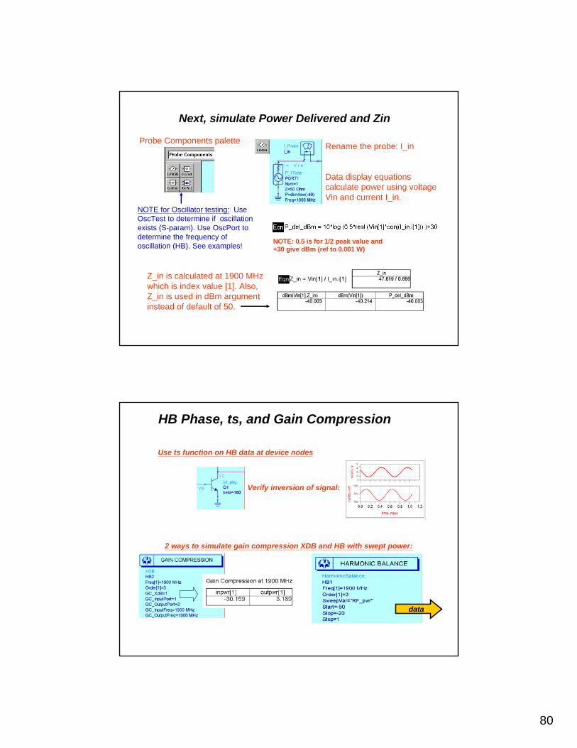
Next, simulate Power Delivered and Zin

NOTE: 0.5 is for 1/2 peak value and +30 give dBm (ref to 0.001 W)

NOTE for Oscillator testing: Use OscTest to determine if oscillation exists (S-param). Use OscPort to determine the frequency of oscillation (HB). See examples!

Data display equations calculate power using voltage Vin and current I_in.

Rename the probe: I_in

Z_in is calculated at 1900 MHz which is index value [1]. Also, Z_in is used in dBm argument instead of default of 50.

Probe Components palette

HB Phase, ts, and Gain Compression

Use ts function on HB data at device nodes

2 ways to simulate gain compression XDB and HB with swept power:

data

Verify inversion of signal:

81

HB swept power compression data

Plot_vs(dB_gain,hb_comp..dbm_out)Plot_vs function

Creating a line: nonlinear to linear

Simulating closely spaced tones...

AMPS use 2 tones, such as RF +/- spacing (VAR)

IF

[2, -1]

- LO, 2RF1 - RF2

- LO, RF1

- LO, 3RF1 -2RF2

[-1, 2,-1] [-1, 1, -2][-1, 1, 0]Mix index [tone 1, tone 2, tone 3]:

RF1 + SPACING

RF2 + SPACING

RF1 - SPACING

[1, 0]

RF2 - SPACING

Freq[1]

Freq[2]

Mix table

Lab setup and data

[-1, 2] [0, 1]

Mixer is 3 tones

82

Two-tone HB simulation and dataSpacing @ 10 MHz = 1.895 and 1.905 GHz

Use [ brackets to generate a matrix ] and { curly braces to

vector the data from Mix table}

TOI or IP3 Measurement

When the input power drives the non-linear device into saturation or distortion, third order products near the desired frequency can become large. The point at which 3rd order products intercept the linear rise in output power is the intercept point TOI or IP3.

-40 - 30 -20 -10 0 10 20

10

0

-10

-20

--30

TOI

3rd order intermod product

(dBm) at Voutslope = 3.

Linear Outputof fund(dBm)

slope = 1

Input Power (dBm)

Output Power (dBm)

A measurementequation is

used to get the answer...

mix {1,

0}

mix

{2, -

1}

NOTE for mixer 3 tones use:mix{-1,1,0}

mix {-1, 2, -1}

Lab setup and data

83

IP3 or TOI simulation setupBuilt-in measurements use functions -you set the arguments.

NOTE: Mixers use this setup for 3 tone TOI.

Result of IP3 eqns in DDS:

OPTIONAL: Sweep RF pwr vs TOI

Compare swept values to values in the TOI measurement range:

Swept values used for IP3

The Eqn, my_toi, is on the right Y axis. When RF_pwr is greater than 39dBm, RF and third order slopes are no longer 1:3, so IP3 Eqnbecomes invalid.

Start the lab now!

84

Circuit Envelope Simulation

Topic 8:

What is Circuit Envelope ?

• Time samples the modulation envelope (not carrier)• Compute the spectrum at each time sample• Output a time-varying spectrum• Use equations on the data• Faster than HB or Spice in many cases• Integrates with System Simulation & HP Ptolemy

85

Use realistic Signals with CE

– Adjacent Channel Power Ratio– Noise Power Ratio– Error Vector Magnitude– Power Added Efficiency– Bit Error Rate

2-tone tests and linearized models do not predict this behavior as easily!

GSM, CDMA, GMSK, pi/4DQPSK, QPSK, etc.40 kHz BW for NADC

890 MHzcarrier

Simulations include:

Circuit Envelope Technology:

Time sample the envelope and then

performs Harmonic Balance on the samples!

V(t) * e j2π fot

tt11

tt44tt22

tt33

ModulationCarrier

Periodic input signal

NOTE: V(t) can be complex - am or fm or pm

Circuit Vout

86

…more on CE Technology

Captures time and frequency impairments:

dBm (fs (Vout))

CE example: AMP with RF pulse

•mag of Vin [1]: envelope• ts of Vout: signal• mag of Vout [1]: envelope

Step time is critical for sampling the envelope: rise, fall, and modulation rate. Therefore, Step (sample time) is NOT the same as Transient.

You will do this in the lab!

...where [1] is the carrier Freq[1].

ONE TONE

87

Env Setup tab in dialog

Time step– Determines bandwidth of Circuit Envelope simulation– Small enough to capture highest modulation frequency

Stop time– Determines resolution bandwidth of output spectrum– Large enough to resolve spectral components of interest

(Reference slide for one tone with 3 harmonics)

more

Time step

Modulation BW

Resolution BW

Stop Time

ENV Steup tab (continued)

7 Harmonics of Fundamental: Freq [1]3 Harmonics of Fundamental: Freq [2]

Harmonic Balance

t0

t1

time

t2t3

t4

(Reference slide for multiple tones: mixer)

Multiple tone simulation requires more data display

88

Lab 8:

Circuit Envelope Simulations




You are here:

89

First, simulate an RF pulse

Use a behavioral amp and different time steps:

Add distortion: get odd harmonics out-of-phase!

Next, phase distortion bits (baseband)

After simulating the response of the amplifier, insert a filter at Vin to alter the phase response.

Look at the bit stream:bits_out node and Vout.

Plot the GSM BW spectrum with windowing.

90

GSM source on your amp_1900

Verify baseband integrity using an equation that is like a demodulator:

Simulation with variables set t_step = 1 / (5X BW of GSM)

Optional - channel power calculation

On a new page in DDS, write two equations:limits defines the bandwidth and

channel_pwr calculates power in the channel.

Start the lab now!

No need to resimulate, simply use Vout[1] which is 1900 MHz!

91

Final Circuit / System Simulation and Co-

Simulation

Topic 9:

What is the final topic in this class?

• Simulation of your amp_1900 and filters in the receiver system to verify analog performance.

• Co-simulation: simulation of the entire system using digital circuits and analog circuits together.

Constellation, spectrum, etc...

Gain (S-21), HB with swept LO, and CE with a CDMA source

A little on co-simulation before starting the lab...

The co-simulation is optional if you have time - otherwise, take the CommSys class.

92

What is a co-simulation?

Man can not live by DSP alone

Agilent Ptolemy: a bridge between DSP and RF/Analog

worlds

It is your amp_1900 and filters in the receiver system at the bottom level. On the top level is a Data Flow simulation.

Co-simulation is digital & RF/analog circuits simulating together.

This is your rf_systemwith amp_1900.

What is Ptolemy ?

• TSDF is a unique Agilent EEsof Innovation• Agilent Ptolemy adds timed elements

- parameters on signals are t, I, Q, Fc (rf carrier)

• Benefits:- easy to add real RF effects on signals- more efficient simulations- more accurate modeling of RF effects

Agilent Ptolemy is a Timed Synchronous Data Flow Simulator

Agilent Ptolemy is the data flow simulator used in the DSP schematic window...

93

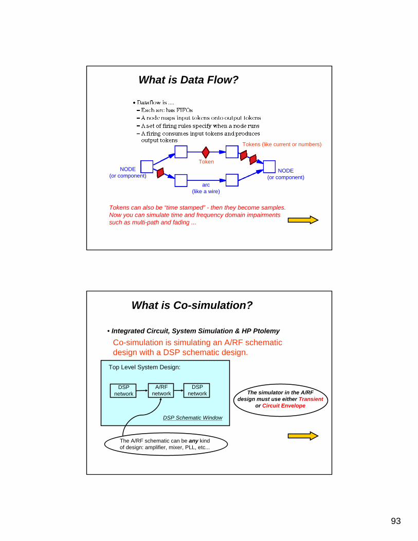
What is Data Flow?

Tokens can also be “time stamped” - then they become samples. Now you can simulate time and frequency domain impairments such as multi-path and fading ...

arc(like a wire)

NODE (or component)

NODE (or component)

Token

Tokens (like current or numbers)

What is Co-simulation?

• Integrated Circuit, System Simulation & HP Ptolemy

Co-simulation is simulating an A/RF schematicdesign with a DSP schematic design.

Top Level System Design:

DSPnetwork

A/RFnetwork

DSPnetwork

The A/RF schematic can be any kindof design: amplifier, mixer, PLL, etc...

The simulator in the A/RFdesign must use either Transient

or Circuit Envelope

DSP Schematic Window

94

The DSP components library…Many palette selections and additional libraries:

The use of these tools is covered in the DSP course and also in part of the CommSys course. In this class, it is only briefly introduced!

Lab 9:

Final System Simulation using: amp_1900 and filters


95


• Design the rf_sys behavioral model receiver • Test conversion, budget gain, spectrum, etc. • Start amp_1900 design – subckt parasitics• Simulate amp DC conditions & bias network• Simulate amp AC response - verify gain• Test amp noise contributions – tune parameters• Simulate amp S-parameter response• Define amp matching topology and tune input• Optimize the amp in & out matching networks• Filter design – lumped 200MHz LPF use E-Syn• Filter design – microstrip 1900 MHz BPF • Transient and Momentum filter analysis• Amp spectrum, delivered power, Zin - HB• Test amp comp, distortion, two-tone, TOI • CE basics for spectrum and baseband• CE for amp_1900 with GSM source• Replace amp and filters in rf_sys receiver• Test conversion gain, NF, swept LO power• Final CDMA system test CE with fancy DDS • Co-simulation of behavioral system

You are here:

First, system setup with S-params

Setup sub-circuit using: File > Design Parameters

First, simulate system S21 with frequency conversion to see gain!

96

Next, HB simulation with swept LO

Noise measurement givesNF and conversion gain when status level = 4.

dBm_out vs LO_pwr

OutVar = “variable” to dataset

Final system CE simulation with CDMA

NOTE: Other = SaveToDataset = no It means only the MeasEqn IF_out goes to dataset.

data

97

Power calculations from an example DDS

Simply change the eqn name to Vfund=IF_out and all the data fills in the plots and equations values!

1. Open the example DDS file from the Tutorials/ModSources /IS95_Fwd_PwrCalcs

2. Save it in your system_prj.3. Change the dataset and MeasEqn

Vfund = IF_out

Use your CE data:

Fancy Data Display for CDMA spectrumSet up a marker slider using equations: m1 slides to a frequency and the spectrum of that carrier frequency is displayed: RF, LO, IF, etc.

m1 is at the IF

NOTE: If you finish this step in the lab, you have achieved all the goals for this class!

98

OPTIONAL - Co-simulation of rf_sysThis process requires several steps:

First step: Modify the system to become a sub-circuit (bottom CE simulation level) as shown here. Co-simulation requires a Transient or CE simulation setup.

In this class, it is easier and faster to set up and run co-simulation using the behavioral system. The Extra exercise shows even more co-simulations you can try after the course!

Co-simulation continued...Next step: Open a top level DSP network so that the Ptolemy / DSP palettes become available in schematic.

Then build the system shown here:All the steps are in the lab, including the settings for the data components, filters, etc. The t_step and t_stop are now set for symbol rate and time.

Bottom level system.

Data flow controller runs showing filtered bits and IF signal: TkXY plots

99

Data Flow simulation - TK plots are active!

Quit the DF simulation and connect a SpectrumAnalyzer sink to collect the data. Results of this co-simulation show spectrum of the behavioral system. To use amp_1900 and your filters, replace them in the system and setup a new simulation (requires more time).

Spectrum Analyzer sink:

Start the lab now!

By the way...RF Board and RFIC Design Flow Integration Solutions from Agilent EEsof EDA

• Software and Services available to integrate ADS into existing design flow based on:

– Schematic transfer via IFF– Layout transfer via IFF– Schematic sharing via Dynamic Link

• For more info, contact your Agilent EEsof Sales Representative, or visit:

RFIC Design Flow:http://www.tm.agilent.com/tmo/hpeesof/products/ads/prod600a.ht

mlRF Board Design Flow:

http://www.tm.agilent.com/tmo/hpeesof/products/ads/prod600b.html

100

End of the Course

Look for us on the WWW for more ADS training and

applications.

Goodbye and see you next time!www.agilent.com

Agilent EEsof EDA - Customer Education

Before you leave, please fill-out the course evaluation…thanks!

ADS and Circuit Simulation Fundamentals

Documents

Transcript of ADS and Circuit Simulation Fundamentals