Admixture and ancestry inference from ancient and modern ...
51
Wayne State University Human Biology Open Access Pre-Prints WSU Press 7-1-2016 Admixture and ancestry inference from ancient and modern samples through measures of population genetic driſt Alexandre M. Harris Pennsylvania State University, [email protected] Michael DeGiorgio Pennsylvania State University, [email protected] is Open Access Preprint is brought to you for free and open access by the WSU Press at DigitalCommons@WayneState. It has been accepted for inclusion in Human Biology Open Access Pre-Prints by an authorized administrator of DigitalCommons@WayneState. Recommended Citation Harris, Alexandre M. and DeGiorgio, Michael, "Admixture and ancestry inference from ancient and modern samples through measures of population genetic driſt" (2016). Human Biology Open Access Pre-Prints. 114. hp://digitalcommons.wayne.edu/humbiol_preprints/114
-
Upload
khangminh22 -
Category
Documents
-
view
1 -
download
0
Transcript of Admixture and ancestry inference from ancient and modern ...

Wayne State University
Human Biology Open Access Pre-Prints WSU Press
7-1-2016
Admixture and ancestry inference from ancient andmodern samples through measures of populationgenetic driftAlexandre M. HarrisPennsylvania State University, [email protected]
Michael DeGiorgioPennsylvania State University, [email protected]
This Open Access Preprint is brought to you for free and open access by the WSU Press at DigitalCommons@WayneState. It has been accepted forinclusion in Human Biology Open Access Pre-Prints by an authorized administrator of DigitalCommons@WayneState.
Recommended CitationHarris, Alexandre M. and DeGiorgio, Michael, "Admixture and ancestry inference from ancient and modern samples throughmeasures of population genetic drift" (2016). Human Biology Open Access Pre-Prints. 114.http://digitalcommons.wayne.edu/humbiol_preprints/114

Pre-print version. Visit http://digitalcommons.wayne.edu/humbiol/ after publication to acquire the final version.
Admixture and ancestry inference from ancient and modern
samples through measures of population genetic drift
Authors: Alexandre M. Harris (Pennsylvania State University), Michael
DeGiorgio (Pennsylvania State University)
Corresponding Author: Michael DeGiorgio Pennsylvania State University
[email protected] 502B Wartik Lab University Park, PA 16802
Abstract: Methods that leverage the information about population history
contained within the increasingly abundant genetic sequences of extant and
extinct Hominid populations are diverse in form and versatile in application.
Here, we review key methods recently developed to detect and quantify
admixture and ancestry in modern human populations. We begin with an
overview of the f- and D-statistics, covering their conceptual principles and
important applications, as well as any extensions developed for them. We then
cover a combination of more recent and more complex methods for admixture
and ancestry inference, discussing tests for direct ancestry between two
populations, quantification of admixture in large datasets, and determination of
admixture dates. These methods have revolutionized our understanding of
human population history and additionally highlighted its complexity. Therefore,
we emphasize that current methods may not capture this population history in its
entirety, but nonetheless provide a reasonable picture that is supported by data
from multiple methods, and from the historical record.
Keywords: Introgression, Contamination, Ancient DNA, Genetic drift,
Microsatellite
Short Title: Ancestry and admixture inferred by drift
Submitted: December 15 2016
Accepted: May 4 2017
The wealth of genome-wide polymorphism data from diverse human
populations around the world (Cann et al., 2002; Gibbs et al., 2003; Altshuler et al.,
2010; McVean et al., 2012) has allowed researchers to access a record of human
history unprecedented in its breadth, spanning thousands of years (Patterson et al.,
2012; Jones et al., 2015; Mendez et al., 2015; Lazaridis et al., 2016). With this data,
new insights into human migration (Rasmussen et al., 2014; Lazaridis et al., 2014;
Skoglund and Reich, 2016) and interbreeding (Hellenthal et al., 2014) during the
peopling of the world have emerged. Specifically, the recent publication of

Pre-print version. Visit http://digitalcommons.wayne.edu/humbiol/ after publication to acquire the final version.
genomes from ancient human remains (Rasmussen et al., 2010; Olalde et al., 2014;
Fu et al., 2014; Lindo et al., 2016, 2017), Neanderthals (Green et al., 2010; Prüfer
et al., 2014), and the Denisovan (Reich et al., 2010) have further complemented,
corroborated, and enhanced our understanding of these events, and spurred the
development of new tools and novel applications to existing ones. Here, we review
some of the key methods developed to detect and quantify admixture through
measurements of genetic drift that are currently in use, summarizing the conceptual
and mathematical principles that underlie them, as well as the significant
discoveries they have produced. We additionally show the applicability of methods
across different data types where possible, including the f-statistics (Reich et al.,
2009), DFOIL (Pease and Hahn, 2015), and TreeMix (Pickrell and Pritchard, 2012).
These developments have thus opened the field to questions that were
previously difficult or impossible to answer. These include inquiries about the date
of an admixture event, the admixture proportion of one population in an interacting
population, whether a population is truly admixed from two selected putative
progenitor lineages, whether an ancient population is ancestral to a modern one, and
how a population of interest is related by a graph to other studied populations. In
addition to disentangling the genetic heritage of modern populations, the answers
to these questions provide clues about the migration patterns that shaped the
distribution of modern humans, including the occurrence of multiple migrations
into certain geographic regions, the order in which these occurred, and the manner
in which these contributed to the human genetic variation succeeding them.
Admixture inference from an unrooted phylogeny using f-
statistics
We begin with the f-statistics, originally introduced by Reich et al. (2009) as tools
to determine the ancestry of Indian populations, which were found to be heavily
structured by caste and geographic location. Broadly, these statistics, f2, f3, and f4,
are interpretable as measures of genetic drift applied to unrooted population
phylogenies. They require only allele frequency data from each of two, three, or
four populations, respectively, for computation, and are therefore convenient to use
in the absence of genome-wide sequence data. Additionally, these methods are
robust to ascertainment bias outside of extreme cases (Patterson et al., 2012).
Because the two-population statistic f2 is similar in interpretation to FST as a measure
of differentiation between a pair of populations (but Patterson et al., 2012, note that
f2 values, unlike FST, are additive along the branch of a phylogenetic tree, and
smaller for parts of the tree farther from the root), we will not go into greater detail
about this statistic here. A recent review by Peter (2016) provides a myriad of
additional interpretations of the f-statistics, including as coalescence times, pairwise

Pre-print version. Visit http://digitalcommons.wayne.edu/humbiol/ after publication to acquire the final version.
differences, tree topologies, and genealogies, and we briefly cover the major results
from this work as well.
A simple admixture test using the f3-statistic
The f3-statistic emerges from a test of three populations that explicitly asks whether
a population of interest (say, A), is the result of admixture between two other
populations (say, B and C). It measures the covariance of the difference in allele
frequencies between populations A and B and populations A and C across genomic
loci. It is calculated across J biallelic loci as
𝑓3(𝐴; 𝐵, 𝐶) =1
𝐽∑(𝑎𝑗 − 𝑏𝑗)(𝑎𝑗 − 𝑐𝑗)
𝐽
𝑗=1
, (1)
where aj, bj, and cj are the frequencies of derived allele at site j in populations A, B,
and C, respectively. Because the magnitude of f3 (and the other f-statistics) depends
highly on the distribution of allele frequencies within the three populations, smaller
values of the derived allele frequency contribute less to the value of f3. Patterson et
al. (2012) address this issue by normalizing f3 across J loci such that
𝑓3(𝐴; 𝐵, 𝐶) =∑ (𝑎𝑗 − 𝑏𝑗)(𝑎𝑗 − 𝑐𝑗)𝐽
𝑗=1
∑ 2𝑎𝑗(1 − 𝑎𝑗)𝐽𝑗=1
, (2)
where the denominator is the expected heterozygosity of population A summed
across J loci.
If the test result is positive, i.e., 𝑓3(𝐴; 𝐵, 𝐶) > 0, then there is no evidence that
A is descended from an admixture event of B and C. Interpreting this value as
genetic drift, we can see that 𝑓3(𝐴; 𝐵, 𝐶) is the length of the branch in the unrooted
three-population phylogeny leading to A from the internal node (Figure 1A).
Meanwhile, if 𝑓3(𝐴; 𝐵, 𝐶) is significantly negative, then A may be admixed from B
and C. Significance of results against the null hypothesis of no admixture is
evaluated by weighted block jackknife to obtain a mean Z-score, which is the
weighted mean value of the statistic across all blocks of equal length, divided by
the standard error of the statistic. The length of the blocks is the smallest value for
which increasing the length does not increase the standard error (the point at which
estimated standard errors converge; Schaefer et al., 2016). This method assumes a
normal distribution of the statistic. For M blocks and any test statistic T, this
computation is

Pre-print version. Visit http://digitalcommons.wayne.edu/humbiol/ after publication to acquire the final version.
𝑍 =�̅�
𝑆𝐸𝑇=
∑ 𝑊𝑖𝑇𝑖𝑀𝑖=1
√∑ 𝑊𝑖[𝑇𝑖 − �̅�]2𝑀𝑖=1
𝑀
, (3)
where the weight 𝑊𝑖 = 𝑁𝑖/ ∑ 𝑁𝑗𝑀𝑗=1 is the number of informative sites in block i (Ni)
divided by the total number of informative sites across all blocks. An f3-statistic for
which 𝑍 < −3 is significantly negative. We can therefore represent the relationship
of the three populations in this scenario as an admixture graph (Figure 1B). Here,
we assign the value 𝑝 to represent the proportion of A’s ancestry that is derived
from an ancestor of B, and the value 1 − 𝑝 to represent the remaining proportion of
A’s ancestry that is derived from an ancestor of C. Quantities 𝑝 and 1 − 𝑝 are thus
the probabilities that a randomly-chosen allele at the site under investigation has
descended from the same lineage as a specific reference population.
To understand the manner in which genetic drift contributes to the expected
value of f3, we demonstrate the four ways in which the two alleles drawn at a site
from an individual in admixed population A (descended from the mixture of the
ancestors of populations B and C) trace their ancestry to B and C, weighted by 𝑝 or
1 − 𝑝 (Figure 2A). Tracing ancestry to B with red arrows, and ancestry to C with
blue arrows, we see that for two alleles descended from the B lineage, the red and
blue paths overlap a branch length totaling 𝑖 + 𝑖𝑖. Likewise, if both alleles are more
closely related to the C lineage, then they will only overlap over a branch length
totaling 𝑖 + 𝑖𝑖𝑖. Two possibilities exist for a pair of alleles in which one allele is
more closely related to the B lineage and one is more closely related to the C lineage.
The two paths may only overlap in the same direction over branch length 𝑖, or they
may overlap in opposite directions over branch length 𝑣 + 𝑣𝑖 , in addition to
overlapping in the same direction over 𝑖. Overlap in the same direction is weighted
positively because this is shared drift between the two drawn alleles, while overlap
in opposite directions is weighted negatively, because this is not shared drift but
divergence.
Thus, the expected value of f3 is
𝑓3(𝐴; 𝐵, 𝐶) = 𝑖 + 𝑝2(𝑖𝑖) + (1 − 𝑝)2(𝑖𝑖𝑖) − 𝑝(1 − 𝑝)(𝑣 + 𝑣𝑖). (4) Therefore, the only term in Equation 4 that contributes negatively to f3 is the final
term, which is proportional to the length of 𝑣 + 𝑣𝑖. Once again, we can see that if
A is not admixed from lineages B and C, the value of 𝑝 is zero and the expected
value of f3 equals 𝑖 + 𝑖𝑖𝑖, the length of the branch between population A and the
common ancestor of A, B, and C on the unrooted tree. It is important to note,
however, that a significantly negative value of f3 may not arise even if admixture
has occurred. Patterson et al. (2012) point out that high population-specific drift in

Pre-print version. Visit http://digitalcommons.wayne.edu/humbiol/ after publication to acquire the final version.
the admixed population, which increases the value of branch length 𝑖, may mask
the signal of admixture. Additionally, a significantly negative value of f3 can
emerge in what Patterson et al. (2012) call the outgroup case. Here, a misleading
signal of admixture emerges for the test 𝑓3(𝐴; 𝐵, 𝑂), where A is admixed from B
and C as in Figure 1B, but population O, an outgroup that diverged basally to the
split of B and C, is used as the second reference population. A signal of admixture
is still detected because the drift paths of the two alleles drawn at that site still
overlap in opposite directions. Thus, even if the f3-statistic is improperly set up in
this manner, the admixed population is still identified, though the proper population
history is not represented. For this reason, a significantly negative f3-statistic should
be interpreted as evidence that the target population is admixed, but not necessarily
admixed with the two reference populations.
This formulation is different from the outgroup f3-statistic presented in
Raghavan et al. (2014b) to quantify the Western Eurasian-Siberian ancestry of
modern Native American populations. The outgroup f3-statistic measures the shared
genetic drift between two populations relative to an outgroup, and the specific
measurement of only shared genetic drift is the proposed advantage of this method
over the use of pairwise distance measures such as FST, which are sensitive to
lineage-specific genetic drift. Because the underlying phylogeny is a three-
population tree (Figure 1A), the outgroup f3 once again represents the length of the
branch between the outgroup and the internal node. This approach necessarily
yields a value greater than zero if the outgroup is properly assigned, and this is to
be expected because it measures a positive branch length (or, an overlap of drift
paths in the same direction). The quantity 𝑓3(𝑂; 𝑊, 𝑋) increases with increasing
shared ancestry of populations W and X and can be used to provide evidence of
recent and exclusive common ancestry provided that W and X are not related by
admixture (Raghavan et al., 2015). Therefore, typical use of the outgroup f3 involves
multiple calculations wherein W and O are fixed and X is changed such that
inferences can be made about the affinity of W to all tested populations X.
We demonstrate this principle in Figure 3 with microsatellite data rather than
allele frequencies from biallelic sites. The f3-statistic can accommodate
microsatellite data by measuring the covariance in mean microsatellite lengths
between populations across loci. This was first proposed by Pickrell and Pritchard
(2012) for TreeMix, which also normally uses allele frequency data from biallelic
sites. For this set of tests, we prepared biplots in which each axis represents the
shared ancestry between fixed population W and other global human populations X,
compared with the sub-Saharan Yoruba (genotypes from the dataset assembled by
Pemberton et al., 2013) as the outgroup: 𝑓3(Yoruba; 𝑊, 𝑋). Using the outgroup f3
in this manner allows us to resolve clusters within population data and display
ancestry intuitively, when the two axes are appropriately selected.

Pre-print version. Visit http://digitalcommons.wayne.edu/humbiol/ after publication to acquire the final version.
In Figure 3A, we see that all populations have shared ancestry to the Native
American Pima and Huilliche populations at approximately equal levels, falling on
the diagonal line indicating equal affinity. Middle Eastern populations (yellow)
yielded the lowest levels of shared ancestry with the Pima and Huilliche, and other
Native American (purple) populations yielded the highest levels. Outgroup f3
biplots of shared ancestry with two populations from different geographic regions
provide a greater ability to separate populations in two dimensions, highlighting
differences in population affinities to one geographic region relative to another.
Figure 3B compares affinity with the East Asian Han to affinity with the European
Sardinian population. This test has a greater ability to resolve the Oceanian (green)
populations from the Central/South Asian (red) populations than does the first
because it exploits their differing levels of shared ancestry to the European lineage.
The biplots in Figures 3C and D demonstrate the effect of changing a single axis.
The East Asian (pink) and Native American populations overlap substantially in
their affinity to the Han and admixed Australian populations (Figure 3C), but are
noticeably different in their affinity to the Native American Karitiana population
and unambiguously cluster separately for this comparison (Figure 3D).
We conclude our overview of f3 with a proposed redefinition of f3 from
Peter (2016). Throughout this work, the author emphasizes the usefulness of
defining the f-statistics using coalescent theory. This redefinition is to alleviate the
computational difficulty of tracing all allele paths in admixture plots, especially as
the number of admixture events increases, and to avoid the restriction that admixing
subpopulations cannot be structured themselves. Thus, the coalescent theory
perspective does not require a defined admixture graph. The f3-statistic can be
written in terms of f2 (the measure of drift between two populations; Patterson et al.,
2012) and f2 can be written as the difference of expected coalescence times (Peter,
2016). We can therefore write f3 in terms of the expected coalescence times of
lineages drawn from populations A, B, and C as
𝑓3(𝐴; 𝐵, 𝐶) =𝜃
2(𝑇𝐴𝐵 + 𝑇𝐴𝐶 − 𝑇𝐵𝐶 − 𝑇𝐴𝐴), (5)
where 𝜃 is the population-scaled mutation rate and 𝑇𝐴𝐵 is the expected time to
coalescence of lineages from populations A and B.
Interestingly, Peter (2016) demonstrated that the use of the mean pairwise
sequence difference 𝜋𝐵𝐶 between populations B and C has a stronger correlation
with the divergence time of B and C than does 𝑓3(𝐴; 𝐵, 𝐶). To illustrate this result,
the author considers the outgroup f3-statistic in terms of expected coalescence times.
In determining the affinity of a test population, B, to a series of known populations,
each taken as C in a separate test, the only term in Equation 5 that changes across
tests is 𝑇𝐵𝐶 . Therefore, measurement of 𝜋𝐵𝐶 alone is sufficient to compare the

Pre-print version. Visit http://digitalcommons.wayne.edu/humbiol/ after publication to acquire the final version.
difference in affinity between population B and all populations C. Because the
measurement of 𝜋𝐵𝐶 has a smaller variance than the measurement of 𝑓3(𝐴; 𝐵, 𝐶),
we can see that the correlation of the former with the time of divergence between B
and C is greater than that of the latter. For this reason, the author suggests that 𝜋𝐵𝐶
should supplant 𝑓3(𝐴; 𝐵, 𝐶) as a measure of affinity between populations.
A model-based test of treeness with the f4-statistic
Reich et al. (2009) additionally used measurements of shared drift as a method of
validating a proposed tree topology, and we therefore refer to the f4-statistic as a
test of treeness. That is, it tests whether a particular unrooted, four-population
phylogeny (of which there are three; see Felsenstein, 2004) accurately describes the
relationship between the tested populations. Similarly to f3, the formula for f4 is
based on the difference in allele frequencies at biallelic loci (but the difference in
mean microsatellite lengths is also compatible here, as with f3; see Pickrell and
Pritchard, 2012). Here, the f4-statistic represents the covariance of allele frequency
differences between populations A and B and populations C and D, and is calculated
across all J loci as
𝑓4(𝐴, 𝐵; 𝐶, 𝐷) =1
𝐽∑(𝑎𝑗 − 𝑏𝑗)(𝑐𝑗 − 𝑑𝑗)
𝐽
𝑗=1
, (6)
where 𝑎𝑗 , 𝑏𝑗 , 𝑐𝑗 , and 𝑑𝑗 are the frequencies of a reference allele at site j in
populations A, B, C, and D, respectively. The particular test in Equation 6 is a test
of whether an unrooted tree wherein populations A and B form a cluster, and C and
D form a cluster, is correct (Figure 1C). Because the f4-statistic is based on the
difference of allele frequencies, normalizing the statistic may be required, as with
f3. The authors suggest a normalized f4-statistic of the form
𝑓4(𝐴, 𝐵; 𝐶, 𝐷) =∑ (𝑎𝑗 − 𝑏𝑗)(𝑐𝑗 − 𝑑𝑗)𝐽
𝑗=1
∑ 𝑥𝑗(1 − 𝑥𝑗)𝐽𝑗=1
. (7)
Here, the choice of denominator is flexible, and so population X, whose derived
allele frequency at site j is denoted by 𝑥𝑗, can be any of the four populations (A, B,
C, or D) incorporated into the test. The authors explain that in principle,
normalizing by the most diverged population (e.g., an African population such as
Yoruba or San, whose diversity encompasses most of the diversity other human
populations; see Rosenberg, 2011) is a reasonable choice. However, if one is
interested in measuring the drift specific to a branch of the tree highly diverged

Pre-print version. Visit http://digitalcommons.wayne.edu/humbiol/ after publication to acquire the final version.
from an African outgroup, then normalizing f4 using a population more closely
related to the branch of interest may be more appropriate. The authors suggest, for
example, normalizing using Han allele frequencies for a set of East Asian ingroup
populations. In this way, the value of the denominator is reduced and misleadingly
small f4 values are avoided (Reich et al., 2009).
Interpreting the value of the f4-statistic requires visualizing the shared drift of
the two paths defined in the test. For 𝑓4(𝐴, 𝐵; 𝐶, 𝐷), the two defined paths are from
A to B and from C to D. It is evident from the first tree of Figure 2B that
𝑓4(𝐴, 𝐵; 𝐶, 𝐷) = 0 for a phylogeny in which A and B form a cluster, and in which
C and D form a cluster. This is because there is no overlap (no correlation) in drift
between members of the two clusters, indicating that they do not share a recent or
significant population history. If, however, the true relationship between these four
populations at the site under investigation is ((A,C), (B,D)), then 𝑓4(𝐴, 𝐵; 𝐶, 𝐷) is
equal to the length of the internal branch of the tree, and positive because the drift
paths overlap in the same direction (Figure 2B, second tree). Conversely, if the
correct relationship is ((A,D), (B,C)), then the drift paths overlap in the opposite
direction and 𝑓4(𝐴, 𝐵; 𝐶, 𝐷) is again equal in magnitude to the length of the internal
branch, but negative. (Figure 2B, third tree). The f4-statistic can therefore be used
to calculate the length of the internal branch for a phylogeny concordant with the
test. This value is simply 𝑓4(𝐴, 𝐶; 𝐵, 𝐷) for cases in which the true tree is ((A,B),
(C,D)) (Peter, 2016). As with the f3-statistic, the significance of the f4-statistic is
based on a Z-score calculated by block jackknife (Equation 3), with significantly
positive (𝑍 > 3) and significantly negative (𝑍 < −3) values rejecting the null
hypothesis of correct tree topology ((A,B),(C,D)).
The properties of the f4-statistic make it a powerful tool for inferring admixture,
especially in conjunction with an f3 test. The result of a discordant tree topology (a
significantly nonzero value for 𝑓4(𝐴, 𝐵; 𝐶, 𝐷) across all sites), is alone enough to
suggest significant common ancestry between clusters, which traverses their
divergence on the tree. The f4-statistic does not, though, indicate the direction of
admixture. If the goal of the tests is to determine whether population D is admixed
from populations B and C, with A as a verified outgroup, an appropriate subsequent
test is 𝑓3(𝐷; 𝐵, 𝐶) . A significantly negative result here would represent strong
evidence for admixture between B and C to produce D. A caveat, however unlikely,
to the result of the f4-statistic is that it may yield a false result of no admixture if D
is admixed from B and C in equal proportions across the genome. This phenomenon
occurs because the signal of discordance from each source of ancestry is equal in
magnitude, opposite in direction, and weighed by admixture proportion
(represented as 𝑝 and 1 − 𝑝 in Figures 1B and 2A). This does not affect the value
of the f3-statistic, which would remain significantly negative in this scenario (Reich
et al., 2009).

Pre-print version. Visit http://digitalcommons.wayne.edu/humbiol/ after publication to acquire the final version.
Two other important applications of the f4-statistic exist, the f4-ratio, and the f4-
rank test (Reich et al., 2009, 2012; Patterson et al., 2012; Peter, 2016). The f4-ratio,
introduced by Reich et al. (2009) as f4 ancestry estimation, quantifies the proportion
of ancestry that an admixed population derives from its progenitor lineages. The f4-
ratio is calculated from the quotient of two f4-statistics generated from five
populations wherein one is the result of admixture between two others, neither of
which is the outgroup (Figure 1D). If the proportion of admixture of lineage C into
A is defined as 𝑝, and the proportion of admixture of lineage D into A is 1 − 𝑝, then
𝑓4(𝐵, 𝑂; 𝐴, 𝐷) = 𝑝𝑓4(𝐵, 𝑂; 𝐶, 𝐷) . Therefore, the proportion of ancestry deriving
from C in admixed population A is
𝑝 =𝑓4(𝐵, 𝑂; 𝐴, 𝐷)
𝑓4(𝐵, 𝑂; 𝐶, 𝐷). (8)
The theory underlying the f4-rank test, implemented in qpWave (see Reich et al.,
2012, and Skoglund et al., 2015) is founded in linear algebra, and we will not
discuss the mathematical details further here. The principle of the f4-rank test is that
by measuring the rank of a matrix of f4-statistics, we can infer the number of
admixture events in the history of a population of interest. Briefly, the matrix of f4-
statistics is of dimension 𝑚 × 𝑛 where 𝑚 is the number of putatively admixed
sampled populations to test (drawn from set A, containing admixed and unadmixed
populations), and 𝑛 is the number of sampled outgroup populations (e.g., more
recently diverged than African lineages for analyses not involving African
individuals, drawn from set B of unadmixed populations). Each entry in the matrix
is an f4-statistic tested for a particular combination of admixed population 𝑗
(denoted Aj) drawn from the set of 𝑚 populations in A and unadmixed outgroup
population 𝑘 (denoted Bk) drawn from the set of 𝑛 populations in B. The jth row
and kth column of the f4 matrix is the f4-statistic of the form 𝑓4(𝑌, 𝐴𝑗 ; 𝑍, 𝐵𝑘), where
Y is a non-admixed sister population to the test population Aj and is drawn from set
A, and Z is a fixed other outgroup (unadmixed) that is a sister population to Bk and
is drawn from set B. The rank of the matrix increases by one for each additional
admixture event that occurred in the shared ancestry of the sampled populations,
and is zero for population histories with no admixture. From this result, Reich et al.
(2012) determined that Native American population history was consistent with at
least three migrations from East Asia.
We finally note that f4, similarly to f3, has interpretations in terms of both f2 and
expected coalescence times and that this simplifies the estimation of ancestry
proportion (Peter, 2016). First, f4 can be written as the combination of the four
possible f2 drift values for all pairs of populations A, B, C, and D (Patterson et al.,
2012). Because f2 can be written in terms of expected coalescence times, the f4-
statistic for populations A, B, C, and D can be formulated as

Pre-print version. Visit http://digitalcommons.wayne.edu/humbiol/ after publication to acquire the final version.
𝑓4(𝐴, 𝐵; 𝐶, 𝐷) = 𝜃(𝑇𝐴𝐷 + 𝑇𝐵𝐶 − 𝑇𝐴𝐶 − 𝑇𝐵𝐷)/2. From this notation, it is possible
now to redefine the formula for the f4-ratio estimator of the admixture proportion.
Because the expected coalescence times for any ingroup with the outgroup will be
equal, f4-ratio simplifies to 𝑝 = (𝑇𝐵𝐷 − 𝑇𝐵𝐴)/(𝑇𝐵𝐷 − 𝑇𝐵𝐶). Lastly, Peter (2016)
points out that substituting expected coalescence times for pairwise differences
yields the admixture proportion 𝑝 = (𝜋𝐵𝐷 − 𝜋𝐵𝐴)/(𝜋𝐵𝐷 − 𝜋𝐵𝐶), and obviates the
need for an outgroup in the f4-ratio test.
To conclude our discussion of four-population tests, we highlight another
powerful tool, known as the h4-statistic, which uses differences in linkage
disequilibrium (LD) rather than in allele frequencies to measure treeness (Skoglund
et al., 2015). Specifically, the statistic is of the form ℎ4(𝐴, 𝐵; 𝐶, 𝐷) and tests the
null hypothesis that the unrooted topology is of the form ((A,B),(C,D)), with
populations A and B forming a cluster and C and D forming a cluster. Under no
admixture, h4 is zero, and the interpretation of significant deviations from zero
(computed with weighted block jackknife) is analogous to f4. Based on haplotype
frequencies, the h4-statistic can be employed to provide evidence of shared ancestry
independent of the f4-statistic, which only uses allele frequencies. However,
Skoglund et al. (2015) indicated that h4 may be biased by demographic history such
that the length of the region to consider for calculation of LD needs to be determined
in advance in order to incorporate sufficient polymorphism. Further, the need for
haplotype data may limit the application of h4 to well-studied organisms such as
humans, but may be more difficult to apply to other, less-studied primates.
Testing for introgression using D-statistics
First formulated for a three-taxon case by Huson et al. (2005) and reapplied to four-
taxon Drosophila data by Kulathinal et al. (2009), then proposed in its most well-
known form by Green et al. (2010) and since expanded by Eaton and Ree (2013)
and Pease and Hahn (2015), the D-statistics represent a model-based approach for
detecting gene flow between candidate populations using sequence data. As with
the f-statistics, the D-statistics are robust to ascertainment bias (Patterson et al.,
2012). For each type of test, an outgroup is selected (for applications to human data,
this is typically a chimpanzee sequence), as well as three to four ingroup taxa of
which two may have hybridized. Two of the ingroup taxa must be from sister
lineages, only one of which has admixed with another (non-sister) ingroup lineage.
The D-statistics therefore examine whether the frequency of apparent incomplete
lineage sorting (ILS) between each sister lineage and the other ingroup lineage is
significantly different. This is because while introgression and ILS both produce
gene trees that are discordant with the species tree, in the absence of hybridization,
it is expected that the frequency of ILS between each sister population and any other
population is equal (or not significantly different). For this reason, the value of the

Pre-print version. Visit http://digitalcommons.wayne.edu/humbiol/ after publication to acquire the final version.
D-statistics in the absence of admixture will be zero. Admixture between only one
of the sister lineages and another ingroup lineage would increase the number of
observations in which the two share the same allele while other populations have a
different allele, significantly deviating the value of the statistics from zero. The D-
statistics are for this reason a test of treeness, but for a proposed outgroup-rooted
topology.
Testing for gene flow using Patterson’s D-statistic
Testing for introgression with the D-statistic is distinguished from testing with f3
because it requires the user to provide a rooted, asymmetric, four-population tree
for which incomplete lineage sorting events are defined as deviations from the
proposed topology. The original application of this method was to detect signatures
of gene flow between Neanderthals and modern humans (Green et al., 2010). These
periods of gene flow may have occurred on multiple occasions across Western Asia
and Europe between 37,000 and 86,000 years ago, though apparently more so in
the lineage leading to East Asians and Native Americans (Vernot and Akey, 2015;
Fu et al., 2015). Thus, the phylogeny describing this history is of the form
(((African,non-African),Neanderthal),Chimpanzee), where the two modern human
populations are sisters, the Neanderthal has putatively admixed with the non-
African population, and the chimpanzee is the outgroup to all species in the genus
Homo (Figure 1E).
The theoretical basis of the D-statistic is quite straightforward. Across the
genome, sites at which the two sister populations exhibit a different allele, but for
which one of the two shares an allele with the putatively introgressing population,
are identified. Additionally, the outgroup population must share the same allele as
the non-admixed sister population. Labeling the ancestral allele as a and the derived
allele as b for a biallelic locus, the only sites informative for calculation of the D-
statistic are abba- and baba-sites. For the tree in Figure 1E, abba-sites are those for
which the non-African and Neanderthal populations share the derived allele, and
the African and chimpanzee populations share the ancestral allele, whereas baba-
sites are those for which the African and Neanderthal populations share the derived
allele, while the non-African and chimpanzee share the ancestral. The D-statistic is
then calculated as
𝐷 =𝑛𝑎𝑏𝑏𝑎 − 𝑛𝑏𝑎𝑏𝑎
𝑛𝑎𝑏𝑏𝑎 + 𝑛𝑏𝑎𝑏𝑎, (9)
where nabba and nbaba are the numbers of abba and baba sites across the genome.
The value of the D-statistic lies between −1 and 1. When the number of abba-
sites is equal to the number of baba-sites, the value of the statistic is 0. An excess

Pre-print version. Visit http://digitalcommons.wayne.edu/humbiol/ after publication to acquire the final version.
of alleles shared between the second sister population and the admixing population
(non-Africans and Neanderthals, respectively, in Figure 1E) yields a positive D-
statistic, whereas an excess of alleles shared between the first sister population and
the admixing population (Africans and Neanderthals) yields a negative D-statistic.
As with the f-statistics, significance of the D-statistic is inferred by the weighted
block jackknife method against the null hypothesis that the proposed tree topology
is correct, wherein 𝑍 > 3 and 𝑍 < −3 are considered statistically significant.
Since the D-statistic is calculated across all sequenced sites, a primary practical
limitation of the method is sequencing depth. This limitation may not apply when
all samples are from modern whole genomes, but for ancient DNA studies, where
coverage may be too low to call genotypes (Skoglund et al., 2012; Fu et al., 2013;
Lazaridis et al., 2014; Olalde et al., 2014; Skoglund et al., 2014a; Raghavan et al.,
2014a,b; Seguin-Orlando et al., 2014; Fu et al., 2015; Raghavan et al., 2015;
Rasmussen et al., 2015; Moorjani et al., 2016), and cytosine deamination in
conjunction with overall DNA fragmentation further reduces the number of
informative sites available (Dabney et al., 2013), statistically significant relatedness
between two populations may go unnoticed. To emphasize this, we display the
distribution of D-statistics for three different population histories (Figure 4). In the
first scenario, ancient DNA is collected from an individual belonging to an ancestral
population A that is the direct ancestor of modern population 1 (Figure 4A, first
tree). In the second, A is equally related to modern populations 1 and 2, having
diverged from their common ancestor 13,000 years before the present (Figure 4A,
second tree). For the third scenario, A and modern population 1 share a common
ancestor more recently than do modern populations 1 and 2 (Figure 4A, third tree).
Whereas the first of these scenarios should produce a significantly nonzero D-
statistic, and the second should produce a D-statistic not significantly different from
zero (with the third scenario between these), neither shows significant deviation
from zero at “low coverage” (Figure 4B). Even at tenfold higher coverage
(Figure 4C), the distributions for both the first and third scenarios are mostly below
the significance threshold. It is only at 100-fold higher coverage that the low
coverage scenario (Figure 4D) that the null hypothesis may be consistently rejected
for the first scenario, and rejected at a rate of more than 50% for the third.
Furthermore, studies subsequent to Green et al. (2010) have indicated that the D-
statistic is not robust to ancestral population structure such that instantaneous
unidirectional admixture produces the same signal as ancestral structure, and the D-
statistic cannot distinguish these (Durand et al., 2011). That is, the data used to
support the hypothesis of Neanderthal admixture into non-African anatomically-
modern humans also supports a model in which ancient humans were deeply
structured, but received no gene flow from Neanderthal lineages (Eriksson and
Manica, 2012). We note, though, that other approaches, such as the doubly-
conditioned frequency spectrum, have been proposed to distinguish between these

Pre-print version. Visit http://digitalcommons.wayne.edu/humbiol/ after publication to acquire the final version.
two scenarios (Yang et al., 2012; Eriksson and Manica, 2014). Additionally, other
lines of evidence suggest that admixture has occurred, but that there was no
extensive human ancestral population structure in Africa (Lohse and Frantz, 2014).
Although the standard application of the D-statistic is with sequence data
(calculating across all sites), various authors have demonstrated the compatibility
of the D-statistic with allele frequency data (Durand et al., 2011; Patterson et al.,
2012; Raghavan et al., 2014b). Reformulated for this purpose, the D-statistic can
be computed across J loci as
𝐷(𝐴, 𝐵, 𝐶, 𝐷) =∑ (𝑎𝑗 − 𝑏𝑗)(𝑑𝑗 − 𝑐𝑗)𝐽
𝑗=1
∑ (𝑎𝑗 + 𝑏𝑗 − 2𝑎𝑗𝑏𝑗)(𝑐𝑗 + 𝑑𝑗 − 2𝑐𝑗𝑑𝑗)𝐽𝑗=1
, (10)
where aj, bj, cj, and dj are the frequencies of a derived allele at the site j for
populations A, B, C, and D, respectively. This formula can be obtained by sampling
a single allele from each of the four populations (A, B, C, and D) uniformly at
random according to the allele frequencies within the populations to create the abba
and baba site patterns. Note that the numerator of the frequency-based D statistic is
equal to −𝑓4(𝐴, 𝐵; 𝐶, 𝐷). This makes sense considering that the two statistics are
four-population tests whose purpose is to determine whether a particular population
phylogeny is valid. Consequently, similar inferences emerge from both methods,
though we emphasize that the D-statistic was designed as an explicit test of
admixture given a proposed rooted phylogeny, while f4 does not make the starting
assumption of a rooted treelike relationship between populations. Furthermore, the
value of the D-statistic is normalized to lie between −1 and 1, whereas f4 does not
have this attribute.
Raghavan et al. (2014b) also demonstrate that sample contamination can be
corrected within the D-statistic framework, and this is a necessary consideration as
contamination can leave similar signatures as introgression and can obscure
population relationships. To illustrate this point, it is helpful to consider a plausible
population history for which this application of the D-statistic can identify incorrect
inferences (Figure 5). With a chimpanzee (Chimp) sequence as the outgroup, we
define an ancient human (Ancient) as basal to modern Native Americans (NA),
having diverged with the ancestors of Native Americans from the lineage leading
to East Asian (EA) populations (Figure 5A). However, following contamination
from a European (Eur) sequence into the Ancient sequence, the true relationship of
Ancient to modern Native Americans may not be recovered, and
𝐷(EA, NA, Ancient, Chimp) may instead suggest the topology in Figure 5B (that is,
D is not significantly different from zero). To determine whether such an
observation could be the result of contamination, Raghavan et al. (2014b)

Pre-print version. Visit http://digitalcommons.wayne.edu/humbiol/ after publication to acquire the final version.
considered that both the true signal of admixture and modern contamination
contribute to the observed value of the D-statistic. Therefore,
𝐷obs = 𝛾𝐷Eur + (1 − 𝛾)𝐷cor , (11)
where Dobs is the observed D-statistic, DEur is 𝐷(EA, NA, Eur, Chimp), Dcor is the
pre-contamination (or corrected) value of 𝐷(EA, NA, Ancient, Chimp), and 𝛾 is the
proportion of contamination from modern European sources handling the ancient
sample. A contamination-corrected D-statistic (Dcor) can then be computed as
𝐷cor =𝐷obs − 𝛾𝐷Eur
1 − 𝛾. (12)
An estimate of the contamination rate is necessary for this D-statistic correction,
and can be obtained from a number of different methods. Raghavan et al. (2014b)
discuss measuring the proportion of sites in ancient mtDNA (haploid) and on male
X-chromosomes (hemizygous) for which two different alleles are detected. In the
case of mitochondria, though heteroplasmy may exist (Ye et al., 2014; Stewart and
Chinnery, 2015; Rensch et al., 2016), deviations from the rare variants specific to
the ancient population are highly unlikely and interpreted as contamination.
Skoglund et al. (2014b) distinguish ancient from modern DNA by its characteristic
pattern of degradation. Racimo et al. (2016b) have developed a Markov chain
Monte Carlo method of inferring the rate of modern DNA contamination into
ancient samples.
Contamination can make it difficult to reject the null hypothesis of a D-statistic
of the form 𝐷(𝐴, 𝐵, 𝐶, 𝐷) if C is contaminated. This issue can arise if population B
is more closely related to population C than is population A, for example.
Contamination into C from a distant population would make B look more distantly
related to C than it truly is, and may lead to C having similar affinity to both A and
B. Therefore, under this scenario, the null hypothesis may only be rejected after
correcting for potential contamination in C. Similarly, the null hypothesis may be
erroneously rejected if C is contaminated such that it incorrectly appears more
closely related to B.
Determining the direction of gene flow using partitioned D-
statistics and DFOIL
While the D-statistic is a powerful method for detecting a signal of gene flow in the
absence of confounding ancestral structure between two populations, it does not
detect the direction in which admixture has occurred. Consequently, inferences
based on the D-statistic require an understanding of the population history

Pre-print version. Visit http://digitalcommons.wayne.edu/humbiol/ after publication to acquire the final version.
underlying selected taxa in order to gain an understanding of directionality. For the
partitioned D-statistic (Eaton and Ree, 2013) and the DFOIL-statistics (Pease and
Hahn, 2015), this requirement is relaxed because as each possible tree topology
input is assessed, the methods return a specific signature that indicates not only
evidence of introgression, but its direction as well.
The strength of these methods is undercut, however, by two constraints. First,
data from four ingroup taxa are required for computation of these statistics, as well
as an outgroup for the partitioned D-statistics. This requirement likely limits the
amount of informative sites available for analysis compared to the D-statistic
because once again, particular configurations of ancestral and derived states
between the five taxa are needed, just as the particular configurations abba and
baba are needed for the D-statistic. Further, these methods are necessarily unusable
in the absence of a fourth ingroup population. This underscores the second
limitation, which is that the four ingroup taxa must be related as a symmetric rooted
tree with the two clades having different divergence times (Figure 1F). We
nonetheless emphasize that methods for polarizing introgression represent an
important update to the original D-statistic framework, and have the potential to
provide important inferences in the population histories of humans and other
organisms.
In particular, the partitioned D-statistic focuses on an aspect of admixture
unavoidably overlooked by Patterson’s D-statistic. Given a set of four populations
and an outgroup, called A, B, C, D, and O, it may appear as if introgression from a
donor (say, C) into a recipient (either A or B) has occurred, even though it was the
sister lineage (D) to the presumed donor rather than the C lineage itself, which
introgressed into the recipient (Figure 6A). Because the sequences of C and D are
highly similar, the D-statistic computed from four taxa, 𝐷(𝐴, 𝐵, 𝐶, 𝑂) or
𝐷(𝐴, 𝐵, 𝐷, 𝑂), cannot distinguish between these events (both of these would detect
significant admixture). In contrast, the partitioned D-statistic incorporates
information from five taxa, including both of the potential donors C and D, which
have not admixed with each other. Therefore, sites polymorphic among the four
ingroup taxa, yielding five-population patterns such as babaa and abbaa, are
informative here. Further, only sites for which the outgroup has the ancestral allele
are considered.
The partitioned D-statistic is so named because inferences using this method are
based on the combined results of three separate five-population tests—D1, D2, and
D12—each of which reports part of the whole history of the studied populations. D1
measures the deviation from zero between the frequency of abbaa-sites and babaa-
sites, whereas D2 measures the deviation of ababa-sites and baaba sites, and D12
measures the deviation of abbba-sites and babba sites. Thus,

Pre-print version. Visit http://digitalcommons.wayne.edu/humbiol/ after publication to acquire the final version.
𝐷1 =𝑛𝑎𝑏𝑏𝑎𝑎 − 𝑛𝑏𝑎𝑏𝑎𝑎
𝑛𝑎𝑏𝑏𝑎𝑎 + 𝑛𝑏𝑎𝑏𝑎𝑎
(13)
𝐷2 =𝑛𝑎𝑏𝑎𝑏𝑎 − 𝑛𝑏𝑎𝑎𝑏𝑎
𝑛𝑎𝑏𝑎𝑏𝑎 + 𝑛𝑏𝑎𝑎𝑏𝑎
(14)
𝐷12 =𝑛𝑎𝑏𝑏𝑏𝑎 − 𝑛𝑏𝑎𝑏𝑏𝑎
𝑛𝑎𝑏𝑏𝑏𝑎 + 𝑛𝑏𝑎𝑏𝑏𝑎. (15)
As with Patterson’s D-statistic, the partitioned D-statistics take values between −1
and 1, and a significant Z-score for D1 or D2 (inferred once again by block jackknife)
indicates introgression between one of the two putative recipient taxa, and either C
or D, respectively.
In addition to an equivalent interpretation, the value of D12 indicates the
direction in which gene flow has occurred. The value of D12 is significantly nonzero
only when the putative recipient population (either A or B) shares excess alleles in
common with the putative donor lineage (that is, sites for which C and D both carry
the derived allele) compared to its sister population. This suggests that these alleles
came from the putative donor defined from the D1 and D2 admixture tests. If,
however, introgression with D1 or D2 has been detected, but D12 is not significantly
different from zero, then introgression occurred in the other direction, from A or B
into either C or D, because the presumed recipient population is the true donor, and
does not share an excess of alleles common to both C and D, but rather to one or
the other.
Pease and Hahn (2015) expand the concept of a specialized D-statistic profile
with DFOIL, a method that classifies the 16 possible introgressions available to a
four-population symmetric tree with an outgroup (Figure 6B). For this method, the
tree is not set up to imply a particular hypothesis (such as lineages B and C being
admixed, or determining whether C or its sister have admixed with A), and the tests
are more exploratory than Patterson’s D-statistic and the partitioned D-statistic.
Detected gene flow is classified as inter-group, intra-group, or ancestral. Inter-
group introgression is the standard model, wherein one lineage from one clade
admixes with one lineage from the other clade. Intra-group introgression is between
sister lineages of the same clade. Ancestral introgression occurs only when the
divergence times of the two clades are different. Here, the ancestor to the more
recently diverged populations has admixed with one lineage of the more ancestrally
diverged clade.
The four DFOIL statistics are DFO, DIL, DFI, and DOL. The subscripts of these
statistics refer to the pairs of populations under comparison for a particular statistic.
This principle is analogous to that of Patterson’s D-statistic in that it measures the
difference in the counts of two equally probable gene tree scenarios, where a
significant deviation from the expected value of zero indicates admixture. Pease

Pre-print version. Visit http://digitalcommons.wayne.edu/humbiol/ after publication to acquire the final version.
and Hahn (2015) point out that this constraint of equal probability prevents DFOIL
from applying to an asymmetric ingroup phylogeny. For an asymmetric rooted
phylogeny (((A,B),C),D), A and B are more closely related to C than to D and
therefore share more alleles with C.
For ingroup taxa with a symmetric topology ((A,B),(C,D)), DFO tests whether
there is a differing count of identical sites between the “first” (F) pair of A and C
and the “outer” (O) pair of A and D. Similarly, DIL tests whether there is a differing
count of identical sites between the “inner” (I) pair of B and C and the “last” (L)
pair of B and D. Each of these statistics tests for gene flow between an ingroup
population in one clade and both of the ingroup populations in the other clade.
Because multiple equally probable discordant site tree pairs underlie a symmetric
ingroup population phylogeny, the computation of these statistics requires more
terms than for Patterson’s D-statistic and the partitioned D-statistic. The structure
of the equations is still familiar, such that
𝐷FO =(𝑛𝑏𝑎𝑏𝑎𝑎 + 𝑛𝑏𝑏𝑏𝑎𝑎 + 𝑛𝑎𝑏𝑎𝑏𝑎 + 𝑛𝑎𝑎𝑎𝑏𝑎) − (𝑛𝑏𝑎𝑎𝑏𝑎 + 𝑛𝑏𝑏𝑎𝑏𝑎 + 𝑛𝑎𝑏𝑏𝑎𝑎 + 𝑛𝑎𝑎𝑏𝑎𝑎)
(𝑛𝑏𝑎𝑏𝑎𝑎 + 𝑛𝑏𝑏𝑏𝑎𝑎 + 𝑛𝑎𝑏𝑎𝑏𝑎 + 𝑛𝑎𝑎𝑎𝑏𝑎) + (𝑛𝑏𝑎𝑎𝑏𝑎 + 𝑛𝑏𝑏𝑎𝑏𝑎 + 𝑛𝑎𝑏𝑏𝑎𝑎 + 𝑛𝑎𝑎𝑏𝑎𝑎)(16)
𝐷IL =(𝑛𝑎𝑏𝑏𝑎𝑎 + 𝑛𝑏𝑏𝑏𝑎𝑎 + 𝑛𝑏𝑎𝑎𝑏𝑎 + 𝑛𝑎𝑎𝑎𝑏𝑎) − (𝑛𝑎𝑏𝑎𝑏𝑎 + 𝑛𝑏𝑏𝑎𝑏𝑎 + 𝑛𝑏𝑎𝑏𝑎𝑎 + 𝑛𝑎𝑎𝑏𝑎𝑎)
(𝑛𝑎𝑏𝑏𝑎𝑎 + 𝑛𝑏𝑏𝑏𝑎𝑎 + 𝑛𝑏𝑎𝑎𝑏𝑎 + 𝑛𝑎𝑎𝑎𝑏𝑎) + (𝑛𝑎𝑏𝑎𝑏𝑎 + 𝑛𝑏𝑏𝑎𝑏𝑎 + 𝑛𝑏𝑎𝑏𝑎𝑎 + 𝑛𝑎𝑎𝑏𝑎𝑎)(17)
𝐷FI =(𝑛𝑏𝑎𝑏𝑎𝑎 + 𝑛𝑏𝑎𝑏𝑏𝑎 + 𝑛𝑎𝑏𝑎𝑏𝑎 + 𝑛𝑎𝑏𝑎𝑎𝑎) − (𝑛𝑎𝑏𝑏𝑎𝑎 + 𝑛𝑎𝑏𝑏𝑏𝑎 + 𝑛𝑏𝑎𝑎𝑏𝑎 + 𝑛𝑏𝑎𝑎𝑎𝑎)
(𝑛𝑏𝑎𝑏𝑎𝑎 + 𝑛𝑏𝑎𝑏𝑏𝑎 + 𝑛𝑎𝑏𝑎𝑏𝑎 + 𝑛𝑎𝑏𝑎𝑎𝑎) + (𝑛𝑎𝑏𝑏𝑎𝑎 + 𝑛𝑎𝑏𝑏𝑏𝑎 + 𝑛𝑏𝑎𝑎𝑏𝑎 + 𝑛𝑏𝑎𝑎𝑎𝑎)(18)
𝐷OL =(𝑛𝑏𝑎𝑎𝑏𝑎 + 𝑛𝑏𝑎𝑏𝑏𝑎 + 𝑛𝑎𝑏𝑏𝑎𝑎 + 𝑛𝑎𝑏𝑎𝑎𝑎) − (𝑛𝑎𝑏𝑎𝑏𝑎 + 𝑛𝑎𝑏𝑏𝑏𝑎 + 𝑛𝑏𝑎𝑏𝑎𝑎 + 𝑛𝑏𝑎𝑎𝑎𝑎)
(𝑛𝑏𝑎𝑎𝑏𝑎 + 𝑛𝑏𝑎𝑏𝑏𝑎 + 𝑛𝑎𝑏𝑏𝑎𝑎 + 𝑛𝑎𝑏𝑎𝑎𝑎) + (𝑛𝑎𝑏𝑎𝑏𝑎 + 𝑛𝑎𝑏𝑏𝑏𝑎 + 𝑛𝑏𝑎𝑏𝑎𝑎 + 𝑛𝑏𝑎𝑎𝑎𝑎)(19)
with each of the four statistics taking values between −1 and 1. It is important to
note from these equations that a major deviation from other methods is that DFOIL
considers both shared derived states, and shared ancestral states between tested
populations. For example, sites contributing positively to DFO include babaa and
bbbaa (for which the first and third population share the derived state) as well as
ababa and aaaba (for which they share the ancestral state). While Pease and Hahn
(2015) propose that the significance of a DFOIL-statistic be determined by a simple
goodness-of-fit (𝜒2) test which takes the form 𝜒2 = (𝑛𝐿 − 𝑛𝑅)2/(𝑛𝐿 + 𝑛𝑅), it is
also possible to perform a block jackknife inference of significance. This is because
the expectation of each statistic is zero in the absence of gene flow.
From each unique valid combination of significantly positive, significantly
negative, and non-significant DFOIL-statistics for ancestral and inter-group
introgressions, it is possible to detect the direction of gene flow. As an example,
consider gene flow from population B into population C. DFO will be significantly
positive because many alleles identical by descent between A and B flow into C,

Pre-print version. Visit http://digitalcommons.wayne.edu/humbiol/ after publication to acquire the final version.
creating what would be a confounding situation for Patterson’s D-statistic (this
situation is also addressed by the partitioned D-statistic). DIL is significantly
positive because it directly detects the introgression we defined. DFI, meanwhile, is
significantly negative because there will be more alleles in common between B and
C than between A and C because B admixed into C. Finally, DOL is expected to be
zero because neither A nor B admixed with D, and therefore the occurrence of
sequence identity between A and D should match that of B and D. Because there is
no significant excess of shared alleles between clades in the case of intragroup
introgression, these cannot be polarized and all DFOIL-statistics are non-significant
(see Table 1 of Pease and Hahn, 2015, for complete interpretation of possible valid
results).
We conclude our discussion of the DFOIL method by redefining its statistics in
terms of population allele frequencies, as Patterson et al. (2012) did with Patterson’s
D-statistic. The most consequential result that emerges from this is mathematical
support to show that a fifth population—the outgroup—is not necessary for the
computation of the frequency-based DFOIL-statistics. That is, any non-concordant
ingroup site pattern is usable with DFOIL, regardless of outgroup population chosen,
as long as the ingroup taxa can be related as a symmetric rooted tree. Pease and
Hahn (2015) also indicate the outgroup is ultimately unnecessary, but that from an
experimental perspective its inclusion may be useful for determining the relative
substitution rates on each branch and determining the phylogeny. We can derive
frequency-based DFOIL-statistics by sampling alleles uniformly at random according
to the frequencies in each of the five populations to define the probabilities of each
site pattern (analogous to the derivation of the frequency-based D-statistic). Based
on these probabilities, we can formulate the four DFOIL-statistics in terms of allele
frequencies across J loci as
𝐷FO =∑ (1 − 2𝑎𝑗)(𝑑𝑗 − 𝑐𝑗)𝐽
𝑗=1
∑ (𝑐𝑗 + 𝑑𝑗 − 2𝑐𝑗𝑑𝑗)𝐽𝑗=1
(20)
𝐷IL =∑ (1 − 2𝑏𝑗)(𝑑𝑗 − 𝑐𝑗)𝐽
𝑗=1
∑ (𝑐𝑗 + 𝑑𝑗 − 2𝑐𝑗𝑑𝑗)𝐽𝑗=1
(21)
𝐷FI =∑ (1 − 2𝑐𝑗)(𝑏𝑗 − 𝑎𝑗)
𝐽𝑗=1
∑ (𝑎𝑗 + 𝑏𝑗 − 2𝑎𝑗𝑏𝑗)𝐽𝑗=1
(22)
𝐷OL =∑ (1 − 2𝑑𝑗)(𝑏𝑗 − 𝑎𝑗)𝐽
𝑗=1
∑ (𝑎𝑗 + 𝑏𝑗 − 2𝑎𝑗𝑏𝑗)𝐽𝑗=1
, (23)

Pre-print version. Visit http://digitalcommons.wayne.edu/humbiol/ after publication to acquire the final version.
where aj, bj, cj, and dj are the derived allele frequencies at site j in populations A, B,
C, and D, respectively. The partitioned D-statistic could also be represented in terms
of allele frequencies (for which the frequency for the outgroup is mathematically
required), however due to its limitations relative to the DFOIL-statistics, most notably
its lower resolution in detecting all introgression types (discussed further in Pease
and Hahn, 2015), we have chosen not to present analogous frequency-based
formulas for the partitioned D-statistics.
Other prominent tools for ancestry and admixture
analyses
Although the f- and D-statistics alone can resolve a variety of population histories
and lend support to hypotheses concerning migration, admixture, and divergence,
additional questions may emerge from the data that require methods tailored to
detect and quantify specific attributes of these histories that the aforementioned
methods either do not address or cannot distinguish. Among these are the direct
ancestry test (Rasmussen et al., 2014), ROLLOFF (Moorjani et al., 2011; Patterson
et al., 2012) and ALDER (Loh et al., 2013), and graph construction methods
(Pickrell and Pritchard, 2012; Patterson et al., 2012; Lipson et al., 2013). These
methods fit complex models to the data and provide estimates of drift, dates of
admixture, and the most likely number of admixture events, implied by the
covariance and correlation of alleles across sampled lineages.
Direct ancestry test
The direct ancestry test (Rasmussen et al., 2014) is a likelihood-based approach that
quantifies the genetic drift separately along each branch since a pair of populations
diverged. It was developed for a scenario in which data consist of two diploid
whole-genome sequences, one of which is sampled from an ancestral population as
would occur when using DNA from ancient remains. This method assumes that the
two samples are representative of their populations, and tests whether the drift along
the branch leading to the ancient sample is significantly different from zero. The
use of a single diploid individual to represent a population is reasonable if the
sample is non-inbred, as the two haplotypes within the individual should represent
random draws from the population in which it was sampled.
The model underlying the direct ancestry test requires five parameters: the
probability of coalescence of a pair of alleles in the first population (c1) and the
second (c2), as well as probabilities of the three possible allelic configurations
existing for four alleles sampled two each from both ancestral populations at

Pre-print version. Visit http://digitalcommons.wayne.edu/humbiol/ after publication to acquire the final version.
biallelic sites at the time of divergence (k1,3, k2,2, and k4,0, such that the subscripts
represent the count of one type of allele and the other, making no distinction
between ancestral and derived alleles). These parameters are sufficient to describe
the counts of the five configurations of sites across sampled genomes—both
samples homozygous for the same allele, both homozygous for different alleles
(called a fixed difference), both heterozygous (called a shared polymorphism), only
the first heterozygous, or only the second heterozygous. The counts of these site
configurations are denoted by 𝑛𝐴𝐴𝐴𝐴, 𝑛𝐴𝐴𝑎𝑎, 𝑛𝐴𝑎𝐴𝑎, 𝑛𝐴𝑎𝐴𝐴, and 𝑛𝐴𝐴𝐴𝑎, respectively.
Defining the vector of parameters as 𝜃 = (𝑐1, 𝑐2, 𝑘1,3, 𝑘2,2, 𝑘4,0) , as do
Rasmussen et al. (2014), the likelihood function for the direct ancestry test is
defined as
ℒ(𝜃) = ℙ(𝐴𝐴𝐴𝐴|𝜃)𝑛𝐴𝐴𝐴𝐴
×ℙ(𝐴𝐴𝑎𝑎|𝜃)𝑛𝐴𝐴𝑎𝑎
×ℙ(𝐴𝑎𝐴𝑎|𝜃)𝑛𝐴𝑎𝐴𝑎
×ℙ(𝐴𝑎𝐴𝐴|𝜃)𝑛𝐴𝑎𝐴𝐴
×ℙ(𝐴𝐴𝐴𝑎|𝜃)𝑛𝐴𝐴𝐴𝑎 (24)
where ℙ(𝑋|𝜃) is the probability of site configuration 𝑋 given model parameters 𝜃.
While this likelihood is independent of demography in the ancestral populations,
Rasmussen et al. (2014) indicate that divergence times can be inferred by coalescent
theory if assumptions are made about the population size.
With the first sample from an ancestral population and the second from a
descendant population, the null hypothesis of the direct ancestry test that this
relationship is correct has the constraint 𝑐1 = 0, and can be tested by likelihood
ratio. Rasmussen et al. (2014) suggest increasing the power of this test by ignoring
C/T and G/A polymorphisms, which may be the result of post-mortem deamination
events in the ancient sample (Dabney et al., 2013). Additionally, the power of the
method increases when only sites that are polymorphic across strict outgroup
populations are analyzed because the model assumes no new mutations since the
divergence of the tested lineages. A visual representation of a result consistent with
the null hypothesis of 𝑐1 = 0 is featured in Figure 7. In both of these graphs, the
Ancient North American sample shows no genetic drift with the common ancestor
of the modern Central and South American populations. Thus, the length of the
branch between this divergence event and the Ancient North American is zero,
consistent with an expected coalescence time between the two Ancient North
American lineages of zero.

Pre-print version. Visit http://digitalcommons.wayne.edu/humbiol/ after publication to acquire the final version.
Graph construction methods
As we have described, statistics that measure genetic drift provide significant
information about the relationships between populations. With the power afforded
by these statistics, the graph construction methods assemble large phylogenies with
topologies more complex than what the f- and D-statistics alone can produce. Using
allele frequency data, TreeMix (Pickrell and Pritchard, 2012) and MixMapper
(Lipson et al., 2013)—two widely-used graph construction approaches—create
best-fit admixture graphs to explain relationships among sampled populations. With
these methods, it is possible to visualize the networks of migration and gene flow
that underlie global human diversity in an efficient and intelligible manner.
TreeMix
TreeMix is a maximum-likelihood method introduced by Pickrell and Pritchard
(2012) that infers the phylogenetic relationship between taxa in the form of a
directed acyclic graph (Figure 7) for a set of study populations. However, the
method does not provide divergence times in years or generations and instead
focuses on building the network with branch lengths that best fit the data (thereby
outputting inferred drift measurements for branch lengths). This method may be
applied to allele frequency data at biallelic loci, and has been extended to
microsatellite data (Pickrell and Pritchard, 2012) using the same framework as for
the f-statistics to which we alluded in previous sections. The power of TreeMix in
the study of ancient admixture lies in its ability to corroborate the results of other
methods, providing a visual representation of the histories suggested by analysis
with the f- and D-statistics while adding complementary evidence for these
inferences as well. Additionally, TreeMix allows users to explore various
alternative admixture scenarios by evaluating the fit of the data to graphs without
migration events, as well as with a user-specified number of admixture events.
Assuming neutral evolution (i.e., absence of selection), TreeMix models allele
frequencies at biallelic loci across a set of populations according to a multivariate
normal distribution. Descendant populations have the same mean allele frequencies
as their ancestor, and the covariance in allele frequency between sampled pairs of
descendant populations increases proportionally to the genetic drift that they share
relative to their ancestor. For n sampled populations, TreeMix stores these values
as a 𝑛 × 𝑛 matrix. For microsatellite data, the assumption is that the population
mean lengths of microsatellites are distributed as a multivariate normal, also with a
covariance matrix whose entries are the shared genetic drift between pairs of
populations. Treating allele frequencies and mean microsatellite lengths in the same
manner, the computations underlying both applications of TreeMix are identical,
and so we will continue to refer to allele frequencies in our discussion of this
method.

Pre-print version. Visit http://digitalcommons.wayne.edu/humbiol/ after publication to acquire the final version.
The population covariance matrix under a particular model relating the set of
populations is fit to the sample covariance matrix using maximum likelihood
through an iterative approach. That is, the population covariance matrix is not
directly estimated from the data. Each iteration of TreeMix begins with the creation
of a maximum-likelihood tree formed from three randomly-selected populations, to
which each remaining population is randomly added. The fit of the proposed
population covariance matrix given user data is evaluated for various
rearrangements of the tree following a greedy approach. The population covariance
matrix is additionally fit for the number of migration edges that minimizes the
magnitude of the residuals, which are assembled as the residual covariance matrix.
We have provided examples of what TreeMix output may look like in Figure 7.
For these graphs, we illustrate a global human phylogeny featuring samples from
one African, five western European, two east Asian, two northwestern Native
American (ancient unadmixed and modern admixed), two southern Native
American, one ancient Siberian, and one ancient Native American populations. In
Figure 7A, we display the relationship among these populations that may have been
inferred for a history in which no migration has occurred between any of the
lineages. While the residual covariance matrix (not depicted) would indicate that
an edge between the European and the admixed Northwest American lineages
would improve the fit of this graph, it is clear as well from the position of the
admixed Northwest American population that the tree is incorrect. This population
derives most of its ancestry from the American lineage, but its sequence identity
with the European lineage is large enough that it appears ancestral to all other
American groups.
We contrast this graph and Figure 7B, which provides an example of the most
likely history for these populations, wherein gene flow has occurred from Europe
to the admixed Northwest American population, which is a sister lineage to the
unadmixed Northwest American population. We note that it is also possible to
perform a likelihood ratio test between the admixture and non-admixture scenarios
to assess whether adding a particular number of admixture edges produces a
significantly better fit to the data, because the former model is nested within the
latter.
For high quality modern samples, TreeMix graphs are generally easy to interpret
as measures of population differentiation. In the case of ancient samples, this is
moderately more nuanced. When an ancient sample of high quality is included
among modern samples for analysis, the ancient sample may appear at the end of a
vertical branch in the graph, as is the case with the ancient North American sample
in Figure 7. In conjunction with the direct ancestry test, this result indicates that the
sampled population may be a direct ancestor to the descendants of the lineage in
which it appears, since it has not drifted from that branch (alternatively, it may be
so closely related to the true ancestor that it has not appreciably diverged from it).

Pre-print version. Visit http://digitalcommons.wayne.edu/humbiol/ after publication to acquire the final version.
In contrast, branch lengths may appear inflated in low quality ancient samples
(as with the low coverage ancient Siberian in Figure 7), for which only a single
allele (rather than a diploid genotype) is called at each genomic site. Due to the
abundance of sites for which only one allele is called, it appears as if there is excess
homozygosity in the branch leading to this population, and it appears greatly
diverged from the closest internal node, though it is still assigned to the proper
branch. Therefore, the length of the branch should not be interpreted when
including low-coverage samples in this manner, but the placement relative to other
populations remains informative.
MixMapper
The other commonly-encountered tools for graph construction in admixture
inference and quantification are qpGraph (Patterson et al., 2012) and its extension
MixMapper (Lipson et al., 2013, 2014). While similar insights emerge from both
MixMapper and TreeMix (Pickrell and Pritchard, 2012), the mathematical
architecture of each method is unique. Broadly, MixMapper (designed as a
generalization of qpGraph, introduced in Patterson et al., 2012) first builds a tree
relating unadmixed populations to one another, and then incorporates admixed
populations onto this tree. Admixed and unadmixed populations must be defined a
priori, whereas this is not the case for TreeMix. For this reason, the authors
recommend applying MixMapper to a set of specific study populations, and
TreeMix to the construction of larger admixture graphs.
MixMapper uses genotype data to generate allele frequency values across all
sites (though formulations for microsatellite data should be possible due to its
reliance on f-statistics; see Pickrell and Pritchard, 2012). From these frequencies,
the f2-statistic (Patterson et al., 2012) can be calculated and used to infer branch
lengths and proportions of admixture for a graph relating sampled populations. The
graph is prepared in two stages. First, a neighbor-joining tree of unadmixed
populations is prepared according to the values of all paired f2-statistics for these
populations. Valid subtrees for the neighbor-joining tree have branch lengths that
are additive, indicating no admixture. The admixed populations are determined by
testing with f3, wherein population A is considered admixed from B and C if
𝑓3(𝐴; 𝐵, 𝐶) < 0. Second, the most optimal placements for admixed populations is
determined, along with the proportion of admixture from each contributing lineage.
In addition to detecting admixture between two lineages, MixMapper detects three-
way admixture by fitting gene flow events between an admixed population and
another (non-admixed) population. As with TreeMix, branch lengths are calculated
in drift units, and this allows MixMapper to display the point of admixture between
lineages in the output graph.

Pre-print version. Visit http://digitalcommons.wayne.edu/humbiol/ after publication to acquire the final version.
Because the computations performed by MixMapper rely on the theory of the f-
statistics (which Lipson et al., 2013, call the allele frequency moment statistics),
this method can be understood as an extension of the f-statistics to more populations.
Consequently, MixMapper analysis reduces to the f4 ratio for five populations
arranged as in Figure 1D. MixMapper also supplants qpGraph for ancestry
inference in large datasets because unlike qpGraph, MixMapper does not require a
proposed graph topology as input, or any prior knowledge of population
relationships except for assignment as admixed or unadmixed (though the authors
point out that the output of qpGraph may be more precise). MixMapper may also
provide more accurate admixture graphs than TreeMix because it requires this
additional level of user input. TreeMix starts with a maximum-likelihood tree of
three populations from the dataset without considering whether any of these three
populations is related to the others in a treelike manner, and therefore the most
likely topology inferred from multiple iterations of this process can be incorrect.
Lipson et al. (2013) found this to occur especially frequently for cases of three-way
admixture, and therefore caution that each graph construction method may be most
appropriate in a particular situation. Ultimately, the choice of graph construction
method is most likely to depend on the level of user prior knowledge, and
assumptions about the complexity of the demography underlying populations of
interest.
Dating the time of admixture
So far, we have discussed a number of approaches for detecting admixture,
measuring levels of admixture, determining the number of admixture events, and
identifying sets of source populations contributing to admixed populations.
However, to obtain a complete picture of the admixture history of a population, it
is equally important to also know when such admixture occurred. In this section,
we discuss two related approaches, ROLLOFF (Moorjani et al., 2011) and ALDER
(Loh et al., 2013), which leverage measures of genetic drift and linkage
disequilibrium to make inferences about the timings and levels of admixture events.
ROLLOFF
Both ROLLOFF (Moorjani et al., 2011) and ALDER (Loh et al., 2013) are able to
infer the date of gene flow into a population by modeling the signature of decay in
linkage disequilibrium between a pair of sites located on the same chromosome as
the distance between these sites increases. The occurrence of LD decreases between
more distant sites because the genetic recombination events that occur each
generation result in the disassociation of specific alleles with one another, and the
occurrence of at least one recombination event is more likely for a larger genomic

Pre-print version. Visit http://digitalcommons.wayne.edu/humbiol/ after publication to acquire the final version.
region. Thus, genomic tracts in which a pair of selectively neutral markers are found
together within a haplotype reduce in size over time since admixture and can be
used to determine the date of admixture. Therefore, LD-based inference methods
are most powerful for dating recent admixture, on the order of 104 years, though
this power increases for increasing sample sizes and accordingly decreases
(yielding biased estimates) for smaller sample sizes (Moorjani et al., 2011;
Patterson et al., 2012; Loh et al., 2013).
ROLLOFF (Moorjani et al., 2011) is the original application of LD inference to
estimate the date at which two populations mixed. Each test requires data from three
populations—the product of this admixture (A, the target of the test), and a
population from each of its progenitor lineages (B and C)—forming a relationship
as in Figure 1B. This method assumes that the signature of admixture is
homogenous in population A and that the admixture event occurred in a single pulse.
ROLLOFF works with unphased diploid genotype data and fits the decay of LD for
sites X and Y separated by a genetic distance d to a model of exponential decay by
least-squares.
For two alleles 𝑋𝑎 and 𝑌𝑎 drawn from an individual in population A at sites 𝑋
and 𝑌, the probability after 𝑛 generations that 𝑋𝑎 and 𝑌𝑎 originated from the same
haplotype is 𝑒−𝑛𝑑, and the observed correlation of alleles as a function of their
genetic distance, the weighted LD statistic 𝐴(𝑑), is approximately the result of
decay from the initial state 𝐴0 such that 𝐴(𝑑) ≈ 𝐴0𝑒−𝑛𝑑. Here, the value of 𝐴(𝑑)
depends on the weight of the polymorphic site (positive if the frequency of a
reference allele is greater in population B than C, and negative if the frequency is
greater in C than B) and an LD-based score resulting from Fisher’s z-transformation
of the Pearson correlation in reference allele counts between sites 𝑋 and 𝑌 (see
Patterson et al., 2012 for relevant equations). The LD-based score is also used to
normalize 𝐴(𝑑). The stability of the estimated mixture date is conservatively tested
by jackknife with chromosome-sized blocks, with each replicate weighted by the
number of excluded SNPs.
We note that while fitting decay in LD to an exponential function yields results
that are concordant with the historical record (Moorjani et al., 2011; Patterson et al.,
2012), a single-exponential model is likely too simple to adequately resolve more
complex admixture histories (Liang and Nielsen, 2016). This is also the case for the
assumption of a single admixture pulse, although the authors have shown that the
inferred date of admixture lies within the true period of admixture for multiple or
continuous mixing between populations (Patterson et al., 2012). However, the
robustness of ROLLOFF in non-ideal scenarios means that this method is still
widely applicable. Patterson et al. (2012) indicate that ROLLOFF is accurate for
mixture up to 500 generations old, assuming a generation time of 29 years (this
result was obtained for 20 individuals genotyped at 378,000 SNPs). Additionally,
if populations appropriately representative of the two admixing lineages B and C

Pre-print version. Visit http://digitalcommons.wayne.edu/humbiol/ after publication to acquire the final version.
are unavailable, even populations highly divergent from their admixing ancestors
are usable for ROLLOFF computations. In general, genetic drift of populations A,
B, and C since admixture has little effect on the accuracy of ROLLOFF.
ALDER
The concept of LD-based inference, introduced in ROLLOFF and expanded by
Pickrell et al. (2012), was extended to a variety of different applications as ALDER
(Loh et al., 2013). Broadly, ALDER begins from the same theoretical framework
as ROLLOFF, but further derives the formula for the expectation of 𝐴(𝑑) into a
form dependent on the mixture proportions (𝑝 and 1 − 𝑝) of each admixing lineage
and the square of 𝑓2(𝐵, 𝐶), as well as the scaling factor 𝑒−𝑛𝑑. Additionally, it is
orders of magnitude faster than ROLLOFF due to the implementation of a fast
Fourier transform to calculate 𝐴(𝑑). Furthermore, because this formulation is not
normalized by the LD-based score as is ROLLOFF, it does not risk introducing bias
for samples from populations that are large, recently admixed, or experienced a
strong bottleneck (Loh et al., 2013).
Another advantage of ALDER over ROLLOFF is that it can compute dates of
admixture from a single reference (B or C) and the admixed population (A) when
one admixing population is unavailable or unknown, by simply changing the
weights assigned to 𝑝 and 1 − 𝑝 in the calculation. ALDER is also able to fit the
data to an inferred weighted LD curve that does not tend to zero with increasing
distance between sites. This feature is required in cases for which nonrandom
mating violates the basic model assumption of homogeneity in the sampled
populations. ALDER must also correct for background levels of LD that would
otherwise confound inference, and so the weighted LD curve is fitted for pairs of
loci far enough apart from one another that the signal of background LD shared
between the target and references is negligible.
Since the formulation of 𝐴(𝑑) in ALDER directly contains a measure of
mixture proportion from each admixing lineage, it is possible to solve for one of
these values using the amplitude (𝐴0) of 𝐴(𝑑), which is the point at which the LD
curve 𝐴(𝑑) intersects the y-axis (i.e., A(0)). This takes the form
𝐴0 = 2𝑝(1 − 𝑝)𝑓2(𝐵′, 𝐶′)2 for an admixture scenario as in Figure 1B (Loh et al.,
2013), where 𝐵′ and 𝐶′ represent populations ancestral to present-day populations
B and C, respectively. The value of 𝑓2(𝐵′, 𝐶′) can be determined from an admixture
graph (see section Graph Construction Methods). The weighted LD statistic also
provides information as to whether population A is truly admixed from B and C,
similarly to the function 𝑓3(𝐴; 𝐵, 𝐶). Loh et al. (2013) point out that weighted LD
interestingly complements the application of f3. Unlike f3, 𝐴(𝑑) still detects
admixture even if the admixed population has experienced extensive drift
(measures relating to this drift are not part of the computation). The f3-statistic does,

Pre-print version. Visit http://digitalcommons.wayne.edu/humbiol/ after publication to acquire the final version.
in contrast, maintain greater power to detect more ancient admixture events because
it does not detect a quantity whose signal decreases in intensity over time.
Although the detection of a positive weighted LD signal for population A
computed from B and C generally indicates that A is admixed (once again,
confounding demographic events in A are not considered here), shared confounding
demography between A and one of the references (say, B) such as a bottleneck can
lead to incorrect inference that A is admixed for the computation of 𝐴(𝑑) from B
and C, and from A and C. However, 𝐴(𝑑) computed with references A and B will
properly yield no positive weighted LD signal and indicate that A is not admixed
(Loh et al., 2013).
Finally, ALDER can infer phylogenetic relationships underlying the weighted
LD curve generated from modern populations A, B, and C. If A is admixed from a
pair of populations 𝐵′′ and 𝐶′′, which are respectively descendants of 𝐵′ and 𝐶′
(Figure 1B, not directly labeled), then it is possible to set up computations for 𝐴(𝑑)
using fixed modern reference B and multiple test references C and examine changes
in curve amplitude. Larger amplitudes imply a closer branch point 𝐶′ (Loh et al.,
2013). In the absence of more sophisticated models of ancient admixture, we expect
that the inferences emerging from ALDER analysis will continue to provide
insights that enhance both the broad perspectives afforded by the graph construction
methods, and the specific perspectives afforded by test statistics such as f3, f4, and
D.
A brief summary of major results and conclusions
emerging from these genetic drift measurement methods
We conclude our review by illustrating the advances that the admixture and
ancestry inference methods we discussed have made. Using the resolution afforded
by these tools, as well as the emergence of myriad ancient and modern human
genomic data, researchers have uncovered and characterized the mixtures and
movements of ancient humans. We highlight here discoveries of gene flow between
anatomically-modern humans and archaic hominins, and of the complex and
unexpected patterns of worldwide migration that ancient humans undertook, and
the signatures of these events that remains in the genomes of their descendants.
Following extensive speculation about the likelihood of admixture between the
ancestors to modern humans and Neanderthals (Plagnol and Wall, 2006; Wall and
Hammer, 2006; Noonan et al., 2006; Wall and Kim, 2007; Hodgson and Disotell,
2008; Wall et al., 2009), Green et al. (2010) applied the D-statistic to this question
and found convincing evidence that these two populations did interbreed outside of
Africa at least once (but see Kim and Lohmueller, 2015, and Vernot and Akey,
2015, for a discussion of more complex models to describe this admixture). This

Pre-print version. Visit http://digitalcommons.wayne.edu/humbiol/ after publication to acquire the final version.
interbreeding left a significant trace of Neanderthal-specific variants in the genomes
of non-African humans that initially may have been selectively disadvantageous,
which is why these variants are especially found in non-coding regions (Harris and
Nielsen, 2016; Juric et al., 2016). Since the initial emergence of the D-statistic as
an answer to the question of admixture between modern humans and Neanderthals,
further evidence has emerged to support this hypothesis. The estimated time of
interbreeding between humans and Neanderthals is between 37,000 and 86,000
years ago (Sankararaman et al., 2012), and the discovery of an ancient human living
in Romania during this period with a recent Neanderthal ancestor (Fu et al., 2015)
fits well within this framework. Additionally, the complete genome of a female
Neanderthal individual (Prüfer et al., 2014) once again indicated a significantly
elevated relatedness between modern humans and Neanderthals.
Modern humans have also admixed with the archaic human population whose
remains were found in Denisova Cave (Reich et al., 2010). With evidence from the
D-statistic, the authors discovered that only Melanesians retain significantly
elevated Denisovan ancestry. Subsequent studies showed that Denisovan ancestry
exists outside of Melanesian populations as well, with signatures of Denisovan
introgression found in the Philippines (Reich et al., 2011) as well as South Asia
(Sankararaman et al., 2016). This indicates that despite their status as a sister
population to Neanderthals, the population history of Denisovans with
anatomically-modern humans may be quite different.
However, overlap in Denisovan- and Neanderthal-depleted tracts in the
genomes of non-African human populations suggest that the introgression of
Denisovan genes was similarly deleterious to the recipients of this gene flow
(Vernot et al., 2016). Interestingly, though, there are examples of adaptive
introgression between Denisovans and humans. Huerta-Sánchez et al. (2014)
identified an EPAS1 haplotype private to Denisovans and Tibetans associated with
high-altitude adaptation in the latter population. Racimo et al. (2015) additionally
review adaptive introgression and present functions of introgressed Neanderthal
and Denisovan genomic segments including immunity, skin pigmentation, and
metabolism. Racimo et al. (2016a) further expand upon these examples and name
specific genes historically under selection. The relationship between ancient human,
Denisovan, and Neanderthal populations is likely quite complex and may feature
more currently undiscovered admixing hominins (Prüfer et al., 2014) and may not
be resolved without more complex models from which to make inferences.
The population history of humans after the extinction of Neanderthals is
complex as well, indicating that modern populations are the result of various
admixture events following the migration and colonization of new territory.
Applications of the f3-, f4-, and D-statistics to the genomes of modern and ancient
Native American populations have demonstrated that the New World was colonized
by Asian populations on multiple occasions, and that these groups certainly

Pre-print version. Visit http://digitalcommons.wayne.edu/humbiol/ after publication to acquire the final version.
admixed with one another. Around 23,000 years ago at most, and possibly as late
as 16,000 years ago, the ancestor to Native Americans arrived to North America
from Siberia via Beringia, and diverged into a lineage ancestral to only North
American populations (including the PRH ancients of Lindo et al., 2016), and to a
lineage ancestral to both North and South American populations, to which
Anzick- 1 (Rasmussen et al., 2014) belonged (Raghavan et al., 2015; Llamas et al.,
2016). The discovery and analysis of a genome for a 24,000-year ancient Siberian
(MA-1) suggests, however, that the ancestor to Native Americans was admixed
from both East Asian and Eurasian sources, explaining the presence of pre-
Columbian signatures of European ancestry in these populations (Raghavan et al.,
2014a). An additional population closely related to Australasians has been proposed
as an ancestor to Amazonian Native Americans specifically (Skoglund et al., 2015).
Raghavan et al. (2015) also detected this ancestry in Native Americans, and suggest
that it arrived to the New World through Beringia as well.
The population history of Western Eurasia appears no less complex than that of
the Americas. The first wave of humans into Europe arrived approximately 45,000
years before the present, though these populations did not contribute to the genomes
of modern Europeans. Rather, two subsequent migrations into Europe comprise the
majority of the genetic constitutions of modern Europeans (Fu et al., 2016). Results
from Lazaridis et al. (2014) indicate that modern Europeans descend from the
mixture of western European hunter-gatherers, northern Eurasians closely related
to MA-1, and eastern European farmers of Near Eastern ancestry. The Near East
itself was appreciably heterogeneous upon initial colonization by modern humans.
The first farming civilizations in this region displayed strong genetic differentiation
that dissipated after a period of mixture (Lazaridis et al., 2016).
Although the complex histories of human populations both locally and globally
suggest that current methods may miss important differentiating signatures between
sampled lineages, ignoring complexity is less likely to bias results than is ignoring
contamination. This is because the signature of contamination is analogous to the
signal of admixture, thus making two lineages appear genetically more related to
one another than they actually are. Furthermore, some of the statistics which we
have reviewed are more robust to contamination than others. For example, an
outgroup f3-statistic of the form 𝑓3(𝑂; 𝐴, 𝐵) yields the correct relationship between
tested populations as long as contamination into the ingroup taxa does not increase
their apparent pairwise distance to a value greater than their pairwise distance with
the outgroup. This result is illustrated in Figure 8, in which the contamination rate
𝛾 in an ancient sample needs to be prohibitively high to mislead the outgroup f3-
statistics. In addition, graph construction methods may be able to account for
contamination by directly modeling an admixture edge between the source of the
contamination and the recipient. Further, their outputs may show clearly misleading
branch points in the presence of uncorrected contamination (similar to unmasked

Pre-print version. Visit http://digitalcommons.wayne.edu/humbiol/ after publication to acquire the final version.
admixture), as in Figure 7. Ultimately, the increasing availability of high-quality
ancient genomes means that measures of population genetic drift will continue to
play a central role in characterizing our rich history, and foster an increasingly
complete view of the networks that shaped it.
Acknowledgments
This work was supported by Pennsylvania State University startup funds from the
Eberly College of Science. We additionally thank two anonymous reviewers and
the editor for their helpful comments in improving the content of this review.
References
Altshuler, D. M., R. A. Gibbs, L. Peltonen et al. 2010. Integrating common and rare
genetic variation in diverse human populations. Nature 467:52–58.
Cann, H. M., C. de Toma, L. Cazes et al. 2002. A Human Genome Diversity Cell
Line Panel. Science 296:261–262.
Dabney, J., M. Meyer, and S. Pääbo. 2013. Ancient DNA Damage. Cold Spring
Harb. Perspect. Biol., 5:a012567..
Durand, E. Y., N. Patterson, D. Reich et al. 2011. Testing for Ancient Admixture
between Closely Related Populations. Mol. Biol. Evol. 28:2239–2252.
Eaton, D. A. R. and R. H. Ree. 2013. Inferring Phylogeny and Introgression using
RADseq Data: An Example from Flowering Plants (Pedicularis: Orobanchaceae).
Syst. Biol. 62:689–706.
Eriksson, A. and A. Manica. 2012. Effect of ancient population structure on the
degree of polymorphism shared between modern human populations and ancient
hominins. Proc. Natl. Acad. Sci. U.S.A. 109:13956–13960.
Eriksson, A. and A. Manica. 2012. The Doubly Conditioned Frequency Spectrum
Does Not Distinguish between Ancient Population Structure and Hybridization.
Mol. Biol. Evol. 31:1618–1621.
Excoffier, L., L. Dupanloup, E. Huerta-Sánchezet al. 2013. Robust Demographic
Inference from Genomic and SNP Data. PLoS Genet. 9:e1003905.
Felsenstein, J. Inferring Phylogenies. Sinauer Associates, Inc., Sunderland MA, 1st
edition, 2004.

Pre-print version. Visit http://digitalcommons.wayne.edu/humbiol/ after publication to acquire the final version.
Fontaine, M. C., J. B. Pease, A. Steele et al. 2015. Extensive introgression in a
malaria vector species complex revealed by phylogenomics. Science
347:1258524.
Fu, Q., M. Meyer, X. Gao et al. 2013. DNA analysis of an early modern human
from Tianyuan Cave, China. Proc. Natl. Acad. Sci. U.S.A. 110:2223–2227.
Fu, Q., M. Hajdinjak, O. Moldovan et al. 2015. An early modern human from
Romania with a recent Neanderthal ancestor. Nature 524:216–219.
Fu, Q., C. Posth, M. Hajdinjak et al. 2016. The genetic history of Ice Age Europe.
Nature 534:200–205.
Fu, X., H. Li, P. Moorjani et al. 2014. Genome sequence of a 45,000-year-old
modern human from western Siberia. Nature 514:445–449.
Gibbs, R. A., J. W. Belmont, P. Hardenbol et al. 2003. The International HapMap
Project. Nature 426:789–796.
Green, R. E., J. Krause, A. W. Briggs et al. 2010. A Draft Sequence of the
Neandertal Genome. Science 328:710–722.
Harris, K. and R. Nielsen. 2016. The Genetic Cost of Neanderthal Introgression.
Genet. 203:881–891.
Hellenthal, G., G. B. J. Busby, G. Band et al. 2014. A Genetic Atlas of Human
Admixture History. Science 343:747–751.
Hodgson, J. A. and T. R. Disotell. 2008. No evidence of a Neanderthal contribution
to modern human diversity. Genome Biol. 9:206.
Huerta-Sánchez, E., X. Jin, X., Asan et al. 2014. Altitude adaptation in Tibetans
caused by introgression of Denisovan-like DNA. Nature 512:194–197.
Huson, D. H., T. Klöpper, P. J. Lockhart et al. 2005. Reconstruction of reticulate
networks from gene trees. In Recomb, pages 233–249. Springer.
Jones, E. R., G. Gonzales-Fortes, S. Connell et al. 2015. Upper Palaeolithic
genomes reveal deep roots of modern Eurasians. Nat. Commun. 6:8912.
Juric, I., S. Aeschbacher, and G. Coop, G. 2016. The Strength of Selection against
Neanderthal Introgression. PLoS Genet. 12:e1006340.
Kim, B. Y. and K. E. Lohmueller. 2015. Selection and reduced population size
cannot explain higher amounts of Neandertal ancestry in East Asian than in
European human populations. Am. J. Hum. Genet. 96:454–461.

Pre-print version. Visit http://digitalcommons.wayne.edu/humbiol/ after publication to acquire the final version.
Kulathinal, R. J., L. S. Stevison, and M. A. F. Noor. 2009. The Genomics of
Speciation in Drosophila: Diversity, Divergence, and Introgression Estimated
Using Low Coverage Genome Sequencing. PLoS Genet. 5:e1000550.
Lazaridis, I., D. Patterson, A. Mittnik et al. 2014. Ancient human genomes suggest
three ancestral populations for present-day Europeans. Nature 513:409–413.
Lazaridis, I., D. Nadel, G. Rollefson et al. 2016. Genomic insights into the origin
of farming in the ancient Near East. Nature 536:419–424.
Liang, M. and R. Nielsen. 2016. Estimating the timing of multiple admixture events
using 3-locus Linkage Disequilibrium. bioRxiv, page 078378.
Lindo, J., E. Huerta-Sánchez, S. Nakagome et al. 2016. A time transect of exomes
from a Native American population before and after European contact. Nat.
Commun. 7:13175.
Lindo, J., A. Achilli, U. Perego et al. 2017. Ancient individuals from the North
American Northwest Coast reveal 10,000 years of regional genetic continuity.
Proc. Natl. Acad. Sci. U.S.A. 114:4093–4098.
Lipson, M., P. Loh, A. Levin et al. 2013. Efficient Moment-Based Inference of
Admixture Parameters and Sources of Gene Flow. Mol. Biol. Evol. 30:1788–
1802.
Lipson, M., P. Loh, N. Patterson et al. 2014. Reconstructing Austronesian
population history in Island Southeast Asia. Nature Commun. 5:4689.
Llamas, B., L. Fehren-Schmitz, G. Valverde et al. 2016. Ancient mitochondrial
DNA provides high-resolution time scale of the peopling of the Americas. Sci.
Adv. 2:e1501385.
Loh, P., M. Lipson, N. Patterson et al. 2013. Inferring Admixture Histories of
Human Populations Using Linkage Disequilibrium. Genet. 193:1233–1254.
Lohse, K. and L. A. F. Frantz. 2014. Neandertal Admixture in Eurasia Confirmed
by Maximum-Likelihood Analysis of Three Genomes. Genet. 196:1241–1251.
McVean, G. A., D. M. Altshuler, R. M. Durbin et al. 2012. An integrated map of
genetic variation from 1,092 human genomes. Nature 491:56–65.
Mendez, F. L., G. D. Poznik, S. Castellando et al. 2015. The Divergence of
Neandertal and Modern Human Y Chromosomes. Am. J. Hum. Genet. 98:728–
734.
Moorjani, P., N. Patterson, J. Hirschhorn et al. 2011. The History of African Gene
Flow into Southern Europeans, Levantines, and Jews. PLoS Genet. 7:e1001373.

Pre-print version. Visit http://digitalcommons.wayne.edu/humbiol/ after publication to acquire the final version.
Moorjani, P., S. Sankararaman, Q. Fu et al. 2016. A genetic method for dating
ancient genomes provides a direct estimate of human generation interval in the
last 45,000 years. Proc. Natl. Acad. Sci. U.S.A. 113:5652–5657.
Noonan, J. P., G. Coop, S. Kudaravalli et al. 2006. Sequencing and Analysis of
Neanderthal Genomic DNA. Science 314:1113–1118.
Olalde, I., M. E. Allentoft, F. Sánchez-Quinto et al. 2014. Derived immune and
ancestral pigmentation alleles in a 7,000-year-old Mesolithic European. Nature
507:225–228.
Patterson, N., P. Moorjani, Y. Luo et al. 2012. Ancient Admixture in Human
History. Genet. 192:1065–1093.
Pease, J. B. and M. W. Hahn. 2015. Detection and Polarization of Introgression in
a Five-Taxon Phylogeny. Syst. Biol. 64:651–662.
Pemberton, T. J., M. DeGiorgio, and N. A. Rosenberg. 2013. Population structure
in a comprehensive data set on human microsatellite variation. G3 (Bethesda),
3:909–916.
Peter, B. M. 2016. Admixture, Population Structure, and F-Statistics. Genet.
202:1485–1501.
Pickrell, J. K. and J. K. Pritchard. 2012. Inference of Population Splits and Mixtures
from Genome-Wide Allele Frequency Data. PLoS Genet. 8:e1002967.
Pickrell, J. K., N. Patterson, C. Barbieri et al. 2012. The genetic prehistory of
southern Africa. Nat. Commun. 3:1143.
Plagnol, V. and J. D. Wall. 2006. Possible Ancestral Structure in Human
Populations. PLoS Genet. 2:e105.
Prüfer, K., F. Racimo, N. Patterson et al. 2014. The complete genome sequence of
a Neanderthal from the Altai Mountains. Nature 505: 43–49.
Racimo, F., S. Sankararaman, R. Nielsen et al. 2015. Evidence for archaic adaptive
introgression in humans. Nature Rev. Genet. 16:359–371.
Racimo, F., D. Marnetto, and E. Huerta-Sánchez. 2017. Signatures of archaic
adaptive introgression in present-day human populations. Mol. Biol. Evol. 34:
296-317. doi: 10.1093/molbev/msw216.
Racimo, F., G. Renaud, and M. Slatkin. 2016. Joint Estimation of Contamination,
Error and Demography for Nuclear DNA from Ancient Humans. PLoS Genet.,
12:e1005972.

Pre-print version. Visit http://digitalcommons.wayne.edu/humbiol/ after publication to acquire the final version.
Raghavan, M., M. DeGiorgio, A. Albrechtsen et al. 2014a. The genetic prehistory
of the New World Arctic. Science 345:1255832.
Raghavan, M., P. Skoglund, K. E. Graf et al. 2014b. Upper Palaeolithic Siberian
genome reveals dual ancestry of Native Americans. Nature 505:87–91.
Raghavan, M., M. Steinrücken, K. Harris et al. 2015. Genomic evidence for the
Pleistocene and recent population history of Native Americans. Science 349:
aab3884.
Rasmussen, M., Y. Li, S. Lindgreen et al. 2010. Ancient human genome sequence
of an extinct Palaeo-Eskimo. Nature 463:757–762.
Rasmussen, M., S. A. Anzick, M. R. Waters. 2014. The genome of a Late
Pleistocene human from a Clovis burial site in western Montana. Nature
506:225–229.
Rasmussen, M., M. Sikora, A. Albrechtsen et al. 2015. The ancestry and affiliations
of Kennewick Man. Nature 523:455–458.
Reich, D., K. Thangaraj, N. Patterson et al. 2009. Reconstructing Indian population
history. Nature 461:489–495.
Reich, D., R. E. Green, M. Kircher et al. 2010. Genetic history of an archaic
hominin group from Denisova Cave in Siberia. Nature 468:1053–1060.
Reich, D., N. Patterson, M. Kircher et al. 2011. Denisova Admixture and the First
Modern Human Dispersals into Southeast Asia and Oceania. Am. J. Hum. Genet.
89:516–528.
Reich, D., N. Patterson, D. Campbell et al. 2012. Reconstructing Native American
population history. Nature 488:370–374.
Rensch, T., D. Villar, J. Horvath et al. 2016. Mitochondrial heteroplasmy in
vertebrates using ChIP-sequencing data. Genome Biol. 17: 139.
Rosenberg, N. A. 2011. Population-Genetic Perspective on the Similarities and
Differences Among Worldwide Human Populations. Hum. Biol. 83:659–684.
Sankararaman, S., N. Patterson, H. Li et al. 2012. The Date of Interbreeding
between Neandertals and Modern Humans. PLoS Genet. 8:e1002947.
Sankararaman, S., S. Mallick, N. Patterson et al. 2016. The Combined Landscape
of Denisovan and Neanderthal Ancestry in Present-Day Humans. Curr. Biol.
26:1241–1247.

Pre-print version. Visit http://digitalcommons.wayne.edu/humbiol/ after publication to acquire the final version.
Schaefer, N. K., B. Shapiro, and R. E. Green. 2016. Detecting hybridization using
ancient DNA. Mol. Ecol. 25:2398–2412.
Seguin-Orlando, A., T. S. Korneliussen, M. Sikora et al. 2014. Genomic structure
in Europeans dating back at least 36,200 years. Science 346:1113–1118.
Skoglund, P. and D. Reich. 2016. A genomic view of the peopling of the Americas.
Curr. Opin. Genet. Dev. 41:27–35.
Skoglund, P., H. Malmström, M. Raghavan et al. 2012. Origins and Genetic Legacy
of Neolithic Farmers and Hunter-Gatherers in Europe. Science 336: 466–469.
Skoglund, P., H. Malmström, A. Omrak et al. 2014a. Genomic Diversity and
Admixture Differs for Stone-Age Scandinavian Foragers and Farmers. Science
344:747–750.
Skoglund, P., B. H. Northoff, M. V. Shunkov et al. 2014b. Separating endogenous
ancient DNA from modern day contamination in a Siberian Neandertal. Proc.
Natl. Acad. Sci. U.S.A., 111:2229–2234.
Skoglund, P., S. Mallick, M. C. Bortolini et al. 2015. Genetic evidence for two
founding populations of the Americas. Nature 525:104–108.
Stewart, J. B. and P. F. Chinnery. 2015. The dynamics of mitochondrial DNA
heteroplasmy: implications for human health and disease. Nature Rev. Genet.
16:530–542.
Vernot, B. and J. M. Akey. 2015. Complex History of Admixture between Modern
Humans and Neandertals. Am. J. Hum. Genet. 96:448–453.
Vernot, B., S. Tucci, J. Kelso et al. 2016. Excavating Neandertal and Denisovan
DNA from the genomes of Melanesian individuals. Science 352:235–239.
Wall, J. D. and M. F. Hammer. 2006. Archaic admixture in the human genome.
Curr. Opin. Genet. Dev. 16:606–610.
Wall, J. D. and S. K. Kim. 2007. Inconsistencies in Neanderthal Genomic DNA
Sequences. PLoS Genet. 3:e175.
Wall, J. D., K. E. Lohmueller, and V. Plagnol. 2009. Detecting Ancient Admixture
and Estimating Demographic Parameters in Multiple Human Populations. Mol.
Biol. Evol. 26:1823–1827.
Yang, M. A., A. Malaspinas, E. Y. Durand et al. 2012. Ancient Structure in Africa
Unlikely to Explain Neanderthal and Non-African Genetic Similarity. Mol. Biol.
Evol. 29:2987–2995.

Pre-print version. Visit http://digitalcommons.wayne.edu/humbiol/ after publication to acquire the final version.
Ye, K., J. Lu, F. Ma et al. 2014. Extensive pathogenicity of mitochondrial
heteroplasmy in healthy human individuals. Proc. Natl. Acad. Sci. U.S.A.
111:10654–1065
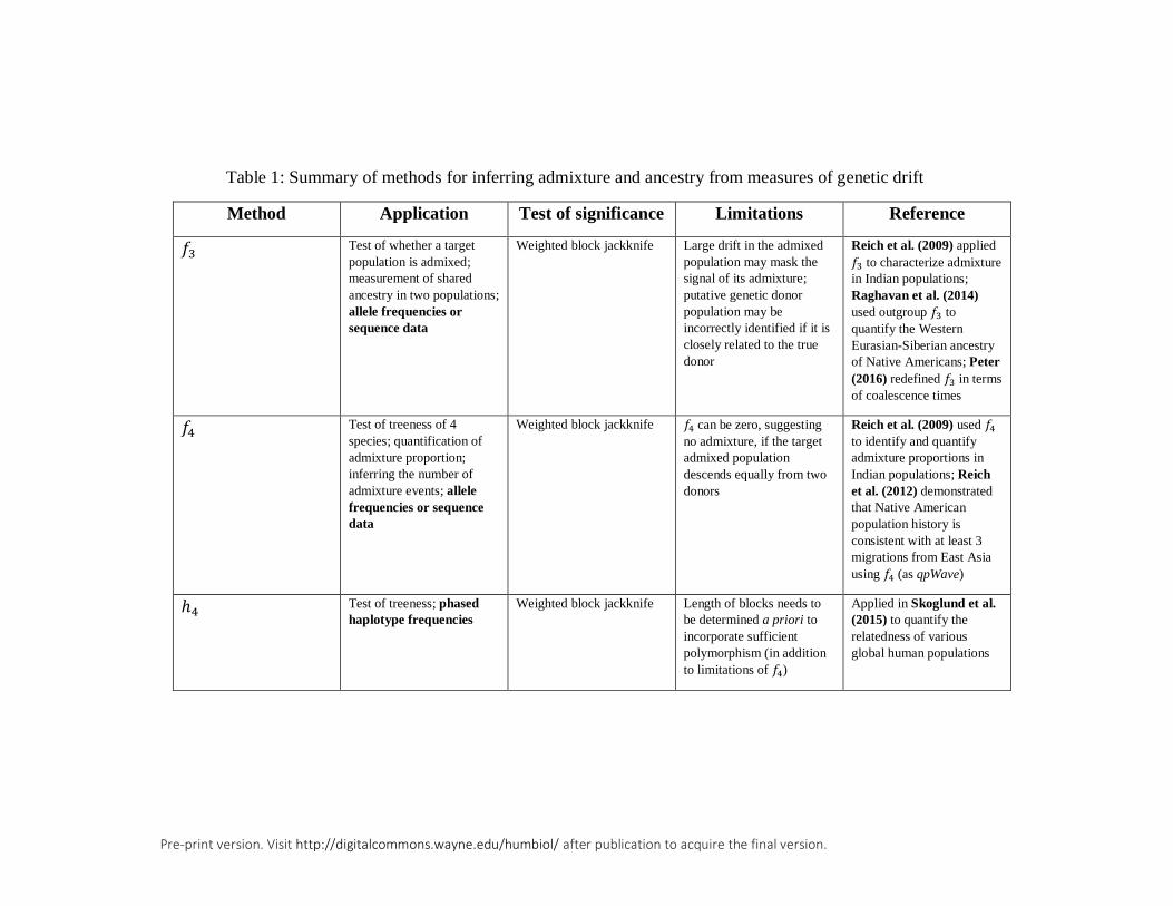
Pre-print version. Visit http://digitalcommons.wayne.edu/humbiol/ after publication to acquire the final version.
Table 1: Summary of methods for inferring admixture and ancestry from measures of genetic drift
Method Application Test of significance Limitations Reference
𝑓3 Test of whether a target
population is admixed;
measurement of shared
ancestry in two populations;
allele frequencies or
sequence data
Weighted block jackknife Large drift in the admixed
population may mask the
signal of its admixture;
putative genetic donor
population may be
incorrectly identified if it is
closely related to the true
donor
Reich et al. (2009) applied
𝑓3 to characterize admixture
in Indian populations;
Raghavan et al. (2014)
used outgroup 𝑓3 to
quantify the Western
Eurasian-Siberian ancestry
of Native Americans; Peter
(2016) redefined 𝑓3 in terms
of coalescence times
𝑓4 Test of treeness of 4
species; quantification of
admixture proportion;
inferring the number of
admixture events; allele
frequencies or sequence
data
Weighted block jackknife 𝑓4 can be zero, suggesting
no admixture, if the target
admixed population
descends equally from two
donors
Reich et al. (2009) used 𝑓4
to identify and quantify
admixture proportions in
Indian populations; Reich
et al. (2012) demonstrated
that Native American
population history is
consistent with at least 3
migrations from East Asia
using 𝑓4 (as qpWave)
ℎ4 Test of treeness; phased
haplotype frequencies
Weighted block jackknife Length of blocks needs to
be determined a priori to
incorporate sufficient
polymorphism (in addition
to limitations of 𝑓4)
Applied in Skoglund et al.
(2015) to quantify the
relatedness of various
global human populations

Pre-print version. Visit http://digitalcommons.wayne.edu/humbiol/ after publication to acquire the final version.
Table 1: Summary of methods for inferring admixture and ancestry from measures of genetic drift (continued)
Method Application Test of significance Limitations Reference
Patterson’s D Model-based test for
introgression between
candidate populations;
sequence data or allele
frequencies
Weighted block jackknife Results do not imply a
direction of gene flow;
method cannot distinguish
between ancestral
population structure and
introgression; ability to
infer significance depends
on the number of
informative sites available;
can be misled by
contamination (also applies
to 𝑓4 and other D-statistics)
Used by Green et al.
(2010) to support the
hypothesis that
Neanderthals interbred with
non-African humans
Partitioned D Test for introgression with
polarized direction of gene
flow; sequence data (and
implicitly, allele
frequencies)
Weighted block jackknife Detects few introgression
types compared to DFOIL;
the number of informative
sites available for this test is
smaller than for D (also
applies to DFOIL); requires 4
ingroup taxa related as a
symmetric tree (as does
DFOIL)
Applied by Eaton and Ree
(2013) to show extensive
introgression in the plant
family Orobanchaceae
DFOIL Improved polarized test for
introgression across more
gene flow types than the
partitioned D-statistic;
sequence and allele
frequency data
Weighted block jackknife
or 𝜒2
More complex to calculate
than other D-statistics;
intragroup introgressions
not detectable; invalid
combinations of DFOIL
statistics cannot be
interpreted
Pease and Hahn (2015)
develop DFOIL with
simulated data, and apply it
to mosquito population
genetic data in Fontaine et
al. (2015)

Pre-print version. Visit http://digitalcommons.wayne.edu/humbiol/ after publication to acquire the final version.
Table 1: Summary of methods for inferring admixture and ancestry from measures of genetic drift (continued)
Method Application Test of significance Limitations Reference
Direct ancestry test Measurement of genetic
drift separating two
lineages; diploid whole-
genome sequence data
Likelihood ratio test C/T and G/A
polymorphisms should be
filtered out; only sites that
are polymorphic across
strict outgroup populations
should be tested
First used by Rasmussen et
al. (2014) to demonstrate
that Anzick-1 belonged to
the population ancestral to
modern Central and South
Americans, or to a closely-
related population
TreeMix Inference of phylogenetic
relationships between
populations, of which some
may be admixed (better
suited for exploratory
investigations); allele
frequency data, biallelic
and microsatellite loci
Measurement of residual
covariance or likelihood
ratio
Low-quality samples are
assigned a spuriously longer
branch length on the graph;
user must specify number
of admixture events to fit to
the data
Pickrell and Pritchard
(2012) develop and applied
TreeMix to canine and
human data, uncovering
new admixture networks
MixMapper Inference of phylogenetic
relationships between
populations, of which some
may be admixed (better
suited for classifying a
specific, known set of study
populations); allele
frequency data (biallelic
loci, and implicitly
microsatellites)
Weighted block jackknife
or measurement of residual
covariance
User must know a priori
whether populations are
admixed or not
First applied to genome-
wide single-nucleotide
polymorphism data from
worldwide human
populations in Lipson et al.
(2013), revealing that
previously-unknown gene
flow between southern
Europe and northern
Eurasia

Pre-print version. Visit http://digitalcommons.wayne.edu/humbiol/ after publication to acquire the final version.
Table 1: Summary of methods for inferring admixture and ancestry from measures of genetic drift (continued)
Method Application Test of significance Limitations Reference
ROLLOFF and
ALDER
Approximating date of
admixture; estimating
admixture proportion;
unphased diploid
genotype sequence data
Weighted block jackknife
(test of estimate stability)
Reduced power to detect
older admixture events;
demographic events shared
between a subset of tested
populations can lead to
spurious inference of
admixture
First used in Moorjani et
al. (2011) (ROLLOFF) to
demonstrate recent
admixture from Africa into
Eurasia and Loh et al.
(2013) (ALDER) to
uncover new details about
the admixture history of
various global populations

Pre-print version. Visit http://digitalcommons.wayne.edu/humbiol/ after publication to acquire the final version.
Figure 1: Phylogenetic tree and admixture graph topologies representing important
theoretical and practical scenarios for f- and D-statistic applications. (A) Unrooted
three-population phylogeny showing the relationship between populations A, B, and
C wherein A descends from the common ancestor of A, B, and C. The f3-statistic
traces the marked paths and measures only the overlap of these paths, which is the
length of the branch connecting A to the internal node. (B) Three-population
admixture graph showing the relationship between populations A, B, and C wherein
population A derives a proportion 𝑝 of its ancestry from the lineage of population
B (specifically population 𝐵′ ) and a proportion 1 − 𝑝 of its ancestry from the
lineage of population C (specifically 𝐶′). Branch lengths 𝑖 through 𝑣𝑖𝑖 represent
drift between ancestral and descendant nodes. (C) Unrooted four-population
phylogeny showing the relationship between populations A, B, C, and D wherein
the former pair represent a cluster, and the latter pair represent a cluster. This tree
is consistent with the result 𝑓4(𝐴, 𝐵; 𝐶, 𝐷) = 0 . (D) Five-population admixture
graph to which the f4-ratio test is applied. Population A derives a proportion 𝑝 of its
ancestry from population 𝐶′ and 1 − 𝑝 of its ancestry from population 𝐷′ ,
belonging to the lineages of populations C and D, respectively. (E) Asymmetric
four-population tree rooted to chimpanzee outgroup, to which the D-statistic was
originally applied in Green et al. (2010). (F) Outgroup-rooted five-population tree
with symmetrically-related ingroups and a different divergence time for A and B
than for C and D. The partitioned D-statistics (Eaton and Ree, 2013) and DFOIL
(Pease and Hahn, 2015) apply to this topology. Adapted from Reich et al. (2009),
Patterson et al. (2012), Green et al. (2010), Eaton and Ree (2013), and Pease and
Hahn (2015).

Pre-print version. Visit http://digitalcommons.wayne.edu/humbiol/ after publication to acquire the final version.
Figure 2: Practical visualizations of the f3- and f4-statistics. (A) Representation of
the four allele drift trajectories available to a three-population admixture graph.
Two alleles are drawn for a locus in population A and their overlap in each
configuration additively contributes to the value of 𝑓3(𝐴; 𝐵, 𝐶). The path colored in
red traces the drift between the first drawn allele of A and population B, while the
path colored in blue traces the drift between second drawn allele of A and population
C. (B) Unrooted four-population trees showing the traced drift paths for
𝑓4(𝐴, 𝐵; 𝐶, 𝐷) for the three possible topologies. The red arrow traces the genetic
drift between A and B and can also be interpreted as 𝑓2(𝐴, 𝐵), while the blue arrow
traces the genetic drift between C and D and can be interpreted as 𝑓2(𝐶, 𝐷). The
value of 𝑓4(𝐴, 𝐵; 𝐶, 𝐷) is zero for the first tree, positive for the second, and negative
for the third. In the case of the latter two trees, the magnitude of 𝑓4(𝐴, 𝐵; 𝐶, 𝐷) is
equivalent to the length of the internal branch. (C) Five-population admixture graph
indicating drift paths underlying the computation of 𝑓4(𝐵, 𝑂; 𝐴, 𝐷) . Note that
𝑓4(𝐵, 𝑂; 𝐴, 𝐷) = 𝑝𝑓4(𝐵, 𝑂; 𝐶, 𝐷) because the drift path tracing the 𝐶′ -derived
ancestry of A with D (red) overlaps with the drift path between B and O, while the
drift path tracing the 𝐷′-derived ancestry of A with D (blue) does not. Adapted from
Reich et al. (2009) and Patterson et al. (2012).

Pre-print version. Visit http://digitalcommons.wayne.edu/humbiol/ after publication to acquire the final version.
Figure 3: f3 biplots demonstrating an application of the outgroup f3-statistic to global
human microsatellite data (Pemberton et al., 2013). Each axis of each plot is set up
as 𝑓3(Yoruba; 𝑊, 𝑋) and measures the divergence of populations W and X with the
outgroup Yoruba population (YRI). Population W is fixed for each axis of each plot,
while population X is one of various European (blue), Middle Eastern (yellow),
Central/South Asian (red), Oceanian (green), East Asian (pink), Native American
of any latitude (purple), or admixed (gray) samples. Larger values of
𝑓3(Yoruba; 𝑊, 𝑋) reflect greater proportions of shared ancestry between W and X.
(A) Measures common ancestry between population X and the Pima against the
common ancestry of population X and the Huilliche, both Central American
populations. (B) Measures common ancestry with Han (East Asian) against
Sardinian (European). (C) Measures common ancestry with Han against Australian
(admixed). (D) Measures common ancestry with Karitiana (South American)
against Australian. Each of these plots yields a unique clustering of global human
populations from which their affinity may be inferred.

Pre-print version. Visit http://digitalcommons.wayne.edu/humbiol/ after publication to acquire the final version.
Figure 4: Simulations demonstrating the increasing power of the D-statistic to reject
the null hypothesis that the tree topology is correct, as the number of available
informative sites increases. (A) Three scenarios relating an ancient sample to a pair
of modern samples and a sequence from an outgroup species (e.g., chimpanzee).
The scenarios represent situations in which the ancient sample is a direct ancestor
of modern population 2 (Scenario 1), is equally related to modern populations 1 and
2 (Scenario 2), or is a member of a population related to modern population 2
(Scenario 3). We use 𝐷(Modern1, Modern2, Ancient, Chimp) to test the null
hypothesis that the ancient sample is equally related to the two modern populations
(Scenario 2), and we are specifically interested in the ability of Scenarios 1 and 3
to reject the null hypothesis with a positive D-statistic. Each of the following
distributions is based on 103 simulated replicates. (B) With a small number of D-
statistic informative sites (across 2 × 10² sequences of 100 kilobases in length), the
null hypothesis was erroneously rejected with a positive D for Scenario 2 in only 4
times, and Scenarios 1 and 3 rejected the null with a positive D only 16 and 13
times, respectively. (C) Increasing the number of informative sites by an order of
magnitude (across 2 × 10³ 100 kilobase sequences), the distributions of Scenarios
1 and 3 are shifted to higher Z scores, as expected based on the placement of the
ancient sample. However, the majority of the distributions fall within |𝑍| < 3.
Scenarios 1 and 3 only reject the null with a positive D 195 and 53 times,
respectively, and therefore the null hypothesis is often still not rejected. (D) Further
increasing the number of informative sites by an order of magnitude (across
2 × 10⁴ 100 kilobase sequences) shifts the majority of the distribution for Scenario
3 (712 replicates) and almost all the distribution of Scenario 1 (999 replicates) past
the significance threshold 𝑍 ≥ 3. These results show that if the relationships among
populations are close enough, then it may be difficult to reject the null hypothesis
of the D statistic with low-coverage ancient samples, for which there may be few

Pre-print version. Visit http://digitalcommons.wayne.edu/humbiol/ after publication to acquire the final version.
D-statistic informative sites. Simulations were performed using FastSimCoal2
(Excoffier et al., 2013), with a single sequence sampled from each of the four
populations.

Pre-print version. Visit http://digitalcommons.wayne.edu/humbiol/ after publication to acquire the final version.
Figure 5: Representation of a contamination scenario similar to the one addressed
in Raghavan et al. (2014b). (A) When an ancient DNA sample (Ancient) is
contaminated during handling by researchers (European) such that a proportion 𝛾
of the inferred genetic sequence of the ancient sample is actually from the
researchers, the observed magnitude of
𝐷(East Asian, American, Ancient, Chimpanzee) may be smaller than the true
value. This contamination results from the reduction of abba-sites as a proportion
of total informative sites (𝑛𝑎𝑏𝑏𝑎 + 𝑛𝑏𝑎𝑏𝑎) across the sampled genomes. (B) After
contamination, the apparent topology of the tree relating these populations now
supports the Ancient sample as basal to East Asians and Native Americans, due to
an increased presence of European-specific variants in the Ancient sample.
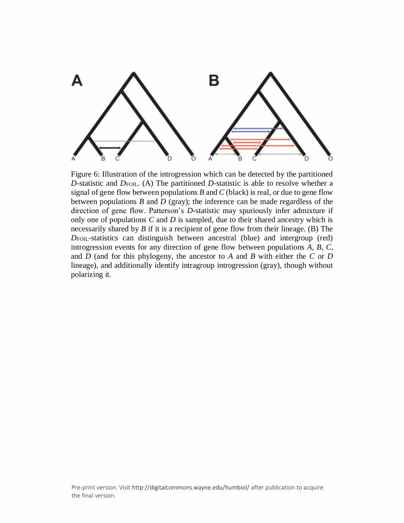
Pre-print version. Visit http://digitalcommons.wayne.edu/humbiol/ after publication to acquire the final version.
Figure 6: Illustration of the introgression which can be detected by the partitioned
D-statistic and DFOIL. (A) The partitioned D-statistic is able to resolve whether a
signal of gene flow between populations B and C (black) is real, or due to gene flow
between populations B and D (gray); the inference can be made regardless of the
direction of gene flow. Patterson’s D-statistic may spuriously infer admixture if
only one of populations C and D is sampled, due to their shared ancestry which is
necessarily shared by B if it is a recipient of gene flow from their lineage. (B) The
DFOIL-statistics can distinguish between ancestral (blue) and intergroup (red)
introgression events for any direction of gene flow between populations A, B, C,
and D (and for this phylogeny, the ancestor to A and B with either the C or D
lineage), and additionally identify intragroup introgression (gray), though without
polarizing it.

Pre-print version. Visit http://digitalcommons.wayne.edu/humbiol/ after publication to acquire the final version.
Figure 7: Schematic illustrating the behavior of TreeMix for various global human
populations. Important samples are located on the branch diverging from the East
Asian lineage. These are the low-coverage ancient Siberian sample (MA-1 from
Raghavan et al. (2014b), for which only a single allele is sampled at each site), the
high-coverage ancient North American sample (Anzick-1 from Rasmussen et al.
(2014), for which genotypes have been called), and the unadmixed and admixed
Northwest American samples (ancient and modern, respectively, from Lindo et al.
(2016), for which genotypes have been called). (A) Example assuming no migration
events in TreeMix. The low-coverage ancient sample exhibits a long branch,
indicating extensive genetic drift because all sites are called as homozygous, and so
the sample appears completely inbred. This branch length should not be interpreted,
but the position in which it has diverged relative to the tree is correct. The high-
coverage ancient North American sample exhibits no genetic drift because it is
either the direct ancestor of the Central and South American populations, or a
member of a population closely-related to a direct ancestor of the Central/South
American populations. This result can be used to support findings from the direct
ancestry test. The admixed Northwest American population also has no genetic drift
along its branch, which appears to indicate direct ancestry. (B) Accounting for a
single admixture (migration) event with Europeans, the admixed Northwest
American population shifts from being ancestral to all samples from the Americas
to a sister population to the unadmixed Northwest American population. This result
suggests that the lack of genetic drift along the branch leading to the admixed
Northwest American population was likely due its genetic profile lying
intermediate between the unadmixed Northwest American population the
Europeans.

Pre-print version. Visit http://digitalcommons.wayne.edu/humbiol/ after publication to acquire the final version.
Figure 8: Robustness of outgroup f3-statistics to contamination. This tree relates an
outgroup population (O) and four ingroup populations A, B, C, and D. Population
A is admixed, and derives a fraction 𝑝 of its ancestry from the ancestral lineage of
D. In addition, an ancient sample belonging to a population directly ancestral to B
is contaminated by modern population D, with a fraction 𝛾 of its genome sequence
deriving from this contamination. Branch lengths 𝑖 through 𝑣 represent lengths in
drift units. If outgroup f3-statistics are robust to contamination, then it is important
that they indicate that the ancient sample has higher affinity to population B than
populations to A, C, and D. This situation occurs if 𝑓3(𝑂; Ancient, 𝐵) is greater
than 𝑓3(𝑂; Ancient, 𝐴) , 𝑓3(𝑂; Ancient, 𝐶) , and 𝑓3(𝑂; Ancient, 𝐷) , which
occurs when 𝑖 + 𝑖𝑖 > 0 , 𝛾 < (𝑖 + 𝑖𝑖 + 𝑖𝑖𝑖)/ (𝑖 + 𝑖𝑖 + 𝑖𝑖𝑖 + 𝑖𝑣 + 𝑣) , and
𝛾 < [𝑖 + 𝑝(𝑖𝑖 + 𝑖𝑖𝑖)]/ [𝑖 + 𝑝(𝑖𝑖 + 𝑖𝑖𝑖 + 𝑖𝑣)] . The first constraint should hold
under most situations. Under situations in which population A is not admixed
(𝑝 = 0), the third constraint is trivial as it implies that the contamination rate must
be less than 1. The second constraint will be satisfied in almost all practical
applications, as it requires prohibitively large contamination rates for it not to hold.
For example, consider a situation in which 2(𝑖 + 𝑖𝑖 + 𝑖𝑖𝑖) = (𝑖𝑣 + 𝑣). That is, the
branch length leading from the ancestor of B and D is at least twice as long leading
to D as it is leading to B. Under such a scenario, the second constraint implies that
we need a contamination rate less than 1/3 for the outgroup-f3 statistic to not be

Pre-print version. Visit http://digitalcommons.wayne.edu/humbiol/ after publication to acquire the final version.
misled by contamination. Further, if population A were indeed admixed, say at rate
𝑝 = 0.5, then the branch length (𝑖𝑣) leading to population D must be extremely
long or the contamination rate must be enormous for the outgroup f3-statistic to
again be misled.