
ADHESION AND FRICTION OF A BIO-INSPIRED DRY ...
302
ADHESION AND FRICTION OF A BIO-INSPIRED DRY ADHESIVE AND VAN DER WAALS INTERACTIONS A Dissertation Presented to the Faculty of the Graduate School of Cornell University In Partial Fulfillment of the Requirements for the Degree of Doctor of Philosophy by Jingzhou Liu August 2009
-
Upload
khangminh22 -
Category
Documents
-
view
2 -
download
0
Transcript of ADHESION AND FRICTION OF A BIO-INSPIRED DRY ...
ADHESION AND FRICTION OF A BIO-INSPIRED DRY ADHESIVE
AND
VAN DER WAALS INTERACTIONS
A Dissertation
Presented to the Faculty of the Graduate School
of Cornell University
In Partial Fulfillment of the Requirements for the Degree of
Doctor of Philosophy
by
Jingzhou Liu
August 2009

© 2009 Jingzhou Liu
ADHESION AND FRICTION OF A BIO-INSPIRED DRY ADHESIVE
AND
VAN DER WAALS INTERACTIONS
Jingzhou Liu, Ph. D.
Cornell University 2009
This dissertation contains two parts. The part I is on the theory of adhesion
and friction behaviors of dry adhesives. Many synthetic bio-inspired adhesives consist
of an array of micro-fibrils attached to an elastic backing layer, resulting in a tough
and compliant structure. In this part, we first present a three dimensional (3D) model
for adhesion enhancement that occurs due to trapping of the interfacial crack in the
region between fibrils. Energy release to the crack tip is attenuated because it has to
go through the compliant terminal film between fibrils. Using perturbation theory
and a finite element method (FEM) we solve for the shape of crack front. Our model
also allows us to study how adhesion enhancement depends on the arrangement of
fibrils. Then, we examine the nonlinear deformation of a single fibril subjected to a
combination of shear and normal loads. An exact closed-form solution is obtained
using elliptic functions. The prediction of our model compares well with the results of
an indentation experiment. Finally, we model the response of a film-terminated
micro-fibril array subjected to shear through contact with a rigid cylindrical indenter.
The model matches the experimentally measured shear-force response.
The second part is on van der Waals interactions. Van der Waals (vdW) forces
are forces between neutral atoms or molecules and are present in all materials.

Lifshitz theory of van der Waals interactions is reviewed in the first chapter of this
part. It is often assumed that Lifshitz’s theory is equivalent to the surface mode
method proposed by van Kampen et al. A revisit of van der Waals force between
two parallel plates shows that certain procedures in the surface mode method are
inconsistent with Lifshitz’s theory. Finally, numerical techniques (boundary element
method and finite element analysis) to compute vdW forces are formulated. In
principle, these numerical approaches can be used to evaluate the van der Waals force
between dielectric solids with arbitrary shapes.

iii
BIOGRAPHICAL SKETCH
The author was born on Febrary 27, 1978 in a remote village in western China. He
began his schooling when he was seven. He stayed in his hometown (Shangluo City,
Shaanxi Province) till his high school education. In 1997, he got admitted by Beijing
Normal University, where he majored in Physics. Beginning Fall 2004, he started
pursing his PhD study at Cornell University in Theoretical and Applied Mechanics.
iv
ACKNOWLEDGMENTS
First of all I would like to express my sincere gratitude to my advisor and the
chairman of my committee, Professor C.-Y. Hui. He has been extremely
understanding, supportive and inspiring during the course of this work. I would like
to thank Dr. Anand Jagota, a professor of Chemical Engineering at Lehigh University.
He has provided me with many helpful suggestions, important advice and constant
encouragement during my research. I am very thankful to Sujata Jagota (Prof.
Jagota’s wife). She not only cooked me very delicious food but also encouraged me
with my research when I stayed with them during my visits to Lehigh.
I also would like to thank Prof. S. Mukherjee, Prof. M. Thompson, and Prof. S.
Weber for all the help during the work and for serving in my committee.
Thanks are also due to Tian Tang, Vijayanand Muralidharan, Lulin Shen,
Shilpi Vajpayee, Venkat Krishnan, and Rong Long for all their help and support in my
research.
Finally, I would like to express deepest gratitude to my parents. They have no
idea of what PhD is, but they always use their special way to encourage me. Special
thanks should go to my girlfriend and best friend Na Xu for her support, love, and
encouragement during this work.
v
TABLE OF CONTENTS
BIOGRAPHICAL SKETCH.........................................................................................iii
ACKNOWLEDGMENTS............................................................................................. iv
LIST OF FIGURES.....................................................................................................viii
LIST OF TABLES .......................................................................................................xii
LIST OF ABBREVIATIONS .....................................................................................xiii
Part I: Theory on Adhesion and Friction of Fry Adhesives ..........................................1
Chapter 0 Introduction..............................................................................................1
Chapter 1 Effect of Fibril Arrangement on Crack Trapping In a Film-Terminated
Fibrillar Interface........................................................................................................6
1.1 Introduction .....................................................................................................6
1.2 Model for Crack Between a Plate and Substrate Trapped by An Array of
Fibrils....................................................................................................................13
1.3 Perturbation Theory........................................................................................18
1.4 Finite Element Analysis ................................................................................27
1.5 Effect of Pattern (Orientation).......................................................................27
1.6 Summary and Discussion ...............................................................................32
1.7 Future work ...................................................................................................35
Chapter 2 Compliance of a Micro-Fibril subjected to Shear and Normal loads ....69
2. 1 Introduction ..................................................................................................69
2.2 Elastica Model of a Stretchable Beam...........................................................74
2.3 Comparison with experiments.......................................................................87
2.4 Discussion and Conclusion............................................................................91
Chapter 3 A Model for Static Friction in a Film-terminated Micro-fibril Array ..105
3.1. Introduction .................................................................................................106
3.2. Review of Experiments ..............................................................................107
vi
3.3 Contact mechanics.......................................................................................110
3.4 Results .........................................................................................................124
3.5 Summary and Conclusion.............................................................................132
Chapter 4 Introduction...........................................................................................147
Chapter 5 Lifshitz Theory .....................................................................................154
5.1 Constitutive Model of a Linear Dielectric....................................................155
5.2 Property of Dielectric Susceptibility ............................................................156
5.3 ( )ε ω′′ and Dissipation..................................................................................157
5.4 Complex ω and the Kramer-Kronig relation..............................................158
5.5 Correlation and Spectral density .................................................................161
5.6 Dissipation- Fluctuation Theorem (DFT) – a simple example....................164
5.7 Fluctuation and van der Waals Interaction...................................................165
5.8 Dissipation and Equation (5.40) ...................................................................170
5.9 Correlations and Dissipation ........................................................................174
5.10 An Example: a 3-layer Problem --Detailed Derivation of the Lifshitz
Theory.................................................................................................................178
Chapter 6 Lifshitz versus van Kampen: A revisit of van der Waals force between
two parallel plates...................................................................................................222
6.1 Introduction .................................................................................................222
6.2 Geometry and Summary of Previous Results..............................................224
6.3 Two Difficulties with the VKNS Method ...................................................228
6.4 Discussion and Summary ............................................................................233
Chapter 7 Green’s Function and Boundary Element Method ...............................238
7.1 Green’s Function .........................................................................................238
7.2 Boundary Element Method (BEM) .............................................................244
7.3 Discussion....................................................................................................252
Charter 8 Finite element Method (FEM)................................................................263
8.1 Random field ( )tK r, and its time derivative...............................................263
8.2 Finite Element Method ................................................................................274

vii
8.3 Future work .................................................................................................283
viii
LIST OF FIGURES
Part I
Figure 1. 1 An SEM image of a thin-film-terminated fibril array..................................7
Figure 1. 2 A schematic drawing of the indentation test. ..............................................8
Figure 1. 3 A 2-D crack trapping model.......................................................................11
Figure 1. 4 Square pattern and hexagonal pattern of fibrils ........................................12
Figure 1. 5 A 3-D crack trapping model .....................................................................14
Figure 1. 6 Normalized energy release rate along a straight crack front for one period
for / 1/ 2d s = . . ..........................................................................................................20
Figure 1. 7 Normalized crack shape as a function of y/L for different d/s. ..................23
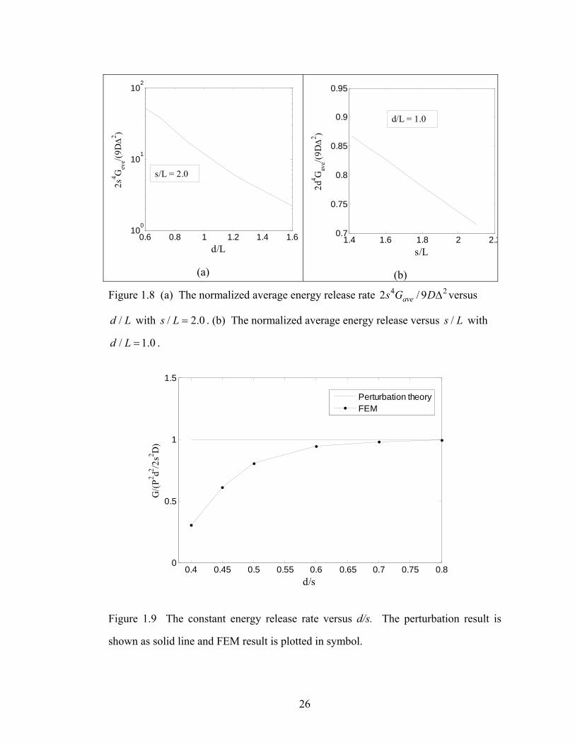
Figure 1. 8 (a) The normalized average energy release rate versus /d L with
/ 2.0s L = . (b) The normalized average energy release versus /s L ..........................26
Figure 1. 9 The constant energy release rate versus d/s. The perturbation result is
shown as solid line and FEM result is plotted in symbol. ............................................26
Figure 1. 10 Comparison of crack front profiles .........................................................29
Figure 1. 11 Normalized minimum energy release rate versus normalized number
density 2 4Lρ . ................................................................................................................31
Figure 2.1 A schematic drawing of shear test..............................................................71
Figure 2.2 Optical micrographs of the contact region.................................................73
Figure 2.3 Coordinate system used in our analysis. ....................................................75
Figure 2.4 Free body diagram of a section of the deformed bar. .................................75
Figure 2.5 Normalized shear displacement, TΔ , versus normalized shear force, 0T . for
0 0N = (or 0oθ = ) and / ob L = 14/67...........................................................................83
Figure 2.6 Figure 2.6a plots the normalized shear displacement versus shear force for
different applied normal loads. Figure 2.6b plots the incremental shear compliance
versus normalized shear displacement for different applied normal loads. .................85

ix
Figure 2.7 plots the normalized normal displacement, NΔ , versus normalized shear
force 0T for 0 0N = (or 0oθ = )......................................................................................86
Figure 2.8 The dependence of NΔ on 0N for different 0T is shown in Fig. 8a. Fig. 8b
plots the normalized normal compliance of a fibril against 0N for different 0T .........87
Figure 2.9 Normalized shear force versus normalized shear displacement for No = 0.
......................................................................................................................................88
Figure 2.10 Comparison of the experimental data (stage 1) with the large and small
deflection theoretical results. ......................................................................................89
Figure 3.1 (a) An SEM image of the fibril array; (b) Schematic drawing of a rigid
cylindrical indenter on a fibrillar sample....................................................................108
Figure 3.2 Shear force versus shear displacement for a film-terminated sample with
spacing 65w mμ= . ..................................................................................................109
Figure 3.3 Geometry of a deformed fibril. .............................................................111
Figure 3.4 Normalized normal displacement v/L versus normalized shear force sF for
different normal loads.................................................................................................113
Figure 3.5 Schematic drawing of the deformation of the fibrils inside and outside the
contact zone ................................................................................................................115
Figure 3.6 Comparison of shear displacements using linear and nonlinear theories.118
Figure 3.7 Normal indenter force versus indenter displacement for a load-unload
cycle. Note compression is positive. .........................................................................121
Figure 3.8 Free body diagram of indenter. ................................................................122
Figure 3.9 Half contact width a/L versus normalized applied shear displacement
/s LΔ ..........................................................................................................................124
Figure 3.10 The normal force acting on each fibril (fibrils 1 and 2, see insert) along a
row in the contact zone. The sum of normal forces acting on fibrils 1 and 2 is also
plotted. ......................................................................................................................125
Figure 3.11 Shear force acting on each fibril along a row in the contact zone (see
insert of Fig. 3.10). .....................................................................................................126
x
Figure 3.12 Nonlinear theory prediction of the shear force on the indenter with
experimental results at different applied shear displacement with spacing 65w mμ= .
....................................................................................................................................127
Figure 3.13 Comparison of the measured displacements of the fibrils in the shear lag
zone with equation (3.21) for different shear displacements with spacing 65 mμ . ...128
Part II
Figure 4.1 Coordinates of two interacting hydrogen atoms ......................................147
Figure 5.1 Real and imaginary parts of dielectric function versus ω for polystyrene
....................................................................................................................................157
Figure 5.2 Isotropic non-magnetic dielectric solids separated by vacuum in thermal
equilibrium. ................................................................................................................165
Figure 5.3 A schematic drawing of a 3-layer problem..............................................178
Figure 5.4 Integration contour ( ) ( )/ ,0 0,c iωΓ = ∪ ∞ .............................................192
Figure 5.5 The dielectric function versus pure imaginary frequency for Polystyrene
....................................................................................................................................206
Figure 5.6 F versus l for the polystyrene (PS) – vacuum – polystyrene (PS) system.
And the insert plots the slope ( ) ( )log / logd F d l versus l........................................206
Figure 6.1 Geometry of the three-layer problem.......................................................224
Figure 6.2 The closed contour Rγ ..............................................................................231
Figure 7.1 Schematic drawing of two dielectrics seperated by vacuum ...................245
Figure 8.1 Auto-correlations τ+tftf ()( or ( ) ( )τ+⋅ tt ff on the vertical axis as
functions of τ on the horizontal-axis..........................................................................268
Figure 8.2 f(t) and ( )tK1 versus t with 1,1.0,1 11 ===Δ At ω ..................................270

xi
Figure 8.3 The comparison of the simulation and exact results for τ+tKtK ()( 11 .270
Figure 8.4 1S and 2S are the surfaces of dielectrics 1 and 2 respectively. Π is a closed
surface which encloses medium 2 in vacuum 3Ω . .....................................................275
Figure 8.5 Brick element ...........................................................................................276

xii
LIST OF TABLES
Table 8.1 Edge numbers ............................................................................................276

xiii
LIST OF ABBREVIATIONS
BEM: Boundary element method
FEM: Finite element method
PDMS: polydimethlysiloxane
vdw: van der Waals
1
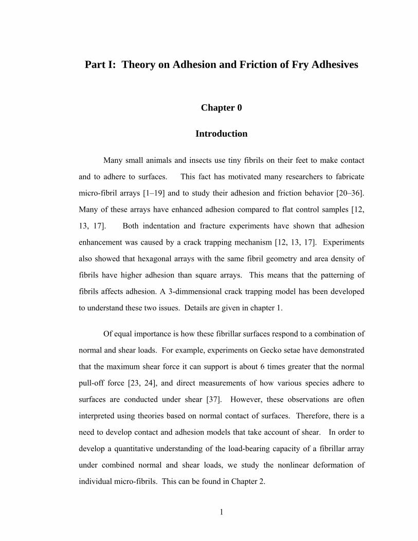
Part I: Theory on Adhesion and Friction of Fry Adhesives
Chapter 0
Introduction
Many small animals and insects use tiny fibrils on their feet to make contact
and to adhere to surfaces. This fact has motivated many researchers to fabricate
micro-fibril arrays [1–19] and to study their adhesion and friction behavior [20–36].
Many of these arrays have enhanced adhesion compared to flat control samples [12,
13, 17]. Both indentation and fracture experiments have shown that adhesion
enhancement was caused by a crack trapping mechanism [12, 13, 17]. Experiments
also showed that hexagonal arrays with the same fibril geometry and area density of
fibrils have higher adhesion than square arrays. This means that the patterning of
fibrils affects adhesion. A 3-dimmensional crack trapping model has been developed
to understand these two issues. Details are given in chapter 1.
Of equal importance is how these fibrillar surfaces respond to a combination of
normal and shear loads. For example, experiments on Gecko setae have demonstrated
that the maximum shear force it can support is about 6 times greater that the normal
pull-off force [23, 24], and direct measurements of how various species adhere to
surfaces are conducted under shear [37]. However, these observations are often
interpreted using theories based on normal contact of surfaces. Therefore, there is a
need to develop contact and adhesion models that take account of shear. In order to
develop a quantitative understanding of the load-bearing capacity of a fibrillar array
under combined normal and shear loads, we study the nonlinear deformation of
individual micro-fibrils. This can be found in Chapter 2.
2
Another important issue is the frictional behavior of a micro-fibril array. In
the past few years, there have been several experimental studies on the frictional
behavior of micro-fibril arrays against a flat substrate [8, 17, 36, 38]. The fibril arrays
fabricated by Majidi et al [8] and Ge et al [38] consists of very stiff fibrils, whereas
those fabricated by Guduru [39] and Shen et al [17, 36] are made of
poly(dimethlysiloxane) (PDMS), a soft elastomer with shear modulus on the order 1
MPa. Despite the large differences in modulus, what emerges from these
experiments is that the static friction of these arrays is much higher than that exhibited
by flat unstructured controls made of the same material. The friction test on the film-
terminated fibril arrays [36] also showed that the contact area does not change much
with increasing shear. A model for static friction in a film-terminated micro-fibril
array is given in chapter 3. The model accurately matches the experimentally
measured shear-force response. With the use of an independently measured critical
energy release rate for unstable release of the contact, the model shows how this
architecture achieves a strong enhancement in static friction.
3
REFERENCES
1 M. Sitti and R. S. Fearing, J. Adhes. Sci. Technol. 17, 1055 (2003).
2 N. J. Glassmaker, A. Jagota, C.-Y. Hui, and J. Kim, J. R. Soc. Interface 1, 22
(2004).
3 C.-Y. Hui, N. J. Glassmaker, T. Tang, and A. Jagota, J. R. Soc. Interface 1, 35
(2004).
4 A. Peressadko and S. N. Gorb, J. Adhes. 80, 247 (2004).
5 B. Yurdumakan, N. R. Raravikar, P. M. Ajayan, and A. Dhinojwala, Chem.
Commun. 30, 3799 (2005).
6 S. Gorb, M. Varenberg, A. Peressadko, and J. Tuma, J. R. Soc. Interface 4, 271
(2006).
7 S. Kim and M. Sitti, Appl. Phys. Lett. 89, 261911 (2006).
8 C. Majidi, R. E. Groff, Y. Maeno, B. Schubert, S. Baek, B. Bush, R. Maboudian,
N. Gravish, M. Wilkinson, K. Autumn, and R. S. Fearing, Phys. Rev. Lett. 97,
076103 (2006).
9 B. Aksak, M. Murphy, and M. Sitti, Langmuir 23, 3322 (2007).
10 B. Bhushan and R. A. Sayer, Microsystem Technologies 13, 71 (2007).
11 C. Greiner, A. D. Campo, and E. Arzt, Langmuir 23, 3495 (2007).
12 W. L. Noderer, L. Shen, S. Vajpayee, N. J. Glassmaker, A. Jagota, and C.-Y. Hui,
Proc. R. Soc. A 463, 2631 (2007).
13 N. J. Glassmaker, A. Jagota, C.-Y. Hui, W. L. Noderer, and M. K. Chaudhury,
Proc. Natl Acad. Sci. USA 104, 10786 (2007).
14 M. P. Murphy, B. Aksak, and M. Sitti, J. Adhesion Sci. Technol. 21, 1281
(2007).
4
15 B. Schubert, C. Majidi, R. E. Groff, S. Baek, B. Bush, R. Maboudian, and R.S.
Fearing, J. Adhes. Sci. Technol. 21, 1297 (2007).
16 M. Varenberg and S. Gorb, J. R. Soc. Interface 4, 721 (2007).
17 L. Shen, A. Jagota, C.-Y. Hui, and N.J. Glassmaker, Proc. Annual Meeting of the
Adhesion (2007).
18 L. Shen, N.J. Glassmaker, A. Jagota, and C.-Y. Hui, Soft Matter 4, 618 (2008).
19 H. Yao, G. D. Rocca, P.R. Guduru, and H. Gao, R. Soc. Interface 5, 723 (2008).
20 B. N. J. Persson and S. Gorb, J. Chem. Phys. 119, 11437 (2003).
21 H. J. Gao and H. M. Yao, Proc. Natl Acad. Sci. USA 101, 7851 (2004).
22 H. Gao, X. Wang, H. Yao, S. Gorb, and E. Arzt, Mech. Mater. 37, 275 (2005).
23 K. Autumn, S. T. Hsieh, D. M. Dudek, J. Chen, C. Chitaphan, and R. J. Full, J.
Exp. Biol. 209, 260 (2006).
24 K. Autumn, A. Dittmore, D. Santos, M. Spenko, and M. Cutkosky, J. Exp. Biol.
209, 3569 (2006).
25 Y. Tian, N. Pesika, H. Zeng, K. Rosenberg, B. Zhao, P. McGuiggan, K.Autumn,
and J. Israelachvili, Proc. Natl Acad. Sci. USA 103, 19320 (2006).
26 H. Yao and H. Gao, J. Mech. Phys. Solids. 54, 1120 (2006).
27 N. J. Glassmaker, A. Jagota, and C.-Y. Hui, Acta Biomater. 1, 367 (2005).
28 N. J. Glassmaker, A. Jagota, C.-Y. Hui, and M. K. Chaudhury, Proc. Annual
Meeting of the Adhesion, 93 (2006).
29 T. W. Kim and B. Bhushan, J. R. Soc. Interface 5, 319 (2007).
30 A. M. Peattie and R. J. Full, Proc. Natl Acad. Sci. USA 104, 18595 (2007).
31 A. M. Peattie, C. Majidi, A. Corder, and R. J. Full, J. R. Soc. Interface 4, 1071
(2007).
32 B. Zhao, N. Pesika, K. Rosenberg, Y. Tian, H. Zeng, P. McGuiggan, K. Autumn,
and J. Israelachvili, Langmuir 24 (4), 1517 (2007).
5
33 N. Gravish, M. Wilkinson, and K. Autumn, J. R. Soc. Interface 5, 339 (2008).
34 J. Liu, C-Y. Hui, L. Shen, and A. Jagota, J. R. Soc. Interface 5 (26), 1087 (2008).
35 B. Chen, P. D. Wu, H. Gao, Proc. R. Soc. A 464, 1639 (2008).
36 L. Shen, N.J. Glassmaker, A. Jagota, and C.-Y. Hui, Langmuir 25 (5), 2772
(2009).
37 Irschick, D.J., Austin, C.C., Petren, K., Fisher, R., Losos, J.B., and Ellers, O.
1996. Biol. J. Linn. Soc. 59, 21-35.
38 L.Ge, S.Sethi, L.Ci, P. M.Ajayan, and A. Dhinojwala, Proc. Natl. Acad. Sci.
USA 104, 26, 10792-10795 (2007).
39 P.R. Guduru and C.Bull. J. Mech. Phys. Solid 55, 473-488, 2007.
6
Chapter 1
Effect of Fibril Arrangement on Crack Trapping In a Film-
Terminated Fibrillar Interface*
Abstract
We present a three dimensional (3D) model for adhesion enhancement due to crack
trapping in a film-terminated fibrillar structure. Adhesion enhancement occurs due to
trapping of the interfacial crack in the region between fibrils. Energy release to the
crack tip is attenuated because, between fibrils, it has to pass through the compliant
terminal film. Using perturbation theory and a finite element method (FEM) we
solve for the shape of crack front, which is unknown. Our model thus also allows us
to study how adhesion enhancement depends on the arrangement of fibrils. For
example, our model explains why, for a fixed area density of fibrils and for similar
crack orientations, hexagonal arrays have higher adhesion than square arrays.
Keywords Adhesion enhancement, fibrillar structure, adhesive, crack trapping, work
of adhesion
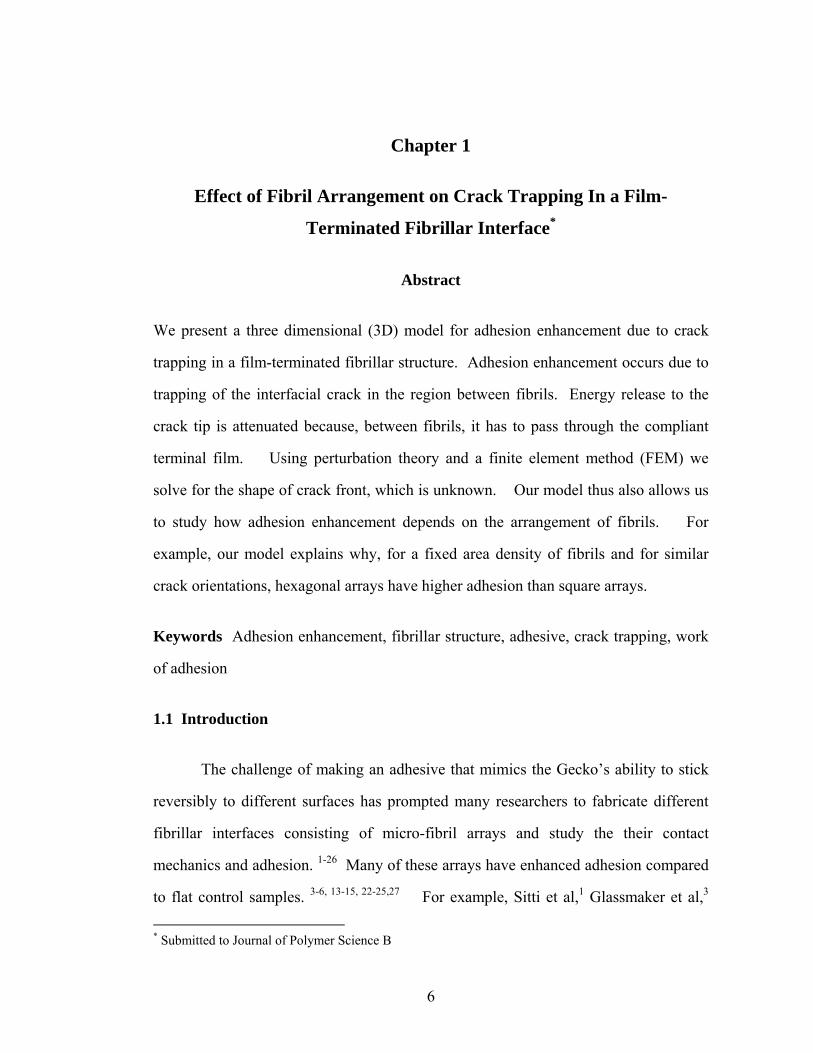
1.1 Introduction
The challenge of making an adhesive that mimics the Gecko’s ability to stick
reversibly to different surfaces has prompted many researchers to fabricate different
fibrillar interfaces consisting of micro-fibril arrays and study the their contact
mechanics and adhesion. 1-26 Many of these arrays have enhanced adhesion compared
to flat control samples. 3-6, 13-15, 22-25,27 For example, Sitti et al,1 Glassmaker et al,3
* Submitted to Journal of Polymer Science B
7
Peressadko and Gorb,5 and Chan et al 28 have fabricated single level structures which
have been shown to enhance adhesion per unit contact area. However these
structures generally can not achieve theoretically predicted enhancement in both
strength and toughness due to the loss of contact area, lateral collapse and buckling of
fibrils.3,4 Later, fibrillar structures with ‘mushroom’ ends were fabricated and have
been shown to enhance adhesion significantly.7,8,10,12 Hierarchical structures have
also been made by several groups.24, 28-31 These hierarchical structures help to make
intimate surface contact, thus enhancing adhesion. In addition, the hierarchical
structures have been shown to provide a fast and effective release mechanism.32
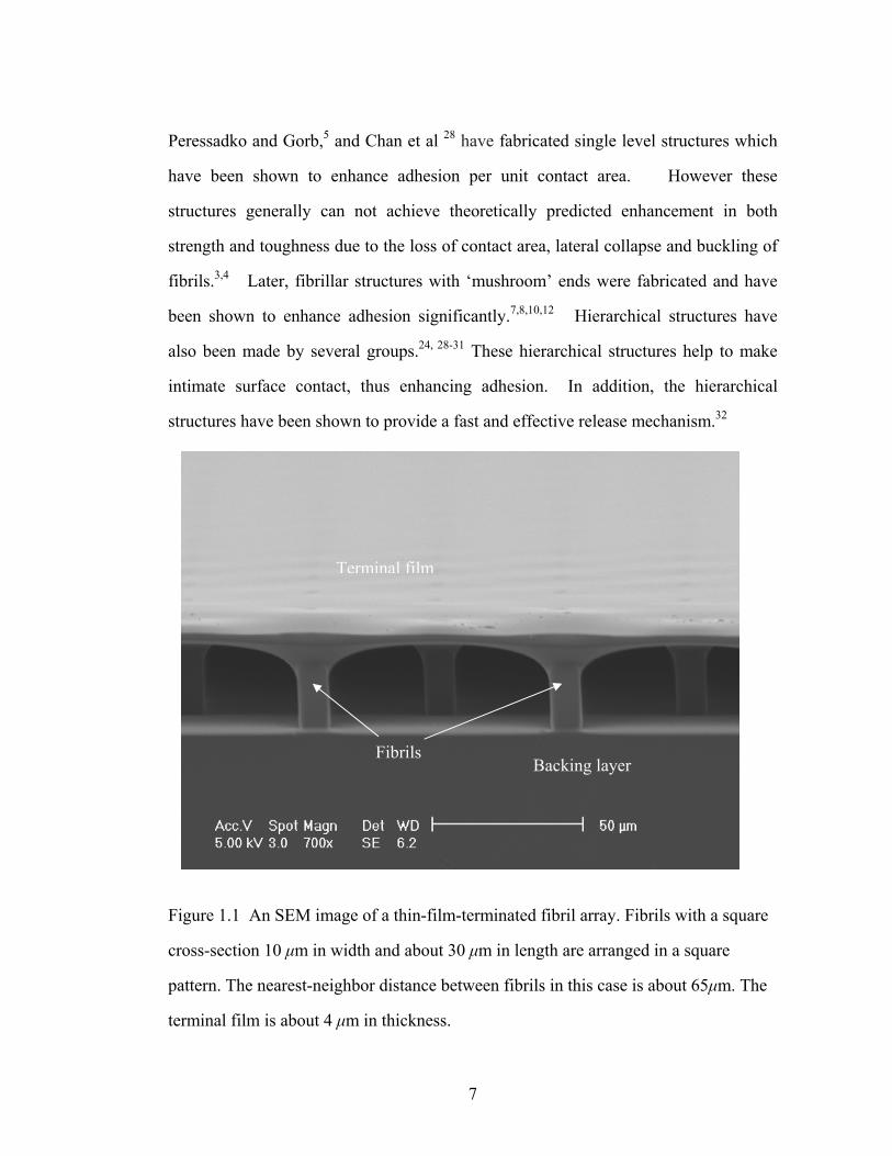
Figure 1.1 An SEM image of a thin-film-terminated fibril array. Fibrils with a square
cross-section 10 μm in width and about 30 μm in length are arranged in a square
pattern. The nearest-neighbor distance between fibrils in this case is about 65μm. The
terminal film is about 4 μm in thickness.
Terminal film
Backing layer Fibrils
8
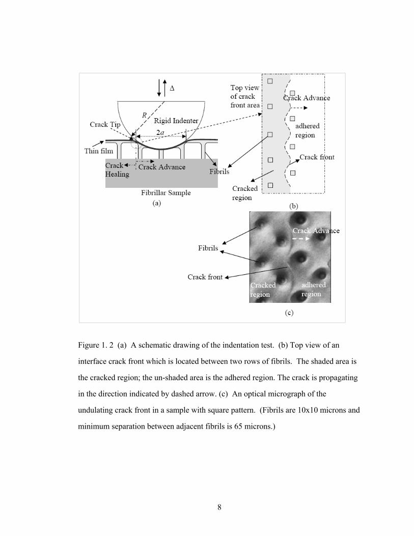
Figure 1. 2 (a) A schematic drawing of the indentation test. (b) Top view of an
interface crack front which is located between two rows of fibrils. The shaded area is
the cracked region; the un-shaded area is the adhered region. The crack is propagating
in the direction indicated by dashed arrow. (c) An optical micrograph of the
undulating crack front in a sample with square pattern. (Fibrils are 10x10 microns and
minimum separation between adjacent fibrils is 65 microns.)
9
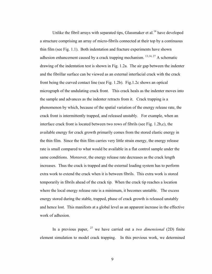
Unlike the fibril arrays with separated tips, Glassmaker et al.14 have developed
a structure comprising an array of micro-fibrils connected at their top by a continuous
thin film (see Fig. 1.1). Both indentation and fracture experiments have shown
adhesion enhancement caused by a crack trapping mechanism. 13,14, 27 A schematic
drawing of the indentation test is shown in Fig. 1.2a. The air gap between the indenter
and the fibrillar surface can be viewed as an external interfacial crack with the crack
front being the curved contact line (see Fig. 1.2b). Fig.1.2c shows an optical
micrograph of the undulating crack front. This crack heals as the indenter moves into
the sample and advances as the indenter retracts from it. Crack trapping is a
phenomenon by which, because of the spatial variation of the energy release rate, the
crack front is intermittently trapped, and released unstably. For example, when an
interface crack front is located between two rows of fibrils (see Fig. 1.2b,c), the
available energy for crack growth primarily comes from the stored elastic energy in
the thin film. Since the thin film carries very little strain energy, the energy release
rate is small compared to what would be available in a flat control sample under the
same conditions. Moreover, the energy release rate decreases as the crack length
increases. Thus the crack is trapped and the external loading system has to perform
extra work to extend the crack when it is between fibrils. This extra work is stored
temporarily in fibrils ahead of the crack tip. When the crack tip reaches a location
where the local energy release rate is a minimum, it becomes unstable. The excess
energy stored during the stable, trapped, phase of crack growth is released unstably
and hence lost. This manifests at a global level as an apparent increase in the effective
work of adhesion.
In a previous paper, 27 we have carried out a two dimensional (2D) finite
element simulation to model crack trapping. In this previous work, we determined
10
the spatial variation of the energy release rate of an interface plane stress crack in an
infinitely long strip of elastomer in contact with a rigid substrate. The bottom of the
strip consists of a single row of fibrils with length L separated by their minimum
spacing w (see Fig. 1.3a). The thickness of the strip in the out-of-plane direction is
assumed to be b, which is the lateral dimension of a fibril with a square cross-section
(see Fig. 1.3b). Because b is much smaller than the length of the crack, the specimen
is considered to be loaded in plane stress. We also developed an approximate
analytic solution in which the fibrils are modeled as linear springs and the thin film as
an elastic beam (see Fig. 1.3c). In the approximate model, we assume that the energy
release rate to the crack when it lies between fibrils comes from the supported and
released plate behind the crack tip. Based on finite element calculations, we further
assumed that the point of instability, i.e., the location where the energy release rate is a
minimum, occurs when the advancing crack just reaches the edge of a fibril, (at the
left edge of the fibril in Fig. 1.3a). By comparing this approximate model with our
finite element result, we showed that the analytical model captures the essential
features of crack trapping. In agreement with finite element results, we showed that
adhesion enhancement due to crack trapping scales strongly with inter-fibrillar spacing
as w4, with terminal film thickness as t-3, and only weakly with fibril length as L-1//4.
Although the 2D model captures the essence of crack trapping, it is unable to make
quantitative predictions of the shape of the crack front nor can it handle the effect of
discrete fibril arrangements. This is because of the 2D simplification in which only a
single row of fibrils is considered, the crack front is straight and the deformations and
stresses are independent of the out of plane (y) direction, resulting in an energy release
rate that is independent of y. As illustrated in Figs. 1.2b and 1.2c, the fibrils are
arranged in a 2D array, and the crack front is not straight; rather, it undulates.
11
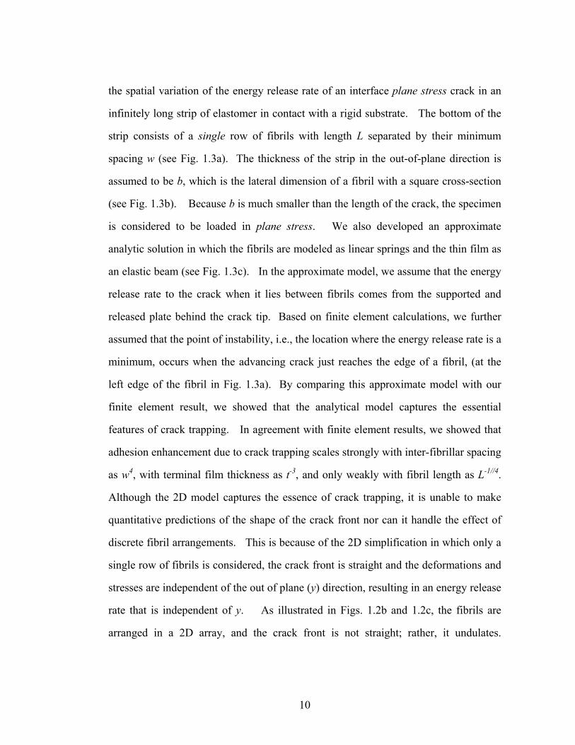
Predicting the behavior of crack propagation through such a structure requires one to
handle a curved crack front.
Figure 1. 3 (a) Geometry of a strip with a semi-infinite crack on the film/substrate
interface. (b) Geometry of fibrils. (c) Schematic drawing of a beam model adhered to
a substrate at its right end and loaded at the left via linear springs.
In addition to quantitatively predicting the shape of the crack front, the model
we present in this work allows us to address questions such as how patterning of
fibrils affects adhesion. To the best of our knowledge, this problem has not been
studied in the literature. For example, experiments show that, with the same fibril
geometry and area density of fibrils, hexagonal arrays have higher adhesion than
square arrays. The 2D model of crack trapping cannot explain this phenomenon. For
simplicity, in this work we consider square and hexagonal patterns where there is a
b
(c)
w L
b
Rigid substrate
H
x
z
y
Interfacial crack (a)
(b)
Δ
pp
d
Backing layer (elastomer strip)
film
12
unique minimum spacing for each case; the methods we develop can be applied to
other regular patterns of fibril arrangement.
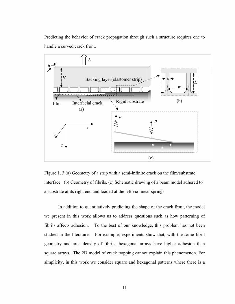
Figure 1.4 below shows two different arrays. Fig. 1.4a is a schematic drawing
of the top view of a square pattern of fibrils with minimum center-to-center
distance sw , and Fig. 1.4b is for a hexagonal pattern with minimum center-to-center
distance hw .
Figure 1. 4 (a) Top view of a square pattern of fibrils with minimum center-to-center
distance sw ; (b) top view of a hexagonal pattern of fibrils with minimum center-to-
center distance hw . Two of the possible crack growth directions are indicated by x′
and x .
(a)
sw
hw
(b)
x
y
x′
y′
x
y
x′
y′
13
Modeling the motion of a crack front through such a microstructure is a
difficult three-dimensional problem because the shape of the crack front is not known
and has to be determined as part of the solution. A fully numerical approach (e.g.,
using the finite element method) to solve for the position of the crack front would be a
formidable challenge with doubtful efficacy because it would require a very large
number of elements, likely with adaptive meshing to follow the evolving crack front,
and the ability to handle variations in a large number of geometrical and material
parameters that remain numerous even when reduced to a set of dimensionless
parameters. Moreover, it would be difficult to gain physical insight from these
numerical results. Fortunately, our previous 2D analysis has yielded approximations
that accurately capture the results of full 2D numerical simulations.27 The critical
quantity one needs to calculate is the minimum energy release rate. For an idealized
geometry in which the fibril ends join the film making a sharp corner, we found that it
is a good approximation to assume that this occurs when the crack tip just reaches the
edge of a fibril. That is, the energy stored in the fibril is available to the crack only
when the crack tip goes under it. This allowed us to develop a simplified analytical
model in which, to calculate the energy release rate under this condition, the fibrils can
be modeled as linear springs and the film as a linear elastic plate. In this work, we
develop a 3D model based on these approximations that has sufficiently reduced
complexity to be solvable, and that also retains an ability to provide physical insight.
1.2 Model for Crack Between a Plate and Substrate Trapped by An Array of
Fibrils
14
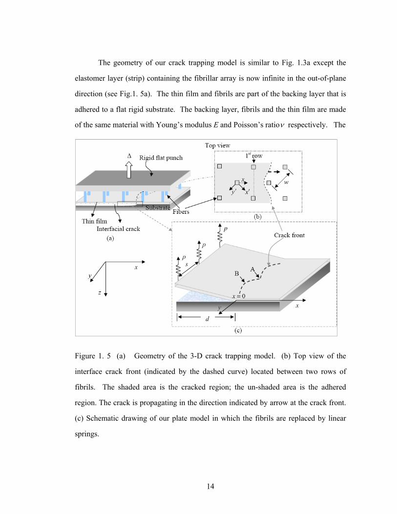
The geometry of our crack trapping model is similar to Fig. 1.3a except the
elastomer layer (strip) containing the fibrillar array is now infinite in the out-of-plane
direction (see Fig.1. 5a). The thin film and fibrils are part of the backing layer that is
adhered to a flat rigid substrate. The backing layer, fibrils and the thin film are made
of the same material with Young’s modulus E and Poisson’s ratioν respectively. The
Figure 1. 5 (a) Geometry of the 3-D crack trapping model. (b) Top view of the
interface crack front (indicated by the dashed curve) located between two rows of
fibrils. The shaded area is the cracked region; the un-shaded area is the adhered
region. The crack is propagating in the direction indicated by arrow at the crack front.
(c) Schematic drawing of our plate model in which the fibrils are replaced by linear
springs.
15
orientation of the fibrils is specified by a local coordinate system ( x′ , y′ ) (see Fig.
1.5b) and the minimum spacing between fibrils is denoted by w. The interface crack
occupies part of the (x, y) plane and its front lies between two rows of fibrils as shown
in Fig. 1.5b. The position of this crack front is specified by a function ( )x g y= ,
where 0x = corresponds to the position of the crack front where it is maximally
extended. In Fig. 1.5b, the crack propagates in the x direction, which is oriented 45o
from the x′ axis. For the square pattern shown in Fig. 1.5b, the function ( )x g y= is
periodic in y with period 2s w= . Note that, in general, both s and the angle between
(x,y) and ( ,x y′ ′ ) frames depend on the orientation of the crack growth direction as
well as the fibril pattern.
The crack is loaded by applying a vertical displacement Δ to the rigid punch.
To compute the local energy release rate, we make use of the fact that the fibrils are
more compliant than the backing layer. We also assume that the plate is very
compliant compared to the fibril so that in the cracked region we need to model only
up to the first row of fibrils at x d= − to which we apply the deformation (see Fig.
1.5b). The maximum distance of the crack front from the line joining this row of
fibrils is denoted by d (see Fig. 1.5c). As in Shen et al,27 we model the film as an
elastic plate and replace the fibrils by a linear spring with stiffness 2 /k Eb L= . Due
to the applied displacement at x d= − , the plate is subjected to periodic point forces p
via the discrete array of springs. Since material points directly ahead of the crack
front are bonded to the rigid substrate, the plate is clamped at ( )x g y= . The shear
force and bending moment on the plate at x d= − are zero, consistent with our
assumption that all the deformation is concentrated on this row of fibrils. Finally, the
relation between p and Δ is given by
( )( ), 0p k u x d y= Δ + = − = (1.1)
16
where u is the deflection of plate and the displacement is assumed to be positive
downwards. Note, for a fixed applied displacement Δ , the energy release rate is
expected to decrease with the “effective crack” length d.
The key quantity to be evaluated is the local energy release rate
( ( ), )L LG G x g y y= = along the curved crack front. The local energy release rate for
a curved crack front is derived in Appendix A. The result is
( )2 23 ( )
6L n t x g y
G M MEh =
= − , (1.2)
where n and t denote local normal and tangential unit vectors of the curve ( )x g y=
at ( ),x y . nM and tM are principal bending moments that are related to the principal
curvatures ,nnu and ,ttu by 33
( ), ,n nn ttM D u uν= − + (1.3a)
( ), ,t tt nnM D u uν= − + (1.3b)
where ,nnu denotes 2 2/u n∂ ∂ and D is the bending stiffness of the plate,
( )3
212 1EhD
ν=
−. (1.4)
The plate deflection u obeys the biharmonic equation 33
4 4 2 2
4 4 2 22 0u u u uDx y x y
⎛ ⎞∂ ∂ ∂ ∂+ + =⎜ ⎟∂ ∂ ∂ ∂⎝ ⎠
with ( , ( ))x d g y∈ − and y < ∞ (1.5)
The boundary conditions are
17
( ( ), ) 0u x g y y= = (1.6a)
( ( ), ) 0u x g y yn
∂= =
∂ (1.6b)
2 2
2 2 0x d
u uvx y
=−
⎡ ⎤∂ ∂+ =⎢ ⎥∂ ∂⎣ ⎦
(1.6c)
( )3 2
3 22 ( )kx d
u u pv y ksx x y D
δ∞
=−∞=−
⎡ ⎤∂ ∂ −+ − = −⎢ ⎥∂ ∂ ∂⎣ ⎦
∑ integerk = (1.6d)
where δ is the Dirac delta function and the negative sign in front of p in (1.6d) is
because of the convention that positive shear force is along the negative z-direction.
Equations (1.6a) and (1.6b) state that the plate is clamped at ( )x g y= , whereas (1.6c)
states that the bending moment 0xM = at x d= − . Finally, (1.6d) enforces the
condition that points loads are applied periodically at x d= − , where the LHS of eq
(1.6d) is the formula for shear force in a plate 33.
The position of the crack front ( )x g y= is not known a priori. It is
determined by the crack growth condition
( ( ), )L adG x g y y W= = , (1.7)
where adW is the intrinsic work of adhesion of the interface between the film and the
indenter and is assumed to be a material constant. The inverse problem specified by
equations (1.5), (1.6a) – (1.6d) and (1.7) will be solved using two different methods:
perturbation theory and a finite element method. The perturbation method will be
given in Section 1.3 whereas the finite element results are given in Section 1.4.
18
1.3 Perturbation Theory
This method assumes that the amplitude of the curved crack front undulations
is small in comparison with the spacing s, that is,
( ) ( )g y d yε φ= (1.8)
where ( )yφ is an order 1 function and 0 1ε< << . We seek a solution in the form of a
perturbation series
1( , ) ( , ) ......ou u x y u x yε= + + (1.9)
The zeroth order solution ou corresponds to a straight crack front located at
( ) 0x g y= = . For this case the effective length of the crack is d. This case can be
solved exactly (see Appendix B for details). The displacement field is
3 2
21
23 ( / ) cos6o m
m
pd x x m yu x sDs d sd
π∞
=
⎡ ⎤⎛ ⎞ ⎛ ⎞= − + + Ω⎢ ⎥⎜ ⎟ ⎜ ⎟⎝ ⎠ ⎝ ⎠⎣ ⎦
∑ (1.10)
where ( / )m x sΩ is
( ) ( ) ( )( / ) 1 / sinh 2 / / cosh 2 /m m m m mx s B x d m x s x d m x sλ α π α π⎡ ⎤Ω = − −⎣ ⎦ (1.11a)
in which mλ , Bm, and mα are dimensionless quantities defined by
(1 ) tanh( ) (1 )2 (1 ) tanh( )
m mm
m m
v vv
α αλα α
+ + −=
+ − (1.11b)
and
( ) ( )[ ] 32 (1 ) cosh( ) (1 ) (1 ) sinh( )
2
m m m m m mm
mv v vB
λ α α λ α α α+ − − + + −= (1.11c)
19
2 /m m d sα π= (1.11d)
The local energy release rate can be calculated using (1.2) and (1.3a,b). Since the
fibrils are discretely spaced, it varies periodically along the straight front
22 22
21
21 2 cos2o m m m
m
p d m yG BsDsπα λ
∞
=
⎡ ⎤⎛ ⎞= +⎢ ⎥⎜ ⎟⎝ ⎠⎣ ⎦
∑ (1.12)
Note that (1.12) expresses the local energy release rate in terms of the force on a fibril,
p. The relation of the local energy release rate with the applied displacement Δ will
be discussed later in this section.
The first term of (1.12) is the energy release rate obtained in a plane stress
analysis which was obtained by Shen et al.27 As mentioned earlier, this previous
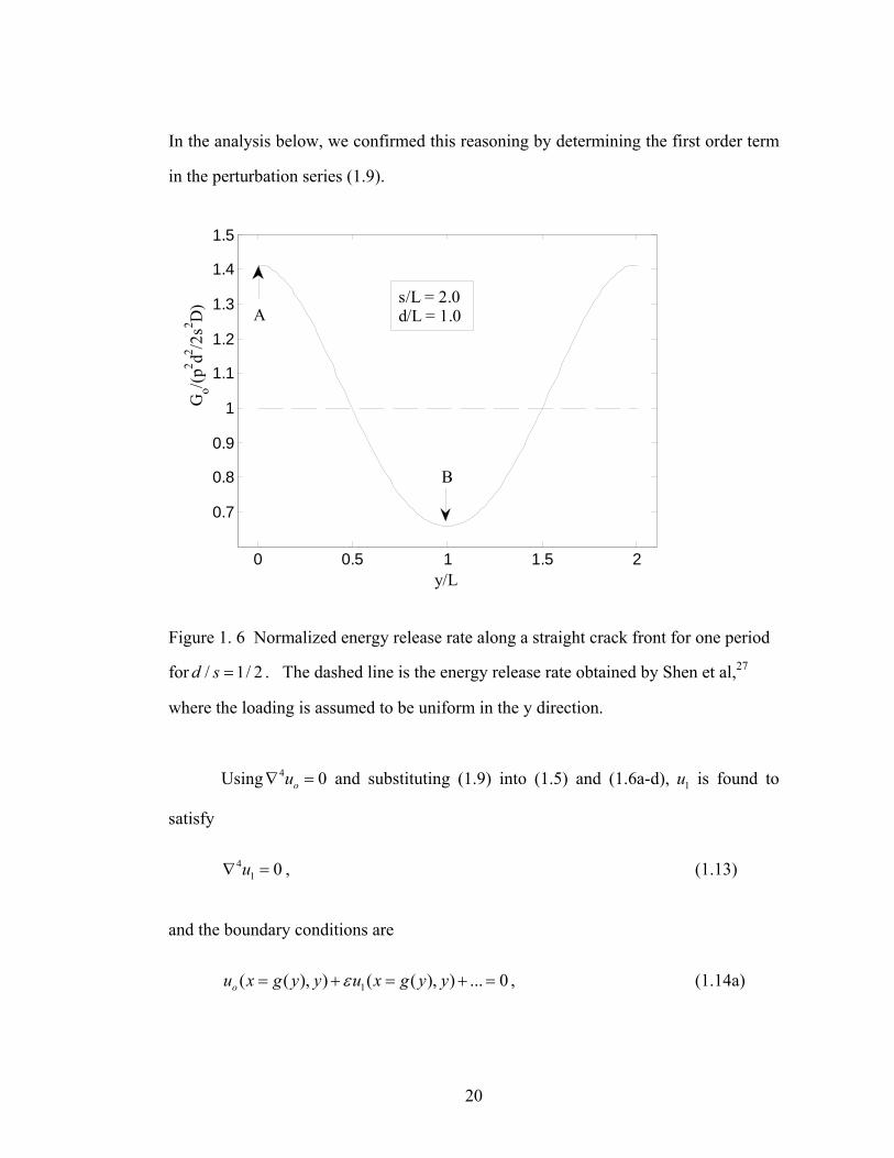
analysis ignores the distribution of fibrils in the y direction. Figure 1.6 plots the normalized zeroth order energy release rate ( )2 2 2/ / 2oG p d Ds as a function of
normalized position /y L for one period with / 0.5d s = . Since we are interested in
the dependence of local energy release rate on crack length (d) and on the spacing
/ 2w s= (square pattern), we normalized y by the fibril length L, which we
consider to be fixed. Physically, we expect the minimum energy release rate to occur
midway between two fibrils (B in Fig. 1.5c) whereas the maximum occurs directly
ahead of the two fibrils (A in Fig. 1.5c). This is confirmed by (1.12), which shows that oG achieves its maxima at 0,y ms= ± and minima at ( )2 1 / 2y m s= ± − . The fact
that the energy release rate is a constant along the equilibrium crack front (see (1.7))
suggests that the actual crack front should be longer (point A in Fig. 1.5c) than the
case of straight crack front when the energy release rate is high (e.g. A in Fig. 1.6) and
shorter (indicated by point B in Fig. 1.5c) when the energy release rate is low (e.g. B
in Fig. 1.6). A schematic picture of the actual crack front is indicated in Fig. 1.5c.
20
In the analysis below, we confirmed this reasoning by determining the first order term
in the perturbation series (1.9).
0 0.5 1 1.5 2
0.7
0.8
0.9
1
1.1
1.2
1.3
1.4
1.5
y/L
Go/(p
2 d2 /2s2 D
)
B
As/L = 2.0d/L = 1.0
Figure 1. 6 Normalized energy release rate along a straight crack front for one period
for / 1/ 2d s = . The dashed line is the energy release rate obtained by Shen et al,27
where the loading is assumed to be uniform in the y direction.
Using 4 0ou∇ = and substituting (1.9) into (1.5) and (1.6a-d), 1u is found to
satisfy
41 0u∇ = , (1.13)
and the boundary conditions are
1( ( ), ) ( ( ), ) ... 0ou x g y y u x g y yε= + = + = , (1.14a)
21
1( ( ), ) ( ( ), ) ... 0ou ux g y y x g y yn n
ε∂ ∂= + = + =
∂ ∂ (1.14b)
2 2
1 12 2 0
x d
u uvx y
=−
⎡ ⎤∂ ∂+ =⎢ ⎥∂ ∂⎣ ⎦
(1.14c)
( )3 2
1 13 22 0
x d
u uvx x y
=−
⎡ ⎤∂ ∂+ − =⎢ ⎥∂ ∂ ∂⎣ ⎦
(1.14d)
where ( ) ( )2 2
1 ( ),1 ( ) 1 ( )
g yng y g y
⎛ ⎞′−⎜ ⎟=⎜ ⎟′ ′+ +⎝ ⎠
r is the unit normal vector to the curve
( )x g y= . Equations (1.14a,b) can be expanded into a perturbation series by noting
that,
( ) ( )1, ( ) 1, ( )n g y d yε φ′ ′≈ − = −r (1.15)
or
( ),
( )x d y y
u u ud yn x yε φ
ε φ=
∂ ∂ ∂′= −∂ ∂ ∂
(1.16)
Using (1.16) and neglecting higher order terms in (1.14a) – (1.14b), the boundary
conditions for 1u are
1(0, ) 0u y ≈ (1.17a)
2
12( 0, ) ( 0, ) ( )ouu x y x y d y
x xφ∂∂
= ≈ − =∂ ∂
(1.17b)
2 21 1
2 2 0x d
u uvx y
=−
⎡ ⎤∂ ∂+ =⎢ ⎥∂ ∂⎣ ⎦
(1.17c)
22
( )3 2
1 13 22 0
x d
u uvx x y
=−
⎡ ⎤∂ ∂+ − =⎢ ⎥∂ ∂ ∂⎣ ⎦
(1.17d)
In deriving equation (1.17a), we have made use of the fact that ( ) ( )g y d yε φ= , / 0ou n∂ ∂ = and / 0u n∂ ∂ = on the boundary. Note that ( )yφ is a
periodic function with period s . Our numerical results show that ou is well
approximated by the first two terms in (1.10), i.e., we consider only the term m=1 in
the summation. Using this approximation, (1.17b) becomes
221
1 1 12( 0, ) 1 2 cos ( )u pd yx y B y
x Ds sπα λ φ∂ ⎡ ⎤⎛ ⎞= = − ⎜ ⎟⎢ ⎥∂ ⎝ ⎠⎣ ⎦
(1.18)
The unknown crack front position ( )yφ is obtained using the condition that the local
energy release rate is constant along the crack front. According to (1.2), at
equilibrium, the energy release rate along the crack front is
2 2, ,( ) 0
.2 2L nn xx adx d y x
D DG u u Wε φ= =
= ≈ ≈ (1.19)
where we have assumed that 1ou u uε≈ + and , 0ttu = zero along the crack front
because of the clamped boundary condition.
Since ( )yφ is periodic, it can be expanded as a Fourier series. A simple
calculation shows that 1u has a Fourier series solution (see Appendix C) for any
continuous ( )yφ . However, our problem is more complicated since ( )yφ is an
unknown function determined by the crack growth condition (1.19). This is
accomplished using the following procedure.
1. Assume a functional form for ( )yφ ,
23
( ) 2 4 6cos 1 cos 1 cos 1y y yys s sπ χ π β πφ
ε ε⎛ ⎞ ⎛ ⎞ ⎛ ⎞⎛ ⎞ ⎛ ⎞ ⎛ ⎞= − + − + −⎜ ⎟ ⎜ ⎟ ⎜ ⎟⎜ ⎟ ⎜ ⎟ ⎜ ⎟⎝ ⎠ ⎝ ⎠ ⎝ ⎠⎝ ⎠ ⎝ ⎠ ⎝ ⎠
(1.20)
where , ,ε χ β are unknown parameters to be determined.
2. Use the exact solution derived in Appendix C to express the energy release rate
in terms of these unknown parameters (e.g. , ,ε χ β ). Minimize the variance of
the energy release rate along the crack front to determine the values of these
parameters. Details are also given in Appendix C.
-0.5 -0.4 -0.3 -0.2 -0.1 0g(y/L)/L
y/L
d/s=0.8d/s=0.5d/s=0.4
L = 30 μms/L=2 1.5
1.0
0.5
0
2.0
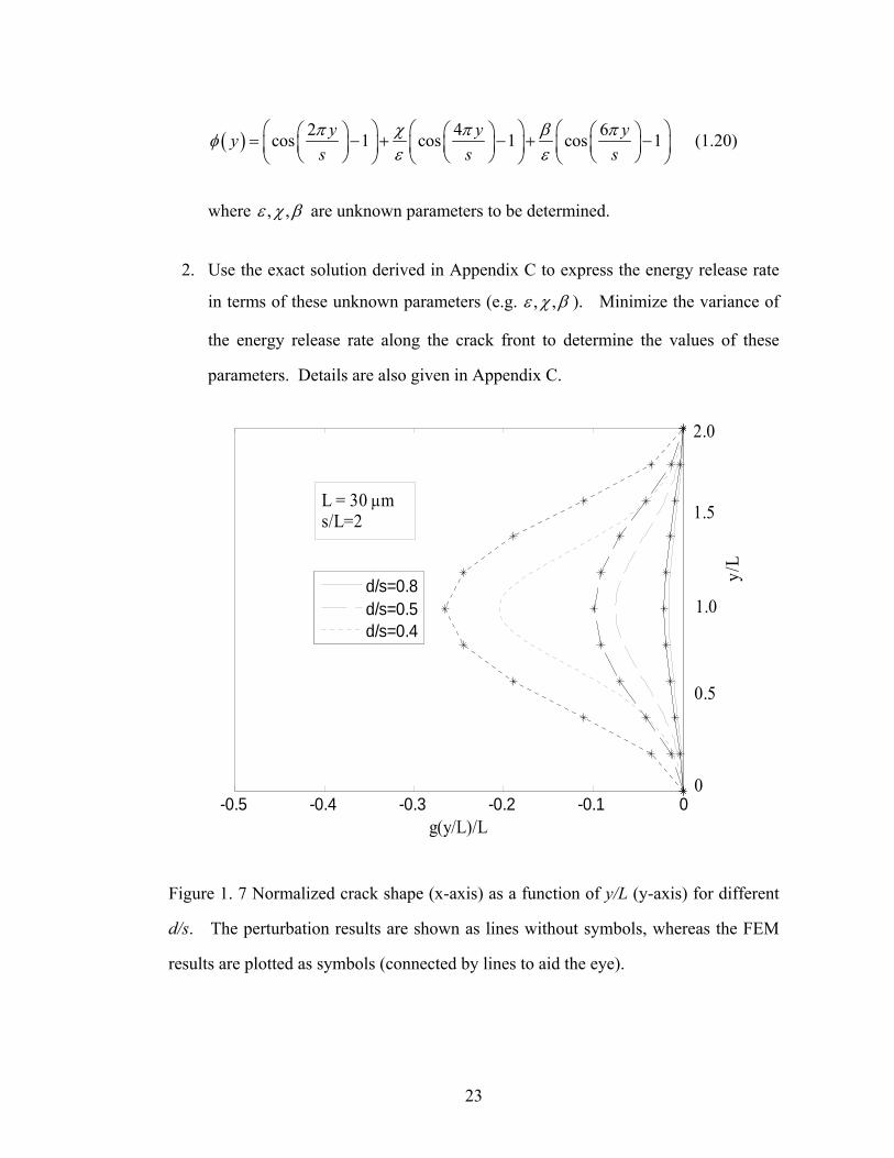
Figure 1. 7 Normalized crack shape (x-axis) as a function of y/L (y-axis) for different
d/s. The perturbation results are shown as lines without symbols, whereas the FEM
results are plotted as symbols (connected by lines to aid the eye).
24
Fig. 1.7 plots the normalized crack shape ( )/ / ( / ) /g y L L d y L Lε φ= for
different values of d/s with / 2s L = . Lines without symbols are the perturbation
results. Lines with symbols are finite element results which will be discussed in the
next section. Note that each crack front in Fig. 1.7 has a different effective work of
adhesion. This is because the equilibrium position of the crack front is determined
by the energy release rate, which increases with d for a fixed applied load. In order
words, for the same p, s and w, the work of adhesion must increase to maintain
equilibrium if d increases. This figure shows that the shape of the crack front is
sensitive to the work of adhesion. The equilibrium crack front is more curved for
smaller work of adhesion. Fig.1.7 shows that the amplitude of the crack front
increases as /d s decreases, which is consistent with experimental observations.
Figure 1.7 shows that the perturbation theory breaks down as d/s decreases, that is, the
crack becomes shorter. Later, we will show that the perturbation theory works very
well for d/s > 0.6 (see Figure. 1.9).
Since the local energy release rate can be expanded in terms of a cosine series
about / 2y s= , and the integral average of the energy release rate in a period is given
by the first (constant) term of the cosine series. According to our perturbation theory
(see (C19) Appendix C), this constant term is2 2
22 adp d WDs
= . Thus, the average energy
release rate is
2 2 2 2
2 3 22avep d p dGDs h s
= ∝ , (1.21)
which is the energy release rate of a straight interface crack lying between a rigid
substrate and a plate subject to a uniformly distributed shear load /p s at the edge
x d= − .
25
We should point out that, since we control the displacement Δ , force p is
related to the Δ through (1.1). Evaluating the perturbation solution 1ou u uε= + at
, 0x d y= − = , and using (1.1), we found
313
pd d
k Ds s
Δ=
⎛ ⎞+ Κ ⎜ ⎟⎝ ⎠
(1.22)
where ( )/d sΚ is a dimensionless function of d/s. It is zero at / 0d s = and increases
monotonically to 1 as /d s → ∞ . The full expression of ( )/d sΚ is given in appendix
C. The average energy release rate expressed in terms of Δ is
22
4 39 32aveD d DsG
sd kd
−Δ ⎡ ⎤⎛ ⎞= Κ +⎜ ⎟⎢ ⎥⎝ ⎠⎣ ⎦
(1.23)
The normalized average energy release rate 4 22 / 9aves G DΔ versus /d L is shown in
Figure 1.8a for / 2.0s L = . For fixed s, the average applied energy release rate
decreases rapidly with increasing d. This means that the minimum average release
rate occurs at maxd , that is, at the left edge of a row of fibrils. As a consequence, the
crack front will be trapped along this edge and crack growth is unstable when
aveG reaches adW . Figure 1.8b plots the normalized average energy release versus
/s L for / 1.0d L = . In both figures, we used 3 ,E MPa= 0.5ν = , 30 ,L mμ=
/ 1/10h L = , and / 1/ 3b L = . Figure 1.8b shows that the normalized average energy
release rate decreases linearly with s in the typical range of interest.
26
0.6 0.8 1 1.2 1.4 1.610
0
101
102
d/L
2s4 G
eve/(9
DΔ
2 )
s/L = 2.0
(a)
1.4 1.6 1.8 2 2.20.7
0.75
0.8
0.85
0.9
0.95
s/L
2d4 G
ave/(9
DΔ
2 )
d/L = 1.0
(b)
Figure 1.8 (a) The normalized average energy release rate 4 22 / 9aves G DΔ versus
/d L with / 2.0s L = . (b) The normalized average energy release versus /s L with
/ 1.0d L = .
0.4 0.45 0.5 0.55 0.6 0.65 0.7 0.75 0.80
0.5
1
1.5
d/s
G/(P
2 d2 /2s2 D
)
Perturbation theoryFEM
Figure 1.9 The constant energy release rate versus d/s. The perturbation result is
shown as solid line and FEM result is plotted in symbol.
27
1.4 Finite Element Analysis
In the previous section we obtained an approximate solution using perturbation
theory. In this section we investigate the limitation of the perturbation theory using
finite element method (FEM) to solve the plate equations we developed in section 1.2.
Because of periodicity in the y-direction, we need only to consider the domain
[ ], ( )x d g y∈ − and [ ]0,y s∈ . In our FEM, we vary the shape of the crack front until
the local energy release rate LG is uniform along the crack front. The value of this
constant LG will depend on the specimen geometry (e.g. d) and the applied load.
Details of the FEM are given in supplementary materials; here we summarize the results. The normalized crack profiles ( )/ /g y L L versus /y L for different
/d s (and hence different effective work of adhesion) are plotted in Figure 1.7 as
symbols. Figure 1.9 plots the constant energy release rate along the crack front
against d/s. The symbols (connected by straight lines for viewing) are the FEM result.
Energy release rate obtained using perturbation theory is the solid line. Figure 1.9
shows that, for the same geometry and applied load, the perturbation theory
overestimates the energy release rate. However, there is no practical difference
between the two methods for long cracks (large d/s). Since the crack traps near the
edge of fibrils, the perturbation theory should work well for most situations.
1.5 Effect of Pattern (Orientation)
In this section we investigate the effect of fibril pattern and crack growth
directions on the energy release rate. For concreteness, we compare hexagonal and
square arrays at the same area density of fibrils (see Fig. 1.4).
28
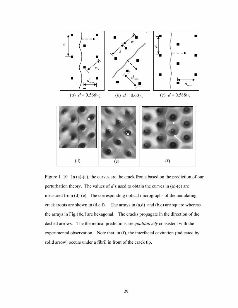
Fig. 1.8 shows that, as long at the crack lies between two rows of fibrils, the
average energy release rate, aveG , decreases monotonically with increasing crack
length. For the sake of simplicity, we assume that crack growth is stable until aveG
reaches its minimum value, minaveG , i.e., when min
ave adG W= , even though local crack
instability could occur before aveG = minaveG due to the curvature of the crack front. In
the previous section we assume that d and s are quantities that can vary independently.
However, to apply the model to a given lattice, we pick a crack growth direction on
that lattice. Once we do so, both dmax and s are specified and are no longer
independent quantities (see Figs. 1.10 a-c). In these figures, the dashed curves
indicate the crack fronts based on the prediction of the perturbation theory. The
corresponding optical micrographs of the undulating crack fronts are shown in Fig.
1.10d,e,f, where Fig. 1.10d corresponds to Fig.10a, Fig.10e corresponds to Fig. 1.10b,
and Fig. 1.10f corresponds to Fig. 1.10c. The cracks propagate in the direction
indicated by the dashed arrows. Note that the theoretical predictions are qualitatively
consistent with the experimental observations. Let sw ( hw ) be the minimum distance
between fibrils in a square (hexagon) array. The period is 2 ss w= for crack
orientation shown in in Fig.1.10a and ss w= for crack orientation in Fig.1.10b,
whereas the period s is found to be hw for crack orientation in Fig.1.10c. In these
three figures, d achieves its maximum value denoted by maxd which is approximately
equal to max / 2sd w= in Fig. 1.10a, max sd w= in Fig. 10b, and max 3 / 2hd w= in
Fig. 1.10c.
29
(d)
(f)
Figure 1. 10 In (a)-(c), the curves are the crack fronts based on the prediction of our
perturbation theory. The values of d’s used to obtain the curves in (a)-(c) are
measured from (d)-(e). The corresponding optical micrographs of the undulating
crack fronts are shown in (d,e,f). The arrays in (a,d) and (b,e) are square whereas
the arrays in Fig.10c,f are hexagonal. The cracks propagate in the direction of the
dashed arrows. The theoretical predictions are qualitatively consistent with the
experimental observation. Note that, in (f), the interfacial cavitation (indicated by
solid arrow) occurs under a fibril in front of the crack tip.
s
sw
sw hw
maxd maxd maxd
( ) 0.566 sa d w= ( ) 0.60 sb d w= ( ) 0.588 hc d w=
s
(e)
30
To quantify the effect of patterns and orientation on the minimum average energy
release rate, we compare patterns with the same number of fibrils per unit area (area
density). The area density sρ for a square pattern is
21/s swρ = . (1.24)
Since the area of a hexagon is 23 3 / 2hw and the total effective number of fibrils
within a hexagon is 3, the area density for a hexagon pattern hρ is
22
3 233 3 / 2
hhh ww
ρ = =⎡ ⎤⎣ ⎦
. (1.25)
The two patterns have the same area density if
1/ 4
23h sw w= . (1.26)
For a given pattern, one can also compare minaveG for different crack orientations
shown in Fig.1.10a and Fig. 1.10b using (1.23). For example, at the same applied
displacement on a square pattern, we have
( )2 2min
maxmin 2 2
max
( 2 , / 2) 1 3 34 1 32( , ) 16
ave s s s
ave s s s s s
G s w d w D DG s w d w kw kw
−⎡ ⎤ ⎡ ⎤= = ⎛ ⎞= Κ + Κ + ≈⎢ ⎥ ⎢ ⎥⎜ ⎟= = ⎝ ⎠⎣ ⎦ ⎣ ⎦
(1.27)
where we have used 0.5ν = , 3 ,E MPa= 30 ,L mμ= / 2 /15h L = , and / 1/ 3b L = .
Equations (1.27) and (1.23) imply that that the applied displacement required to
propagate the crack in Fig.10a is smaller than the displacement to propagate the crack
in Fig. 10b by about a factor of 3 .
31
Next, we compare the hexagon pattern in Fig.1.10c with the square pattern in
Fig.1.10a at the same number density ρ . The ratio of the minimum average energy
release rate ( ) ( )min min/ave aveG square G hexagon in this case is
( )( )
min minmax
min min 1/4max
( 2 , / 2) 2( 2 / 3 , 3 / 2 )
ave ave s s s
ave ave h s s
G square G s w d wG hexagon G s w d w
= == ≈
= = (1.28)
where we have used (1.26) and 0.5ν = , 3 ,E MPa= 30 ,L mμ= / 2 /15h L = ,
and / 1/ 3b L = . Thus, for the same applied displacement and the same number density,
the square pattern has an energy release rate 2 times larger than that of the hexagonal
pattern. This means for a given area density of fibrils, hexagonal arrays should have
close to twice the effective work of adhesion than square arrays for similar crack
orientations. This is consistent with the experimental results .15,22
0 0.5 1 1.5 2 2.50
1
2
3
4
5
6
7
8
ρ2L4
2Gav
em
inL4 /9
DΔ
2
Fig.10aFig.10cFig.10b
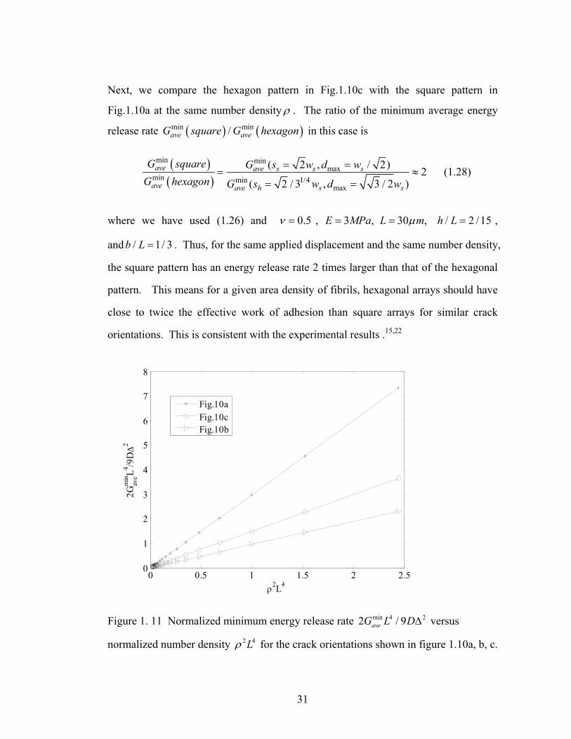
Figure 1. 11 Normalized minimum energy release rate min 4 22 / 9aveG L DΔ versus
normalized number density 2 4Lρ for the crack orientations shown in figure 1.10a, b, c.
32
Our results in this section can be summarized by Fig.1.11 which plots the
minimum average energy release rate min 4 22 / 9aveG L DΔ for both patterns and for the two
different crack orientations shown in figure 1.10a,b. The parameters we used to
obtain Figure 1.11 are 3 ,E MPa= 30 ,L mμ= / 2 /15h L = , and / 1/ 3b L = . Figure
1.11 shows that, for all cases, the normalized minimum energy release rate increases
approximately linearly with 2 4Lρ . Since 21/ wρ ∝ , the minimum energy release rate
is proportional to 4w− , consistent with our previous plane stress result. 27 Fig. 1.11
shows that, for the same number density ρ and applied displacement Δ , the square
pattern with crack orientation in Fig. 10a has the largest minimum average energy
release rate, while the square pattern with crack orientation in Fig. 1.10b has the
smallest minimum average energy release rate. The minimum average energy release
rate of the hexagon pattern (Fig. 1.10c) lies in between.
1.6 Summary and Discussion
In this paper, we propose a three dimensional model to study crack trapping on
a film-terminated fibril array. A perturbation method was developed to compute the
shape of crack front based on the assumption that the local energy release rate along
the crack front is a material constant which is equal to effective work of adhesion.
Our result shows that the shape of the crack front is sensitive to the work of adhesion.
The equilibrium crack front is more curved for smaller work of adhesion. The average
applied energy release rate along the crack front was also evaluated. Our numerical
results showed that the average applied energy release rate decreases rapidly with
increasing crack length. FEM calculations are carried out to compare with the
perturbation theory. It was shown that there is no practical difference between the
33
two methods for long cracks. Based on our perturbation solution, we derived an exact
expression for the average minimum energy release rate where crack is trapped. The
minimum energy release rate was found to be proportional to 4w− . This result is
consistent with our previous plane stress result. 27
As an application of the 3-D crack trapping model, we studied the effect of the
fibril patterns and the crack orientations on the effective work of adhesion. First we
compared the minimum average energy release rate of two different crack orientations
on the same square array. We showed that the one with the crack propagating in the
minimum spacing direction (Fig. 1.10b) should have higher effective work of adhesion
than the one propagating along the diagonal direction of the square pattern (Fig.1.10a).
We also compared minimum average energy release rate the hexagon pattern with the
square pattern for the same fibrils density. We found that, consistent with experiments,
hexagonal arrays (Fig. 1.10c) have higher effective work of adhesion than square
arrays (Fig. 1.10a) for similar crack orientations.
In the idealized sample we considered in this work, the far field energy release
rate is given by
2
2f
f
E AG
LρΔ
= (1.29)
where 2A b= is the area of the cross section of a fibril. Equation (1.29) can be
interpreted as the average energy release rate in the x direction. The crack growth
condition f adG W= implies that the critical applied displacement for crack growth to
take place without crack trapping is
2 2 adf
LWE Aρ
Δ = (1.30)
34
However, with crack trapping, the critical applied displacement cΔ for growth to
occur can be obtained using (1.23) and the condition minave adG W= , i.e.,
24
23
2 39
adc
d W d DsD s kd
⎡ ⎤⎛ ⎞Δ = Κ +⎜ ⎟⎢ ⎥⎝ ⎠⎣ ⎦ (1.31)
The ratio of (1.31) and (1.30) is
242max maxmin
2 3max
39f
d E A d DsDL s kd
ρ ⎡ ⎤Δ ⎛ ⎞= Κ +⎢ ⎥⎜ ⎟Δ ⎝ ⎠⎣ ⎦ (1.32)
which is very sensitive to maxd .
For the hexagonal pattern with crack orientation shown in Fig. 10c, (1.32) is
2 2min / 174fΔ Δ ≈ (1.33)
with typical values of parameters 0.5,ν = 3 ,E MPa= 52.5L mμ= , 4h mμ=
14b mμ= , 62w mμ= , and max / 3 / 2 1.02d L w L= = . The ratio (1.33) is much
larger than experimental data which is in the range of 4.0 – 6.0. 14, 15 This is a
limitation of our model in that it is very sensitive to the choice of maxd – taking it to be
at the edge of the fibril results in too large a number. Experimental behavior of the
actual material is more complicated for two reasons. Firstly, the corner where the
fibril meets the plate is rounded because of how the structure was fabricated (Fig. 1.1).
This moves the point of minimum energy release rate some distance away from the
fibril, thus reducing maxd . Secondly, as we have noted elsewhere, 34 for larger inter-
fibril separation, the mechanism of failure shifts to one limited by cavitation under the
fibril ahead of the crack (Fig. 1.10f). Although the 3D crack trapping model is
therefore unable to make quantitatively accurate predictions of adhesion enhancement,
it remains useful as a comparative tool to study the effect of fibril arrangements.

35
1.7 Future work
As pointed out in previous section, our 3D model has limitations in that it
overestimates the factor of adhesion enhancement. The following suggestions can be
considered to overcome the difficulty and improve the model.
1. Relax the approximation that only one row of fibrils behind the crack were
considered.
2. Include the backing layer in the model. In other words, the compliance of the
backing is considered when modeling.
3. To extend our 3-D crack trapping model to study the real spherical problem, a
full FFM may be used. This is not trivial because the crack front is not known.
36
APPENDIX A
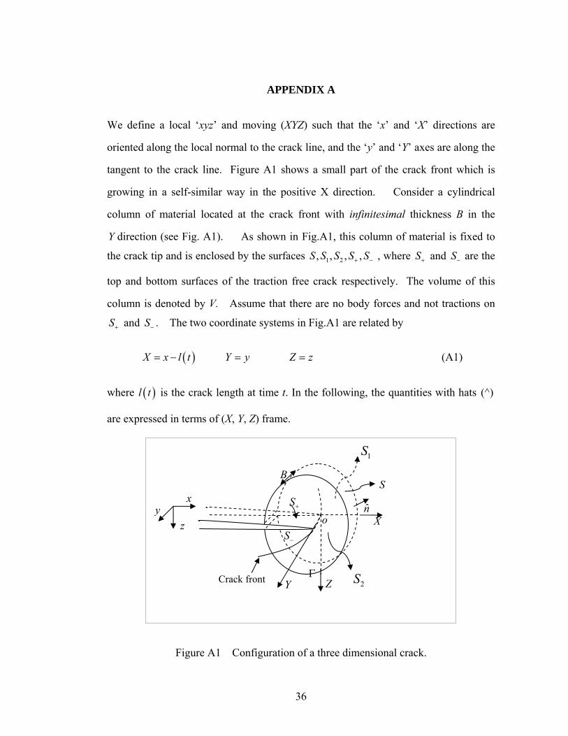
We define a local ‘xyz’ and moving (XYZ) such that the ‘x’ and ‘X’ directions are
oriented along the local normal to the crack line, and the ‘y’ and ‘Y’ axes are along the
tangent to the crack line. Figure A1 shows a small part of the crack front which is
growing in a self-similar way in the positive X direction. Consider a cylindrical
column of material located at the crack front with infinitesimal thickness B in the
Y direction (see Fig. A1). As shown in Fig.A1, this column of material is fixed to
the crack tip and is enclosed by the surfaces 1 2, , , ,S S S S S+ − , where S+ and S− are the
top and bottom surfaces of the traction free crack respectively. The volume of this
column is denoted by V. Assume that there are no body forces and not tractions on
S+ and S− . The two coordinate systems in Fig.A1 are related by
( ) X x l t Y y Z z= − = = (A1)
where ( )l t is the crack length at time t. In the following, the quantities with hats (^)
are expressed in terms of (X, Y, Z) frame.
Figure A1 Configuration of a three dimensional crack.
X
Y
o
BS
1S
2SΓZ
x
z y n
Crack front
S+
S−
37
To compute the local energy release rate due to a small extension of this section of the
crack front, we first compute the rate of stress work on surfaces 1 2S S S+ + , which is
1 2
ij j iS S S
n u dSσ+ +
Σ = ∫& & (A2)
where nr is the outward unit normal vector of surfaces, ijσ is the stress tensor, iu are
the displacements and
( ), ,
, , ,ii
x y z
u x y z tu
t∂
=∂
& . (A3)
Note, since the crack faces are traction free, the work done on S+ and S− is zero. In
the local coordinate system (X, Y, Z), (A2) is
( ) ( )1 2 , ,
ˆ , , ,ˆ ˆˆ ˆ iiij j
S S S X Y Z
u X Y Z tun v t dSX t
σ+ +
⎛ ⎞∂∂⎜ ⎟Σ = − +⎜ ⎟∂ ∂⎝ ⎠
∫& (A4)
where
( ) ( )( )ˆ , , , , , ,ij ijX Y Z t x l t y z tσ σ= − (A5)
( ) ( )( )ˆ , , , , , ,i iu X Y Z t u x l t y z t= − (A6)
( ) ( )dl tv t
dt≡ (A7)
Let 12 ij ijW σ ε= denote the energy density, where ijε is strain tensor. The rate of
change of elastic strain energy of the material points inside V , E& , is:
38
( ) ( ) ( )
( )1 2 1 2
1 2 1 2
1 , 1
, 1
ˆ , , , ˆ ˆˆ ˆ ˆ ˆˆ ˆ ˆ ˆ
ˆˆ ˆˆ ˆ ˆ ˆ
V
ij i jt j jV S S S V S S S
ij i t j j jS S S S S S
dWE dVdt
W X Y Z tdV Wv t n dS u dV v t Wn dS
t
u n dV v t Wn dS
σ δ
σ δ
+ + + +
+ + + +
=
∂= − = −
∂
= −
∫
∫ ∫ ∫ ∫
∫ ∫
&
(A8)
where we have used the divergence theorem and ,i xu denotes /iu x∂ ∂ . The rate of
energy flow into this small section of the crack front is the difference between (A4)
and (A8), i.e.,
( )1 2
1ˆ ˆˆˆ ˆ ˆ( ) i
ij j j jS S S
uJ Bv t E v t n Wn dSX
σ δ+ +
∂⎛ ⎞⋅ = Σ − = − +⎜ ⎟∂⎝ ⎠∫&& (A9)
Thus,
( )1 2
1 ,11 ˆˆ ˆ ˆ ˆ ˆj j ij j i
S S S
J Wn n u dSB
δ σ+ +
= −∫ (A10)
As is well known, the J – integral in (A10) is surface independent. 33 For a very small
section of the crack front, 0B → so ˆ ˆdS Bd= Γ on S, and (A10) becomes
( ) ( )1 2
1 ,1 1 ,11 1ˆ ˆ ˆˆ ˆˆˆ ˆ ˆ ˆ ˆ ˆj ij i j j ij i j
S S
J W u n Bd W u n dSB B
δ σ δ σΓ +
= − Γ + −∫ ∫ (A11)
where Γ is the boundary of 1S . One can pick a contour Γ so that 1 0S → , therefore the
second term of (A11) vanishes. So
( )1 ,1ˆˆ ˆˆ ˆ ˆj ij i jJ W u n dδ σ
Γ
= − Γ∫ (A12)
The surface independence of (A10) implies that (A12) is independent of the path.
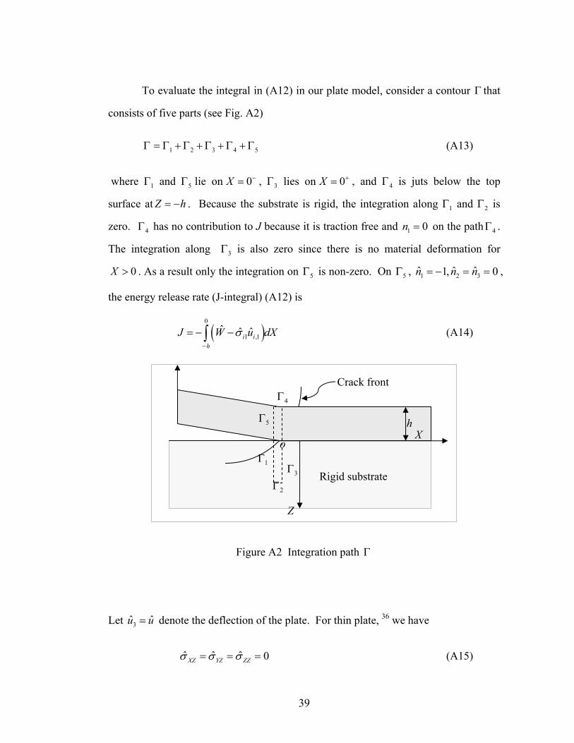
39
To evaluate the integral in (A12) in our plate model, consider a contour Γ that
consists of five parts (see Fig. A2)
Γ 1 2 3 4 5= Γ + Γ + Γ + Γ + Γ (A13)
where 1Γ and 5Γ lie on 0X −= , 3Γ lies on 0X += , and 4Γ is juts below the top
surface at Z h= − . Because the substrate is rigid, the integration along 1Γ and 2Γ is
zero. 4Γ has no contribution to J because it is traction free and 1 0n = on the path 4Γ .
The integration along 3Γ is also zero since there is no material deformation for
0X > . As a result only the integration on 5Γ is non-zero. On 5Γ , 1 2 3ˆ ˆ ˆ1, 0n n n= − = = ,
the energy release rate (J-integral) (A12) is
( )0
1 ,1ˆ ˆ ˆi i
h
J W u dXσ−
= − −∫ (A14)
Figure A2 Integration path Γ
Let 3ˆ ˆu u= denote the deflection of the plate. For thin plate, 36 we have
ˆ ˆ ˆ 0XZ YZ ZZσ σ σ= = = (A15)
X
Z
o
2Γ
5Γ
1Γ 3Γ
4Γ
Rigid substrate
Crack front
h
40
1ˆˆ
2h uu Z
X∂⎛ ⎞= − +⎜ ⎟ ∂⎝ ⎠
(A16)
2ˆˆ
2h uu Z
Y∂⎛ ⎞= − +⎜ ⎟ ∂⎝ ⎠
(A17)
Substituting (A15) to (A17) into (A14) gives
( )0
2, 1,
0
1 1 1ˆ ˆˆ ˆ ˆ ˆ ˆ2 2 2
1 1ˆ ˆˆ ˆ2 2
XX XX YY YY XY X Yh
XX XX YY YYh
J u u dX
dX
σ ε σ ε σ
σ ε σ ε
−
−
⎛ ⎞⎛ ⎞= − + −⎜ ⎟⎜ ⎟⎝ ⎠⎝ ⎠
⎛ ⎞= −⎜ ⎟⎝ ⎠
∫
∫ (A18)
For a thin plate, the normal stresses and strains are related by
( )( ) ( ) ˆ ˆˆ 11 1 2XX XX YY
Eσ ν ε νεν ν
= − +⎡ ⎤⎣ ⎦+ − (A19)
( )( ) ( ) ˆ ˆˆ 11 1 2YY YY XX
Eσ ν ε νεν ν
= − +⎡ ⎤⎣ ⎦+ − (A20)
where
( ) ( )2
1 ˆ ˆˆ2 1XX YY XXhZ M M
Dε ν
ν⎛ ⎞= − + −⎜ ⎟ −⎝ ⎠
(A21)
( ) ( )2
1 ˆ ˆˆ2 1YY XX YYhZ M M
Dε ν
ν⎛ ⎞= − + −⎜ ⎟ −⎝ ⎠
(A22)
where ˆXXM and ˆ
YYM are principle moments. Recall that the X and Y axes are normal
and tangential to the crack front respectively, so ˆXXM and ˆ
YYM are also nM and tM
that are related to the principal curvatures ,nnu and ,ttu by (3a) and (3b).
Substituting (A19) – (A22) to (A18) and evaluating the integral gives
41
( )2 23 0
6XX YY X
J M MEh =
= − (A23)
(A23) is the same as (2) in the (x, y, z) coordinate system.
42
APPENDIX B
For the zeroth order perturbation, ( ) 0g y = , the governing equation of ou is
4 4 2 2
4 4 2 22 0o o o ou u u uDx y x y
⎛ ⎞∂ ∂ ∂ ∂+ + =⎜ ⎟∂ ∂ ∂ ∂⎝ ⎠
with ( ,0)x d∈ − and y < ∞ (B1)
The boundary conditions are
( 0, ) 0ou x y= = (B2a)
( 0, ) 0ou x yn
∂= =
∂ (B2b)
2 2
2 2 0o o
x d
u uvx y
=−
∂ ∂+ =
∂ ∂ (B2c)
( )3 2
3 22 ( )o o
kx d
u u pv y ksx x y D
δ∞
=−∞=−
∂ ∂ −+ − = −
∂ ∂ ∂ ∑ integerk = (B2d)
Let us look for a periodic solution of the form:
( )( ) cos / 2 /m m m mu f x y d m d sα α π= = integerm = (B3)
Substituting (B3) into the biharmonic equation (B1) gives:
4 2 2 4
4 2 2 4
( ) ( )2 + ( ) 0m m m mm
d f x d f x f xdx d dx d
α α− = (B4)
There are two cases:
(i) For 0m ≠ , the solution of (B4) is
43
( ) ( ) ( ) ( )cosh / sinh / cosh / sinh /m m m m m m m m mf A x d B x d C x x d D x x dα α α α= + + +
(B5)
Using boundary conditions (B2a) – (B2d), we have
( ) ( ) ( ) ( ) ( )( )3
sinh / / cosh / / sinh /m m m m m m m mpdf B x d x d x d x d x dDs
α α α λ α α= − −
(B6)
where
(1 ) tanh( ) (1 )2 (1 ) tanh( )
m mm
m m
v vv
α αλα α
+ + −≡
+ − (B7)
and
( ) ( )[ ] 32 (1 ) cosh( ) (1 ) (1 ) sinh( )2
m m m m m mm
mv v vB
λ α α λ α α α+ − − + + −= (B8)
(ii) For 0 ( 0)m mα = = , we seek a solution of the form 3 20 0
ou A x B x= + . Boundary
condition (B2.a) – (B2.d) imply
( )2
36
o pxu d xDs
= − + (B9)
Combing the results from (i) and (ii), we have the zeroth order solution,
( ) ( )2 3
13 cos /
6o m mm
px pdu d x y dDs Ds
α∞
=
≡ − + + Ω∑ (B10)
where
( ) ( ) ( ) ( )1 / sinh / / cosh /m m m m m m mB x d x d x d x dλ α α α α⎡ ⎤Ω = − −⎣ ⎦ (B11)
44
and mB is given by (B8).
The bending moments at 0x = are
( ), , ,x o xx o yy o xxM D u u Duν= − + = − (B12.a)
( ), , ,y o yy o xx o xxM D u u D uν ν= − + = − (B12.b)
From the moments at 0x = , we can compute energy release rate using (1.2)
( )2 2 2,3 0
62o x y o xxx
DG M M uEh =
= − = (B13)
where , ( 0, )o xxu x y= is evaluated using (B10)
( )2,
1( 0, ) 2 cos /o xx m m m m
m
pd pdu x y B y dDs Ds
α λ α∞
=
= = − − ∑ (B14)
45
APPENDIX C
In this appendix, we derive the first order perturbation solution 1u that satisfies the
biharmonic equation
41 0u∇ = (C1)
and the boundary conditions
1(0, ) 0u x ≈ (C2a)
( )2
211 1 1
2( 0, ) 1 2 cos ( )u pd yx y B y yx Ds s
πα λ φ ψ∂ ⎡ ⎤⎛ ⎞= = + ≡⎜ ⎟⎢ ⎥∂ ⎝ ⎠⎣ ⎦ (C2b)
2 21 1
2 2 0x d
u uvx y
=−
⎡ ⎤∂ ∂+ =⎢ ⎥∂ ∂⎣ ⎦
(C2c)
( )3 2
1 13 22 0
x d
u uvx x y
=−
⎡ ⎤∂ ∂+ − =⎢ ⎥∂ ∂ ∂⎣ ⎦
(C2d)
Note that ( )yψ is a periodic function of the period s , so we can expand it into cosine
series
( ) ( )0
cos 2 /ii
y j i y sψ π∞
=
= ∑ (C3)
Therefore for any given function ( )yφ , we can solve for 1u using superposition. Let
us consider
( ) ( )( ) ( )( ) ( )( )1 2 3cos 1 cos 1 cos 1y y y yχ βφ α α αε ε
= − + − + − (C4)
46
where , ,ε χ β are parameters to be determined. Then (C3) becomes
( )3
21 1 1
3 4
01
21 2 cos
2 4 6cos 1 cos 1 cos 1
2coskk
pd yy BDs s
y y ys s s
pd k yj jDs s
πψ α λ
π χ π β πε ε
π=
⎡ ⎤⎛ ⎞= + ⎜ ⎟⎢ ⎥⎝ ⎠⎣ ⎦⎡ ⎤⎛ ⎞ ⎛ ⎞ ⎛ ⎞⎛ ⎞ ⎛ ⎞ ⎛ ⎞× − + − + −⎢ ⎥⎜ ⎟ ⎜ ⎟ ⎜ ⎟⎜ ⎟ ⎜ ⎟ ⎜ ⎟⎝ ⎠ ⎝ ⎠ ⎝ ⎠⎝ ⎠ ⎝ ⎠ ⎝ ⎠⎣ ⎦
⎧ ⎫⎛ ⎞≡ +⎨ ⎬⎜ ⎟⎝ ⎠⎩ ⎭
∑
(C5)
where
( )21 1 1 1 /oj Bα λ χ β ε= − − + (C6a)
( ) ( )2 21 1 1 1 1 1 12 / 2 1j B Bα λ χ β ε α λ= − + − − (C6b)
( )2 22 1 1 1 1 1 1/j B Bα λ β χ ε α λ= + + (C6c)
( )23 1 1 1 /j Bα λ χ β ε= + (C6d)
24 1 1 1 /j Bα λ β ε= (C6e)
After tedious calculations, we obtain
( ) ( ) ( )3 4
1 0 01
cos /k k kk
pdu j x j x y dDs
θ θ α=
⎡ ⎤= +⎢ ⎥⎣ ⎦∑ (C7)
where
( )0xxd
θ = (C8)
47
( ) 22 1 12 2
11 22 12 21
22 1 12 2 11 2 21 1
11 22 12 21 11 22 12 21
cosh
1 sinh2
kk
k
xxxd d
xs xkd d d
αθ
απ
Π Λ − Π Λ=
Π Π − Π Π
⎡ ⎤⎛ ⎞Π Λ − Π Λ Π Λ − Π Λ+ − +⎢ ⎥⎜ ⎟Π Π − Π Π Π Π − Π Π⎝ ⎠⎣ ⎦
(C9)
and
( )1 1 sinhk kα ν αΛ = − (C10a)
( )22 1 coshk kα ν αΛ = − (C10b)
( ) ( )211 1 cosh 1 sinhk k k kν α α α ν αΠ = − − + (C10c)
( ) 212 2 cosh 1 sinhk k k kα α ν α αΠ = + − (C10d)
( )2 321 2 cosh 1 sinhk k k kα α ν α αΠ = − − (C10e)
( ) ( )2 322 2 3 sinh 1 coshk k k kν α α α ν αΠ = − − + − (C10f)
Combing ou and 1u , we obtain the first order perturbation solution
1( , ) ( , )ou u x y u x yε≅ + (C11)
Then we compute the second order derivative of u with respect to x
( )4
2, 1 1 1 1 1 10
2
2 21 2 cos 2 cosxx k k mxk
pd y kyu j q B j qDs s s
π πε α α λ ε α=
=
⎧ ⎫⎛ ⎞ ⎛ ⎞= − − − −⎨ ⎬⎜ ⎟ ⎜ ⎟⎝ ⎠ ⎝ ⎠⎩ ⎭
∑ (C12)
where
11 2 21 1
11 22 12 21kq Π Λ − Π Λ
=Π Π − Π Π
(C13)
48
To satisfy the condition (7), we minimize the variance of , 0xx xu
= with respect to ,ε χ ,
and β . Because of periodic property of , 0xx xu
=, we only need to consider one period
for [ ]0,y s∈ . By definition, the variance of , 0xx xu
= is
[ ] ( ) ( ) ( )2 42 22 22
, 1 1 1 1 1 1020
1 2 2s
p xx k k mxk
pdu dy j q B j qs Ds
σ μ ε α α λ ε α=
=
⎡ ⎤⎛ ⎞= − = − +⎜ ⎟ ⎢ ⎥⎝ ⎠ ⎣ ⎦∑∫ (C14)
where μ is the mean of , 0xx xu
= on interval [ ]0, s
pdDs
μ = − (C15)
The undetermined parameters ,ε ρ , and β are determined by solving following
equations
[ ]2
0σε
∂=
∂ (C16a)
[ ]2
0σχ
∂=
∂ (C17b)
[ ]2
0σβ
∂=
∂ (C18c)
Using (C15) and (19), we can compute the average local energy release rate
2 2 2 2
2 3 22avep d p dGDs h s
= ∝ (C19)
Finally, we evaluate (C11) at point ( , 0x d y= − = )
49
( )3 3 34
10
13 3k k
k
pd pd pd du j xDs Ds Ds s
ε θ=
⎡ ⎤ ⎛ ⎞= − + Ω + = − = − Κ⎢ ⎥ ⎜ ⎟⎝ ⎠⎣ ⎦
∑ (C20)
Where
( )4
10
1 3 1k kk
d j xs
ε θ=
⎡ ⎤⎛ ⎞Κ ≡ − Ω + = −⎢ ⎥⎜ ⎟⎝ ⎠ ⎣ ⎦
∑ (C21)
where 1Ω is given by (B11) with m = 1.
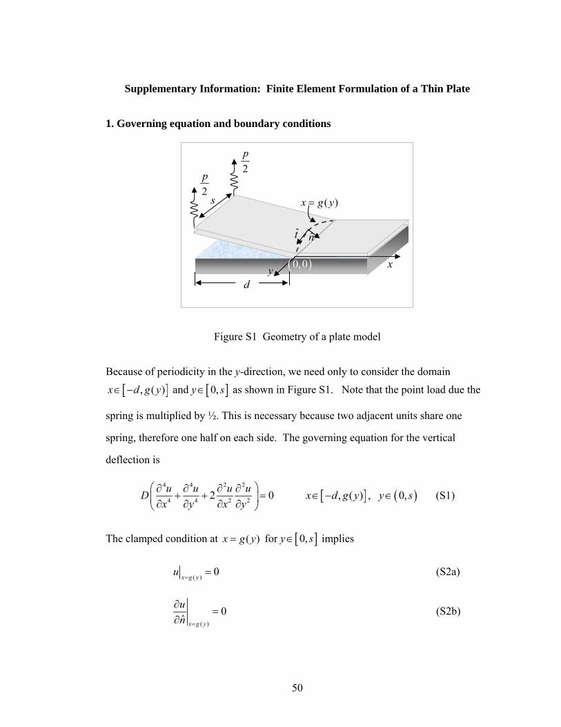
50
Supplementary Information: Finite Element Formulation of a Thin Plate
1. Governing equation and boundary conditions
Figure S1 Geometry of a plate model
Because of periodicity in the y-direction, we need only to consider the domain
[ ], ( )x d g y∈ − and [ ]0,y s∈ as shown in Figure S1. Note that the point load due the
spring is multiplied by ½. This is necessary because two adjacent units share one
spring, therefore one half on each side. The governing equation for the vertical
deflection is
4 4 2 2
4 4 2 22 0u u u uDx y x y
⎛ ⎞∂ ∂ ∂ ∂+ + =⎜ ⎟∂ ∂ ∂ ∂⎝ ⎠
[ ], ( )x d g y∈ − , ( )0,y s∈ (S1)
The clamped condition at ( )x g y= for [ ]0,y s∈ implies
( )0
x g yu
== (S2a)
( )
0ˆ x g y
un =
∂=
∂ (S2b)
2p
2p
s
d
x y
( )x g y=
t n
( )0,0
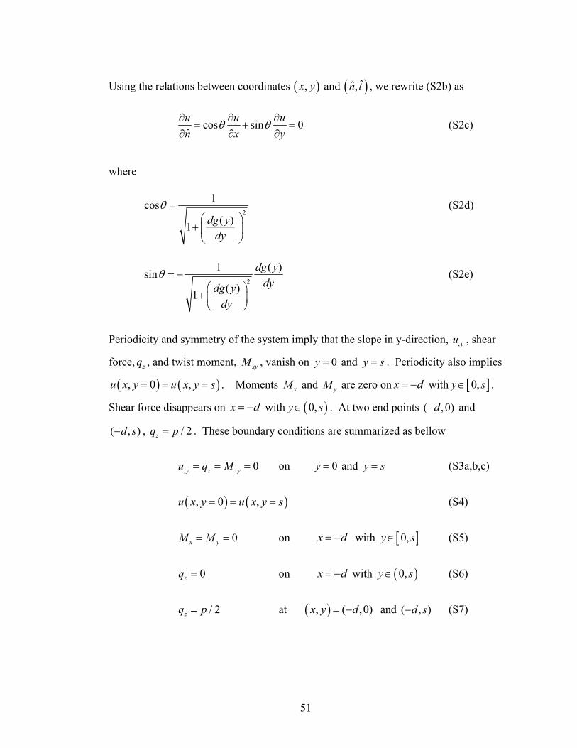
51
Using the relations between coordinates ( ),x y and ( )ˆˆ,n t , we rewrite (S2b) as
cos sin 0ˆu u un x y
θ θ∂ ∂ ∂= + =
∂ ∂ ∂ (S2c)
where
2
1cos( )1 dg y
dy
θ =⎛ ⎞
+ ⎜ ⎟⎝ ⎠
(S2d)
2
1 ( )sin( )1
dg ydydg y
dy
θ = −⎛ ⎞
+ ⎜ ⎟⎝ ⎠
(S2e)
Periodicity and symmetry of the system imply that the slope in y-direction, , yu , shear
force, zq , and twist moment, xyM , vanish on 0y = and y s= . Periodicity also implies
( ) ( ), 0 ,u x y u x y s= = = . Moments xM and yM are zero on x d= − with [ ]0,y s∈ .
Shear force disappears on x d= − with ( )0,y s∈ . At two end points ( ,0)d− and
( , )d s− , / 2zq p= . These boundary conditions are summarized as bellow
, 0y z xyu q M= = = on 0y = and y s= (S3a,b,c)
( ) ( ), 0 ,u x y u x y s= = = (S4)
0x yM M= = on x d= − with [ ]0,y s∈ (S5)
0zq = on x d= − with ( )0,y s∈ (S6)
/ 2zq p= at ( ), ( ,0)x y d= − and ( , )d s− (S7)
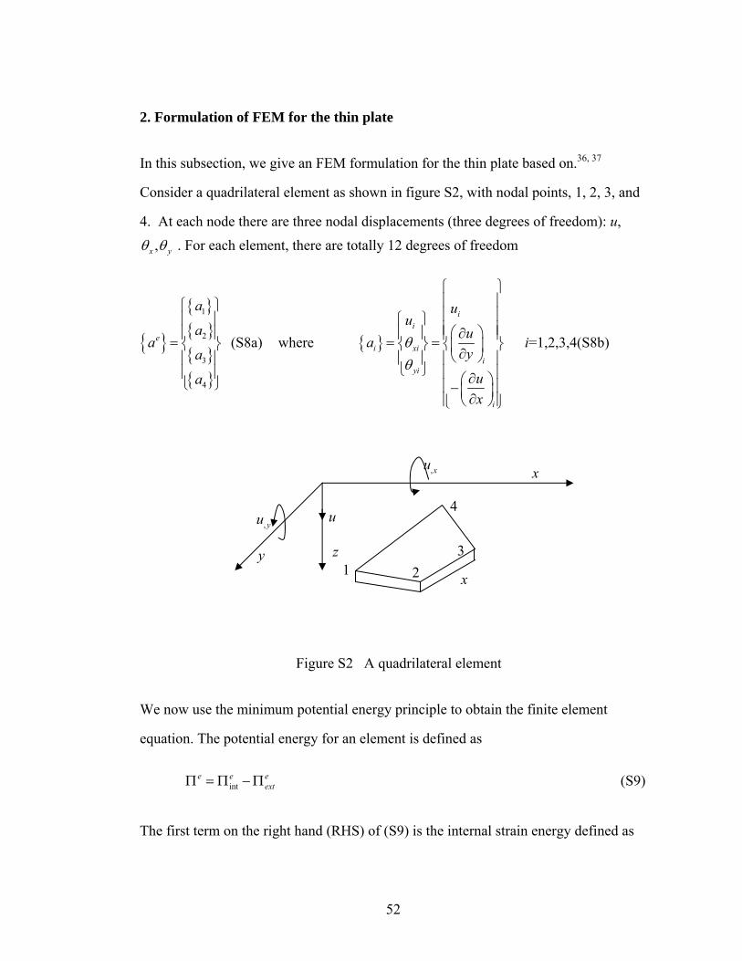
52
2. Formulation of FEM for the thin plate
In this subsection, we give an FEM formulation for the thin plate based on.36, 37
Consider a quadrilateral element as shown in figure S2, with nodal points, 1, 2, 3, and
4. At each node there are three nodal displacements (three degrees of freedom): u,
,x yθ θ . For each element, there are totally 12 degrees of freedom
{ }
{ }{ }{ }{ }
1
2
3
4
e
a
aa
a
a
⎧ ⎫⎪ ⎪⎪ ⎪= ⎨ ⎬⎪ ⎪⎪ ⎪⎩ ⎭
(S8a) where { }
ii
i xii
yi
i
uu
uay
ux
θθ
⎧ ⎫⎪ ⎪⎪ ⎪⎧ ⎫⎪ ⎪⎛ ⎞∂⎪ ⎪ ⎪ ⎪= =⎨ ⎬ ⎨ ⎬⎜ ⎟∂⎝ ⎠⎪ ⎪ ⎪ ⎪
⎩ ⎭ ⎪ ⎪∂⎛ ⎞⎪ ⎪−⎜ ⎟∂⎪ ⎪⎝ ⎠⎩ ⎭
i=1,2,3,4(S8b)
Figure S2 A quadrilateral element
We now use the minimum potential energy principle to obtain the finite element
equation. The potential energy for an element is defined as
inte e e
extΠ = Π − Π (S9)
The first term on the right hand (RHS) of (S9) is the internal strain energy defined as
x
y z
u
1 2
, yu 4
x
,xu
3
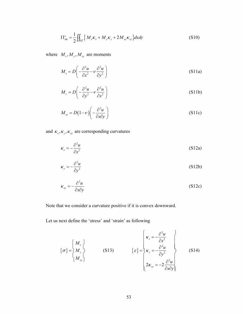
53
{ }int1 22 e
ex x y y xy xyM M M dxdyκ κ κ
ΩΠ = + +∫∫ (S10)
where , ,x y xyM M M are moments
2 2
2 2xu uM D
x yν
⎛ ⎞∂ ∂= − −⎜ ⎟∂ ∂⎝ ⎠
(S11a)
2 2
2 2yu uM D
y xν
⎛ ⎞∂ ∂= − −⎜ ⎟∂ ∂⎝ ⎠
(S11b)
( )2
1xyuM D
x yν
⎛ ⎞∂= − −⎜ ⎟∂ ∂⎝ ⎠
(S11c)
and , ,x y xyκ κ κ are corresponding curvatures
2
2xu
xκ ∂
= −∂
(S12a)
2
2yu
yκ ∂
= −∂
(S12b)
2
xyu
x yκ ∂
= −∂ ∂
(S12c)
Note that we consider a curvature positive if it is convex downward.
Let us next define the ‘stress’ and ‘strain’ as following
{ }x
y
xy
MM
M
σ
⎧ ⎫⎪ ⎪
= ⎨ ⎬⎪ ⎪⎩ ⎭
(S13) { }
2
2
2
2
2
2 2
x
y
xy
uxu
yu
x y
κ
ε κ
κ
⎧ ⎫∂= −⎪ ⎪
∂⎪ ⎪⎪ ⎪∂⎪ ⎪= = −⎨ ⎬∂⎪ ⎪⎪ ⎪∂
= −⎪ ⎪∂ ∂⎪ ⎪⎩ ⎭
(S14)
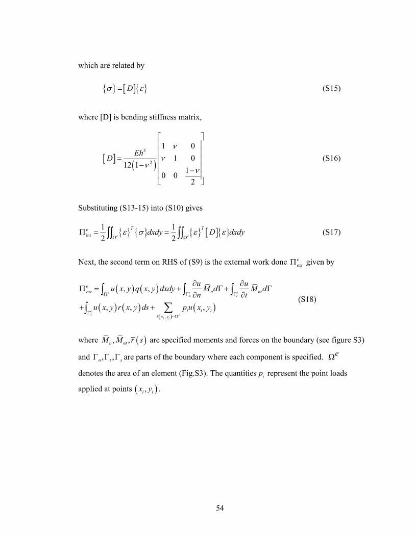
54
which are related by
{ } [ ]{ }Dσ ε= (S15)
where [D] is bending stiffness matrix,
[ ] ( )3
2
1 01 0
12 110 0
2
EhDν
νν
ν
⎡ ⎤⎢ ⎥⎢ ⎥
= ⎢ ⎥− ⎢ ⎥−⎢ ⎥⎣ ⎦
(S16)
Substituting (S13-15) into (S10) gives
{ } { } { } [ ]{ }int1 12 2e e
T Te dxdy D dxdyε σ ε εΩ Ω
Π = =∫∫ ∫∫ (S17)
Next, the second term on RHS of (S9) is the external work done eextΠ given by
( ) ( )
( ) ( ) ( )( ): ,
, ,
, , ,
e e en t
es e
i i
eext n nt
i i ii x y
u uu x y q x y dxdy M d M dn t
u x y r x y ds p u x y
Ω Γ Γ
Γ∈Ω
∂ ∂Π = + Γ + Γ
∂ ∂+ +
∫ ∫ ∫∑∫
(S18)
where ( ), ,n ntM M r s are specified moments and forces on the boundary (see figure S3)
and , ,n t sΓ Γ Γ are parts of the boundary where each component is specified. eΩ
denotes the area of an element (Fig.S3). The quantities ip represent the point loads
applied at points ( ),i ix y .
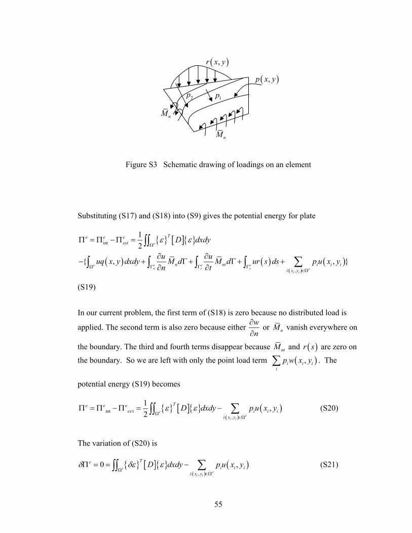
55
Figure S3 Schematic drawing of loadings on an element
Substituting (S17) and (S18) into (S9) gives the potential energy for plate
{ } [ ]{ }
( ) ( ) ( )( )
int
: ,
12
{ , , }
e
e e e en t s e
i i
Te e eext
n nt i i ii x y
D dxdy
u uuq x y dxdy M d M d ur s ds p u x yn t
ε εΩ
Ω Γ Γ Γ∈Ω
Π = Π − Π =
∂ ∂− + Γ + Γ + +
∂ ∂
∫∫
∑∫ ∫ ∫ ∫
(S19)
In our current problem, the first term of (S18) is zero because no distributed load is
applied. The second term is also zero because either wn
∂∂
or nM vanish everywhere on
the boundary. The third and fourth terms disappear because ntM and ( )r s are zero on
the boundary. So we are left with only the point load term ( ),i i ii
p w x y∑ . The
potential energy (S19) becomes
{ } [ ]{ } ( )( )
int t: ,
1 ,2 e
ei i
Te e eex i i i
i x y
D dxdy p u x yε εΩ
∈Ω
Π = Π − Π = − ∑∫∫ (S20)
The variation of (S20) is
{ } [ ]{ } ( )( ): ,
0 ,e
ei i
Tei i i
i x y
D dxdy p u x yδ δε εΩ
∈Ω
Π = = − ∑∫∫ (S21)
( ),p x y
( ),r x y
nM
1p 2p
nM
56
We write the deflection u inside an element in terms of a standard form
( ){ }{ }, eu N x y a= (S22)
where ( ){ },N x y will be determined later and { }ea is defined by (S8a) Substituting
(S22) and
{ } Luε = with 2 2 2
2 2, , 2TLx y x y
⎧ ⎫∂ ∂ ∂= − − −⎨ ⎬∂ ∂ ∂ ∂⎩ ⎭
(S23)
into (S21) gives
{ } [ ] [ ][ ] { } ( )( )( ): ,
0 ,e
ei i
T TTe e ei i i
i x y
a B D B dxdy a p N x yδ δΩ
∈Ω
Π = = − ∑∫∫ (S24)
where
[ ] { }B L N= (S25)
Since { }eaδ is arbitrary, therefore we can obtain the following finite element equation
from (S24)
{ } { }e eeK a q⎡ ⎤ =⎣ ⎦ (S26)
where eK⎡ ⎤⎣ ⎦ is the stiffness matrix for an element which is
[ ] [ ][ ]e
TeK B D B dxdyΩ
⎡ ⎤ ≡⎣ ⎦ ∫∫ (S27)
and { }eq is the load vector for an element
{ } ( )( )( ): ,
,e
i i
Tei i i
i x y
q p N x y∈Ω
≡ ∑ (S28)
57
3. Evaluation of stiffness matrix for the rectangular element
In order to evaluate the stiffness matrix (S27), we assume the deflection u has the form
[ ]{ }
2 2 3 2 2 3 3 31 2 3 4 5 6 7 8 9 10 11 12u x y x xy y x x y xy y x y xy
Cα α α α α α α α α α α α
α= + + + + + + + + + + +
≡
(S29)
where
[ ] 2 2 3 2 2 3 3 31, , , , , , , , , , ,C x y x xy y x x y xy y x y xy⎡ ⎤= ⎣ ⎦ (S30a)
{ } 1 2 3 4 5 6 7 8 9 10 11 12{ , , , , , , , , , , , }Tα α α α α α α α α α α α α= (S30b)
Note that (S29) is complete polynomial of order 2. Along any x constant or y constant
line, the deflection u varies as a cubic. The element boundaries or interfaces are
composed of those lines. As a cubic is uniquely defined by four constants, the two end
values of slope and displacement at two ends will therefore define the cubic uniquely.
Since such end values are common to adjacent elements, the continuity of
displacement and slope will be imposed along any interface. However, the continuity
of second derivatives is not imposed.
Substituting (S29) into (S8b) gives
{ } { }
2 2 3 2 2 3 3 3
2 2 3 2
2 2 2 3
10 0 1 0 2 0 2 3 30 1 0 2 0 3 2 0 3
i i i i i i i i i i i i i i i i i
i xi i i i i i i i i i
i i i i i i i i iyi
u x y x x y y x x y x y y x y x ya x y x x y y x x y
x y x x y y x y yθ αθ
⎧ ⎫ ⎡ ⎤⎪ ⎪ ⎢ ⎥= =⎨ ⎬ ⎢ ⎥⎪ ⎪ ⎢ ⎥− − − − − − − −⎣ ⎦⎩ ⎭
(S31)
where ( ),i ix y is the coordinate of node i (i = 1, 2, 3, 4) in the element e. We then
obtain { }ea by substituting (S31) into (S8a). This results in
58
{ } [ ]{ }ea A α= (S32)
where
[ ]
2 2 3 2 2 3 3 31 1 1 1 1 1 1 1 1 1 1 1 1 1 1 1
2 2 3 21 1 1 1 1 1 1 1 1
2 2 2 31 1 1 1 1 1 1 1 1
2 2 3 2 2 3 3 32 2 2 2 2 2 2 2 2 2 2 2 2 2 2 2
2 2 3 22 2 2 2 2 2 2 2 2
2 2
10 0 1 0 2 0 2 3 30 1 0 2 0 3 2 0 3
10 0 1 0 2 0 2 3 30 1 0 2 0 3
x y x x y y x x y x y y x y x yx y x x y y x x y
x y x x y y x y y
x y x x y y x x y x y y x y x yx y x x y y x x y
x y xA
− − − − − − − −
− − − −=
2 2 2 32 2 2 2 2 2 2
2 2 2 2 2 2 2 33 3 3 3 3 3 3 3 3 3 3 3 3 2 3 3
2 2 3 23 3 3 3 3 2 3 3 3
2 2 2 33 3 3 3 3 3 3 3 3
2 2 3 2 2 3 3 34 4 4 4 4 4 4 4 4 4 4 4 4 4 4 4
2 24 4 4 4 4 4
2 0 3
10 0 1 0 2 0 2 3 30 1 0 2 0 3 2 0 3
10 0 1 0 2 0 2 3l
x y y x y y
x y x x y y x x y x y y x y x yx y x x y y x x y
x y x x y y x y y
x y x x y y x x y x y y x y x yx y x x y y x
− − − −
− − − − − − − −
3 24 4
2 2 2 34 4 4 4 4 4 4 4 4
30 1 0 2 0 3 2 0 3
x yx y x x y y x y y
⎡ ⎤⎢ ⎥⎢ ⎥⎢ ⎥⎢ ⎥⎢ ⎥⎢ ⎥⎢ ⎥⎢ ⎥⎢ ⎥⎢ ⎥⎢ ⎥⎢ ⎥⎢ ⎥⎢ ⎥⎢ ⎥⎢ ⎥⎢ ⎥
− − − − − − − −⎣ ⎦
(S33)
Note that the matrix [ ]A is evaluated in global coordinate system. Substituting (S33)
into (S22) gives
( ){ }[ ]{ },u N x y A α= (S34)
We can obtain ( ){ },N x y by comparing (S29) with (S34),
[ ]{ } ( ){ }[ ]{ } ( ){ } [ ][ ] 1, ,C N x y A N x y C Aα α −= ⇒ = (S35)
Note that we have used the fact that { }α is nonzero matrix in (S35). Then (S25)
becomes
[ ] [ ][ ] 1B H A −= (S36)
59
Where
[ ] [ ]
2
2
22 2 3 2 2 3 3 3
2
2
2 2
1, , , , , , , , , , ,
2
0 0 0 2 0 0 6 2 0 0 6 00 0 0 0 0 2 0 0 2 6 0 60 0 0 0 2 0 0 4 4 0 6 6
x
H L C x y x xy y x x y xy y x y xyy
x yx y xy
x y xyx y x y
⎧ ⎫∂−⎪ ⎪
∂⎪ ⎪⎪ ⎪∂⎪ ⎪ ⎡ ⎤= = −⎨ ⎬ ⎣ ⎦∂⎪ ⎪⎪ ⎪∂
−⎪ ⎪∂ ∂⎪ ⎪⎩ ⎭
− − − −⎡ ⎤⎢ ⎥= − − − −⎢ ⎥⎢ ⎥− − − − −⎣ ⎦
(S37)
Substituting (S37) into (S27), we arrive at the stiffness matrix for an element
[ ] [ ]( ) [ ] [ ][ ]( )[ ]1 1e
Te TK A H D H dxdy A− −
Ω= ∫∫ (S38)
4. Mapping
Evaluating the integral in (S38) in (x, y) coordinate is usually difficult because the
integration domain eΩ is irregular. One can find a master element ( [ ] [ ]ˆ : 1,1 , 1,1e ξ ηΩ ∈ − ∈ − ) that is mapped appropriately to an element eΩ . Then with
mapping ˆ e eΩ → Ω one can perform all integrations for all elements at the master
element ˆ eΩ . As shown in Figure S4, the mapping ˆ e eΩ → Ω is defined by
( )4
1
ˆ ,i ii
x x N ξ η=
= ∑ (S39a)
( )4
1
ˆ ,i ii
y y N ξ η=
= ∑ (S39b)
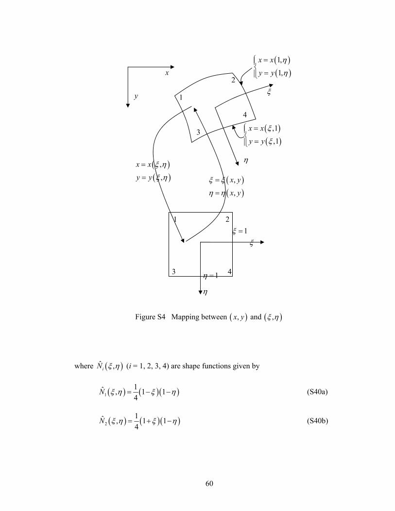
60
Figure S4 Mapping between ( ),x y and ( ),ξ η
where ( )ˆ ,iN ξ η (i = 1, 2, 3, 4) are shape functions given by
( ) ( )( )11ˆ , 1 14
N ξ η ξ η= − − (S40a)
( ) ( )( )21ˆ , 1 14
N ξ η ξ η= + − (S40b)
x
y ξ
η
ξ
η
1 2
3 4
1
2
3
4
1η =
1ξ =
( )( )
,
,
x y
x y
ξ ξ
η η
=
=
( )( )
,
,
x x
y y
ξ η
ξ η
=
=
( )( )
,1
,1
x x
y y
ξ
ξ
=⎧⎪⎨
=⎪⎩
( )( )1,
1,
x x
y y
η
η
=⎧⎪⎨
=⎪⎩
61
( ) ( )( )31ˆ , 1 14
N ξ η ξ η= + + (S40c)
( ) ( )( )41ˆ , 1 14
N ξ η ξ η= − + (S40d)
The areas of element at ( )( , ), ( , )x x y yξ η ξ η= = and ( , )ξ η are related by
( ) ( )dxdy J d dξ η= (S41)
where J is the determinant of the Jacobian matrix
( )( ) ( )( ) ( )( ) ( )( )
( )( ) ( )( ) ( )( ) ( )( )
2 1 3 4 4 1 3 2
4 1 3 2 2 1 3 4
1 1 1 1 1161 1 1 1 1
16
x y x yJ
x x x x y y y y
x x x x y y y y
ξ η η ξ
η η ξ ξ
ξ ξ η η
∂ ∂ ∂ ∂= −
∂ ∂ ∂ ∂
= − − + − + − − + − +⎡ ⎤ ⎡ ⎤⎣ ⎦ ⎣ ⎦
− − − + − + − − + − +⎡ ⎤ ⎡ ⎤⎣ ⎦ ⎣ ⎦
(S42)
Substituting (S39a, b) and (S41) into (S38), we get the stiffness matrix in terms of
( , )ξ η
[ ] [ ]( ) [ ] [ ]1 1
1 1
1 1
ˆ ˆT TeK A H D H J d d Aξ η− −
− −
⎛ ⎞⎡ ⎤ ⎡ ⎤= ⎜ ⎟⎣ ⎦ ⎣ ⎦
⎝ ⎠∫ ∫ (S43)
where
( ) ( )( )ˆ , , ,H H x yξ η ξ η⎡ ⎤ ⎡ ⎤= ⎣ ⎦⎣ ⎦ (S45)
The double integral in (S45) can be estimated using Gaussian Quadrature.
( ) ( )1 1
1 11 1
, ,m m
i j i jj i
d dξ η ξ η ξ η ω ω= =− −
ϒ = ϒ∑∑∫ ∫ (S46)
62
where ( ) [ ]ˆ ˆ,T
H D H Jξ η ⎡ ⎤ ⎡ ⎤ϒ ≡ ⎣ ⎦ ⎣ ⎦ , and ( ),i jξ η are Gaussian points, iω are weights,
m is the number of Gaussian points in a master element. Note that an m-point
Gaussian quadrature rule can yield an exact result for polynomials of degree 2m − 1 or less. In our thin plate problem, ( ),g ξ η is a polynomial of degree 6 in both ξ and
η , so we need 4 Gaussian points for each dimension. These 4 Gaussian points for ξ
are
( )1 3 2 6 / 5 / 7ξ = − , ( )2 3 2 6 / 5 / 7ξ = − − ,
( )3 3 2 6 / 5 / 7ξ = + , ( )4 3 2 6 / 5 / 7ξ = − + ,
and the corresponding weights are
1 218 30
36ω ω +
= = 3 418 30
36ω ω −
= =
The Gaussian points and the corresponding weights for η are the same as those for ξ .
Similarly, one can use Gaussian Quadrature to evaluate load vector (S28).
5. Meshing
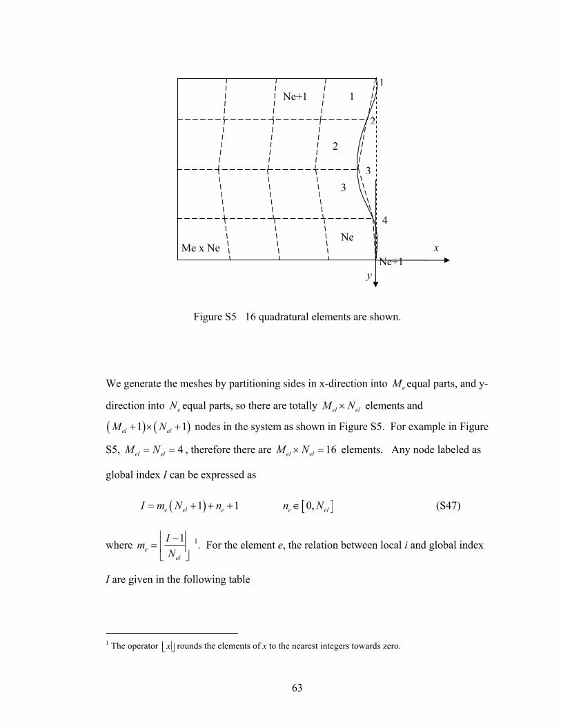
63
Figure S5 16 quadratural elements are shown.
We generate the meshes by partitioning sides in x-direction into eM equal parts, and y-
direction into eN equal parts, so there are totally el elM N× elements and
( ) ( )1 1el elM N+ × + nodes in the system as shown in Figure S5. For example in Figure
S5, 4el elM N= = , therefore there are 16el elM N× = elements. Any node labeled as
global index I can be expressed as
( ) [ ]1 1 0,e el e e elI m N n n N= + + + ∈ (S47)
where 1e
el
ImN
⎢ ⎥−= ⎢ ⎥
⎣ ⎦ 1. For the element e, the relation between local i and global index
I are given in the following table
1 The operator x⎢ ⎥⎣ ⎦ rounds the elements of x to the nearest integers towards zero.
1
2
3
Ne
Ne+1
Me x Ne
1
2
3
4
Ne+1x
y
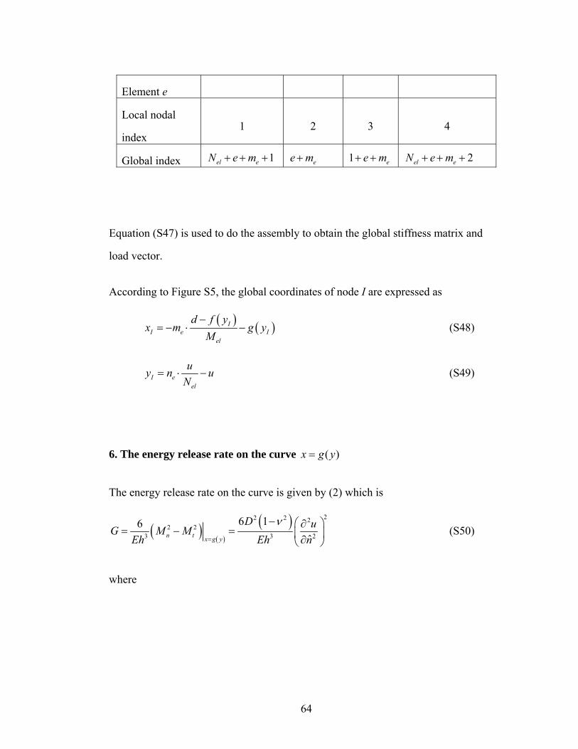
64
Element e
Local nodal
index 1 2 3 4
Global index 1el eN e m+ + + ee m+ 1 ee m+ + 2el eN e m+ + +
Equation (S47) is used to do the assembly to obtain the global stiffness matrix and
load vector.
According to Figure S5, the global coordinates of node I are expressed as
( ) ( )II e I
el
d f yx m g y
M−
= − ⋅ − (S48)
I eel
uy n uN
= ⋅ − (S49)
6. The energy release rate on the curve ( )x g y=
The energy release rate on the curve is given by (2) which is
( )( )
( ) 22 2 22 2
3 3 2
6 16ˆn t x g y
D uG M MEh Eh n
ν=
− ⎛ ⎞∂= − = ⎜ ⎟∂⎝ ⎠
(S50)
where
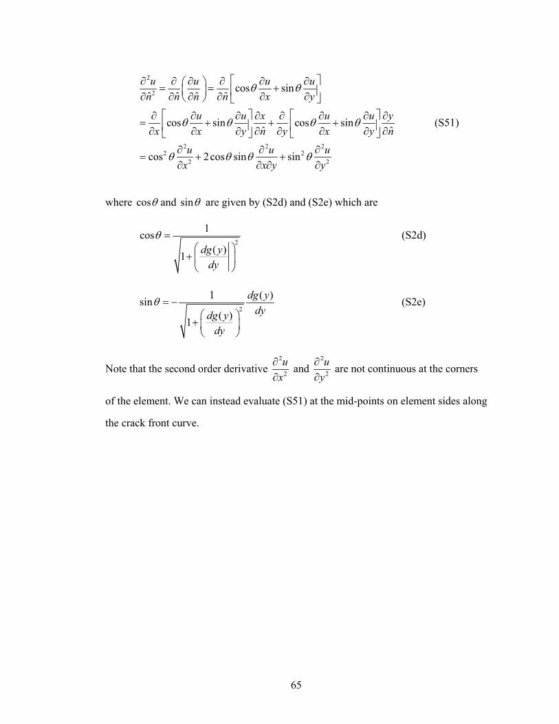
65
2
2
2 2 22 2
2 2
cos sinˆ ˆ ˆ ˆ
cos sin cos sinˆ ˆ
cos 2cos sin sin
u u u un n n n x y
u u x u u yx x y n y x y n
u u ux x y y
θ θ
θ θ θ θ
θ θ θ θ
⎡ ⎤∂ ∂ ∂ ∂ ∂ ∂⎛ ⎞= = +⎜ ⎟ ⎢ ⎥∂ ∂ ∂ ∂ ∂ ∂⎝ ⎠ ⎣ ⎦⎡ ⎤ ⎡ ⎤∂ ∂ ∂ ∂ ∂ ∂ ∂ ∂
= + + +⎢ ⎥ ⎢ ⎥∂ ∂ ∂ ∂ ∂ ∂ ∂ ∂⎣ ⎦ ⎣ ⎦∂ ∂ ∂
= + +∂ ∂ ∂ ∂
(S51)
where cosθ and sinθ are given by (S2d) and (S2e) which are
2
1cos( )1 dg y
dy
θ =⎛ ⎞
+ ⎜ ⎟⎝ ⎠
(S2d)
2
1 ( )sin( )1
dg ydydg y
dy
θ = −⎛ ⎞
+ ⎜ ⎟⎝ ⎠
(S2e)
Note that the second order derivative 2
2
ux
∂∂
and 2
2
uy
∂∂
are not continuous at the corners
of the element. We can instead evaluate (S51) at the mid-points on element sides along
the crack front curve.
66
REFERENCES
1. Sitti, M.; Fearing, R. S. J Adhes Sci Technol 2003, 17, 1055-1073.
2. Arzt, E.; Gorb, S.; Spolenak, R. Proc Natl Acad Sci 2003,100, 10603.
3. Glassmaker, N. J.; Jagota, A.; Hui, C.-Y.; Kim, J. J R Soc Interface 2004, 1, 22-33.
4. Hui, C.-Y.; Glassmaker, N. J.; Tang, T.; Jagota, A. J R Soc Interface 2004,1, 35-
48.
5. Peressadko, A.; Gorb, S. N. J Adhes 2004, 80, 247-261.
6. Yurdumakan, B.; Raravikar, N. R.; Ajayan, P. M.; Dhinojwala, A. Chem
Commun 2005, 30, 3799-3801.
7. Gorb, S.; Varenberg, M.; Peressadko, A.; Tuma, J. J R Soc Interface 2006, 4, 271-
275.
8. Kim, S.; Sitti, M. Appl Phys Lett 2006, 89, 261911.
9. Majidi, C.; Groff, R. E.; Maeno, Y.; Schubert, B.; Baek, S.; Bush, B.; Maboudian,
R.; Gravish, N.; Wilkinson, M.; Autumn, K.; Fearing, R. S. Phys Rev Lett 2006,
97, 076103.
10. Aksak, B.; Murphy, M.; Sitti, M. Langmuir 2007, 23, 3322-3332.
11. Bhushan B.; Sayer, R. A. Microsystem Technologies 2007, 13 (1),71-78.
12. Greiner, C.; Campo, A. D.; Arzt, E. Langmuir 2007, 23, 3495-3502.
13. Noderer, W.L.; Shen, L.; Vajpayee, S.; Glassmaker, N.J.; Jagota, A.; Hui, C.-Y.
Proc R Soc A 2007, 463, 2631-2654.
14. Glassmaker, N. J.; Jagota, A.; Hui, C.-Y.; Noderer, W. L.; Chaudhury, M. K. Proc
Natl Acad Sci 2007, 104, 10 786-10 791.
15. Ge, L.; Sethi, S.; Ci, L.; Ajayan, P. M.; Dhinojwala, A. Proc Natl Acad Sci 2007,
104, 10792.
67
16. Murphy, M. P.; Aksak, B.; Sitti, M. J Adhesion Sci Technol 2007, 21(12-13),
1281-1296.
17. Schubert, B.; Majidi, C.; Groff, R. E.; Baek, S.; Bush, B.; Maboudian, R.; Fearing,
R.S. J Adhesion Sci Technol 2007, 21(12-13), 1297-1315.
18. Varenberg, M.,; Gorb, S. J R Soc Interface 2007, 4, 721-725.
19. Shen, L.; Jagota, A.; Hui, C.-Y.; Glassmaker, N.J. Proceedings of 30th Annual
Meeting of the Adhesion Society, Tampa Bay, USA, 18-21st Feb. 2007.
20. Jagota, A.; Hui, C. -Y.; Glassmaker, N. J.; Tang, T. MRS Bull 2007, 32, 492.
21. Shen, L.; Glassmaker, N.J.; Jagota, A.; Hui, C.-Y. Soft Matter 2008, 4, 618-625.
22. Yao, H.; Rocca, G. D.; Guduru, P.R.; Gao, H. R Soc Interface 2008, 5, 723 - 733.
23. Autumn, K. MRS Bulletin 2007, Vol. 32, 473.
24. Murphy, M.P.; Kim, S.; Sitti, M. Applied Materials & Interfaces 2009, 1 (4), 849
- 855.
25. Parness, A.; Soto, D.; Esparza, N.; Gravish, N.; Wilkinson, M.; Autumn, K.;
Cutkosky, M. J R Soc Interface 2007, March 18.
26. Liu, J.; Hui, C.-Y.; Shen, L.; Jagota, A. J R Soc Interface 2008, 5, 1087-1097. doi:
10.1098/rsif.2007.1336.
27. Shen, L.; Hui, C.-Y.; Jagota, A. J Appl Phys 2008, 104, 123506.
28. Chan, E.P.; Greiner, C.; Arzt, E.; Crosby, A.J. MRS Bulletin 2007, vol. 32, 496-
503.
29. Gao, H.; Wang, X.; Yao, H.; Gorb, S.; Arzt, E. Mech Mat 2005, 37, 275–285.
30. Jeong, H.E.; Lee, J.-K.; Kim, H. N.; Moon, S. H.; Suh, K.Y. PNAS 2009, 106,
5639-5644.
31. Greiner, C.; Arzt, E.; del Campo, A. Adv Mater 2009, 21, 479–482.
32. Autumn, K. In Biological Adhesives; Smith, A. M.; Callow, J. A., Eds.; Springer:
Berlin, 2006; pp.225-255.
68
33. Timoshenko, S. P.; Woinowsky-Krieger, S. Theory of Plates and Shells,
McGraw-Hill, 2nd Edition, 1959.
34. Vajpayee, S.; Jagota, A.; Hui, C-Y. Adhesion of a Fibrillar Interface on Wet and
Rough Surfaces, under review.
35. A1. Rice, J. R. Journal of Applied Mechanics 1968, 35, 379-386.
36. Zienkiewicz, O. C.; Taylor, R. L. Finite Element Method: Volume 2, Solid
Mechanics, Butterworth-Heinemann, 5th edition, September 4, 2000.
37. Shames, I. H.; Dym, C. L. Energy and Finite Element Methods in Structural
Mechanics, McGraw Hill Higher Education, May 1985.
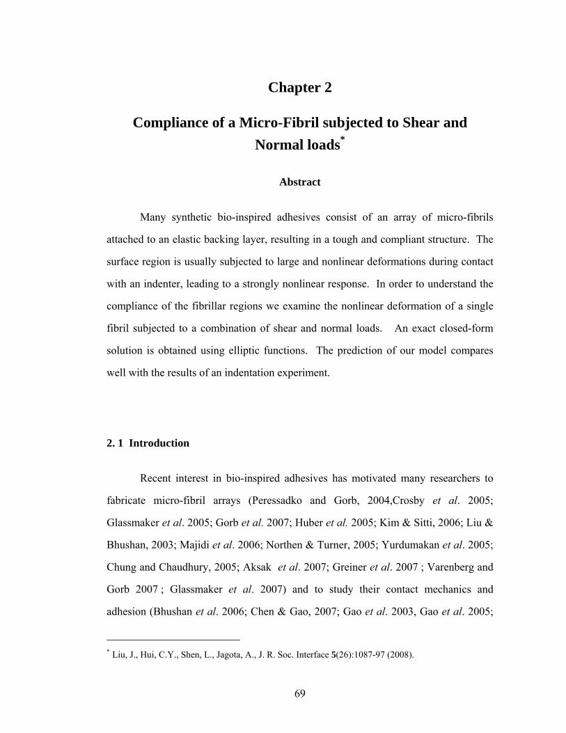
69
Chapter 2
Compliance of a Micro-Fibril subjected to Shear and Normal loads*
Abstract
Many synthetic bio-inspired adhesives consist of an array of micro-fibrils
attached to an elastic backing layer, resulting in a tough and compliant structure. The
surface region is usually subjected to large and nonlinear deformations during contact
with an indenter, leading to a strongly nonlinear response. In order to understand the
compliance of the fibrillar regions we examine the nonlinear deformation of a single
fibril subjected to a combination of shear and normal loads. An exact closed-form
solution is obtained using elliptic functions. The prediction of our model compares
well with the results of an indentation experiment.
2. 1 Introduction
Recent interest in bio-inspired adhesives has motivated many researchers to
fabricate micro-fibril arrays (Peressadko and Gorb, 2004,Crosby et al. 2005;
Glassmaker et al. 2005; Gorb et al. 2007; Huber et al. 2005; Kim & Sitti, 2006; Liu &
Bhushan, 2003; Majidi et al. 2006; Northen & Turner, 2005; Yurdumakan et al. 2005;
Chung and Chaudhury, 2005; Aksak et al. 2007; Greiner et al. 2007 ; Varenberg and
Gorb 2007 ; Glassmaker et al. 2007) and to study their contact mechanics and
adhesion (Bhushan et al. 2006; Chen & Gao, 2007; Gao et al. 2003, Gao et al. 2005;
* Liu, J., Hui, C.Y., Shen, L., Jagota, A., J. R. Soc. Interface 5(26):1087-97 (2008).
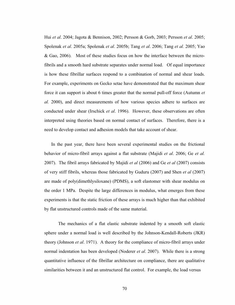
70
Hui et al. 2004; Jagota & Bennison, 2002; Persson & Gorb, 2003; Persson et al. 2005;
Spolenak et al. 2005a; Spolenak et al. 2005b; Tang et al. 2006; Tang et al. 2005; Yao
& Gao, 2006). Most of these studies focus on how the interface between the micro-
fibrils and a smooth hard substrate separates under normal load. Of equal importance
is how these fibrillar surfaces respond to a combination of normal and shear loads.
For example, experiments on Gecko setae have demonstrated that the maximum shear
force it can support is about 6 times greater that the normal pull-off force (Autumn et
al. 2000), and direct measurements of how various species adhere to surfaces are
conducted under shear (Irschick et al. 1996). However, these observations are often
interpreted using theories based on normal contact of surfaces. Therefore, there is a
need to develop contact and adhesion models that take account of shear.
In the past year, there have been several experimental studies on the frictional
behavior of micro-fibril arrays against a flat substrate (Majidi et al. 2006; Ge et al.
2007). The fibril arrays fabricated by Majidi et al (2006) and Ge et al (2007) consists
of very stiff fibrils, whereas those fabricated by Guduru (2007) and Shen et al (2007)
are made of poly(dimethlysiloxane) (PDMS), a soft elastomer with shear modulus on
the order 1 MPa. Despite the large differences in modulus, what emerges from these
experiments is that the static friction of these arrays is much higher than that exhibited
by flat unstructured controls made of the same material.
The mechanics of a flat elastic substrate indented by a smooth soft elastic
sphere under a normal load is well described by the Johnson-Kendall-Roberts (JKR)
theory (Johnson et al. 1971). A theory for the compliance of micro-fibril arrays under
normal indentation has been developed (Noderer et al. 2007). While there is a strong
quantitative influence of the fibrillar architecture on compliance, there are qualitative
similarities between it and an unstructured flat control. For example, the load versus
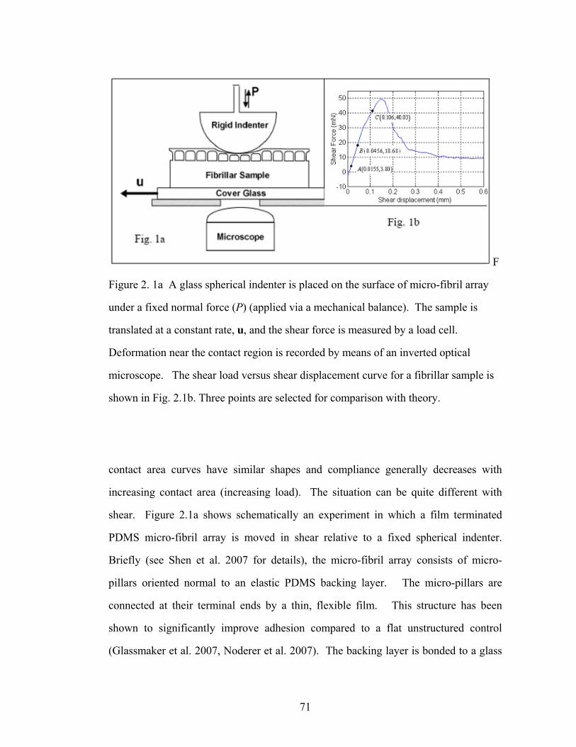
71
F
Figure 2. 1a A glass spherical indenter is placed on the surface of micro-fibril array
under a fixed normal force (P) (applied via a mechanical balance). The sample is
translated at a constant rate, u, and the shear force is measured by a load cell.
Deformation near the contact region is recorded by means of an inverted optical
microscope. The shear load versus shear displacement curve for a fibrillar sample is
shown in Fig. 2.1b. Three points are selected for comparison with theory.
contact area curves have similar shapes and compliance generally decreases with
increasing contact area (increasing load). The situation can be quite different with
shear. Figure 2.1a shows schematically an experiment in which a film terminated
PDMS micro-fibril array is moved in shear relative to a fixed spherical indenter.
Briefly (see Shen et al. 2007 for details), the micro-fibril array consists of micro-
pillars oriented normal to an elastic PDMS backing layer. The micro-pillars are
connected at their terminal ends by a thin, flexible film. This structure has been
shown to significantly improve adhesion compared to a flat unstructured control
(Glassmaker et al. 2007, Noderer et al. 2007). The backing layer is bonded to a glass
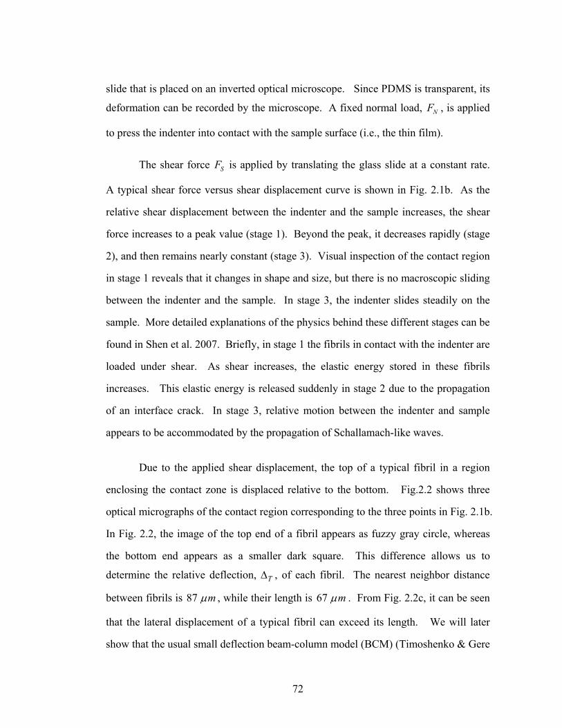
72
slide that is placed on an inverted optical microscope. Since PDMS is transparent, its
deformation can be recorded by the microscope. A fixed normal load, NF , is applied
to press the indenter into contact with the sample surface (i.e., the thin film).
The shear force SF is applied by translating the glass slide at a constant rate.
A typical shear force versus shear displacement curve is shown in Fig. 2.1b. As the
relative shear displacement between the indenter and the sample increases, the shear
force increases to a peak value (stage 1). Beyond the peak, it decreases rapidly (stage
2), and then remains nearly constant (stage 3). Visual inspection of the contact region
in stage 1 reveals that it changes in shape and size, but there is no macroscopic sliding
between the indenter and the sample. In stage 3, the indenter slides steadily on the
sample. More detailed explanations of the physics behind these different stages can be
found in Shen et al. 2007. Briefly, in stage 1 the fibrils in contact with the indenter are
loaded under shear. As shear increases, the elastic energy stored in these fibrils
increases. This elastic energy is released suddenly in stage 2 due to the propagation
of an interface crack. In stage 3, relative motion between the indenter and sample
appears to be accommodated by the propagation of Schallamach-like waves.
Due to the applied shear displacement, the top of a typical fibril in a region
enclosing the contact zone is displaced relative to the bottom. Fig.2.2 shows three
optical micrographs of the contact region corresponding to the three points in Fig. 2.1b.
In Fig. 2.2, the image of the top end of a fibril appears as fuzzy gray circle, whereas
the bottom end appears as a smaller dark square. This difference allows us to
determine the relative deflection, TΔ , of each fibril. The nearest neighbor distance
between fibrils is 87 mμ , while their length is 67 mμ . From Fig. 2.2c, it can be seen
that the lateral displacement of a typical fibril can exceed its length. We will later
show that the usual small deflection beam-column model (BCM) (Timoshenko & Gere
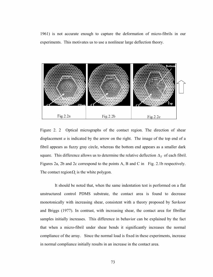
73
1961) is not accurate enough to capture the deformation of micro-fibrils in our
experiments. This motivates us to use a nonlinear large deflection theory.
Figure 2. 2 Optical micrographs of the contact region. The direction of shear
displacement u is indicated by the arrow on the right. The image of the top end of a
fibril appears as fuzzy gray circle, whereas the bottom end appears as a smaller dark
square. This difference allows us to determine the relative deflection TΔ of each fibril.
Figures 2a, 2b and 2c correspond to the points A, B and C in Fig. 2.1b respectively.
The contact region cΩ is the white polygon.
It should be noted that, when the same indentation test is performed on a flat
unstructured control PDMS substrate, the contact area is found to decrease
monotonically with increasing shear, consistent with a theory proposed by Savkoor
and Briggs (1977). In contrast, with increasing shear, the contact area for fibrillar
samples initially increases. This difference in behavior can be explained by the fact
that when a micro-fibril under shear bends it significantly increases the normal
compliance of the array. Since the normal load is fixed in these experiments, increase
in normal compliance initially results in an increase in the contact area.
74
In order to develop a quantitative understanding of the load-bearing capacity of
a fibrillar array under combined normal and shear loads, we study the nonlinear
deformation of individual micro-fibrils. The model for fibril deflection and theoretical
results based on it are presented in section 2.2. In section 2.3 we compare model
predictions with experiments.
2.2 Elastica Model of a Stretchable Beam
We model the deformation of a typical micro-fibril in stage 1. Since the
length of a typical micro-fibril is significantly greater than its lateral dimensions, it
will be modeled as a stretchable elastica. Inside the contact zone, which is denoted by
cΩ , the thin film is well adhered to the indenter. Therefore, a fibril in cΩ cannot
rotate at this end, implying a clamped boundary condition. For a sufficiently long
fibril, it is reasonable to assume that its bottom end is also clamped. We further
assume that fibrils do not twist; this assumption is consistent with the loading
conditions in our experiments. Finally, we neglect the compliance of the half-space to
which the fibril is attached; this is again reasonable since fibrils are slender.
The problem of interest is an initially straight elastic beam with initial length,
oL , that is clamped at both ends. One end of the beam is fixed to a rigid wall (the
backing layer) while the other end is subjected to vertical and tangential displacements
NΔ and TΔ , respectively. Let , , o o oN T M denote the unknown normal, shear and
moment applied at this end. Let s denote the arc length of the deformed beam and let
( ), ( )x s y s denote the deformed coordinates of the beam at a point p on the bar. (See
Fig. 2.3)
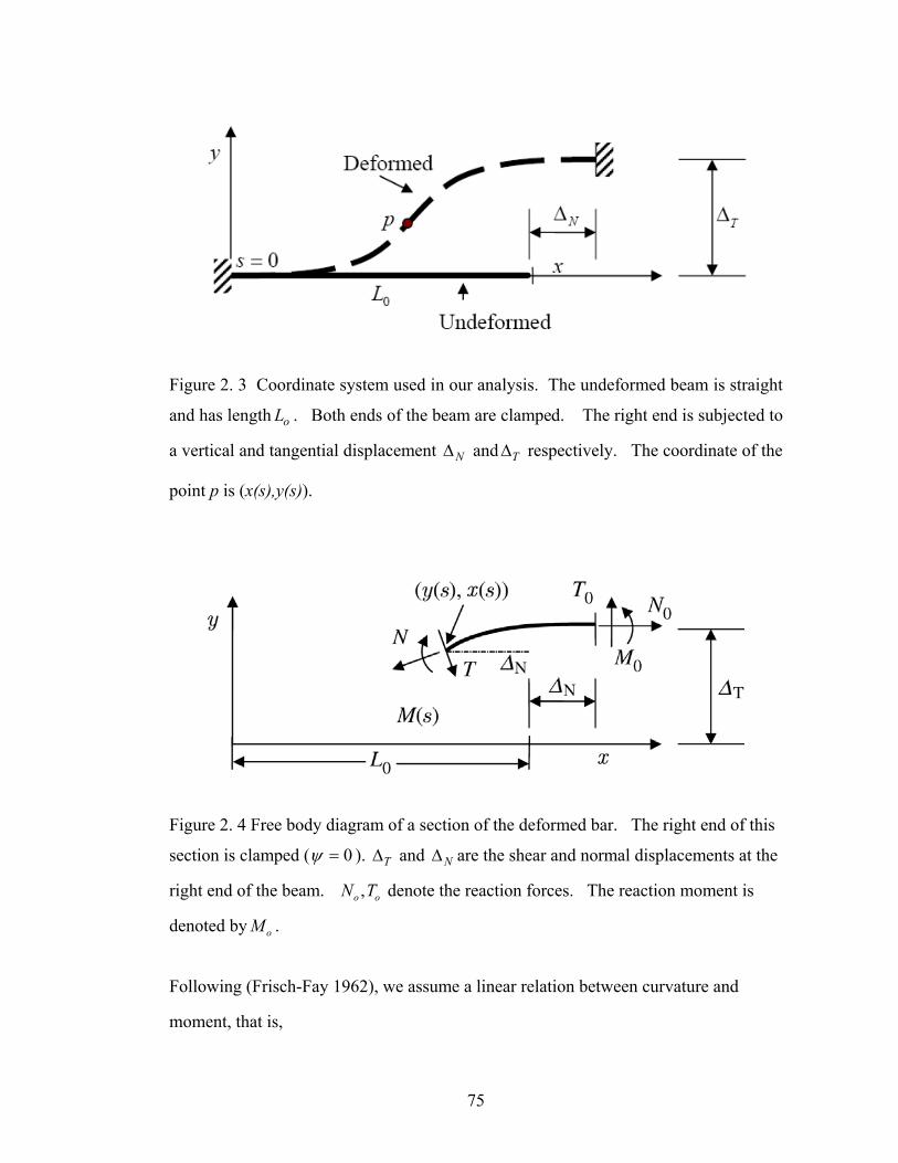
75
Figure 2. 3 Coordinate system used in our analysis. The undeformed beam is straight
and has length oL . Both ends of the beam are clamped. The right end is subjected to
a vertical and tangential displacement NΔ and TΔ respectively. The coordinate of the
point p is (x(s),y(s)).
Figure 2. 4 Free body diagram of a section of the deformed bar. The right end of this
section is clamped ( 0=ψ ). TΔ and NΔ are the shear and normal displacements at the
right end of the beam. ,o oN T denote the reaction forces. The reaction moment is
denoted by oM .
Following (Frisch-Fay 1962), we assume a linear relation between curvature and
moment, that is,
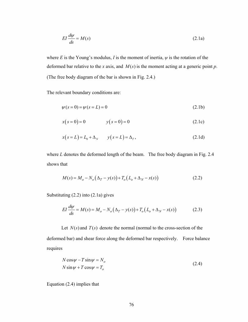
76
( )dEI M sdsψ
= (2.1a)
where E is the Young’s modulus, I is the moment of inertia, ψ is the rotation of the
deformed bar relative to the x axis, and ( )M s is the moment acting at a generic point p.
(The free body diagram of the bar is shown in Fig. 2.4.)
The relevant boundary conditions are:
( 0) ( ) 0s s Lψ ψ= = = = (2.1b)
( )0 0x s = = ( )0 0y s = = (2.1c)
( ) 0 Nx s L L= = + Δ ( ) Ty s L= = Δ , (2.1d)
where L denotes the deformed length of the beam. The free body diagram in Fig. 2.4
shows that
( ) ( )( ) ( ) ( )o o T o o NM s M N y s T L x s= − Δ − + + Δ − (2.2)
Substituting (2.2) into (2.1a) gives
( ) ( )( ) ( ) ( )o o T o o NdEI M s M N y s T L x sdsψ
= = − Δ − + + Δ − (2.3)
Let ( )N s and ( )T s denote the normal (normal to the cross-section of the
deformed bar) and shear force along the deformed bar respectively. Force balance
requires
cos sinsin cos
o
o
N T NN T T
ψ ψψ ψ
− =+ =
(2.4)
Equation (2.4) implies that
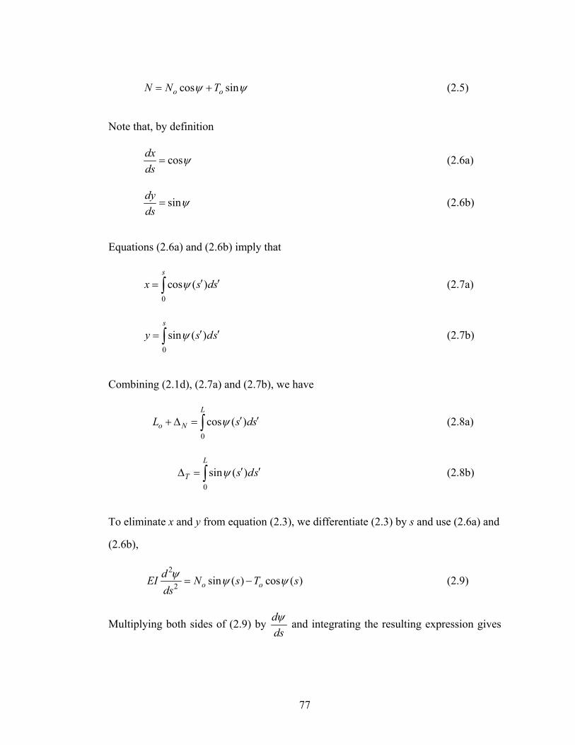
77
cos sino oN N Tψ ψ= + (2.5)
Note that, by definition
cosdxds
ψ= (2.6a)
sindyds
ψ= (2.6b)
Equations (2.6a) and (2.6b) imply that
0
cos ( )s
x s dsψ ′ ′= ∫ (2.7a)
0
sin ( )s
y s dsψ ′ ′= ∫ (2.7b)
Combining (2.1d), (2.7a) and (2.7b), we have
0
cos ( )L
o NL s dsψ ′ ′+ Δ = ∫ (2.8a)
0
sin ( )L
T s dsψ ′ ′Δ = ∫ (2.8b)
To eliminate x and y from equation (2.3), we differentiate (2.3) by s and use (2.6a) and
(2.6b),
2
2 sin ( ) cos ( )o odEI N s T sds
ψ ψ ψ= − (2.9)
Multiplying both sides of (2.9) by ddsψ and integrating the resulting expression gives
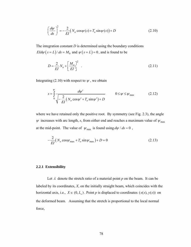
78
( )2 2 cos ( ) sin ( )o o
d N s T s Dds EIψ ψ ψ⎛ ⎞ = − + +⎜ ⎟
⎝ ⎠ (2.10)
The integration constant D is determined using the boundary conditions
( ) 0/EId s L ds Mψ = = and ( ) 0s Lψ = = , and is found to be
22 o
oMD N
EI EI⎡ ⎤= + ⎢ ⎥⎣ ⎦
. (2.11)
Integrating (2.10) with respect to ψ , we obtain
( )0 2 cos sino o
dsN T D
EI
ψ ψ
ψ ψ
′=
′ ′− + +∫ max0 ψ ψ≤ ≤ (2.12)
where we have retained only the positive root. By symmetry (see Fig. 2.3), the angle
ψ increases with arc length, s, from either end and reaches a maximum value of maxψ
at the mid-point. The value of maxψ is found using / 0d dsψ = ,
( )max max2 cos sin 0o oN T D
EIψ ψ− + + = (2.13)
2.2.1 Extensibility
Let λ denote the stretch ratio of a material point p on the beam. It can be
labeled by its coordinates, X, on the initially straight beam, which coincides with the
horizontal axis, i.e., ),0( oLX ∈ . Point p is displaced to coordinates ( ( ), ( ))x s y s on
the deformed beam. Assuming that the stretch is proportional to the local normal
force,
79
1 ( ( ), ( )) 1 ( ( ), ( ))ds ds dX dscN x s y s cN x s y sdX dX dX
λ λ −= ⇔ − = = ⇔ = + (2.14)
where 1/c EA= and A is the cross-sectional area of the beam. Equation (2.14) can be
integrated to give
0 01 ( ( ), ( ))
oLL
ods dX L
cN x s y s′
= =′ ′+∫ ∫ (2.15)
Using (2.5), equation (2.15) is
( ) ( )0 1 cos sin
L
oo o
ds Lc N s T sψ ψ
′=
′ ′+ +⎡ ⎤⎣ ⎦∫ (2.16)
For a given 0T and 0N , one can solve equations (2.8a), (2.8b), (2.12), and (2.16) for
NΔ , TΔ , 0M , and L , with
max2Lsψ ψ⎛ ⎞= =⎜ ⎟
⎝ ⎠ (2.17)
2.2.2 An Equivalent Problem
The deflection in Fig. 2.3 can also be obtained by moving the right (left) end of
the beam up (down) by / 2T±Δ and outwards by / 2NΔ , with the midpoint of the
beam fixed. If we measure s from the left end of the beam, then it is easily seen that
maxψ is attained at / 2s L= . In addition, we can solve the problem for (0, / 2)s L∈ .
The boundary conditions are
( 0) 0sψ = = (2.18a)
80
( / 2) 0s Lψ ′ = = (2.18b)
max2Lsψ ψ⎛ ⎞= =⎜ ⎟
⎝ ⎠. (2.18c)
( 0) ( 0) 0x s y s= = = = (2.18d)
( )( / 2) / 2o Nx s L L= = + Δ (2.18e)
( / 2) / 2Ty s L= = Δ (2.18f)
The known quantities are 0, ,o oN T L ; the unknowns are , ,N T LΔ Δ and the constant D.
The constant D can be expressed in terms of the unknowns ,N TΔ Δ using (2.11) and
noting that the moment at the center of the deflected beam is zero, that is:
( ) 02 2
o N o To o
L TM N+ Δ Δ+ − = . (2.19)
The extensibility condition, Equation (2.16), becomes:
( ) ( )
/ 2
0
/ 21 cos sin
L
oo o
ds Lc N s T sψ ψ
′=
′ ′+ +⎡ ⎤⎣ ⎦∫ (2.20)
Likewise, Equations (2.8a) and (2.8b) become:
/ 2
0
cos ( )2
Lo NL s dsψ
+ Δ ′ ′= ∫ (2.21a)
/ 2
0
sin ( )2
LT s dsψΔ ′ ′= ∫ (2.21b)
Given 0, ,o oN T L , equations (2.12), (2.20) and (2.21a,b) can be solved to find the
unknowns , ,N T LΔ Δ .
81
2.2.3 Results
There is a simple way to solve the above problem and to reduce the solution to
elliptic integrals (see equations A20, A22 and A23b in Appendix A). Details are
given in Appendix 1, here we state the main results.
The problem can be reduced to the solution of three decoupled equations:
( )max
max/ 2
2 1 sin sin sino
q
oEI dq L
c q q qθ
=Λ + Λ −∫ (2.22)
( )max
maxsin
2 2 sin sino
qT
oEI dqq
q qθ
θΔ= −
Λ −∫ (2.23)
( ) ( )max
maxcos
2 2 sin sino
qo N
oL EI dqq
q qθ
θ+ Δ
= −Λ −∫ (2.24)
where Λ is the magnitude of the total applied force, i.e.,
2 2o oN TΛ = + (2.25a)
and oθ is the phase angle of the applied force, i.e.,
/ sin , / coso o o oN Tθ θΛ = Λ = . (2.25b)
Finally,
max maxoq θ ψ≡ + (2.26)
in (2.22-24). To find NΔ and TΔ given 0T and 0N , we solve equation (2.22) for maxq
given 0T and 0N . We then substitute maxq into (2.23) and (2.24) to find NΔ and TΔ .
82
2.2.4 Normalization
To expedite the analysis, define the following normalized variables:
20 0
0 2T LT
EI= (2.27)
20 0
0 2N LN
EI=
20
2LEI
ΛΛ = , , 0/T N T N LΔ = Δ
After normalization, equations (2.22-24) become
max
0max2
0
21 sin sin sin
q dqEIc q q qL
θ
= Λ⎛ ⎞
+ Λ −⎜ ⎟⎝ ⎠
∫ (2.28)
max
0
0
max
sin( )1sin sin
q
Tq dq
q qθ
θ−Δ =
−Λ ∫ (2.29)
( )max
max
11 cossin sin
o
q
N odqq
q qθ
θ+ Δ = −−Λ ∫ (2.30)
It is interesting to note that the normalized equations (2.28-30) depend on two
dimensionless parameters: oθ , which is the phase angle of loading, and 22 /2/2 oo ALILcEI = , which is a purely geometric quantity. For a beam with square
cross-section with side length b, 2/2 oALI is proportional to ( )2/ ob L , the aspect ratio
squared. The numerical results presented in the next section are for 14 b mμ= and
length 67 oL mμ= , which are the dimensions of fibrils used in our experiments.
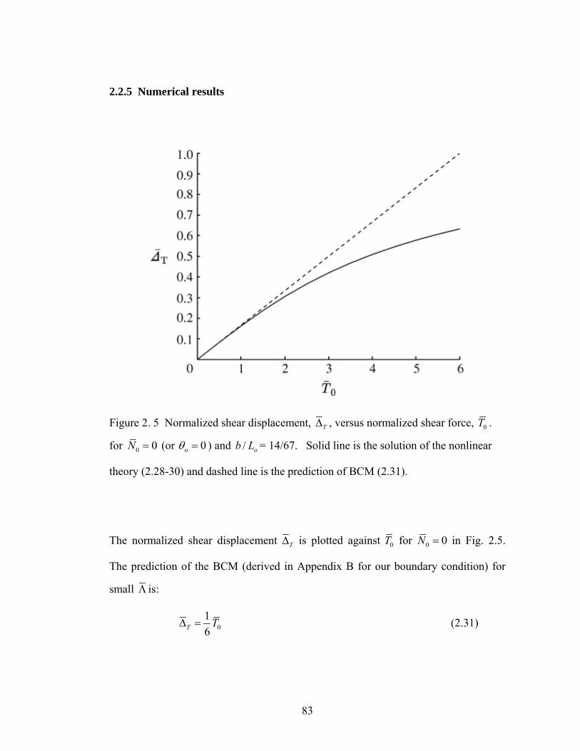
83
2.2.5 Numerical results
Figure 2. 5 Normalized shear displacement, TΔ , versus normalized shear force, 0T .
for 0 0N = (or 0oθ = ) and / ob L = 14/67. Solid line is the solution of the nonlinear
theory (2.28-30) and dashed line is the prediction of BCM (2.31).
The normalized shear displacement TΔ is plotted against 0T for 0 0N = in Fig. 2.5.
The prediction of the BCM (derived in Appendix B for our boundary condition) for
small Λ is:
016T TΔ = (2.31)
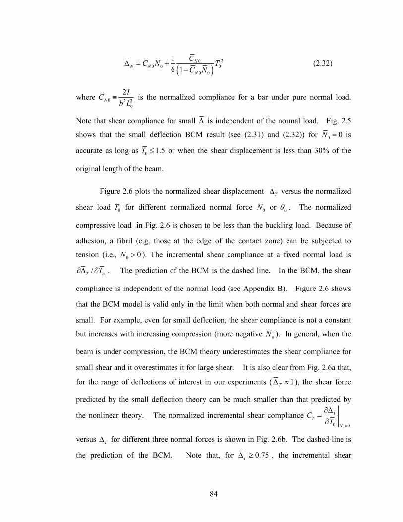
84
( )20
0 0 00 0
16 1
NN N
N
CC N TC N
Δ = +−
(2.32)
where 0 2 20
2N
ICb L
≡ is the normalized compliance for a bar under pure normal load.
Note that shear compliance for small Λ is independent of the normal load. Fig. 2.5
shows that the small deflection BCM result (see (2.31) and (2.32)) for 0 0N = is
accurate as long as 0 1.5T ≤ or when the shear displacement is less than 30% of the
original length of the beam.
Figure 2.6 plots the normalized shear displacement TΔ versus the normalized
shear load 0T for different normalized normal force 0N or oθ . The normalized
compressive load in Fig. 2.6 is chosen to be less than the buckling load. Because of
adhesion, a fibril (e.g. those at the edge of the contact zone) can be subjected to
tension (i.e., 0 0N > ). The incremental shear compliance at a fixed normal load is
/T oT∂Δ ∂ . The prediction of the BCM is the dashed line. In the BCM, the shear
compliance is independent of the normal load (see Appendix B). Figure 2.6 shows
that the BCM model is valid only in the limit when both normal and shear forces are
small. For example, even for small deflection, the shear compliance is not a constant
but increases with increasing compression (more negative oN ). In general, when the
beam is under compression, the BCM theory underestimates the shear compliance for
small shear and it overestimates it for large shear. It is also clear from Fig. 2.6a that,
for the range of deflections of interest in our experiments ( 1≈ΔT ), the shear force
predicted by the small deflection theory can be much smaller than that predicted by
the nonlinear theory. The normalized incremental shear compliance 0 0o
TT
N
CT
=
∂Δ=
∂
versus TΔ for different three normal forces is shown in Fig. 2.6b. The dashed-line is
the prediction of the BCM. Note that, for 0.75TΔ ≥ , the incremental shear
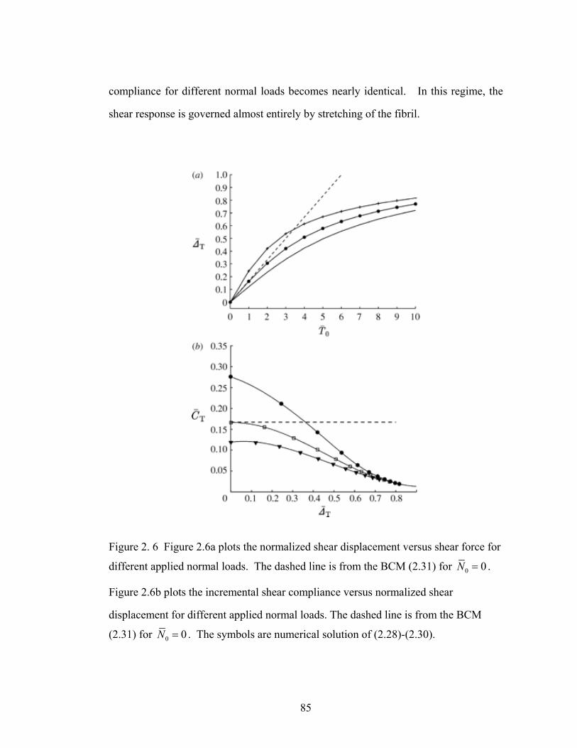
85
compliance for different normal loads becomes nearly identical. In this regime, the
shear response is governed almost entirely by stretching of the fibril.
Figure 2. 6 Figure 2.6a plots the normalized shear displacement versus shear force for
different applied normal loads. The dashed line is from the BCM (2.31) for 0 0N = .
Figure 2.6b plots the incremental shear compliance versus normalized shear
displacement for different applied normal loads. The dashed line is from the BCM
(2.31) for 0 0N = . The symbols are numerical solution of (2.28)-(2.30).
86
Figure 2.7 shows that a fibril with no applied normal load can still have normal
displacement due to shear. This figure shows that the small deflection theory
considerably underestimates the normal displacement for large 0T . To study the
incremental normal compliance of the fibril /o
N N o TC N= ∂Δ ∂ , the dependence of NΔ
on 0N for different 0T is shown in Fig. 2.8a. For small 0T , the compliance is small.
For a fixed 0N , the incremental normal compliance increases significantly with
increasing applied shear load 0T ; for fixed 0T it also increases slightly with increasing
compressive normal load, as shown in Fig. 2.8b.
Figure 2.7 plots the normalized normal displacement, NΔ , versus normalized shear
force 0T for 0 0N = (or 0oθ = ). It shows that significant normal deflection at the fibril
end can occur with no applied normal force. Note that the small deflection theory
underestimates the normal displacement.
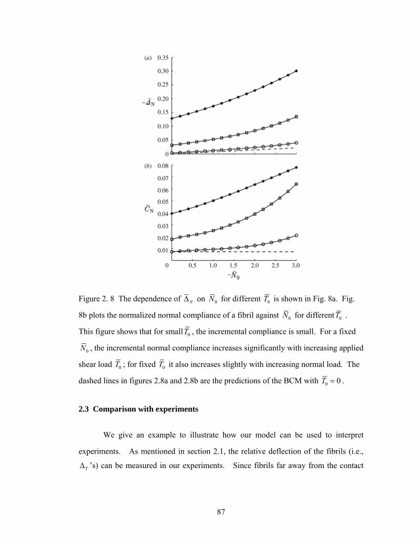
87
Figure 2. 8 The dependence of NΔ on 0N for different 0T is shown in Fig. 8a. Fig.
8b plots the normalized normal compliance of a fibril against 0N for different 0T .
This figure shows that for small 0T , the incremental compliance is small. For a fixed
0N , the incremental normal compliance increases significantly with increasing applied
shear load 0T ; for fixed 0T it also increases slightly with increasing normal load. The
dashed lines in figures 2.8a and 2.8b are the predictions of the BCM with 0 0T = .
2.3 Comparison with experiments
We give an example to illustrate how our model can be used to interpret
experiments. As mentioned in section 2.1, the relative deflection of the fibrils (i.e.,
TΔ ’s) can be measured in our experiments. Since fibrils far away from the contact
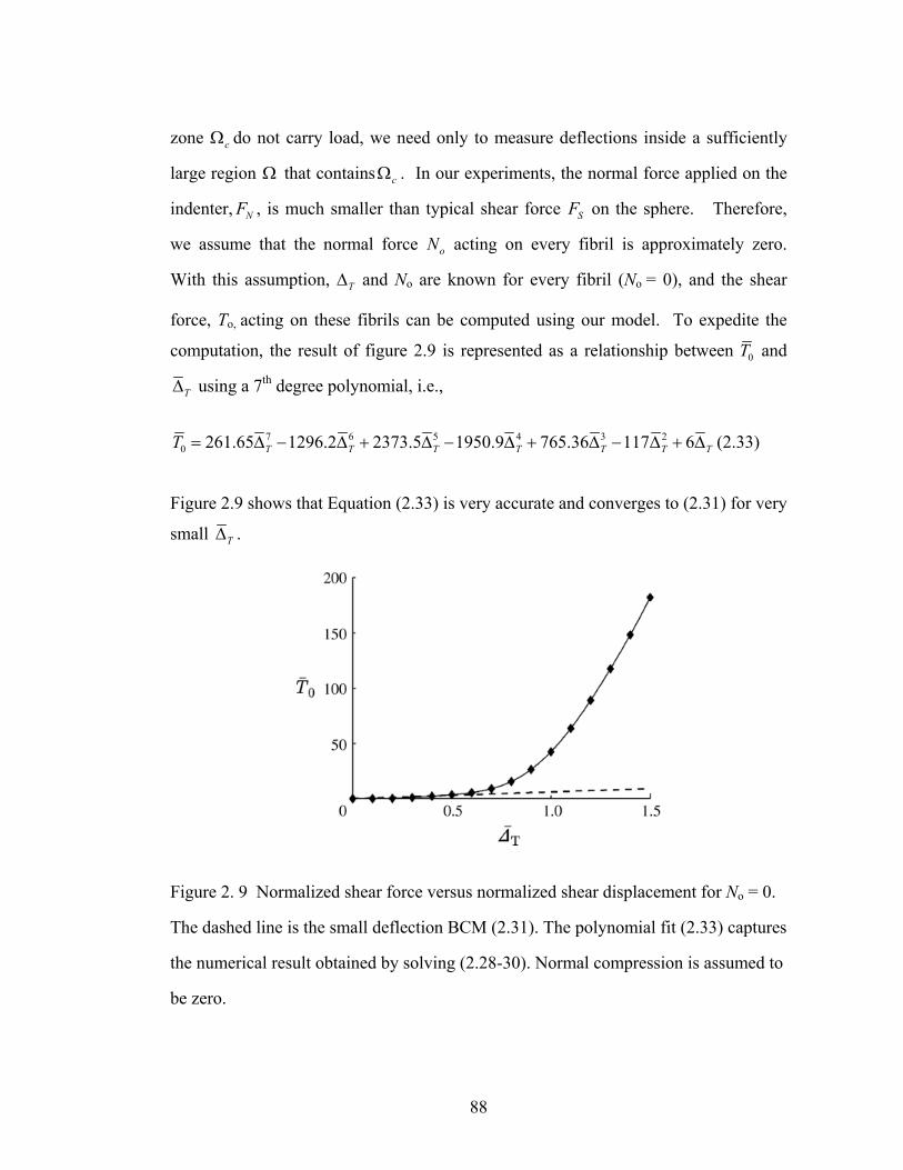
88
zone cΩ do not carry load, we need only to measure deflections inside a sufficiently
large region Ω that contains cΩ . In our experiments, the normal force applied on the
indenter, NF , is much smaller than typical shear force SF on the sphere. Therefore,
we assume that the normal force oN acting on every fibril is approximately zero.
With this assumption, TΔ and No are known for every fibril (No = 0), and the shear
force, To, acting on these fibrils can be computed using our model. To expedite the
computation, the result of figure 2.9 is represented as a relationship between 0T and
TΔ using a 7th degree polynomial, i.e.,
7 6 5 4 3 20 261.65 1296.2 2373.5 1950.9 765.36 117 6T T T T T T TT = Δ − Δ + Δ − Δ + Δ − Δ + Δ (2.33)
Figure 2.9 shows that Equation (2.33) is very accurate and converges to (2.31) for very
small TΔ .
Figure 2. 9 Normalized shear force versus normalized shear displacement for No = 0.
The dashed line is the small deflection BCM (2.31). The polynomial fit (2.33) captures
the numerical result obtained by solving (2.28-30). Normal compression is assumed to
be zero.
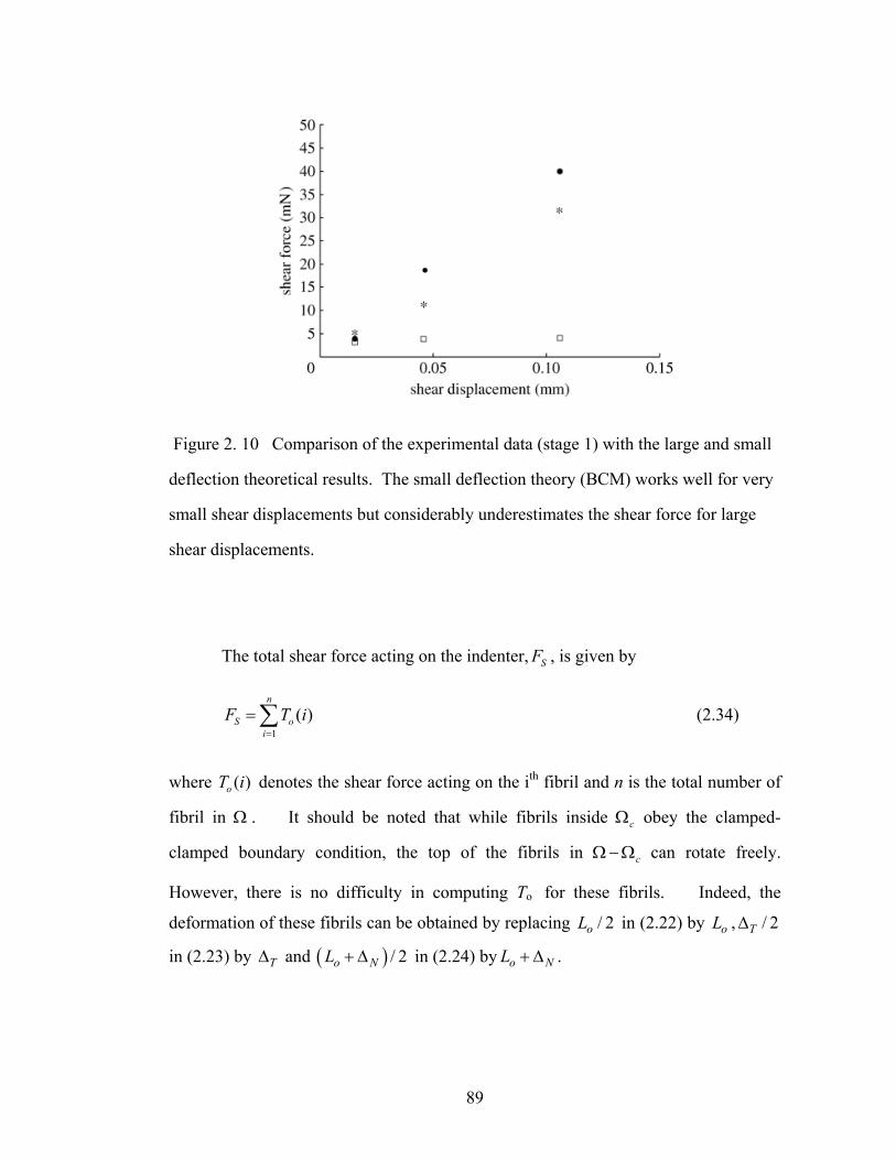
89
Figure 2. 10 Comparison of the experimental data (stage 1) with the large and small
deflection theoretical results. The small deflection theory (BCM) works well for very
small shear displacements but considerably underestimates the shear force for large
shear displacements.
The total shear force acting on the indenter, SF , is given by
1
( )n
S oi
F T i=
= ∑ (2.34)
where ( )oT i denotes the shear force acting on the ith fibril and n is the total number of
fibril in Ω . It should be noted that while fibrils inside cΩ obey the clamped-
clamped boundary condition, the top of the fibrils in cΩ − Ω can rotate freely.
However, there is no difficulty in computing To for these fibrils. Indeed, the
deformation of these fibrils can be obtained by replacing / 2oL in (2.22) by oL , / 2TΔ
in (2.23) by TΔ and ( ) / 2o NL + Δ in (2.24) by o NL + Δ .
90
We obtain ( )oT i using the following procedure. First, we select three points on
the shear force versus shear displacement curve in Fig. 2.1b. The coordinates of these points are ( )0.0155 , 3.80 A mm mN , ( )0.0456 , 18.68 B mm mN
and ( )0.106 , 40.03 C mm mN respectively. We select Ω with the condition that
fibrils outside of Ω do not have measurable deflections. Once this is done, we
measure the deflection for each fibril ( ( ))T iΔ inside Ω . ( )T iΔ in (2.33) is computed
from ( )T iΔ using L = 67 μm. We then use (2.33) to obtain ( )oT i . To compute ( )oT i
from ( )oT i , we need the Young’s modulus and the moment of inertia I. We use a
Young’s modulus of 3 MPa for PDMS, the fibril material. This modulus has been
measured independently using an indentation test, see (Noderer et al. 2007). The moment of inertia I is ( )433.2 10 mμ× since the fibrils in our experiments have a
square cross-section of 14 μm. The number of fibrils in Ω is 324. We then compute
the indenter shear forces using (2.34). They are 5.23 mN for point A, 11.22 mN for
point B and 31.54 mN for point C respectively. We also use the small deflection
theory (2.31) to compute these shear forces. They are 3.24 mN for point A, 3.75 mN
for point B and 4.02 mN for point C. These results are shown in Fig 2.10, which
compares the experimental data (stage 1) with the large and small deflection results.
As expected, the small deflection theory works well for small shear displacement but
strongly underestimates the shear force for large shear displacement. For example,
near the peak load (e.g. point C), the use of small deflection theory underestimates the
shear force by about an order of magnitude. Given the fact that we have used no
adjustable parameters, the agreement between our large deflection theory and the
experimental data is quite good.
91
2.4 Discussion and Conclusion
The mechanical behavior of fibrils under combined normal and shear loads
underlies the response of biomimetic fibrillar arrays. Deformations are typically large
compared to fibril dimensions. We have developed a nonlinear model to compute the
deflection of fibrils in micro-fibril arrays subjected to normal and shear loads. To
simplify the analysis, we have assumed that the fibrils do not twist. Also, we assume
the beam can undergo very large deflection but material behavior is still linear.
Our model isolates a single fibril in the array to study its behavior, whereas in
practice, the entire array is subjected to normal and shear loads. To illustrate how our
model can be applied in this situation, we use our model to predict the shear force
acting on a glass indenter in contact with an array of film terminated fibrils. The
computed shear forces are then compared with those obtained from experiments. In
the simulations, we have made the approximation that the normal force acting on all
the fibrils is zero, which is strictly valid only for fibrils that are outside the contact
zone. For fibrils inside the contact zone, some of the fibrils can be under tension (e.g.
those close to the contact edge) whereas others can be under compression so our
assumption is only approximately valid if the normal indentation force is very small in
comparison with the shear forces, which is the case in our experiments. Nevertheless,
the prediction of our nonlinear model is in reasonably good agreement with the
experimental data. We should point out that there is some error in measuring the
relative displacement of each fibril. Since the nonlinear theory is very sensitive to the
relative shear displacement, it is not surprising that the nonlinear theory did worst for
small deflections, where the relative error of the measurements can be large. Finally,
there is no fitting parameter in our calculation.

92
Although our analysis is valid for any loading phase angles as well as for
arbitrary aspect ratios, explicit results are presented for a particular aspect ratio. Also,
we focus on the case where the normal load is zero. In general, there is no difficulty
in generating results for other aspect ratios and different phase angle. Also, our
model can be easily modified to describe the deformation of pre-oriented fibrils.
The model of fibril deformation studied in this work is quite general and can
be used to study fibrillar structures other than our own. For example, it is applicable
to a similar fibrillar structure (with angled fibrils) fabricated recently by Guduru et al
(2007). It can also be used to analyze the shear deformation of fibrils with spatulated
tips, such as those fabricated by Kim et al (2007).
The analysis will be more complicated for the general case where the normal
indentation force is significant. In this case, most of the fibrils inside the contact zone
will be under compression except those near the edge. These edge fibrils will be
under tension because of adhesion. For this case, the normal and shear load on each
fibril in the array must be determined using the contact condition. This will be
studied in a future work.
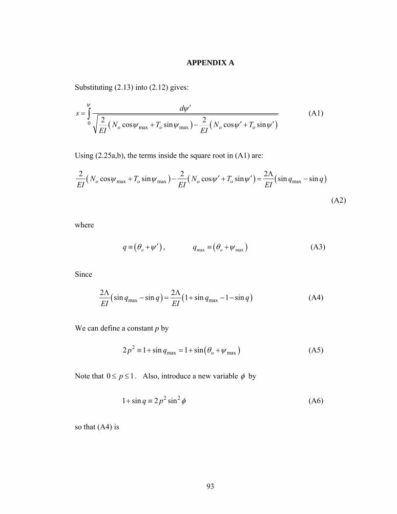
93
APPENDIX A
Substituting (2.13) into (2.12) gives:
( ) ( )0max max
2 2cos sin cos sino o o o
dsN T N T
EI EI
ψ ψ
ψ ψ ψ ψ
′=
′ ′+ − +∫ (A1)
Using (2.25a,b), the terms inside the square root in (A1) are:
( ) ( ) ( )max max max2 2 2cos sin cos sin sin sino o o oN T N T q q
EI EI EIψ ψ ψ ψ Λ′ ′+ − + = −
(A2)
where
( )oq θ ψ ′≡ + , ( )max maxoq θ ψ≡ + (A3)
Since
( ) ( )max max2 2sin sin 1 sin 1 sinq q q qEI EIΛ Λ
− = + − − (A4)
We can define a constant p by
( )2max max2 1 sin 1 sin op q θ ψ≡ + = + + (A5)
Note that 0 1p≤ ≤ . Also, introduce a new variable φ by
2 21 sin 2 sinq p φ+ ≡ (A6)
so that (A4) is
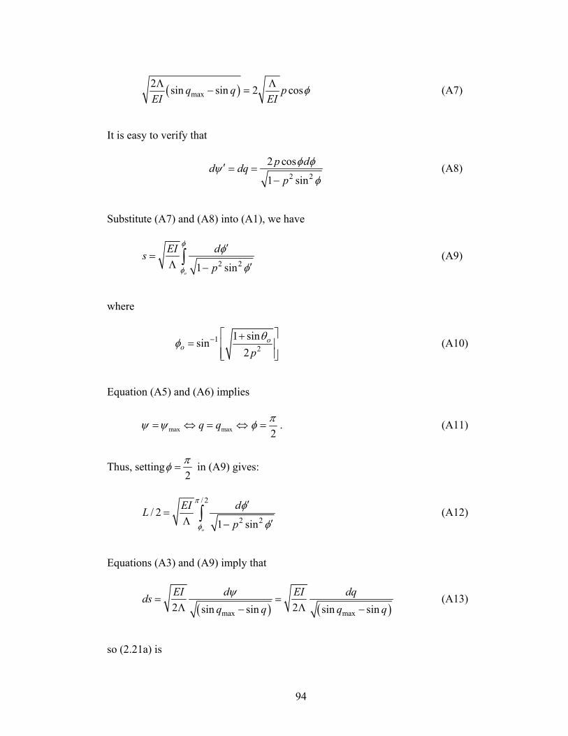
94
( )max2 sin sin 2 cosq q pEI EI
φΛ Λ− = (A7)
It is easy to verify that
2 2
2 cos
1 sin
p dd dqp
φ φψφ
′ = =−
(A8)
Substitute (A7) and (A8) into (A1), we have
2 21 sin
o
EI dsp
φ
φ
φ
φ
′=
Λ ′−∫ (A9)
where
12
1 sinsin2
oo p
θφ − ⎡ ⎤+= ⎢ ⎥
⎢ ⎥⎣ ⎦ (A10)
Equation (A5) and (A6) implies
max maxq qψ ψ= ⇔ = ⇔2πφ = . (A11)
Thus, setting2πφ = in (A9) gives:
/ 2
2 2/ 2
1 sino
EI dLp
π
φ
φ
φ
′=
Λ ′−∫ (A12)
Equations (A3) and (A9) imply that
( ) ( )max max2 2sin sin sin sin
EI d EI dqdsq q q q
ψ= =
Λ Λ− − (A13)
so (2.21a) is
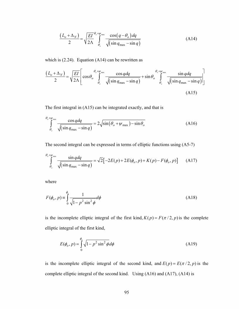
95
( ) ( )( )
max
max
cos2 2 sin sin
o
o
o N oL q dqEIq q
θ ψ
θ
θ++ Δ −=
Λ −∫ (A14)
which is (2.24). Equation (A14) can be rewritten as
( )( ) ( )
max max
max max
cos sincos sin2 2 sin sin sin sin
o o
o o
o No o
L EI qdq qdqq q q q
θ ψ θ ψ
θ θ
θ θ+ +⎡ ⎤+ Δ
⎢ ⎥= +Λ ⎢ ⎥− −⎣ ⎦
∫ ∫
(A15)
The first integral in (A15) can be integrated exactly, and that is
( )( )
max
maxmax
cos 2 sin sinsin sin
o
o
o oqdq
q q
θ ψ
θ
θ ψ θ+
= + −−∫ (A16)
The second integral can be expressed in terms of elliptic functions using (A5-7)
( )[ ]
max
max
sin 2 2 ( ) 2 ( , ) ( ) ( , )sin sin
o
o
o oqdq E p E p K p F p
q q
θ ψ
θ
φ φ+
= − + + −−∫ (A17)
where
2 20
1( , )1 sin
o
oF p dp
φ
φ φφ
≡−
∫ (A18)
is the incomplete elliptic integral of the first kind, ( ) ( / 2, )K p F pπ= is the complete
elliptic integral of the first kind,
2 2
0
( , ) 1 sino
oE p p dφ
φ φ φ= −∫ (A19)
is the incomplete elliptic integral of the second kind, and ( ) ( / 2, )E p E pπ= is the
complete elliptic integral of the second kind. Using (A16) and (A17), (A14) is
96
( ) ( )[ ]
max2 cos sin sin2 sin 2 ( ) 2 ( , ) ( ) ( , )
o o oo N
o o o
L EIE p E p K p F p
θ θ ψ θ
θ φ φ
⎡ ⎤+ −+ Δ⎢ ⎥=
Λ ⎢ ⎥+ − + + −⎣ ⎦ (A20)
Likewise, (2.23) can be obtained by substituting (A13) to (21b),
( )max/ 2
max0
/ 2 sin ( ) sin2 sin sin
o
qL
T oEI dqs ds q
q qθ
ψ θ′ ′Δ = = −Λ −∫ ∫ (A21)
In exactly the same way, (A21) is:
( )[ ]
max2 sin sin sin/ 2
cos 2 ( ) 2 ( , ) ( ) ( , )o o o
To o o
EIE p E p K p F p
θ θ ψ θ
θ φ φ
⎡ ⎤− + −⎢ ⎥Δ =
Λ ⎢ ⎥+ − + + −⎣ ⎦ (A22)
Using (A2) and (A13), (2.20) is
( )
max
max/ 2
2 1 sin sin sino
q
oEI dq L
c q q qθ
=Λ + Λ −∫ (A23a)
(A23a) can be expressed in terms of incomplete elliptic integral of the third kind,
( ); ,n kφΠ , that is:
( )max max0 max
max max maxmax max
20
sin 1 cossin sin1 ; , 1 sin 1 sin 1 sin(1 sin ) 1 sin
12 2
q c qq iq c q qc q q
LEI
θ⎛ ⎞− Λ−− Π ⎜ ⎟⎜ ⎟− + Λ ++ Λ + ⎝ ⎠
Λ=
(A23b)
where
( )( )2 2 2
0
; ,1 sin 1 sin
dn kn k
φ θφθ θ
Π =− −
∫ . (A24)
97
APPENDIX B
Assuming ψ is small, (2.10) can be approximated at:
( )2 ( )o od N T s Dds EIψ ψ≈ − + + 0 / 2s L< < (A25)
Substitute ( ) ( )max max max2 2cos sino o o oD N T N T
EI EIψ ψ ψ= + ≈ + into (A25) and
integrate, we have,
max maxmax0
22 o o
EI d EIsT T
ψ ψ ψ ψ ψψ ψ
′ ⎡ ⎤≈ = − −⎣ ⎦′−∫ maxψ ψ> (A26)
or
2
max max 2
oT sEI
ψ ψ ψ⎡ ⎤
= − −⎢ ⎥⎣ ⎦
(A27)
Using (2.10) and (2.11) and the fact that 0ddsψ
= at maxψ ψ= , we have
( )2 2
max max max2 2 10 0
2o o
o o oo
M MN T D TEI EI EI T EI
ψ ψ ψ⎡ ⎤⎡ ⎤− + + = ⇔ − + = ⇒ = ⎢ ⎥⎢ ⎥⎣ ⎦ ⎣ ⎦
(A28)
Since maxψ ψ= when / 2s L= , (A27) implies that
2
max 8
oT LEI
ψ = (A29)
Using (A28), we have
98
2o
oT LM = − (A30)
Combining (A27) and (A29) gives:
( )2
oT s L sEI
ψ = − (A31)
Using (A29), the small deflection version of (2.21b) is
/ 2 3
0
/ 2 ( )24
Lo
TT Ls ds
EIψ ′ ′Δ ≈ =∫ (A32)
The normalized form of (A32) is (2.31) using 0L L≈ .
016T TΔ = (A33)
To determine the relation normal displacement and normal load for small deflection,
we approximate (2.20) by assuming that the slope is small, so that yψ ′≈ , ds dx≈ , i.e.,
[ ]/ 2
0
/ 21
L
oo o
dx Lc N T y
=′+ +∫ , (A34)
Consistent with small deflection, we assume
( )/ 1 1o ocT y cN′ + << (A35)
The integral in (A34) is
( ) ( )
( ) ( )
( ) ( )
/2 /2
0 0
1 11 1
1 11
11 2 2 1
L Lo
o ooo
o
o T
o o
cT ydx dxcN cNcT ycN
cN
cTLcN cN
⎡ ⎤′≈ −⎢ ⎥
+ +⎡ ⎤′ ⎢ ⎥⎣ ⎦+ +⎢ ⎥+⎣ ⎦⎡ ⎤Δ
= −⎢ ⎥+ +⎢ ⎥⎣ ⎦
∫ ∫ (A36)
99
where we have used
/ 2
0
( / 2) / 2L
Ty dx y L′ = = Δ∫ (A37)
Using (A36) and (A37), (A34) is:
( )1
o Tn o o
o
cT L cNcNΔ
Δ − =+
(A38)
where o NL L≈ + Δ . Equation (2.32) is obtained by substitute (A32) into (A 38), i.e.,
( )2
312
1T
n o oo
cEIL cNL cN
ΔΔ = +
+ (A39)
100
REFERENCES
Aksak, B, Murphy, M.P. and Sitti, M. 2007. Adhesion of Biologically Inspired
Vertical and Angled Polymer Microfiber Arrays. Langmuir, 23 (6), 3322 -3332.
Autumn, K., Liang, Y.A., Hsieh, S.T., Zesch, W., Chan, W.P., Kenny, T.W., Fearing,
R. and Full, R.J. 2000. Adhesive force of a single gecko foot-hair. Nature 405, 681-
685.
Bhushan, B., Peressadko, A.G. and Kim, T.W. 2006. Adhesion analysis of two-level
hierarchical morphology in natural attachment systems for 'smart adhesion'. J. Adhes.
Sci. Technol. 20, 1475-1491.
Chen, S. and Gao, H. 2007. Non-slipping adhesive contact between mismatched
elastic spheres: A model of adhesion mediated deformation sensor. J. Mech.Phys.
Solids 55, 1001-1015.
Chung, J.Y. and Chaudhury, M.K. 2005. Roles of discontinuities in bio-inspired
adhesive pads. J. R. Soc. Interface 2, 55-61.
Crosby, A.J., Hageman, M. and Duncan, A. 2005. Controlling polymer adhesion
with"pancakes". Langmuir 21, 11738-11743.
Frisch-Fay, R. 1962. Flexible Bars. Washington: Butterworths. pp. 33–44.
Gao, H., Ji, B., Jäger, I.L., Arzt, E. and Fratzl, P. 2003. Materials become insensitive
to flaws at nanoscale: Lessons from nature. Proc. Natl. Acad. Sci. USA 100, 5597-
5600.
Gao, H., Wang, X., Yao, H., Gorb, S. and Arzt, E. 2005. Mechanics of hierarchical
adhesion structures of geckos. Mech. Mater. 37, 275-285.
101
Ge, L., Sethi, S., Ci, L., Ajayan, P. M., and Dhinojwala, A. 2007. Carbon nanotube-
based synthetic gecko tapes. Proc. Natl. Acad. Sci. USA 104, 26, 10792-10795.
Glassmaker, N.J., Jagota, A. and Hui, C.Y. 2005. Adhesion enhancement in a
biomimetic fibrillar interface. Acta Biomater 4, 367-375.
Glassmaker, N.J., Jagota, A., Hui, C.-Y. and Chaudhury, M.K.2006. Proc. Annual
Meeting of the Adhesion, Blacksburg, VA: Adhesion Society. pp. 93–95.
Glassmaker, N. J., Jagota, A., Hui, C.-Y., Noderer, W. L. and Chaudhury, M. K. 2007.
Proc. Natl. Acad. Sci. USA 104, 26, 10786-10791.
Gorb, S., Varenberg, M., Peressadko, A. and Tuma, J. 2007. Biomimetic mushroom-
shaped fibrillar adhesive microstructure. J. R. Soc. Interface 4, 271-275.
Greiner, C., Campo, A.D., Arzt, E., 2007. Adhesion of bioinspired micropatterned
surfaces: effects of pillar radius, aspect ratio, and preload. Langmuir 23, 3495-502.
Guduru, P.R., personal communication, 2007.
Huber, G., Gorb, S., Spolenak, R. and Arzt, E. 2005. Resolving the nanoscale
adhesion of individual gecko spatulae by atomic force microscopy. Biol. Lett. 1, 2-4.
Hui, C.-Y., Glassmaker, N.J., Tang, T. and Jagota, A. 2004. Design of biomimetic
fibrillar interfaces: 2. Mechanics of enhanced adhesion. J. R. Soc. London Interface 1,
35-48.
Irschick, D.J., Austin, C.C., Petren, K., Fisher, R., Losos, J.B., and Ellers, O. 1996. A
comparative analysis of clinging ability among pad-bearing lizards. Biol. J. Linn. Soc.
59, 21-35.
Jagota, A. and Bennison, S.J. 2002. Mechanics of adhesion through a fibrillar
microstructure Integr. Comp. Biol. 42, 1140-1145.
102
Johnson, K.L., Kendall, K. and Roberts, A.D. 1971. Surface energy and the contact of
elastic solids. Proc. R. Soc. London, A 324, 301.
Kim, S., Aksak, B. and Sitti, M. 2007. Enhanced friction of elastomer microfiber
adhesives with spatulate tips. Appl. Phys. Lett. 91, 221913.
Kim, S. and Sitti, M. 2006. Biologically inspired polymer microfibers with spatulate
tips as repeatable fibrillar adhesives. Appl. Phys. Lett. 89, 261911.
Liu, H.W. and Bhushan, B. 2003. Adhesion and friction studies of
microelectromechanical systems/nanoelectromechanical systems materials using a
novel microtriboapparatus. J.Vacuum Sci. Technol. A 21, 1528-1538.
Majidi, C., Groff, R.E., Maeno, Y., Schubert, B., Baek, S., Bush, B., Maboudian, R.,
Gravish, N., Wilkinson, M., Autumn, K., and Fearing, R.S. 2006. High Friction from a
Stiff Polymer Using Microfiber Arrays. Phys. Rev. Lett. 97, 076103.
Noderer, W.L., Shen, L., Vajpayee, S., Glassmaker, N.J., Jagota, A. and Hui, C.-
Y.2007. Enhanced adhesion and compliance of film-terminated fibrillar surfaces. Proc.
R. Soc. London, A 463, 2631-2654.
Northen, M.T. and Turner, K.L. 2005. A batch fabricated biomimetic dry adhesive.
Nanotechnology 16, 1159-1166.
Peressadko, A. and Gorb, S.N. 2004. When less is more: Experimental evidence for
tenacity enhancement by division of contact area. Journal of Adhesion 80, 247-261.
Persson, B.N.J., Albohr, O., Tartaglino, U., Volokitin, A.I. and Tosatti, E. 2005. On
the nature of surface roughness with application to contact mechanics, sealing, rubber
friction and adhesion. J. Phys.: Condens. Matter 17, R1-R62.
103
Persson, B.N.J. and Gorb, S. 2003. The effect of surface roughness on the adhesion of
elastic plates with application to biological systems. J. Chem. Phys. 119, 11437-11444.
Savkoor, A.R. and Briggs, G.A.D. 1977. The Effect of Tangential Force on the
Contact of Elastic Solids in Adhesion. Proc. R. Soc. London, A 356, 103-114.
Shen, L., Glassmaker, N.J., Jagota, A.,and Hui, C.-Y. 2007. Strongly Enhanced Static
Friction Using a Film-Terminated Fibrillar Interface, accepted by Soft Matter.
Spolenak, R., Gorb, S. and Arzt, E.. 2005a. Adhesion design maps for bio-inspired
attachment systems. Acta Biomater. 1, 5-13.
Spolenak, R., Gorb, S., Gao, H. and Arzt, E. 2005b. Effects of contact shape on the
scaling of biological attachments. Proc. R. Soc. London A 461, 305-319.
Tang, T. Hui, C.-Y. and Glassmaker, N.J. 2005. Can a fibrillar interface be stronger
and tougher than a non-fibrillar one? J. R. Soc. Interface 2, 505-516.
Tian, Y., Pesika, N., Zeng, H., Rosenberg, K., Zhao, B., McGuiggan, P., Autumn, K.
and
Israelachvili, J. 2006. Adhesion and friction in gecko toe attachment and detachment.
Proc.
Natl. Acad. Sci. USA 103, 19320-19325.
Timoshenko, S. P. and Gere, J. M. 1961. Theory of Elastic Stability. New York:
McGraw-Hill. Chap. 1.
Varenberg, M. and Gorb, S. 2007. Shearing of fibrillar adhesive microstructure:
friction and shear-related changes in pull-off force. J. R. Soc. Interface, 4, 721-725.

104
Yao, H. and Gao, H. 2006. Mechanics of robust and releasable adhesion in biology:
Bottom-up designed hierarchical structures of gecko. J. Mech. Phys. Solids 54, 1120-
1146.
Yurdumakan, B., Raravikar, N.R., Ajayan, P.M. and Dhinojwala. 2005. Synthetic
gecko foothairs from multiwalled carbon nanotubes. A., Chem. Commun. 30, 3799-
3801.
105
Chapter 3
A Model for Static Friction in a Film-terminated Micro-fibril Array*
Abstract
We model the response of a film-terminated micro-fibril array subjected to shear
through contact with a rigid cylindrical indenter. Our model determines the shear
force acting on the indenter for a fixed normal indenter force before the onset of
uniform sliding. Consistent with experiment, our model shows that (1) the contact
area increases only slightly with applied shear and (2) the fibrils inside the contact
zone are subjected to tension at intermediate to large applied shear displacement
despite the fact that the applied normal load is compressive. These features can be
explained by the fact that in our samples the continuous terminal film supports tension.
The model accurately matches the experimentally measured shear-force response.
With the use of an independently measured critical energy release rate for unstable
release of the contact, the model shows how this architecture achieves a strong
enhancement in static friction.
Keywords: friction, adhesion, film-terminate fibril array, energy release rate, contact
area
* Accepted to publish Journal of Applied Physics.
106
3.1. Introduction
Many small animals and insects use tiny fibrils on their feet to make contact
and to adhere to surfaces. This fact has motivated many researchers to fabricate
micro-fibril arrays 1–19 and to study their adhesion and friction behavior. 20–36 It has
been found that friction behavior of fibrillar arrays depends on the stiffness of the
fibril material. For example, arrays made of soft fibrils with spatulated tips have
static and dynamic friction that is lower than a flat control surface made of the same
material.14,16 In contrast, arrays composed of stiffer fibers typically exhibit static and
dynamic friction8,15 higher than that of a flat control sample.
The fibril arrays mentioned above have tips that are isolated from each other.
In previous work 17,18 we have shown that an array with soft fibers connected by a
terminal thin film has many interesting friction characteristics. Specifically, when a
shear displacement is applied to a glass indenter that is in contact with the surface of
the fibrillar array under a fixed normal load, the following behavior is observed:36
a) Static friction is represented by a peak load under shear, which increases with
the minimum inter-fibril spacing between fibrils, w. In particular, the static
friction is much higher in fibrillar samples compared with the flat control.
b) The contact area does not change much with increasing shear.
c) Sliding friction is independent of fibril spacing and is the same as the flat
control samples.
The third observation has been addressed in our recent work.36 Here, the
important observations we wish to understand are related to behavior prior to onset of
overall slip between the sample and indenter, i.e., the static friction. The paper is
organized as follows. We briefly review our experiments in section 3.2. Our contact
107
mechanics model is given in section 3.3 which has four sub-sections. A nonlinear rod
theory which accounts for the shearing and stretching of a micro-fibril is used to
determine the response a micro-fibril in subsection 3.3.1. The shear deformation of
fibrils and the film tension outside the contact zone are modeled in subsection 3.3.2.
Subsection 3.3.3 presents a model for normal contact. Numerical results for the
contact width and distribution of fibril forces are presented in 3.3.4. Comparisons of
theory with experiments are given in section 3.4. We conclude the Summary and
Discussion in Section 3.5.
3.2. Review of Experiments
A scanning electron microscope (SEM) image of our fibril array is shown Fig.
3.1a. The array is part of a poly(dimethylsiloxane) block (PDMS, Sylgard 184, Dow
Corning) which has a thickness of 650 μm. The fibrils have square cross-section b =
10 μm in width, are L = 30 μm in length and are arranged in a square pattern. The
fibrils are topped by a continuous film of thickness 4h mμ= . The fibrils, terminal thin
film, and backing are all of the same material (PDMS); a highly elastic incompressible
solid with a Young’s modulus E ≈ 3MPa. Fabrication procedures are described in
detail in.12,13,18 With all other dimensions fixed as described above, a series of
samples with varying nearest center-to-center distance between fibrils, 35w mμ= ,
50 mμ , and 65 mμ were used in our friction experiments. Details of these
experiments can be found in Shen et al. 36 Here we give a brief review.
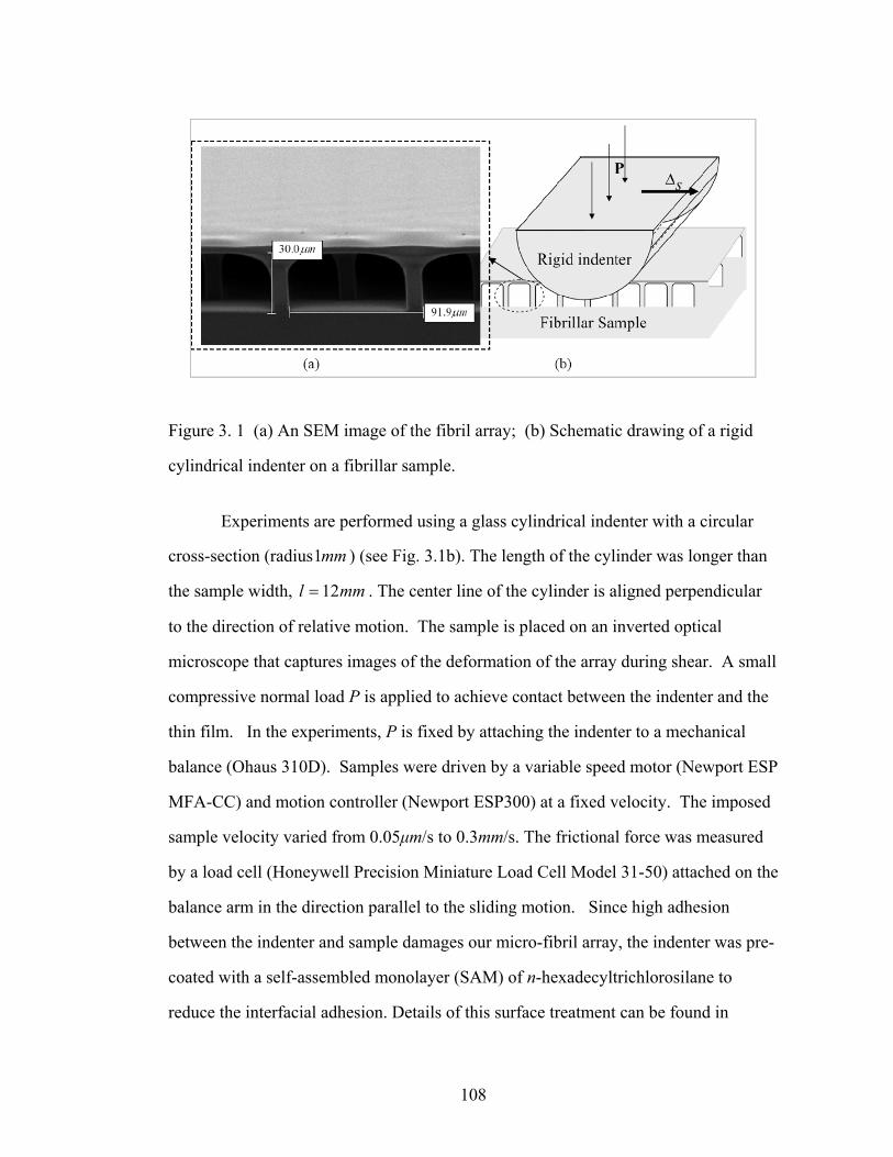
108
Figure 3. 1 (a) An SEM image of the fibril array; (b) Schematic drawing of a rigid
cylindrical indenter on a fibrillar sample.
Experiments are performed using a glass cylindrical indenter with a circular
cross-section (radius1mm ) (see Fig. 3.1b). The length of the cylinder was longer than
the sample width, 12l mm= . The center line of the cylinder is aligned perpendicular
to the direction of relative motion. The sample is placed on an inverted optical
microscope that captures images of the deformation of the array during shear. A small
compressive normal load P is applied to achieve contact between the indenter and the
thin film. In the experiments, P is fixed by attaching the indenter to a mechanical
balance (Ohaus 310D). Samples were driven by a variable speed motor (Newport ESP
MFA-CC) and motion controller (Newport ESP300) at a fixed velocity. The imposed
sample velocity varied from 0.05μm/s to 0.3mm/s. The frictional force was measured
by a load cell (Honeywell Precision Miniature Load Cell Model 31-50) attached on the
balance arm in the direction parallel to the sliding motion. Since high adhesion
between the indenter and sample damages our micro-fibril array, the indenter was pre-
coated with a self-assembled monolayer (SAM) of n-hexadecyltrichlorosilane to
reduce the interfacial adhesion. Details of this surface treatment can be found in
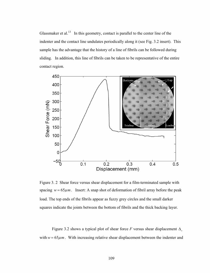
109
Glassmaker et al.13 In this geometry, contact is parallel to the center line of the
indenter and the contact line undulates periodically along it (see Fig. 3.2 insert). This
sample has the advantage that the history of a line of fibrils can be followed during
sliding. In addition, this line of fibrils can be taken to be representative of the entire
contact region.
Figure 3. 2 Shear force versus shear displacement for a film-terminated sample with
spacing 65w mμ= . Insert: A snap shot of deformation of fibril array before the peak
load. The top ends of the fibrils appear as fuzzy grey circles and the small darker
squares indicate the joints between the bottom of fibrils and the thick backing layer.
Figure 3.2 shows a typical plot of shear force F versus shear displacement sΔ
with 65w mμ= . With increasing relative shear displacement between the indenter and
110
the sample, the force first increases to a peak value (static friction). Beyond the peak,
it decreases rapidly, and then remains nearly constant (sliding friction). Visual
inspection of the contact region before the peak load reveals that it changes slightly in
size, with the number of fibrils in contact remaining independent of applied shear. In
addition, there is no overall sliding between the indenter and the sample before the
static friction peak. In the region where the load is nearly constant, the indenter slides
steadily on the sample.
The observation that the contact area changes little with increasing shear is
puzzling. The shear displacement of a typical fibril inside the contact zone near the
static peak is very large, close to the length of the fibril. Therefore, one would expect
a significant increase of the normal displacement of a fibril (a detailed analysis is
given below). Since the normal force on the indenter is kept constant throughout the
experiment, such a drastic increase of normal displacement should result in very large
increase in contact area during shear. However, the number of fibrils in contact in our
experiments does not increase with shear – an apparent paradox.
3.3 Contact mechanics
3.3.1 Shear and stretch of an individual fibril
A necessary first step to understand the contact mechanics is to quantify how
an individual fibril behaves under a combination of shear and normal load. An
approximate solution of this problem was given in Liu et al.34 The calculation below
is based on a slightly more accurate theory of Healy (lecture notes),37 see
Supplementary Information 1 . The geometry and the boundary conditions are shown
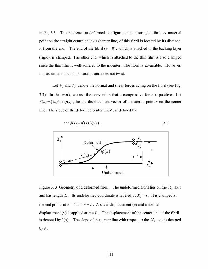
111
in Fig.3.3. The reference undeformed configuration is a straight fibril. A material
point on the straight centroidal axis (center line) of this fibril is located by its distance,
s, from the end. The end of the fibril ( 0)s = , which is attached to the backing layer
(rigid), is clamped. The other end, which is attached to the thin film is also clamped
since the thin film is well-adhered to the indenter. The fibril is extensible. However,
it is assumed to be non-shearable and does not twist.
Let nF and sF denote the normal and shear forces acting on the fibril (see Fig.
3.3). In this work, we use the convention that a compressive force is positive. Let
3 1ˆ ˆ( ) ( ) ( )r s s e s eξ η= +r be the displacement vector of a material point s on the center
line. The slope of the deformed center lineφ , is defined by
tan ( ) ( ) / ( )s s sφ η ξ′ ′= , (3.1)
Figure 3. 3 Geometry of a deformed fibril. The undeformed fibril lies on the 3X axis
and has length L . Its undeformed coordinate is labeled by 3X s= . It is clamped at
the end points at s = 0 and s L= . A shear displacement (u) and a normal
displacement (v) is applied at s L= . The displacement of the center line of the fibril
is denoted by ( )r sr . The slope of the center line with respect to the 3X axis is denoted
byφ .
112
where a prime denotes differentiation with respect to s. The governing equation is
(see Supplementary Information 1)
( ) [ ]sin cos1 cos sins n
s nF F
EI F FEA
φ φφ φ φ
⎛ ⎞−′′ = − + +⎜ ⎟
⎝ ⎠ (3.2)
where 4 /12I b= is the area moment of inertia of the fibril. Note that the
displacement of a clamped-clamped fibril in Fig. 3.3 can also be obtained by moving
the right (left) end of the fibril up (down) by / 2u and outwards (inwards) by v / 2 ,
with the midpoint of the fibril fixed at its initial location. Symmetry implies that the
moment at the midpoint of the fibril, i.e., at / 2s L= , is zero. Force balance shows
that normal and shear loads at / 2s L= are the same as those at s L= . Therefore, we
can replace the clamped boundary condition at s L= by the simply-supported
condition
( 0) 0, ( / 2) 0s s Lφ φ′= = = = (3.3)
Onceφ is found by solving (3.2) and (3.3), the stretch of an element on the center line,
denoted by 1v − , is computed according to
( )sin cos1 s nF F
EAφ φ
ν−
− = , (3.4)
The shear and normal displacements, ,η ξ are obtained by integrating the equations
2( ) ( ) tan ( ) / 1 tans s sη ν φ φ′ = + , 2( ) ( ) / 1 tan ( )s s sξ ν φ′ = + (3.5)
subjected to the boundary conditions
( 0) ( 0) 0s sη ξ= = = = . (3.6)
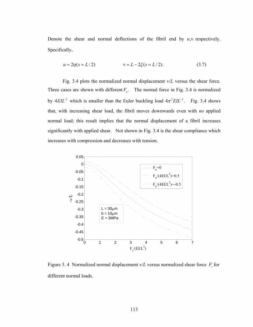
113
Denote the shear and normal deflections of the fibril end by ,vu respectively.
Specifically,
2 ( / 2)u s Lη= = v 2 ( / 2)L s Lξ= − = . (3.7)
Fig. 3.4 plots the normalized normal displacement v/L versus the shear force.
Three cases are shown with different nF . The normal force in Fig. 3.4 is normalized
by 24EIL− which is smaller than the Euler buckling load 2 24 EILπ − . Fig. 3.4 shows
that, with increasing shear load, the fibril moves downwards even with no applied
normal load; this result implies that the normal displacement of a fibril increases
significantly with applied shear. Not shown in Fig. 3.4 is the shear compliance which
increases with compression and decreases with tension.
0 1 2 3 4 5 6 7-0.5
-0.45
-0.4
-0.35
-0.3
-0.25
-0.2
-0.15
-0.1
-0.05
0
0.05
Fs/(EI/L2)
-v/L
Fn=0
Fn/(4EI/L2)=0.5
Fn/(4EI/L2)=-0.5
L = 30μmb = 10μmE = 3MPa
Figure 3. 4 Normalized normal displacement v/L versus normalized shear force sF for
different normal loads.
114
A result we will need later is the strain energy stored in a fibril in the contact
zone. The strain energy density (per unit length) Γ is
( )2 21( , ) ( 1)2
E I Aν κ κ νΓ = + − (3.8)
where
/d dsκ φ= (3.9)
is the local curvature. The total strain energy stored in a fibril U is given by
/ 2
0
( , ) 2L
U dsν κ = Γ∫ (3.10)
Numerical results of (3.10) evaluated using 3E MPa= , 10 , 30b m L mμ μ= = show
that the effect of shear is much more significant than the normal load as far as the
elastic strain energy of the fibril is concerned. Therefore, we can approximate the
strain energy of a fibril in the contact zone by assuming that the fiber is subjected to a
zero normal load. Using this approximation, the strain energy is given by
2 12 ,3
u bU LEbL L
⎛ ⎞= Φ =⎜ ⎟⎝ ⎠
, (3.11)
where Φ is found to fit well by
8 6 4 21, 0.005958 0.02629 0.0122 0.037
3u b u u u uL L L L L L
⎛ ⎞ ⎛ ⎞ ⎛ ⎞ ⎛ ⎞ ⎛ ⎞Φ = = − + − +⎜ ⎟ ⎜ ⎟ ⎜ ⎟ ⎜ ⎟ ⎜ ⎟⎝ ⎠ ⎝ ⎠ ⎝ ⎠ ⎝ ⎠ ⎝ ⎠
(3.12)
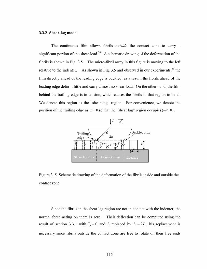
115
3.3.2 Shear-lag model
The continuous film allows fibrils outside the contact zone to carry a
significant portion of the shear load.36 A schematic drawing of the deformation of the
fibrils is shown in Fig. 3.5. The micro-fibril array in this figure is moving to the left
relative to the indenter. As shown in Fig. 3.5 and observed in our experiments,36 the
film directly ahead of the leading edge is buckled; as a result, the fibrils ahead of the
leading edge deform little and carry almost no shear load. On the other hand, the film
behind the trailing edge is in tension, which causes the fibrils in that region to bend.
We denote this region as the “shear lag” region. For convenience, we denote the
position of the trailing edge as 0x = so that the “shear lag” region occupies ( ,0)−∞ .
Figure 3. 5 Schematic drawing of the deformation of the fibrils inside and outside the
contact zone
Since the fibrils in the shear lag region are not in contact with the indenter, the
normal force acting on them is zero. Their deflection can be computed using the
result of section 3.3.1 with 0nF = and L replaced by 2L L′ = . his replacement is
necessary since fibrils outside the contact zone are free to rotate on their free ends
116
whereas fibrils in the contact zone are clamped as long as the film maintains good
contact with the indenter. Denote the shear displacement of a typical fibril by u and
let sf F= . Then
( / , / )sof k u L b L uψ ′ ′= (3.13)
where ( )33 /sok EI L′= is the stiffness of a clamped/simply supported fibril for small
deflections and ψ is the normalized shear stiffness of a fibril under zero normal load.
ψ is an even function of /u L′ with ( / 0, / ) 1u L b Lψ ′ ′= = . Since / 1/ 6b L′ = for all
our samples, we denote ( / , / 1/ 6)u L b Lψ ′ ′ = by ( / )u Lψ ′ . For this case, ψ can be
fitted well using the polynomial function
2 4 6 8
1 0.9523 1.236 0.3372 3.876u u u u uL L L L L
ψ ⎛ ⎞ ⎛ ⎞ ⎛ ⎞ ⎛ ⎞ ⎛ ⎞= + + − +⎜ ⎟ ⎜ ⎟ ⎜ ⎟ ⎜ ⎟ ⎜ ⎟′ ′ ′ ′ ′⎝ ⎠ ⎝ ⎠ ⎝ ⎠ ⎝ ⎠ ⎝ ⎠(3.14)
The fibrils in the “shear lag” region resists bending by exerting a shear force on the
film. We replace the discrete fibrils by a continuous foundation. As a result, these
shear forces are continuously distributed on the bottom surface of the film, resulting in
a shear stress τ which varies continuously with x. In the foundation model, the shear
stress τ is related to the shear force on each fibril f by
( / )sof k u L uτ ρ ρ ψ ′= = (3.15)
where ρ is the number of fibrils per unit area. Assuming the film is linear elastic,
force balance of the film implies that
2
*2
d uE hdx
τ= ( ,0)x ∈ −∞ (3.16)
Substituting (3.15) into (3.16) results in:
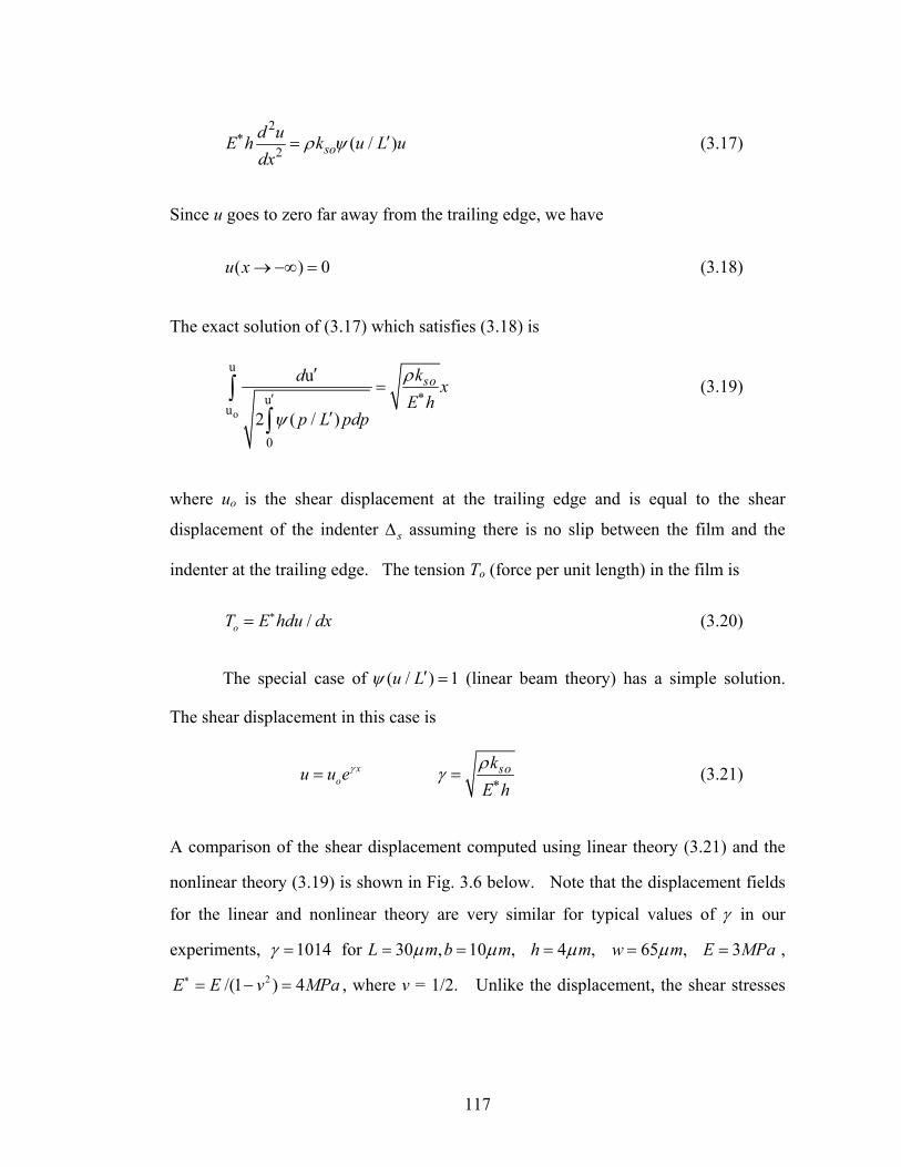
117
2
2 ( / )sod uE h k u L udx
ρ ψ∗ ′= (3.17)
Since u goes to zero far away from the trailing edge, we have
( ) 0u x → −∞ = (3.18)
The exact solution of (3.17) which satisfies (3.18) is
o
u
uu
0
u
2 ( / )
sokd xE h
p L pdp
ρ
ψ∗′
′=
′∫
∫ (3.19)
where uo is the shear displacement at the trailing edge and is equal to the shear
displacement of the indenter sΔ assuming there is no slip between the film and the
indenter at the trailing edge. The tension To (force per unit length) in the film is
/oT E hdu dx∗= (3.20)
The special case of ( / ) 1u Lψ ′ = (linear beam theory) has a simple solution.
The shear displacement in this case is
xou u eγ= sok
E hργ ∗= (3.21)
A comparison of the shear displacement computed using linear theory (3.21) and the
nonlinear theory (3.19) is shown in Fig. 3.6 below. Note that the displacement fields
for the linear and nonlinear theory are very similar for typical values of γ in our
experiments, 1014γ = for 30 , 10 ,L m b mμ μ= = 4 ,h mμ= 65 ,w mμ= 3E MPa= , 2/(1 ) 4E E v MPa∗ = − = , where v = 1/2. Unlike the displacement, the shear stresses
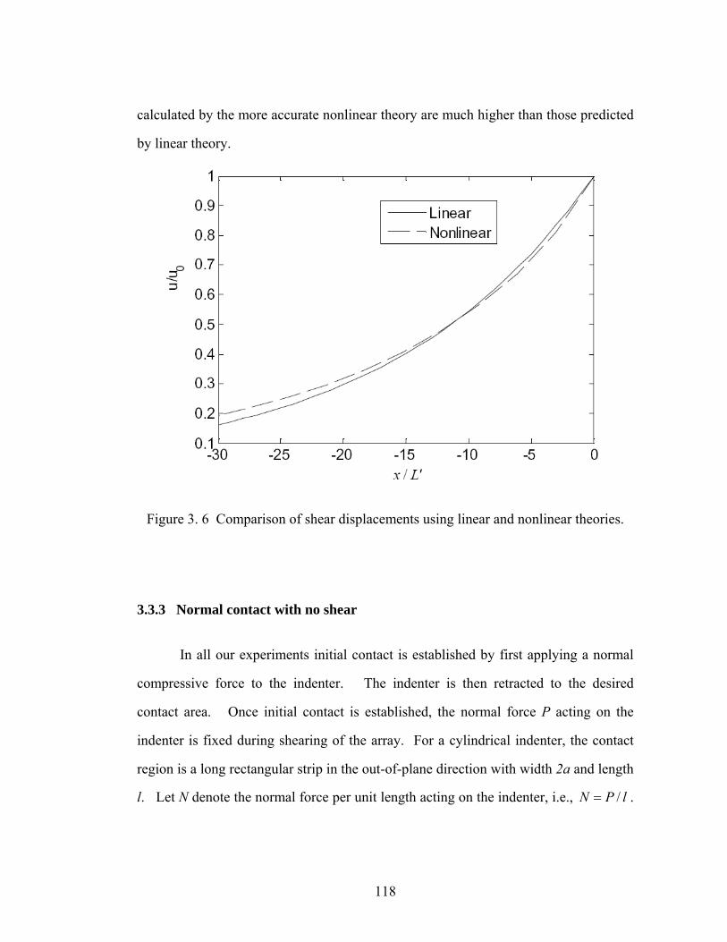
118
calculated by the more accurate nonlinear theory are much higher than those predicted
by linear theory.
Figure 3. 6 Comparison of shear displacements using linear and nonlinear theories.
3.3.3 Normal contact with no shear
In all our experiments initial contact is established by first applying a normal
compressive force to the indenter. The indenter is then retracted to the desired
contact area. Once initial contact is established, the normal force P acting on the
indenter is fixed during shearing of the array. For a cylindrical indenter, the contact
region is a long rectangular strip in the out-of-plane direction with width 2a and length
l. Let N denote the normal force per unit length acting on the indenter, i.e., /N P l= .
119
In this subsection we develop a simple expression to estimate the initial contact width,
2 oa , before the application of shear.
Following Long et al.,38 the deformation of the fibril array is modeled as a
continuous elastic foundation with normal stiffness nk given by
/nk EA Lρ= , (3.22)
where 2A b= is the cross-sectional area of a fibril. The elastic foundation model is
valid if the spacing between fibrils is small compared with the contact width. For our
samples, the fibrils are more compliant than the elastic backing layer. For simplicity,
we ignore the deformation of the backing layer. In a previous work where we studied
normal indentation using a spherical indenter,39 we found that neglecting the normal
compliance of the backing layer can lead to errors. For example, neglecting the
normal compliance of the backing layer will give a pull-off force that occurs always at
zero indenter displacement. In this paper, we knowingly neglect the compliance of the
backing layer since the shear compliance of the fibrils is much higher than that of the
backing layer. A model which takes into account the deformation of the backing layer
can be found in Long et al.38
In a displacement control test, the free energy of the system Γ is:
2U aWΓ = − (3.23)
where U is the strain energy and W is the work of adhesion. In the following, we
neglect the bending energy of the thin terminal film. To compute U, let nΔ denote the
normal displacement of the indenter. Then, the displacement of the foundation, v , is
given by the contact condition, i.e.,
120
2
v 22nx x aR
= Δ − < (3.24)
The strain energy, U , is:
5
2 2 32v
2 3 20
an n n n
c n na
k k k aU dx ak aR R−
Δ= = Δ − +∫ (3.25)
Evaluating /n
a Δ∂Γ ∂ using (3.23), and setting the resulting expression equal to zero
gives an expression for the equilibrium contact width ao , i.e.,
22 2o nn
Wa R Rk
= Δ + (3.26)
The relation between N and the normal displacement can be determined using force
balance, i.e.,
( )0
0
30
023
a
n n n na
aN k v x dx a k kR−
= = Δ −∫ (3.27)
Substituting (3.26) into (3.27) gives
( ) 42 22 2 2
3 3n n
n n nn
kWN R R k W
kΔ
Δ = Δ + −⎡ ⎤⎢ ⎥⎣ ⎦
(3.28)
The relation between normal force per unit length N and contact width can be found
using (3.26) and (3.27),
30
02
2 23
nn
k aN a k W
R= − (3.29)
Generally, the work of adhesion during crack closure, W− , (indentation of the
sample) is different from and lower than the work of adhesion during crack opening,
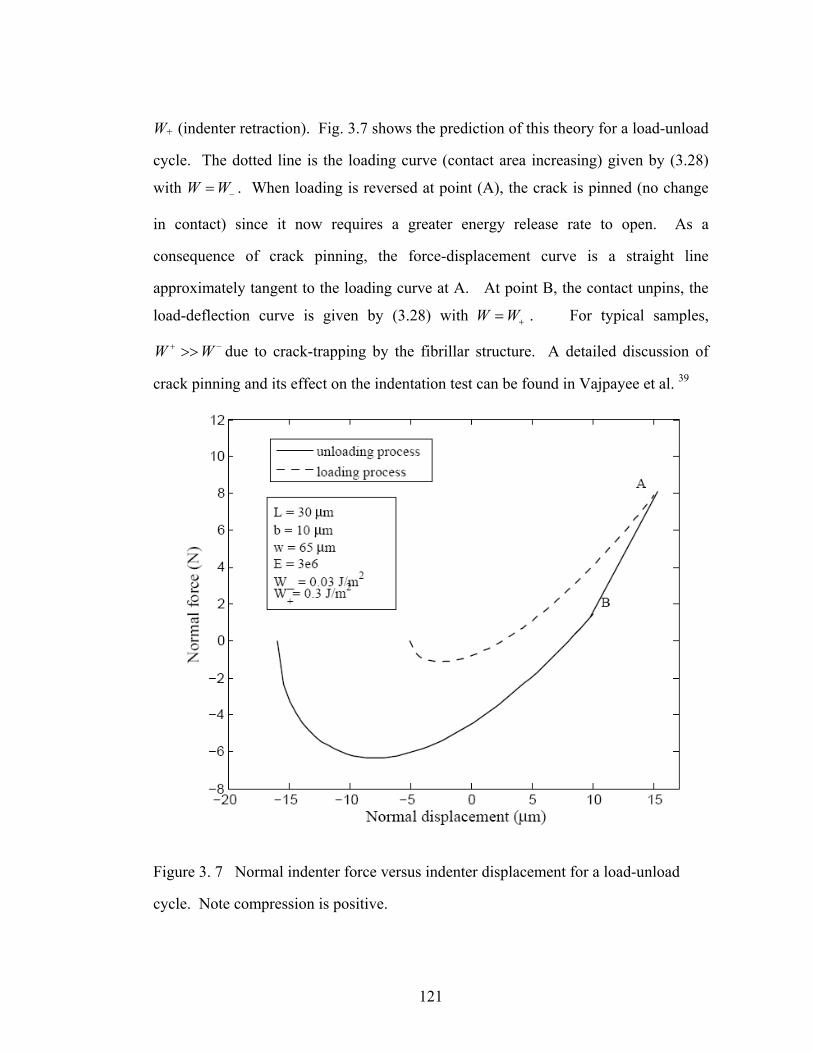
121
W+ (indenter retraction). Fig. 3.7 shows the prediction of this theory for a load-unload
cycle. The dotted line is the loading curve (contact area increasing) given by (3.28)
with W W−= . When loading is reversed at point (A), the crack is pinned (no change
in contact) since it now requires a greater energy release rate to open. As a
consequence of crack pinning, the force-displacement curve is a straight line
approximately tangent to the loading curve at A. At point B, the contact unpins, the
load-deflection curve is given by (3.28) with W W+= . For typical samples,
W W+ −>> due to crack-trapping by the fibrillar structure. A detailed discussion of
crack pinning and its effect on the indentation test can be found in Vajpayee et al. 39
Figure 3. 7 Normal indenter force versus indenter displacement for a load-unload
cycle. Note compression is positive.
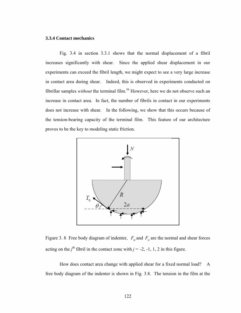
122
3.3.4 Contact mechanics
Fig. 3.4 in section 3.3.1 shows that the normal displacement of a fibril
increases significantly with shear. Since the applied shear displacement in our
experiments can exceed the fibril length, we might expect to see a very large increase
in contact area during shear. Indeed, this is observed in experiments conducted on
fibrillar samples without the terminal film.36 However, here we do not observe such an
increase in contact area. In fact, the number of fibrils in contact in our experiments
does not increase with shear. In the following, we show that this occurs because of
the tension-bearing capacity of the terminal film. This feature of our architecture
proves to be the key to modeling static friction.
Figure 3. 8 Free body diagram of indenter, njF and sjF are the normal and shear forces
acting on the jth fibril in the contact zone with j = -2, -1, 1, 2 in this figure.
How does contact area change with applied shear for a fixed normal load? A
free body diagram of the indenter is shown in Fig. 3.8. The tension in the film at the
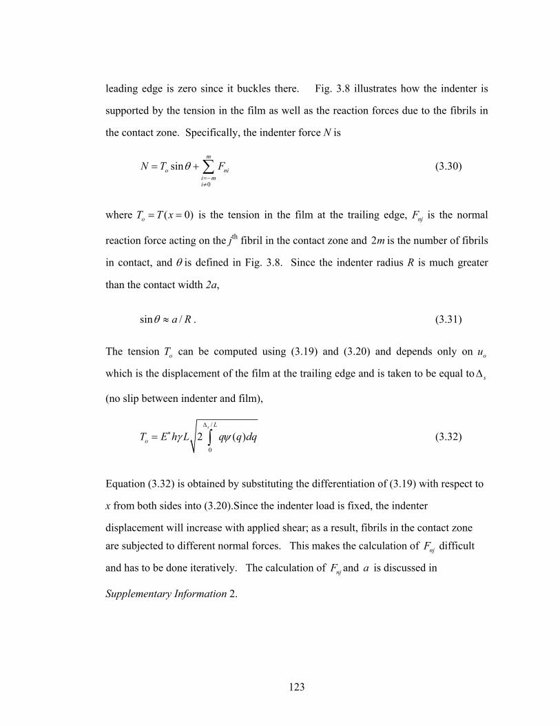
123
leading edge is zero since it buckles there. Fig. 3.8 illustrates how the indenter is
supported by the tension in the film as well as the reaction forces due to the fibrils in
the contact zone. Specifically, the indenter force N is
0
sinm
o nii mi
N T Fθ=−≠
= + ∑ (3.30)
where ( 0)oT T x= = is the tension in the film at the trailing edge, njF is the normal
reaction force acting on the jth fibril in the contact zone and 2m is the number of fibrils
in contact, and θ is defined in Fig. 3.8. Since the indenter radius R is much greater
than the contact width 2a,
sin /a Rθ ≈ . (3.31)
The tension oT can be computed using (3.19) and (3.20) and depends only on ou
which is the displacement of the film at the trailing edge and is taken to be equal to sΔ
(no slip between indenter and film),
/
0
2 ( )s L
oT E h L q q dqγ ψΔ
∗= ∫ (3.32)
Equation (3.32) is obtained by substituting the differentiation of (3.19) with respect to
x from both sides into (3.20).Since the indenter load is fixed, the indenter
displacement will increase with applied shear; as a result, fibrils in the contact zone are subjected to different normal forces. This makes the calculation of njF difficult
and has to be done iteratively. The calculation of njF and a is discussed in
Supplementary Information 2.
124
3.4 Results
3.4.1 Contact area
We apply the procedure described in Supplementary Information 2 to a fibril
array with spacing 65w mμ= . The contact area versus shear displacement is plotted in
Fig. 3.9 with an indenter load 0P = and the radius of indenter 1R mm= . We do not
compute past / 1.6s LΔ = since the peak load in our experiment for this spacing occurs
at / 1.57s LΔ ≈ . Simple geometry implies that, as long as 3 52 2
w a wL L L
< < , the
number of fibrils in contact is 4. Since 3 4.592wL
≈ and 5 7.662
wL
≈ , This inequality
is indeed satisfied by our result in Fig. 3.9, consistent with our experiment.
Figure 3. 9 Half contact width a/L versus normalized applied shear displacement
/s LΔ .
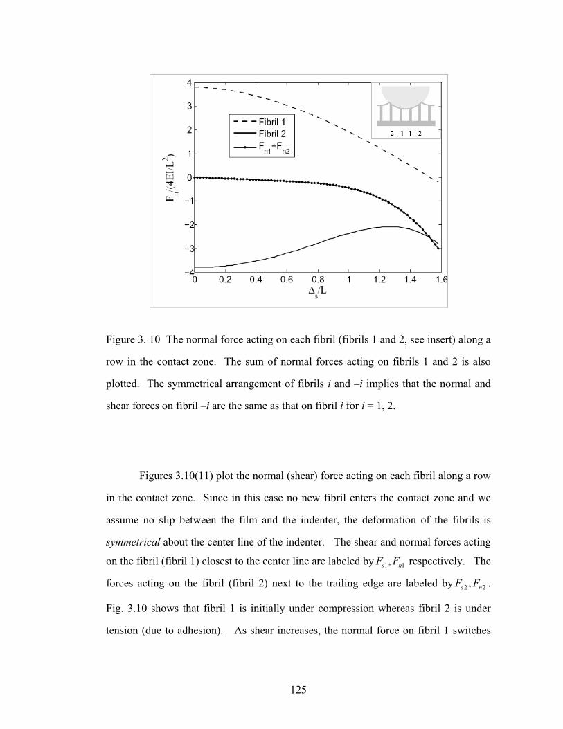
125
Figure 3. 10 The normal force acting on each fibril (fibrils 1 and 2, see insert) along a
row in the contact zone. The sum of normal forces acting on fibrils 1 and 2 is also
plotted. The symmetrical arrangement of fibrils i and –i implies that the normal and
shear forces on fibril –i are the same as that on fibril i for i = 1, 2.
Figures 3.10(11) plot the normal (shear) force acting on each fibril along a row
in the contact zone. Since in this case no new fibril enters the contact zone and we
assume no slip between the film and the indenter, the deformation of the fibrils is
symmetrical about the center line of the indenter. The shear and normal forces acting
on the fibril (fibril 1) closest to the center line are labeled by 1 1,s nF F respectively. The
forces acting on the fibril (fibril 2) next to the trailing edge are labeled by 2 2,s nF F .
Fig. 3.10 shows that fibril 1 is initially under compression whereas fibril 2 is under
tension (due to adhesion). As shear increases, the normal force on fibril 1 switches
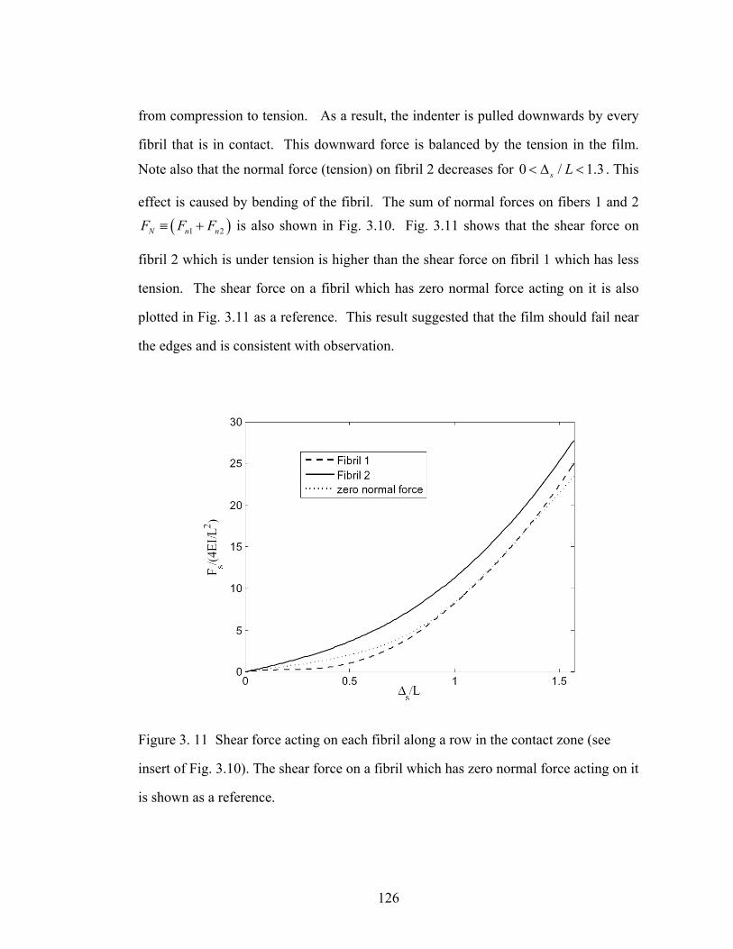
126
from compression to tension. As a result, the indenter is pulled downwards by every
fibril that is in contact. This downward force is balanced by the tension in the film.
Note also that the normal force (tension) on fibril 2 decreases for 0 / 1.3s L< Δ < . This
effect is caused by bending of the fibril. The sum of normal forces on fibers 1 and 2
( )1 2N n nF F F≡ + is also shown in Fig. 3.10. Fig. 3.11 shows that the shear force on
fibril 2 which is under tension is higher than the shear force on fibril 1 which has less
tension. The shear force on a fibril which has zero normal force acting on it is also
plotted in Fig. 3.11 as a reference. This result suggested that the film should fail near
the edges and is consistent with observation.
Figure 3. 11 Shear force acting on each fibril along a row in the contact zone (see
insert of Fig. 3.10). The shear force on a fibril which has zero normal force acting on it
is shown as a reference.
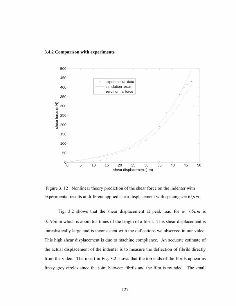
127
3.4.2 Comparison with experiments
0 5 10 15 20 25 30 35 40 45 500
50
100
150
200
250
300
350
400
450
500
shear displacement (μm)
shea
r for
ce (m
N)
experimental datasimulation resultzero normal force
Figure 3. 12 Nonlinear theory prediction of the shear force on the indenter with
experimental results at different applied shear displacement with spacing 65w mμ= .
Fig. 3.2 shows that the shear displacement at peak load for 65w mμ= is
0.195mm which is about 6.5 times of the length of a fibril. This shear displacement is
unrealistically large and is inconsistent with the deflections we observed in our video.
This high shear displacement is due to machine compliance. An accurate estimate of
the actual displacement of the indenter is to measure the deflection of fibrils directly
from the video. The insert in Fig. 3.2 shows that the top ends of the fibrils appear as
fuzzy grey circles since the joint between fibrils and the film is rounded. The small
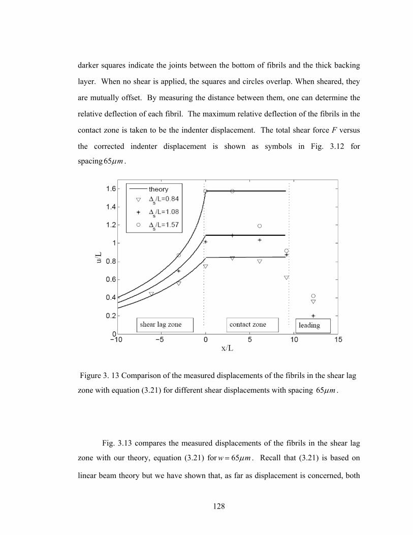
128
darker squares indicate the joints between the bottom of fibrils and the thick backing
layer. When no shear is applied, the squares and circles overlap. When sheared, they
are mutually offset. By measuring the distance between them, one can determine the
relative deflection of each fibril. The maximum relative deflection of the fibrils in the
contact zone is taken to be the indenter displacement. The total shear force F versus
the corrected indenter displacement is shown as symbols in Fig. 3.12 for
spacing 65 mμ .
Figure 3. 13 Comparison of the measured displacements of the fibrils in the shear lag
zone with equation (3.21) for different shear displacements with spacing 65 mμ .
Fig. 3.13 compares the measured displacements of the fibrils in the shear lag
zone with our theory, equation (3.21) for 65w mμ= . Recall that (3.21) is based on
linear beam theory but we have shown that, as far as displacement is concerned, both
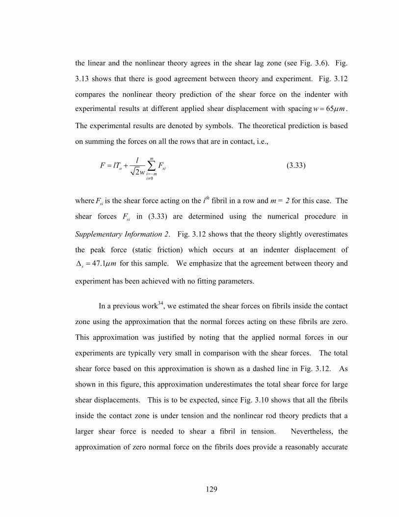
129
the linear and the nonlinear theory agrees in the shear lag zone (see Fig. 3.6). Fig.
3.13 shows that there is good agreement between theory and experiment. Fig. 3.12
compares the nonlinear theory prediction of the shear force on the indenter with
experimental results at different applied shear displacement with spacing 65w mμ= .
The experimental results are denoted by symbols. The theoretical prediction is based
on summing the forces on all the rows that are in contact, i.e.,
02
m
o sii mi
lF lT Fw =−
≠
= + ∑ (3.33)
where siF is the shear force acting on the ith fibril in a row and m = 2 for this case. The
shear forces siF in (3.33) are determined using the numerical procedure in
Supplementary Information 2. Fig. 3.12 shows that the theory slightly overestimates
the peak force (static friction) which occurs at an indenter displacement of
47.1s mμΔ = for this sample. We emphasize that the agreement between theory and
experiment has been achieved with no fitting parameters.
In a previous work34, we estimated the shear forces on fibrils inside the contact
zone using the approximation that the normal forces acting on these fibrils are zero.
This approximation was justified by noting that the applied normal forces in our
experiments are typically very small in comparison with the shear forces. The total
shear force based on this approximation is shown as a dashed line in Fig. 3.12. As
shown in this figure, this approximation underestimates the total shear force for large
shear displacements. This is to be expected, since Fig. 3.10 shows that all the fibrils
inside the contact zone is under tension and the nonlinear rod theory predicts that a
larger shear force is needed to shear a fibril in tension. Nevertheless, the
approximation of zero normal force on the fibrils does provide a reasonably accurate
130
description of how the indenter force varies with the applied shear displacement. The
advantage of this approximation is that we can obtain an analytical expression for siF
as a function of sΔ , that is:
( )2
4 u / , / 1/ 3siEIF L b LL
= ϒ = (3.34)
where
( ) ( ) ( ) ( ) ( )7 5 3/ , / 1/ 3 0.8234 / 2.646 / 2.676 / 3 /u L b L u L u L u L u Lϒ = = − + + + (3.35)
Using (3.34) and (3.35), the total shear force given by (3.33) can be evaluated easily.
We note that, irrespective of the method used to compute siF , our theory
overestimates the peak load slightly. This is because the film inside the contact zone
is assumed not to slip before the peak load, whereas our experiments show that micro-
slip can occur in the trailing edge; 36 slip decreases shear deformation, hence reducing
the shear force. In addition, in our experiments, there is a slight reduction of contact
area before the static peak due to the propagation of a buckled front inward from the
leading edge, causing fibrils there to slip (see dashed-arrow in the insert of Fig. 3.2).
It is possible to develop an analytical model which takes into account of the micro-slip.
However, such a model will complicate the analysis and will only slightly improve our
prediction of the peak load.
3.4.3 Criterion for static friction
Our contact mechanics model allows us to determine the shear force on the
indenter in terms of the applied shear displacement. However, the development
131
presented thus far cannot predict the peak load (static friction). We now turn our
attention to the question of how to determine the peak load, or corresponding shear
displacement, s∗Δ , in terms of an effective work of adhesion.
We have observed that the transition to sliding is caused by sudden detachment
of fibrils at the leading edge of contact. This observation is consistent with our
analysis which shows that the fibrils at both leading and trailing edges are subjected to
the highest tension and shear (see Fig. 3.10 and Fig. 3.11). However, the fiber at
leading edge has a higher moment due to the curvature of indenter, and this effect is
ignored in our model. Therefore, the fiber at leading edge is expected to fail first. A
simple model for static friction is to assume that instability occurs when the fibril in
the leading edge fails. Specifically, we assume that the fibril fails when its strain
energy Γ reaches a critical level cΓ , i.e.,
cΓ = Γ (3.36)
Next, we relate cΓ to the effective work of adhesion eW . The trailing edge of contact
can be viewed as the front of a mixed mode interface crack. Suppose we fix the
indenter displacements and advance this crack by one “fibril spacing”, in our
case 2w . The energy release is the energy change when the fibril at the leading edge
of contact is moved to a location far behind the trailing edge. Since a fibril far behind
the trailing edge has zero strain energy, the energy release is Γ . Γ can be evaluated
using (3.11) and (3.12) if the shear displacement and normal force acting on it is
known. We define the energy release rate G by
2/ 2G w= Γ (3.37)
132
Thus, the instability criterion in (3.36) is equivalent to a critical energy release rate
criterion. We call
2/ 2e cW w≡ Γ (3.38)
the effective work of adhesion.
To make further progress, let us assume that eW is approximately independent
of the failure mode so eW W += . We have previously determined W + experimentally.
For the case of 65w mμ= and 50 mμ , W + is found to be 0.37 2/J m and 0.35 2/J m
respectively. We compute the critical applied shear displacement *sΔ needed to
satisfy (3.36) with eW W +Γ = = for the fibril at the leading edge. This calculation can
be done easily by assuming that the normal force on this fibril is zero or we can
determine *sΔ numerically using the numerical procedure discussed above. For the
parameters used in this study, we do not find much difference between these two
approaches. *sΔ is found be 45.5 mμ for 65w mμ= and 38.0 mμ for 50w mμ= .
These values are surprisingly close to our experimental observations: *sΔ = 47.1 mμ for
65w mμ= and *sΔ =38.5 mμ for 50w mμ= .
3.5 Summary and Conclusion
A theoretical model is developed to study the contact mechanics of a smooth
cylindrical indenter on a film-terminated micro-fibril array. The indenter is subjected
to a combination of normal and shear forces. The model assumes that there is no
macroscopic sliding between the indenter and the array. Using this model, we are
able to explain all our experimental observations, including the connection between
133
static friction peak, applied shear displacement, and array geometry. The key
findings are:
1. During shear, the film behind the trailing edge is under tension. This
tension is transmitted to the fibrils behind the trailing edge causing them to
bend.
2. Tension in the terminal thin film provides a normal force to support the
indenter. For sufficiently large shear displacements, all the fibrils inside
the contact zone can be under tension even if the applied normal force on
the indenter is compressive.
3. During shear, fibrils in the trailing or leading edge are subjected to the
highest shear and tension.
4. Our theory, as well as the experiments, shows that there is no significant
increase in contact area during shear. This is in contrast to our earlier
observations which use a spherical indenter where we did observe a
significant initial increase in contact stiffness, which we attributed to initial
increase in contact area. This difference is due to difference in indenter
geometry. For the cylindrical indenter, the film tension along the contact
edge is uniform. This is not true for a spherical indenter, the film tension
along the contact edge is maximum in the direction of shear and decreases
to a minimum in the direction perpendicular to the shear direction. This
will cause the contact area to increase in this direction. As a consequence,
the contact shape is elliptical with the long axis perpendicular to the
direction of shear. This shape is consistent with our observations.
Finally, the static friction peak can be understood in the same way as we have
explained normal adhesion enhancement (section 3.3.3) as long as one tackles the
134
complication of calculating energy release rate in a microstructure subjected to both
normal and shear load. In our case, the energy release rate G is given by (3.37). Once
the energy release rate is known, the remaining issue is to establish the quantitative
relationship between the effective work of adhesion and the microstructure. In turns
out in our case, the effective work of adhesion seems to be approximately independent
of failure mode (e.g. shear versus normal separation) since the static friction peak can
be predicted using (3.37) using an effective work of adhesion which was based on
experiments where the fibril array fails by normal separation.
Although the goal of this paper is to develop a static friction model for film-
terminated micro-fibril arrays, many of our results can be applied to systems without a
continuous terminal film. For example, the results in sections 3.3.1 and 3.3.3 can be
applied to study deformation of fibrils in systems without a continuous terminal film.
Also, the numerical procedure in Supplementary Information 2 can be modified (e.g.
with 0oT = ) to study the size of contact and the distribution of shear and normal
forces on fibers in contact. It should be noted that, if a constant compressive indenter
load is applied to a fibrillar array without a continuous film, the contact area will
increase rapidly with applied shear. Indeed, in absence of a continuous terminal film,
all fibrils in contact will eventually buckle with increasing shear. This will result in
very different sliding behavior as shown experimentally by Shen et al.36 This
explains why friction experiments on fibril array without continuous terminal films40
are usually conducted under fixed normal indenter displacement instead of fixed
normal force. Under fixed normal displacement, our theory will predict that the
normal load will change from compression to tension as the shear displacement
increases, with no significant increase in contact area, which is consistent with
observation.

135
Acknowledgment: Support from Department of Energy grant DE-FG02-07ER46463
is acknowledged by the authors of this work.
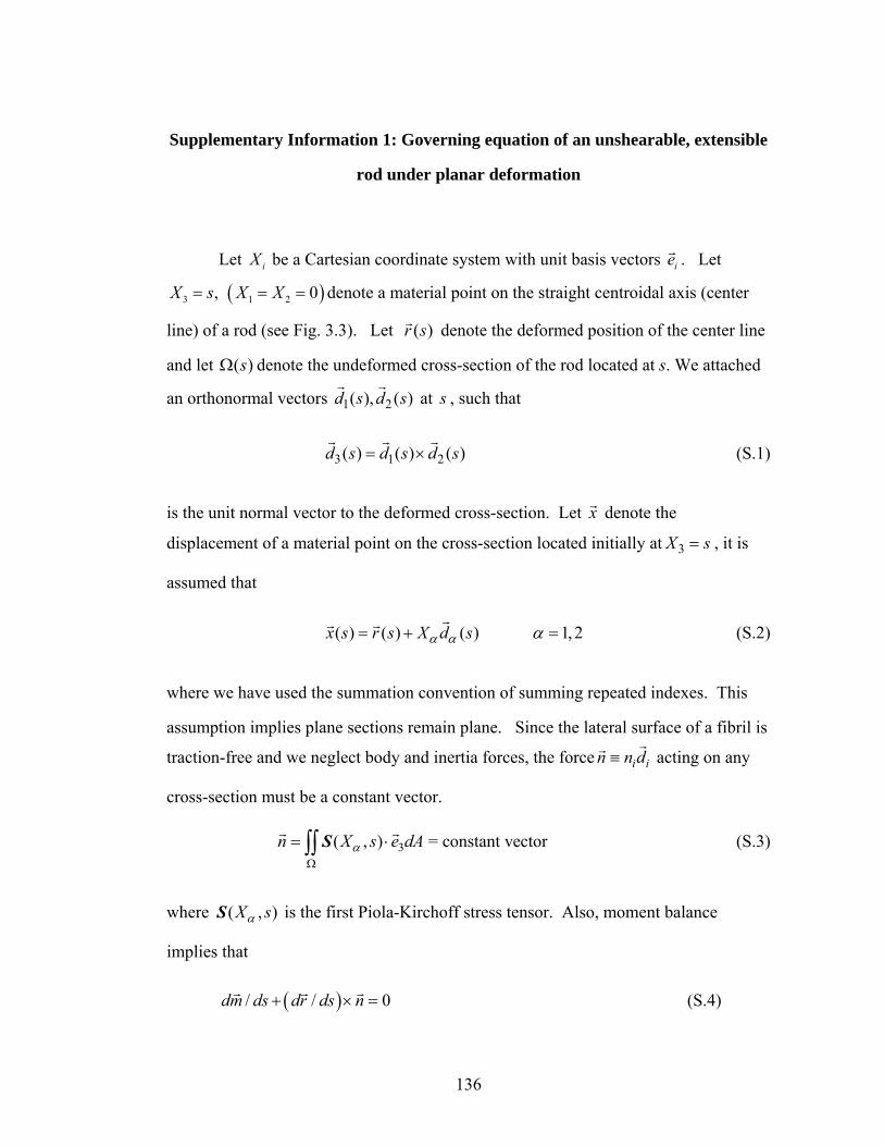
136
Supplementary Information 1: Governing equation of an unshearable, extensible
rod under planar deformation
Let iX be a Cartesian coordinate system with unit basis vectors ier . Let
3 ,X s= ( )1 2 0X X= = denote a material point on the straight centroidal axis (center
line) of a rod (see Fig. 3.3). Let ( )r sr denote the deformed position of the center line
and let ( )sΩ denote the undeformed cross-section of the rod located at s. We attached
an orthonormal vectors 1 2( ), ( )d s d sr r
at s , such that
3 1 2( ) ( ) ( )d s d s d s= ×r r r
(S.1)
is the unit normal vector to the deformed cross-section. Let xr denote the
displacement of a material point on the cross-section located initially at 3X s= , it is
assumed that
( ) ( ) ( )x s r s X d sα α= +rr r 1, 2α = (S.2)
where we have used the summation convention of summing repeated indexes. This
assumption implies plane sections remain plane. Since the lateral surface of a fibril is
traction-free and we neglect body and inertia forces, the force i in n d≡rr acting on any
cross-section must be a constant vector.
3( , ) = constant vectorn X s e dAαΩ
= ⋅∫∫r rS (S.3)
where ( , )X sαS is the first Piola-Kirchoff stress tensor. Also, moment balance
implies that
( )/ / 0dm ds dr ds n+ × =r r r (S.4)
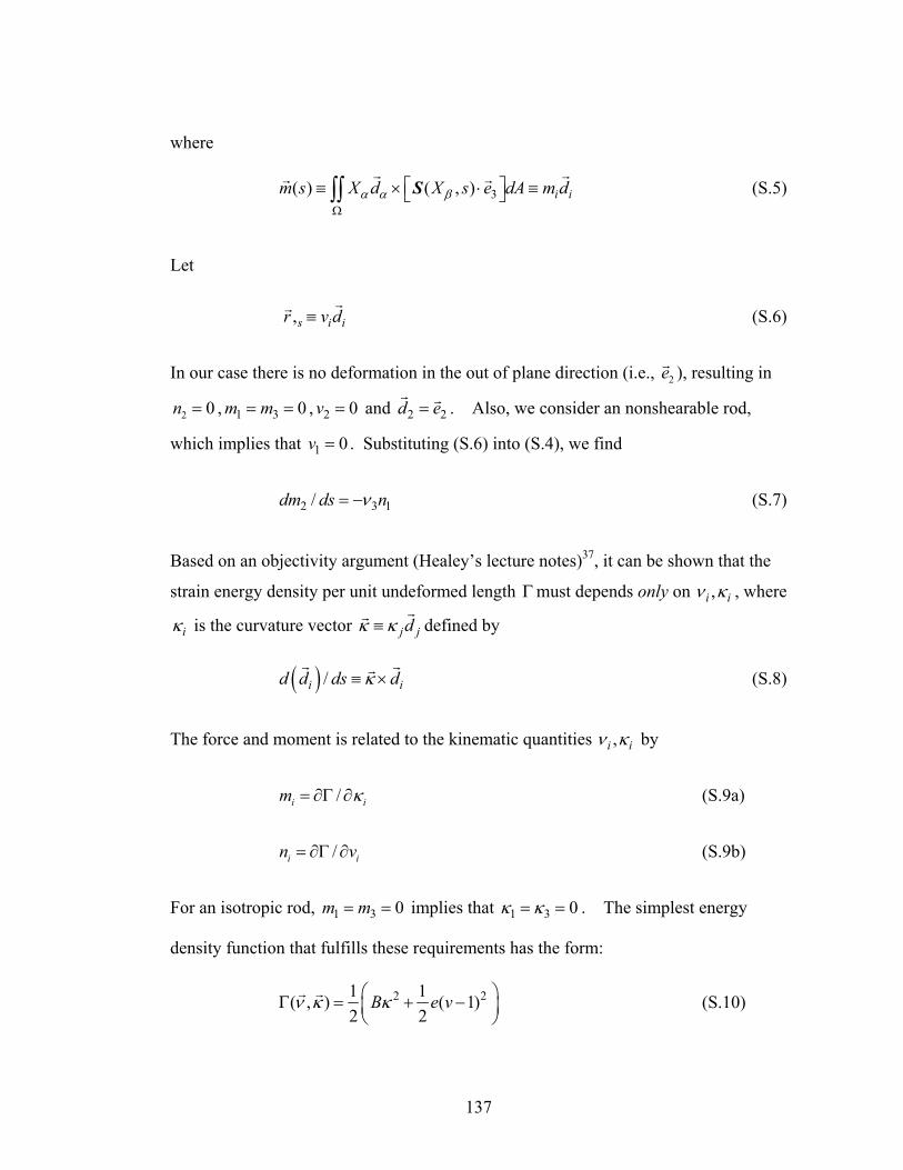
137
where
3( ) ( , ) i im s X d X s e dA m dα α βΩ
⎡ ⎤≡ × ⋅ ≡⎣ ⎦∫∫r rr rS (S.5)
Let
,s i ir v d≡rr (S.6)
In our case there is no deformation in the out of plane direction (i.e., 2er ), resulting in
2 0n = , 1 3 0m m= = , 2 0v = and 2 2d e=r r . Also, we consider an nonshearable rod,
which implies that 1 0v = . Substituting (S.6) into (S.4), we find
2 3 1/dm ds nν= − (S.7)
Based on an objectivity argument (Healey’s lecture notes)37, it can be shown that the
strain energy density per unit undeformed length Γ must depends only on ,i iν κ , where
iκ is the curvature vector j jdκ κ≡rr defined by
( ) /i id d ds dκ≡ ×r rr (S.8)
The force and moment is related to the kinematic quantities ,i iν κ by
/i im κ= ∂Γ ∂ (S.9a)
/i in v= ∂Γ ∂ (S.9b)
For an isotropic rod, 1 3 0m m= = implies that 1 3 0κ κ= = . The simplest energy
density function that fulfills these requirements has the form:
2 21 1( , ) ( 1)2 2
B e vν κ κ⎛ ⎞Γ = + −⎜ ⎟⎝ ⎠
r r (S.10)
138
where we have used the notation 3 2,ν ν κ κ≡ = . Using (S.9a,b) and (S.10), we have
3 3 21 ( 1), 2
n e m Bν κ= − = (S.11)
By considering two special cases of deformation (pure tension and pure bending), it
can be shown that B EI= and / 2e EA= . Let ( )sφ be the angle between the tangent
vector of the deformed center line ( )r s%
and the 3X axis. Then
1 1 3
3 1 3
cos sin ,
sin cos
d e e
d e e
φ φ
φ φ
= −
= +
r r r
r r r (S.12)
Using (S.12) and (S.8), it is easy to verify that 1 3 0κ κ= = and
2 /d dsκ κ φ= = . (S.13)
Note that
1( 0) sn s F= = 3( 0) nn s F= = − (S.14)
where ,s nF F are the reaction force at s = 0. The negative sign on nF is due to our sign
convention that compression is positive. Force equilibrium (S.3) implies that
1( ) cos sins nn s F Fφ φ= + (S.15a)
3( ) sin coss nn s F Fφ φ= − (S.15b)
Equation (3.2) is obtained by combining (S.7), (S.11), (S.13), (S.15a) and (S.15b).
139
Supplementary Information 2: Determination of a and fibril forces inside
contact zone
The known quantities are sΔ , the shear displacement applied to the sample, and
the applied normal force P that is related to N by
P Nl= . (S.16)
Let iX X= denote the center position of the bottom of the ith fibril which is attached
to the fibril backing layer,
2iX iw= , (S.17)
where i is an integer. The factor 2 in (S.17) corresponds to the fact that the
centerline of the indenter is parallel to a main diagonal of the square array in the
experiments. At 0sΔ = , the center line of the punch is placed in a position so that the
number of fibrils in contact with the indenter on each side of the center line is the
same. This means that, in total, the number of fibrils in contact along a row can either
be 2 1m + fibrils or 2m. The first case corresponds to the case where a fibril is in
contact with the center line. In the following, we consider the second case, which is
observed in our experiments. The analysis of the first case is similar. For our case,
fibrils i = 1, 2… are to the right of the center line of the cylinder and fibrils
1, 2,...i = − − are to the left (see insert in Fig. 3.10). For 0sΔ = , the maximum half
length of the contact zone is determined by the contact condition (3.26), i.e.,
22 2o non
Wa R Rk
+= Δ + (S.18)
140
where noΔ is the normal indenter displacement at zero shear and is related to the
preload by (3.28). The number of fibril in the contact zone is 2m and can be found
using the contact condition
1 & m mX a X a+< > (S.19)
Force balance implies
2
02
mi
n ni mi
XN kR=−
≠
⎛ ⎞= Δ −⎜ ⎟
⎝ ⎠∑ (S.20)
When a shear displacement sΔ is imposed on the indenter, the center line of the
indenter moves to sX = Δ . As long as there is good contact between the film and the
indenter, the first 2m fibrils (due to initial normal contact) all have the same shear
displacement. However, since the normal displacement of a fibril increases due to
shear, the contact width can increase by the addition of new fibrils even if the normal
indenter force is held constant. The first fibril that enters the contact zone must come
from the leading edge, i.e., fibril 1m + . In general, there are 2m k+ fibrils in contact
along a line perpendicular to the centerline, where k is the number of fibrils that enters the contact zone due to shear. Let sjΔ be the shear displacement of the indenter when
the jth fibril enters the contact zone ( 2j m> ). sjΔ is estimated using the contact
condition, i.e.,
( )2
2 00
02 2j sj j n j
n sjjj n
X X R XXR X R
⎧− Δ − Δ >⎪Δ − = ⇒ Δ = ⎨ <+ Δ⎪⎩ (S.21)
Since the shear displacement on a fibril is zero before it enters the contact zone, the
shear displacement of the jth fibril at any indenter displacement sΔ
141
( ) ( )s sj s sjHΔ − Δ Δ − Δ . 2j m> (S.22)
where H is the Heavside function. Thus, fibrils that were in contact before the
application of shear will have maximum shear and fibrils near the leading or trailing
edges can be subjected to less shear. The normal displacement of a fibril inside the
contact zone is given by the contact condition,
( )2
v2
j sjj n
XR
− Δ= Δ − . v 0j > (S.23)
For 2j m≤ , that is, for fibrils that are inside the contact zone before the application of
shear, we have
0sjΔ = 2j m≤ . (S.24)
Before the peak load, nΔ increases with increasing shear. This means that the
contact area increases with shear. Since the work required to heal a crack is very
small in comparison to that required to advance a crack by the same distance, we
ignore the contribution of crack healing to the contact area. This allow us to
determine the contact width 2a using
{ }max , 2o na a R= Δ (S.25)
where oa is the contact radius without shear. Note that a necessary (but not sufficient)
condition for a new fibril to make contact is 2o na R< Δ . In general, the number of
new fibrils inside the contact zone is determined by finding all jX that satisfy the
contact condition v 0j > . Equations (S.21), (S.22), and (S.25) imply that the normal
and shear displacements of fibrils inside the contact zone as well as its width can be
142
determined if nΔ is known as a function of sΔ . The problem is that nΔ is not known.
To determine nΔ , we use the following procedure:
1. Start with the initial state of normal contact where 0 0s sΔ ≡ Δ = . The
contact width in this initial state is given by oa and the indenter
displacement noΔ is related to the normal force N by (3.28). At this point
there are 2m fibrils inside the contact zone.
2. Increase 0 0sΔ = to {
1 0 1
0
s s sδΔ = Δ + Δ and increase nΔ from 0nΔ
to 1 0 1p pn n nδΔ = Δ + Δ , starting with p=1, where p identifies the iteration
number. Update the new contact width using (S.25). Find the number of
fibrils inside the contact zone and update the displacements on these fibrils
by
1j su = Δ
21v
2jp
j n
XR
= Δ − for 2j m≤ (S.26a)
1j su δ= Δ
( )211v
2j sp
j n
XRδ− Δ
= Δ − for 2j m> (S.26b)
Typically, 1sδΔ and 1 j
nδΔ are kept sufficiently small so that at most one new
fibril enters the contact zone. Use nonlinear rod theory in section 3.3.1 to determine the shear and normal ,sj njF F loads on all fibrils in contact.
Compute the tension 1poT in the film at the trailing edge using (3.32) with
1s sΔ = Δ . Define 11
11
Mpp
p sj ok
aN F T
Rε
=
≡ − −∑ . The equilibrium of force in
the normal direction (3.30) is satisfied if 1pε is smaller than some chosen
143
small positive number ε . If this condition is not satisfied, change 1pnΔ to
1( 1)pn
+Δ and repeat the procedure until 1pε is less thanε .
This procedure is applied (e.g. by updating 1sΔ to 2 1
s sΔ > Δ ) until the desired
shear displacement sΔ is achieved.
144
REFERENCES
1. M. Sitti and R. S. Fearing, J. Adhes. Sci. Technol. 17, 1055 (2003).
2. N. J. Glassmaker, A. Jagota, C.-Y. Hui, and J. Kim, J. R. Soc. Interface 1, 22 (2004).
3. C.-Y. Hui, N. J. Glassmaker, T. Tang, and A. Jagota, J. R. Soc. Interface 1, 35
(2004).
4. A. Peressadko and S. N. Gorb, J. Adhes. 80, 247 (2004).
5. B. Yurdumakan, N. R. Raravikar, P. M. Ajayan, and A. Dhinojwala, Chem.
Commun. 30, 3799 (2005).
6. S. Gorb, M. Varenberg, A. Peressadko, and J. Tuma, J. R. Soc. Interface 4, 271
(2006).
7. S. Kim and M. Sitti, Appl. Phys. Lett. 89, 261911 (2006).
8. C. Majidi, R. E. Groff, Y. Maeno, B. Schubert, S. Baek, B. Bush, R. Maboudian, N.
Gravish, M. Wilkinson, K. Autumn, and R. S. Fearing, Phys. Rev. Lett. 97, 076103
(2006).
9. B. Aksak, M. Murphy, and M. Sitti, Langmuir 23, 3322 (2007).
10. B. Bhushan and R. A. Sayer, Microsystem Technologies 13, 71 (2007).
11. C. Greiner, A. D. Campo, and E. Arzt, Langmuir 23, 3495 (2007).
12. W. L. Noderer, L. Shen, S. Vajpayee, N. J. Glassmaker, A. Jagota, and C.-Y. Hui,
Proc. R. Soc. A 463, 2631 (2007).
13. N. J. Glassmaker, A. Jagota, C.-Y. Hui, W. L. Noderer, and M. K. Chaudhury,
Proc. Natl Acad. Sci. USA 104, 10786 (2007).
14. M. P. Murphy, B. Aksak, and M. Sitti, J. Adhesion Sci. Technol. 21, 1281 (2007).
15. B. Schubert, C. Majidi, R. E. Groff, S. Baek, B. Bush, R. Maboudian, and R.S.
Fearing, J. Adhes. Sci. Technol. 21, 1297 (2007).
16. M. Varenberg and S. Gorb, J. R. Soc. Interface 4, 721 (2007).
145
17. L. Shen, A. Jagota, C.-Y. Hui, and N.J. Glassmaker, Proc. Annual Meeting of the
Adhesion (2007).
18. L. Shen, N.J. Glassmaker, A. Jagota, and C.-Y. Hui, Soft Matter 4, 618 (2008).
19. H. Yao, G. D. Rocca, P.R. Guduru, and H. Gao, R. Soc. Interface 5, 723 (2008).
20. B. N. J. Persson and S. Gorb, J. Chem. Phys. 119, 11437 (2003).
21. H. J. Gao and H. M. Yao, Proc. Natl Acad. Sci. USA 101, 7851 (2004).
22. H. Gao, X. Wang, H. Yao, S. Gorb, and E. Arzt, Mech. Mater. 37, 275 (2005).
23. K. Autumn, S. T. Hsieh, D. M. Dudek, J. Chen, C. Chitaphan, and R. J. Full, J.
Exp. Biol. 209, 260 (2006).
24. K. Autumn, A. Dittmore, D. Santos, M. Spenko, and M. Cutkosky, J. Exp. Biol.
209, 3569 (2006).
25. Y. Tian, N. Pesika, H. Zeng, K. Rosenberg, B. Zhao, P. McGuiggan, K.Autumn,
and J. Israelachvili, Proc. Natl Acad. Sci. USA 103, 19320 (2006).
26. H. Yao and H. Gao, J. Mech. Phys. Solids. 54, 1120 (2006).
27. N. J. Glassmaker, A. Jagota, and C.-Y. Hui, Acta Biomater. 1, 367 (2005).
28. N. J. Glassmaker, A. Jagota, C.-Y. Hui, and M. K. Chaudhury, Proc. Annual
Meeting of the Adhesion, 93 (2006).
29. T. W. Kim and B. Bhushan, J. R. Soc. Interface 5, 319 (2007).
30. A. M. Peattie and R. J. Full, Proc. Natl Acad. Sci. USA 104, 18595 (2007).
31. A. M. Peattie, C. Majidi, A. Corder, and R. J. Full, J. R. Soc. Interface 4, 1071
(2007).
32. B. Zhao, N. Pesika, K. Rosenberg, Y. Tian, H. Zeng, P. McGuiggan, K. Autumn,
and J. Israelachvili, Langmuir 24 (4), 1517 (2007).
33. N. Gravish, M. Wilkinson, and K. Autumn, J. R. Soc. Interface 5, 339 (2008).
34. J. Liu, C-Y. Hui, L. Shen, and A. Jagota, J. R. Soc. Interface 5 (26), 1087 (2008).
35. B. Chen, P. D. Wu, H. Gao, Proc. R. Soc. A 464, 1639 (2008).
146
36. L. Shen, N.J. Glassmaker, A. Jagota, and C.-Y. Hui, Langmuir 25 (5), 2772 (2009).
37. T. Healey, Lecture Notes of Nonlinear Elasticity, Cornell University, available
upon request.
38. R. Long, C.-Y. Hui, S. Kim, and M. Sitti, J. Appl. Phys. 104, 044301 (2008).
39. S. Vajpayee, R. Long, L. Shen, A. Jagota, and C-Y. Hui, Langmuir 25 (5), 2765
(2009).
40. S. Kim, B. Aksak, and M. Sitti, Appl. Phys. Lett. 91, 221913 (2007).
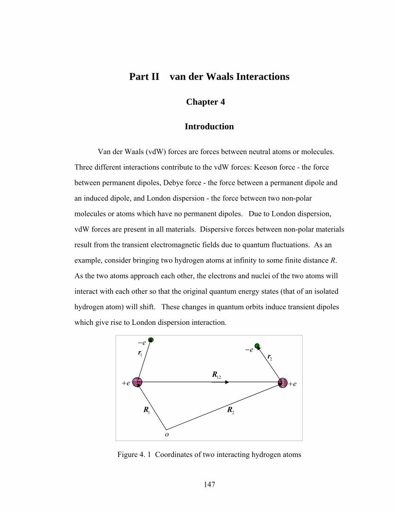
147
Part II van der Waals Interactions
Chapter 4
Introduction
Van der Waals (vdW) forces are forces between neutral atoms or molecules.
Three different interactions contribute to the vdW forces: Keeson force - the force
between permanent dipoles, Debye force - the force between a permanent dipole and
an induced dipole, and London dispersion - the force between two non-polar
molecules or atoms which have no permanent dipoles. Due to London dispersion,
vdW forces are present in all materials. Dispersive forces between non-polar materials
result from the transient electromagnetic fields due to quantum fluctuations. As an
example, consider bringing two hydrogen atoms at infinity to some finite distance R.
As the two atoms approach each other, the electrons and nuclei of the two atoms will
interact with each other so that the original quantum energy states (that of an isolated
hydrogen atom) will shift. These changes in quantum orbits induce transient dipoles
which give rise to London dispersion interaction.
Figure 4. 1 Coordinates of two interacting hydrogen atoms
12R
o
2R 1R
1r 2r
e+ e+
e−e−
148
The first calculation that studied the dispersive interaction between two
molecules without permanent dipole moments is due to Wang and London [1].
Wang’s calculation is for two hydrogen atoms separated by a sufficiently large separation 12R = R (see Figure 0.1) so that perturbation theory is applicable. The
Hamiltonian of two hydrogen atoms, H, is
0 1H H H= + (4.1)
where
( )2 2 2
2 20 1 2
1 22e eH
m r r= − ∇ + ∇ − −
h , (4.2)
is the unperturbed Hamiltonian of two isolated Hydrogen atoms, and m and e are the
mass and electric charge of an electron respectively. The perturbation Hamiltonian is
2 2 2 2
112 1 12 2 12 1 2 12
e e e eHR
= − − +− − −r R r + R r r R
. (4.3)
Assuming both atoms are in ground states, the change in energy due to the perturbed
1H is
21
10
00 0
n o n
H nW H
E E≠
Δ = +−∑ (4.4)
where nE is the energy corresponding to the unperturbed eigenstate n . It turns out
that the first order perturbation 10 0 0H = , but the second order perturbation term 2
1
0
0
n o n
H nE E≠ −∑ gives an interaction potential that is proportional to 6R− . This results
in an interaction force that is proportional to 7R− , i.e.,
149
7
BFR
= − (4.5)
where the negative sign in (4.5) indicates an attractive interaction. The constant
coefficient B is related to the molecular polarizability 1( )α ω by
1 20
18 ( ) ( )B i i dα ξ α ξ ξπ
∞
= ∫h (4.6)
The molecular polarizability ( )α ω is often related to the dielectric function ( )ε ω via
the Clausius – Mosotti equation which is
( ) ( )( )
13 2
N α ω ε ωε ω
⋅ −=
+ (4.7)
where N is the number density of the atoms per unit volume. Note that this relation is
approximate.
D. Kleppner [2] pointed out a simple way to understand the 6R− dependence of
the vdW potential. The motion of electrons in atoms, in classical electromagnetic
theory, can be thought of as simple harmonic electronic oscillators [3]. In analogy,
the charges in an LC circuit oscillate with natural frequency1/ LC . If we bring two
identical circuits from infinity so that they are separated by a distance R, the capacitors
in the circuit will interact with each other. Since R is large, the capacitors can be
treated as two electric dipoles. The interaction of these dipoles causes a shift in the
ground state energy of these two harmonic oscillators. A straight forward calculation
shows that the change in the ground state energy of the two oscillators is
proportional 6R− .
We should point out that the 6R− dependence of vdW potential is valid only if
the separation R is small in comparison to the wavelength λ corresponding to
150
transitions between the ground and excited states of atoms or molecules. Since
electromagnetic wave can not travel faster than the speed of light, when R λ> ,
retardation effect becomes important and dynamics effect must be included in the
calculation. In the limit R λ>> , the vdW interaction energy for two nonpolar
molecules is found to be proportional to 7R− [4].
Actually the idea of Kleppner[2] is not new. Langbein in 1971 [5] estimated
the dispersion interaction between macroscopic bodies by assuming that each body is
a collection of atoms each of which can be modeled as an electronic harmonic
oscillator. The interaction energy between two bodies is the sum of the change in the
ground state energy of each molecule (which interacts with each other) as these bodies
approach each other. This method is called the Microscopic Method. Since real
systems contain a very large number of molecules, the microscopic method is very
difficult to apply.
The simplest way to compute vdw interaction between macroscopic bodies is
to assume the pair-wise additivity of forces, as suggested by Hamaker [6]. This is the
method that is currently employed by molecular dynamics simulations. This method
can only be justified for dilute gases. Continuum model of adhesion between solids
due to vdw interaction that is based on pairwise additivity assumption was proposed
by many investigators [6 – 9].
The most successful theory of vdW interactions between macroscopic bodies
was proposed by Lifshitz in 1955 which was translated into English in 1956 [10].
Lifshitz used a result from Rytov[11] on fluctuating electromagnetic field to extend
the theory of Casmir [4], who determined the interaction force between two perfect
parallel conductors separated by vacuum. Casmir’s idea is that the electromagnetic
151
fields are confined to the surfaces of the perfect conductors. These fields are called
surface modes. Each surface mode (with frequency iω ), at zero temperature,
contributes a free energy of / 2iωh . The total free energy G of the system is the sum
over all modes,
( ) / 2iG L ω= ∑h (4.8)
Since iω depends on the separation L, the force of interaction per unit area is given by
/F G L= −∂ ∂ . Lifshitz considered essentially the same problem as Casmir, except
that Lifshitz replaced the perfect conductors by two different linear dielectrics. The
basic idea of Lifshitz’s theory can be explained as follows. The two plates attract each
other due to the change in interaction energy by assembling the macroscopic bodies,
molecule by molecule. Obviously, it is impossible to compute this change of
interaction energy using quantum mechanics. This change of interaction energy
causes fluctuating electromagnetic field in the bodies. In classical physics, we know
that the Maxwell stress tensor allows us to compute the energetic force between two
bodies. The question is how to compute the fluctuating macroscopic electromagnetic
fields. The macroscopic electromagnetic field is determined by the electromagnetic
force acting on an infinitesimal test charge. The situation is analogous to the
Brownian motion of a small particle in a viscous fluid. The particle moves because it
constantly collides with surrounding fluid molecules. There is no hope of solving the
interaction of this particle with the surrounding fluid molecules using quantum
mechanics, so the motion of this particle is determined by Newton’s second law with a
random driving force. In Lifshitz’s approach [10], the macroscopic electromagnetic
field is determined by solving the Maxwell equation with a random polarization field.
His idea and his paper in 1956 will be examined in details in the chapter 1.
152
LLiiffsshhiittzz’s theory has a limitation, in that the medium between the two
dielectric plates is required to be vacuum. The difficulty with a non-vacuum medium
is that the integral of the Maxwell stress tensor is no longer surface independent. As a
result, the concept of energetic force breaks down. In 1961, DDzzyyaalloosshhiinnsskkiiii,, LLiiffsshhiittzz
aanndd PPiittaaeevvsskkiiii ((DDLLPP)) iinn 11996611[[1122]] oobbttaaiinneedd aann aapppprrooxxiimmaattee ssoolluuttiioonn ooff tthhee pprroobblleemm ooff
ccaallccuullaattiinngg tthhee vvddww ffoorrccee bbeettwweeeenn ttwwoo lliinneeaarr ddiieelleeccttrriicc hhaallff ssppaacceess sseeppaarraatteedd bbyy aa
ddiieelleeccttrriicc ssttrriipp uussiinngg qquuaannttuumm eelleeccttrrooddyynnaammiiccss..
The theory of Lifshitz [8] and DLP[9] are very complicated. This motivated
van Kampen, Nijboer and Schram (VKNS) [13] to develop a different approach to the
same problem. Instead of computing the electromagnetic field caused by a random
field, they looked for surface modes in the homogeneous Maxwell equations. The
frequencies of these surface modes are determined by a dispersive relation. As in
Casmir [4], VKNS assumed that the force of interaction per unit area is given
by /F G L= −∂ ∂ . Their results for the vdw force in the parallel plate problem are
identical to those obtained by Lifshitz [10] and DLP [12]. However for the VKNS
formulation to arrive at the same result as Lifshitz’s, one has to accept at least two
assumptions that are difficult to justify. This issue will be addressed in Chapter 2.
Lifshitz’s formulation for vdw interaction can be extended to finite solids of
any geometry, as long as one of the medium is vacuum. For finite solids with
complicated boundaries, it is impossible to find analytical solutions of Maxwell
equations. This motivates us to develop numerical techniques to compute vdW forces.
Boundary element method will be discussed in chapter 3. Chapter 4 will be the finite
element formulation.
153
REFERENCES
1. Wang, S.C., Phys. z. 28 663 (1927); London, F., Z. Phys.63, 245(1930);
London, F., Z. f. Phys. Chem. B 11, 222 (1930).
2. Kleppner, D., Physics Today, Oct. 1990, p9-11.
3. Rossi, B., Optics, Addison-Wesley, 1965, p348-350.
4. Casimir, H. B. G. and Polder, D., Phys. Rev. 73, 360 (1948).
5. Langbein, D., J. Chem. Phys. Solids 32, 133 (1971).
6. Hamaker, H. C., Physica 4, p1058-1072 (1937).
7. de Boer., J. H., Trans. Faraday Soc. 32, p10-38 (1936).
8. Argento, C. and French, R. H., J. Appl. Phys. 80, p6081-6090 (1996).
9. Jagota,A., Argento, C., J. of Colloid and Interface Sci. 191, 326-336 (1997).
10. Lifshitz, E. M., Soviet Physics 2, 73-83 (1956).
11. Rytov, S.M., Theory of Electrical Fluctuations and Thermal Radiation,
Publishing House, Academy of Sciences, USSR, 1953.
12. DDzzyyaalloosshhiinnsskkiiii,, II.. EE..,, LLiiffsshhiittzz,, EE.. MM..,, aanndd PPiittaaeevvsskkiiii,, LL.. PP..,, AAddvv.. PPhhyyss.. 1100,, 116655
((11996611))..
13. Van Kampen, N. G., Nijboer, B. R. A., and Schram, K., Physics Letters 26A,
307-308 (1968).
154
Chapter 5
Lifshitz Theory
This chapter provides the background for the calculation of van der Waals
interaction based on the continuum theory of Landau and Lifshitz [1, 2]. Most of the
results in this chapter can be found in Lifshitz [3], Felderhof [4], McQuarrie [5] and
Rief [6]. Our goal is to derive these results assuming a rudimentary knowledge of
statistical and quantum mechanics. In the following, we assume that the
electromagnetic properties of the materials are homogeneous, isotropic and non-
magnetic. The generalization to anisotropic materials is straightforward and can be
found in Landau and Lifshitz [1].
This chapter is organized as follows. Sections 5.1 – 5.4 review the properties
of the linear dielectric functions. Correlation and spectral density is studied in section
5.5. In section 5.6, we develop the dissipation- fluctuation theorem. The fluctuation
and van der Waals Interaction relation is given in sections 5.7– 5.8. Section 5.9
determines the relation between the correlation and dissipation using quantum
mechanics. Finally, one example (Lifshitz’s three-layer problem) is revisited with
more details and comments in section 5.10.
Notations: Vectors and Tensors will be denoted by bold letters. The time Fourier
transform of a vector E will be denoted by %E . The quantum mechanics operator
associated with an observable E is denoted by E . We follow Lifshitz [3] who used
Gaussian units for Maxwell’s equations.
155
5.1 Constitutive Model of a Linear Dielectric
For a linear dielectric, linear response theory [1, 2] states that the electric
displacement D is related to the electric field E by
( ) ( )t
k t dτ τ τ−∞
= + −∫D E E (5.1)
where k is a real positive function defined for all positive arguments (that is
( 0) 0k t ≤ = ). It is known as the after effect function. Note that the upper limit of the
integral in (5.1) is t due to causality. A change of variable t uτ− = gives:
0
( ) ( ) ( ) ( )t t k u t u du∞
= + −∫D E E (5.2)
Taking the Fourier transform of (5.2), i.e.,
1( ) ( )2
i tt e dtωωπ
∞
−∞
= ∫%D D (5.3)
where the inverse transform is
( ) ( ) i tt e dωω ω∞
−
−∞
= ∫ %D D (5.4)
Taking the Fourier transform of (5.2) and after some simple manipulation, we found
( ) ( ) ( )ω ω ε ω=% %D E (5.5)
where
0
( ) 1 ( ) i tk t e dtωε ω∞
= + ∫ (5.6)
156
is the dielectric susceptibility. If k is in 1[0, )L ∞ , the Riemann-Lebesque theorem
implies that
0
lim ( ) 0i tk t e dtω
ω
∞
→∞=∫
so
( ) 1ε ω → ∞ = (5.7)
5.2 Property of Dielectric Susceptibility
Equation (5.6) implies that ( )ε ω is a complex function of the frequency. Let
( ) ( ) ( )iε ω ε ω ε ω′ ′′= + (5.8)
where Reε ε′ = and Imε ε′′ = . The right hand side (RHS) of (5.6) implies that
( )0
( ) 1 ( ) cosk t t dtε ω ω∞
′ = + ∫ (5.9a)
( )0
( ) ( )sink t t dtε ω ω∞
′′ = ∫ (5.9b)
Equations (5.9a, b) imply that ( )ε ω′ is an even function of the frequency and ( )ε ω′′ is
an odd function. In addition, equations (5.8) - (5.9b) imply that
( ) ( ) ( ) ( )iε ω ε ω ε ω ε ω∗′ ′′− = − ≡ , (ω real) (5.10)
where the * indicates the complex conjugate of a complex quantity. By
(5.7), ( ) 0ε ω′′ → ∞ = , so dissipation vanishes at very high frequencies. In addition,
since ( )ε ω′′ is odd, ( 0) 0ε ω′′ = = if ( )ε ω′′ is continuous at zero. This is the case for
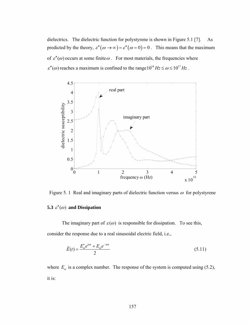
157
dielectrics. The dielectric function for polystyrene is shown in Figure 5.1 [7]. As predicted by the theory, ( ) ( )0 0ε ω ε ω′′ ′′→ ∞ = = = . This means that the maximum
of ( )ε ω′′ occurs at some finiteω . For most materials, the frequencies where
( )ε ω′′ reaches a maximum is confined to the range 14 1710 10Hz Hzω≤ ≤ .
0 1 2 3 4 5
x 1016
0
0.5
1
1.5
2
2.5
3
3.5
4
4.5
frequency ω (Hz)
diel
ectri
c su
scep
tibili
ty
real part
imaginary part
Figure 5. 1 Real and imaginary parts of dielectric function versus ω for polystyrene
5.3 ( )ε ω′′ and Dissipation
The imaginary part of ( )ε ω is responsible for dissipation. To see this,
consider the response due to a real sinusoidal electric field, i.e.,
( )2
i t i tE e E eE tω ω
ω ω∗ −+
=r
(5.11)
where Eω is a complex number. The response of the system is computed using (5.2),
it is:
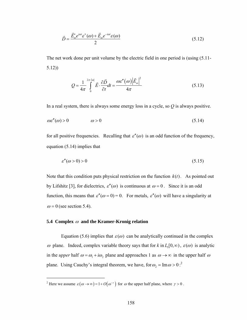
158
( ) ( )2
i t i tE e E eDω ω
ω ωε ω ε ω∗ ∗ −+=r r
r (5.12)
The net work done per unit volume by the electric field in one period is (using (5.11-
5.12))
( )
22 /
0
14 4
EDQ E dtt
π ωωωε ω
π π
′′∂= ⋅ =
∂∫rr
r (5.13)
In a real system, there is always some energy loss in a cycle, so Q is always positive.
( ) 0ωε ω′′ > 0ω > (5.14)
for all positive frequencies. Recalling that ( )ε ω′′ is an odd function of the frequency,
equation (5.14) implies that
( 0) 0ε ω′′ > > (5.15)
Note that this condition puts physical restriction on the function ( )k t . As pointed out
by Lifshitz [3], for dielectrics, ( )ε ω′′ is continuous at 0ω = . Since it is an odd
function, this means that ( 0)ε ω′′ = = 0. For metals, ( )ε ω′′ will have a singularity at
0ω = (see section 5.4).
5.4 Complex ω and the Kramer-Kronig relation
Equation (5.6) implies that ( )ε ω can be analytically continued in the complex
ω plane. Indeed, complex variable theory says that for k in 1[0, )L ∞ , ( )ε ω is analytic
in the upper half 1 2iω ω ω= + plane and approaches 1 as ω → ∞ in the upper half ω
plane. Using Cauchy’s integral theorem, we have, for 2 Im 0ω ω= > :2
2 Here we assume ( ) ( )1 O γε ω ω−→ ∞ = + for ω the upper half plane, where 0γ > .
159
[ ]( ) 11( ) 12
u dui u
εε ω
π ω
∞
−∞
−− =
−∫ . (5.16)
The limit as ω approaches the real axis from the upper half plane can be obtained
using the Plemelj formulae:
( ) [ ] [ ]1
11
( ) 11 1lim ( ) 1 ( ) 12 2
u duP
i uω ω
εε ω ε ω
π ω+
∞
→−∞
−− = + −
−∫ , (5.17)
where P denotes a principal value integral. This results in:
[ ]1
1
( ) 11( ) 1u du
Pi u
εε ω
π ω
∞
−∞
−− =
−∫ (5.18)
Separating the real and imaginary part in (5.17) gives the Kramer-Kronig relation:
11
1 ( )( ) 1 u duPu
εε ωπ ω
∞
−∞
′′′ = +
−∫ (5.19a)
11
1 ( )( ) u duPu
εε ωπ ω
∞
−∞
′′′ = −
−∫ (5.19b)
where we have used the result that
1
0duPu ω
∞
−∞
=−∫ . (5.19c)
The Kramer-Kronig relation states that the real and imaginary of the susceptibility are
not independent. Indeed, knowing one completely determines the other. Since ε can
be analytically continued to the upper half ω plane, (5.6) implies that
22
0
( ) 1 ( ) ti k t e dtωε ω ω∞
−= = + ∫ 2 0ω > (5.20a)
160
Note that 2 2( ) 1 ( , )i L kε ω ω ω= − = , where L is the Laplace transform of ( )k t . Since k
is real, (5.20a) implies that 2( )iε ω ω= is real on the imaginary axis. Lifshitz [3] has
shown that ( )ε ω does not take real values at any finite point in the upper half plane
except on the imaginary axis, where it decreases monotonically from (0) 1ε > (for
dielectrics) or from ( +∞ ) (for metals) as 0iω +→ to 1 at iω → ∞ . As a consequence,
it follows that ( )ε ω has no zero in the upper half plane. Since ( )ε ω′′ is positive on the
positive real ω axis, and does not vanish in the first quadrant of the ω plane, it must
remain positive there by continuity. It should be noted that, for metals, Landau and
Lifshitz have shown that [1],
2 20
1 ( )( ) 1 x x dxPxεε ω
π ω
∞ ′′′ = +
−∫ realω (5.20b)
0
1 ( ) 4( ) x dxPx
ε πσε ωπ ω ω
∞ ′′′ = − +
−∫ realω (5.20c)
where σ is the conductivity. For very good conductors, 4( ) πσε ωω
′′ ≈ for all
frequencies. Using this approximation, it is easy to verify that
2 20
( ) 0x x dxPxε
ω
∞ ′′=
−∫ for all 0ω > (5.20d)
Thus, ( ) 1ε ω′ = for all frequencies in this approximation. Therefore, for good
conductors,
4( ) 1 πσε ωω
≈ + (5.20e)
161
5.5 Correlation and Spectral density
Let ( ) ( )i jX t X t′ denote the equilibrium ensemble average of two physical
quantities iX and jX at t and t t τ′ = + . It is called the “correlation function” of
iX and jX . In our case iX represents components of the electromagnetic field, e.g. iE .
The ensemble average is taken in the equilibrium situation where the distribution of
systems in the ensemble is independent of the absolute value of time. Thus,
( ) ( ) ( ) ( ) ( )i j i j ijX t X t X t X t Fτ τ′ = + = (5.21a)
is a function of τ only. In general, the ensemble average of a quantity X is defined
by
1
1 ( )N
kk
X X tN =
= ∑ (5.21b)
where ( )kX t is the value taken by ( )X t in the kth system of the ensemble and N the
total number of identical systems in the ensemble. In a stationary process, there is
no preferred origin in time for the statistical description of X, in this case the “ergodic” hypothesis X implies that
1lim ( )2
X X t t dtτ
τττ→∞
−
⎛ ⎞′ ′= +⎜ ⎟
⎝ ⎠∫ (5.21c)
An excellent discussion of correlation function and the relation between time and
ensemble average can be found in Reif [6]. By definition, the spectral density of ( )ijF τ is the Fourier transform of ( )ijF τ .
Note that the dependence of iX on r is not indicated in (5.21a-c) or in the
equations below. This is because we are considering the response of a material point.
162
The macroscopic fields in this material point are assumed to be spatially homogeneous.
Of course, each continuum point is composed of a very large of atoms/molecules. The
ensemble average in (5.21a-c) can also be computed using the equilibrium distribution
function in classical statistical mechanics which depends only on the coordinates and
momentum of these particles.
These correlations are particularly simple in the frequency domain for
stationary process. To see this, note that
( )
( ) ( ) ( ) ( )
( ) ( )
i t i ti j i j
i ti si j
X t X t X e d X e d
e d X X e d
ω ω
ω ωω
ω ω ω ω
ω ω ω ω
∞ ∞′ ′− −
−∞ −∞
∞ ∞′− +−
−∞ −∞
′ ′ ′=
′ ′=
∫ ∫
∫ ∫
% %
% %
(5.22)
In a stationary process, these cross correlations are functions of τ only; this means that ( ) ( )i jX Xω ω′% % must be proportional to ( )δ ω ω′+ . Because of the delta function, the
proportional factor is a function only ofω ; this function is denoted by ( )i jX Xω
% % , i.e.,
( )( ) ( ) ( )i j i jX X X Xω
ω ω δ ω ω′ ′= +% % % % (5.23)
Substituting (5.23) into (5.22) shows that ( )i jX Xω
% % is the spectral density, i.e.,
( )( ) ( ) ii j i jX t X t e X X dωτ
ωτ ω
∞−
−∞
+ = ∫ % % . (5.24)
Recall the spectral density of a quantity Y is the Fourier transform of the time
correlation function of Y. Note that, since the iX ’s are real, we have
163
( )
( ) ( ) ( ) ( )
( ) ( ) ( ) ( )
i t i ti j i j
i ti t i t ii j i j
X t X t X e d X e d
X e d X e d e d X X e d
ω ω
ω ωω ω ωτ
ω ω ω ω
ω ω ω ω ω ω ω ω
∗∞ ∞′ ′− −
−∞ −∞
∞ ∞ ∞ ∞′− −′ ′− ∗ ∗
−∞ −∞ −∞ −∞
⎛ ⎞′ ′ ′= ⎜ ⎟
⎝ ⎠
⎛ ⎞′ ′ ′ ′= =⎜ ⎟
⎝ ⎠
∫ ∫
∫ ∫ ∫ ∫
% %
% % % %
(5.25)
Using the same argument as before, we have
( )( ) ( ) ( )i j i jX X X Xω
ω ω δ ω ω∗ ∗′ ′= −% % % % (5.26)
Since ( ) ( )i jX t X t′ is real, the complex conjugate of (5.25) is itself, so
( )( ) ( ) ( ) ( ) i ti si j i jX t X t e d X X e dω ωω ω ω ω ω
∞ ∞∗ ′−− ∗
−∞ −∞
′ ′ ′= ∫ ∫ % % (5.27)
Substitute (5.26) into (5.27), we have:
( )( ) ( ) ii j i jX t X t e X X dωτ
ωω
∞∗− ∗
−∞
′ = ∫ % % (5.28a)
Comparing (5.28a) and (5.24), we have
( ) ( )i j i jX X X Xω ω
∗∗ =% % % % . (5.28b)
If we set 0τ = in (5.24), we have,
( )( ) ( )i j i jX t X t X X dω
ω∞
−∞
= ∫ % % (5.29)
Finally, we note that in a stationary process, the auto-correlation function ( ) ( )X t X t s+ is even. This is because
{( ) ( ) ( ) ( ) ( ) (0)t t
X t X t X t X t X Xτ
τ τ τ→ −
+ = − = − (5.30)
164
Physical reasoning tells us that for large τ , the correlation function must goes to 0.
5.6 Dissipation- Fluctuation Theorem (DFT) – a simple example
To motivate our approach below, we give a simple example to illustrate the
dissipation-fluctuation theorem (DFT) (see for example, Rief [6]). Let us consider a
one dimensional problem where
( ) ( )t
D h t E dτ τ τ−∞
= −∫ (5.31)
where ( )h k tδ τ≡ + − . DFT implies that
1( ) (0) ( )B
h t D D tk T
= 0t > (5.32)
where Bk is the Boltzmann constant and T is the absolute temperature in Kelvin. Note
that h is defined for positive times only. That is, the after effect function defined
earlier is proportional to correlation function of D. In the static case where ( ) oE t E= ,
we have
0 0
( ) ( ) 1 ( ) ( 0)t
o o o oD E h t d E h t d E k d Eτ τ τ τ τ ε ω∞ ∞
−∞
⎛ ⎞= − = = + = =⎜ ⎟
⎝ ⎠∫ ∫ ∫ (5.33a)
If we take ( ) i toE t E e ω−= , then
( ) ( )( ) 1 ( )t t
i ti i t i to o oD h t E e d E e e k t d E eω τωτ ω ωτ τ τ τ ε ω−− − −
−∞ −∞
⎛ ⎞= − = + − =⎜ ⎟
⎝ ⎠∫ ∫ (5.33b)
However,
( )
0
( ) ( ) (0) ( )t t i
i i t i t io o o
eh t E e d e h t E e d D D E e dkT
ωτωτ ω ω τ ωητ τ τ τ η η
∞−− − −
−∞ −∞
− = − =∫ ∫ ∫ (5.34)
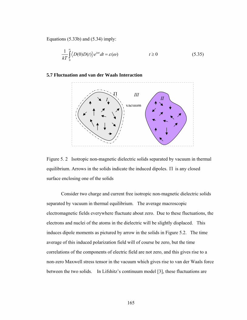
165
Equations (5.33b) and (5.34) imply:
0
1 (0) ( ) ( )i tD D t e dtkT
ω ε ω∞
=∫ 0t ≥ (5.35)
5.7 Fluctuation and van der Waals Interaction
Figure 5. 2 Isotropic non-magnetic dielectric solids separated by vacuum in thermal
equilibrium. Arrows in the solids indicate the induced dipoles. Π is any closed
surface enclosing one of the solids
Consider two charge and current free isotropic non-magnetic dielectric solids
separated by vacuum in thermal equilibrium. The average macroscopic
electromagnetic fields everywhere fluctuate about zero. Due to these fluctuations, the
electrons and nuclei of the atoms in the dielectric will be slightly displaced. This
induces dipole moments as pictured by arrow in the solids in Figure 5.2. The time
average of this induced polarization field will of course be zero, but the time
correlations of the components of electric field are not zero, and this gives rise to a
non-zero Maxwell stress tensor in the vacuum which gives rise to van der Waals force
between the two solids. In Lifshitz’s continuum model [3], these fluctuations are
vacuum
ΠI
IIIII
166
simulated by imposing a random polarization field ( )tK r, in the Maxwell Equations
which are:
1c t
∂∇× + =
∂BE 0 (5.36a)
1c t t
∂ ∂⎡ ⎤∇× = +⎢ ⎥∂ ∂⎣ ⎦D KB (5.36b)
0∇ ⋅ =B (5.36c)
∇ ⋅ = −∇ ⋅D K (5.36d)
for each media (of course, in vacuum, K = 0, D = E). With appropriate boundary
conditions (see below), the van der Waals force F between the two dielectrics is
determined by computing the ensemble average of the Maxwell stress tensor3 S in
vacuum which is
1 1 14 2 2ij i j k k ij i j k k ijS E E E E B B B Bδ δπ
⎛ ⎞≡ − + −⎜ ⎟⎝ ⎠
(5.37a)
and evaluating the surface integral
( )i ij jF S t n dAΩ
= ∫∫ (5.37b)
where in is the unit normal vector of a smooth closed surface Π containing one of the
solids (see Figure 5.2).
3 The complete form of Maxwell stress tensor is
( ) ( )1 1 14 2 2ij i j j k k k ij i j k k ijS E D K E D K B B B Bδ δπ
⎛ ⎞≡ + − + + −⎜ ⎟⎝ ⎠
167
Note that, since ijS is a linear combination of ,i jX X ’s. The ensemble average
of S is
1 1 1( )4 2 2ij i j k k ij i j k k ijS t E E E E B B B Bδ δπ
⎛ ⎞= − + −⎜ ⎟⎝ ⎠
(5.38a)
where ( ) ( )i j i jE E E t E t= etc. According to (5.38a), the ensemble average of S is
a linear combination of the terms of the form ( ) ( )i jE t E t . The RHS of (5.38a),
according to (5.29) is
( ) ( ) ( ) ( )1 1 14 2 2
( )
i j k k ij i j k k ij
ij
E E E E B B B B d
s
ω ω ω ωδ δ ω
πω
∞
−∞
⎛ ⎞− + −⎜ ⎟⎝ ⎠∫ % % % % % % % %
14444444444244444444443
(5.38b)
or
( ) ( )ij ijS t s dω ω∞
−∞
= ∫ (5.38c)
As expected, ( )ijS t is independent of time. Combining (5.37b) and (5.38c), we have
( )i ij jF s d n dAω ω∞
Ω −∞
⎛ ⎞= ⎜ ⎟
⎝ ⎠∫∫ ∫ (5.38d)
Since ( )ijS t is independent of time, the vdw interaction force is independent of time.
Note that since ( )ijS t is real, the imaginary part of ( )ijs ω must be an odd function
of the frequency, since it must integrates to zero.
Of course, ( )tK r, is not just any random field, since it is supposed to model the
induced polarization caused by fluctuations. In addition, the time correlation of this
168
random polarization must be related to the time correlation of the electric fields.
Physically, we anticipate the following properties of ( )tK r, :
1. The time average of K is zero
2. The correlation of K at two different spatial points r and ′r is zero.
Note, analogous to Brownian motion, where the acceleration of the particle is related
to the random force field through the solution of Newton law (a classical mechanics
equation), and the induced polarization of the molecules in the solid is related to the
random dipole field K through the solution of the classical Maxwell equation.
Lifshitz’s theory of vdw interaction made use of the fact that in the frequency domain,
the random dipole field K satisfies
( )( ) ( ) ( ) ( )i j i jK , K , K Kω
ω ω δ δ ω ω′ ′ ′ ′= − +% % % %r r r r (5.39)
where ( )i jK Kω
% % is
( ) 2 ( ) coth2i j ij
B
K Kk Tω
ωε ω δ⎛ ⎞
′′= ⎜ ⎟⎝ ⎠
h% % h (5.40)
where 341.0545 10 Js−= ×h is the Planck’s constant, 23 o1.3805 10 J/KBk −= × and T is
the absolute temperature in degree Kelvin. Note that jK% in (5.40) is evaluated at ω− .
We will derive equation (5.39) and (5.40) in the following sections. Note that just as
the fluctuation-dissipation theorem states that there is a relation between the
fluctuation force and the viscosity of the fluid, Lifshitz’s approach[3] shows that the
connection between the random force field and the imaginary part of ε , which as we
have shown, is responsible for dissipation.
169
Equation (5.38d) and (5.39) and the fact that D is related to E by a convolution
integral suggest that it is easier to operate in the frequency domain. A straightforward
Fourier transform of (5.36a-d) leads to
ic
α αω−∇× =% %E B 0 (5.41a)
ic
α α αω ⎡ ⎤∇× = − +⎣ ⎦% % %B D K (5.41b)
0α∇ ⋅ =%B (5.41c)
α α∇ ⋅ = −∇ ⋅% %D K (5.41d)
where
( , )i te t dtω∞
−∞
≡ ∫%E E r (5.42)
is the Fourier transform of E . , ,I II IIIα = denotes different domain. Note that
0III =%K . It should be noted that equations (5.41a) – (5.41d) are not independent.
Clearly, the divergence of (5.41a) implies (5.41c) and the divergence of (5.41b) gives
(5.41d). In other words, only two of the four Maxwell equations are independent.
Indeed, we need only to solve (5.41a) and (5.41b) subject to the boundary conditions:
(a) 0= =% %E B at infinity.
(b) The tangential components of %E and %B are continuous on the interfaces.
(c) The normal component of ( )+% %D K 4and %B are continuous on the interfaces.
4 This is because of ( ) 0∇ • + =% %D K
170
It should be pointed out that condition (b) is derived from (5.41a,b) and (c) is derived
from (5.41c,d). Since equations (5.41c,d) can be derived from (5.41a,b), thus
conditions (b) and (c) are not independent. Indeed, (b) is sufficient to assure (c).
5.8 Dissipation and Equation (5.40)
As our simple example shows (see (5.36)), equation (5.40) states that the
fluctuating fields iK are related to dissipation. In the macroscopic problem, the
energy balance is:
1 14 4 4c
t t tπ π π∂ ∂ ∂⎛ ⎞ ⎛ ⎞∇ ⋅ × + ⋅ + ⋅ = − ⋅⎜ ⎟ ⎜ ⎟∂ ∂ ∂⎝ ⎠ ⎝ ⎠D B KE B E H E (5.43a)
where
4cπ
×E B (5.43b)
is the flux density, and
14 tπ
∂− ⋅
∂KE (5.43c)
is the energy loss due to fluctuations.
1 1( ) ( ) ( )4 8 8c
t tπ π π∂ ∂
∇ ⋅ × + ⋅ ⋅ = − ⋅∂ ∂
B E E D + B B E K (5.43d)
where we have used the assumption that the material is non-magnetic, charge and
current free. The second term in (5.44) is the rate of change of the electromagnetic
energy density. Since the fields are homogeneous (we are looking at a material point
171
in this calculation), the first term in (5.44) is zero. Since E is a linear functional of K,
the change in energy density, 1 ( )8 tπ
∂− ⋅
∂E K is:
1 ( )4 tπ
∂− ⋅
∂KE (5.43e)
Therefore, the change in energy density due to fluctuation is / 4i iK E π− & . In the
frequency domain, we have:
( )i iK Eε ω− =% % 5 or ( )i iE Kα ω=% % ( ) 1/ ( )ε ω α ω= − (5.43f)
Since iK can be decomposed into its Fourier components, we consider input of the
form
( ) / 2i t i ti i iK K e K eω ω− ∗= +% % . (5.44a)
According to (5.43f), the electric field due to this input is:
( ) / 2i t i ti i iE K e K eω ωα α− ∗ ∗= +% % . (5.44b)
Substituting (5.48) and (5.47) into (5.45) and averaging over the period 2 /π ω gives
the total energy density change at a material point,
21 ( )
8Q ωα ω
π′′= %K . (5.45)
Since ( )α ω′′ is a odd function of the frequency and is positive for positive
frequencies, 0Q ≥ , that is, energy is always dissipated in a cycle.
5 Actually, there are also random magnetic fields corresponding to B. However, the materials are nonmagnetic, so these random magnetic fields are independent of positions, therefore these fields will have no contribution to van der Waals interaction.
172
We can also compute Q using quantum mechanics. Let Ho be the time
independent Hamiltonian of the system (a continuum point r in the macroscopic body)
without perturbation (i.e., K = 0). Because the fields are spatially uniform, the
perturbation operator associated with the random field is:
/ 4i iK π= −V E (5.46)
As before, assume iK is given by (5.43f). Let nΨ denote the stationary state of the
system, i.e.,
( )o n n nΨ = Γ ΨH (no sum on n) (5.47)
where nΓ are the energies of the stationary state. For stationary states, the time
dependent Schrodinger’s equation can be integrated with respect to time, resulting in
ni tn ne ω ϕ−Ψ = (no sum on n) (5.48)
where /n nω ≡ Γ h , and nϕ is a state vector which depends on the coordinates of the
particles in the continuum point.
Let us assume the system is in the eigenstate n. As a result of perturbation, the
system makes transitions. Let nmP denote the probability per unit time of the transition
from the state n to a state m. This transition rate can be determined using quantum
perturbation theory and it is called Fermi’s golden rule:
( )( ) ( ) ( ) ( )2 ( ) ( )
2 4i k
nm i k mn i k nmnm mn mn nm
K KP e e e eπ δ ω ω δ ω ωπ
∗⎧ ⎫⎪ ⎪⎡ ⎤= + + +⎨ ⎬⎣ ⎦⎪ ⎪⎩ ⎭
% %
h (5.49)
where ( )i mne are the time independent matrix elements of the operator Ei , i.e.,
173
( )i n i mnme ϕ ϕ= E (5.50a)
and
( )ω = Γ Γ- /mn m n h (5.50b)
is the frequency of transition between the states n and m. In each transition the system
absorbs or emits ωh mn . The average energy density per unit time absorbed by a
system at the nth eigenstate is therefore
n nm mnm
Q P ω= ∑h (5.51)
Substituting (5.49) into (5.51) results in:
( ) ( ) ( ) ( ){ }
( ) ( ) ( ) ( ){ }
( ) ( )32
( ) ( )32
i kn i k mn i k nm mnnm mn mn nm
m
i ki k mn i k nmnm mn mn nm
m
K KQ e e e e
K K e e e e
δ ω ω δ ω ω ωπω δ ω ω δ ω ω
π
∗
∗
⎡ ⎤= + + +⎣ ⎦
⎡ ⎤= − + − +⎣ ⎦
∑
∑
% %
% % (5.52)
Note nQ is the rate of change of energy density for a system in the nth eigenstate. To
find the total average energy density absorbed by the system at unit time, we need to
average over all eigenstates. This is done using the Gibb’s distribution, where the
probability of occupying the state n is given by
( )/ /n BE k Tn ne Zρ −= F (5.53)
where F is the free energy of the system and nZ is the partition function (it is actually
a normalization factor). Thus,
( ) ( ) ( ) ( ){ }( ) ( )32i k
n i k mn i k nmnm mn mn nmn m
K KQ e e e eω ρ δ ω ω δ ω ωπ
∗
⎡ ⎤= − + − +⎣ ⎦∑ ∑% %
(5.54)
174
Comparing (5.54) with (5.45), we have:
( ) ( ) ( ) ( ){ }4 ( ) ( ) ( )ik n i k mn i k nmnm mn mn nmn m
e e e eππα ω δ ρ δ ω ω δ ω ω⎡ ⎤′′ = − + − +⎣ ⎦∑ ∑h
(5.55)
Since interchanging n and m does not change the result in the double sum, we have:
( ) ( ) ( ) ( )( ) ( )n i k mn m i k nmnm mn mn nmn m n m
e e e eρ δ ω ω ρ δ ω ω⎡ ⎤ ⎡ ⎤+ = +⎣ ⎦ ⎣ ⎦∑∑ ∑∑ (5.56)
This implies that
( ) ( ) ( )
( ) ( )
( ) ( ) ( )
( ) ( ) ( )
( ) ( ) ( )
,
,
( ) /
,
/
,
/
4 ( ) ( )
1 ( )
1 ( )
1 ( )
1 ( )
n m B
nm B
B
ik n m i k nmmn nmn m
mn i k nmmn nm
n m n
k Tn i k nmmn nm
n m
k Tn i k nmmn nm
n m
k Tn i k nmmn nm
e e
e e
e e e
e e e
e e e
ω
ω
ππα ω δ ρ ρ δ ω ω
ρπ ρ δ ω ωρ
π ρ δ ω ω
π ρ δ ω ω
π ρ δ ω ω
Γ −Γ
−
⎡ ⎤′′ = − +⎣ ⎦
⎛ ⎞⎡ ⎤= − +⎜ ⎟ ⎣ ⎦
⎝ ⎠
⎡ ⎤= − +⎣ ⎦
⎡ ⎤= − +⎣ ⎦
⎡= − +⎣
∑
∑
∑
∑ h
h
h
h
h
h
h ,n m
⎤⎦∑
(5.57)
The last step is because of the delta function.
5.9 Correlations and Dissipation
Recall our goal is to evaluate the ensemble average Maxwell stress tensor.
Equations (5.23) and (5.37a,b) imply that if we want to do the calculation in the
frequency domain, then we have to evaluate the spectral densities of terms like ( ) ( )i jE t E t′ , which is related to the dissipation. Equation (5.57) shows that
dissipation is related to the matrix elements of the time independent Hamiltonian.
This suggests that one can determine these correlations using quantum mechanics. To
175
deduce ( )i kE Eω
% % , we consider the quantum-mechanical expression for the correlation
function ( ) ( )i kE t E t′ which is:
[ ]1( ) ( ) ( ) ( ) ( ) ( )2i k i k k iE t E t t t t t′ ′ ′= +E E E E (5.58)
where a bar denotes quantum average over states and we have used the fact that the
ensemble average is the same as the quantum mechanics average over states. Denote
the Fourier transform of the operator ( )i tE by
1 ( )2
i ti ie t dtE Eω
π
∞
−∞
= ∫ (5.59)
Then,
1( ) ( ) ( ) ( ) ( ) ( )2i k i k k iE Eω ω ω ω ω ω⎡ ⎤′ ′ ′= +⎣ ⎦
% % % %% % E E E E (5.60)
According to (5.29),
( )1 ( ) ( ) ( ) ( ) ( )2 i k k i i kE E
ωω ω ω ω δ ω ω⎡ ⎤′ ′ ′+ = +⎣ ⎦
% % % % % %E E E E (5.61)
As in the previous section, we consider first the system is in some stationary
state nΨ , then the quantum average over this state is:
1 1 1( ) ( ) ( ) ( ) ( ) ( ) ( ) ( )2 2 2i k k i n i k n n k i nω ω ω ω ω ω ω ω⎡ ⎤′ ′ ′ ′+ = Ψ Ψ + Ψ Ψ⎣ ⎦
% % % % % % % %E E E E E E E E
(5.62)
Since m mm
Ψ Ψ =∑ I , where I is the identity operator, we have:
176
( ) ( ) ( ) ( )
( ) ( )
n i k n n i m m k nm
n i m m k nm
ω ω ω ω
ω ω
′ ′Ψ Ψ = Ψ Ψ Ψ Ψ
′= Ψ Ψ Ψ Ψ
∑
∑
% % % %
% %
E E E E
E E (5.63)
On the other hand, using (5.48),
( )( )1( ) ( )2
n mi ti tn i m n i m nmnm
e e dt eω ωωω ψ ψ δ ω ωπ
∞−
−∞
Ψ Ψ = = +∫%E E (5.64)
Therefore,
( ) ( ) ( ) ( )
( ) ( ) ( ) ( )
( ) ( ) ( ) ( )
i k k i
i k nm mn k i nm mnnm mn nm mnm
e e e e
ω ω ω ω
δ ω ω δ ω ω δ ω ω δ ω ω
⎡ ⎤′ ′+⎣ ⎦⎡ ⎤′ ′= + + + + +⎣ ⎦∑
% % % %E E E E(5.65)
Using the identities
( ) ( ) ( ) ( ) ( ) ( )nm mn nm nm nmδ ω ω δ ω ω δ ω ω δ ω ω δ ω ω δ ω ω′ ′ ′+ + = + − = + +
and
( ) ( ) ( ) ( )nm mn mnδ ω ω δ ω ω δ ω ω δ ω ω′ ′+ + = + + (5.66)
we have:
( ) ( ) ( ) ( )
( ) ( ) ( ) ( )
( ) ( ) ( )m
i ik k
i nm i mnk knm mnmn nme e e e
ω ω ω ω
δ ω ω δ ω ω δ ω ω
⎡ ⎤⎣ ⎦
⎡ ⎤⎣ ⎦
′ ′+
′= + + + +∑
% % % %E E E E (5.67)
Equations (5.61) and (5.67) imply that
( ) ( ) ( ) ( ) ( )1 ( ) ( )2i k n
mi nm i mnk knm mnmn nm
E E e e e eω
δ ω ω δ ω ω⎡ ⎤= ⎣ ⎦+ + +∑% % (5.68)
177
where the extra subscript n emphasizes that we have assumed that the state vector is in the n-th eigenstate. As before, to obtain ( )i kE E
ω% % , we average over the Gibbs
distribution. Following the same procedure as in last section, this gives:
( ) ( ) ( ) ( )/
,1 ( )1
2Bk T
i k n i k nmnm mnn m
E E e e eω
ωρ δ ω ω−= + +∑h% % (5.69)
Comparing (5.57), which is
( ) ( ) ( )/
,
4 ( ) 1 ( )Bk Tik n i k nmmn nm
n m
e e eωππα ω δ ρ δ ω ω− ⎡ ⎤′′ = − +⎣ ⎦∑h
h (5.57)
with (5.69), we have:
( ) 2 ( ) coth2i k ik
B
E Ek Tω
ωα ω δ⎛ ⎞
′′= ⎜ ⎟⎝ ⎠
h% % h (5.70)
Since ( )i iE Kα ω=% % , we have:
( ) ( ) ( ) ( ) ( ) ( ) ( ) ( )( ) ( )
( ) ( )( ) ( ) ( ) ( ) ( )2
i k i k i k
i k i k
E E K K K K
K K K K
ω
ω ω
ω ω α ω α ω ω ω α ω α ω δ ω ω
α ω α ω δ ω ω α ω δ ω ω
′ ′ ′ ′ ′= = +
′ ′= − + = +
% % % % % %
% % % %(5.71)
Therefore,
( ) ( ) ( ) ( )( )
2
2( )2 coth
2i k i k i k ikB
E E K K K Kk Tω ω ω
α ω ωα ω δα ω
⎛ ⎞′′= ⇒ = ⎜ ⎟
⎝ ⎠
h% % % % % % h (5.72)
However,
( ) 2( ) 1 1 1 ( )
2 2 2 2α ω α α ε ε ε
αα α αα ω
∗∗
∗ ∗
′′ − ′′= = − = − = (5.73)
Therefore,
178
( ) 2 ( ) coth2i k ik
B
K Kk Tω
ωε ω δ⎛ ⎞
′′= ⎜ ⎟⎝ ⎠
h% % h (5.74)
which is the same as equation (5.40).
5.10 An Example: a 3-layer Problem --Detailed Derivation of the Lifshitz
Theory
To gain an insight into Lifshitz’s continuum theory, we revisit the problem of
finding the van der Waals (vdw) force between two planar infinite non-magnetic
dielectric materials separated by vacuum. This problem was solved by Lifshitz [3] in
1955 (Russian, translated into English in 1956) using the formulation in section 5.7.
Lifshitz’s paper is not easy to read, as many steps are skipped. In this section we give
a detailed derivation of this paper. We also discovered some typos in that paper.
Figure 5. 3 A schematic drawing of a 3-layer problem
The geometry of the 3-layer problem is shown in Figure 5.3: two semi-infinite
linear dielectrics (1 and 2) are separated by vacuum (3). The surfaces of the layers (1
1 3 (Vacuum)
2
xx=l x=0
179
and 2) are planar and are oriented parallel to each other. The separation between 1
and 2 is denoted by l. Points in layers 1, 2 and 3 are specified by a Cartesian coordinate system (x, y, z) with origin on the surface of the layer 5. Let ( )ˆ ˆ ˆ, ,i j k be
the orthornormal basis associated with the Cartesian coordinate system (x, y, z). The
normal to the layers is along the x direction.
For a dielectric, non-magnetic media, =H B , the governing equations of
electromagnetic fields E and B in frequency domain are (see section 5.7 for a
discussion of why only two Maxwell equations are sufficient)
icω
∇× =% %E B (5.75)
( )i ic cω ωε ω∇× = − −% % %B E K (5.76)
( , )i te t dtω∞
−∞
≡ ∫%K K r (5.77a)
where ε is the complex dielectric function, and %K is random field due to the
fluctuations. The correlation of %K ’s components is given by equation (5.40)
( ) ( ) ( ) ( ) ( ) ( )2 coth2i j ij
B
K K x x y y z zk Tωω ω ε δ δ δ δ δ ω ω′ ′′ ′ ′ ′ ′< >= − − − +h% % h (5.77b)
The boundary conditions are
(a). 0= =% %E B , as x → ∞ .
(b). The tangential components of %E and %B are continuous on the interfaces
0x = and x l= .
180
The van der Waals interaction is obtained in two steps. The first is to
determine %E and %B in the middle layer (vacuum) by solving (5.75) and (5.76) subject
to the boundary conditions stated above. These solutions ( %E and %B ) are expressed in
%K . The second step is to substitute %E and %B into Maxwell stress tensor (5.37a, b) to
obtain van der Waals forces.
Substituting (5.75) to (5.76) gives
( )2 2
2 2c cω ωε∇× ∇× = +% % %E E K (5.78)
Expanding the LHS of (5.78), (5.78) becomes
( )2 2
22 2c c
ω ωε∇ ∇ ⋅ − ∇ = +% % % %E E E K (5.79)
Taking divergence of (5.76) on both sides gives
1ε
∇ ⋅ − ∇ ⋅% %E = K (5.80)
(5.79) and (5.80) imply
( )2 2
22 2
1c cω ωε
ε∇ = − ∇ ∇ ⋅ −% % % %E + E K K (5.81)
We solve (5.81) by using spatial Fourier transform. Let ( ),xe q be the Fourier
transform of %E in the y-z plane, that is:
( ) 2, ix e d∞ ∞
⋅
−∞ −∞∫ ∫% q rE = e q q (5.82)
181
where ( ),y zk kq = is a 2-D wave vector, and ( ) ˆ ˆ,y z y z≡ = +r i j is a 2-D position
vector in the y-z plane. Similarly, ( ), xf q is the Fourier transformation of %K in the
y-z plane, i.e.,
( ) 2, ix e d∞ ∞
⋅
−∞ −∞∫ ∫% q rK = f q q (5.83)
Using (5.83), the divergence ∇ ⋅ %K is
( ) 2, ixr
f i x e dx
∞ ∞⋅
−∞ −∞
∂⎡ ⎤∇ ⋅ + ⋅⎢ ⎥∂⎣ ⎦∫ ∫% q rK = q f q q (5.84a)
where
( )ˆ ,x rf xf = i + f q (5.84b)
( ) ( ) ( )ˆ ˆ, , ,r y zx f x f x= +f q q j q k (5.84c)
The gradient of (5.84a) is
( ) ( ) ( )2
22
, ˆ ,r ix xr
xf fi i x e dx x x
∞ ∞⋅
−∞ −∞
⎧ ⎫∂⎡ ⎤∂ ∂⎪ ⎪⎡ ⎤∇ ∇ ⋅ + ⋅ + − ⋅⎨ ⎬⎢ ⎥ ⎢ ⎥∂ ∂ ∂⎣ ⎦⎪ ⎪⎣ ⎦⎩ ⎭∫ ∫% q rf q
K = q i q f q q q (5.85)
Substituting (5.82) - (5.85) to (5.81) gives
( ) ( ) ( )
( ) ( )
2 2 22
2 2 2
2
2
, , ,
,1 ˆ ,rx xr
x q x xx c c
xf fi i xx x x
ω ωε
ε
⎛ ⎞∂+ − = −⎜ ⎟∂ ⎝ ⎠
⎡ ⎤∂⎛ ⎞∂ ∂⎛ ⎞− + ⋅ + − ⋅⎢ ⎥⎜ ⎟ ⎜ ⎟∂ ∂ ∂⎝ ⎠⎢ ⎥⎝ ⎠⎣ ⎦
e q e q f q
f qq i q f q q
(5.86)
To solve (5.86), we first determine the homogeneous solutions by setting f = 0 .
Linearity allows us to seek solution of the form:
182
( ) ( )isx isxh e e−+e = t q u q with
22 2
2s qcω ε= − (5.87a)
where
2 2 2y zq q q= + (5.87b)
Since f = 0 for the homogeneous solution, the electric fields determined by (5.87a)
must be required to satisfy 0∇ ⋅ %E = (see (5.80) with 0=K ). Lifshitz called this the
transversality condition on the homogeneous solution [3]. Applying this condition to
(5.87a), we found
( ) ( ) 0isx isx isx isxx x r ris t e u e i e e− −− + ⋅ + =q t u (5.88a)
The linear independence of isxe and isxe− implies that
0xst + ⋅ =rq t (5.88b)
0xsu − ⋅ =rq u (5.88c)
It should be pointed out the results obtained above in (5.75) – (5.88c) can be applied
for any dielectric, non-magnetic medium. In the following, the notation αA is used to
denote a vector in layer α . Also, iAα denotes the i-th component of A in the
α medium.
Determination of E and B in Layer I
We investigate each layer separately. For layer 1 ( 0x < ), the homogeneous
solution (5.87a) is
( ) 11 1
is xh e−e = u q with 1Im 0s > (5.89)
183
where the boundary 0= =% %E B as x → ∞ has been used to obtain (5.89). To find the
particular solution for this layer, Lifshitz [3] chose an even extension of ( ), xf q in x
and express ( ), xf q in terms of Fourier cosine integral
( ) ( ) ( )1 1, , cosx x xx k k x dk∞
−∞
= ∫f q g q (5.90a)
Note that ( )1 , xkg q is an even function of xk , it is related to 1%K by
( ) ( ) ( ) ( )( ) ( )
( ) ( )
1 1 1 1
13
, , , ,
4
i j i j
ij
g g g g
Aω
ω ω ω ω δ ω ω
ε δ δ δ ω ωπ
′ ′ ′ ′< >= − +
′′′ ′= + +
k k k k
k k (5.90b)6
where
2 coth2 B
ATkω
=h
h (5.90c)
At room temperature 300 oT K≈ , 341.0545 10 Js−= ×h , 23 o1.3805 10 J/KBk −= × ,
typical values of 14 16~ 10 10ω − , we have ( )coth / 2 1BTkω ≈h , so 2A ≈ h in the
frequency range which is responsible for vdw force.
To obtain (5.90b), substitute (5.90a) to (5.83) gives
( ) ( ) ( ) 21 1, , , , cos i
x x xx k k x e dk dω ω∞ ∞
⋅
−∞ −∞∫ ∫% q rK r = g q q (5.90d))
The inverse transformation of 1%K is
( ) ( ) ( )3
21 1
1, , , , cos2
ix xk x k x e dxdω ω
π
∞ ∞ ∞− ⋅
−∞ −∞ −∞
⎛ ⎞= ⎜ ⎟⎝ ⎠ ∫ ∫ ∫ % q rg q K r r (5.90e))
6 Note in Lifshitz paper [3], there is a typo in (1.4): ( )δ ′−k k should be ( )δ ′+k k .
184
Since ( )1 ,x%K r is an even function of x, (5.90e) can also be written as
( ) ( ) ( )3
21 1
1, , , ,2
xi k xxk x e dxdω ω
π
∞ ∞ ∞− + ⋅
−∞ −∞ −∞
⎛ ⎞= ⎜ ⎟⎝ ⎠ ∫ ∫ ∫ % q rg q K r r (5.90f)
(5.90f) and (5.77a) imply
( )( ) ( )1 1, , , ,x xk kω ω∗
= − − −g q g q (5.90g)
Thus,
( ) ( )
( ) ( ) ( ) ( )
( ) ( ) ( ) ( ) ( )
1 1
62 2
1 1
62 2
1
, , , ,
1 , , , ,2
1 2 coth2 2
12
x x
x x
i x j x
i k x i k xi j
i k x i k xij
B
g k g k
K x K x e e dxd dx d
x x e e dxd dx dk T
ω ω
ω ωπ
ω ε δ δ δ δ ω ωπ
π
∞ ∞′ ′ ′ ′− + ⋅ − + ⋅
−∞ −∞
∞ ∞′ ′ ′ ′− + ⋅ − + ⋅
−∞ −∞
′ ′ ′
⎛ ⎞ ′ ′ ′ ′= ⎜ ⎟⎝ ⎠
⎛ ⎞⎛ ⎞ ′′ ′ ′ ′ ′ ′= − +⎜ ⎟⎜ ⎟⎝ ⎠ ⎝ ⎠
⎛ ⎞= ⎜⎝ ⎠
∫ ∫
∫ ∫
% %
hh
q r q r
q r q r
q q
r r r r
r - r r r
( ) ( ) ( )
( ) ( ) ( )
3
1
13
2 coth2
1 coth4 2
ij x xB
ij x xB
k kk T
k kk T
ω ε δ δ δ δ ω ω
ω ε δ δ δ δ ω ωπ
⎛ ⎞′′ ′ ′ ′+ +⎜ ⎟⎟
⎝ ⎠⎛ ⎞
′′ ′ ′ ′= + + +⎜ ⎟⎝ ⎠
hh
hh
q+ q
q q
(5.90h)
which is the same as (5.90b). Note that there is a typo in equation (5.4) of Lifshitz’s priginal paper. The delta function on the RHS of (5.4) should be ( )δ ′+k k .
Substitute (5.90a) into the R.H.S. of (5.86) gives
( ) ( ) ( ) ( )2
21 1 1 1 1 12
1 1
1 ˆ ˆcos sinxx x r x r x x x
ikk g k x g k x dkcω ε
ε ε
∞
−∞
⎧ ⎫⎡ ⎤⎪ ⎪⎡ ⎤+ ⋅ − + ⋅ +⎨ ⎬⎢ ⎥ ⎣ ⎦⎪ ⎪⎣ ⎦⎩ ⎭∫ i q g q g q g i q
(5.91)
The particular solution of (5.86), 1pe , has the form:
185
( ) ( ) ( ) ( )1 1 1cos sinpx x xk x i k x dk
∞
−∞
= +⎡ ⎤⎣ ⎦∫e a k b k (5.92)
The undetermined coefficients 1a and 1b are determined by substituting (5.92) into
(5.86) and replacing the RHS of (5.86) by (5.91). This results in
( ) ( )2
2 11 1 122 2
1 1
1 ˆx x 1r
x
k gcs k
ω εε
⎡ ⎤= + ⋅ −⎢ ⎥− ⎣ ⎦
a i q q g g (5.93a)
( ) ( )1 12 21 1
ˆx1r x
x
k gs kε
= ⋅ +−
b q g i q (5.93b)
The general solution of (5.86) is the sum of the homogeneous and particular solutions
(5.89) and (5.92), i.e.,
( ) ( ) ( ) ( ) ( ) 1 21 1 1 1cos sin i is xi
x xk x i k x e d e d∞ ∞ ⋅ −⋅
−∞ −∞= + +⎡ ⎤⎣ ⎦∫ ∫% q rq rE a k b k k u q q (5.93a)
This procedure completely determines the electric field in the region x < 0.
Once the electric field is determined, the magnetic field can be found using one
of the Maxwell’s equations, that is,
( ) ( ) ( ) ( )
( ) ( ) 1
1
1 1 1 1
21 1 1
ˆ ˆcos sin
ˆ
ix x x x
i is x
ci
c k k x i k k x e d
c s e d
ω
ω
ω
∞ ⋅
−∞
∞ ⋅ −
−∞
= − ∇×
⎡ ⎤= × + × + × + ×⎣ ⎦
⎡ ⎤+ − × + ×⎣ ⎦
∫
∫
%1
q r
q r
B E
q a i b q b i a k
i u q q u q q
(5.93b)
where ˆ ˆy zk k+q = j k , ˆ ˆ ˆ
x y za a a+ +a = i j k .
Solution in Layer 2
186
For layer 2 ( x l> ), the electromagnetic fields can be obtained using the
following replacements to the solutions in region 1:
1 2→a a , 1 2→b b , 1 2→u u , 1 2s s→ − , x x l→ − , 2
2 22 22s q
cω ε= −
The electromagnetic fields are found to be:
( ) ( )( ) ( ) ( )( ) ( ) ( )2 22 2 2 2cos sin i is x li
x xk x l i k x l e d e d∞ ∞ ⋅ −⋅
−∞ −∞⎡ ⎤= − + − +⎣ ⎦∫ ∫% q r+q rE a k b k k u q q
(5.94a)
And
( ) ( )( ) ( ) ( )( )
( ) ( ) ( )2
2 2 2 2 2
22 2 2
ˆ ˆcos sin
ˆ
ix x x x
i is x l
c k k x l i k k x l e d
c s e d
ω
ω
∞ ⋅
−∞
∞ ⋅ −
−∞
⎡ ⎤= × + × − + × + × −⎣ ⎦
⎡ ⎤+ × + ×⎣ ⎦
∫
∫
% q r
q r+
B q a i b q b i a k
i u q q u q q(5.94b)
Solution in Layer 3 (vacuum)
In region 3 ( 0 x l< < ) there is no random field, that is, %K = 0 and 1ε = . The
general solutions of (5.86) (with f = 0) are:
( ) ( ) 23
ipx ipx ie e e d∞ − ⋅
−∞⎡ ⎤= +⎣ ⎦∫% q rE v q w q q (5.95a)
( ) ( ) ( ) 23 , ,ipx ipx ic p e p e e d
ω∞ − ⋅
−∞⎡ ⎤= × + − ×⎣ ⎦∫% q rB q v q w q q (5.95b)
where ( ) ˆ ˆ ˆ, y zp p k k≡ + +q i j k , 2
22p q
cω
= − . For convenience, we chose Im 0p >
for complex p7.
7 We are allowed to choose the sign of Im p, since p appears in both ipxe and ipxe− .
187
We now proceed to apply the boundary conditions to (5.93a) – (5.95b). This
allows us to determine the unknown coefficients v and w in (5.95a,b ). Continuity of
the tangential components of %E and %B across the interfaces at x=0 and x=l requires
1 1r x r r rdk∞
−∞
+ = +∫ a u v w (5.96a)
( ) ( ) ( )1 1 1 1 1x x r x x r x x r ra k dk u s v w p∞
−∞
− + + = + − −∫ q b q u q v w (5.96b)
2 2ipl ipl
r x r r rdk e e∞
−
−∞
+ = +∫ a u v w (5.97a)
( ) ( ) ( )2 2 2 2 2ipl ipl ipl ipl
x x r x x r x x r ra k dk u s v e w e p e e∞
− −
−∞
− + − = + − −∫ q b q u q v w (5.97b)
The transversality conditions on the homogeneous solutions in each region give the
following four equations:
1 1 1 0x rs u − ⋅ =q u (5.98a)
0x rpv + ⋅ =q v (5.98b)
0x rpw − ⋅ =q w (5.98c)
2 2 2 0x rs u + ⋅ =q u (5.98d)
Note that there are 12 scalar equations in (5.96a) – (5.98d) which can be used to
determine the 12 unknowns, 1u , w , v , and 2u . Since we are interested only in layer 3,
we focus on w and v . In addition, since the solution has rotational symmetry about
the x axis, we can choose ˆq=q j . After making this choice, the 12 equations can be
188
decoupled which allows us to solve (by hand) for the components of w and v . These
are:
( ) ( )1 1 1 2 2 21 2 2 2 1 12 2 2 2
1 2
x y x yiply x
x x
qg s g qg s gpv s e p s s p s dkk s k s
ε ε∞
−
−∞
− +⎧ ⎫= + + −⎨ ⎬Δ − −⎩ ⎭
∫ (5.99a)
( ) ( )1 1 1 2 2 21 2 2 2 1 12 2 2 2
1 2
x y x yiply x
x x
qg s g qg s gpw s e p s s p s dkk s k s
ε ε∞
−∞
− +⎧ ⎫= − − − +⎨ ⎬Δ − −⎩ ⎭
∫ (5.99b)
( ) ( )2
1 2 21 2 12 2 2 2 2
1 2
zipl zz x
x x
g s p gv s e s s p dkc k s k sω∞
−
−∞
+⎧ ⎫= − + −⎨ ⎬′Δ − −⎩ ⎭
∫ (5.99c)
( ) ( )2
1 2 21 2 12 2 2 2 2
1 2
zipl zz x
x x
g s p gw s e s s p dkc k s k sω∞
−∞
−⎧ ⎫= − +⎨ ⎬′Δ − −⎩ ⎭
∫ (5.99d)
yx
qvv
p= − (5.99e)
yx
qww
p= (5.99f)
where
( )( ) ( )( )1 1 2 2 1 1 2 2ipl iple s p s p e s p s pε ε ε ε−Δ = − − − + + (5.99g)
( )( ) ( )( )1 2 1 2ipl iple s p s p e s p s p−′Δ = − − − + + (5.99h)
We found a typographical error in the expression for zw in the original paper (4th
equation in (5.13) of [3]), iple− in that equation should be iple .
Determination of the Maxwell Stress Tensor and vdw force F
The fact that the surface integral of the Maxwell stress tensor in vacuum is
independent of surface allows us to define a unique interaction force. Indeed, we can
189
choose the surface x = 0 to evaluate the Maxwell stress tensor. The interaction force
ˆF=F i acting on a unit area on the surface x = 0 in material 1 is equal to the xx -
component of Maxwell stress tensor xxS at x=0 . Using equation (5.38b),
0 0( ) 2 ( )xx ij ijF S s d s d F dωω ω ω ω ω
∞ ∞ ∞
−∞= = = =∫ ∫ ∫ % (5.100)
where
( ) ( ) ( ) ( ) ( ) ( )12 ( )4ij x x y y z z x x y y z zF s E E E E E E B B B B B Bω ω ω ω ω ω ω
ωπ
⎡ ⎤≡ = − − + − −⎣ ⎦% % % % % % % % % % % % (5.101)
Note: there is no sum on repeated index in equation (5.101). The second quantity xE%
in ( )x xE Eω
% % in (5.101) is evaluated at ω− , that is ( ) ( ) ( )( )x x x xE E E Eω ω
ω ω= −% % % % . Also,
note the equality 0
( ) 2 ( )ij ijs d s dω ω ω ω∞ ∞
−∞=∫ ∫ is valid since ( )ijs ω is an even function
of ω . This is because each of the terms on the RHS of (5.101) is proportional to ( )i jK K
ω% % which is proportional to Aε ′′ (see (5.77b) and (5.90c)). The fact that the
terms like ( )x xE Eω
% % and ( )x xB Bω
% % are proportional to ( )i jK Kω
% % will be shown below.
Evaluation of Maxwell stress tensor
Replacing x’s in (5.95a) and (5.95b) by 0 gives
( ) ( )3i
x x x xE E v w e d∞ ⋅
−∞= = +⎡ ⎤⎣ ⎦∫% % q rq q q (5.102a)
( ) ( )3i
y y y yE E v w e d∞ ⋅
−∞⎡ ⎤= = +⎣ ⎦∫% % q rq q q (5.102b)
( ) ( )3i
z z z zE E v w e d∞ ⋅
−∞= = +⎡ ⎤⎣ ⎦∫% % q rq q q (5.102c)
( ) ( )3i
z z z zcE E q v w e dω
∞ ⋅
−∞= = +⎡ ⎤⎣ ⎦∫% % q rq q q (5.103a)
190
( ) ( )3i
y y z zcB B q v w e dω
∞ ⋅
−∞= = − +⎡ ⎤⎣ ⎦∫% % q rq q q (5.103b)
( ) ( )31 i
z z y yB B v w e dc pω ∞ ⋅
−∞
⎧ ⎫⎡ ⎤−⎨ ⎬⎣ ⎦
⎩ ⎭∫% % q r= = q q q (5.103c)
The spectral density ( ) ( ) ( )( )x x x xE E E Eω ω
ω ω= −% % % % is
( ) ( ) ( ) ( ) ( )( )( ) ( ) ( ) ( )( ) ( )
( ) ( ) ( ) ( ) ( ) ( )2 2 22
2
, , , ,
, , , ,
i ix x x x x x
ix x x x
x x y y y y
E E v w e d v w e d
d v w v w e d
q q qv w d v w d v w dp p p
ω ω
ω
ω ω ω ω
ω ω ω ω
∞ ∞ ′⋅ ⋅
−∞ −∞
∞ ∞ ′ ⋅
−∞ −∞
∞ ∞ ∞
−∞ −∞ −∞
′ ′ ′= + ⋅ − + −⎡ ⎤ ⎡ ⎤⎣ ⎦ ⎣ ⎦
′ ′ ′= + − + −⎡ ⎤ ⎡ ⎤⎣ ⎦ ⎣ ⎦
= + − + −
∫ ∫
∫ ∫
∫ ∫ ∫
% % q r q r
q+q r
q q q q q q
q q q q q q
q q q = q q q = q q q
(5.104a)
where
( ) ( )( ) ( ) ( )2x x xv v v
ωδ′ ′≡ +q q q q q (5.104b)8
has been used. The delta function in (5.104b) is due to the fact that ( )xv q is linear in
( )1ig k and ( )2ig k , the correlation of ( )1ig k and ( )2ig k is a delta function in
( , )xkk = q (see (5.90b, g)).
Similarly,
( ) ( ) ( ) 2
y y y yE E v w dω
∞
−∞= +∫% % q q q (5.105a)
( ) ( ) ( ) 2z z z zE E v w d
ω
∞
−∞= +∫% % q q q (5.105b)
( ) ( ) ( )2
222x x z z
cB B q v w dω ω
∞
−∞= +∫% % q q q (5.105c)
8 ( ) ( )( ) ( ) ( ) ( ) ( ) ( )( ) ( ), , , , , ,x x x x x xv v v v v v
ωω ω ω ω δ ω ω δ
∗′ ′ ′− = − − + = +q q q q q q q q q q
191
( ) ( ) ( )2
222y y z z
cB B p v w dω ω
∞
−∞= −∫% % q q q (5.105d)
( ) ( ) ( )2 2
22
1z z y yB B v w d
c pω
ω ∞
−∞= −∫% % q q q (5.105e)
Substituting (5.105a) – (5.105e) into (5.101) gives
( ) ( ) ( ) ( )
( ) ( ) ( ) ( )
( ) ( ) ( ) ( )
( ) ( ) ( ) ( )
2 2 2
2
22 22
2
2 2 22222 2
2 2 222 2
2 2
2
14
1
1 14
1
y y y y
z z z z
z z y y
y y y y
qF v w d v w dp
cv w d q v w d
c p v w d v w dc p
q v w d v w dcp
c q v
ω π
ω
ωω
ωπ
ω
∞ ∞
−∞ −∞
∞ ∞
−∞ −∞
∞ ∞
−∞ −∞
∞ ∞
−∞ −∞
⎧⎪= − − +⎨⎪⎩
− + +
⎫⎪− − − − ⎬⎪⎭
⎧ ⎛ ⎞⎪= − − − +⎨ ⎜ ⎟⎝ ⎠⎪⎩
⎛ ⎞−⎜ ⎟
⎝ ⎠
∫ ∫
∫ ∫
∫ ∫
∫ ∫
q q q q q q
q q q + q q q
q q q q q q
q q q q q q
+ ( ) ( ) ( ) ( )
( ) ( ) ( ) ( )
( ) ( ) ( ) ( )
( ) ( ) ( ) ( )
( ) ( ) ( ) ( )
22 22
2
*2 2
222 22 2
2 2
*2 2
222 22 20
2 2
1
4
1 24
z z z z
y y y y
z z z z
y y y y
z z z z
E H
cw d p v w
pv w v wp
dc pc p v w v w
pv w v wp
qdqc pc p v w v w
F Fω ω
ω
πω ω
ππ
ω ω
∞ ∞
−∞ −∞
∞
−∞
∞
⎫+ − − ⎬
⎭⎧
+ + −⎨⎩
= −⎫⎪+ + − ⎬⎪⎭
⎧+ + −⎨
⎩−
⎫⎪+ + − ⎬⎪⎭
= +
∫ ∫
∫
∫
q q q q q
q q q q +
qq q q q
q q q q +
=q q q q
(5.106a)
where
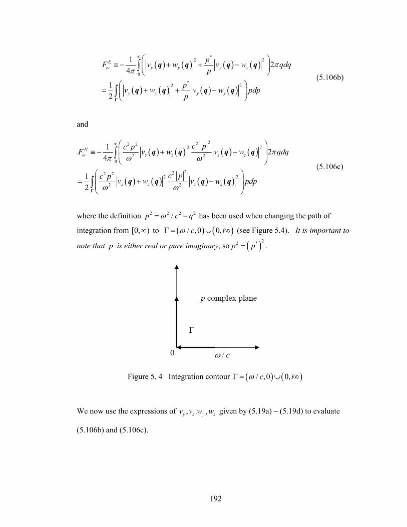
192
( ) ( ) ( ) ( )
( ) ( ) ( ) ( )
*2 2
0
*2 2
1 2 4
1 2
Ey y y y
y y y y
pF v w v w qdqp
pv w v w pdpp
ω ππ
∞
Γ
⎛ ⎞≡ − + + −⎜ ⎟
⎝ ⎠⎛ ⎞
= + + −⎜ ⎟⎝ ⎠
∫
∫
q q q q
q q q q (5.106b)
and
( ) ( ) ( ) ( )
( ) ( ) ( ) ( )
222 22 2
2 20
222 22 2
2 2
1 2 4
1 2
Hz z z z
z z z z
c pc pF v w v w qdq
c pc p v w v w pdp
ω ππ ω ω
ω ω
∞
Γ
⎛ ⎞≡ − ⎜ + − ⎟
⎜ ⎟⎝ ⎠
⎛ ⎞= ⎜ + − ⎟
⎜ ⎟⎝ ⎠
∫
∫
q q q q
q q q q
(5.106c)
where the definition 2 2 2 2/p c qω= − has been used when changing the path of
integration from [0, )∞ to ( ) ( )/ ,0 0,c iωΓ = ∪ ∞ (see Figure 5.4). It is important to
note that p is either real or pure imaginary, so ( )22 *p p= .
Figure 5. 4 Integration contour ( ) ( )/ ,0 0,c iωΓ = ∪ ∞
We now use the expressions of , . ,y z y zv v w w given by (5.19a) – (5.19d) to evaluate
(5.106b) and (5.106c).
193
( ) ( )
( ) ( )
21
1 2 22 2 21
22 1 1 2 2
2
1 ipl ipl zz z
x
zx
x
gv w s e s p e s pc k s
gs s p s p dkk s
ω∞−
−∞
⎧⎡ ⎤± = − + −⎨ ⎣ ⎦′Δ −⎩
⎫+ − +⎡ ⎤ ⎬⎣ ⎦ − ⎭
∫ m
m
(5.107)
We compute 2z zv w± using ( ) ( ) ( )*
34i x j x ik x xAg k g k k kα β αβ
ε δ δ δπ
′′′ ′= − , with , 1,2i j = ,
, , ,x y zα β = :
( ) ( ) 22 11 2 2 23 2 24 12
242 2
2 23 2 22
41
44
ipl ipl x
x
z zx
x
dkAs e s p e s pk s
v wc dkAs p
k s
επω
επ
∞−
−∞
∞
−∞
⎧ ⎫′′+ − −⎪ ⎪
−⎪ ⎪⎪ ⎪+ = ⎨ ⎬′ ′′Δ ⎪ ⎪+⎪ ⎪−⎪ ⎪⎩ ⎭
∫
∫ (5.108)
( ) ( ) 22 11 2 2 23 2 24 12
242 2
1 2 23 2 22
41
44
ipl ipl x
x
z zx
x
dkAs e s p e s pk s
v wc dkAs s
k s
επω
επ
∞−
−∞
∞
−∞
⎧ ⎫′′+ + −⎪ ⎪
−⎪ ⎪⎪ ⎪− = ⎨ ⎬′ ′′Δ ⎪ ⎪+⎪ ⎪−⎪ ⎪⎩ ⎭
∫
∫ (5.109)
The integrals over xk in (5.108-109) can be evaluated using elementary contour
integration techniques and is found to be
( )2 2 *2 21
x
x
dk is s sk s
π∞
−∞
=−−
∫ . (5.110)
Note that if s is real on the real ω axis (this may occur when ( )ε ω is real on the real
ω axis which would violate one of the properties of a dielectric), then this integral
does not exist. Using (5.110) and (5.108) – (5.109),
194
( ) ( )
( ) ( )
2 22
2
2 2 2 21 22 222 2 * *
1 1 2 2
1 44
z z
ipl ipl
c p v w
i iA p e s p e s p pc s s s s
ωε εω
π−
+
⎧ ⎫⎡ ⎤′′ ′′⎪ ⎪= + − − +⎨ ⎬⎢ ⎥− −′Δ ⎪ ⎪⎣ ⎦⎩ ⎭
q q (5.111)
( ) ( )
( ) ( )
222
2
222 21 2
2 2 122 2 * *1 1 2 2
1 44
z z
ipl ipl
c pv w
p i iA e s p e s p sc s s s s
ωω ε ε
π−
−
⎧ ⎫⎡ ⎤′′ ′′⎪ ⎪= + + − +⎨ ⎬⎢ ⎥− −′Δ ⎪ ⎪⎣ ⎦⎩ ⎭
q q (5.112)
By definition,
22 2
2i
is qc
ω ε= − , (5.113)
The complex conjugate of (5.113) is
2 *
*2 22
iis q
cω ε
= − (5.114)
Subtracting (5.114) from (5.113) gives:
2 2 *2 *2
2 2i i
i is sc c
ω ε ω ε− = − (5.115a)
then
( )*2
2* 2i i
i i
s sics s
ε ω′′ +=
− (5.115b)
It is important to note that (5.116) is valid only if ( ) 0iε ω′′ > for real ω so
( )* 0i is s− ≠ according (5.113). If this is not true that we will have division by zero
which is not allowed. This is important because using this relation allows the final
result (i.e., vdw force, see below) to depend only on the dielectric function ( )iε ω .
195
Therefore, one may be tempted to claim that vdw force exist even if ( )0 0iε ω′′ > =
which is not true in Lifshitz’s theory [1, 3]. For example, various authors [8 – 10]
have computed vdw interaction using dielectric functions of the form:
2 21
( ) 1( )
Mk
k k
cε ωω ω=
= +−∑ (5.116a)
2 21
( ) 1( )
Mk
k k
ciε ωω ω=
= ++∑ (5.116b)
where M is a positive integer, ,k kc ω are real material constants. Note that
( ) 0ε ω′′ = on the real ω axis so this material does not satisfy the requirements of
Lifshitz’s theory. Furthermore, this material also violated the Kramer-Kronig relation.
In particular, it also has simple poles on the real axis. As Landau and Lifshitz [1]
pointed out,”the function ( )ε ω has no singularity on the real ω axis, except
possibility at the origin, (where, for metals, ( )ε ω has a simple pole)”.
Substitute (5.116) into (5.111) and (5.112),
( ) ( ) ( ) ( )* *2 2 2 22 21 1 2 2
2 222 2 44 2 2
ipl iplz z
s s s sc p A pv w e s p e s p pω π
−⎧ ⎫⎡ ⎤+ +⎪ ⎪+ = + − − +⎨ ⎬⎢ ⎥′Δ ⎪ ⎪⎣ ⎦⎩ ⎭q q
(5.117)
( ) ( ) ( ) ( )2 22 * *22 21 1 2 2
2 2 122 2 44 2 2
ipl iplz z
c p p s s s sAv w e s p e s p sω π
−⎧ ⎫⎡ ⎤+ +⎪ ⎪− = + + − +⎨ ⎬⎢ ⎥′Δ ⎪ ⎪⎣ ⎦⎩ ⎭q q
(5.118)
Let ( )2ipla e s p−= + and ( )2
iplb e s p= − , adding (5.117) to (5.118) gives
196
( ) ( ) ( ) ( )
( )
( )( ) ( )( ){ } ( )
( )( )
222 22 2
2 2
* *2 2 2 2 22 21 1 2 2
122
2 2 2 2 2 22 2 *2 2 1 1
222 2 2 *
1 2 2
1 44 2 2
11 2
2
z z z z
c pc p v w v w
s s s sA p a b p a b p s p
p p s p p p s p s sA
p s p s s
ω ω
π
π
+ + −
⎧ ⎫+ +⎡ ⎤= + + − + +⎨ ⎬⎣ ⎦′Δ ⎩ ⎭
⎧ ⎫⎡ ⎤+ + + − − +⎪ ⎪⎢ ⎥⎪ ⎪⎣ ⎦= ⎨ ⎬′Δ ⎪ ⎪+ + +⎪ ⎪⎩ ⎭
q q q q
(5.119) 9
To proceed further, we prove the following identity:
( )( ) ( )( ) ( ) ( )( )
( )( ) ( )( )
2 2 2 2 2 2 2 22 2 * 2 *2 2 1 1 1 2 22
1 2 1 2
1 12
12
ipl ipl
p p s p p p s p s s p s p s s
e s p s p e s p s pp
⎡ ⎤+ + + − − + + + +⎣ ⎦′Δ
⎛ ⎞⎡ ⎤− − − −⎜ ⎟= − − ⎢ ⎥′ ′⎜ ⎟Δ Δ⎣ ⎦⎝ ⎠
(5.120)
As we note earlier, p is either real or purely imaginary. Consider first the case where p is real, which implies that 2 2p p= . We need to prove
( )( ) ( )( ){ }( )( ) ( )( )
22 22 * 2 *
2 1 1 1 2 22
1 2 1 212
ipl ipl
p s p s s s p s s
e s p s p e s p s pp
+ + + + +′Δ
⎛ ⎞− − − −⎜ ⎟= − −⎜ ⎟′ ′Δ Δ⎝ ⎠
(5.121)
9 ( )( ) ( )( )2 2 2 2 2 2 22 2 2 * *p a b p a b p p a b p p a b ab+ + − = + + + − +
( ) ( ) ( ) ( ) ( ) ( )( )( )( ) ( ) ( )( )
( )( ) ( )( ){ }
2 22 22 2 *2 2 2 2
2 2 2 22 22 2 2
2 2 2 2 2 22 22 2
* * . .
2 * * . .
2
ip l iplp p s p s p p p e s p e s p c c
p p s p p p s p s p c c
p p s p p p s p
⎡ ⎤= + + + − + − + − +⎣ ⎦
= + + + − + − +⎡ ⎤⎣ ⎦
= + + + − −
where . .c c stands for the complex conjugate of the expression in front of it inside the bracket. Note that 1ip l iple e
∗
= if p is pure imaginary. Note that if p is real, then 2 2 1p p− = so the second term in these expressions is also zero. In other words, the equality is valid whether p is real or pure imaginary.
197
Let ( )( )1 2iplc e s p s p= − − and ( )( )1 2
ipld e s p s p−= + + , then the R.H.S of (5.121)
becomes
( )( ) ( )( )( )
( )( ) ( )( )( )
2 2 2
2 2
2 21 2 1 22
22 22 * 2 *
2 1 1 1 2 22
2 21 1
2 2 2
12
cd cd c cd cd c c dp c c p pd c d c c d c d
p s p s p s p s p
p s p s s s p s s
⎛ ⎞+ − + − + −⎛ ⎞+ + = ⎜ + ⎟ =⎜ ⎟ ⎜ ⎟− −⎝ ⎠ − −⎝ ⎠
= + + − − −′Δ
= + + + + +′Δ
(5.122)
This completes the proof of (5.120) for the case of real p . The same procedure can be
used to show that (5.120) is also true for pure imaginary p . Substituting (5.119) and
(5.120) into (5.106c) gives
( )( ) ( )( )
( )( )( )( )
( )( )( )( )
21 2 1 2
2
1 2
1 2 1 22 2 22
1 2 1 2
1 4 2
1 1 1 1 4 2
ipl iplH
ipl ipl
e s p s p e s p s pA pF dp
s p s p s p s pA e e p dps p s p s p s p
ω π
π
Γ
−
− −
Γ
⎛ ⎞− − − −⎜ ⎟= − −⎜ ⎟′ ′Δ Δ⎝ ⎠
⎛ ⎞⎡ ⎤ ⎡ ⎤+ + + +⎜ ⎟= + − + −⎢ ⎥ ⎢ ⎥⎜ ⎟− − − −⎣ ⎦ ⎣ ⎦⎝ ⎠
∫
∫(5.123)
Similarly, one can evaluate (5.106b), and the result is
( )( )( )( )
( )( )( )( )
1 1
1 1 2 2 1 1 2 22 2 22
1 1 2 2 1 1 2 2
1 1 1 1 4 2
E ipl ipls p s p s p s pAF e e p dps p s p s p s pω
ε ε ε επ ε ε ε ε
− −
− −
Γ
⎛ ⎞⎡ ⎤ ⎡ ⎤+ + + +⎜ ⎟= + − + −⎢ ⎥ ⎢ ⎥⎜ ⎟− − − −⎣ ⎦ ⎣ ⎦⎝ ⎠∫ (5.124)
Finally, adding (5.123) and (5.124) gives (5.106a) which is the vdw interaction force,
( )( )( )( )
( )( )( )( )
1 1
1 2 1 1 2 22 2 22
1 2 1 1 2 2
1 1 1 . . 8
ipl ipls p s p s p s pAF e e p dp c cs p s p s p s pω
ε επ ε ε
− −
− −
Γ
⎧ ⎫⎡ ⎤ ⎡ ⎤+ + + +⎪ ⎪= − + − + +⎨ ⎬⎢ ⎥ ⎢ ⎥− − − −⎣ ⎦ ⎣ ⎦⎪ ⎪⎩ ⎭∫
(5.125)
198
where 2 coth2 B
ATkω
=h
h and . .c c denotes the complex conjugate of the first term.
Note that a factor ½ is missing in the first term of the equation (2.3) in Lifshitz’s
original paper[3]. Using (5.100), the van der Waals force per unit area is
20
coth ( ) ( )4 2 B
F I I dTkω ω ω ω
π
∞∗⎡ ⎤= +⎣ ⎦∫
h h (5.126)
where
( )( )( )( )
( )( )( )( )
1 1
1 2 1 1 2 22 2 2
1 2 1 1 2 2
( ) 1 1 1 ipl ipls p s p s p s pI e e p dp
s p s p s p s pε ε
ωε ε
− −
− −
Γ
⎧ ⎫⎡ ⎤ ⎡ ⎤+ + + +⎪ ⎪= − + − +⎨ ⎬⎢ ⎥ ⎢ ⎥− − − −⎣ ⎦ ⎣ ⎦⎪ ⎪⎩ ⎭∫
As pointed out by Lifshitz, (5.126) will diverge upon the integration over ω due to the
constant term 1. However, this term is independent of separation l, so it should be
dropped from the expression. This constant term corresponds to self-interactions of
the bodies. After dropping the divergent term 1, (5.126) becomes
( )( )( )( )
( )( )( )( )
1
1 2 2
1 2 22 1
0 1 1 2 2 2
1 1 2 2
1
Re coth2 2
1
ipl
Bipl
s p s pe
s p s pF p dpd
Tk s p s pe
s p s p
ω ωπ ε ε
ε ε
−
−
∞
−Γ
−
⎡ ⎤⎧ ⎫⎡ ⎤+ +⎢ ⎥⎪ ⎪−⎢ ⎥− −⎢ ⎥⎪ ⎪⎛ ⎞ ⎪⎣ ⎦ ⎪= ⎢ ⎥⎨ ⎬⎜ ⎟⎢ ⎥⎝ ⎠ ⎡ ⎤⎪ ⎪+ +
+ −⎢ ⎥⎢ ⎥⎪ ⎪− −⎢ ⎥⎪ ⎪⎣ ⎦⎩ ⎭⎣ ⎦
∫ ∫h h (5.127)
where Re stands for the real part of a complex number. Changing the variables
/p p cω→ and /i is s cω→ , (5.127) becomes:
( )( )( )( )
( )( )( )( )
1
1 2 2 /
1 23 22 3 1
0 1 1 2 2 2 /
1 1 2 2
1
Re coth2 2
1
ipl c
Bipl c
s p s pe
s p s pF p dpd
c Tk s p s pe
s p s p
ω
ω
ωω ωπ ε ε
ε ε
−
−
∞
−
−Γ′
⎧ ⎫⎡ ⎤+ +⎪ ⎪−⎢ ⎥− −⎪ ⎪⎛ ⎞⎪⎣ ⎦ ⎪= ⎨ ⎬⎜ ⎟
⎝ ⎠ ⎡ ⎤⎪ ⎪+ ++ −⎢ ⎥⎪ ⎪− −⎪ ⎪⎣ ⎦⎩ ⎭
∫ ∫h h (5.128)
199
where the contour ′Γ of integration over p is ( ) ( )1,0 0, i′Γ = ∪ ∞ , and
( ) 21i is pε ω= − + (5.129)
Equation (5.128) is not convenient to evaluate numerically because 2 /ipl ce ω− fluctuates
very fast for large ω . To overcome this difficulty, Lifshitz deformed the contour of
integration in theω and p planes so that the integral of p is over real axis and the
integral of ω is on imaginary axis. His procedure is explained below.
Let us break (5.128) into two integrals:
( )1 22 32F I I
cπ= +
h (5.130)
Where
( ) ( )( ) ( )
( ) ( )( ) ( )
1 101 2 1 1 2 23 2 2 / 2 /
11 2 1 1 2 20 1
Re 1 1ipl c ipl cs p s p s p s pI p e e dpd
s p s p s p s pω ωε ε
ω ωε ε
− −∞− −
⎧ ⎫⎡ ⎤ ⎡ ⎤+ + + +⎪ ⎪= − + −⎨ ⎬⎢ ⎥ ⎢ ⎥− − − −⎣ ⎦ ⎣ ⎦⎪ ⎪⎩ ⎭∫∫
(5.131)
( )( )( )( )
( )( )( )( )
1 1
1 2 1 1 2 23 2 2 / 2 /2
1 2 1 1 2 20 0
Re 1 1i
ipl c ipl cs p s p s p s pI p e e dpd
s p s p s p s pω ωε ε
ω ωε ε
− −∞ ∞− −
⎧ ⎫⎡ ⎤ ⎡ ⎤+ + + +⎪ ⎪= − + −⎨ ⎬⎢ ⎥ ⎢ ⎥− − − −⎣ ⎦ ⎣ ⎦⎪ ⎪⎩ ⎭∫ ∫
(5.132)
First, we note that the iε ’s are analytic in the upper half ω plane. The contour in the
ω integral in (5.131) can be deformed from (0, )∞ to (0, )i∞ as long as
(i) We can switch the order of integration which is true here.
(ii) The integrand of (5.131) is analytic in the first quadrant in the complex ω
plane and continuous on the positive real and imaginaryω axis.
200
(iii) The integrand along the circular arc ie θω ( 0 / 2θ π= → ) vanishes faster
than1/ ω as ω → ∞ .
These conditions will be demonstrated below. Assuming this is the case, we
can use residue theorem to transform (5.131) to
( ) ( )( ) ( )
( ) ( )( ) ( )
1 101 2 1 1 2 23 2 2 / 2 /
11 2 1 1 2 20 1
1 1i
ipl c ipl cs p s p s p s pI p e e dpd
s p s p s p s pω ωε ε
ω ωε ε
− −∞− −
⎧ ⎫⎡ ⎤ ⎡ ⎤+ + + +⎪ ⎪= − + −⎨ ⎬⎢ ⎥ ⎢ ⎥− − − −⎣ ⎦ ⎣ ⎦⎪ ⎪⎩ ⎭∫ ∫ (5.133)
Note that ( )iε ω , ( )is ω and 3dω ω are real on the imaginary ω axis, in addition, p is
real, so we can dropped the Re in (5.133).
Condition (iii) is straightforward since 2 /ipl ce ω− increases exponentially fast
as ω → ∞ for ( )Im 0ω > . Also, for any finite p, since ( )is pω → ∞ →
( )( )( )( )
( )( )( )( )
1 1 2 2 1 2
1 1 2 2 1 2
s p s p s p s ps p s p s p s p
ε εε ε
+ + + +→ → ∞
− − − −
Therefore, the integrand goes to zero faster than 1/ ω as ω → ∞ . Next, we show on
(ii). From (5.129) and the property of dielectric function ( )ε ω , ( ( ) 0ε ω′′ >
everywhere except on imaginary axis, and on positive imaginary axis including origin,
( )ε ω decreases from ( )0 1ε > to 1 at infinity, see end of section 5.4),
( ) 21i i i is p s isε ω ′ ′′= − + = + ( ( )0,1p ∈ ) (5.134)
is non-zero everywhere in the first quadrant as well as the positive real axis and upper
imaginary axis of complex ω plane so that there is no branch point. Indeed,
( ) ( )( ) ( )2 21 1i i ip p iε ω ε ω ε ω′ ′′− + = − + + . (5.135)
201
Since ( ) 0ε ω′′ > is positive in the first quadrant, the square root of ( ) 21i pε ω − + must
have positive real and imaginary parts, i.e., 0is ′ > and 0is ′′ > .
To show that the integrand of (5.133) has no pole in the first quadrant, we note that, for ( )0,1p ∈
( )1 2 22 / 2 /2 / 1ipl i c pl cipl ce e eω ω ωω + −= = < (5.136)
Next, we show that
( )( )( )( )
1 2
1 2
1s p s ps p s p
+ +>
− −, (5.137)
in the first quadrant. Note that
( )( )
( )( )
22
22
( )( ) 1( ) ( )
i i ii i
i i i i
s p s p ss p iss p s p is s p s
′ ′′+ + +′ ′′+ += = >
′ ′′− − + ′ ′′− + since 0, 0is p′ > > (5.138a)
So
( )( )( )( )
( )( )
( )( )
1 2 1 2
1 2 1 2
1s p s p s p s ps p s p s p s p
+ + + += >
− − − − (5.138b)
Equations (5.136 – 5.138) imply that
( )( ) ( )( ) 2 /1 2 1 2/ 0ipl cs p s p s p s p e ω+ + − − − = (5.139)
cannot have a root in the first quadrant of the ω plane. This means that
( )( )( )( )
1
1 2 2 /
1 2
1ipl cs p s pe
s p s pω
−
−⎡ ⎤+ +−⎢ ⎥− −⎣ ⎦
(5.140)
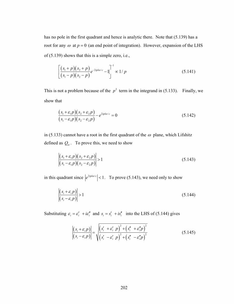
202
has no pole in the first quadrant and hence is analytic there. Note that (5.139) has a
root for any ω at 0p = (an end point of integration). However, expansion of the LHS
of (5.139) shows that this is a simple zero, i.e.,
( )( )( )( )
1
1 2 2 /
1 2
1 1/ipl cs p s pe p
s p s pω
−
−⎡ ⎤+ +− ∝⎢ ⎥− −⎣ ⎦
(5.141)
This is not a problem because of the 2p term in the integrand in (5.133). Finally, we
show that
( )( )( )( )
1 1 2 2 2 /
1 1 2 2
0ipl cs p s pe
s p s pωε ε
ε ε+ +
− =− −
(5.142)
in (5.133) cannot have a root in the first quadrant of the ω plane, which Lifshitz
defined as Qω . To prove this, we need to show
( )( )( )( )
1 1 2 2
1 1 2 2
1s p s ps p s p
ε εε ε
+ +>
− − (5.143)
in this quadrant since 2 / 1ipl ce ω < . To prove (5.143), we need only to show
( )( )
1i i
i i
s ps p
εε
+>
− (5.144)
Substituting i i iiε ε ε′ ′′= + and i i is s is′ ′′= + into the LHS of (5.144) gives
( )( )
( ) ( )( ) ( )
2 2
2 2i i i ii i
i i i i i i
s p s ps ps p s p s p
ε εεε ε ε
′ ′ ′′ ′′+ + ++=
− ′ ′ ′′ ′′− + − (5.145)
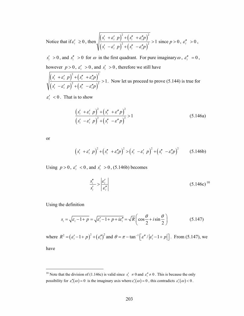
203
Notice that if 0iε ′ ≥ , then( ) ( )( ) ( )
2 2
2 2 1i i i i
i i i i
s p s p
s p s p
ε ε
ε ε
′ ′ ′′ ′′+ + +>
′ ′ ′′ ′′− + − since 0p > , 0iε ′′ > ,
0is′ > , and 0is′′ > for ω in the first quadrant. For pure imaginaryω , 0iε ′′ = ,
however 0p > , 0iε ′ > , and 0is′ > , therefore we still have
( ) ( )( ) ( )
2 2
2 2 1i i i i
i i i i
s p s p
s p s p
ε ε
ε ε
′ ′ ′′ ′′+ + +>
′ ′ ′′ ′′− + −. Now let us proceed to prove (5.144) is true for
0iε ′ < . That is to show
( ) ( )( ) ( )
2 2
2 2 1i i i
i i i
s p s p
s p s p
ε ε
ε ε
′ ′ ′′ ′′+ + +>
′ ′ ′′ ′′− + − (5.146a)
or
( ) ( ) ( ) ( )2 2 2 2
i i i i i i i is p s p s p s pε ε ε ε′ ′ ′′ ′′ ′ ′ ′′ ′′+ + + > − + − (5.146b)
Using 0p > , 0iε ′ < , and 0is′ > , (5.146b) becomes
i i
i i
ss
εε
′′ ′>
′ ′′ (5.146c) 10
Using the definition
1 1 cos sin2 2i i i is p p i R iθ θε ε ε ⎛ ⎞′ ′′= − + = − + + = +⎜ ⎟
⎝ ⎠ (5.147)
where ( ) ( )2 22 1i iR pε ε′ ′′= − + + and 1tan / 1i pθ π ε ε− ′′ ′= − ⎡ − + ⎤⎣ ⎦ . From (5.147), we
have
10 Note that the division of (1.146c) is valid since 0is′ ≠ and 0iε ′′≠ . This is because the only possibility for ( ) 0iε ω′′ = is the imaginary axis where ( ) 0iε ω′ = , this contradicts ( ) 0iε ω′ < .
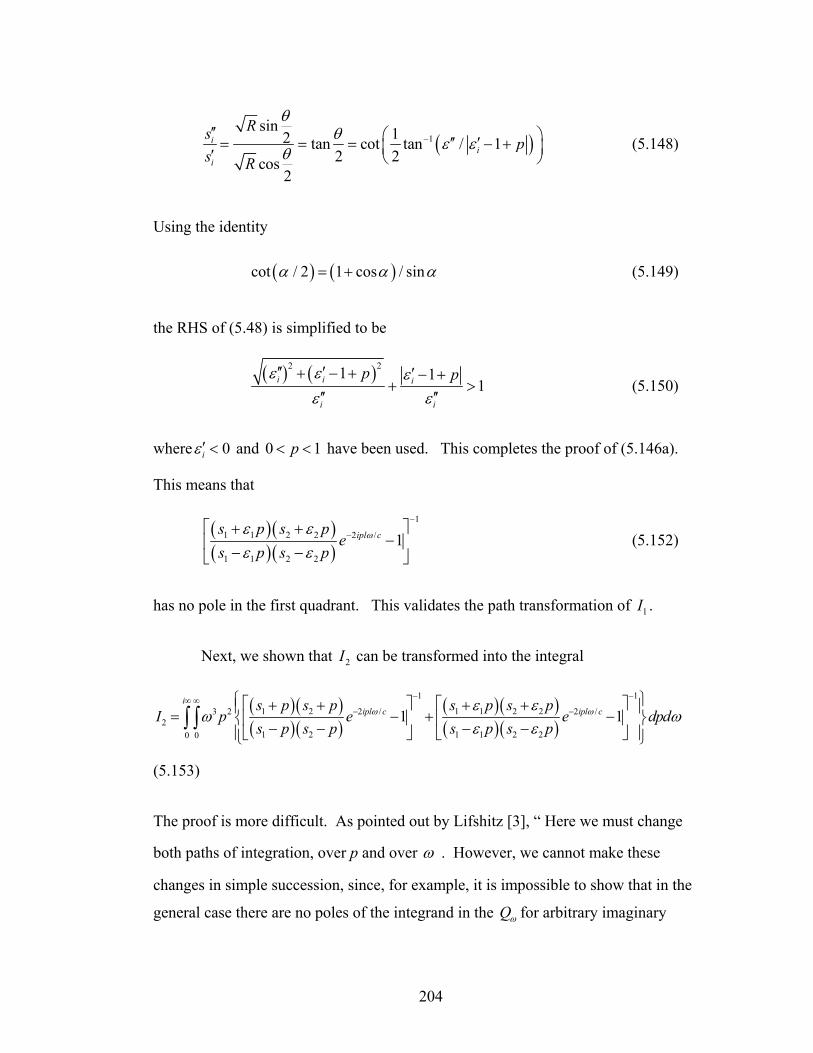
204
( )1sin 12 tan cot tan / 1
2 2cos2
ii
i
Rs ps R
θθ ε εθ
−′′ ⎛ ⎞′′ ′= = = − +⎜ ⎟′ ⎝ ⎠ (5.148)
Using the identity
( ) ( )cot / 2 1 cos / sinα α α= + (5.149)
the RHS of (5.48) is simplified to be
( ) ( )2 21 11i i i
i i
p pε ε εε ε
′′ ′+ − + ′ − ++ >
′′ ′′ (5.150)
where 0iε ′ < and 0 1p< < have been used. This completes the proof of (5.146a).
This means that
( )( )( )( )
1
1 1 2 2 2 /
1 1 2 2
1ipl cs p s pe
s p s pωε ε
ε ε
−
−⎡ ⎤+ +−⎢ ⎥− −⎣ ⎦
(5.152)
has no pole in the first quadrant. This validates the path transformation of 1I .
Next, we shown that 2I can be transformed into the integral
( )( )( )( )
( )( )( )( )
1 1
1 2 1 1 2 23 2 2 / 2 /2
1 2 1 1 2 20 0
1 1i
ipl c ipl cs p s p s p s pI p e e dpd
s p s p s p s pω ωε ε
ω ωε ε
− −∞ ∞− −
⎧ ⎫⎡ ⎤ ⎡ ⎤+ + + +⎪ ⎪= − + −⎨ ⎬⎢ ⎥ ⎢ ⎥− − − −⎣ ⎦ ⎣ ⎦⎪ ⎪⎩ ⎭∫ ∫
(5.153)
The proof is more difficult. As pointed out by Lifshitz [3], “ Here we must change
both paths of integration, over p and over ω . However, we cannot make these
changes in simple succession, since, for example, it is impossible to show that in the
general case there are no poles of the integrand in the Qω for arbitrary imaginary
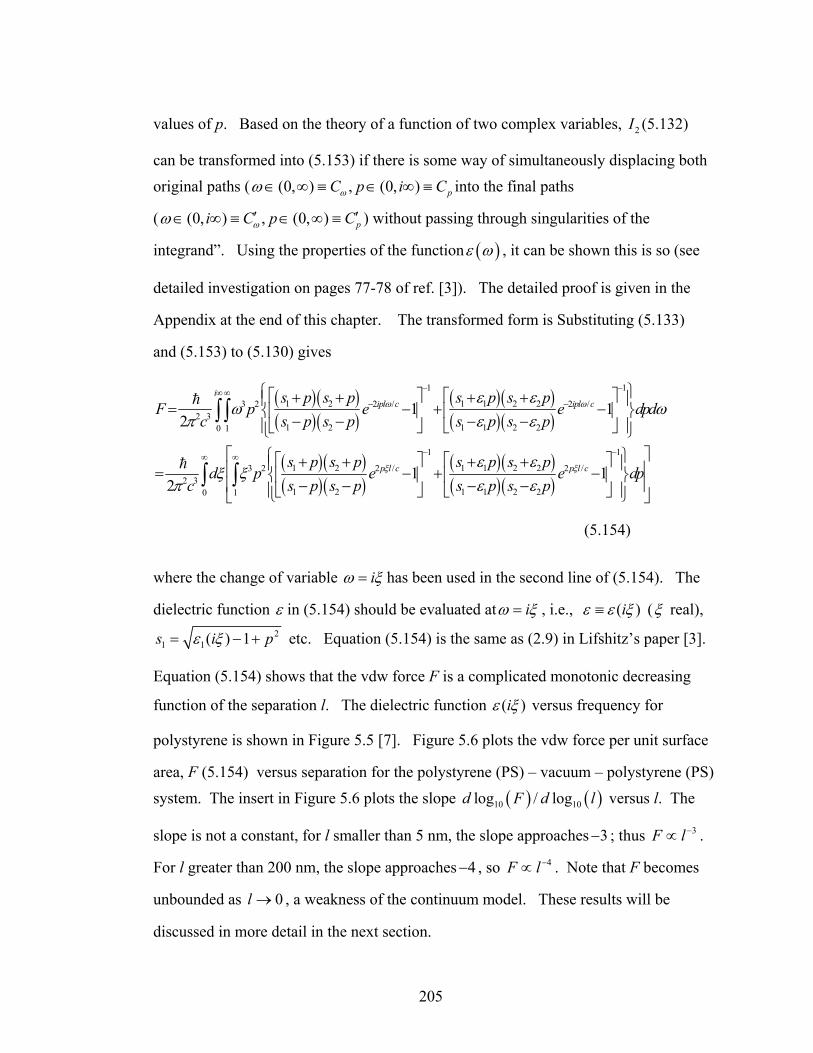
205
values of p. Based on the theory of a function of two complex variables, 2I (5.132)
can be transformed into (5.153) if there is some way of simultaneously displacing both original paths ( (0, ) , (0, ) pC p i Cωω ∈ ∞ ≡ ∈ ∞ ≡ into the final paths
( (0, ) , (0, ) pi C p Cωω ′ ′∈ ∞ ≡ ∈ ∞ ≡ ) without passing through singularities of the
integrand”. Using the properties of the function ( )ε ω , it can be shown this is so (see
detailed investigation on pages 77-78 of ref. [3]). The detailed proof is given in the
Appendix at the end of this chapter. The transformed form is Substituting (5.133)
and (5.153) to (5.130) gives
( ) ( )( ) ( )
( )( )( )( )
( ) ( )( ) ( )
( ) ( )( ) ( )
1 1
1 2 1 1 2 23 2 2 / 2 /2 3
1 2 1 1 2 20 1
1 1
1 2 1 1 2 23 2 2 / 2 /2 3
1 2 1 1 2 2
1 12
1 12
iipl c ipl c
p l c p l c
s p s p s p s pF p e e dpd
c s p s p s p s p
s p s p s p s pd p e e
c s p s p s p s p
ω ω
ξ ξ
ε εω ω
π ε ε
ε εξ ξ
π ε ε
− −∞ ∞− −
− −
⎧ ⎫⎡ ⎤ ⎡ ⎤+ + + +⎪ ⎪= − + −⎨ ⎬⎢ ⎥ ⎢ ⎥− − − −⎣ ⎦ ⎣ ⎦⎪ ⎪⎩ ⎭
⎡ ⎤ ⎡ ⎤+ + + += − + −⎢ ⎥ ⎢ ⎥− − − −⎣ ⎦ ⎣ ⎦
∫ ∫h
h
0 1
dp∞ ∞⎡ ⎤⎧ ⎫⎪ ⎪⎢ ⎥⎨ ⎬⎢ ⎥⎪ ⎪⎩ ⎭⎣ ⎦∫ ∫
(5.154)
where the change of variable iω ξ= has been used in the second line of (5.154). The
dielectric function ε in (5.154) should be evaluated at iω ξ= , i.e., ( )iε ε ξ≡ (ξ real), 2
1 1( ) 1s i pε ξ= − + etc. Equation (5.154) is the same as (2.9) in Lifshitz’s paper [3].
Equation (5.154) shows that the vdw force F is a complicated monotonic decreasing
function of the separation l. The dielectric function ( )iε ξ versus frequency for
polystyrene is shown in Figure 5.5 [7]. Figure 5.6 plots the vdw force per unit surface
area, F (5.154) versus separation for the polystyrene (PS) – vacuum – polystyrene (PS) system. The insert in Figure 5.6 plots the slope ( ) ( )10 10log / logd F d l versus l. The
slope is not a constant, for l smaller than 5 nm, the slope approaches 3− ; thus 3F l−∝ .
For l greater than 200 nm, the slope approaches 4− , so 4F l−∝ . Note that F becomes
unbounded as 0l → , a weakness of the continuum model. These results will be
discussed in more detail in the next section.
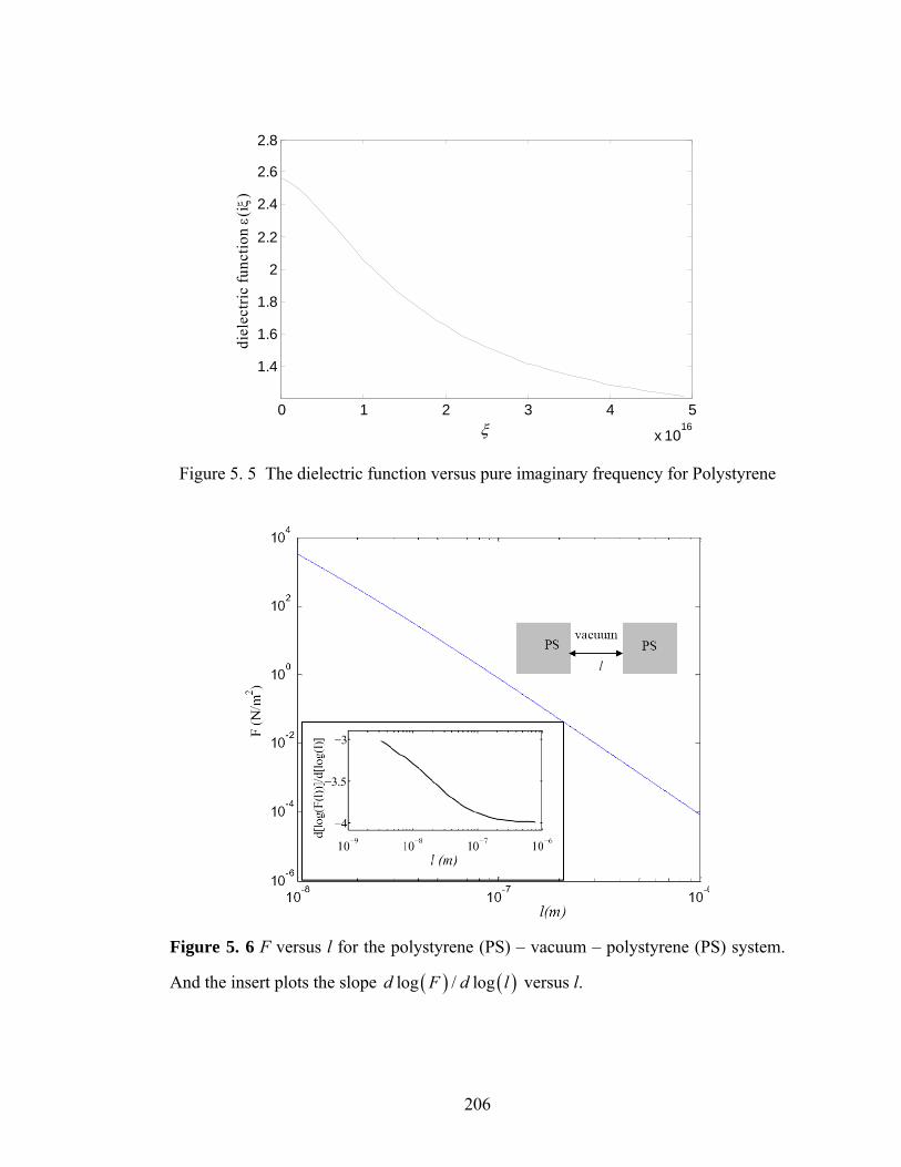
206
0 1 2 3 4 5
x 1016
1.4
1.6
1.8
2
2.2
2.4
2.6
2.8
ξ
diel
ectri
c fu
nctio
n ε(
iξ)
Figure 5. 5 The dielectric function versus pure imaginary frequency for Polystyrene
Figure 5. 6 F versus l for the polystyrene (PS) – vacuum – polystyrene (PS) system.
And the insert plots the slope ( ) ( )log / logd F d l versus l.
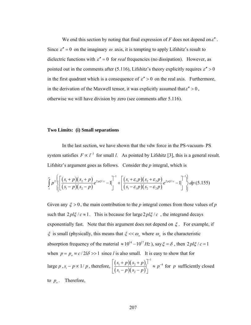
207
We end this section by noting that final expression of F does not depend onε ′′ .
Since 0ε ′′ = on the imaginary ω axis, it is tempting to apply Lifshitz’s result to
dielectric functions with 0ε ′′ = for real frequencies (no dissipation). However, as
pointed out in the comments after (5.116), Lifshitz’s theory explicitly requires 0ε ′′ >
in the first quadrant which is a consequence of 0ε ′′ > on the real axis. Furthermore,
in the derivation of the Maxwell tensor, it was explicitly assumed that 0ε ′′ > ,
otherwise we will have division by zero (see comments after 5.116).
Two Limits: (i) Small separations
In the last section, we have shown that the vdw force in the PS-vacuum- PS
system satisfies 3F l−∝ for small l. As pointed by Lifshitz [3], this is a general result.
Lifshitz’s argument goes as follows. Consider the p integral, which is
( )( )( )( )
( )( )( )( )
1 1
1 2 1 1 2 22 2 / 2 /
1 2 1 1 2 21
1 1p l c p l cs p s p s p s pp e e dp
s p s p s p s pξ ξε ε
ε ε
− −∞ ⎧ ⎫⎡ ⎤ ⎡ ⎤+ + + +⎪ ⎪− + −⎨ ⎬⎢ ⎥ ⎢ ⎥− − − −⎣ ⎦ ⎣ ⎦⎪ ⎪⎩ ⎭∫ (5.155)
Given any 0ξ > , the main contribution to the p integral comes from those values of p
such that 2 / 1pl cξ ≈ . This is because for large 2 /pl cξ , the integrand decays
exponentially fast. Note that this argument does not depend on ξ . For example, if
ξ is small (physically, this means that oξ ω<< where oω is the characteristic
absorption frequency of the material 14 1710 10 Hz≈ − ), sayξ δ= , then 2 / 1pl cξ =
when / 2 1op p c lδ= ≡ >> since l is also small. It is easy to show that for
large p , 1/is p p− ∝ , therefore, ( )( )( )( )
1
1 2 4
1 2
s p s pp
s p s p
−
−⎡ ⎤+ +≈⎢ ⎥− −⎣ ⎦
for p sufficiently closed
to op . Therefore,
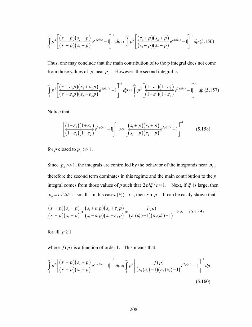
208
( )( )( )( )
( )( )( )( )
1 1
1 2 1 22 2 / 2 2 /
1 2 1 21 1
1 1op
p l c p l cs p s p s p s pp e dp p e dp
s p s p s p s pξ ξ
− −∞ ⎡ ⎤ ⎡ ⎤+ + + +− ≈ −⎢ ⎥ ⎢ ⎥− − − −⎣ ⎦ ⎣ ⎦
∫ ∫ (5.156)
Thus, one may conclude that the main contribution of to the p integral does not come
from those values of p near op . However, the second integral is
( )( )( )( )
( )( )( )( )
1 1
1 1 2 2 1 22 2 / 2 2 /
1 1 2 2 1 21 1
1 11 1
1 1
opp l c p l cs p s p
p e dp p e dps p s p
ξ ξε ε ε εε ε ε ε
− −∞ ⎡ ⎤ ⎡ ⎤+ + + +− ≈ −⎢ ⎥ ⎢ ⎥− − − −⎣ ⎦ ⎣ ⎦
∫ ∫ (5.157)
Notice that
( )( )( )( )
( )( )( )( )
1 1
1 2 1 22 / 2 /
1 2 1 2
1 11 1
1 1p l c p l cs p s p
e es p s p
ξ ξε εε ε
− −⎡ ⎤ ⎡ ⎤+ + + +
− >> −⎢ ⎥ ⎢ ⎥− − − −⎣ ⎦ ⎣ ⎦ (5.158)
for p closed to 1op >> .
Since 1op >> , the integrals are controlled by the behavior of the integrands near op ,
therefore the second term dominates in this regime and the main contribution to the p
integral comes from those values of p such that 2 / 1pl cξ ≈ . Next, if ξ is large, then
/ 2op c lξ≡ is small. In this case ( ) 1iε ξ → , then s p≈ . It can be easily shown that
( )( )( )( )
( )( )( )( ) ( )( )
1 2 1 1 2 2
1 2 1 1 2 2 1 2
( )( ) 1 ( ) 1
s p s p s p s p f ps p s p s p s p i i
ε εε ε ε ξ ε ξ
+ + + +≈ ≈ → ∞
− − − − − − (5.159)
for all 1p ≥
where ( )f p is a function of order 1. This means that
( )( )( )( ) ( )( )
1 1
1 22 2 / 2 2 /
1 2 1 21 1
( )1 1( ) 1 ( ) 1
p l c p l cs p s p f pp e dp p e dps p s p i i
ξ ξ
ε ξ ε ξ
− −∞ ∞⎡ ⎤ ⎡ ⎤+ +− ≈ −⎢ ⎥ ⎢ ⎥− − − −⎣ ⎦ ⎣ ⎦
∫ ∫
(5.160)
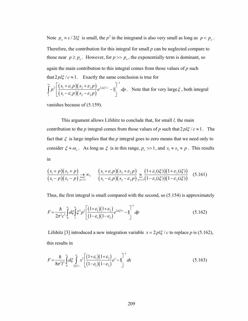
209
Note / 2op c lξ≡ is small, the 2p in the integrand is also very small as long as op p< .
Therefore, the contribution for this integral for small p can be neglected compare to
those near op p≥ . However, for op p>> , the exponentially term is dominant, so
again the main contribution to this integral comes from those values of p such
that 2 / 1pl cξ ≈ . Exactly the same conclusion is true for
( )( )( )( )
1
1 1 2 22 2 /
1 1 2 21
1p l cs p s pp e dp
s p s pξε ε
ε ε
−∞ ⎡ ⎤+ +−⎢ ⎥− −⎣ ⎦
∫ . Note that for very largeξ , both integral
vanishes because of (5.159).
This argument allows Lifshitz to conclude that, for small l, the main
contribution to the p integral comes from those values of p such that 2 / 1pl cξ ≈ . The
fact that ξ is large implies that the p integral goes to zero means that we need only to
consider oξ ω≈ . As long as ξ is in this range, 1op >> , and 1 2s s p≈ ≈ . This results
in
( )( )( )( ) {
( )( )( )( ) {
( )( )( )( )
1 2 1 1 2 2 1 2
111 2 1 1 2 2 1 2
1 ( ) 1 ( ),
1 ( ) 1 ( )pp
s p s p s p s p i is p s p s p s p i i
ε ε ε ξ ε ξε ε ε ξ ε ξ>>>>
+ + + + + +→ ∞ ≈
− − − − − − (5.161)
Thus, the first integral is small compared with the second, so (5.154) is approximately
( )( )( )( )
1
1 23 2 2 /2 3
1 20 1
1 11
2 1 1p l cF d p e dp
cξε ε
ξ ξπ ε ε
−∞ ∞ ⎡ ⎤+ += −⎢ ⎥− −⎣ ⎦
∫ ∫h (5.162)
Lifshitz [3] introduced a new integration variable 2 /x pl cξ= to replace p is (5.162),
this results in
( )( )( )( )
1
1 232 3
1 20 2 /
1 11
8 1 1x
l c
F d x e dxl ξ
ε εξ
π ε ε
−∞ ∞ ⎡ ⎤+ += −⎢ ⎥− −⎣ ⎦
∫ ∫h (5.163)
210
where ( )i i iε ε ξ= . For small l, 2 / 0l cξ → so the lower limit in the x integral can be
replaced by 0, resulting in
( )( )( )( )
1
1 232 3
1 20 0
1 11
8 1 1xF d x e dx
lε ε
ξπ ε ε
−∞ ∞ ⎡ ⎤+ += −⎢ ⎥− −⎣ ⎦
∫ ∫h (5.164)
Since the integral is independent of l, (5.164) implies that for small separation, the
interaction force is inversely proportional to the cube of the separation, that is
13F
lγ
≈ (5.165a)
where
( )( )( )( )
1
1 231 2
1 20 0
1 11
8 1 1xd x e dx
ε εγ ξ
π ε ε
−∞ ∞ ⎡ ⎤+ += −⎢ ⎥− −⎣ ⎦
∫ ∫h (5.165b)
Large separation
For large separation ( / ol c ω>> ), Lifshitz [3] introduced a new integration
variable 2 /x pl cξ= to replaceξ . Using this substitution, (5.154) is
( )( )( )( )
( )( )( )( )
1 131 2 1 1 2 2
2 4 21 2 1 1 2 20 1
1 132
x xs p s p s p s pc xF dx e e dpl p s p s p s p s p
ε επ ε ε
− −∞ ∞⎡ ⎤⎧ ⎫⎡ ⎤ ⎡ ⎤+ + + +⎪ ⎪⎢ ⎥= − + −⎨ ⎬⎢ ⎥ ⎢ ⎥− − − −⎢ ⎥⎣ ⎦ ⎣ ⎦⎪ ⎪⎩ ⎭⎣ ⎦∫ ∫
h (5.166)
where
( )/ 2i i ixc plε ε= (5.167a)
( ) 2/ 2 1i is ixc pl pε= − + (5.167b)
211
As discussed before, the behavior of the x integral is concentrated near x = 1, so larger
value of x need not be considered. For 1x ≈ and / ol c ω>> , / 2 1oxc plω << (note p >
1). In this regime, 0i iε ε≈ , where 0iε is the static dielectric constant at zero
frequency. With this approximation, (5.166) becomes
( )( )( )( )
( )( )( )( )
1 1310 20 10 10 20 20
2 4 210 20 10 10 20 200 1
1 132
x xs p s p s p s pc xF dx e e dpl p s p s p s p s p
ε επ ε ε
− −∞ ∞⎡ ⎤⎧ ⎫⎡ ⎤ ⎡ ⎤+ + + +⎪ ⎪⎢ ⎥= − + −⎨ ⎬⎢ ⎥ ⎢ ⎥− − − −⎢ ⎥⎣ ⎦ ⎣ ⎦⎪ ⎪⎩ ⎭⎣ ⎦∫ ∫
h
(5.168)
where 20 0 1i is pε≡ − + . This integral is independent of l so for large separation,
(5.168) states that the vdw force is inversely proportional to the 4th power of l, that is
24F
lγ
= (5.169a)
where
( )( )( )( )
( )( )( )( )
1 1310 20 10 10 20 20
2 2 210 20 10 10 20 200 1
1 132
x xs p s p s p s pc xdx e e dpp s p s p s p s p
ε εγ
π ε ε
− −∞ ∞⎡ ⎤⎧ ⎫⎡ ⎤ ⎡ ⎤+ + + +⎪ ⎪⎢ ⎥≡ − + −⎨ ⎬⎢ ⎥ ⎢ ⎥− − − −⎢ ⎥⎣ ⎦ ⎣ ⎦⎪ ⎪⎩ ⎭⎣ ⎦∫ ∫
h .
Casimir’s result
For a perfect conductor, ( 0)i iε ω → → ∞ (see (5.20d)). This means that
0 ~ ( 0)i is iε ω → → ∞ . Therefore, ( )( )( )( )
( )( )( )( )
10 20 10 10 20 20
10 20 10 10 20 20
1s p s p s p s ps p s p s p s p
ε εε ε
+ + + += =
− − − −,
and equation (5.168) becomes:
( )3 2
2 4 420 116 2401x
c x cF dpdxl lp e
ππ
∞ ∞
= =−∫ ∫
h h (5.170)
212
Equation (5.170) coincides with Casimir’s result for perfect conductor, but only for
large l . It should be pointed out that the limit iε → ∞ is valid only for sufficiently
large separation l because the dielectric function for a conductor goes to infinity only
at zero frequency. This is equivalent to the requirement that / 2xc pl is small
comparing to the resonance frequency of the metal, the typical value of which
is 14~1710 Hz . Due to the presence of xe in the denominators of (5.166), the main
contribution to the x integral comes from ~ 1x , therefore
/ 2 ~ / 2 /xc pl c pl c l< (5.171)
where the second inequality in (5.171) is due to 1p ≥ in (5.166). The condition 14/ 10c l < implies that 63 10 3.0l m mμ−> × = . Thus if the separation is larger than
several microns, iε → ∞ is a good approximation.
213
APPENDIX
We explain the method Lifshitz [3] transformed 2I (5.132) into (5.153). The
first step is to introduce a real positive variable x i pω= − to replaceω in the
integral 2I (recall p is a pure positive imaginary number and ω is real, i.e., 0x > .
This results in
( )( )( )( )
( )( )( )( )
1 13
1 2 1 1 2 22 / 2 /2 2
1 2 1 1 2 20 0
Re 1 1i
lx c lx cs p s p s p s pxI dx e e dpp s p s p s p s p
ε εε ε
− −∞ ∞⎧ ⎫⎧ ⎫⎡ ⎤ ⎡ ⎤+ + + +⎪ ⎪ ⎪ ⎪= − + −⎨ ⎨ ⎬ ⎬⎢ ⎥ ⎢ ⎥− − − −⎣ ⎦ ⎣ ⎦⎪ ⎪ ⎪ ⎪⎩ ⎭⎩ ⎭∫ ∫
(A1)
where ( )1 /i ix pε ε= and ( ) 2/ 1i is ix p pε= − + . For a fixed positive x, the second
step is to shift the integration path from the positive imaginary p axis to the positive
real p axis. That is
( )( )( )( )
( )( )( )( )
1 13
1 2 1 1 2 22 / 2 /2 2
1 2 1 1 2 20 0
Re 1 1lx c lx cs p s p s p s pxI dx e e dpp s p s p s p s p
ε εε ε
− −∞ ∞⎧ ⎫⎧ ⎫⎡ ⎤ ⎡ ⎤+ + + +⎪ ⎪ ⎪ ⎪= − + −⎨ ⎨ ⎬ ⎬⎢ ⎥ ⎢ ⎥− − − −⎣ ⎦ ⎣ ⎦⎪ ⎪ ⎪ ⎪⎩ ⎭⎩ ⎭∫ ∫
(A2a)
The third step is to replace x by x i pω= − in (A2a), and this gives
( ) ( )( ) ( )
( )( )( )( )
1 1
1 2 1 1 2 23 2 2 / 2 /2
1 2 1 1 2 20 0
1 1i
i pl c i pl cs p s p s p s pI d p e e dp
s p s p s p s pω ωε ε
ω ωε ε
− −∞ ∞− −
⎧ ⎫⎡ ⎤ ⎡ ⎤+ + + +⎪ ⎪= − + −⎨ ⎬⎢ ⎥ ⎢ ⎥− − − −⎣ ⎦ ⎣ ⎦⎪ ⎪⎩ ⎭∫ ∫
(A2b)
which is the same as (5.153). Note that the first and the third steps involve only
change of variables, whereas the second step has used the residue theorem which
relies on three assumptions:
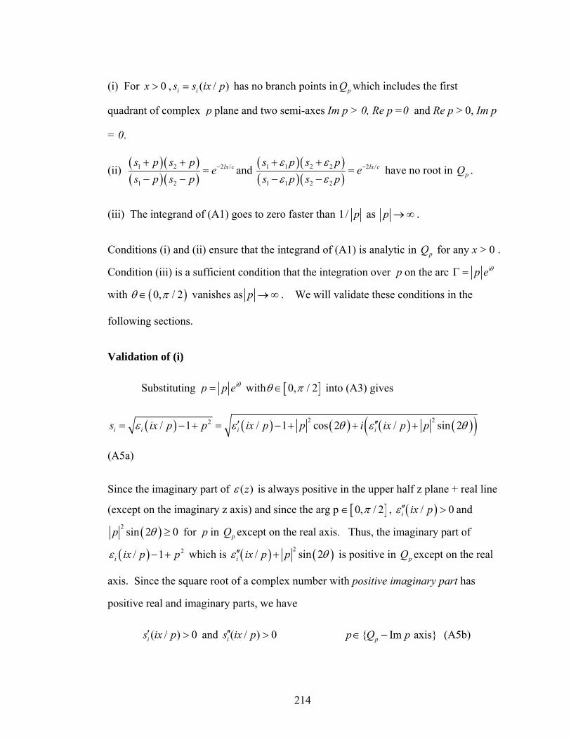
214
(i) For 0x > , ( / )i is s ix p= has no branch points in pQ which includes the first
quadrant of complex p plane and two semi-axes Im p > 0, Re p =0 and Re p > 0, Im p
= 0.
(ii) ( )( )( )( )
1 2 2 /
1 2
lx cs p s pe
s p s p−+ +
=− −
and ( )( )( )( )
1 1 2 2 2 /
1 1 2 2
lx cs p s pe
s p s pε εε ε
−+ +=
− − have no root in pQ .
(iii) The integrand of (A1) goes to zero faster than 1/ p as p → ∞ .
Conditions (i) and (ii) ensure that the integrand of (A1) is analytic in pQ for any x > 0 .
Condition (iii) is a sufficient condition that the integration over p on the arc ip e θΓ =
with ( )0, / 2θ π∈ vanishes as p → ∞ . We will validate these conditions in the
following sections.
Validation of (i)
Substituting ip p e θ= with [ ]0, / 2θ π∈ into (A3) gives
( ) ( ) ( ) ( ) ( )( )2 22/ 1 / 1 cos 2 / sin 2i i i is ix p p ix p p i ix p pε ε θ ε θ′ ′′= − + = − + + +
(A5a)
Since the imaginary part of ( )zε is always positive in the upper half z plane + real line
(except on the imaginary z axis) and since the arg p [ ]0, / 2π∈ , ( )/ 0i ix pε ′′ > and
( )2 sin 2 0p θ ≥ for p in pQ except on the real axis. Thus, the imaginary part of
( ) 2/ 1i ix p pε − + which is ( ) ( )2/ sin 2i ix p pε θ′′ + is positive in pQ except on the real
axis. Since the square root of a complex number with positive imaginary part has
positive real and imaginary parts, we have
( / ) 0is ix p′ > and ( / ) 0is ix p′′ > { Im axis}pp Q p∈ − (A5b)
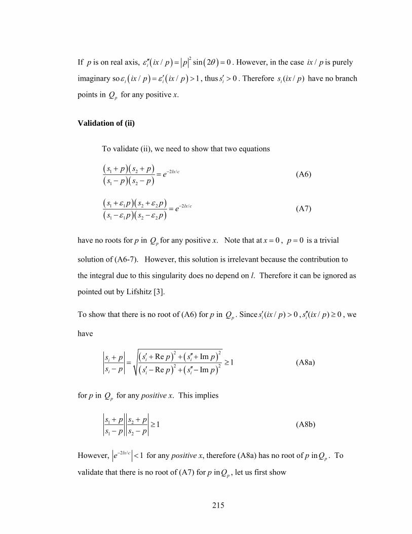
215
If p is on real axis, ( ) ( )2/ sin 2 0i ix p pε θ′′ = = . However, in the case /ix p is purely
imaginary so ( ) ( )/ / 1i iix p ix pε ε ′= > , thus 0is′ > . Therefore ( / )is ix p have no branch
points in pQ for any positive x.
Validation of (ii)
To validate (ii), we need to show that two equations
( )( )( )( )
1 2 2 /
1 2
lx cs p s pe
s p s p−+ +
=− −
(A6)
( )( )( )( )
1 1 2 2 2 /
1 1 2 2
lx cs p s pe
s p s pε εε ε
−+ +=
− − (A7)
have no roots for p in pQ for any positive x. Note that at 0x = , 0p = is a trivial
solution of (A6-7). However, this solution is irrelevant because the contribution to
the integral due to this singularity does no depend on l. Therefore it can be ignored as
pointed out by Lifshitz [3].
To show that there is no root of (A6) for p in pQ . Since ( / ) 0is ix p′ > , ( / ) 0is ix p′′ ≥ , we
have
( ) ( )( ) ( )
2 2
2 2
Re Im1
Re Imi ii
i i i
s p s ps ps p s p s p
′ ′′+ + ++= ≥
− ′ ′′− + − (A8a)
for p in pQ for any positive x. This implies
1 2
1 2
1s p s ps p s p
+ +≥
− − (A8b)
However, 2 / 1lx ce− < for any positive x, therefore (A8a) has no root of p in pQ . To
validate that there is no root of (A7) for p in pQ , let us first show
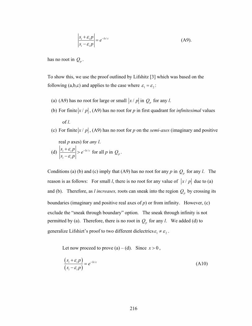
216
/lx ci i
i i
s p es p
εε
−+=
− (A9).
has no root in pQ .
To show this, we use the proof outlined by Lifshitz [3] which was based on the
following (a,b,c) and applies to the case where 1 2ε ε= :
(a) (A9) has no root for large or small /x p in pQ for any l.
(b) For finite /x p , (A9) has no root for p in first quadrant for infinitesimal values
of l. (c) For finite /x p , (A9) has no root for p on the semi-axes (imaginary and positive
real p axes) for any l.
(d) /lx ci i
i i
s p es p
εε
−+>
− for all p in pQ .
Conditions (a) (b) and (c) imply that (A9) has no root for any p in pQ for any l. The
reason is as follows: For small l, there is no root for any value of /x p due to (a)
and (b). Therefore, as l increases, roots can sneak into the region pQ by crossing its
boundaries (imaginary and positive real axes of p) or from infinity. However, (c)
exclude the “sneak through boundary” option. The sneak through infinity is not permitted by (a). Therefore, there is no root in pQ for any l. We added (d) to
generalize Lifshizt’s proof to two different dielectrics 1 2ε ε≠ .
Let now proceed to prove (a) – (d). Since 0x > ,
( )( )
/i i lx c
i i
s pe
s pεε
−+=
− (A10)
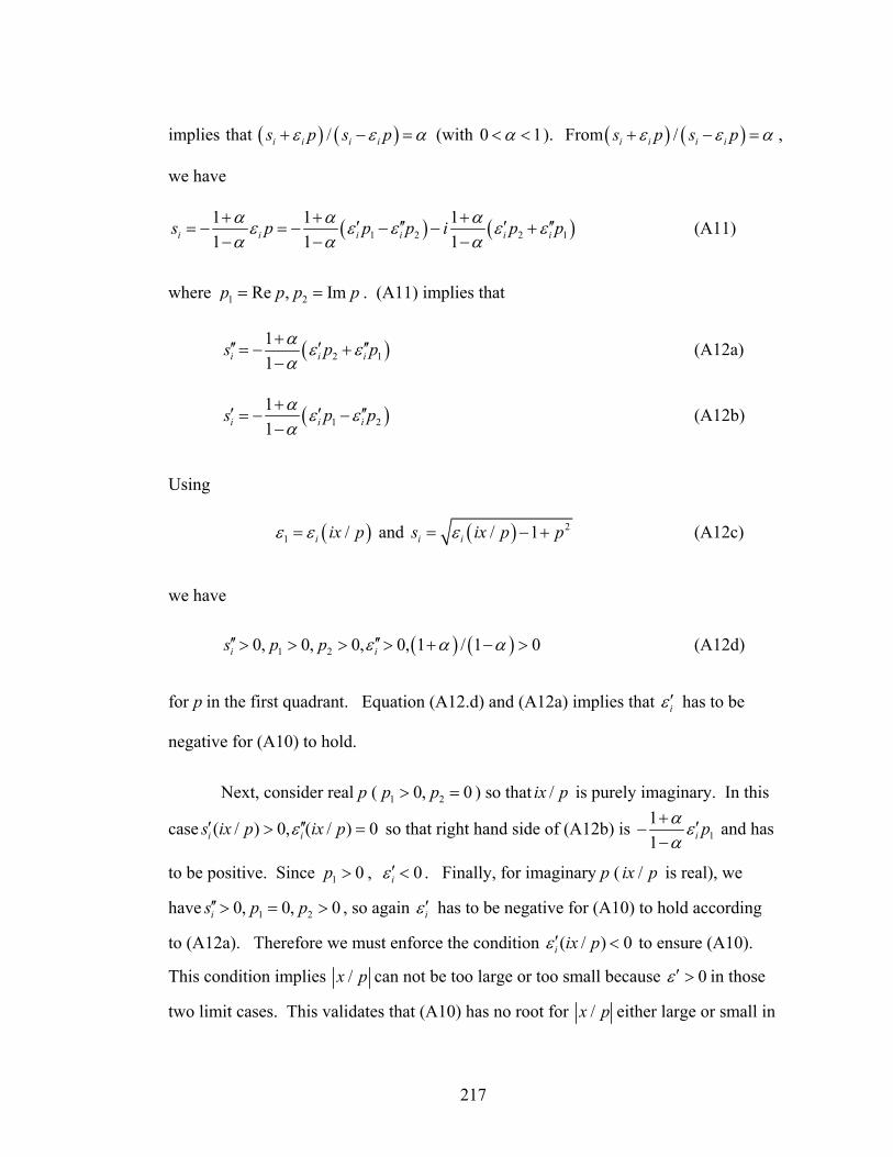
217
implies that ( ) ( )/i i i is p s pε ε α+ − = (with 0 1α< < ). From ( ) ( )/i i i is p s pε ε α+ − = ,
we have
( ) ( )1 2 2 11 1 11 1 1i i i i i is p p p i p pα α αε ε ε ε ε
α α α+ + +′ ′′ ′ ′′= − = − − − +− − −
(A11)
where 1 2Re , Imp p p p= = . (A11) implies that
( )2 111i i is p pα ε ε
α+′′ ′ ′′= − +−
(A12a)
( )1 211i i is p pα ε ε
α+′ ′ ′′= − −−
(A12b)
Using
( )1 /i ix pε ε= and ( ) 2/ 1i is ix p pε= − + (A12c)
we have
( ) ( )1 20, 0, 0, 0, 1 / 1 0i is p p ε α α′′ ′′> > > > + − > (A12d)
for p in the first quadrant. Equation (A12.d) and (A12a) implies that iε ′ has to be
negative for (A10) to hold.
Next, consider real p ( 1 20, 0p p> = ) so that /ix p is purely imaginary. In this
case ( / ) 0, ( / ) 0i is ix p ix pε′ ′′> = so that right hand side of (A12b) is 111 i pα ε
α+ ′−−
and has
to be positive. Since 1 0p > , 0iε ′ < . Finally, for imaginary p ( /ix p is real), we
have 1 20, 0, 0is p p′′> = > , so again iε ′ has to be negative for (A10) to hold according
to (A12a). Therefore we must enforce the condition ( / ) 0i ix pε ′ < to ensure (A10).
This condition implies /x p can not be too large or too small because 0ε ′ > in those
two limit cases. This validates that (A10) has no root for /x p either large or small in
218
pQ any l. In other words, a necessary condition for the existence of a root is that
/x p cannot be large or small.
Next, we prove (b). Notice that for very large x, (A10) will not hold for any l.
This is because the RHS of A10 goes to zero while the LHS goes to infinity
(note ( / ) 1i ix pε → ∞ = ). For finite x, the RHS (A10) approaches 1 as 0l → . The
LHS of (A10) goes to 1 only if 0p → . In order to keep /x p finite, we must have
0x → at the same rate of 0p → . In this situation, the LHS of (A10) behaves as
( ) ( )21 / 1 / 1 2 /1 /
i i i ii i i i
i i i i
s p p s p s s ps p p s
ε ε ε εε ε
+ += ≈ + ≈ +
− − (A13)
which means that the LHS of (A10) approaches 1 on the order of p as 0p → .
However, the RHS of (A10) behaves as
/ 1 /lx ce lx c− ≈ − (A14)
Since 0l → and 0x → (at the same rate of 0p → ), we conclude that (A13)
approaches 1 slower than (A14). Therefore there can be no roots of (A10) for
infinitesimal values of l in the first quadrant.
Finally, we prove (c). We need to consider the situation where p is on either
the real or imaginary axis of the complex p plane for any positive x. For real 0p > ,
/ix p is imaginary, which implies that 1, 0i iε ε′ ′′≥ = , thus 0, 0i is s′ ′′> = according to
(A12c). This implies that 1i i
i i
s ps p
εε
+>
−. Therefore ( )
( )/i i lx c
i i
s pe
s pεε
−+=
−can not hold for
real 0p > and arbitrary l . For pure imaginary p , /ix p is real, thus
1 21, 0, 0, 0i i p pε ε′ ′′≠ > = > , and (A12a) and (A12b) become
211i is pα ε
α+′′ ′= −−
(A15a)
219
211i is pα ε
α+′ ′′=−
(A15b)
Substituting (A15a) and (A15b) into (A3) gives
( ) ( ) 22 2
1 / 11 i i ip i p ix p pα ε ε ε
α+ ′′ ′− = − +−
(A16)
Taking square of (A16), we have
( ) ( )( )2
2 2 2 22 2 2
1 2 11 i i i i i ip p i p p iα ε ε ε ε ε ε
α+⎛ ⎞ ⎡ ⎤′′ ′ ′ ′′ ′ ′′− − = − + +⎜ ⎟ ⎣ ⎦−⎝ ⎠
(A17)
222
1 21 i i ipα ε ε ε
α+⎛ ⎞ ′ ′′ ′′− =⎜ ⎟−⎝ ⎠
(A18)
(A18) implies that 0ε ′′ = , which contradicts 0iε ′′> . Therefore ( )( )
/i i lx c
i i
s pe
s pεε
−+=
−can
not hold for imaginary p and arbitrary l . Lifshitz’s continuity argument now implies
that ( )( )
/i i lx c
i i
s pe
s pεε
−+=
− can not hold for any pp Q∈ , where x is positive and l is
arbitrary. However, for large p, is p≈ , i i
i i
s ps p
εε
+→ ∞
−, so /lx ci i
i i
s p es p
εε
−+>
−. By a
continuity argument, we claim that
/lx ci i
i i
s p es p
εε
−+>
− (A19a)
for any p in pQ . This is because if for there exist some pp Q∈ such that
/lx ci i
i i
s p es p
εε
−+<
− (A19b)
220
Then continuity implies that there will be some pp Q∈ where /lx ci i
i i
s p es p
εε
−+=
−, which
is impossible. Equation (A19a) implies that
( )( )( )( )
1 1 2 2 2 /
1 1 2 2
lx cs p s pe
s p s pε εε ε
−+ +>
− − (A20)
for any p in pQ . Therefore (A7) has no roots of p in pQ . This completes the proof of
(ii).
Validation of (iii)
The validation (iii) is straightforward. Since 22 /2 / p l ci pl ce e ωω− = → ∞ as p → ∞ , it is
clear that (iii) is true.

221
REFERENCES
1. Landau, L. D. and Lifshitz, E. M., Electrodynamics of continuous media,
Addison-Wesley, 2nd Edition, 1966.
2. Landau, L. D. and Lifshitz, E. M., Statistical physics, Oxford; New York:
Pergamon Press, 3rd Edition, 1980.
3. Lifshitz, E. M., Soviet Physics 2, 73-83 (1956).
4. Felderhof, B. U., J. Phys. C: Solid State Phys. 10 (1977).
5. McQuarrie, D. A., Statistical mechanics, University Science Books, 2nd Edition,
2000.
6. Reif, F., Statistical Physics, McGraw-Hill, 1967.
7. Parsegian, V. A., in ‘‘Physical Chemistry: Enriching Topics from Colloid and
Surface Science’’ (H. van Olphen and K. J. Mysels, Eds.). Theorex, La Jolla,
1975.
8. Van Kampen, N.G., Nijboer, B.R.A., and Schram, K., Phys. Lett. 26A:307
(1968).
9. Ninham, B.W., Parsegian,V.A., and Weiss, G.H., J. Stat. Phys. 2, 323 (1970).
10. Pasquali, S. and Maggs, A. C., Phys. Rev. A. 79, 020102(R) (2009).
222
Chapter 6
Lifshitz versus van Kampen: A revisit of van der Waals force between two parallel plates
Abstract
It is often assumed that Lifshitz’s theory of van der Waals force [1] is
equivalent to the surface mode method proposed by van Kampen et al [2]. In
Lifshitz’s theory, dispersive interaction is due to fluctuating electromagnetic fields in
dissipative media. In Van Kampen’s surface mode method, the van der Waals force
is computed by taking the gradient of the total energy of electromagnetic surface
modes. However, a direct calculation using any dielectric that satisfies the Kramer-
Kronig relations shows that this energy is complex in the non-retarded limit. This
result indicates that certain procedures in the surface mode method are inconsistent
with Lifshitz’s theory. A discussion of these inconsistencies is given in this work.
6.1 Introduction
The van der Waals (vdw) force between two planar infinite non-magnetic dielectric
materials separated by vacuum, without using the assumption of pairwise summation
of potentials, was first obtained by Lifshitz [1] in 1955 (Russian, translated into
English in 1956). The same problem, with the vacuum replaced by a linear dielectric,
was solved by DDzzyyaalloosshhiinnsskkiiii,, LLiiffsshhiittzz aanndd PPiittaaeevvsskkiiii ((DDLLPP)) iinn 11996611 [[33]].. Lifshitz
represented the dielectric media as a continuum, which is governed by Maxwell
223
equations of electrodynamics. The vdw force arises from electromagnetic radiations
due to random dipole fields in each dielectric. These random fields are uncorrelated
in space but correlated in time. These time correlations are related to the imaginary
part of the dielectric susceptibilities. Lifshitz’s solution is very complicated. This
motivated van Kampen, Nijboer and Schram (VKNS) [2] to develop a different
approach to the same problem. Instead of computing the electromagnetic field caused
by a random field, they looked for surface modes in the homogeneous Maxwell
equations. The frequencies of these surface modes are determined by a dispersive
relation. This approach has been used earlier by Casmir [4] to obtain the dispersive
force between two perfect conductors separated by vacuum. As in Casmir [4], VKNS
assumed that each surface mode (with frequency iω ), at zero temperature, contributes a
free energy of / 2iωh . The total excess free energy of the system is the sum over all
modes, i.e.,
( ) / 2iG L ω= ∑h .
Since iω depends on the separation L, the force of interaction per unit area is given by
/F G L= −∂ ∂ . VKNS developed this method for the non-retarded case where the
separation between plates is sufficiently small so that the speed of light can be taken to
be infinite. Later, Ninham, Parsegian and Weiss generalized van Kampen’s method
to the retarded and temperature dependent cases for three dielectric layers [5]. Their
results for the interaction force are identical to those obtained by Lifshitz [1] and DLP
[3]. The simplicity of van Kampen’s method has allowed interaction force to be
derived for multilayer or anisotropic media [6-11] as well as other geometries such as
the interaction between cylinders [12-14]. As pointed out by Richmond and Ninham
[15], “the great advantage of using the VKNS surface-mode analysis is the triviality of
generalizing the simplest results for the interaction of two semi-infinite media. One
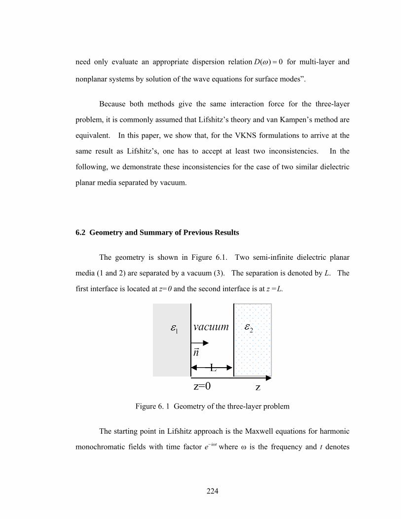
224
need only evaluate an appropriate dispersion relation ( ) 0D ω = for multi-layer and
nonplanar systems by solution of the wave equations for surface modes”.
Because both methods give the same interaction force for the three-layer
problem, it is commonly assumed that Lifshitz’s theory and van Kampen’s method are
equivalent. In this paper, we show that, for the VKNS formulations to arrive at the
same result as Lifshitz’s, one has to accept at least two inconsistencies. In the
following, we demonstrate these inconsistencies for the case of two similar dielectric
planar media separated by vacuum.
6.2 Geometry and Summary of Previous Results
The geometry is shown in Figure 6.1. Two semi-infinite dielectric planar
media (1 and 2) are separated by a vacuum (3). The separation is denoted by L. The
first interface is located at z=0 and the second interface is at z =L.
Figure 6. 1 Geometry of the three-layer problem
The starting point in Lifshitz approach is the Maxwell equations for harmonic
monochromatic fields with time factor i te ω− where ω is the frequency and t denotes
225
time. For the case of a linear homogeneous non-magnetic dielectric medium, the
electric and magnetic fields ( , )i iE Br r
satisfy:
0i iiE Bcω
∇× − =rr r
(6.1a)
( )i i i iiB E Kcω ε ω⎡ ⎤∇× = − +⎣ ⎦
r r r (6.1b)
0iB∇ ⋅ =r
(6.1c)
i i iE Kε ∇ ⋅ = −∇ ⋅r r
(6.1d)
where iKr
denote the random dipole fields in each dielectric and
( ) ( ) ( )i i iiε ω ε ω ε ω′ ′′= + is the complex dielectric susceptibility for medium i =1,2,3.
Lifshitz assumed that iε satisfies the Kramer-Kronig relations [16]. The ensemble
average of the product of the components of iKr
, denoted by ,i jK at two spatial points
rr and r′r is [1, 16]:
, , 2 coth ( ) ( )i j i k i jkB
K K r rk T
ω ε ω δ δ⎛ ⎞
′′ ′= −⎜ ⎟⎝ ⎠
h r rh (6.2)
where ( )iε ω′′ is the imaginary part of the complex dielectric susceptibility in medium i.
Equation (6.2) shows that the ensemble average of the random field is proportional to
the imaginary part of the complex dielectric susceptibility. Note that the random field
vanishes in a non-dissipative medium. For example, 3Kr
= 0r
in vacuum. The
boundary conditions are the continuity of the tangential components of the electric and
magnetic fields, as well as the continuity of the normal displacements. Lifshitz [1]
showed that equations (6.1a-d) subjected to the above boundary conditions can be
solved exactly. He computed the zz component of the Maxwell stress tensor in
medium 3 for each monochromatic field. The interaction force F between the medium
226
1 and 2 is determined by integrating this component of the stress tensor over all
frequencies. The result is [1]:
( )( )( )( )
( )( )( )( )
1 1
1 2 1 1 2 23 2 2 / 2 /2 3
1 2 1 1 2 20 1
1 12
p l c p l cs p s p s p s pF d p e e dp
c s p s p s p s pξ ξε ε
ξ ξπ ε ε
− −∞ ∞⎡ ⎤⎧ ⎫⎡ ⎤ ⎡ ⎤+ + + +⎪ ⎪⎢ ⎥= − + −⎨ ⎬⎢ ⎥ ⎢ ⎥− − − −⎢ ⎥⎣ ⎦ ⎣ ⎦⎪ ⎪⎩ ⎭⎣ ⎦∫ ∫
h
(6.3)
where 2( ) 1i is i pε ξ= − + and ( )i i iε ε ξ= i =1,2 (6.4)
For the non-retarded limit, and (6.3) reduces to [1]:
( )( )( )( )
1
1 222 3
1 20 0
1 ( ) 1 ( )1
2 (8 ) ( ) 1 ( ) 1xi i
F x e dxdL i i
ε ξ ε ξξ
π ε ξ ε ξ
−∞ ∞ ⎡ ⎤+ += −⎢ ⎥− −⎣ ⎦
∫ ∫h (6.5)
Finally, one should note that in Lifshitz’s formulation, the interaction force is
identically zero if all the media are non-dissipative. This is because all the random
fields are identically zero, as seen from (6.2).
The basic idea of VKNS is to seek surface modes (electromagnetic waves that
decay away from boundaries) of the homogeneous Maxwell equations. Specifically,
they considered the special case 1 2ε ε ε= ≡ and sought time harmonic solutions of the
form:
[ ] [ ]1 21 2 3( ), ( ), ( ) i q x q y t
i i i iE e z e z e z e ω+ −=r
, (6.6)
in each media. Since the governing equations and boundary conditions are homogeneous, non-trivial solution for each wave number 2 2
1 2 0q q q≡ + ≥ exist if and
only if ( , )q Lω∗ satisfy the dispersion relation
227
( ) 0D ω = (6.7a)
where
22( ) 1( ) 1
( ) 1qLD eε ωω
ε ω−⎡ ⎤−
≡ − ⎢ ⎥+⎣ ⎦ (6.7b)
VKNS called the fields associated with these eigenfrequencies surface modes. They assumed that, at temperature 0T = , each surface mode with frequency jω∗ carries a
zero point energy / 2jω∗h . Specifically, let ( )m q be the number of surface modes
associated with the wave number q, the total excess free energy of the system is
( )
10
( , )4
m q
jj
q L qdqωπ
∞∗
=∑∫
h . (6.8)
The interaction force F is obtained by differentiating the negative of the excess free
energy by L. VKNS claimed that (6.8) can be transformed to (6.5), using a theorem
based on the argument principle in analytic function theory [2].
Since the free energy is real, the implicit assumption in VKNS’s formulation is
that the roots of (6.7a) are always positive and complex roots are not allowed. We
will later show that real roots cannot exist for a linear dielectric that obeys the
principle of causality; such a dielectric obeys the well known Kramer-Kronig relations
[16]. The following properties of ε are stated in Landau and Lifshitz [16]:
(a) If ω is regarded as a complex variable, then ( )ε ω is analytic in the upper half
ω plane, the function has no singularity on the real axis, except for a simple pole at the
origin;
228
(b) ( )ε ω does not take real values at any finite point in the upper half ω plane except
on the imaginary axis, where it is real and decreases monotonically from
( 0 ) 1iε ω += > to 1 at iω = ∞ .
(c) the imaginary part of ( )ε ω is an odd function on the real axis. It is real and
positive for real positiveω , that is, ( ) 0ε ω′′ > for ( )0,ω ∈ ∞ ; the only point on the real
ω axis for which the imaginary part of ( )ε ω can vanish is at the origin.
6.3 Two Difficulties with the VKNS Method
The first difficulty with the VKNS method is that the free energy is always
complex, as demonstrated below.
Based on properties (a-c), we study the existence of real and positive roots of
( )D ω in (6.7a). Simple algebra shows that, if ω∗ is a root of ( )D ω , i.e.,
2
2( ) 11 0( ) 1
qLeε ωε ω
∗−
∗
⎛ ⎞−− =⎜ ⎟+⎝ ⎠
, (6.9)
then
1( )1
qL
qL
ee
ε ω−
∗−
±= −
m. (6.10)
Since 1qLe− < for 0q > , the right hand side of (6.10) is always real and negative. Thus,
roots of (6.9) exist only if the imaginary part of the dielectric susceptibility vanishes
and the real part is negative. However, according to (c), the imaginary part of the dielectric function can never vanish for ( ) ( ),0 0,ω ∈ −∞ ∪ ∞ . Thus, the characteristic
equation has no real roots. This means that the free energy of the system is complex.
229
It should be noted that, complex ω means that the surface modes will decay or grow
exponentially with time, a contradiction to the assumption of surface modes.
As an example, consider the simple case of
( ) ( )1 ,o
o
bi
ωε ωω ω
= +−
(6.11)
where oω and b are positive material constants. The dielectric susceptibility (6.11) can
be shown to satisfy the Kramer-Kronig relations. Lifshitz’s theory (using (6.5)) gives
an attractive force of
22 3
0
2ln8 2
xxo
x
b b beF x e dxL b be
ωπ
∞ −−
−
+ +=
+ −∫h . (6.12)
To compute the excess free energy using VKNS, we find the frequency of the surface modes. A straightforward calculation using (6.10) shows that all the roots of ( )D ω
lies on the negative imaginary axis. They are:
( )1 12
qLo
bi eω ω∗ −⎡ ⎤= − +⎢ ⎥⎣ ⎦m . (6.13)
According to (6.13), the excess free energy in this example is a purely imaginary
number.
In [2], VKNS explicitly computed the van der Waals force between two
identical materials separated by vacuum and demonstrated that the free energy is non-
zero. The dielectric susceptibility they used is
2 2o
1 Bεω ω
= +−
, (6.14)
230
where B and oω are real constants. However, this dielectric material does not satisfy
the Kramer-Kronig relations. Indeed, the Kramer-Kronig relation implies that 0ε ′′ ≠
except for vacuum. Note that, since 0ε ′′ = in (6.14), Lifshitz’s theory would predict
an interaction force of zero.
What about VKNS’s claim that (6.8) is identical to (6.5)? Although they did
not give the details of the derivation in their original work [2], their argument can be
found in many references and textbooks, e.g. see [5-6, 17-22]. It is based on the
argument principle in analytic function theory. The method can be summarized as
follows: For a given wave number q, denote the sum of zeroes of ( )D ω inside the first
and fourth quadrant of the complex ω plane by
( )
*
1
( , )m q
kk
q Lω=
∑
where ( )m q is the number of zeroes for a given q. Assume
( )
*
1
( , )m q
kk
q Lω=
=∑ ( )( )
1 lim2
R
R
Dd
i Dγ
ωω ω
π ω→∞
′∫ (6.15)
where ( ) /D dD dω ω′ = . The closed contour Rγ is defined by [ ] [ ]0, ,0RiR C iR∪ ∪ −
where RC is the semi-circle of radius R defined by e , / 2 / 2iR θω π θ π= − ≤ ≤ , (see
Figure 6.2).
As long as ( ) 1 (1/ )Oε ω ω→ ∞ = + , it can be shown that
( )( )
2lim 0R
DD
ωω
ω→∞
′= . (6.16)
Therefore, the integral along RC vanishes, and
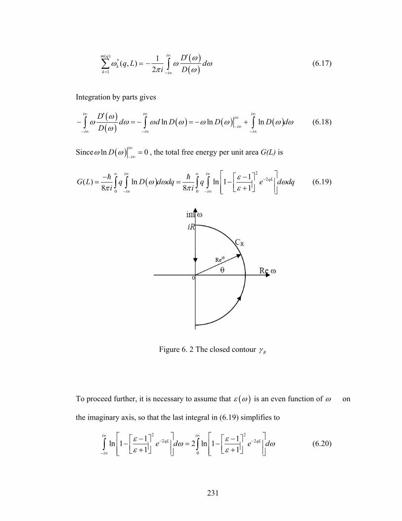
231
( )
*
1
( , )m q
kk
q Lω=
=∑ ( )( )
12
i
i
Dd
i Dω
ω ωπ ω
∞
− ∞
′− ∫ (6.17)
Integration by parts gives
( )( ) ( ) ( ) ( )ln ln ln
i i ii
ii i i
Dd d D D D d
Dω
ω ω ω ω ω ω ω ωω
∞ ∞ ∞∞
− ∞− ∞ − ∞ − ∞
′− = − = − +∫ ∫ ∫ (6.18)
Since ( )ln 0i
iDω ω
∞
− ∞= , the total free energy per unit area G(L) is
( )2
2
0 0
1( ) ln ln 18 8 1
i iqL
i i
G L q D d dq q e d dqi i
εω ω ωπ π ε
∞ ∞ ∞ ∞−
− ∞ − ∞
⎡ ⎤− −⎡ ⎤= = −⎢ ⎥⎢ ⎥+⎣ ⎦⎢ ⎥⎣ ⎦∫ ∫ ∫ ∫
h h (6.19)
Figure 6. 2 The closed contour Rγ
To proceed further, it is necessary to assume that ( )ε ω is an even function of ω on
the imaginary axis, so that the last integral in (6.19) simplifies to
2 2
2 2
0
1 1ln 1 2 ln 11 1
i iqL qL
i
e d e dε εω ωε ε
∞ ∞− −
− ∞
⎡ ⎤ ⎡ ⎤− −⎡ ⎤ ⎡ ⎤− = −⎢ ⎥ ⎢ ⎥⎢ ⎥ ⎢ ⎥+ +⎣ ⎦ ⎣ ⎦⎢ ⎥ ⎢ ⎥⎣ ⎦ ⎣ ⎦∫ ∫ (6.20)
232
Combining (6.19) and (6.20) gives:
22
0 0
1( ) ln 14 1
iqLG L q e d dq
iε ω
π ε
∞ ∞−
⎡ ⎤−⎡ ⎤= −⎢ ⎥⎢ ⎥+⎣ ⎦⎢ ⎥⎣ ⎦∫ ∫
h (6.21)
The force is obtained by differentiating (6.21) with respect to L, this results in (6.5)
after a change of integration variable.
The second difficulty is that the above argument relies on several assumptions. First, (6.15) is valid only if ( )D ω is a meromorphic function (that is, all the singular
points of D are poles) in the right half ω plane, including the imaginary axis. This is
not true in general since ( )ε ω is known to be analytic only in the upper half ω plane.
In other words, there is no guarantee that ( )ε ω can be analytically continued to the
lower half plane. Since D is a function of ( )ε ω , D may not be analytically continued
to the lower half plane. In addition, even if analytic continuation were possible, D
could have zeroes and singularities (including branch points) in the lower half plane,
including the negative imaginary axis. An example is the dielectric susceptibility
specified by (6.11) where a simple pole is located at oiω− . Note this does not violate
the Kramer-Kronig relation since the singularity occurs in the lower half plane. For
this special case, the integrand in (6.19) is singular along the path of integration.
Another complication is that the analytically continued function D may not satisfy the assumption that ( )ε ω is an even function of ω on the imaginary axis.
Indeed, it is possible to show that if analytic continuation were possible, then the only singled value analytic function that satisfies the condition that ( )ε ω is even on the
imaginary axis must necessarily be real and has singularities on the real axis11. As a
11 Note that these conditions are satisfied by the dielectric susceptibilities used by VKNS (see equation (14)).
233
consequence, both properties (a) and (c) are violated. This result is proved in the
Appendix. In other words, no non-constant analytic function exists which satisfies
both (6.20) and the Kramer-Kronig conditions.
Another problem that can arise is that D may have complex zeroes so the free
energy is complex. This is the case for the material specified by (6.11), for example. Finally, we note that the analytic continuation of ( )D ω may have poles in the fourth
quadrant ( ( )D ω has no singularities in the upper half plane since ( )ε ω is analytic there
and because of property (b) above) so (6.15) should be replaced by
( ) ( )
*
1 1( , ) ( )
m q n qPole
j jj j
q L qω ω= =
− =∑ ∑ ( )( )
12
i
i
Dd
i Dω
ω ωπ ω
∞
− ∞
′− ∫ (6.23)
However, in some cases the location of these poles is independent of L, therefore, the
presence of this extra term does not affect the vdw force, at least for the parallel plate
problem.
6.4 Discussion and Summary
Our analysis implies that VKNS’s method of computing van der Waals
interaction is not equivalent to that proposed by Lifshitz for dielectric materials which
obey the Kramer-Kronig relations. In Lifshitz’s theory, the imaginary part of the
dielectric susceptibility must be positive for positive frequencies. This requirement is
necessary for the existence of the random fields as well as for the validity of (6.5),
since the representation of the Maxwell stress tensor as the real part of an analytic
function of ω relies explicitly on this condition. Details can be found on pages 76-78
of Lifshitz’s paper [1].
234
The assumption that each surface mode contributes a free energy of / 2iωh is
questionable for a dissipative dielectric. Indeed, the proof that a plane
monochromatic electromagnetic wave carries a zero point energy of / 2ωh is derived
under the condition that the media be non-dissipative [22]. However, dielectric
materials are dissipative ( ( 0) 0ε ω′′ > > ) and therefore this result does not apply.
Perhaps this is why the proof of the equivalence of the two theories has to rely on ε
being an even function of ω on the imaginary axis. As pointed out earlier, this
assumption automatically rules out dissipation.
In summary, the derivation of the surface mode method implicitly assumes that
all media are non-dissipative. These media do not satisfy the Kramer-Kronig
relations since the imaginary part of their dielectric susceptibilities is zero for real
frequencies. For this reason, the surface mode method is not equivalent to Lifshitz’s
theory, which assumes ( 0) 0ε ω′′ > > . Finally, we point out that our conclusion
applies also to the case of finite temperature since the dispersion relation is the same
for zero and finite temperatures.
235
APPENDIX
Suppose ( )ε ω can be analytically continued to the lower half plane. In addition, the
analytically continued function satisfies the condition that ( ) ( )i iε η ε η− = for all 0η > .
Since analytic continuation is unique, we need only to find a function that is analytic in
the lower half plane that exhibits this property. This function is the reflection of ε about
the real axis, defined by ( ) ( )ε ω ε ω∗ ≡ , where a bar denotes complex conjugate. Since
ε is analytic in the upper half plane, ε ∗ is analytic in the lower half plane. Furthermore,
( ) ( ) ( )i i iε η ε η ε η∗ − = = since ε is real on the positive imaginary axis. Note that since
( )ε ω is analytic in the upper half ω plane, ε ∗ is analytic in the lower half plane. The
paths of analytical continuation must go from the upper half plane to the lower half plane.
Since the continued function is assumed to be single-valued, there cannot be branch points
on the real axis, thus there must exist isolated or non-isolated singularities on the real axis.
Apart from these singularities, the function is real on the real axis, sinceω ω= . It is
therefore not surprising that functions that are selected in the literature to illustrate VKNS
method always have poles on the real axis. Finally, we note that, if there were no
singularities on the real axis, then the analytically continued function is entire and since it
is bounded at infinity, it is a constant by Liouville’s theorem. Thus, the only dielectric
material that satisfies the Kramer-Kronig relation and the condition that it is an even
function on the imaginary axis is a constant and therefore must be vacuum.
236
REFERENCES
1. E. M. Lifshitz, the Theory of Molecular Forces between Solids, Soviet Physics,
Vol.2, 73-83 (1956).
2. N. G. van Kampen, B. R. A. Nijboer, and K. Schram, On the Macroscopic Theory
of van der Waals Forces, Physics Letters, Vol. 26A, 307-308 (1968).
3. II.. EE.. DDzzyyaalloosshhiinnsskkiiii,, EE.. MM.. LLiiffsshhiittzz aanndd LL.. PP.. PPiittaaeevvsskkiiii,, GGeenneerraall TThheeoorryy ooff vvaann ddeerr
WWaaaallss’’ FFoorrcceess,, AAddvv.. PPhhyyss..,, 1100,, 116655 ((11996611))..
4. H. B. G. Casimir, On the Attraction between Two Perfectly Conducting Plates,
Proc. Kon. Ned. Akad. Wetenschap 51, 793–795 (1948).
5. B. W. Ninham, V. A. Parsegian, and G. H. Weiss, On the Macroscopic Theory of
Temperature-Dependent van der Waals Forces, J. Stat. Phys., Vol. 2, 232-328
(1970).
6. B. W. Ninham and V. A. Parsegian, van der Waals Forces across Triple-Layer
Films, J. Chem. Phys., Vol. 52, 4578-4587 (1970).
7. V. A. Parsegian nd G.H. Weiss, Dielectric Anisotropy and the van der Waals
Interaction between Bulk Media , J. Adhesion., Vol. 3, 259-267 (1972).
8. R. Podgornik, P. L. Hansen, and V. A. Parsegian, On a Reformulation of the
Theory of Lifshitz-van der Waals Interactions in Multilayered Systems, J. Chem.
Phys., Vol. 119, 1070-1077 (2003).
9. R. Podgornik and V. A. Parsegian, van der Waals Interactions across Stratified
Media, J. Chem. Phys., Vol. 120, 3401-3405 (2004).
10. R. Podgornik and V. A. Parsegian, van der Waals Interactions in a Dielectric with
Continuously Varying Dielectric Function, J. Chem. Phys., Vol. 121, 7467 (2004).
11. R. Podgornik, R. H. French, and V. A. Parsegian, Nonadditivity in van der Waals
Interactions within Multilayers, J. Chem. Phys., Vol. 124, 7467-7473 (2006).
237
12. V. A. Parsegian, Nonretarded van der Waals Interaction between Anisotropic
Long Thin Rods at All Angles, J. Chem. Phys., Vol. 56, 4393-4393 (1972).
13. D. J. Mitchell, B. W. Ninham, and P. Richmond, van der Waals Forces between
Cylinders: I. Nonretarded Forces between Thin Isotropic Rods and Finite Size
Corrections, Biophys J. Vol.13, 359–369 (1973).
14. V. A. Parsegian and G. H. Weiss, Electrodynamic Interactions between Curved
Parallel Surfaces, J. Chem. Phys., Vol. 60, 5080-5085 (1974).
15. P. Richmond and B. W. Ninham, A Note on the Extension of the Lifshitz Theory of
van der Waals Forces to Magnetic Media, J. Phys. C: Solid St. Phys., Vol. 4, 1988
-1993 (1971).
16. L. D. Landau and E. M. Lifshitz, Electrodynamics of continuous media, p. 256-262,
Addison-Wesley, 2nd Edition,(1966).
17. E. Gerlack, Equivalence of van der Waals Forces between Solids and the
Surface-Plasmon Interaction, Phys. Rev. B, Vol. 4, 393-396 (1971).
18. K. Schram, On the Macroscopic Theory of Retarded van der Waals Forces,
Physics Letters A, Vol. 43, 282-284 (1973).
19. Yu. S. Barash and V. L. Ginzburg, Electromagnetic Fluctuations in Matter and
Molecular (van-der- Waals) Forces between Them, Sov. Phys. Usp., Vol. 18, 305-
322 (1975).
20. D. Langbein, On the Share of Vacuum Modes in van der Waals’ Attraction, J.
Chem. Phys., Vol 58, 4476-4481 (1973).
21. Mahanty and B. W. Ninham, Dispersion Force, Academic Press (1976), p217.P.
W. Milonni, the Quantum Vacuum—an Introduction to Quantum Electrodynamics,
Academic Press (1993). .
238
Chapter 7
Green’s Function and Boundary Element Method
In chapter 5, we have reviewed the general macroscopic van der Waals (vdw)
theory (Lifshitz theory). Lifshitz’s formulation for vdw interaction can be extended
to finite solids of any geometry, as long as one of the medium is a vacuum. However,
for finite solids with complicated boundaries, it is impossible to find analytical
solutions of Maxwell equations. This motivates us to develop numerical techniques
to compute vdW forces. In the first part of this chapter (section 7.1), we provide the
Green’s function theory for the van der Waals interactions based on the work of
Felderhof [1]. The Maxwell stress tensor is then expressed in terms of Green’s
functions associated with the electric and magnetic fields. Felderhof actually
formulated the problem for a general dielectric medium. Since the Maxwell stress
tensor is only well defined in vacuum, we will only focus on evaluating the Maxwell
stress tensor in vacuum. In the second part (section 7.2), a boundary element method
of computing van der Waal interaction between two dielectric solids separated by a
vacuum is developed. In principle, this method can be used to evaluate the van der
Waals force for the dielectric solids with arbitrary shapes. However, this method has
some limitations which will be discussed in section 7.3. In the following, we assume
that the electromagnetic properties of the materials are homogeneous, isotropic and
non-magnetic.
7.1 Green’s Function
The starting point is Maxwell equations in each medium, where the Maxwell
equations (5.36a-d) must be satisfied. The transformed Maxwell equations are given
by (5.41a-b), which are
239
icω−∇× =% %E B 0 (7.1a)
icω ⎡ ⎤∇× = − +⎣ ⎦
% % %B D K (7.1b)12
0∇ ⋅ =%B (7.1c)
∇ ⋅ = −∇ ⋅% %D K (7.1d)
As pointed in section 5.7, equations (7.1a) – (7.1d) are not independent. Clearly, the
divergence of (7.1a) implies (7.1c) and the divergence of (7.1b) gives (7.1d). In other
words, only two of the four Maxwell equations are independent. Indeed, the two
independent equations are (7.1a) and (7.1b). From (7.1a), we have
icω
= − ∇×% %B E (7.2)
Substituting (7.2) into (7.1b) gives
2 2
2 2
( , )c c
ω ε ω ω∇×∇× − =% % %rE E K (7.3)
where ( , )ε ω% %D = r E has been used. Note that equations (7.2) and (7.3) are equivalent
to (7.1a) – (7.1d). Therefore, we need only to solve (7.2) and (7.3) for the
electromagnetic fields %E and %B . Equation (7.3) can be simplified by using the vector
identity
( ) 2∇×∇× = ∇ ∇⋅ − ∇% % %E E E (7.4)
Thus, (7.3) can be rewritten as
12 Note %K in this work is the same as ( )4 ,r ωπκ ω F in Feldeon’s paper[1].
240
( )2 2
22 2
( , )c c
ω ε ω ω∇ ∇⋅ − ∇ − =% % % %rE E E K (7.5)
Using (7.1d) and ( , )ε ω% %D = r E , (7.5) becomes
( )2 2
22 2
( , ) 1( , )c c
ω ε ω ωε ω
⎡ ⎤∇ + = − − ∇ ∇⋅⎢ ⎥
⎣ ⎦% % % %rE E K K
r (7.6)
The material homogeneity implies that ( , )ε ωr is independent of r in each medium, so
we can move 1/ ( )ε ω out of the gradient operator in (7.6). This results in
( )2 2
22 2
( , ) 1( , )c c
ω ε ω ωε ω
⎡ ⎤∇ + = − − ∇ ∇ ⋅⎣ ⎦% % % %rE E K K
r (7.7)
It should be noted that equation (7.7) is not equivalent to (7.3) because we have used
(7.1d) to get (7.6) from (7.3). We must add (7.1d) as a constraint to equation (7.7).
Now the independent Maxwell equations are (7.3) and (7.7) along with (7.1d) as a
constraint.
In the following, let subscript j in j%K and j
%E denote the fields in media j =1, 2
and 3. The components of vectors and tensors will be denoted by Greek subscripts. Summation convention will be used. Let ( , , )EGαβ ω′r r denote the Green’s function of
(7.3). Physically, ( , , )EGαβ ω′r r is the electric field ( , )Eα ω% r due to a concentrated
dipole of unit magnitude at ′r acting in the direction ˆβe , where 1 2 3ˆ ˆ ˆ, ,e e e are the
Cartesian basis. In general, the end of ′r can be in any media. Specifically,
( )2
2 , ( )E Ec G Gαβ αβ αβε ω δ δω
′∇×∇× − = −r r r (7.8)13
13 Note that our definition of EGαβ differs from Felderhof ’s by a factor of 4π . Specifically, our EGαβ is 1/ 4π of his.
241
where ∇ is with respect to r unless stated otherwise. Note that ( , )ε ωr is a step
function in each medium. By this definition of EGαβ , the electric field due to
( ),Kβ ω′% r is:
( )3
( ) ( , , ) ,EE G K dα αβ βω ω′ ′ ′= ∫R
% %r r r r r (7.9a)
Because ( , )ε ωr is discontinuous across the boundary of the medium,
( , , )EGαβ ω′r r is also discontinuous across these boundaries. Therefore one must
impose the continuity boundary conditions on the tangential components of the electric fields. This results in the continuity of ˆEG tαβ α at a boundary point, where tα is
the unit tangent vector at this point. Likewise, the tangential component of the
magnetic field must also be continuous across a boundary.
Our primary interest is to evaluate the Maxwell stress tensor in the vacuum.
This means that we have to evaluate “spectral density” of the Maxwell stress tensor,
i.e., equation (5.38a)
( ) ( ) ( ) ( )1 1 14 2 2k k k ks E E E E B B B Bαβ α β αβ α β αβω ω ω ω
δ δπ
⎛ ⎞= − + −⎜ ⎟⎝ ⎠% % % % % % % % (7.9b)
Felderhof [1] has shown that
( )( , ) ( ) ( , ) Im ( , )EE E A T G ,α β αβω ω ω ω δ ω ω∗ ′ ′ ′ ′⎡ ⎤= −⎣ ⎦% %r r , r r (7.10a)14
where
( , ) 2 coth2 B
A Tk Tωω
⎛ ⎞= ⎜ ⎟
⎝ ⎠
hh (7.10b)
14Note, *( , ) ( ) ( , ) ( )K K , K K ,ω ω ω ωα αβ β′ ′ ′ ′= −% % % %r r r r , so (2.10a) is equivalent to
( )( , ) ( , ) 4 ( , ) Im ( , )EE E C T G ,α β αβω ω π ω ω δ ω ω⎡ ⎤′ ′ ′ ′= +⎣ ⎦% %r r r r
242
We give the detailed proof of (7.10a) in Appendix A. (7.10a) and (5.23) imply that
( ) ( , ) Im ( , )EE E A T G ,α β αβωω ω′⎡ ⎤= ⎣ ⎦
% % r r (7.10c)
which will be used to determine the spectral density sαβ .
Next, we show that ( )( , ) ( ) ( , ) Im ( , )BB B A T G ,α β αβω ω ω ω δ ω ω∗ ′ ′ ′ ′⎡ ⎤= −⎣ ⎦
% %r r , r r (7.11)
In (7.11), ( , )BG ,αβ ω′r r is the magnetic Green’s function defined as:
2
2( , ) ( , )B Ev
cG , e e G ,αβ αμν βρσ μ ρ σω ωω
′ ′ ′= ∂ ∂r r r r (7.12)
where eαμν is the permutation tensor and
, x xμ ρ
μ ρ
∂ ∂′∂ ≡ ∂ ≡′∂ ∂
and
ˆ ˆ, x xμ μ μ μ′ ′≡ ≡r e r e
To show (7.11), we consider
2
2( , ) ( ) ( , ) ( ) ( , ) ( )cωω ω ω ω ω ω∗ ∗ ∗′ ′ ′ ′ ′ ′ ′ ′∇ ×∇× = ∇× ∇ × =% % % % % %E r E r , E r E r , B r B r , (7.13)
where (7.2) has been used in the second equality of (7.13a) and the gradient operator
′∇ is with respect to ′r . (7.10a) implies that the LHS of (7.13) is equal to
( )( , ) ( ) ( , ) Im ( , )EA T ,ω ω ω ω δ ω ω∗′ ′ ′ ′ ′ ′⎡ ⎤∇ ×∇× = ∇ ×∇× −⎣ ⎦% %E r E r , G r r (7.14)
Substituting
243
ˆ ˆ( , ) ( , )E Ev, e e G ,αμν βρσ μ ρ σω ω′ ′ ′ ′∇ ×∇× = ∂ ∂ α βG r r r r e e (7.15)
into (7.14) gives
( )ˆ ˆ( , ) ( ) ( , ) Im ( , )EvA T e e G ,αμν βρσ μ ρ σω ω ω ω δ ω ω∗′ ′ ′ ′ ′ ′⎡ ⎤∇ ×∇× = ∂ ∂ −⎣ ⎦
% %α βE r E r , r r e e
(7.16)
Comparing (7.13) and (7.16) yields
( )2
2ˆ ˆ( , ) ( ) ( , ) Im ( , )E
vA T e e G ,c αμν βρσ μ ρ σω ω ω ω ω δ ω ω∗ ′ ′ ′ ′ ′⎡ ⎤= ∂ ∂ −⎣ ⎦
% %α βB r B r , r r e e (7.17)
which is the vector form of (7.11). From (7.12), we have
( ) ( , ) Im ( , )BB B A T G ,α β αβωω ω′⎡ ⎤= ⎣ ⎦
% % r r (7.18)
Finally, the spectral density of the Maxwell stress tensor is obtained by substituting
(7.10c) and (7.18) into (7.9b). This results in:
( , ) 1 1lim Im ( , ) ( , ) ( , ) ( , )4 2 2
E E B BA Ts G , G , G , G ,αβ αβ μμ αβ αβ μμ αβω ω ω δ ω ω δπ ′→
⎛ ⎞′ ′ ′ ′= − + −⎜ ⎟⎝ ⎠r r
r r r r r r r r
(7.19)
We note that the spectral density sαβ is unbounded at the limit ′=r r since the
Green’s functions have a singularity there. These local singularities do not depend on
the distance between bodies and therefore do not contribute to the van der Waals
interaction. Therefore, they should be subtracted from the Green’s functions in (7.19)
to give a finite spectral density. Specifically, the spectral density in (7.19) should be
replaced by:
244
( , ) 1 1Im ( , , ) ( , , ) ( , , ) ( , , )4 2 2
E E B BA Ts G G G Gαβ αβ γγ αβ αβ γγ αβω ω ω δ ω ω δπ
⎡ ⎤Δ = Δ − Δ + Δ − Δ⎢ ⎥⎣ ⎦r r r r r r r r
(7.20)
Where
( , , ) lim ( , , ) ( , , )E E EG G Gαβ αβ αβω ω ω∞
′→′ ′⎡ ⎤Δ ≡ −⎣ ⎦r r
r r r r r r (7.21)
( , , ) lim ( , , ) ( , , )B B BG G Gαβ αβ αβω ω ω∞
′→′ ′⎡ ⎤Δ ≡ −⎣ ⎦r r
r r r r r r (7.22)
The superscript ∞ in ( , , )EGαβ ω∞ r r denotes the Green’s function in an infinite
homogeneous dielectric. In Appendix C, we will show that
221( , , )
4
ik ikE e eG k
x xαβ αβα β
ω δπε
′ ′− −∞
⎡ ⎤⎡ ⎤∂′ = +⎢ ⎥⎢ ⎥′ ′− ∂ ∂ −⎢ ⎥⎢ ⎥⎣ ⎦⎣ ⎦
r r r r
r rr r r r
(7.23a)
Where
( , )kcω ε ω≡ r (7.23b)
The branch of the square root function must be chosen so that Im ( , )ε ωr > 0.
7.2 Boundary Element Method (BEM)
One way of evaluating the Maxwell stress tensor is to use (7.20) by evaluating ( , , )EGαβ ωΔ r r at every spatial point r on a convenient surface in vacuum. Once this
tensor is obtained, the van der Waals force can be computed using (5.38c, d). Since we are only interested in evaluating ( , , )EGαβ ωΔ r r on a surface and not in the entire
domain, we propose to use boundary element approach to compute ( , , )EGαβ ωΔ r r .
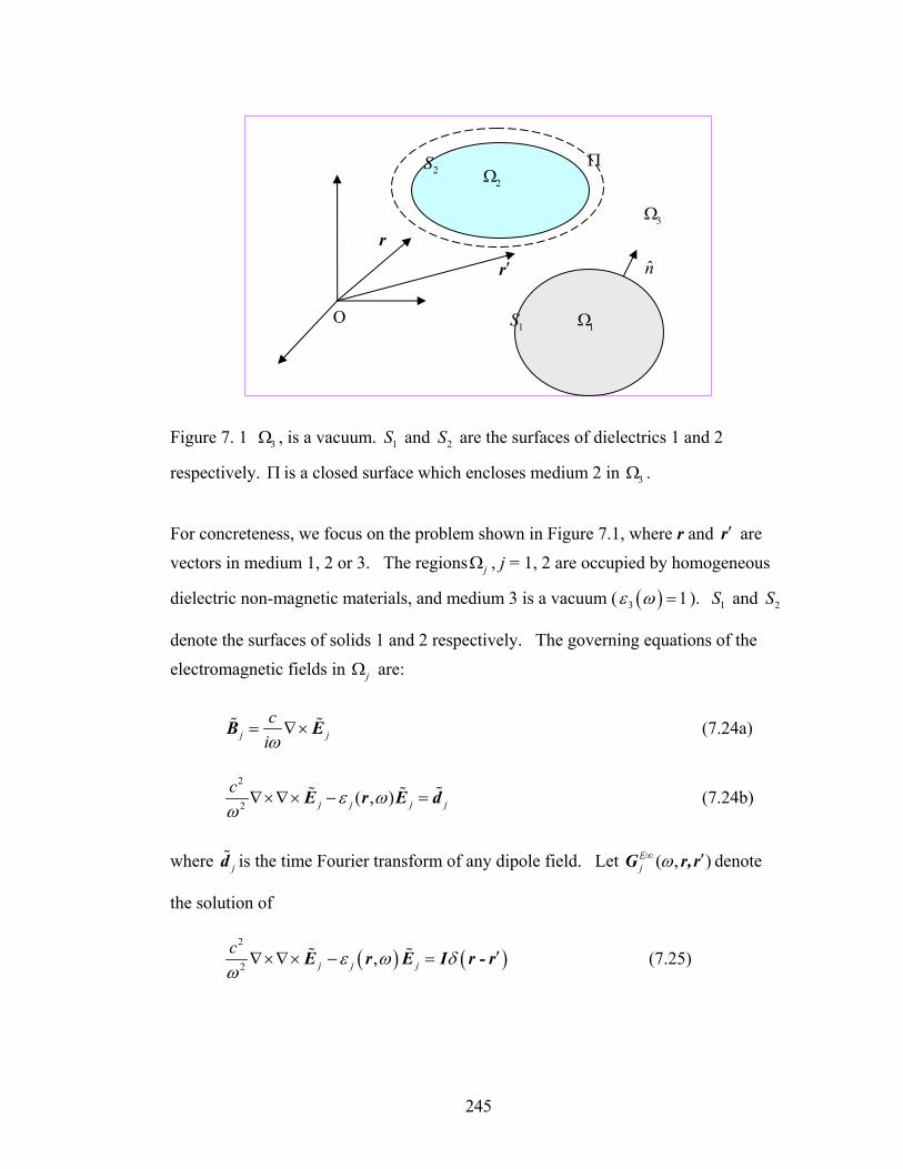
245
Figure 7. 1 3Ω , is a vacuum. 1S and 2S are the surfaces of dielectrics 1 and 2
respectively. Π is a closed surface which encloses medium 2 in 3Ω .
For concreteness, we focus on the problem shown in Figure 7.1, where r and ′r are
vectors in medium 1, 2 or 3. The regions jΩ , j = 1, 2 are occupied by homogeneous
dielectric non-magnetic materials, and medium 3 is a vacuum ( ( )3 1ε ω = ). 1S and 2S
denote the surfaces of solids 1 and 2 respectively. The governing equations of the electromagnetic fields in jΩ are:
j jc
iω= ∇×% %B E (7.24a)
2
2 ( , )j j j jc ε ωω
∇×∇× − = %% %E r E d (7.24b)
where j%d is the time Fourier transform of any dipole field. Let ( , )E
j ω∞ ′G r,r denote
the solution of
( ) ( )2
2 ,j j jc ε ω δω
′∇×∇× − =% %E r E I r - r (7.25)
rn
O
′r
2Ω
2S Π
1S 1Ω
3Ω
246
where I is an identity tensor. Note that ( , )Ej ω∞ ′G r,r is the Green’s function for an
infinite homogeneous medium consisting of dielectric j. The expression of ( , )E
j ω∞ ′G r,r is given by (7.23a).
Let us first consider the medium 3. The governing equations for electric field
and Green’s function in 3 are
2
3 3 3 32
c εω
∇×∇× − = %% %E E d (7.26)
( )2
3 3 32E Ec ε δ
ω∞ ∞ ′∇×∇× − =G G I r - r (7.27)
Taking the right dot product of (7.26) with 3 ( , )E∞ ′G r r and the left dot product of (7.27))
with 3( )′%E r and subtracting the resulting equations, we obtain
2
3 3 3 3 3 3 32 ( ) ( , ) ( ) ( , ) ( , ) ( ) ( )E E Ec δω
∞ ∞ ∞⎡ ⎤′ ′ ′ ′ ′ ′ ′∇×∇× ⋅ − ⋅∇×∇× = ⋅ − −⎣ ⎦%% % %E r G r r E r G r r d G r r E r r r
(7.28)
Using the vector identity ( ) ( ) ( )∇ ⋅ × = ∇× ⋅ − ⋅ ∇×a b a b a b , the LHD of (7.28) can be
rewritten as
( )3 3 3 3
3 3 3 3
( ) ( , ) ( ) ( , )
( ) ( , ) ( ) ( , )
E E
E E
∞ ∞
∞ ∞
′ ′ ′ ′∇×∇× ⋅ − ⋅∇×∇×
⎡ ⎤′ ′ ′ ′= ∇ ⋅ ∇× × + ×∇×⎣ ⎦
% %
% %
E r G r r E r G r r
E r G r r E r G r r (7.29)
Substituting (7.29) into (7.28) gives
( )2
3 3 3 32
3 3 3
( ) ( , ) ( ) ( , )
( , ) ( ) ( )
E E
E
cω
δ
∞ ∞
∞
⎡ ⎤′ ′ ′ ′∇ ⋅ ∇× × + ×∇×⎣ ⎦
′ ′ ′= ⋅ − −
% %
% %
E r G r r E r G r r
K G r r E r r r (7.30)
247
Integrating both sides of (7.30) over 3Ω with respect to ′r and using the divergence
theorem result in
( )1 2 inf
3 3
2
3 3 3 32
3 3 3
ˆ( ) ( , ) ( ) ( , ) ( )
( ) ( , ) ( ) ( )
E E
S S S
E
c dS
dV dV
ω
δ
∞ ∞
+ +
∞
Ω Ω
⎡ ⎤′ ′ ′ ′ ′ ′∇× × + ×∇× ⋅⎣ ⎦
′ ′ ′ ′ ′ ′= ⋅ − −
∫
∫ ∫
% %
% %
E r G r r E r G r r n r
K r G r r E r r r (7.31a)
where ˆ( )′n r is the unit normal vector pointing into 1Ω and 2Ω , infS is the surface of an
infinite space in 3Ω enclosing both 1Ω and 2Ω . Note, if 3∈Ωr , then the second
integral on the right hand side of (7.31a) is 3( )%E r ; if 1 2S S∈ ∪r , then the second
integral on the right hand side of (7.31a) is 31/ 2 ( )%E r ; and otherwise it is identically
zero [2]. We also note that at infinity, the surface integral goes to zero if
3 ( , )E∞ ′G r r satisfies the radiation condition (imposing out-going wave condition at
infinity ikre ). Assuming this is the case and using (7.24a), (7.31a) can be written as
( )1 2
2
3 3 3 32
3 3
3 3 1 2
3
ˆ ˆ( ) ( ) ( , ) ( ) ( ) ( , )
( )
( ) 1/ 2 ( )0
E E
S S
d
c i dSc
S S
ωω
∞ ∞
+
⎡ ⎤′ ′ ′ ′ ′ ′ ′⎡ ⎤− × ⋅ + × ⋅ ∇×⎣ ⎦⎢ ⎥⎣ ⎦
⎧ ∈Ω⎪
= ∈ ∪⎨⎪ ∉Ω⎩
∫ % %
%
% %
n r B r G r r n r E r G r r
E r r
E r E r rr
(7.31b)
Where
3
3 3 3( ) ( ) ( , )d E dVΩ
′ ′ ′≡ ⋅∫ %%E r d r G r r (7.32)
Let ˆ ( )′ ′n r denote the unit normal vector pointing out of 1Ω and 2Ω , so ˆ ˆ( ) ( )′ ′ ′= −n r n r .
(7.31b) becomes
248
( )1 2
2
3 3 3 32
3 3
3 3 1 2
3
ˆ ˆ( ) ( ) ( , ) ( ) ( ) ( , )
( )
( ) 1/ 2 ( )0
E E
S S
d
c i dSc
S S
ωω
∞ ∞
+
⎡ ⎤′ ′ ′ ′ ′ ′ ′ ′ ′⎡ ⎤× ⋅ + × ⋅ ∇×⎣ ⎦⎢ ⎥⎣ ⎦
⎧ ∈Ω⎪
+ = ∈ ∪⎨⎪ ∉Ω⎩
∫ % %
%
% %
n r B r G r r n r E r G r r
E r r
E r E r rr
(7.33)
Note that the surface integral in (7.33) is over ′r . Repeating the same procedure in
1Ω and 2Ω , we obtain two more sets of equations:
1
2
1 1 1 12
1 1
1 3 1
1
ˆ ˆ( ) ( , ) ( ) ( , )
( )
( ) 1/ 2 ( )0
E E
S
d
c i dSc
S
ωω
∞ ∞⎡ ⎤′ ′ ′ ′ ′ ′ ′⎡ ⎤− × ⋅ + × ⋅ ∇×⎣ ⎦⎢ ⎥⎣ ⎦
⎧ ∈Ω⎪
+ = ∈⎨⎪ ∉Ω⎩
∫ % %
%
% %
n B r G r r n E r G r r
E r r
E r E r rr
(7.34)
2
2
2 22
3 2
ˆ ˆ( ) ( , ) ( ) ( , )
( )
( ) 1/ 2 ( )0
E E
S
d
c i dSc
S
ωω
∞ ∞⎡ ⎤′ ′ ′ ′ ′ ′ ′⎡ ⎤− × ⋅ + × ⋅ ∇×⎣ ⎦⎢ ⎥⎣ ⎦
⎧ ∈Ω⎪
+ = ∈⎨⎪ ∉Ω⎩
∫ % %
%
% %
2 2
2 2
2
2
n B r G r r n E r G r r
E r r
E r E r rr
(7.35)
Note that the minus signs in front of the integrals in (7.34) and (7.35 ) come from the
definition of ˆ′n ,which points outward of the regions 1Ω and 2Ω . 1 ( )d%E r and ( )d%2E r are
defined in the same way as (7.32).
Note that the “surface densities” such as ˆ ( )j′ ′× %n B r and ˆ ( )j′ ′× %n E r in (7.33) -
(7.35) are unknowns. ˆ ( )j′ ′× %n B r and ˆ ( )j′ ′× %n E r are not independent because of
(7.24), so they can not be prescribed independent on the boundary. The “surface
densities” will be determined using the third equations from (7.33) - (7.35), which are:
249
1 2
2
3 3 3 3 32ˆ ˆ( ) ( , ) ( ) ( , ) ( ) 0E E d
S S
c i dScω
ω∞ ∞
+
⎡ ⎤′ ′ ′ ′ ′ ′ ′⎡ ⎤× ⋅ + × ⋅ ∇× + =⎣ ⎦⎢ ⎥⎣ ⎦∫ % % %n B r G r r n E r G r r E r
( 3∉Ωr ) (7.36)
1
2
1 1 1 1 12ˆ ˆ( ) ( , ) ( ) ( , ) ( ) 0E E d
S
c i dScω
ω∞ ∞⎡ ⎤′ ′ ′ ′ ′ ′ ′⎡ ⎤− × ⋅ + × ⋅ ∇× + =⎣ ⎦⎢ ⎥⎣ ⎦∫ % % %n B r G r r n E r G r r E r
( 1∉Ωr ) (7.37)
2
2
2 22ˆ ˆ( ) ( , ) ( ) ( , ) ( ) 0E E d
S
c i dScω
ω∞ ∞⎡ ⎤′ ′ ′ ′ ′ ′ ′⎡ ⎤− × ⋅ + × ⋅ ∇× + =⎣ ⎦⎢ ⎥⎣ ⎦∫ % % %
2 2 2n B r G r r n E r G r r E r
( 2∉Ωr ) (7.38)
Note that if j%d (j = 1, 2, 3) are given, then ( )d
j%E r in equations (7.36) – (7.38) are
known. The continuity of the tangential components of the electric and magnetic
fields implies that on the interface between regions 1 and 3, we must impose
1 3ˆ ˆ( ) ( )′ ′ ′ ′× = ×% %n B r n B r ; 1 3ˆ ˆ( ) ( )′ ′ ′ ′× = ×% %n E r n E r (7.39)
Likewise, on the interface between regions 2 and 3, we must impose
2ˆ ˆ( ) ( )′ ′ ′ ′× = ×% %3n B r n B r ; 2ˆ ˆ( ) ( )′ ′ ′ ′× = ×% %
3n E r n E r (7.40)
Note that the continuity of tangential components of the electric and magnetic fields
implies the continuity of normal components of displacement fields automatically.
This is because the Maxwell equations are not independent. The continuity conditions
are derived from the Maxwell equations; therefore the continuity conditions are also
not independent.
Substituting (7.439) and (7.40) into (7.36) – (7.38) gives
250
1 2
2
3 3 3 3 32ˆ ˆ( ) ( , ) ( ) ( , ) ( ) 0E E d
S S
c i dScω
ω∞ ∞
+
⎡ ⎤′ ′ ′ ′ ′ ′ ′⎡ ⎤× ⋅ + × ⋅ ∇× + =⎣ ⎦⎢ ⎥⎣ ⎦∫ % % %n B r G r r n E r G r r E r
( 3∉Ωr ) (7.41a)
1
2
3 1 3 1 12ˆ ˆ( ) ( , ) ( ) ( , ) ( ) 0E E d
S
c i dScω
ω∞ ∞⎡ ⎤′ ′ ′ ′ ′ ′ ′⎡ ⎤− × ⋅ + × ⋅ ∇× + =⎣ ⎦⎢ ⎥⎣ ⎦∫ % % %n B r G r r n E r G r r E r
( 1∉Ωr ) (7.41b)
2
2
3 2 3 22ˆ ˆ( ) ( , ) ( ) ( , ) ( ) 0E E d
S
c i dScω
ω∞ ∞⎡ ⎤′ ′ ′ ′ ′ ′ ′⎡ ⎤− × ⋅ + × ⋅ ∇× + =⎣ ⎦⎢ ⎥⎣ ⎦∫ % % %
2n B r G r r n E r G r r E r
( 2∉Ωr ) (7.41c)
Note that ( , )Ej
∞ ′G r r (j = 1, 2, 3) are the homogeneous Green’s functions for infinite
media, and ( )Ej
∞ ′ −G r r is given by (7.23a). For given j%d j = 1, 2, 3), the “surface
densities” 3ˆ ( )′ ′× %n B r and 3ˆ ( )′ ′× %n E r on 1S and 2S can be obtained by solving
equations (7.41a – c). Once these “surface densities” are found, the electric fields ( )j %E r in each domain can be computed using the first equations in equations (7.33) –
(7.35). It should be point out that the end of vector r in equations (7.33) – (7.35) and
(7.41a-c) can be anywhere except on the boundary of the corresponding domain. For
example, for (7.41c), the end of r can not be on 2S .
The above formulation is entirely general. We now specialize to solve our problem where 3Ω is a vacuum, ( )3 1ε ω = . Since we are interested in evaluating the
Maxwell stress tensor in vacuum, we only need to find ( , , )E ω′′ ′′ΔG r r in medium 3.
We artificially put a discrete unit dipole in the direction 1e at 3′′∈Ωr , e.g.,
1 2= =% %d d 0 and 3 1( )δ ′ ′′= −%d r r e . (7.42)
Substituting (7.42) into (7.32), we have
251
1 2 3 1( ) ( ) 0, ( ) ( )d d d E∞ ′′= = ≡ − ⋅% % %E r E r E r G r r e . (7.43)
Substituting 3 1( )δ ′ ′′= −%d r r e into (7.9a) gives
3 1( ) ( )E′′ ′′= ⋅%E r,r G r,r e . (7.44)
We then substitute (7.43) and (7.44) into the first equation of (7.33),
( )1 2
2
3 3 3 32
1 1
ˆ ˆ( ) ( ) ( , ) ( ) ( ) ( , )
ˆ ˆ ( ) ( )
E E
S S
E E
c i dScω
ω∞ ∞
+
∞
⎡ ⎤′ ′ ′ ′ ′ ′ ′ ′ ′⎡ ⎤× ⋅ + × ⋅ ∇×⎣ ⎦⎢ ⎥⎣ ⎦
′′ ′′+ ⋅ = ⋅
∫ % %n r B r G r r n r E r G r r
G r,r e G r,r e3∈Ωr
(7.46)
(7.46) implies
( )1 2
2
3 3 3 32
1
ˆ ˆ( ) ( ) ( , ) ( ) ( ) ( , )
ˆ( )
E E
S S
E
c i dScω
ω∞ ∞
+
⎡ ⎤′ ′ ′ ′ ′ ′ ′ ′ ′⎡ ⎤× ⋅ + × ⋅ ∇×⎣ ⎦⎢ ⎥⎣ ⎦
′′⎡ ⎤= Δ ⋅⎣ ⎦
∫ % %n r B r G r r n r E r G r r
G r,r e (7.47)
where 3ˆ ( )′ ′ ′′× %n B r ,r and 3ˆ ( )′ ′ ′′× %n E r ,r are the densities obtained by solving the
following equations:
1 2
2
3 3 3 3 12ˆ ˆ ˆ( ) ( , ) ( ) ( , ) ( ) 0E E E
S S
c i dScω
ω∞ ∞ ∞
+
⎡ ⎤′ ′ ′ ′ ′ ′ ′ ′′⎡ ⎤× ⋅ + × ⋅ ∇× + ⋅ =⎣ ⎦⎢ ⎥⎣ ⎦∫ % %n B r G r r n E r G r r G r,r e
( 3∉Ωr ) (7.48a)
1
3 1 3 1ˆ ˆ( ) ( , ) ( ) ( , ) 0E E
S
i dScω ∞ ∞⎡ ⎤′ ′ ′ ′ ′ ′ ′⎡ ⎤× ⋅ + × ⋅ ∇× =⎣ ⎦⎢ ⎥⎣ ⎦∫ % %n B r G r r n E r G r r ( 1∉Ωr ) (7.48b)
2
3 2 3 2ˆ ˆ( ) ( , ) ( ) ( , ) 0E E
S
i dScω ∞ ∞⎡ ⎤′ ′ ′ ′ ′ ′ ′⎡ ⎤× ⋅ + × ⋅ ∇× =⎣ ⎦⎢ ⎥⎣ ⎦∫ % %n B r G r r n E r G r r ( 2∉Ωr ) (7.48c)
Note the end of vector r is not on the surface of corresponding domain.
252
Once the surface densities are found, 1( )E ′′⎡ ⎤Δ ⋅⎣ ⎦G r,r e can be obtained from (7.47). By
repeating the same procedure, one can set up the equations for 2ˆ( )E ′′⎡ ⎤Δ ⋅⎣ ⎦G r,r e and
3ˆ( )E ′′⎡ ⎤Δ ⋅⎣ ⎦G r,r e . Once ( )E ω′′⎡ ⎤Δ ⎣ ⎦G r,r , is found, the Maxwell Stress tensor for a
specific frequency ω in vacuum is given by (7.20), which is
( )1( , , ) ( , , )2( , ) Im
1( , , ) ( , , )2
E E
B B
G Gs A T
G G
αβ γγ αβ
αβ
αβ γγ αβ
ω ω δω ω
ω ω δ
⎡ ⎤Δ − Δ⎢ ⎥Δ = ⎢ ⎥
⎢ ⎥+Δ − Δ⎢ ⎥⎣ ⎦
r r r r
r r r r (7.49)
Maxwell Stress tensor for full spectra can be obtained by substituting (7.49) into
(5.38c) that is
( )S s dαβ αβ ω ω∞
−∞= Δ∫ (7.50)
7.3 Discussion
A boundary element method (BEM) to find the Maxwell stress tensor was
suggested in previous section. The advantages of this methods are: 1) it is
straightforward theoretically; 2) one does not have to specify the random field K; 3)
The Maxwell stress tenor can be computed easily once Green’s functions for each
continuum point for a given frequency are obtained. However, there are
disadvantages associated with BME for the current problem, such as, 1). BEM
requires a large amount of computations because one needs to evaluate a large number
of frequencies in order to calculate the Maxwell stress at a given point; 2) since
typically one is interested in evaluating the Maxwell stress tensor at many points, a
large number of computations is needed.
253
APPENDIX A
Note by definition,
( )( , ) ( , , ) ,EE G K dα αλ λω ω ω′′ ′′ ′′= ∫% %r r r r r (A.1)
Assuming inverse operator exists, we have
( ) ( ) ( )1
, ( , ) ,EK G E dλ λτ τω ω ω−
′′ ′′ ′ ′ ′= ∫% %r r r , r r (A.2)
Substituting (A.2) into (A.1) implies that
( ) ( ) 1( , ) , ( , , ) ( , )E EE E d G G dα τ αλ λτω ω ω ω
−′ ′ ′′ ′′ ′ ′′= ∫ ∫% %r r r r r r r , r (A.3)
This means that
( ) 1( , , ) ( , ) ( )E EG G dαλ λτ ατω ω δ δ
−′′ ′′ ′ ′′ ′∫ r r r r , r = r - r (A.4)
By definition,
( )2
2 ( , ) ( , ) ( )E Ec G Gαβ αβ αβω ε ω ω δ δω
′ ′ ′∇ ×∇ × − = −r r r r , r, r r , r r (A.5)
The subscript in the gradient denotes that the gradient is taken with respect to the variable r. Multiply both sides of (A.5) by ( ) 1
( )EGβγ ω−
′ ′′r ,r , and integrate with respect
to ′r , using (A.4), we find
( ) ( )2 1
2 ( ) ( ) ( )Ec Gαγ αγ αγδ δ ε ω δ δ ωω
−′′ ′′ ′′∇ ×∇ × − − − =r r r r r, r r r,r , (A.6)
The complex conjugate and transpose of (A.6) is
254
( ) ( )2 1
2 ( ) ( ) ( )Ec Gαγ αγ γαδ δ ε ω δ δ ωω
− ∗∗′′ ′′ ′′∇ ×∇ × − − − =r r r r r, r r r,r , (A.7)
Subtracting (A.6) from (A.7) gives
( ) ( ) ( )1 1
( ) ( ) 2 ( )E EG G iγα αγ αγω ω ε ω δ δ− ∗ −
′′ ′′ ′′ ′′− = −r,r , r,r , r, r r (A.8)
On the other hand, using (A.1),
( ) ( )
( ) ( )
( , ) ( ) ( , , ) , ( , , ) ,
( , , ) ( , , ) , ,
E E
E E
E E G K d G K d
G G K K d d
α β αλ λ βς ς
αλ βς λ ς
ω ω ω ω ω ω
ω ω ω ω
∗ ∗ ∗
∗ ∗
′ ′ ′′ ′′ ′′ ′ ′′′ ′ ′′′ ′ ′′′=
′′ ′ ′′′ ′ ′′ ′′′ ′ ′′ ′′′=
∫ ∫
∫ ∫
% % % %
% %
r r , r r r r r r r r
r r r r r r r r(A.9)
Using (7.16), equation (A.9) becomes:
( )( )
( , ) ( )
( , ) ( ) ( , , ) ( , , ) , ( )
( , ) ( ) ( , , ) ( , , ) , ( )
E E
E E
E E
A T G G d d
A T G G d d
α β
λα ςβ ςλ
αλ βς ςλ
ω ω
ω δ ω ω ω ω ε ω δ δ
ω δ ω ω ω ω ε ω δ δ
∗
∗
∗
′ ′
′ ′′ ′′′ ′ ′ ′′ ′′ ′′′ ′′ ′′ ′′′− −
′ ′′ ′ ′′′ ′ ′′ ′′ ′′′ ′′ ′′ ′′′− −
∫ ∫∫ ∫
% %r r ,
= r r r r r r r r r
= r r r r r r r r r
(A.10)
where we have used the reciprocal theorem (see Appendix B)
1 2 2 1( , ; ) ( , ; )E Eij jiG r r G r rω ω=r r r r (A.11)
in the last step. The proof of (7.10a) is completed by substituting (A.8) into (A.10),
this results in
255
( ) ( )
( )
1 1
1
( , ) ( )
( , ) ( )2
( , , ) ( , , ) ( ) ( )
( , ) ( ) ( , , ) ( , , ) ( )2
E E E E
E E E
E E
i A T
G G G G d d
iA T G G G d d
α β
αλ βς ςλ λς
αλ βς ςλ
ω ω
ω δ ω ω
ω ω ω ω
ω δ ω ω ω ω ω
∗
− ∗ −∗
− ∗∗
′ ′
− ′−
⎡ ⎤′′ ′ ′′′ ′′′ ′′ ′′ ′′′ ′′ ′′′× −⎢ ⎥⎣ ⎦
⎛ ⎞′ ′′ ′ ′′′ ′′′ ′′ ′′′= − − ⎜ ⎟
⎝ ⎠
∫ ∫
∫ ∫
% %r r ,
=
r r r r r ,r , r ,r , r r
r r r r r ,r , r
( ) 1( , , ) ( , , ) ( )E E EG G G d dβς αλ λςω ω ω
−∗
⎧ ⎡⎪ ′′⎢⎨⎢⎪ ⎣⎩
⎫⎤⎛ ⎞ ⎪′ ′′′ ′′ ′′ ′′′ ′′ ′′′− ⎥⎜ ⎟ ⎬⎥⎝ ⎠ ⎪⎦⎭
∫ ∫
r
r r r r r ,r , r r
(A.12)
Using (A.4), the terms in the curly bracket in (A.12) can be simplified to:
( )
( )
1
1
( , , ) ( , , ) ( )2
( , , ) ( , , ) ( )
( , , ) ( ) ( , , ) (2
E E E
E E E
E E
i G G G d d
G G G d d
i G d G
αλ βς ςλ
βς αλ λς
αλ βλ βς ας
ω ω ω
ω ω ω
ω δ δ ω δ δ
− ∗∗
−∗
∗
⎡ ⎛ ⎞′′ ′ ′′′ ′′′ ′′ ′′′ ′′− ⎢ ⎜ ⎟
⎢ ⎝ ⎠⎣⎤⎛ ⎞
′ ′′′ ′′ ′′ ′′′ ′′ ′′′− ⎥⎜ ⎟⎥⎝ ⎠ ⎦
′′ ′ ′′ ′′ ′ ′′′= − − − −
∫ ∫
∫ ∫
∫ ∫
r r r r r ,r , r r
r r r r r ,r , r r
r r r r r r r r
{ }
)
( , , ) ( , , )2
( , , ) ( , , )2
Im ( , , )
E E
E E
E
d
i G G
i G G
G
αβ βα
αβ αβ
αβ
ω ω
ω ω
ω
∗
∗
⎡ ⎤′′′ ′′′⎣ ⎦
′ ′⎡ ⎤= − −⎣ ⎦
′ ′⎡ ⎤= − −⎣ ⎦
′=
r r
r r r r
r r r r
r r
(A.13)
Combining (A.13) and (A.12) gives (7.10a).
256
APPENDIX B
We assume there is no free charge or current in the space under study, and the
Maxwell equations are:
icω−∇× =% %E B 0 (B.1a)
icω ⎡ ⎤∇× = − +⎣ ⎦
% % %B D K (B.1b)
0∇ ⋅ =%B (B.1c)
∇ ⋅ = −∇ ⋅% %D K (B.1d)
where ( )ε ω=% %D E , and %Κ is the random field due to thermal fluctuation.
From (B.1a-b), one can easily get
2k− λ∇×∇× =% % %2E E K (B.2)
where the assumption of non-magnetic materials has been used, and
22 2
2kcωε ελ= = (B.3)
Now assume we have two sets of electromagnetic fields ,a a% %E Β and ,b b
% %E Β due to the
fluctuations a%K and b
%K respectively, then
2( ) ( ) ( )a a ar k r r− λ∇×∇× =r r r% % %2E E K (B.4)
2( ) ( ) ( )b b br k r r− λ∇×∇× =r r r% % %2E E K (B.5)
Recall the vector Green’s theorem:
257
( ) ( ) ( ) ( ){ }( ) ( ) ( ) ( ){ }ˆ ˆ
V
r r r r dV
n r r n r r dS
⋅ ∇×∇× − ⋅ ∇×∇×⎡ ⎤ ⎡ ⎤⎣ ⎦ ⎣ ⎦
= − ×∇× ⋅ + × ⋅ ∇×⎡ ⎤ ⎡ ⎤ ⎡ ⎤⎣ ⎦ ⎣ ⎦ ⎣ ⎦
∫∫∫
∫∫
r r r r
r r r r
P Q Q P
P Q P Q (B.6)
which can be derived by means of the Gauss theorem. Substituting ( ) ( )ar r=r r%P E and
( ) ( )br r=r r%Q E into (B.6) implies
{ }{ }
( ) ( ) ( ) ( )
ˆ ˆ( ) ( ) ( ) ( )
a b b aV
a b a b
r r r r dV
n r r n r r dS
⎡ ⎤ ⎡ ⎤⋅ ∇×∇× − ⋅ ∇×∇×⎣ ⎦ ⎣ ⎦
⎡ ⎤ ⎡ ⎤ ⎡ ⎤= − ×∇× ⋅ + × ⋅ ∇×⎣ ⎦ ⎣ ⎦ ⎣ ⎦
∫∫∫
∫∫
r r r r% % % %
r r r r% % % %
E E E E
E E E E (B.7)
We can simplify (B.7) using (B.1a), (B.4) and (B.5). The result is
{ }2 2( ) ( ) ( ) ( ) ( ) ( )
ˆ ˆ( ) ( )
a b b b a aV
a b a b
r k r r r k r r dV
i in r n r dSc c
λ λ
ω ω
⎡ ⎤ ⎡ ⎤⋅ + − ⋅ +⎣ ⎦ ⎣ ⎦
⎧ ⎫⎡ ⎤ ⎡ ⎤⎡ ⎤= − × ⋅ + × ⋅ ⎨ ⎬⎣ ⎦⎢ ⎥ ⎢ ⎥⎣ ⎦ ⎣ ⎦⎩ ⎭
∫∫∫
∫∫
r r r r r r% % % % % %
r r% %% %
2 2E E K E E K
E EΒ Β (B.8)
That is
{ }
{ }{ }
( ) ( ) ( ) ( )
ˆ ( ) ( )
ˆ ( ) ( )
a b b aV
a b a b
a b b a
r r r r dV
i n r r dS
i n r r dS
λ
λ
λ
⋅ − ⋅
⎡ ⎤= − ⋅ × + ×⎣ ⎦
⎡ ⎤= − ⋅ × − ×⎣ ⎦
∫∫∫
∫∫∫∫
r r r r% % % %
r r% %% %
r r% %% %
2 E K E K
E E
E E
Β Β
Β Β
(B.9)
For infinite space, the surface integral of (B.9) is zero, so we have
( ) ( ) ( ) ( )a b b aV V
r r dV r r dV⋅ = ⋅∫∫∫ ∫∫∫r r r r% % % %E K E K (B.10)
Suppose 1ˆ( ) ( )a ir e r rδ= −r r r%K , 2ˆ( ) ( )b jr e r rδ= −
r r r%K , then the corresponding electric
fields are
( ) ( ) ( )1 ˆ( ) , ; , ;E Ea ir r r r dr r r eω ω′ ′ ′= ⋅ = ⋅∫G Gr r r r r r r% %E K (B.11a)
258
( ) ( ) ( )2 ˆ( ) , ; , ;E Eb jr r r r dr r r eω ω′ ′ ′= ⋅ = ⋅∫G Gr r r r r r r% %E K (B.11b)
Substitutiing of (B.11a) and (B.11b) into (B.10) gives
( ) ( )2 1 1 2ˆ ˆ ˆ ˆ( ) , ; ( ) , ;E Ej i i j
V V
r r e r r e dV r r e r r e dVδ ω δ ω− ⋅ ⋅ = − ⋅ ⋅∫∫∫ ∫∫∫G Gr r r r r r r r (B.12)
So
( ) ( )2 1 1 2ˆ ˆ ˆ ˆ, ; , ;E Ej i i je r r e e r r eω ω⋅ ⋅ = ⋅ ⋅G Gr r r r (B.13)
Therefore
( ) ( )2 1 1 2, ; , ;E Eij ijG r r G r rω ω=
r r r r (B.14)
259
APPENDIX C
Since the problem is translational invariant, we need only to solve (7.7) with
( ) 1, 2,3kK e kδ= =r% r (C.1)
To do this, we first find the Green function of the scalar Helmholtz’s equation
2
22 ( )
cωφ εφ δ∇ + = r (C.2)
For r > 0, (C.2) is
2
22 0
cωφ εφ∇ + = (C.3)
The solution is spherically symmetric, so φ is a function of r=r only. In spherical
coordinates, (C.3) is:
2 2
2 2 2
1 2 0d dr dr r dr c
φ φ εω φ+ + = (C.4)
The general solution of (C.4) is
ikr ikre eA Br r
φ−
= + kcω ε= (C.5)
where A and B are arbitrary constants. Recall ε is complex so we pick the branch of
square root function so that the imaginary part of k is positive. In this case, ikre decays exponentially for large r where as the term ikre− increases exponentially for
large r, so 0B = .
To determine A, we make use of
260
2 2
2 2 2 22 2
0 0
( ) 4 4 1R R
r r dr r drc cω ωφ εφ δ π φ ε π φ∇ + = ⇒ ∇ + =∫ ∫
r (C.6)
for any R > 0. For very small R, the second integral goes to zero, so (C.6) becomes
2
0
4 ( ) 1R d dr dr
dr drφπ =∫ 0R → (C.7)
Substituting ikreAr
φ = in (C.7), we found
1/ 4A π= − (C.8)
so the Green function oG for the scalar equation is:
4
ikr
oeG
rπ= − (C.9)
We are now in a position to solve
( )2 2
22 2
1ˆ ˆ( ) ( )i i i ic cω ωε δ δ
ε⎡ ⎤∇ + = − − ∇ ∇ ⋅⎣ ⎦
% %E E r e r e (C.10)
Note that (C.10) was obtained by substituting (C.1) into (7.7).
Consider first i = 1, for this case, we have
2 2 2 2 22
1 1 1 1 2 32 2 21 1 2 1 3
1 ( ) ( ) ( )( )c c x x x x xω ω δ δ δε δ
ε⎡ ⎤∂ ∂ ∂
∇ + = − − + +⎢ ⎥∂ ∂ ∂ ∂ ∂⎣ ⎦% % r r rE E r e e e e (C.11)
Let ˆi ji jE=% %E e , then (C.11) is
2 2 22
11 112 2 21
( )( )
E Ec c xω ω δε δ
ε∂
∇ + = − −∂
% % rr (C. 12a)
261
2 22
21 2121 2
( )
E Ec x xω δε
ε∂
∇ + = −∂ ∂
% % r (C.12b)
2 22
31 3121 3
( )
E Ec x xω δε
ε∂
∇ + = −∂ ∂
% % r (C.12c)
Thus, (C.11) consists of three uncoupled scalar Helmholtz equations, since
2 2 2 2
2 22 2
( )( )o o o oi j i j
G G G Gc x x c x xω ω δε δ ε
⎡ ⎤∂ ∂∇ + = ⇒ ∇ + =⎢ ⎥∂ ∂ ∂ ∂⎣ ⎦
rr (C.13)
the solutions of (C.12a-c) are
22
1 121
( )1( ) oj o j
j
GE Gc x xω δ
ε∂
= − −∂ ∂
% rr (C.14)
For the general case where the delta function is applied in the ith direction, we have:
22 2 2
2 2
( )1 1( )4 4
ikr ikro
ij o ij iji j i j
G e eE Gc x x c r x x rω ωδ δ
ε π πε⎡ ⎤∂ ∂
= − − = + ⎢ ⎥∂ ∂ ∂ ∂ ⎣ ⎦% rr (C.15)
or
2
214
ikr ikr
ij iji j
e eE kr x x r
δπε
⎡ ⎤⎡ ⎤∂= +⎢ ⎥⎢ ⎥∂ ∂⎢ ⎥⎣ ⎦⎣ ⎦
% (C.16)
which is the same as (7.23a).

262
REFERENCES
1. Felderhof, B. U., J. Phys. C: Solid State Phys. 10 (1977).
2. Poljak, D., Advanced Modeling in Computational Electromagnetic
Compatibility, Wiley-Interscience, p109 (2007).
263
Charter 8
Finite element Method (FEM)
A direct way to obtain the Maxwell stress tensor is to solve the Maxwell
equations (5.36a-d) in the time domain subjected to the condition that the tangential
components of the electric and magnetic fields are continuous across the interfaces.
As pointed in Chapter 5, only two of the four Maxwell equations are independent
((5.36a) and (5.36b)). After these fields are obtained, the Maxwell stress tensor is
found using (5.37a). The van der Waals (vdw) force is then computed using (5.37b).
According to (5.36b), we need to specify the random field ( )tK r, and its time
derivative at every point in the spatial domain. This will be addressed in section 8.1.
A general FEM scheme of solving (5.36a,b) in time domain will be developed in
section 8.2.
8.1 Random field ( )tK r, and its time derivative
Since (5.39) implies that the random fluctuating fields are uncorrelated in
space, we only need to determine them in the time domain. Once these fluctuating
fields are known, we use finite element method to compute the electric and magnetic
fields. The ensemble average of the Maxwell stress tensor can be computed using
(5.38a)
1 1 1( )4 2 2ij i j k k ij i j k k ijS t E E E E B B B Bδ δπ
⎛ ⎞= − + −⎜ ⎟⎝ ⎠
(5.38a)
264
where i jE E is the correlation in the time domain. Recall, for stationary processes,
we have shown that
( )( ) ( ) ( )i j i jX X X Xω
ω ω δ ω ω′ ′= +% % % % (5.23)
where ( )i jX Xω
% % is the spectral density which is related to the correlation via
( )( ) ( ) ii j i jX t X t e X X dωτ
ωτ ω
∞−
−∞
+ = ∫ % % (5.24)
Since the iK and jK are uncorrelated if i j≠ (see 5.39), we only need to consider the
case i = j. Without loss of generality, we will focus on 1K in the following.
The goal is to generate a random field 1K with spectral density given by (5.39).
Numerically it is possible to generate a random field f with the following property
( )( ) ( )f t f t τ δ τ+ = (t > 0) (8.1)15
Our goal is to find a real filter G(t), such that ( )0 0G t < = and
1 0 0( ) ( ) ( ) ( ) ( )
tK t G t f d G t f dτ τ τ τ τ τ
∞= − = −∫ ∫ (8.2)
and
( )1 1 2 ( )coth2 B
K Kk Tω
ωε ω⎛ ⎞
′′= ⎜ ⎟⎝ ⎠
h% % h (8.3)
Fourier transform (8.2) gives
15 Here we assume ( 0) 0f t < ≡ . If ( 0) 0f t < ≠ , then equation (4.2) should be replaced by
( ) ( )t
G t f dτ τ τ−∞
−∫ .
265
1ˆ( ) ( ) ( )K G fω ω ω= %% (8.4)
where
1 11( ) ( )
2i tK K t e dtωω
π
∞
−∞
= ∫% (8.5)
0
ˆ ( ) ( ) i tG G t e dtωω∞
= ∫ (8.6)
Equation (8.6) implies that ˆ ( )G ω is analytic in the upper half ω plane. In addition,
( ) ( )ˆ ˆG Gω ω∗= − (8.7)
Using (5.24), we rewrite (8.1) as
( ) ( )( ) ( ) if t f t e ff dωτ
ωδ τ τ ω
∞ −
−∞= + = ∫ %% ( 0t ≥ ) (8.8)
By comparing (8.8) with the definition of ( )tδ function
1( )2
i tt e dωδ ωπ
∞ −
−∞= ∫ (8.9)
we obtain
( ) 12
ffω π
=%% (8.10)
Using (5.23) and (8.10), we have the correlation of ( )f ω%
( ) ( )( ) ( ) ( )2
f f ffω
δ ω ωω ω δ ω ωπ
′+′ ′= + =% % %% (8.11)
Equations (8.4) and (5.23) imply
266
( ) ( ) ( ) ( ) ( ) ( )1 1 1 1ˆ ˆ( ) ( )K K K K G G f f
ωδ ω ω ω ω ω ω ω ω′ ′ ′ ′+ = = % %% % % % (8.12a)
Substituting (8.11) into (8.12a) gives
( ) ( ) ( )1 11 ˆ ˆ
2K K G G
ωω ω
π= −% % (8.12b)
Therefore
( ) ( ) ( )1 1ˆ ˆ 2 4 ( )coth( )
2 B
G G K Kk Tω
ωω ω π π ε ω′′− = =h% % h (8.13)
where (8.3) has been used in (8.13). Using (8.7), (8.13) can be rewritten as
( )2ˆ 4 ( ) coth( )
2 B
Gk Tωω π ε ω′′=h
h (8.14)
Since ( ) ( ) ( )ˆ ˆ ˆG G iGω ω ω′ ′′= + is analytic in the upper half ω plane and if we assume
that ( )ˆ 0G ω → ∞ → , then we must have:
ˆ1 ( )ˆ ( ) G u duG Pu
ωπ ω
∞
−∞
′′′ =
−∫ (8.15)
ˆ1 ( )ˆ ( ) G u duG Pu
ωπ ω
∞
−∞
′′′ = −
−∫ (8.16)
Equations (8.15-16) imply that the real and imaginary part of ( )G ω are not
independent, hence (8.15) alone is sufficient to determine ( )G ω , i.e.,
22ˆ1 ( ) ˆ ( ) 4 ( ) coth( )
2 B
G u duP Gu k T
ωω π ε ωπ ω
∞
−∞
⎡ ⎤′′ ⎡ ⎤′′ ′′+ =⎢ ⎥ ⎣ ⎦−⎣ ⎦∫
hh (ω real) (8.17)
In practice, (8.17) is too complicated to solve, instead, we shall assume
267
1 0
( ) 0 0
k
Mt
kk
A e tG t
t
ω−
=
⎧≥⎪= ⎨
⎪ <⎩
∑ (8.18)
where ,k kA ω are real positive constants. In the following, we demonstrate the method
using
1
1 0( )
00
t tA eG t
t
ω− ≥⎧= ⎨ <⎩
(8.19)
For this case,
( ) 1 10 0
1
ˆ ( ) i t ti t AG G t e dt A e dti
ω ωωωω ω
∞ ∞ −= = =−∫ ∫ (8.20)
For real ω , we have
( ) ( )2
12 21
ˆ ˆ AG Gω ωω ω
∗ =+ (8.21)
This means that we must prescribe
( )
212 21
( ) tanh( )24 B
Ak Tωε ω
π ω ω′′ =
+h
h (real ω ) (8.22)
From (8.22), we compute ( )ε ω using Kramer-Kronig formula (see Appendix for
details). The result for zero temperature16 is
2 2211
2 2 21
ln ln1
4iA ω ω π
επ ω ω
− += +
+h ( Im 0ω ≥ ) (8.23)
16 It should be noted that at room temperature, tanh( / 2 ) 1Bk Tω ≈h is a good approximation except for
very low frequencies.
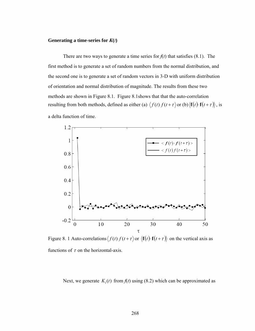
268
Generating a time-series for K(t)
There are two ways to generate a time series for f(t) that satisfies (8.1). The
first method is to generate a set of random numbers from the normal distribution, and
the second one is to generate a set of random vectors in 3-D with uniform distribution
of orientation and normal distribution of magnitude. The results from these two
methods are shown in Figure 8.1. Figure 8.1shows that that the auto-correlation resulting from both methods, defined as either (a) τ+tftf ()( or (b) ( ) ( )τ+⋅ tt ff , is
a delta function of time.
Figure 8. 1 Auto-correlations τ+tftf ()( or ( ) ( )τ+⋅ tt ff on the vertical axis as
functions of τ on the horizontal-axis.
Next, we generate 1( )K t from f(t) using (8.2) which can be approximated as
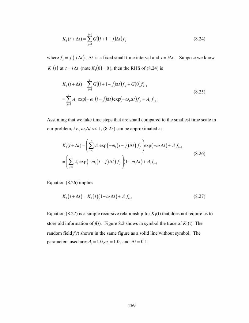
269
( )( )∑+
=
Δ−+=Δ+1
11 1)(
i
jjftjiGttK (8.24)
where ( )jf f j t= Δ , tΔ is a fixed small time interval and t i t= Δ . Suppose we know
( )tK1 at t i t= Δ (note ( ) 001 =K ), then the RHS of (8.24) is
( )( ) ( )
( )( ) ( ) 111
111
11
1
expexp
01)(
+=
+=
+Δ−Δ−−=
+Δ−+=Δ+
∑
∑
i
i
jj
i
i
jj
fAfttjiA
fGftjiGttK
ωω (8.25)
Assuming that we take time steps that are small compared to the smallest time scale in
our problem, i.e., 11 <<Δtω , (8.25) can be approximated as
( )( ) ( )
( )( ) ( )
1 1 1 1 1 11
1 1 1 1 11
( ) exp exp
exp 1
i
j ij
i
j ij
K t t A i j t f t A f
A i j t f t A f
ω ω
ω ω
+=
+=
⎛ ⎞+ Δ = − − Δ − Δ +⎜ ⎟
⎝ ⎠⎛ ⎞
≈ − − Δ − Δ +⎜ ⎟⎝ ⎠
∑
∑ (8.26)
Equation (8.26) implies
( ) ( )( )1 1 1 1 11 iK t t K t t A fω ++ Δ = − Δ + (8.27)
Equation (8.27) is a simple recursive relationship for K1(t) that does not require us to
store old information of f(t). Figure 8.2 shows in symbol the trace of K1(t). The
random field f(t) shown in the same figure as a solid line without symbol. The
parameters used are: 1 11.0, 1.0A ω= = , and 0.1tΔ = .
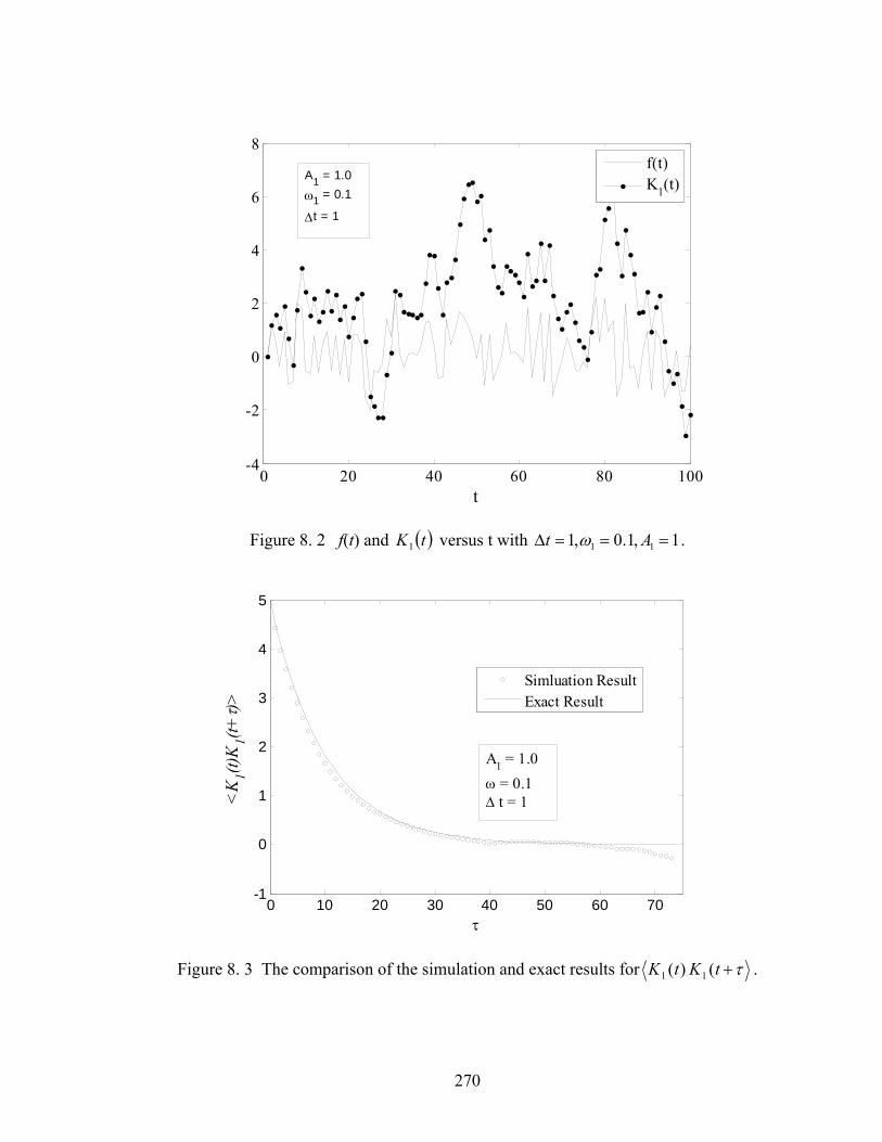
270
0 20 40 60 80 100-4
-2
0
2
4
6
8
t
f(t)K1(t)
A1 = 1.0ω1 = 0.1
Δt = 1
Figure 8. 2 f(t) and ( )tK1 versus t with 1,1.0,1 11 ===Δ At ω .
0 10 20 30 40 50 60 70-1
0
1
2
3
4
5
τ
<K
1(t)K
1(t+τ )
>
Simluation ResultExact Result
A1 = 1.0ω = 0.1 Δ t = 1
Figure 8. 3 The comparison of the simulation and exact results for τ+tKtK ()( 11 .
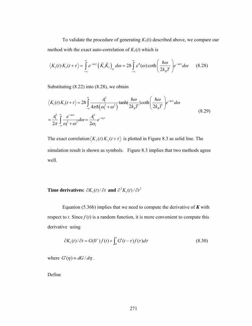
271
To validate the procedure of generating K1(t) described above, we compare our
method with the exact auto-correlation of K1(t) which is
( )1 1 1 1( ) ( 2 ( ) coth2
i i
B
K t K t e K K d e dk T
ωτ ωτ
ω
ωτ ω ε ω ω∞ ∞
− −
−∞ −∞
⎛ ⎞′′+ = = ⎜ ⎟
⎝ ⎠∫ ∫
h% % h (8.28)
Substituting (8.22) into (8.28), we obtain
( )1
21
1 1 2 21
2 21 1
2 21 1
( ) ( 2 tanh( )coth2 24
2 2
i
B B
i
AK t K t e dk T k T
A Ae d e
ωτ
ωτω τ
ω ωτ ωπ ω ω
ωπ ω ω ω
∞−
−∞
∞ −−
−∞
⎛ ⎞+ = ⎜ ⎟
+ ⎝ ⎠
= =+
∫
∫
h hh
h (8.29)
The exact correlation τ+tKtK ()( 11 is plotted in Figure 8.3 as solid line. The
simulation result is shown as symbols. Figure 8.3 implies that two methods agree
well.
Time derivatives: 1( ) /K t t∂ ∂ and 2 21( ) /K t t∂ ∂
Equation (5.36b) implies that we need to compute the derivative of K with
respect to t. Since f (t) is a random function, it is more convenient to compute this
derivative using
1 0( ) / (0 ) ( ) ( ) ( )
tK t t G f t G t f dτ τ τ+ ′∂ ∂ = + −∫ (8.30)
where ( ) /G dG dη η′ ≡ .
Define
272
1 0( ) ( ) / (0 ) ( ) ( ) ( )
tt K t t G f t G t f dϕ τ τ τ+ ′≡ ∂ ∂ = + −∫ (8.31)
then
0( ) ( ) ( ) (0 ) ( )
tG t f d t G f tτ τ τ ϕ +′ − = −∫ (8.32)
At time step t t+ Δ , we have
0
0
( ) (0 ) ( ) ( ) ( )
(0 ) ( ) ( ) ( ) ( ) ( )
t t
t t t
t
t t G f t t G t t f d
G f t t G t t f d G t t f d
ϕ τ τ τ
τ τ τ τ τ τ
+Δ+
+Δ+
′+ Δ = + Δ + + Δ −
′ ′= + Δ + + Δ − + + Δ −
∫∫ ∫
(8.33)
Substituting 11( ) tG t A e ω−= into (8.33) gives
[ ]( )
1 1
1
1 1
( )1 1 10
1 1 1 1
1 1 1
( ) ( ) ( ) ( ) ( )
( ) ( ) ( ) ( )
( ) 1 ( ) ( )
t t tt t t
t
t
t t
t t A f t t e G t f d A e f d
A f t t e t A f t A t f t t
e t A t f t t Ae f t
ω ω τ
ω
ω ω
ϕ τ τ τ ω τ τ
ϕ ω
ϕ ω
+Δ− Δ − +Δ −
− Δ
− Δ − Δ
′+ Δ = + Δ + − −
= + Δ + − − Δ + Δ
= + − Δ + Δ −
∫ ∫ (8.34)
That is
( )1 11 11 1 1
( ) ( ) 1 ( ) ( )t tK t t K te A t f t t A e f tt t
ω ωω− Δ − Δ∂ + Δ ∂= + − Δ + Δ −
∂ ∂ (8.35)
Note that (8.35) is a very simple recursive relationship for 1( ) /K t t∂ ∂ that does not
require us to store old information of f(t).
We can also derive the second order derivative of 1( )K t with respect to t based
on (8.30),
21
2
( , ) (0) (0) ( ) ( ) ( )tK t fG G f t G t f d
t tτ τ τ
−∞
∂ ∂ ′ ′′= + + −∂ ∂ ∫
r (8.36)
Similarly, let
273
21
2
( , )( , ) (0) (0) ( ) ( ) ( )tK t ft G G f t G t f d
t tφ τ τ τ
−∞
∂ ∂ ′ ′′= = + + −∂ ∂ ∫
rr (8.37)
then we have
( ) ( ) ( , ) (0) (0) ( )t fG t f d t G G f t
tτ τ τ φ
−∞
∂′′ ′− = − −∂∫ r (8.38)
We φ at time t t+ Δ ,
1
21
2
( , )( , ) (0) (0) ( , ) ( ) ( , )
(0) (0) ( , ) ( ) ( , ) ( ) ( , )
(0) (0) ( , ) ( , )
t t
t t
t t t
t t t
t
t t
K t t fr t t G G f r t t G t t f r dt t
fG G f r t t G t t f r d G t t f r dt
fG G f r t t e r tt
ω
φ τ τ τ
τ τ τ τ τ τ
φ
+Δ
+Δ −∞
+Δ
+Δ −∞
− Δ
+Δ
∂ +Δ ∂ ′ ′′+Δ = = + +Δ + +Δ −∂ ∂
∂ ′ ′′ ′′= + +Δ + +Δ − + +Δ −∂
∂ ′= + +Δ + −∂
∫
∫ ∫
r
[ ]1 1 1
(0) (0) ( ) ( ) ( , )
( , ) (0) (0) ( , ) (0) ( ) (0) ( , )
t t
t t
t t t
t t t
fG G f t G t t f r dt
f fe r t G e G f r t t G e f t t G f r t tt t
ω ω ω
τ τ τ
φ
+Δ
− Δ − Δ − Δ
+Δ
⎧ ⎫∂ ′ ′′− + +Δ −⎨ ⎬∂⎩ ⎭⎡ ⎤∂ ∂ ′ ′ ′′= + − + +Δ − +Δ +Δ⎢ ⎥∂ ∂⎣ ⎦
∫
(8.39)
We can rewrite (8.39) as
[ ]1 1 1( , ) ( , ) (0) (0) (0) ( , ) (0) ( )t t t
t t t
f fr t t e r t G e G tG f r t t G e f tt t
ω ω ωφ φ− Δ − Δ − Δ
+Δ
⎡ ⎤∂ ∂ ′ ′′ ′+Δ = + − + +Δ +Δ −⎢ ⎥∂ ∂⎣ ⎦
(8.40)
Substituting 11( ) tG t A e ω−= into (8.40) gives
[ ]1 1 1
2 21 1
1 1 1 1 1 12 2
( , ) ( , ) 1 ( , ) ( )t t t
t t t
K r t t K r t f fe A e A t f r t t A e f tt t t t
ω ω ωω ω ω− Δ − Δ − Δ
+Δ
⎡ ⎤∂ +Δ ∂ ∂ ∂= + − − −Δ +Δ +⎢ ⎥∂ ∂ ∂ ∂⎣ ⎦
(8.41)
Note that (8.41) is a simple recursive relationship for 2 21( ) /K t t∂ ∂ that does not
require us to store old information about f(t) and /f t∂ ∂ . However, it is difficult to
evaluate /f t∂ ∂ , because f is a discontinuous function of time. One way of
274
overcoming this difficulty is to assume that f changes linearly with time during any
time step, that is
( ) ( ) ( )f t f t t f tt t
∂ + Δ −≈
∂ Δ (8.42)
8.2 Finite Element Method
In this section, we develop a finite element formulation to solve the Maxwell
equations in time domain based on [1]. The starting point is the two independent
Maxwell’s equations
1 ( , )( , ) ttc t
∂∇× = −
∂B rE r (8.43a)
1 ( , ) ( , )( , ) t ttc t t
∂ ∂⎛ ⎞∇× = +⎜ ⎟∂ ∂⎝ ⎠D r K rB r (8.43b) 17
subjected to the continuity condition of tangential components of E and B .
There are two approaches to solve for E and B from equations (8.43a) and
(8.43b). One method is to solve (8.43a) and (8.43b) simultaneously. In this method,
we need to know ( , ) /t t∂ ∂K r , which is given by (8.35). The other one is to
eliminate ( , )tB r by substituting (8.43a) into (8.43b), resulting in
2 2
2 2 2 2
1 ( , ) 1 ( , )( , ) t ttc t c t
∂ ∂∇×∇× + = −
∂ ∂D r K rE r (8.44a)
17 ( , 0) ( , 0) 0= =B r E r is assumed. This is fine because the initial value will not affect the correlations
i jE E and i jB B which give rise to van der Waals interactions.
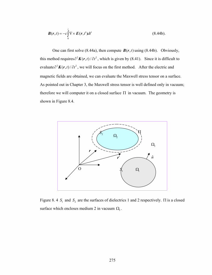
275
0
( , ) ( , )t
t c t dt′ ′= − ∇×∫B r E r (8.44b).
One can first solve (8.44a), then compute ( , )tB r using (8.44b). Obviously,
this method requires 2 2( , ) /t t∂ ∂K r , which is given by (8.41). Since it is difficult to
evaluate 2 2( , ) /t t∂ ∂K r , we will focus on the first method. After the electric and
magnetic fields are obtained, we can evaluate the Maxwell stress tensor on a surface.
As pointed out in Chapter 3, the Maxwell stress tensor is well defined only in vacuum;
therefore we will computer it on a closed surface Π in vacuum. The geometry is
shown in Figure 8.4.
Figure 8. 4 1S and 2S are the surfaces of dielectrics 1 and 2 respectively. Π is a closed
surface which encloses medium 2 in vacuum 3Ω .
r n
O
′r
2Ω
2S Π
1S 1Ω
3Ω
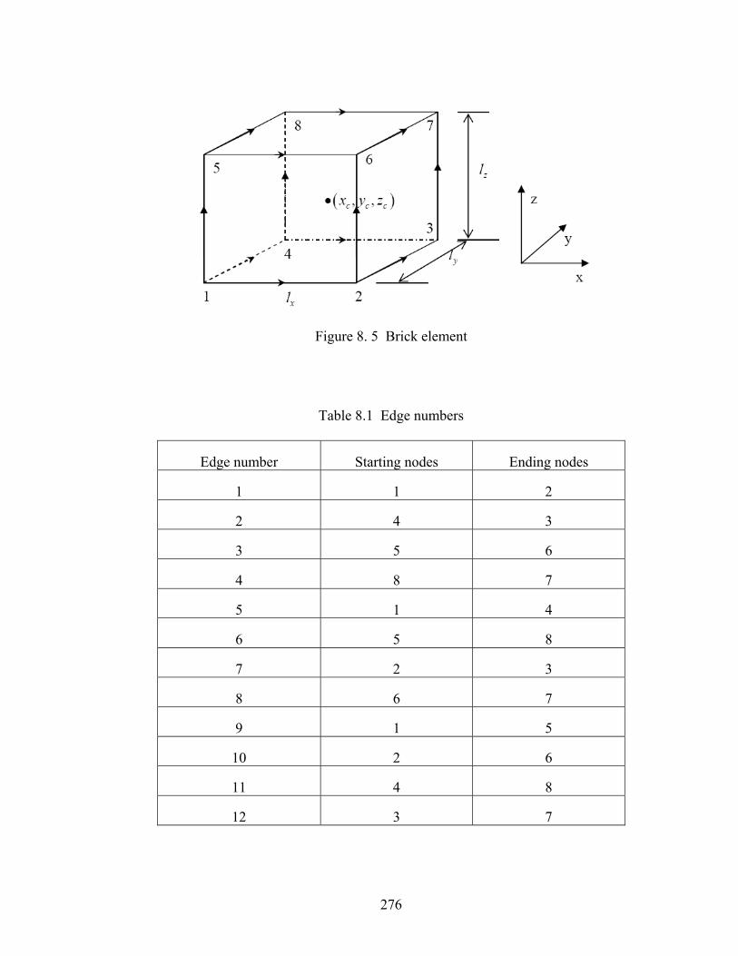
276
Figure 8. 5 Brick element
Table 8.1 Edge numbers
Edge number Starting nodes Ending nodes
1 1 2
2 4 3
3 5 6
4 8 7
5 1 4
6 5 8
7 2 3
8 6 7
9 1 5
10 2 6
11 4 8
12 3 7
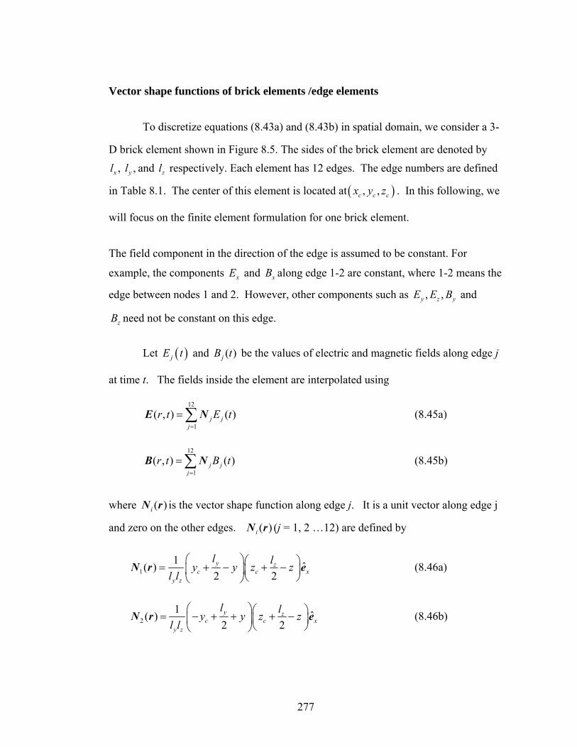
277
Vector shape functions of brick elements /edge elements
To discretize equations (8.43a) and (8.43b) in spatial domain, we consider a 3-
D brick element shown in Figure 8.5. The sides of the brick element are denoted by
, ,x yl l and zl respectively. Each element has 12 edges. The edge numbers are defined
in Table 8.1. The center of this element is located at ( ), ,c c cx y z . In this following, we
will focus on the finite element formulation for one brick element.
The field component in the direction of the edge is assumed to be constant. For
example, the components xE and xB along edge 1-2 are constant, where 1-2 means the
edge between nodes 1 and 2. However, other components such as , ,y z yE E B and
zB need not be constant on this edge.
Let ( )jE t and ( )jB t be the values of electric and magnetic fields along edge j
at time t. The fields inside the element are interpolated using
12
1
( , ) ( )j jj
r t E t=
= ∑E N (8.45a)
12
1
( , ) ( )j jj
r t B t=
= ∑B N (8.45b)
where ( )iN r is the vector shape function along edge j. It is a unit vector along edge j
and zero on the other edges. ( )iN r (j = 1, 2 …12) are defined by
11 ˆ( )
2 2y z
c c xy z
l ly y z zl l
⎛ ⎞⎛ ⎞= + − + −⎜ ⎟⎜ ⎟⎝ ⎠⎝ ⎠
N r e (8.46a)
21 ˆ( )
2 2y z
c c xy z
l ly y z zl l
⎛ ⎞⎛ ⎞= − + + + −⎜ ⎟⎜ ⎟⎝ ⎠⎝ ⎠
N r e (8.46b)
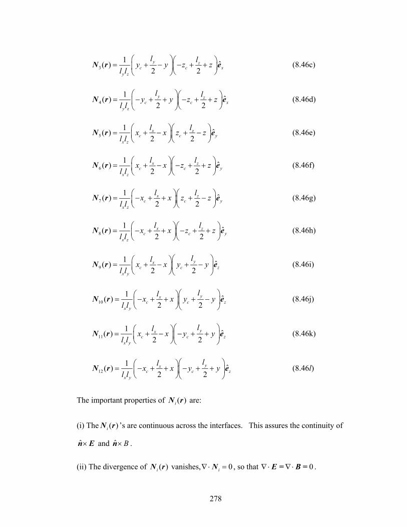
278
31 ˆ( )
2 2y z
c c xy z
l ly y z zl l
⎛ ⎞⎛ ⎞= + − − + +⎜ ⎟⎜ ⎟⎝ ⎠⎝ ⎠
N r e (8.46c)
41 ˆ( )
2 2y z
c c xy z
l ly y z zl l
⎛ ⎞⎛ ⎞= − + + − + +⎜ ⎟⎜ ⎟⎝ ⎠⎝ ⎠
N r e (8.46d)
51 ˆ( )
2 2x z
c c yx z
l lx x z zl l
⎛ ⎞⎛ ⎞= + − + −⎜ ⎟⎜ ⎟⎝ ⎠⎝ ⎠
N r e (8.46e)
61 ˆ( )
2 2x z
c c yx z
l lx x z zl l
⎛ ⎞⎛ ⎞= + − − + +⎜ ⎟⎜ ⎟⎝ ⎠⎝ ⎠
N r e (8.46f)
71 ˆ( )
2 2x z
c c yx z
l lx x z zl l
⎛ ⎞⎛ ⎞= − + + + −⎜ ⎟⎜ ⎟⎝ ⎠⎝ ⎠
N r e (8.46g)
81 ˆ( )
2 2x z
c c yx z
l lx x z zl l
⎛ ⎞⎛ ⎞= − + + − + +⎜ ⎟⎜ ⎟⎝ ⎠⎝ ⎠
N r e (8.46h)
91 ˆ( )
2 2yx
c c zx y
llx x y yl l
⎛ ⎞⎛ ⎞= + − + −⎜ ⎟⎜ ⎟⎝ ⎠⎝ ⎠
N r e (8.46i)
101 ˆ( )
2 2yx
c c zx y
llx x y yl l
⎛ ⎞⎛ ⎞= − + + + −⎜ ⎟⎜ ⎟⎝ ⎠⎝ ⎠
N r e (8.46j)
111 ˆ( )
2 2yx
c c zx y
llx x y yl l
⎛ ⎞⎛ ⎞= + − − + +⎜ ⎟⎜ ⎟⎝ ⎠⎝ ⎠
N r e (8.46k)
121 ˆ( )
2 2yx
c c zx y
llx x y yl l
⎛ ⎞⎛ ⎞= − + + − + +⎜ ⎟⎜ ⎟⎝ ⎠⎝ ⎠
N r e (8.46l)
The important properties of ( )iN r are:
(i) The ( )iN r ’s are continuous across the interfaces. This assures the continuity of
ˆ ×n E and ˆ B×n .
(ii) The divergence of ( )iN r vanishes, 0i∇ ⋅ =N , so that 0∇ ⋅ ∇ ⋅E = B = .
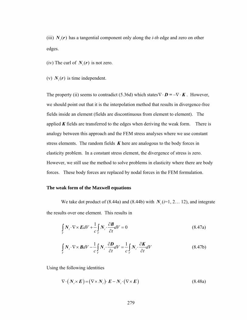
279
(iii) ( )iN r has a tangential component only along the i-th edge and zero on other
edges.
(iv) The curl of ( )iN r is not zero.
(v) ( )iN r is time independent.
The property (ii) seems to contradict (5.36d) which states∇ ⋅ −∇ ⋅D = K . However,
we should point out that it is the interpolation method that results in divergence-free
fields inside an element (fields are discontinuous from element to element). The
applied K fields are transferred to the edges when deriving the weak form. There is
analogy between this approach and the FEM stress analyses where we use constant
stress elements. The random fields K here are analogous to the body forces in
elasticity problem. In a constant stress element, the divergence of stress is zero.
However, we still use the method to solve problems in elasticity where there are body
forces. These body forces are replaced by nodal forces in the FEM formulation.
The weak form of the Maxwell equations
We take dot product of (8.44a) and (8.44b) with iN (i=1, 2… 12), and integrate
the results over one element. This results in
1 0i iV V
dV dVc t
∂⋅∇× + ⋅ =
∂∫ ∫BN E N (8.47a)
1 1i i i
V V V
dV dV dVc t c t
∂ ∂⋅∇× − ⋅ = ⋅
∂ ∂∫ ∫ ∫D KN B N N (8.47b)
Using the following identities
( ) ( ) ( )i i i∇ ⋅ × = ∇× ⋅ − ⋅ ∇×N E N E N E (8.48a)
280
( ) ( ) ( )i i i∇ ⋅ × = ∇× ⋅ − ⋅ ∇×N B N B N B (8.48b)
(8.47a) and (8.47b) can be rewritten as
( ) ( ) 1 0i i iV V
dV dVc t
∂∇× ⋅ − ∇ ⋅ × + ⋅ =⎡ ⎤⎣ ⎦ ∂∫ ∫
BN E N E N (8.49a)
( ) ( ) 1 1i i i i
V V V
dV dV dVc t c t
∂ ∂∇× ⋅ − ∇ ⋅ × − ⋅ = ⋅⎡ ⎤⎣ ⎦ ∂ ∂∫ ∫ ∫
D KN B N B N N (8.49b)
Applying divergence theorem
( ) ( )ˆi iV S
dV dS∇ ⋅ × = ⋅ ×∫ ∫N E n N E (8.50)
to (8.49a, b) gives
( ) ( ) 1ˆ 0i i iV S V
dV dS dVc t
∂∇× ⋅ − ⋅ × + ⋅ =⎡ ⎤⎣ ⎦ ∂∫ ∫ ∫
BN E n N E N (8.51a)
( ) ( ) 1 1ˆi i i iV S V V
dV dS dV dVc t c t
∂ ∂∇× ⋅ − ⋅ × − ⋅ = ⋅⎡ ⎤⎣ ⎦ ∂ ∂∫ ∫ ∫ ∫
D KN B n N B N N (8.51b)
Or
( ) ( ) 1ˆ 0i i iV S V
dV dS dVc t
∂∇× ⋅ + ⋅ × + ⋅ =⎡ ⎤⎣ ⎦ ∂∫ ∫ ∫
BN E N n E N (8.52a)
( ) ( ) 1 1ˆi i i iV S V V
dV dS dV dVc t c t
∂ ∂∇× ⋅ + ⋅ × − ⋅ = ⋅⎡ ⎤⎣ ⎦ ∂ ∂∫ ∫ ∫ ∫
D KN B N n B N N (8.52b)
where S is the surface of the brick element and n is a unit normal vector of S .
Next, we substitute the expansions of E and B (8.45a) and (8.45b) into (8.52a,
b). This results in
281
( ) ( )12 12
1 1
( )1 ˆ( ) ji j j i j i
j jV V S
dB tdV E t dV dS
c dt= =
⎛ ⎞ ⎛ ⎞⎡ ⎤∇× ⋅ + ⋅ = − ⋅ ×⎜ ⎟ ⎜ ⎟⎣ ⎦
⎝ ⎠ ⎝ ⎠∑ ∑∫ ∫ ∫N N N N N n E
(8.53a)
( )
( )
12 12
1 1
1 ( ) ( )
1 ˆ
i j j i j jj jV V
i iV S
dV E t dV B tc
dV B dSc t
= =
⎛ ⎞ ⎛ ⎞⎡ ⎤− ⋅ ℜ∗ + ∇× ⋅⎜ ⎟ ⎜ ⎟⎣ ⎦
⎝ ⎠ ⎝ ⎠∂
= ⋅ − ⋅ ×∂
∑ ∑∫ ∫
∫ ∫
N N N N
KN N n (8.53b)
where ℜ∗ in (8.53b) is defined by
0
0
( , ) ( ) ( )
( , )( , ) ( ,0) ( )
t
t
t k t d
r tk r t r k d
τ τ τ
ττ τ
∂ ∂ ∂ℜ∗ ≡ = + −
∂ ∂ ∂
∂ ∂ −= + +
∂ ∂
∫
∫
D EE r Et t t
E EEt t
(8.54)
The response function ( )k τ can be obtained from the inverse Fourier transform of
( )ε ω (see (5.6)), that is
( )1( ) ( ) 12
i tk t e dωε ω ωπ
∞−
−∞
= −∫ (8.55)
Note that ( , )k r t is homogeneous in each element. Let cr be the center of element. The
matrix forms of (8.53a, b) are
{ } { }11 121
( )( ) ( )d tA t A tdt
⎧ ⎫⎡ ⎤ ⎡ ⎤+ =⎨ ⎬⎣ ⎦ ⎣ ⎦ ⎩ ⎭BE f (8.56a)
{ } { }21 2220
( ) ( )( , ) (0) ( , ) ( ) ( )t
c cd t d tA k r t k r d A t t
d dtττ τ−⎧ ⎫⎡ ⎤ ⎡ ⎤+ + + =⎨ ⎬⎣ ⎦ ⎣ ⎦⎩ ⎭∫
E EE B ft
(8.56b)
where
282
1 1 1 1211 22
12 1 12 12V
A A dV∇× ⋅ ∇× ⋅⎛ ⎞
⎜ ⎟⎡ ⎤ ⎡ ⎤= =⎣ ⎦ ⎣ ⎦ ⎜ ⎟⎜ ⎟∇× ⋅ ∇× ⋅⎝ ⎠
∫L
M
N N N N
N N N N (8.57a)
1 1 1 1212
12 1 12 12
1
V
A dVc
⋅ ⋅⎛ ⎞⎜ ⎟⎡ ⎤ =⎣ ⎦ ⎜ ⎟⎜ ⎟⋅ ⋅⎝ ⎠
∫L
M
N N N N
N N N N (8.57b)
21 12A A⎡ ⎤ ⎡ ⎤= −⎣ ⎦ ⎣ ⎦ (8.57c)
{ } ( )1 ˆiS
dS= − ⋅ ×∫f N n E (8.57d)
{ } ( ) ( )2
,1 ˆi iV S
r tdV dS
c t∂
= ⋅ − ⋅ ×∂∫ ∫
Kf N N n B (8.57e)
Note that matrices 11 12 21 22, , ,A A A A⎡ ⎤ ⎡ ⎤ ⎡ ⎤ ⎡ ⎤⎣ ⎦ ⎣ ⎦ ⎣ ⎦ ⎣ ⎦ are time independent.
Next, backward finite time difference scheme is used to discretize (8.56a) and
(8.56b) in the time domain. For a smooth function ( )g t , the first order time derivative
( ) /dg t dt can be approximated as backward finite difference
( ) ( ) ( )dg t g t g t tdt t
− − Δ≈
Δ (8.58)
Denoting ( ) ( ) jg t g j t g= Δ = , we can rewrite (8.58) as
1( ) j jdg t g gdt t
−−≈
Δ (8.59)
Using this approximation, we obtain the finite difference form of (8.56a) and (8.56b)
{ } { } { } { }12 12
11 11
j j j jA A
At t
−⎡ ⎤ ⎡ ⎤⎣ ⎦ ⎣ ⎦⎡ ⎤ + = +⎣ ⎦ Δ Δ
E B f B (8.60)
283
{ } { }
{ } ( ){ } ( )
21 22
1212 0
1
1 ( )( ) (0) ( , )
j j
tj jjc c
A At
d tA k r k r dt dt
ττ τ−
⎡ ⎤ ⎡ ⎤+⎣ ⎦ ⎣ ⎦Δ−⎡ ⎤⎡ ⎤= + − −⎣ ⎦ ⎢ ⎥Δ⎣ ⎦∫
E B
Ef E E (8.61)
From (8.60) and (8.61), for given initial values { (0)}E and{ (0)}B , we can solve for
the electric and magnetic fields at the next time step (Note: ( )k τ is a known function).
The numerical solutions of this method are unconditionally stable.
8.3 Future work
The general methods (BEM and FEM) have been developed in Chapters 7and 8. It
remains to implement them to solve real problems. The following suggestions can be
considered as the future work on van der Waals forces.
1. Develop computer programs to solve the Lifshitz’s problem. In this way, one
can check the validity of the numerical methods. We have tried to use FEM to
solve the famous three-layer problem. The difficulties we encountered are 1)
dealing with the reflections and radiations of electromagnetic fields on the
boundaries; 2) enforcing the boundary conditions.
2. Extend the lifshitz’ theory to multilayer system. There is a difficulty because
the Maxwell stress tensor is not well defined in non-vacuum media.
3. Develop computer programs to evaluate the van der Waals force for any
systems with arbitrary geometries.
284
APPENDIX
The imaginary part of the dielectric constant is given by (8.22)
( )2
12 21
( ) tanh( )24 B
Ak Tωε ω
π ω ω′′ =
+h
h (8.22)
or for 0T → ,
( )2
12 21
( ) ( )4
A signε ω ωπ ω ω
′′ =+h
(A.1)
By Kramer-Kronig formula, we can calculate the real part of dielectric function
1 ( )( ) 1 uP duuεε ω
π ω
∞
−∞
′′′ = +
−∫ (A.2)
Plemelj formulae implies that
1 ( ) 1 1 ( )( )2 2 2z
u uLim du P dui u z i uω
ε εε ωπ π ω+
∞ ∞
→−∞ −∞
′′ ′′′′= +
− −∫ ∫ (A.3)
Substituting (A.2) into (A.3) gives
( ) ( ) ( )1 ( ) 1 1 1 1( ) ( ) 1 1 12 2 2 2 2z
uLim du ii u z i i iω
ε ε ω ε ω ε ε επ+
∞
→−∞
′′′′ ′ ′ ′′= + − = + − = −
−∫ (A.4)
so
1 ( )1z
uLim duu zω
εεπ +
∞
→−∞
′′= +
−∫ (A.5)
First we consider zero-temperature. In this case, ( )uε ′′ is given by (A.1) which is
285
( )2
12 21
( ) ( )4
A signε ω ωπ ω ω
′′ =+h
(A.6)
where ( )sign ω is defined as
1 if 0( ) 0 if 0
1 if 0sign
ωω ω
ω
>⎧⎪= =⎨⎪− <⎩
(A.7)
Substituting (A.6) into (A.5) gives
( )( ) ( )( )
2 21 12 22 2 2 2 2 2
01 1
( ) 21 14 4z z
A Asign u uLim du Lim duu z u u z uω ω
επ πω ω+ +
∞ ∞
→ →−∞
= + = +− + − +∫ ∫h h
(A.8)
Changing the variable 2v u= implies
( )( )2
12 2 2
0 1
14 z
A dvLimv z vω
επ ω+
∞
→= +
− +∫h (A.9)
(A.9) can be evaluated using residue theorem, and the result is
2 2 22 221 11 1
2 2 2 2 2 2 2 21 1 1
ln ln lnln1 14 4z
i iA AzLimz zω
ω π ω ω πε
π ω ω π ω ω+→
⎡ ⎤+ − += + − = +⎢ ⎥
+ + +⎢ ⎥⎣ ⎦h h (A.10)
For the finite temperature, ( )uε ′′ is given by (8.22). By substituting (8.22) into
(A.5) and evaluating the integral, one can obtain the following complicated result
286
( )
( ) ( )
12
12 2 2 2 2 2
0 1 1
12
12 2 2 2 2 2 2 2
0 1 1 1 1
tan2 21
2 ( )( ) 2
tan tanh2 2 2
2 ( )( ) 2
nB B
n n n
B B B
n n n
A k T k T
A k T k T k Ti
ωβε
π ω β ω β ω ω
ω ωωω
π ω β ω β ω ω ω ω ω
∞
=
∞
=
⎡ ⎤⎢ ⎥⎢ ⎥= + +
+ − +⎢ ⎥⎢ ⎥⎣ ⎦
⎡ ⎤⎢ ⎥−⎢ ⎥+ − +
+ − + +⎢ ⎥⎢ ⎥⎣ ⎦
∑
∑
h
h h
h h
h h
(A.11)
where ( )2 2 1Bn
k T n πβ
+=
h. Finally, it should be noted that at room temperature,
tanh( / 2 ) 1Bk Tω ≈h is a good approximation.

287
REFERENCES
1. Jianming Jin, Finite Element Method in Electromagnetics, 2th edition, 2002.