Adaptive Radar Sensor Model for Tracking Structured Extended Objects

Chalmers Publication Library

Adaptive Radar Sensor Model for Tracking Structured Extended Objects

This document has been downloaded from Chalmers Publication Library (CPL). It is the author´s

version of a work that was accepted for publication in:

IEEE Transactions on Aerospace and Electronic Systems (ISSN: 0018-9251)

Citation for the published paper:Hammarstrand, L. ; Lundgren, M. ; Svensson, L. (2012) "Adaptive Radar Sensor Model forTracking Structured Extended Objects". IEEE Transactions on Aerospace and ElectronicSystems, vol. 48(3), pp. 1975 - 1995.

http://dx.doi.org/10.1109/TAES.2012.6237574

Downloaded from: http://publications.lib.chalmers.se/publication/161483

Notice: Changes introduced as a result of publishing processes such as copy-editing and

formatting may not be reflected in this document. For a definitive version of this work, please refer

to the published source. Please note that access to the published version might require a

subscription.

Chalmers Publication Library (CPL) offers the possibility of retrieving research publications produced at ChalmersUniversity of Technology. It covers all types of publications: articles, dissertations, licentiate theses, masters theses,conference papers, reports etc. Since 2006 it is the official tool for Chalmers official publication statistics. To ensure thatChalmers research results are disseminated as widely as possible, an Open Access Policy has been adopted.The CPL service is administrated and maintained by Chalmers Library.

(article starts on next page)

http://dx.doi.org/10.1109/TAES.2012.6237574

http://publications.lib.chalmers.se/publication/161483

HAMMARSTRAND et al.: ADAPTIVE RADAR SENSOR MODEL FOR TRACKING STRUCTURED EXTENDED OBJECTS 1

Adaptive radar sensor model for tracking structuredextended objects

Lars Hammarstrand, Malin Lundgren, and Lennart Svensson senior member, IEEE

Abstract—In this paper, we propose a tracking frameworkjointly estimating the position of a single extended object andthe set of radar reflectors that it contains. The reflectors areassumed to lie on a line structure, but the number of reflectorsand their positions on the line are unknown. Additionally,we incorporate an accurate radar sensor model consideringthe resolution capabilities of the sensor. The evaluation of theframework on radar measurements shows promising results.

Index Terms—Radar, Sensor model, Extended targets, Track-ing.

I. INTRODUCTION

H ISTORICALLY, multi target radar tracking research hasfocused on tracking targets at large distances in the

presence of clutter [1], [2]. In such scenarios, the return froma target, e.g. an aircraft, is accurately modelled as a pointsource, and the radar (with limited resolution) is not capable ofresolving multiple features on the object. Thus it is common toassume that the object’s physical extent is negligible comparedto the measurement noise and that each object generates atmost one measurement, which is known as the point sourceassumption.

In many other applications, such as vehicle tracking inautomotive active safety systems [3], the situation is different.Here, the distance to objects is instead in the order of tens ofmetres and at these distances, the physical extent of objects istypically larger than the resolution of the radar sensor. Con-sequently, the radar is capable of resolving multiple features(reflection centres) on an object, which can lead to multiplemeasurements originating from the same object. The radarliterature refers to these types of objects as extended targets[4]. Attempting to track this type of object using methodsoriginally developed for point source targets will likely lead tolarge estimation errors as the multiple received measurementsare not accurately described as originating from a point source.This is illustrated in, e.g. [3], where a detailed extended objectmodel of radar returns from a car is compared to a simplerpoint source model. The extended object model provides botha better description of the vehicle-generated detections anda more accurate tracking performance compared to the pointsource model.

This work was sponsored by the Swedish Intelligent Vehicle Safety Systems(IVSS) program, and is a part of the SEnsor Fusion for Safety Systems (SEFS)project.

L. Hammarstrand is with Volvo Car Corporation, Gothenburg, [email protected].

L. Hammarstrand, M. Lundgren and L. Svensson are with theDepartment of Signals and Systems, Chalmers University of Technology,Gothenburg, Sweden [email protected],[email protected], [email protected].

Clearly, it is possible to benefit from the fact that anobject generates multiple radar measurements. In addition toa more accurate tracking it is also possible to extract moredetailed information about the object, e.g., the spread of themeasurements provides information about the extension andheading of the object. However, there are several difficultiesthat arise when tracking extended objects. For example, aconsiderably more complex sensor model is needed to describethe object-generated measurements with sufficient accuracy, asthe measurements are spread across the whole extension of theobject. Additionally, it needs to handle the situation that sev-eral features on an object might or might not be resolved by theradar sensor [5], and moreover, also describe the measurementuncertainty caused by measurements from unresolved features.The resulting tracking framework consequently, needs to treatthe occurrence of possibly multiple measurements from eachobject, in contrast to at most one measurement in the pointsource case.

A comprehensive overview of the research in the area oftracking extended objects, and the closely related problemof group tracking, up to the year 2004, can be found in[6]. The PHD framework, proposed by Mahler [7], has beenused extensively to address the problem of tracking groups oftargets and adaptations to track extended targets are presentedin [8] and [9]. In [10] and [11], Koch and Saul present aBayesian framework for tracking an extended object or agroup of closely spaced objects, under the assumption thatmultiple measurements can originate from the same object.The object/group extension is modelled by an elliptical shape,defined by a symmetric positive definite random matrix. Thismatrix is included in the state vector together with the kine-matical states, and all states are jointly estimated from data. Asimilar model of extended objects is also in [12] but here ina combined set-theoretic and stochastic estimator. Both thesemodels has shown to be robust against object shape but itis difficult to exploit more specific shape information if suchinformation is available. A different approach is to model theextended object as a set of point features positioned on a(semi-) rigid structure, where each feature may be the originof at most one measurement. This idea is adopted in, forexample, [13]–[17]. However, little attention has been givento practical issues such as how to handle the uncertaintiesassociated with limited sensor resolution or how to consideran unknown number of features on the object.

The problem of data association using possibly unresolvedmeasurements is treated in [18] and [19], which propose twodifferent sets of models for a joint measurement from twounresolved point sources and for the probability that the two

2 HAMMARSTRAND et al.: ADAPTIVE RADAR SENSOR MODEL FOR TRACKING STRUCTURED EXTENDED OBJECTS

sources are unresolved. Using these models, the traditionaldata association hypotheses and measurement models areexpanded to also consider merged measurements. Proposalsthat consider resolution uncertainty for a known but arbitrarynumber of sources are [3], [20]. The approach proposedin [20] is a generalised version of the probabilistic modelin [19], evaluating all possible combinations of associatingmeasurements to inter-resolved clusters of sources. In [3],the resolution uncertainty is handled by letting sources thatare possibly unresolved form independent groups, where eachgroup is capable of generating multiple measurements. Incontrast to [20], the solution in [3] considers only the moreprobable formations of inter-resolvable sources.

In this paper, we propose a complete framework for trackinga single extended object, including estimation of both theposition and kinematics of the object as well as the positionsof radar reflecting features. The object is modelled, similarto [13]–[17], as (loosely) structured reflection centres sharinga common kinematic description. However, the concept isextended here to also consider uncertainty in the number offeatures on the structure. Additionally, we propose a radarsensor model that considers the arbitrary and unknown numberof reflection centres, and which incorporates the limited reso-lution model presented in [20]. As a result, we are capable ofadapting the description of the object-generated measurementsover time as the same object might look very different to theradar depending on angle and distance. The proposed trackingframework is compared to that in [3], using data from twotypes of automotive radars, a 77 GHz long range radar1 anda 24 GHz medium range radar, and the true position of thetracked vehicle is provided by an accurate differential GPS.

The paper is organised as follows. Section II introducesthe notation and the problem considered in this paper. InSection III, the extended object model is presented, andSection IV describes the proposed radar sensor model in detail.A derivation of the posterior density is found in Section Vwhile Section VI discusses how this is treated in a trackingframework. Finally, Section VII presents the results from theproposed models in a tracking framework.

Notation: To facilitate the reading of this paper, we hereexplain the general structure of the notation used. Vectorvariables are boldface, e.g. x. Subscripts and superscripts initalic are used as indexes of some sort, e.g. time index inxk, whereas regular letters shall be interpreted as part of thevariable name, e.g., Pd for the probability of detection. Regularcalligraphic letters are used to indicate probabilistic events orhypotheses (C, D, E) and boldface calligraphic letters (X , G)denote sets and graphs.

II. PROBLEM FORMULATION AND MODELLINGASSUMPTIONS

The problem that is studied in this paper is twofold: to usemeasurements from a radar to jointly estimate the position andkinematics of an extended object, and to adapt a structure thatdescribes the possibly multiple radar returns from the object.

1Long range radar in automotive applications entails a detection range of150 m and above.

The ultimate aim is to improve the tracking of an extendedobject through adaptation of the radar sensor model to fit theunknown and changing behaviour of the object’s radar returns.

In the coming sections we define the conditions and as-sumptions needed to solve this problem in a Bayesian track-ing framework. The extended object model is introducedin Section II-A. In Section II-B, the radar observations aredescribed and finally Section II-C formally defines the problemconsidered in the paper.

A. Extended object model

Similarly to the approach in [21], the radar return fromthe object of interest is assumed to be accurately modelledas originating from a set of reflection centres, i.e., a set offeatures on the object that are more likely to generate a strongreturn. The reflection centres are organised on a structure (rigidbody) capturing the position, kinematics and shape of theextended object. We assume that we know that there existsone and only one visible extended object but, in contrast to[21], we assume that neither the number of reflection centresnor their initial positions are known. The information about theextended object at a discrete time instance k is summarised inan extended object state

xk =[(zk)

T, (ξk)

T]T. (1)

The vector zk, called the structure state (bulk) vector, typicallydescribes the common position and velocity of the extendedobject. The feature vector,

ξk =

[(ξ1k

)T, . . . ,

(ξnξkk

)T]T, (2)

contains parameters describing the positions of nξk reflectioncentres in relation to the structure. For a line structure, like theone in Figure 1a, ξik describes the distance (length on the struc-ture) from the target centre to the ith reflector. The positionof reflection centre i in the global coordinate system is foundusing the mapping function g(zk, ξ

ik). This representation can

be interpreted as the positions of the reflector centres in statespace being restricted to a subspace S(zk) ⊆ Rnz defined bythe structure state vector zk.

Using this general description, it is possible to modeldifferent types of extended objects with a variety of imposedstructures for positioning of individual reflection centres. Fig-ure 1 shows three examples of how one can represent extendedobjects on the form in (1). In all the examples, the kinematicdescription of the object is included in the structure statevector, zk, which for the arc and box object also includes somedescription of the curved and rectangular shape, respectively.For the graph representation, the imposed structure is morelimited and the position of the individual reflectors make upthe shape of the object.

It is assumed in this paper that the time evolution of theextended object state, xk, can be divided into two parts,

xk+1 =

[zk+1

ξk+1

]=

[fz(xk,v

zk)

fξ(xk,vξk)

], (3)


(a) Line structure (b) Box structure (c) Graph structure

Figure 1. Different structure model alternatives for representing an extended object. Example (a) models the extended object as a line with the reflectorspositioned along it, example (b) as a rectangle and example (c) as a more general graph shape.

where fz(·) describes the dynamic behaviour of the structureand fξ(·) captures the dynamics of the reflector centres in rela-tion to the structure and the change in the number of reflectors.The variables, vzk and vξk, are noise process accounting formodel uncertainties.

B. Radar observationsObservations on the positions of the reflection centres are

provided by radar sensors mounted on a possibly moving hostplatform, and it is assumed that both the position of the sensorsand the state of the host platform, denoted zh

k, are knownparameters in the measurement model. The sensors are similarin that if a feature on the extended object is a strong scattererfor one sensor, this is also true for the others. At each time k,only one of the radar sensors provides a set of measurements,and as a result, although we have a multi-sensor system, weonly need to consider measurements from one sensor at eachupdate step. All sensors are thus treated separately and in asimilar manner and to simplify notation, the presentation islimited to one of the sensors.

At each time instance k, a sensor provides Mk detections,where mt

k detections are generated by the extended objectand mc

k observations are clutter. All detections are stored inthe unlabelled measurement vector,

yk =[(y1k)T , (y2

k)T , . . . , (yMk

k )T]T. (4)

Each measurement in (4) contains an observation of therelative range, rik, angle, φik, and range rate, rik, between oneradar reflection source (object related or clutter) and the sensor,such that

yik = [rik, φik, r

ik]T . (5)

The collection of all measurement vectors up to and includingtime instance k is denoted Yk , {y1,y2, . . . ,yk}.

Let us define an ordered collection of the detections whichoriginate from the extended object and those which originatefrom clutter as

ytk =

[(yt,1k

)T, . . . ,

(y

t,mtk

k

)T]T(6)

yck =

[(yc,1k

)T, . . . ,

(y

c,mck

k

)T]T. (7)

These two vectors are connected to the measurement vector,yk, through an unknown random permutation matrix, ΠMk

p ,with dimension [Mk ×Mk]. This relation can mathematicallybe expressed as

yk = (ΠMkp ⊗ I3×3)

[yck

ytk

], (8)

where ⊗ is the Kronecker product and I3×3 is a three-by-three-dimensional identity matrix. The purpose of ΠMk

p

is to describe the uncertainty in measurement origin (dataassociation uncertainty). The treatment of this uncertainty isan important part in the derivation of the tracking framework,and is further discussed in Section VI.

The clutter measurement vector, yck, is assumed to behave

according to a known and object-independent clutter modeldescribing both the number of clutter detections mc

k and theirspatial distribution. The mt

k object-generated detections arenaturally described by the reflection centres on the structure.Given a state vector xk with Nξ

k reflectors2, the positionsof these reflectors in the observation space, denoted rk, andthe parameter describing the expected return signal amplitudefrom the reflectors, denoted σk, are given by a known function

[(rk)T , (σk)T ]T = hξ(xk) (9)

where rk = [(r1k)T , . . . , (r

Nξkk )T ]T and σk = [σ1

k, . . . , σNξkk ]T .

Under ideal conditions, the object measurement vector, ytk,

would contain one detection from each reflection centre,i.e., yt,i

k = rik. However, due to limitations in radar signalbandwidth and pulse duration as well as antenna aperture size,radar sensors are not capable of resolving reflection centresthat are too closely spaced. As such, all reflectors are notalways resolvable and the response from a cluster of reflectorsmight merge to form a joint detection. Additionally, a reflectoror a cluster of reflectors will be detected only if the signal tonoise ratio of its radar return is sufficiently large. We assumethat the object measurements from a reflector or a cluster ofreflectors can be described as

ytk = hc (rk,σk,wk) , (10)

2Conditioned on xk , the number of reflection centres is known. This isindicated by denoting the number of reflectors using uppercase N instead oflowercase.


where hc(·) is a stochastic function and wk is a measurementnoise process capturing both model uncertainties and measure-ment disturbances. The function hc(·) describes mt

k detectionsfrom inter-resolved reflector clusters and is stochastic in thesense that it changes depending on how the nξk reflectors arepartitioned into resolvable reflector clusters, and which of theclusters that are detected by the sensor.

C. Tracking problem

As aforementioned, the aim of this paper is to derive aBayesian tracking framework for jointly estimating the struc-ture state, zk, as well as the number of reflection centres, nξk,and their positions, ξk, on the extended object, based on noisyradar observations, Yk. As new measurements are available,the posterior density, p

(xk∣∣Yk

), is recursively calculated.

From this density it is possible to compute estimates includinguncertainty measures under different optimality constraints.

For the type of problem considered in this paper, thecalculation of p

(xk∣∣Yk

)is feasible using knowledge from

two types of probabilistic models: the process model definedby (3) and the measurement model defined in (8). Furthermore,we need to consider three additional types of uncertaintiesinfluencing our ability to interpret the measurements. First,we need to handle that the number of reflection centres on thestructure is unknown and time-varying (existence uncertainty).Second, even under known number of reflection centres, theobject measurement model (10) is stochastic due to uncer-tainty regarding how the reflectors are partitioned into inter-resolvable reflector clusters (resolution uncertainty). Finally,we do not know which of the clusters that are detected by thesensor and which of the measurements in yk corresponds towhich object detection (data association uncertainty).

These aspects of the calculation of the posterior density areaddressed in the following sections. In Section III, we definethe parametrisation of the extended object considered in thispaper, together with the process model (3). The radar sensormodel which incorporates resolution uncertainty is derivedin Section IV. By introducing interdependent hypotheses tohandle the existence, cluster and data association uncertaintieswith associated probabilistic models, the derivation of theposterior density based on the process and radar sensor modelis concluded in Section V. The existence, cluster and dataassociation hypotheses indicate which reflectors on the objectexists, which of these form inter-resolvable clusters and whichmeasurement originated from which cluster, respectively. Fi-nally, to arrive at a more computational tractable solution,we marginalise over the hypotheses and introduce suitableapproximations in Section VI.

III. STRUCTURE MODEL

This section describes the specific extended object modelused in this paper, i.e., a structure to which a collectionof reflector centres are attached. We will discuss the stateparametrisation of the extended object as well as models forits evolution over time. This includes both the motion of thestructure and the reflection centres, as well as how the numberof reflectors changes over time.

A. Structure parametrisationIn this paper we propose to use a simple yet useful structure

model. We assume that an extended object can be modelledas a straight line to which the unknown number of reflectorcentres are associated, as shown in Figure 2. All parameters ofinterest for describing this structure are collected in a discretetime state vector, xk. As in [21], this vector consists of twoparts, namely a structure state vector zk containing, e.g., theposition, velocity and heading of the line, and a feature vector,ξk, describing the positions of the reflector centres on thestructure.

The state vector for the line structure in this paper isparameterised as

zk = [xk, yk, ψk, vk, ck, ak, θk]T , (11)

where (xk, yk) is defined as the mid point as well as therotation point of the line, and is expressed in global Cartesiancoordinates. The rotation point travels at an instantaneousspeed vk and acceleration ak in the direction of travel de-scribed by the heading angle ψk. Further, the heading and theline rotates along the trajectory described by the curvature ck3,and the line itself is rotated relative to its heading accordingto θk.

The feature vector ξk, that describes the reflector positionson the structure, is defined as

ξk = [l1k, l2k, . . . , l

nξkk ]T , (12)

where nξk is the unknown (and stochastic) number of re-flectors, and lik is the distance from the line centre to theith reflector. The complete extended object state vector is

xk =

[zTk , l

1k, l

2k, . . . , l

nξkk

]T.

B. Structure process modelThe structure state evolves over time according to the time-

continuous motion model

z(t) =

v(t)cos (ψ(t))v(t)sin (ψ(t))

c(t)v(t)a(t)

000

+

0000

νc(t)νa(t)νθ(t)

, (13)

where νc, νa and νθ are white time-continuous zero-meanGaussian noise processes with variances σ2

c , σ2a and σ2

θ ,respectively. A discrete-time version of (13) is readily availableon the form

zk = fz(zk−1) + vzk−1 (14)

derived assuming constant noise increments during one sam-pling period, and where vzk ∼ N (0,Qz) is the correspondingdiscrete time noise process. The exact expression of (14) isnot given here for brevity, but the interested reader can findthe discrete time version of a similar model in [3].

3The curvature ck is here used to describe the heading change rate of theline structure as a function of distance. Definition: The rotation point travelson the circumference of a circle with radius 1/ck (see Fig. 2).


Figure 2. In this paper an extended object is modelled as a line to which a collection of reflection centres is associated. The state vector, zk , describing thestructure is parameterised in a global Cartesian coordinate system.

C. Feature process modelThe process model for the feature state, as defined in

(3), needs both to describe how the reflectors move on thestructure, and account for changes in the number of reflectors.The number of reflectors can change in part due to existingreflectors disappearing and in part due to new reflectorsappearing. Let us assume that the feature process model canbe partitioned as

ξk =

[ξsk

ξbk

]=

[f sξ(xk−1,v

sk−1)

f bξ (xk−1,v

bk)

], (15)

where ξsk and ξb

k are random vectors containing the positionsof the ns

k surviving reflectors from time k − 1 and the nbk

appearing reflectors at time k. Both nsk and nb

k are assumedunknown and random and the respective feature vector ismodelled by the survival process model f s

ξ(·) and the birthprocess model f b

ξ (·). The noise processes, vsk−1 and vb

k, de-scribe uncertainties in the dynamics of the surviving reflectorsand in the position of born reflectors.

1) Survival model: To indicate whether reflector i in ξk−1

is still present at time k (survives until time k) or not, weintroduce an existence (survival) variable eis,k ∈ {0, 1}, whereeis,k = 1 indicates that the ith reflector survived and vice versa

for eis,k = 0. Further, we denote P is,k = Pr{eis,k = 1

∣∣ ξk−1

}and 1 − P is,k as the probability of the respective outcome.Let the survival hypothesis, denoted E s

k, indicate one possibleordered set of N s

k surviving reflectors, {s1, . . . , sN sk} = {i :

eis,k = 1}, such that 1 ≤ s1 < · · · < sN sk≤ Nξ

k−1. Usingthis hypothesis, the survival process model is modelled as asimple random walk,

ξsk = f s

ξ(ξk−1, E sk,v

sk−1) =

ls1k−1...

lsNsk

k−1

+

vs,s1k−1...

vs,sNs

k

k−1

, (16)

where vs,ik−1 ∼ N (0, σ2

s ) is a noise process included to allowfor a small movement of a reflector along the line structure.

From the survival model, the transition density for ξsk can

be formed as

p(ξsk

∣∣ ξk−1) =∑E sk

p(ξsk

∣∣ E sk, ξk−1)Pr

{E sk

∣∣ ξk−1

}(17)

where

p(ξsk

∣∣ E sk, ξk−1

)=

N sk∏

j=1

N(ljk; l

sjk−1, σ

2s

)(18)

Pr{E sk

∣∣ ξk−1

}=

Nξk−1∏i=1

(1− P is,k

) N sk∏

j=1

Psjs,k

1− P sjs,k. (19)

2) Birth model: At a time k, we assume that a maximumnumber of Bk new reflectors appear on the structure, each witha position described by a Gaussian density lb,ik ∼ N

(lb,ik , σ

2b

).

Again, we introduce an existence variable, eib,k ∈ {0, 1}stating whether reflector i is born or not and denote the corre-sponding birth probability as P ib,k. Similarly as in the survivalprocess, we let a birth hypothesis Eb

k indicate one possibleordered set of N b

k appearing reflectors, {b1, . . . , bN bk} = {i :

eib,k = 1}, such that the birth process can be written as

ξbk = f b

ξ (Ebk,v

bk) =

lb,b1k

...

lb,b

Nbk

k

+

vb,b1k...

vb,b

Nbk

k

, (20)

where vb,bik ∼ N

(0, σ2

b

). Using (20), the pdf of ξb

k can beformed as

p(ξbk

)=∑Ebk

p(ξbk

∣∣ Ebk

)Pr{Ebk

}(21)


where

p(ξbk

∣∣ Ebk

)=

Nbk∏j=1

N(ljk; l

b,bjk , σ2

b

)(22)

Pr{Ebk

}=

Bk∏j=1

(1− P jb,k

) N bk∏

j=1

Pbjb,k

1− P bjb,k

. (23)

D. Extended object process model

Through forming an existence hypothesis, Ek ={E sk, Eb

k

},

and using the process models for the structure and the reflectorcentres, the complete process model for the extended object,conditioned on the existence hypothesis, can be stated

xk = f (xk−1, Ek,vk−1) =

fz (zk−1) + vzk−1

f sξ(ξk−1, E s

k,vsk−1)

f bξ (Eb

k,vbk)

. (24)

The corresponding conditional transition density can be ex-pressed as

p(xk∣∣ Ek,xk−1

)= N (zk; fz(zk−1),Qz)×N sk∏

j=1

N(ljk; l

sjk , σ

2s

) N sk+N b

k∏j=N s

k+1

N(ljk; l

b,bjk , σ2

b

), N

(xk; xEk ,Q

Ek

), (25)

where xEk = f (xk−1, Ek,0) is the determinstic part of (24),and QEk is the process noice covariance. The transitionalexistence hypothesis probability is found as Pr

{Ek∣∣ ξk−1

}=

Pr{E sk

∣∣ ξk−1

}Pr{Ebk

}.

IV. RADAR SENSOR MODEL

The objective of this section is to present the radar sensormodel for the clutter measurement vector, yc

k, and the objectmeasurement vector, yt

k, in (8) given an extended object statevector xk. Recall that xk includes both the structure state aswell as the number of reflectors and their positions on thestructure. From yc

k and ytk it is then possible to form the

measurement vector, yk, by generating a random permutationmatrix ΠMk

p .For the clutter measurements we adopt the assumption that

yck is described by a homogenous Poisson process in the

observation space according to

yc,ik ∼ Uniform(V ), (26)mck ∼ Poisson(µV ), (27)

where yc,ik is the ith clutter measurement, µ is the clutter

intensity and V the volume of the observation space. Inaddition, we assume that the clutter detections are independentfrom each other and from the object detections.

Under ideal conditions the object measurement vector, ytk,

would contain one detection from each reflection centre, andthe vector yt,i

k would be the corresponding reflector positionin observation space as defined in (9). However, due tomeasurement noise, limited sensor resolution and a probabilityof detection less than one, the situation is not that simple.

To start with, the exact physical model for determiningwhich reflectors that are resolved and which are clustered,i.e. unresolved, is not easily derived. For this reason, weresort to a stochastic description of the phenomenon based onevaluating all possible cluster formations. Given a state vectorxk, a cluster formation is a partitioning of the Nξ

k reflectorsin ξk into a set of inter-resolvable clusters of reflectors, i.e.,the returns from reflectors in a cluster are unresolvable tothe radar while the radar is capable of distinguishing returnsfrom reflectors in different clusters. Let a cluster hypothesis Ckindicate one of these formations and let the probability of Ckbe modelled by Pr

{Ck∣∣xk}. The resolution capabilities of a

sensor can thus be probabilistically described by generating allpossible cluster formations and evaluating their probabilitiesusing Pr

{Ck∣∣xk}.

Under a given cluster hypothesis, it is assumed that eachcluster in the formation can generate at most one detection.This holds for both clusters containing only one reflectorand clusters containing multiple unresolved reflectors. Con-sequently, to model the object-generated measurements givena cluster hypothesis, we need to describe: 1) the probabilityof detecting a cluster, and 2) the distribution of that possibledetection. The model of the individual reflector positions inthe observation space and the model of their received signalamplitudes are discussed in Section IV-A. Based on thesemodels, both the distribution of the object-generated detectionsand the probability of detecting a cluster is presented fora given cluster hypothesis in Section IV-B. Finally, how togenerate the possible cluster hypotheses, Ck, and evaluate theirprobabilities, Pr

{Ck∣∣xk}, is given in Section IV-C.

A. Reflector model

The full mathematical details of the reflector model (9) aregiven in Appendix A and summarised here for clarity. Thepurpose of the model, defined as

[(rk)T , (σk)T ]T = hξ(xk) (28)

is twofold: to, given xk, describe the position of the reflectioncentres in measurement space, rk, and to model the expectedreturn signal amplitude from each centre, described by theparameter vector σk. In our case, σk is a vector of Rayleighparameters as we assume that the return signal power ofreflector i, denoted Aik, is behaving according to the Swerling Imodel [22]. The Swerling I model stipulates that the amplitudeof the received signal fluctuates between scans according tothe Rayleigh distribution

Aik ∼ Rayleigh(σik), (29)

where E{Aik}

= σik√π/2.

B. Cluster model

We assume that the jth measurement in ytk originated from

the ith cluster in the cluster formation indicated by Ck. Thiscluster is assumed to consist of a number of unresolved


reflectors4, and is defined by a set of reflector indices,

ICi = {l: reflector number l is in cluster number i}. (30)

A simple, yet useful, model is to describe the (state dependent)signal component of a merged detection from this cluster as aweighted sum of the included reflection centres,

cC,ik =∑l∈ ICi

wlkrlk, (31)

where the weights are determined by the relative signalstrength of the reflection centres according to

wlk =Alk∑

m∈ ICi

Amk. (32)

The signal amplitude of the cluster detection, denoted AC,ik , isalso Rayleigh distributed but with parameter

σC,ik =

√√√√√∑l∈ ICi

(σlk)2. (33)

Assuming additive Gaussian measurement noise, thejth measurement in yk is

yt,jk = cC,ik + wj

k (34)

where wjk ∼ N (0,Wk) denotes (sensor dependent) measure-

ment noise, and the probability of receiving this detection isgiven by

PC,id,k = Pr{AC,ik > γsA

∣∣xk} . (35)

Note that, even given xk, the signal component of the clus-ter measurement, cC,ik , is stochastic as the weights wjk arestochastic. The distribution of cC,ik is defined by (29) – (32),which is difficult to evaluate. For this reason, we proposeto approximate the cluster density as a Gaussian density,p(cC,ik∣∣xk) ≈ N (cC,ik ; cC,ik ,CC,ik

), with the same first two

moments as the underlying distribution.Let overscore denote the expected value of stochastic vari-

ables conditioned on xk, such that, e.g., cC,ik = E{

cC,ik∣∣xk}.

The first moment of cik, as given by (31), is

cC,ik =∑l∈ ICi

wlkrlk (36)

and after some manipulations, an expression for the covariancecan be found as

CC,ik =∑

s, t∈ ICi

(rsk − cC,ik

)(rtk − cC,ik

)TCov

{wsk, w

tk

}.

(37)

The position of each reflector, rik, is given by (100) in Ap-pendix A, but we also need to express wik and Cov {wsk, wtk}.As the moments of a Rayleigh distribution are well known,approximations of these quantities are readily found throughTaylor expansion.

4A resolved reflector can be viewed as a cluster of reflectors wherecontaining only one reflector.

C. Sensor resolution model

In [11], [19], a simple but qualitatively correct and tractablemodel is proposed for describing the probability that two pointsources (targets) are unresolved by a radar sensor. Based onthis two-source model, a sensor resolution model coveringan arbitrary number of sources was derived in [20]. Thismodel is also used in this paper to model the probability ofreceiving merged measurements from the reflection centres onthe structure. We start by presenting the model in the caseof two sources followed by the expansion to a more generalformulation with multiple interacting sources.

1) Two source model: Denoting by Uij the event thatreflector i and reflector j are positioned sufficiently close to beunresolved, a model for the probability of this pairwise clusterevent is found in [11], [19] as,

Pr{Uij∣∣xk} = e−

12 (∆rijk )T (Ru)

−1∆rijk

= |2πRu|1/2N (0; ∆rijk ,Ru), (38)

where ∆rijk = rik − rjk is the distance between the reflectorsin observation space and Ru = (2 ln 2)

−3/2 diag {[δr, δφ, δr]}2represents the modelled resolution of the sensor. The parame-ters, δr, δφ and δr, describe the specified resolution capabilityof the sensor in each dimension of the observations space andare set based on sensor parameters such as the bandwidth,pulse duration and the antenna beam width. Note that thediagonal form of Ru implies that the resolution capabilityof the sensor is modelled as independent in the differentdimensions.

2) Multi-source model: The sensor resolution model formultiple sources in [20] is based on evaluating all possi-ble pairwise interactions between the reflection sources. Itis assumed that each reflector only has the possibility toindependently interact with (to be pairwise connected to) itsdirect neighbours in each dimension of the observation space.In other words, projecting the position of the reflectors ontoeach dimension, a reflector can only interact with (connect to)the first reflector to the left and right in each dimension. Theevent that two neighbouring reflectors, i and j, are pairwiseunresolved is modelled by the pairwise cluster event Uij andthe probability of this event is assumed to be described bythe two source resolution model in (38). Additionally, thecluster events for two different neighbours, Uij and Uik,are assumed mutually independent, and reflectors that arenot direct neighbours are considered unresolved if they areconnected through a series of pairwise cluster events.

The formulation of the resolution problem can be repre-sented by a simple and undirected graph, here denoted GX ,where the set of reflector indexes, X = {1, 2, . . . , N ξ

k}, arevertices and all possible pairwise cluster events, Uij , are edges.Thus, an edge between reflector i and j in GX describes thepossibility for reflector i and j to be pairwise unresolved.Figure 3 shows two examples of the cluster hypothesis graphGX for three reflectors in two dimensions. In Figure 3athe reflectors are positioned on a straight line (as with ourstructure), whereas in Figure 3b, the reflectors are positionedin a triangular pattern. In Example B, all cluster events arepossible between the three reflectors, but in Example A, the


cluster hypothesis graph has only two possible edges (clusterevents), U12 and U23. As the area spanned by reflector 1 and3 encloses reflector 2 it is not possible that the cluster eventU13 is independent of U12 and U23.

Let us again consider a cluster described by ICi , as definedin (30). All possible pairwise cluster events (edges) betweenthe reflectors in ICi can be described by an induced subgraph5

to GX , denoted GICi . This induced subgraph has the verticesICi and the same edges between these vertices as in GX . Inthis context, a sufficient requirement for the reflectors in ICito be unresolved (form a joint detection) is that there exist atleast one walk through GICi including all reflectors (vertices).Generally there may exist multiple spanning subgraphs6 toGICi for which this holds true. Returning to Example B inFigure 3b, if ICi = {1, 2, 3} (all reflectors are clustered),then any graph that contains at least two edges is a spanningsubgraph. Let SICi be the set of all unique spanning subgraphsfor which there exists a walk including all reflectors in ICi .Again, using the assumption that all possible cluster eventsare mutually independent, the probability that the reflectors inICi form a joint detection can be written as

Pr{ICi unresolved

∣∣xk} , Pc{ICi∣∣xk} =∑

Gj∈ SICi

Pu{Gj∣∣xk}Pr

{Gj∣∣xk} ,

(39)

where Gj denotes one of the spanning subgraphs in SICi andGj is its complement, i.e., if an edge exist in Gj it is not inGj and vise versa. Further, Pu{·

∣∣xk} and Pr{·∣∣xk} denote the

probabilities that the reflectors connected by an edge in G areunresolved or resolved, respectively, and are defined as

Pu{G∣∣xk} ,

∏Umn∈ G

Pr{Umn

∣∣xk} (40)

Pr{G∣∣xk} ,

∏Umn∈ G

(1− Pr

{Umn

∣∣xk}) , (41)

For the example shown in Figure 3a, the probability that allreflectors are unresolved, i.e. ICi = {1, 2, 3}, is

Pc

{ICi∣∣xk} = Pr

{U12

∣∣xk}Pr{U23

∣∣xk} , (42)

as there is only one walk, namely U12 and U23, that connectsall reflectors. For the example in Figure 3b, however, the sameprobability is formulated as

Pc{ICi∣∣xk} = Pr

{U12

∣∣xk}Pr{U23

∣∣xk} (1− Pr{U13

∣∣xk})+ Pr

{U12

∣∣xk}Pr{U13

∣∣xk} (1− Pr{U23

∣∣xk})

+ Pr{U13

∣∣xk}Pr{U23

∣∣xk} (1− Pr{U12

∣∣xk})

+ Pr{U12

∣∣xk}Pr{U13

∣∣xk}Pr{U23

∣∣xk} ,(43)

as there exist four spanning subgraphs where there is one walkconnecting all reflectors.

5An induced subgraph is a graph with a subset of the vertices of its parentbut the same edges between these vertices.

6A spanning subgraph is a subgraph with the same vertices as its parent.

In the most general case, a cluster hypothesis Ck indicates a

set of disjoint cluster sets, J Ck ={ICi}NCki=1

, where we want toevaluate the probability that all reflectors are unresolved withineach cluster and resolved between clusters. The probability ofthis cluster hypothesis can thus be written as

Pr{Ck∣∣xk} =

NCk∏i=1

Pc{ICi∣∣xk}

Pr

GX \NCk⋃u=1

GICu

∣∣xk

=

NCk∏i=1

∑Gj∈ SIC

i

Pu{Gj∣∣xk}Pr

{Gj∣∣xk}

× Pr

GX \NCk⋃u=1

GICu

∣∣xk . (44)

The first part in (44) describes the probability that the reflectorsin each clusters are unresolved and the second part considersthat all possible connections between different clusters, de-scribed by the graph GX \

⋃NCku=1 GICu , are resolved.

D. Summary

In this section we give a summary of the radar sensormodel proposed in this paper. The clutter measurement vec-tor, yc

k, can be found by generating the number of cluttermeasurements, mc

k, according to (26), and then generate mck

independent clutter measurements in the manner of (27). Togenerate the target measurements, yt

k, the reflector positionsin xk are mapped to the measurement space using (100).In order to probabilistically model the sensor’s resolutioncapability we construct a set of cluster hypotheses, i.e. possibleways of partitioning the reflectors into inter-resolvable clusters,and evaluate their probabilities using (44). Under a clusterhypothesis, Ck, there is a formation of NCk inter-resolvableclusters. Each of these clusters is detected with a probability,PC,id,k, as described in (35), and the measurement generated bya detected cluster is given by (34). Conditioned on Ck, theordered object measurement vector can hence be described as

p(ytk

∣∣ Ck,xk) =

NCk∏j=1

(1− P C,jd,k

)×

∑1≤d1<···<dmt

k≤NCk

mtk∏

j=1

PC,djd,k

1− P C,djd,k

N(yt,jk ; c

C,djk ,C

C,djk + Wk

).

(45)

This concludes the radar sensor model from which we cangenerate clutter as well as object-originated measurements, andwhere the limited resolution and detection capability of thesensor is taken into account.

V. POSTERIOR DENSITY

In this section we derive one recursion in the calculationof p

(xk∣∣Yk

). That is, we describe the update of the pos-

terior from the previous scan, p(xk−1

∣∣Yk−1

), with the new

information in the observations made at time k. To accomplish


(a) Example A: Reflectors on a straight line. (b) Example B: Reflectors on triangle formation.

Figure 3. Example of two cluster hypothesis graphs containing three reflectors and two and three pairwise cluster events respectively.

this, we need to define the density from which the derivationstarts. Furthermore, as mentioned in Section II-C, there arethree types of uncertainties that need to be considered. Thereis uncertainty in the number of reflectors on the structure, inwhich reflectors that are resolved and which that are clustered,as well as in the association between the measurements in ykand the reflector clusters.

We start by introducing the posterior from the previous scan,followed by the introduction of a hypothesis set to handle thethree types of uncertainties discussed above. Last but not leastwe derive an expression for the exact posterior density.

A. Posterior from the previous scanWe assume that the information in the observations up to

and including time k − 1 indicate that a maximum numberof Nξ

k−1 reflector centres exist on the structure. The existencevariable, eik−1 ∈ {0, 1} indicates whether the ith reflector existor not and we let P ie,k−1 = Pr

{eik−1 = 1

∣∣Yk−1

}denote

the probability of existence of reflector i at time k − 1.Using this description, the density is assumed to be formulated(approximated) as,

p(xk−1

∣∣Yk−1) =

Nξk−1∏j=1

(1− P je,k−1

)

×∑Ek−1

nξk−1∏j=1

Pije,k−1

1− P ije,k−1

N (xk−1; xEk−1,PEk−1

). (46)

where nξk−1 is the number of reflectors in xk−1 and Ek−1 isan existence hypothesis specifying an ordered set of existingreflector indices, {i1, . . . , inξk−1

} = {i : eik−1 = 1}, such that

1 ≤ i1 < · · · < inξk−1≤ Nξ

k−1. The vector xEk−1 and the

matrix PEk−1 are defined as

xEk−1 = E{xk−1

∣∣ Ek−1,Yk−1

}(47)

PEk−1 = Cov{xk−1

∣∣ Ek−1,Yk−1

}(48)

Note that the covariance matrix PEk−1 may include non-zerooff-diagonal elements as the structure and feature states arecorrelated conditioned on data.

B. Hypothesis set

To compute p(xk∣∣Yk

)from p

(xk−1

∣∣Yk−1

)we need to

handle what we call existence, cluster and data association un-certainties. To facilitate this we introduce a coupled hypothesisset

Hk = {Ek, Ck,Dk} (49)

where Ek indicates the existence of one possible combina-tion of reflector components, Ck indicates one possible inter-resolvable cluster formation out of the existing reflectors andDk indicates one possible association between the clustersstipulated by Ck and the measurements in yk. The set iscoupled in the sense that an existence hypothesis generatesa set of cluster hypotheses which, in turn, results in a setof possible measurement-to-cluster associations. More formaldefinitions of the different hypotheses are given below.

1) Existence hypotheses: Given that xk|Yk−1 can be de-scribed using a maximum of Nξ

k = Nξk−1 +N b

k reflectors, wecan define an existence hypothesis Ek = {E s

k, Ebk} indicating

which of these reflectors actually exist at time k. The first part,E sk, indicates which of the Nξ

k−1 possible reflectors existed attime k−1 and survived, whereas the second part, Eb

k, indicateswhich of N b

k possible new reflectors that are born.2) Cluster hypotheses: The cluster hypotheses are thor-

oughly discussed in Section IV-C and summarised here forclarity. A cluster hypothesis Ck stipulates one possible way offorming inter-resolvable cluster formations out of the reflectorsgiven by the existence hypothesis, Ek. Each Ck describes a setof NCk disjoint reflector sets as

J Ck = {IC1 ,IC2 , . . . ,I

CNCk}, (50)

where ICi = {ij}NCij=1 such that ij 6= il if j 6= l and if m ∈ ICi

then m /∈ ICj .3) Data association hypotheses: Given an existence hy-

pothesis and a cluster hypothesis, there are still uncertaintiesregarding which of the clusters that are detected and theorder of the measurement vector modelled by the permutationmatrix ΠMk

p in (8). These uncertainties are treated with adata association hypothesis, Dk, which indicates one possibleassociation between the clusters, given by a cluster hypothesis


Ck, and the Mk measurements in yk. Each data associationhypothesis is connected to a data association vector,

dk = [d1, d2, . . . , dMk], (51)

where dj = 0 implies that yjk originated from clutter and dj >0 implies that yjk originated from cluster number dj . Recallthat the information regarding which reflectors that belong tocluster dj is given by the cluster hypothesis Ck.

C. Derivation of posterior density

From the previous posterior defined in Section V-A andusing the hypothesis set introduced in Section V-B we want toderive a manageable expression for p

(xk∣∣Yk

). By marginal-

ising over the hypothesis set, using Bayes’ rule and the Markovproperty, the posterior density can be found as

p(xk∣∣Yk

)=∑Hk

p(xk∣∣Hk,Yk

)Pr{Hk∣∣Yk

}=∑Hk

p(yk∣∣Hk,xk,Yk−1

)p(xk∣∣Hk,Yk−1

)p(yk∣∣Hk,Yk−1

)×p(yk∣∣Hk,Yk−1

)Pr{Hk∣∣Yk−1

}p(yk

∣∣Yk−1)

=∑Hk

p(yk∣∣Hk,xk)Pr

{Ck,Dk

∣∣ Ek,xk} p (xk∣∣ Ek,Yk−1

)p(yk

∣∣Yk−1)Pr{Ck,Dk

∣∣ Ek,Yk−1

}× Pr

{Ck,Dk

∣∣ Ek,Yk−1

}Pr{Ek∣∣Yk−1

}=∑Hk

p(yk∣∣Hk,xk)Pr

{Ck,Dk

∣∣ Ek,xk} p (xk∣∣ Ek,Yk−1

)p(yk

∣∣Yk−1)

× Pr{Ek∣∣Yk−1

}. (52)

Ignoring the proportionality constant, p(yk∣∣Yk−1), and by

splitting the sum over Hk into the individual hypotheses, thesought posterior can be partitioned as

p(xk∣∣Yk

)∝∑Ek

Pr{Ek∣∣Yk−1

}∑Ck

Pr{Ck∣∣ Ek,xk}

×∑Dk

Pr{Dk∣∣ Ck, Ek,xk} p (yk∣∣Hk,xk) p (xk∣∣ Ek,Yk−1

).

(53)

From (53), we see that the posterior can be partitioned intothree mixtures, the sought posterior, and

pE,C(xk∣∣Yk

)=∑

Dk

Pr{Dk∣∣ Ck, Ek,xk} p (yk∣∣Hk,xk) p (xk∣∣ Ek,Yk−1

)(54)

pE(xk∣∣Yk

)=∑Ck

Pr{Ck∣∣ Ek,xk} pE,C (xk∣∣Yk

). (55)

Each mixture considers one of the three uncertainties. Start-ing from the right in (53), an unnomalised mixture density,denoted pE,C

(xk∣∣Yk

), is produced of posteriors for all data

associations conditioned on an existence and a cluster hypoth-esis. Similarly, the mixture, pE

(xk∣∣Yk

), is created for all

cluster formations under an existence hypothesis. Finally, thesought posterior is formulated as the mixture of pE

(xk∣∣Yk

)over all reflector existence hypotheses.

TABLE ITRACKING FRAMEWORK ALGORITHM

1: Given p (xk−1,Yk−1)2: Construct existence hypotheses Ek3: For each Ek4: Calculate predicted density:

p(xk∣∣ Ek,Yk−1

)≈ N

(xk; x

Ek|k−1

,PEk|k−1

)4: Construct cluster hypotheses Ck5: For each Ck6: Construct data association hypotheses Dk7: For each Dk8: Measurement update (EKF or UKF):

qE,C,D (Yk)N(xk; x

Hk ,P

Hk

)≈ p

(yk∣∣Hk,xk) p (xk∣∣ Ek,Yk−1

)9: end

10: Form pE,C(xk∣∣Yk

)=∑

Dk Pr{Dk∣∣ Ck, Ek,Yk−1

}qE,C,D (Yk)N

(xk; x

Hk|k,P

Hk|k

)11: Moment matching:

qE,C (Yk)N(xk; x

E,Ck|k ,P

E,Ck|k

)≈ pE,C

(xk∣∣Yk

)12: end13: Resolution model update:

pE(xk∣∣Yk

)≈∑Ck βC(E,Yk) qE,C (Yk)N

(xk; x

E,Ck|k , P

E,Ck|k

)14: Moment matching: qE (Yk)N

(xk; x

Ek|k,P

Ek|k

)≈ pE

(xk∣∣Yk

)15: end16: Form posterior density:

p(x∣∣Yk) ≈

Pr{Ek∣∣Yk−1

}qE (Yk)N

(xk;x

Ek|k,P

Ek|k

)∑Ek

Pr{Ek,∣∣Yk−1

}qE (Yk)

17: Prune and merge

VI. TRACKING FRAMEWORK

In this section we propose a Bayesian tracking frameworkfor calculating the posterior density derived in Section V, andan estimator for the extended object state. In order to arriveat a tractable solution we will find suitable approximationsfor each mixture density in (53) separately. Furthermore, wewill propose methods for controlling the maximum numberof possible reflection centres on the structure, Nξ

k . This isimportant as the number of possible reflectors will influencethe dimensionality of the hypothesis set Hk and, consequently,also the number of components in the mixtures and thecomputational complexity.

The approach described here is a Kalman filter-like frame-work where each mixture is approximated by a Gaussiandensity with the same first two moments. Table I gives anoverview of the different steps in the proposed frameworkand is intended as a guide throughout this section. A detaileddiscussion of the steps is given below, where the includeddensities are defined using the hypothesis set,Hk, the structureand process models defined in Section III and the sensor modelderived in Section IV.

A. Measurement update mixture

Given knowledge of which reflectors that exist on the struc-ture (Ek), and how they are partitioned into inter-resolvableclusters (Ck), the tracking problem boils down to a non-linear point source multi-target tracking problem. The dataassociation hypotheses specified by Dk can be generatedconsidering any suitable multi-target (point source) data as-sociation algorithm, such as JPDA [23] or GNN [1].


1) Predicted density: Conditioned on an existence hypoth-esis, the predicted density is given by (25) and (46) as


)=

∫p(xk∣∣ Ek,xk−1

)p(xk−1

∣∣ Ek,Yk−1

)dxk−1

=

∫N(xk; xEk ,Q

Ek

)N(xk−1; xEk−1,P

Ek−1

)dxk−1. (56)

Like above, Ek = {E sk, Eb

k} states which reflectors that surviveand which appear, and therefore (56) reduces to the problem ofpropagating a Gaussian density through a nonlinear function.A Gaussian approximation of this density is found as


)≈ N

(xk; xEk|k−1,P

Ek|k−1

), (57)

by propagating N(xk−1; xE

s

k−1,PE s

k−1

), given by (47) – (48),

through the process model (24). In practice, the prediction iscarried out in three steps. First, the structure state zk−1 ispropagated through the non-linear process model (14) usingthe unscented transform [24]. Second, the predicted positionsof the surviving reflectors, stated in E s

k, are found using thesurvival process model (16) and the Kalman filter. Last, thepredicted positions of the born reflectors in Eb

k, are foundthrough the birth process model (20).

2) Measurement update: Due to the assumption that themeasurements are independent conditioned on xk and Hk ={E , C,D}, the likelihood function, p

(yk∣∣Hk,xk), can be

decomposed as

p(yk∣∣Hk,xk) =

Mk∏j=1

p(yjk∣∣Hk,xk) . (58)

Conditioned on the current data association hypothesis, themeasurement equation for the object generated measurementsin (34) can be written as

yjk = cC,djk + wj

k, (59)

where cC,djk

∣∣xk ∼ N(cC,djk ,C

C,djk

)and

wjk ∼ N (0,Wk). Note that c

C,djk is a nonlinear function

of the state according to (36). Using the measurement modelin (59) and the clutter density in (27), each component in (58)is described by

p(yjk∣∣Hk,xk) =

{N(yjk; c

C,djk ,C

C,djk + Wk

)if dj 6= 0

1/V if dj = 0

(60)

where V is the volume of the observation space.The predicted density in (56) can now be updated using the

likelihood in (58). From the Gaussian re-factorisation lemma[25], it is known that the product of two Gaussian densitiesdescribing two linearly dependent random vectors, e.g., x andy = Hx + n, where n ∼ N (0,R), can be rewritten as

N (y; Hx, R)N (x; x0, P0) = N (y; y, S)N (x; x, P) .(61)

As a function of x, this is a scaled Gaussian density. Themean y and the covariance S are the first two moments of

y = Hx + n, whereas x and P are given by the Kalmanfilter equations. To be able to apply this lemma on theproduct p

(yk∣∣Hk,xk) p (xk∣∣ Ek,Yk−1

), where the mean of

yk is a non-linear function of xk, we resort to a Gaussianapproximation

p(yk∣∣Hk,xk) p (xk∣∣ Ek,Yk−1

)≈ qE,C,D (Yk)N

(xk; xHk|k,P

Hk|k

). (62)

Here, qE,C,D (Yk) is regarded as a scaling factor, and the den-sity N

(xk; xHk|k,P

Hk|k

)is obtained from the update equations

of the unscented Kalman filter (UKF) [24]. The scaling factoris found using the approximation

qE,C,D (Yk) ≈(

1

V

)Mck

N(yt,Dk ; yHk|k−1,P

Hyy

), (63)

where M ck is the number of clutter measurements and yt,D

k

is an ordered vector of the object measurements, under thecurrent data association hypothesis. Approximations of thepredicted measurement mean and covariance, yHk|k−1 and PHyy,are found as a part of the UKF update by propagating (56)through (59) using the unscented transform.

3) Data association probability: As stated in Section IV-A,the probability of detection, P id,k, is assumed to be locallystate independent. That is, P id,k is regarded as approximately

constant where N(xk; xHk|k,P

Hk|k

)has significant support,

and thus, Pr{Dk∣∣ Ck, Ek,xk} ≈ Pr

{Dk∣∣ Ck, Ek,Yk−1

}. This

hypothesis probability, is calculated as

Pr{Dk∣∣ Ck, Ek,Yk−1

}= Pr

{dk∣∣ Ck, Ek,Yk−1

}=

(M tk +M c

k

M tk

)−1

×NCk∏i=1

(1− PC,id,k

) ∏dj> 0

PC,djd,k

1− PC,djd,k

Pr {M ck} , (64)

where M tk and M c

k are the number of object and cluttermeasurements, respectively. The probability PC,id,k is foundusing xk = xEk−1 in (35), and since M c is Poisson distributedPr {M c

k} = (µV )Mck exp(−µV )/M c

k !.4) Moment matching: Using (62) and (64) the measurement

update mixture can be approximated as

pE,C(xk∣∣Yk

)≈∑

Dk


}qE,C,D (Yk)N

(xk; xHk|k,P

Hk|k

).

(65)

In concurrence with the general idea of JPDA, this mixture isapproximated as a single scaled Gaussian

pE,C(xk∣∣Yk

)≈ qE,C (Yk)N

(xk; xE,Ck|k ,P

E,Ck|k

), (66)

using moment matching. The new scaling factor

qE,C (Yk) =∑Dk


}qE,C,D (Yk) , (67)

ensures that the integral∫pE,C

(xk∣∣Yk

)dxk is identical

in (65) and (66).


B. Resolution model mixture

In this section we discuss the resolution model mixturewhich, in (53), is defined as

pE(xk∣∣Yk

)=∑Ck

Pr{Ck∣∣ Ek,xk} pE,C (xk∣∣Yk

). (68)

In (66) the measurement update mixture is approximated aspE,C

(xk∣∣Yk

)≈ qE,C (Yk)N

(xk; xE,Ck|k ,P

E,Ck|k

), where the

density N(xk; xE,Ck|k ,P

E,Ck|k

)will be affected by the resolution

model, Pr{Ck∣∣ Ek,xk}. In contrast to Pr

{Dk∣∣ Ck,xk}, the

cluster hypothesis probability is not approximately locallyconstant. In fact, the resolution probability is strongly de-pendent on the relative distance between the reflectors in themeasurement space (cf. (38)). As a result, Pr

{Ck∣∣ Ek,xk} will

not only influence the scaling of pE,C(xk∣∣Yk

), but it will also

contain information regarding the state and thus actually haveeffect on the shape of pE

(xk∣∣Yk

)as a function of xk.

In [19] it is shown how Pr{Ck∣∣ Ek,xk} influences a Gaus-

sian density in the case of maximum two sources, which isextended to the case of an arbitrary but known number ofsources in [20]. The principle derived in [20] is used also inthis paper. We illustrate it for a simple two source example inSection VI-B1, and later generalise it to the case of multiplesources in Section VI-B2. For a more detailed description werefer the reader to [20].

1) Two source example: Suppose the existence hypothesis,Ek, states that there exist two reflection centres on the struc-ture, here called reflector i and j. Consequently, we have twopossible cluster hypotheses; the reflectors are either resolved orclustered. Let us denote these cluster hypotheses as Ck = 1 andCk = 2, respectively. Note that Pr

{Ck∣∣ Ek,xk} = Pr

{Ck∣∣xk}

since if xk is known, there are no uncertainties regardingthe existence. This allow us to state the cluster hypothesisprobabilities according to (44) as

Pr{Ck = 1

∣∣ Ek,xk} = 1− Pr{Uij∣∣ Ek,xk} (69)

Pr{Ck = 2

∣∣ Ek,xk} = Pr{Uij∣∣ Ek,xk} , (70)

where

Pr{Uij∣∣ Ek,xk} = |2πRu|1/2N

(0; ∆rijk ,Ru

), (71)

as given by (38).Additionally, assuming that the object state after measure-

ment update under each of the two cluster hypotheses canbe described by the Gaussian densities N

(xk; xE,1k|k,P

E,1k|k

)and N

(xk; xE,2k|k,P

E,2k|k

), respectively, the resolution mixture

components are

Pr{Ck = 1

∣∣ Ek,xk}N (xk; xE,1k|k,PE,1k|k

)=(1− Pr

{Uij∣∣ Ek,xk})N (xk; xE,1k|k,P

E,1k|k

)= N

(xk; xE,1k|k,P

E,1k|k

)−

= |2πRu|1/2N(0; ∆rijk ,Ru

)N(xk; xE,1k|k,P

E,1k|k

)(72)

Pr{Ck = 2


)

= Pr{Uij∣∣ Ek,xk}N (xk; xE,2k|k,P

E,2k|k

)= |2πRu|1/2N

(0; ∆rijk ,Ru

)N(xk; xE,2k|k,P

E,2k|k

). (73)

In this context, the factors N(0; ∆rijk ,Ru

)can be considered

as describing a non-linear pseudo-measurement model, withadditive Gaussian noise

δijk = ∆rijk + wuk = rik − rjk + wu

k (74)

where rjk and rik are non-linear functions of xk as de-scribed in (100), and wu

k ∼ N (0,Ru). The received pseudo-measurement of the relative distance between the reflectors isalways δijk = 0. As a result, the productN(0; ∆rijk ,Ru

)N(xk; xE,Ck ,PE,Ck

)can be considered as a

measurement update step using the non-linear measurementequation (74) and the measurement δijk = 0. Again usingthe approximation of the Gaussian re-factorisation lemma, aGaussian approximation of this measurement update is foundusing the UKF update equations as

|2πRu|1/2N(0; ∆rijk ,Ru

)N(xk; xE,Ck|k ,P

E,Ck|k

)≈ |2πRu|1/2N

(0; δ

ij

k ,Pijδδ

)N(xk; x

E,C,Uijk|k ,P

E,C,Uijk|k

)(75)

where δij

k the predicted relative distance between the reflectorsand Pij

δδ is the corresponding covariance conditioned on Yk.We approximate these using the unscented transform andthe “pseudo-measurement equation” in (74). The updatedmean x

E,C,Uijk|k and covariance P

E,C,Uijk|k are found using the

corresponding Kalman filter update equations with δijk = 0 asobservation. Denoting

βUij (Ek,Yk) = |2πRu|1/2N(0; δ

ij

k ,Pijδδ

), (76)

the expressions in (72) and (73) can be written as

Pr{Ck = 1


)≈ N

(xk; xE,1k|k,P

E,1k|k

)−

βUij (Ek,Yk)N(xk; x

E,1,Uijk|k ,P

E,1,Uijk|k

)(77)

Pr{Ck = 2


)≈

βUij (Ek,Yk)N(xk; x

E,2,Uijk|k ,P

E,2,Uijk|k

).

(78)

By again approximating the updated mixture densitiesfor each cluster hypothesis as a scaled Gaussian den-sity, βC(Ek,Yk)N

(xk; xE,Ck|k , P

E,Ck|k

), the resulting resolution

model mixture can be written as

pE(xk∣∣Yk

)≈∑Ck

qE,C (Yk)βC(Ek,Yk)N(xk; xE,Ck|k , P

E,Ck|k

). (79)

Here, xE,Ck|k and PE,Ck|k denote the first and second moment ofthe updated mixture density, whereas βC(Ek,Yk) is selected


to ensure that∫

Pr{Ck∣∣ Ek,xk}N (xk; xE,Ck|k ,P

E,Ck|k

)dxk =∫

βC(Ek,Yk)N(xk; xE,Ck|k , P

E,Ck|k

)dxk = βC(Ek,Yk). For in-

stance, in (77) we get βC(Ek,Yk) = 1− βUij (Ek,Yk).2) General example and further approximations: In its

most general form, the cluster hypothesis probability, as de-fined in (44), consists of a product of sums

Pr{Ck∣∣ Ek,xk} =

NCk∏i=1

∑Gj∈ SIC

i

Pu{Gj∣∣xk}Pr

{Gj∣∣xk}

× Pr

Gξ \NCk⋃u=1

GICu

∣∣xk .

Through expansion, this expression can be transformed into asum of products where each term can be considered indepen-dently. Each term in the sum will have the same form as theterms in (72) – (73), however, in the general case each termcan be the product of several probabilities, Pr

{Uij∣∣xk}, and

a Gaussian density. We have seen how to treat the product of

Pr{Uij∣∣xk}N (xk; xE,Ck|k ,P

E,Ck|k

),

in the case of two sources and in the general case this is donerecursively to replace the full product by a scaled Gaussiandensity. The resulting sum of scaled Gaussian densities isthen approximated by βC(Ek,Yk)N

(xk; xE,Ck|k , P

E,Ck|k

)in the

same manner as for the case of two sources. The mixturepE(xk∣∣Yk

)is found by considering all possible cluster hy-

potheses

pE(xk∣∣Yk

)≈∑Ck

qE,C (Yk)βC(Ek,Yk)N(xk; xE,Ck|k , P

E,Ck|k

)≈ qE (Yk)N

(xk; xEk|k,P

Ek|k

), (80)

where xEk|k and PEk|k are found as the first two moments of

∑Ck qE,C (Yk)βC(Ek,Yk)N

(xk; xE,Ck|k , P

E,Ck|k

)qE (Yk)

, (81)

and the scaling factor is

qE (Yk) =∑Ck

qE,C (Yk)βC(Ek,Yk). (82)

C. Existence model mixture

The final expression of the posterior density is foundusing (80) as

p(xk∣∣Yk

)∝∑Ek

Pr{Ek∣∣Yk−1

}pE(xk∣∣Yk

)≈∑Ek

Pr{Ek∣∣Yk−1

}qE (Yk)N

(xk; xEk|k,P

Ek|k

),

(83)

where

Pr{Ek∣∣Yk−1

}= Pr

{E sk

∣∣Yk−1

}Pr{Ebk

∣∣Yk−1

}=∏i/∈E s

k

(1− P is,kP ie,k−1

) ∏i∈E s

k

P is,kPie,k−1

×∏i/∈Eb

k

(1− P ib,k

) ∏i∈Eb

k

P ib,k. (84)

The updated existence hypotheses probabilities are found as

Pr{Ek∣∣Yk

}=

Pr{Ek∣∣Yk−1

}qE (Yk)∑

Ek Pr{Ek∣∣Yk−1

}qE (Yk)

. (85)

Using (85), the probability of existence for a reflector i at timek can be calculated as

P ie,k =∑Eik

Pr{E ik∣∣Yk

}, (86)

where E ik are the existence hypotheses where reflector i exists.Using this expression, the posterior density can be written onthe same form as the posterior from the previous time indexfrom which we started,

p(xk∣∣Yk)

=

Nξk∏j=1

(1− P je,k

)∑Ek

nξk∏j=1

Pije,k

1− P ije,k

N (xk; xEk ,PEk

).

(87)

D. Merge and prune

To limit the number of possible reflectors on the structureto a tractable number, we propose to prune unlikely reflectioncentres, and to merge reflection centres that are closely spaced.The pruning of reflectors is performed by removing reflectorswith a probability of existence lower than a pre-specifiedthreshold γe.

Like the algorithm proposed in [26], the merging algorithmproposed here starts by choosing the most probable reflector,i.e., the reflector with the largest P ie,k, and then grouping thereflectors that are within some distance from this reflector.Subsequently, the most probable reflector out of the remainingreflectors is considered in the same manner. This is repeateduntil all reflectors are included in a group. Consequently, N g

k ≤Nξk groups are constructed where the ith group is formed as

gik = [gi1, . . . , giNi ], (88)

where gij is the index of the jth reflector in group i.Each group of reflectors is replaced by one new reflection

centre. The probability of existence for the new reflector iscalculated using local existence hypotheses defining whichreflectors within the group that exist. To indicate whether a re-flector exists or not, we use an existence variable ei,jg,k ∈ {0, 1},such that ei,jg,k = 1 indicates that reflector gij exists and viseversa for ei,jg,k = 0. An existence hypothesis for group i canthen be described by the vector eig,k = [ei,1g,k, ..., e

i,Nig,k ], and the


probability of existence for the new reflector is

P ig,k =∑

eig,k 6=0

Pr{eig,k

∣∣Yk

}=∑

eig,k 6=0

∏{j:ei,jg,k=0}

(1− P g

ij

e,k

) ∏{j:ei,jg,k=1}

Pgije,k. (89)

The position of the group reflector is described as

lg,ik =1

P ig,k

∑eig,k 6=0

Pr{eig,k

∣∣Yk

}f ig(ξk, e

ig,k) (90)

where f ig(·) models the position of the new reflector for agiven existence hypothesis as,

f ig(ξk, eig,k) =

1

Ni

∑{j:ei,jg,k=1}

ljk. (91)

From the Ngk groups of reflectors, the state vector repre-

senting the extended target can be stated as

xgk =

[zTk , l

g,1k , . . . , l

g,Ngk

k

]T∼ N

(xgk|k,P

gk|k

)(92)

where

xgk|k = E

{xgk

∣∣Yk

}, Pg

k|k = Cov{xgk

∣∣Yk

}. (93)

The full description of the extended target given measurementsup to time k, is found using (89), (92) and the model for theupdated density in (87).

VII. EVALUATION

In this section, we evaluate the proposed models and thetracking framework on a vehicle scenario. The evaluation isperformed using real radar data and we compare our proposedtracking framework to that presented in [3]. This comparison isperformed both regarding estimation error in position, headingand speed of the vehicle, and regarding how well the vehicleextent is described.

A. The evaluation setting

This section describes the scenario and the radar data usedfor evaluation. The model to which we compare our proposedmodel will also be briefly discussed and last we give somedetails about the implementations.

1) Sensor types: For the evaluation, radar data is collectedfrom three sensors mounted on a host vehicle as illustrated inFigure 4. The sensor denoted s1 is a 77 GHz long-range radarwith an update rate of 10 Hz, a field of view of 16° and adetection range of approximately 150 metres. The sensors s2

and s3, are 24 GHz medium-range radars covering a 150° fieldof view up to approximately 70 metres using 13 independentreceive beams, each delivering detections every 40 ms. Theresolution cell for the sensor s1 is described by the vector[δr, δφ, δr]

s1 = [2m, 3.5°, .5m/s], and for each receiving beamin s2 and s3, the resolution is given by [δr, δφ, δr]

s2,3 =[2m,∞, 6m/s]. The measurement noise covariance for apoint target is specified as Ws1

k = diag{

[.4, 1π180 , .5]

}2and

Ws2,3k = diag

{[.4, 1.2π

180 , 2]}2

. The host and target referencepositions are acquired using accurate DGPS data.

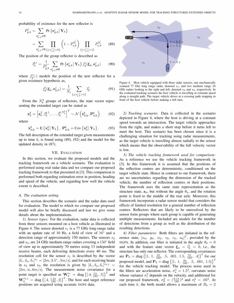
Figure 4. Host vehicle equipped with three radar sensors, one mechanicallyscanned 77 Ghz long range radar, denoted s1, and two medium range 24GHz radars looking to the right and left, denoted s2 and s3, respectively. Inthe evaluated tracking scenario the host vehicle is travelling at constant speedalong a straight path. The target vehicle drives at a crossing path stopping infront of the host vehicle before making a left turn.

2) Tracking scenario: Data is collected in the scenariodepicted in Figure 4, where the host is driving at a constantspeed towards an intersection. The target vehicle approachesfrom the right, and makes a short stop before it turns left tomeet the host. This scenario has been chosen since it is achallenging situation for tracking using radar measurements,as the target vehicle is travelling almost radially to the sensorwhich means that the observability of the full velocity vectoris low.

3) The vehicle tracking framework used for comparison:As a reference we use the vehicle tracking framework in[3]. In this framework it is assumed that the positions ofthe reflection centres are deterministic, conditioned on thetarget vehicle state. Hence in contrast to our framework, thereare no uncertainties regarding the dimension of the trackedvehicle, the number of reflection centres or their positions.The framework uses the same state representation as thestructure state, zk, but without the angle θk, and the rotationpoint is fixed to the middle of the rear axle. Moreover, thisframework incorporate a radar sensor model that considers theeffects of limited resolution for a general number of reflectioncentres. Reflectors that are likely to be unresolved by thesensor form groups where each group is capable of generatingmultiple measurements. Included are models for the numberof detections from a group as well as the distribution of theresulting detections.

4) Filter parameters: Both filters are initiated in the ref-erence state, [x0, y0, ψ0, v0, c0, a0]T , provided by theDGPS. In addition, our filter is initiated in the angle θ0 = 0and with the feature state vector ξ0 = l10 = 0, i.e., thestructure has only one reflector. The corresponding covariancesare P0 = diag

{[1, 1, 3π

180 , .5, .001, 1.5, 5π180 , .4]

}2for our

proposed model, and P0 = diag{

[1, 1, 3π180 , .5, .001, 1.5]

}2

for the vehicle tracking model. The process noise used inthe filters are acceleration noise, σ2

a = 1.52, curvature noisewhose variance σ2

c depends on the velocity, and additional forour proposed framework, σ2

θ = ( 0.1π180 )2 and σ2

l = .052. Ateach time k, the birth model allows a maximum of Bk = 2


0 2 4 6 8 100

0.2

0.4

0 2 4 6 8 100

5

10

15

0 2 4 6 8 100

1

2

3

Figure 5. Error in estimated lateral position, elat, heading angle, eψ , andvelocity, ev . The solid (blue) lines shows the result for our proposed trackingframework and the dashed (red) lines for the vehicle tracking framework

new reflectors to appear on the structure. The reflectors areuniformly distributed on lb,ik ∈ [−5, 5] and the positionof each new reflector is Gaussian distributed N (lb,i, σ2

b ),where σ2

b = .752 and the corresponding birth probabilityP ib,k = 0.1

Bk. To reduce the computational complexity, the

number of reflection centres on the structure is limited tofour in this implementation. In our proposed filter we havea uniform clutter intensity set to µ = 0.1 for all sensors,while in the vehicle tracking framework, the clutter intensity isestimated from data. The matrix, Ru, that represents the sensorresolution in the resolution models is set based on the specifiedresolution cell, [δr, δφ, δr], and is described in Section IV-Cabove and in Section IV-B in [3], respectively.

B. Tracking filter comparison

During the evaluated scenario, the side of the target vehicleis headed towards the host so that most measurements originatefrom features along that side, and consequently, the structurewill adapt to represent the side of the target vehicle. Thisallows us to evaluate both lateral position and longitudinalextension together with the errors in angle and speed.

Figure 5 displays the absolute errors in lateral position, elat,heading angle, eψ , and speed, ev . The error in lateral positionis calculated as the mean distance between the referencevehicle side and the estimated side, i.e., the line structure orthe estimated position of the side in the vehicle model. Forthe

most part, it is shown that the errors using our frameworkare similar as for the reference vehicle tracking framework.The main difference is found in ev at t ∈ [3, 6]s which iswhen the target slows down until standstill. Because of thelow observability of the velocity, this is not clearly captured inthe measurements. This situation causes problem for our modeldue to the uncertainties regarding the number and the positionsof the reflection centres on the structure. The model thus needsto determine whether a received measurement originates from

0 2 4 6 8 10

−5

0

5

0 2 4 6 8 10

−5

0

5

0 2 4 6 8 100

2

4

Figure 6. The top figure shows the estimated front and rear (dashed lines)using the vehicle tracking framework and the grey dashed lines shows thefront and rear of the reference vehicle. The middle figure shows the sameestimates for our proposed framework (solid line) while the bottom figureshows the expected number of reflector centres on the structure.

a reflection centre already on the structure or if a new reflectorhas become visible, and as a result, the model may add newreflectors to the structure instead of changing the velocity.However, as measurements are received while the target isstationary, the structure model recovers and the speed errorsagain resemble the ones for the reference vehicle trackingframework.

There are no obvious measures for evaluating how wellthe models describe the vehicle, since the object size is notincluded in our model but is a given parameter in the vehiclemodel. Nevertheless, to get an idea of how the structure modelbehaves, we compare the longitudinal extension of the twoobject models to the reference vehicle. The extension of thestructure is here defined as the largest distance between anytwo reflectors, without taking into account the uncertaintyregarding which reflectors that exist. Figure 6 shows theestimated front and rear positions of the vehicle side, using thevehicle tracking model (top) and the structure model (middle).The positions of the front and rear of the reference vehicleare indicated by the dashed grey lines in both cases. Thebottom figure shows the expected number of reflection centreson the structure, E{nξk

∣∣Yk}, and it is worth noting that thestructure in this implementation is limited to have at mostfour reflectors. During t ∈ [2, 4]s, it is clearly illustrated howthe structure moves along the reference vehicle as it starts tobreak which causes an increase in the absolute speed error.An additional increase in ev , and also a longitudinal error,occur after approximately 4.2 s as the structure adapts to someclutter measurements ahead of the vehicle. This is shown bythe peak in the upper blue curve which clearly exceeds thereference front, and is also seen in the expected number ofreflectors which increases at this time. The figures also showhow the structure drops reflectors at t ∈ [4.5, 5]s when itno longer accurately describes the received measurements.After that, it starts to recover and as the target gets closer


to the host and generates more measurements, the numberof reflectors increases and the structure is covering almostthe whole side of the reference. At two times in t ∈ [6, 7]sthe structure again adapts to clutter in front of the vehicle,which temporarily causes a longitudinal error. However, theprobabilities of existence of these new reflectors soon get lowand the reflectors are pruned.

VIII. CONCLUSION

In this paper we have presented a Bayesian filter frameworkfor tracking an extended object using radar measurements.The object is modelled as a set of reflection centres on a linestructure. The position of the object and the reflection centresare estimated recursively from data. This includes both esti-mating the number of reflectors and their positions. Moreover,the filter framework incorporates a radar sensor model thattreats the limited sensor resolution and describes unresolvedmeasurements from an arbitrary number of reflection centres.

The tracking framework has been evaluated using real radardata from an automotive scenario, and for reference we usedthe vehicle tracking framework in [3]. In contrast to ourproposed model, the object size is known in the referencemodel, and conditioned on the state, the number of reflectioncentres and their positions are deterministic. For most parts,the evaluation shows similar results for the two models eventhough our model must use the received radar data to learnabout the object. At a few occasions, it shows that our adaptivemodel is more sensitive to clutter than the reference model.That is when the structure adapts to clutter that is interpretedas a new reflection centre that has become visible.

APPENDIX A

There are two parts to the reflector model in (9): thedeterministic positions of the reflectors in measurement space,rk, and a stochastic model of received signal amplitudes, σk.In this section we present these two parts separately, startingwith the reflector positions.

A. Reflector model

To formulate rik, we start by finding the position of thereflector and the sensor in global Cartesian coordinates. Theith reflection centre is positioned on the structure zk at anoffset lik from the rotation centre and, as a result, its globalposition is given as[

xikyik

]=

[xkyk

]+ lik

[cos(ψk + θk)sin(ψk + θk)

]. (94)

In addition, the velocity of the reflection centre has twocomponents, one from the global velocity of the structure,viv = vk in the ψk direction, and one from the rotation of thestructure, vi⊥ = vkckl

ik in the π − (ψk + θk) direction.

The global position of the host platform is described by theknown host state,

zhk = [xhk , yhk , v

hk , ψ

hk , c

hk ]T (95)

on which a sensor, m, is mounted at pms = [xms , yms ]T with

an mounting angle of ψms . The global position of the sensorcan, hence, be written as[

xskysk

]=

[xhkyhk

]+ R(ψegok )

[xmsyms

]. (96)

From (94) and (96), the relative azimuth angle betweensensor m and reflector centre i is found as

αi,s = arg

([xik − xskyik − ysk

]). (97)

The velocity component of the reflector in this direction (rangerate) is given as

rrk =(vk cos(ψk − αi,s) + v⊥ cos

(π2

+ ψk + θk − αi,s))(98)

and for the host platform

rhk =(vhk cos(ψhk − αi,s) + vh⊥ cos

(π2

+ arg(xs)− αi,s))(99)

where v⊥ = vhkchk‖pms ‖ is the velocity component due to

rotation of the host platform.The position of the ith reflector in each dimension of the

measurement space of sensor s can now be expressed as

rik =

√(xik − xsk)2 + (yik − ysk)2

αi,s − ψhk − ψmsrrk − rhk

. (100)

B. Signal amplitude

The expected signal power of a reflector is characterised bytwo known functions, the angle dependent reciprocal antennagain pattern, gs

φ(·), and the range dependent signal attenuation,gs

r (·). Using these models, the expected return amplitude ofreflector i is calculated as,

σik = gsφ(rik)gs

r (rik)σrcs, (101)

where σrcs is the expected radar cross section of a reflectorwhich is assumed to be known and constant. Furthermore,it is assumed that the functions, gs

φ(·) and gsr (·), are locally

constant. As a result, the probability of detecting reflector i,determined by Pr

{Aik > γA

}, is assumed to be locally state

independent.

REFERENCES

[1] S. Blackman and R. Popoli, Design and analysis of modern trackingsystems. Norwood, MA: Artech House, 1999.

[2] Y. Bar-Shalom and W. D. Blair, Multitarget-Multisensor Tracking Vol-ume III: Applications and Advances. Norwood, MA: Artech House,2000.

[3] J. Gunnarsson, L. Svensson, L. Danielsson, and F. Bengtsson, “Trackingvehicles using radar detections,” in Intelligent Vehicles Symposium,2007. Proceedings IEEE, Istanbul, June 2007.

[4] R. Ostrovityanov and F. Basalov, Statistical Theory of Extended RadarTargets. Artech House, 1985.

[5] F. E. Daum and R. J. Fitzgerald, “Importance of resolution inmultiple-target tracking,” Signal and Data Processing of Small Targets1994, vol. 2235, no. 1, pp. 329–338, 1994. [Online]. Available:http://link.aip.org/link/?PSI/2235/329/1


[6] M. Waxman and O. Drummond, “A bibliography of cluster (group)tracking,” in Signal and Data Processing of Small Targets 2004. Editedby Drummond, Oliver E. Proceedings of the SPIE, vol. 5428, 2004, pp.551–560.

[7] R. Mahler, “Multitarget Bayes filtering via first-order multitarget mo-ments,” Aerospace and Electronic Systems, IEEE Transactions on,vol. 39, no. 4, pp. 1152–1178, 2004.

[8] ——, “Multitarget bayes filtering via first-order multitarget moments,”Aerospace and Electronic Systems, IEEE Transactions on, vol. 39, no. 4,pp. 1152–1178, 2003.

[9] K. Granstrom, C. Lundquist, and U. Orguner, “A gaussian mixture phdfilter for extended target tracking,” in Information Fusion (FUSION),2010 13th Conference on, 2010, pp. 1–8.

[10] J. Koch, “Bayesian approach to extended object and cluster trackingusing random matrices,” Aerospace and Electronic Systems, IEEE Trans-actions on, vol. 44, no. 3, pp. 1042–1059, 2008.

[11] W. Koch, “Advanced sensor models: Benefits for target tracking andsensor data fusion,” in Multisensor Fusion and Integration for IntelligentSystems, 2006 IEEE International Conference on, sep 2006, pp. 565–570.

[12] M. Baum and U. Hanebeck, “Extended object tracking based on com-bined set-theoretic and stochastic fusion,” in Information Fusion, 2009.FUSION ’09. 12th International Conference on, 2009, pp. 1288–1295.

[13] T. Broida and R. Chellappa, “Estimating the kinematics and structure ofa rigid object from a sequence of monocular images,” IEEE Transactionson Pattern Analysis and Machine Intelligence, vol. 13, no. 6, pp. 497–513, 1991.

[14] T. Huang and A. Netravalj, “Motion and structure from feature corre-spondences: A review,” Advances in image processing and understand-ing: a festschrift for Thomas S. Huang, p. 331, 2002.

[15] J. Dezert, “Tracking maneuvering and bending extended target in clut-tered environment,” in Proceedings of SPIE, vol. 3373, 1998, p. 283.

[16] D. Salmond and N. Gordon, “Group and extended object tracking,” inIEE Colloquium on Target Tracking: Algorithms and Applications (Ref.No. 1999/090, 1999/215), 1999, pp. 16/1–16/4.

[17] K. Gilholm, S. J. Godsill, S. Maskell, and D. J. Salmond, “Poissonmodels for extended target and group tracking,” SPIE, October 2005.

[18] K.-C. Chang and Y. Bar-Shalom, “Joint probabilistic data associationfor multitarget tracking with possibly unresolved measurements andmaneuvers,” Automatic Control, IEEE Transactions on, vol. 29, no. 7,pp. 585–594, Jul 1984.

[19] W. Koch and G. Van Keuk, “Multiple hypothesis track maintenance withpossibly unresolved measurements,” Aerospace and Electronic Systems,IEEE Transactions on, vol. 33, no. 3, pp. 883–892, July 1997.

[20] D. Svensson, M. Ulmke, and L. Danielsson, “Multi-target sensor resolu-tion model for arbitrary target numbers,” in Proceedings of SPIE Signaland Data Processing of Small Targets 2010, April 2010.

[21] N. Gordon, D. Salmond, and D. Fisher, “Bayesian target tracking aftergroup pattern distortion,” in Proceedings of SPIE, vol. 3163, 1997, p.238.

[22] P. Swerling, “Probability of detection for fluctuating targets,” Informa-tion Theory, IRE Transactions on, vol. 6, no. 2, pp. 269–308, 1960.

[23] T. Fortmann, Y. Bar-Shalom, and M. Scheffe, “Sonar tracking of multipletargets using joint probabilistic data association,” IEEE Journal ofOceanic Engineering, vol. 8, July 1983.

[24] S. Julier and J. Uhlmann, “Unscented filtering and nonlinear estimation,”Proceedings of the IEEE, vol. 92, no. 3, pp. 401 – 22, 2004.

[25] P. Ainsleigh, N. Kehtarnavaz, and R. Streit, “Hidden Gauss-Markovmodels for signal classification,” IEEE Transactions on Signal Process-ing, vol. 50, no. 6, pp. 1355–1367, 2002.

[26] D. Salmond, “Mixture reduction algorithms for target tracking in clutter,”in Proceedings of SPIE, vol. 1305, 1990, p. 434.

Lars Hammarstrand was born in Landvetter, Swe-den in 1979. He received his M.Sc. and Ph.D. degreein electrical engineering from Chalmers Universityof Technology, Gothenburg, Sweden, in 2004 and2010, respectively.

He is currently with the Active Safety and ChassisDepartment at Volvo Car Corporation, Gothenburgresponsible for sensor data fusion developments. Hismain research interests are in the fields of sensorfusion and radar sensor modeling, especially withapplication to active safety systems.

Malin Lundgren was born in Skovde, Sweden in1979. She received the M.Sc. degree in ElectricalEngineering from Chalmers University of Technol-ogy, Goteborg, Sweden, in 2004. After a couple ofyears in the industry she returned to Chalmers whereshe is currently working as a Ph.D. student with in-terest in sensor fusion and extended object tracking,primarily for automotive safety applications.

Lennart Svensson was born in Alvangen, Swedenin 1976. He received the M.S. degree in electri-cal engineering in 1999 and the Ph.D. degree in2004, both from Chalmers University of Technology,Gothenburg, Sweden.

He is currently an Associate Professor at theSignal Processing group, again at Chalmers Uni-versity of Technology. His research interests includeBayesian inference in general, and nonlinear filteringand tracking in particular.

Adaptive Radar Sensor Model for Tracking Structured Extended Objects

Documents

Transcript of Adaptive Radar Sensor Model for Tracking Structured Extended Objects