Acyclic directed graphs to represent conditionalindependence models

Marco Baioletti1 Giuseppe Busanello2 Barbara Vantaggi2

1 Dip. Matematica e Informatica, Universita di Perugia, Italy,e-mail: baioletti@dipmat.unipg.it

2 Dip. Metodi e Modelli Matematici, Universita “La Sapienza” Roma, Italy,e-mail: {busanello, vantaggi}@dmmm.uniroma1.it

Abstract. In this paper we consider conditional independence modelsclosed under graphoid properties. We investigate their representationby means of acyclic directed graphs (DAG). A new algorithm to builda DAG, given an ordering among random variables, is described andpeculiarities and advantages of this approach are discussed. Finally, someproperties ensuring the existence of perfect maps are provided. Theseconditions can be used to define a procedure able to find a perfect mapfor some classes of independence models.

Key words: Conditional independence models, Graphoid properties, Infer-ential rules, Acyclic directed graphs, Perfect map.

1 Introduction

Graphical models [6, 8–10, 12, 15] play a fundamental role in probability andstatistics and they have been deeply developed as a tool for representing condi-tional independence models. It is well known (see for instance [6]) that, underthe classical definition, the independence model M associated to any probabilitymeasure P is a semi–graphoid and, if P is strictly positive, M is a graphoid.On the other hand, an alternative definition of independence (a reinforcement ofcs–independence [4, 5]), which avoids the well known critical situations relatedto 0 and 1 evalutations, induces independence models closed under graphoidproperties [13].

In this paper the attention is focusing on graphoid structures and we considera set J of conditional independence statements, compatible with a (conditional)probability, and its closure J with respect to graphoid properties. Since thecomputation of J is infeasible (its size is exponentially larger than the size ofJ), then, as shown in [10, 11, 1], we will use a suitable set J∗ of independencestatements (obviously included in J), that we call “fast closure”, from which itis easy to verify whether a given relation is implied, i.e. whether a given relationbelongs to J . Some of the main properties of fast closure will be described.

The fast closure is also relevant for building the relevant acyclic directedgraph (DAG), which is able to concisely represent the independence model. In

fact we will define the procedure BN-draw which builds, starting from this setand an ordering on the random variables, the corresponding independence map.The main difference between BN-draw and the classical procedures (see e.g. [7,9]) is that the relevant DAG is built without referring to the whole closure.

Finally, we give a condition assuring the existence of a perfect map, i.e. aDAG able to represent all the independence statements of a given independencemodel. By using this result it is possible to define a correct but incompletemethod to find a perfect map. First, a suitable ordering, satisfying this condition,is searched by means of a backtracking procedure. If such an ordering exists, aperfect map for the independence model can be found by using the procedureBN-draw.

Since the above condition is not necessary, but only sufficient, as shown inExample 3, such condition can fail even if a perfect map exists. The providedresult is a first step to look for a characterization of orderings giving rise toperfect maps.

2 Graphoid

Throughout the paper the symbol S = {Y1, . . . , Yn} denotes a finite not emptyset of variables. Given a probability P , a conditional independence statementYA⊥⊥YB |YC (compatible with P ), where A, B, C are disjoint subsets of the setS = {1, . . . , n} of indices associated to S, is simply denoted by the ordered triple(A,B, C). Furthermore, S(3) is the set of all ordered triples (A,B, C) of disjointsubsets of S, such that A and B are not empty. A conditional independence modelI, related to a probability P , is a subset of S(3). As recalled in the introductionwe refer to probabilistic independence models even if the results are valid forany graphoid structure.

We recall that a graphoid is a couple (S, I), with I a ternary relation on theset S(3), satisfying the following properties:

G1 if (A,B,C) ∈ I, then (B, A,C) ∈ I (Symmetry);G2 if (A,B, C) ∈ I, then (A,B′, C) ∈ I for any nonempty subset B′ of B

(Decomposition);G3 if (A, B1 ∪ B2, C) ∈ I with B1 and B2 disjoint, then (A,B1, C ∪ B2) ∈ I

(Weak Union);G4 if (A,B,C∪D) ∈ I and (A,C, D) ∈ I, then (A, B∪C, D) ∈ I (Contraction);G5 if (A,B, C ∪D) ∈ I and (A, C,B ∪D) ∈ I, then (A, B ∪ C, D) ∈ I (Inter-

section).

A semi–graphoid is a couple (S, I) satisfying only the properties G1–G4.The symmetric version of rules G2 and G3 will be denoted by

G2s if (A,B,C) ∈ I, then (A′, B, C) ∈ I for any nonempty subset A′ of A;G3s if (A1 ∪A2, B,C) ∈ I, then (A1, B,C ∪A2) ∈ I.

2

3 Generalized inference rules

Given a set J of conditional independence statements compatible with a prob-ability, a relevant problem about graphoids is to find, in an efficient way, theclosure of J with respect to G1–G5

J = {θ ∈ S(3) : θ is obtained from J by G1−G5} .

A related problem, called implication, concerns to establish whether a tripleθ ∈ S(3) can be derived from J , see [16].

It is clear that the implication problem can be easily solved once the closurehas been computed. But, the computation of the closure is infeasible becauseits size is exponentially larger than the size of J . In [1–3] we describe how itis possible to compute a smaller set of triples having the same information asthe closure. The same problem has been already faced successfully in [11], withparticular attention to semi–graphoid structures.

In the following for a generic triple θi = (Ai, Bi, Ci), the set Xi stands for(Ai ∪Bi ∪ Ci).

We recall some definitions and properties introduced and studied in [1–3]useful to efficiently compute the closure of a set of conditional independencestatements. Given a pair of triples θ1, θ2 ∈ S(3) we say that θ1 is generalized–included in θ2 (briefly g–included), in symbol θ1 v θ2, if θ1 can be obtained fromθ2 by a finite number of applications of G1, G2 and G3.

Proposition 1. Given θ1 = (A1, B1, C1) and θ2 = (A2, B2, C2), then θ1 v θ2 ifand only if the following conditions hold

(i) C2 ⊆ C1 ⊆ X2;(ii) either A1 ⊆ A2 and B1 ⊆ B2 or A1 ⊆ B2 and B1 ⊆ A2.

Generalized inclusion is strictly related to the concept of dominance va on S(3),already defined in [10, 11]. We say θ1 va θ2 if θ1 can be obtained from θ2 witha finite number of applications of G2, G3, G2s and G3s.

Therefore it is easy to see that θ′ v θ if and only if either θ′ va θ or θ′ va θT

where θT is the transpose of θ (θT = (B, A,C) if θ = (A,B, C)).The definition of g–inclusion between triples can be extended to sets of triples

and its properties are showed in [2, 3].

Definition 1. Let H and J be subsets of S(3). J is a covering of H (in symbolH v J) if and only if for any triple θ ∈ H there exists a triple θ′ ∈ J such thatθ v θ′.

3.1 Closure through one generalized rule

The target of [10, 2, 3] is to find a fast method to compute a reduced (withrespect to g–inclusion v) set J∗ bearing the same information of J , that is forany triple θ ∈ J there exists a triple θ′ ∈ J∗ such that θ v θ′.

3

Therefore, the computation of J∗ provides a simple solution to the implica-tion problem for J . The strategy to compute J∗ is to use a generalized versionof the remaining graphoid rules G4, G5 and their symmetric ones (see also [11]).

These two inference rules are called generalized contraction (G4∗) and gener-alized intersection (G5∗). The rule G4∗ allows to deduce from θ1, θ2 the greatest(with respect to v) triple τ which derives from the application of G4 to all thepossible pairs of triples θ′1, θ

′2 such that θ′1 v θ1 and θ′2 v θ2. The rule G5∗ is

analogously defined and it is based on G5 instead of G4.It is possible to compute the closure of a set J of triples in S(3), with respect

to G4∗ and G5∗, that isJ∗ = {τ : J `∗G τ} (1)

where J `∗G τ means that τ is obtained from J by applying a finite number oftimes the rules G4∗ and G5∗.

In [2, 3] it is proved that J∗, even if it is smaller, is equivalent to J withrespect to graphoids, in that J∗ v J and J v J∗.

A further reduction is to keep only the “maximal”(with respect to g–inclusion)triples of J∗

J∗/v

= {τ ∈ J∗ : @τ ∈ J∗ with τ 6= τ, τT such that τ v τ}.

Obviously, J∗/v⊆ J∗.

In [2, 3] it is proved that J∗ v J∗/v

, therefore there is no loss of information

by using J∗/v

instead of J∗. Then, given a set J of triples in S(3), we compute

the set J∗/v

, which we call “fast closure” and denote with J∗.

In [2, 3] it is proved that the fast closure set {θ1, θ2}∗ of two triples θ1, θ2 ∈S(3) is formed with at most eleven triples. Furthermore, these triples have a par-ticular structure strictly related to θ1 and θ2 and they can be easily computed.By using {θ1, θ2}∗, it is possible to define a new inference rule

C : from θ1, θ2 deduce any triple τ ∈ {θ1, θ2}∗.

We denote with J+ the set of triples obtained from J by applying a finitenumber of times the rule C. As proved in [2, 3], J+ is equivalent to J with respectto graphoids, that means J+ v J and J v J+. Obviously, by transitivity J+ isequivalent to J∗.

Therefore, it is possible to design an algorithm, called FC1, which startsfrom J and recursively applies the rule C and a procedure, called FindMaximal(which computes H/

v for a given set H ⊆ S(3)), until it arrives to a set of triples

closed with respect to C and maximal with respect to g–inclusion.In [2, 3] completeness and correctness of FC1 are proved.Note that, as confirmed in [2, 3] by some experimental results, FC1 is more

efficient than the algorithms based on G4∗ and G5∗.

4

4 Graphs

In the following, we refer to the usual graph definitions (see e.g. [9]). We denoteby G = (U , E) a graph with set of nodes U and oriented arcs E formed by orderedpairs of nodes. In particular, we consider directed graphs having no cycles, i.e.acyclic directed graphs (DAG). We denote for any u ∈ U , as usual, with pa(u)the parents of u, ch(u) the child of u, ds(u) the sets of descendants and an(u)the set of ancestors. We use the convention that each node u belongs to an(u)and to ds(u), but not to pa(u) and ch(u).

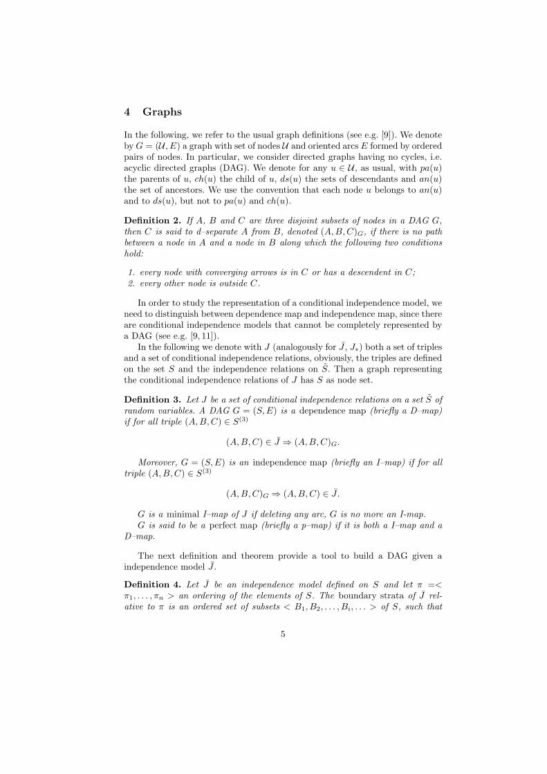
Definition 2. If A, B and C are three disjoint subsets of nodes in a DAG G,then C is said to d–separate A from B, denoted (A,B, C)G, if there is no pathbetween a node in A and a node in B along which the following two conditionshold:

1. every node with converging arrows is in C or has a descendent in C;2. every other node is outside C.

In order to study the representation of a conditional independence model, weneed to distinguish between dependence map and independence map, since thereare conditional independence models that cannot be completely represented bya DAG (see e.g. [9, 11]).

In the following we denote with J (analogously for J , J∗) both a set of triplesand a set of conditional independence relations, obviously, the triples are definedon the set S and the independence relations on S. Then a graph representingthe conditional independence relations of J has S as node set.

Definition 3. Let J be a set of conditional independence relations on a set S ofrandom variables. A DAG G = (S, E) is a dependence map (briefly a D–map)if for all triple (A,B, C) ∈ S(3)

(A, B,C) ∈ J ⇒ (A,B, C)G.

Moreover, G = (S, E) is an independence map (briefly an I–map) if for alltriple (A, B,C) ∈ S(3)

(A, B,C)G ⇒ (A,B,C) ∈ J .

G is a minimal I–map of J if deleting any arc, G is no more an I-map.G is said to be a perfect map (briefly a p–map) if it is both a I–map and a

D–map.

The next definition and theorem provide a tool to build a DAG given aindependence model J .

Definition 4. Let J be an independence model defined on S and let π =<π1, . . . , πn > an ordering of the elements of S. The boundary strata of J rel-ative to π is an ordered set of subsets < B1, B2, . . . , Bi, . . . > of S, such that

5

each Bi is a minimal set satisfying Bi ⊆ S(i) = {π1, . . . , πi−1} and γi =({πi}, S(i) \Bi, Bi) ∈ J .

The DAG created by setting each Bi as parent set of the node πi is calledboundary DAG of J relative to π.

The triple γi is known as basic triple.The next theorem is an extension of Verma’s Theorem [14] stated for condi-

tional independence relations (see [9]).

Theorem 1. Let J be a independence model closed with respect to the semi–graphoid properties. If G is a boundary DAG of J relative to any ordering π,then G is a minimal I–map of J .

The previous theorem helps to build a DAG for an independence model JP

induced by a probability assessment P on a set of random variables S and afixed ordering π on indices of S.

Now, we recall an interesting result [9].

Corollary 1. An acyclic directed graph G = (S,E) is a minimal I–map of anindependence model J if and only if any index i ∈ S is conditionally independentof all its non-descendants, given its parents pa(i), and no proper subset of pa(i)satisfies this condition.

It is well known (see [9]) that the boundary DAG of J relative to π is aminimal I-map.

5 BN-draw function

The aim of this section is to define the procedure BN–draw, which builds aminimal I–map G (see Definition 3) given the fast closure J∗ (introduced inSection 3) of a set J of independence relations. The procedure is described inthe algorithm 1.

Given the fast closure set J∗, we cannot apply the standard procedure (see[7, 9]) described in Definition 4 to draw an I–map because, in general, the basictriples related to an arbitrary ordering π could not be elements of J∗, but theycould be just g–included to some triples of J∗, as shown in Example 1.

Example 1. Given J = {({1}, {2}, {3, 4}), ({1}, {3}, {4})}, we want to find thecorresponding basic triples and to draw the relevant DAG G related to theordering π =< 4, 2, 1, 3 >.

By the closure with respect to graphoid properties we obtainJ = { ({1}, {2}, {3, 4}), ({1}, {3}, {4}), ({1}, {2, 3}, {4}), ({1}, {2}, {4}),({1}, {3}, {2, 4}), ({2}, {1}, {3, 4}), ({3}, {1}, {4}), ({2, 3}, {1}, {4}), ({2}, {1}, {4}),({3}, {1}, {2, 4}) }and the set of basic triples is Γ = {({1}, {2}, {4}), ({3}, {1}, {2, 4})}.

By FC1 we botain J∗ = {({1}, {2, 3}, {4})} and it is simple to observe thatΓ v J∗.

6

Algorithm 1 DAG from J∗ given an order π of S

1: function BN-draw(n, π, J∗) . n is the cardinality of S2: for i ← 2 to n do3: pa ← S(i)

4: for each (A, B, C) ∈ J∗ do5: if πi ∈ A then6: p ← C ∪ (A ∩ S(i))7: r ← B ∩ S(i)

8: if (C ⊆ S(i)) and (p ∪ r = S(i)) and (r 6= φ) and (|p| < |pa|) then9: pa ← p

10: end if11: end if12: if πi ∈ B then13: p ← C ∪ (B ∩ S(i))14: r ← A ∩ S(i)

15: if (C ⊆ S(i)) and (p ∪ r = S(i)) and (r 6= φ) and (|p| < |pa|) then16: pa ← p17: end if18: end if19: end for20: draw an arc from each index in pa to πi

21: end for22: end function

The procedure BN-draw finds, for each πi, with i = 2, . . . , n, and possiblyfor each θ ∈ J∗, a triple ({πi}, B,C) v θ such that B ∪ C = S(i) and C has theminimum cardinality (analogously for the triples of the form (A, {πi}, C)). It iseasy to see that for each πi, the triple with the smallest cardinality of C amongall the selected triples, coincides with the basic triple γi, if γi exists. The formaljustification of this statement is given by the following result:

Proposition 2. Let J be an independence model on an index set S, J∗ its fastclosure and π an ordering on S. Then, the set

Bi = {({πi}, B,C) ∈ S(3) : B ∪ C = S(i), {({πi}, B,C)} v J∗}is not empty if and only if the basic triple γi = ({πi}, S(i) \ Bi, Bi) related to πexists, for i = 1, . . . , |S|.Proof. Suppose that Bi is not empty. If there are two triples θ1, θ2 having thesame cardinality of pa(i) then, by definition of J∗, there is also the triple θ3

obtained by applying the intersection rule between them. Since the third com-ponent of θ3 has a smaller cardinality than those of θ1 and θ2, this means thatthe triple with the minimum cardinality of C is unique and it coincides withthe basic triple γi. Vice versa, if the basic triple γi = ({πi}, S(i) \ Bi, Bi) for πi

exists, then it is straightforward to see that γi ∈ Bi. utNote that BN–draw allows to make the corresponding I–map related to π

in linear time with respect to the cardinality of J∗, while the standard procedure

7

requires a time proportional to the size of J , which is usually much larger, asshown also in the empirical tests in [1]. Also the space needed in memory is almostexclusively used to contain the fast closure. Note that a theoretical comparisonbetween the size of the whole closure and the size of the fast closure has notalready been found and seems to be a very difficult problem.

The next example compares the standard procedure recalled in Definition 4with BN-draw to build the I–map, given a subset J of S(3) and an ordering πamong the elements of S.

Example 2. Consider the same independence set J of Example 1 and the orderingπ =< 4, 2, 1, 3 >, we compute the basic triple by applying BN-draw to J∗ ={θ = ({1}, {2, 3}, {4})}. For i = 2 we have 2 ∈ B, p = φ, r = φ, C = {4} ⊆ {4},then there is no basic triple. For i = 3 we have 1 ∈ A, p = φ, r = {2}, C = {4}then (1, 2, 4) is a basic triple g–included to θ. For i = 4 we have 3 ∈ B, p = {2},r = {1}, C = {4} then ({3}, {1}, {2, 4}) is a basic triple g–included to θ.

Therefore, we obtain the same set Γ computed in Example 1.

Y1

Y4

Y2

Y3

Fig. 1. I −map related to π =< 4, 2, 1, 3 >

6 Perfect map

In this section we introduce a condition ensuring the existence of a perfect mapfor an independence model J , starting from the fast closure J∗ of J (avoidingto build the whole J , as recalled in Section 2). Given an ordering π on S, wedenote with Gπ the corresponding I–map of J∗ with respect to π. Furthermore,we associate to any index s ∈ S the set S(s) of indices appearing in π before sand the minimal subset Bs of S(s) such that γs = (s, S(s) \ Bs, Bs) is the basictriple, if any, as introduced in Definition 4.

Before stating the sufficient condition that ensures the existence of a perfectmap Gπ of the fast closure J∗, with respect to π, we want to underline some

8

relations among the indices of a triple represented in Gπ and g–included in J∗. Inparticular, we focus our attention on the relationship among the nodes associatedto C and those related to pa(A ∪B).

By Corollary 1, for any index i ∈ S the triple {({i}, S \ ds(i), pa(i))} isrepresented in Gπ and, since Gπ is an I–map, {({i}, S \ ds(i), pa(i))} v J∗.Moreover, by d–separation, for any K ⊆ ds(i) \ {i} such that pa(i) d–separatesS \ ds(i) and K, also {({i}∪K,S \ ds(i), pa(i)), ({i}, S \ ds(i), pa(i)∪K)} v J∗.

Moreover, we have the following result considering I–maps and fast closureJ∗.

Proposition 3. Let J be a set of conditional independence relations and J∗ itsfast closure.

If Gπ is an I–map of J∗, with respect to π, then, for any triple θ = (A,B, C) ∈J∗ represented in Gπ, it holds pa(DB

A) ∪ pa(DAB) ⊆ C, where DB

A = ds(A) ∩ Band DA

B = ds(B) ∩A.

Proof. Suppose by absurd that there exist α ∈ DBA and j ∈ pa(α) such that

j 6∈ C. We want to show that θ′ = (A,B ∪ {j}, C) is represented in Gπ. Let ρa path from a ∈ A to j. If ρ passes through α, then ρ is blocked by C (because(A,B, C)Gπ ). Otherwise, if ρ does not pass through α, then the path ρ′ from ato α obtained from ρ adding the edge (j, α) is blocked by C. Since j is not aconverging node (and j 6∈ C), ρ is blocked by C.

Since Gπ is an I–map, it follows that {θ′} v J∗, but θ v θ′ and then θ wouldnot be a maximal triple. ut

By the previous observations and Proposition 3 it comes out the idea relatedto the relationship between the component C and pa(A∪B) of a triple (A,B, C),behind the condition introduced in the next proposition assuring the existenceof a perfect map.

Proposition 4. Let J be a set of conditional independence relations and J∗ itsfast closure.

Given an ordering π on S, if for any triple θ = (A,B, C) ∈ J∗ the orderingπ satisfies the following conditions

1. all indices of C appear before all indices belonging to one of the sets A or B;2. all indices of X = (A ∪ B ∪ C) appear in π before all indices belonging to

S \X;

then the related I–map Gπ is a perfect map.

Proof. Consider a triple θ = (A, B,C) ∈ J∗. Under the hypotheses 1. and 2.,consider the restriction πX of π to X = (A∪B ∪C). If we assume (without lossof generality) that all indices of C appear before of all those of B in πX , thenany index b ∈ B has as parents the set of indices Bb ⊆ C ∪ (S(b) ∩B). Thereforeno index of A is a parent of any index of B. Moreover, no index of A can bea descendent of any index of B. In fact, the basic triple γb = (b, S(b) \ Bb, Bb)associated to b satisfies the condition A ∩ S(b) ⊆ S(b) \ Bb, by construction,

9

and for any index a ∈ A appearing in π after at least a index b′ ∈ B, thebasic triple γa = (a, S(a) \Ba, Ba) satisfies conditions: B ∩ S(a) ⊆ S(a) \Ba andBa ⊆ C ∪ (S(a) ∩A).

We prove now that θ is represented in Gπ. By the previous observations, inGπ no arc can join any element of A and any element of B. Let us consider apath between a node a ∈ A and a node b ∈ B. If the path passes through a nodey outside X, then y must be a collider (i.e. both edges end in y), because eachindex of X precedes each index outside X and therefore there are no arc fromy to any index of X. Since neither y nor any of its descendent is in C, this pathis blocked by C.

On the other hand, if the path passes only inside X, it must pass througha node c in C which cannot be a collider, since c precedes all the elements ofB. ut

This result is a generalization to triples of J∗ to that proved for basic triplesin Pearl [9].

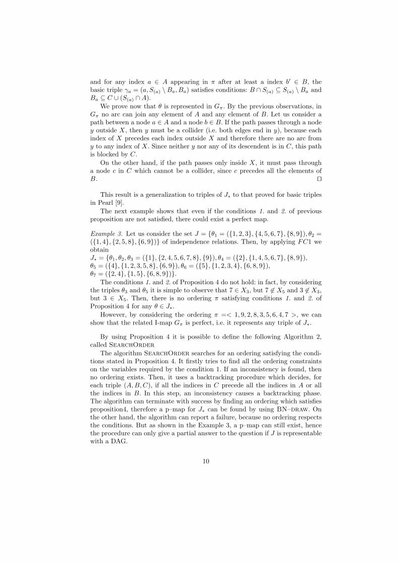
The next example shows that even if the conditions 1. and 2. of previousproposition are not satisfied, there could exist a perfect map.

Example 3. Let us consider the set J = {θ1 = ({1, 2, 3}, {4, 5, 6, 7}, {8, 9}), θ2 =({1, 4}, {2, 5, 8}, {6, 9})} of independence relations. Then, by applying FC1 weobtainJ∗ = {θ1, θ2, θ3 = ({1}, {2, 4, 5, 6, 7, 8}, {9}), θ4 = ({2}, {1, 4, 5, 6, 7}, {8, 9}),θ5 = ({4}, {1, 2, 3, 5, 8}, {6, 9}), θ6 = ({5}, {1, 2, 3, 4}, {6, 8, 9}),θ7 = ({2, 4}, {1, 5}, {6, 8, 9})}.

The conditions 1. and 2. of Proposition 4 do not hold: in fact, by consideringthe triples θ3 and θ5 it is simple to observe that 7 ∈ X3, but 7 6∈ X5 and 3 6∈ X3,but 3 ∈ X5. Then, there is no ordering π satisfying conditions 1. and 2. ofProposition 4 for any θ ∈ J∗.

However, by considering the ordering π =< 1, 9, 2, 8, 3, 5, 6, 4, 7 >, we canshow that the related I-map Gπ is perfect, i.e. it represents any triple of J∗.

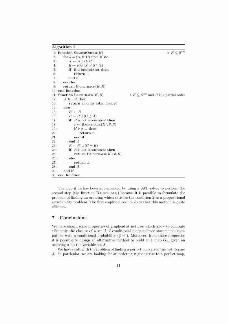
By using Proposition 4 it is possible to define the following Algorithm 2,called SearchOrder

The algorithm SearchOrder searches for an ordering satisfying the condi-tions stated in Proposition 4. It firstly tries to find all the ordering constraintson the variables required by the condition 1. If an inconsistency is found, thenno ordering exists. Then, it uses a backtracking procedure which decides, foreach triple (A, B,C), if all the indices in C precede all the indices in A or allthe indices in B. In this step, an inconsistency causes a backtracking phase.The algorithm can terminate with success by finding an ordering which satisfiesproposition4, therefore a p–map for J∗ can be found by using BN–draw. Onthe other hand, the algorithm can report a failure, because no ordering respectsthe conditions. But as shown in the Example 3, a p–map can still exist, hencethe procedure can only give a partial answer to the question if J is representablewith a DAG.

10

Algorithm 21: function SearchOrder(K) . K ⊆ S(3)

2: for θ = (A, B, C) from K do3: X ← A ∪B ∪ C4: R ← R ∪ (X ¹ S \X)5: if R is inconsistent then6: return ⊥7: end if8: end for9: return Backtrack(K, R)

10: end function11: function Backtrack(K, R) . K ⊆ S(3) and R is a partial order12: if K = ∅ then13: return an order taken from R14: else15: R′ ← R16: R ← R ∪ (C ¹ A)17: if R is not inconsistent then18: r ← Backtrack(K \ θ, R)19: if r 6= ⊥ then20: return r21: end if22: end if23: R ← R′ ∪ (C ¹ B)24: if R is not inconsistent then25: return Backtrack(K \ θ, R)26: else27: return ⊥28: end if29: end if30: end function

The algorithm has been implemented by using a SAT solver to perform thesecond step (the function Backtrack) because it is possible to formulate theproblem of finding an ordering which satisfies the condition 2 as a propositionalsatisfiability problem. The first empirical results show that this method is quiteefficient.

7 Conclusions

We have shown some properties of graphoid structures, which allow to computeefficiently the closure of a set J of conditional independence statements, com-patible with a conditional probability ([1–3]). Moreover, from these propertiesit is possible to design an alternative method to build an I–map Gπ, given anordering π on the variable set S.

We have dealt with the problem of finding a perfect map given the fast closureJ∗. In particular, we are looking for an ordering π giving rise to a perfect map,

11

if there exists. Actually, we have made a first step in this direction by obtaininga partial goal. In fact, we have introduced a sufficient condition for the existenceof a perfect map.

We are now working to relax this condition with the aim of finding a necessaryand sufficient condition for the existence of an ordering generating a perfectmap. For what we understand, such a condition will need to explore the relationsamong the triples in J∗ and the components of each triple. We are also interestedin translating this condition into an efficient algorithm.

Another strictly related, open problem is to find more efficient techniques tocompute J∗, because it is clearly the first step needed by any algorithm whichfinds, if any, a DAG representing J .

References

1. M. Baioletti, G. Busanello, B. Vantaggi (2008). Algorithms for the closure ofgraphoid structures. Proc. of 12th Inter. Conf. IPMU 2008, Malaga pp. 930–937.

2. M. Baioletti, G. Busanello, B. Vantaggi (2008). Conditional independence struc-ture and its closure: inferential rules and algorithms. In International Journal ofApproximate Reasoning (submitted).

3. M. Baioletti, G. Busanello, B. Vantaggi (2009). Conditional independence structureand its closure: inferential rules and algorithms. In Technical Report, 5/2009 ofUniversity of Perugia.

4. G. Coletti, R. Scozzafava (2000). Zero probabilities in stochastical independence.In Information, Uncertainty, Fusion, Kluwer Academic Publishers, Dordrecht, B.Bouchon- Meunier, R.R. Yager, L.A. Zadeh (Eds.), pp. 185–196.

5. G. Coletti, R. Scozzafava (2002). Probabilistic logic in a coherent setting. Dor-drecht/Boston/London: Kluwer (Trends in logic n.15).

6. A.P. Dawid (1979). Conditional independence in statistical theory. J. Roy. Stat.Soc. B, 41, pages 15–31.

7. F.V. Jensen (1966). An Introduction to bayesian Networks, UCL Press and SpringerVerlag.

8. S.L. Lauritzen (1996). Graphical models. Clarendon Press, Oxford.9. J. Pearl (1988). Probabilistic reasoning in intelligent systems: networks of plausible

inference, Morgan Kaufmann, Los Altos, CA.10. M. Studeny (1997). Semigraphoids and structures of probabilistic conditional in-

dependence. Ann. Math. Artif. Intell., 21, pages 71–98.11. M. Studeny (1998). Complexity of structural models. Proc. Prague Stochastics ’98,

Prague, pages 521–528.12. M. Studeny, R.R. Bouckaert (1998). On chain graph models for description of

conditional independence structures. Ann. Statist., 26 (4), pages 1434–1495.13. B. Vantaggi (2001). Conditional independence in a coherent setting. Ann. Math.

Artif. Intell., 32, pages 287–313.14. T. S. Verma (1986). Causal networks: semantics and expressiveness. Technical Re-

port R–65, Cognitive Systems Laboratory, University of California, Los Angeles.15. J. Witthaker, J. (1990). Graphical models in applied multivariate statistic. Wiley

& Sons, New York.16. S.K.M. Wong, C.J. Butz, D. Wu (2000). On the Implication Problem for Proba-

bilistic Conditional Independency. IEEE Transactions on Systems, Man, and Cy-bernetics, Part A: Systems and Humans, 30, 6, pp. 785–805.

12