Morphometrical and acoustical comparison between diploid and tetraploid green toads
Upload
khangminh22Category
view
1download
0
ACOUSTICAL IMPROVEMENT OF TYPICAL SPORT HALLS
FOR MULTI-PURPOSE USE
A THESIS SUBMITTED TO
THE GRADUATE SCHOOL OF NATURAL AND APPLIED SCIENCES
OF
MIDDLE EAST TECHNICAL UNIVERSITY
BY
GÖKÇE ULUSOY
IN PARTIAL FULFILLMENT OF THE REQUIREMENTS
FOR
THE DEGREE OF MASTER OF SCIENCE
IN
BUILDING SCIENCE
IN
ARCHITECTURE
SEPTEMBER 2014

Approval of the thesis:
ACOUSTICAL IMPROVEMENT OF TYPICAL SPORT HALLS FOR
MULTI-PURPOSE USE
submitted by GÖKÇE ULUSOY in partial fulfilment of the requirements for the
degree of Master of Science in Building Science, Department of Architecture,
Middle East Technical University by,
Prof. Dr. Gülbin Dural Ünver
Dean, Graduate School of Natural and Applied Sciences
Prof. Dr.Güven Arif Sargın
Head of Department, Architecture Dept.
Assoc. Prof. Dr. Ayşe Tavukçuoğlu
Supervisor, Architecture Dept., METU
Prof. Dr. Mehmet Çalışkan
Co-Supervisor, Mechanical Engineering Dept., METU
Examining Committee Members:
Assoc. Prof. Dr. Ali Murat Tanyer
Architecture Dept., METU
Assoc. Prof. Dr. Ayşe Tavukçuoğlu
Architecture Dept., METU
Assoc. Prof. Dr. M. HalisGünel
Architecture Dept., METU
Nesrin Yatman, B.Arch, M.S.
A.N. YatmanMimarlarCo. Ltd., Ankara
İ. Gürkan Akdoğan, B.Eng, M.S.
Polarkon Co. Ltd., Ankara
Date: 18.09.2014

iv
I hereby declare that all information in this document has been obtained and
presented in accordance with academic rules and ethical conduct. I also declare
that, as required by these rules and conduct, I have fully cited and referenced
all material and results that are not original to this work.
Name, Last Name: Gökçe ULUSOY
Signature:
v
ABSTRACT
ACOUSTICAL IMPROVEMENT OF TYPICAL SPORT HALLS
FOR MULTI-PURPOSE USE
Ulusoy, Gökçe
M.S., in Building Science, Department of Architecture
Supervisor: Doç. Dr. Ayşe Tavukçuoğlu
Co-Supervisor: Prof. Dr. Mehmet Çalışkan
September 2014, 155 pages
In recent years, in addition to the education and sport activities of sport halls, they
began to be commonly used for several musical and speech activities, since those
structures are available to serve large crowds of people. Most sport halls in Turkey
are built as typical projects without considering their potential of use and activity-
related acoustical features.
The study was conducted on sport halls, the typical projects designed for the
Ministry of Education (Code: MEB 2004.63), with the audience capacity of 70
people. Their acoustical performances are examined by the use of 3-D computer
modelling and acoustical simulation methods with the software “ODEON combined
8.5”. The examinations were based on the Global Reverberation Time (GRT) at low
(125-250Hz), mid (500-1000Hz) and high frequency (2000-4000Hz) ranges andgrid
responses analyses. The acoustical parameters used for the grid response analyses
wereEDT, STI, SPL(A), T30 and C80with an emphasis on the values at mid-
frequency band (500-1000Hz) and their cumulative distribution.
vi
The results have shown that acoustical features of the project are inadequate for
education and sport activities, and multi-purpose use.Among the ceiling treatments
proposed, baffle suspended ceiling proposals are observed to be the most efficient
intervention in terms of acoustical improvement of the hall and material economy.
The permanent interventions recommended are:“the use of baffle panelled suspended
ceiling”made of 10-cm-thick rock wool panels with 60cm intervals and “the use of
sound absorbing perforated metal sheet” covering the parapets between the playfield
and the tribune.For the multi purpose use of the sport hall, it is recommended to use
sound absorbing curtain modules in front of tribune’s rear wall, side walls, front
walls and at the openings between the service and sports areas.The budget needed for
a satisfactory remedial work was estimated to vary in the range of 4.5% and 6.9% of
the overall construction cost. The results also pointed out the key concerns of the
acoustical designparticular tothe sport halls.
Keywords: typical sport hall project (MEB 2004.63), multi-purpose use, 3D
acoustical modelling and simulation, room acoustics, sport hall acoustics

vii
ÖZ
ÇOK AMAÇLI KULLANIMLAR İÇİN TİP SPOR SALONLARININ
AKUSTİK NİTELİKLERİNİN İYİLEŞTİRİLMESİ
Ulusoy, Gökçe
Yüksek Lisans, Yapı Bilgisi Anabilim Dalı, Mimarlık Bölümü
Tez Yöneticisi: Doç. Dr. Ayşe Tavukçuoğlu
Ortak Tez Yöneticisi: Prof. Dr. Mehmet Çalışkan
Eylül 2014, 155 sayfa
Son yıllarda spor salonları, eğitim ve spor etkinliklerinin yanı sıra, diploma törenleri,
bayram ve/veya festival etkinlikleri, eğitim konferansları ve konserler gibi çeşitli
müzikal ve konuşma etkinlikleri için de yaygın olarak kullanılmaya başlamıştır. Bu
tür yapılar, çok kişinin bir araya gelebildiği büyük mekânlar olduğundan, çok amaçlı
kullanım için tercih edilmektedirler. Oysaki Türkiye’nin birçok yerinde spor
salonları tip projeler olarak inşa edilmekte ve olası kullanım potansiyelleri ile
etkinliklere bağlı akustik nitelikleri göz ardı edilmektedir.
Bu çalışmada, Milli Eğitim Bakanlığı tarafından tip okul projeleri kapsamında
hazırlatılan 70 kişi seyirci kapasiteli, tip spor salonu uygulama projeleri incelenmiştir
(Kod: MEB 2004.63). Mekanların akustik performansı, bilgisayar ortamında yapılan
üç boyutlu modelleme ve akustik benzetim yöntemleri ile incelenmiş; analizler için
“ODEON combined8.5” yazılımı kullanılmıştır. Elde edilen veriler, düşük, orta ve
yüksek frekans aralığındaki ortamdaki ortalama çınlama süresi değerleri (GRT) ve
erken sönümleme süresi (EDT), sesin anlaşılabilirliği indisi (STI), A-ağırlıklı ses
düzeyleri (SPL(A)), çınlama süresi (T30) ve berraklık (C80) akustik parametrelerinin

viii
orta frekans aralığındaki (500-1000Hz) verilerinin ortamdaki dağılımı dikkate
alınarak analiz edilmiştir.
Sonuçlar, mevcut projenin akustik niteliklerinin hem eğitim ve spor etkinlikleri hem
de çok amaçlı kullanımlar için yetersiz olduğunu göstermiştir. Önerilen tavan
müdahaleleri içinde, düşey ekran asma tavan önerilerinin salonun akustik
niteliklerinin iyileştirilmesi ve malzeme ekonomisi yönünden en verimli öneri olduğu
görülmüştür. Önerilen kalıcı müdahaleler: 10cm kalınlığında taş yünü panellerin
60cm aralıklarla yerleştirildiği “düşey ekran asma tavan kullanımı” ve spor sahası ve
seyirci tribünü arasında bulunan parapet yüzeylerini kaplayan “ses yutucu delikli
metal levha kullanımı” olarak belirlenmiştir. Salonun çok amaçlı kullanımı için,
tribünün arka duvarında, ön ve yan duvarlarda ve servis ve spor alanları arasında
bulunan kapı boşluklarında ses yutucu perdelerin kullanılması önerilmektedir. Yeterli
iyileşmeyi sağlayacağı düşünülen öneri için gerekli maliyetin, toplam inşaat
maliyetine oranının %4.5-%6.9 aralığında olacağı öngörülmüştür. Bu çalışmanın
sonuçları, ayrıca, spor salonlarının akustik tasarımına yönelik temel sorun ve
çözümleri ortaya koymaktadır.
Anahtar sözcükler: spor salonu tip projesi(MEB 2004.63), çok amaçlı kullanım,
bilgisayar destekli akustik modelleme ve benzetim, hacim akustiği, spor salonu
akustiği.

ix
to my beloved parents and brother…

x
ACKNOWLEDGEMENTS
Firstly, I would like to thank my supervisor Assoc. Prof. Dr. Ayşe Tavukçuoğlu for
her guidance, sincere and endless support, encouragement and patience throughout
this study. Also, I would like to thank my co-supervisor Prof. Dr. Mehmet Çalışkan
who has shared with me his wise instructions and for his encouragement and trust.
Without their valuable help and technical support, this study would never have come
into life. It is an honor for me to having the chance to study with them.
I would like to thank İ. Gürkan Akdoğan and Polarkon Co. Ltd. for providing me the
necessary information about the project. I am also grateful to İ. Gürkan Akdoğan for
sharing his innovative vision which gave me a lifelong perspective.
I would also like to thank Mezzo Studio Team Zuhre Sü-Gül, Işın Meriç and Serkan
Atamer for their technical support and help.
I am grateful to the jury members Assoc. Prof. Dr. A. Murat Tanyer, Assoc. Prof. Dr.
M. Halis Günel, Nesrin Yatman and İ. Gürkan Akdoğan for their valuable comments
and contributions in the improvement of this study.
I owe to my friends Ozan Y. Baytemir, Taylan Aksoy, Tulû Tohumcu, Meltem Erdil
and Seda Avgın for their moral support and motivation which helped me a lot in
completing this study.
Finally, I would like to give my greatest thanks to my lovely parents Rafet and
Hatice and my dearest brother Erdem for their endless, unconditional love and
support which always gives me the strength to walk on my path without hesitation.

xi
TABLE OF CONTENTS
ABSTRACT ............................................................................................................... V
ÖZ ............................................................................................................................ VII
ACKNOWLEDGEMENTS ...................................................................................... X
TABLE OF CONTENTS ......................................................................................... XI
LIST OF FIGURES ............................................................................................... XV
LIST OF TABLES ................................................................................................ XXI
ABBREVIATIONS ............................................................................................. XXV
CHAPTERS
1. INTRODUCTION .................................................................................................. 1
1.1. ARGUMENT ................................................................................................................ 1
1.2 OBJECTIVES ................................................................................................................ 4
1.3. PROCEDURE ............................................................................................................... 5
1.4. DISPOSITION .............................................................................................................. 5
2. LITERATURE REVIEW ...................................................................................... 7
2.1. SPORT HALL DESIGN AND ACOUSTICS IN SPORT HALLS ............................... 7
2.1.1 Architectural Requirements for Sport Halls ............................................................ 8
2.1.2 Acoustical Requirements for Sport Halls ................................................................ 8
2.2. ARCHITECTURAL FEATURES AFFECTING THE ACOUSTICAL DESIGN OF
HALLS ............................................................................................................................... 10
2.2.1. Architectural Elements in the Acoustical Design of Halls ................................... 11
2.2.2. Audience Absorption and Type of Chairs ............................................................ 14
2.2.3. Design of Rooms for Multi-Purpose Use ............................................................. 15
2.3. ACOUSTICAL PARAMETERS ................................................................................ 19

xii
2.3.1. Reverberation Time (RT) ..................................................................................... 19
2.3.2. Early Decay Time (EDT) ..................................................................................... 21
2.3.3. Speech Transmission Index (STI) ........................................................................ 22
2.3.4. A-Weighted Sound Pressure Level (SPL (A)): .................................................... 23
2.3.5. Reverberation Time (T30) .................................................................................... 25
2.3.6. Clarity (C80)......................................................................................................... 25
2.3.7. Echo ...................................................................................................................... 25
2.4 3D-ACOUSTICAL MODELLING AND SIMULATION USED FOR THE
ASSESSMENT OF ACOUSTICAL PERFORMANCE .................................................... 26
3. MATERIAL & METHOD .................................................................................. 31
3.1. SPORT HALL TYPICAL PROJECT DESIGNED FOR STATE SCHOOLS (CODE:
MEB2004.63) ..................................................................................................................... 31
3.2. PROPOSALS INTRODUCED TO THE STRUCTURE FOR ACOUSTICAL
IMPROVEMENT ............................................................................................................... 33
3.2.1. Suspended Ceiling Systems .................................................................................. 34
3.2.2. Suspended Curtain Modules for Vertical Surfaces ............................................... 39
3.2.3. Wall Cladding with Sound Absorbing Perforated Metal Sheets .......................... 40
3.2.4. Abbreviations for Proposals ................................................................................. 40
3.3. ACTIVITIES-RELATED SCENARIOS ..................................................................... 43
3.3.1. Scenario 1: Physical EducationClass Activities (PEC) ........................................ 43
3.3.2. Scenario 2/3: Sport Games Activities – Sound Source: Player (SG-p) / Audience
(SG-a) ............................................................................................................................. 44
3.3.3.Scenario 4: Multi-Purpose Use: Speech Activities (MP-S) ................................... 45
3.3.4. Scenario 5: Multi-Purpose Use: Performance Activities (MP-P) ......................... 46
3.4. 3D MODELLING & ACOUSTICAL SIMULATIONS .............................................. 48
3.5. ECHO CONTROL ANALYSES ................................................................................. 55
4. RESULTS .............................................................................................................. 59
4.1. ACOUSTICAL FEATURES OF THE TYPICAL SMALLSPORT HALL FOR THE
AS-IS CASE: BASED ON ACTIVITIES-RELATED SCENARIOS ................................ 59
4.1.1. Estimated Global Reverberation Time Values (GRT-Global T30) ...................... 59
4.1.2. Grid Response Analyses ....................................................................................... 60
4.1.3. Echo Control Analyses of the AS-IS Case ........................................................... 61
xiii
4.2. ESTIMATED GRT VALUES OF TYPICAL SPORT HALLS WHEN TREATED
WITH DIFFERENT TYPES OF SUSPENDED CEILING SYSTEMS ............................ 62
4.3 ACOUSTICAL FEATURES OF THE TYPICAL SPORT HALL FOR THE
IMPROVED CASES: BASED ON ACTIVITIES-RELATED SCENARIOS ................... 73
4.3.1. Estimated GRT Values Based on Physical Education Class and Multi-Purpose
Activities ........................................................................................................................ 73
4.3.2. Grid Response AnalysesBased on Physical Education Class and Multi-Purpose
Activities ........................................................................................................................ 80
4.3.3. Estimated GRT Values and Grid Response Analyses with Additional Treatment
on Parapet Surfaces Based on Activities-Related Scenarios .......................................... 85
5. DISCUSSION ....................................................................................................... 89
5.1 ACOUSTICAL PERFORMANCE ASSESSMENT OF TYPICAL SPORT HALLS
FOR THE AS-ISCASE ...................................................................................................... 89
5.2 ACOUSTICAL PERFORMACE ASSESSMENT OF SUSPENDED CEILINGS
MADE OF ROCK WOOL PANELS ................................................................................. 91
5.3 ACOUSTICAL IMPROVEMENTS WITH THE PROPOSED SUSPENDED CEILING
SYSTEMS: PERMANENT INTERVENTIONS ............................................................... 98
5.4 ACOUSTICAL IMPROVEMENTS WITH THE JOINT USE OF PROPOSED
SUSPENDED CEILING SYSTEMS AND SOUND ABSORBING CURTAIN
MODULES ...................................................................................................................... 103
5.5 GUIDING REMARKS FOR ACOUSTICAL IMPROVEMENT OF TYPICAL SPORT
HALLS ............................................................................................................................. 112
6. CONCLUSION ................................................................................................... 115
REFERENCES ....................................................................................................... 119
APPENDICES
A.SIMULATION DATA FOR THE SCENARIO PEC ..................................... 123
B. SIMULATION DATA FOR THE SCENARIO SG-P ................................... 129
C. SIMULATION DATA FOR THE SCENARIO SG-A ................................... 135
D. SIMULATION DATA FOR THE SCENARIO MP-S .................................. 141
E. SIMULATION DATA FOR THE SCENARIO MP-P .................................. 147

xiv
F. MATERIAL QUANTITIES ............................................................................. 153
G.TRIAL FOR THE ESTIMATED COST ANALYSES FOR THE
CALCULATION OF B10@60(AT)+MS+CA+CO TREATMENT .................. 155

xv
LIST OF FIGURES
FIGURES
Figure 2.1 Boston Symphony Hall- interior view (University of Cambridge, 2013). 12
Figure 2.2 Tanglewood Music Shed - interior view (Kwaree, 2013). ....................... 12
Figure 2.3 Berlin Philharmonie- interior view (Mulyadi, 2013). ............................... 13
Figure 2.4 Simple plan schemes for shoe-box, fan-shape and vineyard forms. ........ 14
Figure 2.5 Sound decay in coupled rooms. (a) The sound source is in the room 1, (b)
The source is in room 2 (Egan, 1988). ....................................................................... 17
Figure 2.6 Schematic drawings of retractable sound-absorbing curtains (Egan, 1988).
.................................................................................................................................... 17
Figure 2.7 Schematic drawings of sliding faces between the surfaces with different
sound absorption characteristics (Egan, 1988)........................................................... 18
Figure 2.8 Schematic Drawings of Hinged Panels with Sound Absorbing Material
(Egan 1988). ............................................................................................................... 18
Figure 2.9 Schematic Drawings of Rotatable Elements with Different Acoustical
Characteristics of Different Surfaces (Egan, 1988). .................................................. 19
Figure 3.1 Ground floor plan of the sport hall. (Polarkon Co. Ltd., 2012) ................ 32
Figure 3.2 Sport hall section AA. (Polarkon Co. Ltd., 2012) .................................... 33
Figure 3.3 Sport hall section BB. (Polarkon Co. Ltd., 2012) ..................................... 33
Figure 3.4 Sport hall section AA with paneled suspended ceiling, flatly mounted
(Polarkon Co. Ltd., 2012) .......................................................................................... 35
Figure 3.5 3-Dimensional drawing of 1 baffle module. ............................................. 35
Figure 3.6 Ceiling plan– ceiling configuration of baffles with 60cmx360cm intervals
.................................................................................................................................... 36
Figure 3.7 Partial ceiling plan above the playfield – ceiling configuration of baffles
with 60cmx360cm intervals, 10 cm thick rock wool as material ............................... 37
Figure 3.8 Baffles suspended between steel trusses-interior 3-D drawing ................ 37
Figure 3.9 Sport hall section AA with suspended ceiling, transversely mounted...... 38

xvi
Figure 3.10 Transversely suspended materials to the ceiling between steel trusses
above the playfield -interior 3-D drawing .................................................................. 38
Figure 3.11 Transversely suspended materials between steel trusses above the
playfield – 3-D Elevation ........................................................................................... 38
Figure 3.12 Suspended curtain modules in front of the rear wall .............................. 44
Figure 3.13 Audience seating layout during multi-purpose use for speech activities.
.................................................................................................................................... 45
Figure 3.14 Sport hall internal view during multi-purpose use for speech activities. 46
Figure 3.15 Sport hall internal view during multi-purpose use for performance
activities. .................................................................................................................... 47
Figure 3.16 Audience seating layout during multi-purpose use for performance
activities. .................................................................................................................... 48
Figure 3.17 Sound source locations and directions according to activities ............... 52
Figure 3.18 Echo analyses of PEC scenario from ceiling and wall surfaces ............. 55
Figure 3.19 Echo analyses of SG-p scenario from ceiling and wall surfaces ............ 56
Figure 3.20 Echo analyses of SG-a scenario from ceiling and wall surfaces ............ 57
Figure 4.1 Estimated GRT values for the AS-IS and IMPROVED cases with ceiling
treatments in comparison with the required GRT value for sportive activities: ........ 70
Figure 5.1 The estimated GRT values obtained for the treatments FP10, B5@30(at),
B10@60(at), B10@60(bt) and TP10 for Scenarios of (a) PEC, (b) SG-p, (c) SG-a. 92
Figure 5.2 Comparison of treatment proposals FP5, B5@60(bt) and TP5 in terms of
estimated GRT values for the PEC scenario. ............................................................. 93
Figure 5.3 The relationship between the amount of rock wool used for the suspended
ceiling treatments and their estimated GRT values (average of 500Hz and 1000Hz)
for the Scenario PEC. ................................................................................................. 93
Figure 5.4 Comparison of treatment proposals B5@30(at) and B10@60(at) in terms
of estimated GRT values for the PEC, SG-p and SG-a scenarios. ............................. 95
Figure 5.5 Comparison of treatment proposals B10@30(at) and B10@60(at) in terms
of estimated GRT values for the PEC, SG-p and SG-a scenarios. ............................. 95
Figure 5.6 Comparison of treatment proposals B10@60(bt) and B10@90(bt) in terms
of estimated GRT values for the PEC, SG-p and SG-a scenarios. ............................. 96

xvii
Figure 5.7 Estimated GRT values of proposals B10@60(bt) (above) and B10@90(bt)
(below) ....................................................................................................................... 97
Figure 5.8 Estimated GRT values for the selected IMPROVED cases with ceiling
treatments in comparison with the required GRT value for sportive activities: ...... 100
Figure 5.9 Estimated EDT and T30 X(50) cumulative distribution values of AS-IS
and IMPROVED cases (ceiling treatments B10@60at, B10@60bt, TP10) for
sportive activities – SG-p, SG-a, PEC scenarios...................................................... 102
Figure 5.10 For the Scenario PEC, the estimated GRT values determined for the
IMPROVED cases representing the performance of sound absorbing curtain modules
positioned whether in front of windows or in front of tribune’s rear wall, together
with permanent ceiling treatments. .......................................................................... 104
Figure 5.11 Estimated GRT values of the AS-IS case for PEC scenario and
IMPROVED cases with ceiling and wall treatments for MP scenarios. .................. 106
Figure 5.12 Estimated EDT and T30 X(50) cumulative distribution values of
IMPROVED case with the ceiling treatments B10@60(at), B10@60(bt) and TP10
and all curtain modules on wall surfaces for MP scenarios. .................................... 108
Figure 5.13 Estimated GRT values of the permanent treatments B10@60(at)+MS
with the joint use of determined temporary treatment for PEC, SG-p, SG-a scenarios
with required/acceptable limit (a), for MP scenarios with required interval (b). ..... 109
Figure 5.14 Estimated EDT and T30 X(50) cumulative distribution values of
IMPROVED case with the treatments B10@60(at)+MS with the joint use of
determined curtain modules for all scenarios........................................................... 111
Figure A.1 Estimated GRT (T20 and T30) values (at the left) and T30 noise
reduction curves (at the right) obtained for the Scenario PEC: ............................... 123
Figure A.2 The maps showing the distribution of estimated EDT data at 500Hz (at
the left) and 1000Hz (at the right) together with their cumulative distribution
function graphics for the Scenario PEC: .................................................................. 124
Figure A.3 The maps showing the estimated T30 data at 500Hz (at the left) and
1000Hz (at the right) together with their cumulative distribution function graphics for
the Scenario PEC, :(a)AS-IS case, (b) Treatment B10@60(at)+Cr, (c) Treatment
B10@60(bt) +Cr, (d) Treatment TP10+Cr, (e) Treatment B10@60(at)+MS+Cr. .. 125
xviii
Figure A.4 The maps showing the distribution of STI data together with their
cumulative distribution function graphics for the Scenario PEC, : .......................... 126
Figure A.5 The maps showing the distribution of estimated SPL(A) data together
with their cumulative distribution function graphics for the Scenario PEC: ........... 127
Figure B.1 Estimated GRT (T20 and T30) values (at the left) and T30 noise
reduction curves (at the right) obtained for the SG-p scenario: ............................... 129
Figure B.2 The maps showing the distribution of estimated EDT data at 500Hz (at
the left) and 1000Hz (at the right) together with their cumulative distribution
function graphicsfor the Scenario SG-p: .................................................................. 130
Figure B.3 The maps showing the distribution of estimated T30 data at 500Hz (at the
left) and 1000Hz (at the right) together with their cumulative distribution function
graphicsfor the Scenario SG-p: ................................................................................ 131
Figure B.4 The maps showing the distribution of STI data for the Scenario SG-p,
together with their cumulative distribution function graphics: ................................ 132
Figure B.5 The maps showing the distribution of estimated SPL(A) data together
with their cumulative distribution function graphics for the Scenario SG-p: .......... 133
Figure C.1 The estimated GRT (T20 and T30) values (at the left) and T30 noise
reduction curves (at the right) obtained for the Scenario SG-a: ............................... 135
Figure C.2 The maps showing the distribution of estimated EDT data at 500Hz (at
the left) and 1000Hz (at the right) together with their cumulative distribution
function graphic for the Scenario SG-a, :. ................................................................ 136
Figure C.3 The maps showing the distribution of estimated T30 data at 500Hz (at the
left) and 1000Hz (at the right) together with their cumulative distribution function
graphicsfor the Scenario SG-a: ................................................................................ 137
Figure C.4 The maps showing the distribution of estimated STI data together with
their cumulative distribution function graphics for the Scenario SG-a: ................... 138
Figure C.5 The maps showing the distribution of estimated SPL(A) data together
with their cumulative distribution function graphics for the Scenario SG-a: .......... 139
Figure D.1 Estimated GRT (T20 and T30) values (at the left) and T30 noise
reduction curves (at the right) obtained for the MP-S scenario: .............................. 141

xix
Figure D.2 Estimated GRT (T20 and T30) values (at the left) and T30 noise
reduction curves (at the right) obtained for the MP-S scenario: .............................. 142
Figure D.3 The maps showing the distribution of estimated EDT data at 500Hz (at
the left) and 1000Hz (at the right) together with their cumulative distribution
function graphics for the ScenarioMP-S: ................................................................. 143
Figure D.4 The maps showing the distribution of estimated T30 data at 500Hz (at the
left) and 1000Hz (at the right) together with their cumulative distribution function
graphics for the Scenario MP-S: .............................................................................. 144
Figure D.5 The maps showing the distribution of estimated STI data together with
their cumulative distribution function graphics for the ScenarioMP-S: .................. 145
Figure D.6 The maps showing the distribution of estimated SPL(A) data together
with their cumulative distribution function graphics for the Scenario MP-S: ......... 146
Figure E.1 Estimated GRT (T20 and T30) values (at the left) and T30 noise reduction
curves (at the right) obtained for the MP-P scenario: .............................................. 147
Figure E.2 Estimated GRT (T20 and T30) values (at the left) and T30 noise reduction
curves (at the right) obtained for the MP-P scenario: .............................................. 148
Figure E.3 The maps showing the distribution of estimated EDT data at 500Hz (at
the left) and 1000Hz (at the right) together with their cumulative distribution
function graphics for the Scenario MP-P: ................................................................ 149
Figure E.4 The maps showing the distribution of estimated T30 data at 500Hz (at the
left) and 1000Hz (at the right) together with their cumulative distribution function
graphics for the ScenarioMP-P: ............................................................................... 150
Figure E.5 The maps showing the distribution of estimated C80 data at 500Hz (at the
left) and 1000Hz (at the right) together with their cumulative distribution function
graphics for the Scenario MP-P: .............................................................................. 151
Figure E.6 The maps showing the distribution of estimated SPL(A) data together
with their cumulative distribution function graphics for the Scenario MP-P: ......... 152
Figure G.1The description of work items for the construction of the acoustical
treatment B10@60(at)+MS+Ca+Co and their unit prices: the estimated cost of the
proposed treatment and rate of increase in the estimated cost of the overall
xx
construction. (Calculations are done by taking the unit prices from the market in
2014). ........................................................................................................................ 155

xxi
LIST OF TABLES
TABLES
Table 2.1 Typical dBA Levels (Sengpielaudio, 2014) ............................................... 24
Table 3.1 List of abbreviations for scenarios ............................................................. 43
Table 3.2 Acoustical parameters used for the examinations for each scenario ......... 49
Table 3.3 Sound source coordinates of the activities-related scenarios ..................... 51
Table 3.4 Sound absorption coefficients of the floor, wall and ceiling materials and
doors and windows used in the AS-IS case of the hall at 125-4000 Hz frequency
range in 1/1 octave band (Mezzo Stüdyo Co. Ltd., 2014) ......................................... 53
Table 3.5 Room finish materials of the untreated hall on floor, wall and ceiling
surfaces of each room and doors & windows used in each room. (Polarkon Co. Ltd.,
2012) .......................................................................................................................... 54
Table 3.6 Descriptions of the materials used in the treatment proposals and their
sound absorption coefficients at 125-4000Hz frequency range in 1/1 octave band
(Mezzo Stüdyo Co. Ltd., 2014) .................................................................................. 54
Table 4.1 The estimated Global Reverberation Time (GRT- Global T30) values
obtained for the AS-IS Case: for the scenarios PEC, SG-p, SG-a. ............................ 60
Table 4.2 The results of grid response analyses for the AS-IS case in terms of EDT,
T30and STI values (the data X(50) that is the threshold value showing the 50% of
cumulative distribution), SPL(A) (the data X(95)-X(5), that is the difference between
the SPL values at 95%and 5% of cumulative distribution. ........................................ 61
Table 4.3 The Estimated Global Reverberation Time (GRT-Global T30) values
obtained from the configurations with flat panelled suspended ceiling for PEC
scenario. ..................................................................................................................... 63
Table 4.4 The Estimated Global Reverberation Time (GRT-Global T30) values
obtained for the configurations with baffle suspended ceiling–above truss level for
Scenario PEC. ............................................................................................................ 63
xxii
Table 4.5 The Estimated Global Reverberation Time (GRT-Global T30) values
obtained for the configurations with baffle suspended ceiling-below truss level for
Scenario PEC. ............................................................................................................. 64
Table 4.6 The Estimated Global Reverberation Time (GRT-Global T30) values
obtained from the configurations with transverse suspended ceiling for PEC scenario.
.................................................................................................................................... 64
Table 4.7 The Estimated Global Reverberation Time (GRT-Global T30) values
obtained from the configurations with flat panelled suspended ceiling for SG-p
scenario. ...................................................................................................................... 65
Table 4.8 The Estimated Global Reverberation Time (GRT-Global T30) values
obtained from the configurations with baffle suspended ceiling–above truss level for
SG-p scenario ............................................................................................................. 66
Table 4.9 The Estimated Global Reverberation Time (GRT-Global T30) values
obtained from the configurations with Baffle suspended ceiling–below truss level for
SG-p scenario ............................................................................................................. 66
Table 4.10 The Estimated Global Reverberation Time (GRT-Global T30) values
obtained from the configurations with Transverse suspended ceiling for SG-p
scenario ....................................................................................................................... 67
Table 4.11 The Estimated Global Reverberation Time (GRT-Global T30) values
obtained from the configurations with flat panelled suspended ceiling for SG-a
scenario ....................................................................................................................... 68
Table 4.12 The Estimated Global Reverberation Time (GRT-Global T30) values
obtained from the configurations with baffle suspended ceiling–above truss level for
SG-a scenario ............................................................................................................. 68
Table 4.13 The Estimated Global Reverberation Time (GRT-Global T30) values
obtained from the configurations with baffle suspended ceiling–below truss level for
SG-a scenario ............................................................................................................. 69
Table 4.14 The Estimated Global Reverberation Time (GRT-Global T30) values
obtained from the configurations with transverse suspended ceiling for SG-a scenario
.................................................................................................................................... 69
xxiii
Table 4.15 The results of grid response analyses for the ceiling treatments
B10@60at, B10@60bt, TP10 during the sport games activities: EDT, T30, STI
values (the X(50) data which is the threshold value showing the 50% of cumulative
distribution), and SPL(A) values (the X(95)-X(5) data which is the difference
between the SPL values at 95%and 5% of cumulative distribution). ........................ 73
Table 4.16 The estimated Global Reverberation Time (GRT- Global T30) values
obtained for the configurations with flat panelled suspended ceiling for PEC scenario
.................................................................................................................................... 74
Table 4.17 The estimated Global Reverberation Time (GRT- Global T30) values
obtained for the configurations with baffle suspended ceiling–above truss for
scenario PEC .............................................................................................................. 75
Table 4.18 The estimated Global Reverberation Time (GRT- Global T30) values
obtained for the configurations with baffle suspended ceiling-below truss level for
scenario PEC .............................................................................................................. 76
Table 4.19 The estimated Global Reverberation Time (GRT- Global T30) values
obtained for the configurations with transverse suspended ceiling for PEC scenario 77
Table 4.20 The estimated Global Reverberation Time (GRT- Global T30) values
obtained for the configurations composed of Baffle suspended ceiling–above truss
level and sound curtain modules for MP-S and MP-P activities ............................... 78
Table 4.21 The estimated Global Reverberation Time (GRT- Global T30) values
obtained for the configurations composed of baffle suspended ceiling–below truss
level and sound curtain modules for MP-S and MP-P activities ............................... 78
Table 4.22 The estimated Global Reverberation Time (GRT- Global T30) values
obtained for the configurations composed of transverse suspended ceiling and sound
curtain modules for MP-S and MP-P activities ......................................................... 79
Table 4.23 The results of grid response analyses for all the scenarios with the
proposed configurations with baffle suspended ceiling–above truss level in terms of
EDT, T30, STI and C80 values (the data X(50) that is the threshold value showing
the 50% of cumulative distribution), SPL(A) (the data X(95)-X(5), that is the
difference between the SPL values at 95% and 5% of cumulative distribution. ....... 84
xxiv
Table 4.24 The results of grid response analyses for all the scenarios with the
proposed configurations with baffle suspended ceiling–below truss level in terms of
EDT, T30, STI and C80 values (the data X(50) that is the threshold value showing
the 50% of cumulative distribution), SPL(A) (the data X(95)-X(5), that is the
difference between the SPL values at 95% and 5% of cumulative distribution. ....... 84
Table 4.25 The results of grid response analyses for all the scenarios with the
proposed configurations with transverse suspended ceiling in terms of EDT, T30,
STI and C80 values (the data X(50) that is the threshold value showing the 50% of
cumulative distribution), SPL(A) (the data X(95)-X(5), that is the difference between
the SPL values at 95% and 5% of cumulative distribution. ....................................... 85
Table 4.26 The estimated GRT values obtained for the selected configurations with
Baffle suspended ceiling–above truss level for all scenarios ..................................... 86
Table 4.27 The results of grid response analyses for all scenarios with the proposed
configurations with Baffle suspended ceiling–above truss level in terms of EDT,
T30, STI and C80 values (the data X(50) that is the threshold value showing the 50%
of cumulative distribution), SPL(A) (the data X(95)-X(5), that is the difference
between the SPL values at 95% and 5% of cumulative distribution. ......................... 87
Table F. 1. The treatments proposed for the ceiling and the amount of materials used
for each proposal ...................................................................................................... 153
Table F. 2 The treatments proposed for the walls and the amount of materials used
for each proposal ...................................................................................................... 153

xxv
ABBREVIATIONS
Hz Hertz
dBA Decibel, A-Weighted
α Sound absorption coefficient
GRT Global Reverberation Time
EDT Early Decay Time
STI Speech Transmission Index
SPL(A) A-weighted Sound Pressure Level
T30 Reverberation Time
C80 Clarity

xxvi

1
CHAPTER 1
INTRODUCTION
Due to the large audience capacity of sport halls and economical reasons, there is a
tendency to use the large spaces designed for sportive activities, such as olympic
stadiums, arenas, and sport halls, for multi-purposes including musical and speech
activities. Each function loaded to such sport halls requires particular acoustical
specifications. This implies that, well-designed acoustical environments should be
provided for the sport halls to overcome the acoustical needs for multi-purpose uses.
However, acoustical features of many sport halls are not satisfactory to support
multi-purpose needs, even far away being enough for sports activities. The study is,
therefore, conducted on the adequacy assessment and improvement of acoustical
features for sport halls.
In this chapter the argument and objectives of the studyare presented. A brief
overview of procedure is followed by the section describing the disposition of the
chapters remained.
1.1. ARGUMENT
In Turkey, after the legislation of eight years compulsory education, as a method of
rapid building production convenient to the new education program, elementary
schools were being constructed with respect to typical or standardized projects
(Köse, 2012). In order to minimize mistakes during the planning of schools and
provide economy in construction, applications of the typical projects are still on the
2
agenda (Terzioğlu, 2005). Necessities of typical project applications are given by the
authorities as (i) speed up the construction, (ii) easing cost preassumptions, (iii)
giving the possibility for standardization, (iv) utilization of present resources all
across the country equally, (v) providing maximum project service with limited
technical team (Gür & Zorlu, 2002). School buildings are commonly constructed
with respect to the typical projects due to these reasons. However, convenience of
those typical projects is questionable.Major issues in the design of these schools are
they need to be designed in order to achieve creative, competitive and productive
educational enviroment(Köse, 2010). But, insufficiency of the acoustical
ambiencewithin these halls prevents achieving such environment.
Due to the developments in construction technology and changes in the needs of
these buildings and socio-economical life, the government of Turkey decided upon a
general revision in typical project from the years 1999-2000. These projects were
designed mostly by means of architectural competitions and the remaining, by means
of private offices or within the municipality(Köse, 2010). Considering this situation,
due to commonly existing tendancy, instead of designing new project, revision of
already existing project with respect to the needs and requirements was thought to be
more feasible solution (Köse, 2010). Within this content, in the year 2004, typical
sport hall projects were designed by the Ministry of Education to be constructed in
small towns in Turkey.Typical small type sport hall project with 70 people capacity
(Code: MEB 2004:63) is mostly constructed in the state schools of those small
towns. According to the project investment distribution report of Ministry of
Education for 2013-2015 years, out of 69 sport halls, 66 halls constructed/to be
constructed to the schools are the small type sport hall project (Ministry of
Education, 2013). Although most of these schoolsinclude sports halls, halls for
musical activities or congresses are rarely included in these school buildings. Due to
limited resources, such uses are planned to take place within these already
constructed sports halls.However, their functional and technological features needto
be improved. Those structures, therefore, need to be re-evaluated in order to satisfy
functional requirements for their complex uses. Well-designed acoustical ambience
is essential for the recreational uses of those large spaces in order to establish clear,

3
comfortable conversation for speech activities and satisfactory musical
performances. However, the acoustical features of those sport halls are taken into
consideration during neither design nor construction periods. Large volume of these
halls and sound reflective character of the materials with hard and smooth surfaces
such as concrete, glass, steel increase the reverberation and affect the acoustical
ambience negatively, regarding the activities taking place in these halls(Yoo, 2001;
Bošnjakovic & Tomic, 2007).
Excessive reverberation results in high sound pressure levels and leads to decrease in
clarity and intelligibility of speech. For instance, the results of a survey conducted
with 3000 thousand students points out that sport halls are the most difficult place for
hearing (Conetta, Shield, Cox, Mydlarz, & Dockrell, 2012). These mean that the
physical education classes are taking place in a noisy environment with high sound
pressure levels which degrade speech intelligibility and obligates the teachers to
communicate loudly with the students. Because of this obligation, health problems
such as vocal fatigue and dryness in the throat are observed in physical education
teachers due to prolonged use during the lectures (Jonsdottir, 2003). Besides,
acoustical inefficiency of these halls makes it difficult for the students to hear the
teacher which causes the halls to be inefficient core learning spaces. Furthermore,
during the sportive activities in these halls, communication in the playfield between
the players or the referees is poor because of low intelligibility of sound.In addition
to these problems, although such halls are commonly preferred for several musical
and speech activities such as graduation ceremonies, student concerts, educational
conferences, national festival activities, etc., they cannot be utilized effectively
because of the acoustical inefficiency.Therefore, special attention is required for the
acoustical improvement of those sports halls.Despite application of well-established
regulations and standards defining the acoustical ambience in the sport halls
(Department of Education and Skills, 2004), there are not any regulations or
standards applied currently in Turkey.
4
1.2 OBJECTIVES
The main aim of this study is to develop proposals to improve acoustical conditions
of existing sports halls for speech and musical performances. Here, sports halls are
examined in terms of their existing acoustical features, their improvement to satisfy
acoustical requirements expected for their AS-IS use and multi-purpose uses and
development of acoustical elements/components for those improvements. It is aimed
to point out design principles in order to satisfy the acoustical needs for several
functions which might be performed in the sport halls selected.
The specific objectives of the study are:
1. to evaluate the existing situation of the sport halls whether the acoustical
requirements are satisfactory or not for their AS-IS use, i.e. physical education
(PE) classes and sports games, with the help of the acoustical simulation
software, Odeon 8.5.
2. to decide on applications and improvements needed for proper/satisfactory
acoustical environment for the AS-IS use of the halls.
3. to decide on the possible seating layout for multi-purpose uses of halls.
4. to decide on applications and improvements needed for proper/satisfactory
speech and musical performances.
5. to make the acoustical analyses of each proposal by the use of acoustical
simulation program, Odeon 8.5.
6. to decide the optimum solution in terms of efficiency for the acoustical
improvement and the use of material and application cost for feasibility.
Sports hall typical project design by the Ministry of Education (Code: MEB
2004.63), which are constructed in small towns of Turkey, are selected to be studied
based on these objectives.
5
1.3. PROCEDURE
This study is conducted in three phases. First study consists of literature survey
conducted on acoustical requirements for sport halls, musical performances and
several speech activities.
In the second study, sports hall typical project design by the Ministry of Education
(Code: MEB 2004.63) which is constructed in small towns in Turkey is selected to
be studied. A design principle suggested to be applied for those sport halls is
proposed for achieving acoustically proper environment for their AS-IS uses.
In the third study, with respect to the acoustical requirements of the foreseen
additional activities taking place in those halls, a design principle suggested to be
applied for those sport halls is proposed in order to establish proper acoustical
environment for their multi-purpose use (sportive, speech and musical activities).
After the design principles are determined and the materials to be used are selected
with the help of the acoustical computer simulations, the study is finalized with the
selection of most feasible proposal.
1.4. DISPOSITION
The study is presented in five chapters. In the first chapter, an introduction to
acoustics of sport halls and the extent and objectives of this study is explained.
In the second chapter, a literature survey about the developments and studies made
for the improvement of acoustics of sport halls, which are used for other activities as
well is reviewed.
The third chapter comprises the methods and their usage in deciding the design
principles and materials suggested to be applied for the selected sport halls in order
to fulfil different acoustical requirements for sport events, speech activities and
musical performances within the same room.
6
The fourth chapter is presenting the acoustical analyses of the hall selected and
results of acoustical simulations. The values of essential acoustical parameters i.e.
global reverberation time (GRT), early decay time (EDT), speech transmission index
(STI), A-weighted sound pressure level (SPL-A), C80 and T30 are submitted in
tables. The data obtained from the acoustical simulations of the AS-IS and Improved
cases are given with figures in appendices.
In the fifth chapter, discussion of the results, guiding remarks for the acoustical
treatment or design and conclusion are explained.

7
CHAPTER 2
LITERATURE REVIEW
In this chapter, literature survey about sport hall acoustics, directly or indirectly
concerning the study, is presented.
2.1. SPORT HALL DESIGN AND ACOUSTICS IN SPORT HALLS
Typical project design is a concept discussed in the world of architecture considered
as a kind of “plagiarism” by the architects; on the other hand, as a mass productionby
the users. Typical projects are applied in Turkey as well as in the whole world while
that application is argued and reacted (Köse, 2010). In the content of “Eğitime
Fiziksel Katkı Projesi –EFİKAP” (Physical Contribution to Education
Project),supported by the Ministry of Education in Turkey, typical project of
educational structureswere designed in the years 2000-2004 (Köse, 2010). In
accordance with the requirement program, elementary schools with 240 to 1200
students capacity were designed. In addition to the school building, the requirement
program inclueded dormitory, cafeteria, multi-purpose hall, sport hall, kindergarden
and supplementary classroom when necessary (Köse, 2010).
Köse (2012) mentions the statement of Özbulut that major function of education,
which is considered to be the most significant element of development, is to enable
the self-development of people according to their personal skills and, consequently,
increasing the creativite power and efficiency of the society. According to the main
principle of Ministry of Education regarding the compulsory eight-years education,

8
school buildings need to be planned in order to provide social and personal
improvement of the students (Köse, 2012). The limited spatial renovations in the
existing schools in order to increase their capacities were not satisfactory for such
improvement (Köse, 2012). Köse (2012) refers to Yüksel & Tokay that in order to
solve this problem, supplementary spaces such as laboratories, library or sport halls
were turned into classrooms. Moreover, sport halls are rented to the teams out of
schoolduring vacations to provide income for the schools (Köse, 2010). In the
guidebook for elementary schools prepared by the Ministry of Education in 1998, the
priorities of the spaces in schools was re-arranged for the design of school
buildingsin the future. Among those spaces, the priority of sporth halls was raised
from 3rd
to 2nd
degree (Köse, 2012).
Below are mentioned the architectural requirements followed by the acoustical
requirementsfor sport halls.
2.1.1 Architectural Requirements for Sport Halls
Regulations are broght to the sport halls by federations in terms ofplayfield sizes and
material spesifications.According to the requirements given by Turkish Volleyball
Federations (2014), the playfield should be shaped in a rectangule with 18mx9m
sizes surrounded by the 3m free-field in minimum and with a clear height of 7m in
minimum. According to the regulations defined by the Turkish Basketball Federation
(2014), the playfield size should be shaped in 28mx15m surrounded by 3m free field
in minimum and with a clear height of 7m.
2.1.2 Acoustical Requirements for Sport Halls
During the design of sport halls, environmental design requirements including
natural ventilation, sufficient daylighting and adequate acoustical environment
should be considered (Köse, 2012). Köse (2010) mentions about the statement of
Şerefhanoğlu that in addition to the subjective parameters like personal skills and
qualifications of the teachers and students, intelligibility of speech in these halls are
9
to have strong relation with room geometry, acoustical characteristics of the finishing
materials and furnishing.
For the design of rooms for speech activities, the ability of the listeners to understand
speech is very important (Long, 2006). The fundamental acoustical requirements
according to Doelle (1972) are mentioned by Long as follows (Long, 2006):
adequate loudness
uniform sound level
appropriate reverberation
background noise levels low enough not to interfere with the listening
environment
defect-free acoustical environment that eliminate long delayed reflections,
flutter echoes, focusing and resonance
Several standards based on the RT in relation to the volume of the space are defined
for the acoustical design of the sport halls (Department of Education and Skills,
2004; Wattez, 2012). According to the acoustical standards defined in Building
Bulletin 93 (BB-93) prepared by the Department of Education-England in 2004,the
reverberation time is required to be below 1.5s at mid-frequency range in unoccupied
sport halls of the schools (Department of Education and Skills, 2004). The Dutch
questionnaires in mid-sized facilities, such as in a volume of 5000m3 revealed that
the reverberation time should not exceed 1.5s, and that condition could be achieved
by the average absorption coefficient,α,of 0.28 at minimum (Rychtáriková, Nijs,
Şaher, & Voorden, 2004). The global reverberation time required in classrooms with
respect to volume, with or without sound reinforcement systems, was described by
Beranek (1993) with the equation 2.1 below:
where:
RT is the global reverberation time in seconds
V is the volume of the hall in cubic meters

10
The other parameters, such as, the location of these halls in the building, the
background noise levels and the features of the mechanical equipment should be
considered during the acoustical design of sport halls. Noise control should be
provided as much as possible by keeping the background noise level below 40dB(A)
according to the Dutch standards (Wattez, 2012) and 55dB(A) according to the
Turkish standards, in the sport halls (Ministry of Environment and Forestry, 2010).
During the multi-purpose use of these sport halls, sound reinforcement systems
containing microphones, loudspeakers, etc. are also used in order to provide more
variability of reverberation time when compared with the passive control elements
such as sound absorptive materials. It is stated that the best-rated halls using sound
reinforcement systems provided the frequency-independent reverberationtimes in the
range of 0.6s to 1.2s for halls in the range of 1000m3and6000 m3 while the worst
rated halls provided significantly long reverberation times especially in the 63Hz and
125Hz frequency bands (Adelman-Larsen, Thompson, & Gade, 2010).
2.2. ARCHITECTURAL FEATURES AFFECTING THE ACOUSTICAL
DESIGN OF HALLS
Every building acoustics consideration can be thought of as a system of sources,
paths and recievers of sound. The building design is influential on transmission paths
of the sound since it determines the sound source and reciever locations and the paths
that the sound will travel (Cavanaugh, Tocci, & Wilkes, 2010). Moreover, the
materials and construction elements that shape the finished spaces determine how
sounds will be percieved in that space (Cavanaugh, Tocci, & Wilkes, 2010). The
architectural elements influentialon the acoustical design of halls and design of
rooms for multi-purpose use in order to provide variable acoustical environment are
explained below.

11
2.2.1. Architectural Elements in the Acoustical Design of Halls
The architectural components of the halls namely size, shape, surface orientation
and materials influence intelligibility of speech (Long, 2006). Basic architectural
factors to be considered in the design of hallsgiven asshape, audience absorption and
type of chairs, materials for walls, ceiling and stage by Beranek are explained below
(Beranek, 2004):
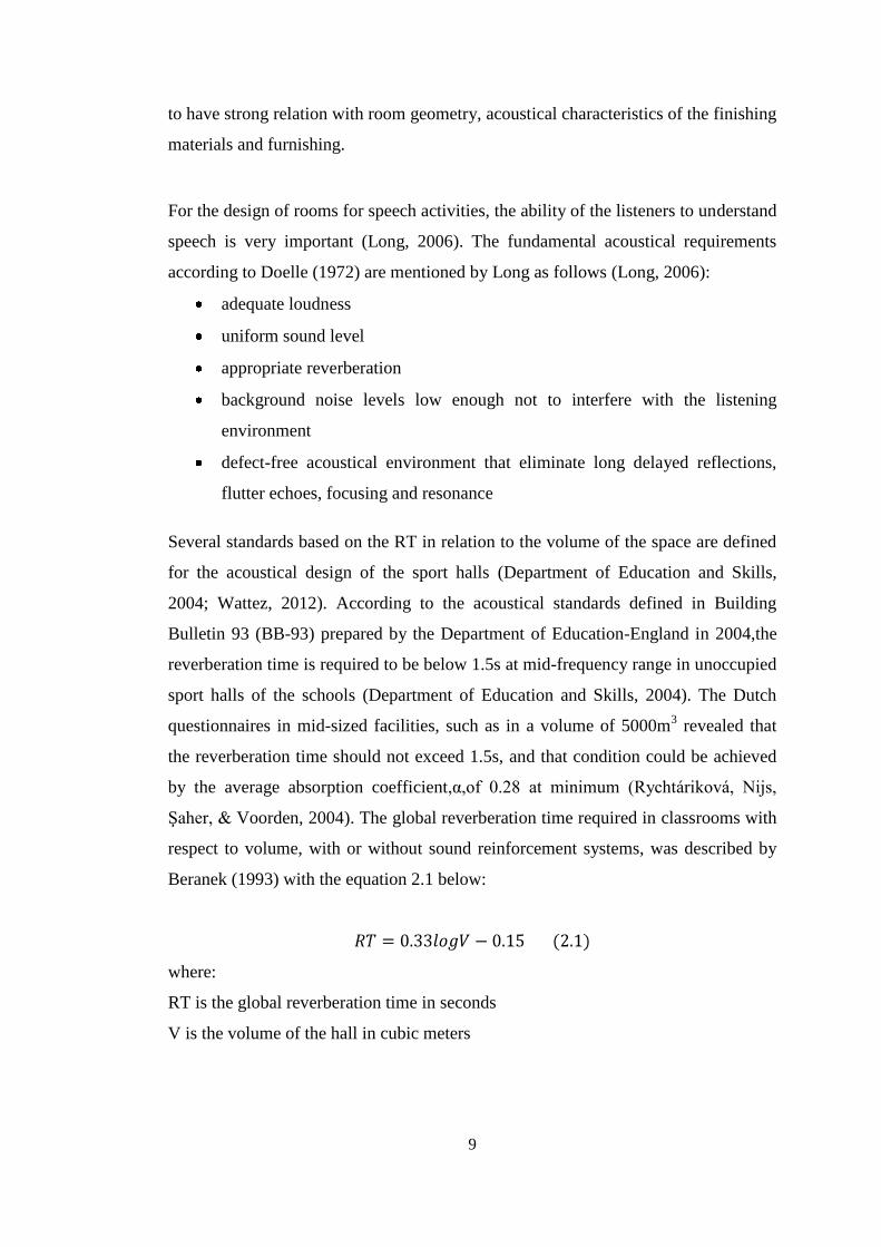
Shape (Geometry):Hall geometry is an important parameter affecting the acoustics
of a space. Below mentioned are the most commonly preferred geometrical forms of
the hallsand their influence on acoustics of the spaces.
Shoebox: Determined by the interviews of Beranek and questionnaire survey
by Haan/Fricketo be “excellent”, of the top 15 halls, two thirds are “shoebox”
shaped. Certainly, the shoebox shape, provided the hall is not too wide, is a
safe acoustical design. Parallel sidewalls assure early lateral reflections to the
audience on the main floor, essential to the desired acoustical attribute
“spaciousness”. But as demonstrated in several recent halls, spaciousness can
also be achieved by one of three means: (i) some combination of suspended
or sidewall-splayed panels and by taking steps to preserve bass energy, (ii)
shaping of the sidewalls near the proscenium and the sides of the performing
space so as to direct the sound more uniformly to the audience areas, or (iii)
interspersing seating areas with “walls” that are located to provide lateral
reflections as are found in several “surround” halls. Boston Symphony Hall
(Figure 2.1), which has shoe-box form in plan, is mentioned by Beranek
(2004) as one of the five highest ranked halls in the world.
12
Figure 2.1 Boston Symphony Hall- interior view (University of Cambridge, 2013).
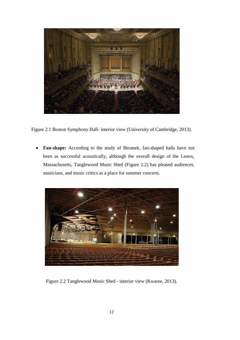
Fan-shape: According to the study of Beranek, fan-shaped halls have not
been as successful acoustically, although the overall design of the Lenox,
Massachusetts, Tanglewood Music Shed (Figure 2.2) has pleased audiences,
musicians, and music critics as a place for summer concerts.
Figure 2.2 Tanglewood Music Shed - interior view (Kwaree, 2013).
13
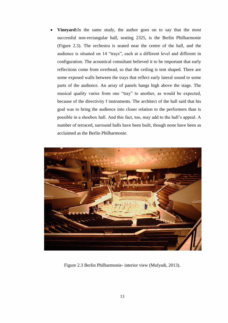
Vineyard:In the same study, the author goes on to say that the most
successful non-rectangular hall, seating 2325, is the Berlin Philharmonie
(Figure 2.3). The orchestra is seated near the centre of the hall, and the
audience is situated on 14 “trays”, each at a different level and different in
configuration. The acoustical consultant believed it to be important that early
reflections come from overhead, so that the ceiling is tent shaped. There are
some exposed walls between the trays that reflect early lateral sound to some
parts of the audience. An array of panels hangs high above the stage. The
musical quality varies from one “tray” to another, as would be expected,
because of the directivity f instruments. The architect of the hall said that his
goal was to bring the audience into closer relation to the performers than is
possible in a shoebox hall. And this fact, too, may add to the hall’s appeal. A
number of terraced, surround halls have been built, though none have been as
acclaimed as the Berlin Philharmonie.
Figure 2.3 Berlin Philharmonie- interior view (Mulyadi, 2013).

14
Simple plan schemes of the shoe-box, fan-shape and vineyard forms are given in
Figure 2.4.
Figure 2.4 Simple plan schemes for shoe-box, fan-shape and vineyard forms.
2.2.2. Audience Absorption and Type of Chairs
In the design of halls audience density, chairs, audience absorption due to the type of
chairs and materials for walls, ceiling and stageare described as the architectural
elementsaffecting the acoustical environment in a hall (Beranek, 2004).
Audience density: An audience area that is divided into a number of small
seating blocks absorbs more sound than if it is comprised only a few blocks.
To preserve loudness, the total seating area must not become too large,
because to a first approximation, the power available to each person (i.e. per
unit area) is equal to the total power radiated by the performing group divided
by the total audience area.
Chairs: Widely spaced seats are more luxurious, but they come at the
expense of acoustical quality and high building costs in halls with a large
seating capacity. If the seats in a large hall are too generously spaced, the
architect is likely to design a wide hall in order to obtain the necessary floor
area. This causes the back-row listeners to be very far from the stage, thus
diminishing the strength of the direct and early sound.

15
Audience Absorption due to Type of Chairs: People seated in heavily
upholstered chairs absorb more sound than those seated in a medium, lightly
or non-upholstered chair. The difference is particularly noticeable at bass
frequencies. A common cause of bass deficiency in concert halls is overly
sound absorbent chairs. It is strongly recommended that a chair be made of
molded material, such as plywood, and that the upholstering on the top of the
seat bottom be no thicker than 2in. (=5cm), and, on the seat back, no thicker
than 1in. (=2.5cm), and, if comfortable, cover only two-thirds of the seat
back. Also, the armrest and the rear of the seat back of a chair should not be
upholstered. These requirements rule out thick seat bottoms containing
springs.
Materials for Walls, Ceiling and Stage: When the audience sits over the
raised floor, their weight suppress some of the vibration and the loss of bass
is not excessive. In most modern halls where the bass response is good the
floors are concrete, covered with either wooden parquet or some synthetic
material that is cemented to the concrete, and the walls and ceiling are
constructed with materials that have a large weight per square foot.Thin wood
paneling strongly absorbs bass energy, where “thin” means 1in. (=2.5cm) or
less. For a hall that is lined with wood, it should be as near 2in. (=5cm)in
thickness as possible. For the sidewalls of many halls, wood veneer
(“wallpaper”) on solid (plaster) backing is employed to give the hall a warm,
traditional appearance.
2.2.3. Design of Rooms for Multi-Purpose Use
Variable RT is considered to be the most valuable feature for a well-designed
auditoria since it may accommadate several types of musical & speech performances
and flexible acoustical environments.Acoustic character is more a question of gross
shape than small detail which means for variable acoustics, major changes are
required. Variable acoustical elements, within this content, are mainly (i) variable
auditorium volume, (ii) variable acoustic absorption within the hall (Barron, 1998).

16
i. Variable Auditorium Volume: There are basically two methods of providing
variable volume: by a movable panel/ partition or by a movable shutter system
(Barron, 1998).
The movable panels are to vary the floor area and the seating capacity with it in
case used as vertical partitions or as non-vertical surfaces to provide extra
volumes with little absorbent materials in them. Suspended ceilings constructed
of many independent panels that can be raised or lowered are used as an
alternative solution as well.
The shutter system in which a suspended ceiling can be opened or closed is
considered to be another feasible option. For this system to be effective, in the
open condition, an open area of 40% is required and the void above the
suspended ceiling must be reverberant and behave acoustically as a void. In case
the existence of significant acoustically absorbent or diffusing surfaces n the
void, the extra volume might not make a worthwhile contribution to the
reverberation time.
In addition to the variable volume in halls, coupled rooms are also preferred for
variable acoustics (Mehta, Johnson, & Rocafort, 1999). Coupled rooms are basically
two spaces linked to each other through an opening between them. In coupled rooms,
sound energy is exchanged between the rooms through the opening. When the sound
source is turned off, the sound in both rooms decays at their own individual decay
rates and in case the reverberation times of the rooms are not equal, an energy
surplus in one room to the other during the decay process which leads to a
modification in the reverberation characteristics of rooms (Figure 2.5) (Mehta,
Johnson, & Rocafort, 1999).
17
Figure 2.5 Sound decay in coupled rooms. (a) The sound source is in the room 1, (b)
The source is in room 2 (Egan, 1988).
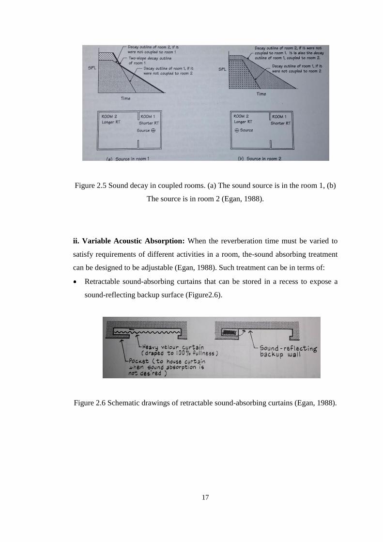
ii. Variable Acoustic Absorption: When the reverberation time must be varied to
satisfy requirements of different activities in a room, the-sound absorbing treatment
can be designed to be adjustable (Egan, 1988). Such treatment can be in terms of:
Retractable sound-absorbing curtains that can be stored in a recess to expose a
sound-reflecting backup surface (Figure2.6).
Figure 2.6 Schematic drawings of retractable sound-absorbing curtains (Egan, 1988).
18
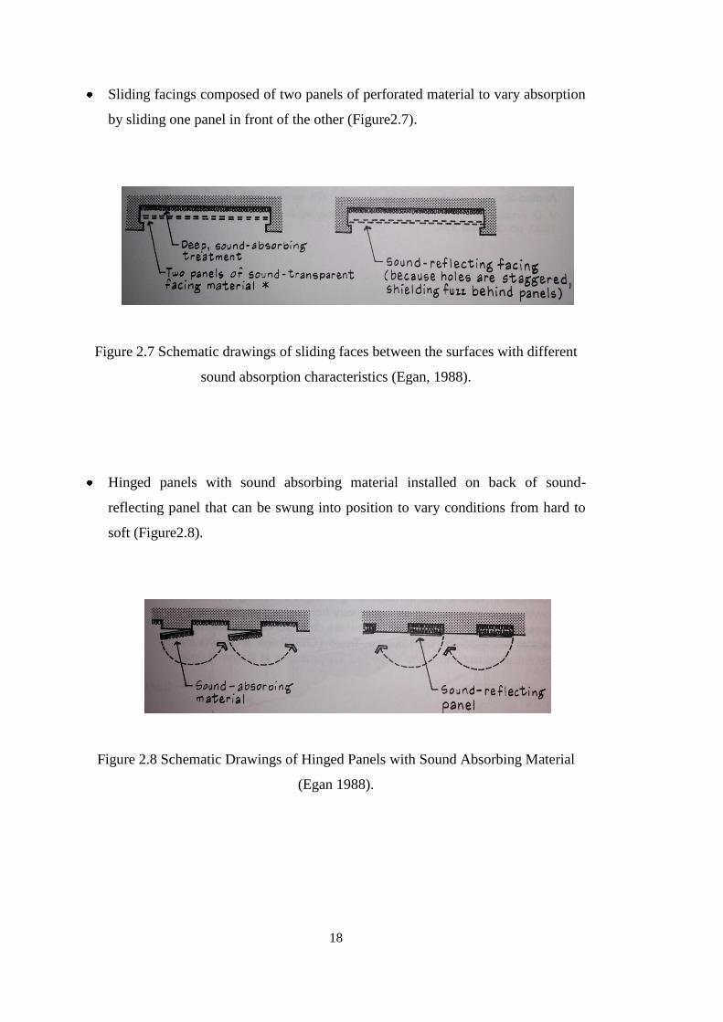
Sliding facings composed of two panels of perforated material to vary absorption
by sliding one panel in front of the other (Figure2.7).
Figure 2.7 Schematic drawings of sliding faces between the surfaces with different
sound absorption characteristics (Egan, 1988).
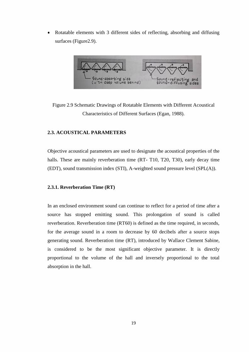
Hinged panels with sound absorbing material installed on back of sound-
reflecting panel that can be swung into position to vary conditions from hard to
soft (Figure2.8).
Figure 2.8 Schematic Drawings of Hinged Panels with Sound Absorbing Material
(Egan 1988).
19
Rotatable elements with 3 different sides of reflecting, absorbing and diffusing
surfaces (Figure2.9).
Figure 2.9 Schematic Drawings of Rotatable Elements with Different Acoustical
Characteristics of Different Surfaces (Egan, 1988).
2.3. ACOUSTICAL PARAMETERS
Objective acoustical parameters are used to designate the acoustical properties of the
halls. These are mainly reverberation time (RT- T10, T20, T30), early decay time
(EDT), sound transmission index (STI), A-weighted sound pressure level (SPL(A)).
2.3.1. Reverberation Time (RT)
In an enclosed environment sound can continue to reflect for a period of time after a
source has stopped emitting sound. This prolongation of sound is called
reverberation. Reverberation time (RT60) is defined as the time required, in seconds,
for the average sound in a room to decrease by 60 decibels after a source stops
generating sound. Reverberation time (RT), introduced by Wallace Clement Sabine,
is considered to be the most significant objective parameter. It is directly
proportional to the volume of the hall and inversely proportional to the total
absorption in the hall.

20
where:
is the volume of the hall.
is total absorption in the hall.
(2.2)
where:
is the surface area of the material
is the sound absorption coefficient with respect to frequency
is air absorption
At high frequencies above 1000Hz, the reverberation time inevitably decreases due
to air absorption. At low frequencies, the situation can be controlled by the designer.
For speech there is good reason to keep the reverberation characteristic constant with
frequency; a rise in the bass undermines intelligibility. But for music a bass rise in
reverberation time is considered by most people as desirable (Barron,
1998).Optimum reverberation time intervals are given in Figure 2.10.
According to the analyses conducted on eleven concert halls in Europe, from
reverberation time, volume and sound-source distance, four out of the five listener
aspects Level, Reverberance, Clarity and Listener Envelopment can be predicted
(Skålevik, 2010).
Although reverberation time is described as the most important acoustical parameter,
further investigations display the fact of existence of other significant parameters
(Beranek, 2004).

21
Figure 2.10 Optimum RT values with respect to functions (Egan, 1988)
2.3.2. Early Decay Time (EDT)
The earlier studies of sound decay assumed that the entire 60dB decay of sound is
smooth and uniform. Measurements in actual have revealed that the 60dB decay may
not be uniform (Mehta, Johnson, & Rocafort, 1999). Experimental investigations
have revealed that mainly the initial decay of sound is subjectively significant. The
time associated with the early part of the decay process is called the Early Decay
Time (EDT). It is described as the time passed during the initial rate of decay of
10dB of the reverberant sound multiplied by six. Early decay time includes more
explanatory information than the reverberation time. The multiplication is included
to establish a comparison with the global reverberation time (GRT-RT). A shorter
EDT provides “clarity” and a long RT provides “liveness” to music (Mehta, Johnson,
& Rocafort, 1999). High EDT value indicates that the sound is not intelligible
enough but the environment is reverberant.

22
2.3.3. Speech Transmission Index (STI)
The speech intelligibility of a transmission system, e.g. a telephone line or a room, is
usually measured by means of a list of words (or sentences) where the percentage of
correctly understood words gives the intelligibility score. The intelligibility depends
on the word material (sentences, single words, numbers, etc.), the speaker, the
listener, the scoring method and the quality of the transmission system (Jacobsen,
Poulsen, Rindel, Gade, & Ohlrich, 2011). The components of speech intelligibility
involve only some of several important acoustical qualities of rooms for listening.
The concept that early sound reflections are useful and increase the loudness of
sounds, thus increasing intelligibility and that sounds from late-arriving reflections,
reverberation and background noise in the room decrease intelligibility (Cavanaugh,
Tocci, & Wilkes, 2010). Speech transmission index (STI) is determined to be an
important acoustical measurement that relates the levels of direct sound and early
reflections to the reverberant sounds and background noise for a simulated speech
signal. It is thought to account for the relative degradation of speech by the
combination of background noise, reverberation and distance in a specific acoustic
environment (Cavanaugh, Tocci, & Wilkes, 2010). STI values range from 1.0 (ideal)
that refers to the highest to 0.0 refers to the worst (Cavanaugh, Tocci, & Wilkes,
2010) (Figure.2.11).
Rapid Speech Transmission Index, RASTI:The RASTI is a simplified version of
the STI and it is used for room acoustics and direct communication situations. It is
calculated using only the 500Hz and 2000Hz frequency bands (Larm & Hongisto,
2005). The result is an index which is used in the same way as in STI (Jacobsen,
Poulsen, Rindel, Gade, & Ohlrich, 2011).

23
Figure 2.11 STI (RASTI) Value Evaluation Table
2.3.4. A-Weighted Sound Pressure Level (SPL (A)):
Sound pressure level (SPL) or sound level is a logarithmic measure of the effective
sound pressure of a sound relative to a reference value. It is measured in
decibels (dB) above a standard reference level of 20 µPa which is usually considered
the threshold of human hearing (at 1000 Hz) (Wikipedia, 2014). The SPL is
expressed as the logarithm of the ratio in order to not to deal with a large range of
numbers (Mehta, Johnson, & Rocafort, 1999).
(2.3)
where:
I= sound intensity level of the sound
Iref= 10-12
W/m2
The most common weighting that is used in noise measurement is A-Weighting. Like
the human ear, this effectively cuts off the lower and higher frequencies that the
average person cannot hear. A-weighted measurements are expressed
as dBA or dB(A) (Noise Meters Inc., 2014). Ideal sound pressure level difference in
a hall at different seats should not exceed 10 dB(A). The idealSPL(A) difference is 6

24
dB(A) showing the existence of adequate loudness in the overall hall.Typical sound
pressure levels are given in Table 2.1.
Table 2.1 Typical dBA Levels (Sengpielaudio, 2014)
190 dBA Heavy weapons, 10 m behind the weapon (peak level)
180 dBA Toy pistol fired close to ear (peak level)
170 dBA Slap on the ear, fire cracker explodes on shoulder, small arms at a
distance of 50 cm (peak level)
160 dBA Hammer stroke on brass tubing or steel plate at 1 m distance, airbag
deployment very close at a distance of 30 cm (peak level)
150 dBA Hammer stroke in a smithy at 5 m distance (peak level)
130 dBA Loud hand clapping at 1 m distance (peak level)
120 dBA Whistle at 1 m distance, test run of a jet at 15 m distance
Threshold of pain, above this fast-acting hearing damage in short
action is possible
115 dBA Take-off sound of planes at 10 m distance
110 dBA
Siren *) at 10 m distance, frequent sound level in discotheques and close
to loudspeakers at rock concerts, violin close to the ear of an orchestra
musicians (maximum level)
105 dBA Chain saw at 1 m distance, banging car door at 1 m distance (maximum
level), racing car at 40 m distance, possible level with music head phones
100 dBA Frequent level with music via head phones, jack hammer at 10 m
distance
95 dBA Loud crying, hand circular saw at 1 m distance
90 dBA Angle grinder outside at 1 m distance
Over a duration of 40 hours a week hearing damage is possible
80 dBA Very loud traffic noise of passing lorries at 7.5 m distance,
high traffic on an expressway at 25 m distance
75 dBA Passing car at 7.5 m distance, un-silenced wood shredder at 10 m
distance
70 dBA Level close to a main road by day, quiet hair dryer at 1 m distance to ear
65 dBA Bad risk of heart circulation disease at constant impact is possible
60 dBA Noisy lawn mower at 10 m distance
55 dBA Low volume of radio or TV at 1 m distance, noisy vacuum cleaner at
10 m distance
50 dBA Refrigerator at 1 m distance, bird twitter outside at 15 m distance
45 dBA Noise of normal living; talking, or radio in the background
40 dBA Distraction when learning or concentration is possible
35 dBA Very quiet room fan at low speed at 1 m distance
25 dBA Sound of breathing at 1 m distance
0 dB Auditory threshold

25
2.3.5. Reverberation Time (T30)
T30 is the reverberation time for 60 dB of room decay, based on a straight line curve
fit between the time passes for 5 dB drop of the sound and the time passes for 35 dB
drop of the sound is doubled to be made consistent with the traditional reverberation
time for 60 dB of decay (RT60). The T30 is a measure of the “persistence” of sound
in the space.The T30 and EDT provide important information about the way that
sound behaves in a room. Both are most applicable when a homogeneous reverberant
field exists (i.e. medium to large rooms with low absorption). However,
reverberation times are not the same in all parts of a hall and it is necessary to
measure it at different seats for averaging (Beranek, 2004).
2.3.6. Clarity (C80)
The usual physical measurement of clarity is the ratio of the energy in the early
sound to that in the reverberant sound, a ratio that is expressed in decibels (dB) by
C80. The number “80” designates the time considered for the early reflections.
Clarity decreases with increased reverberation and vice versa (Beranek, 2004).C80 is
a widely used parameter for music (Echenagucia & Sassone, 2013). Barron explains
that there is negative correlation between EDT and C80. A High C80corresponds to a
low EDT and vice versa (Barron, 1995).
2.3.7. Echo
An echois the distinct repetition of the original sound and is sufficiently loud to be
clearly heard above the general reverberation and background noise in a space (Egan,
1988).Echo, typically observed for delays beyond 50 ms and at high reflection levels.
If the delay is very long, say 200 ms, then the echo may even be detected at a much
lower level (Rossing (Ed.), 2007). In auditoria, sound-reflecting flat or concave rear
walls and high or vaulted ceilings are potential echo producers (Egan, 1988). Echoes
interfere with speech intelligibility and cause confused perception of music and
therefore, must be avoided (Mehta, Johnson, & Rocafort, 1999). Difference between
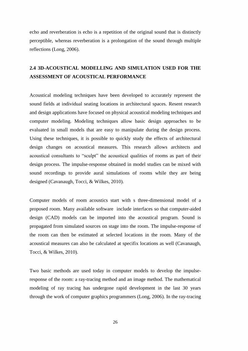
26
echo and reverberation is echo is a repetition of the original sound that is distinctly
perceptible, whereas reverberation is a prolongation of the sound through multiple
reflections (Long, 2006).
2.4 3D-ACOUSTICAL MODELLING AND SIMULATION USED FOR THE
ASSESSMENT OF ACOUSTICAL PERFORMANCE
Acoustical modeling techniques have been developed to accurately represent the
sound fields at individual seating locations in architectural spaces. Resent research
and design applications have focused on physical acoustical modeling techniques and
computer modeling. Modeling techniques allow basic design approaches to be
evaluated in small models that are easy to manipulate during the design process.
Using these techniques, it is possible to quickly study the effects of architectural
design changes on acoustical measures. This research allows architects and
acoustical consultants to “sculpt” the acoustical qualities of rooms as part of their
design process. The impulse-response obtained in model studies can be mixed with
sound recordings to provide aural simulations of rooms while they are being
designed (Cavanaugh, Tocci, & Wilkes, 2010).
Computer models of room acoustics start with s three-dimensional model of a
proposed room. Many available software include interfaces so that computer-aided
design (CAD) models can be imported into the acoustical program. Sound is
propagated from simulated sources on stage into the room. The impulse-response of
the room can then be estimated at selected locations in the room. Many of the
acoustical measures can also be calculated at specifix locations as well (Cavanaugh,
Tocci, & Wilkes, 2010).
Two basic methods are used today in computer models to develop the impulse-
response of the room: a ray-tracing method and an image method. The mathematical
modeling of ray tracing has undergone rapid development in the last 30 years
through the work of computer graphics programmers (Long, 2006). In the ray-tracing

27
method, a selected number of sound rays are propagated from the source into the
room. The rays will reflect off surfaces in the room as sound waves would. The
amplitude and arrival time of the sound waves will be recorded at selected locations
in the model. The room surfaces are assigned absorption coefficients in octave band
frequencies. Many current programs can also approximate the diffusion and
diffraction of sound that is so important in auditorium acoustics. Some programs
provide abbreviated estimation procedures, in which the reverberant energy is
approximated by an envelope derived from the reverberation time of the room. This
means that the multiple high-order reflections that occur in the reverberant field are
not individually calculated. The image method, on the other hand, works backwards.
The computer locates all of the surfaces from a given reciever location that can
project reflections to it from the source. Rays are then traced from the reciever to the
surface on stage (Cavanaugh, Tocci, & Wilkes, 2010).
Computer model studies show the distribution of sound pressure levels in rooms,
create ray diagrams of specific sound paths between the source and reciever, estimate
the impulse response at specific locations and calculate many acoustical design
parameters (Cavanaugh, Tocci, & Wilkes, 2010).
Today’s room acoustical computer models have several advantages compared to
scale models. They have become reliable and efficient design tools for the acoustic
consultants, and the results of a simulation can be presented not only for the eyes but
also for the ears with new techniques for auralisation (Rindel J. H., 2000). It is found
quite obvious that a computer model is much more flexible than a scale model
because of being easy to modify the geometry of a computer model and the surface
materials can easily be changed by changing the absorption coefficients. The
advantage of the computer model is not only it is fast, but also the results can be
visualised and analysed much better than a scale model because it contains more
information than a set of measurements done in a scale model with small
microphones (Rindel J. H., 2000). It is also stated that the best programs do neither
28
require extremely long calculation times nor extremely detailed room geometries
(Rindel J. H., 2000).
One of the most commonly used acoustical simulation software is ODEON. The
software is developed for simulating the interior acoustics of buildings. Given the
geometry and surface-properties, the acoustics can be predicted, illustrated and
listened to. Sound reinforcement is claimed to be easily integrated in the acoustic
predictions. ODEON uses the image-source method combined with ray tracing
(Odeon A/S, 2014). The applications of the software include concert and opera halls,
theatres, churches and mosques, open plan offices, foyers, restaurants, music studios,
underground and railway stations, airport terminals, industrial environments, outdoor
areas with complicated geometry(Odeon A/S, 2014).
With a computer model it is straightforward to calculate the response at a large
number of recievers distributed in a grid that covers the audience area. It is stated to
be very useful for the acoustic designer to see a mapping of the spatial distribution of
acoustical parameters. Uneven sound distribution and acoustically weak spots can
easily be localised and appropriate countermeasures can be taken (Rindel J. H.,
2000).
Computer techniques for simulation of sound in rooms have improved significantly
in recent years (Rindel J. H., 2000). There are several studies on the reliability of
these techniques (Rindel J. H., 2000; Rindel & Christensen, 2003; Shiokawa &
Rindel, 2007). According to a study conducted on the validation of the quality of
room acoustic auralization, comparisons between the auralizations from the
computer simulation and dummy head recordings in the same postion in the same
room, the differences are claimed to be hardly audible (Rindel & Christensen, 2003).
In the content of another study conducted in the search for reliability of the
acoustical simulation, comparisons were made between measured room acoustical
parameters and those obtained from computer simulations using the software
ODEON v.3.1on two concert halls (Shiokawa & Rindel, 2007). Comparisons were
29
also made between the results obtained from computer simulations and those from
models on both concert halls. According to the results,measured and calculated
reverberation times in single positions were found to be in good match (Shiokawa &
Rindel, 2007).

30

31
CHAPTER 3
MATERIAL & METHOD
Here are presented the material and method of the study. The former describes the
architectural features of typical project of small sport halldesigned for the schools.
The latter describes the proposals/treatments suggested for the acoustical
improvement of the hall. Afterwards, the activities-related scenarios composed of the
AS-IS uses of the hall, namely physical education classes and sport games, and
multi-purpose use of the hall for speech and musical activities are defined. The
methods of 3-D modelling and acoustical simulation methods used for the acoustical
assessment of the hall are also explained here in detail.
3.1. SPORT HALL TYPICAL PROJECT DESIGNED FOR STATE
SCHOOLS (Code: MEB2004.63)
In this research, typical small sport hall project with 70 audience capacity designed
by Ministry of Education as part ofits “Physical Contribution to Education Project -
Eğitime Fiziksel Katkı Projesi (EFİKAP)”was examined.
Sport hall typical project is designed for physical education (PE) classes and sportive
activities such as basketball, volleyball games (Figure 3.1). The design is composed
of two parts: first is the “service area” which consists an office, changing rooms,
showers and toilets; second is the “sports area” which consists the playfield and the
tribune (Figure 3.1).
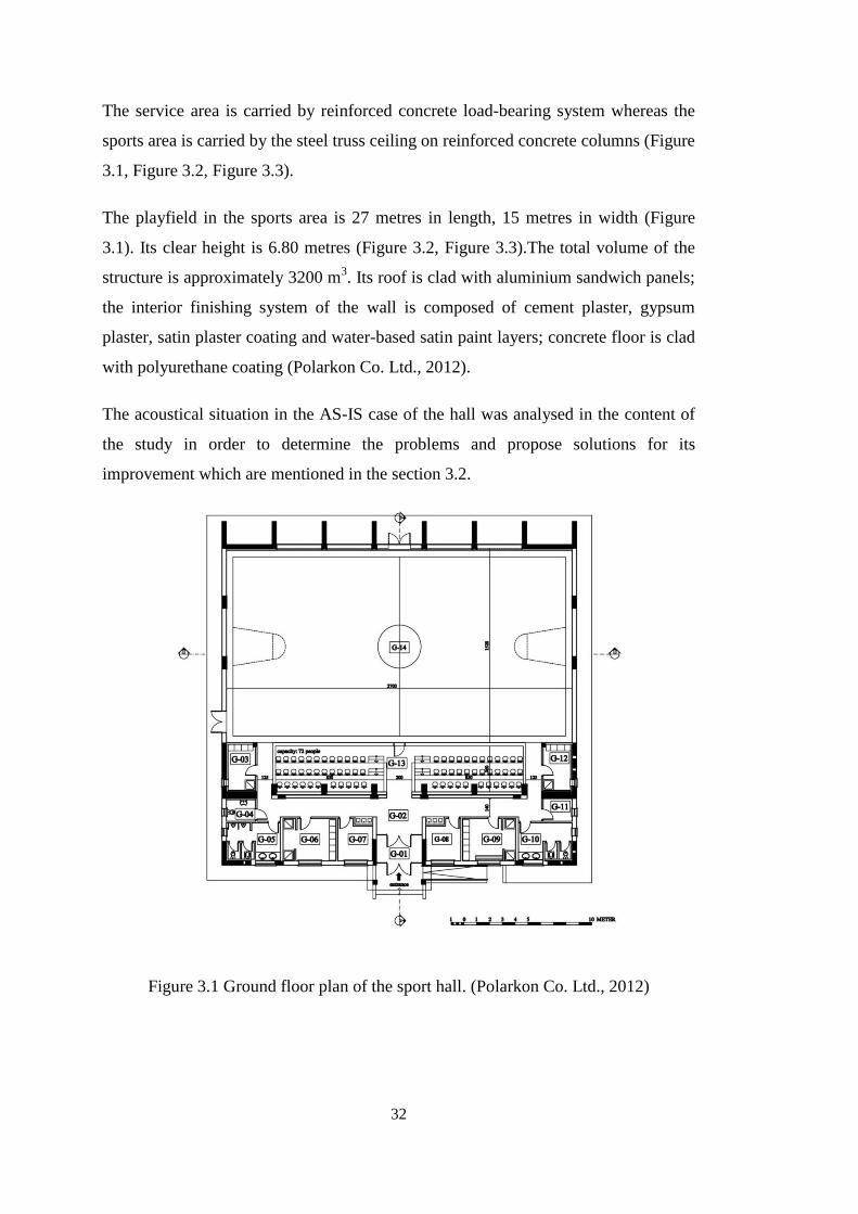
32
The service area is carried by reinforced concrete load-bearing system whereas the
sports area is carried by the steel truss ceiling on reinforced concrete columns (Figure
3.1, Figure 3.2, Figure 3.3).
The playfield in the sports area is 27 metres in length, 15 metres in width (Figure
3.1). Its clear height is 6.80 metres (Figure 3.2, Figure 3.3).The total volume of the
structure is approximately 3200 m3. Its roof is clad with aluminium sandwich panels;
the interior finishing system of the wall is composed of cement plaster, gypsum
plaster, satin plaster coating and water-based satin paint layers; concrete floor is clad
with polyurethane coating (Polarkon Co. Ltd., 2012).
The acoustical situation in the AS-IS case of the hall was analysed in the content of
the study in order to determine the problems and propose solutions for its
improvement which are mentioned in the section 3.2.
Figure 3.1 Ground floor plan of the sport hall. (Polarkon Co. Ltd., 2012)

33
Figure 3.2 Sport hall section AA. (Polarkon Co. Ltd., 2012)
Figure 3.3 Sport hall section BB. (Polarkon Co. Ltd., 2012)
3.2. PROPOSALS INTRODUCED TO THE STRUCTURE FOR
ACOUSTICAL IMPROVEMENT
In order to provide a better acoustical environment within the hall, i.e. more
intelligible, free from acoustical defects like flutter echoes, etc, a convenient solution
was searched.Since thesport halls under study here already been constructed, the
solution was needed to be adaptable to the existing structures. For the acoustical
improvement of the sport halls, main design principle in this study was respecting the
original architectural project and not removing/changing any architectural element
within the hall. Within this content, mountable systems and materials were taken into
consideration and designed. Furthermore, with the system design proposals and
material selections, special care was given to economy, durability, convenience for

34
repairing, maintenance and cleaning, which are the basic principles need to be
considered in the design of schools (Karabey, 2003).
In the light of these design principles and the intended uses of the hall, the systems
proposed for the design were classified as permanent components and temporary
components. The permanent components are the suspended ceiling systems and wall
cladding with metal sheets. The temporary components are the suspended curtain
modules.
These systems are described in the following sections:
3.2.1. Suspended Ceiling Systems
During the study, one of the primary decisions was clarifying the location and
properties of the permanent components. The preliminary aim was to decrease the
global reverberation times to the acceptable values in low (125-250 Hz), middle
(500-1000 Hz) and high (2000-4000 Hz) frequency ranges.
It was determined that the ceiling is the most appropriate component for permanently
mounted systems due to its large amount of surface area that gives the possibility to
add large amounts of sound absorbing materials and convenience of its position in
terms of damage risk.
In order to achieve required GRT values, designs with variations of 3 different
suspended ceiling systems were analyzed. During the study, optimum solution within
these variations was searched which were selected as samples.
Flat panelled suspended ceiling system was the first treatment proposed in the
study. Acoustical simulations were conducted after adding panelled suspended
ceiling system composed of rock wool sound absorbing panels covered with
acoustically transparent fabric which were mounted flatly to the trusses at the ceiling,
above the playfield, to 6.80 m level (Figure 3.4). During the simulations, first, 5 cm
thick rock wool; second, 10 cm thick rock wool was selected as the material.
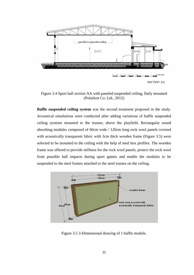
35
Figure 3.4 Sport hall section AA with paneled suspended ceiling, flatly mounted
(Polarkon Co. Ltd., 2012)
Baffle suspended ceiling system was the second treatment proposed in the study.
Acoustical simulations were conducted after adding variations of baffle suspended
ceiling systems mounted to the trusses, above the playfield. Rectangular sound
absorbing modules composed of 60cm wide / 120cm long rock wool panels covered
with acoustically transparent fabric with 3cm thick wooden frame (Figure 3.5) were
selected to be mounted to the ceiling with the help of steel box profiles. The wooden
frame was offered to provide stiffness for the rock wool panels, protect the rock wool
from possible ball impacts during sport games and enable the modules to be
suspended to the steel frames attached to the steel trusses on the ceiling.
Figure 3.5 3-Dimensional drawing of 1 baffle module.

36
Acoustical simulations were conducted with several layouts of this system. First,
baffles were mounted between the trusses to the 7.40m level. The modules were
inserted in the middle of the trusses in order to form grates with the size of 60cmx
360cm. During the simulations, firstly 5cm thick mineral wool was selected for the
material. Secondly, 10 cm thick mineral wool was selected. The same procedure was
followed with the baffle system forming grates with 30cm x 360cm sizes. Then,
baffles were mounted between the trusses at 6.80m level. The modules were inserted
in the middle of the trusses in order to form grates with the size of 90cm x 360cm.
During the simulations, firstly 5cm thick mineral wool was selected as the material.
Secondly, 10 cm thick mineral wool was selected. The same procedure was followed
with the baffle system forming grates with 60cm x 360cm sizes (Figure 3.6, Figure
3.7, Figure 3.8). During the simulations, the sound absorption caused by the wooden
frame was neglected.
Figure 3.6 Ceiling plan– ceiling configuration of baffles with 60cmx360cm intervals
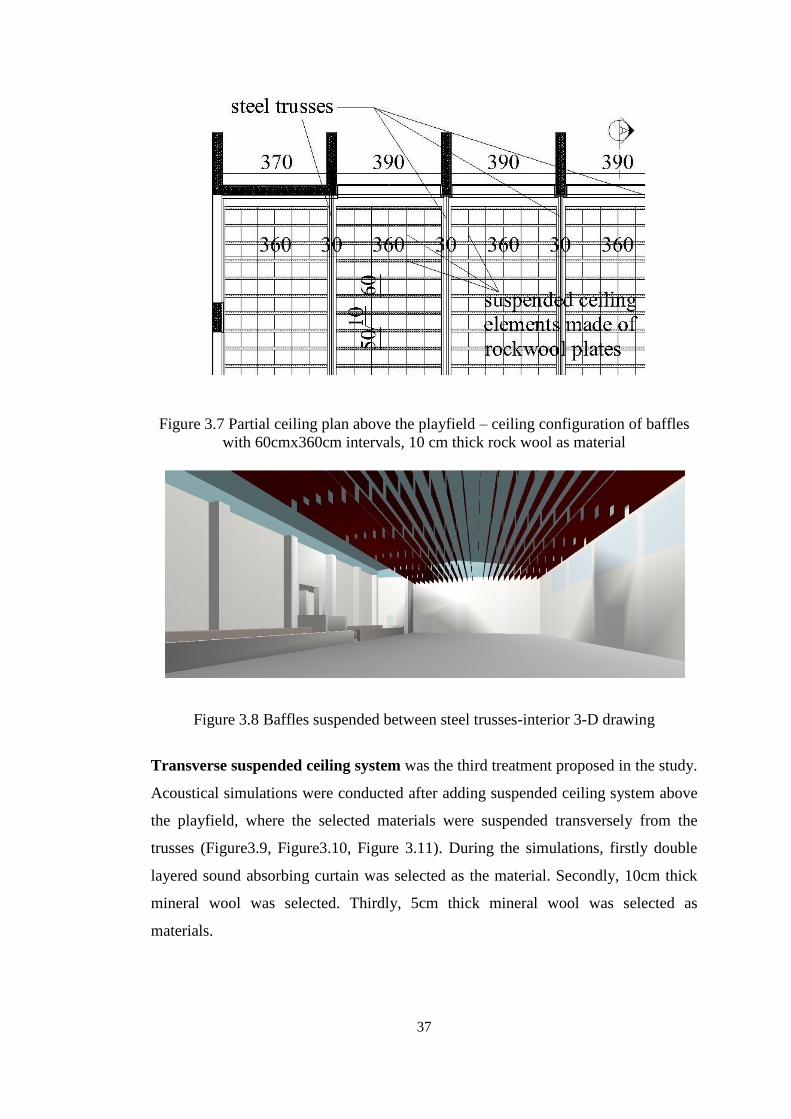
37
Figure 3.7 Partial ceiling plan above the playfield – ceiling configuration of baffles
with 60cmx360cm intervals, 10 cm thick rock wool as material
Figure 3.8 Baffles suspended between steel trusses-interior 3-D drawing
Transverse suspended ceiling system was the third treatment proposed in the study.
Acoustical simulations were conducted after adding suspended ceiling system above
the playfield, where the selected materials were suspended transversely from the
trusses (Figure3.9, Figure3.10, Figure 3.11). During the simulations, firstly double
layered sound absorbing curtain was selected as the material. Secondly, 10cm thick
mineral wool was selected. Thirdly, 5cm thick mineral wool was selected as
materials.
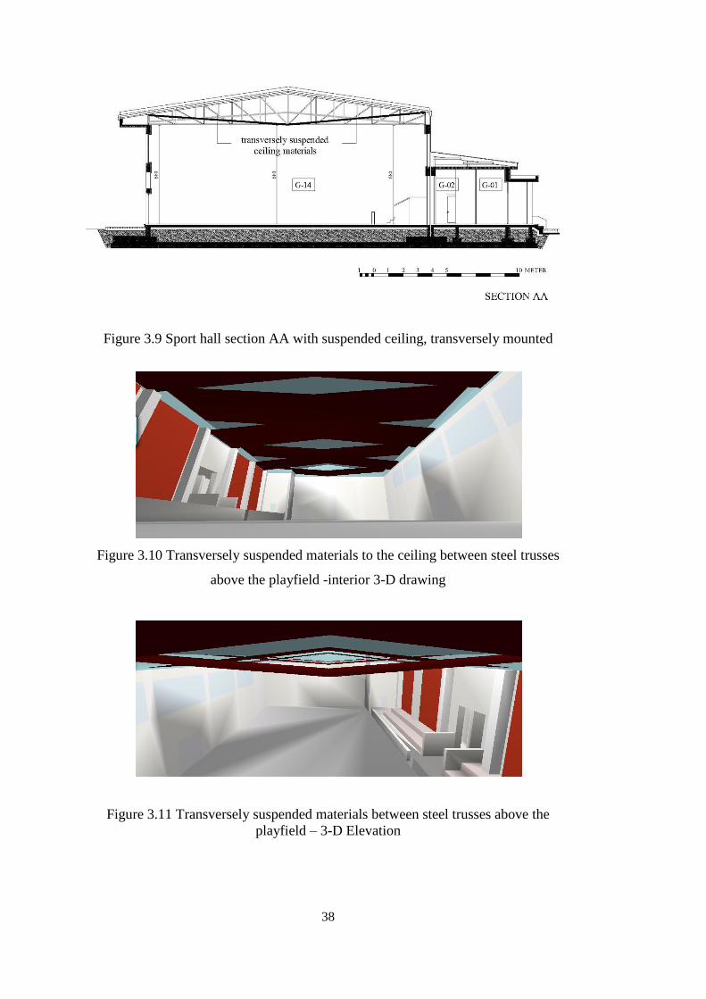
38
Figure 3.9 Sport hall section AA with suspended ceiling, transversely mounted
Figure 3.10 Transversely suspended materials to the ceiling between steel trusses
above the playfield -interior 3-D drawing
Figure 3.11 Transversely suspended materials between steel trusses above the
playfield – 3-D Elevation

39
According to the simulation results for estimated global RT (GRT-T30) values,the
most appropriate T30 values, i.e. closest values to those described in the standards,
were obtained with three proposals: (i) baffles suspended below the trusses with
60cm x 360cm grids, (ii) baffles suspended above the trusses with 60cm x 360cm
grids, (iii) panels mounted transversely to the trusses and when 10 cm thick mineral
wool was used as the material. The amount of the materials used in the suspended
ceiling proposal are given in Figure F.1.
3.2.2. Suspended Curtain Modules for Vertical Surfaces
After selection of the most appropriate ceiling system as the permanent
implementation, convenient proposal for the temporary implementation was searched
in order to achieve variable acoustical environment within the hall and to be used
during different activities when necessary. For the temporarily used materials,
vertical surfaces of the playfield, i.e. walls, windows, openings, etc., were considered
to be the most appropriate location due to its surface area amount and giving
possibility to easy access to the materials mounted.
Since the studied halls belong to schools, the procedure for removing when
unnecessary / implementing when necessary is going to be conducted by the school
janitor, not by specialized operators. Hence, the system proposed needed to be easily
operable; requiring as few assisting materials as possible. Additionally, it needed to
be economical and easily mountable at the first place. In the light of these principles,
instead of automatic system implementation, mechanical system was preferred.
Within this content, roller blind curtains were found to be appropriate for the
temporary implementation. Double-layered satin curtains with roller blind
mechanisms were mounted 15cm from the wall in front of the tribune’s back wall
with the height of 5.80m, in front of the side walls and front walls in the playfield
with the height of 5.30m and in front of the windows with the height of 2.50m. The
amount of the materials used in the wall surfaces are given in Figure F.2.
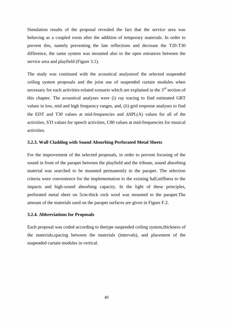
40
Simulation results of the proposal revealed the fact that the service area was
behaving as a coupled room after the addition of temporary materials. In order to
prevent this, namely preventing the late reflections and decrease the T20-T30
difference, the same system was mounted also to the open entrances between the
service area and playfield (Figure 3.1).
The study was continued with the acoustical analysesof the selected suspended
ceiling system proposals and the joint use of suspended curtain modules when
necessary for each activities-related scenario which are explained in the 3rd
section of
this chapter. The acoustical analyses were (i) ray tracing to find estimated GRT
values in low, mid and high frequency ranges, and, (ii) grid response analyses to find
the EDT and T30 values at mid-frequencies and SPL(A) values for all of the
activities, STI values for speech activities, C80 values at mid-frequencies for musical
activities.
3.2.3. Wall Cladding with Sound Absorbing Perforated Metal Sheets
For the improvement of the selected proposals, in order to prevent focusing of the
sound in front of the parapet between the playfield and the tribune, sound absorbing
material was searched to be mounted permanently to the parapet. The selection
criteria were convenience for the implementation to the existing hall,stiffness to the
impacts and high-sound absorbing capacity. In the light of these principles,
perforated metal sheet on 5cm-thick rock wool was mounted to the parapet.The
amount of the materials used on the parapet surfaces are given in Figure F.2.
3.2.4. Abbreviations for Proposals
Each proposal was coded according to thetype suspended ceiling system,thickness of
the materials,spacing between the materials (intervals), and placement of the
suspended curtain modules in vertical.
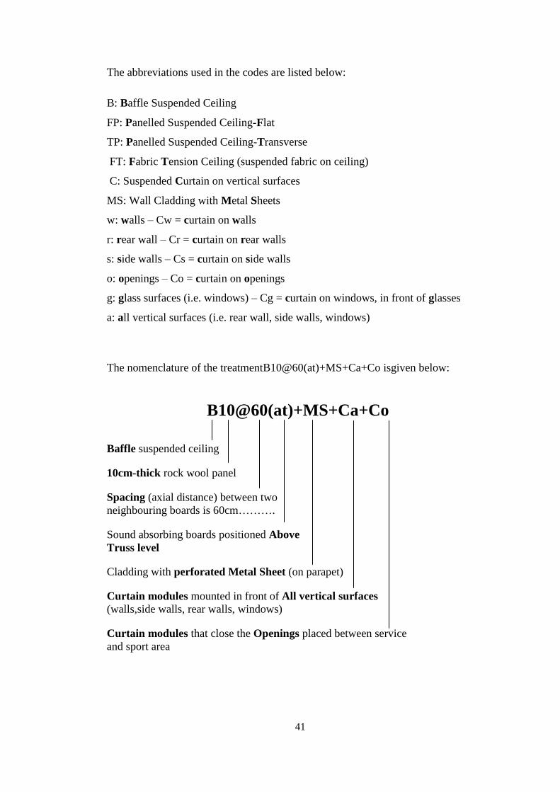
41
The abbreviations used in the codes are listed below:
B: Baffle Suspended Ceiling
FP: Panelled Suspended Ceiling-Flat
TP: Panelled Suspended Ceiling-Transverse
FT: Fabric Tension Ceiling (suspended fabric on ceiling)
C: Suspended Curtain on vertical surfaces
MS: Wall Cladding with Metal Sheets
w: walls – Cw = curtain on walls
r: rear wall – Cr = curtain on rear walls
s: side walls – Cs = curtain on side walls
o: openings – Co = curtain on openings
g: glass surfaces (i.e. windows) – Cg = curtain on windows, in front of glasses
a: all vertical surfaces (i.e. rear wall, side walls, windows)
The nomenclature of the treatmentB10@60(at)+MS+Ca+Co isgiven below:
B10@60(at)+MS+Ca+Co
Baffle suspended ceiling
10cm-thick rock wool panel
Spacing (axial distance) between two
neighbouring boards is 60cm……….
Sound absorbing boards positioned Above
Truss level
Cladding with perforated Metal Sheet (on parapet)
Curtain modules mounted in front of All vertical surfaces
(walls,side walls, rear walls, windows)
Curtain modules that close the Openings placed between service
and sport area
42
According to this nomenclature, the treatment is composed of 10cm-thick rock wool
boards fixed at 60cm intervals, sound absorbing perforated metal sheet covering the
surfaces of parapet located between the tribune and playfield, curtain modules
mounted in front of walls, windows and at the entrances/openings between the
service area and sport area.
The nomenclature of the treatment FP5+Cr is given below:
FP5+Cr
Flat panelled suspended ceiling …
5cm-thick rock wool panel……………
Curtain modules mounted in front of tribune’s rear wall
According to this nomenclature, the treatment is composed of flat panelled
suspended ceiling made of 5cm-thick rockwool boards (mountedin lateral to produce
a flatsuspended ceiling)and the curtain modules mounted in front of the tribune’s rear
wall.
The nomenclature of the treatment FT+Cg isgiven below:
FT+Cg
Fabric Tension suspended ceiling…..
Curtain modules mounted in front of the windows
According to this nomenclature, the treatment is composed of sound
absorbingcurtains/fabrics stretched crosswise between the trusses and the curtain
modules mounted in front of the windows.
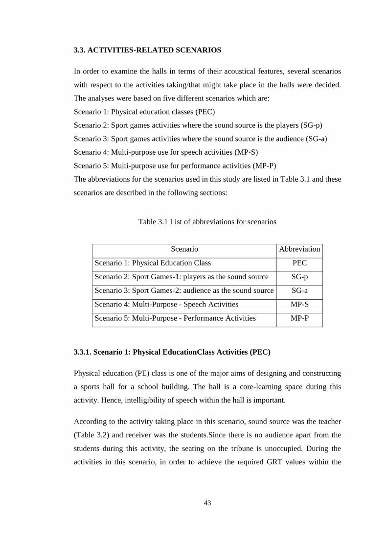
43
3.3. ACTIVITIES-RELATED SCENARIOS
In order to examine the halls in terms of their acoustical features, several scenarios
with respect to the activities taking/that might take place in the halls were decided.
The analyses were based on five different scenarios which are:
Scenario 1: Physical education classes (PEC)
Scenario 2: Sport games activities where the sound source is the players (SG-p)
Scenario 3: Sport games activities where the sound source is the audience (SG-a)
Scenario 4: Multi-purpose use for speech activities (MP-S)
Scenario 5: Multi-purpose use for performance activities (MP-P)
The abbreviations for the scenarios used in this study are listed in Table 3.1 and these
scenarios are described in the following sections:
Table 3.1 List of abbreviations for scenarios
Scenario Abbreviation
Scenario 1: Physical Education Class PEC
Scenario 2: Sport Games-1: players as the sound source SG-p
Scenario 3: Sport Games-2: audience as the sound source SG-a
Scenario 4: Multi-Purpose - Speech Activities MP-S
Scenario 5: Multi-Purpose - Performance Activities MP-P
3.3.1. Scenario 1: Physical EducationClass Activities (PEC)
Physical education (PE) class is one of the major aims of designing and constructing
a sports hall for a school building. The hall is a core-learning space during this
activity. Hence, intelligibility of speech within the hall is important.
According to the activity taking place in this scenario, sound source was the teacher
(Table 3.2) and receiver was the students.Since there is no audience apart from the
students during this activity, the seating on the tribune is unoccupied. During the
activities in this scenario, in order to achieve the required GRT values within the

44
hall, apart from the permanently mounted systems, i.e. suspended ceiling and metal
sheet on parapet, suspended curtain modules in front of the rear wall (Figure 3.12) or
in front of the windows were also used. Selection criteria for the location of the
curtain modules used was thedamage risk. The simulations were conducted with
combinations of the selected curtain modules.
Figure 3.12 Suspended curtain modules in front of the rear wall
3.3.2. Scenario 2/3: Sport Games Activities – Sound Source: Player (SG-p) /
Audience (SG-a)
Apart from physical education classes, another major aim of use of the sport halls in
schools is the sport games played by the students in the school or teams of the town,
since such halls are rented in summer for training or tournaments (Köse, 2012).
Scenario 2, where the sound source was the player located in the middle of the
playfield,was simulated in order to check communication intelligibility within the
playfield between the players.
For the simulations, the seats at the tribune were modelled as occupied seats with 70
audience capacity. Considering the possible damages that might be caused by the
spectators, players, etc., it was not possible to use the curtain modules during this
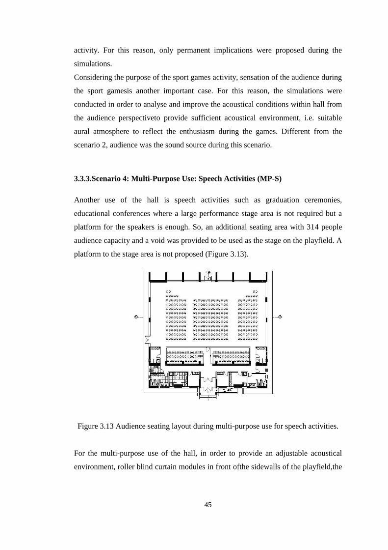
45
activity. For this reason, only permanent implications were proposed during the
simulations.
Considering the purpose of the sport games activity, sensation of the audience during
the sport gamesis another important case. For this reason, the simulations were
conducted in order to analyse and improve the acoustical conditions within hall from
the audience perspectiveto provide sufficient acoustical environment, i.e. suitable
aural atmosphere to reflect the enthusiasm during the games. Different from the
scenario 2, audience was the sound source during this scenario.
3.3.3.Scenario 4: Multi-Purpose Use: Speech Activities (MP-S)
Another use of the hall is speech activities such as graduation ceremonies,
educational conferences where a large performance stage area is not required but a
platform for the speakers is enough. So, an additional seating area with 314 people
audience capacity and a void was provided to be used as the stage on the playfield. A
platform to the stage area is not proposed (Figure 3.13).
Figure 3.13 Audience seating layout during multi-purpose use for speech activities.
For the multi-purpose use of the hall, in order to provide an adjustable acoustical
environment, roller blind curtain modules in front ofthe sidewalls of the playfield,the
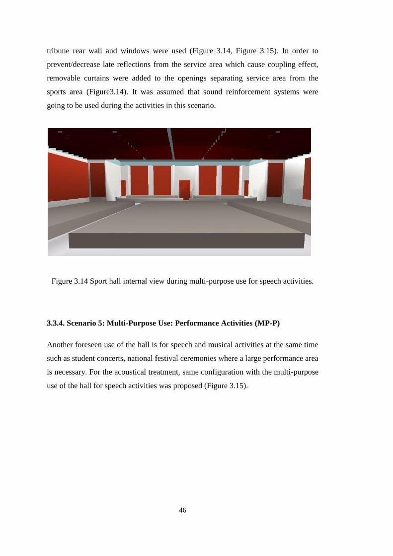
46
tribune rear wall and windows were used (Figure 3.14, Figure 3.15). In order to
prevent/decrease late reflections from the service area which cause coupling effect,
removable curtains were added to the openings separating service area from the
sports area (Figure3.14). It was assumed that sound reinforcement systems were
going to be used during the activities in this scenario.
Figure 3.14 Sport hall internal view during multi-purpose use for speech activities.
3.3.4. Scenario 5: Multi-Purpose Use: Performance Activities (MP-P)
Another foreseen use of the hall is for speech and musical activities at the same time
such as student concerts, national festival ceremonies where a large performance area
is necessary. For the acoustical treatment, same configuration with the multi-purpose
use of the hall for speech activities was proposed (Figure 3.15).

47
Figure 3.15 Sport hall internal view during multi-purpose use for performance
activities.
However, due to need for larger stage area, the seating was planned in order to
provide wider performance area to be used as the stage on the playfield. Additional
audience seating capacity is 314 people. A platform to the stage area was not
proposed (Figure 3.16). It was assumed that sound reinforcement systems were going
to be used during the activities in this scenario.
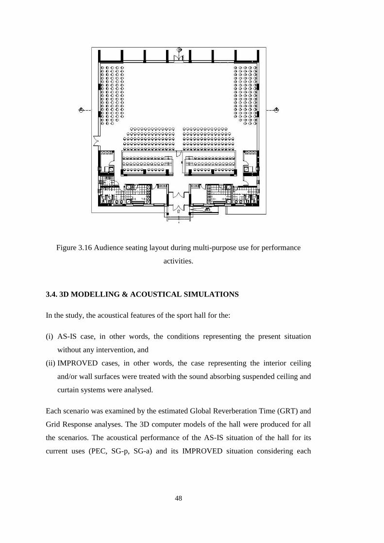
48
Figure 3.16 Audience seating layout during multi-purpose use for performance
activities.
3.4. 3D MODELLING & ACOUSTICAL SIMULATIONS
In the study, the acoustical features of the sport hall for the:
(i) AS-IS case, in other words, the conditions representing the present situation
without any intervention, and
(ii) IMPROVED cases, in other words, the case representing the interior ceiling
and/or wall surfaces were treated with the sound absorbing suspended ceiling and
curtain systems were analysed.
Each scenario was examined by the estimated Global Reverberation Time (GRT) and
Grid Response analyses. The 3D computer models of the hall were produced for all
the scenarios. The acoustical performance of the AS-IS situation of the hall for its
current uses (PEC, SG-p, SG-a) and its IMPROVED situation considering each
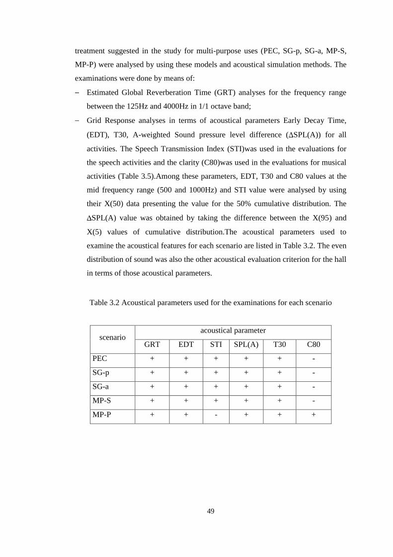
49
treatment suggested in the study for multi-purpose uses (PEC, SG-p, SG-a, MP-S,
MP-P) were analysed by using these models and acoustical simulation methods. The
examinations were done by means of:
Estimated Global Reverberation Time (GRT) analyses for the frequency range
between the 125Hz and 4000Hz in 1/1 octave band;
Grid Response analyses in terms of acoustical parameters Early Decay Time,
(EDT), T30, A-weighted Sound pressure level difference ( SPL(A)) for all
activities. The Speech Transmission Index (STI)was used in the evaluations for
the speech activities and the clarity (C80)was used in the evaluations for musical
activities (Table 3.5).Among these parameters, EDT, T30 and C80 values at the
mid frequency range (500 and 1000Hz) and STI value were analysed by using
their X(50) data presenting the value for the 50% cumulative distribution. The
SPL(A) value was obtained by taking the difference between the X(95) and
X(5) values of cumulative distribution.The acoustical parameters used to
examine the acoustical features for each scenario are listed in Table 3.2. The even
distribution of sound was also the other acoustical evaluation criterion for the hall
in terms of those acoustical parameters.
Table 3.2 Acoustical parameters used for the examinations for each scenario
scenario acoustical parameter
GRT EDT STI SPL(A) T30 C80
PEC + + + + + -
SG-p + + + + + -
SG-a + + + + + -
MP-S + + + + + -
MP-P + + - + + +

50
The acoustical features were determined for the AS-IS case, and then the acoustical
performance of each configuration suggested as improvements were analysed by
using the software AUTOCAD v.2007, Sketch Up v.7.0 and ODEON v.8.5. The
analyses of improved cases were conducted for the individual use of suspended
ceiling systems and the joint use of suspended ceiling and curtain module systems. In
order to eliminate the sound focusing problem observed in the playfield after the
treatments, the use of sound absorptive perforated metal sheets on parapets was
suggested as the second permanent treatment, in addition to the suspended ceiling
system.
Among the suspended ceiling configurations proposed in the study, the ones that
provided the ideal or acceptable estimated GRT values for sportive activities were
selected to analyse the scenarios representing the physical education class activities
and multi-purpose use of the sport hall for speech and musical activities. Those
treatments are namely flat panelled suspended ceiling, baffle suspended ceiling,
crosswise (transverse) suspended ceiling. Some of those treatments were supported
with the additional use of curtain modules with roller blind mechanism covering the
wall surfaces in order to achieve the ideal or acceptable acoustical environment for
the physical education class and multi-purpose activities. For physical education
class activity, treatments with additional curtain in front of windows or tribune’s rear
wall were proposed. For the multi-purpose activities, treatments with additional
curtain only in front of walls and later in front of walls and at the openings were
proposed. The grid response analyses were conducted with the selected
configurations for each scenario which are given in the chapter 4. The optimum
configurations/treatments providing appropriate/efficient acoustical environment in
the sport hall for each scenario were defined in terms of relevant acoustical design
requirements (see Section 2.1.2 for the requirements).
Among the simulated proposals, 3 ceiling treatments, namely B10@60 above and
below truss level and TP10, were found suitable to be applied to the hall in addition
to the metal sheet in front of the parapet. Using curtain modules in front of the
tribune’s rear wall during the physical education class activity and in front of the all

51
wall surfaces and at the entrances during multi-purpose activities were found to be
the most sufficient solutions.
The variations of the proposals for each scenario that the acoustical analyses of the
hall were based on, the results from the acoustical simulations and the adequacy of
the estimated Global Reverberation Times (GRT-T30) in 125-4000 Hz frequency
range in 1/1 octave band, grid responses of EDT, T30 and C80 at 500 and 1000Hz,
STI and SPL(A) values obtained from simulation results of the proposals for the
activities related scenarios are given Chapter 4.
The acoustical model representing the AS-IS situation of the hall was made with
respect to the project drawings and material information provided by Polarkon Co.
Ltd. During the simulations, scattering coefficient was given to the seats, both while
occupied and unoccupied, and to the steel trusses on the ceiling owing to their
diffusive character. The absorption caused by the students during the physical
education classes, by the players during the games and by the speakers and the
performers during the multi-purpose activities was neglected because of the large
volume of the hall, lack of sound absorption from the surfaces within the hall in the
AS-IS case and little amount of sound absorption in the improved cases. During the
simulations, background noise level was taken as 35dB, overall gain within hall was
taken as 89dB. The sound source locations decided for the physical education
classes, sport games and multi-purpose activities and their directions are indicated on
Figure 3.17. Their numerical coordinates in metres (x,y) and the height in metres (z)
in the 3D acoustical model are given in Table 3.3.
Table 3.3 Sound source coordinates of the activities-related scenarios
Scenario Abbreviation Sound Source Location
x (m) y (m) z (m)
Physical Education Class PEC 15 10 1.5
Sport Games 1 SG-p 14 17 1.5
Sport Games 2 SG-a 16 7 1.5
Multi-Purpose Use-Speech MP-S 14.5 23 1.5
Multi-Purpose-Performance MP-P 14 19 1.5

52
Figure 3.17 Sound source locations and directions according to activities
The surface materials of the AS-IS case,descriptions of the materials and their sound
absorption coefficients in 125Hz-4000Hz frequency range in 1/1 octave bandare
given in Table 3.4, room finish schedules for the AS-IS case are given in Table 3.5.
Descriptions of the materials used in the treatment proposals and their sound
absorption coefficients in 125-4000 Hz frequency range in 1/1 octave band are given
in Table 3.6.

53
Table 3.4 Sound absorption coefficients of the floor, wall and ceiling materials and
doors and windows used in the AS-IS case of the hall at 125-4000 Hz frequency
range in 1/1 octave band (Mezzo Stüdyo Co. Ltd., 2014)
Material Description - AS-IS
Case
Sound Absorption Coefficients
125Hz 250Hz 500Hz 1kHz 2kHz 4kHz
flo
or
1-Plastics, Vinyl tile or
linoleum on concrete 0.02 0.3 0.3 0.3 0.3 0.02
2-Ceramics&Stones,
Ceramic tiles with smooth
surface
0.01 0.01 0.01 0.02 0.02 0.02
3-Audience&Seats,Empty
plastic or metal chairs 0.07 0.07 0.14 0.14 0.14 0.14
4-Children, seated in plastic
or metal chairs (per child) in
m2 units
0.28 0.31 0.33 0.35 0.37 0.37
wal
l
5-Concrete, Smooth
concrete, painted or glazed 0.01 0.01 0.01 0.02 0.02 0.02
6-Brick, Brick,smooth,
plaster finish 0.01 0.02 0.02 0.03 0.04 0.05
ceil
ing
7-Metals, Steel trapez profile 0.3 0.25 0.2 0.1 0.1 0.15
8-Concrete on ceiling
(poured, rough finish,
unpainted)
0.01 0.02 0.04 0.06 0.08 0.1
do
ors
/ w
ind
ow
s
9-Doors&Windows, Steel
Door 0.05 0.05 0.05 0.06 0.04 0.02
10-Doors&Windows, Solid
timber door 0.14 0.1 0.06 0.08 0.1 0.1
11-Doors&Windows, Double
glazing, 2-3mm glass, 10mm
air gap
0.15 0.05 0.03 0.03 0.02 0.02
12-Doors&Windows, Double
Glazing, 2-3 mm glass, 10
mm gap
0.1 0.07 0.05 0.03 0.02 0.02

54
Table 3.5 Room finish materials of the untreated hall on floor, wall and ceiling
surfaces of each room and doors&windows used in each room. (Polarkon Co. Ltd.,
2012)
floor wall ceiling doors & windows
1 2 3 4 5 6 7 8 9 10 11 12
G01 - + - - + + - + + - + +
G02 - + - - + + - + + - + +
G03 - + - - + + - + - + + +
G04 - + - - + + - + + + + +
G05 - + - - + + - + + + + +
G06 - + - - + + - + - + + +
G07 - - - - + + - + + - + +
G08 - - - - + + - + - + + +
G09 - + - - + + - + - + + +
G10 - + - - + + - + + + + +
G11 - + - - + + - + + - + +
G12 - + - - + + - + - + + +
G13 - + + + + + + + - + + +
G14 + - - - + + + - - - + +
Table 3.6 Descriptions of the materials used in the treatment proposals and their
sound absorption coefficients at 125-4000Hz frequency range in 1/1 octave band
(Mezzo Stüdyo Co. Ltd., 2014)
Material Description - Proposals
Sound Absorption Coefficients
125Hz 250Hz 500Hz 1kHz 2kHz 4kHz
ceil
ing
Mineral Wool, fibreglass or rockwool,
Thickness [cm]=48 kg/m3, 50 mm thick 0.30 0.80 1.00 1.00 1.00 1.00
Mineral Wool, fibreglass or rockwool,
Thickness [cm]=48 kg/m3, 100 mm thick 0.65 1.00 1.00 1.00 1.00 1.00
Curtains, 0.194psf DbLayer Nomex@30" 0.53 0.57 0.82 1.00 1.00 1.00
wal
l
Metals, Performated metal (13% open,
over 50mm(2") fiberglass) 0.25 0.64 0.99 0.97 0.88 0.92
Curtains, AV20 double layer satin 550
g/m2 15 cm from wall 0.17 0.45 0.76 0.89 0.91 0.88

55
3.5. ECHO CONTROL ANALYSES
For the echo analyses within the hall, arrival time difference between the first
reflected sound and direct sound was found. During the analyses, reflections from the
untreated ceiling and reflections from the untreated wall surfaces were controlled for
the AS-IS case. Length difference between the paths travelled by the reflected sound
and direct sound was calculated to find out whether echo occurs or not.
For the echo analysis of Scenario 1: Physical Education Class (PEC), sound source
and location were explained in section 3.3.1. The receivers are the students who were
assumed to be alignedin front of the teacher, in the middle of the playfield. The
analyses were conducted (i) in terms of the sound reflections from the ceiling; (ii) in
terms of the sound reflections from the front wall that the sound source, namely the
teacher, is facing. Three receiver positions were selected: (i) in the middle, (ii) at the
right edge (iii) at the left edge of the line (Figure 3.18).
Figure 3.18 Echo analyses of PEC scenario from ceiling and wall surfaces
(r: reflected sound, d: direct sound)
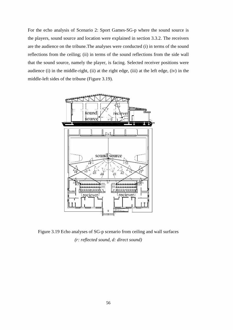
56
For the echo analysis of Scenario 2: Sport Games-SG-p where the sound source is
the players, sound source and location were explained in section 3.3.2. The receivers
are the audience on the tribune.The analyses were conducted (i) in terms of the sound
reflections from the ceiling; (ii) in terms of the sound reflections from the side wall
that the sound source, namely the player, is facing. Selected receiver positions were
audience (i) in the middle-right, (ii) at the right edge, (iii) at the left edge, (iv) in the
middle-left sides of the tribune (Figure 3.19).
Figure 3.19 Echo analyses of SG-p scenario from ceiling and wall surfaces
(r: reflected sound, d: direct sound)

57
For the echo analysis of Scenario 3: Sport Games-SG-a where the sound source is the
audience (spectators), sound source and location wereexplained in section 3.3.2. The
receivers are the players on the playfield.The analyses were conducted (i) in terms of
the sound reflections from the ceiling; (ii) in terms of the sound reflections from the
front wall that the sound source, namely the audience (spectators), is facing (Figure
3.20).
Figure 3.20 Echo analyses of SG-a scenario from ceiling and wall surfaces
(r: reflected sound, d: direct sound)
For the IMPROVED cases of sportive activities (PEC, SG-p, SG-a scenarios), the
analyses were not repeated since the procedure is the same with the AS-IS case.For
the IMPROVED cases of multi-purpose scenarios (MP-S, MP-P)the analyses were
not necessary since ceiling and wall surfaces were treated with sound absorbing
materials.

58

59
CHAPTER 4
RESULTS
In this chapter, data obtained from the acoustical simulation analyses are summarized
to determine the AS-IS acoustical features of the typical small sport hall. Acoustical
performances of different types of suspended ceiling systems suggested as
improvements, and acoustical features of the typical sport hall for the improved cases
based on activities-related scenarios are assessed. Results are presented under
respective headings.
4.1. ACOUSTICAL FEATURES OF THE TYPICAL SMALLSPORT HALL
FOR THE AS-IS CASE: BASED ON ACTIVITIES-RELATED SCENARIOS
The simulation data obtained for the AS-IS case of the hall based on physical
education class and sport games activities are presented in the following sections.
4.1.1. Estimated Global Reverberation Time Values (GRT-Global T30)
The estimated GRT values within the sport hall for the as-is uses of the hall, i.e. PE
classes and sportive activitieswere predicted to lie in between 3.06s and 3.47s at low
frequencies (125 Hz, 250 Hz), 3.46s and 5.08s at mid frequencies (500 Hz, 1000 Hz),
and 2.34s and 4.25s at high frequencies (2000 Hz, 4000 Hz) (Table 4.1, Figure A.1,
Figure B.1, Figure C.1). These values obtained from the simulation highly exceed the
recommended reverberation time limits for those activities (Department of Education
and Skills, 2004; Beranek, Acoustics, 1993).
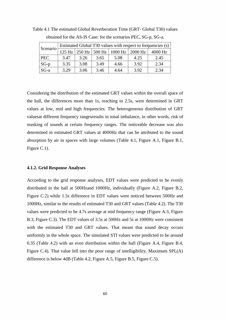
60
Table 4.1 The estimated Global Reverberation Time (GRT- Global T30) values
obtained for the AS-IS Case: for the scenarios PEC, SG-p, SG-a.
Scenario Estimated Global T30 values with respect to frequencies (s)
125 Hz 250 Hz 500 Hz 1000 Hz 2000 Hz 4000 Hz
PEC 3.47 3.26 3.65 5.08 4.25 2.45
SG-p 3.35 3.08 3.49 4.66 3.92 2.34
SG-a 3.29 3.06 3.46 4.64 3.92 2.34
Considering the distribution of the estimated GRT values within the overall space of
the hall, the differences more than 1s, reaching to 2.5s, were determined in GRT
values at low, mid and high frequencies. The heterogeneous distribution of GRT
valuesat different frequency rangesresults in tonal imbalance, in other words, risk of
masking of sounds at certain frequency ranges. The noticeable decrease was also
determined in estimated GRT values at 4000Hz that can be attributed to the sound
absorption by air in spaces with large volumes (Table 4.1, Figure A.1, Figure B.1,
Figure C.1).
4.1.2. Grid Response Analyses
According to the grid response analyses, EDT values were predicted to be evenly
distributed in the hall at 500Hzand 1000Hz, individually (Figure A.2, Figure B.2,
Figure C.2) while 1.5s difference in EDT values were noticed between 500Hz and
1000Hz, similar to the results of estimated T30 and GRT values (Table 4.2). The T30
values were predicted to be 4.7s average at mid frequency range (Figure A.3, Figure
B.3, Figure C.3). The EDT values of 3.5s at 500Hz and 5s at 1000Hz were consistent
with the estimated T30 and GRT values. That meant that sound decay occurs
uniformly in the whole space. The simulated STI values were predicted to be around
0.35 (Table 4.2) with an even distribution within the hall (Figure A.4, Figure B.4,
Figure C.4). That value fell into the poor range of intelligibility. Maximum SPL(A)
difference is below 4dB (Table 4.2, Figure A.5, Figure B.5, Figure C.5).
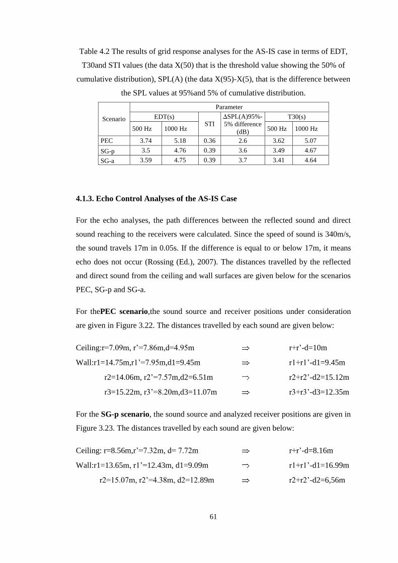
61
Table 4.2 The results of grid response analyses for the AS-IS case in terms of EDT,
T30and STI values (the data X(50) that is the threshold value showing the 50% of
cumulative distribution), SPL(A) (the data X(95)-X(5), that is the difference between
the SPL values at 95%and 5% of cumulative distribution.
Scenario
Parameter
EDT(s) STI
SPL(A)95%-
5% difference
(dB)
T30(s)
500 Hz 1000 Hz 500 Hz 1000 Hz
PEC 3.74 5.18 0.36 2.6 3.62 5.07
SG-p 3.5 4.76 0.39 3.6 3.49 4.67
SG-a 3.59 4.75 0.39 3.7 3.41 4.64
4.1.3. Echo Control Analyses of the AS-IS Case
For the echo analyses, the path differences between the reflected sound and direct
sound reaching to the receivers were calculated. Since the speed of sound is 340m/s,
the sound travels 17m in 0.05s. If the difference is equal to or below 17m, it means
echo does not occur (Rossing (Ed.), 2007). The distances travelled by the reflected
and direct sound from the ceiling and wall surfaces are given below for the scenarios
PEC, SG-p and SG-a.
For thePEC scenario,the sound source and receiver positions under consideration
are given in Figure 3.22. The distances travelled by each sound are given below:
Ceiling:r=7.09m, r’=7.86m,d=4.95m r+r’-d=10m
Wall:r1=14.75m,r1’=7.95m,d1=9.45m r1+r1’-d1=9.45m
r2=14.06m, r2’=7.57m,d2=6.51m r2+r2’-d2=15.12m
r3=15.22m, r3’=8.20m,d3=11.07m r3+r3’-d3=12.35m
For the SG-p scenario, the sound source and analyzed receiver positions are given in
Figure 3.23. The distances travelled by each sound are given below:
Ceiling: r=8.56m,r’=7.32m, d= 7.72m r+r’-d=8.16m
Wall:r1=13.65m, r1’=12.43m, d1=9.09m r1+r1’-d1=16.99m
r2=15.07m, r2’=4.38m, d2=12.89m r2+r2’-d2=6,56m

62
r3=15.07m, r3’=4.38m, d3=12.89m r3+r3’-d3=6,56m
r4=13.65m, r4’=12.43m, d4=9.09m r4+r4’-d4=16.99m
For the SG-a scenario, the sound source and analyzed receiver positions are given in
Figure 3.24. The distances travelled by each sound are given below:
Ceiling:r=7.32m, r’=8.56m, d=7.72m r+r’-d=8.16m
Wall: r1=17.32m, r1’=8.01m, d1=12.70m r1+r1’-d1=12.63m
r2=16.08m, r2’=7.49m, d2=9.14m r2+r2’-d2=14.73m
r3=16.08m, r3’=7.49m, d3=9.14m r3+r3’-d3=14.73m
r4=17.32m, r4’=8.01m, d4=12.70m r4+r4’-d4=12.63m
The path difference between reflected and direct sound from the ceiling and wall
surfaces are below 17m for the PEC, SG-p and SG-a scenarios. According to these
results, echo does not occur in the hall at the determined sound source and receiver
positions in the untreated hall for these activities and in the treated hall for all
activities.
4.2. ESTIMATED GRT VALUES OF TYPICAL SPORT HALLS WHEN
TREATED WITH DIFFERENT TYPES OF SUSPENDED CEILING
SYSTEMS
Considering the PEC scenario, the estimated GRT values obtained for the hall treated
with flat panelled, baffle and transverse suspended ceiling systemsare given in
relevant tables below. The estimated GRT data achieved was summarized below:
In the application of flat panelled suspended ceiling mounted immediately below
the truss level, the estimated GRT values at mid frequencies (500Hz and 1000Hz)
were predicted to be:
1.82s with the use of 5cm-thick panels (FP5),
1.79s with the use of 10cm-thick panels (FP10) (Table 4.3).
The estimated GRT values at frequencies above 250Hz presented a gradual decrease
with the increase in frequency. The GRT values at 125Hz were the longest with
2.63s for the ceiling FP5 and 2.29s for the ceiling FP10.

63
Table 4.3 The Estimated Global Reverberation Time (GRT-Global T30) values
obtained from the configurations with flat paneled suspended ceiling for PEC
scenario.
configuration Global T30 values (s) with respect to frequency
125 Hz 250 Hz 500 Hz 1000 Hz 2000 Hz 4000 Hz
FP5 2.63 2.23 1.93 1.71 1.58 1.26
FP10 2.29 1.87 1.85 1.73 1.58 1.28
In the application baffle suspended ceiling mounted 60cm above the truss level,
the estimated GRT values at mid frequencies were predicted to be:
1.75s with 10cm-thick panels fixed at 60cm intervals (B10@60),
1.72s with 10cm-thick panels fixed at 30cm intervals (B10@30),
1.70s with 5cm-thickpanels fixed at 30cm intervals (B5@30) (Table 4.4).
Similar to the flat panelled suspended ceiling, the baffle system presented the longest
GRT values at 125Hz with the values 2.09s, 2.05 and 2.32s, respectively.
Table 4.4 The Estimated Global Reverberation Time (GRT-Global T30) values
obtained for the configurations with baffle suspended ceiling–above truss level for
Scenario PEC.
configuration Global T30 values (s)
125 Hz 250 Hz 500 Hz 1000 Hz 2000 Hz 4000 Hz
B10@60 2.09 1.84 1.82 1.69 1.55 1.22
B10@30 2.05 1.82 1.78 1.66 1.49 1.19
B5@30 2.32 1.87 1.76 1.64 1.49 1.19
In the application of baffle suspended ceiling mounted immediately below the
truss level, the GRT values at mid frequencies were predicted to be:
1.74s with the 10cm-thick panels fixed at 90cm intervals (B10@90),
1.64s with 10cm-thick panels fixed at 60cm intervals (B10@60),
1.66s with the 5cm-thick panelsfixedat 60cm intervals (B5@60).
The longest GRT was observed at 125Hz for the ceiling B5@60 while a certain
decrease seemed to be achieved at the other proposals, namely B10@90 and

64
B10@60, where 10cm-thick panels were used and suspended below the truss level
(Table 4.5).
Table 4.5 The Estimated Global Reverberation Time (GRT-Global T30) values
obtained for the configurations with baffle suspended ceiling-below truss level for
ScenarioPEC.
configuration Global T30 values (s) with respect to frequency
125 Hz 250 Hz 500 Hz 1000 Hz 2000 Hz 4000 Hz
B5@60 2.38 1.84 1.73 1.60 1.46 1.19
B10@60 1.98 1.71 1.69 1.60 1.46 1.17
B10@90 1.93 1.8 1.78 1.71 1.57 1.24
In the application of transverse suspended ceiling, the GRT values at mid
frequencies were predicted to be:
1.75s with 10cm-thick panels suspended crosswise between the trusses
(Transverse suspended ceiling - TP10),
1.73s with 5cm-thick panels suspended crosswise between the trusses (TP5),
1.82s with sound absorptive fabric stretched crosswise between the trusses
(Stretched Fabric suspended ceiling - FT).
Similar to the others, the longest GRT values were observed at 125Hz with the
values of 2.14s, 2.84s and 2.29s respectively (Table 4.6).
Table 4.6 The Estimated Global Reverberation Time (GRT-Global T30) values
obtained from the configurations with transverse suspended ceiling for PEC scenario.
configuration Global T30values (s) with respect to frequency
125 Hz 250 Hz 500 Hz 1000 Hz 2000 Hz 4000 Hz
TP5 2.84 1.93 1.80 1.67 1.57 1.24
TP10 2.14 1.84 1.82 1.69 1.57 1.24
FT 2.29 2.12 1.93 1.71 1.57 1.26

65
Estimated GRT values within the sport hall for the improved cases regarding sportive
activities where the player located in the middle of the playfield is the sound source
are given in Table 4.7, Table 4.8, Table 4.9 and Table 4.10.
Considering the SG-p scenario, the estimated GRT values obtained for the hall
treated with flat panelled, baffle and transverse suspended ceiling systemsare
summarized in relevant tables below. The estimated GRT data was summarized
below:
In the application of flat panelled suspended ceiling mounted immediately below
the truss level, the estimated GRT values at mid frequencies (500Hz and 1000Hz)
were predicted to be:
1.85s by the use of 5cm-thick panels (FP5)
1.86s by the use of 10cm-thick panels (FP10) (Table 4.7).
While the GRT values at frequencies above 250Hz presented a gradual decrease with
the increase in frequency, the GRT values at 125Hz were the longest with 3.62s for
the ceiling FP5 and 2.72s for the ceiling FP10.
Table 4.7 The Estimated Global Reverberation Time (GRT-Global T30) values
obtained from the configurations with flat paneled suspended ceiling for SG-p
scenario.
configuration Global T30 (s) values with respect to frequency
125 Hz 250 Hz 500 Hz 1000 Hz 2000 Hz 4000 Hz
FP5 3.62 2.30 1.91 1.80 1.66 1.33
FP10 2.72 1.89 1.91 1.82 1.67 1.33
In the application of baffle suspended ceiling mounted 60cm above the truss
level, the GRT values at mid frequencies were predicted to be:
1.71s with 10cm-thick panels fixed at 60cm intervals (B10@60),
1.67s with 10cm-thick panels fixed at 30cm intervals (B10@30)
1.67s with 5cm-thickpanels fixed at 30cm intervals (B5@30) (Table 4.8,
Figure B.1).

66
Similar to the flat panelled suspended ceiling, the baffle system presented the longest
GRT values at 125Hz with the values 1.91s, 1.89 and 2.07s, respectively.
Table 4.8 The Estimated Global Reverberation Time (GRT-Global T30) values
obtained from the configurations with baffle suspended ceiling–above truss level for
SG-p scenario
configuration Global T30 values (s) with respect to frequency
125 Hz 250 Hz 500 Hz 1000 Hz 2000 Hz 4000 Hz
B10@60 1.91 1.78 1.76 1.67 1.53 1.22
B10@30 1.89 1.76 1.73 s 1.62 1.48 1.19
B5@30 2.07 1.76 1.73 s 1.62 1.48 1.19
In the application of baffle suspended ceiling mounted immediately below the
truss level, the GRT values at mid frequencies were predicted to be:
1.70s with the 10cm-thick panels fixed at 90cm intervals (B10@90),
1.62s with 10cm-thick panels fixed at 60cm intervals (B10@60).
The GRT values were the longest at 125Hz for these cases as well, with 1.87s for the
ceiling B10@90 and 1.82s for the ceiling B10@60 (Table 4.9, Figure B.1).
Table 4.9 The Estimated Global Reverberation Time (GRT-Global T30) values
obtained from the configurations with Baffle suspended ceiling–below truss level for
SG-p scenario
configuration Global T30 values (s) with respect to frequency
125 Hz 250 Hz 500 Hz 1000 Hz 2000 Hz 4000 Hz
B10@90 1.87 1.75 1.73 1.67 1.55 1.24
B10@60 1.82 1.69 1.67 1.57 1.46 1.17
In the application of crosswise suspended ceiling, the GRT values at mid
frequencies were predicted to be:
1.70s with 10cm-thick panels suspended crosswise between the trusses
(Transverse suspended ceiling - TP10),
1.71s with 5cm-thick panels suspended crosswise between the trusses (TP5),
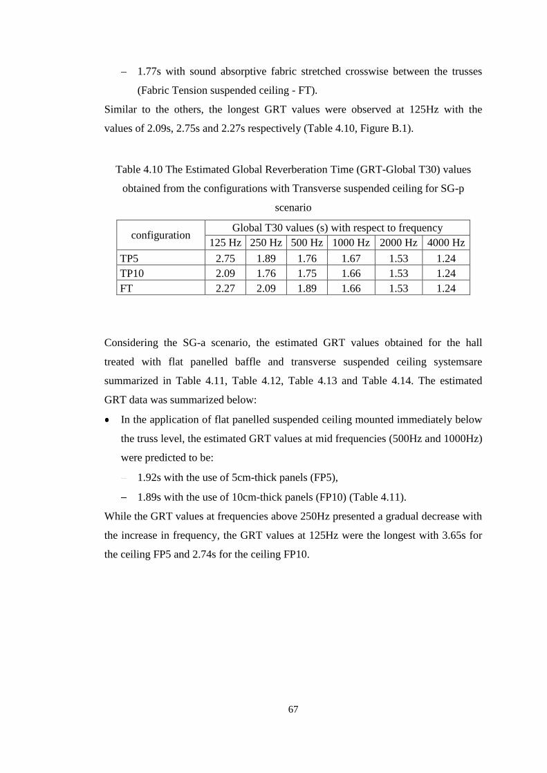
67
1.77s with sound absorptive fabric stretched crosswise between the trusses
(Fabric Tension suspended ceiling - FT).
Similar to the others, the longest GRT values were observed at 125Hz with the
values of 2.09s, 2.75s and 2.27s respectively (Table 4.10, Figure B.1).
Table 4.10 The Estimated Global Reverberation Time (GRT-Global T30) values
obtained from the configurations with Transverse suspended ceiling for SG-p
scenario
configuration Global T30 values (s) with respect to frequency
125 Hz 250 Hz 500 Hz 1000 Hz 2000 Hz 4000 Hz
TP5 2.75 1.89 1.76 1.67 1.53 1.24
TP10 2.09 1.76 1.75 1.66 1.53 1.24
FT 2.27 2.09 1.89 1.66 1.53 1.24
Considering the SG-a scenario, the estimated GRT values obtained for the hall
treated with flat panelled baffle and transverse suspended ceiling systemsare
summarized in Table 4.11, Table 4.12, Table 4.13 and Table 4.14. The estimated
GRT data was summarized below:
In the application of flat panelled suspended ceiling mounted immediately below
the truss level, the estimated GRT values at mid frequencies (500Hz and 1000Hz)
were predicted to be:
1.92s with the use of 5cm-thick panels (FP5),
1.89s with the use of 10cm-thick panels (FP10) (Table 4.11).
While the GRT values at frequencies above 250Hz presented a gradual decrease with
the increase in frequency, the GRT values at 125Hz were the longest with 3.65s for
the ceiling FP5 and 2.74s for the ceiling FP10.
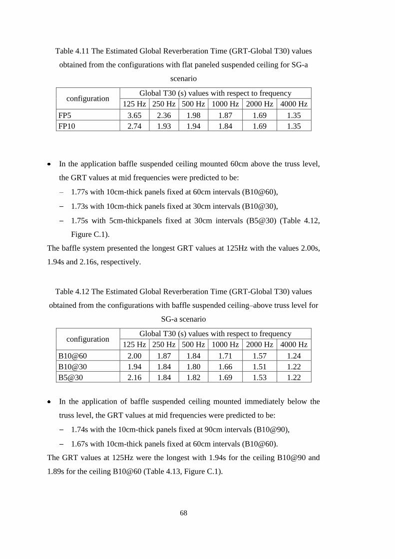
68
Table 4.11 The Estimated Global Reverberation Time (GRT-Global T30) values
obtained from the configurations with flat paneled suspended ceiling for SG-a
scenario
configuration Global T30 (s) values with respect to frequency
125 Hz 250 Hz 500 Hz 1000 Hz 2000 Hz 4000 Hz
FP5 3.65 2.36 1.98 1.87 1.69 1.35
FP10 2.74 1.93 1.94 1.84 1.69 1.35
In the application baffle suspended ceiling mounted 60cm above the truss level,
the GRT values at mid frequencies were predicted to be:
1.77s with 10cm-thick panels fixed at 60cm intervals (B10@60),
1.73s with 10cm-thick panels fixed at 30cm intervals (B10@30),
1.75s with 5cm-thickpanels fixed at 30cm intervals (B5@30) (Table 4.12,
Figure C.1).
The baffle system presented the longest GRT values at 125Hz with the values 2.00s,
1.94s and 2.16s, respectively.
Table 4.12 The Estimated Global Reverberation Time (GRT-Global T30) values
obtained from the configurations with baffle suspended ceiling–above truss level for
SG-a scenario
configuration Global T30 (s) values with respect to frequency
125 Hz 250 Hz 500 Hz 1000 Hz 2000 Hz 4000 Hz
B10@60 2.00 1.87 1.84 1.71 1.57 1.24
B10@30 1.94 1.84 1.80 1.66 1.51 1.22
B5@30 2.16 1.84 1.82 1.69 1.53 1.22
In the application of baffle suspended ceiling mounted immediately below the
truss level, the GRT values at mid frequencies were predicted to be:
1.74s with the 10cm-thick panels fixed at 90cm intervals (B10@90),
1.67s with 10cm-thick panels fixed at 60cm intervals (B10@60).
The GRT values at 125Hz were the longest with 1.94s for the ceiling B10@90 and
1.89s for the ceiling B10@60 (Table 4.13, Figure C.1).

69
Table 4.13 The Estimated Global Reverberation Time (GRT-Global T30) values
obtained from the configurations with baffle suspended ceiling–below truss level for
SG-a scenario
configuration Global T30 values (s) with respect to frequency
125 Hz 250 Hz 500 Hz 1000 Hz 2000 Hz 4000 Hz
B10@90 1.94 1.80 1.78 1.71 1.55 1.26
B10@60 1.89 1.76 1.73 1.62 1.49 1.21
In the application of crosswise suspended ceiling, the GRT values at mid frequencies
were predicted to be:
1.76s with 10cm-thick panels suspended crosswise between the trusses
(Transverse suspended ceiling - TP10),
1.76s with 5cm-thick panels suspended crosswise between the trusses (TP5),
1.82s with sound absorptive fabric stretched crosswise between the trusses
(Stretched Fabric suspended ceiling - FT).
Likewise the other treatments, the longest GRT values were observed at 125Hz with
the values of 2.12s, 2.79s and 2.27s respectively (Table 4.14, Figure C.1).
Table 4.14 The Estimated Global Reverberation Time (GRT-Global T30) values
obtained from the configurations with transverse suspended ceiling for SG-a scenario
configuration Global T30 values (s) with respect to frequency
125 Hz 250 Hz 500 Hz 1000 Hz 2000 Hz 4000 Hz
TP5 2.79 1.93 1.82 1.71 1.58 1.28
TP10 2.12 1.84 1.82 1.71 1.58 1.28
FT 2.27 2.11 1.93 1.71 1.58 1.28
Each ceiling treatment proposed in the study provided remarkable decreases in GRT
values at high, mid and low frequencies. Among all the proposals,GRT values in the
treatments B10@60 – baffles suspended above truss level, B10@60 – baffles
suspended below truss level and TP10 were found to be sufficientfor sportive
activitiesin all frequency ranges with respect to the specified criterion, 1.5s limit

70
(Department of Education and Skills, 2004). However, for physical education class
activity, obtained GRTvalues are estimated to be above the criterion, 1.02s limit
(Beranek, 1993) and there was the necessity of additional treatment in order to
decrease the estimated GRT values to acceptable values during PEC activity (Figure
4.1).
(a)
(b)
(c)
Figure 4.1 Estimated GRT values for the AS-IS and IMPROVED cases with ceiling
treatments in comparison with the required GRT value for sportive activities:
(a) PEC, (b) SG-p, (c) SG-a.
0
1
2
3
4
5
6
125 Hz 250 Hz 500 Hz 1000 Hz 2000 Hz 4000 Hz
Esti
mat
ed G
lob
al R
ever
ber
atio
n T
ime,
s
Frequency, Hz
AS-IS
FP5
FP10
B10@60(at)
B10@30(at)
B5@30(at)
B10@90(bt)
B10@60(bt)
TP5
TP10
0
0.5
1
1.5
2
2.5
3
3.5
4
4.5
5
125 Hz 250 Hz 500 Hz 1000 Hz 2000 Hz 4000 Hz
Esti
mat
ed G
lob
al R
ever
ber
atio
n T
ime,
s
Frequency, Hz
AS-IS
FP5
FP10
B10@60(at)
B10@30(at)
B5@30(at)
B10@90(bt)
B10@60(bt)
TP5
TP10
FT
Required Value
0
0.5
1
1.5
2
2.5
3
3.5
4
4.5
5
125 Hz 250 Hz 500 Hz 1000 Hz 2000 Hz 4000 Hz
Esti
mat
ed G
lob
al R
ever
ber
atio
n T
ime,
s
Frequency, Hz
AS-IS
FP5
FP10
B10@60(at)
B10@30(at)
B5@30(at)
B10@90(bt)
B10@60(bt)
TP5
TP10
FT
Required Value

71
Grid response analyses of the hall were conducted for the SG-p and SG-a scenarios
with the selected ceiling treatments: baffle (B10@60 above and below truss level)
and transversely suspended ceiling (TP10) systems. The data X(50), that is the
threshold value showing the 50% of cumulative distribution for the parameters EDT
and T30 at 500Hz and 1000Hz, STI and SPL(A),the data X(95)-X(5) that is the
difference between the SPL values at 95%and 5% of cumulative distribution,
obtained for the hall are given in Table 4.15 and in relevant figures in Appendix B
and Appendix C. The grid response analyses were summarized below:
In the application of baffle suspended ceiling mounted 60cm above the truss level
with 10cm-thick panels fixed at 60cm intervals (B10@60), the EDT values were
predicted to be 1.29s at 500Hz and 1.28s at 1000Hzfor the SG-p scenario, 1.38s
at 500Hz and 1.31s at 1000Hzfor the SG-a scenario (Figure B.2, Figure C.2).
These values were below the estimated GRT values which indicate that the sound
is intelligible. This is also supported by the STI values of 0.59 for SG-p scenario
(Figure B.4) and 0.58 for SG-a scenario (Figure C.4) which signals that in the
50% of the hall, the speech intelligibility is in good range. The estimated T30
values of 1.61s at 500Hz and 1.55s at 1000Hz for SG-p scenario (Figure B.3) and
1.88s at 500Hz and 1.79s at 1000Hz for SG-a scenario (Figure C.3) are close to
the estimated GRT values and close to the required ranges of ≤1.5s for both SG-p
and SG-a scenarios. Maximum SPL(A) differences were 6.4 dB for SG-p
scenario (Figure B.5) and9.2dBfor SG-a scenario (Figure C.5), which is below
the required limit of 10dB. According to the grid response analyses results, in
both of the scenarios, for all the parameters checked, the sound is evenly
distributed within the area with acceptable differences (Appendix B, Appendix
C).
In the application of baffle suspended ceiling mounted immediately below the
truss level with 10cm-thick panels fixed at 60cm intervals (B10@60), the EDT
values were predicted to be 1.22s at 500Hz and 1.25s at 1000Hzfor the SG-p
scenario (Figure B.2), 1.28s at 500Hz and 1.28s at 1000Hz for the SG-a
scenario(Figure C.2). Similar to the treatment B10@60 above truss level, these
values were below the estimated GRT values which mean that the sound is
72
intelligible. This is also supported with the STI values of 0.60 for SG-p scenario
(Figure B.4) and 0.57 for SG-a scenario (Figure C.4) which signals that in the
50% of the hall, the speech intelligibility is in good range. The estimated T30
values of 1.53s at 500Hz and 1.41s at 1000Hz for SG-p scenario (Figure B.3) and
1.79s at 500Hz and 1.73s at 1000Hz for SG-a scenario (Figure C.3) are close to
the estimated GRT values and in required range of≤1.5s for SG-p scenario and
close to it for SG-a scenario. Maximum SPL(A) differences were 6.4dB for SG-p
scenario (Figure B.5) and 9.2dB for SG-a scenario (Figure C.5), which is below
the required limit of 10dB. According to the grid response analyses results, in
both of the scenarios, for all the parameters checked, the sound is evenly
distributed within the areawith acceptable differences (Appendix B, Appendix
C).
In the application of transversely suspended ceiling with 10cm-thick panels
suspended crosswise between the trusses (Transverse suspended ceiling-TP10),
the EDT values were predicted to be1.35s at 500Hz and 1.28s at 1000Hz for the
SG-p scenario (Figure B.2), 1.50s at 500Hz and 1.46s at 1000Hz for the SG-a
scenario (Figure C.2). Similar to the treatment B10@60 above truss level, these
values were below the estimated GRT values, but above the values obtained in
the treatments with baffles. The STI values were predicted to be 0.62 for SG-p
scenario (Figure B.4) and 0.59 for SG-a scenario (Figure C.4) which signals that
in the 50% of the hall, the speech intelligibility is in good range. The estimated
T30 values of 1.59s at 500Hz and 1.51s at 1000Hz for SG-p scenario are below
the estimated GRT values and close the required range of ≤1.5s (Figure B.3). The
estimated T30 values of 1.99s at 500Hz and 1.82s at 1000Hz for SG-a scenario
(Figure C.3) were above the estimated GRT values and exceed the specified
criterion ≤1.5s. Maximum SPL(A) differences were 7.3dB for SG-p scenario
(Figure B.5) and 9.8dB for SG-a scenario (Figure C.5), which is below the
required limit of 10dB. However, unlike the results in the treatments with baffles,
in both of the scenarios, for the parameters EDT at 500Hz and 1000Hz and T30
at 500Hz the sound is not evenly distributed within the hall at different receiver
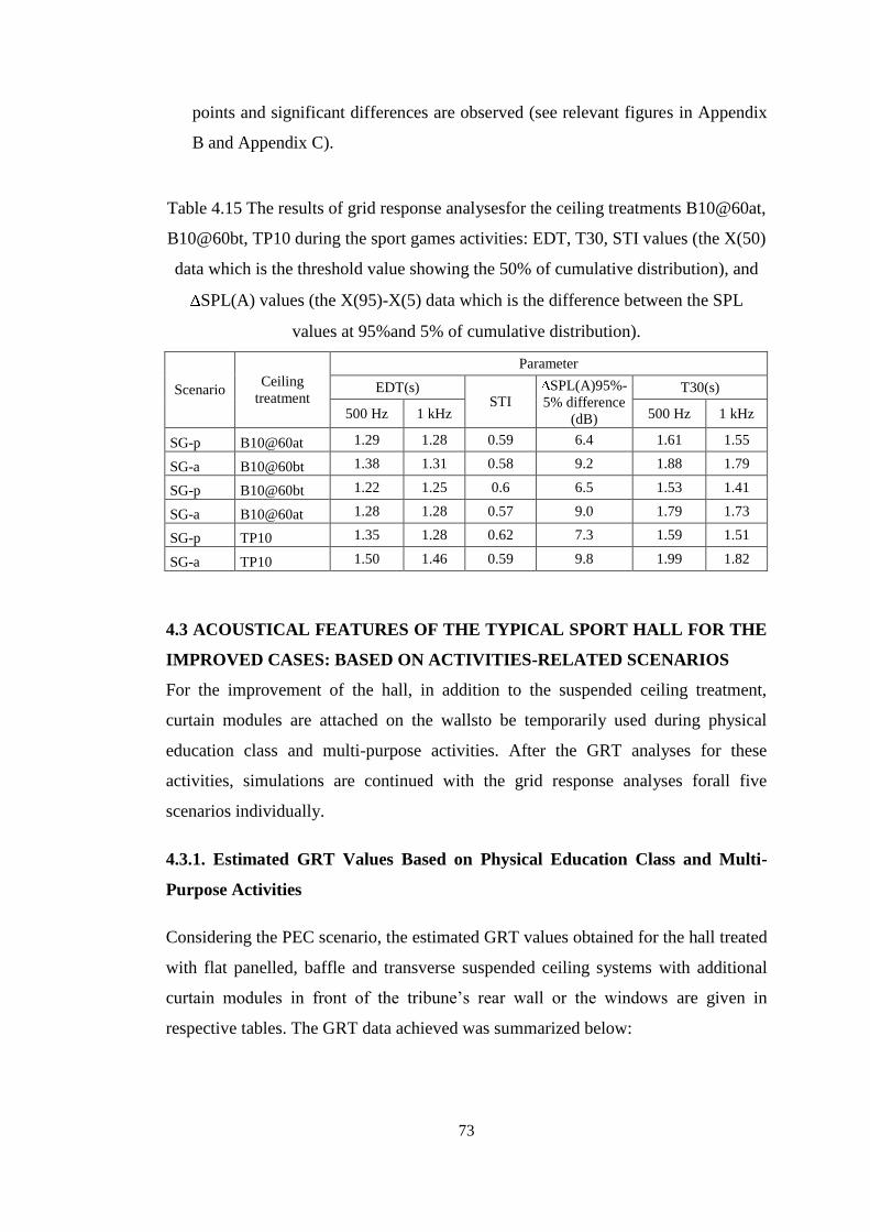
73
points and significant differences are observed (see relevant figures in Appendix
B and Appendix C).
Table 4.15 The results of grid response analysesfor the ceiling treatments B10@60at,
B10@60bt, TP10 during the sport games activities: EDT, T30, STI values (the X(50)
data which is the threshold value showing the 50% of cumulative distribution), and
SPL(A) values (the X(95)-X(5) data which is the difference between the SPL
values at 95%and 5% of cumulative distribution).
Scenario Ceiling
treatment
Parameter
EDT(s) STI
SPL(A)95%-
5% difference
(dB)
T30(s)
500 Hz 1 kHz 500 Hz 1 kHz
SG-p B10@60at 1.29 1.28 0.59 6.4 1.61 1.55
SG-a B10@60bt 1.38 1.31 0.58 9.2 1.88 1.79
SG-p B10@60bt 1.22 1.25 0.6 6.5 1.53 1.41
SG-a B10@60at 1.28 1.28 0.57 9.0 1.79 1.73
SG-p TP10 1.35 1.28 0.62 7.3 1.59 1.51
SG-a TP10 1.50 1.46 0.59 9.8 1.99 1.82
4.3 ACOUSTICAL FEATURES OF THE TYPICAL SPORT HALL FOR THE
IMPROVED CASES: BASED ON ACTIVITIES-RELATED SCENARIOS
For the improvement of the hall, in addition to the suspended ceiling treatment,
curtain modules are attached on the wallsto be temporarily used during physical
education class and multi-purpose activities. After the GRT analyses for these
activities, simulations are continued with the grid response analyses forall five
scenarios individually.
4.3.1. Estimated GRT Values Based on Physical Education Class and Multi-
Purpose Activities
Considering the PEC scenario, the estimated GRT values obtained for the hall treated
with flat panelled, baffle and transverse suspended ceiling systems with additional
curtain modules in front of the tribune’s rear wall or the windows are given in
respective tables. The GRT data achieved was summarized below:
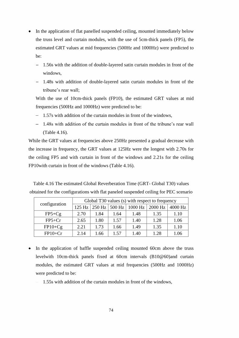
74
In the application of flat panelled suspended ceiling, mounted immediately below
the truss level and curtain modules, with the use of 5cm-thick panels (FP5), the
estimated GRT values at mid frequencies (500Hz and 1000Hz) were predicted to
be:
1.56s with the addition of double-layered satin curtain modules in front of the
windows,
1.48s with addition of double-layered satin curtain modules in front of the
tribune’s rear wall;
With the use of 10cm-thick panels (FP10), the estimated GRT values at mid
frequencies (500Hz and 1000Hz) were predicted to be:
1.57s with addition of the curtain modules in front of the windows,
1.48s with addition of the curtain modules in front of the tribune’s rear wall
(Table 4.16).
While the GRT values at frequencies above 250Hz presented a gradual decrease with
the increase in frequency, the GRT values at 125Hz were the longest with 2.70s for
the ceiling FP5 and with curtain in front of the windows and 2.21s for the ceiling
FP10with curtain in front of the windows (Table 4.16).
Table 4.16 The estimated Global Reverberation Time (GRT- Global T30) values
obtained for the configurations with flat paneled suspended ceiling for PEC scenario
configuration Global T30 values (s) with respect to frequency
125 Hz 250 Hz 500 Hz 1000 Hz 2000 Hz 4000 Hz
FP5+Cg 2.70 1.84 1.64 1.48 1.35 1.10
FP5+Cr 2.65 1.80 1.57 1.40 1.28 1.06
FP10+Cg 2.21 1.73 1.66 1.49 1.35 1.10
FP10+Cr 2.14 1.66 1.57 1.40 1.28 1.06
In the application of baffle suspended ceiling mounted 60cm above the truss
levelwith 10cm-thick panels fixed at 60cm intervals (B10@60)and curtain
modules, the estimated GRT values at mid frequencies (500Hz and 1000Hz)
were predicted to be:
1.55s with addition of the curtain modules in front of the windows,

75
1.49swith addition of the curtain modules in front of the tribune’s rear wall
(Figure A.1).
For the treatmentwith 10cm-thick panels fixed at 30cm intervals (B10@30) the
estimated GRT values at mid frequencies (500Hz and 1000Hz) were predicted to
be:
1.48s with addition of the curtain modules in front of the windows,
1.44s with addition of the curtain modules in front of the tribune’s rear wall.
For the treatment with 5cm-thickpanels fixed at 30cm intervals (B5@30) the
estimated GRT values at mid frequencies (500Hz and 1000Hz) were predicted to
be:
1.53s with addition of double-layered satin curtain in front of the windows,
1.42s with addition of double-layered satin curtain in front of the tribune’s
rear wall (Table 4.16).
Similar to the flat panelled suspended ceiling, treatment with the baffle system
presented the longest GRT values at 125Hz with the values 2.03s, 1.93s and 2.23s
respectively with the joint use of curtainsin front of the windows and 1.98s, 1.94s
and 2.2s with the joint use of curtainsin front of the tribune’s rear wall (Table 4.17).
Table 4.17 The estimated Global Reverberation Time (GRT- Global T30) values
obtained for the configurations with baffle suspended ceiling–above truss for
scenario PEC
configuration Global T30 values (s) with respect to frequency
125 Hz 250 Hz 500 Hz 1000 Hz 2000 Hz 4000 Hz
B10@60(at)+Cg 2.03 1.69 1.62 1.49 1.37 1.12
B10@60(at)+Cr 1.98 1.64 1.57 1.42 1.30 1.04
B10@30(at)+Cg 1.93 1.62 1.55 1.42 1.31 1.08
B10@30(at)+Cr 1.94 1.64 1.53 1.35 1.22 0.99
B5@30(at)+Cg 2.23 1.75 1.60 1.46 1.31 1.08
B5@30(at)+Cr 2.20 1.66 1.51 1.33 1.21 0.99
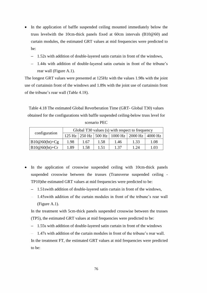
76
In the application of baffle suspended ceiling mounted immediately below the
truss levelwith the 10cm-thick panels fixed at 60cm intervals (B10@60) and
curtain modules, the estimated GRT values at mid frequencies were predicted to
be:
1.52s with addition of double-layered satin curtain in front of the windows,
1.44s with addition of double-layered satin curtain in front of the tribune’s
rear wall (Figure A.1).
The longest GRT values were presented at 125Hz with the values 1.98s with the joint
use of curtainsin front of the windows and 1.89s with the joint use of curtainsin front
of the tribune’s rear wall (Table 4.18).
Table 4.18 The estimated Global Reverberation Time (GRT- Global T30) values
obtained for the configurations with baffle suspended ceiling-below truss level for
scenario PEC
configuration Global T30 values (s) with respect to frequency
125 Hz 250 Hz 500 Hz 1000 Hz 2000 Hz 4000 Hz
B10@60(bt)+Cg 1.98 1.67 1.58 1.46 1.33 1.08
B10@60(bt)+Cr 1.89 1.58 1.51 1.37 1.24 1.03
In the application of crosswise suspended ceiling with 10cm-thick panels
suspended crosswise between the trusses (Transverse suspended ceiling -
TP10)the estimated GRT values at mid frequencies were predicted to be:
1.51swith addition of double-layered satin curtain in front of the windows,
1.45swith addition of the curtain modules in front of the tribune’s rear wall
(Figure A.1).
In the treatment with 5cm-thick panels suspended crosswise between the trusses
(TP5), the estimated GRT values at mid frequencies were predicted to be:
1.55s with addition of double-layered satin curtain in front of the windows
1.47s with addition of the curtain modules in front of the tribune’s rear wall.
In the treatment FT, the estimated GRT values at mid frequencies were predicted
to be:

77
1.56s with addition of double-layered satin curtain in front of the windows,
1.49s with addition of the curtain modules in front of the tribune’s rear wall.
Just like the other treatments, the longest GRT values were observed at 125Hz and
presented 2.03s, 2.70s and 2.29s respectivelywith the joint use of curtainsin front of
the windows and 2.00s, 2.65s and 2.16s with the joint use of curtainsin front of the
tribune’s rear wall (Table 4.19).
Table 4.19 The estimated Global Reverberation Time (GRT- Global T30) values
obtained for the configurations with transverse suspended ceiling for PEC scenario
configuration Global T30 values (s) with respect to frequency
125 Hz 250 Hz 500 Hz 1000 Hz 2000 Hz 4000 Hz
TP5+Cg 2.70 1.75 1.62 1.48 1.35 1.10
TP5+Cr 2.65 1.69 1.55 1.39 1.28 1.03
TP10+Cg 2.03 1.67 1.58 1.44 1.31 1.10
TP10+Cr 2.00 1.62 1.53 1.37 1.26 1.03
FT+Cg 2.20 1.94 1.67 1.46 1.33 1.12
FT+Cr 2.16 1.85 1.60 1.39 1.28 1.03
Considering the multi-purpose use of the hall for speech and performance activities,
the estimated GRT values obtained for the hall treated with the selected baffle and
transverse suspended ceiling systems with additional curtain modules in front of the
wall surfaces and on the open entrances are given in relevant tables. The GRT data
achieved was summarized below:
In the application of baffle suspended ceiling mounted 60cm above the truss
levelwith 10cm-thick panels fixed at 60cm intervals (B10@60) and curtain
modules in front of the wall surfaces the estimated GRT values at mid
frequencies were predicted to be 0.82s for MP-S scenario (Figure D.1) and 0.89s
for MP-P scenario (Figure E.1); with additional curtain modules in front of the
wall surfaces and on the openings at the entrances, the estimated GRT values at
mid frequencies were predicted to be 0.60s for MP-S scenario (Figure D.2) and
0.67s for MP-P scenario (Figure E.2) (Table 4.20).

78
Table 4.20 The estimated Global Reverberation Time (GRT- Global T30) values
obtained for the configurations composed of Baffle suspended ceiling–above truss
level and sound curtain modules for MP-S and MP-P activities
scenario configuration Global T30 values with respect to frequency (s)
125 Hz 250 Hz 500 Hz 1000 Hz 2000 Hz 4000 Hz
MP-S B10@60(at)+Ca 1.33 1.01 0.88 0.76 0.68 0.59
B10@60(at)+Ca+Co 1.15 0.79 0.61 0.59 0.58 0.52
MP-P B10@60(at)+Ca 1.39 1.06 0.95 0.83 0.76 0.63
B10@60(at)+Ca+Co 1.19 0.83 0.67 0.68 0.65 0.58
In the application of baffle suspended ceiling mounted 60cm below the truss
levelwith 10cm-thick panels fixed at 60cm intervals (B10@60) and curtain
modules in front of the wall surfaces the estimated GRT values at mid
frequencies were predicted to be 0.79s for MP-S scenario (Figure D.1) and 0.87s
for MP-P scenario (Figure E.1); with additional curtain modules in front of the
wall surfaces and on the openings at the entrances, the estimated GRT values at
mid frequencies were predicted to be 0.58s for MP-S scenario (Figure D.2) and
0.66s for MP-P scenario (Figure E.2) (Table 4.21).
Table 4.21 The estimated Global Reverberation Time (GRT- Global T30) values
obtained for the configurations composed of baffle suspended ceiling–below truss
level and sound curtain modules for MP-S and MP-P activities
scenario configuration Global T30 values with respect to frequency (s)
125 Hz 250 Hz 500 Hz 1000 Hz 2000 Hz 4000 Hz
MP-S B10@60(bt)+Ca 1.28 0.95 0.85 0.74 0.67 0.58
B10@60(bt)+Ca+Co 1.10 0.76 0.59 0.58 0.56 0.50
MP-P B10@60(bt)+Ca 1.33 1.03 0.94 0.81 0.74 0.63
B10@60(bt)+Ca+Co 1.13 0.77 0.65 0.67 0.65 0.58

79
In the application of crosswise suspended ceiling with 10cm-thick panels
suspended crosswise between the trusses (Transversely suspended ceiling -
TP10) and curtain modules in front of the wall surfaces the estimated GRT values
at mid frequencies were predicted to be 0.76s for MP-S scenario (Figure D.1) and
0.80s for MP-P scenario (Figure E.1); with additional curtain modules in front of
the wall surfaces and on the openings at the entrances, the estimated GRT values
at mid frequencies were predicted to be 0.50s for MP-S scenario (Figure D.2) and
0.51s for MP-P scenario (Figure E.2) (Table 4.22).
Table 4.22 The estimated Global Reverberation Time (GRT- Global T30) values
obtained for the configurations composed of transverse suspended ceiling and sound
curtain modules for MP-S and MP-P activities
scenario configuration Global T30 values with respect to frequency (s)
125 Hz 250 Hz 500 Hz 1000 Hz 2000 Hz 4000 Hz
MP-S TP10+Ca 1.46 0.94 0.83 0.70 0.61 0.52
TP10+Ca+Co 1.22 0.72 0.52 0.49 0.47 0.43
MP-P TP10+Ca 1.53 0.99 0.88 0.72 0.63 0.54
TP10+Ca+Co 1.30 0.74 0.54 0.49 0.47 0.43
With the joint uses of curtain modules on the wall surfaces and the selected
suspended ceiling systems, B10@60at, B10@60bt and TP10, for the multi-purpose
activities where sound reinforcement systems are used, estimated GRT time values
were decreased to the required interval of 0.6.s-1.2s. However, according to the T20-
T30 difference on the estimated GRT bar graph, coupling effect phenomenon was
observed in all the treatments with curtain modules only in front of the walls (Figure
D.1, Figure E.1). According to the estimated GRT bar graphs for all the treatments
with curtain modules in front of the walls and at the entrances, coupling effect
phenomenon was no longer observed (Figure D.2, Figure E.2).

80
4.3.2. Grid Response AnalysesBased on Physical Education Class and Multi-
Purpose Activities
Grid response analyses of the hall were done for the PEC scenario with the joint use
of curtain modules on tribune’s rear wall and the selected ceiling treatments; baffle
(B10@60 above and below truss level) and transverse suspended ceiling (TP10)
systems. The results for the parameters EDT and T30 at 500Hz and 1000Hz, STI and
SPL(A) obtained for the hall are analyzed. The data X(50), that is the threshold value
showing the 50% of cumulative distribution for the parameters EDT, T30 and C80 at
500Hz and 1000Hz, STI and SPL(A),the data X(95)-X(5) that is the difference
between the SPL values at 95%and 5% of cumulative distribution, obtained for the
hall are given in Table 4.23, Table 4.24 and Table 4.25 and with respective figures in
appendices. The grid response analyses data achieved were summarized below:
In the application of baffle suspended ceiling mounted 60cm above the truss level
with 10cm-thick panels fixed at 60cm intervals (B10@60) with curtain modules
in front of tribune’s rear wall, EDT values were predicted to be 1.12s at 500Hz
and 1.15s at 1000Hz (Figure A.2).These values were below the estimated GRT
value which indicates that the sound is intelligible. This is also supported by the
STI value of 0.59which signals that in the 50% of the hall, the speech
intelligibility is in good range (Figure A.4).The estimated T30 values of 1.47s at
500Hz and 1.29s at 1000Hz are below the estimated GRT values, but still above
the required ranges of ≤1.02s (Figure A.3). Maximum SPL(A) difference within
the hall is 7.3 dB which is below the required limit of 10dB (Table 4.23, Figure
A.5). According to the grid responses analyses results, for all the parameters
checked, the sound is evenly distributed within the area at different receiver
points with acceptable differences (see relevant figures in Appendix A).
In the application of baffle suspended ceiling mounted 60cm below the truss
level with 10cm-thick panels fixed at 60cm intervals (B10@60) with curtain
modules in front of tribune’s rear wall, EDT values were predicted to be1.04s at
500Hz and 1.03s at 1000Hz (Figure A.2). These values were below the estimated
GRT value which indicates that the sound is intelligible. This is also supported
with the STI value of 0.61which signals that in more than the 50% of the hall, the
81
speech intelligibility is in good range (Figure A.4).The estimated T30 values of
1.73s at 500Hz and 1.63s at 1000Hzare above the estimated GRT values and the
required ranges of ≤1.02s (Figure A.3). Maximum SPL(A) difference is
7.5dBwhich is below the specified limit of 10dB (Figure A.5, Table 4.24).
According to the grid responses analyses results, for all the parameters checked,
the sound is evenly distributed within the area at different receiver points with
acceptable differences (see relevant figures in Appendix A).
In the application of transversely suspended ceiling with 10cm-thick panels
suspended crosswise between the trusses (Transverse suspended ceiling - TP10)
with curtain modules in front of tribune’s rear wall, EDT values were predicted
to be 0.88s at 500Hz and 0.86s at 1000Hz (Figure A.2). These values were below
the estimated GRT values which indicate that the sound is intelligible. This is
also supported by the STI value of 0.63which signals that in more than the 50%
of the hall, the speech intelligibility is in good range (Figure A.4).The estimated
T30 values of 1.29s at 500Hz and 1.22s at 1000Hzare above to the estimated
GRT values and the required ranges of ≤1.02s. Maximum SPL(A) difference is
8.1dBwhich is below the required limit of 10dB (Figure A.3, Table 4.25).
However, unlikely the results in the treatments with baffles, similar to the grid
response analyses for sport games activities, for the parameters EDT at 500Hz
and 1000Hz and T30 at 500Hz the sound is not evenly distributedwithin the hall
at the receiver area (Figure A2, Figure A3).
Grid response analyses of the hall were done for the multi-purpose use of the hall for
speech and performance activities with the joint use of curtain modules in front of
the walls and at the entrances and the selected ceiling treatments, baffle (B10@60
above and below truss level) and transverse suspended ceiling (TP10) systems. The
results for the parameters EDT and T30 at 500Hz and 1000Hz and SPL(A) obtained
for the hall are analyzed for both of the scenarios, STI for MP-S scenario, C80 at
500Hz and 1000Hz for MP-P scenario. The data X(50), that is the threshold value
showing the 50% of cumulative distribution for the parameters EDT, T30 and C80 at
500Hz and 1000Hz,STI and SPL(A), the data X(95)-X(5) that is the difference
between the SPL values at 95% and 5% of cumulative distribution, obtained for the
82
hall are given in Table 4.23, Table 4.24, Table 4.25 and with relevant figures in
appendices. The grid response analyses data achieved were summarized below:
In the application of baffle suspended ceiling mounted 60cm above the truss level
with 10cm-thick panels fixed at 60cm intervals (B10@60) with curtain modules
in front of the walls and at the entrances, EDT values were predicted to be 0.44s
at 500Hz and 0.43s at 1000Hz for MP-S scenario (Figure D.3), 0.54s at 500Hz
and 1000Hz for MP-P scenario (Figure E.3). These values indicate the good
intelligibility of the sound for both scenarios. This is also supported with the STI
value of 0.75 for MP-S scenario which signals that in more than 50% of the hall,
the speech intelligibility for MP-S scenario is in excellent range (Figure D.5).The
estimated T30 values of 0.57s at 500Hz and 1000Hz for MP-S scenario (Figure
D.4) and 0.56s at 500Hz and 0.53s at 1000Hz for MP-P scenario (Figure E.4) are
close to the estimated GRT values, and almost in the required range of 06.s-1.2s.
Maximum SPL(A) difference is 10.2dB for MP-S scenario which is acceptable
considering the required limit of 10dB and 6.1dB (Figure D.6) for MP-P scenario
which is almost at the ideal limit of 6dB (Table 4.23). The C80 values for MP-P
scenario are 8.6dB at 500Hz and 1000Hz (Figure E.5). These values are above
the required interval which means this treated hall is suitable for rock, pop or
similar music genre where intelligibility of the sound is important; however, not
suitable for orchestral music where clarity is required to be in the range of -4dB
and +4dB (Noack, 2014). According to the grid responses analyses results, for all
the parameters checked, the sound is evenly distributed at different receiver
points with acceptable differences (Appendix D, Appendix E).
In the application of baffle suspended ceiling mounted 60cm below the truss
level with 10cm-thick panels fixed at 60cm intervals (B10@60) with curtain
modules in front of the walls and at the entrances, EDT values were predicted to
be 0.52s at 500Hz and 0.48s at 1000Hz for MP-S scenario (Figure D.3), 0.56s at
500Hz and 0.55s 1000Hz for MP-P scenario (Figure E.3). Similar to the previous
treatment, these values indicate the intelligibility of the sound for both scenarios
and the STI value of 0.74 for MP-S scenario signals that in the 50% of the hall,
the speech intelligibilityis in excellent range (Figure D.5). The estimated T30
83
values of 0.66s at 500Hz and 0.67s at 1000Hz for MP-S scenario (Figure D.4)
and 0.59s at 500Hz and 0.61s at 1000Hz for MP-P scenario (Figure E.4) are close
to the estimated GRT values, and in the required range of 06.s-1.2s. Maximum
SPL(A) difference is 10.5dB for MP-S scenario that can be acceptable
considering the required limit of 10dB (Figure D.6) and 6.7dB for MP-P scenario
which is almost at the ideal limit of 6dB (Figure E.6, Table 4.24). The C80 values
for MP-P scenario are 8.4dB at 500Hz and 8.6dB at 1000Hz (Figure E.5). Similar
to the values in the treatment above truss level, these values are above the
required interval and shows that this treated hall is suitable for rock, pop or
similar music genre where intelligibility of the sound is important and not
suitable for orchestral music due to the required range of -4dB and +4dB for
clarity (Noack, 2014). According to the grid responses analyses results, for all the
parameters checked, the sound is evenly distributed at different receiver points
with acceptable differences for multi-purpose uses of the hall (see relevant
figures in Appendix D and Appendix E).
In the application of transverse suspended ceiling (TP10) with curtain modules in
front of the walls and at the entrances, EDT values were predicted to be 0.39s at
500Hz and 0.35s at 1000Hz for MP-S scenario (Figure D.3), 0.35s at 500Hz and
0.30s at 1000Hz for MP-P scenario (Figure E.3). The STI value of 0.77 for MP-S
scenario signals that in more than 50% of the hall, the speech intelligibility is in
excellent range (Figure D.5). The estimated T30 values of 0.49s at 500Hz and
0.42s 1000Hz for MP-S scenario (Figure D.4) and 0.44s at 500Hz and 0.37s at
1000Hz for MP-P scenario (Figure E.4) are below the estimated GRT values, and
the required range of 06.s-1.2s. Maximum SPL(A) difference is 10.6dB for MP-S
scenario which can be acceptable considering the required limit of 10dB (Figure
D.6) and 8dB for MP-P scenario which is below the required limit (Figure E.6,
Table 4.25). The C80 values for MP-P scenario are 13dB at 500Hz and 14.2dB at
1000Hz (Figure E.5). These values are highly above the required interval of -4dB
and +4dB for clarity for orchestral music (Noack, 2014). According to the grid
responses analyses results, the sound is not evenly distributed within the hall
84
which means this treatment is not sufficient for multi-purpose uses of the hall
(see relevant figures in Appendix D and Appendix E).
Table 4.23 The results of grid response analyses for all the scenarios with the
proposed configurations with baffle suspended ceiling–above truss level in terms of
EDT, T30, STI and C80 values (the data X(50) that is the threshold value showing
the 50% of cumulative distribution), SPL(A) (the data X(95)-X(5), that is the
difference between the SPL values at 95% and 5% of cumulative distribution.
Scenario Configuration
Parameter
EDT STI
SPL(A)95%-
5% difference
(dB)
T30 C80
500Hz 1kHz 500Hz 1kHz 500Hz 1kHz
PEC B10@60(at)+Cr 1.12 1.15 0.59 7.3 1.47 1.29 - -
SG-p B10@60(at) 1.29 1.28 0.59 6.4 1.61 1.55 - -
SG-a B10@60(at) 1.28 1.28 0.57 9.0 1.79 1.73 - -
MP-S B10@60(at)+Ca+Co 0.44 0.43 0.75 10.2 0.57 0.57 - -
MP-P B10@60(at)+Ca+Co 0.54 0.54 - 6.1 0.56 0.53 8.60 8.60
Table 4.24 The results of grid response analyses for all the scenarios with the
proposed configurations with baffle suspended ceiling–below truss level in terms of
EDT, T30, STI and C80 values (the data X(50) that is the threshold value showing
the 50% of cumulative distribution), SPL(A) (the data X(95)-X(5), that is the
difference between the SPL values at 95% and 5% of cumulative distribution.
Scenari
o Configuration
Parameter
EDT
STI
SPL(A)
95%-5%
difference
(dB)
T30 C80
500Hz 1kHz 500Hz 1kHz 500Hz 1kHz
PEC B10@60(bt)+Cr 1.04 1.03 0.61 7.5 1.73 1.63 - -
SG-p B10@60(bt) 1.22 1.25 0.60 6.5 1.53 1.41 - -
SG-a B10@60(bt) 1.38 1.31 0.58 9.2 1.88 1.79 - -
MP-S
B10@60(bt)+Ca+C
o 0.52 0.48 0.74 10.5 0.66 0.67 - -
MP-P
B10@60(bt)+Ca+C
o 0.56 0.55 - 6.7 0.59 0.61 8.40 8.60

85
Table 4.25 The results of grid response analyses for all the scenarios with the
proposed configurations with transverse suspended ceiling in terms of EDT, T30,
STI and C80 values (the data X(50) that is the threshold value showing the 50% of
cumulative distribution), SPL(A) (the data X(95)-X(5), that is the difference between
the SPL values at 95% and 5% of cumulative distribution.
Scenario Configuration
Parameter
EDT STI
SPL(A)
95%-5%
difference (dB)
T30 C80
500Hz 1kHz 500Hz 1kHz 500Hz 1kHz
PEC TP10+Cr 0.88 0.86 0.63 8.1 1.29 1.22 - -
SG-p TP10 1.35 1.28 0.62 7.3 1.59 1.51 - -
SG-a TP10 1.50 1.46 0.59 9.8 1.99 1.82 - -
MP-S TP10+Ca+Co 0.39 0.35 0.77 10.6 0.49 0.42 - -
MP-P TP10+Ca+Co 0.35 0.30 - 8.0 0.44 0.37 13 14.2
4.3.3. Estimated GRT Values and Grid Response Analyses with Additional
Treatment on Parapet Surfaces Based on Activities-Related Scenarios
In order to remove local T30 increases on the receiver area during the physical
education class and sport games activities, parapet surface between the tribune and
playfield is covered with sound absorbing perforated metal sheet. Estimated GRT
values for the joint uses of the metal sheet, ceiling treatmentB10@60above truss
level and respective curtain treatment are given in Table 4.26 and grid response
analyses results for each scenarioare given in Table 4.27 and in relevant figures
below and in appendices. According to the simulation results, the focusing of the
sound disappeared with non-remarkable changes in the values of the parameters and
a sufficient variable acoustical environment was provided for different scenarios
(Figure 4.2).
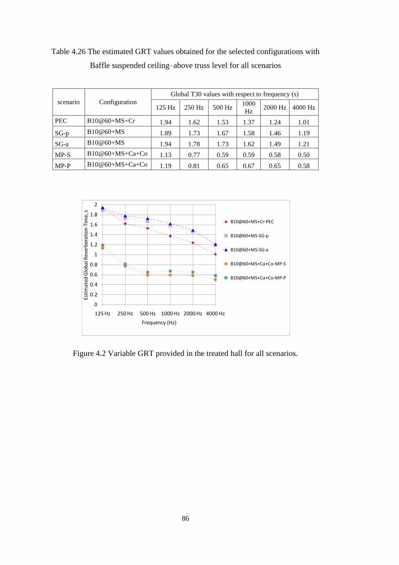
86
Table 4.26 The estimated GRT values obtained for the selected configurations with
Baffle suspended ceiling–above truss level for all scenarios
scenario Configuration
Global T30 values with respect to frequency (s)
125 Hz 250 Hz 500 Hz 1000
Hz 2000 Hz 4000 Hz
PEC B10@60+MS+Cr 1.94 1.62 1.53 1.37 1.24 1.01
SG-p B10@60+MS 1.89 1.73 1.67 1.58 1.46 1.19
SG-a B10@60+MS 1.94 1.78 1.73 1.62 1.49 1.21
MP-S B10@60+MS+Ca+Co 1.13 0.77 0.59 0.59 0.58 0.50
MP-P B10@60+MS+Ca+Co 1.19 0.81 0.65 0.67 0.65 0.58
Figure 4.2 Variable GRT provided in the treated hall for all scenarios.
0
0.2
0.4
0.6
0.8
1
1.2
1.4
1.6
1.8
2
125 Hz 250 Hz 500 Hz 1000 Hz 2000 Hz 4000 Hz
Esti
mat
ed G
lob
al R
ever
ber
atio
n T
ime,
s
Frequency (Hz)
B10@60+MS+Cr-PEC
B10@60+MS-SG-p
B10@60+MS-SG-a
B10@60+MS+Ca+Co-MP-S
B10@60+MS+Ca+Co-MP-P
87
Table 4.27 The results of grid response analyses for all scenarios with the proposed
configurations with Baffle suspended ceiling–above truss level in terms of EDT,
T30, STI and C80 values (the data X(50) that is the threshold value showing the 50%
of cumulative distribution), SPL(A) (the data X(95)-X(5), that is the difference
between the SPL values at 95% and 5% of cumulative distribution.
Scenario Configuration
Parameter
EDT
STI
SPL(A)
95%-5%
difference
(dB)
T30 C80
500Hz 1kHz 500Hz 1kHz 500Hz 1kHz
PEC B10@60+MS+Cr 1.02 1.03 0.61 7.3 1.51 1.32 - -
SG-p B10@60+MS 1.19 1.19 0.6 6.6 1.62 1.55 - -
SG-a B10@60+MS 1.07 1.11 0.59 8.9 1.65 1.6 - -
MP-S B10@60+MS+Ca+Co 0.43 0.42 0.75 10.3 0.54 0.55 - -
MP-P B10@60+MS+Ca+Co 0.53 0.51 - 6.2 0.53 0.48 8.9 9.3
In the study, cost analyses was also conducted: the total material and construction
cost of the proposal with B10@60(at) and MS as the permanent intervention and
Ca+Co as the temporary intervention (Figure G.1). Regarding the analyses, the
construction cost of the proposal brings 4.70% - 7.40% increase to the construction
cost of the sport hall.

88

89
CHAPTER 5
DISCUSSION
In this chapter, the joint interpretation of the data obtained from the simulation
analyses are done “to assess the acoustical adequacy of the typical sport hall
(Code:MEB-2004.63) in AS-IS case”, “to evaluate the acoustical improvements
achieved by the addition of acoustical treatments”. The knowledge achieved from the
evaluations is also summarized as “guiding remarks for the acoustical improvement
of a typical sport hall for its multi-purpose uses”. The discussions are done under
respective subheadings.
5.1 ACOUSTICAL PERFORMANCE ASSESSMENT OF TYPICAL SPORT
HALLS FOR THE AS-ISCASE
The estimated data which represented the AS-IS case of the typical sport hall and
their interpretation according to the acoustical requirements defined in the standards
have shown the insufficient acoustical performance of the hall and their causes.
For the AS-IS case, the simulated GRT data, being in the range of 3.46s and 5.08s at
mid-frequency range, were determined to be highly above the required values of
1.02s for PEC and 1.5s for sportive activities(Department of Education and Skills,
2004; Ellison & Schwenke, 2010). Excessive reverberation causes high sound
pressure levels and decrease in the clarity and intelligibility of speech. The
significant differences were also observed in estimated GRT values at different
frequencies. That signalled the presence of tonal imbalance in the space which may
cause masking of sounds at certain frequencies resulting in disturbing, noisy and

90
unintelligible acoustical environment. On the other hand, the long GRT values due to
the sound reflective envelope seemed to be decreased to some extent by the sound
absorption of air in the large volume of the hall, especially at 4000Hz and 8000Hz
(Table 4.1, Figure A.1, Figure B.1, Figure C.1).
The data obtained from the grid response analyses also supported the GRT values.
For instance, the STI values of 0.36 and 0.39 for the AS-IS case, were determined to
be in the poor range and exhibited the poor intelligibility of speech in the hall (Table
4.2, Figure A.4, Figure B.4, Figure C.4). Thedata exhibited the presence of “noisy
environment with high sound pressure level” that degrades speech intelligibility
during the physical education classes. That is the reason why teachers
necessitatecommunicating loudly with the students. Such a troublesome acoustical
environment of the hall results in an unintelligible core learning space for the
students and poor communication in the playfield between the teachers and students
during PE classes as well as among the players or the referees during sport games.
The results also proved that the AS-IS features of the sport hall are not appropriate
and sufficient for its multi-purpose use. Multi-purpose activities require the
involvement of sound reinforcement systems. Specifically, when the sound
reinforcement systems are used, the GRT values are required to be in the range of
0.6s and 1.2s for speech and musical activities (Adelman-Larsen, Thompson, &
Gade, 2010) and STI values are required to be equal to or above 0.56 for speech
activities (DIN 18041 2004-05, 2004). Due to the GRT values reaching to 5.08s and
STI values below 0.4, the acoustical features of the AS-IS case are not appropriate
for adapting sound reinforcement systems.
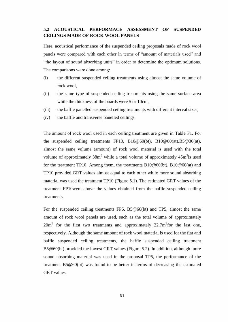
91
5.2 ACOUSTICAL PERFORMACE ASSESSMENT OF SUSPENDED
CEILINGS MADE OF ROCK WOOL PANELS
Here, acoustical performance of the suspended ceiling proposals made of rock wool
panels were compared with each other in terms of “amount of materials used” and
“the layout of sound absorbing units” in order to determine the optimum solutions.
The comparisons were done among:
(i) the different suspended ceiling treatments using almost the same volume of
rock wool,
(ii) the same type of suspended ceiling treatments using the same surface area
while the thickness of the boards were 5 or 10cm,
(iii) the baffle panelled suspended ceiling treatments with different interval sizes;
(iv) the baffle and transverse panelled ceilings
The amount of rock wool used in each ceiling treatment are given in Table F1. For
the suspended ceiling treatments FP10, B10@60(bt), B10@60(at),B5@30(at),
almost the same volume (amount) of rock wool material is used with the total
volume of approximately 38m3 while a total volume of approximately 45m
3is used
for the treatment TP10. Among them, the treatments B10@60(bt), B10@60(at) and
TP10 provided GRT values almost equal to each other while more sound absorbing
material was used the treatment TP10 (Figure 5.1). The estimated GRT values of the
treatment FP10were above the values obtained from the baffle suspended ceiling
treatments.
For the suspended ceiling treatments FP5, B5@60(bt) and TP5, almost the same
amount of rock wool panels are used, such as the total volume of approximately
20m3 for the first two treatments and approximately 22.7m
3for the last one,
respectively. Although the same amount of rock wool material is used for the flat and
baffle suspended ceiling treatments, the baffle suspended ceiling treatment
B5@60(bt) provided the lowest GRT values (Figure 5.2). In addition, although more
sound absorbing material was used in the proposal TP5, the performance of the
treatment B5@60(bt) was found to be better in terms of decreasing the estimated
GRT values.
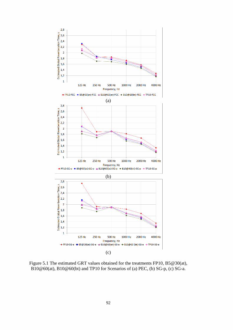
92
(a)
(b)
(c)
Figure 5.1 The estimated GRT values obtained for the treatments FP10, B5@30(at),
B10@60(at), B10@60(bt) and TP10 for Scenarios of (a) PEC, (b) SG-p, (c) SG-a.

93
Figure 5.2 Comparison of treatment proposals FP5, B5@60(bt) and TP5 in terms of
estimated GRT values for the PEC scenario.
(a)
(b)
Figure 5.3 The relationship between the amount of rock wool used for the suspended
ceiling treatments and their estimated GRT values (average of 500Hz and 1000Hz)
for the Scenario PEC.
1
1.2
1.4
1.6
1.8
2
2.2
2.4
2.6
2.8
3
125 Hz 250 Hz 500 Hz 1000 Hz 2000 Hz 4000 Hz
Esti
mat
ed G
lob
al R
ever
ber
atio
n T
ime,
s
Frequency, Hz
FP5-PEC B5@60 (bt)-PEC TP5-PEC

94
Despite the use of same amount of material in flat and baffle panelled suspended
ceilings,the sound waves hit one side of the panels in flat panelled system while; both
sides of the baffle modules were interacting with the sound waves. The increase
sound absorbing surface area seemed to provide more absorption of the sound (See
groups in circles in Figure 5.3a).
The performance of baffle suspended ceiling systems (B10@60, B5@60) were better
than the transverse suspended ceiling systems (TP10, TP5) despite the use of fewer
amount of rock wool. This shows that in order to reduce the reverberation time,
excessive amount of material is not the only solution, but the configuration of the
material and system of the application is effective as well. Moreover, according to
the grid response analyses results of the parameters EDT, T30 and C80 at mid
frequencies, STI and SPL(A), (See relevant figures in Appendix A, Appendix B,
and Appendix C), for evenly distribution of the sound within the hall, due to their
diffusive character, proposals B10@60(at) and (bt) were found to be better solutions
than the proposal TP10.
Role of thickness for the rock wool boards on the acoustical performance of
suspended ceilings is also analysed. According to the comparison of treatments with
the same surface area, namely FP5, B5@60(at), TP5 with FP10, B10@60(at), TP10,
for PEC, SG-p and SG-a scenarios, treatments with thicker material provided more
decrease in estimated GRT value especially at 125Hz.Moreover, In the treatments
B10@60(at) and B5@30(at) for the scenarios PEC, SG-p and SG-a, same amount of
rock wool was used. According the simulation results, estimated GRT values at mid
and high frequencies were almost equal to each other in both proposals. However, at
125Hz, estimated GRT was longer in the proposal B5@30(at) (Table 4.4, Table 4.8,
Table 4.12 and Figure 5.4). This was because of sound absorption coefficient (α)
difference between 5cm and 10cm thick rock wool at 125Hz (Table 3.4). These
results mean that in addition to the amount of the material used, sound absorption
characteristics of the material in all frequency ranges (related with the thickness of
boards) is also important.

95
Figure 5.4 Comparison of treatment proposals B5@30(at) and B10@60(at) in terms
of estimated GRT values for the PEC, SG-p and SG-a scenarios.
In the treatment proposal B10@30(at), the amount of rock wool used was twice the
amount used in B10@60(at) for the scenarios PEC, SG-p and SG-a. However, the
decrease in the estimated GRT values in all frequency ranges was not remarkable
(around 0.03s) which means doubling the amount of material did not provide a
remarkably efficient solution in these cases (Table 4.4, Table 4.8, Table 4.12). The
performance comparison of ceiling treatments B10@30(at) and B10@60(at) is given
in Figure 5.5.
Figure 5.5 Comparison of treatment proposals B10@30(at) and B10@60(at) in terms
of estimated GRT values for the PEC, SG-p and SG-a scenarios.
1.1
1.3
1.5
1.7
1.9
2.1
2.3
2.5
125 Hz 250 Hz 500 Hz 1000 Hz 2000 Hz 4000 Hz
Esti
mat
ed G
lob
al R
ever
ber
atio
n T
ime,
s
Frequency (Hz)
B5@30(at)-PEC B10@60(at)-PEC B5@30(at)-SG-p
B10@60(at)-SG-p B5@30(at)-SG-a B10@60(at)-SG-a
1.1
1.3
1.5
1.7
1.9
2.1
2.3
125 Hz 250 Hz 500 Hz 1000 Hz 2000 Hz 4000 Hz
Esti
mat
ed G
lob
al R
ever
ber
atio
n T
ime,
s
Frequency (Hz)
B10@60(at)-PEC
B10@30(at)-PEC
B10@60(at)-SG-p
B10@30(at)-SG-p
B10@60(at)-SG-a
B10@30(at)-SG-a
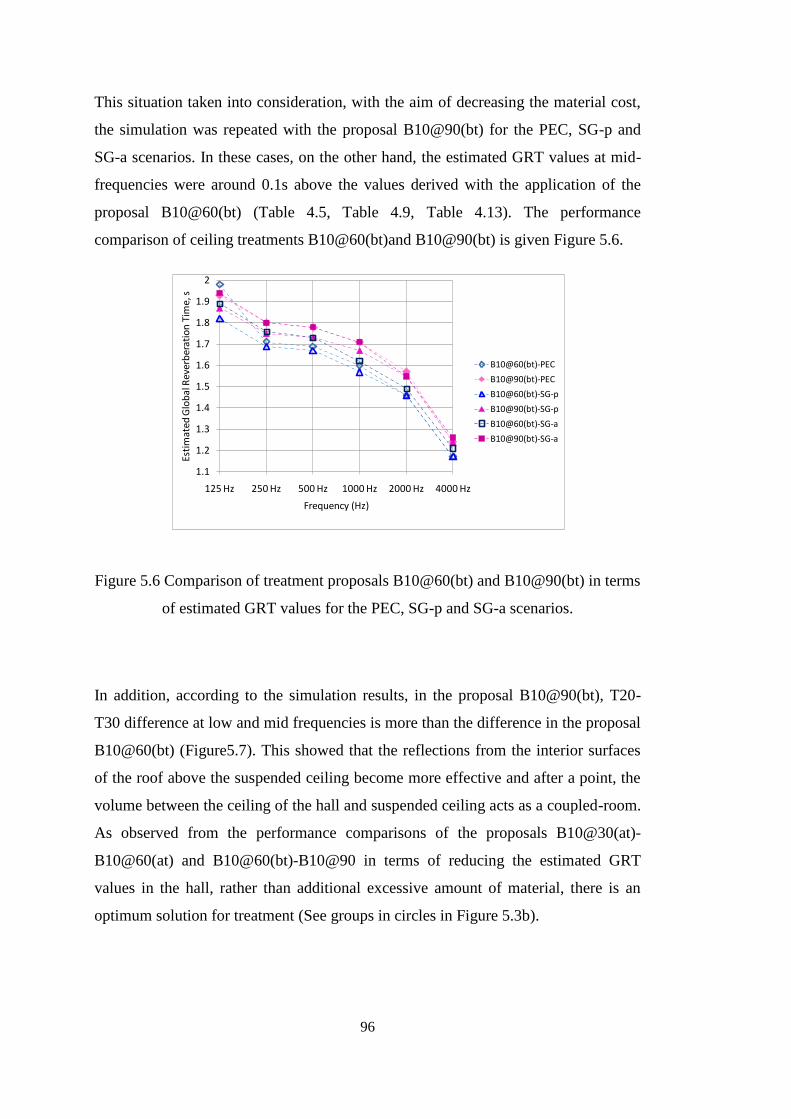
96
This situation taken into consideration, with the aim of decreasing the material cost,
the simulation was repeated with the proposal B10@90(bt) for the PEC, SG-p and
SG-a scenarios. In these cases, on the other hand, the estimated GRT values at mid-
frequencies were around 0.1s above the values derived with the application of the
proposal B10@60(bt) (Table 4.5, Table 4.9, Table 4.13). The performance
comparison of ceiling treatments B10@60(bt)and B10@90(bt) is given Figure 5.6.
Figure 5.6 Comparison of treatment proposals B10@60(bt) and B10@90(bt) in terms
of estimated GRT values for the PEC, SG-p and SG-a scenarios.
In addition, according to the simulation results, in the proposal B10@90(bt), T20-
T30 difference at low and mid frequencies is more than the difference in the proposal
B10@60(bt) (Figure5.7). This showed that the reflections from the interior surfaces
of the roof above the suspended ceiling become more effective and after a point, the
volume between the ceiling of the hall and suspended ceiling acts as a coupled-room.
As observed from the performance comparisons of the proposals B10@30(at)-
B10@60(at) and B10@60(bt)-B10@90 in terms of reducing the estimated GRT
values in the hall, rather than additional excessive amount of material, there is an
optimum solution for treatment (See groups in circles in Figure 5.3b).
1.1
1.2
1.3
1.4
1.5
1.6
1.7
1.8
1.9
2
125 Hz 250 Hz 500 Hz 1000 Hz 2000 Hz 4000 Hz
Esti
mat
ed G
lob
al R
ever
ber
atio
n T
ime,
s
Frequency (Hz)
B10@60(bt)-PEC
B10@90(bt)-PEC
B10@60(bt)-SG-p
B10@90(bt)-SG-p
B10@60(bt)-SG-a
B10@90(bt)-SG-a

97
Figure 5.7 Estimated GRT values of proposals B10@60(bt) (above) and B10@90(bt)
(below)
T30
T20
Estimated global reverberation times (Source 2, 469621 rays used)
Frequency (Hertz)
63 125 250 500 1000 2000 4000 8000
Reverberation tim
e (
s)
1.9
1.8
1.7
1.6
1.5
1.4
1.3
1.2
1.1
1
0.9
0.8
0.7
0.6
0.5
0.4
0.3
0.2
0.1
0
Odeon©1985-2006
T30
T20
Estimated global reverberation times (Source 2, 839673 rays used)
Frequency (Hertz)
63 125 250 500 1000 2000 4000 8000
Reverberation tim
e (
s)
1.9
1.8
1.7
1.6
1.5
1.4
1.3
1.2
1.1
1
0.9
0.8
0.7
0.6
0.5
0.4
0.3
0.2
0.1
0
Odeon©1985-2006
T30
T20
Estimated global reverberation times (Source 1, 320293 rays used)
Frequency (Hertz)
63 125 250 500 1000 2000 4000 8000
Rev
erbe
ratio
n tim
e (s
)
1.15
1.1
1.05
1
0.95
0.9
0.85
0.8
0.75
0.7
0.65
0.6
0.55
0.5
0.45
0.4
0.35
0.3
0.25
0.2
0.15
0.1
0.05
0
Odeon©1985-2006

98
Among the types of baffle panelled suspended ceiling systems, the ceiling
B10@60(at) is suggested for the acoustical improvement of the hall for its multi-
purpose use due to the reasons of (i) its performance for reducing the GRT value of
the hall, (ii) feasible use of materials and (iii) level of its application. Although
treatment B10@60(bt) satisfies the first and second reasons mentioned above, the
applications below the truss level reduce the overall volume of the hall with a
decrease in the overall height about 60cm. That results in the height of the hall to be
below the minimum height requirement given by Turkish Volleyball Federation
(2014) and Turkish Basketball Federation (2014). A special care should be given
while selecting those ceiling treatments since below-truss treatments may limit the
height of the hall for some sportive activities and it is not suitable to be applied to the
studied hall.
5.3 ACOUSTICAL IMPROVEMENTS WITH THE PROPOSED SUSPENDED
CEILING SYSTEMS: PERMANENT INTERVENTIONS
All suspended ceiling treatments proposed in the study, mainly the “flat panelled”,
"baffle panelled”, “transverse panelled” and “fabric tension suspended ceiling
systems” are the permanent interventions suggested for the main acoustical
improvement of the sport hall. Those interventions were determined to decrease the
GRT values in the hall noticeably. In other words, all these suspended ceiling
systems that were suggested in the study provided considerable improvement in the
acoustical features of the hall, especially for sportive activities including physical
education class and sport games (Figure 4.1).
According to the simulation analyses, among four suspended ceiling proposals (flat
panelled, baffle, transverse panelled and fabric tension), the application of baffle
panelled suspended ceiling is determined to be the most effective treatment (Figure
5.8) due to the:
lowest GRT values provided in the hall,
gradual decrease of GRT provided with increase in frequency, and

99
even distribution of sound in the hall determined by the grid response analyses.
Among the types of baffle panelled suspended systems, the ceilingsB10@30(at),
B10@60(at) and B10@60(bt) decreased the GRT to the lowest levels, in the range
of1.67s-1.73s, 1.71s-1.77s and 1.62s-1.67s, respectively, for sport activities (Table
4.4, Table 4.5).The transverse panelled suspended ceiling with 10cm-thick rock wool
panels fixed between trusses (TP10) provided the similar performance with those
baffle panelled ones with the GRT values in the range of 1.70s-1.76s. Following the
baffle suspended ceiling treatments and the TP10 treatment, flat panelled suspended
ceiling with 10 cm-thick rock wool panels (FP10) provided the next appropriate GRT
values in the range of 1.79s-1.89s at mid-frequencies. The least decrease in GRT
values was observed for the treatment of fabric tension suspended ceiling (FT) with
the values in the range of 1.77s-1.82s at mid frequencies (Figure 5.8).
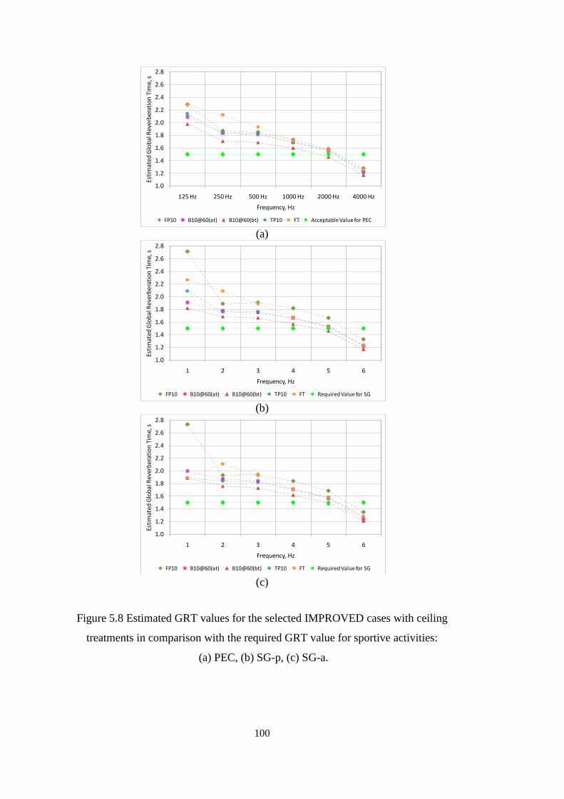
100
(a)
(b)
(c)
Figure 5.8 Estimated GRT values for the selected IMPROVED cases with ceiling
treatments in comparison with the required GRT value for sportive activities:
(a) PEC, (b) SG-p, (c) SG-a.
1.0
1.2
1.4
1.6
1.8
2.0
2.2
2.4
2.6
2.8
125 Hz 250 Hz 500 Hz 1000 Hz 2000 Hz 4000 Hz
Esti
mat
ed G
lob
al R
ever
ber
atio
n T
ime,
s
Frequency, Hz
FP10 B10@60(at) B10@60(bt) TP10 FT Acceptable Value for PEC
1.0
1.2
1.4
1.6
1.8
2.0
2.2
2.4
2.6
2.8
1 2 3 4 5 6
Esti
mat
ed G
lob
al R
ever
ber
atio
n T
ime,
s
Frequency, Hz
FP10 B10@60(at) B10@60(bt) TP10 FT Required Value for SG
1.0
1.2
1.4
1.6
1.8
2.0
2.2
2.4
2.6
2.8
1 2 3 4 5 6
Esti
mat
ed G
lob
al R
ever
ber
atio
n T
ime,
s
Frequency, Hz
FP10 B10@60(at) B10@60(bt) TP10 FT Required Value for SG

101
The simulation analyses have shown that both baffle and transverse suspended
ceilings are still above the required GRT value of 1.02s at mid frequencies for the
PEC scenario. This meant that there is the necessity for the use of additional
treatments to the walls, such as use of sound absorptive curtains on wall surfaces in
order to decrease the estimated GRT values to the acceptable ranges. The baffle and
transverse panelled ceilings, on the other hand, are accepted to be enough to establish
appropriate acoustical environment for the sport games due to their estimated GRT
values close to the required values of 1.5s at mid frequencies. In short, in terms of
GRT values, the baffle and transverse panelled suspended ceilings were determined
to be the most effective proposal for sport games activities while additional
interventions seemed to be needed for PEC and multi-purpose activities, such as
sound absorptive curtains on wall surfaces.
According to grid response analyses, the suspended ceiling treatments B10@60
below and above truss level and TP10, providing the acceptable GRT values for
sport game activities, were determined to improve the speech intelligibility within
the hall due to the:
decrease in the estimated EDT and T30 valuesat mid frequencies with the values
in the range of 1.23s-1.48s and 1.47s-1.90s, respectively;
estimated EDT values being lower than the GRT values;
estimated T30 values similar with GRT values;
increase in the STI values in the range of 0.57-0.62which fell into the STI ranges
of “fair” and “good”(Figure 5.9, Table 4.15).
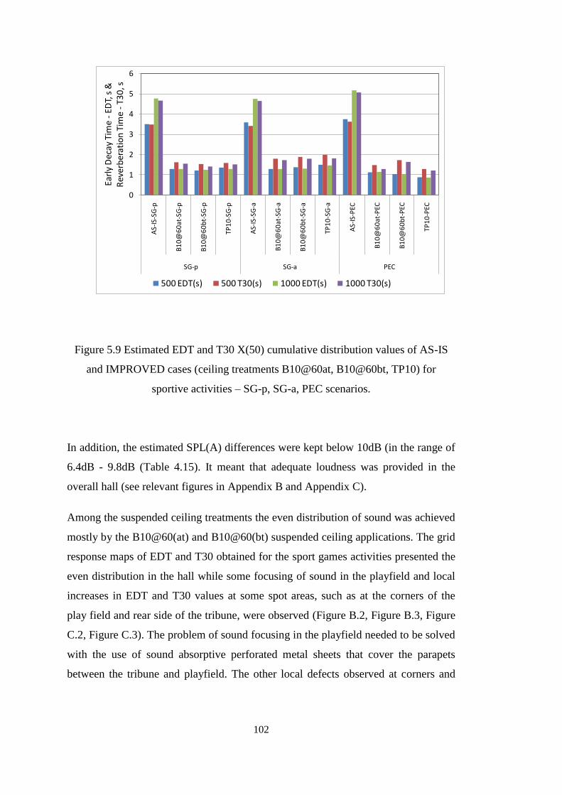
102
Figure 5.9 Estimated EDT and T30 X(50) cumulative distribution values of AS-IS
and IMPROVED cases (ceiling treatments B10@60at, B10@60bt, TP10) for
sportive activities – SG-p, SG-a, PEC scenarios.
In addition, the estimated SPL(A) differences were kept below 10dB (in the range of
6.4dB - 9.8dB (Table 4.15). It meant that adequate loudness was provided in the
overall hall (see relevant figures in Appendix B and Appendix C).
Among the suspended ceiling treatments the even distribution of sound was achieved
mostly by the B10@60(at) and B10@60(bt) suspended ceiling applications. The grid
response maps of EDT and T30 obtained for the sport games activities presented the
even distribution in the hall while some focusing of sound in the playfield and local
increases in EDT and T30 values at some spot areas, such as at the corners of the
play field and rear side of the tribune, were observed (Figure B.2, Figure B.3, Figure
C.2, Figure C.3). The problem of sound focusing in the playfield needed to be solved
with the use of sound absorptive perforated metal sheets that cover the parapets
between the tribune and playfield. The other local defects observed at corners and
0
1
2
3
4
5
6
AS-
IS-S
G-p
B1
0@
60
at-S
G-p
B1
0@
60
bt-
SG-p
TP1
0-S
G-p
AS-
IS-S
G-a
B1
0@
60
at-S
G-a
B1
0@
60
bt-
SG-a
TP1
0-S
G-a
AS-
IS-P
EC
B1
0@
60
at-P
EC
B1
0@
60
bt-
PEC
TP1
0-P
EC
SG-p SG-a PEC
Earl
y D
ecay
Tim
e-
EDT,
s &
R
ever
ber
atio
n T
ime
-T3
0, s
500 EDT(s) 500 T30(s) 1000 EDT(s) 1000 T30(s)

103
edges seemed not to disturb the even-distribution of sound for the receiver positions
(audience and/or the players). Those local defects can be eliminated simply with the
use of sound absorptive or diffusive materials where defects are observed (Beranek,
2004). Considering all, the B10@60(at) and B10@60(bt) treatments were assessed to
provide sufficient even distribution for PEC and sport games while some additional
interventions were still needed.
The transverse panelled suspended ceiling with 10cm-thick panels (TP10), on the
other hand, was not satisfactory to provide even distribution of sound in the hall for
PEC and sport games activities (see relevant figures in Appendix A, Appendix B and
Appendix C). Additional improvements such as using sound absorptive and/or
diffusers at wall surfaces were necessary to achieve uniformity of sound in audience
areas and eliminate the remarkable differences in EDT and T30 values at 500Hz and
1000Hz.
5.4 ACOUSTICAL IMPROVEMENTS WITH THE JOINT USE OF
PROPOSED SUSPENDED CEILING SYSTEMS AND SOUND ABSORBING
CURTAIN MODULES
All permanent treatments with additional use of satin curtain provided a decrease in
the estimated GRT values in the hall for physical education class and multi-purpose
activities.
The physical education class activity:
The configurations composed of both permanent suspended ceiling treatment and
sound absorbing curtain modules attached in front of tribune’s rear-wall was
observed to decrease GRT values more than the configurations using the curtain
modules in front of the windows.The average estimated GRT values at mid-
frequencies were in the range of 1.48s-1.58s with the joint use of curtain modules in
front of the windows; 1.42s-1.50s with the joint use of curtain modules in front of the
tribune’s rear wall and suspended ceiling proposals flat panelled suspended ceiling

104
systems (FP5, FP10) (Table 4.16), baffle panelled suspended ceiling systems
(B10@60(at), B10@30(at), B5@30(at), B10@60(bt)) (Table 4.17, Table 4.18),
transverse panelled suspended ceiling systems (TP5, TP10) and fabric tension
suspended ceiling system (FT) (Table 4.19). In short, when compared with the
estimated GRT values provided by the permanent suspended ceiling treatments, a
reduction of approximately 0.2s in GRT values was provided by the addition of
curtain modules mounted in front of windows while a reduction of approximately
0.3s was achieved by mounting the curtain modules in front of the tribune’s rear wall
(Figure 5.10).
Figure 5.10 For the Scenario PEC, the estimated GRT values determined for the
IMPROVED cases representing the performance of sound absorbing curtain modules
positioned whether in front of windows or in front of tribune’s rear wall, together
with permanent ceiling treatments.

105
The average of GRT values at mid frequencies obtained for the treatments
B10@60(at)+Cr, B10@60(bt)+Crand TP10+Cr were found to be below 1.5s, the
required GRT value for sportive activities (Table 4.17, Table 4.18, Table 4.19 and
Figure A.1). This means that those treatments are the configurations sufficient to
decrease GRT values to required ranges. However, all treatments suggested are still
above 1.02s, the required GRT value for lectures.
For the multi-purpose activities:
The additional treatments composed of 390-people filled seat, 263m2 double layered
satin curtains on walls, estimated GRT values decreased the average GRT values of
selected ceiling treatments B10@60(bt), B10@60(at) and TP10 from approximately
2.0s to approximately 1.3s at low frequency range, approximately 1.7s to
approximately 0.8s at mid-frequency range, approximately 1.5s to approximately
0.6s at high-frequency range for the speech and musical activities: MP-S and MP-P
scenarios. The joint use of curtain modules in front of the windows, side walls and
tribune’s rear-wall with the baffle panelled suspended ceiling systems
B10@60(at)+Ca, B10@60(bt)+Ca and TP10+Ca decreased the average GRT values
at mid-frequencies to 0.82s, 0.80s, and 0.77s for speech activities(MP-S scenario);
0.89s, 0.88s, 0.80s for performance activities: (MP-P scenario) respectively.
After the addition of occupied seating and the curtain modules on the walls during
multi-purpose activities, although GRT values decreased to the required values,the
difference between T30 and T20 observed signalled the presence of acoustical
coupling phenomenon after the joint use of ceiling and curtain (Figure D.1, Figure
E.1).
In order to eliminate those late reflections, the sound breaks were provided with the
use of double-layered satin curtains at the open entrances between the service area
and the playfield. After the addition of curtain modules and with the joint use of all
proposed curtain modules and ceiling treatments B10@60(at)+Ca+Co,
B10@60(bt)+Ca+Co and TP10+Ca+Co, the average GRT values at mid-frequencies
were found to be0.60s, 0.59s, and 0.51s for MP-S scenario; 0.68s, 0.66s, and 0.52s
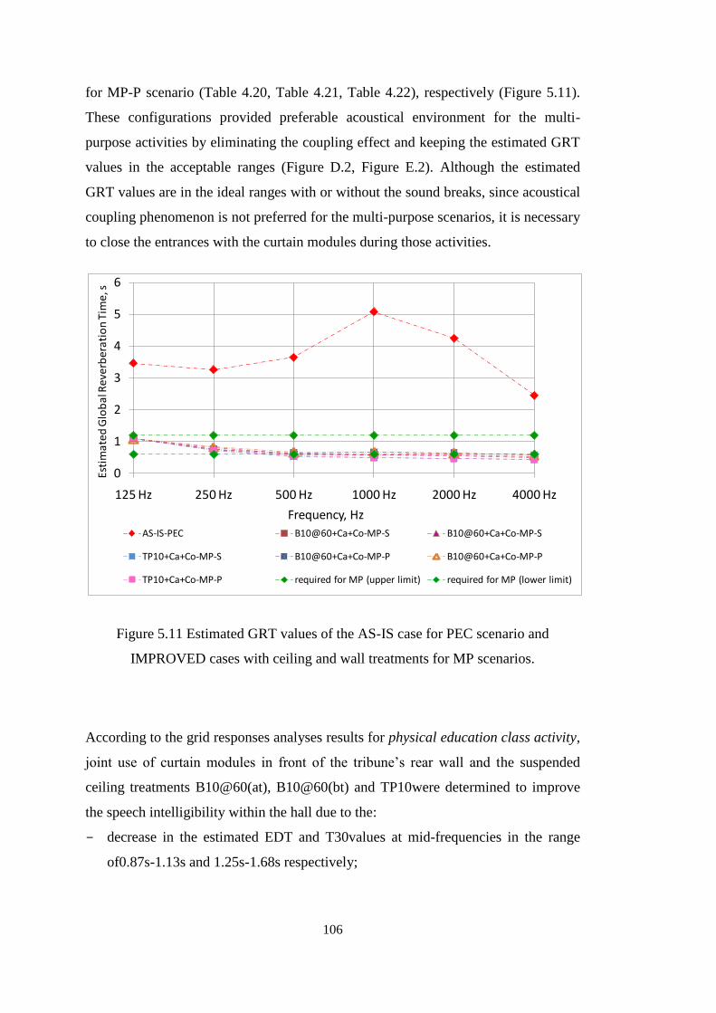
106
for MP-P scenario (Table 4.20, Table 4.21, Table 4.22), respectively (Figure 5.11).
These configurations provided preferable acoustical environment for the multi-
purpose activities by eliminating the coupling effect and keeping the estimated GRT
values in the acceptable ranges (Figure D.2, Figure E.2). Although the estimated
GRT values are in the ideal ranges with or without the sound breaks, since acoustical
coupling phenomenon is not preferred for the multi-purpose scenarios, it is necessary
to close the entrances with the curtain modules during those activities.
Figure 5.11 Estimated GRT values of the AS-IS case for PEC scenario and
IMPROVED cases with ceiling and wall treatments for MP scenarios.
According to the grid responses analyses results for physical education class activity,
joint use of curtain modules in front of the tribune’s rear wall and the suspended
ceiling treatments B10@60(at), B10@60(bt) and TP10were determined to improve
the speech intelligibility within the hall due to the:
decrease in the estimated EDT and T30values at mid-frequencies in the range
of0.87s-1.13s and 1.25s-1.68s respectively;
0
1
2
3
4
5
6
125 Hz 250 Hz 500 Hz 1000 Hz 2000 Hz 4000 Hz
Esti
mat
ed G
lob
al R
ever
ber
atio
n T
ime,
s
Frequency, Hz
AS-IS-PEC B10@60+Ca+Co-MP-S B10@60+Ca+Co-MP-S
TP10+Ca+Co-MP-S B10@60+Ca+Co-MP-P B10@60+Ca+Co-MP-P
TP10+Ca+Co-MP-P required for MP (upper limit) required for MP (lower limit)

107
estimated EDT values being lower than the estimated GRT values;
estimated T30 values similar with GRT values;
increase in the STI valuesin the range of 0.59-0.63which fell into the STI ranges
of “fair” and “good”(Figure 5.8, Table 4.23, Table 4.24, Table 4.25).
In addition, the estimated SPL(A) differences were kept below 10dB (in the range of
7.3dB-8.1dB). It meant that adequate loudness was providedin the overall hall (see
relevant figures in Appendix A).
According to the grid responses analyses results for multi-purpose use for speech and
performance activities, joint use of curtain modules in front of the wall surfaces and
at the openings with the suspended ceiling treatments B10@60 above and below
truss level and TP10, providing the acceptable estimated GRT values for sport game
activities, were also determined to improve the speech intelligibility within the hall
due to the:
decrease in the estimated EDT and T30 valuesat mid frequencies with the values
in the range of 0.32s-0.54s and 0.40s-0.66s, respectively;
estimated EDT values being lower than the GRT values;
estimated T30 values similar with GRT values;
high average C80 values at mid frequencies in the range of 8.5dB-13.6dB (for
performance activities - MP-P scenario);
increase in the STI values in the range of0.74-0.77 (for speech activities –MP-S
scenario)which fell into the STI range of “excellent” (Figure 5.12, Table 4.23,
Table 4.24, Table 4.25).

108
Figure 5.12 Estimated EDT and T30 X(50) cumulative distribution values of
IMPROVED case with the ceiling treatments B10@60(at), B10@60(bt) and TP10
and all curtain modules on wall surfaces for MP scenarios.
In addition, the estimated SPL(A) differences were kept below 10dB (in the range of
6.1dB-10.5dB). It meant that adequate loudness was provided in the overall hall
(Appendix D, Appendix E).
Similar to the analyses results for sport games activities, according to the estimated
GRT values and grid response analyses maps, among the three suspended ceiling
proposals, the baffle panelled ones provided sufficient acoustical improvement
within the hall for the physical education class activity and multi-purpose activities.
Due to height restrictions of the sports federations, baffle panelled suspended ceiling
system with baffles located above truss level were selected as the appropriate ceiling
treatment as permanent implementation. As temporary implementation, on the other
hand, during PEC activities, curtain modules in front of the tribune’s rear wall
(configuration B10@60(at)+Cr); during MP activities, use of curtain modules in front
of all proposed wall surfaces and at the openings between the service and sports
0
0.1
0.2
0.3
0.4
0.5
0.6
0.7
0.8
B10@60(at) B10@60(bt) TP10 B10@60(at) B10@60(bt) TP10
Earl
y D
ecay
Tim
e-
EDT,
s &
R
ever
ber
atio
n T
ime
-T3
0, s
MP-S MP_P
EDT-500Hz EDT-1kHz T30-500Hz T30-1kHz

109
areas (configuration B10@60(at)+Ca+Co) provided the sufficient improvement
within the hall. However, according to the grid response analyses results of the
treatment configurations B10@60(at)+Cr for physical education class and
B10@60(at) for sport games activities, focusing of the sound for the parameter
T30was observed on the playfield(FigureA.3, Figure B.3, Figure C.3). This was
thought to be caused by the reflections from the parapet between the playfield and
the tribune which might have become more effective after additional sound
absorption atthe walls and the ceiling. After the addition of sound absorbing
perforated metal sheet as the second permanent material, the average estimated GRT
values at mid frequencies were found to be 1.45s, 1.62s, 1.67s, 0.59s, 0.66s for PEC,
SG-p, SG-a, MP-S, MP-P scenarios respectively which were in the required or
acceptable ranges for each activity (Figure 5.13, Figure A.1, Figure B.1, Figure
C.1,Figure D.2, Figure E.2).
(a)
(b)
Figure 5.13 Estimated GRT values of the permanent treatments B10@60(at)+MS
with the joint use of determined temporary treatment for PEC, SG-p, SG-a scenarios
with required/acceptable limit (a), for MP scenarios with required interval (b).
0
0.5
1
1.5
2
2.5
125 Hz 250 Hz 500 Hz 1000 Hz 2000 Hz 4000 Hz
Esti
mat
ed G
lob
al R
ever
ber
atio
n T
ime,
s
Frequency, Hz
B10@60+MS+Cr-PEC B10@60+MS-SG-p
B10@60+MS-SG-a required for SG / acceptable for PEC
0
0.2
0.4
0.6
0.8
1
1.2
1.4
125 Hz 250 Hz 500 Hz 1000 Hz 2000 Hz 4000 Hz
Esti
mat
ed G
lob
al R
ever
ber
atio
n T
ime,
s
Frequency, Hz
B10@60+MS+Ca+Co-MP-S B10@60+MS+Ca+Co-MP-P
required for MP (upper limit) required for MP (lower limit)
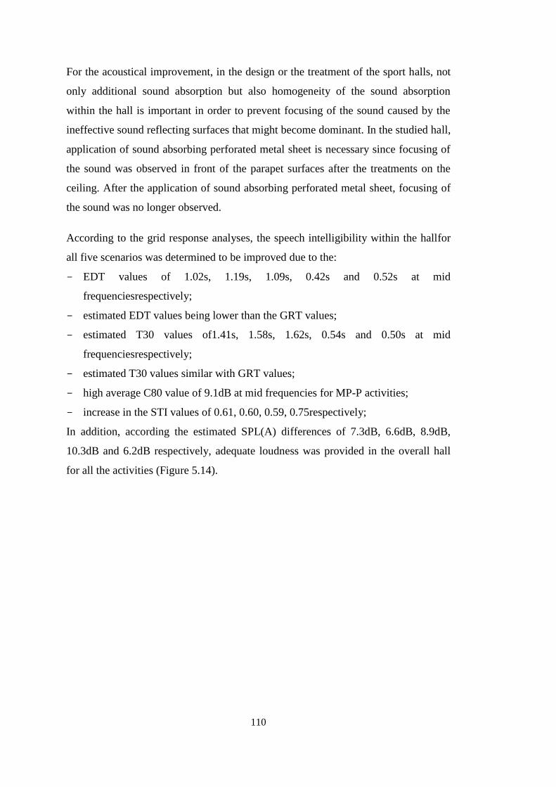
110
For the acoustical improvement, in the design or the treatment of the sport halls, not
only additional sound absorption but also homogeneity of the sound absorption
within the hall is important in order to prevent focusing of the sound caused by the
ineffective sound reflecting surfaces that might become dominant. In the studied hall,
application of sound absorbing perforated metal sheet is necessary since focusing of
the sound was observed in front of the parapet surfaces after the treatments on the
ceiling. After the application of sound absorbing perforated metal sheet, focusing of
the sound was no longer observed.
According to the grid response analyses, the speech intelligibility within the hallfor
all five scenarios was determined to be improved due to the:
EDT values of 1.02s, 1.19s, 1.09s, 0.42s and 0.52s at mid
frequenciesrespectively;
estimated EDT values being lower than the GRT values;
estimated T30 values of1.41s, 1.58s, 1.62s, 0.54s and 0.50s at mid
frequenciesrespectively;
estimated T30 values similar with GRT values;
high average C80 value of 9.1dB at mid frequencies for MP-P activities;
increase in the STI values of 0.61, 0.60, 0.59, 0.75respectively;
In addition, according the estimated SPL(A) differences of 7.3dB, 6.6dB, 8.9dB,
10.3dB and 6.2dB respectively, adequate loudness was provided in the overall hall
for all the activities (Figure 5.14).
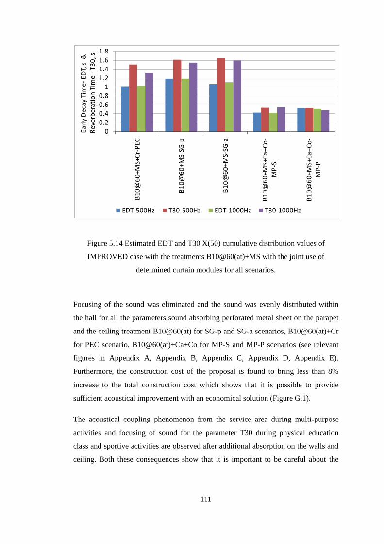
111
Figure 5.14 Estimated EDT and T30 X(50) cumulative distribution values of
IMPROVED case with the treatments B10@60(at)+MS with the joint use of
determined curtain modules for all scenarios.
Focusing of the sound was eliminated and the sound was evenly distributed within
the hall for all the parameters sound absorbing perforated metal sheet on the parapet
and the ceiling treatment B10@60(at) for SG-p and SG-a scenarios, B10@60(at)+Cr
for PEC scenario, B10@60(at)+Ca+Co for MP-S and MP-P scenarios (see relevant
figures in Appendix A, Appendix B, Appendix C, Appendix D, Appendix E).
Furthermore, the construction cost of the proposal is found to bring less than 8%
increase to the total construction cost which shows that it is possible to provide
sufficient acoustical improvement with an economical solution (Figure G.1).
The acoustical coupling phenomenon from the service area during multi-purpose
activities and focusing of sound for the parameter T30 during physical education
class and sportive activities are observed after additional absorption on the walls and
ceiling. Both these consequences show that it is important to be careful about the
00.20.40.60.8
11.21.41.61.8
B1
0@
60
+MS+
Cr-
PEC
B1
0@
60
+MS-
SG-p
B1
0@
60
+MS-
SG-a
B1
0@
60
+MS+
Ca+
Co
-M
P-S
B1
0@
60
+MS+
Ca+
Co
-M
P-P
Earl
y D
ecay
Tim
e-ED
T, s
&
Rev
erb
erat
ion
Tim
e -
T30
, s
EDT-500Hz T30-500Hz EDT-1000Hz T30-1000Hz
112
reflections from the untreated surfaces that might become influential which were not
before the treatments. These situations reveal the fact that that not only the amount or
the location of the materials used but also evenly distribution of those materials
within the hall isimportant.
For providing variable acoustical environment, since they are easily mountable and
operable, treatment by means of sound absorbing curtains with roller blind
mechanism is a simple and economical solution in terms of its material and
application cost. The disadvantage of these curtain modules is they are not diffusive.
However, this is not obligatory in the content of this study since the curtains are used
during the multi-purpose activities where the audience covering the playfield
provides the necessary scattering as observed from the grid response analyses results
(Appendix D, Appendix E).
5.5 GUIDING REMARKS FOR ACOUSTICAL IMPROVEMENT OF
TYPICAL SPORT HALLS
The knowledge achieved by the study are summarized here in the form of guiding
remarks for the renovation processes of typical sport halls, especially for the
designers, engineers and practitioners. Those remarks should be taken into
consideration to provide appropriate acoustical environment in sport halls for its use
as physical education classes, sport games activities, speech and musical multi-
purpose activities. They are also useful for the preliminary stages of design to obtain
inherently well-designed acoustical conditions in typical sport halls.
The guiding remarks are summarised below:
The GRT values at mid frequencies required for the lectures should be below
1.02s; for the sportive activities should be below 1.5sin case sound reinforcement
systems are whether used or not; for multi-purpose activities should be between
0.6s 1.2s in case sound reinforcement systems are used. According to the results
of this study, the acoustical situation in the untreated hall is improper for those
activities and need to be improved.
113
In order to enable different requirements for different activities, variable
acoustical environment is needed to be provided within these halls.
Because of their large surface areas, the ceiling, walls and floor are the key
components for the control of sound field in the hall. Therefore, treatments with
the sound absorptive and/or diffusive materials on those surfaces, such as
application of a suspended ceiling on the playfield, are dominant interventions
while precise adjustments can be done by local treatments.
For the sports hall, the ceiling is the most appropriate component for making
interventions and for the implementation of sound absorptive materials.
For the major acoustical improvement of the sport hall, mainly four types of
suspended ceiling systems are suggested. These are the flat panelled, baffle
panelled, transverse panelled and fabric tension suspended ceiling systems.
Among these suspended ceiling systems, baffle suspended ceiling proposals,
especially the one composed of 10cm-thick rock wool panels which are
positioned at 60cm intervals and aligned with the bottom level of trusses
(B10@60(at)), provided the most efficient solution. That treatment provided
GRT values in acceptable ranges and more even sound distribution in the hallin
comparison to the flat, transverseand fabric tension suspended ceiling systems.
If the budget is limited, instead of baffle panelled suspended systems, the fabric
tension suspended ceilings, such as the ceiling composed of double layered sound
absorptive fabric stretched crosswise between the trusses, is an alternative for the
acoustical improvement in the sports hall. However, that proposal seems to be
insufficient for the control of sound especially in low frequencies (125Hz and
250Hz).
The permanent interventions recommended for the acoustical improvement of
sports hall are:
- the use of baffle panelled suspended ceiling with 10-cm-thick rock wool
panels with 60cm intervals where the baffles are suspended 60cm above truss
level (B10@60(at));
- the use of sound absorbing perforated metal sheet covering the parapets
which are located between the playfield and the tribune (B10@60(at)+MS).
114
For sport games activities, those permanent interventions mentioned above are
enough.
For the physical education classes, in addition to the permanent interventions
mentioned above, it is advised to use sound absorbing curtain modules with roller
blind mechanism in front of tribune’s rear wall (Cr). The sound absorption
performance of curtain modules are satisfactory when double-layered satin fabric
is used and a cavity of 15 cm is kept between the wall surface and the curtain.
Here, a special care should be given to keep that cavity to achieve the particular
sound absorption required from the curtain application.
For the multi purposes use of the sport hall, in addition to the permanent
interventions, it is recommended to use double-layered satin fabric sound
absorbing curtain modules with roller blind mechanism in front of tribune’s rear
wall, side walls, front walls and at the openings between the service and sports
areas. Here, the use of curtains at the openings between the service area and
sports hall are essential to eliminate undesirable sound reflections.Again, a
special care should be given to keep the cavity of 15 cm between the wall surface
and the curtain.
Apart from the acoustical concerns, the suspended ceiling and curtain modules
proposed in the study should be considered as the architectural tools and have
role to motivate the occupants. Therefore, the relationships especially between
the baffle panels and curtain modules can be built for improving the indoor
aesthetic quality and establishing more pleasant sport hall interiors.
115
CHAPTER 6
CONCLUSION
In this study, acoustical analyses of a typical sport hall project (Code: MEB 2004-63)
were made with the help of the computer simulations regarding the AS-IS uses of the
hall, namely physical education classes and sport activities, such as basketball and
volleyball games. In addition to those activities, requirements for the acoustical
environment during the multi-purpose use of the hall were explained. Treatments for
the acoustical improvement and providing variable acoustical environment were
suggested.
Acoustical problems within the typical sport hall project were defined with respect to
the simulation results. According to those results, the acoustical performance of the
AS-IS case is not suitable for the activities taking place in these halls. The estimated
GRT values were found to be highly above the requirements at low, mid and high
frequencieswhich signalled the insufficiency of the acoustical environment in these
halls since long reverberation time degrades speech intelligibility and causes high
ambient noise levels resulting in inconvenient environment for verbal
communication.
Moreover, the results obtained from grid response analyses also signalled the
existence of noisy and unintelligible environment in the halls. These problems lead to
tiring communication ambience and cause improper environments for the
activities/functions. Those results also showed that in addition to the lectures and
sport activities, the acoustical environment in these halls is not suitable during their
multi-purpose use for several speech and musical activities.
For the acoustical treatment of the hall, some types of sound-absorbing suspended
ceiling systems were proposed. All proposed ceiling treatments provided acoustical

116
improvement within the hall in terms of decreasing the estimated GRT values.
Among all the ceiling treatment proposals (flat, baffle, transverse, fabric tension),
baffle suspended ceiling proposals provided the most efficient solution in terms of
acoustical improvement of the hall and material economy. The least efficient
improvement was provided by fabric tension ceiling proposal.
For the optimization of the ceiling treatment and the selection of the most feasible
proposal, suspended ceiling systems were compared in terms of material use and the
layout of the sound absorbing units: When same amount of sound absorbing units are
used, use of thicker material (10cm rock wool panels) was more effective than
thinner material (5cm rock wool panel) in decreasing the estimated GRT values
especially in low frequency ranges. The increase in amount of sound absorbing units
resulting in frequently-spaced panels is effective to decrease GRT values due to the
increase in sound absorbing surface area, but until a certain interval. The layout of
sound absorbing units requires an optimized interval.
Ceiling treatments B10@60(at), B10@60(bt) and TP10 provided remarkable
increase in the intelligibility of speech and adequate loudness in the overall hall was
obtained. Baffle panelled suspended ceilings provided evenly distributed sound field
in the overall hall, except some spot areas where local increases of the EDT and
T30values at the corners, wall-floor intersections and focusing of the sound on the
playfield were observed.The sound focusing observed on the playfield in front of the
parapet surfaces was eliminated after covering the parapet surfaces with sound
absorbing perforated metal sheet. The configuration composed baffle panelled
suspended ceiling and parapet cladding with perforated metal sheet was
recommended as permanent treatment for the acoustical improvement of a sport hall,
especially for sport games activities.
Additional sound absorption treatment was needed to provide sufficient improvement
for the physical education class and/or multi-purpose activities. The attachment of
sound-absorbing curtain modules with roller-blind mechanism mounted in front of
the wall surfaces with a 15cm cavity was suggested.For PEC activity, additional
treatment of using sound absorptive curtains in front of the tribune’s rear wall
provided acceptable GRT values. For the multi-purpose activities, additional seating
117
and sound absorbing curtains in front of wall surfaces provided ideal GRT values.
Excessive sound absorption let late reflections from the service area become
effective. Sound absorbing curtains were mounted at the openings between the
service and sports areas. That treatment eliminated later reflection.
After these treatments, variable acoustical environment with acceptable/required
values for the parameters checked (GRT, EDT, T30, STI, C80 and SPL(A)) were
provided during the physical education classes, sport games and multi-purpose
activities with evenly distribution of the sound in the overall hall. This implies that
during those activities, a comfortable verbal communication environment free from
echoes, with good/excellent speech intelligibility, with adequate loudness and
without high ambient noise levels in the overall hall is achieved.
Total material and application cost of the selected proposals is found to be below8%
of the total construction cost. So, it is possible to provide a sufficient solution to the
obvious problem with a nominal cost increase.
To sum up, large volume character of the halls and use of rigid surfaces cause
acoustical problems such as long reverberation, echoes and high ambient noise
levels.This situation, which can be experienced in real life, is supported with the
simulation results and it is revealed with this study conducted by the help of
computer-based acoustical simulation that the acoustical situation in the hall is
improper for the activities taking place. The simulation results provide scientific
evidence/information to the already perceived condition causing the problems
mentioned above, which has not been verified before. In the light of the results of
this study it is found that additional sound absorption to these halls is needed. Even
distribution of the sound absorption is important in order to provide evenly
distributed sound field in the overall hall and prevent focusing of the sound caused
by ineffective surfaces that might become effective after treatments. In addition,
corners and wall-floor intersections are the surfaces that require attention.While
deciding on the treatments, size requirements of sport federations for sport activities,
spatial needs and requirements for multi-purpose activities and their convenience in
terms of fire regulations must be taken into consideration. Due to different
requirements for different activities taking place in these halls, variable acoustical
118
conditions must be provided for each activity. It is noticed that the clear height of the
typical sport halls with the value of 6.80m is below than the required clear height of
7.00m for basketball and volleyball games as defined by the relevant federations.
Any intervention to the ceiling in the form of a suspended ceiling, therefore, is
restricted due to the improper AS-IS height of the sport hall. The typical sports hall
of schools should be designed according to the height requirements given by the
federations. The sports hall designed with a certain height more than the required
levels is recommended to tolerate any intervention to the ceiling which may be
introduced during the renovations.
The results of this study are essential in terms of acoustical improvement of the sport
halls for their current and multi-purpose uses. The definitions given in the content of
this study also include acoustical design criteria in order to provide proper acoustical
environment which enable to offer several system details regarding the sound
absorption characteristics of the materials used on the surfaces of these halls and
their organization within the hall. Such criteria were described as guiding remarks to
the attention of the architects, engineers and acoustical designers. In addition to the
computer simulation analyses, in-situ measurements are essential for the
development of the proposals and for providing better acoustical environment within
the sport halls.Furthermore, this study points out the hints for the acoustical design of
the typical projects that has to be considered for better acoustical performance in
sport halls, in future.

119
REFERENCES
Adelman-Larsen, N. W., Thompson, E. R., & Gade, A. C. (2010). Suitable
Reverberation Times for Halls for Rock and Pop Music. Journal of Acoustical
Society of America , 247–255.
Barron, M. (1998). Auditorium Acoustics and Architectural Design. E & FN Spoon.
Barron, M. (1995, July). Interpretation of Early Decay Times in Concert Auditoria.
Acta Acustica united with Acustica, Volume 81, Number 4 , s. 320-331.
Beranek, L. L. (1993). Acoustics. Cambridge, MA: American Institute of Physics,
Inc.
Beranek, L. L. (2004). Concert Halls and Opera Houses. New York, USA: Springer-
Verlag New York, INC.
Bošnjakovic, R., & Tomic, D. (2007). Acoustical Treatment of Multipurpose Sport
Halls. 3rd Congress of the Alps Adria Acoustics Association. Graz, Austria:
Joanneum Research.
Cavanaugh, W. J., Tocci, G. C., & Wilkes, J. A. (2010). Architectural Acoustics.
New Jersey, US: John Wiley & Sons, Inc.
Conetta, R., Shield, B., Cox, T., Mydlarz, C., & Dockrell, J. (2012). Acoustics of
Indoor Sports Halls and Gymnasia. Acoustics Bulletin Vol. 37 No.4 Institute of
Acoustics UK .
Department of Education and Skills. (2004). Acoustic Design of Schools - A Design
Guide Architects and Building Branch. Building Bulletin 93 . London, UK.
Echenagucia, T. M., & Sassone, M. (2013). EDT, C80 and G Driven Auditorium
Design. Proceedings of International Symposium on Room Acoustics. Toronto,
Canada: ISRA 2013.
Egan, M. D. (1988). Architectural Acoustics. New York: McGraw-Hill Inc.
Ellison, S., & Schwenke, R. (2010). The Case for Widely Variable Acoustics.
Proceedings of the International Symposium on Room Acoustics. Melbourne,
Australia: ISRA.
120
Gür, Ş. Ö., & Zorlu, T. (2002). Çocuk Mekanları. İstanbul: Yapı-Endüstri Merkezi.
Jacobsen, F., Poulsen, T., Rindel, J. H., Gade, A. C., & Ohlrich, M. (2011).
Fundamentals of Acoustics and Noise Control. Lyngby: Department of Electrical
Engineering, Technical University of Denmark.
Jonsdottir, V. I. (2003, November 7). Academic Dissertation. The Voice - an
Occupational Tool, A Study of Teacher’s Classroom Speech and the Effects of
Amplification . Tampere, Finland: The Faculty of Humanities of the University of
Tampere.
Karabey, H. (2003). Eğitim Yapıları. İstanbul: Literatür Yayıncılık.
Köse, Ç. (2012). İlköğretim Yapılarında Tip Proje Uygulama Sorunları Üzerine Bir
İnceleme - A Study on The Problems of The Implementation of Project Type
Primary Structures. Megaron Volume 6 Issue 2 , 94-102.
Köse, Ç. (2010). Yüksek Lisans Tezi. İlköğretim Yapılarında Tip Proje
Uygulamaları . İstanbul, Türkiye: Yıldız Teknik Üniversitesi Fen Bilimleri Enstitüsü
Mimarlık Anabilim Dalı Mimari Tasarım Programı.
Kwaree. (2013). Retrieved December 05, 2013, from
http://www.kwaree.com/blog/wp-content/uploads/2008/08/koussevitzky-music-shed-
2.jpg
Larm, P., & Hongisto, V. (2005). Experimental comparison between speech
transmission index, rapid speech transmission index and speech intelligibility index.
Journal of Acoustical Society of America , 1106-1117.
Long, M. (2006). Architectural Acoustics. Boston, US: Elsevier/Academic Press.
Luykx, M. P., & Vercammen, M. L. (2013). Evaluation and Measuring Procedure.
Acs , 1-5.
Mehta, M., Johnson, J., & Rocafort, J. (1999). Architectural Acoustics: Principles
and Design. New Jersey: Merrill Prentice-Hall Inc.
Mezzo Stüdyo Co. Ltd. (2014). Odeon Material Library . Ankara, Turkey.
Ministry of Education. (2013). 2013-2015 Yılı Yatırım Programı Detay Dağılımı.
Turkey.
Ministry of Environment and Forestry. (2010, June 4). Çevresel Gürültünün
Değerlendirilmesi ve Yönetimi Yönetmeliği. Turkey.
121
Mulyadi, M. B. (2013). A Musical Promenade - Dynamics of the Arts. Retrieved
December 06, 2013, from Music & Heart:
http://mikebm.files.wordpress.com/2008/09/berlin-philharmonie.gif
Noack, B. (2014). Room Acoustics / Concert Hall Acoustics - an Overview.
Retrieved September 11, 2014, from http://www.bnoack.com/:
http://www.bnoack.com/index.html?http&&&www.bnoack.com/acoustic/concerthall
.html
Noise Meters Inc. (2014). Frequency Weightings - A-Weighted, C-Weighted or Z-
Weighted? Retrieved September 15, 2014, from Noise Meters Inc.:
https://www.noisemeters.com/help/faq/frequency-weighting.asp
Odeon A/S. (2014). ODEON Room Acoustics Software. Retrieved September 13,
2014, from http://www.odeon.dk/home: ODEON Room Acoustics Software
Polarkon Co. Ltd. (2012). Drawing Archive. MEB-2004.63 Typical Sport Hall
Project Drawings . Ankara, Turkey.
Rindel, J. H. (2000) “The Use of Computer Modeling in Room Acoustics”, Journal
of Vibroengineering, 2000 No3(4) Index 41-72 in Proceedings of the International
Conference BALTIC-ACOUSTIC 2000, pp.219-224.
Rindel, J. H., & Christensen, C. L. (2003). Room Acoustic Simulation and
Auralization-How Close can We Get to the Real Room? Proceedings of WESPAC 8,
The Eight Western Pasific Acoustics Conference. Melbourne, Australia: WESPAC.
Rossing, T. D. (Ed.) (2007). Handbook of Acoustics. Stanford, USA: Springer.
Rychtáriková, M., Nijs, L., Şaher, K., & Voorden, M. v. (2004). Architectural
Guidelines for Living Rooms, Classrooms, Offices, Sports Facilities and Restaurants.
Proceedings of the 33rd International Congress and Exposition on Noise Control
Engineering. Prague, Czech Republic: Inter-Noise.
Sengpielaudio. (2014). Typical dBA levels. Retrieved September 15, 2014, from
Sengpielaudio: http://www.sengpielaudio.com/TableOfSoundPressureLevels.htm
Shiokawa, H., & Rindel, J. H. (2007). Comparisons between Computer Simulations
of Room Acoustical Parameters and Those Measured in Concert Halls. Report of the
Research Institute of Industrial Technology, Nihon University (pp. 1-13). Narashino:
Institute of Industrial Technology, Nihon University.
Skålevik, M. (2010). Reverberation Time - The Mother of All Room Acoustic
Parameters. Proceedings of 20th International Congress on Acoustics. Sydney,
Australia: ICA 2010.
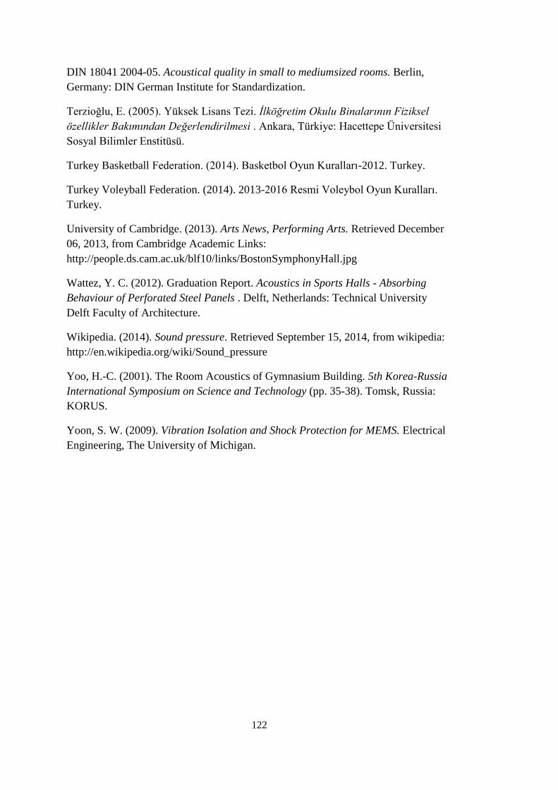
122
DIN 18041 2004-05. Acoustical quality in small to mediumsized rooms. Berlin,
Germany: DIN German Institute for Standardization.
Terzioğlu, E. (2005). Yüksek Lisans Tezi. İlköğretim Okulu Binalarının Fiziksel
özellikler Bakımından Değerlendirilmesi . Ankara, Türkiye: Hacettepe Üniversitesi
Sosyal Bilimler Enstitüsü.
Turkey Basketball Federation. (2014). Basketbol Oyun Kuralları-2012. Turkey.
Turkey Voleyball Federation. (2014). 2013-2016 Resmi Voleybol Oyun Kuralları.
Turkey.
University of Cambridge. (2013). Arts News, Performing Arts. Retrieved December
06, 2013, from Cambridge Academic Links:
http://people.ds.cam.ac.uk/blf10/links/BostonSymphonyHall.jpg
Wattez, Y. C. (2012). Graduation Report. Acoustics in Sports Halls - Absorbing
Behaviour of Perforated Steel Panels . Delft, Netherlands: Technical University
Delft Faculty of Architecture.
Wikipedia. (2014). Sound pressure. Retrieved September 15, 2014, from wikipedia:
http://en.wikipedia.org/wiki/Sound_pressure
Yoo, H.-C. (2001). The Room Acoustics of Gymnasium Building. 5th Korea-Russia
International Symposium on Science and Technology (pp. 35-38). Tomsk, Russia:
KORUS.
Yoon, S. W. (2009). Vibration Isolation and Shock Protection for MEMS. Electrical
Engineering, The University of Michigan.
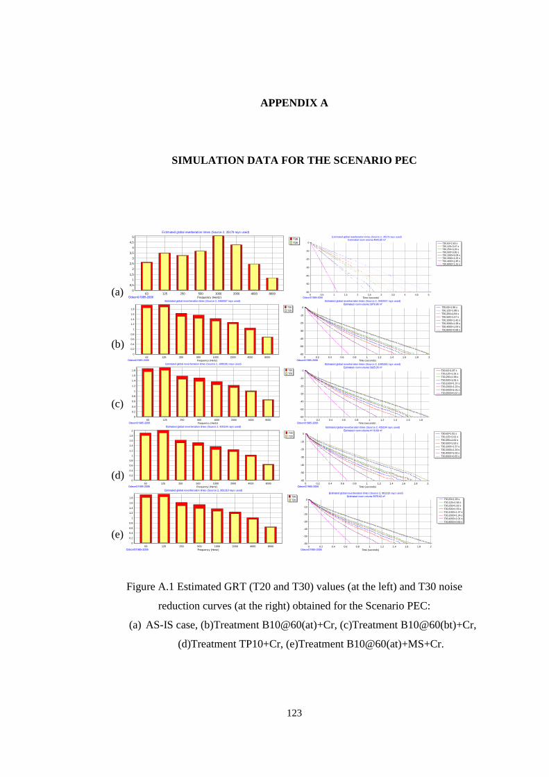
123
APPENDIX A
SIMULATION DATA FOR THE SCENARIO PEC
Figure A.1 Estimated GRT (T20 and T30) values (at the left) and T30 noise
reduction curves (at the right) obtained for the Scenario PEC:
(a) AS-IS case, (b)Treatment B10@60(at)+Cr, (c)Treatment B10@60(bt)+Cr,
(d)Treatment TP10+Cr, (e)Treatment B10@60(at)+MS+Cr.
T30
T20
Estimated global reverberation times (Source 2, 35179 rays used)
Frequency (Hertz)
63 125 250 500 1000 2000 4000 8000
Reverb
era
tion t
ime (
s)
5
4,5
4
3,5
3
2,5
2
1,5
1
0,5
0
Odeon©1985-2006
T30,63=2,63 s
T30,125=3,47 s
T30,250=3,26 s
T30,500=3,65 s
T30,1000=5,08 s
T30,2000=4,25 s
T30,4000=2,45 s
T30,8000=1,15 s
Estimated global reverberation times (Source 2, 35179 rays used)
Estimated room volume:4543,60 m³
Time (seconds)
54,543,532,521,510,50
SP
L (
dB
)
0
-10
-20
-30
-40
-50
-60
Odeon©1985-2006
T30
T20
Estimated global reverberation times (Source 2, 3460007 rays used)
Frequency (Hertz)
63 125 250 500 1000 2000 4000 8000
Reverb
era
tion tim
e (
s)
1.8
1.6
1.4
1.2
1
0.8
0.6
0.4
0.2
0
Odeon©1985-2006
T30,63=1.96 s
T30,125=1.98 s
T30,250=1.64 s
T30,500=1.57 s
T30,1000=1.42 s
T30,2000=1.28 s
T30,4000=1.04 s
T30,8000=0.68 s
Estimated global reverberation times (Source 2, 3460007 rays used)
Estimated room volume:3979.96 m³
Time (seconds)
21.81.61.41.210.80.60.40.20
SP
L (
dB
)
0
-10
-20
-30
-40
-50
-60
Odeon©1985-2006
T30
T20
Estimated global reverberation times (Source 2, 1085281 rays used)
Frequency (Hertz)
63 125 250 500 1000 2000 4000 8000
Reverb
era
tion tim
e (
s)
1.8
1.6
1.4
1.2
1
0.8
0.6
0.4
0.2
0
Odeon©1985-2006
T30,63=1.87 s
T30,125=1.91 s
T30,250=1.58 s
T30,500=1.51 s
T30,1000=1.37 s
T30,2000=1.22 s
T30,4000=1.01 s
T30,8000=0.67 s
Estimated global reverberation times (Source 2, 1085281 rays used)
Estimated room volume:3925.00 m³
Time (seconds)
1.81.61.41.210.80.60.40.20
SP
L (
dB
)
0
-10
-20
-30
-40
-50
-60
Odeon©1985-2006
T30
T20
Estimated global reverberation times (Source 2, 435194 rays used)
Frequency (Hertz)
63 125 250 500 1000 2000 4000 8000
Reverb
era
tion tim
e (
s)
2
1.8
1.6
1.4
1.2
1
0.8
0.6
0.4
0.2
0
Odeon©1985-2006
T30,63=1.91 s
T30,125=2.02 s
T30,250=1.62 s
T30,500=1.53 s
T30,1000=1.37 s
T30,2000=1.24 s
T30,4000=1.03 s
T30,8000=0.65 s
Estimated global reverberation times (Source 2, 435194 rays used)
Estimated room volume:4118.69 m³
Time (seconds)
21.81.61.41.210.80.60.40.20
SP
L (
dB
)
0
-10
-20
-30
-40
-50
-60
Odeon©1985-2006
T30
T20
Estimated global reverberation times (Source 2, 981310 rays used)
Frequency (Hertz)
63 125 250 500 1000 2000 4000 8000
Reverb
era
tion tim
e (
s)
1.8
1.6
1.4
1.2
1
0.8
0.6
0.4
0.2
0
Odeon©1985-2006
T30,63=1.93 s
T30,125=1.94 s
T30,250=1.62 s
T30,500=1.53 s
T30,1000=1.37 s
T30,2000=1.24 s
T30,4000=1.01 s
T30,8000=0.65 s
Estimated global reverberation times (Source 2, 981310 rays used)
Estimated room volume:3979.82 m³
Time (seconds)
21.81.61.41.210.80.60.40.20
SP
L (
dB
)
0
-10
-20
-30
-40
-50
-60
Odeon©1985-2006
(a)
(b)
(c)
(d)
(e)
124
(a)
(b)
(c)
(d)
(e)
Figure A.2 The maps showing the distribution of estimated EDT data at 500Hz (at
the left) and 1000Hz (at the right) together with their cumulative distribution
function graphics for the Scenario PEC:
(a) AS-IS case, (b)Treatment B10@60(at)+Cr, (c)Treatment B10@60(bt)
+Cr, (d)Treatment TP10+Cr, (e)Treatment B10@60(at)+MS+Cr.
P2P2
0,00 5,00 10,00 15,00 20,00 25,00 30,00 35,00 metres
0,00
5,00
10,00
15,00
20,00 metres
7,04
6,40
5,76
5,12
4,48
3,84
3,20
2,56
1,92
1,28
0,64
EDT at 500 Hz > 8,00
< 0,08Odeon©1985-2006
Cumulative distribution function
X(5,95) = (3,43, 4,00) X(10,90) = (3,54, 3,93) X(25,75) = (3,64, 3,84) X(50) = (3,74)
X(95)-X(5) = 0,57 X(90)-X(10) = 0,39 X(75)-X(25) = 0,19
EDT (s) at 500 Hz
43,953,93,853,83,753,73,653,63,553,53,45
Perc
ent
90
80
70
60
50
40
30
20
10
Odeon©1985-2006
P2P2
0,00 5,00 10,00 15,00 20,00 25,00 30,00 35,00 metres
0,00
5,00
10,00
15,00
20,00 metres
7,04
6,40
5,76
5,12
4,48
3,84
3,20
2,56
1,92
1,28
0,64
EDT at 1000 Hz > 8,00
< 0,08Odeon©1985-2006
Cumulative distribution function
X(5,95) = (4,82, 5,39) X(10,90) = (4,96, 5,35) X(25,75) = (5,07, 5,27) X(50) = (5,18)
X(95)-X(5) = 0,57 X(90)-X(10) = 0,39 X(75)-X(25) = 0,20
EDT (s) at 1000 Hz
5,355,35,255,25,155,15,0554,954,94,85
Perc
ent
90
80
70
60
50
40
30
20
10
Odeon©1985-2006
P2P2
0.00 5.00 10.00 15.00 20.00 25.00 metres
0.00
5.00
10.00
15.00 metres
2.25
2.13
2.00
1.88
1.75
1.63
1.50
1.38
1.25
1.13
1.00
0.88
0.75
0.63
0.50
0.38
0.25
0.13
EDT at 500 Hz > 2.50
< 0.03Odeon©1985-2006
Cumulative distribution function
X(5,95) = (0.65, 1.65) X(10,90) = (0.81, 1.49) X(25,75) = (0.98, 1.33) X(50) = (1.12)
X(95)-X(5) = 1.00 X(90)-X(10) = 0.69 X(75)-X(25) = 0.35
EDT (s) at 500 Hz
3.63.43.232.82.62.42.221.81.61.41.210.80.60.40.2
Perc
ent
100
95
90
85
80
75
70
65
60
55
50
45
40
35
30
25
20
15
10
5
Odeon©1985-2006
P2P2
0.00 5.00 10.00 15.00 20.00 25.00 metres
0.00
5.00
10.00
15.00 metres
2.25
2.13
2.00
1.88
1.75
1.63
1.50
1.38
1.25
1.13
1.00
0.88
0.75
0.63
0.50
0.38
0.25
0.13
EDT at 1000 Hz > 2.50
< 0.03Odeon©1985-2006
Cumulative distribution function
X(5,95) = (0.66, 1.64) X(10,90) = (0.84, 1.52) X(25,75) = (0.99, 1.36) X(50) = (1.15)
X(95)-X(5) = 0.98 X(90)-X(10) = 0.69 X(75)-X(25) = 0.37
EDT (s) at 1000 Hz
3.232.82.62.42.221.81.61.41.210.80.60.40.2
Perc
ent
100
95
90
85
80
75
70
65
60
55
50
45
40
35
30
25
20
15
10
5
Odeon©1985-2006
P2P2
0.00 5.00 10.00 15.00 20.00 25.00 metres
0.00
5.00
10.00
15.00 metres
2.25
2.13
2.00
1.88
1.75
1.63
1.50
1.38
1.25
1.13
1.00
0.88
0.75
0.63
0.50
0.38
0.25
0.13
EDT at 500 Hz > 2.50
< 0.03Odeon©1985-2006
Cumulative distribution function
X(5,95) = (0.61, 1.54) X(10,90) = (0.74, 1.42) X(25,75) = (0.92, 1.24) X(50) = (1.04)
X(95)-X(5) = 0.93 X(90)-X(10) = 0.68 X(75)-X(25) = 0.32
EDT (s) at 500 Hz
24222018161412108642
Perc
ent
100
95
90
85
80
75
70
65
60
55
50
45
40
35
30
25
20
15
10
5
Odeon©1985-2006
P2P2
0.00 5.00 10.00 15.00 20.00 25.00 metres
0.00
5.00
10.00
15.00 metres
2.25
2.13
2.00
1.88
1.75
1.63
1.50
1.38
1.25
1.13
1.00
0.88
0.75
0.63
0.50
0.38
0.25
0.13
EDT at 1000 Hz > 2.50
< 0.03Odeon©1985-2006
Cumulative distribution function
X(5,95) = (0.63, 1.57) X(10,90) = (0.75, 1.43) X(25,75) = (0.92, 1.24) X(50) = (1.03)
X(95)-X(5) = 0.94 X(90)-X(10) = 0.68 X(75)-X(25) = 0.32
EDT (s) at 1000 Hz
24222018161412108642
Perc
ent
100
95
90
85
80
75
70
65
60
55
50
45
40
35
30
25
20
15
10
5
Odeon©1985-2006
P2P2
0.00 5.00 10.00 15.00 20.00 25.00 metres
0.00
5.00
10.00
15.00 metres
2.70
2.55
2.40
2.25
2.10
1.95
1.80
1.65
1.50
1.35
1.20
1.05
0.90
0.75
0.60
0.45
0.30
0.15
EDT at 500 Hz > 3.00
< 0.03Odeon©1985-2006
Cumulative distribution function
X(5,95) = (0.46, 1.99) X(10,90) = (0.57, 1.48) X(25,75) = (0.78, 1.00) X(50) = (0.88)
X(95)-X(5) = 1.53 X(90)-X(10) = 0.90 X(75)-X(25) = 0.22
EDT (s) at 500 Hz
3230282624222018161412108642
Perc
ent
100
95
90
85
80
75
70
65
60
55
50
45
40
35
30
25
20
15
10
5
Odeon©1985-2006
P2P2
0.00 5.00 10.00 15.00 20.00 25.00 metres
0.00
5.00
10.00
15.00 metres
2.70
2.55
2.40
2.25
2.10
1.95
1.80
1.65
1.50
1.35
1.20
1.05
0.90
0.75
0.60
0.45
0.30
0.15
EDT at 1000 Hz > 3.00
< 0.03Odeon©1985-2006
Cumulative distribution function
X(5,95) = (0.45, 1.87) X(10,90) = (0.55, 1.32) X(25,75) = (0.76, 0.96) X(50) = (0.86)
X(95)-X(5) = 1.42 X(90)-X(10) = 0.77 X(75)-X(25) = 0.20
EDT (s) at 1000 Hz
3230282624222018161412108642
Perc
ent
100
95
90
85
80
75
70
65
60
55
50
45
40
35
30
25
20
15
10
5
Odeon©1985-2006
P2P2
0.00 5.00 10.00 15.00 20.00 metres
0.00
5.00
10.00
15.00
20.00 metres
2.25
2.13
2.00
1.88
1.75
1.63
1.50
1.38
1.25
1.13
1.00
0.88
0.75
0.63
0.50
0.38
0.25
0.13
EDT at 500 Hz > 2.50
< 0.03Odeon©1985-2006
Cumulative distribution function
X(5,95) = (0.60, 1.69) X(10,90) = (0.72, 1.50) X(25,75) = (0.89, 1.29) X(50) = (1.02)
X(95)-X(5) = 1.09 X(90)-X(10) = 0.78 X(75)-X(25) = 0.40
EDT (s) at 500 Hz
54.543.532.521.510.5
Perc
ent
100
95
90
85
80
75
70
65
60
55
50
45
40
35
30
25
20
15
10
5
Odeon©1985-2006
P2P2
0.00 5.00 10.00 15.00 20.00 metres
0.00
5.00
10.00
15.00
20.00 metres
2.25
2.13
2.00
1.88
1.75
1.63
1.50
1.38
1.25
1.13
1.00
0.88
0.75
0.63
0.50
0.38
0.25
0.13
EDT at 1000 Hz > 2.50
< 0.03Odeon©1985-2006
Cumulative distribution function
X(5,95) = (0.61, 1.66) X(10,90) = (0.74, 1.51) X(25,75) = (0.90, 1.30) X(50) = (1.03)
X(95)-X(5) = 1.05 X(90)-X(10) = 0.77 X(75)-X(25) = 0.40
EDT (s) at 1000 Hz
3.63.43.232.82.62.42.221.81.61.41.210.80.60.40.2
Perc
ent
100
95
90
85
80
75
70
65
60
55
50
45
40
35
30
25
20
15
10
5
Odeon©1985-2006

125
(a)
(b)
(c)
(d)
(e)
Figure A.3 The maps showing the estimated T30 data at 500Hz (at the left) and
1000Hz (at the right) together with their cumulative distribution function graphics for
the Scenario PEC, :(a)AS-IS case, (b) Treatment B10@60(at)+Cr, (c) Treatment
B10@60(bt) +Cr, (d) Treatment TP10+Cr, (e) Treatment B10@60(at)+MS+Cr.
P2P2
0,00 5,00 10,00 15,00 20,00 25,00 30,00 35,00 metres
0,00
5,00
10,00
15,00
20,00 metres
7,04
6,40
5,76
5,12
4,48
3,84
3,20
2,56
1,92
1,28
0,64
T30 at 500 Hz > 8,00
< 0,08Odeon©1985-2006
Cumulative distribution function
X(5,95) = (3,50, 3,74) X(10,90) = (3,53, 3,71) X(25,75) = (3,57, 3,67) X(50) = (3,62)
X(95)-X(5) = 0,24 X(90)-X(10) = 0,18 X(75)-X(25) = 0,10
T30 (s) at 500 Hz
3,743,723,73,683,663,643,623,63,583,563,543,52
Perc
ent
90
80
70
60
50
40
30
20
10
Odeon©1985-2006
P2P2
0,00 5,00 10,00 15,00 20,00 25,00 30,00 35,00 metres
0,00
5,00
10,00
15,00
20,00 metres
7,04
6,40
5,76
5,12
4,48
3,84
3,20
2,56
1,92
1,28
0,64
T30 at 1000 Hz > 8,00
< 0,08Odeon©1985-2006
Cumulative distribution function
X(5,95) = (4,94, 5,19) X(10,90) = (4,97, 5,16) X(25,75) = (5,02, 5,12) X(50) = (5,07)
X(95)-X(5) = 0,24 X(90)-X(10) = 0,18 X(75)-X(25) = 0,10
T30 (s) at 1000 Hz
5,185,165,145,125,15,085,065,045,0254,984,96
Perc
ent
90
80
70
60
50
40
30
20
10
Odeon©1985-2006
P2P2
0.00 5.00 10.00 15.00 20.00 25.00 metres
0.00
5.00
10.00
15.00 metres
3.60
3.40
3.20
3.00
2.80
2.60
2.40
2.20
2.00
1.80
1.60
1.40
1.20
1.00
0.80
0.60
0.40
0.20
T30 at 500 Hz > 4.00
< 0.04Odeon©1985-2006
Cumulative distribution function
X(5,95) = (1.15, 2.15) X(10,90) = (1.23, 1.90) X(25,75) = (1.33, 1.68) X(50) = (1.47)
X(95)-X(5) = 1.00 X(90)-X(10) = 0.67 X(75)-X(25) = 0.34
T30 (s) at 500 Hz
54.543.532.521.510.5
Perc
ent
100
95
90
85
80
75
70
65
60
55
50
45
40
35
30
25
20
15
10
5
Odeon©1985-2006
P2P2
0.00 5.00 10.00 15.00 20.00 25.00 metres
0.00
5.00
10.00
15.00 metres
3.60
3.40
3.20
3.00
2.80
2.60
2.40
2.20
2.00
1.80
1.60
1.40
1.20
1.00
0.80
0.60
0.40
0.20
T30 at 1000 Hz > 4.00
< 0.04Odeon©1985-2006
Cumulative distribution function
X(5,95) = (1.01, 2.05) X(10,90) = (1.07, 1.76) X(25,75) = (1.14, 1.56) X(50) = (1.29)
X(95)-X(5) = 1.04 X(90)-X(10) = 0.70 X(75)-X(25) = 0.41
T30 (s) at 1000 Hz
6.565.554.543.532.521.510.50
Perc
ent
100
95
90
85
80
75
70
65
60
55
50
45
40
35
30
25
20
15
10
5
Odeon©1985-2006
P2P2
0.00 5.00 10.00 15.00 20.00 25.00 metres
0.00
5.00
10.00
15.00 metres
3.60
3.40
3.20
3.00
2.80
2.60
2.40
2.20
2.00
1.80
1.60
1.40
1.20
1.00
0.80
0.60
0.40
0.20
T30 at 500 Hz > 4.00
< 0.04Odeon©1985-2006
Cumulative distribution function
X(5,95) = (1.45, 3.73) X(10,90) = (1.52, 2.46) X(25,75) = (1.62, 1.91) X(50) = (1.73)
X(95)-X(5) = 2.28 X(90)-X(10) = 0.94 X(75)-X(25) = 0.29
T30 (s) at 500 Hz
87.576.565.554.543.532.521.510.50
Perc
ent
100
95
90
85
80
75
70
65
60
55
50
45
40
35
30
25
20
15
10
5
Odeon©1985-2006
P2P2
0.00 5.00 10.00 15.00 20.00 25.00 metres
0.00
5.00
10.00
15.00 metres
3.60
3.40
3.20
3.00
2.80
2.60
2.40
2.20
2.00
1.80
1.60
1.40
1.20
1.00
0.80
0.60
0.40
0.20
T30 at 1000 Hz > 4.00
< 0.04Odeon©1985-2006
Cumulative distribution function
X(5,95) = (1.10, 4.11) X(10,90) = (1.41, 2.46) X(25,75) = (1.52, 1.87) X(50) = (1.63)
X(95)-X(5) = 3.01 X(90)-X(10) = 1.05 X(75)-X(25) = 0.35
T30 (s) at 1000 Hz
109876543210
Perc
ent
100
95
90
85
80
75
70
65
60
55
50
45
40
35
30
25
20
15
10
5
Odeon©1985-2006
P2P2
0.00 5.00 10.00 15.00 20.00 25.00 metres
0.00
5.00
10.00
15.00 metres
2.70
2.55
2.40
2.25
2.10
1.95
1.80
1.65
1.50
1.35
1.20
1.05
0.90
0.75
0.60
0.45
0.30
0.15
T30 at 500 Hz > 3.00
< 0.03Odeon©1985-2006
Cumulative distribution function
X(5,95) = (0.96, 1.73) X(10,90) = (1.02, 1.61) X(25,75) = (1.14, 1.46) X(50) = (1.29)
X(95)-X(5) = 0.77 X(90)-X(10) = 0.59 X(75)-X(25) = 0.32
T30 (s) at 500 Hz
3.232.82.62.42.221.81.61.41.210.80.60.40.20
Perc
ent
100
95
90
85
80
75
70
65
60
55
50
45
40
35
30
25
20
15
10
5
Odeon©1985-2006
P2P2
0.00 5.00 10.00 15.00 20.00 25.00 metres
0.00
5.00
10.00
15.00 metres
2.70
2.55
2.40
2.25
2.10
1.95
1.80
1.65
1.50
1.35
1.20
1.05
0.90
0.75
0.60
0.45
0.30
0.15
T30 at 1000 Hz > 3.00
< 0.03Odeon©1985-2006
Cumulative distribution function
X(5,95) = (0.91, 1.69) X(10,90) = (0.97, 1.53) X(25,75) = (1.08, 1.38) X(50) = (1.22)
X(95)-X(5) = 0.77 X(90)-X(10) = 0.55 X(75)-X(25) = 0.31
T30 (s) at 1000 Hz
3.232.82.62.42.221.81.61.41.210.80.60.4
Perc
ent
100
95
90
85
80
75
70
65
60
55
50
45
40
35
30
25
20
15
10
5
Odeon©1985-2006
P2P2
0,00 5,00 10,00 15,00 20,00 metres
0,00
5,00
10,00
15,00
20,00 metres
2,25
2,10
1,95
1,80
1,65
1,50
1,35
1,20
1,05
0,90
0,75
0,60
0,45
0,30
0,15
T30 at 500 Hz > 2,50
< 0,03Odeon©1985-2006
Cumulative distribution function
X(5,95) = (1,18, 1,73) X(10,90) = (1,26, 1,66) X(25,75) = (1,36, 1,56) X(50) = (1,45)
X(95)-X(5) = 0,54 X(90)-X(10) = 0,40 X(75)-X(25) = 0,20
T30 (s) at 500 Hz
2,221,81,61,41,210,80,60,40,2
Perc
ent
100
95
90
85
80
75
70
65
60
55
50
45
40
35
30
25
20
15
10
5
Odeon©1985-2006
P2P2
0,00 5,00 10,00 15,00 20,00 metres
0,00
5,00
10,00
15,00
20,00 metres
2,25
2,10
1,95
1,80
1,65
1,50
1,35
1,20
1,05
0,90
0,75
0,60
0,45
0,30
0,15
T30 at 1000 Hz > 2,50
< 0,03Odeon©1985-2006
Cumulative distribution function
X(5,95) = (1,14, 1,71) X(10,90) = (1,22, 1,64) X(25,75) = (1,30, 1,48) X(50) = (1,38)
X(95)-X(5) = 0,57 X(90)-X(10) = 0,42 X(75)-X(25) = 0,19
T30 (s) at 1000 Hz
2,221,81,61,41,210,80,60,4
Perc
ent
100
95
90
85
80
75
70
65
60
55
50
45
40
35
30
25
20
15
10
5
Odeon©1985-2006
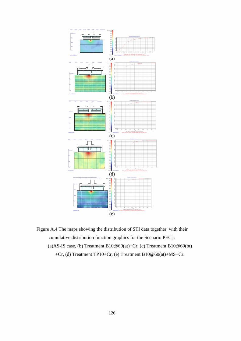
126
(a)
(b)
(c)
(d)
(e)
Figure A.4 The maps showing the distribution of STI data together with their
cumulative distribution function graphics for the Scenario PEC, :
(a)AS-IS case, (b) Treatment B10@60(at)+Cr, (c) Treatment B10@60(bt)
+Cr, (d) Treatment TP10+Cr, (e) Treatment B10@60(at)+MS+Cr.
P2P2
0,00 5,00 10,00 15,00 20,00 25,00 30,00 35,00 metres
0,00
5,00
10,00
15,00
20,00 metres
0,88
0,80
0,72
0,64
0,56
0,48
0,40
0,32
0,24
0,16
0,08
STI > 1,00
< 0,01Odeon©1985-2006
Cumulative distribution function
X(5,95) = (0,33, 0,49) X(10,90) = (0,33, 0,44) X(25,75) = (0,35, 0,39) X(50) = (0,36)
X(95)-X(5) = 0,16 X(90)-X(10) = 0,10 X(75)-X(25) = 0,04
STI
0,480,470,460,450,440,430,420,410,40,390,380,370,360,350,340,33
Perc
ent
90
80
70
60
50
40
30
20
10
Odeon©1985-2006
P2P2
0.00 5.00 10.00 15.00 20.00 25.00 metres
0.00
5.00
10.00
15.00 metres
0.90
0.85
0.80
0.75
0.70
0.65
0.60
0.55
0.50
0.45
0.40
0.35
0.30
0.25
0.20
0.15
0.10
0.05
STI > 1.00
< 0.01Odeon©1985-2006
Cumulative distribution function
X(5,95) = (0.56, 0.73) X(10,90) = (0.56, 0.67) X(25,75) = (0.57, 0.61) X(50) = (0.59)
X(95)-X(5) = 0.17 X(90)-X(10) = 0.11 X(75)-X(25) = 0.04
STI
10.950.90.850.80.750.70.650.60.55
Perc
ent
100
95
90
85
80
75
70
65
60
55
50
45
40
35
30
25
20
15
10
5
Odeon©1985-2006
P2P2
0.00 5.00 10.00 15.00 20.00 25.00 metres
0.00
5.00
10.00
15.00 metres
0.90
0.85
0.80
0.75
0.70
0.65
0.60
0.55
0.50
0.45
0.40
0.35
0.30
0.25
0.20
0.15
0.10
0.05
STI > 1.00
< 0.01Odeon©1985-2006
Cumulative distribution function
X(5,95) = (0.57, 0.74) X(10,90) = (0.58, 0.68) X(25,75) = (0.59, 0.63) X(50) = (0.61)
X(95)-X(5) = 0.17 X(90)-X(10) = 0.10 X(75)-X(25) = 0.04
STI
10.950.90.850.80.750.70.650.60.55
Perc
ent
100
95
90
85
80
75
70
65
60
55
50
45
40
35
30
25
20
15
10
5
Odeon©1985-2006
P2P2
0.00 5.00 10.00 15.00 20.00 25.00 metres
0.00
5.00
10.00
15.00 metres
0.90
0.85
0.80
0.75
0.70
0.65
0.60
0.55
0.50
0.45
0.40
0.35
0.30
0.25
0.20
0.15
0.10
0.05
STI > 1.00
< 0.01Odeon©1985-2006
Cumulative distribution function
X(5,95) = (0.58, 0.78) X(10,90) = (0.59, 0.73) X(25,75) = (0.61, 0.66) X(50) = (0.63)
X(95)-X(5) = 0.20 X(90)-X(10) = 0.13 X(75)-X(25) = 0.05
STI
10.950.90.850.80.750.70.650.60.55
Perc
ent
100
95
90
85
80
75
70
65
60
55
50
45
40
35
30
25
20
15
10
5
Odeon©1985-2006
P2P2
0.00 5.00 10.00 15.00 20.00 metres
0.00
5.00
10.00
15.00
20.00 metres
87.0
85.5
84.0
82.5
81.0
79.5
78.0
76.5
75.0
73.5
72.0
70.5
69.0
67.5
66.0
64.5
63.0
61.5
SPL(A) > 90.0
< 60.3Odeon©1985-2006
Cumulative distribution function
X(5,95) = (0.57, 0.75) X(10,90) = (0.57, 0.69) X(25,75) = (0.59, 0.63) X(50) = (0.61)
X(95)-X(5) = 0.18 X(90)-X(10) = 0.12 X(75)-X(25) = 0.04
STI
10.950.90.850.80.750.70.650.60.55
Perc
ent
100
95
90
85
80
75
70
65
60
55
50
45
40
35
30
25
20
15
10
5
Odeon©1985-2006

127
(a)
(b)
(c)
(d)
(e)
Figure A.5 The maps showing the distribution of estimated SPL(A) data together
with their cumulative distribution function graphics for the Scenario PEC:
(a)AS-IS case, (b) Treatment B10@60(at)+Cr, (c) Treatment B10@60(bt)
+Cr, (d) Treatment TP10+Cr, (e) Treatment B10@60(at)+MS+Cr.
P2P2
0,00 5,00 10,00 15,00 20,00 25,00 30,00 35,00 metres
0,00
5,00
10,00
15,00
20,00 metres
94,0
90,0
86,0
82,0
78,0
74,0
70,0
66,0
62,0
58,0
54,0
SPL(A) > 100,0
< 50,5Odeon©1985-2006
Cumulative distribution function
X(5,95) = (75,9, 78,5) X(10,90) = (76,1, 77,7) X(25,75) = (76,3, 76,9) X(50) = (76,6)
X(95)-X(5) = 2,6 X(90)-X(10) = 1,6 X(75)-X(25) = 0,6
SPL(A) (dB)
78,478,27877,877,677,477,27776,876,676,476,276
Perc
ent
90
80
70
60
50
40
30
20
10
Odeon©1985-2006
P2P2
0.00 5.00 10.00 15.00 20.00 25.00 metres
0.00
5.00
10.00
15.00 metres
87.0
85.5
84.0
82.5
81.0
79.5
78.0
76.5
75.0
73.5
72.0
70.5
69.0
67.5
66.0
64.5
63.0
61.5
SPL(A) > 90.0
< 60.3Odeon©1985-2006
Cumulative distribution function
X(5,95) = (68.3, 75.6) X(10,90) = (68.7, 73.6) X(25,75) = (69.5, 71.6) X(50) = (70.2)
X(95)-X(5) = 7.3 X(90)-X(10) = 4.9 X(75)-X(25) = 2.1
SPL(A) (dB)
98969492908886848280787674727068
Perc
ent
100
95
90
85
80
75
70
65
60
55
50
45
40
35
30
25
20
15
10
5
Odeon©1985-2006
P2P2
0.00 5.00 10.00 15.00 20.00 25.00 metres
0.00
5.00
10.00
15.00 metres
86.5
84.8
83.0
81.3
79.5
77.8
76.0
74.3
72.5
70.8
69.0
67.3
65.5
63.8
62.0
60.3
58.5
56.8
SPL(A) > 90.0
< 55.4Odeon©1985-2006
Cumulative distribution function
X(5,95) = (67.9, 75.4) X(10,90) = (68.2, 73.4) X(25,75) = (68.8, 71.3) X(50) = (69.7)
X(95)-X(5) = 7.5 X(90)-X(10) = 5.2 X(75)-X(25) = 2.5
SPL(A) (dB)
98969492908886848280787674727068
Perc
ent
100
95
90
85
80
75
70
65
60
55
50
45
40
35
30
25
20
15
10
5
Odeon©1985-2006
P2P2
0.00 5.00 10.00 15.00 20.00 25.00 metres
0.00
5.00
10.00
15.00 metres
85.0
82.5
80.0
77.5
75.0
72.5
70.0
67.5
65.0
62.5
60.0
57.5
55.0
52.5
50.0
47.5
45.0
42.5
SPL(A) > 90.0
< 40.5Odeon©1985-2006
Cumulative distribution function
X(5,95) = (66.8, 74.9) X(10,90) = (67.2, 72.7) X(25,75) = (67.8, 70.1) X(50) = (68.7)
X(95)-X(5) = 8.1 X(90)-X(10) = 5.5 X(75)-X(25) = 2.3
SPL(A) (dB)
9896949290888684828078767472706866
Perc
ent
100
95
90
85
80
75
70
65
60
55
50
45
40
35
30
25
20
15
10
5
Odeon©1985-2006
P2P2
0.00 5.00 10.00 15.00 20.00 metres
0.00
5.00
10.00
15.00
20.00 metres
0.90
0.85
0.80
0.75
0.70
0.65
0.60
0.55
0.50
0.45
0.40
0.35
0.30
0.25
0.20
0.15
0.10
0.05
STI > 1.00
< 0.01Odeon©1985-2006
Cumulative distribution function
X(5,95) = (67.9, 75.2) X(10,90) = (68.3, 73.3) X(25,75) = (69.0, 71.1) X(50) = (69.7)
X(95)-X(5) = 7.3 X(90)-X(10) = 5.0 X(75)-X(25) = 2.1
SPL(A) (dB)
9896949290888684828078767472706866
Perc
ent
100
95
90
85
80
75
70
65
60
55
50
45
40
35
30
25
20
15
10
5
Odeon©1985-2006

128

129
APPENDIX B
SIMULATION DATA FOR THE SCENARIO SG-p
(a)
(b)
(c)
(d)
(e)
Figure B.1 Estimated GRT (T20 and T30) values (at the left) and T30 noise
reduction curves (at the right) obtained for the SG-p scenario:
(a) AS-IS case, (b) Treatment B10@60(at), (c)Treatment B10@60(bt), (d)
Treatment TP10, (e) Treatment B10@60(at)+MS
T30
T20
Estimated global reverberation times (Source 1, 24540 rays used)
Frequency (Hertz)
63 125 250 500 1000 2000 4000 8000
Reverb
era
tion t
ime (
s)
4,5
4
3,5
3
2,5
2
1,5
1
0,5
0
Odeon©1985-2006
T30,63=2,52 s
T30,125=3,35 s
T30,250=3,08 s
T30,500=3,49 s
T30,1000=4,66 s
T30,2000=3,92 s
T30,4000=2,34 s
T30,8000=1,13 s
Estimated global reverberation times (Source 1, 24540 rays used)
Estimated room volume:4625,68 m³
Time (seconds)
4,64,44,243,83,63,43,232,82,62,42,221,81,61,41,210,80,60,40,20
SP
L (
dB
)
0
-10
-20
-30
-40
-50
-60
Odeon©1985-2006
T30
T20
Estimated global reverberation times (Source 1, 903899 rays used)
Frequency (Hertz)
63 125 250 500 1000 2000 4000 8000
Reverb
era
tion tim
e (
s)
1.8
1.6
1.4
1.2
1
0.8
0.6
0.4
0.2
0
Odeon©1985-2006
T30,63=1.84 s
T30,125=1.93 s
T30,250=1.78 s
T30,500=1.76 s
T30,1000=1.67 s
T30,2000=1.51 s
T30,4000=1.21 s
T30,8000=0.74 s
Estimated global reverberation times (Source 1, 903899 rays used)
Estimated room volume:3992.47 m³
Time (seconds)
2.221.81.61.41.210.80.60.40.20
SP
L (
dB
)
0
-10
-20
-30
-40
-50
-60
Odeon©1985-2006
T30
T20
Estimated global reverberation times (Source 1, 1345354 rays used)
Frequency (Hertz)
63 125 250 500 1000 2000 4000 8000
Reverb
era
tion tim
e (
s)
1.8
1.6
1.4
1.2
1
0.8
0.6
0.4
0.2
0
Odeon©1985-2006
T30,63=1.75 s
T30,125=1.82 s
T30,250=1.71 s
T30,500=1.67 s
T30,1000=1.57 s
T30,2000=1.44 s
T30,4000=1.17 s
T30,8000=0.74 s
Estimated global reverberation times (Source 1, 1345354 rays used)
Estimated room volume:3941.33 m³
Time (seconds)
1.81.61.41.210.80.60.40.20
SP
L (
dB
)
0
-10
-20
-30
-40
-50
-60
Odeon©1985-2006
T30
T20
Estimated global reverberation times (Source 1, 661670 rays used)
Frequency (Hertz)
63 125 250 500 1000 2000 4000 8000
Reverb
era
tion tim
e (
s)
2
1.8
1.6
1.4
1.2
1
0.8
0.6
0.4
0.2
0
Odeon©1985-2006
T30,63=1.94 s
T30,125=2.09 s
T30,250=1.76 s
T30,500=1.75 s
T30,1000=1.66 s
T30,2000=1.53 s
T30,4000=1.24 s
T30,8000=0.74 s
Estimated global reverberation times (Source 1, 661670 rays used)
Estimated room volume:4144.45 m³
Time (seconds)
21.81.61.41.210.80.60.40.20
SP
L (
dB
)
0
-10
-20
-30
-40
-50
-60
Odeon©1985-2006
T30
T20
Estimated global reverberation times (Source 1, 1990540 rays used)
Frequency (Hertz)
63 125 250 500 1000 2000 4000 8000
Reverb
era
tion tim
e (
s)
1.8
1.6
1.4
1.2
1
0.8
0.6
0.4
0.2
0
Odeon©1985-2006
T30,63=1.80 s
T30,125=1.89 s
T30,250=1.73 s
T30,500=1.67 s
T30,1000=1.58 s
T30,2000=1.46 s
T30,4000=1.19 s
T30,8000=0.72 s
Estimated global reverberation times (Source 1, 1990540 rays used)
Estimated room volume:3994.62 m³
Time (seconds)
1.81.61.41.210.80.60.40.20
SP
L (
dB
)
0
-10
-20
-30
-40
-50
-60
Odeon©1985-2006
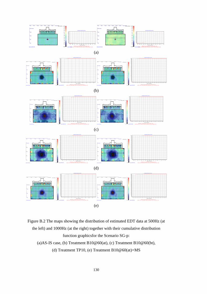
130
(a)
(b)
(c)
(d)
(e)
Figure B.2 The maps showing the distribution of estimated EDT data at 500Hz (at
the left) and 1000Hz (at the right) together with their cumulative distribution
function graphicsfor the Scenario SG-p:
(a)AS-IS case, (b) Treatment B10@60(at), (c) Treatment B10@60(bt),
(d) Treatment TP10, (e) Treatment B10@60(at)+MS
P1P1
0,00 5,00 10,00 15,00 20,00 25,00 30,00 35,00 metres
0,00
5,00
10,00
15,00
20,00 metres
7,04
6,40
5,76
5,12
4,48
3,84
3,20
2,56
1,92
1,28
0,64
EDT at 500 Hz > 8,00
< 0,08Odeon©1985-2006
Cumulative distribution function
X(5,95) = (3,17, 3,77) X(10,90) = (3,29, 3,69) X(25,75) = (3,40, 3,60) X(50) = (3,50)
X(95)-X(5) = 0,60 X(90)-X(10) = 0,41 X(75)-X(25) = 0,20
EDT (s) at 500 Hz
3,753,73,653,63,553,53,453,43,353,33,253,2
Perc
ent
90
80
70
60
50
40
30
20
10
Odeon©1985-2006
P1P1
0,00 5,00 10,00 15,00 20,00 25,00 30,00 35,00 metres
0,00
5,00
10,00
15,00
20,00 metres
7,04
6,40
5,76
5,12
4,48
3,84
3,20
2,56
1,92
1,28
0,64
EDT at 1000 Hz > 8,00
< 0,08Odeon©1985-2006
Cumulative distribution function
X(5,95) = (4,38, 5,05) X(10,90) = (4,48, 4,99) X(25,75) = (4,63, 4,89) X(50) = (4,76)
X(95)-X(5) = 0,68 X(90)-X(10) = 0,51 X(75)-X(25) = 0,26
EDT (s) at 1000 Hz
5,0554,954,94,854,84,754,74,654,64,554,54,454,4
Perc
ent
90
80
70
60
50
40
30
20
10
Odeon©1985-2006
P1P1
0.00 5.00 10.00 15.00 20.00 25.00 metres
0.00
5.00
10.00
15.00
20.00 metres
2.70
2.55
2.40
2.25
2.10
1.95
1.80
1.65
1.50
1.35
1.20
1.05
0.90
0.75
0.60
0.45
0.30
0.15
EDT at 500 Hz > 3.00
< 0.03Odeon©1985-2006
Cumulative distribution function
X(5,95) = (0.78, 1.88) X(10,90) = (0.95, 1.61) X(25,75) = (1.07, 1.43) X(50) = (1.29)
X(95)-X(5) = 1.10 X(90)-X(10) = 0.66 X(75)-X(25) = 0.37
EDT (s) at 500 Hz
18161412108642
Perc
ent
100
95
90
85
80
75
70
65
60
55
50
45
40
35
30
25
20
15
10
5
Odeon©1985-2006
P1P1
0.00 5.00 10.00 15.00 20.00 25.00 metres
0.00
5.00
10.00
15.00
20.00 metres
2.70
2.55
2.40
2.25
2.10
1.95
1.80
1.65
1.50
1.35
1.20
1.05
0.90
0.75
0.60
0.45
0.30
0.15
EDT at 1000 Hz > 3.00
< 0.03Odeon©1985-2006
Cumulative distribution function
X(5,95) = (0.81, 1.80) X(10,90) = (0.95, 1.58) X(25,75) = (1.07, 1.42) X(50) = (1.28)
X(95)-X(5) = 0.99 X(90)-X(10) = 0.63 X(75)-X(25) = 0.36
EDT (s) at 1000 Hz
181716151413121110987654321
Perc
ent
100
95
90
85
80
75
70
65
60
55
50
45
40
35
30
25
20
15
10
5
Odeon©1985-2006
P1P1
0.00 5.00 10.00 15.00 20.00 25.00 metres
0.00
5.00
10.00
15.00
20.00 metres
3.60
3.40
3.20
3.00
2.80
2.60
2.40
2.20
2.00
1.80
1.60
1.40
1.20
1.00
0.80
0.60
0.40
0.20
EDT at 500 Hz > 4.00
< 0.04Odeon©1985-2006
Cumulative distribution function
X(5,95) = (0.60, 1.76) X(10,90) = (0.83, 1.59) X(25,75) = (1.01, 1.40) X(50) = (1.22)
X(95)-X(5) = 1.15 X(90)-X(10) = 0.76 X(75)-X(25) = 0.38
EDT (s) at 500 Hz
7.576.565.554.543.532.521.510.5
Perc
ent
100
95
90
85
80
75
70
65
60
55
50
45
40
35
30
25
20
15
10
5
Odeon©1985-2006
P1P1
0.00 5.00 10.00 15.00 20.00 25.00 metres
0.00
5.00
10.00
15.00
20.00 metres
3.60
3.40
3.20
3.00
2.80
2.60
2.40
2.20
2.00
1.80
1.60
1.40
1.20
1.00
0.80
0.60
0.40
0.20
EDT at 1000 Hz > 4.00
< 0.04Odeon©1985-2006
Cumulative distribution function
X(5,95) = (0.65, 1.67) X(10,90) = (0.89, 1.55) X(25,75) = (1.04, 1.40) X(50) = (1.25)
X(95)-X(5) = 1.03 X(90)-X(10) = 0.66 X(75)-X(25) = 0.36
EDT (s) at 1000 Hz
8.587.576.565.554.543.532.521.510.5
Perc
ent
100
95
90
85
80
75
70
65
60
55
50
45
40
35
30
25
20
15
10
5
Odeon©1985-2006
P1P1
0.00 5.00 10.00 15.00 20.00 25.00 metres
0.00
5.00
10.00
15.00
20.00 metres
3.15
2.97
2.80
2.63
2.45
2.28
2.10
1.92
1.75
1.58
1.40
1.23
1.05
0.88
0.70
0.52
0.35
0.17
EDT at 500 Hz > 3.50
< 0.04Odeon©1985-2006
Cumulative distribution function
X(5,95) = (0.47, 2.20) X(10,90) = (0.62, 1.96) X(25,75) = (0.93, 1.67) X(50) = (1.35)
X(95)-X(5) = 1.73 X(90)-X(10) = 1.34 X(75)-X(25) = 0.74
EDT (s) at 500 Hz
98.587.576.565.554.543.532.521.510.5
Perc
ent
100
95
90
85
80
75
70
65
60
55
50
45
40
35
30
25
20
15
10
5
Odeon©1985-2006
P1P1
0.00 5.00 10.00 15.00 20.00 25.00 metres
0.00
5.00
10.00
15.00
20.00 metres
3.15
2.97
2.80
2.63
2.45
2.28
2.10
1.92
1.75
1.58
1.40
1.23
1.05
0.88
0.70
0.52
0.35
0.17
EDT at 1000 Hz > 3.50
< 0.04Odeon©1985-2006
Cumulative distribution function
X(5,95) = (0.48, 2.03) X(10,90) = (0.63, 1.84) X(25,75) = (0.93, 1.59) X(50) = (1.28)
X(95)-X(5) = 1.56 X(90)-X(10) = 1.21 X(75)-X(25) = 0.65
EDT (s) at 1000 Hz
8.587.576.565.554.543.532.521.510.5
Perc
ent
100
95
90
85
80
75
70
65
60
55
50
45
40
35
30
25
20
15
10
5
Odeon©1985-2006
P1P1
0.00 5.00 10.00 15.00 20.00 25.00 metres
0.00
5.00
10.00
15.00 metres
2.70
2.55
2.40
2.25
2.10
1.95
1.80
1.65
1.50
1.35
1.20
1.05
0.90
0.75
0.60
0.45
0.30
0.15
EDT at 500 Hz > 3.00
< 0.03Odeon©1985-2006
Cumulative distribution function
X(5,95) = (0.72, 1.83) X(10,90) = (0.87, 1.54) X(25,75) = (1.01, 1.36) X(50) = (1.19)
X(95)-X(5) = 1.11 X(90)-X(10) = 0.66 X(75)-X(25) = 0.35
EDT (s) at 500 Hz
18161412108642
Perc
ent
100
95
90
85
80
75
70
65
60
55
50
45
40
35
30
25
20
15
10
5
Odeon©1985-2006
P1P1
0.00 5.00 10.00 15.00 20.00 25.00 metres
0.00
5.00
10.00
15.00 metres
2.70
2.55
2.40
2.25
2.10
1.95
1.80
1.65
1.50
1.35
1.20
1.05
0.90
0.75
0.60
0.45
0.30
0.15
EDT at 1000 Hz > 3.00
< 0.03Odeon©1985-2006
Cumulative distribution function
X(5,95) = (0.77, 1.76) X(10,90) = (0.90, 1.51) X(25,75) = (1.01, 1.35) X(50) = (1.19)
X(95)-X(5) = 0.99 X(90)-X(10) = 0.62 X(75)-X(25) = 0.34
EDT (s) at 1000 Hz
19181716151413121110987654321
Perc
ent
100
95
90
85
80
75
70
65
60
55
50
45
40
35
30
25
20
15
10
5
Odeon©1985-2006
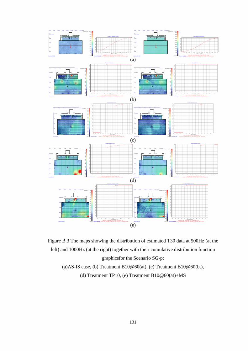
131
(a)
(b)
(c)
(d)
(e)
Figure B.3 The maps showing the distribution of estimated T30 data at 500Hz (at the
left) and 1000Hz (at the right) together with their cumulative distribution function
graphicsfor the Scenario SG-p:
(a)AS-IS case, (b) Treatment B10@60(at), (c) Treatment B10@60(bt),
(d) Treatment TP10, (e) Treatment B10@60(at)+MS
P1P1
0,00 5,00 10,00 15,00 20,00 25,00 30,00 35,00 metres
0,00
5,00
10,00
15,00
20,00 metres
9,10
8,30
7,50
6,70
5,90
5,10
4,30
3,50
2,70
1,90
1,10
T30 at 500 Hz > 10,30
< 0,40Odeon©1985-2006
Cumulative distribution function
X(5,95) = (3,36, 3,69) X(10,90) = (3,39, 3,64) X(25,75) = (3,44, 3,56) X(50) = (3,49)
X(95)-X(5) = 0,33 X(90)-X(10) = 0,25 X(75)-X(25) = 0,12
T30 (s) at 500 Hz
3,683,663,643,623,63,583,563,543,523,53,483,463,443,423,43,383,36
Perc
ent
90
80
70
60
50
40
30
20
10
Odeon©1985-2006
P1P1
0,00 5,00 10,00 15,00 20,00 25,00 30,00 35,00 metres
0,00
5,00
10,00
15,00
20,00 metres
9,10
8,30
7,50
6,70
5,90
5,10
4,30
3,50
2,70
1,90
1,10
T30 at 1000 Hz > 10,30
< 0,40Odeon©1985-2006
Cumulative distribution function
X(5,95) = (4,52, 4,81) X(10,90) = (4,56, 4,78) X(25,75) = (4,61, 4,72) X(50) = (4,67)
X(95)-X(5) = 0,28 X(90)-X(10) = 0,22 X(75)-X(25) = 0,11
T30 (s) at 1000 Hz
4,84,784,764,744,724,74,684,664,644,624,64,584,564,54
Perc
ent
90
80
70
60
50
40
30
20
10
Odeon©1985-2006
P1P1
0.00 5.00 10.00 15.00 20.00 25.00 metres
0.00
5.00
10.00
15.00
20.00 metres
3.20
3.05
2.90
2.75
2.60
2.45
2.30
2.15
2.00
1.85
1.70
1.55
1.40
1.25
1.10
0.95
0.80
0.65
T30 at 500 Hz > 3.50
< 0.53Odeon©1985-2006
Cumulative distribution function
X(5,95) = (1.29, 2.41) X(10,90) = (1.38, 2.22) X(25,75) = (1.49, 1.90) X(50) = (1.61)
X(95)-X(5) = 1.13 X(90)-X(10) = 0.83 X(75)-X(25) = 0.41
T30 (s) at 500 Hz
6.565.554.543.532.521.510.5
Perc
ent
100
95
90
85
80
75
70
65
60
55
50
45
40
35
30
25
20
15
10
5
Odeon©1985-2006
P1P1
0.00 5.00 10.00 15.00 20.00 25.00 metres
0.00
5.00
10.00
15.00
20.00 metres
3.20
3.05
2.90
2.75
2.60
2.45
2.30
2.15
2.00
1.85
1.70
1.55
1.40
1.25
1.10
0.95
0.80
0.65
T30 at 1000 Hz > 3.50
< 0.53Odeon©1985-2006
Cumulative distribution function
X(5,95) = (1.29, 2.32) X(10,90) = (1.36, 2.16) X(25,75) = (1.45, 1.82) X(50) = (1.55)
X(95)-X(5) = 1.03 X(90)-X(10) = 0.81 X(75)-X(25) = 0.38
T30 (s) at 1000 Hz
7.576.565.554.543.532.521.510.5
Perc
ent
100
95
90
85
80
75
70
65
60
55
50
45
40
35
30
25
20
15
10
5
Odeon©1985-2006
P1P1
0.00 5.00 10.00 15.00 20.00 25.00 metres
0.00
5.00
10.00
15.00
20.00 metres
4.50
4.25
4.00
3.75
3.50
3.25
3.00
2.75
2.50
2.25
2.00
1.75
1.50
1.25
1.00
0.75
0.50
0.25
T30 at 500 Hz > 5.00
< 0.05Odeon©1985-2006
Cumulative distribution function
X(5,95) = (1.18, 2.35) X(10,90) = (1.26, 2.08) X(25,75) = (1.39, 1.80) X(50) = (1.53)
X(95)-X(5) = 1.17 X(90)-X(10) = 0.82 X(75)-X(25) = 0.41
T30 (s) at 500 Hz
3.63.43.232.82.62.42.221.81.61.41.210.80.60.4
Perc
ent
100
95
90
85
80
75
70
65
60
55
50
45
40
35
30
25
20
15
10
5
Odeon©1985-2006
P1P1
0.00 5.00 10.00 15.00 20.00 25.00 metres
0.00
5.00
10.00
15.00
20.00 metres
4.50
4.25
4.00
3.75
3.50
3.25
3.00
2.75
2.50
2.25
2.00
1.75
1.50
1.25
1.00
0.75
0.50
0.25
T30 at 1000 Hz > 5.00
< 0.05Odeon©1985-2006
Cumulative distribution function
X(5,95) = (1.14, 1.96) X(10,90) = (1.20, 1.76) X(25,75) = (1.32, 1.53) X(50) = (1.41)
X(95)-X(5) = 0.82 X(90)-X(10) = 0.56 X(75)-X(25) = 0.21
T30 (s) at 1000 Hz
2.82.62.42.221.81.61.41.210.80.60.4
Perc
ent
100
95
90
85
80
75
70
65
60
55
50
45
40
35
30
25
20
15
10
5
Odeon©1985-2006
P1P1
0.00 5.00 10.00 15.00 20.00 25.00 metres
0.00
5.00
10.00
15.00
20.00 metres
3.60
3.40
3.20
3.00
2.80
2.60
2.40
2.20
2.00
1.80
1.60
1.40
1.20
1.00
0.80
0.60
0.40
0.20
T30 at 500 Hz > 4.00
< 0.04Odeon©1985-2006
Cumulative distribution function
X(5,95) = (1.29, 2.85) X(10,90) = (1.37, 2.17) X(25,75) = (1.50, 1.69) X(50) = (1.59)
X(95)-X(5) = 1.56 X(90)-X(10) = 0.80 X(75)-X(25) = 0.20
T30 (s) at 500 Hz
4.543.532.521.510.5
Perc
ent
100
95
90
85
80
75
70
65
60
55
50
45
40
35
30
25
20
15
10
5
Odeon©1985-2006
P1P1
0.00 5.00 10.00 15.00 20.00 25.00 metres
0.00
5.00
10.00
15.00
20.00 metres
3.60
3.40
3.20
3.00
2.80
2.60
2.40
2.20
2.00
1.80
1.60
1.40
1.20
1.00
0.80
0.60
0.40
0.20
T30 at 1000 Hz > 4.00
< 0.04Odeon©1985-2006
Cumulative distribution function
X(5,95) = (1.25, 2.06) X(10,90) = (1.32, 1.86) X(25,75) = (1.42, 1.62) X(50) = (1.51)
X(95)-X(5) = 0.81 X(90)-X(10) = 0.54 X(75)-X(25) = 0.20
T30 (s) at 1000 Hz
3.43.232.82.62.42.221.81.61.41.210.80.60.4
Perc
ent
100
95
90
85
80
75
70
65
60
55
50
45
40
35
30
25
20
15
10
5
Odeon©1985-2006
P1P1
0,00 5,00 10,00 15,00 20,00 metres
0,00
5,00
10,00
15,00
20,00 metres
3,20
3,02
2,84
2,66
2,48
2,30
2,12
1,94
1,76
1,58
1,40
1,22
1,04
0,86
0,68
T30 at 500 Hz > 3,50
< 0,53Odeon©1985-2006
Cumulative distribution function
X(5,95) = (1,37, 2,41) X(10,90) = (1,48, 2,31) X(25,75) = (1,64, 2,09) X(50) = (1,82)
X(95)-X(5) = 1,04 X(90)-X(10) = 0,83 X(75)-X(25) = 0,45
T30 (s) at 500 Hz
4,543,532,521,510,5
Perc
ent
100
95
90
85
80
75
70
65
60
55
50
45
40
35
30
25
20
15
10
5
Odeon©1985-2006
P1P1
0,00 5,00 10,00 15,00 20,00 metres
0,00
5,00
10,00
15,00
20,00 metres
3,20
3,02
2,84
2,66
2,48
2,30
2,12
1,94
1,76
1,58
1,40
1,22
1,04
0,86
0,68
T30 at 1000 Hz > 3,50
< 0,53Odeon©1985-2006
Cumulative distribution function
X(5,95) = (1,23, 2,04) X(10,90) = (1,30, 1,96) X(25,75) = (1,41, 1,74) X(50) = (1,56)
X(95)-X(5) = 0,81 X(90)-X(10) = 0,66 X(75)-X(25) = 0,33
T30 (s) at 1000 Hz
65,554,543,532,521,510,5
Perc
ent
100
95
90
85
80
75
70
65
60
55
50
45
40
35
30
25
20
15
10
5
Odeon©1985-2006
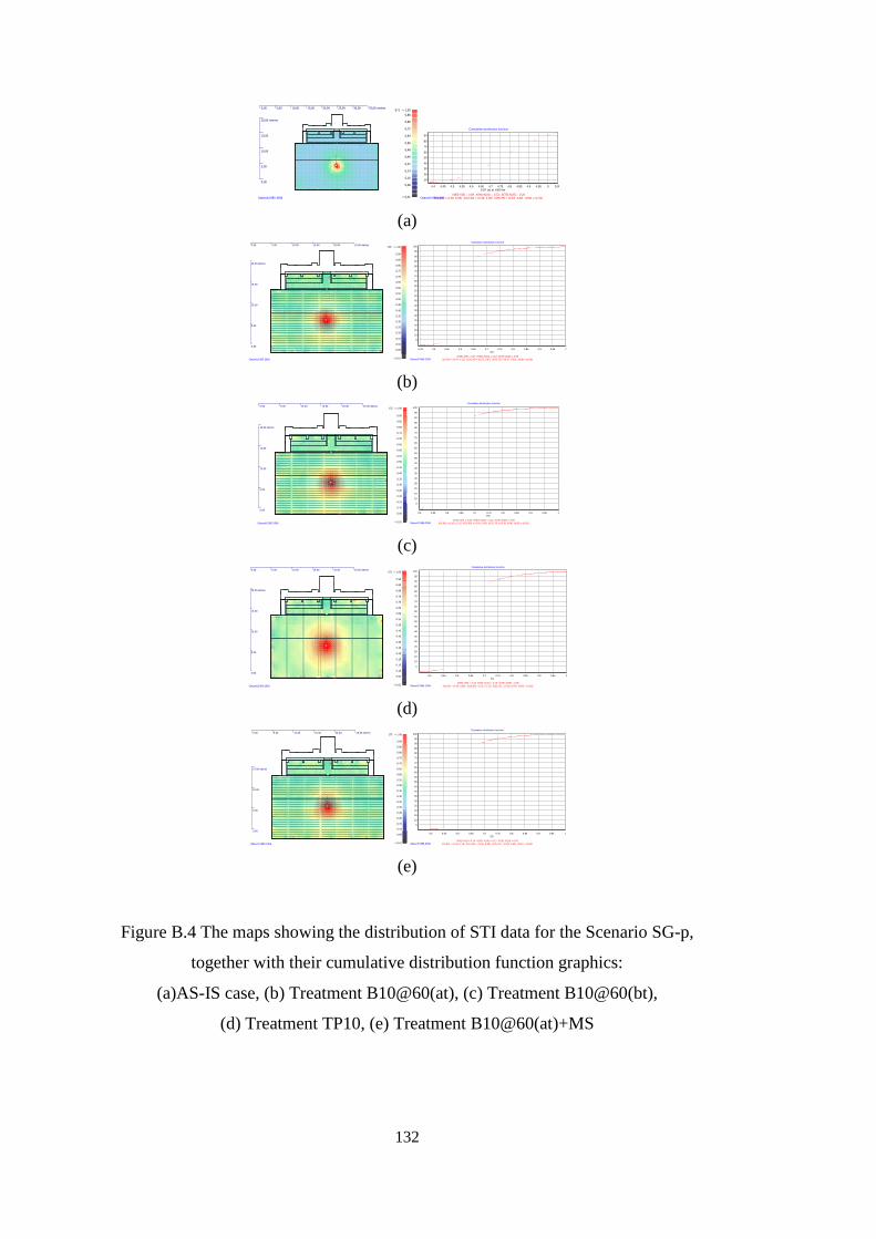
132
(a)
(b)
(c)
(d)
(e)
Figure B.4 The maps showing the distribution of STI data for the Scenario SG-p,
together with their cumulative distribution function graphics:
(a)AS-IS case, (b) Treatment B10@60(at), (c) Treatment B10@60(bt),
(d) Treatment TP10, (e) Treatment B10@60(at)+MS
P1P1
0,00 5,00 10,00 15,00 20,00 25,00 30,00 35,00 metres
0,00
5,00
10,00
15,00
20,00 metres
0,88
0,80
0,72
0,64
0,56
0,48
0,40
0,32
0,24
0,16
0,08
STI > 1,00
< 0,01Odeon©1985-2006
Cumulative distribution function
X(5,95) = (4,38, 5,05) X(10,90) = (4,48, 4,99) X(25,75) = (4,63, 4,89) X(50) = (4,76)
X(95)-X(5) = 0,68 X(90)-X(10) = 0,51 X(75)-X(25) = 0,26
EDT (s) at 1000 Hz
5,0554,954,94,854,84,754,74,654,64,554,54,454,4
Perc
ent
90
80
70
60
50
40
30
20
10
Odeon©1985-2006
P1P1
0.00 5.00 10.00 15.00 20.00 25.00 metres
0.00
5.00
10.00
15.00
20.00 metres
0.90
0.85
0.80
0.75
0.70
0.65
0.60
0.55
0.50
0.45
0.40
0.35
0.30
0.25
0.20
0.15
0.10
0.05
STI > 1.00
< 0.01Odeon©1985-2006
Cumulative distribution function
X(5,95) = (0.54, 0.73) X(10,90) = (0.55, 0.67) X(25,75) = (0.57, 0.62) X(50) = (0.59)
X(95)-X(5) = 0.19 X(90)-X(10) = 0.12 X(75)-X(25) = 0.05
STI
10.950.90.850.80.750.70.650.60.550.50.45
Perc
ent
100
95
90
85
80
75
70
65
60
55
50
45
40
35
30
25
20
15
10
5
Odeon©1985-2006
P1P1
0.00 5.00 10.00 15.00 20.00 25.00 metres
0.00
5.00
10.00
15.00
20.00 metres
0.90
0.85
0.80
0.75
0.70
0.65
0.60
0.55
0.50
0.45
0.40
0.35
0.30
0.25
0.20
0.15
0.10
0.05
STI > 1.00
< 0.01Odeon©1985-2006
Cumulative distribution function
X(5,95) = (0.55, 0.75) X(10,90) = (0.56, 0.69) X(25,75) = (0.58, 0.64) X(50) = (0.60)
X(95)-X(5) = 0.20 X(90)-X(10) = 0.13 X(75)-X(25) = 0.06
STI
10.950.90.850.80.750.70.650.60.550.5
Perc
ent
100
95
90
85
80
75
70
65
60
55
50
45
40
35
30
25
20
15
10
5
Odeon©1985-2006
P1P1
0.00 5.00 10.00 15.00 20.00 25.00 metres
0.00
5.00
10.00
15.00
20.00 metres
0.90
0.85
0.80
0.75
0.70
0.65
0.60
0.55
0.50
0.45
0.40
0.35
0.30
0.25
0.20
0.15
0.10
0.05
STI > 1.00
< 0.01Odeon©1985-2006
Cumulative distribution function
X(5,95) = (0.56, 0.80) X(10,90) = (0.57, 0.73) X(25,75) = (0.59, 0.66) X(50) = (0.62)
X(95)-X(5) = 0.24 X(90)-X(10) = 0.15 X(75)-X(25) = 0.06
STI
10.950.90.850.80.750.70.650.60.550.5
Perc
ent
100
95
90
85
80
75
70
65
60
55
50
45
40
35
30
25
20
15
10
5
Odeon©1985-2006
P1P1
0.00 5.00 10.00 15.00 20.00 25.00 metres
0.00
5.00
10.00
15.00 metres
0.90
0.85
0.80
0.75
0.70
0.65
0.60
0.55
0.50
0.45
0.40
0.35
0.30
0.25
0.20
0.15
0.10
0.05
STI > 1.00
< 0.01Odeon©1985-2006
Cumulative distribution function
X(5,95) = (0.55, 0.74) X(10,90) = (0.56, 0.68) X(25,75) = (0.58, 0.63) X(50) = (0.60)
X(95)-X(5) = 0.19 X(90)-X(10) = 0.12 X(75)-X(25) = 0.05
STI
10.950.90.850.80.750.70.650.60.550.5
Perc
ent
100
95
90
85
80
75
70
65
60
55
50
45
40
35
30
25
20
15
10
5
Odeon©1985-2006
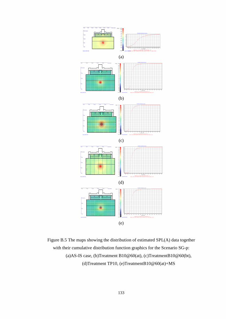
133
(a)
(b)
(c)
(d)
(e)
Figure B.5 The maps showing the distribution of estimated SPL(A) data together
with their cumulative distribution function graphics for the Scenario SG-p:
(a)AS-IS case, (b)Treatment B10@60(at), (c)TreatmentB10@60(bt),
(d)Treatment TP10, (e)TreatmentB10@60(at)+MS
P1P1
0,00 5,00 10,00 15,00 20,00 25,00 30,00 35,00 metres
0,00
5,00
10,00
15,00
20,00 metres
85,2
82,0
78,8
75,6
72,4
69,2
66,0
62,8
59,6
56,4
53,2
SPL(A) > 90,0
< 50,4Odeon©1985-2006
Cumulative distribution function
X(5,95) = (75,4, 79,0) X(10,90) = (75,7, 78,0) X(25,75) = (76,2, 77,1) X(50) = (76,5)
X(95)-X(5) = 3,6 X(90)-X(10) = 2,3 X(75)-X(25) = 0,9
SPL(A) (dB)
7978,878,678,478,27877,877,677,477,27776,876,676,476,27675,875,6
Perc
ent
90
80
70
60
50
40
30
20
10
Odeon©1985-2006
P1P1
0.00 5.00 10.00 15.00 20.00 25.00 metres
0.00
5.00
10.00
15.00
20.00 metres
86.5
84.8
83.0
81.3
79.5
77.8
76.0
74.3
72.5
70.8
69.0
67.3
65.5
63.8
62.0
60.3
58.5
56.8
SPL(A) > 90.0
< 55.4Odeon©1985-2006
Cumulative distribution function
X(5,95) = (70.5, 76.9) X(10,90) = (70.9, 75.1) X(25,75) = (71.5, 73.3) X(50) = (72.2)
X(95)-X(5) = 6.4 X(90)-X(10) = 4.2 X(75)-X(25) = 1.8
SPL(A) (dB)
9896949290888684828078767472706866
Perc
ent
100
95
90
85
80
75
70
65
60
55
50
45
40
35
30
25
20
15
10
5
Odeon©1985-2006
P1P1
0.00 5.00 10.00 15.00 20.00 25.00 metres
0.00
5.00
10.00
15.00
20.00 metres
82.0
80.5
79.0
77.5
76.0
74.5
73.0
71.5
70.0
68.5
67.0
65.5
64.0
62.5
61.0
59.5
58.0
56.5
SPL(A) > 85.0
< 55.3Odeon©1985-2006
Cumulative distribution function
X(5,95) = (70.3, 76.8) X(10,90) = (70.6, 75.0) X(25,75) = (71.2, 72.9) X(50) = (71.8)
X(95)-X(5) = 6.5 X(90)-X(10) = 4.4 X(75)-X(25) = 1.7
SPL(A) (dB)
98969492908886848280787674727068
Perc
ent
100
95
90
85
80
75
70
65
60
55
50
45
40
35
30
25
20
15
10
5
Odeon©1985-2006
P1P1
0.00 5.00 10.00 15.00 20.00 25.00 metres
0.00
5.00
10.00
15.00
20.00 metres
85.0
82.5
80.0
77.5
75.0
72.5
70.0
67.5
65.0
62.5
60.0
57.5
55.0
52.5
50.0
47.5
45.0
42.5
SPL(A) > 90.0
< 40.5Odeon©1985-2006
Cumulative distribution function
X(5,95) = (69.2, 76.5) X(10,90) = (69.5, 74.5) X(25,75) = (70.0, 72.3) X(50) = (70.7)
X(95)-X(5) = 7.3 X(90)-X(10) = 5.0 X(75)-X(25) = 2.3
SPL(A) (dB)
9896949290888684828078767472706866
Perc
ent
100
95
90
85
80
75
70
65
60
55
50
45
40
35
30
25
20
15
10
5
Odeon©1985-2006
P1P1
0.00 5.00 10.00 15.00 20.00 25.00 metres
0.00
5.00
10.00
15.00 metres
86.5
84.8
83.0
81.3
79.5
77.8
76.0
74.3
72.5
70.8
69.0
67.3
65.5
63.8
62.0
60.3
58.5
56.8
SPL(A) > 90.0
< 55.4Odeon©1985-2006
Cumulative distribution function
X(5,95) = (70.2, 76.8) X(10,90) = (70.6, 75.0) X(25,75) = (71.1, 73.0) X(50) = (71.8)
X(95)-X(5) = 6.6 X(90)-X(10) = 4.4 X(75)-X(25) = 1.9
SPL(A) (dB)
9896949290888684828078767472706866
Perc
ent
100
95
90
85
80
75
70
65
60
55
50
45
40
35
30
25
20
15
10
5
Odeon©1985-2006

134

135
APPENDIX C
SIMULATION DATA FOR THE SCENARIO SG-a
Figure C.1 The estimated GRT (T20 and T30) values (at the left) and T30 noise
reduction curves (at the right) obtained for the Scenario SG-a:
(a)AS-IS case, (b) Treatment B10@60(at), (c) Treatment B10@60(bt),
(d) Treatment TP10, (e) Treatment B10@60(at)+MS.
T30
T20
Estimated global reverberation times (Source 3, 20188 rays used)
Frequency (Hertz)
63 125 250 500 1000 2000 4000 8000
Reverb
era
tion t
ime (
s)
4,5
4
3,5
3
2,5
2
1,5
1
0,5
0
Odeon©1985-2006
T30,63=2,50 s
T30,125=3,29 s
T30,250=3,06 s
T30,500=3,46 s
T30,1000=4,64 s
T30,2000=3,92 s
T30,4000=2,34 s
T30,8000=1,12 s
Estimated global reverberation times (Source 3, 20188 rays used)
Estimated room volume:4551,53 m³
Time (seconds)
4,543,532,521,510,50
SP
L (
dB
)
0
-10
-20
-30
-40
-50
-60
Odeon©1985-2006
T30
T20
Estimated global reverberation times (Source 3, 1195748 rays used)
Frequency (Hertz)
63 125 250 500 1000 2000 4000 8000
Reverb
era
tion tim
e (
s)
2
1.8
1.6
1.4
1.2
1
0.8
0.6
0.4
0.2
0
Odeon©1985-2006
T30,63=1.93 s
T30,125=2.02 s
T30,250=1.87 s
T30,500=1.84 s
T30,1000=1.73 s
T30,2000=1.57 s
T30,4000=1.24 s
T30,8000=0.77 s
Estimated global reverberation times (Source 3, 1195748 rays used)
Estimated room volume:4007.24 m³
Time (seconds)
21.81.61.41.210.80.60.40.20
SP
L (
dB
)
0
-10
-20
-30
-40
-50
-60
Odeon©1985-2006
T30
T20
Estimated global reverberation times (Source 3, 720883 rays used)
Frequency (Hertz)
63 125 250 500 1000 2000 4000 8000
Reverb
era
tion tim
e (
s)
1.8
1.6
1.4
1.2
1
0.8
0.6
0.4
0.2
0
Odeon©1985-2006
T30,63=1.84 s
T30,125=1.89 s
T30,250=1.76 s
T30,500=1.73 s
T30,1000=1.62 s
T30,2000=1.48 s
T30,4000=1.21 s
T30,8000=0.74 s
Estimated global reverberation times (Source 3, 720883 rays used)
Estimated room volume:3949.82 m³
Time (seconds)
1.81.61.41.210.80.60.40.20
SP
L (
dB
)
0
-10
-20
-30
-40
-50
-60
Odeon©1985-2006
T30
T20
Estimated global reverberation times (Source 3, 2117725 rays used)
Frequency (Hertz)
63 125 250 500 1000 2000 4000 8000
Reverb
era
tion tim
e (
s)
2
1.8
1.6
1.4
1.2
1
0.8
0.6
0.4
0.2
0
Odeon©1985-2006
T30,63=2.02 s
T30,125=2.12 s
T30,250=1.84 s
T30,500=1.82 s
T30,1000=1.71 s
T30,2000=1.58 s
T30,4000=1.28 s
T30,8000=0.76 s
Estimated global reverberation times (Source 3, 2117725 rays used)
Estimated room volume:4171.56 m³
Time (seconds)
2.221.81.61.41.210.80.60.40.20
SP
L (
dB
)
0
-10
-20
-30
-40
-50
-60
Odeon©1985-2006
T30
T20
Estimated global reverberation times (Source 3, 2929921 rays used)
Frequency (Hertz)
63 125 250 500 1000 2000 4000 8000
Reverb
era
tion tim
e (
s)
1.8
1.6
1.4
1.2
1
0.8
0.6
0.4
0.2
0
Odeon©1985-2006
T30,63=1.87 s
T30,125=1.94 s
T30,250=1.78 s
T30,500=1.73 s
T30,1000=1.62 s
T30,2000=1.49 s
T30,4000=1.21 s
T30,8000=0.76 s
Estimated global reverberation times (Source 3, 2929921 rays used)
Estimated room volume:4006.15 m³
Time (seconds)
21.81.61.41.210.80.60.40.20
SP
L (
dB
)
0
-10
-20
-30
-40
-50
-60
Odeon©1985-2006
(a)
(b)
(c)
(d)
(e)

136
(a)
(b)
(c)
(d)
(e)
Figure C.2 The maps showing the distribution of estimated EDT data at 500Hz (at
the left) and 1000Hz (at the right) together with their cumulative distribution
function graphic for the Scenario SG-a, :.
(a)AS-IS case, (b) Treatment B10@60(at), (c) Treatment B10@60(bt),
(d) Treatment TP10, (e) Treatment B10@60(at)+MS.
P3P3
0,00 5,00 10,00 15,00 20,00 25,00 30,00 metres
0,00
5,00
10,00
15,00
20,00 metres
7,28
6,72
6,16
5,60
5,04
4,48
3,92
3,36
2,80
2,24
1,68
1,12
0,56
EDT at 500 Hz > 8,00
< 0,08Odeon©1985-2006
Cumulative distribution function
X(5,95) = (3,19, 3,88) X(10,90) = (3,36, 3,81) X(25,75) = (3,48, 3,70) X(50) = (3,59)
X(95)-X(5) = 0,69 X(90)-X(10) = 0,45 X(75)-X(25) = 0,22
EDT (s) at 500 Hz
3,853,83,753,73,653,63,553,53,453,43,353,33,253,2
Perc
ent
90
80
70
60
50
40
30
20
10
Odeon©1985-2006
P3P3
0,00 5,00 10,00 15,00 20,00 25,00 30,00 metres
0,00
5,00
10,00
15,00
20,00 metres
7,28
6,72
6,16
5,60
5,04
4,48
3,92
3,36
2,80
2,24
1,68
1,12
0,56
EDT at 1000 Hz > 8,00
< 0,08Odeon©1985-2006
Cumulative distribution function
X(5,95) = (4,42, 5,02) X(10,90) = (4,53, 4,94) X(25,75) = (4,64, 4,85) X(50) = (4,75)
X(95)-X(5) = 0,59 X(90)-X(10) = 0,42 X(75)-X(25) = 0,21
EDT (s) at 1000 Hz
54,954,94,854,84,754,74,654,64,554,54,45
Perc
ent
90
80
70
60
50
40
30
20
10
Odeon©1985-2006
P3P3
0.00 5.00 10.00 15.00 20.00 25.00 metres
0.00
5.00
10.00
15.00 metres
2.70
2.55
2.40
2.25
2.10
1.95
1.80
1.65
1.50
1.35
1.20
1.05
0.90
0.75
0.60
0.45
0.30
0.15
EDT at 500 Hz > 3.00
< 0.03Odeon©1985-2006
Cumulative distribution function
X(5,95) = (0.54, 1.87) X(10,90) = (0.77, 1.64) X(25,75) = (1.09, 1.42) X(50) = (1.28)
X(95)-X(5) = 1.33 X(90)-X(10) = 0.87 X(75)-X(25) = 0.33
EDT (s) at 500 Hz
98.587.576.565.554.543.532.521.510.5
Perc
ent
100
95
90
85
80
75
70
65
60
55
50
45
40
35
30
25
20
15
10
5
Odeon©1985-2006
P3P3
0.00 5.00 10.00 15.00 20.00 25.00 metres
0.00
5.00
10.00
15.00 metres
2.70
2.55
2.40
2.25
2.10
1.95
1.80
1.65
1.50
1.35
1.20
1.05
0.90
0.75
0.60
0.45
0.30
0.15
EDT at 1000 Hz > 3.00
< 0.03Odeon©1985-2006
Cumulative distribution function
X(5,95) = (0.54, 1.77) X(10,90) = (0.77, 1.63) X(25,75) = (1.08, 1.44) X(50) = (1.28)
X(95)-X(5) = 1.24 X(90)-X(10) = 0.86 X(75)-X(25) = 0.36
EDT (s) at 1000 Hz
8.587.576.565.554.543.532.521.510.5
Perc
ent
100
95
90
85
80
75
70
65
60
55
50
45
40
35
30
25
20
15
10
5
Odeon©1985-2006
P3P3
0.00 5.00 10.00 15.00 20.00 25.00 metres
0.00
5.00
10.00
15.00 metres
3.60
3.40
3.20
3.00
2.80
2.60
2.40
2.20
2.00
1.80
1.60
1.40
1.20
1.00
0.80
0.60
0.40
0.20
EDT at 500 Hz > 4.00
< 0.04Odeon©1985-2006
Cumulative distribution function
X(5,95) = (0.58, 1.87) X(10,90) = (0.92, 1.70) X(25,75) = (1.19, 1.53) X(50) = (1.38)
X(95)-X(5) = 1.29 X(90)-X(10) = 0.78 X(75)-X(25) = 0.34
EDT (s) at 500 Hz
121110987654321
Perc
ent
100
95
90
85
80
75
70
65
60
55
50
45
40
35
30
25
20
15
10
5
Odeon©1985-2006
P3P3
0.00 5.00 10.00 15.00 20.00 25.00 metres
0.00
5.00
10.00
15.00 metres
3.60
3.40
3.20
3.00
2.80
2.60
2.40
2.20
2.00
1.80
1.60
1.40
1.20
1.00
0.80
0.60
0.40
0.20
EDT at 1000 Hz > 4.00
< 0.04Odeon©1985-2006
Cumulative distribution function
X(5,95) = (0.58, 1.79) X(10,90) = (0.90, 1.66) X(25,75) = (1.12, 1.48) X(50) = (1.31)
X(95)-X(5) = 1.21 X(90)-X(10) = 0.76 X(75)-X(25) = 0.36
EDT (s) at 1000 Hz
10987654321
Perc
ent
100
95
90
85
80
75
70
65
60
55
50
45
40
35
30
25
20
15
10
5
Odeon©1985-2006
P3P3
0.00 5.00 10.00 15.00 20.00 25.00 metres
0.00
5.00
10.00
15.00 metres
3.15
2.97
2.80
2.63
2.45
2.28
2.10
1.92
1.75
1.58
1.40
1.23
1.05
0.88
0.70
0.52
0.35
0.17
EDT at 500 Hz > 3.50
< 0.04Odeon©1985-2006
Cumulative distribution function
X(5,95) = (0.55, 2.30) X(10,90) = (0.75, 2.12) X(25,75) = (1.23, 1.80) X(50) = (1.50)
X(95)-X(5) = 1.75 X(90)-X(10) = 1.37 X(75)-X(25) = 0.57
EDT (s) at 500 Hz
2018161412108642
Perc
ent
100
95
90
85
80
75
70
65
60
55
50
45
40
35
30
25
20
15
10
5
Odeon©1985-2006
P3P3
0.00 5.00 10.00 15.00 20.00 25.00 metres
0.00
5.00
10.00
15.00 metres
3.15
2.97
2.80
2.63
2.45
2.28
2.10
1.92
1.75
1.58
1.40
1.23
1.05
0.88
0.70
0.52
0.35
0.17
EDT at 1000 Hz > 3.50
< 0.04Odeon©1985-2006
Cumulative distribution function
X(5,95) = (0.52, 2.17) X(10,90) = (0.75, 1.97) X(25,75) = (1.22, 1.70) X(50) = (1.46)
X(95)-X(5) = 1.64 X(90)-X(10) = 1.21 X(75)-X(25) = 0.48
EDT (s) at 1000 Hz
181716151413121110987654321
Perc
ent
100
95
90
85
80
75
70
65
60
55
50
45
40
35
30
25
20
15
10
5
Odeon©1985-2006
P3P3
0.00 5.00 10.00 15.00 20.00 25.00 metres
0.00
5.00
10.00
15.00 metres
2.70
2.55
2.40
2.25
2.10
1.95
1.80
1.65
1.50
1.35
1.20
1.05
0.90
0.75
0.60
0.45
0.30
0.15
EDT at 500 Hz > 3.00
< 0.03Odeon©1985-2006
Cumulative distribution function
X(5,95) = (0.51, 1.78) X(10,90) = (0.72, 1.51) X(25,75) = (0.95, 1.30) X(50) = (1.07)
X(95)-X(5) = 1.27 X(90)-X(10) = 0.79 X(75)-X(25) = 0.35
EDT (s) at 500 Hz
9.598.587.576.565.554.543.532.521.510.5
Perc
ent
100
95
90
85
80
75
70
65
60
55
50
45
40
35
30
25
20
15
10
5
Odeon©1985-2006
P3P3
0.00 5.00 10.00 15.00 20.00 25.00 metres
0.00
5.00
10.00
15.00 metres
2.70
2.55
2.40
2.25
2.10
1.95
1.80
1.65
1.50
1.35
1.20
1.05
0.90
0.75
0.60
0.45
0.30
0.15
EDT at 1000 Hz > 3.00
< 0.03Odeon©1985-2006
Cumulative distribution function
X(5,95) = (0.51, 1.71) X(10,90) = (0.71, 1.52) X(25,75) = (0.96, 1.32) X(50) = (1.11)
X(95)-X(5) = 1.20 X(90)-X(10) = 0.81 X(75)-X(25) = 0.36
EDT (s) at 1000 Hz
98.587.576.565.554.543.532.521.510.5
Perc
ent
100
95
90
85
80
75
70
65
60
55
50
45
40
35
30
25
20
15
10
5
Odeon©1985-2006

137
(a)
(b)
(c)
(d)
(e)
Figure C.3 The maps showing the distribution of estimated T30 data at 500Hz (at the
left) and 1000Hz (at the right) together with their cumulative distribution function
graphicsfor the Scenario SG-a:
(a)AS-IS case, (b) Treatment B10@60(at), (c) Treatment B10@60(bt),
(d) Treatment TP10, (e) Treatment B10@60(at)+MS.
P3P3
0,00 5,00 10,00 15,00 20,00 25,00 30,00 metres
0,00
5,00
10,00
15,00
20,00 metres
9,40
8,70
8,00
7,30
6,60
5,90
5,20
4,50
3,80
3,10
2,40
1,70
1,00
T30 at 500 Hz > 10,30
< 0,40Odeon©1985-2006
Cumulative distribution function
X(5,95) = (3,27, 3,57) X(10,90) = (3,31, 3,53) X(25,75) = (3,36, 3,47) X(50) = (3,41)
X(95)-X(5) = 0,29 X(90)-X(10) = 0,22 X(75)-X(25) = 0,11
T30 (s) at 500 Hz
3,563,543,523,53,483,463,443,423,43,383,363,343,323,33,28
Perc
ent
90
80
70
60
50
40
30
20
10
Odeon©1985-2006
P3P3
0,00 5,00 10,00 15,00 20,00 25,00 30,00 metres
0,00
5,00
10,00
15,00
20,00 metres
9,40
8,70
8,00
7,30
6,60
5,90
5,20
4,50
3,80
3,10
2,40
1,70
1,00
T30 at 1000 Hz > 10,30
< 0,40Odeon©1985-2006
Cumulative distribution function
X(5,95) = (4,50, 4,79) X(10,90) = (4,54, 4,75) X(25,75) = (4,59, 4,70) X(50) = (4,64)
X(95)-X(5) = 0,29 X(90)-X(10) = 0,22 X(75)-X(25) = 0,11
T30 (s) at 1000 Hz
4,784,764,744,724,74,684,664,644,624,64,584,564,544,524,5
Perc
ent
90
80
70
60
50
40
30
20
10
Odeon©1985-2006
P3P3
0.00 5.00 10.00 15.00 20.00 25.00 metres
0.00
5.00
10.00
15.00 metres
3.20
3.05
2.90
2.75
2.60
2.45
2.30
2.15
2.00
1.85
1.70
1.55
1.40
1.25
1.10
0.95
0.80
0.65
T30 at 500 Hz > 3.50
< 0.53Odeon©1985-2006
Cumulative distribution function
X(5,95) = (1.41, 2.75) X(10,90) = (1.51, 2.32) X(25,75) = (1.65, 2.05) X(50) = (1.79)
X(95)-X(5) = 1.34 X(90)-X(10) = 0.80 X(75)-X(25) = 0.40
T30 (s) at 500 Hz
43.83.63.43.232.82.62.42.221.81.61.41.2
Perc
ent
100
95
90
85
80
75
70
65
60
55
50
45
40
35
30
25
20
15
10
5
Odeon©1985-2006
P3P3
0.00 5.00 10.00 15.00 20.00 25.00 metres
0.00
5.00
10.00
15.00 metres
3.20
3.05
2.90
2.75
2.60
2.45
2.30
2.15
2.00
1.85
1.70
1.55
1.40
1.25
1.10
0.95
0.80
0.65
T30 at 1000 Hz > 3.50
< 0.53Odeon©1985-2006
Cumulative distribution function
X(5,95) = (1.36, 2.47) X(10,90) = (1.43, 2.20) X(25,75) = (1.56, 2.01) X(50) = (1.73)
X(95)-X(5) = 1.12 X(90)-X(10) = 0.77 X(75)-X(25) = 0.45
T30 (s) at 1000 Hz
3.43.232.82.62.42.221.81.61.41.2
Perc
ent
100
95
90
85
80
75
70
65
60
55
50
45
40
35
30
25
20
15
10
5
Odeon©1985-2006
P3P3
0.00 5.00 10.00 15.00 20.00 25.00 metres
0.00
5.00
10.00
15.00 metres
4.50
4.25
4.00
3.75
3.50
3.25
3.00
2.75
2.50
2.25
2.00
1.75
1.50
1.25
1.00
0.75
0.50
0.25
T30 at 500 Hz > 5.00
< 0.05Odeon©1985-2006
Cumulative distribution function
X(5,95) = (1.36, 2.75) X(10,90) = (1.44, 2.47) X(25,75) = (1.61, 2.22) X(50) = (1.88)
X(95)-X(5) = 1.40 X(90)-X(10) = 1.03 X(75)-X(25) = 0.60
T30 (s) at 500 Hz
4.44.243.83.63.43.232.82.62.42.221.81.61.41.210.80.6
Perc
ent
100
95
90
85
80
75
70
65
60
55
50
45
40
35
30
25
20
15
10
5
Odeon©1985-2006
P3P3
0.00 5.00 10.00 15.00 20.00 25.00 metres
0.00
5.00
10.00
15.00 metres
4.50
4.25
4.00
3.75
3.50
3.25
3.00
2.75
2.50
2.25
2.00
1.75
1.50
1.25
1.00
0.75
0.50
0.25
T30 at 1000 Hz > 5.00
< 0.05Odeon©1985-2006
Cumulative distribution function
X(5,95) = (1.22, 2.79) X(10,90) = (1.28, 2.53) X(25,75) = (1.42, 2.16) X(50) = (1.79)
X(95)-X(5) = 1.57 X(90)-X(10) = 1.25 X(75)-X(25) = 0.74
T30 (s) at 1000 Hz
54.543.532.521.51
Perc
ent
100
95
90
85
80
75
70
65
60
55
50
45
40
35
30
25
20
15
10
5
Odeon©1985-2006
P3P3
0.00 5.00 10.00 15.00 20.00 25.00 metres
0.00
5.00
10.00
15.00 metres
3.60
3.40
3.20
3.00
2.80
2.60
2.40
2.20
2.00
1.80
1.60
1.40
1.20
1.00
0.80
0.60
0.40
0.20
T30 at 500 Hz > 4.00
< 0.04Odeon©1985-2006
Cumulative distribution function
X(5,95) = (1.27, 2.56) X(10,90) = (1.36, 2.45) X(25,75) = (1.63, 2.24) X(50) = (1.99)
X(95)-X(5) = 1.29 X(90)-X(10) = 1.09 X(75)-X(25) = 0.61
T30 (s) at 500 Hz
5.554.543.532.521.510.5
Perc
ent
100
95
90
85
80
75
70
65
60
55
50
45
40
35
30
25
20
15
10
5
Odeon©1985-2006
P3P3
0.00 5.00 10.00 15.00 20.00 25.00 metres
0.00
5.00
10.00
15.00 metres
3.60
3.40
3.20
3.00
2.80
2.60
2.40
2.20
2.00
1.80
1.60
1.40
1.20
1.00
0.80
0.60
0.40
0.20
T30 at 1000 Hz > 4.00
< 0.04Odeon©1985-2006
Cumulative distribution function
X(5,95) = (1.21, 2.26) X(10,90) = (1.29, 2.18) X(25,75) = (1.48, 2.04) X(50) = (1.82)
X(95)-X(5) = 1.05 X(90)-X(10) = 0.89 X(75)-X(25) = 0.56
T30 (s) at 1000 Hz
76.565.554.543.532.521.510.5
Perc
ent
100
95
90
85
80
75
70
65
60
55
50
45
40
35
30
25
20
15
10
5
Odeon©1985-2006
P3P3
0,00 5,00 10,00 15,00 20,00 metres
0,00
5,00
10,00
15,00
20,00 metres
3,20
3,02
2,84
2,66
2,48
2,30
2,12
1,94
1,76
1,58
1,40
1,22
1,04
0,86
0,68
T30 at 500 Hz > 3,50
< 0,53Odeon©1985-2006
Cumulative distribution function
X(5,95) = (1,19, 1,80) X(10,90) = (1,28, 1,70) X(25,75) = (1,38, 1,55) X(50) = (1,46)
X(95)-X(5) = 0,60 X(90)-X(10) = 0,41 X(75)-X(25) = 0,17
T30 (s) at 500 Hz
43,532,521,510,5
Perc
ent
100
95
90
85
80
75
70
65
60
55
50
45
40
35
30
25
20
15
10
5
Odeon©1985-2006
P3P3
0,00 5,00 10,00 15,00 20,00 metres
0,00
5,00
10,00
15,00
20,00 metres
3,20
3,02
2,84
2,66
2,48
2,30
2,12
1,94
1,76
1,58
1,40
1,22
1,04
0,86
0,68
T30 at 1000 Hz > 3,50
< 0,53Odeon©1985-2006
Cumulative distribution function
X(5,95) = (1,15, 1,79) X(10,90) = (1,22, 1,68) X(25,75) = (1,32, 1,51) X(50) = (1,41)
X(95)-X(5) = 0,64 X(90)-X(10) = 0,46 X(75)-X(25) = 0,20
T30 (s) at 1000 Hz
3,532,521,510,5
Perc
ent
100
95
90
85
80
75
70
65
60
55
50
45
40
35
30
25
20
15
10
5
Odeon©1985-2006

138
(a)
(b)
(c)
(d)
(e)
Figure C.4 The maps showing the distribution of estimated STI data together with
their cumulative distribution function graphics for the Scenario SG-a:
(a)AS-IS case, (b) Treatment B10@60(at), (c) Teatment B10@60(bt), (d)
Treatment TP10, (e) Treatment B10@60(at)+MS.
P3P3
0,00 5,00 10,00 15,00 20,00 25,00 30,00 metres
0,00
5,00
10,00
15,00
20,00 metres
0,91
0,84
0,77
0,70
0,63
0,56
0,49
0,42
0,35
0,28
0,21
0,14
0,07
STI > 1,00
< 0,01Odeon©1985-2006
Cumulative distribution function
X(5,95) = (0,33, 0,56) X(10,90) = (0,33, 0,48) X(25,75) = (0,35, 0,43) X(50) = (0,39)
X(95)-X(5) = 0,24 X(90)-X(10) = 0,15 X(75)-X(25) = 0,08
STI
0,560,540,520,50,480,460,440,420,40,380,360,34
Perc
ent
90
80
70
60
50
40
30
20
10
Odeon©1985-2006
P3P3
0.00 5.00 10.00 15.00 20.00 25.00 metres
0.00
5.00
10.00
15.00 metres
0.90
0.85
0.80
0.75
0.70
0.65
0.60
0.55
0.50
0.45
0.40
0.35
0.30
0.25
0.20
0.15
0.10
0.05
STI > 1.00
< 0.01Odeon©1985-2006
Cumulative distribution function
X(5,95) = (0.51, 0.77) X(10,90) = (0.52, 0.70) X(25,75) = (0.54, 0.62) X(50) = (0.57)
X(95)-X(5) = 0.25 X(90)-X(10) = 0.17 X(75)-X(25) = 0.08
STI
0.950.90.850.80.750.70.650.60.550.5
Perc
ent
100
95
90
85
80
75
70
65
60
55
50
45
40
35
30
25
20
15
10
5
Odeon©1985-2006
P3P3
0.00 5.00 10.00 15.00 20.00 25.00 metres
0.00
5.00
10.00
15.00 metres
0.90
0.85
0.80
0.75
0.70
0.65
0.60
0.55
0.50
0.45
0.40
0.35
0.30
0.25
0.20
0.15
0.10
0.05
STI > 1.00
< 0.01Odeon©1985-2006
Cumulative distribution function
X(5,95) = (0.52, 0.75) X(10,90) = (0.53, 0.68) X(25,75) = (0.56, 0.63) X(50) = (0.58)
X(95)-X(5) = 0.23 X(90)-X(10) = 0.15 X(75)-X(25) = 0.07
STI
0.90.850.80.750.70.650.60.550.5
Perc
ent
100
95
90
85
80
75
70
65
60
55
50
45
40
35
30
25
20
15
10
5
Odeon©1985-2006
P3P3
0.00 5.00 10.00 15.00 20.00 25.00 metres
0.00
5.00
10.00
15.00 metres
0.90
0.85
0.80
0.75
0.70
0.65
0.60
0.55
0.50
0.45
0.40
0.35
0.30
0.25
0.20
0.15
0.10
0.05
STI > 1.00
< 0.01Odeon©1985-2006
Cumulative distribution function
X(5,95) = (0.50, 0.79) X(10,90) = (0.51, 0.71) X(25,75) = (0.53, 0.64) X(50) = (0.59)
X(95)-X(5) = 0.29 X(90)-X(10) = 0.20 X(75)-X(25) = 0.11
STI
0.950.90.850.80.750.70.650.60.550.5
Perc
ent
100
95
90
85
80
75
70
65
60
55
50
45
40
35
30
25
20
15
10
5
Odeon©1985-2006
P3P3
0.00 5.00 10.00 15.00 20.00 25.00 metres
0.00
5.00
10.00
15.00 metres
0.90
0.85
0.80
0.75
0.70
0.65
0.60
0.55
0.50
0.45
0.40
0.35
0.30
0.25
0.20
0.15
0.10
0.05
STI > 1.00
< 0.01Odeon©1985-2006
Cumulative distribution function
X(5,95) = (0.52, 0.78) X(10,90) = (0.53, 0.71) X(25,75) = (0.55, 0.64) X(50) = (0.59)
X(95)-X(5) = 0.26 X(90)-X(10) = 0.18 X(75)-X(25) = 0.09
STI
0.950.90.850.80.750.70.650.60.550.5
Perc
ent
100
95
90
85
80
75
70
65
60
55
50
45
40
35
30
25
20
15
10
5
Odeon©1985-2006
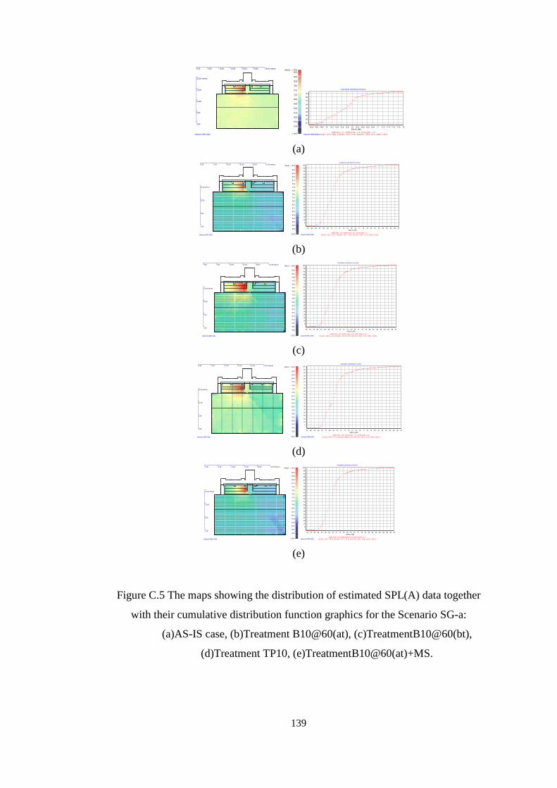
139
(a)
(b)
(c)
(d)
(e)
Figure C.5 The maps showing the distribution of estimated SPL(A) data together
with their cumulative distribution function graphics for the Scenario SG-a:
(a)AS-IS case, (b)Treatment B10@60(at), (c)TreatmentB10@60(bt),
(d)Treatment TP10, (e)TreatmentB10@60(at)+MS.
P3P3
0,00 5,00 10,00 15,00 20,00 25,00 30,00 metres
0,00
5,00
10,00
15,00
20,00 metres
86,4
83,6
80,8
78,0
75,2
72,4
69,6
66,8
64,0
61,2
58,4
55,6
52,8
SPL(A) > 90,0
< 50,4Odeon©1985-2006
Cumulative distribution function
X(5,95) = (74,3, 78,0) X(10,90) = (74,7, 77,0) X(25,75) = (75,1, 76,1) X(50) = (75,7)
X(95)-X(5) = 3,7 X(90)-X(10) = 2,3 X(75)-X(25) = 1,0
SPL(A) (dB)
7877,877,677,477,27776,876,676,476,27675,875,675,475,27574,874,674,4
Perc
ent
90
80
70
60
50
40
30
20
10
Odeon©1985-2006
P3P3
0.00 5.00 10.00 15.00 20.00 25.00 metres
0.00
5.00
10.00
15.00 metres
86.5
84.8
83.0
81.3
79.5
77.8
76.0
74.3
72.5
70.8
69.0
67.3
65.5
63.8
62.0
60.3
58.5
56.8
SPL(A) > 90.0
< 55.4Odeon©1985-2006
Cumulative distribution function
X(5,95) = (67.2, 76.2) X(10,90) = (67.7, 73.8) X(25,75) = (68.7, 71.4) X(50) = (70.0)
X(95)-X(5) = 9.0 X(90)-X(10) = 6.1 X(75)-X(25) = 2.7
SPL(A) (dB)
878685848382818079787776757473727170696867666564
Perc
ent
100
95
90
85
80
75
70
65
60
55
50
45
40
35
30
25
20
15
10
5
Odeon©1985-2006
P3P3
0.00 5.00 10.00 15.00 20.00 25.00 metres
0.00
5.00
10.00
15.00 metres
82.0
80.5
79.0
77.5
76.0
74.5
73.0
71.5
70.0
68.5
67.0
65.5
64.0
62.5
61.0
59.5
58.0
56.5
SPL(A) > 85.0
< 55.3Odeon©1985-2006
Cumulative distribution function
X(5,95) = (66.8, 76.0) X(10,90) = (67.4, 74.0) X(25,75) = (68.3, 71.3) X(50) = (69.8)
X(95)-X(5) = 9.2 X(90)-X(10) = 6.6 X(75)-X(25) = 3.0
SPL(A) (dB)
87868584838281807978777675747372717069686766656463
Perc
ent
100
95
90
85
80
75
70
65
60
55
50
45
40
35
30
25
20
15
10
5
Odeon©1985-2006
P3P3
0.00 5.00 10.00 15.00 20.00 25.00 metres
0.00
5.00
10.00
15.00 metres
85.0
82.5
80.0
77.5
75.0
72.5
70.0
67.5
65.0
62.5
60.0
57.5
55.0
52.5
50.0
47.5
45.0
42.5
SPL(A) > 90.0
< 40.5Odeon©1985-2006
Cumulative distribution function
X(5,95) = (65.9, 75.7) X(10,90) = (66.2, 73.2) X(25,75) = (67.2, 70.3) X(50) = (69.2)
X(95)-X(5) = 9.8 X(90)-X(10) = 7.0 X(75)-X(25) = 3.1
SPL(A) (dB)
8786858483828180797877767574737271706968676665646362
Perc
ent
100
95
90
85
80
75
70
65
60
55
50
45
40
35
30
25
20
15
10
5
Odeon©1985-2006
P3P3
0.00 5.00 10.00 15.00 20.00 25.00 metres
0.00
5.00
10.00
15.00 metres
86.5
84.8
83.0
81.3
79.5
77.8
76.0
74.3
72.5
70.8
69.0
67.3
65.5
63.8
62.0
60.3
58.5
56.8
SPL(A) > 90.0
< 55.4Odeon©1985-2006
Cumulative distribution function
X(5,95) = (66.7, 75.6) X(10,90) = (67.2, 73.3) X(25,75) = (68.1, 70.8) X(50) = (69.6)
X(95)-X(5) = 8.9 X(90)-X(10) = 6.1 X(75)-X(25) = 2.7
SPL(A) (dB)
87868584838281807978777675747372717069686766656463
Perc
ent
100
95
90
85
80
75
70
65
60
55
50
45
40
35
30
25
20
15
10
5
Odeon©1985-2006

140
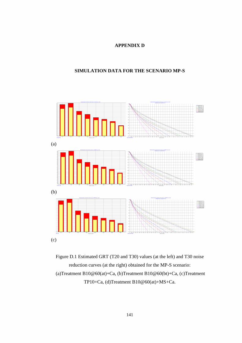
141
APPENDIX D
SIMULATION DATA FOR THE SCENARIO MP-S
(a)
(b)
(c)
Figure D.1 Estimated GRT (T20 and T30) values (at the left) and T30 noise
reduction curves (at the right) obtained for the MP-S scenario:
(a)Treatment B10@60(at)+Ca, (b)Treatment B10@60(bt)+Ca, (c)Treatment
TP10+Ca, (d)Treatment B10@60(at)+MS+Ca.
T30
T20
Estimated global reverberation times (Source 4, 941203 rays used)
Frequency (Hertz)
63 125 250 500 1000 2000 4000 8000
Reverb
era
tion tim
e (
s)
1.3
1.25
1.2
1.15
1.1
1.05
1
0.95
0.9
0.85
0.8
0.75
0.7
0.65
0.6
0.55
0.5
0.45
0.4
0.35
0.3
0.25
0.2
0.15
0.1
0.05
0
Odeon©1985-2006
T30,63=1.28 s
T30,125=1.33 s
T30,250=1.01 s
T30,500=0.88 s
T30,1000=0.76 s
T30,2000=0.68 s
T30,4000=0.59 s
T30,8000=0.43 s
Estimated global reverberation times (Source 4, 941203 rays used)
Estimated room volume:3839.16 m³
Time (seconds)
1.51.451.41.351.31.251.21.151.11.0510.950.90.850.80.750.70.650.60.550.50.450.40.350.30.250.20.150.10.050
SP
L (
dB
)
0
-5
-10
-15
-20
-25
-30
-35
-40
-45
-50
-55
-60
Odeon©1985-2006
T30
T20
Estimated global reverberation times (Source 4, 1688000 rays used)
Frequency (Hertz)
63 125 250 500 1000 2000 4000 8000
Reverb
era
tion tim
e (
s)
1.25
1.2
1.15
1.1
1.05
1
0.95
0.9
0.85
0.8
0.75
0.7
0.65
0.6
0.55
0.5
0.45
0.4
0.35
0.3
0.25
0.2
0.15
0.1
0.05
0
Odeon©1985-2006
T30,63=1.22 s
T30,125=1.28 s
T30,250=0.95 s
T30,500=0.85 s
T30,1000=0.74 s
T30,2000=0.67 s
T30,4000=0.58 s
T30,8000=0.43 s
Estimated global reverberation times (Source 4, 1688000 rays used)
Estimated room volume:3796.53 m³
Time (seconds)
1.41.351.31.251.21.151.11.0510.950.90.850.80.750.70.650.60.550.50.450.40.350.30.250.20.150.10.050
SP
L (
dB
)
0
-5
-10
-15
-20
-25
-30
-35
-40
-45
-50
-55
-60
Odeon©1985-2006
T30
T20
Estimated global reverberation times (Source 4, 955758 rays used)
Frequency (Hertz)
63 125 250 500 1000 2000 4000 8000
Reverb
era
tion tim
e (
s)
1.45
1.4
1.35
1.3
1.25
1.2
1.15
1.1
1.05
1
0.95
0.9
0.85
0.8
0.75
0.7
0.65
0.6
0.55
0.5
0.45
0.4
0.35
0.3
0.25
0.2
0.15
0.1
0.05
0
Odeon©1985-2006
T30,63=1.39 s
T30,125=1.46 s
T30,250=0.94 s
T30,500=0.83 s
T30,1000=0.70 s
T30,2000=0.61 s
T30,4000=0.52 s
T30,8000=0.38 s
Estimated global reverberation times (Source 4, 955758 rays used)
Estimated room volume:4411.20 m³
Time (seconds)
1.61.551.51.451.41.351.31.251.21.151.11.0510.950.90.850.80.750.70.650.60.550.50.450.40.350.30.250.20.150.10.050
SP
L (
dB
)
0
-5
-10
-15
-20
-25
-30
-35
-40
-45
-50
-55
-60
Odeon©1985-2006

142
(a)
(b)
(c)
(d)
Figure D.2 Estimated GRT (T20 and T30) values (at the left) and T30 noise
reduction curves (at the right) obtained for the MP-S scenario:
(a)Treatment B10@60(at)+Ca+Co, (b)Treatment B10@60(bt)+Ca+Co,
(c)Treatment TP10+Ca+Co, (d)Treatment B10@60(at)+MS+Ca+Co.
T30
T20
Estimated global reverberation times (Source 4, 1889964 rays used)
Frequency (Hertz)
63 125 250 500 1000 2000 4000 8000
Reverberation tim
e (
s)
1.1
1
0.9
0.8
0.7
0.6
0.5
0.4
0.3
0.2
0.1
0
Odeon©1985-2006
T30,63=1.10 s
T30,125=1.15 s
T30,250=0.79 s
T30,500=0.61 s
T30,1000=0.59 s
T30,2000=0.58 s
T30,4000=0.52 s
T30,8000=0.41 s
Estimated global reverberation times (Source 4, 1889964 rays used)
Estimated room volume:3601.12 m³
Time (seconds)
1.21.110.90.80.70.60.50.40.30.20.10
SP
L (
dB
)
0
-10
-20
-30
-40
-50
-60
Odeon©1985-2006
T30
T20
Estimated global reverberation times (Source 4, 1034868 rays used)
Frequency (Hertz)
63 125 250 500 1000 2000 4000 8000
Reverberation tim
e (
s)
1
0.9
0.8
0.7
0.6
0.5
0.4
0.3
0.2
0.1
0
Odeon©1985-2006
T30,63=1.04 s
T30,125=1.10 s
T30,250=0.76 s
T30,500=0.59 s
T30,1000=0.58 s
T30,2000=0.56 s
T30,4000=0.50 s
T30,8000=0.40 s
Estimated global reverberation times (Source 4, 1034868 rays used)
Estimated room volume:3444.42 m³
Time (seconds)
1.21.110.90.80.70.60.50.40.30.20.10
SP
L (
dB
)
0
-10
-20
-30
-40
-50
-60
Odeon©1985-2006
T30
T20
Estimated global reverberation times (Source 4, 536126 rays used)
Frequency (Hertz)
63 125 250 500 1000 2000 4000 8000
Reverberation tim
e (
s)
1.2
1.1
1
0.9
0.8
0.7
0.6
0.5
0.4
0.3
0.2
0.1
0
Odeon©1985-2006
T30,63=1.17 s
T30,125=1.22 s
T30,250=0.72 s
T30,500=0.52 s
T30,1000=0.49 s
T30,2000=0.47 s
T30,4000=0.43 s
T30,8000=0.34 s
Estimated global reverberation times (Source 4, 536126 rays used)
Estimated room volume:4143.54 m³
Time (seconds)
1.31.21.110.90.80.70.60.50.40.30.20.10
SP
L (
dB
)
0
-10
-20
-30
-40
-50
-60
Odeon©1985-2006
T30
T20
Estimated global reverberation times (Source 4, 782040 rays used)
Frequency (Hertz)
63 125 250 500 1000 2000 4000 8000
Reverb
era
tion tim
e (
s)
1.1
1
0.9
0.8
0.7
0.6
0.5
0.4
0.3
0.2
0.1
0
Odeon©1985-2006
T30,63=1.08 s
T30,125=1.13 s
T30,250=0.77 s
T30,500=0.59 s
T30,1000=0.59 s
T30,2000=0.58 s
T30,4000=0.50 s
T30,8000=0.40 s
Estimated global reverberation times (Source 4, 782040 rays used)
Estimated room volume:3482.89 m³
Time (seconds)
1.21.110.90.80.70.60.50.40.30.20.10
SP
L (
dB
)
0
-10
-20
-30
-40
-50
-60
Odeon©1985-2006
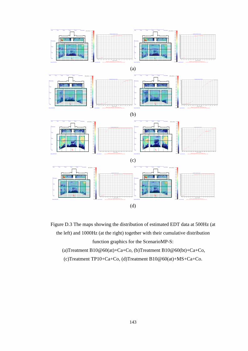
143
(a)
(b)
(c)
(d)
Figure D.3 The maps showing the distribution of estimated EDT data at 500Hz (at
the left) and 1000Hz (at the right) together with their cumulative distribution
function graphics for the ScenarioMP-S:
(a)Treatment B10@60(at)+Ca+Co, (b)Treatment B10@60(bt)+Ca+Co,
(c)Treatment TP10+Ca+Co, (d)Treatment B10@60(at)+MS+Ca+Co.
P4P4
0.00 5.00 10.00 15.00 20.00 25.00 metres
0.00
5.00
10.00
15.00 metres
1.08
1.02
0.96
0.90
0.84
0.78
0.72
0.66
0.60
0.54
0.48
0.42
0.36
0.30
0.24
0.18
0.12
0.06
EDT at 500 Hz > 1.20
< 0.01Odeon©1985-2006
Cumulative distribution function
X(5,95) = (0.24, 0.64) X(10,90) = (0.30, 0.58) X(25,75) = (0.38, 0.50) X(50) = (0.44)
X(95)-X(5) = 0.39 X(90)-X(10) = 0.27 X(75)-X(25) = 0.13
EDT (s) at 500 Hz
1.41.31.21.110.90.80.70.60.50.40.30.20.1
Perc
ent
100
95
90
85
80
75
70
65
60
55
50
45
40
35
30
25
20
15
10
5
Odeon©1985-2006
P4P4
0.00 5.00 10.00 15.00 20.00 25.00 metres
0.00
5.00
10.00
15.00 metres
1.08
1.02
0.96
0.90
0.84
0.78
0.72
0.66
0.60
0.54
0.48
0.42
0.36
0.30
0.24
0.18
0.12
0.06
EDT at 1000 Hz > 1.20
< 0.01Odeon©1985-2006
Cumulative distribution function
X(5,95) = (0.23, 0.63) X(10,90) = (0.29, 0.55) X(25,75) = (0.36, 0.49) X(50) = (0.43)
X(95)-X(5) = 0.40 X(90)-X(10) = 0.26 X(75)-X(25) = 0.12
EDT (s) at 1000 Hz
1.51.41.31.21.110.90.80.70.60.50.40.30.20.1
Perc
ent
100
95
90
85
80
75
70
65
60
55
50
45
40
35
30
25
20
15
10
5
Odeon©1985-2006
P4P4
0.00 5.00 10.00 15.00 20.00 25.00 metres
0.00
5.00
10.00
15.00
20.00 metres
1.35
1.27
1.20
1.13
1.05
0.98
0.90
0.82
0.75
0.68
0.60
0.53
0.45
0.38
0.30
0.23
0.15
0.08
EDT at 500 Hz > 1.50
< 0.02Odeon©1985-2006
Cumulative distribution function
X(5,95) = (0.28, 0.73) X(10,90) = (0.34, 0.70) X(25,75) = (0.43, 0.61) X(50) = (0.52)
X(95)-X(5) = 0.45 X(90)-X(10) = 0.36 X(75)-X(25) = 0.18
EDT (s) at 500 Hz
0.90.850.80.750.70.650.60.550.50.450.40.350.30.250.20.150.1
Perc
ent
100
95
90
85
80
75
70
65
60
55
50
45
40
35
30
25
20
15
10
5
Odeon©1985-2006
P4P4
0.00 5.00 10.00 15.00 20.00 25.00 metres
0.00
5.00
10.00
15.00
20.00 metres
1.35
1.27
1.20
1.13
1.05
0.98
0.90
0.82
0.75
0.68
0.60
0.53
0.45
0.38
0.30
0.23
0.15
0.08
EDT at 1000 Hz > 1.50
< 0.02Odeon©1985-2006
Cumulative distribution function
X(5,95) = (0.26, 0.75) X(10,90) = (0.32, 0.71) X(25,75) = (0.39, 0.59) X(50) = (0.48)
X(95)-X(5) = 0.49 X(90)-X(10) = 0.39 X(75)-X(25) = 0.20
EDT (s) at 1000 Hz
0.90.850.80.750.70.650.60.550.50.450.40.350.30.250.20.150.1
Perc
ent
100
95
90
85
80
75
70
65
60
55
50
45
40
35
30
25
20
15
10
5
Odeon©1985-2006
P4P4
0.00 5.00 10.00 15.00 20.00 25.00 metres
0.00
5.00
10.00
15.00
20.00 metres
0.90
0.85
0.80
0.75
0.70
0.65
0.60
0.55
0.50
0.45
0.40
0.35
0.30
0.25
0.20
0.15
0.10
0.05
EDT at 500 Hz > 1.00
< 0.01Odeon©1985-2006
Cumulative distribution function
X(5,95) = (0.10, 0.72) X(10,90) = (0.15, 0.71) X(25,75) = (0.26, 0.51) X(50) = (0.39)
X(95)-X(5) = 0.63 X(90)-X(10) = 0.56 X(75)-X(25) = 0.25
EDT (s) at 500 Hz
2.62.42.221.81.61.41.210.80.60.40.2
Perc
ent
100
95
90
85
80
75
70
65
60
55
50
45
40
35
30
25
20
15
10
5
Odeon©1985-2006
P4P4
0.00 5.00 10.00 15.00 20.00 25.00 metres
0.00
5.00
10.00
15.00
20.00 metres
0.90
0.85
0.80
0.75
0.70
0.65
0.60
0.55
0.50
0.45
0.40
0.35
0.30
0.25
0.20
0.15
0.10
0.05
EDT at 1000 Hz > 1.00
< 0.01Odeon©1985-2006
Cumulative distribution function
X(5,95) = (0.09, 0.72) X(10,90) = (0.13, 0.71) X(25,75) = (0.22, 0.50) X(50) = (0.35)
X(95)-X(5) = 0.63 X(90)-X(10) = 0.57 X(75)-X(25) = 0.28
EDT (s) at 1000 Hz
0.80.750.70.650.60.550.50.450.40.350.30.250.20.150.10.05
Perc
ent
100
95
90
85
80
75
70
65
60
55
50
45
40
35
30
25
20
15
10
5
Odeon©1985-2006
P4P4
0.00 5.00 10.00 15.00 20.00 25.00 metres
0.00
5.00
10.00
15.00 metres
1.08
1.02
0.96
0.90
0.84
0.78
0.72
0.66
0.60
0.54
0.48
0.42
0.36
0.30
0.24
0.18
0.12
0.06
EDT at 500 Hz > 1.20
< 0.01Odeon©1985-2006
Cumulative distribution function
X(5,95) = (0.24, 0.61) X(10,90) = (0.30, 0.56) X(25,75) = (0.37, 0.49) X(50) = (0.43)
X(95)-X(5) = 0.37 X(90)-X(10) = 0.26 X(75)-X(25) = 0.13
EDT (s) at 500 Hz
1.41.31.21.110.90.80.70.60.50.40.30.20.1
Perc
ent
100
95
90
85
80
75
70
65
60
55
50
45
40
35
30
25
20
15
10
5
Odeon©1985-2006
P4P4
0.00 5.00 10.00 15.00 20.00 25.00 metres
0.00
5.00
10.00
15.00 metres
1.08
1.02
0.96
0.90
0.84
0.78
0.72
0.66
0.60
0.54
0.48
0.42
0.36
0.30
0.24
0.18
0.12
0.06
EDT at 1000 Hz > 1.20
< 0.01Odeon©1985-2006
Cumulative distribution function
X(5,95) = (0.23, 0.61) X(10,90) = (0.29, 0.55) X(25,75) = (0.35, 0.48) X(50) = (0.42)
X(95)-X(5) = 0.38 X(90)-X(10) = 0.26 X(75)-X(25) = 0.12
EDT (s) at 1000 Hz
1.61.51.41.31.21.110.90.80.70.60.50.40.30.20.1
Perc
ent
100
95
90
85
80
75
70
65
60
55
50
45
40
35
30
25
20
15
10
5
Odeon©1985-2006
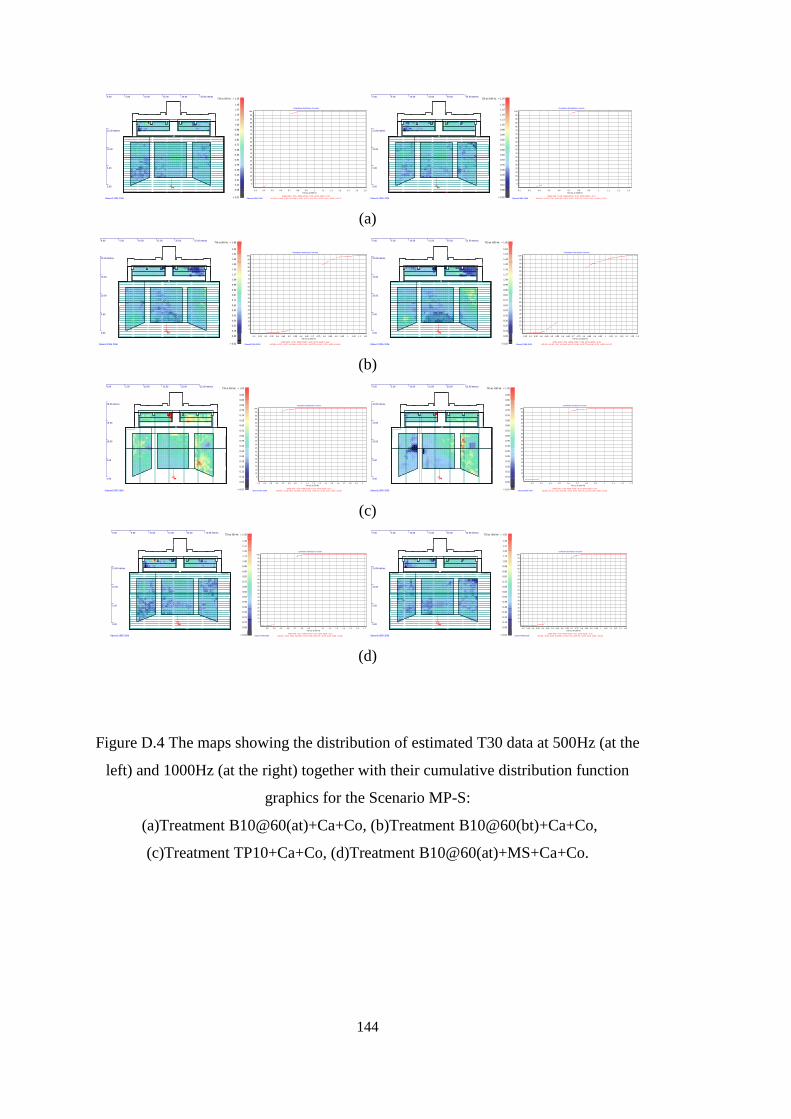
144
(a)
(b)
(c)
(d)
Figure D.4 The maps showing the distribution of estimated T30 data at 500Hz (at the
left) and 1000Hz (at the right) together with their cumulative distribution function
graphics for the Scenario MP-S:
(a)Treatment B10@60(at)+Ca+Co, (b)Treatment B10@60(bt)+Ca+Co,
(c)Treatment TP10+Ca+Co, (d)Treatment B10@60(at)+MS+Ca+Co.
P4P4
0.00 5.00 10.00 15.00 20.00 25.00 metres
0.00
5.00
10.00
15.00 metres
1.35
1.27
1.20
1.13
1.05
0.98
0.90
0.82
0.75
0.68
0.60
0.53
0.45
0.38
0.30
0.23
0.15
0.08
T30 at 500 Hz > 1.50
< 0.02Odeon©1985-2006
Cumulative distribution function
X(5,95) = (0.45, 0.70) X(10,90) = (0.47, 0.67) X(25,75) = (0.52, 0.63) X(50) = (0.57)
X(95)-X(5) = 0.25 X(90)-X(10) = 0.20 X(75)-X(25) = 0.11
T30 (s) at 500 Hz
1.61.51.41.31.21.110.90.80.70.60.50.40.3
Perc
ent
100
95
90
85
80
75
70
65
60
55
50
45
40
35
30
25
20
15
10
5
Odeon©1985-2006
P4P4
0.00 5.00 10.00 15.00 20.00 25.00 metres
0.00
5.00
10.00
15.00 metres
1.35
1.27
1.20
1.13
1.05
0.98
0.90
0.82
0.75
0.68
0.60
0.53
0.45
0.38
0.30
0.23
0.15
0.08
T30 at 1000 Hz > 1.50
< 0.02Odeon©1985-2006
Cumulative distribution function
X(5,95) = (0.45, 0.70) X(10,90) = (0.47, 0.67) X(25,75) = (0.52, 0.63) X(50) = (0.57)
X(95)-X(5) = 0.25 X(90)-X(10) = 0.20 X(75)-X(25) = 0.11
T30 (s) at 1000 Hz
1.31.21.110.90.80.70.60.50.40.30.2
Perc
ent
100
95
90
85
80
75
70
65
60
55
50
45
40
35
30
25
20
15
10
5
Odeon©1985-2006
P4P4
0.00 5.00 10.00 15.00 20.00 25.00 metres
0.00
5.00
10.00
15.00
20.00 metres
1.62
1.53
1.44
1.35
1.26
1.17
1.08
0.99
0.90
0.81
0.72
0.63
0.54
0.45
0.36
0.27
0.18
0.09
T30 at 500 Hz > 1.80
< 0.02Odeon©1985-2006
Cumulative distribution function
X(5,95) = (0.52, 0.87) X(10,90) = (0.56, 0.81) X(25,75) = (0.61, 0.73) X(50) = (0.66)
X(95)-X(5) = 0.35 X(90)-X(10) = 0.25 X(75)-X(25) = 0.12
T30 (s) at 500 Hz
1.151.11.0510.950.90.850.80.750.70.650.60.550.50.450.40.350.30.250.2
Perc
ent
100
95
90
85
80
75
70
65
60
55
50
45
40
35
30
25
20
15
10
5
Odeon©1985-2006
P4P4
0.00 5.00 10.00 15.00 20.00 25.00 metres
0.00
5.00
10.00
15.00
20.00 metres
1.62
1.53
1.44
1.35
1.26
1.17
1.08
0.99
0.90
0.81
0.72
0.63
0.54
0.45
0.36
0.27
0.18
0.09
T30 at 1000 Hz > 1.80
< 0.02Odeon©1985-2006
Cumulative distribution function
X(5,95) = (0.45, 1.01) X(10,90) = (0.51, 0.90) X(25,75) = (0.60, 0.76) X(50) = (0.67)
X(95)-X(5) = 0.55 X(90)-X(10) = 0.39 X(75)-X(25) = 0.16
T30 (s) at 1000 Hz
1.31.251.21.151.11.0510.950.90.850.80.750.70.650.60.550.50.450.40.350.30.25
Perc
ent
100
95
90
85
80
75
70
65
60
55
50
45
40
35
30
25
20
15
10
5
Odeon©1985-2006
P4P4
0.00 5.00 10.00 15.00 20.00 25.00 metres
0.00
5.00
10.00
15.00
20.00 metres
0.90
0.85
0.80
0.75
0.70
0.65
0.60
0.55
0.50
0.45
0.40
0.35
0.30
0.25
0.20
0.15
0.10
0.05
T30 at 500 Hz > 1.00
< 0.01Odeon©1985-2006
Cumulative distribution function
X(5,95) = (0.38, 0.66) X(10,90) = (0.40, 0.63) X(25,75) = (0.43, 0.56) X(50) = (0.49)
X(95)-X(5) = 0.29 X(90)-X(10) = 0.23 X(75)-X(25) = 0.12
T30 (s) at 500 Hz
21.91.81.71.61.51.41.31.21.110.90.80.70.60.50.40.3
Perc
ent
100
95
90
85
80
75
70
65
60
55
50
45
40
35
30
25
20
15
10
5
Odeon©1985-2006
P4P4
0.00 5.00 10.00 15.00 20.00 25.00 metres
0.00
5.00
10.00
15.00
20.00 metres
0.90
0.85
0.80
0.75
0.70
0.65
0.60
0.55
0.50
0.45
0.40
0.35
0.30
0.25
0.20
0.15
0.10
0.05
T30 at 1000 Hz > 1.00
< 0.01Odeon©1985-2006
Cumulative distribution function
X(5,95) = (0.31, 0.61) X(10,90) = (0.33, 0.56) X(25,75) = (0.35, 0.49) X(50) = (0.42)
X(95)-X(5) = 0.30 X(90)-X(10) = 0.23 X(75)-X(25) = 0.15
T30 (s) at 1000 Hz
1.31.21.110.90.80.70.60.50.40.30.2
Perc
ent
100
95
90
85
80
75
70
65
60
55
50
45
40
35
30
25
20
15
10
5
Odeon©1985-2006
P4P4
0.00 5.00 10.00 15.00 20.00 25.00 metres
0.00
5.00
10.00
15.00 metres
1.35
1.27
1.20
1.13
1.05
0.98
0.90
0.82
0.75
0.68
0.60
0.53
0.45
0.38
0.30
0.23
0.15
0.08
T30 at 500 Hz > 1.50
< 0.02Odeon©1985-2006
Cumulative distribution function
X(5,95) = (0.42, 0.69) X(10,90) = (0.45, 0.66) X(25,75) = (0.49, 0.60) X(50) = (0.54)
X(95)-X(5) = 0.27 X(90)-X(10) = 0.21 X(75)-X(25) = 0.11
T30 (s) at 500 Hz
1.71.61.51.41.31.21.110.90.80.70.60.50.40.3
Perc
ent
100
95
90
85
80
75
70
65
60
55
50
45
40
35
30
25
20
15
10
5
Odeon©1985-2006
P4P4
0.00 5.00 10.00 15.00 20.00 25.00 metres
0.00
5.00
10.00
15.00 metres
1.35
1.27
1.20
1.13
1.05
0.98
0.90
0.82
0.75
0.68
0.60
0.53
0.45
0.38
0.30
0.23
0.15
0.08
T30 at 1000 Hz > 1.50
< 0.02Odeon©1985-2006
Cumulative distribution function
X(5,95) = (0.43, 0.69) X(10,90) = (0.46, 0.67) X(25,75) = (0.50, 0.61) X(50) = (0.55)
X(95)-X(5) = 0.26 X(90)-X(10) = 0.21 X(75)-X(25) = 0.12
T30 (s) at 1000 Hz
1.251.21.151.11.0510.950.90.850.80.750.70.650.60.550.50.450.40.350.30.250.2
Perc
ent
100
95
90
85
80
75
70
65
60
55
50
45
40
35
30
25
20
15
10
5
Odeon©1985-2006
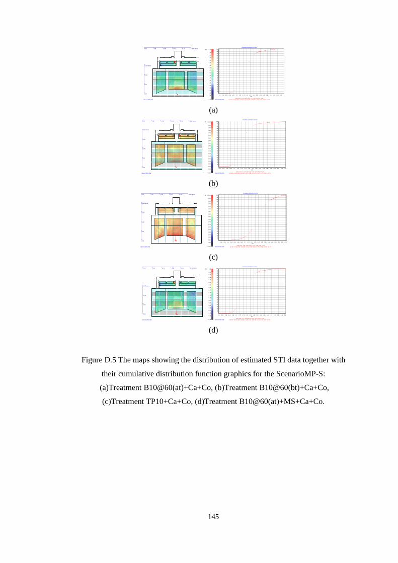
145
(a)
(b)
(c)
(d)
Figure D.5 The maps showing the distribution of estimated STI data together with
their cumulative distribution function graphics for the ScenarioMP-S:
(a)Treatment B10@60(at)+Ca+Co, (b)Treatment B10@60(bt)+Ca+Co,
(c)Treatment TP10+Ca+Co, (d)Treatment B10@60(at)+MS+Ca+Co.
P4P4
0.00 5.00 10.00 15.00 20.00 25.00 metres
0.00
5.00
10.00
15.00 metres
0.95
0.93
0.90
0.88
0.85
0.82
0.80
0.77
0.75
0.72
0.70
0.67
0.65
0.63
0.60
0.57
0.55
0.52
STI > 1.00
< 0.50Odeon©1985-2006
Cumulative distribution function
X(5,95) = (0.68, 0.84) X(10,90) = (0.70, 0.81) X(25,75) = (0.72, 0.78) X(50) = (0.75)
X(95)-X(5) = 0.16 X(90)-X(10) = 0.12 X(75)-X(25) = 0.06
STI
0.960.940.920.90.880.860.840.820.80.780.760.740.720.70.680.660.640.620.6
Perc
ent
100
95
90
85
80
75
70
65
60
55
50
45
40
35
30
25
20
15
10
5
Odeon©1985-2006
P4P4
0.00 5.00 10.00 15.00 20.00 25.00 metres
0.00
5.00
10.00
15.00
20.00 metres
0.90
0.85
0.80
0.75
0.70
0.65
0.60
0.55
0.50
0.45
0.40
0.35
0.30
0.25
0.20
0.15
0.10
0.05
STI > 1.00
< 0.01Odeon©1985-2006
Cumulative distribution function
X(5,95) = (0.69, 0.82) X(10,90) = (0.70, 0.80) X(25,75) = (0.72, 0.77) X(50) = (0.74)
X(95)-X(5) = 0.13 X(90)-X(10) = 0.09 X(75)-X(25) = 0.05
STI
0.980.960.940.920.90.880.860.840.820.80.780.760.740.720.70.680.660.640.62
Perc
ent
100
95
90
85
80
75
70
65
60
55
50
45
40
35
30
25
20
15
10
5
Odeon©1985-2006
P4P4
0.00 5.00 10.00 15.00 20.00 25.00 metres
0.00
5.00
10.00
15.00
20.00 metres
0.90
0.85
0.80
0.75
0.70
0.65
0.60
0.55
0.50
0.45
0.40
0.35
0.30
0.25
0.20
0.15
0.10
0.05
STI > 1.00
< 0.01Odeon©1985-2006
Cumulative distribution function
X(5,95) = (0.69, 0.89) X(10,90) = (0.71, 0.85) X(25,75) = (0.74, 0.81) X(50) = (0.77)
X(95)-X(5) = 0.20 X(90)-X(10) = 0.14 X(75)-X(25) = 0.07
STI
0.940.920.90.880.860.840.820.80.780.760.740.720.70.680.660.640.620.60.580.56
Perc
ent
100
95
90
85
80
75
70
65
60
55
50
45
40
35
30
25
20
15
10
5
Odeon©1985-2006
P4P4
0.00 5.00 10.00 15.00 20.00 25.00 metres
0.00
5.00
10.00
15.00 metres
0.95
0.93
0.90
0.88
0.85
0.82
0.80
0.77
0.75
0.72
0.70
0.67
0.65
0.63
0.60
0.57
0.55
0.52
STI > 1.00
< 0.50Odeon©1985-2006
Cumulative distribution function
X(5,95) = (0.68, 0.84) X(10,90) = (0.70, 0.81) X(25,75) = (0.72, 0.78) X(50) = (0.75)
X(95)-X(5) = 0.15 X(90)-X(10) = 0.11 X(75)-X(25) = 0.06
STI
0.980.960.940.920.90.880.860.840.820.80.780.760.740.720.70.680.660.640.620.6
Perc
ent
100
95
90
85
80
75
70
65
60
55
50
45
40
35
30
25
20
15
10
5
Odeon©1985-2006
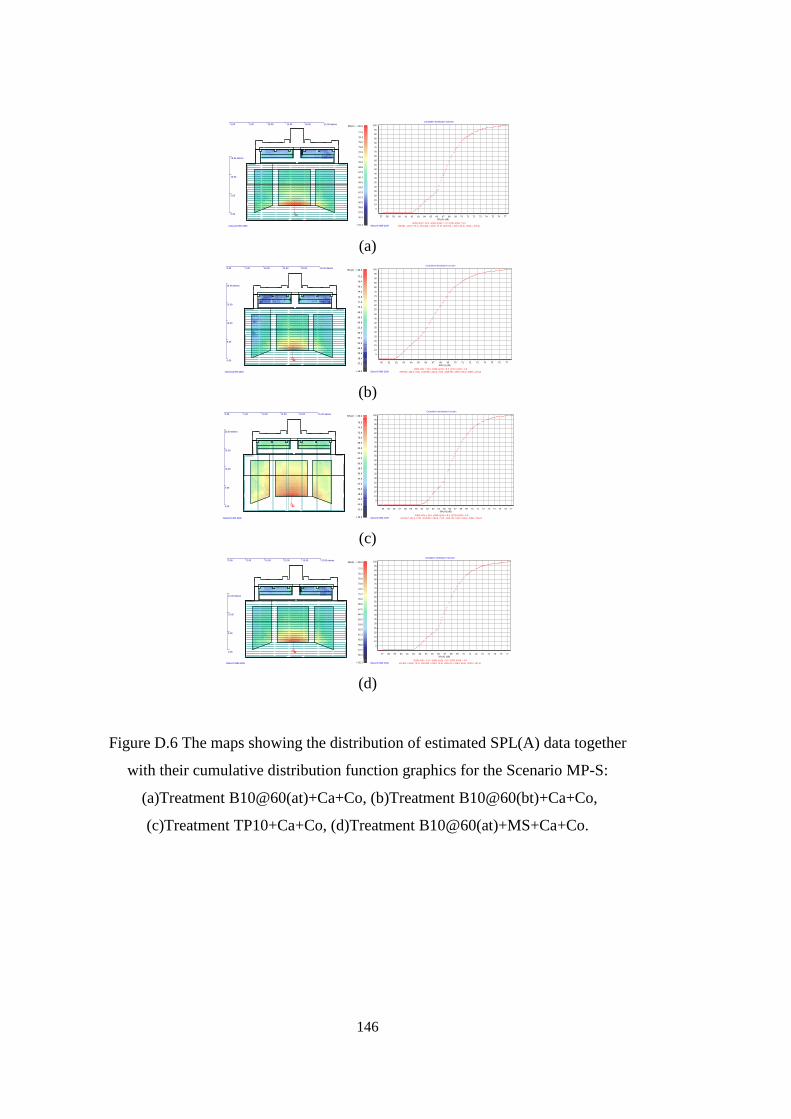
146
(a)
(b)
(c)
(d)
Figure D.6 The maps showing the distribution of estimated SPL(A) data together
with their cumulative distribution function graphics for the Scenario MP-S:
(a)Treatment B10@60(at)+Ca+Co, (b)Treatment B10@60(bt)+Ca+Co,
(c)Treatment TP10+Ca+Co, (d)Treatment B10@60(at)+MS+Ca+Co.
P4P4
0.00 5.00 10.00 15.00 20.00 25.00 metres
0.00
5.00
10.00
15.00 metres
77.5
76.3
75.0
73.8
72.5
71.3
70.0
68.8
67.5
66.3
65.0
63.8
62.5
61.3
60.0
58.8
57.5
56.3
SPL(A) > 80.0
< 55.3Odeon©1985-2006
Cumulative distribution function
X(5,95) = (62.9, 73.1) X(10,90) = (63.6, 71.5) X(25,75) = (66.0, 69.3) X(50) = (67.4)
X(95)-X(5) = 10.2 X(90)-X(10) = 7.9 X(75)-X(25) = 3.3
SPL(A) (dB)
777675747372717069686766656463626160595857
Perc
ent
100
95
90
85
80
75
70
65
60
55
50
45
40
35
30
25
20
15
10
5
Odeon©1985-2006
P4P4
0.00 5.00 10.00 15.00 20.00 25.00 metres
0.00
5.00
10.00
15.00
20.00 metres
77.6
76.4
75.2
74.0
72.8
71.6
70.4
69.2
68.0
66.8
65.6
64.4
63.2
62.0
60.8
59.6
58.4
57.2
SPL(A) > 80.0
< 56.2Odeon©1985-2006
Cumulative distribution function
X(5,95) = (62.6, 73.1) X(10,90) = (63.2, 71.5) X(25,75) = (65.3, 69.3) X(50) = (67.2)
X(95)-X(5) = 10.5 X(90)-X(10) = 8.3 X(75)-X(25) = 4.0
SPL(A) (dB)
777675747372717069686766656463626160P
erc
ent
100
95
90
85
80
75
70
65
60
55
50
45
40
35
30
25
20
15
10
5
Odeon©1985-2006
P4P4
0.00 5.00 10.00 15.00 20.00 25.00 metres
0.00
5.00
10.00
15.00
20.00 metres
76.0
74.0
72.0
70.0
68.0
66.0
64.0
62.0
60.0
58.0
56.0
54.0
52.0
50.0
48.0
46.0
44.0
42.0
SPL(A) > 80.0
< 40.4Odeon©1985-2006
Cumulative distribution function
X(5,95) = (61.9, 72.5) X(10,90) = (62.6, 71.0) X(25,75) = (64.7, 68.6) X(50) = (66.4)
X(95)-X(5) = 10.6 X(90)-X(10) = 8.4 X(75)-X(25) = 3.9
SPL(A) (dB)
777675747372717069686766656463626160595857565554
Perc
ent
100
95
90
85
80
75
70
65
60
55
50
45
40
35
30
25
20
15
10
5
Odeon©1985-2006
P4P4
0.00 5.00 10.00 15.00 20.00 25.00 metres
0.00
5.00
10.00
15.00 metres
77.5
76.3
75.0
73.8
72.5
71.3
70.0
68.8
67.5
66.3
65.0
63.8
62.5
61.3
60.0
58.8
57.5
56.3
SPL(A) > 80.0
< 55.3Odeon©1985-2006
Cumulative distribution function
X(5,95) = (62.8, 73.1) X(10,90) = (63.5, 71.5) X(25,75) = (65.9, 69.3) X(50) = (67.4)
X(95)-X(5) = 10.3 X(90)-X(10) = 8.0 X(75)-X(25) = 3.4
SPL(A) (dB)
777675747372717069686766656463626160595857
Perc
ent
100
95
90
85
80
75
70
65
60
55
50
45
40
35
30
25
20
15
10
5
Odeon©1985-2006

147
APPENDIX E
SIMULATION DATA FOR THE SCENARIO MP-P
(a)
(b)
(c)
Figure E.1 Estimated GRT (T20 and T30) values (at the left) and T30 noise reduction
curves (at the right) obtained for the MP-P scenario:
(a)Treatment B10@60(at)+Ca, (b)Treatment B10@60(bt)+Ca, (c)Treatment
TP10+Ca, (d)Treatment B10@60(at)+MS+Ca.
T30
T20
Estimated global reverberation times (Source 4, 782946 rays used)
Frequency (Hertz)
63 125 250 500 1000 2000 4000 8000
Reverb
era
tion tim
e (
s)
1.35
1.3
1.25
1.2
1.15
1.1
1.05
1
0.95
0.9
0.85
0.8
0.75
0.7
0.65
0.6
0.55
0.5
0.45
0.4
0.35
0.3
0.25
0.2
0.15
0.1
0.05
0
Odeon©1985-2006
T30,63=1.33 s
T30,125=1.39 s
T30,250=1.06 s
T30,500=0.95 s
T30,1000=0.83 s
T30,2000=0.76 s
T30,4000=0.63 s
T30,8000=0.47 s
Estimated global reverberation times (Source 4, 782946 rays used)
Estimated room volume:3978.65 m³
Time (seconds)
1.551.51.451.41.351.31.251.21.151.11.0510.950.90.850.80.750.70.650.60.550.50.450.40.350.30.250.20.150.10.050
SP
L (
dB
)
0
-5
-10
-15
-20
-25
-30
-35
-40
-45
-50
-55
-60
Odeon©1985-2006
T30
T20
Estimated global reverberation times (Source 4, 695601 rays used)
Frequency (Hertz)
63 125 250 500 1000 2000 4000 8000
Reverb
era
tion tim
e (
s)
1.3
1.25
1.2
1.15
1.1
1.05
1
0.95
0.9
0.85
0.8
0.75
0.7
0.65
0.6
0.55
0.5
0.45
0.4
0.35
0.3
0.25
0.2
0.15
0.1
0.05
0
Odeon©1985-2006
T30,63=1.30 s
T30,125=1.33 s
T30,250=1.03 s
T30,500=0.94 s
T30,1000=0.81 s
T30,2000=0.74 s
T30,4000=0.63 s
T30,8000=0.47 s
Estimated global reverberation times (Source 4, 695601 rays used)
Estimated room volume:3940.16 m³
Time (seconds)
1.551.51.451.41.351.31.251.21.151.11.0510.950.90.850.80.750.70.650.60.550.50.450.40.350.30.250.20.150.10.050
SP
L (
dB
)
0
-5
-10
-15
-20
-25
-30
-35
-40
-45
-50
-55
-60
Odeon©1985-2006
T30
T20
Estimated global reverberation times (Source 4, 966753 rays used)
Frequency (Hertz)
63 125 250 500 1000 2000 4000 8000
Reverb
era
tion tim
e (
s)
1.5
1.45
1.4
1.35
1.3
1.25
1.2
1.15
1.1
1.05
1
0.95
0.9
0.85
0.8
0.75
0.7
0.65
0.6
0.55
0.5
0.45
0.4
0.35
0.3
0.25
0.2
0.15
0.1
0.05
0
Odeon©1985-2006
T30,63=1.42 s
T30,125=1.53 s
T30,250=0.99 s
T30,500=0.88 s
T30,1000=0.72 s
T30,2000=0.63 s
T30,4000=0.54 s
T30,8000=0.40 s
Estimated global reverberation times (Source 4, 966753 rays used)
Estimated room volume:3996.88 m³
Time (seconds)
1.651.61.551.51.451.41.351.31.251.21.151.11.0510.950.90.850.80.750.70.650.60.550.50.450.40.350.30.250.20.150.10.050
SP
L (
dB
)
0
-5
-10
-15
-20
-25
-30
-35
-40
-45
-50
-55
-60
Odeon©1985-2006
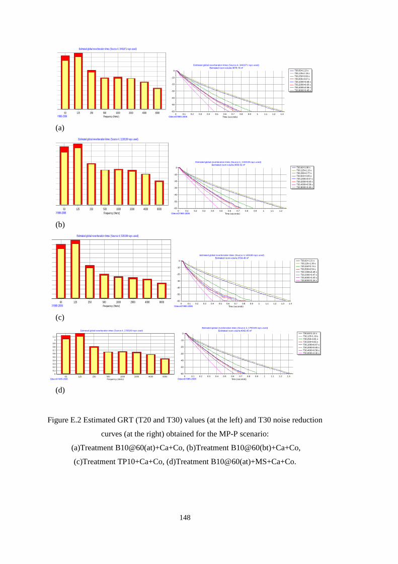
148
(a)
(b)
(c)
(d)
Figure E.2 Estimated GRT (T20 and T30) values (at the left) and T30 noise reduction
curves (at the right) obtained for the MP-P scenario:
(a)Treatment B10@60(at)+Ca+Co, (b)Treatment B10@60(bt)+Ca+Co,
(c)Treatment TP10+Ca+Co, (d)Treatment B10@60(at)+MS+Ca+Co.
T30
T20
Estimated global reverberation times (Source 4, 3441671 rays used)
Frequency (Hertz)
63 125 250 500 1000 2000 4000 8000
Reverberation tim
e (
s)
1.1
1
0.9
0.8
0.7
0.6
0.5
0.4
0.3
0.2
0.1
0
Odeon©1985-2006
T30,63=1.13 s
T30,125=1.19 s
T30,250=0.83 s
T30,500=0.67 s
T30,1000=0.68 s
T30,2000=0.65 s
T30,4000=0.58 s
T30,8000=0.45 s
Estimated global reverberation times (Source 4, 3441671 rays used)
Estimated room volume:3676.16 m³
Time (seconds)
1.31.21.110.90.80.70.60.50.40.30.20.10
SP
L (
dB
)
0
-10
-20
-30
-40
-50
-60
Odeon©1985-2006
T30
T20
Estimated global reverberation times (Source 4, 1130139 rays used)
Frequency (Hertz)
63 125 250 500 1000 2000 4000 8000
Reverberation tim
e (
s)
1.1
1
0.9
0.8
0.7
0.6
0.5
0.4
0.3
0.2
0.1
0
Odeon©1985-2006
T30,63=1.08 s
T30,125=1.13 s
T30,250=0.77 s
T30,500=0.65 s
T30,1000=0.67 s
T30,2000=0.65 s
T30,4000=0.58 s
T30,8000=0.45 s
Estimated global reverberation times (Source 4, 1130139 rays used)
Estimated room volume:3609.52 m³
Time (seconds)
1.21.110.90.80.70.60.50.40.30.20.10
SP
L (
dB
)
0
-10
-20
-30
-40
-50
-60
Odeon©1985-2006
T30
T20
Estimated global reverberation times (Source 4, 520198 rays used)
Frequency (Hertz)
63 125 250 500 1000 2000 4000 8000
Reverberation tim
e (
s)
1.2
1.1
1
0.9
0.8
0.7
0.6
0.5
0.4
0.3
0.2
0.1
0
Odeon©1985-2006
T30,63=1.21 s
T30,125=1.30 s
T30,250=0.74 s
T30,500=0.54 s
T30,1000=0.49 s
T30,2000=0.47 s
T30,4000=0.43 s
T30,8000=0.34 s
Estimated global reverberation times (Source 4, 520198 rays used)
Estimated room volume:3724.46 m³
Time (seconds)
1.41.31.21.110.90.80.70.60.50.40.30.20.10
SP
L (
dB
)
0
-10
-20
-30
-40
-50
-60
Odeon©1985-2006
T30
T20
Estimated global reverberation times (Source 4, 1790169 rays used)
Frequency (Hertz)
63 125 250 500 1000 2000 4000 8000
Reverb
era
tion tim
e (
s)
1.1
1
0.9
0.8
0.7
0.6
0.5
0.4
0.3
0.2
0.1
0
Odeon©1985-2006
T30,63=1.13 s
T30,125=1.19 s
T30,250=0.81 s
T30,500=0.65 s
T30,1000=0.67 s
T30,2000=0.65 s
T30,4000=0.58 s
T30,8000=0.45 s
Estimated global reverberation times (Source 4, 1790169 rays used)
Estimated room volume:4042.45 m³
Time (seconds)
1.31.21.110.90.80.70.60.50.40.30.20.10
SP
L (
dB
)
0
-10
-20
-30
-40
-50
-60
Odeon©1985-2006
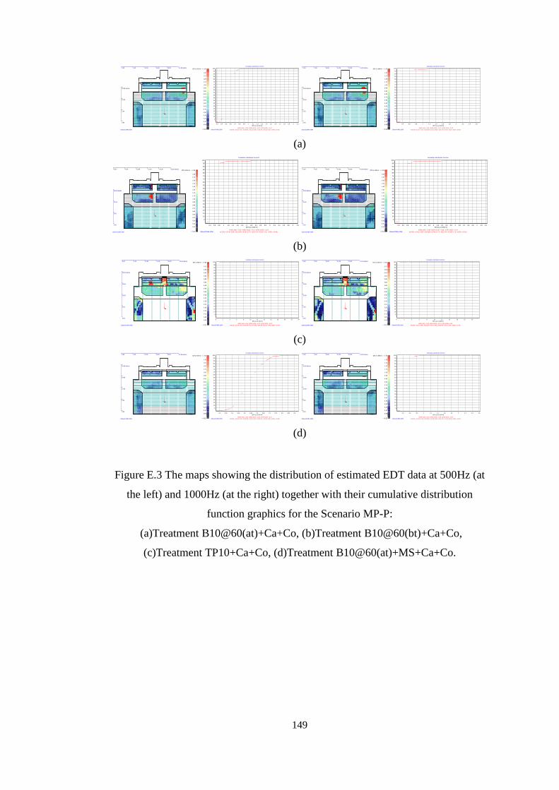
149
(a)
(b)
(c)
(d)
Figure E.3 The maps showing the distribution of estimated EDT data at 500Hz (at
the left) and 1000Hz (at the right) together with their cumulative distribution
function graphics for the Scenario MP-P:
(a)Treatment B10@60(at)+Ca+Co, (b)Treatment B10@60(bt)+Ca+Co,
(c)Treatment TP10+Ca+Co, (d)Treatment B10@60(at)+MS+Ca+Co.
P4P4
0.00 5.00 10.00 15.00 20.00 25.00 metres
0.00
5.00
10.00
15.00 metres
1.35
1.27
1.20
1.13
1.05
0.98
0.90
0.82
0.75
0.68
0.60
0.53
0.45
0.38
0.30
0.23
0.15
0.08
EDT at 500 Hz > 1.50
< 0.02Odeon©1985-2006
Cumulative distribution function
X(5,95) = (0.40, 0.72) X(10,90) = (0.43, 0.68) X(25,75) = (0.48, 0.62) X(50) = (0.54)
X(95)-X(5) = 0.32 X(90)-X(10) = 0.24 X(75)-X(25) = 0.14
EDT (s) at 500 Hz
2.121.91.81.71.61.51.41.31.21.110.90.80.70.60.50.40.3
Perc
ent
100
95
90
85
80
75
70
65
60
55
50
45
40
35
30
25
20
15
10
5
Odeon©1985-2006
P4P4
0.00 5.00 10.00 15.00 20.00 25.00 metres
0.00
5.00
10.00
15.00 metres
1.35
1.27
1.20
1.13
1.05
0.98
0.90
0.82
0.75
0.68
0.60
0.53
0.45
0.38
0.30
0.23
0.15
0.08
EDT at 1000 Hz > 1.50
< 0.02Odeon©1985-2006
Cumulative distribution function
X(5,95) = (0.37, 0.72) X(10,90) = (0.41, 0.68) X(25,75) = (0.47, 0.61) X(50) = (0.54)
X(95)-X(5) = 0.36 X(90)-X(10) = 0.27 X(75)-X(25) = 0.15
EDT (s) at 1000 Hz
2.62.42.221.81.61.41.210.80.60.4
Perc
ent
100
95
90
85
80
75
70
65
60
55
50
45
40
35
30
25
20
15
10
5
Odeon©1985-2006
P4P4
0.00 5.00 10.00 15.00 20.00 25.00 metres
0.00
5.00
10.00
15.00 metres
1.80
1.70
1.60
1.50
1.40
1.30
1.20
1.10
1.00
0.90
0.80
0.70
0.60
0.50
0.40
0.30
0.20
0.10
EDT at 500 Hz > 2.00
< 0.02Odeon©1985-2006
Cumulative distribution function
X(5,95) = (0.44, 0.83) X(10,90) = (0.46, 0.77) X(25,75) = (0.50, 0.71) X(50) = (0.56)
X(95)-X(5) = 0.39 X(90)-X(10) = 0.31 X(75)-X(25) = 0.22
EDT (s) at 500 Hz
4.243.83.63.43.232.82.62.42.221.81.61.41.210.80.60.4
Perc
ent
100
95
90
85
80
75
70
65
60
55
50
45
40
35
30
25
20
15
10
5
Odeon©1985-2006
P4P4
0.00 5.00 10.00 15.00 20.00 25.00 metres
0.00
5.00
10.00
15.00 metres
1.80
1.70
1.60
1.50
1.40
1.30
1.20
1.10
1.00
0.90
0.80
0.70
0.60
0.50
0.40
0.30
0.20
0.10
EDT at 1000 Hz > 2.00
< 0.02Odeon©1985-2006
Cumulative distribution function
X(5,95) = (0.42, 0.85) X(10,90) = (0.44, 0.77) X(25,75) = (0.48, 0.71) X(50) = (0.55)
X(95)-X(5) = 0.44 X(90)-X(10) = 0.34 X(75)-X(25) = 0.23
EDT (s) at 1000 Hz
4.44.243.83.63.43.232.82.62.42.221.81.61.41.210.80.60.4
Perc
ent
100
95
90
85
80
75
70
65
60
55
50
45
40
35
30
25
20
15
10
5
Odeon©1985-2006
P4P4
0.00 5.00 10.00 15.00 20.00 25.00 metres
0.00
5.00
10.00
15.00
20.00 metres
0.72
0.68
0.64
0.60
0.56
0.52
0.48
0.44
0.40
0.36
0.32
0.28
0.24
0.20
0.16
0.12
0.08
0.04
EDT at 500 Hz > 0.80
< 0.01Odeon©1985-2006
Cumulative distribution function
X(5,95) = (0.15, 0.63) X(10,90) = (0.17, 0.54) X(25,75) = (0.27, 0.44) X(50) = (0.35)
X(95)-X(5) = 0.49 X(90)-X(10) = 0.37 X(75)-X(25) = 0.18
EDT (s) at 500 Hz
242220181614121086420
Perc
ent
100
95
90
85
80
75
70
65
60
55
50
45
40
35
30
25
20
15
10
5
Odeon©1985-2006
P4P4
0.00 5.00 10.00 15.00 20.00 25.00 metres
0.00
5.00
10.00
15.00
20.00 metres
0.72
0.68
0.64
0.60
0.56
0.52
0.48
0.44
0.40
0.36
0.32
0.28
0.24
0.20
0.16
0.12
0.08
0.04
EDT at 1000 Hz > 0.80
< 0.01Odeon©1985-2006
Cumulative distribution function
X(5,95) = (0.10, 0.56) X(10,90) = (0.14, 0.51) X(25,75) = (0.21, 0.41) X(50) = (0.30)
X(95)-X(5) = 0.46 X(90)-X(10) = 0.37 X(75)-X(25) = 0.21
EDT (s) at 1000 Hz
20181614121086420
Perc
ent
100
95
90
85
80
75
70
65
60
55
50
45
40
35
30
25
20
15
10
5
Odeon©1985-2006
P4P4
0.00 5.00 10.00 15.00 20.00 25.00 metres
0.00
5.00
10.00
15.00
20.00 metres
1.35
1.27
1.20
1.13
1.05
0.98
0.90
0.82
0.75
0.68
0.60
0.53
0.45
0.38
0.30
0.23
0.15
0.08
EDT at 500 Hz > 1.50
< 0.02Odeon©1985-2006
Cumulative distribution function
X(5,95) = (0.39, 0.70) X(10,90) = (0.42, 0.67) X(25,75) = (0.46, 0.60) X(50) = (0.53)
X(95)-X(5) = 0.32 X(90)-X(10) = 0.25 X(75)-X(25) = 0.14
EDT (s) at 500 Hz
0.90.850.80.750.70.650.60.550.50.450.40.350.3
Perc
ent
100
95
90
85
80
75
70
65
60
55
50
45
40
35
30
25
20
15
10
5
Odeon©1985-2006
P4P4
0.00 5.00 10.00 15.00 20.00 25.00 metres
0.00
5.00
10.00
15.00
20.00 metres
1.35
1.27
1.20
1.13
1.05
0.98
0.90
0.82
0.75
0.68
0.60
0.53
0.45
0.38
0.30
0.23
0.15
0.08
EDT at 1000 Hz > 1.50
< 0.02Odeon©1985-2006
Cumulative distribution function
X(5,95) = (0.35, 0.70) X(10,90) = (0.38, 0.66) X(25,75) = (0.44, 0.60) X(50) = (0.51)
X(95)-X(5) = 0.35 X(90)-X(10) = 0.28 X(75)-X(25) = 0.16
EDT (s) at 1000 Hz
2.62.42.221.81.61.41.210.80.60.4
Perc
ent
100
95
90
85
80
75
70
65
60
55
50
45
40
35
30
25
20
15
10
5
Odeon©1985-2006

150
(a)
(b)
(c)
(d)
Figure E.4 The maps showing the distribution of estimated T30 data at 500Hz (at the
left) and 1000Hz (at the right) together with their cumulative distribution function
graphics for the ScenarioMP-P:
(a)Treatment B10@60(at)+Ca+Co, (b)Treatment B10@60(bt)+Ca+Co,
(c)Treatment TP10+Ca+Co, (d)Treatment B10@60(at)+MS+Ca+Co.
P4P4
0.00 5.00 10.00 15.00 20.00 25.00 metres
0.00
5.00
10.00
15.00 metres
1.13
1.07
1.01
0.95
0.89
0.83
0.77
0.71
0.65
0.59
0.53
0.47
0.41
0.35
0.29
0.23
0.17
0.11
T30 at 500 Hz > 1.25
< 0.06Odeon©1985-2006
Cumulative distribution function
X(5,95) = (0.41, 0.79) X(10,90) = (0.44, 0.69) X(25,75) = (0.49, 0.62) X(50) = (0.56)
X(95)-X(5) = 0.37 X(90)-X(10) = 0.25 X(75)-X(25) = 0.13
T30 (s) at 500 Hz
1.31.251.21.151.11.0510.950.90.850.80.750.70.650.60.550.50.450.40.350.3
Perc
ent
100
95
90
85
80
75
70
65
60
55
50
45
40
35
30
25
20
15
10
5
Odeon©1985-2006
P4P4
0.00 5.00 10.00 15.00 20.00 25.00 metres
0.00
5.00
10.00
15.00 metres
1.13
1.07
1.01
0.95
0.89
0.83
0.77
0.71
0.65
0.59
0.53
0.47
0.41
0.35
0.29
0.23
0.17
0.11
T30 at 1000 Hz > 1.25
< 0.06Odeon©1985-2006
Cumulative distribution function
X(5,95) = (0.39, 0.85) X(10,90) = (0.41, 0.77) X(25,75) = (0.44, 0.62) X(50) = (0.53)
X(95)-X(5) = 0.47 X(90)-X(10) = 0.36 X(75)-X(25) = 0.18
T30 (s) at 1000 Hz
1.151.11.0510.950.90.850.80.750.70.650.60.550.50.450.40.350.3
Perc
ent
100
95
90
85
80
75
70
65
60
55
50
45
40
35
30
25
20
15
10
5
Odeon©1985-2006
P4P4
0.00 5.00 10.00 15.00 20.00 25.00 metres
0.00
5.00
10.00
15.00 metres
1.44
1.36
1.28
1.20
1.12
1.04
0.96
0.88
0.80
0.72
0.64
0.56
0.48
0.40
0.32
0.24
0.16
0.08
T30 at 500 Hz > 1.60
< 0.02Odeon©1985-2006
Cumulative distribution function
X(5,95) = (0.43, 0.99) X(10,90) = (0.46, 0.79) X(25,75) = (0.53, 0.65) X(50) = (0.59)
X(95)-X(5) = 0.56 X(90)-X(10) = 0.33 X(75)-X(25) = 0.12
T30 (s) at 500 Hz
2.32.22.121.91.81.71.61.51.41.31.21.110.90.80.70.60.50.40.3
Perc
ent
100
95
90
85
80
75
70
65
60
55
50
45
40
35
30
25
20
15
10
5
Odeon©1985-2006
P4P4
0.00 5.00 10.00 15.00 20.00 25.00 metres
0.00
5.00
10.00
15.00 metres
1.44
1.36
1.28
1.20
1.12
1.04
0.96
0.88
0.80
0.72
0.64
0.56
0.48
0.40
0.32
0.24
0.16
0.08
T30 at 1000 Hz > 1.60
< 0.02Odeon©1985-2006
Cumulative distribution function
X(5,95) = (0.41, 1.51) X(10,90) = (0.43, 0.85) X(25,75) = (0.49, 0.71) X(50) = (0.61)
X(95)-X(5) = 1.11 X(90)-X(10) = 0.42 X(75)-X(25) = 0.22
T30 (s) at 1000 Hz
4.543.532.521.510.5
Perc
ent
100
95
90
85
80
75
70
65
60
55
50
45
40
35
30
25
20
15
10
5
Odeon©1985-2006
P4P4
0.00 5.00 10.00 15.00 20.00 25.00 metres
0.00
5.00
10.00
15.00
20.00 metres
1.08
1.02
0.96
0.90
0.84
0.78
0.72
0.66
0.60
0.54
0.48
0.42
0.36
0.30
0.24
0.18
0.12
0.06
T30 at 500 Hz > 1.20
< 0.01Odeon©1985-2006
Cumulative distribution function
X(5,95) = (0.34, 1.31) X(10,90) = (0.36, 1.08) X(25,75) = (0.40, 0.60) X(50) = (0.44)
X(95)-X(5) = 0.97 X(90)-X(10) = 0.72 X(75)-X(25) = 0.21
T30 (s) at 500 Hz
2.42.221.81.61.41.210.80.60.40.20
Perc
ent
100
95
90
85
80
75
70
65
60
55
50
45
40
35
30
25
20
15
10
5
Odeon©1985-2006
P4P4
0.00 5.00 10.00 15.00 20.00 25.00 metres
0.00
5.00
10.00
15.00
20.00 metres
1.08
1.02
0.96
0.90
0.84
0.78
0.72
0.66
0.60
0.54
0.48
0.42
0.36
0.30
0.24
0.18
0.12
0.06
T30 at 1000 Hz > 1.20
< 0.01Odeon©1985-2006
Cumulative distribution function
X(5,95) = (0.26, 1.35) X(10,90) = (0.32, 1.01) X(25,75) = (0.34, 0.41) X(50) = (0.37)
X(95)-X(5) = 1.09 X(90)-X(10) = 0.69 X(75)-X(25) = 0.07
T30 (s) at 1000 Hz
3.232.82.62.42.221.81.61.41.210.80.60.40.20
Perc
ent
100
95
90
85
80
75
70
65
60
55
50
45
40
35
30
25
20
15
10
5
Odeon©1985-2006
P4P4
0.00 5.00 10.00 15.00 20.00 25.00 metres
0.00
5.00
10.00
15.00
20.00 metres
1.13
1.07
1.01
0.95
0.89
0.83
0.77
0.71
0.65
0.59
0.53
0.47
0.41
0.35
0.29
0.23
0.17
0.11
T30 at 500 Hz > 1.25
< 0.06Odeon©1985-2006
Cumulative distribution function
X(5,95) = (0.40, 0.71) X(10,90) = (0.43, 0.66) X(25,75) = (0.47, 0.59) X(50) = (0.53)
X(95)-X(5) = 0.31 X(90)-X(10) = 0.23 X(75)-X(25) = 0.12
T30 (s) at 500 Hz
1.41.31.21.110.90.80.70.60.50.40.3
Perc
ent
100
95
90
85
80
75
70
65
60
55
50
45
40
35
30
25
20
15
10
5
Odeon©1985-2006
P4P4
0.00 5.00 10.00 15.00 20.00 25.00 metres
0.00
5.00
10.00
15.00
20.00 metres
1.13
1.07
1.01
0.95
0.89
0.83
0.77
0.71
0.65
0.59
0.53
0.47
0.41
0.35
0.29
0.23
0.17
0.11
T30 at 1000 Hz > 1.25
< 0.06Odeon©1985-2006
Cumulative distribution function
X(5,95) = (0.38, 0.86) X(10,90) = (0.40, 0.75) X(25,75) = (0.43, 0.56) X(50) = (0.48)
X(95)-X(5) = 0.48 X(90)-X(10) = 0.35 X(75)-X(25) = 0.13
T30 (s) at 1000 Hz
1.251.21.151.11.0510.950.90.850.80.750.70.650.60.550.50.450.40.350.3
Perc
ent
100
95
90
85
80
75
70
65
60
55
50
45
40
35
30
25
20
15
10
5
Odeon©1985-2006

151
(a)
(b)
(c)
(d)
Figure E.5 The maps showing the distribution of estimated C80 data at 500Hz (at the
left) and 1000Hz (at the right) together with their cumulative distribution function
graphics for the Scenario MP-P:
(a)Treatment B10@60(at)+Ca+Co, (b)Treatment B10@60(bt)+Ca+Co,
(c)Treatment TP10+Ca+Co, (d)Treatment B10@60(at)+MS+Ca+Co.
P4P4
0.00 5.00 10.00 15.00 20.00 25.00 metres
0.00
5.00
10.00
15.00 metres
12.8
11.7
10.6
9.5
8.4
7.3
6.2
5.1
4.0
2.9
1.8
0.7
-0.4
-1.5
-2.6
-3.7
-4.8
-5.9
C80 at 500 Hz > 15.0
< -6.8Odeon©1985-2006
Cumulative distribution function
X(5,95) = (4.5, 11.0) X(10,90) = (5.5, 10.7) X(25,75) = (6.8, 10.0) X(50) = (8.6)
X(95)-X(5) = 6.5 X(90)-X(10) = 5.2 X(75)-X(25) = 3.2
C80 (dB) at 500 Hz
13121110987654321
Perc
ent
100
95
90
85
80
75
70
65
60
55
50
45
40
35
30
25
20
15
10
5
Odeon©1985-2006
P4P4
0.00 5.00 10.00 15.00 20.00 25.00 metres
0.00
5.00
10.00
15.00 metres
12.8
11.7
10.6
9.5
8.4
7.3
6.2
5.1
4.0
2.9
1.8
0.7
-0.4
-1.5
-2.6
-3.7
-4.8
-5.9
C80 at 1000 Hz > 15.0
< -6.8Odeon©1985-2006
Cumulative distribution function
X(5,95) = (4.0, 11.3) X(10,90) = (5.1, 10.9) X(25,75) = (6.7, 10.2) X(50) = (8.6)
X(95)-X(5) = 7.3 X(90)-X(10) = 5.9 X(75)-X(25) = 3.4
C80 (dB) at 1000 Hz
131211109876543210-1-2-3-4
Perc
ent
100
95
90
85
80
75
70
65
60
55
50
45
40
35
30
25
20
15
10
5
Odeon©1985-2006
P4P4
0.00 5.00 10.00 15.00 20.00 25.00 metres
0.00
5.00
10.00
15.00 metres
14.5
13.3
12.0
10.8
9.5
8.3
7.0
5.8
4.5
3.3
2.0
0.8
-0.5
-1.8
-3.0
-4.3
-5.5
-6.8
C80 at 500 Hz > 17.0
< -7.8Odeon©1985-2006
Cumulative distribution function
X(5,95) = (4.3, 11.0) X(10,90) = (5.7, 10.5) X(25,75) = (7.1, 9.5) X(50) = (8.4)
X(95)-X(5) = 6.7 X(90)-X(10) = 4.8 X(75)-X(25) = 2.4
C80 (dB) at 500 Hz
181614121086420-2-4-6
Perc
ent
100
95
90
85
80
75
70
65
60
55
50
45
40
35
30
25
20
15
10
5
Odeon©1985-2006
P4P4
0.00 5.00 10.00 15.00 20.00 25.00 metres
0.00
5.00
10.00
15.00 metres
14.5
13.3
12.0
10.8
9.5
8.3
7.0
5.8
4.5
3.3
2.0
0.8
-0.5
-1.8
-3.0
-4.3
-5.5
-6.8
C80 at 1000 Hz > 17.0
< -7.8Odeon©1985-2006
Cumulative distribution function
X(5,95) = (4.0, 11.3) X(10,90) = (5.4, 10.9) X(25,75) = (7.2, 9.8) X(50) = (8.6)
X(95)-X(5) = 7.3 X(90)-X(10) = 5.5 X(75)-X(25) = 2.6
C80 (dB) at 1000 Hz
1614121086420-2-4-6-8
Perc
ent
100
95
90
85
80
75
70
65
60
55
50
45
40
35
30
25
20
15
10
5
Odeon©1985-2006
P4P4
0.00 5.00 10.00 15.00 20.00 25.00 metres
0.00
5.00
10.00
15.00
20.00 metres
16.0
14.0
12.0
10.0
8.0
6.0
4.0
2.0
0.0
-2.0
-4.0
-6.0
-8.0
-10.0
-12.0
-14.0
-16.0
-18.0
C80 at 500 Hz > 20.0
< -19.6Odeon©1985-2006
Cumulative distribution function
X(5,95) = (4.6, 16.7) X(10,90) = (8.1, 16.0) X(25,75) = (10.7, 14.9) X(50) = (13.0)
X(95)-X(5) = 12.1 X(90)-X(10) = 7.9 X(75)-X(25) = 4.2
C80 (dB) at 500 Hz
200-20-40-60-80-100-120-140-160-180-200-220-240-260-280-300-320
Perc
ent
100
95
90
85
80
75
70
65
60
55
50
45
40
35
30
25
20
15
10
5
Odeon©1985-2006
P4P4
0.00 5.00 10.00 15.00 20.00 25.00 metres
0.00
5.00
10.00
15.00
20.00 metres
16.0
14.0
12.0
10.0
8.0
6.0
4.0
2.0
0.0
-2.0
-4.0
-6.0
-8.0
-10.0
-12.0
-14.0
-16.0
-18.0
C80 at 1000 Hz > 20.0
< -19.6Odeon©1985-2006
Cumulative distribution function
X(5,95) = (4.8, 18.9) X(10,90) = (8.8, 18.0) X(25,75) = (11.5, 16.6) X(50) = (14.2)
X(95)-X(5) = 14.0 X(90)-X(10) = 9.2 X(75)-X(25) = 5.1
C80 (dB) at 1000 Hz
0-50-100-150-200-250-300
Perc
ent
100
95
90
85
80
75
70
65
60
55
50
45
40
35
30
25
20
15
10
5
Odeon©1985-2006
P4P4
0.00 5.00 10.00 15.00 20.00 25.00 metres
0.00
5.00
10.00
15.00
20.00 metres
12.8
11.7
10.6
9.5
8.4
7.3
6.2
5.1
4.0
2.9
1.8
0.7
-0.4
-1.5
-2.6
-3.7
-4.8
-5.9
C80 at 500 Hz > 15.0
< -6.8Odeon©1985-2006
Cumulative distribution function
X(5,95) = (5.0, 11.3) X(10,90) = (5.9, 11.0) X(25,75) = (7.2, 10.3) X(50) = (8.9)
X(95)-X(5) = 6.3 X(90)-X(10) = 5.1 X(75)-X(25) = 3.1
C80 (dB) at 500 Hz
131211109876543210
Perc
ent
100
95
90
85
80
75
70
65
60
55
50
45
40
35
30
25
20
15
10
5
Odeon©1985-2006
P4P4
0.00 5.00 10.00 15.00 20.00 25.00 metres
0.00
5.00
10.00
15.00
20.00 metres
12.8
11.7
10.6
9.5
8.4
7.3
6.2
5.1
4.0
2.9
1.8
0.7
-0.4
-1.5
-2.6
-3.7
-4.8
-5.9
C80 at 1000 Hz > 15.0
< -6.8Odeon©1985-2006
Cumulative distribution function
X(5,95) = (4.6, 11.9) X(10,90) = (5.7, 11.4) X(25,75) = (7.2, 10.7) X(50) = (9.3)
X(95)-X(5) = 7.3 X(90)-X(10) = 5.7 X(75)-X(25) = 3.4
C80 (dB) at 1000 Hz
131211109876543210-1-2-3-4
Perc
ent
100
95
90
85
80
75
70
65
60
55
50
45
40
35
30
25
20
15
10
5
Odeon©1985-2006

152
(a)
(b)
(c)
(d)
Figure E.6 The maps showing the distribution of estimated SPL(A) data together
with their cumulative distribution function graphics for the Scenario MP-P:
(a)Treatment B10@60(at)+Ca+Co, (b)Treatment B10@60(bt)+Ca+Co,
(c)Treatment TP10+Ca+Co, (d)Treatment B10@60(at)+MS+Ca+Co.
P4P4
0.00 5.00 10.00 15.00 20.00 25.00 metres
0.00
5.00
10.00
15.00 metres
77.5
76.3
75.0
73.8
72.5
71.3
70.0
68.8
67.5
66.3
65.0
63.8
62.5
61.3
60.0
58.8
57.5
56.3
SPL(A) > 80.0
< 55.3Odeon©1985-2006
Cumulative distribution function
X(5,95) = (63.8, 69.9) X(10,90) = (64.3, 68.9) X(25,75) = (65.2, 67.9) X(50) = (66.9)
X(95)-X(5) = 6.1 X(90)-X(10) = 4.6 X(75)-X(25) = 2.8
SPL(A) (dB)
7170.57069.56968.56867.56766.56665.56564.56463.56362.56261.56160.56059.55958.55857.55756.5
Perc
ent
100
95
90
85
80
75
70
65
60
55
50
45
40
35
30
25
20
15
10
5
Odeon©1985-2006
P4P4
0.00 5.00 10.00 15.00 20.00 25.00 metres
0.00
5.00
10.00
15.00 metres
73.0
72.0
71.0
70.0
69.0
68.0
67.0
66.0
65.0
64.0
63.0
62.0
61.0
60.0
59.0
58.0
57.0
56.0
SPL(A) > 75.0
< 55.2Odeon©1985-2006
Cumulative distribution function
X(5,95) = (63.2, 69.9) X(10,90) = (63.8, 68.7) X(25,75) = (64.9, 67.8) X(50) = (66.6)
X(95)-X(5) = 6.7 X(90)-X(10) = 4.9 X(75)-X(25) = 2.9
SPL(A) (dB)
727170696867666564636261605958575655545352
Perc
ent
100
95
90
85
80
75
70
65
60
55
50
45
40
35
30
25
20
15
10
5
Odeon©1985-2006
P4P4
0.00 5.00 10.00 15.00 20.00 25.00 metres
0.00
5.00
10.00
15.00
20.00 metres
92.0
89.5
87.0
84.5
82.0
79.5
77.0
74.5
72.0
69.5
67.0
64.5
62.0
59.5
57.0
54.5
52.0
49.5
SPL(A) > 97.0
< 47.5Odeon©1985-2006
Cumulative distribution function
X(5,95) = (60.8, 68.8) X(10,90) = (61.5, 67.8) X(25,75) = (63.3, 66.6) X(50) = (65.4)
X(95)-X(5) = 8.0 X(90)-X(10) = 6.3 X(75)-X(25) = 3.3
SPL(A) (dB)
500-50-100-150-200-250-300-350-400-450-500-550-600-650-700-750-800-850-900-950
Perc
ent
100
95
90
85
80
75
70
65
60
55
50
45
40
35
30
25
20
15
10
5
Odeon©1985-2006
P4P4
0.00 5.00 10.00 15.00 20.00 25.00 metres
0.00
5.00
10.00
15.00
20.00 metres
77.5
76.3
75.0
73.8
72.5
71.3
70.0
68.8
67.5
66.3
65.0
63.8
62.5
61.3
60.0
58.8
57.5
56.3
SPL(A) > 80.0
< 55.3Odeon©1985-2006
Cumulative distribution function
X(5,95) = (63.7, 69.9) X(10,90) = (64.1, 68.8) X(25,75) = (65.0, 67.8) X(50) = (66.6)
X(95)-X(5) = 6.2 X(90)-X(10) = 4.7 X(75)-X(25) = 2.8
SPL(A) (dB)
7170.57069.56968.56867.56766.56665.56564.56463.56362.56261.56160.56059.55958.55857.55756.5
Perc
ent
100
95
90
85
80
75
70
65
60
55
50
45
40
35
30
25
20
15
10
5
Odeon©1985-2006

153
APPENDIX F
MATERIAL QUANTITIES
Table F. 1. The treatments proposed for the ceiling and the amount of materials used
for each proposal
Theceiling
treatment
Material type Total area
(m2)
Board thickness
(m) Total volume
(m3)
FP5 Rockwool board 405.0 0.05 20.25
FP10 Rockwool board 405.0 0.10 40.50
B10@60 Rockwool board 378.0 0.10 37.80
B10@30 Rockwool board 740.9 0.10 74.09
B5@30 Rockwool board 740.9 0.05 37.04
B5@60 Rockwool board 378.0 0.05 18.9
B10@60 Rockwool board 378.0 0.10 37.8
B10@90
Rockwool board 257.0 0.10 25.7
TP5 Rockwool board 455.2 0.05 22.76
TP10 Rockwool board 455.2 0.10 45.52
FT Curtain fabric 455.2 -
Table F. 2 The treatments proposed for the walls and the amount of materials used
for each proposal
Material type The placement of the material used Total area(m2)
Curtain
(double-layered satin fabric
with roller blind mechanism)
Tribune's rear wall-Cr 70
Windows-Cg 117
Side walls-Cs 122
Openings (entrances)-Co 16
All-Ca 247
Perforated Metal Sheet Parapet between the playfield and
tribune 40

154
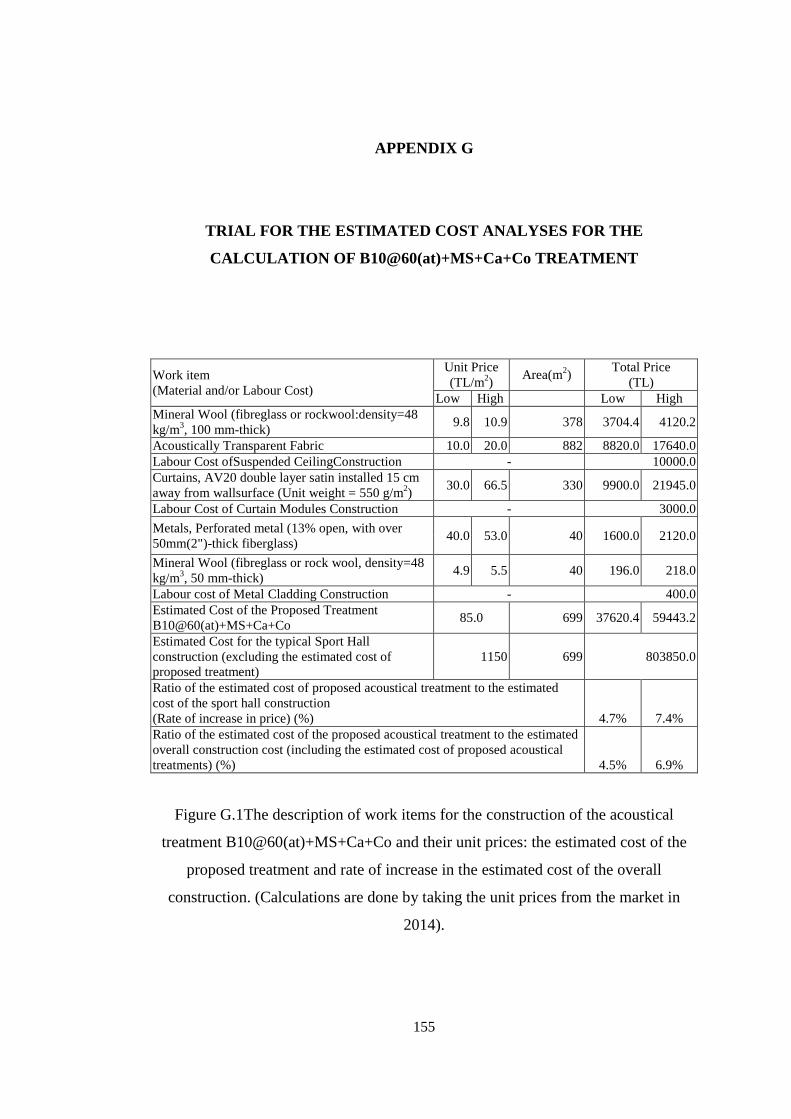
155
APPENDIX G
TRIAL FOR THE ESTIMATED COST ANALYSES FOR THE
CALCULATION OF B10@60(at)+MS+Ca+Co TREATMENT
Work item
(Material and/or Labour Cost)
Unit Price
(TL/m2)
Area(m2)
Total Price
(TL)
Low High
Low High
Mineral Wool (fibreglass or rockwool:density=48
kg/m3, 100 mm-thick)
9.8 10.9 378 3704.4 4120.2
Acoustically Transparent Fabric 10.0 20.0 882 8820.0 17640.0
Labour Cost ofSuspended CeilingConstruction - 10000.0
Curtains, AV20 double layer satin installed 15 cm
away from wallsurface (Unit weight = 550 g/m2)
30.0 66.5 330 9900.0 21945.0
Labour Cost of Curtain Modules Construction - 3000.0
Metals, Perforated metal (13% open, with over
50mm(2")-thick fiberglass) 40.0 53.0 40 1600.0 2120.0
Mineral Wool (fibreglass or rock wool, density=48
kg/m3, 50 mm-thick)
4.9 5.5 40 196.0 218.0
Labour cost of Metal Cladding Construction - 400.0
Estimated Cost of the Proposed Treatment
B10@60(at)+MS+Ca+Co 85.0 699 37620.4 59443.2
Estimated Cost for the typical Sport Hall
construction (excluding the estimated cost of
proposed treatment)
1150 699 803850.0
Ratio of the estimated cost of proposed acoustical treatment to the estimated
cost of the sport hall construction
(Rate of increase in price) (%) 4.7% 7.4%
Ratio of the estimated cost of the proposed acoustical treatment to the estimated
overall construction cost (including the estimated cost of proposed acoustical
treatments) (%) 4.5% 6.9%
Figure G.1The description of work items for the construction of the acoustical
treatment B10@60(at)+MS+Ca+Co and their unit prices: the estimated cost of the
proposed treatment and rate of increase in the estimated cost of the overall
construction. (Calculations are done by taking the unit prices from the market in
2014).
Copyright © 2022 FDOKUMEN