Seediscussions,stats,andauthorprofilesforthispublicationat:https://www.researchgate.net/publication/229212913

Acousticwavesinsolidandfluidlayeredmaterials

ARTICLEinSURFACESCIENCEREPORTS·NOVEMBER2009

ImpactFactor:14.77·DOI:10.1016/j.surfrep.2009.07.005

CITATIONS

22

READS

42

4AUTHORS,INCLUDING:

ElBoudoutiElHoussaine

UniversitéMohammedPremier

93PUBLICATIONS986CITATIONS

SEEPROFILE

AbdellatifAkjouj

UniversitédesSciencesetTechnologiesde…

166PUBLICATIONS1,533CITATIONS

SEEPROFILE

LeonardDobrzynski

FrenchNationalCentreforScientificResea…

255PUBLICATIONS5,647CITATIONS

SEEPROFILE

Availablefrom:ElBoudoutiElHoussaine

Retrievedon:26February2016

Surface Science Reports 64 (2009) 471–594

Contents lists available at ScienceDirect

Surface Science Reports

journal homepage: www.elsevier.com/locate/surfrep

Acoustic waves in solid and fluid layered materialsE.H. El Boudouti a,∗, B. Djafari-Rouhani b, A. Akjouj b, L. Dobrzynski ba LDOM, Département de Physique, Faculté des Sciences, Université Mohamed I, 60000 Oujda, Moroccob Institut d’électronique, de Microélectronique et de Nanotechnologie (IEMN), UMR-CNRS 8520, UFR de Physique, Université de Lille 1, 59655 Villeneuve d’Ascq, France

a r t i c l e i n f o a b s t r a c t

Article history:Accepted 30 July 2009editor: W.H. Weinberg

To our families in partial compensation fortaking so much of our time away from them

Keywords:SurfacesInterfacesThin filmsSuperlatticesElasticityPiezoelectricityPhononsAcoustic wavesDensity of statesGreen’s functionBrillouinRamanScatteringTransmissionFiltering

This is a comprehensive theoretical survey of acoustic wave propagation in layered materials includingelastic, viscoelastic and piezoelectric layers. The phonon modes are particularly emphasized in the caseof periodic multilayered structures such as superlattices though other layeredmaterials such as adsorbedlayers and quasiperiodic structures are also discussed. Besides the bulk waves propagating in the wholematerials, specific attention is paid to the effect of inhomogeneitieswithin the perfect superlattice such asa free surface (with orwithout a cap layer), a superlattice/substrate interface and a defect layer embeddedin the superlattice. Such inhomogeneities are usually present in actual device structures as a support(substrate) or as a protection (cap layer) for the superlattice; the defect layers offer the possibility of wavefiltering and sometimes they can be introduced as an imperfection during the epitaxial growth process.The superlattices are considered as semi-infinite or finite size structures. The symmetry of the materialsare chosen such that the transverse acoustic waves are decoupled from the sagittal one (i.e., those havingcomponents of the acoustic displacement in the sagittal plane formed by the propagation direction andthe normal to the interfaces). A general rule about the existence of localized surface modes in elastic,viscoelastic and piezoelectric semi-infinite superlattices with a free surface is presented. The adsorptionof a hardmaterial on the top of the superlattice (cap layer) has been shown to be appropriate for detectingexperimentally high frequency guided modes within the adsorbed layer. Also, the superlattice/substrateinterfacemay exhibit interfacemodeswhich arewithout analogue in the case of an interface between twohomogeneous media. For a finite size superlattice, due to the interaction between the surface, interfaceand bulkwaves, different localized and resonantmodes are obtained and their properties are investigated.In particular, the effect of a buffer layer embedded between the superlattice and the substrate in confiningguided modes in the superlattice is highlighted. These results are obtained in the frame of a Green’sfunction formalism that enables us to deduce the dispersion curves, local and total densities of states, aswell as the transmission and reflection coefficients and the corresponding phase times. In particular, anexact relation between the density of states and the phase times is pointed out. The application of elasticlayered periodic structures as acoustic mirrors that exhibit total reflection of waves for all incident anglesand polarizations in a given frequency range is indicated. These structures may also be used as acousticfilters when a defect layer is inserted within the finite size layered structure. A discussion is also includedabout some spectroscopic techniques used to probe the acoustic waves such as Raman and Brillouin lightscattering and other acoustic techniques such as the surface acoustic waves and the picosecond lasertechniques among others. A comparison of the theoretical results with experimental data available inthe literature is also presented and the reliability of the theoretical predictions is indicated. Finally, otheracoustic wave properties in quasiperiodic structures are briefly reviewed.

© 2009 Elsevier B.V. All rights reserved.

Contents

1. General introduction..........................................................................................................................................................................................................4732. Interface response theory ..................................................................................................................................................................................................475

2.1. Discrete theory.......................................................................................................................................................................................................4752.2. Continuous theory .................................................................................................................................................................................................476

∗ Corresponding author.E-mail address: elboudouti@yahoo.fr (E.H. El Boudouti).

0167-5729/$ – see front matter© 2009 Elsevier B.V. All rights reserved.doi:10.1016/j.surfrep.2009.07.005

472 E.H. El Boudouti et al. / Surface Science Reports 64 (2009) 471–594

2.3. General equations for an elastic composite material ..........................................................................................................................................4762.3.1. Bulk Green’s function of a solid material ..............................................................................................................................................4772.3.2. Surface Green’s function of a semi-infinite solid..................................................................................................................................4772.3.3. Surface Green’s function of a solid slab.................................................................................................................................................478

2.4. The special case of fluids .......................................................................................................................................................................................4782.5. General equations for a piezoelectric composite material .................................................................................................................................479

2.5.1. Surface Green’s function of a semi-infinite piezoelectric medium .....................................................................................................4792.5.2. Surface Green’s function of a piezoelectric slab ...................................................................................................................................480

3. Adsorbed slabs ...................................................................................................................................................................................................................4803.1. Introduction ...........................................................................................................................................................................................................4803.2. Resonant guided elastic waves in an adsorbed slab on a substrate ...................................................................................................................481

3.2.1. Adsorbed slab density of states .............................................................................................................................................................4813.2.2. An elastic model of the adsorbed slab...................................................................................................................................................4823.2.3. Applications and discussion of the results ............................................................................................................................................483

3.3. Resonant guided elastic waves in an adsorbed bilayer on a substrate...............................................................................................................4853.3.1. Model.......................................................................................................................................................................................................4863.3.2. Numerical results....................................................................................................................................................................................486

3.4. Localized and resonant guided elastic waves in an adsorbed layer on a semi-infinite superlattice................................................................4923.4.1. Method of calculation.............................................................................................................................................................................4923.4.2. Results and discussion............................................................................................................................................................................493

3.5. Relation to experiments ........................................................................................................................................................................................4964. Shear horizontal acoustic waves in semi-infinite superlattices......................................................................................................................................499

4.1. Introduction ...........................................................................................................................................................................................................4994.2. Transverse elastic waves in two-layer semi-infinite superlattices ....................................................................................................................500

4.2.1. Model.......................................................................................................................................................................................................5004.2.2. Density of states......................................................................................................................................................................................5014.2.3. Localized states .......................................................................................................................................................................................5024.2.4. The limit of a semi-infinite superlattice without a cap layer ..............................................................................................................5024.2.5. The limit of an interface between a semi-infinite superlattice and an homogeneous substrate ......................................................5024.2.6. Applications and discussions of the results ..........................................................................................................................................503

4.3. Transverse elastic waves in semi-infinite N-layer superlattices ........................................................................................................................5074.3.1. The infinite N-layer superlattice ...........................................................................................................................................................5074.3.2. The capped surface and the interface....................................................................................................................................................5094.3.3. Application to a four-layer superlattice ................................................................................................................................................510

4.4. Shear horizontal acoustic waves in piezoelectric superlattices .........................................................................................................................5174.4.1. Model and method of calculation ..........................................................................................................................................................5184.4.2. Discussion and results ............................................................................................................................................................................518

5. Shear horizontal acoustic waves in finite superlattices ..................................................................................................................................................5225.1. Introduction ...........................................................................................................................................................................................................5225.2. Density of states and reflection and transmission coefficients ..........................................................................................................................522

5.2.1. The local density of states ......................................................................................................................................................................5235.2.2. The total density of states ......................................................................................................................................................................5235.2.3. Reflection and transmission waves .......................................................................................................................................................5245.2.4. Relations between densities of states and phase times .......................................................................................................................524

5.3. The effect of a cap layer .........................................................................................................................................................................................5255.4. The effect of a buffer layer.....................................................................................................................................................................................528

5.4.1. Case of GaAs buffer layer and Si substrate ............................................................................................................................................5285.4.2. Case of Si buffer layer and GaAs substrate ............................................................................................................................................529

5.5. The effect of a cavity layer.....................................................................................................................................................................................5325.6. Relation to experiments ........................................................................................................................................................................................532

5.6.1. Light scattering by longitudinal acoustic phonons...............................................................................................................................5325.6.2. Picosecond ultrasonics ...........................................................................................................................................................................537

6. Surface and interface sagittal elastic waves in semi-infinite solid–solid superlattices ................................................................................................5406.1. Introduction ...........................................................................................................................................................................................................5406.2. Model and method of calculation .........................................................................................................................................................................5406.3. Results and discussions .........................................................................................................................................................................................540

6.3.1. Bulk and surface elastic waves ..............................................................................................................................................................5406.3.2. Substrate with high elastic wave velocities ..........................................................................................................................................5436.3.3. Substrate with lower elastic wave velocities........................................................................................................................................546

6.4. Relation to experiments ........................................................................................................................................................................................5477. Surface and interface sagittal elastic waves in semi-infinite solid–fluid superlattices.................................................................................................547

7.1. Introduction ...........................................................................................................................................................................................................5477.2. The theoretical model............................................................................................................................................................................................548

7.2.1. Dispersion relations................................................................................................................................................................................5487.2.2. Densities of states ...................................................................................................................................................................................549

7.3. Numerical results and discussions .......................................................................................................................................................................5507.3.1. Semi-infinite superlattice in contact with vacuum..............................................................................................................................5507.3.2. Semi-infinite superlattice in contact with an homogeneous fluid......................................................................................................553

8. Sagittal acoustic waves in finite size solid–fluid superlattices .......................................................................................................................................5558.1. Introduction ...........................................................................................................................................................................................................5558.2. Green’s functions, dispersion relations and transmission and reflection coefficients ......................................................................................556

E.H. El Boudouti et al. / Surface Science Reports 64 (2009) 471–594 473

8.2.1. Surface Green’s function of an infinite solid–fluid superlattice ..........................................................................................................5568.2.2. Inverse surface Green’s functions of finite solid–fluid superlattices with free surfaces....................................................................5578.2.3. Transmission and reflection coefficients of a finite layered media embedded between two fluids.................................................5588.2.4. Relation between the density of states and the phase times...............................................................................................................558

8.3. Application to a finite symmetric SL embedded in a fluid ..................................................................................................................................5598.3.1. Band gap structure and conditions for band and gap closing..............................................................................................................5598.3.2. Brewster acoustic angle .........................................................................................................................................................................5618.3.3. Comparative study of the DOS and phase times...................................................................................................................................562

8.4. General rule about confined and surface modes in a finite asymmetric superlattice.......................................................................................5629. Omnidirectional reflection and selective transmission in layered media......................................................................................................................565

9.1. Introduction ...........................................................................................................................................................................................................5659.2. Model and method of calculation .........................................................................................................................................................................5659.3. Case of solid–solid superlattices ...........................................................................................................................................................................566

9.3.1. Cladded superlattice structure...............................................................................................................................................................5679.3.2. Coupled solid–solid multilayer structures ............................................................................................................................................5699.3.3. Solid–solid layered acoustic filters and mode conversion ...................................................................................................................570

9.4. Case of solid–fluid superlattices ...........................................................................................................................................................................5719.4.1. Cladded solid–fluid superlattice structure............................................................................................................................................5729.4.2. Coupled solid–fluid multilayer structure..............................................................................................................................................5729.4.3. Solid–fluid layered acoustic filters ........................................................................................................................................................573

9.5. Relation to experiments ........................................................................................................................................................................................5769.5.1. Omnidirectional band gap......................................................................................................................................................................5769.5.2. Selective transmission............................................................................................................................................................................576

10. Elastic waves in quasiperiodic superlattices ....................................................................................................................................................................57810.1. Introduction ...........................................................................................................................................................................................................57810.2. Transverse elastic waves in quasiperiodic systems with planar defects ...........................................................................................................579

10.2.1. Results and discussion............................................................................................................................................................................57910.3. Sagittal elastic waves in quasiperiodic systems with planar defects .................................................................................................................582

10.3.1. Results and discussion............................................................................................................................................................................58211. Summary and conclusions.................................................................................................................................................................................................584

Acknowledgements............................................................................................................................................................................................................588Appendix A. Superlattice response functions..............................................................................................................................................................588A.1. For the infinite superlattice...................................................................................................................................................................................588A.2. For the semi-infinite superlattice with a surface cap layer ................................................................................................................................589Appendix B. Transfer matrix method for bulk and surface states..............................................................................................................................589Appendix C. Green’s function for a substrate–buffer-layer– finite-superlattice–cap-layer–substrate system ......................................................590References...........................................................................................................................................................................................................................591

1. General introduction

The interest in surface and interface acousticwaves ranges fromseismology [1] to ultrasonic processing devices [2] with importantapplications to radar and communications [3–6], passing throughflow detection [7] and quite recently to nanodevices for terahertzacoustic phonons in the hypersonic region [8]. Many of the sys-tems used now include one or several layers of different materials,which can be used for various purposes, such as to provide a de-sired dispersion characteristics [9], as part of transducers for gen-erating waves [10] or as guiding region to confine a surface wavelaterally [11].Surface waves can be found in a wide variety of geometries and

are given a variety of names: Rayleigh [12] waves propagate onthe stress-free plane surface of a semi-infinite isotropic half space.Stoneley [13,14] and Scholte [15,16] waves that propagate respec-tively along the plane interface between isotropic solid–solid andsolid–fluidmedia anddecay exponentially into both sides. The fielddisplacement of these waves can be decomposed into two orthog-onal components, one in the direction of surface acoustic wavepropagation and one perpendicular to the free surface. These twodirections define the so-called sagittal plane [3,4]. These surfacesand interfaces do not support shear horizontal waves polarizedperpendicular to the sagittal plane. Different methods have beenused to detect suchmodes including piezoelectric transducers, op-tical interferometry, light diffraction and laser-induced sound ex-citation [17]. The latter method with its optical detection [18,19]proved to be useful for the investigation of surface acoustic wavesin materials science.

In the case of a thin film supported by a substrate, guidedand pseudo-guidedmodes of shear horizontal polarization, the so-called Love waves [20] can be confined in the adsorbed layer de-pending on whether the shear velocities of sound in the adsorbateare lower or are higher than those in the substrate [21]. In additionto Love waves, adsorbed layers may support sagittal guided wavestermed Sezawa waves [22]. These waves involving two degrees ofvibrations, have been predicted first in the low frequency domainaround the shear vertical velocity range of the adsorbate and lateron, in the high frequency domain around the longitudinal veloc-ity range [23], the so-called longitudinal guidedmodes. Among thedifferent experimental acoustic techniques, Brillouin light scatter-ing [23] and picosecond ultrasonics based on pump–probe opti-cal technique [18,19] have been shown as appropriatemethods forexciting and detecting surface acoustic waves. These techniquesenables one to deduce different properties of the film such as thedensity, thickness and elastic constants. Theoretically, Brillouinscattering cross section theory [24] and density of states obtainedfrom the Green’s function [25,26] have been mainly used to repro-duce the experimental data.The goal of the first part of this review is three fold: (i) we

present a simple and general expression to calculate the densityof states of an adsorbed slab which enables us to deduce thedispersion curves for slow adsorbate on fast substrate and viceversa. Then, we propose two structures that can facilitate theconfinement of the modes in the adsorbed layers. (ii) The firstsolution consists to insert a buffer layer between the substrate andthe topmost layer, this layer plays the role of a barrier betweenphonons in these two latter materials when its velocities of soundare higher than those in the topmost layer. A detailed analysis

474 E.H. El Boudouti et al. / Surface Science Reports 64 (2009) 471–594

of local and total densities of states as well as the reflectioncoefficients associated to incident waves in the substrate enablesus to deduce the dispersion curves, the spatial localization of themodes and the delay times during the reflection process. (iii) Thesecond solution consists to change the homogeneous substrate bya superlattice (SL) made of the periodic repetition of two differentlayers. The SL is characterized by the existence of band gaps incertain frequency regions, where the SL can play the role of abarrier for phonons in the layer adsorbed on its surface. Thisoccurs when the guidedmodes of the adsorbed layer fall inside theforbidden bands of the SL, therefore well-confined modes can beobtained in the topmost layer (Section 3).The superlattices are of great importance in material science.

These structures are, in general, composed of two or several lay-ers repeated periodically along the direction of growth. The layersconstituting each cell of the SL can be made of a combinationof solid–solid or solid–fluid layered media. These materials en-ters now in the so-called phononic crystals [27] constituted by in-clusions (spheres, cylinders, . . . ) arranged in a host matrix alongtwo-dimensional (2D) and three-dimensional (3D) of the space.After the proposal of SLs by Esaki [28], the study of elementaryexcitations in multilayered systems has been very active. Amongthese excitations, acoustic phonons have received increased atten-tion after the first observation by Colvard et al. [29] of a doubletassociated to folded longitudinal acoustic phonons by means ofRaman scattering. The essential property of these structures is theexistence of forbidden frequency bands induced by the differencein acoustic properties of the constituents and the periodicity ofthese systems leading to unusual physical phenomena in these het-erostructures in comparison with bulk materials [30].With regard to acoustic waves in solid–solid SLs, a number

of theoretical and experimental works have been devoted to thestudy of the band gap structures of periodic SLs [30–33] composedof crystalline, amorphous semiconductors or metallic multilayersat the nanometric scale. The theoreticalmodels used are essentiallythe transfer matrix [30,34–36] and the Green’s function meth-ods [37–39], whereas the experimental techniques include Ramanscattering [29,40,41], ultrasonics [42–52] and time-resolved x-raydiffraction [53]. Besides the existence of the band gap structuresin perfect periodic SLs, it was shown theoretically and experimen-tally, that the ideal SL should be modified to take into account themedia surrounding the structure as: a free surface [37,38,54–63], aSL/substrate interface [37,38,57,64,65], a cavity layer [66–74], . . .which are often used in experiments together with SLs. In addi-tion to the defect modes that can be introduced by such inhomo-geneities inside the band gaps, some other works have shown theexistence of small peaks in folded longitudinal acoustic phononsand interpreted as confined phonons of thewhole finite SL [75–77].All the above phenomena have been exploited to propose one-

dimensional (1D) solid–solid layered media for several interest-ing applications as in their 2D and 3D counterparts phononiccrystals [27]. Among these applications, one canmention: (i) omni-directional band gaps [78–81], (ii) the possibility to engineer smallsize sonic crystals with locally resonant band gaps in the audi-ble frequency range [82], (iii) hypersonic crystals with high fre-quency band gaps to enhance acousto-optical interaction [72–74]and to realize stimulated emission of acoustic phonons [83], (iv)the possibility to enhance selective transmission through guidedmodes of a cavity layer inserted in the periodic structure [84] or byinterface resonance modes induced by the superlattice/substrateinterface [85–87]. The advantage of 1D systems lies in the fact thattheir design ismore feasible and they require only relatively simpleanalytical and numerical calculations. The analytical calculationsenables us to understand deeply different physical properties re-lated to the band gaps in such systems.In comparison with solid–solid layered media, the propaga-

tion of acoustic waves in the solid–fluid counterparts structures

has received less attention [88]. The first works on these sys-tems have been carried out by Rytov [89] and summarized byBrekhovskikh [88]. Rytov’s approach has been used by Schöen-berg [90] together with propagator matrix formalism to accountfor propagation through such a periodic medium in any direc-tion of propagation and at arbitrary frequency. Similar results arealso obtained by Rousseau [91]. In the low frequency limit, it wasshown [90] that besides the existence of small gaps, there is onewave speed for propagation perpendicular to the layering and twowave speeds for propagation parallel to the layering which arewithout analogue in solid–solid SLs. The two latter speeds bothcorrespond to compressional waves and their existence is sug-gestive of Biot’s theory [92] of wave propagation in porous me-dia. Alternating solid and viscous fluid layers have been proposedrecently [93–95] as an idealized porous medium to evaluate dis-persion and attenuation of acoustic waves in porous solids satu-rated with fluids. The experimental evidence [96] of these wavesis carried out using ultrasonic techniques in Al–water and Plexi-glas–water SLs. Also, it was shown theoretically and experimen-tally that finite size layered structures composed of a few cells ofsolid–fluid layerswith one [97,98] ormultiple [99] periodicitymayexhibit large gaps and the presence of defect layers in these struc-turesmay give rise towell-defined defectmodes in these gaps [98].Recently [100], solid layers separated by graded fluid layers haveshown the possibility of acoustic Bloch oscillations analogous totheWannier–Stark ladders of electronic states in a biased SL [101].The purpose of the second part of this review dealing with

periodic SLs is three fold:(i) We shall give a detailed study on surface and interface

acoustic waves of shear horizontal polarization in semi-infiniteand finite solid–solid SLs. In the case of semi-infinite SLs, we havedemonstrated analytically a general rule about the existence ofsurface and interfacemodes associatedwith a SL free-stress surfaceand a SL/substrate interface respectively. This rule predicts theexistence of one mode per gap when we consider together twosemi-infinite SLs obtained from the cleavage of an infinite SL alonga plane lying inside one layer. This rule has been shown to bevalid either for an elastic SL made of N > 2 layers as well asfor a piezoelectric SL where shear horizontal waves are coupledto electric potential. The effect of the stiffness of an homogeneoussubstrate in contact with a SL on interface modes as well as guidedand pseudo-guided modes induced by a cap layer on top of theSL are analyzed (Section 4). In the case of finite SLs, we give thedetailed expressions of dispersion relations, densities of states aswell as reflection and transmission coefficients for a SL depositedon a substrate or embedded between two substrates. In particular,we show an exact relation between the densities of states andphase times. Several applications are discussed for the effects ofa buffer layer embedded between the SL and the substrate, a caplayer deposited on top of the SL and a cavity layer inserted atdifferent places within the SL (Section 5).(ii) Surface and interface waves of sagittal polarization in

solid–solid SLs involve twodegree of vibrations. The correspondingexpressions of dispersion relations and densities of states arerather complicated event though they remain analytical [102]. Welimit ourselves to show numerical results about the possibilityof existence of surface and pseudo-surface as well as interfaceand pseudo-interface waves induced by a SL free surface anda SL/substrate interface respectively (Section 6). In the caseof solid–fluid SLs, we achieved to reduce the Green’s functioncalculations which enables us to deduce closed form expressionsof dispersion relations, densities of states as well as transmissionand reflection coefficients. Several peculiar properties, relatedto solid–fluid SLs as compared with solid–solid SLs, have beenreported. In the case of semi-infinite solid–fluid SLs, we haveshown that the creation of two semi-infinite SLs from the cleavage

E.H. El Boudouti et al. / Surface Science Reports 64 (2009) 471–594 475

of an infinite SL along a plane lying in the fluid layer, gives riseto one surface mode by gap similarly to shear horizontal waves.However, if the cleavage arises within the solid layer, then this ruleis not fulfilled and one can obtain zero, one or even two modes ineach gap of the two complementary SLs depending on the positionof the plane where the cleavage is reproduced (Section 7). In thecase of finite solid–fluid SLs, wave propagation may exhibit newphenomena as compared to solid–solid SLs such as the existenceof transmission zeros which influences the origin of the band gaps,the conditions for band gap closings and the possibility of existenceof an internal resonance induced by a fluid layer and lying inthe vicinity of a transmission zero, the so-called Fano resonance(Section 7).(iii) We show that similarly to the 2D and 3D phononic

crystals [27], layered media made of alternating solid–solid andsolid–fluid layers may exhibit total reflection of acoustic incidentwaves in a given frequency range for all incident angles. Ingeneral, this property cannot be fulfilled with a simple finite SLif the incident wave is launched from an arbitrary transmittingmedium. Therefore, we propose two solutions to obtain such anomnidirectional band gap, namely: by cladding of the SL with alayer of high acoustic velocities that acts like a barrier for thepropagation of phonons, or by associating in tandem two differentSLs in such a way that the superposition of their band structuresexhibits an absolute acoustic band gap.We discuss the appropriatechoices of the material and geometrical parameters to realizesuch structures. The behavior of the transmission coefficientsis discussed in relation with the dispersion curves of the finitesize structure. Also, these structures may be used as acousticfilters that may transmit selectively certain frequencies within theomnidirectional gaps. The transmission filtering can be achievedeither through the guided modes of a defect layer inserted in theperiodic structure or through the interface modes between theSL and a homogeneous fluid medium when these two media arechosen appropriately (Section 8).Besides the periodic multilayer systems, quasiperiodic systems

have been also intensively studied [103,104]. Many theoreticalstudies based on simple 1D models have been performed, and in-teresting properties have been deduced [103,104]. The high levelof control and perfection reached in the growth techniques ofmicrostructures and nanostructures has allowed the productionof some quasiperiodic systems [105–110] by means of molecularbeam epitaxy (MBE) techniques. It should be stressed that the the-ory of all the mathematical and formal properties of quasiperiodicsystems holds for infinitely large sequences, and this never hap-pens in experiments or calculations. In practice we always dealwith a ‘‘high’’ but finite realization. A finite realization is the n-generation which results from applying the substitution or for-mation rule for the given sequence n times and this is what onegrows experimentally and what one calculates. If n is sufficientlylarge one can think that the description of the properties of thequasiperiodic systems will be reasonably accurate. The aim of thelast part of this review is to give a brief study on the effect of in-troducing planar defects in quasiperiodic systems on the proper-ties of the frequency spectrum of these systems [111]. We shallconcentrate on shear horizontal and sagittal elastic waves in finitequasiperiodic systems constituted from an arrangement of twoblocks labeled A and B following the Fibonacci sequence. The A andB blocks are composed of bilayers. We shall study the evolution ofthe frequency spectrumof thesewaves fromquasiperiodic systemstowards the corresponding spectrum of a finite periodic system.This has been performed by the systematic introduction of planardefects in the quasiperiodic structure. The planar defects were in-troduced by substituting the B blocks present in the quasiperiodicstructures by A blocks (Section 9).These investigations are done within the framework of the

Green’s function method introduced by Leonard Dobrzynski

[112–116] for discrete and continuous composite systems, the so-called ‘‘Interface response theory’’ associated to such heterostruc-tures. We shall start by presenting the basic concepts and thefundamental equations of this theory and its application to deducethe necessary ingredients to study acoustic waves in solid and fluidlayered media (Section 2).

2. Interface response theory

We address the propagation of acoustic waves in layeredstructures. This study is performed with the help of the InterfaceResponse Theory [112–116]which permits to calculate the Green’sfunction of any compositematerial. Inwhat follows,wepresent thebasic concepts and the fundamental equations of this theory.Let us consider any composite material contained in its space

of definition D and formed out of N different homogeneous piecessituated in their domains Di (1 ≤ i ≤ N). Each piece is boundedby an interface Mi, adjacent in general to J other pieces throughsub-interface domains Mij, (1 ≤ j ≤ J). The ensemble of all theseinterface spacesMi is called the interface spaceM of the compositematerial.

2.1. Discrete theory

We consider first the discrete theory designed for problemsusing matrix formulations for linear Hamiltonians. The startingpoint is an infinite homogeneousmaterial i described by an infinitematrix [(ω2 + jε)I − Hi], where ω stands for the eigenfrequency,I is the identity matrix, j =

√−1 and ε for a infinitesimally

positive small number. The inverse of this matrix is called thecorresponding Green’s function Gi and

[(ω2 + jε)I − Hi]Gi = I. (1)

One cuts out of this medium a finite one with free surfacesin its space Di with the help of a cleavage operator V0i in theinterface space Mi. One defines Asi as the truncated part within Diof Ai = V0iGi. In the samemanner one constructs also Gsi out of thetruncated part of the Gi. One defines then block diagonal matricesG and As by juxtaposition of respectively all the Gsi and Asi definedfor N different homogeneous materials i. A composite material isthen constructed by assembling such finite media with the help ofa coupling operator VI defined in the whole interface spaceM . Onedefines then in the whole space D of the composite the matrices

A = As + VIG (2)

and in the interface spaceM

1(MM) = I(MM)+ A(MM). (3)

The elements of the Green’s function g(DD) of any compositematerial can be obtained from [112,114]

g(DD) = G(DD)− G(DM)[1(MM)]−1A(MD). (4)

The new interface states can be calculated from [112,114]

det[1(MM)] = 0, (5)

showing that, if one is interested in calculating the interface statesof a composite, one only needs to know 1(MM) in the interfacespaceM .The density of statesni corresponding toHi can thenbe obtained

from the imaginary part of the trace of Gi, namely,

ni(ω2) = −1πIm TrGi(ω2). (6)

Moreover, if U(D) [117] represents an eigenvector of thereference system formed by all the infinite materials i, Eq. (4)

476 E.H. El Boudouti et al. / Surface Science Reports 64 (2009) 471–594

enables one to calculate the eigenvectors u(D) of the compositematerial

u(D) = U(D)− U(M)[1(MM)]−1A(MD). (7)

In Eq. (7), U(D), U(M) and u(D) are row vectors. Eq. (7)enables also to calculate all the waves reflected and transmittedby the interfaces as well as the reflection and the transmissioncoefficients of the composite system. In this case, U(D) must bereplaced by a bulk wave launched in one homogeneous piece ofthe composite material [117].

2.2. Continuous theory

We consider now the continuous theory designed for problemsusing differential formulations for linear Hamiltonians. Theelements of the Green’s function g(DD) of any composite materialcan now be obtained from [112,114]

g(DD) = G(DD)− G(DM)[G(MM)]−1G(MD)

+G(DM)[G(MM)]−1g(MM)[G(MM)]−1G(MD), (8)

whereG(DD) is the block diagonal Green’s function of the referencesystem and g(MM) are the interface elements of the Green’sfunction of the composite system. The inverse [g(MM)]−1 ofg(MM) is obtained for any points in the interface space M =[⋃Mi]as a superposition of the different [gi(Mi,Mi)]−1 [112–115],

g−1(MijMi′j′) = 0, Mi′j′ 6∈ Mi (9a)

g−1(MijMij′) = g−1si (MijMij′), j 6= j′ (9b)

g−1(MijMij) =∑i′g−1s (MijMi′j′), Mi′j′ ≡ Mij. (9c)

All the boundary conditions at the interfaces are satisfiedthrough Eq. (9) where [gi(Mi,Mi)]−1 being the inverse of the[gi(Mi,Mi)] for each constituent i of the composite system. Thelatter quantities are given by the equation

[gi(Mi,Mi)]−1 = 1i(Mi,Mi)[Gi(Mi,Mi)]−1, (10)

where

1i(Mi,Mi) = I(Mi,Mi)+ Ai(Mi,Mi), (11)

with I being the unit matrix,

Ai(x, x′) =∫V0i(x′′)Gi(x′′, x′)dx′′, (12)

and x′, x′′ ∈ Di and x ∈ Mi.In Eq. (12), the cleavage operator V0i acts only in the surface

domain Mi of Di and cuts the finite or semi-infinite size block outof the infinite homogeneous medium [112–115]. Ai is called thesurface response operator of block i.The new interface states can be calculated from [112,113]

det[g(MM)]−1 = 0, (13)

showing that, if one is interested in calculating the interface statesof a composite, one only needs to know the inverse of the Green’sfunction of each individual block in the space of their respectivesurfaces.The total variation of the density of states 1N(ω2) between

the composite material and the reference one was shown to be[114,115]

1N(ω2) =1π

dη(ω2)dω2

+1π

N∑i=1

Im Tr[G(DiMi)G−1(MiMi)G(MiDi)

], (14)

where the phase shift η(ω2) is given by

η(ω2) = −arg det|g−1(MM)|. (15)

Let us stress finally that if U(D) [117] represents an eigenvectorof the reference system, Eq. (8) enables one to calculate theeigenvectors u(D) of the composite material

u(D) = U(D)− U(M)[G(MM)]−1G(MD)

+U(M)[G(MM)]−1g(MM)[G(MM)]−1G(MD). (16)

In Eq. (16), U(D), U(M) and u(D) are row vectors. Eq. (16)enables also to calculate all the waves reflected and transmittedby the interfaces as well as the reflection and the transmissioncoefficients of the composite system. In this case, U(D) must bereplaced by a bulk wave launched in one homogeneous piece ofthe composite material [117].

2.3. General equations for an elastic composite material

The equation of motion for the displacements uα , α = 1, 2, 3 ofa point of an infinite homogeneous 3D elastic material is

− ρω2uα =∑β

∂Tαβ∂xβ

(17)

where ρ is the mass density, ω the vibrational frequency, Tαβ thestress tensor

Tαβ =∑µν

Cαβµνηµν, (18)

Cαβµν is the elastic constants and ηµν the deformation tensor

ηµν =12

(∂uµ∂xν+∂uν∂xµ

). (19)

Then the bulk equation of motion (17) can be rewritten as

− ρω2uα =∑βµν

∂Cαβµν∂xβ

∂uµ∂xν+

∑βµν

Cαβµν∂2uµ∂xβ∂xν

. (20)

Suppose now that the elastic matter is limited by a free surfacewhose position in the infinite 3D space is given by

x3 = f (x1, x2), (21)

then the elastic constants are

Cαβµν(x) = Θ[x3 − f (x1, x2)]Cαβµν, (22)

where the Heaviside step function is such that

Θ[x3 − f (x1, x2)] =1, for x3 ≥ f (x1, x2)0, for x3 < f (x1, x2),

(23)

and defines in general a void in an infinite elastic matter. Notethat if one uses in Eq. (22),Θ[−x3 + f (x1, x2)] rather thanΘ[x3 −f (x1, x2)], then, one has in general a finite piece of elastic matterbounded by a free surface.Define with the help of Eqs. (20) and (22) the bulk operator

Hαµ(x) = Θ[x3 − f (x1, x2)]

(ρω2δαµ +

∑βν

Cαβµν∂2

∂xβ∂xν

), (24)

and the cleavage operator

Vαµ(x) =∑βν

∂Cαβµν∂xβ

∂

∂xν, (25)

such that

h = H+ V. (26)

E.H. El Boudouti et al. / Surface Science Reports 64 (2009) 471–594 477

Note that after differentiation of the right-hand side of Eq. (25),one has

Vαµ = +δ[x3 − f (x1, x2)]

×

∑ν

[−Cα1µν

∂ f (x1, x2)∂x1

− Cα2µν∂ f (x1, x2)∂x2

+ Cα3µν

]∂

∂xν.

(27)

Define then a surface response operatorA such that its elementsare

Aαγ (x, x′) =∫ ∑

µ

Vαµ(x)Gµγ (x, x′)dx, (28)

where the bulk response function G is defined by∑µ

Hαµ(x)Gµν(x, x′) = δανδ(x− x′). (29)

Any layered compositematerial can be built out of semi-infiniteand slab pieces. We will therefore first show here how to obtainfrom Eq. (10) the corresponding g−1s (MiMi) for a semi-infinite solidand then for a solid slab. Then we will indicate how these resultscan be also used for viscous and non-viscous fluids. Finally we willdescribe how to use these results for any layered composite.

2.3.1. Bulk Green’s function of a solid materialIn all what follows we assume the interfaces perpendicular to

the x3 axis. Then the function f (x1, x2) vanishes (see Eq. (21)).Taking advantage of the infinitesimal translational invariance ofthis layered composite in directions parallel to the interfaces, onecan Fourier analyze all operators, and in particular the responsefunctions g and G, according to

Gαβ(x, x′) =∫ ∫

d2k‖(2π)2

Gαβ(k‖|x3, x′3)eik‖(x‖−x′‖), (30)

where

k‖ = i1k1 + i2k2 (31)

x‖ = i1x1 + i2x2 (32)

i1 and i2 being unit vectors in the 1- and 2-directions, respectively.Using Eqs. (24) and (29), one finds that the Fourier coefficientGαβ(k‖|x3, x′3) of the bulk response function G is the solution of thefollowing system of ordinary differential equations∑µ

δαµρω

2+

∑βν

Cαβµν

[(1− δβ3)ikβ + δβ3

ddx3

]

×

[(1− δν3)ikν + δν3

ddx3

]Gµγ (k‖|x3, x′3) = δαγ δ(x3 − x

′

3).

(33)

Let us now choose an isotropic elastic medium for which thebulk response function G can be calculated in closed form.An isotropic elastic medium is a medium whose properties are

isotropic in all directions of space. For such a medium

Cαβµν = C12δαβδµν + C44(δαµδβν + δανδβµ), (34)

with

C12 = C11 − 2C44. (35)

The squares of the longitudinal and shear plane wave velocitiesare respectively

C2` =C11ρ

and C2t =C44ρ. (36)

Such a material is also isotropic within the (x1, x2) plane. It ispossible to choose in Eqs. (31) and (33) k2 = 0. The results obtainedfor G(k1|x3, x′3) can be used for any other direction of k‖, after arotation of the x1 and x2 axes such that k‖ lies along x1. As in thiscase |k‖| = k‖ = k1, we will write them as a function of k‖ ratherthan k1. Let us define also

α2` = k2‖−ω2

C2`, (37)

α2t = k2‖−ω2

C2t, (38)

ε =αtα`

k2‖

. (39)

Another interesting property due to the isotropy in the (x1, x2)plane is the decoupling of the transverse vibrations polarized alongx2 from the sagittal vibrations polarized in the (x1, x2) plane. Thisdecoupling will remain for all layered composites and it is possibleto study separately the x2 polarized transverse vibrations and thesagittal ones in such composites.The elements of G(k‖ω|x3, x′3) solutions of Eq. (33) were

obtained [115] to be

Gα2(k‖|x3, x′3) = G2α(k‖|x3, x′

3) = 0, α = 1, 3, (40a)

G11(k‖|x3, x′3) = −k2‖

2ρα`ω2

[e−α`|x3−x

′3| − εe−αt |x3−x

′3|], (40b)

G13(k‖|x3, x′3) =ik‖2ρω2

sgn(x3 − x′3)[e−αt |x3−x

′3| − e−α`|x3−x

′3|],

G22(k‖|x3, x′3) =−12ραtc2t

e−αt |x3−x′3|, (40c)

G31(k‖|x3, x′3) =ik‖2ρω2

sgn(x3 − x′3)[e−αt |x3−x

′3| − e−α`|x3−x

′3|],

G33(k‖|x3, x′3) = −k2‖

2ραtω2

[−εe−α`|x3−x

′3| + e−αt |x3−x

′3|]. (40d)

Let us remark that αt = (k2‖−ω2

C2t)12 is real forω < Ctk‖ and that

we choose αt = −i(ω2

C2t− k2‖)12 for ω > Ctk‖. The negative sign in

this last result corresponds in the response functions to outgoingwaves at x3 = ±∞. The same consideration applies to α`.

2.3.2. Surface Green’s function of a semi-infinite solidLet us consider now a semi-infinite solid such that x3 ≥ a. For

the isotropic solid described above and for k‖ = ik1, the elementsof the cleavage operator defined by Eq. (27) become

Vα2(k‖|x3) = V2α(k‖|x3) = 0, α = 1, 3, (41a)

V11(k‖|x3) = C44δ(x3 − a)ddx3

, (41b)

V13(k‖|x3) = ik‖C44δ(x3 − a), (41c)

V22(k‖|x3) = C44δ(x3 − a)ddx3

, (41d)

V31(k‖|x3) = ik‖C12δ(x3 − a), (41e)

V33(k‖|x3) = C11δ(x3 − a)ddx3

. (41f)

478 E.H. El Boudouti et al. / Surface Science Reports 64 (2009) 471–594

With the help of Eqs. (10), (11), (28), (40) and (41) one obtainsg−1s (a, a)

=

−

ρω2α`

k2‖(1− ε)

0 −iρk‖

[−2C2t +

ω2

k2‖(1− ε)

]0 −ραtC2t 0

iρk‖

[−2C2t +

ω2

k2‖(1− ε)

]0 −

ρω2αt

k2‖(1− ε)

.

(42)

Let us note that the g−1s (a, a) for the same elastic mediumbut such that x3 ≤ a has the same expression (42) but with achange of sign in the off-diagonal elements coupling the x1 and x3polarizations. Note also that

det|g−1s (a, a)| = −ρ2C4t

k2‖(1− ε)

[(α2t + k

2‖)2 − 4k2

‖αtα`

], (43)

which gives the well-known Rayleigh wave dispersion relation.With the help of Eq. (8), one recovers also the response functiongs of the semi-infinite solid.

2.3.3. Surface Green’s function of a solid slabLet us consider now an isotropic elastic slab such that− a ≤ x3 ≤ a. (44)The interface spaceM is now formed out of these two surfaces

x3 = ±a. The cleavage operator has contributions proportional toδ(x3+a) and δ(x3−a); the coefficients of the first one are equal tothose given by Eq. (41), the sign of the coefficients of the secondcontribution are just changed. As above, one can calculate thecorresponding g−1s (MM). As the transverse vibrations polarizedalong x2 decouple from the sagittal ones, it is convenient to deriveseparately their contribution to this g−1s (MM), namely

g−1s22(MM) = −ρc2t αtsh2αta

(ch2αta −1−1 ch2αta

). (45)

The calculation of the sagittal contribution to g−1s (MM) canbe obtained easier, with the help of the reflection symmetrythrough the middle of the slab. This decouples the corresponding4 × 4 matrix in two (2 × 2) ones, respectively g−1ss (MM) for thesymmetrical coordinates

(| − a, x1〉 + |a, x1〉)/√2, (| − a, x3〉 − |a, x3〉)/

√2

and g−1sAs for the antisymmetrical ones

(| − a, x1〉 − | − a, x1〉)/√2, (| − a, x3〉 + |a, x3〉)/

√2

whose expressions areg−1ss (MM)

=11s

α`ω2

k‖Ct2sh α`a sh αta i[2α`αtchαta sh α`a−

(α2t + k2‖)ch α`a sh αta]

−i[2α`αtch αta shα`a

−(α2t + k2‖)ch α`a shαta]

αtω2

k‖C2tch α`a ch αta

, (46)

where1s = −k‖ρC2t(chα`a sh αta− εsh α`achαta), and

g−1sAs (MM)

=11As

α`ω2

k‖C2tch α`a ch αta i[2α`αt sh αtach α`a

−(α2t + k2‖)sh α`a ch αta]

−i[2α`αt sh αta chα`a

−(α2t + k2‖)sh α`a chαta]

αtω2

k‖C2tshα`a sh αta

, (47)

where1As = −k‖ρC2t(shα`a ch αta− ε ch α`a shαta).

The above expressions are particularly useful for compositeskeeping this reflection symmetry through the middle of a centralslab. In general, however we will need the (4 × 4) expressionof the slab g−1s (MM) for the normal coordinates | − a, x1〉, | −a, x3〉, |a, x1〉, |a, x3〉. This expression is obtained easily fromEqs. (46) and (47) to be

g−1s (MM) =

a0 iq d if−iq b if ed −if a0 −iq−if e iq b

, (48)

where

a0 =Fα`ω2

2k‖C2t[sh(2αta) ch(2α`a)− ε sh(2α`a) ch(2αta)], (49)

b =Fαtω2

2k‖C2t[sh(2α`a) ch(2αta)− ε sh(2αta) ch(2α`a)], (50)

q = Fε(3k2

‖+ α2t )[sh

2(α`a)ch2(αta)+ sh2(αta)ch2(α`a)]

−12[2αlαtε + (k2‖ + α

2t )]sh(2α`a)sh(2αta)

, (51)

d = −Fα`ω2

2k‖C2t[sh(2αta)− ε sh(2α`a)], (52)

e = −Fαtω2

2k‖C2t[sh(2αla)− ε sh(2αta)] (53)

f = −F [2α`αt − ε (k2‖ + α2t )][sh

2(α`a)− sh2(αta)] (54)

with

F = −ρC2t2k‖[ch(α`a) sh(αta)− ε ch(αta) sh(α`a)]−1

×[sh(α`a) ch(αta)− ε sh(αta) ch(α`a)]−1. (55)

2.4. The special case of fluids

It was shown before [118–120] that the motion of a fluidgoverned by the linearized Navier–Stokes equation can be studiedwith the help of the same equations as for the motion of a solidproviding that

C2` = v2f −

(iω

ρf

)(µ′ +

43µ

), (56a)

C2t = −iωµρf, (56b)

where vf is the longitudinal speed of sound in the fluid, ρf itsdensity and µ and µ′ the coefficients of shear and dilatationviscosity.A non-viscous fluid can also be studied from the above

equations, by taking the limit Ct → 0 and C` = vf in them. Inthis particular case, the Green’s functions of an infinite ideal fluidis given by

Gf (x3, x′3)

=

2δ(x3 − x′3)− k2‖αf e−αf |x3−x′3| −ik‖sgn(x3 − x′3)e−αf |x3−x′3|−ik‖sgn(x3 − x′3)e

−αf |x3−x′3| αf e−αf |x3−x′3|

,(57)

where α2f = k2‖−

ω2

v2f.

E.H. El Boudouti et al. / Surface Science Reports 64 (2009) 471–594 479

ρω2 − C66k2‖ + C11d2

dx21ik‖ (C12 + C66)

ddx1

0 0

ik‖ (C12 + C66)ddx1

ρω2 − C11k2‖ + C66d2

dx210 0

0 0 ρω2 + C44

[d2

dx21− k2‖

]e15

[d2

dx21− k2‖

]0 0 e15

[d2

dx21− k2‖

]−ε11

[d2

dx21− k2‖

]

×

u1u2u3Φ

= 0

Box I.

The Green’s function of a semi-infinite fluid such that x3 ≥ a isgiven by [115]

g−1f (a, a) =(0 00 −Ff

)(58)

where Ff is defined as Ff = −ρfω2/αf .The Green’s function of a fluid layer in its space of interface

M = −a,+a is given by [115]

g−1f (MM) =

0 0 0 00 af 0 bf0 0 0 00 bf 0 af

, (59)

where

af =ρfω

2

αf

ch(2αf a)sh(2αf a)

(60)

bf = −ρfω

2

αf

1sh(2αf a)

. (61)

2.5. General equations for a piezoelectric composite material

The propagation of elastic waves in a piezoelectric crystal isgoverned by the following equation [4]

−ρω2uα =∑βγ δ

Cαβγ δ∂2uδ∂xβ∂xγ

+

∑βγ

eβαγ∂2φ

∂xβ∂xγ

α = 1, 2, 3 (62)∑βγ δ

eβγ δ∂2uδ∂xβ∂xγ

−

∑βγ

εβγ∂2φ

∂xβ∂xγ= 0 (63)

where ρ, Cαβγ δ , eαβδ and εαβ are respectively the mass density,the elastic, the piezoelectric and the dielectric constants, U is thedisplacement vector and φ the electric potential. In the followingwe shall use the elastic and piezoelectric constantswith condensedindex notations [4], namely Cij and eiα with i, j = 1 to 6 andα = 1, 2, 3.We assume that the piezoelectric medium belongs to the 6 mm

class with its c axis along the x3 axis of a reference basis set, whilethe normal to the layers is x1 and the wave vector k‖, parallelto the layers, oriented along x2. By writing an harmonic timedependence of the fields U , φ and doing a Fourier analysis alongx2 one obtains [30]

U(−→x ) = u (x1, k‖) ei(k‖x2−ωt) (64)

φ(−→x ) = φ (x1, k‖) ei(k‖x2−ωt). (65)

With the symmetry of our problem, the equations of motion (62)and (63) become the expression as given in Box I, [30]

As can be seen from this equation, the shear horizontal waves(parallel to x3) is accompanied by an electric potential, while thesagittal vibrations polarized in the (x1, x2) plane are decoupledfrom the later. In this section we are interested essentially toshear horizontal waves u3 coupled to the electric potential φ. Byconsidering only the reduced bulk Green’s function, the elementsof G

(k‖, ω; x1, x′1

)solutions of the expression in Box I were

obtained to be [84]

G33(k‖, ω; x1, x′1

)=

−1

2αC44

(1+ e215

ε11C44

)e−α|x1−x′1| (66)

G34(k‖, ω; x1, x′1

)=

−e15ε11

2αC44

(1+ e215

ε11C44

)e−α|x1−x′1| (67)

G43(k‖, ω; x1, x′1

)=

−e15ε11

2αC44

(1+ e215

ε11C44

)e−α|x1−x′1| (68)

G44(k‖, ω; x1, x′1

)=

−1

2C44

(1+ e215

ε11C44

)

×

[e215ε211

e−α|x1−x′1|

α−C44ε11

(1+

e215ε11C44

)e−k‖|x1−x

′1|

k‖

](69)

where

α2 = k2‖−

ρω2

C44

(1+ e215

ε11C44

) . (70)

2.5.1. Surface Green’s function of a semi-infinite piezoelectricmediumLet us consider now a semi-infinite piezoelectric medium such

that x1 ≥ a. For the piezoelectric medium described above and fork‖ = ik2, the elements of the cleavage operator defined by Eq. (27)become

V(x1, k‖

)

= δ [x1 − a]

C11ddx1

ik‖C12 0 0

ik‖C12 C66ddx1

0 0

0 0 C44ddx1

e15ddx1

0 0 e15ddx1

−ε11ddx1

. (71)

By considering the reduced cleavage operator related to theshear waves coupled to the potential and by using Eqs. (10), (11),

480 E.H. El Boudouti et al. / Surface Science Reports 64 (2009) 471–594

(28), (40) and (71) one obtains

g−1p (a, a)

=

k‖α(k2‖− α2

)ρω2 − C44

(k2‖− α2

)α

−ρω2

k‖

−k‖e15

−k‖e15 k‖ε11

. (72)

Let us noticing that the well-known Bleustein–Gulyaev [121,122] wave dispersion relation can be obtained easily by matchingthe Green’s function g−1p (h, h) with the corresponding one tovacuum, namely

g−1v (a, a) =[0 00 k‖ε0

], (73)

where ε0 is the dielectric constant in vacuum. Therefore, thesurface waves of the so-called open surface are obtained fromdet[g−1(a, a)] = det[g−1p (a, a)+ g

−1v (a, a)] = 0, namely

C0 =

√C44(1+ χ)

ρ

√1−

χ2

(1+ χ)21

(1+ ε/ε0)2, (74)

where χ = e215ε11C44

. The particular case of the short circuit (ormetallized) surface can be obtained from Eq. (74) by taking ε0 →∞, namely

Cs =

√C44(1+ χ)

ρ

√1−

χ2

(1+ χ)2. (75)

With the help of Eq. (8), one recovers also the response function gpof the semi-infinite piezoelectric medium.

2.5.2. Surface Green’s function of a piezoelectric slabLet us consider now a piezoelectric slab such that

− a ≤ x1 ≤ a. (76)

The interface space M is now formed out of these two surfacesx1 = ±a. The cleavage operator has contributions proportionalto δ(x1 + a) and δ(x1 − a); the coefficients of the first one areequal to those given by Eq. (71), the sign of the coefficients of thesecond contribution are just changed. As above, one can calculatethe (4× 4) expression of the slab g−1p (MM) as follows

g−1p (M,M) =

a′ q d fq b f ed f a qf e q b

(77)

where

a′ = ε11k‖

×

[(e15ε11

)2 ch (2k‖a)sh(2k‖a

) − αC44ε11k‖

(1+

e215ε11C44

)ch (2αa)sh (2αa)

](78)

d = ε11k‖

×

[−

(e15ε11

)2 1sh(2k‖a

) + αC44ε11k‖

(1+

e215ε11C44

)1

sh (2αa)

](79)

b = ε11k‖ch(2k‖a

)sh(2k‖a

) (80)

q = −e15k‖ch(2k‖a

)sh(2k‖a

) (81)

e = −ε11k‖1

sh(2k‖a

) (82)

f =e15k‖sh(2k‖a

) . (83)

In summary, we have reviewed in this section the basicequations of the Interface Response Theory and the expressionsof the Green’s functions associated to an elastic solid and viscousor non-viscous (ideal) fluid as well as to a piezoelectric materialswith infinite, semi-infinite and finite extensions. These expressionsrepresent the necessary ingredients for the study of acousticwavesin multilayered structures composed of solid–solid and solid–fluidmedia as will be described in the next sections.

3. Adsorbed slabs

3.1. Introduction

The propagation of surface acoustic waves in adsorbed layers,the so-called Love [20] and Sezawa and Kanai [22]modes, has beenextensively studied since the beginning of the last century. Thesemodes [20,21] are respectively of shear horizontal and sagittalpolarizations,whichmeans a polarization perpendicular or parallelto the sagittal plane defined by the normal to the surface and thewave vector k‖, parallel to the surface. The existence and behaviorof these modes in film/substrate systems depends strongly on therelative values of transverse and longitudinal velocities of sound inthe film (C ft , C

fl ) and the substrate (C

st , C

sl ) [23].

In the case where C ft < C st and Cfl < C

sl , called slow film on fast

substrate, different modes characterized by their speed of sound Csuch as Rayleigh, Sezawa, Love, pseudo-Sezawa and pseudo-Lovehave been studiedmostly in the vicinity of the transverse thresholdof adsorbate layers and below the transverse velocity of soundin the substrate C ft < C < C st [24,25,123–139] and thereforethese modes become guided waves of transverse character inadsorbed layers. These studies have been followed later by ananalysis of the high frequency region lying above the substratevelocity of sound and at the vicinity of the longitudinal thresholdof the adsorbate C st < C < C fl [26,138–151], the so-calledlongitudinal guided modes. The longitudinal guided modes areresonances (also called leaky or pseudowaves)with a displacementfield having longitudinal character and propagating in the film.These modes are of sagittal polarization and are without analoguein the case of shear horizontal polarization. Among the differentexperimental acoustic techniques, Brillouin light scattering [152,153] has been shown to be more appropriate for studyingsurface acoustic phonons in slow films such as Si–SiO2/Si [130,131,147–149], Mo/Si [133], Si(amorphous)/Si(crystalline) [25],SiO2/GaAs [26,134], ZnSe/GaAs [141–143,150], GaN–AlN/Si [139],Si–SiON/Si [140], WC/Si [136]. The experimental results have beenfound in good agreement with Brillouin scattering cross sectiontheory [24,148] and densities of states obtained from the Green’sfunction [25,26,136,139,150].In the case where C ft > C st and C

fl > C sl , called fast film

on slow substrate, only one surface Rayleigh branch exists in thevelocity region limited by C st and for an adsorbed layer thick-ness not exceeding a critical value [20,21]. For C > C st , all theabove waves become resonant with the bulk bands of the sub-strate. Contrary to slow films on fast substrate, thesemodes appearas small peaks in light scattering spectra and densities of states,and become, therefore, difficult to be detected experimentally.However, recently [154–164] some Brillouin scattering experi-ments performed on fast films such as Carbone/Si [154–159] and c-BN/Si [160,161], have shown with success the existence of guided

E.H. El Boudouti et al. / Surface Science Reports 64 (2009) 471–594 481

modes of transverse and longitudinal character as well as Stoneleyinterface modes localized at the interface between the substrateand the adsorbed layer [162–164]. Other recent Brillouin scatter-ing experiments [165,166] on free-standing films, have shown dif-ferent discrete modes (symmetrical and asymmetrical modes andflexion and dilatation modes) in one layer of SiN [165] as well as inone bilayer made of Si3N4 and a synthetic polymer [166]. Themea-sure of surfacemodes andpseudo-modes byBrillouin spectroscopyhelps one to characterize the elastic properties (elastic constants,mass densities, thickness, . . . ) of thin films [136,138,139,166] andsuperlattices [124–128,167,168].Among different mathematical approaches, the Green’s func-

tion method [23,115] is quite suitable for studying the spectralproperties of these composite materials; in particular, it enablesus to calculate the total or local densities of states. Their knowl-edge in these structures enables us to determine the spatial dis-tribution of the modes and in particular the possibility of guidedpseudo-modes, which may appear as well-defined peaks of thedensity of states in the continuum of the substrate bulk band. TheGreen’s function approach used in this work is also of interest forthe calculation of transmission and reflection coefficients [117], orfor studying the scattering of light by surface phonons [23,25].This section will be organized as follows: in Section 3.2 we

will present an overview of the results concerning one adsorbedlayer for two cases fast/slow and slow/fast systems. Section 3.3 willbe devoted to the case of two adsorbed layers, in particular weshall focus our attention on the possibility of finding well-definedguided pseudo-modes in the topmost layer, as a consequence ofits separation from the substrate by the buffer layer, when thevelocities of sound in the buffer are higher than those in thetopmost layer. This phenomenon results from the fact that some ofthe slab modes of the top layer, even if they are in resonance withthe substrate bulk modes, cannot propagate in the intermediatelayer and therefore remain well-defined guided waves of thehigher slab. In Section 3.4, we put forward a new idea for makingpossible, or at least facilitate, the observation of the guided modesin an adsorbed layer, namely, to use a superlattice, instead of ahomogeneous medium, as the substrate. This opens the possibilityof finding true guided modes in the adsorbed layer, when thesemodes fall inside the minigaps of the superlattice. Section 3.5summarizes some experimental results related to this work.

3.2. Resonant guided elastic waves in an adsorbed slab on a substrate

As mentioned above, vibrational modes of an isotropic adsor-bate slab on an isotropic substrate include shear horizontal andsagittal polarizations, whichmeans a polarization perpendicular orparallel to the sagittal plane defined by the normal to the surfaceand the wave vector k‖, parallel to the surface. When Ct1 < Ct2,where Ct1 and Ct2 are the transverse velocities of sound in the ad-sorbate and substrate respectively, these waves emerge from thebottom of the substrate bulk bands with increasing k‖; their dis-persion is a function of the quantity 2k‖awhere 2a is the thicknessof the slab. Their extension into the substrate bulk bands corre-sponds to resonant or leaky waves which can have the character oflongitudinal guided waves in the slab when their velocity lies be-low Cl2 (the substrate longitudinal velocity of sound). For Ct1 > Ct2all the above waves become resonant with the bulk bands of thesubstrate.In this section we give a general expression for the calculation

of the total density of states associated with an adsorbed slab(Section 3.2.1). This expression is then used in the frame of theelasticity theory of isotropic media and provides semi-analyticalexpressions for the densities of states associated with the modespolarized perpendicular to the sagittal plane as well as withthose polarized within the sagittal plane (Section 3.2.2). Some

0

g

2

12a

x3

0

gS2

2

22a

x3

2

1

gS2

gS2

gS

gL1

gL2

2

2

a b

c d

Fig. 1. The adsorbed slab (a) as constructed from the reference system of (b).The corresponding Green’s functions are given on the right-hand side of thesefigures. The semi-infinite substrate (c) and its reference system (d) as used in thedemonstration given in the text, togetherwith the correspondingGreen’s functions.

applications to W/Al (slow/fast) and Al/W (fast/slow), as well asto ZnSe slabs on a GaAs substrate, illustrate these general results(Section 3.2.3).

3.2.1. Adsorbed slab density of statesConsider a slab of a material i = 1 adsorbed on a semi-infinite

substrate of a different material i = 2 (Fig. 1(a)). The vibrationalproperties of such a system can be modeled either by a dynamicalmatrix within a lattice dynamics approach or by a differential formwithin elasticity theory (For simplicity Fig. 1 was drawn only forthe latter case). In both cases, one can associate with this systema Green’s function g(ω) where ω is the frequency. This responsefunction g(ω) can be constructed out of a reference Green’sfunction gs(ω); the latter can be taken to be formed from twodisconnected parts, namely the Green’s functions gL1(ω2) for a freeslab of material 1 and gs2(ω2) for the semi-infinite substrate madeofmaterial 2 (see Fig. 1(b)). Several general relations exist betweeng(ω2) and gs(ω2). We use here the one given initially [169,170]for an interface between two continuous media. As this relationis in fact valid for any composite material in a discrete as well as ina continuous approach, we write it in the following matrix form:

g(DD) = gs(DD)− gs(DM)[gs(MM)]−1gs(MD)

+ g(DM)[g(MM)]−1g(MD) (84)

where D stands for the total real space of the system and M forthe interface space between the slab and the substrate. Within anelastic model, M is just limited to the plane x3 = 2a, shown inFig. 1.The total density of states n(ω) for the adsorbed slab can be

obtained from the trace of the imaginary part of g(ω). It can berelated to the density of state ns(ω) of the reference system by

n(ω)− ns(ω) =1πImddωln det

(g(MM)gs(MM)

). (85)

A demonstration of this relation can be obtained followingthose given in [169,170] (see also, for example, [115,171]).However the (85) is simpler here because we use for the referenceGreen’s function the complete matrix gs rather than the truncatedbulk Green’s functions.So in order to calculate the difference between the densities of

states of the adsorbed slab and of the reference system (i.e. a freeslab of material 1 and the semi-infinite substrate of material 2), weneed only to know the interface elements g(MM), gL1(MM) and

482 E.H. El Boudouti et al. / Surface Science Reports 64 (2009) 471–594

gs2(MM). We may search for the difference between the densitiesof states of the adsorbed slab and the substrate alone; then wehave to subtract out in the numerical computations the density ofstates of the free slab, formed out of delta peaks situated at theslab eigenfrequencies ω2(k‖) for a given value of the propagationvector k‖ parallel to the surface. The drawback in such a procedureis that we compare two systems that do not have the same degreeof freedom (see Figs. 1(a) and 1(b)). In order to improve on this,it is helpful to compare the density of states of the adsorbed slabwith that of a semi-infinite substrate having its free surface at theplane x3 = 0 rather than at x3 = 2a (Fig. 1(c)). This differencecan be obtained by using Eq. (85) twice, namely once to obtain thevariation of the density of states between the systems displayedin Figs. 1(a) and 1(b) and a second time to compare the systemsshown in Figs. 1(c) and 1(d). Then

1n(ω) = na(ω)− nc(ω)

=1πImddωln det

[g(2a, 2a)gL2(2a, 2a)gs2(2a, 2a)gL1(2a, 2a)

]+ density of states of slab L1− density of states of slab L2 (86)

where L1 and L2 refer to slabs of thickness 2amade respectively ofmaterials 1 and 2.With a slight modification of the notations for the interface

space, this relation remains valid for a lattice dynamical model.Note that the densities of states of slabs L1 and L2 provide onlydelta peaks situated at the eigenfrequencies ω(k‖) of the freesurface slabs L1 and L2.In the next section, we apply this general result to an elastic

model for which all the Green’s function elements appearing inEq. (86) can be obtained in closed form.

3.2.2. An elastic model of the adsorbed slabWe choose now to describe the media forming the slabs and

the substrate as isotropic elastic media. The parameters involvedfor each material are its mass density ρ and its elastic constantsC11, and C44. The squares of the bulk longitudinal and shear planewave velocities are respectively

C2l =C11ρ

and C2t =C44ρ. (87)

Such a material is also isotropic within the (x1, x2) plane.This enables for a given value for the propagation vector k‖parallel to the surface, to decouple the shear horizontal vibrationsfrom those polarized within the sagittal plane. The correspondingGreen’s functions were derived in closed form for a semi-infinitesolid [172], for an isolated slab [173,174], and for the shearhorizontal component of an adsorbed slab [174].Here, we shall give the Green’s functions corresponding to the

modes of shear and sagittal polarizations. In the derivation of thedensity of states, we only need its truncated part in the interfacespace, i.e. g(2a, 2a), which can be easily obtained [115,171] fromEq. (9):

[g(2a, 2a)]−1 = [gL1(2a, 2a)]−1 + [gs2(0, 0)]−1. (88)

Using the Green’s function interface elements given be-fore [115,171–174], one obtains the expressions necessary inEq. (86) for the density of states calculation.In what follows we give explicit expressions for gs(0, 0) and

gs(2a, 2a) for a semi-infinite substrate and for gL(2a, 2a) for afree slab. As mentioned in Section 2.3.1, the component g22 of theGreen’s functions is decoupled from the components g11, g13, g31,g33, i.e. g12 = g21 = g23 = g32 = 0. The contribution of theshear horizontal vibrations to the density of states only comes from

the 22 component whereas components 11, 13, 31, 33 give thecontribution to the density of states of sagittal modes.We first define the following quantities:

α2t = k2‖−ω2

C2t, (89)

α2l = k2‖−ω2

C2l, (90)

ε =αtαl

k2‖

, (91)

C t = cosh(αta), C l = cosh(αla), (92)

St = sinh(αta) and S l = sinh(αla) (93)

and give then the transverse and sagittal components of the surfaceGreen’s function elements appearing in Eq. (86).

3.2.2.1. The transverse components of the surface Green’s functionelements.

gs(0, 0) = −1

ραtC2t(94)

gs(2a, 2a) = −1

2ραtC2t(1+ e−4αta) (95)

gL(2a, 2a) = −cosh(2αta) sinh(2αta)

ραtC2t. (96)

3.2.2.2. The sagittal components of the surface Green’s functionelements.

gs(0, 0) =1

ρc2t[(k2‖+ α2t )

2 − 4αlαtk2‖]

×

(αtω

2/c2t ik‖[k2‖+ α2t − 2αlαt

]−ik‖

[k2‖+ α2t − 2αlαt

]αtω

2/c2t

)(97)

gs(2a, 2a) =(m in−in p

)(98)

where

m =Fαtω2

k‖c2t

[(k2‖+ α2t )

2S lC l(C t2+ St

2)

− 4αlαtk2‖StC t(C l

2+ S l

2)], (99)

n = 2Fαlαt(k2‖ + α

2t )(3k

2‖+ α2t )(S

l2C t2+ C l

2St2)

− C lS lStC t[(k2‖+ α2t )

3+ 8ε2k6

‖

](100)

p =Fαlω2

k‖c2t

[(k2‖+ α2t )

2StC t(C l2+ S l

2)

− 4αlαtk2‖SlC l(C t

2+ St

2)], (101)

1F=2ρc2tk‖

[(k2‖+ α2t )

2StC l − 4αlαtk2‖SlC t]

×[(k2‖+ α2t )

2S lC t − 4αlαtk2‖StC l]

(102)

gL(2a, 2a) =k‖

2ρω2r+

(u iv−iv w

)(103)

E.H. El Boudouti et al. / Surface Science Reports 64 (2009) 471–594 483

Table 1Transverse and longitudinal sound velocities andmass densities forW, Al, ZnSe andGaAs.

Ct (m/s) Cl (m/s) ρ (kg/m3)

W 2860 5231 19300Al 3110 6422 2700Si 5845 8440 2330ZnSe 2725 4065 5264GaAs 3342 4710 5316.9

4.5

4

3.5

C (

km/s

)

3

0 5 10 15 20 252 k//a

Ct(W)

Fig. 2. The dispersion curves (velocity C versus the reduced wave vector 2k‖a) oflocalized and resonant transverse modes for a W slab on an Al substrate. Full andbroken curves respectively represent localized and resonant modes.

where

u = −k‖αl

[(1− ε)r+ + 2e−2a(αl+αt ) + r−

(e−4αla + εe−4αta

)](104)

v = e−2a(αl+αt )(1+

1ε

)+ r−

(e−4αla + e−4αta

)(105)

w = −k‖αt

[(1− ε)r+ + 2e−2a(αl+αt ) + r−

(e−4αta + εe−4αla

)](106)

r± =−4αlαtk2‖ ± (k

2‖+ α2t )

2

4αlαt(k2‖ + α2t )

. (107)

3.2.3. Applications and discussion of the resultsThis section contains a few illustration of the densities of states

and dispersion curves for a W slab of thickness 2a deposited onan Al substrate and vice versa; the parameters for these materialsare listed in Table 1. We shall discuss the general behavior of theseproperties as well as their peculiarities for the example underconsideration. In particular, it should be noticed that due to thelarge difference between the elastic constants forWandAl,most ofthe dispersion curves in the caseW/Al (respectively Al/W) are veryclose to those of a free slab of W (respectively a slab of Al havingone surface free of stress and the other rigidly bound).Before discussing the results in a range of longitudinal velocities

of sound, let us first present in Fig. 2 the dispersion of localizedand resonant modes of shear horizontal polarization for a W slabon an Al substrate; these modes are obtained from the peaks ofthe density of states (DOS) n(ω, k‖), as illustrated in Fig. 3 for agiven value of the dimensionless wave vector 2k‖a. In Fig. 2, the

DE

NSI

TY

OF

STA

TE

S

Ct(Al)

10

5

0

-53.5 4.0

C (km/s)

3.0 4.5

Fig. 3. The variation of the density of states of transverse modes in units of2a/Ct (Al) between an adsorbed slab of W on an Al substrate and the same amountof a semi-infinite crystal of Al. The figure is sketched for 2k‖a = 20.

curves below the transverse sound line of the substrate representlocalized modes decaying exponentially into the substrate andappearing as delta peaks in the DOS. In the limit of k‖a→∞, theyasymptotically tend to the limit of Ct(W ). On the other hand, theirextension into the substrate bands represents resonant states (orleaky waves) whose lifetimes are related to the finite widths of thepeaks in the density of states. Fig. 3 shows that, for a given value fork‖a these peaks becomewider and their intensities decrease whenthe frequency increases.As pointed out above, the dispersion curves in Fig. 2 are very

close to those obtained for a free slab of W; in the same waythe results for an Al slab on W (not shown here) are similar tothose for an isolated Al slab with one surface free of stress and theother rigidly bound. These are two particularly extreme situationswhich are not realized in general for arbitrary parameters of theconstituents. However, they may be satisfactorily reproduced forthe parts of the dispersion curves which are far from the substratesound line, this means at frequencies which are significantly loweror higher than the bottom of the substrate bands. As a particularexample let us notice that for k‖a = 0, the positions of the resonantstates are exactly given by sin(2ωa/Ct) = 0 or cos(2ωa/Ct) = 0,i.e. the dispersion curves of an isolated slab in the two above-mentioned limits, depending on whether Ct1 < Ct2 or Ct2 < Ct1.This demonstration at k‖ = 0 is also valid for pure longitudinalwaves propagating perpendicular to the surface, provided thetransverse velocities are replaced by the longitudinal ones. Suchan analysis was successfully used [146] to explain the positionsof the resonant longitudinal waves in Na/Cu(001) multilayersobserved by helium scattering. Shear horizontal [130,131,134,137]and longitudinal [26,175] waves have been evidenced by Brillouinscattering and ultrasonic techniques.Fig. 4 presents the dispersion curves for sagittal waves in the

case W/Al; the behavior of the DOS is illustrated in Fig. 5 for afew values for k‖. In the limit k‖a → ∞ in Fig. 4, the lowesttwo branches respectively move to the velocities of the Rayleighwave on a W crystal and of the Stoneley wave at the Al–Winterface; the next branches move to the W transverse sound line.An analysis of the partial densities of states shows a gradual changeof the predominant character of these waves from transverse tolongitudinal when the frequency (or the velocity C) increases. Inthis figure, one can also notice an important interaction in thevicinity of the W longitudinal sound line.

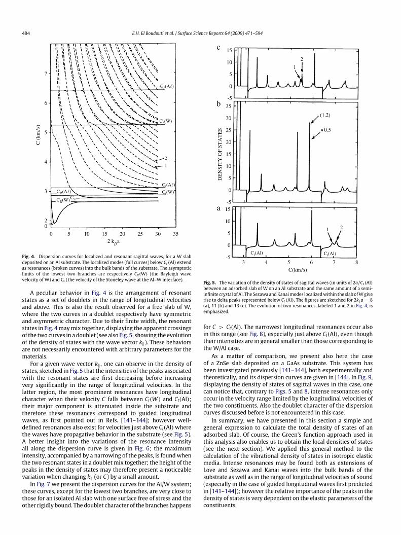
484 E.H. El Boudouti et al. / Surface Science Reports 64 (2009) 471–594

CSCR(W)

Ct(W)

105 2515 20

C (

km/s

)

30

5

7

6

4

3

02

3502 k//a

2

1

Fig. 4. Dispersion curves for localized and resonant sagittal waves, for a W slabdeposited on an Al substrate. The localized modes (full curves) below Ct (Al) extendas resonances (broken curves) into the bulk bands of the substrate. The asymptoticlimits of the lowest two branches are respectively CR(W) (the Rayleigh wavevelocity of W) and Cs (the velocity of the Stoneley wave at the Al–W interface).

A peculiar behavior in Fig. 4 is the arrangement of resonantstates as a set of doublets in the range of longitudinal velocitiesand above. This is also the result observed for a free slab of W,where the two curves in a doublet respectively have symmetricand asymmetric character. Due to their finite width, the resonantstates in Fig. 4maymix together, displaying the apparent crossingsof the two curves in a doublet (see also Fig. 5, showing the evolutionof the density of states with the wave vector k‖). These behaviorsare not necessarily encountered with arbitrary parameters for thematerials.For a given wave vector k‖, one can observe in the density of

states, sketched in Fig. 5 that the intensities of the peaks associatedwith the resonant states are first decreasing before increasingvery significantly in the range of longitudinal velocities. In thelatter region, the most prominent resonances have longitudinalcharacter when their velocity C falls between Cl(W ) and Cl(Al);their major component is attenuated inside the substrate andtherefore these resonances correspond to guided longitudinalwaves, as first pointed out in Refs. [141–144]; however well-defined resonances also exist for velocities just above Cl(Al)wherethe waves have propagative behavior in the substrate (see Fig. 5).A better insight into the variations of the resonance intensityall along the dispersion curve is given in Fig. 6; the maximumintensity, accompanied by a narrowing of the peaks, is foundwhenthe two resonant states in a doubletmix together; the height of thepeaks in the density of states may therefore present a noticeablevariation when changing k‖ (or C) by a small amount.In Fig. 7 we present the dispersion curves for the Al/W system;

these curves, except for the lowest two branches, are very close tothose for an isolated Al slab with one surface free of stress and theother rigidly bound. The doublet character of the branches happens

4 75 6 83

C(km/s)

10

5

0

-5

35

30

25

20

15

10

5

0

-515

10

5

0

DE

NSI

TY

OF

STA

TE

S

15

1

2

-5

(1.2)

0.5

Ct(Al) Ct(Al)

1 2

c

b

a

Fig. 5. The variation of the density of states of sagittal waves (in units of 2a/Ct (Al)between an adsorbed slab of W on an Al substrate and the same amount of a semi-infinite crystal of Al. The SezawaandKanaimodes localizedwithin the slab ofWgiverise to delta peaks represented below Ct (Al). The figures are sketched for 2k‖a = 8(a), 11 (b) and 13 (c). The evolution of two resonances, labeled 1 and 2 in Fig. 4, isemphasized.

for C > Cl(Al). The narrowest longitudinal resonances occur alsoin this range (see Fig. 8), especially just above Cl(Al), even thoughtheir intensities are in general smaller than those corresponding tothe W/Al case.As a matter of comparison, we present also here the case

of a ZnSe slab deposited on a GaAs substrate. This system hasbeen investigated previously [141–144], both experimentally andtheoretically, and its dispersion curves are given in [144]. In Fig. 9,displaying the density of states of sagittal waves in this case, onecan notice that, contrary to Figs. 5 and 8, intense resonances onlyoccur in the velocity range limited by the longitudinal velocities ofthe two constituents. Also the doublet character of the dispersioncurves discussed before is not encountered in this case.In summary, we have presented in this section a simple and

general expression to calculate the total density of states of anadsorbed slab. Of course, the Green’s function approach used inthis analysis also enables us to obtain the local densities of states(see the next section). We applied this general method to thecalculation of the vibrational density of states in isotropic elasticmedia. Intense resonances may be found both as extensions ofLove and Sezawa and Kanai waves into the bulk bands of thesubstrate as well as in the range of longitudinal velocities of sound(especially in the case of guided longitudinal waves first predictedin [141–144]); however the relative importance of the peaks in thedensity of states is very dependent on the elastic parameters of theconstituents.

E.H. El Boudouti et al. / Surface Science Reports 64 (2009) 471–594 485

60

45

30

RE

SON

AN

CE

IN

TE

NSI

TY

(un

its o

f 2a

/Ct(

Al)

)

15

0

7

6

5

8 10 12 142 k//a

16 18 20 22

1

2

(1.2)

8

C(k

m/s

)

4

Fig. 6. The intensities of the resonances, labeled 1 and 2 in Figs. 4 and 5, along thedispersion curves. The intensity becomes very important when the two resonancesmix together. To emphasize this behavior, the dispersion curves are also reproducedin this figure.

7

6

5

4

3

0

0 5 10 15

2 k//a

C (

km/s

)

20 25 30

CR(W)

Ct(W)

CS

4

3

Fig. 7. The same as in Fig. 4 for the case of an Al slab deposited on a W substrate.

4 75 6

3 4

0.75

0.7

0.7

0.5

(3.4)

34

c

b

a

20

15

10

5

0

-5

20

15

10

5

0

10

15

5

0

-5

DE

NSI

TY

OF

STA

TE

S

-5

20

Ct(W) Ct(W)

83

C(km/s)

Fig. 8. The same as in Fig. 5 for the case Al/W. The figures are sketched for 2k‖a =19 (a), 24.3 (b) and 29 (c).

3.3. Resonant guided elastic waves in an adsorbed bilayer on asubstrate

In the same way as for one adsorbed layer, two adsorbedlayers have been the subject of experimental and theoreticalstudies [147–149] in structures composed of a Si–SiO2 doublelayer on a Si substrate. The main features in this system arerelated to the buried Si02 layer. The Brillouin spectra show, inaddition to the usual sagittal modes (Rayleigh and Sezawa waves),two longitudinal guided pseudo-modes near the longitudinalthreshold of Si that are analogous to those previously observedin a single adsorbed layer [141–144]. Similar investigations wereperformed on a silicon-oxynitride-fused-silica (Si–SiON) doublelayer deposited onto a Si substrate [140].In this section, we are interested in calculating both local and

total density of states associated with an adsorbed bilayer. Theseanalytical results can of course be applied to any combinationof material parameters in the bilayer and in the substrate. Weshall focus our attention on the possibility of finding well-definedguided pseudo-modes in the topmost layer, as a consequence ofits separation from the substrate by the buffer layer, when thevelocities of sound in the buffer are higher than those in thetopmost layer. This phenomenon results from the fact that some ofthe slab modes of the top layer, even if they are in resonance withthe substrate bulk modes, cannot propagate in the intermediatelayer and therefore remain well-defined guided waves of thehigher slab.

486 E.H. El Boudouti et al. / Surface Science Reports 64 (2009) 471–594

0.75

a

b

c

10

5

0

-5

Ct(GaAs) Ct(GaAs)

15

10

5

0

-5

15

10

5

0

4 5

C(km/s)

63

15

DE

NSI

TY

OF

STA

TE

S

-5

Fig. 9. The same as in Figs. 5 and 8 for the case ZnSe/GaAs. The figures are sketchedfor 2k‖a = 20 (a), 30 (b) and 40 (c).

3.3.1. ModelThe adsorbed bilayer is formed out of two different slabs (i =

1, 2) deposited on a homogeneous substrate i = s. The slabs arerespectively of thickness d1 and d2. All the interfaces are taken tobe parallel to the (x1, x2) plane. A space position along the x3 axisin medium i is indicated by (i, x3), where−di/2 ≤ x3 ≤ di/2 in thetwo adsorbed layers and x3 ≤ 0 in the substrate (see Fig. 10).The media forming the slabs and the substrate are assumed

to be isotropic elastic media. From the knowledge of the Green’sfunction in the supported double layers, one obtains for a givenvalue of k‖, the local density of states

nα(ω2, k‖; x3) = −1πImgαα(ω2, k‖|i, x3; i, x3),

(α = 1, 2, 3), (108)

or

nα(ω, k‖; x3) = −2ωπImgαα(ω2, k‖|i, x3; i, x3),

(α = 1, 2, 3). (109)

The total density of states for a given value of k‖, is obtained byintegrating over x3 the local density of state n(ω2, k‖; x3) and bysumming over the index α. This expression can be written as thesum of three contributions:

n(ω2) = n1(ω2)+ n2(ω2)+ ns(ω2) (110)

where n1(ω2) and n2(ω2) are the contributions of layers 1 and2, respectively, and ns(ω2) comes from the substrate. Actually, in

Fig. 10. Schematic representation of a bilayer deposited on a homogeneoussubstrate. d1 and d2 are, respectively, the thickness of the buffer and of the surfacelayer.

the latter term, we subtract the contribution nB(ω2) of the bulkof the substrate, which is an infinite quantity and write ns(ω2) =nB(ω2)+1sn(ω2).Then we have

n1(ω2) = −ρ(1)

πIm Tr

∫ d1/2

−d1/2g(i = 1, x3; i = 1, x3)dx3, (111)

n2(ω2) = −ρ(2)

πIm Tr

∫ d2/2

−d2/2g(i = 2, x3; i = 2, x3)dx3, (112)

1sn(ω2) = −ρ(s)

πIm Tr

×

∫ 0

−∞

[g(i = s, x3; i = s, x3)− Gs(x3, x3)] dx3. (113)

g and Gs are, respectively, the response functions of the adsorbedbilayer and of an infinite substrate. The trace is taken over thecomponents 11 and 33, which contribute to the sagittal modes,whereas the 22 component gives the contribution of transversemodes. The integration over x3 can be performed analyticallybecause the Green’s functions elements are only composed ofexponential terms [102,176,177].To end this section, let us notice that the supported double

layer Green’s function associated with sagittal modes has beencalculated in Ref. [176]. The shear horizontal component of thisGreen’s function is given in Refs. [130,177].

3.3.2. Numerical results

3.3.2.1. Dispersion curves and densities of states. This sectioncontains a few illustrations of local and total densities of statesand dispersion curves for sagittal acoustic waves in a GaAs–Sibilayer deposited on a GaAs substrate cut along the (001) planeand for propagation wave vector k‖ along the [100] direction (seeFig. 10). The parameters for the materials are listed in Table 1. Inthis structure the velocities of sound in the Si buffer layer are higherthan those in the GaAs topmost layer; therefore the former actsas a barrier between phonons of the topmost layer and those ofthe substrate, and well-confined resonant waves may exist in the

E.H. El Boudouti et al. / Surface Science Reports 64 (2009) 471–594 487

a

b

Fig. 11. (a) Dispersion curves of resonant transverse modes for a GaAs/Si bilayeron a GaAs substrate. C is the velocity. The figure is sketched for d1/d2 = 0.5 whered1 and d2 are respectively the thicknesses of the Si and GaAs slabs. (b) Variation ofthe DOS due to the adsorption of the GaAs/Si bilayer, at k‖d2 = 7.

higher slab in such a way as to realize an acoustic waveguide. Inthe case of transverse and sagittal acoustic waves studied here, weshow that guided acoustic waves with velocities lying in the rangeof transverse and longitudinal velocities of sound may be confinedin the topmost layer.Before discussing the results in a range of longitudinal velocities

of sound, let us first present in Fig. 11(a) an illustration of thedispersion curves (velocity C versus the reduced parallel wavevector k‖d2) of shear horizontal modes for a GaAs/Si bilayer on aGaAs substrate. The thickness d1 of the Si slab is such that d1 =0.5d2, where d2 is the thickness of the GaAs layer (see Fig. 10).All the branches in Fig. 11(a) represent resonant modes obtainedfrom the peaks of the variation of the DOS between a bilayer-adsorbate system and a GaAs semi-infinite system, as illustrated inFig. 11(b) for a given value of the dimensionless wave vector k‖d2.The lifetimes of these resonances are related to the finite widthsof the peaks in the DOS. The curves below Ct(Si) in Fig. 11(a) arevery similar to those of localized Love modes associated with aGaAs layer adsorbed on a Si substrate, apart for the lowest onewhich starts from Ct(GaAs) instead of Ct(Si). The peaks in the DOSassociated with these latter branches (Fig. 11(b)) are very narrowand their intensities are very high. One can, however, notice thatthe width of these peaks becomes large when either k‖d2 or thethickness d1 of the buffer layer decreases (see below). An analysisof the local density of states (LDOS) as a function of the spaceposition (Fig. 12(a)) clearly shows that these pseudo-modes areconfined in the GaAs slab, and do not propagate into the Si bufferlayer. Consequently, they remain well-defined guided waves of

a

b

Fig. 12. (a) Spatial representation of the local DOS for C = 3.89 km/s and k‖d2 = 7.(b) The same figure as in (a) but for C = 6.778 km/s and k‖d2 = 7. These modesare labeled 1 and 2 in Fig. 11(b). The space position of the different interfaces aremarked by vertical lines.

the GaAs slab. Let us notice that the LDOS reflects the spatialbehavior of the square modulus of the displacement field. AboveCt(Si), the resonant modes are due to the interaction between theGaAs–Si bilayer modes and the substrate modes. Now, an analysisof the LDOS as a function of the space position (Fig. 12(b)) shows apropagating behavior in the bilayer with a pronounced amplitudein the Si buffer layer.As mentioned above, the pseudo-modes induced by the bilayer

are dependent on thewidth of the buffer layer. Fig. 13(a) illustratesthe variation of the velocity of the pseudo-modes as a functionof the thickness ratio d1/d2 for a given value of the surface layerthickness d2 such that k‖d2 = 7. The four curves situated betweenCt(GaAs) and Ct(Si) represent sharp resonant guided waves in theGaAs slab; the corresponding frequencies present a very smallvariation with d1/d2. However, the curves lying above Ct(Si)present a noticeable variationwith varying d1/d2; they correspondto resonant waves propagating in the whole system GaAs/Si/GaAs(see Fig. 12(b)). The heights of the peaks in the DOS associatedwiththe first four guided waves are very dependent on the thicknessof the buffer layer,while the intensities of the highest resonances(above Ct(Si)) remain small and almost independent of d1/d2.In the same manner, we have also studied the behavior of the

resonant modes as function of the surface GaAs layer thickness.Fig. 13(b) presents the variation of the velocity of the resonancesas a function of the ratio d2/d1, for a given value of the buffer layerthickness d1 such that k‖d1 = 7. The pseudo-modes lying betweenCt(GaAs) and Ct(Si) tend asymptotically to the limit of Ct(GaAs)when d2/d1 → ∞. Above Ct(Si), one can notice an importantinteraction of these pseudo-modes in the vicinity of Ct(Si).Fig. 14 gives an illustration of the dispersion curves for sagittal

waves. Apart the lowest branch corresponding to the Rayleighwave localized at the surface of the GaAs layer, the other branches

488 E.H. El Boudouti et al. / Surface Science Reports 64 (2009) 471–594

Fig. 13. (a) Variation of the velocity of the resonant modes, for k‖d2 = 7, as afunction of d1/d2 . (b) Variation of the velocity of the resonant modes, for k‖d1 = 7,as a function of d2/d1 .

represent resonantmodes induced by the bilayer in the continuumof the substrate bulk band, which means above the transversevelocity of sound of the GaAs substrate. These resonant modesare depicted from the maxima of the density of states, shown inFig. 15 for a few values of the wave vector k‖d2. The full (dashed)horizontal lines in Fig. 14 represent the positions of transverseand longitudinal velocities of sound of GaAs (Si) medium. In thelimit k‖d2 → ∞ in Fig. 14, the resonant modes move to the GaAstransverse sound line. The pseudo-modes below Ct(Si) representresonant guided waves of the topmost GaAs layer, and appear aswell-defined peaks in the density of states of Fig. 15, even thoughthey are in resonance with the bulk modes of the GaAs substrate.For the sake of illustration of very narrow peaks, these resonancesare enlarged by adding a small imaginary part ε to the velocity c[ε = 10−3 × Ct(GaAs)]. One can, however, notice that the widthsof these peaks become large when either k‖d2 or the thickness d1of the buffer layer decreases (see below).Among the above guided waves, one can distinguish the modes

falling between Ct (GaAs) and Cl(GaAs), which are predominantly ofshear vertical character and the branches falling between Cl(GaAs)and Ct (Si), which are predominantly of longitudinal character.This is shown in Fig. 16 where we have separated in the densityof states the contributions of shear vertical (full curves) and oflongitudinal (dashed curves) components. One can also notice inFig. 14 important coupling and anti-crossing of these pseudo-modes in the vicinity of the GaAs longitudinal sound line. In Fig. 14there are also well-defined resonances with velocities fallingbetween Ct (Si) and Cl(Si), which are guided waves of the wholeGaAs/Si bilayer. More specifically, as will be shown below, one candistinguish in this velocity range narrow and intense resonancesthat are associated with the GaAs topmost layer, separated by

Fig. 14. Dispersion curves of resonant sagittal modes for a GaAs–Si bilayer ona GaAs substrate. The figure is sketched for d1/d2 = 0.5, where d1 and d2 are,respectively, the thickness of Si and GaAs slabs.

a

b

c

Fig. 15. Variation of the DOS due to the adsorption of the GaAs–Si bilayer on theGaAs substrate, at k‖d2 = 5 (a), 10 (b) and 15 (c). the antiresonances appearing atCt (GaAs) and Cl(GaAs) correspond to δ peaks of the weight − 14 , resulting from thesubtraction of the substrate bulk band in the variation of the DOS (see Eq. (113)).The arrows indicate the positions of the transverse and longitudinal velocities of Si.

small and broad peaks corresponding to the Si buffer layer (seeFig. 15(b) and (c)). These resonances have mixed shear verticaland longitudinal character as shown in Fig. 16. Above Cl(Si), theresonances become very weak especially for small values of k‖d2.An analysis of the local density of states as a function of the

space position x3 (Fig. 17) clearly shows the localization propertiesof the different kinds of modes belonging to different velocityrange. Fig. 17(a) and (b) correspond to the modes respectively

E.H. El Boudouti et al. / Surface Science Reports 64 (2009) 471–594 489

Fig. 16. Same as in Fig. 15, where the contributions of shear vertical (full curves)and of longitudinal (dashed curves) components in the DOS are separated.

labeled 1 and 2 in Figs. 15(b) and 16(b), showing that thesepseudo-modes are confined in the GaAs slab and do not propagateinto the Si buffer layer. Consequently, they remain well-definedguided waves of the topmost GaAs slab; however, the first one(Fig. 17(a)) is predominately of shear vertical character as itsvelocity (C = 4.116 km/s) lies between Cl(GaAs) and Ct (GaAs),while the secondone Fig. 17(b)with a velocityC = 5.11 km/s lyingbetween Cl(GaAs) and Ct (Si) is mostly of longitudinal character.Fig. 17(c) and (d) correspond to the modes respectively labeled3 and 4 in Fig. 15(b) with velocities lying between Ct (Si) andCl(Si). The mode labeled 3 in Fig. 15(b) (C = 6.609 km/s) showsa strong localization in the topmost GaAs layer (see Fig. 17(c))and, therefore, is confined in the latter even though the shearcomponent of this wave is travelling in the Si buffer layer. Themode labeled 4 in Fig. 15(b) is propagating in the two adsorbedlayers with a pronounced amplitude of the transverse componentin the Si buffer layer, while the longitudinal partial wave isevanescent in the latter as its velocity (C = 7.032 km/s) liesbelow Cl(Si). The mode labeled 5 in Fig. 15(b) shows, as predicted,a propagation of the acoustic wave in the whole GaAs/Si/GaAssystem (Fig. 17(e)) as its velocity (C = 9.335 km/s) lies aboveCl(Si). Fig. 17(a), (b), and (c) evidence what we believe is one ofthe main outcomes of this section, namely, the existence of well-confinedmodes in the topmost GaAs layer even though they are inresonance with the bulk modes of the GaAs substrate. Fig. 17(d)and (e) have been presented for the sake of completeness butthe corresponding peaks are probably very weak to be observableexperimentally.As mentioned above, the pseudo-modes induced by the bilayer

are dependent on the width of the buffer layer. Fig. 18 illustratesthe variation of the velocity of the pseudo-modes as a functionof the thickness ratio d1/d2, for a given value of the surface layerthickness d2 such that k‖d2 = 10. Besides the Rayleigh branch, thenext branches below Ct (Si) and a few branches between Ct (Si) andCl(Si) are almost horizontal, which means that the velocities of the

Fig. 17. Spatial representation of the local DOS for C = 4.116 km/s, 5.11 km/s,6.609 km/s, 7.032 km/s, and 9.335 km/s at k‖d2 = 10. These pseudo-modes are,respectively, labeled 1, 2, 3, 4, and5 in Fig. 15(b). The full (dashed) curves correspondto shear vertical (longitudinal) components of the local DOS. The space positions ofthe different interfaces are marked by vertical lines.

corresponding pseudo-modes are independent of the thickness d1of the Si buffer layer; these pseudo-modes, which are essentiallyguided modes of the topmost GaAs layer, appear in general as verysharp peaks in the DOS (illustrated in Fig. 19), except for smallvalues of d1 (Fig. 19(a))where the phonons in the surface layermaykeep an important interaction with those in the substrate. In thevelocity range between Ct (Si) and Cl(Si) there also exist dispersivebranches in Fig. 18 that go asymptotically to Ct (Si) for increasingvalues of d1. The latter pseudo-modes actually correspond to smallpeaks of the DOS (Fig. 19) and are associated with a resonantbehavior inside the Si buffer layer or in both surface layers. At thecrossings of the flat and dispersive branches in Fig. 18, the peaks inthe DOS broaden and become rather small. Finally in the velocityrange above Cl(Si) the peaks in the DOS remain always very small(see Fig. 19).In the same manner, we have studied the behavior of the

resonant modes as a function of the surface GaAs layer thickness.Fig. 20 presents the variation of the velocity of the resonancesas a function of the ratio d2/d1, for a given value of the bufferlayer thickness d1 such that k‖d1 = 10. Except the lowestbranch associated with the Rayleigh wave, the next branches areall dispersive and go asymptotically to the limit of Ct (GaAs) foran increasing value of d2. One can observe coupling and anti-crossing between the branches in the vicinity of Cl(GaAs) as wellas in the velocity range from Cl(GaAs) to Ct (Si). Between Ct (Si)and Cl(Si), we obtained guided resonant modes in the adsorbedbilayer with an important coupling of these pseudo-modes at thecrossing points. In addition there are no flat branches associatedwith guided modes of the Si buffer layer because the velocities

490 E.H. El Boudouti et al. / Surface Science Reports 64 (2009) 471–594

Fig. 18. Variation of the velocity of the resonantmodes, for k‖d2 = 10, as a functionof d1/d2 .

Fig. 19. Variation of the DOS due to the adsorption of the GaAs–Si bilayer on theGaAs substrate, for k‖d2 = 10 and different values of d1/d2: 0.2(a), 1.5(b) and 3(c).

of sound in Si are higher than those of GaAs. To emphasize theguided modes of the buried layer, its velocities of sound have to bechosen lower than those of the topmost layer and of the substrate;this requirement is, for example, achieved in the case of a Si–SiO2bilayer on a Si substrate [147–149].Let us mention that a structure similar to the one proposed

in this section has been studied by Brillouin scattering by Chiritaet al. [139] in order to obtain the guided modes of a GaN layeradsorbed on a Si substrate. A buffer layer of AlN which acts as

Fig. 20. Variation of the velocity of the resonantmodes, for k‖d1 = 10, as a functionof d2/d1 .

a barrier between phonons in GaN and Si, has been insertedbetween these two materials. The elastic constants of GaN havebeen deduced from the dispersion curves experiments.

3.3.2.2. Reflection coefficients. Another quantity that can giveinformation on guided modes in adsorbed layers is the reflectioncoefficient associated to an incident wave launched from asubstrate which serves as a support for the adsorbed layers (seeFig. 10). Indeed, in the case of the modes of sagittal polarization,an incident wave of transverse vertical polarization is totallyreflected because of the free surface of the adsorbed layers. Thisincident wave gives rise to two reflected waves of transverse andlongitudinal polarizations with amplitudes Γtt and Γ`t and phasesΦtt and Φ`t respectively. Also, an incident wave of longitudinalpolarization gives rise to two reflected waves with amplitudesΓ`` and Γt` and phases Φ`` and Φt` respectively. We have shownanalytically that the different amplitudes of the reflectedwaves arerelated by the following equations [102]

|Γ``| = |Γtt | (114)

and

|Γ``|2+ |Γ`t ||Γt`| = 1. (115)

Eq. (115) reflects the conservation energy condition. Also, wehave shown analytically that the different phases of the reflectedwaves are related by the following equations [102]

Φt` = Φ`t =Φ`` + Φtt

2. (116)

Let us notice 1n(ω) the variation of the DOS between the twoadsorbed layers and the substrate along. We have shown thatthe phase times, defined as the derivatives of the phases withrespect to the pulsation ω, are related to 1n(ω) by the followingequation [102]

π1n(ω) = τt` = τ`t

=τ`` + τtt

2for C > C`(GaAs) (117)

E.H. El Boudouti et al. / Surface Science Reports 64 (2009) 471–594 491

a

b

c

d

Fig. 21. Variation of the DOS (a) and the different reflection amplitudes Rtt = R``(b), R`t (c) and Rt` (d) as a function of the velocity for k‖d2 = 10 and d1/d2 = 0.2 inFig. 14.

and

π1n(ω) =τtt

2for Ct(GaAs) < C < C`(GaAs) (118)

where τtt , τ``, τ`t and τt` are the derivatives with respect to thepulsation ω of the phasesΦtt ,Φ``,Φ`t andΦt` respectively.These derivatives are an indication of the times needed

by a wave packet to accomplish the reflection process. Thesederivatives are usually called phase times [178–187]. Thesequantities have been first introduced for the study of electronstunneling [178–181] through potential barriers and then appliedalso to photons [182] and phonons [183,184] in dielectric andelastic multilayers respectively. Recently [185–187], phase timesassociated to electromagnetic wave propagation in coaxial cablewaveguides have been shown to be useful quantities to determinethe DOS and group velocities in these structures.Figs. 21 and 22 give a comparison between the DOS and the

different reflection amplitudes (Fig. 21) on one side and betweenthe DOS and the different phase times (Fig. 22) on the other side.The thickness of the buffer layer is chosen such that d1/d2 =0.2. The positions of the different resonant modes in the DOS(Fig. 21(a)) are slightly shifted from the maxima of the peaks inthe reflection rate Rtt = |Γtt |2 (Fig. 21(b)) and the minima of thepeaks in R`t = |Γ`t |2 (Fig. 21(c)) and Rt` = |Γt`|2 (Fig. 21(d)).In particular, one can notice in the region C > C`(GaAs), thatthe width of the peaks in Rtt = R`` (Fig. 21(b)) are more or lessweak depending on the width of the peaks in the correspondingDOS (Fig. 21(a)); their intensity reaches almost unity. These resultsshow that at the vicinity of the resonances, an incident waveof transverse vertical (or longitudinal) polarization is subject oftotal reflection by almost the same polarization. However, In thevelocity region Ct(GaAs) < C < C`(GaAs), an incident wave oftransverse vertical polarization is totally reflected with the samepolarization similarly to shear horizontal waves, i.e., Rtt = 1

a

b

c

d

Fig. 22. Variation of the DOS (a) and the different phase times: τt` = τ`t (b), τtt/2(c) and τ``/2 (d) as a function of the velocity for k‖d2 = 10 and d1/d2 = 0.2 inFig. 14.

(see Fig. 21(c)). In this case, only the phase time can inform us onthe resonant modes (see below).An analysis of the phase time (Fig. 22(b), (c) and (d)), clearly

shows that τ`t = τt` presents the same behavior as the DOSin the velocity region C > C`(GaAs) (Fig. 22(b)). This timeis divided separately on both quantities τtt/2 (Fig. 22(c)) andτ``/2 (Fig. 22(d)) according to Eq. (117). The two latter phasetimes may present a very different behavior in comparison withthe DOS (see Fig. 22(c) and (d)). In addition, one can noticethat the peaks in τt` = τ`t are usually positive as function ofthe velocity C of phonons, which means that the correspondingreflected waves appear with delay time. However, the quantitiesτtt and τ`` may exhibit around certain frequencies positive peaksfollowed by negative peaks showing a delay time followed by anadvance time for the waves corresponding to these resonances.These results show that among the different reflection amplitudesand the corresponding phase times, only the delay time of areflected transverse vertical (longitudinal) wave corresponding toan incident longitudinal (transverse vertical) wave, reproducesexactly the DOS (Fig. 22(b)) according to the analytical result(Eq. (117)). In the velocity region Ct(GaAs) < C < C`(GaAs), theincident wave is totally reflected. In this case, only the phase timeτtt (Fig. 22(c)) gives the same behavior as the DOS in accordancewith Eq. (118).In summary, the results presented in this section are based

on an analytical calculation of the response functions for acousticwaves of transverse and sagittal polarizations in an adsorbedbilayer [176,177]. These complete response functions can be usedto study any physical property of the adsorbed bilayer [174].These include the calculation of local and total densities ofstates, the determination of the dispersion relations as wellas the reflection coefficients for surface guided waves in thisstructure. Particular attention was devoted to sharp guided

492 E.H. El Boudouti et al. / Surface Science Reports 64 (2009) 471–594

resonant waves confined in the topmost layer, as a consequenceof its separation from the substrate by the buffer layer, whenthe velocities of sound in the buffer are higher than those in thetopmost layer. These resonances appear as well-defined peaksof the DOS and the reflection phase times, with their relativeimportance being very dependent on the wave vector k‖ andthe thicknesses of the buffer and topmost layers as well as onthe parameters of the constituents. Although in our illustrations(Figs. 14, 18 and 20) most of these resonances were situatedbelow the buffer bulk band, the opposite situation can also berealized by interchanging the two constituentmaterials [147–149].The experimental observation of the sharp resonances in anadsorbed slab predicted here can be possible with Brillouinscattering [23,140,147–149].

3.4. Localized and resonant guided elastic waves in an adsorbed layeron a semi-infinite superlattice

As mentioned above, the adsorbed layers are in general de-posited on a homogeneous substrate; therefore the guided modesin these layers fall inside the substrate bulk bands. This is, in par-ticular, the case for high velocity longitudinal guided modes inthe vicinity of the adsorbate longitudinal velocity of sound, andthus some of these modes can propagate into the substrate. Con-sequently, these modes may strongly interact with the substratemodes giving rise to weak resonances or pseudo-modes, whichare not usually easy to detect experimentally [24,138,141–144].Some recent papers [154–163] have shown experimentally the ex-istence of high velocity acoustic modes in a layer deposited on asubstrate. Although the possibility of detecting some resonanceshas been shown in a few systems, theseworks again emphasize thegeneral difficulty of observing the guided modes of adlayers whentheir velocities fall inside the substrate bulk bands.The object of the present section is to put forward a new idea

for making possible, or at least facilitate, the observation of theguided modes in an adlayer, namely, to use a superlattice, insteadof a homogeneous medium, as the substrate (see Fig. 23). Thisopens the possibility of finding true guided modes in the adsorbedlayer,when thesemodes fall inside theminigaps of the superlattice(SL). Indeed the SL acts as a barrier for the propagation of thesemodes that remain well-defined guided waves of the topmostlayer. Some of the modes of the adlayer fall inside the minibandsof the SL, giving rise to pseudo-guided modes; however, eventhese resonances may still remain very sharp, in particular due tothe existence of two types of polarization of the waves in the SLminibands. The advantage of using a SL rather than a homogeneousmedium as the substrate is especially relevant in the high acousticvelocity range.The above physical idea is demonstrated here by calculating the

total and local density of states (DOS) associated with an adlayerdeposited on a superlattice, where the true (or localized) andresonant surface modes appear as well-defined peaks of the DOSperformed within a Green’s function formalism. The knowledge ofthe DOS in these structures enables us to determine the spatialdistribution of the modes and, in particular, the possibility oflocalized and resonant guided modes that appear as well-definedpeaks of the DOS inside the minigaps and inside the bulk bandsof the SL, respectively. One can compare the sharpness of thesepeaks when the adlayer is deposited on a SL or on a homogeneoussubstrate. The latter structure is obtained from the former oneby taking the two layers constituting the SL (Fig. 23) of the samematerial. Our main object is to discuss the physical behavior of theguidedmodes associatedwith the adlayer and the details about thetheoretical calculations are given elsewhere [102].

layer 1

x3

da

Cel

l - 2

Cel

l -

1

Cel

l 0

d1

d2

Dlayer 1

Adsrobed layer(a)

Laye r 2

Laye r 2

Fig. 23. A schematic representation of a semi-infinite two-layer SL (i = 1, 2) withan adsorbed layer (i = a). da , d1 , and d2 are, respectively, the thicknesses of theadsorbed layer and of the two different slabs out of which the unit cell of the SL isbuilt. D is the period of the SL.

3.4.1. Method of calculationConsider a slab of material i = a adsorbed on a semi-infinite SL

formed from a semi-infinite repetition of two different slabs i = 1,2. We call di (i = 1, 2, a) the thickness of each type of slab. Allthe interfaces are taken to be parallel to the (x1, x2) plane. A spaceposition along the x3 axis in medium i belonging to the unit cell nis indicated by (n, i, x3), where −di/2 < x3 < di/2 (see Fig. 23).The period of the SL is called D = d1 + d2. All the three media areassumed to be isotropic elastic media.In our case, the composite material is composed of a SL

built out of alternating slabs of materials i (i = 1, 2) withthickness di, in contact with an adsorbed layer of material i =a. Let us emphasize that, in the geometry of the SL/adsorbedlayer structure, the elements of the Green’s function take theform gαβ(ω2, k‖|n, i, x3; n′, i′, x′3), where ω is the frequency of theacoustic wave, k‖ the wave vector parallel to the interfaces, andα, β denote the directions x1 (≡ 1), x2 (≡ 2), and x3 (≡ 3). For thesake of simplicity, we shall omit in the following the parametersω2and k‖, and we note as g(n, i, x3; n′, i′, x′3) the 3× 3 matrix whoseelements are gαβ(n, i, x3; n′, i′, x′3) (α, β = 1, 2, 3).The knowledge of the Greens function g in the SL/adsorbed

layer system enable us to calculate the local density of states fora given value of the wave vector k‖

nα(ω2, k‖; n, i, x3) = −ρ(i)

πImgαα(ω2, k‖|n, i, x3; n, i, x3),

(α = 1, 2, 3) (119)

or

nα(ω, k‖; n, i, x3) = −2ωρ(i)

πImgαα(ω2, k‖|n, i, x3; n, i, x3),

(α = 1, 2, 3). (120)

The total density of states for a given value of k‖ is obtained byintegrating over x3 and summing over n, i, and α the local densitynα(ω2, k‖; n, i, x3).More particularly,we are interested in this totaldensity of states from which the contribution of the infinite SLhas been subtracted. This variation 1n(ω2) can be written as thesums of the variations1n1(ω2),1n2(ω2) in the densities of statesin layers 1 and 2 and the DOS na(ω2) in the adsorbed layer (a),respectively.

1n(ω2) = 1n1(ω2)+1n2(ω2)+ na(ω2), (121)

E.H. El Boudouti et al. / Surface Science Reports 64 (2009) 471–594 493

where

1n1(ω2) = −ρ(1)

πIm Tr

×

0∑

n=−∞

∫−d1/2

−d1/2[d(n, i = 1, x3; n, i = 1, x3)

− g(n, i = 1, x3; n, i = 1, x3)] dx3

, (122)

1n2(ω2) = −ρ(2)

πIm Tr

×

−1∑

n=−∞

∫−d2/2

−d2/2[d(n, i = 2, x3; n, i = 2, x3)

− g(n, i = 2, x3; n, i = 2, x3)] dx3

, (123)

na(ω2) = −ρ(a)

πIm Tr

×

∫ da/2

−da/2d(n = 0, i = a, x3; n = 0, i = a, x3)dx3

, (124)

d and g are the Green’s functions of the coupled (SL/adsorbedlayer) system and of the infinite SL, respectively. The trace inEqs. (122)–(124) is taken over the components 11 and 33, whichcontribute to the sagittal modes we are studying in this section.The 2 × 2 component associated to pure transverse modes inSLs will be presented in the next section. The integration over x3and the summation over n can be performed very easily becausethe Green’s functions elements are only composed of exponentialterms [188].

3.4.2. Results and discussionThis section contains a discussion of the dispersion curves and

behaviors of sagittal acoustic waves induced by an adsorbed layeron a semi-infinite SL. These localized and resonant modes appearas well-defined features of the local or total density-of-states. Wecompare these results with the corresponding results when theadlayer is deposited on a homogeneous substrate.In our study, the SL is made of Al and W, while the adsorbed

layer is assumed to be Si material. The thicknesses of the layersare taken such that d1 = d2 and da = 3D, where D = d1 + d2is the period of the SL. Table 1 gives the numerical values of thetransverse and longitudinal velocities of sound and mass densitiesof the materials. We shall focus our attention on the differentlocalized and resonant guidedwaves inducedby the adsorbed layerinside theminigaps and inside the bulk bands of the SL as a functionof thewave vector k‖ (parallel to the interface) and thenature of thelayer in the SL that is in contact with the adsorbed layer. We showin particular that, though the velocities of sound in the Si adlayerare higher than those in the (W, Al) layers constituting the SL, bothtransverse and longitudinal guided waves with velocities lying inthe range of transverse and longitudinal velocities of sound maybe confined in the topmost layer in such a way as to produce anacoustic waveguide.Fig. 24 gives the dispersion curves (velocity C versus the

reduced wave vector k‖D) of sagittal acoustic waves for a Si slabon a semi-infinite W–Al SL (Si/W–Al) terminated with a W layer.The shaded areas in Fig. 24 represent the bulk bands of the SL.Due to the coupling of two degrees of freedom for vibrations, thebulk structure involves two regions of frequencies, representedby horizontally and vertically dashed lines, associated with eachpolarization of the waves [65,67,189]. One can distinguish alsothe ranges of frequencies belonging simultaneously to both types

CR

i

i

13

2

5 64

Cl(Si)

Ct(Si)

2

4

6

8

C(k

m/s

)

0

10

41 2 3 5 6

k//D

0 7

Fig. 24. Dispersion of localized and resonant sagittal modes (full circles) inducedby an adsorbed layer of Si material of thickness da = 3D deposited on the top ofthe Al–W SL with a W termination. The resonant and localized modes are falling,respectively, in the bulk bands (shaded areas) and the minigaps (separating theshaded areas) of the SL. The horizontally and vertically shaded areas correspondto bulk bands associated with each of the two polarizations of the waves. C is thevelocity, k‖ the propagation vector parallel to the interfaces, and D = d1 + d2 theperiod of the SL. The heavy straight lines indicate the transverse and longitudinalvelocities of sound of the Si adsorbed layer. The branches labeled (i) correspond tomodes localized at the SL/adlayer interface.

of bands horizontally plus vertically dashed lines and the regionsseparating the different shaded areas corresponding to minigaps.The dotted curves in Fig. 24 correspond to localized and resonantguided modes induced by a Si adsorbed layer of thickness da =3D. The full horizontal lines in Fig. 24 represent the values oftransverse and longitudinal velocities of sound for the Si material.The branches lying above the transverse velocity of sound in Si[Ct(Si)] represent localized and resonant modes induced by theSi adsorbed layer; these modes move to the Si transverse soundvelocity in the limit k‖D→∞. The horizontal branch (labeled CR)lying below Ct(Si) corresponds to the Rayleigh or pseudo-Rayleighmode on the Si adsorbed layer depending on whether its velocitylies inside a minigap or inside a bulk band of the SL. The otherbranches (labeled i in Fig. 24) represent interface modes localizedat the SL/adlayer interface.The different modes in Fig. 24 are obtained from the maxima

of the DOS, illustrated in Fig. 25 (heavy solid curves) for a fewvalues of the wave vector k‖D. For the sake of clarity and despitethe analytical nature of our calculations, the δ peaks in the DOSare broadened by adding a small imaginary part to the velocity C(i.e., C → C + iε). Li and Ri, respectively, indicate the localized andresonant modes induced by the Si adsorbed layer in the minigapsand in the bulk bands of the SL. Bi and Ti, respectively, represent δpeaks ofweight (−1/4) (antiresonances) located at the bottom andthe top of the minibands [65,67,189]. The positions of the modesin Fig. 24 are, in general, almost the same as those correspondingto a Si adsorbed layer on a homogeneous W substrate (Si/W);this can be observed in Fig. 25 where we have plotted togetherthe DOS for the Si/W case (thin solid curves) and the Si/SL case(heavy solid curves). However, because of the existence of the SLminigaps in Fig. 24, the guided modes falling in these minigapsdo not propagate in the SL and remain well-defined guided waves

494 E.H. El Boudouti et al. / Surface Science Reports 64 (2009) 471–594

a

b

c

Fig. 25. Variation of the DOS due to the adsorption of the Si layer on an Al–W SL (heavy solid curves) at k‖D = 3(a), 4(b), and 5(c). As a matter of comparison, we have alsoplotted (thin solid curves) the DOS due to the adsorption of the Si layer on a homogeneous W substrate (Si/W). The arrows on the velocity axis indicate the transverse andlongitudinal velocities of sound in the Si layer. Bi and Ti refer to δ peaks of weight (−1/4) at the edges of the different bulk bands, Li and Ri indicate localized and resonantmodes induced by the adsorbed layer.

in the adsorbed layer (see below); therefore, they appear as trueδ peaks in the DOS of the Si/SL system (labeled Li in the heavysolid curves of Fig. 25). On the contrary, they appear, in general,as weak resonances in the DOS associated with the Si/W case(thin solid curves of Fig. 25) because in this case these modes arefalling in the continuum of the substrate bulk bands. Therefore, theexperimental observation of such localizedmodes should be easierwhen the substrate is a SL instead of a homogeneous material;indeed, the confinement of these modes in the adsorbed layerbecomes more pronounced in the former case than in the latter.One can also notice in Fig. 24 an important coupling and anti-crossing of the modes induced by the adlayer in the vicinity oftransverse and longitudinal velocities of sound in Si.Among the above guidedwaves, one can distinguish themodes

in the vicinity of Ct(Si), which are predominantly of shear verticalcharacter and the branches in the vicinity of Cl(Si), which arepredominantly of longitudinal character. However, the branchesfalling between Ct(Si) and Cl(Si) are of mixed transverse andlongitudinal character. This is shown in Fig. 26 where we haveseparated in the DOS the contribution of shear vertical (full curves)and of longitudinal (dashed curves) components. An analysis ofthe local DOS as a function of the space position x3 (Fig. 27)clearly shows the localization properties of the different kinds ofmodes belonging to various velocity ranges. The local DOS reflectsthe spatial behavior of the square modulus of the displacementfield. Fig. 27(a)–(f) correspond to the modes, respectively, labeled1, 2, . . . , 6 in Fig. 24, showing that these modes are confinedin the Si adsorbed layer. However, the first three modes arepredominantly of shear vertical character as their velocities liein the vicinity of Ct(Si), while the latter three modes are mostlyof longitudinal character as their velocities lie in the vicinityof Cl(Si).

a

b

c

Fig. 26. Same as in Fig. 25, where the contributions of shear vertical (full curves)and longitudinal (dotted curves) components in the DOS are separated.

Furthermore, among the different modes cited above, onecan distinguish the modes falling inside the SL minigaps (calledlocalized modes and labeled 1 and 4 in Fig. 24); therefore, thesemodes do not propagate into the SL and remain well confined in

E.H. El Boudouti et al. / Surface Science Reports 64 (2009) 471–594 495

-6 -5 -4 -3 -2 -1 0 1 2 3

x 3/D

Superlattice Si adsorbed layer

0

5

5

10

0

5

10

0

5

10

0

3

6

0

2

4

Loc

al d

ensi

ty o

f st

ates

1 0

0

a

b

c

d

e

f

Fig. 27. Spatial representation of the local DOS for the modes labeled 1–6 in Fig. 24. The first three modes (a), (b), and (c) lie in the vicinity of Ct (Si) and fall, respectively,at [k‖D = 3.5, C = 6.314 km/s]; [k‖D = 4.5, C = 6.827 km/s]; [k‖D = 4.5, C = 6.112 km/s]. The next three modes (d), (e), and (f) lie in the vicinity of Cl(Si) and fall,respectively, at [k‖D = 5, C = 8.491 km/s] ; [k‖D = 3, C = 8.544 km/s]; [k‖D = 4, C = 8.538 km/s]. The full (dotted) curves correspond to shear vertical (longitudinal)components of the local DOS, respectively. The space position at the SL/adsorbed layer interface (x3 = 0) is marked by a vertical line.

the topmost layer (Fig. 27(a) and (d)). Indeed, in Fig. 27(a) and (d),the SL plays the role of a barrier that prevents the penetration intothe SL of the phonons propagating in the Si adsorbed layer. Theother modes (called resonant or pseudo-modes and labeled 2, 3, 5,and 6 in Fig. 24) fall either inside one of the two types of bands ofthe SL (as it is the case for themodes 2, 3, and 5) or inside both typesof bands of the SL (as it is the case for the mode 6). These modesstill remain well confined in the Si adsorbed layer even thoughthey are in resonance with the bulk bands of the SL. However, theresonances are stronger for the modes falling inside one type ofbulk bands, since these waves are composed of one propagatingand one evanescent component inside the SL.Concerning the modes falling between Ct(Si) and Cl(Si)

(not presented here), they exhibit a mixed shear vertical andlongitudinal character. Let us mention that longitudinal guidedmodes with high velocities of sound are usually difficult to detectexperimentally, and therefore using a SL as a support instead ofa homogeneous substrate presents a very useful device for thedetection of these kind of modes.In the same manner, we have studied (Fig. 28) localized and

resonant modes induced by a Si adsorbed layer deposited on thesame SL but terminated with an Al layer instead of a W one.The results in Fig. 28 are quite different from those presentedpreviously (Fig. 24); they show the dependence of the modesinduced by the adsorbed layer on the nature of the topmost layer inthe SL. In particular, besides the transverse and longitudinal guided

modes (similar to those in Fig. 24), one can notice, for increasingk‖D, an interaction between interface branches (localized at theSL/adlayer interface and labeled i in Fig. 28) and the Rayleighsurface branch (localized at the surface of the Si adsorbed layer),which is independent of k‖D. This interaction gives rise to thelifting of the degeneracy at the crossing points around k‖D ≈4.2, 6.9, etc, as it is emphasized in Fig. 29, around k‖D ≈ 4.2.One can notice, in particular, a decrease in the coupling betweenthe modes by increasing the thickness da of the adsorbed layer.Before the anti-crossing point, the higher (resp. lower) mode isessentially localized at the SL/adlayer interface (resp. at the surfaceof the adlayer); the opposite situation occurs after the anti-crossingpoint. This smooth evolution of the character of the two branches isillustrated in Fig. 30. Let us stress that the different modes inducedby the Si adlayer deposited on a homogeneous Al substrate presentvery small features in the DOS as compared to the case of Si/SLsystem.Finally, we have also studied the case when the adsorbed layer

is of the same nature (W or Al) as one of the layers constituting theSL but with a different thickness. The velocities of themodes in thecase of the W/SL and Al/SL systems are, respectively, almost thesame as in the case of the W/Al (substrate) and Al/W (substrate)systems (see Section 3.2). However, the modes falling in the SLminigaps appear as true δ peaks instead of being weak resonancesas in the case of a homogeneous substrate [188]. Moreover,because of the low velocities of sound in W and Al (in comparison

496 E.H. El Boudouti et al. / Surface Science Reports 64 (2009) 471–594

C

(km

/s)

0

2

4

6

8

10

C R

i

i

i

Cl(Si)

Ct(Si)

51 2 3 4 6

k//D

0 7

Fig. 28. Same as in Fig. 24 for the case of a Si adsorbed layer deposited on the topof an Al–W SL terminated with a full layer of Al material.

k//D

C (

km/s

)

1

2

3

i

CR

i

5.0

5.5

6.0

3.0 3.5 4.0 4.5 5.0

Fig. 29. The interaction between the Rayleigh surface and interface modes neark‖D ≈ 4.2 in Fig. 28, is emphasized for several values of the thickness da of theadsorbed layer: da = D (—), da = 1.5D (– – –), and da = 3D (. . . ).

with Si), only one interface branch appears below the transversevelocities of sound in these materials [190], the so-called Stoneleybranch [13]. The details of these calculations are presented inRef. [188].In this section, we have developed the idea that the observation

of the guided modes of sagittal polarization in an adlayer can bemade possible or at least facilitated if the substrate is a SL insteadof being a homogeneous material. For this purpose, we studied thelocalized and resonant modes confined in the topmost layer andcompared their behaviors in the DOS with those obtained whenthe adlayer is deposited on a homogeneous substrate. We studied

Mode 1

Super-réseau couche adsorbée de Si

Mode 2

Mode 3

Superlattice Si adsorbed layer

0

5

10

20

300

10

20

Loc

al d

ensi

ty o

f st

ates

10

0-5 -4 -3 -2 -1 0 1 2

x3/D-6 3

a

b

c

Fig. 30. Spatial representation of the local DOS for the modes labeled 1, 2, and 3 inFig. 29 and corresponding, respectively, to [k‖D = 3.5, C = 3.5 km/s, da = 3D] (a),[k‖D = 4.1, C = 5.163 km/s, da = 3D] (b) and [k‖D = 4.8, C = 5.1686 km/s,da = 3D] (c). The full and dotted curves correspond to longitudinal and shearvertical components of the local DOS, respectively.

both localized and resonant guided modes that have, respectively,their velocities lying in the minigaps and in the minibands of theSL. Indeed, in the first case, the SL plays the role of a barrier forphonons in the adsorbed layer leading to their confinement inthe topmost layer; while in the second case, phonons may stillremain well confined in the topmost layer, in particular due tothe existence of two types of polarizations of the waves in theSL minibands. Moreover, the well-confined guided waves do notdepend on whether the velocities of sound in the adsorbed layerare lower or higher than those of the materials constituting theSL. This property is without analogue in the usual case where thesubstrate is made of a homogeneous material.Due to the SL/adlayer interaction, different localized and

resonant modes were obtained and their properties investigated.These modes appear as well-defined peaks of the DOS, with theirrelative importance being strongly dependent on the wave vectork‖, on the thickness and the nature of the adsorbed layer, as wellas on the nature of the layer in the SL that is in contact with theadsorbed layer. The experimental observation of the guidedmodespredicted here can be performed with the Brillouin scatteringtechnique [147–149,154,163].Let us notice that similar results can be obtained for shear

horizontal waves [102]. These results as well as a rule on theexistence of surface and interface modes in semi-infinite SLs willbe the subject of Section 4.

3.5. Relation to experiments

In this section, we shall give some experimental results relatedto this work. In particular, we show briefly how the Green’sfunction calculation can be used in the determination of thesurface Brillouin scattering (SBS) spectra. This technique probethe near-surface elastic properties of a solid or thin supportedlayer by coupling into acoustic modes which are localized mainlynear the surface or within the layer. As mentioned before,several experimental studies based on SBS have been performedon adsorbed layers [23]. In order to observe surface phonon

E.H. El Boudouti et al. / Surface Science Reports 64 (2009) 471–594 497

Fig. 31. Conventional scattering geometry for surface Brillouin scattering.

excitation the 180 backscattering geometry was chosen to obtainmaximum momentum transfer. Laser light of wave vector ki isimpinging on the sample with an angle of incidence θ (anglebetween the incident light direction and the normal to thesurface, see Fig. 31) and the light backscattered into a cone iscollected by the same lens and analyzed using a Sandercock-typeFabry–Perot interferometer [152,153]. The application of energyand wave vector conservation applied to Brillouin scatteringprocess involving an acoustic excitation with surface wave vectork‖ and angular frequency ω yields the following equations

k‖ = 2ki sin(θ) =4π sin(θ)

λand vmes =

ω

k‖=

λi1f2sin(θ)

(125)

where vmes is the phase velocity of the surface excitation and1f isthe frequency shift of the scattered light.Theoretical treatment of SBS have been published by a number

of authors [24,191–201]. The scattering is mediated by twoprincipal mechanisms, surface ripple scattering and the elasto-optic effect.In the surface ripple mechanism, the light is scattered by

dynamic corrugations in the surface profile [191,199]. For opaquesolids, this is the dominant scattering mechanism. At roomtemperature and above where T hω/kB (kB is the Boltzmann’sconstant and h is the Plank’s constant), the surface Brillouinscattering efficiency for this mechanism is proportional to thepower spectrum of the normal displacement of the surface withthat wave vector and that frequency. The power spectrum isrelated to the component G33 of the Green function evaluated atthe surface (z = d) by [198]

I(ω) = ATωImG33(k‖, x3 = d, ω + i0) (126)

where A depends on the properties of the medium, the scatteringgeometry, and the frequency and polarization of the incident light.An example of opaque film was studied a few years ago by

Wittkowski et al. [136,202]. Fig. 32(a) and (b) give the measureand calculated Brillouin spectra for the tungsten carbide (WC)films on a Si substrate. This structure corresponds to slow on fastsystem. Brillouin scattering were excited using an argon ion laserof wavelength λ = 514.5 nm. The thickness of the films ared = 60 nm (Fig. 32(a)) and d = 417 nm (Fig. 32(b)) for a value ofk‖ = 17.27 µm−1 yielding k‖d = 1.04 and 7.2 respectively. Theseare representative of the spectra for low values of k‖d inwhich onlyone Sezawa mode is observed besides the Rayleigh mode (Fig. 32(a)) and spectra for high values of k‖d where numerous Sezawamodes are seen (Fig. 32(b)).The dispersion curves (phase velocity versus k‖d) for the various

film steps over the complete range of film thickness of the sample isshown in Fig. 32(c). The homogeneity of the film and the precisionof the thickness measurements also permit a precise match withadditional data provided by the variation of k‖ by a change in the

angle of incidence θ yielding a particularly large data set consistingof 87 measured points.Using the extensive velocity dispersion data, five independent

material parameters, namely the effective elastic constantsC11, C13, C33 and C55 and the film density ρ have been determinedby statistical approaches including a developed Monte Carlomethod. The evaluation of the G33 component of the Green’sfunction at the free surface yields the scattered mode intensitiesfor a given value of k‖d as shown in Fig. 32(d). Excellent agreementbetween the measured and the calculated Brillouin spectra hasbeen achieved with respect to the frequencies (Fig. 32(c)) andrelative mode intensities (Fig. 32 (a),(b)). The low intensitiesobserved around C fl =

√C11/ρ = 5178 m/s for k‖d > 4 is due to

themainly longitudinal character of partial waves and correspondsto the longitudinal sound velocity of the material parallel to thefilm. A detailed study of the longitudinal guided modes aroundC fl was given by the same authors [202]. The presence of severalresonant modes in the continuous spectrum (i.e., C > C st =5822 m/s) is also shown.In the elasto-optic mechanismwhere the material is not totally

opaque, the incident light is able to penetrate some distanceinto the material to probe dynamic fluctuations in the strainfield. These fluctuations, through the elasto-optic effect, causefluctuations in the refractive index and this results in inelasticscattering of the light. In the case of semi-transparent layer, the fullcalculation requires a knowledge of the complex refractive indicesand elasto-optic constants of the layer and substrate (which arenot always readily available) and the near-surface dynamics, andtakes account of the interference between ripple and elasto-opticscattering [200].To overcome these calculations, Itwas shown that an integrated

density of states for each polarization component can be analyzedfor a given frequency allowing the relative contribution of eachpolarization component to be evaluated. An example of suchstructures was studied some years ago by Chirita et al. [154] forfast on slow substrate. The structure consists on hard diamond-like-carbon (DLC) layers deposited on Silicon. In this study, theauthors observed longitudinal guided modes with high velocitygreater than C st and C

sl and thus all partial waves of this mode can

propagate into the substrate.Fig. 33 (a) shows three typical spectra recorded from two DLC

films of thickness d = 320 nm and d = 160 nm at θ = 60 and80 and d = 160 nm at θ = 80 respectively. The strong lowestfrequency peak in each spectrum lying between 26 and 30 GHzis identified as scattering from the pseudo-surface wave (pSAW).The second prominent feature in the date is the mode labeledlongitudinal guided mode LGM. It is observed from all films atdifferent angles of incidence θ ; the corresponding phase velocitiesare, within experimental error, independent of k‖d over the regimeprobed. In addition, there are weaker peaks, identified by thesymbol ‘‘∗’’ in Fig. 33 (a) that are in fact dispersive. Fig. 33(b) (fullcurves) gives the longitudinal component of the density of states(DOS) integrated over the layer. These curves are in agreementwith experiments (Fig. 33(a)) and show practically no thicknessdependence of the LGM velocity as function of θ . Being principallya longitudinally polarized excitation, no significant transversedensity of states was found at the velocity of the LGM (see thedotted curve in Fig. 33(b)). The experimental and theoreticalfindings are summarized in the dispersion curves (Fig. 33(c)). Thisstudy has allowed the determination of two independent elasticconstants C11 and C44 of the isotropic DLC layer.Now, we shall concentrate on two other examples in which

LGMmodes have been observed in supported bilayers either in thebuffer layer or in the topmost layer. The first structure studied byNizzoli et al. [147], consists on an Si–SiO2 bilayer deposited on a

498 E.H. El Boudouti et al. / Surface Science Reports 64 (2009) 471–594

16-16 -12 -8 8 12

-12 -8 8 12

Exp.

Theo.

Exp.

Theo.

k//d=1.04

k//d=7.2

Inte

nsity

(a.

u)In

tens

ity (

a.u)

5000

4500

4000

3500

3000

Vel

ocity

(m

/s)

5500

2500

6000

5000

4000

3000

Vel

ocity

(m

/s)

7000

0 2 4 6 8 10 12

2 4 6 8 10

RW

Cts

Clf

a

b

c

d

0 12k//d

16-16

Frequency shift (GHz)

Fig. 32. (a) Theoretical and experimental Brillouin spectra for the WC film of thickness d = 60 nm with k‖ = 17.47µm−1 yielding k‖d = 1.04. The calculated spectrumuses the elastic constant values determined from fitting of the dispersion curves. Spectra are relatively displaced for ease of observation; the elastically scattered peaks areremoved. (b) The same as (a) but for d = 417 nmwith k‖ = 17.27 µm−1 yielding k‖d = 7.2. (c) Phase velocity dispersion curves for the discrete sagittally polarized surfacewaves (Rayleigh and Sezawa) as a function of k‖d in which the filled circles represent measurements made with a constant k‖ value of 17.27µm−1 over the complete rangeof film thickness. The lines represents the computed best fit to the experimental data. (d) Brillouin intensities calculated from Eq. (126). C st = 5822 m/s indicates the lineseparation between the discrete and the continuum spectrum (after Ref. [136]).

Si(001) substrate. This structure is particularly interesting becausethe buried SiO2 layer exhibits phonon propagation velocities lowerthan those of Si in such a way as to realize an acoustic waveguide.A measured Brillouin scattering spectrum taken with an angle ofincidence θ = 30 is shown in Fig. 34(a). In order to assign themain features of this spectrum, it is convenient to recall that thediscrete spectrum extends below the transverse threshold of thesemi-infinite substrate ωT = Ct(Si)k‖ ' 11GHz. The continuousspectrum begin at ωL = Cl(Si)k‖ ' 16.3 GHz. Ct and Cl are thetransverse and longitudinal velocities of sound in Si. Among thedifferent modes displayed in Fig. 34(a), one can distinguish thesmall peak in the discrete spectrum labeled 1which is the Rayleighwave of the system, the other modes are guided modes inducedby the bilayer. The continuous spectrum shows two remarkablepeaks (labeled 4 and 5), with no similarity with the experimentalspectrum of a film of SiO2 of comparable thickness deposited onsilicon [200]. The two structures are situated one on each side ofωL.In order to assign the peaks the same authors have performed

a full calculation of the p–p Brillouin scattering cross section [148](Fig. 34 (b)). The agreement between the measured and calculatedspectrum is quite good. The peak labeled 1 corresponds to theRayleigh wave. The two small peaks present in the calculationbetween 10 and 11 GHz (labeled 2 and 3) are not identified inthe measured data due to the noise; the same situation occurs forthe other small mode 6. An analysis of the spatial localization ofthe two pseudo-modes 4 and 5 has shown that the mode labeled

4, lying just below Cl(Si), is mainly localized in the buried SiO2layer with a large value of the longitudinal displacement field;whereas themode labeled 5, lying just above Cl(Si), shows a stronglocalization at the free surface of the Si layer. In order to reproducethe main features of this spectrum, we have given in Fig. 34(c)the DOS calculated for the whole bilayer. One can notice that theDOS shows almost similar features as the Brillouin scattering crosssection (see Fig. 34(b), (c)).The same study has been performed on GaN–AlN bilayer

adsorbed on Si substrate by Chirita et al. [139]. This structure isequivalent to the one studied previously by our group (Section 3.3and Ref. [176]). Indeed, the AlN layer plays the role of a barrierbetween phonons in the topmost GaN layer and the Si substrate.Fig. 35(a) shows typical polarized (p–p), depolarized (p–s)

and unpolarized (p–p+s) Brillouin spectra below 30 GHz forthe sample stack GaN(130 nm)–AlN(200 nm)/Si(111). The angleof incidence is chosen θ = 60. In addition to the principalRayleigh mode (R) another mode identified as the longitudinalguided resonance (LGR) of GaN, is present in the polarized (p–p)spectra. The low frequency p–s spectra reveal the presence of themode labeled SH (shear horizontal) that corresponds to the in-plane polarized acoustic wave. The unpolarized (p–p+s) spectrumreflects a superposition of the three excitations (R, SH, LGR).In order to gain insight into the character of the LGR and SH

modes, the local density of phonon modes was evaluated at thesurface of the structure (Fig. 35(b)). On can notice the presence of a

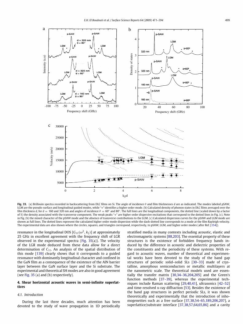
E.H. El Boudouti et al. / Surface Science Reports 64 (2009) 471–594 499

Inte

nsity

(a.

u)

Den

sity

of

stat

es

-75 -50 -25 25 500 75

Frequency shift (GHz) Frequency shift (GHz)

100-100

4

3

2

1

020 40 60 80 100

25000

20000

15000

10000

Vel

ocity

(m

/s)

30000

5000

0 2 4

k//d

6 8

a

c

b

Fig. 33. (a) Brillouin spectra recorded in backscattering from DLC films on Si. The angle of incidence θ and film thicknesses d are as indicated. The modes labeled pSAW,LGM are the pseudo-surface and longitudinal guidedmodes, while ‘‘∗’’ identifies a higher order mode. (b) Calculated density of phonon states in DLC films averaged over thefilm thickness d, for d = 160 and 320 nm and angles of incidence θ = 60 and 80 . The full lines are the longitudinal components, the dotted line (scaled down by a factorof 5) the density associated with the transverse component. The weak peaks ‘‘∗’’ are higher order dispersive excitations that correspond to the dotted lines in Fig. (c). Notein Fig. (b) the mixed character of the pSAWmode and the absence of transverse contributions to the LGM. (c) Calculated dispersion curves for the pSAW and LGMmode areshown as full lines. The dotted lines represent the calculated higher order mode dispersion while the dash-dotted line corresponds to a mode at the film Rayleigh velocity.The experimental data are also shown where the circles, squares, and triangles correspond, respectively, to pSAW, LGM, and higher order modes (after Ref. [154]).

resonance in the longitudinal DOS [G11(ω2, k‖)] at approximately25 GHz in excellent agreement with the frequency shift of LGRobserved in the experimental spectra (Fig. 35(a)). The velocityof the LGR mode deduced from these data allow for a directdetermination of C11. An analysis of the spatial distribution ofthis mode [139] clearly shows that it corresponds to a guidedresonance with dominantly longitudinal character and confined inthe GaN film as a consequence of the existence of the AlN barrierlayer between the GaN surface layer and the Si substrate. Theexperimental and theoretical SHmodes are also in good agreement(see Fig. 35 (a) and (b) respectively).

4. Shear horizontal acoustic waves in semi-infinite superlat-tices

4.1. Introduction

During the last three decades, much attention has beendevoted to the study of wave propagation in 1D periodically

stratified media in many contexts including acoustic, elastic andelectromagnetic systems [88,203]. The essential property of thesestructures is the existence of forbidden frequency bands in-duced by the difference in acoustic and dielectric properties ofthe constituents and the periodicity of these systems. With re-gard to acoustic waves, number of theoretical and experimen-tal works have been devoted to the study of the band gapstructures of periodic solid–solid SLs [30–33] made of crys-talline, amorphous semiconductors or metallic multilayers atthe nanometric scale. The theoretical models used are essen-tially the transfer matrix [30,34–36,204,205] and the Green’sfunction methods [37–39], whereas the experimental tech-niques include Raman scattering [29,40,41], ultrasonics [42–52]and time-resolved x-ray diffraction [53]. Besides the existence ofthe band gap structures in perfect periodic SLs, it was showntheoretically and experimentally that the introduction of inho-mogeneities such as a free surface [37,38,54–65,189,206,207], asuperlattice/substrate interface [37,38,57,64,65,86] and a cavity

500 E.H. El Boudouti et al. / Surface Science Reports 64 (2009) 471–594

5 10 2015 25

Frequency shift (GHz)

0 30

Frequency shift (GHz)

6 10 1814 26222 30

1

1

2

2

3

3

4

4

5

5

6

6

a

b

c

DO

S (a

.u.)

Bri

lloui

n Sc

atte

ring

Fig. 34. Brillouin p–p backscattering cross section and power spectrum for aSi/SiO2 bilayer on Si(001) substrate. k‖ is along [100] and the scattering angle is 30 .(a) measured anti-Stokes spectrum. (b) Calculated total cross section (afterRef. [147]). (c) The DOS integrated over the surface layer is obtained from ourcalculations.

layer [66–74,208,209] within such SLs may induce defect modesinside the gaps. Recently [78–81], it was shown that periodiclamellar structures may exhibit the property of omnidirectionalreflection for acoustic waves (acoustic mirror), i.e., it reflects anyacoustic wave independent of its polarization and incidence anglein analogywith 2D and 3Dphononic crystals [210–214]. Also, thesestructures may be used as acoustic filters if a defect layer (cavity)is introduced in the perfect structure [84].This section is organized as follows: in Sections 4.2 and 4.3, we

give the details of the analytical expressions of dispersion relationsof bulk and surface modes as well as local and total densitiesof states for two and N layer elastic superlattices respectively.Numerical applications are given for semiconductor and metalliclayered media. Section 4.4 is devoted to surface and interfacemodes in piezoelectric SLs.

4.2. Transverse elastic waves in two-layer semi-infinite superlattices

Since the pioneering work of Camley et al. [215] and Djafari-Rouhani et al. [54], surface acoustic waves in elastic SLs has beenthe subject of intense theoretical and experimental studies [37,38,45,54–63,65,189,206,207,215–218]. In the present paragraph, westudy resonant and localized modes together with the variationof the density of states associated with surfaces and interfaces insuperlatticesmade of two different layers. Closed formexpressionsare obtained for transverse elastic waves polarized perpendicularto the sagittal plane, i.e., the plane containing the propagationvector k‖ (parallel to the interfaces) and the normal to theinterfaces. However, these results also remain valid in the case of

longitudinal waves propagating along the axis of the superlattice,which means in the limit of k‖ = 0.

4.2.1. ModelThe superlattice is formed out of an infinite repetition of two

different slabs, labeled by the unit-cell index n. Each of these slabsof width di is labeled by the index i = 1 or 2, within the unit celln. All the interfaces are taken to be parallel to the (x1, x2) plane.A space position along the x3 axis in medium i belonging to theunit cell n is indicated by (n, i, x3), where−di/2 < x3 < di/2. Theperiod of the superlattice is called D = d1 + d2.We limit ourselves to the simplest case of shear horizontal

vibrations where the field displacements u2(x3) are along the axisx2 and the wave vector k‖ (parallel to the interfaces) is directedalong the x1 axis. We can then consider with the same generalequations the two following cases.(i) A superlattice built out of cubic crystals with (001)

interfaces and k‖ along the [100] crystallographic direction. Thecorresponding bulk equation of motion for medium i is [30](ρ(i)ω2 − k2

‖C (i)44 + C

(i)44d2

dx23

)u2(x3) = 0, (127)

where ρ(i) and C (i)44 are, respectively, the mass density and theelastic constant and ω is the frequency of the vibrations.(ii) A superlattice built out of hexagonal crystals with (0001)

interfaces. The isotropy of these interfaces enables us to choosek‖ along any direction within the (x1, x2) plane. For simplicity weshall leave k‖ along the x1 axis. In this case, the bulk equation ofmotion for medium i becomes [30](ρ(i)ω2 − k2

‖

[C (i)11 − C

(i)12

2

]+ C (i)44

d2

dx23

)u2(x3) = 0, (128)

where C (i)11 , C(i)12 and C

(i)44 are the elastic constants of medium i.

We also took advantage of the infinitesimal translationalinvariance in directions parallel to the interfaces and Fourieranalyzed the equations of motion and all operators according to,for example,

g(ω; x3, x′3) =∫d2k‖(2π)2

g(ω, k‖; x3, x′3)eik‖(x‖−x′‖) (129)

where x‖ ≡ (x1, x2) is the component parallel to the interfacesof the real-space position x. In the following, we shall drop forsimplicity the ω and k‖ dependence of the functions g.Let us define

α2i = k2‖− ρ(i)

ω2

C (i)44(130)

for the cubic crystals and

α2i = k2‖

[C (i)11 − C

(i)12

2C (i)44

]− ρ(i)

ω2

C (i)44(131)

for the hexagonal ones. Then, as mentioned above, Eqs. (127) and(128) have the same expression,

C (i)44

(d2

dx23− α2i

)u2(x3) = 0. (132)

The corresponding bulk response function for medium i isdefined by

C (i)44

(d2

dx23− α2i

)Gi(x3 − x′3) = δ(x3 − x

′

3). (133)

E.H. El Boudouti et al. / Surface Science Reports 64 (2009) 471–594 501

Inte

nsity

(a.

u)

LGR

LGR

LGR

LGR

LGR

SHSH SH

SH SH

R R

RR

R

R

P-S

P-P

P-P+S

θ=60° θ=60°

θ=60°

θ=60°

-20 -10 100 20

Frequency shift (GHz)

-30 30 20 30

45

40

35

30

25

20

15

10

5

Den

sity

of

stat

es

50

0

G22(ω2, k//)

G33(ω2, k//)

G11(ω2, k//)

Frequency shift (GHz)

10 40

a b

Fig. 35. Low frequency Brillouin light scattering spectra recorded in backscattering from GaN/AlN/SiC Si(111) film for p–p, p–s, and p–p+s polarizations. LGR labels thelongitudinal guided resonance, SH the shear horizontal mode, and R the Rayleigh mode. The angle of incidence θ is as indicated and the thickness of the GaN layer is 1.3µm.(b) Calculated local density of states as a function of frequency for GaN/AlN/Si(111) after convoluting with a Gaussian with a full width at half maximum of 0.3 GHz. The G33and G22 are the sagittal and transverse horizontal components, respectively, and G11 is the longitudinal component (after Ref. [139]).

The response functions associated to the different heterostruc-tures considered here are defined in the same manner taking intoaccount the appropriate boundary conditions.Let us recall [215] that the implicit expression giving the bulk

dispersion relations of such an infinite superlattice is

cos(k3D) = C1C2 +12

(F1F2+F2F1

)S1S2, (134)

where

Ci = cosh(αidi) (135)Si = sinh(αidi) (136)

Fi = αiC(i)44 (137)

and k3 is the component perpendicular to the slabs of thepropagation vector k‖ ≡ (k1, k3).

4.2.2. Density of statesKnowing the response functions given in the Appendix A, one

obtains for a given value of k‖ the local and total density of statesfor a semi-infinite superlattice with a surface cap layer. We shallindicate at the end of this section how one can obtain from thesequantities similar results for two limiting cases, namely the case ofthe interface between a superlattice and a homogeneous substrate,and that of a semi-infinite superlattice without a cap layer.

4.2.2.1. The local densities of states. The local densities of states onthe plane (n, i, x3) are given by

n(ω2, k‖; n, i, x3) = −ρ(i)

πIm d+(ω2, k‖; n, i, x3; n, i, x3), (138)

where

d+(ω2) = limε→0d(ω2 + iε) (139)

and d(ω2) is the response function whose elements are givenin the Appendix A. The density of states can also be given as afunction of ω, instead of ω2 using the well-known relation n(ω) =2ωn(ω2). From the elements of the response function given inthe Appendix A, we obtained the following explicit expressionsfor the local densities of states on the surface of the semi-infinitesuperlattice with a cap layer (n = 0, i = 0) of width d0,

ns

(ω2, k‖; 0, 0,

d02

)= −

1πIm[C1S2F2+C2S1F1+S0F0C0

(C1C2 +

F1F2S1S2 − t

)]1−1,

(140)

where C0, S0, F0 have the same definitions as Ci, Si, Fi given by Eqs.(135)–(137) for i = 0,

t =

η + (η2− 1)1/2 η < −1

η + i(1− η2)1/2 −1 < η < +1η − (η2 − 1)1/2 η > 1

(141)

with

η = C1C2 +12

(F1F2+F2F1

)S1S2, (142)

and

1 = C1C2 +F2F1S1S2 −

1t−F0S0C0

(C1S2F2+C2S1F1

). (143)

In the same manner the local density of states at the interfacebetween the cap layer and the semi-infinite superlatticewas foundto be

ni

(ω2, k‖; 0, 0,−

d02

)= −

1πIm(C1S2F2+C2S1F1

)1−1. (144)

502 E.H. El Boudouti et al. / Surface Science Reports 64 (2009) 471–594

4.2.2.2. The total density of states. The total density of states for agiven value of k‖ is obtained by integrating over x3 and summing onn and i the local density n(ω2, k‖; n, i, x3). A particularly interestingquantity is the variation of the total density of states between thesemi-infinite superlattice with the cap layer n = 0 and the infinitesuperlattice having the same number of slabs as the semi-infinitesuperlattice without the cap layer. The variation 1n(ω2) can bewritten as the sums of the variations1n1(ω2) and1n2(ω2) of thedensity of states in slabs 1 and 2 and the density of states n0(ω2)inside the cap layer

1n(ω2) = 1n1(ω2)+1n2(ω2)+ n0(ω2), (145)

where

1n1(ω2) = −ρ(1)

π

0∑n=−∞

Im∫+d12

−d12

[d(n, 1, x3; n, 1, x3)

− g(n, 1, x3; n, 1, x3)] dx3, (146)

1n2(ω2) = −ρ(2)

π

−1∑n=−∞

Im∫+d22

−d22

[d(n, 2, x3; n, 2, x3)

− g(n, 2, x3; n, 2, x3)] dx3, (147)

n0(ω2) = −ρ(0)

πIm∫+d02

−d02

d(0, 0, x3; 0, 0, x3)dx3, (148)

and d and g are the response function of, respectively, thesemi-infinite superlattice with the cap layer and of the infinitesuperlattice. With the help of the explicit expressions of theseresponse functions, we obtained

1n1(ω2) = −ρ(1)

πIm

t(t2 − 1)

S1α1F1

×

[C2S1 +

12C1S2

(F1F2+F2F1

)]+d1S22F2

(1−

F 22F 21

)Y1, (149)

1n2(ω2) = −ρ(2)

πIm

t(t2 − 1)

S2α2F2

×

[C1S2 +

12C2S1

(F1F2+F2F1

)]+d2S12F1

(1−

F 21F 22

)Y1, (150)

n0(ω2) = −ρ(0)

2πImS0α0C0

(C1S2F2+C2S1F1

)+ d0

[(C1C2 +

F1F2S1S2 − t

)S0F0C0+C1S2F2+C2S1F1

]11, (151)

where

Y = C2 − C1t −F0S0C0

(S1F1t +S2F2

). (152)

At the limits of the bulk bands of the superlattice given byt(ω0) = ±1, an expansion to first order in (ω − ω0) provides

tt2 − 1

=18

(dηdω

)ω0

−1 P(

1ω − ω0

)− iπδ(ω − ω0)

(153)

and then

1n1(ω2)+1n2(ω2) = −14δ(ω − ω0). (154)

So, the creation of a semi-infinite superlattice from an infiniteone gives rise to δ peaks of weight (−1/4) in the density of statesat the edges of the superlattice bulk bands.

4.2.3. Localized statesWhen the denominator of 1n(ω2) vanishes for a frequency

lying inside the gaps of the infinite superlattice, one obtainslocalized states within the cap layer which decay exponentiallyinside the bulk of the superlattice. The explicit expression givingthese localized states is

C1S2

(F0S0F2C0−F2C0F0S0

)+ S1S2

(F1F2−F2F1

)+ C2S1

(F0S0F1C0−F1C0F0S0

)= 0 (155)

together with the condition∣∣∣∣C1C2 + F2F1 S1S2 − F0S0C0(C1S2F2+C2S1F1

)∣∣∣∣ > 1. (156)

4.2.4. The limit of a semi-infinite superlattice without a cap layerIn the limit when the thickness d0 of the cap layer goes to

zero, S0 → 0 and the above results (140), (149), (150) and(154)–(156) remain valid for a semi-infinite superlattice endingwith a complete i = 1 surface layer. We remark on Eq. (151) thatin this limit, n0(ω2) vanishes.In the limitwhere the cap layer i = 0 is of the samenature as the

i = 2 superlattice layer and d0 = ds < d2, the same results providethe localized modes for a semi-infinite superlattice ending withan incomplete i = 2 surface layer. In this case, we can calculatethe variation of the density of states between such a semi-infinitesuperlattice and the same amount of the bulk superlattice, using inEq. (145)1n2(ω2) integrated to ds/2 rather than to d2/2 in the lastlayer, and taking n0(ω2) = 0.A particularly interesting result can be obtained when cleaving

an infinite superlattice for the variation 1nc(ω2) of the totaldensity of states between the two complementary semi-infinitesuperlattices and the infinite one. It is possible to show byusing standard transformation of the trace of the responsefunctions [115] that1nc(ω2) can be obtained from the knowledgeof the elements d1(0, 2, ds; 0, 2, ds) and d2(0, 2, ds; 0, 2, ds) of thesurface response function of the two complementary semi-infinitesuperlattices, namely,

1nc(ω2) =1π

ddω2Im ln det [d1(0, 2, ds; 0, 2, ds)

+ d2(0, 2, ds; 0, 2, ds)] . (157)

Using the expressions given in the Appendix A for theseelements of the response functions, one finds that 1nc(ω2) iszero inside the bulk bands of the superlattice and that at alledges of these bulk bands 1nc(ω2) display δ functions of weight(−1/2). These two facts, together with the necessary conservationof the number of states, enable us to conclude that when oneconsiders together the two semi-infinite superlattices obtained bythe cleavage of an infinite one, one has as many localized surfacemodes as minigaps for each value of k‖. There is only one veryspecial exception to this general rule for a cleavage done along aplane situated exactly in the middle of a given slab.

4.2.5. The limit of an interface between a semi-infinite superlatticeand an homogeneous substrateWhen the thickness d0 of the cap layer goes to infinity, S0/C0 →

1 in the above expressions which remains valid and enables usto study the interface between a semi-infinite superlattice and anhomogeneous semi-infinite substrate. In particular, the results ofEqs. (155) and (156) remain valid in this limit giving the localizedinterface states, Eq. (154) giving δ peaks of weight (−1/4) at theedges of the superlattice bulk bands with Eqs. (149) and (150)

E.H. El Boudouti et al. / Surface Science Reports 64 (2009) 471–594 503

Table 2Elastic constants and mass densities of Y and Dy.

C11 (1010 N/m2) C12 (1010 N/m2) C44 (1010 N/m2) ρ (kg/m3)

Y 7.79 2.85 2.431 4450Dy 7.31 2.53 2.4 8560

Table 3Elastic constants and mass densities of GaAs, AlAs and Si.

C44 (1010 N/m2) ρ (kg/m3)

GaAs 5.94 5316.9AlAs 5.42 3721.8Si 7.96 2330

giving the variation of the density of states within the space of thesuperlattice.Within the space of the semi-infinite substrate, ratherthan n0(ω2)we shall calculate the variation10n(ω2) of the densityof states between the substrate in contactwith the superlattice andthe same volume of the infinite substrate, namely

10n(ω2) = −ρ(0)

π

∫+∞

0[d0(x3, x3)− G0(x3, x3)] dx3 (158)

where

d0(x3, x′3) =−12F0e−α0|x3−x

′3|

+

[12F0+110

(C1S2F2+C2S1F1

)]e−α0(x3+x

′3), (159)

10 = C1C2 +F2F1S1S2 −

1t− F0

(C1S2F2+C2S1F1

)(160)

and

G0(x3, x′3) = −1

2α0C(0)44

e−α0|x3−x′3|. (161)

We obtained like that

10n(ω2) = −ρ(0)

πIm12α0

[12F0+110

(C1S2F2+C2S1F1

)].

(162)

Here also it is interesting to calculate the variation of the densityof states 1(1)nI(ω2) between the semi-infinite superlattice andsubstrate on one hand and these same elements but coupled.1(1)nI(ω2) can be obtained in the same manner as above (Eq.(157)) but with d2(0, 2, ds; 0, 2, ds) now being the surface elementof the response function of a semi-infinite homogeneous substrate.Consider now the semi-infinite superlattice complementary tothe one above, in the same cleavage of an infinite superlatticeand calculate as above the variation of the density of states1(2)nI(ω2) between this complementary semi-infinite superlatticeand the above substrate, on one hand, and these same elementsbut coupled. Such calculations provide one exact result, namelythat the sum of the variation of the density of states of the twocomplementary systems 1nIC (ω2) = 1(1)nI(ω2) + 1(2)nI(ω2)is zero for ω belonging at the same time to the substrateand superlattice bulk bands. Bearing in mind the result ofSection 4.2.4 regarding the existence of surface states on these twocomplementary semi-infinite superlattices, we can now expectresonances, associated with the superlattice/substrate interface,which fall within the superlattice gaps and inside the bulk bandof the substrate.

10

8

6

4

Dc t

(Ga

As)

2

ω

0 2 4 6k//D

Fig. 36. Bulk and surface transverse elastic waves in a GaAs–AlAs superlattice. Thecurves give ωD/Ct (GaAs) as a function of k‖D, where ω is the frequency, k‖ thepropagation vector parallel to the interfaces, Ct (GaAs) the transverse speed of soundin GaAs, and D = dl + d2 the period of the superlattice. The shaded areas representthe bulk bands. The dotted lines represent the surface phonons for the semi-infinitesuperlattice terminated by a GaAs layer of thickness ds = 0.7d2 . The dashed linesrepresent the surface phonons for the complementary superlattice terminated by aGaAs layer of thickness ds = 0.3d2 .

4.2.6. Applications and discussions of the resultsIn what follows, specific results will be given for Y–Dy

(Ref. [219]) or GaAs–AlAs superlattices and also for this lastsuperlattice with a Si surface cap layer. Tables 2 and 3 give thenumerical values of the elastic constants and of the mass densitiesof these crystals.We shall first consider semi-infinite superlattices, then semi-

infinite superlattices with a surface cap layer and finally semi-infinite superlattices on a semi-infinite homogeneous substrate.All the specific results presented here are given for transverseelastic waves with polarization perpendicular to the sagittal planecontaining the normal to the interfaces and the propagation vectork‖ parallel to the interfaces.

4.2.6.1. Semi-infinite superlattices. The applications presentedhererefer to a GaAs–AlAs superlattice with d1 = d2 and the periodD = d1+ d2. Fig. 36 gives the dispersion of bulk bands and surfacemodes as a function of k‖D.Wehave represented the surfacemodesof the two complementary semi-infinite superlattices obtained bycleaving the infinite GaAs–AlAs superlattice within one GaAs slab,such that the thickness of the remaining surface GaAs layer is, re-spectively, ds = 0.3d2 and ds = 0.7d2 in each semi-infinite part. Asdemonstrated in Section 4.2.4, one obtains as many surface statesas gaps and moreover there is one surface state in each gap asso-ciated with either one or the other of the complementary semi-infinite superlattices. One can observe that the surface modes arevery dependent on the thickness of the last surface layer of GaAs.We shall come back to this point in the discussion of Fig. 38.For the moment, let us show in Fig. 37, for k‖D = 6, the

variation of the vibrational density of states between the semi-infinite superlattice terminated by a GaAs layer of width ds =0.7d2 and the same amount of the bulk superlattice, as defined inSection 4.2.4. The δ functions appearing in this figure are enlarged

504 E.H. El Boudouti et al. / Surface Science Reports 64 (2009) 471–594

30

20

10

0

,K//D

=6)

-10

ωΔ

n(

D /Ct (GaAs)ω6 8 10

Fig. 37. Variation of the density of states in units of D/Ct (GaAs) between a semi-infinite GaAs–AlAs superlattice terminated by a GaAs layer of width ds = 0.7d2and the same amount of a bulk superlattice, for k‖D = 6 and as a function ofωD/Ct (GaAs). Bi and Ti , respectively, refer to δ peaks of weight (−1/4) situatedat the bottom and the top of the bulk bands and Li indicates the localized surfacemodes.

10.77

10.32

7.4897.366

4.890

4.364

3.177

Dc t

(Ga

As)

ω

0 0.5 1dSd2

1.5 2

Fig. 38. Variation of the dimensionless frequencies ωD/Ct (GaAs) of the surfacemodes of semi-infinite GaAs–AlAs superlattices, for k‖D = 3, as a function of ds/d2 ,where ds is the width of the surface layer whichmay be GaAs (dashed lines) or AlAs(full lines). The shaded areas show the first three bulk bands of the superlattice.

by the addition of a small imaginary part to the frequency ω. Theδ functions associated with the surface localized states are notedas Li and the δ functions of weight (−1/4) situated, respectively,at the bottom and top of the bulk bands are called Bi and Ti. Theform of these enlarged δ functions Bi and Ti of weight (−1/4) arenot exactly the same because of the contributions coming from thedivergences in (ω−ωTi)−1/2 or (ω−ωBi)−1/2 existing in the densityof states in one dimension. Apart from the above δ peaks and theparticular behavior near the band edges, the variation 1n(ω, k‖)of the density of states does not show any other significant effectinside the bulk bands of the superlattice.

10

8

6

4

Dc t

(Ga

As)

2

ωk//D

0 2 4 6

Fig. 39. Dispersion of localized and resonant modes (dashed lines) induced by aSi cap layer of thickness d0 = 4D, deposited on top of the GaAs–AlAs superlatticeterminated by a full GaAs layer. The shaded areas are the superlattice bulk bands.The heavy line indicates the bottom of the bulk band of Si. The branches labeled (i)correspond to modes localized at the superlattice–adlayer interface.

Having seen that the frequencies of the surface states is verysensitive to the width ds of the last surface layer, we present inFig. 38 the variation of these frequencies, for k‖D = 3, as a functionof ds/d2, as well for a surface GaAs layer (dashed lines) as for asurface AlAs layer (full lines). One can see in this figure, for ds/d2 ≤1, that for all combinations of two complementary superlatticessuch that ds1 + ds2 = d2, one always has a surface state in eachgap. Let us also note that the same frequency of a surface statereappears with a given periodicity when ds/d2 takes values greaterthan one.When ds increases, the frequencies of the existing surfacemodes decrease until the corresponding branches merge into thebulk bands and become resonant states; at the same time newlocalized branches are extracted from the bulk bands. However,the resonant modes remain well-defined features of the density ofstates only as far as their frequencies remain in the vicinity of theband edges.Let usmention that the rule about the existence of onemode by

gap has been shown experimentallywithin the first gaps [59,62,63,207] bymany authors in metallic SLs using ultrasonic experiments(see Section 5.6).

4.2.6.2. Semi-infinite superlattices with a surface cap layer. Nowweassume that a cap layer of Si, of thickness d0, is deposited on topof the GaAs–AlAs superlattice terminated by a full GaAs layer. Thedispersion of localized and resonant modes induced by a cap layerof relative width d0/D = 4 is presented in Fig. 39. Depending ontheir frequencies, these modes may propagate along the directionperpendicular to the interfaces in both the superlattice and the caplayer, or propagate in one and decay in the other, or decay on bothsides of the superlattice–adlayer interface. The interface localizedmodes corresponding to this last case are labeled by the index iin Fig. 39. Note that when the Si cap layer is deposited on a AlAslayer of the superlattice, different localized and resonant modesappear [216].

E.H. El Boudouti et al. / Surface Science Reports 64 (2009) 471–594 505

40

30

20

10

0

,K//D

=3,

d 0/D

=4)

-10

ωΔ

n(

D /Ct (GaAs)ω64 8 10

Fig. 40. Density of states [in units of D/Ct (GaAs)] corresponding to the casedepicted in Fig. 39, for k‖D = 3. The contribution of the same amount of the bulkGaAs–AlAs superlattice was subtracted. Bi , Ti , and Li have the same meaning as inFig. 37; Ri refers to resonant modes.

The variation of the density of states 1n(ω) between thissuperlattice with the Si cap layer and the same amount of the bulksuperlattice without the cap layer was calculated as explained inSection 4.2.2.2. This 1n(ω) is plotted in Fig. 40, for k‖D = 3, asa function of ωD/Ct (GaAs). Bi and Ti here also refer to δ peaks ofweight (−1/4) at the edges of the superlattice bulk bands; Li andRi, respectively, indicate the localized and resonantmodes inducedby the Si cap layer. The most intense resonance R2 is the lowestone situated just above the Si sound line. The next resonances areless intense, especially at higher frequencieswhere the separationsbetween the successive branches increase.With the help of Eqs. (140) and (144), we also studied local

densities of states. We found that they change with the position ofthe plane onwhich they are calculated. In particular, we found thatthe local density of states on the surface of the Si adlayer shows thesamebehavior as the total density of states illustrated by Fig. 40. Onthe contrary, the local density of states at the superlattice–adlayerinterface is pretty different. These behaviors can be understood bythe very different boundary conditions exiting on these twoplanes.The frequencies of the localized and resonant modes vary with

the thickness d0 of the cap layer. Fig. 41 presents these variations,for k‖D = 1. The first branches become closer one to each otherwhen d0 increases, and as a consequence the intensities of thecorresponding resonances increase. Let us also notice that thecurves in this figure are almost horizontal when a localized branchis going to become resonant by merging into a bulk band. Thevariation with d0 is faster when the resonant branch penetratesdeep into the band, but then the intensity of the resonant statedecreases, or may even vanish in particular when d0 is small or thefrequency is high. Finally, let usmention here too that for any givenfrequency ω in Fig. 41, there is a periodic repetition of the modesas a function of d0.Let us mention that guided modes induced by a cap layer at

the surface of the SL have been observed in several works usingRaman scattering in amorphous and semiconductor SLs [58,218]and ultrasonic techniques in metallic SLs [45].When the thickness d0 of the cap layer goes to infinite, we

find the situation of a semi-infinite superlattice in contact with ahomogeneous substrate. We address this case in Section 4.2.6.3.

Dc t

(Ga

As)

ω

0 1 2d0D

43 5

10

8

6

4

2

Fig. 41. Dimensionless frequencies ωD/Ct (GaAs) of the localized and resonantmodes induced by a Si cap layer of width d0 on the semi-infinite GaAs–AlAssuperlattice of Fig. 39, for k‖D = 1.

4.2.6.3. Semi-infinite superlattices on a semi-infinite substrate. Thepossibility of shear horizontal waves localized at the interfacebetween a superlattice and a substratewas first demonstrated [64]using a transfer matrix method. Here we show the possibility ofresonant modes, associated with this interface, which appear aswell-defined features of the density of states. The results will beillustrated, as in Ref. [64], for a Y–Dy superlattice such that d1 = d2and D = 2d2, in contact with a substrate having its transversespeed of sound equal to two times the Dy transverse speed ofsound.In Ref. [64] the existence of localized modes was discussed as a

function of the parameter γ = C (s)44 /C(Dy)44 (where the index s refers

to the substrate), considering either that a Dy or a Y layer of thesuperlattice is in contact with the substrate. The interface localizedmodes originated in general fromone of the two following extremecases: γ = 0 or γ → ∞; in the former case the localized modesare those associated with the free surface of the superlattice,whereas in the latter the amplitudes of the vibrations go to zeroat the interface and remain vanishingly small in the substrate. Toshow the interface resonant modes in this section, we present,respectively, in Figs. 42 and 44 two examples in which the elasticconstant C (s)44 of the substrate takes two very different values, suchthat γ = C (s)44 /C

(Dy)44 = 0.5 or 4.

(i) Case γ = 0.5. Fig. 42 gives the localized and resonantinterface modes for both the complementary superlattices inwhich the substrate is either in contact with a full Y or a fullDy layer. In the former case, the two full lines in the minigapsof the superlattice are localized interface modes which continue(dashed lines) as well-defined resonances inside the bulk band ofthe substrate and within the superlattice minigaps. As the elasticconstant C (s)44 of the substrate has here a weak value γ = 0.5,these resonances are close to the surface states of the semi-infinitesuperlattice (γ = 0). Their intensities, of course, decrease when γincreases.Now, if the substrate is in contact with a Dy layer, one obtains

the dash-dotted branch near the bottomof the bulk bands,which ispartly localized (k‖D ≥ 5) andpartly resonantwith the superlatticestates (k‖D ≤ 5). However the dashed lines mentioned in thepreceding paragraph are also associated with small resonances inthis case.

506 E.H. El Boudouti et al. / Surface Science Reports 64 (2009) 471–594

10

8

6

4

D/C

t(D

y)

2

ω

k//D0 2 4 6

Fig. 42. Interface localized and resonant modes associated with the twocomplementary Y–Dy superlattices in which the substrate is either in contact witha Y or a Dy layer. The shaded areas are the bulk bands of the superlattice. The heavystraight line indicates the bottom of the substrate bulk band. The parameters ofthe substrate are defined as C (s)t = 2C

(Dy)t and γ = C (s)44 /C

(Dy)44 = 0.5. When the

superlattice terminates with a Y layer, the localized (respectively, resonant) modesare presented by the full (respectively, dashed) lines. The dash-dotted line is aninterface branch associated with a Dy termination of the superlattice.

When one creates the two complementary superlattices usedin Fig. 42 from the infinite superlattice and the infinite substrate,the variation of the density of states 1nIC (ω) can again showthe new distribution of the states. We have presented such anexample in Fig. 43(a), for k‖D = 1: the loss of states due to theδ peaks of weight (−1/2) at every edge of the bulk bands is mostlycompensated by the peaks associated with the resonant states (R1,R2, R3). This compensation can even be observed more easily inFig. 43(b) showing the variation of the number of states, defined as1NIC (ω) =

∫ ω0 1nIC (ω

′)dω′. One can also check the validity of thestatement presented in Section 4.2.5, namely, that1nIC (ω2) is zerofor ω belonging at the same time to the substrate and superlatticebulk bands.(ii) Case γ = 4. In Fig. 44 we have considered the case of a

superlattice terminated by a Dy layer. The two localized interfacestates (full lines) continue as resonances (dashed lines) lying justbelow the substrate bulk band. They correspond tomodes localizedon the side of the substrate and progressive on the side of thesuperlattice. Note also the existence of two other resonances in theminigaps of the superlattice; they are localized on the side of thesuperlattice and progressive on the side of the substrate. A studyof the density of states shows that the resonance appearing in thelowest superlattice minigap is as wide in frequency as the gap andis less sharp than the resonance lying in the second minigap. Thefrequencies of these last two resonances are rather close to those ofthe localizedmodes appearing on the surface of this superlattice inthe limit γ →∞ (Ref. [64]) (this imposes on the displacements tovanish on this surface). When γ decreases, the intensities of theseresonances decrease and their widths increase over the wholeminigaps.Now if the substrate is in contact with a Y layer, the dashed

curves in Fig. 44 still correspond to interface resonant states, which

0

-10

-20

-30

0.5

0

,K//D

=1,

γ=0.

5)

-0.5

ωΔn

IC(

ωΔN

IC (

21 4 63 5 7 8

(

R1

B1

B2BsB3

T2

T1

R2 R3a

b

Fig. 43. Variation of the density of states (a) and of the number of states (b), atk‖D = 1, for the two complementary superlattices of Fig. 42 created from theinfinite superlattice and the infinite substrate. Bi and Ti have the same meaning asin Fig. 37, whereas Bs refers to the δ peak of weight (−1/2) situated at the bottomof the substrate bulk band.

10

8

6

4

D/C

t(D

y)

2

ω

k//D0 2 4 6

Fig. 44. Interface localized and resonant modes, as in Fig. 42, but for a substratesuch that C (s)44 = 4C (Dy)44 and C (s)t = 2C (Dy)t in contact with a Dy slab of thesuperlattice.

are however less intense than in the case of a superlattice withDy termination. (The localized modes are, however, different fromthose presented in Fig. 44.)In the above discussions, the resonances were defined as

peaks in the density of states of the whole system. It is worthmentioning that these features do not necessarily appear in the

E.H. El Boudouti et al. / Surface Science Reports 64 (2009) 471–594 507

local density of states at the superlattice–substrate interface. Thisespecially happens when the stiffness of the substrate (parameterγ ) is high; indeed, in this case, the frequencies of the resonantmodes are practically the same as in the case γ → ∞, butthe Green’s function (and therefore the local density of states) atthe superlattice–substrate interface vanishes exactly at the latterfrequencies.Let us mention that recent theoretical and experimental

works [85–87] have shown the possibility of enhanced transmis-sion between two substrates separated by a SL. The transmissionoccurs through surface resonant modes induced by the interfacebetween the SL and one of the two substrates.In summary, we have presented in this section an analytical

study of the density of transverse elastic waves for two-layer semi-infinite superlattices with or without a cap layer or in contactwith a substrate. Particular attention was devoted to resonances(also called leaky waves) appearing in such heterostructures andto their relations with the localized modes. It was demonstratedin particular that when one considers together the two semi-infinite superlattices obtained by cleavage of an infinite one alonga plane parallel to the interfaces, as many localized surface statesas minigaps exist for all values of k‖.As a final remark, let us emphasize that the calculations

presented here for the transverse elastic waves can be transposedstraightforwardly to the electronic structure of superlattices inthe effective-mass approximation [220] or to the propagation ofpolaritons [221] in these heterostructures when each constituentis characterized by a local dielectric constant ε(ω). This is becauseboth the equations of motion and the boundary conditions in theabove problems involve similar mathematical equations.

4.3. Transverse elastic waves in semi-infinite N-layer superlattices

The growth of N-layered superlattices for N ≥ 3 becamestandard in the last decade. Investigations of the physicalproperties of such poly-type superlattices attract increasinginterest connected with the search of more performant newmaterials for microelectronics, see, for example, Refs. [222–224] and references therein. The idea of poly-type three-layersuperlattices was proposed first [225] together with an applicationto InAs–GaSb–AlSb multi-heterojunctions. Many theoretical andexperimental investigations appeared since dealing with nearlyfree electrons [226–235], elastic transverse waves [35,40,41,229,236–240], polaritons [229,241–243] and electromagneticwaves [244–246].The theories for all these waves are isomorphic [115,229].

A general dispersion relation for all these excitations in bulkN-layered superlattices was given before [229]. Almost all theabove cited papers give this dispersion relation for N = 3 or4 and even for N = 6 [230]. A few papers [115,231,234,240]address this question for any value of N with different recursivemethods but without reaching the explicit expression given inRef. [229]. Let us also cite studies of spin waves in N-layeredsuperlattices [247]. There are also several experimental Ramanstudies of folded acoustic modes in periodic superlattices withN > 2 constituents [40,41,236,237], as well as in quasiperiodicsuperlattices [105,248,249] based on the Fibonacci sequence,approximated by periodic superlattices with N > 2.The object of this section is to investigate the transverse elastic

waves in semi-infinite N-layer superlattices. The superlatticewhich may possibly be covered by a cap layer is in contacteither with vacuum or with a substrate. Following Ref. [229]dealing with infinite N-layer superlattices, a main result of thissection gives explicit dispersion relations for surface and interfacewaves in semi-infinite superlattices which can be used by anyreader interested by the subject without going into a detailed

calculation. Such expressions can actually be derived by usingeither the transfer matrix or the Green’s function methods. Inorder to investigate also other vibrational properties of semi-infinite superlattices such as the local and total densities ofstates, and therefore the spatial distribution of the states and, inparticular, the possibility of resonant (or leaky) waves, we presentin this section explicit expressions of the Green’s function in theseheterostructures. The simplermethod of transfermatrix is given inRefs [30,229]. Although our attention will be focused in this workon transverse elastic waves in superlattices, our calculation cansimply be transposed by standard mathematical isomorphism forstudying electrons [235], polaritons [221] or photons [246] in thesesystems.The organization of this section is as follows. Section 4.3.1 deals

with the infinite N-layer superlattice and Section 4.3.2 with acapped semi-infinite superlattice in contact with an homogeneoussubstrate. The particular limits of a free surface with or withouta cap layer and of an interface between an uncapped superlatticeand a substrate will also be outlined from the above general case.In Section 4.3.3, we illustrate these general results by analyticaland numerical applications to surface and interface waves in four-layer superlatticeswith emphasis on the existence and localizationproperties of surface modes and on the increase of their numberwith the number of layers in each unit cell of the superlattice.

4.3.1. The infinite N-layer superlatticeThe N-layer superlattice is formed out of an infinite repetition

of a unit cell labeled by the index n and containing N differentslabs. Each of these slabs labeled i (1 ≤ i ≤ N) is characterized byits elastic constants C (i)αβ , its mass density ρi, and a width di. All ofthe interfaces are taken to be parallel to the (x1, x2) plane. A spaceposition along the x3 axis in medium i belonging to the unit cell nis indicated by (n, i, x3), where −di/2 ≤ x3 ≤ di/2. The period ofthe superlattice is called

D =N∑i=1

di. (163)

Due to the symmetry of translation parallel to the (x1, x2) plane,one can define a wave vector k‖ parallel to the interfaces andreduce the whole problem to a 1D problem, function of k‖. In theinfinite superlattice, one can also define a wave vector k3 along theaxis of the superlattice associated with the period D.In this section, we limit ourselves to the case of shear horizontal

vibrations where the displacement field u is along the x2 axis andthe wave vector k‖ is directed parallel to the x1 axis. Then (as itis shown in Section 4.2), one can consider with the same generalequations the case of a superlattice built of isotropic materials,or built of hexagonal crystals with (0001) (isotropic) interfaces,or of cubic crystals with (001) interfaces and k‖ along the [100]crystallographic direction.Within the total interface space of the N-layered superlattice,

the inverse of the matrix giving all the interface elements of theGreen’s function g of this superlattice is an infinite tridiagonalmatrix formed by linear superposition of the elements of the[gsi(Mi,Mi)]−1.Taking advantage of the periodicity D in the direction x3 of the

N-layered superlattice, the Fourier transformed [g(k3;M,M)]−1 ofthe infinite tridiagonal matrix within one unit cell (1 ≤ i ≤ N) hasthe form of the equation in Box II: where

Ai = −FiCiSi, (164)

Bi =FiSi, (165)

Ci = cosh(αidi), (166)

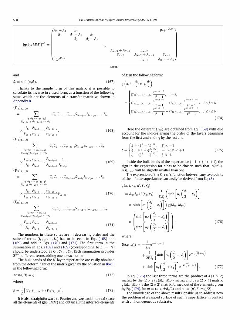
508 E.H. El Boudouti et al. / Surface Science Reports 64 (2009) 471–594

[g(k3;MM)]−1 =

AN + A1 B1 BNe−ik3D

B1 A1 + A2 B2B2 A2 + A3

. . .

AN−3 + AN−2 BN−2BN−2 AN−2 + AN−1 BN−1

BNeik3D BN−1 AN−1 + AN

Box II.

and

Si = sinh(αidi). (167)

Thanks to the simple form of this matrix, it is possible tocalculate its inverse in closed form, as a function of the followingsums which are the elements of a transfer matrix as shown inAppendix B.

(T11)1,...,N=

∑i1>i2>···>iN−2p

iN−2p+1>iN−2p+2>···>iN

Ci1Ci2 . . . CiN−2pSiN−2p+1SiN−2p+2 . . . SiN

×FiNFiN−1

FiN−2FiN−3· · ·FiN−2p+2FiN−2p+1

, (168)

(T12)1,...,N=

∑i1>i2>···>iN−2p−1iN−2p>iN−2p+1>···>iN

Ci1Ci2 . . . CiN−2p−1SiN−2pSiN−2p+1 . . . SiN

×FiN−1FiN

FiN−3FiN−2· · ·FiN−2p+1FiN−2p+2

1FiN−2p

, (169)

(T21)1,...,N=

∑i1>i2>···>iN−2p−1iN−2p>iN−2p+1>···>iN

Ci1Ci2 . . . CiN−2p−1SiN−2pSiN−2p+1 . . . SiN

×FiNFiN−1

FiN−2FiN−3· · ·FiN−2p+2FiN−2p+1

FiN−2p , (170)

(T22)1,...,N=

∑i1>i2>···>iN−2p

iN−2p+1>iN−2p+2>···>iN

Ci1Ci2 . . . CiN−2pSiN−2p+1SiN−2p+2 . . . SiN

×FiN−1FiN

FiN−3FiN−2· · ·FiN−2p+1FiN−2p+2

. (171)

The numbers in these suites are in decreasing order and thesuite of terms (ip+1, . . . , iN ) has to be even in Eqs. (168) and(169) and odd in Eqs. (170) and (171). The first term in thesummation in Eqs. (168) and (169) (corresponding to p = N)should be understood as C1, C2 . . . CN . Each summation provides2N−1 different terms adding one to each other.The bulk bands of the N-layer superlattice are easily obtained

from the determinant of the matrix given by the equation in Box IIin the following form:

cos(k3D) = ξ, (172)

where

ξ =12

[(T11)1,...,N + (T22)1,...,N

]. (173)

It is also straightforward to Fourier analyze back into real spaceall the elements of g(k3;MM) and obtain all the interface elements

of g, in the following form:

g(n, i,−

di2; n′, j,

dj2

)

=

(T12)i,...,N,1,...,i−1t |n−n

′|+1

t2 − 1, i = j,

(T12)j,...,N,1,...,i−1t |n−n

′|+1

t2 − 1+ (T12)i,...,j−1

t |n−n′−1|+1

t2 − 1, i ≤ j ≤ N,

(T12)i,...,N,1,...,j−1t |n−n

′|+1

t2 − 1+ (T12)j,...,i−1

t |n−n′+1|+1

t2 − 1, j ≤ i ≤ N

(174)

Here the different (T12) are obtained from Eq. (169) with dueaccount for the indices giving the order of the layers beginningfrom the first and ending by the last and

t =

ξ + (ξ2− 1)1/2, ξ < −1

ξ ± i(1− ξ 2)1/2, −1 < ξ < +1ξ − (ξ 2 − 1)1/2, ξ > 1.

(175)

Inside the bulk bands of the superlattice (−1 < ξ < +1), thesign in the expression for t has to be chosen such that |t(ω2 +iε)|ε→∞ will be slightly smaller than one.The expression of the Green’s function between any two points

of the infinite superlattice can easily be derived from Eq. (8),

g(n, i, x3; n′, i′, x′3)

= δnn′δii′ Ui(x3, x′3)+1SiS ′i

(sinh

[αi

(di2− x3

)];

× sinh[αi

(di2+ xi

)])g(Mm,Mm′)

×

sinh[αi′

(di′2− x′3

)]sinh

[αi′

(di′2+ x′3

)] , (176)

where

Ui(x3, x′3) = −12Fie−αi|xi−x

′i |

+12FiSi

sinh

[αi

(di2− x′3

)]e−αi

(di2 +x3

)

+ sinh[αi

(di2+ x′3

)]e−αi

(di2 −x3

). (177)

In Eq. (176) the last three terms are the product of a (1 × 2)matrix by the (2× 2) g(Mm,Mm′)matrix and by a (2× 1)matrix.g(Mm,Mm′) is the (2× 2)matrix formed out of the elements givenby Eq. (174), form ≡ (n, i,±di/2) andm′ ≡ (n′, i′,±d′i/2).The knowledge of the above results, enable us to address now

the problem of a capped surface of such a superlattice in contactwith an homogeneous substrate.

E.H. El Boudouti et al. / Surface Science Reports 64 (2009) 471–594 509

x3

Cell 1

Cell 0

Layer N

Layer 2

Layer 1

Layer N

Layer 2

Layer 1

Cap layer (0)

semi-infinite medium (v)

dN

d2

d1

d0

D

Fig. 45. Schematic representation of a capped semi-infinite N-layer superlatticein contact with an homogeneous substrate. d0, d1, d2, . . . , dN , respectively, are thethicknesses of the cap layer and of the N different slabs out of which the unit cell ofthe superlattice is built. D is the period of the superlattice.

4.3.2. The capped surface and the interfaceIn this subsection, we will first outline the derivation of the

Green’s function and then give the results for the surface states andthe density of states.

4.3.2.1. The Green’s function. In order to obtain the physicalproperties of a semi-infinite N-layer superlattice terminated bya capped surface in contact with a semi-infinite homogeneousmedium (Fig. 45), it is convenient to consider the following threesteps:(i) The semi-infinite superlattice, with a stress-free surface

terminated by the layer (n = 0, i = 1), is obtained by removingthe (n = −1, i = N) layer out of the infinite N-layer superlattice.The corresponding [gs(Ms,Ms)]−1 in theMs semi-infinite interfacespace (n ≥ 0, i = 1, . . . ,N), is represented by a semi-infinitetridiagonalmatrixwhose surface diagonal element situated at (n =0, i = 1,−d1/2) is equal to A1.(ii) We consider a semi-infinite homogeneous medium charac-

terized by the parameters αv , Fv (Eqs. (130) and (137)) and cappedby a layer characterized by the parameters α0, F0 (Eqs. (130) and(137)) and by C0 and S0 (Eqs. (135) and (136)).Within the interface space M0 = (−1, 0,±d0/2), of this

system, one obtains [115]

[gs0(M0,M0)]−1 =(A0 − Fv B0B0 A0

). (178)

By inversion of this matrix, one gets

g−1s0

(−1, 0,

d02;−1, 0,

d02

)= −RFv, (179)

where

R =1+ F0S0/FvC01+ FvS0/F0C0

. (180)

(iii) The above semi-infinite superlattice is coupled to the caplayer 0 deposited on the substrate v. The Green’s function of thisfinal system in the interface space has as its inverse d−1(Ms,Ms)

a semi-infinite tridiagonal matrix. The surface diagonal elementof this matrix situated at (n = 0, i = 1, −d1/2) is equal to(A1−RFv). By standard diagonalization [115] of such a semi-infinitetridiagonal matrix, one obtains for n, n′ ≥ 0 and i, j = 1, . . . ,N:

d(n, i,−di2; n′, j,

−dj2

)= g

(n, i,−di2; n′, j,

−dj2

)−tn+n

′+1

t2 − 1YiYjW, (181)

where

W = (RFv)2(T12)1,...,N + (RFv)[(T11)1,...,N− (T22)1,...,N ] − (T21)1,...,N , (182)

and the Yi take the form

Y1 = −RFv(T12)1,...,N − t + (T22)1,...,N , (183)

and for i = 2, . . . ,N ,

Yi = −(RFv)[t(T12)1,...,i−1 + (T12)i,...,N ]

− t(T11)1,...,N + (T22)1,...,N . (184)

The cap layer interface elements of d can also be worked out inthe following closed forms:

d(0, 1,−d12; 0, 1,

−d12

)=Y1W, (185)

d(−1, 0,

−d02;−1, 0,

−d02

)=Y1F0C0 + S0

(T21)1,...,N − (RFv)[−t + (T11)1,...,N ]

W (F0C0 + FvS0)

, (186)

d(−1, 0,

−d02; 0, 1,

−d12

)= d

(0, 1,−d12;−1, 0,

−d02

)=

Y1F0W (F0C0 + FvS0)

, (187)

d(−1, 0,

−d02; n, i,

−di2

)=

YiF0tn

W (F0C0 + FvS0). (188)

From the knowledge of these interface matrix elements onecan obtain the elements of the Green’s function between anytwo points of the whole system (Eq. (8)). Here, we only givetheir expressions for two points belonging both either to thesuperlattice, or to the cap layer, or to the substrate:(i) When the two points are inside the superlattice,

d(n, i, x3; n′, i′, x′3) is given by Eq. (176) inwhich one has to replaceg(Mm,Mm′) by d(Mm,Mm′) given by Eq. (181).(ii) When the two points are inside the cap layer,

d(−1, 0, x3;−1, 0, x′3) is given by Eq. (176) for i = 0 and inwhich one has to replace g(Mm,Mm′) by d(M0,M0), with M0 ≡(−1, 0,±d0/2). The elements of this (2 × 2) matrix are given byEqs. (185)–(188).(iii) When the two points are inside the substrate

d(x3, x′3) = −e−αv |x3−x

′3|

2Fv

+

[d(−1, 0,

−d02;−1, 0,

−d02

)+12Fv

]e−αv(x3+x

′3), (189)

where d(−1, 0, −d02 ;−1, 0,

−d02

)is given by Eq. (186).

510 E.H. El Boudouti et al. / Surface Science Reports 64 (2009) 471–594

4.3.2.2. Eigenfrequencies and eigenfunctions of the localized states.When the denominator of the Green’s function d vanishes for afrequency lying inside the gaps of the semi-infinite superlattice,one obtains localized states within the cap layer which decayexponentially inside the bulk band of the superlattice. The explicitexpression giving the frequency ω of these localized states is

W (ω) = 0, (190)

whereW (ω) is given by Eq. (182), together with the condition∣∣(T22)1,...,N − RFv(T12)1,...,N ∣∣ > 1. (191)

Condition (191) ensures that the wave is decaying whenpenetrating into the superlattice far from the surface.The eigenfunctions associated with these localized states are

found to be

u(x3) ∝ Wd(−1, 0,

−d02;−1, 0,

−d02

)eαvx3 , x3 ≤ 0, (192)

u(x3) ∝ Wd(−1, 0,

−d02;−1, 0,

−d02

)sinh

[α0

(d02− x3

)]+Wd

(−1, 0,

−d02; 0, 1,

−d12

)sinh

[α0

(d02+ x3

)],

−d02≤ x3 ≤

d02, (193)

u(n, i, x3) ∝ Wd(−1, 0,

−d02; n, i,

−di2

)sinh

[αi

(di2− x3

)]+Wd

(−1, 0,

−d02; n, i,

di2

)sinh

[αi

(di2+ x3

)],

−di2≤ x3 ≤

di2, i = 1, . . . ,N, (194)

where the Green’s functionmatrix elements defined by Eqs. (186)–(188) appear.

4.3.2.3. The local densities of states. The local densities of states onthe plane (n, i, x3) are given by

n(ω2, k‖; n, i, x3) = −ρ

πIm d+(ω2, k‖; n, i, x3; n, i, x3), (195)

where

d+(ω2) = limε→0d(ω2 + iε) (196)

and d(ω2) is the above defined Green’s function.

4.3.2.4. The total density of states. The total density of states for agiven value of k‖ is obtained by integrating over x3 and summing onn and i the local density n(ω2, k‖; n, i, x3). A particularly interestingquantity is the density of states of the above defined compositesystem from which the contributions of bulk substrate and bulksuperlattice are subtracted. This variation 1n(ω2) can be writtenas

1n(ω2) =N∑i=1

1in(ω2)+ n0(ω2)+1vn(ω2), (197)

where 1in(ω2) is the variation of the density of states in anyslab i, n0(ω2) the density of states in the cap layer, and 1vn(ω2)the variation of the density of states in the substrate. The explicit

expressions for these quantities were found to be

1in(ω2) = −ρi

2πIm

t(t2 − 1)2

(1

αiS2i W

)×[(Y 2i + Y

2i+1)(CiSi − αidi)+ 2YiYi+1(αidiCi − Si)

],

i = 1, . . . ,N − 1, (198)

1Nn(ω2) = −ρN

2πIm

t(t2 − 1)2

(1

αNS2NW

)×[(Y 2N + (tY1)

2)(CNSN − αNdN)+ 2YNY1t(αNdNCN − SN)],

(199)

n0(ω2) = −ρN

2πIm

Y1W (T12)i,...,N

×

d0[(T12)i,...,N + [(T11)i,...,N − t]R

FvF 20

]

+

S0F0

[(T12)i,...,N − [(T11)i,...,N − t] FvF20

]α0(F0C0 + FvS0)

, (200)

and

1vn(ω2) = −ρv

πIm12αv

×

12Fv+Y1F0C0 + S0(T21)i,...,N − RFv[(T11)i,...,N − t]

W (F0C0 + FvS0)

. (201)

4.3.2.5. The limit of a semi-infinite superlattice. (i) The case of asemi-infinite superlattice with a cap layer can be described fromthe above results, by making Fv = 0 and RFv → F0S0/C0. Inparticular, if the cap layer is of the same nature as the Nth layerand of width d0 < dN , we obtain from the above results (Eqs.(181)–(184) and (190)–(200)) the properties of a semi-infinitesuperlattice ending with an incomplete i = N surface layer.(ii) A semi-infinite superlattice ending with a complete i = 1

surface layer is obtained from the above case (i) by taking the limitwhere the thickness d0 of the cap layer goes to zero. This impliesthat C0 is equal to 1 and S0 vanishes. Eqs. (181)–(184) and (190)–(199) remain valid in this limit and provide all the physical resultsfor such a semi-infinite superlattice. Let us precise that in this limitn0(ω2) and1vn(ω2) vanish.

4.3.2.6. The limit of an interface between a semi-infinite superlatticeand a homogeneous substrate. An interface between a semi-infinitesuperlattice and a homogeneous substrate is interesting by itself,in particular because specific localized and resonant modes mayexist in its vicinity. Such a limit can be obtained from the aboveresults given by Eqs. (181)–(200) by setting the width d0 of the caplayer going to zero; this implies S0 → 0, C0 → 1, R → 1, andn0(ω2)→ 0.

4.3.3. Application to a four-layer superlattice

4.3.3.1. Analytical results. In order to illustrate the general resultsgiven before, we present here a simple application to the specialcase of a four-layer superlattice. First, we show in this examplehow one calculates the unconventional sums appearing in the

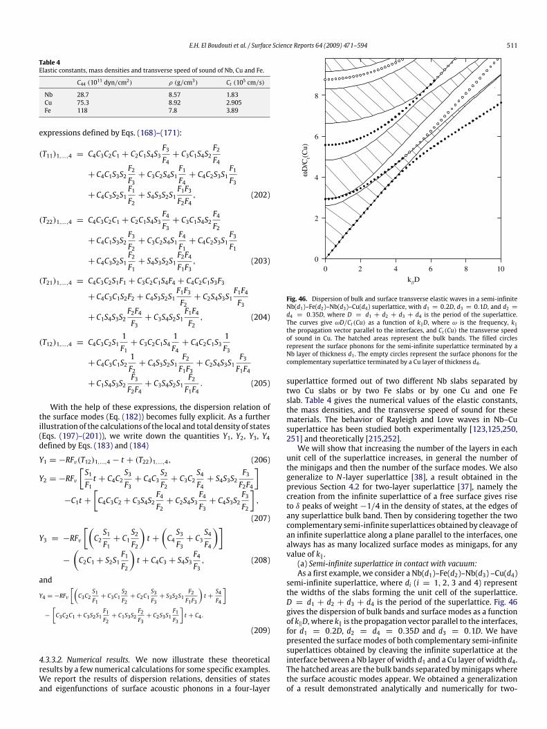
E.H. El Boudouti et al. / Surface Science Reports 64 (2009) 471–594 511

Table 4Elastic constants, mass densities and transverse speed of sound of Nb, Cu and Fe.

C44 (1011 dyn/cm2) ρ (g/cm3) Ct (105 cm/s)

Nb 28.7 8.57 1.83Cu 75.3 8.92 2.905Fe 118 7.8 3.89

expressions defined by Eqs. (168)–(171):

(T11)1,...,4 = C4C3C2C1 + C2C1S4S3F3F4+ C3C1S4S2

F2F4

+ C4C1S3S2F2F3+ C3C2S4S1

F1F4+ C4C2S3S1

F1F3

+ C4C3S2S1F1F2+ S4S3S2S1

F1F3F2F4

, (202)

(T22)1,...,4 = C4C3C2C1 + C2C1S4S3F4F3+ C3C1S4S2

F4F2

+ C4C1S3S2F3F2+ C3C2S4S1

F4F1+ C4C2S3S1

F3F1

+ C4C3S2S1F2F1+ S4S3S2S1

F2F4F1F3

, (203)

(T21)1,...,4 = C4C3C2S1F1 + C3C2C1S4F4 + C4C2C1S3F3

+ C4C3C1S2F2 + C4S3S2S1F1F3F2+ C2S4S3S1

F1F4F3

+ C1S4S3S2F2F4F3+ C3S4S2S1

F1F4F2, (204)

(T12)1,...,4 = C4C3C2S11F1+ C3C2C1S4

1F4+ C4C2C1S3

1F3

+ C4C3C1S21F2+ C4S3S2S1

F2F1F3+ C2S4S3S1

F3F1F4

+ C1S4S3S2F3F2F4+ C3S4S2S1

F2F1F4

. (205)

With the help of these expressions, the dispersion relation ofthe surface modes (Eq. (182)) becomes fully explicit. As a furtherillustration of the calculations of the local and total density of states(Eqs. (197)–(201)), we write down the quantities Y1, Y2, Y3, Y4defined by Eqs. (183) and (184)

Y1 = −RFv(T12)1,...,4 − t + (T22)1,...,4, (206)

Y2 = −RFv

[S1F1t + C4C2

S3F3+ C4C3

S2F2+ C3C2

S4F4+ S4S3S2

F3F2F4

]−C1t +

[C4C3C2 + C3S4S2

F4F2+ C2S4S3

F4F3+ C4S3S2

F3F2

],

(207)

Y3 = −RFv

[(C2S1F1+ C1

S2F2

)t +

(C4S3F3+ C3

S4F4

)]−

(C2C1 + S2S1

F1F2

)t + C4C3 + S4S3

F4F3, (208)

and

Y4 = −RFv

[(C3C2

S1F1+ C3C1

S2F2+ C2C1

S3F3+ S3S2S1

F2F1F3

)t +

S4F4

]−

[C3C2C1 + C3S2S1

F1F2+ C1S3S2

F2F3+ C2S3S1

F1F3

]t + C4.

(209)

4.3.3.2. Numerical results. We now illustrate these theoreticalresults by a few numerical calculations for some specific examples.We report the results of dispersion relations, densities of statesand eigenfunctions of surface acoustic phonons in a four-layer

k//D

0 2 4 6 8 10

ωD

/Ct(C

u)

0

2

4

6

8

Fig. 46. Dispersion of bulk and surface transverse elastic waves in a semi-infiniteNb(d1)–Fe(d2)–Nb(d3)–Cu(d4) superlattice, with d1 = 0.2D, d3 = 0.1D, and d2 =d4 = 0.35D, where D = d1 + d2 + d3 + d4 is the period of the superlattice.The curves give ωD/Ct (Cu) as a function of k‖D, where ω is the frequency, k‖the propagation vector parallel to the interfaces, and Ct (Cu) the transverse speedof sound in Cu. The hatched areas represent the bulk bands. The filled circlesrepresent the surface phonons for the semi-infinite superlattice terminated by aNb layer of thickness d1 . The empty circles represent the surface phonons for thecomplementary superlattice terminated by a Cu layer of thickness d4 .

superlattice formed out of two different Nb slabs separated bytwo Cu slabs or by two Fe slabs or by one Cu and one Feslab. Table 4 gives the numerical values of the elastic constants,the mass densities, and the transverse speed of sound for thesematerials. The behavior of Rayleigh and Love waves in Nb–Cusuperlattice has been studied both experimentally [123,125,250,251] and theoretically [215,252].We will show that increasing the number of the layers in each

unit cell of the superlattice increases, in general the number ofthe minigaps and then the number of the surface modes. We alsogeneralize to N-layer superlattice [38], a result obtained in theprevious Section 4.2 for two-layer superlattice [37], namely thecreation from the infinite superlattice of a free surface gives riseto δ peaks of weight −1/4 in the density of states, at the edges ofany superlattice bulk band. Then by considering together the twocomplementary semi-infinite superlattices obtained by cleavage ofan infinite superlattice along a plane parallel to the interfaces, onealways has as many localized surface modes as minigaps, for anyvalue of k‖.(a) Semi-infinite superlattice in contact with vacuum:As a first example, we consider a Nb(d1)–Fe(d2)–Nb(d3) –Cu(d4)

semi-infinite superlattice, where di (i = 1, 2, 3 and 4) representthe widths of the slabs forming the unit cell of the superlattice.D = d1 + d2 + d3 + d4 is the period of the superlattice. Fig. 46gives the dispersion of bulk bands and surface modes as a functionof k‖D, where k‖ is the propagation vector parallel to the interfaces,for d1 = 0.2D, d2 = d4 = 0.35D and d3 = 0.1D. We havepresented the surface modes of both complementary semi-infinitesuperlattices obtained by cleaving the infinite superlattice at theinterface between a Nb layer of width d1 and a Cu layer of width d4.The hatched areas are the bulk bands separated byminigapswherethe surface acoustic modes appear. We obtained a generalizationof a result demonstrated analytically and numerically for two-

512 E.H. El Boudouti et al. / Surface Science Reports 64 (2009) 471–594

3 4 5 6 7 8 9 10 11

3 4 5 6 7 8 9 10 11

3 4 5 6 7 8 9 10 11

L1L2

B1

T1 B2 T2B3

B1 T1B2

T2 B3

L3

L1L3 L2

B1

T1 B2 T2B3

L4

T3 B4

T3 B4

L4

T3B4

-10

0

10

20

30

-10

0

10

20

30

-20

-10

0

10

20

30

a

b

c

Fig. 47. (a) Variation in the density of states [in units of D/Ct (Cu)] between asemi-infinite Nb(d1)–Fe(d2)-Nb(d3)–Cu(d4) superlattice terminated by a Nb layer ofthickness d1 and the same amount of a bulk superlattice, as a function ofωD/Ct (Cu),for k‖D = 5. Bi and Ti , respectively, refer to δ peaks of weight (−1/4) situated at thebottom and the top of the bulk bands and Li indicates the localized surface modes.(b) Same as (a) but for the complementary superlattice terminated by a Cu layer ofthickness d4 . (c) Same as (a) but for both complementary superlattices, Bi and Ti ,respectively, refer to δ peaks of weight (−1/2).

layer superlattices (Section 4.2) and observed experimentally forAl–Ag superlattices [59], namely, there are as many surface statesas minigaps, each surface mode being associated with either oneor the other of the complementary semi-infinite superlattices. Onecan also observe that the surface modes are very dependent onthe type of crystal which is at the surface. On the other hand,there is a continuity between the surface branches of the twocomplementary superlattices when these branches reach a bulkband edge.It can be shown analytically that the expression giving the

frequencies of the surface modes for two complementary semi-infinite superlattices terminated by slabs of the same thicknessas in the bulk is identical to the expression giving the standingwaves of one unit cell with stress-free boundary conditions. Thisexpression is given by (T21)1,...,4 = 0.The variation in the vibrational DOS 1na(ω) [respectively,

1nb(ω)] between the semi-infinite superlattice terminated by acrystal of Nb of width d1 = 0.2D (respectively, Cu of width d4 =0.35D) and the same amount of the bulk superlattice was deducedfrom the calculation described in Sections 4.3.2.5 and 4.3.3.1. These1na(ω) and1nb(ω) are plotted in Figs. 47(a) and (b) for k‖D = 5,as a function of the reduced frequency [ωD/Ct(Cu)]. The δ functionsappearing at the bulk band edges and at the frequencies of thesurface modes are enlarged by the addition of a small imaginarypart to the frequencyω. The δ functions associatedwith the surfacelocalized states are noted Li and the δ functions of weight (−1/4)situated, respectively, at the bottom and top of any bulk band arecalled Bi and Ti. The form of these latter enlarged δ functions Bi andTi are not exactly the same because of the contributions comingfrom the divergence in (ω− ωBi)−1/2 or (ω− ωTi)−1/2 (ωBi and ωTi

are the frequencies of the bottom and the top of every bulk bandof the superlattice), existing near the band edges in the densitiesof states in one dimension. Apart from the above δ peaks andthe particular behavior near the band edges, the variation of thevibrational density of states does not show any other significanteffect inside the bulk bands of the superlattice.It is worth considering the variation in the density of

states 1n(ω) between the two complementary semi-infinitesuperlattices, given in Fig. 47(a) and (b), and the initial infinitesuperlattice. Fig. 47(c) gives the sumof the variations in the densityof states of these complementary systems 1n(ω) = 1na(ω) +1nb(ω). This quantity is equal to zero for ω falling inside anysuperlattice bulk band. The loss of states due to the peaks of weight(−1/2) at every edge of the bulk bands is then compensated by thegain associated with the localized states (L1, L2, L3, L4) inside theminigaps in order to ensure the conservation of the total numberof states.The behavior of surface modes displacement field as a function

of the distance x3 to the surface is sketched in Fig. 48 for the wavevector k‖D = 5. Fig. 48(a), (b), (c), and (d), respectively, refer tothe surface modes labeled L1, L2, L3, L4 in Fig. 47 which occur atthe following frequencies ωD/Ct(Cu) = 4.745, 7.69, 5.375, and10.03. The parameter t (Eq. (175)) which gives the attenuation ofthe surface wave from one period of the superlattice to the nextwhen penetrating deep into the superlattice far from the surfacetakes, respectively, the values 0.205, 0.745, 0.74, and 0.828. Besidesthis exponential decrease of the envelope of the displacement field,one can also observe an increasing number of oscillations in eachperiod of the superlattice when going to higher frequencies (let usnotice that the frequencies of the modes L2, L3, L4 fall inside thebulk bands of the constituent materials of the superlattice).Now, in a second illustration, we assume that the Fe layers of

width d2 in the previous superlattice are replaced by Cu layers ofthe samewidth. Fig. 49 gives the bulk bands and surface modes forthe two complementary semi-infinite superlattices obtained in thesame manner as in the previous example. The positions of surfacemodes are very different from those given in Fig. 46 even thoughthe superlattices are terminated by the same layers at the surface.One peculiarity of the example shown in Fig. 49 is the existence

of successive bulk bands crossings; the crossing points are situatedalong a straight line defined as

ω

k‖=

(C244 − C

′244

ρC244 − ρ ′C′244

). (210)

This equation is obtained from the condition

F(Nb) = F(Cu), (211)

where F is defined in Eq. (137). This is a sufficient condition fortwo bands to cross each other or, equivalently, a gap to close. Thepossibility of band crossing occurs if the slope of the straight linedefined in Eq. (210) is such that it cuts the bulk bands of the SL.This straight line corresponds to a Brewster acoustic angle [253]between two elastic materials, i.e., any wave launched throughsuch angle is totally transmitted through the system. Eq. (210) isactually valid for any N-layer SL composed of only two differentmaterials. One can notice that the surfacemodes of one or the otherof the complementary SLs in Fig. 49 reach the crossing points of thebulk bands and are in continuation of each other.The number of the bulk bands and surface modes increases in

general, with the number of the layers contained in each unit cellof the SL. Fig. 50(a) [respectively, Fig. 50(b)] gives, for k‖D = 0[respectively, for k‖D = 10], the dispersion of the bulk bandsand surface modes as a function of the widths d1/D or d3/D, theperiod of the SL being kept constant (d1/D increases from 0 to 0.3when d3/D decreases from 0.3 to 0). For d1/D = d3/D = 0.15,

E.H. El Boudouti et al. / Surface Science Reports 64 (2009) 471–594 513

0 1 2 3 40

4

8

0 1 2 3 40

1

0 1 2 3 40

1

0 1 2 3 40

1

2

a b

c d

Fig. 48. Modulus of the displacement field versus depth for the surface waves occurring in Fig. 47 (i.e., for k‖D = 5) at reduced frequencies ωD/Ct (Cu) = 4.745 (a),ωD/Ct (Cu) = 7.69 (b), ωD/Ct (Cu) = 5.375 (c), and ωD/Ct (Cu) = 10.03 (d). The surface waves represented in Figs. (a) and (b) (respectively, (c) and (d)) are obtained whena Nb [respectively, a Cu] layer is at the surface of the semi-infinite superlattice (see Fig. 47(a) and (b)).

0

2

4

6

8

0 2 4 6 8 10

Fig. 49. Same as in Fig. 46 but for a semi-infinite Nb(d1)–Cu(d2)–Nb(d3)–Cu(d4)superlattice. The width of the slabs are the same as in Fig. 46. The filled circlesrepresent the surface phonons for the semi-infinite superlattice terminated by aNb layer of thickness d1 . The empty circles represent the surface phonons for thecomplementary superlattice terminated by a Cu layer of thickness d4 .

one finds the situation of a two-layer SL studied before by Camleyet al. [215]. For the other values of d1/D, the number of the bulkbands and surface modes is multiplied by two as the number ofthe layers forming the unit cell is four instead of two. There areexceptions at some particular values of d1 where two bulk bandscross each other and a gap disappears. The surface modes whichare presented for both complementary semi-infinite SLs reachthe bulk band crossing points. One can also notice the continuitybetween surface modes corresponding to the complementarysemi-infinite SLs, both at the bulk bands crossing points and at thecrossings of surface branches with the bulk band edges (see alsoFigs. 46 and 49).(b) Capped semi-infinite superlattice in contact with vacuum:Now we assume that a cap layer of Fe, of thickness d0,

is deposited on top of the Nb(d1)–Cu(d2)–Nb(d3)–Cu(d4) semi-infinite superlattice terminated by a full Nb layer of width d1,where d1 = 0.2D, d2 = d4 = 0.35D, and d3 = 0.1D. Fig. 51gives the dispersion of localized and resonant modes induced bya cap layer of width d0 = 4D. These modes are obtained as well-defined peaks in the variation1n(ω) (see Fig. 52) in the density ofstates between the capped superlattice and the sameamount of thebulk superlatticewithout the cap layer (the calculation is explainedin Sections 4.3.2.4 and 4.3.3.1). It is worth noting that for anothertermination of the semi-infinite superlattice these modes will bequite different.The localized and resonant modes induced by the cap layer

can be divided in different groups according to the behavior ofthe corresponding eigenstates along the axis of the superlattice;they may propagate in both the superlattice and the cap layer,

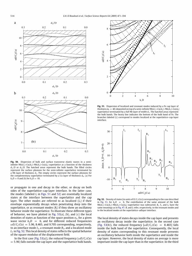
514 E.H. El Boudouti et al. / Surface Science Reports 64 (2009) 471–594

t

7

8

9

10

0.3 0.2 0.1 0.0

0

2

4

6

8

10

0.0 0.1 0.2 0.3

0.3 0.2 0.1 0.0

0.0 0.1 0.2 0.3

a

b

Fig. 50. Dispersion of bulk and surface transverse elastic waves in a semi-infinite Nb(d1)–Cu(d2)–Nb(d3)–Cu(d4) superlattice as a function of the thicknessd1/D or d3/D. The hatched areas represent the bulk bands. The filled circlesrepresent the surface phonons for the semi-infinite superlattice terminated bya Nb layer of thickness d1 . The empty circles represent the surface phonons forthe complementary superlattice terminated by a Cu layer of thickness d4 . (a) Fork‖D = 0 and (b) for k‖D = 10.

or propagate in one and decay in the other, or decay on bothsides of the superlattice–cap-layer interface. In the latter case,the modes (labeled Ii in Figs. 51 and 52) are essentially localizedstates at the interface between the superlattice and the caplayer. The other modes are referred to as localized (Li) if theirenvelope exponentially decays when penetrating deep into thesuperlattice, or as resonant modes (Ri) if they show an oscillatorybehavior inside the superlattice. To illustrate these different typesof behavior, we have plotted in Fig. 53(a), (b), and (c) the localdensities of states as function of the space position x3, for a givenwave vector k‖D = 6, and for different reduced frequenciesωD/Ct(Cu) = 5.96, 8.465, and 9.705 corresponding, respectively,to an interface mode I1, a resonant mode R3, and a localized modeL1 in Fig. 52. This local density of states reflects the spatial behaviorof the square modulus of the displacement field.In the first case (Fig. 53(a)), the reduced frequency (ωD/Ct(Cu)

= 5.96) falls outside the cap layer and the superlattice bulk bands.

0 2 4 6 8 100

2

4

6

8

Fig. 51. Dispersion of localized and resonant modes induced by a Fe cap layer ofthicknessd0 = 4D, deposited on topof a semi-infiniteNb(d1)–Cu(d2)–Nb(d3)–Cu(d4)superlattice terminated by a full Nb layer of width d1 . The hatched areas representthe bulk bands. The heavy line indicates the bottom of the bulk band of Fe. Thebranches labeled (Ii) correspond to modes localized at the superlattice–cap-layerinterface.

5 6 7 8 9 10

B1T1

B2T2 B3

T3B4

I1I2

R1

R2

R3R4

R5

L1

R6

-10

0

10

20

30

Fig. 52. Density of states [in units ofD/Ct (Cu)] corresponding to the case describedin Fig. 51, for k‖D = 6. The contribution of the same amount of the bulkNb(d1)–Cu(d2)–Nb(d3)–Cu(d4) superlattice was subtracted. Bi , Ti , and Li have thesamemeanings as in Fig. 47; Ri and Ii refer, respectively, to the resonant modes andto the localized modes at the superlattice–adlayer interface.

The local density of states decays inside the cap layer and presentsan oscillatory decay inside the superlattice. In the second case(Fig. 53(b)), the reduced frequency [ωD/Ct(Cu) = 8.465] fallsinside the bulk band of the superlattice. Consequently, the localdensity of states corresponding to this resonant mode presentsan oscillatory behavior both inside the superlattice and inside thecap layer. However, the local density of states on average is moreimportant inside the cap layer than in the superlattice. In the third

E.H. El Boudouti et al. / Surface Science Reports 64 (2009) 471–594 515

-4 -3 -2 -1 0

Loc

al D

OS

Loc

al D

OS

0

1

2

3

4

x3/D

4

8

Cap layerSuperlattice

Cap layer

Superlattice

Cap layerSuperlattice

0

10

20

30

40

1 2 3 4

-4 -3 -2 -1 0 1 2 3 4

-4 -3 -2 -1 0 1 2 3 4

Loc

al D

OS

0

12

a

b

c

Fig. 53. (a) Spatial dependence of the local density of states [DOS] [in units ofD/Ct (Cu)] corresponding to the case described in Fig. 51 at ωD/Ct (Cu) = 5.96 andk‖D = 6. (b) The same as (a) but for ωD/Ct (Cu) = 8.565. (c) The same as (a) but forωD/Ct (Cu) = 9.705.

case (Fig. 53(c)), the reduced frequency [ωD/Ct(Cu) = 9.705] fallsinside the gap of the superlattice. Now, the local density of statespresents an oscillatory behavior in the space occupied by the caplayer and an oscillatory decay inside the superlattice.The frequencies of the localized and resonant modes are very

dependent upon the thickness d0 of the cap layer as shown inFig. 54, for k‖D = 6. The lowest two branches which correspond tocap-layer–superlattice interface modes become almost indepen-dent of d0 for d0 > 0.5D. The next branches corresponding to res-onant modes become closer to one another when d0 increases, andas a consequence the intensities of the corresponding resonancesincrease. Let us also note that the curves in this figure becomesalmost flat when a localized branch is going to become resonantby merging into a bulk band. The variation with d0 is faster whenthe resonant branch penetrates deep into the band, but then theintensity of the resonant mode decreases, or may even vanish, inparticular, when d0 is small or the frequency is high. Finally, let usmention that for any given frequencyω in Fig. 54, there is a periodicrepetition of the modes as a function of d0.When the thickness d0 of the cap layer goes to infinite, we

find the situation of a semi-infinite superlattice in contact withan homogeneous substrate. We address this case in the nextsubsection.(c) A semi-infinite superlattice in contact with a semi-infinite

substrate:To show the interface localized modes associated with the

deposition of a semi-infinite superlattice on a semi-infinitesubstrate,wehave chosen the same superlattice as in paragraph (b)deposited on a substrate of Fe. Fig. 55 gives the localized interfacemodes for the superlattice terminated by a full Nb layer of widthd1. One can remark that the frequencies of the interface modes inFigs. 51 and 55 are almost the same even though in the former casethe substrate is replaced by a cap layer of finite thickness d0 = 4D;

0 1 2 3 4

6

8

10

12

Fig. 54. Cap-layer-induced localized and resonant modes versus the width d0 ofthe cap layer. The superlattice is the same as in Fig. 51 and k‖D = 6. The lowest twobranches correspond to modes localized at the superlattice–cap-layer interface.

0

2

4

6

8

0 4 8 102 6

Fig. 55. Localized modes associated with the interface of the semi-infinite SLNb(d1)–Cu(d2)–Nb(d3)–Cu(d4) described in Fig. 51 in contact with a substrate of Fe.The heavy straight line indicates the bottom of the substrate bulk band.

moreover, the localization of the interface modes is similar in bothcases. Let us also note that the frequencies of interface modes arevery sensitive to the nature of the substrate and to the type of layerwhich is at the surface of the superlattice.The variation 1n11(ω) (respectively, 1n12(ω)) in the density

of states between the semi-infinite superlattice terminated by acrystal of Nb of width d1 = 0.2D [respectively, Cu of width d4 =0.35D], in contact with a substrate of Fe and the same amount ofthe bulk superlattice and of the bulk homogeneous medium areplotted in Fig. 56(a) and (b) for k‖D = 1, as a function ofωD/Ct(Cu).The δ functions of weight (−1/4) situated, respectively, at the

516 E.H. El Boudouti et al. / Surface Science Reports 64 (2009) 471–594

B1 Bs

T1B2

B2

B2

T2

B3 T3B4

B1

B1

Bs

Bs

T1

T1

T2

T2 B3

B3

T3

T3

B4

B4

-4

0

-4

0

-16

-8

0

8

ΔnI(

ω ;

k //D

=1)

-8

4

ΔnI2

(ω ;

k //D

=1)

-8

4

ΔnI1

(ω ;

k //D

=1)

0 2 4 6 8 10

0 2 4 6 8 10

2 4 6 80 10ωD/Ct(Cu)

a

b

c

Fig. 56. (a) Variation in the density of states [in units of D/Ct (Cu)] at k‖D = 1, dueto the creation of the superlattice/substrate interface. The superlattice is the sameas in Fig. 51 and the substrate is Fe. Bi and Ti have the same meanings as in Fig. 47.Bs refers to a δ peak of weight (−1/4) situated at the bottom of the substrate bulkband. (b) Same as (a) but for the complementary superlattice terminated by a Culayer of thickness d4 . (c) Sum of the curves in (a) and (b).

bottom and top of any bulk band are called Bi and Ti. Bs refers toa δ peak of weight (−1/4) situated at the bottom of the substratebulk band.When one takes both complementary superlattices used in

Fig. 56(a) and (b), the variation in the density of states [1n1(ω) =1n11(ω) + 1n12(ω)] is shown to be equal to zero for frequenciesω belonging at the same time to the bulk bands of the substrateand the superlattice [38]. We have presented in Fig. 56(c) anexample of this variation in the density of states for k‖D = 1 forboth complementary superlattices. Bearing in mind the loss of the(−1/2) state at the limits of any bulk band and the conservationof the total number of states, we are led to the necessary existenceof positive contributions in the density of states lying inside theminigaps of the superlattice. The loss of states due to the peaksof weight (−1/2) at every edge of the bulk bands is compensatedfor by the gain associatedwith the positive contribution of1n1(ω)in the minigaps. This positive contribution is, however, differentlypartitioned between the two complementary superlattices.(d) Particular case of symmetric termination of the superlattice:In the previous sections (Figs. 42, 44 and 55) we have shown

that localized modes at the SL/substrate interface exist whenthe substrate is different from the two materials constitutingthe SL. In this section, we show that interface modes mayexist even if the substrate is the same as one the materialsin the SL. An example is given in Fig. 57 for the structureFe(substrate)/Nb(d1)–Fe(d2)–Nb(d3)–Fe(d4) with d1 = 0.2D, d2 =0.6D and d3 = d4 = 0.1D. One can notice the existence of aninterface branch below the substrate bulk band and inside the firstgap. One can show analytically that these modes cannot exist for atwo-layer SL (i.e., when d1 = d3 and d2 = d4). An analysis of theLDOS for the interfacemode lying at k‖D = 7 (see the inset) clearlyshows that this mode is localized at the SL/substrate interface and

1

2

3

4

5

6

7

8

9

0

10

ωD

/Ct(C

u)

LD

OS

k//D = 7

0

50

100

150

-1 0 1 2 3x3/D

-2 4

1 2 3 4 5 6 7 8 9K//D

0 10

substrate Superlattice

Fig. 57. (a) Same as in Fig. 55 but for a semi-infinite Nb(d1)–Fe(d2)–Nb(d3)–Fe(d4)SL in contact with a substrate made of Fe. The substrate is in contact with theNb layer of thickness d1 . The thicknesses of the layers are chosen such that d1 =0.2D, d2 = 0.6D, d3 = d4 = 0.1D. The filled circles indicate the interface modes.The inset shows the spatial localization of the mode at k‖D = 7.

decreases rapidly on both sides. In Fig. 58(a) we have sketchedthe dispersion curves of the interface modes as functions of thethickness d2/D (or d4/D) of Fe such that d2 + d4 = 0.7D whereasthe thicknesses of Nb are kept constant as in Fig. 57 (i.e., d1 = 0.2Dand d3 = 0.1D). One can notice that (i) the frequencies of theinterface branches are independent of the thicknesses d2 and d4of Fe and (ii) these modes appear for d2 > d4 (see Fig. 58(a)).These results are equivalent to those we found analytically inour previous work [254] on electronic states in complex-basis Sls.Even though, the frequencies of the interface modes in Fig. 58 areconstant, their spatial localization depend considerably on d2 andd4 as it is illustrated in the inset of Fig. 58(a) where the localizationlength of these modes increases as far as their frequencies tend tothe bulk band edges. Now, if d2 and d4 are kept fixed as in Fig. 58(a)(i.e., d2 = 0.6D and d4 = 0.1D), but we change the thicknesses d1and d3 such that d1 + d3 = 0.3D, then the results (Fig. 58(b)) arequit different from those in Fig. 58(a). In particular, one can noticethat the interface branch depends strongly on d1 and d3.In summary, we have presented in this section an analytical

calculation of the Green’s function for acoustic waves of shearhorizontal polarization in a semi-infinite N-layer superlattice,with or without a cap layer or in contact with an homogeneoussubstrate. These results are applicable to any N-layer superlatticesystem for which the elastic constants and the mass densities ofthe component crystals can be specified. These complete Green’sfunction can be used for studying any vibrational property of thesuperlattice systems [174,255]. This includes the calculation oflight scattering spectra by acoustic phonons, the calculation ofthe eigenfunctions associated with the reflected and transmittedwaves, the determination of the dispersion relations for surface (orinterface) modes and their attenuation factors, and the calculationof the densities of states.We focused our attention on the derivation of closed form

expressions for the local and total densities of states and thedispersion relation of bulk and surface or interface localized andresonant modes. One interest of the latter relations is that theycan be used without a need of going into a detailed calculation.

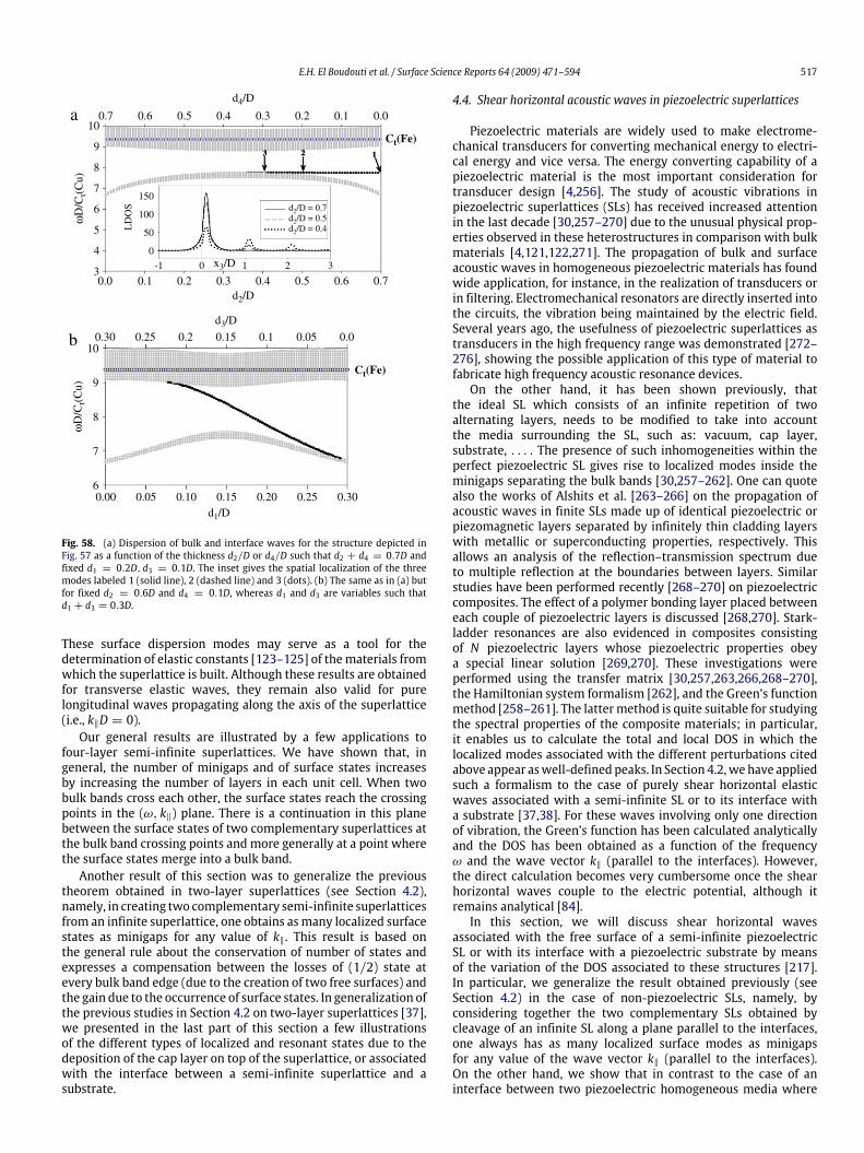
E.H. El Boudouti et al. / Surface Science Reports 64 (2009) 471–594 517

3 2 1

0.6 0.5 0.4 0.3 0.2 0.1

d4/D

0.7 0.0

4

5

6

7

8

9

3

10

ωD

/Ct(C

u)ω

D/C

t(Cu)

0

50

100

150

LD

OS

x3/D-1 0 1 2 3

0.10.0 0.2 0.3 0.4 0.5 0.6d2/D

d1/D

0.25 0.2 0.15 0.050.1

0.7

d2/D = 0.7d2/D = 0.5d2/D = 0.4

6

7

8

9

10

0.00 0.05 0.10 0.15 0.20 0.25 0.30

Ct(Fe)

Ct(Fe)

d3/D

0.30 0.0

a

b

Fig. 58. (a) Dispersion of bulk and interface waves for the structure depicted inFig. 57 as a function of the thickness d2/D or d4/D such that d2 + d4 = 0.7D andfixed d1 = 0.2D, d3 = 0.1D. The inset gives the spatial localization of the threemodes labeled 1 (solid line), 2 (dashed line) and 3 (dots). (b) The same as in (a) butfor fixed d2 = 0.6D and d4 = 0.1D, whereas d1 and d3 are variables such thatd1 + d3 = 0.3D.

These surface dispersion modes may serve as a tool for thedetermination of elastic constants [123–125] of thematerials fromwhich the superlattice is built. Although these results are obtainedfor transverse elastic waves, they remain also valid for purelongitudinal waves propagating along the axis of the superlattice(i.e., k‖D = 0).Our general results are illustrated by a few applications to

four-layer semi-infinite superlattices. We have shown that, ingeneral, the number of minigaps and of surface states increasesby increasing the number of layers in each unit cell. When twobulk bands cross each other, the surface states reach the crossingpoints in the (ω, k‖) plane. There is a continuation in this planebetween the surface states of two complementary superlattices atthe bulk band crossing points and more generally at a point wherethe surface states merge into a bulk band.Another result of this section was to generalize the previous

theorem obtained in two-layer superlattices (see Section 4.2),namely, in creating two complementary semi-infinite superlatticesfrom an infinite superlattice, one obtains asmany localized surfacestates as minigaps for any value of k‖. This result is based onthe general rule about the conservation of number of states andexpresses a compensation between the losses of (1/2) state atevery bulk band edge (due to the creation of two free surfaces) andthe gain due to the occurrence of surface states. In generalization ofthe previous studies in Section 4.2 on two-layer superlattices [37],we presented in the last part of this section a few illustrationsof the different types of localized and resonant states due to thedeposition of the cap layer on top of the superlattice, or associatedwith the interface between a semi-infinite superlattice and asubstrate.

4.4. Shear horizontal acoustic waves in piezoelectric superlattices

Piezoelectric materials are widely used to make electrome-chanical transducers for converting mechanical energy to electri-cal energy and vice versa. The energy converting capability of apiezoelectric material is the most important consideration fortransducer design [4,256]. The study of acoustic vibrations inpiezoelectric superlattices (SLs) has received increased attentionin the last decade [30,257–270] due to the unusual physical prop-erties observed in these heterostructures in comparison with bulkmaterials [4,121,122,271]. The propagation of bulk and surfaceacoustic waves in homogeneous piezoelectric materials has foundwide application, for instance, in the realization of transducers orin filtering. Electromechanical resonators are directly inserted intothe circuits, the vibration being maintained by the electric field.Several years ago, the usefulness of piezoelectric superlattices astransducers in the high frequency range was demonstrated [272–276], showing the possible application of this type of material tofabricate high frequency acoustic resonance devices.On the other hand, it has been shown previously, that

the ideal SL which consists of an infinite repetition of twoalternating layers, needs to be modified to take into accountthe media surrounding the SL, such as: vacuum, cap layer,substrate, . . . . The presence of such inhomogeneities within theperfect piezoelectric SL gives rise to localized modes inside theminigaps separating the bulk bands [30,257–262]. One can quotealso the works of Alshits et al. [263–266] on the propagation ofacoustic waves in finite SLs made up of identical piezoelectric orpiezomagnetic layers separated by infinitely thin cladding layerswith metallic or superconducting properties, respectively. Thisallows an analysis of the reflection–transmission spectrum dueto multiple reflection at the boundaries between layers. Similarstudies have been performed recently [268–270] on piezoelectriccomposites. The effect of a polymer bonding layer placed betweeneach couple of piezoelectric layers is discussed [268,270]. Stark-ladder resonances are also evidenced in composites consistingof N piezoelectric layers whose piezoelectric properties obeya special linear solution [269,270]. These investigations wereperformed using the transfer matrix [30,257,263,266,268–270],the Hamiltonian system formalism [262], and the Green’s functionmethod [258–261]. The lattermethod is quite suitable for studyingthe spectral properties of the composite materials; in particular,it enables us to calculate the total and local DOS in which thelocalized modes associated with the different perturbations citedabove appear aswell-defined peaks. In Section 4.2,wehave appliedsuch a formalism to the case of purely shear horizontal elasticwaves associated with a semi-infinite SL or to its interface witha substrate [37,38]. For these waves involving only one directionof vibration, the Green’s function has been calculated analyticallyand the DOS has been obtained as a function of the frequencyω and the wave vector k‖ (parallel to the interfaces). However,the direct calculation becomes very cumbersome once the shearhorizontal waves couple to the electric potential, although itremains analytical [84].In this section, we will discuss shear horizontal waves

associated with the free surface of a semi-infinite piezoelectricSL or with its interface with a piezoelectric substrate by meansof the variation of the DOS associated to these structures [217].In particular, we generalize the result obtained previously (seeSection 4.2) in the case of non-piezoelectric SLs, namely, byconsidering together the two complementary SLs obtained bycleavage of an infinite SL along a plane parallel to the interfaces,one always has as many localized surface modes as minigapsfor any value of the wave vector k‖ (parallel to the interfaces).On the other hand, we show that in contrast to the case of aninterface between two piezoelectric homogeneous media where

518 E.H. El Boudouti et al. / Surface Science Reports 64 (2009) 471–594

Table 5Elastic, piezoelectric and dielectric parameters of the materials CdS, ZnO and BeO.

Materials C44 (1010N/m2) ρ (kg/m3) e15 (C/m) ε11 (10−11F/m)

CdS 1.49 4824 −0.21 7.99ZnO 4.25 5876 −0.59 7.38BeO 14.77 3009 – 5.99

interface modes are rather rare to find [271], localized modes withhigh degree of localization may exist at the interface between apiezoelectric SL and a piezoelectric substrate.After a brief presentation of the model and the method

of calculation in Section 4.4.1, we give in Section 4.4.2 somenumerical results for a CdS/ZnO SL with a free surface or in contactwith a BeO substrate.

4.4.1. Model and method of calculationThe interface SL/substrate under consideration here is com-

posed of a semi-infinite SL formed out of a semi-infinite repetitionof two different stabs (i = 1, 2) within the unit cell n, the SL be-ing in contact with homogeneous substrate i = s. The interfaceSL/vacuum can be obtained as a particular case of the SL/substratesystem by replacing the substrate with a vacuum. All the interfacesare taken to be parallel to the (x2, x3) plane of a reference orthonor-mal basis set. A space position along the x1 axis (perpendicular tothe interfaces) in medium i belonging to the unit cell n is indi-cated by (n, i, x1), where −di/2 ≤ x1 ≤ di/2, while x1 ≥ 0 in thesubstrate. The layers and the substrate are characterized by theirelastic, dielectric, and piezoelectric constants and by their massdensities. The thicknesses d1 and d2 of the layers are assumedto be equal without loss of generality, the period of the SL beingD = d1 + d2.The media forming the layers of the SL and the substrate are

assumed to be of hexagonal symmetry belonging to the 6 mmclass with their c axis along the x3 axis and the wave vector k‖,parallel to the interfaces, is along x2. In this particular geometry, theshear horizontal vibrations (parallel to x3) are accompanied by anelectric potential, while the sagittal vibrations [polarized in the (x1,x2) plane] are decoupled from the latter [30,257] (see Section 2.5).Surface and interface elastic waves of sagittal polarization in semi-infinite SLs will be the subject of Section 7.In our case, the composite material is composed of a SL built

out of alternating slabs of materials i (i = 1, 2) with thickness di, incontactwith a substrate ofmaterial i = s. The details of the analysisare the same as for shear horizontal waves (Section 4.2), but withmore complicated calculations [84]. Let us emphasize that, in thegeometry of the SL/substrate structure, the elements of the Green’sfunction take the form gαβ(ω2, k‖|n, i, x1; n′, i′, x′1), where ω is thefrequency of the acoustic wave, k‖ the wave vector parallel to theinterfaces, and α, β denote the components of a 4 × 4 matrix(α, β = 1, 2, 3, 4) representing the coupling between the acousticwaves (α, β = 1, 2, 3) and the electric field (α, β = 4). For thesake of simplicity, we shall omit in the following the parametersω2and k‖, and we note as g(n, i, x1; n′, i′, x′1) the 4× 4 matrix whoseelements are gαβ(n, i, x1; n′, i′, x′1) (α, β = 1, 2, 3, 4).By assuming that k‖ is along the x2 direction, the component

gαβ (α, β = 1, 2) of the Green function decouple [84] from thecomponents gαβ (α, β = 3, 4) (i.e., g13 = g14 = g23 = g24 =g31 = g32 = g41 = g42 = 0); the former corresponds tovibrations polarized in the sagittal plane, whereas the latter areassociated with shear horizontal vibrations accompanied by theelectric potential.For the shear horizontal vibrations coupled to the electric

potential studied here, the knowledge of the Green’s function g inthe SL/substrate system enables us to calculate the local density of

states, for a given value of the wave vector k‖

nα(ω2, k‖; n, i, x1) = −1πImgαα(ω2, k‖|n, i, x1; n, i, x1),

(α = 3, 4), (212)

or

nα(ω, k‖; n, i, x1) = −2ωπImgαα(ω2, k‖|n, i, x1; n, i, x1),

(α = 3, 4). (213)

The total DOS can be obtained either by integrating directly overthe space variable x1 or by using a method that involves only theinterface matrix elements of the Green’s functions. In the lattermethod, one can calculate the difference between the total DOS oftwo complementary semi-infinite superlattices (terminating withlayers i = 1 and i = 2) in contact with two substrates and thereference system (i.e., an infinite SL, and an infinite substrate), ifwe only know [115] the elements of the Green’s function at thesurface Ms of the two complementary semi-infinite SLs and of thetwo substrates. By calling d1(Ms,Ms), d2(Ms,Ms), and gs(Ms,Ms)these Green’s functions matrix elements, one can write

1n(ω) = −1πImddωln det

[d1(Ms,Ms)+ gs(Ms,Ms)][d2(Ms,Ms)+ gs(Ms,Ms)]2[d1(Ms,Ms)+ d2(Ms,Ms)]gs(Ms,Ms)

. (214)

As mentioned above, the interface SL/vacuum is obtained fromEq. (214) by replacing the Green’s function gs of the substrateby the Green’s function gv of vacuum. We shall distinguish also,as in usual piezoelectric materials [121,122,271], two types ofsurface boundary conditions depending on whether the surface ismetallized (short circuit) or not (open circuit).

4.4.2. Discussion and resultsIn the following, we shall give some specific illustrations of

these results. In these examples, the SL is made of CdS and ZnOwith a free surface or in contact with a BeO substrate, havinga high transverse velocity. The characteristic parameters of thematerials used here are listed in Table 5. For given ω and k‖, thewave vectors along the axis x1 of the SL, which can be deducedfrom the bulk dispersion, are called k1. In the case of piezoelectricwaves involving two components of the displacement vector andthe electric potential, there are two pairs of values of k1 withgiven k‖ and ω, which can be written as [30,257] ±(K ′1 + iL

′

1) and±(K ′2+iL

′

2). Now an elasticwavewith a frequencyωwill propagatein the SL if L′1 = 0 or L

′

2 = 0, while it is attenuated if both L′

1 andL′2 are different from zero. Each pair of values of k1 (the first forinstance) can take four different forms [217,257](i) pure real (L′1 = 0)(ii) pure imaginary (K ′1 = 0)(iii) complex but with (K ′1 = ±π/D)(iv) complex with (K ′1 6= π/D).

(215)

However, in case (iv) the two pairs of k1 necessarily become

K ′ + iL, −(K ′ + iL′), (K ′ − iL′), −(K ′ − iL′). (216)

Fig. 59(a) and (b) give two examples of the complex bandstructure (thin solid curves) in a CdS/ZnO SL showing combinationsof the above-mentioned cases for small and large values of k‖D,namely, k‖D = 0.2 (Fig. 59(a)) and k‖D = 4 (Fig. 59(b)). Onecan see the dispersion of the displacement component in Fig. 59(a)and (b) giving rise to direct gaps at the center and at the edgeof the reduced Brillouin zone, while the potential component isdispersionless and appears as a vertical line at the imaginary part

E.H. El Boudouti et al. / Surface Science Reports 64 (2009) 471–594 519

Re(k1D)-0

Im(k1D) Im(k1D)

ωL2

ωL3

Im(k1D) Re(k1D) Im(k1D)

ωL5

ωL6

ωL4

π

ωL1 ,ωL'

1

2

4

6

8

0

10a

b

2

4

6

8

π040

10

Fig. 59. Complex band structure (ω vs. complex k1) in a CdS/ZnO SLwith d1 = d2 =D/2 and k‖D = 0.2(a), 4(b). Thin solid curves are k1 real (middle panel of the figure).Dashed curves are k1 imaginary (left panel). Dotted curves are the imaginary part ofk1when its real part is equal toπ/D (right panel). Heavy solid curves in (a) representthe complex band structure but neglecting the piezoelectricity. The horizontally full(dashed) arrows give the frequencies of the surface modes inside the minigaps ofthe SL when the layer at the surface of the SL is CdS (ZnO).

of k1 such that Im(k1D) = k‖D. However, for small values of k‖D,the potential curvemay interactwith the vibrational one leading tothe lifting of the degeneracy at the crossing points as is the case inthe second gap of Fig. 59(a). As a matter of comparison, we havealso plotted in Fig. 59(a) the complex band structure associatedwith pure transverse elastic waves (heavy solid curves), i.e., whenthe piezoelectric constant e15 is taken equal to zero. The dispersioncurves are slightly shifted toward lower frequencies at small valuesof k‖D (Fig. 59(a)); however, the shifting disappears for large valuesof k‖D (Fig. 59(b)), wherewe have not plotted the curves associatedwith the pure elastic waves.Now, the creation of the free surface of the SL gives rise to

localized modes inside the minigaps of the SL; their frequencies,indicated by arrows in Fig. 59(a) and (b), are very dependentupon the composition of the layer that terminates the SL. The full(dashed) arrows in Fig. 59 represent the surface modes when aCdS (ZnO) film is at the surface of the SL; moreover if the surfaceis metallized, the surface modes change slightly but cannot bedistinguished from the preceding ones at the scale of the figure. Letusmention that in the small range of k‖D (Fig. 59(a)), there are twosurface modes (labeled ωL1 and ω′L1) lying below the bulk bands.Thesemodesmay exist for both CdS and ZnO terminations of the SLdepending on whether the surface is metallized or not (see detailsbelow).The surface modes are poles of the Green’s function and

therefore appear as δ peaks in the DOS as illustrated in Fig. 60. Inthis figure, we have presented, for k‖D = 0.2, the variation of thetotal DOS when two complementary semi-infinite SLs are createdby the cleavage of an infinite SL in such a way that one obtains

-15

0

15

30

-15

0

15

0

15

30

2 4 6 8ωD/Ct(CdS)

0 10

0.27 0.28

-20

0

20

0.27 0.28-20

0

20

a

b

c

Var

iatio

n of

the

tota

l den

sity

of

stat

es (

k //D

= 0

.2)

30

-15

Fig. 60. Variation of the DOS [in units of D/Ct (CdS)] when creating twocomplementary semi-infinite SLs from the infinite SL, for k‖D = 0.2. Panels (a), (b),and (c) correspond, respectively, to the case when the films at the surfaces of theSLs are metallized, nonmetallized, and pure elastic. L1 , L2 , and L3 represent surfacemodeswhenCdS is at the surface of the SL. L1 corresponds to the surfacemodewhenZnO is at the surface; it appears when the surface is metallized. Bi and Ti correspondto δ peaks ofweight−(1/2)which appear, respectively, at the bottomand the top ofeach bulk band. In the low frequency range, the surfacemodes are located very closeto the limits of the bulk bands and therefore mask the band-edge antiresonances.Therefore, the low frequency region is enlarged in the insets of panels (a) and (b).

one SL with a full CdS layer at the surface and its complementaryone with a full ZnO layer at the surface. For the sake of clarityand despite the analytic nature of our calculation, the δ peaksin the DOS are broadened by adding a small imaginary part tothe frequency ω (ω → ω + iε). Fig. 60(a)–(c), are respectively,associated with the cases where the surface of the SL is metallized(Fig. 60(a)), nonmetallized (Fig. 60(b)), and pure elastic (Fig. 60(c)).Li are δ peaks associated with surface localized modes, whereas Biand Ti refer to δ peaks of weight (−1/2) situated at the bottom andthe top of the minibands [37,38,65,189,217] given by k1D = 0 andk1D = π . One can see that the positions of the surface modes arealmost the same in the first two cases. However, there exists two(respectively, one) surface modes below the bulk bands in the caseof metallized (respectively, nonmetallized) surfaces (see the insetsin Fig. 60(a) and (b)); thesemodes, labeled L1 and L′1, are associatedwith CdS and ZnO terminations of the SL, respectively. Fig. 60(c),corresponding to the pure elastic case, shows a shift of the bulkbands and surface modes toward lower frequencies.In Fig. 61we represent the so-called projected band structure of

the bulk bands and surfacemodes, namely,ω versus k‖. The shadedareas represent bulk bands separated by minigaps. Inside thesegaps,wehave represented surfacemodes corresponding to the twocomplementary semi-infinite SLs with CdS termination (dashedcurves) and ZnO termination (dotted curves). As mentioned above,the frequencies of the surface modes are almost the same inthe case of metallized and nonmetallized surfaces. A particularsituation occurs in the long wavelength limit (see the inset ofFig. 61): when the SL terminateswith a CdS layer, the surfacemodebelow the bulk band exists whether the surface is metallized ornonmetallized; on the other hand, for a ZnO termination of the SL,the surface mode exists over a short range of the dimensionlesswave vector k‖D only if the surface is metallized. These results are

520 E.H. El Boudouti et al. / Surface Science Reports 64 (2009) 471–594

1.365

1.370

1.375

a

bc

d

k//D

2

4

6

8

0

10

ωD

/Ct(C

dS)

1 2 3 4 5 6K//D

0 7

ω/k

//C

t(CdS

)

0.0 0.2 0.4

Fig. 61. Bulk band and surface wave dispersion for a CdS/ZnO SL with d1 = d2 .The curves give ωD/Ct (CdS) as a function of k‖D, where ω is the frequency, k‖ thepropagation vector parallel to the interfaces. The shaded areas are the bulk bands.The dashed (dotted) curves represent the surfacemodes when a nonmetallized CdS(ZnO) layer is at the surface. For a metallized surface, the surface modes are slightlydifferent but cannot be distinguished from the preceding ones at the scale of thefigure. The inset shows, in units of Ct (CdS), the phase velocities of the bottom of thebulk bands (a) and of the surface waves below it [(b), (c) and (d)] over a small rangeof k‖D. The curves (b), (d) and (c), respectively, correspond to the casewhen the filmat the surface is CdS nonmetallized, CdS metallized, and ZnO metallized.

in accordance with those presented in the insets of Fig. 60(a) and(b). From the results given in Fig. 61, one should notice that apartfrom the long wavelength region, there are as many surface statesasminigaps for each value of thewave vector k‖. Each surfacemodeis associated with either one or the other of the complementarysemi-infinite SLs. This result is obtained numerically based on thefollowing two steps: (i) the variation of the DOSwhen creating twocomplementary semi-infinite SLs from an infinite one is equal tozero for any frequency ω falling inside a SL bulk band (ii) there isa loss of 1/2 state at every edge of a bulk band (see Fig. Fig. 60),i.e., a loss of one state per miniband. Therefore, to ensure theconservation of the total number of states, it is necessary to have asmany localizedmodes asminigaps in the band structure. The aboverule generalizes the result presented previously in Section 4.2 fornon-piezoelectric SLs.To illustrate the spatial localization of the surface modes, we

have sketched in Fig. 62 the LDOS associated with the modeslabeled ωL2, ωL3 and ωL6 in Fig. 59. The LDOS is presented as afunction of the space position x1, at k‖D = 0.2 and k‖D = 4. Boththe vibrational and the electric components of the DOS are givenfor two types of electric boundary conditions, namely a metallized(dotted curves) and a nonmetallized (solid lines) surface. Thedisplacement field is not greatly affected by the electric boundarycondition, while the electric field shows different behaviors for ametallized or a nonmetallized surface. However, these differencesbecome less important when going to higher values of k‖D. Forboth vibrational and electric components of the surface wave,one should notice an exponential decrease of their envelopeswhen penetrating deep into the interior of the SL; this attenuationis accompanied by an increasing number of oscillations in eachperiod of the SL as far as one is dealing with higher frequencymodes.In the following we show the possibility of the existence

of piezoelectric waves localized at the interface between apiezoelectric SL and a piezoelectric substrate. The results will beillustrated for the sameCdS/ZnO SL in contactwith a BeO substrate.

V ide

vide

SR

SR

com posante vibrationnelle

P otential électrique

ω L2, k//D = 0,2

SR V ide

ω L3, k//D = 0,2com posan te vib ra tionnelle

P oten tia l électrique

P otential électrique

com posante vibrationnelle ω L6, k//D = 4

Vacuum

ωL2, k//D =0.2

Superlattice

Vibrational component

Superlattice

Vibrational component

Superlattice

Vibrational component

Vacuum

ωL3, k//D =0.2

Potential component

Potential component

Potential component

Vacuum

a

b

c

d

e

f

0

10

20

0

400

0

30

0

60

120

0

10

20

0

20

40

LD

OS

(u.a

.) L

DO

S (u

.a.)

LD

OS

(u.a

.)-8 -6 -4 -2 0 2 4

x1/D-10 6

-8 -6 -4 -2 0 2 4-10 6

-8 -6 -4 -2 0 2 4-10 6

Fig. 62. Spatial representation of the local DOS for the modes labeled ωL2 [(a), (b)],ωL3 [(c), (d)], and ωL6 [(e), (f)] in Fig. 59. The curves in (a), (c), and (e) [respectively(b), (d), and (f)] correspond to the vibrational (respectively potential) componentsof the local DOS. The full (dotted) curves correspond to the case when the film atthe surface is CdS metallized (CdS nonmetallized).

The velocity of the transverse speed of sound in the BeO substrateis rather high, which enables us to give a qualitative description ofthe different localizedmodes inducedby the SL/substrate interface,inside the minigaps and below the substrate bulk band.Fig. 63 gives the interface modes for both the complementary

SLs in which the substrate is either in contact with a ZnO layer(triangles) or with a CdS layer (dotted curves). One can clearlynotice that the frequencies of the interface modes are verysensitive to the type of layer which is at the surface of the SL.Let us mention that, to our knowledge, the piezoelectric constante15 of the BeO substrate is not available in the literature [4].However, we have determined that physically acceptable values ofthe substrate piezoelectric constant e15 (Ref. [4]) do not affect thefrequencies of the interface modes. As in the case of a free surface,one can distinguish two types of boundary conditions (metallizedor nonmetallized interface). The interfacemodes in Fig. 63 are veryclose for both boundary conditions and cannot be distinguished atthe scale of Fig. 63.However, the frequencies of the interfacemodesslightly shift toward lower frequencies when the piezoelectriccoupling is not taken into account as it can be seen in Fig. 64. Inthis figure we have plotted, at k‖D = 5, the variation of the totalDOS for the metallized (Fig. 64(a)) nonmetallized (Fig. 64(b)), andpure elastic (Fig. 64(c)) cases. The latter case is obtained by takingthe piezoelectric constants equal to zero in the media constitutingthe SL and the substrate. The interface modes labeled L1 and L2 inFig. 64 are associated with CdS and ZnO terminations of the SL,respectively.The spatial localization of the interface mode L1 is illustrated

in Fig. 65 where we have presented both the vibrational andelectric components of the DOS. The vibrational component is notaffected by the electric boundary condition, while the behavior ofthe electric component is slightly different in the vicinity of theinterface for both types of boundary conditions. Let us mentionfinally that the interface modes between two homogeneous

E.H. El Boudouti et al. / Surface Science Reports 64 (2009) 471–594 521

0

2

4

6

8

10

1 2 3 4 5 6K//D

0 7

Fig. 63. Interface localized modes associated with a CdS/ZnO SL in contact with aBeO substrate. The shaded areas are the bulk bands of the SL. The heavy straightline indicates the bottom of the substrate bulk band. When the SL terminates witha ZnO (respectively CdS) layer, the localizedmodes are represented by the triangles(dotted curves).

0

10

20

30

40

-20

-10

L2L 1

T 1 T 2

B1

B2

B2

B3

B2

L1

L1

L2

L 2

T 1

T1

T2

T 2

B3

B3

B1

B1

0102030

-40-30-20-10

-20

-10

0

10

20

30

4 5 6 7 8 9 10 11

a

b

c

-30

40

Var

iatio

n of

the

tota

l den

sity

of

stat

es (

k //D

= 5

)

Fig. 64. Variation of the DOS at k‖D = 5, for the two complementary SLs of Fig. 63created from the infinite SL and the infinite substrate. L1 and L2 represent interfacemodes associated with CdS and ZnO terminations of the SL respectively, whereas Biand Ti have the same meaning as in Fig. 60.

piezoelectric media (the so-called Maerfeld–Tournois modes) arerather rare to find [271]. In our case, for instance, the interfaceBeO/CdS and BeO/ ZnO do not support interface modes. Therefore,the SL/ substrate interface presents a useful structure for theexistence of interface modes in comparison with the interfacebetween two homogeneous media.

k//D = 5, ω L1

x 2.10 5

SR

SR

Potentia l électrique

Com posnate virationnelle

Substrat

Substrat

Superlattice

Vibrational component

k//D = 5, ωL1

Superlattice

Potential component

Substrate

Substrate

LD

OS

(u.a

.)L

DO

S (u

.a.)

0

10

20

30

40

0

10

20

30

40

-4 -2 0-6 2

-4 -2 0-6 2

x1/D

a

b

Fig. 65. Same as in Fig. 62, but for the interface mode labeled L1 in Fig. 64.

Finally, let us mention that from the above results one canstudy also surface acoustic waves in piezoelectric/metal SLs bytaking the piezoelectric constant e15 in one layer equal to zero. Thiscase has been studied recently by Chen et al. [277] and analyticalexpressions have been deduced for surface waves in semi-infiniteSLs ended with a piezoelectric layer at the surface. The free surfaceof the SL can be either metallized or nonmetallized. From thesetwo boundary conditions, one can define the electromechanicalcoupling coefficient as κ = (v0 − vs)/vs, here v0 and vs denotethe phase velocity of the surface waves with open (nonmetallized)and short (metallized) circuit surface respectively. Fig. 66(a) givesthe first band structure (the phase velocity versus ωD) of theinfinite PZT4/Fe SL (gray areas), whereas the surface branchesfor open and short circuit surfaces are sketched by open andfilled circles respectively. The thickness of the layers in the SL aresupposed equal. As it was shown by Chen et al. [277], only thesurface branches lying below the bulk bands give rise to significantsurface electromechanical coupling and can be excited effectivelyby interdigital transducers (IDT). Therefore, we limited ourselvesto these branches; the corresponding electromechanical couplingis illustrated in Fig. 66(b). These results are similar to those foundby Chen et al. [277] using another method of calculation basedon the boundary conditions at the different interfaces. WhenωD is very large, the phase velocity of the first surface modeof the SL with short and open circuit surface tend to Cs and C0respectively (see the horizontal dashed lines in Fig. 66(a)). Cs andC0 are, respectively, the phase velocities of the surface wave inthe semi-infinite uniform PZT4 crystal with short and open circuitsurface, their expressions are given by Eqs. (74) and (75). Theseresults are predicted, indeed when ωD is large, the surface wavesbecome strongly localized near to the surface and therefore arenot affected by the layers inside the SL. At very low frequencycase, the κ of the surface modes leads to zero which implies thatthe surface modes with very low frequency cannot be excitedeffectively by IDT’s. When the frequency is not very low, the κ islarger than of the surface modes of a semi-infinite uniform crystalκPZT4 = (C0 − Cs)/Cs = 6.34% for PZT4. This is a prominentadvantage of the piezoelectric/metal SL. It is worth mentioningthat electromechanical coupling for surface acoustic waves inKNbO3 [278], AlN [279], GaN [280] and ceramic thin plate [281] has

522 E.H. El Boudouti et al. / Surface Science Reports 64 (2009) 471–594

2.5

3.0

3.5

0.0634

2.3154

2.4624

10 20 30 40 50ω.D

0 60

10 20 30 40 50

2.0

4.0

Phas

e ve

loci

ty (

km/s

)

0.02

0.04

0.06

0.08

0.10

0.12

κ(%

)

0.00

0.14

ω.D (GHz μm)

0 60

a

b

Fig. 66. (a) The band structure and dispersion curves of the lowest two shearhorizontal surface waves of the semi-infinite PZT4/Fe superlattice. The open andfilled circles denote dispersion curves of the system with open and short circuitsurfaces, respectively. The gray areas represent the bulk bands. (b) Variation of theelectromechanical coupling κ as function ofωD for the lowest two surface waves ofthe semi-infinite PZT4/Fe superlattices (Reproduced after Ref. [277]).

beenmeasured experimentally. These studies enable to deduce theelastic, dielectric and piezoelectric parameters of these materials.In summary, the main points presented in this section, apart

from the analytical derivation of the Green’s function and thecorresponding DOS [84] are:(i) The generalization to piezoelectric SLs of the previous

theorem (Section 4.2) about the existence and number of surfacestates. More precisely, we have shown that, apart from the longwavelength limit, one obtains as many localized surface statesas minigaps for any value of the wave vector k‖. This result isbased on the general rule about the conservation of the totalnumber of states and expresses a compensation between the lossesof (1/2) state at every bulk band edge (due to the creation ofthe free surfaces) and the gain due to the occurrence of surfacestates. The imaginary part of the k1 wave vectors obtained in thecomplex band structure calculation, gives the attenuation of thesurface waves in a semi-infinite SL. Although the frequencies ofthe localizedmodes associated withmetallized and nonmetallizedsurfaces are almost the same, their spatial localizationmay exhibitnoticeable differences, in particular, for small values of k‖D.(ii) The derivation of the dispersion curves and the localization

properties of the interface modes at the SL/ substrate boundary,with specific application to the CdS/ZnO piezoelectric SL in contactwith a BeO piezoelectric substrate. The dispersion curves of theinterface modes are very dependent upon the nature of the layerin the SL which is in contact with the substrate.(iii) The interface between a homogeneous and a periodic

layered media appears as a fruitful structure for the existenceof interface modes in comparison with the interface betweentwo homogeneous media where the existence of localizedmodes (called Maerfeld–Tournois modes) becomes rather hard to

find [271]. This opens, at least in principle, some newopportunitiesfor guided waves and filtering which is of potential value inthe interface characterization of the multilayer/homogeneousstructure.(iv) We have reproduced the recent results of Chen et al. [277]

on surface acoustic waves in piezoelectric/metal SLs. It was shownthat at some frequency ranges, the electromechanical coupling atthe surface of such SLsmay exhibit large values in comparisonwiththe one associated to a semi-infinite homogeneous piezoelectricmedium. Therefore this study may be of interest in the field of thedynamics of piezoelectric layered structures and in particular forthose applications which deal with the propagation of surface andinterface acoustic waves in the high frequency range.

5. Shear horizontal acoustic waves in finite superlattices

5.1. Introduction

In Section 4, we have considered SLs with infinite and semi-infinite extension to study the bulk and surface acoustic waves.However, from the practical point of view, the SLs are constitutedof a finite number of cells deposited on a substrate. Often, a bufferlayer is first grown before the deposition of the SL in order torelieve strains and defects of the underlying substrate surfacecaused by damage due to polishing or other imperfections. Inother experiments, a defect layer is introduced at the surface ofthe SL (as a cap layer) or inside the SL (as a cavity layer) forsome applications as selective filters and efficient waveguides.Therefore, it is interesting to take into account the finite size effectof the SL as well as the media surrounding the perfect SL.Experimentally, very small peaks [75–77] have been observed

in the folded longitudinal acoustic phonons of Si/Ge1−xSix andGaAs–AlAs SLs by high resolution Raman measurements andinterpreted as confined phonons of the whole finite SL. In addition,surface acoustic waves induced by a cap layer in the minigaps ofa SL have been shown in metallic [45,59] and semiconductor [58,60–63,206,207,218,282] SLs by using picosecond ultrasonic studyand Raman scattering experiments, respectively. The effect ofa cavity layer inserted in the middle [72–74,208,209] or atdifferent places [71] within the SL has been also well studiedby Raman scattering. From the theoretical point of view, Ramanscattering [72–74,283,284], densities of states [57,129] andreflection–transmission coefficients [34,35,43,44,56,78–81] havebeen performed to understand the propagation and localizationproperties of different confined modes within the finite size SL.The aim of the present section is to investigate localized

and resonant modes of shear horizontal polarization in finitesize SLs, in particular we shall emphasize the effect of thedifferent inhomogeneities cited above on acoustic waves in suchSLs. Section 5.2 presents the analytical results of dispersionrelations, densities of states as well as transmission and reflectioncoefficients for a finite SL inserted between two substrates and inpresence of buffer and cap layers (see Fig. 67). Sections 5.3–5.5will be devoted to numerical applications concerning the effectsof respectively the cap layer, buffer layer and cavity layer insertedwithin the SL. Section 5.6 gives some experimental results relatedto this work.

5.2. Density of states and reflection and transmission coefficients

In the present study we are dealing with a general structure,often used experimentally [285], that consists of a substrate–bufferlayer (b) finite SL–cap-layer (c) semi-infinite medium (v) (seeFig. 67). The finite SL has a total N unit cells, where a unit cell iscomposed of two different slabs denoted by the unit-cell index n.

E.H. El Boudouti et al. / Surface Science Reports 64 (2009) 471–594 523

x3

da d2 d1 d

(v)

x3

c

Cell 0 Cell N

x3 = 0 x3 = da+db+ND

BufferLayer

Cap LayerSubstrate

(s)

Substrate2 1 2 1

(a) (c)

Fig. 67. Schematic representation of a finite SL (i = 1, 2) with a buffer layer (n = 0, i = b) and a cap layer (n = N , i = c) and sandwiched between two substrates s and v.db , dc , d1 , and d2 , respectively, are the thicknesses of the buffer layer, the cap layer and of the two different slabs out of which the unit cell of the superlattice is built. D is theperiod of the SL.

Each of these slabs is characterized by its elastic constant C (i)44 , massdensity ρ(i) and thickness di (i = 1, 2) within the unit cell n.The repetition period is called D = d1 + d2. Similarly, the bufferlayer, the cap layer, the semi-infinite medium, and the substrateinvolve the parameters (C (b)44 , ρ

(b), db), (C(c)44 , ρ

(c), dc), (C(v)44 , ρ

(v)),and (C (s)44 , ρ

(s)), respectively. A space position along the x3 axis inmedium i belonging to the cell n is indicated by (n, i, x3), where−di/2 ≤ x3 ≤ di/2 (i = 1, 2).We limit ourselves to the simplest case of shear horizontal

vibrations where the field displacements u2(x3) are along the axisx2 and the wave vector k‖ (parallel to the interfaces) is directedalong the x1 axis. We consider then a SL built out of cubic crystalswith (001) interfaces and k‖ along the [100] direction. In this case,as it was shown in the previous sections, the transverse wavesare not coupled to the other waves polarized in the sagittal planewhich contains the normal to the interfaces and thewave vector k‖.Knowing the Green’s function given in the Appendix C, one

obtains for a given value of k‖ the local and total DOS for asubstrate–buffer layer (b) finite SL–cap-layer (c) semi-infinitemedium composite system (see Fig. 67).

5.2.1. The local density of statesThe local densities of states on the plane (n, i, x3) are given by

n(ω2, k‖; n, i, x3) = −ρ(i)

πImd+(ω2, k‖; n, i, x3; n, i, x3), (217)

where

d+(ω2) = limε→0d(ω2 + iε) (218)

and d(ω2) is the response function whose elements are given inthe Appendix C. Asmentioned before, the density of states can alsobe given as a function of ω, instead of ω2 using the well-knownrelation n(ω) = 2ωn(ω2).

5.2.2. The total density of statesThe total density of states for a given value of k‖ is obtained

by integrating over x3 and summing on n and i the local densityn(ω2, k‖; n, i, x3). More particularly, we are interested in thistotal density of states from which the substrate and semi-infinitemedium contribution have been subtracted. The expression of thevariation of the density of states when the buffer layer (b) and thecap layer (c) are in contact with materials 2 and 1, respectively, ofthe SL, can be written as the sum of six contributions,

n(ω2) = n1(ω2)+ n2(ω2)+ nb(ω2)

+ nc(ω2)+1ns(ω2)+1nv(ω2), (219)

where n1(ω2) and n2(ω2) are the contributions of layers 1 and 2,respectively, of the SL; nb(ω2) and nc(ω2) are the contributionsof buffer layer (b) and cap layer (c); and 1ns(ω2) and 1nv(ω2)come from the substrate and semi-infinite medium, respectively.Actually, in the latter terms we subtract the bulk contributions ofthe substrate and the semi-infinite medium.Then the six quantities in Eq. (219) are given by [286]

n1(ω2) = −ρ(1)

π

N∑n=1

Im∫+d12

−d12

d(n, 1, x3; n, 1, x3)dx3, (220)

n2(ω2) = −ρ(2)

π

N−1∑n=0

Im∫+d22

−d22

d(n, 2, x3; n, 2, x3)dx3, (221)

nb(ω2) = −ρ(b)

πIm∫+db2

−db2

d(0, b, x3; 0, b, x3)dx3, (222)

nc(ω2) = −ρ(c)

πIm∫+dc2

−dc2

d(N, c, x3;N, c, x3)dx3, (223)

1sn(ω2) = −ρ(s)

πIm∫ 0

−∞

[d(x3, x3)− Gs(x3, x3)]dx3, (224)

1vn(ω2) = −ρ(v)

πIm∫+∞

xc[d(x3, x3)− Gv(x3, x3)]dx3, (225)

where

xc = db + ND+ dc (226)

and N is the number of the finite SL cells.The quantities d, Gs and Gv are, respectively, the Green’s

functions of (1) the coupled substrate–buffer layer (b) finiteSL–cap-layer (c) semi-infinite medium system, (2) the infinitehomogeneous substrate (s), and (3) the infinite homogeneousmedium (v).Let us define the following quantities in each material i = 1, 2,

b, c , s, and v:

α2i = k2‖− ρ(i)

ω2

C (i)44, (227)

Ci = cosh(αidi), Si = sinh(αidi), (228)

Fi = αiC(i)44 , i = 1, 2, b, c, s, v, (229)

Rs =1+ FbSb/FsCb1+ FsSb/FbCb

, (230)

524 E.H. El Boudouti et al. / Surface Science Reports 64 (2009) 471–594

Rv =1+ FcSc/FvCc1+ FvSc/FcCc

, (231)

t = exp(ik3D), (232)where k3 is a wave vector along the axis of the SL and that satisfiesthe following dispersion relation in the infinite SL

cos(k3D) = C1C2 +12

(F1F2+F2F1

)S1S2. (233)

Therefore, with the help of the explicit expressions of theGreen’s functions given in Appendix C and Eqs. (220)–(225), weobtain

n1(ω2) = −ρ(1)

πIm

t(t2 − 1)1−

t1− t2N

t2 − 1(AB0t + A0B)

×

S1α1F1

[C2S1 +

12C1S2

(F1F2+F2F1

)]+S2d12F2

(1−

F 22F 21

)+ N1+

d1F1

[C2S1 +

12C1S2

×

(F1F2+F2F1

)]+S2S12α1F2

(1−

F 22F 21

), (234)

n2(ω2) = −ρ(2)

πIm

t(t2 − 1)1−

t1− t2N

t2 − 1(AB0 + A0Bt)

×

S2α2F2

[C1S2 +

12C2S1

(F1F2+F2F1

)]+S1d22F1

(1−

F 21F 22

)+ N1+

d2F2

[C1S2 +

12C2S1

×

(F1F2+F2F1

)]+S2S12α2F1

(1−

F 21F 22

), (235)

nb(ω2) = −ρ(b)

2πIm

1(1+ FsSb

FbCb

)1−

×

[Y(SbαbCb+ db

)+dbSbFbCb

(Z + YFs)

−ZFsF 2b

(SbαbCb− db

)]B0t − t2N

[Y(SbαbCb+ db

)+dbSbFbCb

(Z0 + YFs)−Z0FsF 2b

(SbαbCb− db

)]Bt, (236)

nc(ω2) = −ρ(c)

2πIm

1(1+ FvSc

FcCc

)1−

×

[X(ScαcCc+ dc

)−dcScFcCc

(K − XFv)

+KFvF 2c

(ScαcCc− dc

)]A0 − t2N

[X0

(ScαcCc+ dc

)−dcScFcCc

(K0 − X0Fv)+K0FvF 2c

(ScαcCc− dc

)]A, (237)

1sn(ω2) = −ρ(s)

πIm12αs

×

12Fs+

(Y + Z Sb

FbCb

)B0t − t2N

(Y + Z0

SbFbCb

)Bt(

1+ FsSbFbCb

)1−

, (238)

1vn(ω2) = −ρ(s)

πIm12αv

×

12Fv+

(−X + K Sc

FcCc

)A0 − t2N

(−X0 + K0 ScFcCc

)A(

1+ FvScFcCc

)1−

, (239)

where

1± = Yt(A0B0X0± t2N

ABX

), (240)

A0 = FsRsX0 + K0, A = FsRsX + K , (241)B0 = FvRvy− Z0, B = FvRvY − Z, (242)

X0 =S1F1t +S2F2, X =

S1F1+S2F2t, (243)

Z0 = C1C2 +F1F2S1S2 −

1t, Z = C1C2 +

F1F2S1S2 − t, (244)

K0 = C2 − C1t, K = C2t − C1, (245)

and

Y =C1S2F2+C2S1F1. (246)

The localized waves are given by the poles of the Green’sfunction, namely,

1− = 0. (247)

Our general expressions admit the following particular cases:(i) A finite SL sandwiched between two semi-infinite substrates

(i.e., db = d1 and dc = d2).(ii) A finite superlattice deposited on the substrate (s) with only

a cap layer (i.e., db = 0 and Fv = 0).(iii) A finite superlattice deposited on the substrate (s)with only

a buffer layer (i.e., dc = 0 and Fv = 0).We can also deduce the limiting case N →∞ that corresponds

to a semi-infinite SL with or without a cap layer or in contact witha substrate.

5.2.3. Reflection and transmission wavesConsider an incident wave in the substrate represented by

the plane wave exp(−αsx3) of unit amplitude, propagating fromx3 = −∞ toward the SL. The incident waves are scattered fromthe interfaces between dissimilar layers constituting the system.The square modulus of the wave function of the reflected waves(denoted R) in the substrate and the transmitted waves in semi-infinite medium v (denoted T ) are expressed, with the help of theinterface response theory [117], as

R =

∣∣∣∣∣∣(1− FsSb/FbCb1+ FsSb/FbCb

) Yt ( B0A0−X0 − t2N BA−X )1−

∣∣∣∣∣∣2

, (248)

T =FvFs

∣∣∣∣ 2YFstN(t2 − 1)CbCc(1+ FsSb/FbCb)(1+ FvSc/FcCc)1−

∣∣∣∣2 , (249)

respectively, where

A0− = −FsX0Rs− + K0, A− = −FsXRs− + K , (250)

and

Rs− =1− FbSb/FsCb1− FsSb/FbCb

. (251)

5.2.4. Relations between densities of states and phase timesBesides the information obtained from the imaginary part of the

system Green’s function (namely the DOS) giving the frequenciesof the different modes of the system [115], it is possible to obtainadditional information by using the transmission and reflectioncoefficients and the corresponding phase times [286]. A detailedaccount for nonmagnetic dielectric media and electromagneticwaves has been presented in [286], and we shall give here only the

E.H. El Boudouti et al. / Surface Science Reports 64 (2009) 471–594 525

transposition and the essential expressions for the understandingof the transverse elastic waves case.We shall consider in a general way a finite multilayer system

denoted by an index i = 2 sandwiched between two differenthomogeneous semi-infinite media having indices i = 1 and 3,respectively. In the case of the structure studied here, 1 = s,3 = v and 2 represents the finite SL with free surfaces. Wehave two interfaces bounding the multilayer system, we shall callthem l (left) and r (right) respectively. The system inverse Green’sfunction projected at the interfaces can be expressed as

g−1S =[g−1S (l, l) g−1S (l, r)g−1S (r, l) g−1S (r, r)

].

Let us then consider an incident wave in the semi-infinitemedium 1

u(x3) = exp(−iα1x3), (252)

where

αi =

√ρ(i)ω2

C (i)44− k2‖, (i = 1, 2, 3), (253)

and k‖ is the wave vector parallel to the interfaces.Following the expressions detailed in [286] it can be found that

the transmitted wave in medium 3 has the form

uT (x3) = −2iα1gS(l, r) exp(−iα3x3), (254)

whereas the reflected wave has the form

uR(x3) = −[1+ 2iα1gS(l, l)] exp(iα1x3). (255)

It is then clear that Eqs. (254) and (255) can be written as

uT (x3) = CT exp(−iα3x3), (256)uR(x3) = CR exp(iα1x3),

where CT and CR are the transmission and reflection amplitudesgiven by

CT = −2iα1g−1S (l, r) det|gS |, (257)

CR = −[1+ 2iα1g−1S (l, l) det|gS |].

From Eq. (257) it is possible to obtain the derivatives of thephases θT and θR of the transmission and reflection coefficientswith respect to the frequency. These derivatives are an indicationof the times needed by awave packet to complete the transmissionor reflection processes. These derivatives are usually called phasetimes [178–181] and are given by

τT =dθTdω

, (258)

τR =dθRdω.

From Eqs. (257) and (258) we obtain

τT =ddωarg det|gS |. (259)

The general expression for τR can also be obtained, but thereare two particular cases related to important physical situations,in which τR is related to τT . If the system is symmetric, α1 = α3and g−1S (l, l) = g

−1S (r, r), then we have

τR = τT =ddωarg det|gS |. (260)

If α3 becomes pure imaginary (total reflection), the transmis-sion vanishes and then we have

τR = 2ddωarg det|gS | = 2τT . (261)

Let us now recall that the difference of the DOS between thepresent composite system and a reference system formed out ofthe same volumes of the bulkmedia 1 and 3 and the finite medium2, can be obtained from (Eq. (85))

1′n(ω) = −1π

ddωArg det[

g2(M,M)[G1(0, 0)G3(0, 0)]1/2

g(M,M)

]. (262)

If one subtracts the discrete states of the finite medium 2, thenthe variation of the DOS between the composite system and thesame volumes of the bulkmedia 1 and 3 is given by Eq. (14), namely

1n(ω) =1π

ddωArg det [g(M,M)] . (263)

This relation is equivalent to the obtained one by using adirect calculation of the imaginary part of the trace of the Green’sfunction. Then for all frequencies, one obtains

τT = π1n(ω) (264)

which is equivalent to the result of Ref. [287]. Moreover,

τR = τT = π1n(ω) (265)

when the composite system is symmetric and

τR = 2π1n(ω) (266)

when one has total reflection.In what follows, we shall give numerical applications of the

analytical expressions given above for a SL with either a cap layer,a buffer layer or a cavity layer.

5.3. The effect of a cap layer

In the following we give a few illustrations related to a finiteGaAs–AlAs SL deposited on a Si substrate with or without a surfaceGaAs cap layer of different thickness, and for such a finite SLsandwiched between two Si substrates [129]. The thickness of thebuffer layer is reduced to zero, whereas the thicknesses d1 and d2of the layers in the SL are assumed to be equal, the period of the SLbeing D = d1 + d2 = 2d1.Fig. 68 gives the Love modes, as deduced from the peaks of

the DOS (see also Fig. 69), for a finite GaAs–AlAs SL deposited ona Si substrate, assuming that the outermost layers in the SL areboth of AlAs type. For the sake of clarity in Fig. 68, the SL onlycontains N = 5 layers of GaAs and N + 1 = 6 layers of AlAs.The branches situated below the substrate bulk band correspondto Love waves confined in the finite SL and decaying exponentiallyinto the substrate; they appear as true δ functions in the DOS(Fig. 69). The extension of these curves into the substrate bandrepresents resonant modes (also called leaky waves) associatedwith the deposition of the finite SL on top of the substrate. Thefine structure features observed [75–77] in the Ramanexperimentson Si–Si1−xGex and GaAs–AlAs SLs seems to be analogous to thesewaves, in the case of longitudinal vibrations and for k‖D = 0.The curves in Fig. 68 can also be classified according to their

oscillatory (full lines) or localized character in the SL; the latterare decaying either from the free surface (dash-dotted lines arealso labeled s as surface) or from the SL–substrate interface(dashed lines, also labeled i as interface). The number of branchescorresponding to oscillatory waves in the SL increases with thenumberN of periods (see also Fig. 71(a) forN = 20, to be discussedbelow), leading to the bulk bands of an infinite SL in the limit N →∞. On the other hand, the surface and interface localized modes,which are already distinguishable in Fig. 68, even for such a smallnumber of periods as N = 5, shift only slightly with N when going

526 E.H. El Boudouti et al. / Surface Science Reports 64 (2009) 471–594

0

1

2

3

4

5

6

7

8

9

10

11

1 2 3 4 5 6

Ct (

GaA

s)

0 7k // D

Fig. 68. Dispersion of Love waves associated with the deposition of a finiteGaAs–AlAs SL on a Si substrate. The SL contains N = 5 layer of GaAs and 6 layers ofAlAs. The heavy line corresponds to the sound line of the substrate, separating theLove modes confined within the SL from their extension as resonant waves into thesubstrate bulk band. When the dispersion curves belong to the SL minibands, theyare drawn as full lines; when falling inside the SLminigaps, they are represented bydash-dotted lines (labeled s) or dashed lines (labeled i) corresponding, respectively,to attenuated waves in SL either from the free surface or from the SL–substrateinterface. The label r refers to a resonance obtained from the mixing of a surfaceand an interface mode.

9

6

3

0

6

3

0

−33 4 5 6 7 8 9

DE

NSI

TY

OF

STA

TE

S

a

b

Fig. 69. DOS n(ω, k‖), in units of D/Ct (GaAs), depicted for (a) k‖D = 2.6 and (b)k‖D = 1.9 in Fig. 68. The Love modes localized within the SL give rise to δ peaksrepresented by arrows. The symbols s, r and i have the samemeanings as in Fig. 68.(The bulk contribution of the substrate to the DOS is subtracted. Bs is a δ function ofweight−1/4 appearing at the bottom of the substrate bulk band.)

2.0

1.5

1.0

0.5

0.0

2.5

-0.5

-0.2

0.0

0.2

0.4

0.6

DE

NSI

TY

OF

STA

TE

SD

EN

SIT

Y O

F ST

AT

ES

3.6 3.8 4.0 4.2 4.4

3.7 3.8 3.9 4.0 4.1 4.2

a

b

Fig. 70. (a) Spatial distribution of the resonance r depicted in Fig. 69(b): curves Aand B, respectively represent the local DOS integrated over the first and the thirdperiod of the SL from the free surface; curve C refers to the same quantity for theperiod in contact with the substrate, whereas curve D gives the modification of thesubstrate DOS after the deposition of the SL on its top. (b) Same as in (a) but for a SLcontaining N = 20 layers of GaAs and 21 layers of AlAs. Note that the local DOS atthe surface becomes like a δ function.

to the limit of a semi-infinite SL; however, due to the finitenessof the SL, a surface and an interface branch may interact togetherwhen falling in the same minigap of the SL, as for k‖D ∼= 2.3 inFig. 68 (dotted lines).The general behavior of the resonant states in the DOS is

illustrated in Fig. 69 where the widths of the peaks are due to theinteraction between the SL states and the substrate. In particular,we have shown the mixing of the surface and interface states,around k‖D = 2.3 in Fig. 68, into a resonant peak r whose weightis almost equal to two states; this peak remains very near to thefree surface mode of a semi-infinite SL. The interaction betweenthe surface and interface states disappears by increasing N; thisdecoupling occurs in the present example for N of the order of10–15.As a matter of completeness, we have also studied the spatial

distribution of this resonance r in the SL by presenting (Fig. 70)the local DOS integrated over each period of the SL in the casesN = 5 and 20. The two sets of results present both similaritiesand differences. In both cases, the intensity of the peak in the DOSdecreases by penetrating from the surface into the SL, as a result ofthe decay of the surface acoustic wave; also, in both cases, the DOSnear the interface with the substrate remains very broad, coveringthe whole minigap of the SL. On the contrary, by increasing N , theDOS near the surface becomes very narrow and almost similar to aδ function; near the interface, the DOS loses small features which

E.H. El Boudouti et al. / Surface Science Reports 64 (2009) 471–594 527

i

L

1.5 2 2.5 3

4.364

4.89

7.4897.366

0

20

10

0

40

30

20

10

5.5 6.0 6.5 7.0 7.5

Ct (

GaA

s)

1.25 1.5 1.75

5

4.9

4.8

4.7

4.6

a

1 3.5

dc/d2

b

1 2dc/d2

c10

0

0D

EN

SIT

Y O

F ST

AT

ES

5.0 8.0

Fig. 71. (a) Variations of the frequencies of the Love and pseudo-Love modes versus the thickness dc of the cap layer. The SL contains N = 20 periods of GaAs–AlAs and it iscapped with a GaAs layer of varying thickness dc . The wave vector k‖ is chosen such that k‖D = 3. The symbol i refers to SL–substrate interface modes, whereas L and R referto the free surface modes of the SL, respectively, evanescent in or resonant with the substrate. The heavy line indicates the sound line of the substrate; the arrows give thelimits of the SL minigaps. (b) The interaction between the surface and interface states near dc/d2 = 1.45, in (a), is emphasized for several values of the number N of periodsin the SL: N = 20 (—–), 10 (–), 7 (−. − . − .) and 5 (....). (c) Density of states n(ω, k‖) for k‖D = 3 and dc/d2 = 1.8, for several values of N: N = 20(A), 12(B) and 7(C). Rcorresponds to the resonance depicted in (a). In this figure we have avoided the representation of the δ peaks.

exist for a very thin SL as in the case N = 5. The modification ofthe DOS inside the substrate, due to the deposition of the SL on itstop, is a small quantity oscillating around zero.We have shown in Section 4.2 that surface localized modes in

semi-infinite SL’s are very sensitive to the nature and width ofthe outermost cap layer. Considering here the case of the finite SLwith N = 20 and with a GaAs cap layer of varying thickness dc ,Fig. 71(a) presents the frequencies of the discrete modes versusdc , for a given value of k‖, namely, k‖D = 3. The classification ofthe curves is similar to that in Fig. 68. We shall be interested in thebranches L and R (dash-dotted lines), which are associatedwith thefree surface of the SL and are rather close to the surface modes of asemi-infinite SL. The former branches L correspond to attenuatedwaves in the substrate; they take place when the lowest discretemode emerges from the bulk (an effect which is periodicallyreproduced as a function of dc). This branch interacts with theSL–substrate interface branch i (dashed line) giving rise to thelifting of degeneracy at the crossing points around dc/d2 ∼= 1.45,3.1, etc. This interaction is more important for smaller values of N ,

as emphasized in Fig. 71(b) around dc/d2 ∼= 1.45. The branchesR are resonant with the substrate bulk band; the correspondingpeaks in the DOS become wider and decrease in intensity when Ndecreases, as illustrated in Fig. 71(c) in the case of dc/d2 = 1.8.This behavior can be attributed to the finiteness of the SL andthe interaction between the capped SL modes with the substrate;indeed, in the limit of N →∞, the resonant mode at dc/d2 = 1.8becomes a surface localizedmode of a semi-infinite SL and appearsas a δ peak in the DOS. We can push further this discussion byconsidering again the local DOS integrated over each period ofthe SL; the surface mode R at dc/d2 = 1.8 extends over 10–15periods of the SL and therefore its interaction with the substrate issignificant as far as N does not exceed this order of magnitude.Finally, we have illustrated in Fig. 72 the dispersion curves of

a finite GaAs–AlAs SL sandwiched between two semi-infinite Sisubstrates. This geometry, which is the same as the one studied inRef. [66] by a transfer matrix method, is interesting for resonanttransmission of acoustic waves from one substrate to the other.It can be obtained as a particular case of our general result when

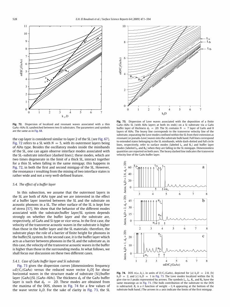
528 E.H. El Boudouti et al. / Surface Science Reports 64 (2009) 471–594

1

2

3

4

5

6

7

8

9

10

1 2 3 4 5 6k // D

0 70

11

Fig. 72. Dispersion of localized and resonant waves associated with a thinGaAs–AlAs SL sandwiched between two Si substrates. The parameters and symbolsare the same as in Fig. 68.

the cap layer is considered similar to layer 2 of the SL (see Fig. 67).Fig. 72 refers to a SL with N = 5, with its outermost layers beingof AlAs type. Besides the oscillatory modes inside the minibandsof the SL, one can again observe interface modes associated withthe SL–substrate interface (dashed lines); these modes, which aretwo times degenerate in the limit of a thick SL, interact togetherfor a thin SL when falling in the same minigap; this happens inFig. 72, in both the first and second minigap of the SL. However,the resonance r resulting from themixing of two interface states israther wide and not a very well-defined feature.

5.4. The effect of a buffer layer

In this subsection, we assume that the outermost layers inthe SL are both of AlAs type and we are interested in the effectof a buffer layer inserted between the SL and the substrate onacoustic phonons in a SL. The other surface of the SL is kept freeof stress [57]. We show that the behavior of the different modesassociated with the substrate/buffer layer/SL system dependsstrongly on whether the buffer layer and the substrate are,respectively, of GaAs and Si type or vice versa. In the first case, thevelocity of the transverse acoustic waves in the substrate is higherthan those in the buffer layer and the SL materials; therefore, thesubstrate plays the role of a barrier of finite height for phonons inthe buffer/SL system. In the second case, it is the buffer layer whichacts as a barrier between phonons in the SL and the substrate as, inthis case, the velocity of the transverse acoustic waves in the bufferis higher than those in the surrounding media. In what follows, weshall focus our discussion on these two different cases.

5.4.1. Case of GaAs buffer layer and Si substrateFig. 73 gives the dispersion curves [dimensionless frequency

ωD/Ct(GaAs) versus the reduced wave vector k‖D] for shearhorizontal waves in the structure made of substrate (Si)/bufferlayer (GaAs)/SL (GaAs–AlAs). The thickness db of the GaAs bufferlayer is such that db = 2D. These modes are obtained fromthe maxima of the DOS, shown in Fig. 74 for a few values ofthe wave vector k‖D. For the sake of clarity in Fig. 73, the SL

Lb

LbLs

RbRs

0

2

4

6

8

10

1 2 3 5 64k||D

0 7

Fig. 73. Dispersion of Love waves associated with the deposition of a finiteGaAs–AlAs SL (with AlAs layers at both its ends) on a Si substrate via a GaAsbuffer layer of thickness db = 2D. The SL contains N = 7 layer of GaAs and 8layers of AlAs. The heavy line corresponds to the transverse velocity line of thesubstrate, separating the Lovemodes confinedwithin the SL from their extension asresonant (or pseudo-Love)waves into the substrate bulk band. Full lines correspondto extended states belonging to the SL minibands, while dash-dotted and full circlelines, respectively, refer to surface modes (labeled Ls and Rs) and buffer layermodes (labeled Lb and Rb) when they are falling in the SL minigaps. Dimensionlessquantities are reported on both axes. The heavy dashed line indicates the transversevelocity line of the GaAs buffer layer.

Rb

Bs

Rs

Lb LsLb

Bs

Rs

Rb

Bs

0

20

40

60

0

15

30

45

0

10

20

3 4 5 6 7 8

2 3 4 5 6 7 8

2 3 4 5 6 7

Δn(ω

, k||D

= 1

, db

= 2

D)

Δn(ω

, k||D

= 2

, db

= 2

D)

Δn(ω

, k||D

= 2

.8, d

b =

2D

)

a

b

c

ωD/Ct(GaAs)1 8

Fig. 74. DOS n(ω, k‖), in units of D/Ct (GaAs), depicted for (a) k‖D = 2.8, (b)k‖D = 2, and (c) k‖D = 1 in Fig. 73. The Love modes localized within the SLgive rise to δ peaks represented by arrows. The symbols Ls , Lb , Rs , and Rb have thesame meanings as in Fig. 73. (The bulk contribution of the substrate to the DOSis subtracted. Bs is a δ function of weight −1/4 appearing at the bottom of thesubstrate bulk band.) The arrows in ω axis indicate the limits of the first minigap.

E.H. El Boudouti et al. / Surface Science Reports 64 (2009) 471–594 529

(c) ωD/Ct(GaAs)=4.020

k||D=2

(d) ωD/Ct(GaAs)=3.830 k||D=2

(a) ωD/Ct(GaAs)=4.555

k||D=2.8

(b) ωD/Ct(GaAs)=4.435

k||D=2.8

Substrate (Si)Buffer (GaAs)

Superlattice (GaAs / AlAs)

10

20

30

6

12

10

20

0.5

1.0

0.0

1.5

0

0

0

Loc

al D

OS

Loc

al D

OS

Loc

al D

OS

Loc

al D

OS

-4 -2 80 2 4 6x3/D

Fig. 75. Spatial representation of the local DOS forωD/Ct (GaAs) = 4.555 (a), 4.435(b) at k‖D = 2.8 and ωD/Ct (GaAs) = 4.020 (c), 3.830 (d) at k‖D = 2. These modes,respectively, are labeled Ls , Lb in Fig. 74(a) andRs ,Rb in Fig. 74(b). The space positionsof the different interfaces are marked by vertical lines.

only contains N = 7 layers of GaAs and N + 1 = 8 layersof AlAs. The branches situated below the substrate bulk bandcorrespond to Love waves confined in the finite SL and decayingexponentially into the substrate (as will be shown later); theyappear as true δ functions in the DOS. The extension of thesecurves into the substrate band (continuum) represents resonantmodes (also called leaky or pseudo-Love waves) associated withthe deposition of the finite SL on the top of the substrate, and theyappear as well-defined peaks in the DOS of Fig. 74.There are three categories of normal modes in the present

structure (Fig. 73) according to their oscillatory (full lines) orlocalized character in the SL. The former are extended (or bulk)states, while the latter are decaying either from the free surface(dash-dotted line, also labeled LS and RS as localized and resonantsurface states) or confined in the buffer layer (dotted lines, alsolabeled Lb and Rb as localized and resonant buffer states). Thelocalization properties of these different modes will be shownbelow. The positions of the surface and buffer localized modes,which are already distinguishable in Fig. 73, even for a smallnumber of periods as N = 7, shift only slightly with N whengoing to the limit of a semi-infinite SL. Moreover, the surfaceand buffer localized branches lying in the first minigap presentdifferent behaviors when penetrating into the substrate bulk bandas resonances. Indeed, in Fig. 73 the surface branch continues toexist as well-defined resonance until k‖D = 0, while the bufferbranch vanishes at about k‖D ≈ 1.5, as the corresponding peaks inthe DOS become rather wide and not a very well-defined featurefor k‖D ≤ 1.5 (see Fig. 74). The buffer branch lying below theSL bulk bands goes asymptotically to the limit of the GaAs bufferlayer bulk band (dashed line) when increasing k‖D. An analysisof the local DOS as a function of the space position x3 (Fig. 75)clearly shows the localization properties of the surface and bufferbranches lying in the first minigap at the vicinity of the substratetransverse velocity line (heavy line). The local DOS reflects thespatial behavior of the square modulus of the displacement field.Fig. 75(a) and (b) correspond, respectively, to the localized modes

labeled Ls and Lb in Fig. 74(a), showing that the surface mode islocalized at the surface of the SL and decays exponentially overseveral layers from the surface, while the buffer mode is confinedin the buffer layer and decays exponentially in the surroundingmedia. Fig. 75(c) and (d) correspond to the resonantmodes labeledRs and Rb in Fig. 74(b) showing, respectively, the same behaviors asthe Ls and Lb modes in Figs. 75(a) and (b); however, one can noticethe propagation of the Rs and Rbmodes in the substratemedium astheir frequencies lie in the continuum of the substrate bulk band.The frequencies of the modes induced by the buffer layer/SL

structure are very sensitive to the buffer layer thickness db.Fig. 76(a) illustrates the variation of these frequencies versus db, fora given value of k‖, namely, k‖D = 2.8. The classification of thesecurves is similar to that in Fig. 73. One can notice that the branchesassociated with the buffer (labeled Lb) are very dependent onthe thickness db; they take place when the lowest discrete modeemerges from the bulk (an effect which is periodically reproducedas a function of db). These branches interactwith the surface branch(labeled Ls), which is independent of the thickness db, giving rise tothe lifting of degeneracy at the anti-crossing points around db/D ≈0.9, 1.8, 2.7, etc. Due to the finiteness of the SL, this interaction ismore important for small values of N , as emphasized in Fig. 76(b)around db/D ≈ 0.9. The interaction between the surface and bufferstates disappears by increasing N; this decoupling occurs in thepresent example for N of the order of 10–15.

5.4.2. Case of Si buffer layer and GaAs substrateNow, we substitute the substrate and buffer constituent

materials in the previous structure [i.e., we consider the substrate(GaAs)/buffer layer (Si)/SL (GaAs–AlAs) system]. Fig. 77 shows thedispersion curves for the same SL as in Fig. 73 and for a Si bufferlayer of thickness db = 2D. All the branches in Fig. 77 representnow resonant (or pseudo-Love) modes induced by the buffer/SLmultilayers in the continuum of the substrate bulk band, whichmeans above the transverse velocity line of the GaAs substrate(heavy line). Among the above resonantmodes, one candistinguishthemodes falling below the buffer transverse velocity line (dashedline) and those falling above the buffer transverse velocity line.The branches situated below the buffer transverse velocity linerepresent resonant waves of the finite SL, and appear as well-defined peaks in the DOS (see Fig. 78), even though they are inresonance with the bulk states of the GaAs substrate. One can,however, notice that the width of these peaks becomes largewhen either k‖D or the thickness db of the buffer layer decreases(see below). Let us emphasize here also that the oscillations inthe DOS of Fig. 78 are equivalent to the fine structure observedexperimentally by Lockwood et al. [75,76] and Trigo et al. [77]in semiconductor SLs; however, the presence of the buffer layerin Fig. 78 increases strongly the intensity of the oscillations inthe DOS, lying below the buffer layer transverse velocity line.Therefore, such confined modes in the SL could be observed easilyby Raman experiments [75–77]. The bulk and surface curves lyingbelow the buffer transverse velocity line in Fig. 77 are very similarto those of localized Love modes of Fig. 73; however, the inducedbuffer modes disappear in this region as their frequencies arelying below the buffer transverse velocity line, while interfacebranches associated with the buffer/SL interface (labeled Ib inFig. 77) appear. The surface and interface modes may interacttogether when falling in the same minigap, leading to the liftingof degeneracy at the anti-crossing points around k‖D ≈ 2.3. Ananalysis of the local DOS as a function of the space position x3(Fig. 79) for the modes labeled Re, Rs and Ib and corresponding,respectively, to extended, surface, and interfacemodes in Fig. 78(c)clearly shows the localization properties of the different kinds ofstates belonging to a different frequency range. Fig. 79(a) shows

530 E.H. El Boudouti et al. / Surface Science Reports 64 (2009) 471–594

N = 11 N = 7 N = 4

3

4

5

6

7

8

Lb LbLs

Lb

7.4007.280

4.745

4.225

ωD

/Ct(G

aAs)

ωD

/Ct(G

aAs)

1 2 3 40db/D

db/D

4.45

4.50

4.55

4.60

4.65

4.70

0.6 0.8 1.0 1.2 1.4

a

b

Fig. 76. (a) Variations of the frequencies of the Love and pseudo-Love modes versus the thickness db of the buffer layer for the SL depicted in Fig. 73. The wave vector k‖ ischosen such that k‖D = 2.8. The notations have the same meaning as in Fig. 73; the arrows give the limits of the SL minigaps. (b) The interaction between the surface andbuffer layer states near db = 0.9D in (a) is emphasized for several values of the number N of periods in the SL: 11 (– ––), 7 (. . . ), and 4 (—).

that the extended mode Re is confined in the finite SL and does notpropagate into the Si buffer layer. Consequently, it remains a well-defined guided wave of the finite GaAs–AlAs SL. Similar behaviorsare found in the topmost layer of an adsorbed bilayer on a substrate(see Section 3.3). On the contrary, the surface (Rs) and the interface(Ib) modes in Fig. 78(c) show a strong localization at the surfaceof the SL and at the SL/buffer layer interface, respectively (seeFigs. 79(b) and (c)). Above the buffer transverse velocity line, theresonant modes are due to the interaction between the SL/buffermodes and the substrate modes. Now, an analysis of the local DOSas a function of the space position shows a propagation behavior inthe substrate/buffer layer/SL system (see Fig. 79(d) related to themode labeled Rb in Fig. 78(c)) with a pronounced amplitude in theSi buffer layer.As mentioned above, the pseudo-Love modes induced by the

SL/buffer are dependent on the width db of the buffer layer. Fig. 80illustrates the variation of the frequency of the pseudo-Lovemodesas a function of the thickness ratio db/D, for a given value ofthe reduced wave vector k‖D such that k‖D = 2.8. Let us recallthat apart from the surface and interface curves falling in thefirst minigap and situated below the buffer transverse velocityline (short-dashed line), the other curves represent sharp resonantguided waves in the SL; the corresponding frequencies of allthese modes present a very small variation with db. Moreover,the intensity of the resonances in this region of frequenciesincreases by increasing the thickness db of the Si buffer layer(see Fig. 81(a) and (c)), and for large values of db (Fig. 81(c)) theresonances appear as δ functions of weight 1 as the interactionbetween the GaAs–AlAs SL and the GaAs substrate becomes weak.Concerning the curves lying above the buffer transverse velocityline, they present a noticeable variation with varying db/D andtend asymptotically to the buffer bulk band when db →∞. Theseresonances correspond to waves with predominant amplitudes in

Rs

Rs

Ib

Ib

Ib

2

4

6

8

1 2 3 4 5 60 7k||D

0

10

ωD

/Ct(G

aAs)

Fig. 77. Same as in Fig. 73, but for the GaAs (substrate)/Si (buffer layer)/GaAs–AlAs(SL) structure. The heavy line (dashed line) represents here the GaAs (Si) transversevelocity line. The branches labeled Ib refer to the SL/buffer layer interface modes.

the Si buffer layer (see Fig. 79(d)) even though they are propagatingin the whole GaAs/Si/GaAs–AlAs (SL) system. The correspondingpeaks in theDOSpresent a noticeable intensity only for large valuesof db and at the vicinity of the buffer bulk band (Fig. 81(d)).

E.H. El Boudouti et al. / Surface Science Reports 64 (2009) 471–594 531

Rs

Rs

Ib

(x 0.4)

(x 0.4)

Bs

Bs

IbRs

Re

Bs

Rb

c

b

a

0

20

40

0

20

40

60

-20

0

20

40

60

80

Δn(ω

, k||D

= 2

.8, d

b =

2D

)Δn

(ω, k

||D =

2, d

b =

2D

)Δn

(ω, k

||D =

1, d

b =

2D

)

2 3 4 5 6 71 8

2 3 4 5 6 7 8

4 5 6 73 8

ωD/Ct(GaAs)

Fig. 78. Same as in Fig. 74, but for the system depicted in Fig. 77.

x3/D

-4 -2 0 2 4 6 8

Loc

al D

OS

Loc

al D

OS

Loc

al D

OS

(b) ωD/Ct(GaAs) = 4.540

(a) ωD/Ct(GaAs) = 3.785

(d) ωD/Ct(GaAs) = 5.620

(c) ωD/Ct(GaAs) = 4.720

Substrate (GaAs)

Buffer (Si)

Superlattice (GaAs/AlAs)

0

5

10

0

10

20

30

0

6

12

18

1

2

Loc

al D

OS

0

3

-4 -2 0 2 4 6 8

x3/D

Fig. 79. Spatial representation of the local DOS forωD/Ct (GaAs) = 3.785 (a), 4.540(b), 4.720 (c), and 5.620 (d) at k‖D = 2.8. These modes, respectively, are labeled Re ,Rs , Ib , and Rb in Fig. 78(c) and correspond to extended, surface, interface, and bufferlayer modes.

The reflection from the buffer/SL of an incident phonon in theGaAs substrate is explained quantitatively in terms of phonontrapping times. Because of the free surface of the SL, the incidentphonons with frequencies lying above the substrate bulk band

Rs4.225

4.745

7.2807.400

Ib

3

4

5

6

7

8

9

ωD

/Ct(G

aAs)

1 2 3db/D

0 4

Fig. 80. Same as in Fig. 76(a) but for the system depicted in Fig. 77. The heavy long-dashed (short-dashed) line represents here the transverse velocity line of the GaAs(Si).

ωD/Ct(GaAs)

X Axis

(x 0.4)

(x 0.4)

(x 0.4)

(x 0.4)Rs

Rs

(x 0.5)

IbRs (x 0.5)

IbRs

a

b

c

d

0

10

20

30

40

60

120

10

20

30

0

0

60

120

180

0

180

Tra

ppin

g tim

eΔn

(ω, k

||D =

2.8

, db =

4D)

Δn(ω

, k||D

= 2

.8, d

b = 0

)T

rapp

ing

time

3 4 5 6 72 8ωD/Ct(GaAs)

Fig. 81. Frequency dependence of the DOS and trapping time [in units ofD/Ct (GaAs))] for db = 0 [(a) and (b)] and db = 4D [(c) and (d)] in Fig. 80. Thearrows indicate the positions of the substrate and buffer transverse velocity lines.

are entirely reflected. Therefore, the reflection rate is unity andonly the phase or the phase time gives us the information on theinteraction of an incident phonon with resonant modes confinedin the SL/buffer system. The interaction of phonons with surfacemodes in a substrate/SL system has been pointed out first byMizuno and Tamura [56], showing a large time delay when thephonon frequency coincides with an eigenfrequency of the surfacemode. This time is interpreted as the time needed for a phononto complete the reflection process. In the present work, we adopt

532 E.H. El Boudouti et al. / Surface Science Reports 64 (2009) 471–594

the same analysis to study the substrate/buffer/SL system takinginto account the effect of the buffer layer. In addition, we give acomparison between theDOS and trapping time as a function of thefrequency. In Fig. 81, we give a comparison between the DOS andtrapping time for two different values of the buffer layer thicknessin Fig. 80: db = 0 (Fig. 81(a) and (b)) and db = 4D (Fig. 81(c)and (d)). In Fig. 81(b), the resonances are similar to those obtainedby Mizuno and Tamura [56] (i.e., without buffer layers), but forshear horizontal waves instead of longitudinal ones [56]; one candistinguish, in particular, the resonance mode (Rs) which exhibitsa large time delay in the trapping time. Indeed, the magnitude ofthe peak associated with this surface resonance is about 70 [inunits of D/Ct (GaAs)]. This means that for a typical value of theperiod D used in experiments [283,284], for example D = 200 Å,the magnitude of the time delay is of the order of 0.4 ns, which isin the range detectable by a phonon experiment using picosecondlaser technique [59]. On the other hand, the trapping time gives thesame behavior as the DOS (Fig. 81(a)) in accordance with Eq. (266).The half widths of the peaks in these two quantities are relatedto the lifetimes of the resonances: the intensity of the peaksin the trapping time describes the time needed for phonons tocomplete the reflection process, while the DOS gives the weightof the resonances. For a large value of db (Fig. 81(c) and (d)) andfor frequencies lying below the buffer trapping velocity line, theresonant modes become quasibound (quasi-localized) modes andgive rise to extremely sharp resonances in the DOS and trappingtime [indicated by arrows in Fig. 81(c) and (d)] as the interactionbetween the SL and the substrate modes is rather weak. Indeed, byusing a very finemesh in the numerical calculation, themagnitudeof the sharp resonances in the trapping time (Fig. 81(d)) reaches104 [in units of D/Ct (GaAs)], i.e., about 60 ns for a period D =200 Å. Of course, to observe these resonances, a very extendedwave packet (of spectral width less than that of the resonance)would have to be used. On the other hand, one can notice that inaddition to the surface mode Rs in Fig. 81(c) and (d), an interfacemode Ib associated with the buffer/SL interface appears also in thefrequency gap. Moreover, for the frequency range situated abovethe buffer transverse velocity line, the intensity of the resonancesbecomes important especially in the vicinity of the bottom of thebuffer band.

5.5. The effect of a cavity layer

We have also studied the case of a defect layer inserted insidea finite size SL as a cavity layer [84]. The schematic illustrationis sketched in Fig. 82(a) for a finite SL composed of N = 10GaAs–AlAs cells deposited on a GaAs substrate, while the othersurface is supposed free of stress. A Si cavity layer of thicknessd0 = 3D is inserted within the SL. Because of the existence of twoperturbations (cavity and surface) within the SL, one can expecttwo types of defect modes inside the band gaps and an interactionbetween these modes depending on the distance between thesetwo defects. An analysis of the variation of the DOS as functionof the reduced frequency ωD/Ct(GaAs) for different positions ofthe defect layer inside this structure (Fig. 82(b)–(d)), clearly showsthis interaction. We have sketched these DOS for a defect layernear the surface of the SL (j = 9, Fig. 82(b)), in the middle of thestructure (j = 5, Fig. 82(c)) and near the interface SL/substrate(j = 2, Fig. 82(d)). One can notice that, as expected, the interactionbetween the surface and defect modes falling within the first bandgap of the SL becomes important (weak) when the defect layer iscloser to (far from) the surface, as it is illustrated in Fig. 82(b)–(d).Let us notice that several works have been devoted to the

modes induced by a cavity layer inserted in the middle [72–74,208,209] or at different places [71] within the finite SLby means of Raman scattering techniques (see Section 5.6.1).

Recently, cavity phonons in SLs have been also investigated usingthe so-called asynchronous optical sampling [288] and ultrafastcoherent generation of acoustic phonons in the presence of photonconfinement in an optical resonator [289].

5.6. Relation to experiments

In this section, we shall give some experimental resultsrelated to the determination of bulk and defect modes in finitesuperlattices. In particular, we shall concentrate essentially onexperimental measurements based on two techniques, namelythe light scattering by longitudinal acoustic phonons and laserpicosecond ultrasonics.

5.6.1. Light scattering by longitudinal acoustic phononsThe principle of this scattering can be summarized as follows:

the propagation of an acoustic wave in the superlattice excitesperiodic variations of strain which in turn induce a modulation ofthe dielectric tensor εij from the photoelastic coupling to elasticfluctuations,

δεij = εiiεjj∑kl

Pijkl12

(∂uk∂xl+∂ul∂xk

). (267)

Pijkl are the elements of the photoelastic tensor and can beconsidered as functions of x3. The coupling of incident light tophonons gives rise to a polarization in the superlattice whichcreates a scattered field. In this work we are interested in purelongitudinal phonons along the axis x3 of a multilayer structurecomposed of cubic materials with (001) interfaces. In this case, wecan assume that all the electromagnetic fields (incident, scatteredand polarization waves) are polarized parallel to the x1 axis andpropagates along x3. Then each medium α in the structure canbe characterized by an elastic constant Cα (which means C11), themass density ρα , the dielectric constant εα = n2α (where n is theindex of refraction in themediumα) and one photoelastic constantpα = −ε2αP

α1133.

Eq. (267) becomes for each medium α

δεα = pα∂uα(x3)∂x3

. (268)

The calculation of the emitted electric field Es(x3, t) when thesuperlattice is submitted to an incident electromagnetic field canbe done following the Green’s function method [193,290]

Es(x3, t) = −ω2i

ε0c2∑α

∫pα G(x3, x′3)

∂uα(x′3)∂x′3

E0i (x′

3, t) dx′

3. (269)

Here ωi is the angular frequency of the incident wave, ε0 and care the permittivity and the speed of light in vacuum respectively,E0i (x

′

3, t) is the electric field in the SL, and G(x3, x′

3) is the Green’sfunction associated with the propagation of an electromagneticfiled along x3 in the vacuum/superlattice system in the absence ofacoustic deformation.In the particular case where the dielectric modulation of the

multilayer structure can be neglected (which happens when thelayers are thin as compared to the opticalwavelengths), the systemcan be considered as an homogeneous medium from the opticalpoint of view, then E0i (x

′

3) = E0i eikix′3 is a plane wave (instead

of being a Bloch wave) and G(x3, x′3) ∝ eiks(x3−x′3). ki and ks are

the wave vectors of the incident and scattered waves. Therefore,Eq. (269) becomes

Es(x3, t) ∝ −ω2i

ε0c2∑α

∫pα eiqx

′3∂uα(x′3)∂x′3

dx′3 (270)

E.H. El Boudouti et al. / Surface Science Reports 64 (2009) 471–594 533

ωωωωD/Ct(GaAs)

[N=10 ; jdéf=9]

ΔΔ ΔΔ n[ ω

ω ω ω

][N=10 ; jdéf=2]

[N=10 ; jdéf=5] (b)

(a)

(c)

i = 0

x3

n = N

n = N – 1

n = j

n = –1

n = 0

0

d1

d

d 0

(S)

i = 1

i = 2

i = 2

i = 2

i = 2

i = 1

AlAs

GaAs

GaAs

GaAs

GaAs

Si

AlAs

GaAs

x3

n=N

n=N-1

n=j

n=j-1

n=0

d1

d2

d0

0

a

b

c

d

N = 10, j = 2

N = 10, j = 5

N = 10, j = 9

DO

S

0

10

20

30

40

0

10

20

30

0

10

20

30

DO

S

-10

40-10

DO

S

40

3.8 3.9 4.0 4.1 4.2ωD/Ct(GaAs)

3.7 4.3

Fig. 82. (a) Schematic representation of a finite GaAs–AlAs SL terminated on both sides with AlAs layers and in presence of a Si cavity layer embedded within the cell j. Thewhole structure is deposited on a GaAs substrate. (b), (c), (d) DOS (in units of D/Ct (GaAs)) as a function of the reduced frequency for a finite size SL composed of N = 10GaAs–AlAs cells and in presence of a Si defect layer inserted in the sites: j = 2 (b), j = 5 (c) and j = 9 (d) at k‖D = 2.

where

q = ki − ks = 2ki = 4πneff /λ (271)

is the wave vector of the phonon in the backscattering geometryand neff is the effective index of refraction of the whole system.A great deal of work has been devoted to light scattering

from acoustic phonons in multilayered structures, since the firstobservation of folded longitudinal acoustic modes by Colvardet al. [29]. Several experimental studies have been reported onGaAs–GaxAl1−xAs and Si–GexSi1−x systems. As mentioned before,in an ideal periodic structure (superlattice) consisting of an infinitesequence of building blocks AB made of different semiconductorsA and B, the branches of the acoustic phonon dispersion are back-folded inside theBrillouin zonedue to theperiodicity of the system.In the Raman process involving longitudinal acoustic phonons inbackscattering geometry along the growth direction (x3), crystalmomentum is conserved, i.e., the wave vector transfer to thephonon corresponds to the sum of the magnitudes of the wavevectors of incident and scattered photons ki and ks, respectively.Characteristic doublets are observed in the spectrum whichreflects the folding of the superlattice dispersion curves in thefirst Brillouin zone. Crystalmomentum conservation at the doubletfrequencies implies that all partial waves are coherently scattered,i.e., all layers of the superlattice contribute constructively tothe total intensity. Therefore, the doublets are very sharp andpronounced.In a real superlattice, the coherence of the scattering contribu-

tions from the individual layers is partly removed due to interfaceroughness and layer thickness fluctuations, finite size effect of thesuperlattice as well as the effect of different defects that may be

introduced inside these systems such as surfaces, interfaces anddefect layers (cavities, buffers, . . . ).In view of the relatively small thicknesses of the layers in

the superlattice, the acoustic phonon Raman scattering can beobtained from Eq. (270) as

I(ω) ∝

∣∣∣∣∣∑α

∫pαeiqx

′3∂uα(x′3)∂x′3

dx′3

∣∣∣∣∣2

. (272)

Here we assume that the light propagates like in a homoge-neous medium and u(x3) is the normalized lattice displacement.Fig. 83(a) gives the experimental results of Raman intensity ob-tained by Zhang et al. [75,76] for a superlattice composed of 15 pe-riods of 20.5 nm of Si and 4.9 nm of Si0.52Ge0.48 epitaxially grownon a [100] oriented Si substrate. The different curves in Fig. 83(a)correspond to different laser wavelengths (i.e, different phononwave vectors). By reporting the frequency positions of the doubletswithin the band gap structure (Fig. 83(b)), good agreement be-tween the dispersion curves of the infinite superlattice (full curves)and the experimental results (dots) has been obtained. These re-sults enable one to deduce a precise measurement of the width ofthe first three gaps. Besides the description of the band gap struc-ture, the Raman spectra show also small features (indicated bysmall vertical arrows in Fig. 83(a)) which are interpreted as con-fined modes (discrete modes) due to the finite size structure ofthe superlattice. By using our theoretical model [291], we havereproduced theoretically in Fig. 83(c) the different Raman spec-tra of Fig. 83(a) and the agreement between theoretical and ex-perimental results is quite good. In Fig. 83(d) we have calculatedthe intensity variation of different phonon branches labeled 1–6 in

534 E.H. El Boudouti et al. / Surface Science Reports 64 (2009) 471–594

123456

10

20

30

40

50

60

70

80

90

5 10 15 20 25 30 35

541.5 nm

496.5 nm

488 nm

476 nm

457.9 nm

0

100

Ram

an I

nten

sity

(a.

u.)

0 40Frequency shift (cm-1)

a

0

1

2

3

4

5

10 15 20 25 30 355

Frequency shift (cm-1)

400

c

b d

5

10

15

20

25

0

30

Freq

uenc

y sh

ift (

cm-1

)

0.50.0 1.0

qD/π qD/π

100

200

300

400

500

Inte

nsity

(a.

u.)

0

600

0.0 0.2 0.4 0.6 0.8 1.0

Fig. 83. (a) Room-temperature acoustic phonon Raman spectra in the Si/Si0.52Ge0.48 superlattice, excited with the five studied laser lines (after Ref. [76]). (b) Calculateddispersion curves of the infinite SL (solid lines). The filled circles are obtained from the doublets of the theoretical spectra sketched in (c) using our theoretical model. (d)Variation of the intensities of the six first folded branches as functions of the diffusion wave vector qD/π .

Fig. 83(b) within the reduced Brillouin zone. The intensities showdrastic variations, especially for q close to the Brillouin edges. TheBrillouin line (branch labeled 1) is themost intensemode for a largerange of q values except near the zone boundary. These behaviorsare similar to the theoretical predictions obtained byHe et al. [283]on GaAs–GaxAl1−xAs superlattices.Besides the doublets associated to folded longitudinal acoustic

phonons, Lemos et al. [218] have shown the existence of additionalmodes between the doublets which are induced by a cap layerdeposited at the surface of the superlattice. Thesemodes fall insidethe gap located at ∼15 cm−1. The superlattice is composed of 20periods of 21.5 nm of Si and 5.0 nm of Ge0.44Si0.56 terminated by acap layer made of Ge0.44Si0.56 with a thickness dc = 1.5 nm. Thetop and bottom curves in Fig. 84(a) are drawn for two differentwavelengths 514.5 nm and 496.5 nm respectively. By using ourtheoretical model [291], we have reproduced correctly (Fig. 84(b))the main features of these results, except for the gap mode whichgreatly surpassed the observed value. To confirm that the gapmodeis induced by the cap layer, we have calculated the local DOS as afunction of the space position for themode lying at∼15 cm−1. Thespatial localization of this mode (see Fig. 84(c)) shows clearly thatit is localized in the cap layer and decreases inside the SL.Another examplewehave considered concerns a finite sizemir-

ror plane superlattice with building blocks SL = GaAs–AlAs andLS = AlAs–GaAs arranged to form layer sequences (SL)m/2/(LS)m/2

with different numbers of building blocks m. This leads to mir-ror plane superlattices with different numbers of building blocksm. (SL)m/2/(LS)m/2 with m = 10, 20 and 40 as well as a refer-ence specimen (SL)20 have been investigated byGiehler et al. [208].Fig. 85(a) shows the experimental Raman spectra of three mirrorplane superlattices and the (SL)20 reference sample (bottom curve)in the frequency range of the first longitudinal acoustic phonondoublet. For the reference sample, the crystal momentum trans-fer q is about 0.3π/D where D = 86.8 nm is the period of the su-perlattice. The thickness d1 and d2 of the GaAs and AlAs layers arechosen such that d1 = 36.4 nm and d2 = 50.4 nm respectively.One therefore observes a folded-phonon doublet close to the cen-ter of the superlattice Brillouin zone whose components are de-noted by ω±1. In contrast to the periodic structure, the spectra ofthe mirror plane superlattice display pronounced splittings of thedoublet lines. These splittings increasewith decreasing total lengthof the SL and LS building blocks. These effects are interpreted as be-ing due to the interference of the scattering contributions from thedifferent quantumwells in the sample, and reflect a phase shift in-troduced by the mirror plane symmetry. Furthermore additionalmirror lines in Fig. 85(a) (marked by vertical bars) with charac-teristic separations appear. These modes have been interpreted asconfined modes induced by the finite size effects. With the help ofour model calculation [291], we have first reproduced in Fig. 85(b)the main features of Fig. 85(a) where we can clearly distinguish,

E.H. El Boudouti et al. / Surface Science Reports 64 (2009) 471–594 535

Frequency Shift (cm-1) Frequency Shift (cm-1)

Ram

an I

nten

sity

(a.

u.) 514.5 nm

496.5 nm

10 20

10

20

30

40

50

LD

OS

0

60

x3/D

10 150 5

252015105

a b

c

Si/Ge0.44Si0.56

Fig. 84. (a) Raman spectra of a SL composed of 20 periods of 21.5 nm of Si and 5.0 nm of Ge0.44Si0.56 terminated by a cap layer made of Ge0.44Si0.56 with a thicknessdc = 1.5 nm. The top and bottom curves are drawn for two different wavelengths 514.5 nm and 496.5 nm respectively (After Ref. [218]). (b) Theoretical results obtainedfrom our theoretical model.

(SL)20(LS)20

(SL)1 0(LS)1 0

(SL)5(LS)5

(SL)20

Ram

an I

nten

sity

(a.

u.)

15 20 25

Frequency Shift (cm-1)

10 3015 20 25

Frequency Shift (cm-1)

10 3015 20 25

Frequency Shift (cm-1)

10 30

a b c

0

2

4

6

8

Fig. 85. (a) Raman spectra of folded longitudinal acoustic phonons of mirror plane superlattices (SL)m/2/(LS)m/2 with m = 10, 20, and 40 compared with that of the idealfinite size (SL)20 . The building blocks are SL = GaAs–AlAs and LS = AlAs–GaAs respectively. Minor peaks are marked by vertical bars (after Ref. [208]). (b), (c) Theoreticalresults obtained from our theoretical model in absence (b) and presence (c) of absorption.

besides the splitting of each peak in a doublet, satellites (weakpeaks) around the main peaks. In order to describe more preciselythe experimental curves, we have introduced the absorption effectin the system by adding a small imaginary part to the effective in-dex of refraction (see also Ref. [292]). These results are reported

in Fig. 85(c) and show very good agreement with the experimen-tal results (Fig. 85(a)). One can notice that light absorption smearsout the split lines considerably because the field scattered fromthe (LS)m/2 unit incompletely cancels the field from the (SL)m/2unit.

536 E.H. El Boudouti et al. / Surface Science Reports 64 (2009) 471–594

28 32 36

647

647

568568

514514

488488

458458

Ram

an I

nten

sity

(a.

u)

24 40Frequency shift (cm-1)

28 32 3624 40

Frequency shift (cm-1)

a b

Fig. 86. (a) Room-temperature acoustic phonon Raman spectra collected with the five studied laser lines. The spectra were acquired with high resolution on ten periodsGa0.47In0.53As-Al0.48In0.52As SL enclosing a cavity made of InP. The intensities have been normalized. Solid (dashed) lines are guides to the eye indicating the dispersion ofthe main (secondary) doublets (after Ref. [209]). (b) The theoretical spectra obtained using our theoretical model.

A similar study has been developed by Pascual et al. [209]on an acoustical phonon cavity that consists of phonon mirrorsmade of ten periods (λ/4, 3λ/4) stacks of two materials, namely(Ga0.47In0.53As, Al0.48In0.52As) enclosing a 7λ/2 cavity made of InP.The whole structure is grown on InP substrate. λ refers to thesound wavelength in the specific material making the mirror orthe cavity layer. The period of the superlattice is estimated by x-ray diffraction to be 45.2 Å. The Raman spectra are shown to behighly sensitive to the details of the structure, allowing a propercharacterization of the device. The interest of such a structureconsists in reflecting back and forth the longitudinal acousticphonon in the cavity before escaping by tunneling, thus enhancingthe anharmonic coupling with longitudinal optic phonons. Ameasure of this enhancement is the longitudinal acoustic phononlifetime in the device, that for typical phonon mirror reflectivitiescan be augmented by a factor larger than 100. An example ofRaman spectra in the acoustical domain is given in Fig. 86(a) forfive laser wavelengths. Several features can be highlighted fromthe measured spectra: (i) the spectra are dominated by an intenseacoustical phonon doublet which disperses with laser wavelength,(ii) in addition to this main doublet, a small intensity secondarydoublet shifted to smaller energies and also displaying dispersionis observed and (iii) some weaker oscillations can be discernedtowards smaller energies (not shown in the figure). These latteroscillations arise from the finite size effects as discussed in Figs. 83and 85. Here also, it was shown that the observed splitting of thelongitudinal acoustic doublets can be traced down to interferenceeffects on the Raman spectra coming from the two mirrorssuperlattices and the phase shift introduced between them by theInP spacer. By using our theoretical model [291], we have sketchedin Fig. 86(b) the numerical curves by taking the elastic, photoelasticand refractive index parameters of the materials as described inRef. [209]. The agreement between theoretical and experimentalresults is quit good.The case of a cavity layer embedded at different positions

within a finite SL has been examined by Schwartz et al. [71].The structure consists on 9 periods of 50/25Å AlSb/GaSb layers

grown on (001) GaSb in which an additional 50 Å layer of AlSbwas embedded either at the substrate/superlattice interface, inthe center of the structure, or near the superlattice/air interface(see the insets in Fig. 87(a)). The exact placement of the defectlayer can also be viewed as a ten-period SL with a missingGaSb layer. A ten periodic SL was also examined for comparison.Raman scattering using 5145 Å excitation was utilized to studythe zone-folded acoustic phonon spectra. Data values appropriatefor GaSb and AlSb at 5145 Å are given in Ref. [293]. Fig. 87(a)shows the Raman spectra of the zone-folded acoustic phononsfor the periodic SL and the three samples grown with a singledefect layer. Additional strong scattering peaks indicated by thevertical arrows are seen in the samples with the defect layermoved away from the substrate interface. Weaker structureswhich show up as shoulders or bumps between the periodiczone-folded doublets are also evident. In order to explain theexperimental spectra, Raman intensity has been calculated [71]but these results did not match the experimental data becausecyclic boundary conditions was assumed. This approximationmakes the calculated spectrum independent of the location of thedefect layer. By using our theoretical model, where the boundaryconditions at the different interfaces are taken appropriately, wehave reproduced the four spectra (Fig. 87(b)). One can noticethat when the defect layer is placed near to the substrate, thedoublets resemble those of the periodic structure, whereas whenthe defect is inserted in the middle of the structure or nearto the free surface, then each doublet splits into two peakswith different shapes depending on the position of the defectwithin the finite SL. This behavior is mainly due to interferencephenomenonbetweendifferent layers of the system. Asmentionedin Ref. [71], the lower resolution (2 cm−1) and inherent noise inthe experimental data obscure most of the less intense features.Also, the observation of the third doublet around 55 cm−1 inthe experimental data and its absence in the theoretical spectra,reflects the fact that the actual layer widths are not in aprecise 2:1 ratio rather than representing a shortcoming of themodel.

E.H. El Boudouti et al. / Surface Science Reports 64 (2009) 471–594 537

Frequency Shift (cm-1)

Ram

an I

nten

sity

(a.

u.)

a b

0 20 40 60

Frequency Shift (cm-1)

0 20 40 60

Fig. 87. (a)Raman spectra of folded longitudinal acoustic phonons in samples with and without (periodic) a single embedded defect layer. The location of the defect layer isshown in the schematic inset in which S and DL designate the substrate and defect layer, and the integers represent the number of regular 50/25 Å AlSb/GaSb periods. Themost intense defect-induced features are marked by vertical arrows (after Ref. [71]). (b) The theoretical spectra obtained using our theoretical model.

Finally, let us quote the recent experimental work of Rozaset al. [294] where ultrahigh resolution Raman study of the lifetimeof 1 THz acoustic phonons confined in nanocavities has beenperformed. The structure consists on an asymmetric acousticmirror made of GaAs(3.5 nm)/AlAs(1.5 nm) in presence of a GaAscavity layer (7 nm). The GaAs spacer is broadened from one side bya finite SL (20 periods), whereas the other side is constituted of afinite SL made of N = 4, 8, 12, or 16 periods. The whole structureis deposited on an optical cavitymade of AlAs/Al0.33Ga0.67As Braggreflector. The presence of the optical microcavity has a twofoldpurpose: increasing the Raman signal, and enabling the detectionin backscattering geometry of the cavity peak, otherwise accessibleonly in a forward scattering configuration [72,73]. This study hasshown that the quality factor Q of the cavity (defined as Q = λ

1λwhere λ is the acoustic wavelength and1λ is the full width at halfmaximum of the cavity mode) can be tailored by designing and aQ factor as high as 1000 can be achieved by MBE technology in the0.1–1 MHz range.

5.6.2. Picosecond ultrasonicsIn addition to the Raman scattering, picosecond ultrasonics

(the pump–probe technique) has proven to be a useful techniquefor the study of the dynamics of phonons and carriers in thinfilms, superlattices, and other nanostructures [295–297]. In thistype of experiments a subpicosecond light pulse is absorbed insome region of a nanostructure. The absorption of the light pulsesets up a local stress. The relaxation of this stress launches strainpulses that propagate through the structure. As these strain pulsespropagate they change the optical properties of the different partsof the structure, and consequently lead to a change 1R(t) in theoverall optical reflectivity of the structure [298]. This change isthen measured by a probe pulse that is time delayed relative tothe light pulse used to generate the phonons (the ‘‘pump’’ pulse).Theoretical models for the generation and detection of normalmodes are derived from the elastic continuum [49,59,63].

Besides the study of bulk phonon modes [51,52,285,299–304],surface acoustic waves in superlattices have been studied byseveral groups [49,59–63]. The first studies have been performedby Maris and his co-workers [49,59] on metallic Al(111)/Ag(111)superlattices grown on Si(111) substrate. Series of samples werepreparedwith bilayer thickness ranging from30 to 240 Å. The ratioof the thickness of the Ag layers to Al layers was approximately 0.8in all the samples. The total number of bilayers is about 70. Theexperimental configuration is shown schematically in Fig. 88(a).The pump and prob light pulses are focused onto an area ofthe structure that is 20 µm in diameter. The light pulses usedin the experiment were produced by hybrid mode-locked dyelaser operating at 632 nm. After the absorption of the light, thestress excites the vibrational modes of the superlattice structure.However, after a short time, the vibrations associated with thepropagating modes will have moved deep into the superlatticeand can no longer be detected by the probe pulse; only themotion associated withe the localized surface modes remainsnear to the free surface. This component makes a contribution tothe reflectivity change 1R(t) which has the form of a persistentoscillation at a definite frequency. An example of this effect isshown in Fig. 88(b). These data were taken for a sample with 75bilayers, each consisting of 121 Å of Al and 97 Å of Ag, and the layerthat is adjacent to the free surface was Al layer. The frequency ofthe oscillations is 122 GHz. However, if the superlattice is endedwith Ag layer, there cannot be any surface modes as it can beseen in Fig. 88(c) where the optical reflectivity do not show anyoscillation. A series of regular superlattices with periods varyingfrom 50 to 227 Å have been studied. For each sample only onepersistent oscillation was detected when the superlattice is endedwith Al layer. The results of the surface-mode frequencies are listedin Table 6 for different bilayer thicknesses. It is worth to notice thatsamples with smaller periods do not exhibit such oscillation. Thetheoretical results of surface modes (νth) are obtained using Eqs.(182), (190) and (191). These results agree within a few percent

538 E.H. El Boudouti et al. / Surface Science Reports 64 (2009) 471–594

Probe

20 40 60 80 100 120 140 160

ΔR (

a.u.

)Pump

a

Al Ag Al

1800Time delay (ps)

b c

0 100 200 300 400 500 600 700 800

Time delay (ps)

-100 900

Fig. 88. (a)Schematic diagram of the pump–probe experiment.(b)Measured change 1R(t) in optical reflectivity as a function of time. These data were taken for a samplewith 75 layers, each consisting of 121 Å of Al and 97 Å of Ag and terminated with Al. (c) The same as (b) but the superlattice is terminated by Ag (after Ref. [59]).

Table 6Comparison of the experimentally measured surface-mode frequencies (νexp withthose calculated from the transfer matrix theory: νth (without taking into accountthe Al oxidation) and νOx (taking into account the oxidation).

D (Å) νth (GHz) νexp (GHz) νOx (GHz)

227 117 110 109218 122 122 113163 166 151 153120 222 196 19989.3 298 251 26570.4 376 303 334

for the superlattices with large respect periods, but differ by anincreasing amount as the period becomes smaller. The authorsattributed this discrepancy to the possible oxidation of the Alsurface layer (e.g., Al2O3). The surface-mode frequency νOx thatwas calculated by taking into account this oxidized layer (withassumed thickness of 25 Å) are listed in Table 6. They are in muchbetter agreementwith the experimental data than those calculatedassuming no oxidation. It is worth noticing that surface modesinduced by cap layers with different thicknesses have been alsoinvestigated by the same group [59] and more than one modeper gap as well as modes lying inside the second gap have beendetected. In addition, a Pippard’s theory of the electron–phononinteraction for bulkmaterials andmultilayered structures has beenproposed to explain the attenuation of surface phonons observedin metallic superlattices. However, the calculated attenuationrate has been found much smaller than the measured dampingrate [305,306].

Similar studies have been performed on Si/Mo [62,63],Be/Mo [63] and Cu/W [61] SLs. Besides the surface modes lyingwithin the two first gaps, a higher mode falling inside the sixthgap has been detected by Pu et al. in Si/Mo SLs [62,63]. A selectionrule has been derived for symmetry considerations to providenew understanding of why certain modes are seen and not theothers, and analytical expressions for the delectability as well asthe spatial and temporal excitability are derived by the methodof normal mode expansion [63]. Fig. 89(a) shows the band gapstructure of Si/Mo superlattice, the two layers have the samethickness. The right and left halves of the figure show, respectively,the real and imaginary part of the phonon wave vector q. Thehorizontal lines indicate the positions of the surface modes whenthe superlattice terminates with Si, i.e., the material with a loweracoustic impedance. Fig. 89(b) displays the measured1R(t) tracesfor samples with various periods D: 326, 196 and 68.4 Å. Thenumber of periods is 40. The beating seen in the traces indicatessimultaneous excitation of at least two surface modes. Fig. 89(c)shows the Fourier-transform spectra of d

dt1R(t). In all of thesamples, the surface modes in the first (lowest zone edge) gapand the second (lowest zone center) gap have been detected. Inaddition to these two modes, a higher order surface mode is alsoseen in samples with D = 326 and 196 Å. The amplitude of thismode decreases rapidly as D is reduced from D = 326 to 196 Å,and vanishes in the thinnest sample (D = 68.4 Å). The theoreticaland measured values of the first, second and sixth surface modesare listed in Table 7. The measured frequencies have been foundless than 16% than the theoretical values. This discrepancy hasbeen attributed by the authors to the possibility of the formation

Table 7Frequencies of the surface modes in the first, second and sixth gaps determined from the theory (νs1th , νs2th , νs3th) and experiment (νs1 exp , νs2 exp , νs3 exp).

D (Å) νs1th (Hz) νs2th (GHz) νs6th (GHz) νs1 exp (GHz) νs2 exp (GHz) νs6 exp (GHz)

326 103 194 584 94 179 532196 172 323 972 158 298 90468.4 491 923 2780 413 873 . . .

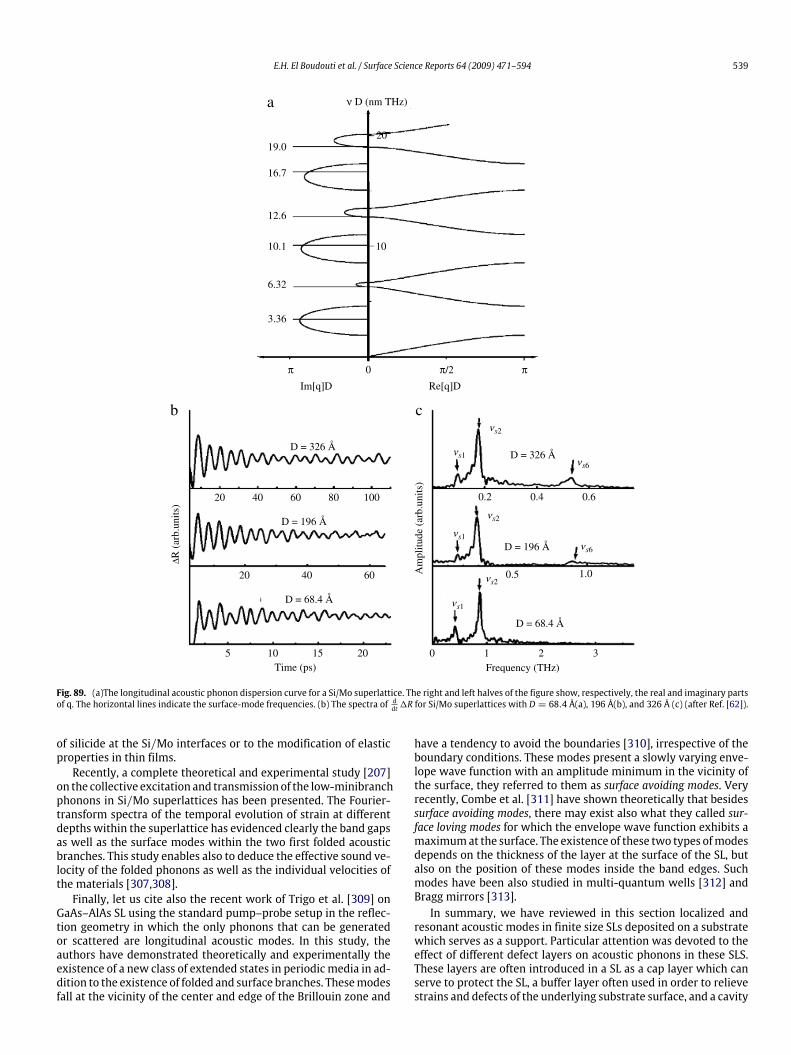
E.H. El Boudouti et al. / Surface Science Reports 64 (2009) 471–594 539

a ν D (nm THz)

19.0

16.7

12.6

10.1

6.32

3.36

20

10

Re[q]DIm[q]D

D = 326 Å

D = 196 Å

D = 68.4 Å

10 15

ΔR (

arb.

units

)

Am

plitu

de (

arb.

units

)

Frequency (THz)0 1 2 3

D = 68.4 Å

D = 196 Å

D = 326 Å

0.5 1.0

0.2 0.4 0.6

0 π ππ/2

20 40 60 80 100

20 40 60

5 20Time (ps)

b c

Fig. 89. (a)The longitudinal acoustic phonon dispersion curve for a Si/Mo superlattice. The right and left halves of the figure show, respectively, the real and imaginary partsof q. The horizontal lines indicate the surface-mode frequencies. (b) The spectra of ddt1R for Si/Mo superlattices with D = 68.4 Å(a), 196 Å(b), and 326 Å (c) (after Ref. [62]).

of silicide at the Si/Mo interfaces or to the modification of elasticproperties in thin films.Recently, a complete theoretical and experimental study [207]

on the collective excitation and transmission of the low-minibranchphonons in Si/Mo superlattices has been presented. The Fourier-transform spectra of the temporal evolution of strain at differentdepths within the superlattice has evidenced clearly the band gapsas well as the surface modes within the two first folded acousticbranches. This study enables also to deduce the effective sound ve-locity of the folded phonons as well as the individual velocities ofthe materials [307,308].Finally, let us cite also the recent work of Trigo et al. [309] on

GaAs–AlAs SL using the standard pump–probe setup in the reflec-tion geometry in which the only phonons that can be generatedor scattered are longitudinal acoustic modes. In this study, theauthors have demonstrated theoretically and experimentally theexistence of a new class of extended states in periodic media in ad-dition to the existence of folded and surface branches. Thesemodesfall at the vicinity of the center and edge of the Brillouin zone and

have a tendency to avoid the boundaries [310], irrespective of theboundary conditions. These modes present a slowly varying enve-lope wave function with an amplitude minimum in the vicinity ofthe surface, they referred to them as surface avoiding modes. Veryrecently, Combe et al. [311] have shown theoretically that besidessurface avoiding modes, there may exist also what they called sur-face loving modes for which the envelope wave function exhibits amaximumat the surface. The existence of these two types ofmodesdepends on the thickness of the layer at the surface of the SL, butalso on the position of these modes inside the band edges. Suchmodes have been also studied in multi-quantum wells [312] andBragg mirrors [313].In summary, we have reviewed in this section localized and

resonant acoustic modes in finite size SLs deposited on a substratewhich serves as a support. Particular attention was devoted to theeffect of different defect layers on acoustic phonons in these SLS.These layers are often introduced in a SL as a cap layer which canserve to protect the SL, a buffer layer often used in order to relievestrains and defects of the underlying substrate surface, and a cavity

540 E.H. El Boudouti et al. / Surface Science Reports 64 (2009) 471–594

layer that can be used for filtering certain frequencies. Differentguided modes induced by these layers have been investigatedand their interaction with modes localized at the free surfaceof the SL has been detailed. The localized and resonant modesassociated with these structures appear as well-defined peaks inthe DOS, with their relative importance being very dependenton the size of the SL, the wave vector k‖ and the defect layerthickness as well as on the parameters of the different constituentmaterials.On the other hand, we have also calculated the phonon phase

time expressions and shown that they present similar behaviors tothe DOS versus the frequency. We have shown that the presenceof the buffer layer (Fig. 81) increases strongly themagnitude of thetimedelay of the reflectedphonon associatedwith substrate/bufferlayer/SL interaction. This is in particular the case of a buffer layercharacterized by high velocities of sound which can play the roleof a barrier between phonons in the SL and the substrate. Theexperimental observation of the localized and resonant modespredicted here in such finite SLs may be possible with Ramanexperiments [75–77,206,208,209,218,282] and picosecond lasertechniques [45,59–63,207]. Some of the Raman experiments havebeen reproduced by our theoretical model.

6. Surface and interface sagittal elastic waves in semi-infinitesolid–solid superlattices

6.1. Introduction

Acoustic waves polarized in the sagittal plane which is definedby the normal to the surface and the wave vector k‖ parallel to thesurface involve two degree of vibrations. These modes have beeninvestigated theoretically during the last years using the transfermatrix [54,55,257,314] and the Green’s function [65,67,70,189,315–317] methods. In particular, surface localized and resonantmodes have been obtained and discussed in detail [54,55,65,67,189,257,317]. Experimentally, Brillouin scattering was performedon finite and semi-infinite SLs deposited on a substrate to observesome of the sagittal waves (Rayleigh, Sezawa) localized at thesurface of the SL [124–126,318,319]. In these works, the SL isconsidered as an effective homogeneous adlayer on a substrate;therefore, the effect of the elastic modulation properties of theSL (folding of bands, appearance of minigaps) is not taken intoaccount.The aim of this section is to investigate localized and resonant

modes induced by a free surface of the SL as well as by aSL/substrate interface inside the minigaps and the bulk bands ofthe SL. The effect of a cap layer has been discussed in Section 3.4.We shall focus our attention on the effect of the substrateparameters on interface modes, while the SL parameters are keptconstant. In particular, we shall discuss the effect of the stiffnessof the substrate [64], which acts as a barrier for phonons in the SL,on interface modes depending on whether the velocities of soundin the substrate are higher or lower than those of the materialsconstituting the SL. Such discussion enables us to turn smoothlyfrom the case of a free SL surface to the case of a rigidly boundSL surface. Due to the coupling of two degrees of vibrations, theGreen’s function calculation, from which the density of states andreflection coefficients are deduced, becomes rather complicatedas compared to the case of transverse vibrations (see Section 4)although it remains analytical [102].After a brief presentation of the model and the method of

calculation in Section 6.2, we give in Section 6.3 some numericalresults for a W/Al SL in contact with an homogeneous isotropicsubstrate. Section 6.4 gives some experimental techniques inrelation with the analytical results.

6.2. Model and method of calculation

The interface SL/substrate under consideration here is com-posed of a semi-infinite SL formed out of a semi-infinite repetitionof two different slabs (i = 1, 2) within the unit cell n, the SL is incontact with an homogeneous substrate i = s. All the interfacesare taken to be parallel to the (x1, x2) plane. The media forming thelayers of the SL and the substrate are assumed to be isotropic elas-tic media characterized by their mass densities ρ and their elasticconstants C11 and C44. The local and total densities of states are ob-tained exactly in the same way as those performed in Section 3.4for a semi-infinite SL ended with a cap layer, it is sufficient to con-sider this layer of semi-infinite extent.On the other hand, one of the most important boundary

value problems in acoustics is the scattering of a uniform planewave incident upon a plane boundary between two differentmedia [3]. Similarly to Section 3.3.2.2, one can calculate all thewaves reflected and transmitted at the substrate/SL interface [115].We shall focus our attention on reflected waves that are physicalquantities related to experiments [59,320–322]. Let us mentionthat our analytical results can of course be applied to anisotropicmedia without any formal problem [64,102,257]. The isotropiccontinuum model employed here is chosen for the sake ofsimplicity in order to obtain the basic information with thefewest complications possible. Let us notice that sagittal elasticwaves localized at the interface between two isotropic [13] orhexagonal [323] crystals, the so-called Stoneley waves, have beenstudied a long time ago.

6.3. Results and discussions

This subsection contains a discussion of the dispersion curvesand behavior of sagittal acoustic waves associated to the surface ofa SL or to the interface between a SL and a substrate. These localizedand resonant modes appear as well-defined features of the localor total densities of states. It will be shown that these modes alsogive rise to structures in the phases of the reflection coefficients. Inthese examples, the SLs are made of Al andWwith the parametersgiven in Table 1. The thicknesses d1 and d2 of the layers in the SLare assumed to be equal, the period of SL being D = d1+d2 = 2d1.The velocities of sound in the substrate are taken to be equal to βtimes those of the Al material (C (s)t = βC (Al)t and C (s)l = βC (Al)l )representing different barrier levels of the substrate for phononsin the SL. Furthermore, as in our works on shear horizontal wavesdeveloped in Section 4 (see also Refs. [37,38]), we shall discussthe existence of localized and resonant modes as a function of theparameter γ = C (s)44 /C

(Al)44 = C

(s)11 /C

(Al)11 , considering either that an

Al or aW layer of the SL is in contactwith the substrate. Though thisrepresentation was chosen for the sake of clarity, it is worthwhiletomention that the stress boundary conditions at the SL/ substrateinterface depend upon all the substrate parameters (C (s)44 , C

(s)11 , ρ

(s)).For a given value of β , the localized and resonant modes are givenfor several sets of the parameter γ presenting the stiffness of thesubstrate, which enables us to turn smoothly from the case of afree SL surface (γ = 0) to the case of a rigidly bound SL surface(γ →∞).

6.3.1. Bulk and surface elastic wavesFor a given frequency ω and k‖, the wave vectors along the

axis x3 of the SL which can be deduced from the bulk dispersionrelations are called k3. In the case of sagittal modes involving twocomponents of the displacement field, there are two pairs of k3associatedwith given k‖ andω, which can bewritten as±(K1+iL1)and±(K2+iL2). Nowan elasticwave at the frequencyω propagatesin the SL if L1 = 0 or L2 = 0 while it is attenuated if both L1 and L2

E.H. El Boudouti et al. / Surface Science Reports 64 (2009) 471–594 541

Im(k3D)

Im(k3D)

Re(k3D)

Re(k3D)

Im(k3D)

Im(k3D)

ωD

/Ct(A

l)

ωD/Ct(Al)

ab

Fig. 90. (a) Complex band structure (ω versus complex k3) in a W–Al SL with d1 = d2 = D/2 and k‖D = 3. Solid curves are k3 real (middle panel of the figure). Dash-dottedcurves are k3 imaginary (left panel). Dashed curves are the imaginary part of k3 when its real part is equal to π/D (right panel). In addition, when k3 is a complex quantity(Eq. (274)), the dotted curves give both its real and imaginary parts; in this case the imaginary part is presented in the left panel. (b) Same as in (a) enlarged in the range offrequencies where the indirect gap appears.

are different from zero. Each pair of k3 (the first, for instance) cantake four different forms; it can be(i) pure real (L1 = 0)(ii) pure imaginary (K1 = 0)(iii) complex but with (K1 = ±π/D)(iv) complex with (K1 6= π/D).

(273)

However, in case (iv) the two pairs of k3 necessarily become

K + iL, −(K + iL), K − iL, −(K − iL). (274)

Fig. 90(a) gives an example of the complex band structure(i.e., Ω = ωD/Ct(Al) versus k3D) in a W–Al SL showing thecombinations of the above-mentioned cases. One can see thepresence of direct gaps at the center and the edge of the reducedBrillouin zone, but also the possibility of indirect gaps inside thiszone (see Fig. 90(b) enlarged in the frequency domain 6.5 ≤ Ω ≤7.5). This is a consequence of coupling between the components ofthe displacement, i.e., themixing betweenwaves polarized in eachconstituent as a result of reflection and transmission phenomenaat the interfaces. Let us also mention that the imaginary parts ofk3 wave vectors in Fig. 90(a) give the attenuation of the possiblelocalized waves in the gaps.Fig. 91 gives the dispersion of the projected bulk bands

and surface modes (i.e., Ω versus k‖D). Due to the coupling oftwo degrees of freedom for vibrations, the bulk band structureinvolves two regions of frequencies, represented by horizontallyand vertically dashed lines, associated with each polarization ofthe waves. One can distinguish also the ranges of frequenciesbelonging simultaneously to both types of bands (horizontal plusvertical dashed lines) and the regions separating the differentshaded areas corresponding to gaps. Inside these gaps, wehave represented surface localized modes corresponding to twocomplementary semi-infinite SLs obtained by cleaving the infiniteW/Al SL in such a way that one obtains one SL with a full Al layer atthe surface (full lines) and its complementary with a fullW layer at

2

4

6

8

0

10

ωD

/Ct(A

l)

k//D1 2 3 4 5 60 7

Fig. 91. Bulk and surface sagittal elastic waves in W/Al SL. The curves giveωD/Ct (Al) as a function of k‖D, whereω is the frequency, k‖ the propagation vectorparallel to the interfaces. The horizontally and vertically shaded areas correspond tobulk bands associated with each of the two polarizations of the waves. The surfacemodes associated with two complementary SLs (ending, respectively, with a fullW layer or a full Al layer) are represented by dashed lines (W at the surface) andfull lines (Al at the surface). Some of the surface modes are very close to the bulkbands and cannot be distinguished from the latter at the scale of the figure; theyare indicated by arrows. The extensions of the localized modes into the bulk bandsas resonances are indicated by full circles when the SL terminates with an Al layer.

the surface (dashed lines). In this figure some of the surface modesassociated with a W layer at the surface, are very close to the bulk

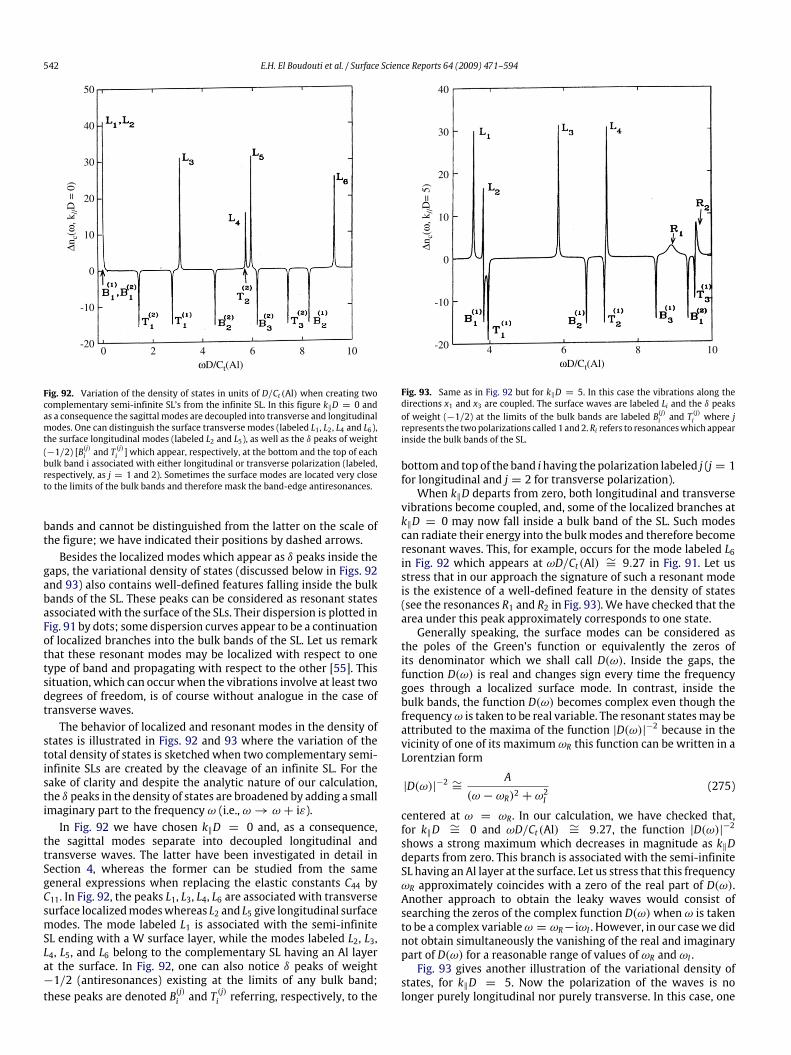
542 E.H. El Boudouti et al. / Surface Science Reports 64 (2009) 471–594

-10

0

10

20

30

40

4 6 82ωD/Ct(Al)

100-20

50

Δnc(

ω, k

//D =

0)

Fig. 92. Variation of the density of states in units of D/Ct (Al) when creating twocomplementary semi-infinite SL’s from the infinite SL. In this figure k‖D = 0 andas a consequence the sagittal modes are decoupled into transverse and longitudinalmodes. One can distinguish the surface transverse modes (labeled L1 , L2 , L4 and L6),the surface longitudinal modes (labeled L2 and L5), as well as the δ peaks of weight(−1/2) [B(j)i and T

(j)i ] which appear, respectively, at the bottom and the top of each

bulk band i associated with either longitudinal or transverse polarization (labeled,respectively, as j = 1 and 2). Sometimes the surface modes are located very closeto the limits of the bulk bands and therefore mask the band-edge antiresonances.

bands and cannot be distinguished from the latter on the scale ofthe figure; we have indicated their positions by dashed arrows.Besides the localized modes which appear as δ peaks inside the

gaps, the variational density of states (discussed below in Figs. 92and 93) also contains well-defined features falling inside the bulkbands of the SL. These peaks can be considered as resonant statesassociatedwith the surface of the SLs. Their dispersion is plotted inFig. 91 by dots; some dispersion curves appear to be a continuationof localized branches into the bulk bands of the SL. Let us remarkthat these resonant modes may be localized with respect to onetype of band and propagating with respect to the other [55]. Thissituation, which can occur when the vibrations involve at least twodegrees of freedom, is of course without analogue in the case oftransverse waves.The behavior of localized and resonant modes in the density of

states is illustrated in Figs. 92 and 93 where the variation of thetotal density of states is sketched when two complementary semi-infinite SLs are created by the cleavage of an infinite SL. For thesake of clarity and despite the analytic nature of our calculation,the δ peaks in the density of states are broadened by adding a smallimaginary part to the frequency ω (i.e., ω→ ω + iε).In Fig. 92 we have chosen k‖D = 0 and, as a consequence,

the sagittal modes separate into decoupled longitudinal andtransverse waves. The latter have been investigated in detail inSection 4, whereas the former can be studied from the samegeneral expressions when replacing the elastic constants C44 byC11. In Fig. 92, the peaks L1, L3, L4, L6 are associated with transversesurface localizedmodeswhereas L2 and L5 give longitudinal surfacemodes. The mode labeled L1 is associated with the semi-infiniteSL ending with a W surface layer, while the modes labeled L2, L3,L4, L5, and L6 belong to the complementary SL having an Al layerat the surface. In Fig. 92, one can also notice δ peaks of weight−1/2 (antiresonances) existing at the limits of any bulk band;these peaks are denoted B(j)i and T

(j)i referring, respectively, to the

4 6 8 10ωD/Ct(Al)

-10

0

10

20

30

-20

40

Δnc(

ω, k

//D=

5)

Fig. 93. Same as in Fig. 92 but for k‖D = 5. In this case the vibrations along thedirections x1 and x3 are coupled. The surface waves are labeled Li and the δ peaksof weight (−1/2) at the limits of the bulk bands are labeled B(j)i and T

(j)i where j

represents the twopolarizations called 1 and2.Ri refers to resonanceswhich appearinside the bulk bands of the SL.

bottomand top of the band ihaving the polarization labeled j (j = 1for longitudinal and j = 2 for transverse polarization).When k‖D departs from zero, both longitudinal and transverse

vibrations become coupled, and, some of the localized branches atk‖D = 0 may now fall inside a bulk band of the SL. Such modescan radiate their energy into the bulkmodes and therefore becomeresonant waves. This, for example, occurs for the mode labeled L6in Fig. 92 which appears at ωD/Ct(Al) ∼= 9.27 in Fig. 91. Let usstress that in our approach the signature of such a resonant modeis the existence of a well-defined feature in the density of states(see the resonances R1 and R2 in Fig. 93). We have checked that thearea under this peak approximately corresponds to one state.Generally speaking, the surface modes can be considered as

the poles of the Green’s function or equivalently the zeros ofits denominator which we shall call D(ω). Inside the gaps, thefunction D(ω) is real and changes sign every time the frequencygoes through a localized surface mode. In contrast, inside thebulk bands, the function D(ω) becomes complex even though thefrequencyω is taken to be real variable. The resonant statesmay beattributed to the maxima of the function |D(ω)|−2 because in thevicinity of one of its maximum ωR this function can be written in aLorentzian form

|D(ω)|−2 ∼=A

(ω − ωR)2 + ω2I

(275)

centered at ω = ωR. In our calculation, we have checked that,for k‖D ∼= 0 and ωD/Ct(Al) ∼= 9.27, the function |D(ω)|−2

shows a strong maximum which decreases in magnitude as k‖Ddeparts from zero. This branch is associated with the semi-infiniteSL having an Al layer at the surface. Let us stress that this frequencyωR approximately coincides with a zero of the real part of D(ω).Another approach to obtain the leaky waves would consist ofsearching the zeros of the complex function D(ω)when ω is takento be a complex variableω = ωR−iωI . However, in our casewe didnot obtain simultaneously the vanishing of the real and imaginarypart of D(ω) for a reasonable range of values of ωR and ωI .Fig. 93 gives another illustration of the variational density of

states, for k‖D = 5. Now the polarization of the waves is nolonger purely longitudinal nor purely transverse. In this case, one

E.H. El Boudouti et al. / Surface Science Reports 64 (2009) 471–594 543

1

2

4

3

2

4

6

8

0

10ω

D/C

t(Al)

1 2 3 4 5 6k//D

0 7

Fig. 94. Interface localized and resonant modes associated with the twocomplementary W/Al SLs in which the substrate is either in contact with an Alor a W layer. The heavy straight lines indicate the transverse and longitudinalvelocities of sound of the substrate. The parameters of the substrate are defined asβ = C (s)t /C

(Al)t = C (s)l /C

(Al)l = 2 and γ = C (s)44 /C

(Al)44 = C

(s)11 /C

(Al)11 = 0.5. When

the SL terminates with an Al layer, the localized (respectively, resonant) modesare presented by the full lines (respectively, full circles). The dashed line and thedashed arrows indicate an interface branch and the positions of some resonantmodes associated with a W termination of the SL, respectively.

can still notice the existence of antiresonances of weight −1/2at every edge of the bulk bands. The localized surface modes areagain denoted Li, whereas R1 and R2 are two resonant modeswhich appear as extensions of localizedmodes (see Fig. 91) locatedin the second and third minigaps into the bulk bands. We haveagain checked that the function |D(ω)|−2 contains maxima atthe frequencies of these resonant states when considering the SLterminated by an Al layer (but not the complementary SL endingwith a W layer).An interesting result is the observation that the variation of the

density of states (due to the creation of the two complementarySLs) is exactly equal to zero when the frequency ω belongssimultaneously to the bulk bands of both polarizations (domainswith horizontal and vertical dashed lines in Fig. 91). This result puttogether with the existence of antiresonances at the band limitsand the conservation of the total number of states implies thenecessary existence of surface states which may appear either aslocalized modes in the gaps or as resonant states belonging toonly one type of band (there is no analogue of such resonancesin the case of pure longitudinal or pure transverse waves).Let us emphasize that the localized states are a combinationof two decaying waves while the eigenvectors of the resonantmodes contain one propagating and one decaying component. Adetailed analysis of surface and pseudo-surface waves of sagittalpolarization has been given by Aono and Tamura [55].Now, to illustrate the interface localized and resonant modes,

we shall first discuss in detail two examples inwhich the velocitiesof sound in the substrate are fixed to two times those of the Almaterial (i.e., β = 2), while the substrate parameter γ takes twovery different values corresponding to a soft or to a stiff substrate.Although the velocities of sound in the substrate are rather high torepresent a given material, they have been chosen for the sake ofsimplicity in order to give a qualitative description of the differentkinds of modes induced by the SL/substrate interface. When the

0

20

0

20

0

20

0

20

0

20

4 6 80 10ωD/Ct(Al)

a

b

c

d

e

2Δn

(ω, k

//D =

3.8

)Δn

(ω, k

//D =

3.4

)Δn

(ω, k

//D =

3 )

Δn(ω

, k//D

= 1

.7 )

Δn(ω

, k//D

= 1

.9 )

Fig. 95. Variation of theDOS [in units ofD/Ct (Al)] for the semi-infinite SLwith anAllayer in contact with the substrate for: k‖D = 1.7 (a), 1.9(b), 3(c), 3.4(d), and 3.8(e).The contributions of the infinite SL and substrate have been subtracted. Bi and Tirefer to δ peaks of weight (−1/4) at the edges of the different bulk bands, Li andRi indicate localized and resonant modes induced by the SL/substrate interface. Btsand Bls refer to δ peaks of weight (−1/4) situated at the transverse and longitudinalvelocities of sound in the substrate.

velocities of sound in the substrate are less or equal to those of theAlmaterial (i.e.,β ≤ 1), the localized and resonant interfacemodeshave different behaviors, which are discussed in the second part ofthis subsection.

6.3.2. Substrate with high elastic wave velocities

6.3.2.1. Case of a soft substrate. Let us consider first a soft substratein which β = 2 and γ takes a weak value (e.g., γ = 0.5).Fig. 94 gives the localized and resonant interface modes for boththe complementary SLs in which the substrate is either in contactwith a full Al or a full W layer. When the substrate is in contactwith a full Al layer, the two full lines in the minigaps of the SL inFig. 94 are localized interface modes, while the modes lying abovethe transverse velocity of sound of the substrate (continuum)represent resonant modes (full circle curves). We shall also callresonances, the modes falling inside the SL bulk bands. In spiteof the small value of γ (γ = 0.5), the frequencies of the interfacecurves (especially those of the resonant modes) drastically changein comparison with the case γ = 0 (Fig. 91), showing that theinterfacemodes strongly depend on the parameter γ . The interfacemodes in Fig. 94 are obtained from the maxima of the DOS, shownin Fig. 95 for a few values of the wave vector k‖D. Li and Ri,respectively, indicate the localized and resonantmodes induced bythe SL/substrate interface. Bi and Ti, respectively, represent δ peaksof weight (−1/4) (antiresonances) located at the bottom and thetop of the bands. Bts and Bls, respectively, indicate δ peaks of weight(−1/4) at the bottom of the transverse and longitudinal velocitiesof sound in the substrate. One cannotice in Fig. 95 that the resonantmodes labeled R2 and R3 and associated with the two curves lyingbetween Bts and Bls in Fig. 94, present a noticeable intensity forsome ranges of k‖D and even appear as δ functions at k‖D ∼= 1.9[Fig. 95(b)] for the lower resonance R2 and at k‖D ∼= 3.4 [Fig. 95(d)]for the upper resonance R3. A better insight into the variation of

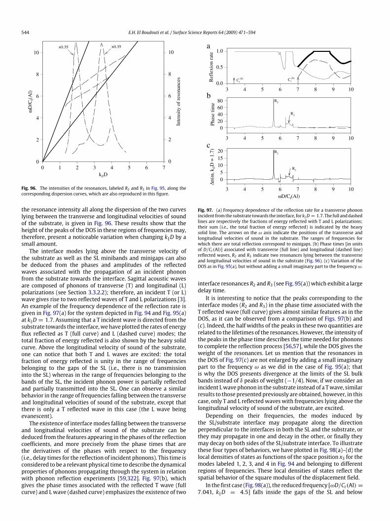
544 E.H. El Boudouti et al. / Surface Science Reports 64 (2009) 471–594

x0.35x0.35

0

2

4

6

8

10

ωD

/Ct(A

l)

1 2 3 4 5 6k//D

0 70

2

4

6

8

10

Inte

nsity

of

reso

nanc

es

Fig. 96. The intensities of the resonances, labeled R2 and R3 in Fig. 95, along thecorresponding dispersion curves, which are also reproduced in this figure.

the resonance intensity all along the dispersion of the two curveslying between the transverse and longitudinal velocities of soundof the substrate, is given in Fig. 96. These results show that theheight of the peaks of the DOS in these regions of frequencies may,therefore, present a noticeable variation when changing k‖D by asmall amount.The interface modes lying above the transverse velocity of

the substrate as well as the SL minibands and minigaps can alsobe deduced from the phases and amplitudes of the reflectedwaves associated with the propagation of an incident phononfrom the substrate towards the interface. Sagittal acoustic wavesare composed of phonons of transverse (T) and longitudinal (L)polarizations (see Section 3.3.2.2); therefore, an incident T (or L)wave gives rise to two reflected waves of T and L polarizations [3].An example of the frequency dependence of the reflection rate isgiven in Fig. 97(a) for the system depicted in Fig. 94 and Fig. 95(a)at k‖D = 1.7. Assuming that a T incident wave is directed from thesubstrate towards the interface,wehaveplotted the rates of energyflux reflected as T (full curve) and L (dashed curve) modes; thetotal fraction of energy reflected is also shown by the heavy solidcurve. Above the longitudinal velocity of sound of the substrate,one can notice that both T and L waves are excited: the totalfraction of energy reflected is unity in the range of frequenciesbelonging to the gaps of the SL (i.e., there is no transmissioninto the SL) whereas in the range of frequencies belonging to thebands of the SL, the incident phonon power is partially reflectedand partially transmitted into the SL. One can observe a similarbehavior in the range of frequencies falling between the transverseand longitudinal velocities of sound of the substrate, except thatthere is only a T reflected wave in this case (the L wave beingevanescent).The existence of interfacemodes falling between the transverse

and longitudinal velocities of sound of the substrate can bededuced from the features appearing in the phases of the reflectioncoefficients, and more precisely from the phase times that arethe derivatives of the phases with respect to the frequency(i.e., delay times for the reflection of incident phonons). This time isconsidered to be a relevant physical time to describe the dynamicalproperties of phonons propagating through the system in relationwith phonon reflection experiments [59,322]. Fig. 97(b), whichgives the phase times associated with the reflected T wave (fullcurve) and L wave (dashed curve) emphasizes the existence of two

R2

R2

R3

R3

Ct(S) C (S)

103 4 5 6 7 8 9

103 4 5 6 7 8 9

4 5 6 7 8 9 103ωD/Ct(Al)

204060

0.5

Ref

lexi

on r

ate

0.0

1.0

Phas

e tim

e

0

80

05

101520

Δn(ω

, k//D

= 1

.7)

a

b

c

Fig. 97. (a) Frequency dependence of the reflection rate for a transverse phononincident from the substrate towards the interface, for k‖D = 1.7. The full anddashedlines are respectively the fractions of energy reflected with T and L polarizations;their sum (i.e., the total fraction of energy reflected) is indicated by the heavysolid line. The arrows on the ω axis indicate the positions of the transverse andlongitudinal velocities of sound in the substrate. The ranges of frequencies forwhich there are total reflection correspond to minigaps. (b) Phase times [in unitsof D/Ct (Al)] associated with transverse (full line) and longitudinal (dashed line)reflected waves, R2 and R3 indicate two resonances lying between the transverseand longitudinal velocities of sound in the substrate (Fig. 96). (c) Variation of theDOS as in Fig. 95(a), but without adding a small imaginary part to the frequency ω.

interface resonances R2 and R3 (see Fig. 95(a)) which exhibit a largedelay time.It is interesting to notice that the peaks corresponding to the

interface modes (R2 and R3) in the phase time associated with theT reflected wave (full curve) gives almost similar features as in theDOS, as it can be observed from a comparison of Figs. 97(b) and(c). Indeed, the half widths of the peaks in these two quantities arerelated to the lifetimes of the resonances. However, the intensity ofthe peaks in the phase time describes the time needed for phononsto complete the reflection process [56,57], while the DOS gives theweight of the resonances. Let us mention that the resonances inthe DOS of Fig. 97(c) are not enlarged by adding a small imaginarypart to the frequency ω as we did in the case of Fig. 95(a); thatis why the DOS presents divergence at the limits of the SL bulkbands instead of δ peaks of weight (−1/4). Now, if we consider anincident Lwave phonon in the substrate instead of a Twave, similarresults to those presented previously are obtained, however, in thiscase, only T and L reflected waves with frequencies lying above thelongitudinal velocity of sound of the substrate, are excited.Depending on their frequencies, the modes induced by

the SL/substrate interface may propagate along the directionperpendicular to the interfaces in both the SL and the substrate, orthey may propagate in one and decay in the other, or finally theymay decay on both sides of the SL/substrate interface. To illustratethese four types of behaviors, we have plotted in Fig. 98(a)–(d) thelocal densities of states as functions of the space position x3 for themodes labeled 1, 2, 3, and 4 in Fig. 94 and belonging to differentregions of frequencies. These local densities of states reflect thespatial behavior of the square modulus of the displacement field.In the first case (Fig. 98(a)), the reduced frequency [ωD/Ct(Al) =

7.041, k‖D = 4.5] falls inside the gaps of the SL and below

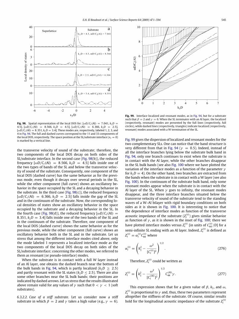
E.H. El Boudouti et al. / Surface Science Reports 64 (2009) 471–594 545

0

20

0

3

6

0

10

20

10

40

0

Loc

al d

ensi

ty o

f st

ates

-6 -4 -2 0 2 4x3/D

a

b

c

d

Fig. 98. Spatial representation of the local DOS for: [ωD/Ct (Al) = 7.041, k‖D =4.5], [ωD/Ct (Al) = 8.566, k‖D = 4.5], [ωD/Ct (Al) = 6.366, k‖D = 2.5],[ωD/Ct (Al) = 8.351, k‖D = 3.4]. These modes are, respectively, labeled 1, 2, 3, and4 in Fig. 94. The full and dashed curves correspond to the 11 and 33 components ofthe local DOS, respectively. The space position at the SL/substrate interface (x3 = 0)is marked by a vertical line.

the transverse velocity of sound of the substrate; therefore, thetwo components of the local DOS decay on both sides of theSL/substrate interface. In the second case (Fig. 98(b)), the reducedfrequency [ωD/Ct(Al) = 8.566, k‖D = 4.5] falls inside one ofthe two types of bands of the SL and below the transverse veloc-ity of sound of the substrate. Consequently, one component of thelocal DOS (dashed curve) has the same behavior as for the previ-ous mode, even though it decays over several periods in the SL,while the other component (full curve) shows an oscillatory be-havior in the space occupied by the SL and a decaying behavior inthe substrate. In the third case (Fig. 98(c)), the reduced frequency[ωD/Ct(Al) = 6.366, k‖D = 2.5] falls inside the gap of the SLand in the continuum of the substrate. Now, the corresponding lo-cal densities of states show an oscillatory behavior in the spaceoccupied by the substrate and a decaying behavior in the SL. Inthe fourth case (Fig. 98(d)), the reduced frequency [ωD/Ct(Al) =8.351, k‖D = 3.4] falls inside one of the two bands of the SL andin the continuum of the substrate. Therefore, one component ofthe local DOS (dashed curve) shows the same behavior as for theprevious mode, while the other component (full curve) shows anoscillatory behavior both in the SL and in the substrate. Let usstress that among the different interface modes cited above, onlythe mode labeled 1 represents a localized interface mode as thetwo components of the local DOS decay on both sides of theSL/substrate interface; concerning the other modes, we referred tothem as resonant (or pseudo-interface) modes.When the substrate is in contact with a full W layer instead

of an Al layer, one obtains the dashed branch near the bottom ofthe bulk bands in Fig. 94, which is partly localized (k‖D ≥ 2.5)and partly resonant with the SL states (k‖D ≤ 2.5). There are alsosome other branches near the SL bulk bands; their positions areindicated by dashed arrows. Let us stress that the results illustratedabove remain valid for any values of γ such that 0 < γ < 1 (softsubstrates).

6.3.2.2. Case of a stiff substrate. Let us consider now a stiffsubstrate in which β = 2 and γ takes a high value (e.g., γ = 6).

2

4

6

8

0

10

ωD

/Ct(A

l)

1 2 3 4 5 60 7k//D

Fig. 99. Interface localized and resonant modes, as in Fig. 94, but for a substratesuch that β = 2 and γ = 6. When the SL terminates with an Al layer, the localized(respectively, resonant) modes are presented by the full lines (respectively, fullcircles), while dashed lines (respectively, triangles) indicate localized (respectively,resonant) modes associated with a W termination of the SL.

Fig. 99 gives the dispersion of localized and resonantmodes for thetwo complementary SLs. One can notice that the band structure isvery different from that in Fig. 94 (γ = 0.5). Indeed, instead ofall the interface branches lying below the substrate bulk band inFig. 94, only one branch continues to exist when the substrate isin contact with the Al layer, while the other branches disappearin the SL bulk bands (see also Fig. 100 where we have plotted thevariation of the interface modes as a function of the parameter γfor k‖D = 4). On the other hand, two branches are extracted fromthe bands when the substrate is in contact with aW layer (see alsoFig. 100). In the continuum of the substrate bulk band, only someresonant modes appear when the substrate is in contact with theAl layer of the SL. When γ goes to infinity, the resonant modesdisappear, and the three interface branches situated below thetransverse velocity of sound of the substrate tend to the standingwaves of a W–Al bilayer with rigid boundary conditions on bothsides as it is shown in Fig. 100. It is interesting to notice thatthe dependence of interface modes as function of the transverseacoustic impedance of the substrate (Z (s)t ) gives similar behavioras function of γ , as it is shown in the inset of Fig. 100; there wehave plotted interface modes versus Z (s)t [in units of C

(s)44 /D] for a

semi-infinite SL ending with an Al layer. Indeed, Z (s)t is defined asZ (s)t = α

(s)t C

(s)44 where

α(s)t =

(k2‖−

ω2

[C (s)t ]2

)1/2. (276)

Therefore, Z (s)t could be written as

Z (s)t =

(k2‖−

ω2

[C (Al)t ]2

)1/2C (Al)44 γ . (277)

This expression shows that for a given value of β , k‖, and ω,Z (s)t is proportional to γ and, thus, these two parameters representaltogether the stiffness of the substrate. Of course, similar resultshold for the longitudinal acoustic impedance of the substrate Z (s)l

546 E.H. El Boudouti et al. / Surface Science Reports 64 (2009) 471–594

γ

1

32

( S )

0 1 0 2 0 3 0

ωD

/Ct(A

l)

2

4

6

8

1

23

zt(s)

8

6

4

2

1 2 3

4

6

2

8

ωD

/Ct(A

l)

180 3 6 9 12 15

0 10 20 30

ωD

/Ct(A

l)

Fig. 100. Variation of the frequencies of the interface modes as a function of theparameter γ , for β = 2 and k‖D = 4. The substrate is either in contact withan Al layer (full lines) or a W layer (dashed lines) of the SL. When the interfacebranches penetrate in the SL bulk bands (shaded areas), they become resonantstates represented by full circles (respectively, triangles) when the SL terminateswith an Al layer (respectively, a W layer). The horizontal heavy line atωD/Ct (Al) =8 indicates the bottom of the substrate bulk band. When γ increases from 0 to∞,the interface modes of the two complementary SLs move from the standing modesof a W–Al unit cell with stress-free boundary conditions (given by horizontallydashed arrows on the left-hand side of the figure) to the standing modes of theW–Al unit cell with rigid boundary conditions (given by horizontally dashed arrowson the right-hand side of the figure). Inset: Frequency dependence of the interfacemodes as a function of the transverse acoustic impedance of the substrate Z (s)t [inunits of C (Al)44 /D] when the SL terminates with an Al layer.

defined as Z (s)l = α(s)l C

(s)11 where

α(s)l =

(k2‖−

ω2

[C (s)l ]2

)1/2. (278)

On the other hand, when γ (or Z (s)t ) increases, the amplitudeof the vibrations goes to zero at the SL/substrate interface (inaccordance with the rigid boundary conditions); this is shown inFig. 101 where we have given the local DOS for the modes labeled1, 2, and 3 in Fig. 100 and corresponding to γ = 0.5, 6 and 20[or Z (s)t = 1.128, 10.267, and 30.494, see the inset of Fig. 100],respectively.

6.3.3. Substrate with lower elastic wave velocitiesThe frequencies of the interface modes are also very sensitive

to the velocities of sound in the substrate. We have presented inFig. 102 the dispersion of interface modes for two lower valuesof the parameter β representing the level of the substrate barrierβ = 1 (Fig. 102(a)) and β = 0.5 (Fig. 102(b)) and for two differentvalues of the parameter γ (γ = 0.5 and γ = 6) correspondingto soft and stiff substrates, respectively. Note that for the sakeof clarity, we have plotted in these figures the reduced velocityC/Ct(Al) instead of the reduced frequency ωD/Ct(Al). Fig. 102(a)and (b) clearly show that the interface modes depend strongly onβ . Indeed, in the first case (Fig. 102(a)) corresponding to β = 1,all the interface branches lying above the transverse velocity ofsound of the substrate disappear.When the substrate is consideredas a stiff material (γ = 6), one obtains only two interfacebranches below the transverse velocity of sound of the substrate

0

10

20

0

10

20

30

10

20

30

-3 -2 -1 0 1 2 3-4 4x3/D

30

0

Loc

al d

ensi

y of

sta

tes

a

b

c

Fig. 101. Spatial representation of the local DOS for the modes labeled 1, 2, and3 in Fig. 100 and corresponding, respectively, to ωD/Ct (Al) = 6.606(a), 7.231(b),and 7.396(c) at γ = 0.5, 6, and 20 [or Z (s)t = 1.128, 10.267, and 30.494]. Thefull and dashed curves correspond to the 11 and 33 components of the local DOS,respectively.

0.50

0.75

1.00

C/C

t(Al)

2 3 4 5 61k//D

0 7

2 3 4 5 61k//D

0 7

a

b

Ct(S)

Ct(S)

C (S)

0.75

C/C

t(Al)

0.50

1.00

Fig. 102. Same as in Fig. 94 but for different parameters of the substrate. (a) β = 1and γ takes two different values: γ = 6 (the corresponding curves are indicated byfull and dash-dotted curves associated with two complementary SLs ending withan Al and a W layers, respectively) and γ = 0.5 (the corresponding curves areindicated by dotted and dashed curves associated with the two complementarySLs cited above, respectively). (b) Same as in (a) but for a substrate with velocitiesof sound such that β = 0.5. Notice that the dashed interface localized branch in(a) becomes now a resonant branch indicated by triangles. The horizontally heavylines indicate the positions of transverse and longitudinal velocities of sound in thesubstrate. In order to obtain a good separation between the interface modes, wehave represented the reduced velocity C/Ct (Al) instead of the reduced frequencyωD/Ct (Al).

E.H. El Boudouti et al. / Surface Science Reports 64 (2009) 471–594 547

corresponding respectively to two complementary SLs endingwithan Al layer (full line) and aW layer (dash-dotted line); thesemodesappear as localizedmodeswithin the first SLminigap for k‖D ≥ 2.5and continue as resonances in the first miniband for k‖D ≤ 2.5.When the substrate is assumed to be a soft material (γ = 0.5),one obtains two branches near the bottom of the first miniband ofthe SL as in Fig. 94, and corresponding also to two complementarySLs ending either with an Al layer (dotted curve) or with a W layer(dashed curve).When β decreases (see Fig. 102(b) for β = 0.5), the two

latter branches corresponding to a soft substrate, shift slightly asfunction of k‖D and become now two resonant modes lying abovethe transverse velocity of sound of the substrate and in the vicinityof the first SL miniband. Furthermore, the branch represented bythe triangle curve in Fig. 102(b) appears as a well-defined peakin the DOS and give rise to a large time delay in the phase time,similarly to the example shown in Fig. 97(b). However, in thecase of a stiff substrate, the two branches obtained in Fig. 102(a)(full and dash-dotted curves), shift downwards when β decreases,giving rise to only one localized interface branch in Fig. 102(b) (fullcurve) at the vicinity of the transverse velocity of sound of thesubstrate when the SL terminates with an Al material.Finally, let us mention that when the stiffness of the substrate

goes from zero [γ (or Z (s)t ) = 0] to infinity [γ (or Z(s)t )→∞], the

interface localized branches in Fig. 102 move smoothly from thestanding modes of a unit cell with stress-free boundary conditionsto the standingmodes of a unit cell with rigid boundary conditions.Another interesting result (not detailed here) is to observe that,contrary to the case of shear horizontal waves, the interfacemodesof sagittal polarizationmay exist at the SL/substrate interface eventhough the substrate is of the same nature as one of the twomaterials constituting the SL (symmetrical termination of the SL);for instance, this is the case for aWsubstrate in contactwith aW/AlSL ending with an Al layer. These modes are equivalent to the so-called Stoneley modes at the W/Al interface.

6.4. Relation to experiments

The observation of the different kinds of localized and resonantmodes predicted here at the SL/substrate interface may bepossible with Brillouin scattering experiments [123–125,163–165,250,324–326] and picosecond laser technique [59,322]. Indeed, inBrillouin experiments, the radiation often used is λ = 5145 Å,which leads to a range of wave vectors k‖D < 5 when themodulation wavelength D is such that D < 4000 Å. MetallicSLs with such periods have been realized [250,325,326] even ifin general the SL periods do not exceed 400 Å (Refs. [123–125]).In addition, the observation of sagittal acoustic waves below andabove the transverse velocity of sound of the substrate has beenperformed [123–125,147–149]. On the other hand, the magnitudeof the peaks associated with the interface resonances in the phasetime (Fig. 97(b)) reaches a value as large as 90 [in units ofD/Ct(Al)].This means that for a typical value of the period D (D < 4000 Å),themagnitude of the time delay τ is such τ < 11 ns, which is in therange detectable by a phonon experiment using picosecond lasertechnique [59,322]. Let us also stress that the reflection coefficients(deduced here from the knowledge of the Green’s function) areuseful quantities in calculating the thermal transport between asolid and a multilayered medium instead of a solid–solid [327]interface. Our calculation can also be easily extended to the caseof a multilayer–liquid interface [320,328,329] as it will be detailedin the next section.In summary, the results presented in this section are based

on an analytical calculation of the Green’s functions of acousticwaves of sagittal polarization associated with the SL/substrate

interface [65]. These complete Green’s functions can be used tostudy any physical property of the SL/substrate system. Theseinclude the calculations of local and total densities of states and thedetermination of the dispersion relation for surface and interfacemodes in this structure. Of course, the Green’s function approachused in this analysis also enables us to obtain the reflection ratesand the corresponding phase times associated with a reflectedwave from an incident phonon in the substrate.In the case of semi-infinite SLs, we have shown the existence

of antiresonances of weight (−1/2) at the edges of any bulk banddue to the creation of two semi-infinite SLs from an infinite one,and, as a consequence, the necessary existence of localized andresonant surface modes associated with either one or the othercomplementary SL. The resonant or pseudo-surface waves mayappear as extensions of localized modes into the bulk bands of SLs.In the case of semi-infinite SLs in contact with substrate, we

have shown the existence of localized and resonant modes (alsocalled leaky or pseudowaves) induced by such interface. Particularattention was devoted to the effect of the stiffness of the substrateon these interface modes depending on whether the velocitiesof sound in the substrate are lower or higher than those in thematerials constituting the SL. In particular, we have shown thatthe localized interface modes of two complementary SLs movefrom the standing waves of a unit cell with stress-free boundaryconditions to the standing waves of a unit cell with rigid boundaryconditions, when the stiffness of the substrate goes from zeroto infinity (Fig. 100). The localized and resonant interface modesappear as well-defined peaks of the DOS, with their relativeimportance being very dependent on the wave vector k‖ and thenature of the layer of the SL in contact with the substrate.On the other hand, the calculations of the reflection coefficients

at the substrate/SL interface show that their amplitudes do not giveany information on interfacemodes lying inside the gaps, howevertheir phase times illustrate clearly the positions of these modeswith their corresponding time delays. Moreover, these interfacemodes present almost similar features in the phase time andthe DOS versus the frequency. Let us mention finally, that theSL/substrate interface presents a fruitful structure for the existenceof interface modes in comparison with the interface betweentwo homogeneous media where the existence of interface modes(Stoneley modes) becomes rather rare to find [3].

7. Surface and interface sagittal elastic waves in semi-infinitesolid–fluid superlattices

7.1. Introduction

Wave propagation in alternating elastic solid and idealfluid layers is carried out by Rytov [89] and summarized byBrekhovskikh [88]. Rytov’s approach has been used by Schöen-berg [90] together with propagator matrix formalism to accountfor propagation through such a periodic medium in any directionof propagation and at arbitrary frequency. Similar results are alsoobtained byRousseau [91]. In the low frequency limit, itwas shownthat besides the existence of small gaps, there is one wave speedfor propagation perpendicular to the layering and twowave speedsfor propagation parallel to the layeringwhich arewithout analoguein solid–solid SLs. The two latter speeds both correspond to com-pressional waves and their existence is suggestive of Biot’s the-ory [92] of wave propagation in porous media. The experimentalevidence [96] of these waves is carried out using ultrasonic tech-niques in Al–water and Plexiglas–water SLs. Also, it was showntheoretically and experimentally that finite size layered structurescomposed of a few cells of solid–fluid layers with one [97,98] ormultiple [99] periodicity may exhibit large gaps and the presence

548 E.H. El Boudouti et al. / Surface Science Reports 64 (2009) 471–594

of defect layers in these structures may give rise to well-defineddefect modes in these gaps [98].In this section, we show the possibility of existence of surface

and interface waves associated with the surface of a semi-infinitesolid–fluid SL or its interface with an homogeneous fluid [330].We give explicit dispersion relations for surface acoustic wavesin semi-infinite solid–fluid SLs with a surface cap layer. The caplayer may be a fluid layer or a solid layer different from thoseconstituting the bulk SL. When the thickness of the cap layer goesto zero or to infinity, we obtain the results for a SL with a freesurface or for the interface between a SL and an homogeneousmedium respectively.The organization of this section is as follows. Section 7.2

presents themodelweuse for these studies aswell as the analyticalresults obtained for the dispersion relations of bulk and surfacewaves in the above-discussed heterostructures. The analyticalexpressions of local and total DOS are rather complicated, thereforewe shall present a brief summary of the method of calculation ofthese DOS. The expressions of the Green’s functions necessary forall these studies are given in Section 2. Section 7.3 contains thenumerical results for Plexiglas–water and Al–water semi-infiniteSLs with or without a surface cap layer and for such semi-infiniteSLs in contact with a homogeneous fluid.

7.2. The theoretical model

We are interested in the propagation of acoustic wavespolarized in the sagittal plane defined by the normal to theinterfaces (x3 direction) and the wave vector k‖ (parallel to theinterfaces). We choose k‖ along the x1 direction. Before addressingthe problem of the fluid–solid SL, it is helpful to know the surfaceelements of its elementary constituents, namely, the Green’sfunction of an ideal fluid of thickness df , sound speed vf andmass density ρf and an elastic isotropic solid characterized byits thickness ds, longitudinal speed v`, transverse speed vt , andmass density ρs. The Green’s function of the elastic solid in thespace of the two surfaces of the layer is a 4 × 4 matrix as itexhibits two directions of vibrations (see Section 2.3.3), while theGreen’s function of an ideal fluid (for which the viscous shearstress vanishes) is a 4× 4 matrix where only x3x3 components aredifferent from zero (see Section 2.4) [115]. Therefore, the 4 × 4matrix of the fluid layer may be reduced to only a 2 × 2 matrixcomposed by the x3x3 elements. We shall call this matrix

[gf (MM)]−1 =(a bb a

), (279)

where

a = −FCfSf, b =

FSf, F = −ρf

ω2

αf, (280)

Cf = cosh(αf df ), Sf = sinh(αf df ), (281)

and

α2f = k2‖−ω2

v2f. (282)

It is worthwhile to notice that the assumption of ideal fluidbehavior is valid over a very broad frequency range for which theviscous skin depth σ = (2η/ρω), is much smaller than the fluidlayer thickness df (η is the viscosity of the fluid).As concerns the elastic layer, its 4 × 4 matrix may be also

reduced to a 2 × 2 matrix as far as it is surrounded by fluids onboth sides. This is due to the fact that the shear stress vanisheson both surfaces. The reduction of the 4 × 4 matrix of the elasticsolid must be done carefully by inverting the 4× 4 matrix given in

Section 2.3.3 and keeping only the x3x3 components of this matrixto form a 2 × 2 matrix. Then by inverting again this matrix, weobtain a 2 × 2 Green’s function matrix of the solid layer that maybe juxtaposed to the 2× 2 matrix of the fluid layer to form the SL.After some algebraic calculations, the expression of this matrix canbe written in a closed form as

[gs(MM)]−1 =(A BB A

), (283)

where

A = −γC`S`− β

CtSt, B =

γ

S`+β

St, (284)

γ = ρv4t

ω2α`(k2‖+ α2t )

2, β = −4ρv4t

ω2αtk2‖ (285)

Ct = cosh(αtds), C` = cosh(α`ds), (286)St = sinh(αtds), S` = sinh(α`ds) (287)

and

α2t = k2‖−ω2

v2t, α2` = k

2‖−ω2

v2`. (288)

The inverse Green’s function of a semi-infinite fluid and a semi-infinite solid with free surfaces are given respectively by

g−1f (0, 0) = −F (289)

and

g−1s (0, 0) = −γ − β (290)

where F is defined by Eq. (280) and γ and β are given by Eq. (285).Now, the calculation of the dispersion relations of an infinite SL

or a semi-infinite SL with or without a surface cap layer becomesanalogous to that of shear horizontal waves in solid–solid SLs (seeSection 4) including only one degree of vibration. The effect of theshear waves in solid layers implicitly appears in the terms A and B(Eqs. (283)–(288)). Indeed, if the transverse velocity of sound in thesolid layer vanishes (i.e., vt = 0 in Eqs. (283)–(288)), one obtainsthe results for a SL made of alternating two different fluids.

7.2.1. Dispersion relationsThe Green’s function of the infinite SL (Fig. 103(a)) is obtained

by a linear juxtaposition of the 2×2matrices (Eqs. (279) and (283))at the different interfaces, leading to a tridiagonal matrix. After aFourier transform, we obtain the following expression giving thedispersion relation of an infinite SL:

cos(k3D) =A2 − B2 + a2 − b2 + 2Aa

2Bb(291)

where k3 is the component perpendicular to the slabs of thepropagation vector

−→k ≡ (k‖, k3).

In the same way, the dispersion relation giving the surfacemodes for a semi-infinite SL terminated with a fluid cap layercharacterized by its mass density ρ0, sound speed v0 and thicknessd0 (Fig. 103(b)), is given by

a(B2 − A2)− A(a2 − b2)−f0S0C0[A2 − B2 − a2 + b2]

+

(f0S0C0

)2(A+ a) = 0 (292)

together with the following condition:∣∣∣∣∣Bb(a+ f0S0

C0

A− f0S0C0

)∣∣∣∣∣ > 1 (293)

E.H. El Boudouti et al. / Surface Science Reports 64 (2009) 471–594 549

d

df

ds

D

F0

S

F

F

S

d0

Cel

l -2

C

ell

-1

Cel

l 0

S

F

S

S

F

F

a b

ds

df

D

F

S

S

F

Cel

l -2

C

ell

-1

Cel

l 0

c

S0

•

••

•

••

••

x3 x3 x3

Cel

l -1

C

ell

0

Cel

l 1

Fig. 103. (a) Schematic representation of an infinite solid/fluid superlattice (SL).(b): Schematic representation of a semi-infinite solid/fluid SL with a fluid cap layer.(c): Schematic representation of a semi-infinite solid/fluid SL with a solid cap layer.ds , df and d0 are, respectively, the thicknesses of the solid, fluid and cap layers.D = df + ds is the period of the SL.

where

C0 = cosh(α0d0), S0 = sinh(α0d0), (294)

and

f0 = −ρ0ω2

v20, α20 = k

2‖−ω2

v20. (295)

The latter condition (Eq. (293)) ensures that thewaves are decayingfrom the surface when penetrating into the SL.From these general expressions, we can deduce:(i) the expressions giving the surface modes for a semi-infinite

SL without a cap layer (i.e., d0 = 0, S0 = 0)

a(B2 − A2)− A(a2 − b2) = 0 (296)

with the condition∣∣∣∣ a BA b∣∣∣∣ > 1. (297)

(ii) The expressions giving the interface modes between a SL andan homogeneous fluid of a semi-infinite extent (i.e., d0 −→ ∞,S0C0−→ 1)

a(B2 − A2)− A(a2 − b2)− f0[A2 − B2 − a2 + b2]

+ (f0)2(A+ a) = 0 (298)

with the condition∣∣∣∣Bb(a+ f0A− f0

)∣∣∣∣ > 1. (299)

When the SL is terminated with a solid cap layer (Fig. 103(c))characterized by its thickness d0, mass density ρ0 and transverseand longitudinal sound speeds vt0 and v`0 respectively, theexpression giving the surface modes is given by

a(B2 − A2)− A(a2 − b2)− F0[A2 − B2 − a2 + b2]

+ F 20 (A+ a) = 0 (300)

together with the condition∣∣∣∣bB(A− F0a+ F0

)∣∣∣∣ > 1 (301)

where

F0 =A20 − B

20

A0, (302)

A0 = −γ0C`0S`0− β0

Ct0St0, B0 =

γ0

S`0+β0

St0, (303)

γ0 = ρ0v4t0

ω2α`0(k2‖+ α2t0)

2, β0 = −4ρv4t0

ω2αt0k2‖, (304)

Ct0 = cosh(αt0d0), C`0 = cosh(α`0d0), (305)St0 = sinh(αt0d0), S`0 = sinh(α`0d0), (306)

and

α2t0 = k2‖−ω2

v2t0, α2`0 = k

2‖−ω2

v2`0. (307)

As before, from these general expressions, we can obtain:(i) the expressions giving the surface modes for a semi-infinite

SL without a cap layer (i.e., d0 = 0, St0 = 0 and S`0 = 0)

a(B2 − A2)− A(a2 − b2) = 0 (308)

with∣∣∣∣A ba B∣∣∣∣ > 1. (309)

(ii) The expressions giving the interface modes between a SL andan homogeneous solid of a semi-infinite extent (i.e., d0 −→ ∞,St0/Ct0 −→ 1 and S`0/Ct0 −→ 1). These expressions are thesame as in (Eqs. (300) and (301)) with F0 (Eq. (302)) given byF0 = −(γ0 + β0).It is worthwhile to mention that the expressions giving the

surface states for a semi-infinite SL endedwith a full fluid layer (Eq.(296)) or a full solid layer (Eq. (308)) are exactly the same, howeverthe conditions ensuring the decaying of these surface modes (Eqs.(297) and (309)) are different in both cases. In particular, we cannotice that these two conditions are the inverse of each other,which means that if a surface mode exists on one SL, it does notexist on the surface of the complementary SL. More interestingly,it can be shown easily from Eq. (13), (279) and (283) that theexpression giving the surface waves for the two complementarysemi-infinite SLs is exactly the same expression giving the standingwaves of a fluid–solid bilayerwith stress-free boundary conditions.

7.2.2. Densities of statesThe calculation of the densities of states can be carried out from

the calculation of the Green’s function for the infinite and semi-infinite SLs described in Fig. 103. This can be done using Eq. (8) andthe Green’s functions given in Section 2 for the infinite continuousmedia and the layered media. The details of the analysis are thesame as for shear horizontal waves (see Section 4) but with morecomplicated calculations. Let us emphasize that in the geometryof the studied structures, all the interfaces are taken to be parallelto (x1, x2) plane. A space position along the x3 axis in medium ibelonging to the unit cell n is indicated by (n, i, x3) where−di/2 <x3 < di/2 (i = f for the fluid and i = s for the solid, see Fig. 103).As we are interested by the propagation of sagittal acoustic wavesin such structures, the elements of the Green’s functions take theform gαβ (ω2, k‖|n, i, x3; n′, i′, x′3), where ω is the frequency of theacoustic wave, k‖ the wave vector parallel to the interfaces, and α,β denote the directions x1 and x3. For the sake of simplicity, weshall omit in the following the parameters ω2 and k‖, and we noteas g (n, i, x3; n′, i′, x′3) the 2 × 2 matrix whose elements are gαβ

550 E.H. El Boudouti et al. / Surface Science Reports 64 (2009) 471–594

Table 8Mass densities, transverse and longitudinal velocities of Plexiglas, Aluminium,Water and Mercury.

Material ρ (g/cm3) vt (105 cm/s) vl (km/s)

Plexiglas 1 200 1.38 2.7Aluminium 2700 3.15 6.45Water 1 000 – 1.49Mercury 13500 – 1.45

(n, i, x3; n′, i′, x′3) (α, β = x1, x3). From these Green’s functions,one obtains for a given value of k‖, the local density of states

nα(ω2, k‖; n, i, x3) = −1πIm gαα(ω2, k‖|n, i, x3; n, i, x3)

(α = x1, x3) (310)

or equivalently

nα(ω, k‖; n, i, x3) = −2ωπIm gαα(ω2, k‖|n, i, x3; n, i, x3)

(α = x1, x3). (311)

The total density of states for a given value of k‖ is obtained byintegrating over x3 and summing over n, i, and α the local densityof states from which the contributions of the infinite SL have beensubtracted. This variation1n(ω) can be written as the sums of thevariations 1nf (ω) and 1ns(ω) in the DOS in the fluid and solidlayers, and the DOS n0(ω) in the cap layer, respectively.

1n(ω2) = 1nf (ω2)+1ns(ω2)+ n0(ω2) (312)

where

1nf (ω2) = −ρf

πIm tr

∑∫[d(n, i = f , x3; n, i = f , x3)

− g(n, i = f , x3; n, i = f , x3)]dx3 (313)

1ns(ω2) = −ρs

πIm tr

∑∫[d(n, i = s, x3; n, i = s, x3)

− g(n, i = s, x3; n, i = s, x3)]dx3 (314)

n0(ω2) = −ρ0

πIm tr

∫d(n, i = 0, x3; n, i = 0, x3)dx3, (315)

where d and g are the Green’s functions of the coupled (SL/caplayer) system and of the infinite SL, respectively. The trace inEqs. (313)–(315) is taken over the components x1x1 and x3x3,which contribute to the sagittal modes we are studying in thissection. The integration over x3 and the summation over n canbe performed very easily because the Green’s functions are onlycomposed of exponential terms [102]. Let us notice that if thehomogeneous medium 0 is semi-infinite instead of finite, wecalculate1n0(ω2) instead of n0(ω2), where the contribution of theinfinite homogeneous medium is subtracted (more details aboutthe calculation of these variational densities of states (VDOS) aregiven in Section 4).

7.3. Numerical results and discussions

We now illustrate these theoretical results by a few numer-ical calculations for some specific examples. We report the re-sults of dispersion relations, densities of states of acoustic wavesin semi-infinite solid–fluid SLs made of Plexiglas–water and Alu-minium–water with a free surface or capped with a mercury fluidmedium of finite or infinite extent. The existence of allowed andforbidden bands in these structures has been shown theoreti-cally [90] and verified experimentally [96,97]. The thicknesses ofthe fluid and solid layers are assumed to be equal df = ds and

2

4

6

8

1

4

5

3

6

2

7

0

10

ωD

/vt(P

lexi

glas

)

2 4 6 8k//D

100

Fig. 104. Bulk and surface sagittal acoustic waves in a Plexiglas/water SL. Thecurves give ωD/vt(Plexiglas) as a function of k‖D, where ω is the frequency, k‖ thepropagation vector parallel to the interface, vt(Plexiglas) the transverse speed of soundin Plexiglas, and D the period of the SL. The gray areas represent the bulk bands.The dotes represent the surface modes for the semi-infinite SL terminated by awater layer. The open circles represent the surface modes for the complementarySL terminated by a Plexiglas layer.

the period D = df + ds = 2df as in Refs. [90,96]. Table 8gives the numerical values of speed velocities of sound and massdensities of the materials used in this work. We shall focus ourattention first on the existence and behavior of acoustic wavesassociated with a free surface of the SL depending on whether thelatter is terminated with a fluid layer or a solid layer. In particular,for a fluid layer termination, we shall generalize the rule obtainedbefore (see Section 4) on the existence of shear horizontal surfacewaves in solid–solid SLs, namely the creation of two semi-infiniteSLs obtained by the cleavage of an infinite SL along a plane paral-lel to the interfaces inside the fluid layer gives rise to one modeper gap for any value of the wave vector k‖. In contrary, for a solidtermination, this rule is not fulfilled, in particular, zero, one or twomodes may appear in the gaps of two semi-infinite SLs. Then, weaddress the interface modes between a solid–fluid SL and an ho-mogeneous fluid and show that this interface may support newinterface modes in comparison with the interface between twohomogeneous solid–fluid media. Finally, we investigate the prob-lem of localized and resonant guided modes induced by a fluid offinite size (cap layer) made of mercury. In particular, we show thatthe band gap structure of the SL can be used as a tool for confiningthe standing modes inside a fluid layer adsorbed on top of the SL.

7.3.1. Semi-infinite superlattice in contact with vacuumFig. 104 gives the dispersion of bulk bands and surface modes,

i.e., the reduced frequency Ω = ωD/vt(Plexiglas) as a functionof the wave vector k‖D for two complementary semi-infinitePlexiglas–water SLs obtained by the cleavage of the infinite SL atthe interface between a solid and a fluid layer. The gray areas arethe bulk bands where acoustic waves are allowed to propagate inthese structures. Theses areas are separated by forbidden bands(gaps). One can notice that because of the small contrast betweenPlexiglas and water acoustic parameters, the gaps are not verylarge as compared to Al–water SL (see below). The two lowerbands lying below the velocities of sound in Plexiglas and water

E.H. El Boudouti et al. / Surface Science Reports 64 (2009) 471–594 551

3

2

1

6

4

5

7

0.5

1.0

1.5

2.0

0.1

0.2

0.3

0.4

LD

OS

(a.u

.)

0.0

2.5

0.0

0.5

LD

OS

(a.u

.)

510152025

-2.5 -2.0 -1.5 -1.0 -0.5x3/D

-3.0 0.0

-2.5 -2.0 -1.5 -1.0 -0.5x3/D

-3.0 0.0

0.5 1.0 1.5 2.0 2.5

x3/D0.0 3.0

LD

OS

(a.u

.)

0

30

a

b

c

Fig. 105. Spatial representation of the local density of states (LDOS) correspondingto localized modes labeled 1, 2, 3 (a) and 4, 5, 6 (b) in Fig. 104 at k‖D = 2, 6, 10respectively. (c) The same as in (a) and (b) but for the localized mode labeled 7 inFig. 104 at k‖D = 4.5.

are constituted by evanescentwaves in these twomedia. These twobands tend asymptotically to the interfacemode between Plexiglasand water for large values of k‖D.The creation of the surface of the SL gives rise to surface modes

inside the gaps. The dotes (open circles) represent surface modeswhen a water layer (Plexiglas layer) is at the surface of the SL.These modes are obtained from Eqs. (296), (297), (308) and (309).At k‖D = 0 (normal incidence), there is a decoupling betweenlongitudinal and transverse waves in solid layers and the band gapstructure results only from the interaction between longitudinalwaves in solid and fluid layers. In this case, it is known that thesurface modes appear on the surface layer of the SL that has alower acoustic impedance [54] Z = ρ v. This is clearly shownin Fig. 104 where all the surface modes appear on the surfaceterminated by a water layer since Zwater < ZPlexiglas. By increasingk‖D, these surface modes still exist in the highest gaps until theclosing of the gaps. When the SL terminates with a Plexiglas layer,we obtain two branches (open circles). When k‖D increases, one ofthese branches (the lowest) tends to the interface mode betweenPlexiglas and water in the same way as the two lowest bands do.However, the highest branch tends asymptotically to the Rayleighwave at the surface of the Plexiglas layer. This is clearly shown inthe local density of states (LDOS) sketched in Fig. 105(a) and (b) forthe modes labeled 1, 2, 3 and 4, 5, 6 at k‖D = 2, 6, 10 respectively.The LDOS reflects the square modulus of the displacement field inthe layers. One can see clearly (Fig. 105(a)) that the modes in thelowest branch (labeled 1, 2 and 3 in Fig. 104) become localized atthe interface between Plexiglas and water when increasing k‖D.However, the modes in the highest branch (labeled 4, 5 and 6 inFig. 2) represent Rayleigh waves localized at the surface of thePlexiglas layer (Fig. 105(b)). We have also drawn (Fig. 105(c)) theLDOS for the mode labeled 7 at k‖D = 4.5 in Fig. 104. This modeshows a strong localization at the surface of the water layer anddecreases when penetrating into the SL.

0

10

20

-10

30

Δns(

ω,k

//D=

4.5)

0

10

20

-10

30

Δnf(

ω,k

//D=

4.5)

0

10

20

-20

-10

30

Δn(ω

,k//D

=4.

5)ωD/Ct(Plexiglas)

2 4 6 8 10

2 4 6 8 10

2 4 6 8 10

(a)

(b)

(a)+(b)=(c)

Fig. 106. (a) The variation of the density of states (VDOS) of sagittal waves (in unitsofD/vt(Plexiglas)) between a semi-infinite SL terminated by a complete solid layer andthe same amount of the infinite SL, as a function of ωD/vt(Plexiglas) at k‖D = 4.5. Biand Ti , respectively, refer to δ peaks of weight (−1/4) situated at the bottom andthe top of the bulk bands and Li indicates the localized surface modes. (b) The sameas in (a) but for the complementary SL terminated by a complete fluid layer. (c) Thesame as in (a) and (b), but for two complementary SLs (a) and (b).

An interesting result in Fig. 104 is the existence of one modeper gap associated with either one or the other of the twocomplementary semi-infinite SLs. The origin of this result comesfrom the analysis of the variational density of states (VDOS)1ns(ω)(respectively, 1nf (ω)) between the semi-infinite SL terminatedby a solid layer (respectively, a fluid layer) and the same amountof the bulk SL as described in Section 7.2.2. These 1ns(ω) and1nf (ω) are plotted in Fig. 106(a) and (b) for k‖D = 4.5, as afunction of the reduced frequencyΩ . The δ functions appearing atthe bulk band edges and at the frequencies of the surfacemodes areenlarged by adding a small imaginary part to the frequency ω. Theδ functions associated with the surface localized modes are notedLi and the δ functions of weight (−1/4) situated, respectively, atthe bottom and top of any bulk band i are called Bi and Ti. The formof these latter enlarged δ functions Bi and Ti are not exactly thesame because of the contributions coming from the divergence in(ω − ωBi)

−1/2 or (ω − ωTi)−1/2 (ωBi and ωTi are the frequenciesof the bottom and the top of every bulk band of the SL), existingnear the band edges in the densities of states in 1D systems. Apartfrom the above δ peaks and the particular behavior near the bandedges, the VDOS does not show any other significant effect insidethe bulk bands of the SL. Now, by considering the variational DOS1n(ω) = 1ns(ω) + 1nf (ω) between the two complementarysemi-infinite SLs and the initial infinite SL, given in Fig. 106(a) and(b), one can show both analytically and numerically (Fig. 106(c))that (i)1n(ω) is equal to zero forω falling inside any SL bulk band.(ii) The loss of modes due to the peaks of weight (−1/2) at everyedge of the bulk bands (as we consider two semi-infinite SLs) isthen compensated by the gain associated with the localized states(L1, L2, L3, L4) inside the gaps in order to ensure the conservation ofthe total number of states.A remarkable point to notice is the generalization of this rule

when the cleavage is produced inside a fluid layer along a plane

552 E.H. El Boudouti et al. / Surface Science Reports 64 (2009) 471–594

2

4

6

8

0

10

ωD

/vt(P

lexi

glas

)

8642 100k//D

df2/df

0.50.60.70.80.91.0

4

6

8

2

10

ωD

/vt(P

lexi

glas

)

k//D = 4.5

0.1 0.2 0.3 0.4df1/df

0.0 0.5

df2 = 0.6 df df1 = 0.4 df

a

b

Fig. 107. (a) The same as in Fig. 104, but for two complementary SLs obtained bythe cleavage of an infinite SL inside a fluid layer such that df 1 = 0.4df (dotes) anddf 2 = 0.6df (open circles). (b) Dimensionless frequencies (ωD/vt(Plexiglas)) of thelocalized modes induced by a water cap layer of thickness df 1 (dotes) and df 2 (opencircles) for k‖D = 4.5. df 1 and df 2 are chosen such that df 1 + df 2 = df .

parallel to the interfaces (Fig. 107(a)). These results are obtainedfrom Eqs. (292) and (293) by taking the fluid layer of the samenature as the bulk fluid (water) but with different thickness d0(d0 = 0.6df open circles and d0 = 0.4df dotes). The results inFig. 107(a) clearly show the existence of one mode per gap andthe dependence of the surfacemodes on the thickness of the waterlayer at the surface. To give a better insight on this general result,we present in Fig. 107(b) the variation of the surface modes as afunction of the widths df 1 and df 2 of the surface fluid layers fortwo complementary SLs such that df 1+df 2 = df at k‖D = 4.5. Thedotes (open circles) are surface modes induced by the water layerof thickness df 1 (df 2). One can see clearly that for any combinationof two complementary SLs such that df 1+df 2 = df there is usuallyone surface state per gap. This is valid for any value of the wavevector k‖D. However, a very specific case where no surface modesappear inside the gaps, occurs when the cleavage is producedexactly at the middle of the fluid layer, i.e., df 1 = df 2 = 0.5df .In order to show the dependence of the band gap structure as

well as the surface modes on the nature of the solid constitutingthe SL, we have plotted in Fig. 108 the reduced frequency Ω =ωD/vt(Al) as a function of the reduced parallel wave vector k‖Dfor a SL composed of Al and water layers with df = ds = D/2.Due to the large acoustic contrast between these twomaterials, weobtain large gaps in comparison with the case of Plexiglas–waterSL. Also, the dispersion of the surfacemodes exhibits quite differentbehavior. For example, when the cleavage is carried out betweenan Al and a water layer of the infinite SL (Fig. 108(a)), one observesthat apart from the lowest branch (open circles) lying at the surfaceof the Al layer all the other branches (dotes) are localized at the

0

2

4

6

8

10

ωD

/vt(A

l)2

4

6

8

ωD

/vt(A

l)

0

10

2 4 6 8

df1= 0.4 dfdf2 = 0.6 df

df2= 0dfdf1 = df

a

b

100k//D

2 4 6 8k//D

100

Fig. 108. (a) The same as in Fig. 104 but for the Al–water SL. The curves give thedimensionless frequency ωD/vt(Al) as a function of the reduced wave vector k‖D.(b) The same as in Fig. 107(a) but for the Al–water SL.

surface of the water layer. Fig. 108(b) gives the same results as inFig. 108(a) but for two complementary SLs terminated with twofluid layers such that df 1 = 0.4df (dotes) and df 2 = 0.6df (opencircles). These results show again the existence of one mode pergap and the dependence of the surface modes on the thickness ofthe fluid layer at the surface.Nowwe turn to the casewhere the cleavage occurs inside a solid

layer along a plane parallel to the interfaces. Fig. 109(a) and (b)show the dispersion curves for two semi-infinite complementaryAl–water SLs ending with incomplete Al surface layers such thatds1 = ds2 = ds/2 (Fig. 109(a)) and ds1 = 0.2ds, ds2 = 0.8ds(Fig. 109(b)). These results are obtained from Eqs. (300) and (301)by considering the solid cap layer of the same nature as thoseconstituting the bulk SL but with different thicknesses. In contrastto the case we cut in the middle of a fluid layer where no surfacemodes exist, Fig. 109(a) shows that cutting in the middle of asolid layer induces two degenerated surface branches in some gapsand no surface modes in other gaps for two complementary SLs.Starting from this situation, one can notice (Fig. 109(b)) a lifting ofthe degeneracy of the surface modes as far as ds1 and ds2 becomedifferent from 0.5 ds. Therefore, zero, one or two surface branchesmay exist inside the different gaps in the (Ω , k‖D) plane. This isclearly shown in Fig. 110 where we have plotted the evolutionof the surface modes for two complementary SLs with differentthicknesses ds1 and ds2 such that ds1 + ds2 = ds at k‖D = 7.One can notice that (i) for ds1 = 0 and ds2 = ds, there is onemode per gap (as discussed before), (ii) for ds1 = ds2 = 0.5ds,there is two degenerated branches in the lowest three gaps andno modes in the highest three gaps, (iii) for arbitrary values of ds1and ds2 (with ds1 + ds2 = ds), there may exist zero, one or twomodes for any combination of the two complementary SLs. Theresults for twoPlexiglas–water SLswith complementary solid layerthicknesses at the surface are sketched in Fig. 111. These results

E.H. El Boudouti et al. / Surface Science Reports 64 (2009) 471–594 553

0

2

4

6

8

10ω

D/v

t(Al)

2

4

6

8

ωD

/vt(A

l)

0

10

100 2 4 6 8k//D

100 2 4 6 8k//D

ds1=ds2=0.5ds

ds1= 0.2 dsds2 = 0.8 ds

a

b

Fig. 109. (a), (b) The same as in Fig. 108 but for two complementary SLs obtainedby the cleavage of an infinite SL inside a solid layer such that: (a) ds1 = ds2 = 0.5dsand (b) ds1 = 0.2ds and ds2 = 0.8ds .

2

4

6

8

0.60.70.80.9 0.51.0

ds2/ds

ds1/ds

k//D = 7

0.0 0.1 0.2 0.3 0.4 0.50

10

ωD

/vt(A

l)

Fig. 110. Dimensionless frequencies (ωD/vt(Al)) of the localized modes induced bya solid cap layer of thickness ds1 (dotes) and ds2 (open circles) for k‖D = 7. ds1 andds2 are chosen such that ds1 + ds2 = ds .

show the same conclusions as in Fig. 109, namely the existence oftwo degenerated branches in some gaps and no modes in othergaps for ds1 = ds2 = 0.5ds (Fig. 111(a)), whereas far from thissituation there may exist zero, one or two modes in each gap fortwo complementary SLs (Fig. 111(b)).

7.3.2. Semi-infinite superlattice in contact with an homogeneous fluidIn this subsection, we study localized and resonant modes

induced by the interface between a semi-infinite SL in contact with

k//D

ωD

/vt(P

lexi

glas

)ω

D/v

t(Ple

xigl

as)

d s1 = d s2 = 0.5ds

d s2 = 0. 7dsd s1 = 0. 3ds

0

2

4

6

8

10

0

2

4

6

8

10

0 2 4 6 8 10

k//D

0 2 4 6 8 10

a

b

Fig. 111. The same as in Fig. 104 but for two complementary Plexiglas–water SLsendedwith a Plexiglas cap layer such that: (a) ds1 = ds2 = 0.5ds and (b) ds1 = 0.3dsand ds2 = 0.7ds .

a semi-infinite homogeneous fluid or a semi-infinite SL cappedwith a finite fluid cap layer.First, we consider the interface modes induced by the interface

between a semi-infinite Plexiglas–water SL terminated by aPlexiglas layer and a semi-infinite fluid made of mercury (Hg).Fig. 112(a) gives the dispersion of localized (resonant) modesinduced by this interface below (above) the Hg bulk band (straightline). These modes are obtained from the maxima of the variationof the DOS 1n(ω) between the coupled SL–Hg system and thesame amount of the bulk SL and of the bulk Hg (as described inSection 7.2.2). Two examples of 1n(ω) are plotted in Fig. 112(b)and (c) for k‖D = 2.5 and k‖D = 7 respectively. The δ functionsof weight (−1/4) situated respectively, at the bottom and topof any bulk band are called Bi and Ti. Bf refers to a δ peak ofweight (−1/4) situated at the bottom of the Hg fluid bulk band.The two positive δ functions lying below Bf are true localizedinterface modes, their positions may be deduced also from Eqs.(298) and (299). However, the small peaks lying above Bf areinterface resonances (labeled R1 and R2 in Fig. 112(b)). The lattermodes are evanescent when penetrating into the SL and propagatein the Hg medium as it is shown in the LDOS sketched in the insetof Fig. 112(b) for the resonance R2. Let us recall that the interfacelocalized modes in Fig. 112(b) are enlarged artificially by addinga small imaginary part to the frequency ω, whereas the interfaceresonances are intrinsically widened because of their interactionwith the Hg bulk band. Resonances R1 and R2 could be detectedexperimentally from the reflection coefficient of an incident wavelaunched in the Hg homogeneous medium. The two localizedbranches lying below the Hg bulk band exhibit different spatiallocalization. The lowest branch shows a strong localization at theinterface SL/Hg, whereas the highest branch shows an importantlocalization at the internal interface between Plexiglas and waterjust below the SL/Hg interface. These results are illustrated in the

554 E.H. El Boudouti et al. / Surface Science Reports 64 (2009) 471–594

ω

D/v

t(Ple

xigl

as)

LD

OS

0.00

0.04

0.08

0.12L 1 L 2

R 1R 2

L 3 L 4

x /D3

x /D3

LD

OS Superlattice Hg

Superlattice Hg

B 1 T 1 B fB 2 B 4B 3B 5

B 6T 2 T 3T 4T 5

B 1 T 1 B 2 T 2 B f B 3T 3

0

2

4

6

8

10

0

10

20

VD

OS

(K//D

= 2

.5)

-10

30

0

10

20

VD

OS

(K//D

= 7

)

-10

30

0

60

2 4 6 80 10

2 4 6 80 10

ωD/vt(Plexiglas)

-2.0 -1.5 -1.0 -0.5 0.0 0.5 1.0

-4 -2 0 2 4

k// D

0 1 2 3 4 5 6 7 8 9 10

a

b

c

Fig. 112. (a) Dispersion of interface sagittal modes induced by the interfacebetween a semi-infinite Plexiglas–water SL and an homogeneous fluid mercury(Hg). The curves are localized (resonant) when their frequencies lie below (above)the velocity of sound in Hg indicated by a straight line. (b) The variation of the DOSof sagittal waves (in units of D/vt(Plexiglas)) between a semi-infinite SL in contactwith Hg and the same amount of the infinite SL and the infinite Hg, as a function ofωD/vt(Plexiglas) at k‖D = 2.5. Bi and Ti , respectively, refer to δ peaks ofweight (−1/4)situated at the bottom and the top of the SL bulk bands and Bf refers to the bottomof the Hg bulk band. Li indicates localized interface modes, whereas Ri indicatesresonant modes. The inset gives the LDOS for the mode labeled R2 in Fig.(b). (c) Thesame as in (b) but for k‖D = 7. The dashed and full curves in the inset give the LDOSfor the modes labeled respectively L3 and L4 in Fig.(c).

LDOS sketched in the inset of Fig. 112(c) by dashed and solid curvesassociated to the lowest and highest modes labeled respectivelyL3 and L4 in Fig. 112(c). Now, if the Hg medium is in contact withan Al–water SL (not given here), one obtains only one interfacebranch below the Hg sound line which is mainly localized at theSL/Hg interface. Besides this interface localized branch, one obtainsone resonant branch above the Hg sound line. Let us mention thatrecent works [85–87] have shown that the interface between asolid–solid SL and an homogeneous liquid can be used to enhancethe resonant transmission of acoustic waves from a SL into a liquid.Nowwe assume that themercurymedium is of finite size (with

a thickness d0) instead of semi-infinite extent. Fig. 113(a) and (b)give the dispersion of localized and resonant modes (open circles)induced by a cap layer of width d0 = 0.5D and d0 = 1.5Drespectively. The straight line indicates the sound line in Hg. Thesemodes are obtained as well-defined peaks (not shown here) in thevariation of the DOS 1n(ω) between the capped SL and the sameamount of the bulk SL without the cap layer (see Section 7.2.2).The localized modes inside the gaps can be obtained from thedispersion relations (Eqs. (292) and (293)).The localized and resonant modes induced by the cap layer

can be divided into three categories according to the behavior of

k//D

ωD

/vt(P

lexi

glas

)ω

D/v

t(Ple

xigl

as)

0

2

4

6

8

10

0

2

4

6

8

10

0 2 4 6 8 10

k//D

0 2 4 6 8 10

a

b

Fig. 113. (a) Dispersion of localized and resonant guided modes (open circles)induced by an adsorbed fluid layer of thickness d0 = 0.5D deposited on top ofthe Plexiglas–water SL terminated by a Plexiglas layer. (b) The same as in (a) but ford0 = 1.5D.

the corresponding eigenstates along the axis of the SL; they maypropagate in both the SL and the cap layer (pseudo-guided waves)when their frequencies fall inside the SL bulk band and above theHg sound line, or propagate in the cap layer and decay in the SL(guided waves) when their frequencies fall inside the SL gaps andabove the Hg sound line, or decay on both sides of the SL–Hginterface when their frequencies lie inside the SL gaps and belowthe Hg sound line. In Fig. 113(a), one can notice that for a smallthickness of Hg (d0 = 0.5D), all the guided modes are localizedwithin the gaps of the SL,whereas for a large value of d0 (d0 = 1.5D,Fig. 113(b)), the localized modes lying inside the gaps continue toexist aswell-defined resonances (or leakywaves) inside the SL bulkbands. The two lowest branches lying below the Hg sound line inFig. 113(a) and (b) coincide with the interface localized branchesin Fig. 112(a).These results show that the frequencies of the localized and

resonant modes are very dependent upon the thickness d0 ofthe cap layer. A better insight into this variation is shown inFig. 114(a) for k‖D = 3. The lowest twobrancheswhich correspondto localized modes at the cap-layer–SL interface become almostindependent of d0 for d0 ≥ 0.5D (see also Fig. 113(a) and (b)). Thehigher branches corresponding to the Hg guided modes becomeclose to each other when d0 increases. Let us also notice that thecurves in this figure become almost flat when a localized branch isgoing to become resonant by merging into a bulk band, whereasthe variation with d0 becomes faster when the resonant branchpenetrates deep into the band. The intensity of the resonantmodesin the DOS (not shown here) decreases or even vanishes when d0 issmall or the frequency is high. Finally, let us mention that for anygiven frequency in Fig. 114(a), there is a periodic repetition of themodes as a function of d0.

E.H. El Boudouti et al. / Surface Science Reports 64 (2009) 471–594 555

d0/D

k//D = 3

d0/D

k// D = 7

2

4

6

8

ωD/v

t(Ple

xigl

as)

0

10

0.0 0.5 1.0 1.5 2.0

3

4

5

6

7

0.0 0.1 0.2 0.3 0.4 0.5

ωD/v

t(Ple

xigl

as)

2

8

a

b

Fig. 114. (a) Frequencies of localized and resonant modes induced by a Hg Caplayer versus the width d0 of the cap layer. The SL is the same as in Fig. 113 andk‖D = 3. The guided modes tend asymptotically to the sound velocity in Hg(indicated by an horizontal solid line) when d0 increases, whereas the lowest twobranches correspond tomodes localized at the SL–cap-layer interface. (b) The sameas in (a) but for k‖D = 7.

Fig. 114(b) gives a better insight into the variation of the twolowest interface branches as a function of d0 for k‖D = 7. Ford0 = 0, the two branches coincide with the surface modesof the SL terminated with a Plexiglas layer (Fig. 104). When d0increases, these two branches decrease, cross the lowest bandsand tend asymptotically to the localized branches associated tothe SL/Hg interface (Fig. 112(a)). The spatial localization of thesetwo branches depends strongly on d0. Indeed the highest branch,first strongly localized at the surface of the SL for d0 = 0(Fig. 105(b)), becomes localized at the internal surface betweenPlexiglas and water for d0 ≥ 0.5D (see the solid curve in theinset of Fig. 112(c)). In contrary, the lowest branch, first stronglylocalized at the internal surface between Plexiglas and water ford0 = 0 (Fig. 105(a)), becomes localized at the interface SL/Hgwhend0 ≥ 0.5D (see the dashed curve in the inset of Fig. 112(c)).It is worthwhile to notice that the detection of surface acoustic

waves in solid–fluid SL with a fluid cap layer can be achieved bymeans of reflection coefficient measurements [331–333]. Indeed,an incident wave launched from a semi-infinite substrate on top ofwhich we deposit a finite SL with a fluid cap layer, will be totallyreflected back. Therefore, the amplitude of the reflected wave isunity and only its phase or equivalently the phase time, definedas the derivative of the phase with respect to the frequency ω,may give information on the surface modes induced by the caplayer. Indeed, the surface modes appear as well-defined peaksin the phase time which is equivalent to the density of states(see Section 8 for more detail). Another method which enables todeduce the guided modes of the fluid cap layer consists on puttinga solid reflector on its top. The different modes of the structureare obtained from the minima of the reflection amplitudes. Thismethod is reported in Ref. [334] where vibrations of an Al plateloaded with a water layer are demonstrated.

Another important quantity that may affect considerably thespectra of the density of states, reflection and transmissioncoefficients and the corresponding phase times is the viscosityη of the fluid. This quantity may be introduced by adding asmall imaginary part to the square velocity in the fluid [98,99].Indeed, the viscosity may enlarge the delta peaks of the densityof states in the same way as the artificial imaginary part addedto the frequency ω does (see Fig. 106). Also, it was shownthat the viscosity may reduce the intensity of the peaks in thereflection [335] and transmission [98,99] spectra. However, asmentioned before, if the fluid layer thickness is greater than theviscous skin depth σ = (2η/ρω), then the assumption of an idealfluid remains valid.In summary, we have presented in this section an analytical

calculation of the Green’s function for acoustic waves of sagittalpolarization in a semi-infinite SL made of alternating solid andfluid layers, with or without a cap layer or in contact with anhomogeneous medium. These calculations enables us to deducethe local and total densities of states as well as the dispersionrelations. These latter quantities are obtained in closed form thatcan be used by any reader interested in the subject withoutgoing into the details of the calculations. Although our results areobtained for solid–fluid SLs, they remain also valid for fluid–fluidSLs at oblique incidence. It is enough to take the transverse speedof sound in solid layers equal to zero. Of course, in practice, thetwo fluids would be separated by means of some latex material.The mass density and speed of sound in rubber are comparable tothose of water [336]. Hence, for a sufficiently thin latex partition,the presence of this extra layer should not affect the calculation ina significant way.Different surface modes are obtained depending on whether

the SL is terminated by a fluid layer or a solid layer. In the caseof a fluid layer termination, we have generalized the rule aboutthe existence of shear horizontal surface modes in solid–solidSLs (see Section 4), namely in creating two complementary semi-infinite SLs from cutting an infinite SL within a fluid layer, oneobtains as many localized surface states as gaps for any value ofk‖. This result is based on the general rule about the conservationof number of states and expresses a compensation between theloss of (1/2) state at every bulk band edge (due to the creation oftwo free surfaces) and the gain due to the occurrence of surfacestates. However, the results are at variance if the cleavage is carriedout inside a solid layer, in particular the compensation of theloss of (1/2) state at every edge of the bulk bands can be madeby the existence of zero, one or even two surface states in eachgap. In addition, we have discussed the modes induced by a fluidcap layer at the surface of the SL and discussed the resultingguided and pseudo-guided modes. When the cap layer is of semi-infinite extent, we obtain the interface modes between a SL andan homogeneous fluid. Here also, we have shown the existence ofdifferent interface and pseudo-interface modes which are withoutanalogue in the case of homogeneous media.

8. Sagittal acoustic waves in finite size solid–fluid superlattices

8.1. Introduction

In the previous section, we have shown the possibility of theexistence of surface acoustic waves in semi-infinite solid–fluidsuperlattices with different surface terminations. In this section,we are interested in sagittal acousticwaves in finite size solid–fluidSLs in contact with one or two semi-infinite fluids on both sides.Our goal is to give closed form expressions of dispersion relations,densities of states as well as the transmission and reflectioncoefficients associated to such systems [337]. These analytical

556 E.H. El Boudouti et al. / Surface Science Reports 64 (2009) 471–594

a

b

c

d

e

Fig. 115. (a): Schematic representation of an infinite solid–fluid superlattice (SL). df and ds are the thicknesses of the fluid and solid layers respectively. D = df + ds is theperiod of the SL. (b) Schematic representation of a finite SL composed of N cells with (solid, solid) terminations on both sides. (c), (d) The same as (b) but for a SL with (solid,fluid) and (fluid, solid) terminations respectively. The two extremities are free of stress. (e) Schematic representation of a finite SL with a cavity fluid layer in the cell p+ 1.The whole system is embedded between two semi-infinite fluids.

expressions enables us to show peculiar properties related tosolid–fluid SLs as compared to solid–solid SLs, namely: (i) the stopbands originate both from the periodicity of the system (Bragg-like gaps) and the transmission zeros induced by the presence ofthe solid layers immersed in the fluid. The width of the band gapsstrongly depends on the thickness and the contrast between theelastic parameters of the two constituting layers. (ii) In addition tothe usual crossing of subsequent bands, we show that solid–fluidSLs may present a closing of the bands giving rise to large gapsseparated by flat bands for which the group velocity vanishes.Also, we give an analytical expression that relates the density ofstates and the transmission and reflection phase times in finitesize systems embedded between two fluids. In particular, we showthat the transmission zeros may give rise to a phase drop of π inthe transmission phase and therefore a negative delta peak in thephase time (or equivalently a negative group velocity) when theabsorption is taken into account in the system. (iii) The possibilityof the existence of internal resonance induced by a fluid layerand lying at the vicinity of a transmission zero, the so-called Fanoresonance.The organization of this section is as follows. Section 8.2

presents the analytical results obtained for the Green’s function,dispersion relations, transmission and reflection coefficients anddensities of states associated to different solid–fluid layeredmedia.All these quantities represent the ingredients necessary to studyanalytically and numerically new features on wave propagation in

solid–fluid layered systems like the origin of the band gaps andthe conditions for band gaps closing (Section 8.3) as well as ageneral rule on confined and surfacemodes in finite solid–fluid SLs(Section 8.4).

8.2. Green’s functions, dispersion relations and transmission andreflection coefficients

8.2.1. Surface Green’s function of an infinite solid–fluid superlatticeLet us emphasize that in the geometry of the structures studied,

all the interfaces are taken to be parallel to (x1, x2) plane. A spaceposition along the x3 axis in medium i belonging to the unit celln is indicated by (n, i, x3) where −di/2 < x3 < di/2 (i = ffor the fluid and i = s for the solid, see Fig. 115(a)). As we areinterested by the propagation of sagittal acoustic waves in suchstructures, the elements of the Green’s functions take the formg(ω2, k‖|n, i, x3; n′, i′, x′3), whereω is the frequency of the acousticwave, k‖ the wave vector parallel to the interfaces. For the sake ofsimplicity, we shall omit in the following the parameters ω2 andk‖, and we note as g(n, i, x3; n′, i′, x′3) the x3x3 component of theGreen’s function.The Green’s function of the infinite SL (Fig. 115(a)) in the space

of interfaces is obtained by a linear juxtaposition of the 2 × 2matrices (Eqs. (279) and (283)) at the different interfaces, leadingto a tridiagonal matrix.

E.H. El Boudouti et al. / Surface Science Reports 64 (2009) 471–594 557

Taking advantage of the periodicity D in the direction x3 ofthe solid–fluid SL, the Fourier transformed [g(k3;M,M)]−1 of theabove infinite tridiagonal matrix within one unit cell (1 ≤ i ≤ N)has the following form:

[g(k3;MM)]−1 =(A+ a B+ be−jk3D

B+ bejk3D A+ a

). (316)

The bulk bands (eigenmodes) of the infinite solid–fluid SL areeasily obtained from Eqs. (13) and (316), namely:

cos(k3D) =A2 − B2 + a2 − b2 + 2Aa

2Bb= η (317)

where k3 is the component perpendicular to the slabs of thepropagation vector

−→k ≡ (k‖, k3).

It is also straightforward to Fourier analyze back into real spaceall the elements of g(k3;MM) and obtain all the interface elementsof g in the following form

g(n, f ,−

df2; n′, f ,−

df2

)= g

(n, f ,

df2; n′, f ,

df2

)= −

(A+ a)Bb

t |n−n′|+1

t2 − 1(318a)

g(n, f ,−

df2; n′, f ,

df2

)= −

t |n−n′|+1

B(t2 − 1)+t |n−n

′−1|+1

b(t2 − 1)(318b)

g(n, f ,

df2; n′, f ,−

df2

)= −

t |n−n′|+1

B(t2 − 1)+t |n−n

′+1|+1

b(t2 − 1). (318c)

In this expressions, t represents eik3D and is defined by

t = η +√η2 − 1 if η < −1 (319a)

t = η + i√1− η2 if |η| ≤ 1 (319b)

t = η −√η2 − 1 if η > −1. (319c)

8.2.2. Inverse surface Green’s functions of finite solid–fluid superlat-tices with free surfacesWe consider in this subsection different finite size solid–fluid

SLs with free surfaces. The surface layers on both ends ofthese systems could be (solid, solid) (Fig. 115(b)), (solid, fluid)(Fig. 115(c)) or (fluid, solid) (Fig. 115(d)). The knowledge ofthe inverse of the Green’s functions on both ends of thesesystems constitutes the necessary ingredients to deduce easilythe dispersion relations as well as the transmission and reflectioncoefficients through different finite size solid–fluid SLs withor without defect layers. In what follows, we shall detail theresults concerning the Green’s function calculation of the structuredepicted in Fig. 115(b) with (solid, solid) terminations and givebriefly the results concerning the other structures in Fig. 115(c) and(d) with (solid, fluid) and (fluid, solid) terminations respectively.The structure in Fig. 115(b) is constructed from the infinite SL

of Fig. 115(a). In a first step, one suppresses the fluid layers in thecells n = 1 and n = N + 1. For this new system composed of afinite SL and two semi-infinite SLs on both sides (not shown here),the inverse surface Green’s function, [gs(M,M)]−1, is an infinitetridiagonal matrix defined in the interface domain of all the sitesn, (−∞ ≤ n ≤ +∞). The matrix is similar to the one associatedwith the infinite SL. Only a few matrix elements differ, namely,those associated with the interface space Ms = (n = 1, i =f ,− df2 ), (n = 1, i = f , df2 ), (n = N + 1, i = f ,− df2 ), (n =

N + 1, i = f , df2 ). The cleavage operator

Vc(MM) = [gs(M,M)]−1 − [g(M,M)]−1 (320)

is the following 4×4 squarematrix defined in the interface domainMs

Vc(MsMs) =

−a −b 0 0−b −a 0 00 0 −a −b0 0 −b −a

. (321)

On the other hand, using Eq. (318) one canwrite the elements ofthe surface Green’s function of the infinite SL in the interface spaceMs in the form of a 4× 4 square matrix

g(MsMs) =t

t2 − 1

×

−A+ aBb

b+ BtBb

−A+ aBbtN

b+ BtBb

tN

b+ BtBb

−A+ aBb

B+ btBb

tN−1 −A+ aBbtN

−A+ aBbtN

B+ btBb

tN−1 −A+ aBb

b+ BtBb

b+ BtBb

tN −A+ aBbtN

b+ BtBb

−A+ aBb

(322)

where a, b, A and B are defined by Eqs. (280) and (284).Using Eqs. (321) and (322), one obtains the matrix operator

1(MsMs) = I(MsMs) + Vc(MsMs)g(MsMs) in the space Ms. Forthe calculation of the inverse Green’s function on both ends of thestructure in Fig. 115(b), we only need the matrix1(M0M0) whereM0 = (n = 1, i = f ,

df2 ), (n = N + 1, i = f ,−

df2 ) represents the

interface space corresponding to both extremities of the system inFig. 115(b)

1(M0M0) =

1− tt2 − 1

Y1Bb

−tN

t2 − 1Y2Bb

−tN

t2 − 1Y2Bb

1−t

t2 − 1Y1Bb

, (323)

where Y1 = b2 − a2 − aA+ Bbt and Y2 = aB− Abt .The inverse of the surface Green’s function d−1ss (M0M0) in the

interface spaceM0 of the finite SL in Fig. 115(b) is given by Eq. (10)

d−1ss (M0M0) = 1(M0M0)g−1(M0M0) (324)

with

g(M0M0) =t

t2 − 1

−A+ aBb

B+ btBb

tN−1

B+ btBb

tN−1 −A+ aBb

. (325)

From Eqs. (323)–(325), one obtains finally

d−1ss (M0M0) =(A(N) B(N)B(N) A(N)

), (326)

with

A(N) =(Y1A+ a

)[1− Bb

(t −1t

)Y11

], (327)

B(N) = Bb(t −1t

)Y1Y2

(A+ a)1tN−1 (328)

and

1 = Y 21 − Y22 t2(N−1). (329)

By following the same procedure and after some algebraiccalculations, one can obtain respectively the operator 1(M ′0M

′

0)

and the inverse Green’s function d−1sf (M′

0M′

0) in the interface space

M ′0 = (n = 1, i = f ,df2 ), (n = N+1, i = f ,−

df2 ) of the structure

558 E.H. El Boudouti et al. / Surface Science Reports 64 (2009) 471–594

Fig. 116. Schematic representation of a finite layered structure inserted between two different semi-infinite fluids labeled 1 and 2. k‖ is the component of the wave vectork parallel to the layers. θ is the incident angle in the fluid 1.

depicted in Fig. 115(c) ended at the left side by a solid layer and atthe right side by a fluid layer, namely←→1 (M ′0M

′

0)

=

1−t

t2 − 1Y1Bb

−tN+1

t2 − 1Y1Bb

tN+1

t2 − 1

[t +

1t+Y1Bb

]1−

tt2 − 1

[t +

1t+Y1Bb

] , (330)

and

d−1sf (M′

0M′

0) =

(X(N) Y (N)Y (N) Z(N)

), (331)

where

X(N) =[−

Bb(A+ a)(1− t2N)

] [t −1t−Y1Bb(1− t2N)

],

Y (N) =[−

Bb(A+ a)(1− t2N)

](t −1t

)tN

and Z(N) =[

Bb(A+ a)(1− t2N)

] [2t +

Y1Bb(1− t2N)

].

(332)

Now, if the structure is ended by a fluid layer on the left sideand a solid layer on the right side [Fig. 115(d)], the inverse Green’sfunction d−1fs has the same form as in Eq. (331) where we shouldjust permute the terms X(N) and Z(N).

8.2.3. Transmission and reflection coefficients of a finite layeredmedia embedded between two fluidsConsider a structure made of solid–fluid layered media and

embedded between two fluids characterized by their massdensities ρ1 and ρ2 and sound velocities v1 and v2 (see Fig. 116).Consider now an incident longitudinal wave launched in the fluid1 and polarized in the sagittal plane (x1, x3) (Fig. 116). The incident,reflected and transmitted waves can be written respectively asfollows

Ui(x3) =v1k‖ω

1iα1k‖

e−α1x3 , (333)

Ur(x3) =v1k‖ω

1−iα1k‖

eα1x3 , (334)

and

Ut(x3) =v2k‖ω

1iα2k‖

e−α2(x3−L), (335)

where α1 = j√ω2

v21− k2‖, α2 = j

√ω2

v22− k2‖and L is the total length

of the multilayered structure.

The transmission coefficient can be obtained from the thirdterm in Eq. (16), namely

ut(x3) = G2(x3, L)G−12 (L, L)g(L, 0)G−11 (0, 0)Ui(0). (336)

From Eqs. (57), (333) and (336), one obtains

ut(x3) =v1

v2

2ρ1ω2

α2g(L, 0)Ut(x3), (337)

where g(L, 0) is the x3x3 component of the Green’s function thatrelates the interfaces L and 0 at both extremities of the finitestructure.Therefore, the transmission coefficient is given by

t = −v1α1

v2α2F1 g(L, 0), (338)

where F1 is defined as in Eq. (280): F1 = −ρ1ω

2

α1.

By the same way, the reflection coefficient is given by thesecond and third terms in Eq. (16), namely

Ur(x3) = −G1(x3, 0)G−11 (0, 0)Ui(0)

+G1(x3, 0)G−11 (0, 0)g(0, 0)G−11 (0, 0)Ui(0). (339)

From Eqs. (57), (333) and (339), one obtains

ur(x3) =[1−

2ρ1ω2

α1g(0, 0)

]Ur(x3), (340)

where g(0, 0) is the x3x3 component of the Green’s function at theinterface between the fluid 1 and the multilayers. Therefore, thereflection coefficient is given by

r = 1+ 2F1 g(0, 0). (341)

Eqs. (338) and (341) show that the calculation of transmissionand reflection coefficients requires the knowledge of only the x3x3component of the Green’s function in the space of interfaces at theextremities of the whole system.The reflection and transmission rates are given as follows

R = |r|2 (342)

and

T = |t|2ρ2α1

ρ1α2. (343)

The term ρ2α1ρ1α2

is a correction term that ensures the conservationof sound power through such supposed lossless systems.

8.2.4. Relation between the density of states and the phase timesConsider a finite layered structure inserted between two

different semi-infinite fluids labeled 1 and 2 (Fig. 116). The inverseof the Green’s function in the interface space M is formed here bythe two planes separating these three media (M = 0, L).For each sagittalmode, the x3x3 component of the above defined

[g(MM)]−1 can be obtained from the surface [gi(MM)]−1 of thesethree media, namely

[gi(0, 0)]−1 = −Fi for the two semi-infinite fluidsi = 1 and 2 (Eq. (280)) (344)

E.H. El Boudouti et al. / Surface Science Reports 64 (2009) 471–594 559

and

[gL(MM)]−1 =(A1 B′

B′ A2

)for the layered media with free surfaces. (345)

The detailed expressions for A1, A2 and B′ are given inSection 8.2.2 for finite solid–fluid SLs with different terminations.A1 and A2 are identical (different) for symmetrical (asymmetrical)structures (see Eqs. (326) and (331)). The important point to noticeis that these three quantities are purely real functions in a finitesystem, however F1 and F2 are pure imaginary functions for thesemi-infinite fluid media (Eq. (280)). Therefore, [g(MM)]−1 of thewhole composite system can be obtained as follows [115]

[g(MM)]−1 =(A1 − F1 B′

B′ A2 − F2

). (346)

From Eqs. (338) and (346), one obtains the transmissioncoefficient as follows

t =v1α1

v2α22F1B′[det(g(MM))], (347)

where det(g(MM)) =[A1A2 − B′

2+ F1F2 − F1A2 − F2A1

]−1.

The reflection coefficient is given by Eqs. (341) and (346)

r = [A1A2 − B′2− F1F2 + F1A2 − F2A1] det(g(MM)). (348)

From Eqs. (347) and (348), one can obtain the phases θT and θRof the transmission and reflection coefficients. Ofmore interest arethe derivatives of these phases with respect to the frequency thatare indicative of the times needed by a wave packet to completethe transmission or reflection processes. These quantities, usuallycalled phase times [178–187], are defined by

τT =dθTdω

, (349a)

and

τR =dθRdω. (349b)

FromEqs. (347) and (349), one can deduce that the transmissionphase time can be written as

τT =ddωArg det[g(MM)] + π

∑n

sgn

[dB′

dω

∣∣∣∣ω=ωn

]δ(ω − ωn).

(350)

The reflection phase time τR can also be derived from Eqs. (348),(349) and (351) as

τR =ddωArg(det[g(MM)])+

ddωArg(A1A2 − B′

2− F1F2

+ F1A2 − F2A1). (351)

Let us now recall [171] that the difference of the DOS betweenthe present composite system and a reference system formed outof the same volumes of the semi-infinite fluids 1 and 2 and thefinite structure, can be obtained from

1n(ω) =1π

ddωArg(det[g(MM)]). (352)

From Eqs. (350) and (352) one can deduce two cases:

(i) if the structure do not present transmission zeros (i.e., B′ 6= 0).Then Arg(B′) = 0 and

τT = π1n(ω). (353)

(ii) if the transmission zeros occur at some frequencies. Then thetransmission coefficient changes sign, its phase exhibits a jumpof π and

τT 6= π1n(ω). (354)

Eqs. (351) and (352) show that τR is in general different from1n(ω). However, if medium 2 is evanescent (i.e., F2 is real and theincident wave is totally reflected) then

τR = 2π1n(ω). (355)

It is worth to notice that the calculation of the phase timeenables to deduce the group velocity in such structures using therelation [338]

vg = L/τ , (356)

where L represents the size of the structure.

8.3. Application to a finite symmetric SL embedded in a fluid

8.3.1. Band gap structure and conditions for band and gap closingIn order to illustrate the general results given before, we

present here a simple application for sagittal acoustic waves in thespecial case of periodic solid plates immersed in the same fluid(for example water). In this case, the transmission and reflectioncoefficients are given by Eqs. (347) and (348), namely

tN = 2FB(N)

A2(N)− B2(N)+ F 2 − 2FA(N)(357)

and

rN =A2(N)− B2(N)− F 2

A2(N)− B2(N)+ F 2 − 2FA(N)(358)

where A(N), B(N) and F are given by Eqs. (327), (328) and(280) respectively.In the particular case of one solid layer inserted in the fluid (i.e.,

N = 1), one can show easily that A(N) = A and B(N) = B (Eqs.(327) and (328)) and tN and rN become respectively

t1 = 2FB

A2 − B2 + F 2 − 2FA(359)

and

r1 =A2 − B2 − F 2

A2 − B2 + F 2 − 2FA. (360)

Also, it is worth to notice that the numerator of rN (Eq. (358))can be written after some algebraic calculation as

A2(N)− B2(N)− F 2

= [A2 − B2 − F 2](t2N − 1t2

)(Y 21 − Y

22

1

). (361)

Eqs. (358) and (361) clearly show that the reflection zerosassociated to a finite SL made of N plates inserted periodically ina fluid are given either by

A2 − B2 − F 2 = 0, (362)

which coincides also with the reflection zeros associated to justone solid layer inserted in the fluid (Eq. (360)) or

sin(NkD) = 0, i.e., kD =mπN,m = 1, 2, . . . . . . ,N − 1. (363)

The third term in the right-hand side of Eq. (361) cannot vanishesas Y1 6= ± Y2.The transmission zeros are given by B(N) = 0 (Eq. (357)) or

equivalently B = 0 (see Eq. (328)). This result shows that the

560 E.H. El Boudouti et al. / Surface Science Reports 64 (2009) 471–594

2

4

6

8

10

12

ωD/v

t(Ple

xigl

as)

0

14

2 4 6 8

k//D

0 10

Fig. 117. Dispersion curves for a SL made of Plexiglas and water layers. The curvesgive Ω = ωD/vt(Plexiglas) as a function of k‖D. The widths of fluid and solid layersare supposed equal: df = ds = D/2. The gray areas represent the bulk bandsfor an infinite SL. The thin solid lines and dotted curves show the positions of thereflection zeros (total transmission). Whereas, The open circles give the positionsof the transmission zeros (total reflection). The dashed straight lines represent thetransverse and longitudinal velocities of sound in Plexiglas. The dash-dotted linerepresents the longitudinal velocity of sound in water.

transmission zeros of the whole structure coincide exactly withthe transmission zeros of just one solid layer inserted in the fluid(Eq. (359)). In addition, the parameter B characterizes only the solidlayer (Eq. (284)), therefore the transmission zeros are independenton the choice of the fluid surrounding the solid layer, but dependonly on the thickness and the elastic parameters of the solid.Fig. 117 gives the dispersion curves (gray areas) for an infinite

SL made of Plexiglas and water layers. In this figure we havereproduced the dispersion curve in Fig. 104 The dashed straightlines represent the transverse and longitudinal velocities of soundin Plexiglas, whereas the dashed dotted line gives the longitudinalvelocity of sound in water. The thin solid and dotted curvesrepresent the dispersion curves obtained from the reflection zeros(total transmission) for a finite SL composed of N = 5 Plexiglaslayers inserted in water. The thin solid curves correspond to theN − 1 branches given by Eq. (363) whereas the dotted curves aregiven by Eq. (362). The open circles curves show the positions ofthe transmission zeros (total reflection). One can notice a shrinkingof the N − 1 branches when they intercept the transmission zerobranch around (Ω = 4.07, k‖D = 2.3) and (Ω = 7.64, k‖D = 3.8).This phenomenon reproduces for other values of the couple (Ω ,k‖D) not shown here. This property of the shrinking of the modesis a characteristic of solid–fluid SLs and iswithout analogue in theircounterpart solid–solid SLs (see Sections 4–6).Now, if we compare together the different branches associated

to reflection and transmission zeros and the band gap structureof the infinite Plexiglas–water SL, one can notice (Fig. 117) thefollowing:

(i) as predicted, the thin solid and dotted curves corresponding tototal transmission fall inside the allowed bands (gray areas), inparticular the positions of the closing of the gaps are given bythe intersection of the limits of the band gaps and the dotted

curves, i.e., we should have simultaneously

cos(k3D) =A2 − B2 + F 2 + 2Aa

Bb= ±1, (364)

and

A2 − B2 − F 2 = 0. (365)

(ii) the open circles curveswith total reflection (zero transmission)fall inside the forbidden bands and the position of the closingof the bands should satisfy the two following conditions

cos(k3D) =A2 − B2 + F 2 + 2Aa

Bb= ±1, (366)

and

B = 0. (367)

These particular crossings of the gaps give rise to a no dispersivecurves (flat bands) for which the group velocity vanishes.It is worth to notice that the transmission zeros (open circles)

fall above a straight line, i.e., below a critical angle θcr . Indeed, asimple Taylor expansion of the function B(ω) in Eqs. (284) and(285) at the low frequency limit (i.,e., around ω ' 0 and k‖ ' 0),gives

ω

k‖= 2 vt

√1−

(vt

v`

)2= vcr . (368)

However, k‖ is related to the incident angle θ by the relationk‖ = ω

vfsin(θ) (see Fig. 116). Thus, one obtains transmission zeros

for wave velocities v > vcr , or equivalently

θ < θcr = arcsin

12vfvt√

1−(vtv`

)2 = 39. (369)

However, let us mention that at normal incidence (i.e., k‖ = 0or θ = 0), B(ω) cannot vanishes and one obtains the well-knowndispersion relation [97–99]

cos(k3D) = C`Cf +12

(Z`Zf+ZfZ`

)S`Sf (370)

where Z` = ρsv` and Zf = ρf vf are the acoustic impedances oflongitudinal waves in solid and fluid layers respectively. The aboveresults show that the transmission zeros occur only for incidenceangles θ such that 0 < θ < θcr .Fig. 118 gives the variation of the transmission rates T

(Fig. 118(a–c), (e–g) and (i–k)) as a function of the reducedfrequency Ω for a finite SL composed of N = 1, 2 and 5Plexiglas layers immersed in water. The left, middle and rightpanels correspond to incident angles: θ = 0, 25 and 40respectively. At the bottom of these panels we plotted thecorresponding dispersion curves (i.e., Ω versus the Bloch wavevector k3) (Fig. 118(d), (h) and (l)). As predicted above, for θ = 0(left panel) and θ > θcr (right panel), the transmission exhibitsdips at some frequency regions which transform into gaps as far asN increases. These gaps are due to the periodicity of the system(Bragg gaps) and coincide with the band gap structure of theinfinite SL shown in Fig. 118 (d) and (l). For an incident angle0 < θ < θcr (middle panel), one can notice the existence of atransmission zero around Ω = 7.64 (Fig. 118(e)) which is dueto the insertion of one Plexiglas layer (N = 1) in water. Thistransmission zero transforms to a large gap when N increases.Besides this gap there exists a dip around Ω = 5 for N = 2(Fig. 118(f)) which also transforms to a gap when N increases; this

E.H. El Boudouti et al. / Surface Science Reports 64 (2009) 471–594 561

0 2 4 6 8 10

N=5

0 2 4 6 8 100

1

N=2

0 2 4 6 8 100

1

N=1

0 2 4 6 8 100

1

N=2

0 2 4 6 8 10

Tra

nsm

isso

n

0

1

N=1

0 2 4 6 8 100

1

N=5

0 2 4 6 8 100

1

ωD/vt(Plexiglas) ωD/vt(Plexiglas)ωD/vt(Plexiglas)

0 2 4 6 8 10

π/D

0

k3D

N=1

0 2 4 6 8 100

1

N=2

0 2 4 6 8 100

1

N=5

0 2 4 6 8 100

1

0 2 4 6 8 10

π/D

0

θ=0° θ=40°

π/D

0

θ=25°

a

b

c

d

e

f

g

h

i

j

k

l

Fig. 118. Variation of the transmission coefficients as a function of the reduced frequencyΩ for a finite SL composed of N = 1 [(a), (e) and (i)], N = 2 [(b), (f) and (j)] andN = 5 [(c), (g) and (k)] Plexiglas layers immersed in water. The left, middle and right panels correspond to incident angles: θ = 0 , 25 and 40 respectively. (d), (h) and (l)give the dispersion curves (i.e.,Ω versus the Bloch wave vector k3) inside the reduced Brillouin zone 0 < k3 < π/D. Outside this zone are represented the imaginary partsof k3 .

gap is due to the periodicity of the structure. The transmission gapsmap the band gap structure of the infinite SL (Fig. 118(h)), whereone can notice that the imaginary part of the Bloch wave vector(responsible of the attenuation of the waves associated to defectmodes) is finite in the Bragg gaps and tends to infinity inside thegaps due to the transmission zeros. These latter gaps can be usedto localize strongly defect modes within the structure (see below).From all the above results, one can conclude that for an incident

angle 0 < θ < θcr (middle panel) there exists two types of gaps:Bragg gaps which are due to the periodicity of the structure andgaps which are induced by the transmission zeros. However, atnormal incidence (θ = 0) (left panel) and for θ > θcr (right panel)all the gaps are due to the periodicity of the system. The existenceof these two types of gaps has been discussed also by Shuvalovand Gorkunova [339] in periodic systems of planar sliding-contactinterfaces.

8.3.2. Brewster acoustic angleAnother interesting result that may be exhibited by solid–fluid

layered media is the possibility of existence of Brewster acousticangles as for electromagnetic waves in dielectric media [203].The Brewster angle corresponds to an incident angle betweentwo homogeneous media for which there is no reflection. Byanalogy with transverse magnetic waves in 1D photonic crystals,

the existence of such angles for transverse acousticwaves betweentwo solids has been shown [253]. This angle leads to the shrinkingof the SL gaps to zero along a straight line whose slope is definedby the Brewster condition. The reflection zeros between solid andfluid media can be obtained by matching the Green’s function ofa semi-infinite solid (Eq. (289)) with that of a semi-infinite fluid(Eq. (290)), namely

ρv4t

ω2α`(k2‖+ α2t )

2− 4ρ

v4t

ω2αtk2‖ = ρf

ω2

αf. (371)

In the velocity region vt < v < v`, α` is real (evanescentwave), whereas αt and αf are pure imaginary (propagative waves).Therefore, Eq. (371) is satisfied if

vf

vt=

√√√√ 2

1+ρ2fρ2

. (372)

and

ω =√2k‖vt or equivalently θB = arcsin

vf√2 vt

(373)

where θB is the Brewster angle. Through such angle, the incidentlongitudinal wave in the fluid enters completely the solid butconverts to transverse wave. By using Snell’s Law, Eq. (373) shows

562 E.H. El Boudouti et al. / Surface Science Reports 64 (2009) 471–594

N=1

N=5

1

0

1

0

0 2 4 6 8 10

0 2 4 6 8 10

0 2 4 6 8 10

π/D

0

θ=θB

a

b

c

Fig. 119. Same as in Fig. 118 but for the Brewster angle: θ = θB = 49 .

that thewave enters the solid at 45 to the interface. Let usmentionthat a study of the Brewster acoustic angles at the fluid–solidinterface in all the velocity regions has been performed some yearsago by Sotiropoulos et al. [340,341].Now, if a layered structure is made from such solid–fluid

interfaces, then an incident wave will be totally transmitted givingrise to the closing of the gaps along a straight line correspondingto Brewster angle. Such an angle is independent of the thicknessof the layers in the SL as well as on the longitudinal velocity ofsound in the solid (see Eq. (373)). In general, Eq. (372) is not easyto be satisfied by solid and fluid materials. However, in the caseof Plexiglas–water structure considered here, Eq. (372) is almostsatisfied and Eq. (373) gives θB = 49.77. Now, if we take anincident angle near to θB one obtains almost total transmission as itis shown in Fig. 119(a) and (b) corresponding respectively toN = 1and 5 Plexiglas layers immersed in water. The dispersion curves(Fig. 119(c)) show clearly the closing of the gaps at the center andedges of the reduced Brillouin zone for this incidence angle.

8.3.3. Comparative study of the DOS and phase timesA comparative analysis of the transmission phase time and the

density of states (DOS) is given in Fig. 120. The phase times τ(ω)[Fig. 120(a), (b), (c)] and the variation of the density of states1n(ω) [Fig. 120 (d), (e), (f)] are plotted as function of the reducedfrequency Ω for a finite SL composed of N = 5 Plexiglas layersimmersed in water and for three incident angles: θ = 0 (a)and (d), θ = 30 (b) and (e), and θ = 60 (c) and (f). Thephase time gives information on the time spent by the phononinside the structure before its transmission, while the DOS givesthe weight of the modes. In Fig. 120, the DOS and the phase timeare strongly reduced in the band gap regions. As predicted by the

analytical results in Section 8.2.4, the phase time may give riseto delta functions around the transmission zeros as it is shown inFig. 120(b) around Ω ' 8 for 0 < θ < θcr . This delta function,which does not exist in the DOS [Fig. 120(e)] has been enlargedby adding a small imaginary part to the pulsation ω, which playsthe role of absorption in the system. Such negative delta peakshave been shown experimentally in simple photonic [185–187]and phononic [342] loop waveguides, giving rise to the so-calledsuperluminal or negative group velocity (Eq. (356)). Because of thenon-existence of transmission zeros, solid–solid layered media donot exhibit such negative phase times or negative group velocities.Fig. 120(a)–(c) and (d)–(f) clearly show, in accordance with Eqs.(350) and (352), that except the frequencies lying around thetransmission zeros, the DOS and the phase time exhibit exactly thesame behavior.

8.4. General rule about confined and surface modes in a finiteasymmetric superlattice

In the previous section, we have demonstrated that the creationof two semi-infinite SLs from the cleavage of an infinite solid–fluidSL, gives rise to one surface mode per gap for any value of thewave vector k‖. This mode belongs to one or the other of thetwo complementary SLs. In this section, we give a generalizationof these results to a finite size SL made of N solid–fluid cells(Fig. 115(c) and (d)) with both extremities in contact with vacuum.The expression giving the eigenmodes of such a structure is givenby Eqs. (13), (331) and (332) and can be written in the followingform[t −a2 − b2 + Aa

Bb

] [1t−a2 − b2 + Aa

Bb

] (1− t2N

)= 0. (374)

This expression shows that there are two types of eigenmodesin this kind of finite structure:(1) if thewave vector k3 is real which corresponds to an allowed

band, then the eigenmodes of the finite SL are given by the thirdterm in Eq. (374), namely

sin(Nk3D) = 0, (375)

which gives

k3D =mπN, m = 1, 2, . . . . . . ,N − 1, (376)

whereas the first and second terms in Eq. (374) cannot vanish inthe bulk bands as t = ejk3D is complex and a, b, A and B are real.(2) if the wave vector k3 is imaginary (modulo π ) which

corresponds to a forbidden band, then the eigenmodes are givenby the two first terms of Eq. (374), namely

t =a2 − b2 + Aa

Bb(377)

and

1t=a2 − b2 + Aa

Bb. (378)

These two expressions give the localized modes associated tothe two surfaces surrounding the structure. The third term inEq. (374) cannot vanish inside the gap since t should satisfy thecondition

|t| < 1 (379)

to ensure the decaying of surface modes from the surface.In addition, we remark that if N → ∞ the term t2N vanishes

and therefore the two expressions (Eqs. (377) and (378)) give thesurfacemodes for two semi-infinite SLs obtained from the cleavage

E.H. El Boudouti et al. / Surface Science Reports 64 (2009) 471–594 563

0 2 4 6 8 100

2

4

6

8

0<θ=30°< θcr

0 2 4 6 8 10

0

20

40

60

80

θcr<θ=60°< π/2

4 6 8 16

1.8

2.0

2.2

2.4

2.6

2.8

3.0

0 2 4 6 8 100

2

4

6

8

10

0<θ=30°< θcr

0 2 4 6 8 10

0

20

40

60

80

100

θcr<θ=60°< π/2

0 2 4 6 8 101.6

1.8

2.0

2.2

2.4

2.6

2.8

3.0

θ=0°θ=0° a

b

c

d

e

f

10

1.

DO

S

Phas

e tim

e

0 2 0

ωD/vt(Plexiglas) ωD/vt(Plexiglas)

Fig. 120. Transmission phase time (left panel) and density of states (DOS) (right panel) [(in units of D/vt (Plexiglas))] as a function of the reduced frequencyΩ for a finite SLcomposed of N = 5 Plexiglas layers immersed in water and for three incident angles: θ = 0 (a) and (d), θ = 30 (b) and (e), and θ = 60 (c) and (f).

of the infinite SL between the solid and fluid layers (see Section 7).Eq. (374) clearly show that the surface modes are independent ofthe number N of cells in the finite system.Eqs. (377) and (378) can be written in a unique explicit form by

replacing them in Eq. (317) and factorizing by the factor 1Bb , oneobtains

a(B2 − A2)− A(a2 − b2) = 0. (380)

Therefore, the surface modes associated to one surface aregiven by Eq. (380) together with the condition | aBAb | > 1 (Eqs.(377) and (379)), whereas the surface modes of the other surfaceare given by Eq. (380) but with the condition | aBAb | < 1 (Eqs.(378) and (379)). This result shows that if a surface mode appearson one surface of the finite SL, it does not appear on the othersurface. Eq. (380) with the supplementary condition are similarto those given in Eqs. (296), (297) and (308) and (308) for semi-infinite SLs. The above results clearly show that a finite SL madeof N solid–fluid layers exhibits N − 1 modes in each allowedband and one additional mode per gap induced by one of thetwo surfaces surrounding the structure. These results generalizeour previous findings on semi-infinite solid–fluid SLs [343] (seeSection 7).An example of the dispersion curves is given in Fig. 121 for a

SL composed of N = 4 Plexiglas–water cells. The other parametersare the same as in Fig. 117. One can notice the existence ofN−1 =3 modes in each band, these modes correspond to confined modes(stationary waves) and one surface branch in each gap induced

by one or the other of the two surfaces ending the structure. Theopen circles and triangles correspond to surface modes inducedby fluid and solid layers terminations respectively. As mentionedabove, these modes coincide exactly with the surface modes oftwo complementary SLs obtained from the cleavage of an infiniteSL between the solid and fluid layers (see Fig. 104). When Nincreases, the number of branches in each band increases, whereasthe surface branches fall at the same frequencies.The detection of such surface acoustic modes in a solid–fluid SL

with a fluid or a solid at the surface can be achieved by means ofthe reflection coefficient. Indeed, an incident wave launched froma semi-infinite fluid in contact with a finite SL terminated by a freesurface will be totally reflected back. Therefore, the amplitude ofthe reflected wave is unity and only its phase or equivalently thephase timemay give information on the surface modes induced bythe surface layer [56,57]. Indeed, the surfacemodes appear aswell-defined peaks in the phase time, which is equivalent to the densityof states as it was demonstrated in Eq. (355). Fig. 122 gives thebulk and surface modes of a finite SL terminated by water. Thesemodes are obtained from the maxima of the phase time as it isillustrated in the inset for k‖D = 1. One can notice that the bulkmodes (dots) as well as the surface modes (open circles) appearas well-defined peaks in the delay time which represents the timeneeded for a phonon to accomplish the reflection process. Themodes in Fig. 122 are resonant (or leaky)modes, the correspondingfrequencies underwent a small shift in comparison with those inFig. 121 because of their coupling with water radiation modes. In

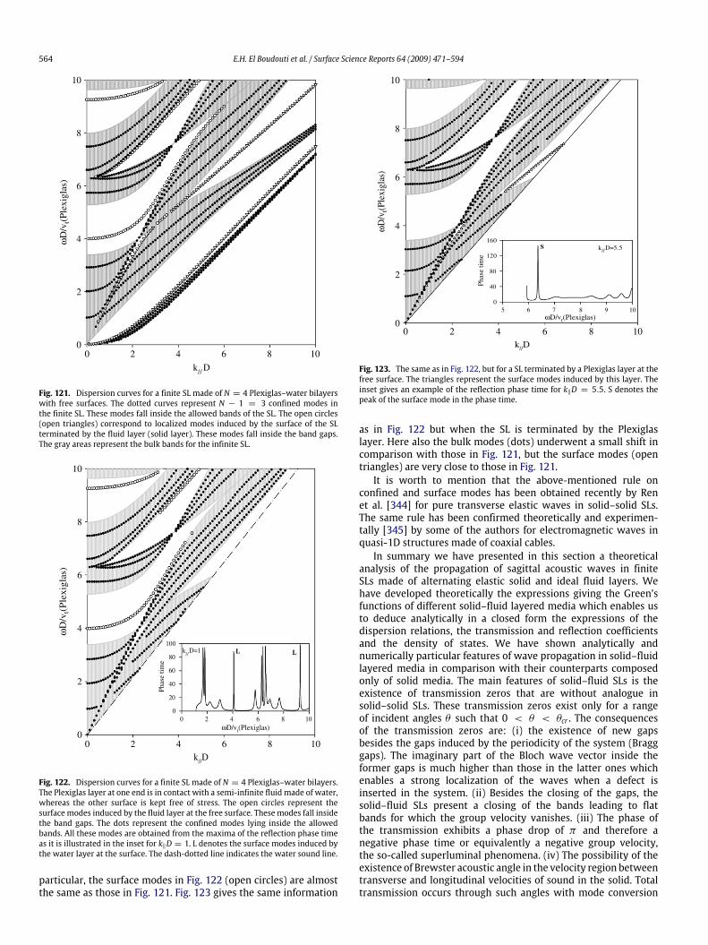
564 E.H. El Boudouti et al. / Surface Science Reports 64 (2009) 471–594

k// D

2

4

6

8

0 2 4 6 8 10

ωD

/vt(P

lexi

glas

)

0

10

Fig. 121. Dispersion curves for a finite SL made of N = 4 Plexiglas–water bilayerswith free surfaces. The dotted curves represent N − 1 = 3 confined modes inthe finite SL. These modes fall inside the allowed bands of the SL. The open circles(open triangles) correspond to localized modes induced by the surface of the SLterminated by the fluid layer (solid layer). These modes fall inside the band gaps.The gray areas represent the bulk bands for the infinite SL.

k//D

ωD

/vt(

Ple

xigl

as)

k//

D=1

ωD/vt(Plexiglas)0 2 4 6 8 10

Phas

e tim

e

0

20

40

60

80

100L L

0

2

4

6

8

10

0 2 4 6 8 10

Fig. 122. Dispersion curves for a finite SL made of N = 4 Plexiglas–water bilayers.The Plexiglas layer at one end is in contact with a semi-infinite fluid made of water,whereas the other surface is kept free of stress. The open circles represent thesurface modes induced by the fluid layer at the free surface. These modes fall insidethe band gaps. The dots represent the confined modes lying inside the allowedbands. All these modes are obtained from the maxima of the reflection phase timeas it is illustrated in the inset for k‖D = 1. L denotes the surface modes induced bythe water layer at the surface. The dash-dotted line indicates the water sound line.

particular, the surface modes in Fig. 122 (open circles) are almostthe same as those in Fig. 121. Fig. 123 gives the same information

k//D

ωD/v

t(Ple

xigl

as)

k//D=5.5

ωD/vt(Plexiglas)5 6 7 8 9 10

Phas

e tim

e

0

40

80

120

160S

0

2

4

6

8

10

0 2 4 6 8 10

Fig. 123. The same as in Fig. 122, but for a SL terminated by a Plexiglas layer at thefree surface. The triangles represent the surface modes induced by this layer. Theinset gives an example of the reflection phase time for k‖D = 5.5. S denotes thepeak of the surface mode in the phase time.

as in Fig. 122 but when the SL is terminated by the Plexiglaslayer. Here also the bulk modes (dots) underwent a small shift incomparison with those in Fig. 121, but the surface modes (opentriangles) are very close to those in Fig. 121.It is worth to mention that the above-mentioned rule on

confined and surface modes has been obtained recently by Renet al. [344] for pure transverse elastic waves in solid–solid SLs.The same rule has been confirmed theoretically and experimen-tally [345] by some of the authors for electromagnetic waves inquasi-1D structures made of coaxial cables.In summary we have presented in this section a theoretical

analysis of the propagation of sagittal acoustic waves in finiteSLs made of alternating elastic solid and ideal fluid layers. Wehave developed theoretically the expressions giving the Green’sfunctions of different solid–fluid layered media which enables usto deduce analytically in a closed form the expressions of thedispersion relations, the transmission and reflection coefficientsand the density of states. We have shown analytically andnumerically particular features of wave propagation in solid–fluidlayered media in comparison with their counterparts composedonly of solid media. The main features of solid–fluid SLs is theexistence of transmission zeros that are without analogue insolid–solid SLs. These transmission zeros exist only for a rangeof incident angles θ such that 0 < θ < θcr . The consequencesof the transmission zeros are: (i) the existence of new gapsbesides the gaps induced by the periodicity of the system (Bragggaps). The imaginary part of the Bloch wave vector inside theformer gaps is much higher than those in the latter ones whichenables a strong localization of the waves when a defect isinserted in the system. (ii) Besides the closing of the gaps, thesolid–fluid SLs present a closing of the bands leading to flatbands for which the group velocity vanishes. (iii) The phase ofthe transmission exhibits a phase drop of π and therefore anegative phase time or equivalently a negative group velocity,the so-called superluminal phenomena. (iv) The possibility of theexistence of Brewster acoustic angle in the velocity region betweentransverse and longitudinal velocities of sound in the solid. Totaltransmission occurs through such angles with mode conversion

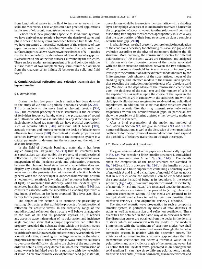
E.H. El Boudouti et al. / Surface Science Reports 64 (2009) 471–594 565

from longitudinal waves in the fluid to transverse waves in thesolid and vice versa. These angles can have practical applicationsin the area of ultrasonic nondestructive evaluation.Besides these new properties specific to solid–fluid systems,

we have derived exact relations between the density of states andphase times in finite systems embedded between two fluids. Also,we have presented a theoretical evidence of the existence of twotypes modes in a finite solid–fluid SL made of N cells with freesurfaces. In particular, we have shown the existence ofN−1modesthat fall inside the bulk bands and one additional mode by gap thatis associated to one of the two surfaces surrounding the structure.These surface modes are independent of N and coincide with thesurface modes of two complementary semi-infinite SLs obtainedfrom the cleavage of an infinite SL between the solid and fluidlayers.

9. Omnidirectional reflection and selective transmission inlayered media

9.1. Introduction

During the last few years, much attention has been devotedto the study of 2D and 3D periodic phononic crystals [27,210–214]. In analogy to the more familiar photonic crystals [346,347], the essential property of these structures is the existenceof forbidden frequency bands, where the propagation of soundand ultrasonic vibrations is inhibited in any direction of space.Such phononic band gap materials can have practical applicationssuch as acoustic filters [348], ultrasonic silent blocks [349],acoustic mirrors, and improvements in the design of piezoelectricultrasonic transducers [350]. The contrast in elastic properties anddensities between the constituents of the composite system is acritical parameter in determining the existence and the width ofabsolute band gaps.In the field of photonic band gap materials, it has been

argued during the last years [351–353] that 1D structures suchas superlattices can also exhibit the property of omnidirectionalreflection, i.e., the existence of a band gap for any incident waveindependent of the incidence angle and polarization. However,because the photonic band structure of a superlattice does notdisplay any absolute band gap (i.e., a gap for any value of thewave vector), the property of omnidirectional reflection holds ingeneral when the incident light is launched from vacuum, or froma medium with relatively low index of refraction (or high velocityof light). To overcome this difficulty, when the incident light isgenerated in a high refraction index medium, a solution [354] thatconsists to associate with the superlattice a cladding layer with alow index of refraction has been proposed. This layer acts like abarrier for the propagation of light.The object of this section is to examine the possibility of

realizing 1D structures that exhibit the property of omnidirectionalreflection for acoustic waves. In the frequency range of theomnidirectional reflection, the structure will behave analogouslyto the case of 2D and 3D phononic crystals, i.e., it reflectsany acoustic wave independent of its polarization and incidenceangle. We shall show that a simple superlattice can fulfill thisproperty, provided the substrate from which the incident wavesare launched is made of a material with relatively high acousticvelocities of sound.However, the substratemayhave relatively lowacoustic velocities, according to the large varieties in the elasticproperties ofmaterials. Then,we propose two alternative solutionsto overcome the difficulty related to the choice of the substrate, inorder to obtain a frequency domain in which the transmission ofsound waves is inhibited even for a substrate with low velocitiesof sound. Asmentioned in the case of photonic band gapmaterials,

one solution would be to associate the superlattice with a claddinglayer having high velocities of sound in order to create a barrier forthe propagation of acoustic waves. Another solution will consist ofassociating two superlattices chosen appropriately in such a waythat the superposition of their band structures displays a completeacoustic band gap [79,80].Inwhat follows,we shall present a comprehensive investigation

of the conditions necessary for obtaining this acoustic gap and itsevolution according to the physical parameters defining the 1Dstructure. More precisely, the transmission spectra for differentpolarizations of the incident waves are calculated and analyzedin relation with the dispersion curves of the modes associatedwith the finite structure embedded between the two substrates.When a maximum threshold for transmittance is imposed, weinvestigate the contributions of the differentmodes induced by thefinite structure (bulk phonons of the superlattices, modes of thecladding layer, and interface modes) to the transmission spectra,thus revealing the limitations on the existence of an absolute bandgap. We discuss the dependence of the transmission coefficientsupon the thickness of the clad layer and the number of cells inthe superlattices, as well as upon the choice of the layers in thesuperlattice, which are in contact with the substrates and with theclad. Specific illustrations are given for solid–solid and solid–fluidsuperlattices. In addition, we show that these structures can beused as an acoustic filter that may transmit selectively certainfrequencies within the omnidirectional gaps. In particular, weshow the possibility of filtering assisted either by cavity modes orby interface resonances.After a brief presentation of the model and method of

calculation in Section 9.2, we give in Sections 9.3 and 9.4 thenumerical illustrations aswell as the discussion of the transmissioncoefficients for the occurrence of an omnidirectional band gap andthe possibility of selective transmission through these gaps.

9.2. Model and method of calculation

The geometries studied in this paper are schematically depictedin Fig. 124. We consider a finite lamellar structure L sandwichedbetween two substrates S1 and S2 (Fig. 124(a)). The detailsabout the composition of the finite structure are sketched inFig. 124(b) and (c). In one case (Fig. 124(b)), the lamellar structureis composed of a finite superlattice containing alternating layersof materials A and B, and a clad layer of material C. Let us noticethat in our calculation, the material C can be embedded insidethe superlattice instead of being at its boundary. In the secondgeometry (Fig. 124(c)), two finite superlattices made, respectively,of materials (A1, B1) and (A2, B2) are associated together in tandem.All the interfaces are taken to be parallel to (x1, x2) plane of aCartesian coordinates system. All the media are assumed to beisotropic elastic media characterized by their mass densities, theirtransverse velocity Ct , and longitudinal velocity Cl of sound.The study of acoustic wave propagation in such a composite

lamellar system is performed by means of total densities ofstates as well as transmission and reflection coefficients. Thesequantities are obtained in the same way as in previous sections.The dispersion curves are obtained from the peaks in the densityof states which are associated with the modes of the mediumL interacting with the continuum of substrate modes. We shallfocus our attention on transmitted waves through the lamellarcomposite system, in relation with the dispersion curves. Theexistence of an omnidirectional acoustic gap requires that thetransmission coefficients fall below a threshold value for allpolarizations and any incidence angle of the incoming waves. Letus notice that the incident wave, generated in an homogeneoussolid medium S1, can have three different polarizations; namely,transverse horizontal (or shear horizontal), transverse vertical, and

566 E.H. El Boudouti et al. / Surface Science Reports 64 (2009) 471–594

a

b

c

Fig. 124. Geometries of the omnidirectional band gap structure. (a) A finite lamellar composite system L embedded between two homogeneous media S1 and S2 . (b) Thesystem L is constituted by a superlattice cladded with a material C. (c) The system L is constituted by a combination in tandem of two different superlattices.

longitudinal. However, only longitudinal wave can be launchedthrough an homogeneous fluid medium S1.

9.3. Case of solid–solid superlattices

In this subsection, we show that omnidirectional reflection ofacoustic waves can be achieved with only 1D systems insteadof 2D or 3D phononic crystals. First, we emphasize that asingle superlattice can display an omnidirectional reflection band,provided the substrate is made of a material with relatively highvelocities of sound. Then, in order to remove the limitation aboutthe choice of the substrate, we consider the geometries describedin Fig. 124 where either a clad layer is added to the superlattice, ortwo different superlattices with appropriately chosen parametersare combined in tandem. The expressions of the transmission andreflection coefficients and densities of states are cumbersome. Weshall avoid the details of these calculations which are given inRef. [84].Let us first examine the so-called projected band structure of

a superlattice, i.e., the frequency ω versus the wave vector k‖.Fig. 125 displays the phononic band structure of an infinite super-lattice composed of Al and W materials with thicknesses d1 andd2, such as d1 = d2 = 0.5D, D being the period of the superlat-tice. We have used a dimensionless frequency Ω = ωD/Ct(Al),where Ct(Al) is the transverse velocity of sound in Al (the elasticparameters of thematerials are listed in Table 9). The left and rightpanels, respectively, give the band structure for transverse andsagittal acoustic waves. For every value of k‖, the shaded andwhite areas in the projected band structure, respectively, cor-respond to the minibands and to the minigaps of the super-lattice, where the propagation of acoustic waves is allowed or

6

4

2

Red

uced

fre

quen

cy

8

04 3 2 1 0 1 2 3 4

Reduced wave vector

5 5

8

6

4

2

0

Fig. 125. Projected band structure of sagittal (right panel) and transverse (leftpanel) elastic waves in aW/AL superlattice. The reduced frequencyΩ = ωD/Ct (Al)is presented as a function of the reduced wave vector k‖D. The shaded and whiteareas, respectively, correspond to the minibands and minigaps of the superlattice.The heavy and thin straight lines correspond, respectively, to sound velocities equalto transverse and longitudinal velocities of sound in epoxy.

forbidden. Due to the large contrast between the elastic pa-rameters of Al and W, the minigaps of the superlattice arerather large in contrast to the case of other systems such asGaAs–AlAs superlattices. Nevertheless, it can be easily noticedthat the band structure shown in Fig. 125 does not display anyabsolute gap, this means a gap existing for every value of thewave vector k‖. However, the superlattice can display an omni-directional reflection band in the frequency range of the minigap

E.H. El Boudouti et al. / Surface Science Reports 64 (2009) 471–594 567

Table 9Elastic parameters of the materials involved in the calculations.

Materials Mass density (kg m−3) Ct (m/s) Cl (m/s)

W 19300 2860 5231Al 2 700 3110 6422Si 2 330 5845 8440Fe 8133 2669 4757Epoxy 1200 1160 2830Pb 10760 850 1960Nylon 1110 1100 2600

(2.952 < Ω < 4.585) if the velocities of sound in the substrateare high enough. More precisely, let us assume that the transversevelocity of sound in the substrate Ct(s) is greater than 5543 m/s,(the heavy line in Fig. 125 indicates the sound line with the ve-locity 5543 m/s). For any wave launched from this substrate, thefrequency will be situated above the sound line ω = Ct(s)k‖,i.e., above the heavy line in Fig. 125. When the frequency falls inthe range 2.952 < Ω < 4.585 (corresponding to the minigap ofthe superlattice at k‖ = 0), the wave cannot propagate inside thesuperlattice and will be reflected back. Thus, the frequency range2.952 < Ω < 4.585 corresponds to an omnidirectional reflectionband for the chosen substrate. Generally speaking, the above con-dition expresses that the cone defined by the transverse velocity ofsound in the substrate contains a minigap of the superlattice. Withthe Al/W superlattice, this condition is, for instance, fulfilled if thesubstrate is made of Si [78–80]. Of course, in practice, due to thefiniteness of the omnidirectional mirror, one can only impose thatthe transmittance remains below a given threshold (for instance,10−3 or 10−2). A recent experiment [81] has been performed byManzanares-Martinez on Pb/Epoxy SLs to show the occurrence ofsuch omnidirectional band gaps.Now, if the incident wave is initiated in a substrate made of a

material with low velocities of sound such as epoxy [with Ct(s) =1160 m/s, see the thin straight line in Fig. 125], the wave is notprohibited from propagation inside the superlattice, whatever thefrequency. Thus, thewavewill be partially transmitted through thesuperlattice, and only partially reflected back, depending upon theincidence angle (or equivalently, upon the wave vector k‖).Therefore the occurrence of an omnidirectional band gap

introduces a limitation regarding the choice of the substratematerial, namely, thismaterial should have relatively high acousticvelocities as compared to the typical velocities of the materialsconstituting the superlattice. In order to remove this limitationor at least facilitate the existence of an omnidirectional reflectionband, we, respectively, present in the next two sections thesolutions mentioned above. The first one consists of cladding thesuperlattice (SL) with a layer of high acoustic velocities, whichcan act like a barrier for the propagation of phonons. The secondsolution consists of considering a combination of two differentsuperlattices, provided their band structures do not overlap overthe frequency range of the omnidirectional band gap.

9.3.1. Cladded superlattice structureThis section contains results of the transmission spectra,

density of states, and dispersion curves for acoustic modes in afinite Al/W SL cladded on one side by a Si layer of thickness dSi,and embedded between two substrates made of epoxy (Fig. 124).Fig. 126 gives an example of the dispersion curves for the

above structure, togetherwith the frequency domains inwhich thetransmission power exceeds a threshold of 10−3 (shaded areas).In this example, the thickness of the Si layer is dSi = 8D, andthe superlattice contains four bilayers of Al and W; the clad layeris in contact with either an Al layer (Fig. 126(a)) or a W layer(Fig. 126(b)) in the superlattice (see Fig. 124(b)). The branchesthat fall outside the minibands of the superlattice are essentially

4

3

2

1

0

5

4

3

2

1

5

Red

uced

fre

quen

cy

0

4

3

2

1

0

5

4

3

2

1

5

0

-3 -2 -1 0 1 2 3

-3 -2 -1 0Reduced wave vector

1 2 3

a

b

Fig. 126. Dispersion curves of the cladded finite superlattice embedded betweentwo substrates. The shaded area correspond to the frequency domain in which thetransmission power can exceed a threshold of 10−3 . The thickness of the clad layeris dSi = 8D, and the superlattice contains four bilayers of Al and W. The clad is incontact either with an Al layer (a) or with a W layer (b). The left and right panels,respectively, refer to shear horizontal and sagittal acoustics modes. The horizontaldashed lines delimit the edges of the omnidirectional acoustic band gap. The heavyand thin straight lines, respectively, show the transverse sound lines of the substrate(epoxy) and the clad (Si).

associated either with the guided modes of the Si layer or withthe interface modes localized at the Si–superlattice boundary (thelatter are located below the sound lines of Si).As compared to the superlattice minigap, the omnidirectional

reflection band (delimited by the two horizontal dashed lines inFig. 126) can be significantly reduced. In the case of Fig. 126(b)where the omnidirectional gap almost disappears, the mainlimitation is due to transmission through the modes belongingto a narrow miniband of the superlattice; this correspondsto a narrow range of the incidence angle in the substrate(around 14). Therefore, with the geometrical parameters chosenin this example, the clad layer is not efficient to bring thetransmission below the threshold of 10−3 in a broad frequencyrange, for all incidence angles and all polarizations. Actually,increasing the threshold to 10−2 does not significantly improvethe omnidirectional gap in this case. In the example of Fig. 126(a)where an Al layer in the superlattice is in contact with the Si clad,the omnidirectional gap extends from Ω = 3.176 to Ω = 4.Here the upper edge of the gap is decreased as compared to thesuperlattice minigap, due to transmission around the frequenciesΩ = 4–4.5 (upper right corner of the figure). From right to left,the transmission occurs through bulk modes of the superlatticebelonging to a narrow miniband, through an interface mode atthe boundary between the superlattice and the Si clad layer, andthrough a guided mode of the Si layer. Although the transmittancethrough the latter modes exceeds the chosen threshold of 10−3,still it remains very small (see Fig. 128).One can notice that the presence of the clad layer has

two opposite effects. It decreases the transmittance in somefrequency domains (essentially below the sound line defined bythe transverse velocity of sound in the clad), but also introducesnew modes that can contribute themselves to transmission. Thetransmission by the latter modes is prevented by the superlatticewhen the corresponding branches fall inside the minigaps.

568 E.H. El Boudouti et al. / Surface Science Reports 64 (2009) 471–594

604020

1

0

Ttr

ansH

80

0

DO

S

604020

80

0

DO

ST

long

1

0

0 1 2 3 4 5 6

0 1 2 3Reduced frequency

4 5 6

a

b

c

d

Fig. 127. Transmission coefficients and densities of states for the claddedsuperlattice structure of Fig. 126(a), at k‖D = 0. The panels (a) and (b) are plottedfor acoustic waves of transverse polarization. Panels (c) and (d) refer to waves oflongitudinal polarization.

To give a better insight into the behaviors of the transmissioncoefficients, we present in Figs. 127 and 128, for two values ofk‖D, the transmitted intensities through the cladded superlattice.For the sake of comparison, we have also given the densitiesof states. The results are presented for different polarizations,namely, the incident wave can be shear horizontal, transverse inthe sagittal plane, or longitudinal, and the DOS is given for eithershear horizontal or sagittal modes. The thickness of the Si layer isagain dSi = 8D, the superlattice is composed of N = 4 bilayers ofAl and W, and the clad layer is in contact with an Al layer.At k‖D = 0 (Fig. 127), corresponding to a normal incidence,

there is a decoupling betweenwaves of transverse and longitudinalpolarizations. One can observe that the presence of the clad layerdoes not affect the band gap that is almost identical to the minigapof the superlattice (2.95 < Ω < 4.58). The clad layer inducesadditional modes (see the peaks in the DOS), which are the guidedmodes of the Si layer, but these modes do not contribute totransmission when they fall inside the minigap of the superlattice(see, for instance, the peaks in DOS around the frequencies 3 <Ω < 4). At k‖D = 2 (Fig. 128), the presence of the clad layer ofSi prevents the propagation of sound in the frequency range thatlies below the transverse sound line of Si (Ω < 3.5). Hence, inthis range of frequency, the clad layer plays the role of a barrierbetween phonons in the substrate and the superlattice, leadingto a decrease in the transmitted intensity [please notice the verysmall scales in the vertical axes of Fig. 128(c) and (d)]. On theother hand, the modes induced by the Si layer, which fall in thesuperlattice minigap (around Ω = 4.5) contribute very weaklyto the transmission process, as mentioned in connection with thediscussion of Fig. 126(a).To investigate the effect of superlattice termination on the

existence of the omnidirectional gap, we have also considered,besides the examples of Fig. 126, two other cases; namely, the caseof a superlattice containing N + 1 = 5 layers of Al and N = 4layers of W (with Al termination on both sides of the superlattice)and the case of a superlattice containing five layers of W and four

604020

80

120

80

40

160

0

0

0 1 2 3 4 5 6

0 1 2 3Reduced frequency

4 5 6

1

0100

0

1.5 10-4

5 10-5

8. 10-5

4. 10-5

0

10-4

DO

ST

long

Ttr

ansV

Ttr

ansH

DO

S

a

b

c

e

d

Fig. 128. Same as in Fig. 127 but for k‖D = 2. Panels (a), (c), and (d), respectively,give the transmission power for an incident wave of the following polarization:shear horizontal, transverse in the sagittal plane, and longitudinal in the sagittalplane (one can notice the small scales on the vertical axes of panels (c) and (d)).Panels (b) and (e) present the densities of states, respectively, associatedwith shearhorizontal and sagittal waves.

layers of Al (withW termination on both sides). These cases are lessfavorable than those presented in Fig. 126 and,more especially, theabsolute acoustic gap disappears in the latter case.We can now briefly discuss the existence and behavior of the

omnidirectional reflection band as a function of the geometricalparameters involved in our structure, namely, the thickness dSi ofthe Si layer and the number N of unit cells in the superlattice. Themaximum tolerance for transmission is chosen to be either 10−3or 10−2. A detailed investigation of the transmission coefficientsshows that the gap stabilizes for dSi exceeding a thickness of 5.5Dand N greater than 4. In Fig. 129, we present the variation of thegap as a function of dSi for three values of N; namely, N = 5, 8,and 10. In each case, the omnidirectional gap is sketched for bothchoices of the transmittance threshold.First, let us notice that the limitation about the width of the

absolute gap comes from the waves of sagittal polarization, sincethe gap in the shear horizontal polarization is relatively broad andalready exists for values of dSi and N of the order of 1.5D and2D, respectively. The sagittal gap shown in Fig. 129 widens withincreasing the thickness of the Si layer, although some irregularbehaviors can be noticed at the edges of the gap. It is even worthmentioning that for N below or equal to 4, the gapmay close whengoing to increasing value of dSi; this means that the transmissionthrough the guided modes of the clad layer are not efficientlyprevented by the superlattice. From Fig. 129, one can conclude thatthe acoustic gap almost reaches its maximum value for N = 6 anddSi = 11D. For the sake of completeness, we also present in Fig. 130

E.H. El Boudouti et al. / Surface Science Reports 64 (2009) 471–594 569

4

3

2

1

5

4

3

2

1-15 -12 -9 -6 -3 0 3 6 9 12 15

5

4

3

2

1

5

4

3

2

1

-15 -12 -9 -6 -3 0 3 6 9 12 15

5

4

3

2

5

4

3

2

1-15 -12 -9 -6 -3 0

Clad layer thickness dSi

3 6 9 12 15

5

1

Red

uced

fre

quen

cy

a

b

c

N = 5

N = 8

N = 10

Fig. 129. Dependence of the omnidirectional gap with the thickness dSi of the cladlayer for different numbers of Al/Wbilayers in the superlattice: (a)N = 5, (b)N = 8,and (c) N = 10. The gray and dark areas, respectively, correspond to the frequencydomains where the transmission exceeds 10−3 or 10−2 . The left and right panels,respectively, refer to shear horizontal and sagittal acoustic modes.

4

3

2

1

5

4

3

2

5

4

3

2

1

5

4

3

2

1

(a) T > 10-3

(b) T > 10-2

5

1

Red

uced

fre

quen

cy

-12 -10 -8 -6 -4 -2 0 2 4 6 8 10 12

-14 -12 -10 -8 -6 -4 -2 0 2 4 6 8 10 12 14

-14

Number N of (Al/W) cells

14

Fig. 130. Dependence of the omnidirectional gap with the number N of unit cellsin the Al/W superlattice. The Si clad is in contactwith an Al layer and has a thicknessof dSi = 8D. The transmission threshold is fixed to 10−3 (a) and 10−2 (b).

the variation of the gaps as a function of the number of unit cellsin the superlattice, for dSi = 8D.Finally, we have compared the behavior of the transmission

coefficients when an additional Si layer is inserted at differentplaces inside the superlattice. It turns out that the best solution isobtained when the Si layer is added as a clad, i.e., at the boundaryof the superlattice. More precisely, with N = 4 and dSi = 8D,there is no absolute gap when the Si layer is inserted inside thesuperlattice.

6

4

2

8

6

4

2

0-5 -4 -3 -2 -1 0

Reduced wave vector1 2 3 4 5

8

0

Red

uced

fre

quen

cy

Red

uced

fre

quen

cy

Fig. 131. Projected band structures of two different superlattices, namely, Al/W(bright gray) and Fe/epoxy (dark gray). The overlap between both band structuresis presented as black areas. The right and left panels represent the sagittal and thetransverse band structures, respectively.

4

3

2

1

-5 -4 -3 -2 -1 0 1 2 3 4 5

6

5

0

4

3

2

1

6

5

0

Red

uced

fre

quen

cy

-6Reduced wave vector

6

Fig. 132. Dispersion curves of two finite superlattices combined in tandem andembedded between two substrates. The shaded area corresponds to the frequencydomain in which the transmission power can exceed a threshold of 10−3 . The Al/Wsuperlattice contains N + 1 = 9 layers of Al and N = 8 layers of W. The epoxy/Fesuperlattice contains N ′ + 1 = 6 layers of epoxy and N ′ = 5 layers of Fe.

9.3.2. Coupled solid–solid multilayer structuresIn this subsection, we study the transmission of acoustic waves

through a layered structure composed of two coupled superlattices(Fig. 124(c)) chosen in such a way that the superposition of theirband structure displays an absolute band gap. This means, in somefrequency range, the minibands of one superlattice overlap withthe minigaps of the other, and vice versa.We have investigated several possibilities of elastic and geo-

metric parameters for the coupled superlattice structure. Amonga few possibilities that give rise to the occurrence of an omnidi-rectional band gap, one interesting solution consists of combiningthe Al/W superlattice with a Fe/epoxy superlattice of the same pe-riod D but with d′1 = 0.8D and d

′

2 = 0.2D. The superposition ofthe band structures for these superlattices is presented in Fig. 131and clearly displays a broad absolute acoustic gap in the frequencyrange 2.54 < Ω < 5.29 (delimited by the dashed horizontal lines).One can expect that in this frequency domain, any wave generatedin any substrate will be totally reflected. In practice, the coupledsuperlattice structure is of finite width, and one can only impose amaximum tolerance on the transmission coefficients.In the following, we assume that the substrates are made

of a low velocity material such as epoxy. Fig. 132 displays the

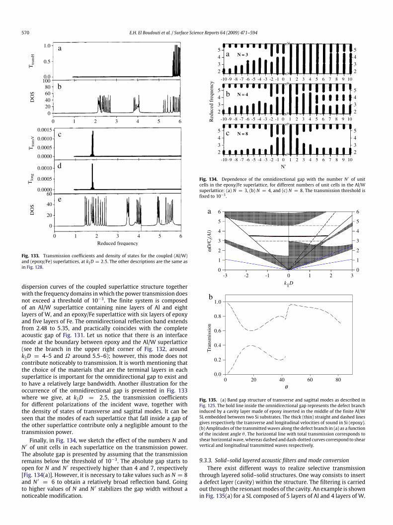
570 E.H. El Boudouti et al. / Surface Science Reports 64 (2009) 471–594

0.5

80604020

0.0010

0.0005

0.0005

40

20

0 2 3 4 5 6

1 2 3 4 50 6Reduced frequency

1.0

0.0100

0

0.0015

0.0000

Ttr

ansH

DO

ST

tran

sV

0.0010

0.0000

Tlo

ng

60

0

DO

S

1

a

b

c

d

e

Fig. 133. Transmission coefficients and density of states for the coupled (Al/W)and (epoxy/Fe) superlattices, at k‖D = 2.5. The other descriptions are the same asin Fig. 128.

dispersion curves of the coupled superlattice structure togetherwith the frequency domains inwhich the power transmission doesnot exceed a threshold of 10−3. The finite system is composedof an Al/W superlattice containing nine layers of Al and eightlayers of W, and an epoxy/Fe superlattice with six layers of epoxyand five layers of Fe. The omnidirectional reflection band extendsfrom 2.48 to 5.35, and practically coincides with the completeacoustic gap of Fig. 131. Let us notice that there is an interfacemode at the boundary between epoxy and the Al/W superlattice(see the branch in the upper right corner of Fig. 132, aroundk‖D = 4–5 and Ω around 5.5–6); however, this mode does notcontribute noticeably to transmission. It is worth mentioning thatthe choice of the materials that are the terminal layers in eachsuperlattice is important for the omnidirectional gap to exist andto have a relatively large bandwidth. Another illustration for theoccurrence of the omnidirectional gap is presented in Fig. 133where we give, at k‖D = 2.5, the transmission coefficientsfor different polarizations of the incident wave, together withthe density of states of transverse and sagittal modes. It can beseen that the modes of each superlattice that fall inside a gap ofthe other superlattice contribute only a negligible amount to thetransmission power.Finally, in Fig. 134, we sketch the effect of the numbers N and

N ′ of unit cells in each superlattice on the transmission power.The absolute gap is presented by assuming that the transmissionremains below the threshold of 10−3. The absolute gap starts toopen for N and N ′ respectively higher than 4 and 7, respectively[Fig. 134(a)]. However, it is necessary to take values such as N = 8and N ′ = 6 to obtain a relatively broad reflection band. Goingto higher values of N and N ′ stabilizes the gap width without anoticeable modification.

a

b

c

N = 3

N = 4

N = 8

5432

5432

5432

5432

5432

5432

-10 -9 -8 -7 -6 -5 -4 -3 -2 -1 0

N'

Red

uced

fre

quen

cy

1 2 3 4 5 6 7 8 9 10

-10 -9 -8 -7 -6 -5 -4 -3 -2 -1 0 1 2 3 4 5 6 7 8 9 10

-10 -9 -8 -7 -6 -5 -4 -3 -2 -1 0 1 2 3 4 5 6 7 8 9 10

Fig. 134. Dependence of the omnidirectional gap with the number N ′ of unitcells in the epoxy/Fe superlattice, for different numbers of unit cells in the Al/Wsuperlattice: (a) N = 3, (b) N = 4, and (c) N = 8. The transmission threshold isfixed to 10−3 .

k D

a

b

0

1

2

3

4

5

6

1

2

3

4

5

0

0.2

0.4

0.6

0.8

0

Tra

nsm

issi

on

0.

1.

0

6D

/Ct(A

l)ω

θ

-3 -2 -1 0 1 2 3

0 20 40 60 80

||

Fig. 135. (a) Band gap structure of transverse and sagittal modes as described inFig. 125. The bold line inside the omnidirectional gap represents the defect branchinduced by a cavity layer made of epoxy inserted in the middle of the finite Al/WSL embedded between two Si substrates. The thick (thin) straight and dashed linesgives respectively the transverse and longitudinal velocities of sound in Si (epoxy).(b) Amplitudes of the transmittedwaves along the defect branch in (a) as a functionof the incident angle θ . The horizontal line with total transmission corresponds toshear horizontalwave,whereas dashed and dash-dotted curves correspond to shearvertical and longitudinal transmitted waves respectively.

9.3.3. Solid–solid layered acoustic filters and mode conversionThere exist different ways to realize selective transmission

through layered solid–solid structures. One way consists to inserta defect layer (cavity) within the structure. The filtering is carriedout through the resonantmodes of the cavity. An example is shownin Fig. 135(a) for a SL composed of 5 layers of Al and 4 layers of W.

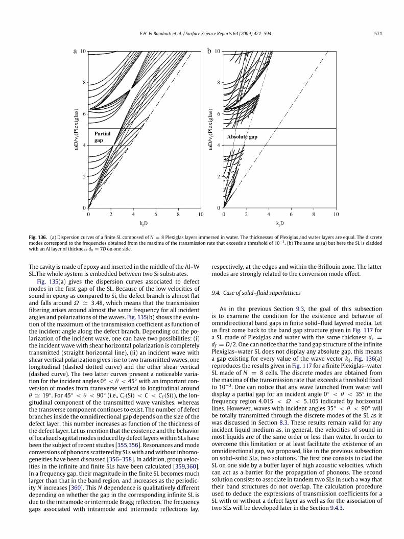
E.H. El Boudouti et al. / Surface Science Reports 64 (2009) 471–594 571

2

4

6

8ω

D/v

t(P

lexig

las)

0

10

2

4

6

8

ωD

/vt(

Ple

xig

las)

0

10

Partial gap

Absolute gap

0 2 4 6 8 10 0 2 4 6 8 10

k//Dk//D

a b

Fig. 136. (a) Dispersion curves of a finite SL composed of N = 8 Plexiglas layers immersed in water. The thicknesses of Plexiglas and water layers are equal. The discretemodes correspond to the frequencies obtained from the maxima of the transmission rate that exceeds a threshold of 10−3 . (b) The same as (a) but here the SL is claddedwith an Al layer of thickness d0 = 7D on one side.

The cavity is made of epoxy and inserted in themiddle of the Al–WSL.The whole system is embedded between two Si substrates.Fig. 135(a) gives the dispersion curves associated to defect

modes in the first gap of the SL. Because of the low velocities ofsound in epoxy as compared to Si, the defect branch is almost flatand falls around Ω ' 3.48, which means that the transmissionfiltering arises around almost the same frequency for all incidentangles and polarizations of the waves. Fig. 135(b) shows the evolu-tion of the maximum of the transmission coefficient as function ofthe incident angle along the defect branch. Depending on the po-larization of the incident wave, one can have two possibilities: (i)the incident wave with shear horizontal polarization is completelytransmitted (straight horizontal line), (ii) an incident wave withshear vertical polarization gives rise to two transmittedwaves, onelongitudinal (dashed dotted curve) and the other shear vertical(dashed curve). The two latter curves present a noticeable varia-tion for the incident angles 0 < θ < 45 with an important con-version of modes from transverse vertical to longitudinal aroundθ ' 19. For 45 < θ < 90 (i.e., Ct(Si) < C < C`(Si)), the lon-gitudinal component of the transmitted wave vanishes, whereasthe transverse component continues to exist. The number of defectbranches inside the omnidirectional gap depends on the size of thedefect layer, this number increases as function of the thickness ofthe defect layer. Let usmention that the existence and the behaviorof localized sagittalmodes induced by defect layerswithin SLs havebeen the subject of recent studies [355,356]. Resonances andmodeconversions of phonons scattered by SLswith andwithout inhomo-geneities have been discussed [356–358]. In addition, group veloc-ities in the infinite and finite SLs have been calculated [359,360].In a frequency gap, their magnitude in the finite SL becomes muchlarger than that in the band region, and increases as the periodic-ity N increases [360]. This N dependence is qualitatively differentdepending on whether the gap in the corresponding infinite SL isdue to the intramode or intermode Bragg reflection. The frequencygaps associated with intramode and intermode reflections lay,

respectively, at the edges and within the Brillouin zone. The lattermodes are strongly related to the conversion mode effect.

9.4. Case of solid–fluid superlattices

As in the previous Section 9.3, the goal of this subsectionis to examine the condition for the existence and behavior ofomnidirectional band gaps in finite solid–fluid layered media. Letus first come back to the band gap structure given in Fig. 117 fora SL made of Plexiglas and water with the same thickness ds =df = D/2. One can notice that the band gap structure of the infinitePlexiglas–water SL does not display any absolute gap, this meansa gap existing for every value of the wave vector k‖. Fig. 136(a)reproduces the results given in Fig. 117 for a finite Plexiglas–waterSL made of N = 8 cells. The discrete modes are obtained fromthemaxima of the transmission rate that exceeds a threshold fixedto 10−3. One can notice that any wave launched from water willdisplay a partial gap for an incident angle 0 < θ < 35 in thefrequency region 4.015 < Ω < 5.105 indicated by horizontallines. However, waves with incident angles 35 < θ < 90 willbe totally transmitted through the discrete modes of the SL as itwas discussed in Section 8.3. These results remain valid for anyincident liquid medium as, in general, the velocities of sound inmost liquids are of the same order or less than water. In order toovercome this limitation or at least facilitate the existence of anomnidirectional gap, we proposed, like in the previous subsectionon solid–solid SLs, two solutions. The first one consists to clad theSL on one side by a buffer layer of high acoustic velocities, whichcan act as a barrier for the propagation of phonons. The secondsolution consists to associate in tandem two SLs in such a way thattheir band structures do not overlap. The calculation procedureused to deduce the expressions of transmission coefficients for aSL with or without a defect layer as well as for the association oftwo SLs will be developed later in the Section 9.4.3.

572 E.H. El Boudouti et al. / Surface Science Reports 64 (2009) 471–594

0.0

0.4

0.8

k//D=1

Tra

nsm

issi

on

0.0

0.4

0.8

0.0

0.4

0.8

k//D=0

k//D=3

DO

S

0

30

60

90

0

30

60

90

0

30

60

90a

b

c

d

e

f

2 4 6 8ωD/vt(Plexiglas)

0 10 2 4 6 8ωD/vt(Plexiglas)

0 10

Fig. 137. Transmission rate (left panel) and density of states (DOS) (right panel) as a function of the reduced frequency Ω for the finite SL depicted in Fig. 136(b) and forthree values of k‖D: k‖D = 0 (a) and (d), k‖D = 1 (b) and (e) and k‖D = 2 (c) and (f).

9.4.1. Cladded solid–fluid superlattice structureFig. 136(b) gives the discrete modes associated to the cladded-

SL structure, i.e., the frequency domains in which the transmissionrate exceeds a threshold of 10−3. In this example the clad layer ismade of Al with transverse and longitudinal velocities of sound(dashed and straight lines) higher than the SL bulk modes lyingin the frequency region 4.015 < Ω < 5.105 (Fig. 136(a), (b)).The thickness of the Al layer is d0 = 7D and the SL containsN = 8 cells of Plexiglas–water. By combining these two systems,the allowed modes of the SL and the guided modes induced bythe Al clad layer above its velocities of sound do not overlap overthe frequency range of the omnidirectional gap. This means thateach system acts as a barrier for phonons of the other system. Insuch a way, one obtains an omnidirectional band gap indicatedby the two horizontal lines in Fig. 136(b) in the frequency region4.015 < Ω < 5.105. By comparing Fig. 136(a) and (b), one cannotice clearly that the presence of the clad layer has two oppositeeffects. It decreases the transmittance in some frequency domains(essentially below the sound line defined by the transverse velocityof sound in the clad), but also introduces new modes that cancontribute themselves to transmission. The transmission by thelatter modes is prevented by the SL when the correspondingbranches fall inside theminigaps. In the allowed frequency regionsbelonging to both the SL and the clad layer, one can notice aninteraction and an anti-crossing of the modes associated to thesetwo systems.To give a better insight into the behavior of the transmission

coefficient, we present in Fig. 137 the transmission rates throughthe cladded-SL system for three reduced wave vectors: k‖D =0 (Fig. 137(a)), 1 (Fig. 137(b)) and 3 (Fig. 137(c)). One can seeclearly the common forbidden region in the transmission spectra

indicated by the two vertical lines, showing the mirror effectplayed by the layered structure in the frequency region 4.015 <Ω < 5.105. For the sake of comparison, we have also given inFig. 137(d)–(f) the DOS (or equivalently the phase time). One cannotice that the Al clad layer induces guidedmodeswhich appear aspeaks in the DOS. These modes do not contribute to transmissionwhen they fall inside the minigap of the SL as it is clearly shownfor the modes lying in the frequency region 4.015 < Ω < 5.105in Fig. 137(d)–(f) in comparison to Fig. 137(a)–(c) respectively.The existence and behavior of the omnidirectional reflection

depends on the geometrical parameters involved in the structure,namely, the thickness d0 of the Al layer and the number N of unitcells in the SL. In Fig. 138(a), we present the variation of the gapwidth as a function of d0 for a finite SL made of N = 8 cells. Theomnidirectional gapwidenswith increasing the thickness of Al andreaches a constant width for d0 > 3D. Similarly, if the thickness ofthe Al layer is fixed to d0 = 4D, then a finite SL made of at leastN = 7 cells is required to reach a large omnidirectional gap (seeFig. 138(b)).

9.4.2. Coupled solid–fluid multilayer structureAs mentioned in the case of solid–solid multilayered structure,

the second solution that enables us to perform omnidirectionaltransmission gaps consists of considering a combination of twoSLs chosen in such a way that the superposition of their bandstructures displays an absolute band gap. This means that theminibands of one SL overlap with the minigaps of the other SL,and vice versa in some frequency range. An example showingthis property is given in Fig. 139(a) for a combination of theband structures of two SLs made of Plexiglas–Hg and PVC–Hg. Theperiods of the two SLs aswell as the thickness of the corresponding

E.H. El Boudouti et al. / Surface Science Reports 64 (2009) 471–594 573

d 0(Al)=4 D

N (Number of cells)

N = 8

d0(Al)0 2 4 6 8 10 12 14

0 5 10 15 20

a

b

2

4

6

8

2

4

6

8

ωD/v

t(Ple

xigl

as)

0

10ωD

/vt(P

lexi

glas

)

0

10

Fig. 138. (a) Variation of the omnidirectional gap width as a function of thethickness d0 of the Al clad layer for a finite SL made of N = 8 cells. (b) Variationof the omnidirectional gap width as a function of the number N of unit cells in thefinite SL for a fixed thickness of the Al layer such that d0 = 4D.

layers are supposed to be equal: d(Plexiglas) = d(PVC) = d(Hg) =D/2. The band structures of Plexiglas–Hg and PVC–Hg SLs areindicted by black and gray areas respectively. The superposition ofthese two types of bands clearly displays two broad acoustic gapsin the frequency ranges 2.72 < Ω < 4.94 and 5.14 < Ω < 5.96.One can expect that in these frequency domains, an incident wavelaunched from any semi-infinite fluid will be totally reflected. Inpractice the two coupled SL structure is of finitewidth, and one canonly impose a maximum threshold on the transmission coefficient(T > 10−3).

Anexample is sketched in Fig. 139(b)wherewehave consideredtwo finite SLs made of N1 = 4 layers of Plexiglas and N2 = 4 layersof PVC immersed in Hg. The two omnidirectional band gaps fall inthe frequency ranges 2.72 < Ω < 4.94 and 5.14 < Ω < 5.96 andpractically coincide with acoustic band gap of Fig. 139(a). Similarlyto the cladded-SL structure discussed above, the bulk modes ofeach of the two SLs may give rise to well-defined peaks in the DOSwithin the omnidirectional gaps (not shown here). However, thesemodes do not contribute to the transmission spectra. Obviously,the width and the position of the omnidirectional gaps dependupon the relative widths of the layers in each SL but also upon thenumbers N1 and N2 of cells in each SL. Let us mention that a partialgap obtained from the association of two solid–fluid SLs has beenshown theoretically and experimentally [99] for normal incidence.

9.4.3. Solid–fluid layered acoustic filtersIn this section we shall discuss the possibility of acoustic waves

filtering through the band gap of solid–fluid layered media. Thisselective transmission can be realized either by inserting a defectlayer within the finite SL or through the modes induced by theinterface between the SL and an homogeneous fluid medium.

9.4.3.1. Transmission through resonant cavity modes. The cavitymodes can be created in the solid–fluid SL by replacing for examplea fluid layer of width df in the cell (n = P) by a different fluidof width d0 and characterized by the density ρ0 and the soundvelocity v0. Consider a solid–fluid SLwith a finite numberN of cellsand containing a defect fluid in the cell P (1 < P ≤ N), the wholestructure is inserted between two fluids characterized by theirdensity ρs and sound velocity vs (Fig. 115(e)). The transmissioncoefficient through the system described above can be obtainedin the same way as for the structure without defect (Section 8.2).It consists in coupling two finite SLs made of P and N − P cellsby a fluid layer and inserting the whole system between two fluidmedia (Fig. 115(e)). The inverse of the Green’s function in the spaceof interfacesM = (1, f , df2 ), (P + 1, f ,−

df2 ), (P + 1, f ,

df2 ), (N +

1, f ,− df2 ) of the whole system is given by a superposition ofthe Green’s functions matrices associated to the different media

0 2 4 6 8 10 0 2 4 6 8 10

Absolute gap

Absolu

te ga

p

2

4

6

8

ωD

/vt(

Ple

xigl

as)

0

10

2

4

6

8

ωD

/vt(

Ple

xigl

as)

0

10

k//D k//D

a b

Fig. 139. Band structures for two different SLs, namely Plexiglas–Hg (dark areas) and PVC–Hg (gray areas). The thickness of the layers are considered to be the same:d(Plexiglas) = d(PVC) = d(Hg) = D/2. (b) Dispersion curves for two coupled finite SLs structures made of N1 = 4 layers of Plexiglas and N2 = 4 layers of PVC immersed inHg. The discrete modes are obtained from the maxima of the transmission rate that exceeds a threshold of 10−3 . The straight line indicates the Hg sound line.

574 E.H. El Boudouti et al. / Surface Science Reports 64 (2009) 471–594

constituting the system, namely

g−1(MM)

=

A(P)− Fs B(P) 0 0B(P) A(P)+ a0 b0 00 b0 A(N − P)+ a0 B(N − P)0 0 B(N − P) A(N − P)− Fs

(381)

where A(P), B(P), A(N − P), B(N − P) are defined by Eqs. (327)and (328) and (329) for N = P and N = N − P , a0 and b0 are givenby Eq. (280) for a layer fluid labeled ‘‘0’’ and Fs is the same as in Eq.(280) for a semi-infinite fluid labeled ‘‘s’’.From Eqs. (381) and (338), one can deduce the transmission

coefficient as follows

t =2Fsb0B(P)B(N − P)

Ψ (P)Ψ (N − P)− b20[A(P)− Fs][A(N − P)− Fs](382)

where

Ψ (l) = B2(l)− [A(l)− Fs][A(l)+ a0] (383)

for l = P,N − P .It is well known that the introduction of a defect layer (cavity)

in a periodic structure can give rise to defectmodes inside the bandgaps [66–74,98]. These modes appear as well-defined peaks in theDOS, however their contribution to the transmission rate dependsstrongly on the position of these defects inside the structure.Indeed, as it was shown before, a defect layer placed at the contactbetween the SL and the substrate (clad layer) induces guidedmodes in the band gap of the SL but without contributing to thetransmission. However, the transmission through thesemodes canbe significantly enhanced if the cavity layer is placed at the middleof the structure [69,72–74,84]. In general, a periodic structuremade of N cells (N > 2) is needed to create a transmissiongap in which a defect mode is then introduced for filtering.In this subsection, we are interested to show that contrary tosolid–solid SLs, it is possible to achieve large gaps as well as sharpresonances inside these gaps with a solid–fluid structure as smallas a solid–fluid–solid sandwich triple layers (i.e., N = 2 seeFig. 115(b)). This property is associated with the existence of zerosof transmission.Fig. 140(a) gives the transmission rate as a function of the

reduced frequency Ω for a finite Plexiglas–water SL composedof N = 2 (solid curves) and N = 4 (dotted curves) cells andfor and incidence angle θ = 35. The fluid and solid layershave the same width df = ds = D/2. One can notice thatthe transmission rate exhibits a large dip in the frequency region4 < Ω < 8 around the transmission zero indicated by an opencircle on the abscissa. This transmission gap maps the band gapof the infinite system indicated by solid circles on the abscissa.As it was discussed above, the transmission gap becomes welldefined as far asN increases. Now, if a fluid cavity layer of thicknessd0 = D is inserted in the middle of the structure, then a resonancewith total transmission can be introduced in the gap [Fig. 140(b)].This resonance falls at almost the same frequency and its widthdecreases when N increases. Let us mention that the structuredepicted in Fig. 140(a) and (b) with N = 2 consists on a sandwichsystem made of two Plexiglas layers separated by a water layer.Therefore, such a small size structure clearly show the possibilityof obtaining a large gap and a sharp resonance inside the gap by justtailoring the width of these three layered media. This property isspecific to solid–fluid structures and is without analogue for theircounterparts solid–solid systemswhere at least a numberN > 2 oflayers is needed to achieve well-defined gaps and cavity modes. Inwhat follows,we shall focus on the simple case of sandwich system(i.e., N = 2).An important point to notice in Fig. 140(b) is the shape of

the resonance lying in the vicinity of the transmission zero. Such

d0 = 0. 5D

0.0

0.2

0.4

0.6

0.8

0

0

0.2

0.4

0.6

0.8

1.0

d0 = 1D

0.0

0.2

0.4

0.6

0.8

1.0

θ=35°

N= 4N= 2

N= 2

d0 = 1Dd0 = 0.8Dd0 = 0.65Dd0 = 0.6D

a

b

c

1.

0.

Tra

nsm

issi

on

0 2 4 6 8 10

0 2 4 6 8 10

4 5 6 7

ωD/vt(Plexiglas)

N= 4N= 2

Fig. 140. (a) Transmission rate for a finite SL composed of N = 2 (solid curves)and N = 4 (dotted curves) Plexiglas layers immersed in water at an incidenceangle θ = 35 . The solid and open circles on the abscissa indicate the positionsof the band gap edges and transmission zeros respectively. (b) Same as in (a) but inpresence of a defect fluid layer of thickness d0 = D at the middle of the structure[see the structure in Fig. 115(e)]. (c) Same as in (b) for N = 2 and different valuesof the thickness d0 of the cavity fluid layer as indicated in the inset.

a resonance is called Fano resonance [361]. The origin and theasymmetry Fano profile of this resonancewas explained as a resultof the interference between the discrete resonance and the smoothcontinuum background in which the former is embedded. Theexistence of such resonances in 2D and 3D phononic crystals,the so-called locally resonant band gap materials [362,363], hasbeen shown recently [364–366]. Some analytical models havebeen proposed to explain the origin and the behavior of theseresonances [364–366]. In the case of 1D model proposed here,the Fano resonance in Fig. 140 (b) is just an internal resonanceinduced by the discrete modes of the fluid layer when thesemodes fall at the vicinity of the transmission zeros induced by thesurrounding solid layers. By decreasing the width of the fluid layerfrom d0 = 1D to d0 = 0.6D [Fig. 140(c)], one can notice thatthe position of the Fano resonancemoves to higher frequencies, itswidth decreases and vanishes for a particular value of d0 = 0.71Dbefore increasing again. At exactly d0 = 0.71D, the transmissionvanishes and the resonance collapses giving rise to the so-calledghost Fano resonance [367]. Around d0 = 0.71D, the asymmetricFano profile of the resonance becomes symmetric and changes theshape.In Fig. 140(c), the two solids surrounding the fluid layer have

the same widths ds, therefore the transmission zeros inducedby the solid layers fall at the same frequency. Now, if the twosolids have different widths (labeled for example ds1 and ds2), thenone can obtain two transmission zeros and a resonance that canbe squeezed between these two dips if ds1 and ds2 are chosenappropriately. In this case a symmetric Fano resonance can beobtained whose width can be tuned by adjusting the frequenciesof the zeros of transmission. Such resonances have been foundalso for acoustic and magnetic circuits formed by a guide insertedbetween two dangling resonators [368,369].

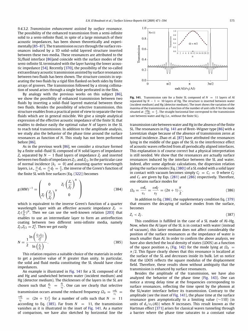
E.H. El Boudouti et al. / Surface Science Reports 64 (2009) 471–594 575

9.4.3.2. Transmission enhancement assisted by surface resonance.The possibility of the enhanced transmission from a semi-infinitesolid to a semi-infinite fluid, in spite of a large mismatch of theiracoustic impedances, has been shown theoretically and experi-mentally [85–87]. The transmission occurs through the surface res-onances induced by a 1D solid–solid layered structure insertedbetween these two media. These resonances are attributed to theSL/fluid interface [86]and coincide with the surface modes of thesemi-infinite SL terminated with the layer having the lower acous-tic impedance [54]. Recently [370], the possibility of the so-calledextraordinary acoustic transmission assisted by surface resonancesbetween two fluids has been shown. The structure consists in sep-arating the two fluids by a rigid film flanked on both sides by finitearrays of grooves. The transmission followed by a strong collima-tion of sound arises through a single hole perforated in the film.By analogy with the previous works on this subject [86],

we show the possibility of enhanced transmission between twofluids by inserting a solid–fluid layered material between thesetwo fluids. Besides the possibility of selective transmission, thisstructure enables from a practical point of view to separate the twofluids which are in general miscible. We give a simple analyticalexpression of the effective acoustic impedance of the finite SL thatenables to deduce easily the optimal value N of layers in the SLto reach total transmission. In addition to the amplitude analysis,we study also the behavior of the phase time around the surfaceresonances as function of N . This study has not been performedbefore [86].As in the previous work [86], we consider a structure formed

by a finite solid–fluid SL composed of N solid layers of impedanceZs separated by N − 1 fluid layers of impedance Zf and insertedbetween two fluids of impedances Zf 1 and Zf 2. In the particular caseof normal incidence (k‖ = 0) and assuming quarter wavelengthlayers, i.e., ω

v`ds = ω

vfdf = π

2 , the inverse of the Green’s function ofthe finite SL with free surfaces (Eq. (322)) becomes

g(MM)−1 =

0 Zf

(ZsZf

)NZf

(ZsZf

)N0

(384)

which is equivalent to the inverse Green’s function of a quarterwavelength layer with an effective acoustic impedance Ze =Zf ( ZsZf )

N . Then we can use the well-known relation [203] thatenables to use an intermediate layer to form an antireflectioncoating between two different semi-infinite media, namelyZf 1Zf 2 = Z2e . Then we get easily

N =12

ln(Zf 1Zf 2Z2f

)ln(ZsZf

) . (385)

This relation requires a suitable choice of the materials in orderto get a positive value of N greater than unity. In particular,the solid and fluid media constituting the SL should have closeimpedances.An example is illustrated in Fig. 141 for a SL composed of Al

and Hg and sandwiched between water (incident medium) andHg (detector medium). The thicknesses of the layers in the SL arechosen such that ds

v`=

dfvf. One can see clearly that selective

transmission occurs around the reduced frequency Ω0 = ωdsv`=

ωdfvf= (2n + 1)π2 for a number of cells such that N = 11

according to Eq. (385). Far from N = 11, the transmissionvanishes as it is illustrated in the inset of Fig. 141. As a matterof comparison, we have also sketched by horizontal line the

0

0.2

0.4

0.6

0.8

0

N

Tra

nsm

issi

on

0.0

0.2

0.4

0.6

0.8

1.0N=11

Ω = π/2

ωd(Al)/vl(Al)

Tra

nsm

issi

on

0.

1.

0 π/2 π 3π/2

0 2 4 6 8 10 12 14 16 18 20 22

Fig. 141. Transmission rate for a finite SL composed of N = 11 layers of Alseparated by N − 1 = 10 layers of Hg. The structure is inserted between water(incident medium) and Hg (detector medium). The inset shows the variation of themaxima of the transmission as a function of the number of unit cellsN for themodesituated at ωdAl

v`(Al)=

π2 . The straight horizontal line correspond to the transmission

rate between water and Hg (i.e., without the finite SL).

transmission rate betweenwater andHg in the absence of the finiteSL. The resonances in Fig. 141 are of Breit–Wigner type [86] with aLorentzian shape because of the absence of transmission zeros atnormal incidence. Zhao et al. [87] have attributed the resonanceslying in the middle of the gaps of the SL to the interference effectof acoustic waves reflected from all periodically aligned interfaces.This explanation is of course correct but a physical interpretationis still needed. We show that the resonances are actually surfaceresonances induced by the interface between the SL and water.Indeed, after some algebraic calculations, the dispersion relationgiving the surfacemodes (Eq. (380)) of a SL endedwith a solid layerin contact with vacuum becomes simply Cf = C` = 0 where Cfand C` are given by Eqs. (281) and (286) respectively. Therefore,one obtains surface modes for

Ω0 =ωdsv`=ωdfvf= (2n+ 1)

π

2. (386)

In addition to Eq. (386), the supplementary condition Eq. (379)that ensures the decaying of surface modes from the surface,becomes

Zs < Zf . (387)

This condition is fulfilled in the case of a SL made of Al–Hg.Now, when the Al layer of the SL is in contact with water (insteadof vacuum), this latter medium does not affect considerably theposition of the surface resonances as the impedance of water ismuch smaller than Al. In order to confirm the above analysis, wehave also sketched the local density of states (LDOS) as a functionof the space position x3 (Fig. 142) for the mode lying at Ω0 =π/2. This figure clearly shows that this resonance is localized atthe surface of the SL and decreases inside its bulk. Let us noticethat the LDOS reflects the square modulus of the displacementfield. Therefore, these results show without ambiguity that thetransmission is enhanced by surface resonances.Besides the amplitude of the transmission, we have also

analyzed the behavior of the phase time (Fig. 143). One cannotice a strong delay time at the frequencies corresponding tosurface resonances, reflecting the time spent by the phonon atthe SL/water interface before its transmission. Contrary to theamplitude (see the inset of Fig. 141), the phase time at the surfaceresonance goes asymptotically to a limiting value (∼110) (inunits of ds/v`(Al)) when N increases. This result known as theHartman effect [371] arises for classical waves tunneling througha barrier where the phase time saturates to a constant value

576 E.H. El Boudouti et al. / Surface Science Reports 64 (2009) 471–594

x3 /D

Al-Hg Superlattice

N=11

HgWater

LD

OS

0.0

0.4

0.8

1.2

1.6

-2 -1 0 1 2 3 4 5 6 8 97 10 11 12 13 14 15

Fig. 142. Variation of the local density of states (LDOS) (in arbitrary units) as afunction of the space position x3/D for the surface resonance situated at

ωdAlv`(Al)=

π2

in Fig. 141 and for N = 11.

N

N=11

ωsd(Al)/vl(Al)

20

30

40

50

Phas

e tim

e

10

60

0 π/2 π 3π/2

20

40

60

80

100

Phas

e tim

e

0

120

0 5 10 15 20 25 30 35 40 45 50

Fig. 143. Same as in Fig. 141, but for the transmission phase time (in units ofdAl/v`(Al)).

for a sufficiently barrier’s thickness. This phenomenon has beenobserved experimentally [372] and explained theoretically [373–375] in 1D photonic crystals. For a frequency lying in the allowedbands, the phase time (not shown here) increases linearly as afunction of N .The above results can be explained in terms of the DOS. Indeed,

due to the similarity between the DOS and the phase time (seeSection 8.2.4), Fig. 143 reflects also the DOS where the differentresonant modes are enlarged because of their interaction withthe bulk waves of the surrounding media. When N increases, thenumber of oscillations in the bulk bands (which is related to thenumber of cells in the system) and the correspondingDOS increase.However, the behavior is different for the peak associated to thesurface resonance. Indeed, for low values of N , the localizationof this mode increases as a function of N because the modeinteracts less with the second substrate. So, its width decreasesand its maximum increases to ensure an area equal to unity underthe resonance peak. However, the peak width cannot decreaseindefinitely and reaches a threshold because of its interactionwith the first substrate. Therefore, the DOS (or the phase time)saturates to a constant value. By using Eq. (356), we have alsoexamined the group velocity vg in such structures and found thatvg oscillates around the mean velocity vm = D(df /vf + ds/v`)−1inside the bands, whereas this quantity is strongly reduced aroundthe surface resonance. Therefore, such structures can be used as atool to reduce the speed of wave propagation.As a matter of completeness we have also checked two other

cases: (i) the case where there is no surface resonance in the gapof the SL. This can be obtained by using Hg on both sides of thestructure. In this case, even if Eqs. (386) and (387) are satisfied, Eq.(385) gives unacceptable value ofN (N < 0). In spite of the absenceof surface resonances, the phase time saturates to a constant value(∼17) (in units of ds/v`(Al)) at the mid-gap frequencies, becauseof the Hartman effect [371,373]. This value is much smaller than

in the presence of a surface resonance. (ii) The case where there istwo surface resonances in the gap of the SL. This can be obtainedby using water on both sides of the structure. In this case, Eqs.(386) and (387) are satisfied and Eq. (385) gives N ' 22. Becauseof the existence of two symmetrical surfaces that can supportsurface modes, one obtains a large surface resonance at Ω0 =π/2, 3π/2, . . . for N = 22. For smaller values of N , this resonancesplits into two distinguished resonances aroundΩ0 because of theinteraction between the two surfaces. A total transmission is stillobtained at each resonance. On the contrary, for higher values ofN (N > 22), there is a single peak in the transmission becausethe two surface resonances become decoupled, although beingenlarged due to their interaction with the substrates. In this case,the transmission peak decreases as far as N increases.

9.5. Relation to experiments

9.5.1. Omnidirectional band gapSome years ago, Manzanares-Martinez et al. [81] have demon-

strated experimentally and theoretically the occurrence of omnidi-rectional reflection in a finite SL made of a few periods of Pb/epoxyand sandwiched between substrates made of Nylon. The param-eters of the materials are given in Table 9. The thicknesses of thelayers were chosen so that the structure has its omnidirectionalgap in the working frequencies of the transducers. They took lay-ers of the same thickness 1 mm so as to generate a gap centered ataround 300 kHz.Fig. 144(a) displays the band gap structure for transverse and

sagittal acoustic waves. An omnidirectional gap is predicted in thefrequency region 273 kHz ≤ f ≤ 371 kHz, which corresponds tothe normal incidence band edges of the sagittal modes. However,it is worth to notice that the proposed structure does not havethe property of omnidirectional reflection for transverse waves forwhich the velocity is about half of the longitudinal waves. Thetransmission measurements (Fig. 144 (b)) have been performedfor longitudinal incident waves and the waves detected aftertravelling the system, consist of the projection in the radialdirection of the transmitted waves (longitudinal and transverse).Fig. 144(b) shows the transmission amplitude measured atdifferent angles of incidence for the samples analyzed. One cannotice that the transmission is almost negligible in the regionswhere a gap (shadowed regions) is predicted by the band structure.The commungap region indicated by vertical dashed lines has beenfound in very good agreement with the theoretical predictions.

9.5.2. Selective transmissionA recent experiment has been realized by Zhao et al. [87] on

a layered structure that consists of an alternative stacking of Alu-minium andGlass planar sheets, which have the same dimensions:12× 12 cm section and 3 cm thickness. The experimental setup isbased on the ultrasonic transmission technique. Fig. 145(a) givesa schematic diagram of the sample and the experimental setup,showing that the emitter contact transducer is coupled to substrateusing a coupling gel and the last layer is immersed inwater. The re-ceiver transducer is placed at a distance away from the interface ofthe last layer B and water. A pulse generator produces a short du-ration pulse. The pulses transmitted through the sample were de-tected by an immersion transducer, which has a central frequencyof 0.5 MHz and a diameter of 12.5 mm. Because of the limit of cen-tral frequency of the transducers, only the first peculiar transmis-sion peak was studied [87].Fig. 145 (b), (c) and (d) give the transmission coefficient versus

the frequency for different structures as depicted in the insetswhere materials A, B and C denote Aluminium, Glass, and Waterrespectively. The elastic parameters of these materials are given

E.H. El Boudouti et al. / Surface Science Reports 64 (2009) 471–594 577

k// D k// D

500

400

300

200

100

-3 -2 -1 0 1 2 3

transversal sagittal

Ll, Ny

60

30

090

60

30

090

60

30

090

60

30

090

60

30

100 200 300Frequency (kHz)

400 500 600

a b600

0

Freq

uenc

y (k

Hz)

90

0

Tra

nsm

issi

on a

mpl

itude

(ar

b. u

nits

)

Fig. 144. (a) Projected band structure of sagittal and transverse elastic waves in a Pb/epoxy superlattice with layer thickness d1 = d2 = 1mm. The frequencies (in kHz) arerepresented as function of the reduced parallel wave vector k‖D. The horizontal dashed lines delimit the frequencies where no transmission occurs at every angle, i.e., theband of omnidirectional reflection. (b) Experimental transmission spectra obtained for the three samples described in the text. The gray areas define the gaps calculated foreach angle of incidence θi , and the vertical dashed lines describe the commun omnidirectional gap (After Ref. [81]).

PCs

Air

Substrate B

B

B

B

A

A

A

A B A B A B C B

Al

Al

Al

Gla

ss

Gla

ss

Gla

ss

Gla

ss

A B A B A B C B

Al

Al

Al

Gla

ss

Gla

ss

Gla

ss

Gla

ss

Wat

er

Al

A A B A B A B C B

Al

Al

Al

Wat

er

Al

A A

Wat

er

Emittertransducer a

Computer 5900P/R

Receiver transducer

Water

c b d0.8

0.6

0.4

0.2

1.0

0.8

0.6

0.4

0.2

0.0

1.0

0.8

0.6

0.4

0.2

0.00.2 0.4 0.6 0.8 0.2 0.4 0.6 0.8 0.2 0.4 0.6 0.8

Frequency (MHz) Frequency (MHz) Frequency (MHz)

Tra

nsm

issi

on

1.0

0.0

Gla

ss

Gla

ss

Gla

ss

Gla

ss

Fig. 145. (a)Configuration of a finite SL and the liquid detector. The free surface of the sample is immersed in liquid. Two kinds of solid layers (A and B) are alternatelystacked in the sample. (b), (c), (d) Transmission rate of acoustic waves in water (medium C) for three different samples as described in the insets. Dashed and solid curvesrepresent theoretical and experimental results respectively. (after Ref. [87]).

in Table 10. The layers in the SL are chosen such that ωdA/vA =ωdB/vB = π/2 (i.e., quarter wavelength layers). In the case where

the SL starts with layer A and terminates with layer B, Fig. 145(b)shows a peculiar peak in the first gap around f = 0.5 MHz for

578 E.H. El Boudouti et al. / Surface Science Reports 64 (2009) 471–594

Table 10Elastic parameters of Aluminium, Glass and Water.

Materials Mass density ρ(kg/m3)

Longitudinalvelocity (m/s)

Wave impedanceZ (kg/m2 s)

Aluminium: A 2.716× 103 6.17× 103 16.758× 106

Glass: B 2.427× 103 5.40× 103 13.106× 106

Water: C 1.00× 103 1.479× 103 1.479× 106

a finite SL composed of N ' 4 periods. An analytical expressiongiving the number of bilayers necessary to attain the transmissionunity has been derived and shown to be N = 1

2ln(ZB/ZC )ln(ZA/ZB)

(i.e.,N ' 4 in the present case). The experimental measurements (solidcurves) agree well with the theoretical results (dashed curves).Inside the bands, the transmission coefficient oscillates around thetransmission value T ' 0.36when thewave is transmitteddirectlyfrom the substrate B (i.e., Glass) to Water without the presence ofthe finite SL.In addition to the expression giving the optimized value of

N to get the total transmission, the authors have attributed thisenhancement to an interference of the acoustic waves reflectedfrom all the interfaces. Whereas, Mizuno [86] has associated thesepeculiar transmission phenomenon to surface (or interface) wavesthat can exist between the last layer and the receiver medium(i.e., Water). In addition to this structure (considered as thereference system), Zhao et al. [87] have studied also experimentallytwo other structures: the first one consists on a SL ending by layerA layer (i.e. Al) on both sides (Fig. 145(c)) and the second structureconsists on a SL starting with A layer and ending with two layersA (i.e., layer A with thickness 2 dA) (Fig. 145(d)). Fig. 145(c) didnot show any selective transmission around 0.5 MHz, whereasFig. 145(d) exhibits the reappearance of the transmission mode.The authors have explained in terms of interference phenomenonbetween the different materials how the selective transmissioncan appear and disappear depending on the nature of the layer incontact with the last substrate (i.e., Water).In order to give another insight and explanation to these results,

we have taken the same structure as in Fig. 145(a) (i.e., composedof N periods A–B, but ended with a cap layer (e.g., D) in contactwith the substrate C as follows: B|A|B|A|B|A|B| . . . |A|B|A|B|D|C . Wesuppose that A and B are quarter wavelength layers (as in Zhao’swork), whereas the cap layer D can take any thickness dD, velocityvD, density ρD, and impedance ZD. By doing the same calculation asin Section 9.4.3.2, one can show that the transmission coefficientreaches unity in three situations, namely

(i) N =12ln(ZB/ZC )ln(ZA/ZB)

and ZC = ZD

(ii) N =12ln(Z2D/ZBZC )ln(ZA/ZB)

and cos(ωdD/vD) = 0

(iii) N =12ln(ZB/ZC )ln(ZA/ZB)

and sin(ωdD/vD) = 0.

(388)

These three conditions can explain easily the three spectra inFig. 145. One can see that Fig. 145(b) corresponds to the firstsituation (i) and gives N ' 4 as in Zhao’s work [87]. Fig. 145(c)corresponds to the second situation (ii) where the cap layer D= A;in this case one can check easily that N becomes negative whichmeans that this condition cannot be fulfilled and therefore thetransmission cannot reaches unity around f ' 0.5MHz. Fig. 145(d)corresponds to the third situation (iii) where the cap layer D= 2A(i.e., the double layer dD = 2dA). In this case D becomes a halfwavelength layer (i.e., sin(ωdD/vD) = 0 or ωdD/vD = mπ ) andN ' 4.It is worth mentioning that Zhao et al. [87] have also studied

theoretically the situation where the receiver substrate presents a

high impedance like tungsten for example. In this case, itwas foundthat contrary to the situation where the system is in contact withwater, the selective transmission arises when the SL terminateswith A layer (i.e., Aluminium) or B layer (i.e., Glass) butwith doublethickness. The optimized number of periods to reach themaximumtransmission when ωdA/vA 6= ωdB/vB has been also examinednumerically.In summary, we have developed in this section the idea that

1D lamellar structures can exhibit an omnidirectional reflectionband, analogous to the case of 2D and 3D phononic crystals. Thisproperty can be fulfilled with a superlattice when the velocities ofsound in the substrate are higher than the characteristic velocitiesof the superlattice constituents. In the more general case whenthe substrate is made of a soft material, we have proposedtwo solutions to realize the omnidirectional mirror, namely, thecladding of a superlattice with a hard material that acts likea barrier for the propagation of phonons, or a combination intandem of two different superlattices in such a way that theirband structures do not overlap over a given frequency range. Thelatter solution gives rise to a relatively broad band gap, providedan appropriate choice of the material and geometrical propertiesis made. With the former solution, the contribution of the guidedmodes induced by the clad layer to power transmission shouldbe more carefully taken into account. The thickness of the cladlayer, the number of unit cells in the superlattices, as well asthe nature of the terminal layers in the superlattices involved inthe structure are also important parameters for determining themaximum tolerance for power transmission.Also, we have shown that layered media can play the role of

acoustic filters. In the case of solid–solid multilayers, we haveshown the possibility of filtering through guided modes of a cavitysolid layer inserted in the middle of the structure. In particular,we have shown the possibility of transmitting around almostthe same frequency for all incident angles and polarizations ofthe waves, if the velocities of sound in the cavity layer arechosen very lower than those in the substrates. In the caseof solid–fluid multilayers, we have shown two possibilities ofenhanced transmission between two fluids. i) The first solutionconsists to insert a cavity fluid layer inside the perfect SL. We haveevidenced that a simple structure as small as a solid–fluid–solidsandwich can exhibit a large gap with sharp resonances of Fanotype. This is due to an internal resonance induced by the fluid layerwhen it falls in the vicinity of the transmission zeros induced bythe solid layers. (ii) The second solution consists to insert a finitesolid–fluid SL between two fluids. An effective acoustic impedanceof the SL has been derived which enables to deduce the optimalvalue of the number N of cells needed to reach the antireflectioncoating. This occurs around some specific frequencies close to thefree surface modes lying in the mid-gap of the SL, the so-calledsurface resonances. Contrary to the amplitude, the phase timearound these resonances increases monotonically as function ofN before saturating at a constant value for a large value of N .This phenomena known as the Hartman effect arises in evanescentregions where waves are travelling by tunneling effect.

10. Elastic waves in quasiperiodic superlattices

10.1. Introduction

Besides the periodic multilayer systems, quasiperiodic systemshave been also intensively studied [103,104]. Many theoreticalstudies based on simple 1D models have been performed, andinteresting properties have been deduced [103,104]. The high levelof control and perfection reached in the growth techniques ofmicrostructures and nanostructures has allowed the production

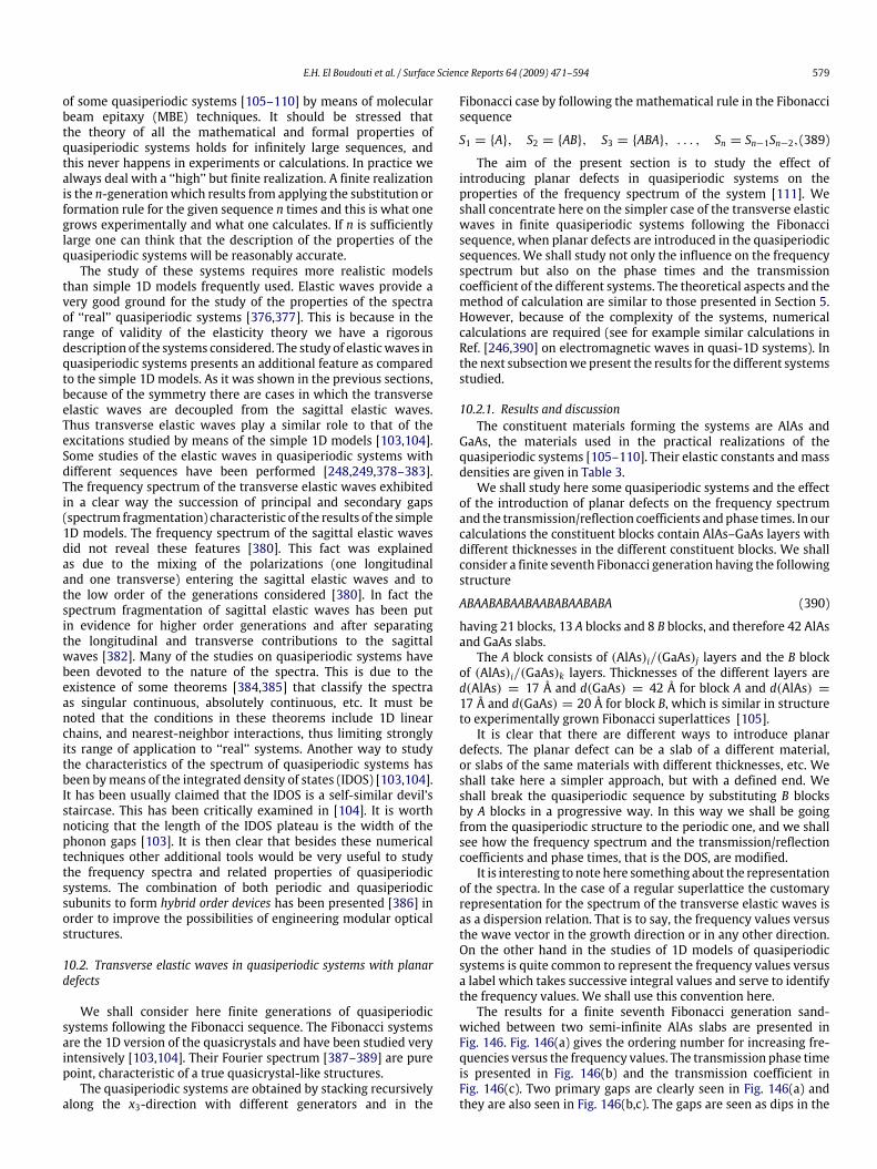
E.H. El Boudouti et al. / Surface Science Reports 64 (2009) 471–594 579

of some quasiperiodic systems [105–110] by means of molecularbeam epitaxy (MBE) techniques. It should be stressed thatthe theory of all the mathematical and formal properties ofquasiperiodic systems holds for infinitely large sequences, andthis never happens in experiments or calculations. In practice wealways deal with a ‘‘high’’ but finite realization. A finite realizationis the n-generationwhich results from applying the substitution orformation rule for the given sequence n times and this is what onegrows experimentally and what one calculates. If n is sufficientlylarge one can think that the description of the properties of thequasiperiodic systems will be reasonably accurate.The study of these systems requires more realistic models

than simple 1D models frequently used. Elastic waves provide avery good ground for the study of the properties of the spectraof ‘‘real’’ quasiperiodic systems [376,377]. This is because in therange of validity of the elasticity theory we have a rigorousdescription of the systems considered. The study of elasticwaves inquasiperiodic systems presents an additional feature as comparedto the simple 1Dmodels. As it was shown in the previous sections,because of the symmetry there are cases in which the transverseelastic waves are decoupled from the sagittal elastic waves.Thus transverse elastic waves play a similar role to that of theexcitations studied by means of the simple 1D models [103,104].Some studies of the elastic waves in quasiperiodic systems withdifferent sequences have been performed [248,249,378–383].The frequency spectrum of the transverse elastic waves exhibitedin a clear way the succession of principal and secondary gaps(spectrum fragmentation) characteristic of the results of the simple1D models. The frequency spectrum of the sagittal elastic wavesdid not reveal these features [380]. This fact was explainedas due to the mixing of the polarizations (one longitudinaland one transverse) entering the sagittal elastic waves and tothe low order of the generations considered [380]. In fact thespectrum fragmentation of sagittal elastic waves has been putin evidence for higher order generations and after separatingthe longitudinal and transverse contributions to the sagittalwaves [382]. Many of the studies on quasiperiodic systems havebeen devoted to the nature of the spectra. This is due to theexistence of some theorems [384,385] that classify the spectraas singular continuous, absolutely continuous, etc. It must benoted that the conditions in these theorems include 1D linearchains, and nearest-neighbor interactions, thus limiting stronglyits range of application to ‘‘real’’ systems. Another way to studythe characteristics of the spectrum of quasiperiodic systems hasbeen bymeans of the integrated density of states (IDOS) [103,104].It has been usually claimed that the IDOS is a self-similar devil’sstaircase. This has been critically examined in [104]. It is worthnoticing that the length of the IDOS plateau is the width of thephonon gaps [103]. It is then clear that besides these numericaltechniques other additional tools would be very useful to studythe frequency spectra and related properties of quasiperiodicsystems. The combination of both periodic and quasiperiodicsubunits to form hybrid order devices has been presented [386] inorder to improve the possibilities of engineering modular opticalstructures.

10.2. Transverse elastic waves in quasiperiodic systems with planardefects

We shall consider here finite generations of quasiperiodicsystems following the Fibonacci sequence. The Fibonacci systemsare the 1D version of the quasicrystals and have been studied veryintensively [103,104]. Their Fourier spectrum [387–389] are purepoint, characteristic of a true quasicrystal-like structures.The quasiperiodic systems are obtained by stacking recursively

along the x3-direction with different generators and in the

Fibonacci case by following the mathematical rule in the Fibonaccisequence

S1 = A, S2 = AB, S3 = ABA, . . . , Sn = Sn−1Sn−2,(389)

The aim of the present section is to study the effect ofintroducing planar defects in quasiperiodic systems on theproperties of the frequency spectrum of the system [111]. Weshall concentrate here on the simpler case of the transverse elasticwaves in finite quasiperiodic systems following the Fibonaccisequence, when planar defects are introduced in the quasiperiodicsequences. We shall study not only the influence on the frequencyspectrum but also on the phase times and the transmissioncoefficient of the different systems. The theoretical aspects and themethod of calculation are similar to those presented in Section 5.However, because of the complexity of the systems, numericalcalculations are required (see for example similar calculations inRef. [246,390] on electromagnetic waves in quasi-1D systems). Inthe next subsectionwepresent the results for the different systemsstudied.

10.2.1. Results and discussionThe constituent materials forming the systems are AlAs and

GaAs, the materials used in the practical realizations of thequasiperiodic systems [105–110]. Their elastic constants andmassdensities are given in Table 3.We shall study here some quasiperiodic systems and the effect

of the introduction of planar defects on the frequency spectrumand the transmission/reflection coefficients andphase times. In ourcalculations the constituent blocks contain AlAs–GaAs layers withdifferent thicknesses in the different constituent blocks. We shallconsider a finite seventh Fibonacci generation having the followingstructure

ABAABABAABAABABAABABA (390)

having 21 blocks, 13 A blocks and 8 B blocks, and therefore 42 AlAsand GaAs slabs.The A block consists of (AlAs)i/(GaAs)j layers and the B block

of (AlAs)i/(GaAs)k layers. Thicknesses of the different layers ared(AlAs) = 17 Å and d(GaAs) = 42 Å for block A and d(AlAs) =17 Å and d(GaAs) = 20 Å for block B, which is similar in structureto experimentally grown Fibonacci superlattices [105].It is clear that there are different ways to introduce planar

defects. The planar defect can be a slab of a different material,or slabs of the same materials with different thicknesses, etc. Weshall take here a simpler approach, but with a defined end. Weshall break the quasiperiodic sequence by substituting B blocksby A blocks in a progressive way. In this way we shall be goingfrom the quasiperiodic structure to the periodic one, and we shallsee how the frequency spectrum and the transmission/reflectioncoefficients and phase times, that is the DOS, are modified.It is interesting to note here something about the representation

of the spectra. In the case of a regular superlattice the customaryrepresentation for the spectrum of the transverse elastic waves isas a dispersion relation. That is to say, the frequency values versusthe wave vector in the growth direction or in any other direction.On the other hand in the studies of 1D models of quasiperiodicsystems is quite common to represent the frequency values versusa label which takes successive integral values and serve to identifythe frequency values. We shall use this convention here.The results for a finite seventh Fibonacci generation sand-

wiched between two semi-infinite AlAs slabs are presented inFig. 146. Fig. 146(a) gives the ordering number for increasing fre-quencies versus the frequency values. The transmission phase timeis presented in Fig. 146(b) and the transmission coefficient inFig. 146(c). Two primary gaps are clearly seen in Fig. 146(a) andthey are also seen in Fig. 146(b,c). The gaps are seen as dips in the

580 E.H. El Boudouti et al. / Surface Science Reports 64 (2009) 471–594

a

b

c

0 10 20 30 40 50

0 10 20 30 40 50

10 20 30 40

10

20

30

40

N (

orde

r of

fre

quen

cies

)

0

50

2

4

6

8

1

0 50ω (THz)

0

10

τ T(1

0-11

s)

0

2

|CT|2

Fig. 146. (a) Ordering number for increasing frequencies of transverse elasticwaves of a finite seventh Fibonacci generation versus the frequency values;(b) transmission phase time versus the frequency values; (c) transmissioncoefficient versus the frequency values.

a

b

c

0 10 20 30 40 50

0 10 20 30 40 50

10 20 30 40

10

20

30

40

N (

orde

r of

fre

quen

cies

)

0

50

2

4

6

8

1

0 50ω (THz)

0

10

τ T(1

0-11

s)

0

2

|CT|2

Fig. 147. As in Fig. 146 for a finite seventh Fibonacci generation where the blocksranging from the fifth to the seventh have been substituted by A blocks.

transmission coefficient. Because our system has not a very highnumber of modes and they are not very densely packed we seefluctuations in the transmission coefficient.We have performed progressive substitutions in the sequence

starting from the fifth block, thus leaving unchanged the first Bblock occupying the second place in the sequence, and substitutingthe other B blocks by A blocks, thus going towards a finitesuperlattice having 21 A blocks.

a

b

c

0 10 20 30 40 50

0 10 20 30 40 50

10 20 30 40

10

20

30

40

N (

orde

r of

fre

quen

cies

)

0

50

2

4

6

8

1

0 50ω (THz)

0

10

τ T(1

0-11

s)

0

2

|CT|2

Fig. 148. As in Fig. 146 for a finite seventh Fibonacci generation where the blocksranging from the fifth to the thirteenth have been substituted by A blocks.

Fig. 147 gives the same information as Fig. 146 for the Fibonaccistructure with the blocks ranging from the fifth to the seventhsubstituted by A blocks. As it can be seen from (390) this affectstwo B blocks, but we see drastic changes in the picture and theappearance of modes in the primary gaps reflected as peaks inthe transmission phase time. The appearance of localized modesinduced by the presence of planar defects could be anticipated, butwe see that the transmission coefficient is drastically affected, evenwith a small break in the quasiperiodic sequence.The overall picture is similar for further substitutions until we

reach the thirteenth block in the sequence. Fig. 148 correspondsto the Fibonacci structure with the blocks ranging from the fifth tothe thirteenth substituted by A blocks. We see now in Fig. 148(a)that the regions of the original primary gaps are greatly distorted,whereas a succession of peaks is present in the phase time and amore regular structure is evident in the transmission coefficient.This image holds for successive substitutions until we have astructure with A blocks, the second one excepted. This case can beseen in Fig. 149 corresponding to the Fibonacci structure with theblocks ranging from the fifth to the 20th substituted by A blocks.We have here the primary gaps, although in different frequencyranges, and we have a very regular structure in the transmissionphase time and coefficient.Fig. 150 gives the same information for a finite superlatticewith

21 A blocks. It can be seen that the picture is almost the same asthat presented in Fig. 149, where some small differences can beseen due to the presence of the B block.When comparing Figs. 146 and 150we can see some differences

that would not be evident if we were looking at the frequencyspectrum only. The primary gaps are present in both cases, but wesee that both spectra have different influences on the transmissionphase time and coefficient. For the finite periodic system we havetwo transmission dips in some frequency ranges with very smallfluctuations for the other frequencies. This is in deep contrastwith the irregular structure and pronounced dips seen in thetransmission coefficient of the Fibonacci sequence. The same istrue for the transmission phase time.

E.H. El Boudouti et al. / Surface Science Reports 64 (2009) 471–594 581

a

b

c

0 10 20 30 40 50

0 10 20 30 40 50

10 20 30 40

10203040

N (

orde

r of

fre

quen

cies

)

0

50

2

4

6

8

1

0 50ω (THz)

0

10

τ T(1

0-11

s)

0

2

|CT|2

Fig. 149. As in Fig. 146 for a finite seventh Fibonacci generation where the blocksranging from the fifth to the 20th have been substituted by A blocks.

0102030405060

a

b

c

0 10 20 30 40 50

0 10 20 30 40 50

10 20 30 40

N (

orde

r of

fre

quen

cies

)

2

4

6

8

1

0 50ω (THz)

0

10

τ T(1

0-11

s)

0

2

|CT|2

Fig. 150. As in Fig. 146 for a finite periodic superlattice having 21 A blocks.

We have seen a progressive evolution of the frequencyspectrum of the Fibonacci structure to the periodic one bymeans of a progressive substitution of the B blocks by Ablocks in the Fibonacci structure (obviously the process could beinterpreted in the reverse way). The central part of the spectrumseen in the former figures gets more eigenvalues coming fromthe lower and upper parts, respectively, via the motion andredistribution of localized modes in the primary gaps, until thenew spectrum corresponding to the periodic case is formed.Nevertheless themost gripping features are the important changesin the transmission phase time and the transmission coefficient

0

20

40

60

80

100

0

5

10

15

20

1

0

2

τ R(1

0-11

s)N

(or

der

of f

requ

enci

es)

|CR

|2

0 10 20 30 40 50

0 10 20 30 40 50

10 20 30 400 50ω (THz)

a

b

c

Fig. 151. (a) Ordering number for increasing frequencies of transverse elasticwaves of a finite seventh Fibonacci generation, with the outer surface stress-free,versus the frequency values; (b) reflection phase time versus the frequency values;(c) reflection coefficient versus the frequency values.

during the different steps of the process. The presence of planardefects in the quasiperiodic sequence, as introduced here, tendsto restore the order of the periodic structure. The breaking ofthe periodic order due to the presence of B blocks introducesconstructive and destructive interference on the waves travellingalong the heterostructure. This gives rise to dips and maxima inthe transmission coefficient in different parts of the spectra ascompared to the periodic case exhibitingwell-defined gap regions.Another situation that can be considered is that corresponding

to a quasiperiodic system grown on a semi-infinite substrate andwith the outer surface being stress-free, that is bound by thevacuum. As no elastic wave can propagate in the vacuum thesituation corresponds to the one of total reflection.Fig. 151 corresponds to the case of a finite seventh Fibonacci

generation deposited on a semi-infinite AlAl substrate and withits outer surface stress-free. Fig. 151(a) gives the increasing ordernumber of the frequencies versus the frequency spectrum, andwe see the primary gaps, with some localized modes inside them.These localized modes are seen in the reflection phase time asnarrow peaks inside the regions of almost zero value (Fig. 151(b)).The reflection coefficient presented in Fig. 151(c) is equal to one asit corresponds to the total reflection situation in this case.Fig. 152 gives the same information as Fig. 151 for the case of

a substitution ranging from the fifth to the tenth block. We seethe localized modes in the gaps and the corresponding peaks inthe reflection phase time. Further substitutions allows the additionand condensing of eigenvalues to the middle frequency range,thus reforming the primary gaps and going towards the finitesuperlattice case. This can be clearly seen in Fig. 153 correspondingto substitutions ranging from the fifth to the 18th blocks, andwhere the features corresponding to the finite superlattice arepractically completed, as also seen in the former cases.The important changes seen in the transmission coefficient

and phase times when performing the progressive introductionof the planar defects are a manifestation of the strong changesinduced in the density of states, related to these features as seenabove, even when only small changes in frequency are present.Constructive and destructive interference effects associated to the

582 E.H. El Boudouti et al. / Surface Science Reports 64 (2009) 471–594

0

20

40

60

80

100

0

5

10

15

20

1

0

2

τ R(1

0-11

s)N

(or

der

of f

requ

enci

es)

|CR

|2

0 10 20 30 40 50

0 10 20 30 40 50

10 20 30 400 50ω (THz)

a

b

c

Fig. 152. As in Fig. 151 for a finite seventh Fibonacci generation where the blocksranging from the fifth to the tenth have been substituted by A blocks.

presence of B blocks in the quasiperiodic sequence, with andwithout defects, gives rise to dips and maxima in the transmissioncoefficient. Besides this there is not a clear way to tie these effectsto other possible mechanisms, such as resonant effects or coupledcorrelation effects.In summary, we have shown in this subsection the evolution

of the frequency spectrum of the transverse elastic waves ofquasiperiodic systems towards the corresponding spectrum of afinite periodic system. This has been performed by the systematicintroduction of planar defects in the quasiperiodic structure. Theplanar defectswere introducedby substituting theBblocks presentin the quasiperiodic structures considered by A blocks.We have seen that the introduction of these planar defects

is reflected in the progressive shifting of the frequencies nearthe primary gaps from the lower and upper edges, respectively,towards the central part of the frequency spectrum. During someintermediate substitution steps these modes appear as localizedmodes inside the gaps, until they get coupled to the middle band.The use of the transmission and reflection phase times, that areassociated to the DOS, allows the clear characterization of thelocalized modes, appearing as narrow peaks in the phase timegraphs. The transmission coefficient is also a very useful tool andgives a rich information, not evident in the frequency spectrum.Some small changes and frequency redistributions in the spectrumproduce very important changes in the transmission coefficient.The transmission coefficient opens also the possibility of anotherexperimental way to study these systems.In a recentwork,wehave shown that the transmission/reflection

coefficients and phase times can be a very useful tool in the study ofthe spectra and thephysical properties of electromagneticwaves inquasiperiodic systems made of coaxial cables (see Refs. [246,390,391]). In particular, the evolution of the transmission and phasetime spectra from quasiperiodic to periodic structures has beenevidenced [390]. In addition, we have shown that when one con-siders one Fibonacci sequence, there is a self-similarity betweenthe transmission spectra with a scaling factor [391]. Also, we havedemonstrated the existence of two types of surface modes in Fi-bonacci SLs [246] where the layers in each period of the SL are

0

20

40

60

80100

0

5

10

15

20

1

0

2

τ R(1

0-11

s)N

(or

der

of f

requ

enci

es)

|CR

|2

0 10 20 30 40 50

0 10 20 30 40 50

10 20 30 400 50ω (THz)

a

b

c

Fig. 153. As in Fig. 151 for a finite seventh Fibonacci generation where the blocksranging from the fifth to the 18th have been substituted by A blocks.

staked according to the Fibonacci sequence. The fragmentation ofthe bulk bands spectra following a power law [244,245] has beenalso discussed. We think that all these phenomenon should existalso in the case of pure transverse or longitudinal acoustic wavesat normal incidence. This is due essentially to the similarity exist-ing between the equations governing all these excitations.

10.3. Sagittal elastic waves in quasiperiodic systems with planardefects

In this subsection, we are interested by the study of sagittalelastic waves in periodic and Fibonacci superlattices. The sagit-tal elastic waves can give rise to localized modes in systems withinterfaces thus introducing additional properties, in principle, tothe study of quasiregular multilayer systems. We choose the Fi-bonacci systems as representative of the quasiregular ones becausethey are the 1D representation of the quasicrystals [392–394].Its Fourier spectrum [395–397] is pure point, characteristic of atrue quasicrystal-like structure. We shall concentrate on the fre-quency dispersion relation and the density of states (DOS) that isan important quantity for the understanding of many phenomenain a large number of physical systems.It is interesting to note here something about the representation

of the spectra. In the studies of 1Dmodels of quasiregular systems,it is quite common to represent the frequency values versus a labelwhich takes successive integral values and serve to identify thefrequency values (see the previous subsection). On the other handin the case of a regular superlattice the customary representationfor the spectrum of the elastic waves is as a dispersion relation.That is to say, the frequency values versus the wave vector inthe growth direction or in any other direction. We shall use thisconvention here.

10.3.1. Results and discussionWe shall consider that the A and B blocks are formed by two

slabs of differentmaterials, with different thicknesses in each case,as in the experimental realizations [105–110].In order to illustrate the systems in a practical and manageable

way we shall concentrate on the sixth and eighth Fibonacci

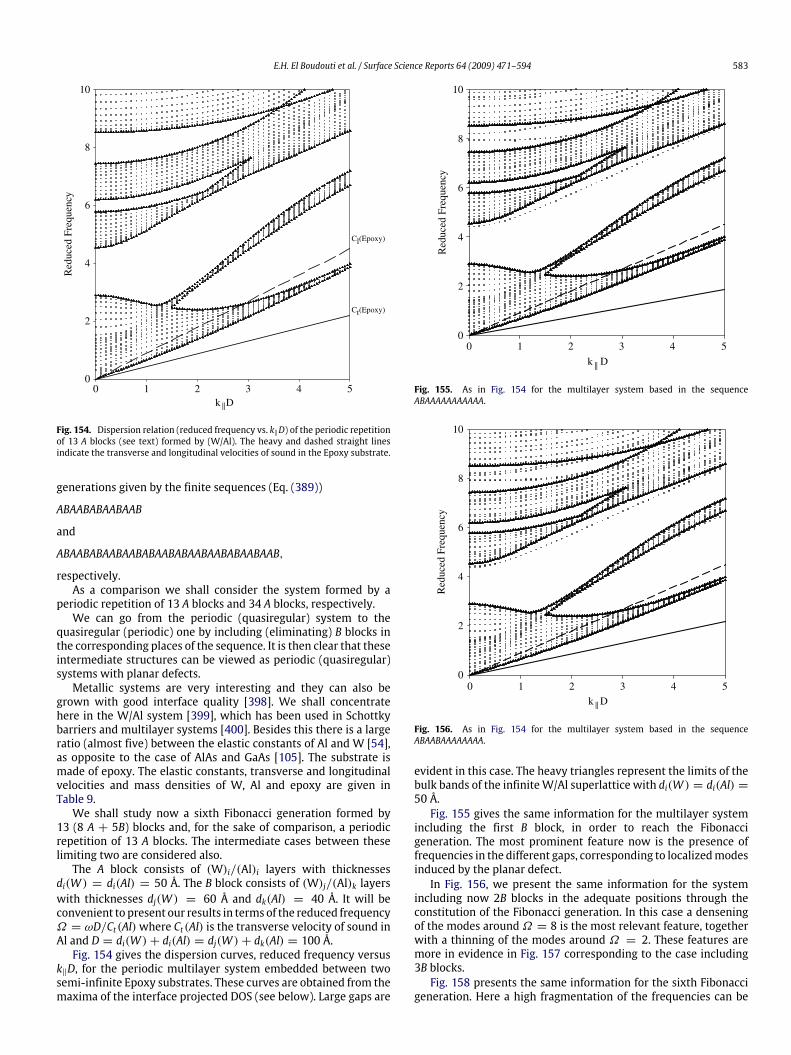
E.H. El Boudouti et al. / Surface Science Reports 64 (2009) 471–594 583

k ||D

Cl(Epoxy)

Ct(Epoxy)

0 1 2 3 4 5

2

4

6

8

0

10

Red

uced

Fre

quen

cy

Fig. 154. Dispersion relation (reduced frequency vs. k‖D) of the periodic repetitionof 13 A blocks (see text) formed by (W/Al). The heavy and dashed straight linesindicate the transverse and longitudinal velocities of sound in the Epoxy substrate.

generations given by the finite sequences (Eq. (389))

ABAABABAABAAB

and

ABAABABAABAABABAABABAABAABABAABAAB,

respectively.As a comparison we shall consider the system formed by a

periodic repetition of 13 A blocks and 34 A blocks, respectively.We can go from the periodic (quasiregular) system to the

quasiregular (periodic) one by including (eliminating) B blocks inthe corresponding places of the sequence. It is then clear that theseintermediate structures can be viewed as periodic (quasiregular)systems with planar defects.Metallic systems are very interesting and they can also be

grown with good interface quality [398]. We shall concentratehere in the W/Al system [399], which has been used in Schottkybarriers and multilayer systems [400]. Besides this there is a largeratio (almost five) between the elastic constants of Al and W [54],as opposite to the case of AlAs and GaAs [105]. The substrate ismade of epoxy. The elastic constants, transverse and longitudinalvelocities and mass densities of W, Al and epoxy are given inTable 9.We shall study now a sixth Fibonacci generation formed by

13 (8 A + 5B) blocks and, for the sake of comparison, a periodicrepetition of 13 A blocks. The intermediate cases between theselimiting two are considered also.The A block consists of (W)i/(Al)i layers with thicknesses

di(W ) = di(Al) = 50 Å. The B block consists of (W)j/(Al)k layerswith thicknesses dj(W ) = 60 Å and dk(Al) = 40 Å. It will beconvenient to present our results in terms of the reduced frequencyΩ = ωD/Ct(Al)where Ct(Al) is the transverse velocity of sound inAl and D = di(W )+ di(Al) = dj(W )+ dk(Al) = 100 Å.Fig. 154 gives the dispersion curves, reduced frequency versus

k‖D, for the periodic multilayer system embedded between twosemi-infinite Epoxy substrates. These curves are obtained from themaxima of the interface projected DOS (see below). Large gaps are

k || D

0 1 2 3 4 5

2

4

6

8

0

10

Red

uced

Fre

quen

cy

Fig. 155. As in Fig. 154 for the multilayer system based in the sequenceABAAAAAAAAAAA.

k || D0 1 2 3 4 5

2

4

6

8

Red

uced

Fre

quen

cy

0

10

Fig. 156. As in Fig. 154 for the multilayer system based in the sequenceABAABAAAAAAAA.

evident in this case. The heavy triangles represent the limits of thebulk bands of the infiniteW/Al superlattice with di(W ) = di(Al) =50 Å.Fig. 155 gives the same information for the multilayer system

including the first B block, in order to reach the Fibonaccigeneration. The most prominent feature now is the presence offrequencies in the different gaps, corresponding to localizedmodesinduced by the planar defect.In Fig. 156, we present the same information for the system

including now 2B blocks in the adequate positions through theconstitution of the Fibonacci generation. In this case a denseningof the modes aroundΩ = 8 is the most relevant feature, togetherwith a thinning of the modes around Ω = 2. These features aremore in evidence in Fig. 157 corresponding to the case including3B blocks.Fig. 158 presents the same information for the sixth Fibonacci

generation. Here a high fragmentation of the frequencies can be

584 E.H. El Boudouti et al. / Surface Science Reports 64 (2009) 471–594

k || D0 1 2 3 4 5

Cl(Epoxy)

Ct(Epoxy)2

4

6

8

Red

uced

Fre

quen

cy

0

10

Fig. 157. As in Fig. 154 for the multilayer system based in the sequenceABAABABAAAAAA.

observed for Ω > 6. One can notice in Figs. 154–158 that byintroducing the B blocks, a narrow band appear in the second gap,this band is wider for small and large values of k‖D and becomesflat for intermediate values (1 < k‖D < 4).The different dispersion curves in Figs. 154–158 are obtained

from themaximaof theDOS. Some examples of theDOS as functionof the reduced frequency are sketched in Figs. 159–161 in orderto ascertain the importance and possible influence of the localizedmodes and the redistribution of the spectrum.Fig. 159 gives the DOS as a function of the reduced frequency

for k‖D = 0. It is evident here the existence of three well-definedgaps marked by the vertical dot-dashed lines. One can notice theappearance of the localized modes as narrow peaks of strongintensity in the gaps. Themodifications at high frequencies are alsodrastically reflected in the DOS.Fig. 160 illustrates the same information as Fig. 159 for the case

k‖D = 2. It can be seen that we have now a new gap for Ω < 1and another one beyond Ω = 2, but no localized modes appearthere. The gap beyondΩ = 3 is wider now. It can be seen that thelow frequency region Ω ≤ 3 suffers only very small changes. Asdiscussed before, the localized modes atΩ ≈ 5.7 appear with theintroduction of the first B block and have almost no variations untilarriving to the Fibonacci structure. On the other hand the region offrequencies beyondΩ = 6 presents very important variations andparticularly in the fourth gapwith an increasing presence ofmodesthere, thus closing it partially.Fig. 161 presents the same information as Fig. 160 for the k‖D =

4 case.We have a very wide gap forΩ < 2, but no localizedmodesappear there. We have also other two wide gaps. In the first onethere appear some localized modes very close to the upper borderof the gap. We have also clear signatures of localized modes in thesecond gap around Ω ≈ 7.75. The most drastic changes can beseen in the bands aroundΩ = 6 andΩ > 8.We have seen that theW/Al system exhibits wide gaps inwhich

strong localizedmodes introduced by the planar defects associatedto the B blocks appear. Strong modifications of the frequencyspectrum aroundΩ ≈ 6 and beyond, are also present, even closingpartially the upper gaps. The quasiregular structures exhibit animportant fragmentation of the frequency spectrum. Important

k ||D

2

4

6

8

Red

uced

Fre

quen

cy

0

10

0 1 2 3 4 5

Fig. 158. As in Fig. 154 for the sixth Fibonacci generation ABAABABAABAAB.

differences in the characteristics of the frequency spectrumand theinterface projected DOS are evident for different values of k‖D.In order to study the spatial localization of the different modes

in these quasiperiodic structures, we have sketched in Fig. 162 thelocal DOS as function of the space position for themodes labeled 1,2, 3, 4, 5 and 6 in Fig. 160. The local DOS reflects the squaremodulusof the displacement field. The modes labeled 1, 2 and 3 fall withinthe pass band of the infinite A bilayer superlattice and thereforepresent a propagative behavior in the whole structure, particularlyin the region of the unperturbed A blocks (see Fig. 162(a), (b),(c)) and vanish in the disordered region containing the B blocks.However, the modes labeled 4, 5 and 6 fall in the forbidden bandof the infinite A bilayer superlattice and therefore show a spatiallocalization within the disordered region containing the B blocks(see Fig. 162(d), (e), (f)) and vanish in the ordered region containingthe A blocks. In this figure one can see that the x1x1 contribution tothe local DOS (full line) is smaller than the x3x3 one (dashed line),by the different factors shown in the figure.It is then clear that theW/Al system together with the interplay

of the quasiregularity factor can be a suitable candidate forapplications in filtering and guiding processes.In summary, we have presented in this subsection sagittal

elastic waves in quasiperiodic structures for different values ofthe wave vector parallel to the interfaces. The multilayer systemsare ranged from the periodic case to the quasiregular Fibonaccione. We have considered characteristic metallic materials asrepresentatives of multilayer systems exhibiting wide gaps. Inthe case of metallic W/Al materials, we have seen that thesestructures exhibit wide gaps. This property allows, by meansof the introduction of planar defects covering the whole rangebetween the periodic and quasiregular Fibonacci structures, theexistence of strongly localized modes in these gaps. These modesare clearly identifiable in the frequency dispersion relations andby the intense and narrow peaks in the DOS. Thus, these materialsmay be well adapted as filtering and guiding systems. An analysisof the local DOS clearly shows the spatial localization of thepropagative and localized modes in these quasiregular structures.

11. Summary and conclusions

In this review paper we have presented a comprehensivetheoretical analysis of the propagation and localization of acoustic

E.H. El Boudouti et al. / Surface Science Reports 64 (2009) 471–594 585

AAAAAAAAAAAAA

ABAAAAAAAAAAA

ABAABAAAAAAAA

ABAABABAAAAAA

ABAABABAABAAA

ABAABABAABAAB

0

80

160

240

0

80

160

240

320

0

80

160

240

320

0

80

160

240

320

0

80

160

240

320

80

160

240

320

2 4 6 8

Reduced Frequency

0 10

320

0

Δn(ω

, k||D

= 0

)

Fig. 159. Interface projected DOS as a function of the reduced frequency for k‖D = 0, for the (W/Al) multilayer systems whose stackings appear in the figure.

waves in solid, non-viscous fluid and piezoelectric layeredmaterials. In general, we have limited ourselves to the case ofisotropicmaterials forwhich shear horizontalwaves are decoupledfrom sagittal waves polarized in the plane defined by the normalto the surface and the wave vector parallel to the surface. Thephonon modes are particularly emphasized in the case of periodicmultilayered systems such as superlattices even though othermaterials such as adsorbed layers and quasiperiodic structuresare also discussed. This study has been performed within theframework of the Green’s function method which enables usto deduce the dispersion curves, densities of states as well asthe transmission and reflection coefficients. The Green’s functionapproach used in this work is also of interest for studying thescattering of light by surface phonons. The advantage of the 1Dlayered media treated here in comparison with their 2D and 3Dcounterparts systems, resides in obtaining, in general, closed formexpressions that enables us to discuss deeply different physicalproperties related to band gaps in such systems.Despite the problem of acoustic waves in solid and fluid

materials has been intensively studied since the beginning of the

last century, this subject still attracts attention of researchersbecause of the high quality level of control and perfection reachedin the growth techniques of microstructures and nanostructures,but also due to the sophisticated experimental techniquesused to probe different modes of these systems in differentfrequency domains. In addition, these systemsmay present severalapplications in guiding, stopping and filtering waves.We would like to summarize here what has been reviewed

in the previous sections. In the case of adsorbed layers, we havepresented first a simple analytical expression to calculate theDOS of one adsorbed slab. This quantity has been shown to bevery close to Brillouin scattering spectra and permits to draw thedispersion curves in slow and high frequency domains, from themaxima of the DOS. An analysis of the LDOS shows clearly thespatial localization of the different modes belonging to differentfrequency regions. Then, we have proposed two structures thatcan make possible, or at least facilitate, the confinement of themodes. The first structure consists to insert a buffer layer withhigh velocities of sound between the substrate and the topmostlayer, this layer plays the role of a barrier between phonons in

586 E.H. El Boudouti et al. / Surface Science Reports 64 (2009) 471–594

AAAAAAAAAAAAA

ABAAAAAAAAAAA

ABAABAAAAAAAA

ABAABABAAAAAA

ABAABABAABAAA

ABAABABAABAAB

1

2

3

4

6

5

0

80

160

240

0

80

160

240

320

0

80

160

240

320

0

80

160

240

320

0

80

160

240

320

80

160

240

320

320

0

Δn(ω

, k||D

= 2

)

1 2 3 4 5 6 7 8 9

Reduced Frequency

0 10

Fig. 160. As in Fig. 159 for k‖D = 2.

these two latter materials giving rise to well-confined modesin the topmost layer. The second solution consists to adsorbatethe layer on a superlattice (SL) made of the periodic repetitionof two different layers instead of a homogeneous substrate.When the guided modes of the adsorbed layer fall inside theforbidden bands of the SL, these modes do not propagate inthe SL and remain well confined in the topmost layer. Someexperimental results and the interest of the Green’s functioncalculation in explaining the surface Brillouin scattering spectra isalso outlined.In the case of periodic structures made of an alternative

repetition of two or several layers, we have treated separatelyshear horizontal waves in solid–solid SLs and sagittal wavesin both solid–solid and solid–fluid SLs. In practice, the SLs arecomposed of finite number of cells deposited on a substrate,however if the number of cells is big enough, one can treat the freesurface independently of the SL/substrate interface, each systembeing considered as semi-infinite. Even though surface acousticwaves in semi-infinite SLs have been intensively studied since the

pioneering work of Djafari-Rouhani et al. [54,215], however a clearevidence about the conditions of their existence lacks. We havedemonstrated in this work a general rule about the existence ofthese modes. More generally, we have shown that the eigenmodesof a finite SL constituted of N cells with free-stress surfaces arecomposed of N − 1 modes in each band and one mode by gapwhich is associated to one of the two surfaces surrounding thesystem. These lattermodes are independent ofN and coincidewiththe surface modes of two complementary SLs obtained from thecleavage of an infinite SL along a plane parallel to the interfaces.This rule has been shown to be valid for shear horizontal wavesin elastic and piezoelectric SLs and sagittal waves in solid–fluid SLswhen the cleavage is produced inside the fluid layer. However, thisrule is not fulfilled for sagittal waves in solid–solid and solid–fluidSLs when the cleavage occurs in the solid layers and one can havezero, one or even two modes in each gap. Nevertheless, in theselatter cases, pseudo-surface (or leaky-surface) modes may existinside the bulk bands of the SL. These modes are without analoguefor shear horizontal waves.

E.H. El Boudouti et al. / Surface Science Reports 64 (2009) 471–594 587

0

80

160

240

0

0

80

160

240

320

0

80

160

240

320

0

80

160

240

320

0

80

160

240

320

80

160

240

320

AAAAAAAAAAAAA

ABAAAAAAAAAAA

ABAABAAAAAAAA

ABAABABAAAAAA

ABAABABAABAAA

ABAABABAABAAB

2 4 6 80 10Reduced Frequency

32

0

Δn(ω

, k||D

= 4

)

Fig. 161. As in Fig. 159 for k‖D = 4.

In addition to these rules, we have investigated interfaceand pseudo-interface modes induced by the interface betweenan homogeneous substrate and a SL depending on the stiffnessof the substrate but also on the layer in the SL which isin contact with the substrate. We have also given a detailedstudy about the interaction of the different modes existingin a finite size SL, in particular we have emphasized theinteraction between the surface and interface (or cavity) modesdepending on the distance between these two defects. Thetransmission and reflection coefficients of wave propagationthrough these systems has shown several new properties as therelation between the DOS and the transmission and reflectionphase times, the existence of transmission zeros in solid–fluidSLs and therefore new gaps in addition to Bragg gaps, theconditions of band gap closings, the existence of Fano resonancesand the possibility of enhanced transmission between twomedia through cavity modes or interface modes. The applicationof multilayered media as acoustic mirrors has been shown.Some experimental results and the interest of the Green’s

function calculation in explaining the Raman spectra is alsoreviewed.Finally, by analogy with the previous works on periodic

systems,we have discussed briefly the effect of introducing defectsin quasiperiodic structures on acoustic waves in these systems.Wehave focused our study on the well-known quasiperiodic systemsmade of two blocks A and B arranged according to the Fibonaccisequence. Each of the A and B blocks is constituted of a bilayer.By substituting progressively the blocks A by B or vice versa, wehave shown the evolution of the DOS spectra and dispersion curvesbetween periodic and quasiperiodic structures.This Report represents a modest contribution of its authors to

this wide area of research during the last fifteen years. We hopethat this contribution will bring a new piece of work to the fieldof acoustic waves in solid and fluid layered materials. This workcould be considered as the continuity of the reviewpaper by Saprieland Djafari-Rouhani [30] twenty years ago on the same subject. Inwriting this review, we have made an effort to cite most works ofthe groups working in these topics even though we think that it is

588 E.H. El Boudouti et al. / Surface Science Reports 64 (2009) 471–594

A

A B A A A A A A A A A A A

A B A A B A A A A A A A A

A B A A B A B A A B A A B

A B A A A A A A A A A A A

A B A A B A A A A A A A A

B A A B AB BAA A A B

x 40

x 40

x 40

x 4

x 6

x 10

mode 1

mode 2

mode 3

mode 4

mode 5

mode 6

a

b

c

d

e

f

0

1

2

012345

0

1

2

0

2

4

6

0

2

4

6

8

1

2

3

2 3 41 6 75 8 9 10 11 120 13

z/D

Loca

l den

sity

of s

tate

s (k

//D =

2)

3

0

Fig. 162. (a) Representation of local DOS for the modes labeled 1, 2, 3, 4, 5 and 6 in Fig. 160 and corresponding, respectively, to ωD/Ct (Al) = 7.562 (a), 7.677 (b), 7.71 (c),8.665 (d), 8.62 (e), 8.604 (f). The full and dashed curves correspond to the x1x1 and x3x3 components of local DOS, respectively.

not obvious to quote all of themand to give them the right citationsthey deserve. If so, we hope that their authors will excuse us.The interested readers will probably notice that this review

paper is mostly theoretical. That is because our competencies liemostly in theory. Rather than trying to give all the emphasis itdeserves on the very important experimental and applied aspectsof acoustic waves in layered materials, we prefer to leave spacefor another Surface Science Report written by experimentalists.Hoping that this paper will stimulate at least one colleague toundertake such a task, we wish him in advance good luck andsuccess.

Acknowledgements

One of us (E.H. El Boudouti) gratefully acknowledges thehospitality of the Institut d’Electronique, de Microélectroniqueet de Nanotechnologie (IEMN), UMR-CNRS 8520, and UFR dePhysique, Université des Sciences et Technologies de Lille. Thiswork was realized within the framework of a scientific conventionbetween the universities of Lille 1 and Oujda and it was supportedin part by the European Commission (EC) 7th FrameworkProgramme (FP7) under the (IP) project reference No. 216176(NANOPACK, www.nanopack.org).

Appendix A. Superlattice response functions

Following the interface response theory [115], we obtained thefollowing.

A.1. For the infinite superlattice

(a) The elements g(m,m′), where m ≡ (n, i,±di/2) of theresponse function g between the different interface planes, asfunction of Ci, Si, Fi, t and η (Eqs. (135)–(137), (141) and (142)) are

g(n, i,−d1/2; n′, i,−d1/2) =(C1S2F2+C2S1F1

)t |n−n

′|+1

t2 − 1(391)

g(n, i,−d1/2; n′, i,+d1/2) =S2F2

t |n−n′|+1

t2 − 1+S1F1

t |n−n′−1|+1

t2 − 1(392)

g(n, i,+d1/2; n′, i,−d1/2) =S2F2

t |n−n′|+1

t2 − 1+S1F1

t |n−n′+1|+1

t2 − 1(393)

g(n, i,+d1/2; n′, i,+d1/2) =(C1S2F2+C2S1F1

)t |n−n

′|+1

t2 − 1. (394)

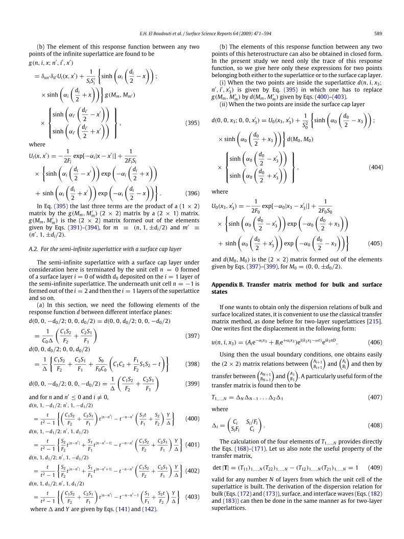
E.H. El Boudouti et al. / Surface Science Reports 64 (2009) 471–594 589

(b) The element of this response function between any twopoints of the infinite superlattice are found to beg(n, i, x; n′, i′, x′)

= δnn′δii′Ui(x, x′)+1SiS ′i

sinh

(αi

(di2− x

));

× sinh(αi

(di2+ x

))g(Mm,Mm′)

×

sinh

(αi′

(di′2− x′

))sinh

(αi′

(di′2+ x′

)) , (395)

where

Ui(x, x′) = −12Fiexp[−αi|x− x′|] +

12FiSi

×

sinh

(αi

(di2− x′

))exp

(−αi

(di2+ x

))+ sinh

(αi

(di2+ x′

))exp

(−αi

(di2− x

)). (396)

In Eq. (395) the last three terms are the product of a (1 × 2)matrix by the g(Mm,M ′m) (2 × 2) matrix by a (2 × 1) matrix.g(Mm,M ′m) is the (2 × 2) matrix formed out of the elementsgiven by Eqs. (391)–(394), for m ≡ (n, 1,±di/2) and m′ ≡(n′, 1,±di/2).

A.2. For the semi-infinite superlattice with a surface cap layer

The semi-infinite superlattice with a surface cap layer underconsideration here is terminated by the unit cell n = 0 formedof a surface layer i = 0 of width d0 deposited on the i = 1 layer ofthe semi-infinite superlattice. The underneath unit cell n = −1 isformed out of the i = 2 and then the i = 1 layers of the superlatticeand so on.(a) In this section, we need the following elements of the

response function d between different interface planes:d(0, 0,−d0/2; 0, 0, d0/2) = d(0, 0, d0/2; 0, 0,−d0/2)

=1C01

(C1S2F2+C2S1F1

)(397)

d(0, 0, d0/2; 0, 0, d0/2)

=11

C1S2F2+C2S1F1+S0F0C0

(C1C2 +

F1F2S1S2 − t

)(398)

d(0, 0,−d0/2; 0, 0,−d0/2) =11

(C1S2F2+C2S1F1

)(399)

and for n and n′ ≤ 0 and i 6= 0,d(n, 1,−d1/2; n′, 1,−d1/2)

=t

t2 − 1

(C1S2F2+C2S1F1

)t |n−n

′|− t−n−n

′

(S1tF1+S2F2

)Y1

(400)

d(n, 1,−d1/2; n′, 1, d1/2)

=t

t2 − 1

S2F2t |n−n

′|+S1F1t |n−n

′−1|− t−n−n

′

(C1S2F2+C2S1F1

)Y1

(401)

d(n, 1, d1/2; n′, 1,−d1/2)

=t

t2 − 1

S2F2t |n−n

′|+S1F1t |n−n

′+1|− t−n−n

′

(C1S2F2+C2S1F1

)Y1

(402)

d(n, 1, d1/2; n′, 1, d1/2)

=t

t2 − 1

(C1S2F2+C2S1F1

)t |n−n

′|− t−n−n

′−1(S1F1+S2tF2

)Y1

(403)

where1 and Y are given by Eqs. (141) and (142).

(b) The elements of this response function between any twopoints of this heterostructure can also be obtained in closed form.In the present study we need only the trace of this responsefunction, so we give here only these expressions for two pointsbelonging both either to the superlattice or to the surface cap layer.(i) When the two points are inside the superlattice d(n, i, x3;

n′, i′, x′3) is given by Eq. (395) in which one has to replaceg(Mm,M ′m) by d(Mm,M

′m) given by Eqs. (400)–(403).

(ii) When the two points are inside the surface cap layer

d(0, 0, x3; 0, 0, x′3) = U0(x3, x′

3)+1S20

sinh

(α0

(d02− x3

));

× sinh(α0

(d02+ x3

))d(M0,M0)

×

sinh

(α0

(d02− x′3

))sinh

(α0

(d02+ x′3

)) , (404)

where

U0(x3, x′3) = −12F0exp[−α0|x3 − x′3|] +

12F0S0

×

sinh

(α0

(d02− x′3

))exp

(−α0

(d02+ x3

))+ sinh

(α0

(d02+ x′3

))exp

(−α0

(d02− x3

))(405)

and d(M0,M0) is the (2 × 2) matrix formed out of the elementsgiven by Eqs. (397)–(399), forM0 = (0, 0,±d0/2).

Appendix B. Transfer matrix method for bulk and surfacestates

If one wants to obtain only the dispersion relations of bulk andsurface localized states, it is convenient to use the classical transfermatrix method, as done before for two-layer superlattices [215].One writes first the displacement in the following form:

u(n, i, x3) = (Aie−αix3 + Bie+αix3)ei(k‖x‖−ωt)eik3nD. (406)

Using then the usual boundary conditions, one obtains easilythe (2 × 2)matrix relations between

(Ai+1Bi+1

)and

(AiBi

)and then by

transfer between(AN+1BN+1

)and

(A1B1

). A particularly useful form of the

transfer matrix is found then to be

T1,...,N = 1N1N−1 . . .1211 (407)

where

1i =

(Ci Si/FiSiFi Ci

). (408)

The calculation of the four elements of T1,...,N provides directlythe Eqs. (168)–(171). Let us also note the useful property of thetransfer matrix,

det |T| = (T11)1,...,N(T22)1,...,N − (T12)1,...,N(T21)1,...,N = 1 (409)

valid for any number N of layers from which the unit cell of thesuperlattice is built. The derivation of the dispersion relation forbulk (Eqs. (172) and (173)), surface, and interfacewaves (Eqs. (182)and (183)) can then be done in the same manner as for two-layersuperlattices.

590 E.H. El Boudouti et al. / Surface Science Reports 64 (2009) 471–594

Appendix C. Green’s function for a substrate–buffer-layer–finite-superlattice–cap-layer–substrate system

Knowing the Green’s function for an infinite homogeneousmedium and for an infinite superlattice given in the Appendix A,we obtained, with the help of the interface response theory [115],the Green’s function for the substrate(s)–buffer layer (b) finitesuperlattice(2-1)–cap layer (c) substrate (v) system (see Fig. 67).1. In this section we need the following elements of the

response function d between different interface planes:(i) For n = 0, i = a:

d(0, a,−

da2; 0, a,−

da2

)

= −(y+ z SaFaCa )B0t − t

2N(y+ z0 SaFaCa )Bt

(1+ FsSaFaCa

)1−(410)

d(0, a,−

da2; 0, a,+

da2

)= d

(0, a,+

da2; 0, a,−

da2

)= −yt

B0 − t2NB

Ca(1+ FsSa

FaCa

)1−

(411)

d(0, a,

da2; 0, a,

da2

)= −yt

B0 − t2NB1−

. (412)

(ii) for n = N, i = b:

d(N, b,−

db2;N, b,−

db2

)= −

xA0 − t2Nx0A1−

(413)

d(N, b,

db2;N, b,−

db2

)= d

(N, b,−

db2;N, b,

db2

)= −

xA0 − t2Nx0A

Cb(1+ FvSb

FbCb

)1−

(414)

d(N, b,

db2;N, b,

db2

)

=

(−x+ k SbFbCb )A0 − t2N(−x0 + k0

SbFbCb

)A

(1+ FvSbFbCb

)1−. (415)

(iii) for 0≤ n, n′ ≤ N and i 6= a, b;

d(n, 1,−

d12; n′, 1,−

d12

)=

tt2 − 1

yt|n−n

′| −11−[xAB0tn+n

′−1

− x0ABt2N(tn−n′

+ tn′−n)+ x0tA0Bt2N−n−n

′

]

(416)

d(n, 1,−

d12; n′, 1,

d12

)=

tt2 − 1

S2F2t|n−n

′| +S1F1t|n−n

′−1| −

11−[yAB0tn+n

′

−ytxABt2N(xtn−n

′−1+ x0tn

′−n)− ytA0Bt2N−n−n

′

]

(417)

d(n, 1,

d12; n′, 1,−

d12

)= d

(n, 1,−

d12; n′, 1,

d12

)(418)

d(n, 1,

d12; n′, 1,

d12

)=

tt2 − 1

yt|n−n

′| −11−[x0AB0tn+n

′

− x0ABt2N(tn−n′

+ tn′−n)+ xA0Bt2N−n−n

′

]

. (419)

2. The elements of this response function between any two pointsof this heterostructure can also be obtained in closed from. Since inthe present study we need only the trace of this response function,we give here only those expression for two points both of whichbelong to the substrates (s) or (v), both to cap layer (a) or bufferlayer (b), or both to the superlattice.(i) When the tow points are inside the substrate (s):

d(x3, x′3) = −12FSexp[−αs|x3−x

′3|]

+

[12Fs−(y+ z SaFaCa )B0t − t

2N(y+ z0 SaFaCa )Bt

(1+ FsSaFaCa

)1−

]× exp[αs(x3+x

′3)] . (420)

(ii) When the tow points are inside buffer layer (a):

d(n, a, x3; n′, a, x′3) = Ua(x3, x′

3)

+1S2a

sinh

[αa

(da2− x3

)]; sinh

[αa

(da2+ x3

)]

× d(Ma,Ma)

sinh[αa

(da2− x′3

)]sinh

[αa

(da2+ x′3

)] (421)

where

Ua(x3, x′3) = −12Faexp[−αa|x3−x

′3|]

+12FaSa

sinh

[αa

(da2− x′3

)]× exp

[−αa

(da2+ x3

)]+ sinh

[−αa

(da2+ x′3

)]× exp

[−αa

(da2− x3

)](422)

and d(Ma,Ma) is the (2 × 2) matrix formed by the element givenby Eqs. (410)–(412). forMa = (0, a,± da2 ).(iii) When the tow points are inside the superlattice:

d(n, i, x3; n′, i′, x′3) = δnn′δii′Ui(x3, x′

3)

+1SiSi′

sinh

[αi

(di2− x3

)]; sinh

[αi

(di2+ x3

)]

× d(Mm,Mm′)

sinh[αi′

(d1′2− x′3

)]sinh

[αi′

(d′2+ x′3

)] (423)

where

Ui(x3, x′3) = −12Fiexp[−αi|x3−x

′3|]+

12FiSi

×

[sinh

[αi

(di2− x′3

)]exp

[−αi

(di2+ x3

)]+ sinh

[αi

(di2+ x′3

)]exp

[−αi

(di2− x3

)]]. (424)

E.H. El Boudouti et al. / Surface Science Reports 64 (2009) 471–594 591

(iv) When the tow points are inside the surface cap layer (b):

d(N, b, x3;N, b, x′3) = Ub(x3, x′

3)

+1S2b

[sinh

[αb

(db2− x3

)]; sinh

[αb

(db2+ x3

)]]

× d(Mb,Mb)

sinh[αb

(db2− x′3

)]sinh

[αb

(db2+ x′3

)] (425)

where

Ub(x3, x′3) = −12Fbexp[−αb|x3−x

′3|]+

12FbSb

×

[sinh

[αb

(db2− x′3

)]exp

[−αb

(db2+ x3

)]+ sinh

[−αb

(di2+ x′3

)]exp

[−αb

(db2− x3

)]](426)

and d(Mb,Mb) is the (2 × 2) matrix formed by the element givenby Eqs. (413)–(415) forMb = (N, b,±

db2 ).

(v) When the tow points are inside the substrate (v):

d(x3, x′3) = −12Fvexp[−αv|x3−x

′3|]

+

[12Fv+

(−x+ k SbFbCb )A0 − t2N(−x0 + k0

SbFbCb

)A

(1+ FvSbFbCb

)1−

]

× exp[−αv(x3+x′3−2xb)] . (427)

References

[1] W.M. Ewing, W.S. Jardetski, F. Press, Elastic Waves in Layered Media,McGraw-Hill, New York, 1957.

[2] R.M. White, Proc. IEEE 58 (1970) 1238.[3] B.A. Auld, Acoustic Fields and Waves in Solids, Wiley, New York, 1973.[4] E.E. Dieulesaint, D. Royer, in: L. Dobrzynski (Ed.), Handbook of Surfaces andInterfaces, vol. 2, Garland STPM, New York, 1978, p. 66.

[5] J.D. Maines, E.G.S. Paige, Proc. IEEE 64 (1976) 639.[6] A.A. Oliner, in: A.A. Oliner (Ed.), Surface Acoustic Waves, Springer, New York,1978, p. 1.

[7] I.A. Viktorov, Rayleigh and LambWaves, Plenum, New York, 1967.[8] N.D. Lanzillotti-Kimura, A. Fainstein, A. Lematre, B. Jusserand, Appl. Phys. Lett.88 (2006) 083113.

[9] P. Tournois, C. Lardat, IEEE Trans. Sonics Ultrason. 16 (1969) 107.[10] P. Schuitzler, L. Bergstein, L. Strauss, IEEE Trans. Sonics Ultrason. 17 (1970)

585.[11] H.F. Tiersten, J. Appl. Phys. 40 (1969) 770.[12] J.W.S. Rayleigh, Proc. London Math. Soc. 17 (1885) 4.[13] R. Stoneley, Proc. R. Soc. London, Ser. A 106 (1927) 421.[14] R.O. Claus, C.H. Palmer, Appl. Phys. Lett. 31 (1977) 547.[15] J.G. Scholte, Proc. K. Ned. Akad.Wel. Amsterdam, vol. 45, pt1, 1942, pp. 20–25,

and pt2, pp. 159–162.[16] V. Gusev, C. Desmet, W. Lauriks, C. Glorieux, J. Thoen, J. Acoust. Soc. Am. 100

(1996) 1514.[17] C. Glorieux, K.de Van de Rostyne, J.D. Beers, W. Gao, S. Petillion, N. Van Riet,

K.A. Nelson, J.F. Allard, V.E. Gusev, W. Lauriks, J. Thoen, Rev. Sci. Instrum. 74(2003) 465.

[18] P. Hess, Phys. Today 15 (March) (2002) 42.[19] C. Desmet, V. Gusev, W. Lauriks, C. Glorieux, J. Thoen, Opt. Lett. 22 (2003) 69.[20] A.E.H. Love, Some Problems of Geodynamics, Cambridge University Press,

London, 1911.[21] G.W. Farnell, E.L. Adler, in: W.P. Mason, R.N. Thurston (Eds.), Physical

Acoustics Principles and Methods, vol. 9, Academic, New York, 1972, p. 35.[22] K. Sezawa, K. Kanai, Bull. Earth. Res. Inst. Univ. Tokyo 13 (1933) 237.[23] A.G. Every, Meas. Sci. Technol. 13 (2002) R21–R39.[24] V. Bortolani, A.M. Marvin, F. Nizzoli, G. Santoro, J. Phys. C: Solid State Phys. 16

(1983) 1755.[25] X. Zhang, J.D. Comins, A.G. Every, P.R. Stoddart, W. Pang, T.E. Derry, Phys. Rev.

B 58 (1998) 13677.[26] X. Zhang, R. Sooryakumar, A.G. Every,M.H.Manghnani, Phys. Rev. B 64 (2001)

R081402.[27] M.S. Kushwaha, Int. J. Mod. Phys. B 10 (1996) 977.[28] L. Esaki, R. Tsu, IBM J. Res. Dev. 14 (1970) 61.[29] L. Colvard, R. Merlin, M.V. Klein, A.C. Gossard, Phys. Rev. Lett. 45 (1980) 298.

[30] J. Sapriel, B. Djafari-Rouhani, Surf. Sci. Rep. 10 (1989) 189.[31] S. Tamura, Proceedings of the 6th International Conference on Phonon Scat-

tering in Condensed Matter, Heidelberg, 1989, World Scientific, Singapore,1990, p. 703.

[32] D.J. Lockwood, J.F. Young, Light Scattering in Semiconductor Structures andSuperlattices, Plenum, New York, 1991.

[33] B. Jusserand, M. Cardona, in: M. Cardona, G. Güntherodt (Eds.), LightScattering in Solids, Springer, Berlin, 1989, p. 49.

[34] S. Tamura, Phys. Rev. B 39 (1989) 1261.[35] S. Mizuno, S. Tamura, Phys. Rev. B 45 (1992) 13423.[36] M.J.S. Lowe, IEEE Trans. Ferroelectr. Freq. Contr. 42 (1995) 525.[37] E.H. El Boudouti, B. Djafari-Rouhani, E.M. Khourdifi, L. Dobrzynski, Phys. Rev.

B 48 (1993) 10987.[38] E.H. El Boudouti, B. Djafari-Rouhani, A. Akjouj, L. Dobrzynski, Phys. Rev. B 54

(1996) 14728.[39] F. Garcia-Moliner, V.R. Velasco, Theory of single and multiple interfaces,

in: The Method of Surface Green Function Matching, World Scientific,Singapore, 1992.

[40] B. Jusserand, D. Paquet, F. Mollot, F. Alexandre, G. Leroux, Phys. Rev. B 35(1987) 2808.

[41] D.J. Lockwood, R.L.S. Devine, A. Rodriguez, J. Mendialdua, B. Djafari-Rouhani,L. Dobrzynski, Phys. Rev. B 47 (1993) 13553.

[42] A.S. Barker, J.L. Merz, A.C. Gossard, Phys. Rev. B 17 (1978) 3181.[43] V. Narayanamurti, H.L. Stormer, M.A. Chin, A.C. Gossard,W.Wiegmann, Phys.

Rev. Lett. 43 (1979) 2012.[44] O. Koblinger, J. Mebert, E. Dittrich, S. Dottinger, W. Eisenmenger, P.V. Santos,

L. Ley, Phys. Rev. B 35 (1987) 9372.[45] D.J. Dielemen, A.F. Koenderink, M.G.A. van Veghel, A.F.M. Arts, H.W. de Wijn,

Phys. Rev. B 64 (2001) 174304.[46] S. Tamura, D.C. Hurley, J.P. Wolf, Phys. Rev. B 38 (1988) 1427.[47] P.J. Shull, D.E. Chimenti, A. Safaeinili, J. Acoust. Soc. Am. 95 (1994) 99.[48] A. Safaeinili, D.E. Chimenti, J. Acoust. Soc. Am. 98 (1995) 2336.[49] H.T. Grahn, H.J. Maris, J. Tauc, B. Abeles, Phys. Rev. B 38 (1988) 6066.[50] A. Yamamoto, T. Mishina, Y. Masumoto, M. Nakayama, Phys. Rev. Lett. 73

(1994) 740.[51] A. Bartels, T. Dekorsy, H. Kurz, Appl. Phys. Lett. 72 (1998) 2844.[52] A. Bartels, T. Dekorsy, H. Kurz, K. Köhler, Phys. Rev. Lett. 82 (1999) 1044.[53] P. Sondhauss, J. Larsson, M. Harbst, G.A. Naylor, A. Plech, K. Scheidt, O.

Synnergren, M. Wulff, J.S. Wark, Phys. Rev. Lett. 94 (2005) 125509.[54] B. Djafari-Rouhani, L. Dobrzynski, O. Hardouin Duparc, R.E. Camley, A.A.

Maradudin, Phys. Rev. B 28 (1983) 1711.[55] T. Aono, S. Tamura, Phys. Rev. B 58 (1998) 4838.[56] S. Mizuno, S. Tamura, Phys. Rev. B 53 (1996) 4549.[57] M. Hammouchi, E.H. El Boudouti, A. Nougaoui, B. Djafari-Rouhani, M.L.H.

Lahlaouti, A. Akjouj, L. Dobrzynski, Phys. Rev. B 59 (1999) 1999.[58] H.J. Trodahl, P.V. Santos, G.V.M. Williams, A. Bittar, Phys. Rev. B 40 (1989)

R8577.[59] W. Chen, Y. Lu, H.J. Maris, G. Xiao, Phys. Rev. B 50 (1994) 14506.[60] B. Perrin, B. Bonello, J.C. Jeannet, E. Romatet, Physica B 219-220 (1996) 681.[61] B. Bonello, B. Perrin, E. Romatet, J.C. Jeannet, Ultrasonics 35 (1997) 223.[62] N.-W. Pu, J. Bokor, Phys. Rev. Lett. 91 (2003) 076101.[63] N.-W. Pu, Phys. Rev. B 72 (2005) 115428.[64] E.M. Khourdifi, B. Djafari-Rouhani, Surf. Sci. 211/212 (1989) 361.[65] D. Bria, E.H. El Boudouti, A. Nougaoui, B. Djafari-Rouhani, V.R. Velasco, Phys.

Rev. B 60 (1999) 2505.[66] E.M. Khourdifi, B. Djafari-Rouhani, J. Phys. Condens. Matter 1 (1989) 7543.[67] D. Bria, E.H. El Boudouti, A. Nougaoui, B. Djafari-Rouhani, V.R. Velasco, Phys.

Rev. B 61 (2000) 15858.[68] K.-Q. Chen, X.-H. Wang, B.-Y. Gu, Phys. Rev. B 61 (2000) 12075.[69] S. Mizuno, Phys. Rev. B 65 (2002) 193302.[70] S. Tamura, H. Watanabe, T. Kawasaki, Phys. Rev. B 72 (2005) 165306.[71] G.P. Schwartz, G.J. Gualtieri, W.A. Sunder, Appl. Phys. Lett. 58 (1991) 971.[72] M. Trigo, A. Bruchhausen, A. Fainstein, B. Jusserand, V. Thierry-Mieg, Phys.

Rev. Lett. 89 (2002) 227402.[73] P. Lacharmoise, A. Fainstein, B. Jusserand, V. Thierry-Mieg, Appl. Phys. Lett.

84 (2004) 3274.[74] N.D. Lanzillotti Kimura, A. Fainstein, B. Jusserand, Phys. Rev. B 71 (2005)

041305(R).[75] P.X. Zhang, D.J. Lockwood, J.M. Baribeau, Can. J. Phys. 70 (1992) 843.[76] P.X. Zhang, D.J. Lockwood, H.J. Labbe, J.M. Baribeau, Phys. Rev. B 46 (1992)

9881.[77] M. Trigo, A. Fainstein, B. Jusserand, V. Thierry-Mieg, Phys. Rev. B 66 (2002)

125311.[78] A. Bousfia, E.H. El Boudouti, B. Djafari-Rouhani, D. Bria, A. Nougaoui, V.R.

Velasco, Surf. Sci. 482–485 (2001) 1175.[79] D. Bria, B. Djafari-Rouhani, A. Bousfia, E.H. El Boudouti, A. Nougaoui,

Europhys. Lett. 55 (2001) 841.[80] D. Bria, B. Djafari-Rouhani, Phys. Rev. E 66 (2002) 056609.[81] B. Manzanares-Martinez, J. Sanchez-Dehesa, A. Hakansson, F. Cervera, F.

Ramos-Mendieta, Appl. Phys. Lett. 85 (2004) 154.[82] G. Wang, D. Yu, J. Wen, Y. Liu, X. Wen, Phys. Lett. A 327 (2004) 512.[83] A.J. Kent, R.N. Kini, N.M. Stanton, M. Henini, B.A. Glavin, V.A. Kochelap, T.L.

Linnik, Phys. Rev. Lett. 96 (2006) 215504.[84] A. Bousfia, Ph.D. Thesis, University Mohamed I, Oujda, Morocco (2004).[85] H. Kato, Phys. Rev. B 59 (1999) 11136.[86] S. Mizuno, Phys. Rev. B 63 (2000) 035301.[87] D. Zhao, W. Wang, Z. Liu, J. Shi, W. Wen, Physica B 390 (2007) 159.

592 E.H. El Boudouti et al. / Surface Science Reports 64 (2009) 471–594

[88] L.M. Brekhovskikh, Waves in Layered Media, Academic, New York, 1981.[89] S.M. Rytov, Phys. Acoust. 2 (1956) 68.[90] M. Schöenberg, Wave Motion 6 (1984) 303.[91] M. Rousseau, J. Acoust. Soc. Am. 86 (1989) 2369.[92] M.A. Biot, J. Acoust. Soc. Am. 28 (1962) 168.[93] B. Gurevich, J. Acoust. Soc. Am. 106 (1999) 57.[94] B. Gurevich, Goephysics 67 (2002) 264.[95] R. Ciz, E.H. Saenger, B. Gurevich, J. Acoust. Soc. Am. 120 (2006) 642.[96] T.J. Plona, K.W. Winkler, M. Schoenberg, J. Acoust. Soc. Am. 81 (1987) 1227.[97] C. Gazanhes, J. Sageloli, Acustica 81 (1995) 221.[98] R. James, S.M.Woodley, C.M. Dyer, F. Humphrey, J. Acoust. Soc. Am. 97 (1995)

2041.[99] M. Shen, W. Cao, Appl. Phys. Lett. 75 (1999) 3713.[100] H. Sanchis-Alepuz, Y.A. Kosevich, J. Sánchez-Dehesa, Phys. Rev. Lett. 98

(2007) 134301.[101] E.E. Mendez, F. Agullo-Rueda, J.M. Hong, Phys. Rev. Lett. 60 (1988) 2426.[102] E.H. El Boudouti, Ph.D. thesis, University Mohammed I, Oujda, Morocco

(1998).[103] E. Maciá, F. Domínguez-Adame, Electrons, Phonons and Excitons in Low

Dimensional Aperiodic Systems, Editorial Complutense, Madrid, 2000.[104] R. Pérez-Alvarez, F. García-Moliner, in: S.J. Vlaev, L.M. Gaggero-Sager (Eds.),

Some Contemporary Problems of Condensed Matter Physics, Nova Science,New York, 2001, pp. 1–37.

[105] R. Merlin, K. Bajema, R. Clarke, F.Y. Juang, P.K. Bhattacharya, Phys. Rev. Lett.55 (1985) 1768.

[106] J. Todd, R. Merlin, R. Clarke, K.M. Mohanty, J.D. Axe, Phys. Rev. Lett. 57 (1986)1157.

[107] R. Merlin, K. Bajema, J. Nagle, K. Ploog, J. Physique 48 (1987) C5–503.[108] D.C. Hurley, S. Tamura, J.P. Wolfe, Phys. Rev. B 37 (1988) 8829.[109] F. Laruelle, B. Etienne, Phys. Rev. B 37 (1988) 4816.[110] A.A. Yamaguchi, T. Saiki, T. Tada, T. Ninomiya, K. Misawa, T. Kobayashi, M.

Kuwata-Gonokami, T. Yao, Solid State Commun. 75 (1990) 955.[111] H. Aynaou, V.R. Velasco, A. Nougaoui, E.H. El Boudouti, B. Djafari-Rouhani, D.

Bria, Surf. Sci. 538 (2003) 101.[112] L. Dobrzynski, Surf. Sci. 180 (1987) 489.[113] L. Dobrzynski, Surf. Sci. 180 (1987) 505.[114] L. Dobrzynski, Surf. Sci. Rep. 6 (1986) 119.[115] L. Dobrzynski, Surf. Sci. Rep. 11 (1990) 139.[116] L. Dobrzynski, Phys. Rev.B 37 (1988) 8027.[117] L. Dobrzynski, H. Puszkarski, J. Phys.: Condens. Matter 1 (1989) 1239.[118] F. Garcia-Moliner, Ann. Phys. Fr. 2 (1977) 179.[119] V.R. Velasco, F. Garcia-Moliner, Phys. Scr. 20 (1979) 111.[120] B. Djafari-Rouhani, L. Dobrzynski, J. Phys. Fr. 43 (1982) 523.[121] J.L. Bleustein, Appl. Phys. Lett. 13 (1986) 412.[122] Yu. V.Gulyaev, JETP Lett. 9 (1969) 37.[123] J.A. Bell, R.J. Zanoni, C.T. Seaton, G.I. Stegeman,W.R. Bennett, C.M. Falco, Appl.

Phys. Lett. 51 (1987) 652.[124] J.A. Bell, W.R. Bennett, R. Zanoni, G.I. Stegeman, C.M. Falco, F. Nizzoli, Phys.

Rev. B 35 (1987) 4127.[125] J.A. Bell, W.R. Bennett, R. Zanoni, G.I. Stegeman, C.M. Falco, C.T. Seaton, Solid

State Commun. 64 (1987) 1339.[126] P. Baumgart, B. Hillebrands, R. Mock, G. Gntherodt, A. Boufelfel, C.M. Falco,

Phys. Rev. B 34 (1986) 9004.[127] P. Bisanti, M.B. Brodsky, G.P. Felcher, M. Grimsditch, L.R. Sill, Phys. Rev. B 35

(1987) 7813.[128] G. Carlotti, D. Fioretto, L. Giovannini, G. Socini, V. Pelosin, B. Rodmacq, Solid

State Commun. 81 (1992) 487.[129] E.H. El Boudouti, B. Djafari-Rouhani, Phys. Rev. B 49 (1994) 4586.[130] C.E. Bottani, G. Ghislotti, P. Mutti, J. Phys. : Condens. Matter 6 (1994) L85.[131] G. Ghislotti, C.E. Bottani, Phys. Rev. B 50 (1994) 12131.[132] E.L. Albuquerque, R. Loudon, D.R. Tilley, J. Phys. C: Solid State Phys. 13 (1980)

1775.[133] J.A. Bell, R. Zanoni, C.T. Seaton, G.I. Stegman, J. Makous, C.M. Falco, Appl. Phys.

Lett. 52 (1988) 610.[134] X. Zhang, M.H. Manghnani, A.G. Every, Phys. Rev. B 62 (2000) R2271.[135] J.C. Crowhurst, G.R. Hearne, J.D. Comins, A.G. Every, P.R. Stoddart, Phys. Rev.

B 60 (1999) R14990.[136] T. Wittkowski, G. Distler, K. Jung, B. Hillebrands, J.D. Comins, Phys. Rev. B 69

(2004) 205401.[137] M.I. Newton, G. Mchale, F. Martin, E. Gizeli, K.A. Melzak, Europhys. Lett. 58

(2002) 818.[138] G. Carlotti, D. Fioretto, G. Socino, E. Verona, J. Phys.: Condens. Matter 7 (1995)

9147.[139] M. Chirita, R. Sooryakumar, R. Venugopal, J. Wan, M.R. Melloch, Phys. Rev. B

63 (2001) 205302.[140] R.J. Van wijk, A.F.M. Arts, H.W. de Wijn, J. Appl. Phys. 74 (1993) 2475.[141] B. Hillebrands, S. Lee, G.I. Stegman, H. Cheng, J.E. Potts, F. Nizzoli, Phys. Rev.

Lett. 60 (1988) 832.[142] B. Hillebrands, S. Lee, G.I. Stegman, H. Cheng, J.E. Potts, F. Nizzoli, Surf. Sci.

211/212 (1989) 387.[143] S. Lee, B. Hillebrands, G.I. Stegman, H. Cheng, J.E. Potts, F. Nizzoli, J. Appl. Phys.

63 (1988) 1914.[144] F. Nizzoli, B. Hillebrands, S. Lee, G.I. Stegman, G. Duda, G. Wegner, W. Knoll,

Phys. Rev. B 40 (1989) 3323.[145] A. Akjouj, E.H. El Boudouti, B. Djafari-Rouhani, L. Dobrzynski, J. Phys. :

Condens. Matter 6 (1994) 1089.

[146] G. Benedek, J. Ellis, A. Reichmuth, P. Ruggerone, H. Schief, J.P. Toennies, Phys.Rev. Lett. 69 (1992) 2951.

[147] F. Nizzoli, C. Byllos, L. Giovannini, C.E. Bottani, G. Ghislotti, P. Mutti, Phys. Rev.B 50 (1994) 2027.

[148] C. Byloos, L. Giovannini, F. Nizzoli, Phys. Rev. B 51 (1995) 9867.[149] G. Ghislotti, C.E. Bottani, P. Mutti, C. Byloos, L. Giovannini, F. Nizzoli, Phys.

Rev. B 51 (1995) 9875.[150] X. Zhang, R.S. Bandhu, R. Sooryakumar, B.T. Jonker, Phys. Rev. B 67 (2003)

075407.[151] A. Link, R. Soryakumar, R.S. Bandhu, G.A. Antonelli, J. Appl. Phys. 100 (2006)

013507.[152] J.R. Sandercock, in: M. Cardona, G. Guntherodt (Eds.), Light Scattering in

Solids, vol. 3, Springer, Berlin, 1982.[153] F. Nizzoli, J.R. Sandercock, in: G.K. Norton (Ed.), Dynamical Properties of

Solids, vol. 6, North-Hollan, Amsterdam, 1990, p. 281.[154] M. Chirita, R. Sooryakumar, H. Xia, O.R. Monteiro, I.G. Brown, Phys. Rev. B 60

(1999) R5153.[155] M.H. Manghnani, S. Tkachev, P.V. Zinin, X. Zhang, V.V. Brazhkin, A.G. Lyapin,

I.A. Trojan, Phys. Rev. B 64 (2001) 121403.[156] A.C. Ferrari, J. Robertson, M.G. Beghi, C.E. Bottani, R. Ferulano, R. Pastorelli,

Appl. Phys. Lett. 75 (1999) 1893.[157] C.E. Bottani, A.C. Ferrari, A.Li. Bassi, P. Milani, P. Piseri, Europhys. Lett. 42

(1998) 431.[158] D. Fioretto, G. Carlotti, G. Socino, S. Modesti, C. Cepek, L. Giovannini, O.

Donzelli, F. Nizolli, Phys. Rev. B 52 (1995) R8707.[159] C.S. Casari, A. Li Bassi, C.E. Bottani, E. Barborini, P. Piseri, A. Podesta, P. Milani,

Phys. Rev. B 64 (2001) 085417.[160] T. Wittkowski, J. Jorzick, K. Jung, B. Hillebrands, M. Kennecke, K. Bewilogna,

J. Appl. Phys. 91 (2002) 2729.[161] P.V. Zinin, M.H. Manghnani, X. Zhang, H. Feldermann, C. Ronning, H. Hofsss,

J. Appl. Phys. 91 (2002) 4196.[162] O. Lefeuvre, P.V. Zinin, G.A.D. Briggs, A. Every, Appl. Phys. Lett. 72 (1998) 856.[163] P.V. Zinin, M.H. Manghnani, S. Tkachev, V. Askarpour, O. Lefeuvre, A. Every,

Phys. Rev. B 60 (1999) 2844.[164] X. Zhang, R. Sooryakumar, Appl. Phys. Lett. 80 (2002) 4501.[165] X. Zhang, R. Sooryakumar, K. Bussman, Phys. Rev. B 68 (2003) 115430.[166] R.S. Bandhu, X. Zhang, R. Sooryakumar, K. Bussman, Phys. Rev. B 70 (2004)

075409.[167] Z.P. Guan, X.W. Fan, H. Xia, S. Jiang, X.K. Zhang, J. Appl. Phys. 76 (1994) 7619.[168] Z.R. Dutcher, S. Lu, J. Kim, G.I. Stegeman, C.M. Fales, Phys. Rev. Lett. 65 (1990)

1231.[169] F. Garcia-Moliner, J. Rubio, J. Phys. C: Solid State Phys. 2 (1969) 1789.[170] F. Garcia-Moliner, J. Rubio, Proc. R. Soc. A 234 (1971) 257.[171] B. Djafari-Rouhani, L. Dobrzynski, J. Phys.: Condens. Matter 5 (1993) 8177.[172] A.A. Maradudin, D.L. Mills, Ann. Phys. 100 (1976) 262.[173] K. Portz, Ph.D Dissertation, University of California, Irvine, 1979.[174] M.G. Cottam, A.A. Maradudin, Surface Excitations Modern Problems in

Condensed Matter Sciences 9, North-Holland, Amsterdam, 1986, p. 108.[175] B.A. Mathe, J.D. Cowins, A.G. Every, J. Phys.: Conf. Ser. 92 (2007) 012096.[176] E.H. El Boudouti, B. Djafari-Rouhani, A. Akjouj, Phys. Rev. B 55 (1997) 4442.[177] A. Akjouj, E.H. El Boudouti, B. Sylla, B. Djafari-Rouhani, L. Dobrzynski, Solid

State Commun. 97 (1996) 611.[178] M. Buttiker, R. Landauer, Phys. Rev. Lett. 49 (1982) 1739;

M. Buttiker, Phys. Rev. B 27 (1983) 6178.[179] E.H. Hauge, J.P. Falck, T.A. Fjeldly, Phys. Rev. B 36 (1987) 4203.[180] E.P. Wigner, Phys. Rev. 98 (1955) 145.[181] E.H. Hauge, J.A. Støvneng, Rev. Modern Phys. 61 (1989) 917.[182] A.M. Steinberg, P.G. Kwiat, R.Y. Chiao, Phys. Rev. Lett. 71 (1993) 708.[183] S. Mizuno, M. Ito, S. Tamura, Japan J. Appl. Phys. 33 (1994) 2880.[184] S. Mizuno, S. Tamura, Phys. Rev. B 50 (1994) 7708.[185] E.H. El Boudouti, N. Fettouhi, A. Akjouj, B. Djafari-Rouhani, A. Mir, J. Vasseur,

L. Dobrzynski, J. Zammouri, J. Appl. Phys. 95 (2004) 1102.[186] A. Haché, L. Poirier, Phys. Rev. E 65 (2002) 036608.[187] J.N. Munday, W. Robertson, Appl. Phys. Lett. 80 (2002) 518.[188] D. Bria, Ph.D. thesis, University Mohammed I, Oujda, Morocco (2000).[189] E.H.El. Boudouti, B. Djafari-Rouhani, A. Nougaoui, Phys. Rev. B 51 (1995) 13.[190] B. Djafari-Rouhani, D. Bria, E.H.El. Boudouti, A. Nougaoui, V.R. Velasco,

Vacuum 63/1-2 (2001) 171.[191] R. Loudon, Phys. Rev. Lett. 40 (1978) 581.[192] R. Loudon, J. Phys. C: Solid State Phys. 11 (1978) 403.[193] K.R. Subbaswamy, A.A. Maradudin, Phys. Rev. B 18 (1978) 4181.[194] V.R. Velasco, F. Garcia-Moliner, J. Phys. C: Solid State Phys. 13 (1980) 2237.[195] N.L. Rowell, G.I. Stegeman, Phys. Rev. B 18 (1978) 2598.[196] A.M.Marvin, V. Bortolani, F. Nizzoli, J. Phys. C: Solid State Phys. 13 (1980) 299.[197] A.M. Marvin, V. Bortolani, F. Nizzoli, G. Santoro, J. Phys. C: Solid State Phys. 13

(1980) 1607.[198] R. Loudon, J.R. Sandercock, J. Phys. C: Solid State Phys. 13 (1980) 2609.[199] V. Bortolani, F. Nizzoli, G. Santoro, Phys. Lett. A 68 (1978) 342.[200] V. Bortolani, F. Nizzoli, G. Santoro, J.R. Sandercock, Phys. Rev. B 25 (1982)

3442.[201] F. Nizzoli, O. Donzelli, C. Arcangeli, J. Phys.: Condens. Matter 5 (1993) 7353.[202] T. Wittkowski, K. Jung, B. Hillebrands, J.D. Comins, J. Appl. Phys. 100 (2006)

073513.[203] P. Yeh, OpticalWaves in LayeredMedia, JohnWiley and sons, NewYork, 1988.[204] A. Nayfeh, J. Acoust. Soc. Am. 89 (1991) 1521.[205] A. Nayfeh, Wave Propagation in Layered Anisotropic Media, North-Holland,

Amsterdam, 1995.

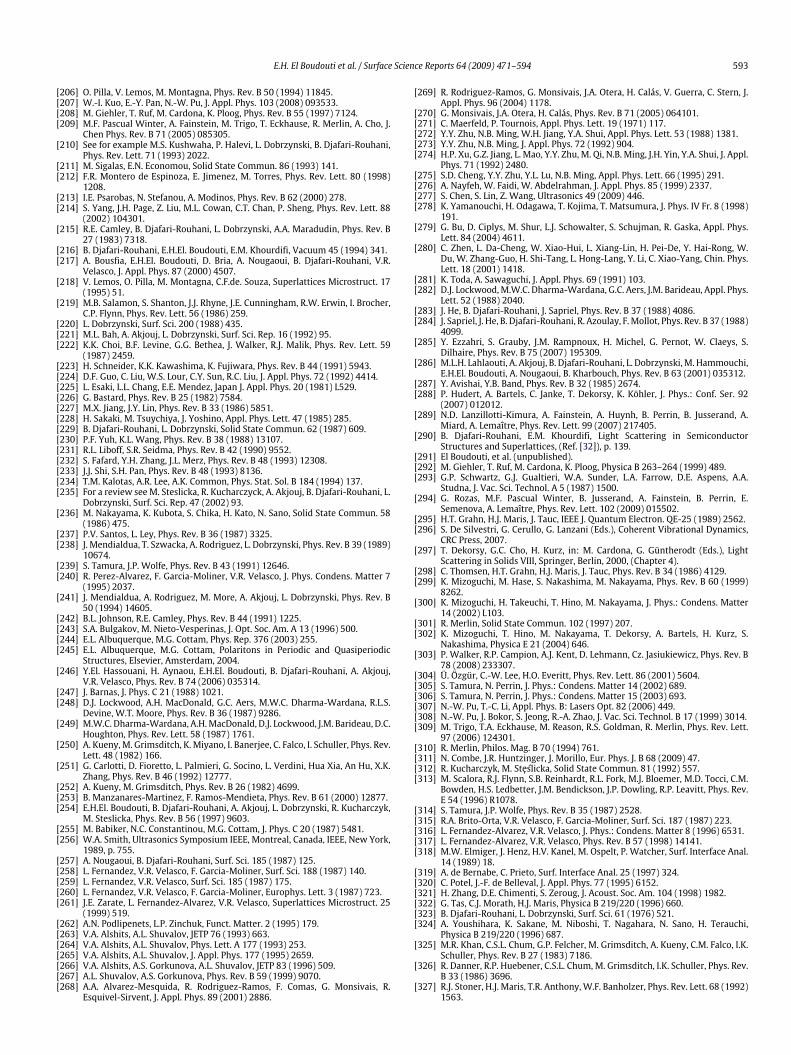
E.H. El Boudouti et al. / Surface Science Reports 64 (2009) 471–594 593

[206] O. Pilla, V. Lemos, M. Montagna, Phys. Rev. B 50 (1994) 11845.[207] W.-I. Kuo, E.-Y. Pan, N.-W. Pu, J. Appl. Phys. 103 (2008) 093533.[208] M. Giehler, T. Ruf, M. Cardona, K. Ploog, Phys. Rev. B 55 (1997) 7124.[209] M.F. Pascual Winter, A. Fainstein, M. Trigo, T. Eckhause, R. Merlin, A. Cho, J.

Chen Phys. Rev. B 71 (2005) 085305.[210] See for example M.S. Kushwaha, P. Halevi, L. Dobrzynski, B. Djafari-Rouhani,

Phys. Rev. Lett. 71 (1993) 2022.[211] M. Sigalas, E.N. Economou, Solid State Commun. 86 (1993) 141.[212] F.R. Montero de Espinoza, E. Jimenez, M. Torres, Phys. Rev. Lett. 80 (1998)

1208.[213] I.E. Psarobas, N. Stefanou, A. Modinos, Phys. Rev. B 62 (2000) 278.[214] S. Yang, J.H. Page, Z. Liu, M.L. Cowan, C.T. Chan, P. Sheng, Phys. Rev. Lett. 88

(2002) 104301.[215] R.E. Camley, B. Djafari-Rouhani, L. Dobrzynski, A.A. Maradudin, Phys. Rev. B

27 (1983) 7318.[216] B. Djafari-Rouhani, E.H.El. Boudouti, E.M. Khourdifi, Vacuum 45 (1994) 341.[217] A. Bousfia, E.H.El. Boudouti, D. Bria, A. Nougaoui, B. Djafari-Rouhani, V.R.

Velasco, J. Appl. Phys. 87 (2000) 4507.[218] V. Lemos, O. Pilla, M. Montagna, C.F.de. Souza, Superlattices Microstruct. 17

(1995) 51.[219] M.B. Salamon, S. Shanton, J.J. Rhyne, J.E. Cunningham, R.W. Erwin, I. Brocher,

C.P. Flynn, Phys. Rev. Lett. 56 (1986) 259.[220] L. Dobrzynski, Surf. Sci. 200 (1988) 435.[221] M.L. Bah, A. Akjouj, L. Dobrzynski, Surf. Sci. Rep. 16 (1992) 95.[222] K.K. Choi, B.F. Levine, G.G. Bethea, J. Walker, R.J. Malik, Phys. Rev. Lett. 59

(1987) 2459.[223] H. Schneider, K.K. Kawashima, K. Fujiwara, Phys. Rev. B 44 (1991) 5943.[224] D.F. Guo, C. Liu, W.S. Lour, C.Y. Sun, R.C. Liu, J. Appl. Phys. 72 (1992) 4414.[225] L. Esaki, L.L. Chang, E.E. Mendez, Japan J. Appl. Phys. 20 (1981) L529.[226] G. Bastard, Phys. Rev. B 25 (1982) 7584.[227] M.X. Jiang, J.Y. Lin, Phys. Rev. B 33 (1986) 5851.[228] H. Sakaki, M. Tsuychiya, J. Yoshino, Appl. Phys. Lett. 47 (1985) 285.[229] B. Djafari-Rouhani, L. Dobrzynski, Solid State Commun. 62 (1987) 609.[230] P.F. Yuh, K.L. Wang, Phys. Rev. B 38 (1988) 13107.[231] R.L. Liboff, S.R. Seidma, Phys. Rev. B 42 (1990) 9552.[232] S. Fafard, Y.H. Zhang, J.L. Merz, Phys. Rev. B 48 (1993) 12308.[233] J.J. Shi, S.H. Pan, Phys. Rev. B 48 (1993) 8136.[234] T.M. Kalotas, A.R. Lee, A.K. Common, Phys. Stat. Sol. B 184 (1994) 137.[235] For a review seeM. Steslicka, R. Kucharczyck, A. Akjouj, B. Djafari-Rouhani, L.

Dobrzynski, Surf. Sci. Rep. 47 (2002) 93.[236] M. Nakayama, K. Kubota, S. Chika, H. Kato, N. Sano, Solid State Commun. 58

(1986) 475.[237] P.V. Santos, L. Ley, Phys. Rev. B 36 (1987) 3325.[238] J. Mendialdua, T. Szwacka, A. Rodriguez, L. Dobrzynski, Phys. Rev. B 39 (1989)

10674.[239] S. Tamura, J.P. Wolfe, Phys. Rev. B 43 (1991) 12646.[240] R. Perez-Alvarez, F. Garcia-Moliner, V.R. Velasco, J. Phys. Condens. Matter 7

(1995) 2037.[241] J. Mendialdua, A. Rodriguez, M. More, A. Akjouj, L. Dobrzynski, Phys. Rev. B

50 (1994) 14605.[242] B.L. Johnson, R.E. Camley, Phys. Rev. B 44 (1991) 1225.[243] S.A. Bulgakov, M. Nieto-Vesperinas, J. Opt. Soc. Am. A 13 (1996) 500.[244] E.L. Albuquerque, M.G. Cottam, Phys. Rep. 376 (2003) 255.[245] E.L. Albuquerque, M.G. Cottam, Polaritons in Periodic and Quasiperiodic

Structures, Elsevier, Amsterdam, 2004.[246] Y.El. Hassouani, H. Aynaou, E.H.El. Boudouti, B. Djafari-Rouhani, A. Akjouj,

V.R. Velasco, Phys. Rev. B 74 (2006) 035314.[247] J. Barnas, J. Phys. C 21 (1988) 1021.[248] D.J. Lockwood, A.H. MacDonald, G.C. Aers, M.W.C. Dharma-Wardana, R.L.S.

Devine, W.T. Moore, Phys. Rev. B 36 (1987) 9286.[249] M.W.C. Dharma-Wardana, A.H.MacDonald, D.J. Lockwood, J.M. Barideau, D.C.

Houghton, Phys. Rev. Lett. 58 (1987) 1761.[250] A. Kueny,M. Grimsditch, K. Miyano, I. Banerjee, C. Falco, I. Schuller, Phys. Rev.

Lett. 48 (1982) 166.[251] G. Carlotti, D. Fioretto, L. Palmieri, G. Socino, L. Verdini, Hua Xia, An Hu, X.K.

Zhang, Phys. Rev. B 46 (1992) 12777.[252] A. Kueny, M. Grimsditch, Phys. Rev. B 26 (1982) 4699.[253] B. Manzanares-Martinez, F. Ramos-Mendieta, Phys. Rev. B 61 (2000) 12877.[254] E.H.El. Boudouti, B. Djafari-Rouhani, A. Akjouj, L. Dobrzynski, R. Kucharczyk,

M. Steslicka, Phys. Rev. B 56 (1997) 9603.[255] M. Babiker, N.C. Constantinou, M.G. Cottam, J. Phys. C 20 (1987) 5481.[256] W.A. Smith, Ultrasonics Symposium IEEE, Montreal, Canada, IEEE, New York,

1989, p. 755.[257] A. Nougaoui, B. Djafari-Rouhani, Surf. Sci. 185 (1987) 125.[258] L. Fernandez, V.R. Velasco, F. Garcia-Moliner, Surf. Sci. 188 (1987) 140.[259] L. Fernandez, V.R. Velasco, Surf. Sci. 185 (1987) 175.[260] L. Fernandez, V.R. Velasco, F. Garcia-Moliner, Europhys. Lett. 3 (1987) 723.[261] J.E. Zarate, L. Fernandez-Alvarez, V.R. Velasco, Superlattices Microstruct. 25

(1999) 519.[262] A.N. Podlipenets, L.P. Zinchuk, Funct. Matter. 2 (1995) 179.[263] V.A. Alshits, A.L. Shuvalov, JETP 76 (1993) 663.[264] V.A. Alshits, A.L. Shuvalov, Phys. Lett. A 177 (1993) 253.[265] V.A. Alshits, A.L. Shuvalov, J. Appl. Phys. 177 (1995) 2659.[266] V.A. Alshits, A.S. Gorkunova, A.L. Shuvalov, JETP 83 (1996) 509.[267] A.L. Shuvalov, A.S. Gorkunova, Phys. Rev. B 59 (1999) 9070.[268] A.A. Alvarez-Mesquida, R. Rodriguez-Ramos, F. Comas, G. Monsivais, R.

Esquivel-Sirvent, J. Appl. Phys. 89 (2001) 2886.

[269] R. Rodriguez-Ramos, G. Monsivais, J.A. Otera, H. Calás, V. Guerra, C. Stern, J.Appl. Phys. 96 (2004) 1178.

[270] G. Monsivais, J.A. Otera, H. Calás, Phys. Rev. B 71 (2005) 064101.[271] C. Maerfeld, P. Tournois, Appl. Phys. Lett. 19 (1971) 117.[272] Y.Y. Zhu, N.B. Ming, W.H. Jiang, Y.A. Shui, Appl. Phys. Lett. 53 (1988) 1381.[273] Y.Y. Zhu, N.B. Ming, J. Appl. Phys. 72 (1992) 904.[274] H.P. Xu, G.Z. Jiang, L. Mao, Y.Y. Zhu, M. Qi, N.B. Ming, J.H. Yin, Y.A. Shui, J. Appl.

Phys. 71 (1992) 2480.[275] S.D. Cheng, Y.Y. Zhu, Y.L. Lu, N.B. Ming, Appl. Phys. Lett. 66 (1995) 291.[276] A. Nayfeh, W. Faidi, W. Abdelrahman, J. Appl. Phys. 85 (1999) 2337.[277] S. Chen, S. Lin, Z. Wang, Ultrasonics 49 (2009) 446.[278] K. Yamanouchi, H. Odagawa, T. Kojima, T. Matsumura, J. Phys. IV Fr. 8 (1998)

191.[279] G. Bu, D. Ciplys, M. Shur, L.J. Schowalter, S. Schujman, R. Gaska, Appl. Phys.

Lett. 84 (2004) 4611.[280] C. Zhen, L. Da-Cheng, W. Xiao-Hui, L. Xiang-Lin, H. Pei-De, Y. Hai-Rong, W.

Du, W. Zhang-Guo, H. Shi-Tang, L. Hong-Lang, Y. Li, C. Xiao-Yang, Chin. Phys.Lett. 18 (2001) 1418.

[281] K. Toda, A. Sawaguchi, J. Appl. Phys. 69 (1991) 103.[282] D.J. Lockwood,M.W.C. Dharma-Wardana, G.C. Aers, J.M. Barideau, Appl. Phys.

Lett. 52 (1988) 2040.[283] J. He, B. Djafari-Rouhani, J. Sapriel, Phys. Rev. B 37 (1988) 4086.[284] J. Sapriel, J. He, B. Djafari-Rouhani, R. Azoulay, F.Mollot, Phys. Rev. B 37 (1988)

4099.[285] Y. Ezzahri, S. Grauby, J.M. Rampnoux, H. Michel, G. Pernot, W. Claeys, S.

Dilhaire, Phys. Rev. B 75 (2007) 195309.[286] M.L.H. Lahlaouti, A. Akjouj, B. Djafari-Rouhani, L. Dobrzynski,M. Hammouchi,

E.H.El. Boudouti, A. Nougaoui, B. Kharbouch, Phys. Rev. B 63 (2001) 035312.[287] Y. Avishai, Y.B. Band, Phys. Rev. B 32 (1985) 2674.[288] P. Hudert, A. Bartels, C. Janke, T. Dekorsy, K. Köhler, J. Phys.: Conf. Ser. 92

(2007) 012012.[289] N.D. Lanzillotti-Kimura, A. Fainstein, A. Huynh, B. Perrin, B. Jusserand, A.

Miard, A. Lemaître, Phys. Rev. Lett. 99 (2007) 217405.[290] B. Djafari-Rouhani, E.M. Khourdifi, Light Scattering in Semiconductor

Structures and Superlattices, (Ref. [32]), p. 139.[291] El Boudouti, et al. (unpublished).[292] M. Giehler, T. Ruf, M. Cardona, K. Ploog, Physica B 263–264 (1999) 489.[293] G.P. Schwartz, G.J. Gualtieri, W.A. Sunder, L.A. Farrow, D.E. Aspens, A.A.

Studna, J. Vac. Sci. Technol. A 5 (1987) 1500.[294] G. Rozas, M.F. Pascual Winter, B. Jusserand, A. Fainstein, B. Perrin, E.

Semenova, A. Lemaître, Phys. Rev. Lett. 102 (2009) 015502.[295] H.T. Grahn, H.J. Maris, J. Tauc, IEEE J. Quantum Electron. QE-25 (1989) 2562.[296] S. De Silvestri, G. Cerullo, G. Lanzani (Eds.), Coherent Vibrational Dynamics,

CRC Press, 2007.[297] T. Dekorsy, G.C. Cho, H. Kurz, in: M. Cardona, G. Güntherodt (Eds.), Light

Scattering in Solids VIII, Springer, Berlin, 2000, (Chapter 4).[298] C. Thomsen, H.T. Grahn, H.J. Maris, J. Tauc, Phys. Rev. B 34 (1986) 4129.[299] K. Mizoguchi, M. Hase, S. Nakashima, M. Nakayama, Phys. Rev. B 60 (1999)

8262.[300] K. Mizoguchi, H. Takeuchi, T. Hino, M. Nakayama, J. Phys.: Condens. Matter

14 (2002) L103.[301] R. Merlin, Solid State Commun. 102 (1997) 207.[302] K. Mizoguchi, T. Hino, M. Nakayama, T. Dekorsy, A. Bartels, H. Kurz, S.

Nakashima, Physica E 21 (2004) 646.[303] P. Walker, R.P. Campion, A.J. Kent, D. Lehmann, Cz. Jasiukiewicz, Phys. Rev. B

78 (2008) 233307.[304] Ü. Özgür, C.-W. Lee, H.O. Everitt, Phys. Rev. Lett. 86 (2001) 5604.[305] S. Tamura, N. Perrin, J. Phys.: Condens. Matter 14 (2002) 689.[306] S. Tamura, N. Perrin, J. Phys.: Condens. Matter 15 (2003) 693.[307] N.-W. Pu, T.-C. Li, Appl. Phys. B: Lasers Opt. 82 (2006) 449.[308] N.-W. Pu, J. Bokor, S. Jeong, R.-A. Zhao, J. Vac. Sci. Technol. B 17 (1999) 3014.[309] M. Trigo, T.A. Eckhause, M. Reason, R.S. Goldman, R. Merlin, Phys. Rev. Lett.

97 (2006) 124301.[310] R. Merlin, Philos. Mag. B 70 (1994) 761.[311] N. Combe, J.R. Huntzinger, J. Morillo, Eur. Phys. J. B 68 (2009) 47.[312] R. Kucharczyk, M. Steślicka, Solid State Commun. 81 (1992) 557.[313] M. Scalora, R.J. Flynn, S.B. Reinhardt, R.L. Fork, M.J. Bloemer, M.D. Tocci, C.M.

Bowden, H.S. Ledbetter, J.M. Bendickson, J.P. Dowling, R.P. Leavitt, Phys. Rev.E 54 (1996) R1078.

[314] S. Tamura, J.P. Wolfe, Phys. Rev. B 35 (1987) 2528.[315] R.A. Brito-Orta, V.R. Velasco, F. Garcia-Moliner, Surf. Sci. 187 (1987) 223.[316] L. Fernandez-Alvarez, V.R. Velasco, J. Phys.: Condens. Matter 8 (1996) 6531.[317] L. Fernandez-Alvarez, V.R. Velasco, Phys. Rev. B 57 (1998) 14141.[318] M.W. Elmiger, J. Henz, H.V. Kanel, M. Ospelt, P. Watcher, Surf. Interface Anal.

14 (1989) 18.[319] A. de Bernabe, C. Prieto, Surf. Interface Anal. 25 (1997) 324.[320] C. Potel, J.-F. de Belleval, J. Appl. Phys. 77 (1995) 6152.[321] H. Zhang, D.E. Chimenti, S. Zeroug, J. Acoust. Soc. Am. 104 (1998) 1982.[322] G. Tas, C.J. Morath, H.J. Maris, Physica B 219/220 (1996) 660.[323] B. Djafari-Rouhani, L. Dobrzynski, Surf. Sci. 61 (1976) 521.[324] A. Youshihara, K. Sakane, M. Niboshi, T. Nagahara, N. Sano, H. Terauchi,

Physica B 219/220 (1996) 687.[325] M.R. Khan, C.S.L. Chum, G.P. Felcher, M. Grimsditch, A. Kueny, C.M. Falco, I.K.

Schuller, Phys. Rev. B 27 (1983) 7186.[326] R. Danner, R.P. Huebener, C.S.L. Chum, M. Grimsditch, I.K. Schuller, Phys. Rev.

B 33 (1986) 3696.[327] R.J. Stoner, H.J. Maris, T.R. Anthony,W.F. Banholzer, Phys. Rev. Lett. 68 (1992)

1563.

594 E.H. El Boudouti et al. / Surface Science Reports 64 (2009) 471–594

[328] K.H. Wichert, C. Reimann, G. Blahusch, H. Kinder, Physica B 219–220 (1996)653.

[329] R. Esquivel-Sirvent, G.H. Cocoletzi, J. Acoust. Soc. Am. 95 (1993) 86.[330] Y. El Hassouani, E.H. El Boudouti, B. Djafari-Rouhani, H. Aynaou, L.

Dobrzynski, Phys. Rev. B 74 (2006) 144306.[331] Safaeinli, D.E. Chimenti, J. Acoust. Soc. Am. 98 (1995) 2336.[332] H. Zhang, D.E. Chimenti, S. Zeroug, J. Acoust. Soc. Am. 104 (1998) 1982.[333] O. Lenoir, J.L. Izbicki, P. Rembert, G. Maze, J. Ripoche, J. Acoust. Soc. Am. 9

(1991) 601.[334] J. Laperre, W. Thys, J. Acoust. Soc. Am. 92 (1992) 909.[335] E. Chimenti, A. Nayfeh, J. Acoust. Soc. Am. 85 (1988) 555.[336] CRC Handbook of Chemistry and Physics, 66th ed., CRC, Boca Raton, FL, 1985,

E-43.[337] Y. El Hassouani, E.H. El Boudouti, B. Djafari-Rouhani, H. Aynaou, Phys. Rev. B

78 (2008) 174306.[338] S. Zhu, N. Liu, H. Zheng, H. Chen, Opt. Commun. B 174 (2000) 139.[339] A.L. Shuvalov, A.S. Gorkunova, J. Sound Vib. 243 (2001) 679.[340] D.A. Sotiropoulos, J. Sound Vib. 185 (1995) 501.[341] D.A. Sotiropoulos, R.W. Ogden, Ultrasonics 34 (1996) 487.[342] W.M. Robertson, J. Pappafotis, P. Flannigan, Appl. Phys. Lett. 90 (2007)

014102.[343] Y. El Hassouani, E.H. El Boudouti, B. Djafari-Rouhani, R. Rais, J. Phys.: Conf.

Ser. 92 (2007) 012113.[344] S.-Y. Ren, Y.-C. Chang, Phys. Rev. B 75 (2007) 212301.[345] E.H. El Boudouti, Y. El Hassouani, B. Djafari-Rouhani, H. Aynaou, Phys. Rev. E

76 (2007) 026607.[346] J.D. Joannopoulos, R.D. Meade, J.N. Winn (Eds.), Photonic Crystals, Princeton

University Press, Princeton, NJ, 1995.[347] C.M. Soukoulis (Ed.), Photonic Crystals and Light Localization in the 21st

Century, in: NATO Advanced Study Institute, Series C: Mathematical andPhysical Sciences, vol. 563, Kluwer, Dordrecht, 2001.

[348] V. Narayanamurti, Science 213 (1981) 717.[349] K. Sagami, H. Gen, M. Morimoto, D. Takahashi, Acoustica 82 (1996) 45.[350] S.D. Cheng, Y.Y. Zhu, Y.L. Lu, N.B. Ming, Appl. Phys. Lett. 66 (1995) 291.[351] J.P. Dowling, Science 282 (1998) 1841.[352] Y. Fink, J.N. Winn, S. Fan, C. Chen, J. Michel, J.D. Joannopoulos, E.L. Thomas,

Science 282 (1998) 1679.[353] D.N. Chigrin, A.V. Lavrinenko, D.A. Yarotsky, S.V. Gaponenko, Appl. Phys. A:

Mater. Sci. Process. A 68 (1999) 25.[354] D. Bria, B. Djafari-Rouhani, E.H. El Boudouti, A. Mir, A. Akjouj, A. Nougaoui, J.

Appl. Phys. 91 (2002) 2569.[355] Xue-Hua Wang, Ke-Qiu Chen, Ben-Yuan Gu, J. Appl. Phys. 92 (2002) 5113.[356] S. Mizuno, Phys. Rev. B 68 (2003) 193305.[357] H. Kato, H.J. Maris, S.I. Tamura, Phys. Rev. B 53 (1996) 7884.[358] B. Manzanares-Martínez, F. Ramos-Mendieta, Phys. Rev. B 76 (2007) 134303.[359] Y. Tanaka, M. Narita, S.-I. Tamura, J. Phys.: Condens. Matter 10 (1998) 8787.[360] K. Imamura, Y. Tanaka, S. Tamura, Phys. Rev. B 65 (2007) 174301.[361] U. Fano, Phys. Rev. 124 (1961) 1866.[362] Z. Liu, X. Zhang, Y. Mao, Y.Y. Zhu, Z. Yang, C.T. Chan, P. Sheng, Science 289

(2000) 1734.

[363] S. Yang, J.H. Page, Z. Liu, M.L. Cowan, C.T. Chan, P. Sheng, Phys. Rev. Lett. 88(2002) 104301.

[364] C. Goffaux, J. Sánchez-Dehesa, A.L. Yeyati, P. Lambin, A. Khelif, J.O. Vasseur, B.Djafari-Rouhani, Phys. Rev. Lett. 88 (2002) 225502.

[365] Z. Liu, C.T. Chan, P. Sheng, Phys. Rev. B 71 (2005) 014103.[366] Y.A. Kosevich, C. Goffaux, J. Sánchez-Dehesa, Phys. Rev. B 74 (2006) 012301.[367] M.L. Ladrón de Guevara, F. Claro, P.A. Orellana, Phys. Rev. B 67 (2003) 195335.[368] E.H. El Boudouti, T. Mrabti, H. Al-Wahsh, B. Djafari-Rouhani, A. Akjouj, L.

Dobrzynski, J. Phys.: Condens. Matter 20 (2008) 255212.[369] H. Al-Wahsh, E.H. El Boudouti, B. Djafari-Rouhani, A. Akjouj, T. Mrabti, L.

Dobrzynski, Phys. Rev. B 78 (2008) 075401.[370] J. Christensen, A.I. Fernandez-Dominguez, F. de Leon-Perez, L. Martin-

Moreno, F.J. Garcia-Vidal, Nature Phys. 3 (2007) 851.[371] T.E. Hartman, J. Appl. Phys. 33 (1962) 3427.[372] Ch. Spielmann, R. Szipöcs, A. Stingl, F. Krausz, Phys. Rev. Lett. 73 (1994) 2308.[373] P. Pereyra, Phys. Rev. Lett. 84 (2000) 1772.[374] S. Esposito, Phys. Rev. E 64 (2001) 026609.[375] G. Nimtz, A.A. Stahlhofen, Ann. Phys. (Berlin) 17 (2008) 374.[376] F.M. Pan, G.J. Jin, X.L. Wu, J.W. Feng, A. Hu, S.S. Jiang, J. Appl. Phys. 80 (1996)

4063.[377] F.M. Pan, G.J. Jin, X.S. Wu, X.L. Wu, A. Hu, S.S. Jiang, Phys. Lett. A 228 (1997)

301.[378] K. Bajema, R. Merlin, Phys. Rev. B 36 (1987) 4555.[379] S. Tamura, J.P. Wolfe, Phys. Rev. B 36 (1987) 3491.[380] L. Fernández-Alvarez, V.R. Velasco, Phys. Rev. B 57 (1998) 14141.[381] J.E. Zárate, L. Fernández-Alvarez, V.R. Velasco, Superlatt. Microstruct. 25

(1999) 519.[382] V.R. Velasco, J.E. Zárate, Prog. Surf. Sci. 67 (2001) 383.[383] J. Tutor, V.R. Velasco, Int. J. Modern Phys. B 21 (2001) 2925.[384] A. Süttő, J. Stat. Phys. 56 (1989) 525.[385] A. Bovier, J.M. Ghez, J. Phys. A 28 (1995) 2313.[386] E. Maciá, Phys. Rev. B 63 (2001) 20542.[387] C. Godrèche, J.-M. Luck, J. Phys. A 23 (1990) 3769.[388] J.-M. Luck, C. Godrèche, A. Janner, T. Janssen, J. Phys. A 26 (1993) 1951.[389] M. Kolar, B. Iochum, L. Raymond, J. Phys. A 26 (1993) 7343.[390] H. Aynaou, E.H. El Boudouti, Y. El Hassouani, A. Akjouj, B. Djafari-Rouhani, J.

Vasseur, A. Benomar, V.R. Velasco, Phys. Rev. E 72 (2005) 056601.[391] E.H. El Boudouti, Y. El Hassouani, H. Aynaou, B. Djafar-Rouhani, A. Akjouj, V.R.

Velasco, J. Phys.: Condens. Matter 19 (2007) 246217.[392] D. Shechtman, I. Blech, D. Gratias, J.W. Cahn, Phys. Rev. Lett. 53 (1984) 1951.[393] D. Shechtman, I. Blech, Metall. Trans. A 16 (1985) 1005.[394] A.I. Goldman, R.F. Ketton, Rev. Mod. Phys. 65 (1993) 213.[395] C. Godrèche, J.-M. Luck, J. Phys. A 23 (1990) 3769.[396] J.-M. Luck, C. Godrèche, A. Janner, T. Janssen, J. Phys. A 26 (1993) 1951.[397] M. Kolar, B. Iochum, L. Raymond, J. Phys. A 26 (1993) 7343.[398] J.J. de Miguel, R. Miranda, J. Phys.: Condens. Matter 14 (2002) R1063.[399] H. Aynaou, A. Nougaoui, E.H. El Boudouti, D. Bria, V.R. Velasco, B. Djafari-

Rouhani, Surf. Sci. 584 (2005) 199.[400] Y. Sekino, T. Kimura, K. Inokuchi, Y. Sano, M. Sakuta, Jap. J. Appl. Phys. 27

(1988) L2183.