Achieving compact social networkrepresentation with variable length

quantities and hash table

Nikola PavlicevicMilos Radovanovic, adviser

Seminar paper

Department of Mathematics and InformaticsFaculty of Sciences, Univeristy of Novi Sad

May 20, 2015

1

Contents

1 Introduction 3

2 Related work 4

3 Content indexing 6

4 Hash table 6

5 Linear probing 75.1 Linear probing for graphs . . . . . . . . . . . . . . . . . . . . 8

6 Graph 96.1 Adjecency list . . . . . . . . . . . . . . . . . . . . . . . . . . . 96.2 Adjecency matrix . . . . . . . . . . . . . . . . . . . . . . . . . 9

7 Compact graph representation with variable length quanti-ties and adjacency list 10

8 Graph search 11

9 Go language 15

10 Results 16

11 Conclusion 20

2

Abstract

In this paper we look at possibility of using variable length quan-tities (VLQ) and hash table to index in compact manner and querysocial networks, although it is possible to work with any graph. Tothis end we constructed a hash table and byte array supporting VLQin Go. We find that running implementation in single process achievescomparable results to Unqlite database benchmarked earlier.

1 Introduction

Social network indexing and querying is important for many reasons. Onereason being that social networks occur naturally since humans are socialbeings. An example is network formed by people shopping online or com-menting on a product. There may be incentive to store social networks indigital form and be able to query them in order to discover some insights.For example we may discover that two people are connected while not know-ing this before. In current context, they may have bought or commented onsame item. Looking further we may assume they share similar tastes and usethis knowledge to construct a simple recommender engine.

The idea about social network indexing and querying comes from a broaderfield called social network analysis and is the study of individuals or organi-zations such as companies and their replationships [6]. It uses network theoryto analyse social networks. Individual actors are represented as nodes andtheir relationships (for example friendships, economic or sexual) are repre-sented as edges. The study originated in sociology where it was noticed thatstructure of relationships can influence spread of information and actions ofindividuals and groups. The reason why we study social networks is dueto highly connected world where individuals have immediate contacts span-ning the globe. Considering individual actions they can have both positiveand negative effects locally and globally. Using computers to analyse socialnetworks can help us understand better information spread in population,network and opinion formation and effects of behaviour.

We can see here two directions where working with social networks cantake us. One direction is indexing and querying social networks, that isworking with graph data that arises naturally [15], and using it as a supportto another system such as recommender or an online store.

3

On the other hand, we can analyse networks further to discover additionalfacts. For example how does structure of social network affect purchasingdecisions of people.

Looking at two different directions we are likely to need different ap-proaches to accommodate them. On one hand, considering we are mostlyworking with sparse graphs, we can use hash tables to create adjacency lists.Their O(|V | + |E|) space complexity allows us to create stores with lowmemory footprint and run queries on them.

On the other hand, deeper analysis is better handled with matrices. Thereason being that graph algorithms are mostly based on matrices and efficientparallel implementations exist [12].

This implies hybrid approach. Any solution that offers comprehensivegraph exploration should support both approaches or come up with ap-proaches to facilitate database paradigm and deeper graph exploration.

At this stage of project we look at hash table to facilitate indexing in com-pact manner and querying of social networks. We implemented a hash tablealong with conflict resolution strategy, linear probing, and used it to storerealistic social networks. We observe insert speeds, search speeds, memoryconsumed and required capacity in terms of buckets for three sets of socialnetwork data. We would like to see whether this approach is comparable tocurrent solutions and whether it offers any advantages. The solution is im-plemented in Go programming language making use of some of the benefitsnot available in traditional languages. Some of them are more rapid devel-opment, availability of testing environment, testing in parallel and resizeablememory slices which allow us to work with arbitrary number of nodes withoutexplicit memory management.

2 Related work

Up to this point we are aware of several in-memory graph databases anddata structures that can support graphs in multiple languages. One exam-ple is Stinger written in C++ developed at Georgia Tech as part of HighPerformance Computing programme [1][4]. This graph library contains mul-tiple data structures for storing graphs suitable for number of purposes. Anexample is key value store that allows graph traversal. Although excellentresults can be achieved with this library, portability and scalability can poseissues. Regarding portability the library needs to be compiled for specific

4

platform. It is also required to write additional code if we want to use iton embedded and system on chip or card platform. Regarding scalability, intheory it should be very easy. In practice usually it is not because we needto spin multiple instances of the server.

Another in-memory store is Netflix graph written in Java [7]. Regardingperformance we find the same situation, it is possible to achieve excellentefficiency on large graphs with low memory footprint. Netflix graph usesvariable encoding to achieve lower memory footprint. Only required numberof bytes are used to store integers while remaining bytes are used for anyadditional values. This approach is similar to one employed in this project,where we use byte slices to represent values. Since Netflix graph is writtenin Java it is more portable that previous library written in C++. This getsus close to the goal we are trying to achieve, easy portability to number ofhardware platforms. On the other hand, since Java was chosen, there aresome inherent penalties. We know that Java only supports signed numbers,so 1 bit is always reserved for sign and therefore additional work is requiredin encoding and interpreting data.

Third library is Graphstore for Gephi in Java [2]. We are able to achieveresults compared to previous two projects but we still have to deal withinherited penalties because of Java implementation.

We also consider available in-memory hash table implementations thatcan support graph indexing and querying. We found large number of freeand open source implementations that can provide excellent results, withminor tweaks. We based our implementation on such projects adding abilityto work with graphs rather than single key value pairs. Another idea thatinfluenced us is having the solution as open as possible. This means thatcode is easily accessible and can be easily tweaked for any purpose.

One project that influenced us is called simply hash table, created byuser called sploit, hosted on Bitbucket and written in C [13]. The interface isclean and simple, can easily be tweaked for specific application and supportsworking with large number of keys out of the box.

Similar project is called hashing by user deepshah22 written in Java andhosted on Git hub [14]. The project implements different hashing strategiesand provides clean and easily understood interface for working with hashtables.

Third implementation we looked at is Unqlite database [5]. This is mul-tiparadigm No Sql database supporting in-memory key value storage. It isopen source database written mostly in C. We benchmarked it in earlier pa-

5

per [10] and achieved good memory efficiency and search time. The databaseis primarily key value store and we needed to write additional code to makeit work with graphs. We try to achieve comparable results in this projectand to improve on some parts.

3 Content indexing

The goal of content indexing is storage of information so that it can efficientlybe retreived at later date. In our case these are social networks Skitter,Livejournal and Orkut. We use hash table to index these datasets, usinglinear probing for conflict resolution.

We are aware of byte representation benefits in terms of speed versusmemory usage tradeoff so we used it to build hash table. We constructed alight API to work with byte slices while the rest of implementation was madeeasier with built in slice constructs.

Before zeroing in on current setup we considered few other options. Namelychaining as conflict resolution strategy. Although chaining supports more sta-ble performance at high load factors, it is evident that search time increaseswith chain length so we thought of it as unsuitable for high volume of datathat needs to be frequently searched.

4 Hash table

A hash table is a map M with abstraction of using keys as indices with formM[i], where index i is obtained by means of hash function h(k) = i. A hashfunction represents mapping from data point value to position in hash table.Based on data type we can use appropriate hash function. For instance ifwe are computing hash value for strings, or byte arrays, we can use sum of

constituent bytesn∑

i=0

bi. Although we can get valid hash value this way, we

can also experience large numbers of collisions, since it easy to find differentstrings that sum to same value. More collision resistant way is to weigh

each byte according to positionn∑

i=0

wibi. We can compute it efficiently using

Horner’s rule, for ASCII characters we can have hi = 128 ∗ hi−1 + bi. For themost part this would gives us hash value unique to the string but collisions

6

occur. For that reason we next look at collision resolution strategy, linearprobing.

5 Linear probing

Linear probing is strategy based on open addressing, figure 1 [16]. That iswe place value directly in the hash table at given index without storing anyadditional information about that particular value. More formally, linearprobing is collision resolution method where we place value at position h(k)+ f(j), where f(j) is collision resolution strategy. In case of linear probing f(j)= j, for j = 1, 2, 3, ..., capacity. Linear probing is shown to perform well forload factors below λ = 0.5, where expected lookup time is 1

2(1 + 1/(1− λ)2).

Once the set load factor is reached, the table is resized, usually by factor of2.

It is reported that linear hashing suffers from primary clustering. Thatis blocks or clusters of occupied cells start to form and operations becomeincreasingly slower even if the table is relatively empty.

7

Figure 1: Linear probe

5.1 Linear probing for graphs

When dealing with graphs we can expect large number of collisions becausea single node can have multiple connections. In this case collision is legal,and chained to existing set of values for that particular node. In case anothernode creates collision, we probe to find it appopriate place. For this reasonwe keep two memory slices, one for keys and another for values. When keysmatch, value is appended. When key is empty value is added in single step.When keys do not match we probe to find appropriate position.

8

6 Graph

A graph G=(V, E) consists of a set of vertices V and set of edges E. Eachedge (v, w) is a pair where v, w ∈ V. v is adjecent to w if (v, w) ∈ in E. In anundirected graph with we have edge {v, w} where v is adjecent to w and wis adjecent to v. Sometimes edge has third component called weight or cost.

A path in the graph is sequence of vertices w1, w2, w3, ..., wn such that(wi, wi+1) ∈ E. The path length is n - 1. A path can be simple, in that caseall nodes are distinct except first and last, which can be same. If first andlast nodes are the same and the length is at least 1 then we have a cycle.

A graph is connected if there is a path from every node to every othernode. A graph is complete if there is an edge between all pairs of nodes.

6.1 Adjecency list

If the graph is sparse, the number of edges being close to minimal numberof edges, we can use adjacency list to store it. Adjecency list is a structurewhere we keep a list of adjecent nodes for every node. Space complexity isO(|V | + |E|). The structure is suitable for querying the graph, for examplefinding adjecent nodes, as well as holding properties of nodes and edges, inwhich case we have a property graph.

6.2 Adjecency matrix

If the graph is dense, number of edges being close to maximum numberof edges, adjecency matrix may be suitable representation, figure 2. If thegraph is dense space complexities for adjecency matrix and list are same, butmatrix is preferable for analysis because of efficient parallel algorithms. Atthe same time matrix is not suitable for querying. It may not be suitabledata structure if we are trying to index graph and build query engine.

9

Figure 2: Adjecency matrix (b) and adjecency list (c)

7 Compact graph representation with vari-

able length quantities and adjacency list

A variable length quantity (VLQ) is universal code used to represent arbi-trarily large integers as sequences of binary octets or 8 bit strings.

Figure 3: Number representation using VLQ

10

Each binary octet has most significant bit, usually leftmost, set to 0 if itis last in the sequence or set to 1 if it is not. Using this format we are able torepresent integers with variable quantity of octets rather than fixed quantityof octets as it is case with 32 bit (4 octets) or 64 bit (8 octets) numbers. Ifwe consider 32 bit numbers in number of cases we do not need all 4 octetsto represent a number. In number of cases we can use 1, 2, or 3 octets. Weuse this format to construct adjacency list.

8 Graph search

Graph search, speaking generally, attempts to find a node in the graph ora path connecting source node and destination node. The first case is sim-pler and can be done with simple table lookup. This case usually occurs inproperty graph when we are trying to locate a node with specific property.

The second case is more interesting and applicable in queryies, for exam-ple finding how two nodes are connected. Breadth first search can help us dothis since it constructs path from source node to destination node. Breadthfirst search, as name suggests, proceeds in layers. We begin search at distance1 from source node. If we find destination node we stop. If not we increasedistance by 1 and continue searching. The process repeats until we reachdestination node. To keep the algorithm going and not falling into loops weneed to know the nodes we visited. Traditionally visited nodes were colored[3]. Initially we start with all white nodes, because they are not visited. Aswe progress we color nodes gray once visited and black once all children ofthe node are visited. We only expand white nodes, figure 4.

This search requires extra information, the colour, and can take morememory. Since we are using hash table we can remove visited nodes thuskeeping space complexity lower, listing 2 [11].

The algorithm uses queue, first in first out, data structure. As nodes areencountered they are appended to the end of the queue. Existing nodes arepopped from front of the queue. Traditionally queue has been implementedwith linked lists or fixed size arrays. In case of linked lists we keep a pointerto know next item in line which creates additional memory requirements.

On the other hand, in case of fixed size array, we initially reserve requiredamount of memory. In this case the array only contains data without addi-tional information. If we outgrow the initial array we resize it. We opted forthis option in Go language due to facilities provided to work with memory

11

slices, listing 1.

Listing 1: Queue in Go implemented with memory slices

1 type QueueInter face i n t e r f a c e {2 QueuePush ( entry ∗Entry )3 QueuePushRange ( s i z e uint32 , e n t r i e s [ ] ∗ Entry )4 QueueGet ( ) u int325 QueuePop ( )6 QueueSize ( ) u int327 }89 type Queue s t r u c t {

10 e n t r i e s ∗ByteArray11 s i z e u int3212 }1314 func NewQueue( e n t r i e s . . . [ ] ∗ Entry ) ∗Queue {15 // make a queue16 queue := &Queue{}17 i f l en ( e n t r i e s ) > 0 {18 queue . QueuePushRange ( u int32 ( l en ( e n t r i e s [ 0 ] ) ) ,

e n t r i e s [ 0 ] )19 }20 re turn queue21 }2223 func ( t h i s ∗Queue ) QueuePush ( entry ∗Entry ) {24 // push s i n g l e element to queue25 i f t h i s . e n t r i e s == n i l {26 t h i s . e n t r i e s = NewByteArray ( )27 }28 t h i s . e n t r i e s . ByteArrayAppendCompact ( entry . id )29 t h i s . s i z e += 130 }3132 func ( t h i s ∗Queue ) QueuePushRange ( s i z e uint32 , e n t r i e s

[ ] ∗ Entry ) {33 // push mul t ip l e element to queue

12

34 i f s i z e <= 0 {35 re turn36 }37 f o r , entry := range e n t r i e s {38 t h i s . QueuePush ( entry )39 }40 }4142 func ( t h i s ∗Queue ) QueueGet ( ) u int32 {43 // get element from queue44 re turn t h i s . e n t r i e s . ByteArrayFirstCompact ( )45 }4647 func ( t h i s ∗Queue ) QueuePop ( ) {48 // pop element from queue49 t h i s . e n t r i e s . ByteArrayPopCompact ( )50 t h i s . s i z e −= 151 }5253 func ( t h i s ∗Queue ) QueueSize ( ) u int32 {54 // get queue s i z e55 re turn t h i s . s i z e56 }

13

Figure 4: Breadth first search

Listing 2: Breadth first search in Go

1 func ( t h i s ∗TableArrayAny ) TableSearch ( id uint32 ) (f l o a t32 , f l o a t 3 2 ) {

2 // search tab l e breadth f i r s t3 s i z e , ne ighbours := t h i s . TableNeighbours ( id )4 depth := uint32 (0 )5 paths := f l o a t 3 2 (0 )6 l eng th s := f l o a t 3 2 (0 )7 i f s i z e <= 0 {8 re turn f l o a t 3 2 ( depth ) , paths9 }

14

10 t h i s . TableRemove ( id )11 queue := NewQueue( ne ighbours )12 depth = 113 f o r queue . QueueSize ( ) > 0 {14 entry := queue . QueueGet ( )15 queue . QueuePop ( )16 s i z e −= 117 queue . QueuePushRange ( t h i s . TableNeighbours ( entry ) )18 t h i s . TableRemove ( entry )19 paths += 120 l eng th s += f l o a t 3 2 ( depth )21 i f s i z e == 0 {22 s i z e = queue . QueueSize ( )23 depth += 124 }25 }26 re turn f l o a t 3 2 ( depth ) , l eng th s / paths27 }

9 Go language

Go is strong, statically typed and inferred language. The syntax is looselyderived from C adding garbage collection, type safety and additional builtin types such as variable size arrays, called slices. At this point go compiler,gc, supports i386, amd64 and arm architectures. The initial work on Golanguage started in 2007 at Google by Robert Greisemer, Rob Pike and KenThompson. The first public release of the language was in 2009.

The language design includes some of the features listed next. In orderto keep language specification in programmer’s head some of the followingdecisions were made regarding simplicity.

1. No type inheritance.

2. No method or operator overloading.

3. No pointer arithmetic.

4. No assetions.

15

5. No generic programming.

6. No circular dependencies among packages.

In terms of conciseness, programmer can make use of type inference. Ingo it is allowed to write expression like a := 1 and let compiler assign type,in this case var a int = 1.

Further syntax supports receiver objects, the ones receiving functionbody, and short hand signature syntax. The first allows to specify functionbody separately from class, as seen in more traditional languages, keeping thecode more readable. The second keeps code more concise by avoid repetitionsof the type, two statements in listing 3 are equivalent.

Listing 3: Go function notation

1 func ( t h i s ∗TableArray ) Tab l e In se r t ( key [ ] byte , va lue [ ] byte ) {2 // . . .3 }4 func ( t h i s ∗TableArray ) Tab l e In se r t ( key , va lue [ ] byte ) {5 // . . .6 }

Go language also introduces changes to tool chain allowing more stream-lined build process. Some of the changes are listed next.

1. Package system allowing installation of remote packages.

2. No circular dependencies among packages.

3. Lightweight concurrency in form of go routines and channels withoutreliance on third party libraries.

10 Results

In this section we look at time achieved indexing, figure 5, and searching inseconds, figure 6, virtual memory occupied, figure 7, in bytes and numberof buckets, figure 8, required to index 3 data sets Skitter, Livejournal andOrkut.

Skitter data set [8] has 1696415 nodes, 11095298 edges and roughly takes147 MB on disk. Livejournal data set [9] has 3997962 nodes, 34681189 edges

16

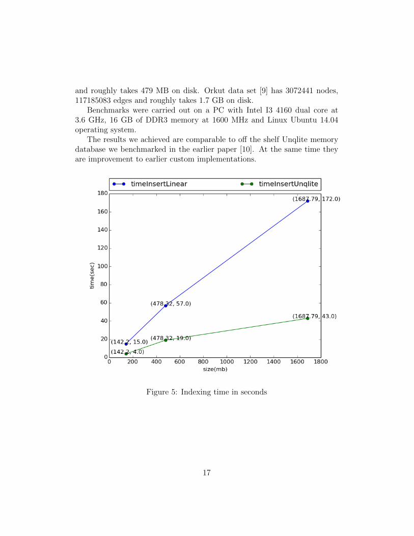
and roughly takes 479 MB on disk. Orkut data set [9] has 3072441 nodes,117185083 edges and roughly takes 1.7 GB on disk.

Benchmarks were carried out on a PC with Intel I3 4160 dual core at3.6 GHz, 16 GB of DDR3 memory at 1600 MHz and Linux Ubuntu 14.04operating system.

The results we achieved are comparable to off the shelf Unqlite memorydatabase we benchmarked in the earlier paper [10]. At the same time theyare improvement to earlier custom implementations.

Figure 5: Indexing time in seconds

17

Figure 6: Breadth first search time in seconds

18

Figure 7: Virtual memory occupied in megabytes

19

Figure 8: Table capacities in number of buckets

11 Conclusion

Looking at indexing time, we can observe that it is somewhat slower com-pared to Unqlite. On the other hand, we were able to work with memoryslices, and implement some of the algorithms and data structures, namely thequeue, in a simpler way. We were also able to get familiar with concurrencyfacilities provided by Go language and hope to make use of them to makeimplementation more efficient. Although we do not gain on performance atthis point, we gain on implementation speed and stability. This is the trade-off to be addressed, since we are trying to have a solution that will work withlarge graphs in realistic environment efficiently.

Looking at search time, we can say the same thing. We do not immedi-ately gain in performance, but we gain in implementation speed and solution

20

stability (we are able to update solution easier and there is less chance ofexisting code breaking down due to facilities provided by the language).

Looking at occupied virtual memory, it was an improvement comparedto Unqlite. For data sets used in the benchmark virtual memory occupiedwas less than that of Unqlite. One reason is compression of integer valueswhen constructing adjacency list. Another reason is less memory reservedin advance. When table is first created conservative amount of memory isreserved and expanded if required.

References

[1] D. Bader. Stinger graph library. 2014. url: https://github.com/robmccoll/stinger.

[2] M. Bastian. Gephi graph library. 2013. url: https://github.com/gephi/graphstore.

[3] H. T. Cormen. Introduction to algorithms. The MIT Press, 2003.

[4] Bader D.A. and Berry J. “STINGER: Spatio-Temporal InteractionNetworks and Graphs (STING) Extensible Representation”. In: Geor-gia Institute of Technology, Tech. Rep (2009).

[5] G. Douglas and R. Lawrence. “LittleD: a SQL database for sensor nodesand embedded applications”. In: ACM (2014).

[6] K. Guiffre. Communities and networks. Polity Press, 2013.

[7] D. Koszewnik. Netflix graph library. 2013. url: https://github.com/Netflix/netflix-graph.

[8] J. Leskovec, J. Kleinberg, and C. Faloutsos. “Graphs over time: densi-fication laws, shrinking diameters and possible explanations”. In: ACMSIGKDD International Conference on Knowledge Discovery and DataMining (KDD) (2005).

[9] J. Leskovec and J. Yang. “Defining and evaluating network communi-ties based on ground truth”. In: ICDM (2012).

[10] N. Pavlicevic. Benchmarking off the shelf memory stores for social net-work analysis. 2014.

[11] N. Pavlicevic. Hash table. 2015. url: https : / / bitbucket . org /

npavlicevic/byte_table_benchmark.

21

[12] W. H. Press. Numerical reciped 3rd edition: the art of scientific com-puting. Cambridge University Press, 2007.

[13] V. Roemer. Hash table. 2012. url: https://bitbucket.org/sploit/hash-table.

[14] D. Shah. Hash table. 2013. url: https://github.com/deepshah22/hashing.

[15] P. Symeonidis, D. Ntempos, and Y. Manolopoulos. Recommender Sys-tems for Location-based Social Networks. Springer, 2014.

[16] M. A. Weiss. Data structures and algorithm analysis in C++. Pearson,2014.

22