
Accurate Analysis of IEEE 802.15.4 Slotted CSMA/CA over a Real-Time Wireless Sensor Network
298
-
Upload
independent -
Category
Documents
-
view
0 -
download
0
Transcript of Accurate Analysis of IEEE 802.15.4 Slotted CSMA/CA over a Real-Time Wireless Sensor Network


Lecture Notes of the Institutefor Computer Sciences, Social-Informaticsand Telecommunications Engineering 24
Editorial Board
Ozgur AkanMiddle East Technical University, Ankara, Turkey
Paolo BellavistaUniversity of Bologna, Italy
Jiannong CaoHong Kong Polytechnic University, Hong Kong
Falko DresslerUniversity of Erlangen, Germany
Domenico FerrariUniversità Cattolica Piacenza, Italy
Mario GerlaUCLA, USA
Hisashi KobayashiPrinceton University, USA
Sergio PalazzoUniversity of Catania, Italy
Sartaj SahniUniversity of Florida, USA
Xuemin (Sherman) ShenUniversity of Waterloo, Canada
Mircea StanUniversity of Virginia, USA
Jia XiaohuaCity University of Hong Kong, Hong Kong
Albert ZomayaUniversity of Sydney, Australia
Geoffrey CoulsonLancaster University, UK

Stephen Hailes Sabrina SicariGeorge Roussos (Eds.)
Sensor Systemsand Software
First International ICST Conference, S-CUBE 2009Pisa, Italy, September 7-9, 2009Revised Selected Papers
13

Volume Editors
Stephen HailesUniversity College LondonDepartment of Computer ScienceLondon, WC1E 6BT, United KingkomE-mail: [email protected]
Sabrina SicariUniversity of InsubriaDipartimento di Informatica e Comunicazione21100 Varese, ItalyE-mail: [email protected]
George RoussosUniversity of LondonSchool of Computer Science and Information SystemsLondon WC1E 7HX, United KingdomE-mail: [email protected]
Library of Congress Control Number: 2009942541
CR Subject Classification (1998): C.2, J.3, K.4.2, K.6, C.2.1, C.3
ISSN 1867-8211ISBN-10 3-642-11527-6 Springer Berlin Heidelberg New YorkISBN-13 978-3-642-11527-1 Springer Berlin Heidelberg New York
This work is subject to copyright. All rights are reserved, whether the whole or part of the material isconcerned, specifically the rights of translation, reprinting, re-use of illustrations, recitation, broadcasting,reproduction on microfilms or in any other way, and storage in data banks. Duplication of this publicationor parts thereof is permitted only under the provisions of the German Copyright Law of September 9, 1965,in its current version, and permission for use must always be obtained from Springer. Violations are liableto prosecution under the German Copyright Law.
springer.com
© ICST Institute for Computer Sciences, Social-Informatics and Telecommunications Engineering 2010Printed in Germany
Typesetting: Camera-ready by author, data conversion by Scientific Publishing Services, Chennai, IndiaPrinted on acid-free paper SPIN: 12830282 06/3180 5 4 3 2 1 0
Preface
The First International ICST Conference on Sensor Systems and Software (S-cube 2009) was held during 7–8 September in Pisa, Italy. This new international conference was dedicated to addressing the research challenges facing system devel-opment and software support for systems based on wireless sensor networks (WSNs) that have the potential to impact society in many ways. Currently, wireless sensor networks introduce innovative and interesting application scenarios that may support a large amount of different applications including environmental monitoring, disaster prevention, building automation, object tracking, nuclear reactor control, fire detec-tion, agriculture, healthcare, and traffic monitoring. The widespread acceptance of these new services can be improved by the definition of frameworks and architectures that have the potential to radically simplify software development for wireless sensor network-based applications. The aim of these new architectures is to support flexible, scalable programming of applications based on adaptive middleware. As a conse-quence, WSNs require novel programming paradigms and technologies. Moreover, the design of new complex systems, characterized by the interaction of different and heterogeneous resources, will allow the development of innovative applications that meet high-performance goals. Hence, WSNs require contributions from many fields such as embedded systems, distributed systems, data management, system security and applications. The conference places emphasis on layers well above the traditional MAC and routing and transport layer protocols. The aim of the conference is to create a forum in which researchers from academia and industry, practitioners, business leaders, intellectual property experts and venture capitalists may work together in order to compare and debate different innovative solutions.
The technical program of S-cube 2009 well reflected the current priorities in wire-less sensor networks. Several papers addressed modeling and performance evaluation; several contributions were related to support sensor programming paradigms and infrastructure properties, such as middleware architectures and security. In addition, a considerable part of the technical program was devoted to consolidated and emerging application areas for wireless sensor network services, such as e-health applications and home applications.
The conference program started with a keynote speech followed by seven technical sessions distributed over a period of two days. There were around 50 registrants for the conference.
The conference received around 45 submissions from different countries. After a thorough review process, 16 papers were accepted from an open call and 3 distin-guished researchers were invited to contribute 3 invited papers. The overall paper acceptance rate is around 35%. The keynote speech titled “From Sensor Networks to the Web of Things” was delivered by Kay Römer from the University of Luebeck, Germany.

Preface
VI
The social program included a tour of the city and a social dinner held on the first day of the conference. It provided a good opportunity for networking among the attendees.
S-CUBE 2010 is under organization. In addition to the technical sessions, S-CUBE 2010 is also soliciting tutorials and workshop proposals.

Organization
Steering Committee Chair
Imrich Chlamtac Create-Net, Italy
Conference General Co-chairs
Sabrina Sicari Universitá degli studi dell'Insubria, Italy Stephen Hailes University College of London, UK
Technical Program Chair
George Roussos Birkbeck College, University of London, UK
Local Chair
Gianluca Dini Universitá di Pisa, Italy
Publications Chair
Luca Mottola Swedish Institute of Computer Science, Sweden
Publicity Co-chairs
Matteo Cesana Politecnico di Milano, Italy Houda Labiod Telecom Paris, France
Web Chair
Pietro Colombo Universitá degli studi dell'Insubria, Italy
Conference Coordinator
Barbara Török ICST Technical Program Committee
Marco Benini Universitá dell'Insubria, Italy Jan Beutel ETH Zurich, Switzerland Alberto Coen Porisini Universitá dell'Insubria, Italy Christine Julien The University of Texas at Austin, USA

Organization VIII
Eli Katsiri Birkbeck College, UK Gerd Kortuem Lancaster University, UK Houda Labiod Telecom Paris, France Akos Ledeczi Vanderbilt University, USA Luis Lopes University of Porto, Portugal Sam Michiels K.U. Leuven, Belgium Daniele Miorandi Create-net, Italy Mattia Monga Universitá di Milano, Italy Mirco Musolesi University of Cambridge, UK Tatsuo Nakajima Waseda University, Japan Animesh Pathak INRIA, France Jochen Schiller Freie Universität Berlin, Germany Krishna M. Sivalingam University of Maryland, USA Robert Szewczyk Sentilla Corporation, USA Andreas Terzis Johns Hopkins University, USA Eiko Yoneki University of Cambridge, UK
Sponsored by ICST
Technically Co-Sponsored by Create-Net, ACM SIGBED, UKRI IEEE, University of Pisa
Table of Contents
Applying Complex Event Processing and Extending Sensor WebEnablement to a Health Care Sensor Network Architecture . . . . . . . . . . . . 1
Gavin E. Churcher and Jeff Foley
Turn-Based Gesture Interaction in Mobile Devices . . . . . . . . . . . . . . . . . . . 11Sanna Kallio, Panu Korpipaa, Jukka Linjama, and Juha Kela
A Large-Scale Wireless Network Approach for Intelligent andAutomated Meter Reading of Residential Electricity . . . . . . . . . . . . . . . . . . 20
Victor Custodio, Jose Ignacio Moreno, and Juan Pablo Vinuela
Weak Process Models for Attack Detection in a Clustered SensorNetwork Using Mobile Agents . . . . . . . . . . . . . . . . . . . . . . . . . . . . . . . . . . . . . 33
Marco Pugliese, Annarita Giani, and Fortunato Santucci
Key Establishment Using Group Information for Wireless SensorNetworks . . . . . . . . . . . . . . . . . . . . . . . . . . . . . . . . . . . . . . . . . . . . . . . . . . . . . . . 51
William R. Claycomb, Rodrigo Lopes, Dongwan Shin, andByunggi Kim
A Forward and Backward Secure Key Management in Wireless SensorNetworks for PCS/SCADA . . . . . . . . . . . . . . . . . . . . . . . . . . . . . . . . . . . . . . . . 66
Hani Alzaid, DongGook Park, Juan Gonzalez Nieto,Colin Boyd, and Ernest Foo
Analysis of Channel Access Delay of Slotted CSMA/CA in a WSN . . . . . 83Alexandre Guitton and Nassima Hadid
Accurate Analysis of IEEE 802.15.4 Slotted CSMA/CA over aReal-Time Wireless Sensor Network . . . . . . . . . . . . . . . . . . . . . . . . . . . . . . . . 98
Wen-Tzeng Huang, Jing-Ting Lin, Chin-Hsing Chen,Yuan-Jen Chang, and You-Yin Chen
Physical Characterization of Acoustic Communication ChannelProperties in Underwater Mobile Sensor Networks . . . . . . . . . . . . . . . . . . . . 111
Andrea Caiti, Emanuele Crisostomi, and Andrea Munafo
A Code Generator for Distributing Sensor Data Models . . . . . . . . . . . . . . . 127Urs Hunkeler and Paolo Scotton
Integer-Based Optimisations for Resource-Constrained SensorPlatforms . . . . . . . . . . . . . . . . . . . . . . . . . . . . . . . . . . . . . . . . . . . . . . . . . . . . . . . 144
Michael Zoumboulakis and George Roussos

X Table of Contents
ProSe: A Programming Tool for Rapid Prototyping of SensorNetworks . . . . . . . . . . . . . . . . . . . . . . . . . . . . . . . . . . . . . . . . . . . . . . . . . . . . . . . 158
Mahesh Arumugam and Sandeep S. Kulkarni
Energy-Aware Dynamic Route Management for THAWS . . . . . . . . . . . . . . 174Chong Shen, Sean Harte, Emanuel Popovici, Brendan O’Flynn, andJohn Barton
All Roads Lead to Rome: Data Highways for Dense Wireless SensorNetworks . . . . . . . . . . . . . . . . . . . . . . . . . . . . . . . . . . . . . . . . . . . . . . . . . . . . . . . 189
David Lowe and Daniele Miorandi
Sensor Data Fusion for Activity Monitoring in Ambient Assisted LivingEnvironments . . . . . . . . . . . . . . . . . . . . . . . . . . . . . . . . . . . . . . . . . . . . . . . . . . . 206
M. Amoretti, F. Wientapper, F. Furfari, S. Lenzi, and S. Chessa
Trade-off Analysis of a MAC Protocol for Wireless e-EmergencySystems . . . . . . . . . . . . . . . . . . . . . . . . . . . . . . . . . . . . . . . . . . . . . . . . . . . . . . . . 222
Oscar Gama, Paulo Carvalho, J.A. Afonso, and P.M. Mendes
An Underwater Robotic Network for Monitoring Nuclear Waste StoragePools . . . . . . . . . . . . . . . . . . . . . . . . . . . . . . . . . . . . . . . . . . . . . . . . . . . . . . . . . . . 236
Sarfraz Nawaz, Muzammil Hussain, Simon Watson,Niki Trigoni, and Peter N. Green
Evaluation of the Impact of the Topology and Hidden Nodes in thePerformance of a ZigBee Network . . . . . . . . . . . . . . . . . . . . . . . . . . . . . . . . . . 256
Helena Fernandez-Lopez, Pedro Macedo, Jose A. Afonso,J.H. Correia, and Ricardo Simoes
Coordinated Sleeping for Beaconless 802.15.4-Based MultihopNetworks . . . . . . . . . . . . . . . . . . . . . . . . . . . . . . . . . . . . . . . . . . . . . . . . . . . . . . . 272
A.G. Ruzzelli, A. Schoofs, G.M.P. O’Hare, M. Aoun, andP. van der Stok
Author Index . . . . . . . . . . . . . . . . . . . . . . . . . . . . . . . . . . . . . . . . . . . . . . . . . . 289
S. Hailes, S. Sicari, and G. Roussos (Eds.): S-Cube 2009, LNICST 24, pp. 1–10, 2009. © Institute for Computer Sciences, Social-Informatics and Telecommunications Engineering 2009
Applying Complex Event Processing and Extending Sensor Web Enablement to a Health Care Sensor Network Architecture
Gavin E. Churcher and Jeff Foley
BT Research Adastral Park, Martlesham Heath, Ipswich IP5 3RE
{gavin.churcher,jeff.foley}@bt.com
Abstract. The limited reuse of middleware components for wireless sensor networking projects has driven interest in emerging standards from the Sensor Web Enablement Working Group which offers methods to virtualize sensor data into a common, self-describing format, using access mechanisms based on HTTP. Using these standards, applications are able to discover and access dif-ferent sensor offerings, automatically understand the data format used and even specify conditions in the sensor data. This paper examines how an existing sen-sor network platform in the health care domain can make use of these standards and examines the possibility of extending the Sensor Alert Service with a richer set of functions. Concepts taken from Complex Event Processing engines are explored in the context of this particular health care platform, where it is shown that there are clear advantages to extending the standard.
Keywords: Complex Event Processing, Health Care, Sensor Web Enablement.
1 Introduction
The Sensor Network Group in BT Research has had a long interest in wireless sensor networking based projects and has participated in a number of collaborations covering a wide range of domains from health care and assisted living through to environ-mental monitoring, and traffic management. Typically, these projects have required bespoke solutions where middleware reuse has been minimal. Our interest in emerg-ing standards to address this issue has led us to investigate the use of Sensor Web Enablement (SWE) from the Open Geospatial Consortium (OGC) [1] as a possible approach for the virtualization of sensors. This would form part of our strategy for building a more generic sensor network architecture with components that could be reused in a diverse range of sensor network projects. We feel that the use of standard-ized middleware will help drive the acceptance of sensor network solutions as we move away from costly, bespoke solutions; a problem particularly relevant to our approach given the broad range of application areas.
We have investigated the SWE standards for the Sensor Observation Service (SOS) [2] and Sensor Alert Service (SAS) and how they may be applied to one of our existing sensor network projects, SAPHE (Smart and Aware Pervasive Healthcare Environment) [3]. SAPHE is one of a number of growing industrial and academic

2 G.E. Churcher and J. Foley
wireless sensor network projects in the health care domain. The most notable being Intel IrisNet [4], Hitachi Collectlo [5], and A Remote Health Care System Based on Wireless Sensor Networks [6].
This paper reviews the previously published findings where we applied SWE to SAPHE [7] and highlights the possibilities of extending the SAS service with more advanced filtering mechanisms, such as those found in Complex Event Processing (CEP). An example CEP engine, Esper [9] was investigated with the view that the application of CEP to the SAS service may result in a number of benefits to sensor network architectures and to SAPHE in particular. CEP is particularly relevant to SAS as it offers the ability to aggregate and correlate large volumes of events through the real-time processing of continuous queries. It is possible to apply pattern matching to asynchronous events through the use of logical and temporal event correlation, and defined ‘window’ views of the event streams. Current standards for defining which events are relevant to an application using SAS are severely limited to a simple defi-nition of a property of a single event. It is not possible to correlate multiple events, a capability that has the potential to reduce bandwidth and processing overheads of edge network applications.
2 Sensor Web Enablement
The concept of Sensor Webs was coined in the 1990’s: millions of connected on-line sensors monitoring the physical world, the sensor capabilities being described using metadata so they can be published and understood by anyone with web access and appropriate authentication. This model is similar in concept to the World Wide Web where a standard web browser can access this vast information space due to the adop-tion of key standards such as HTTP, HTML and XML. In 2001, a data modeling language for sensors, SensorML [10], was introduced into the OGC which led to the SWE working group. The group was tasked to produce a framework of open stan-dards for Web connected sensors and all types of sensor systems. The SWE standards draw from a number of existing OGC standards from SensorML to Observations & Measurements [11] and propose a number of services that use the HTTP protocol for access. The services are able to self-describe the data they represent and the access mechanisms they provide.
Version 1.0 of the Sensor Observation Service (SOS) was published as an OGC OpenGIS Implementation Standard in October 2007 [2]. Of particular interest to SAPHE are the proposed standards for SOS and SAS. Together they provide the abil-ity to store data that can be accessed and queried by an external application and to detect simple conditions that can then generate an alert, published to the external network and various application subscribers.
The role of the SOS is to translate incoming sensor data into a data model that represents the sensor and the data as a series of observations of a particular feature of interest. This translated representation is then archived until an external client makes a request for data, providing a number of parameters that act as filters. The parameters for the SOS include the ability to specify a time constraint, for example, between two time periods, or after a time point, and the identification of the particular sensor clus-ter. In the case of multiple sets of data from a sensor cluster, the observed property (phenomenon) can be specified along with the features of interest. Once the request

Applying Complex Event Processing and Extending Sensor Web Enablement 3
for data has been made, the application client receives a set of Observations and Measurements which encapsulate the sensor data in the data model. Sensor data can also be streamed into an SAS where a similar transformation occurs. An external application is able to specify conditions for data as it arrives at the SAS. When the data meets those conditions an event is sent to the application using the pub-lisher/subscriber methodology. The conditions that can be applied in the current pro-posal for the SAS are limited to specifying whether a sensor data value is less than (or equal to), greater than (or equal to), equal to, not equal to a value, or between two values. For example, an application could specify that an alert should be sent when a PIR sensor detects movement, or when a temperature sensor reports a value over 40ºC which could be critical for certain medicines.
Fig. 1. SAPHE high level architecture
3 Key Challenges in SAPHE
SAPHE is a collaborative research project co-funded by the UK’s Technology Strat-egy Board, involving Imperial College, BT, Philips UK, University of Dundee, Car-dionetics and Docobo. It aims to develop a holistic monitoring solution to support the care and self-care of people with long-term health conditions with the placement of a number of sensors around the home and on the patient that monitor both the immedi-ate environment in the home along with physiological traits. SAPHE targets patients who typically receive a specialist service provided by community matrons and multi-disciplinary teams. The desire is to support these users, providing a new tool for pro-fessional care, encouraging greater patient self-care and to monitor the patient in order

4 G.E. Churcher and J. Foley
to detect early indications that a patient’s wellbeing is changing and preventative care is required. Independent monitoring of the patient and their environment can lead to early detection of worsening conditions that may either not be reported by the patient nor detected by the health care professional and help prevent escalation of a patient’s conditions and their ability for self-care. For example, changes in sleeping patterns, mobility around and outside of the home, and eating habits can be early indicators of a worsening of a patient’s condition.
The present SAPHE system architecture is shown in Fig. 1. Within the home envi-ronment there are a number of sensors that use either ZigBee or Bluetooth to commu-nicate to the SAPHE set-top box which has the task of managing the communication from the sensors and reformatting the sensor data into a common format based on BinX [12]. The canonized data is then sent securely to the SAPHE network platform via the Internet, using the BT Home Hub as a gateway. Within this network the data is analyzed for significant events and other factors that can lead to an assessment of the patient’s wellbeing. This information is then sent on to health care professionals. For example, patient data is visualized in real-time on the secure SAPHE health care monitoring portal as a series of histograms or line graphs using Dundas Chart, which the authors helped to develop and is shown in Fig. 2.
The patient also wears a number of sensors in the form of a single device worn on the ear. This device reports back blood oxygen levels, heart rate and an activity index derived from a 3D accelerometer when within range of the set-top box within the home. When outside the home environment, the patient wears a mobile device that stores the body-worn sensor data until it is in range of the set-top box at which point it uploads all cached data. The mobile device is also able to communicate directly with the SAPHE network platform in the case of an emergency via a Bluetooth connection to the patient’s mobile phone and GPRS connection.
The SAPHE environmental and physiological sensors and the observations they report are listed in Table 1, below.
Table 1. SAPHE Sensors
Sensor Reports Comms Message Frequency
PIR room sensors Detection of move-ment within range of sensor
ZigBee Up to 10,000 per 24h period
Entry/exit door sensors door open/close event
ZigBee Varies according to patient
Fridge door sensor door open/close event
ZigBee Varies according to patient
Activity sensor activity index, SpO2 and bpm
Proprietary low-power radio
Aggregate 1 per second
Weighing scales weight when used Bluetooth 2 per day Blood pressure monitor blood pressure when
used Bluetooth 2 per day
Bed sensor number of bed exits, first time in bed, last time out of bed
Bluetooth Every 30 seconds

Applying Complex Event Processing and Extending Sensor Web Enablement 5
Fig. 2. SAPHE monitoring portal showing room temperature sensor data
4 Lessons Learned
In the current proposed SAPHE architecture, all sensor data from each patient and home environment is sent to the external, back-end servers in the SAPHE platform network which archive and check for patterns and trends in the data that are indicators of deteriorating health in the patient. The frequency of sensor communication and the overhead of BinX sent externally would indicate large volumes of bandwidth usage growing as the patient user base expands.
Creating SWE services offers a number of generic advantages and some specific to this type of application where local processing could prove advantageous. SWE offers a standardized protocol for discovering and accessing sensor data which enables data to be reused in potentially new and novel ways. An application could simply repurpose sensor data for another domain, or fuse together data from several services to provide radically different applications. Standardizing on the access mechanism and the data model for the sensor data conveys advantages to the application develop-ers as there are a growing number of 3rd party tools that facilitate access, analysis and visualization of data, reducing the time to develop new applications and facilitating innovation [13].

6 G.E. Churcher and J. Foley
SWE services can exist anywhere in the architecture between the sensors and the applications that utilize their data. Specific to SAPHE and similar sensor network architectures, placing the SWE services at the local level could reduce real-time bandwidth requirements. An SOS archives sensor data in a common data format al-lowing applications to query and retrieve data as appropriate. An SAS would be able to offer basic analysis of sensor data, publishing an alert or data fragment to subscrib-ing applications. An application could then use the SOS to access relevant data when appropriate rather than receiving data in real-time for analysis.
The architecture and protocols were already established for the SAPHE system, making use of proprietary data formats and protocols. The SWE services were created in parallel to the existing framework, an approach not untypical for sensor network platforms where such services can readily be developed as an adjunct to an existing platform; in effect, applications can be retro-fitted to provide SWE services. Our previous research [7] shows how an SOS service could be retro-fitted to the existing framework. The exercise was a valuable one and clearly showed that there was quite a high overhead in creating a standards-based service. The cost in doing so would hope-fully, with time, be mitigated through the reuse of that service by new applications, although it remains to be seen whether the cost would be simply too high for closed solutions.
The process of creating an SOS service began with the definition of the data mod-els that represented the sensor data in terms of ‘observations’ of ‘features of interest’ that were presented in the form of ‘offerings’. There were two initial types of offer-ing: sensor data from the ambient sensors around the house, and body-worn physio-logical sensor data, neatly mapping on to two features of interest being the house and the patient. Sensors and sensor clusters are known as ‘procedures’ under SWE termi-nology. A simple example of how the data model would look for a set of single sensor observations follows:
Table 2. SAPHE Data Model
Offering: Physiological observations Feature of Interest: Patient Phenomenon: Heart rate Procedure: Cardionetics ECG Sensor Unit: Beats per minute
The process of creating an SAS overlaps with that of creating the SOS since the
definition of the data models and the transformation from raw sensor data to these models is the same. The SWE standards do not stipulate how the services should be implemented and so an SOS and SAS can exist on the same extended platform, re-ceiving the same sensor data and even sharing the data transformation overhead. The SAS provides a service where an external application can specify the sensor data conditions which would lead to an alert being generated and published to that sub-scribing application. The contents of that alert could be simple message or actual sensor data. In this discussion we consider the arrival of sensor data at a service to be an event.
Applying Complex Event Processing and Extending Sensor Web Enablement 7
The role of an SAS as defined in the current proposed specification would be of limited benefit to the SAPHE platform because of the narrow range of conditions that can be tested for in the filter schema. The SAPHE system relies on the detection of patterns in the sensor data often over differing periods of time. One main limitation of the current filter specification is the inability to aggregate sensor readings over time. The data collected from both body-worn and ambient house sensors provide a rich picture of a patient’s activity and wellbeing. The notion of wellbeing depends on the context of the individual and their own patterns of behaviour. Detecting deviation from the norm in certain behaviours, for example increased activity in the night in-dicative of a deteriorating sleep pattern or a drop in consumption of food and water, requires specialist applications that perform statistical analysis on large volumes of data.
An SAS functioning at the local level could still be of benefit to SAPHE if it could be extended to handle more sophisticated conditions on the sensor data. The ability to examine sensor data for patterns of behaviour and create appropriate abstract events that can be published to applications could lead to the advantages of SWE being real-ized in SAPHE and reduce the bandwidth needed for real-time communication of sensor data to applications.
Complex Event Processing (CEP) is an event processing concept that takes asyn-chronous, real-time, high-volume data event streams and provides a mechanism for application developers to specify correlations, aggregations and other forms of event pattern matching. The approach taken by CEP turns the traditional, database-led approach of application development upside-down. Rather than an application repeat-edly compiling a query, submitting it to a database and waiting for a result, applica-tions using CEP submit a query once. This is compiled by the engine and as data events arrive they are passed through this query. When conditions are met, the result-ing data is published to the subscribing application. CEP provides a publish/subscribe view of event streams that supports complex analysis of the data stream and negates the need for an application to repeatedly poll a database.
Typically an application registers one or more queries that are similar in style to SQL but have been extended to support the correlation and pattern matching of asyn-chronous events. Pattern matching for instance, supports the occurrence of sequences of events meeting certain criteria, and even detect the non-occurrence of events. The versatility of CEP to specify correlations and analysis of data streams, makes it poten-tially a very useful component to use in the analysis of sensor data and applicable to a wide range of wireless sensor networking applications.
From the small number of CEP engines available we chose Esper [9], a Java and .NET based framework because of its extensive documentation, online community support and open source licensing. Esper supports many of the critical functions needed by CEP applications that require low-latency analysis of real-time data. Esper supports the following key methods of analysis in CEP:
– windows on events: sliding windows (time, length, sorted, time-ordered); tumbling windows (time, length, multi-policy, first-event) – grouping, aggregation, sorting, filtering and merging of event streams – output rate limiting and stabilizing – access to a wide range of data formats using a standardized interface language – logical and temporal event correlation

8 G.E. Churcher and J. Foley
One of the basic, yet powerful ways of using a CEP engine is to define a pattern. These examples are taken from [9] and use the EPL language to define rules. Pro-grammatic handlers can detect when a pattern has a match and report back to the CEP container/application. The following is an example of a time-based pattern where after event ‘A’ arrives it will wait 10 seconds before reporting:
A -> timer:interval(10 seconds)
More sophisticated patterns using sequences and time windows can be easily ex-pressed, for example the following detects event ‘A’ followed by event ‘B’. Once ‘B’ is found then reset the pattern:
every ( A -> B )
Patterns can be combined with SQL-style SELECT statements to create increas-ingly sophisticated rules, for example the following taken from [9] will look for the occurrence of three temperature sensor events that report a temperature of more than 50 degrees within 90 seconds of the first event, with no events reporting a reading below that threshold. This pattern is inserted into another internal stream upon which other rules can be based. Chaining of rules can lead to sophisticated pattern matching.
insert into TemperatureWarning select * from pattern [every sample=Sample(temp > 50) -> ((Sample(sensor=sample.sensor, temp > 50) and not Sam-ple(sensor=sample.sensor, temp <= 50)) -> (Sample(sensor=sample.sensor, temp > 50) and not Sam-ple(sensor=sample.sensor, temp <= 50)) ) where timer:within(90 seconds))]
There are a number of design patterns for applications that analyze asynchronous, real-time, high-volume event streams.
Within SAPHE there is the need for applications to abstract away from the raw sensor data and look for patterns which could indicate certain events have occurred. These events could then form the basis for further statistical analysis, contributing to a broad picture of a patient’s wellbeing and the detection of early symptoms of a dete-riorating situation. One factor of a patient’s wellbeing relates to how sociable the patient is, for example, how often they leave their house, or whether they have visitors on a regular basis. A good example of this is automatically detecting when there is more than one person in the patient’s house which can then form the basis for more sophisticated analysis. The PIR sensors in each room send data whenever movement is detected, potentially up to 10,000 events per 24 hour period per sensor. Providing the logic to look for meaningful events such as multiple occupancy or an empty house from this at a local level would negate the need to transmit the raw sensor data to the back-end applications. The logic to detect multiple occupancy could be represented as follows:
if a PIR sensor (PIR_A) reports movement and a different PIR sensor (PIR_B) re-ports movement within 5 seconds of the first, then report multiple occupancy
Applying Complex Event Processing and Extending Sensor Web Enablement 9
This simple example can be extended much further where sensors in non-adjacent rooms are triggered within a specified time-frame, or combined with other sensors such as the bed activity sensor and the front-door. The ability to specify a window of time from which to look for patterns in the data is essential to detect these higher-level, application specific events. CEP is adeptly suited to detect these types of events from the real-time data. CEP engines such as Esper also provide statistical analysis of patterns of events.
An SAS based on the current proposed standard could readily be implemented us-ing a CEP engine, however it would be unable to take advantage of the level of so-phistication possible in CEP, particularly the ability to analyze across a number of sensor data readings. The SAPHE platform needs to perform high-level correlations and analysis of sensor data in order to calculate critical factors for a patient. Some of this correlation and analysis could be performed ‘in-network’ using CEP as opposed to at the ‘edge’. Exposing the rich functionality of a CEP engine through an SAS would convey the advantages of both – expressiveness in pattern matching alongside access to data and its derivatives through a standard protocol. The ability to process this data in-network also has a tangible benefit to the network bandwidth and process-ing overhead of the edge SAPHE applications. As the application domain scales up the number of sensors and patients, placing processing close to the data source will lead to lower overheads and a more rapid response from a system that is critical to the welfare of its patients.
5 Conclusions and Future Work
This paper has reviewed how Sensor Web Enablement services can be retro-fitted to an existing sensor network platform and has highlighted what the potential benefits are in doing so. SWE enables sensor data to be virtualized, providing a common, self-describing data format and access protocol. The number of domain-agnostic toolkits becoming available indicates that the rather large overhead in creating new applica-tions based on accessing these services can be mitigated by the re-use of data, the use of third-party analysis engines and the reductions in bandwidth and processing overhead to edge applications. The ability to access a diverse range of real-time data has the potential to lead to exciting and radically different applications including health care.
Considering the range and growing number of sensors monitoring each patient and his or her environment, there is a recognized need to optimize the processing of sen-sor data in order to make informed inferences on the well-being of each patient. Sup-port for data fusion using components from the SWE framework (e.g. SAS) extended through concepts such as CEP may prove to be a valid approach to meeting this grow-ing volume and complexity of data whilst providing a standard method for accessing this data.
Technologies such as Complex Event Processing are designed to process high-volumes of sensor data with minimal latency. They provide a potential solution to the growing world of sensor data that is becoming available. Our experiences with Esper highlights that CEP is ideal for this critical and dynamic environment in contrast to a traditional database approach, where real-time processing of large volumes of data is

10 G.E. Churcher and J. Foley
critical. With respect to the SAPHE project, we have shown that in this and previous research, it is possible to retrofit existing wireless sensor network projects with SWE services.
Recent events have seen the publication of two OGC discussion papers proposing the adoption of Event Pattern Markup Language (EML) [14] and OpenGIS Sensor Event Service Interface Specification [15] for SWE services and in particular SAS. These approaches continue the discussion on the need for a more flexible and extensi-ble method of defining which events and sequences of events are of interest to edge applications. The exercise of applying SWE to SAPHE has added to that discussion and the potential benefits of using a CEP-style aggregation/correlation engine made clear.
Acknowledgements
This research was supported by British Telecommunications Plc., University College London and the EPSRC. Our thanks to J. Echterhoff (iGSI) for SAS developments, T. Mizutani (BT) for SAPHE sensor capabilities, and Dr. Yang (UCL) for suggested revisions.
References
1. Botts, M., Percivall, G., Reed, C., Davidson, J.: OGC Sensor Web Enablement: Overview and High Level Architecture. OGC Inc. 06-050r2 (2006)
2. Na, A., Priest, M.: Sensor Observation Service. OGC Inc. 06-009r6 (2007) 3. Barnes, N., Mizutani, T., et al.: SAPHE Architecture Overview (2008), http://ubimon.doc.ic.ac.uk/saphe/m338.html
4. Gibbons, P.B., Carp, B., Ke, Y., Nath, S., Seshan, S.: IrisNet: An Architecture for a Worldwide Sensor Web. In: Pervasive Computing. IEEE, Los Alamitos (2003)
5. Ando, N.: Sensor Information Web Service for Healthcare Management at Home Powered by Collectlo. Hitachi (2008)
6. Zhang, P., Chen, M.: A Remote Health Care System Based on Wireless Sensor Networks. IEEE Xplore (2008)
7. Churcher, G., Foley, J., Bilchev, G., et al.: Experiences Applying Sensor Web Enablement to a Practical Telecare Application. In: ISWPC, Greece (2008)
8. Foley, J., Churcher, G.: Recent Developments in the Design of Sensor Network Architec-tures. In: 2nd European Conference on Smart Sensing and Context, England (2007)
9. EsperTech: Esper Reference Documentation, Version 2.2.0, http://esper.codehaus.org/
10. Botts, M.: Sensor Model Language for In-situ and Remote Sensors. OGC Inc. 02-026r4 (2002)
11. Cox, S.: Observations and Measurements. OGC Inc. 05-087r4 (2006) 12. Binary XML Description Language, http://www.edikt.org/binx 13. 52North OX-Framework, http://52north.org/ 14. Everding, T., Echterhoff, J.: Event Pattern Markup Language 08-132 (2008) 15. Echterhoff, J., Everding, T.: OpenGIS Sensor Event Service Interface Specification 08-133
(2008)

S. Hailes, S. Sicari, and G. Roussos (Eds.): S-Cube 2009, LNICST 24, pp. 11–19, 2009. © Institute for Computer Sciences, Social-Informatics and Telecommunications Engineering 2009
Turn-Based Gesture Interaction in Mobile Devices
Sanna Kallio1, Panu Korpipää1, Jukka Linjama2, and Juha Kela1
1 Finwe Ltd, Elektroniikkatie 8, 90570 Oulu, Finland 2 Senseg, Valimotie 27, 00380 Helsinki, Finland
{sanna.kallio,juha.kela,panu.korpipaa}@finwe.fi, [email protected]
Abstract. When properly designed, gesture interaction can bring usability benefits to mobile device users. This article introduces a new accelerometer-enabled method of mobile device gesture control, namely the turn-based inter-action. Turning is a commonly understood concept in interaction with tangible objects. Applied in mobile devices as an abstracted virtual key command, it ex-tends the variety of potentially useful gesture control use cases. This article compactly explains the essential factors of designing a successful sensor-enabled gesture interface for mobile devices. In the light of these design factors, two example use cases of turn-based interaction with a prototype are presented. The reliability of recognizing a turn gesture is verified quantitatively to confirm that the introduced method is technically feasible.
Keywords: Gesture interface, acceleration sensors, turn, gesture interaction, haptic interaction, feedback.
1 Introduction
Advances in the research of sensor technologies in the last decade have led to their deployment in variety of application domains. As mobile devices are used in a diverse and dynamic context, development of new sensor-enabled applications and, espe-cially, interaction methods has lately been a subject of great interest. As a result, the mobile computing community has recently witnessed large-scale deployment of smartphones applying sensor-enabled gesture control as a complementary user inter-action modality [1].
1.1 Gesture Input
Generally, movement-based interaction can bring several advantages to the user of a mobile device in use cases where traditional modalities are insufficient [2], [3], [4]. Gesture control is eyes-free, button-free, and silent. The user is not required to see the keyboard or display to interact. The modality is “keypad lock”-free, which is a spe-cifically beneficial property in mobile phones. The user does not have to look at the phone, open the keypad lock, and press buttons to navigate and perform a control ac-tion. Moreover, gestures can be performed while wearing gloves.

12 S. Kallio et al.
Traditionally, many gesture recognition systems have been based on visual recog-nition. Although more and more mobile phones are equipped with camera, this ap-proach has limited potential in mobile context. Another emerging approach is to use position and/or acceleration sensors embedded into mobile devices themselves. Ac-celeration sensors indicate the motion of the device in one to three dimensions. Thus, user can move the device and perform some controls by gestures [5]. Acceleration sensors measure both dynamic and static acceleration and can thus also be used to implement, e.g., tilt control.
1.2 Related Work
Common examples of small to medium-scale types of gestures, captured using accel-eration sensors, include shaking the device [6], and swinging it from side to side [7]. However, both of these interaction methods can be considered quite noticeable to other people, regardless of scale. Tapping control, in turn, stands for a minimalist ex-treme in hand gestures for interacting with mobile devices [8], [9]. Simple acceler-ometer-based tilting and orientation controls have been discussed in the literature in many studies over the years [10], but also more recently, e.g. combining tilting with vibrotactile feedback [11], and switching between landscape and portrait display ori-entations [12], a use case that has gained a lot of commercial popularity lately. Tilting and orientation are unobtrusive, and very simple to implement movement-based inter-action types applicable to well-selected use cases in mobile computing. Tilting com-bined with a set of free form gesture commands can also be used to control external entities such as a 3D design studio [4]. However, as far as is known, the literature to date has not addressed simple turning movement as a separate type of method for ges-ture interaction.
1.3 Aims
This study addresses the relevant factors in designing successful sensor-enabled ges-ture input and, on this basis, introduces new gesture interaction modality, namely, turn-based interaction. The most important design factors are the user effort in per-forming gestures, reliability of recognition, clarity of function, social acceptability [8], feedback during interaction, multimodality, and well-selected use cases that match the metaphors behind the interaction. Based on the addressed design factors, turn-based interaction is introduced and two use cases are presented. Method for de-tecting turn-gestures using acceleration sensor is contemplated and discussed in the light of experience. The emphasis is on the user-friendly timing of acceleration se-quence as well as on the feedback design. To validate that the gesture detection method is feasible in practice, the reliability of the method is quantitatively evaluated based on collected user data. Finally, a video demonstration is given to illustrate the application of turn gestures with example use cases [13].
2 Guidelines of Gesture Interaction Design
Complementary to the commonly applied usability criteria [14], gesture interaction has specific characteristics that affect the flavor of design parameters. Experience of

Turn-Based Gesture Interaction in Mobile Devices 13
movement-based interaction design has indicated that at least the following guidelines need to be considered in order to reach a properly balanced outcome.
1. User effort: the user task should become more effortless to perform than before, and the user experience should improve.
2. Multimodality: the gesture should be provided in addition to the traditional mo-dality, if any, to perform the same task.
3. Reliability: it should not be possible to perform the gesture command by accident when not intending to do it, and when intending to perform the gesture, it should be consistently recognized correctly.
4. Feedback: it should be clearly, but not too obtrusively, indicated to the user whether the gesture was performed successfully.
5. Clarity of function: if there are multiple different gestures available in a device, their function should be clearly distinguishable from each other and clearly communicated to the user (e.g. by providing different feedback content).
6. Social acceptability: gestures should be as unnoticeable as possible, i.e. small in spatial scale [3].
7. Use case: the use of the new modality for a selected task should bring benefit to the user in terms of usability or joy of use.
3 Turn-Based Interaction
Turning an object is a commonly understood concept in interaction with tangible ob-jects and is familiar to most people. The main contribution of this paper is in describ-ing and evaluating a type of mobile device gesture interaction that is based on turning the device with regard to gravity.
Turn-based interaction is different from the common tilting and orientation-based interaction described in the literature [10], [11], [12]. The main difference is that an abstracted turn gesture is applied as a single discrete command instead of controlling an application with events from tilt angles or related orientation states. A single ab-stracted turn gesture command consists of a sequence of turn movements and orienta-tions. It is important to handle a turn-based gesture as a single abstracted entity since this facilitates using turn gestures in a mobile device as virtual key-press commands that can be easily connected to perform various actions, in addition to the existing input methods. Moreover, as a separate abstraction, turn gestures can potentially be applied together with, and additionally to, other types of gestures. Table 1 presents a categorization of mobile device movement interaction types to clarify the main differ-ences of the methods.
The suitability of movement interaction to a selected use case strongly depends on the type of gesture applied. Increased variety in the types of available common ges-tures enables mobile device usage to benefit from the new modality potentially more widely than before.
As a type of gesture, compared to the others in Table 1, turning has the primary advantage of being very effortless for a user to perform. It does not require accurate aimed motion from the user, nor excess concentration and attention focus. From a technical perspective, turn gestures can be recognized with a low event-based sam-pling rate, thus facilitating low power operation, which is essential in mobile devices containing limited battery resources.

14 S. Kallio et al.
Table 1. Categorization of movement interaction types applied in mobile devices
Gesture type Control type Movement characteristics
Movement scale
Tilting Stream of angles Aimed angle Small Orientation Discrete state Keep/change state Small Free-form trainable
Discrete event Match form Small to large
Tapping / knocking
Discrete event Aimed event Tiny
Shaking / Swinging
Stream or discrete Coarse match form Medium to large
Turning Discrete event Coarse match form Small
4 Turn Gestures with Example Use Cases
Following the addressed design guidelines, two use cases were selected to demon-strate the use of the interaction method. Two gestures that utilize a turning movement of the device are applied for the selected tasks. Turn gestures function as virtual keys, which are named TurnDown and DoubleTurn, Figures 1 and 2 respectively. Virtual keys can be connected to any action in the mobile device, similarly to tapping com-mands in the Nokia 5500 phone [1]. Use cases 1 and 2 illustrate the use of turn ges-tures to control two different common tasks of a mobile phone user.
4.1 Use Case 1
In use case 1, TurnDown is applied to mute the ringing of the phone. The procedure of the scenario for TurnDown in Figure 1 is the following:
1. The phone is “ringing”. 2. The user turns the phone display up, then display down and holds it still - sound
and vibra feedback notify the recognized TurnDown gesture. 3. Ringing tone is muted.
Fig. 1. Use case 1: TurnDown gesture use. Turn the phone display down to mute ringing.
4.2 Use Case 2
In use case 2, DoubleTurn is used to switch the screen lights on. The procedure of the scenario for DoubleTurn in Figure 2 is the following:

Turn-Based Gesture Interaction in Mobile Devices 15
1. The user starts the gesture from display up and then turns the display down. 2. The user turns the display back up - sound and vibra feedback notify recognized
DoubleTurn gesture. 3. Device wakes up and turns the display light on.
Fig. 2. Use case 2: DoubleTurn gesture use. Turn the phone display down and then up to switch the screen light on.
5 Input Methods
Two specific turn gestures, TurnDown and DoubleTurn, are used for controlling the device. The turn gestures are detected using accelerometer built inside the mobile device (STMicroelectronics, type LIS302DL) and Nokia sensor API is utilized to get data from the embedded sensors.
The algorithm designed is simply based on applying a threshold to the acceleration value within a time interval window. Performance optimization and tuning is done case-by-case. Basically, the TurnDown is a simple common movement pattern that could easily occur also in other than intended situations. However, in this case, the gesture detection needs to be active only when the phone is ringing. Binding the gesture to the controlled situation restricts misrecognitions. As a result, observing a single threshold crossing within a certain time interval window provides a reliable recognition in the use case 1.
In the use case 2, the detection must always be active. This increases the likelihood of false positives resulting from other daily user activities similar to the DoubleTurn gesture pattern. To develop, improve and optimize DoubleTurn algorithm, an exten-sive dataset was collected and analyzed.
6 Algorithm Optimization and Evaluation
The importance of reliability depends on a use case. When a gesture is used for a function that should never occur by accident, e.g. opening a keypad lock or calling, the corresponding gesture detection must have very high reliability. In practice, this is such a demanding requirement that these kinds of critical actions should not be se-lected to be controlled with gestures at all.
In the example use cases, false positives are not critical. In the use case 1, detecting the TurnDown gesture is only active while the phone is ringing. This narrows the ap-plication scope so that misrecognitions are only inconvenient. In the use case 2, the possible misrecognitions wake up the phone and turn the screen light on, which is
16 S. Kallio et al.
inconvenient at most. However, should there be too frequent false positives, the bat-tery consumption increases and the unintentional display light activations may be-come unwanted. More importantly, the gesture should be detected correctly when the user, any user, does intend to perform it (true positive), even if the user is simultane-ously performing another movement activity, such as walking.
6.1 Data Collection
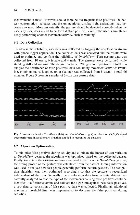
To address the reliability, user data was collected by logging the acceleration stream with phone logger application. The collected data was analyzed and the results were used to optimize and confirm the reliability of DoubleTurn. Turn gesture data was collected from 10 users, 6 female and 4 male. The gestures were performed while standing still and walking. The dataset contained 200 gesture repetitions in total. To analyze the occurrence of false positives, data containing movement activities (walk-ing, climbing stairs, jogging, roller-skating) was collected from 8 users, in total 96 minutes. Figure 3 presents samples of 3-axis turn gesture data.
Fig. 3. An example of a TurnDown (left) and DoubleTurn (right) acceleration (X,Y,Z) signal trace performed in a stationary situation, applied to recognize the gestures
6.2 Algorithm Optimization
To minimize false positives during activity and eliminate the impact of user variation to DoubleTurn gesture, the algorithm was optimized based on the collected dataset. Firstly, to capture the variation on how users tend to perform the DoubleTurn gesture, the timing profile of the gesture was calculated from the dataset. Timing information was used to analyze how fast people generally perform the turn gestures. The recogni-tion algorithm was then optimized accordingly so that the gesture is recognized independent of the user. Secondly, the acceleration data from activity dataset was carefully analyzed so that the type of the movements causing false positives could be identified. To further examine and validate the algorithm against these false positives, a new data set consisting of false positive data was collected. Finally, an additional maximum threshold limit was implemented to decrease the false positives during activities.

Turn-Based Gesture Interaction in Mobile Devices 17
6.3 Recognition Results
Table 2 shows recognition results for basic dataset consisting of DoubleTurn gestures performed while standing still and walking. When standing still, a user-independent recognition accuracy is 100% and when walking and performing the DoubleTurn ges-ture concurrently, the recognition accuracy is 96%. The total recognition accuracy is 98%. The occurrence of false positives was calculated from the activity dataset. Dur-ing 96 minutes, only 8 false positive occurred. Most of the false positives occurred during jogging and roller-skating.
Table 2. Recognition accuracy of DoubleTurn gesture
Situation of performing DoubleTurn User-independent average true positive %
Standing still 100 Walking 96
Total 98
7 Feedback Design
In gesture interaction it is important to deliver information on the result of the per-formed control action to the user; otherwise, the user does not know whether the ges-ture was detected and may repeat it. Because the gestures are captured by acceleration sensor, they can also be performed eyes-free. As a concequence, a visual feedback may not be the best option.
The interaction feedback in the example use cases was designed to examine whether multiple feedback elements add value to the interaction. In addition to the feedback from the phone function performed as a result of a successful gesture, tactile (vibration) and sound feedback was applied to enforce the message.
The aim in the feedback indicator content design was minimalism. Subtle short vi-bration pulses were applied with rhythm as a parameter. The key benefit with this approach is that with proper content design, the same rhythm can be rendered with multiple modalities (touch, hearing, vision). Thus, in different contexts, when one particular modality is not available, the intended feedback metaphor can still be perceived.
8 Discussion
The results of the experiences are qualitatively discussed in this section. A formal usability study is beyond the scope of this study. Thus, for factors other than reliabil-ity, the discussion is based on the experiences gathered informally from the develop-ment team during the interaction design process, and on the prior experience of the authors.

18 S. Kallio et al.
8.1 Use Cases
Gestures can only be used for a restricted set of carefully selected control tasks, and the type of gesture should be selected to fit and benefit the task. Failure in matching the gesture type and the target task will lead to user confusion and disturbance, at the least. The selected example use cases demonstrated how turn gestures benefit the user by relieving the attention focus through button-free interaction. Multimodal operation allows using the gestures alternatively to the traditional way of performing the tasks.
8.2 Reliability
The reliability evaluation confirmed that the DoubleTurn gesture can be recognized user independently with a high accuracy, even when the user is on the move. False positives occurred infrequently enough, having an insignificant effect on power con-sumption and on the user experience.
8.3 Feedback Indicators
During the feedback development process, four users experimented with vibration pulses in various phases of interaction. The sound pulses were then added, experi-menting with different pitch and character. An essential goal of the feedback content design was that it is not disturbing, but still clearly noticeable. To help the user distin-guish the two gestures, a different number and rhythm of feedback pulses was pro-vided for each gesture.
It was found that when sound and vibration are in synchrony, they enhance each other. The actual vibration pulse details are not important, as sound, when perceiv-able, grabs the attention. Vibration, on the other hand, adds to the perception of the sound as being more distinct and clear, compared to having just subtle sound without vibration.
9 Conclusion
Turn-based interaction was presented as a new type of method for gesture interaction with mobile devices. The accelerometer-enabled method was introduced and evalu-ated through example use cases and related user experiences. An essential element in the design was providing feedback indicators during interaction. The reliability of recognizing a turn-based gesture was verified quantitatively with user data. Turn-based interaction can benefit the mobile device user by extending the variety of usable gesture control use cases, potentially enhancing the user experience.
References
1. Nokia Corporation. 5500 phone (2006), http://europe.nokia.com/5500 2. Pirhonen, A., Brewster, S., Holguin, C.: Gestural and Audio Metaphors as a Means of
Control for Mobile Devices. In: Proc. CHI 2002, pp. 291–298. ACM Press, New York (2002)

Turn-Based Gesture Interaction in Mobile Devices 19
3. Brewster, S., Lumsden, J., Bell, M., Hall, M., Tasker, S.: Multimodal ‘eyes-free’ interac-tion techniques for wearable devices. In: Proc. SIGCHI conference on human factors in computing systems, pp. 473–480. ACM Press, New York (2003)
4. Kela, J., Korpipää, P., Mäntyjärvi, J., Kallio, S., Savino, G., Jozzo, L., Di Marca, S.: Ac-celerometer based gesture control for a design environment. Personal and Ubiquitous Computing, 1–15 (2006); Online First Springer
5. Linjama, J., Häkkilä, J., Ronkainen, S.: Gesture Interfaces for Mobile Devices – Minimal-ist Approach for Haptic Interaction. Position paper in CHI 2005 Workshop Hands on Hap-tics, Portland, Oregon, April 3-4 (2005)
6. Levin, G., Yarin, P.: Bringing sketching tools to keychain computers with an acceleration-based interface. In: Proc. CHI 1999, pp. 268–269. ACM Press, New York (1999)
7. Sawada, H., Uta, S., Hashimoto, S.: Gesture recognition for human-friendly interface in designer - consumer cooperate design system. In: Proc. IEEE International Workshop on Robot and Human Interaction, pp. 400–405 (1999)
8. Linjama, J., Kaaresoja, T.: Novel, minimalist haptic gesture interaction for mobile devices. In: Proc. NordicCHI 2004, pp. 457–458 (2004)
9. Ronkainen, S., Häkkilä, J., Kaleva, S., Colley, A., Linjama, J.: Tap input as an embedded interaction method for mobile devices. In: Proc. TEI 2007, pp. 263–270. ACM Press, New York (2007)
10. Rekimoto, J.: Tilting operations for small screen interfaces. In: Proc. ACM Symposium on User Interface Software and Technology, pp. 167–168 (1996)
11. Oakley, I., Ängeslevä, J., Hughes, S., O’Modhrain, S.: Tilt and Feel: Scrolling with Vibro-tactile Display. In: Proc. Eurohaptics, pp. 316–323 (2004)
12. Hinckley, K., Pierce, J., Horvitz, E., Sinclair, M.: Foreground and background interaction with sensor-enhanced mobile devices. ACM Transactions on Computer-Human Interac-tion 12(1), 31–52 (2005)
13. Video available, http://www.finwe.fi/video 14. Shneiderman, B., Plaisant, C.: Designing the User Interface: Strategies for Effective Hu-
man-Computer Interaction, 4th edn., p. 672. Addison-Wesley, Reading (2005)

S. Hailes, S. Sicari, and G. Roussos (Eds.): S-Cube 2009, LNICST 24, pp. 20–32, 2009. © Institute for Computer Sciences, Social-Informatics and Telecommunications Engineering 2009
A Large-Scale Wireless Network Approach for Intelligent and Automated Meter Reading
of Residential Electricity
Victor Custodio, Jose Ignacio Moreno, and Juan Pablo Viñuela
Telematic Engineering, Carlos III University of Madrid, Av. Universidad, 30, E. Torres Quevedo. E-28911 Leganés (Madrid), España
{victor.custodio,joseignacio.moreno,juanpablo.vinuela}@uc3m.es
Abstract. Control of electrical energy consumption is a critical aspect when electric companies try to establish the correct balance between the supply and demand of energy. Current solutions are based on experience, historical demand behavior and global control of the electrical grid, but they lack of detailed information about users consumption behavior. In the future, electric companies will need to know, almost in real time, user needs on energy to avoid extra costs of an over provisioning infrastructure or a lack of service during peak times. In this paper we address network topology, capacity planning and security issues of an IT platform, based on wireless sensor networks, to meet the new market requirements. The resulting automated control system will be able to provide real-time control of user demands, as well as to open the market to future services in this area: differential billing schemes, remote control and others.
Keywords: Electricity Metering Platform, AMR, Security, ZigBee, WSN.
1 Introduction
Electricity meter reading is a common task that must be accomplished by every single electric company in the market. Why? This is a standard way they have to measure the effective amount of energy a certain user consumes over a period of time.
Until now, traditional methods for residential meter reading, involves the physical presence of companies’ personnel at the user premises every one or two months to visually read the corresponding meters for every user or client of the service, a number big enough to reach hundreds of thousands or even millions of devices to be read. Although, many solutions have been developed to improve the time required to get manual readings from the meters through the use of wireless equipment, just a few of them, if any, introduces the possibility to do it remotely and automatically. Another big problem that electric companies have is that they face an uneven consumption curve during the day, forcing them to provision enough network infrastructure and operations to support periods of peak demand. This difference between the supply and demand of energy, introduces high operational costs and complex grid management.
Naturally, the described process leads to very high operational costs for the electric companies and also, complex logistics and management problems. But even more

A Large-Scale Wireless Network Approach for Intelligent and Automated Meter Reading 21
important, this old-fashioned method does not allow these companies to be major players, and actively participate in one of today’s world-most significant challenge which is energy efficiency, as stated by the European Union as one of the top important subjects in energy field for the next coming years [1].
In this work we present an IT platform to perform remote electricity-meter readings, which will enable companies to automate the process without the need of in-premises personnel, reducing operational expenditures and opening an unprecedented way for real-time energy metering, and consequently, the possibility of energy efficiency, not only saving money for electric companies and end-users, but also making big savings to the environment and the world. Moreover, companies will have the possibility to offer new services related to energy consumption. The proposed IT platform will make use of different communication technologies depending on the requirements and restrictions of each network segment of the design.
With the evolution of technology in recent years, new communications systems are coming into the markets. Wireless networks are no exception of this phenomenon, and these kinds of technologies are even more present in people’s today’s life, having outstanding advantages for a meter-reading platform such the one presented here. In the access network, there will be no need to deploy costly wired infrastructure around user premises, where wireless sensor networks (WSN) will be a good solutions due to its low cost and low power consumption. In the other hand, for a long range path, WSN won’t provide the necessary range and processing power, where a different technology, wireless or not, will be more suitable (GPRS, WiMAX, ADSL, etc).
The main objective of this paper is to present an IT platform capable of reading every meter from the electric-service users at previously designated time-intervals of the day, or even on demand, and then send this information to the central servers of the electric company. This will enable them to develop differential billing schemes based on the energy demand during the day and the real-time knowledge of energy consumption, as well as to reduce the operational costs associated with the reading of the meters. It is important to mention that even thou this work have been done in an electricity meter context, it can also be applied to any other utility application.
The rest of this paper is organized as follows: Section 2 focuses on the analysis of requirements and the architecture for the meter reading platform. Section 3 explains the core aspects of network deployment and security for the platform. Section 4 shows a sample deployment and network dimensioning using typical values for an average electric company. Finally, we present some conclusions and future work.
2 Requirements and Architecture for Electricity Meter Reading
Until now, traditional methods of residential electricity metering has consisted in electric companies having to send dedicated employees to client premises (houses, buildings, etc) every one or two months to visually read the customer meter, and take note of the readings. Based on the reading made by the employee, the company is able to charge the user for the amount of energy consumed over the period of time being measured. Unfortunately, such method requires a big effort in terms of the number of employees needed to perform the task and many times involves having to get into users home to reach a meter, which could also represent a problem.

22 V. Custodio, J.I. Moreno, and J.P. Viñuela
The purpose of Automated Meter Reading (AMR) technology is to enable electric companies to perform meter readings remotely, without sending employees to users home. Many technologies exist today for the automation of the process, but they generally involve sending an employee to the neighborhood or to a point of close vicinity of a group of users, or deploying wired infrastructures at user’s premises.
With the introduction of WSN’s, we can develop a distributed and automated process to perform the readings, where the edge is that we can avoid costly and/or complex situations such as the ones mentioned above. In this sense, the results obtained will turn into great improvements for electrical companies and end-users:
• Billing Schemes: Encourages energy use during low demand periods. • Operational Expenditures Reduction: There is no longer need to send huge
number of employees to customers’ premises to perform readings. • New Services: Companies can offer new services to their customers.
Automating the process through the use of WSN’s, involves taking into account several aspects related to features, requirements and the specific scenario and architecture of applications, all of which we will describe in the rest of this section.
2.1 Features and Requirements
The proposed IT platform is based in a group of features and requirements for the technology to be used, as well as a series of features related to the specific applications to be implemented. Depending on these parameters, the proposed methodology tries to accommodate and solve the majority of the different scenarios.
2.1.1 Application Requirements
Nodes Identification. The EndPoints (devices attached to meters) have to be uniquely identifiable in the network and correctly associated to a specific customer.
Node Mobility. This is a very important feature of general WSN’s, but in this case is not very relevant. Most of the time there will be no movement of the EndPoints.
Energy Consumption and Battery Lifetime. This is a very restrictive parameter for WSN’s, especially if units are battery powered. For electricity meters, endpoints are expected to draw power from the corresponding electricity meter they are attached to.
Scalability. In the future, new endpoints will be joining the network. The design should consider the possibility of automatic growth of the network, without the need to perform specific and/or technical modifications to the design.
Reliability. This is one of the most important requirements for an AMR platform. Information cannot get lost, even considering that there could be connection dropouts in the network. Readings must be taken in a secure and timely manner.

A Large-Scale Wireless Network Approach for Intelligent and Automated Meter Reading 23
2.1.2 Requirements Imposed by the Technology
Identification of Devices. Wireless endpoints will be based on ZigBee technology. There are two possibilities of addresses for the devices: 64 bits pre-encoded MAC addresses and 16 bits network addresses. The first of them are globally unique and usually used when a device is about to join a ZigBee network. The second of these two, is a much shorter address used for routing purposes inside the network.
Network Size. The size of a ZigBee network is theoretically determined by the limitation of the 16 bits addresses. Nevertheless, because of physical limitations, the maximum number of devices is 100 per ZigBee network, a much smaller amount.
Type of Sensors. Sensors connect to electricity meters through serial interfaces, so the wireless device will be inside the meter, thus reducing the range for the devices.
Maximum Number of Coordinators. There is a limit, by design, of 4 coordinators that can be directly attached to the interfaces of the concentrator.
2.2 Scenario Description
A typical scenario consists of a group of houses or buildings in dense urban areas, where the different buildings are in proximity one from another. We will find other situations too (small towns or isolated houses) but this scenario is a good start.
Every house has an electricity meter to be read. The location of the meter will depend on the type of edification: in houses, most of the time it will be just outside of the house; in buildings, it could be just outside of the apartment or sometimes in a special designated area to group a number of them. The meters connect through a wireless interface to a special device called concentrator, which aggregates all the readings of the meters in close proximity. The concentrator is responsible for sending all the information back to the management servers of the electric company, which in most cases will be several miles away from the customer’s premises.
As we can see in Fig. 1, the scenario comprises a series of important elements, each of them having different roles. The combination of these elements in a network, make possible the automated meter reading process.
EndPoint. Network element integrated into the meter. It implements a physical and logical interface so it can interact with the meter to obtain the readings and manage the device.
Coordinator. Device responsible for the coordination of a ZigBee network. It allows nodes to join the network and assigns them network addresses, and it is in charge of routing, outside the network, the information from all the meters.
Concentrator. It’s the network element responsible for collecting and aggregating all the information generated by a group of endpoints. It implements the logical interfaces to communicate with endpoints and the middleware platform
24 V. Custodio, J.I. Moreno, and J.P. Viñuela
Management Servers. They represent the middleware platform that is responsible of making requests to nodes and storing the information of the readings from meters.
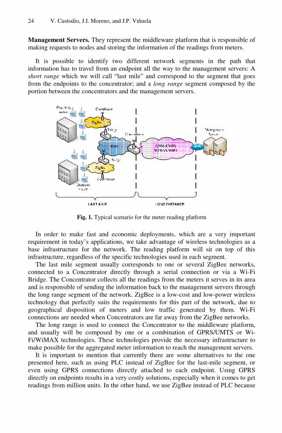
It is possible to identify two different network segments in the path that
information has to travel from an endpoint all the way to the management servers: A short range which we will call “last mile” and correspond to the segment that goes from the endpoints to the concentrator; and a long range segment composed by the portion between the concentrators and the management servers.
Fig. 1. Typical scenario for the meter reading platform
In order to make fast and economic deployments, which are a very important requirement in today’s applications, we take advantage of wireless technologies as a base infrastructure for the network. The reading platform will sit on top of this infrastructure, regardless of the specific technologies used in each segment.
The last mile segment usually corresponds to one or several ZigBee networks, connected to a Concentrator directly through a serial connection or via a Wi-Fi Bridge. The Concentrator collects all the readings from the meters it serves in its area and is responsible of sending the information back to the management servers through the long range segment of the network. ZigBee is a low-cost and low-power wireless technology that perfectly suits the requirements for this part of the network, due to geographical disposition of meters and low traffic generated by them. Wi-Fi connections are needed when Concentrators are far away from the ZigBee networks.
The long range is used to connect the Concentrator to the middleware platform, and usually will be composed by one or a combination of GPRS/UMTS or Wi-Fi/WiMAX technologies. These technologies provide the necessary infrastructure to make possible for the aggregated meter information to reach the management servers.
It is important to mention that currently there are some alternatives to the one presented here, such as using PLC instead of ZigBee for the last-mile segment, or even using GPRS connections directly attached to each endpoint. Using GPRS directly on endpoints results in a very costly solutions, especially when it comes to get readings from million units. In the other hand, we use ZigBee instead of PLC because

A Large-Scale Wireless Network Approach for Intelligent and Automated Meter Reading 25
has some bandwidth limitations (depending on the place of deployment) and also it is not as flexible as ZigBee. In the future, this platform could be used for other utilities, like gas or water, where a PLC connection could not be fully guaranteed.
3 Network Deployment Analysis
The main objective of the deployment analysis is to correctly identify problems and solutions related to the deployment of the network, to be able to successfully obtain the readings of all the electricity meters, subject to a series of constraints, such as reliability, costs, scalability and others. From this point of view, we have stated three fundamental tasks in the deployment activity: Sensor Identification, Network Security and Capacity Planning. The first one specifies how to univocally identify each and every node of the network, letting the management servers, or any other network element, to communicate with a specific endpoint; Network Security section explains the mechanisms to obtain authentication, data confidentiality and integrity, and high availability of the service; The third part, analyzes the different data size related to the meter, and uses this information to plan the capacity, in terms of needed bandwidth, to be supported in every section of the network.
3.1 Sensor Identification, Addressing and Naming Convention
Devices identification is one of the important and challenging parts of the deployment of the solution. As stated before, the number of meters for an electric company can easily reach hundreds of thousands or million units. Having a way to univocally identify them, involves the association of the meter with a specific customer.
Even if it was possible to use all the 16 bits addressing space given by ZigBee technology, it wouldn’t be enough. Besides the number of addresses problem, there is a problem related to persistency. A ZigBee coordinator assigns networks addresses to devices dynamically, thus, the address of a specific device can change in time. This means that we cannot use only network addresses as a way to identify nodes. In a situation like this, it is convenient to use the long 64 bits MAC addresses as a way to uniquely identifying the nodes, although its use is not meant for routing purposes.
Now, provided that we are going to use 64 bits MAC addresses for identification, there is still a need to associate these addresses with specific customers. Taking into account that the meters will be grouped under concentrator devices, which will be operating on an IP network in the long-range segment, we will have the following tuple of information that has to be recorded into the management servers:
customer_id node_mac_address concentrator_id
The customer_id corresponds to a company-assigned identification for its
customers, node_mac_address is the unique 64 bits addresses for ZigBee devices, and concentrator_id corresponds to an identifier for the concentrators of the network.
Using a scheme like this requires additional considerations and could introduce some potential problems. The row has to be repeated for each and every customer of the service, which can grow to a very large number and could lead to data-access

26 V. Custodio, J.I. Moreno, and J.P. Viñuela
efficiency problems. Each time the management middleware has to contact a customer meter, it first has to consult the database to obtain the MAC address of the corresponding device, as well as the information regarding to the identification of the concentrator under which the meter operates. This way, the platform knows which concentrator to send a request to, in order to communicate with a certain meter. Once a concentrator receives a request, it passes the request, along with the MAC address to the coordinators it has attached to its interfaces, and the coordinators in turn, using the MAC address, search for the corresponding device inside the ZigBee network. Under a situation like this one, there is no chance for a good organization or hierarchy of the network, thus increasing complexity of the process.
As a workaround of the problems mentioned above, we propose the use of virtual networks and addresses. The main idea behind this is to build a complete IP-based network on top of the heterogeneous infrastructure of the different network technologies used. We have seen in the scenario description, that there will be an IP portion in the design, primarily corresponding to the long distance segment and maybe some portion in the short range part. The last mile, which considers the endpoints (electricity meter nodes), is based on ZigBee technology. The virtual network will sit just on top of this infrastructure.
ZigBee technology does not support the TCP/IP stack, mainly because of its size, but it is possible to implement a network address translation between IP and ZigBee addresses [2], without having to use the whole TCP/IP stack. This method is intended to be used for naming and addressing purposes but not for routing purposes. This means that the ZigBee network remains intact from the network-inside point of view. For the addresses translation to work, it is needed to add a gateway at the edge of the ZigBee network, which will be in charge of the translations. This way, from the outside, it will be possible to address endpoints through an IP address, simplifying the whole process of communicating with an endpoint. The main advantages will be:
• No need to send long MAC addresses through the network (end-to-end). Just the
gateways need to know them. • Network Hierarchy. It is possible to subdivide the network into subnets. • The whole meter-reading process becomes more transparent to middleware.
Finally, to implement a solution like this one, it is needed to know what will be the size of the network, in terms of how many endpoints and concentrators there will be. This will lead to a correct address or naming convention and how to structure the network. The important things to take into account in this section are:
• Estimated number of endpoints • Estimated number of concentrators • Network planning: IP addresses to use and number of subnets
3.2 Network and Data Security
The AMR communication platform presented here is mainly based on wireless networks. These types of networks are generally exposed to a number of vulnerabilities that wired networks do not have, starting with the fact that possible

A Large-Scale Wireless Network Approach for Intelligent and Automated Meter Reading 27
attackers have direct access to the network media. This way, anyone being in range and knowing the frequency of transmission could have access to the network, almost like any other device does. Among the most common and important types of attacks we have:
• Denial of Service: causing interference, taking advantage of the vulnerability of the CSMA-CA protocol. This is used in ZigBee and Wi-Fi.[3]
• Attack to the Confidentiality of the Data • Replay Attacks • Supplanting of endpoints
In the context of automated meter reading, the supplanting of endpoints will be the most likely attack to occur, therefore, authentication is one of the most important aspects to take into account, without leaving behind confidentiality and integrity of the data, and the availability of the service, which are of extreme importance too.
Now we describe possible solutions to provide security mechanisms for, at least, each of the five characteristics mentioned above, considering last mile and long-range segments.
3.2.1 Last Mile Segment The communications in the last mile correspond to ZigBee and Wi-Fi networks.
The ZigBee Pro standards [4][5] provides two types of security: Standard Security and High Security. The standard mode is focused to avoid the access of external devices to the network, and it is based on a trust center that authenticates and distributes a network key that is used to encrypt all messages that flow through the network.
The high security mode is thought for networks where the security control is critical, and in order to satisfy the requirements of the system, it adds two more keys, master and link keys, besides the secure key exchange (handshake). In this mode all the messages are encrypted from point-to-point with a link key that is generated from a master key, after a handshake between both points. This way, the high security of ZigBee also avoids insider attacks. Because of its strength, this is the security standard that we are going to use for the meter reading platform.
In order to provide for the minimum security needed for the Wi-Fi network, we can make use of Wi-Fi security standard 802.11i (WPA/WPA2) with 802.1x authentication (EAP), which currently is considered to be safe. To strengthen its security even more, there are several mechanisms to consider:
• IPSEC (VPN tunnels): The information travels encrypted through the tunnel from the client to the VPN server.
• MAC Filtering: Only authorized devices are allowed access to the network. • Hiding Access Point: Hiding the access point is possible (if available)
Given that we are working with mesh networks, hiding the access point is not supported, and the management of MAC filtering tables becomes very costly for large deployments. That’s why both of these are not to be used.

28 V. Custodio, J.I. Moreno, and J.P. Viñuela
On the other hand, due to high sensitivity of information against attacks and future potential vulnerabilities of the 802.11i standard, we introduce an extra level of security through the use of IPSec VPN tunneling.
3.2.2 Long Distance Segment The communications in this segment consider any or a combination of GPRS/UMTS and/or Wi-Fi/WiMAX. In the latter case, the same safety mechanisms considered in the last mile apply here, because they are considered to be safe enough for now. The standards to be used consider 802.11i (WPA2) and 802.1x (EAP) authentication for Wi-Fi networks, 802.16g with EAP and PKMv2 for authentication in WiMAX networks [6]. Like in the last mile, we also increase security by using VPN tunneling based on IPSec.
Table 1. Security Mechanisms
Network Link level Network level Application level
ZigBee High Security
Wifi WPA2 VPN based in IPsec -
GPRS Security offered by telecomm operator AES Encryption + PKI-based Authentication and key exchange
WIMAX 802.16g security with EAP and PKMv2
VPN based in IPsec -
In situations where the information through the long range segment is sent over
GPRS/UMTS, the telecomm operator that offers the service will be responsible for ensuring authentication, confidentiality, integrity, and service availability, in an end-to-end basis. As a safety measure, we again provide an extra level of security. In this case, all messages are encrypted using application-level AES. The exchange of symmetric keys for AES encryption and a second authentication is performed using a system public key (PKI). This information is summarized in Table 1.
3.3 Network Capacity Planning
Capacity planning is about estimating and knowing what are going to be the limitations and restrictions with respect to the different technologies involved in the design, making it possible to address and provision the necessary equipment for the system to work in optimal conditions, based on a set of requirements. This will lead to an estimation of the number of the different equipment needed for deployment and the bandwidth requirements over the different networks segments, among others.
The most important requirements and capacities limits for the design are:
• Number of Nodes • Number of ZigBee Coordinators • Number of Concentrators • Size of summarized meter readings and firmware in each network segment.

A Large-Scale Wireless Network Approach for Intelligent and Automated Meter Reading 29
To calculate the above restrictions, it is needed the following list of parameters:
• Number of customers to obtain energy consumption information from. • Maximum number of nodes per ZigBee network • Maximum number of coordinators supported per Concentrator • Size of an electricity-meter reading • Time interval between each reading.
These kind of considerations are well suited for a general purpose scenario, but in a real case deployment, it is necessary to take into account other parameters such as the types and level of isolation of buildings involved, communications technology availability and coverage in the specific area of deployment, among others.
The next section will show an example of a deployment and how the above information is useful to obtain gross estimations for infrastructure requirements.
4 Practical-Case Application of the Deployment
In this section we present an application of the deployment methodology presented in the previous section, covering the most relevant aspects of identification and capacity planning. Security parameters correspond to the ones presented in previous sections.
Fig. 2. Sample scenario for the application of the deployment methodology
The example is based on Fig. 2, where we assume the values presented in Table 2 for the different parameters involved the scenario. There are 5 buildings in the scenario. Four of them will connect to one concentrator through Wi-Fi bridges, and the fifth one will connect to another concentrator through its serial interface, because it is not close to the rest of the buildings. It has been stated that the reading of a meter consumes at most 60 bytes, including headers and security redundancy.

30 V. Custodio, J.I. Moreno, and J.P. Viñuela
Table 2. Parameters for the example of the applications of the deployment methodology
Parameter Value Number of Buildings 5 Number of Floors per Building 8 Number of Apartments per Floor 6 Distance Between Buildings < 30 mt Distance from the Buildings To Management Servers 5 km Maximum number of nodes per ZigBee network 50 Number of ZigBee interfaces per Concentrator 4 Size of an electricity-meter reading (including headers) 60 bytes Size of a Firmware Update of a Meter 60 Kb Meter-Reading Interval 15 min
Based on information from Table 2, it’s possible to estimate the requirements on
equipment and devices to be used for the solution. This is presented in Table 3.
Table 3. Estimation of number of needed devices based on parameters of the scenario
Parameter Value Number of Electricity-Meters/EndPoints 240 Number of Coordinators (ZigBee networks) 5 Number of Bridges (one per coordinator not connected directly) 4 Number of Concentrators 2
4.1 Identification and Addressing
In this scenario, we need to be able to uniquely identify 240 nodes, each of them corresponding to a customer. This is a very small number, so if we consider the use of Virtual IP, a Class C IPv4-network would be enough. Scalability is one of the requirements for the solution, so we have to consider the possibility of future growth of the network as new EndPoints are added under the management of an existing concentrator. Here is where we make use of the advantages of IP hierarchy characteristics, so we can assign a different Class C network to each of the concentrators. Table 4 shows the addressing scheme. For this purpose, we make use of private addresses. There is plenty of space for adding new endpoints.
Table 4. EndPoint identification and addressing scheme
Network Parameters Concentrator 1 Concentrator 2 Network 192.168.1.0 192.168.2.0 IP Address 192.168.1.1 192.168.2.1 IP Range for Bridges 192.168.1.10-192.168.1.20 N/A IP Range for End-Points 192.168.1.128-192.168.1.254 192.168.2.128-192.168.2.254

A Large-Scale Wireless Network Approach for Intelligent and Automated Meter Reading 31
For Virtual IP to work, a special gateway is needed which is going to be in charge to do the translation between IP addresses and ZigBee address. That way, the coordinator will receive a request in a protocol it can understand. One gateway is needed per concentrator. Now, when the middleware platform makes a request to one of the EndPoints, it only need to know the IP address of the node, and the request automatically will arrive to the corresponding concentrator, where the gateway will make the address translation and then send it to the appropriate coordinator.
4.2 Capacity Planning
We already calculated, in Table 2, the requirements about number of nodes (endpoints), number of ZigBee coordinators and the number of needed concentrators. Now we are going to calculate what are going to be the amount of information to be handled by each device and, consequently, the capacity requirements on the communications links. This is calculated for meter readings and firmware updates.
Table 5. Total traffic to be managed by each element of the network
Network Element Energy Reading Firmware Update Node (endpoint) 60 bytes 60 Kb Coordinator 3 Kb 3 Mb Bridge 3 Kb 60 Kb Concentrator 1 2.88 Kb 60 Kb Concentrator 2 11.5 Kb 240 Kb Management Server 14.38 Kb 120 Kb
We assume mean values for coordinators and bridges, that is, they handle about the
same amount of information regardless if they are alone or grouped under a concentrator. On the other hand, this design corresponds to a distributed network, so firmware updates only needs to be sent once to each concentrator, and this device is in charge to send the necessary copies to each endpoint.
The requirements on the amount of information are not so big, and this mainly reflects the fact that this is a small example. If we consider a complete deployment for a modern mid-size city, we can end up having about 2 millions electricity meters. For such condition, it would be needed around 10.000 concentrators, each having to manage 12 Kb. This implies a total of 120 Mb on the management server. Special care has to be taken, because some connections between a concentrator and the core could be over a GPRS connection, which has important restriction of bandwidth.
5 Conclusions and Future Work
Throughout this article we have presented an IT platform for remote management of electricity meters, covering deployment and security of the platform.
The implantation of this platform will enable electric companies to develop sophisticated billing schemes, helping to mange smartly and more efficiently the great differences that companies have to face between supply and demand of electric energy during a day. This energetic efficiency will make big savings for the companies, end-users and with no doubt, for energy resources in the world. The key

32 V. Custodio, J.I. Moreno, and J.P. Viñuela
of the solution is the ability to do real-time and on demand electricity consumption readings. Another great advantage, besides the energy efficiency, is that electric companies will have the opportunity to offer new services, like differential billing, on-line service management and promotional offers with minimal operational costs.
ZigBee is a low-cost and low-power wireless technology that perfectly suits the requirements for the last mile segment, which are related to the geographical disposition of the meters and low traffic generated by them. Moreover, if we combine ZigBee with better-cover wireless technology such as Wi-Fi, WiMax, GPRS and/or UMTS, we obtain a complete solution for the remote AMR system. There is no need for expensive deployments of wired networks.
Unlike the standard and well-know data networks mentioned above which have better range, ZigBee does not support the TCP/IP stack, which generates problems for addressing and identification of the endpoints. Fortunately, these problems are resolved by the use of virtual IP addresses, which provide network hierarchy and transparency to middleware.
This platform could be extended for the use of other utilities companies, like gas and water. It is also possible to do remote readings of water or gas meters, as long as they can be integrated with sensor networks technologies. The communications system has been designed to be flexible and to be able to support the integration of other meter equipment. Nevertheless, it is quite important to take into account that these other purposes, most probably will have special requirements. Just to mention one, water or gas meters cannot draw electric power from the very service supply like electricity meters do, thus introducing new challenges worth a specific analysis before adopting this platform to the new scenario.
Acknowledgements
The presented work was mainly done within the research project IRIDIUM [7], which was partly funded by the Spanish Ministry of Industry, Tourism and Trade under the contract TSI-020400-2008-152. The authors would like to thank all the members of the project that contribute with fruitful discussion.
References
1. European Parliament: Action Plan for Energy Efficiency: Realising the Potential (2007/2106(INI))
2. Transmission of IPv6 Packets over IEEE 802.15.4 Networks. RFC4944, IETF 3. Raymond, D.R., Midkiff, S.F.: Virginia Tech:Denial-of-Service in Wireless sensor
Networks: Attacks and Defenses (January-March 2008), http://www.ieee.org 4. ZigBee Alliance: ZigBee Specification (January 2008), http://www.zigbee.org 5. ZigBee-PRO Stack Profile: Platform restrictions for compliant platform testing and
interoperability (January 2008), http://www.zigbee.org 6. 802.16g-2007 IEEE Standards for Local and metropolitan area networks, http://standards.ieee.org/getieee802/download/ 802.16g-2007.pdf
7. Project IRIDIUM, http://www.amr-iridium.com/

Weak Process Models for Attack Detection in aClustered Sensor Network Using Mobile Agents
Marco Pugliese1, Annarita Giani2, and Fortunato Santucci1
1 Center of Excellence DEWS, University of L’Aquila, L’Aquila, [email protected], [email protected]
2 Department of Electrical Engineering and Computer Sciences,University of California at Berkeley, Berkeley, CA, USA
Abstract. This paper proposes a methodology for detecting network-layer anomalies in wireless sensor networks using weak process models(WPM). Weak process models are a non-parametric version of HiddenMarkov models (HMM), wherein state transition probabilities are re-duced to rules of reachability. Specifically, we present an intrusion detec-tion system based on anomaly detection logic. It identifies any observableevent correlated to a threat by applying a set of anomaly rules to the in-coming traffic. Attacks are classified into low and high potential attacksaccording to its final state. Alarms are issued as soon as one or morehigh potential attacks are detected.
We model hello flooding, sinkhole and wormhole. We introduced singlethreat models and aggregated models and study how effective they areto detect each attack.
We present the design approach for the proposed WPM-based detec-tion technique using mobile agents. Early implementations of the agentbased secure platform have already been implemented.
Keywords: Weak Process Models, Anomaly Detection, Threat Identi-fication, Alarm Generation.
1 Introduction
Sensor networks permit data collection and computation to be deeply embeddedin the physical environment. Sensor nodes are often left unattended so thatthey are susceptible to security attacks. Typical threats affecting wireless sensornetworks (WSNs) are reported in [1]. An intrusion detection system (IDS) is adefense system, which detects hostile network activities. It recognizes patternsof known attacks (signature based) [19,18], or identifies network activities thatdiffer from historical norms (anomaly based) [2].
This work considers an IDS based on anomaly detection logic (ADL). Threatsare correlated to any sequences of observable events by applying a set of anomalyrules to the incoming traffic. Computer networks are typically provided withmechanisms to identify changes in system parameters or anomalous exchange of
S. Hailes, S. Sicari, and G. Roussos (Eds.): S-Cube 2009, LNICST 24, pp. 33–50, 2009.c© Institute for Computer Sciences, Social-Informatics and Telecommunications Engineering 2009

34 M. Pugliese, A. Giani, and F. Santucci
information. Such data can be used as relevant observations to predict the hiddenstate of the system and infer if it is under attack. A HMM is a doubly stochasticfinite state machine with an underlying stochastic process that represents thereal state of the system. The real state of the system is hidden but indirectlyobservable through another stochastic process that produce a sequence of observ-able events [5,15]. The relationships between hidden states and observable dataare stochastic as well as the transitions between states. HMMs [5,15] have beenwidely used in network-based IDS for wired systems [9,10,11,12,22,23] as wellas for modeling Internet traffic [21]. The Baum-Welch algorithm as likelihoodcriterion and parameter estimation is extensively used [5].
Silva et al. [13] have proposed a decentralized IDS that fits demands and re-strictions of WSNs. The network behavior is obtained from the analysis of eventsdetected by a monitor node. A set of rules are compared with the informationgathered from the network traffic. In general, application of traditional IDSs tosensor networks is challenging. In fact they require intense computation capa-bility [20] and they are too limited to a restricted number of threats [7]. Someconventional intrusion detection systems perform cross-correlation and aggrega-tion of data. For example, they analyze fluctuation in sensor readings [6], ordetect abnormal traffic patterns [26].
Implementing an effective IDS on a wireless sensor network leads to the prob-lem of finding a trade-off between the capability of identifying threats (i.e. witha bounded false alarm rate), the complexity of the algorithms and memoryusage [8]. Doumit and Agrawal [7] proposed a novel approach for applying alightweight, yet robust IDS designed for wireless sensor networks based on self-organized criticality and HMM. They model the natural dynamic of the systemso that unusual activity can be identified. We propose here an intrusion detec-tion system which replaces HMMs with WPMs. WPMs are a non-parametricversion of HMMs wherein state transition probabilities are reduced to rules ofreachability.
Very low state transition probabilities are reduced to zero which increasesfalse negatives. This means that some sequences are classified as not possiblewhen instead in a probabilistic model would be achievable. The number of falsenegatives decreases if we add states [4] but the drawback is a larger memoryrequirement. The matrices that describe the models are sparse and can be com-pacted for faster computation.
The estimation of a threat in the case of weak processes is greatly simplifiedand less demanding for resources. The most probable state sequence generatedby the Viterbi algorithm [3] for HMM becomes the possible state sequence. Theintensity of the attack is evaluated by introducing a threat score, a likelihoodcriterion based on weighting states and transitions [4]. Intrusions and violationsare classified into low potential attacks (LPA) and high potential attacks (HPA)depending on their distance from the state corresponding to a successful attack.When at least one HPA occurs, an alarm is issued.
We assume that a secure routing protocol [14,24] is running on the networkand that routing messages are ciphered and authenticated through an underlying

Weak Process Models for Attack Detection in a Clustered Sensor Network 35
cryptographic scheme. We analyze hello flooding, sinkhole and wormhole. A se-cure routing protocol would result not effective to protect from these threats [2,1].According to these assumptions, we can mainly focus on threats from internalintruders that generate control messages that are syntactically and semanticallywell-formed.
In summary, the main contributions of this paper are as follows:
– Application of our method to the detection of sinkhole and wormhole (helloflooding was considered in [4]);
– Extension to models that describe aggregate threats;– Comparison of models that describe a single attack and models that describe
more than one attack in terms of detection capability.
The remainder of this paper is organized as follows. In section 2 we presentsome background material on weak process models and show how it is appliedto the problem of detecting sinkhole and wormhole. In section 3 we analyze falsealarms and misdetection of single threat models compared to aggregated models.In section 4 we will present the design approach for the proposed WPM-baseddetection technique: mobile agents and enhancements to the execution environ-ment in [31] have been proposed. Early implementations of the agent basedsecure platform are already available in our lab. Section 5 contains concludingdiscussion and future work.
2 Threat Detection and Alarm Generation
In our anomaly-based approach the anomaly rules are defined through inequalityso that they define regions of the state space. This allows us to introduce aranking among states that leads to a hierarchical structure. The number of falsenegative (mis-detection) is reduced since inequalities are satisfied by a largernumber of values with respect to equalities. Also the number of false positivedecreases given that we choose to associate an alert only to the state with thehighest risk. States are classified according to two hazard levels, low potentialattack (LPA) states and high potential attack (HPA) states. We also introduce ascore mechanism to weight state sequences where LPA and HPA states contributedifferently. Now we give formal definitions of WPMs, threat score, low potentialattack and high potential attack.
A WPM, as any Markov model, can be formally represented using the canon-ical form: {
xk+1 = Axk
ok = Bxk(1)
where:
– X = (x1, x2, . . . , x3) is the state set ;– xk is the state at step k. x0 is the initial state;

36 M. Pugliese, A. Giani, and F. Santucci
– O = (o1, o2, . . . , oq) is the the set of observations ;– ok is the observable o at step k ;– A is a n×n matrix representing state transition distribution. Matrix elements
are defined as:
Ai,j =
{1 if p(xk+1 = xj |xk = xi) = 10 otherwise
– B is a q × n matrix representing the emission distribution, that maps eachobservable with the states. Matrix elements are defined as
Bi,j =
{1 if p(ok = oj |xk = xi) = 10 otherwise
Definition 1. Let sk be the threat score after k observations. sk is the result of aweighting mechanism applied to states and transitions belonging to the hypotheticstate trace. Weights are represented by a square n x n matrix S, where is n thenumber of states in the model. The elements of the matrix are defined as follows:
sij =
{weight assigned to the transition from xi to xj if i �= j
weight assigned to the state xi if i = j
Definition 2. A Low Potential Attack (LPA) is an attack defined by a state xj
whose distance from the final state is at least 2 hops.
Definition 3. A High Potential Attack (HPA) is an attack defined by a statexj whose distance from the final state is less than 2 hops.
Let us assume now that, if a node represents a LPA state, then its score is L. If anode represents a HPA state, then its score is H and, if a node neither representsan attack state nor is the final state, then its score is 0. L and H are integers.We define the elements of the score matrix S as follows:
sij =
{ai,j · (si − sj) if i �= j
{0, L, H} if i = j
where aij are the elements of matrix associated to the model describing thethreat.
Let us define nkhpa and nk
lpa the numbers of high potential and low poten-tial states, respectively, reached in the observation interval. These numbers arenot limited to a single trace, but include states belonging to all possible statesequences at time k. With the above assumptions the threat score at time k is
sk = H · nkhpa + L · nk
lpa (2)
The choice of H and L depends on the length of the memory that we allocated tostore the various states of the model. We call it WML, the weak process model
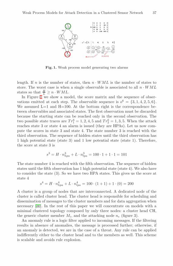
Weak Process Models for Attack Detection in a Clustered Sensor Network 37
Fig. 1. Weak process model generating two alarms
length. If n is the number of states, then n · WML is the number of states tostore. The worst case is when a single observable is associated to all n · WMLstates so that H
L ≥ n · WML.In Figure 1 we show a model, the score matrix and the sequence of obser-
vations emitted at each step. The observable sequence is o6 = {3, 1, 4, 2, 5, 6}.We assumed L=1 and H=100. At the bottom right is the correspondence be-tween observables and associated states. The first observation must be discardedbecause the starting state can be reached only in the second observation. Thetwo possible state traces are Tr6
1 = 1, 2, 4, 5 and Tr62 = 1, 3, 5. When the attack
reaches state 3 or state 4 an alarm is issued (they are HPAs). Let us now com-pute the scores in state 3 and state 4. The state number 3 is reached with thethird observation. The sequence of hidden states until the third observation has1 high potential state (state 3) and 1 low potential state (state 1). Therefore,the score at state 3 is
s3 = H · n3hpa + L · n3
lpa = 100 · 1 + 1 · 1 = 101
The state number 4 is reached with the fifth observation. The sequence of hiddenstates until the fifth observation has 1 high potential state (state 4). We also haveto consider the state (3). So we have two HPA states. This gives us the score atstate 4
s4 = H · n4hpa + L · n4
lpa = 100 · (1 + 1) + 1 · (0) = 200
A cluster is a group of nodes that are interconnected. A dedicated node of thecluster is called cluster head. The cluster head is responsible for scheduling anddissemination of messages to the cluster members and for data aggregation whennecessary [30]. In the rest of this paper we will concentrate on models with aminimal clustered topology composed by only three nodes: a cluster head CH,the generic cluster member Mi, and the attacking node ne (figure 3).
An anomaly rule is a logic filter applied to incoming messages. If the filteringresults in absence of anomalies, the message is processed further; otherwise, ifan anomaly is detected, we are in the case of a threat. Any rule can be appliedindifferently either to the cluster head and to the members as well. This schemeis scalable and avoids rule explosion.

38 M. Pugliese, A. Giani, and F. Santucci
Fig. 2. Model with a minimal clustered topology
We follow a four step process when modeling a threat.
1. Analyze the behaviour of the threat;2. Derive the Anomaly Rules;3. Derive the WPM-based threat model;4. Assign weights to WPM states and transitions.
Given the set of threat observables collected during two consecutive observationsteps, the observable with the highest score back-propagates. In [4] we describehow to model the hello flooding attack and how WPMs are used to detect it. Inthis work we concentrate instead on the sinkhole and wormhole attack modelingand detection.
In the following threat scenarios, dotted arrows indicate the malicious trafficflow and the label refers to the anomaly rule used to detect it.
2.1 Sinkhole Modeling and Detection
In this threat nearly all traffic from a particular area is lured through a specificcompromised node with unfaithful routing information [14]. Each neighbouringnode of the adversary node is induced to forward packets directed to a basestation through the adversary. The malicious node can then suppress, modifyor redirect the packets. Geographic routing protocol are resistant to this threatsince traffic is routed based on physical location. Protocols that construct atopology initiated by a base station are most susceptible to wormhole and sink-hole attacks. Those protocols that construct a topology on demand using onlylocalized interactions and information are more resistant to these attacks. In [27]a light-weighted algorithm is proposed for detecting sinkhole attacks. It assumesa base station centric approach for network flow collection and intrusion detec-tion. In [28] a distributed IDS is introduced using MintRoute as underlying notsecured routing protocol (widely implemented in TinyOS [16]). The importanceof monitoring the hop-count parameter in order to detect sinkhole attacks ispresented in [29]. The authors also present a computationally efficient schemefor detecting abnormal route advertisements.
We assume that the attack is highly hazardous if at least 2 nodes in thenetwork are attacked. The numeric labels that appears in Figure 3 refers to thecorresponding observables listed in Table 1.

Weak Process Models for Attack Detection in a Clustered Sensor Network 39
Fig. 3. Sinkhole attack. The attacker induces cluster members ni and nj to redirectmessages to it.
Table 1. Anomaly rules description for sinkhole
ID
If node ni has authenticated node ne but node ne declares that he < hi
AR1 with hi �= 0 (ne declares it is the new cluster head of ni but it is not)then ok = o1
AR2 If node ni is the cluster head and (rule AR1 or rule AR2) in nj is truethen ok = o2
We introduce a counter R that is set to zero every time a new observationarrives. This is important to detect when observations are not arriving for morethan a certain number of steps.
We indicate the malicious node with ne, as evil. The attack is transparent ifthe compromised node ne does not generate any anomalies and nodes ni andnj believe that they are supposed to connect with node e when instead theircurrent cluster heads are alive. In [17] we stated the quantitative conditionsamong nodes hop distances h from the true sink to detect this anomaly: e.g. ifnode ni is the cluster head of node nj then hi = hj − 1 holds, where hi and hj
are the respective distance hops from the sink.The WPM-based sinkhole is represented in Figure 4. It has 4 states and 3
observables. The threat starts if observable 1 or 2 occurs and state SH1 definesa LPA. If no more observables are identified in the following K steps (with Kpredefined threshold) then the threat is considered ”reset”, which means eitherthat the attack is temporary suspended or there were no attack at all (SH3). Ifeither the observable 1 or 2 occurs again then the attack is dangerous. State SH2is high potential and an alarm is issued. If no more observables are identifiedin the following K steps then the attack is reset. The final state SH4, labelledSUCCESSFULL ATTACK, is never reached so that the alarm remains on untilan appropriate countermeasure has been taken or the threat returns reset.
The canonical form (1) and the score matrix can be specialized using matricesASH and BSH and SSH in (3).
ASH =
⎡⎢⎢⎣0 0 0 01 0 0 01 1 0 00 1 0 0
⎤⎥⎥⎦ BSH =
⎡⎣1 1 0 0
1 1 0 00 0 1 0
⎤⎦ SSH =
⎡⎢⎢⎣
1 0 0 099 −100 0 0−1 0 0 00 0 0 0
⎤⎥⎥⎦ (3)
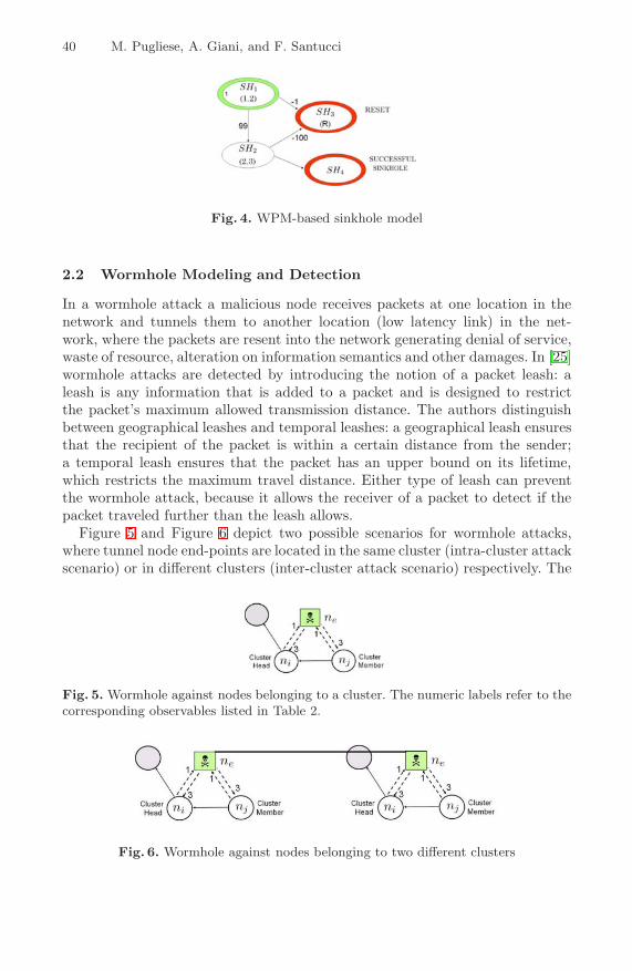
40 M. Pugliese, A. Giani, and F. Santucci
Fig. 4. WPM-based sinkhole model
2.2 Wormhole Modeling and Detection
In a wormhole attack a malicious node receives packets at one location in thenetwork and tunnels them to another location (low latency link) in the net-work, where the packets are resent into the network generating denial of service,waste of resource, alteration on information semantics and other damages. In [25]wormhole attacks are detected by introducing the notion of a packet leash: aleash is any information that is added to a packet and is designed to restrictthe packet’s maximum allowed transmission distance. The authors distinguishbetween geographical leashes and temporal leashes: a geographical leash ensuresthat the recipient of the packet is within a certain distance from the sender;a temporal leash ensures that the packet has an upper bound on its lifetime,which restricts the maximum travel distance. Either type of leash can preventthe wormhole attack, because it allows the receiver of a packet to detect if thepacket traveled further than the leash allows.
Figure 5 and Figure 6 depict two possible scenarios for wormhole attacks,where tunnel node end-points are located in the same cluster (intra-cluster attackscenario) or in different clusters (inter-cluster attack scenario) respectively. The
Fig. 5. Wormhole against nodes belonging to a cluster. The numeric labels refer to thecorresponding observables listed in Table 2.
Fig. 6. Wormhole against nodes belonging to two different clusters

Weak Process Models for Attack Detection in a Clustered Sensor Network 41
attacker emulates to be cluster head in order to receive traffic and to be clustermember to resend traffic or vice-versa. For example, in Figure 5 the sequence 1- 3 (corresponding to the observable sequence o1, . . . , o3) indicates a potentialwormhole.
An informal description of the anomaly rules is provided in Table 2.Observation oR is emitted when no observables are detected for a certain
number of steps. The last two anomaly rules, 3 and 4, describe a request to joina network. This can be an ordinary procedure as well as the precondition fora security attack. Therefore we suggest that the behavior related to AR3 andAR4 were consider normal and abnormal simultaneously. We retain as ambiguousthreat observables with this characteristic. AR2 and AR4 enable the generationof the back propagation of the observables to the sink. This is important todetect complex threats attacking nodes that are distant to each other.
The WPM-based wormhole is represented in figure 7. The same considerationsabout RESET and SUCCESSFULLY ATTACK states made for sinkhole apply tothis case. The number of states is 6 and the number of observables is 5. Itis important to note that observables for sinkhole are a sub-set of those forwormhole. The canonical form (1) can be specialized using matrices AWH andBWH and the score matrix SWH in eq. (4).
Table 2. Anomaly rules description for wormhole
ID
If node ni has authenticated node ne but node ne declares he < hi
AR1 with hi �= 0 (ne declares it is the new cluster head but it is not)then ok = o1
AR2 If node ni is the cluster head and (rule AR1 or rule AR2) applied to nj is truethen ok = o2
If node ni has authenticated node ne but node nE declare that he ≥ hi
AR3 with hi �= 0 (ne declares it is the new cluster member but it is not)then ok = o3
AR4 If node ni is the cluster head and (rule AR3 or rule AR4) applied to nj is truethen ok = o4
Fig. 7. WPM-based wormhole model

42 M. Pugliese, A. Giani, and F. Santucci
The threat starts with observables o1 or o2 or o3 or o4. If no more observablesare identified in the next K steps the threat is considered suspended. If observ-ables o1 or o2 or o3 or o4 occur again, then the attack moves to a high potentialstate.
AWH =
⎡⎢⎢⎢⎢⎢⎢⎣
0 0 0 0 0 00 0 0 0 0 01 0 0 0 0 00 1 0 0 0 01 1 1 1 0 00 0 1 1 0 0
⎤⎥⎥⎥⎥⎥⎥⎦ BWH =
⎡⎢⎢⎢⎢⎢⎢⎢⎢⎢⎢⎢⎢⎣
1 0 0 1 0 01 0 0 1 0 01 1 1 0 0 00 1 1 0 0 00 0 0 0 0 00 0 0 0 0 00 0 0 0 0 00 0 0 0 0 00 0 0 0 1 0
⎤⎥⎥⎥⎥⎥⎥⎥⎥⎥⎥⎥⎥⎦
SWH =
⎡⎢⎢⎢⎢⎢⎢⎣
1 0 0 0 0 00 1 0 0 0 099 0 0 0 0 00 99 0 0 0 0−1 −1 −100 −100 0 00 0 1 1 0 0
⎤⎥⎥⎥⎥⎥⎥⎦ (4)
2.3 Aggregated Models
Single threat models can be aggregated in a multi threat model using booleanOR. The complete list of anomaly rules and the produced observables is thecollection of the anomaly rules and observables related to single threats. Weassume that cluster heads aggregate only the observable coming from the clustermembers that has the highest score.
The aggregated threat model of hello flooding, sinkhole and a wormhole attackis shown in figure 8. When no more observables are identified in K consecutiveobservation steps the RESET state is reached. In that case the attack is sus-pended or there was no attack at all. Aggregated models allow to detect a largerclass of attacks compared to single models.
In the next section we will show how the IDS proposed behaves in termsof false negative (mis-detection) or false positive (false alarms). The experimentinvestigates the accuracy of threat identification for single models and aggregatedmodels.
Fig. 8. Aggregated threat model for hello flooding, sinkhole and wormhole

Weak Process Models for Attack Detection in a Clustered Sensor Network 43
3 Mis-Detection and False Alarm
It is important to check that if a threat occurs than an alarm is generated andthat the number of false alarms is low. We investigate mis-detection and falsealarm in the case of aggregated models in comparison to single threat models.
3.1 Mis-Detection Analysis
We apply the observable sequences produced by single hello flooding, sinkholeor wormhole. Each sequence will be applied to both single and aggregated modeland their detection capabilities will be investigated. We assume 32 observablesper sequence, n · WML ≤ 100 and k = 3. We consider the following observa-tion sequences generated in the case of hello flooding, sinkhole and wormholerespectively.
{5, 5, ∗, 8, 7, ∗, ∗, 6, 6, 8, 8, ∗, ∗, ∗, 8, ∗, ∗, 5, 7, ∗, ∗, 7, ∗, 6, 8, ∗, ∗, ∗, 5, 5, ∗, ∗} (5)
{2, 1, ∗, ∗, ∗, 1, ∗, 1, 2, 2, ∗, ∗, ∗, 1, 2, ∗, ∗, 1, 2, ∗, ∗, ∗, 2, 2, ∗, ∗, 1, ∗, 1, ∗, ∗, ∗} (6)
{2, 4, ∗, ∗, ∗, 3, ∗, 3, 1, 2, 2, ∗, ∗, 1, 3, ∗, ∗, 4, 4, ∗, ∗, ∗, 2, 2, ∗, ∗, 4, ∗, 3, ∗, ∗, ∗} (7)
It is important to note that there is no overlapping between observables fromhello flooding and observables from sinkhole or wormhole. And the observablesfrom sinkhole are observables from wormhole too.
Simulations provide the results graphically reported in figure 9, 10, and fig-ure 11 respectively. Red bars refer to scores produced by individual threat modelswhile yellow bars refer to aggregated threat models. To be noted that scores goto zero when the system is in a RESET state.
As expected the same outputs single model and aggregated model are obtainedfor threats not sharing any threat observables with each other. In fact figure 9and figure 10 show that the aggregate and the single models have the samedetection capability in cases of hello flooding and sinkhole respectively. Different
Fig. 9. Hello flooding detection scores when (5) is applied as input

44 M. Pugliese, A. Giani, and F. Santucci
Fig. 10. Sinkhole detection scores when (6) is applied as input
Fig. 11. Wormhole detection scores when (7) is applied as input
outputs are obtained for threats sharing at least one threat observables. Forexample sinkhole and wormhole in figure 10 and 11 share threat observables 1and 2. In particular a sinkhole is an attack or is the initial step of a wormhole.Accordingly the score for wormhole in the case of the aggregated model is alwaysgreater than the score resulting from the single threat model (figure 11).
Attacks against distant nodes. Now we examine the capability of detectingthe same threat attacking nodes that are not close to each other. In this test weassume a wormhole against nodes 4 and 5 in Figure 12. We consider the test suc-cessful if alarms were generated also in nodes 1, 2 and 3 (not directly attacked).
Fig. 12. Wormhole attack against nodes 4 and 5

Weak Process Models for Attack Detection in a Clustered Sensor Network 45
Rule AR2, AR4 (from wormhole and the aggregate model) allow observable backpropagation to nodes 4-2-1 and to nodes 5-3-1.
The criterion for the aggregation of observables is as follows. At the genericobservation step k, the cluster head CH considers only observables with the high-est score from neighbors. Accordingly, if the observable sequence 7 is producedin nodes 4 and 5, the following observables sequence 8 will be produced in nodes1, 2 and 3:
{2, 4, ∗, ∗, ∗, 4, ∗, 4, 4, 2, 4, ∗, ∗, 2, 4, ∗, ∗, 4, 4, ∗, ∗, ∗, 2, 2, ∗, ∗, 4, ∗, 4, ∗, ∗, ∗} (8)
Figure 13 shows the related threat scores. If no countermeasures are appliedto nodes 4 and 5 observables propagates back from the compromised node tothe sink until an alarm is triggered.
Fig. 13. Scores in nodes 1, 2, 3 from wormhole attack to nodes 4 and 5
3.2 False Alarm Detection
Test for positives will be performed through the analysis of the structure ofthe anomaly rules and the internal structure of the aggregated threat model infigure 8.
Among the anomaly rules in Table 2, AR3 and AR4 are associated to observ-ables that can potentially produce false positives. This can lead to false alarms.But alarms be triggered only if the observations generate is a high potentialattack. For example in figure 8, state X3 is associated to observation o3 or o4produced by AR3 and AR4 respectively. We propose two approaches reduce falsepositives.
1. Introducing further states associated to certain threat observables in pathswhere at least one state is associated to ambiguous threat observables. Thisapproach lowers the probability for false positives (p �→ 0 ), as the longer thepath to HPA the more reliable would be an alarm. A drawback is that longpaths to HPA states, would reduce the reactivity in the monitoring service.
2. Introducing a further class of states associated to ambiguous threat observ-ables. This approach cannot lower the probability for false positives, but

46 M. Pugliese, A. Giani, and F. Santucci
Fig. 14. WPM-based IDS component-based internal structure
”ad-hoc” lighter countermeasures can be applied to nodes where alarmsfrom dubious observables are generated (e.g. node quarantine rather thanlink release).
4 Mobile Agent-Based Design
We adopt a mobile agent architecture to design and develop the proposed WPM-based intrusion detection. Resource constraints and topology dynamics in WSNimply restrictions for the software architectural choices where fundamental re-quirements are distribution, flexibility and scalability.
We will show that the agent based middleware proposed in [31] optimizes thedesign of distributed applications on clustered sensor networks. Cluster headsare not permanently assigned to specific nodes but dynamically re-assigned toany node according to eligibility criteria. This justify our choice of agents. A keyconcept from [31] is agent migration. During cloning, it copies its code and stateto another node (strong cloning) and resumes executing on both the old and newnodes. Mobile agents support data-centric applications. Code migrates towardsdata independently from node addressing. Applications distribution through mo-bile agents results much less costly compared to traditional data broadcasting orcode diffusion approaches. From [31] we will recall the concept of ‘tuple space’as a local memory shared by local agents.
Figure 14 shows the basic functionalities of our intrusion detection system.Other functions related to intrusion reaction logic, including defence strategy,alarm tracking and countermeasures will be mapped into mobile agents as thesefunctions will be performed at cluster level and data aggregation from neighbornodes is mandatory. We denote this agent as ‘Intrusion Reaction Agent’ (IRA),

Weak Process Models for Attack Detection in a Clustered Sensor Network 47
Fig. 15. IRA agent forward propagation vs. threat observables and alarms back prop-agation
represented by the oval in figure 14, which is hosted only by cluster heads. Themobile agent mechanism leads to forward propagation or diffusion from sink toleaves of IRA agents and to a back-propagation (from leaves to sink) of threatobservables and alarms. In a clustered network, if IRA agent are hosted only ona cluster head, the agent diffusion mechanism across the network is describedin figure 15 . IRA agent is initially hosted on node 1 and node 2 is a clustermember. The cluster head can read remotely threat observables stored on thetuple space of the neighboring node 2. When node 2 becomes cluster head, IRA(weakly) clones to it. The final agent distribution is depicted in figure 15. Thismechanism allows each IRA to aggregate threat observables and alarms fromcluster nodes, generate iteratively further observables and alarm. This aggregateand back-propagate mechanism for alarms and observables, leads to the detectionof organized threats attacking nodes topologically distant. The ADL will storethe produced observables and alarms into the ‘local tuple’ space. The middlewaresupporting the mobile agent execution environment is denoted as Mobile AgentApplication Execution Environment (MA-AEE).
Our contribution is the definite verticality respect to WSN technology. Our ap-proach to detection is fully distributed with a dynamic hierarchical architecturerather than centralized with a static hierarchical architecture. Security functionsare executed autonomously by nodes in the network without any support fromoutside (like servers or database) as in [32,33], and complexity in IDS manage-ment is reduced due to the clustered tree topology which avoids overheads forloop checks and polling routines among neighboring nodes as in [34,35].
5 Conclusion and Future Work
In this paper we propose a new approach to anomaly detection and alarm gen-eration logic using weak process models. Weak models are a simplified versionof hidden markov models.
The proposed anomaly detection logic for threat modeling, threat identifi-cation, and alarm generation has been validated using MATLAB simulations.
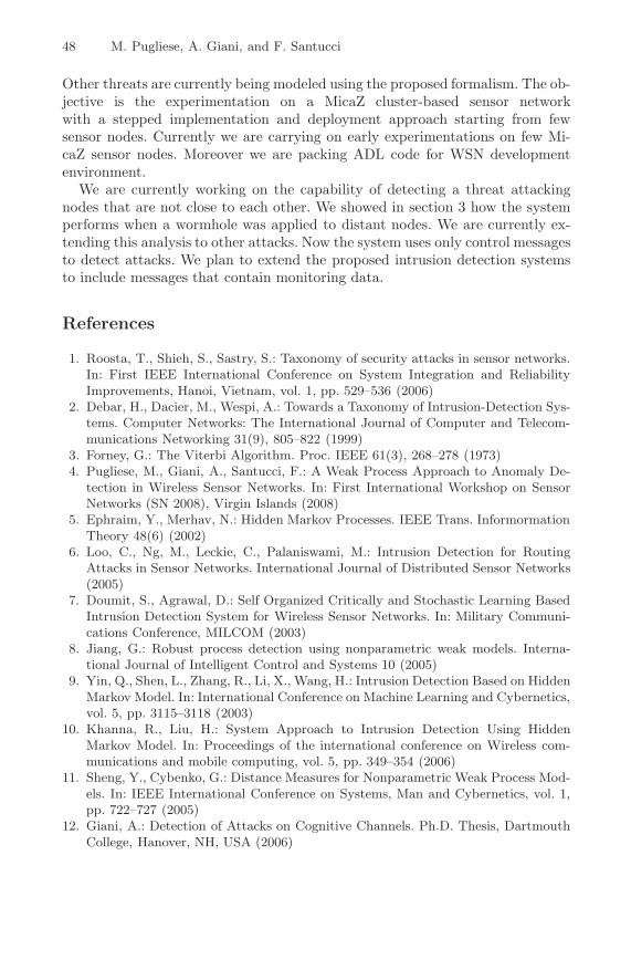
48 M. Pugliese, A. Giani, and F. Santucci
Other threats are currently being modeled using the proposed formalism. The ob-jective is the experimentation on a MicaZ cluster-based sensor networkwith a stepped implementation and deployment approach starting from fewsensor nodes. Currently we are carrying on early experimentations on few Mi-caZ sensor nodes. Moreover we are packing ADL code for WSN developmentenvironment.
We are currently working on the capability of detecting a threat attackingnodes that are not close to each other. We showed in section 3 how the systemperforms when a wormhole was applied to distant nodes. We are currently ex-tending this analysis to other attacks. Now the system uses only control messagesto detect attacks. We plan to extend the proposed intrusion detection systemsto include messages that contain monitoring data.
References
1. Roosta, T., Shieh, S., Sastry, S.: Taxonomy of security attacks in sensor networks.In: First IEEE International Conference on System Integration and ReliabilityImprovements, Hanoi, Vietnam, vol. 1, pp. 529–536 (2006)
2. Debar, H., Dacier, M., Wespi, A.: Towards a Taxonomy of Intrusion-Detection Sys-tems. Computer Networks: The International Journal of Computer and Telecom-munications Networking 31(9), 805–822 (1999)
3. Forney, G.: The Viterbi Algorithm. Proc. IEEE 61(3), 268–278 (1973)4. Pugliese, M., Giani, A., Santucci, F.: A Weak Process Approach to Anomaly De-
tection in Wireless Sensor Networks. In: First International Workshop on SensorNetworks (SN 2008), Virgin Islands (2008)
5. Ephraim, Y., Merhav, N.: Hidden Markov Processes. IEEE Trans. InformormationTheory 48(6) (2002)
6. Loo, C., Ng, M., Leckie, C., Palaniswami, M.: Intrusion Detection for RoutingAttacks in Sensor Networks. International Journal of Distributed Sensor Networks(2005)
7. Doumit, S., Agrawal, D.: Self Organized Critically and Stochastic Learning BasedIntrusion Detection System for Wireless Sensor Networks. In: Military Communi-cations Conference, MILCOM (2003)
8. Jiang, G.: Robust process detection using nonparametric weak models. Interna-tional Journal of Intelligent Control and Systems 10 (2005)
9. Yin, Q., Shen, L., Zhang, R., Li, X., Wang, H.: Intrusion Detection Based on HiddenMarkov Model. In: International Conference on Machine Learning and Cybernetics,vol. 5, pp. 3115–3118 (2003)
10. Khanna, R., Liu, H.: System Approach to Intrusion Detection Using HiddenMarkov Model. In: Proceedings of the international conference on Wireless com-munications and mobile computing, vol. 5, pp. 349–354 (2006)
11. Sheng, Y., Cybenko, G.: Distance Measures for Nonparametric Weak Process Mod-els. In: IEEE International Conference on Systems, Man and Cybernetics, vol. 1,pp. 722–727 (2005)
12. Giani, A.: Detection of Attacks on Cognitive Channels. Ph.D. Thesis, DartmouthCollege, Hanover, NH, USA (2006)
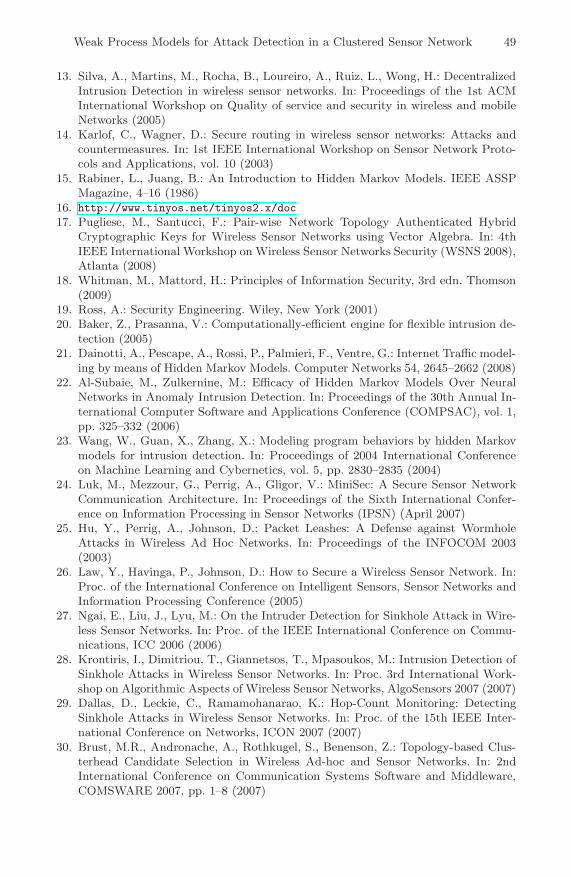
Weak Process Models for Attack Detection in a Clustered Sensor Network 49
13. Silva, A., Martins, M., Rocha, B., Loureiro, A., Ruiz, L., Wong, H.: DecentralizedIntrusion Detection in wireless sensor networks. In: Proceedings of the 1st ACMInternational Workshop on Quality of service and security in wireless and mobileNetworks (2005)
14. Karlof, C., Wagner, D.: Secure routing in wireless sensor networks: Attacks andcountermeasures. In: 1st IEEE International Workshop on Sensor Network Proto-cols and Applications, vol. 10 (2003)
15. Rabiner, L., Juang, B.: An Introduction to Hidden Markov Models. IEEE ASSPMagazine, 4–16 (1986)
16. http://www.tinyos.net/tinyos2.x/doc
17. Pugliese, M., Santucci, F.: Pair-wise Network Topology Authenticated HybridCryptographic Keys for Wireless Sensor Networks using Vector Algebra. In: 4thIEEE International Workshop on Wireless Sensor Networks Security (WSNS 2008),Atlanta (2008)
18. Whitman, M., Mattord, H.: Principles of Information Security, 3rd edn. Thomson(2009)
19. Ross, A.: Security Engineering. Wiley, New York (2001)20. Baker, Z., Prasanna, V.: Computationally-efficient engine for flexible intrusion de-
tection (2005)21. Dainotti, A., Pescape, A., Rossi, P., Palmieri, F., Ventre, G.: Internet Traffic model-
ing by means of Hidden Markov Models. Computer Networks 54, 2645–2662 (2008)22. Al-Subaie, M., Zulkernine, M.: Efficacy of Hidden Markov Models Over Neural
Networks in Anomaly Intrusion Detection. In: Proceedings of the 30th Annual In-ternational Computer Software and Applications Conference (COMPSAC), vol. 1,pp. 325–332 (2006)
23. Wang, W., Guan, X., Zhang, X.: Modeling program behaviors by hidden Markovmodels for intrusion detection. In: Proceedings of 2004 International Conferenceon Machine Learning and Cybernetics, vol. 5, pp. 2830–2835 (2004)
24. Luk, M., Mezzour, G., Perrig, A., Gligor, V.: MiniSec: A Secure Sensor NetworkCommunication Architecture. In: Proceedings of the Sixth International Confer-ence on Information Processing in Sensor Networks (IPSN) (April 2007)
25. Hu, Y., Perrig, A., Johnson, D.: Packet Leashes: A Defense against WormholeAttacks in Wireless Ad Hoc Networks. In: Proceedings of the INFOCOM 2003(2003)
26. Law, Y., Havinga, P., Johnson, D.: How to Secure a Wireless Sensor Network. In:Proc. of the International Conference on Intelligent Sensors, Sensor Networks andInformation Processing Conference (2005)
27. Ngai, E., Liu, J., Lyu, M.: On the Intruder Detection for Sinkhole Attack in Wire-less Sensor Networks. In: Proc. of the IEEE International Conference on Commu-nications, ICC 2006 (2006)
28. Krontiris, I., Dimitriou, T., Giannetsos, T., Mpasoukos, M.: Intrusion Detection ofSinkhole Attacks in Wireless Sensor Networks. In: Proc. 3rd International Work-shop on Algorithmic Aspects of Wireless Sensor Networks, AlgoSensors 2007 (2007)
29. Dallas, D., Leckie, C., Ramamohanarao, K.: Hop-Count Monitoring: DetectingSinkhole Attacks in Wireless Sensor Networks. In: Proc. of the 15th IEEE Inter-national Conference on Networks, ICON 2007 (2007)
30. Brust, M.R., Andronache, A., Rothkugel, S., Benenson, Z.: Topology-based Clus-terhead Candidate Selection in Wireless Ad-hoc and Sensor Networks. In: 2ndInternational Conference on Communication Systems Software and Middleware,COMSWARE 2007, pp. 1–8 (2007)

50 M. Pugliese, A. Giani, and F. Santucci
31. Fok, C.-L., Roman, G.C., Lu, C.: Agilla: A Mobile Agent Middleware for Sen-sor Networks. Tech. Report, Washington University in St. Louis, WUCSE-2006-16(2006)
32. Balasubramainyan, J., Garcia-Fernandez, J.O., Isacoff, D., Spafford, E., Zamboni,D.: An architecture of Intrusion Detection using Autonomous Agents, Departmentof Computer Science, Purdue University TR 98-05 (1998)
33. Vahid Dastjerdi, A., Abu Bakar, K.: A Novel Hybrid Mobile Agent Based Dis-tributed Intrusion Detection System. Proc. of World Academy of Science Engi-neering and Technology 35 (November 2008)
34. Ramachandran, G., Hart, D.: A P2P Intrusion Detection System based on MobileAgents. ACM, New York (2004)
35. Zhou, C.V., Karunasekera, S., Leckie, C.: A Peer-to-Peer Collaborative IntrusionDetection System. In: Proc. of 13th IEEE International Conference on Communi-cations, ICC 2005 (2005)

Key Establishment Using Group Information forWireless Sensor Networks
William R. Claycomb1, Rodrigo Lopes1, Dongwan Shin1, and Byunggi Kim2
1 Secure Computing Laboratory, New Mexico Tech,801 Leroy Place, Socorro, NM, USA, 87801
{billc,rodrigo,doshin}@nmt.edu2 College of Information Technology, Soongsil University,
511 Sangdo-dong, Dongjak-gu, Seoul 156-743, [email protected]
Abstract. Wireless sensor networks are commonly used for critical se-curity tasks such as intrusion or tamper detection, and therefore mustbe protected. To date, security of these networks relies mostly on keyestablishment and routing protocols. We present a new approach to keyestablishment, which combines a group-based distribution model andidentity-based cryptography. Using this solution enables sensor nodes toauthenticate each other, and provides them with a structure to build se-cure communications between one another, and between various groups.Using our key establishment protocol, we show how to reduce or preventsignificant attacks on wireless sensor networks.
Keywords: Group-based security, key establishment, wireless sensornetworks.
1 Introduction
Wireless sensor networks (WSNs) have become commonplace in applicationsranging from simple light, temperature, and sound measurements to sophisti-cated military and industrial applications. In some cases the security of thesensors, the data collection, and the communication of that data to a collectionpoint is unimportant. However, for sensitive applications, the security of thesetasks is paramount.
One of the core components to securing WSN data is the establishment of se-cret keys between sensor nodes in a network. In contrast to other mobile networkapplications, WSN have the property that key establishment information can bepre-loaded onto sensor nodes prior to deployment. However, the limitations ofsensor nodes have traditionally limited key establishment and data encryptiontechniques to simple and symmetric cryptographic applications.
Recently, due to advances in sensor hardware, the field of asymmetric cryp-tography has become a realistic option for various operations in WSN.Usingasymmetric cryptography for key establishment greatly simplifies many of thechallenges currently faced by schemes relying on symmetric key establishment
S. Hailes, S. Sicari, and G. Roussos (Eds.): S-Cube 2009, LNICST 24, pp. 51–65, 2009.c© Institute for Computer Sciences, Social-Informatics and Telecommunications Engineering 2009

52 W.R. Claycomb et al.
protocols. For instance, node authentication is possible. Also, compromising evena large subset of nodes and communication keys does not compromise all commu-nication keys for the network - a goal many of the solutions to date have strivedto achieve. However, using asymmetric cryptography does not solve all the prob-lems of WSN security. Specifically, three attacks that still present problems forWSN are node replication, Sybil, and wormhole attacks.
In this paper, we present a novel scheme for key establishment in WSN whichcombines the notion of group-based key predistribution with identity based cryp-tography (IBC). We show how this approach enables secure key establishment inWSN, and show how our solution improves upon the security of existing key es-tablishment schemes. We discuss considerations in design for this type of WSN,including an analysis of group communication dynamics. We also demonstratehow our solution addresses various attacks on WSNs.
The remainder of this paper is structured as follows. Section 2 describes re-lated work, including a description of identity based cryptography components.Section 3 describes our new key establishment protocol, followed by Section 4which presents a detailed description of various attacks and how our solutionaddresses them. Section 5 presents a discussion of group distribution decisionsand the impact to sensor nodes. In Section 6, we conclude the paper with adiscussion of future work.
2 Background and Related Work
Key establishment in WSNs has been an active area of research for many years,and several approaches have been proposed. The simplest method of key estab-lishment between nodes in a WSN is to preload each node with the same sharedsecret key, and use that key to secure transmission between every node pair.While this is simple in terms of protocol and storage requirements, it has thedisadvantage that compromising a single node reveals all communication to anadversary. The simple solution to prevent this is to pre-load each node with aunique shared key for pairwise communication with every other node in the net-work. This is a more secure network than the previous one, as compromising asingle node only reveals the data transmitted between it and its node partners.However, the storage overhead per node is unrealistic, particularly in the caseof very large networks.
Several researchers have developed solutions for pairwise key establishmentthat fall between these two extremes. Recently, proposals have included thenotion of location-based, or group-based schemes. These approaches observe thatin large-scale sensor node distributions, nodes deployed in a group tend to endup near each other physically. By tailoring key predistribution to take advantageof this property, efficient schemes have been presented [1,2,3,4].
However, these solutions rely on symmetric key agreement protocols, andlargely ignore the application of asymmetric key agreement methods. It hasbeen commonly believed that the increased computational and time constraintsrequired by asymmetric solutions are too costly for WSNs. Recently, though,

Key Establishment Using Group Information for Wireless Sensor Networks 53
researchers have studied implementations of asymmetric protocols such as el-liptic curve cryptography (ECC) on sensor nodes [5,6,7,8,9]. Results have beenpromising, and various proposals for key establishment and key managementusing ECC-based approaches have been suggested [10].
2.1 Identity Based Cryptography
In [11], the authors propose using an identity based cryptography technique calledpairing [12,13] to facilitate secure key establishment between nodes in WSNs.First proposed by [14], identity based cryptography (IBC), or identity based en-cryption, is similar to traditional public-key based cryptography systems, butinstead of using a randomly generated public key, entities use unique strings orother short identifiers, such as email addresses, as their public key. For instance,to send an encrypted email to ”[email protected],” Alice would encrypt themessage using the email address as the public key. Bob would obtain his cor-responding private key from a Private Key Generator to decrypt the message.Therefore, IBC helps negate the use of public key certificate in PKC-based ap-plications.
As one of the critical components to optimizing the performance of WSNsis minimizing data storage and transmission size, IBC is an excellent choicefor exchanging key establishment information in this regard. The only thingnecessary to begin key establishment is the identity of the source node, whichonly has to be large enough to ensure a unique ID among the entire network. A16 bit ID would provide unique IDs for 216 = 65536 sensor nodes.
Definitions. The following definitions will be used in describing our solution:p, q large primesE/Fp An elliptic curve y2 = x3 + ax + b over the finite field Fp
G1 A q-order subgroup of the additive group of points of E/Fp
G2 A q-order subgroup of the multiplicative group of the finite field F∗p2
e A mapping G1 × G1 → G2H A cryptographic hash function which maps to elements in G1h A standard cryptographic hash functionA, B, ... Groups of sensor nodesx, y, ... Individual sensor nodesIDA Unique ID of group AIDx Unique ID of sensor node xKx:A Secret key for node x among group AKxy Shared pairwise key between nodes x and ymA Master key for group A
The modified Weil pairing scheme in [12] is used for the basis of our key estab-lishment protocol. This allows two sensor nodes to establish a shared secret keyusing only the knowledge of an individual secret key and the unique identity ofthe other node, as long as the secret key of the first node was generated usingthe same keying information as the identity information of the second node. The
54 W.R. Claycomb et al.
pairing is based on the bilinear Diffie-Hellman Problem (DLP), which is provento be computationally hard.
Pairing. A pairing is the mapping of two points P and Q, from separate sub-groups of points on an elliptic curve, to a third point in a finite field, and is de-noted e(P, Q). Usually P and Q are linearly independent of each other, otherwisethe pairing is considered degenerate, and e(P, Q) = 1. To use P and Q from thesame group G1, a distortion map ψ is used to make the second element linearlyindependent of the first. This distortion pairing is denoted e(P, Q) = e(P, ψ(Q)).The distorted pairing is symmetric, that is ∀P, Q ∈ G1, e(P, Q) = e(Q, P ). Fora more thorough description of pairings over elliptic curves, please see [12,13].
Due to the distortion map, we can use a pairing which is a mapping G1×G1 →G2. It has the following properties [12]:
– Bilinear: ∀P, Q ∈ G1 and ∀a, b ∈ Z, e(aP, bQ) = e(P, Q)ab.– Non-degenerate: If P is a generator of G1 then e(P, P ) ∈ F
∗p2 is a generator
of G2.– Computable: Given P, Q ∈ G1, there is an efficient algorithm to compute
e(P, Q) ∈ G2
3 Group-Based Key Establishment
While some node deployment scenarios allow for manual or automated place-ment of nodes, or for key nodes to have known fixed positions [11], we believethat certain critical applications, such as battlefield deployments, do not providesuch means. Therefore, it is desirable to have a solution which provides securekey establishment without requiring specific location knowledge for each node.Instead, we propose that in a group-based distribution, assuming nodes deployedtogether end up near each other [3,15], that each group of nodes deployed be pre-keyed using key information unique to that group. Doing so would allow nodescontaining keying information for a specific group A to establish pairwise keyswith nodes from group A. We will show that in order to establish this pairwisekey, both nodes must have keying information for group A.
To detail our solution, we propose that a successful deployment of a WSNwould consist of the following phases:
– Provisioning authority initialization– Sensor key initialization (key pre-distribution)– Sensor deployment– Pair-wise key establishment
3.1 Provisioning Authority Initialization
A separate provisioning authority (PA) is created for each group of nodes to bedeployed. A master PA is responsible for generating the pairing information foreach PA. This information, as described in § 2.1, is (p, q, E/Fp, G1, G2, e). The

Key Establishment Using Group Information for Wireless Sensor Networks 55
master PA also selects two hash functions, H and h, where H maps to nonzeroelements in G1, and h is a secure cryptographic hash function. Then, for a groupof sensors to be deployed, A, the master PA randomly selects mA as the mastersecret for A. This sequence is loosely based on the work of [11], but has beenmodified to meet the specific needs of our solution.
3.2 Sensor Key Initialization
During this phase, we assume each group has a unique identity IDA, and everynode has a unique identity IDx. The PA provides every sensor x, in groupA, a unique identity-based key Kx:A. The unique key is calculated as Kx:A =mAH(IDx). Along with the unique Kx:A, each node in A is pre-loaded with thepublic information for group A, (p, q, E/Fp, G1, G2, e, H, h, IDA). Compromisinga node will not reveal the group secret key mA. This is due to the intractabilityof the discrete logarithm problem for elliptic curves (ECDLP). That is, consideran elliptic curve E defined over Fq and P ∈ E(Fq), which is a point of ordern. Given Q ∈ E(Fq), it is infeasible to find an integer 0 ≤ d ≤ n such thatQ = dP . Therefore, it is also infeasible to find mA, given Kx:A and IDx, sinceKx:A = mAH(IDx).
In addition to the unique key for group A, each node x is also pre-loaded witha unique key corresponding to each adjacent group B, which is calculated asKx:AB = mAmBH(IDx). Nodes are also given the identifier for group B, IDB.At this point, it is possible to pre-load x with additional unique keys and groupidentifiers for the groups beyond those immediately adjacent to A. The numberof adjacent and surrounding group keys loaded on each node in A is determinedby the needs of the network, noting that each additional layer of depth i adds2i+2 public keys, if adjacent groups are arranged in a grid, as shown in Figure 1.
A
Groups1-level from
Group A
Groups2-levels from
Group A
Fig. 1. Layers of sensor network groups
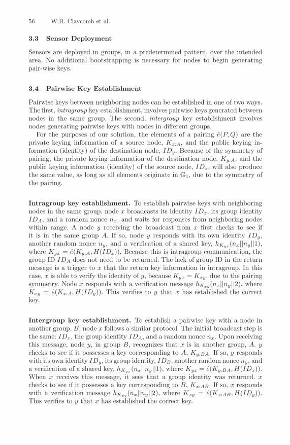
56 W.R. Claycomb et al.
3.3 Sensor Deployment
Sensors are deployed in groups, in a predetermined pattern, over the intendedarea. No additional bootstrapping is necessary for nodes to begin generatingpair-wise keys.
3.4 Pairwise Key Establishment
Pairwise keys between neighboring nodes can be established in one of two ways.The first, intragroup key establishment, involves pairwise keys generated betweennodes in the same group. The second, intergroup key establishment involvesnodes generating pairwise keys with nodes in different groups.
For the purposes of our solution, the elements of a pairing e(P, Q) are theprivate keying information of a source node, Kx:A, and the public keying in-formation (identity) of the destination node, IDy. Because of the symmetry ofpairing, the private keying information of the destination node, Ky:A, and thepublic keying information (identity) of the source node, IDx, will also producethe same value, as long as all elements originate in G1, due to the symmetry ofthe pairing.
Intragroup key establishment. To establish pairwise keys with neighboringnodes in the same group, node x broadcasts its identity IDx, its group identityIDA, and a random nonce nx, and waits for responses from neighboring nodeswithin range. A node y receiving the broadcast from x first checks to see ifit is in the same group A. If so, node y responds with its own identity IDy,another random nonce ny, and a verification of a shared key, hKyx(nx||ny||1),where Kyx = e(Ky:A, H(IDx)). Because this is intragroup communication, thegroup ID IDA does not need to be returned. The lack of group ID in the returnmessage is a trigger to x that the return key information in intragroup. In thiscase, x is able to verify the identity of y, because Kyx = Kxy, due to the pairingsymmetry. Node x responds with a verification message hKxy(nx||ny||2), whereKxy = e(Kx:A, H(IDy)). This verifies to y that x has established the correctkey.
Intergroup key establishment. To establish a pairwise key with a node inanother group, B, node x follows a similar protocol. The initial broadcast step isthe same: IDx, the group identity IDA, and a random nonce nx. Upon receivingthis message, node y, in group B, recognizes that x is in another group, A. ychecks to see if it possesses a key corresponding to A, Ky:BA. If so, y respondswith its own identity IDy, its group identity, IDB, another random nonce ny, anda verification of a shared key, hKyx(nx||ny||1), where Kyx = e(Ky:BA, H(IDx)).When x receives this message, it sees that a group identity was returned. xchecks to see if it possesses a key corresponding to B, Kx:AB. If so, x respondswith a verification message hKxy(nx||ny||2), where Kxy = e(Kx:AB, H(IDy)).This verifies to y that x has established the correct key.

Key Establishment Using Group Information for Wireless Sensor Networks 57
4 Attacks and Resistance
Various attacks on WSNs have been described in the literature. Some of themore difficult to defend against are the node replication, node addition, Sybil,and wormhole attacks. Our solution either prevents these attacks from occurring,or minimizes their impact to the point of inefficacy.
4.1 Node Replication Attack
A node replication attack [16] consists of an adversary compromising one or moreexisting nodes, duplicating (and perhaps modifying) the information retrieved,provisioning new nodes with the stolen information, and placing the replicatednodes into the network. Under simple authentication schemes, a network is un-able to detect the duplicated nodes, particularly if they are placed far apart, andthey are able to authenticate and interact with existing nodes. This provides theattacker with a means of intercepting communication, affecting network routing,or even skewing reputation-based trust management systems.
Our solution eliminates the node replication attack over multiple groups. Toshow this, consider a compromised node x, from group A. If placed in a groupwhere nodes do not share keying information with A, the replicated node (de-noted x’) would be unable to establish any pairwise keys. To be successful, anattacker could only place x into a group where the nodes have shared key in-formation with A. In a large network, the number of such groups is likely to besmall. Additionally, placing x’ into one of these groups would be likely to causedetection, as the real x is nearby, and nodes receiving another authenticationrequest from a duplicate node proclaiming to be x would detect the attack.
4.2 Node Addition Attack
In a node addition attack [17], an adversary injects new nodes into a WSN. Thisdiffers from a node replication attack because the new nodes are not duplicatesof an existing node, but rather are provisioned correctly as unique nodes in thenetwork. To carry out this attack in a network with pairwise key establishment,an adversary must have access to keying information, such as a master key(mA in our solution.) While some solutions allow the master key to exist fora short period of time on individual nodes during the distribution of a newnetwork [11,17], ours does not allow mA to exist on any node or base station inthe network. Without mA, an attacker can only gain information such as IDx,Kx:A, IDA, etc. Even with the pairing components (IDx, Kx:A), mA cannot bededuced, due to the properties of the pairing scheme.
4.3 Sybil Attack
The Sybil attack [18] describes a situation where an attacker generates multiplefake identities in one location, appearing to be many legitimate nodes, and usesthose identities to influence the existing WSN. This influence can be against

58 W.R. Claycomb et al.
routing, trust management, reputation, or other elements of network manage-ment. In contrast to the node replication attack, the nodes in the Sybil attackare not real nodes, nor are they distributed throughout the network.
Our solution prevents this attack by preventing an attacker from spoofinglegitimate nodes. Without the master key to generate pairing information, anattacker cannot generate correct pairing information. Without this information,a Sybil node cannot establish pairwise keys with any legitimate node in thenetwork.
4.4 Wormhole Attack
One of the more interesting attacks in WSNs, the wormhole attack involves anattacker using a covert, high-speed side channel to tunnel information acrossthe network. The effect is to allow two distant nodes to communicate with eachother, fooling them into believing they are neighbors. This can disrupt networkrouting, potentially preventing critical messages from being received by the cor-rect locations. It can also affect networks which use relative node location fordecision-making. The wormhole attack is shown in Figure 2.
Detecting and preventing wormhole attacks are challenging issues. Most so-lutions to date involve the use of mechanisms based on the physical location ofnodes, or the physical distance between them. These solutions use either location-fixing devices, such as GPS, or tight time synchronization between nodes todetect wormholes [11,19,20].
Our solution prevents wormhole attacks between nodes in distant groups be-cause they do not share key information, and cannot form pairwise keys, as shownin Figure 3. However, a wormhole between two nearby groups is possible. Creat-ing a wormhole for nodes within adjacent groups would have a limited effect, andwould be physically more difficult, because creating a high-speed side-channeland processing information through it faster than the normal network routingbecomes tricky as the distance between the wormhole ends grows smaller.
With this in mind, a network designer can carefully plan node group size toreduce the threat of wormhole attacks to an acceptable level. For instance, if an
AttackerTx/RxDevice
AttackerTx/RxDevice
HighSpeedCovert
Channel
Fig. 2. A wormhole attack

Key Establishment Using Group Information for Wireless Sensor Networks 59
AttackerTx/RxDevice
AttackerTx/RxDevice
HighSpeedCovert
Channel
Fig. 3. A wormhole attack prevented in a group-based network
attack between nodes 50 m apart would not compromise the overall integrityof the system, then groups can be distributed with a diameter of 25 m, so thegreatest distance between any two nodes allowed to communicate is 50 m.
Wormhole attacks can be prevented by a carefully designed security policy aswell. If a policy is designed such that a group A only trusts connections to groupB, then a wormhole attack is only possible from group A to group B. Becausethis is an asymmetric trust, a wormhole attack from B to A is not possible. Thisis an important step towards preventing a wormhole attack that seeks to “skip”a sensor or group of sensors in a sequence by generating a wormhole around it.
5 Discussion
The discussion of our solution will focus on two areas. The first part deals withthe network design. Next, we discuss the impact to sensor nodes themselves.
5.1 Network Design
When looking at a group-based deployment, we must consider how the nodeswill be distributed. Will they be distributed evenly over an area, or will theytend to be more densely populated near the center of an area? How does thisaffect the chances of multi-group communication? We attempt to answer thesequestions here.
Node distributions are not always uniform. Sometimes the reasons for this aresimple physics (i.e. dropping a box of sensor nodes from an airplane at differentheights, with different wind patterns, will result in greatly different distributionson the ground). Other times, the reasons for a certain distribution are moresophisticated, such as the desire to prevent a wormhole attack between nodes ofa certain distance, n.
To help analyze communication between groups in our solution, we considertwo variations of node distribution, one where nodes are distributed evenly over

60 W.R. Claycomb et al.
Fig. 4. Nodes able to communicate with other groups using an even distribution
the entire group, and one where nodes are distributed according to a normal(Gaussian) distribution.
Two key factors in determining how well two groups will communicate arethe node coverage over the group, and the overlap between groups. Our simula-tion results show the percentage of nodes within a group able to communicatewith adjacent groups, given the node coverage and overlap size of the network.Figure 4 shows the results for an even distribution of nodes over a group, andFigure 5 shows the results for a Gaussian distribution of nodes over a group.
Based on these results, it is clear that a more even distribution of nodes isdesirable when implementing a group-based model. It is interesting to note themuch higher percentage of nodes able to communicate in even distributions.The lower figure for the Gaussian distribution is due to the lower density ofnodes distributed over the edge of the Gaussian group. Based on these results,we can make decisions regarding network architecture, taking into account thedistribution method, and how nodes are likely to be distributed in their finalstate.
5.2 Sensor Impact
A critical analysis of any sensor network application must include the impact tothe sensors in terms of space requirements, processing time, and power consumed.We believe the solution presented here has an acceptable footprint upon thesensor nodes. For analysis purposes, we will consider an implementation wherep is a 512-bit prime and q is a 160-bit prime.

Key Establishment Using Group Information for Wireless Sensor Networks 61
Fig. 5. Nodes able to communicate with other groups using a normal (Gaussian) dis-tribution
Sensor memory requirements. The use of elliptic curve cryptography (ECC)based mechanisms means that less space is required to store key information. Toachieve the same public key security as a 1024-bit RSA [21] implementation, only160-bit keys are needed for ECC [6]. Standard ECC-based digital certificates,used in traditional key establishment, are ∼530 bytes in size. This can be reducedto 86 bytes by removing all but the most important data [8]. Our proposalreduces this size even further, requiring only 40 bytes to store node identificationand keying information. This improvement becomes even more important whenwe consider how much energy is consumed during data transmission - sendinga singe bit of information can take the same power as 2090 clock cycles ofexecution [8].
However, in our solution, more than just one key is stored on each node.Adding keys for adjacent group key establishment depends on the topology ofthe network. Without loss of generality, we assume a topology similar to Figure 1.In this instance, the total number of keys to be stored on each node is
∑ni=1 2i+2.
To store 1 layer of key establishment information requires 160 bytes. For 2 layers,480 bytes are needed. 3 layers require 1120 bytes. This must be considered innetwork design.
Grouppublic information, (p, q, E/Fp, G1, G2, e, H, h, IDA),mustalsobe loadedonto each node. Due to space requirements, we will not detail each component, butwill note that p is a 512 bit prime, G1, G2 are 160 bit primes, IDA can be relativelysmall (16 bits), and the components relating to key generation code can be esti-mated at ∼3.6KB [6] for 160-bit ECC operations.

62 W.R. Claycomb et al.
We note that the Atmel ATmega128 [22], a common micro-controller used onmany sensor devices, has 128KB of FLASH program memory. Another commonsensor network node, the Crossbow Imote2 has 256KB of SRAM memory, 32MBof SDRAM memory, and 32MB of FLASH memory [23]. We believe sensor de-ployments where > 3 layers of shared key information are unlikely, so a totaloverhead of < 5KB seems reasonable for this application.
Processing time. Several works have analyzed processing time for ECC-basedoperation on various sensor devices. While some report times in excess of 30seconds for generating shared secret keys [7], improvements in hardware, as wellas algorithm design, have made significant improvements. In [6], an average timeof 0.81s for 160-bit ECC operations is given.
Other papers have shown efficient implementations of pairing schemes. In [11],it is shown that a commonly used processor, the Intel PXA255, can generate aTate pairing in approximately 62 ms. However, this is a 32-bit processor typicallyused on network gateway devices, such as the Crossbow Stargate, not on actualsensor nodes. Typical 8-bit sensor nodes take > 30 seconds on average to computeTate pairings [24].
Recent advances in sensor nodes have included the addition of more powerful32-bit processors at the node level. In [13], it is shown that it takes 290 msto compute a Tate pairing on a 32-bit MIPS-32 based SmartMIPS architecturefor smartcards, running at 36MHz. The Crossbow Imote2, uses a 32-bit IntelPXA271 scalable processor (13MHz - 416 MHz), and would require ∼23.2 msfor the same operation at its highest speed, 92 ms at 104MHz (normal operatingspeed), and 736 ms at 13MHz (low-power operating speed).
Processing power. We show the power consumption for various components ofour solution, using an Imote2 sensor node running at the most conservative powerlevel. The power consumption figures, including both computational operationsand radio transmission, for establishing a pairwise key between two sensor nodesare shown in Table 1.
Transmission power. Because our solution uses such a small footprint foridentity and group identification information, the transmission power necessaryto establish a pairing is small. The total power required to establish a pairing,
Table 1. Power consumption of pairwise key establishment operations on an Imote2Sensor node
Operation EnergyAll transmissions for pairing 203 μJCompute pairing (low power) 27.53 mJCompute pairing (normal power) 41.29 mJ

Key Establishment Using Group Information for Wireless Sensor Networks 63
using a CC2420 IEEE 802.15.4 radio transciever [25], is approximately 203 μJ .This figure represents all transmission and reception power for a single nodeinvolved in the pairing operation, regardless of whether the node initiates thetransaction or not.
6 Conclusion
We have demonstrated a method for key establishment in WSNs which leveragesthe properties of node authentication and group-based keys to strengthen thesecurity of a network. Our solution is a novel approach to key establishment inWSNs that uses a group-based technique combined with identity based cryptog-raphy to provide node authentication and intergroup communication. We showedhow our solution is resistant to some of the more difficult attacks to prevent inWSNs, including the node replication, Sybil, and wormhole attacks.
Future work will include multi-hop key establishment, which would furtherenhance the capabilities of a network of this type. Another interesting area ofstudy would be to leverage the capabilities provided by this solution to establisha fine-grained security policy for WSN. Using knowledge such as authenticatednode identity and group membership, this security policy could be fine-tunedto provide differing levels of access control to different sensors based on groupmembership.
Sensor networks will continue to be part of everyday life. As sensors becomesmaller and more capable, their potential uses will only increase. In many cases,the security of the networks they form is critical to maintain, and we believe thiswill continue to be an important area of research.
Acknowledgements
This work was partially supported at the Secure Computing Laboratory at NewMexico Tech by the grant from the National Science Foundation (NSF-CNS-0709437).
References
1. Du, W., Deng, J., Han, Y., Chen, S., Varshney, P.: A key management schemefor wireless sensor networks using deployment knowledge. In: INFOCOM 2004.Twenty-third AnnualJoint Conference of the IEEE Computer and CommunicationsSocieties, vol. 1, p. 597 (2004)
2. Huang, D., Mehta, M., Medhi, D., Harn, L.: Location-aware key managementscheme for wireless sensor networks. In: Proceedings of the 2nd ACM workshopon Security of ad hoc and sensor networks, pp. 29–42. ACM, Washington (2004)
3. Liu, D., Ning, P.: Location-based pairwise key establishments for static sensornetworks. In: Proceedings of the 1st ACM workshop on Security of ad hoc andsensor networks, pp. 72–82. ACM, Fairfax (2003)
64 W.R. Claycomb et al.
4. Yu, Z., Guan, Y.: A key management scheme using deployment knowledge forwireless sensor networks. IEEE Transactions on Parallel and Distributed Sys-tems 19(10), 1411–1425 (2008)
5. Gaubatz, G., Kaps, J., Sunar, B.: Public key cryptography in sensor Networks– Revisited. In: The Proceedings of the 1st European Workshop on Security inAd-Hoc and Sensor Networks, ESAS (2005)
6. Gura, N., Patel, A., Wander, A., Eberle, H., Shantz, S.C.: Comparing elliptic curvecryptography and RSA on 8-bit CPUs. In: Joye, M., Quisquater, J.-J. (eds.) CHES2004. LNCS, vol. 3156, pp. 119–132. Springer, Heidelberg (2004)
7. Malan, D., Welsh, M., Smith, M.: A public-key infrastructure for key distribu-tion in TinyOS based on elliptic curve cryptography. In: 2004 First Annual IEEECommunications Society Conference on Sensor and Ad Hoc Communications andNetworks, IEEE SECON 2004, pp. 71–80 (2004)
8. Wander, A.S., Gura, N., Eberle, H., Gupta, V., Shantz, S.C.: Energy analysis ofPublic-Key cryptography for wireless sensor networks. In: Proceedings of the ThirdIEEE International Conference on Pervasive Computing and Communications, pp.324–328. IEEE Computer Society, Los Alamitos (2005)
9. Watro, R., Kong, D., fen Cuti, S., Gardiner, C., Lynn, C., Kruus, P.: TinyPK: se-curing sensor networks with public key technology. In: Proceedings of the 2nd ACMworkshop on Security of ad hoc and sensor networks, pp. 59–64. ACM, Washington(2004)
10. Zhou, Y., Zhang, Y., Fang, Y.: Access control in wireless sensor networks. Ad HocNetworks 5(1), 3–13 (2007)
11. Zhang, Y., Liu, W., Lou, W., Fang, Y.: Location-based compromise-tolerant secu-rity mechanisms for wireless sensor networks. IEEE Journal on Selected Areas inCommunications 24(2), 247–260 (2006)
12. Boneh, D., Franklin, M.: Identity-Based Encryption from the Weil Pairing, pp.213–229 (2001)
13. Scott, M., Costigan, N., Abdulwahab, W.: Implementing cryptographic pairingson smartcards. In: Goubin, L., Matsui, M. (eds.) CHES 2006. LNCS, vol. 4249, pp.134–147. Springer, Heidelberg (2006)
14. Shamir, A.: Identity-based cryptosystems and signature schemes. In: Blakely, G.R.,Chaum, D. (eds.) CRYPTO 1984. LNCS, vol. 196, pp. 47–53. Springer, Heidelberg(1985)
15. Liu, D., Ning, P., Du, W.: Group-based key predistribution for wireless sensornetworks. ACM Trans. Sen. Netw. 4(2), 1–30 (2008)
16. Parno, B., Perrig, A., Gligor, V.: Distributed detection of node replication attacksin sensor networks. In: SP 2005: Proceedings of the 2005 IEEE Symposium onSecurity and Privacy, pp. 49–63. IEEE Computer Society, Washington (2005)
17. Zhu, S., Setia, S., Jajodia, S.: LEAP: efficient security mechanisms for large-scaledistributed sensor networks. In: Proceedings of the 10th ACM conference on Com-puter and communications security, pp. 62–72. ACM, Washington (2003)
18. Douceur, J.R.: The sybil attack. In: Druschel, P., Kaashoek, M.F., Rowstron, A.(eds.) IPTPS 2002. LNCS, vol. 2429, pp. 251–260. Springer, Heidelberg (2002)
19. Hu, Y.-C., Perrig, A., Johnson, D.: Packet leashes: a defense against wormholeattacks in wireless networks. In: Twenty-Second Annual Joint Conference of theIEEE Computer and Communications Societies, INFOCOM 2003, vol. 3, pp. 1976–1986. IEEE, Los Alamitos (2003)

Key Establishment Using Group Information for Wireless Sensor Networks 65
20. Lazos, L., Poovendran, R., Meadows, C., Syverson, P., Chang, L.: Preventing worm-hole attacks on wireless ad hoc networks: a graph theoretic approach. In: WirelessCommunications and Networking Conference, vol. 2, pp. 1193–1199. IEEE, LosAlamitos (2005)
21. Rivest, R.L., Shamir, A., Adleman, L.: A method for obtaining digital signaturesand public-key cryptosystems. Commun. ACM 21(2), 120–126 (1978)
22. Amtel Corporation, Amtel ATmega128 (2009),http://www.atmel.com/dyn/products/product_card.asp?part_id=2018
23. Crossbow Technology, iMote2 (2009),http://www.xbow.com/Products/Product pdf files/Wireless pdf/
Imote2 Datasheet.pdf
24. Oliveira, L., Aranha, D., Morais, E., Daguano, F., Lopez, J., Dahab, R.: Tinytate:Computing the tate pairing in resource-constrained sensor nodes. In: Sixth IEEEInternational Symposium on Network Computing and Applications, NCA 2007,pp. 318–323 (2007)
25. Texas Instruments, CC2420 (2008),http://focus.ti.com/lit/ds/symlink/cc2420.pdf

A Forward and Backward Secure KeyManagement in Wireless Sensor Networks for
PCS/SCADA
Hani Alzaid1, DongGook Park2, Juan Gonzalez Nieto1, Colin Boyd1,and Ernest Foo1
1 Information Security Institute, Queensland University of Technology,Brisbane QLD 4000, Australia
{h.alzaid,juanma,c.boyd,e.foo}@isi.qut.edu.au2 School of Information Technology, Sunchon University, Korea
Abstract. Process Control Systems (PCSs) or Supervisory Control andData Acquisition (SCADA) systems have recently been added to thealready wide collection of wireless sensor networks applications. ThePCS/SCADA environment is somewhat more amenable to the use ofheavy cryptographic mechanisms such as public key cryptography thanother sensor application environments. The sensor nodes in the environ-ment, however, are still open to devastating attacks such as node capture,which makes designing a secure key management challenging. In this pa-per, a key management scheme is proposed to defeat node capture attackby offering both forward and backward secrecies. Our scheme overcomesthe pitfalls which Nilsson et al.’s scheme suffers from, and is not moreexpensive than their scheme.
Keywords: Wireless sensor network, forward and backward secrecy, keymanagement, process control systems, supervisory control and data ac-quisition.
1 Introduction
Process Control Systems (PCSs) or Supervisory Control and Data Acquisition(SCADA) systems are used to monitor and control a plant or equipment inindustries such as energy, oil and gas refining and transportation. These systemsencompass the transfer of data between the network manager and a number ofRemote Terminal Units (RTUs), sensor nodes, etc. A SCADA system gatherscritical information (such as where a leak in a pipeline has occurred) and thentransfers this information back to the network manager. The network manageris responsible for alerting the home station about the leak and carrying outnecessary analysis such as determining whether the leak is critical or not.
The owners and operators of SCADA systems aim to increase the monitoringsensitivity of their systems and reduce the day to day running cost wherever
S. Hailes, S. Sicari, and G. Roussos (Eds.): S-Cube 2009, LNICST 24, pp. 66–82, 2009.c© Institute for Computer Sciences, Social-Informatics and Telecommunications Engineering 2009

Key Management in WSNs for PCS/SCADA 67
it is possible. Due to the intelligent monitoring capabilities of Wireless Sen-sor Networks (WSNs), integration between SCADA and WSNs can be one wayto achieve these aims. WSNs facilitate the monitoring process by performingspecific tasks such as sensing physical phenomena at a remote field and then re-porting them back to the network manager. They can form the “eyes and ears”of SCADA systems. Nodes, which are capable of performing functions such asgas detection and temperature sensing, provide information that can tell anexperienced operator how well oil/gas pipelines are performing.
Roman et al. highlighted the role that WSNs can play in SCADA [14]. Theyargued that WSNs can aid SCADA’s functionalities by providing monitoring,alerts, and information on demand. However, vulnerabilities related to WSNscan be introduced to SCADA. One of those potential vulnerabilities is the secu-rity compromise of sensor nodes given the lack of tamper resistance packaging[4]. An adversary can gain control of one or more sensor nodes and readily accesssensitive information such as keys or passwords. The adversary therefore can eas-ily get access to the plain text of the encrypted messages that are routed throughthe controlled nodes – this compromises the data confidentiality. The adversarymay also inject their own commodity nodes into the network by fooling nodesso that they believe that these commodity nodes are legitimate members of thenetwork. Another adversary activity is launching a selective forwarding attackwhere the node, that is under the control of the adversary, selectively dropslegitimate packets in order to affect the overall performance of the system [5].
In this paper, we focus on strengthening the security level at the weakestcomponent of the SCADA system which exists in remote fields [1]. The remotefield has the weakest physical security requirements and consists of substationsand intelligent electronic devices such as sensors (will be discussed in a latersection). We propose a new key management protocol that updates the sharedsymmetric key between the network manager and a sensor node or between thenetwork manager and a group of sensor nodes.
The rest of this paper is organized as follows. Section 2 provides an overview ofSCADA systems. Section 3 explains the different types of the adversarial model.Section 4 discusses some of the related work. Section 5 explains the proposedkey management protocol. Finally, the paper is concluded in Section 6.
2 SCADA
To best understand the added value of the proposed scheme, some understand-ing of SCADA is in order. Today’s SCADA systems (the third generation) area combination of legacy and modern technology [9]. It has become an open sys-tem architecture rather than a vendor controlled architecture as in the secondgeneration of SCADA. It uses open standards and protocols which facilitatedistribution of the functionalities of SCADA. We refer the readers interestedin the differences between these generations to the paper by McClanahan [9].Figure 1 shows a simplified SCADA system architecture which is composed ofthe following components:

68 H. Alzaid et al.
Fig. 1. The simplified version of PCS/SCADA
Master Center. The master center component contains the network man-ager, human machine interaction, database storage, processing server, etc. Ithas the highest physical security level compared to other components. Gener-ally speaking, it receives monitoring information from remote fields (through thecommunication system component), processes it, and then makes decisions.
Historian. The historian is a backup for the SCADA system data which isoften located in a separate subnet different to the one where the master centercomponent exists. The master center component is able to access the historianin order to backup the data of the SCADA system.
Remote Fields. The remote fields are composed of substations (gateways) andintelligent electronic devices (IEDs) [1] which can be physically distant from theSCADA master center and in many cases are not physically secured due to thelargeness or remoteness of the coverage area. The substation connects IEDs withthe master center component through the communication component. It has ahigh degree of complexity and might have better physical security than IEDs.The IEDs can be sensor nodes, remote terminal units, or relays to name a few.
Communication System. The communication systems are responsible fortransferring monitored data (control data) from remote field components (mas-ter center) to master center component (remote field components). This com-munication can be done via fiber optics, radio, satellite, etc.

Key Management in WSNs for PCS/SCADA 69
3 Adversary Model and Security Concerns
When designing a key management protocol for WSNs, the most challenging andunique security threat would be node capture. With limited resources in sensornodes, defeating this type of threat is very hard. Node capture will translateinto compromise of all the credentials stored in the sensor node. Furthermore,the adversary can compromise all the software codes installed within the sensornode, especially random number generation functions. For example, he can mod-ify the codes or replace them with his own codes to mislead functions relatedto SCADA/PCS use a fixed number for random numbers for input to securityprotocols, or launch a selective forwarding attack. However, the computationpower of the adversary falls short of compromising the network manager andgateways which have reasonable physical security. Their physical security in-creases in proportion to the importance of the domain where a SCADA/PCS isdeployed.
Our purpose in this paper is to design a key management scheme which isresilient to node capture: i.e., a scheme that enables sensor nodes to recoverits secure status even after they have been captured and then released back.Consequently, we are interested in what the adversary can do both when a nodeis captured, and after it is released back. Key disclosure is technically simple[4]; what else should be done by the adversary to keep control of the node afterhe put it back to the field? He will hope that the node uses values of his choicefor all cryptographic keys or keying materials. For this purpose, he may try tomodify software components (especially the random number generation part),and monitor all or part of the subsequent key update messages. In this regard,we use the following criteria to classify the adversaries.
– The adversary can read and modify all the software codes and configurations,including secret keys, installed in the sensor node.
– The adversary can carry out seamless monitoring of all the subsequent keyupdate protocol exchanges.
According to the above two criteria, we divide the adversaries into four distincttypes as shown in Figure 2. Type I is the weakest adversary: neither seamlessmonitoring nor software compromise; Type IV is the strongest: seamless moni-toring and software compromise. Type IV is so much powerful that it is unlikelyto devise any practical cryptographic countermeasure for WSNs. The use oftamper-proof technology will be needed to cope with this type of adversary, butit is outside the scope of this paper. Our goal in the paper is to have a new keymanagement scheme which is resilient to all the other three types of attackersonly with cryptographic countermeasures.
One interesting point here is that the assumption of software modification isequivalent to that of software-based random number generation, in terms of theirconsequence in the context of cryptographic protocols. Software algorithm-basedrandom number generation does not give true random numbers, which can onlybe obtained from a strong physical source of randomness. One consequence of thisequivalence is that it makes no sense to use expensive tamper-proof technologies

70 H. Alzaid et al.
Adversarytype I
Adversarytype II
Adversarytype III
Adversarytype IV
Seamless monitoring?
Software modificationpossible?
Software modificationpossible?
No Yes
No Yes No Yes
Fig. 2. Classification of Adversaries. “Seamless monitoring” means the adversarykeeps monitoring every subsequent key update message after compromising a sensornode; “software modification” includes alteration of any software installed in the node,especially the random number generator.
while true random number generation not used. Put a different way, we do nothave to bother with true random number generation when software modificationis assumed to be an easy work for the adversary.
Having identified different types of adversaries, we have the following concernswith regard to node capture and the consequent disclosure of all the internal dataof the captured node:
– Past key secrecy: The past keys should not be compromised.– Future key secrecy: The future keys should not be compromised.
The requirement of resilience to node capture rules out the use of any long-termkeys; the keys must change or evolve continuously over time, with old prior keysdeleted securely. In other words, we require a key evolution scheme in order toachieve past/future key secrecy against the threat of node capture.
Terminology. To the best of our knowledge, the terms “past/future key se-crecy” have never been used in previous literature. Similar terminology include“(perfect) forward secrecy” and “backward secrecy”, which has always been quiteconfusing. The term “(perfect) forward secrecy” goes back to Gunther [3]. Theoriginal term assumes a long-term key and session keys established by the key,and means that the current session key is not compromised by the “future”(thus, the expression “forward”) exposure of the long-term key. This terminol-ogy, somehow, seems to have got a slightly different usage in the context ofgroup key communication; it concerns about the contamination of a group keyat a particular time by the compromise of an older/newer group key. The in-herent ambiguity has brought a twin terminology: “backward secrecy”. Someauthors choose the term “backward secrecy” to mean “forward secrecy” calledby other authors, and vice versa. To avoid all this confusion, we will use a newmore concrete expression: “past/future key secrecy”. The notation to be used inthe rest of the paper can be found in Table 1.
4 Related Work
There are several papers dealing with key management designs for SCADAsystems such as [2,12]. However, these designs either use heavy cryptographic
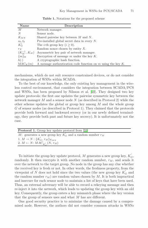
Key Management in WSNs for PCS/SCADA 71
Table 1. Notations for the proposed scheme
Name Description
M Network manager.N Sensor node.KMN Shared pairwise key between M and N .s0, t0 Pre-installed global secret data in every N .Ki
G The i-th group key (i ≥ 0).rX Random nonce chosen by entity X.(K−1
M , KM ) Asymmetric key pair of network manager.{m}K Encryption of message m under the key K.h(·) A cryptographic hash function.MACK(m) A message authentication code function on m using the key K.
mechanisms, which do not suit resource constrained devices, or do not considerthe integration of WSNs within SCADA.
To the best of our knowledge, the only existing key management in the wire-less control environment, that considers the integration between SCADA/PCSand WSNs, has been proposed by Nilsson et al. [10]. They designed two keyupdate protocols: the first one updates the pairwise symmetric key between thenetwork manager M and a sensor node N (as described in Protocol 2) while theother scheme updates the global or group key among M and the whole groupG of sensor nodes (as described in Protocol 1). They claimed that the protocolsprovide both forward and backward secrecy (or in our newly defined terminol-ogy, they provide both past and future key secrecy). It is unfortunately not thecase.
Protocol 1. Group key update protocol from [10]M : generates a new group key K
′G and a random number rM
1. M → N : {K′G, rM}KMN
2. M ← N : MACK
′G
(N, rM )
To initiate the group key update protocol, M generates a new group key, K′G,
randomly. It then encrypts it with another random number, rM , and sends itover the network to the target group. No node in the group has any clue whetherthe received key is fresh or not. In other words, the freshness property, from theviewpoint of N does not hold since the two values (the new group key K
′G and
the random number rM ) are random values chosen by M . It is both impracticaland insecure for each sensor node to maintain a list of keys that have been used.Thus, an external adversary will be able to record a rekeying message and thenre-inject it into the network, which leads to updating the group key with an oldkey. Consequently, the group enters a key mismatch phase where the key versionthat the group of sensors uses and what M has are different.
One good security practice is to minimize the damage caused by a compro-mised node. However, the authors did not consider common attacks in WSNs
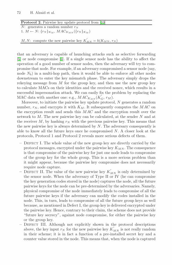
72 H. Alzaid et al.
Protocol 2. Pairwise key update protocol from [10]N : generates a random number rN
1. M ← N : {rN}KM , MACKMN ({rN}KM )
M, N : compute the new pairwise key K′MN = h(KMN , rN)
that an adversary is capable of launching attacks such as selective forwarding[5] or node compromise [4]. If a single sensor node has the ability to affect theoperation of a good number of sensor nodes, then the adversary will try to com-promise that node. For example, if an adversary compromised a sensor node (say,node Nb) in a multi-hop path, then it would be able to enforce all other nodesdownstream to enter the key mismatch phase. The adversary simply drops therekeying message from M for the group key, and then use the new group keyto calculate MACs on their identities and the received nonce, which results in asuccessful impersonation attack. We can easily fix the problem by replacing theMAC data with another one: e.g., MACKMN (K
′G, rM ).
Moreover, to initiate the pairwise key update protocol, N generates a randomnumber, rN , and encrypts it with KM . It subsequently computes the MAC onthe encryption result and sends this MAC and the encryption result over thenetwork to M . The new pairwise key can be calculated, at the sender N and atthe receiver M , by hashing rN with the previous pairwise key. This means thatthe new pairwise key is always determined by N . The adversary consequently isable to know all the future keys once he compromised N . A closer look at theprotocols, Protocol 1 and Protocol 2 reveals more serious defects of them.
– Defect I. The whole value of the new group key are directly carried by theprotocol messages, encrypted under the pairwise key KMN . The consequenceis that compromise of the pairwise key for just one node leads to compromiseof the group key for the whole group. This is a more serious problem thanit might appear, because the pairwise key compromise does not necessarilyrequire node capture.
– Defect II. The value of the new pairwise key K′MN is only determined by
the sensor node. When the adversary of Type II or IV (he can compromisethe key generation codes stored in the node) captures the node, all the futurepairwise keys for the node can be pre-determined by the adversaries. Namely,physical compromise of the node immediately leads to compromise of all thefuture pairwise keys if the adversary can modify the codes installed in thenode. This, in turn, leads to compromise of all the future group keys as wellbecause, as mentioned in Defect I, the group key is delivered encrypted underthe pairwise key. Hence, contrary to their claim, the scheme does not provide“future key secrecy”, against node compromise, for either the pairwise keyor the group key.
– Defect III. Although not explicitly shown in the protocol descriptionsabove, the key input rN for the new pairwise key K
′MN is not really random
in their scheme; it is in fact a function of a pre-installed secret key and acounter value stored in the node. This means that, when the node is captured

Key Management in WSNs for PCS/SCADA 73
and all the installed data including keys exposed to the adversary, all thepast pairwise keys as well as the future keys can immediately be computedeven without recording a single key update message! In fact, this disaster isnot just because of Defect III, but also due to Defect II. Note that, due toDefect III combined with Defect II, the adversary does not have to modifythe node’s software at all in order to extract all the past and future pairwisekeys. Hence no minimum level of past or future key secrecy against nodecompromise in their scheme. Moreover, the adversary can extract any groupkey in the past or future if he has got the records of the corresponding groupkey update message. Note also that, for this, “seamless” monitoring is notneeded by the adversary. What does this mean? The scheme is, in terms ofeither kind of key, neither forward nor backward secure against node com-promise for all the types of adversary I, II, III and IV (see Figure 2).
As for past key secrecy, we note two proposed schemes in the WSN context:Klonowski et al. [6] and Mauw et al. [8]. Both schemes use hash functions inorder to achieve key evolution. Both schemes, however, are intended to be usednot for group key update but for updating pairwise keys for node-to-node [6,13]or node-to-base station communication [8].
On the other hand, as for future key secrecy, Mauw et al.’s protocol doesnot provide this property. The protocol is based on a hash chain scheme origi-nally proposed for RFID security [11]. In RFID environments, protecting secrettag information from tampering in the future is a big concern while it doesnot seem to be such a prime concern in WSNs. This is because it is more au-thentication and integrity than privacy that really matters in WSNs, especiallySCADA/PCS. Hence, future key secrecy is more valued than past key secrecy.On the other hand, the protocol proposed by Klonowski provides future keysecrecy in a “weak” sense; namely, it will be computationally hard for the ad-versary to compute a future key from the current compromised key if he fails torecord, say ten, subsequent evolution steps [13].
5 The Proposed Scheme
Devising a key management for WSNs is not trivial and in particular may not besuccessfully accomplished by simple adaptation of security solutions designed forwired networks. This is because of the limited resources such as limited energylifetime, slow computation, small memory, and limited communication capabili-ties which exist in WSNs [16,17]. In this section, we describe a key managementscheme which secures communication between remote fields (where the WSN re-sides) and the master center (where the network manager resides) by consideringvulnerabilities that are associated with WSNs.
5.1 Key Management Protocols
This paper focuses on updating two types of keys, which are the group key andthe pairwise key, in the wireless process control environments. A pairwise key

74 H. Alzaid et al.
is shared between the network manager M and each sensor node N while thegroup key is shared among M and the whole group of sensor nodes.
Group Key Update Protocol. Our solution for group key rekeying alsoexploits the idea of key evolution using a hash chain in order to achieve pastkey secrecy. The protocol uses a hash chain, hi(s0), where s0 is a pre-installedkey component at the pre-deployment phase and i ≥ 0 denotes the index for keyupdate phases.
As for future key secrecy, we use the reverse hash chain technique, which wasfirst introduced by Lamport [7]. The network manager prepares in advance ahash chain of length n, starting from a random seed tn−1 and ending with thefinal value t0:
tn−1, tn−2 := h(tn−1), tn−3 := h(tn−2), . . . , t1 := h(t2), t0 := h(t1) .
For reasons of convenience which will become clearer shortly, we write h−i(t0)instead of ti although h is not an invertible function and h−1(x) can only meanthe set of all preimages of x in a strict sense. Roughly speaking, h−i(t0) is the i-thpreimage of t0 in the reverse hash chain. The secret data, t0, will be pre-installedinto sensor nodes together with another key component s0.
Protocol 3. The protocol for group key update1. M → N : i, {h−i(t0)}KMN
2. M ← N : hKMN (KiG)
M, N : update the value of the group key (i.e., KiG = hi(s0) ⊕ h−i(t0) ).
Now, with two secret key components s0 and t0 pre-installed within all sensornodes, using Protocol 3, the group key Ki
G evolves as follows:
KiG = hi(s0) ⊕ h−i(t0) , i ≥ 0 ,
where we define h0(s0) = s0 and h0(t0) = t0. Figure 3 explains the key evolutionin the protocol.
Any sensor node can easily compute the i-th hash image hi(s0) from hi−1(s0)while only the network manager knows the value of the i-th preimage h−i(t0).Thus, it is only the network manager who can release the preimage into the sensorfield. As a consequence, the first message in the protocol provides the sensor nodewith a weak form of signature from the network manager: the message could havebeen generated only by the network manager, not by any sensor nodes includingthe node itself. The check of the preimage (i.e., h(h−i(t0)) = h−(i−1)(t0) ) alsomakes sure that the key update message is fresh.
After the i-th key update, the sensor node stores the index i and the secretdata: hi(s0), h−i(t0) and Ki
G. Considering the highly lossy communication en-vironment of sensor networks, the sensor node may sometimes fall behind the

Key Management in WSNs for PCS/SCADA 75
0t 0s 10( )h s 0( )ih s0( )ih t 1
0( )h t
1GK
iGK
0GK
Fig. 3. Key evolution in the proposed protocol
group key update schedule. The sensor node, however, will soon be able to catchup at the next rekeying: it can compute the correct value of the new group keysimply by checking the difference of two index values – the received and thestored – and applying the corresponding number of hash operations.
Now let’s assume that the adversary has somehow extracted the current valueof the group key, Ki
G. However, he cannot extract from this the previous keyKi−1
G because he cannot compute the value of hi−1(s0). Note that this holdseven when the adversary has recorded all the previous key update messages,and compromised all the previous manager-to-node pairwise keys. In fact, thenode capturing and extracting all the stored secret data does not surrenderthe past group key to the adversary. This is because the previous values forhi(s0) were never exchanged over the air, and were deleted after group keycomputation. Hence we can say that the protocol provides past key secrecy forany kind of compromise: group key compromise, pairwise key compromise, andthe compromise of the node itself.
The protocol also provides future key secrecy in the sense that the adversary,just with knowledge of the current group key Ki
G, cannot predict the next groupkey Ki+1
G . The computation of Ki+1G requires knowledge of h−(i+1)(t0), which
has not yet been exchanged. In the next step of the key update, the adversary,without knowledge of the pairwise key KMN , will not be able to obtain the valueof h−(i+1)(t0) from the protocol message. In fact, the pairwise key compromisealone does not lead to the future group key compromise; it will only happen whenthe adversary captures a sensor node, thereby extracting the hidden componenthi(s0). Hence, the protocol satisfies future key secrecy in the face of group keyand/or pairwise key compromise; simple delivery of the encrypted value of thenew group key, as in [10], cannot provide this kind of resilience. The protocol willfail to provide future key secrecy only when the node is physically captured. Evenin the case of capture, the adversary should listen to the key update message toextract the future group key. Furthermore, when the pairwise key is updated,any adversary of type I, II, or III will not be able to have any knowledge ofthe new pairwise key. This, in turn, leads to the adversary’s failure to have anyknowledge of the new group key established using the new pairwise key. Hence,
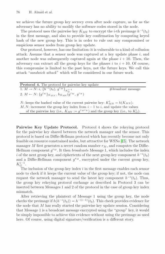
76 H. Alzaid et al.
we achieve the future group key secrecy even after node capture, as far as theadversary has no ability to modify the software codes stored in the node.
The protocol uses the pairwise key KMN to encrypt the i-th preimage h−i(t0)in the first message, and also to provide key confirmation by computing keyedhash of the new group key. This is in order to rule out any compromised orsuspicious sensor nodes from group key update.
Our protocol, however, has one limitation: it is vulnerable to a kind of collusionattack. Assume that a sensor node was captured at a key update phase i, andanother node was subsequently captured again at the phase i + 10. Then, theadversary can extract all the group keys for the phases i to i + 10. Of course,this compromise is limited to the past keys, not the future keys. We call thisattack “sandwich attack” which will be considered in our future work.
Protocol 4. The protocol for pairwise key update1. M → N : i, {h−i(t0), grM }
Ki−1G
#broadcast message2. M ← N : {grN }KMN , hKMN (grM , grN )
N : keeps the hashed value of the current pairwise key: K1MN = h(KMN ).
M, N : increment the group key index from i − 1 to i, and update the valuesof the pairwise key (i.e., KMN := grM rN ) and the group key (i.e., to Ki
G).
Pairwise Key Update Protocol. Protocol 4 shows the rekeying protocolfor the pairwise key shared between the network manager and the sensor. Thisprotocol is based on Diffie-Hellman protocol which has recently become not onlyfeasible on resource constrained nodes, but attractive for WSNs [15]. The networkmanager M first generates a secret random number rM , and computes the Diffie-Hellman component grM . It then broadcasts Message 1, which includes the indexi of the next group key, and ciphertexts of the next group key component h−i(t0)and a Diffie-Hellman component grM , encrypted under the current group key,Ki−1
G .The inclusion of the group key index i in the first message enables each sensor
node to check if it keeps the current value of the group key; if not, the node canrequest the network manager to send the latest key component h−i(t0). Thus,the group key rekeying protocol exchange as described in Protocol 3 can beinserted between Messages 1 and 2 of the protocol in the case of group key indexmismatch.
After retrieving the plaintext of Message 1 using the group key, the nodechecks the preimage if h(h−i(t0)) = h−(i−1)(t0). This check provides evidence forthe node that M has really started the pairwise key update session. Consideringthat Message 1 is a broadcast message encrypted using the “group” key, it wouldbe simply impossible to achieve this evidence without using the preimage as usedhere. Of course, using digital signature/verification is a different story.

Key Management in WSNs for PCS/SCADA 77
Now the node constructs the second message of the protocol: it generatesits own Diffie-Hellman component grN , encrypts it, and generates the keyedhash of both Diffie-Hellman components under the current pairwise key KMN .After sending the message to M , the node computes the new group key, Ki
G =hi(s0) ⊕ h−i(t0), increments the group key index from i− 1 to i, and computesthe Diffie-Hellman key grM rN to be used as the new pairwise key, while keepingthe hash h(KMN ) of the old pairwise key and safely deleting the old key.
On receiving Message 2, M decrypts grN , and verifies the keyed hash fromN . The inclusion of grM and grN in the hash provides M with confidence aboutthe freshness and authenticity, respectively, of the message.
Use of Diffie-Hellman key agreement for the pairwise key update provides thepast and future pairwise key secrecy; the key inputs are temporary randoms, andthus no relation to the previous or next key inputs. Even after node compromise,if the attacker is not able to modify the software codes in the node (i.e., theadversary of type I or III), or if he fails to record the key update messages(i.e., the adversary of type I or II), the node will escape from the control of theadversary to recover the secure status. Thus, our scheme satisfies past pairwisekey secrecy for all the adversary types, and future pairwise key secrecy for anyadversary type except type IV, even against node capture and its compromise.
Impersonation attack. If the adversary is in full control of a compromisednode, in which he installed his own malicious attacking software, then the adver-sary’s node can still impersonate M to some other victim node, succeeding in caus-ing the victim to receive a fake Diffie-Hellman component, say gx. But the attack islimited to that. The attacking node has only two options when receiving Message2 of the victim node: (1) forward the message verbatim to M , or (2) cut out themessage. In the former case, M will get not the expected hash hKMN (grM , grN )but a strange one hKMN (gx, grN ). In the latter case, M will see no response fromN . In both cases, M will issue Message 1 again through the unicast channel to N ,which will finally lead to key agreement between M and N .
Delivery failure management. The delivery failure in the WSNs will leadto key mismatches of group keys and/or pairwise keys. With no long term keyavailable in our key update protocols, key mismatch is a big concern and shouldbe handled carefully. Simple retransmission of the protocol messages is not asolution; it may open the door to replay attacks. Moreover, it may require thesensor node to go back to the old key even after it has successfully updated thepairwise key. Consequentially, the node must keep two keys at the same time:the old key and the new updated key.
Our solution is to use key evolution here again. With no response from thenode N , the manager M initiates Protocol 5 over the unicast channel to N . Here,Kj
MN = hj(KMN ) is a hashed copy of the current key from M ’s viewpoint. Forthe time of the first protocol run, the index j is set to 1; it will be incrementedby one whenever the protocol is retried. On receipt of Message 1 over the unicastchannel, the sensor node N compares the received group key indice i, j with thestored indice i′, j′, and executes the required action as follows:

78 H. Alzaid et al.
Protocol 5. The protocol to handle delivery failure1. M → N : i, j, {h−i(t0), grM }
KjMN
# unicast message
2. M ← N : {grN }K
jMN
, hK
jMN
(grM , grN )
M, N : update the values of the pairwise key (i.e., KMN := grM rN )N : increments the indice i and j, and updates the values of the pairwise key
(i.e., KMN := grM rN ) and the group key (i.e., to KiG), and then keeps
the hashed value of old key: Kj+1MN := h(Kj
MN )
Fig. 4. Relations between keys and keying materials and the significance of node com-promise
– Case 1: i = i′ and j ≥ j′. For simplicity, consider the case j = j′ = 1.The pairwise key update protocol (Protocol 4 ) has just been run, but thereply message of the protocol failed to arrive at M . The node N has beenkeeping the hashed copy K1
MN = h(KMN ) of the old pairwise key, which isapplied to the ciphertext for Message 1 of Protocol 5. The retrieved valueof h−i(t0) ensures the authenticity of the message; the entity other than N ,in possession of h−i(t0) and K1
MN , should be M . The node decrypts theencrypted part of Message 1 using K1
MN . Then, N follows exactly the samestep as in Protocol 4 except that it uses the hash of the old pairwise keyinstead of the current pairwise key. At the end of the protocol run, N willend up with a new pairwise key, and the hash of K1
MN , i.e., K2MN ; now j = 2.
The current pairwise key is simply deleted. One or more failure again will befollowed by reinitiation of the protocol by M with j incremented. It couldalso happen that Message 1 itself fails to arrive at N , and subsequently Mretries the protocol. This will lead to the case j > j′.
– Case 2: i = i′ and j < j′. This cannot happen; otherwise it is simply abogus message from another sensor node. N should ignore Message 1.
– Case 3: i > i′. This happens when the node N has never been involvedin the pairwise key update protocol due to delivery failure of Message 1 of

Key Management in WSNs for PCS/SCADA 79
Protocol 4 . In this case, N applies the hash to the current pairwise key jtimes, and uses the resulting value as the description key for Message 1.
– Case 4: i < i′. This is another case of replay attack. N should ignoreMessage 1.
Now, the old key does not need to be kept just for handling key mismatch;Protocol 5 does not come with any breach of security.
5.2 Putting It All Together
In our scheme, the pairwise key is used for secure delivery of the group key updateinformation in Protocol 3; the group key, in turn, encrypts the Diffie-Hellmancomponents to establish a new pairwise key in Protocol 4. This combinationhelps the sensor networks to recover its security quickly after some sensor nodesare captured and their keys are compromised.
Figure 4 illustrates how all the keys and keying data are related to each otheras they evolve over time. Note that no keys are delivered over the air; only theirkeying materials, such as h−i(t0), are exchanged or even never exchanged overthe air (e.g., hi(s0) ). Thus, unlike the scheme of Nilsson et al. (see Defect I inSection 4), the pairwise key compromise alone does not lead to the group keycompromise, and vice versa.
Using the inverse hash chain as well as the hash chain, we achieve bothpast/future group key secrecy at the same time; furthermore the group keyupdate message provides an inherent message authenticity.
Both M and N contribute their Diffie-Hellman inputs to the computationof the new pairwise key, and thus the adversary can not determine the futurevalues of the pairwise key even after node capture and the resulting compromiseof the built-in software, which was not the case in the scheme of Nilsson et al.(see Defect II in Section 4).
Group key not disclosedPairwise key not disclosed
Group key disclosedPairwise key disclosed
Group key not disclosedPairwise key disclosed
Group key disclosedPairwise key not disclosed
Not monitored
Monitored & SW not compromised
Monitored & SW compromised
Fig. 5. State diagram of key disclosure

80 H. Alzaid et al.
Carefully designed with node capture in mind, our scheme does not surrenderall the key components required to retrieve the past/future group/pairwise keys.Only the adversary equipped with seamless monitoring and software compromise(i.e., the type IV adversary) can keep the control of the once-captured node.
Figure 5 shows how the node recovers its secure state with the help of thekey update protocols, after it has been captured and all the keys in it are com-promised. Without seamless monitoring (i.e., adversary types I and II), the ad-versary will soon lose all the control of the keys. Even with adversary type III(i.e., seamless monitoring but no software compromise), the node will eventuallyrecover the secrecy of both keys. Only for adversary type IV (i.e., both seamlessmonitoring and software compromise), there is no path available back to theoriginal secure state. We argue that a non cryptographic countermeasure suchas tamper-proof technology is additionally required to fight against the strongestadversary of type IV.
6 Conclusion
Wireless sensor networks (WSNs) has brought a devastating security threat:node capture. The threat is so powerful that almost all existing key managementprotocols are just helpless because it overthrows the fundamental assumption forcryptographic system design: long term secret keys are securely stored. This iswhy so called forward secrecy and backward secrecy are required in cryptographickey management protocols for WSNs. Both terminologies are rather misleadingand confusing, and so we propose more proper ones: future key secrecy and pastkey secrecy.
Nilsson et al. [10] have recently proposed a key management scheme for WSNapplications in PCS/SCADA environments, which was incorrectly claimed toprovide future and past key secrecies. Some proposals (only for pairwise keyupdate) provide past key secrecy, but not future key secrecy [6,8].
We noticed that any cryptographic countermeasure alone cannot prevent themost powerful adversary in the WSN context; he can capture a node to extractall confidential data, modify any built-in codes, and seamlessly monitor to keepcontrol of the node. This kind of attackers can only be fought by using tamper-proof technologies as well as cryptographic ones. The assumption regarding thistype of adversaries, however, is by no means the most usual or reasonable as-sumption. Seamless monitoring requires the adversary not to lose every singlesession for group key or pairwise key update. The task of modification of randomnumber generation codes will add another burden to that.
In order to measure the resilience of key management protocols, we derivedfour different types of adversaries varying in their capability with regard toseamless monitoring and software manipulation. As shown in Section 3, Nilssonet al.’s scheme, contrary to their claims, turned out to provide neither pastkey secrecy nor future key secrecy against node compromise by any type ofadversaries.
We applied Lamport’s reverse hash chain as well as usual hash chain to provideboth past and future key secrecies. Our scheme avoids the delivery of the whole

Key Management in WSNs for PCS/SCADA 81
value of new group key for group key update; instead only the half of the valueis transmitted from the network manager to the sensor nodes. This way, thecompromise of a pairwise key alone does not lead to the compromise of the groupkey, which was not the case in the scheme by Nilsson et al. The new pairwisekey in our scheme is determined by Diffie-Hellman based key agreement. As forthe scheme of Nilsson’s et al., it uses key transport, not key agreement, wherethe new pairwise key is determined by the sensor node and then delivered to thenetwork manager by using public key encryption. This has brought a vital flawto their scheme.
In short, our scheme provides a very strong resilience; both past and futurekey secrecies against node capture by all the adversary types except the strongestone, Type IV. A sensor node attacked by the adversary of Type IV, in theory,cannot be quarantined by a cryptographic method alone; a non-cryptographiccountermeasure such as tamper-proof protection is needed together.
References
1. Beaver, C., Gallup, D., Neumann, W., Torgerson, M.: Key management forSCADA. Technical Report SAND2001-3252, Sandia National Laboratories - Cryp-tography and Information Systems Surety Department (March 2002)
2. Dawson, R., Boyd, C., Dawson, E., Gonzalez Nieto, J.M.: SKMA: a key man-agement architecture for SCADA systems. In: Buyya, R., Ma, T., Safavi-Naini,R., Steketee, C., Susilo, W. (eds.) ACSW Frontiers. CRPIT, vol. 54, pp. 183–192.Australian Computer Society (2006)
3. Gunther, C.G.: An identity-based key-exchange protocol. In: Quisquater, J.-J.,Vandewalle, J. (eds.) EUROCRYPT 1989. LNCS, vol. 434, pp. 29–37. Springer,Heidelberg (1990)
4. Hartung, C., Balasalle, J., Han, R.: Node compromise in sensor networks: Theneed for secure systems. Technical Report CU-CS-990-05, University of Coloradoat Boulder - Department of Computer Science (January 2005)
5. Karlof, C., Wagner, D.: Secure routing in wireless sensor networks: attacks andcountermeasures. Ad Hoc Networks 1(2-3), 293–315 (2003)
6. Klonowski, M., Kutylowski, M., Ren, M., Rybarczyk, K.: Forward-secure key evo-lution in wireless sensor networks. In: Bao, F., Ling, S., Okamoto, T., Wang, H.,Xing, C. (eds.) CANS 2007. LNCS, vol. 4856, pp. 102–120. Springer, Heidelberg(2007)
7. Lamport, L.: Password authentification with insecure communication. Commun.ACM 24(11), 770–772 (1981)
8. Mauw, S., van Vessem, I., Bos, B.: Forward secure communication in wireless sensornetworks. In: Clark, J.A., Paige, R.F., Polack, F.A.C., Brooke, P.J. (eds.) SPC2006. LNCS, vol. 3934, pp. 32–42. Springer, Heidelberg (2006)
9. McClanahan, R.: SCADA and IP: is network convergence really here? IEEE In-dustry Applications Magazine 9(2), 29–36 (2003)
10. Nilsson, D.K., Roosta, T., Lindqvist, U., Valdes, A.: Key management and se-cure software updates in wireless process control environments. In: Gligor, V.D.,Hubaux, J.-P., Poovendran, R. (eds.) WISEC, pp. 100–108. ACM, New York (2008)
11. Ohkubo, M., Suzuki, K., Kinoshita, S.: Cryptographic approach to privacy-friendlytags. In: RFID Privacy Workshop (2003)

82 H. Alzaid et al.
12. Pietre-Cambacedes, L., Sitbon, P.: Cryptographic key management for SCADAsystems-issues and perspectives. International Journal of Security and its Applica-tions 2(3), 31–40 (2008)
13. Ren, M., Das, T.K., Zhou, J.: Diverging keys in wireless sensor networks. In: Kat-sikas, S.K., Lopez, J., Backes, M., Gritzalis, S., Preneel, B. (eds.) ISC 2006. LNCS,vol. 4176, pp. 257–269. Springer, Heidelberg (2006)
14. Roman, R., Alcaraz, C., Lopez, J.: The role of wireless sensor networks in the areaof critical information infrastructure protection. Information Security TechnicalReport 12(1), 24–31 (2007)
15. Szczechowiak, P., Oliveira, L.B., Scott, M., Collier, M., Dahab, R.: NanoECC:Testing the limits of elliptic curve cryptography in sensor networks. In: Verdone,R. (ed.) EWSN 2008. LNCS, vol. 4913, pp. 305–320. Springer, Heidelberg (2008)
16. Vieiral, M.A.M., Coelho Jr., C.N., Cecilio da Silva Junio, D., da Mata, J.M.: Surveyon wireless sensor network devices, September 2003, vol. 1, pp. 537–544 (2003)
17. Walters, J.P., Liang, Z., Shi, W., Chaudhary, V.: Security in Distributed, Grid,and Pervasive Computing. In: Xiao, Y. (ed.) Wireless sensor network security: Asurvey, ch. 17. Auerbach Publications, CRC Press (2006)

Analysis of Channel Access Delay of SlottedCSMA/CA in a WSN
Alexandre Guitton and Nassima Hadid
LIMOS CNRS, Clermont UniversityComplexe scientifique des Cezeaux, 63173 Aubiere Cedex, France
{guitton,hadid}@sancy.univ-bpclermont.fr
Abstract. Wireless sensor networks are often designed to operate onremote areas. Thus, sensor devices need to operate for years and have tosave energy by switching their radio component off as often as possible.IEEE 802.15.4 is a standard that induces a low energy consumption.It divides time into an active period, where devices communicate, andan inactive period, where devices sleep. Many research has been doneon how to optimize the medium access delay during the active period.Surprisingly, few studies take into account the inactive periods whenanalyzing the delay.
In this paper, we give a macroscopic analysis of the medium accessdelay of a low-power wireless sensor network that operates in the beacon-enabled mode of IEEE 802.15.4. We conduct multiple simulations in or-der to study the impact of the network parameters such as the numberof devices in range and the traffic production. We also propose an esti-mation of the access delay in the case of a traffic uniformly distributedamong devices, and in the case of a traffic non-uniformly distributedamong devices.
Keywords: IEEE 802.15.4, slotted CSMA/CA, low-power WSN,medium access delay, estimation model.
1 Introduction
Recently, many industrial applications have been developed based on the technol-ogy of wireless sensor nodes. Sensor nodes are cheap energy-constrained devicesthat perform some monitoring tasks. They are often deployed in low populatedor dangerous areas. The goal of such networks is to monitor the environment forseveral years without requiring to change the batteries of the devices. The IEEE802.15.4 standard [IEE06] describes a medium access control (MAC) protocolthat suits the requirements of such sensor nodes. The standard describes twomodes of operation for the MAC sublayer, one of them being slotted CSMA/CA(which stands for Carrier Sense Multiple Access with Collision Avoidance), whichis the focus of this paper.
Slotted CSMA/CA divides time into two periods: an active period and aninactive period. During the active period, all the devices can communicate to-gether. They are often in competition for the medium access. During the inactive
S. Hailes, S. Sicari, and G. Roussos (Eds.): S-Cube 2009, LNICST 24, pp. 83–97, 2009.c© Institute for Computer Sciences, Social-Informatics and Telecommunications Engineering 2009

84 A. Guitton and N. Hadid
period, they save energy by turning their radio component off. Low-power wire-less sensor networks tend to have devices inactive most of the time. This hasa clear impact on delay, as communications are only possible during the shortactive periods.
In this paper, we give a macroscopic analysis of the medium access delay ofa low-power wireless sensor network that operates with the slotted CSMA/CAalgorithm of IEEE 802.15.4. We conduct multiple simulations in order to studythe impact of the network parameters such as the number of devices in rangeand the traffic production. We also propose an estimation of the access delay inthe case of traffic uniformly and non-uniformly distributed among devices.
Section 2 describes the IEEE 802.15.4 standard and slotted CSMA/CA. Itdescribes related analytical and experimental analyzes and shows that previ-ous research mainly focuses on active periods, while we concentrate on inactiveperiods. In Sect. 3, we study the medium access delay in scenarios where thetraffic is uniformly distributed among the data sources. In Sect. 4, we extendthis study to scenarios where the traffic is non-uniformly distributed among thedata sources. Then, we propose a linear estimation model for the delay in Sect. 5and we present a discussion in Sect. 6. Section 7 concludes our work.
2 State of the Art
In this section, we first describe the IEEE 802.15.4 standard and slotted CSMA/CA. Then, we present the related work on slotted CSMA/CA that is devoted tothe delay analysis, with analytical or experimental approaches.
2.1 Overview of the IEEE 802.15.4 MAC Layer
The IEEE 802.15.4 standard [IEE06] supports two operational modes: (i) thebeacon-enabled mode in which periodic beacon frames are transmitted to syn-chronize nodes according to a superframe structure depicted in Fig. 1, and (ii)the non-beacon-enabled mode in which unslotted CSMA/CA is used. In thispaper, we focus on the beacon-enabled mode as it is more energy-efficient thanthe non-beacon-enabled mode.
In the beacon-enabled mode, the active period (also called the superframe) isdivided into two periods: the contention access period (CAP) during which slot-ted CSMA/CA is used to avoid collisions, and the contention free period (CFP)where nodes have guaranteed time slots ensuring a collision free transmission.Note that slotted CSMA/CA is only used during the CAP. The interval thatseparates two consecutive beacons (BI) and the superframe duration (SD) aredetermined by two parameters: the superframe order (SO) and the beacon order(BO). BI and SD are defined as follows:{
BI = aBaseSuperframeDuration.2BO,
SD = aBaseSuperframeDuration.2SO,
where 0 ≤ SO ≤ BO ≤ 14 and aBaseSuperframeDuration = 15.36 ms.
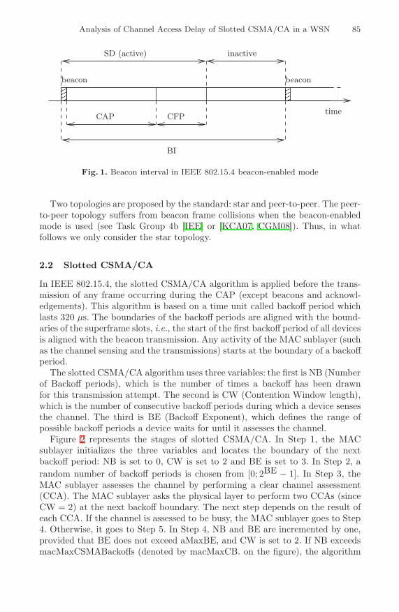
Analysis of Channel Access Delay of Slotted CSMA/CA in a WSN 85
����
����
CAP CFP
beaconbeacon
inactiveSD (active)
BI
time
Fig. 1. Beacon interval in IEEE 802.15.4 beacon-enabled mode
Two topologies are proposed by the standard: star and peer-to-peer. The peer-to-peer topology suffers from beacon frame collisions when the beacon-enabledmode is used (see Task Group 4b [IEE] or [KCA07, CGM08]). Thus, in whatfollows we only consider the star topology.
2.2 Slotted CSMA/CA
In IEEE 802.15.4, the slotted CSMA/CA algorithm is applied before the trans-mission of any frame occurring during the CAP (except beacons and acknowl-edgements). This algorithm is based on a time unit called backoff period whichlasts 320 μs. The boundaries of the backoff periods are aligned with the bound-aries of the superframe slots, i.e., the start of the first backoff period of all devicesis aligned with the beacon transmission. Any activity of the MAC sublayer (suchas the channel sensing and the transmissions) starts at the boundary of a backoffperiod.
The slotted CSMA/CA algorithm uses three variables: the first is NB (Numberof Backoff periods), which is the number of times a backoff has been drawnfor this transmission attempt. The second is CW (Contention Window length),which is the number of consecutive backoff periods during which a device sensesthe channel. The third is BE (Backoff Exponent), which defines the range ofpossible backoff periods a device waits for until it assesses the channel.
Figure 2 represents the stages of slotted CSMA/CA. In Step 1, the MACsublayer initializes the three variables and locates the boundary of the nextbackoff period: NB is set to 0, CW is set to 2 and BE is set to 3. In Step 2, arandom number of backoff periods is chosen from [0; 2BE − 1]. In Step 3, theMAC sublayer assesses the channel by performing a clear channel assessment(CCA). The MAC sublayer asks the physical layer to perform two CCAs (sinceCW = 2) at the next backoff boundary. The next step depends on the result ofeach CCA. If the channel is assessed to be busy, the MAC sublayer goes to Step4. Otherwise, it goes to Step 5. In Step 4, NB and BE are incremented by one,provided that BE does not exceed aMaxBE, and CW is set to 2. If NB exceedsmacMaxCSMABackoffs (denoted by macMaxCB. on the figure), the algorithm

86 A. Guitton and N. Hadid
slotted CSMA/CA
NB = 0, CW = 2
BE = macMinBE
locate backoffperiod boundary
delay for random (2BE − 1)unit backoff periods
perform CCA onbackoff period boundary
channel idle?
CW = 2, NB = NB + 1,BE = min(BE + 1, aMaxBE) CW = CW − 1
NB > macMaxCB.? CW = 0?
failure success
(Step 1)
(Step 2)
(Step 3)
(Step 4) (Step 5)yes
yes yes
no
nono
Fig. 2. IEEE 802.15.4 slotted CSMA/CA (without the battery life extension)
terminates with a channel access failure, otherwise it goes back to Step 2. In Step5, CW is decremented. If CW becomes equal to zero, the transmission begins atthe boundary of the next backoff period. Otherwise, the MAC sublayer returnsto Step 3.
2.3 Analytical Analyzes of the Delay of Slotted CSMA/CA
Here, we focus on the papers that propose analytical models to evaluate the per-formance of slotted CSMA/CA. In all the following papers, authors focused onthe evaluation of the delay during the active period. The key difference between

Analysis of Channel Access Delay of Slotted CSMA/CA in a WSN 87
their approach and ours is that we claim that the inactive period accounts formost of the delay.
In [PEE+06], the authors considered both saturated and periodic traffic sce-narios in a star topology. They validated their analytical results on throughputand energy consumption by simulation. They simulated a long active period of108 backoff periods, that is, of more than 8 hours.
In [PKC+05], the authors evaluated slotted CSMA/CA in terms of through-put and energy consumption, in saturation conditions in a star topology. Theyassumed that each time a frame is sent, a new frame arrives at the MAC sub-layer. Their analysis is validated by simulations with the network simulator NS-2. Again, as the authors focused on the active period, they fixed a long beaconinterval (BO = 10 which corresponds to 15.4 seconds).
In [TPGZ06], the authors proposed a Markov chain in order to analyze thethroughput of slotted CSMA/CA. The authors developed a custom C simulatorto validate their analysis. However, since no value for BO, SO, BI or SD is given,we assume that their simulation did not take into consideration the inactiveperiod.
In [SS07], the authors studied the throughput and energy consumption of slot-ted CSMA/CA in both saturated and periodic traffic conditions. Their main con-tribution is the use of a single, simple, one-dimensional Markov chain while[PEE+06], [PKC+05] and [TPGZ06] use complex two-dimensional Markov chains.They validated their analysis through simulations. However, they simulated a sin-gle active period of 5.105 backoff periods, that is, of 160 seconds.
2.4 Experimental Analyzes of the Delay of Slotted CSMA/CA
Researchers have also performed simulation analyzes on slotted CSMA/CA.Among multiple parameters, they varied BO and SO and observed the impacton the performance of the protocol.
In [LKR04], the authors studied the delivery ratio, the throughput and thedelay as a function of the duty cycle and the energy consumption of slottedCSMA/CA. Concerning the delay, they have shown that delay increases as theduty cycle decreases by plotting the average delay as a function of 2SO/2BO, fora single source. In this paper, we propose a more detailed analysis of this phe-nomenon. Notably, we relate the medium access delay to the frame productiontime. We also study scenarios where multiple sources transmit data frames.
In [KAT06], the authors observed the effect of BO and SO on the behavior ofslotted CSMA/CA and analyzed its impact on the average delay, the throughputand the number of collisions. However, in all their simulations, the values of BOand SO are the same. Thus, there is no inactive period.
In [CHGM09], the authors have shown that the deference mechanisms usedtowards the end of the CAP have a major impact on the delay of slottedCSMA/CA. Although deference mechanisms occur rarely, their penalty on de-lay is so large that deference becomes significant for short global cycles. In thispaper, we encounter the same situation: the inactive period has a large impact

88 A. Guitton and N. Hadid
on delay. We give here a macroscopic analysis of the medium access delay, asopposed to [CHGM09].
3 Analysis of Uniform Traffic
We start our analysis by a scenario where the traffic is uniformly distributedamong the sources. After describing the simulation setup, we give results for asingle source. Then, we extend the results to a scenario with multiple sources.
3.1 Simulation Setup
Our simulations are done with NS-2, version 2.31. We used a simple star topologywith one coordinator and ten end-devices. We deployed the nodes so that theyare in range of each other. We used the two-ray ground shadowing model withdefault parameters, and we used 1.33 × 10⁻⁶ W for the reception and carriersense threshold. However, we deployed the nodes close enough to ensure thatthe propagation model has no impact on the reception of frames.
The PHY and MAC layers used in our simulation are those of the wpan moduleof NS-2, and correspond to IEEE 802.15.4 specifications. The coordinator gener-ates periodic beacons, according to the value of BO. After all the end-devices areassociated to the coordinator, some of them are chosen as traffic sources. Eachtraffic source periodically sends data frames to the coordinator. Data frameshave a MAC payload of 30 bytes, plus 7 bytes added by the PHY layer. Eachdata frame is acknowledged. We set the size of the frame queues to 100 framesto reduce the effect of queue overflows (this is discussed in the following). Lastly,simulations are run 100 times and last for 100 seconds; frames in the queueswhen the simulation stops are discarded.
In the following, we consider two scenarios: one with a single traffic source,the other with multiple traffic sources. The varying parameters are described atthe beginning of the corresponding subsection.
3.2 Single Source Scenario
In the single source scenario, only one end-device is configured as a traffic source.We set BO to 7, which results into a global cycle of 27 × 15.36 = 1966.08 ms(i.e., about two seconds). In most simulations, we vary SO from 4 to 6, whichresults into activity durations from 245.76 ms to 983.04 ms (from 12.5% to 50%of the global cycle). This is a typical case for LP-WPANs. We also vary thetraffic generation frequency from five frames per second to twenty frames persecond.
Figure 3 shows a graphical representation of the medium usage on two samplesimulations: one with a traffic frequency of five frames per second (referred toas low traffic), the other with a traffic frequency of twenty frames per second(referred to as high traffic), both with SO = 6. The medium usage is shown ona time axis for about 3 seconds, which is larger than one global cycle. Beacons,

Analysis of Channel Access Delay of Slotted CSMA/CA in a WSN 89
time
time
Fig. 3. Medium occupation in the single source scenario, for low traffic (upper part)and high traffic (lower part). Medium occupation is high at the very beginning of theactive period.
data frames and acknowledgments are represented by a vertical line at the timewhen they are transmitted. Active and inactive periods can be clearly seen onthe figure. It can also be seen that the beginning of the active period is theperiod when the channel is the most busy. This is more obvious when the trafficfrequency is high. The modeling of this phenomenon is the basis of this paper.
As we have seen, the medium is highly occupied at the beginning of the activeperiod (which follows the beacon transmission), and is mostly idle the remainingof the time. This means that frames produced in the middle of the active periodcan be transmitted quickly, while frames produced at the beginning of the activeperiod might experience larger delays. Our goal now is to quantify the delay offrames with respect to their production time.
Figure 4 shows the average medium access delay as a function of the trafficfrequency. The delay is computed as the time that separates the frame production(at the application layer) to the frame transmission (at the physical layer). Notethat in our simulation, the frame is only delayed at the MAC layer. The trafficfrequency varies from five frames per seconds to twenty frames per second. Notethat all times are normalized according to the beginning of the active periodand are averaged over 100 simulations. Thus, each point of the figure representsthe average of 5,000 global cycles (100 simulations for 100 seconds, with a globalcycle of 2 seconds). Finally, times are rounded to 0.1 seconds.
Figure 5 displays the frame loss as a function of the traffic frequency. As theaverage medium access delay only takes into account the received frames, delayand frame loss have to be considered at the same time. As expected on thisfigure, frames are lost when the queues are full, that is towards the end of theinactive period, and at the beginning of the active period.
The active and inactive periods are shown very clearly on Fig. 4. As the activeperiod directly follows the beacon frame transmission, it is normal that framesexperience small delay on the left part of the graph. All the frames producedduring the inactive periods experience large delays (reaching a peak at 1 second,which is the length of the inactive period).
There are two main results that can be extracted from Fig. 4 and from Fig. 5.First, it can be seen that the average delay decreases linearly during the inactiveperiod, with a speed that depends on the traffic. When the number of framesaccumulated during the inactive period is small, these frames are sent quickly by
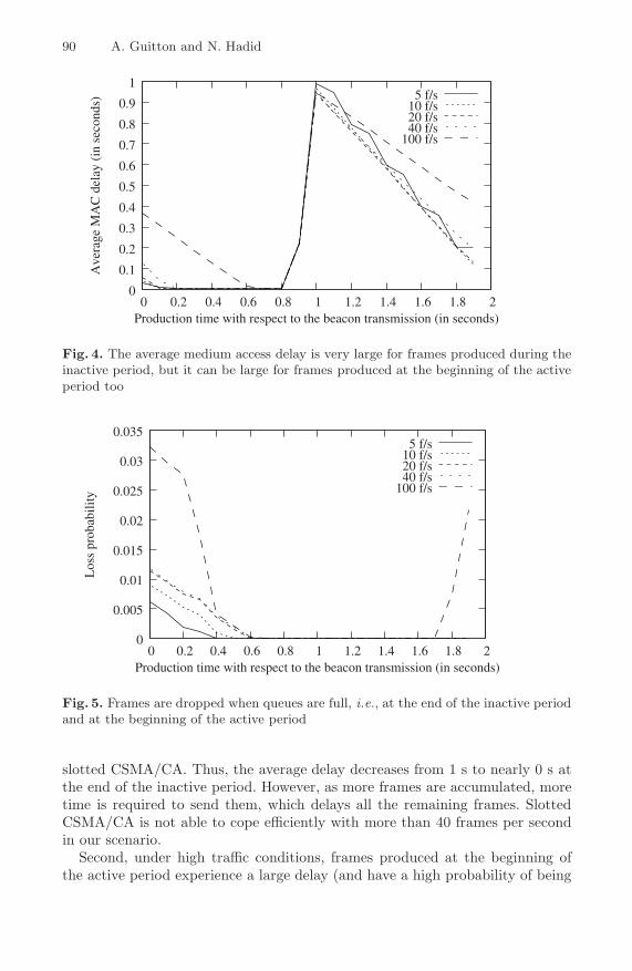
90 A. Guitton and N. Hadid
0
0.1
0.2
0.3
0.4
0.5
0.6
0.7
0.8
0.9
1
0 0.2 0.4 0.6 0.8 1 1.2 1.4 1.6 1.8 2
Ave
rage
MA
C d
elay
(in
sec
onds
)
Production time with respect to the beacon transmission (in seconds)
5 f/s10 f/s20 f/s40 f/s
100 f/s
Fig. 4. The average medium access delay is very large for frames produced during theinactive period, but it can be large for frames produced at the beginning of the activeperiod too
0
0.005
0.01
0.015
0.02
0.025
0.03
0.035
0 0.2 0.4 0.6 0.8 1 1.2 1.4 1.6 1.8 2
Los
s pr
obab
ility
Production time with respect to the beacon transmission (in seconds)
5 f/s10 f/s20 f/s40 f/s
100 f/s
Fig. 5. Frames are dropped when queues are full, i.e., at the end of the inactive periodand at the beginning of the active period
slotted CSMA/CA. Thus, the average delay decreases from 1 s to nearly 0 s atthe end of the inactive period. However, as more frames are accumulated, moretime is required to send them, which delays all the remaining frames. SlottedCSMA/CA is not able to cope efficiently with more than 40 frames per secondin our scenario.
Second, under high traffic conditions, frames produced at the beginning ofthe active period experience a large delay (and have a high probability of being
Analysis of Channel Access Delay of Slotted CSMA/CA in a WSN 91
lost). This is due to the fact that frames produced during the inactive periodare already queued, and are trying to access the medium. When 100 framesare produced per second, more than 60% of the active period is devoted totransmitting the frames produced in the previous inactive period.
3.3 Multiple Sources Scenario
In the multiple source scenario, we varied the number of sources and kept thetraffic constant. We used the following settings: 100 frames per second for onesource, 20 frames per second for five sources, and 10 frames per second for tensources. The overall traffic generated is 100 frames per second. Traffic productionstarts randomly within the first second for each source.
Results on delay are shown on Fig. 6. It can be seen that delay is reducedwhen the number of sources is increased. This general behavior is known forCSMA/CA algorithms. When a single node transmits data, it cannot use themedium very often. Indeed, it has to wait for the mandatory backoff (between0 and 7 backoff slots) before transmitting any frame. Thus, it cannot use themedium to its full extent. When there are more sources in the network, theprobability that one source transmits while the other performs the backoff islarger. This increases the medium usage, and reduces the average delay.
Results on frame loss are shown on Fig. 7. When there was only one source,queue overflow was the only cause of frame loss. As soon as multiple sources arecompeting for the channel, frame collisions appear. Many frames queued duringthe inactive period are dropped due to collisions. This number increases withthe number of sources. The number of frames dropped due to queue overflows isnegligible.
Slotted CSMA/CA is not very efficient in avoiding collisions. Let us considera simple example when a collision occurs. Let us assume that the channel is idle,and two sources decide at the same time to perform the first CCA (this situationcan happen even if the two sources have drawn different backoffs, provided thatthe difference of backoff cancels the difference of time when the decisions weretaken). Both CCAs return idle, and both sources perform the second CCA.Again, both CCAs return idle. Then, the two sources start the transmission, anda collision occurs. Slotted CSMA/CA performs a few retries (four by default)before discarding the frame. Notice that in a real scenario, the capture effectmight lessen this problem.
4 Analysis of Non-uniform Traffic
In this section, we used a non-uniform traffic in order to determine if the trafficdistribution among sources had an impact on the average medium access delay.We used the same simulation setup as before, except for the traffic production.We decided to have five sources producing a total of 100 frames per second, thatis an average of 20 frames per second and per source, but distributed among thesources in a non-uniform manner. Sources 1 and 2 produce 25 frames per second,

92 A. Guitton and N. Hadid
0
0.1
0.2
0.3
0.4
0.5
0.6
0.7
0.8
0.9
1
0 0.2 0.4 0.6 0.8 1 1.2 1.4 1.6 1.8 2
Ave
rage
MA
C d
elay
(in
sec
onds
)
Production time with respect to the beacon transmission (in seconds)
10 f/s for 10 sources20 f/s for 5 sources100 f/s for 1 source
Fig. 6. The average medium access delay is reduced when several sources send traffic
0
0.05
0.1
0.15
0.2
0.25
0.3
0.35
0.4
0 0.2 0.4 0.6 0.8 1 1.2 1.4 1.6 1.8 2
Los
s pr
obab
ility
Production time with respect to the beacon transmission (in seconds)
10 f/s for 10 sources20 f/s for 5 sources100 f/s for 1 source
Fig. 7. The more sources, the more collisions
sources 3 produce 20 frames per second, and sources 4 and 5 produce 15 framesper second.
Fig. 8 present the medium usage for five sources on a sample simulation.It can be seen that sources 4 and 5, which produce less traffic than the othernodes, only suffer from the contention of the medium at the beginning of theCAP. The medium usage is high for sources 1 and 2 for more than a third of theactive period. However, this medium usage snapshot is obtained only from onesimulation.
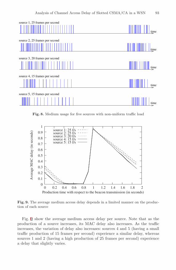
Analysis of Channel Access Delay of Slotted CSMA/CA in a WSN 93
time
time
time
time
time
source 1, 25 frames per second
source 2, 25 frames per second
source 3, 20 frames per second
source 4, 15 frames per second
source 5, 15 frames per second
Fig. 8. Medium usage for five sources with non-uniform traffic load
0
0.1
0.2
0.3
0.4
0.5
0.6
0.7
0.8
0.9
1
0 0.2 0.4 0.6 0.8 1 1.2 1.4 1.6 1.8 2
Ave
rage
MA
C d
elay
(in
sec
onds
)
Production time with respect to the beacon transmission (in seconds)
source 1: 25 f/ssource 2: 25 f/ssource 3: 20 f/ssource 4: 15 f/ssource 5: 15 f/s
Fig. 9. The average medium access delay depends in a limited manner on the produc-tion of each source
Fig. 9 show the average medium access delay per source. Note that as theproduction of a source increases, its MAC delay also increases. As the trafficincreases, the variation of delay also increases: sources 4 and 5 (having a smalltraffic production of 15 frames per second) experience a similar delay, whereassources 1 and 2 (having a high production of 25 frames per second) experiencea delay that slightly varies.

94 A. Guitton and N. Hadid
5 Linear Model of the Delay
As can be seen on Fig. 4, 6 and 9, the average MAC delay can be approximatedas a linear function of the time. In this section, we propose such a model.
Figure 10 shows the important points of our model. Notice that O denotes theorigin, that is, the beacon transmission time. b represents the beacon interval,and s represents the superframe duration (that is, the duration of the activeperiod). Frames produced shortly before point A can be sent without a largedelay. However, once the inactivity period starts, frames experience large delays.This is represented by point B. Frames accumulated during the inactivity periodcannot be sent instantaneously at the beginning of the next active period. It takesup to a certain time, represented by point C, to have all the accumulated framessent. We assume that the traffic load does not change a lot from one activeperiod to the next active period. That is why our model uses in fact a point C′,which corresponds to point C but in the current active period.
Our goal now is to determine the coordinates of each point. Trivially, xO =yO = yA = yC = yC′ = 0. We also have xB = xA = b and xC = xC′ + b. Fromthe IEEE 802.15.4 standard, we know that b = 15.36 × 2BO × 10−3 secondsand s = 15.36 × 2SO × 10−3 seconds. As the nodes queues are traditionally ofa first in first out (FIFO) type, the first frame that is queued at the beginningof the inactivity period is the first that is transmitted. This transmission occursat the beginning of the active period (after waiting for a backoff and winningthe competition for the medium). As the channel access time during the activeperiod is negligible compared to the inactive period duration, the delay for thefirst frame (which is the highest delay) is equal to the inactive period duration.Thus, yB = b − s.
The remaining value, xC′ , is computed using our experimental values, whichare summarized in Table 1. Let n denote the number of sources and l the total
A
B
CC′O
activityactivity inactivity
s
b
Fig. 10. A simple linear model of the average MAC delay

Analysis of Channel Access Delay of Slotted CSMA/CA in a WSN 95
Table 1. Value of xC as a function of the number of sources n and the traffic load l
Sources Load xC Sources Load xC
1 5 0.1 5 100 0.351 10 0.1 10 100 0.251 20 0.1 5 40 0.151 40 0.15 10 40 0.151 100 0.6
traffic load produced. From the values corresponding to n = 1, we have xC′ ≈6.5 × 10⁻⁵l2 − 1.5 × 10⁻³l + 0.1 (by using a polynomial regression of order 2).The number of sources only has a significant impact on the delay when l is high.That is why we started by expressing xC′ as a function of l. From the previousexpression of xC′ as a function of l, we injected n in the following way. Wenoticed that:
– xC′ for n = 5 and a given l is close to xC′ for n = 1 and 6 × l/8,– xC′ for n = 10 and a given l is close to xC′ for n = 1 and 5 × l/8.
Then, we found out a logarithmic fit for those values. We obtained the followingformula for xC′ :
xC′ = 6.5 × 10⁻⁵(8.18 × 0.94n × l/8)2 − 1.5 × 10⁻³(8.18 × 0.94n × l/8) + 0.1.
This model uses the total traffic load in the vicinity of the sensor, which canbe obtained by overhearing, by computing the average number of clear channelassessments that failed, by computing the average number of frame failures orby other mechanisms.
Our model could be improved by determining the final equation as a functionof n and l at the same time, rather than estimating it from l first, and adjustingit with n. Also, our model could be improved by taking into consideration thetraffic load of each source independently, in addition to the total traffic load.However, from the results of Sect. 4, we expect only a small improvement inthe approximation accuracy. A better improvement is certainly to model whathappens at point C′. Indeed, the delay is not linear at this point, especially whenthe traffic load is high.
6 Discussion on Aperiodic Traffic
In this section, we discuss about non-periodic traffic. While all the simulationsdone for this paper concerned periodic traffic, we believe that the traffic distri-bution is not a parameter that has a significant impact on the results presentedin this paper.
During the inactive period, the traffic is accumulated in the source queues.They serve as buffers, in the way of a leaky bucket: although they might be filledwith aperiodic traffic, they are still emptied with linear speed (see the left partof Fig. 4 and 6).

96 A. Guitton and N. Hadid
During the active period, the traffic arrival distribution has an impact ondelay. It is easier to deal with periodic frames in a fast manner than with burst offrames. However, this impact is limited. During the part of the active period whenall the accumulated frames have been sent (or dropped), frames can be dealt withvery efficiently. For example, we can see on Fig. 4 that it takes approximately0.2 seconds for one node to transmit 40 frames (on the line with 40 framesper second, approximately 40 frames have been accumulated during the inactiveperiod). Thus, even large bursts of 40 frames could be dealt with quickly. Duringthe part of the active period when there are still some accumulated frames thathave neither been sent nor dropped, the bursty frames accumulate with theprevious frames, in the same manner as during the inactive period.
7 Conclusion
Low-power wireless sensor networks are designed to operate for years. The priceto pay for the long energy autonomy of the devices is a larger medium accessdelay due to the long inactive periods. While many researchers have focused onoptimizing the delay in the active period, we studied in this paper the impact ofthe inactive period on the delay.
We have shown that inactive periods cause a bottleneck at the beginningof the activity period. This bottleneck takes a significant amount of time to bedealt with, which increases the delay of all the waiting packets, and increases theframe loss probability. We have also shown that having more sources can reducethe delay, but at the cost of greatly increasing the frame loss probability. Wehave concluded our analysies by providing an estimation model of the averagedelay as a function of the number of sources and the traffic load.
References
[CGM08] Chalhoub, G., Guitton, A., Misson, M.: MAC specifications for a WPANallowing both energy saving and guaranted delay - Part A: MaCARI: asynchronized tree-based MAC protocol. In: IFIP WSAN (2008)
[CHGM09] Chalhoub, G., Hadid, N., Guitton, A., Misson, M.: Deference mechanismssignificantly increase the MAC delay of slotted CSMA/CA. In: IEEE ICC(2009)
[IEE] IEEE 802.15 Task Group 4b. TG4b contributions,http://grouper.ieee.org/groups/802/15/pub/TG4b.html
[IEE06] IEEE 802.15. Part 15.4: Wireless medium access control (MAC) and phys-ical layer (PHY) specifications for low-rate wireless personal area networks(WPANs). Standard 802.15.4 R2006, ANSI/IEEE (2006)
[KAT06] Koubaa, A., Alves, M., Tovar, E.: A comprehensive simulation study ofslotted CSMA/CA for IEEE 802.15.4 wireless sensor networks. In: WFCS,July 2006, pp. 1–10 (2006)
[KCA07] Koubaa, A., Cunha, A., Alves, M.: A time division beacon schedulingmechanism for IEEE 802.15.4/Zigbee cluster-tree wireless sensor net-works. In: ECRTS (2007)

Analysis of Channel Access Delay of Slotted CSMA/CA in a WSN 97
[LKR04] Lu, G., Krishnamachari, B., Raghavendra, C.S.: Performance evaluationof the IEEE 802.15.4 MAC for low-rate low-power wireless networks. In:IPCCC, April 2004, pp. 701–706 (2004)
[PEE+06] Pollin, S., Ergen, M., Ergen, S.C., Bougard, B., Van Der Perre, L.,Catthoor, F., Moerman, I., Bahai, A., Varaiya, P.: Performance analy-sis of slotted carrier sense IEEE 802.15.4 medium access layer. In: IEEEGlobecom, November 2006, pp. 1–6 (2006)
[PKC+05] Park, T.R., Kim, T.H., Choi, J.Y., Choi, S., Kwon, W.H.: Throughputand energy consumption analysis of IEEE 802.15.4 slotted CSMA/CA.Electronics Letters 41(18), 1017–1019 (2005)
[SS07] Shu, F., Sakurai, T.: Analysis of an energy conserving CSMA-CA. In:IEEE Globecom, November 2007, pp. 2536–2540 (2007)
[TPGZ06] Tao, Z., Panwar, S., Gu, D., Zhang, J.: Performance analysis and a pro-posed improvement for the IEEE 802.15.4 contention access period. In:WCNC, April 2006, pp. 1–8 (2006)

S. Hailes, S. Sicari, and G. Roussos (Eds.): S-Cube 2009, LNICST 24, pp. 98–110, 2009. © Institute for Computer Sciences, Social-Informatics and Telecommunications Engineering 2009
Accurate Analysis of IEEE 802.15.4 Slotted CSMA/CA over a Real-Time Wireless Sensor Network
Wen-Tzeng Huang1, Jing-Ting Lin2, Chin-Hsing Chen3, Yuan-Jen Chang3, and You-Yin Chen4
1 Department of Computer Science & Information Engineering Minghsin University of Science & Technology
1, Hsin-Hsing Rd, Hsin-Fong, Hsin-Chu 30401, Taiwan, R.O.C. 2 Department of Graduate Institute of Computer and Communication Engineering
National Taipei University of Technology 1, Sec. 3, Chung-hsiao E. Rd., Taipei, 10608, Taiwan, R.O.C.
3 Department of Management Information Systems Central Taiwan University of Science and Technology
No.666, Buzih Road, Beitun District, Taichung City 40601, Taiwan R.O.C. 4 Department of Electrical and Control Engineering
National Chiao Tung University 1001 University Road, Hsinchu, 300, Taiwan, R.O.C
[email protected], [email protected], {chchen,ronchang}@ctust.edu.tw, [email protected]
Abstract. Here, we present the collision probability of the IEEE 802.15.4 slotted Carrier Sense Multiple Access/Collision Avoidance (CSMA/CA) mechanism over a real-time wireless sensor network (RT-WSN), also called a synchronous network system. The “backoff,” the random delay of CSMA/CA, can be used to create a probability model and to determine the average packet delay over RT-WSN. The proposed theoretical analysis model was nearly con-sistent with the simulation and with experimental results. This suggests that the slotted CSMA/CA mechanism cannot be applied effectively to RT-WSN be-cause it cannot avoid a high collision rate with RT-WSN application require-ments and, therefore, may waste a great deal of system bandwidth. We found that the packet collision rate increased up to 731% compared to an ideal model with more than 10 users within an RT-WSN. Without improvements in meth-odology, the high collision rate makes this slotted CSMA/CA mechanism un-suitable for RT-WSN applications.
Keywords: Real-time, wireless sensor network, collision, IEEE 802.15.4, CSMA/CA.
1 Introduction
The numerous advantages of wireless networking technology, including portability, no requirements for cables, flexibility, and low cost of constructing a network topol-ogy, have allowed it to be applied successfully in industry, medicine, transportation,

Accurate Analysis of IEEE 802.15.4 Slotted CSMA/CA 99
telemedicine, and home applications. Technological progress and the integration of wireless communication, batteries, and embedded processors have driven the devel-opment of Wireless Sensor Networks (WSN) [1]. In contrast with other types of wire-less networks, the WSN data transmission method uses many sensing sources, called sensor nodes, routed to a single destination, called the sink node. The sensor nodes can detect various environmental parameters within their effective sensing distance, such as temperature, humidity, luminosity, wind speed, and pressure. The sensed information is gathered by the sink node, and then may be analyzed by network ad-ministrators and users. Recently, WSN has become increasingly widespread and its applications have expanded to sensor networks [2], industrial communication [3], home applications, and medical treatment [4]. This has produced ever-increasing de-mands for WSN. Real-time performance is sometimes required, especially in multi-media applications, and, to guarantee real-time execution, the access time of wireless media applications must occur within a maximum delay time. In many networks, packet faults can be revised by the acknowledge/retransmit mechanism of the protocol used. Such systems will become paralyzed by the uncertain delays experienced in real-time applications [5].
Medium access control (MAC) performance analysis of the IEEE 802.15.4 low-rate wireless personal area network (LR-WPAN) [6] is discussed in this study. The beacon mode with slotted Carrier Sense Multiple Access/Collision Avoidance (CSMA/CA) applied to real-time WSN (RT-WSN) was evaluated under real-time conditions in a star network topology. Singh et al. [7] analyses the performance under the IEEE 802.15.4 star topology. They found that the saturation throughput of n nodes can be calculated by an embedded Markov renewal process, and also the relation be-tween the size of backoff and throughput. Therefore, they obtain an analytical model for the finite arrival rate case from the relation. This finite load model captures very well the qualitative behavior of the system. Finally, they used ns2 simulator to verify their model and simulation results. Kim et al. [8] studied the focus of the IEEE 802.15.4 unslotted CSMA/CA and proposed a simple mathematics model that utilized the wireless channel in the busy state to got the M/G/1 queueing system to make analysis. They can calculate the throughput, delay, and energy consumption in the bust state. Park et al. [9] proposed a new analysis model, which utilized the discrete time Markov chain to analyse the throughput and energy consumption of the slotted CSMA/CA. Timmons et al. [10] analysed the performance of the medical sensor body area networking context, which works in long-time operation. Hence, they focus on the power consumption issue.
The network performance parameters, time delay, throughput, and power con-sumption were also measured in these studies, and shown to affect the CSMA/CA RT-WSN. In this study, we evaluated the MAC performance required in real-time ap-plications and then analyzed the effects of CSMA/CA RT-WSN when users need to use as much bandwidth as possible.
Sections 2 and 3 of this paper describe the IEEE 802.15.4 standard and the con-struction of the network model, respectively. Section 4 shows the mathematical analy-sis of our proposed network model. The performance results of the simulation and experiment are verified in Section 5. Section 6 presents our conclusions.

100 W.-T. Huang et al.
2 Overview of the IEEE 802.15.4 Standard
The new standard of 802.15.4 was used to develop two-layer protocol stacks, the physical layer (PHY) and MAC, for LP-WPAN applications [6]. This standard has a number of characteristics, as follows:
• The data transmission rate can be 250, 40, or 20 kbps through the air. • Star or peer-to-peer operation. • Allocated 16-bit short address, with a maximum of 65535 connections. • CSMA-CA channel access. • Acknowledged protocol for transfer reliability. • Low power consumption. • Energy detection. • Link quality indication. • 16 channels in the 2450 MHz band; 10 channels in the 915 MHz band; and 1
channel in the 868 MHz band.
Figure 1 shows the two-layer structure of a star topology sensor network consisting of one personal area network (PAN) coordinator and several sensor nodes. The data flow path is from leaf nodes, called sensor nodes, to the PAN coordinator.
Fig. 1. The structure of a Star topology sensor network
There are two working modes, beacon and non-beacon, in the IEEE 802.15.4 stan-dard. The beacon mode uses broadcast communication to synchronize the network. The coordinator periodically broadcasts the beacon frame to all of the sensor nodes. The superframe structure, which is largely designed to allocate the time distribution mechanism, is defined in the beacon mode, as shown in Figure 2 [6]. This causes all of the sensor nodes in the network to synchronize two functions, sleep and wake-up. As the network works only in the active state, the time in this state can be divided into 16 equal segments, called time slots. Any action involves the use of one time slot as the basic working unit. For example, the transmission operation costs three time slots, and the waiting operation costs five time slots.
The two-part active state consists of the contention access period (CAP) and the contention-free period (CFP). During the CAP, the system will allow the sensor nodes

Accurate Analysis of IEEE 802.15.4 Slotted CSMA/CA 101
to compete freely to obtain channel access rights in the slotted CSMA/CA mecha-nism. Then, during the CFP, the system gives the sensor node exclusive access to the channel within its allocated time slot(s). Under these conditions, one node does not need to compete with other nodes to obtain access rights, guaranteeing the specificity of the sent data. The sensor node can also enter the power-saving mode to reduce power consumption during the inactive period. The lengths of the active and inactive periods can be adjusted by the superframe Order (SO) and Beacon Order (BO), re-spectively. According to the definition of the IEEE 802.15.4 standard, these can be set as follows: 0≦SO≦BO≦14, aBaseSuperframeDuration (which is a constant) = 960 as the default value, and one symbol (which is also a constant) = 16 µs in 2.4 GHz bandwidth operation. Therefore, the duration of the superframe is from 15.36 ms to 215.7 s. It does not use the superframe structure as SO = 15.
Fig. 2. The superframe structure of IEEE 802.15.4
During CAP, the sensor node competes with others to obtain channel access rights using the slotted CSMA/CA mechanism, as shown in Figure 3 [6]. The backoff period represents one unit of the time slots in CSMA/CA. In the slotted CSMA/CA, the backoff period boundaries of the sensor devices cannot be aligned with the time slot boundaries of the coordinator. Each sensor device maintains three variables, NB, CW, and BE. NB, which is used to determine when the channel is in the busy state, has an initial value of 0. CW indicates when the channel is empty and when it begins to transmit the data. PHY performing clear channel assessment (CCA) is used to detect whether the channel is idle or not. According to the range, 2BE
– 1, CSMA/CA allows the sensor node to delay one random backoff period. As this allows sensor nodes to transmit without overlapping with each other, their collision probability can be effec-tively reduced. When the channel is in the busy state, it can reattempt access within the number of macMaxCSMAbackoffs, which is a constant. Then, BE will be incre-mented by 1 such that it can increase the random range. The competition fails when the retry number is greater than macMaxCSMAbackoffs. After ensuring that the chan-nel is empty twice (CW = 2), the node begins to access the channel for successful competition.

102 W.-T. Huang et al.
Fig. 3. The slotted CSMA/CA mechanism
Table 1. Default values of the CSMA/CA parameters
Parameters Default ValueaMaxBE 5macMaxCSMABackoffs 4macMinBE 3macBattLifeExt FALSE

Accurate Analysis of IEEE 802.15.4 Slotted CSMA/CA 103
CSMA/CA contains one other parameter, the binary constant macBattLifeExt. If the system needs to reduce the duty cycle of the network, macBattLifeExt can be set as “TRUE,” which can reduce the delay of the backoff period and conserve battery energy. The default values of the CSMA/CA parameters are shown in Table 1.
3 Our Network Module
Our proposed network system is constructed as a star network consisting of one mas-ter node and many slave devices for monitoring. This protocol includes two classic tasks, a synchronous and an asynchronous task [11, 12]. The synchronous task in-volves periodic polling of each slave node for received data (e.g., temperature, lumi-nosity, humidity, pressure, rotation, and angle) from monitoring sensor devices. The asynchronous task does not involve periodic transmission and its transmission time is therefore fixed (event-driven). In comparison with previous systems, this type of sys-tem generally requires the ability to take the bounded time to be finished within the critical path.
In the synchronous task, data from the sensor nodes will be periodically and con-tinuously sent to the coordinator. Generally, the system is capable of maintaining the sampling rate so that it can be implemented within the limitations of the memory buffer. For real-time requirements, the synchronous task of the sensor network is de-fined by RT-WSN.
The star topology sensor network of the IEEE 802.15.4 standard was employed in this study. Our system used the beacon-enabled configuration, which allows the coor-dinator to periodically broadcast beacons to all of the sensor nodes. After receiving the beacon, the sensor node performs the slotted CSMA/CA mechanism to obtain the access rights of the channel. Then, the successful node sends its packet to the coordi-nator. This is just one way to transmit the packet from the sensing node to the coordi-nator. Although the CSMA/CA mechanism can decrease the probability of collision, too many sensors and too heavy a traffic load within the network will cause a high collision rate. This results in the loss of the packet, increased delays and decreased the bandwidth, and the gradual degradation of network performance. To analyze, in de-tail, collision performance under the CSMA/CA mechanism, some terms of the net-work model are defined as follows:
• Maximize traffic load: The traffic load is equal to the maximum throughput
of the system. Under the IEEE 802.15.4 standard at 2.4 GHz, the maximum bandwidth is 250 kbps. Throughput is possible in the saturate case, although the network simultaneously uses many sensor nodes.
• Fixed packet length: The length of all packets is set to a fixed value with a maximum of 128 bytes, according to the IEEE 802.15.4 standard.
• Without re-transmit/acknowledgment: Because of the requirements for real-time operation, the re-transmit mechanism settings do not provide redundant time for re-transmission by the network's sensor nodes [5]. When data are missing or the transmission is in error, the sensor node waits until the next beacon cycle to re-send the packet.
• Without inactive/sleep mode: When the system is operating at a high utiliza-tion rate or in a high duty cycle, it disables the sleep mode.

104 W.-T. Huang et al.
• Without packet loss rate: The packet cannot be lost in the normal case. Al-though some packets will be lost because of factors related to environment, distance, interference, and signal intensity, this study does not consider the effects of these factors.
When the sensor nodes are sent their packets passively according to the requirements of the coordinator, the maximum sampling rate of the system corresponds to the set
Fig. 4. Our network module
Fig. 5. The slotted CSMA/CA mechanism after adjusting

Accurate Analysis of IEEE 802.15.4 Slotted CSMA/CA 105
beacon period. To obtain real-time data in our model, we set the beacon period time equal to the sum of the packet transmission times of all of the sensor nodes. For ex-ample, when five sensor nodes are in the network, each with a packet transmission time of 4 ms, the beacon period is set to a minimum of 5 × 4 = 20 ms. In the beacon enabled mode, the superframe structure can be adjusted by our proposed method to reduce the redundant action. Hence, the length of one time slot equals the transmis-sion time of one packet, and the number of time slots equals the number of sensor nodes, as shown in Figure 4.
In our module without collision, the packets of all of the sensor nodes can only be sent once during the beacon period. The system waits until the next beacon cycle to transmit, because collisions may cause the loss of the packet. In this case, this time slot cannot be used by any node, which wastes bandwidth. Although the backoff pe-riod is one random time slot length, it cannot run over the beacon period time. The maximum of the random variable is (n – 1), where n is the number of sensor nodes. For example, the maximum length of the backoff period is four when the number of sensor nodes is five. With clear channel assessment (CCA), there is no time to com-pete again if the channel is in the busy state.
4 Mathematical Analysis
In this study, we propose a network analysis model to analyze the behavior of the slotted CSMA/CA over RT-WSN. Too many collisions cause time delays, which waste bandwidth and prevent the requirements of real-time operation. An analysis of the degree of network collisions therefore allows an evaluation system performance.
From the protocol of one packet, it will be allocated one random length of the backoff period during the competition case. Here, one unit of the backoff period is equal to the unit length of one time slot. There are n time slots during the beacon pe-riod, where n is the number of sensor nodes. The packet can randomly choose one of n time slots to access, as shown in Figure 6. Two sensor nodes will choose the ran-dom variables in the system. A collision will occur if more than two nodes choose the same random variable. In this case, both of the packets may be lost. This is one of the major causes of network performance degradation.
Fig. 6. Packets to be transmitted during any time slot

106 W.-T. Huang et al.
The following important parameters are defined for our model:
• n : Number of sensor nodes. • Network(i) : There are i sensor nodes inour network model. • slot : The time slot is equal to the packet transmission time. • #slot : Number of time slot. • DAvg(n) : Average of packet delay of the sensor node in n sensor nodes. • Collision(i) : The number of sensor nodes that simultaneously choose the
same random variable is “i,” which will generate “i” collisions and lose “i” packets during the same “backoff” period.
• P(e) : Outcome probability of the event e. • S(e) : One set contains the amount of all possible outcome samples during
event e, also called “sample space” of the event e.
To analyze the collision probability within n sensor nodes over RT-WSN, or P(Collision(n)), the statistics of the sample space are be gathered first. We assume that one slot can be chosen as the candidate element among n sensor nodes. One can-didate element among n time slots with n packets can be chosen, and all candidate elements can be counted by the statistics method as shown in (1).
nn nslotnNetworkS ==#))(( (1)
Let S(Network) be the total sample space over RT-WSN, containing a combination of collision and non-collision incidents. Let “#slot” be the number of slots, and Colli-sion(0), …, Collision(n) be the collision probability of the nodes 0, 1, …, n, respec-tively. Therefore, the sample S(Network) of the network is the union of all incidents as shown in (2).
))( ())2( ())1( ())0( ()( nCollisionSCollisionSCollisionSCollisionSNetworkS ∪∪∪= (2)
Let Set(Collision(i)) be the set number of Collision(i). Hence, the collision probability within i sensor nodes, P(Sollision(i)), under S(Network) is shown in Eq. (3).
))((
))( ())( (
nNetworkS
iCollisionSiCollisionP = (3)
Therefore, Collision(i) means that there are i time slots to be wasted. Then, it will take more cost of i × slot time delays. Hence, The average packet time delays under n sen-sor nodes, DAvg(n), is the summation of the wasted time delays of all possible collision probability as shown in Eq. (4).
( )
slotnnNetworkS
nCollisionS
nNetworkS
CollisionS
nNetworkS
CollisionS
slotnnCollisionPCollisionPCollisionPnDAvg
⋅⋅++⋅+⋅=
⋅⋅++⋅+⋅=
⎟⎠⎞
⎜⎝⎛
))((
))( (1
))((
))1( (0
))((
))0( (
))( ( 1))1( (0))0( ()(
(4)
First, to get (n – i) elements without collision from n sensor node samples, let the amount of them be shown in Eq. (5).

Accurate Analysis of IEEE 802.15.4 Slotted CSMA/CA 107
))!(()!(
!
innin
nnin
C−−−
=−
(5)
Second, let the permutation of (n – i) elements within n time slots be shown in Eq. (6).
))!((
!
inn
nnin
P−−
=−
(6)
Finally, let DAvg(n) be the average package delay with the collision case in n sensor nodes, and it can be derived from above equations and shown in Eq. (7), where Set(G(i , i)) will be shown in Eq. (8).
iiiGSPCn
slotnD
n
i
nin
ninnAvg ⋅⋅⋅= ∑
=−− )),(()(
0
(7)
Then, the recursion relation S(G(i , k)) can be defined as Eq. (8). There are 2 initial conditions are as follows. One, S(G(0 , 0)) = 1, is non-collision and the other, S(G(1 , 1)) = 0, is one sensor node with the collision case.
kiddGSPCk
kiGS
k
d
kdk
kdk
i =⎪⎪⎪
⎩
⎪⎪⎪
⎨
⎧
>⋅⋅−
=
=
=
∑−
=−−
1.i if,)) , ((
1,i if,0
0,i if ,1
)) , ((
1
0
(8)
5 Simulation and Experiment Results
To confirm our methodology, we verified our proposed theoretical analysis with simulation and experimental results. We found that the slotted CSMA/CA mechanism cannot be applied effectively to RT-WSN because it cannot avoid a high collision rate with real-time application requirements, and wastes a great deal of system bandwidth. We used the simulation tool Matlab to create the network model to be simulated. Fig-ure 7(a) shows our implementation hardware [13] with the ZigBee RF module [14] and the MPS430 microcontroller [15]. The real experiments over RT-WSN within one office are shown in Figure 7(b). In our experiment, the transmission packet time was 8.706 ms and the number of sensor nodes ranged from 1 to 10.
A comparison among the numerical, simulation, and experimental results is shown in Figure 8(a); the number of sensor nodes is on the horizontal axis and the average transmission delay within one packet on the vertical axis. We found few differences among all three sets of results. The average delay per packet was 55 ms in the 10 sen-sor nodes. Therefore, the packet load was (8.7 + 55) / 8.7 × 100% = 731% that of the standard mode.

108 W.-T. Huang et al.
The real bandwidth effect of the measurement collision is shown in Figure 8. In this experimental platform, the access critical time of one packet was about 14.712 ms, and the length of one packet without the header was 115 bytes (IEEE 802.15.4 standard). Hence, the system bandwidth within one sensor node was 62 kbps.
(a) (b)
Fig. 7. (a) Our experiment platform. (b) The experiment of the RT-WSN environment with eight sensor nodes.
(a) (b)
Fig. 8. (a) The average packet delay on 10 nodes. (b) The bandwidth effect of collision on 10 nodes.
6 Conclusions
In this study, we proposed an effective mathematical analysis methodology to be ap-plied to real-time WSN under the IEEE 802.15.4 standard. Our theoretical analysis model was consistent with the simulation and experimental results indicating that this slotted CSMA/CA mechanism cannot be effectively applied to RT-WSN because it cannot avoid the high collision rate with real-time application requirements and wastes a great deal of system bandwidth. We found that the packet collision rate in-creased up to 731% compared to an ideal model with 10 users within RT-WSN.

Accurate Analysis of IEEE 802.15.4 Slotted CSMA/CA 109
Generally, most synchronous network systems possess real-time characteristics be-cause they need to use as much network bandwidth as possible. We found that the slotted CSMA/CA mechanism is not a good choice for real-time applications, when the user wants to increase sensor nodes in the system to consider that there is the side effect of the high packet collision rate. The IEEE 802.15.4 standard is suitable for asynchronous system applications in distributed networks in the home, industry, and medical settings.
Acknowledgment
The authors would like to thank the National Science Council of the Republic of China for financially supporting this research under Contract No. NSC 97-2218-E-159 -002-, NSC 97-2622-E-027-009-CC3 and NSC 97-3114-E-002-003-.
References
1. Akyildiz, I.F., Su, W., Sankarasubramaniam, Y., et al.: Wireless sensor networks: s survey. Computer Networks 38, 393–422 (2002)
2. Callaway, E.H.: Wireless sensor networks: Architectures and protocols. CRC Press, Boca Raton (2004)
3. Willig, A., Matheus, K., Wolisz, A.: Wireless technology in industrial networks. Proc. IEEE 93, 1130–1151 (2005)
4. Golmie, N., Cypher, D., Rebala, O.: Performance evaluation of low rate WPANs for medi-cal applications. In: Military Communications Conference 2004, pp. 927–933 (2004)
5. Van Den Bossche, A., Val, T., Campo, E.: Metrologie pour l’analyse comparative des per-formances temporelles des liens Bluetooth. Sciences of Electronic, Technologies of Infor-mation and Telecommunications 2005 (2005)
6. IEEE 802.15.4: Wireless LAN medium access control (MAC) and physical layer (PHY) specifications for low-rate wireless personal area network, LR-WPANs (2006)
7. Singh, C.K., Kumar, A., Ameer, P.M.: Performance evaluation of an IEEE 802.15.4 sensor network with a star topology. Wireless Networks 14, 543–568 (2008)
8. Kim, T.O., Park, J.S., Chong, H.J., Kim, K.J., Choi, B.D.: Performance analysis of IEEE 802.15. 4 non-beacon mode with the unslotted CSMA/CA. IEEE Communications Let-ters 12, 238–240 (2008)
9. Park, T.R., Kim, T.H., Choi, J.Y., Choi, S., Kwon, W.H.: Throughput and energy con-sumption analysis of IEEE 802.15. 4 slotted CSMA/CA. Electronics Letters 41, 1017–1019 (2005)
10. Timmons, N.F., Scanlon, W.G.: Analysis of the performance of IEEE 802.15.4 for medical sensor body area networking. IEEE SECON 4, 16–24 (2004)
11. Bertocco, M., Gamba, G., Sona, A.: Is CSMA/CA really efficient against interference in a wireless control system? An experimental answer. In: 13th. IEEE International Conference on Emerging Technologies and Factory Automation, pp. 885–892 (2008)
12. Bertocco, M., Gamba, G., Sona, A., Vitturi, S.: Performance measurements of CSMA/CA-based wireless sensor networks for industrial applications. In: IEEE Instrumentation And Measurement Technology Conference 2007, pp. 1–6 (2007)

110 W.-T. Huang et al.
13. Huang, W.T., Jeong, H.D.J.: A novel implementation of high-reliability wireless sensor network platform with serpentine-antenna design. In: The 3rd International Workshop on Intelligent, Mobile and Internet Services in Ubiquitous Computing (to be published, 2009)
14. Uniband Electronic Corp. (UBEC), U-Force Module User Manual, http://www.ubec.com.tw/product/U-Force.html
15. Texas Instruments Incorporated, MSP430x15x, MSP430x16x, MSP430x161x mixed sig-nal microcontroller, http://www.ti.com/lit/gpn/msp430f1611/

S. Hailes, S. Sicari, and G. Roussos (Eds.): S-Cube 2009, LNICST 24, pp. 111–126, 2009. © Institute for Computer Sciences, Social-Informatics and Telecommunications Engineering 2009
Physical Characterization of Acoustic Communication Channel Properties in Underwater Mobile Sensor
Networks
Andrea Caiti, Emanuele Crisostomi, and Andrea Munafò
ISME, Interuniversity Research Centre on Integrated Systems for the Marine Environment, c/o DSEA, Dept. Electrical Systems and Automation, University of Pisa,
Largo Lucio Lazzarino (già via Diotisalvi 2), 56100 Pisa, Italy {caiti,munafo}@dsea.unipi.it, [email protected]
Abstract. A methodology to predict underwater acoustic channel communica-tion properties (capacity, bandwidth, range) from the environmental conditions in the ocean is proposed. The methodology is based on the use of acoustic propagation models coupled to a set of equations proposed firstly by Stojanovic [1]. A parametric study of channel characteristics as a function of changing en-vironmental conditions is presented, showing in particular how channel range and/or source transmission power are influenced by the relative position of source and receiver with respect to the ocean temperature thermocline. This kind of results is crucial to adaptively configure the relative position of mobile nodes (typically AUVs – Autonomous Underwater Vehicles) in underwater sensor networks, with the final goal of mitigating the effects of environmental changes on the network communication capabilities.
Keywords: AUV, underwater sensor networks, underwater communication, underwater acoustics, acoustic propagation.
1 Introduction
Since the seminal work of Curtin et al. [2], many progresses have been made toward the operational implementation of Autonomous Ocean Sampling Networks (AOSN). In particular, advances in miniaturization and embedded systems technology has now made possible the design and realization of low-cost Autonomous Underwater Vehi-cles (AUVs) [3], [4], that, equipped with appropriate oceanographic payloads, can act as a team in mapping specific areas of the ocean. Cooperation and coordination algo-rithms for mobile robotic vehicles have been successfully applied to teams of AUVs and/or oceanographic gliders [5]. Some large scale experimentation, in which net-works of mobile and fixed sensors, autonomous or semi-autonomous, have been em-ployed to monitor the evolution of ocean dynamics, have been successfully reported [6]. Nevertheless, the challenges posed by the ocean environments are such that there are still scientific and technological problems to be solved for the realization of the original AOSN vision.

112 A. Caiti, E. Crisostomi, and A. Munafò
One challenge not yet solved is related to the problem of communication among the underwater platforms, either fixed or mobile, composing the sensor network. Since electromagnetic waves are so strongly attenuated in salty waters to prevent any radio communication at distances exceeding few meters, acoustic waves are used for underwater communication. Hence, the physics of underwater acoustic propagation plays a key role in the determination of the communication channel characteristics. In turn, the physics of acoustic propagation is strongly influenced by the oceanographic conditions, since the sound speed in the water is a function of temperature, salinity and depth, and these quantities vary both in space and in time [7]. While several ap-proaches have been proposed to model the underwater acoustic communication chan-nel (see for instance [8] for a recent review), there still appears to be a gap in the sci-entific literature between the channel characterization which is required for communi-cation system design, and the physical modeling of acoustic propagation.
In an attempt to bridge the above mentioned gap, Stojanovic [1] has proposed a set of expressions to determine maximum channel capacity and bandwidth as a function of the intensity loss of the acoustic signal. In [1], analytical computations are given for the case in which the medium (i.e., the ocean channel) is homogeneous and the intensity loss is due only to geometrical spreading and to the intrinsic attenuation of the medium. However, intensity loss is among the parameters computed by acoustic propagation codes: so, at least in principle, the approach of [1] can be extended in a straightforward manner by using appropriate numerical models of the acoustic channel.
The contributions of this paper are twofold:
• it is shown how indeed a specific computational code (the code “Bellhop”, based on ray theory [7], [9]) can be used in order to derive communication channel characteristics following the approach of [1]; in doing this, we also discuss the set of modifications and/or caveat that have to be considered be-fore transposing directly the results of the model into the channel equations.
• a parametric study based on the above mentioned channel modeling is per-formed to determine the variability of the communication channel perform-ance as a function of the variability of the environmental conditions (and therefore of the acoustic propagation conditions).
The sensitivity study is directed toward the determination of optimal strategies for mobile nodes motion in an AOSN to maximize communication performance or to maintain team communication connectivity [10], [11]. While this latter problem is not treated in this paper, the results reported here are instrumental to the implementation of cooperative distributed motion algorithms in underwater sensor networks.
The paper is organized as follows: in the next section the main aspects of acoustic propagation relevant to the communication problem are briefly reviewed, the ap-proach of [1] to the modeling of the acoustic communication channel reported, and the assumptions, validity limits and implementation choices adopted in coupling the physical model Bellhop to the communication channel equations illustrated. In Sec-tion 3 the simulative scenarios are described; in particular, we consider three cases, and in all of them sound speed changes only as a function of depth in the water col-umn, but not of range between transmitter and receiver: in one case the sound speed is constant with depth (similar to the analytical case of [1]), in the other two cases a thermocline region is considered (i.e., a region in which temperature, and hence sound

Physical Characterization of Acoustic Communication Channel Properties 113
speed, has a constant gradient with depth), and transmitter and receivers are located within the thermocline, or on opposite sides of the thermocline. Simulations for the three cases are referred to two different scenarios, one taken from the original Stoja-novic paper [1], and the other, considering higher frequencies and shorter ranges, corresponding to a more realistic operational configuration. Conclusions and future work are addressed in Section 4.
2 Acoustic Propagation and Communication Channel Characterization
In this section we first review the physics of acoustic propagation and the assumptions of the ray modeling approximation. Subsequently, the channel characterization pro-posed in [1] is reported and linked to the ray model.
2.1 The Physics of Acoustic Propagation
The pressure field generated by an acoustic (compressional) wave traveling in the ocean medium is governed, in the linear approximation, by the Helmholtz equation [7]:
2 2[ ( )] ( , ) ( ) ( )k fψ ω ω δ∇ + = − sx x x x (1)
where ω is the angular frequency, x is the position in the space coordinate frame, 2∇ is the Laplacian operator, ( ) / ( )k cω=x x is the wavenumber, ( )c x is the sound
speed in the medium as a function of geographical position, ( )f ω is the forcing term
due to a point source at location sx , δ is the Dirac’s delta function, ψ is the wave
potential. The pressure is related to the wave potential by the equation:
( , ) ( , )p ω ρω ψ ω= 2x x (2)
where ρ is the medium density, and it is considered constant in the following. To
solve the Helmholtz equation it is necessary to specify the boundary conditions, in terms of sea surface and bottom depth, and the medium characteristics, in terms of the sound speed in the medium, which in practice depends on the ocean dynamics. The coordinate reference frame is usually taken with the origin at the sea surface and the z axis pointing downward toward the sea bottom. By assuming the existence of a solu-tion to the homogenous Helmholtz equation of the form:
( )
0
( , ) j hh
h
ap e ωτω
ω
+∞
=
= ∑xx . (3)
and substituting (3) into equations (1) and (2), neglecting the terms where ω appears at the denominator, one gets the ray-theory approximation equations:

114 A. Caiti, E. Crisostomi, and A. Munafò
22
1( )
( )cτ∇ =x
x (eikonal equation)
20 02 ( ) 0a aτ τ∇ ⋅∇ + ∇ = (transport equation)
(4)
(5)
where ( )τ x is the time of arrival of an acoustic ray from the origin to the position x.
The above derivation has been outlined to emphasize that the ray theory approach, which is followed since now on, due to its intuitive appeal, it is an approximation which is valid only in the high frequency regime (usually above the KHz).
In qualitative terms, using the ray approximation, an acoustic wave traveling from a source in the ocean water column will manifest itself as a sequence of arrivals corre-sponding to the various rays (Fig.1, left). Different rays will arrive at the receiver following different paths (multi-path arrivals). The paths themselves will be deter-mined by the sound speed in the medium through the Snell’s refraction law (which is embedded in the eikonal equation). In (Fig. 1, centre) a typical sound speed profile as a function of depth is shown. The corresponding ray paths are shown in (Fig. 1, right) assuming cylindrical coordinates and sound speed constant with range.
Fig. 1. The geometry of the transmitter and the receiver is shown on the left. Rays can arrive to the destination following different paths. A typical sound speed profile is shown in the middle, while the corresponding ray paths are shown on the right.
The acoustic intensity ( )I x is the power per unit surface of an acoustic wave, and it
is proportional to the square of the pressure. The transmission loss TL of an acoustic wave is defined as:
( )10 0( , ) 10 ( , ) /TL Log I Iω ω= −x x . (6)
where 0I is the reference intensity. In underwater acoustics, the reference intensity is
the intensity of a plane wave having rms pressure amplitude of 1 Paμ at 1m distance
from the source. By numerical solution of the transport equation, it is possible to numerically compute TL in the ray approximation. The computational code “Bellhop”

Physical Characterization of Acoustic Communication Channel Properties 115
[9] is such a code; it is widespread in the scientific community, having passed the appropriate recognized benchmark tests. In the following of the paper, all the simula-tive results will be obtained through Bellhop. Moreover, in all our simulations we will refer to the so-called “range independent” environmental conditions: a cylindrical coordinate frame will be assumed, with axis r (range) and z (depth); the source is always placed on the 0z = axis, and ( , ) ( )c r z c z= .
It is important to remark that the Bellhop model includes the following physical mechanisms of intensity loss: the geometrical spreading, computed along the paths for each ray; the intrinsic attenuation, which is the attenuation due to mechanical and thermodynamic effects of pressure propagation in salty water, and which is frequency dependent; the wave interference patterns due to the superposition of different rays.
The transmission loss can be used to predict the intensity level S at the receiver due to a source of intensity SL through the so-called passive sonar equation:
( ) ( )S SL TL= −x x (7)
By considering also an ambient noise term, the passive sonar equation can be formu-lated in terms of the Signal-to-Noise Ratio (SNR) at the receiver as follows:
( , ) ( , ) ( )SNR SL TL Nω ω ω= − −x x (8)
where all the above quantities are in dB ref 1 Paμ @1m. The same SNR can be ex-
pressed in natural scale as: ( , ) ( ) ( )snr I nω ω ω=x . The ambient noise term ( )N ω , or
( )n ω in natural scale, may depend on a series of factors (ship traffic, wave mo-
tions,…) and the noise model defined in [1], [12], is considered in the remainder of this paper, with the same parameter choices of [1]. Space limitations prevent to report the model here.
For any given source position sx , and for any receiver position x and any fre-
quency ω it is possible to define the channel transfer function ( , , )G ωsx x satisfying
the following relation between transmitted and received pressure:
( , ) ( , , ) ( )sp G pω ω ω= sx x x . (9)
where ( )sp ω is the source signal. The transmission loss can also be computed from
the transfer function as:
1020 ( , , )TL Log G ω= − sx x . (10)
while the SNR in terms of transfer function is given as:
( )22
10 1010 10 sp GSNR Log snr Log
n
⎛ ⎞⎜ ⎟= − = −⎜ ⎟⎝ ⎠
. (11)

116 A. Caiti, E. Crisostomi, and A. Munafò
2.2 Acoustic Communication Channel Characterization
This section reports the definitions and equations proposed in [1] to characterize an acoustic communication channel on the basis of the transmission loss (equation (6)), of the SNR (equations (8) and (11)) and of the channel transfer function (equation 9). The original equations of [1] are slightly reformulated here to better link them to the physical description of the previous section, but preserving the same approach and considerations of [1]. We first note that, for any source-receiver geometric configura-tion ( , )sx x it is possible to define an optimal transmission frequency as:
2
0
( , , )( , ) arg max
( )
G
nω
ωω
ω= s
s
x xx x . (12)
A heuristic 3-dB bandwidth 3 0( )B ω can then be defined as the range of frequencies in
the neighborhood of 0ω such that 0( ) ( ) 3SNR SNRω ω> − . For any given transmitted
source signal ( )Sp ω , the source intensity in the bandwidth 3 0( )B ω is proportional to
the square of the pressure spectrum integrated over the bandwidth:
3
2 ( )S sBI p dω ω∝ ∫ . (13)
The SNR, expressed in natural scale, within the 3dB bandwidth, is thus obtained by integrating the argument of the Log function in equation (11) over the bandwidth:
3
3
3
22 ( ) ( )( )
( )
sB
B
B
p G dsnr
n d
ω ω ωω
ω ω=∫
∫. (14)
Equation (14) can then be used to dimension the source level (through ( )Sp ω ) in
order to achieve a prescribed SNR gain. In particular, assuming a constant source level 3p over the 3dB bandwidth, in order to obtain a prescribed SNR γ (in natural
scale) the following relation must hold:
3
3
23 2
( )
( )
B
B
n dp
G d
ω ωγ
ω ω≥
∫∫
. (15)
The corresponding channel capacity is given as:
3
223
3 2
( )log 1
( )B
p GC d
n
ωω
ω
⎛ ⎞⎜ ⎟= +⎜ ⎟⎝ ⎠
∫ . (16)

Physical Characterization of Acoustic Communication Channel Properties 117
As observed in [1], the above heuristic definition does not guarantee the optimality in the energy distribution across the system bandwidth. Therefore, in [1] it is proposed also the following approach, termed capacity-based bandwidth definition, in which the bandwidth is indeed defined in order to maximize the channel capacity. In particu-lar, under the assumption of time-invariance of the channel, by subdividing the band-width in sub-bands of width ωΔ such that the channel transfer function G can be considered constant within the sub-band and the noise term n white within the sub-band, the channel capacity for a receiver located in x is given by:
22
2
( ) ( )( ) log 1
( )s h h
h h
p GC
n
ω ωω
ω
⎛ ⎞⎜ ⎟= Δ +⎜ ⎟⎝ ⎠
∑x . (17)
The optimal energy distribution within the bandwidth is obtained by maximizing the
capacity in equation (17) with the constraint of finite transmitted power 2sp∫ . The
optimal signal power spectrum must satisfy the water-filling principle [13]:
22
( )( )
( )s
np
G
ωω κω
+ = . (18)
where the constant κ is determined from the resulting signal power. The SNR corre-sponding to the optimal energy distribution is obtained as:
2 22 ( ) ( ) ( )( ) 1
( ) ( )
sB B
B B
p G d G dsnr
n d n d
ω ω ω ω ωω κ
ω ω ω ω= = −∫ ∫
∫ ∫. (19)
and the transmitted power is:
22
( )( )
( )S s
B B
nP p d B d
G
ωω ω κ ωω
= = −∫ ∫ . (20)
Once a prescribed SNR γ (in natural scale) is given, the following iterative procedure
can be employed to determine the optimal energy distribution:
1. For each receiver position x, the optimal transmission frequency (equation
12) is determined; (0)κ is initialized as 2
0 0(0) ( ) 2 ( )n Gκ ω ω= (note that
κ will vary with receiver position) 2. given ( )mκ , determine the bandwidth ( )B m as the region of frequencies
around 0ω such that 2
0 0( ) ( ) ( )m n Gκ ω ω> ;
3. compute snr(m) from equation (19) using ( )B m and ( )mκ ;
4. if ( )snr m γ< , set ( 1) ( )m mκ κ ε+ = + , with ε (small) constant and go to
step 2; otherwise, exit with ( )mκ κ= and ( )B B m=
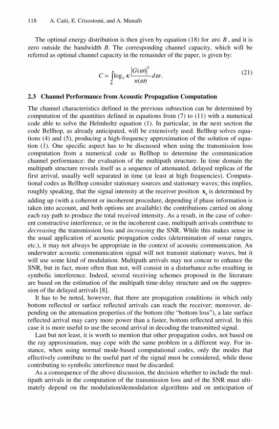
118 A. Caiti, E. Crisostomi, and A. Munafò
The optimal energy distribution is then given by equation (18) for Bω ∈ , and it is zero outside the bandwidth B. The corresponding channel capacity, which will be referred as optimal channel capacity in the remainder of the paper, is given by:
2
2
( )log
( )B
GC d
n
ωκ ω
ω= ∫ . (21)
2.3 Channel Performance from Acoustic Propagation Computation
The channel characteristics defined in the previous subsection can be determined by computation of the quantities defined in equations from (7) to (11) with a numerical code able to solve the Helmholtz equation (1). In particular, in the next section the code Bellhop, as already anticipated, will be extensively used. Bellhop solves equa-tions (4) and (5), producing a high-frequency approximation of the solution of equa-tion (1). One specific aspect has to be discussed when using the transmission loss computation from a numerical code as Bellhop to determine the communication channel performance: the evaluation of the multipath structure. In time domain the multipath structure reveals itself as a sequence of attenuated, delayed replicas of the first arrival, usually well separated in time (at least at high frequencies). Computa-tional codes as Bellhop consider stationary sources and stationary waves; this implies, roughly speaking, that the signal intensity at the receiver position sx is determined by
adding up (with a coherent or incoherent procedure, depending if phase information is taken into account, and both options are available) the contributions carried on along each ray path to produce the total received intensity. As a result, in the case of coher-ent constructive interference, or in the incoherent case, multipath arrivals contribute to decreasing the transmission loss and increasing the SNR. While this makes sense in the usual application of acoustic propagation codes (determination of sonar ranges, etc.), it may not always be appropriate in the context of acoustic communication. An underwater acoustic communication signal will not transmit stationary waves, but it will use some kind of modulation. Multipath arrivals may not concur to enhance the SNR, but in fact, more often than not, will consist in a disturbance echo resulting in symbolic interference. Indeed, several receiving schemes proposed in the literature are based on the estimation of the multipath time-delay structure and on the suppres-sion of the delayed arrivals [8].
It has to be noted, however, that there are propagation conditions in which only bottom reflected or surface reflected arrivals can reach the receiver; moreover, de-pending on the attenuation properties of the bottom (the “bottom loss”), a late surface reflected arrival may carry more power than a faster, bottom reflected arrival. In this case it is more useful to use the second arrival in decoding the transmitted signal.
Last but not least, it is worth to mention that other propagation codes, not based on the ray approximation, may cope with the same problem in a different way. For in-stance, when using normal mode-based computational codes, only the modes that effectively contribute to the useful part of the signal must be considered, while those contributing to symbolic interference must be discarded.
As a consequence of the above discussion, the decision whether to include the mul-tipath arrivals in the computation of the transmission loss and of the SNR must ulti-mately depend on the modulation/demodulation algorithms and on anticipation of

Physical Characterization of Acoustic Communication Channel Properties 119
some peculiarities in the propagation behaviour. In the simulations reported in the next section, we have not considered multipath arrivals; all else being equal, inclu-sions of the multipath structure would have led to an increase in the estimated per-formance of the channel. This means that the results obtained are valid only for those demodulating schemes that suppress the delayed echoes due to the multipath structure and for situations in which a direct path is always present between transmitter and receiver.
3 Simulations and Sensitivity Analysis to Sound Speed Variation in the Water Column
In this section we consider two different scenarios and three cases for each scenario. The first case is indicated as “nominal scenario”, and it is similar to that analyzed in [1]: frequencies vary from 10 Hz to 20 KHz, transmitter-receiver ranges vary from 1Km to 100Km. The nominal scenario has been included in order to allow an easy comparison between our computational results and the analytical results reported in [1]. The second case is indicated as “operative scenario”, since it is closer to the ex-pected frequencies and ranges that are or may be used in AOSN applications: fre-quencies vary between 20 and 50 KHz, and transmitter-receiver ranges vary from 100m to 6000m. In both scenarios, three cases are considered with different environ-mental conditions: constant sound speed profile (equivalent to the analytical case of [1]); presence of a thermocline with both transmitter and receiver in the thermocline region; presence of a thermocline with the transmitter above the thermocline and the receiver below. The transmitter depth is 300 m above the receiver depth in the nomi-nal scenario, and 100 m above the receiver depth in the operational scenario. The results are always reported as a function of the horizontal range between transmitter and receiver. Water depth and bottom absorption do not play any role since we are considering only direct arrivals. The sound speed profile varies with depth (hence the presence of a thermocline) but not with range (range independent environmental conditions).
In both scenarios, the following results have been produced and presented as graphical output for the three cases considered: SNR as a function of frequency; optimal frequency as a function of range; heuristic bandwidth and capacity; optimal bandwidth and capacity; source power required to reach a 20 dB gain in SNR as a function of range.
3.1 Nominal Scenario
The three cases considered for the nominal scenario, in terms of relative position and sound speed profile in the water column, are reported in Fig. 2. The gradient in the sound speed profile corresponds to the thermocline region. In the simulations, fre-quencies from 10Hz to 20KHz have been considered, with 100Hz spacing starting from 100Hz. Horizontal range varies between 1 and 100Km; 200 range slices have been considered.

120 A. Caiti, E. Crisostomi, and A. Munafò
Fig. 2. The three cases considered, with different speed profiles as a function of depth, from the left to the right
In Fig. 3 the SNR as a function of range is reported for the three cases. The SNR decreases when propagation within the thermocline is considered. Note that in case 3, at 5 km distance, there is a direct path between the transmitter and the receiver that does not cross the thermocline.
Fig. 3. SNR as a function of frequency. Solid lines refer to a range of 5 Km, dashed lines to range equal to 50 Km and dotted lines to 100 Km. For each of the three ranges, graphs corre-sponding to three cases are shown.
In Fig. 4 the optimal propagation frequency is indicated for the three cases; here it is worth to note that the optimal frequency is not influenced by the propagation condition.

Physical Characterization of Acoustic Communication Channel Properties 121
Fig. 4. Optimal frequency as a function of the range. There are not significant differences among the three studied cases.
Fig.s 5 to 8 show bandwith, capacity and power (in both heuristic and optimal definitions). Power is intended as the power required to achieve a 20 dB SNR gain. Similarly to the optimal frequency shown in Fig. 4, the bandwith is not influenced by the propagation conditions; this may appear surprising at first, since bandwidth does depend on the SNR. However, bandwidth depends on the relative differences of the SNR at adjacent frequencies; while the absolute SNR level is different from case to case, this is not so for the relative differences, hence the invariance of bandwidth with respect to environmental conditions. Differently from the bandwith, the reason why the capacity is apparently not affected by the propagation conditions in Figs. 7 and 8 is that here the source power compensates for SNR differences.
Finally, in Figs. 7 and 8, it can also be noted that at long ranges the environmental condition of case 2 (with both transmission ends within the thermocline region) is the one requiring the maximum power from the transmitter, while there are shorter ranges in which the most power consuming environmental conditions is the one of case 2 (transmitter and receiver on the opposite sides of the thermocline). In any case, the presence of the thermocline is detrimental to the system power consumption.
Fig. 5-6. The heuristic bandwith and capacity are shown on the left, while the optimal bandwith and capacity are on the right. There are not visible differences among the three studied cases.

122 A. Caiti, E. Crisostomi, and A. Munafò
Fig. 7-8. On the left heuristic power and on the right optimal power required to achieve an SNR greater than 20 dB. Now differences among the three studied cases are evident.
3.2 Operational Scenario
The three cases considered for the operational scenario, in terms of relative position and sound speed profile in the water column, are reported in Fig. 9. In the simulations, frequencies from 20Hz to 50KHz have been considered, at 100Hz steps. Horizontal range varies between 100m and 6000m; 100 range slices have been considered.
Fig. 9. The three cases considered, with different speed profiles as a function of depth, are shown from the left to the right
In Fig. 10 the SNR as a function of range is reported for the three cases; also in this scenario the SNR decreases when the direct path propagates through the thermocline.
In Fig. 11 the optimal propagation frequency is indicated for the three cases; while it is confirmed that also at higher frequencies the optimal frequency is not influenced by the propagation condition, here it is worth noting that the there is no optimal fre-quency above 38 KHz; the curve flattens at the 20 KHz value slightly above 1000m because 20 KHz is the inferior range considered in the scenario.

Physical Characterization of Acoustic Communication Channel Properties 123
Fig. 10. SNR as a function of frequency. Solid lines refer to a range of 1 Km, dashed lines to range equal to 2 Km and dotted lines to 5 Km. For each of the three ranges, graphs correspond-ing to three cases are shown.
Fig. 11. Optimal frequency as a function of the range. There are not significant differences among the three studied cases.

124 A. Caiti, E. Crisostomi, and A. Munafò
Figs. 12 and 13, reports bandwidth and channel capacity (heuristic and optimal definition) while Figs. 14 and 15 report the required source power as a function of range to achieve a 20 dB SNR gain; here, in both cases, are more evident the nonlin-ear variations with range in the required power when propagation within the thermo-cline is considered.
Fig. 12-13. On the left, heuristic bandwith and capacity as a function of the distance, while on the right the optimal bandwith and capacity are shown. There are not significant differences among the three studied cases.
Fig. 14-15. On the left the heuristic power and on the right the optimal power required to achieve an SNR greater than 20 dB are shown. Now differences among the three studied cases are evident.
4 Discussion and Conclusions
In this work we have applied the theory developed in [1] to the computation of the underwater communication channel characteristics through the use of acoustic propa-gation simulators. In this way it is possible to consider the effective environmental conditions of the acoustic channel. This capability can be exploited in various ways: in the field, the on-line measurement of the sound speed profile in the water column (or equivalently the measurement of temperature and salinity) may be used to adapt on-line the characteristics of the communication system. At the design stage, sensitiv-ity studies can be performed, similarly to what has been done in this contribution, analyzing particular environmental situations. In this paper such a sensitivity study

Physical Characterization of Acoustic Communication Channel Properties 125
has been carried out considering the very frequent situation in which a thermocline region is present in the water column. While the main result may not come as a sur-prise (the best situation, from the point of view of communication performance, is when both transmitter and receiver are either above or below the thermocline), the sensitivity analysis shows how the transmission power, and hence the source level, is influenced in order to achieve a prescribed SNR. The same results can be used to determine, with a given source level, what is the maximum range at which transmitter and receiver can be positioned to guarantee a prescribed SNR.
As discussed in the paper, the numerical results obtained are subject to a series of assumptions that may not apply to any underwater communication system or envi-ronmental situation. In addition to the multi-path arrival contribution to the SNR, discussed in section 2.3, another notable effect not included in this study and that must be part of a thorough analysis of communication strategies for an AOSN is the Doppler effect due to relative transmitter-receiver motion. Our future work will de-velop on two directions: on one side, we will enhance the communication-oriented modeling of the acoustic channel; on a parallel line, we intend to exploit the results of sensitivity studies similar to the one reported here in order to devise collective motion strategies in AOSN that guarantee some quality of service requirements in the com-munication and networking. Acknowledgments. This work has been partially supported by European Union, project UAN – Underwater Acoustic Networks, 7th Framework Programme, grant agreement no. 225669.
References
1. Stojanovic, M.: On the Relationship Between Capacity and Distance in an Underwater Acoustic Communication Channel. ACM SIGMOBILE Mobile Computing and Commu-nications Review (MC2R) 11(4), 34–43 (2007)
2. Curtin, T., Bellingham, J., Catopovic, J., Webb, D.: Autonomous Oceanographic Sampling Networks. Oceanography 6(3), 86–94 (1993)
3. Anderson, B., Crowell, J.: Workhorse AUV – A cost-sensible new Autonomous Underwa-ter Vehicle for Surveys/ Soundings, Search & Rescue, and Research. In: Proc. IEEE Oceans 2005 Conference (2005)
4. Alvarez, A., Caffaz, A., Caiti, A., Casalino, G., Gualdesi, L., Turetta, A., Viviani, R.: Fòlaga: A low-cost autonomous underwater vehicle combining glider and AUV capabili-ties. Ocean Engineering 36(1), 24–38 (2009)
5. Paley, D.A., Zhang, F., Leonard, N.E.: Cooperative Control for Ocean Sampling: The Glider Coordinated Control System. IEEE Trans. Control Systems Technology 16(4), 735–744 (2008)
6. Curtin, T.B., Bellingham, J.: Progress toward autonomous ocean sampling networks, Deep Sea Research – Part II. Topical studies in Oceanography (2008) (in press), doi:10.1016/j.dsr2.2008.09.005
7. Jensen, F., Kuperman, W., Porter, M., Schmidt, H.: Computational Ocean Acoustics. American Institute of Physics (AIP), New York (1995)

126 A. Caiti, E. Crisostomi, and A. Munafò
8. Chitre, M., Shahabodeen, S., Stojanovic, M.: Underwater Acoustic Communications and Networking: Recent Advances and Future Challenges. Marine Technology Society Jour-nal 42(1), 103–116 (2008)
9. Ocean Acoustic Library, http://oalib.hlsresearch.com/ 10. Caiti, A., Casalino, G., Lorenzi, E., Turetta, A., Viviani, R.: Distributed adaptive environ-
mental sampling with AUVs: Cooperation and team coordination through minimum-spanning-tree graph searching algorithms. In: Proc. IFAC Conf. Navigation, Guidance and Control of Underwater Vehicles, Killakoe, Ireland (2008)
11. Ghabcheloo, R., Aguiar, A.P., Pascoal, A., Silvestre, C.: Coordinated Path-Following Con-trol of Multiple Auvs in the Presence of Communication Failures and Time Delays. In: Proc. IFAC Conf. Manoeuvering and Control of Marine Crafts, Lisbon (2006)
12. Coates, R.: Underwater Acoustic Systems. Wiley, New York (1989) 13. Telatar, I.E.: Capacity of multi-antenna Gaussian channels. Eur. Trans. Telecom. 10,
585–595 (1999)

A Code Generator for Distributing Sensor DataModels
Urs Hunkeler and Paolo Scotton
IBM Zurich Research Laboratory,Saumerstrasse 4, 8803 Ruschlikon, Switzerland
{hun,psc}@zurich.ibm.com
Abstract. As wireless sensor networks mature, it becomes clear thatthe raw data collected by this technology can only be used in a mean-ingful way if it can be analyzed automatically. Describing the behaviorof the data with a model, and then looking at the parameters of themodel, or detecting differences between the model and the real data, ishow experimental data is typically used in other fields. The work pre-sented here aims at facilitating the use of sensor data models to describethe expected behavior of the sensor observations. The processing of suchmodels can be pushed into the wireless sensor network to eliminate re-dundant information as early in the data collection chain as possible,thus minimizing both bandwidth requirements and energy consumption.
1 Introduction
Wireless sensor networks (WSNs) promise cheap sensor deployment to monitoran area of interest in great detail. WSNs are, for instance, being used to measureseismic activity at volcanoes [17] or the micro-climate of glaciers [3]. Such sensornetwork deployments generate data at a much greater spatial resolution thanmore traditional observation techniques such as wired networks or data loggers.In addition, the data generated by these networks is available for immediateuse. However, the huge amount of data has to be processed. Nobody will look atevery single sensor reading. Instead, the data is used to evaluate physical modelsof the observed phenomena, and to detect situations where such models do notrepresent the observed behavior accurately.
To illustrate this, let us consider a hypothetical sensor network deployment(partially based on a real case [2]). In this hypothetical deployment a moun-tain village experiences sporadic floods caused by a glacier. To predict floodsand alert the population, climatologists install a sensor network to monitor themicro-climate of the glacier by observing the surface temperature of the ice, theduration and intensity of sunshine, the amount of precipitation, and other simi-lar factors. Based on a model of the glacier’s behavior the data from the WSNis used to predict floods. The model could describe how water accumulates, andunder what conditions the ice barrier breaks and releases the water. The modelwill not accurately predict the behavior of the glacier if an unexpected event oc-curs. For instance, a nearby dirt avalanche could cause the glacier to be covered
S. Hailes, S. Sicari, and G. Roussos (Eds.): S-Cube 2009, LNICST 24, pp. 127–143, 2009.c© Institute for Computer Sciences, Social-Informatics and Telecommunications Engineering 2009
128 U. Hunkeler and P. Scotton
with a small layer of dust. The dust could completely change the heat absorp-tion rate of the glacier, and thus how much water is melted on a sunny day. Thismodel rupture might be detected because the measured surface temperature ofthe glacier differs from the expected surface temperature.
To deal with the large amount of data generated by a WSN, it is necessaryto use data models to simplify the analysis of this data. Currently, data modelsare processed on back-end systems. Many data models, especially if based oncomplex physical models, are computationally expensive and therefore cannot beprocessed efficiently on the low-power devices typically used for sensor networks.It is, however, possible to do a first part of the processing already within theWSN. In this way, only the data necessary for the model processing ratherthan every single sensor reading is transmitted. This helps both to reduce thepower consumption and to resolve bandwidth bottlenecks. In addition, somedata models are able to exploit redundancy in sensor readings to make the dataassimilation of a sensor network more robust to transmission errors.
When using data models it is important to be clear about quality-of-information (QoI) needs. QoI has been defined [4] as a collection of attributesincluding timeliness, accuracy, reliability, throughput, and cost. A WSN hassome obvious QoI characteristics, such as the amount of data to be transmit-ted and the measurement accuracy and frequency. Data models can increase theconfidence in the data by combining information from multiple sensors. On theother hand, it is possible to increase the life-time of a WSN by allowing the QoIto be reduced.
We propose a framework that facilitates using data models to process sensordata, and that enables us to push part of the model processing into the WSN.The concepts behind this framework have been introduced in the positioning pa-per [11], which presented a model processing mechanism running entirely on theback-end system. In this paper we present a first implementation of a distributedmodel processing mechanism running partially inside the senor network, and inparticular show how model descriptions can be compiled into a distributed pro-gram and how optimization techniques can be applied. The key contributionspresented in this paper are: (1) the description of a framework to automaticallyprocess generic sensor data models, which also pushes part of the data processinginto the WSN, (2) the presentation of the implementation of a concrete modelcalled distributed linear regression, and (3) the lessons we learned by imple-menting this framework. Section 2 presents related work. Section 3 presents adata model based on linear regression that will be used throughout this paperto explain the concepts of the framework. Section 4 describes the network con-cept of WSNs and presents a concrete network topology that will be used inthe examples. Section 5 introduces our model description language. Section 6discusses distributed aggregation of linear functions. Section 7 explains how thedistributed model-processing algorithm is generated. Section 8 describes the sup-porting services that are needed to run the model-processing algorithm. Section 9presents the experience we gained by implementing the framework. Section 10concludes the paper.

A Code Generator for Distributing Sensor Data Models 129
2 Related Work
TinyDB [14] is a framework based on TinyOS that lets users see the WSN asa database. Querying sensors results in data being acquired by the network.In some cases, queries using aggregation functions are calculated partially in-side the network. TinyDB supports aggregation, energy-aware query constraints,and continuously running queries. However, TinyDB was never aimed at model-processing. The language is based on SQL and might not be intuitive for users ofWSNs without a computer-science background. TinyDB is no longer maintained.
MauveDB [6] is an extension of Apache Derby, an open source relationaldatabase implemented in JavaTM1. MauveDB offers the user a novel kind ofview that calculates its data based on a sensor data model. Currently, supportedmodels are based on either linear regression or correlated Gaussian random vari-ables. Model processing is done entirely on the back-end system.
In Distributed Regression [9], a model based on linear regression has beenimplemented to run entirely within the WSN. The observations are approximatedwith a base function that linearly combines model coefficients with functions ofthe query parameters. The network transmits the model coefficients describingthe observations in the network to the sink. An application on the sink canthen approximate values of the observations anywhere within the network. Usingthis linear regression model enables a significant reduction of the amount ofdata being transmitted in the network. The implementation is specific to andoptimized for this type of models.
BBQ [5] implements a model based on multivariate Gaussian random variablesthat runs entirely on the back-end system. Sensor readings and correlationsamong the readings of different sensors are used to determine a query plan thatuses the least amount of energy to gather just enough new information from thenetwork to answer a query while respecting the error bounds given.
3 Linear Regression
The framework is designed to be applicable to a wide range of different sensordata models and processing algorithms. Throughout the remainder of this paperwe will focus on linear regression [9] as our example to explain different concepts.In this section we introduce the model and show in detail how it can be appliedto sensor data.
Linear regression is a method for finding a set of dependent variables suchthat the regression function best fits the data. Let f() be the regression func-tion, x1, . . . , xp the function arguments, a1 . . . ac the dependent variables, andg1() . . . gc() a set of functions that combine the arguments of the outer function.The linear regression function then has the basic form:
f(x1, . . . , xp) = a1g1(x1, . . . , xn) + · · · + acgc(x1, . . . , xn) . (1)1 Java and all Java-based trademarks and logos are trademarks of Sun Microsystems,
Inc. in the United States, other countries, or both. Other company, product, orservice names may be trademarks or service marks of others.

130 U. Hunkeler and P. Scotton
Let a data set D be composed of tuples, and let a tuple di ∈ D be composed ofthe actual value vi and a set of meta-data xi,1, . . . , xi,p:
di = {vi, xi,1, . . . xi,p} . (2)
Linear regression finds the dependent variables a1 . . . ac such that the sum of thesquared difference between the values in vi and the corresponding values fromthe regression function f(xi,1, . . .xi,p) is minimized. If D consist of k tuplesd1 . . . dk, linear regression finds
argmina1,...,ac
k∑i=1
(vi − f(xi,1, . . .xi,p))2 . (3)
Let us use linear regression to model the temperature measured in a WSN as afunction of the physical sensor locations and the measurement time. Let x andy be the Cartesian coordinates of the sensor’s location (measured for instancein meters), and let t be the time of the measurement (for instance expressed inseconds since the start of the experiment). Throughout this paper, we will usethe following function to model the temperature readings:
f(x, y, t) = a1 + a2x + a3y + a4t + a5t2 . (4)
We call the linear regression function model function, as we use it to modelthe sensor data. Similarly, we call the dependent parameters a0 . . . a4 linear co-efficients or model parameters. The model function and the model parameterstogether fully define the model for a particular set of data. In our model, thefunctions g0(), . . . , gc() are
g1(x, y, t) = 1 (5a)g2(x, y, t) = x (5b)g3(x, y, t) = y (5c)g4(x, y, t) = t (5d)g5(x, y, t) = t2 . (5e)
We define a query on the model to be equivalent to the evaluation of a modelfunction with a set of arguments, and the set of arguments used in the queryis called query arguments. In our example, the query arguments are x, y, and t.In most cases the model will not be perfect and will produce results that differfrom the measured values. This modeling error is a measure of the ability of themodel function to represent the data accurately.
Before the model can be used to answer queries, its parameters a1 . . . a5 needto be determined. We call functions that determine the values of model param-eters learning functions. To determine a1 . . .a5 in our example, let S be a set ofn sensors and for each sensor si ∈ S let us consider a set of measurement valuesat times t1 . . . tr noted {vi,1 . . . vi,r}. In addition, for each sensor si ∈ S, let xi

A Code Generator for Distributing Sensor Data Models 131
and yi be its Cartesian coordinates. The model function and the measurementsform the following equation system:
v1,1 = u1 + u2x1 + u3y1 + u4t1 + u5t21
v1,2 = u1 + u2x1 + u3y1 + u4t2 + u5t22
...v2,1 = u1 + u2x2 + u3y2 + u4t1 + u5t
21
...vn,r = u1 + u2xn + u3yn + u4tr + u5t
2r . (6)
This linear equation system can be written in matrix form:⎡⎢⎢⎢⎢⎢⎢⎢⎢⎣
1 x1 y1 t1 t211 x1 y1 t2 t22...
......
......
1 x2 y2 t1 t21...
......
......
1 xn yn tr t2r
⎤⎥⎥⎥⎥⎥⎥⎥⎥⎦
︸ ︷︷ ︸H
⎡⎢⎢⎢⎢⎢⎢⎢⎢⎣
u1...
...uc
⎤⎥⎥⎥⎥⎥⎥⎥⎥⎦
︸ ︷︷ ︸u
=
⎡⎢⎢⎢⎢⎢⎢⎢⎢⎣
v1,1v1,2...
v2,1...
vn,r
⎤⎥⎥⎥⎥⎥⎥⎥⎥⎦
︸ ︷︷ ︸v
. (7)
The factors of the linear equation system can be represented as a matrix H . Thecoefficients we would like to determine form the vector u. The sensor readingsare grouped into vector v. The linear coefficients should be determined such asto minimize the overall error (see Equation 3). We can do this with the followingequation:
(HT H)u = HT v , (8)
where u represents the estimate of the linear coefficients minimizing the er-ror. The matrix H = HT H has the dimensions c × c, where c is the numberof unknowns in the equation system. This equation can easily be solved usingGaussian elimination.
The matrix H = HT H and the vector v = HT v have interesting propertiesthat enable a distributed determination of their values. To simplify notations,let gk(i, j) = gk(xi, yi, tj). Then the elements of H and v are calculated with thefollowing formulas:
Hl,m =n∑
i=1
r∑j=1
gl(i, j)gm(i, j) ∀l, m ∈ {1, . . . , c}2 (9)
vl =n∑
i=1
r∑j=1
gl(i, j)vi,j ∀l ∈ {1, . . . , c} . (10)
From Equation 9 it is clear that H is symmetric and thus only has∑c
i=1 i =c(c+1)
2 unique elements. Consequently, the total number of unique elements fromboth H and v that need to be known to solve the linear equation systems is

132 U. Hunkeler and P. Scotton
Ntx =c(c + 1)
2︸ ︷︷ ︸for H
+ c︸︷︷︸for v
=c(c + 3)
2. (11)
Both H and v are sums of elements only depending on information provided by asingle sensor node. As we will see, sums are easy to aggregate, and breaking linearregression down in the way shown here is key to distributing the calculation oflinear regression across nodes in the WSN.
4 Network Setup
To illustrate the concepts in this paper we will use a sample network setup,which is defined and described next.
A WSN consists of sensor nodes, which have as basic components a number ofsensors, a processing unit, a wireless transceiver, and some form of power supply.Sensor nodes are sometimes called motes. In our work, we use the Tmote Skynodes (also known as TelosB) equipped with sensors measuring temperature,humidity and light. As software environment we use TinyOS [10]. Programs arewritten in NesC, which is a C-like programming language with WSN-specific ex-tensions to easily modularize programming. TinyOS itself is an operating systemfor embedded sensor devices. As it is available in source code, users can modifyevery aspect of the system.
A WSN is a set of sensor nodes organized as a meshed network. If a radio con-nection can be established between two sensor nodes of the network, these twonodes are said to be directly connected. In the remainder of this paper, we will as-sume that connections between nodes are always bidirectional. This assumptionis based on link quality measurements in [16] and on our own observations. Fora given sensor node, we will call neighbors the set of sensor nodes to which thisnode is directly connected. We will assume that the sensor network is not parti-tioned and that it provides a routing mechanism: if two arbitrary sensor nodesare not directly connected, then they can communicate through other nodes inthe network.
A complete system consists of the WSN and a back-end system connectedthrough gateways. The back-end system might consist of several computers andsoftware components that can communicate over a network different from theWSN, for example over a company’s local area network (LAN). As a gateway ispresent in both the WSN and the back-end system, it needs to be able to com-municate with both networks. This is typically solved by connecting a gatewaysensor node to a gateway computer over a serial or USB cable. In this paperwe will assume that only one gateway exists and that all components of theback-end system run on the gateway computer.
Typically, most communications in a WSN send observation data from everysensor to a data sink. The collection tree protocol (CTP) [7] in TinyOS is anexample of a routing protocol that lets any node in the WSN send data to a sink.For the purpose of this paper, we only consider the case of a single sink in the

A Code Generator for Distributing Sensor Data Models 133
s5
s0
s6
s4
s3
s7
s1
s8
s11
s9
s2
s10
(a) A WSN topology. Thick lines areroutes to the sink
s4
s0
s8
s3s10 s11
s1
s7
s6 s2s5
s9
Level 0
Level 1
Level 2
Level 3
Level 4
(b) A hierarchical view of the WSNtopology in Figure 1(a)
Fig. 1. A sample WSN configuration showing 1(a) the geographical distribution ofmotes and their connections, and 1(b) a hierarchical view of the routing tree
network. We further assume that the sink is also the gateway node connected tothe back-end system. Routing algorithms based on the CTP principle operate asfollows. The routing protocol establishes a spanning tree rooted at the sink andconnecting all nodes in the network. When a sensor node wants to send data tothe sink, it passes the data to its parent in the spanning tree. This operationis repeated by all parents of the node until the information reaches the sink.Therefore, to be able to communicate with the sink, a node only needs to knowits parent in the spanning tree.
Figure 1(a) shows the geographic distribution of the sensor nodes in our sam-ple WSN setup. The lines between the nodes indicate communication links; thicklines are links used for sending data towards the sink (s0). Figure 1(b) shows thesame network as a hierarchy of nodes. The top node is the sink. Nodes withoutchildren (s2, s3, s6, s7, s8, and s9) are leaf nodes. All other nodes relay messagesfrom their children in addition to their own data.
5 Model Description Language
To describe sensor data models in an abstract way, we designed a model de-scription language, whereby the aim was to design a language that is intuitiveto use by people with little programming experience. For this reason we decidedto develop a language similar to the mathematical languages used, for instance,in Matlab, SciLab or Octave. We presented this language in [11]. In this section,we explain the motivation behind these language design points that are specificto distributed model processing.
A model description essentially consists of the model function and theparameter-learning functions. In addition, it may contain configuration options
134 U. Hunkeler and P. Scotton
that determine, for instance, the applicable QoI parameters. The basic conceptof the language is the sensor node. As models usually operate on a set of sen-sors, the model description language has to be able to express sets of sensors.As a starting point for doing this, let S denote the set of all sensor nodes in thenetwork. In addition, each sensor node object also has a neighbors set and anumber of associated sensors. The language uses the forall qualifier to apply agiven expression to all elements in a given set. The forall qualifier allows thespecification of additional constraints with an optional where clause.
Sensor readings can be accessed through sensor objects associated to a givennode. For instance, if a sensor node has a temperature sensor, the current tem-perature value can be read with an expression of the form sn.temp. It is possibleto access the n-th value in the past with the syntax sn.temp[n]. An index of 0is equivalent to reading the current value. If values of two different sensor nodesare accessed, then an appropriate synchronization mechanism ensures that thesensors are sampled at the same time.
Mathematical operations clearly are an essential part of any model descrip-tion. In addition to the basic mathematical operators, the model description lan-guage supports a number of special operators often used in model descriptions.This set of operators will be expanded in the future as need arises. Currently wehave predefined the functions sum, avg and LMS, which are used to calculate thesum and average over a set of values, and the best fit of a function to a set ofdata, respectively. The principle of the LMS operator was discussed in Section 3,and its implementation is the subject of Section 6.
Model parameters and model functions are declared with an assignment usingthe equals sign (=). Model parameters describe the state of the model based onthe measured sensor values. They can be global (the same value is shared in theentire network) or local (the value is only valid for a particular sensor node). Inaddition, a model parameter can be defined for a pair of sensors, for instance, toexpress the covariance of their readings. Model functions, in contrast, have a listof function arguments. The arguments qualify what exactly should be modeled,e.g., which sensor value should be modeled. As querying the model involvesevaluating a model function, we call the function arguments query parameters.The model function definition on the right-hand side of the assignment involvesa computation based on the model parameters.
In our sensor data model language, the model (Equation 4) can be expressedas shown in Listing 1. The learning function for the model parameters (basedon Equation 3) is shown in Listing 2.
The computation of the model function is obvious, but the learning functiondoes not appear in an explicit form. LMS stands for least mean squares. This op-erator calculates the coefficients for a linear regression function over a data set.LMS operates on the sensed values and the factors of the regression coefficientsas expressed in Equation 4. As for this minimization problem we consider allsensors simultaneously, LMS takes as arguments vectors whose elements corre-spond to individual sensors. The first element in the vector is the actual valueto be approximated by the linear regression. In this example, the value of the

A Code Generator for Distributing Sensor Data Models 135
Listing 1. Model Function
1 b( f l o a t x , f l o a t y , i n t t ) = a [ 0 ] + s i . x ∗ a [ 1 ] +2 s i . y ∗ a [ 2 ] + t ∗ a [ 3 ] + t ˆ2 ∗ a [ 4 ] ;
Listing 2. Learning Function
1 a = LMS( f o r a l l s i in S , t = 1 . . 5 : s i . temp [ t ] ,2 1 , s i . x , s i . y , t , t ˆ2) ;
first element in the vector, si.temp[t], corresponds to s(x, y, t). The remain-ing elements are the factors with which the coefficients are to be multiplied. Inthis example, the first factor is the numerical constant 1, which means that thecoefficient a0 stands by itself. The second and the third factor, si.x and si.y,are the x and y coordinates of sensor si. The forth factor is simply the time t,and the fifth factor is the squared time, t2. In our example each vector containssix elements, or five factors, which means that the linear regression function hasfive coefficients. Thus, the LMS operator will return a five-element vector.
A data set given as argument to the LMS operator usually consists of more thanone vector. In the example above, the data set contains a vector for every sensorsi ∈ S and for every time t ∈ {1, 2, 3, 4, 5}. The actual temperature readings andthe x and y coordinates are associated with si.
The sensor data model language is designed such that it can represent any math-ematical closed-form expression. As the compiler needs to be able to determine thecost of calculating a sub-expression on a mote, the language is designed to be de-terministic and does not support jumps and non-deterministic loops. More com-plex functionality can be achieved, if needed, by including additional elementaryfunctions. These additional functions should be implemented such that the cost ofcomputing them, or at least an upper bound for the cost, is known.
6 Aggregation and Linear Regression
Often an aggregate value over a set of sensor readings is desired, such as aver-age, minimum and maximum values, and standard deviation. Madden et al. [13]describe aggregation in three steps: determining a partial state record for indi-vidual sensor readings by applying an initializer i, then combining these partialstate records using a merging function f , and finally calculating the value of theaggregation using an evaluator e. Aggregations in which the size of the partialstate record is significantly smaller than the original data set potentially enablea reduction of the amount of data to be transmitted in the network. Insteadof transmitting and relaying every sensor reading in the network, nodes onlytransmit partial state records based on the data from their own sensor readingsand the partial state records of their children. This is particularly interesting
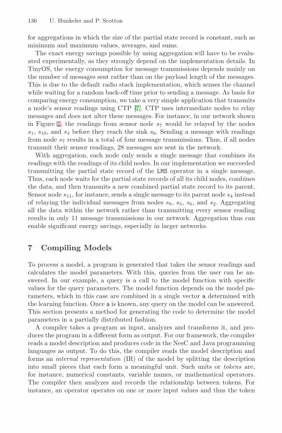
136 U. Hunkeler and P. Scotton
for aggregations in which the size of the partial state record is constant, such asminimum and maximum values, averages, and sums.
The exact energy savings possible by using aggregation will have to be evalu-ated experimentally, as they strongly depend on the implementation details. InTinyOS, the energy consumption for message transmissions depends mainly onthe number of messages sent rather than on the payload length of the messages.This is due to the default radio stack implementation, which senses the channelwhile waiting for a random back-off time prior to sending a message. As basis forcomparing energy consumption, we take a very simple application that transmitsa node’s sensor readings using CTP [7]. CTP uses intermediate nodes to relaymessages and does not alter these messages. For instance, in our network shownin Figure 1, the readings from sensor node s7 would be relayed by the nodess1, s10, and s4 before they reach the sink s0. Sending a message with readingsfrom node s7 results in a total of four message transmissions. Thus, if all nodestransmit their sensor readings, 28 messages are sent in the network.
With aggregation, each node only sends a single message that combines itsreadings with the readings of its child nodes. In our implementation we succeededtransmitting the partial state record of the LMS operator in a single message.Thus, each node waits for the partial state records of all its child nodes, combinesthe data, and then transmits a new combined partial state record to its parent.Sensor node s11, for instance, sends a single message to its parent node s4 insteadof relaying the individual messages from nodes s9, s5, s6, and s2. Aggregatingall the data within the network rather than transmitting every sensor readingresults in only 11 message transmissions in our network. Aggregation thus canenable significant energy savings, especially in larger networks.
7 Compiling Models
To process a model, a program is generated that takes the sensor readings andcalculates the model parameters. With this, queries from the user can be an-swered. In our example, a query is a call to the model function with specificvalues for the query parameters. The model function depends on the model pa-rameters, which in this case are combined in a single vector a determined withthe learning function. Once a is known, any query on the model can be answered.This section presents a method for generating the code to determine the modelparameters in a partially distributed fashion.
A compiler takes a program as input, analyzes and transforms it, and pro-duces the program in a different form as output. For our framework, the compilerreads a model description and produces code in the NesC and Java programminglanguages as output. To do this, the compiler reads the model description andforms an internal representation (IR) of the model by splitting the descriptioninto small pieces that each form a meaningful unit. Such units or tokens are,for instance, numerical constants, variable names, or mathematical operators.The compiler then analyzes and records the relationship between tokens. Forinstance, an operator operates on one or more input values and thus the token

A Code Generator for Distributing Sensor Data Models 137
associated with it has a relationship with the tokens that describe the operator’sinput values. Certain tokens, such as parentheses, only serve to determine therelationships between other tokens and can be discarded once all relationshipshave been established. The resulting representation of the model can be seenas a tree (shown in Figure 2(a)) in which the root node represents the modelas a whole. The child nodes of the model node represent the different learn-ing and model functions that together form the model. The nodes representingthese functions in turn have child nodes that represent, in the case of modelfunctions, the arguments to the functions, and that describe the mathematicalexpressions used to calculate the function. The representation of a program, orin our case a model, in such a tree form is called abstract syntax tree (AST).We use Java Compiler Compiler (JavaCC [12]) to help us generate the codefor reading and analyzing the model description. Additional information aboutcompiling in general can be found in [1].
Sensor Data Model
Learning Function
a[] LMS
forall
si t
si.temp[t]
1 si.x si.y t
*
t t
Model Function
Parameters
x y t
+
a0 +
*
a1 x
+
Sensor x y
History(6)
t tttt1
1
temp[t], 1, x, y, t, t2temp[t], 1, x, y, t, t2temp[t], 1, x, y, t, t2temp[t], 1, x, y, t, t2temp[t], 1, x, y, t, t2
Aggregation
Gaussian elimination
a3 a4a2a1a0
Sensor x y
History(6)
t tttt1
1
temp[t], 1, x, y, t, t2temp[t], 1, x, y, t, t2temp[t], 1, x, y, t, t2temp[t], 1, x, y, t, t2temp[t], 1, x, y, t, t2
Sensor x y
History(6)
t tttt1
1
temp[t], 1, x, y, t, t2temp[t], 1, x, y, t, t2temp[t], 1, x, y, t, t2temp[t], 1, x, y, t, t2temp[t], 1, x, y, t, t2
Sensor x y
History(6)
t tttt1
1
temp[t], 1, x, y, t, t2temp[t], 1, x, y, t, t2temp[t], 1, x, y, t, t2temp[t], 1, x, y, t, t2temp[t], 1, x, y, t, t2
Sensor x y
History(6)
t tttt1
1
temp[t], 1, x, y, t, t2temp[t], 1, x, y, t, t2temp[t], 1, x, y, t, t2temp[t], 1, x, y, t, t2temp[t], 1, x, y, t, t2For each sensor reading
For each sensor node
Fig. 2. (a) The linear regression model with (b) the learning function shown as abstractsyntax trees. Note that because of space constraints not the entire model function isshown. In (b) the learning function has been arranged such that the multiplicity of thedata sources and paths can be seen.
The basic AST plainly represents the model description. Before being able togenerate distributed code to process this model, the AST must be augmentedto include information related to specific nodes in the tree, such as the datatype of each node. We distinguish between integer and floating point numbers,sensor nodes, sensors, vectors, and matrices. Vectors and matrices have associ-ated dimensions and their elements in turn have associated data types. In thecase of sensor nodes, the compiler needs to know which sensors are actually used

138 U. Hunkeler and P. Scotton
and what information needs to be stored on the nodes. In addition, we need todetermine how many sensor readings have to be retained. To do so, we start bydetermining the data types of the leaf nodes, and then work our way back up thetree. For constants and sensors, the data type is clear. Before we can determinethe data type of a variable or model parameter, however, we need to determinethe data type of the expression defining this variable or parameter. The datatype of an expression is typically based on the data types of its arguments. Also,if all arguments of an operator are constants, the result of the computation rep-resented by this operator can be calculated at compile time, and the operatorcan be replaced by a constant. Similarly, if a variable is assigned a constant, allof its occurrences can be replaced by this constant. Sometimes, information inone part of the tree affects a completely different part of the tree, for instance,when the data type of a variable is determined in one place but the variableis also used in a different place. It is thus possible that not everything can bedetermined in one pass. Therefore, we reiterate the passes for as long as therestill exists information to be determined and new information is still obtainedin every pass. If no new information is obtained, but not everything has beendetermined, the compilation process is aborted with an error.
A fundamental aspect of model processing is to get the source data (e.g.,sensor readings). The compiler determines which sensors are accessed on a nodeand then includes the appropriate code to sample the sensors. For instance, theexpression si.temp[t] in the learning function in Listing 2 tells the compilerthat the temperature sensor is accessed. If an element of a sensor node is accessed,and that element is not a known sensor, the compiler assumes it to be a variableassociated with the sensor node. For instance, the expressions si.x and si.y inthe learning function do not refer to any known sensors. As no method has beendefined to determine the values for x and y, the compiler adds the necessarycode for the execution environment to configure these values (see Section 8).
For every sensor used by the model, the model processing code will reservememory for storing a history of the sensor readings. By default, the historysize is 1, which means that only the last (current) sensor reading is stored. Thecurrent sensor reading is accessed from the model either by simply accessingthe sensor object (e.g., si.temp) or by specifying 0 as the time value (e.g.,si.temp[0]). Older readings are accessed by specifying a time value greaterthan 0. To determine the amount of memory to be reserved for storing the sensorreadings’ history, the compiler analyzes how the sensor readings are accessed.In our learning function (Listing 2), the sensor readings are accessed with theexpression si.temp[t]. The compiler then analyzes the potential values that tcan take. The variable t is defined in the context of a forall statement, whichdeclares t = 1 .. 5. Thus in the example above the compiler deducts that thevalues for t vary between 1 and 5, and therefore reserves memory space for 6sensor readings2.
With the information we extracted from the model definition so far, it isstraightforward to generate code that takes sensor readings as input and com-
2 The compiler also needs to store the current sensor reading.

A Code Generator for Distributing Sensor Data Models 139
putes the results for a given query. All that needs to be done is to calculate theexpressions and update the model parameters. Our framework can produce codethat reads sensor data from a variety of different sources and answers queries.We compared two different statistical sensor data models and published ourfindings in [11]. The next step is to generate code that can run in a distributedenvironment, such as a WSN. To do this, the compiler needs to determine foreach node in the AST whether the node is to be processed in the network or onthe back-end system.
Sensors obviously have to be sampled on the sensor nodes. Currently, ourframework simply stores all sensor readings retained and all node variables on thesensor nodes themselves. Constants are located in the same place as the operatoraccessing them. This reduces the problem to determining where to locate theoperators such that the overall energy consumption in the WSN is minimized.Once data has reached the back-end system, it makes little sense to send it backinto the WSN to process it further. Thus, operators that are closely associatedwith sensor nodes are more likely to minimize overall energy consumption ifthey are also located in the WSN. If there is an aggregation operator somewherein the data flow, then in most cases the optimal approach is to process alloperators between the sensor readings and the aggregation inside the WSN, toperform a distributed aggregation, and then to compute the remaining operatorson the back-end system. Therefore, the framework currently focuses on findingan aggregation operator, and then using it to separate the AST into a part to beprocessed in the WSN and a part to be processed on the back-end system. Theoperator placement for our model is shown in Figure 2(b). Every sensor nodeexecutes the code in the rectangle in the lower part of the AST (this multiplicityis indicated by overlapping rectangles). For a specific number of past sensorreadings, a port of this code execution is repeated (again, the multiplicity isindicated in the graph). The aggregation is distributed among the nodes, andGaussian elimination takes place on the back-end system.
Once the elements of the AST that should run in the WSN have been deter-mined, the corresponding code has to be generated. The framework bases itselfon TinyOS and thus generates code in the NesC programming language [8].Besides generating the node processing code for the WSN, it also includes theappropriate modules from the execution framework (see Section 8). In particular,it includes code to allow the execution framework to configure node variables(such as the x and y coordinates for the linear regression model presented inSection 5), and the code to access the communication modules. The communi-cation methods supported currently allow data to be sent to the sink as-is orperform distributed aggregation of the data.
The framework generates Java code for that part of the model processing thatis performed on the back-end system. It includes the appropriate interface codeto communicate with the WSN. The code generated offers a dynamic interface tothe application to specify the query and change the configuration of the nodes.However, at this stage the code is not self-sufficient and needs an appropriateexecution environment.
140 U. Hunkeler and P. Scotton
8 Execution Framework
While testing our framework with the linear regression model, we found thatdistributed model processing needs basic support services. Every sensor networkneeds to transmit data to a sink. If the network performs aggregation, then nodesneed to know their parents and potentially also their children. For many applica-tions, the physical position of each node needs to be known. To demonstrate theproper operation of the linear regression model, we thus implemented a config-uration mechanism, a tree routing algorithm for aggregation, and a simple timesynchronization method.
We implemented a configuration service that enables the setting of parametersfor a particular node. With this service, we configure the x and y coordinatesof the physical location of a node prior to starting the model processing. Analternative would be to estimate the physical location during run-time (see, forexample, [15]). We decided to use a configuration service rather than a location-ing service, as for most locationing algorithms some nodes need to know theirposition in advance and therefore still would have to be configured.
When compiling a model, the framework assumes that any variable for whichno explicit means to determine its value exists, is a configuration parameter. Itwill then generate a configuration message type with fields for all parameters.An application can set a configuration parameter for a particular node throughthe framework. The framework checks the parameter name against the list ofconfiguration parameters. If the parameter name specified is valid, the frameworkwill set the corresponding field, include the identity of the targeted node in theconfiguration message, and broadcast the message in the network.
Data collected in a sensor network needs to be routed to a sink. To do this,WSNs form a collection tree. When processing a model instead of simply col-lection raw data, the data is often aggregated within the network. The routingstructure for a network that aggregates the data is essentially the same as for aWSN collecting raw data, as the data still needs to reach the sink. The differenceis that every node, instead of relaying the data of its children as-is, aggregatesits own data with that from its children before sending the data to its parent(see Section 6). This means that for one data-collection epoch each node sendsexactly one message to its parent. We call this setup an aggregation tree.
We use the collection tree protocol (CTP) [7] in TinyOS to establish the rout-ing tree. Instead of letting the collection tree forward messages automatically,we intercept each message and signal that the message should not be forwarded.We aggregate the information in the message with the node’s own informationand the information received from the other children. The information is thensent to the node’s parent.
Before sending data to the parent, a node has to receive data from all itschildren. To do this, a node could keep track of its children and which onesalready sent data in the current epoch. Once all children have sent their data,the node in turn sends its data to its parent. The version of CTP provided inTinyOS does not maintain a list of a node’s children. Also, with this method itwould be difficult for a node to predict when a child node is ready to send data,

A Code Generator for Distributing Sensor Data Models 141
which in turn makes it difficult for nodes to turn their radios off to save energy.Therefore, we adopted a time-synchronization strategy.
Synchronizing the clock of the nodes can be achieved by a variety of differ-ent protocols and algorithms. We found that one of the simplest approaches isalso well suited to minimize energy consumption as determining required activeperiods for the radio is straight forward. In our implementation the network issynchronized by broadcasting the time from the sink node to the leaves of thetree. Based on the common view of the time, all nodes start the epoch at thesame point in time. The nodes furthest down in the tree (level 4 in our samplenetwork in Figure 1(b)) start by sending their data to their parents. After afixed timeout, the nodes in the next higher level in the routing tree assume thatall their children have sent their data, and send their aggregated data to theirparent, until the data finally reaches the sink. This approach is simpler thanexplicitly waiting for data from all children, as nodes do not need to maintaina list of children. As the time period in which a node can expect transmissionsfrom its children is well defined, nodes can turn off their radio when they do notexpect transmissions, and thus achieve significant energy savings.
The basic services presented here are sufficient to implement the distributedlinear regression model with the help of our framework. Other models mightrequire additional services. A service can have multiple implementations, forinstance, to optimize for speed, latency, reliability, or energy savings. We cur-rently implemented very simple services as a proof of concept. Our frameworkfacilitates uniting contributions from experts in different fields.
9 Results and Future Work
We implemented a framework for distributedly processing generic sensor datamodels. In this paper we focused on the model called distributed linear regres-sion. The framework can be used for other models and we have, for instance,successfully implemented a model based on multivariate Gaussian random vari-ables, which was inspired by [5].
The framework consists of the model description language, the compiler togenerate the distributed code, and the execution framework that enables thecode to run. During the implementation and testing process, we refined themodel description language to make it easier to compile and also render it moreintuitive to program. For instance, we removed a separate keyword for specifyingmodel parameters. Instead, the compiler now recognizes model parameters bythe form of their definition.
The implementation of the compiler also elucidated the key differences be-tween normal programs and distributed WSN programs. Whereas for traditionalASTs it is sufficient to show the dependencies of nodes, for the distributed ap-proach the dependencies themselves have properties that describe how the in-formation flowing from the child to the parent is communicated and what theassociated cost is. The main challenge in compiling distributed programs lies inoptimizing this communication.
142 U. Hunkeler and P. Scotton
After having generated the distributed code, we realized that prior to runningit we needed an execution framework for configuring the nodes, and for handlingthe communication between network and gateway. Especially communicatingfloating point values was challenging, as TinyOS does not directly support them.We solved this issue by copying a memory image of the variables holding floatingpoint values. The Float class in Java has methods to convert between floatingpoint numbers and byte arrays. Fortunately, the floating point representation ofthe TinyOS devices is compatible with Java’s byte array representation.
Running linear regression as a distributed model in the current executionframework confirmed that the algorithm was running properly. However, some-times CTP delayed messages, such that with the staged aggregation not allmessages were received on time. We will have to analyze the exact reasons forthis behavior. We will also implement our own version of a tree-routing algo-rithm that will enable us to turn off the radio when the mote is not expectingany messages. This will enable us to experimentally confirm the energy savingsof our approach.
10 Conclusion
In this paper we presented an integrated approach for distributing the calcu-lation of sensor data model processing. Our framework consists of a model de-scription language, a compiler for this language that generates distributed code,and an execution framework needed for running the distributed programs. Theframework is extensible and open for contributions from experts in very diversefields. In contrast to previous work, which concentrated on studying a specificaspect of model processing and then optimizing it, our work is, to the best ofour knowledge, the first holistic approach to generic model processing.
References
1. Appel, A.W., Palsberg, J.: Modern Compiler Implementation in Java. CambridgeUniversity Press, New York (2003)
2. Barrenetxea, G., Ingelrest, F., Lu, Y.M., Vetterli, M.: Assessing the challengesof environmental signal processing through the SensorScope project. In: Proceed-ings of the 33rd IEEE International Conference on Acoustics, Speech, and SignalProcessing (ICASSP 2008), pp. 5149–5152 (2008)
3. Barrenetxea, G., Ingelrest, F., Schaefer, G., Vetterli, M., Couach, O., Parlange, M.:SensorScope: Out-of-the-box environmental monitoring. In: Proceedings of the 7thACM/IEEE International Conference on Information Processing in Sensor Net-works (IPSN 2008), pp. 332–343 (2008)
4. Bisdikian, C.: On sensor sampling and quality of information: A starting point. In:Proceedings of the Fifth IEEE International Conference on Pervasive Computingand Communications Workshops (PERCOMW 2007), pp. 279–284 (2007)
5. Deshpande, A., Guestrin, C., Madden, S., Hellerstein, J.M., Hong, W.: Model-driven data acquisition in sensor networks. In: Proceedings of the Thirtieth Inter-national Conference on Very Large Data Bases (VLDB 2004), pp. 588–599 (2004)

A Code Generator for Distributing Sensor Data Models 143
6. Deshpande, A., Madden, S.: MauveDB: Supporting model-based user views indatabase systems. In: Proceedings of the 2006 ACM SIGMOD International Con-ference on Management of Data (SIGMOD 2006), pp. 73–84 (2006)
7. Fonseca, R., Gnawali, O., Jamieson, K., Kim, S., Levis, P., Woo, A.: The collectiontree protocol (CTP), version 1.8 (February 2007),http://www.tinyos.net/tinyos-2.x/doc/html/tep123.html
8. Gay, D., Welsh, M., Levis, P., Brewer, E., Von Behren, R., Culler, D.: The nesClanguage: A holistic approach to networked embedded systems. In: Proceedingsof the ACM SIGPLAN 2003 conference on Programming Language Design andImplementation (PLDI 2003), pp. 1–11 (2003)
9. Guestrin, C., Bodik, P., Thibaux, R., Paskin, M., Madden, S.: Distributed regres-sion: An efficient framework for modeling sensor network data. In: Proceedings ofthe Third International Symposium on Information Processing in Sensor Networks(IPSN 2004), April 2004, pp. 1–10 (2004)
10. Hill, J., Szewczyk, R., Woo, A., Hollar, S., Culler, D.E., Pister, K.S.J.: Systemarchitecture directions for networked sensors. ACM SIGPLAN Notices 35(11), 93–104 (2000)
11. Hunkeler, U., Scotton, P.: A quality-of-information-aware framework for data mod-els in wireless sensor networks. In: Proceedings of the First International Workshopon Quality of Information in Sensor Networks (QoISN 2008), September 2008, pp.742–747 (2008)
12. JavaCC - a parser/scanner generator for Java (November 2008),https://javacc.dev.java.net/
13. Madden, S., Franklin, M.J., Hellerstein, J.M., Hong, W.: TAG: A tiny aggregationservice for ad-hoc sensor networks. SIGOPS Oper. Syst. Rev. 36, 131–146 (2002)
14. Madden, S., Franklin, M.J., Hellerstein, J.M., Hong, W.: The design of an acqui-sitional query processor for sensor networks. In: Proceedings of the 2003 ACMSIGMOD International Conference on Management of Data (SIGMOD 2003), pp.491–502 (2003)
15. Savarese, C., Rabaey, J.M., Beutel, J.: Locationing in distributed ad-hoc wirelesssensor networks. In: Proceedings of the 2001 International Conference on Acoustics,Speech, and Signal Processing (ICASSP 2001), May 2001, pp. 2037–2040 (2001)
16. Srinivasan, K., Levis, P.: RSSI is under appreciated. In: Proceedings of the ThirdWorkshop on Embedded Networked Sensors (EmNets 2006) (May 2006)
17. Werner-Allen, G., Lorincz, K., Johnson, J., Lees, J., Welsh, M.: Fidelity and yieldin a volcano monitoring sensor network. In: Proceedings of the 7th Symposium onOperating Systems Design and Implementation (OSDI 2006), pp. 381–396 (2006)

Integer-Based Optimisations forResource-Constrained Sensor Platforms
Michael Zoumboulakis and George Roussos
School of Computer Science and Information SystemsBirkbeck College, University of London
{mz,gr}@dcs.bbk.ac.uk
Abstract. In this paper we argue that the fundamental constrains ofWSNs impose the need to re-discover programming optimisation tech-niques that were widely used a few decades ago but are less commontoday, at least in the conventional computing arena. Integer techniques,code tuning and profiling are absolutely essential in the world of the verysmall devices. We present three alternative methods of integer program-ming: scaling, fixed-point and rational arithmetic. These techniques arecomplemented by a brief review of bitwise and general optimisation tech-niques. As artifact of the usefulness of these techniques, we discuss theimplementation details of a data mining algorithm that gained over afactor of 10 improvement in performance as a result of integer program-ming. We conclude by presenting a widely accepted time model adaptedfor a WSN platform.
Keywords: WirelessSensorNetworks,Optimisation, IntegerTechniques,Fixed-Point Arithmetic, Rational Arithmetic, Data Mining.
1 Introduction
There was a time when programmers used to go to great lengths in order toensure that their programs were efficient. Computers were slow and expensivepushing program performance optimisation very high on the list of software en-gineering priorities. As the years passed, advances in circuit design and memorydensity translated into faster machine speeds. Today we live in an era of power-ful, transistor-dense, multi-core machines with abundant memory and storage.Inevitably, this fact had an impact in modern software engineering priorities:programmers chose to attach more gravity to other important goals such as sta-bility, portability and maintainability whilst performance and efficiency gradu-ally dropped towards the bottom of the priorities list.
However, the resource-constrained end of the Wireless Sensor Network (WSN)spectrum is comprised of devices whose datasheets are very similar to thoseof computers from a couple of decades ago. Furthermore, we know that therate of growth of WSN nodes’ capabilities is much slower than that of theirconsumer electronics counterparts. For instance, memory in low-cost, ultra-lowpower devices does not track Moore’s law — a micro-controller RAM costs three
S. Hailes, S. Sicari, and G. Roussos (Eds.): S-Cube 2009, LNICST 24, pp. 144–157, 2009.� Institute for Computer Sciences, Social-Informatics and Telecommunications Engineering 2009

Integer-Based Optimisations for Resource-Constrained Sensor Platforms 145
orders of magnitude more than PC SRAM and five orders more than PC DRAM[12]. Even more importantly, energy density does not seem to track Moore’s laweither — over a decade energy density of commercially available batteries haschanged only modestly [4].
These fundamental constraints suggest that programming optimisation tech-niques widely used a few decades ago need to be re-discovered. Consequently,we address the importance of programming efficiency in WSNs and we discussmethods that contribute to the attainment of this goal.
In the remainder of the paper, we draw from our own experience of imple-menting an established data mining algorithm in a resource-constrained platformand we present the direct performance gains of applying a few straightforwardcoding techniques. Moreover, we focus on integer programming complementedby bitwise techniques and general code tuning — combined, they form a toolboxof techniques that can greatly improve program efficiency. Lastly, we adapt theconventional time model of [2] for a sensor platform with a view to identify costlyoperations and provide rough estimates of the time needed for typical tasks.
2 Case Study: TinySAX — Efficient Implementation of aData Mining Algorithm
Symbolic Aggregate Approximation (SAX) [7] is a widely-accepted and maturealgorithm used for data mining. Essentially SAX performs Symbolic Conversion:it maps an ordered sequence of sensor readings to a sequence of letters from afinite alphabet Σ according to a set of well-defined rules. Formally, the input isa sequence of readings r = 〈r1, r2, . . . , rn〉, ri ∈ Z and the output is a sequenceof letters s = 〈s1, s2, . . . , sm〉, si ∈ Σ with 0 < m ≤ n. In this respect SAX is adiscretisation technique.
Applying SAX to a time-series stream has many attractive properties such asdimensionality reduction due to the Piecewise Aggregate Approximation (PAA)that is central to the algorithm. A PAA representation has been found to rivalmore sophisticated dimensionality reduction techniques such as Fourier trans-forms and wavelets [6]. The core idea of obtaining a PAA from a sequence ofreadings is based on dividing the sequence into m equal-sized frames and tak-ing the mean of the values that fall within each frame. The PAA representationcomprises the vector of the mean values. The final step involves transforming thePAA into a sequence of equiprobable symbols. For this, SAX uses a sorted listof breakpoints (found in statistical tables) β = 〈β1, β2, . . . , βα−1〉, with α =sizeof the alphabet, such that the area under a N(0,1) Gaussian curve from βi toβi+1 is 1/a with β0 and βα set to −∞ and ∞ respectively [14]. The final stringis obtained according to the range of the PAA coefficients i.e. if a coefficientis less than β1 it is mapped to 1, if it is lies between β1 and β2 is is mappedto 2 and so forth. The precise details of the PAA transformation and the fur-ther symbolic transformation are well-described in the SAX literature [7,6] (andreferences therein).

146 M. Zoumboulakis and G. Roussos
Table 1. Performance Times (in ms) for a Symbolic Conversion using naive imple-mentation with floating-point operations
SizeOperation 40 80 120
S2. Standardise
a. Mean 12ms (10.62%) 24ms (10.62%) 37ms (11.01%)b. Std Dev 42ms (37.17%) 81ms (35.84%) 120ms (35.71%)c. Subtract & Divide 25ms (22.12%) 53ms (23.45%) 78ms (23.21%)
S3. Get PAA 24ms (21.24%) 48ms (21.24%) 73ms (21.73%)S4. Get Symbols 10ms (8.85%) 20ms (8.85%) 28ms (8.33%)
Total Time 113ms 226ms 336msRAM Image Size (Bytes) 766 846 926
One of the common uses of SAX is for Anomaly Detection in a time-series.We use SAX in the WSN setting for a similar purpose, namely Complex EventDetection. We use the following definition of Complex Events:
Complex Event. An interesting or unusual pattern in the data gathered andprocessed by WSN nodes that can be very difficult or even impossible todetect using threshold-based techniques.
This method allows us to detect many complex patterns simultaneously withoutsignificant overhead to the resources of the WSN nodes. We use SAX in an onlinefashion where sensor nodes continuously convert sliding windows of readings tosymbols and then compare them against patterns of symbols submitted by usersas event interests.
SAX relies on various operations involving floating-point numbers and a firstimplementation attempt was running prohibitively slow on the target platform(TMote Sky [16]). A single symbolic conversion was taking approximately 113msfor a sliding window of 40 readings. Profiling the code, by timing the entry andexit points of every function, provided the information shown on Table 1.
2.1 Refactoring SAX into TinySAX
This slow implementation had to be reviewed and re-written in a manner suitablefor the constraints of the WSN. The outcome was TinySAX; an efficient integer-only implementation that reduced the active CPU time by more than a factor of10. This was achieved by a combination of the following actions, listed in orderof importance:
– Integer Programming. Firstly, all floating point variables were replacedby integers. Functions such as standardisation — that relies on the costlyformula zi = ri−μ
σ where μ is the mean and σ is the Standard Deviationof the sliding window r — were re-written with elimination of the divisionoperation. Instead, the breakpoint vector β was scaled by σ. The size of
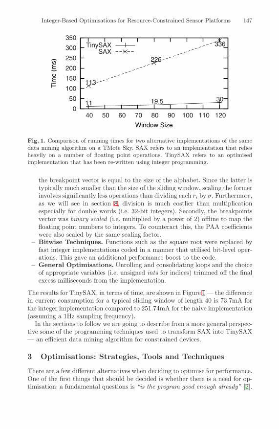
Integer-Based Optimisations for Resource-Constrained Sensor Platforms 147
0
50
100
150
200
250
300
350
40 50 60 70 80 90 100 110 120
Tim
e (m
s)
Window Size
11
113
19.5
226
30
336TinySAXSAX
Fig. 1. Comparison of running times for two alternative implementations of the samedata mining algorithm on a TMote Sky. SAX refers to an implementation that reliesheavily on a number of floating point operations. TinySAX refers to an optimisedimplementation that has been re-written using integer programming.
the breakpoint vector is equal to the size of the alphabet. Since the latter istypically much smaller than the size of the sliding window, scaling the formerinvolves significantly less operations than dividing each ri by σ. Furthermore,as we will see in section 8, division is much costlier than multiplicationespecially for double words (i.e. 32-bit integers). Secondly, the breakpointsvector was binary scaled (i.e. multiplied by a power of 2) offline to map thefloating point numbers to integers. To counteract this, the PAA coefficientswere also scaled by the same scaling factor.
– Bitwise Techniques. Functions such as the square root were replaced byfast integer implementations coded in a manner that utilised bit-level oper-ations. This gave an additional performance boost to the code.
– General Optimisations. Unrolling and consolidating loops and the choiceof appropriate variables (i.e. unsigned ints for indices) trimmed off the finalexcess milliseconds from the implementation.
The results for TinySAX, in terms of time, are shown in Figure 1 — the differencein current consumption for a typical sliding window of length 40 is 73.7mA forthe integer implementation compared to 251.74mA for the naive implementation(assuming a 1Hz sampling frequency).
In the sections to follow we are going to describe from a more general perspec-tive some of the programming techniques used to transform SAX into TinySAX— an efficient data mining algorithm for constrained devices.
3 Optimisations: Strategies, Tools and Techniques
There are a few different alternatives when deciding to optimise for performance.One of the first things that should be decided is whether there is a need for op-timisation: a fundamental questions is “is the program good enough already” [2].

148 M. Zoumboulakis and G. Roussos
The answer depends on the context in which the program must execute. If it hasbeen stress-tested under different realistic workloads and it is found to performwell, then clearly there is little need to optimise. Aggressively optimising a pro-gram still in the early design stage can adversely impact the quality of the codeand compromise its correctness. In the words of Donald Knuth [8]: “we shouldforget about small inefficiencies, say about 97% of the time: premature optimi-sation is the root of all evil”. A program should be subjected to an optimisationprocess once it has been profiled and its runtime behaviour is well-understood.
If optimisation passes the above suitability test, it should then be decidedwhether to opt for node-level optimisation, network-wide optimisation, or both.Node-level optimisation targets the specific program image that executes on asingle node and attempts to re-design it so it is highly efficient. Network-wideoptimisation, as the name suggests, targets the entire network: local decisions ofindividual nodes may be sub-optimal for the benefit of the whole network e.g.an example of this is distribution of processing load among nodes or avoidingbottlenecks such as the funnelling effect [1] that penalises nodes near a base sta-tion. Network-wide optimisation largely depends on application-specific factorsand network characteristics such as density and therefore is beyond the scopeof this paper. The techniques that follow are primarily aimed at node-leveloptimisation.
4 Integer Techniques
Integer techniques is a broad term for a family of methods relating to computerprograms using integral data types. Although the term has been used to refer totechniques that sometimes use a mixture of floating-point and integer numbers,in this context we use it to refer to programs that use exclusively integers.
The motivation for re-introducing integer techniques into WSN programsstems from the following:
1. Floating Point on Software. The majority of low-end microcontrollers(MCUs) lack Floating Point Units (FPUs). Floating point numbers are rep-resented in software and operations involving these data types are inherentlyslow and expensive.
2. Lack of Standardisation. Programs that use floats in WSNs are lessportable since there exist variations in the floating point representationacross different compilers and microcontrollers. Programs in heterogeneousnetworks that need to communicate floating point values over the radio, suf-fer from the added complexity that the lack of a common standardintroduces.
3. Application needs. Many real-world applications have a requirement foroperations involving real numbers — typical examples are object trackingand target estimation applications. In general, a large number of trigonomet-ric and statistic functions are prime candidates for integer transformation.
In the following, we will discuss some of the specific techniques that are availableto a programmer.

Integer-Based Optimisations for Resource-Constrained Sensor Platforms 149
4.1 Scaling
We have briefly discussed scaling in section 2.1 where it was used in the im-plementation of TinySAX. Scaling is a well-understood technique that involvesmultiplying a floating point number by an integer, usually a power of two (bi-nary scaling) to represent it as an integer. Arithmetic operations can then beperformed using the scaled numbers and the result can be divided by the samescaling factor. As an example consider the floating point numbers −0.52 and1.28. Scaling both by 211 and rounding toward zero gives −1064 and 2621 re-spectively. Any arithmetic operation can be performed using the integers: i.e.multiplication would yield −2788744. If we divide the result by the same scalingfactor we obtain −1361. To retrieve the floating point result we divide again andobtain 0.6645 (the exact floating point result is 0.6656).
Care must be taken to prevent arithmetic overflow. This is usually done byperforming some analysis of the range of values that a program variable willtake. The maximum of these values is taken and scaled. To accommodate themaximum value xmax, M bits will be needed with log2 xmax ≤ M . Numericalprecision requirements vary across applications, so N bits must be reserved tosatisfy the accuracy requirements Δx with 2−N ≤ Δx. The total number of bitsthat will be needed to represent the floating point number in an integer typewithin the accuracy requirements is therefore M+N . There is a tradeoff betweenthe maximum range of a variable and the accuracy required [17], but this is verymuch application dependent.
Embedded operating systems such as TinyOS [13] employ scaling techniquesin the design of certain components — an example of this is the implementationof Timers: a second equals 1,024 milliseconds. So if we need to represent the timevalue of 1.875 seconds we scale it by 210 and use 1,920 to perform any arithmeticoperations. This level of accuracy is good enough for many applications.
Generally speaking, there will always be a tradeoff between speed and accu-racy: if an application requires very high numerical fidelity in its calculationsthen performance may need to be sacrificed, for instance by using arbitraryprecision data types.
4.2 Fixed-Point Arithmetic
Fixed-point arithmetic is very closely related to the scaling technique but itinvolves slightly higher degree of programming effort. It is estimated that ap-proximately 30 % of the software development for the first NASA Apollo spacemissions was spent on fixed-point arithmetic and scaling [3]. Nowadays, it is stillwidely used by DSP programmers, graphics developers, computer typesettingand other applications where there is a combined need for real-valued numbersand high performance.
In floating-point numbers the radix point is generally allowed to be determineddynamically or to “float” thus being capable of representing a wide range ofvalues. Conversely, in fixed-point arithmetic the radix point is fixed. There is afixed number of digits after the radix point reserved for the fractional part.

150 M. Zoumboulakis and G. Roussos
Let N represent the total number of bits needed to accommodate a fixed-pointvariable. We can then split a type of length N into Integer bits and Fractionalbits. The integer bits are to the left of the hypothetical or implied binary radixpoint and the fractional bits are the remaining bits to the right. We use the no-tation (I, F )1 to represent the Integer part and the Fractional part respectively.The number of bits needed for an unsigned type is I + F and for a signed typeI +F +1. The range of unsigned fixed-point numbers is from 0 to 2i−2−f whilethe range for singed fixed-point numbers is from −2i−1 to 2i−1 − 2−f , wherei and f are the number of bits needed to represent the integer and fractionalparts respectively. To obtain the value of unsigned and signed numbers in (I, F )(fixed-point) representation we use equations 1 and 2 respectively [19]:
x = 2−fN−1∑n=0
2nxn (1)
x = 2−f
(−2N−1xN−1 +
N−2∑n=0
2nxn
)(2)
Where xn denotes bit n of x.Consider the following example: an unsigned fixed-point data type of the
form (3, 5). This type can accommodate a range from 0 to 7.96875 and has thefollowing representation:
← Integer Part → ←− Fractional Part −→I I I F F F F F
The number (00101011)2 is then 2−5(1 + 2 + 23 + 25) = 1.34375. Similarly, ifwe were using a signed type (3, 5) requiring (I +F )+1 = 9 bits the range wouldbecome −4 ≤ x ≤ 3.96875, with the MSB reserved for sign in two’s complementnotation. The code (in C) needed for the transformation is shown below:
#define FB 5 /* (3,5) Representation */
float f=1.34375; uint8_t fp;
fp = (uint8_t)(f * (1<<FB) + (f>=0 ? 0.5 : -0.5));
f = (float) fp / (1<<FB); /* Fixed-point back to float */
All arithmetic operations are defined using the fixed-point representation butcare needs to be taken to ensure that the types are in the same sign representationand that the result does not overflow. Operations can still be performed onnumbers with different bit (I, F ) representations but somewhat more effort isrequired for bit alignment.
Although measurable performance improvements can be gained by using fixed-point arithmetic, it suffers from certain disadvantages: it can hinder code portabil-ity. Moreover, it can make the programming task tedious resulting in error-pronecode.1 Other common notations are (M, N) and Q.
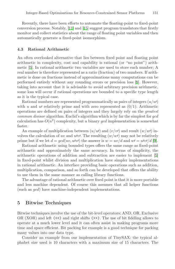
Integer-Based Optimisations for Resource-Constrained Sensor Platforms 151
Recently, there have been efforts to automate the floating-point to fixed-pointconversion process. Notably, [11] and [15] suggest program translators that firstlymonitor and collect statistics about the range of floating point variables and thenautomatically generate a fixed-point isomorphism.
4.3 Rational Arithmetic
An often overlooked alternative that lies between fixed point and floating pointarithmetic in complexity, cost and capability is rational (or “no point”) arith-metic [5]. In rational arithmetic two variables are used to store each number; Areal number is therefore represented as a ratio (fraction) of two numbers. If arith-metic is done on fractions instead of approximations many computations can beperformed entirely without any rounding errors or precision loss [9]. However,taking into account that it is advisable to avoid arbitrary precision arithmetic,some loss will occur if rational operations are bounded to a specific type lengthas it is the typical case.
Rational numbers are represented programmatically as pairs of integers (u/u′)with u and u′ relatively prime and with zero represented as (0/1). Arithmeticoperations are defined on pairs of integers and they largely rely on the greatestcommon divisor algorithm. Euclid’s algorithm which is by far the simplest for gcdcalculation has O(n2) complexity, but a binary gcd implementation is somewhatfaster.
An example of multiplication between (u/u′) and (v/v′) and result (w/w′) in-volves the calculation of uv and u′v′. The resulting (w/w′) may not be relativelyprime but if we let d = gcd(uv, u′v′) the answer is w = uv/d and w′ = u′v′/d [9].
Rational arithmetic using bounded types offers the same range as fixed-pointarithmetic and approximately the same accuracy. In terms of simplicity, thearithmetic operations of addition and subtraction are easier to implement [5]in fixed-point whilst division and multiplication have simpler implementationsin rational arithmetic. An interface providing basic operations such as addition,multiplication, comparison, and so forth can be developed that offers the abilityto use them in the same manner as calling library functions.
The advantage of rational arithmetic over fixed point is that it is more portableand less machine dependent. Of course this assumes that all helper functions(such as gcd) have machine-independent implementations.
5 Bitwise Techniques
Bitwise techniques involve the use of the bit-level operators: AND, OR, ExclusiveOR (XOR) and left (<<) and right shifts (>>). The use of bit fiddling allows tooperate at a much lower level and it can often assist in making programs moretime and space efficient. Bit packing for example is a good technique for packingmany values into one data type.
Consider an example from our implementation of TinySAX: the typical al-phabet size used is 10 characters with a maximum size of 15 characters. The

152 M. Zoumboulakis and G. Roussos
application has a requirement to send over the radio a string of characters. Thesmallest data type that a language provides is one byte, however 4 bits are suf-ficient to represent a character from an alphabet of size 15 (with range 0-15).The listing below shows a code example used to pack 4-bit nibbles into a 64-bitinteger.
uint64_t y=0; /* 64-bit var to be packed with 16 nibbles */
for (i=0; i < length-1; i++)
{ y = (y+data[i]) << 0x4; }
y += data[length-1];
With this code we can encode twice the amount of information in a singlevariable. If there is a requirement to send such a variable once a second overthe radio, in the course of a whole day we save 675 kilobytes (or little over 2megabytes if we include the packet headers and footers) at the expense of a littlecomputation. The packed value can be unpacked using the code below:
for (i=shift=0; i < length; i++, shift+=0x4)
unpacked_data[(length-1)-i] = (y>>shift)%0x10;
Note that the modulo operation is inexpensive since it does not require divi-sion i.e. x mod 2n = x&(2n − 1) [10].
Bit fields such as the above are particularly useful in WSNs when there is aneed to keep track of a neighbour table. For instance if neighbours with identifi-cation numbers 1,5,8 are awake, this can be encoded in a bit field in the followingmanner: {1, 0, 0, 0, 1, 0, 0, 1}. This a very compact representation and individualbits from the field can be toggled, as neighbours appear or disappear, at a verysmall computational cost.
Furthermore, bitwise operations are useful for the reduction or elimination ofbranching — a part of the program where control flow is decided on evaluatingsome condition — in programs. For example the simple line x - ((x - y) &-(x < y)) can be used to determine the maximum of the two values (x, y) or(x ˆ (x >> (16 - 1))) - (x >> (16 - 1)) to determine the absolute (abs)value of x (assuming 16-bit integers).
The usefulness of bit-level techniques in embedded devices is undisputed —in the words of the author of one of the leading works in bit fiddling [18] “It isamazing what can done with binary addition and subtraction and maybe somebitwise operations”. The main criticism for bit fiddling is that it can make pro-grams less portable. The majority of bit-level operations depend on endianness(i.e. the byte ordering) and therefore can make programs platform-specific.
6 Profiling
Profiling or benchmarking is a useful form of empirical analysis that aims toidentify which parts of a computer program consume the most time or otherresources such as memory, registers or disk. With respect to time, a straightfor-ward way of profiling a program is the use of timers at entry and exit points of
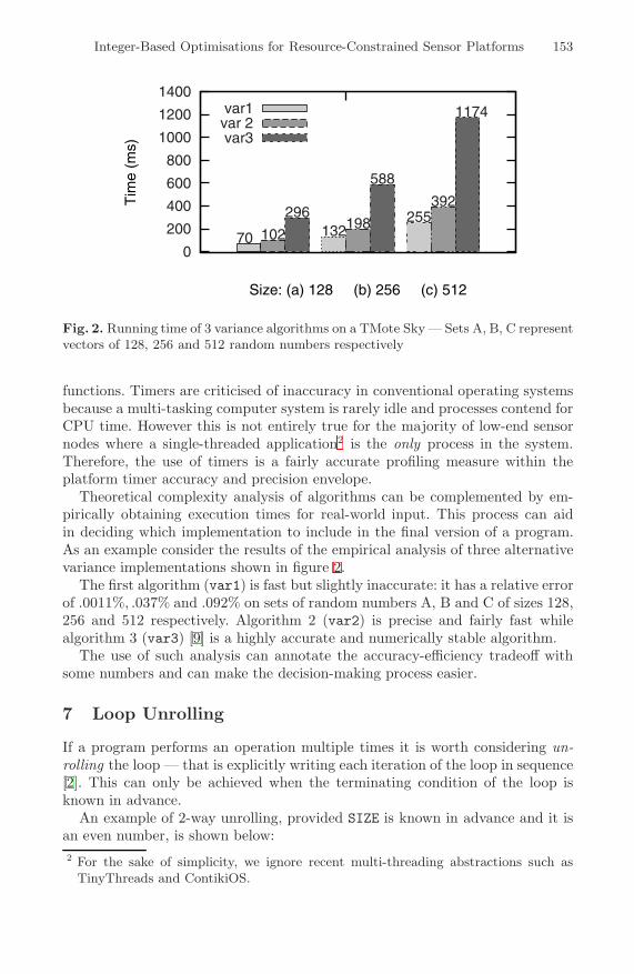
Integer-Based Optimisations for Resource-Constrained Sensor Platforms 153
0
200
400
600
800
1000
1200
1400
Tim
e (m
s)
Size: (a) 128 (b) 256 (c) 512
70 102
296132198
588
255392
1174var1var 2var3
Fig. 2. Running time of 3 variance algorithms on a TMote Sky — Sets A, B, C representvectors of 128, 256 and 512 random numbers respectively
functions. Timers are criticised of inaccuracy in conventional operating systemsbecause a multi-tasking computer system is rarely idle and processes contend forCPU time. However this is not entirely true for the majority of low-end sensornodes where a single-threaded application2 is the only process in the system.Therefore, the use of timers is a fairly accurate profiling measure within theplatform timer accuracy and precision envelope.
Theoretical complexity analysis of algorithms can be complemented by em-pirically obtaining execution times for real-world input. This process can aidin deciding which implementation to include in the final version of a program.As an example consider the results of the empirical analysis of three alternativevariance implementations shown in figure 2.
The first algorithm (var1) is fast but slightly inaccurate: it has a relative errorof .0011%, .037% and .092% on sets of random numbers A, B and C of sizes 128,256 and 512 respectively. Algorithm 2 (var2) is precise and fairly fast whilealgorithm 3 (var3) [9] is a highly accurate and numerically stable algorithm.
The use of such analysis can annotate the accuracy-efficiency tradeoff withsome numbers and can make the decision-making process easier.
7 Loop Unrolling
If a program performs an operation multiple times it is worth considering un-rolling the loop — that is explicitly writing each iteration of the loop in sequence[2]. This can only be achieved when the terminating condition of the loop isknown in advance.
An example of 2-way unrolling, provided SIZE is known in advance and it isan even number, is shown below:2 For the sake of simplicity, we ignore recent multi-threading abstractions such as
TinyThreads and ContikiOS.

154 M. Zoumboulakis and G. Roussos
for (i=0; i < SIZE; i+=2)
{ c[i] = a[i]+b[i];
c[i+1] = a[i+1]+b[i+1]; }
Table 2. Results from unrolling a basic loop that executes the one-line statementc[i]=a[i]+b[i] in its body
Degree of Unrolling Time (ms)
Normal Loop 220ms2-way Unrolling 173msLoop Elimination 112ms
The loop can be unrolled further as long as (SIZE mod increment) ==0 andit can even be eliminated altogether by writing out explicitly every instruction.The runtime results from unrolling the simple loop described above are shownon Table 2.
Another optimisation technique, involves removing any conditional expres-sions that are inside the body of a loop. This will reduce branching and the codecan be re-factored by enclosing a copy of the loop inside the bodies of the ifand else clauses respectively. Similarly, any expensive operations inside the loopbody should be examined: for instance if a loop involves an expression that con-tains division, then this expression should be re-arranged to use multiplicatione.g. (u/u′) ≤ (v/v′) is equivalent to (uv′) ≤ (vu′) — the latter is significantlycheaper, as we will see in the next section.
Generally speaking, loops are usually the first part of the program to target.Eliminating the loop completely will almost always yield a gain in performance.Critics of this technique assert that there is a side-effect of higher register usageto keep track of intermediate results. Empirical analysis suggests that this ishighly compiler-dependent; run-time results can always assist in measuring thebenefit for loop elimination.
8 A Time Model for WSNs
In this section, we apply the methodologies introduced by Bentley [2] for theconstruction of a time model that can be used to identify the relative cost oftypical operations. The model is adapted so it tests various platform-specificcomponents such as the time it takes to sample the on-board sensors. The resultsare shown in Table 3. Reported times are in milliseconds per 5,000 trials. Asexpected the arithmetic operations that are larger than the MCU word size (16-bit) are taking much longer. For example, 64-bit integer division is almost asslow as floating point division, while for other operations using a 64-bit type ischeaper than floating-point. 64-bit types can be useful for temporary storage i.e.holding results, when scaling is employed.
The lack of FPU slows down floating point operations — by a factor of 432in the case of addition — making floating point operations unacceptably slow.

Integer-Based Optimisations for Resource-Constrained Sensor Platforms 155
Table 3. Performance Times (in ms) for various operations executed by the TMoteSky (timed using TinyOS 2.x and msp430-gcc 3.2.3)
Arithmetic (Integer)
Operation 16-bit 32-bit 64-bit
Increment 6,734 12,824 67,271Addition 7,955 15,319 88,301Subtraction 7,969 15,310 87,985Multiplication 145,020 159,060 316,755Division 226,265 709,720 3,519,055Remainder 225,375 706,875 3,540,080
Bitwise
AND 7,965 15,285 88,095OR 7,985 15,325 88,360XOR 7,955 15,315 88,310SHIFT 56,735 62,880 573,665
Floating Point Arithmetic
Assignment & Cast 2,687,535Addition 3,438,530Subtraction 3,499,920Multiplication 4,841,490Division 4,041,785
Array Comparisons & Swaps
Straight Comp 104,095Comp C Fcn 83,315Comp TOS Fcn 83,335Comp TOS task 159,055Swap C Macro 93,085Swap C Function 83,320
Max Function
Straight Max 137,565Max C Macro 137,075Max C Function 79,110
Built-in Sensors
ReadLight 327,510ReadTemperature 154,125ReadHumidity 154,175ReadIVoltage 321,635
External Flash Chip IO
Reads (4-bytes) 158,750Writes (4-bytes) 191,280
Surprisingly, bitwise operations are slightly slower than addition and subtractionbut shifts are still considerably faster than division and multiplication.
Subscripted array operations are generally fast, and according to [2] this isdue to favourable memory access predictability. A TinyOS function — which isplatform-independent and hence portable — is infinitesimally slower (by 20ms)than a C function performing the same operation. However, a TinyOS task,

156 M. Zoumboulakis and G. Roussos
which is placed on a separate FIFO queue, is somewhat slower — almost by afactor of 2 — than the C or TinyOS function. The debate of whether a functionor a preprocessor macro is faster, appears to have settled on the fact that on amote the C function is faster than its macro equivalent.
Sampling Light and Internal Voltage sensors is more expensive than samplingTemperature and Humidity — the internal temperature and humidity sensorsare on the same chip, hence the similarity in terms of performance. Flash Input-Output is generally slow3 and as expected writes and slower than reads. Thereads are not cached, in contrast with traditional disks and flash chips.
Lastly, we expect this table to provide a suitable guide into the tradeoffs ofoperations and data types that partially determine the running time of programs.
9 Summary
There is a wide variety of real-world WSN applications that have a need forrepresentation of real numbers in programs. However, many MCUs lack Float-ing Point Units (FPUs) and as a result computations are performed in software.This has the undesirable impact of slow performance and increased energy cost;both factors are burdensome in any embedded environment. Furthermore thelack of a common floating point representation across different node platformsand compilers can introduce runtime errors in heterogeneous networks that needto communicate such values over the air. In this paper, we focus on three maininteger programming techniques: Scaling, Fixed-point and Rational-point Arith-metic. Each one of these varies in complexity, cost and implementation and agood understanding of their relative strengths and weaknesses is essential fordesigners who aim to shave off valuable time units from their implementations.Moreover, bitwise techniques and other optimisations such as loop unrolling canassist in compounding significant performance gains. We have highlighted theapplicability of these methods, combined with integer techniques, by present-ing a case study of an implementation of a data mining algorithm for a WSNplatform. By re-writing the program with efficiency as the ultimate goal perfor-mance improved by a factor of more than 10. Finally, we assert that operationalawareness of a program’s performance together with application of an appropri-ate optimisation strategy are essential factors in software engineering for WSNswith direct implications to network and device lifetime.
References
1. Ahn, G.-S., Hong, S.G., Miluzzo, E., Campbell, A.T., Cuomo, F.: Funneling-MAC:a localized, sink-oriented MAC for boosting fidelity in sensor networks. In: SenSys,pp. 293–306. ACM, New York (2006)
2. Bentley, J.: Programming Pearls, 2nd edn. Addison-Wesley Pub. Co., Reading(1999)
3 The results reported are using the ConfigStorage TinyOS component.

Integer-Based Optimisations for Resource-Constrained Sensor Platforms 157
3. Kreide, H., Lambert, D.W.: Computation: Aerospace Computers in Aircraft, Mis-siles and Spacecraft. Space/Aeronaut 78 (1964)
4. Hellerstein, J.M., Hong, W., Madden, S.: The sensor spectrum: technology, trends,and requirements. SIGMOD Record 32(4), 22–27 (2003)
5. Horn, B.K.P.: Rational arithmetic for minicomputers. Softw. Pract. Exper. 8(2),171–176 (1978)
6. Keogh, E., Lin, J., Fu, A.: HOT SAX: Efficiently Finding the Most Unusual TimeSeries Subsequence. In: IEEE International Conference on Data Mining, pp. 226–233 (2005)
7. Keogh, E., Lonardi, S., Ratanamahatana, C.A.: Towards parameter-free data min-ing. In: KDD 2004: Proceedings of the tenth ACM SIGKDD international confer-ence on Knowledge discovery and data mining, New York, NY, USA, pp. 206–215(2004)
8. Knuth, D.E.: Structured Programming with go to Statements. ACM Comput.Surv. 6(4), 261–301 (1974)
9. Knuth, D.E.: The Art of Computer Programming, 2nd edn. Seminumerical Algo-rithms, vol. II. Addison-Wesley, Reading (1981)
10. Knuth, D.E.: The Art of Computer Programming. F.1, Binary Tricks and Tech-niques, vol. 4. Addison-Wesley, Reading (2009)
11. Kum, K.-I., Kang, J., Wonyong, S.: AUTOSCALER for C: an optimizing floating-point to integer C program converter for fixed-point digital signal processors. IEEETransactions on Circuits and Syst.—Part II 47, 840–848 (2000)
12. Levis, P., Brewer, E., Culler, D., Gay, D., Madden, S., Patel, N., Polastre, J.,Shenker, S., Szewczyk, R., Woo, A.: The Emergence of a Networking Primitive inWireless Sensor Networks. Communications of the ACM 51(7), 99–106 (2008)
13. Levis, P.A.: TinyOS: An Open Operating System for Wireless Sensor Networks(Invited Seminar). In: MDM 2006: Proceedings of the 7th International Conferenceon Mobile Data Management, Washington, DC, USA, p. 63 (2006)
14. Lonardi, S., Lin, J., Keogh, E.J., Chiu, B.: Efficient discovery of unusual patternsin time series. New Generation Comput. 25(1), 61–93 (2006)
15. Menard, D., Chillet, D., Sentieys, O.: Floating-to-fixed-point conversion for digitalsignal processors. EURASIP J. Appl. Signal Process. 2006, 77–77 (2006)
16. MoteIV (later renamed to Sentilla). TMote Sky Datasheets and Downloads,http://www.sentilla.com/pdf/eol/tmote-sky-datasheet.pdf
17. Tan, J., Kyriakopoulos, N.: Implementation of a Tracking Kalman Filter on aDigital Signal Processor. IEEE Transactions on Industrial Electronics 35, 126–135(1988)
18. Warren, H.S.: Hacker’s Delight. Addison-Wesley, Reading (2002)19. Yates, R.: Fixed-point arithmetic: An introduction — digital signal labs, technical
reference (2007), http://www.digitalsignallabs.com/fp.pdf

ProSe: A Programming Tool for Rapid Prototyping ofSensor Networks�
Mahesh Arumugam1 and Sandeep S. Kulkarni2
1 Cisco Systems, Inc., San Jose, CA 95134, [email protected]
2 Michigan State University, East Lansing, MI 48823, [email protected]
Abstract. We focus on application of abstract network protocols towards pro-totyping sensor networks. Such abstract programs exist for several applications,e.g., routing, tracking, dissemination, etc. These programs are often specified interms of event-driven actions where the program responds to actions in the en-vironment or previous actions taken by the program. Hence, they are easy tospecify, verify and manipulate. However, they cannot be applied directly in sen-sor networks as the computation model in sensor networks (write all with colli-sion) differs from that (read/write or shared memory) used in abstract programs.Towards this end, we propose ProSe, a programming tool that enables the de-signers to (1) specify protocols in simple, abstract models, (2) reuse existingfault-tolerant/self-stabilizing protocols from the literature, and (3) automaticallygenerate and deploy code. ProSe hides the deficiencies of existing programmingplatforms that require the designers to explicitly deal with buffer management,stack management, and flow control. As a result, we expect that ProSe will en-able rapid prototyping and quick deployment of protocols.
Keywords: Programming Tool, Network Protocols, Sensor Networks.
1 Introduction
Sensor networks have become popular due to their applications in border patrolling,critical infrastructure protection, habitat monitoring, structural health monitoring, andhazard detection. Furthermore, due to the development in MEMS technology, tiny low-power sensors can now be manufactured and deployed in large numbers. They havebeen successfully used in large scale deployments of several applications.
One of the important challenges in deploying sensor network applications is pro-gramming. Most of the existing platforms (e.g., nesC/TinyOS [2]) for developing sen-sor network programs use event-driven programming model [3]. As identified in [3–5],while an event-driven programming platform has the potential to simplify concurrencyby reducing race conditions and deadlocks, the programmer is responsible for stackmanagement and flow control. For example, in nesC/TinyOS platform, the state of anoperation does not persist over the duration of entire operation. As a result, program-mers need to manually maintain the stack for the operation. Moreover, the state of the
� A preliminary version of this paper appeared as a poster in [1].
S. Hailes, S. Sicari, and G. Roussos (Eds.): S-Cube 2009, LNICST 24, pp. 158–173, 2009.c© Institute for Computer Sciences, Social-Informatics and Telecommunications Engineering 2009

ProSe: A Programming Tool for Rapid Prototyping of Sensor Networks 159
operation is shared across several functions. Hence, the designer has to manually con-trol the execution flow. As the program size grows, such manual management becomescomplex and is often the source of programming errors.
In addition, typical sensor network platforms require the programmers to managebuffers, contend for access to radio channel, and deal with faults. Hence, as mentionedin [6], programming in nesC/TinyOS platform is “somewhat tricky.” In [6], the authorsmotivate the need for a simpler model that allows one to specify applications in termsof event-driven model (that hides several programming level issues).
To simplify programming sensor networks, several approaches are proposed (e.g.,[6–24]). These approaches hide most of the low-level details of the network. (We referthe reader to Section 2 for more details on these approaches.) Existing work on macro-programming primitives require implementation of such primitives in a target platform(e.g., nesC/TinyOS). Moreover, most of these primitives still require the designer tospecify protocols in a target platform (though some intricate details are hidden).
Contributions of the paper. With this motivation, in this paper, we propose ProSe, aprogramming platform for sensor networks that allows designers to concisely specifysensor network protocols. ProSe is based on the theoretical foundation on computa-tional model in sensor networks [25, 26]. In [25, 26], the authors model the computa-tions in sensor networks as a write all with collision (WAC) model. In this model, inone atomic step, a sensor can write its own state as well as the state of all its neighbors.However, if two sensors try to update the state of a common neighbor (say, k) simultane-ously then, due to collision, the state of k remains unchanged. Thus, this model capturesthe nature of communication in sensor networks. Moreover, in [25, 26], the authors pro-posed transformation algorithms that allow the designers to specify programs in abstractmodels (e.g., read/write model, shared-memory model) and transform them into WACmodel (cf. Section 3.1 for a brief introduction to these models).
ProSe enables the designers to (1) specify sensor network protocols and macropro-gramming primitives in simple, abstract models, (2) transform the programs into WACmodel while preserving properties such as fault-tolerance and self-stabilization [27] ofthe original programs, and (3) automatically generate and deploy code. An advantageof ProSe is that it will facilitate the designer to use existing algorithms for automatingthe addition of fault-tolerance to existing programs. Moreover, since abstract modelsare used to specify protocols, ProSe allows the designer to gain assurance about theprograms deployed in the network using tools such as model checkers [28].
Additionally, we observe that the work on distributed computing and traditional net-working has focused on problems such as consensus, agreement in the presence offaulty/malicious sensors, reliable broadcast, routing, leader election, synchronization,and tracking. These problems (or variations thereof) also need to be solved in the con-text of sensor networks, either in the design of sensor network protocols or in the designof macroprogramming primitives. However, existing solutions to these problems arewritten in abstract models such as read/write model and shared-memory model. Sinceit is desirable to utilize the vast literature in this area, to speed up the development and
160 M. Arumugam and S.S. Kulkarni
deployment of sensor networks, ProSe enables the designers to reuse existing algorithmsby automatically transforming them into WAC model.
Organization of the paper. In Section 2, we discuss the related work. In Section 3, weprovide a detailed discussion on ProSe. Then, in Section 4, we discuss two case studies.Finally, in Section 5, we make the concluding remarks.
2 Background on Programming Platforms for Sensor Networks
Related work that deals with programming platforms include [6–24].
Macroprogramming. In [7], collaboration groups are proposed that hides the de-signer from issues such as communication protocols, event handling, etc. In [8–10],macroprogramming primitives that abstract communication, data sharing and gatheringoperations are proposed. These primitives are exposed in a high-level language. How-ever, these primitives are application-specific (e.g., abstract regions for tracking andgathering [8] and region streams for aggregation [9]). And, in [11], semantic servicesprogramming model is proposed where each service provides semantic interpretationof the raw sensor data or data provided by other semantic services. In this model, usersonly specify the end goal on what semantic data to collect.
In [12], macroprogramming model, called Kairos, that hides the details of code-generation and instantiation, data management, and control is proposed. Kairosprovides three abstractions; (1) node-level abstraction, (2) one-hop neighbor list ab-straction for performing operations on the neighbor list, and (3) remote data access. In[13], programming language called Pleiades is proposed that extends C language withconstructs for addressing nodes in a network and accessing local data from individualnodes. In [14], virtual node abstraction is proposed where the physical nodes in the net-work emulate the virtual node application (specified by the designer). The emulation isdivided among three main components: (1) to elect a region leader in each region of thenetwork, (2) to retrieve the current state of virtual node application, and (3) to keep thevirtual node state synchronized with the physical nodes in the region.
While [7–14] are designed for simplifying programming application services suchas tracking, aggregation, etc, ProSe is designed to simplify programming both networkservices (e.g., routing, clustering, leader election, distributed reset, etc) and applicationservices. Furthermore, ProSe hides low-level details such as message collisions, corrup-tion, sensor failures, etc. Moreover, unlike Kairos and Pleiades, ProSe does not requireany runtime support. Additionally, ProSe enables reuse of existing algorithms whilepreserving properties such as self-stabilization of the input program.
Rule-based programming. In [15–18], rule based programming approaches areproposed. These approaches allow designers to specify programs similar to guardedcommands format. However, unlike ProSe, approaches proposed in [15, 16] require de-signers to explicitly specify send/receive message actions of the sensors. As a result,the designers have to decide what messages to transmit (e.g., raw data vs. some inter-pretation of data), when message transmissions are scheduled (e.g., backoff based vs.timeslot based), and when to listen to the medium for new messages (e.g, always onradio vs. schedule based). In [18], a declarative sensor network programming paradigm

ProSe: A Programming Tool for Rapid Prototyping of Sensor Networks 161
called DSN is proposed. DSN uses Snlog, a high-level specification language based onfacts and rules, for specifying programs. DSN provides an easy mechanism for inter-acting with the lower layers of the stack and components written in systems languages.
The approaches proposed in [15–18] do not facilitate the reuse of abstract proto-cols from the literature. Moreover, dynamic embedded sensing and actuation language(DESAL) proposed in [17] does not provide a mechanism for preserving properties ofinterest (e.g., fault-tolerance, self-stabilization) in the transformed programs. Addition-ally, unlike [18], ProSe does not require any runtime support.
Transaction-based programming. In [19], a transactional framework, called TRANS-ACT, is proposed for programming wireless sensor/actor networks. In this approach, anexecution of a non-local method is of the form: read[write-all]. In other words, a non-local method consists of: (1) a read operation that reads the state of the neighbors and (2)a write-all operation that updates the state of all the neighbors. This model differs fromWAC model as follows. Specifically, read action is modeled in [25] as a write-all actionthat updates the state of a sensor at all its neighbors. Therefore, expect for the write-allaction, each method accesses only local variables. On the other hand, in TRASACT,designers have to specify what variables to read and what variables to update at theneigbhors in every method. As a result, TRASACT introduces unnecessary overheadsin the implementation of read and write-all operations (e.g., read request, read reply,write-all, acknowledgment, conflict detection, cancellation, and c ancel acks).
Programming tools. Techniques like virtual machine (e.g., Mate [6]), middleware(e.g., EnviroTrack [20]), library (e.g., SNACK [21], TASK [22]), and database (e.g.,TinyDB [23]) are proposed for simplifying programming sensor network applications.Another interesting approach for development of mobile sensor network applicationsis CarTel [24]. CarTel provides a simple querying infrastructure. However, these so-lutions are (i) application-specific, and/or (ii) restrict the designer to what is availablein the virtual machine, middleware, library, or network. By contrast, ProSe provides asimple abstraction while allowing the designer to specify wide variety of protocols.
3 ProSe: Overview, Architecture, and Features
In this section, we present: (1) the theoretical background of ProSe, (2) the architectureof ProSe, (3) the internals of ProSe, and (4) the features of ProSe that simplify sensornetwork programming.
3.1 Preliminaries and Theoretical Background
Programs are specified in terms of guarded commands [29]; each guarded command(respectively, action) is of the form:
guard −→ statement,
where guard is a predicate over program variables, and statement updates programvariables. An action g −→ st is enabled when g evaluates to true and to execute that

162 M. Arumugam and S.S. Kulkarni
action, st is executed. A computation of this program consists of a sequence s0,s1, . . . ,where s j+1 is obtained from s j by executing actions in the program (0 ≤ j).
A computation model limits the variables that an action can read and write. Pro-gram actions are split into a set of processes. Each action is associated with one of theprocesses. (Note that in this paper, the terms process and sensor are synonymous.)
Shared-memory model. In this model, in one atomic step, a sensor can read its state aswell as the state of its neighbors and write its own variables.
Read/Write model. In this model, in one atomic step, a sensor can either (1) read thestate of one of its neighbors and update its private variables, or (2) write its own state.
Write all with collision (WAC) model. In this model, each sensor consists of write-allactions. In one atomic step, a sensor can update its own state and the state of all itsneighbors. However, if two or more sensors simultaneously try to update the state ofa sensor, say k, then the state of k remains unchanged. Thus, this model captures thenature of communication in sensor networks (i.e., local broadcast with collision).
Transformations for WAC model. Recently, approaches have been proposed for trans-forming programs into WAC model. They can be classified as: (a) TDMA based deter-ministic transformation [25] and (b) CSMA based probabilistic transformation [26].
TDMA based deterministic transformation. In [25], Kulkarni and Arumugam proposedalgorithms for transforming programs written in read/write model into programs inWAC model. In [25], the action by which a process (say, j) reads the state of process kin read/write model is modeled in WAC model by requiring process k to write the ap-propriate value at process j. However, if another neighbor of j is trying to write the stateof j at the same time then, due to collision, none of the write actions succeed. In orderto deal with this problem, in [25], time division multiple access (TDMA) is used to en-sure that collisions do not occur during write actions. Specifically, in WAC model, eachprocess executes the enabled actions and writes (broadcasts) its state to all its neighborsin its TDMA slots. Note that with TDMA based transformation, the model of compu-tation does not change. Rather, TDMA avoids collisions during execution. However, ifthe slots are corrupted then collisions may occur during execution.
If the transformation uses a deterministic TDMA service (e.g., [30–32]) to imple-ment the write-all action, the resulting program in WAC model is also deterministic.Additionally, in [25], the authors propose extensions for transforming programs writtenin shared-memory model into programs in WAC model.
TDMA based transformation algorithms proposed in [25] preserve self-stabilizationproperty of the original programs. A program is self-stabilizing if starting from arbitraryinitial states the program (eventually) recovers to states from where the computation pro-ceeds in accordance with its specification. In [25], it has been shown that for every com-putation of the transformed program in WAC model there is an equivalent computationof the given program. Therefore, if the transformed program transitions into arbitrarystates then there is a corresponding transition in the given program. Now, if the givenprogram is self-stabilizing then it will recover to legitimate states. In the transformed pro-gram, if the TDMA slots are not corrupted then the transformed program will recover to

ProSe: A Programming Tool for Rapid Prototyping of Sensor Networks 163
legitimate states. Hence, if the TDMA algorithm is self-stabilizing (e.g., [30, 32]) thenthe transformation preserves self-stabilizing property.
CSMA based probabilistic transformation. In [26], Herman proposed cached sensortransform (CST) that allows one to correctly simulate a program written for shared-memory model in sensor networks. CST uses CSMA to broadcast the state of a sensorand, hence, the transformed program is randomized.
Dealing with lossy channels. The WAC model captures the nature of communicationin sensor networks. However, in practice, messages may be lost due to various factorsincluding corruption and varying signal-to-noise ratio. We argue that the transforma-tions proposed for WAC model is valid in the presence of lossy channels.
Towards this end, first, we note that a message loss can be treated as a write actionof a sensor did not update one or more its neighbors. This is equivalent to the com-putation of original program, say, in read/write model, where the sensor did not readthe corresponding neighbor(s). Therefore, it follows that, for every computation of thetransformed program in WAC model, there is an equivalent computation of the originalprogram in read/write model.
In the presence of lossy channels, if a sensor executes the write-all action infinitelyoften then the state of the sensor is updated at all its neighbors infinitely often. In case ofCSMA based transformation, thus, only probabilistic gurantees about the transformedprograms can be provided in the presence of lossy channels. Likewise, in case of TDMAbased transformation, although collisions are not a concern, the presence of lossy chan-nels enable only probabilistic guarantees about the transformed programs. Additionally,since the transformation preserves the stabilization property of the original program,eventually, the transformed program in WAC model also self-stabilizes to states whereeach sensor correctly captures the state of all its neighbors.
3.2 Programming Architecture
The programming architecture of ProSe is shown in Figure 1. ProSe transforms the in-put guarded commands program into a program in WAC model. Subsequently, ProSegenerates the corresponding nesC code (targeted for TinyOS). Furthermore, ProSe wiresthe generated code with a MAC layer to implement the write-all action in the WACmodel. The MAC layer provides an interface for broadcasting (i.e., writing all neigh-bors) and receiving WAC messages. ProSe also wires the generated code with Neigh-borStateM.nc that maintains the state of the neighbors of each sensor. The designer canthen use the nesC/TinyOS platform to build the binary of the nesC code that can subse-quently be disseminated across the network using a network programming service.
Input guarded commands program. In the input program, the designer has to specifywhether a variable is public or private. Also, the designer has to identify the sensor towhich the variable belongs. For example, if sensor j accesses its local variable x, it isspecified as x. j. Consider the MAX program (cf. Program 1). Each sensor maintains apublic variable x. The goal of MAX is to eventually identify the maximum value of xacross the network. Whenever x. j is less than x.k, j copies x.k to x. j. This allows j toupdate x. j and, eventually, x. j holds the maximum value of x.

164 M. Arumugam and S.S. Kulkarni
ProSe
ProSe input program in guarded commands format
program psensor jvar public <>const <>begin<guarded commands>end
Topology file (optional)
pC.nc
pM.nc
NeighborState.nc
NeighborStateM.nc
makefilenesC compiler
Other nesC component(s) source files (invoked in p)
nesC binary image
Generated program image (with NeighborState)
MAC layer
Physical layer and Radio
Transformation to WAC model and nesC
code generation
Program image with MAC layer to implement the write-all action
Fig. 1. Programming architecture of ProSe
Program 1. MAX program in shared-memory model1program max2sensor j;3var public int x.j;4begin5 (x.k > x.j) -> x.j = x.k;6end7init state x.j = j;
Initial states. The designer also specifies zero or more initial states in the program. Ifinitial states are not specified then the variables are initialized to arbitrary values. And,if the program contains more than one initial state then the variables are initialized to arandomly selected state. In the MAX program example, x. j is initialized to j.
Topology information. ProSe wires a component (NeighborStateM) that maintains thestate of the neighbors at each sensor, with the generated code. Each sensor should iden-tify its neighborhood either dynamically using a neighborhood abstraction layer (e.g.,[33]) or statically using a topology file which specifies the communication topology[34]. Then, ProSe configures the MAC layer and NeighborStateM.
3.3 Implementation
In the generated program, each sensor maintains a copy vector for each public variableof its neighbor (in NeighborStateM, the module that implements NeighborState inter-face to get/set copy vectors). Each copy vector captures the value of the correspondingvariable at its neighbors. The size of this vector is determined using the neighborhoodinformation of each sensor.

ProSe: A Programming Tool for Rapid Prototyping of Sensor Networks 165
The actions of the input program are executed whenever a timer fires. Then, it mar-shals all the public variables as a message wacMsg and schedules it for transmission(broadcast). Depending on the transformation algorithm and the MAC layer selectedby the user, ProSe configures when the timer fires and how wacMsg is transmitted. Incase of a TDMA based transformation (e.g., [25]), ProSe configures the timer to fire inevery TDMA slot assigned to the sensor and broadcasts wacMsg using a TDMA service(e.g., [30–32]). In case of a CSMA based transformation (e.g., [26]), it configures thetimer to fire in a random interval whenever the sensor receives a message. And, it usesa CSMA service to broadcast wacMsg. Thus, as identified in Figure 1, ProSe generatesthe following nesC files: a configuration file, an interface file, and 2 module files.
Configuration file. Configurations wire components together, connecting interfacesused by components to interfaces provided by others [2]. ProSe generates pC.nc, giventhe input program p. pC.nc wires pM.nc, NeighborStateM.nc, network services (e.g.,TDMA, CSMA, etc), and other interfaces required by the module.
Interface and module files. Modules provide the application code and implement oneor more interfaces [2]. ProSe generates pM.nc (given the input program p) and (2)NeighborStateM.nc as outlined below. (For reasons of space, we refer the reader to [34]for the steps involved in the generation of these files.)
– Initializing nesC modules. ProSe generates NeighborState.nc that provides get/setfunctions for public variables of the program. For each public variable, ProSe gen-erates a copy vector in NeighborStateM (with entries for all neighbors of a sensor).NeighborStateM.nc implements NeighborState.nc. In pM.nc, ProSe generates codeto (1) initialize components (e.g., TDMA, CSMA, Timer, NeighborStateM) and (2)start network/middleware services (e.g., TDMA, CSMA, Timer).
– Implementing the guarded commands. ProSe generates the nesC code for the ac-tions specified in the input program in Timer.fired() event. For each action g −→ st,it generates the corresponding nesC code of the form if(g){st;}. And, ProSe gener-ates code for implementing the write-all action.
– Updating the neighbor state. ProSe generates code for updating NeighborStateMwhenever it receives a message. The values of the public variables of the sender areupdated in the corresponding copy vectors (in NeighborStateM).
Once code is generated, the designer can use the nesC/TinyOS platform to build thebinary image. This image can then be deployed across the network.
3.4 Additional Features
Dealing with faults in protocol design. The normal operation of a network is af-fected by (1) failure of sensors, (2) state corruption, and (3) message loss. Regardingfailure of sensors, ProSe provides an abstraction which allows a sensor (say, j) to de-termine whether its neighbor (say, k) is alive or failed. In the input program, sensorj can access the public variable up.k; if up.k is TRUE (respectively, FALSE) then kis alive (respectively, failed). ProSe implements this variable using heartbeat protocol(e.g., [35]). For example, if j fails to receive update messages (i.e., WAC messages)

166 M. Arumugam and S.S. Kulkarni
for a pre-determined time interval from its neighbor k then j declares k as failed. Thus,designers can use this abstract variable to simplify the design of programs. Similarly,ProSe also models Byzantine sensors through abstract variables (b.k).
Regarding state corruption, ProSe permits arbitrary initial states. This allows thedesigner to model systems that are perturbed to an arbitrary state. When used in thecontext of a self-stabilization preserving transformation (e.g., [25, 26]), this featureenables the design of self-stabilizing protocols. Finally, regarding message loss, ProSeallows the designer to provide probability of transmission on any given link.
Priorities of actions. Consider a routing protocol. The actions in the protocol can beclassified as either heartbeat or protocol actions. Heartbeat actions are responsible forchecking the status of the neighbors and protocol actions are responsible for construc-tion/maintenance of the routing structure. These two classes of actions may have differ-ent priorities, i.e., the frequency of execution of heartbeat actions may be different fromprotocol actions. Typically, in a network where failures are common, heartbeat actionshave higher priority. To represent such actions, ProSe allows the designer to specify pri-orities for each action. Priority characterizes the frequency with which an action wouldbe executed. And, priorities are specified along with the guarded commands.
Local component invocations. ProSe makes protocol design highly intuitive and con-cise. However, it is not always desirable to use guarded commands. For example, con-sider the design of a routing protocol, where the sensors maintain a spanning tree rootedat the base station. In this program, whenever the parent of a sensor fails, it chooses oneof its active neighbors for which the link quality is greater than a certain threshold, as itsparent. Towards this end, the sensor has to compute the link quality of each of its neigh-bors. Specifying this action in guarded commands is difficult. Moreover, nesC/TinyOScomponents may exist that provide the desired functionality.
To enable reuse of existing nesC/TinyOS components, ProSe allows component in-vocations in guarded commands. For example. in a routing protocol, the designer mayinvoke the interface LinkQuality (implemented by LinkEstimatorM) to compute the linkquality. Thus, parent update action in the routing protocol can be specified in guardedcommands as shown in Program 2. Note that LinkEstimatorM should be implementedin nesC/TinyOS. This component, however, uses only local data (e.g., using Neigh-borStateM). ProSe wires this component with the generated code.
Program 2. Illustration of local component invocation1...2component LinkEstimatorM provides LinkQuality;3begin4...5| (up.(p.j) == FALSE) && (up.k == TRUE) &&6 (LinkQuality.quality(k) > THRESHOLD)7 -> p.j = k; quality.j = LinkQuality.quality(k);8...9end
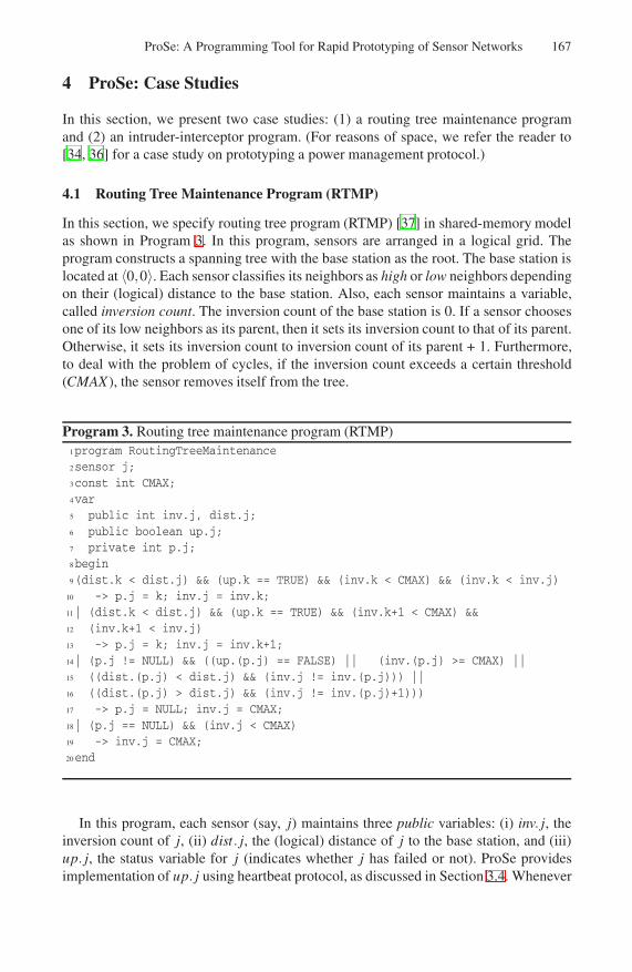
ProSe: A Programming Tool for Rapid Prototyping of Sensor Networks 167
4 ProSe: Case Studies
In this section, we present two case studies: (1) a routing tree maintenance programand (2) an intruder-interceptor program. (For reasons of space, we refer the reader to[34, 36] for a case study on prototyping a power management protocol.)
4.1 Routing Tree Maintenance Program (RTMP)
In this section, we specify routing tree program (RTMP) [37] in shared-memory modelas shown in Program 3. In this program, sensors are arranged in a logical grid. Theprogram constructs a spanning tree with the base station as the root. The base station islocated at 〈0,0〉. Each sensor classifies its neighbors as high or low neighbors dependingon their (logical) distance to the base station. Also, each sensor maintains a variable,called inversion count. The inversion count of the base station is 0. If a sensor choosesone of its low neighbors as its parent, then it sets its inversion count to that of its parent.Otherwise, it sets its inversion count to inversion count of its parent + 1. Furthermore,to deal with the problem of cycles, if the inversion count exceeds a certain threshold(CMAX), the sensor removes itself from the tree.
Program 3. Routing tree maintenance program (RTMP)1program RoutingTreeMaintenance2sensor j;3const int CMAX;4var5 public int inv.j, dist.j;6 public boolean up.j;7 private int p.j;8begin9(dist.k < dist.j) && (up.k == TRUE) && (inv.k < CMAX) && (inv.k < inv.j)
10 -> p.j = k; inv.j = inv.k;11| (dist.k < dist.j) && (up.k == TRUE) && (inv.k+1 < CMAX) &&12 (inv.k+1 < inv.j)13 -> p.j = k; inv.j = inv.k+1;14| (p.j != NULL) && ((up.(p.j) == FALSE) || (inv.(p.j) >= CMAX) ||15 ((dist.(p.j) < dist.j) && (inv.j != inv.(p.j))) ||16 ((dist.(p.j) > dist.j) && (inv.j != inv.(p.j)+1)))17 -> p.j = NULL; inv.j = CMAX;18| (p.j == NULL) && (inv.j < CMAX)19 -> inv.j = CMAX;20end
In this program, each sensor (say, j) maintains three public variables: (i) inv. j, theinversion count of j, (ii) dist. j, the (logical) distance of j to the base station, and (iii)up. j, the status variable for j (indicates whether j has failed or not). ProSe providesimplementation of up. j using heartbeat protocol, as discussed in Section 3.4. Whenever

168 M. Arumugam and S.S. Kulkarni
Table 1. Memory footprint of the generated RTMP program
Program ROM RAM(in bytes) (in bytes)
routingM + NeighborStateM 42 106SS-TDMA 108 586other components (Timer, FramerM, LedsC, etc) 15934 404
5x5 7x7 10x10 14x14 20x200
10
20
30
40
50
60
70
80
Network size
Initi
al L
aten
cy (
in s
econ
ds) ProSe−RTMP (Latency)
ProSe−RTMP (Active Radio Time)MintRoute (Latency/Active Radio Time)
5x5 10x1020x20 5x5 10x1020x200
20
40
60
80
100
Network sizeC
onve
rgen
ce ti
me
(in s
econ
ds)
5 failures10 failures20 failures50 failures100 failures
ProSe−RTMP
MintRoute
(a) (b)
Fig. 2. Simulations results of the generated program. With 90% link reliability: (a) initial latencyand (b) convergence time. Note that the black bars in the convergence time graph shows the activeradio time during the convergence period. (The result was similar for simulations with 95% linkreliability.
j finds a low/high neighbor that provides a better path (in terms of inversion count) tothe base station, it updates its private variable, p. j, the parent of j, and inversion countinv. j. Whenever a sensor fails or inversion count is not consistent with its parent, thesensor sets its parent to NULL and its inversion count to CMAX (i.e., it removes itselffrom the routing tree). Subsequently, when it finds a neighbor with a better inversioncount value, it rejoins the tree.
We used ProSe to transform the program and integrated SS-TDMA [32] with thegenerated program (cf. Table 1 for memory footprint of the generated program).
Simulation results. We simulated the generated program (ProSe-RTMP) and MintRoute[38] using TOSSIM [39]. (For experimental results, we refer the reader to [34].) In oursimulations, the base station is located at 〈0,0〉 (i.e., sensor 0) and the inter-sensorseparation is 10 ft. In the absence of any interference, we have observed that probabilityof successful communication is more than 98% among the neighbors. However, randomchannel errors can cause the reliability to go down. Hence, we choose conservativeestimate of 90% link reliability (that correspond to the analysis in [40, 41]).
In our simulation, each sensor executes the write-all action of the program once inevery 2 seconds. And, in MintRoute, the sensors exchange routing information every2 seconds. Once the initial tree is constructed, we simultaneously fail some sensorsand measure the convergence time. The simulation results are shown in Figure 2. Theinitial latency to construct the routing tree for ProSe-RTMP and MintRoute are sim-ilar. MintRoute maintains link estimates of the active links of a sensor and updatesthe estimate periodically. As a result, the radio is active all the time. By contrast, withProSe-RTMP, the active radio time of the sensors during this period is significantly less(i.e., around 20% of the initial latency).

ProSe: A Programming Tool for Rapid Prototyping of Sensor Networks 169
Figure 2(b) presents the convergence time of the protocols in the presence of failedsensors. MintRoute converges to a new routing tree quickly. By contrast, ProSe-RTMPconverges within 30-50 seconds. We note that this behavior is not because of prototyp-ing with ProSe. Rather, it is because of the nature of the original protocol specified withProSe. More specifically, MintRoute is pessimistic in nature, i.e., it maintains a movingaverage of link estimates of all active links of a sensor all the time. Hence, when sensorsfail, it converges to a new tree quickly. By contrast, RTMP is optimistic in nature. Inother words, whenever a sensor chooses one of its neighbors as its parent, it does notchange its parent unless the parent has failed or the tree is corrupted. As a result, whensensors fail, it takes sometime for the protocol to update the tree. On the other hand, theactive radio time during recovery is small with ProSe-RTMP.
4.2 Pursuer-Evader Tracking Program
Sensor networks are often used in intruder-interception games, where the sensors guidethe pursuer (e.g., a robot, a soldier, etc) to track and intercept the evader (e.g., intruder,hostile vehicle, etc). In this section, we specify the evader-centric program for intruder-interception from [42] in shared-memory model as shown in Program 4. In this pro-gram, sensors maintain a tracking structure rooted at the evader. The pursuer followsthis tracking structure to intercept the evader. Whenever the pursuer arrives at a sensor(say, k), it consults k to determine its next move. Specifically, it moves to the parent ofk. And, since the pursuer is faster than the evader, it eventually intercepts the evader.
Program 4. Pursuer-evader tracking program1program PursuerEvaderTracking sensor j; var2 public int dist2Evader.j, detectTimeStamp.j, p.j;3 private boolean isEvaderHere.j;4begin (isEvaderHere.j == TRUE)5 -> p.j = j; dist2Evader.j = 0; detectTimeStamp.j = TIME;6| (detectTimeStamp.k > detectTimeStamp.j) ||7 ((detectTimeStamp.k == detectTimeStamp.j) &&8 (dist2Evader.k+1 < dist2Evader.j))9 -> p.j = k; detectTimeStamp.j = detectTimeStamp.k;
10 dist2Evader.j = dist2Evader.k+1;11end
Each sensor (say, j) maintains three public variables: (i) dist2Evader.j, distance tothe root of the tracking structure, (ii) detectTimeStamp.j, the timestamp that j knowswhen the evader was detected at the root, and (iii) p. j, the parent of j. Whenever jdetects the evader, it sets detectTimeStamp.j to its current clock value (using the T IMEkeyword), dist2Evader.j to 0 and p. j to itself. If it finds one of its neighbors (say, k)has the latest detection timestamp, then it updates its public variables accordingly andsets its p. j to k. In Program 4, for simplicity, we do not show the actions of the pursuer.Since the pursuer can listen to the messages transmitted by the sensors, whenever thepursuer is near j, it reads the public variable p. j and moves to p. j.

170 M. Arumugam and S.S. Kulkarni
Table 2. Memory footprint of the generated tracking program
Program ROM RAM(in bytes) (in bytes)
trackingM + NeighborStateM N/A* 91SS-TDMA 108 586other components (Timer, FramerM, LedsC, etc) 14920 404
* The perl script tinyos-1.x/contrib/SystemC/module_memory_usage used to obtain
the breakdown of program ROM and RAM used by various components only provides the
RAM usage data for trackingM; it does not report the ROM usage for trackingM. We expect
this value to be small.
5x5 7x7 10x10 14x14 20x200
10
20
30
40
50
60
70
Network size
Tra
ckin
g La
tenc
y (in
sec
onds
)
Pursuer initially at sensor 0Puruser initially at center
5x5 7x7 10x10 14x14 20x200
10
20
30
40
50
60
70
Network size
Tra
ckin
g La
tenc
y (in
sec
onds
)
Pursuer initially at sensor 0Puruser initially at center
(a) (b)
Fig. 3. Tracking latency of the generated program: (a) with 90% link reliability and (b) with 95%link reliability
We used ProSe to transform the program and integrated SS-TDMA [32] with thegenerated program (cf. Table 2 for memory footprint of the generated program). In thisprogram, we need to wire components that detect whether the evader is present neara sensor. For example, if the goal is to intercept vehicles then we need to integratecomponents that can signal whether a vehicle is present or moving near a sensor (e.g.,magnetometer components, accelerometer components). Based on this signal, the vari-able isEvaderHere.j at sensor j is either set or unset. Such components are independentof the design of a tracking service.
Simulation results. We simulated the generated program using TOSSIM [39]. Theinter-sensor separation is 10 ft and the TDMA period in SS-TDMA is 0.78 seconds.Similar to Section 4.1, we choose the link reliability to be 90% and 95%. In our sim-ulations, we use a virtual pursuer and a virtual evader. The evader moves randomly inthe network. The variable isEvaderHere. j at j is set to T RUE or FALSE depending onthe current location of the evader. The pursuer is twice as fast as the evader. We did twosets of simulations: (1) the initial location of pursuer is at 〈0,0〉 and (2) initial locationof pursuer is at the center of the network. In both scenarios, the initial location of evaderis at the corner (i.e., 〈N − 1,N − 1〉 on NxN grid). From Figure 3, we observe that thetracking latency increases as the network size increases. The latency when the pursueris initially near the center is significantly less than the case where the pursuer is initiallyat 〈0,0〉. And, the active radio time is at most 20% of the time required by the pursuer tointercept the evader. Thus, these results demonstrate the potential of ProSe to generateapplication-level services for sensor networks.

ProSe: A Programming Tool for Rapid Prototyping of Sensor Networks 171
5 Conclusion
We expect that the programs generated by ProSe are competitive to related programsdesigned manually for sensor networks. Since ProSe hides low-level details from thedesigner, it allows rapid prototyping of sensor network protocols. Therefore, we ex-pect that the development time of a typical application (composed of several protocols)is small. Furthermore, since ProSe automatically transforms the program in abstractmodel to generate the corresponding nesC/TinyOS code, it enables quick deploymentof applications. We demonstrated this for (1) routing tree maintenance program (cf.Section 4.1), (2) pursuer-evader tracking service (cf. Section 4.2), and (3) power man-agement protocol [36].
We note that program analysis of nesC/TinyOS programs is gaining attention re-cently as it assists in programmer understanding, error detection, and program valida-tion (e.g., [43]). Specifically, in [43], program analysis is performed on state machinesderived from nesC/TinyOS programs. Such analysis is straight-forward in ProSe as theprograms are specified in a simple guarded commands format and several analysis toolsand model checkers [28] are readily available.
There are several possible future directions to this work. First, we would like toto combine this work with [44] where the sensor network protocols are proposed ina model that is similar to the abstract models used in ProSe. Since [44] focuses onverification aspects of the abstract protocols, combining it with ProSe, will provideassurance guarantees about the deployed programs. Additionally, we are also focusingon integrating ProSe with tools that automatically synthesize fault-tolerant programsfrom their fault-intolerant versions (e.g., FTSyn [45]).
References
1. Arumugam, M., Kulkarni, S.S.: Prose - a programming tool for rapid prototyping of sensornetworks. Poster at the Conference on Sensor, Mesh, and Ad Hoc Communications andNetworks, SECON (2007)
2. Gay, D., Levis, P., von Behren, R., Welsh, M., Brewer, E., Culler, D.: The nesC language: Aholistic approach to networked embedded systems. In: Programming Language Design andImplementation (PLDI) (June 2003)
3. Adya, A., Howell, J., Theimer, M., Bolosky, W.J., Douceur, J.R.: Cooperative task manage-ment without manual stack management or, event driven programming is not the opposite ofthreaded programming. In: USENIX Annual Technical Conference (June 2002)
4. Dunkels, A., Schmidt, O., Voigt, T., Ali, M.: Protothreads: Simplifying event-driven pro-gramming of memory-constrained embedded systems. In: Fourth ACM Conference on Em-bedded Networked Sensor Systems (SenSys) (November 2006)
5. Kasten, O., Romer, K.: Beyond event handlers: Programming sensor networks with attributedstate machines. In: Fourth Internation Conference on Information Processing in Sensor Net-works (IPSN) (April 2005)
6. Levis, P., Culler, D.: Mate: A tiny virtual machine for sensor networks. ACM SIGOPS Op-erating Systems Review 36(5), 85–95 (2002)
7. Liu, J., Chu, M., Liu, J., Reich, J., Zhao, F.: State-centric programming for sensor-actuatornetwork systems. Pervasive Computing 2(4), 50–62 (2003)

172 M. Arumugam and S.S. Kulkarni
8. Welsh, M., Mainland, G.: Programming sensor networks using abstract regions. In: Net-worked Systems Design and Implementation, NSDI (2004)
9. Newton, R., Welsh, M.: Region streams: Functional macroprogramming for sensor networks.In: Workshop on Data Management for Sensor Networks (2004)
10. Newton, R., Arvind, Welsh, M.: Building up to macroprogramming: An intermediate lan-guage for sensor networks. In: International Conference on Information Processing in SensorNetworks (IPSN) (April 2005)
11. Whitehouse, K., Zhao, F., Liu, J.: Semantic streams: A framework for composable semanticinterpretation of sensor data. In: Romer, K., Karl, H., Mattern, F. (eds.) EWSN 2006. LNCS,vol. 3868, pp. 5–20. Springer, Heidelberg (2006)
12. Gummadi, R., Gnawali, O., Govindan, R.: Macro-programming wireless sensor networksusing kairos. In: Prasanna, V.K., Iyengar, S.S., Spirakis, P.G., Welsh, M. (eds.) DCOSS 2005.LNCS, vol. 3560, pp. 126–140. Springer, Heidelberg (2005)
13. Kothari, N., Gummadi, R., Millstein, T., Govindan, R.: Reliable and efficient programmingabstractions for wireless sensor networks. In: Programming Language Design and Imple-mentation, PLDI (2007)
14. Brown, M., Gilbert, S., Lynch, N., Newport, C., Nolte, T., Spindel, M.: The virtual nodelayer: A programming abstraction for wireless sensor networks. In: International Workshopon Wireless Sensor Network Architecture (April 2007)
15. Sen, S., Cardell-Oliver, R.: A rule-based language for programming wireless sensor actua-tor networks using frequence and communication. In: Workshop on Embedded NetworkedSensors (EmNets) (May 2006)
16. Terfloth, K., Wittenburg, G., Schiller, J.: Rule-oriented programming for wireless sensor net-works. In: Conference on Distributed Computing in Sensor Networks (2006)
17. Arora, A., Gouda, M., Hallstrom, J., Herman, T., Leal, B., Sridhar, N.: A state-based lan-guage for sensor-actuator networks. In: International Workshop on Wireless Sensor NetworkArchitecture (April 2007)
18. Tavakoli, A., Chu, D., Hellerstein, J., Levis, P., Shenker, S.: A declarative sensornet archi-tecture. In: Workshop on Wireless Sensor Network Architecture (2007)
19. Demirbas, M., Soysal, O., Hussain, M.: TRANSACT: A transactional framework for pro-gramming wireless sensor/actor networks. In: International Conference on Information Pro-cessing in Sensor Networks (April 2008)
20. Abdelzaher, T., et al.: EnviroTrack: Towards an environmental computing paradigm for dis-tributed sensor networks. In: International Conference on Distributed Computing Systems(ICDCS) (March 2004)
21. Greenstein, B., Kohler, E., Estrin, D.: A sensor network application construction kit(SNACK). In: Conference on Embedded Networked Sensing Systems (2004)
22. Buonadonna, P., Gay, D., Hellerstein, J., Hong, W., Madden, S.: TASK: Sensor network in abox. In: European Workshop on Wireless Sensor Networks (2005)
23. Madden, S., Franklin, M., Hellerstein, J., Hong, W.: TinyDB: An acquisitional query pro-cessing system for sensor networks. ACM Transactions on Database Systems, TODS (2005)
24. Hull, B., Bychkovsky, V., Chen, K., Goraczko, M., Miu, A., Shih, E., Zhang, Y., Balakr-ishnan, H., Madden, S.: CarTel: A distributed mobile sensor computing system. In: ACMConference on Embedded Networked Sensor Systems, SenSys (2006)
25. Kulkarni, S.S., Arumugam, M.: Transformations for write-all-with-collision model. Com-puter Communications (Elsevier) 29(2), 183–199 (2006)
26. Herman, T.: Models of self-stabilization and sensor networks. In: Workshop on DistributedComputing (2003)
27. Dijkstra, E.W.: Self-stabilizing systems in spite of distributed control. Communications ofthe ACM 17(11) (1974)

ProSe: A Programming Tool for Rapid Prototyping of Sensor Networks 173
28. Holzmann, G.J.: The model checker Spin. IEEE Transactions on Software Engineer-ing 23(5), 279–295 (1997)
29. Dijkstra, E.W.: A Discipline of Programming. Prentice Hall PTR, Englewood Cliffs (1997)30. Arumugam, M.: A distributed and deterministic TDMA algorithm for write-all-with-
collision model. In: Kulkarni, S., Schiper, A. (eds.) SSS 2008. LNCS, vol. 5340, pp. 4–18.Springer, Heidelberg (2008)
31. Arumugam, M., Kulkarni, S.S.: Self-stabilizing deterministic time division multiple accessfor sensor networks. AIAA Journal of Aerospace Computing, Information, and Communi-cation (JACIC) 3, 403–419 (2006)
32. Kulkarni, S.S., Arumugam, M.: SS-TDMA: A self-stabilizing mac for sensor networks. In:Sensor Network Operations. Wiley-IEEE Press (2006)
33. Whitehouse, K., Sharp, C., Brewer, E., Culler, D.: Hood: A neighborhood abstraction forsensor networks. In: ACM International Conference on Mobile Systems, Applications, andServices (MobiSys) (June 2004)
34. Arumugam, M.: Rapid prototyping and quick deployment of sensor networks. PhD thesis,Michigan State University (2006)
35. Gouda, M.G., McGuire, T.M.: Accelerated heartbeat protocols. In: International Conferneceon Distributed Computing Systems, ICDCS (1998)
36. Arumugam, M., Wang, L., Kulkarni, S.S.: A case study on prototyping power managementprotocols for sensor networks. In: Datta, A.K., Gradinariu, M. (eds.) SSS 2006. LNCS,vol. 4280, pp. 50–64. Springer, Heidelberg (2006)
37. Choi, Y.-R., Gouda, M.G., Zhang, H., Arora, A.: Stabilization of grid routing in sen-sor networks. AIAA Journal of Aerospace Computing, Information, and Communication(JACIC) 3, 214–233 (2006)
38. Woo, A., Culler, D.: Taming the challenges of reliable multihop routing in sensor networks.In: Conference on Embedded Networked Sensing Systems (2003)
39. Levis, P., Lee, N., Welsh, M., Culler, D.: TOSSIM: Accurate and scalable simulation ofentire tinyOS applications. In: First International Conference on Embedded Networed SensorSystems (SenSys), November 2003, pp. 126–137 (2003)
40. Ganesan, D., Krishnamachari, B., Woo, A., Culler, D., Estrin, D., Wicker, S.: An empiricalstudy of epidemic algorithms in large scale multihop wireless networks. Technical ReportIRB-TR-02-003, Intel Research (March 2002)
41. Zuniga, M., Krishnamachari, B.: Analyzing the transitional region in low power wirelesslinks. In: Conference on Sensor and Ad hoc Communications and Networks (2004)
42. Demirbas, M., Arora, A., Gouda, M.: Pursuer-evader tracking in sensor networks. In: SensorNetwork Operations. Wiley-IEEE Press (May 2006)
43. Kothari, N., Millstein, T., Govindan, R.: Deriving state machines from TinyOS programsusing symbolic execution. In: Seventh Conference on Information Processing in Sensor Net-works, IPSN (2008)
44. Gouda, M.G., Choi, Y.-R.: A state-based model for sensor protocols. In: Anderson, J.H.,Prencipe, G., Wattenhofer, R. (eds.) OPODIS 2005. LNCS, vol. 3974, pp. 246–260. Springer,Heidelberg (2006)
45. Ebnenasir, A., Kulkarni, S.S., Arora, A.: FTSyn: A framework for automatic synthe-sis of fault-tolerance. International Journal of Software Tools for Technology Transfer(STTT) 10(5), 455–471 (2008)

Energy-Aware Dynamic Route Management forTHAWS
Chong Shen, Sean Harte, Emanuel Popovici, Brendan O’Flynn,and John Barton
CLARITY Centre, Tyndall National Institute, Lee Maltings, Cork, [email protected]
http://www.tyndall.ie/mai/
Abstract. In this research we focus on the Tyndall 25mm and 10mmnodes energy-aware topology management to extend sensor network lifes-pan and optimise node power consumption. The two tiered Tyndall Het-erogeneous Automated Wireless Sensors (THAWS) tool is used to quicklycreate and configure application-specific sensor networks. To this end,we propose to implement a distributed route discovery algorithm and apractical energy-aware reaction model on the 25mm nodes. Triggered bythe energy-warning events, the miniaturised Tyndall 10mm data collec-tor nodes adaptively and periodically change their association to 25mmbase station nodes, while 25mm nodes also change the inter-connectionsbetween themselves, which results in reconfiguration of the 25mm nodestier topology. The distributed routing protocol uses combined weightfunctions to balance the sensor network traffic. A system level simula-tion is used to quantify the benefit of the route management frameworkwhen compared to other state of the art approaches in terms of thesystem power-saving.
Keywords: THAWS, Energy-aware, Routing, Energy model, Sensornetwork.
1 Introduction
The Tyndall Heterogeneous Automated Wireless Sensors (THAWS) tool hastwo types of nodes with different functions selected from a number of differentnode layers developed by Tyndall Nation Institute [1]. Two modular nodes havebeen designed with a size of 10 mm by 10 mm, and 25 mm by 25 mm [2].These are referred to as the 10mm and 25mm nodes shown in Figure 1. Eachnode has a processing and transceiver layer. Sensor layers can then be connectedwith application specific sensors. In addition to sensors, a battery or energyharvesting device can be connected to provide a power supply and each nodecan also provide its own energy level reading.
The 25mm node has more powerful processing capabilities than the 10mmnode. This is provided by a layer with an Atmel ATmega128 microcontrollerwith 128 kB of program memory. There is also an FPGA layer and a number of
S. Hailes, S. Sicari, and G. Roussos (Eds.): S-Cube 2009, LNICST 24, pp. 174–188, 2009.c© Institute for Computer Sciences, Social-Informatics and Telecommunications Engineering 2009

Energy-Aware Dynamic Route Management for THAWS 175
Fig. 1. 10mm (left) and 25mm (right) modular Tyndall nodes
different layers for RF communications. In the 2.45 GHz frequency band thereis a layer using a Nordic nRF2401 transceiver and another layer using an EmberEM2420 ZigBee 802.15.4 compatible transceiver. There is also a 433/868/915MHz layer using a Nordic nRF905 transceiver, which allows a longer range, ofup to 3.8 km in line-of-sight conditions, compared to the 2.45 GHz options, whichhave a maximum range of about 200 m [1]. The drawback is that bandwidth islimited to 50 kbps, compared to 1000 kbps for the Nordic nRF2401. The tradeoffbetween data rate and bandwidth is that a small bandwith requires the radiotransmit for a longer time, which consumes more energy. The 10mm node is cur-rently a single transceiver layer, which uses a Nordic nRF9E5 chip. The chip hasa radio that is compatible with the Nordic nRF905 so this allows heterogeneousnetworks to be built. This chip also has an integrated 8051-compatible microcon-troller with a limited 4kB program memory. However, the 4KB memory is morethan enough to be programmed to read and transmit sensor data, and handle25mm association and deassociation in the THAWS. Meanwhile, the small sizeof the 10mm nodes allows a greater range of application with cheaper cost dueto reduced PCB size, the lower component count, and cheaper assembly costs.The range of the 10mm node is less as the antenna does not perform will withsuch a small ground reference, and also less than optimal design of the baluncircuitry in order to fit it into such a small area [2].
The core of the THAWS is an application generating tool, which has two mainparts. The first of these is a software library containing modules of code that actas primitives in building up a WSN application. The second part is a descrip-tion of the desired application. The second step of developing the THAWS toolis to propose energy-aware adaptive communication protocol considering self-organised medium access and energy-oriented dynamic routing path discoveryas the key enablers. In this paper we propose a distributed route management

176 C. Shen et al.
25 mm25 mm
25 mmGATEWAY
10 mm
10 mm
10 mm
10 mm
Fig. 2. Two-tiered heterogeneous network. The 25mm Tyndall nodes compose the firsttier and some of them serve as gateway. The 10mm Tyndall nodes compose the secondtier.
protocol and an efficient energy model specifically for the THAWS tool, wherethe 25mm nodes are exclusively used as the base station nodes creating the firstnetwork tier, and the 10mm nodes are used as the normal data collectors creat-ing the second tier. Figure 2 presents an example THAWS tool topology withtwo tiers. Each 10mm node is associated with a 25mm node. It only has partof the 25mm communication functionalities. The 10mm only transmits collecteddata to its serving(associated) 25mm node base station. Complicated tasks suchas data dissemination, topology control, fault recovery, internet gateway connec-tion, etc. can be solely carried out at the 25mm nodes tier with more computa-tion power when compared to the 10mm nodes tier. In the rest of the paper, wefirst review the state of art energy-aware routing protocols for the heterogeneouswireless sensor networks in Section 2. An energy model and a distributed net-work layer routing protocol will be detailed in Section 3. Section 4 provides thesimulation models and protocols performance result with discussion. And finallyin Section 5, a conclusion will be made with future research outlook.
2 Related Work
Current research is making an effort to improve the heterogeneous wireless sensornetwork overall lifetime at the network layer. The sensor networks can be classi-fied as one type of ad hoc networks but the ad hoc routing protocols e.g. Ad hocOn-Demand Vector (AODV) and Direct Source Routing (DSR) [6] can not beimported directly due to problems such as power constraints, limited microcon-troller computation capability, different radio access methods, Radio Frequency(RF) modules, etc. In order to find a path from the source node to the destina-tion node, usually, flooding is a classical way to propagate and disseminate data

Energy-Aware Dynamic Route Management for THAWS 177
but it always results in the broadcast storm problem, high message exchangeoverhead and fast node power consumption, which are unacceptable in wirelesssensor networks.
Different proposals provided solutions for those problems mentioned above.Gossiping [3] is a probabilistic based flooding scheme, which tries to overcomethe broadcast storm problem locally but at the cost of reliability. The use ofgossiping method for unstable sensor networks routing may increase the overallor partial system failure rate. Sensor Protocol for information via negotiation(SPIN) [4] is a flat data centric routing technique based on exchange of meta-databefore actual transmission. The meta-data exchange via data advertisements hasproven to be very useful in overcoming the broadcast storm problem includingredundancy, overlapping, and resource blindness. However, SPIN does not guar-antee information delivery if intermediate nodes between the source node anddestination node are not interested in the data advertisements. This disaccordthe objective of Tyndall 25mm nodes tier guaranteed Quality of Service (QoS)data delivery. Directed Diffusion [5] is an important paradigm for the eventmonitoring of sensor networks. It uses attribute value pair for naming the dataand queries the nodes or sensors in an on demand fashion by using the namingscheme and has achieved many fold energy efficiency as compared to classicalflooding techniques but its emphasis on life time of an overall system is less. TheTHAWS tool prefers system-wide power saving rather than reduced individualnode power consumption. On the other hand, The gradient set up phase is alsoexpensive in terms of latency and energy consumption. Moreover, being a querydriven data model, directed diffusion is not very efficient in applications wheredata is sent to the sink on continuous basis while the THAWS tool requires the10mm tier continuously sends data to the 25mm tier.
For the AODV and DSR as mentioned previously, nodes periodically transmitrouting table updates and generate networking traffic. As network size grows,the size of the routing tables and the bandwidth required to update them grows.The AODV is a reactive routing protocol, which uses sequence numbers of thedestination that results in loop free topologies. Routes are acquired on demand,which results in extra delay known as route acquisition delay. Moreover, a largevolume of message overhead is incurred if the routing information is changedwhen nodes are moved, but the power-aware THAWS tool constantly copes withthe situations e. g. 25mm node failure or medium access slot failure. The DSRis very similar to the AODV, which is based on source routing where the sourcespecifies the complete path to be taken by a packet. The Energy Aware Routing(EAR) [7] argues that using the minimum energy path all the time depletesthe node energy on this path and result in a disconnected network topology.It instead uses a probabilistic approach in selecting the path to the destinationby keeping more than one path toward the destination. The problem associatedwith the probability can be magnified when the THAWS scales to a large numberof nodes. First of all, the multiple routing path storage requires sensor memory,which is not adaptive and consumes a lot sensor power. Secondly, we can nottreat the 25mm and 10mm equally and nevertheless, it is impractical to have

178 C. Shen et al.
a big routing table at each 10mm Tyndall node. There are few other complexrouting protocols available such as gradient based routing, rumor routing, whichare also not adaptive for a sensor system with ultra low power design objective.
3 Energy-Aware Route Management for THAWS
With the aim to provide energy-aware and energy-efficient sensor network appli-cations through the THAWS tool, we at the Tyndall National Institute (TNI)first identify and investigate a fixed heterogeneous sensor network infrastructurewhere all the positions of 25mm nodes and 10mm nodes are fixed thus the nodemobility issues are not considered. The infrastructure, as a IEEE 802.15.4 com-patible sub-network along with other different sub-networks at the Dublin CityUniversity (DCU), will be eventually connected to the University College Dublin(UCD) Internet database via IEFT IPv6 over Low power wireless Personal AreaNetworks (6LowPan) technology within the Science Foundation Ireland fundedCLARITY [9] project. Figure 3 presents the cooperation plan between differentinstitutes at different locations.
Fig. 3. The CLARITY project 6LowPan and IEEE 802.15.4 based system
As specified in previous description for the 25mm nodes and 10 nodes atSection 1, due to the hardware limitation for the miniaturised 10mm node,it doesn’t support 802.15.4 using Nordic radio mircocontroller. Therefore, the6LowPan gateway connections and distributed route management functions forthe THAWS tool have to be handled at the 25mm nodes.
3.1 Node Energy Model
The goal of the use of an energy model control is to periodically monitor 25mmbase station nodes energy consumption status in order to maintain some property

Energy-Aware Dynamic Route Management for THAWS 179
of the communication graph, while dynamically change the number of 10mmnodes association as the energy consumed by the communications between theserving 25mm node and its associated 10mm nodes is one of the primary sourcesof energy consumption. The Tyndall 25mm node can also adaptively changethe transmission range to achieve a good energy efficiency using different RFmodules. The route management protocol considers the THAWS power efficiencyas the primary optimisation objective, and packet transmission delay and packetsuccessful delivery ratio as the secondary optimisation objectives. Therefore, apractical three states energy model is first proposed for the 25mm nodes.
The THAWS topology has been analysed as shown in Figure 4. Based onthe energy mapping technology for both 25mm nodes and 10mm nodes, givenenergy levels of the nodes, the THAWS tool can roughly predict future state ofthe network. The spatial and temporal energy gradient of the network nodes mayalso be modelled. Coupled with network topology, this can be used to identify“weak areas” of the network. Most importantly, each 25mm node decides howmany 10mm nodes it serves at first instance and exchanges information withother 25mm nodes to handover or accommodate 10mm nodes.
Fig. 4. The Tyndall 25mm nodes practical energy model based traffic offloadingillustration
The 25mm distributed energy-aware offloading mechanism includes two sub-algorithms in respect to the node energy states as presented in Figure 4. Theenergy-model at each 25mm node uses a linear energy function to describe theenergy level:
E = 1 − TaCa − TsCs (1)
Where 1 stands for full energy level. Ta and Ts are the Tyndall 25mm node usagetime accumulated in the active mode and sleep mode, respectively. Ca and Cs

180 C. Shen et al.
are the 25mm typical energy used at the active mode and sleep mode. The 10mmnode uses a similar energy-model and it shuts down when the energy is empty.Two hard boundaries, which are 0.33 and 0.67, have been introduced to triggerthe two sub-protocol named Level 1 Offloading (L1O) and Level 2 Offloading(L2O). The three energy states are Full E = (0.67, 1], Normal E = (0.33, 0.67]and Restricted E = (0, 0.33]. The reason to only have two sub-protocols withtwo hard boundaries is the energy saving consideration because the frequentnetwork topology and unnecessary information exchange must be avoided.
As shown in Figure 4, the example network (cluster) consists of 7 first tier25mm nodes and a number of second tier 10mm nodes connected to the 25mmnodes. When 25mm node 2 and node 4 change the energy state to Normal (redcoloured) state, the L1O protocol is triggered:
L1O. A 25mm node searches other first tier 25mm nodes using Routing Request(RREQ) message to reduce the number of intra-tier connections, which resultin the node energy saving since the time spent on active transmission modewill be reduced. In order to retain the connectivity of the entire network, aspanning tree [10] algorithm is used. To avoid flooding information throughthe entire 25mm node tier, it is divided into several clusters and each clusterincludes a number of 25mm nodes e.g. 7 nodes. Therefore in a sensor nodemapped graph (a cluster) there is a subgraph which is a tree and connectsall the vertices together. A single graph can have many different spanningtrees. We assign a energy model based weight function to each edge, which isa number representing how unfavorable it is, and use this to assign a weightto a spanning tree by computing the sum of the weights of the edges inthat spanning tree. We also assign a higher energy weight upon the linksassociated with state change. A minimum weight spanning tree is then aspanning tree with a weight less than or equal to the weight of every otherspanning tree.
Using the L1O protocol, the connection within the seven 25mm nodes clusterhas been changed after node energy based weight calculation at each link. Node1 connects to node 3 and node 3 disconnects from node 2. Node 2 disconnectsfrom node 3. Node 4 disconnects from both node 6 and node 7. Node 5 connectsto node 6. Node 6 connects to node 5 and disconnects from node 4. Node 7connects to node 6 which has a higher energy left and disconnects from node 4.
When 25mm node 2 changes the energy state from Normal state to Restricted(write coloured) state, the L2O protocol is triggered:
L2O. A 25mm node searches other first tier 25mm nodes using Routing Request(RREQ) message to reduce the number of inter-tier connections and shift anumber of its associated 10mm nodes to its neighbouring 25mm nodes, afteracknowledged answer from the neighbouring 25mm nodes through RoutingReply (RREP). The neighbouring nodes will not reply RREP to the request-ing 25mm node unless two conditions are satisfied, which are the transmissionrange of a candidate 10mm node & available medium access slots.

Energy-Aware Dynamic Route Management for THAWS 181
Using the L2O protocol, as indicated in 4, 25mm node 2 with restricted energystate disconnects two of its associated 10mm nodes. The two 10mm node arethen connects to 25mm node 1. The other 10mm node can not be connected tonode 1 due to the transmission range problem.
3.2 Energy-Aware Power Saving Protocol
The Energy-aware power saving protocol for the THAWS operates distributedly.It comprehensively considers three parameters: Energy Consumption (E), PacketDelivery Delay (D) and Packet Successful Delivery Ratio (S) to the distributedprotocol. The shortest path between the source node to the sink node (or sayhop distance) is usually a critical parameter for a dynamic environment, but forthe nodes position fixed THAWS it is not necessary. A function is assigned toeach 25mm node and the routing path between the source 25mm node and thedestination 25mm node is based on the calculation of a function:
Fn = αEn + βDn + γSn (2)
Where n is the node number or an identifier assigned to a 25mm node. Eachparameter has been given a weight factor, which are α for energy consumption),β for packet Delivery Delay and γ for packet successful delivery ratio dependingon different wireless sensor network application requirement, and the add sumof α + β + γ = 1. A localised flooding technique is used to find next hop neigh-bouring 25mm node distributedly and system-wide probing message flooding isprohibited to reduce data exchange overhead. For example, if an applicationrequires a guaranteed packet delivery with a time restriction, we can assign ahigher weight factor value to β and γ while reducing the value of α. Instead ofreacting to the environmental change (power level) in a reactive manner as inthe proposed energy model based L1O & L2O, the protocol operates proactivelyto balance traffic within the THAWS. For example, as shown in Table 1 with 7nodes scenario, we first assign 0.5, 0.25 and 0.25 to α, β and γ to prioritse anenergy-efficient sensor network application. We also assume node 1 is the sourcenode and node 7 is the destination node (sink) which connects to the 6LowPanbased IP network.
The label routing concept and routing table style originated in ATM networks[11] and has been introduced to the protocol since the position of the 25mm node
Table 1. An example weighted function calculation for 7 nodes
αE βD γS FNode1 0.50 0.25 0.25 1.00Node2 0.48 0.25 0.25 0.98Node3 0.37 0.24 0.24 0.85Node4 0.46 0.25 0.25 0.96Node5 0.42 0.24 0.24 0.90Node6 0.39 0.25 0.25 0.89Node7 0.50 0.25 0.25 1.00

182 C. Shen et al.
Table 2. An example label based added value calculation for 7 nodes
Node1 Node2 Node3 Node4 Node5 Node6 Node7Node1 N/A 1.98 1.85 N/A N/A N/A N/ANode2 1.98 N/A 1.83 1.94 N/A N/A N/ANode3 1.85 1.83 N/A N/A N/A N/A N/ANode4 N/A 1.94 N/A N/A 1.86 1.85 1.96Node5 N/A N/A N/A 1.86 N/A 1.79 N/ANode6 N/A N/A N/A N/A 1.79 N/A 1.89Node7 N/A N/A N/A 1.96 N/A 1.89 N/A
is fixed and the label based switching provides faster packet forwarding than IPbased indexing or other mature reactive routing protocol such as AODV andDSR. Instead of finding the next relay node hop by hop, the path from thesource node to the sink node is identified by multiple labels where the label isrepresented by the added value of two neighbouring nodes La.b = Fa +Fb. Thenthe next actual node the source node is hopping to is decided by a comparisonof the added value between next hopping neighbours as shown in Table 2. Wecan also understand that the path is separated by several labelled segments. Therouting table at each 25mm node has seven message types: Label in, Label out,Source node, Destination node, Destination Sequence, Hop count and Time tolive (TTL). The relay nodes only need to find the available entry indexed bylabel in the packet, swap it with respective label out of this entry, and then sendit out to the next relay node.
Figure 5 illustrates the label exchange over seven 25mm nodes scenario. Aftercompare the added weight value function La.b, source node 1 checks the sequence
Fig. 5. The energy-aware power saving routing protocol illustration with fast labelexchange

Energy-Aware Dynamic Route Management for THAWS 183
number (SEQ) of the destination node 7 in the current path in order to avoidold path information. It should be at least as great as the value entry in thecurrent request otherwise the existing path in the table will be discarded. An-other function of the SEQ is to compare with its older value to increase the hopcount, e.g. if the source node can not find the destination node, it will incre-ment the hop count by one and then broadcast it to its neighbours. The hopdistance is not necessarily considered due to the fixed infrastructure and eventu-ally balanced traffic distribution. However, it is defined that the path keeps thehop count as small as possible to avoid abused path violation. Meanwhile, thelabel request will repeat once for each connection request. The second plot inFigure 5 presents the propagation mechanism and the label based routing pathsegmentation. The third plot presents that the routing path has been establishedbetween the source Node 1, Node 2, Node 4, and the destination Node 7 afterlabel message exchange and weight functions comparison.
4 Simulations
Before deploying C based code to both 10mm and 25mm Tyndall nodes, a dis-crete event simulation tool known as OMNeT++ [8] is used for the evaluations.The simulation provides facilities to model the communications between thenodes. It serves as a validation and optimisation tool for THAWS fast sensornetwork applications development and deployment.
In the experiment, 98 25mm nodes are modelled and placed in a 3000 m x3000 m area and 196 10mm nodes are also randomly distributed. Each 10mmnode is first associated with a 25mm node. For 25mm base station nodes, 7 ofthem are grouped as a cluster therefore 14 clusters are formed. The gateway (orsay clusterhead for 6LowPan deployment) is randomly positioned at the clusterboundaries. At the beginning of the simulation, all 25mm nodes starts with fullenergy unit (1 Unit). With every reception, transmission and message exchangea 25mm node constantly decreases the energy at the active mode otherwise itis in the sleep mode. The 10mm node also starts with full energy unit. Nodeonly periodically transmits data and then puts itself in sleep mode. Free spacepropagation model and Additive White Gaussian Noise (AWGN) environmentare used. Each 25mm transmission range is set to 3 km while 10mm is set to 100m. The network stack consists of physical layer, Address Resolution Protocol(ARP) module, modified 802.11 based slotted medium access module, link layerand interface priority queue. The bandwidth is fixed at 2 Mbps for a higherbound optimisation. The data is transmitted at Constant Bit Rate (CBR) atpayload of 512 bytes with different deadlines. Data packets are generated at thesource at a rate of 0.5, 1.0, 1.5, 2.0, 2.5 and 3.0 packets/s.
We have compared the performance of our THAWS energy-aware label basedrouting management (THAWS-R) with EAR and a modified classic AODV(without mobility header packets) protocol. The energy-model with L1O andL2O mechanisms proposed is also used at each 25mm node.

184 C. Shen et al.
4.1 System Lifetime
Figure 6 compares the system lifetime for different route management approachesas it is a critical objective for the THAWS-R to achieve. The system life timeparameter is scaled from 0-100 according to the system power left at all Tyndall25mm and 10mm nodes. We first define system failure as the time after which33% of sensor nodes run out of batteries that resulting in a routing hole. In theresult, the simplified AODV presents the worst performance as expected becausethe system wide flooding produces a large number of signalling exchange over-head. The sensor system consumes a large amount of power at 25mm base stationnodes when active. It has been proved that the protocol is neither adaptive norenergy-efficient also due to the route change latency. On the other hand, as a lin-ear energy model is used in each 25mm node, the rate of partial or system wide25mm nodes power drainage is increased, which resulting in a shorter systemlifetime. EAR gives a higher priority to energy-efficiency therefore it presentsa better performance than AODV. However, it implements multicast instead ofunicast, and does not consider a restricted neighbouring path finding mechanismwith weight functions as compared to THAW-R, both the 25mm and 10mm willhave to spend more time at active mode. As evident by the graph, the THAWS-R management is the most energy-efficient protocol when compared to the othertwo. It is able to balance node energy utilisation system wide and also accountsfor the delay critical to real-time applications by using label routing mechanism.
Figure 7 presents the average active mode rate of all 25mm and 10mm nodesafter a simulated 70 hours run. All packets are transmitted at 2 packets/s. Fromthe results we notice that the node active mode rates using simplified AODVincrease rapidly after 30 hours run. The trend is approaching the maximumwhen the simulation is finishing. The 25 sensor node consumes a large amountof battery power to find a route to the sink node. After a long run, many sensornodes even go down if the detected events are not arriving at the sink node
Fig. 6. System lifetime for different route management schemes and protocols

Energy-Aware Dynamic Route Management for THAWS 185
Fig. 7. Average nodes at active mode rate for different route management schemes andprotocols
or due to power drainage. The rest of the sensor nodes have to make efforton path finding repeatedly and data forwarding, which results in more sensornodes works at active mode. EAR protocol without an adaptive localised routingfunctions, presents a slight better results than the simplified AODV. During the70 hours run, the average rate that nodes at active mode is smooth. Less nodesgo down due to issues such as power drainage and the traffic is reasonablydistributed across the system. However, this probability based approach mainlyconsiders power criteria but not the packet delivery rate, delivery delay andlink establishment speed. The proposed THAWS-R route management protocol,again, gives the best results against the other two. The active sensor node rateusing distributed weight functions and label based route establishment evendecreases with increasing simulation time. This is because the restricted flooding(local neighbour finding) and label routing help to construct adaptive routes tosink nodes across the system. The label indexing other than direct next hopindexing, greatly reduces the time that nodes spend on active mode.
4.2 Packet Delievery
For the packet level data delivery, it is important that traffic should reach thedestination within the deadline, otherwise the data must be resent or recollected,which consumes nodes power. Our route management strategy is aware of packetdelivery using the weighted Equation 2 thus low-rated routes (packet deliveryerror-prone paths) are avoided largely to make sure packets reaching the destina-tion before the deadline proactively. AODV sends packet by different routes thatincreases the reliability. This is evident in Figure 8, where we have compared thepacket delivery percentage with the deadlines. When the deadline is long enough,all three schemes achieve a satisfactory packet delivery percentage. When the

186 C. Shen et al.
Fig. 8. Packet delivery ratio for different route management schemes and protocols
deadlines are configured more and more aggressive, the results show the deliverypercentage reduces drastically for EAR protocol. The proposed THAWS routingscheme has a slightly higher successful delivery ratio than AODV with aggres-sive deadlines (starting from 200 milliseconds) due to its adaptivity. However, asstated previously, the THAWS weight function based routing can enhance oneperformance metric while worsening another. Therefore choosing the routing ap-proach is greatly influenced by the performance qualification metrics, which arehighly dependent on the nature of sensor network applications. If data deliveryloss rate is of great interest, and latency and energy conservation are of concern,one might pick a higher weight factor to further enhance the system packetdelivery rate.
Fig. 9. Average packet delay for different route management schemes and protocols

Energy-Aware Dynamic Route Management for THAWS 187
For the average packet delay evaluation, the THAWS route management,again, gives the best performance when compared to the other two schemes asindicated in Figure 9. This is expected as the delay function has been includedin the protocol to find the next hop node, the traffic has been evenly distributedwith reduced congestion and the fast label routing speeds up the route establish-ment process. Meanwhile, AODV gives the worst result as it tries to exhaustivelyflood the system with large number of hops. This makes packets visit multiplenodes incurring more transmission and queuing delay. EAR presents a slightlybetter result than AODV but it also tries to minimise the transmission powerby taking shorter distance, is not aware of system wide power utilisation, andchooses the next hop node solely based on geographic information with energymapping.
5 Conclusions
This paper has presented a practical route management framework specificallyfor the Tyndall heterogeneous automated wireless sensor tool. The analysis andsimulation results confirm that the proposed protocol and the 25mm tier energymodel based dynamic load balancing significantly improve the platform perfor-mance in terms of node energy consumption, packet delivery delay and packetsuccessful delivery ratio. Moreover, the lifetime of the overall THAWS tool isconsiderably increased. Future work will look at the deployment issues for the10mm nodes and 25mm nodes and Tyndall nodes based embedded system soft-ware development and hardware updates.
References
1. Harte, S., Popovici, E., O’Flynn, B., O’Mathuna, C.: THAWS: Automated De-sign and Deployment of Heterogeneous Wireless Sensor Networks. WSEAS Trans.Circuits and Systems 7(9), 829–838 (2008)
2. Harte, S., O’Flynn, B., Martinez-Catal, R., Popovici, E.: Design and Implemen-tation of a Miniaturised, Low Power Wireless Sensor Node. In: Proc. 18th Euro.Conf. Circuit Theory and Design, Seville, pp. 894–897 (2007)
3. Akyildiz, I., Su, W., Sankarasubramaniam, W., Cayirci, E.: Wireless Sensor Net-works: a Survey. Computer Networks Elsevier Journal 38(4) (March 2002)
4. Heinzelman, W., Kulik, J., Balakrishnan, H.: Adaptive Protocols for InformationDissemination in wireless sensor networks. In: Proc. of IEEE MobiCom., Seattle,WA (August 1999)
5. Wattenhofer, R., Li, P., Wang, Y.: Distributed Topology Control for Power EfficientOperation in Multihop Wireless Ad Hoc Networks. In: Proc. of IEEE InfoCom(April 2001)
6. Ganesan, D., Govindan, R., Shenker, S., Estrin, D.: Highly-Resilient, Energy-Efficient Multipath Routing in Wireless Sensor Networks. Mobile Computing andCommunications Review, 1–2 (1997)
7. Shah, R., Rabaey, J.: Energy Aware Routing for Low Energy Ad Hoc Sensor Net-works. In: Proc. of IEEE WCNC, Orlando, FL (March 2002)

188 C. Shen et al.
8. Varga, A.: Using the OMNeT++ Discrete Event Simulation System in Education.IEEE Trans. on Education 42(4) (1999)
9. CLARITY: The Centre for Sensor Web Technologies Bringing Information to Life,http://www.clarity-centre.com
10. Chazelle, B., Rubinfeld, Trevisan, L.: Approximating the Minimum Spanning TreeWeight in Sublinear Time. Computation Journal, 1370–1379, 34 (2005)
11. Leon-Garia, A., Widjaja, I.: Communications Networks. McGraw-Hill, New York(1999)

All Roads Lead to Rome: Data Highways forDense Wireless Sensor Networks�
David Lowe1,2 and Daniele Miorandi2
1 Centre for Real-Time Information Networks, UTS, Ultimo, NSW 2007, [email protected]
2 CREATE-NET, v. alla Cascata 56/D, 38123 – Povo, Trento, IT{daniele.miorandi,david.lowe}@create-net.org
Abstract. The design of efficient routing algorithms is an importantissue in dense ad hoc wireless networks. Previous work has shown thatbenefits can be achieved through the creation of a set of data “highways”that carry packets across the network, from source(s) to sink(s). Cur-rent approaches to the design of these highways however require a–prioriknowledge of the global network topology, with consequent communi-cations burden and scalability issues, particularly with regard to recon-figuration after node failures. In this paper we describe an approach togenerating these data highways through a distributed reaction-diffusionmodel that uses localised convolution with activation-inhibition filters.The result is the distributed emergence of data highways that can betuned to provide appropriate highway separation and connection to datasinks. We present the underlying models and the algorithms for generat-ing the highways, as well as preliminary simulation results.
Keywords: Wireless sensor networks, routing, data highways,activation–inhibition mechanisms, reaction–diffusion patterns.
1 Introduction
A key issue in dense ad hoc wireless networks is the design of efficient routingalgorithms. This can affect the performance of the resultant system in terms ofpower efficiency, communication latency and robustness. For example, an effi-cient routing algorithm can lead to reductions in both the number of networknodes that need to remain awake to route traffic and the total transmissionpower required for the multi–hop communication along the routing path fromdata source to data sink.
Previous work [10] has shown that the creation of a set of wireless “backbones”or data highways that carry packets across the network, from source to sink, canprovide a network capacity that follows the same pattern for randomly locatednodes as can be achieved for arbitrarily placed nodes. In effect, the highways are� This work has been partially supported by the European Commission
within the framework of the BIONETS project EU-IST-FET-SAC-FP6-027748,www.bionets.eu
S. Hailes, S. Sicari, and G. Roussos (Eds.): S-Cube 2009, LNICST 24, pp. 189–205, 2009.c© Institute for Computer Sciences, Social-Informatics and Telecommunications Engineering 2009

190 D. Lowe and D. Miorandi
constructed such that every source node is within range of at least one highway(implying it can access it in a single hop). The highways then drain packets tothe sinks along a series of shorter length hops, with correspondingly lower powerrequirements and hence a lower interference footprint.
In previous work, these highways have been constructed based on approachessuch as percolation theory [10]. This has the disadvantage that it requires ana–priori analysis of the entire network structure, with the consequence that theapproaches cannot readily accommodate randomly placed nodes unless there isa mechanism for determining and communicating node location — a constraintthat adds a layer of complexity and a performance burden. It also typically makesthe network less robust, as any change (such as a failure or location change of ahighway node) requires a global recalculation of the routing pathways.
In this paper we discuss an approach to addressing this problem throughdistributed determination of the data highways based on an activation-inhibitiondiffusion that generates optimal highway separation. We argue that this approachrepresents a significant contribution, insofar as it will improve robustness andallow localised self–healing of the data highways — an important characteristicof dense networks with randomly placed nodes.
In section 2 we discuss previous work in this area and in particular on theapplication of distributed diffusion model for engineering the emergence of pat-terns in large–scale networks. Following this, in section 3, we consider the modelsthat underpin the highway generation and the mechanisms that we have usedfor their distributed construction. Section 4 discusses the way in which data isthen routed within this data highway system, and section 5 presents prelimi-nary results and analysis showing the performance of the approach. Finally, wepresent our conclusions in section 6.
2 Related Work
Wireless sensor networks (WSNs) [1] have become an important tool in manyreal–world settings. For example, they are being increasingly used for the mon-itoring of environmental parameters, where nodes are deployed over space, eachnode sensing a given environmental parameter (temperature, light, level of pollu-tants etc.). In most real–world settings multiple sinks are present, each sink beingconnected, usually through some form of long–range wireless communications,with a remote data center where information is processed. When fine–grainedinformation is needed, the net result can be – from a communications perspective– the formation of dense WSNs.
Current state–of–the–art routing schemes for WSNs, for communicating sen-sory data to the sinks, are most often based on the construction of trees, astructure that lends itself naturally to perform en route aggregation of data [7].For dense WSNs, various authors have proposed optimal routing strategies basedon the use of a continuum model of node placement over space. In particular,routing strategies based on analogies with physical phenomena have been pro-posed (optics [12,6] and electromagnetism [17]), as well as routing strategies builtusing models inspired by road traffic engineering [2].

All Roads Lead to Rome: Data Highways for Dense WSNs 191
In their seminal work, Gupta and Kumar [11] proved that the communicationcapacity of (dense) ad hoc networks, with n nodes within a given area, canscale, in terms of per source–destination throughput, as 1√
nbit/s in the case of
arbitrary node placement and as 1√n log n
in the case of randomly (uniformly)located nodes. The existence of such a gap gave rise to various investigations,aimed at finding suitable strategies for closing it. This is particularly importantgiven that many (indeed possibly most) sensor networks are likely to have nodesthat are randomly placed.
In a series of papers, Franceschetti et al. [10] demonstrated, using tools andresults from percolation theory, that such a gap could be closed by introducingnon–uniform transmission power schemes. The concept of data highways wasintroduced in [10], where it was shown that it was always possible to build high–throughput paths crossing a given section of the network. Such paths resultin high–throughput as they can be operated at very low transmission power,hence limiting self–interference. The optimal routing strategy would then be: (i)from a source reach the closest highway with a single (possibly high–power) hop;(ii) route packets along the highway using low–power hops; (iii) drain packetsfrom the highway to the appropriate sink when in proximity. Such a scheme wasshown to be able to attain a throughput per source–destination pair of the orderof 1√
n, thereby effectively closing the gap in the Gupta–Kumar result. A sample
representation of a set of data highways is reported in Fig. 1 (taken from [10]).The intuition behind such a result is that by using highways it is possible
to limit mutual interference among nodes in the network. To the best of theauthors’ knowledge, however, such a result has not yet found any applicationto routing problems in realistic environments. The main difficulty is the con-struction of highways. In order to have a feasible solution (in terms of scalabilityand complexity), the formation of highways should be achieved by means of adistributed process based on local information only. Rather than a global designof the highways, the nodes should self–organize to achieve the desired spatial
Fig. 1. Typical data highways through a 40x40 grid, obtained using a bond percolationmodel (from [10])

192 D. Lowe and D. Miorandi
structures that can in turn be used to generate the data highways. This raisesthe question of what form of self-organising process may be relevant in thisparticular scenario?
The use of self–organizing processes has seen wide consideration. For example,their use for building “spatial” computers was at the heart of the MIT’s Amor-phous Computing initiative1. One of the application scenarios envisioned for the(programming) techniques developed within the framework of such an initiativewas to engineer the emergence of structures in sensor–actuator networks [4].
The use of related self–organizing spatial processes for building overlays foundapplications in various networking fields. In WSNs, Bicocchi et al. proposedto use a field–based mechanism for aggregating WSNs into logical neighbor-hoods [5]. In peer–to–peer systems, probabilistic distributed mechanisms wereproposed by Jelasity et al. for dynamically rewiring links in overlays [14,13].In particular, it was shown that, by relying on local interactions only, it waspossible to build system–level structures with desired topological properties.
In [16] Saffre and Shackleton propose the use of an embryogenies–inspiredmechanism for efficiently allocating ’roles’ in an autonomic manner in a peer–to–peer service infrastructure. In such a work, nodes communicate via gossipingtechniques, and differentiation decisions are taken at each node based on thenodes’ current status and the status of neighbours. The mechanism is reported tobe able to build efficient structures (in terms of topology and role assignments).
Possibly the most relevant form of self-organising process to our particularproblem are reaction-diffusion processes. These processes are at the basis of var-ious natural mechanisms that result in the emergence of patterns, in particularof cell differentiation and morphogenesis [3]. The use of reaction–diffusion pro-cesses (and in particular of activation–inhibition mechanisms) has been proposedin the context of ad hoc networks to deal with activation problems. In partic-ular, it has been proposed by Durvy and Thiran for dealing with activation atthe MAC level [9] and by Neglia et al. for addressing clustering problems inWSNs [15]. In both cases, the pattern to be created presents isolated activationpeaks (corresponding to ’active nodes’) divided by large valleys. Such patternsare different from those needed to engineer data highways, which require thecreation of zebra–like stripes, which should furthermore converge to one of thesinks present in the network. We will consider these processes in more detail,and how we might adapt them, in the following section.
3 Models and Mechanisms for Data Highways Formation
3.1 Reaction Diffusion Modeling
As outlined above, we wish to develop self-organising processes that lead to thenatural emergence of data highways through a wireless network. These highwaysneed to be optimally spaced such that all nodes are within a single hop of ahighway, but the highways themselves utilise short-range hops to transport data1 http://groups.csail.mit.edu/mac/projects/amorphous/

All Roads Lead to Rome: Data Highways for Dense WSNs 193
to any data sink. This concept was shown in Figure 1. Further, the highwaysshould be able to be derived only through local interactions between nodes.
In developing an approach to this problem, we have taken inspiration frommechanisms that utilise activation-inhibition reaction-diffusion [3,9,15]. Thesemechanisms describe how a field strength variable or substance concentrationwithin each cell or node can vary in space and time under a pair of competinginfluences – a short range positive activation region within which the field ofneigbouring cells is strengthened, and a longer range negative inhibition regionwithin which the field of neighbour cells is retarded – with the resultant emer-gence of specific patterns when the effects are diffused through the network. Theresultant models have been used widely to describe behaviours in biological andphysical processes (see [8] for a discussion). The simplest formulation of thisapproach, using a single field variable, is modelled in the discrete time domainas follows:
u(k, t + 1) = g
⎛⎝ϕsu(k, t) +
∑j∈Ri
ϕi(j)u(k + j, t) +∑j∈Ra
ϕa(j)u(k + j, t)
⎞⎠ (1)
where u(k, t) is the field strength in cell k at time t, Ri is the region overwhich the inhibition function ϕi is applied, Ra is the region over which theactivation function ϕa is applied, and g() is a limiting function. The activationfunctions are time invariant, and applied uniformly across the sensor field. Notethat this is equivalent to the convolution of u(t) with the sum of ϕi, ϕa and theself-activation value ϕs. Note also that, in general, it is assumed that ϕi takesnegative values, while ϕa and ϕs take positive values.
As discussed in the previous section, recent work has adapted reaction dif-fusion models to the design and/or configuration of wireless networks. As anexample, Neglia and Reina [15] have used activator-inhibitor diffusion to selectactive nodes within a dense wireless sensor network. The nodes have deeply over-lapping sensing fields, and hence only a small number of nodes are required to beactive in order to adequately provide full data on the region to be sensed. Theoperation of this approach can be seen in Figure 2. A random dense wireless sen-sor network (Figure 2a) is repeatedly convolved with a symmetric 2-dimensionaldiffusion filter (Figure 2b). The resultant field strength after 20 iterations of afilter2 (Figure 2d) is then analysed to determine local maxima (Figure 2e) –which represent the nodes to be activated. All other nodes can be switched to alow-power non-sensing state. The result is a distributed process for identifyinga subset of nodes to be activated, such the nodes are suitably distributed.
The repeated filter convolution causes the emergence of the peaks in the ac-tivation field by activating localised regions whilst inhibiting the areas betweenthese regions. The width of the inhibition zone controls the separation of theresultant peaks and the width of the activation zone controls the kurtosis of
2 The filter used in this case was a simplified version, with a central self-activationstrength ϕs = 2, a flat activation ring of strength ϕa = 1 and radius 1, and a flatinhibition ring of strength ϕi = −0.1 and radius 6.
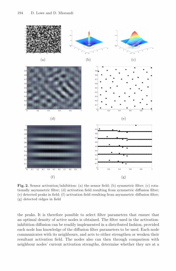
194 D. Lowe and D. Miorandi
0 0.2 0.4 0.6 0.8 10
0.1
0.2
0.3
0.4
0.5
0.6
0.7
0.8
0.9
1
−10−5
05
10
−10
−5
0
5
10−0.5
0
0.5
1
−10−5
05
10
−10
−5
0
5
10−0.5
0
0.5
1
(a) (b) (c)
0 0.2 0.4 0.6 0.8 10
0.1
0.2
0.3
0.4
0.5
0.6
0.7
0.8
0.9
1
0 0.2 0.4 0.6 0.8 10
0.1
0.2
0.3
0.4
0.5
0.6
0.7
0.8
0.9
1
(d) (e)
0 0.2 0.4 0.6 0.8 10
0.1
0.2
0.3
0.4
0.5
0.6
0.7
0.8
0.9
1
(f) (g)
Fig. 2. Sensor activation/inhibition: (a) the sensor field; (b) symmetric filter; (c) rota-tionally asymmetric filter; (d) activation field resulting from symmetric diffusion filter;(e) detected peaks in field; (f) activation field resulting from asymmetric diffusion filter;(g) detected ridges in field
the peaks. It is therefore possible to select filter parameters that ensure thatan optimal density of active nodes is obtained. The filter used in the activation-inhibition diffusion can be readily implemented in a distributed fashion, providedeach node has knowledge of the diffusion filter parameters to be used. Each nodecommunicates with its neighbours, and acts to either strengthen or weaken theirresultant activation field. The nodes also can then through comparison withneighbour nodes’ current activation strengths, determine whether they are at a

All Roads Lead to Rome: Data Highways for Dense WSNs 195
local maxima and hence should be active. This means that this approach can befully distributed within a wireless network, leading to active node selection withno network-wide oversight.
3.2 Highway Generation
What we are seeking in the design of the data highways is analogous to this– the localised selection of the nodes which form the highways without anyglobal design or control. The natural question to ask is therefore whether or notan activation-inhibition diffusion model can be adapted such that the result isconnected nodes that together make data highways, rather than single activenodes.
The solution is based on changing the nature of the diffusion filter. Previouswork on wireless networks has used symmetric filters, leading to the emergenceof patterns that have isolated peaks in the sensor activation field. Work in otherareas (e.g. [8]) has shown that changing the nature of the diffusion filter can leadto changes in the patterns that emerge in the activation field. As an example,consider the bottom row of Figure 2. In this case the random dense wirelesssensor network is repeatedly convolved with a rotationally asymmetric filter thathas a dominant horizontal activation axis, whilst inhibiting along the verticalaxis (Figure 2c). The resultant field strength patter after 20 iterations of a filterthat has this structure is shown in (Figure 2f). This has developed a stripedpattern of ridges and troughs, with the orientation controlled by the orientationof the activation axis in the filter and the separation determined by the rangeof the filter inhibition. The ridges in this pattern can then be used to determinelocal ridge maxima (Figure 2g) – giving the potential data highways that weare seeking. Nodes at ridge maxima become highway nodes, and all other nodescommunicate with the highways in order to deliver data to desired data sinks. Bytuning the filter parameters appropriately, we can control the separation betweenthe highways, and thereby ensure that all non-highway nodes are within a singlehop of a highway.
3.3 Controlling Highway Orientation and Destination
Having demonstrated that it is possible to generate ‘striped’ patterns that canbe used to generate highways, we next consider the question of how we orientthese stripes so that the highways converge on data sinks. One possibility is toconstruct artificial “bridges” between the highways and relevant sinks (takinginto account the overall topology as well as load balancing between the sinks).These bridges can be either multi-hop paths, or could be a single high-powerconnection. In either case, this solution requires the artificial construction ofadditional routes3.
An alternative is to investigate whether it is possible to control the directionsof the highways such that as the ridges are generated during the diffusion process,
3 This is actually the solution originally discussed in [10].

196 D. Lowe and D. Miorandi
they naturally converge to the data sinks. Given that the orientation of the ridgesare controlled by the orientation of the activation axis in the filter, we shouldtherefore be able to create ridges that converge on a sink by making the directionof the filter activation axis spatially dependent.
Consider the case of a network field with a single sink. Each node in thenetwork determines the direction to that sink, and rotates its local instance ofthe diffusion filter so that the activation axis is aligned with the direction tothe sink. The diffusion filter contains a square inhibition zone Ri of dimension2R×2R (with an inhibition level of ϕi), and a wedge-shaped activation zone Ra
with an angular size ρ (with an activation level of ϕa). We rotate the filter byrotating just the activation band within the overall square filter.
Applying this filter so that the activation band is always oriented towards thesingle sink gives an activation field as shown in Figure 3a, with all ridges havinga dominant orientation towards the sink. Performing a ridge detection on thisthen gives the ridges shown in Figure 3b4. A simple growth of any ridge pointthat is at the end of a ridge can be used as a final step in connecting any isolateddata highways, to form a connected data highway network.
0 0.2 0.4 0.6 0.8 10
0.1
0.2
0.3
0.4
0.5
0.6
0.7
0.8
0.9
1
0 0.2 0.4 0.6 0.8 10
0.1
0.2
0.3
0.4
0.5
0.6
0.7
0.8
0.9
1
(a) (b)
Fig. 3. Sensor activation/inhibition with local filters rotated towards a single sink: (a)activation field resulting from rotated filters; (b) detected ridges in field
If we add additional data sinks then the filter orientation, and hence theactivation field orientation, can be derived based on a gravitational attractionmodel. For each node, the activation field direction should be a weighted sum ofthe directions to each sink, with the weight inversely proportional to the squareof the distance to the sink. In other words, the direction of the diffusion filter atnode Ni can be given by the vector Di:
Di =
∑j∈S(Ni − Sj)|Ni − Sj |−2∑
j∈S |Ni − Sj |−2 (2)
where S is the set of sink nodes Si.4 It is worth remarking that, whereas for the detection of single points a 2-dimensional
local maxima was used, in this case the ridge detection is done by looking for localmaxima in only one dimension perpendicular to the filter orientation.

All Roads Lead to Rome: Data Highways for Dense WSNs 197
As with the previous example, this approach is still able to be implemented ina distributed fashion. The only aspect that unavoidably requires global knowl-edge is the relative location of the data sinks – or rather, whilst each node doesneed to know its own location, it does need to know the direction and (network)distance to each sink. Without this knowledge it would be impossible to locallyorient the filter, and hence activation bands and the resultant highways. Knowl-edge of the sinks can however be readily achieved through a broadcast beaconsignal from each sink node when it activates. The beacon propagates through thenetwork, with each node recording the number of hops to each sink from each ofits neighbour nodes, and hence the distance and dominant direction. In the nextsection, we will present a distributed procedure for gathering such informationat each node in the network.
4 Routing on Data Highways
Let us now consider the algorithms for implementing the models discussed above,as well as how the resultant highways are then used to route data. We assumethe following:
– Nodes are assigned a unique identifier;– Nodes can tune dynamically their transmission power level Ptx in the range
[Pmin, Pmax];– The network is connected when all nodes use Ptx = Pmin;– Nodes transmit at Pmin unless otherwise specified.
Each node maintains the following data structures:
– A database of all data sink(s), called sinkDB, having entries of the type< sinkID, distance >, where distance denotes the (minimum) distance interms of number of hops from a given sink;
– a database for the state of neighbouring nodes, where the size of the neigh-bourhood is determined by the filter to be applied, as detailed in Sec. 3.We denote by nodeDB such a database, whose entries have the form <nodeID, distance, state, sinkDB >, where nodeID is the identifier of a nodein the neighbourhood, distance is its minimum distance (in hops) from thegiven node, state is its current state (activation level) and sinkDB is a datastructure containing information on distance from the sinks present in thenetwork.
We first detail the algorithms necessary for initializing the network and settingup the highways. The algorithms work in two steps. First, sinks need to announcetheir presence, and nodes to compute their distance from them. To accomplishsuch a task, sinks broadcast a beacon message (sinkBeacon) containing boththeir sinkID and a distance field in the header. The field distance is initialisedto one. Nodes receiving the beacon check if an entry with the same sinkID ispresent in their sinkDB. If there is no entry, or the distance field in the receivedbeacon is less than the distance in the stored entry, then the sinkDB is updated,

198 D. Lowe and D. Miorandi
the distance field is incremented by one and the beacon is forwarded on. In sucha way, the field distance in the sinkBeacon corresponds to the minimum distance(in hops) from the corresponding sink. At the end of the process each node hasthe complete list of sinks in the network and the corresponding distance fromany of them. Such an information is needed for setting up the filter, as outlinedin Sec. 3. A detailed description of the algorithm is reported in the App. A(Alg. 1).
The next step is to let nodes construct their neighbourhood map, accordingto the filter parameters (in particular the dimension of the activation/inhibitionneighbourhood, denoted by the filter radius R parameter5). In order to do so,they need to collect information about the state of their k–hop neighbours (k ≤R) and their distance from the sinks present in the system, as outlined in theprevious section. Such a procedure is then repeated periodically to maintain anupdated view of the system state. This process is carried out using a gossip–basedmechanism for spreading information about nodes’ state in a distributed fashion.Each node periodically broadcasts a nodeQuery message, where it includes itsown ID, current activation state and the information contained in the sinkDB(i.e., distance from any sink). Upon reception of a nodeQuery message, one–hopneighbours first update the state field of the corresponding nodeDB entry. Then,they query their own nodeDB for information about the state of nodes that areat distance (in hops) less than or equal to (R− 1). This retrieves all informationthat is at most R hops from the node issuing the original query. The informationcollected is then included in an acknowledgment message that is sent back to thenode originating the query. A detailed description of the algorithm is reportedin the App. A (Alg. 2)6. Once each node has the relevant filter information theyare able to recalculate their activation level, and subsequently compare this toneighbouring values to determine if they are a “ridge” node, and hence on ahighway.
Given the mechanisms for building data highways, we now need to introducemechanisms for routing messages containing sensed data from any node to one ofthe sinks present in the system. The routing protocol envisioned can be broadlydivided in two phases. In the first phase, nodes not belonging to an highway haveto find a way to reach one. This is done by simply broadcasting a beacon messagewith increasing transmission power (and hence communication range) until anode on an highway is reached and sends back an acknowledgment message.Such a node will constitute the entry point to the highway. From that momenton, all messages generated will be forwarded to the entry point. A detaileddescription of the algorithm is reported in the App. A (Alg. 3). Note that if at
5 The parameter R, which roughly correspond to the distance among highways, shouldbe chosen in such a way to ensure that, by transmitting at Pmax, a node will be ableto join an highway.
6 With such a procedure, information on the state of nodes is received incrementally,each round bringing information to nodes located one hop further. When bootstrap-ping the system, it takes R rounds to acquire the knowledge necessary for buildingthe filter.

All Roads Lead to Rome: Data Highways for Dense WSNs 199
any point there is a failure in a highway node, the source node can repeat theabove process to locate a new highway entry point.
The second phase is concerned with the routing of messages along an highway,in order to reach an appropriate sink. In general, following the procedure high-lighted in the previous section, we will achieve highways connected to one singlesink. However, the activation–inhibition mechanism presented in Sec. 3 cannotprevent highways to be connected to two or more sinks. In order to optimize theusage of resources, messages should be directed towards the closest sink.7 Oncethe highway setup phase is completed, nodes on the highway(s) will reset theirsinkDB data base. Sinks will then broadcast a beacon message (beaconSinkH),which will be propagated only by nodes belonging to an highway. Such messageswill include a distance field that will be initially set to 1. Upon reception ofsuch a message, nodes on the highway(s) will check their internal sinkDB database; if an entry corresponding to the sink ID is already present, it is updatedif the distance contained in the beacon is smaller than that maintained in thecorresponding entry of the data base. The beacon message is then relayed, afterhaving increased by one the value of the distance field. A detailed descriptionof the algorithm is reported in the App. A (Alg. 4).
As with reconnecting of source nodes to highways, the highways themselvesare also able to self-heal. When the failure of a highway node is detected bya neighbouring highway node being unable to route traffic to the failed node,the neighbour can trigger a new localised diffusion process, that leads to theemergence of new highway in the local region of the failed node. Given the localnature of this process, this resultant highway will be operational, but may notbe optimal. Whilst the highway is being used, further diffusion can progressivelyrefine the highway route. The result is an inherent self-healing of the network.
5 Numerical Example
In order to illustrate the approach we have developed, we provide a simple ex-ample. Figure 4a shows a sample 200 × 200 wireless node grid. We have thenallocated three sink nodes at (25, 140), (120, 180), and (175, 25). We have as-sumed a maximum communication desired range of 5 units (from a non-highwaynode to a highway node). Consequently a distributed diffusion filter is imple-mented by each node, with a radius R = 5 hops. Other parameters used were aself-activation factor ϕs = 1.5, a constant mutual activation factor ϕa = 0.7, aconstant inhibition factor ϕi = −0.3, and an activation band with angular widthρ = ±20 deg. This was then simulated in Matlab. Note that the simulation as-sumed a simple communication model that focused on routing behaviours, andassumed communication links that varied within a fixed range. Further workwill need to investigate the validity of these assumptions. and the consequenceswhen they fail.7 It is worth remarking that the ‘distance’ in this case has to be understood as distance
along the highway, and not as distance on the connectivity graph of the network ascomputed at system initialisation phase.

200 D. Lowe and D. Miorandi
(a)
(b) (c)
Fig. 4. Determination of wireless network data highways in a multiple sink environ-ment: (a) Example node field (200 x 200 grid); (b) resultant activation field; (c) deriveddata highways from ridges in activation field
The resultant activation field after 20 iterations of the simulated convolutionis shown in Figure 4b. From this it is possible to see clearly the pattern of ridgesthat form, and in particular, the way in which the mechanism for calculating thedirectionality of the diffusion filter has led to ridges that converge on the datasinks. In numerous cases, as the ridges converge on the sinks, two or more ridgesmerge into a single ridge, thereby keeping the spatial separation of the ridgesconstant.
It is also worth noting that the resultant pattern exhibits some unusual arte-facts. For example, there are several unusual bands that run orthogonally to themain ridges. We are still investigating these, though our current hypothesis isthat they arise from the interactions that are occurring when different localisedridge patterns spread, and meet, during the diffusion process. These localisedridge patterns emerge early due to high local node densities. These artifacts donot appear to be problematic, though we are currently investigating this further.
From the ridge patterns we are then able to extract local ridge maxima, andthen post-process these ridge maxima to ensure full connectivity is achieved.The result of this is shown in Figure 4c. As can be seen from this figure, we

All Roads Lead to Rome: Data Highways for Dense WSNs 201
have a connected network of localised highways that can carry data to one ormore data sinks. No non-highway node is further than 5 units from the nearesthighway node, as desired.
Note that we have not yet evaluated the performance load that this approachplaces on the network. We are current implementing an OMNeT++ simulationto investigate this issue.
6 Conclusions and Discussion
As outlined in Section 1, the design of efficient routing algorithms is a key issuein wireless ad hoc networks. In this paper we have described an approach to thedistributed design of data highways for use in routing data within dense wirelesssensor networks. The algorithms developed allow these data highways to emergenaturally from localised processing in the network, without requiring network-wide knowledge or oversight, while still ensuring that design criteria are met. Inparticular, the highways will converge to the data sinks and ensure a maximumhighway separation that allows all non–highway nodes to be within a desiredmaximum distance of a data highway.
As discussed in Section 4 it is expected that this approach will lead naturallyto self-healing of the network – in terms of regeneration of the highways in theevent of a sink failure, localised recalculation of highway routes in the event ofthe failure of a highway node, and reconnection of source nodes to the highwayswhen necessary. Ongoing work will explore these self-healing characteristics.
Other questions that remain open, and represent ongoing research, relate torefining the mechanisms for determining the local diffusion mechanisms and onconsidering the impacts of the sink locations.
In terms of the local filter orientation, our current implementation assumesthat each node is aware of its location and that of each sink, and can hencedirectly calculate the orientation of the activation band in the diffusion filter.As discussed in Section 3.3 it is possible for local nodes to obtain sufficientinformation about sink distance and direction through a sink beacon process.We are currently exploring the implementation of a simulation based on thisprinciple.
A further refinement that is yet to be analysed in depth involves a modificationto the convolution process that removes the need for local knowledge of thesink directions and only requires distance information. Rather than applying thediffusion as a direct convolution of a fixed (albeit locally rotated) filter, it may bepossible to directly diffuse the activation-inhibition data, and the receiving nodedetermines itself whether to treat the diffusion from a neighbour as an activationor an inhibition based on distance parameters. If the distance from the receivingnode to the nearest sink is similar enough to the distance from the diffusingnode to the sink, then the diffusion is treated as an inhibition (since both neednot be on a highway). Conversely, if the distances are sufficiently different, thenit is treated as an activation, since they can be on the same highway. Furtherinvestigation will explore whether this approach is feasible.

202 D. Lowe and D. Miorandi
Finally, another key avenue for further exploration is to consider the impactof sink location on the structure of the data highways. In particular, it may bepossible to selectively position the sinks in order to allow the highways to betuned, and the data loads across the highways to be optimally balanced.
References
1. Akyildiz, I.F., Su, W., Sankarasubramaniam, Y., Cayirci, E.: Wireless sensor net-works: a survey. Computer Networks 38(4), 393–422 (2002)
2. Altman, E., Bernhard, P., Silva, A.: The mathematics of routing in massively densead-hoc networks. In: Coudert, D., Simplot-Ryl, D., Stojmenovic, I. (eds.) ADHOC-NOW 2008. LNCS, vol. 5198, pp. 122–134. Springer, Heidelberg (2008)
3. Bar-Yam, Y.: Dynamics Of Complex Systems. Westview Press (2003)4. Beal, J., Bachrach, J.: Infrastructure for engineered emergence on sensor/actuator
networks. IEEE Intelligent Systems 21(2), 10–19 (2006)5. Bicocchi, N., Mamei, M., Zambonelli, F.: Towards self-organizing virtual macro
sensors. In: Proc. of IEEE SASO, pp. 355–358 (2007)6. Catanuto, R., Toumpis, S., Morabito, G.: Opti{c, m}al: Optical/optimal routing
in massively dense wireless networks. In: Proc. of IEEE INFOCOM, pp. 1010–1018(2007)
7. Ciciriello, P., Mottola, L., Picco, G.P.: Efficient routing from multiple sources tomultiple sinks in wireless sensor networks. In: Langendoen, K.G., Voigt, T. (eds.)EWSN 2007. LNCS, vol. 4373, pp. 34–50. Springer, Heidelberg (2007)
8. Deutsch, A., Dormann, S.: Cellular automaton modeling of biological pattern for-mation: characterization, applications, and analysis. Birkhauser, Basel (2005)
9. Durvy, M., Thiran, P.: Reaction-diffusion based transmission patterns for ad hocnetworks. In: Proc. of IEEE INFOCOM, pp. 2195–2205 (2005)
10. Franceschetti, M., Dousse, O., Tse, D.N.C., Thiran, P.: Closing the gap in thecapacity of wireless networks via percolation theory. IEEE Transactions on Infor-mation Theory 53(3), 1009–1018 (2007)
11. Gupta, P., Kumar, P.R.: The capacity of wireless networks. IEEE Transactions onInformation Theory 46(2), 388–404 (2000)
12. Jacquet, P.: Geometry of information propagation in massively dense ad hoc net-works. In: Proc. of ACM MobiHoc, pp. 157–162 (2004)
13. Jelasity, M.: Engineering emergence through gossip. In: Proceedings of the JointSymposium on Socially Inspired Computing, AISB Convention, Hatfield, UK, pp.123–126 (2005)
14. Jelasity, M., Babaoglu, O.: T-man: Gossip-based overlay topology management. In:Brueckner, S.A., Di Marzo Serugendo, G., Hales, D., Zambonelli, F. (eds.) ESOA2005. LNCS (LNAI), vol. 3910, pp. 1–15. Springer, Heidelberg (2006)
15. Neglia, G., Reina, G.: Evaluating activator-inhibitor mechanisms for sensors coor-dination. In: Proc. of Bionetics, Budapest, Hungary, ICST (2007)
16. Saffre, F., Shackleton, M.: “Embryo”: an autonomic co-operative service man-agement framework. In: Bullock, S., Noble, J., Watson, R., Bedau, M.A. (eds.)Artificial Life XI: Proceedings of the Eleventh International Conference on theSimulation and Synthesis of Living Systems, pp. 513–520. MIT Press, Cambridge(2008)
17. Toumpis, S., Tassiulas, L.: Packetostatics: deployment of massively dense sensornetworks as an electrostatics problem. In: Proc. of IEEE INFOCOM, pp. 2290–2301(2005)

All Roads Lead to Rome: Data Highways for Dense WSNs 203
A Detailed Algorithms Description
Procedure at the sink(s)distance ← 1 {Set distance field to 1}broadcast(sinkBeacon, sinkID, distance) {Sink broadcasts beacon}
Procedure at other nodesreceive(sinkBeacon, sinkID, distance) {Node receives a beacon}if sinkID already present as sinkDB(k) then
if sinkDB(k).distance < distance thenreturn {Terminate, as already have a shorter path}
elsesinkDB(k).distance ← distance {Store new shorter path}
end ifelse
sinkDB.create(sinkID, distance) {Add new sinkDB entry}end ifbroadcast (sinkBeacon, sinkID, distance + 1) {Node forwards beacon}
Algorithm 1. Sink(s) announcement procedure

204 D. Lowe and D. Miorandi
Announcement procedure at each nodenodeDist ← 1broadcast(nodeQuery, R, nodeID, state, sinkDB)
Response to a query messagereceive(nodeQuery, R, nodeID, state, sinkDB)if nodeID already present as nodeDB(k) then
nodeDB(k).state ← state {Update state}else
nodeDB.create(nodeID, 1, state, sinkDB) {Add new nodeDB entry, distance fieldset to 1}
end ifcreate empty list tmp
for all entry k in nodeDB doif nodeDB(k).nodeID �= nodeID & nodeDB(k).nodeDist + 1 ≤ R then
tmp.add(< nodeDB(k).nodeID, nodeDB(k).distance + 1, nodeDB(k).state
, nodeDB(k).sinkDB >) {Add entry k of nodeDB to the list}end if
end forsend(nodeQueryACK, list) {Send response}
Update of nodeDB at each nodereceive(nodeQueryACK, < nodeID1, nodeDist1, state1, sinkDB1 >, . . . ,< nodeIDh, nodeDisth,stateh, sinkDBh >) {Node receives an ACK message withinformation on state of neighbours}for all i = 1 to h do
if nodeIDi already present as nodeDB(k) thennodeDB(k).state ← statei {Update state}if nodeDB(k).distance > nodeDisti) then
nodeDB(k).distance ← nodeDisti {Update distance}end if
elsenodeDB.create(nodeIDi, nodeDisti, statei, sinkDBi) {Add new nodeDB en-try}
end ifend for
Algorithm 2. Initialisation and update of filter at each node

All Roads Lead to Rome: Data Highways for Dense WSNs 205
At nodes not on highwaysnextHop ← 0while nextHop = 0 do
send(beaconNotHighway, nodeID)if no reply within τ then
increase Ptx until Pmax is reachedelse
receive(beaconNotHighwayACK, nodeHighwayID)nextHop ← nodeHighwayID
end ifend while
At nodes on highwaysreceive(beaconNotHighway, nodeID)send(beaconNotHighwayACK, ID)
Algorithm3. Routing along highways
Initialisation: at the sink node(s).distance ← 1broadcast(sinkBeaconH, ID, distance)
Initialisation: at the highway nodes.reset sinkDBreceive(sinkBeaconH, sinkID, distance)if sinkID already present as sinkDB(k) then
if sinkDB(k).distance < distance thenreturn {Terminate, as already have a shorter path}
elsesinkDB(k).distance ← distance {Update distance}
end ifelse
sinkDB.create(sinkID, distance) {add new sinkDB entry}end ifbroadcast(sinkBeaconH, sinkID, distance + 1) {Node forwards beacon to othernodes on the highway.}
Highway nodes announcing distancemyDistance ← arg min
sinkDB
distance {Computes minimum distance from a sink.}
broadcast(beaconHighway, nodeID, myDistance)
Highway nodes updating next hopreceive(beaconHighway, nodeID, distance)if distance = myDistance − 1 then
nextHop ← nodeID
end if
Algorithm4. Building routes: procedures for nodes on highways

Sensor Data Fusion for Activity Monitoringin Ambient Assisted Living Environments
M. Amoretti1,5, F. Wientapper2, F. Furfari3, S. Lenzi3, and S. Chessa3,4
1 R&S INFO, Parma, [email protected]
2 Fraunhofer IGD, Darmstadt, [email protected]
3 CNR-ISTI, Pisa, Italy{furfari,lenzi,chessa}@isti.cnr.it
4 Computer Science Dep., Univ. of Pisa, Italy5 Dep. of Information Engineering, Univ. of Parma, Italy
Abstract. We illustrate the PERSONA context-awareness frameworkapplied to a major problem in Ambient Intelligence, namely user activ-ity monitoring, that requires to infer new knowledge from collected andfused sensor data, dealing with highly dynamic environments where de-vices continuously change their availability and (or) physical location. Wedescribe the Sensor Abstraction and Integration Layer (SAIL), we intro-duce the Human Posture Classification component, which is one partic-ular context information provider, and finally we describe the ActivityMonitor, which is a reasoner that delivers aggregated/derived contextevents in terms of the context ontology.
Keywords: Ambient intelligence, context-awareness, data fusion, arti-ficial vision, activity monitoring.
1 Introduction
The concept of Ambient Intelligence (AmI), which refers to a digital environ-ment that proactively supports people in their daily lives, was introduced bythe Information Society Technologies Advisory Group (ISTAG) of the EuropeanCommission [13]. AmI overlaps with other concepts, such as ubiquitous comput-ing, pervasive computing, context awareness, embedded systems and artificialintelligence [7].
In the AmI context, the European Commission recently started the AmbientAssisted Living (AAL) technology and innovation funding programme, aimingat improving the quality of life of older people in their homes, by increasing theirautonomy and assisting them in their daily activities, and by letting them feelingincluded, secure, protected and supported. AAL spaces are physical places fea-tured with AmI enabling technologies, including the intelligence which supports
S. Hailes, S. Sicari, and G. Roussos (Eds.): S-Cube 2009, LNICST 24, pp. 206–221, 2009.c© Institute for Computer Sciences, Social-Informatics and Telecommunications Engineering 2009

Sensor Data Fusion for Activity Monitoring 207
the services. Examples of AAL spaces are the home where the user lives, theneighborhood, the town, but also the body of the user itself. The technical chal-lenge is to develop an integrated technological platform that allows the practicalimplementation of the AAL concept for the seamless and natural access to thoseservices indicated above, to empower the citizen to adopt ambient intelligenceas a natural environment in which to live.
For the creation of AmI environments, it is essential to have a frameworksupporting context-awareness. The scope of the contextual information spans thesituational user context (his or her identity, capabilities, preferences, tasks, andstate) over temporal, spatial, and environmental parameters (e.g. time, location,temperature, etc.), the available and accessible resources, and their capabilitiesand states. In general, context sources are manifold (several sensors, differentprofiles, and still others not enumerated explicitly), and the data coming fromthese sources must comply with a shared data model (the context ontology)in order for them to be used further by the consumers. In particular, somemultidimensional (i.e. non-binary) sensors such as cameras, microphones, inertialsensors, must have a conversion of their data (pixel values, bit-encoded acousticsignals, etc.) into basic but at least meaningful, ontological states. Moreover,there must be an aggregation and reasoning mechanism aimed at deriving moresignificant context information, and there must be a subscription and notificationmechanism aimed at triggering actions within an AmI system.
In this paper we illustrate a modular solution for sensor data fusion, allow-ing run-time connection and disconnection of components (sensors, data filters,reasoners, actuators). This is made possible by the PERSONA context aware-ness framework (introduced in section 2), which defines the concept of contextbus, shared by specialized software components that produce and consume con-text events characterized by different granularity. Some components are directlyconnected to hardware sensors, and publish raw data in the context bus. Suchbasic context events are consumed by specialized data filters and reasoners, thatinfer high-level knowledge. The PERSONA middleware enables data fusion andaggregation at three levels: network, virtual network and application.
Such a modular approach allows to cope with a wide range of context aware-ness problems. In this paper we focus on user activity monitoring, that needs toinfer new knowledge from collected and fused sensor data, dealing with highlydynamic environments where devices continuously change their availability and(or) physical location (e.g. those which are carried or worn by the user). In Sec-tion 3 we describe the Sensor Abstraction and Integration Layer (SAIL), witha specific discussion on the integration of ZigBee devices. Then, in Section 4,we introduce one particular context information provider, the Human PostureClassification component, which processes images coming from a camera in or-der to retrieve static estimates about meaningful, ontological posture states of aperson being in the field of view. Finally, in Section 5, we describe the ActivityMonitor, which is a reasoner that delivers aggregated/derived context events interms of the context ontology (in particular, the action ontology). In the finalsection we summarize the work presented in this paper and discuss future work.
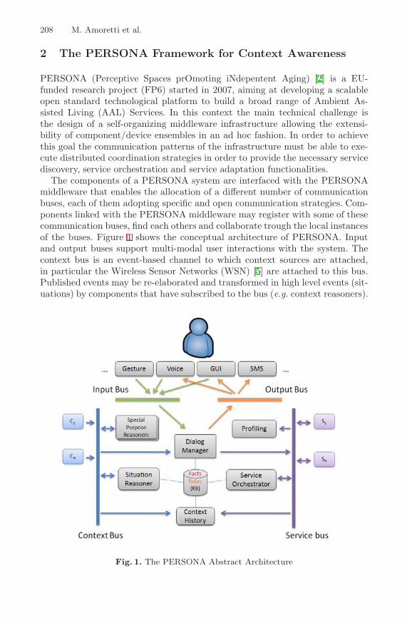
208 M. Amoretti et al.
2 The PERSONA Framework for Context Awareness
PERSONA (Perceptive Spaces prOmoting iNdepentent Aging) [2] is a EU-funded research project (FP6) started in 2007, aiming at developing a scalableopen standard technological platform to build a broad range of Ambient As-sisted Living (AAL) Services. In this context the main technical challenge isthe design of a self-organizing middleware infrastructure allowing the extensi-bility of component/device ensembles in an ad hoc fashion. In order to achievethis goal the communication patterns of the infrastructure must be able to exe-cute distributed coordination strategies in order to provide the necessary servicediscovery, service orchestration and service adaptation functionalities.
The components of a PERSONA system are interfaced with the PERSONAmiddleware that enables the allocation of a different number of communicationbuses, each of them adopting specific and open communication strategies. Com-ponents linked with the PERSONA middleware may register with some of thesecommunication buses, find each others and collaborate trough the local instancesof the buses. Figure 1 shows the conceptual architecture of PERSONA. Inputand output buses support multi-modal user interactions with the system. Thecontext bus is an event-based channel to which context sources are attached,in particular the Wireless Sensor Networks (WSN) [5] are attached to this bus.Published events may be re-elaborated and transformed in high level events (sit-uations) by components that have subscribed to the bus (e.g. context reasoners).
Fig. 1. The PERSONA Abstract Architecture

Sensor Data Fusion for Activity Monitoring 209
The service bus is used to group all the services available in the AAL-space,being them atomic or composite (whose availability is managed by a ServiceOrchestrator component). Services belonging to the service bus may be requestedby the Situation Manager in consequence of situation detections and rules storedin the Knowledge Base of the system. Generally, devices are attached to boththe context and service bus. The former is used to send notifications of statuschanges, the latter to answer to status query or execute actions (e.g. switchon the light device). Many other basic components are foreseen in PERSONAsystem, but their discussion is out of the scope of this paper (see [11] for details).
As in other international research projects (Gator Tech [17], Amigo [4], Socam[14]), we developed a middleware implementation based on the OSGi Platform[1]. The OSGi specification provides a standardized way to manage the softwarelife cycle of Java applications. OSGi implementations are containers running ontop of a JVM which enable installation, removal, start, and stop of componentsat run time. An OSGi component is a JAR file called bundle which containsJava classes, resources and metadata describing the dependencies with otherbundles. A feature of the OSGi platform that is useful to recall here is the OSGiservice model. A component can register with the OSGi Registry instances ofservices implementing specific interfaces and described by key-value properties.Every other component interested to monitor the presence of a particular servicecan register listeners with filter properties that will be notified by the OSGiframework when there is a match.
3 Sensor Abstraction and Integration Layer
The artifacts composing AAL-spaces can be classified in stationary, portableand wearable components. The first ones run on desktop PCs, Set Top Boxes,Residential Gateways or they belong to the environmental infrastructures likeHome Automation sub-systems; portable components are, for instance, medi-cal devices or mobile/smart phones, while wearable components are based ongarments equipped with sensors. The PERSONA middleware targets small butreasonably powerful devices, therefore not all the components can be integratedby using an instance of the PERSONA middleware. Typically, wearable compo-nents, as well as nodes of WSNs or Home Automation Systems (HAS) require adifferent approach because of their limited computation resources; in such casesPERSONA adopts a solution based on a gateway, which allows the PERSONAapplication layer to share information by communicating with other applicationlayers resident on different network infrastructures (e.g. ZigBee [5] or Bluetoothapplications). Due to the features of the OSGi Platform1, it is sufficient to writea bridging component that interacts from one side with the PERSONA middle-ware and from the other side with the software drivers that access the networkeddevices. In the following, we briefly introduce the Sensors Abstraction and Inte-gration Layer (SAIL) developed in PERSONA, by highlighting different aspects
1 Initially OSGi was designed as a framework to develop Open Service Gateways.

210 M. Amoretti et al.
and requirements of sensor network applications. A specific section related tothe integration of ZigBee devices concludes the chapter.
3.1 Wireless Sensor Networks
Wireless Sensor Networks are an important technological support for smart en-vironments and ambient assisted applications. Up to now, most applicationsare based on ad-hoc solutions for WSNs, and solutions providing uniform andreusable applications are still in their youth. Note that AAL spaces can be pop-ulated by many sensor networks (e.g ZigBee or IEEE 802.15.4 standard, andBluetooth). The main requirements, in the integration of WSN into PERSONA,are:
- R1: Integration of the different sensor network technologies.- R2: Sharing of communication medium by concurrent sensor applications.- R3: Management of different applications on the same WSN.- R5: Dynamic discovery of sensor applications.- R6: Management of logical sensors.- R7: Configuration and calibration of sensor applications.
The requirement R1 is usually satisfied by enabling the dynamic deployment ofad-hoc network drivers in the system, while we can assume that requirementsfrom R2 to R5 largely depend on the operating systems and middleware usedfor the sensor nodes programming (e.g. ZigBee, TinyOS, TinyDB, TeenyLIMEand others [22]). The requirement R6 concerns the possible virtualization of thesensors deployed either in the environment or worn by the users. For example,let’s consider an application that detects the user’s posture by means of a numberof accelerometers placed on the body: in this case, the posture can be representedby a single logical sensor, which aggregates information produced by all theaccelerometers for producing the state of the user (sitting, walking, etc.). In thisexample, the accelerometers may not even be visible to the application layer.Such a virtualization can be implemented directly on the sensor network orimplemented at application level within the gateway.
In order to face these requirements, we developed SAIL [12] an architectureorganized in three layers, namely the Access, Abstraction, and Integration layer,constructed over the OSGi platoform. The Access layer is a collection of driversthat provides basic access to WSNs. The Abstraction layer, if needed, can beused to elaborate the data received by the sensors before of exporting them atapplication level, and the last layer exposes the sensors to one or more accesstechnologies, that in the context of PERSONA project is the middleware.
3.2 ZigBee Networks Integration
A diagram of the current SAIL architecture with ZigBee networks is depictedin figure 2. The ZigBee Base Driver is a network driver in charge of executingthe scan of the network, getting the description of the ZigBee devices, and reg-istering a proxy service for accessing the discovered remote services. This proxy

Sensor Data Fusion for Activity Monitoring 211
Fig. 2. The SAIL layered architecture
is a generic ZigBee service, registered with the OSGi Platform, which exposesthe properties retrieved during the network inquiry. It enables the access to theremote service by means of simple primitives (e.g. invoke(byte[] payload))that have to be filled by the proper cluster message. The components on the up-per layers may act as Refinement Drivers (in OSGi terms). By using the OSGiFramework facilities, as soon as a service implementing a known cluster is reg-istered, these drivers refine the service by registering another service proxy witha more detailed interface (e.g. action/command based). Thus the second layer isspecialized to represent the service according to a specific profile, for instance theHome Automation profile. The upper layer integrates the ZigBee services withinPERSONA. It is composed of Sensor Technology Exporters (STE), which dis-cover the services by implementing standard or extended profiles and registersproxies that are PERSONA-aware components2. The mapping between servicescompliant to the ZigBee model and PERSONA model is realized at this level;these proxies send events or register service callees according to the PERSONAontologies.
In conclusion, the abstract layer is populated by custom drivers which maycombine and process the sensed data to instantiate logical sensor services andrefine the cluster-based services. All the code for ZigBee network access will bereleased with OS license as soon as the integration with a commisioning tool willbe completed.
2 The same approach can be used to expose the services according other access tech-nologies (e.g. UPnP).

212 M. Amoretti et al.
4 Vision-Based Human Posture Classification
Concerning the acquisition of context information, some sensors require a trans-formation of their output into meaningful, ontological states such that reasoningmechanisms may work upon it. In this section we will we introduce one partic-ular context information provider that has been developed in the course of thePERSONA project. The Human Posture Classification (HPC) component is acamera based solution designed to retrieve static estimates about discrete (i.e.ontological) posture states of a person being in the field of view of the cam-era. ”Static” means that the postures are derived from single images and arerelated to one concrete time instant. Furthermore, in contrast to the main re-search stream on human pose estimation (see [21] and [25] for in-depth reviews)no continuous pose is estimated. So instead of estimating the configuration ofthe skeletal configuration of the articulated body in a parameterized fashion e.g.by means of expressing it by joint angles of limbs and the general body orien-tation, the postures are directly classified according to a finite set of discreteposture states such as ”Sitting”, ”Standing”, ”Bending”, etc. Such a representa-tion is needed to support higher level reasoning within a semantic / ontologicalAAL-architecture like the PERSONA framework.
Compared to related work in the field of discrete posture classification fordomestic services ([10],[9],[23]), our approach is characterized by its simplicityand effectiveness. Firstly, we do not require multiple cameras in order to resolveambiguities arising from self-occlusion of the body parts or to handle difficul-ties caused by poor segmentation when using conventional color based cameras.Instead, we advocate the use of Time-Of-Flight cameras which produce a three-dimensional, geometric representation of the scene. This reveals much bettersegmentation results and provides additional information for ambiguity han-dling. Secondly, we do not use a particular model of the human body in orderto estimate a complete, parameterized body configuration prior classification.In fact, only few image processing steps are needed to obtain a low resolutionfeature image which in turn is used to train a recently proposed machine learn-ing approach. It is clear that due to the high amount of computational effortneeded for image processing applications, the HPC-component should run on adedicated machine. It is the output of this preprocessing step - the extractedcontext information (posture states) - which is fused within the communicationframework for Activity Monitoring.
In the following two subsections a brief overview over the particular advan-tages of using TOF-cameras instead of conventional types is given. Next, weexplain the image processing steps for obtaining feature vectors that are usedfor training and online classification. Technical details and an evaluation of thesolution are presented in [30].
4.1 Advantages of Time-of-Flight Cameras
Common to most of the human pose estimation approaches is the assumptionthat the camera is placed at a fixed spot in the room. This allows for applying a

Sensor Data Fusion for Activity Monitoring 213
background-foreground segmentation (or background-subtraction) technique toobtain a silhouette image of the person. The basic idea is that the appearanceof the scene is learned once beforehand, without any person in the field of viewof the camera. While processing the live image the foreground can in turn besegmented by identifying changes with respect to the background model.
In fact, most pose estimation approaches rely heavily on a good segmentationresult. However, despite many years of research (see [24] for a review on back-ground segmentation), in practical, realistic environments conventional camerasstill pose certain difficulties to obtaining a clear silhouette. These difficultiesinclude the following:
– noise in the image,– similar colors of the background and the clothes worn by persons,– shadows that result in additional, unwanted variations between the back-
ground model and the live images,– changing lighting conditions (e.g. when someone switches a light on or off)
and,– completely dark environments, as in the case of monitoring the behaviour of
people at night, where conventional cameras are not applicable, at all.
Due to these difficulties we propose to use images coming from Time-Of-Flight(TOF) cameras ([20]), instead. TOF cameras produce a three dimensional, ge-ometrical representation of the scene by emitting infra-red light and measuringthe time the light takes to returning back to the camera.3 With TOF-camerasmost of the abovementioned difficulties are overcome, as the representation ofthe scene is based on its geometry and not on its visual appearance, thus makingit more robust and more applicable in realistic scenarios.
4.2 Time-of-Flight Image Feature Extraction, Learning andClassification
The implemented algorithmic solution to camera based posture classificationcomprises four main steps which are briefly summarized, subsequently:
1. Background subtraction and connected component merging: Although TOF-cameras directly produce a cloud of 3D-coordinates of the perceived sceneas output, each depth value is also associated to a pixel-coordinate. Thusmany of the conventional image processing techniques may be applied toTOF-images in a similar fashion, including background-subtraction. How-ever, compared to grey-level images from conventional cameras, the pixelvalues (depth-value) have much higher and very heterogeneous noise. To ac-count to these peculiarities we adopted a recently proposed algorithm [26]that estimates the mean and covariance for each pixel in the backgroundmodel (see figure 3, top-right). Next, the perceived differences between the
3 More precisely, a TOF camera emits sinusodial light impulses and measures thephase shift of the returning light for each pixel.

214 M. Amoretti et al.
background and the live image are grouped into connected pixel regions(”blobs”). This step is used to remove any false positives arising e.g. due toimage noise. A simple threshold is applied to the size of the connected com-ponents, i.e. blobs below a certain size are simply discarded. Furthermorethe largest blob among the remaining is assumed to be the one correspondingto a person.
2. Subimage cropping, resampling and vectorization: Based on the previousregion-of-interest detection, a sub-image is cropped in such a way that itcontains as much foreground as possible. The sub-image is centred and re-sampled to a low resolution while keeping the aspect ratio constant (seefigure 3, bottom-left). The cropped and resampled sub-image is interpretedas a high dimensional feature vector with each pixel value being one elementof the vector (e.g. a 20-by-24 image results in a 480 dimensional vector).
3. Learning a transformation from image space to posture space (offline): Inorder to infer the posture from the high dimensional feature vectors, a re-cently proposed machine learning approach is used (”Locality PreservingProjections”) [15]4. A set of reference images needs to be captured andannotated manually according to their corresponding discrete states (”sit-ting”, ”standing”, etc.). The machine learning approach is closely related toPrincipal Component Analysis (PCA), but, by contrast, takes into accountneighbouring relations between the feature vectors, and thus, can also beused in a supervised manner (refer to [27] for details). It works by find-ing an optimal transformation from high dimensional feature space to a lowdimensional representation. Image vectors belonging to the same or simi-lar state are mapped to nearby points in the low dimensional space, suchthat points belonging to same states form clusters (see figure 3, bottom-right). For each cluster the mean and covariance is computed, which are usedlater for classifying the transformed image vectors into the correspondingstates.
4. Feature projection and classification (online): The optimal projection de-rived from the training data is applied to the online image vectors. Thisprojected online feature is then classified according to the closest mean vec-tor of the projected training data. Furthermore we apply a threshold on theMahalanobis distance between the online feature vector and the covarianceof the projected training data of each class (see figure 3, bottom-right). I.e.if the normalized distance to the closest mean exceeds a certain threshold,the state is considered to be ”Unknown”. As we can show on real data, themachine learning approach has good generalization capabilities, i.e. previ-ously unseen images not contained in the training set are correctly projectedand classified.
4 Wang and Suter ([28], [29]) already adopted LPP in the context of human mon-itoring. However their approach differs from ours in that they use it to obtain aparameterization of the image manifold and, in turn, use the evolution of the pro-jected feature vectors to classify dynamic activities.

Sensor Data Fusion for Activity Monitoring 215
Fig. 3. Illustration of the image processing and classification steps for the human pos-ture recognition (best viewed in color): Color encoded visualization of the 3D raw datacoming from a TOF-camera (tl), result after background-subtraction (tr), croppedfeature-image with grey-valued encoded relative depths (bl), projected training datafor three states, ”Standing”, ”Sitting and ”Lying” (cyan, purple and blue), and theprojection of the current feature image on the left (red point above the ”Sitting” cap-tion)(br)
5 Data Fusion for User Activity Monitoring
Understanding of human behaviors may be thought as the classification of timevarying feature data, i.e. matching an unlabeled set of context events and otheruseful information with a group of labeled reference sets representing typical be-haviors. A distinction between static and dynamic activities is necessary. Staticactivities like ”standing” or ”sitting” can be inferred directly from low-level dataat a particular time instant (such as the pose of the person at a certain timeusing some kind of thresholding mechanism on the pose estimate). By contrastdynamic activities, such as ”moving around”, are usually composite activitiesrequiring a monitoring of a full sequence of low-level data (e.g. context eventsdescribing ongoing sub-activities). Low-level data needs to be stored for severaltime frames (in a context buffer), as the whole sequence is needed to infer thatactivity from an evolution of the low level data. For example: ”cooking” maybe composed of several low-level data at different time instances: ”opening thefridge”, ”closing the fridge”, ”standing in front of the oven”, etc.
The existing body of literature in automatic reasoning can be decomposedaccording to two basic approaches. A pure ”rule-based” approach that is a

216 M. Amoretti et al.
composition of several ”If...Then...” conditions. E.g. for ”cooking”, it might beused ”fridge has been opened for several times” && ”hotplate was on for > xxminutes” && ”activity of person in the kitchen” && ”...”. A ”supervised learn-ing” based approach [18], where the system is trained with a history of low-leveldata and corresponding output states (the low-level data is labeled with corre-sponding output states). Usually such supervised learning methods work by find-ing a decision surface in the high-dimensional (labeled) input data. Supervisedlearning (a.k.a. inductive machine learning) applied to human behavior detectionhas two advantages. First, the system can be configured (trained) by performingthe activities themselves instead of programming the rule-based conditions. Sec-ond, the system can updated/trained online, for example by asking the personif the inferred activity was correct. Then with the confirmation/disagreement ofthe user, the training space (e.g. decision surface) is updated.
Our approach is based on probabilistic rules, with absolute probabilities ofhigh-level actions can be automatically updated by means of long-term behaviordetection (which is not discussed in this paper). The Activity Monitor (AM)is a reasoner that delivers aggregated/derived context events in terms of thecontext ontology (in particular, the action ontology). Thus the AM registers tothe context bus (c-bus) both as subscriber and publisher in order to use contextevents from lower levels, and produces context events on a higher level. In details,the AM is a special-purpose reasoner that aggregates context events related tobasic user activities (AtomicActions), recognized by the HPC component, andto user localization, as well as information about the status of user-controlleddevices, such as the TV, to produce context events describing complex useractivities such as ”eating”, ”watching tv”, etc (CompositeActions).
Figure 4 summarizes the internal architecture of the AM, which is registeredon the c-bus as context subscriber for many user-related context events (e.g.those published by the HPE). When a context event of type AtomicAction isreceived, the Classifier decides whether to consume it immediately (to infer aCompositeAction and publish it as context event) or to store it in the ActionArchiver, for later use.
The Classifier is based on a Bayesian network (BN) approach [16,19]. ABayesian network is a graphical model enabling the description of probabilityrelationships among a set of variables (features). The graph allows the user tounderstand which variables affect which other ones, and also serves as the back-bone for efficiently computing marginal and conditional probabilities that maybe required for inference and learning. Because a Bayesian network is a com-plete model for the variables and their relationships, it can be used to answerprobabilistic queries about them. For example, the network can be used to findout updated knowledge of the state of a subset of variables when other variables(the evidence variables) are observed. The process of computing the posteriordistribution of variables given evidence is called probabilistic inference.
We illustrate how BNs have been used to implement the Activity Monitorwith a simple example. Then we briefly illustrate the classification algorithmimplemented in the AM.
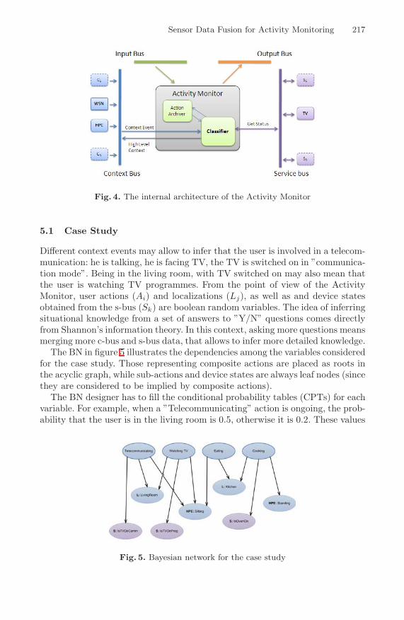
Sensor Data Fusion for Activity Monitoring 217
Fig. 4. The internal architecture of the Activity Monitor
5.1 Case Study
Different context events may allow to infer that the user is involved in a telecom-munication: he is talking, he is facing TV, the TV is switched on in ”communica-tion mode”. Being in the living room, with TV switched on may also mean thatthe user is watching TV programmes. From the point of view of the ActivityMonitor, user actions (Ai) and localizations (Lj), as well as and device statesobtained from the s-bus (Sk) are boolean random variables. The idea of inferringsituational knowledge from a set of answers to ”Y/N” questions comes directlyfrom Shannon’s information theory. In this context, asking more questions meansmerging more c-bus and s-bus data, that allows to infer more detailed knowledge.
The BN in figure 5 illustrates the dependencies among the variables consideredfor the case study. Those representing composite actions are placed as roots inthe acyclic graph, while sub-actions and device states are always leaf nodes (sincethey are considered to be implied by composite actions).
The BN designer has to fill the conditional probability tables (CPTs) for eachvariable. For example, when a ”Telecommunicating” action is ongoing, the prob-ability that the user is in the living room is 0.5, otherwise it is 0.2. These values
Fig. 5. Bayesian network for the case study
218 M. Amoretti et al.
can be set taking into account the average time spent by the user, each day, toperform the composite actions of interest (cooking, watching TV, etc.), observedby relatives, caregivers and friends. Their values can be updated automatically,by using long-term behavior detection.
The Activity Monitor is thus able to compute, for example:
P(”Telecommunicating” | ”L:LivingRoom”=T, ”S:IsTVOnComm”=T)
i.e. ”what is the likelihood that the user is telecommunicating, given that he isin the living room, and the TV is in communication mode?”.
5.2 Implementation of the Activity Monitor
To implement the classifier based on BNs, we adopted the Weka library (version3.5.8) [3,6], which is a collection of machine learning algorithms for data miningtasks. The algorithms can either be applied directly to a dataset or called fromJava code. For Bayesian network design and management, Weka provides a JavaAPI and a graphical editor.
The Weka BN GUI allows to create Bayesian networks and to store them onfiles in XML BIF format [8]. To create a BN, nodes can be placed and linkedtogether in a free space, and CPTs can be defined. A BN stored in a XML BIFfile can be read, modified and stored in a new file by means of the Weka API.
Context events describing simple actions (such as ”Sitting”) are used by theAM to infer the CompositeAction context events. If a simple action does notcontribute immediately to the inference of a composite action, it is stored in theAction Archiver, which is a continuously updated list.
When a context event describing a basic Action is intercepted, the BN isexplored and the composite action with higher marginal probability is returned,using the following algorithm:
1. get node i from the BN, such that (descr(i) == descr(theAtomicAction))2. get the set Ni of parents of node i3. for each node in Ni compute the marginal probability Pm, considering other
evidences4. select node j in Ni with the highest marginal probability Pm(j)5. return descr(j) and Pm(j)
Step 4 is the most important. It requires to take into account, for each nodein Ni, the current values (evidences), whether they are available, of all its childnodes (that do not always represent context events, but information to be re-quested on the s-bus). For example (still referring to the case study), suppose the”Sitting” event has been detected. Its parent set Ni includes ”Watching TV”,which has two more child nodes, one describing the presence of the user in theliving room, the other describing the programming state of the TV. By invok-ing an appropriate service, the AM can retrieve the current value of the variablerepresented by the ”S:IsTVOnProg” node (T or F). Moreover, the AM can checkits internal location archive, searching for recent evidence of use presence in theliving room. These facts are then used to compute the marginal probability ofthe considered parent node, e.g.

Sensor Data Fusion for Activity Monitoring 219
P(”Watching TV” | ”Sitting”=T, ”L:LivingRoom”=T, ”S:IsTVOnProg”=F)
If a parent node has, among its child nodes, other context events representingactions, the AM inspects the Action Archiver, looking for recent evidence of suchactions. If no recent evidence of actions related to a composite action is foundin the archive, the evidence of those actions is set to F.
6 Conclusions
The PERSONA framework that we presented in this paper addresses three majorissues for user related context awareness in an AmI environment.
We presented a general communication framework that allows to exchangecontext information, thus supporting context reasoning and data fusion in adistributed manner. A key concept is the context bus, to different componentsmay subscribe for publishing and consuming context events. Within this papera special focus has been given to the design of the wireless sensor network inte-gration. The framework supports data fusion and aggregation at three levels ofabstraction: network, virtual network (SAIL) and application level.
We addressed the problem of context data acquisition, i.e. the preprocessingof sensor output in order to obtain meaningful, ontological information such thathigh-level reasoners may work upon it. Here we focused on a particular problemin computer vision: the acquisition of posture information of the user when cap-tured by a camera. We suggested to use Time-Of-Flight cameras to circumventseveral difficulties (e.g. changing lighting conditions) that usually decrease therobustness of any solution in realistic and practical situations. Furthermore, weadopted a machine learning approach that can be trained to detect a varietyof different posture states of interest. Of course, postures of persons are of spe-cial interest for activity monitoring as they provide important clues about theactivities being performed.
Finally, a powerful and flexible context data fusion approach was introduced,i.e. the Activity Monitor. It is a reactive component that produces informationabout ongoing user activities, merging context events such as humanpostures and localization, with information about the status of user-controlleddevices. The Activity Monitor is composed by a classifier and a short-term con-text archiver. The classifier is based on a Bayesian network (BN) approach,which allows to infer high-level knowledge with associated marginal probability.To improve the component, we are studying mechanisms for allowing to dynami-cally update the absolute probabilities of composite actions, taking into accountthe results produced by another PERSONA reasoner which is the Long-termBehavioral Analyzer (whose development is in progress).
Acknowledgements
This work has been partially funded by the EU IST Project PERSONA (FP6contract N.045459).
220 M. Amoretti et al.
References
1. OSGi web site, http://www.osgi.org2. PERSONA project web site, http://www.aal-persona.org3. Weka 3: Data mining software in java, http://www.cs.waikato.ac.nz/ml/weka/4. AMIGO project. Ambient intelligence for the networked home environment
(September 2004), http://www.amigo-project.org5. Baronti, P., Pillai, P., Chook, V.W.C., Chessa, S., Gotta, A., Hu, Y.F.: Wireless
sensor networks: A survey on the state of the art and the 802.15.4 and zigbeestandards. Computer Communications 30(7), 1655–1695 (2007)
6. Bouckaert, R.: Bayesian network classifiers in weka for version 3-5-8 (July 2008)7. Ramos, D.S.C., Augusto, J.C.: Ambient intelligence - the next step for artificial
intelligence. IEEE Intelligent Systems 23(2) (March/April 2008)8. Cozman, F.G.: The interchange format for bayesian networks,
http://www.cs.cmu.edu/~fgcozman/research/interchangeformat/
9. Cucchiara, R., Grana, C., Prati, A., Vezzani, R.: Probabilistic posture classificationfor human-behavior analysis. IEEE Transactions on Systems, Man and Cybernet-ics, Part A 35(1), 42–54 (2005)
10. Cucchiara, R., Prati, A., Vezzani, R.: Posture classification in a multi-camera in-door environment. In: ICIP (1), pp. 725–728 (2005)
11. Fides-Valero, A., Freddi, M., Furfari, F., Tazari, M.-R.: The PERSONA frame-work for supporting context-awareness in open distributed systems. In: Aarts, E.,Crowley, J.L., de Ruyter, B., Gerhauser, H., Pflaum, A., Schmidt, J., Wichert, R.(eds.) AmI 2008. LNCS, vol. 5355, pp. 91–108. Springer, Heidelberg (2008)
12. Girolami, M., Lenzi, S., Furfari, F., Chessa, S.: SAIL: a Sensor Abstraction andIntegration Layer for Context Aware Architectures. In: Proceedings of the 34thEUROMICRO Conference on Software Engineering and Advanced Applications(SEAA 2008), Parma, Italy, pp. 374–381. IEEE, Los Alamitos (2008)
13. I. A. Group. Scenarios for ambient intelligence in 2010, european commission (2001)14. Gu, T., Pung, H.K., Zhang, D.Q.: A middleware for building context-aware mobile
services. In: IEEE Vehicular Technology Conference, pp. 2656–2660 (2004)15. He, X., Niyogi, P.: Locality preserving projections. In: Advances in Neural Infor-
mation Processing Systems, vol. 16. MIT Press, Cambridge (2003)16. Heckerman, D.: A tutorial on learning with bayesian networks. In: m. i. (ed.) Learn-
ing in graphical models. Kluwer, Dordrecht (1998)17. Helal, S., Mann, W., El-Zabadani, H., King, J., Kaddoura, Y., Jansen, E.: The
gator tech smart house: A programmable pervasive space. IEEE Computer 1(3),64–74 (2005)
18. Kotsiantis, S.: Supervised machine learning: A review of classification techniques.Informatica Journal 31, 249–268 (2007)
19. Madden, M.: The performance of bayesian network classifiers constructed using dif-ferent techniques. In: Proc. of european conference on machine learning, workshopon probabilistic graphical models for classification (September 2003)
20. MESA Imaging (February 2009), http://www.mesa-imaging.ch/21. Moeslund, T.B., Hilton, A., Krueger, V.: A survey of advances in vision-based
human motion capture and analysis. Computer Vision and Image Understand-ing 104(2), 90–126 (2006)
22. Molla, S., Ahamed, M.M.: A survey of middleware for sensor network and chal-lenges. In: Proceedings of nternational Conference on Parallel Processing Workshop(ICPP 2006) (August 2006)

Sensor Data Fusion for Activity Monitoring 221
23. Pellegrini, S., Iocchi, L.: Human posture tracking and classification through stereovision and 3d model matching. J. Image Video Process. 8(2), 1–12 (2008)
24. Piccardi, M.: Background subtraction techniques: a review. In: 2004 IEEE Interna-tional Conference on Systems, Man and Cybernetics, vol. 4, pp. 3099–3104 (2004)
25. Poppe, R.: Vision-based human motion analysis: An overview. Comput. Vis. ImageUnderst. 108(1-2), 4–18 (2007)
26. Porikli, F., Tuzel, O.: Bayesian background modeling for foreground detection.In: VSSN 2005: Proceedings of the third ACM international workshop on Videosurveillance & sensor networks, pp. 55–58. ACM, New York (2005)
27. Wang, H., Chen, S., Hu, Z., Zheng, W.: Locality-preserved maximum informationprojection. IEEE Transactions on Neural Networks 19(4), 571–585 (2008)
28. Wang, L., Suter, D.: Analyzing human movements from silhouettes using manifoldlearning. In: IEEE Conference on Advanced Video and Signal Based Surveillance,vol. 7 (2006)
29. Wang, L., Suter, D.: Learning and matching of dynamic shape manifolds for hu-man action recognition. IEEE Transactions on Image Processing 16(6), 1646–1661(2007)
30. Wientapper, F., Ahrens, K., Wuest, H., Bockholt, U.: Linear-projection-based clas-sification of human postures in time-of-flight data. IEEE Transactions on Systems,Man and Cybernetics (October 2009)

S. Hailes, S. Sicari, and G. Roussos (Eds.): S-Cube 2009, LNICST 24, pp. 222–235, 2009. © Institute for Computer Sciences, Social-Informatics and Telecommunications Engineering 2009
Trade-off Analysis of a MAC Protocol for Wireless e-Emergency Systems
Óscar Gama1, Paulo Carvalho1, J.A. Afonso2, and P.M. Mendes2
1 Department of Informatics, University of Minho, Braga, Portugal {osg,pmc}@di.uminho.pt
2 Department of Industrial Electronics, University of Minho, Guimarães, Portugal
{jose.afonso,paulo.mendes}@dei.uminho.pt
Abstract. Wireless sensor networks are envisioned to be deployed in health-care. Since emergency and intensive care applications need to assure reliable and timely data delivery, they have increased demands for quality of service, including at the MAC layer. Amongst MAC protocols available for WSNs, the Low Power Real Time (LPRT) presents suitable characteristics to be deployed in emergency platforms due to its rational bandwidth allocation, low energy consumption, and bounded latency. Yet, this protocol may present a significant packet loss ratio in a wireless channel with bit error ratio. In order to define a MAC protocol more robust to bit error conditions and able to fulfill the required quality of service, solutions based on short size beacons and multiple retrans-missions are proposed and tested. The results showed that such strategies led to meaningful improvements regarding packet loss ratio, without compromising significantly the energy consumption.
Keywords: e-Emergency, Quality of Service, Wireless Sensor Networks.
1 Introduction
An e-health monitoring system commonly grounds on a group of sensors attached non-invasively to a patient in order to monitor some physiological parameters. In case of emergency clinical scenarios, a healthcare network should provide quality of ser-vice (QoS) facilities since these clearly demand for high reliability, guaranteed band-width and short delays [1]. Therefore, communication protocol layers need to assure a reliable and timely data delivery.
Many Medium Access Control (MAC) protocols have been developed for wireless networks using contention or multiplexing-based algorithms. Traditional contention-based protocols assume traffic is distributed stochastically. As traffic in a wireless sensor network (WSN) tends to be highly correlated and dominantly regular, conven-tional Carrier Sense Multiple Access (CSMA) protocols are not advised for WSNs [2]. S-MAC [3] and WiseMAC [4] are typical examples of CSMA-based protocols designed for low duty-cycle WSNs, developed to help saving energy in applications whose nodes remain idle for long time until an event is detected (e.g. surveillance).

Trade-off Analysis of a MAC Protocol for Wireless e-Emergency Systems 223
These protocols are convenient for WSNs having usually low traffic loads. Conse-quently, these MAC protocols are inadequate for networks requiring high throughput and low latency.
Amongst multiplexing-based protocols, Time Division Multiple Access (TDMA) is a commonly used technique. Time is divided into slots, which are used by motes (wireless sensor nodes) to transmit data without the need to contend for the medium. If a base-station (BS) is available to keep the WSN scheduling and synchronization, then TDMA-based MAC protocols are usually a preferable choice to satisfy the QoS requirements of e-emergency systems, as QoS is easier assured in a collision-free environment than in a contention-prone medium. Within TDMA-based MAC protocols, LPRT [5] is a con-venient choice to provide efficient bandwidth allocation, low energy consumption, and bounded latency, as required by e-emergency wireless networks. However, it may pre-sent a significant packet loss ratio in a wireless channel affected by errors. In order to improve its robustness to bit errors, new solutions based on short size beacons and mul-tiple retransmissions are proposed and verified in a WSN simulator.
The remaining of this paper is organized as follows; the related work is discussed in Section 2; proposals to improve LPRT protocol are presented in Section 3; the simula-tion testbed setup is described in Section 4; the results are discussed in Section 5; and, finally, the conclusions are presented in Section 6.
2 Related Work
TDMA-based protocols available for WSNs include IEEE 802.15.4/GTS [7], LMAC [8], TRAMA [9], and LPRT.
The IEEE 802.15.4 standard specifies the physical layer and the MAC sublayer, al-lowing the optional use of a TDMA-based superframe structure. However, the low granularity of the time slots leads to poor bandwidth efficiency, making it unsuitable to e-emergency scenarios [1].
LMAC allows a WSN to self-organize in terms of slot assignment and synchroni-zation, without requiring a central manager, through a distributed algorithm running in every mote. Nodes wake up at the start of each slot to stay synchronized and to listen to a message. If the message is not addressed to the node, it will sleep until the next slot. Since each node has only one slot assigned and one transmission per super-frame (32 slots) allowed, LMAC is inadequate to e-emergency systems.
TRAMA uses a distributed election scheme based on information about the traffic at each node to decide which node can transmit at a particular slot. It avoids the as-signment of slots to nodes without traffic to send, and also allows nodes to decide when they can sleep. It is well suited for applications that require high-delivery guar-antee and energy efficiency, without being delay sensitive. The latter characteristic impairs the support of real-time applications.
LPRT is a simple, beacon-based protocol that uses dynamic and efficiently the available bandwidth. Its highly-grained superframe (Figure 1) starts with the trans-mission of a beacon frame (B) by the BS, followed by the Contention Access Period (CAP), also called Contention Period (CP). The CAP may be used for the (dis)association or configuration of a body sensor network (BSN). The Contention
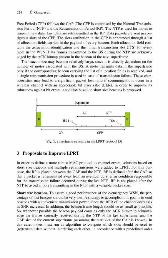
224 Ó. Gama et al.
Free Period (CFP) follows the CAP. The CFP is composed by the Normal Transmis-sion Period (NTP) and the Retransmission Period (RP). The NTP is used for motes to transmit new data. Lost data are retransmitted in the RP. Data packets are sent in con-tiguous slots of the CFP. The slots attribution in the CFP is announced through a list of allocation fields carried in the payload of every beacon. Each allocation field con-tains the association identification and the initial transmission slot (ITS) for every mote in the WSN. Data frames transmitted to the BS during the NTP are acknowl-edged by the ACK bitmap present in the beacon of the next superframe.
The beacon size may become relatively large, since it is directly dependent on the number of motes associated with the BS. A mote transmits data in the superframe only if the corresponding beacon carrying the list of allocation fields is received, and a single retransmission procedure is used in case of transmission failure. These char-acteristics may lead to a significant packet loss ratio if communications occur in a wireless channel with an appreciable bit error ratio (BER). In order to improve its robustness against bit errors, a solution based on short size beacons is proposed.
Fig. 1. Superframe structure in the LPRT protocol [5]
3 Proposals to Improve LPRT
In order to define a more robust MAC protocol to channel errors, solutions based on short size beacons and multiple retransmissions were added to LPRT. For this pur-pose, the RP is placed between the CAP and the NTP. RP is defined after the CAP so that a packet is retransmitted away from an eventual burst error condition responsible for the transmission failure occurred during the last NTP. RP is not placed after the NTP to avoid a mote transmitting in the NTP with a variable packet size.
Short size beacons. To assure a good performance of the e-emergency WSN, the per-centage of lost beacons should be very low. A strategy to accomplish this goal is to send beacons with a convenient transmission power, since the BER of the channel decreases as SNR increases. In addition, the beacon frame length should be as small as possible. So, whenever possible the beacon payload contains only the ACK bitmap to acknowl-edge the frames correctly received during the NTP of the last superframe, and the CAP size of the current superframe (assuming the start slot of the CAP is known). In this case, motes must run an algorithm to compute which slots should be used to (re)transmit data without interfering each other, in accordance with a predefined order

Trade-off Analysis of a MAC Protocol for Wireless e-Emergency Systems 225
schema. Using this strategy, the energy consumption in each BSN improves too, since smaller size beacons are received by the motes.
According to the received ACK bitmap, each mote must calculate the correspond-ing superframe slots to transmit its data. If a mote does not receive a beacon or a short sequence of beacons, it may continue to send its new data in the NTP, since a mote clock drift in the order of microseconds should permit the WSN to continue synchro-nized during a few consecutive beacon intervals. However, the mote cannot retransmit any data in the RP because the ACK bitmap is not available and so it does not know how the RP slots are being allocated to the motes.
In order to save energy, it might be tempting to retransmit the lost data aggregated to the new data sent in the NTP, instead of retransmitting it in the RP. However such strategy should be avoided because the number of slots allocated in the NTP to each mote becomes variable. Consequently, if a mote does not receive the beacon, it has no way to know a priori which slots to use for transmission. Indeed, if a mote does not receive the ACK bitmap, it does not know which motes are going to transmit aggre-gated data in the current superframe, making impossible to compute the new slot allo-cation schema. This situation does not occur if the NTP is used only to transmit new data packets. Hence, aggregated retransmissions in the NTP are not recommended, except in cases where aggregation does not imply taking more slots, such as packets carrying temperature data.
Besides the ACK bitmap and the CAP size, a beacon may need to send reconfigu-ration instructions if a new clinical situation is detected in some BSN. For instance, higher monitoring activity and lower delay transmission of the vital signals might be required when a patient´s clinical situation changes from non-critical to critical. In this case, the BS should inform all motes about the new situation and eventually re-configure the WSN. To perform this action all motes must follow a reconfiguration scheme, such as the algorithm proposed in [6].
Retransmission in the RP. The retransmission order in the RP depends on the ACK bitmap received from the BS. Using an increasing slot sequence, firstly data of all motes having the highest-priority and the bit false in the ACK bitmap are retransmitted succes-sively. Then, data of all motes having the second higher-priority and the bit false in the ACK bitmap are retransmitted successively, and so on. If slots are not enough to permit all required retransmissions, then schedule truncation is done in order to guarantee that no retransmission occurs in the NTP. It should be noted that retransmissions may not be the appropriate error recovery mechanism if losses are due to fading.
Retransmission in the CAP. If a mote does not receive the beacon then it fails to re-ceive the ACK bitmap, and therefore it does not know if the BS correctly received the packet sent in the NTP of the last superframe. Retransmitting properly that packet in the RP is impossible because such mote cannot compute the slot allocation schema of RP. A solution to overcome this problem is to retransmit it during the CAP using the slotted CSMA/CA [7]. This procedure should improve the packet loss ratio at expense of some energy consumption and CAP slots waste, since the mote may be transmitting a dupli-cated packet. Indeed, a packet already received by the BS may be retransmitted again in the CAP of the next superframe if the mote does not receive the beacon.

226 Ó. Gama et al.
4 Simulation Testbed
To test the solutions proposed in the previous section and to compare them with LPRT, the Castalia simulator [10] was used. For that purpose, a case-study and dis-tinct MAC protocol operation modes were programmed in Castalia.
4.1 Castalia Simulator
Castalia is a discrete event-driven simulator designed specifically for wireless sensor networks. It uses the communication model proposed by Zuniga et. al. [11]. In a wire-less channel the BER is variable because errors may occur in long bursts due to fading or shadowing. Castalia does not support currently these time-varying effects.
Castalia provides a tuneable CSMA-based MAC protocol in order to model several link protocols. However this protocol was built for broadcast communications, not unicast, and so it does not currently support acknowledgements. For this reason, ac-knowledgements are performed at the application level.
In order to compute the total energy consumed by a mote, Castalia takes into account not only the consumed power while the radio is in listening, sleeping, trans-mitting or receiving state, but also the power consumed by state switching. It also accounts the energy consumed per sample by the sensing devices present at each node. CPU energy consumption and memory access cost are not accounted in the cur-rent version of Castalia.
4.2 Case-Study
The testbed is based on a hospital room containing six beds with one patient per bed. Each patient is monitored by a body sensor network, and a BS collects and analyses the vital signals of all patients. The signals being monitored are temperature (T), oximetry (OXI), arterial pressure (ART), respiration rate (RR) and electrocardiography (ECG). Each signal is collected and transmitted by a dedicated mote. The MAC protocol de-ployed in the network must guarantee a maximum latency below 500 ms, low packet loss ratio, 10.5 kbps of bandwidth to each BSN and low energy consumption [1].
4.3 Operation Modes
In order to compare different MAC strategies, five operation modes were defined in the simulation testbed: 0, 1, 2, 3, and 4. In all modes, frames transmitted at the NTP are acknowledged through the ACK bitmap sent in the payload of the next beacon. Also, a mote may transmit data in the NTP even if a short size beacon is not received.
In operation mode 0, there are no retransmissions of lost frames. This mode is used as the worst-case, as no error control mechanism is present in the system.
In operation mode 1, lost packets are retransmitted once at the RP and these re-transmitted packets are not acknowledged. This mode differs of LPRT, because in this protocol a mote only transmits data in the NTP if a relatively large size beacon is re-ceived. Hence, if the channel BER is not null, the packet loss ratio in a WSN operat-ing at mode 1 is lower than using LPRT.

Trade-off Analysis of a MAC Protocol for Wireless e-Emergency Systems 227
In operation mode 2, packets with a payload size above a fixed threshold may be retransmitted during RP at most twice. The threshold was set to 40 bytes, so ECG and ART motes have two chances to retransmit the lost data. The second retransmission occurs only if the frame is not correctly received by the BS during the first retrans-mission. Hence, the first retransmission must be acknowledged, although the second one does not need to be. Packets with a payload size below the threshold may be re-transmitted once in the RP and they are not acknowledged.
In operation mode 3, packets with a payload size above a fixed threshold may be retransmitted at most three times in the RP.
Operation mode 4 is similar to operation mode 2, but if a mote does not receive a beacon, it tries to send in the CAP the packet transmitted in the NTP of the last super-frame. A minimum CAP size is available in all superframes.
4.4 Testbed Setup
The relevant setup and parameterization steps followed in the simulation testbed are presented next.
Wireless Channel. Since the room considered in our case-study is relatively small (10mx10m), the BER given by the simulator was always null, meaning that all motes worked in a good connected region. In order to test the robustness of the diverse protocols to different BERs, an additional random error generator was introduced in the wireless channel module of Castalia to force the degradation of the bit error probability.
Radio Model and Operating States. In the present protocol implementation, a mote radio is normally in the sleeping state. It switches automatically to the transmission state whenever it has a packet to send and enters in listening mode five slots before the ending of the superframe to receive the next beacon. The BS never enters in the sleeping state because conserving energy is not a concern for this device.
The CC2420 radio model, used by the popular TelosB motes, and a transmission power level of -10 dBm were chosen.
Beacon Interval and Superframe Time-Slots. The number of slots in the super-frame should be as high as possible to tune accurately the time division allocated to each mote and so minimizing the bandwidth waste, but not too high so that the slot duration is beyond the mote timer resolution. Since this is typically in order of micro-seconds, it was chosen 512 slots per superframe, which means that the duration of each slot is around 0.43ms, considering a beacon interval of 0.220s. This period was chosen for ECG packets to be sent with the payload almost fully-loaded to save en-ergy, and it must not be above 0.250s to respect the maximum delay of 0.500s im-posed to all signals, including the retransmitted frames [1].
Physical, MAC, and ACK Frames. Since many commercial motes use ZigBee, a physical layer frame having a total maximum size of 133 bytes (B) was assumed, the same length as specified in IEEE 802.15.4. Its physical header of 6B was also adopted: preamble sequence (4B), start frame delimiter (1B), and frame length (1B).
228 Ó. Gama et al.
A MAC header of 6B was tailored to this case-study, containing the fields: frame control (1B), sequence number (1B), destination address (1B), source address (1B), WSN identification (1B), and frame check sequence (2B).
The ACK frame has a MAC header of 6B and payload size null.
Data Packet Payload. ECG motes sample the physical signal at 250 Hz, ART motes at 120 Hz, OXI motes at 60 Hz, RR motes at 20 Hz, and T motes at 2 Hz [1]. The samples of every mote have a resolution of 16 bits. Consequently, packets transmitted from ECG, ART, OXI, RR, and T motes present a payload of 110B, 54B, 28B, 10B, and 2B, respectively.
Transmission in the NTP. The number of slots Ns each mote occupies in the NTP of the superframe to transmit data is:
Ns = ceil( ttx*S/ tSD ) (1)
where ttx is the transmission duration (in seconds), S is the total number of slots in the superframe, and tSD is the superframe duration (in seconds). The ceiling function ceil(x) returns the integer part of the argument rounded up. For a packet with a physi-cal header Ph, a MAC header Mh, a MAC payload length Mp bytes, and a transmission rate R bps:
ttx = (Ph+Mh+Mp)*8/R (2)
Considering a null overhead for the layers above the MAC layer,
Mp= tSD*F*r/8 (3)
where F is the sample rate (samples/s) of a specific mote type, and r is the sampling resolution in bits. As S=512 and R=250 kbps, each ECG, ART, OXI, RR, T frame takes respectively 10, 5, 3, 2, and 1 slots in the superframe.
When allocating each set of slots in NTP to the motes, two additional slots are in-cluded for safeguarding purposes. The slots in the superframe are occupied in the fol-lowing order:
Beacon | CAP | RP | T(5-0), RR(5-0), OXI(5-0), ART(5-0), ECG(5-0) |
–--------------- NTP ---------------
where ECG(5-0)=ECG(5,4,3,2,1,0) represents the following transmission sequence in NTP: after ECG mote of BSN 5 (ECG5) transmitting its packet, then ECG4, ECG3, ECG2, ECG1, and ECG0 transmit successively their data. The same criterion is ap-plied to the remaining types of motes.
Retransmission in the RP. The retransmission order in the RP depends on the ACK bitmap received from the BS. Using an increasing slot sequence, firstly the data of ECG motes having the bit false in the ACK bitmap are retransmitted successively. Then, if the respective ACK bits are false, ART motes retransmit their data, followed by the OXI motes, the RR motes, and finally the T motes. The number of slots allo-cated in RP to the motes includes two slots for safeguarding purposes, plus two slots if ACK receiving is required.

Trade-off Analysis of a MAC Protocol for Wireless e-Emergency Systems 229
In case of no more slots available to be allocated for retransmission, the less impor-tant vital signals should not be retransmitted. Since body temperature changes slowly along time, this signal is the first to be discarded in such situation.
One, two or three consecutive set of slots may be used for a single retransmission, according to the operation mode used. In mode 2, the second set of slots is used for retransmission if the packet is not correctly received by the BS during the first re-transmission. Accordingly, the first retransmission must be acknowledged. If a packet is sent with success during the first retransmission, then the slots reserved for the sec-ond retransmission are unused, resulting in bandwidth waste. The second retransmis-sion is not acknowledged. The same reasoning is applied for mode 3.
Retransmission in the CAP. In operation mode 4, a minimum CAP size of fifty slots is defined for every superframe so that motes have a chance to retransmit data in case of not receiving a beacon. To free some slots, T motes are not allowed to retransmit data in the CAP. The remaining operation modes have no minimum CAP size.
5 Simulation Results
In order to study the improvement obtained in LPRT when short size beacons and multiple retransmissions are deployed in this protocol, several simulation tests were carried out for different operation modes. Packet loss ratio, energy consumption, CAP availability, and scalability were the parameters under test. The performance of a WSN using beacons with different sizes was tested as well.
For each test run, a simulation time of one hour was defined. Extending the simula-tion time would not affect significantly the results. During that time period, the BS sends around 16363 beacons, carrying in the payload only the ACK bitmap (4B). It is assumed that BER is equal in both communication directions.
In some graphics the probability P of a fully-loaded packet to be received at desti-nation is used instead of the BER. Both parameters are related by:
BER= 1-P1/(8*MPS) (4)
where MPS is the maximum physical frame size. Considering MPS=133B, the BER changes between 0 and around 6.5*10-4 as P decreases from 1 to 0.5 along the simula-tion runs. Typical values for BER in a good real wireless channel are of the order 10-5 and in a bad channel may be less than 10-3.
5.1 Performance of a WSN with Short Size Beacons
The beacon size should be as small as possible to improve the performance of the WSN. In order to evaluate the impact of the beacon size in a WSN, the loss ratio of ECG packets for the beacon payloads of 4B (the minimum size to contain a bitmap for 30 motes, as required by the case-study), 36B, 68B, and 100B, were tested in the testbed using operation mode 2. The results are presented in Figure 2. It is observed that as the beacon payload becomes larger, the beacon loss probability increases, and so the packet loss ratio.
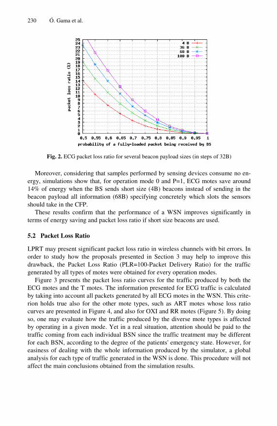
230 Ó. Gama et al.
Fig. 2. ECG packet loss ratio for several beacon payload sizes (in steps of 32B)
Moreover, considering that samples performed by sensing devices consume no en-ergy, simulations show that, for operation mode 0 and P=1, ECG motes save around 14% of energy when the BS sends short size (4B) beacons instead of sending in the beacon payload all information (68B) specifying concretely which slots the sensors should take in the CFP.
These results confirm that the performance of a WSN improves significantly in terms of energy saving and packet loss ratio if short size beacons are used.
5.2 Packet Loss Ratio
LPRT may present significant packet loss ratio in wireless channels with bit errors. In order to study how the proposals presented in Section 3 may help to improve this drawback, the Packet Loss Ratio (PLR=100-Packet Delivery Ratio) for the traffic generated by all types of motes were obtained for every operation modes.
Figure 3 presents the packet loss ratio curves for the traffic produced by both the ECG motes and the T motes. The information presented for ECG traffic is calculated by taking into account all packets generated by all ECG motes in the WSN. This crite-rion holds true also for the other mote types, such as ART motes whose loss ratio curves are presented in Figure 4, and also for OXI and RR motes (Figure 5). By doing so, one may evaluate how the traffic produced by the diverse mote types is affected by operating in a given mode. Yet in a real situation, attention should be paid to the traffic coming from each individual BSN since the traffic treatment may be different for each BSN, according to the degree of the patients' emergency state. However, for easiness of dealing with the whole information produced by the simulator, a global analysis for each type of traffic generated in the WSN is done. This procedure will not affect the main conclusions obtained from the simulation results.

Trade-off Analysis of a MAC Protocol for Wireless e-Emergency Systems 231
Fig. 3. Packet loss ratio for ECG and T traffic
Fig. 4. Packet loss ratio for ART traffic Fig. 5. Packet loss ratio for OXI and RR traffic
Comparatively to mode 1, Figures 3 and 4 illustrate clearly the improvement
achieved when the WSN operates in modes 2, 3, or 4. These operation modes present an ECG packet loss below 1% when probability P > 0.8. Such improvement is due to the multiple retransmission process occurred in the superframe. The ECG traffic pre-sents a lower loss ratio in a WSN operating in mode 3 than in mode 4. However for ART traffic it is almost irrelevant to work in mode 3 or 4. This occurs because the probability of losing an ART packet is lower than the probability of losing an ECG packet, as the packet size is smaller in the former.
Since OXI, RR, and T motes may only retransmit once in RCFP, no significant dif-ference is detected in such traffic by operating in modes 1, 2, or 3. However an im-provement is noticed at OXI and RR traffic by operating at mode 4. T traffic does not have such improvement because it cannot make use of the CAP.

232 Ó. Gama et al.
5.3 Energy Consumption
Since WSNs are operated by low-capacity batteries, energy preservation is important to guarantee that the e-emergency WSN operates for a long time. In order to evaluate the impact of the diverse operation modes on the energy consumption, the lifetime of the motes was studied.
To better evince the impact of each operation mode on the energy cost of the WSN, the consumption due to samplings performed by the sensing devices is ignored ini-tially. For every operation mode, Figure 6 presents the average lifetime per initial energy of the battery for each mote type relative to the simulations run with a prob-ability P=0.75. To know how many minutes a type of mote would live in such condi-tions, the values in the y-axis must be multiplied by the available energy in the battery (in Joules) when the mote started working. The available energy E in a battery with n cells, having each cell V Volts and a capacity of C mAh, is: E=n*V*C*3.6 J. For in-stance, one 3V, 1000 mAh lithium coin battery (CR2477) contains 10800 J of initial energy. So, according to Figure 6, an ECG mote operating in mode 4 and powered by that battery would live for 3.68*10800 min = 662.4 hours.
Fig. 6. Lifetime ignoring the sensing consume
For every mote type, the energy consumption does not change significantly with probability P > 0.75 and operation mode 1, 2, 3, or 4.
Figure 7 presents the results when each sampling performed by a sensing device consumes 0.01 mJ of energy. As shown, the effect of the sampling rates on the life-time of the motes is notorious. As ECG motes have both the highest sampling rate and the largest transmitted packet size, the energy drainage is faster than in the other mote types. However, the lifetime differences observed in each mote type for the diverse operating modes are almost negligible.

Trade-off Analysis of a MAC Protocol for Wireless e-Emergency Systems 233
Fig. 7. Lifetime for a sensing consume of 0.01mJ
5.4 CAP Availability
The association or disassociation of a BSN in the WSN is done during the CAP. To see how long is the CAP available for these operations, Figure 8 shows the percentage of superframes containing a CAP with a given size using P=0.75 and operation mode 3, the most limited mode regarding CAP size. In the y-axis, S1 is the number of super-frames with n free slots. For example, a CAP with 255 slots is available in 6.45% of all superframes. It is also shown that information considering groups of slot intervals (bar graph). The values are calculated performing the discrete integral along the speci-fied slot interval. In this case, the values in y-axis must be multiplied by ten, and Sintv
Fig. 8. Free slots for operation mode 3, P=0.75

234 Ó. Gama et al.
is the number of superframes with free slots in each interval. For instance, 30.5% of all superframes have a CAP size comprised between 200 and 239 slots.
It is observed that 99.3% of all superframes contain a CAP size above 80 slots, which are enough to perform (dis)association operations. Since CAP size is variable, the beacon should carry the superframe CAP size to inform the motes wishing to as-sociate to the WSN about the available contention slots. It is assumed that the start slot of the CAP is fixed and known previously.
5.5 Scalability
The WSN must be scalable in order to admit additional BSNs. In a LPRT-based sys-tem, scalability may be evaluated from the CAP available beyond the minimum CAP size. Indeed, if all superframes have a CAP size bigger than the minimum CAP size, it means that RP and NTP do not take all slots, which eventually may be used by an additional BSN. Figure 9 presents the percentage of superframes with a CAP size equal to the minimum value for several operation modes. This minimum value is fifty slots for operation mode 4, and null for the remaining modes. It is observed that a WSN operating in modes 1, 2, 3, and 4 may admit respectively 5, 3, 1, and 2 addi-tional BSNs without losing significant performance.
Fig. 9. Evaluation of scalability for P=0.75
5.6 Latency and Goodput
Since all packets are delivered to the BS with a delay below 500ms, the graphs report-ing this parameter are not presented. In this slotted framework, goodput is correlated with the packet loss ratio, therefore goodput graphics are not shown too.

Trade-off Analysis of a MAC Protocol for Wireless e-Emergency Systems 235
6 Conclusions
The deployment of LPRT in e-health systems leads to low power consumption, con-trolled latency, and throughput efficiency. However, as simulations have shown, LPRT is unreliable if the wireless channel is affected by appreciable bit errors. In or-der to define a MAC protocol more robust than LPRT, different approaches based on short size beacons and multiple retransmissions have been proposed and tested. The results have shown that such approaches lead to meaningful improvements regarding packet loss ratio, without compromising significantly the energy consumption.
Despite of presenting the best performance regarding packet loss ratio, a network operating in mode 3 faces scalability problems, since significant waste of time slots occurs in the RP. The results have revealed that operation mode 4 offers a better scal-ability and a good compromise in terms of packet loss. Therefore, we believe that LPRT operating in this mode will enhance QoS in e-health networks. Currently, we are implementing this operation mode in a real testbed for experimental analysis. Acknowledgments. Óscar Gama is supported by FCT (SFRH/BD/34621/2007), Portugal.
References
1. Gama, O., Carvalho, P., Afonso, J.A., Mendes, P.M.: Quality of service in wireless e-emergency: main issues and a case-study. In: Proc. of 3rd UCAmI, Salamanca, Spain (October 2008)
2. Akyildiz, J.F., Su, W., Sankarasubramaniam, Y., Cayirci, E.: A survey on sensor networks. IEEE Communications Magazine, 102–114 (August 2002)
3. Ye, I., Heidemann, J., Estrin, D.: MAC with coordinated adaptive sleeping for wireless sensor networks. IEEE/ACM Trans. Networks 12(3) (June 2004)
4. El-Hoiydi, A., Decotignie, J.D.: WiseMAC, An ultra low power MAC protocol for the Wise-NET wireless sensor network. In: Proc. of 1st ACM SenSys Conf., USA (November 2003)
5. Afonso, J.A., Rocha, L.A., Silva, H.R., Correia, J.H.: MAC protocol for low-power real-time wireless sensing and actuation. In: 13th IEEE International Conference on Electron-ics, Circuits and Systems, Nice (December 2006)
6. Gama, O., Carvalho, P., Afonso, J.A., Mendes, P.M.: An Improved MAC Protocol with a Reconfiguration Scheme for Wireless e-Health Systems Requiring Quality of Service. In: 1st Wireless Vitae 2009, Aalborg, Denmark (May 2009)
7. IEEE Std 802.15.4-2003, Wireless Medium Access Control (MAC) and Physical Layer (PHY) Specifications for Low-Rate Wireless Personal Area Networks (October 2003)
8. van Hoesel, L.F.W., Havinga, P.J.M.: A lightweight medium access protocol (LMAC) for Wireless Sensor Networks. In: Proc. 3rd Information Processing in Sensor Networks, Berkeley (April 2004)
9. Rajendran, V., Obraczka, K., Garcia-Luna-Aceves, J.J.: Energy-Efficient, Collision-Free MAC for Wireless Sensor Networks. In: Proc. ACM SenSys 2003, LosAngeles, USA (November 2003)
10. Castalia Simulator, http://castalia.npc.nicta.com.au 11. Zuniga, M., Krishnamachari, B.: Analyzing the transitional region in low power wireless
links. In: 1st IEEE Annual Conference on Sensor and Ad Hoc Communications and Net-works (October 2004)

An Underwater Robotic Network for MonitoringNuclear Waste Storage Pools
Sarfraz Nawaz1, Muzammil Hussain1, Simon Watson2, Niki Trigoni1,and Peter N. Green2
1 Oxford University Computing LaboratoryWolfson Building, Parks Road,
Oxford OX1 3QD{Sarfraz.Nawaz,Muzammil.Hussain,Niki.Trigoni}@comlab.ox.ac.uk
2 School of Electrical and Electronic EngineeringUniversity of ManchesterSackville Street BuildingManchester M60 1QD
[email protected],[email protected]
Abstract. Nuclear power provides a significant portion of our currentenergy demand and is likely to become more wide spread with grow-ing world population. However, the radioactive waste generated in thesepower plants must be stored for around 60 years in underwater storagepools before permanent disposal. These underwater storage environmentsmust be carefully monitored and controlled to avoid an environmentalcatastrophe. In this paper, we present an underwater mobile sensor net-work that is being developed to monitor these waste storage pools. Thissensing system will also be used in very old storage pools to build mapsof their internal structure which can then be used for waste removal andpool decommissioning. In this paper, we outline the unique challenges ofour application scenario which include robot localization in cluttered un-derwater environments and the effect of location errors on environmentmapping. We also list other industrial applications that can benefit fromour underwater sensor network.
1 Introduction
According to the World Nuclear Association [1], there are a total of 437 oper-ational nuclear reactors around the world supplying approximately 15% of thetotal electricity consumption. In the UK alone, there are 19 nuclear power plantsgenerating electricity for civilian use and 25 old power plants that are in var-ious stages of shutdown and decommissioning. As the world population grows,increased energy demand is likely to make nuclear energy generation more widespread. However, the biggest issue associated with nuclear power is the genera-tion of radioactive waste which must be managed and stored over a long periodof time. This radioactive waste can be classified as low level waste (LLW), in-termediate level waste (ILW) and high level waste (HLW). Low level waste con-tains paper, tools, clothing and other material that produce very small amount
S. Hailes, S. Sicari, and G. Roussos (Eds.): S-Cube 2009, LNICST 24, pp. 236–255, 2009.c© Institute for Computer Sciences, Social-Informatics and Telecommunications Engineering 2009

Underwater Robotic Network for Monitoring Nuclear Waste Storage Pools 237
of radioactivity. It is generally incinerated or processed as ordinary waste. In-termediate level waste comprises of chemicals, resins and metal fuel cladding.It contains higher amounts of radioactivity and thus requires shielding. It issometimes stored in short term storage facilities for a few weeks or months be-fore being solidified and buried in near surface trenches. Spent nuclear fuel andproducts of the fission reaction form high level waste. It generates the highestamount of radioactivity and thus requires shielding and careful handling. It isheld in interim storage for 20 to 60 years before it can be transferred to perma-nent disposal sites. Some of these high level wastes can have a half-life rangingfrom hundreds of thousands to millions of years and thus require special treat-ment. The most popular proposal is deep geological disposal in which the wastewould be solidified in glass or ceramic through a process called vitrification andthen buried in very deep rock formations ranging from 300m to 800m below theearth surface [2]. There are also some proposals to bury these wastes under theseabed [3].
Although, deep geological disposal is in its advanced stages of research, thereare no fully functional waste disposal repositories available at present. Even ifsuch repositories were available, it is still necessary to store this waste in cool-ing ponds for 20 to 60 years to remove the heat that is continuously generatedby this waste. After this extended underwater storage, the amount of heat gen-erated is reduced to a level that is suitable for deep rock burial. During thisextended underwater storage, the cooling ponds must be carefully monitoredfor temperature hot-spots and leakage in storage canisters. We are developingan underwater mobile sensor network for these nuclear waste storage pools incollaboration with our partners at University of Manchester and the NationalNuclear Laboratory. This network will consist of a swarm of small scale robots.Each robot will be approximately 10cm in diameter and will collaborate withother robots to monitor the conditions inside the storage pool. The clutteredunderwater environment of these pools presents significant difficulties for accu-rate robot localization. Inaccurate robot positions in turn influence the higherlayer tasks of environment mapping and high density spatial sampling. In thispaper, we discuss these challenges in detail and highlight these issues with ourpreliminary results. We also list underwater processes in other industrial appli-cations outside the nuclear domain that can benefit from our mobile sensingsystem.
The rest of this paper is organized as follows. Section (2) introduces the overallarchitecture and design of our mobile sensing system. Section (3) outlines theissues faced by robot localization algorithms and some preliminary experiences.Section (4) discusses the challenges in performing mapping and exploration tasks.Section (5) outlines the open issues and a research vision that we intend topursue. Section (6) presents the simulation environment that has been set up totest and analyze the performance of various algorithms. Section (7) lists otherindustrial applications of our mobile sensor network. Section (8) reviews relatedwork and Section (9) concludes this paper.

238 S. Nawaz et al.
2 System Architecture
In this section, we describe our application environment in detail and outlinea high level architecture of our mobile sensing system. There are two differenttypes of storage pools that we are targeting. In the following, we describe thedifferences between these two types and then present our system design.
The first type of storage ponds are modern, well maintained and clean pools.These are generally indoor concrete structures that are designed to be resistantto movements generated by events like earthquakes. Their sizes vary with thelargest ones approaching the dimensions of an Olympic sized swimming pool i.e.50m×25m. These pools can be as deep as 20m and are equipped with pumps andheat exchangers. The waste is sealed in steel flasks and then put in large skips.These skips are stacked on top of each other with the help of an overhead craneassembly. This creates an underwater landscape of rows of towers of skips. Thedistance between the surface of water and the top of skip towers is generally oneto two meters. This thick layer of water prevents any radiation from escapingthe pool. Pools are also equipped with cleaning systems to control water qualitythat is necessary to prevent any corrosion of storage skips. Fig. (1) shows aphotograph of one such storage pool at a reprocessing facility in the UK. In theseponds, our mobile sensor network will be used to perform dense spatial samplingof temperature, pH and radioactivity. It will also be used to monitor for anyleakages. Our specific research objective is to accurately sample temperature andradioactivity fields in these storage ponds using a swarm of resource constrainedrobots.
The second type of storage ponds are very old ponds that were built duringthe early 1950s and used until late 1980s. Over the years, a lot of intermediateand high level waste has been dumped in these ponds. The metal structures
Fig. 1. Modern Storage Pool

Underwater Robotic Network for Monitoring Nuclear Waste Storage Pools 239
and spent fuel rods in these ponds have decomposed and formed a thick sludgethat has settled on the bottom over time. This sludge may contain pocketsof hydrogen and other solid objects. Visibility inside these ponds is very poorbecause of the suspended particulates. Skip towers have also toppled over and theinternal structure is not known. There are no detailed records regarding the exactcontents of these ponds. Some of these ponds are extremely hazardous and onlyvery little human activity is allowed in the vicinity of these ponds. It is necessaryto gain more information about the internal structure of these ponds so that thewaste can be removed and stored in modern well maintained ponds until deepgeological disposal is available. In these ponds, our specific research objective isto build accurate maps of the internal structure of the ponds using a swarm ofresource constrained robots. Both tasks of spatial sampling (in new ponds) andmapping (in old ponds) require robots to be able to localize themselves withinthe pond. The main questions discussed in this paper are, how the presence ofclutter - stored nuclear waste - impacts localization errors, and how these errorsinfluence the spatial sampling and mapping processes.
Fig. (2) shows an overall architecture of our underwater mobile sensing sys-tem. The storage pond is instrumented with a number of fixed anchor nodes.These anchor nodes periodically transmit acoustic beacons that are used by mo-bile nodes to determine their position inside the pool. These nodes also act ascollection sinks and are used to receive data transmitted by robots on the acous-tic channel. Robots can also communicate with each other and perform distancemeasurements among themselves using acoustic signals. This allows the robotsto collaborate with each other during the localization, sensing and mappingtasks. Both the payload and propulsion system of the underwater robots arecurrently under investigation. At this point, it is envisaged that the the pay-load will initially consist of a pressure sensor to measure depth, a temperaturesensor and a number of obstacle detection sensors that will be based on the
Fig. 2. Underwater Sensor Network Architecture

240 S. Nawaz et al.
(a) Robot Internals (b) Robot size (c) Prototype Robot
Fig. 3. Size comparison of prototype robot
communication and positioning acoustic transducers. There will also be a hard-ness sensor based on the same technology and an optical based turbidity sensor.The propulsion system is split into the z plane and x-y plane and will provideat least 4 degrees of freedom (surge, sway, heave and yaw) [4]. Movement in thez-plane will come from propellers while the x-y plane movement will be achievedby a combination of propellers and/or miniaturized vortex ring thrusters [5].The propulsion systems will be controlled by an embedded system in the formof a 32-bit microprocessor with DSP. Each robot is expected to be approxi-mately 10cm in diameter. Fig. (3) shows an initial prototype version of ourrobot.
Fig. (4) shows how different components of the software system interact witheach other and the hardware components. The lowest layer consists of varioushardware components that include acoustic communication and ranging, varioussensors and propulsion system. These hardware components are in various stagesof development. Middle level layers are responsible for localizing the robot andfor performing reactive obstacle avoidance. These middle layer components havebeen implemented in a simulation environment. The higher layer consists of ourtwo distinct applications i.e. spatial sampling in new ponds and exploration andmapping in old ponds.
Fig. 4. Software Architecture

Underwater Robotic Network for Monitoring Nuclear Waste Storage Pools 241
3 Robot Localization
3.1 Background
Location awareness is a basic requirement for a robot swarm to explore and mapan enclosed underwater environment such as a nuclear waste storage pond. It isnecessary for the robots to have accurate position information not just for actualmapping but also for navigating through the pond. Anchor nodes, nodes con-nected to external reference systems that supply positional information, enablethe use of trilateration for localizing robots. The technique exploits geometricalconstraints, given the locations of a number of anchors and distances to them, tocalculate the position. Even though for three-dimensional positioning we requireat least four anchors, the underwater robots we are designing have pressure sen-sors which can be used to determine the depth (z-coordinate) of the robot. Thisobviates the need for a fourth anchor.
Distance measurements to the anchors, in noisy environments, have smallGaussian errors [6], thus introducing an error in the calculated position. In largenetworks, where the number of anchors is small compared to the remaining non-localized nodes, it could be the case due to the limited transmission range of theacoustic communication and the attenuating effects of cluttered environments,that all anchors would not be heard by all the nodes in the network. It ispossible that a particular unpositioned node cannot hear the required numberof anchors in order to calculate its position thus requiring neighbouring nodeswhich have already been localized (owing to their proximity to the requirednumber of anchors) to assist them. These neighbouring nodes are used as virtualanchors and the process is called iterative localization. However these virtualanchors, having previously localized themselves, contain inherent errors in theirown positions. These errors, compounded by the noisy distance measurements,could propagate via successive iterative localization steps. It is vital to controlthe propagation of error due to noisy distance measurements and inaccuratevirtual anchors positions.
Iterative localization has been a well researched topic for the past few years.Collaborative multi-lateration is introduced in [7] where location informationfrom across multiple hops is used to localize a node. In [8], the authors pro-pose a method to quantify the errors introduced by virtual anchors and noisyrange measurements. Each node can thus prevent the accumulation of local-ization errors by maintaining a registry of its neighbouring anchor nodes andusing those anchors in trilateration that have the smallest errors. Another ap-proach [9] to quantifying error in iterative localization takes into account thegeometric relationships between the anchors during selection. Localization inunderwater environments has also been an active area of research [10]. However,almost all of this work deals with localizing sensor nodes in open sea environ-ments [11,12]. Our research, on the other hand, deals with localizing sensingrobots in cluttered underwater environments. This is discussed in detail in thefollowing subsection.

242 S. Nawaz et al.
3.2 Localization in Cluttered Underwater Environments
One of the primary areas of interest in this project is the challenges faced bya network of robots in exploring cluttered environments. Clutter is generallyirregularly shaped obstacles that obstruct acoustic propagation paths betweenrobots or worse introduce multipath acoustic communication.
The underlying concept behind range-based localization is that the distancebetween the robot and the anchors can be obtained by sending a communica-tion signal between them and the distance is derived from the characteristicsof the received signal. In case of acoustic/ultrasound signals, the propagationtime translates into the distance travelled, assuming that we know the velocityof sound in that particular medium accurately. This, however, hinges on theassumption that the signal travels straight from the anchor to the non-localizedrobot along the shortest path, without bouncing off any obstacles in between.Such signals are called Line Of Sight (LOS) signals. The measurements fromsuch signals would yield the least distance errors. However in reality, in clutteredenvironments with obstacles between the transmitter and receiver, it is possiblethat a large number of signals are Non Line Of Sight (NLOS). Such signalshave large distance measurement errors.
There has been extensive research in the mitigation of non line-of-sight mea-surements, particularly in cellular network research. It was motivated by therequirement put forth by Federal Communications Commission (FCC) to cellu-lar operators to be able to locate a mobile handset within an accuracy of 300meters for 95% of calls [13]. In current literature [14,15,16,17,18,19,20,21] thereare three general methods to deal with NLOS readings. The first method at-tempts to identify and use only LOS measurements. Distinguishing NLOS fromLOS distance measurements could either be done using a time-varying hypothe-sis test [14], a probabilistic model [18] or residual information [15,21]. The secondmethod incorporates both LOS and NLOS distance measurements with appro-priate weighting to minimize the contribution of NLOS observations. Here theprimary assumption made is that the number of LOS readings is much greaterthan the number of NLOS readings [16,17], which may not be the case in ourunderwater cluttered environment. The third method advocates the use of scat-tering models. This method takes into account the propagation characteristicsof the channel and then directly determines the actual line-of-sight distance us-ing the NLOS readings using a scattering model [19,20]. However this requiresperfect knowledge of the underwater environment, including the topology andtype of clutter, which may not be possible in most cases.
We have simulated robot localization in the presence of LOS signals and NLOSsignals inFig. (5). InFig. (5a),we see that the smallest localization error is obtainedwhenonlyLOSdistancemeasurements areused. InFig. (5b)we see that localizationerror increases with a smaller number of LOS distance measurements, even thoughwe have filtered out NLOS measurements. Fig. (5c) shows that using NLOS mea-surements in addition to LOS measurements gives a large localization error. Hencewe can conclude that not only should we filter out NLOS measurements but alsohave enough LOS measurements to get an accurate position estimate.

Underwater Robotic Network for Monitoring Nuclear Waste Storage Pools 243
(a) LOS anchors only (b) LOS and NLOS anchors
(c) NLOS anchors filtered
Fig. 5. Robot localization errors when LOS distance estimates have a small Gaussianerror (σ = 6.5cm) [6] and NLOS distance estimates have a large constant error (30 cm)
From the preliminary experiments we have conducted, we envisage two sce-narios as illustrated in Fig. (6). In the first scenario, the clutter is impermeable toacoustic signals. Here only reflected non line-of-sight (NLOS) signals, which havelarge errors in distance estimates, are present. These have to be detected andfiltered from the remaining range measurements before calculating the position.In the second case, the clutter is actually permeable to acoustic signals wherebythe signal can ’resonate’ through the obstacle without losing all the energy. Inthis case, the distance estimate of the NLOS signal would be comparable to thatof a LOS signal.
When the majority of the NLOS measurements are of the first type i.e., re-flected NLOS, it may be the case that filtering out NLOS measurements (an-chors) could lead to a non-localized robot not having access to the requirednumber of anchors. For example, in Fig. (5c), if three of the five measurementshad been NLOS, the non-localized robot would not have been able to calculate

244 S. Nawaz et al.
(a) Non-Permeable Obstacles (b) Permeable Obstacles
Fig. 6. Possible types of obstacles in a nuclear storage tank. Permeable obstacles givingrise to ’near-LOS’ NLOS range measurements.
its position. Also the reduced number of LOS anchors increases the error in theposition estimate. In this scenario it may become necessary to develop a strategyto deploy previously localized robots to help their non-localized neighbours tolocalize, so as to maximize the chances that a node, at any given position in theunderwater pond, can localize itself accurately. At first we would want to workwith the static case where the robots are stationary. Here emphasis is put onthe initial position of the robots so as to enable all/most of the robots to belocalized.
Now that we have introduced the challenges of robot localization in clutteredunderwater environments, in the next section, we discuss how these localizationerrors effect the mapping task.
4 Exploration and Mapping
Creating maps of the bottom of old waste storage ponds where sludge and otherparticulate material has settled down over long periods of time is an importantaspect of our mobile sensing system. In order to create these maps, the robotsmust be aware of their surroundings as well so that they can safely move aroundin the pond without colliding with the waste storage canisters. Thus, to accom-plish this task, the robots must explore and map the entire pond. These robotsmust also collaborate with each other to map the environment efficiently. Inthis section, we discuss some related work on robotic mapping and exploration,and outline the challenges of performing the mapping task in the pesence ofrobot localization errors. We also present some preliminary simulation resultsthat highlight these issues.
When a robot is placed in an unknown environment and it does not haveaccess to any location information, it has to determine its location and build themap of the environment at the same time. This problem is known as Simultane-ous Localization and Mapping (SLAM) or Concurrent Mapping and Localization

Underwater Robotic Network for Monitoring Nuclear Waste Storage Pools 245
(CML) and has received considerable attention from the robotics research com-munity. Smith and Cheeseman [22] used an Extended Kalman Filter (EKF)to solve the SLAM problem for the first time and since then it has been ahighly active field of research. Thrun [23] provides an extensive survey of SLAMtechniques.
When the location information is available to a robot, the problem of mappingthe environment becomes easier as compared to SLAM. However, noisy sensormeasurements and complex environments can still pose significant challenges tomapping and exploration algorithms. The most widely used family of algorithmsused to map environments with known robot locations is called Occupancy GridMapping. Occupancy grid based mapping was introduced by Elfes [24] and latera Bayesian statistical basis of this approach was developed by Moravec [25].Moravec [26] also extended this approach to build three-dimensional maps us-ing stereo cameras. Occupancy grids have also received a wider acceptance inrobotics because they are commonly used as input to algorithms for path plan-ning, collision avoidance, sensor fusion etc. In our system, a group of anchornodes provide an infrastructure that is used by robots to determine their posi-tions. Therefore, we use occupancy grids for building the maps of underwaterenvironments of the storage pools.
The basic idea of occupancy grid mapping is that the space that has to bemapped is divided in small uniform sized cells, for example, 10cm × 10cm. Foreach cell, the robot maintains a probabilistic belief about the occupancy of thecell. In the beginning, no information is available and the status of each cell isunknown. As the robot moves around, it gathers measurements from its percep-tion sensors (e.g. sonar, laser range finder, stereo cameras or some other sensor)and the corresponding cells are updated with these measurements according toa Bayesian reasoning approach. In order to determine which cells to update, therobot must know its position in the environment and the characteristics of itssensors. For example, if a robot is using a sonar sensor to perceive its environ-ment, then all the cells mi of the occupancy grid that lie within the beamwidthof sonar sensor are updated according to the Bayes rule using the log odds rep-resentation as,
lt,i = lt−1,i + logp (mi|xt, zt)
1 − p (mi|xt, zt)(1)
where xt is the location of the robot at time t, zt is the sonar measurementand p is the occupancy probability derived from a sensor model given the rangemeasurement zt returned from the sonar and lt,i is
lt,i = logp (mi|x1:t, z1:t)
1 − p (mi|x1:t, z1:t)(2)
Generally, the log odds of prior probability l0 is set to zero for all cells mi. The logodds representation provides an easy update rule in the form of Eq. (1). Whenit is required to determine whether a cell mi is occupied or free, the probabilityp (mi|x1:t, z1:t) can be recovered as

246 S. Nawaz et al.
p (mi|x1:t, z1:t) = 1 − 11 + exp (lt,i)
(3)
and compared against thresholds thres-occ and thres-free to decide on itsoccupancy,
p (mi|x1:t, z1:t)
⎧⎪⎨⎪⎩
≥ thres-occ mi is occupied≤ thres-free mi is freeotherwise mi is unknown
(4)
The probabilistic belief for each cell in the grid is derived using sensor measure-ments and robot location. Therefore, any measurement or location error affectsthe occupancy grid. We have shown in Section (3) that the cluttered environ-ment of the storage pools can introduce significant errors in estimated robotpositions. These location errors in turn introduce anomalies in the storage poolmaps built by robots in the form of occupancy grids. Fig. (7a) shows a 6m ×6m simulated pool where two towers of storage skips have been placed. Anchor
(a) Simulated Cluttered Pond
(b) Mapping without loca-tion errors
(c) Mapping with locationerrors
Fig. 7. Mapping in cluttered ponds

Underwater Robotic Network for Monitoring Nuclear Waste Storage Pools 247
nodes have been placed at four out of the eight corners of pool and a singlerobot moves through this lightly cluttered pool localizing itself through single-hop trilateration. For direct line of sight distance estimates, a small error froma normal distribution N(0, σ) with σ = 5cm is introduced. For non line of sightdistances between the anchors and robots, a uniform distribution U(0, b) withb = 30cm is used to introduce errors. The robot uses sonar measurements and itsestimated location to build a 2D map of the simulated pool using frontier basedexploration and mapping [27]. A number of such 2D maps can be built at variousdepths to create a three dimensional map of the environment. Further detailsof our simulation environment are described in Section (6). Fig. (7b) shows a2D map that is built using the perfect location information without any errors.Fig. (7c), on the other hand, shows a map when the estimated robot locationcontains significant errors due to non line of sight (NLOS) distance estimatesbetween the robot and the anchor nodes. These location errors not only distortthe map but since the partial map is also used by the robot for exploration andpath planning, they also affect the efficiency of the mapping process. Our aim isto quantify the effect of these errors on the mapping process and then developefficient exploration strategies that can mitigate the effect of these errors on themapping process.
5 Open Research Issues
Now that we have described the specific challenges of robot localization and itseffects on mapping and exploration tasks in the previous two sections, we nowpresent a vision that we intend to pursue in our future research. We envisagethree different types of environment mapping systems using our swarm of robots.In the following, we outline these three systems and the individual questions thatwe intend to answer for each of these systems.
Our first system consists of robots that have been classified in two differentcategories depending on their role. We term the robots belonging to the firstcategory as localizers and those belonging to the second category as explorers.The role of the localizer robots is to position themselves in such a manner thatthe explorer robots can localize themselves and thus explore the cluttered envi-ronment. The main challenge of this approach is to optimally place localizers sothat the explorers can build an accurate map of the environment.
In our first system, there is no feedback mechanism between the localizationand the exploration tasks. Explorers only explore those regions where the localiz-ers are available to provide positioning infrastructure. In the second system thatwe envisage an explicit feedback mechanism is available between the explorersand localizers. Thus the explorers can request the localizers to move to a certainregion to provide positioning infrastructure so that that region can be exploredand mapped. The main challenge of this approach is to design efficient resourceallocation strategies that can be used to assign localizers to explorers.
In our third system, there is no distinction of roles and each robot performsboth of the tasks simultaneously i.e. each robot not only explores and maps the
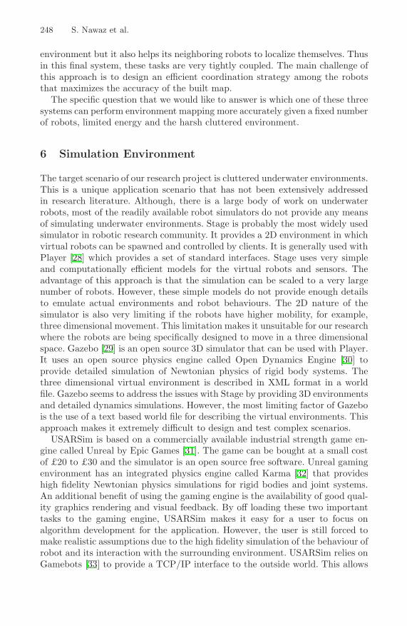
248 S. Nawaz et al.
environment but it also helps its neighboring robots to localize themselves. Thusin this final system, these tasks are very tightly coupled. The main challenge ofthis approach is to design an efficient coordination strategy among the robotsthat maximizes the accuracy of the built map.
The specific question that we would like to answer is which one of these threesystems can perform environment mapping more accurately given a fixed numberof robots, limited energy and the harsh cluttered environment.
6 Simulation Environment
The target scenario of our research project is cluttered underwater environments.This is a unique application scenario that has not been extensively addressedin research literature. Although, there is a large body of work on underwaterrobots, most of the readily available robot simulators do not provide any meansof simulating underwater environments. Stage is probably the most widely usedsimulator in robotic research community. It provides a 2D environment in whichvirtual robots can be spawned and controlled by clients. It is generally used withPlayer [28] which provides a set of standard interfaces. Stage uses very simpleand computationally efficient models for the virtual robots and sensors. Theadvantage of this approach is that the simulation can be scaled to a very largenumber of robots. However, these simple models do not provide enough detailsto emulate actual environments and robot behaviours. The 2D nature of thesimulator is also very limiting if the robots have higher mobility, for example,three dimensional movement. This limitation makes it unsuitable for our researchwhere the robots are being specifically designed to move in a three dimensionalspace. Gazebo [29] is an open source 3D simulator that can be used with Player.It uses an open source physics engine called Open Dynamics Engine [30] toprovide detailed simulation of Newtonian physics of rigid body systems. Thethree dimensional virtual environment is described in XML format in a worldfile. Gazebo seems to address the issues with Stage by providing 3D environmentsand detailed dynamics simulations. However, the most limiting factor of Gazebois the use of a text based world file for describing the virtual environments. Thisapproach makes it extremely difficult to design and test complex scenarios.
USARSim is based on a commercially available industrial strength game en-gine called Unreal by Epic Games [31]. The game can be bought at a small costof £20 to £30 and the simulator is an open source free software. Unreal gamingenvironment has an integrated physics engine called Karma [32] that provideshigh fidelity Newtonian physics simulations for rigid bodies and joint systems.An additional benefit of using the gaming engine is the availability of good qual-ity graphics rendering and visual feedback. By off loading these two importanttasks to the gaming engine, USARSim makes it easy for a user to focus onalgorithm development for the application. However, the user is still forced tomake realistic assumptions due to the high fidelity simulation of the behaviour ofrobot and its interaction with the surrounding environment. USARSim relies onGamebots [33] to provide a TCP/IP interface to the outside world. This allows

Underwater Robotic Network for Monitoring Nuclear Waste Storage Pools 249
Fig. 8. Structure of USARSim
the controller programs to connect to the simulation environment and spawnand control different robots. Fig. (8) shows the overall structure of USARSimsimulator and how different components fit together.
Unreal gaming engine also ships with a 3D editor UnrealEd that can be usedto easily create 3D virtual environments. It includes all the necessary facilitiesto easily create the target environments for our research. The most important ofthese facilities is the ability to create a Water Volume. A water volume is a regionof space where the physics engine modifies its behaviour to simulate a fluid. Thus,in a water volume, a robot experiences fluid friction and buoyancy in additionto gravity. It is also possible to change the default values of these parametersto match those of an actual pond. Using UnrealEd, we have created virtual 3Dstorage pools. We can also create towers of skips and other clutter of differentsizes in these simulated pools. Therefore, this simulation set up can faithfullyreproduce the actual storage pools in the virtual simulated environment.
(a) UnrealEd (b) USARSim
Fig. 9. Screenshot of the simulated pond and the robot

250 S. Nawaz et al.
Due to the above mentioned benefits, we decided to use USARSim for investi-gating the mapping, exploration and localization algorithms for our underwatermobile sensing system. Fig. (9) shows a screen shot of one of the pools in Un-realEd and a robot moving around in this pool in the USARSim simulator.
7 Other Industries
The technologies and the algorithms developed during the course of this re-search can be used in a wide range of applications in addition to nuclear wastemonitoring. In this section, we outline some of the potential industries thatoperate aqueous environments similar to waste storage ponds and thus can sig-nificantly benefit from a networked mobile sensing system for these underwaterenvironments.
Industrial scale process monitoring in chemical industry is an area that canbenefit from our contributions. A large portion of these processes involve largescale vessels where different chemicals are mixed together. For these processes,the chemical engineers are generally interested in temperature, pressure, con-centration of chemicals, turbidity and other parameters inside the vessel. At themoment, the only technique available to measure some of these parameters istomography where sensors are placed outside the vessel. However, only some ofthe above parameters can be estimated using tomography. Another disadvantageof tomography is that it offers very limited spatial and temporal resolution. Aswarm of our submersible robots can be placed inside such vessels to performhigh density spatial measurements of all of these parameters. These measure-ments would allow the chemical engineers to develop a better understanding ofthese chemical processes. This data can then also be used to redesign and im-prove the chemical processes in terms of energy savings and material usage. Therobots can also be used to monitor the wear and tear of reaction vessels fromthe inside.
Almost all of the chemical plants have large scale settling ponds that areused to clean water after it has been used in a chemical process. These pondsare generally outdoors and could be as big as 100m in diameter. These settlingponds are filled with water and the particulates in water are allowed to settledown. The water is then drained off and recycled. Any leakage in these pondscan have a detrimental effect on the surrounding environment. Therefore, it isnecessary to monitor these ponds for any such leakages. Current methods usedfor these inspections are manual and thus expensive and time consuming. Oursystem of networked robots can be used to continuously monitor the pond forany anomalies at significantly reduced costs.
Another industry where our mobile sensor system can be used is sewagewastew-ater treatment. Thewastewater generatedby our cities and communities is on aver-age 99.94%water by weight and only 0.06% solid waste [34]. Wastewater treatmentplants collect this sewage and process it in an extensive network of chambers andponds to separate these solid wastes from the water. The first stage of this net-work is similar to settling ponds mentioned above where the water is held for few

Underwater Robotic Network for Monitoring Nuclear Waste Storage Pools 251
hours and the solid waste is allowed to settle down. The second stage consists of alarge number of aeration ponds where microorganisms are used to breakdown thedissolved waste materials. This process is similar to essentially what happens innature. However, in a wastewater treatment plant the speed of this process has toincreased toprocess the largequantitiesofwater.Therefore, it isnecessary to createoptimum conditions for microorganisms in these ponds. This includes mixing theright quantities of oxygen and nutrients in these ponds. Our mobile sensor networkcan be used in these ponds to monitor the concentration of these substances. Usingthese observations, the plant engineers can control the amount of oxygen and nu-trients injected into the ponds as the wastewater concentration changes every fewhours during the course of the entire day.
8 Related Work
In this section, we outline some of the related work to put our research in properperspective. We discuss some underwater autonomous robots and robotic swarmsystems and highlight the challenges that differentiate our research from theseefforts.
It is generallymore difficult to workwith underwater environments as comparedto the terrestrial one and therefore the development of underwater robots and espe-cially autonomous underwater vehicles (AUVs) has been relatively slow. However,the military, scientific and commercial applications of these autonomous underwa-ter vehicles has contributed to a very rapid progress in recent years. A databaseof currently available AUVs hosted by Autonomous Undersea Systems Institutelists a total of 103 AUVs available from 51 different manufacturers [35]. More so-phisticated systems that consist of swarms of cooperating AUVs, nodes anchoredto the seabed and floating buoys have also been developed. Autonomous OceanSampling Network [36] and Autonomous Systems Network [37] are a couple ofexamples of such underwater networked sensing systems. The deployment andcoverage analysis of such underwater sensing systems has also been studied [38].However, almost all of these platforms and networked systems are targeted to-wards and deployed in open ocean environments. Open sea is an extremely vastenvironment that presents its own unique challenges. The AUVs used in this en-vironment are relatively large in size and have significant movement, sensing andcomputational resources available on board. Networks of such vehicles are alsoof relatively large size with individual communication links usually stretching totens of kilometers. Our application, on the other hand, requires the developmentof very small scale robots that can move in cluttered aqueous environments withdimensions ranging from tens to a few hundred meters. In addition to beingsmall, these robots must have enough resources to safely navigate, sense andmap these constrained cluttered ponds.
Serafina is a small scale AUV developed at Australian National University [39].It is 50cm long and weighs around 5kg. It has five fixed thrusters with twoin horizontal and three in vertical configuration. These thrusters provide fivedegrees of freedom of movement to the AUV. An inertial sensor and a compassare used to perform attitude control and communication among different nodes

252 S. Nawaz et al.
is achieved through a long wave radio with a carrier frequency of 122.88kHz. Therelative distance and heading of nearby nodes in a swarm of Serafina vehicles isdetermined by using a pair of hydrophones to receive acoustic signals. However,the performance of these techniques has only been measured in a small tankwith clear line of sight and without any clutter [40]. Kalantar and Zimmer [41]have also proposed swarming algorithms to track and map environmental fieldslike chemical concentration spread and ocean bottom mapping.
Researchers have always looked towards nature to draw inspiration for theirown creations and this has resulted in various bio-mimetic robots. The roboticfish [42] developed at University of Essex is one such underwater autonomousrobot. It uses the oscillatory movement of its body just like an actual fishto propel itself through water instead of using the traditional propeller basedpropulsion systems. It can move autonomously in an unknown environment in acomplete 3D manner. Researchers at University of Essex are proposing to usethese autonomous robots for pollution monitoring in sea ports. The current gen-eration of this robot is 52cm long. Three servo motors and mechanical joints areused to generate the oscillatory movement of the body. Four IR sensors and onesonar sensor is used for obstacle detection. However, at the moment there is nocommunication functionality available to exchange information between differ-ent robotic fishes. Therefore, these robots cannot collaborate with each other toform swarms of mobile sensors.
Hydron was developed as part of the Hydra project [43]. It is a very smallunderwater robot that has a roughly spherical shape with approximately 11cmdiameter. Movement in the horizontal direction is achieved by expelling waterthat is drawn in through an impeller from one of the four nozzles selected througha rotating collar. A syringe is used to draw in or expel the water through thebottom. This alters the buoyancy of the robot and thus allows movement invertical direction. Each hydron robot can communicate with other units withshort range optical transceivers. Hydron robots were developed as basic unitsthat could act as building blocks to automatically form more complex struc-tures by rearranging themselves around each other. However, these units are notequipped with localization facilities that could allow them to determine theirposition in the aqueous environment.
The cluttered nature of industrial ponds creates a very harsh environmentfor communication and positioning systems and the focus of our research is toaddress this challenge at each individual layer of our mobile sensing systemranging from low level distance estimation to application level mapping andexploration algorithms. This is a unique application scenario and to the bestof our knowledge has never been addressed before. The robotic platforms andsensing systems that we discussed in this section are either too large for ourpurposes or have never been tested in our unique application scenario.
9 Conclusion
In this paper, we discussed a novel application of nuclear waste storage pool mon-itoring and outlined a detailed architecture of our proposed underwater mobile

Underwater Robotic Network for Monitoring Nuclear Waste Storage Pools 253
sensor network for monitoring these pools. We described the difficulties faced byrobot localization and environment mapping algorithms due to the cluttered andenclosed nature of these underwater environments with preliminary results. Weoutlined the future research challenges of our unique application and also high-lighted various other industrial applications that can potentially benefit fromour underwater mobile sensor network.
Acknowledgements. This work is supported by the EPSRC grants EP/F064209/1 and EP/F064578/1 on Actuated Acoustic Sensor Networks for In-dustrial Processes (AASN4IP). We would also like to thank the National NuclearLaboratory (NNL) for their contribution to this paper.
References
1. World Nuclear Association, http://www.world-nuclear.org2. Roberts, L.E.J.: Radioactive waste management. Annual Review of Nuclear and
Particle Science 40(1), 79–112 (1990)3. Hollister, C.D., Nadis, S.: Burial of radioactive waste under the seabed. Scientific
American (January 1998)4. Fossen, T.I.: Guidance and Control of Ocean Vehicles. John Wiley & Sons, Chich-
ester (1994)5. Krieg, M., Mohseni, K.: Thrust characterization of a bioinspired vortex ring
thruster for locomotion of underwater robots. IEEE Journal of Oceanic Engineer-ing 33(2), 123–132 (2008)
6. Whitehouse, K., Karlof, C., Woo, A., Jiang, F., Culler, D.: The effects of rang-ing noise on multihop localization: an empirical study. In: Fourth InternationalSymposium on Information Processing in Sensor Networks, IPSN 2005, pp. 73–80(2005)
7. Savvides, A., Han, C.C., Strivastava, M.B.: Dynamic fine-grained localization in ad-hoc networks of sensors. In: Proceedings of the 7th annual international conferenceon Mobile computing and networking, pp. 166–179. ACM, New York (2001)
8. Liu, J., Zhang, Y., Zhao, F.: Robust distributed node localization with error man-agement. In: Proceedings of the 7th ACM international symposium on Mobile adhoc networking and computing, pp. 250–261. ACM, New York (2006)
9. Yang, Z., Liu, Y.: Quality of Trilateration: Confidence Based Iterative Localization.In: The 28th International Conference on Distributed Computing Systems, ICDCS2008, pp. 446–453 (2008)
10. Chandrasekhar, V., Seah, W.K., Choo, Y.S., Ee, H.V.: Localization in underwatersensor networks: survey and challenges. In: WUWNet 2006: Proceedings of the 1stACM international workshop on Underwater networks, pp. 33–40. ACM, New York(2006)
11. Erol, M., Vieira, L., Caruso, A., Paparella, F., Gerla, M., Oktug, S.: Multi stageunderwater sensor localization using mobile beacons. In: Second International Con-ference on Sensor Technologies and Applications, SENSORCOMM 2008, August2008, pp. 710–714 (2008)
12. Erol, M., Vieira, L.F.M., Gerla, M.: Auv-aided localization for underwater sen-sor networks. In: International Conference on Wireless Algorithms, Systems andApplications, WASA 2007, August 2007, pp. 44–54 (2007)

254 S. Nawaz et al.
13. Enhanced Wireless 911 Services,http://www.fcc.gov/Bureaus/Wireless/News_Releases/1999/nrwl9040.html
14. Wylie, M.P., Holtzman, J.: The non-line of sight problem in mobile location esti-mation. In: 5th IEEE International Conference on Universal Personal Communi-cations, 1996. Record, September-2 October, vol. 2, pp. 827–831 (1996)
15. Cong, L., Zhuang, W.: Non-line-of-sight error mitigation in tdoa mobile location.In: Global Telecommunications Conference, GLOBECOM 2001, vol. 1, pp. 680–684. IEEE, Los Alamitos (2001)
16. Chen, P.C.: A non-line-of-sight error mitigation algorithm in locationestimation.In: Wireless Communications and Networking Conference, WCNC 1999, pp. 316–320. IEEE, Los Alamitos (1999)
17. Venkatraman, S., Caffery Jr., J., You, H.R.: Location using LOS range estimationin NLOS environments. In: IEEE 55th Vehicular Technology Conference, VTCSpring 2002, vol. 2 (2002)
18. Borras, J., Hatrack, P., Mandayam, N.B.: Decision theoretic framework for nlosidentification. In: 48th IEEE Vehicular Technology Conference, VTC 1998, May1998, vol. 2, pp. 1583–1587 (1998)
19. Al-Jazzar, S., Caffery Jr., J.: New algorithms for nlos identification. In: Proceedingsof the 14th IST Mobile and Wireless Communications Summit (2005)
20. Al-Jazzar, S., Caffery Jr., J., You, H.R.: A scattering model based approach toNLOS mitigation in TOA location systems. In: IEEE 55th Vehicular TechnologyConference, VTC Spring 2002, vol. 2 (2002)
21. Chan, Y.-T., Tsui, W.-Y., So, H.-C., Ching, P.c.: Time-of-arrival based localizationunder nlos conditions. IEEE Transactions on Vehicular Technology 55(1), 17–24(2006)
22. Smith, R.C., Cheeseman, P.: On the Representation and Estimation of SpatialUncertainty. The International Journal of Robotics Research 5(4), 56–68 (1986)
23. Thrun, S.: Robotic mapping: a survey, pp. 1–35 (2003)24. Elfes, A.: Sonar-based real-world mapping and navigation. IEEE Journal of
Robotics and Automation 3(3), 249–265 (1987)25. Moravec, H.: Sensor fusion in certainty grids for mobile robots. AI Magazine 9(2),
61–74 (1988)26. Moravec, H.: Robot spatial perception by stereoscopic vision and 3d evidence grids.
Technical Report CMU-RI-TR-96-34, Robotics Institute, Pittsburgh, PA (Septem-ber 1996)
27. Yamauchi, B.: A frontier-based approach for autonomous exploration, July 1997,pp. 146–151 (1997)
28. Gerkey, B., Vaughan, R., Howard, A.: The Player/Stage Project: tools for multi-robot and distributed sensor systems. In: 11th International Conference on Ad-vanced Robotics (ICAR 2003), Coimbra, Portugal (June 2003)
29. Gazebo, http://playerstage.sourceforge.net/index.php?src=gazebo30. Smith, R.: Open dynamics engine, http://www.ode.org31. Epic Games, http://www.epicgames.com32. Karma physical engine, http://wiki.beyondunreal.com/wiki/Karma33. Kaminka, G.A., Veloso, M.M., Schaffer, S., Sollitto, C., Adobbati, R., Marshall,
A.N., Scholer, A., Tejada, S.: Gamebots: a flexible test bed for multiagent teamresearch. Commun. ACM 45(1), 43–45 (2002)
34. Following the flow: An inside look at wastewater treatment,http://www.wef.org/AboutWater/ForThePublic/WastewaterTreatment
35. AUV Database, http://auvac.org/resources/browse/

Underwater Robotic Network for Monitoring Nuclear Waste Storage Pools 255
36. Autonomous Ocean Sampling Network (AOSN) II,http://www.princeton.edu/~dcsl/aosn
37. Chappell, S.G., Komerska, R.J., Blidberg, D.R., Duarte, C.N., Martel, G.R., Crim-mins, D.M., Beliard, M.A., Nitzel, R., Jalbert, J.C., Bartos, R.: Recent field experi-ences with multiple cooperating solar-powered vehicles. In: Fifteenth InternationalSymposium on Unmanned Untethered Submersible Technology, Durham, NH (Au-gust 2007)
38. Pompili, D., Melodia, T., Akyildiz, I.F.: Three-dimensional and two-dimensionaldeployment analysis for underwater acoustic sensor networks. Ad Hoc Net-works 7(4), 778–790 (2009)
39. Schill, F.: Distributed Communication in Swarms of Autonomous Underwater Ve-hicles. PhD thesis, The Australian National University (July 2007)
40. Kottege, N., Zimmer, U.R.: Acoustical methods for azimuth, range and headingestimation in underwater swarms. In: Acoustics 2008, Palais des Congrs, Paris(June 2008)
41. Kalantar, S., Zimmer, U.R.: IEEE/RSJ International Conference on IntelligentRobots and Systems, IROS 2008, September 2008, pp. 3146–3151 (2008)
42. Hu, H.: Biologically inspired design of autonomous robotic fish at Essex. In:IEEE SMC Chapter Conference on Advances in Cybernetic Systems, Sheffield,UK (September 2006)
43. Østergaard, E.H., Christensen, D.J., Eggenberger, P., Taylor, T., Ottery, P., Hau-top Lund, H.: HYDRA: From cellular biology to shape-changing artefacts. In:Duch, W., Kacprzyk, J., Oja, E., Zadrozny, S. (eds.) ICANN 2005. LNCS, vol. 3696,pp. 275–281. Springer, Heidelberg (2005)

S. Hailes, S. Sicari, and G. Roussos (Eds.): S-Cube 2009, LNICST 24, pp. 256–271, 2009. © Institute for Computer Sciences, Social-Informatics and Telecommunications Engineering 2009
Evaluation of the Impact of the Topology and Hidden Nodes in the Performance of a ZigBee Network
Helena Fernández-López1, Pedro Macedo1, José A. Afonso1, J.H. Correia1, and Ricardo Simões2,3
1 Industrial Electronics Engineering Department, University of Minho, Guimarães, Portugal {hlopez,pmacedo,jose.afonso,higino.correia}@dei.uminho.pt
2 Institute of Polymers and Composites, University of Minho, Guimarães, Portugal [email protected]
3 Polytechnic Institute of Cávado and Ave, Barcelos, Portugal
Abstract. Low power and small footprint IEEE 802.15.4/ZigBee based devices are a promising alternative to 802.11a/b/g and proprietary protocols for non-critical patient monitoring under important scenarios such as post-op and emergency rooms. However, their use in a healthcare facility to monitor several mobile patients poses several difficulties, mainly because these protocols were primarily designed to operate in low traffic load scenarios. This work presents simulation results used to evaluate the performance of an IEEE 802.15.4/ Zig-Bee based wireless sensors network (WSN) in a vital signs monitoring scenario, for both star and tree based network topologies. The scalability problem in non-beacon enabled networks is addressed to quantify the degradation in quality of service (QoS) markers when the number of sensor nodes increase. Additionally, the impact of hidden nodes is assessed for the star topology. Results indicate that, to achieve a delivery ratio (DR) higher than 99%, the number of electro-cardiogram (ECG) nodes in a star network must not exceed 35. However, con-sidering a tree topology, the maximum number of nodes must be reduced to 18 to maintain the same DR. The network performance is severely impacted by hidden nodes. For instance, in the absence of hidden nodes, a star network consisting of 32 ECG nodes presents a DR higher than 99%; however, if the percentage of hidden nodes is increased to 5%, it drops to 94%. If the same per-centage of hidden nodes is maintained, it is necessary to reduce the number of nodes to 13 to reestablish a 99% DR.
Keywords: ZigBee, wireless sensor networks, e-Health, remote vital signs monitoring.
1 Introduction
Non-critical patients can greatly benefit from continuous vital signs monitoring based on WSN technologies. WSNs are comprised of a large number of spatially distrib-uted small devices with sensing, processing and radio communication capabilities [1]. Low power consumption, topology adaptation in response to changes in propagation conditions or node failures, and multi-hop routing, among other important features,

Evaluation of the Impact of the Topology and Hidden Nodes 257
make these networks attractive for pervasive healthcare applications. Despite of the evident benefits wireless communications can offer, some concerns prevent the spread use of WSNs for patient monitoring purposes. In a system designed to constantly monitor patients, large amounts of data have to be gathered and transmitted by the network, which is forced to operate in a high load scenario, non-typical for WSNs. A healthcare monitoring system should satisfy strict QoS requirements, such as sustain-able throughput, small delay and high reliability; nevertheless, most of the research carried out in the field of WSNs does not address these issues.
In [2], we have proposed a wireless vital signs monitoring system for non-critical in-patients based on non-beacon enabled mode IEEE 802.15.4/ZigBee networks. Medical sensors were designed to be minimally obtrusive and modular. In this work, we present the performance analysis of an IEEE 802.15.4/ZigBee network in star and tree topologies and analyze the behavior of important QoS markers when the number of sensor nodes increases. We consider that each node generates traffic corresponding to one ECG signal. Only ECG sensors are considered because they are the most de-manding ones, since they generate the largest amount of traffic. Although we examine the transmission of biomedical signals in this paper, results are also relevant for other WSN applications, especially for data-intensive scenarios.
This paper is organized as follows. In the next section, we present the related work and their conclusions. In Section 3, we briefly review the IEEE 802.15.4 and ZigBee protocols, focusing on the CSMA-CA algorithm. In Section 4, the star and tree net-work simulation scenarios and parameters are introduced, followed by the presenta-tion and discussion of the results. The hidden node simulation scenario, including results and discussion, is also presented in this section. Finally, in Section 5, the con-clusions and future work are presented.
2 Related Work
Several authors have assessed the performance of IEEE 802.15.4 based star networks used specifically for patient monitoring [3-5]; however, as far as we know, none have considered tree networks or the presence of hidden nodes. Most of the authors have also considered that each sensor node integrate a body area network (BAN) whose coordinator (usually, a PDA) also functions as a gateway, relaying traffic to a local area network (LAN). In the motivating application behind this work, sensor nodes from several patients share a common WSN infrastructure, which relays the data generated by all sensors to the coordinator, avoiding the need of several BAN coordi-nators.
In [6], the maximum data throughput and the delay of unslotted IEEE 802.15.4 is evaluated, in a simple one sender one receiver network, in different frequency bands and address structures. Due to the limited packet length of 127 bytes (maximum PHY service data unit size) and the relatively large overhead required, the maximum band-width efficiency under optimal circumstances (addressing field are omitted and no acknowledgment - ACK - is used) for the 2.4 GHz band is 64.9%. The maximum and minimum delays are also determined considering the use of the maximum data packet length. Although it is not referred, the packet delay varies as a function of the number of nodes and the network topology, among other factors. Therefore, in larger net-works, packets can experience considerably higher delays.

258 H. Fernández-López et al.
In [7], the authors considered a non-beacon enabled star network consisting of IEEE 802.15.4 based ECG monitoring nodes as a case study to analyze the network performance as a function of the payload size variation. Considering a restricted sce-nario consisting of 10, 15 or 20 ECG nodes, where each ECG node generates 12 kbps of data, the authors observe that although the DR grows as the payload size increases, larger size packets may experience larger transmission delays due to the larger trans-mission times. So, in critical time medical applications, it is suggested that the trade-off between end-to-end latency and packet DR is considered.
In [8], the authors present simulation results used to evaluate the suitability of the IEEE 802.15.4 standard to a healthcare monitoring application. In a first experience, a star network consisting of up to 16 patient monitoring devices operating in the unslot-ted mode is considered. The most demanding sensor, a multiple-lead ECG, generates 1500 bytes every 250 ms. It is shown that using just three of such devices results in an overload of the network capacity. If packets are spaced out, rather than transmitted successively, the goodput is slightly improved, but the effects on packet loss and DR are not shown. Higher throughput and smaller delays are also achieved decreasing the maximum number of backoff periods or reducing the backoff exponent. Again, the impact of these changes in the DR is not analyzed. Unlike the monitoring device considered by the authors, our system uses three-lead one-channel ECG sensors, which generates much less data but are appropriate for continuous cardiac activity observation and arrhythmia detection.
No specific mechanism to avoid the hidden node problem is provided by the IEEE 802.15.4 protocol, which motivated some authors to consider specific scenarios and propose strategies to mitigate this problem. In [9], the author specifies, implements and evaluates H-NAMe, a new mechanism to solve the hidden node problem in syn-chronized multiple cluster tree IEEE 802.15.4/ZigBee networks. It is assumed that a synchronization service able to reach all nodes exists. Inside a cluster, time windows during the contention access period are assigned to groups consisting of fully con-nected nodes. As a result, these nodes can transmit without the risk of hidden-node collisions. The proposed mechanism is shown to improve the network performance by up to 100%. An alternative approach to mitigate the hidden node problem in IEEE 802.15.4 beacon enabled networks is proposed in [10]. Unlikely H-NAMe, this strat-egy requires that the network coordinator discover the hidden node situation before proceeding on a grouping strategy. Based on simulations, the authors demonstrate that, in the presence of hidden nodes, the proposed strategy guarantees the goodput achieved by the standard protocol in a hidden node free environment. Moreover, a considerable power saving is achieved. In [11], the authors propose TIme zone COor-dinated Sleep Scheduling (TICOSS), a mechanism that provides multi-hop support over IEEE 802.15.4 through the division of the network in time zones to mitigate packet collision due to hidden nodes belonging to nearby clusters. According to the time zone where a device is located; a time slot is allocated for it to transmit. Three timeslots types are allocated: upstream transmission, downstream transmission and local broadcast. Based on experiments and simulation, the authors conclude that TI-COSS considerably extends nodes lifetime and provides more stable and deterministic performance in IEEE 802.15.4 networks. All the mechanisms presented consider

Evaluation of the Impact of the Topology and Hidden Nodes 259
beacon-enabled networks consisting of static nodes, which is not the scenario consid-ered in this work. Rather than proposing a mechanism to solve the problem, the effect of hidden-nodes will be quantified, in order to contribute to further understanding of the problem.
3 IEEE 802.15.4 and ZigBee Protocols
The IEEE 802.15.4 standard [12] defines the physical (PHY) and medium access control (MAC) layers of the ZigBee network. The standard defines three operating frequency bands. The higher frequency band ranges from 2400 MHz to 2483.5 MHz and is divided into sixteen channels that operate at a rate of 250 kbps. The two other bands operate at lower data rates and will not be considered here. The MAC layer uses a contention based CSMA-CA scheme. An optional TDMA (Time Division Multiple Access) based scheme called guaranteed time slot (GTS) is also provided.
The unslotted CSMA-CA algorithm is represented in Fig. 1 [12]. Before accessing the channel, the device must wait for a random backoff interval defined in the interval from 0 to (2BE – 1) backoff periods, where BE, the backoff exponent, initially takes the value macMinBE and one backoff period is equal to aUnitBackoffPeriod symbols. After that, if the clear channel assessment (CCA) function indicates that the channel is idle, the device starts its transmission after a turnaround time delay, which is the time necessary to for the radio transceiver to switch from receive to the transmit state. If the channel is busy, the device defers its transmission and increments NB, the number of transmission attempts for the current packet. BE is also incremented if it has not reached its maximum value, aMaxBE. If the maximum number of transmission attempts, macMaxCSMAbackoffs, was not reached, a new backoff interval is deter-mined; otherwise, the algorithm declares a channel access failure. Unslotted CSMA-CA parameters are described in Table 1.
Fig. 1. Unslotted CSMA-CA algorithm

260 H. Fernández-López et al.
Table 1. Unslotted CSMA-CA parameters
Parameter Description Value macMinBE The minimum value of the backoff exponent [0-3], default = 3 aUnitBackoffPeriod The length of the backoff period, where the
symbol period (SP) is 16 µs 20 SP
aMaxBE The maximum value of the backoff exponent 5 macMaxCSMAbackoffs The maximum number of backoff periods [0-5], default = 4
The ZigBee protocol [13], developed by the ZigBee Alliance, stands on top of the
IEEE 802.15.4 and defines the network and application layers. The network layer is responsible for routing frames to their intended destinations and provides functional-ities such as network starting, newly associated devices address assignment, and mechanisms to join and leave the network. It also provides an interface to the applica-tion layer, which holds application objects and provides mechanisms for discovering and binding devices.
4 IEEE 802.15.4/ZigBee Performance Analysis
The performance of the IEEE 802.15.4 protocol was evaluated through simulations performed using OMNeT++ [14]. In all simulations, an increasing number of ECG sensors was considered. The unslotted mode is used because it presents the least overhead and complexity. It is assumed that the wireless channel is not affected by fading or external interferences, yet packets can be lost due to collisions or failure to access the channel, according to the CSMA-CA algorithm.
Every 250 ms, ECG sensors generate 108-byte messages. These messages are made up of 75 data bytes, 3 control bytes added by the application, 15 ZigBee over-head bytes, and 15 overhead bytes included by the IEEE 802.15.4 protocol. ACK packets consist of 5 bytes sent by the coordinator back to the sensor node. A retrans-mission is triggered in case of channel access failure or when a transmitted packet is not acknowledged. Sensors start to generate data at a random instant between the beginning of the simulation and 250 ms, so data generation from different sensors is not synchronized. Each simulation run ends when the network coordinator receives 100,000 messages.
In this paper, the terms message and packet are frequently used. A message repre-sents a piece of information to be sent and a packet is an instance of a message that is transmitted in the channel. To send one message, a node may need to transmit more than one packet, depending on whether collisions occur.
4.1 Topology Analysis
The topologies considered in this section are exemplified in Fig. 2. Fig. 2 (a) shows a star network that consists of three end nodes, N1 to N3, which communicate directly to the network coordinator, C. A simple tree network is shown in Fig. 2 (b). In this case, all end nodes communicate to the coordinator through the router R.

Evaluation of the Impact of the Topology and Hidden Nodes 261
(a) (b)
Fig. 2. Star (a) and tree (b) network topologies
Two sets of simulations were done to compare the performance of a star and a tree network consisting of an increasing number of ECG nodes. This analysis assumed that each node could hear each other’s transmissions. Four operation modes were considered:
a) no retransmissions (without ACK – 0 Ret); b) up to one retransmission attempt per message (1 Ret); c) up to three retransmission attempts (3 Ret); and d) up to six retransmission attempts (6 Ret).
In the first case, the acknowledgment mechanism is not used. In the other cases, a retransmission is triggered each time a packet is not acknowledged or the channel access fails.
Collisions and failed transmission attempts. As the presence of hidden nodes is not considered in this section, collisions are only possible if, during a node’s turnaround time, another node senses the idle channel and, consequently, starts to transmit after its own turnaround time. In this case, it is considered that both packets are lost. Fig. 3 presents the collided packets (a) and failed transmission attempts (b) curves for the star network, where it is possible to observe that, in general, when the number of nodes increases, the percentage of collided packets and failed transmission attempts also increases as a result of the crescent number of messages. It is also possible to verify that, for the same number of nodes, if more retransmissions are possible, the channel gets more congested and, consequently, more packets collide and more failed transmission attempts occur. Moreover, when a critical number of nodes is exceeded, the slopes of the curves increase quickly, which, depending on the number of allowed retransmissions, might cause an abrupt deterioration in the network performance if only a few more nodes are added.
0
0.1
0.2
0.3
0.4
0.5
0.6
0.7
0 5 10 15 20 25 30 35 40 45 50
Colli
ded
Fram
es (%
)
Number of Nodes
Without ack - 0 Ret 1 Ret 3 Ret 6 Ret
0
0.1
0.2
0.3
0.4
0.5
0.6
0 5 10 15 20 25 30 35 40 45 50Faile
d Tr
ansm
issi
on A
ttem
pts
(%)
Number of Nodes
Without ack - 0 Ret 1 Ret 3 Ret 6 Ret (a) (b)
Fig. 3. Star network curves: (a) collided packets; and (b) failed transmission attempts
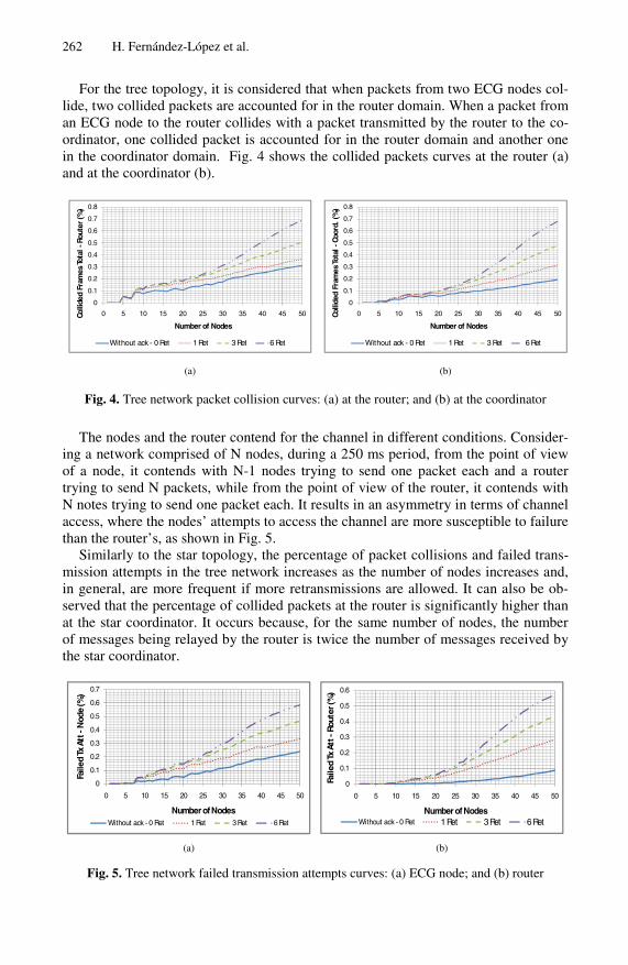
262 H. Fernández-López et al.
For the tree topology, it is considered that when packets from two ECG nodes col-lide, two collided packets are accounted for in the router domain. When a packet from an ECG node to the router collides with a packet transmitted by the router to the co-ordinator, one collided packet is accounted for in the router domain and another one in the coordinator domain. Fig. 4 shows the collided packets curves at the router (a) and at the coordinator (b).
0
0.1
0.2
0.3
0.4
0.5
0.6
0.7
0.8
0 5 10 15 20 25 30 35 40 45 50Colli
ded
Fram
es T
otal
-Ro
uter
(%)
Number of Nodes
Without ack - 0 Ret 1 Ret 3 Ret 6 Ret
0
0.1
0.2
0.3
0.4
0.5
0.6
0.7
0.8
0 5 10 15 20 25 30 35 40 45 50Colli
ded
Fram
es T
otal
-Co
ord.
(%
)Number of Nodes
Without ack - 0 Ret 1 Ret 3 Ret 6 Ret
(a) (b)
Fig. 4. Tree network packet collision curves: (a) at the router; and (b) at the coordinator
The nodes and the router contend for the channel in different conditions. Consider-ing a network comprised of N nodes, during a 250 ms period, from the point of view of a node, it contends with N-1 nodes trying to send one packet each and a router trying to send N packets, while from the point of view of the router, it contends with N notes trying to send one packet each. It results in an asymmetry in terms of channel access, where the nodes’ attempts to access the channel are more susceptible to failure than the router’s, as shown in Fig. 5.
Similarly to the star topology, the percentage of packet collisions and failed trans-mission attempts in the tree network increases as the number of nodes increases and, in general, are more frequent if more retransmissions are allowed. It can also be ob-served that the percentage of collided packets at the router is significantly higher than at the star coordinator. It occurs because, for the same number of nodes, the number of messages being relayed by the router is twice the number of messages received by the star coordinator.
0
0.1
0.2
0.3
0.4
0.5
0.6
0.7
0 5 10 15 20 25 30 35 40 45 50
Faile
d Tx
Att
-N
ode
(%)
Number of NodesWithout ack - 0 Ret 1 Ret 3 Ret 6 Ret
0
0.1
0.2
0.3
0.4
0.5
0.6
0 5 10 15 20 25 30 35 40 45 50
Faile
d Tx
Att
-Ro
uter
(%)
Number of NodesWithout ack - 0 Ret 1 Ret 3 Ret 6 Ret
(a) (b)
Fig. 5. Tree network failed transmission attempts curves: (a) ECG node; and (b) router

Evaluation of the Impact of the Topology and Hidden Nodes 263
Throughput. The normalized throughput represents the ratio between the amount of traffic successfully received by the network coordinator and the network data rate. Fig. 6 presents the normalized throughput curves as a function of the number of ECG nodes for the star (a) and tree (b) topologies. The dark straight lines in both graphs represent the ideal throughput.
If up to six retransmissions are allowed, the star network can handle the traffic from 37 ECG nodes with a deviation from the ideal throughput smaller than 1%. It happens because despite the collided packets and failed transmission attempts, most of the messages are transmitted and reach the coordinator. Nevertheless, as collided packets and failed transmission attempts curves have a high slope when the number of nodes is high, a small increment in the number of nodes can cause the network to start collapsing. The performance of the tree network is worse. If up to six retransmissions are allowed, the network presents a deviation smaller than 1% from the ideal through-put for up to 18 ECG nodes; still, it starts to collapse if one node is added. It happens because messages transmitted by a node must be retransmitted by the router, resulting in a duplication of the network traffic load relatively to the star network.
0
0.1
0.2
0.3
0.4
0.5
0.6
0.7
0.8
0 5 10 15 20 25 30 35 40 45 50
Nor
mal
ized
thr
ough
put
(%)
Number of Nodes
Ideal Without ack - 0 Ret 1 Ret 3 Ret 6 Ret
0
0.1
0.2
0.3
0.4
0.5
0.6
0.7
0.8
0 5 10 15 20 25 30 35 40 45 50
Nor
mal
ized
thr
ough
put
(%)
Number of Nodes
Ideal Without ack - 0 Ret 1 Ret 3 Ret 6 Ret
(a) (b)
Fig. 6. Normalized throughput curves: (a) star network; and (b) tree network
Delivery Ratio. The DR curves for the star and tree networks are shown in Fig. 7. If retransmissions are allowed, high DR values can be achieved even when a relatively large quantity of nodes is active. The reduction in the DR for both networks when the number of nodes increases reflects the deviations from the ideal throughput shown in the graphs, and is ultimately caused by collisions and failed transmission attempts.
0.4
0.5
0.6
0.7
0.8
0.9
1
0 5 10 15 20 25 30 35 40 45 50
Del
iver
y Ra
tio
Number of Nodes
Without ack - 0 Ret 1 Ret 3 Ret 6 Ret
00.10.20.30.40.50.60.70.80.9
1
0 5 10 15 20 25 30 35 40 45 50
Del
iver
y Ra
tio
Number of Nodes
Without ack - 0 Ret 1 Ret 3 Ret 6 Ret (a) (b)
Fig. 7. DR curves: (a) star network; and (b) tree network

264 H. Fernández-López et al.
Delay. The delay a message experiences includes the queuing delay (time spent in the buffer of the node/router) and the access delay (time spent in the backoff process). Fig. 8 (a) and Fig. 8 (b) show the mean and maximum delay curves for the star net-work. It is possible to observe that the maximum delay is smaller than 150 ms for all cases. Since packets are generated with an interval of 250 ms, the buffer is always empty in this case.
0
10
20
30
40
50
0 5 10 15 20 25 30 35 40 45 50
Mea
n D
elay
(m
s)
Number of Nodes
Without ack - 0 Ret 1 Ret 3 Ret 6 Ret
0
50
100
150
200
0 5 10 15 20 25 30 35 40 45 50
Max
imum
Del
ay (m
s)Number of Nodes
Without ack - 0 Ret 1 Ret 3 Ret 6 Ret
(a) (b)
Fig. 8. Star network curves: (a) mean delay; and (b) maximum delay
Fig. 9 (a) and Fig. 9 (b) show the mean and maximum delay for tree network. For a small number of nodes, the maximum delay is small; however, when the number of nodes reaches 18 and up to six retransmissions are allowed, the maximum delay ex-ceeds 250 ms. It was observed that message delays occur mainly due to the time they wait in the router’s buffer to be transmitted, so the maximum number of nodes of the network and the router buffer size must be carefully considered depending on the delay bound requirements of the network.
0
1
2
3
4
5
6
7
8
0 5 10 15 20 25 30 35 40 45 50
Mea
n D
elay
(s)
Number of Nodes
Without ack - 0 Ret 1 Ret 3 Ret 6 Ret
0123456789
10
0 5 10 15 20 25 30 35 40 45 50
Max
imum
Del
ay (s
)
Number of Nodes
Without ack - 0 Ret 1 Ret 3 Ret 6 Ret
(a) (b)
Fig. 9. Tree network curves: (a) mean delay (up to 50 nodes); (b) maximum delay (up to 50 nodes)
Energy Consumption. The average value of the energy spent by one node to deliver a message to the coordinator can be obtained as the ratio of the total energy spent by the node to deliver all messages, including packets retransmissions where applicable, to the number of messages sent by the node. For the energy consumption estimation,

Evaluation of the Impact of the Topology and Hidden Nodes 265
we have considered the voltage and current consumption values specified for JN5139 ZigBee modules [15], as we have based our sensors nodes on these devices. A voltage supply of 3 V was considered. When the microcontroller (CPU) of the module is on, the module consumption is 9.21 mA, as shown in Fig. 10. During sampling, the ADC is switched on, and the current increases to 9.79 mA. When the module switches the transceiver on during the backoff process, the current increases to 32 mA and, when the module starts transmitting, the current increases to 37 mA.
Fig. 10. JN5139 ZigBee module current consumption in distinct modes
Fig. 11 presents the curves of energy consumption per message, considering only the transceiver consumption. The total energy consumption of a node during one second interval is calculated as follows. For instance, for a star network consisting of 15 nodes that are allowed to make up to three retransmissions, the average energy spent by a node to transmit a message is equal to 0.607 mJ. Since during any one second interval the node transmits 4 messages, the consumption relative to the trans-ceiver is 2.43 mJ. Additionally, the ADC is used to make 200 measurements, with each measurement taking 1 ms, which results in a consumption of 0.348 mJ [3 * 200 * (9.79 – 9.21) * 0.001]. The consumption of the microcontroller is 27.63 mJ (3 * 9.21 * 1), so the total energy consumption is equal to 30.41 mJ. If the module is pow-ered by a +3V, 1200 mAh battery (12960 J), a lifetime of 118 hours of continuous operation can be achieved.
0.0
0.5
1.0
1.5
2.0
2.5
3.0
3.5
4.0
4.5
0 5 10 15 20 25 30 35 40 45 50
Ener
gy p
er M
essa
ge -
Star
(m
J)
Number of Nodes
Without ack - 0 Ret 1 Ret 3 Ret 6 Ret
0.0
1.0
2.0
3.0
4.0
5.0
6.0
0 5 10 15 20 25 30 35 40 45 50
Ener
gy p
er M
essa
ge -
Tree
(mJ)
Number of Nodes
Without ack - 0 ret 1 ret 3 ret 6 Ret
(a) (b)
Fig. 11. Transceiver consumption per message curves: (a) star network; and (b) tree network
As can be observed from this analysis, the module consumption is dominated by the microcontroller consumption, which is constantly on as a consequence of the frequent ADC measurements required by the ECG signal. So, although the nodes from the star network spend less energy to transmit each message than the nodes from the tree network, the resulting lifetime of both sensors will not be much different.

266 H. Fernández-López et al.
Star and tree topologies comparison analysis. Table 2 summarizes the simulation results presented in this section. Three important QoS markers are considered: a throughput deviation from ideal smaller than 1%, a delivery rate greater than 99% and a maximum message delay smaller than 250 ms. The maximum number of nodes each network can have and still comply with the established requirements are shown in the unshaded cells. The % columns refer to the reduction in the number of ECG nodes supported by the tree network with relation to the star network. For instance, if up to 3 retransmissions are allowed, a star network with up to 35 ECG nodes presents a throughput deviation smaller than 1% from the ideal throughput. In the same operation mode, a tree network must contain no more than 18 ECG nodes to achieve a similar performance, which means a reduction of 47% in the number of ECG nodes.
Table 2. Star and tree topologies comparison summary
Throughput dev. < 1% DR > 99% Max. delay < 250 ms Operation mode Star Tree % Star Tree % Star Tree
Without ACK – 0 Ret 16 7 56 4 4 0 > 50 42 1 Ret 25 11 56 7 7 0 > 50 19 3 Ret 34 18 47 32 12 62 > 50 18 6 Ret 37 18 51 35 18 49 > 50 17
It is possible to observe that an increase in the maximum number of allowed re-
transmissions contributes favorably to the performance of the networks, though an increase in the maximum delay is experienced and a small decrease in the lifetime of each ECG node is also expected. If up to three retransmissions are allowed, a star network must not exceed 32 ECG nodes to comply with the QoS requirements estab-lished, while in the case of a tree network, the maximum number of ECG nodes can-not exceed 12.
4.2 Hidden-Node Analysis
The performance of WSNs can be seriously degraded by collisions caused by hidden nodes. In a CSMA-based network, a node can only transmit if it senses the channel idle. The hidden-node problem occurs when the carrier sensing fails, so a node starts transmitting when other node has already occupied the channel. If both transmissions are within the reach of a receiver, a collision occurs. A generic hidden-node situation is illustrated in Fig. 12 (a), where the transmission range of nodes A and B are repre-sented by circles drawn around the nodes. If B starts to transmit to D while A is transmitting to C, A’s and B’s packets collide at C. In this case, the transmission from A, which is hidden from B, is corrupted by the B’s transmission. A more severe prob-lem happens if C and D happen to be the same node, that is, if A and B transmit to a common receiver, C, as seen in Fig. 12 (b). In this case, if B starts to transmit while A is transmitting (or vice-versa), both packets are corrupted.
The hidden-node simulation runs were executed considering an increasing number of ECG sensors that send data directly to the coordinator, in a star topology. Five scenarios were simulated, considering that up to three retransmissions are allowed. Each scenario considered a different percentage of hidden nodes in the network, vary-ing from 0% to 20%. The situation depicted in Fig. 12 (b) was simulated, since in the

Evaluation of the Impact of the Topology and Hidden Nodes 267
star topology all nodes transmit to the coordinator. In this case, if one node starts to transmit when a node that is hidden from it is already transmitting, both packets are lost and no acknowledgements are sent back by the network coordinator.
(a) (b)
Fig. 12. The hidden-node problem schematics
Collisions and failed transmission attempts. Fig. 13 (a) shows the collided packets curves. It is possible to observe a pronounced increase in the number of collisions due to hidden-node collisions. Apart from collisions between packets, collisions between a node packet and an ACK transmitted by the network coordinator are also considered. This situation can occur if a node fails to detect a packet transmission but only starts transmitting just after the packet is received by the network coordinator. The packet-ACK collision curves are shown in Fig. 13 (b) and demonstrate that the
0
0.1
0.2
0.3
0.4
0.5
0.6
0.7
0.8
0.9
1
0 5 10 15 20 25 30 35 40 45 50
Colli
ded
Pack
ets
(%)
Number of Nodes
0% 5% 10% 15% 20%
0
0.001
0.002
0.003
0.004
0.005
0 5 10 15 20 25 30 35 40 45 50
Pack
et-A
CK C
ollis
ion
(%)
Number of Nodes
0% 5% 10% 15% 20%
(a) (b)
0
0.1
0.2
0.3
0.4
0.5
0 5 10 15 20 25 30 35 40 45 50
Faile
d Tr
ansm
issi
on A
ttem
pts
(%)
Number of Nodes0% 5% 10% 15% 20%
(c)
Fig. 13. Hidden-nodes analysis curves: (a) collided packets ratio; (b) packet-ACK collision ratio; and (c) failed transmission attempts ratio
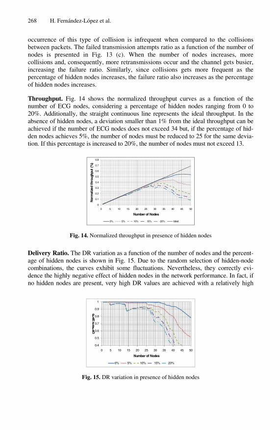
268 H. Fernández-López et al.
occurrence of this type of collision is infrequent when compared to the collisions between packets. The failed transmission attempts ratio as a function of the number of nodes is presented in Fig. 13 (c). When the number of nodes increases, more collisions and, consequently, more retransmissions occur and the channel gets busier, increasing the failure ratio. Similarly, since collisions gets more frequent as the percentage of hidden nodes increases, the failure ratio also increases as the percentage of hidden nodes increases.
Throughput. Fig. 14 shows the normalized throughput curves as a function of the number of ECG nodes, considering a percentage of hidden nodes ranging from 0 to 20%. Additionally, the straight continuous line represents the ideal throughput. In the absence of hidden nodes, a deviation smaller than 1% from the ideal throughput can be achieved if the number of ECG nodes does not exceed 34 but, if the percentage of hid-den nodes achieves 5%, the number of nodes must be reduced to 25 for the same devia-tion. If this percentage is increased to 20%, the number of nodes must not exceed 13.
0
0.1
0.2
0.3
0.4
0.5
0.6
0.7
0.8
0 5 10 15 20 25 30 35 40 45 50
Nor
mal
ized
thr
ough
put
(%)
Number of Nodes
0% 5% 10% 15% 20% Ideal
Fig. 14. Normalized throughput in presence of hidden nodes
Delivery Ratio. The DR variation as a function of the number of nodes and the percent-age of hidden nodes is shown in Fig. 15. Due to the random selection of hidden-node combinations, the curves exhibit some fluctuations. Nevertheless, they correctly evi-dence the highly negative effect of hidden nodes in the network performance. In fact, if no hidden nodes are present, very high DR values are achieved with a relatively high
0.4
0.5
0.6
0.7
0.8
0.9
1
0 5 10 15 20 25 30 35 40 45 50
Delivery Ratio
Number of Nodes
0% 5% 10% 15% 20%
Fig. 15. DR variation in presence of hidden nodes

Evaluation of the Impact of the Topology and Hidden Nodes 269
number of nodes, but if even a small amount of hidden nodes is present, the perform-ance of the network is seriously affected by the high amount of resulting packet colli-sions. For instance, more than 99% of the messages are delivered if the number of ECG nodes is equal to 32 but, if the percentage of hidden nodes is increased to 5% or 10%, the number of ECG nodes must be reduced to 13 or 4, respectively.
Delay. The maximum and mean message delay curves are shown in Fig. 16. It can be observed that the maximum delay is smaller than 150 ms for all cases. Additionally, it can be noticed that the mean delay is quite small, not exceeding 34 ms.
0
20
40
60
80
100
120
140
0 5 10 15 20 25 30 35 40 45 50
Max
imum
Del
ay (m
s)
Number of Nodes
0% 5% 10% 15% 20%
0
5
10
15
20
25
30
35
0 5 10 15 20 25 30 35 40 45 50
Mea
n D
elay
(m
s)
Number of Nodes
0% 5% 10% 15% 20% (a) (b)
Fig. 16. Maximum (a) and mean (b) delay curves in presence of hidden nodes
Energy Consumption. The energy consumption curves shown in Fig. 17 were de-termined following the same procedure explained in Section 4.1, that is, they just consider the consumption from the transceiver. It is possible to notice that if the per-centage of hidden nodes increases, the energy consumption also increases. Despite of this, the reduction in nodes’ lifetime is not high, since most of the energy consump-tion is due to the microcontroller. If we consider a network with 25 nodes, with no hidden nodes, the average energy spent by each node to transmit a message is equal to 0.718 mJ. In this case, the energy spent during one second is equal to 30.85 mJ, re-sulting in a lifetime equal to approximately 117 hours. On the other hand, if the per-centage of hidden nodes is 20%, each node spends an average of 1.22 mJ to transmit each message, resulting in an average consumption of 32.06 mJ during one second and a lifetime of approximately 112 hours, a small reduction of 4%.
0.0
0.5
1.0
1.5
2.0
2.5
3.0
3.5
4.0
4.5
0 5 10 15 20 25 30 35 40 45 50
Ener
gy p
er M
essa
ge (
mJ)
Number of Nodes
0% 5% 10% 15% 20%
Fig. 17. Energy per message in the presence of hidden nodes
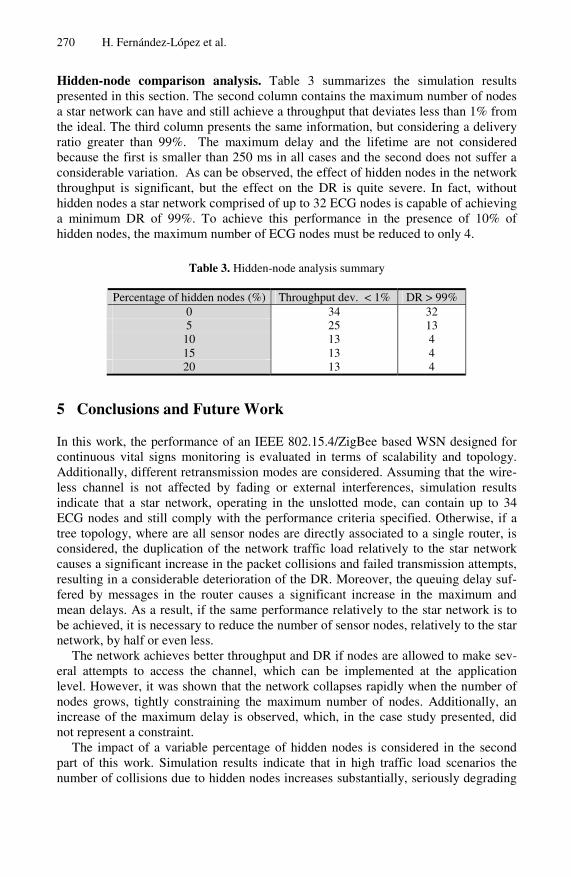
270 H. Fernández-López et al.
Hidden-node comparison analysis. Table 3 summarizes the simulation results presented in this section. The second column contains the maximum number of nodes a star network can have and still achieve a throughput that deviates less than 1% from the ideal. The third column presents the same information, but considering a delivery ratio greater than 99%. The maximum delay and the lifetime are not considered because the first is smaller than 250 ms in all cases and the second does not suffer a considerable variation. As can be observed, the effect of hidden nodes in the network throughput is significant, but the effect on the DR is quite severe. In fact, without hidden nodes a star network comprised of up to 32 ECG nodes is capable of achieving a minimum DR of 99%. To achieve this performance in the presence of 10% of hidden nodes, the maximum number of ECG nodes must be reduced to only 4.
Table 3. Hidden-node analysis summary
Percentage of hidden nodes (%) Throughput dev. < 1% DR > 99% 0 34 32 5 25 13
10 13 4 15 13 4 20 13 4
5 Conclusions and Future Work
In this work, the performance of an IEEE 802.15.4/ZigBee based WSN designed for continuous vital signs monitoring is evaluated in terms of scalability and topology. Additionally, different retransmission modes are considered. Assuming that the wire-less channel is not affected by fading or external interferences, simulation results indicate that a star network, operating in the unslotted mode, can contain up to 34 ECG nodes and still comply with the performance criteria specified. Otherwise, if a tree topology, where are all sensor nodes are directly associated to a single router, is considered, the duplication of the network traffic load relatively to the star network causes a significant increase in the packet collisions and failed transmission attempts, resulting in a considerable deterioration of the DR. Moreover, the queuing delay suf-fered by messages in the router causes a significant increase in the maximum and mean delays. As a result, if the same performance relatively to the star network is to be achieved, it is necessary to reduce the number of sensor nodes, relatively to the star network, by half or even less.
The network achieves better throughput and DR if nodes are allowed to make sev-eral attempts to access the channel, which can be implemented at the application level. However, it was shown that the network collapses rapidly when the number of nodes grows, tightly constraining the maximum number of nodes. Additionally, an increase of the maximum delay is observed, which, in the case study presented, did not represent a constraint.
The impact of a variable percentage of hidden nodes is considered in the second part of this work. Simulation results indicate that in high traffic load scenarios the number of collisions due to hidden nodes increases substantially, seriously degrading
Evaluation of the Impact of the Topology and Hidden Nodes 271
the network performance, namely the throughput and the DR. This scenario is valid even for a small percentage of hidden nodes, as we have considered it ranging from 5% to 20%. For instance, in the absence of hidden nodes, a star network consisting of 32 ECG nodes presents a DR greater than 99%; however, if the percentage of hidden nodes is increased to 5%, it drops to 94%. Moreover, if the percentage of hidden nodes increases to 20%, it is necessary to further reduce the number of ECG nodes to only 4 to sustain the desired DR.
Our future work includes the study of techniques that could help alleviate the hidden-node problem in non-beacon enabled networks where nodes can be highly mobile.
Acknowledgments. This work has been supported by the Portuguese Foundation for Science and Technology and the POCTI and FEDER programs.
References
1. Ilyas, M., Mahgoub, I. (eds.): Handbook of Sensor Networks: Compact Wireless and Wired Sensing Systems. CRC Press, New York (2004)
2. Fernández-López, H., Afonso, J.A., Correia, J.H., Simões, R.: Extended Health Visibility in the Hospital Environment. In: BioDevices 2009, pp. 422–425 (2009)
3. Gao, T., Pesto, C., Selavo, L., Chen, Y., Ko, G., Lim, H., Terzis, A., Watt, A., Jeng, J., Chen, B., Lorincz, K., Welsh, M.: Wireless Medical Sensor Networks in Emergency Response: Im-plementation and Pilot Results. In: IEEE Conf. on Tech. for Homeland Security (2008)
4. Patel, S., Lorincz, K., Hughes, R., Huggins, N., Growdon, J.H., Welsh, M., Bonato, P.: Analysis of Feature Space for Monitoring Persons with Parkinson’s Disease With Applica-tion to a Wireless Wearable Sensor System. In: 29th Annual International Conference of the Engineering in Medicine and Biology Society (2007)
5. Lorincz, K., Malan, D.J., Fulford-Jones, T.R.F., Nawoj, A., Clavel, A., Shnayder, V., Mainland, G., Welsh, M., Moulton, S.: Sensor networks for emergency response: chal-lenges and opportunities. IEEE Pervasive Computing 3(4), 16–23 (2004)
6. Latre, B., Mil, P.D., Moerman, I., Dhoedt, B., Demeester, P., Dierdonck, N.V.: Through-put and Delay Analysis of Unslotted IEEE 802.15.4. J. Networks 1(1), 20–28 (2006)
7. Liang, X., Balasingham, I.: Performance Analysis of the IEEE 802.15.4 based ECG Moni-toring Network. In: 7th IASTED, pp. 100–104 (2007)
8. Golmie, N., Cypher, D., Rebala, O.: Performance Analysis of Low Rate Wireless Tech-nologies for Medical Applications. Computer Comm. (28), 1266–1275 (2005)
9. Severino, R.: On the use of the IEEE 802.15.4/ZigBee for Time-Sensitive Wireless Sensor Network Applications. Polytechnic Institute of Porto, MSc Thesis (2008)
10. Lain-Jinn, H., Lain-Jinn, H., Shiann-Tsong, S., Yun-Yen, S., Yen-Chieh, C.: Grouping strategy for solving hidden node problem in IEEE 802.15.4 LR-WPAN. In: First Interna-tional Conference on Wireless Internet, pp. 26–32 (2005)
11. Ruzzelli, A.G., Tynan, R., O’Hare, G.M.P.: An energy-efficient and low-latency routing protocol for wireless sensor networks. Systems Communications, 449–454 (2005)
12. IEEE Std 802.15.4-2003—Part 15.4: Wireless LAN Medium Access Control (MAC) and Physical Layer (PHY) Specifications for Low-Rate Wireless Personal Area Networks (2003)
13. ZigBee Alliance, ZigBee Specification 053474r17, v. 1.0 r17 (2007) 14. OMNet++ Discrete Event Simulation System, http://www.omnet.org 15. Jennic Wireless Microcontrollers, http://www.jennic.com/

Coordinated Sleeping for Beaconless802.15.4-Based Multihop Networks
A.G. Ruzzelli1, A. Schoofs1, G.M.P. O’Hare1, M. Aoun2, and P. van der Stok2
1 CLARITY: Centre for Sensor Web Technologies, Dublin, Ireland{ruzzelli,anthony.schoofs,gregory.ohare}@ucd.ie
2 Philips Research Laboratories, Eindhoven, The Netherlands{peter.van.der.stok,marc.aoun}@philips.com
Abstract. The last few years have seen a wide adoption of the IEEE802.15.4 MAC/PHY standard for low-power communication betweenwireless sensor nodes. Within this work we study some fundamentaldrawbacks of the 802.15.4 specifications for multihop network deploy-ments, which adversely affect efficient node energy consumption. Theseissues are rectified by investigating a timezone-based scheduling,V-Route, that builds on 802.15.4 beaconless mode to enable both a syn-chronized sleep scheduling and a bidirectional communication betweennodes in the sensor network and the PAN coordinator. The contribu-tions of V-Route are threefold: (1) mitigate collisions, (2) enable packetrouting and (3) provide energy saving in a multihop context, while main-taining the full compliancy with the 802.15.4 standard. We present aperformance evaluation on energy consumption and latency with realexperiments on Philips AquisGrain sensor nodes. Enhancing 802.15.4-based multi-hop networks with V-Route yields energy reduction rangingfrom 27.3% to 85.3%.
Keywords: Sensor, network, wireless, routing, energy, 802.15.4.
1 Introduction
The advent of sensor-based wireless networks requires standard communicationcompliancy to allow interoperability among vendors in a multitude of appli-cations. To this objective, IEEE defined in 2003 the 802.15.4-2003 standard [1]that specifies MAC and physical (PHY) layers to enable wireless communicationbetween small battery-operated devices. In particular, the standard targets lowdata-rate communication in single-hop and multi-hop sensor networks. However,choosing a reliable, energy-efficient, and 802.15.4 compatible routing protocolthat can relay packets from the Personal Area Network (PAN) coordinator tothe sensor nodes and vice-versa is not part of the standard.
Energy-efficiency in low-power wireless PANs is fundamental, and relatedwork has shown relevant drawbacks for both single-hop and multi-hop -enabled802.15.4 communication [6,17,19,20]. This paper confirms such prior works andpresents experiments on 802.15.4 single-hop and multi-hop networks that exhib-ited similar issues.
S. Hailes, S. Sicari, and G. Roussos (Eds.): S-Cube 2009, LNICST 24, pp. 272–287, 2009.c© Institute for Computer Sciences, Social-Informatics and Telecommunications Engineering 2009
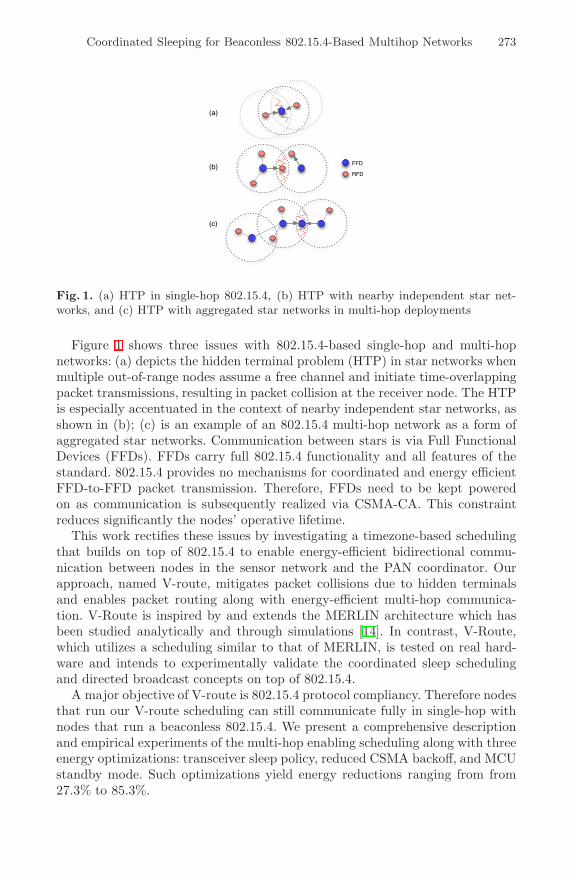
Coordinated Sleeping for Beaconless 802.15.4-Based Multihop Networks 273
(a)
(c)
(b) FFD
RFD
Fig. 1. (a) HTP in single-hop 802.15.4, (b) HTP with nearby independent star net-works, and (c) HTP with aggregated star networks in multi-hop deployments
Figure 1 shows three issues with 802.15.4-based single-hop and multi-hopnetworks: (a) depicts the hidden terminal problem (HTP) in star networks whenmultiple out-of-range nodes assume a free channel and initiate time-overlappingpacket transmissions, resulting in packet collision at the receiver node. The HTPis especially accentuated in the context of nearby independent star networks, asshown in (b); (c) is an example of an 802.15.4 multi-hop network as a form ofaggregated star networks. Communication between stars is via Full FunctionalDevices (FFDs). FFDs carry full 802.15.4 functionality and all features of thestandard. 802.15.4 provides no mechanisms for coordinated and energy efficientFFD-to-FFD packet transmission. Therefore, FFDs need to be kept poweredon as communication is subsequently realized via CSMA-CA. This constraintreduces significantly the nodes’ operative lifetime.
This work rectifies these issues by investigating a timezone-based schedulingthat builds on top of 802.15.4 to enable energy-efficient bidirectional commu-nication between nodes in the sensor network and the PAN coordinator. Ourapproach, named V-route, mitigates packet collisions due to hidden terminalsand enables packet routing along with energy-efficient multi-hop communica-tion. V-Route is inspired by and extends the MERLIN architecture which hasbeen studied analytically and through simulations [14]. In contrast, V-Route,which utilizes a scheduling similar to that of MERLIN, is tested on real hard-ware and intends to experimentally validate the coordinated sleep schedulingand directed broadcast concepts on top of 802.15.4.
A major objective of V-route is 802.15.4 protocol compliancy. Therefore nodesthat run our V-route scheduling can still communicate fully in single-hop withnodes that run a beaconless 802.15.4. We present a comprehensive descriptionand empirical experiments of the multi-hop enabling scheduling along with threeenergy optimizations: transceiver sleep policy, reduced CSMA backoff, and MCUstandby mode. Such optimizations yield energy reductions ranging from from27.3% to 85.3%.

274 A.G. Ruzzelli et al.
The remainder of this paper is organized as follows. Section 2 provides anoverview of related work and compares our approach against existing architec-tures. Section 3.3 details the sleep scheduling and routing technique. Section 4evaluates the proposed technique on Philips AquisGrain nodes. In Section 5 wepropose some guidelines to decrease energy consumption for a multihop-enabled802.15.4 network. Finally, we conclude the paper.
2 Related Work
Literature shows a great number of studies of the different issues intrinsic to the802.15.4 standard. The problems of high energy cost for idle listening [15], colli-sions from hidden terminals due to the lack of RTS and CTS mechanisms [18,6],and the risk of frame collisions for nearby coordinators in a multi-hop deploy-ment [19] have been investigated and demonstrated.
Some efforts in adapting energy-efficient mechanisms, such as Low Power Lis-tening (LPL) [13] to 802.15.4, are presented in [10]. Since TI CC2420-like radiosdo not support long preambles similar to the ones implemented in BMAC, thelong preamble is simulated by transmitting a train of same packet. However,the LPL/802.15.4 adaptation revealed serious reliability problems due to the in-terleave between such packet train as studied in [5]. Furthermore, enabling LPLon 802.15.4-based nodes prevents them from communicating with non-enabledLPL nodes, therefore reversing the 802.15.4 compliancy.
A more general approach to reducing energy consumption in the networkis to provide a duty-cycle mechanism that regulates the activity of the nodes.However, there is a trade-off between energy efficiency and latency in packetdelivery. Studies in [12] demonstrated that latency in packet delivery is heavilyaffected by the node duty-cycle. Some other experiments, for example in [14],confirmed that forwarding techniques for wireless networks such as [11,7] showa poor performance in delivery rate when deployed in a lossy environment [16]with unreliable nodes.
Besides, although the revised 802.15.4-2006 specifications [2] mention the clus-ter tree formation where most nodes are FFDs, the standard leaves the resolu-tion of issues related to more complex topologies for higher layers. In particular,ZigBee [3] implements a version of the AODV [11] routing algorithm to auto-matically construct low-speed ad-hoc networks in the form of mesh or clusters.The current profiles derived from the ZigBee protocols support beaconless andbeacon-enabled networks. In beaconless networks, CSMA/CA is used. In thistype of network, ZigBee Routers typically have their receivers continuously ac-tive, requiring a more robust power supply and subsequently depreciating energyefficiency. In beacon-enabled networks, ZigBee Routers transmit beacons period-ically to end-nodes that are able to sleep between beacon receptions, allowing forlonger battery life. The usage of the beacon-enabled 802.15.4 is subject to thefollowing issues: (1) ZigBee RFDs can communicate to only one parent FFD,the one responsible for both coordinating RFD sleeping intervals and routingpackets from one star to another. However, there is no agreement for a dis-tributed sleeping policy among FFD routers. Therefore, the FFDs must stay

Coordinated Sleeping for Beaconless 802.15.4-Based Multihop Networks 275
awake the whole time while only RFDs can go to sleep after transmission; (2)The uncoordinated activity of nearby stars especially affects FFD beacons thatare transmitted without checking the channel condition. Beacons are prone tocollide in presence of nearby stars activity. Such issues, confirmed by some ofour initial experiments, prevented us from adopting the 802.15.4 beacon-enabledfunctionality in a multihop network. Therefore, in the rest of this paper, we willconcentrate on studying the 802.15.4 beaconless mode.
3 Coordinated Sleeping Scheduling over 802.15.4
In order to mitigate packet collisions without affecting the 802.15.4 compliancyand to enable multihop communication we adopt the following 802.15.4 settings:
– FFD functionality for all nodes: It allows all nodes to communicatewith each other in a peer-to-peer fashion by performing CSMA/CA beforetransmitting;
– Beaconless configuration: 802.15.4 reduces to a plain CSMA/CA with nohandshake mechanism in place.
3.1 Traffic Patterns
The performance of a multihop routing algorithm and transmission schedulingcan vary greatly according to the traffic patterns. In contrast to applicationsfor mesh networks that might have any node exchanging packets with any othernode, most sensor network applications requires many-to-one (towards the sink)or one-to-many (from the sink to the other nodes) multihop communication,referred to as upstream and downstream communication, respectively. There-fore, a cooperation between a routing algorithm and a sequential scheduling oftransmission is advantageous. In other words, it is beneficial if a packetretransmission is scheduled immediately after a node receives a packettraveling upstream or downstream. Furthermore, theoretical studies in [8]demonstrate that an address-less forwarding policy merely based on directedbroadcast towards nodes with higher or lower hop count relative to the sinknode achieves greater energy saving and reliability than an address-based ap-proach. V-route adopts this communication trend by transmitting allthe upstream or downstream packets without specifying a particularforwarder with smaller or higher hop count respectively. This minimal-ist communication approach is named timezone-based directed broadcastas nodes with different hop count are defined to be in a different timezone.This approach generates packet duplication which is appropriately reduced byallowing nodes to overhear packets being transmitted by neighbours and deletethe ones successfully transmitted, in what amounts to a packet overhearingmechanism. Optimizing transmission allocation to forward packets consecu-tively to nodes with lower or higher hop count (i.e. to a lower or to a highertimezone) reduces the packet latency that can effectively be traded-off for en-ergy savings. Within this work we apply and demonstrate that directed broadcast

276 A.G. Ruzzelli et al.
Fig. 2. The table of scheduling with periodic local broadcast
with overhearing is beneficial for 802.15.4 networks. In general, a certain num-ber of consecutive upstream transmissions should also be followed by a numberof downstream consecutive transmissions. This can be represented as an up-stream/downstream V-shaped scheduling as shown in Figure 2. The next twosections highlight the division in zones of the 802.15.4 network and how thescheduling table of V-Route is implemented.
3.2 Setup and Maintenance Phases
802.15.4 beacons are used only during the association phase to form the network.Once completed, CSMA-CA is used for all communication. At the beginning ofnetwork formation, 802.15.4 nodes broadcast periodically a 802.15.4 AssociationRequest (AR) in order to find a coordinator in the vicinity. When the PANcoordinator receives a AR, it starts associating neighboring nodes by an Asso-ciation Response (AR) that contains the 802.15.4 PAN specifications. At thispoint the V-Route procedure begins. Following a subsequent Data Request fromthe node, the PAN coordinator issues a 2 − byte short address to the node to-gether with timing information for synchronization. The node is now associatedto the network. Using V-Route, the node can become a FFD in timezone 1 andtherefore act as coordinator delegate for further nodes. Newly associated nodeswill then be in timezone 2; the process is repeated recursively until all nodes areassociated. The timezone is provided in an extra byte field in each packet trans-mitted. At the end of the association process the network is divided in timezonesas shown in Figure 3. The timezone of a node is the minimum number of hopsrequired for its packets to reach the PAN coordinator. For instance, the packetsof nodes within the 3rd timezone need to be forwarded at least three times to getto the PAN coordinator. Nodes are now ready to adopt a coordinated sleepingpolicy provided by the scheduling table as described in Section 3.3.
In order to cope with network changes such as battery depletion, replacementand mobility, a node’s timezone has a preset expiration time. A node’s timezoneexpires if the node does not receive a zone update message, which all nodes sendperiodically, within a certain timeout period. In case of zone expiration due toa parent node failure or a link break, the node follows a zone re-establishmentprocess.The node start broadcasting upstream and then downstream a Timezone

Coordinated Sleeping for Beaconless 802.15.4-Based Multihop Networks 277
Fig. 3. The initial timezone setup by flooding and different path generation
Update Request (TUR). In case of no response, the node disregards the sleepingscheduling policy until it listens to any packet being transmitted to acquire thetimezone and then restore the scheduling.
An important aspect of V-Route maintenance phase is the node synchroniza-tion. In order to synchronize the clocks of the AquisGrain sensor nodes in ourtestbed, we implemented an improved version of the FTSP protocol [9] enhancedwith efficient linear regression and Kalman filtering as detailed in [4]. Network-wide time synchronization, relative to a unique time master node, is achieved.The adopted MAC-layer time-stamping, explained further on, effectively mini-mizes nondeterministic delay components that affect the time synchronizationperformance [9]. Clock drift rate estimation is used to estimate the differencein counting rate between nodes. It is used to decrease the sending rate of timesynchronization messages and thus the energy consumption needed to achievetime synchronization, by estimating the time offset progress behavior in betweensynchronization instances.
3.3 V-Route Communication Scheduling
Following the setup phases described in section 3.2, the node can avail of thescheduling table shown in Figure 2 to regulate sleeping and activity periods ofnodes. Although 802.15.4 does not support multicast, V-route can practicallyachieve it by broadcasting when either nodes with a lower or higher hop countare sleeping i.e. upstream or downstream broadcast. The V-Table is important asit regulates the cyclic sleeping of nodes within a frame so to reduce the chances ofrunning into a HTP. We present the scheduling for 802.15.4 and its performancethrough experiments on real hardware. Following are the 3 types of transmissionssupported by the V-table:
– Upstream transmission in which a node can transmit to nodes located 1hop closer to PAN coordinator, i.e. to nodes in a lower timezone;

278 A.G. Ruzzelli et al.
– Downstream transmission in which a node can transmit to nodes located1 hop at a longer distance from the PAN coordinator, i.e. to nodes in a highertimezone;
– Local broadcast in which a node transmits simultaneously to all the neigh-boring nodes, i.e. those that are in the directly higher timezone, those fromthe directly lower timezone and those in the same timezone as the transmit-ting node.
While nodes within the same timezone contend the channel for transmission, theadjacent zone owns the slot for reception andnodes in further timezones are in sleepmode, to prevent possibilities of packet collisions due to HTPs. Packets traveling ineach of the above directions are respectively enqueued separately in 3 small FIFObuffers. Packets are thendequeued according to the current slot time in theV-table.The total length of the V-table is equal to the length of a single frame while eachsmall rectangle depicted in Figure 2 represents a time slot. It supports consecu-tive transmission of 4 timezones and therefore it consists of 4 × 2 + 1 timeslots: 4timeslots for upstream transmission, 4 timeslots for downstream transmission, and1 timeslot for local broadcast. Replicating the same table allows scheduling packettransmission for nodes located more than 4 hops away from the PAN coordinator.In general, the allocation of upstream, downstream, and local broadcast transmis-sions in a symmetric network of N zones requires N × 2 + 1 timeslots per frame.We refer to [14] for more information about the V scheduling table, the optimalnumber of slots in a table an how to access it.
4 Optimization Techniques
This section describes three energy saving V-route based optimization techniquesfor beaconless 802.15.4. The techniques are presented in an incremental manner:Each optimization uses the previous optimization in addition to a new energysaving technique.
1. Transceiver Sleep Policy: This optimization regards the powering downof the transceiver at the transmitter and receiver sides. Recall that in V-route, packets of upstream, downstream and local broadcast communicationare enqueued in 3 distinctive FIFO buffers. At the transmitter side, ratherthan waiting for the end of the allocated transmission slot before poweringdown the radio, we allow the transmitter’s radio to be turned off right afterthe last packet transmission from the appropriate queue is acknowledgedsuccessfully. In addition, we provide each packet with a check-bit that is setto one if the packet being transmitted is the last in the sender buffer. Thisallows the receiver to turn off the radio immediately after the last packetin the queue is received correctly and the acknowledgment is sent. Enablingthe transceiver sleep policy optmises the activity time both at transmitterand receiver sides according to the node data traffic.
2. V-Route Short CSMA: This optimization regards the 802.15.4 idle listen-ing. With the CSMA-CA used by 802.15.4, a node with a packet to transmit

Coordinated Sleeping for Beaconless 802.15.4-Based Multihop Networks 279
End of 2nd contention Packet receptionEnd of 1st
contention
Fig. 4. Receiver idle listening of the CSMA period in 802.15.4
at time t picks up a time between t and t + 2BE−1units(1unit = 320μsec)where BE is the backoff exponent. The protocol provides a variable, namelymacMaxCSMABackoffs, that regulates the number of packet retransmis-sions, which the standard 802.15.4 configuration sets to 3. This means thata transmitter can assess the channel 3 times consecutively after which itdeclares access failure and the packet is dropped. Although the backoff pe-riod is effectively used to increase the data rate in protocols such as IEEE802.11, it is known to cause long period of idle listening at the receiver.On the other hand, decreasing the backoff period would adversely affect thereliability. To explain the CSMA idle listening of 802.15.4, Figure 4 showshow nodes in receiving zones would need to keep listening on the channelfor at least 53.5 units (53 units for CSMA and 1/2 units for CCA), in orderto catch a possibly late packet transmission and even if no packet is beingtransmitted.
Notifying V-route to re-schedule the packet in the next frame if a chan-nel access failure occurs can solve this issue. Figure 5 shows how addinga function call, namely V-Route Handle, into the 802.15.4 code allows no-tifying V-Route of a channel access failure. Subsequently V-Route will beresponsible for rescheduling the packet transmission in the next frame. Thisoptimization allows the number of backoffs, macMaxCSMABackoffs, tobe set to 0, hence reducing the receiver idle listening from 53 to 8 units oftime (7 for CSMA and 1 for CCA). This translates in a reduction of receiveridle listening from 17.2ms to 2.56ms. The number of packet retransmissionsbefore transmission failure is now handled by V-route therefore allowingadaptation for example depending on the relevance of the packet itself.
3. MCU Stand-by Mode: This optimization regards putting the MCU instandby mode by availing of the V-Route zone activity coordination. Asshown in Figure 7, some of our initial measurements at the oscilloscope ofthe beaconless 802.15.4 demonstrate that the current needed to power onthe MCU can be greater than the current needed for the radio in trans-mitting mode. These measurements highlight the importance to implementcoordinated duty-cycled activities also for the MCU, which is often over-looked when developing energy-efficient communication architectures.Using

280 A.G. Ruzzelli et al.
Channel idle?
NB = NB + 1,BE = min(BE+1, aMaxBE)
NB>macMaxCSMABa
ckoffs?
V-Route_Handle(struct* packet)
Success
Unslotted CSMA-CA
NB = 0,BE = macMinBE
Delay for random(2^BE -1)
unit backoff periods
Perform CCA
Y
N
Y
N
Fig. 5. The V-Route packet handling mechanism included in the unslotted CSMA of802.15.4
Fig. 6. The electrical node specifications measured at the oscilloscope

Coordinated Sleeping for Beaconless 802.15.4-Based Multihop Networks 281
Fig. 7. Initial results of transmitter energy in single-hop 802.15.4
the scheduling of V-route, the MCU can go into stand-by mode in each timeslot where the node is not scheduled to transmit or receive.
The next section highlights the performance evaluation of V-route along with thethree energy optimization techniques for V-route-enhanced 802.15.4 presentedin this section.
5 Performance Evaluation
This section presents the energy results obtained through experimentations on anetwork of Philips AquisGrain sensor nodes. Firstly, we specify the experimentconfiguration and related performance metrics. We then present the comprehen-sive results for V-route over 802.15.4 and plain 802.15.4 for both star networkand multihop network environments.
5.1 Metrics and Setup
V-route is validated by the node energy consumption per second metricconsidering both CPU and transceiver consumptions. In order to include diverseapplication scenarios, we set 3 different data rates: (1) a low data rate of 1 pkt permin, (2) a medium data rate of 1 pkt per sec, and (3) a high data rate of 10 pktper sec. Each packet transmission from zone to zone was acknowledged by thereceiver. The length of the packet payload was fixed to 30 bytes while the lengthof each experiment was slightly more than 10 minutes. All the experiments wereconducted in an office environment consisting of few rooms, corridors and peopleon their usual business activity.
The Philips AquisGrain sensor module includes a CC2420 radio transceiver(2400-2483 Mhz, 250 kbps, output power ranging from -25 to 0 dBm) and anATMega128L microcontroller (4K RAM, 128K program memory). To improvethe accuracy of the experiment we measured the node’s consumption at theoscilloscope. The relevant electrical specifications are detailed in Figure 6. It is

282 A.G. Ruzzelli et al.
interesting to note that such values, which have been obtained by direct measure-ments at the oscilloscope in a Philips laboratory, differ slightly from the standarddata sheet values though they do not affect the final energy consumption trendof the protocol.
The final energy was obtained by considering both transceiver and micropro-cessor consumption as they proved to be the two most consuming componentson our nodes as shown in Figure 6. The energy calculation was achieved by time-stamping each time the transceiver changed a state and then by incrementing 4variables that held sleeping, receiving, transmitting and switching times. Suchtimes were then periodically transmitted to the PAN coordinator, which wasconnected to a PC, that estimates the energy by using the values in Figure 6.Rather than calculating the energy directly at the sensor, this method provedto be largely more accurate due to difficulty of handling 64-bit variables at thenode.
An important setup aspect is to calculate the minimum slot length to allowaccommodating at least one packet transmission. In 802.15.4, the packet lengthvaries depending on the data carried, with a payload that may vary from 0 to127 bytes, always prefixed with 6 bytes of preamble and header. This makes amaximum packet length of 135 bytes which are transmitted in 4.256 ms at 250kbps on 2400 MHz frequency band. Each packet is then transmitted with a priorCSMA-CA period of maximum 17.120 ms as described in section 6. This leadto a minimum possible V-route slot length of 21.376 ms plus a short time forpacket ACK. In the experiments we tested 3 different slot times of 50 ms, 100ms and 250 ms that allow transmitting 2, 4 and 6 packets respectively withinthe same slot.
5.2 802.15.4 Transmitter Measurements
The transmitter measurements are carried out in a single-hop environment con-sisting of a receiving node connected to the PC through serial port and 10transmitter nodes. We set a high data rate scenario of 10 pkt per sec. The ex-periment is repeated for 3 different transmission powers that correspond to thehighest, the medium and the lowest possible transmitting power with a CC2420chip. The goal is to identify the significant components that regulate the trans-mitter energy consumption in a high contention scenario. The results shown inFigure 7 are obtained by averaging the consumption of all the transmitters. Themain interesting implications are summarized as follow:
– In contrast to common expectations, increasing the transmission power hasan almost insignificant effect on the overall energy consumed by the 802.15.4transmitter, as the percentage of time the transceiver is transmitting is verylow. However, the transmission power to choose might be pondered tak-ing into account that an excess of transmission power notably increases thechances of packet collisions and reduces the number of simultaneous trans-missions in a multihop environment. This aspect may be a point for furtherstudies.

Coordinated Sleeping for Beaconless 802.15.4-Based Multihop Networks 283
Fig. 8. Comparison between the energy consumption of a plain multihop-enabled802.15.4 and 802.15.4 enhanced with V-route
– In spite of a high traffic condition per node, the transmission energy spentis almost insignificant with respect to the node’s overall consumption. Infact the node spends a great amount of time in sensing the channel prior totransmission;
– Idle listening when no packets are sent and CPU energy consumption dom-inate the node energy utilizations. This confirms the 802.15.4 idle listeningissue.
These transmitter measurements presented some relevant 802.15.4 drawbacksthat will be addressed by V-Route and its optimization techniques, as detailedin the next section.
5.3 Energy Results
This section presents energy consumption results in a V-Route enhanced single-hop 802.15.4 network. These single-hop experiments compare a plain beaconless802.15.4 to V-Route enhanced 802.15.4, providing us with energy gains achievedwith the V-Table sleep scheduling. As shown in Figure 8, the node’s energyconsumption is reduced from an average of 108 mJ/s for a plain 802.15.4 to78 mJ/s for a V-route-enhanced 802.15.4. This yields to about 27.3% energysavings.
In contrast to what we initially expected, figure 8 also shows that varying theslot time has no significant effect on the node’s energy consumption. Clearly, byincreasing the slot length we are in fact modifying both the active and sleepingslots and therefore the node duty cycle remains unchanged. Optimizations 1rectifies this situation while Optimizations 2 and 3 focus on the 802.1.5.4 CSMA-CA backoff and microcontroller activity, respectively.
Figure 9 shows the improvements achieved with turning off the transceiverimmediately after transmission of the last packet to a receiving zone (Transceiver
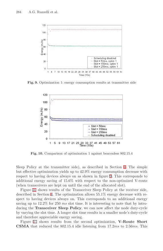
284 A.G. Ruzzelli et al.
Fig. 9. Optimization 1: energy consumption results at transmitter side
Fig. 10. Comparison of optimization 1 against beaconless 802.15.4
Sleep Policy at the transmitter side), as described in Section 4. The simplebut effective optimization yields up to 42.9% energy consumption decrease withrespect to having devices always on as shown in figure 9. This corresponds toadditional energy saving of 15.6% with respect to the non-optimized V-route(when transceivers are kept on until the end of the allocated slot).
Figure 10 shows results of the Transceiver Sleep Policy at the receiver side,described in Section 4. The optimization allows 55.1% energy decrease with re-spect to having devices always on. This corresponds to an additional energysaving up to 12.2% for 250 ms slot time. It is interesting to note that by intro-ducing the Transceiver Sleep Policy, we can now affect the node duty-cycleby varying the slot time. A longer slot time results in a smaller node’s duty-cycleand therefore appreciable energy saving.
Figure 11 shows results from the second optimization, V-Route ShortCSMA that reduced the 802.15.4 idle listening from 17.2ms to 2.56ms. This

Coordinated Sleeping for Beaconless 802.15.4-Based Multihop Networks 285
Fig. 11. Optimization 2 energy consumption results
Fig. 12. Optimization 3 energy consumption results
allowed an significant increase of the 802.15.4 packet delivery rate. In contrast,the subsequent rescheduling of packets by V-Route generated an increase ofpacket overhearing. However, the optimization allowed further 1.3% energy re-duction with respect to the previous optimization, therefore leading to 56.4%overall energy reduction.
Figure 12 shows results from the MCU Stand-by Mode optimization thatallows coordinated MCU stand-by mode. The ATMega128 processor allowsa 250 μA standby current that is restored to activity by clocking an external 32KHz crystal. This optimization yields 15.9 mJ/s of energy which results to anextreme 85.3% overall energy saving. This is a further 28.9% energy saving withrespect to the V-Route Short CSMA optimization.

286 A.G. Ruzzelli et al.
6 Conclusion
802.15.4 intends to offer MAC and Phy layer capabilities for WPAN and wire-less sensor networks. Therefore, it is key to understand the real performance ofthe protocol on typical multihop WSN scenarios. Furthermore, a major goal ofthis work is to build a routing architecture over 802.15.4 that preserves fully theprotocol compliance. Initially this paper highlighted some key issues of 802.15.4beacon-enabled mode for multihop networks. This imposes the usage of bea-conless mode and a subsequent implementation of activity coordination amongnodes. The paper proposes V-route as an 802.15.4 compliant packet schedulingand routing policy to enable energy-efficiency and high reliability in both single-hop and multihop environments. V-Route is allows enhancing the 802.15.4 withthree energy optimization techniques. Experimentations of V-route yielded highdata delivery rate and energy reduction ranging from 27.3% to 85.3% against abeaconless 802.15.4.
Acknowledgments
This work is supported by Science Foundation Ireland under grant 07/CE/I1147.
References
1. IEEE standard for information technology - information exchange between systems- local and metropolitan area networks specific requirements part 15.4: wirelessmedium access control (mac) and physical layer (phy) specifications for low-ratewireless personal area networks (lr-wpans), IEEE Std 802.15.4-2003, 1–670 (2003)
2. IEEE standard for information technology - information exchange betweensystems- local and metropolitan area networks- specific requirements part 15.4:Wireless medium access control (mac) and physical layer (phy) specifications forlow-rate wireless personal area networks (wpans), IEEE Std 802.15.4-2006 (Revi-sion of IEEE Std 802.15.4-2003), 1–305 (2006)
3. Zigbee Alliance, Zigbee working group web page for rf-lite (2002)4. Aoun, M., Schoofs, A., van der Stok, P.: Efficient time synchronization for wireless
sensor networks in an industrial setting, pp. 419–420 (2008)5. Benson, J., O’Donovan, T., Roedig, U., Sreenan, C.J.: Opportunistic aggrega-
tion over duty cycled communications in wireless sensor networks. In: In Proc.of ACM/IEEE Symposium on Information Processing in Sensor Networks (IPSN),April 2008, pp. 307–318 (2008)
6. Harthikote-Matha, M., Banka, T., Jayasumana, A.P.: Performance degradation ofieee 802.15.4 slotted csma/ca due to hidden nodes, pp. 264–266 (2007)
7. Johnson, D.B., Maltz, D.A.: Dinamic source routing in ad hoc wireless networks.Mobile Computing 353, 153–181 (1996)
8. Jurdak, R., Ruzzelli, A.G., O’Hare, G.M.P., Higgs, R.: Directed broadcast withoverhearing for sensor networks. To appear on Transactions for Sensor Networks 2,1443–1448 (2009)
9. Maroti, M., Kusy, B., Simon, G., Ledeczi, A.: The flooding time synchronizationprotocol. In: Proc. of Sensys 2004 the 2nd Conference on Embedded networkedsensor systems, pp. 39–49 (2004)

Coordinated Sleeping for Beaconless 802.15.4-Based Multihop Networks 287
10. Moon, S., Kim, T., Cha, H.: Enabling low power listening on ieee 802.15.4-basedsensor nodes. In: Proc. of WCNC 2007, Wireless Communications and NetworkingConference, March 11-15, pp. 2305–2310 (2007)
11. Perkins, C.E., Royer, E.M.: Ad-hoc on-demand distance vector routing. In: Proc.of WMCSA the Second IEEE Workshop on Mobile Computer Systems and Appli-cations, p. 90 (1999)
12. Petrova, M., Riihijarvi, J., Mahonen, P., Labella, S.: Performance study of ieee802.15.4 using measurements and simulations. In: Proc. of WCNC 2006, WirelessCommunications and Networking Conference, vol. 1, pp. 487–492 (2006)
13. Polastre, J., Hill, J., Culler, D.: Versatile low power media access for wireless sensornetworks. In: Proc. of Sensys 2004, the 4th Conference on Embedded networkedsensor systems, pp. 95–107 (2004)
14. Ruzzelli, A.G., O’Hare, G.M.P., O’Grady, M.J., Jurdak, R.: Merlin: Cross-layerintegration mac and routing for low duty-cycle sensor networks. Elsevier JournalAd Hoc Networks Special Issue on Energy efficient design in wireless ad hoc andsensor networks 5(8) (2008)
15. Suh, C., Ko, Y.-B., Lee, C.-H., Kim, H.-J.: Numerical analysis of the idle listeningproblem in ieee 802.15.4 beacon-enable mode, pp. 1–5 (2006)
16. Vyas, A.K., Tobagi, F.A.: Impact of interference on the throughput of a multihoppath in a wireless network. In: Proc. of Conference on Broadband Communications,Networks and Systems, pp. 39–49 (2006)
17. Woon, W.T.H., Wan, T.-C.: Performance evaluation of ieee 802.15.4 wireless multi-hop networks: Simulation and testbed approach. Int. J. Ad Hoc Ubiquitous Com-put. 3(1), 57–66 (2008)
18. Woon, W.T.H., Wan, T.C.: Performance evaluation of ieee 802.15.4 ad hoc wire-less sensor networks: Simulation approach. In: IEEE International Conference onSystems, Man and Cybernetics, SMC 2006, vol. 2, pp. 1443–1448 (2006)
19. You-min, Z., Mao-heng, S., Peng, R.: An enhanced scheme for the ieee 802.15.4multi-hop network. In: Wireless Communications, Networking and Mobile Com-puting, WiCOM 2006, pp. 1–4 (2006)
20. Zheng, J., Lee, M.J.: A comprehensive performance study of ieee 802.15.4, 218237(2006)

Author Index
Afonso, Jose A. 222, 256Alzaid, Hani 66Amoretti, M. 206Aoun, M. 272Arumugam, Mahesh 158
Barton, John 174Boyd, Colin 66
Caiti, Andrea 111Carvalho, Paulo 222Chang, Yuan-Jen 98Chen, Chin-Hsing 98Chen, You-Yin 98Chessa, S. 206Churcher, Gavin E. 1Claycomb, William R. 51Correia, J.H. 256Crisostomi, Emanuele 111Custodio, Victor 20
Fernandez-Lopez, Helena 256Foley, Jeff 1Foo, Ernest 66Furfari, F. 206
Gama, Oscar 222Giani, Annarita 33Green, Peter N. 236Guitton, Alexandre 83
Hadid, Nassima 83Harte, Sean 174Huang, Wen-Tzeng 98Hunkeler, Urs 127Hussain, Muzammil 236
Kallio, Sanna 11Kela, Juha 11Kim, Byunggi 51Korpipaa, Panu 11Kulkarni, Sandeep S. 158
Lenzi, S. 206Lin, Jing-Ting 98Linjama, Jukka 11Lopes, Rodrigo 51Lowe, David 189
Macedo, Pedro 256Mendes, P.M. 222Miorandi, Daniele 189Moreno, Jose Ignacio 20Munafo, Andrea 111
Nawaz, Sarfraz 236Nieto, Juan Gonzalez 66
O’Flynn, Brendan 174O’Hare, G.M.P. 272
Park, DongGook 66Popovici, Emanuel 174Pugliese, Marco 33
Roussos, George 144Ruzzelli, A.G. 272
Santucci, Fortunato 33Schoofs, A. 272Scotton, Paolo 127Shen, Chong 174Shin, Dongwan 51Simoes, Ricardo 256Stok, P. van der 272
Trigoni, Niki 236
Vinuela, Juan Pablo 20
Watson, Simon 236Wientapper, F. 206
Zoumboulakis, Michael 144