ACCELERATING APPLIED SUSTAINABILITY BY UTILIZING RETURN ON INVESTMENT FOR ENERGY CONSERVATION...

International Journal of Energy, Environment and Economics ISSN: 1054853XVolume 17, Issue 1 ©2009 Nova Science Publishers,Inc

ACCELERATING APPLIED SUSTAINABILITY BY UTILIZING RETURN ON INVESTMENT FOR ENERGY CONSERVATION

MEASURES

J. M. Pearcea, D. Denkenbergerb, and H. Zielonkac

a. Department of Mechanical and Materials Engineering,Queen's University, Kingston, ON K7L 3N6, Canadab. Building Systems Program, Department of Civil,

Architectural and Environmental EngineeringUniversity of Colorado at Boulder, Boulder, CO 80309, USAc. Physics Department, Clarion University of Pennsylvania,

Clarion, PA 16214, USA

ABSTRACT

Many energy conservation measures (ECMs) that utilize energy more efficiently than standard devices or practices will save money in the long term; however, decision makers often fail to deploy ECMs because of what is viewed as a prohibitively long payback time. This paper provides a graphical tool to determine the return on investment (ROI) of any ECM from only the simple payback and device lifetime, which corrects this common economic error. Utilizing this method will encourage the increased deployment of energy efficiency and renewable energy technologies, while improving the economic performance of the companies and individuals that utilize the method.

KEYWORDS:Economics, investing, energy conservation, energy efficiency, energy retrofit, payback, sustainability

NOMENCLATURE

Symbol DefinitionCCFL Purchase cost of the compact fluorescent lamp (CFL)Clab Cost of labor of installing either lampCIL Cost of incandescent lamp (IL)

J. M. Pearce, D. Denkenberger, and H. Zielonka

NOMENCLATURE (continued)H Number of hours used per yearL Lifetime of the incandescent bulb (hours)P The difference in principal investment between the energy conservation

measure (ECM) and the standard device the purchase price including installation costs

R Rate of interest or return on investment (ROI) in percentS Savings from the use of the ECM per yearSE Cost savings due to saved electricity of the CFLSIL Cost savings due to not having to buy as many ILsSlab Cost savings due to not having to install as many ILsT Time of life of the ECM in years (lifetime)

INTRODUCTION

No other aspect of our lack of global sustainability in the long list of mounting environmental problems is more sobering than the destabilization of the global climate. The consensus among the 2004 Intergovernmental Panel on Climate Change (IPCC) and the 1993 World Energy Council’s Global Energy Scenarios to 2050, is that if we maintain the same path towards continued climate destabilization, the planet will reach a point of no return [1]. Global climate destabilization is primarily due to the combustion of fossil fuels for energy and the resultant greenhouse gas (GHG) emissions [2; 3]. Global warming is already occurring, and if combustion of fossil fuels continues, temperatures are projected to rise 1.4°C to 5.8°C in the next 100 years [4; 5]. A global increase in temperatures has a litany of likely results: i) the melting of glaciated ice sheets, raising the sea level up to seven meters, and flooding many important coastal cities [6; 7], ii) aggravated “heat sensitive” diseases such as cholera, malaria, and dengue fever [8; 9], iii) increase in number and severity of summer heatwaves [10], iv) migration routes will change [11], and most importantly, v) extinction rates will increase [12]. Furthermore, carbon dioxide (CO2) in the atmosphere will cause the pH levels in the oceans to drop [13]. Despite these consequences, CO2 emissions from the combustion of fossil fuel have consistently been increasing. In the U.S. in 2004, CO2 emissions from the burning of fossil fuels increased 1.5% [14]. In addition, energy use contributes to urban air pollution, the energy supply of petroleum is uncertain (as will the supply of natural gas as the U.S. begins to rely to a greater degree on the importation of liquefied natural gas), and the consumption of petroleum and natural gas increases the price that others have to pay (e.g. those in the developing world). The consequences of our continued inefficient use of fossil fuel combustion are clearly unacceptable. Yet, we burn more fossil fuels every year [15] because it would be “unrealistic” to do otherwise. This common sentiment, often targeted at the emissionslimiting Kyoto Protocol, is possibly best

2

Accelerating Applied Sustainability By Utilizing Return on Investment …

expressed by a company that earns the most profits1 from the status quo, ExxonMobile [16]: “Here’s another way of seeing it. Official U.S. government forecasts project that emissions in the year 2010 will exceed the Kyoto target by 44 percent. To get to the target, we would have to stop all driving in the U.S. or close all electric power plants or shut down every industry. Obviously, those are not realistic options.” However, for the vast majority of businesses, institutions and individuals limiting green house gas emissions is equivalent to lowering energy use, which can actually save money. Many sustainable practices that utilize energy more efficiently than standard devices or practices will save money in the long term yet are often not deployed because of the initial investments necessary. In order to improve the probability of implementation of largescale sustainable practices, the economic justification should be clarified for decision makers at all levels. In this article, a method is developed that overcomes a common mistake that encourages poor economic decisions to be made in favor of less efficient technologies or processes. Utilizing this method will encourage a transition to environmental sustainability with the deployment of energy efficiency and renewable energy to decrease greenhouse gas emissions while maintaining standards of living and, most importantly, being economically sustainable. The specific energy conservation measures (ECMs) addressed are the devices and processes that have a lower recurring cost than the standard devices or processes. So, for example, this method would apply in the case of comparing a hybrid Honda Civic to a standard Honda Civic. The hybrid has a larger first cost but is more fuelefficient so it avoids operational costs as it is driven compared the standard Civic.

THE PLIGHT OF THE GOOD ENGINEER (OR WHY WE NEED A NEW METHOD TO DISCUSS EFFICIENCY RETROFITS)

Any competent engineer that has taken a basic engineering economics course can quickly show that there are literally thousands of ECMs that provide a fiscally sound investment. In many cases, it is profitable to reduce energy use and greenhouse gas emissions. For example, most of the hundreds of Energy Star products are candidates for such profit when compared to standard products.2 However, despite the many opportunities at the home or the office,

1 ExxonMobil reported the largest annual profit in U.S. corporate history for the second time in 2005 with a $36.1 billion profit even beating its own 2004 record of $25.3 billion. Their fourth quarter was particularly profitable as they earned $10.7 billion, or $116 million every 24 hours [17]. According to Friends of the Earth, for many years ExxonMobil has been active in undermining climate science and policy making, in particular by lobbying against the Kyoto Protocol, the main international agreement to tackle climate change. From 18822002, ExxonMobil’s emissions of carbon dioxide total an estimated 20.3 billion tons of carbon – or 4.7% 5.3% of global carbon dioxide emissions [18].

2 Energy Star is a U.S. governmentbacked program helping businesses and individuals protect the environment by labeling thousands of products with superior energy efficiency [19].

3 of 21

3


inefficient devices and antiquated processes abound. This waste due to the technological inertia is primarily caused by the investment cost to switch to a more efficient or environmentally sustainable alternative. The lack of exploitation of enviroeconomically beneficial opportunities can in some cases be due a true dearth of capital of the potential investor, whether the investor is an individual, family, community, business/corporation, school, state, nation, or the U.N. But even in these cases, if one can receive a greater return on investment (ROI) with the ECM than the interest rate, it is profitable to borrow money to pay for the ECM. However, normally it is caused by an incorrect allocation into a lower return investment based on a confusing (yet common) engineering economics methodology.

Engineering economics specifies that the life cycle cost or net present value analyses be used to compare two similar devices [20; 21]. However, these methods are complex and not intuitive for the decision maker. Therefore, decision makers generally request reporting of the results in the form of the payback time (or payback period). The payback time in economics is the length of time required to recover an initial investment through cash flows generated by the investment. In general, the shorter the payback time is, the better the investment opportunity. In this case, the payback time is the time (usually measured in years) until investing additional capital in the more efficient energy choice (A) saves enough money through saved energy to pay for itself as compared to choice (B). Many ECMs easily pay for themselves over their lifetime; however, many ECMs such as window replacements require considerable payback times. The good engineer dutifully reports the payback time, and despite the ECM’s profitability, it is passed by because the length of time is psychologically daunting for decision makers. How can a 12 year payback for a fancy window be a good deal? Such an investment, however, if the window lasts 70 years, yields an ROI of >8%, which is a greater return than is garnered by many financial investments. For example, all in inflation adjusted values, the before tax “internal rate of return” of companies is about 10%, then after they have to pay corporate income taxes, it goes down to 7%, and then after the investors pay capital gains taxes, it goes down to 4% [22].

There is a vast quantity of ECMs being underutilized [23], literally so many that an entire industry has grown to profit from them. These companies, known as energy service companies (ESCOs), perform guaranteed energy savings contracts (also known as energy performance contracting). Guaranteed energy saving contracts guarantee that the energy and cost savings produced by the comprehensive capital energy project will cover all the costs associated with implementing the project [24]. An ESCO’s services include: i) developing, designing, and (sometimes) financing energy efficiency projects; ii) installing and maintaining the energy efficient equipment involved; iii) measuring, monitoring, and verifying the project’s energy savings; and iv) assuming the risk that the project will save the amount of energy guaranteed. These services are bundled into the project’s cost and are repaid through the economic savings generated. ECMs provided by ESCOs include: high efficiency lighting, high efficiency heating and air conditioning, efficient motors and variable speed drives, insulation and weatherproofing, new water heaters, piping and steam traps, pumps and priming systems, motion sensors, cooling towers, water conservation, and centralized energy management systems [25]. Generally, the comprehensive energy efficiency retrofits inherent in ESCO projects require a large initial capital investment (on the order of $1 million) and offer a relatively long payback period (7 to 10 years). The high labor

4


cost of ESCO projects eliminates most families and smallmedium businesses and institutions. A decision making tool is needed that can be applied at any level to convey more intuitive information from the negatively bent payback time. This article proposes the use of the return on investment to make decisions about ECMs by comparing them to other investments.

THEORY: DERIVATION OF THE RETURN ON INVESTMENT FROM PAYBACK AND DEVICE LIFE TIMES

The easytounderstand method of translating payback time and the more familiar return on investment is valid for the majority of cases in which environmental improvements are under consideration. In this case only ECMs that have a lower recurring cost than the standard devices or processes are considered. This derivation applies to any type of energy efficient retrofit (e.g. Energy Star appliances) and combined heat and power (CHP) devices such as microturbines or fuel cells. Finally, this analysis can also assist the large scale deployment of renewable energy sources (e.g. microhydro, wind generators, and photovoltaic panels). Solar photovoltaic devices and other emerging distributed renewable energy technologies would particularly benefit because an increased deployment would drive down first costs further because of economies of scale and encouragement of industrial symbiosis [26; 27]).

The following assumptions were made for the equation derivation:

1. The ECM is purchased, not put on credit2. The ECM is put into use at the same time as it is purchased (or, to a good

approximation, if the time between purchase and installation is small compared to the payback time)

3. The salvage value of the reference device is the same as the salvage value of the ECM

4. There are no income taxes or the entity cannot deduct energy, water, maintenance etc. costs from their taxable income, and there are no property taxes

5. The real (inflationadjusted) saved cost of energy, water, maintenance, etc. remains constant over time

6. There are no tax credits for any of the devices purchased7. Any saved money is continuously either invested in more energy efficiency, or is

invested in the stock market, the latter assuming that the return on investment of the energy efficiency and the stock market are equated (for relatively small returns on investment, there is little difference between continuous, monthly, and yearly reinvestment of cost savings3)

3 Assume that the interest rate is 6% or I = 0.06. Yearly compounding yields (1+0.06)1 = 1.06

5 of 21

5


If the particular case that is being analyzed does not conform to the above assumptions a full net present value calculation may be necessary. However, these assumptions hold in most cases because deviation from the assumptions can kept in mind to create boundaries for investment decisions. For example, if the decision maker is sure that the cost of energy (assumption 5) is not constant, and actually increasing the return on investment calculated would be a low boundary approximation. This is treated in the Extensions of the Model section below.

Two options are considered and their net present value is determined assuming a discount rate of R. Then the net present values are equated, and the resultant discount rate is the discount or interest rate that must prevail in order for the two options to have an equal net present value. This rate is the equivalent return on investment of the ECM. Converting the equation into the quantities most frequently used, the equation is:

PS=

1−e−RT

R(1)

Thus, the ratio P/S is the payback time of the ECM. The annual savings (S) should take into account the net cost savings in energy, power, water, maintenance, etc. in the present year. Most simply, the principle investment is the difference in upfront cost between the two alternatives. However, a very efficient new technology might justify replacing existing technology even before the latter has fully depreciated. This situation is treated later. Another factor in determining P are synergistic effects or the ripple effect. For instance, increased insulation not only saves energy, but it also allows the heater to be sized smaller. This can work even with retrofits if the heater is going to be replaced soon after the insulation is added. Another example is the sizing of pipes and ducts. Larger sizes not only save energy, but also allow the use of a smaller pump or blower. A further example is efficient lighting reducing air conditioning energy and power, but also increasing heating energy and power. T is the expected device life of the ECM. The “expected device life” is not necessarily the rated device life or warranted lifetime, but instead the number of years that the device is expected to be used, recognizing that it might be replaced by a new technology before it fully depreciates. If the technological change in the particular field of the ECM is relatively small, then this distinction can be disregarded. Similarly the T should not be set at the warranty time; T should be increased if the ECM is likely to last far in excess of its warranty.

If the ECM lasted forever (T ∞), one can easily see that equation (1) reduces to →

PS=

1R (2)

growth per year. Monthly compounding yields (1+0.06/12)12 = 1.0617 growth per year. And continuous compounding yields e0.06(1) = 1.0618. Both of these differences are approximately 2%, which is within the uncertainty in estimating the return on investment on the stock market.

6


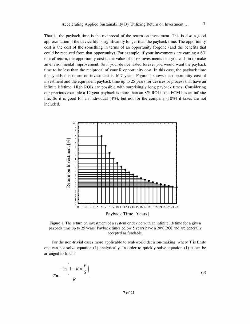
That is, the payback time is the reciprocal of the return on investment. This is also a good approximation if the device life is significantly longer than the payback time. The opportunity cost is the cost of the something in terms of an opportunity forgone (and the benefits that could be received from that opportunity). For example, if your investments are earning a 6% rate of return, the opportunity cost is the value of those investments that you cash in to make an environmental improvement. So if your device lasted forever you would want the payback time to be less than the reciprocal of your R opportunity cost. In this case, the payback time that yields this return on investment is 16.7 years. Figure 1 shows the opportunity cost of investment and the equivalent payback time up to 25 years for devices or process that have an infinite lifetime. High ROIs are possible with surprisingly long payback times. Considering our previous example a 12 year payback is more than an 8% ROI if the ECM has an infinite life. So it is good for an individual (4%), but not for the company (10%) if taxes are not included.

Payback Time [Years]

0 1 2 3 4 5 6 7 8 9 10 11 12 13 14 15 16 17 18 19 20 21 22 23 24 25

Ret

urn

on In

vest

men

t [%

]

0123456789

1011121314151617181920

Figure 1. The return on investment of a system or device with an infinite lifetime for a given payback time up to 25 years. Payback times below 5 years have a 20% ROI and are generally

accepted as fundable.

For the nontrivial cases more applicable to realworld decisionmaking, where T is finite one can not solve equation (1) analytically. In order to quickly solve equation (1) it can be arranged to find T:

T=−ln 1−R×

PS

R(3)

7 of 21

7


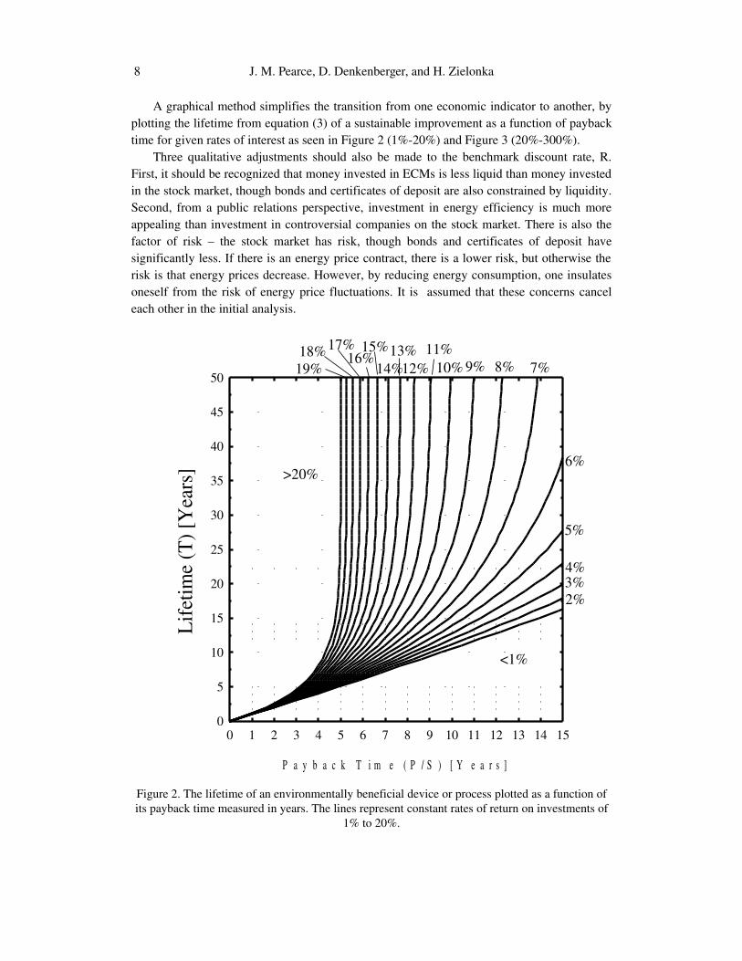
A graphical method simplifies the transition from one economic indicator to another, by plotting the lifetime from equation (3) of a sustainable improvement as a function of payback time for given rates of interest as seen in Figure 2 (1%20%) and Figure 3 (20%300%).

Three qualitative adjustments should also be made to the benchmark discount rate, R. First, it should be recognized that money invested in ECMs is less liquid than money invested in the stock market, though bonds and certificates of deposit are also constrained by liquidity. Second, from a public relations perspective, investment in energy efficiency is much more appealing than investment in controversial companies on the stock market. There is also the factor of risk – the stock market has risk, though bonds and certificates of deposit have significantly less. If there is an energy price contract, there is a lower risk, but otherwise the risk is that energy prices decrease. However, by reducing energy consumption, one insulates oneself from the risk of energy price fluctuations. It is assumed that these concerns cancel each other in the initial analysis.

P a y b a c k T i m e ( P / S ) [ Y e a r s ]

0 1 2 3 4 5 6 7 8 9 10 11 12 13 14 15

Life

time

(T) [

Yea

rs]

0

5

10

15

20

25

30

35

40

45

50

2%

<1%

3%4%

6%

5%

7%9% 8%18%17%

16%15%

14%13%

12%11%

10%

>20%

19%

Figure 2. The lifetime of an environmentally beneficial device or process plotted as a function of its payback time measured in years. The lines represent constant rates of return on investments of

1% to 20%.

8


P a y b a c k T im e (P /S ) [Y e a rs ]

0.0 0.5 1.0 1.5 2.0 2.5 3.0 3.5 4.0 4.5 5.0

Life

time (

T) [Y

ears

]

0123456789

10111213141516171819202122232425

<20%

30%40%60%

50%

70%80%

90%100%150%

125%300%

200%

Figure 3. The lifetime of an environmentally beneficial device or process plotted as a function of its payback time measured in years. The lines represent constant rates of return on investments of

20% to 300%.

APPLYING THIS EQUATION TO A SPECIFIC ENERGY CONSERVATION MEASURE

When applying equation (1) to a specific ECM, the economic environment the decision maker is in is extremely important. First, in order to satisfy assumption 5) the fuel, water,

9 of 21

9


maintenance, energy, etc. inflation rate is equal to the general inflation rate. This is actually a very conservative estimate based on the price of energy over the last five years as generally speaking the rates of energy costs are climbing faster than general inflation. This means that when one assumes (to meet the requirements of 5) that the saved annual amounts of energy, water, maintenance, etc. remain constant, in reality, you will save more. One opportunity cost of investment in energy efficiency is the real (adjusted for inflation) return on investment on the stock market and that this real return on investment on the stock market is assumed to be constant over time. As stated above, this is roughly 4% for an individual and the after tax return is 7% for a company. If the individual is in credit card debt, the opportunity cost of investment would be closer to 15%.

To illustrate how irrational many decisions based on payback are, consider the following case. If the nominal, aftertax return on investment for company X on the stock market is 6% and the general inflation rate is 1% (a conservative estimate); therefore, by assumption 5) the nominal fuel, water, maintenance, energy etc. inflation rate is also 1% (a very conservative estimate), the benchmark return on investment is 5%. However, company X is only willing to invest in processes or technologies that pay for themselves before five years have passed. At first, this may seem like a generous amount of time to wait for an efficiency device to pay for itself.4 The error of this arbitrary payback rule is graphically shown in Figure 4. The dark grey area on the left of the 5 year P/S line represents the “investment space” over which the company currently invests, any investment that does not fall in this area the company would not invest. The light grey area of the graph represents the investment space that could be profitably used if money is removed from the 5% money market account and invested in more efficient technologies. As can be seen in Fig. 4 this represents a lot of opportunities, many of which could earn up to four times the return of conventional sources. The white area at the bottom of Fig. 4 should not be invested in if the return on your investment is a primary concern. This includes investment space earning less than 5% (which includes those investments which are not able to pay for themselves before the end of their useful life). Using the graphical representations of equation (1) makes it easy to see why money from the traditional investments should be placed into ECM investments where “greening” beats the return on the < 0% that most people earn on their savings accounts, ~2% on certificate of deposits or money market accounts, or ~4% that they earn on the stock market (adjusted for inflation and taxes).5

4 A 5year payback is indeed generous for most businesses. Many businesses use significantly shorter payback periods to make decisions – generally one to three years.

5 Any income from investments or conventional savings is, of course, taxed; while any savings from ECMs is not taxed because it is simply an avoided cost not a profit. However, it should be noted that businesses can deduct energy use from U.S. taxes. This current tax practice actually encourages energy consumption – a highly dubious incentive based on the negative effects of energy use as outlined in the introduction.

1


Figure 4. Lifetime of an environmental improvement as a function of the payback time for return on investments from 1% to 20%. Example of an arbitrary 5 year payback time cut off and the

resultant investment space for this choice (shown in dark grey to the left of the 5 year line) and greening investment opportunities (ECMs) for a business earning 5% on their money shown in

light grey.

USE OF THE METHOD TO INFLUENCE POLICY TOWARDS SUSTAINABILITY

Clarion University of Pennsylvania recently had the opportunity to significantly reduce operating costs associated with energy use by retrofitting existing incandescent lighting with energy efficient compact fluorescent lamps (CFLs).6 CFLs are classic examples of ECMs because they use one quarter the energy to produce the same amount of light as a standard incandescent light bulb (and thus produce one quarter of the pollution and greenhouse gases), fit in the average light socket, last longer, and cost less over their lifecycle than incandescent bulbs. It is therefore possible to be fiscally responsible while reducing greenhouse gas emissions by retrofitting standard incandescent lamps (ILs) with CFLs. However, despite widespread availability and ease of implementation, they are seldom used [28]. Even the best publicity campaigns generally have success rates 69% or less [29]. In a single building, Clarion students found that over $1,400 could be saved over the lifetime of the CFLs used to retrofit ILs in the Peirce Science Center (details of calculation are in Table 1).

6 “Lamp” is the industry term for the common term “light bulb.”

11 of 21

1


Table 1. Total Savings from CFL retrofit of Peirce Science Center.

Bulb Type 60 WIncandescent

60Wequiv CFL

Number per package (N) 4 1Cost per package (C) $1.37 $2.50Lifetime (T) 1,250 hrs 8,000 hrs1) Cost of bulbs for 8,000 hrs of illumination = (8,000 hrs/Lifetime) x (C/ N)

$2.19 $2.50

Wattage (W) 60 15kWh used in 8,000 hours = (W*8,000hrs)/1000 480 kWhrs 120 kWhrs2) Cost of electricity for 8,000 hrs of illumination at Clarion U. rate $0.038 per kWhr

$18.24 $4.56

Total cost over 8,000 hrs for 1 socket = 1) cost of replacement bulbs during CFL life – cost of initial bulb (C/N) + 2) cost of electricity

(B) $20.09 (A) $4.56

Savings per fixture = B – A $15.53Total Number of fixtures (F) in Peirce 106Total Net Investment= F x – ([C/N]CFL – [C/N]IL)

– $228.70

Total Variable Savings Over CFL Lifetime = F x (BA)

$1,646.18

Total Net Savings of the Investment $1,417.48

1

International Journal of Energy, Environment and Economics ISSN: 1054853XVolume 17, Issue 1 ©2009 Nova Science Publishers,Inc

The initial enthusiasm over the possible savings was quickly dampened as University policy makers considered that many of the lights were used so infrequently, as can be seen in Table 2, that the payback times of the CFL bulbs would be prohibitively long (as can be seen by the payback times in the first three locations). However, using the method described in this paper the rates of return shown in the sixth column of Table 2 were derived from Figure 5. For the calculation of the lifetime of the CFLs, it was assumed that there is no depreciation due to pure age, and the impact of frequent starts was neglected.

Payback Time (P/S) [Years]0.0 0.5 1.0 1.5 2.0 2.5 3.0 3.5 4.0 4.5 5.0

Lif

etim

e (T

) [Y

ears

]

0123456789

10111213141516171819202122232425

ROI linesCase ACase BCase CCase DCase E

<20%

30%40%60%

50%

70%80%

90%100%150%

125%300%

200%

Figure 5. Lifetime of an environmental improvement as a function of the payback time for return on investments from 20% to 300%. One can determine the rate of return of a specific ECM by

plotting the payback time versus the lifetime of the project. For example, the black circles illustrate the economic data for replacing incandescent lighting with CFLs in Clarion’s Peirce

Science Center as detailed in Table 2.

In order to understand how to use Fig. 2 and Fig. 3 the following five examples are presented (A through E) shown in Table 2 for calculating the ROI on CFL retrofits of IL sockets in seven applications in the Peirce Science Center. The seven applications range from worstcase scenario (used only 2 hours/ week in storage closets) to the best case scenario (used continuously in the stairwells). There are other combinations that are straightforward to calculate but the selection here represents the most common situations.

Case A: Pay to install CFL and have an infinite number of incandescent bulbs.In case A, the worstcase scenario is calculated. The worst case is when you already have

invested in an infinite number of incandescent bulbs (i.e. you have cases in storage), you must buy the CFL, and you must pay for the time to install the bulb. However, Case A does not

Cumulative Index

count the saved labor cost associated with the fact that the IL has to be replaced 7 times during the life of the CFL. This is not rational; however, it is sometimes used by institutions that are highly resistant to change. Here it has been assumed that it takes 5 min. to screw in a light bulb and the staff responsible is paid $10/hour. In the specific case of Clarion University, the given “saved labor” of facilities workers freed up by their not having to make bulb changes would simply move onto another project in a long list (e.g. no labor costs would be saved by saving employee working hours). Thus saved labor costs were not included.7 This assumption about labor was used for all the cases. In this case P is the cost of the CFL (CCFL) and the cost of labor Clab and you only receive an S for electricity (SE), which is given by the product of the cost of electricity per kWh, the wattage difference of the bulbs, and the number of hours used per year. So the payback for Case A is given by:

Table 2. Payback time as a function of hours used per week for CFL retrofit of IL in the seven applications in the Peirce Science Center

Hours /week in Use

Application / Location

Bulbs in Use

Lifetime

(years)

Payback (years) Case A

Payback (years) Case B

Payback (years) Case C

Payback (years) Case D

Payback (years) Case E

2 Storage 20 76.9 18.74 14.06 12.12 10.46 7.835 Mechanical

Room10 30.8 7.50 5.62 4.85 4.18 3.13

10 Experiment Labs

7 15.4 3.75 2.81 2.42 2.09 1.57

28 Custodial Closets

24 5.5 1.34 1.00 0.87 0.75 0.56

35 Animal Labs

2 4.4 1.07 0.80 0.69 0.60 0.45

56 Auditorium 29 2.7 0.67 0.50 0.43 0.37 0.28168 Stairwells 14 0.91 0.22 0.17 0.14 0.12 0.09

PS=

CCFL +C lab

S E(4)

As can be seen in Table 2, in the absolute worst case scenario the payback is 18.74 years and the bulb will last for more than 76 years being used only 2 hours a week.

Case B: Filled sockets, an infinite number of incandescent bulbs and no labor costs.Case B simulates the decision present in an old building that already has an infinite

supply of incandescent bulbs and has no labor costs. The sockets are full so P is the entire CCFL and there are no labor costs. This scenario arises when there is no opportunity cost 7 However, it should be noted, that there is real value to the University to have those projects done (or there

is value in delaying the time when another maintenance person must be hired), so it is reasonable to use $10/hour even in this case. This calculation is often not done by institutions and is often a separate argument that must be won to implement smaller ROI ECMs.

14

Cumulative Index

associated with prevented labor (e.g. the laborers can not be fired so they sit around and do nothing when there is no work to do). This might also be appropriate for individuals who have so little work that they get bored (so their opportunity cost of time could be negative). However, the labor costs represent an enormous percentage of many ECMs potential savings and by excluding labor cost considerations many extremely good economic investments may be missed aggravating current energy losses from inefficient equipment. Saturating the ECM possibilities should reduce the maintenance backlog found at many institutions and businesses considerably so one can begin making theoretically correct economic decisions that include labor savings. In Case B the payback time is simply:

PS=

CCFL

S E(5)

This payback time is 75% sooner than Case A. Comparing Case A and Case B demonstrates the importance of including the cost of labor in calculations of ECMs.

Case C: Replacing the incandescent bulbs with no labor costs with full sockets initially.In case C there is already a new incandescent bulb in each socket so P is the entire cost of

the CFL. However, now as the socket is used, the savings from avoiding purchasing incandescent bulbs will function as another recurring cost similar to electricity. The savings from avoiding buying the additional incandescent bulbs can be given by:

S IL=HL×C IL (6)

where H is the number of hours used per year, CIL is the cost per incandescent light bulb, and

L is the lifetime of the incandescent bulb. Thus the payback time for Case C is given by

PS=

CCFL

S E+S IL(7)

The payback time including the savings from replacing the incandescent bulbs drops in all locations by about 14%.

Case D: Starting with empty sockets and paying for incandescent replacements but no labor costs.

Case D simulates the decision present with a new building with empty sockets and no inventory of incandescent bulbs or the case of waiting until the old IL burns out. Thus P is the

15 of 21

1

Cumulative Index

difference between the cost of the CFL bulb and the cost of the incandescent. Because the sockets are initially empty the cost of labor to put in the first bulb of either CFL or incandescent is the same and will be ignored. Again the cost of the incandescent bulb replacements as they burn out will function as another recurring cost like electricity does, so the payback time is given by:

PS=

CCFL−C IL

S E +S IL(8)

The payback for case D is again about 14% less than for case C.Case E: Starting with empty sockets, paying for incandescent replacements and labor.Case E is the bestcase scenario for the superior technology and is also the most realistic

for new buildings or replacement of broken equipment where there is no traditional technology in stock. Again, the labor cost of initial installation is the same, so it cancels. The investment is simply the difference in costs between the two types of bulbs. However, the savings is now made up of electric, cost of bulbs, and labor costs to replace the burnt out incandescent bulbs during the life of the CFL. Thus the payback becomes:

PS=

CCFL−C IL

S E+S IL+S lab(9)

Where Slab is the saved labor costs from replacing incandescent bulbs using the same assumption listed in Case A. The payback times are remarkable for this case. In the stairwells the CFLs pay for themselves in about a month and even in the worst location the payback time is reduced to less than 8 years.

However, as this paper hopes to show, considering only the payback times is a mistake. Thus, the percent return was determined for all five cases in Fig. 5, which shows the lifetime of the CFL retrofit as a function of the payback time from Table 2 to get the ROI for each location and each case. In Fig. 5 the ROI lines are again in black while the case lines have symbols. Many of the locations do not appear to be economically appealing in the simple payback model used by most businesses and institutions when considering renovations because the lifetime of the ECM is not taken into account. However, when the lifetime is included, the economic advantage of decreasing the energy use a given system becomes apparent.

The conclusion, which can be clearly drawn from Table 2 and Figure 5, is that despite long payback times for the application of CFLs in locations that do not frequently need to be illuminated (e.g. the 20 storage closets), CFLs are always a superior economic investment with a rate of return of over 5% in the worst case scenario and rates of return over 100% for other applications as seen in Figure 5. University decision makers quickly had the bulbs changed when the CFL retrofit was expressed in rates of return rather than simply payback time. The savings from this single technology is substantial and can be extrapolated over the entire campus to have all incandescent bulbs retrofitted.

16

Cumulative Index

A relatively astonishing conclusion can be drawn from this result. If the target ROI is 5% or greater all the current incandescent bulbs should be smashed and replaced with CFLs even in the worstcase scenario! One could imagine scenarios where the bulb is used even less than 2 hours per week where it would be optimal to wait until the IL burns out before replacing it with a CFL. Finally, at even lower use, it would be optimal to continue to use ILs, at least until the prices for CFLs drop even further. So these applications present an opportunity to use the ILs that were switched out in favor of the CFLs even before they were broken, instead of discarding those ILs. However, since these ILs are partially burned out, they would not last as long, so labor costs would be larger, so a tradeoff must be performed to see whether the saving of these ILs is economically defensible.

Figure 5 also displays another useful function of using this graphical method to convert payback time to return on investment. It is interesting to note that if any two data points (pairs of P/S and T) are plotted on the graphs and connected with a line for a given ECM, it enables one to determine the P/S and R for any T assuming a given number of useful operation hours (no depreciation due to simply age). This is shown as arrows in Figure 5. T for many devices (like the CFL) are easy to calculate by simply dividing the total number of illumination hours by the number of illumination hours/year.

EXTENSIONS OF THE MODEL

A number of the limiting assumptions of the derivation of the equation can be overcome. First, once one has determined ROI assuming that one purchased the device, as long as that ROI is greater than the interest rate of purchasing the device on credit, doing so makes sense.

The effect of deduction of energy costs is fairly simple to incorporate. If the tax rate is 1/3, this effectively means that the business only pays (1 – 1/3) = 2/3 as much for its energy. This new cost of energy can then be used for the cost savings calculation to find a new P/S. The effect of receiving a tax deduction on the depreciation of equipment is more complicated to analyze because it is not constant over time.

There is a simple extension of this analysis to escalating cost savings. The true rate of return is the escalation rate + the rate of return read off the graph times (1 + escalation rate) [30]. Roughly, for small escalation rates, you just add the escalation rate to the ROI on the graph. For instance, say energy efficient windows had a life of 70 years, and a payback of 30 years. This corresponds to a 3% ROI. However, if the cost savings escalated at 3% per year, this would yield a respectable 6% true ROI. But few people now would ever think of investing in something with a 30year payback.

If there is a tax credit on the purchase of an ECM, this effectively reduces the initial cost of the ECM, which is easy to incorporate.

17 of 21

17

Cumulative Index

LIMITATIONS

There are several drawbacks to this method with respect to economics and sustainability that need to be addressed. First, it should be noted that this analysis is a shortcut and that to be economically rigorous the Net Present Value analysis between two options is technically more accurate. However, the above method based on the graphical use of equation (1) is valid for all but special cases with uncommon cash flows (e.g. a project with a high return initially that decreases with time will appear desirable from a payback time analysis when in fact in may not be). In addition, for the method to be economically rigorous all the costs and benefits must be fully quantified and included in the P/S input. However many costs and benefits are difficult or impossible to quantify (e.g. the longterm costs of pollution on human health, the psychoemotional benefits of creating buildings with ample natural lighting, and the benefits of good environmental publicity). Another example is found in car care facilities that offer free tire pressure checks with oil changes. Correcting the tire pressure of customers will improve their mileage and thus save them money which could be spent in combined car care facilities like WalMart [31]. However, determining what percent of this money will make its way back to the car care facility is very challenging. In these cases and those where the environmentally correct choice is over shadowed by an inexpensive disastrous investment (e.g. single walled oil tankers), pure economics cannot always provide the optimal policy guidelines and some form of ethics or morality is necessary for guiding decision makers towards sustainability [32]. This is particularly important for those designing the future world, the engineers; and has been added to the National Society of Professional Engineers (NSPE) Code of Ethics for Engineers: “Engineers shall strive to adhere to the principles of sustainable development in order to protect the environment for future generations” [33].

Attempting to quantify “fuzzy” quantities such as wellbeing or pushing a particular ethical viewpoint to encourage sustainability also has inherent drawbacks purely from a strategic standpoint. If the goal is to move us as fast as possible towards sustainability, this paper illustrated that society could move very far forward based off of conventional economics elucidated for decision makers. For those considering using this method to accelerate a transition to sustainability, the very successful Green Destiny Council (GDC) at Penn State found that when completing any economic analysis for the university, all of the assumptions should be extremely conservative in order to prevent any disagreement over numbers [34]. All the suggestions in the GDC’s Mueller Report will reduce PSU’s energy use and most of these suggestions will save the University money as well [35]. However, many of these environmentally sound suggestions will entail an initial investment to see future returns. It is possible that this money could be supplied by liquidating University financial investments that supply less of a fiscal return than the given environmental improvement or from loans with a lower interest rate. This method of thinking was instrumental for increasing the University’s use of energy service companies [25]. Finally, it is also important for all work to be as rigorous as possible to maintain credibility with decision makers. Generally,

18

Cumulative Index

when coming at an argument with decision makers from the “green” background making extremely conservative assumptions and using possible savings represent a lowerend estimate are best practices [34].

CONCLUSION

This paper has shown that by considering environmental improvements (energy conservation measures) that have long payback periods as investments the more rational economic decision of putting into practice the technology or process that has a better return on investment will help transition society as a whole move towards sustainability. Although many of the energy saving processes or devices entail an initial investment to see future returns, these investments should be made if their return is higher than standard investments. Initial capital for the necessary investments in ECMs can come from liquidating financial investments that supply less of a fiscal return than the given environmental improvement or from loans at a lower interest rate. Savings from energy conservation and energy efficiency can then be reinvested in future environmental improvements. In conclusion, shifting money from less well performing investments into longterm energy savings provides a conservative, longterm source of savings that also provide an important hedge against the likely inflation in energy prices.

REFERENCES

(1) Hoffert, M. I., Caldeira, K., Benford, G., Criswell, D.R., Green, C., Herzog, H., Jain, A.K., Kheshgi, H.S., Lackner, K.S., Lewis, J.S., Lightfoot, H.D., Manheimer, W., Mankins, J.C., Mauel, M.E., Perkins, L.J., Schlesinger, M.E., Volk, T., and Wigley, T.M.L. (2002).Advanced Technology Paths to Global Climate Stability: Energy for a Greenhouse Planet, Science. 298, 981987.

(2) The Intergovernmental Panel on Climate Change (IPCC). (1995). Climate change 1995: the science of climate change, summary for policy makers and technical summary and IPCC Second Assessment Report: Climate Change. United Nations Environment Program and World Meteorological Organization: New York, NY.

(3) The Intergovernmental Panel on Climate Change (IPCC). (2001). Summary for Policymakers, Climate Change 2001: Impacts, Adaptation, and Vulnerability. United Nations Environment Program and World Meteorological Organization: New York, NY.

(4) Penner, J. (2004). The Cloud Conundrum. Nature, 432, 962963.(5) Stocker, T. (2004). Models Change their Tune. Nature, 430, 737738.

19 of 21

19

Cumulative Index

(6) Gregory, J.M., Huybrechts, P., Raper, S.C. (2004). Threatened Loss of the Greenland Icesheet. Nature. 2004, 428(6983), 616616.

(7) Schiermeier, Q. (2004). A Rising Tide. Nature, 428, 114115.(8) Kovats, R.S., Menne, B., McMichael, A.J., Bertollini, R., Soskolne, C. (1999). Ed.’s,

Early Human Health Effects of Climate Change and Stratospheric Ozone Depletion in Europe. Third Ministerial Conference on Environment and Health, World Health Organization: London, UK.

(9) Koelle, K., Rodo, X., Pascual, M., Yunus, M., and Mostafa, G. (2005). Refractory periods to climate forcing in cholera dynamics. Nature, 436, 696700.

(10) Schar, C., Vidale, P.L., Luthi, D., Frei, C., Haberli, H., Liniger, M.A., Appenzeller, C. (2004).The Role of Increasing Temperature Variability in European Summer Heatwaves. Nature, 427, 332336.

(11) Krajick, K. (2004) All Down hill From Here? Science. 303, 16001602.(12) Thomas, C.D., Cameron, A., Green, R.E., Bakkenes, M., Beaumont, L.J., Collingham,

Y.C., Erasmus, B.F.N., de Siquelra, M.F., Grainger, A., Hannah, L., Hughes, L., Huntley, B., van Jaarsveld, A.S., Midgley, G.F., Miles, L., OrtegaHuerta, M.A., Peterson, A.T., Phillips, O.L., Williams, S.E. (2004). Extinction Risk from Climate Change. Nature, 427, 145148.

(13) Caldeira, K., Wickett, M. E. (2003). Oceanography: Anthropogenic carbon and ocean pH. Nature. 425, 365365.

(14) U.S. Environmental Protection Agency (EPA). (2006). Inventory of U.S. Greenhouse Gas Emissions and Sinks: 19902004, U.S. Environmental Protection Agency: Washington, DC,

(15) Energy Information Administration (EIA). (2006). Annual Energy Outlook 2006 with Projections to 2030. U.S. Department of Energy: Washington, DC, DOE/EIA0383.

(16) Exxon. (1999).Global climate change: everyone’s debate. Exxon brochure.(17) Lynch, D. J. (2006). ExxonMobil amasses record $36B 2005 profit. USA Today, 31 Jan

2006. (18) Friends of the Earth (FOE). (2004). Exxon’s Climate Footprint: the Contribution of

ExxonMobil toClimate Change Since 1882. FOE: London, UK. (19) U.S. Environmental Protection Agency (EPA) and Department of energy (DOE)

(2008). Energy Star. http://www.energystar.gov/(20) Newnan, D. G., Lavelle, J. P. (1998). Essentials of Engineering Economic Analysis;

Engineering Press: Austin, TX.(21) Lindburg, M. (2002). FE review manual, Professional Publications, Inc: Belmont, CA.(22) Newell, R., Pizer, W. (2001). Discounting the benefits of climate change mitigation:

How much do uncertain rates increase valuation? Economics Technical Series, Pew Center on Global Climate Change: Arlington, VA.

(23) Lovins, A., Lovins, H., Hawken, P. (1999). Natural Capitalism – Creating the Next Industrial Revolution, Little Brown and Company: New York, NY.

(24) Donahue, P. (2003). Implementing energy efficient retrofits at state agencies and public sector institutions: commonwealth of Pennsylvania; NAESCO State Guidebook Series; National Association of Energy Service Companies: Washington, D.C.

2

http://www.energystar.gov/

Cumulative Index

(25) Pearce, J.M., Miller, L. L. (2006). Energy Service Companies as a Component of a Comprehensive University Sustainability Strategy. International Journal of Sustainability in Higher Education, 7(1), 1633.

(26) Pearce, J. (2002). Photovoltaics – A Path to Sustainable Futures. Futures, 34 (7), 663674.

(27) Pearce, J. M. (2008). Industrial Symbiosis for Very Large Scale Photovoltaic Manufacturing. Renewable Energy 33, 1101–1108.

(28) Energy Information Administration (EIA). (1996). Residential Lighting: Use and Potential Savings. Office of Energy Markets and End Use. U.S. Department of Energy: Washington, DC, DOE/EIA0555(96)/2.

(29) Pearce, J., Russill, C. (2005). Interdisciplinary Environmental Education: Communicating and Applying Energy Efficiency for Sustainability. Applied Environmental Education and Communication, 4 (1), 6572.

(30) Borbely, A.M., Kreider, J.F. (2001). Distributed Generation: The Power Paradigm for the New Millenium. CRC Press: New York, NY, p. 228.

(31) Pearce, J. M., Hanlon, J. T. (2006) Energy Conservation From Systematic Tire Pressure Regulation, Energy Policy, 35 (4), 26732677.

(32) Uhl, C. (2003). Developing Ecological Consciousness: Path to a Sustainable World. Rowman and Littlefield: Oxford, UK.

(33) National Society for Professional Engineers (NSPE). (2006). NSPE Code of Ethics, National Society of Professional Engineers, http://www.nspe.org/ethics/eh1code.asp.

(34) Pearce, J., Uhl, C. (2003). Getting It Done: Effective Sustainable Policy Implementation at the University Level. Planning for Higher Education, 31 (3), 5361.

(35) Pearce, J., Uhl, C., Mandryk, A., Matalavage, D., Vischer, C., Byrne, L., Eisenfeld, S. (2001). The Mueller Report: Moving Beyond Sustainability Indicators to Sustainability Action. The Green Destiny Council of The Pennsylvania State University: University Park, PA.

21 of 21

21

ACCELERATING APPLIED SUSTAINABILITY BY UTILIZING RETURN ON INVESTMENT FOR ENERGY CONSERVATION...

Documents

Transcript of ACCELERATING APPLIED SUSTAINABILITY BY UTILIZING RETURN ON INVESTMENT FOR ENERGY CONSERVATION...