ACA 2015 - SINGACOM

ACA 2015 July 20 - 23, 2015

Elite City Resort

Kalamata, Greece

21st Conference on

Applications ofComputer

Algebra

General Chair:

Ilias Kotsireas

Program Chair:

Edgar Martınez-Moro

Advisory Committee:

Eugenio Roanes-Lozano

Stanly Steinberg

Michael Wester

Publicity:

Zafeirakis Zafeirakopoulos

http://www.singacom.uva.es/ACA2015/

1

Contents

Sponsors ix

Foreword x

ACA Wordle xi

Schedule xii

Plenary Talks 2Algebras of Differential Invariants

Peter Olver . . . . . . . . . . . . . . . . . . . . . . . . . . . . . . . . . . . . . . . . 2New features in Maple 2015

Jurgen Gerhard . . . . . . . . . . . . . . . . . . . . . . . . . . . . . . . . . . . . . . 2

S1 Computer algebra in quantum computing and quantum information theory 4From Classical Universal and Reversible Logical Operations to Quantum Computation

Arkadiusz Or lowski . . . . . . . . . . . . . . . . . . . . . . . . . . . . . . . . . . . . 5On the orbit space of unitary actions for mixed quantum states

Vladimir Gerdt, Arsen Khvedelidze, Yuri Palii . . . . . . . . . . . . . . . . . . . . 6States and channels in quantum mechanics without complex numbers

J.A. Miszczak . . . . . . . . . . . . . . . . . . . . . . . . . . . . . . . . . . . . . . . 7A Web-based Quantum Computer Simulator with symbolic extensions

O. G. Karamitrou, C. Tsimpouris, P. Mavridi, K. N. Sgarbas . . . . . . . . . . . . 9Practical Difficulty and Techniques in Matrix-Product-State Simulation of Quantum

Computing in Hilbert Space and Liouville SpaceAkira SaiToh . . . . . . . . . . . . . . . . . . . . . . . . . . . . . . . . . . . . . . . 11

Approximate Quantum Fourier Transform and Applications: Simulation with WolframMathematicaAlexander N. Prokopenya . . . . . . . . . . . . . . . . . . . . . . . . . . . . . . . . 12

The ZX-calculus and quantum computationAleks Kissinger . . . . . . . . . . . . . . . . . . . . . . . . . . . . . . . . . . . . . . 14

S2 Human-Computer Algebra Interaction 16Predictive Algorithm from Linear String to Mathematical Formulae for Math Input

MethodT. Fukui, S. Shirai . . . . . . . . . . . . . . . . . . . . . . . . . . . . . . . . . . . . 17

SymbolicData, Computer Algebra and Web 2.0H.-G. Grabe, A. Heinle, S. Johanning . . . . . . . . . . . . . . . . . . . . . . . . . 23

Preserving syntactic correctness while editing mathematical formulasJoris van der Hoeven, Gregoire Lecerf, Denis Raux . . . . . . . . . . . . . . . . . . 29

Collaborative Computer Algebra: Review of FoundationsManfred Minimair . . . . . . . . . . . . . . . . . . . . . . . . . . . . . . . . . . . . 33

Modeling Inductive Reasoning in Collaborative Computer AlgebraManfred Minimair . . . . . . . . . . . . . . . . . . . . . . . . . . . . . . . . . . . . 35

i

CAS wonderland: A journey from user interfaces to user-friendly interfacesElena Smirnova . . . . . . . . . . . . . . . . . . . . . . . . . . . . . . . . . . . . . . 37

Cooperative development and human interface of a computer algebra system with theFormulæ frameworkLaurence R. Ugalde . . . . . . . . . . . . . . . . . . . . . . . . . . . . . . . . . . . 38

Browser-Based Collaboration with InkChatStephen M. Watt . . . . . . . . . . . . . . . . . . . . . . . . . . . . . . . . . . . . . 42

S3 Computer Algebra in Education 44About balanced application of CAS in undergraduate mathematics

E. Varbanova . . . . . . . . . . . . . . . . . . . . . . . . . . . . . . . . . . . . . . . 45Some reflections about open vs. proprietary Computer Algebra Systems in mathematics

teachingF. Botana . . . . . . . . . . . . . . . . . . . . . . . . . . . . . . . . . . . . . . . . . 46

Create SageMath Interacts for All Your Math CoursesRazvan A. Mezei . . . . . . . . . . . . . . . . . . . . . . . . . . . . . . . . . . . . . 47

Using SageMathCell and Sage Interacts to Reach Mathematically Weak Business StudentsGregory V. Bard . . . . . . . . . . . . . . . . . . . . . . . . . . . . . . . . . . . . . 48

GINI-Coefficient, GOZINTO-Graph and Option PricesJosef Bohm . . . . . . . . . . . . . . . . . . . . . . . . . . . . . . . . . . . . . . . . 51

When Mathematics Meet Computer SoftwareM. Beaudin, F. Henri . . . . . . . . . . . . . . . . . . . . . . . . . . . . . . . . . . 52

Revival of a Classical Topic in Differential Geometry: Envelopes of Parameterized Fami-lies of Curves and SurfacesTh. Dana-Picard, N. Zehavi . . . . . . . . . . . . . . . . . . . . . . . . . . . . . . . 53

Generating animations of JPEG images of closed surfaces in space using Maple andQuicktimeG. Labelle . . . . . . . . . . . . . . . . . . . . . . . . . . . . . . . . . . . . . . . . . 57

Plotting technologies for the study of functions of two real variablesDavid Zeitoun, Thierry Dana-Picard . . . . . . . . . . . . . . . . . . . . . . . . . . 58

Some remarks on Taylors polynomials visualization using Mathematica in context offunction approximationW. Wojas, J. Krupa . . . . . . . . . . . . . . . . . . . . . . . . . . . . . . . . . . . 63

Visualization of orthonormal triadsJeanett Lopez-Garcıa, Jorge J. Jimenez-Zamudio, Ma. Eugenia Canut Dıaz-Velarde 76

Contemporary interpretation of a historical locus problem with an unexpected discoveryR. Hasek . . . . . . . . . . . . . . . . . . . . . . . . . . . . . . . . . . . . . . . . . 77

A Constructive Proof of Feuerbachs Theorem Using a Computer Algebra SystemMichael Xue . . . . . . . . . . . . . . . . . . . . . . . . . . . . . . . . . . . . . . . 80

Math Partner and Math TutorG. Malaschonok, N. Malaschonok . . . . . . . . . . . . . . . . . . . . . . . . . . . . 81

Ideas for Teaching Using CASM. Beaudin . . . . . . . . . . . . . . . . . . . . . . . . . . . . . . . . . . . . . . . . 83

Solving Brain Teasers/Twisters CAS AssistedJosef Bohm . . . . . . . . . . . . . . . . . . . . . . . . . . . . . . . . . . . . . . . . 84

Various New Methods for Computing Subresultant Polynomial Remainder Sequences(PRSs)Alkiviadis G. Akritas . . . . . . . . . . . . . . . . . . . . . . . . . . . . . . . . . . . 85

Teaching improper integrals with CASG. Aguilera, J.L. Galan, M.A. Galan, Y. Padilla, P. Rodrıguez, R. Rodrıguez . . . 90

Application of wxMaxima System in LP problem of compound feed mass minimizationW. Wojas, J. Krupa . . . . . . . . . . . . . . . . . . . . . . . . . . . . . . . . . . . 92

The Use of CAS for Logical Analysis in Mathematics EducationT. Takahashi, T. Sakai, F. Iwama . . . . . . . . . . . . . . . . . . . . . . . . . . . 100

Indexed elementary functions in MapleDavid Jeffrey . . . . . . . . . . . . . . . . . . . . . . . . . . . . . . . . . . . . . . . 102

ii

S4 Computer Algebra in Coding Theory and Cryptography 104Trial set and Grbner bases for binary codes

M. Borges-Quintana, M. A. Borges-Trenard, Edgar Martınez-Moro . . . . . . . . . 105Geometric and Computational Approach to Classical and Quantum Secret Sharing

Ryutaroh Matsumoto, Diego Ruano . . . . . . . . . . . . . . . . . . . . . . . . . . . 110Quantum codes with bounded minimum distance

Carlos Galindo, Fernando Hernando, Diego Ruano . . . . . . . . . . . . . . . . . . 115Refined analysis of RGHWs of code pairs coming from Garcia-Stichtenoths second tower

O. Geil, S. Martin, U. Martınez-Penas, D. Ruano . . . . . . . . . . . . . . . . . . 120A new approach to the key equation and to the Berlekamp-Massey algorithm

M. Bras-Amoros, M. E. OSullivan, M. Pujol . . . . . . . . . . . . . . . . . . . . . 125On ZprZps -additive cyclic codes

J. Borges, C. Fernandez-Cordoba, R. Ten-Valls . . . . . . . . . . . . . . . . . . . . 130PD-sets for (nonlinear) Hadamard Z4-linear codes

R. D. Barrolleta, M. Villanueva . . . . . . . . . . . . . . . . . . . . . . . . . . . . 135Kronecker sums to construct Hadamard full propelinear codes of type CnQ8

J. Rifa, E. Suarez-Canedo . . . . . . . . . . . . . . . . . . . . . . . . . . . . . . . . 140A Message Encryption Scheme Using Idempotent Semirings

M. Durcheva . . . . . . . . . . . . . . . . . . . . . . . . . . . . . . . . . . . . . . . 145Simplicial topological coding and homology of spin networks

V. Berec . . . . . . . . . . . . . . . . . . . . . . . . . . . . . . . . . . . . . . . . . . 146Code-Based Cryptosystems Using Generalized Concatenated Codes

Karim Ishak, Sven Muelich, Sven Puchinger, Martin Bossert . . . . . . . . . . . . 147Nearly Sparse Linear Algebra and application to the Discrete Logarithm Problem

A. Joux, C. Pierrot . . . . . . . . . . . . . . . . . . . . . . . . . . . . . . . . . . . 149

S5 Computational Differential and Difference Algebra 153Root Parametrized Differential Equations for the Classical Groups

Matthias Seiß . . . . . . . . . . . . . . . . . . . . . . . . . . . . . . . . . . . . . . . 154Quasi-optimal computation of the p-curvature

A. Bostan, X. Caruso, E. Schost . . . . . . . . . . . . . . . . . . . . . . . . . . . . 156The Positive Part of Multivariate Series

A. Bostan, F. Chyzak, M. Kauers, L. Pech, M. van Hoeij . . . . . . . . . . . . . . 157Prolongation spaces and generalized differentials

F. Heiderich . . . . . . . . . . . . . . . . . . . . . . . . . . . . . . . . . . . . . . . 158Unitary groups of group algebras in characteristic 2

M. Barakat . . . . . . . . . . . . . . . . . . . . . . . . . . . . . . . . . . . . . . . . 159On the computation of the difference-differential Galois group for a second-order linear

difference equationCarlos E. Arreche . . . . . . . . . . . . . . . . . . . . . . . . . . . . . . . . . . . . 160

Differential Galois theory over differentially simple ringsA. Maurischat . . . . . . . . . . . . . . . . . . . . . . . . . . . . . . . . . . . . . . 161

Malher equations, differential Galois theory, and transcendenceT. Dreyfus, C. Hardouin, J. Roques . . . . . . . . . . . . . . . . . . . . . . . . . . 162

Primitive recursive quantifier elimination for existentially closed difference fieldsI. Tomasic . . . . . . . . . . . . . . . . . . . . . . . . . . . . . . . . . . . . . . . . 163

Lagrangian Constraints and Differential Thomas DecompositionV.P. Gerdt, D. Robertz . . . . . . . . . . . . . . . . . . . . . . . . . . . . . . . . . 165

Geometric Singularities of Algebraic Differential EquationsWerner M. Seiler . . . . . . . . . . . . . . . . . . . . . . . . . . . . . . . . . . . . . 166

Symbolic Solution of First-Order Autonomous Algebraic Partial Differential EquationsF. Winkler . . . . . . . . . . . . . . . . . . . . . . . . . . . . . . . . . . . . . . . . 168

S6 Algebraic and Algorithmic Differential and Integral Operator 170Birational Transformations of Algebraic Ordinary Differential Equations

F. Winkler . . . . . . . . . . . . . . . . . . . . . . . . . . . . . . . . . . . . . . . . 171

iii

Controlled and conditioned invariance for polynomial and rational feedback systemsC. Schilli, E. Zerz, V. Levandovskyy . . . . . . . . . . . . . . . . . . . . . . . . . . 172

Invariant histograms and signatures for object recognition, symmetry detection, and jig-saw puzzle assemblyPeter J. Olver . . . . . . . . . . . . . . . . . . . . . . . . . . . . . . . . . . . . . . 173

Jacobi algebras, in-between Poisson, differential, and Lie algebrasL. Poinsot . . . . . . . . . . . . . . . . . . . . . . . . . . . . . . . . . . . . . . . . . 174

Quantized Weyl algebras and AutomorphismsA.Kitchin . . . . . . . . . . . . . . . . . . . . . . . . . . . . . . . . . . . . . . . . . 176

On a generalization of integro-differential operatorsClemens G. Raab, Georg Regensburger . . . . . . . . . . . . . . . . . . . . . . . . . 177

Application of Signature Curves to Characterize Melanomas and MolesCheri Shakiban, Anna Grim . . . . . . . . . . . . . . . . . . . . . . . . . . . . . . . 178

Walks in the quarter plane with multiple stepsM. Kauers, R. Yatchak . . . . . . . . . . . . . . . . . . . . . . . . . . . . . . . . . 179

Computing Resolutions for Linear Differential SystemsWerner M. Seiler . . . . . . . . . . . . . . . . . . . . . . . . . . . . . . . . . . . . . 180

Computing Formal Solutions of Completely Integrable Pfaffian Systems With NormalCrossingsMaximilian Jaroschek . . . . . . . . . . . . . . . . . . . . . . . . . . . . . . . . . . 182

Conservation Laws and the Chazy EquationT.M.N. Goncalves, I.L. Freire . . . . . . . . . . . . . . . . . . . . . . . . . . . . . . 183

Generalized Greens Operators and the Method of CharacteristicsA. Korporal, G. Regensburger . . . . . . . . . . . . . . . . . . . . . . . . . . . . . . 184

Use of a Two-Dimensional Operational Calculus for Nonlocal Vibration Boundary ValueProblemsI. Dimovski, M. Spiridonova . . . . . . . . . . . . . . . . . . . . . . . . . . . . . . 185

Symbolic Computation for Rankin-Cohen Differential AlgebrasEleanor Farrington, Emma Previato . . . . . . . . . . . . . . . . . . . . . . . . . . 186

Formal Solutions of Singularly-Perturbed Linear Differential SystemsM.A. Barkatou, S.S. Maddah . . . . . . . . . . . . . . . . . . . . . . . . . . . . . . 191

Localizable and Weakly Left Localizable RingsV.V. Bavula . . . . . . . . . . . . . . . . . . . . . . . . . . . . . . . . . . . . . . . . 193

Generalized morphisms – turning homological algorithms into closed formulasM. Barakat . . . . . . . . . . . . . . . . . . . . . . . . . . . . . . . . . . . . . . . . 194

Computing Liouvillian solutions of linear difference equationsT. Combot . . . . . . . . . . . . . . . . . . . . . . . . . . . . . . . . . . . . . . . . 195

Symbolic Computation in Studying the Restricted Three-Body Problem with VariableMassesAlexander N. Prokopenya . . . . . . . . . . . . . . . . . . . . . . . . . . . . . . . . 196

One symbolical method for solving differential equations with delayed argumentNatasha Malaschonok . . . . . . . . . . . . . . . . . . . . . . . . . . . . . . . . . . 198

S7 Symbolic summation and integration:algorithms, complexity, and applications 201Explicit generating series for small-step walks in the quarter plane

A. Bostan, F. Chyzak, M. van Hoeij, M. Kauers, L. Pech . . . . . . . . . . . . . . 202Definite Integration of Rational Functions

J. Gerhard . . . . . . . . . . . . . . . . . . . . . . . . . . . . . . . . . . . . . . . . 204Creative Telescoping via Hermite Reduction

S. Chen, H. Huang, M. Kauers, Z. Li . . . . . . . . . . . . . . . . . . . . . . . . . 207Harmonic sums and polylogarithms at negative multiple indices

G.H.E. Duchamp, H.N. Minh, N.Q. Hoan . . . . . . . . . . . . . . . . . . . . . . . 208Symbolic integration of multiple polylogarithms

E. Panzer . . . . . . . . . . . . . . . . . . . . . . . . . . . . . . . . . . . . . . . . . 212

iv

Algorithms in symbolic integrationC.G. Raab . . . . . . . . . . . . . . . . . . . . . . . . . . . . . . . . . . . . . . . . . 213

Refined Holonomic Summation Meets Particle PhysicsJ. Blumlein, M. Round, C. Schneider . . . . . . . . . . . . . . . . . . . . . . . . . 214

Refined Parameterized Telescoping AlgorithmsC. Schneider . . . . . . . . . . . . . . . . . . . . . . . . . . . . . . . . . . . . . . . 215

Dispersion and complexity of indefinite summationE. Zima . . . . . . . . . . . . . . . . . . . . . . . . . . . . . . . . . . . . . . . . . . 216

S8 Cancelled 217

S9 Applied and Computational Algebraic Topology 218Fast computation of Betti numbers on three-dimensional cubical complexes

Aldo Gonzalez-Lorenzo, Alexandra Bac, Jean-Luc Mari, Pedro Real . . . . . . . . 219Computing the homology of the lcm-filtration of a monomial ideal

F. Mohammadi, A. Romero, E. Saenz de Cabezon, H. Wynn . . . . . . . . . . . . 220Estimating the position of the mandibular canal in dental radiographs using the general-

ized Hough transformD.M. Onchis, S.L. Gotia, P. Real . . . . . . . . . . . . . . . . . . . . . . . . . . . . 221

Algebraic-topological invariants for combinatorial multivector fieldsMarian Mrozek . . . . . . . . . . . . . . . . . . . . . . . . . . . . . . . . . . . . . . 223

Persistence over a topos of variable setsJ. Pita Costa, M. Vejdemo Johansson, P. Skraba . . . . . . . . . . . . . . . . . . . 228

Fast and Stable Topological Profiles of Noisy 2D ImagesV. Kurlin . . . . . . . . . . . . . . . . . . . . . . . . . . . . . . . . . . . . . . . . . 230

Using persistent homology to reveal hidden information in place cellsGard Spreemann, Benjamin Dunn, Magnus Botnan, Yasser Roudi, Nils Baas . . . 232

Persistence of generalized eigenspaces of self-mapsH. Edelsbrunner, G. Jablonski, M. Mrozek . . . . . . . . . . . . . . . . . . . . . . . 234

Algebraic Topology For Unitary Reflection Groups - Scalable Homology ComputingM. Juda . . . . . . . . . . . . . . . . . . . . . . . . . . . . . . . . . . . . . . . . . . 236

Computing the persistence of a self-map with the Kronecker canonical formM. Ethier, G. Jab lonski, M. Mrozek . . . . . . . . . . . . . . . . . . . . . . . . . . 238

Exploring relationships between homology generators using algebraic-topological modelsof regular CW-complexesP. Real, A. Gonzalez-Lorenzo, A. Bac, J.L. Mari, D. Onchis-Moaca . . . . . . . . 240

S10 Nonstandard Applications of Computer Algebra 243The root lattice A2 in the construction of tilings and algebraic hypersurfaces with many

singularitiesJuan Garcıa Escudero . . . . . . . . . . . . . . . . . . . . . . . . . . . . . . . . . . 244

Computer Algebra-based RBES personalized menu generatorE. Roanes-Lozano, J.L. Galan-Garcıa, G. Aguilera-Venegas . . . . . . . . . . . . . 246

Symbolic-Numeric Computing: A Polynomial System Arising in Image Analysis of PointCloud DataRobert H. Lewis . . . . . . . . . . . . . . . . . . . . . . . . . . . . . . . . . . . . . . 247

Making more flexible ATISMART+ model for traffic simulations using a CASM. Ramırez, J.M. Gavilan, G. Aguilera, J.L. Galan, M.A. Galan, P. Rodrıguez . . 249

Properties of the SimsonWallace locus applied on a skew quadrilateralP. Pech . . . . . . . . . . . . . . . . . . . . . . . . . . . . . . . . . . . . . . . . . . 251

Truth Value formalization and Groups TheoryFatmaZohra Belkredim . . . . . . . . . . . . . . . . . . . . . . . . . . . . . . . . . . 253

S11 Polynomial System Solving, Grobner Basis, and Applications 256Improved Parallel Gaussian Elimination for Grobner Bases Computations in Finite Fields

B. Boyer, C. Eder, J.-C. Faugere, S. Lachartre, F. Martani . . . . . . . . . . . . . 257

v

Sparse multihomogeneous systems: root counts and discriminantsIoannis Z. Emiris . . . . . . . . . . . . . . . . . . . . . . . . . . . . . . . . . . . . . 259

Tropical Homotopy ContinuationAnders Jensen . . . . . . . . . . . . . . . . . . . . . . . . . . . . . . . . . . . . . . 260

Bounds on the Number of Real Solutions For a Family of Fewnomial Systems of Equationsvia Gale DualityDaniel J. Bates, Jonathan D. Hauenstein, Matthew Niemerg, Frank Sottile . . . . 261

Linear Algebra for Computing Grobner Bases of Linear Recursive Multidimensional Se-quencesJ. Berthomieu, B. Boyer, J.-C. Faugere . . . . . . . . . . . . . . . . . . . . . . . . 262

Nearly optimal algorithms for real and complex root refinementElias Tsigaridas . . . . . . . . . . . . . . . . . . . . . . . . . . . . . . . . . . . . . 264

A Fast Euclid-type Algorithm for Quasiseparable PolynomialsSirani M. Perera . . . . . . . . . . . . . . . . . . . . . . . . . . . . . . . . . . . . . 265

Midway upon the journeyJonh Perry . . . . . . . . . . . . . . . . . . . . . . . . . . . . . . . . . . . . . . . . 267

Application of Computer Algebra in Number Theory Based CryptologyGuenael Renault . . . . . . . . . . . . . . . . . . . . . . . . . . . . . . . . . . . . . 268

The HIMMO SchemeLudo Tolhuizen . . . . . . . . . . . . . . . . . . . . . . . . . . . . . . . . . . . . . . 269

Algebraic Attack against Variants of McEliece with Goppa Polynomial of a Special FormJean-Charles Faugere, Ludovic Perret, Frederic de Portzamparc . . . . . . . . . . . 270

Use of Grobner basis in order to perform a fault attack in pairing-based cryptographyNadia El Mrabet, E. Fouotsa . . . . . . . . . . . . . . . . . . . . . . . . . . . . . . 271

Computation of Grobner bases and tropical Grbner bases over p-adic fieldsTristan Vaccon . . . . . . . . . . . . . . . . . . . . . . . . . . . . . . . . . . . . . . 273

Modular Techniques to Compute Grobner Bases over Non-Commutative Algebras withPBW BasesSharwan K. Tiwari, Christian Eder, Wolfram Decker . . . . . . . . . . . . . . . . 275

Efficient Groebner bases computation for Z[x] latticeChun-Ming Yuan . . . . . . . . . . . . . . . . . . . . . . . . . . . . . . . . . . . . . 278

Solving Polynomial Systems Using the Dixon-EDF Resultant with Emphasis on ImageAnalysis ProblemsRobert H. Lewis . . . . . . . . . . . . . . . . . . . . . . . . . . . . . . . . . . . . . . 279

Solving polynomial system with linear univariate representationJinsan Cheng . . . . . . . . . . . . . . . . . . . . . . . . . . . . . . . . . . . . . . . 280

About triangular matrix decomposition in domainG. Malaschonov, A. Scherbinin . . . . . . . . . . . . . . . . . . . . . . . . . . . . . 281

Polynomial-Time Algorithms for Quadratic Isomorphism of Polynomials: The RegularCaseJ. Berthomieu, Jean-Charles Faugere, L. Perret . . . . . . . . . . . . . . . . . . . . 282

S12 Computational Aspects and Mathematical Methods for Finite Fields 286A characterization of MDS codes that have an error correcting pair

Irene Marquez-Corbella, Ruud Pellikaan . . . . . . . . . . . . . . . . . . . . . . . . 287Simplex and MacDonald Codes over Rq

K. Chatouh, K. Guenda, T. A. Gulliver, L. Noui . . . . . . . . . . . . . . . . . . . 289Algebraic Modelling of Covering Arrays

Bernhard Garn, Dimitris E. Simos . . . . . . . . . . . . . . . . . . . . . . . . . . . 291On the diophantine equation 1 + 5x2 = 3yn

A. Hamttat, D. Behloul . . . . . . . . . . . . . . . . . . . . . . . . . . . . . . . . . 293On defining generalized rank weights

Relinde Jurrius, Ruud Pellikaan . . . . . . . . . . . . . . . . . . . . . . . . . . . . 297SBS: A Fast and Provably Secure Code-Based Stream Cipher

Pierre-Louis Cayrel, Mohammed Meziani, Ousmane Ndiaye . . . . . . . . . . . . . 302

vi

S13 PAC: Polytopes - Algebra - Computation 316A geometric approach for the upper bound theorem for Minkowski sums of convex poly-

topesEleni Tzanaki . . . . . . . . . . . . . . . . . . . . . . . . . . . . . . . . . . . . . . . 317

A sparse implicitisation frameworkChristos Konaxis . . . . . . . . . . . . . . . . . . . . . . . . . . . . . . . . . . . . . 318

Normal lattice polytopesWinfried Bruns . . . . . . . . . . . . . . . . . . . . . . . . . . . . . . . . . . . . . . 319

Enumeration of 2-level polytopesVissarion Fisikopoulos . . . . . . . . . . . . . . . . . . . . . . . . . . . . . . . . . . 320

Recent developments in NormalizChristof Soger . . . . . . . . . . . . . . . . . . . . . . . . . . . . . . . . . . . . . . 321

Starting cones for tropical traversalsAnders Jensen . . . . . . . . . . . . . . . . . . . . . . . . . . . . . . . . . . . . . . 322

Computing the Chern-Scwrartz-MacPherson Class and Euler Characteristic of CompleteSimplical Toric VarietiesMartin Helmer . . . . . . . . . . . . . . . . . . . . . . . . . . . . . . . . . . . . . . 323

S14 Grobner Bases, Resultants and Linear Algebra 329A Brief Introduction to the Extended Linearization Method (or XL Algorithm) for Solving

Polynomial Systems of EquationsGregory V. Bard . . . . . . . . . . . . . . . . . . . . . . . . . . . . . . . . . . . . . 330

Grobner Bases and Structured Systems: an overviewJ.-C. Faugere . . . . . . . . . . . . . . . . . . . . . . . . . . . . . . . . . . . . . . . 332

On the complexity of polynomial reductionJoris van der Hoeven . . . . . . . . . . . . . . . . . . . . . . . . . . . . . . . . . . . 334

The Generalized Rabinowitschs TrickDingkang Wang, Yao Sun, Jie Zhou . . . . . . . . . . . . . . . . . . . . . . . . . . 337

Resultant of an equivariant polynomial system with respect to the symmetri groupLaurent Buse, Anna Karasoulou . . . . . . . . . . . . . . . . . . . . . . . . . . . . 339

Symbolic Solution of Parametric Polynomial Systems with the Dixon ResultantRobert H. Lewis . . . . . . . . . . . . . . . . . . . . . . . . . . . . . . . . . . . . . . 341

Design of a Maple Package for Dixon Resultant ComputationM. Minimair . . . . . . . . . . . . . . . . . . . . . . . . . . . . . . . . . . . . . . . 342

Integral Bases for D-Finite FunctionsM. Kauers, C. Koutschan . . . . . . . . . . . . . . . . . . . . . . . . . . . . . . . . 344

LINDALG: MATHEMAGIX Package for Symbolic Resolution of Linear Differential Sys-tems with SingularitiesS. S. Maddah, M. A. Barkatou . . . . . . . . . . . . . . . . . . . . . . . . . . . . . 345

Bezout Matrices and Complex Roots of Quaternion PolynomialsPetroula Dospra, Dimitrios Poulakis . . . . . . . . . . . . . . . . . . . . . . . . . . 347

Nearly Optimal Bit Complexity Bounds for Computations with Structured MatricesElias Tsigaridas . . . . . . . . . . . . . . . . . . . . . . . . . . . . . . . . . . . . . 348

Linear algebraic approach to H-basis computationE. Yilmaz . . . . . . . . . . . . . . . . . . . . . . . . . . . . . . . . . . . . . . . . . 349

S15 Computer Algebra Methods for Matrices over Rings 352Properties and applications of a simultaneous decomposition of seven matrices over real

quaternion algebraZhuo-Heng He, Qing-Wen Wang . . . . . . . . . . . . . . . . . . . . . . . . . . . . 353

Travelling from matrices to matrix polynomialsP. Psarrakos . . . . . . . . . . . . . . . . . . . . . . . . . . . . . . . . . . . . . . . 354

Algebraic techniques for eigenvalues of a split quaternion matrix in split quaternionicmechanicsTongsong Jiang, Zhaozhong Zhang . . . . . . . . . . . . . . . . . . . . . . . . . . . 355

vii

Algebraic methods for Least Squares problem in split quaternionic mechanicsZhaozhong Zhang, Tongsong Jiang . . . . . . . . . . . . . . . . . . . . . . . . . . . 356

Moore-Penrose inverse and Drazin inverse of some elements in a ringJianlong Chen . . . . . . . . . . . . . . . . . . . . . . . . . . . . . . . . . . . . . . 357

Using Prover9 for proving some matrix equationsR. Padmanabhan, Yang Zhang . . . . . . . . . . . . . . . . . . . . . . . . . . . . . 358

Some results concerning condensed Cramer’s rule for the general solution to some re-stricted quaternion matrix equationsGuang-Jing Song . . . . . . . . . . . . . . . . . . . . . . . . . . . . . . . . . . . . . 359

Inertia of weighted graphsGuihai Yu . . . . . . . . . . . . . . . . . . . . . . . . . . . . . . . . . . . . . . . . . 360

More on minmum skew-rank of graphsHui Qu . . . . . . . . . . . . . . . . . . . . . . . . . . . . . . . . . . . . . . . . . . 361

Post-Lie algebra structures on solvable Lie algebrat t(2, C)Xiaomin Tang . . . . . . . . . . . . . . . . . . . . . . . . . . . . . . . . . . . . . . 362

S16 Open Source Software and Computer Algebra 364Implementation of Coefficient-Parameter Homotopies in Parallel

Daniel J. Bates, Daniel Brake, Matthew Niemerg . . . . . . . . . . . . . . . . . . . 365The Four Corner Magic and semi pandiagonal Squares

S. Al-Ashhab . . . . . . . . . . . . . . . . . . . . . . . . . . . . . . . . . . . . . . . 366Use computer algebra system Piranha for expansion of the Hamiltonian and construction

averaging motion equations of the planetary system problemA.S. Perminov, E.D. Kuznetsov . . . . . . . . . . . . . . . . . . . . . . . . . . . . 373

Use of Linux Open-Source Software and Maple in Analyzing the New Goeken-JohnsonRunge-Kutta Type MethodsAdrian Ionescu, Rea Ulaj . . . . . . . . . . . . . . . . . . . . . . . . . . . . . . . . 374

Using CAS to Uncover Unexpected Hidden Beauty in Radin-Conways Pinwheel TilingD.G. Burkholder . . . . . . . . . . . . . . . . . . . . . . . . . . . . . . . . . . . . . 375

Author Index 376

viii

Sponsors

ix

Foreword

Dear Participants,

it is our great pleasure to welcome you to Kalamata for the 21st edition of the Applications ofComputer Algebra conference, ACA 2015. We want to acknowledge the hard work of all the Ses-sion Organizers, that is a crucial element of the success of every conference in the ACA conferenceseries. Two other important aspects of ACA 2015 are the Twitter account @2015_ACA and therefereed Springe PROMS proceedings ( http://www.springer.com/series/10533 ). We hopethat both will contribute to the success of the conference.

According to the advice of Stanly Steinberg, founder of the ACA conference series and MichaelWester, co(n)-founder of the ACA conference series, as cited in

http://math.unm.edu/ aca/ACA/Organizing/Traditions:

”The conference chairs are the autocrats. The ACA working group can advise (as well asanyone who wishes to contact any member of the working group), but whomever is the chair (orchairs) have final authority over how the conference they are organizing is run. This is only fair,because organizing is a huge amount of work (but the rewards are great), so the chairs should notbe burdened by dilution of authority. (Anyone who has chairs a conference is a bit crazy, eitherbefore or certainly afterwards!) The hard work of the chairs are appreciated by all who participatein the conference and any problems should be diplomatically discussed with them.”

Therefore we would like to express a resounding THANK YOU to a very energetic and en-thusiastic group of people, namely the ACA WG (Working Group) for their invaluable help andunwavering support to us, as ACA 2015 Organizers. Their contributions to the organization ofACA conference over the years are indeed priceless.

We are also very grateful to our sponsors and last but not least we would like to thank a longlist of student volunteers, that make ACA 2015 possible, through their hard work and dedication.

We sincerely hope that you will thoroughly enjoy your stay in Kalamata for ACA 2015 andyour stay in Greece in general.

Edgar Martınez-Moro, ACA 2015 PC Chair

and Ilias Kotsireas, ACA 2015 General Chair

x

General scheduleSunday

1917:00 – 20:00

Registration

Monday 20 Tuesday 21 Wednesday 22 Thursday 23

Track 1 Track 2 Track 3 Track 4 Track 1 Track 2 Track 3 Track 4 Track 1 Track 2 Track 3 Track 4 Track 1 Track 2 Track 3 Track 4

08:00 – 09:00

Registration

09:00 – 09:30

Opening Remarks 53 S7 54 S9 55 S10 56 S11 104 S4 105 S7 106 S13 107 S16 123 S11 124 S5 125 S4 126 S14

09:30 – 10:00

1 S1 2 S2 3 S3 4 S6 57 S7 58 S9 59 S10 60 S11 108 S4 109 S7 110 S13 111 S16 127 S11 128 S5 129 S4 130 S14

10:00 – 10:30


10:30 – 11:00


11:00 – 11:30

Break Break Break Break

11:30 – 12:00


12:00 – 12:30

17 S1 18 S2 19 S3 20 S6

Plenary Talk Maple Talk

143 S11 144 S5 145 S12 146 S14

12:30 – 13:00

21 S1 22 S2 23 S3 24 S6 147 S11 148 S5 149 S12 150 S14

xii

13:00 – 15:00

Lunch Lunch Lunch Lunch

15:00 – 15:30

25 S1 26 S2 27 S3 28 S6 73 S6 74 S9 75 S3 76 S11

EXCURSIONAncient Messini archaeological site

151 S11 167 S10 152 S12 153 S14

15:30 – 16:00

29 S15 30 S2 31 S3 32 S6 77 S6 78 S9 79 S3 80 S11 154 S11 155 S4 156 S14

16:00 – 16:30

33 S15 34 S5 35 S3 36 S6 81 S6 82 S9 83 S3 84 S11 157 S11 158 S4 159 S14

16:30 – 17:00

37 S15 38 S5 39 S3 40 S6 85 S6 86 S12 87 S3 88 S11 160 S11 161 S4 162 S14

17:00 – 17:30

Break Break 163 S11 164 S4 165 S14

17:30 – 18:00

41 S15 42 S5 43 S3 44 S9 89 S6 90 S12 91 S3 92 S15 Closing Remarks

18:00 – 18:30

45 S15 46 S5 47 S3 48 S9 93 S6 94 S13 95 S3 96 S15

18:30 – 19:00

49 S15 50 S5 51 S3 52 S9 97 S6 98 S13 99 S3 100 S15

19:00 – 19:30

166 S15 101 S6 102 S3103 Hands on Banquet

Business meeting

xiii

MondayMonday 20

Track 1 Track 2 Track 3 Track 4

08:00 – 09:00 Registration

09:00 – 09:30 Opening Remarks

09:30 – 10:001 S1A. Orlowski, From classical universal and reversible logical operations to quantum computation

2 S2 Tetsuo Fukui, S. Shirai: Predictive Algorithm from Linear String to Mathematical Formulae for Math Input Method

3 S3Elena Varbanova About balanced application of CAS in undergraduate mathematics

4 S6F. Winkler Birational Transformations of Algebraic Ordinary Differential Equations

10:00 – 10:305 S1V. Gerdt, A. Khvedelidze, Y. Palii, On the orbit space of unitary actions for mixed quantum states

6 S2 Hans-Gert Gräbe, Albert Heinle, Simon Johannig:Symbolic Data, Computer Algebra and the Web 2.0

7 S3F. Botana Some reflections about open vs. proprietaryComputer Algebra Systems in mathematics teaching

8 S6Christian Schilli, Eva Zerz, and Viktor Levandovskyy: Controlled and conditioned invariance for polynomial and rational feedback systems

10:30 – 11:009 S1J.A. Miszczak, States and channels in quantum mechanics without complex numbers

10 S2 Joris van der Hoeven, Grégoire Lecerf, Denis Raux: Preserving Syntactic Correctness While Editing Mathematical Formulas

11 S3Razvan A. Mezei Create SageMath Interacts for All Your Math Courses

12 S6P. Olver Invariant histograms and signatures for object recognition, symmetry detection, and jigsaw puzzle assembly

11:00 – 11:30 Break

11:30 – 12:0013 S1O.G. Karamitrou, C. Tsimpouris, P. Mavridi, K.N. Sgarbas, Web based Quantum Computer Simulator and symbolic extensions

14 S2 Manfred Minimair: Collaborative Computer Algebra: Review of Foundations

15 S3Gregory V. Bard Using SageMathCell and Sage Interacts to Reach Mathematically Weak Business Students

16 S6L. Poinsot Jacobi algebras, in-between Poisson, differential, and Lie algebras

12:00 – 12:3017 S1A. SaiToh, Practical Difficulty and Techniques in Matrix-Product-State Simulation of Quantum Computing in Hilbert Space and Liouville Space

18 S2 Manfred Minimair: Modelling Inductive Reasoningin Collaborative Computer Algebra

19 S3Josef Böhm GINI-Coefficient, GOZINTO-Graph and Option Prices

20 S6A. Kitchin Quantized Weyl algebras and Automorphisms

12:30 – 13:0021 S1A. Prokopenya, Approximate Quantum Fourier Transform and Applications: Simulation with Wolfram Mathematica

22 S2 Elena Smirnova: CAS wonderland: A journey from user interfaces to user-friendly interfaces

23 S3M. Beaudin and F. Henri When Mathematics Meet Computer Software

24 S6C. Raab On a generalization of integro-differential operators

xiv

13:00 – 15:00 Lunch

15:00 – 15:3025 S1A. Kissinger, The ZX-calculus and quantum computation

26 S2 Laurence Ruiz Ugalde: Cooperative developmentand human interface of a computer algebra system with the Fōrmulæ framework

27 S3Th. Dana-Picard and N. Zehavi Revival of a Classical Topic in Differential Geometry: Envelopes of Parametrized Families of Curves and Surfaces

28 S6C. Shakiban Application of Signature Curves to Characterize Melanomas and Moles

15:30 – 16:0029 S15Zhuo-Heng He and Qing-Wen Wang, Properties and applications of a simultaneous decomposition of seven matrices over real quaternion algebra

30 S2 Stephen M. Watt: Browser-based Collaboration with InkChat

31 S3G. Labelle Generating animations of JPEG images of closed surfaces in space using Maple and Quicktime

32 S6M. Kauers Walks in the quarter plane with multiple steps

16:00 – 16:3033 S15P. Psarrakos, Travelling from matrices to matrix polynomials

34 S5Matthias Seiss: Root parameterized differential equations for the classical groups

35 S3David Zeitoun and Thierry Dana-Picard Plotting technologies for the study of functions of two real variables

36 S6W. Seiler Computing Resolutions for Linear Differential Systems

16:30 – 17:0037 S15Tongsong Jiang and Zhaozhong Zhang, Algebraic techniques for eigenvalues of a split quaternion matrix in split quaternionic mechanics

38 S5Alin Bostan: Quasi-optimal computation of the p-curvature

39 S3Wlodzimierz Wojas and Jan Krupa Some remarks on Taylor's polynomials visualization using Mathematica in context of function approximation

40 S6M. Jaroschek Computing Formal Solutions of Completely Integrable Pfaffian Systems With Normal Crossings

17:00 – 17:30 Break

17:30 – 18:0041 S15Zhaozhong Zhang and Tongsong Jiang, Algebraic methods for Least Squares problem in split quaternionic mechanics

42 S5Manuel Kauers: The positive part of multivariate series

43 S3Jeanett López García, Jorge J. Jiménez Zamudio andMa. Eugenia Canut Díaz Velarde Visualization of Orthonormal Triads in Cylindrical and Spherical Coordinates

44 S9Aldo Gonzalez-Lorenzo, Fast computation of Betti numbers on three-dimensional cubical complexes

18:00 – 18:3045 S15Jianlong Chen, Moore-Penrose inverse and Drazininverse of some elements in a ring

46 S5Florian Heiderich: Prolongation spaces and generalized differentials

47 S3R. Hasek Contemporary interpretation of a historical locus problem with an unexpected discovery

48 S9Eduardo Sáenz de Cabezón. Computing the homology of the lcm-filtration of a monomial ideal

18:30 – 19:0049 S15R. Padmanabhan and Y. Zhang, Using Prover9 forproving some matrix equations

50 S5Mohamed Barakat: Unitary groups of group algebras in characteristic 2

51 S3Michael Xue A Constructive Proof of Feuerbach’s Theorem Using a Computer Algebra System

52 S9Darian Onchis. Estimating the position of the mandibular canal in dental radiographs using the generalized Hough transform

19:00 – 19:30166 S15Guang-Jing Song, Some results concerning condensed Cramers rule for the general solution to some restricted quaternion matrix equations

xv

TuesdayTuesday 21


09:00 – 09:30

53 S7Frederic Chyzak Explicit generating series for small-step walks in the quarter plane

54 S9Marian Mrozek. Algebraic-topological invariants for combinatorial multivector fields

55 S10Juan García Escudero The root lattice A2 in the construction of tilings and algebraic hypersurfaces with many singularities

56 S11Christian Eder Improved Parallel Gaussian Elimination for Gröbner Bases Computations in Finite Fields

09:30 – 10:00

57 S7Jürgen Gerhard Definite Integration of Rational Functions

58 S9Joao Pita Costa, Mikael Vejdemo-Johansson and Primoz Skraba. Persistence over a topos of variable sets

59 S10E. Roanes-Lozano, J.L. Galán-Garciía, G. Aguilera-Venegas Computer Algebra-based RBES personalized menu generator

60 S11Ioannis Emiris Sparse multihomogeneous systems, root counts and discriminants

10:00 – 10:30

61 S7Manuel Kauers Creative Telescoping via Hermite Reduction

62 S9Vitaliy Kurlin. Fast and Stable Topological Profiles of Noisy 2D Images

63 S10Robert H. Lewis Symbolic-Numeric Computing: A Polynomial System Arising in Image Analysis of Point Cloud Data

64 S11Anders Jensen Tropical homotopy continuation

10:30 – 11:00

65 S7Ngo Quoc Hoan Harmonic sums and polylogarithms at negative multiple-indices

66 S9Gard Spreemann, Benjamin Dunn, Magnus Botnan, Yasser Roudi and Nils Baas. Using persistent homology to reveal hidden information in place cells

67 S10M. Ramírez, J.M. Gavilán, G. Aguilera, J.L. Galán, M.Á. Galán, P. Rodríguez Making more flexible ATISMART+ model for traffic simulations using a CAS

68 S11Matthew Niemerg Bounds on the Number of Real Solutions For a Family of Fewnomial Systems of Equations via Gale Duality

11:00 – 11:30

Break

11:30 – 12:00

69 S6T. Goncalves Conservation Laws and the Chazy Equation

70 S9Grzegorz Jablonski. Persistence of generalized eigenspaces of self-maps

71 S10 P. Pech Properties of the Simson–Wallace locus applied on a skew quadrilateral

72 S11Jean-Charles Faugere Linear Algebra for Computing Gröbner Bases of Linear Recursive Multidimensional Sequences

12:00 – 12:30

Plenary TalkPeter Olver - Algebras of Differential Invariants

12:30 – 13:00

13:00 – 15:00

Lunch

xvi

15:00 – 15:30

73 S6A. Korporal Generalized Green's Operators and theMethod of Characteristics

74 S9Mateusz Juda. Algebraic Topology For Unitary Reflection Groups - Scalable Homology Computing

75 S3Gennadi and Nastasha Malaschonok Math Partner and Math Tutor

76 S11Victor Pan Real Polynomial Root-finding by Means of Matrix and Polynomial Iterations

15:30 – 16:00

77 S6

E. Previato Symbolic Computation for Rankin-Cohen Differential Algebras

78 S9Marc Ethier, Grzegorz Jabłoński and Marian Mrozek. Computing the persistence of a self-map with the Kronecker canonical form

79 S3Michel Beaudin Ideas for Teaching Using CAS

80 S11Elias Tsigaridas Nearly optimal algorithms for real and complex root refinement

16:00 – 16:30

81 S6S. Maddah Formal Solutions of Singularly-Perturbed Linear Differential Systems

82 S9Pedro Real. Exploring relationships between homology generators using algebraic-topological models of regular CW-complexes.

83 S3Josef Böhm Solving Brain Teasers/Twisters - CAS Assisted

84 S11SiraniPerera A Fast Euclid-type Algorithm for Quasiseparable Polynomials

16:30 – 17:00

85 S6V. Bavula Localizable and Weakly Left Localizable Rings

86 S12K. Chatouh, K. Guenda, T. A. Gulliver and L. Noui Simplex andMacDonald Codes over R_q

87 S3Alkiviadis G. Akritas Various New Methods for Computing Subresultant Polynomial Remainder Sequences (PRS’s)

88 S11John Perry Midway upon the journey

17:00 – 17:30

Break

17:30 – 18:00

89 S6M. Barakat Generalized morphisms – turning homological algorithms into closed formulas

90 S12Pierre-Louis Cayrel Mohammed Meziani and Ousmane Ndiaye. SBS: A Fast and Provably Secure Code-Based Stream Cipher

91 S3G. Aguilera, J.L. Galán, M.Á. Galán, Y. Padilla, P. Rodríguez, R. Rodríguez Teaching improper integrals with CAS

92 S15Guihai Yu, Inertia of weighted graphs

18:00 – 18:30

93 S6T. Combot Computing Liouvillian solutions of linear difference equations

94 S13Eleni Tzanaki - A geometric approach for the upper bound theorem for Minkowski sums of convex polytopes.

95 S3Wlodzimierz Wojas and Jan Krupa Application of wxMaxima System in LP problem of compound feed mass minimization

96 S15Hui Qu, More on minmum skew-rank of graphs

18:30 – 19:00

97 S6A. Prokopenya Symbolic Computation in Studying the Restricted Three-Body Problem with Variable Masses

98 S13Christos Konaxis - A sparse implicitisation framework

99 S3T. Takahashi, T. Sakai, F. Iwama The Use of CAS for Logical Analysis in Mathematics Education

100 S15XiaominTang, Post-Lie algebra structures on solvable Lie algebra t(2, C)

19:00 – 19:30

101 S6N. Malashonok One symbolical method for solving differential equations with delayed argument

102 S3David Jeffrey Indexed elementary functions in Maple

103 SymbolicData aspects hands on sessionHans-Gert Graebe, Albert Heinle, Viktor Levandovsky

Business meeting

xvii

WednesdayWednesday 22


08:00 – 09:00

09:00 – 09:30104 S4M. Borges-Quintana, M.A. Borges-Trenard, E. Martínez-Moro Trial set and Gröbner bases for binary codes

105 S7Erik Panzer Symbolic integration of multiple polylogarithms

106 S13Winfried Bruns - Normal lattice polytopes

107 S16D. J. Bates , D. Brake , M. Niemerg Implementation of Coefficient-Parameter Homotopies in Parallel

09:30 – 10:00108 S4Ryutaroh Matsumoto and Diego Ruano Geometric and Computational Approach to Classical and Quantum Secret Sharing

109 S7Clemens Raab Algorithms in symbolic integration

110 S13Vissarion Fisikopoulos - Enumeration of 2-level polytopes

111 S16S. Al-Ashhab The Four Corner Magic and semi pandiagonal Squares

10:00 – 10:30112 S4C. Galindo, F. Hernándo, D. Ruano Quantum codes with bounded minimum distance

113 S7Mark Round Refined Holonomic Summation Meets Particle Physics

114 S13Christof Soeger - Recent developments in Normaliz

115 S16A. S. Perminov, E. D. Kuznetsov Use computer algebra system Piranha for expansion of the Hamiltonian and construction averaging motion equations of the planetary system problem

10:30 – 11:00116 S4O. Geil, S. Martin, U. Martínez-Peñas and D. Ruano Refined analysis ofRGHWs of code pairs coming from Gracia-Stichtenoth's second tower

117 S7Carsten Schneider Refined Parameterized Telescoping Algorithms

117 S13Anders Jensen - Starting cones for tropical traversals

118 S16Adrian Ionescu, Rea Ulaj Use of Linux Open-Source Software and Maple in Analyzing the New Goeken-Johnson Runge-Kutta Type Methods

11:00 – 11:30 Break

11:30 – 12:00119 S4M. Bras-Amorós, M.E. O'Sullivan and M. Pujol A new approach to the key equation and to the Berlekamp-Massey algorithm

120 S7Eugene Zima Dispersion and complexity of indefinite summation

121 S13Martin Helmer - Computing the Chern-Scwrartz-MacPherson Class and Euler Characteristic of Complete Simplical Toric Varieties

122 S16D. Burkholder Using CAS to Uncover Unexpected Hidden Beauty in Radin-Conway's Pinwheel Tiling

12:00 – 12:30Maple Talk

Juergen Gerhard – New features in Maple 201512:30 – 13:00

13:00 – 15:00 Lunch

xviii

15:00 – 15:30

EXCURSIONAncient Messini archaeological site

15:30 – 16:00

16:00 – 16:30

16:30 – 17:00

17:00 – 17:30

17:30 – 18:00

18:00 – 18:30

18:30 – 19:00

19:00 – 19:30 Banquet

xix

ThursdayThursday 23


08:00 – 09:00

09:00 – 09:30123 S11Guenael Renault Application of Computer Algebra in Number Theory Based Cryptology

124 S5Carlos Arreche: On the computation of the difference-differential Galois group for a second-order linear difference equation

125 S4J. Borges, C. Fernández-Córdoba and R. Ten-Valls On Z_p^rZ_p^s-additive cyclic codes

126 S14Gregory Bard - A Brief Introduction to the Extended Linearization Method (or XL Algorithm) for Solving Polynomial Systemsof Equations.

09:30 – 10:00 127 S11Ludo Tolhuizen The HIMMO Scheme

128 S5Andreas Maurischat: Differential Galois theory over differentially simple rings

129 S4R.D. Barrolleta and M. Villanueva PD-sets for (nonlinear) Hadamard Z4-Linear codes

130 S14Jean-Charles Faugère - Gröbner Bases and Structured Systems: an Overview.

10:00 – 10:30131 S11Ludovic Perret Algebraic Attack against Wild McEliece & Incognito

132 S5Thomas Dreyfus: Malher equations, differential Galois theory, and transcendence

133 S4J. Rifà, E. Suárez-Canedo Kronecker sums to construct Hadamard full propelinear codes of type CnQ8

134 S14Joris van der Hoeven - On the Complexity of Polynomial Reduction.

10:30 – 11:00135 S11Nadia El Mrabet Use of Groebner basis in order to perform a fault attack in pairing-based cryptography

136 S5Ivan Tomasic: Primitive recursive quantifier elimination for existentially closed difference fields

137 S12Irene Márquez-Corbella, Ruud Pellikaan A characterization of MDS codes that have an error correcting pair

138 S14Jie Zhou - The Generalized Rabinowitsch’s Trick.

11:00 – 11:30 Break

11:30 – 12:00139 S11Tristan Vaccon Computation of Groebner bases and tropical Gröbner bases over $p$-adic fields

140 S5Daniel Robertz: Lagrangian constraints and differential Thomas decomposition

141 S12Bernhard Garn and Dimitris E. Simos Algebraic Modelling of Covering Arrays

142 S14Anna Karasoulou - Resultant of an Equivariant Polynomial System with Respect to the Symmetric Group.

12:00 – 12:30143 S11Sharwan Kumar Tiwar Modular Techniques to Compute Grooebner Bases over Non-Commutative Algebras with PBW Bases

144 S5Werner Seiler: Geometric singularities of algebraic differential equations

145 S12Bernhard Garn and Dimitris E. Simos Algebraic Modelling of Covering Arrays

146 S14Robert Lewis - Symbolic Solution of Parametric Polynomial Systems with the Dixon Resultant.

12:30 – 13:00147 S11Chun-Ming Yuan Efficient Groebner bases computation forZ[x] lattice

148 S5148 Franz Winkler: Symbolic solution of first-order autonomous algebraic partial differential equations

149 S12Relinde Jurrius and Ruud Pellikaan On defining generalized rank weights

150 S14Manfred Minimair - Design of a Maple Package for Dixon Resultant Computation.

13:00 – 15:00 Lunch

xx

15:00 – 15:30151 S11Robert H. Lewis Solving Polynomial Systems Using the Dixon-EDF Resultant with Emphasis on Image Analysis Problems

167 S10FatmaZohra Belkredim Truth Value formalization and Groups Theory

152 S12Abdelkader Hamttat and Djilali Behloul On the diophantine equation 1 + 5x^2 = 3y^n

153 S14Manuel Kauers - Integral Bases for D-Finite Functions.

15:30 – 16:00154 S11Anissa Ali An algebraic method to compute the mobility of closed-loop overconstrained mechanisms

155 S4M. Durcheva A Message Encryption Scheme Using Idempotent semirings

156 S14Suzy Maddah - LINDALG: Mathemagix Package for Symbolic Resolution of LinearDifferential Systems with Singularities.

16:00 – 16:30157 S11 Jinsan Cheng Solving polynomial system with linear univariate representation

158 S4V. Berec Simplicial topological coding and homology of spin networks

159 S14Dimitrios Poulakis - Bezout Matrices and Roots of Quaternion Polynomials.

16:30 – 17:00160 S11Gennadi Malaschonok About Triangular Matrix Decomposition in Domain

161 S4Karim Ishak, Sven Muelich, Sven Puchinger, Martin Bossert Code-based Cryptosystems using generalized concatenatedcodes

162 S14Elias Tsigaridas - Nearly optimal bit complexity bounds for computations with structured matrices

17:00 – 17:30163 S11Jérémy Berthomieu Polynomial-Time Algorithms for Quadratic Isomorphism of Polynomials:The Regular Case

164 S4A. Jeux and C. Pierrot Nearly Sparse Linear Algebra and application to the Discrete Logarithm Problem

165 S14Erol Yilmaz - Linear Algebraic Approach toH-Basis Computation.

17:30 – 18:00 Closing Remarks

18:00 – 18:30

18:30 – 19:00

19:00 – 19:30

xxi

Plenary Talks

1

Algebras of Differential Invariants

Peter OlverHead School of MathematicsUniversity of MinnesotaMinneapolis, Minnesota, [email protected]

New features in Maple 2015

Jurgen GerhardDirector of Research at Maplesoft, CanadaFormer member of the Research Group Algorith-mic Mathematics and of the MuPAD ResearchGroup at University of Paderborn, [email protected]

2

Computer algebra in quantumcomputing and quantum

information theory

3

Session Organizers

Vladimir GerdtLaboratory of Information TechnologiesJoint Institute for Nuclear Research [email protected]

Michael Mc GettrickDe Brun Centre for Computational Algebra, School of MathematicsNational University of Ireland [email protected]

Jaroslaw Adam MiszczakInstitute of Theoretical and Applied InformaticsPolish Academy of Sciences [email protected]

Arkadiusz Or lowski and Alexander ProkopenyaFaculty of Applied Informatics and MathematicsWarsaw University of Life Sciences arkadiuszorlowski,alexanderprokopenya @sggw.pl

Overview

Quantum information processing provides a plethora of new problems and research topics suit-able for tackling using computer algebra systems. This includes the problems of characterizingmultipartite entanglement, generation and optimization of quantum computational circuits andanalysis of quantum walks and quantum automata. In the reverse direction, quantum algorithmswhich outperform their classical counterparts may be of use in symbolic calculations (e.g. GrobnerBases).

The aims of this session are to exchange recent results and ideas concerning the applicationof numerical, symbolic and algebraic methods in quantum information processing and quantummechanics.

4

From Classical Universal and Reversible LogicalOperations to Quantum Computation

Arkadiusz Orłowski1

1 Faculty for Applied Informatics and Mathematics, University of Life Sciences - SGGW,Nowoursynowska 166, 02-787 Warszawa, Poland, [email protected]

Reversible logical operations implemented via reversible logic gates (that canbe realized in practice, at least approximately, using various physical processes)play an important role in both low-power electronics [1, 2] and quantum compu-tations [3]. First, reversibility of classical computational circuits helps to avoidadditional energy dissipation and heat generation that is immanently tied to irre-versible computation due to Landauer’s principle [4]. Second, quantum gates andquantum circuits have to be reversible due to the very nature of unitary quantumevolution [5].

Here different classification schemes of reversible logical operations, includingbut not restricted to those obtained via group–theoretical methods, are presented fordifferent logic widths of corresponding gates. Searching for universal subsets ofreversible gates is undertaken with the help of computer algebra systems. New re-sults and nontrivial observations are provided as compared to the pioneering paper[6]. Novel less-typical reversible and universal logic gates are discussed and theirpossible applications are suggested. Some remarks concerning optimal designs ofreversible classical and quantum circuits are also given.

References[1] Kalyan S. Perumalla, Introduction to Reversible Computing, CRC Press, Taylor & Francis

Group, Boca Raton, 2014.[2] Alexis De Vos, Reversible Computing. Fundamentals, Quantum Computing, and Applications,

Wiley–VCH, Weinheim, 2010.[3] Michael A. Nielsen, Isaac L. Chuang, Quantum Computation and Quantum Information,

Cambridge University Press, Cambridge, 2000.[4] Rolf Landauer, Irreversibility and Heat Generation in the Computational Process, IBM Jour-

nal of Research and Development 5 (3), 183-191 (1961).[5] Richard Feynman, Feynman Lectures on Computation, Addison–Wesley Publishing, Reading,

1996.[6] Alexis De Vos, Birger Raa, Leo Storme, Generating the group of reversible logic gates, Journal

of Physics A: Mathematical and General 35, 7063-7078 (2002).

5

On the orbit space of unitary actions for mixedquantum states

Vladimir Gerdt, Arsen Khvedelidze, Yuri Palii

Laboratory of Information Technologies,Joint Institute for Nuclear Research,

141980 Dubna, Moscow Region, RussiaE-mail: [email protected]

Abstract

The space of mixed states, P+ , of n-dimensional binary quantum sys-tem is locus in quo for two unitary groups action: the group U(n) andthe tensor product group U(n1) ⊗ U(n2) , where n1, n2 stand from di-mensions of subsystems, n = n1n2. Both groups act on a state % ∈ P+

in adjoint manner (Ad g )% = g % g−1. As a result of this action one canconsider two equivalent classes of %; the global U(n)−orbit and the lo-cal U(n1)⊗U(n2)−orbit. The collection of all U(n)-orbits, together withthe quotient topology and differentiable structure defines the “global orbitspace”, P+ |U(n) , while the orbit space P+ |U(n1)⊗U(n2) represents the“local orbit space”, or the so-called entanglement space En1×n2 . The latterspace is proscenium for manifestations of the intriguing effects occurringin quantum information processing and communications.

Both orbit spaces admit representations in terms of the elements ofintegrity basis for the corresponding ring of group-invariant polynomials.This can be done implementing the Processi and Schwarz method, intro-duced in the 80th of last century for description of the orbit space of acompact Lie group action on a linear space. According to the Processiand Schwarz the orbit space is identified with the semi-algebraic variety,defined by the syzygy ideal for the integrity basis and the semi-positivitycondition of a special, so-called “gradient matrix”, Grad(z) > 0 , con-structing from the integrity basis elements.

In the present talk we address the question of application of this genericcomputer algebra aided approach to the construction of P+ |U(n) andP+ |U(n1) ⊗ U(n2). Namely, we study whether the semi-positivity ofGrad−matrix introduces a new conditions on the elements of the integritybasis for the corresponding ring R[P+]G.

6

States and channels in quantum mechanics withoutcomplex numbers

J.A. Miszczak1

1 Institute of Theoretical and Applied Informatics of the Polish Academy of Sciences, Bałtycka 5,

44-100 Gliwice, Poland, [email protected]

In this work we demonstrate a simplified version of quantum mechanics inwhich the states are constructed using real numbers only. In the standard for-mulation of quantum mechanics the state is represented by positive semidefinite,normalized linear operators. In the following we focus on linearity and hermic-ity properties of density matrices as they are crucial for the properties of quantumchannels.

The main advantage of the introduced approach is that the simulation of then-dimensional quantum system requires O(n2) real numbers, in contrast to thestandard case where O(n4) real numbers are required.

The main disadvantage is the lack of hermicity in the representation of quantumstates. This leads to the occurrence of complex eigenvalues of the real-valueddensity matrices.

During the last few years Mathematica computing system has become verypopular in the area of quantum information theory and the foundations of quantummechanics. The main reason for this is its ability to merge the symbolic and nu-merical capabilities, both of which are often necessary to understand the theoreticaland practical aspects of quantum mechanical systems [1, 2, 3].

We utilize the symbolic calculation capabilities offered by Mathematica [4, 5]to investigate the properties of the variant of quantum theory based of the repre-sentation of density matrices built using real-numbers only. We develop a set offunctions for manipulating real quantum states. With the help of this tool we studythe properties of the introduced representation and the induced representation ofquantum channels.

We start by introducing the said representation, including the required func-tions. We show how it can be used in Mathematica using symbolic computation.Next we test the behavior of selected partial operations in this representation andwe consider the general case of quantum channels acting on the space of real den-sity matrices. Finally, we provide the summary and the concluding remarks.

Acknowledgements This work has been supported by Polish National ScienceCentre project number 2011/03/D/ST6/00413.

7

References[1] V.P. Gerdt, R. Kragler, A.N. Prokopenya, A Mathematica package for simulation of quantum

computation, in Computer Algebra in Scientific Computing / CASC’2009, V.P. Gerdt, E.W.Mayr, E.V. Vorozhtsov (ed.), LNCS 5743, Springer-Verlag, Berlin, pp. 106-117 (2009).

[2] J.A. Miszczak, Generating and using truly random quantum states in Mathematica, Comput.Phys. Commun., Vol. 183, No. 1 (2012), pp. 118-124. arXiv:1102.4598

[3] B. Julia-Diaz, Simulating quantum computers with Mathematica: QDENSITY et al., In: Proc.Applications of Computer Algebra (ACA2013), Malaga, 2-6 July 2013, J.L. Galan Garcia, G.Aguilera Venegas, P. Rodriguez Cielos, (eds.), 2013.

[4] J.A. Miszczak, Singular value decomposition and matrix reorderings in quantum informationtheory, Int. J. Mod. Phys. C, Vol. 22, No. 9 (2011), pp. 897-918. arXiv:1011.1585

[5] J.A. Miszczak, Functional framework for representing and transforming quantum channels,In: Proc. Applications of Computer Algebra (ACA2013), Malaga, 2-6 July 2013, J.L. GalanGarcia, G. Aguilera Venegas, P. Rodriguez Cielos, (eds.), 2013. arXiv:1307.4906

8

A Web-based Quantum Computer Simulator withsymbolic extensions

O. G. Karamitrou1, C. Tsimpouris2, P. Mavridi3, K. N. Sgarbas4

1 University of Patras, Greece, [email protected] University of Patras, Greece, [email protected] University of Patras, Greece, [email protected] University of Patras, Greece, [email protected]

The objective of this paper is to present a quantum computer simulator with aweb interface based on the circuit model of quantum computation [3]. This is thestandard model for which most quantum algorithms have been developed. Quan-tum algorithms are expressed as circuits of quantum registers (series of qubits) andquantum gates operating on them. Each quantum gate is a unitary transformationon the Hilbert space determined by the quantum register.

The quantum computer simulator is developed in Python, using some extralibraries for our purposes. The fundamental library that is used is Numpy: thepackage for scientific computing with Python.

Because of the limitations of GUI for a large number of qubits, we proposean another version of quantum computer simulator without a user interface, whichcould simulate quantum computations for larger inputs. The inputs of the simula-tor are the number of qubits, the number of computation steps, the initial state ofquantum register and the gates that applied at each step. The outputs of the simu-lator are the quantum register state at each step (the probability of measuring eachone of the possible states and the phases of each state).

The quantum computer simulator is a useful tool for studying and understand-ing quantum circuits, quantum computations and well known quantum algorithmssuch as Grover’s algorithm [1, 2] and Quantum Fourier Transform. It may also bevery useful for the development of new quantum algorithms and the constructionof new quantum gates.

Another approach of developing a quantum simulator in Python, is to use in-stead of Numpy, Sympy python library (Symbolic Python). The advantage of thischange is that you can represent very large numbers, as a result of using arbitraryprecision arithmetic. On the other hand, Numpy uses machine arithmetic, whichimports limitations.

9

References[1] L. K. Grover, Quantum mechanics helps in searching for a needle in a haystack, Phys. Rev.

Lett. 79, 2, pp. 325-328 (1997).[2] L. K. Grover, Quantum computers can search rapidly by using almost any transformation,

Phys. Rev. Lett. 80, 19, pp. 4329-4332 (1998).[3] M. A. Nielsen and I. L. Chuang, Quantum Computation and Quantum Information, Cam-

bridge, U.K.:Cambridge University Press, (2000).

10

Practical Difficulty and Techniques inMatrix-Product-State Simulation of Quantum Computingin Hilbert Space and Liouville Space

Akira SaiToh1

1 Toyohashi University of Technology, Toyohashi, Aichi, Japan, [email protected]

There have been many studies on matrix-product-state (MPS) simulation ofquantum computing for more than a decade [1, 2, 3, 4, 5, 6]. Although it is widelybelieved to be unlikely, it is still an open problem if a practical simulation of a pow-erful quantum algorithm like Shor’s factoring algorithm is possible. This situationis owing to the fact that not only theoretical analyses but numerical investigationson MPS are quite cumbersome.

In practice, coding an MPS simulation program is highly technical. A quantumcircuit should be carefully decomposed as its structure affects the Schmidt ranksof MPS during simulation. In addition, numerical error may accumulate rapidly ifwe use only double-precision floating-point arithmetics because almost always weneed to diagonalize highly degenerate reduced density matrices during simulation.Furthermore, sometimes quantum states initially having very small population playan important role in an algorithm. Thus, multiple-precision computing is oftenrequisite to obtain a reasonable simulation result [5, 6].

In this contribution, I summarize the above-mentioned issues with explicit ex-amples, and how I have been coding my open source C++ library, ZKCM_QC[5, 6]. I also discuss the simulability of spin-Liouville-space quantum computa-tions on the basis of some simulation results.

References[1] G. Vidal, Efficient classical simulation of slightly entangled quantum computations, Phys. Rev.

Lett. 91, 147902 (2003).[2] A. Kawaguchi, K. Shimizu, Y. Tokura, and N. Imoto, Classical simulation of quantum algo-

rithms using the tensor product representation, arXiv:quant-ph/0411205 (2004).[3] M. C. Bañuls, R. Orús, J. I. Latorre, A. Pérez, and P. Ruiz-Femenía, Simulation of many-qubit

quantum computation with matrix product states, Phys. Rev. A 73, 022344 (2006).[4] A. SaiToh and M. Kitagawa, Matrix-product-state simulation of an extended Brüschweiler

bulk-ensemble database search, Phys. Rev. A. 73, 062332 (2006).[5] A. SaiToh, A multiprecision C++ library for matrix-product-state simulation of quantum com-

puting: Evaluation of numerical errors, J. Phys.: Conf. Ser. 454, 012064 (2013).[6] A. SaiToh, ZKCM: A C++ library for multiprecision matrix computation with applications in

quantum information, Comput. Phys. Comm. 184, pp.2005-2020 (2013).

11

Approximate Quantum Fourier Transform andApplications: Simulation with Wolfram Mathematica

Alexander N. Prokopenya

Warsaw University of Life Sciences – SGGW, Poland, [email protected]

The quantum Fourier transform (QFT) is a unitary transformation UFT thatcan be written in the computational basis |x⟩n ≡ |xn−1 . . .x1x0⟩, where the set ofnumbers x j = 0,1 ( j = 0,1, . . . ,n − 1) provides the binary representation of theinteger x (x = 0,1, ...,2n−1), as

UFT |x⟩n → 12n/2

2n−1

∑y=0

exp(

2πi2n xy

)|y⟩n . (1)

Here n is a number of qubits in the memory register.Note that the QFT can be carried out efficiently by a quantum circuit built

entirely out of single-qubit and two-qubit gates. Actually, only n the Hadamardgates, n(n−1)/2 controlled phase shift gates Rk, and ⌊n/2⌋ Swap gates are requiredto build such a circuit (see, for example, [1]). The execution time of the QFT growsonly as n2 and, therefore, the QFT is executed exponentially faster that the classicalfast Fourier transform.

However, in case of a large number of qubits the phase shift 2π/2k becomesexponentially small, while a practical implementation of the high precision con-trolled phase shift gates Rk may be very difficult. So it would be very useful if thefull Fourier transform (1) could be replaced by the approximate QFT, where onlyfinite degree phase shift gates Rk are involved (k ≤ m < n). Analysis of differentquantum algorithms has shown that applying the approximate QFT can yield evenbetter results than the full Fourier transform [2].

In the present paper we discuss an approximate QFT that was first proposedin [3] and can be represented as

UFT |xn−1 . . .x0⟩ → 12n/2

1

∑yn−1=0

. . .1

∑y0=0

exp(

2πi(

xn−1y0

2+ . . .+

xn−m

(ym−1

21 + . . .+y0

2m

)+ xn−m−1

(ym

21 + . . .+y1

2m

)+ . . .+

x0

(yn−1

21 + . . .+yn−m

2m

)))|yn−1 . . .y0⟩ . (2)

Applying the approximate QFT, one can expect that an accuracy of computa-tion decreases in comparison to the case of the full QFT, and probability of getting

12

a correct result reduces, as well. The main purpose of the present paper is to esti-mate a probability of successful solution of a problem in case of the replacement ofthe full QFT by the approximate QFT and to demonstrate the results by simulationof some quantum algorithms, using the Wolfram Mathematica package "Quantum-Circuit" (see [4, 5]). Recall that the package provides a user-friendly interface tospecify a quantum circuit, to draw it, and to construct the corresponding unitarymatrix for quantum computation defined by the circuit. Using this matrix, one canfind the final state of the quantum memory register by its given initial state and tocheck the operation of the algorithm determined by the quantum circuit.

As examples we consider here two known quantum algorithms, where the QFTplays an essential role. The first one is the quantum algorithm for phase estimationbased on the QFT [6]. We have obtained the lower bound on the probability ofthe successful phase estimation in both cases of the full and approximate QFT andshown that the decrease in the accuracy of phase estimation results in increasingthe probability of the successful problem solution [7].

The second example is the Shor algorithm for order finding [8]. Our calcula-tions show that using the approximate QFT gives the same results as in case of thefull QFT even for small enough degree m of approximation. At the same time theprobability to obtain correct result decreases only a little bit in comparison to thecase of the full QFT. The validity of the results is demonstrated by simulation ofthe algorithm using the package "QuantumCircuit".

References[1] M. Nielsen, I. Chuang, Quantum Computation and Quantum Information, Cambridge Univer-

sity Press (2000).[2] A. Barenco, A. Ekert, K.A. Suominen, P. Törmä, Approximate quantum Fourier transform

and decoherence, Phys. Rev. A[3] D. Coppersmith, An approximate Fourier transform useful in quantum factoring, IBM Re-

search Report RC 19642 (1994). 54, 1, pp.139-146 (1996).[4] V.P. Gerdt, R. Kragler, A.N. Prokopenya, A Mathematica program for constructing quantum

circuits and computing their unitary matrices, Physics of Particles and Nuclei, Lett. 6, 7, pp.526-529 (2009).

[5] V.P. Gerdt, R. Kragler, A.N. Prokopenya, A Mathematica package for simulation of quantumcomputation, in Computer Algebra in Scientific Computing / CASC’2009, V.P. Gerdt, E.W.Mayr, E.V. Vorozhtsov (ed.), LNCS 5743, Springer-Verlag, Berlin, pp. 106-117 (2009).

[6] D.S. Abrams, S. Lloyd, Quantum algorithm providing exponential speed increase for findingeigenvales and eigenvectors, Phys. Rev. Lett. 83, 24, pp. 5162-5165 (1999).

[7] A.N. Prokopenya, Simulation of a quantum algorithm for phase estimation, Programming andComputer Software 41, 2, pp. 98-104 (2015).

[8] P.W. Shor, Polynomial-time algorithms for prime factorization and discrete logarithms on aquantum computer, SIAM J. Comp. 26, 5, pp. 1484-1509 (1997).

13

The ZX-calculus and quantum computation

Aleks Kissinger1

1 University of Oxford, UK, [email protected]

The ZX-calculus is a formal system for reasoning diagrammatically about quan-tum computation which admits an encoding of the circuit model and measurement-based quantum computation. In this talk, I’ll give an introduction to the calculusitself, survey some of the most important theorems, techniques, and open prob-lems, and demonstrate the implementation of the ZX-calculus in Quantomatic, adiagrammatic proof assistant.

14

Human-Computer AlgebraInteraction

15

Session Organizers

Manfred MinimairDepartment of Mathematics and Computer ScienceSeton Hall [email protected]

Stephen M. WattComputer Science DepartmentThe University of Western [email protected]

Overview

This session explores how humans interact with computer algebra software to solve problems inapplications and research. The topics for presentations include software to support cooperativework in computer algebra, mathematical experimentation, specialized user interfaces and hard-ware to increase productivity, such as software wizards, mobile devices, and pen-based input, andapplications to artificial intelligence. The session intersects with the 2009 session on Applicationsof Math Software to Mathematical Research and the 2005 session on Pen-Based MathematicalComputing.

16

Predictive Algorithm from Linear String to MathematicalFormulae for Math Input Method

T. Fukui1, S. Shirai2

1 Mukogawa Women’s University, Japan, [email protected] Mukogawa Women’s University, Japan, [email protected]

1 Introduction

In recent years, Computer Aided Assessment (CAA) systems have been used formathematics education. A few CAA systems enable users to directly input mathe-matical expressions to allow their answers to be evaluated automatically by usinga computer algebra system (CAS). These systems have also been used to provideinstruction to students at universities. However, the procedure according to whichan answer is entered into the system by using the standard input method for math-ematics is still troublesome [1, 2].

In 2011, Professor Tetsuo Fukui of Mukogawa Women’s University proposed anew mathematical input method for conversion from a colloquial style mathemati-cal text[3]-[7]. This method is similar to those used for inputting Japanese charac-ters in many operating systems. In this system, the list of candidate characters andsymbols for the desired mathematical expression, as obtained from the user input,is displayed in WYSIWYG format and once all the elements the user wishes to in-clude are chosen, then the expression formatting process is complete. This methodwill enable the user to input almost any mathematical expression without having tolearn a new language or syntax. However, the disadvantage of the abovementionedmethod is that the user has to convert each element contained in the colloquial stylemathematical string by proceeding from left to right, in this order.

This study aimed to address this shortcoming by improving the math inputefficiency using an intelligently predictive conversion from a linear mathematicalstring to an entire expression instead of converting each element individually.

2 Linear String rules

The linear mathematical string rules for a mathematical expression are describedas follows:

Set the key letters (or words) corresponding to the elements of amathematical expression linearly in the order of colloquial (or reading) style,without considering two-dimensional placement and delimiters.

17

In other words, a key letter (or word) consists of the ASCII code(s) correspond-ing to the initial or the clipped form (such as the LATEX-form) of the objective math-ematical symbol. Therefore, one key often supports many mathematical symbols.For example, when a user wants to input α2, the linear string is denoted by “a2"where “a" stands for the “alpha” symbol and it is unnecessary to include a powersign (such as the caret letter (ˆ)). In the case of 1

α2+3 , the linear string is denoted by“1/a2+3" where it is not necessary to surround the denominator (which is generallythe operand of an operator) by parentheses, because they are never printed.

3 Design of intelligently predictive conversion

In this talk, we propose a predictive algorithm to convert a linear string s into themost suitable mathematical expression yp. For prediction purposes, we deviseda method by which each candidate for selection would be ranked in terms of itssuitability. Our method uses a function Score(y) to allocate a score which is pro-portional to the probability of a mathematical expression y occurring, and whichwould enable us to predict the candidate yp by eq.(1) as being the most suitableexpression with the maximum score. Here, Y (s) in eq.(1) is the totality of all thepossible mathematical expressions converted from s.

yp s.t. Score(yp) = maxScore(y)|y ∈ Y (s) (1)

A mathematical expression consists of mathematical symbols, namely num-bers, variables, or operators 1, together with the operating relations between a spe-cific operator and an element. Therefore, we decided to represent a mathematicalexpression by a tree structure consisting of nodes and edges corresponding to thesymbols and operating relations, respectively.

First, all the node elements of mathematical expressions were classified accord-ing to nine types, as listed in Table 1 in this math conversion system. Therefore, anode element is characterized by (k,e, t) where k is the key letter (or word) of itsmathematical symbol e that belongs to type t(= N,V,P,A,BL,BR,C,Q,R, or T ) inTable 1. For example, the number 2 is characterized by (“2",2,N) and similarlya variable x by (“x",x,V ) and, as for the Greek letter α , it can either be charac-terized by (“alpha",α,V ) or (“a",α,V ). In the case of the operator, the character(“/", 1

2,C) represents a fractional symbol with input key “/", where 1,2 repre-

sents arbitrary operands.There are 510 mathematical symbols and the 597 operators in the node element

table D implemented by our prototype system in this study.1In this article, "operator" is used in the sense of operating on, i.e., performing actions on elements

in terms of their arrangements for two-dimensional mathematical notation.

18

Table 1: Nine types of mathematical expressive structures

Math element Codes of type examples (1,2,3 represent operands)Number N 2,128

Variable, Symbol V x,αPrefix unary operator P

√1,sin1Postfix unary operator A ′

1Bracket BL,BR (1)

Infix binary operator C 1 +2,12

Prefix binary operator Q log12

Prefix ternary operator R∫ 21

3

Infix ternary operator T 12→ 3

The totality Y (s) of mathematical expressions converted from s is calculatedby the following procedures (Proc. 1)-(Proc. 3) referring to the node element tableD .

(Proc. 1) A linear string s is separated in the group of keywords defined in eq.(2)by using the parser in this system.

s = k1 ⊎ k2 ⊎·· ·kK where (ki,vi, ti) ∈ D , i = 1, ...,K (2)

(Proc. 2) Predictive expressive structures are fixed by analyzing the group of key-words and comparing the nine types of structures in Table 1.

(Proc. 3) From the fixed structures corresponding to the operating relations be-tween the nodes, we obtain Y (s) by applying all the possible combinationsof math elements belonging to each keyword in D .

4 Predictive Algorithm

Let us assume that the probability of a certain math element occurring is propor-tional to the score depending on its frequency of use. Then, the probability ofoccurrence of a mathematical expression y, which is possibly converted from agiven string s, is estimated by the total of the scores of all the elements included iny. Given the numbering of each element from 1 to Ftotal , which is the total num-ber of all elements, let θ f be the score of the f (= 1, · · · ,Ftotal)-th element and letx f (y) be the number of the f -th element included in y. Then, Score(y) in eq.(1) isestimated by eq.(3) where score vector θ T = (θ1, · · · ,θFtotal ) and Ftotal-dimensional

19

vector X = (x f (y)), f = 1, · · · ,Ftotal .

hθ (X(y)) = θ T ·X(y) =Ftotal

∑f =1

θ f x f (y) (3)

Eq.(3) is in agreement with the hypothesis function of linear regression and X(y)is referred to as the characteristic vector of y. To solve our linear regression prob-lem and predict the probability of a mathematical expression occurring, we haveplanned supervised machine learning by m number of a training dataset(s1,y1),(s2,y2), · · · ,(sm,ym). Our learning algorithm for the optimized scorevector is performed by the following procedure from (Step 1) to (Step 4).

(Step 1) Initialization: θ = 0 , i = 1

(Step 2) Decision of a candidate: yp s.t. hθ (X(yp)) = maxhθ (X(y)) |y ∈ Y (si)

(Step 3) Training parameter: if( yp = yi)

θ f := θ f +1 for ∃ f ≤ Ftotal|x f (yi) = 1θ f := θ f −1 for ∃ f ≤ Ftotal|x f (yp) = 1 (4)

(Step 4) if(i ≤ m) i=i+1; go to Step 2 for repetition.else Output θ and end.

This learning algorithm is very simple, and is similar to machine learning bystructured perceptron in natural language processing[9].

5 Experimental evaluation

We have examined the prediction accuracy using two parameter sets of score learn-ing from an evaluation dataset contained in 800 mathematical formulae which areprinted in a textbook of mathematics[8]. The two parameter sets of θ for scoringare trained by two kinds of algorithm, respectively, that are programed in Java on adesktop computer (MacOS 10.9, 3.2 GHz Intel core i3, 8 GB memory) as follows.

Algorithm 1 (Step 1)–(Step 4) in eq.(4).

Algorithm 2 (Step 1)–(Step 4) that exchanged (Step 3) with the following eq.(5).

θ f := θ f +2 for ∃ f ≤ Ftotal|x f (yi) = 1θ f := θ f −1 for ∃ f ≤ Ftotal|x f (yp) = 1 (5)

20

In this experimental evaluation, we observed the ratios of predictions that wereanswered correctly among the 100 test datasets after learning the parameters witheach of Algorithms 1 and 2 by using a training dataset consisting of another 700formulae.

The machine learning result with Algorithm 1 is given in Table 2 for eachtraining number. It shows that the accuracy of "Best 1" becomes about 79.1%after being trained 700 times. In the top ten ranking ("Best 10"), it achieves about89.2%.

On the other hand, the result obtained by using Algorithm 2 with another learn-ing weight is given in Table 3. The prediction accuracy of "Best 1" becomes about68.5% after being trained 700 times. It achieves about 95.0% in the top ten rank-ing, which is sufficient for a math input interface system. However, we remark thatthe score parameter continues to rise while Algorithm 2 is undergoing learning andthis will be improved in our future work.

Table 2: Prediction accuracy by Algorithm 1

training number Best1 (%) (SD) Best3 (%) (SD) Best10 (%) (SD)0 25.9 3.8 41.3 4.4 52.3 4.3

100 62.7 14.7 75.5 9.2 81.5 6.8200 75.6 6.6 82.7 5.0 86.6 4.3300 79.3 4.1 85.2 4.3 88.1 4.3400 79.2 3.8 85.1 3.8 88.2 3.5500 80.0 4.4 86.7 4.0 89.5 3.3600 79.5 3.7 85.9 3.4 89.2 3.8700 79.1 5.7 85.7 5.3 89.2 4.2

Table 3: Prediction accuracy by Algorithm 2

training number Best1 (%) (SD) Best3 (%) (SD) Best10 (%) (SD)0 25.9 3.8 41.3 4.4 52.3 4.3

100 53.3 14.6 82.5 6.4 88.5 4.3200 60.3 5.0 86.1 4.2 91.7 3.2300 64.1 5.1 89.1 3.2 93.8 2.9400 67.7 5.7 90.1 3.1 94.1 3.1500 67.6 5.7 90.6 2.9 94.5 2.8600 69.1 4.6 90.8 2.7 94.3 2.5700 68.5 6.0 91.1 2.5 95.0 2.5

6 Conclusion and Future work

We propose a predictive algorithm in terms of a structured perceptron in naturallanguage processing. We have examined the prediction accuracy using two param-eter sets of score learning from an evaluation dataset containing 800 mathematical

21

formulae from a textbook of mathematics. The results show that the accuracy withthe first of our proposed algorithms approaches 79.1%. In the top ten ranking, itachieves about 89.2%. On the other hand, the accuracy obtained with the secondalgorithm approaches 68.5% and it achieves about 95.0% in the top ten ranking.The mean real time for prediction per mathematical expression was approximately623 milliseconds (SD = 819).

Finally, we expect many users’ experience in terms of math input efficiency tobe improved using our proposed predictive algorithm. The most important avenuesfor future research are to shorten the time for prediction and develop an intelligentmath input interface system by implementing our proposed predictive algorithm.

This work was supported by JSPS KAKENHI Grant Number 26330413.

References[1] M. Pollanen, T. Wisniewski, and X. Yu, XPRESS: A Novice Interface for the Real-Time Com-

munication of Mathematical Expressions, In Proceedings of MathUI2007 (2007).[2] C.J. Sangwin, Computer Aided Assessment of Mathematics Using STACK, in Proceedings of

ICME,12 (2012).[3] T. Fukui, An Intelligent Method of Interactive User Interface for Digitalized Mathematical

Expressions(in Japanese), RIMS Kokyuroku, 1780, pp.160-171 (2012).[4] T. Fukui, The performance of interactive user interface for digitalized mathematical expres-

sions using an intelligent formatting from linear strings(in Japanese), RIMS Kokyuroku,1785, pp.32-44 (2012).

[5] T. Fukui, An Intelligent User Interface Technology for Easy Formatting of Digitalized Math-ematical Expressions – a Mathematical Expression Editor on Web-Browser –(in Japanese),Interaction 2013 IPSJ Symposium Series, 2013, No.1, 2EXB-50, pp.537-540 (2013).

[6] S. Shirai and T. Fukui, Development and Evaluation of a Web-Based Drill System to MasterBasic Math Formulae Using a New Interactive Math Input Method, International Congress onMathematical Software 2014, Lecture Notes in Computer Science 8592, Springer, pp.621-628(2014).

[7] S. Shirai and T. Fukui, Improvement in the Input of Mathematical Formulae into STACK usingInteractive Methodology (in Japanese), Computer & Education 37, pp.85-90 (2014).

[8] H. Matano, the other 28, Mathematics I, 001, TOKYO SHOSEKI (2012).[9] C. D. Manning and H. Scheutze, Foundations of Statistical Natural Language Processing, The

MIT Press, London (2012).

22

SymbolicData, Computer Algebra and Web 2.0

H.-G. Gräbe1, A. Heinle2, S. Johanning3

1 Leipzig University, Germany, [email protected] University of Waterloo, Canada, [email protected] Leipzig University, Germany, [email protected]

1 Introduction

What is Computer Algebra (CA)? Twenty years ago more than 200 leading edgecomputer algebraists in a worldwide joint effort compiled a description of the CAlandscape [4] and defined the target of CA in the following way:

“Computer Algebra is a subject of science devoted to methods for solvingmathematically formulated problems by symbolic algorithms, and to im-plementation of these algorithms in software and hardware. It is based onthe exact finite representation of finite or infinite mathematical objects andstructures, and allows for symbolic and abstract manipulation by a computer.Structural mathematical knowledge is used during the design as well as forverification and complexity analysis of the respective algorithms. Thereforecomputer algebra can be effectively employed for answering questions fromvarious areas of computer science and mathematics, as well as natural sci-ences and engineering, provided they can be expressed in a mathematicalmodel.” [4, p. 2]

Johannes Grabmeier, at that time head of the German CA Fachgruppe, developedan even broader view of a subject Computer Mathematics as a symbiosis of com-puter technology and mathematics at large as the true core of “Scientific Com-puting” [5]. Such a technology1 of quantitative methods is a corner stone of anyscience, that “can be considered as developed”2. Figure 1 displays these concepts,the difference between deductive and numerical mathematics and the position ofsuch a Computer Mathematics between mathematics and computer science.

Twenty years later a practical incarnation of such a vision is any of the matureGeneral Purpose Computer Algebra Systems, in particular the one that claims tobe “the world’s definitive system for modern technical computing” [9].

1Technology considered in the broad sense of applicable processual knowledge in the ancientgreek meaning, see e.g., [16], not in the narrow meaning of tool, tool making, tool using as, e.g., inthe German VDI-3780 norm [17].

2A claim attributed to Karl Marx by Paul Lafargue. David Hilbert supports such a view: “Every-thing that can be an object of scientific thinking as soon as it matures to formation of theories is inthe bondage of the axiomatic method and thus indirectly of mathematics.” [8]

23

What remained from such an integrated view – a CA Tower of Babel – twentyyears later? What is the relation between the sections of ACA 2015, that addressspecialized and over the years even more and more specialized topics? What arethe consequences of a division of CA into more and more sub- and subsubcommu-nities? Has THE LORD confused their language3 once more?

2 The SYMBOLICDATA Project

2.1 The Roots

SYMBOLICDATA hab been part of CA infrastructural efforts for more than 15years. It grew up from the Special Session on Benchmarking at the 1998 IS-SAC conference, and started to build a reliable and sustainably available referenceof Polynomial Systems data, to extend and update it, to collect meta informationabout the records, and also to develop tools to manage the data and to set up andrun testing and benchmarking computations on the data. The main design deci-sions and implementations of the first prototype were realized by Olaf Bachmannand Hans-Gert Gräbe in 1999 and 2000. We collected data from Polynomial Sys-tems Solving and Geometry Theorem Proving, set up a CVS repository, and startedtest computations with the main focus on Polynomial Systems Solving.

In 2005 the Web site http://www.symbolicdata.org sponsored by the Ger-man CA Fachgruppe went online and a second phase of active development started.Data was supplied by the CoCoA group (F. Cioffi), the Singular group (M. Den-gel, M. Brickenstein, S. Steidel, M. Wenk), V. Levandovskyy (non commutativepolynomial systems, G-Algebras) and Raymond Hemmecke (Test sets from Inte-ger Programming). During the Special Semester on Groebner Bases in March 2006we discussed aspects to extend the project, in particular with Bruno Buchberger,Alexander Zapletal, and Viktor Levandovskyy.

2.2 Version 3 – SYMBOLICDATA Goes Semantic

A third phase started in 2009 when the project joined forces with the Agile Knowl-edge Engineering and Semantic Web (AKSW) Group at Leipzig University [1] inorder to strongly refactor the data along standard Semantic Web concepts based onthe Resource Description Framework (RDF) [15]. In 2012–2014 these efforts were

3But the Lord came down to see the city and the tower which the sons of men had built. And theLord said, “Indeed the people are one and they all have one language, and this is what they beginto do; now nothing that they propose to do will be withheld from them. Come, let Us go down andthere confuse their language, that they may not understand one another’s speech.” (Genesis 11)

24

supported by a 12 month grant for Andreas Nareike and another 5 month grant forSimon Johanning within the Saxonian E-Science Initiative [3].

Within this scope we completed a redesign of the data along the rules of LinkedData and semantic, RDF-based technology, distinguishing more consequently be-tween data (resources in the RDF terminology) and meta data (knowledge bases inthe RDF terminology). The new SYMBOLICDATA data and tools were released asversion 3.0 in September 2013. Version 3.1 is to be released in the mid of 2015.

Resources (examples for testing, profiling and benchmarking software and al-gorithms from different CA areas) are publicly available (mainly) in XML markup,meta data in RDF notation both from a public git repo, hosted at github.org, andfrom an OntoWiki based RDF data store at http://symbolicdata.org/Data.Moreover, we offer a SPARQL endpoint to explore the data by standard LinkedData methods.

The website operates on a standard installation using an Apache web server todeliver the data, a Virtuoso RDF data store as data backend, a SPARQL endpointand (optionally) OntoWiki to explore, display and edit the data. This standardinstallation can easily be rolled out on a local site (tested under Linux Debian andrecent Ubuntu versions; a more detailed description can be found in our wiki [14])to support local testing, profiling and benchmarking.

The distribution offers also tools for integration with a local computational en-vironment as, e.g., provided by Sagemath [13] – the Python based SDEval package[7] by Albert Heinle offers a JUnit-like framework to set up, run, log, monitor andinterrupt testing and benchmarking computations, and the sdsage package [10] byAndreas Nareike provides a showcase for SYMBOLICDATA integration with theSagemath computational environment.

Currently the SYMBOLICDATA data collection contains resources from the ar-eas of Polynomial Systems Solving (390 records, 633 configurations), Free Alge-bras (83 records), G-Algebras (8 records), GeoProofSchemes (297 records) andTest Sets from Integer Programming (49 records).

Note that such a concept is not restricted to resources centrally managed atsymbolicdata.org, but can easily be extended to other data stores on the web thatare operated by different CA subcommunities and offer a minimum of Linked Dataconnectivity. There are draft versions of resource descriptions about Fano Poly-topes (8630 records) and Birkhoff Polytopes (5399 records) from the polymake

project hosted by Andreas Paffenholz and about Transitive Groups (3605 records)from the Database for Number Fields of Jürgen Klüners and Gunter Malle thatpoint to external resources. For Test Sets we joined forces with the Normaliz group— Tim Römer provided some new benchmarks and refactored the old examples tofit with the normaliz syntax.

25

2.3 The Vision: Towards a Computer Algebra Social Network

I come back to the CA Tower of Babel image unfolded in the introduction. If weshift the focus of any project – and we did so for SYMBOLICDATA with version 3.0– from the data to the people and their intentions perspective – why they collectand manipulate such data – new organizational perspectives for common effortsare revealed. The business of any CA project is a techno-social one and we thinkin the spirit of sociomateriality [12], it is time to use the technical means of asemantically enriched Web 2.0 to also strengthen the social part of our cooperationand to contribute to the efforts to build up an interconnected E-Science World.

During the last years such efforts matured within the Science at Large. Servicessuch as MathSciNet, arXiv.org, or EasyChair.org have been established and theirusefulness is widely acknowledged. There are plenty of new activities, in particularby the national libraries and organizations [18], by the Zentralblatt Mathematik[11], or by the IMU, that advances the vision of a 21st Century Global Library forMathematics Research (GDML) [2].

It is a great challenge to smaller scientific communities to adopt such devel-opments for their own scientific communication processes and to join forces withother scientific communities to get own requirements publicly recognised. A firststep in such a direction could be a more detailed description of ongoing scientificprocesses using standard RDF terminology.

With version 3 SYMBOLICDATA started to address the technical aspects ofsuch cooperational needs in more detail, developed a vision of a Computer AlgebraSocial Network (CASN) [6], and started to realize it.

3 About our Talk

In this abstract we tried to explain the background of our project and in particularthe data services available to the public. We operate these services on a stable ba-sis, but the current focus of the project is on the CASN concepts and the difficult(social) task to get them running. In our presentation at ACA 2015 we will con-centrate on a report about the current state of our efforts towards such a CASN. Toprepare for our talk we invite interested people to look at our project wiki [14] andin particular at the survey paper [6].

We expect fruitful discussions and hope to convince more people that such aproject is not only a “nice to have” but also deserves own practical efforts. Thetrain is ready for departure. Don’t miss it!

26

References[1] The Agile Knowledge Engineering and Semantic Web Group at Leipzig University,

http://aksw.org/About.html [2014-02-19].[2] Developing a 21st Century Global Library for Mathematics Research. Report of the

Committee on Planning a Global Library of the Mathematical Sciences, The NationalAcademies Press (2014).

[3] The eScience Research Network Saxony, http://www.escience-sachsen.de[2014-02-19].

[4] J. Grabmeier, E. Kaltofen, V. Weispfenning (eds.), Computer Algebra Handbook.Foundations – Applications – Systems, Springer Verlag, Berlin (2003).

[5] J. Grabmeier, Computeralgebra – eine Säule des Wissenschaftlichen Rechnens, it + ti, 6:5, p.20 (1995).

[6] H.-G. Gräbe, S. Johanning, A. Nareike, The SYMBOLICDATA Project – from Data Store toComputer Algebra Social Network, Computeralgebra Rundbrief, vol. 55, pp. 22–26 (2014),see also http://symbolicdata.org/Papers/car-55.pdf [2015-04-12].

[7] A. Heinle, V. Levandovskyy, The SDEval Benchmarking Toolkit, Communications inComputer Algebra, vol. 49.1, pp. 1–10 (2015), see alsohttp://wiki.symbolicdata.org/SDEval [2015-04-12].

[8] Citation from http://de.wikipedia.org/wiki/Wissen [2015-04-11], attributed toHermann Weyl, Philosophie der Mathematik und Naturwissenschaft, R. Oldenbourg, Munich(1976).

[9] http://www.wolfram.com/mathematica/ [2015-04-11][10] A. Nareike, The SYMBOLICDATA sdsage package,

http://wiki.symbolicdata.org/PolynomialSystems.Sage [2015-04-12].[11] U. Schöneberg, W. Sperber, POS Tagging and its Applications for Mathematics, in Intelligent

Computer Mathematics, LNCS vol. 8543, pp. 213–223 (2014).[12] Sociomateriality, see http://en.wikipedia.org/wiki/Wanda_Orlikowski

[2015-04-12].[13] Sage – a free open-source mathematics software system, http://www.sagemath.org

[2014-02-19].[14] The SYMBOLICDATA Project Wiki, http://wiki.symbolicdata.org [2015-04-12].[15] J. Tauberer, Quick Intro to RDF, http://www.rdfabout.com/quickintro.xpd

[2014-02-20].[16] Technology, http://en.wikipedia.org/wiki/Technology [2015-04-11].[17] DIN Deutsches Institut für Normung e.V., VDI 3780 – Technology Assessment Concepts and

Foundations, VDI-Richtlinie, ed. 2000-09.[18] VIAF: Virtual International Authority File. https://viaf.org/ [2015-04-12].

27

Mathematics

NumericsSymbolic

ComputingDiscrete

Mathematics

Image of anuncountable world inthe finite memory of

a computer

Semantically infinite,descriptionally finite

mathematicalstructures

Structurally finitemathematical

structures

ApproximativeMathematics

deduktive or“exact” Mathematics

⇓ ⇓ ⇓Computer-Mathematics

⇑ ⇑ ⇑Computer Science

(Informatics)

) ?

PPPPPPq

Figure 1: The Genesis of Computermathematics

28

Preserving syntactic correctnesswhile editing mathematical formulasJoris van der Hoevena, Grégoire Lecerfb, Denis Rauxc

Laboratoire d'informatique, UMR 7161 CNRSCampus de l'École polytechnique1, rue Honoré d'Estienne d'OrvesBâtiment Alan Turing, CS3500391120 Palaiseau, Francea. Email: [email protected]. Email: [email protected]. Email: [email protected]

May 31, 2015

Most mathematical formulas in current scientific papers only carry very poorsemantics. For instance, consider the two formulas f (x + y) and a (b + c). Theseformulas are typically entered using the LATEX pseudo-code $f(x+y)$ and$a(b+c)$. Doing so, we do not transmit the important information that we prob-ably meant to apply f to x +y in the first formula and to multiply a with b+ c in thesecond one. The problem to automatically recover such information is very hardin general. For this reason, it would be desirable to have mathematical authoringtools in which it is easy to write formulas which systematically carry this typeof information.

One important application where semantics matters is computer algebra. Pop-ular computer algebra systems such as Mathematica and Maple contain formulaeditors in which it is only possible to input formulas which can at least be under-stood from a syntactic point of view by the system. However, these systems werenot really designed for writing scientific papers: they only offer a suboptimal type-setting quality, no advanced document preparation features, and no support formore informal authoring styles which are typical for scientific papers.

The GNU TEXMACS editor was designed to be a fully fledged wysiwyg alterna-tive for TEX/LATEX, as well as an interface for many computer algebra systems.The software is free and can be downloaded from

http://www.texmacs.org

Although formulas only carried barely more semantics than LATEX in old versionsof TEXMACS, we have recently started to integrate more and more semantic editingfeatures. Let us briefly discuss some of the main ideas behind these developments;we refer to [6] for more details and historical references to related work.

First of all, we are only interested in what we like to call “syntactic seman-tics”. In the formula 2 + 3, this means that we wish to capture the fact that + isan infix operator with arguments 2 and 3, but that we are uninterested in the fact

29

that + stands for addition on integers. Such syntactic semantics can be modeledadequately using a formal grammar. Several other mathematical formula editorsare grammar-based [1, 2, 3, 7, 9, 10], and they make use of various kinds of formalgrammars. In TEXMACS, we have opted for so called packrat grammars [4, 5],which are particularly easy to implement and customize.

A second question concerns the precise grammar that we should use to parseformulas in scientific documents. Instead of using different grammars for variousareas with different notations, we were surprised to emperically find out that a well-designed “universal” mathematical grammar is actually sufficient for most pur-poses; new notations can still be introduced using a suitable macro mechanism.

The last main point concerns the interaction between the editor and thegrammar. So far, we implemented a packrat parser for checking the correctnessof a formula. While editing a formula, its correctness is indicated using coloredboxes. It is also possible to detect and visualize the scopes of operators throughthe grammar. In addition to the parser, we implemented a series of tools whichare able to detect and correct the most common syntactic mistakes and enhanceexisting documents with more semantics.

In the present paper, we wish to go one step further and enforce syntactic cor-rectness throughout the editing process. Ideally speaking, the following require-ments should be met:

− As far as user input is concerned, there should be no essential differencebetween editing formulas with or without the new mechanism for preservingsyntactic correctness. For instance, we do not wish to force users to provideadditional “annotations” for indicating semantics. It should also be possibleto perform any editing action which makes sense from the purely visual pointof view.

− The implementation should be as independent as possible from the actualgrammar being used. In other words, we strive for a generic approach, notone for which specific editing routines are implemented for each individualgrammar symbol.

The main technique that we will use for sticking as closely as possible to theold, presentation oriented editing behaviour is to automatically insert “transient”markup for enforcing correctness during the editing process. For instance, whentyping X + , TEXMACS will display

x +

The transient box is used to indicate a missing symbol or subexpression and willbe removed as soon as the user enters the missing part.

The use of transient boxes for missing symbols or subexpressions is commonin other editors [8]. The question which interests us here is how to automaticallyinsert such markup when needed in a way that is essentially independent fromspecific grammars. In this paper, we work out the following approach which wassuggested in [6]: before and after each editing operation, subject the formula tosuitable “correction” procedures that are only allowed to add or remove transientmarkup. Correcting all errors in a general formula is a very difficult problem, but

30

the power of our approach comes from the fact that the editing process is incre-mental: while typing, the user only introduces small errors—mostly incompleteformulas—, which are highly localized; we may thus hope to deal with all possibleproblems using a small number of “kinds of corrections”.

Obviously, the simplest kinds of corrections are adding or removing a transientbox at the current cursor position. This is indeed sufficient when typing simple for-mulas such as x + y + z, but additional mechanisms are needed in other situations.For instance, in the formula α +∣β (with the cursor between the “+” and the “β”),entering another + results in α + + β (instead of α + + β or a + + b). Hittingbackspace in the same formula α +∣β yields α + β; in this case, the transient “+”should be parsed as an infix addition, and not as an ordinary symbol (as was thecase for a transient box).

The appropriate corrections are not always so simple. For instance, considerthe quantified expression ∀x,∃y,P(x,y). Just after we entered the existential quan-tifier “∃”, the formula will read ∀x,∃, , i.e. it was necessary to add three transientsymbols in order to make the expression syntactically correct. The fact that ourapproach should apply to general scientific documents with mathematical formulasraises several further problems. For instance, in the formula

a2 +b2 =c2,

the trailing ponctuation “,” is incorrect from a mathematical point of view, butneeded inside the surrounding English sentence. Similarly, more work remains tobe done on the most convenient way to include English text inside formulas whilemaintaining syntactic correctness.

Yet another difficulty stems from the implementation: one needs to make surethat the necessary corrections take place after any kind of editing operation. How-ever, for efficiency reasons, it is important to only run the correction procedureson small parts of the document. Inside an existing editor such as TEXMACS, theserequirements turn out to be quite strong, so some trade-offs may be necessary.

In what follows, we report on our first implementation of these ideas insideTEXMACS. We describe and motivate the current design, discuss remaining prob-lems, and outline directions for future improvements. Of course, more user feed-back will be necessary in order to make the new mechanisms suitable for wide-spread use.

References

[1] O. Arsac, S. Dalmas, and M. Gaëtano. The design of a customizable component to display and editformulas. In ACM Proceedings of the 1999 International Symposium on Symbolic and AlgebraicComputation, July 28–31, pages 283–290. 1999.

[2] Y. Bertot. The CtCoq system: design and architecture. Formal Aspects of Computing,11(3):225–243, 1999.

[3] P. Borras, D. Clement, Th. Despeyroux, J. Incerpi, G. Kahn, B. Lang, and V. Pascual. Centaur: thesystem. SIGSOFT Softw. Eng. Notes, 13(5):14–24, 1988.

[4] B. Ford. Packrat parsing: a practical linear-time algorithm with backtracking. Master's thesis,Massachusetts Institute of Technology, September 2002.

31

[5] Bryan Ford. Packrat parsing: simple, powerful, lazy, linear time. In Proceedings of the seventhACM SIGPLAN international conference on Functional programming, ICFP '02, pages 36–47.New York, NY, USA, 2002. ACM Press.

[6] J. van der Hoeven. Towards semantic mathematical editing. JSC , 71:1–46, 2015.[7] N. Kajler. Environnement graphique distribué pour le calcul formel . PhD thesis, Université de

Nice-Sophia Antipolis, 1993.[8] L. Padovani and R. Solmi. An investigation on the dynamics of direct-manipulation editors for

mathematics. In A. Asperti, G. Bancerek, and A. Trybulec, editors, Mathematical KnowledgeManagement, volume 3119 of Lect. Notes Comp. Sci., pages 302–316. Springer Berlin Heidel-berg, 2004.

[9] N. M. Soiffer. The Design of a User Interface for Computer Algebra Systems. PhD thesis, Univer-sity of California at Berkeley, 1991.

[10] L. Théry, Y. Bertot, and G. Kahn. Real theorem provers deserve real user-interfaces. SIGSOFTSoftw. Eng. Notes, 17(5):120–129, nov 1992.

32

Collaborative Computer Algebra: Review of Foundations

M. Minimair1

1 Seton Hall University, South Orange, New Jersey, USA, [email protected]

Introduction: The objective is to review the foundations of CollaborativeComputer Algebra. Collaborative work involving computer algebra in research,applications and education is known to be very common. The reviewed founda-tions include software supporting collaboration in computer algebra and theoreti-cal frameworks from human-computer interactions. The concept of CollaborativeComputer Algebra has been informally introduced by Manfred Minimair at theconference Applications of Computer Algebra (ACA) 2014 [1], without providinga definition. Therefore, subsequently, a definition is proposed.

Software Supporting Collaboration in Computer Algebra: Software sup-porting collaboration is abundant. Computer algebra systems provide shells, work-sheets and active mathematical documents that can be shared for command exe-cution. Databases with mathematical information are used for benchmarking andknowledge management [2]. Tools from open source software development areused to collaboratively build computer algebra software. At the software infrastruc-ture level, the Symbolic Computation Software Composability Protocol (SCSCP)[3] allows to connect different mathematical software products.

Proposed Definition and Significance: Collaborative Computer Algebra isconcerned with designing, evaluating, and applying cyber-human systems (CHS),systems consisting of humans and software, for collaboratively conducting com-puter algebra. Therefore, Collaborative Computer Algebra can be viewed as de-scending from “Symbolic and algebraic manipulation” and from “Collaborativeand social computing” in the 2012 ACM Computing Classification System [4].CHS supporting computer algebra are of significance because they include highlycapable software, some including techniques from artificial intelligence and ma-chine learning [5], for solving difficult mathematical problems. They allow humansto off-load challenging cognitive tasks onto software and enable humans to tran-scend their individual capabilities by meshing human intelligence with softwarecapabilities and artificial intelligence.

Human-Computer Interaction: Frameworks, including Distributed Cogni-tion [6], Activity Theory [7] and Actor-Network Theory [8], used in human-computerinteraction studies are applicable to collaborative computer algebra. Connectivism[9, 10], a more recently emerged collection of ideas, proposed as a new learningtheory for the networked age, may also provide guidance for the investigation ofcollaborative computer algebra.

33

Discussion: The proposed definition of Collaborative Computer Algebra nat-urally leads to the complementary questions: What is the state of the art of thisarea? What are the open problems? A non-exhaustive list of open issues includesdesigning collaboration systems that support the whole process of computer alge-bra work, from mathematical discoveries, algorithm design, implementation, eval-uation and documentation to applications, creating groupware to facilitate workinggroups common in computer algebra practice, and incorporating emerging Webtechnologies, such as Semantic Web.

References[1] M. Minimair, Collaborative Computer Algebra Systems, presented at the Applications of

Computer Algebra (ACA) 2014, Fordham University, The Bronx, New York (09-Jul-2014).[2] A. Heinle and V. Levandovskyy, The SDEval Benchmarking Toolkit, ACM Commun Comput

Algebra, 49, 1, pp. 1–9, (2015).[3] S. Linton, K. Hammond, A. Konovalov, C. Brown, P. W. Trinder, H.-W. Loidl, P. Horn, and

D. Roozemond, Easy composition of symbolic computation software using SCSCP: A newLingua Franca for symbolic computation,J. Symb. Comput, 49, pp. 95–119, (2013).

[4] Association for Computing Machinery, The 2012 ACM Computing Classification System [On-line]. Available: http://www.acm.org/about/class/class/2012. [Accessed: 14-Aug-2014].

[5] Z. Huang, M. England, D. Wilson, J. H. Davenport, L. C. Paulson, and J. Bridge, ApplyingMachine Learning to the Problem of Choosing a Heuristic to Select the Variable Ordering forCylindrical Algebraic Decomposition, in Intelligent Computer Mathematics, S. M. Watt, J. H.Davenport, A. P. Sexton, P. Sojka, and J. Urban, Eds. Springer International Publishing, pp.92–107, (2014).

[6] J. Hollan, E. Hutchins, and D. Kirsh, Distributed Cognition: Toward a New Foundation forHuman-computer Interaction Research, ACM Trans Comput-Hum Interact, 7, 2, pp. 174–196,(2000).

[7] B. A. Nardi, Studying context: A comparison of activity theory, situated action models, anddistributed cognition, Context Conscious. Act. Theory Hum.-Comput. Interact., pp. 69–102,(1996).

[8] B. Latour, Reassembling the Social: An Introduction to Actor-Network-Theory. Oxford; NewYork: Oxford University Press, (2007).

[9] G. Siemens, Connectivism: A learning theory for the digital age, Int. J. Instr. Technol. Dis-tance Learn., 2, 1, pp. 3–10 (2005).

[10] S. Downes, Learning Networks and Connective Knowledge, in Collective Intelligence and E-Learning 2.0: Implications of Web-Based Communities and Networking, H. H. Yang and S.C.-Y. Yuen (eds.), IGI Global (2010).

34

Modeling Inductive Reasoning in Collaborative ComputerAlgebra

M. Minimair1

1 Seton Hall University, South Orange, [email protected]

Introduction: The objective is to provide a testable formal model of induc-tive reasoning by cyber-human systems (CHS), systems consisting of humans andsoftware, collaboratively engaged in computer algebra. Inductive reasoning meansgeneralizing insights from examples, and this work models inductively obtainedknowledge how to compute mathematical objects. The ability to reason induc-tively has been recognized as a main determining factor for human intelligenceand its importance for problem solving, learning and gaining experience has beenestablished [1, 2]. Inductive reasoning fundamentally drives progress in science,including mathematics, because it enables to derive conjectures from observations,which, upon acceptance, become building blocks of theories. The overarchingmotivation is to contribute to the theoretical foundations of collaborative work incomputer algebra and to eventually elucidate design principles for collaborationsoftware based on the theoretical foundations.

Method: Inductively obtaining knowledge how to compute mathematical ob-jects is interpreted as function finding which is fundamental in mathematics andrequires cognitive skills generally applied to inductive reasoning. The developedmodel is based on research literature [2] describing function finding experimentsin cognitive science, outcomes from computer supported collaborative learning [3]and connective knowledge [4] of CHS.

Results: An experimental scheme is proposed that generalizes data collectionprocedures of cognitive science for inductive reasoning of individuals to CHS. Fur-thermore, inductively obtained knowledge how to compute mathematical objectsis formalized by an asynchronous message passing model. The knowledge, ob-servable from the input and output behavior of the CHS, is derived as the extremalobject in a category of equivalence classes of distributed algorithms. It is shownthat testable conjectures can be formulated within this model.

Discussion: Connectivism [5] has been proposed as a new learning theoryfor the networked age. The framework of connective knowledge [4], part of con-nectivism, postulates that CHS obtain knowledge in a way similar to learning byartificial neural networks [6]. In particular, it is postulated that the interactions inthe CHS stabilize in analogy to converging connection weights during training ofartificial neural networks. The proposed formal model supports this analogy be-cause, by learning a distributed algorithm, the interactions of the CHS are matched

35

to the prescribed messages passed by the learned algorithm, which may be inter-preted as convergence. Connectivism has been criticized for lacking testability [7]and therefore this work contributes to the foundations of connectivism by specify-ing a testable model of inductive reasoning. Future work includes collecting dataand refining the proposed model, investigate the relationship between the CHS’and their participants’ knowledge, and elucidating implications for collaborationsoftware design.

References[1] K. J. Klauer and G. D. Phye, Inductive Reasoning: A Training Approach, Rev. Educ. Res., 78,

1, pp. 85–123 (2008).[2] L. A. Haverty, K. R. Koedinger, D. Klahr, and M. W. Alibali, Solving inductive reasoning

problems in mathematics: not-so-trivial pursuit,’ Cogn. Sci., 24, 2, pp. 249–298 (2000).[3] G. Stahl, Studying virtual math teams, vol. 11., Springer (2009).[4] S. Downes, Learning Networks and Connective Knowledge, in Collective Intelligence and E-

Learning 2.0: Implications of Web-Based Communities and Networking, H. H. Yang and S.C.-Y. Yuen (eds.), IGI Global (2010).

[5] G. Siemens, Connectivism: A learning theory for the digital age, Int. J. Instr. Technol. Dis-tance Learn., 2, 1, pp. 3–10 (2005).

[6] G. F. Marcus, The algebraic mind: Integrating connectionism and cognitive science, MITpress (2003).

[7] F. Bell, Connectivism: Its place in theory-informed research and innovation in technology-enabled learning,’ Int. Rev. Res. Open Distance Learn., 12, 3, pp. 98–118 (2010).

36

CAS wonderland: A journey from user interfaces to

user-friendly interfaces

Elena Smirnova1

1 Education Technology, Texas Instruments Inc. [email protected]

What are the ingredients of a good Computer Algebra System?

1. Computational power

2. Coverage of problem set

3. Accuracy and reliability of the results

4. Ease of use

5. 〈 name your own 〉

Depending on whom you talk to (a scientist, an educator, a student, a

product marketer), the importance of the ease of use may supersede the

other three items.

Indeed, what is good about a system that is capable of computing a

determinant of a 50 × 50 symbolic matrix in a split of a second, if it takes

half an hour to enter that matrix and then another ve minutes to nd out

an appropriate syntax for the corresponding command?

This brings us to a discussion about two major aspects of user interfaces

to math systems:

1. how to enter the contents (e.g. math expressions)

2. how to access system tools (e.g. math commands)

Let us try to nd out what techniques are available to the users to make

their experience with Computer Algebra Systems, especially those deployed

on hand-held devices (i.e. missing a native hardware keyboard) more intu-

itive and less frustrating.

37

Cooperative development and human interface of acomputer algebra system with the Formulæ framework

Laurence R. Ugalde1

1 Formulæ project founder, [email protected]

Cooperative development of a computer algebra system (CAS) with the Formulæframework is based in modularity, it is, by the independent development of piecesthat can be published, final users can choose and download a set of them and finallyinserted in a base system, in which these modules can dynamically interoperatewith others. Such these modules could be written by different people, places andtimes. There should not be required that these people or teams be managed by acentral instance, instead they write programs based on a specification.

Traditionally, creating a CAS is much like creating a programming language.It must be previously fully designed and this process involves the creation of itsgrammar. All the programs or snippets created for such that language must becompliant with the syntax in order to be compiled or run, and since the creation ofthe program is usually given as code in form of text, parsers are needed in order tocheck the text against the grammar.

In the Formulæ framework there is no a formal syntax, so there is no grammar.Every structure is dynamically defined, even the basic ones, like numbers, symbols,statements, etc.

The Formulæ framework provides a set of specificaions for writing interopera-ble modules in three different aspects: visualization, edition and reduction.

Visualization

An immediate benefit of modular pieces of code is provided for visualization.There are expressions with different form of visualization, and none of them ispreferable to other because the decision depends on the field of application, per-sonal preference or even localization (i.e. the sine function in Spanish is abbrevi-ated as sen (from seno). Two o more ways of visualization can be downloaded andinstalled and the user could choose which of them he or she wants to use, for ex-ample, there could be two independent modules for programming, one is intendedto show programming elements as a flowchart, and the other one to show elementsin a traditional, indented list of statements.

Visualization is performed in a graphic style, the expressions are shown ina pretty-print fashion which is more natural and close to how human are accus-tomed. for example, instead of showing the following piece of text such like

38

(-b+sqrt(b2-4*a*c))/(2*a), the expression can be seen in a natural way as:

−b +√

b2−4ac2a

(1)

Edition

Usually, the input for a CAS session is provided as a text line, which has to beparsed for syntax verification before it could be processed. Sometimes its syntax isso complex that several CAS and/or programming languajes have been informallyqualified as write-only languages.

Under Formulæ framework, the input is always an expression, the building ofa particular input is a process of tranforming an expression, adding, replacing orremoving subexpressions, so no parsing is needed. An expression is always wellformed. It strongly relies on the null expression. This simple expression resemblesthe zero in our numeral system, it means none by itself, but it provides structureon the positional nature and its discovery represents a great historical advance forhumankind.

As an example, suppose there is a simple expression, a number:

5 (2)

Then, there is the intention of creating an addend for this expression, say an-other number. By any method the addition operation is performed (choosing froma menu, pushing a button, pressing the ’+’ key, etc.) It must be impossible to createthe following pseudo expression:

5+ (3)

Instead the following is obtained. The square is used here to represent the nullexpression.

5 + (4)

Finally, the null expression is selected, and by any other method the secondnumber is created, which replaces the currently selected expression (the null ex-pression) leaving the the result:

5 + 2 (5)

By this simple method is possible to create complex expressions, in a way thatin every step, the expression being built is always well formed.

39

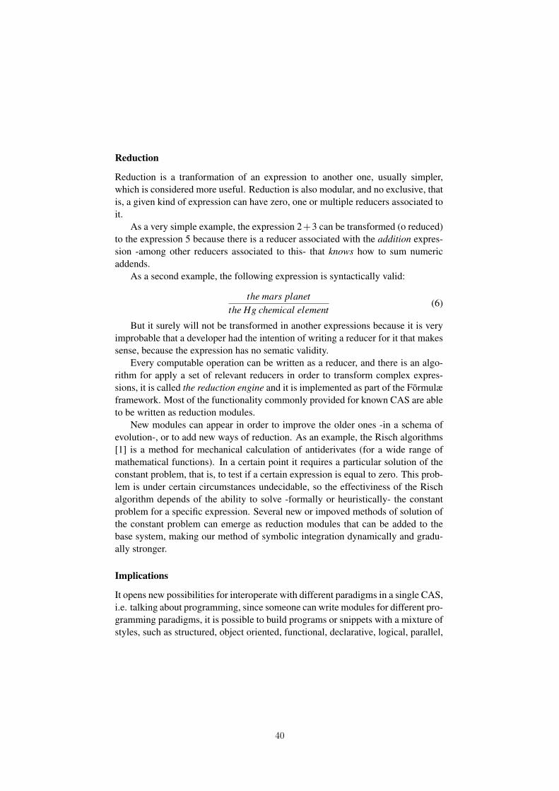
Reduction

Reduction is a tranformation of an expression to another one, usually simpler,which is considered more useful. Reduction is also modular, and no exclusive, thatis, a given kind of expression can have zero, one or multiple reducers associated toit.

As a very simple example, the expression 2+3 can be transformed (o reduced)to the expression 5 because there is a reducer associated with the addition expres-sion -among other reducers associated to this- that knows how to sum numericaddends.

As a second example, the following expression is syntactically valid:

the mars planetthe Hg chemical element

(6)

But it surely will not be transformed in another expressions because it is veryimprobable that a developer had the intention of writing a reducer for it that makessense, because the expression has no sematic validity.

Every computable operation can be written as a reducer, and there is an algo-rithm for apply a set of relevant reducers in order to transform complex expres-sions, it is called the reduction engine and it is implemented as part of the Formulæframework. Most of the functionality commonly provided for known CAS are ableto be written as reduction modules.

New modules can appear in order to improve the older ones -in a schema ofevolution-, or to add new ways of reduction. As an example, the Risch algorithms[1] is a method for mechanical calculation of antiderivates (for a wide range ofmathematical functions). In a certain point it requires a particular solution of theconstant problem, that is, to test if a certain expression is equal to zero. This prob-lem is under certain circumstances undecidable, so the effectiviness of the Rischalgorithm depends of the ability to solve -formally or heuristically- the constantproblem for a specific expression. Several new or impoved methods of solution ofthe constant problem can emerge as reduction modules that can be added to thebase system, making our method of symbolic integration dynamically and gradu-ally stronger.

Implications

It opens new possibilities for interoperate with different paradigms in a single CAS,i.e. talking about programming, since someone can write modules for different pro-gramming paradigms, it is possible to build programs or snippets with a mixture ofstyles, such as structured, object oriented, functional, declarative, logical, parallel,

40

etc. Other solutions can be transported to such an interoperable methodology, forexample, proof assistants and theorem provers.

There are certain computing science implications, the dynamic nature of defin-ing, creating and implement functionality implies a creation of a ontology (a dy-namic one) and it also affects the known methods of representation and transfer orknowledge

According to the results of Kurt Gödel and Alan Turing, there cannot exist aboth complete and consistent system for fundamental mathematics and computabil-ity. Going further, Gregory Chaitin [2] asserts that the concept of truth is not abso-lute, it could either change with time, be sometimes random and even be acciden-tal. In consecuence, as it is impossible to eventually create a complete/consistentmonolithic CAS, we must start to focus on dynamic, cooperative methods of de-velopement.

References[1] R. H Risch, The problem of integration in finite terms, pp. 167-189 (1969).[2] Gregory Chaitin, Meta Math! The Quest for Omega, (2005).

41

Browser-Based Collaboration with InkChat

Stephen M. Watt

University of Waterloo, Canada [email protected]

We present the elements of a new architecture for computer-assisted mathematicalcollaboration based on a shared virtual canvas. Free-hand pen input, geometricsketches, typed input and images can be entered and viewed simultaneously bymultiple participants. In particular, this allows the shared entry and manipulationof mathematics and the annotation of documents. Pen input is captured as InkML,rather than as raster graphics, allowing semantic analysis and manipulation. Unlikeprevious work, we make the communications layer fundamental and base compo-sition and editing functions on top of that, instead of viewing communication as anadd-on to a drawing program. Based on our past experience, we have chosen thistime to make ease of casual use and adoption the principal design criterion. Thishas led to a JavaScript browser implementation and cloud-based storage.

42

Computer Algebra in Education

43

Session Organizers

Alkis AkritasUniversity of [email protected]

Michael WesterUniversity of New [email protected]

Michel BeaudinETS, [email protected]

Jose Luis Galan GarcıaUniversidad de [email protected]

Elena VarbanovaTechnical University of [email protected]

Overview

Education has become one of the fastest growing application areas for computers in general andcomputer algebra in particular. Computer Algebra Systems (CAS) make for powerful teaching andlearning tools within mathematics, physics, chemistry, biology, economics, etc. Among them are:

• the commercial ”heavy weights” such as Casio ClassPad 330, Derive, Magma, Maple, Math-ematica, MuPAD, TI NSpire CAS, and TI Voyage 200, and

• the free software/open source systems such as Axiom, Euler, Fermat, wxMaxima, Reduce,and the rising stars such as GeoGebra, Sage, SymPy and Xcas (the swiss knife for mathe-matics).

The goal of this session is to exchange ideas, discuss classroom experiences, and to explore sig-nificant issues relating to CAS tools/use within education. Subjects of interest for this session willinclude new CAS-based teaching/learning strategies, curriculum changes, new support materials,assessment practices from all scientific fields, and experiences of joint use of applied mathematicsand CAS.

44

About balanced application of CAS in undergraduatemathematics

E. Varbanova

Technical University of Sofia, Bulgaria, [email protected]

In the methodology of mathematics teaching and learning [6] the main ques-tion is "Why?". It is about the learning outcomes and educational goals as wellas about educational values. The chain of questions "What-When-Where-How" isalso associated with it. On one side, they can be related to the curricula and courses.On the other side, they are mostly relevant to the teaching-learning-assessment(TLA) process. In the past two-three decades remarkable creative work with appli-cation of CAS has been done in undergraduate mathematics concerning these fourquestions. The care about the Why-question will never end because the world con-stantly changes. CAS is full of opportunity in this direction as well: for adequatedecisions about this question.

In this paper educational goals and values of the TLA of undergraduates math-ematics [2, 4] are considered. Based on examples [1, 5] the necessity of balancedapplication of CAS in education is discussed. The idea is to make what is importantCAS supported [3], rather than what is CAS supported important.

References[1] T. Arens, Hettlich, F., Karpfinger, Ch., Kockelkorn, U., Lichtenegger, K. & Stachel, H.

Mathematik, Heidelberg, Spektrum (2008).[2] S. Grozdev, For High Achievements in Mathematics. The Bulgarian Experience (Theory and

Practice), Sofia, ADE (2007).[3] E. Varbanova, CAS supported environment for learning and teaching Calculus, CBMS - Issues

in Mathematics Education: Enhancing University Mathematics, vol. 14, AMS & MAA (2007).[4] E. Varbanova, Calculus - I. Lecture Notes, Sofia, TU-Sofia (2009) (in Bulgarian).[5] E. Varbanova, Calculus - I. Exercises, TU-Sofia. (2011) (in Bulgarian).[6] G. Ganchev, Ninova, Yu., Nikova, V. Methodology of mathematics education, Blagoevgrad,

SWU "Neofit Rilski" (2007) (in Bulgarian).

45

Some reflections about open vs. proprietary ComputerAlgebra Systems in mathematics teaching

F. Botana

University of Vigo, Spain, webs.uvigo.es/fbotana

The talk will describe some personal reflections and experiences on using Com-puter Algebra Systems (CAS) for undergraduate mathematics teaching. I discussthe reasons behind my transition from using proprietary CAS to Sage for mathe-matics teaching purposes. Problems on this transition coming from the student andinstitution sides are considered.

Special attention is given to Wolfram|Alpha and Sage Cell. Both applicationsare web-based, suitable to use in small devices. Issues on accessibility, equity andstudent empowerment are discussed when selecting the teaching tool.

46

Create SageMath Interacts for All Your Math CoursesRazvan A. Mezei1

1 Lenoir-Rhyne University, Hickory, NC, USA, [email protected]

SageMath is a Free Open Source Software that is quickly gaining popularityin many areas of Mathematics. It has a very easy to learn Python-like syntax andgives you access to many open source packages such as: NumPy, SciPy, R, andother. One can freely download and use SageMath from their own computer, or canchoose to use it over the Cloud (SageCell and SageCloud are two great options).

In this talk the presenter will talk about the use of SageMath for various Math-ematics courses, for both Graduate and Undergraduate level. He will demonstratehow one can use SageMath as a rich Computer Algebra System (for College Al-gebra, Calculus, Abstract Algebra, Number Theory, etc), as a programming tool(for implementing Numerical Methods) or as a great interactive software (createSageMath interacts to demonstrate various Mathematics concepts).

References

[1] G. A. Anastassiou and Razvan A. Mezei, NUMERICAL ANALYSIS USING SAGE, to appear

Springer 2015.

[2] Razvan A. Mezei, An Introduction to SAGE Programming: with Applications to SAGE Interacts

for Numerical Methods, submitted 2015.

[3] William A. Stein et al., Sage Mathematics Software (Version 6.5), The Sage Development Team,

2015, http://www.sagemath.org.

47

Using SageMathCell and Sage Interacts to ReachMathematically Weak Business Students

Gregory V. Bard1

1 University of Wisconsin—Stout, Wisconsin, USA, [email protected]

In addition to a “business calculus” course, it is frequently required that stu-dents in business, economics, marketing, finance, accounting, and managementtake a course called Finite Mathematics in the USA, or Quantitative Methods inthe UK. These courses often cover an assortment 1 of topics, including financialmathematics, combinatorics/probability/statistics, and problem solving with sys-tems of linear equations, matrices, Gaussian elimination, and linear programming.

The topics of modeling with systems of linear equations and linear program-ming (systems of linear inequalities) are often traumatic for these students, whohave weak mathematical skills, poor study habits, and little motivation. This talkwill highlight some successful strategies that the speaker has used in teaching Fi-nite & Financial Mathematics at the University of Wisconsin—Stout, a polytech-nic located in the midwestern USA. In particular, the use of the computer algebraSage [6], in two forms, was tremendously successful. Sage is the free and open-source competitor to Maple, Mathematica, Matlab, and Magma. Because Sagecosts nothing to use, it is attractive for use in this present era of general fiscaldistress worldwide.

At the start of the class’s exploration of systems of linear equations/inequalities,a Sage “Interact” (a kind of app or interactive webpage) is used to model an indus-trial situation. To paint a clear picture, it is useful to describe this one “interact”in full detail at this time. An old factory is to be decommissioned, and a finalproduction run will be ordered to consume as much as is possible of existing dan-gerous supplies. Any unused supplies must be disposed of resulting in disposalfees which might be catastrophically expensive. The students can move sliders tofind a production schedule that must not use more supplies than actually exist, butthat hopefully uses up “a lot” of the dangerous supplies. Usually a room full of 40students, each experimenting on a laptop, will have a range of solutions resultingin disposal fees of around 5,000,000 to 500,000 dollars. Then a linear system ofequations in four variables can be derived by the instructor, which solves the prob-lem exactly—and which results in disposal fees of 0 dollars. The students see thatknowing how to solve a system of linear equations will save the company between500,000 and 5,000,000 dollars, and this makes them motivated to pay attention

1For a syllabus, see http://www.uwstout.edu/mscs/upload/MATH-123.pdf as an example.

48

during the start of this critical chapter. The reader is now invited to experimentwith this interact, to be found at [1], before reading further in this abstract.

After such an introduction, students will begin to read solutions of longer prob-lems, and then attempt to solve problems on their own. Typical American textbookswill have problems of two, three, and at most four variables during these two topics(systems of linear equations and linear programming) [3], [4], [5], [7]. The prob-lems often are unrealistic, with “round numbers” to facilitate solving the problemsby hand. In stark contrast to this, the speaker uses detailed problems with realisticnumbers, many variables, and many equations/inequalities. Those would be un-pleasant or nearly impossible to solve by hand. However, using SageMathCell, thesystems can be easily solved. Moreover, SageMathCell works through the web-browser2, and therefore the students do not need to install anything.

During this talk, the speaker will present the above example, and then two orthree other examples used in his teaching. The result of using computer algebratools in this manner is that the course is transformed from focusing on the mechan-ical actions of performing Gaussian Elimination and the Simplex Method into onewhere students read complex problems, and then must model the problems as asystem of equations or system of inequalities. While challenging, modeling indus-trial and commercial phenomena is more intellectual and a better preparation forthe modern workplace.

While the speaker is not in a position to run a controlled experiment to provethe efficacy of these teaching methods, there have been several benefits in his ownclassroom. The students are more engaged, more likely to attempt the homeworkproblems, they score higher on examinations, and they give the instructor betterteaching evaluations. Moreover, the faculty members of the College of Manage-ment at the speaker’s university have gone from expressing grave concerns to prais-ing the mathematics department.

References[1] G. Bard, A Production Problem: Shutting down a Solvents Factory. An Interactive Applet

powered by Sage and MathJax. (2013).

http://www.gregorybard.com/interacts/solvent_factory.html[2] G. Bard, and J. Bertino. Applied Finite & Financial Mathematics for University Freshmen. A

textbook in progress.

http://www.gregorybard.com/finite.html[3] R. Barnett, M. Ziegler, and K. Byleen. College Mathematics for Business, Economics, Life

Sciences and Social Sciences. 12th ed. Pearson/Prentice Hall. (2010).

2https://sagecell.sagemath.org/

49

[4] L. Goldstein, D. Schneider, and M. Siegel. Finite Mathematics & Its Applications. 10th ed.Pearson/Prentice Hall. (2010).

[5] M. Lial, R. Greenwell, and N. Ritchey. Finite Mathematics and Calculus with Applications.10th ed. Pearson/Prentice Hall. (2011).

[6] W. Stein, et al, Sage Mathematics Software. The Sage Development Team, 2015.

http://www.sagemath.org/[7] S. Tan. Finite Mathematics for the Managerial, Life, and Social Sciences. 7th ed. Thomson

Brooks/Cole. (2003).

50

GINI-Coefficient, GOZINTO-Graph

and Option Prices

Josef Böhm, ACDCA & DERIVE User Group, [email protected]

Abstract: GINI-Coefficient together with LORENZ-curve and GOZINTO-

Graphs are economic applications of secondary school mathematics. They are

part of the curriculum in Austria’s Colleges for Business Administration (=

Handelsakademie). Basic knowledge about stocks and options became

important during the last years. Treating these issues are easy using

technology.

The GOZINTO-Graph or GOZINTO-Chart is a pictorial representation that

shows how the elements required to build a product fit together. This is often

the first step for several planning functions especially for material

requirements planning, for time and manpower resources planning, for

production cost, etc.

This chart gives the input for building the production matrix. Easy to

understand, and supported by technology, easy to perform matrix calculations,

lead to the results.

Students can easily be inspired to design own tasks. Examples of students’

works will be presented.

The GINI-Coefficient is a means for measuring the income distribution – and

other distributions - of a nation’s population. It is commonly used as a

measure of inequality of income or wealth.

This sounds a little bit complicated but in fact it is an easy to perform

application of integration based on the modelling of the so called LORENZ-

Curve. We should be happy to find an application of definite integral which is

not only calculation of the area between two curves.

Calculation of option prices is based on stock data (average rate of return,

volatility, and other statistics – all well known in school). We will

demonstrate the binomial model and the extend to the famous Black-Scholes

formula.

51

When Mathematics Meet Computer Software

M. Beaudin, F. Henri

École de technologie supérieure (ÉTS), Montréal, Québec, Canada

[email protected], [email protected]

TI-Nspire CAS, from Texas Instruments, is the current computer algebra sys-tem used for both undergraduate level mathematics and science courses at ÉTS.While not as powerful as Maple or Mathematica, it offers some advantages overits competitors, mainly being multi-platform (calculator and computer) and easy touse. However, the lack of some useful functions becomes obvious when someonewants to perform higher mathematical development. A fruitful collaboration be-tween the authors has produced interesting developments regarding the integrationof piecewise functions [1] and the convolution of signals [2]. This talk will focuson our latest additions to the TI-Nspire system, namely automating the series solu-tion for first and second order ODEs.

References[1] Michel Beaudin, Frédérick Henri, Geneviève Savard. Integration of Piecewise Continuous

Functions. The Derive Newsletter 91 (2013) 3–21. http://www.austromath.at/dug/dnl91.pdf[2] Michel Beaudin. https://cours.etsmtl.ca/seg/mbeaudin/Liste_WEB.pdf

52

Revival of a Classical Topic in Differential Geometry:Envelopes of Parameterized Families of Curves andSurfaces

Th. Dana-Picard1, N. Zehavi2

1 Jerusalem College of Technology, [email protected] Weizmann Institute, [email protected]

Classical topics in Differential Geometry like the study of 1-parameter familiesof curves and surfaces in 3D space and their envelopes have been abandoned inthe past for various reasons [4]. Nevertheless, this topic has a great interest inmathematics and in applied science. The topic has lots of applications in scienceand engineering - caustics and wave fronts, i.e. Geometrical Optics and Theoryof Singularities, robotics and kinematics, rigid motion in 2-space and in 3-space,collision avoidance, etc. Envelopes can be studied with paper-and-pencil togetherwith both a Computer Algebra System (CAS) and a Dynamical Geometry System(DGS); see recent papers in [5]. For this work, we used more than one package.

The authors performed similar work for another topic in classical DifferentialGeometry, namely isoptic curves of a given plane curve; see [1]. The influence ofthe technology was important. Here,as we will see, dynamical features are central.

Let be given a family of plane curves by an equation of the form f (x,y,c) = 0,where c is a real parameter. An envelope of the family, if it exists, is a curve tangentto every curve in the family. It can be shown that this envelope is the solution setof the system of equations

f (x,y,c) = 0∂ f∂c f (x,y,c) = 0

(1)

Figure 1 shows the envelope of the family of lines given by the equation x +cy = c2, where c is a real parameter (it is the parabola whose equation is y = −x2/4.and the envelope of the family of circles with radius 1 and center on the parabolawhose equation is y = x2 (here the result has two components, each component isan envelope of the family of circles).

In both cases, the usage of a slider bar enables to build envelopes experimen-tally. The experimental study may enhance the understanding either of the possiblenon-existence or of the possible non-uniqueness of an envelope. An example is dis-played in Figure 2 for the family of circles whose radius is equal to 1 and whosecenter runs on an ellipse. On the left a partial construction is shown, a global con-struction appears on the right. This drawing has been obtained using the slider bar,

53

(a) Lines (b) Circles

Figure 1: Exploration of an envelope in the plane

which yields a uniform spacing between circles. Another possibility offered by thesoftware is to move the center of the circle along the ellipse. In this case, spacingbetween neighboring circles is not uniform, the appearance of the envelopes beingthus slightly different.

Figure 2: Dynamical exploration of the envelope of a family of circles

The transition to parameterized families of curves and surfaces in 3D spacerely on the same techniques. For a 1-parameter family of surfaces, the definingequations for an envelope are now:

f (x,y,z,c) = 0∂ f∂c f (x,y,z,c) = 0

(2)

New issues have to be dealt with: the general visualization problems in this case,

54

the availability of appropriate features in the software, etc. For the family of sur-faces given by the equation x + cy + c2z = c3, where c is a real parameter, an en-velope can be found, shown in Figure 3. A cuspidal edge appears, as for every1-parameter family of planes. In order to understand the surface visually, dynami-cal features of the software are a must. Otherwise, at least two stills pictures haveto been plotted. In particular in such a case, the structure of the envelope as aruled surface can be studied using technology. This topic is sometimes not easyfor beginning students. We could check the influence of the choice of the meshfor plotting surfaces in 3D space on the students’ understanding. For example, inFigure 3, lines can be seen who are tangent to the cuspidal edge; this is a centralfeature of such an envelope.

Figure 3: Exploration of the envelope of a family of planes

Such a study provides an opportunity to discover new topics beyond the scopeof the regular curriculum, sometimes together with applications to practical situ-ations. New computation skills with technology may be developed, in particularfor the experimental aspect of the work (e.g., exploring the existence of cusps, asin Figure 1b). For this, the availability in the software of a slider bar is a centralissue. Moreover, ability to switch between different registers of representation maybe improved, within mathematics themselves (parametric vs implicit) and with thecomputer (algebraic, graphical, etc.).

An envelope may not exist (e.g. for a family of lines where the coefficients ofthe equations are affine functions of the parameter). These issues have been ob-served by the authors in sessions for in-service teachers at the Weizmann Instituteof Science.

The algebraic engine we used in different CAS was the commands based oncomputations of Gröbner bases in order 1) to solve the given system of equations,which yields a parametric representation of the envelopes, and 2) to look for an im-

55

plicitization of this parametric representation. The Gröbner bases algorithms havebeen widely used by Pech [2] for other geometric problems. When such an implic-itization is not to be found, algorithms exist for an approximate implicitization (see[3]).

References[1] Dana-Picard, Th., Mann, G. and Zehavi, N. Bisoptic curves of a hyperbola, International

Journal of Mathematical Education in Science and Technology 45 (5), pp. 762-781 (2014).[2] Pech, P. Selected Topics In Geometry With Classical Vs. Computer Proving, World Scientific

(2007).[3] Pottman, H. and Peternell, M. Envelopes Computational Theory and Applications, in Pro-

ceedings of Spring Conference in Computer Graphic, Budmerice, Slovakia, pp. 3-23 (2000).[4] Thom, R. Sur la théorie des enveloppes. Journal de Mathématiques Pures et Appliquées, XLI

(2), pp. 177-192 (1962).[5] DNL 97. Derive Newsletter 97, April 2015. Available:

http://www.austromath.at/dug/dnl97.pdf

56

Generating animations of JPEG images of closed surfacesin space using Maple and Quicktime

G. Labelle1

1 Université du Québec à Montréal (UQAM), Canada, [email protected]

Too often, in undergraduate several variables calculus courses, surfaces arepresented essentially only in the form,

z = f (x,y), or its variants, y = g(x,z), x = h(y,z), (1)

instead of the more symmetrical and versatile parametric form,

x = x(u,v), y = y(u,v), z = z(u,v). (2)

Forms (1) are not very well adapted to evaluate surface integrals in order to illus-trate, for example, the divergence theorem for closed surfaces in 3D space (such asa deformed sphere or twisted torus). Indeed, one must decompose the surface intosmaller pieces and use several variants of (1) to compute double integrals whichare then added or substracted taking into account various orientation issues.

In this talk, we show how to use periodic functions of u and v in the parametricform (2), to generate, via Maple, various large high quality JPEG images of closedsurfaces in space for which the surface integrals are easily computed, among otherthings. Moreover, we also use QuickTime to pass from one surface to another ina very smooth animated way. Many examples as well as the Maple code used aregiven. Students are then able to easily generate their own surfaces and analyse theirvarious geometrical properties in a very stimulating and colorful way.

References[1] G. Labelle, Des surfaces animées qui respirent dans l’espace, Bulletin AMQ, vol. 50, no.4,

49-58 (2010). http://archimede.mat.ulaval.ca/amq/Bulletins.html[2] G. Labelle, http://www.lacim.uqam.ca/~gilbert

57

Plotting technologies for the study of functions of two realvariables

David Zeitoun1 and Thierry Dana-Picard2

1 Department of Mathematics, Orot College of Education, Rehovot, Israel,[email protected] Department of Mathematics, Jerusalem College of Technology, Jerusalem , Israel, [email protected]

Students learning towards a degree in a STEM related domain learn quite earlya course in Advanced Calculus, i.e. a course where the main object of study aremultivariable functions. It happens that students cannotseehow these objects be-have. In particular, difficulties appear in classroom for functions having differentlimits at a point, according to the path approaching the point. Therefore dynamicalvisualization techniques are important.

The study of functions of two real variables can be supportedby visualizationusing a Computer Algebra System (CAS). Contour plots were the first type ofgraphic representations. With the development of scientific computing, 3D plotswere introduced and plotting the graph of a two-variable function has been madepossible, including parametric plotting and implicit plotting.

Depending both on the hardware and on the software, constraints exist, makingsometimes the plots non accurate. For example, the choice ofthe mesh (using atriangulation of the domain, or using geodesics on the surface, etc.) has a greatinfluence on the representation. Interpolations are performed, which may hidediscontinuities. Other constraints come from the need to control the geometrictransformations of the plotted surface: transformations such as zooming, rotationaround a given axis, displacement along a given path are examples where the visu-alization device needs to understand the mathematical behavior of the function.

Here are examples of non-accurate plots, obtained with a brute force usageof commands, without a suitable analysis of the function. The function we triedto plot in Figure 1 is given byf (x,y) = 1

1−(x2+y2). The only difference in the

command that has been entered is the x-intervals and the y-intervals,[−2,2] in (a)and[−3,3] in (b). The rightmost plot is quite accurate, it uses other techniques.

In the unaccurate plots, interpolations hide the actual discontinuities in differ-ent ways. Regular zooming cannot solve this problem, as it inflates the cells butdoes not recompute the needed numerical data.

Rotation around a given axis often masks discontinuities ofthe function andcan also provide strange plots, not compatible with the mathematics. In recentyears, point based geometry has gained increasing attention as an alternative sur-face representation, both for efficient rendering and for flexible geometry process-

58

(a) (b) (c)

Figure 1: Strange plots

ing of complex surfaces. More sophisticated representations that use lighting ef-fects and virtual reality are available. We analyze the efficiency of the differentrepresentations with respect to the mathematical behaviorof a function of two realvariables.

Figure 2: Interface

An interface written in Matlab 14 has been developed for producing differentrepresentations of a given explicit function of two variables; (see Figure 2). Afterhaving received an analytic expression for the function, the software produces fourtypes of representation, namely:

1. A color contour map of the function.

2. A three dimensional plot of function.

3. A relief terrain map corresponding to the height of the function.

4. A virtual reality scene where the function is a terrain andthe user is flyingover it.

59

The first three representations are illustrated for the function given by f (x,y) =x2 +y2 in Figure 3. Note that this function has a discontinuity at(0,0).

(a) Contours (b) 3D plot (c) Terrain relief

Figure 3: Color plottings

The virtual reality scene is shown for the same function in Figures (4 and 5).

Figure 4: Virtual scene

Figure 5: Path along a discontinuity

Comparison between the different kinds of representation is done with respectto the accuracy and the teaching of:

1. The global plotting of the function.

2. The appearance of the existing discontinuities and the non-appearance ofnon-existing discontinuities.

60

3. The visualization of directional derivatives.

4. The different types of optima, such as maximum. minimum points and sad-dle points.

Some of the issues that are to be discussed are as follows, allof them have aninfluence on the joint work of the students and the educator :

• The domain of the given function may be unbounded. Nevertheless, theplotting domain is always bounded; this is one of the constraints mentionedpreviously.

• Meshing techniques versus isoclines plotting.

This comparison and its outcome were an incitement to the usage of virtualreality in order to represent a function of two variables. Inparticular, the VR deviceunder development is designed to generate paths on the surface under study and toreplace classical zooming which only inflates the existing cells of the mesh by are-computation of the data required for the plotting. This may allow to visualizeclearly discontinuities and different types of extrema.

References

[1] Amenta N, Bern M, Kamvysselis M.A new Voronoi - based surface recon-struction algorithm. In: Proceedings of ACM SIGGRAPH 98, pp. 415-21(1998).

[2] Botsch M, Kobbelt L.,Resampling feature and blend regions in polygonalmeshes for surface antiÂaliasing. In: Proceedings of Eurographics 01, pp.402-10 (2010).

[3] Th. Dana-Picard:Enhancing conceptual insight: plane curves in a comput-erized learning environment, International Journal of Technology in Mathe-matics Education12 (1), pp. 33-43, (2005).

[4] Th. Dana-Picard, I. Kidron and D. Zeitoun:To See or not To See II, Interna-tional Journal of Technology in Mathematics Education 15 (4), pp. 157-166,(2008).

[5] Dos Santos S.R. and Brodlie K.W.,Visualizing and Investigating Multidimen-sional Functions, IEEE TCVG Symposium on Visualization, pp. 1-10. JointEUROGRAPHICS, (2002).

61

[6] Kobbelt L. and Botsh M.,A survey of point-based techniques in computergraphics, Computer and Graphics28, pp. 801-814, (2004).

[7] Kobbelt L, Botsch M, Schwanecke U, Seidel HÂP.Feature sensitive surfaceextraction from volume data, in Proceedings of ACM SIGGRAPH01, pp. 57-66, (2001).

[8] Dana-Picard Th. , Badihi Y. , Zeitoun D. and Israeli O.,Dynamical Ex-ploration of Two-Variable Functions Using Virtual Reality, Proceedings ofCERME 6, Lyon (France), (2009).

[9] Zeitoun D.G. and T. Dana PicardAccurate visualization of graphs of func-tions of two real variables, International Journal of Computational and Math-ematical sciences Vol 4 (1), pp. 1-11, (2010).

[10] Zeitoun D.G., Laible J.P. and G.F. Pinder,An Iterative Penalty Method forthe Least Squares Solution of Boundary Value Problems, Numer. Meth. forP.D.E.13, pp. 257-281, (1997).

62

Some remarks on Taylor’s polynomials visualization usingMathematica in context of function approximation.

Włodzimierz Wojas1, Jan Krupa2

1 Warsaw University of Life Sciences (SGGW), Poland, [email protected] Warsaw University of Life Sciences (SGGW), Poland, [email protected]

In this paper the authors critically analyse popular way of graphic presentationTaylor’s polynomials in context of function approximation. They discuss the dif-ficulties of presentation the best local polynomial approximation of function byTaylor’s polynomials. Proposed by the authors method of graphical presentationbased on table of function and Taylor’s polynomials values in neighbourhood of achosen point. For graphical presentation ListPlot and Plot functions with logarith-mic scale in Mathematica System is used.

Introduction

Taylor’s theorem is one of the most classic results of university course in calculusor mathematical analysis. For the case of one variable function y = f (x) and pointx = x0, Taylor’s polynomial of the n-th order is defined as:

Tn(x) = f (x0)+f ′(x0)

1!(x− x0)+

f ′′(x0)

2!(x− x0)2 + · · ·+ f (n)(x0)

n!(x− x0)n

where a function f (x) have at a point x0 finite derivatives up to the n-th orderinclusively. Many academic books e.g. [1, 2, 3, 4] contain graphs presented Tay-lor’s polynomials for some elementary functions. For example for f (x) = ex orf (x) = sinx as is shown in Figures 1,2. Often these graphs are presented with com-ments that it shows how well these polynomials approximate y = f (x) near a pointx = x0 when n increases.

63

-6 -4 -2 2 4 6x

-10

10

20

y

expHxL

T1HxL

T2HxL

T3HxLT4HxL

Figure 1: Taylor’s polynomials T1(x), T2(x), T3(x), T4(x) for function f (x) = ex atpoint x0 = 0.

Π 2 Πx

-10

-5

0

5

10

y

sinHxL

T1HxL

T3HxL

T5HxL

T7HxL

T9HxL

T11HxL

T13HxL

Figure 2: Taylor’s polynomials T1(x), T3(x), . . . ,T13(x) for function f (x) = sinx atpoint x0 = 0.

64

1 Visualization of Taylor’s polynomials in context of func-tion approximation

Visualization of Taylor’s polynomials is easy and comfortable using CAS packagessuch as Mathematica, Maple, Derive or others. For a one variable function Math-ematica package contains standard procedure Series[ f ,x,x0,n] which generatesTaylor’s polynomial of the n-th order for the function f (x) and point x = x0. Usingprocedure Plot[ f1, f2, . . . , fk,x,xmin,xmax] we can present graphs function f (x)and some its Taylor’s polynomials as is shown in Figures 1, 2. But this kind ofpresentation can be misleading for students in context of the function f (x) approx-imation by Taylor’s polynomials if we do not emphasize the fact of local characterof this approximation. In Figures 3, 4 we see that graph of the function f (x) andgraphs of Taylor’s polynomials seem to overlap close point x = x0. On the base ofthese Figures we cannot settle which Taylor’s polynomial better approximates thefunction close to the point x0.

0.002 0.006 0.01x

1.002

1.004

1.006

1.008

1.010

y

T4HxLT3HxLT2HxLT1HxLexpHxL

Figure 3: function f (x) = ex and its Taylor’s polynomials T1(x), T2(x), T3(x), T4(x)in the reduced right neighbourhood (0,0.01) of the point x0 = 0.

65

0.002 0.005 0.01x0.000

0.002

0.004

0.006

0.008

0.010

y

T13HxLT11HxLT9HxLT7HxLT5HxLT3HxLT1HxLsinHxL

Figure 4: function f (x) = sinx and its Taylor’s polynomials T1(x), T3(x), . . . ,T13(x)in the reduced right neighbourhood (0,0.01) of the point x0 = 0.

In Figures 1, 2 we see that graph of the function f (x) and graphs of Taylor’spolynomials seem to overlap close the point x0 = 0. Next, Taylor’s polynomialsseparate from the graph of the f (x). Closer to the point x0 separates Taylor’s poly-nomial of lower order, further from the point x0 separates Taylor’s polynomial ofhigher order. Figures 1, 2 may suggest that overall Taylor’s polynomial of higherorder better approximates the function than Taylor’s polynomial of lower order.But for example, for the function f (x) = ex, x0 = 0 and the point x =−4 it is easyto check that:T2(x) = 1+x+

12!

x2,T3(x) = 1+x+12!

x2 +13!

x3, | f (−4)−T2(−4)|= |e−4−5|<| f (−4)− T3(−4)| = |e−4 + 17/3|. So, T2(x) better approximates the functionf (x) = ex at the point x = −4 than T3(x). Similarly, for the function f (x) = sinx,x0 = 0 and the point x = 5

4 π we have:T3(x) = x− 1

3! x3,T5(x) = x− 1

3! x3 + 1

5! x5, and | f (5

4 π)−T3(54 π)| ≈ 5.46 < | f (5

4 π)−T5(5

4 π)| ≈ 7.88. So, T3(x) better approximates the function f (x) = sinx at the pointx = 5

4 π than T5(x). Generally, Taylor’s polynomial of higher order better approx-imates the function than Taylor’s polynomial of lower order only locally in someneighbourhood of the point x0.

2 Theorem of the best local polynomial approximation

This theorem and corollaries from it are inspired by theorem of the best local ap-proximation presented in [5].

Let P(x) = p0 + p1(x− x0)+ p2(x− x0)2 + . . .+ pm(x− x0)m and Q(x) = q0 +

66

q1(x− x0) + q2(x− x0)2 + . . .+ qk(x− x0)k are different polynomials. Let r be thesmallest nonnegative integer among numbers i = 0,1,2, . . . which satisfy pi 6= qi (ifm > k then we put qk+1 = . . . = qm = 0, if m < k then we put pm+1 = . . . = pk = 0).

Assume that function f (x) has finite derivative of n order at point x0 and assumer ≤ n.

Theorem. If pi = f (i)(x0)i! for all i < r and | f (r)(x0)

r! − pr| < | f (r)(x0)r! − qr| then there

exists such neighbourhood S of point x0 such that∧

x∈S

| f (x)−P(x)|< | f (x)−Q(x)|.

Proof. By Taylor’s theorem we have: f (x)−Tn(x) = (x− x0)nω(x), whereω(x) is a function continuous at x0 and ω(x0) = 0. Thus:

| f (x)−P(x)|

=∣∣∣(

f r(x0)

r!− pr

)(x− x0)r +

f r+1(x0)

(r + 1)!(x− x0)r+1 + · · ·+ f n(x0)

n!(x− x0)n

+(x− x0)nω(x)− pr+1(x− x0)r+1−·· ·− pm(x− x0)m∣∣∣,

| f (x)−Q(x)|

=∣∣∣(

f r(x0)

r!−qr

)(x− x0)r +

f r+1(x0)

(r + 1)!(x− x0)r+1 + · · ·+ f n(x0)

n!(x− x0)n

+(x− x0)nω(x)−qr+1(x− x0)r+1−·· ·−qk(x− x0)k∣∣∣.

Taking the factor (x− x0)r out we have:

| f (x)−P(x)|

= |(x− x0)r| ·∣∣∣(

f r(x0)

r!− pr

)+

f r+1(x0)

(r + 1)!(x− x0)+ · · ·+ f n(x0)

n!(x− x0)n−r

+(x− x0)n−rω(x)− pr+1(x− x0)−·· ·− pm(x− x0)m−r∣∣∣.

| f (x)−Q(x)|

= |(x− x0)r| ·∣∣∣(

f r(x0)

r!−qr

)+

f r+1(x0)

(r + 1)!(x− x0)+ · · ·+ f n(x0)

n!(x− x0)n−r

+(x− x0)n−rω(x)−qr+1(x− x0)−·· ·−qk(x− x0)k−r∣∣∣.

67

The above equalities are true if m > r and k > r. If m≤ r, then defining pm+1 =pm+2 = . . . = 0 we have:

| f (x)−P(x)|

=∣∣∣(

f r(x0)

r!− pr

)(x− x0)r +

f r+1(x0)

(r + 1)!(x− x0)r+1 + · · ·+ f n(x0)

n!(x− x0)n

+(x− x0)nω(x)∣∣∣

= |(x− x0)r| ·∣∣∣(

f r(x0)

r!− pr

)+

f r+1(x0)

(r + 1)!(x− x0)+ · · ·+ f n(x0)

n!(x− x0)n−r

+(x− x0)n−rω(x)∣∣∣

and if k ≤ r then defining qk+1 = qk+2 = . . . = 0 we have:

| f (x)−Q(x)|

=∣∣∣(

f r(x0)

r!−qr

)(x− x0)r +

f r+1(x0)

(r + 1)!(x− x0)r+1 + · · ·+ f n(x0)

n!(x− x0)n

+(x− x0)nω(x)∣∣∣

= |(x− x0)r| ·∣∣∣(

f r(x0)

r!−qr

)+

f r+1(x0)

(r + 1)!(x− x0)+ · · ·+ f n(x0)

n!(x− x0)n−r

+(x− x0)n−rω(x)∣∣∣

(both numbers k and m cannot be at the same time less than r).As x approaches to x0 we obtain:

limx→x0

∣∣∣( f r(x0)

r!− pr

)+

f r+1(x0)

(r + 1)!(x− x0)+ · · ·+ f n(x0)

n!(x− x0)n−r

+(x− x0)n−rω(x)− pr+1(x− x0)−·· ·− pm(x− x0)m−r∣∣∣

=∣∣∣ f r(x0)

r!− pr

∣∣∣,

limx→x0

∣∣∣( f r(x0)

r!−qr

)+

f r+1(x0)

(r + 1)!(x− x0)+ · · ·+ f n(x0)

n!(x− x0)n−r

+(x− x0)n−rω(x)−qr+1(x− x0)−·· ·−qk(x− x0)k−r∣∣∣

=∣∣∣ f r(x0)

r!−qr

∣∣∣.

68

Because of our assumption∣∣∣ f (r)(x0)

r! − pr

∣∣∣<∣∣∣ f (r)(x0)

r! −qr

∣∣∣ and the last two limits weconclude that there exists such neighbourhood S of point x0 such that

∧

x∈S

∣∣∣( f r(x0)

r!− pr

)+

f r+1(x0)

(r + 1)!(x− x0)+ · · ·+ f n(x0)

n!(x− x0)n−r

+(x− x0)n−rω(x)− pr+1(x− x0)−·· ·− pm(x− x0)m−r∣∣∣

<∣∣∣( f r(x0)

r!−qr

)+

f r+1(x0)

(r + 1)!(x− x0)+ · · ·+ f n(x0)

n!(x− x0)n−r

+(x− x0)n−rω(x)−qr+1(x− x0)−·· ·−qk(x− x0)k−r∣∣∣

Multiplying both sides of the last inequality by |(x− x0)r| we obtain that∧

x∈S

| f (x)−P(x)|< | f (x)−Q(x)|.

In cases m≤ r or k ≤ r the proof is analogous.

Corollary 1. Let Q(x) be a polynomial which satisfies: there exists i (i ≤ n)

such that qi 6=f (i)(x0)

i!(if m < n then we define qm+1 = qm+2 = . . . = qn = 0).

Then there exists such neighbourhood S of point x0 such that,∧

x∈S

| f (x)−Tn(x)| <

| f (x)−Q(x)|. Particularly Q(x) can be any polynomial of order not greater thann different than Tn(x).

Corollary 2. There exists such neighbourhood S of point x0 such that,∧

x∈S

| f (x)−Tn(x)| ≤ | f (x)−Tn−1(x)| ≤ . . .≤ | f (x)−T1(x)|,

where every inequality from the last sequence of inequalities becomes equality ifand only if when the two consecutive Taylor’s polynomial of f (x) in both sides ofthe inequality are identical.

3 Visualization of the best locally approximation by Tay-lor’s polynomials with Mathematica

Let us visualize Corollary 1 and 2 for reduced right neighbourhood (0,0.01) of thepoint x0 = 0 using Wolfram Mathematica System [6, 7].

Example 1. For the Corollary 1 we define: f (x) = ex, x0 = 0, T2(x) = 1+x+ 12! x

2

and P(x) = 1 + x− 12! x

2 for x ∈ (0,0.01). By Taylor’s theorem we get:

ex−T2(x) = ex− (1 + x +12!

x2) =13!

(ex)x3 > 0

69

and ex−P(x) = 1 + x + 12! x

2 + 13!(ex)x3− (1 + x− 1

2 x2) = x2 + 13!(ex)x3 > 0 for

x ∈ (0,x),x ∈ (0,0.01).Hence, we have: | f (x)−T2(x)|− | f (x)−P(x)|= ex− (1 + x + 1

2 x2)− ex + 1 + x−12 x2 =−x2 < 0and finally

∧

x∈(0,0.001)

| f (x)−T2(x)|< | f (x)−P(x)|.

Let us visualize this inequality by creating a table of numerical values for bothsides of inequality with step 0.001.

x fHxL T2HxL PHxL fHxL - T2HxL¤ fHxL - PHxL¤0. 1. 1. 1. 0 0

0.001 1.001 1.001 1.001 1.667083416680558´ 10-10 1.000166708341668´ 10-6

0.002 1.002 1.002 1.002 1.334000266755581´ 10-9 4.001334000266756´ 10-6

0.003 1.003 1.003 1.003 4.503377026012934´ 10-9 9.004503377026013´ 10-6

0.004 1.00401 1.00401 1.00399 1.067734187235881´ 10-8 0.00001601067734187236

0.005 1.00501 1.00501 1.00499 2.085940106338357´ 10-8 0.00002502085940106338

0.006 1.00602 1.00602 1.00598 3.605406486485558´ 10-8 0.00003603605406486486

0.007 1.00702 1.00702 1.00698 5.726684855523160´ 10-8 0.00004905726684855523

0.008 1.00803 1.00803 1.00797 8.550427343117207´ 10-8 0.00006408550427343117

0.009 1.00904 1.00904 1.00896 1.217738678140626´ 10-7 0.00008112177386781406

0.01 1.01005 1.01005 1.00995 1.670841680575422´ 10-7 0.0001001670841680575

Table 1: the values of f (x), T2(x),P(x), | f (x)−T2(x)| and | f (x)−P(x)| with step0.001

We see in Table 1 that for all considered points inequality is true. Based on theTable1 we can prepare Figure 5 using logarithmic scale. Increasing WorkingPreci-sion and Accuracy in Mathematica Plot function we can get the continous graphspresented in Figure 6

70

0.002 0.006 0.01x

-10

-8

-6

-4

-2

0

log10HyL

log10H f HxL - T2HxL¤L

log10H f HxL - PHxL¤L

Figure 5: discrete graphs of | f (x)−T2(x)| and | f (x)−P(x)| in reduced right neigh-bourhood (0,0.01) of the point x0 = 0 with logarithmic scale using MathematicaPlot function.

0.002 0.006 0.01x

-15

-10

-5

0

log10HyL

log10H f HxL - T2HxL¤Llog10H f HxL - PHxL¤L

Figure 6: continuous graphs of | f (x)− T2(x)| and | f (x)−P(x)| in reduced rightneighbourhood (0,0.01) of the point x0 = 0 with logarithmic scale using Mathe-matica Plot function.

In Figure 5 we see that the graphs of | f (x)−T2(x)| and | f (x)−P(x)| are sepa-rated and that | f (x)−T2(x)|< | f (x)−P(x)| for x ∈ (0,0.01).

Example 2. For the Corollary 2 we define: f (x) = sinx,x0 = 0,T3(x) = x− 1

3! x3,

T7(x) = x− 13! x

3 + 15! x

5− 17! x

7,

71

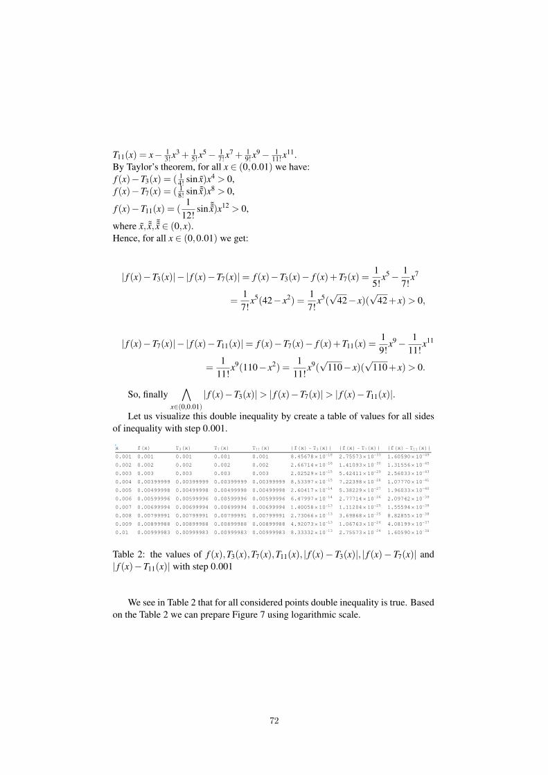
T11(x) = x− 13! x

3 + 15! x

5− 17! x

7 + 19! x

9− 111! x

11.By Taylor’s theorem, for all x ∈ (0,0.01) we have:f (x)−T3(x) = ( 1

4! sin x)x4 > 0,f (x)−T7(x) = ( 1

8! sin ˜x)x8 > 0,

f (x)−T11(x) = (1

12!sin ˜x)x12 > 0,

where x, ˜x, ˜x ∈ (0,x).Hence, for all x ∈ (0,0.01) we get:

| f (x)−T3(x)|− | f (x)−T7(x)|= f (x)−T3(x)− f (x)+ T7(x) =15!

x5− 17!

x7

=17!

x5(42− x2) =17!

x5(√

42− x)(√

42 + x) > 0,

| f (x)−T7(x)|− | f (x)−T11(x)|= f (x)−T7(x)− f (x)+ T11(x) =19!

x9− 111!

x11

=1

11!x9(110− x2) =

111!

x9(√

110− x)(√

110 + x) > 0.

So, finally∧

x∈(0,0.01)

| f (x)−T3(x)|> | f (x)−T7(x)|> | f (x)−T11(x)|.

Let us visualize this double inequality by create a table of values for all sidesof inequality with step 0.001.

x fHxL T3HxL T7HxL T11HxL fHxL - T3HxL¤ fHxL - T7HxL¤ fHxL - T11HxL¤0.001 0.001 0.001 0.001 0.001 8.45678 ´ 10-18 2.75573 ´ 10-33 1.60590 ´ 10-49

0.002 0.002 0.002 0.002 0.002 2.66714 ´ 10-16 1.41093 ´ 10-30 1.31556 ´ 10-45

0.003 0.003 0.003 0.003 0.003 2.02529 ´ 10-15 5.42411 ´ 10-29 2.56033 ´ 10-43

0.004 0.00399999 0.00399999 0.00399999 0.00399999 8.53397 ´ 10-15 7.22398 ´ 10-28 1.07770 ´ 10-41

0.005 0.00499998 0.00499998 0.00499998 0.00499998 2.60417 ´ 10-14 5.38229 ´ 10-27 1.96033 ´ 10-40

0.006 0.00599996 0.00599996 0.00599996 0.00599996 6.47997 ´ 10-14 2.77714 ´ 10-26 2.09742 ´ 10-39

0.007 0.00699994 0.00699994 0.00699994 0.00699994 1.40058 ´ 10-13 1.11204 ´ 10-25 1.55594 ´ 10-38

0.008 0.00799991 0.00799991 0.00799991 0.00799991 2.73066 ´ 10-13 3.69868 ´ 10-25 8.82855 ´ 10-38

0.009 0.00899988 0.00899988 0.00899988 0.00899988 4.92073 ´ 10-13 1.06763 ´ 10-24 4.08199 ´ 10-37

0.01 0.00999983 0.00999983 0.00999983 0.00999983 8.33332 ´ 10-13 2.75573 ´ 10-24 1.60590 ´ 10-36

Table 2: the values of f (x),T3(x),T7(x),T11(x), | f (x)− T3(x)|, | f (x)− T7(x)| and| f (x)−T11(x)| with step 0.001

We see in Table 2 that for all considered points double inequality is true. Basedon the Table 2 we can prepare Figure 7 using logarithmic scale.

72

0.1 0.2 0.3 0.4x

-50

-40

-30

-20

-10

0

log10HyL

log10H f HxL - T3HxL¤Llog10H f HxL - T7HxL¤Llog10H f HxL - T11HxL¤L

Figure 8: continous graphs of | f (x)−T3(x)|, | f (x)−T7(x)| and | f (x)−T11(x)| inreduced right neighbourhood (0,0.4) of the point x0 = 0 with logarithmic scaleusing Mathematica Plot function.

In Figures 6 and 7 we see that graphs of | f (x)− T3(x)|, | f (x)− T7(x)| and| f (x)−T11(x)| are separated.

Summary

In this paper the authors discuss graphic presentation of Taylor’s polynomials incontext of local approximation of a function. In popular way of graphic presen-tation Taylor’s polynomials, graph of the function f (x) and graphs of its Taylor’spolynomials seem to overlap in a neighbourhood of the point x = x0. Using log-arithmic scale to present graphs we can separate graphs of differences betweenfunction and its Taylor’s polynomials. To prepare graphs Mathematica System wasused.

References[1] G. B. Thomas, R. L. Finney, Calculus and Analytic Geometry, 9th ed., Addison-Wesley Pub-

lishing Company, 1998[2] R. E. Larson, R.P. Hostetler, B. H. Edwards, Calculus, 6th ed., Houghton Mifflin Company,

1998[3] C. H. Edwards, D. E. Penney, Calculus, Prentice Hall College Div, 1998

74

[4] G. N. Yakovlev, Higher Mathematics, Mir Publisher Moscow, 1990[5] M.K. Grebencia, C. I. Novosielov, A course of Mathematical Analysis, Part 1 (in Russian),

Moscow 1951[6] H. Ruskeepa Mathematica Navigator: Graphics and Methods of applied Mathematics. Aca-

demic Press, Boston (2005)[7] S. Wolfram The Mathematica Book. Wolfram Media/ Cambridge University Press (1996)

75

VISUALIZATION OF ORTHONORMAL TRIADS IN CYLINDRICAL AND SPHERICAL

COORDINATES.

Jeanett López García*, Jorge J. Jiménez Zamudio*, Ma. Eugenia Canut Díaz Velarde*.

*FES Acatlán. UNAM, Mexico, [email protected]

According with Committee on Programs for Advanced Study of Mathematics and Science in

American High Schools (2002, p. 197), "the primary goal of advanced study in any discipline

should be for students to achieve a deep conceptual understanding of the discipline’s content and

unifying concepts. Well-designed programs help students develop skills of inquiry, analysis, and

problem solving so that they become superior learners."

If it is undoubted that abstraction is one of the skills that teachers wish to improve in their

students, our first question is: Must teachers take advantage of technological resources such as

CAS or DGS as a help in their classes in undergraduates courses and what kind of course could

be the best for proving it really happen?

If we had to decide which courses can be a goal to use any kind of technological help, we will

choose Geometry. Hilbert, D., and Cohn-Vossen, S. (1990, Preface, p. iii) said that Geometry has

had a tendency to magnify some conceptual theories which make extensive use of abstract

reasoning and symbolic calculation in the sense of algebra, but "with the aid of visual imagination

we can illuminate the manifold facts and problems of geometry".

One concept, whose importance is both theoretical and practical, corresponds to the coordinate

transformation, in particular orthogonal coordinate systems. We can use trigonometric

constructions to find the transformation equations, i.e., the algorithm for passing of a Cartesian

system, of two or three dimension, to other coordinate system, such as: polar, cylindrical or

spherical coordinates. But if we add the knowledge and some techniques from Linear Algebra, for

example following the reasoning of the book by Arfken & Weber (2005), we can introduce new

mathematical properties, but we will increase considerably the abstract reasoning and symbolic

calculation.

So, a second question arises: how we can increase the mathematical level and at the same time

help students to understand this knowledge? We know that visualization helps intuitive

understanding. Both of them play a major role in geometry. Therefore we propose using CAS and

DGS to show how a triad, of basis vectors, is continuously changing of direction, keeping the norm

vector without change, and we can match this visualization with the reasoning from theories of

linear algebra.

References

Arfken, G., & Weber, H. (2005). Mathematical Methods for Physicists. USA: Elsevier.

Committee on Programs for Advanced Study of Mathematics and Science in American High

Schools. (2002). Learning and Understanding. Improving Advanced Study Of Mathematics And

Science In U.S. High Schools. Gollub, J., Bertenthal, M., Labov, J. & Curtis, P. Editors.

Washington, D.C.: National Academy Press.

Hilbert, D., and Cohn-Vossen, S. (1990). Geometry and the imagination, Translated into English

by P. Nemenyi from Anschauliche Geometrie. New York: Chelsea.

76

Contemporary interpretation of a historical locus problemwith an unexpected discovery

R. Hašek

University of South Bohemia, Czech Republic, [email protected]

This talk is aimed primarily as a report on experience in the use of computeralgebra (CAS) and dynamic geometry (DGS) systems in the teaching of futuremathematics teachers. Specifically it deals with the detailed analysis of a historicallocus problem selected from the Latin book Exercitationes Geometricae by IoannisHolfeld, published by the Jesuit College of St. Clement in Prague in 1773 [3];namely problem number 35 from a total of 47 solved problems that are presentedin this book.

First, the original solution to problem 35 will be introduced. Then, it will beresolved using current methods supported by the use of GeoGebra and wxMaximasoftware. The different approach to the locus problem compared to the original so-lution allows us to reveal a more complete solution to the problem, which includesthe surprising curve of a pretzel shape (a similar but not identical curve was men-tioned in [1], see also http://mathworld.wolfram.com/KnotCurve.html). Fi-nally we will derive both the algebraic equation and the parametric equations of thecurve. All with the support of the mentioned software, as we solve it with studentsof mathematics teaching in the course of algebra and geometry.

Assignments of the problems in the book, as well as their solutions, illustratethe method of solving geometric problems typical for mathematics of the 17th and18th centuries. Most of the problems, despite their age, are still attractive and areworth resolving with the help of contemporary methods. More information aboutthe exercises, methods of their solutions and about the author of the book can befound in [2] and [4]. A copy of the original Latin assignments of the presentedproblem can be found at http://www.pf.jcu.cz/~hasek/Holfeld.

Problem 35: Given a circle with a diameter MP (see Fig. 1); construct a radiusAB to this circle and a line segment BO perpendicular to MP so that MO : AO =r : BC (r is the radius of the circle). Find the locus of point C. (Remark: Length ofthe segment BC is the fourth proportional of lengths MO, AO and r.) ([3], p. 41,Problema 35).

I. H. begins his solution by labeling lengths of selected segments; AD = x,DC = y, AB = r, OM = z. Then, using the similarity of triangles accompanied bythe right triangle altitude theorem (also known as ‘geometric mean theorem’), how-ever, without mentioning the use of it, he derives the locus equation y2 = r2 − 2rx(considering the configuration of the coordinate axes in Fig. 2), that corresponds

77

Figure 1: Illustration of the assignment of problem 35

to the parabola. Its plot for the particular value of r is shown in Fig. 2, left. Onthe right in the same figure the result is presented of the use of GeoGebra’s tool“Locus” to find the desired locus curve. Considering all possible positions of pointC on the ray AB with respect to point B we receive a surprising result. The curveconsists of two parts; parabola, which was identified as the solution by I. H., anda curve that looks like a pretzel. To learn more about these curves we represent

Figure 2: Solution of problem 35 according to I. H. (left) and the solution by meansof GeoGebra’s tool “Locus” (right)

the task by means of the system of nonlinear equations. Its solution by eliminationleads to the sixth degree algebraic equation in the variables x and y, the polynomialof which can always be factored into the product of two polynomials of the secondand fourth degree respectively (1).

(y2 + 2rx− r2)(y4 + x2y2 − 2rxy2 − 2rx3 + 3r2x2 − r2y2) = 0, (1)

The second degree factor corresponds to the parabola (the solution given by I. H.)and the fourth degree factor defines the ‘pretzel’ curve, both curves shown in Fig. 2,right.

78

This unique event of the discovery of a new curve motivates us to exploreits properties. Above all, we will focus on its parameterization. With the use ofthe computer we can introduce students to the principles of the parameterizationof curves (see Fig. 3), illustrate it in examples and let them find the parametric

Figure 3: The discoveried curve and its parametrization by a system of conics

equations of the new curve that are for example as follows

x =t4 − 4t2 + 3

2t2 + 2, y =

t3 − 3tt2 + 1

. (2)

We have experienced that the return to historical tasks can be inspiring and ben-eficial if the solver is equipped with analytical methods and the proper algebraicand dynamic geometry software. Through the study of the presented historical ge-ometry problem, the solution of which has not been described in any textbook sincethe 18th century, students develop or practice their knowledge of the geometry ofcurves, polynomial algebra and the effective use of mathematical software.

References

[1] H.M. Cundy, Mathematical models, 2nd ed., Oxford University Press, Oxford (1961).[2] R. Hašek and J. Zahradník, Study of historical geometric problems by means of CAS and DGS,

The International Journal for Technology in Mathematics Education, Research InformationLtd., Burnham, UK, Volume 22, Number 2 (it will be published in June) (2015).

[3] I. Holfeld, Exercitationes Geometricae, Charactere Collegii Clementini Societas Jesu, Praha(1773).

[4] J. Zahradník, Problémy z geometrie ve sbírce Ioannise Holfelda Exercitationes geometricae(in Czech), Sborník 34. mezinárodní konference Historie matematiky, Podebrady, 23. - 27.srpna 2013, Matfyzpress, Praha, p. 191 (2013).

79

A Constructive Proof of Feuerbach’s Theorem Using aComputer Algebra System

Michael Xue1

1Vroom Laboratory for Advanced Computing, [email protected]

Feuerbach’s Theorem states that the midpoints of the three sides, the basepoints of the three heights, and the midpoints of the line segments between thecorners of a triangle and the intersection of the heights are on a circle. This talkoffers a constructive proof. It is known that algebraic expression

x2 + y2 + dx + ey + f = 0 (1)

represents a circle centered at (−d2 ,− e

2) with radius

r2 =d2 + e2−4 f

4(2)

provide (2) is positive. Three points among nine stated in the theorem are chosen toform a system of linear equations from (1). The values of d, e and f are determinedby solving the equations. With the solution, (2) is shown to be positive which im-plies (1) indeed represents a circle. We then proceed to verify that the coordinatesof the remain six points statisfy (1). Hence all nine points are on the same circle.

References[1] B. Spain, Analytical Conics pp. 21-23 (2007).[2] J. Gullberg, Mathematics From the Birth of Numbers p. 433 (1997).

80

Math Partner and Math Tutor

Gennadi Malaschonok and Natasha Malaschonok

Abstract. We consider the main features of the Web service Math Partner,as the training system (Math Tutor), which is designed to automate the workof the teacher

Currently, there are a lot of training systems both local, which are installedon users' computers, and cloud, which are available in online mode. The mainadvantage of the system Math Partner in comparison with other learning systemsis a multi-level feedback. It allows students to bring their solution of a problem tothe correct result under the control of MathPartner.

Let us dwell on the description of the main features which allow to considerWeb service Math Partner as a learning system that enables to automate the workof teachers.

1. A user if he is a student may register himself in the system MathPartner,but it is not necessary. The standard process of using the system supposes theregistration by the administrator of educational institution.

2. Logging in with his password, the student will be able to use his curriculum,which must be loaded by his administrator or a teacher.

3. The solution of each task of the test must be put in the workbook of thestudent just after the task (online).

4. After nishing the solution of the test the student asks to check it. Thesystem checks and informs the student about the rightness or wrongness of hisanswer. If the solution is wrong, the student returns and corrects it. He has theopportunity to look at the right solution if he can not solve the problem himself.

5. We organize two modes of problem solving: the student's independent workand tests. In the mode of control work a student can not know whether he solvedthe problem correct or not until he nishes all tasks.

6. The system calculates and stores the percentage of correctly solved prob-lems of the test. It saves information about the number of attempts to solve eachtask.

81

7. In the mode of control work the student can keep all the solutions ofproblems in one le and send it to the teacher, if he doubts in the correctness ofevaluations obtained from the system.

8. The system logs all events and keeps records available to all individualswho are interested in the successful completion of the educational process.

Let us dwell on the rules of recording solutions in the cloud workbook. TheLanguage of the System is a dialect of TeX. Immediately after entering the systemcompiles the solutions resulting text into the PDF le, the solution of the problemis shown in the input eld. The student can switch the form of notebook from theinput language into the pdf-view and back by means of the system.

Conclusion

The system "MathPartner" as a mathematical web service exists during ve years(for details see Ref. [1-4]). Now this service can be used for teaching math andother subjects in secondary schools and in higher education.

References

[1] http://MathPartner.com

[2] Malaschonok G.I. Computer mathematics for computational network // Tambov Uni-versity Reports. Series Natural and Technical Sciences. Tambov, 2010. V. 15. Issue 1.P. 322-327. .

[3] Malaschonok G.I. Language Guide "Mathpar" .Tambov: Publishing House of TSU,2013, 133pp.

[4] Malaschonok G.I. Project of Parallel Computer Algebra // Tambov University Re-ports. Series Natural and Technical Sciences. Tambov, 2010. V. 15. Issue 1. P. 1724-1729.

Gennadi MalaschonokInstitute of Mathematics, Physics and InformaticsTambov State UniversityTambov, Russiae-mail: [email protected]

Natasha MalaschonokInstitute of Mathematics, Physics and InformaticsTambov State UniversityTambov, Russiae-mail: [email protected]

82

Ideas for Teaching Using CAS

M. BEAUDIN

École de technologie supérieure (ETS), Montréal (Québec),Canada, [email protected]

Differential equations courses are among those where use ofCAS is the mostjustified. Namely in engineering mathematics where heavy computations are diffi-cult to perform by hand and many problems are dealing with applications. Unfor-tunately, the use of CAS is rarely applied to theoretical concepts students need tolearn. In this talk, we will use TI-Nspire CAS technology andpresent differentialequations examples where both applications and mathematical theory can be ad-dressed together. Moreover, this approach will allow us to tackle some problemsusing two different methods, creating an opportunity to validate answers.

KeywordsEngineering mathematics, computer algebra systems.

83

Solving Brain Teasers/Twisters – CAS Assisted

Josef Böhm, Austria

Most of brain teasers can be faced using Mathematical Logic procedures. Therefore, using a

CAS, which handles with Logic expressions, may help solving this kind of problems. The

German weekly newspaper Die Zeit offers every week another brain teaser. Just for fun I tried

to solve one or the other problem assisted by CAS. I will apply equations, Boolean

expressions and other tools in order to solve the problems. It is a special challenge to produce

own brain teasers.

The focus will not be directed on programming skills but on the mathematization process of

the problems.

The software chosen for the presentation is my old and good friend DERIVE. I will also use

TI-NspireCAS but the procedures presented can be transferred to all other CAS, of course.

84

Various New Methods for Computing SubresultantPolynomial Remainder Sequences (PRS’s)

Alkiviadis G. Akritas

University of Thessaly, Volos, Greece, [email protected]

To the memory of Anna Johnson Pell1 and R. L. Gordon,for their inspiring Theorem of 1917!2

Teaching subresultant prs’s is an unpleasant experience because there is a mis-understanding about the role of Sylvester’s two matrices and how they affect thesigns of the sequences. Almost all articles and texts on the subject perform op-erations in Z[x] and use a form of pseudo-division that distorts the signs of thepolynomial remainders; hence, sentences like “forget about the signs” appear quiteoften in the literature. In this talk we clarify the mystery about the signs and showhow to compute the subresultant prs’s in various ways — performing operationseven in Q[x]. Briefly stated, here is how.

Consider the polynomials f ,g ∈ Z[x] of degrees n,m, respectively, with n > m.We call Euclidean prs the sequence of polynomial remainders obtained during theexecution of the Euclidean algorithm for polynomial gcd. If the polynomials in thesequence are of degrees n = m + 1,m,m− 1,m− 2, . . . ,0, the sequence is calledcomplete. Otherwise it is called incomplete.

The complete Euclidean prs of two polynomials can be computed either by do-ing polynomial divisions over the integers/rationals or by evaluating determinantsof submatrices of sylvester1 — J.J. Sylvester’s matrix of 1840 [1], [12]. In thelatter case, the coefficients of each polynomial remainder are the above mentioneddeterminants (or subresultants) and we are talking about the subresultant prs [6],[7], [8], [10].

Caveat 1: As demonstrated by f = x8 + x6−3x4−3x3 + 8x2 + 2x−5 and g =3x6 +5x4−4x2−9x+21, the signs of the polynomials in an incomplete Euclideanprs may differ from those of the corresponding subresultant prs [3].

Analogous to Euclidean prs’s are the Sturm sequences, which are obtainedby modifying Euclid’s algorithm; that is, at each step we take the negative of theremainder obtained.

Like their cousins, complete Sturm sequences can be computed either by doingpolynomial divisions over the integers/rationals or by evaluating determinants of

1See the link http://en.wikipedia.org/wiki/Anna_Johnson_Pell_Wheeler for her bi-ography.

2Discovered by Panagiotis S. Vigklas.

85

submatrices of sylvester2 — J.J. Sylvester’s matrix of 1853 [13]. In the lattercase, the coefficients of each polynomial remainder are the modified subresultantsand we have the modified subresultant prs [5].

Caveat 2: As demonstrated by f = x5− 3x− 1 and g = 5x4− 3, the signs ofthe polynomials in an incomplete Sturm sequence may differ from those of thecorresponding modified subresultant prs [5].

Recall that det(sylvester1) defines the resultant of two polynomials and thatin general det(sylvester1) 6= det(sylvester2). A detailed discussion on thesetwo matrices can be found elsewhere [4].

In 1900, E.B. Van Vleck, [14], computed complete Sturm sequences by trian-gularizing sylvester2. Akritas extended Van Vleck’s triangularization methodfor incomplete subresultant prs’s, [2], but in this case it was impossible to computethe correct sign of the polynomials in the sequence. The solution [4] came with thediscovery, by Vigklas, of the Pell-Gordon theorem of 1917 [11].

In short, the Pell-Gordon theorem was a response to Van Vleck’s work andis precisely the tool needed to compute the correct sign of the polynomials in anincomplete Sturm sequence computed with the triangularization method [5]. Theonly difference from what we are used today is the fact that Pell and Gordon dotheir computations in Q[x]. Their theorem is stated below, whereas a detailed ex-ample can be found elsewhere [5].

Theorem (Pell-Gordon, 1917): Let

A = a0xn + a1xn−1 + · · ·+ an

andB = b0xn + b1xn−1 + · · ·+ bn

be two polynomials of the n-th degree. Modify the process of finding the highestcommon factor of A and B by taking at each stage the negative of the remainder.Let the i-th modified remainder be

R(i) = r(i)0 xmi + r(i)

1 xmi−1 + · · ·+ r(i)mi

where (mi +1) is the degree of the preceeding remainder, and where the first (pi−1)coefficients of R(i) are zero, and the pi-th coefficient ρi = r(i)

pi−1 is different from

zero. Then for k = 0,1, . . . ,mi the coefficients r(i)k are given by3

r(i)k =

(−1)ui−1 (−1)ui−2 · · ·(−1)u1 (−1)vi−1

ρ pi−1+1i−1 ρ pi−2+pi−1

i−2 · · ·ρ p1+p21 ρ p1

0

·det(i,k) , (1)

3It is understood in (1) that ρ0 = b0, p0 = 0, and that ai = bi = 0 for i > n.

86

where ui−1 = 1 + 2 + · · ·+ pi−1, vi−1 = p1 + p2 + · · ·+ pi−1 and

det(i,k) =

∣∣∣∣∣∣∣∣∣∣∣∣∣∣

a0 a1 a2 · · · · · · · · a2vi−1 a2vi−1+1+kb0 b1 b2 · · · · · · · · b2vi−1 b2vi−1+1+k0 a0 a1 · · · · · · · · a2vi−1−1 a2vi−1+k0 b0 b1 · · · · · · · · b2vi−1−1 b2vi−1+k· · · · · · · · · · · · ·0 0 0 · · · a0 a1 · · · avi−1 avi−1+1+k0 0 0 · · · b0 b1 · · · bvi−1 bvi−1+1+k

∣∣∣∣∣∣∣∣∣∣∣∣∣∣

.

Proof: The proof by induction of this theorem depends on two Lemmas that canbe found in the original paper of Pell and Gordon.

As indicated elsewhere [5], we use a modification of formula (1) to computethe coefficients of the Sturm sequence. In that case p0 = deg(A)− deg(B) = 1,since B is the derivative of A and, hence, the modified formula is shown belowwith the changes appearing in bold:

r(i)k =

(−1)ui−1 (−1)ui−2 · · ·(−1)u1 (−1)u0 (−1)vi−1

ρpi−1+pi−degDifferi−1 ρ pi−2+pi−1

i−2 · · ·ρ p1+p21 ρp0+p1

0

· det(i,k)

ρ−1, (2)

where ρ−1 = a0, the leading coefficient of A and degDiffer is the differencebetween the expected degree mi and the actual degree of the remainder.

It should be noted that in our (general) case p0 = deg(A)−deg(B) and that thedivision det(i,k)

ρ−1is possible if the leading coefficient of A is the only element in the

first column of sylvester2. Moreover, if the leading coefficient of A is negativewe work with the polynomial negated and at the end we reverse the signs of allpolys in the sequence.

Using formula (2) above we were able to compute [5]:

• complete and incomplete Sturm sequences in Z[x] by doing divisions in Q[x];

• complete and incomplete modified subresultant prs’s by evaluating the signof the determinant of an appropriate submatrix of sylvester2 — one signcomputation for each polynomial.

We also wondered whether the Pell-Gordon theorem can help us compute sub-resultant prs’s and we came up with the following rule.

The Sign/Value Rule for subresultant prs’s:

87

To compute the exact sign of a polynomial and (possibly) adjust its value in a com-plete or incomplete subresultant prs we evaluate the determinant of an appropriatesubmatrix of sylvester1 — one determinant computation for each polynomial.

Three new methods were developed using the above rule [3]. They have beenimplemented in Sympy and can be downloaded from http://inf-server.inf.

uth.gr/~akritas/publications/subresultants.py.

• In the first method, subresultants_prem2(f, g, x), we incorporate thenew pseudo remainder function,4 prem2(f, g, x), which uses the absolutevalue of the leading coefficient of the divisor; that is, prem2 is based onthe identity |lc(g)|deg( f )−deg(g)+1 · f = q · g + r. This way, we preserve the“correct” sign sequence of the Euclidean prs, as discussed elsewhere [5].

• The second method, subresultants_PG(f, g, x), does divisions overthe rationals and uses the Pell-Gordon theorem to convert the coefficients ofthe polynomial remainders to integers. Here we have an implicit interplaybetween the two Sylvester matrices, sylvester1 and sylvester2.

• Finally, in the third method, subresultants_triang(f, g, x), we see— for the first time in the literature — an explicit interplay between thetwo Sylvester matrices, sylvester1 and sylvester2. While we triangu-larize the latter to obtain polynomial-candidates for the subresultant prs, weevaluate determinants of submatrices of the former in order to make the can-didates actual members of the prs by adjusting, if needed, their coefficientsaccordingly — both in value and sign!

Note that, for all three methods, the cost of computing a single subresultant perremainder is negligible if a probabilistic algorithm is available for computing largedeterminants — as is the case in the free computer algebra system Xcas. Moreover,as mentioned in [3], this cost can be further decreased if in the Sign/Value Rule —instead of sylvester1 — we use submatrices of other, equivalent, matrices withsmaller dimensions [9].

References[1] A.G. Akritas, A Simple Proof of the Validity of the Reduced prs Algorithm, Computing, 38, pp.

369-372 (1987).

4To compute pseudo-remainders Sympy has the built-in function prem(f, g, x), which usesthe leading coefficient of the divisor along with its sign, as described in [7], [8]; that is, prem isbased on the identity lc(g)deg( f )−deg(g)+1 · f = q ·g + r.

88

[2] A.G. Akritas, A New Method for Computing Polynomial Greatest Common Divisors and Poly-nomial Remainder Sequences, Numerische Mathematik, 52, pp. 119-127 (1988).

[3] A.G. Akritas, Three New Methods for Computing Subresultant Polynomial Remainder Se-quences (PRS’s), Serdica Journal of Computing, to appear.

[4] A.G. Akritas, G.I. Malaschonok and P.S. Vigklas, On a Theorem by Van Vleck RegardingSturm Sequences, Serdica Journal of Computing, 7(4), pp. 101-134 (2013).

[5] A.G. Akritas, G.I. Malaschonok and P.S. Vigklas, Sturm Sequences and Modified SubresultantPolynomial Remainder Sequences, Serdica Journal of Computing, to appear.

[6] W.S. Brown and J.F. Traub, On Euclids Algorithm and the Theory of subresultants, Journal ofthe ACM, 18, pp. 505-514 (1971).

[7] W.S. Brown, The subresultant PRS Algorithm, ACM Transactions on Mathematical Software,4(3), pp. 237-249 (1978).

[8] G.E. Collins, Subresultants and Reduced Polynomial Remainder Sequences, Journal of theACM, 14, pp. 128-142 (1967).

[9] G.M. Diaz-Toca, and L. Gonzalez-Vega, Various New Expressions for Subresultants and TheirApplications, Applicable Algebra in Engineering, Communication and Computing, 15, pp.233-266 (2004).

[10] W. Habicht, Eine Verallgemeinerung des Sturmschen Wurzelzählverfahrens, CommentariiMathematici Helvetici, 21, pp. 99-116 (1948).

[11] A.J. Pell and R.L. Gordon, The Modified Remainders Obtained in Finding the Highest Com-mon Factor of Two Polynomials, Annals of Mathematics, Second Series, 18(4), pp. 188-193(Jun., 1917).

[12] J.J. Sylvester, A method of determining by mere inspection the derivatives from two equationsof any degree, Philosophical Magazine, 16, pp. 132-135 (1840).

[13] J.J. Sylvester, On a theory of the syzygetic relations of two rational integral functions, com-prising an application to the theory of Sturm’s functions, and that of the greatest algebraicalcommon measure, Philoshophical Transactions, 143, pp. 407-548 (1853)

[14] E.B. Van Vleck, On the Determination of a Series of Sturm’s Functions by the Calculation ofa Single Determinant, Annals of Mathematics, Second Series, 1(1/4), pp. 1-13 (1899 - 1900).

89

Teaching improper integrals with CAS

G. Aguilera1, J.L. Galán1, M.Á. Galán1, Y. Padilla1, P. Rodríguez1, R. Rodríguez2

1 University of Málaga, Spain, [email protected] Technical University of Madrid, Spain

When teaching how to compute improper integrals such as:

∫ ∞

0f (t) dt ;

∫ 0

−∞f (t) dt and

∫ ∞

−∞f (t) dt

the basic approach to compute such improper integrals is as follows:

∫ ∞

0f (t) dt = lim

m→∞

∫ m

0f (t) dt = lim

m→∞

(F(m)−F(0)

)

∫ 0

−∞f (t) dt = lim

m→−∞

∫ 0

mf (t) dt = lim

m→−∞

(F(0)−F(m)

)

∫ ∞

−∞f (t) dt =

∫ 0

−∞f (t) dt +

∫ ∞

0f (t) dt or, in case of convergence,

∫ ∞

−∞f (t) dt = lim

m→∞

∫ m

−mf (t) dt = lim

m→∞

(F(m)−F(−m)

)

(Cauchy principal value)

where F is an antiderivative of f .

But, what happens if an antiderivative F for f or the above limits do not exist?

For example, the antiderivatives for the improper integrals:∫ ∞

0

sin(at)t

dt ;∫ ∞

0

cos(at)− cos(bt)t

dt or∫ ∞

−∞

cos(at)t2 + 1

dt

can not be computed. Hence, the above procedures cannot be used for these exam-ples.

In this talk we will show, as an application of advanced calculus subjects, howto compute this kind of improper integrals using a CAS. Laplace and Fouriertransforms or Residue Theorem in Complex Analysis are some advance techniqueswhich can be used for this matter.

90

As an example of use, we will describe the file ImproperIntegrals.mth,developed in DERIVE 6, which deals with such computations. This utility file wasfirst introduced at TIME 2014 Conference [1].

Some CAS use different rules for computing integrations. For example RUBI

system [2], a rule-based integrator developed by Albert Rich, is a very powerfulsystem for computing integrals using rules. We will be able to develop new rulesschemes for some improper integrals using ImproperIntegrals.mth. These newrules can extend the types of improper integrals that a CAS can compute.

Finally, we will show some examples that we use with our students which cannot be computed with the basic procedures implemented in CAS. Using the utilityfile ImproperIntegrals.mth, these examples will be easily solved.

References[1] G. Aguilera, J.L. Galán, M.Á. Galán, Y. Padilla, P. Rodríguez and R. Rodríguez, Advanced

techniques to compute improper integrals using a CAS, in Proceedings of the InternationalConference Technology and its Integration in Mathematics Education (TIME-2014), Krems,Austria, (2014).

[2] A.D. Rich, Rule-based Mathematics. Symbolic Integration Rules, inhttp://www.apmaths.uwo.ca/˜arich/.

91

Application of wxMaxima System in LP problem ofcompound feed mass minimization

Włodzimierz Wojas1, Jan Krupa2

1 Warsaw University of Life Sciences (SGGW), Poland, [email protected] Warsaw University of Life Sciences (SGGW), Poland, [email protected]

In this paper we present application of CAS in teaching students of WarsawUniversity of Life Science. We apply wxMaxima system in the problem of fodderschoice balancing minerals in compound feed of minimal total mass. We presentprocedure written in Maxima 5.26.0 which determines minimal quantities of fod-ders for supplying requirements of minerals for a selected type of animal.

1 Introduction

Ability to apply computational and programming tools offered by CAS systems,appears to be an important part of education in college of engineering. Students ofengineering meet in the framework of core subjects a variety of practical problems:computational, optimization, data analysis and presentation, where the applicationof CAS systems can be very useful. Systems such as Mathematica, Maple, wx-Maxima, Derive and others offer a whole range of different tools that can be usedin practical engineering problems. This paper presents the application of the sys-tem wxMaxima in the problem of minimizing the mass of balanced compoundfeed. This problem was mandatory project for students of Agricultural and For-est Engineering at Warsaw University of Life Science within the subject HigherMathematics II.

2 Formulation of optimization problem

The compound feed is composed of four fodders for one of the three types of ani-mals in order to ensure daily requirements of four minerals (calcium, phosphorus,magnesium and sodium). The daily requirements of minerals for each of the threetypes of animals are presented in Table 1. Eleven types of fodders are presented inTable 2 together with the amounts in grams of minerals in 1kg of fodder dry mat-ter. Students can choose four types of fodders which are combined into compoundfeed. After the choice of the type of animal and fodders the problem is to determinesuch quantities of four fodders that obtained compound feed contains acceptable

92

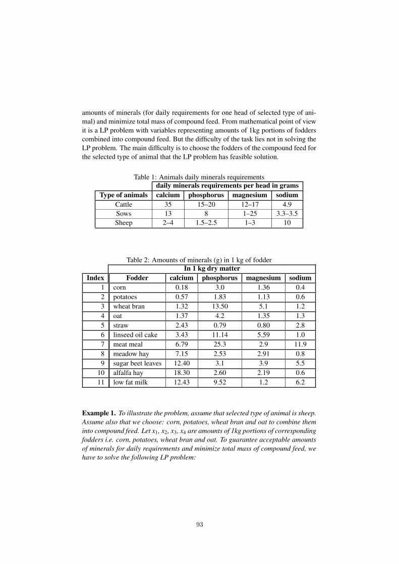
amounts of minerals (for daily requirements for one head of selected type of ani-mal) and minimize total mass of compound feed. From mathematical point of viewit is a LP problem with variables representing amounts of 1kg portions of fodderscombined into compound feed. But the difficulty of the task lies not in solving theLP problem. The main difficulty is to choose the fodders of the compound feed forthe selected type of animal that the LP problem has feasible solution.

Table 1: Animals daily minerals requirementsdaily minerals requirements per head in grams

Type of animals calcium phosphorus magnesium sodiumCattle 35 15–20 12–17 4.9Sows 13 8 1–25 3.3–3.5Sheep 2–4 1.5–2.5 1–3 10

Table 2: Amounts of minerals (g) in 1 kg of fodderIn 1 kg dry matter

Index Fodder calcium phosphorus magnesium sodium1 corn 0.18 3.0 1.36 0.42 potatoes 0.57 1.83 1.13 0.63 wheat bran 1.32 13.50 5.1 1.24 oat 1.37 4.2 1.35 1.35 straw 2.43 0.79 0.80 2.86 linseed oil cake 3.43 11.14 5.59 1.07 meat meal 6.79 25.3 2.9 11.98 meadow hay 7.15 2.53 2.91 0.89 sugar beet leaves 12.40 3.1 3.9 5.5

10 alfalfa hay 18.30 2.60 2.19 0.611 low fat milk 12.43 9.52 1.2 6.2

Example 1. To illustrate the problem, assume that selected type of animal is sheep.Assume also that we choose: corn, potatoes, wheat bran and oat to combine theminto compound feed. Let x1, x2, x3, x4 are amounts of 1kg portions of correspondingfodders i.e. corn, potatoes, wheat bran and oat. To guarantee acceptable amountsof minerals for daily requirements and minimize total mass of compound feed, wehave to solve the following LP problem:

93

Minimize x1 + x2 + x3 + x4

Subject to 0.18x1 + 0.57x2 + 1.32x3 + 1.37x4 ≥ 2

0.18x1 + 0.57x2 + 1.32x3 + 1.37x4 ≤ 4

3x1 + 1.83x2 + 13.5x3 + 4.2x4 ≤ 2.5

3x1 + 1.83x2 + 13.5x3 + 4.2x4 ≥ 1.5

1.36x1 + 1.13x2 + 5.1x3 + 1.35x4 ≥ 1

1.36x1 + 1.13x2 + 5.1x3 + 1.35x4 ≤ 3

0.4x1 + 0.6x2 + 1.2x3 + 1.3x4 = 10

xi ≥ 0 for i = 1,2,3,4.

Applying the standard function minimize_lp(obj, cond,[pos]) in Maxima 5.26.0we get: no feasible solution. The answer is negative - there is no possibility tobalance minerals in compound feed for these four fodders and daily requirementsof minerals for sheep.

3 Numerical procedure to solve the problem

To determine feasible solution for a selected type of animal, students usually tryfrom few to several times considering different types of fodders. This problem canbe solved quite easily using optimization procedure mininimal_mass(A,b1,b2,m)which we wrote in Maxima 5.26.0 programming language. The simpler versionof this problem is presented and solved using Mathematica 8.0 in paper [11]. Theprinciples of programming in Maxima 5.26.0 are presented in [2, 3, 4, 5, 7, 8]The procedure minnimal_mass(A,b1,b2,m) is a function returning as a last com-ponent vector of pairs which first element is a number of fodder (from Table 2)and the second is the amount of this fodder combined into compound feed. If theproblem has no feasible solution the function returns statement: "no feasible so-lution!" The amounts of fodders which we obtained have minimal total sum. Ais a matrix of amounts of minerals in fodders, created on base of Table 2. b1, b2are vectors of minimal and maximal respectively, daily requirement of mineralsfor selected type of animal created on base of Table 1. m is a number of foddersin compound feed. In our problem m = 4. Formal description of the procedureminimal_mass(A,b1,b2,m) is presented below.

Listing 1: Description of the procedure minimal_mass:

minimal_mass (A, b1 , b2 ,m) : = block ( [ n , obj , p , i , L , R1 , R2 , R , xi ,

94

Ai , A1 , A2 , T , x ] , /∗ l o c a l v a r i a b l e s ∗ //∗ you have t o load t h e s i m p l e x packageload ( " s i m p l e x " ) ; ∗ /n : l e n g t h (A) , /∗ n=numbers o f rows i n marix A ∗ /x i : m a k e l i s t ( concat ( x , i ) , i , 1 ,m) , /∗ x i =[x1 , x2 , . . . , xm] ∗ /o b j : sum ( x i [ i ] , i , 1 ,m) , /∗ o b j= x1+x2 + . . . + xm ∗ /L : m a k e l i s t ( i , i , 1 , n ) , /∗ L = [ 1 , 2 , . . . , xn ] , L i sa Maxima l i s t ∗ /L : s e t i f y ( L ) , /∗ L = 1 , 2 , . . . , n , L i s Maxima s e t ,i n o r d e r t o use t h e f u n c t i o n p o w e r s e t ∗ /L : powerset ( L ,m) , /∗ L= a l l m s u b s e t s o f s e t L ∗ /L : f u l l _ l i s t i f y ( L ) , /∗ s e t L i s c o n v e r t e d t oa Maxima l i s t L ∗ /i : 0 , /∗ i n i t i a l number o f i t e r a t i o n s i s 0 ∗ /T : f a l s e , /∗ t h e loop below w i l l run a t l e a s t once ∗ /f o r Ai in L whi le i s ( T= f a l s e ) do (A1 : m a k e l i s t (A[ x ] , x , Ai ) , /∗ Ai i s a l i s t o f m p o s i t i v e

i n t e g e r s [ n_ i 1 , . . . , n_ im ] , A1= m x m m a t r i x ∗ /R1 : m a k e l i s t ( sum ( A1 [ i ] [ j ]∗ x i [ i ] , i , 1 ,m) >= b1 [ j ] , j , 1 ,m) ,/∗ above : we c o n s t r u c t t h e l i s t o f c o n s t r a i ni n e q u a l i t i e s : a_1 j ∗ x_1 + . . . + a_mj∗x_m>=b1 [ j ] , j = 1 , 2 , . . . ,m ∗ /R2 : m a k e l i s t ( sum ( A1 [ i ] [ j ]∗ x i [ i ] , i , 1 ,m) <= b2 [ j ] , j , 1 ,m) ,/∗ above : we c o n s t r u c t t h e l i s t o f c o n s t r a i ni n e q u a l i t i e s : a_1 j ∗ x_1 + . . . + a_mj∗x_m<=b2 [ j ] ,j = 1 , 2 , . . . ,m ∗ /R : f l a t t e n ( [ R1 , R2 ] ) , /∗ R i s a l i s t o f a l l c o n s t r a i n s ∗ /p : minimize_lp ( obj , R , x i ) , /∗ we c a l l t h e Maximaf u n c t i o n m i n i m i z e _ l p , t h e t h i r d argument x i meanst h a t a l l v a r i a b l e s i n l i s t x i are n o n n e g a t i v e ,p=[ min imal v a l u e o f o b j e c t f u n c t i o n ,[xm=value_m , . . . , x1=v a l u e _ 1 ] ∗ /i f ( i s ( p #" Problem n o t f e a s i b l e ! " ) and i s ( p #" Problemn o t bounded ! " ) ) then( T : true ,p1 : p , /∗ we save p i n case we o b t a i n min imalf e a s i b l e s o l u t i o n p ∗ /p : m a k e l i s t ( rhs ( p [ 2 ] [m−i ] ) , i , 0 ,m−1) ,/∗ p [2]=[xm=value_m , . . . , x1=v a l u e _ 1 ] , so we o b t a i np=[ va lue_1 , . . . , value_m ] ∗ /A2 : Ai /∗ we save Ai i n case we o b t a i n min imal

95

f e a s i b l e s o l u t i o n p ∗ /) ,i : i +1 /∗ number o f i t e r a t i o n i n c r e a s e d ∗ /) ,( i f i s ( T= t rue ) then/∗ i f T=t r u e we o b t a i n min imal f e a s i b l e s o l u t i o n p ∗ /[ i , s o l =p1 , t r a n s p o s e ( p ) , map ( lambda ( [ x , y ] , [ x , y ] ) , A2 , p ) ]e l s e [ i , " no n o n n e g a t i v e s o l u t i o n " , p ] )) $ ;

Example 2. Assume that selected type of animal is cattle. We define A, b1, b2, min Figure 1.

A : [[0.18, 3.0, 1.36, 0.4], [0.57, 1.83, 1.13, 0.6], [1.32, 13.50, 5.1, 1.2], [1.37, 4.2,1.35, 1.3], [2.43, 0.79, 0.80, 2.8], [3.43, 11.14, 5.59, 1.0], [6.79, 25.3, 2.9, 11.9],[7.15, 2.53, 2.91, 0.8], [12.40, 3.1, 3.9, 5.5], [18.30, 2.60, 2.19, 0.6], [12.43, 9.52,1.2, 6.2]]; b1 : [35, 15, 12, 4.9]; b2:[35,20,17,4.9]; m:4;

Figure 1: Matrix A, vectors b1, b2 and m.

The computations were conducted in Maxima5.26.0 on PC with 2.6 GHz, Pen-tium 4 processor and 512 Mb RAM under Windows XP platform. Maxima elapsed_run_timewas 0.07 s. The final result is presented in Figure 2.

[5,sol = [6.191975412126295, [x4 = 4.737686504610226,

x3 = 0.3954624196703,x2 = 1.058826487845771,x1 = 0]],

01.0588264878457710.3954624196703

4.737686504610226

,

[[1,0], [2,1.058826487845771], [3,0.3954624196703], [8,4.737686504610226]]]

Figure 2: Final solution of the problem.

This solution was obtained in fifth iteration. First four iterations had no feasi-ble solutions. The obtained result gives us the following amounts of fodders (seecolumn Index in Table 2) : [1,0] means: 0.0000 kg of meadow, [2,1.0588] means1.0588 kg of wheat bran, [3,0.3955] means 0.3955 kg of potatoes and [8,4.7377]means 4.7377 kg of corn. Total mass of compound feed is 6.192 kg. It is minimal

96

mass of compound feed comprised of these four fodders which guarantees dailyrequirement of four minerals for one cattle.

The procedure minimal_mass(A,b1,b2,m) can be easily extended to minimizetotal mass of compound feed among all possible compound feeds balancing min-erals for selected type of animal. The extended procedure is in Figure Listing 2

Listing 2: Description of the procedure minimal_mass1:

minimal_mass1 (A, b1 , b2 ,m) : = block ( [ n , obj , p , p1 , p0 , i , i0 , L ,R1 , R2 , R , xi , Ai , A1 , A2 , T , x , y0 ] ,n : l e n g t h (A) ,x i : m a k e l i s t ( concat ( x , i ) , i , 1 ,m) ,o b j : sum ( x i [ i ] , i , 1 ,m) ,L : m a k e l i s t ( i , i , 1 , n ) ,L : s e t i f y ( L ) ,L : powerset ( L ,m) ,L : f u l l _ l i s t i f y ( L ) ,i : 0 ,i 0 : 0 ,y0 : 1 0 0 ,T : f a l s e ,f o r Ai in L do (/∗ i n minimal_mass we have : f o r Ai i n L w h i l e i s ( T= f a l s e ) :now t h e c o n d i t i o n " w h i l e i s ( T= f a l s e ) " i s n o t needed ∗ /A1 : m a k e l i s t (A[ x ] , x , Ai ) ,R1 : m a k e l i s t ( sum ( A1 [ i ] [ j ]∗ x i [ i ] , i , 1 ,m) >= b1 [ j ] , j , 1 ,m) ,R2 : m a k e l i s t ( sum ( A1 [ i ] [ j ]∗ x i [ i ] , i , 1 ,m) <= b2 [ j ] , j , 1 ,m) ,R : f l a t t e n ( [ R1 , R2 ] ) ,p : minimize_lp ( obj , R , x i ) ,i f ( i s ( p #" Problem n o t f e a s i b l e ! " ) and i s ( p #" Problemn o t bounded ! " ) ) then( T : true ,i f i s ( p [1] < y0 ) then (y0 : p [ 1 ] ,p1 : p ,p0 : m a k e l i s t ( rhs ( p [ 2 ] [ i ] ) , i , 1 ,m) ,A2 : Ai ,i 0 : i) ) ,i : i +1

97

) ,( i f i s ( T= t rue ) then[ i , i0 , s o l =p1 , t r a n s p o s e ( p0 ) , map ( lambda ( [ x , y ] , [ x , y ] ) , A2 , p0 ) ]e l s e [ i , " no n o n n e g a t i v e s o l u t i o n " , p0 ] )) ;

The computations were conducted in Maxima5.26.0 on PC with 2.6 GHz,Pentium 4 processor and 512 Mb RAM under Windows XP platform. Maximaelapsed_run_time was 1.83 s. The final result is presented in Figure 3.

Applying the procedure minimal_mass1(A,b1,b2,m) to the extension of theproblem for cattle we obtain the solution presented in Figure 3.

[330,321,sol = [3.108826328073963, [x4 = 1.325453353602,

x3 = 0.51585666963707,x2 = 0,x1 = 1.267516304834889]],

1.3254533536020.51585666963707

01.267516304834889

[[6,1.325453353602], [8,0.51585666963707], [9,0], [10,1.267516304834889]]]

Figure 3: Final solution of the generalized problem with cattle.

This solution was obtained in 321-th iteration. First 320 iterations give no feasi-ble solutions or feasible solutions with value of object function greater than 3.1088.The obtained result gives us the following amounts of fodders (see column Index inTable 2): [6,1.32545] means: 1.32545 kg of linseed oil cake, [8,0.515856669637]means 0.515856669637 kg of meadow hay, [9,0] means 0.0000 kg of sugar beetleaves and [10,1.2675163] means 1.2675163 kg of alfalfa hay. Total mass of com-pound feed is 3.1088 kg. It is minimal mass of compound feed comprised of thesefour fodders chosen from all eleven fodders, which guarantees daily requirementof four minerals for one cattle.

4 Summary

In this paper the procedure minimal_mass(A,b1,b2,m) implemented in Maxima5.26.0 was presented. This procedure solves the problem of fodders choice forminimal mass compound feed in order to ensure daily requirement of four miner-als (calcium, phosphorus, magnesium and sodium) for a selected type of animal.This problem was assignment for students Agricultural and Forest Engineering at

98

Warsaw University of Life Science. Finding solution of the problem students needquite much of work considering various selection of four fodders in order to obtainbalancing minerals in compound feed. Applying CAS system such as wxMaximaallows find solution of described above problem in a much less time.

References[1] Homepage of the Maxima Project: http://maxima.sourceforge.net[2] Maxima Documentation at http://maxima.sourceforge.net/documentation.html.[3] Maxima 5.36.0 Manual at http://maxima.sourceforge.net/docs/manual/maxima.html.[4] Edwin L. Woollett, Maxima by Example at http://web.csulb.edu/ woollett/#mbe[5] Rafał Topolnicki, Maxima - practical guide (in polish) at

http://www.knf.ifd.uni.wroc.pl/materialy/maxima.pdf[6] Robert Dodier, Minimal Maxima at http://maxima.sourceforge.net/docs/tutorial/en/minimal-

maxima.pdf[7] Paulo Ney de Souza, Richard J. Fateman, Joel Moses, Cliff Yapp, The Maxima Book at

http://maxima.sourceforge.net/docs/maximabook/maximabook-19-Sept-2004.pdf[8] Gilberto E. Urroz, MAXIMA: Science and Engineering Applications at

http://www.neng.usu.edu/cee/faculty/gurro/Maxima.html[9] Jaime E. Villate, Dynamical systems (in Portuguese) at

http://www.villate.org/doc/sistemasdinamicos/sistdinam-1_2.pdf[10] Homepage of the wxMaxima Project: http://andrejv.github.io/wxmaxima/[11] Włodzimierz Wojas, Jan Krupa, Application of Mathematica System in the problem of balance

of ingredients for compound feed, Computer Algebra Systems In Teaching and Research 2013,Vol. 4, No 1, pp. 278-282

[12] Ziołecka A., Kuzdowicz M., Chomszyn M. Tables of ingriedients of domestic fodders (inpolish) PWN Warszawa (1987)

[13] The minerals in animal nutrition. Poznan University of Life Science (1994) (in polish)[14] www.dodatkipaszowe.pl

99

The Use of CAS for Logical Analysis in MathematicsEducation

T. Takahashi1, T. Sakai2, F. Iwama1

1Konan University, Japan, [email protected] Normal University, [email protected]

In mathematics education, ascertaining the concepts of given domains in termsof conceptual and procedural knowledge is essential as a mechanism of knowledgechange during knowledge acquisition. Conceptual knowledge consists of an im-plicit or explicit system of interlinked pieces of knowledge for a given domain, andprocedural knowledge comprises systems of multiple execution series for problemsolution [1], [2]. The concept of ratio is applied in ascertaining the relation be-tween two quantities and in comparing the relative quantities of two sets. It differsin meaning from simple multiplication and is active in the sense of comparing therelative sizes of given quantities and base quantities rather than directly comparingquantities [3]. So, we focused on comparison of the relations between quantitiesin two different sets. It has been noted that the concept of ratio can be investigatedin a fairly pure form as a logical mathematical recognition [4], and we treated thiscomparison as a probabilistic comparison task. Ratio and probability are differentconcepts, but for children unschooled in probability, the ratio concept can be uti-lized as an approach for probability settings. We consider these problems usingtheorem prover.

Computer algebra systems are being used frequently in mathematics education.Although good teaching examples and experiences exist, it is clear that the efficientand successful use is not self-evident. A subtle relationship exists between paper-and-pencil techniques, computer algebra systems, and conceptual understanding.The nature of computer systems is different from that of paper-and-pencil tech-niques. Using a computer algebra system requires insight into procedures as wellas into the concepts involved. In addition, the way computer manages the proce-dures can affect mathematical concepts.

Use of a computer algebra system with a theorem prover can correct the weak-ness in mathematics education. We can clearly understand mathematical conceptsand can minimize the burden of operation opportunities. Computer algebra sys-tems using a theorem prover bring about serious changes in mathematics educa-tion. A theorem prover Theorema uses a computer algebra system, but reduces theoperations of the computer algebra system. Therefore, learners can concentrate onmathematical problems.

In this study, we applied propositional and predicate logic for mathematical

100

explication of the processes of inference by using theorem prover Theorema [5] isa Mathematica package (a collection of packages, in fact) that provides a math-ematical assistant system (MAS) inside of and based on Mathematica. A MASsupports the user in formulating and structuring of mathematical knowledge, prov-ing mathematical statements, formulating and executing mathematical algorithms,performing computations, etc. Theorema allows you to express algorithms usingthe language of predicate logic or parts of the Mathematica programming languagesupporting procedural programming, most importantly various forms of loops.Theorema allows you to organize mathematical knowledge as hierarchies of in-terdependent theories. By settling the definitions, we can continue and try to provesome properties of the newly defined entities.

When considering a human model, the model must be viewed as a processmodel, as a knowledge model, and as a control model. We can consider that suchan approach has been applied to the understanding of theorem proving. A computeralgebra system with a theorem prover is being developed. We must consider thetheorem prover from mathematical studies. This research aims at extending currentcomputer systems using facilities for supporting mathematical proving. The systemconsists of a general higher-order predicate logic prover and a collection of specialprovers. The individual provers imitate the proof style of human mathematiciansand produce human-readable proofs in natural language presented in nested cells.

To do mathematics is gaining knowledge and solving problems by reasoning.Theorem prover Theorema is a powerful tool for learning mathematics.

References[1] J. Hiebert and P. Lefevre,“ Conceptual and Procedural Knowledge in Math-ematics: An

Introductory Analysis”, in J. Hiebert (ed.), Conceptual and Procedural Knowledge: The Caseof Mathematics, Hillsdale, N. J.: Lawrence Erlbaum Associates, pp.1-27 (1986).

[2] B. Rittle-Johnson, R. S. Siegler, and N. W. Alibali,“ Developing Conceptual Understandingand Procedural Skill in Mathematics: An Iterative Process”, Journal of Educational Psychol-ogy, Vol.93, No.2, pp.346-362 (2001).

[3] R. Maeda,“ Concept of the Ratio”, New Arithmetic Education Lecture Vol. 3: Mathemat-ical Relations, in C. Akahane (ed.), Yoshino-shobo Publishing Ltd, pp.239-247 (1960) (inJapanese).

[4] A. Nakagaki,“ How do Children Judge the Size of the Ratio? -The Developmental Study”,Research report of the National Institute for Educational Research, Vol.13, pp.35-55 (1986)(in Japanese).

[5] https://www.risc.jku.at/research/theorema/software/documentation/tutorial/TheTheoremaSystem.html

101

Indexed elementary functions in Maple

David Jeffrey

University of Western Ontario, Canada

Multi-branched functions cause troubles for mathematicians

(particularly

students) and computers. I present implementations of the inverses of

the

elementary functions sin,cos,tan,exp, ^m which handle the branches by

labelling them. The new functions are more elegant, easier to work

with and

easier to understand. At least that is what I think.

102

Computer Algebra in CodingTheory and Cryptography

103

Session Organizers

Irene Marquez-CorbellaINRIA - [email protected]

Ruud PellikaanDep. of Mathematics and Computing ScienceEindhoven University of [email protected]

Overview

This session aims to bring together researchers from all areas related to computer algebra (boththeoretical and algorithmic) applied to Coding theory and Cryptography.

Since much of the work related to these topics is recent or is still ongoing, this session willprovide a stimulating forum where experts will be able to not only report their recent results, butalso to propose new lines of research and discuss open questions.

104

Trial set and Gröbner bases for binary codes

M. Borges-Quintana1a, M. A. Borges-Trenard2, Edgar Martínez Moro3

1 2 Department of Mathematics, Faculty of Mathematics and Computer Science, University ofOriente, Santiago de Cuba, Cuba, [email protected], [email protected] Institute of Mathematics IMUVa, University of Valladolid. Valladolid, Castilla, Spain,[email protected]

We show the connections between trial sets and Gröbner bases for binary codes,which gives more characterizations of trial sets in the context of Gröbner bases andalgorithmic ways for compute them. In this sense, minimal trial set are character-ized as trial sets associated with minimal Gröbner bases.

The concept of trial set was introduced in [6]. This set of codewords can beused to derive and algorithm for doing complete decoding in a similar way that agradient decoding algorithm uses a test set (see [1]). A trial set allows to charac-terize the so called correctable errors and to investigate the monotone structure ofcorrectable and uncorrectable errors, also important bounds on the error-correctioncapability of binary codes beyond half of minimum distance using trial sets arepresented in [6]. One problem posted in the conclusion of [6] was the importanceof charactherize minimal trial sets for families of binary codes.

The ideal associated with any linear code (code ideal for simplicity) was in-troduced in [2] together with applications of Gröbner bases theory in this context,such that the reduction process by Gröbner bases of code ideals w.r.t. to specificorders corresponds to the decoding process of the code.

In Section 1 we give the main concepts and results related with binary codes,trial sets, the code ideals and Gröbner bases which are needed for an understandingof this work. The connection between trial sets for binary codes and Gröbner basesfor the corresponding code ideal is presented in Section 2. The main results in thiscontribution are Proposition 2, Theorems 4 and 5, and the subsection 2.1 aboutminimal trial sets and minimal Gröbner bases.

1 Preliminaries

Binary codesBy Z, K, K[X] and F2 we denote the ring of integers, an arbitrary field, the poly-nomial ring in n variables over the field K and the finite field with 2 elements.

aSupported by a Post-doctorate scholarship at the University of Valladolid (09-2014 to 02-2015)by Erasmus Mundus Program, Mundus Lindo Project.

105

A binary linear code C over F2 of length n and dimension k, or an [n,k] binarycode for short, is a k-dimensional subspace of Fn

2. We will call the vectors v in Fn2

words and in the particular case where v ∈ C , codewords. For every word v ∈ Fn2

its support is defined as supp(v) = i | vi 6= 0 and its Hamming weight, denotedby wH(v) as the cardinality of supp(v).

The Hamming distance, between two vectors x, y∈Fn2 is dH(x,y) = wH(x−y).

The minimum distance d(C ) of a linear code C is defined as the minimum weightamong all nonzero codewords.

For the rest of this section we follow [6]. We will consider ≺ a so called α-ordering on Fn

2 (a weight compatible total ordering on Fn2) which is monotone:

for any y1, y2 s.t. 2≤wH(y1) = wH(y1) < n and supp(y1)∩supp(y1) 6= /0and for any i ∈ supp(y1)∩ supp(y1) and vectors x1 and x2 defined bysupp(x1) = supp(y1) \ i and supp(x2) = supp(y2) \ i then y1 ≺ y2 ifx1 ≺ x2.

(1)

The set of correctable errors of a binary code C (E0(C )) are the minimal elementsw.r.t. ≺ in each coset of Fn

2/C , and the elements of E1(C ) = Fn2 \E0(C ) are called

uncorrectable errors. A trial set T ⊂ C \ 0 of the code C is a set which has theproperty y ∈ E0(C ) if and only if y≤ y + c, for all c ∈ T .

Note that with a trial set we obtain an algorithm which returns the correspond-ing correctable error for a received word y. Since we choose a monotone α-ordering on Fn

2, the set of correctable and uncorrectable errors form a monotonestructure, namely, that if x⊂ y, then x ∈ E1(C ) implies y ∈ E1(C ) and y ∈ E0(C )implies x ∈ E0(C ).

Let M1(C ) be the set of minimal uncorrectable errors i.e. the set of y ∈ E1(C )such that, if x⊆ y and x ∈ E1(C ), then x = y. In a similar way, the set of maximalcorrectable errors is the set M0(C ) of elements x ∈ E0(C ) such that, if x ⊆ y andy ∈ E0(C ), then x = y.

For c ∈ C \ 0, a larger half is defined as a minimal word u in the ordering such that u + c ≺ u. The set of larger halves for a codeword c is denoted by L(c),and for U ⊆ C \ 0 the set of larger halves for elements of U is denoted by L(U).Note that L(C )⊆ E1(C ).

For any y ∈ Fn2, let H(y) = c ∈ C : y + c≺ y, and we have y ∈ E0(C ) if

and only if H(y) = /0, and y ∈ E1(C ) if and only if H(y) 6= /0. Theorem 1 of [6]provides a characterization of the set M1(C ) in terms of H(·) and larger halves ofthe set of minimal codewords M(C ).

Proposition 1 (Corollary 3, [6]) Let C be a binary code and T ⊆ C \ 0. Thefollowing statements are equivalent:

106

1. T is a trial set for C .

2. If y ∈M1(C ), then T ∩H(y) 6= /0.

3. M1(C )⊆ L(T ).

Gröbner bases and binary codesWe define the following characteristic crossing function: ∆ : Fs

2 −→ Zs which re-place the class of 0,1 by the same symbols regarded as integers. This map willbe used with matrices and vectors acting coordinate-wise. Also, for the recip-rocal case, we defined ∇ : Zs −→ Fs

2. Let X denotes n variables x1, . . . ,xn andlet a = (a1, . . . ,an) be an n-tuple of elements of the field F2. We will adopt thefollowing notation:

Xa := x∆a11 · · ·x∆an

n ∈ [X]. (2)

The code ideal can be given by the two equivalent formulas in (3) and (4) below,the equivalency between (3) and (4) was proved in [4]. Let W be a generator matrixof an [n,k] binary code C (the row space of the matrix generates C ) and wi denotesits rows for i = 1, . . .k.

I(C ) =⟨Xa−Xb | a−b ∈ C

⟩⊆K[X]. (3)

I(C ) =⟨Xwi−1 : i = 1, . . .k∪x2

i −1 : i = 1, . . . ,n⟩⊆K[X]. (4)

Note that I(C ) is a zero-dimensional ideal since the quotient ring R = K[X]/I(C )is a finite dimensional vector space and its dimension is equal to the number ofcosets in Fn

2/C .For every element Xa in the monoid [X], with a ∈Nn, we have a corresponding

vector ∇(a) ∈ Fn2, and viceversa, any vector w ∈ Fn

2 has a unique standard repre-sentationb Xw as an element of [X] (see (2)).

Let < be a term order, let us T( f ) denotes the maximal term of a polynomialf with respect to the order <. The set of maximal terms of the set F ⊆ K[X ] isdenoted TF and T(F) denotes the semigroup ideal generated by TF. Finally,〈F〉 is the polynomial ideal in K[X] generated by F . In particular, for the code idealI(C ), T(I(C )) is the set of maximal terms and N(I(C )) = [X]\T(I(C )) the set ofcanonical forms. We emphasize that there is a one to one correspondence betweenthe set of canonical forms and the cosets in Fn

2/C . One characterization of Gröbnerbases is that G is a Gröbner basis of the ideal 〈G〉 if and only if T(〈G〉) = T(G).

bThe exponents of the variables are 0 or 1.

107

2 Gröbner bases and trial set for binary codes

It is not difficult to see also the conection between total degree orders < on [X] andα-orderings monotone ≺ on Fn

2. In essence, any total degree compatible orderinginduces an α-ordering monotone ≺ on Fn

2 such that v ≺ w if Xv < Xw for anyv, w ∈ Fn

2. On the other hand, given an α-ordering monotone on Fn2 we could

define a total ordering on [X] which is not admisible, a class of these orders on [X]were called in [2] error-vector orderings.

In this work we will focus in the first situation, the α-ordering monotone whichis defined in [6] it is derived from the Graduated Lexicographical order. In general,let < be a total degree term order on [X], and let≺ be the corresponding α-orderingmonotone on Fn

2.

Proposition 2 [Correctable and uncorrectable errors and canonical forms andmaximal terms] Let Xw ∈ [X], w ∈ Nn then

1. If Xw is not the standard representation of the word ∇(w) in Fn2, then it is a

maximal term i.e. Xw ∈ T(I(C )).

2. If ∇(w) ∈ E1(C ), then Xw ∈ T(I(C )).

3. If Xw is the standard representation of the word ∇(w) and ∇(w) ∈ E0(C ),then Xw is a canonical form i.e. Xw ∈ N(I(C )).

4. If Xw is the standard representation of the word ∇(w) and ∇(w) ∈M1(C ),then Xw is an irredundant maximal term, i.e. Xw /∈ T(I(C ))\Xw and is amaximal term of any Gröbner basis. The set of irredundant maximal termsare the maximal terms of any minimal Gröbner basis, for example, of thereduced Gröbner basis.

For simplicity, we will assume that the coefficients of the maximal terms in aGröbner basis are positive.

Definition 3 (Gröbner codewords [3]) Let G be a Gröbner basis for I(C ) w.r.t.<, the set of Gröbner codewords CG corresponding to G are the codewords asso-ciated with G by CG = c ∈ C : c = w + v, s.t. Xw−Xv ∈ G, w,v ∈ Fn

2, v≺ w.

Theorem 4 Let G be a Gröbner basis for I(C ) w.r.t. <, then CG is a trial set.

Proof. We will prove the stament 2 in Proposition 1. Let w ∈ M1(C ), thenXw ∈ T(G) (see Proposition 2.4) and there exists c ∈ CG s.t. c = w + v s.t. v≺ w.Thus c + w = v≺ w and c ∈ H(w).

108

Theorem 5 Let T be a trial set, the set GT = Xw−Xv : w ∈ L(c) for some c ∈T and v = c−w∪x2

i −1 : i = 1, . . . ,n is a Gröbner basis for I(C ) w.r.t. <.

Proof. If Xu is a maximal term which is not the standard representation of ∇(u),then it can be reduced to the standard representation of ∇(u) by means of the setx2

i −1 : i = 1, . . . ,n. Thus, let us assume that Xu ∈ T(I(C )) and u ∈ E1(C ). It isclear that there exists w⊆ u s.t. w∈M1(C ), w∈M1(C ) implies there exists c∈ Ts.t. w ∈ L(c) (by Proposition 1.3). Let v = c−w, then we have Xw−Xv ∈GT andXw | Xu (remember w⊆ u). Consequently, GT is a Gröbner basis for I(C ).

2.1 Minimal trial sets and minimal Gröbner bases

A minimal trial set is a trial set such that any strictly subset is not a trial set. Havingan smaller trial set, it is an smaller set that it is used for decoding in order to com-pute the corresponding correctable error to a received word, althought smaller trialsets do not necessaryly ensure more efficiency. In [6] is given a main advantageof having a minimal trial set, because the size of trial sets are used to derive someimportant bounds on the error correction beyond half the minimum distance.

By Proposition 1.3, the set of larger halves of a trial set T should contains atleast the set M1(C ), by Theorem 5 and Proposition 2.4 this means that the cor-responding Gröbner basis GT should coontains at least the irredundant maximalterms (it is the case for any Gröbner basis); therefore, there is a direct connectionbetween minimal trial sets and minimal Gröbner bases. In particular, a distin-guished minimal trial set would be the set of Gröbner codewords corresponding tothe reduced Gröbner basis.

References[1] A. Barg, Complexity issues in coding theory, in Handbook of coding theory, I, North-Holland,

Amsterdam, pp. 649-754 (1998).[2] M. Borges-Quintana, M.A. Borges-Trenard and E. Martínez-Moro, On a Gröbner bases struc-

ture associated to linear codes, J. Discret. Math. Sci. Cryptogr, 10(2), pp. 151-191 (2007).[3] M. Borges-Quintana, M.A. Borges-Trenard and E. Martínez-Moro, A Gröbner representation

for linear codes, in Advances in coding theory and cryptography, Ser. Coding Theory Cryptol.,3, World Sci. Publ., Hackensack, NJ, pp. 17-32, (2007).

[4] M. Borges-Quintana, M.A. Borges-Trenard, P. Fitzpatrick and E. Martínez-Moro, Gröbnerbases and combinatorics for binary codes, Appl. Algebra Engrg. Comm. Comput., 19(5), pp.393-411 (2008).

[5] W.C. Huffman and V. Pless, Fundamentals of error-correcting codes, Cambridge UniversityPress, Cambridge (2003).

[6] T. Helleseth, T. Kløve and I.L. Vladimir, Error-correction capability of binary linear codes,IEEE Transactions on Information Theory, 51(4), pp. 1408-1423 (2005).

109

Geometric and Computational Approach to Classical andQuantum Secret Sharing

Ryutaroh Matsumoto1, Diego Ruano2

1 Tokyo Institute of Technology, Japan, [email protected] Aalborg University, Denmark, [email protected]

1 Introduction

Secret sharing (SS) [15] is a cryptographic scheme to encode a secret to multipleshares being distributed to participants, so that only qualified (or authorized) setsof participants can reconstruct the original secret from their shares. Traditionallyboth secret and shares were classical information (bits). Several authors [5, 7,16] extended the traditional SS to a quantum one so that a quantum secret can beencoded to quantum shares.

When we require unqualified sets of participants to have zero information ofthe secret, the size of each share must be larger than or equal to that of the secret.By tolerating partial information leakage to unqualified sets, the size of shares canbe smaller than that of the secret. Such an SS is called a ramp (or non-perfect) SS[2, 13, 17]. The quantum ramp SS was proposed by Ogawa et al. [14]. In theirconstruction [14] as well as its improvement [18], the size of shares can be L timessmaller relative to quantum secret than its previous construction [5, 7, 16], whereL is the number of qudits in quantum secret.

Classical secret sharing is said to be linear if a linear combination of sharescorresponds to the linear combination of the original secrets [4]. It is also knownthat every linear ramp secret sharing can be expressed by a nested pair of linearcodes C2⊂C1⊂ Fn

q. On the other hand, a nest code pair C2⊂C1⊂ Fnq can also give

a quantum secret sharing as described in [10]. A share set is said to be forbiddenif it has no information about the secret. It is natural to express conditions forqualified and forbidden sets in terms of C2 ⊂C1, and the following is known:

Theorem 1 [1, 9, 10] Let J ⊆ 1, . . . , n, and define PJ : Fnq → F|J|q , (x1, . . . ,

xn) 7→ (x j : j ∈ J). We consider classical and quantum secret sharing constructedfrom C2 ⊂C1. J can be regarded as a share set, and J is qualified in the classicalsecret sharing if and only if

dimPJ(C1)/PJ(C2) = dimC1/C2, (1)

and J is forbidden in the classical secret sharing if and only if

PJ(C1) = PJ(C2). (2)

Let J = 1, . . . , n\ J. In the quantum secret sharing, J is qualified if and only if

both

(1) is true,PJ(C1) = PJ(C2)

i.e.,

J is classically qualified,J is classically forbidden

(3)

110

hold, and J is forbidden if and only if J is qualified.

Since C1 and C2 are linear codes, it is natural to use algebraic geometry codesto construct C1 and C2 [3]. Let F be an algebraic function field of one variablewith genus g(F), P1, . . . , Pn its rational places, G1 ≥ G2 divisors whose supportcontain none of P1, . . . , Pn. Define C(P1 + · · ·+ Pn, G1) = ( f (P1), . . . , f (Pn)) |f ∈L (G1). By the Riemann-Roch theorem, for C1 = C(P1 + · · ·+ Pn, G1) andC2 = C(P1 + · · ·+ Pn, G2), it is straightforward to see

Theorem 2 Equation (1) holds if

|J| ≥ 1 + degG1. (4)

Equation (2) holds if|J| ≤ degG2−2g(F)+ 1. (5)

Equation (3) holds if

|J| ≥max1 + degG1,n− (degG2−2g(F)+ 1). (6)

The purpose of this note is to find sufficient conditions less demanding than(4)–(6) by using geometric properties of the set of points Pj | j ∈ J.

2 Geometric and Computational Analysis of Qualified andForbidden Sets

2.1 Computational Approach

Fix a rational place Q arbitrarily. When C1 = C(P1 + · · ·+Pn, G1) and C2 = C(P1 +· · ·+ Pn, G2), (1) holds

⇔ C(∑j∈J

Pj,G1)/C(∑j∈J

Pj,G2)'C(P1 + · · ·+ Pn,G1)/C(P1 + · · ·+ Pn,G2)

⇔ ker(PJ)∩C(P1 + · · ·+ Pn,G1) = ker(PJ)∩C(P1 + · · ·+ Pn,G2)

⇔ C(∑j/∈J

PJ,G1−∑j∈J

Pj) = C(∑j/∈J

PJ,G2−∑j∈J

Pj)

⇔ f1 ∈L (G1−∑j∈J

Pj)⇒∃ f2 ∈L (G2−∑j∈J

Pj) s.t. f1(Pj) = f2(Pj)∀ j /∈ J

⇔ f1 ∈L (G1−∑j∈J

Pj)⇒∃ f2 ∈L (G2−∑j∈J

Pj) s.t. f1− f2 ∈L (G1−∑j/∈J

Pj)

⇔ ∀ f1 ∈L (G1−∑j∈J

Pj),∃ f2 ∈L (G2−∑j∈J

Pj),∃ f3 ∈L (G1−n

∑j=1

Pj) s.t. f1 = f2 + f3

⇔ L (G1−∑j∈J

Pj)⊆L (G1−n

∑j=1

Pj)+L (G2−∑j∈J

Pj)

111

⇔ vQ(L (G1−∑j∈J

Pj))⊆ vQ(L (G1−n

∑j=1

Pj)+L (G2−∑j∈J

Pj))

⇐ vQ(L (G1−∑j∈J

Pj))⊆ vQ(L (G1−n

∑j=1

Pj))∪ vQ(L (G2−∑j∈J

Pj)). (7)

For any rational place Q and any divisor G of F , vQ(L (G)) can be computed byGröbner bases and the algorithm in [11], provided that the defining equations ofF is in special position with respect to Q [6, 8, 12].

We turn our attention to (2). Equation (2) holds

⇔ C(∑j∈J

Pj,G1) = C(∑j∈J

Pj,G2)

⇔ ∀ f1 ∈L (G1),∃ f2 ∈L (G2) s.t. f1− f2 ∈L (−∑j∈J

Pj + G1)

⇔ ∀ f1 ∈L (G1),∃ f2 ∈L (G2),∃ f3 ∈L (−∑j∈J

Pj + G1) s.t. f1 = f2 + f3

⇔ L (G1) = L (G2)+L (G1−∑j∈J

Pj)

⇔ vQ(L (G1)) = vQ(L (G2)+L (G1−∑j∈J

Pj))

⇐ vQ(L (G1)) = vQ(L (G2))∪ vQ(L (G1−∑j∈J

Pj)). (8)

A similar sufficient condition for (3) can be deduced from (4) and (5).

2.2 Explicit Sufficient Conditions

We explicitly write sufficient conditions for (7) and (8), and examine if they areeasier to hold than (4) and (5) for one point AG codes with G1 = m1Q and G2 =m2Q. For any divisor G, let HQ(G) = −vQ(L (G + ∞Q) \ 0). Observe thatHQ(0) is the Weierstrass semigroup at Q. The conductor of HQ(G) is defined asmini ∈ HQ(G) | i≤ j ∈ N⇒ j ∈ HQ(G), which generalizes the conductor of theWeierstrass semigroup HQ(0).

Equation (7) holds if

vQ(L (m1Q−∑j∈J

Pj)\0) = /0

⇔ m1 ≤minHQ(−∑j∈J

Pj)−1 (9)

We see that condition (9) is less demanding than (4), because minHQ(−∑ j∈J Pj)≥|J|.

Similarly, (8) holds if

m2 ≥ the conductor of HQ(−∑j∈J

Pj)−1 (10)

112

We also see that condition (10) is less demanding than (5), because the conductorof HQ(−∑ j∈J Pj) is ≤ 2g(F). We can also make a similar improvement over (6):Condition (6) holds if

m1 ≤minHQ(−∑j∈J

Pj)−1 and m2 ≥ the conductor of HQ(−∑j/∈J

Pj)−1.

In particular, for elliptic function fields (g(F) = 1),

(9) ⇔

m1 + 1≤ |J| if ∃ f ∈L (∞Q),( f )0 = ∑ j∈J Pj,m1 ≤ |J| otherwise

(11)

(10) ⇔|J| ≤ m2−1 if ∃ f ∈L (∞Q),( f )0 = ∑ j∈J Pj,|J| ≤ m2 otherwise

(12)

Acknowledgment

The authors gratefully acknowledge the support from Japan Society for the Promo-tion of Science (Grant Nos. 23246071 and 26289116), from the Spanish MINECO(Grant No. MTM2012-36917-C03-03), the Danish Council for Independent Re-search (Grant No. DFF-4002-00367) and from the “Program for Promoting theEnhancement of Research Universities” at Tokyo Institute of Technology.

References

[1] T. Bains. Generalized Hamming weights and their applications to secret shar-ing schemes. Master’s thesis, University of Amsterdam, Feb. 2008. super-vised by R. Cramer, G. van der Geer, and R. de Haan.

[2] G. R. Blakley and C. Meadows. Security of ramp schemes. In Advances inCryptology–CRYPTO’84, volume 196 of Lecture Notes in Computer Science,pages 242–269. Springer-Verlag, 1985. doi:10.1007/3-540-39568-7_20.

[3] H. Chen, R. Cramer, R. de Haan, and I. Cascudo Pueyo. Strongly mul-tiplicative ramp schemes from high degree rational points on curves. InN. Smart, editor, Advances in Cryptology – EUROCRYPT 2008, volume4965 of Lecture Notes in Computer Science, pages 451–470. Springer-Verlag,2008. doi:10.1007/978-3-540-78967-3_26.

[4] H. Chen, R. Cramer, S. Goldwasser, R. de Haan, and V. Vaikuntanathan.Secure computation from random error correccting codes. In Advances inCryptology–EUROCRYPT 2007, volume 4515 of Lecture Notes in Com-puter Science, pages 291–310. Springer-Verlag, 2007. doi:10.1007/978-3-540-72540-4_17.

[5] R. Cleve, D. Gottesman, and H.-K. Lo. How to share a quantum secret. Phys.Rev. Lett., 83(3):648–651, July 1999. quant-ph/9901025, doi:10.1103/PhysRevLett.83.648.

113

[6] O. Geil and R. Pellikaan. On the structure of order domains. Finite Fieldsand Their Appl., 8:369–396, 2002.

[7] D. Gottesman. Theory of quantum secret sharing. Phys. Rev. A, 61(4), Mar.2000. quant-ph/9910067, doi:10.1103/PhysRevA.61.042311.

[8] C. Heegard, J. Little, and K. Saints. Systematic encoding via Gröbner basesfor a class of algebraic-geometric Goppa codes. IEEE Trans. Inform. Theory,41(6):1752–1761, Nov. 1995.

[9] J. Kurihara, T. Uyematsu, and R. Matsumoto. Secret sharing schemes basedon linear codes can be precisely characterized by the relative generalizedHamming weight. IEICE Trans. Fundamentals, E95-A(11):2067–2075, Nov.2012. doi:10.1587/transfun.E95.A.2067.

[10] R. Matsumoto. Coding theoretic construction of quantum ramp secret shar-ing. (version 4 or later), May 2014. arXiv:1405.0149v5.

[11] R. Matsumoto and S. Miura. Finding a basis of a linear system with pair-wise distinct discrete valuations on an algebraic curve. J. Symbolic Comput.,30(3):309–323, Sept. 2000. doi:10.1006/jsco.2000.0372.

[12] R. Matsumoto and S. Miura. On construction and generalization of alge-braic geometry codes. In T. Katsura et al., editors, Proc. Algebraic Geom-etry, Number Theory, Coding Theory, and Cryptography, pages 3–15, Univ.Tokyo, Japan, Jan. 2000. Available from: http://www.rmatsumoto.org/repository/weight-construct.pdf.

[13] W. Ogata, K. Kurosawa, and S. Tsujii. Nonperfect secret sharing schemes.In Advances in Cryptology – AUSCRYPT ’92, volume 718 of Lecture Notesin Computer Science, pages 56–66. Springer-Verlag, 1993. doi:10.1007/3-540-57220-1_52.

[14] T. Ogawa, A. Sasaki, M. Iwamoto, and H. Yamamoto. Quantum secret shar-ing schemes and reversibility of quantum operations. Phys. Rev. A, 72(3),Sept. 2005. quant-ph/0505001, doi:10.1103/PhysRevA.72.032318.

[15] A. Shamir. How to share a secret. Comm. ACM, 22(11):612–613, Nov. 1979.doi:10.1145/359168.359176.

[16] A. D. Smith. Quantum secret sharing for general access structures. Jan. 2000.quant-ph/0001087.

[17] H. Yamamoto. Secret sharing system using (k, l,n) threshold scheme. Elec-tronics and Communications in Japan (Part I: Communications), 69(9):46–54, 1986. (the original Japanese version published in 1985). doi:10.1002/ecja.4410690906.

[18] P. Zhang and R. Matsumoto. Quantum strongly secure ramp secret sharing.Quantum Information Processing, 14(2):715–729, Feb. 2015. doi:10.1007/s11128-014-0863-2.

114

Quantum codes with bounded minimum distance

Carlos Galindo1 , Fernando Hernando2, Diego Ruano3

1 Universidad Jaume I, Spain, [email protected] Universidad Jaume I, Spain, [email protected] Aalborg University, Denmark, [email protected]

Polynomial time algorithms for prime factorization and discrete logarithms onquantum computers were given by Shor in 1994 [14]. Thus, if an efficient quantumcomputer existed (see [2, 17], for recent advances), most popular cryptographicsystems could be broken and much computational work could be done much faster.Unlike classical information, quantum information cannot be cloned [5, 20], de-spite this fact quantum (error-correcting) codes do exist [15, 18]. The above factsexplain why, in the last decades, the interest in quantum computations and, in par-ticular, in quantum coding theory grew dramatically.

Set q = pr a positive power of a prime number p, and let Cq be a q-dimensionalcomplex vector space. A ((n,K,d))q quantum error correcting code is a q-arysubspace Q of Cqn

= Cq⊗·· ·⊗Cq with dimension K and minimum distance d. IfK = qk we will write [[n,k,d]]q.

Constructing and computing the paramters of a quantum code is in general adifficult task. In [3] Calderbank et al stablish the basis to use classical linear codes(either with the Hermitian or the Euclidean inner product) to construct a class ofquantum codes named stabilizer codes. Later their results were generalized for anarbitrary finite field [13, 1]. Most of the codes known so far are obtined via thefollowing result.

Theorem 1. [13, 1] The following two statements hold.

1. Let C be a linear [n,k,d] error-correcting code over Fq such that C⊥ ⊆ C.Then, there exists an [[n,2k−n,≥ d]]q stabilizer code which is pure to d. Ifthe minimum distance of C⊥ exceeds d, then the stabilizer code is pure andhas minimum distance d.

2. Let C be a linear [n,k,d] error-correcting code over Fq2 such that C⊥h ⊆C.Then, there exists an [[n,2k− n,≥ d]]q stabilizer code which is pure to d.If the minimum distance d⊥h of the code C⊥h exceeds d, then the stabilizercode is pure and has minimum distance d.

Codes obtained as described in Item (1) of Theorem 1 are usually referred to asobtained from the CSS construction [4, 18]. The parameters of the codes comingfrom Item (1) of Theorem 1 can be improved with the Hamada’s generalization

115

[12] of the Steane’s enlargement procedure [19]. Let us state the result, where wtdenotes minimum weight.

Theorem 2. [12] Let C be an [n,k] linear code over the field Fq such that C⊥ ⊆C.Assume that C can be enlarged to an [n,k′] linear code C′, where k′ ≥ k + 2. Then,there exists a stabilizer code with parameters [[n,k+k′−n,d≥mind′,dq+1

q d”e]]q,where d′ = wt(C \C′⊥) and d” = wt(C′ \C′⊥).

We propose to work with the so called family of J-affine variety codes and char-acterize when a code within this family is contained in its dual (either Hermitian orEuclidean), see [6, 7, 8] for more details.

Consider the ring of polynomials Fq[X1,X2, . . . ,Xm] in m variables over the fieldFq and fix m integers N j > 1 such that N j− 1 divides q− 1 for 1 ≤ j ≤ m. For asubset J ⊆ 1,2, . . . ,m, set IJ the ideal of the ring Fq[X1,X2, . . . ,Xm] generated byXN j

j −X j whenever j 6∈ J and by XN j−1j − 1 otherwise, for 1 ≤ j ≤ m. We denote

by RJ the quotient ring Fq[X1,X2, . . . ,Xm]/IJ .Set ZJ = Z(IJ) = P1,P2, . . . ,PnJ the set of zeros over Fq of the defining ideal

of RJ . Clearly, the points Pi, 1≤ i≤ nJ , can have 0 as a coordinate for those indicesj which are not in J but this is not the case for the remaining coordinates. Denoteby evJ : RJ→ FnJ

q the evaluation map defined as evJ( f ) = ( f (P1), f (P2), . . . , f (PnJ ),where nJ = ∏ j/∈J N j ∏ j∈J(N j−1). Set Tj = N j−1 except when j ∈ J, in this lastcase, Tj = N j−2, consider the set

HJ := 0,1, . . . ,T1×0,1, . . . ,T2× ·· ·×0,1, . . . ,Tmand a nonempty subset ∆⊆HJ . Then, we define the J-affine variety code given by∆, EJ

∆, as the vector subspace (over Fq) of FnJq generated by the evaluation by evJ

of the set of classes in RJ corresponding to monomials Xa := Xa11 Xa2

1 · · ·Xamm such

that a = (a1,a2, . . . ,am) ∈ ∆. Stabilizer codes constructed from 1,2, . . . ,m-affinevariety codes were considered in [6, 7] because they allowed us to do comparisonswith some quantum BCH codes. What we call /0-affine variety codes are simplycalled affine variety codes in [9]. We will stand H for H /0. Notice that consideringdifferent sets J we get codes of different lengths

(N1−1)(N2−1) · · ·(Nm−1) = n1,2,...,m ≤ nJ ≤ n /0 = N1N2 · · ·Nm.

We provide a generalization of the bound given in [10]. We define εi = 1 ifi ∈ J and 0 otherwise.

Proposition 1. Let p(X) ∈ Fq[X1,X2, . . . ,Xm] (we may also think that is a reducedclass on R), with leading monomial Xa := Xa1

1 Xa21 · · ·Xam

m where ai ≤ Ti for i =1, . . . ,m then the number of points in Z(I) which are not a root of p(X) is:

116

δa ≥m

∏j=1

(N j−a j− ε j).

The minimum distance of the quantum code induced by ∆ is bounded by theminimum distance of the dual E⊥∆ = E∆⊥ . In terms of the previous lower bound

d(E∆⊥)≥ minδa | a ∈ ∆⊥. (1)

Hyperbolic-like codes are constructed ad hoc in order to maximize the lowerbound (1). Hyperbolic codes were studied in [11] in the particular case were N1 =· · ·= Nm = qr and J = /0. We propose the following generalization in this work.

Let nJ = ∏mi=1(Ti + 1) be the length of the code (or the size of Z(IJ)). Fix a

positive integer t, 0 ≤ t ≤ nJ , define the linear code Hyp(t,m), over FnJq , as the

image of the evaluation map of the set of monomials:

MJm(t) =

xa1

1 · · ·xamm : 0≤ ai ≤ Ti,1≤ i≤ m,

m

∏i=1

(Ni−ai− εi)≥ t

By definition and (1) the following result is clear.

Proposition 2. The minimum weight, d, of Hyp(t,m) satisfies d ≥ t.

With this definition we maximize the dimension of a code with lower boundgreater than or equal to t.

Next question is to determine its dual. We define the linear code E(t), over FnJq

as the image of the evaluation map of the set of monomials:

NJm(t) =

xb1

1 · · ·xbmm : εi ≤ bi ≤ Ti,1≤ i≤ m,

m

∏i=1

(bi + 1− εi) < t

Proposition 3. Let us assume that there exists j /∈ J such that p| N j. Then E(t)⊥ =Hyp(t,m) (where ⊥ denotes the euclidean dual).

Theorem 3. Let q = pr and N1− 1,N2− 1 | q2− 1 and assume that exists j /∈ Jsuch that p| N j. If any of the following cases hold:

(i) J = /0 and p| N j for all j /∈ J and exists i with Ni−1 | q−1, and Ni−1 > t−3if t i odd and Ni−1 > t−4 if t is even.

(i’) J = /0 and exist i such that Ni−1 | q−1 and Ni−1≥ 2(t−2)+ 1.

(ii) J = 1 and N2−1 | q−1 and N2−1≥ 2(t−2)+ 1.

117

(iii) J = 1 and N1−1 | q−1 and N1−1≥ t if t odd and N1−1≥ t−1 if t even.

(iv) J = 1,2 and exists i such that Ni−1 | q−1 and Ni−1≥ 2(t−1)+ 1.

Then there exist a quantum codes with parameters: [[nJ,≥ nJ−2#E(t),≥ t]]q.

Theorem 4. Let q = pr and N1− 1,N2− 1 | q2− 1 and assume that exists j /∈ Jsuch that p| N j. If any of the following cases hold:

(i) J = /0 and p| N j for all j /∈ J and exists i such that Ni−1 | q2−1 and Ni−1 >( t−1

2 −1)(q + 1) if t is odd and Ni−1 > ( t2 −1)(q + 1) if t is even.

(i’) J = /0 and exist i such that Ni− 1 | q2− 1 and Ni− 1 > (t − 2)(q + 1) ≥(t−2)(q + 1)+ 1.

(ii) J = 1 and N2−1 | q2−1 and N2−1 > (t−2)(q+1)≥ (t−2)(q+1)+1.

(iii) J = 1 and N1−1 | q2−1 and N1−1> ( t−12 )(q+1) if t is odd and N1−1>

( t2 −1)(q + 1) if t is even.

(iv) J = 1,2 and exist i such that Ni−1 | q2−1 and Ni−1 > (q + 1)(t−1).

Then there exist a quantum code with parameters [[nJ,≥ nJ−2#E(t),≥ t]]q.

Furthermore, we present the following generalization of the Steane’s enlarge-ment procedure that allowed us to obtain excellent codes in [8].

Theorem 5. Let C1 and C1 be two linear codes over the field Fq, with parameters[n,k1,d1] and [n, k1, d1] respectively, and such that C⊥1 ⊆ C1. Consider a linearcode D ⊆ Fn

q such that dimD ≥ 2 and (C1 + C1)∩D = 0. Set C2 = C1 + Dand C2 = C2 + D, that enlarge C1 and C1 respectively, with parameters [n,k2,d2]and [n, k2, d2] (k2− k1 = k2− k1 = dimD > 1). Set C3 the code sum of the vectorspaces C1 + C1 + D, whose parameters we denote by [n,k3,d3]. Then, there existsa stabilizer code with parameters

[[n,k2 + k1−n,d ≥min

d1, d1,

⌈d2 + d2 + d3

2

⌉]]

2

,

when q = 2. Otherwise, the parameters are[[

n,k2 + k1−n,d ≥min

d1, d1,M]]

q ,

where M = maxd3 + d(d2/q)e,d3 + d(d2/q)e.Acknowledgment: The authors gratefully acknowledge the support from the Span-ish MINECO (Grant No. MTM2012-36917-C03-03), the Danish Council for In-dependent Research (Grant No. DFF-4002-00367) and from the “Program for Pro-moting the Enhancement of Research Universities” at Tokyo Institute of Technol-ogy.

118

References[1] Aly, S.A., Klappenecker, A., Kumar, S., Sarvepalli, P.K. On quantum and classical BCH codes,

IEEE Trans. Inf. Theory 53 (2007) 1183-1188.[2] Bian, Z. et al. Experimental determination of Ramsey numbers, Phys. Rev. Lett. 111 130505

(2013).[3] Calderbank, A.R., Rains, E.M., Shor, P.W., Sloane, N.J.A. Quantum error correction via codes

over GF(4), IEEE Trans. Inf. Theory 44 (1998) 1369-1387.[4] Calderbank A.R., Shor, P. Good quantum error-correcting codes exist, Phys. Rev. A 54 (1996)

1098-1105.[5] Dieks, D. Communication by EPR devices, Phys. Rev. A 92 (1982) 271.[6] Galindo, C., Hernando, F. Quantum codes from affine variety codes and their subfield sub-

codes. To appear in Des. Codes Crytogr.[7] Galindo, C., Hernando, F., Ruano, D. New quantum codes from evaluation and matrix-product

codes. Preprint arXiv:1406.0650.[8] Galindo, C., Hernando, F., Ruano, D. Stabilizer quantum codes from J-affine variety codes

and a new Steane-like enlargement . Preprint arXiv:1503.00879. To appear in Quantum Inf.Process.

[9] Geil, O. Evaluation codes from an affine variety code perspective. Advances in algebraic ge-ometry codes, Ser. Coding Theory Cryptol. 5 (2008) 153-180. World Sci. Publ., Hackensack,NJ. Eds.: E. Martinez-Moro, C. Munuera, D. Ruano.

[10] Geil, O. Roots and coefficients of multivariate polynomials over finite fields, to appear inFinite Fields and their applications.

[11] Geil, O., Høholdt, T. On hyperbolic codes, Lect. Notes Comp. Sc. 2227 (2001) 159-171.[12] Hamada, M. Concatenated quantum codes constructible in polynomial time: Efficient decod-

ing and error correction, IEEE Trans. Inform. Theory 54 (2008) 5689-5704.[13] Ketkar, A., Klappenecker, A., Kumar, S., Sarvepalli, P.K. Nonbinary stabilizer codes over

finite fields, IEEE Trans. Inform. Theory 52 (2006) 4892-4914.[14] Shor, P.W. Polynomial-time algorithms for prime factorization and discrete logarithms on a

quantum computer, in Proc. 35th ann. symp. found. comp. sc., IEEE Comp. Soc. Press 1994,124-134.

[15] Shor, P.W. Scheme for reducing decoherence in quantum computer memory, Phys. Rev. A 52(1995) 2493-2496.

[16] Shor, P.W., Preskill, J. Simple proof of security of the BB84 quantum key distribution protocol,Phys. Rev. Lett. 85 (2000) 441-444.

[17] Smith, G., Smolin, J. Putting “quantumness" to the test, Physics 6 105 (2013).[18] Steane, A.M. Simple quantum error correcting codes, Phys. Rev. Lett. 77 (1996) 793-797.[19] Steane, A.M. Enlargement of Calderbank-Shor-Steane quantum codes, IEEE Trans. Inform.

Theory 45 (1999) 2492-2495.[20] Wootters W.K., Zurek, W.H. A single quantum cannot be cloned, Nature 299 (1982) 802-803.

119

Refined analysis of RGHWs of code pairs coming fromGarcia-Stichtenoth’s second tower

O. Geil1, S. Martin1, U. Martínez-Peñas1, D. Ruano1

1 Aalborg University, Aalborg, Denmark, olav,stefano,umberto,[email protected]

1 IntroductionRelative generalized Hamming weights (RGHW) of two linear codes are funda-mental for evaluating the security of ramp secret sharing schemes and wire-tapchannels of type II [3, 4]. Until few years ago only for MDS codes and a fewother examples of codes the hierarchy of the RGHWs was known [6], but recentlynew results were discovered for one-point algebraic geometric codes [3], q-aryReed-Muller codes [7] and cyclic codes [8]. In [2] it was discussed how to obtainasymptotically good sequences of ramp secret sharing schemes by using one-pointalgebraic geometric codes defined from good towers of function fields. The toolsused here were the Goppa bound and the Feng-Rao bounds. In the present paperwe focus on secret sharing schemes coming from the Garcia-Stichtenoth secondtower [1]. We demonstrate how to obtain refined information on the RGHW’swhen the codimension is small. For general co-dimension we give an improvedestimate on the highest RGHW. The new results are obtained by studying in detailthe sequence of Weierstrass semigroups related to a sequence of rational places [5].

We recall the definition of RGHWs and briefly mention their use in connectionwith secret sharing schemes.

Definition 1 Let C2 (C1 be two linear codes. For m = 1, . . . ,dimC1−dimC2 them-th relative generalized Hamming weight (RGHW) of C1 with respect to C2 is

Mm(C1,C2) = min#SuppD | D⊆C1 is a linear space,

dimD = m,D∩C2 = ~0. (1)

Here SuppD = #i ∈ N | exists (c1, . . . ,cn) ∈ D with ci 6= 0.For m = 1, . . . ,dimC1 the m-th generalized Hamming weight (GHW) dm(C1) isequal to Mm(C1,~0).

It was proved in [3, 4] that a secret sharing secret scheme obtained from twolinear codes C2 ( C1 has rm = n−M`−m+1(C1,C2) + 1 reconstruction and tm =Mm(C⊥2 ,C

⊥1 )−1 privacy for m = 1, . . . , `. Here, rm and tm are the unique numbers

such that the following holds: It is not possible to recover m q-bits of information

120

about the secret with only tm shares, but it is possible with some tm +1 shares. Withany rm shares it is possible to recover m q-bits of information about the secret, butit is not possible to recover m q-bits of information with some rm−1 shares.

We shall focus on one-point algebraic geometric codes CL (D,G) where D =P1 + · · ·+ Pn, G = µQ, and P1, . . . ,Pn,Q are pairwise different rational places overa function field. By writing νQ for the valuation at Q, the Weierstrass semigroupcorresponding to Q is

H(Q) =−νQ

(∞⋃

µ=0

L (µQ)

)= µ ∈ N0 |L (µQ) 6= L ((µ−1)Q). (2)

We denote by g the genus of the function field and by c the conductor of the Weier-strass semigroup.

We consider C1 = CL (D,µ1Q) and C2 = CL (D,µ2Q), with −1 ≤ µ2 < µ1.Observe that for ` = dim(C1)−dim(C2) and µ = µ1−µ2 we have that `≤ µ , withequality if 2g≤ µ2 < µ1 ≤ n−1 holds.

From [2, Proposition 23 and its proof] we have the following result:

Proposition 2 If 1≤ m≤min`,c, then

Mm(C1,C2)≥ n−µ1 +(m−1)+(m− c + g + hc−m) (3)

where hc−m = #(H(Q)∩ (0,c−m]). If 2g≤ µ1 ≤ n−1, then

Mm(C1,C2)≥ n−dimC1 + 2m− c + hc−m (4)

Applying Proposition 2 to code pairs coming from Garcia-Sticthenoth’s secondtower [1] the following asymptotically result was obtained in [2, Corollary 40]:

Corollary 3 Let q be an even power of a prime and 0≤ ρ ≤ 1√q−1 . There exists a

sequence of one-point algebraic geometric codes Ci = CL (D,µiQ) and a sequenceof positive integers mi such that for i going to infinity: ni = n(Ci)→∞, dimCi/ni→R, µi/ni→ R, mi/ni→ ρ . Let δ = liminfdmi(Ci)/ni, we have that:

δ ≥ 1− R + 2ρ. (5)

If 1√q−1 ≤ R≤ 1, we have that:

δ ≥ 1−R + 2ρ− 1√q−1

. (6)

121

From Garcia-Stichtenoth’s second tower [1] one obtains codes over any fieldFq where q is an even power of a prime. Garcia and Stichtenoth analyzed theasymptotic behavior of the number of rational places and the genus, from which itis clear that the codes beat the Gilbert-Varshamov bound for q≥ 49. Remarkably,a complete description of the Weierstrass semigroups corresponding to a sequenceof rational places was given in [5]. This description is what allows us to refine inthe present paper the analysis of the RGHWs.

2 Small codimensionIn this section we give a sharper bound on the RGHWs of two one-point algebraicgeometric codes coming from Stichtenoth-Garcia’s towers when the codimensionis small.

Proposition 4 Let ν be an even positive integer and q an even power of a prime.Consider two one-point algebraic geometric codes C2 ( C1 defined from the ν-thGarcia-Stichtenoth function field over Fq. For µ < q

ν+12 and m = 1, . . . ,µ , we have

that:

Mm(C1,C2)≥ n−µ1 + min

(m−1)q

ν4− 1

2 u +⌊

qu− 12

(1−q−

12

)⌋:

u ∈⌈

logq(m−1)+12

⌉,

⌊logq(µ−1)+

12

⌋. (7)

Note that there are some cases where the minimum is reached for u = dlogq(m−1)+ 1

2e and other cases where it is reached for u =⌊logq(µ−1)+ 1

2

⌋. For this rea-

son in Proposition 4 the value u is not univocal.As Proposition 2, this result has an asymptotic implication:

Corollary 5 Let q be an even power of a prime, 0 ≤ R2 ≤ R1 < 1, and R =R1− R2 < 1√

q−1 . There exists a sequence of pairs of one-point AG codes C2,i =

CL (Di,µ2,iQ)(C1,i =CL (Di,µ1,iQ), such that: ni = n(C2,i) = n(C1,i)→∞, µ j,i/ni

→ R j for j = 1,2 for i→∞. For a given ρ let mi be such that mi/ni→ ρ for i→∞and let M = liminfMmi(C1,i,C2,i)/ni. The sequence of code pairs satisfies:

M ≥ 1− R1 + minu∈ρ,R

ρ(u(q−√q))−

12 +

uq

(q−√q)

. (8)

122

Note that if we assume that C2,i are zero codes for all i, then limMmi(C1,i,~0)is the asymptotically value of the mi-th general Hamming weight of Ci,1. For R <

14(q−√q) , the bound in Corollary 5 is sharper than the one obtained in Corollary 3.

In the following graph we compare the bound from Corollary 3 (the dashedcurve) with the bound from Corollary 5 (the solid curve). The first axis representsρ = limmi/ni, and the second axis represents δ = liminfMmi(C1,i,~0).

3 The highest RGHWIn this section for 2g ≤ µ2 < µ1 < n− 1, we obtain a new bound for the highestRGHW of two one-point algebraic geometric codes obtained from Stichtenoth-Garcia’s second tower.

Proposition 6 Let ν be an even positive integer and 2g ≤ µ2 < µ1 < n−1. Con-sider two one-point algebraic geometric codes C2 ( C1 built on the ν-th Garcia-Stichtenoth tower. We have that:

M`(C1,C2) = n−dimC2 if `≥ qν−1

2 (9)

M`(C1,C2)≥ n−dimC2−(

qν−1

2

b ν+12 −logq(`)c−1

∑i=1

(q1− i2 −q−

i2 )+

+(qν+1

2 −b ν+12 −logq(`)c− `)q

b ν+12 −logq(`)c

2

)if ` < q

ν−12 (10)

For `≥ qν−1

2 , the Singleton bound is reached. For ` < qν−1

2 it is still an interest-ing bound because we are able to estimate hc−m. This bound has an asymptoticallyimplication as well:

123

Corollary 7 Let q be an even power of a prime, 2√q−1 ≤ R2 ≤ R1 < 1, and R =

R1− R2. There exists a sequence of one-point algebraic geometric codes C2,i =CL (Di,µ2,iQ) ( C1,i = CL (Di,µ1,iQ), µi = µ1,i− µ2,i, such that: ni = n(C2,i) =n(C1,i) → ∞, µ j,i/ni → R j for j = 1,2 for i → ∞. Let `i = dimC1,i − dimC2,i,M = liminfM`i(C1,i,C2,i)/ni, R j = lim dimCi, j

nifor j = 1,2, and R = R1−R2, we

have that:M = 1−R2 if R≥ 1

q−√q(11)

and

M ≥ 1−R2−(

1q−√q

(−blogq(R(1− 1√q ))c−1

∑i=1

(q1− i2 −q−

i2 )+

+q1+ 12 blogq(R(1− 1√

q ))c)−Rq−

12 blogq(R(1− 1√

q ))c)

if R <1

q−√q. (12)

In Corollary 3, ρ is smaller than or equal to 1√q−1 . If we assume C2,i to be the

zero codes for all i, then the value M of Corollary 7 represents the asymptoticallyvalue of the highest generalized Hamming weight of Ci,1. By using Corollary 3 forR = 1√

q−1 it is possible to obtain a similar value, but for the other values of R it isa new bound.

References[1] Arnaldo Garcia and Henning Stichtenoth. On the asymptotic behaviour of some towers of

function fields over finite fields. Journal of Number Theory, 61(2):248–273, 1996.[2] Olav Geil, Stefano Martin, Umberto Martínez-Peñas, Ryutaroh Matsumoto, and Diego Ruano.

Asymptotically good ramp secret sharing schemes. arXiv:1502.05507, 2015.[3] Olav Geil, Stefano Martin, Ryutaroh Matsumoto, Diego Ruano, and Yuan Luo. Relative

generalized hamming weights of one-point algebraic geometric codes. Information Theory,IEEE Transactions on, 60(10):5938–5949, 2014.

[4] Jun Kurihara, Tomohiko Uyematsu, and Ryutaroh Matsumoto. Secret sharing schemes basedon linear codes can be precisely characterized by the relative generalized hamming weight. IE-ICE Transactions on Fundamentals of Electronics, Communications and Computer Sciences,95(11):2067–2075, 2012.

[5] Ruud Pellikaan, Henning Stichtenoth, and Fernando Torres. Weierstrass semigroups in anasymptotically good tower of function fields. Finite fields and their applications, 4(4):381–392, 1998.

[6] Zihui Liu, Wende Chen, and Yuan Luo. The relative generalized Hamming weight of linearq-ary codes and their subcodes. Designs, Codes and Cryptography, 48(2):111–123, 2008.

[7] Stefano Martin and Olav Geil. Relative generalized hamming weights of q-ary reed-mullercodes. arXiv:1407.6185, 2014.

[8] Jun Zhang and Kequin Feng. Relative generalized hamming weights of cyclic codes.arXiv:1505.07277, 2015.

124

A new approach to the key equation and to theBerlekamp-Massey algorithm

M. Bras-Amorós1, M. E. O’Sullivan2, M. Pujol1

1 Universitat Rovira i Virgili, Tarragona, Catalonia, Spain, maria.bras,[email protected] San Diego State University, California, USA, [email protected]

The two primary decoding algorithms for Reed-Solomon codes are the Berlekamp-Massey algorithm [5] and the Sugiyama et al. adaptation of the Euclidean algo-rithm [7], both designed to solve Berlekamp’s key equation [1]. Their connectionsare analyzed in [2, 4, 6]. We present a new version of the key equation for errorsand erasures, more natural somehow, and a way to use the Euclidean algorithm tosolve it. A straightforward reorganization of the algorithm yields the Berlekamp-Massey algorithm.

Settings on Reed-Solomon codes Let F be a finite field of size q and let α be aprimitive element in F. Let n = q−1. We identify the vector u = (u0, . . . ,un−1) withthe polynomial u(x) = u0 + · · ·+ un−1xn−1 and denote u(a) the evaluation of u(x)at a. Classically the (primal) Reed-Solomon code C∗(k) of dimension k is definedas the cyclic code with generator polynomial (x−α)(x−α2) · · ·(x−αn−k), Thedual Reed-Solomon code C(k) of dimension k is the cyclic code with generatorpolynomial (x−αn−(k+1))(x−αn−(k+2)) · · ·(x−α)(x−1).

Both codes have minimum distance d = n− k + 1. Furthermore, C(k)⊥ =C∗(n−k). There is a natural bijection from Fn to itself which we denote by c 7→ c∗.It takes C(k) to C∗(k). The codeword c∗ can be defined either as iG∗(k) ∈ C∗(k)where i is the information vector of dimension k such that c = iG(k) ∈ C(k) orcomponentwise as c∗ = (c0,α−1c1,α−2c2, . . . ,αcn−1) where c = (c0,c1, . . . ,cn−1).Then, (c∗0,αc∗1,α2c∗2, . . . ,αn−1c∗n−1). In particular, c(α i) = c∗(α i+1).

A decoding algorithm for a primal Reed-Solomon code may be used to decodea dual Reed-Solomon code by first applying the bijection ∗ to the received vectoru. If u differs from a codeword c ∈ C(k) by an error vector e of weight t, thenu∗ differs from the codeword c∗ ∈C∗(k) by the error vector e∗ of weight t. If theprimal Reed-Solomon decoding algorithm can decode u∗ to obtain c∗ and e∗ then,transforming by the inverse of ∗ we may obtain c and e. Conversely, a decodingalgorithm for a dual Reed-Solomon code may be used to decode a primal Reed-Solomon code by applying the inverse of ∗, decoding, and then applying ∗.

Decoding for errors and erasures Suppose that c ∈C(k) is transmitted and thaterrors occurred at t different positions and that other s positions were erased, with

125

2t + s < d. Suppose that u is the received word once the erased positions are put to0 and that e = u−c. Define the erasure locator polynomial as Λr = ∏i:ciwas erased(x−α i) and the error locator polynomial as Λe = ∏i:ei 6=0,cinot erased(x−α i). We will use Λfor the product ΛrΛe. Notice that Λr is known from the received word, while Λe isnot. Define the error evaluator as Ω = ∑ i:ei 6=0

or ci erasedei ∏ j:e j 6=0 or c j erased,

and j 6=i(x−α i). The error

positions can be identified by Λe(α i) = 0 and the error values, as well as the erasedvalues, can be derived from an analogue of the Forney formula [3], ei = Ω(α i)

Λ′(α i).

The syndrome polynomial is defined as S = e(αn−1)+e(αn−2)x+· · ·+e(α)xn−2 +e(1)xn−1. It can be proved that Ω(xn−1) = ΛS.The general term of S is e(αn−1−i)xi,but from a received word we only know e(1) = u(1), . . . ,e(αn−k−1) = u(αn−k−1).Define S = e(αn−k−1)xk +e(αn−k−2)xk+1 + · · ·+e(1)xn−1. The polynomial Ω(xn−1)−ΛS = Λ(S− S) has degree at most t + s + k−1 < d−s

2 + s + n−d = n− d−s2 .

Next theorem provides an alternative key equation for dual Reed-Solomon codes.

Theorem 1. If s erasures and at most bd−s−12 c errors occurred, then Λe and

Ω are the unique polynomials f and ϕ satisfying the following properties. 1.deg( f ΛrS−ϕ(xn−1)) < n− d−s

2 ; 2. deg( f ) ≤ d−s2 ; 3. f ,ϕ are coprime; 4. f

is monic

Suppose first that only erasures occurred. Then Λ = Λr, Λe = 1, and Ω can bedirectly derived from this inequality. Indeed, Ω is the sum of monomials in ΛrSwith degrees at least n− d−s

2 , divided by xn− d−s2 .

Suppose that a combination of errors and erasures occured. The extended Eu-clidean algorithm applied to ΛrS and−(xn−1) computes not only gcd(ΛrS,xn−1)but also two polynomials λ (x) and η(x) such that λΛrS−η(xn−1) = gcd(ΛrS,xn−1). At each intermediate step a new remainder ri is computed, with decreased de-gree, together with two intermediate polynomials λi(x) and ηi(x) such that λiΛrS−ηi(xn− 1) = ri. Truncating this algorithm at a proper point we can get a pair ofpolynomials λi and ηi such that λiΛrS−ηi(xn−1) has degree as small as desired(in particular, smaller than n− d−s

2 ). Algorithm 1 is the truncated Euclidean algo-rithm. It satisfies that, for all i≥ 0, deg(ri)≤ deg(ri−1) and deg( fi)≥ deg( fi−1).

Algorithm 1

Initialize:(

r−1 f−1 ϕ−1r−2 f−2 ϕ−2

)=

(−(xn−1) 0 1

ΛrS 1 0

)

while deg(ri)≥ n− d−s2 :

qi = Quotient(ri−2,ri−1)(ri fi ϕi

ri−1 fi−1 ϕi−1

)=

(−qi 1

1 0

)(ri−1 fi−1 ϕi−1ri−2 fi−2 ϕi−2

)

126

end while

Return fi/LC( fi), ϕi/LC( fi)

Theorem 2. If a codeword c ∈ C(k) is transmitted and s erasures and t errorsoccur with 2t + s < d then the algorithm outputs Λe and Ω.

For all i≥−1 consider the matrices(

Ri

FiΦi

Ri

Fi

Φi

)=

(1/LC(ri) 0

0 −LC(ri)

)(ri fi ϕi

ri−1 fi−1 ϕi−1

)

Notice that

Ri is monic. The update step in the algorithm can be replaced by( Ri

Fi

Φi

Ri

Fi

Φi

)=

1

LC(Ri−1−Qi

Ri−1)

0

0 −LC(

Ri−1−Qi

Ri−1)

(−Qi 1

1 0

)( Ri−1

Fi−1

Φi−1

Ri−1

Fi−1

Φi−1

),

where Qi is the quotient of

Ri−1 by

Ri−1. Moreover, if Qi = Q(0)i + Q(1)

i x + · · ·+Q(li)

i xli , then(−Qi 11 0

)=

(1 −Q(0)

i0 1

)(1 −Q(1)

i x0 1

). . .

(1 −Q(l)

i xl

0 1

)(0 11 0

)and

the update step becomes(

Ri

FiΦi

Ri

Fi

Φi

)=

1

LC(Ri−1−Qi

Ri−1)

0

0 −LC(

Ri−1−Qi

Ri−1)

(

1 −Q(0)i

0 1

)(1 −Q(1)

i x0 1

). . .

. . .

(1 −Q(l)

i xl

0 1

)(0 11 0

)( Ri−1

Fi−1

Φi−1

Ri−1

Fi−1

Φi−1

),

It can be easily shown that LC(

Ri−1−Qi

Ri−1) as well as all the Q( j)i ’s, are the

LC of the left-most, top-most element in the previous product of all the previousmatrices. This is because

Ri is monic. If we define µ to be the (changing) LC of

the left-most, top-most element in the product of all the previous matrices, then( Ri

Fi

Φi

Ri

Fi

Φi

)equals

( 1µ 00 −µ

)(1 −µ0 1

)(1 −µx0 1

). . .

(1 −µxli

0 1

)(0 11 0

)( Ri−1

Fi−1

Φi−1

Ri−1

Fi−1

Φi−1

)=

( 1µ 00 −µ

)Mm︷︸︸︷(

1 −µ0 1

)Mm−1︷︸︸︷(

1 −µx0 1

). . .

(1 −µxli−1

0 1

)(1 −µxli

0 1

)(0 −µ1/µ 0

)

...

Ml0︷︸︸︷(1 −µ0 1

)Ml0−1︷︸︸︷(

1 −µx0 1

). . .

M1︷︸︸︷(1 −µxl0−1

0 1

)M0︷︸︸︷(

1 −µxl0

0 1

)(0 11 0

).

( R−1

F−1

Φ−1

R−1

F−1

Φ−1

)

127

Let us define now,(

R−1 F−1 Φ−1R−1 F−1 Φ−1

)=

(0 11 0

)( R−1

F−1

Φ−1

R−1

F−1

Φ−1

)=

(ΛrS 1 0

xn−1 0 −1

)

(Ri Fi ΦiRi Fi Φi

)= Mi ·Mi−1 · · · · ·M0 ·

(R−1 F−1 Φ−1R−1 F−1 Φ−1

)

One can prove that now Ri and Fi are monic for all i≤m. Algorithm 2 computes

the matrices(

Ri Fi ΦiRi Fi Φi

)until deg(Ri) < n− d−s

2 .

Algorithm 2

Initialize:(

R−1 F−1 Φ−1R−1 F−1 Φ−1

)=

(ΛrS 1 0xn−1 0 −1

)

while deg(Ri)≥ n− d−s2 :

µ = LC(Ri)p = deg(Ri)−deg(Ri)

if p≥ 0 then(Ri+1 Fi+1 Φi+1Ri+1 Fi+1 Φi+1

)=

(1 −µxp

0 1

)(Ri Fi ΦiRi Fi Φi

)

else (Ri+1 Fi+1 Φi+1Ri+1 Fi+1 Φi+1

)=

(0 −µ1/µ 0


)

end if

end while

Return Fi, Φi

After each step corresponding to p < 0 the new p is exactly the previous onewith opposite sign and so is µ . This is because the polynomials Ri are monic. So,we can join each step corresponding to p < 0 with the next one and get that, in this

case,(

Ri+1 Fi+1 Φi+1Ri+1 Fi+1 Φi+1

)=

(1 µx−p

0 1

)(0 −µ1/µ 0


)

This modification does not alter the output Fi,Φi. Furthermore, the only reasonto keep the polynomials Ri (and Ri) is that we need to compute their leading coef-ficients (the µi’s). One can show that LC(Ri) = LC(FiΛrS), and so these leadingcoefficients may be obtained without reference to the polynomials Ri. This allowsus to compute the Fi,Φi iteratively and dispense with the polynomials Ri.

Algorithm 2 can be transformed in a way such that the remainders are not keptbut their degrees. We use di, di which satisfy at each step di≥ deg(Ri), di = deg(Ri).

Algorithm 3

128

Initialize:

d−1 = s + deg(S)d−1 = n(

F−1 Φ−1F−1 Φ−1

)=

(1 00 −1

)

while di ≥ n− d−s2 :

µ = Coefficient(FiΛrS,di)p = di− di

if p≥ 0 or µ = 0 then(Fi+1 Φi+1Fi+1 Φi+1

)=

(1 −µxp

0 1

)(Fi ΦiFi Φi

)

di+1 = di−1di+1 = di

else (Fi+1 Φi+1Fi+1 Φi+1

)=

(x−p −µ1/µ 0

)(Fi ΦiFi Φi

)

di+1 = di−1di+1 = di

end if

end while

Return Fi,Φi

Algorithm 3 is exactly the Berlekamp-Massey algorithm that solves the linearrecurrence ∑t

j=0 Λ je(α i+ j−1) = 0 for all i > 0. This recurrence is derived fromΛ S

xn−1 being a polynomial and thus having no terms of negative order in its expres-

sion as a Laurent series in 1/x, and from the equality Sxn−1 = 1

x

(e(1)+ e(α)

x + e(α2)x2 + · · ·

).

References[1] Elwyn R. Berlekamp. Algebraic coding theory. McGraw-Hill Book Co., New York, 1968.[2] Jean-Louis Dornstetter. On the equivalence between Berlekamp’s and Euclid’s algorithms.

IEEE Trans. Inform. Theory, 33(3):428–431, 1987.[3] G. D. Forney, Jr. On decoding BCH codes. IEEE Trans. Inform. Theory, IT-11:549–557, 1965.[4] Agnes E. Heydtmann and Jørn M. Jensen. On the equivalence of the Berlekamp-Massey and

the Euclidean algorithms for decoding. IEEE Trans. Inform. Theory, 46(7):2614–2624, 2000.[5] James L. Massey. Shift-register synthesis and BCH decoding. IEEE Trans. Information The-

ory, IT-15:122–127, 1969.[6] T. D. Mateer. On the equivalence of the Berlekamp-Massey and the Euclidean algorithms for

algebraic decoding. In 12th Canadian Workshop on Inf. Theory (CWIT) pp. 139–142, 2011.[7] Yasuo Sugiyama, Masao Kasahara, Shigeichi Hirasawa, and Toshihiko Namekawa. A method

for solving key equation for decoding Goppa codes. Information and Control, 27:87–99, 1975.

129

On ZprZps-additive cyclic codes

J. Borges1, C. Fernández-Córdoba1, R. Ten-Valls1

1 Department of Information and Communications Engineering, Universitat Autònoma deBarcelona, Spain, joaquim.borges, cristina.fernandez, [email protected]

This work has been partially supported by the Spanish MEC grant TIN2013-40524-P and by the

Catalan AGAUR grant 2014SGR-691.

The Z2Z4-additive codes has been introduced in [3] and intensively studiedduring last years. Recently, Z2Z4-additive cyclic codes has been defined in [1] andidentified as Z4[x]-modules of a certain ring. The duality of Z2Z4-additive cycliccodes has been studied in [5].

In recent times, Z2Z4-additive codes were generalized to ZprZps-additives codesin [2]. They determine, in particular, the standard forms of generator and parity-check matrices and present some bounds on the minimum distance.

Let Zpr and Zps be the rings of integers modulo pr and ps, respectively, withp prime and r ≤ s. Since the residue field of Zpr and Zps is Zp, then an element bof Zpr could be written uniquely as b = b0 + pb1 + p2b2 + · · ·+ pr−1br−1, and anyelement a ∈ Zps as a = a0 + pa1 + p2a2 + · · ·+ ps−1as−1, where bi,a j ∈ Zp.

Then we can consider the surjective ring homomorphism π : Zps Zpr , whereπ(a) = a mod pr.

Note that π(pi) = 0 if i≥ r. Let a∈Zps and b∈Zpr . We define a multiplication∗ as follows: a∗b = π(a)b. Then, Zpr is a Zps-module with external multiplicationgiven by π . Since Zpr is commutative, then ∗ has the commutative property. Then,we can generalize this multiplication over the ring Zα

pr ×Zβps as follows. Let a be an

element of Zps and u = (u | u′) = (u0,u1, . . . ,uα−1 | u′0,u′1, . . . ,u′β−1) ∈ Zαpr ×Zβ

ps .Then, a ∗ u = (π(a)u0,π(a)u1, . . . ,π(a)uα−1 | au′0,au′1, . . . ,au′β−1). With this ex-

ternal operation the ring Zαpr ×Zβ

ps is also a Zps-module.

Definition 1. A ZprZps-additive code C is a Zps-submodule of Zαpr ×Zβ

ps .

The structure of the generator matrices in standard form and the type of ZprZps-additives codes are defined and determinated in [2].

Let Cα be the canonical projection of C on the first α coordinates and Cβ onthe last β coordinates. The canonical projection is a linear map. Then, Cα and Cβare Zpr and Zps linear codes of length α and β , respectively. A code C is calledseparable if C is the direct product of Cα and Cβ , i.e., C = Cα ×Cβ .

130

Since r ≤ s, we consider the inclusion map

ι : Zpr → Zps

b 7→ b.

Let u,v ∈ Zαpr ×Zβ

ps , then the inner product is defined [2] as

u ·v = ps−rα−1

∑i=0

ι(uivi)+β−1

∑j=0

u′jv′j ∈ Zps ,

and the dual code of a ZprZps-additive code C in Zαpr ×Zβ

ps is defined in a naturalway as

C⊥ = v ∈ Zαpr ×Zβ

ps |u ·v = 0,∀u ∈ C .Let C be a separable code, then C⊥ is also separable and C⊥ = C⊥α ×C⊥β .

ZprZps-additive cyclic codes

Definition 2. Let C ⊆ Zαpr ×Zβ

ps be a ZprZps-additive code. The code C is calledcyclic if

(u0,u1, . . . ,uα−2,uα−1 | u′0,u′1, . . . ,u′β−2,u′β−1) ∈ C

implies(uα−1,u0,u1, . . . ,uα−2 | u′β−1,u

′0,u′1, . . . ,u

′β−2) ∈ C .

Let u = (u0,u1, . . . ,uα−1 | u′0, . . . ,u′β−1) be a codeword in C and let i be an

integer. Then we denote by u(i) = (u0−i,u1−i, . . . ,uα−1−i | u′0−i, . . . ,u′β−1−i) the ith

shift of u, where the subscripts are read modulo α and β , respectively.Note that Cα and Cβ are Zpr and Zps cyclic codes of length α and β .In the particular case that r = s, the simultaneous shift of two sets of coordinates

that leave invariant the code C ⊆ Zαpr ×Zβ

pr is known in the literature as doublecyclic code over Zpr , see [4], [8]. The term double cyclic is given in order todistinguish the cyclic code C ⊆ Zα

pr ×Zβpr to the cyclic code C ′ ⊆ Zα+β

pr .

Denote by Rα,βr,s the ring Zpr [x]/(xα−1)×Zps [x]/(xβ −1). There is a bijective

map between Zαpr ×Zβ

ps and Rα,βr,s given by:

(u0,u1, . . . ,uα−1 | u′0, . . . ,u′β−1) 7→ (u0 + u1x + · · ·+ uα−1xα−1 | u′0 + · · ·+ u′β−1xβ−1).

We denote the image of the vector u by u(x). Note that we can extend the mapsι and π to the polynomial rings Zpr [x] and Zps [x] applying this map to each of thecoefficients of a given polynomial.

131

Definition 3. Define the operation ∗ : Zps [x]×Rα,βr,s →Rα,β

r,s as

λ (x)∗ (u(x) | u′(x)) = (π(λ (x))u(x) | λ (x)u′(x)),

where λ (x) ∈ Zps [x] and (u(x) | u′(x)) ∈Rα,βr,s .

The ring Rα,βr,s with the external operation ∗ is a Zps [x]-module. Let u(x) =

(u(x) | u′(x)) be an element of Rα,βr,s . Note that if we operate u(x) by x we get

x∗u(x) = x∗ (u(x) | u′(x))

= (u0x + · · ·+ uα−2xα−1 + uα−1xα | u′0x + · · ·+ u′β−2xβ−1 + u′β−1xβ )

= (uα−1 + u0x + · · ·+ uα−2xα−1 | u′β−1 + u′0x + · · ·+ u′β−2xβ−1).

Hence, x∗u(x) is the image of the vector u(1). Thus, the operation of u(x) by x inRα,β

r,s corresponds to a shift of u. In general, xi ∗u(x) = u(i)(x) for all i.Now, we study submodules of Rα,β

r,s . We describe the generators of such sub-modules and state some properties. From now on, 〈S〉 will denote the Zps [x]-submodule generated by a subset S of Rα,β

r,s .For the rest of the discussion we will consider that α and β are coprime integers

with p. From this assumption we know that Zpr [x]/(xα − 1) and Zps [x]/(xβ − 1)are principal ideal rings, see [6],[7].

Theorem 4. The Zps [x]-module Rα,βr,s is noetherian, and every submodule C of

Rα,βr,s can be written as

C = 〈(b(x) | 0),(`(x) | a(x))〉,

where b(x),a(x) are generator polynomials in Zpr [x]/(xα−1) and Zps [x]/(xβ −1)resp., and `(x) ∈ Zpr [x]/(xα −1).

From the previous results, it is clear that we can identify codes in Zαpr ×Zβ

ps that

are cyclic as submodules of Rα,βr,s . So, any submodule of Rα,β

r,s is a cyclic code.From now on, we will denote by C indistinctly both the code and the correspondingsubmodule.

Proposition 5. Let C ⊆ Zαpr ×Zβ

ps be a ZprZps-additive cyclic code. Then, thereexist polynomials `(x) and b0(x)|b1(x)| . . . |br−1(x)|(xα −1) over Zpr [x], and poly-nomials a0(x)|a1(x)| · · · |as−1(x)|(xβ −1) over Zps [x] such that

C = 〈(b0(x)+ pb1(x)+ · · ·+ pr−1br−1(x) | 0),(`(x) | a0(x)+ pa1(x)+ · · ·+ ps−1as−1(x))〉.

132

Let b(x) = b0(x)+ pb1(x)+ · · ·+ pr−1br−1(x) and a(x) = a0(x)+ pa1(x)+ · · ·+ps−1as−1(x), for polynomials bi(x) and a j(x) as in Proposition 5. Then, for the restof the discussion, we assume that a cyclic code C over Zα

pr ×Zβps is generated by

〈(b(x) | 0),(`(x) | a(x))〉. Since b0(x) is a factor of xα −1 and for i = 1 . . .r−1 thepolynomial bi(x) is a factor of bi−1(x), we will denote b0(x) = xα−1

b0(x) and bi(x) =bi−1(x)bi(x) for i = 1 . . .r−1. In the same way, we define a0(x) = xβ−1

a0(x) , a j(x) =a j−1(x)a j(x)

for j = 1 . . .s−1.


ps be a ZprZps-additive cyclic code. Then,

s−1

∏t=0

at(x)∗ (`(x) | a(x)) ∈ 〈(b(x) | 0)〉.

Theorem 7. Let C ⊆ Zαpr ×Zβ

ps be a ZprZps-additive cyclic code. Define

Bp j =

[xi(

j−1

∏t=0

bt(x))(b(x) | 0)

]deg(b j(x))−1

i=0

,

for 0≤ j ≤ r−1, and

Apk =

[xi(

k−1

∏t=0

at(x))(`(x) | a(x))

]deg(ak(x))−1

i=0

,

for 0≤ k ≤ s−1. Then,

S =r−1⋃

j=0

Bp j

s−1⋃

t=0

Apt

forms a minimal generating set for C as a Zps-module. Moreover,

|C |= p∑r−1i=0 (r−i)deg(bi(x))+∑s−1

j=0(s− j)deg a j(x).

Let C be a cyclic code and C⊥ the dual code of C . Taking a vector v ofC⊥, u · v = 0 for all u in C . Since u belongs to C , we know that u(−1) is also acodeword. So, u(−1) ·v = u ·v(1) = 0 for all u from C , therefore v(1) is in C⊥ andC⊥ is also a cyclic code over Zα

pr ×Zβps . Consequently, we obtain the following

proposition.


ps be a ZprZps-additive cyclic code. Then the dual

code of C is also a cyclic code in Zαpr ×Zβ

ps .

133


ps be a ZprZps-additive cyclic code. Then,

|C⊥|= p∑ri=1 ideg(bi(x))+∑s

j=1 j deg(a j(x)).

The reciprocal polynomial of a polynomial p(x) is xdeg(p(x)) p(x−1) and is de-noted by p∗(x). We denote the polynomial ∑m−1

i=0 xi by θm(x), and the least commonmultiple of α and β by m.

Definition 10. Let u(x) = (u(x) | u′(x)) and v(x) = (v(x) | v′(x)) be elements inRα,β

r,s . We define the map : Rα,βr,s ×Rα,β

r,s −→ Zps [x]/(xm−1), such that

(u(x),v(x)) =ps−rι(u(x)v∗(x))θmr(xr)xm−1−deg(v(x))+

+ u′(x)v′∗(x)θms(xs)xm−1−deg(v′(x)) mod (xm−1).

The map is linear in each of its arguments; i.e., if we fix the first entry of themap invariant, while letting the second entry vary, then the result is a linear map.Similarly, when fixing the second entry invariant. Then, the map is a bilinearmap between Zps [x]-modules.

From now on, we denote (u(x),v(x)) by u(x) v(x). Note that u(x) v(x)belongs to Zps [x]/(xm−1).

Theorem 11. Let u and v be vectors in Zαpr ×Zβ

ps with associated polynomialsu(x) = (u(x) | u′(x)) and v(x) = (v(x) | v′(x)), respectively. Then, v is orthogonalto u and all its shifts if and only if

u(x)v(x) = 0 mod (xm−1).

References[1] T. Abualrub, I. Siap, N. Aydin. Z2Z4-additive cyclic codes. IEEE Trans. Info. Theory, vol. 60,

No. 3, pp. 1508-1514, 2014.[2] I. Aydogdu, I. Siap. On ZprZps -additive codes. Linear and Multilinear Algebra, DOI:

10.1080/03081087.2014.952728, 2014.[3] J. Borges, C. Fernández-Córdoba, J. Pujol, J. Rifà and M. Villanueva. Z2Z4-linear codes:

generator matrices and duality. Designs, Codes and Cryptography, vol. 54, No. 2, pp. 167-179,2010.

[4] J. Borges, C. Fernández-Córdoba, R. Ten-Valls. Z2-double cyclic codes. arXiv:1410.5604,2014.

[5] J. Borges, C. Fernández-Córdoba, R. Ten-Valls. Z2Z4-additive cyclic codes, generator polyno-mials and dual codes. arXiv:1406.4425, 2014.

[6] A.R. Calderbank, N.J.A. Sloane. Modular and p-adic cyclic codes. Designs, Codes and Cryp-tography, vol. 37, No. 6, pp. 21-35, 1995.

[7] H.Q. Dinh, S.R. López-Permouth Cyclic and negacyclic codes over finite chain rings. LectureNotes in Computer Science, n. 5228, pp. 46-55, 2008.

[8] J. Gao, M. Shi, T. Wu and F. Fu. On double cyclic codes over Z4. arXiv: 1501.01360, 2015.

134

PD-sets for (nonlinear) Hadamard Z4-linear codes

R. D. Barrolleta1, M. Villanueva1

1 Universitat Autònoma de Barcelona, Spain, rolanddavid.barrolleta, [email protected]

This work was partially supported by the Spanish MEC under Grant TIN2013-40524-P, and by the

Catalan AGAUR under Grant 2014SGR-691.

Any nonempty subset C of Zn2 is a binary code and a subgroup of Zn

2 is calleda binary linear code. Equivalently, any nonempty subset C of Zn

4 is a quaternarycode and a subgroup of Zn

4 is called a quaternary linear code. Quaternary codescan be seen as binary codes under the usual Gray map Φ : Zn

4 → Z2n2 defined as

Φ((y1, . . . ,yn)) = (φ(y1), . . . ,φ(yn)), where φ(0) = (0,0), φ(1) = (0,1), φ(2) =(1,1), φ(3) = (1,0), for all y = (y1, . . . ,yn) ∈ Zn

4. If C is a quaternary linear code,the binary code C = Φ(C ) is said to be a Z4-linear code.

A Z2Z4-additive code C is a subgroup of Zα2 ×Zβ

4 . We consider the extensionof the Gray map Φ : Zα

2 ×Zβ4 → Zα+2β

2 defined as Φ(x,y) = (x,φ(y1), . . . ,φ(yβ )),

for all x ∈ Zα2 and y = (y1, . . . ,yβ ) ∈ Zβ

4 . This generalization allows us to considerZ2Z4-additive codes also as binary codes. If C is a Z2Z4-additive code, the binarycode C = Φ(C ) is said to be a Z2Z4-linear code. Moreover, since the code Cis isomorphic to an abelian group Zγ

2 ×Zδ4 , we say that C (or equivalently the

corresponding Z2Z4-linear code C = Φ(C )) is of type (α,β ;γ,δ ) [3]. Note thatZ2Z4-additive codes can be seen as a generalization of binary (when β = 0) andquaternary (when α = 0) linear codes. The permutation automorphism group ofC and C = Φ(C ), denoted by PAut(C ) and PAut(C), respectively, is the groupgenerated by all permutations that let the set of codewords invariant.

A binary Hadamard code of length n has 2n codewords and minimum dis-tance n/2. The Z2Z4-additive codes such that, under the Gray map, give a binaryHadamard code are called Z2Z4-additive Hadamard codes and the correspondingZ2Z4-linear codes are called Hadamard Z2Z4-linear codes, or just Hadamard Z4-linear codes when α = 0. The permutation automorphism group of Z2Z4-additiveHadamard codes with α = 0 was characterized in [9] and the permutation auto-morphism group of Z2Z4-linear Hadamard codes was studied in [6].

Let C be a binary code of length n. For a vector v ∈ Zn2 and a set I ⊆ 1, . . . ,n,

we denote by vI the restriction of v to the coordinates in I and by CI the set vI :v ∈C. Suppose that |C|= 2k. A set I ⊆ 1, . . . ,n of k coordinate positions is aninformation set for C if |CI|= 2k. If such I exists, C is said to be a systematic code.

Permutation decoding is a technique, introduced by MacWilliams [8], whichinvolves finding a subset S of the permutation automorphism group PAut(C) of acode C in order to assist in decoding. Let C be a systematic t-error-correcting code

135

with information set I. A subset S⊆ PAut(C) is an s-PD-set for the code C if everys-set of coordinate positions is moved out of the information set I by at least oneelement of the set S, where 1≤ s≤ t. If s = t, S is said to be a PD-set.

In [4], it is shown how to find s-PD-sets of size s + 1 that satisfy the Gordon-Schönheim bound for partial permutation decoding for the binary simplex code Sm

of length 2m− 1, for all m ≥ 4 and 1 < s ≤⌊2m−m−1

m

⌋. In [1], similar results are

establish for the binary linear Hadamard code Hm (extended code of Sm) of length2m , for all m≥ 4 and 1 < s≤

⌊2m−m−11+m

⌋, following the techniques described in [4].

The paper is organized as follows. In Section 1, we show that the Gordon-Schönheim bound can be adapted to systematic codes, not necessarily linear. More-over, we apply the bound of the minimum size of s-PD-sets for binary Hadamardcodes obtained in [1] to Hadamard Z2Z4-linear codes, which are systematic [2] butnot linear in general. In Section 2, we provide a criterion to obtain s-PD-sets of sizes + 1 for Z4-linear codes. Finally, in Section 3, we recall a recursive constructionto obtain all Z2Z4-additive codes with α = 0 [7] and we give a recursive method toobtain s-PD-sets for the corresponding Hadamard Z4-linear codes.

1 Minimum size of s-PD-sets

There is a well-known bound on the minimum size of PD-sets for linear codesbased on the length, dimension and minimum distance of such codes that can beadapted for systematic codes (not necessarily linear) easily:

Proposition 1. Let C be a systematic t-error correcting code of length n, size |C|=2k and minimum distance d. Let r = n− k be the redundancy of C. If S is a PD-setfor C, then

|S| ≥⌈

nr

⌈n−1r−1

⌈. . .

⌈n− t + 1r− t + 1

⌉. . .

⌉⌉⌉. (1)

The above inequality (1) is often called the Gordon-Schönheim bound. Thisresult is quoted and proved for linear codes in [5]. We can follow the same proofsince the linearity of the code C is only used to guarantee that C is systematic.In [2], it is shown that Z2Z4-linear codes are systematic. Moreover, a systematicencoding is given for these codes.

The Gordon-Schönheim bound can be adapted to s-PD-sets for all s up to theerror correcting capability of the code. Note that the error-correcting capability ofany Hadamard Z2Z4-linear code of length n = 2m is tm = b(d−1)/2c= 2m−2−1.Therefore, the right side of the bound given by (1), for Hadamard Z2Z4-linearcodes of length 2m and for all 1≤ s≤ tm, becomes

gm(s) =

⌈2m

2m−m−1

⌈2m−1

2m−m−2

⌈. . .

⌈2m− s + 12m−m− s

⌉⌉. . .

⌉⌉. (2)

136

For any m≥ 4 and 1≤ s≤ tm, we have that gm(s)≥ s + 1. The smaller the size ofthe PD-set is, the more efficient permutation decoding becomes. Because of this,we will focus on the case when gm(s) = s + 1.

2 s-PD-sets of size s + 1 for Z4-linear codes

Let C be a Z2Z4-additive code of type (0,β ;γ,δ ) and let C = Φ(C ) be the corre-sponding Z4-linear code. Let Φ : PAut(C )→ PAut(C) be the map defined as

Φ(τ)(i) =

2τ(i/2), if i is even,2τ( i+1

2 )−1 if i is odd,

for all τ ∈ Sym(β ) and i ∈ 1, . . . ,2β. The map Φ is a group monomorphism.Given a subset S of PAut(C )⊆ Sym(β ), we define the set S = Φ(S ) = Φ(τ) :τ ∈S , which is a subset of PAut(C)⊆ Sym(2β ).

A set I = i1, . . . , iγ+δ ⊆ 1, . . . ,β of γ + δ coordinate positions is saidto be a quaternary information set for the code C if the set Φ(I ), defined asΦ(I ) = 2i1−1,2i1, . . . ,2iδ −1,2iδ ,2iδ+1−1, . . . ,2iδ+γ −1, is an informationset for C = Φ(C ) for some ordering of elements of I .

Let S be an s-PD-set of size s + 1. The set S is a nested s-PD-set if there is anordering of the elements of S, S = σ1, . . . ,σs+1, such that Si = σ1, . . . ,σi+1⊆ Sis an i-PD-set of size i + 1, for all i ∈ 1, . . . ,s.

Proposition 2. Let C be a Z2Z4-additive code of type (0,β ;γ,δ ) with quaternaryinformation set I and let s be a positive integer. If τ ∈ PAut(C ) has at least γ +δdisjoint cycles of length s+1 such that there is exactly one quaternary informationposition per cycle of length s + 1, then S = Φ(τ i)s+1

i=1 is an s-PD-set of size s +1 for the Z4-linear code C = Φ(C ) with information set Φ(I ). Moreover, anyordering of the elements of S gives a nested r-PD-set for any r ∈ 1, . . . ,s.

Example 3. Let C0,3 be the Z2Z4-additive Hadamard code of type (0,16;0,3) withgenerator matrix

G0,3 =

1 1 1 1 1 1 1 1 1 1 1 1 1 1 1 10 1 2 3 0 1 2 3 0 1 2 3 0 1 2 30 0 0 0 1 1 1 1 2 2 2 2 3 3 3 3

.

Let τ = (1,16,11,6)(2,7,12,13)(3,14,9,8)(4,5,10,15) ∈ PAut(C0,3)⊆ Sym(16)[9]. It is straightforward to check that I = 1,2,5 is a quaternary informationset for C0,3. Note that each information position in I is in a different cycle of τ . Letσ = Φ(τ) ∈ PAut(C0,3) ⊆ Sym(32), where C0,3 = Φ(C0,3). Thus, by Proposition

137

2, S = σ ,σ2,σ3,σ4 is a 3-PD-set of size 4 for C0,3 with information set I =1,2,3,4,9,10. Note that C0,3 is the smallest Hadamard Z4-linear code that is abinary nonlinear code.

3 s-PD-sets for Hadamard Z4-linear codes

Let 0,1,2 and 3 be the repetition of symbol 0, 1, 2 and 3, respectively. Let Gγ,δ be agenerator matrix of the Z2Z4-additive Hadamard code Cγ,δ of length β = 2m−1 andtype (0,β ;γ,δ ), where m = γ + 2δ −1. A generator matrix for the Z2Z4-additiveHadamard code Cγ+1,δ of length β ′ = 2β = 2m and type (0,β ′;γ + 1,δ ) can beconstructed as follows [7]:

Gγ+1,δ =

(0 2

Gγ,δ Gγ,δ

). (3)

Equivalently, a generator matrix for the Z2Z4-additive Hadamard code Cγ,δ+1of length β ′′ = 4β = 2m+1 and type (0,β ′′;γ,δ + 1) can be constructed as [7]:

Gγ,δ+1 =

(Gγ,δ Gγ,δ Gγ,δ Gγ,δ

0 1 2 3

). (4)

Note that a generator matrix for every code Cγ,δ can be obtained by applying(3) and (4) recursively over the generator matrix G0,1 = (1) of the code C0,1. Fromnow on, we assume that Cγ,δ is obtained by using these constructions.

Proposition 4. Let Cγ,δ be a Z2Z4-additive Hadamard code of type (0,β ;γ,δ )with quaternary information set I . The set I ∪β + 1 is a suitable quaternaryinformation set for both codes Cγ+1,δ and Cγ,δ+1 obtained from Cγ,δ by applyingconstructions (3) and (4), respectively.

Despite the fact that the quaternary information set is the same for Cγ+1,δ andCγ,δ+1, the information set for the corresponding binary codes Cγ+1,δ and Cγ,δ+1are I′ = Φ(I )∪2β + 1 and I′′ = Φ(I )∪2β + 1,2β + 2, respectively.

Given two permutations σ1 ∈ Sym(n1) and σ2 ∈ Sym(n2), we define the per-mutation (σ1|σ2)∈ Sym(n1 +n2), where σ1 acts on the coordinates 1, . . . ,n1 andσ2 acts on the coordinates n1 +1, . . . ,n1 +n2. Given σi ∈ Sym(ni), i∈1, . . . ,4,we define the permutation (σ1|σ2|σ3|σ4) in the same way.

Proposition 5. Let S be an s-PD-set of size l for the Hadamard Z4-linear codeCγ,δ of binary length n = 2β and type (0,β ;γ,δ ) with respect to an information setI. Then the set (S|S) = (σ |σ) : σ ∈ S is an s-PD-set of size l with respect to theinformation set I′ = I∪n + 1 for the Hadamard Z4-linear code Cγ+1,δ of binarylength 2n and type (0,2β ;γ + 1,δ ) constructed from (3) and the Gray map.

138

Example 6. Let S be the 3-PD-set of size 4 for C0,3 of binary length 32 with respectto the information set I = 1,2,3,4,9,10, given in Example 3. By Propositions 4and 5, the set (S|S) is a 3-PD-set of size 4 for the Hadamard Z4-linear code C1,3 ofbinary length 64 with respect to the information set I′ = 1,2,3,4,9,10,33.

Proposition 5 can not be generalized directly for Hadamard Z4-linear codesCγ,δ+1 constructed from (4). Note that if S is an s-PD-set for the Hadamard Z4-linear code Cγ,δ , then the set (S|S|S|S) = (σ |σ |σ |σ) : σ ∈ S is not in general ans-PD-set for the Hadamard Z4-linear code Cγ,δ+1.

Proposition 7. Let S ⊆ PAut(Cγ,δ ) such that Φ(S ) is an s-PD-set of size l for theHadamard Z4-linear code Cγ,δ of binary length n = 2β and type (0,β ;γ,δ ) withrespect to an information set I. Then the set Φ((S |S |S |S )) = Φ((τ|τ|τ|τ)) :τ ∈S is an s-PD-set of size l with respect to the information set I′′ = I ∪n +1,n + 2 for the Hadamard Z4-linear code Cγ,δ+1 of binary length 4n and type(0,4β ;γ,δ + 1) constructed from (4) and the Gray map.

Example 8. Let S = τ,τ2,τ3,τ4, where τ is defined as in Example 3. ByProposition 7, the set Φ((S |S |S |S )) is a 3-PD-set of size 4 for the HadamardZ4-linear code C0,4 of binary length 128 with respect to the information set I′ =1,2,3,4,9,10,33,34.

Propositions 5 and 7 can be applied recursively to acquire s-PD-sets for theinfinite family of Hadamard Z4-linear codes obtained (by using constructions (3)and (4)) from a given Hadamard Z4-linear code where we already have such set.

References[1] R. Barrolleta and M. Villanueva, “Partial permutation decoding for binary linear Hadamard

codes," Electronic Notes in Discrete Mathematics, 46 (2014) 35-42.[2] J. J. Bernal, J. Borges, C. Fernández-Córboda, and M. Villanueva, “Permutation decoding of

Z2Z4-linear codes," Des. Codes and Cryptogr., DOI 10.1007/s10623-014-9946-4, 2014.[3] J. Borges, C. Fernández-Córdoba, J. Pujol, J. Rifà, and M. Villanueva, “Z2Z4-linear codes:

generator matrices and duality," Des. Codes and Cryptogr., vol. 54: 167–179, 2010.[4] W. Fish, J. D. Key, and E. Mwambene, “Partial permutation decoding for simplex codes,"

Advances in Mathematics of Comunications, vol. 6(4): 505–516, 2012.[5] W. C. Huffman, Codes and groups, Handbook of coding theory, 1998.[6] D. S. Krotov and M. Villanueva “Classification of the Z2Z4-linear Hadamard codes and their

automorphism groups," IEEE Trans. Inf. Theory, vol. 61(2): 887–894, 2015.[7] D. S. Krotov, “Z4-linear Hadamard and extended perfect codes," Electronic Notes in Discrete

Mathematics, vol. 6 (2001), 107-112.[8] F. J. MacWilliams and N. J. A. Sloane, The Theory of Error-Correcting Codes, 1977.[9] J. Pernas, J. Pujol and M. Villanueva. “Characterization of the automorphism group of quater-

nary linear Hadamard Codes," Des. Codes Cryptogr., 70(1-2), 105–115, 2014.

139

Kronecker sums to construct Hadamard full propelinearcodes of type CnQ8

J. Rifà1, E. Suárez Canedo1

1 Universitat Autònoma de Barcelona, Catalunya, Spain, josep.rifa,[email protected]

Hadamard matrices with a subjacent algebraic structure have been deeply stud-ied as well as the links with other topics in algebraic combinatorics [1]. An im-portant and pioneering paper about this subject is [5], where it is introduced theconcept of Hadamard group. In addition, we find beautiful equivalences betweenHadamard groups, 2-cocyclic matrices and relative difference sets [4], [7]. Fromthe side of coding theory, it is desirable that the algebraic structures we are dealingwith preserves the Hamming distance. This is the case of the propelinear codes andspecially those which are translation invariant which has been characterized as theimage, by a suitable Gray map, of a subgroup of a direct product of Z2, Z4 and Q8(see [8] and references there).

As for the 2-cocyclic matrices and relative difference sets it was shown in [10]that the concept of Hadamard group is equivalent to Hadamard full propelinearcodes (HFP for short). This new equivalence provides a good place to study therank and the dimension of the kernel of the Hadamard codes we construct. Theseare important steps trying to solve several conjectures involving Hadamard matri-ces. In [6] it was introduced a special Hadamard group, called type Q and it wasconjectured that Hadamard matrices of this type exists for all possible lengths.

In this paper we are studying Hadamard codes of type CnQ8, which are fullpropelinear and the subjacent group structure is isomorphic to a direct sum of thecyclic group Cn and the quaternion group Q8. The main results we present areabout the links with the Hadamard codes of type Q and the construction of Kro-necker sums allowing to duplicate or quadruplicate the length of the code. With thecurrent results we conjecture that it is not possible to go deeper with the Kroneckerconstruction than duplicate or quadruplicate the initial HFP-code, otherwise wecontradicts the Ryse conjecture [11] about circulant Hadamard matrices.

1 Introduction

We denote by Zq, the ring of integers modulo q and by Fq a finite field with q ele-ments. The Hamming distance between two vectors x,y ∈ F2, denoted by dH(x,y),is the number of coordinates in which they differ, and wtH(x) is the Hammingweight. We write d for the minimum distance of a code which is equal to its mini-

140

mum weight when C is linear. A [n,k,d]-code C over Fq is a k-dimensional vectorsubspace of Fn

q with minimum distance d. Any subset C of Fn2 is called a binary

code. If the code is not linear we say that a (n,M,d)-code has length n, cardinal Mand minimum Hamming distance d. For a vector v in Fn

q, the support of v, denotedby Supp(v), is defined as the set of its nonzero positions. The rank of a binary codeC is the dimension of the linear span of C. The kernel of a binary code is the set ofwords which keeps the code invariant by translation, K(C) : z ∈ Zn

2 : z +C = C.Assuming that the zero vector is in C, the kernel is a linear subspace and we denoteby k its dimension.

An Hadamard matrix of order 4n is a matrix of size 4n× 4n with entries ±1,such that HHT = 4nI. Any two rows (columns) of an Hadamard matrix agree inprecisely 2n components. Two Hadamard matrices are equivalent if one can beobtained from the other by permuting rows and/or columns and multiplying rowsand/or columns by−1. With the last operations we can change the first row and col-umn of H into +1’s and we obtain an equivalent Hadamard matrix which is callednormalized. If +1’s are replaced by 0’s and −1’s by 1’s, the initial Hadamardmatrix is changed into an (binary) Hadamard matrix and, from now on, we willrefer to it when we deal with Hadamard matrices. The binary code consisting ofthe rows of an (binary) Hadamard matrix and their complements is called an (bi-nary) Hadamard code CH , which is of length 4n, with 8n codewords, and minimumdistance 2n.

In Section 1 we introduce some basics about the subject. In Section 2, we definethe concept of Hadamard full propelinear code and we describe the motivationto work using Cn×Q8 group structures. In Section 3, we focus our attention tothe case of n odd, we compute the rank and the dimension of the kernel and weprovide an example of this kind of codes. In Section 4, we use the Kronecker sumconstruction to duplicate and quadruplicate the length of the initial HFP-code oftype CnQ8, with n odd, obtaining new HFP-codes of type C2nQ8 and C4nQ8.

2 Hadamard full propelinear codes

Let Sn denote the symmetric group of permutations of the set 1,2, . . . ,n. Forany π ∈ Sn and v ∈ Fn

2 , we denote by (vπ−1(1),vπ−1(2), . . . ,vπ−1(n)) the image of thevector v = (v1,v2, . . . ,vn) by the permutation π .

Definition 1. [2] A binary code C of length n has a propelinear structure if foreach codeword x ∈C there exists πx ∈ Sn satisfying the following conditions:

For all x,y ∈C, x + πx(y) ∈C and πxπy = πz, where z = x + πx(y).

For all x ∈ C and for all y ∈ Zn2 , denote by ∗ the binary operation such that

x ∗ y = x + πx(y). Then, (C,∗) is a group, which is not abelian in general. The

141

vector 0 is always a codeword and π0 is the identity permutation. Hence, 0 is theidentity element in C and x−1 = πx−1(x), for all x ∈C, [2]. We call C an Hadamardpropelinear code if it has a propelinear structure and it is an Hadamard code.

As an example, let Q8 be the group of quaternions which can be presented asQ8 = a,b : a4 = e; a2 = b2 = u,bab−1 = a−1= e,a,a2,a3,b,ab,a2b,a3b. Weuse the Gray map given by e→ (0,0,0,0), b→ (0,1,1,0), a→ (0,1,0,1), ab→(1,1,0,0), a2→ (1,1,1,1), a2b→ (1,0,0,1), a3→ (1,0,1,0), a3b→ (0,0,1,1).As a propelinear code, the associated permutations to the generator elements ofQ8 are: πa = (1,2)(3,4), πb = (1,3)(2,4). From now on, we use e for the binaryall-zero vector and u for the binary all-one vector.

Definition 2. An Hadamard full propelinear code is an Hadamard propelinearcode C such that for every a ∈ C, a = e, a = u, the permutation πa has not anyfixed coordinate and πe = πu = I. From now on, we denote by HFP-codes theHadamard full propelinear codes.

Ito proved in [6] that there is no Hadamard group realizing a dihedral groupneither a cyclic group C8n, and conjectured that for any length we can construct anHadamard group of type Q, so a dicyclic group or a CnoQ8. Ryser [11] conjecturedthat there is no an Hadamard circulant matrix of length 8n, which corresponds toa C4n×C2 propelinear structure. Along the non-abelian groups of order 8n, wefocused our interest in Hadamard codes realizing a Cn×Q8 group structure.

3 HFP-codes of type CnQ8, n odd

Hadamard codes C of type CnQ8 were partially studied by Baliga and Horadam in[1]. In the current paper we study the minimum number of generators of C, wecompute the rank and the dimension of the kernel and, finally, we give an exampleof such HFP-codes.

Definition 3. Let C be an HFP-code of length 4n. We say that C is a code of typeCnQ8 when C is the direct product Cn×Q8.

Lemma 4. Let C = 〈a,b,c〉 be an HFP-code of type CnQ8, with n odd Then C =〈d,b〉, where d = ac. Further, knowing d we can define b, uniquely (up to comple-mentary).

Proposition 5. Let C be an HFP-code of type CnQ8 and length 4n. Up to equiva-lence, we can fix the value of permutations associated to the elements of C. Further,the group generated by the associated permutations to each element of C is

Π = C/〈u〉= C22×Cn.

142

Proposition 6. Let C be an HFP-code of type CnQ8 with n odd. Then, the rank ofC is r = 4n−1 and the dimension of the kernel is k = 1.

Now, we present an example of an HFP-code of type C3Q8.

Example 7. Let Q8 = 〈a,b |a4 = e,a2 = b2 = u,ab = ba−1〉 and C3 = 〈c | c3 = e〉.We can take a,b,c ∈ Z12

2 with associated permutations as

a = (0,1,1,1,0,0,0,1,0,1,0,1), πa = (1,4)(2,5)(3,6)(7,10)(8,11)(9,12),b = (0,1,1,1,0,1,1,0,0,0,1,0), πb = (1,7)(2,8)(3,9)(4,10)(5,11)(6,12),c = (0,0,0,1,0,1,1,0,1,1,0,1), πc = (1,5,3)(2,6,4)(7,11,9)(8,12,10).

Then C = 〈a,b,c〉 is an HFP-code of type C3×Q8 and Π = 〈πa,πb,πc〉= C22×C3.

4 HFP-codes of type CnQ8, n even

A standard method to construct Hadamard matrices from other Hadamard matri-ces is given by the the Kronecker product construction, [9]. Here, we adapt theKronecker product, that we call Kronecker sum construction, and starting from anHFP-code of type CnQ8, n odd, we obtain HFP-codes of type C2nQ8 and C4nQ8.

Proposition 8. Let A = (ai j),B = (bi j) be Hadamard matrices corresponding toHFP-codes of length m,n, respectively, then the code with corresponding matrixgiven by (1) is an HFP-code.

A⊕B =

a11 + B a12 + B · · · a1m + Ba21 + B a22 + B · · · a2m + B

......

......

a2m,1 + B a2m,2 + B · · · a2m,m + B

(1)

Let S =

(0 00 1

)be the Hadamard matrix of length 2, and CS the corresponding

Hadamard code, which is an HFP-code, CS = (0,0),(0,1)),(1,0),(1,1), withassociated permutations π(0,0) = π(1,1) = I, π(1,0) = π(0,1) = (1,2). Consider also,the propelinear Hadamard code CT of length 4 with associated matrix given by

T =

0 0 0 01 0 0 10 1 0 10 0 1 1

and with associated permutations π0000 = I, π1001 = (1234), π0101 = (13)(24),π0011 = (1432). Note that matrix T is equivalent to the unique circulant matrix oforder 4 and code CT is an HFP-code.

143

Proposition 9. Let C be an HFP-code of type CnQ8 and length 4n, n odd. Let A bethe corresponding Hadamard matrix, so C = CA. Then,

i) We can define a propelinear structure in CS⊕A resulting in an HFP-code of typeC2nQ8. The values of the rank and dimension of the kernel for this code are 4nand 2, respectively.

ii) CT⊕A is an HFP-code of type C4nQ8. The values of the rank and dimension ofthe kernel for this code are 4n + 1 and 3, respectively.

Note that we can not octuplicate C with the same technique as in Proposition 9.To do that we need an Hadamard matrix like T , but of order eight. This goes againstthe circulant Hadamard conjecture [11]. This consideration leads to consider theexistence of HFP-codes of type C2snQ8 as an open problem, for s≥ 3 and n odd.

5 Acknowledgement

This work has been partially supported by the Spanish MICINN grant TIN2013-40524 and the Catalan AGAUR grant 2014SGR-691.

References[1] A. Baliga and K. J. Horadam Cocyclic Hadamard matrices over Zn×Z2

2, Australasian Journalof Combinatorics, 11, pp.123-134, 1995.

[2] J. Basart, L. Huguet and J. Rifà. On completely regular propelinear codes, Applied Algebra,Algebraic Algorithms and Error-Correcting Codes, pp. 341-355, 1989.

[3] A. del Río and J. Rifà. Families of Hadamard Z2Z4Q8-Codes, IEEE Transactions on Informa-tion Theory, 59, 8, pp. 5140-5151, 2013.

[4] W. de Launey, D.L. Flannery and K.J. Horadam. Cocyclic Hadamard matrices and differencesets, Discrete Applied Mathematics 102, pp. 47-61, 2000.

[5] N. Ito. On Hadamard Groups, Journal of Algebra, 3, 168, pp. 981-987, 1994.[6] N. Ito. On Hadamard groups III, Kyushu Journal of Mathematics, 51, 2, pp. 369-379, 1997.[7] D.L. Flannery. Cocyclic Hadamard matrices and Hadamard groups are equivalent, J. Algebra

192, pp. 749-779, 1997.[8] P. Montolio, and J. Rifà. Construction of Hadamard-Codes for Each Allowable Value of the

Rank and Dimension of the Kernel. Information Theory, IEEE Transactions, textbf61.4, pp.1948-1958, 2015.

[9] K. Phelps, J. Rifà and M.Villanueva. Hadamard Codes of Length 2ts (s Odd). Rank and Kernel,Applied Algebra, Algebraic Algorithms and Error-Correcting Codes, pp. 328-337, 2006.

[10] J. Rifà, E. Suárez. About a class of Hadamard propelinear codes, Electronic Notes in DiscreteMathematics, 46, pp.289-296, 2014.

[11] J. H. Ryser. Combinatorial Mathematics, volume 14 of The Carus Mathematical Monographs,The Mathematical Association of America, 342 , 1963.

144

A Message Encryption Scheme Using IdempotentSemirings

M. Durcheva

Technical University of Sofia, Bulgaria, [email protected]

Symmetric-key and public-key encryption have a number of complementaryadvantages. Symmetric key cryptography is faster and more efficient than asym-metric (public key) cryptography, but it lacks security when exchanging keys overunsecured channels. Furthermore, in symmetric key cryptography sound crypto-graphic practice dictates that the key be changed frequently whereas in public keycryptography a private key/public key pair may remain unchanged for considerableperiods of time (see [3]).

In the present work a message encryption scheme based on public key estab-lishment is proposed. For key exchanging phase we suggest using idempotentsemirings [1, 2].

References[1] M. Durcheva, Public Key Cryptosystem Based on Two Sided Action of Different Exotic Semir-

ings, in Journal of Mathematics and System Science 4, pp. 6-13 (2014).[2] M. Durcheva, An application of different dioids in public key cryptography, in AIP Conference

Proceedings 1631, pp. 336-343 (2014).[3] A. Menezes, P. vanOorschot and S. Vanstone Handbook of Applied Cryptography, CRC Press

(1996).

145

Simplicial topological coding and homology of spinnetworks

V. Berec1,2

1 Institute of Nuclear Sciences Vinca, Belgrade, Serbia, [email protected] University of Belgrade, Belgrade, Serbia, [email protected]

We study the commutation of the stabilizer generators embedded in the q-representation of higher dimensional simplicial complex. The specific geometricstructure and topological characterization of 1-simplex connectivity is generalizedto higher dimensional structure of ordered complex in the combinatorial Lapla-cian matrix defined on a closed compact surface. Obtained results of a consistenthomology-chain basis are used to define connectivity and dynamical self organiza-tion of spin network system using quantum Monte Carlo simulation of continuoussequences of simplicial maps.

References[1] A. Hatcher, Algebraic Topology, Cambridge, England: Cambridge University Press, (2002).[2] V. Berec, Phase space dynamics and control of the quantum particles associated to hypergraph

states,arXiv preprint arXiv:1411.4059, (2014).[3] P. J. Pemberton-Ross, A. Kay, Perfect quantum routing in regular spin networks, Phys. Rev.

Lett. 106(2), 020503, (2011).

146

Code-Based Cryptosystems Using GeneralizedConcatenated Codes

Karim Ishak, Sven Müelich, Sven Puchinger, Martin Bossert

Ulm University, Germany,karim.ishak, sven.mueelich, sven.puchinger, [email protected]

Public-key cryptosystems nowadays are mostly based on number theoretic prob-lems like factorization (RSA) and the discrete logarithm problem (Elgamal). How-ever, such systems can be broken with quantum computers by applying Shor’s algo-rithms [1] for solving both problems, factorization and discrete logarithm, in poly-nomial time. Hence there is a need for post-quantum cryptography, i.e., methodsresisting quantum computers. Code-based cryptography, introduced by McEliecein 1978 [2], is one of these candidates. In the original work, the McEliece cryp-tosystem uses Goppa codes. Ongoing research work is investigating other classesof codes for use in this cryptosystem.

Code-based cryptosystems based on Ordinary Concatenated (OC) codes weresuggested by Nicolas Sendrier in [3]. OC codes are characterized by a lower de-coding complexity than non-concatenated codes. However, in order to reach thesame level of security as the original cryptosystem, systems based on OC codesrequire larger key sizes than the ones based on Goppa codes. Generalized Con-catenated (GC) codes also have the advantage of low decoding complexity at thecost of possessing larger key sizes. As explained in [4], comparing a GC and anOC code with the same number of codewords, a GC code has a larger minimumdistance. On the other hand, when they both have the same minimum distance, aGC code has more codewords.

In [3, 5], it is shown that the structure of a randomly permuted OC code couldbe discovered. A cryptosystem using OC codes, can then be attacked through ob-taining the structure of the inner and outer codes from the public generator matrix.The attack consists of three main steps. The first step is based on identifying thepositions of the inner code blocks. The second step orders the positions of the ele-ments of the inner code blocks with respect to each other. Finally, in the third step,a generator matrix for an equivalent inner code is obtained. Moreover, a genera-tor matrix of a π-equivalent outer code is also obtained, where π symbolizes theFrobenius field automorphism and also any power of π results in a field automor-phism. After obtaining the structures of the inner and outer codes, already knownattacks could be applied to each of them in order to break the whole system.

In this work, code-based cryptosystems using GC codes are analyzed in light ofSendrier’s attack [3, 5]. If a GC code could be converted to an OC code, the attack

147

would be directly applicable. However, it is mentioned in [6] that this conversionin general leads to a nonlinear outer code of the OC code. We show that thisconversion always leads to a nonlinear outer code of the OC code if the outercodes of the GC code are not all exactly the same, i.e, do not contain the same setof codewords.

Sendrier’s attack is only partially applicable in a direct way to systems usingGC codes. The first part of the attack can be applied just as for the case of OC codesbut with corresponding conditions for the case of GC codes. The second step of theattack also works straightforwardly. A generator matrix of an equivalent inner codecould also be obtained. However, the part of the third step of the attack, which isresponsible for obtaining a π-equivalent outer code, is not directly applicable. Wepresent a non-structural alternative to this third step that works for both OC andGC codes. Its applicability is based on the corresponding work factor. For the codeparameters suggested by Sendrier in [3], the attack results in a work factor that isconsidered to be insecure. This attack is applied after the first and second stepsof Sendrier’s attack and after obtaining the generator matrix of an equivalent innercode. It is non-structural because it does not obtain a certain structure for the outercode. However, it is able to reconstruct the message. This non-structural attack ismainly based on the information set decoding attack which is mentioned in [2].

Sendrier’s attack on cryptosystems using GC codes is restricted to certain con-straints, similar to OC codes. We investigate the possibilities of choosing GC codesthat might resist the attack, e.g., when the dual distance of the inner code is greaterthan or equal to the minimum of the minimum distances of the outer codes. In thiscase, the first step of Sendrier’s attack is not guaranteed to work. Our work aims toprovide an idea which GC codes might be suited for McEliece cryptosystems.

References[1] Peter W. Shor, Algorithms for Quantum Computation: Discrete Logarithms and Factoring,

35th Annual Symposium on Foundations of Computer Science, 1994 Proceedings. pp. 124–134, IEEE (1994).

[2] Robert J. McEliece, A Public-Key Cryptosystem Based On Algebraic Coding Theory, DSNprogress report. 42(44), pp. 114-116 (1978).

[3] Nicolas Sendrier, On the Structure of Randomly Permuted Concatenated Code, research re-port, RR-2460 <inria-00074216> (1995).

[4] Martin Bossert, Channel Coding for Telecommunications, John Wiley & Sons, Inc. (1999).[5] Nicolas Sendrier, On the Concatenated Structure of a Linear Code, Applicable Algebra in

Engineering, Communication and Computing. 9(3), pp. 221-242, Springer (1998).[6] Hervé Chabanne and Nicolas Sendrier, On the concatenated structures of a [49, 18, 12] binary

abelian code, Discrete mathematics. 112(1), pp. 245-248, Elsevier (1993).

148

Nearly Sparse Linear Algebraand application to the Discrete Logarithm Problem

A. Joux1, C. Pierrot2

1 CryptoExperts and Chaire de Cryptologie de la Fondation de l’UPMC, [email protected] CNRS, DGA, and Sorbonne Universités, LIP6/UPMC, Paris, France, [email protected]

In this talk, we propose a method to perform linear algebra on a matrix withnearly sparse properties. More precisely, although we require the main part of thematrix to be sparse, we allow some dense columns with possibly large coefficients.We modify Block Wiedemann algorithm and show that the contribution of theseheavy columns can be made negligible compared to the one of the sparse part of thematrix. In particular, this eases the computation of discrete logarithms in mediumand high characteristic finite fields, where nearly sparse matrices naturally appear.

Sparse Linear Algebra. Linear algebra is a widely used tool in both mathemat-ics and computer science. At the boundary of these two disciplines, cryptographyis no exception to this rule. Yet, one notable difference is that cryptographersmostly consider linear algebra over finite fields, bringing both drawbacks – the no-tion of convergence is no longer available – and advantages – no stability problemscan occur. As in combinatory analysis or in the course of solving partial differen-tial equations, cryptography also presents the specificity of frequently dealing withsparse matrices.

A sparse matrix is a matrix containing a relatively small number of coefficientsthat are not equal to zero. It often takes the form of a matrix in which each row (orcolumn) only has a small number of non-zero entries, compared to the dimensionof the matrix. With sparse matrices, it is possible to represent in computer memorymuch larger matrices, by giving for each row (or column) the list of positions con-taining a non-zero coefficient, together with its value. When dealing with a sparselinear system of equations, using plain Gaussian Elimination is often a bad idea,since it does not consider nor preserve the sparsity of the input matrix. Indeed,each pivoting step during Gaussian Elimination increases the number of entries inthe matrix and, after a relatively small number of steps, it overflows the availablememory.

Three families of sparse linear algebra algorithms. In order to deal with sparsesystems, a different approach is required. Three main families of algorithms havebeen devised: the first one adapts the ordinary Gaussian Elimination in order tochoose pivots that minimize the loss of sparsity and is generally used to reduce the

149

initial problem to a smaller slightly less sparse problem. The two other algorithmfamilies work in a totally different way. Namely, they do not try to modify the inputmatrix but aim at directly finding a solution of the sparse linear system by comput-ing only matrix-by-vector multiplications. One of these families consists of KrylovSubspace methods, adapted from numerical analysis, and constructs sequences ofmutually orthogonal vectors.

Block Wiedemann algorithm. Throughout this talk, we focus on the third fam-ily that contains Wiedemann algorithm and its generalizations. Instead of comput-ing an orthogonal family of vectors, Wiedemann proposed in 1986 [5] to recon-struct the minimal polynomial of the considered matrix. This algorithm computesa sequence of scalars of the form twAiv where v and w are two vectors and A thesparse matrix of the linear algebra problem. It tries then to extract a recursive re-lationship that holds for this sequence. Coppersmith and Kaltofen [2, 3] adaptedWiedemann algorithm for parallelization and even distributed computations. Themain idea of Coppersmith’s Block Wiedemann algorithm is to compute a sequenceof matrices of the form tWAiV where V and W are not vectors as previously butblocks of vectors. This step is parallelized by distributing the vectors of the block Vto several processors or CPUs – let us say c. The asymptotic complexity ofextracting the recursive relationships within the sequence of small matrices is inO(cN2) where N is the largest dimension of the input matrix. Finally, a furtherimprovement was proposed by Thomé [4] in 2002: he reduced the complexity offinding the recursive relationships to O(c2N).

Note that both Krylov Subspace methods and Wiedemann algorithms cost anumber of matrix-by-vector multiplications equal to a small multiple of the matrixdimension: for a matrix containing λ entries per row in average, the cost ofthese matrix-by-vector multiplications is O(λN2). With Block Wiedemann, it ispossible to distribute the cost of these products on c machines. In this case, thesearch for recursive relationships adds an extra cost of the form O(c2N).

Nearly Sparse Linear Algebra. For a d-nearly sparse matrix, which includesd dense columns in addition to its sparse part, the cost of matrix-by-vector multi-plications increases. As a consequence, the total complexity becomes:

O((λ + d)N2)+ O(c2N) (1)

where the second term is an extra cost for Block Wiedemann.In this talk, we present an algorithm to solve linear algebra problems associated

to these special matrices. Our aim is to adapt the Coppersmith’s Block Wiedemann

150

algorithm to improve the cost of linear algebra on matrices that have nearly sparseproperties and reduce it to:

O(λN2)+ O(max(c,d)2N). (2)

We compare our method with preexisting linear algebra techniques and show thatit is competitive even with a large number of dense columns. In particular, whenthe number of dense columns is lower than the number of processors we use forthe matrix-by-vector steps, we show that the presence of these unwelcome columnsdoes not affect the complexity of solving linear systems associated to these matri-ces.

Application to Discrete Logarithm Computations in Finite Fields. In prac-tice, this result precisely applies to the discrete logarithm problem. Indeed, nearlysparse matrices appear in both medium and high characteristic finite fields discretelogarithm computations. To illustrate this claim, we recall the latest record [1] an-nounced in June 2014 for the computation of discrete logarithms in a prime fieldGFp, where p is a 180 digit prime number. It uses a matrix containing 7.28M rowsand columns with an average weight of 150 non-zero coefficients per row and alsopresents 4 dense Schirokauer maps columns. These columns precisely give to thematrix the nearly sparse structure we study.

References[1] Cyril Bouvier and Pierrick Gaudry and Laurent Imbert and Hamza Jeljeli and Emmanuel

Thomé, Discrete logarithms in GF(p) – 180 digits, Announcement to the NMBRTHRY list,item 003161 (June 2014).

[2] Don Coppersmith, Solving homogeneous linear equations over GF(2) via block Wiedemannalgorithm, in Mathematics of Computation, 62, pp. 333–350 (1994).

[3] Erich Kaltofen, Analysis of Coppersmith’s Block Wiedemann Algorithm for the Parallel Solu-tion of Sparse Linear Systems, in Mathematics of Computation, pp. 777–806 (1995).

[4] Emmanuel Thomé, Subquadratic Computation of Vector Generating Polynomials and Im-provement of the Block Wiedemann Algorithm, in J. Symb. Comput. 33, 5, pp. 757–775 (2002).

[5] Douglas H. Wiedemann, Solving sparse linear equations over finite fields, IEEE Transactionson Information Theory 32, 1, pp. 54–62 (1986).

151

Computational Differential andDifference Algebra

152

Session Organizers

Carlos E. ArrecheDepartment of MathematicsNorth Carolina State [email protected]

Alexey OvchinnikovDepartment of MathematicsCity University of New York, Queens [email protected]

Michael WibmerLehrstuhl fur MathematikRWTH [email protected]

Overview

• Differential and difference Galois theories of linear differential and difference equations (withparameters)

• Applications to differential and difference algebraic dependencies among solutions of differ-ential and difference equations

• Differential and difference elimination

• Interactions with computational aspects of differential and difference equations

• Interactions with traditional areas of symbolic computation

• Applications of differential and difference algebra

153

Root Parametrized Differential Equations for the ClassicalGroups

Matthias Seiß

Universität Kassel, Germany, [email protected]

This talk is about the inverse problem in differential Galois theory over the dif-ferential field C〈t1, . . . , tl〉, where C is an algebraic closed field of characteristiczero and t = (t1, . . . , tl) are l differential indeterminates. For the differential groundfield C(z), i.e. the field of rational functions with standard derivation ∂ = d

dz , it iswell known that every linear algebraic group G defined over C occurs as a differ-ential Galois group. In [3], C. Mitschi and M. Singer used bound criteria for thedifferential Galois group in this setting to construct very specific linear differen-tial equations for connected semisimple linear algebraic groups. In this talk wetransfer their results from C(z) to the differential field C〈t1, . . . , tl〉 via specializa-tions σ : C〈t1, . . . , tl〉 →C(z). More precisely, we develop a lower bound criterionfor the differential Galois group G(C) of a matrix parameter differential equation∂ (y) = A(t)y over C〈t1, . . . , tl〉. We prove that the differential Galois group of thespecialized equation ∂ (y) = A(σ(t))y is a subgroup of the differential Galois groupof the original equation. Combing our bound criterion with the results of [3] weshow that for every semisimple linear algebraic group of Lie rank l there existsan explicit linear parameter differential equation in l parameters, i.e. a differentialequation of shape

y(n)−n−1

∑i=0

ai(t)y(i) = 0 where ai(t) ∈C〈t1, . . . tl〉. (1)

As a second application we compute explicit and nice linear parameter differentialequations over C〈t1, . . . , tl〉 for the groups SLl+1(C), SP2l(C), SO2l+1(C), SO2l(C),i.e. for the classical groups of type Al , Bl , Cl , Dl , and for G2 (l = 2). For eachgroup we explain how we choose the defining matrix A(t) in the Lie algebra withrespect to the root structure to obtain our equations: Given a root space decompo-sition we take for each simple root a constant non-zero matrix from its root spaceand we parametrize l root spaces which correspond to l specific negative roots eachof height equal to one of the exponents of G. We use then results from [1], [2] toshow that a large class of elements in the Lie algebra g⊗C(z) is gauge equivalentto specializations of A(t).In case of SLl+1(C), we prove that our equations are generic in the following sense:If F is an algebraically closed differential field with constants C and E/F is a

154

Picard-Vessiot extension with differential Galois group H(C) ⊂ SLl+1(C), thenthere exists a specialization of our equation which defines a Picard-Vessiot exten-sion differentially isomorphic to E/F . Finally, we give explicit generators for theextensions defined by our differential equations.

References[1] B. Kostant, Lie Group Representations on Polynomial Rings, Amer. J. Math., 85, (1963), 327-

404.[2] B. Kostant, The Principal Three-Dimensional Subgroups and the Betti Numbers of a Complex

Simple Lie Group, Amer. Jour. of Math., 81, (1959), 973-1032.[3] C. Mitschi and M.F. Singer, Connected groups as differential Galois groups, J. Algebra 184

(1996), 333-361.

155

Quasi-optimal computation of the p-curvature

A. Bostan1, X. Caruso2, É. Schost3

1 Inria, France, [email protected] Université Rennes 1, France, [email protected] Western University, London, Canada, [email protected]

The p-curvature of a system of linear differential equations in characteristic pis a matrix that measures to what extent the system is close to having a funda-mental matrix of rational function solutions. We describe a recent algorithm [1]for computing the p-curvature. For a system of dimension r with rational func-tion coefficients of degree at most d, its complexity is O(pdrω) operations in theground field (where ω is the matrix multiplication exponent and the soft-O no-tation O hides polylogarithmic factors), whereas the size of the output is aboutpdr2. Our algorithm is then quasi-optimal assuming that matrix multiplication is(i.e. ω = 2). The design of the algorithm relies on the existence of a well-suitedring of series with divided powers for which an analogue of the Cauchy–LipschitzTheorem holds.

References[1] A. Bostan, X. Caruso and É. Schost, A Fast Algorithm for Computing the p-Curvature, in

Proc. ISSAC 2015, ACM Press, 2015.

156

The Positive Part of Multivariate Series

A. Bostan1, F. Chyzak1, M. Kauers2, L. Pech, M. van Hoeij3.

1 INRIA Saclay Ile de France, France, alin.bostan, [email protected],2 Institute for Algebra, Johannes Kepler University, Linz, Austria, [email protected] Department of Mathematics, Florida State University, USA, [email protected]

For formal Laurent series in one variable, the positive part is defined as theformal power series which is obtained by discarding from the Laurent series all theterms with a negative exponent. In the talk, we shall discuss the case of severalvariables. Certain generating functions in combinatorics are shown to be D-finiteby writing them as the positive part of some multivariate rational function. But itis not so obvious what this really means. We will present a general and formallysound interpretation which gives rise to a new way to construct the differentialequations satisfied by the positive part of a multivariate rational function. Thisresult arose in the context of classifying the generating functions of walks in thequarter plane (cf. my talk in the AADIOS session at this ACA). Details will appearin [2]. For the definition and fundamental properties of formal Laurent series inseveral variables, see [1].

References[1] A. Aparicio Monforte and M. Kauers, Multivariate Laurent Series in Several Variables, Ex-

positiones Mathematicae 31(4):350–367, Dec. 2013[2] A. Bostan, F. Chyzak, M. Kauers, L. Pech, M. van Hoeij, in preparation

157

Prolongation spaces and generalized differentials

F. Heiderich1

1 National Research University Higher School of Economics, Moscow, Russian [email protected]

The tangent bundle of an affine scheme can be described in terms of the moduleof Kähler differentials. The literature contains several definitions of prolongationspaces, which generalize the tangent bundle. We propose a definition of general-ized differentials and show how they can be used to construct the above-mentionedprolongation spaces. Our construction is not limited to the "differential case", butapplies also in the "difference case" and in more general contexts. In particularwe obtain a concrete realization of the prolongation spaces that have been definedrecently by Moosa and Scanlon.

158

Unitary groups of group algebras in characteristic 2

M. Barakat1

1 RWTH Aachen University, Germany, [email protected]

The following problem was posed by J.-P. Serre:Consider the group algebra kG of a finite group G over an algebraically closed fieldk of characteristic 2. Denote by UG := UkG the unitary group of kG quipped withits standard involution generated by g 7→ g−1. Serre was particularly interested indetermining the group of components π0(UA5), where A5 is the alternating group onfive points. Combining Singular and GAP the triviality of π0(UA5) could be proven.Further systematic computations reveal an interesting pattern for π0(UG). Thispattern starts emerge at group orders where hand computations become virtuallyimpossible.

159

On the computation of the difference-differential Galoisgroup for a second-order linear difference equation

C.E. Arreche1

1 North Carolina State University, USA [email protected]

Given a linear difference equation, there is a difference-differential Galoisgroup that encodes the differential-algebraic dependencies among the solutions ofthe equation. I will describe algorithms to compute the Galois group associated toa second-order linear difference equation over C(x), the field of rational functionsover the complex numbers, with respect to the shift automorphism that sends x tox + 1. I will also discuss some concrete examples to illustrate these algorithms.

References[1] C. Hardouin and M.F. Singer, Differential Galois theory of linear difference equations, Math.

Ann. 342, pp. 333–377 (2008).[2] P.A. Hendriks, An algorithm determining the difference Galois group of second order linear

difference equations, J. Symbolic Computation 26, pp. 445–461 (1998).[3] M. van der Put and M.F. Singer, Galois theory of difference equations, Lecture Notes in Math-

ematics, vol. 1666. Springer, Heidelberg (1997).

160

Differential Galois theory over differentially simple rings

A. Maurischat1

1 Goethe University Frankfurt, Germany, [email protected]

Considering fields as commutative rings having only (0) and (1) as ideals, theiranalogs in the differential setting are differentially simple rings. It is therefore nat-ural to ask whether their exists a differential Galois theory of differentially simplerings rather than of differential fields. In this talk, we present a positive answer tothat question which is worked out in [1] in more detail. We also give an exampleof a non-free differential module over a differentially simple ring, and compute thecorresponding Picard-Vessiot ring.

References[1] A. Maurischat, Picard-Vessiot theory of differentially simple rings, Journal of Algebra 409,

pp. 162-181 (2014).

161

Malher equations, differential Galois theory, andtranscendence

T. Dreyfus1, C. Hardouin2, J. Roques3

1 University of Toulouse, France, [email protected] University of Toulouse, France, [email protected] University of Grenoble, France, [email protected]

This is a joint work with C. Hardouin and J. Roques. Malher equations areequations involving the operator φp f (z) := f (zp). Generating series of p-exactesentence are naturally solution of Malher equations.

Nishioka has given necessary and sufficient condition on a,b ∈C(z), to deter-mine whether a solution of φpy = ay+b is hyper-transcendental or not. In this talk,we are going to explain how the parametrized differential Galois theory developedby Hardouin and Singer will help us to give necessary and sufficient conditionon a,b ∈ C(z), to determine whether the solutions of φ 2

py = aφpy + by are hyper-transcendental or not.

162

Primitive recursive quantifier elimination for existentiallyclosed difference fields

I. Tomašic1

1 Queen Mary University of London, UK, [email protected]

Chevalley’s theorem states that the image of a morphism of algebraic varietiesover an algebraically closed fields is constructible. This is equivalent to Tarski’stheorem that the theory of algebraically closed fields admits quantifier elimina-tion. This talk will discuss our solution to the problem of images of morphisms ofdifference varieties over existentially closed difference fields.

It was known since [2] and [1] that the class of existentially closed differencefields is axiomatisable in first-order logic by the theory called ACFA. This theorydoes not eliminate quantifiers in the language of rings, so in order to considerimages of morphisms of difference varieties, one needs to consider formulae witha single (bounded) existential quantifier.

Consequently, ACFA is decidable, but the classical elimination/decision algo-rithm stems from the use of compactness and completeness theorems of first-orderlogic and therefore proceeds via unbounded searches through the list of all suitableexistential formulae and, for each one, through all candidate proofs of either itsequivalence or non-equivalence to the original formula.

Our work on Galois stratification in difference algebraic geometry yields thefollowing improvements.

1. In [5] and [4], we establish a finer description of first-order formulae inACFA in terms of Galois covers of difference varieties, and prove that theresulting quantifier elimination is primitive recursive reducible to a few al-gorithms in difference algebra. Such algebraic-geometric description of for-mulae is suitable for a variety of number-theoretic applications.

2. In [3], we develop the Galois stratification formalism in the context of di-rectly presented difference varieties. The resulting quantifier elimination isequivalent to the logic one, but our elimination procedure is primitive recur-sive.

We will give an overview of these results from the point of view of computabilityin difference algebra.

163

References[1] Zoé Chatzidakis and Ehud Hrushovski. Model theory of difference fields. Trans. Amer. Math.

Soc., 351(8):2997–3071, 1999.[2] Angus Macintyre. Generic automorphisms of fields. Ann. Pure Appl. Logic, 88(2-3):165–180,

1997.[3] Ivan Tomašic. Direct twisted Galois stratification. arXiv:1412.8066, 2014. Submitted.[4] Ivan Tomašic. Galois stratification and ACFA. Ann. Pure Appl. Logic, 166(2015), no. 5,

639–663.[5] Ivan Tomašic. Twisted Galois stratification. arXiv:1112.0802, 2012. To appear in Nagoya

Mathematical Journal.

164

Lagrangian Constraints and Differential ThomasDecomposition

V. P. Gerdt1, D. Robertz2

1 Laboratory of Computing Techniques and Automation, Joint Institute for Nuclear Research,141980 Dubna, Russia, [email protected] Centre for Mathematical Sciences, Plymouth University, 2-5 Kirkby Place, Drake Circus,Plymouth PL4 8AA, UK, [email protected]

Most of the fundamental laws of physics can be described in a field-theoreticalframework by an action, which is an integral of a Lagrangian density. The princi-ple of least action yields Euler-Lagrange equations. It is an important problem tocompute the constraints which follow from the Euler-Lagrange equations. If theLagrangian model is given by differential polynomials, we show that Thomas de-composition is an algorithmic tool for the computation of Lagrangian constraints.We present differential elimination techniques which are relevant for this purpose.The Thomas decomposition method has been implemented in Maple packages byT. Bächler and M. Lange-Hegermann.

References[1] T. Bächler and M. Lange-Hegermann, AlgebraicThomas and DifferentialThomas:

Thomas decomposition of algebraic and differential systems, freely available athttp://wwwb.math.rwth-aachen.de/thomasdecomposition, 2008–2014.

[2] V. P. Gerdt and D. Robertz, Lagrangian Constraints and Differential Thomas Decomposition,submitted for publication.

[3] D. Robertz, Formal Algorithmic Elimination for PDEs, vol. 2121 of Lecture Notes in Mathe-matics, Springer, Cham, 2014.

[4] J. M. Thomas, Differential Systems, vol. XXI of American Mathematical Society ColloquiumPublications, American Mathematical Society, New York, N. Y., 1937.

[5] A. Wipf, Hamilton’s formalism for systems with constraints, in: J. Ehlers and H. Friedrich(eds.), Canonical gravity: from classical to quantum (Bad Honnef, 1993), vol. 434 of LectureNotes in Physics, Springer, Berlin, 22–58, 1994 (arXiv:hep-th/9312078).

165

Geometric Singularities of Algebraic DifferentialEquations

Werner M. Seiler1

1 Institut für Mathematik, Universität Kassel, Germany, [email protected]

Differential equations exhibit many kinds of singular phenomena. In this talk,we will discuss singularities of the equations themselves—which is something dif-ferent than singularities of solutions of the equations. Our approach “interpolates”between three different domains. Within differential algebra, which here meansmainly differential ideal theory [6, 7], the notion of singular integrals as solutionsnot contained in the general solution has played an important role (in fact, it wasthe problem that motivated Ritt to develop this theory). Within differential topol-ogy, singularities of differential equations represent a special case of the theoryof singularities of smooth maps between manifolds [1, 3]. Here the main empha-sis has been on complete classifications for scalar ordinary differential equationsof lower order. In the context of differential algebraic equations, singularities ofquasi-linear systems have been studied mainly by analytic methods [4, 5].

The talk will consist of three parts. In the first part, we develop a suitable notionof algebraic differential equations. As some of the techniques we will later applyassume that the underlying field is algebraically closed, we are dealing throughoutwith complex equations and holomorphic solutions. We then define algebraic dif-ferential equations as certain algebraic subsets of a jet bundle and introduce somealgebraic and geometric structures on them. This leads then to a rigorous notion ofa regular differential equation.

In the second part, we follow ideas from differential topology to define reg-ular and irregular singular points for algebraic differential equations. In contrastto the literature, our definitions are valid for arbitrary systems of ordinary or par-tial differential equations. For systems which are not of finite type, this requiresto consider a whole neighbourhood of the point. For scalar ordinary differentialequations we will demonstrate with some simple examples the typical behaviourof solutions in the neighbourhood of such singularities.

In the last part, we will present an algorithm for the detection of all singulari-ties of a differential equation at a prescribed order. The key tools for this algorithmare the algebraic and the differential Thomas decomposition [2, 8]. With the differ-ential Thomas decomposition, the given system is decomposed in suitably “nice”systems. The differential ideal for each of these is then truncated at the prescribedorder and a purely algebraic analysis of the obtained algebraic differential equationand some geometric structures on it is performed.

166

References[1] V.I. Arnold, S.M. Gusejn-Zade, and A.N. Varchenko. Singularities of Differentiable Maps I:

The Classification of Critical Points, Caustics and Wave Fronts. Monographs in Mathematics82. Birkhäuser, Boston, 1985.

[2] T. Bächler, V.P. Gerdt, M. Lange-Hegermann, and D. Robertz. Algorithmic Thomas decompo-sition of algebraic and differential systems. J. Symb. Comp., 47:1233–1266, 2012.

[3] M. Golubitsky and V.W. Guillemin. Stable Mappings and Their Singularities. Graduate Textsin Mathematics 14. Springer-Verlag, New York, 1973.

[4] P.J. Rabier and W.C. Rheinboldt. Theoretical and numerical analysis of differential-algebraicequations. In P.G. Ciarlet and J.L. Lions, editors, Handbook of Numerical Analysis, volumeVIII, pages 183–540. North-Holland, Amsterdam, 2002.

[5] R. Riaza. Differential-Algebraic Systems. World Scientific, Hackensack, 2008.[6] J.F. Ritt. Differential Equations from the Algebraic Standpoint. Amer. Math. Soc., Providence

(RI), 1932.[7] J.F. Ritt. Differential Algebra. Dover, New York, 1966. (Original: AMS Colloquium Publica-

tions, Vol. XXXIII, 1950).[8] J.M. Thomas. Differential Systems. Colloquium Publications XXI. American Mathematical

Society, New York, 1937.

167

Symbolic Solution of First-Order Autonomous AlgebraicPartial Differential Equations

F. Winkler1

1 Johannes Kepler Universität, Linz, Austria, [email protected]

Recently algebro-geometric solution methods for algebraic ordinary differen-tial equations (AODEs) have been investigated. The starting point was an algo-rithm by Feng and Gao [1] which decides whether or not an autonomous AODE,F(y,y′) = 0, has a rational solution and in the affirmative case computes a rationalgeneral solution. This result was then generalized by Ngô and Winkler [2] to thenon-autonomous case F(x,y,y′) = 0. In the algebro-geometric approach we firstneglect the differential aspect of the problem, and consider the algebraic surfaceS defined by F(x,y,z) = 0. From a parametric representation of S we then de-cide solvability of the differential equation in a given class of functions, and in theaffirmative case compute solutions.

A generalization of the procedure to algebraic partial differential equations(APDEs) in two variables can be found in [3]. Here we present a further gener-alization to the case of APDEs in an arbitrary number of variables.

For example, our method is able to compute the rational solution xy of the in-

viscid Burgers equation (see [4]) uux + uy = 0, or the solutione−xβ (1−exβ )α

(1+eαy)β of the(special case of the) generalized Burgers uy + uux + αu + βu2 = 0.

This is joint research with G. Grasegger, A. Lastra, and J.R. Sendra.

References[1] R. Feng and X.-S. Gao, A polynomial time algorithm for finding rational general solutions of

first order autonomouos ODEs, J. Symbolic Computation 41, pp. 739-762 (2006).[2] L.X.C. Ngô and F. Winkler, Rational general solutions of first order non-autonomous

parametrizable ODEs, J. Symbolic Computation 45/12, pp. 1426-1441 (2010).[3] G. Grasegger, A. Lastra, J.R. Sendra and F. Winkler, On symbolic solutions of algebraic par-

tial differential equations, in V.P. Gerdt et al. (eds.), Proceedings of the 16th Workshop onComputer Algebra in Scientific Computing (CASC-2014), Springer LNCS 8660, pp. 111-120(2014).

[4] D. Zwillinger, Handbook of Differential Equations, Academic Press, 3rd ed. (1998).

168

Algebraic and AlgorithmicDifferential and Integral Operator

169

Session Organizers

Moulay BarkatouUniversity of [email protected]

Thomas CluzeauUniversity of [email protected]

Georg RegensburgerAustrian Academy of SciencesRICAM, [email protected]

Markus RosenkranzUniversity of KentSMSAS, [email protected]

Overview

The algebraic/symbolic treatment of differential equations is a flourishing field, branching out ina variety of subfields committed to different approaches. In this session, we want to give specialemphasis to the operator perspective of both the underlying differential operators and variousassociated integral operators (e.g. as Green’s operators for initial/boundary value problems).

170

Birational Transformations of Algebraic OrdinaryDifferential Equations

F. Winkler1

1 Johannes Kepler Universität, Linz, Austria, [email protected]

An algebraic ordinary differential equation (AODE) is a polynomial relation

F(x,y,y′, . . . ,y(n)) = 0

between the unknown function y and its derivatives, possibly involving the variableof differentiation x, where F is a differential polynomial in K[x]y with K being adifferential field and the derivation ′ being d

dx .In the algebro-geometric approach we consider the algebraic hypersurface de-

fined by the polynomial F . From a rational parametrization of this hypersurface,we can decide the rational solvability of the given AODE, and in fact compute thegeneral rational solution. This approach has been developed for autonomous firstorder AODEs by Feng and Gao [1], and for non-autonomous first order AODEs byNgô and Winkler [2].

Transforming the ambient space by some group of transformations, we geta classification of AODEs, such that equivalent equations share the property ofrational solvability. The action of the group of affine transformations on AODEshas been investigated by Ngô, Sendra, and Winkler in [3]. Here we describe theaction of the group of birational transformations.

For example, the first order AODE

F(x,y,y′) = 25x2y′2−50xyy′+25y2 +12y4−76xy3 +168x2y2−144x3y+32x4 = 0

can be birationally transformed into the AODE G(y,y′) = y′2− 4y = 0. By theinverse transformation we derive from the rational general solution y = (x + c)2 ofG(y,y′) = 0 the rational general solution y = x(2(x+c)2+1)

(x+c)2+3 of F(x,y,y′) = 0.

This is joint research with L.X.C. Ngô and J.R. Sendra.

References[1] R. Feng and X.-S. Gao, A polynomial time algorithm for finding rational general solutions of

first order autonomouos ODEs, J. Symbolic Computation 41, pp. 739-762 (2006).[2] L.X.C. Ngô and F. Winkler, Rational general solutions of first order non-autonomous

parametrizable ODEs, J. Symbolic Computation 45/12, pp. 1426-1441 (2010).[3] L.X.C. Ngô, J.R. Sendra and F. Winkler, Classification of algebraic ODEs with respect to

rational solvability, Contemporary Mathematics 572, pp. 193-210 (2012).

171

Controlled and conditioned invariance for polynomial andrational feedback systems

C. Schilli1, E. Zerz2, V. Levandovskyy3

1 RWTH Aachen University, Aachen, Germany, [email protected] RWTH Aachen University, Aachen, Germany, [email protected] RWTH Aachen University, Aachen, Germany, [email protected]

The investigation of invariant varieties for polynomial control systems leads toseveral algebraic intersection problems: Let K be a field. Given an ideal I of acommutative polynomial ring R = K[x1, . . . ,xn] and polynomials α,h1, . . . ,hp ∈ R,we want to find the intersection of the affine ideal α + I with the subalgebra of Rgenerated by the hi’s; shortly, we want to determine the set

(α + I)∩K[h1, . . . ,hp].

This will be the foundation for the following considerations: If Q is the quotientfield of R and d ∈ R is another polynomial, the set 1

d · I ⊆ Q is a fractional ideal.Similar to the above, we are interested in finding the intersection of the affinefractional ideal α + 1

d · I with the subfield of Q generated by the hi’s:

(α +1d· I)∩K(h1, . . . ,hp).

Using techniques from Gröbner basis theory, we will present methods to computethese intersections. For the second problem, we need to restrict to p = 1 and we willpoint out why the general setting seems more difficult. Further, we give definitionsof controlled and conditioned invariant varieties in the control theoretical setting,and show how the methods from above can be applied to this framework.

References[1] C. Schilli, E. Zerz and V. Levandovskyy, Controlled and conditioned invariant varieties for

polynomial control systems, in Proceedings of the 21st International Symposium on Mathe-matical Theory of Networks and Systems, University of Groningen, pp. 1691-1697 (2014).

[2] E. Zerz, S. Walcher, Controlled invariant hypersurfaces of polynomial control systems, Qual-itative theory of dynamical systems 11, pp. 145-158 (2012).

172

Invariant histograms and signatures for objectrecognition, symmetry detection, and jigsaw puzzleassembly

Peter J. Olver1

1 University of Minnesota, Minneapolis, MN, USA, [email protected]

I will survey recent developments in the use of differentialinvariant signaturesfor object recognition and symmetry detection in images, including applications toautomated jigsaw puzzle assembly in both 2 and 3 dimensions.

References

[1] Calabi, E., Olver, P.J., Shakiban, C., Tannenbaum, A., and Haker, S.,Differential and nu-merically invariant signature curves applied to object recognition, Int. J. Computer Vision26(1998) 107–135.

[2] Brinkman, D., and Olver, P.J.,Invariant histograms, Amer. Math. Monthly119 (2012) 4–24.

[3] Hoff, D., and Olver, P.J.,Extensions of invariant signatures for object recognition, J. Math.Imaging Vision45 (2013) 176–185.

[4] Hoff, D., Olver, P.J.,Automatic solution of jigsaw puzzles, J. Math. Imaging Vision49 (2014)234–250.

[5] Grim, A., Olver, P.J., Shakiban, C., Slechta, R., and Thompson, R.,Automatic reassembly ofthree–dimensional jigsaw puzzles, preprint, 2015.

173

Jacobi algebras, in-between Poisson, differential, and Liealgebras

L. Poinsot1,2

1 LIPN - CNRS (UMR 7030), University Paris 13, Sorbonne Paris Cité, France,[email protected] CReA, French Air Force Academy, Base aérienne 701, France

In the non-differential setting there is a functorial relation between Lie algebrasand associative algebras: any algebra becomes a Lie algebra under the commutatorbracket, and, conversely, to any Lie algebra is attached a universal associative en-velope. In the realm of differential algebras, there are two such adjoint situations.The most obvious is obtained by lifting the above correspondence to differentialalgebras. At the contrary, the second connection is proper to the differential set-ting. Any commutative differential algebra admits the Wronskian bracket xy′− x′yas a Lie bracket, and to any Lie algebra is provided a universal differential andcommutative associative envelope.

A natural question is to know under which conditions a given Lie algebra em-beds into its differential envelope. While an answer, for the non-differential setting,is known – the Poincaré-Birkhoff-Witt theorem – there are no yet any such solu-tion in differential algebra. In a first part of this talk, after having briefly recalledthe above construction, I will present some classes of Lie algebras for which thecanonical map to their differential algebra is one-to-one.

Moreover, differential commutative algebras are merely not just Lie algebras,with help of their Wronskian bracket, but rather Lie-Rinehart algebras [2], thealgebraic counterpart of a Lie algebroid.

However the Lie-Rinehart structure on a differential commutative algebra isjust the consequence of a more abstract structure, namely that of a Jacobi algebra.A Jacobi algebra [1] is a commutative algebra A together with a Lie bracket [−,−](called Jacobi bracket) satisfying the following version of Leibniz rule:

[ab,c] = a[b,c]+ b[a,c]−ab[1A,c], a,b,c ∈ A.

A Jacobi bracket provides a derivation and an alternating biderivation. Hence for-getting one or the other of those differential operators provides a differential or aPoisson algebra, and these relations are functorial.

In a second part of the talk I will also present some of the functorial relationsbetween Jacobi, differential, and Lie algebras, such as, e.g., the Jacobi envelope ofa Lie algebra. I will also explain that the Lie algebra of global smooth sections of

174

a line bundle E over a smooth manifold M (i.e., a vector bundle over M each fibreof which is one-dimensional) embeds, when E is trivial, into its Jacobi envelope.

References[1] J. Grabowski, Abstract Jacobi and Poisson structures. Quantization and star-products, Journal

of Geometry and Physics 9, pp. 45-73 (1992).[2] G. Rinehart, G., Differential forms on general commutative algebras, Trans. Amer. Math. Soc.

108, pp. 195-222 (1963).

175

Quantized Weyl algebras and Automorphisms

A.Kitchin1

1 University of Kent, United Kingdom, [email protected]

In his foundational paper [4], Dixmier made the now famous conjecture: Ev-ery endomorphism of the Weyl algebra is an automorphism. Tsuchimoto, [7], andBelov-Kanel and Kontsevich, [3], proved independently that the Dixmier Conjec-ture is stably equivalent to the Jacobian Conjecture. It is natural to ask Dixmier’squestion for related algebras (see [2, 6]), and especially generalizations and quan-tizations of the Weyl algebras (see [1, 5]). Following this theme we introduce Aq,a quantization of the Weyl algebras, and prove a quantum analogue of the Dixmierconjecture: Every homomorphism of Aq is an automorphism.

This is joint work with Stéphane Launois.

References[1] E. Backelin, Endomorphisms of quantized Weyl algebras, Lett. Math. Phys. 97 (2011), no. 3,

317-338.[2] V. V. Bavula, An analogue of the conjecture of Dixmier is true for the algebra of polynomial

integro-differential operators, J. Algebra 372 (2012), 237-250.[3] A. Belov-Kanel and M. Kontsevich, The Jacobian conjecture is stably equivalent to the

Dixmier conjecture, Mosc. Math. J. 7 (2007), no. 2, 209-218.[4] J. Dixmier, Sur les algèbres de Weyl, Bull. Soc. Math. France 96 (1968), 209-242.[5] G. Benkart, S.A. Lopes and M. Ondrus, A parametric family of subalgebras of the Weyl alge-

bra I. Structure and automorphisms., Trans. Amer. Math. Soc.367 (2015), no. 3.[6] L. Richard, Sur les endomorphismes des tores quantiques, Comm. Algebra 30 (2002), no. 11,

5283-5306.[7] Y. Tsuchimoto, Preliminaries on Dixmier conjecture, Mem. Fac. Sci. Kochi Univ. Ser. A Math.

24 (2003), 43-59.

176

On a generalization of integro-differential operators

Clemens G. Raab1, Georg Regensburger2

1 RICAM, Austrian Academy of Sciences, Linz, Austria, [email protected] RICAM, Austrian Academy of Sciences, Linz, Austria, [email protected]

Algebras of differential and integral operators together with one or more eval-uations (i.e. multiplicative functionals) have been studied and used a lot in recentyears. We generalize the setting by also allowing non-multiplicative functionals.Such functionals arise naturally as generalized evaluation operators acting on func-tions with singularities, for example. Similarities and differences to the standardsetting, in particular regarding identities and normal forms, will be discussed.

177

Application of Signature Curves to CharacterizeMelanomas and Moles

Cheri Shakiban1, Anna Grim2

1 University of St. Thomas, St. Paul, Minnesota, USA [email protected] University of St. Thomas, St. Paul, Minnesota, USA [email protected]

Noninvasive diagnosis of melanoma persists as a challenge for dermatologistsbecause of the structural differences between benign and malignant skin lesionsare often indistinguishable to the human eye. This research focuses on the ap-plication of a 2D invariant curve, called the “signature curve”, formed by takingcurvature and derivative of curvature with respect to arc length of a closed curve:(κ ,κs), [1, 2]. We can calculate the extended signature curves of the contours ofthe skin lesions [3] to detect asymmetry, border irregularity and diameter size ofthe skin lesions. In this paper, by analyzing the signature curves of 50 benign molesand 50 melanomas, we can show that the benign and malignant lesions have con-trasting global and local symmetry patterns in their signature curves, [4]. Further-more, regular moles are distinctive by a high degree of global symmetry whereas,melanomas exhibit multiple types of local symmetry embedded within their signa-ture curves. We will then use ROC Analysis, a key statistical tool for evaluatingdetection, to characterize our diagnostic performance.

References[1] Calabi, E., Olver, P., Shakiban, C., Tannenbaum, A., and Haker, S., Differential and numeri-

cally invariant signature curves applied to object recognition, Int. J. Computer Vision 26, pp.107-135(1998)).

[2] Boutin, M., Numerically invariant signature curves, Int. J. Computer Vision 40, pp. 235-248(2000).

[3] Hoff, D., and Olver, P.J.,Extensions of invariant signatures for object recognition, J. Math.Imaging Vision 45, pp. 176-185 (2013).

[4] Grim, A., and Shakiban, C., Applications of signatures in diagnosing breast tumors, submittedfor publication.

178

Walks in the quarter plane with multiple steps

M. Kauers1, R. Yatchak1

1 Institute for Algebra, Johannes Kepler University, Linz, manuel.kauers,[email protected]

We extend the classification of nearest neighbour walks in the quarter planeto models in which multiplicities are attached to each direction in the step set.Our study leads to a small number of infinite families that completely characterizeall the models whose associated group has order 4, 6, or 8. All these modelshave D-finite generating functions. We also discovered some new models with agroup of order 10, whose generating function seems to be algebraic. Accordingto our investigations, it remains true (and mysterious) that a model has a D-finitegenerating function if and only if its associated group is finite. This work hasbeen accepted for publication at this year’s conference on Formal Power Seriesand Algebraic Combinatorics (FPSAC). See [1] for a preprint.

References[1] M. Kauers and R. Yatchak, Walks in the Quarter Plane with Multiple Steps, ArXiv 1411.3537,

November 2014.

179

Computing Resolutions for Linear Differential Systems

Werner M. Seiler1

1 Institut für Mathematik, Universität Kassel, Germany, [email protected]

Rings of linear differential operators represent a typical example of polynomialalgebras of solvable type. This class of rings was first introduced by Kandry-Rodyand Weispfenning [4] and various variants of it appear for instance in the workof Bueso et al. [3], Kredel [5], Levandovskyy [6] or the author [8]. It containsweakly non-commutative rings whose elements may be considered as polynomi-als in variables which do not necessarily commute and which may operate on thecoefficients. From a theoretical point of view, these rings may have very differentalgebraic properties. However, from an algorithmic point of view, to all these ringsthe classical theory of Gröbner bases can be applied without changes, as one canmeaningful work with leading terms and monomials.

In this talk we are mainly concerned with the problem of computing free res-olutions over polynomial algebras of solvable type with special emphasis on thecase of linear differential operators. In order to motivate this topic, we will firstrecall the relation between free resolutions over the ring of linear differential oper-ators and compatibility complexes as they appear in the theory of overdeterminedsystems (see e. g. [10]). The former ones can be algorithmically computed – asdiscussed below – whereas the latter ones depend on the function space on whichthe operators act and may or may not exist. In the case that the function space isan injective cogenerator the two notions are dual to each other and each resolu-tion yields immediately an exact compatibility complex (this observation followsessentially from results of Oberst [7]).

The main part of the talk will consists of a discussion under which conditionsthe theoretical results of [9] and the algorithmic results of [1] and [2] for the com-mutative polynomial ring remain valid for a polynomial algebra of solvable type.

In [8], the author presented an involutive version of the well-known SchreyerTheorem for Janet and Pommaret bases: given a Janet or Pommaret basis of apolynomial module, it shows how to read off a Janet or Pommaret basis of thefirst syzygy module from the involutive standard representations of the non-multi-plicative prolongations of the generators. In contrast to the classical form of theSchreyer Theorem (which underlies most algorithms for computing resolutions),the involutive version allows to predict without any further computations the shapeof the complete resolution obtained by iterating the theorem. In the case of a Pom-maret basis, this resolution has even the same “bounding box” as the minimal one,i. e. we can read off the projective dimension and the Castelnuovo-Mumford reg-

180

ularity. As a trivial corollary, one then obtains Hilbert’s Syzgy Theorem, i. e. theglobal dimension of the commutative polynomial ring.

In [1], the approach of [9] is complemented by Algebraic Discrete Morse The-ory [11] in order to determine not only the shape but also the differential of thearising resolution. More precisely, it is shown how the results of [12] can be madeeffective via Pommaret bases (in [2], this is extended to Janet bases). This com-bination leads to a novel algorithm for the determination of free resolutions withvery different features than previous algorithms. In particular, in the case that thenotion of a minimal resolution is defined and thus one can speak of Betti numbers,this approach allows for the determination of individual Betti numbers withoutcomputing the minimal resolution. As benchmarks with a first prototypical imple-mentation showed, the new algorithm is for many examples by orders of magnitudefaster than previous ones.

References[1] M. Albert, M. Fetzer, E. Sáenz-de-Cabezón and W.M. Seiler, On the Free Resolution Induced

by a Pommaret Basis, J. Symb. Comp. 68, pp. 4–26 (2015)[2] M. Albert, M. Fetzer and W.M. Seiler, Janet Bases and Resolutions in CoCoALib, Preprint

Universität Kassel (2015)[3] J.L. Bueso, J. Gómez-Torrecillas and A. Verschoren, Algorithmic Methods in Non-Commu-

tative Algebra, Mathematical Modelling: Theory and Applications 17, Kluwer, Dordrecht(2003)

[4] A. Kandry-Rody and V. Weispfenning, Non-commutative Gröbner Bases in Algebras of Solv-able Type, J. Symb. Comp. 9, pp. 1–26 (1990)

[5] H. Kredel, Solvable Polynomial Rings, Verlag Shaker (1993)[6] V. Levandovskyy, Non-commutative Computer Algebra for Polynomial Algebras: Gröbner

Bases, Applications and Implementation, Ph.D. thesis, Kaiserslautern (2005)[7] U. Oberst, Multidimensional Constant Linear Systems, Acta Appl. Math. 20, pp. 1–175 (1990)[8] W.M. Seiler, A Combinatorial Approach to Involution and δ -Regularity I: Involutive Bases in

Polynomial Algebras of Solvable Type, Appl. Alg. Eng. Comm. Comp. 20, pp. 207–259 (2009)[9] W.M. Seiler, A Combinatorial Approach to Involution and δ -Regularity II: Structure Analysis

of Polynomial Modules with Pommaret Bases, Appl. Alg. Eng. Comm. Comp. 20, pp. 261–338(2009)

[10] W.M. Seiler, Involution—The Formal Theory of Differential Equations and Its Applications inComputer Algebra, Algorithms and Computations in Mathematics 24, Springer-Verlag, Hei-delberg (2010)

[11] Sköldberg, E.: Morse theory from an algebraic viewpoint. Trans. Amer. Math. Soc. 358, 115–129 (2006)

[12] Sköldberg, E.: Resolutions of modules with initially linear syzygies. Preprint arXiv:1106.1913(2011)

181

Computing Formal Solutions of Completely

Integrable Pfaffian Systems With Normal

Crossings

Maximilian Jaroschek∗

May 12, 2015

Abstract

In this talk we are interested in the computation of formal solutionsof completely integrable Pfaffian systems with normal crossings via rankreduction. Our investigations treat the generalization of known methodsfor the case of one or two variables to the multivariate setting. We followthe approach of the latter by associating to a given Pfaffian system a setof ordinary linear differential systems from which information on formalinvariants can be retrieved. Furthermore, we introduce a variant of rankreduction facilitated by standard bases of modules over power series rings.

This is joint work with Moulay A. Barkatou and Suzy S. Maddah(University of Limoges, XLIM).

∗Max Planck Institute for Informatics, Campus E1.4, 66123 Saarbrucken, Germany,[email protected]

182

Conservation Laws and the Chazy Equation

T. M. N. Gonçalves 1, I. L. Freire 2

1 Universidade Federal de Goiás, Catalao, Brazil, [email protected] Universidade Federal do ABC, Sao Paulo, Brazil, [email protected]

Noether’s theorem yields conservation laws for systems derived from a vari-ational principle. As not all systems can be derived from a variational principle,the applicability of Noether’s theorem is substantially reduced. Ibragimov in [1, 2]provided a solution to this problem through the construction of a Lagrangian for asystem which is composed of the equation of interest and its adjoint equation.

Using these developments by Ibragimov and the new format for Noether’s con-servation laws (see [3, 4]) which is

d(A d(ρ)−1 (υ1, ...,υp)MJ dx

)= 0,

where A d(ρ)−1 is a moving frame, υi are vectors of invariants and MJ comesfrom the action of the variational symmetry group on the volume form, can leadto the simplification of integration problems. In particular, here we will show howsuch conservation laws can be used to solve the Chazy equation,

yxxx−2yyxx + 3y2x = 0.

References[1] N. H. Ibragimov, Integrating factors, adjoint equations and Lagrangians, J. Math. Anal. Appl.

318, pp. 742–757 (2005).[2] N. H. Ibragimov, A new conservation theorem, J. Math. Anal. Appl. 333, pp. 311–328 (2006).[3] T. M. N. Gonçalves and E. L. Mansfield, On moving frames and Noether’s conservation laws,

Stud. Appl. Math. 128, pp. 1–29 (2011).[4] T. M. N. Gonçalves and E. L. Mansfield, Moving frames and Noether’s conservation laws –

the general case, submitted to Forum Math. Sigma (2015).

183

Generalized Green’s Operators and the Method ofCharacteristics

A. Korporal1, G. Regensburger2

1 RICAM, Austrian Academy of Sciences, Linz, Austria, [email protected] RICAM, Austrian Academy of Sciences, Linz, Austria, [email protected]

Symbolic methods for solving and manipulating linear ordinary boundary prob-lems in the framework of integro-differential operators have been presented in se-veral previous AADIOS sessions. In this talk, we apply the well-known methodof characteristics to present a possible extension to PDEs by translating them to afamily of parametrized ODEs. Although usually applied to first-order equations,the method of characteristics can be generalized to any hyperbolic PDE, and wewill show in several examples how our algorithms for factoring boundary prob-lems or for computing compatibility conditions and generalized Green’s Operatorsof overdetermined boundary problems can be applied in this case.

184

Use of a Two-Dimensional Operational Calculusfor Nonlocal Vibration Boundary Value Problems

I. Dimovski1, M. Spiridonova2

1 Institute of Mathematics and Informatics, Bulgarian Academy of Sciences, [email protected] Institute of Mathematics and Informatics, Bulgarian Academy of Sciences, [email protected]

Nonlocal boundary value problems for the wave and the beam equations infinite space domains are considered. For solving such problems extensions of theFourier method and the Duhamel principle are used in the frames of a two-dimensi-onal operational calculus. Explicit formulae of the solutions are derived. Theseformulae can be used for numerical computation and visualization of the solutions.Examples with use of the computer algebra system Mathematica are included.

185

Symbolic Computation for Rankin-Cohen DifferentialAlgebras

Eleanor Farrington1, Emma Previato2

1 Massachusetts Maritime Academy, Buzzards Bay, MA 02532 [email protected] Department of Mathematics and Statistics, Boston University, Boston, MA 02215 [email protected]

Rankin-Cohen algebras were defined by Zagier [Z], who reprised the role ofdifferential operators in the theory of modular forms, central in the 19th centurybut “surprisingly little (...) in more modern investigations”. In brief, forf (τ) andg(τ) two modular forms of weightsk, l respectively, on some groupΓ⊂PSL(2,R),

let D be the differential operator1

2πıddτ

, given the expansion of the modular forms

in τ, where1

2πıddτ

= qddq, q = e2πıτ as usual. Then-th Rankin-Cohen bracket

(so named by Zagier, after R.A. Rankin who studied the derivations on modularforms and H. Cohen who gave examples) off andg is the only bilinear differentialoperator of degree 2n that acts on the graded vector space of modular forms onΓ,and is defined as follows (denotingDr f by f (r) for a form f ):

[ f ,g]n(τ) = ∑r+s=n

(−1)r(

n−k+1s

)(n− l +1

r

)f (r)(τ)g(s)(τ).

Zagier pursues the study of the algebraic structure that this operation gives to thering of modular forms viewed as a differential module, observing that it is “notclear how far we would have to go to get the first relation or how much furtherto ensure that all subsequent relations obtained would be consequences of onesalready found”. Instead of determining the relations, he proposes the abstract con-cept of a Rankin-Cohen differential algebra and gives a “partial structure theorem”.

In this work, we propose to use Symbolic Computation to detect minimal setsof relations for the case study ofΓ(7), the modular group of the Klein curve,the only algebraic curve of genus three with the largest possible group of auto-morphisms, motivated by the first-named author’s Ph.D. Thesis [Farr], which usestechniques that allow us to deal explicitly with certain modular forms.

We apply the theory of Gröbner bases (as in [EGÔP]) to control the weightof the relations, and then perform a search (implemented inMaple syntax) forcomplete, minimal sets ot relations weight-by-weight; in consequence, our resultsonly reach a(ny) finite given weight, but these relations are of interest, given thelarge number of open problems that concern the Klein curve (more specificallystated below).

186

Then, in order to further exploit the power of computation, we propose to studyRankin-Cohen differential algebras over finite fields; indeed, when giving their ab-stract definition in [Z], “We will suppose the ground fieldK to be of characteristic0 (in our examples it is usuallyQ or C) although it is clear that the theory makessense in any characterisitc or, for that matter, even if we work overZ rather thana field.” Since our strategy is to reduce cusp forms modulo a primep, we assumethat p does not divide the level [CFW], thereforep 6= 7 throughout.

1 Wronskians

The problem of determining the set of Weierstrass points on curves of arithmeticinterest, such as the Fermat curvesxN +yN +zN = 0 and the modular curvesX(N),remains unsolved for all but a few values ofN.

Klein’s curve has been studied by its many different aspects according to theproperties that were best accessible through one or the other: as a covering ofP1,[FK1, VII.3], it is a Riemann surfaceM given by the algebraic equation

w7 = z(z−1)2.

The functionz is ramified (of ramification number 7) at the points 0, 1 and∞, andwe set:P0 = z−1(0), P1 = z−1(1), Q = z−1(∞), and consider the following di-

visors:(z) =P7

0

Q7 , (dz) =P6

0 P61

Q8 , (w) =P0P2

1

Q3 . Per this calculation, the differentials

dzw3 , (z−1)

dzw5 , (z−1)

dzw6

have divisorsP30 Q, P0P3

1 , P1Q3, hence give a basis forΩ1(M). Using thisbasis we can find an embedding ofM in P2 [FK1, III.10]. In fact, if we setw = −XY−1, z− 1 = X3Y−2 we find that the projective equation for the alge-braic curveM is the quartic:X3Y +Y3Z+Z3X = 0.

We can immediately conclude from the divisors of the differentials that thepoints P0, P1 and Q are Weierstrass points of weight 1. We turn to the Wron-skian of to finish the search for the Weierstrass points. We recall that, denotingW( f1, . . . , fg) the Wronskian determinant for a basisf1(z), . . . , fr(z) of the canoni-cal linear system,|K|, with associated linear seriesL (K), over an algebraic curveX of genusg≥ 2, in a local coordinatez, the zeros ofW( f1, . . . , fg)(dz)g(g+1)/2

are the Weierstrass points for the curveX, the multiplicities of the zeros beingtheir Weierstrass weights [M, VII.4]. Using the functionz above as a local co-ordinate, since we already took into account the points over 0, 1 and∞ where itramifies, we computeW(z) = 3!(z3−8z2 + 5z+ 1)/(z8(z−1)5) The polynomial

187

p(z) = z3−8z2 +5z+1 has three distinct real roots, each of which corresponds to7 distinct points onM. ThusM has 24 Weierstrass points, each of weight one.

We now consider a second method for finding the ordinary Weierstrass points,as in [R]. WhenX(Γ) is the modular curveΓH ∗, for Γ a subgroup of finiteindex in SL2(Z) andH ∗ the upper half plane with the cusps ofΓ adjoined, theset of weight-2 cusp forms forΓ, S2(Γ), is isomorphic to the set of holomorphic1-forms for the Riemann surface. Thus to build a Wronskian forΓH ∗ we mayuse a basisf1, f2, . . . , fg for S2(Γ), the WronskianW( f1, f2, . . . , fg) being a modularform of weightg(g+1) for Γ.

The Klein curveX is isomorphic to the modular curveX(7), with Γ = Γ(7).SinceΓ(7) is normal inSL2(Z), this Wronskian is a modular form forSL2(Z)itself, with character detρ, for ρ the natural representation ofSL2(Z) on the spaceof cusp forms of weight 2 forΓ. The choice of basis only affects the Wronskianby a nonzero complex multiple, while we are only concerned about its zeros; toeliminate the dependence on the choice of basis entirely we may require that thefirst nonzero coefficient in the Fourier expansion of the Wronskian at the cusp at∞be 1. Thus we can talk about the Wronskian forΓH ∗.

In general, if the ramification index ofΓ in SL2(Z) is r at∞, we can express theFourier expansion ofW(z) at ∞ as

W(z) = ∑n≥n0

ane2π inz/r , an0= 1.

For the case ofX(7), g = 3, soW(z) is a cusp form of weight 12 with characterfor SL2(Z). The character factors throughSL2(Z)/±1Γ(7), hence is trivial, thusW(z) is a cusp form forSL2(Z) itself. The only possibility is thatW(z) = ∆. Since∆ is never zero onH , we find that the Weierstrass points are the cusps.

The Wronskian for the pluricanonical series,L (nK), n≥ 2 (associated to|nK|)gives the higher-order Weierstrass points [FK1, III.5]. In the pluricanonical case,the Wronskian for a modular curveX(Γ) is an automorphic form of weight(2n−1)2g(g−1)/2 [FK2, 3.1].

Using the model forX(7) given byw7 = z(z− 1)2, we have found bases forthe pluricanonical seriesL (nK) for X. Indeed, we observed that for 2≤ n≤ 5,pairwise multiplication of the elements of our previously found basis forL (K)leads to exactly dimL (nK) = (2n−1)(g−1)−1 independent differentials. Forexample forn = 2, pairwise multiplication of the basis elements ofL (K) aboveled to

1w6 ,

1wz(z−1)

,1

zw3 ,1

w2z(z−1),

1w4z

,1

w5z.

To use these Wronskians in the Rankin-Cohen algebra, we must find theirq-expansion: our strategy is to first identify them as automorphic forms constructed

188

from theta constants [FK2, III.2]; then use classical identities to embed (as Kleindid) the curve inP2 [FK2, III.8.4]; and lastly, use an algebraic map to convertP2-coordinates into the meromorphic functionsw,z on the curve as the 7-sheetedcover; retracing our steps, we have written the pluricanonical Wronskians as classi-cal automorphic forms, and can Fourier-expand them. As Zagier notes, a “canoni-cal” Rankin-Cohen algebra can be generated by a form in degree four and a degree-2 differentiation; our Wronskians are of course of higher degree, but he also con-siders, for comparison, a homogeneous generatorF of arbitrary degree, providedit is not a zero-divisor, so our case study is a legitimate example of his theory.

2 Finite Fields

Modular forms in positive characteristic (we are only considering reduction of co-efficient modulo a primep, not Katz’ theory which has an algebro-geometric def-inition and may give rise to non-liftable forms, an unsettled issue) still presentchallenges, such as the structure of their Hecke algebra [BK]. The Hecke operatormakes sense in characteristicp, but others do not exist in characteristic zero, par-ticularly “multiplication by the Hasse invariant”; the “theta operator”ϑ is definedin characteristic zero, in fact it is precisely what we calledD following [Z], whereit “destroys modularity” [K], but in positive characteristic it raises the weight by

p+1: thisϑ := qddq

acts formally on theq expansion of the discriminant∆ and the

Eisenstein seriesE4, E6, and these can be chosen as generators of the (graded) ringof modular forms. In the recent monograph [K], the author implements some suchoperations in computation, using both MAGMA and its open-source counterpartSAGE, primarily with the goal of computing Fourier coefficients.

We propose to use our case-studyΓ(7) and computation in characteristicp 6=7 (over a finite field or its algebraic closure), not only to study the structure ofRankin-Cohen algebras, but also with the goal of computing “theta cycles”: theseare specific to positive characteristic, and arise as follows. The multiplicationf 7→A f , whereA is the Hasse invariant, in characteristicp raises the weight byp−1 andleaves theq-expansion unchanged: the smallest weight in which a formf appearsis called its “filtration”w( f ). Sincew(ϑ p f ) = w(ϑ f ), one can attach to any modpmodular form f a (p−1)-tuple of integers,

(w(ϑ f ),w(ϑ 2 f ), ...,w(ϑ p−1 f )

), and

this is called its theta cycle. These were investigated by J. Tate and classified byN. Jochnowitz in her thesis: they have applications to estimates on the number oflocal components of Hecke algebras. We study the action of the Rankin-Cohenbrackets on theta cycles: this might give us an extra handle on the relations ofRankin-Cohen algebras in characterisitcp.

189

3 Conclusions

Our underlying theme is that the use of differential operators in the theory of mod-ular forms, especially as regards their dual nature as algebro-geometric or number-theoretic objects, should be revived in the spirit of the nineteeth century and madepowerful by means of symbolic computation. We use cusp forms over the Kleincurve, obtain a relationship between the algebraic and modular aspects, and compu-tationally obtain explicit identities for the little-known Rankin-Cohen differential(graded) algebras; in positive characteristic, even over finite fields, our case-studypotentially aids the quest for the structure of the Hecke algebra. Further motivationfor using the Klein curve is a computational study of its differential-Galois aspects(when viewed as an algebraic cover) [SU], which can be related to the algebraicWronskians, and which we plan to relate to its cusp forms, particularly in positivecharacteristic since the previous work was carried out over the complex numbers.

References

[BK] Bellaïche, J.; Khare, C. Level 1 Hecke algebras of modular forms modulop. Compos. Math.151 (2015), no. 3, 397-415.

[CFW] Conrey, J. B.; Farmer, D. W.; Wallace, P. J. Factoring Hecke polynomials modulo a prime.Pacific J. Math. 196 (2000), no. 1, 123-130.

[EGÔP] J.C. Eilbeck, J. Gibbons, Y. Ônishi and E. Previato, From equations of Jacobians or Kum-mer varieties to Coble hypersurfaces, Preprint 2015.

[FK1] H. Farkas and I. Kra, Riemann Surfaces, 71, Graduate Texts in Mathematics, Springer-Verlag,New York, 1980.

[FK2] H. Farkas and I. Kra, Theta Constants, Riemann Surfaces and the Modular Group, 37, Grad-uate Studies in Mathematics, American Mathematical Society, Providence, R.I. 2001.

[Farr] E.S.A. Farrington, Aspects of Klein’s Quartic Curve, Thesis (Ph.D.) Boston University. 2010.172 pp. ISBN: 978-1124-05913-6 ProQuest LLC2010.

[K] Kilford, L. J. P. Modular forms. A classical and computational introduction. Imperial CollegePress, London, 2008.

[M] R. Miranda, Algebraic Curves and Riemann Surfaces, 5, Graduate Studies in Mathematics,American Mathematical Society, Providence, R.I. 1997.

[R] D.E. Rohrlich,Some remarks on Weierstrass points, in: Number theory related to Fermat’s lasttheorem (Cambridge, MA, 1981), 71-78, Progr. Math.,26, Birkhäuser, Boston, MA, 1982.

[SU] M.F. Singer and F. Ulmer,On a third order differential equation whose differential Galoisgroup is the simple group of168 elements, in: Applied algebra, algebraic algorithms anderror-correcting codes (San Juan, PR, 1993), Lecture Notes in Comput. Sci., Springer, Berlin,316–324, 673, 1993.

[Z] D. Zagier, Modular forms and differential operators, in: K. G. Ramanathan memorial issue.Proc. Indian Acad. Sci. Math. Sci. 104 (1994), no. 1, 57-75.

190

Formal Solutions of Singularly-Perturbed LinearDifferential Systems

M. A. Barkatou, S. S. Maddah

University of Limoges, XLIM, 123, Av. Albert Thomas, 87060 Limoges, France,


Given the singularly-perturbed linear differential system

εh dYdx

= A(x,ε)Y =∞

∑k=0

Ak(x)εkY,

where h is an integer and the Ak(x)’s are n×n matrices whose entries lie in the ringof formal power series in x with complex coefficients.

Such systems are traced back to the year 1817 [10, Historical Introduction]and are exhibited in a myriad of problems within diverse disciplines including as-tronomy, hydrodynamic stability, and quantum physics [1, 5, 8]. Their study en-compasses a vast body of literature as well (see, e.g., [2, 6, 8, 10] and referencestherein). In the case of a regular perturbation, i.e. h≤ 0, this system can be reducedto a set of nonhomogeneous unperturbed linear differential systems which can besolved successively. However, singular perturbations cause major complications.The difficulties are exhibited by the division of the domain |x| ≤ x0 into a finitenumber of subdomains in each of which the solutions, which have yet to be con-structed, behave quite differently [3, 4]. The interest of this article is to constructan asymptotic representation of solutions in any of the corresponding subdomains.

We present an algorithm to compute the asymptotic representations of solu-tions of singularly-perturbed linear differential systems, in a neighborhood of aturning point. Our algorithm is based on an analysis by a Newton polygon and isimplemented in the computer algebra system Maple [7].

Keywords: Singularly-perturbed linear differential systems, turning points, New-ton polygon, rank reduction, formal solutions, Maple.

References[1] C. M. Bender and S. A. Orszag. Advanced mathematical methods for scientists and engineers

I: Asymptotic methods and perturbation theory. Vol. 1. Springer, 1999.[2] G. Chen. Solutions Formelles de Systemes d’Equations Differentielles Lineaires Ordinaires

Homogenes. PhD Thesis. Université Joseph Fourier. Grenoble 1. 1990.

191

[3] M. Iwano, On the study of asymptotic solutions of a system of linear ordinary differentialequations containing a paramter. In Japan Journal of Mathematics, Vol. 35, pp 1-30, 1965.

[4] M. Iwano and Y. Sibuya. Reduction of the Order of a Linear Ordinary Differential EquationContaining a Small Parameter. Kodai Math. Sem. Rep., 15, pp 1 - 28, 1963.

[5] C. C. Lin, The theory of hydrodynamic stability. Cambridge Univ. Press. Cambridge, 1966.[6] Y.O. Macutan. Formal Solutions of Scalar Singularly-Perturbed Linear Differential Equa-

tions. In Proceedings of the International Symposum on Symbolic and Algebraic Computation,pp113-120. ACM Press, USA 1999.

[7] Maple Package for Symbolic Resolution of Singularly- Perturbed Linear Systems of Differ-ential Equations. Available at: htt p : //www.unilim. f r/pages_perso/suzy.maddah/.

[8] J.A.M. McHugh. An historical Survey of Ordinary Linear Differential Equations with a LargeParameter and Turning Points. Archive for History of Exact Sciences, 7(4): pp 277-324,1971.

[9] W. Wasow. Topics in the Theory of Linear Ordinary Differential Equations Having Singu-larities with respect to a Parameter. Institut de Recherche Mathématique Avancée. UniversitéLouis Pasteur. Strasbourg. 1979.

[10] W. Wasow. Linear Turning Point Theory. Springer-Verlag. 1985.

192

Localizable and Weakly Left Localizable Rings

V. V. Bavula1

1 University of Sheffield, UK, [email protected].

Two new classes of rings, the class of left localizable and weakly left localiz-able rings, are introduced. A ring R is called weakly left localizable if each non-nilpotent element of R is invertible in some left localization S−1R of the ring R.Explicit criteria are given for a ring to be a weakly left localizable ring providedthe ring has only finitely many maximal left denominator sets (eg, this is the caseif a ring has a left Artinian left quotient ring).

193

Generalized morphisms – turning homological algorithmsinto closed formulas

M. Barakat1

1 RWTH Aachen University, Aachen, [email protected]

Homological algebra has the reputation of being the theory of abstract notionsand lengthy complex constructions. Generalized morphism is a new notion orrather “data structure” which turns many of these constructions into simple closedformulas, easily implementable on a computer. I will demonstrate two applicationsof constructive spectral sequences.

194

Computing Liouvillian solutions of linear differenceequations

T. Combot1

1 University of Burgundy, France, [email protected]

We present an algorithm to compute Liouvillian solutions of linear differenceequations with polynomials coefficients, without the problem of combinatorialsearch of singularities. The problem of computing Liouvillian solutions comesdown to compute first order right factors of a difference operator L ∈Q[n,τ] but inan extended algebra A [τ] where A is a finite difference ring extension over Q[n],the interlaced polynomials. This representation allows in particular to compute Li-ouvillian solutions in the same way as d’Alembertian solutions, the Galois groupbeing by the way always connected over A . A notion of exponential part for suchsolutions can be defined, and the problem comes down to try all possible exponen-tial parts. Our approach is based on van Hoeijn method for factorizing differentialoperators: some particular singular solutions are computed and a right factor of Lis searched by guessing an annihilating operator. This process, although not suffi-cient to obtain a complete factorization, is enough to compute all first order rightfactors. A particular attention will be given to the coefficient field, which can growin the factorization computation, and in the complexity with respect to the degreein n of L. Several examples which were not accessible by previous methods willbe presented.

195

Symbolic Computation in Studying the RestrictedThree-Body Problem with Variable Masses

Alexander N. Prokopenya

Warsaw University of Life Sciences – SGGW, Poland, [email protected]

The restricted three-body problem is a well-known model of celestial mechan-ics (see, for example, [1]). Recall that in the simplest case it describes a motionof the point P2 of negligible mass in the gravitational field of two massive pointsP0 and P1, moving in Keplerian orbits about their common center of mass. It is as-sumed that the masses of points P0 and P1 are given and their orbits are completelydetermined by the known solution of the two-body problem. This problem is notintegrable, and so the perturbation theory is usually applied to the analysis of thepoint P2 motion. As a general solution of the two-body problem is known, one canconsider in the first approximation that the point P2 moves around the point P0, forexample, as a satellite and its Keplerian orbit is disturbed by the gravity of pointP1. Such a model has been used successfully in the study of satellite motion inthe system Earth–Moon or Sun–planet [2, 3]. It was shown that doubly averagedequations of motion determining the evolution of satellite orbit may become inte-grable. The corresponding general solution may be found in analytic form, and itenables investigation of main qualitative features of the orbit parameters (see, forexample, [4]).

We consider here a generalized case of a satellite version of the restricted three-body problem when two points P0 and P1 form a binary system, losing the mass dueto the corpuscular and photon radiation (see [5]). We assume that the points massesvary isotropically with different rates with the only restriction that their total massreduces according to the joint Meshcherskii law

m00 +m10

m0(t)+m1(t)=

√At2 +2Bt +1 ≡ v(t) , (1)

where m00 = m0(0), m10 = m1(0) are initial values of the points P0, P1 masses, andparameters A,B are chosen in such a way that v(t) is an increasing function fort > 0. In this case equations of the points P0, P1 relative motion are integrable andtheir general solution can be written in symbolic form (see [6]).

We assume further that the point P2 moves around point P0, being perturbed bythe gravity of point P1. Besides, a distance between points P0 and P1 is assumed tobe much greater than distance between points P0 and P2 and the Hill approxima-tion [7] may be applied. Then the evolutionary equations determining long-term

196

behaviour of the point P2 orbital parameters become integrable and their solutionsmay be found in the analytical form (see [8, 9]).

The purpose of this paper is to present the main stages in the investigation ofthe restricted three-body problem with variable masses which requires tedious sym-bolic computations. Derivation of the evolutionary equations and determination ofa class of functions m0(t), m1(t), satisfying equation (1), for which the evolution-ary equations are integrable and describe a quasi-elliptic motion of the point P2,is described in detail. All relevant calculation and visualization of the results arecarried out using the Wolfram Mathematica.

References[1] V. Szebehely. Theory of orbits. The restricted problem of three bodies, Academic Press, New

York, London (1967).[2] M.L. Lidov. The evolution of orbits of artificial satellites of planets under the action of grav-

itational perturbations of external bodies, Planetary and Space Science 9, 10, pp. 719-759(1962)

[3] M.L. Lidov, M.A. Vashkov’yak. On quasi-satellite orbits in a restricted elliptic three-bodyproblem, Astron. Lett. 20, 5, pp. 676-690 (1994).

[4] M.A. Vashkov’yak. Evolution of orbits of distant satellites of Uranus, Astron. Lett. 25, 7, pp.476-481 (1999).

[5] A.A. Bekov, T.B. Omarov. The theory of orbits in non-stationary stellar systems, Astron.Astrophys. Trans. 22, pp. 145-153 (2003).

[6] L.M. Berkovic. Gylden–Mešcerski problem, Cel. Mech. 24, pp. 407-429 (1981).[7] G.W. Hill. Researches in the lunar theory. Am. J. Math. 1, pp. 129-147 (1878).[8] A.N. Prokopenya, M.Zh. Minglibayev, B.A. Beketauov. On integrability of evolutionary equa-

tions in the restricted three-body problem with variable masses, in Computer Algebra in Scien-tific Computing / CASC’2014, V.P Gerdt, W. Koepf, E.W. Mayr, E.V. Vorozhtsov (ed.), LNCS8660, Springer-Verlag, Heidelberg, pp. 375-389 (2014).

[9] A.N. Prokopenya, M.Zh. Minglibayev, B.A. Beketauov. Secular perturbations of quasi-ellipticorbits in the restricted three-body problem with variable masses. Int. J. Non-Lin. Mech. 73,pp. 58-63 (2015).

197

One symbolical method for solving differential equationswith delayed argument

Natasha Malaschonok

Tambov State University

Consider an equation

x(n)(t)+n

∑j=1

N

∑k=0

a jkx(n− j)(t− tk) = f (t), (1)

with initial conditions x(n− j)(0) = x(n− j0 , j = 1, . . . ,n. The function f (t) in the right-

hand part is in general composite. We may consider for it the same partition pointstk.

All functions of the argument t are supposed to satisfy the conditions for ex-isting of their Laplace transform, and they equal zero for negative t. The pointstk, tk−1 < tk, are rational and taken in the set of t ∈ T : 0 ≤ t ≤ T . Writing tk astk = τk

σk, denote σ = LCMk(σk), and tk = τk

σ .Preparation for Laplace transformThe unknown function x(t) and f (t) satisfy the properties, put on above, so

the equation (1) may be written using the Heaviside function η(t) in the followingway:

x(n)(t)+n

∑j=1

N

∑k=0

a jkη(t− tk)x(n− j)(t− tk) = f (t), (2)

f (t) is also written by means of Heaviside function.Laplace transformIt permits to write symbolically the Laplace image of the equation (2):

(pn +

n

∑j=1

N

∑k=0

a jke−ptk pn− j

)X(p) = (3)

n

∑j=1

p j−1x(n− j)0 +

n−1

∑j=1

N

∑k=0

a jk p j−1x(n− j)0 e−ptk + F(p), (4)

where X(p) and F(p) are the Laplace images of x(t) and f (t), correspondingly,and F(p) in general is also a sum of exponents with polynomial coefficients.

Solving the algebraic equation

198

Denote

Q(p) =n

∑j=1

p j−1x(n− j)0 +

n−1

∑j=1

N

∑k=0

a jk p j−1x(n− j)0 e−ptk + F(p), (5)

D(p) = pn +n

∑j=1

N

∑k=0

a jke−ptk pn− j, (6)

then

X(p) =Q(p)

D(p). (7)

Expansion of the solution in a seriesDenote e−

pσ = z. Then

X(p) =∑n

j=1 p j−1x(n− j)0 + ∑n−1

j=1 ∑Nk=0 a jk p j−1x(n− j)

0 zτk + F(p)

pn + ∑nj=1 ∑N

k=0 a jkzτk pn− j. (8)

Formally we expand (5) in a Taylor serious by z at the point z = 0. It corre-sponds to p : Rep = +∞. Substituting e−

pσ instead of z, we obtain the series for

X(p) by e−npσ , which converges in some neighbourhood of ∞:

∑n

Ane−npσ , (9)

where An are proper fractions, and can be represented as sums of partial fractions.Inverse Laplace transformFor the series (6) the Inverse Laplace transform may be written symbolically.We restrict ourselves to the consideration of one equation, but the method

works similarly with systems of equations of such type.

199

Symbolic summation andintegration: algorithms,

complexity, and applications

200

Session Organizers

Carsten SchneiderResearch Institute for Symbolic ComputationJohannes Kepler [email protected]

Eugene ZimaPhysics and Computer ScienceWilfrid Laurier [email protected]

Overview

The purpose of this session is to present some recent developments in the area of symbolic sum-mation and symbolic integration, and their applications in combinatorics, number theory, particlephysics, etc. It is also to highlight current state of the art in both - complexity analysis of summa-tion and integration algorithms, and improvements in the complexity of aforementioned algorithms.Reports on the research in symbolic solution of difference equations and related fields are also mostwelcome.

201

Explicit generating series for small-step walks in thequarter plane

A. Bostan1, F. Chyzak1, M. van Hoeij2, M. Kauers3, L. Pech4

1 INRIA, Palaiseau, France, alin.bostan,[email protected] Florida State University, Tallahassee, USA, [email protected] RISC, Hagenberg, Austria, [email protected] Google, Zürich, Switzerland, [email protected]

Lattice walks are combinatorial objects that occur frequently in discrete math-ematics, statistical physics, probability theory, or operational research. The gener-ating series that enumerate them under certain constraints interest both combina-torialists and the algorithmists of computer algebra. First, their algebraic proper-ties vary greatly according to the family of admissible steps chosen to define them,making their generating series sometimes rational, sometimes algebraic (and there-fore described by a polynomial equation), sometimes D-finite (and therefore de-scribed by a linear differential equation), or sometimes with no apparent equation.Since a few years, this has motivated an effort of classification that has resultedin characterizations that are not sufficiently understood yet to be fully explicit. Inaddition, the computational properties of lattice walks make them an interestingchallenge for computer algebra: indeed, their description often leads to equations,whether polynomial or differential, whose degrees, orders, and sizes are so largethat it becomes difficult to obtain those descriptions explicitly, and to manipulatethem with reasonable efficiency.

Given a family of non-zero vectors of the plane with coordinates ±1, vectorswhich we shall call “steps”, a small-step walk on the plane, square lattice is a fi-nite succession of steps located one after the other. We are particularly interestedin walks that are constrained by being confined to the quarter plane (that is, withnon-negative integer coordinates), and counted according to their length (numberof steps). In this talk, we shall present a work in progress that makes a bridgebetween previous works of different natures on the topic of small-step walks onthe quarter plane. On the one hand, Bousquet-Mélou and Mishna showed [2] thatamong the 79 essentially different models of walks, only 19 possess a D-finite andtranscendental generating series, and thus correspond to linear differential equa-tions, but without making explicit the differential equations whose existence theywere proving. Almost simultaneously, Bostan et Kauers [1] performed non-trivialbut heuristic computations to obtain linear differential equations most probably sat-isfied by the 19 walk models, but without formally proving the correctness of theseequations. In the work described, we shall give the first proof that these equations

202

are satisfied by the corresponding generating series. Our approach proceeds byrepresenting the generating series of constrained walks as coefficient extractions inrational series, and by a thorough validation of the use of the creative-telescopingprocess [3] employed for these extractions.

Once proved, the differential equations allow to compute in a guaranteed waymany formulas and properties of the walk series. First, a suitable factorization ofthe underlying linear differential operators combined with the algorithm of [4] al-lows to represent the walks geenerating series as variations of iterated primitives ofGauss hypergeometric series. It follows that algebraicity and transcendence prop-erties of enumerative series and specializations that are significant to combinatoricsare accessible to computation, as well as asymptotic formulas for a number of walkmodels counted by lengths.

References

[1] Alin Bostan and Manuel Kauers. Automatic classification of restricted latticewalks. In 21st International Conference on Formal Power Series and Al-gebraic Combinatorics (FPSAC 2009), Discrete Math. Theor. Comput. Sci.Proc., AK, pages 201–215.

[2] Mireille Bousquet-Mélou and Marni Mishna. Walks with small steps in thequarter plane. In Algorithmic probability and combinatorics, volume 520 ofContemp. Math., pages 1–39. Amer. Math. Soc., Providence, RI, 2010.

[3] Frédéric Chyzak. An extension of Zeilberger’s fast algorithm to general holo-nomic functions. Discrete Math., 217(1-3):115–134, 2000.

[4] Tingting Fang and Mark van Hoeij. 2-descent for second order linear dif-ferential equations. In ISSAC 2011—Proceedings of the 36th InternationalSymposium on Symbolic and Algebraic Computation, pages 107–114. ACM,New York, 2011.

203

Definite Integration of Rational Functions

J. Gerhard1

1 Maplesoft, Waterloo ON, Canada, [email protected]

Indefinite integration of rational functions has been a well-studied topic. Mostcomputer algebra systems follow the text book algorithms, which first split the in-put rational function into a sum of polynomial part, rational part and transcendentalpart, and then integrate each of the three parts individually.

We will focus on the definite integration of the transcendental part, which isof the form g/ f , where f and g are polynomials with coefficients in a field F ofcharacteristic zero, f is monic, squarefree and non-constant, and g is nonzero andof lower degree than f . In particular, the talk will discuss how to evaluate limits ofthe antiderivative at ±∞ or at one of its discontinuities in closed form without theneed to express the indefinite integral in terms of radicals.

The classical, straightforward formula for the indefinite integral of such a ra-tional function is ∫ g

fdx = ∑

f (α)=0

g(α)

f ′(α)ln(x−α), (1)

where the sum is over all roots α of f (which, by virtue of its squarefreeness, hasonly simple roots) and g(α)/ f ′(α) is the residue of g/ f at x = α .

In the context of definite integration, say, over a real range a..b, a application ofthe Fundamental Theorem of Calculus (FTOC) to the antiderivative obtained fromthe classical formula may not be as straightforward as it sounds, due to branch cutissues. We illustrate this with a simple example.

F =∫ dx

x2 + 1= ∑

α2=−1

ln(x−α)

2α=

i2

(ln(x + i)− ln(x− i)) (2)

Note that, despite its appearance, F is actually real-valued. We apply FTOC tocompute the improper integral from −∞..0:∫ 0

−∞

dxx2 + 1

= F(0)− limx→∞

F(−x) =−π2− i

2limx→∞

(ln(−x + i)− ln(−x− i)) (3)

The difficulty lies in evaluating the limit on the right. Each of the two logarithmsis unbounded for x→ ∞, but the limit of the difference is finite. To see that, werewrite each of the limits as follows:

ln(i− x) = ln(x · (−1 + i/x)) = ln(x)+ ln(−1 + i/x),

ln(−i− x) = ln(x · (−1− i/x)) = ln(x)+ ln(−1− i/x).

204

The two ln(x) terms cancel, and for x→ ∞, we obtain

limx→∞

(ln(−x + i)− ln(−x− i)) = limx→∞

ln(−1 + i/x)− limx→∞

ln(−1− i/x)

= πi− (−πi) = 2πi

Thus the definite integral (3) is evaluated as π/2, as expected.In this derivation, we have used an explicit representation of the indefinite in-

tegral (2) in terms of radicals. However, it is well known from Galois theory that arepresentation in terms of radicals is not possible in general when the denominatorpolynomial is of degree 5 or higher, and even when it is, the corresponding radicalexpressions for the roots of f may become fairly unwieldy. Therefore it would bebetter if the limit could be computed using the implicit form (1).

Suppose again that our lower integration bound is −∞, so we need to evaluate

limx→∞ ∑

f (α)=0

g(α)

f ′(α)ln(−x−α). (4)

Splitting the logarithm as ln(−x−α) = ln(x) + ln(−1−α/x) is valid in generalwhen x→ ∞, but the limit for the second logarithm depends on the imaginary partof each particular root α:

limx→∞

ln(−1−α/x) =

πi if ℑα < 0,−πi if ℑα ≥ 0

If f has only real roots, then the limit is −πi for each such root, and we can find aclosed form for the limit:

limx→∞ ∑

f (α)=0

g(α)

f ′(α)ln(−x−α) = (ln(x)−πi) lim

x→∞ ∑f (α)=0

g(α)

f ′(α)

=

0 if degg≤ deg f −2,−∞−πi if degg = deg f −1 and lc(g) > 0,

∞ + πi if degg = deg f −1 and lc(g) < 0,

where lc(g) is the leading coefficient of g. In the general case, when f has non-realroots, it is not clear how to find a closed form for the limit without using radicals.

Besides the classical formula (1), other approaches to finding antiderivativesof rational functions with squarefree denominators have been proposed and widelyimplemented, with the goal of minimizing the size of the algebraic extension re-quired to express the indefinite integral in closed form [2, 3, 4, 1]. These lead toantiderivatives of the form

∫ gf

dx = ∑r(β )=0

β lns(β ,x), (5)

205

where r is a nonconstant univariate polynomial and s is a bivariate polynomial inβ and x. Every root β of r is a residue g(α)/ f ′(α), and the main advantage ofthese methods is that the minimal polynomial of β , which is r or a divisor of r, hassmaller degree than f .

In this formulation, even though the degree of the algebraic extension is pos-sibly lower, it is even less obvious how to find closed forms for the limit of theantiderivative, since in general s, the argument of the logarithm, is of degree 2 orhigher.

Additional difficulties arise when the interval of integration contains poles ofthe integrand. In such a situation, the definite integral is undefined, but it can stillbe given a finite value as a Cauchy principal value integral. Then, in addition tothe limits of the antiderivative at the integration bounds, limits at the poles of theintegrand have to be computed.

The talk discusses new ways of evaluating such limits in closed form, by di-rectly using one of the implicit representations (1) or (5), without the need to useradicals. Special cases such as when all roots of f are real, or when all roots areon the imaginary axis, can be recognized and lead to simpler formulas. In the gen-eral case, implicit representations for specific roots of f , such as, e.g., isolatingintervals for real roots, are used.

References[1] D. Lazard and R. Rioboo, Integration of Rational Functions: Rational Computation of the

Logarithmic Part, Journal of Symbolic Computation 9, pp. 123-151 (1997).[2] M. Rothstein, Aspects of symbolic integration and simplification of exponential and primitive

functions, Phd thesis, University of Wisconsin-Madison (1976).[3] M. Rothstein, A new algorithm for the integration of exponential and logarithmic functions, in

Proceedings of the 1977 MACSYMA Users Conference, Berkeley CA, NASA, Washington DC,pp. 263-274 (1977).

[4] B. M. Trager, Algebraic Factoring and Rational Function Integration, in Proceedings ofthe 1976 ACM Symposium on Symbolic and Algebraic Computation SYMSAC ’76, YorktownHeights NY, ed. R. D. Jenks, ACM Press, pp. 219-226 (1976).

206

Creative Telescoping via Hermite Reduction

S. Chen1, H. Huang1,2, M. Kauers2, Z. Li2.

1 Institute for Systems Sciences, Chinese Academy of Sciences, Beijing, China,2 Institute for Algebra, Johannes Kepler University, Linz, Austria, hui.huang,[email protected]

Creative telescoping is a key tool in symbolic summation and integration. Itis used for constructing for a given definite sum or integral an associated linearrecurrence or differential equation, which can then be used by other algorithms forfinding out all sorts of interesting facts about the quantity in question. Four genera-tions of creative telescoping algorithms can be distinguished: the first was based onelimination in ideals of operator algebras. The second is the classical Zeilbergeralgorithm and its variants. The third goes back to an idea of Apagodu and Zeil-berger. These algorithms are particularly easy to implement and to analyze, butmay not find optimal solutions. The fourth and final (so far) generation of creativetelescoping algorithms is based on Hermite reduction. This idea was first workedout for definite integrals of multivariate rational functions by Chen in his PhD the-sis. It has since been extended to more general classes of sums and integrals. In thetalk, we will explain the idea of this apprach and a striking advantage over earlieralgorithms. We will also present a Hermite-reduction based algorithm applicableto definite hypergeometric sums, published this year at ISSAC [1].

References[1] S. Chen, H. Huang, M. Kauers and Z. Li, A Modified Abramov-Petkovsek Reduction and

Creative Telescoping for Hypergeometric Terms, Proceedings of ISSAC’15, to appear.

207

Harmonic sums and polylogarithms

at negative multiple-indices

Gérard H. E. Duchamp♥ - Hoang Ngoc Minh♦ - Ngo Quoc Hoan♣

♥ Paris XIII University, 93430 Villetaneuse, France, [email protected]♦ Lille II University, 59024 Lille, France, [email protected]♣ Paris XIII University, 93430 Villetaneuse, France, [email protected]

Abstract

Extending the Faulhaber's formula, the Bernoulli polynomials and the Eulerianpolynomials, we study the multi-indexed harmonic sums and polylogarithms. Ourtechniques are based on the combinatorics of the noncommutative generating seriesin the quasi-shue1 Hopf algebra.

1 Introduction

In this paper, in order to implement the renormalization of the following divergent polyze-tas [11, 12, 6]

∑

n1>...>nr>0

ns11 . . . nsrr , for s1, . . . , sr ∈ N,

we study, via the combinatorics of noncommutative generating series in the Hopf quasi-shue algebra [9, 10], the relations among harmonic sums and polylogarithms, indexed bythe words ys1 . . . ysr belonging to the monoid Y ∗0 , generated by the alphabet Y0 = ykk≥0and among their noncommutative generating series. They are dened as follows

H−ys1 ...ysr (N) :=

N∑

n1>...>nr>0

ns11 . . . nsrr and Li−ys1 ...ysr (z) :=∑

n1>...>nr>0

ns11 . . . nsrr zn1 ,

where r,N ∈ N+ and z ∈ C such that |z |< 1. In particular, for r ∈ N+, we have

H−yr0 (N) =

(N

r

)and Li−yr0 (z) =

(z

1− z

)r

.

Let us introduce also the following noncommutative generating series2, for t ∈ C,

H−(N) :=∑

w∈Y ∗0

H−w(N) w and Θ(t) :=∑

w∈Y ∗0

t(w)+|w|w =

(∑

y∈Y0

t(y)+1y

)∗, (1)

L−(z) :=∑

w∈Y ∗0

Li−w(z) w and Λ(t) :=∑

w∈Y ∗0

((w)+ |w |)!t(w)+|w|w, (2)

C− := 1Y ∗0 +∑

w∈Y0Y ∗0

C−w w, where C−w :=∏

w=uv,v 6=1Y ∗0

1

(v)+ |v | . (3)

1The quasi-shue product is denoted by and its coproduct by ∆ .2We denote the length and the weight of w = ys1 . . . ysr ∈ Y ∗0 by the numbers |w |= r and (w) =

s1 + . . .+ sr, respectively.

208

2 Main results

For harmonic sums, we dene, rstly, the multiple Bernoulli polynomials

Byn1 ...ynrn1,...,nr∈N by their commutative exponential generating series as follows

∑

n1,...,nr∈NByn1 ...ynr

(z)tn11 . . . tnr

r

n1! . . . nr!=t1 . . . tre

z(t1+...+tr)

r∏

k=1

(etk+...+tr − 1)

, for z ∈ C,

or by the following dierence equation, for n1 ∈ N+,

Byn1 ...ynr(z + 1) = Byn1 ...ynr

(z) + n1zn1−1Byn2 ...ynr

(z).

For any w ∈ ysY ∗0 , s > 1, we have Bw(1) = Bw(0). Then let us dene also3 bw := Bw(0)and βw(z) := Bw(z)− bw. In the same way, for polylogarithms, we extend the Eulerianpolynomials [5] as follows, for any w ∈ Y ∗0 ,

A−w(z) :=

1 if w = y0,s1−1∑

k=0

As1,kzk if w = ys1 ∈ Y0 − y0,

s1∑

i=0

(s1i

)A−yi(z)A

−ys1+s2−iys3 ...ysr

(z) if w = ys1 . . . ysr ∈ Y0Y ∗0 , z ∈ C,

where As1,k are Eulerian numbers. We obtain then the following results

1. For any w ∈ Y ∗0 , N ∈ N+ and z ∈ C such that | z |< 1, Li−w(z) and H−w(N) arepolynomials, with rational coecients on (1−z)−1 and N respectively, of valuation1 and of degree (w) + |w|. Moreover,

limN→+∞

H−w(N)

N (w)+|w| = limz→1

(1− z)(w)+|w|

((w)+ |w |)! Li−w(z) = C−w ∈ Q.

2. For any n1, . . . , nr, N ∈ N+, we have4

βyn1 ...ynr(N) =

r∑

k=1

(k∏

i=1

ni)bynk+1...ynr

H−yn1−1...ynk−1(N − 1),

H−yn1 ...ynr(N) =

βyn1+1...ynr+1(N + 1)−r−1∑

k=1

bynk+1+1...ynr+1βyn1+1...ynk+1(N + 1)

r∏

i=1

(ni + 1)

. (4)

3The number bw is also called multiple Bernoulli number which dier from those dened in [3, 8] orin [11, 12].

4The identity (4) extends the Johann Faulhaber's formula (obtained for r = 1) [4].

209

3. For any w = ys1 . . . ysr ∈ Y ∗0 , we get on the one hand5

Li−w(z) = (θs1+10 ι1) . . . (θ

sr−1+10 ι1) Li−ysr (z) =

(z

1− z

)|w| A−w(z)

(1− z)(w),

and on the other hand

(a) If r = 1, then we have Li−ys1 (z) =

s1∑

k=1

S2(s1, k)k!zk

(1− z)k+1, where

S2(s1, k)1≤k≤s1 are the Stirling numbers of second kind. Hence,

∀k ∈ N+,1

(1− z)k =(−1)k+1

1− z +k∑

j=2

(−1)k+jS1(k, j)

k!Li−yj−1

(z),

where S1(s1, k)1≤k≤s1 are the Stirling numbers of rst kind.

(b) If r > 1 then Li−ys1 ...ysr (z) =

(z

1− z

)|w| s1+...+sr∑

i=r

s1...+sr−1∑

j=0

li,jzi−1−j

(1− z)i , where

for r ≤ i ≤ s1 + . . .+ sr and 0 ≤ j ≤ s1 + . . .+ sr−1, li,j are dened as follows,

lij =∑

1≤kt≤stk1+...+kr=i

(r∏

n=1

(kn!S2(sn, kn))

) ∑

0≤tm≤km;∀m=1,...,r−1t1+...+tr−1=j

r−1∏

p=1

(kr + . . .+ kr−p+1 + p− tr−p+1 − . . .− tr−1

tr−p

)(kr−p + tr−p+1 + . . . tr−1

kr−p − tr−p

).

4. The noncommutative generating series H− and C− are group-like, for ∆ , and6

limN→+∞

Θ−1(N)H−(N) = limz→1

Λ−1((1− z)−1) L−(z) = C−.

5. There is a law of algebra > which is not dualizable in Q〈Y0〉 [7] such that thefollowing maps are surjective morphisms of algebras

H−• : (Q〈Y0〉, ) −→ (QH−ww∈Y ∗0 , .), w 7−→ H−w ,

Li−• : (Q〈Y0〉,>) −→ (QLi−ww∈Y ∗0 , .), w 7−→ Li−w .

Moreover, ker H−• = ker Li−• = Q〈w − w>1Y ∗0 |w ∈ Y ∗0 〉.6. Let >′ : Q〈Y0〉×Q〈Y0〉 −→ Q〈Y0〉 be a law such that Li−• is a morphism for >′ and

such that (1Y ∗0 >′Q〈Y0〉) ∩ ker(Li−• ) = 0. Then >′ = g > where g ∈ GL(Q〈Y0〉)such that Li−• g = Li−• .

7. H−ykk≥0 (resp. Li−ykk≥0) are Q− linearly independent.

5Here, we use the operators over polylogarithms θ0 : g(z) 7−→ zd

dzg(z) and ι1 : g(z) 7−→

∫ z

0

g(t)dt

1− t .6Here, the Hadamard product is denoted by and its dual law is denoted by ∆. The inverses of Θ

and Λ, for the Hadamard product [13], are denoted respectively by Θ−1 and Λ−1 (their coecientsdo not vanish). One obtains then an Abel like theorem for the noncommutative generating series givenin (1),(2) and (3).

210

References

[1] G.H.E. Duchamp, S.Goodenough and K.A. Penson Rational Hadamard products via Quan-tum Diagonal Operators,Arxiv arXiv:0810.3641 [cs.SC]

[2] Pawel Blasiak, Philippe Flajolet Combinatorial Models of Creation-Annihilation SéminaireLotharingien de Combinatoire, B65c (2011)

[3] T. Arakawa, M. Kaneko Multiple zeta values, poly-Bernoulli numbers, and related zeta

functions, Nagoya Math. J. 153 (1999), 189-209.

[4] J. Faulhaber Darinnen die miraculosische Inventiones zu den hochsten Cossen weiters

continuirt und protiert werden, Academia Algebrae (1631).

[5] D. Foata, M.-P. Schützenberger Théorie Géométrique des Polynômes Eulériens, LectureNotes in Mathematics, Springer-Verlag, Berlin, Heidelberg, New York, (1970), 138.

[6] H. Furusho, Y. Komori, K. Matsumoto, H. Tsumura Desingularization of multiple zeta-

functions of generalized Hurwitz-Lerch type, 2014.

[7] V.C. Bui, G.H.E. Duchamp, N. Hoang, V. Hoang Ngoc Minh, C. Tollu Combinatorics on

the φ-deformed stue product, arXiv:1302.5391

[8] Hoang Ngoc Minh Finite polyzêtas, Poly-Bernoulli numbers, identities of polyzêtas and

noncommutative rational power series, in the proceeding of 4-th International Conferenceon Words, pp. 232-250, September, 10-13, 2003, Turku, Finland.

[9] Hoang Ngoc Minh On a conjecture by Pierre Cartier about a group of associators, ActaMath. Vietnamica (2013), 38, Issue 3, pp. 339-398.

[10] Hoang Ngoc Minh Structure of polyzetas and Lyndon words, Vietnamese Math. J. (2013),41, Issue 4, pp. 409-450.

[11] Guo L., B. Zhang Renormalization of multiple zeta values, Journal of Algebra 319 (2008):3770-809.

[12] D. Manchon, S. Paycha Nested sums of symbols and renormalized multiple zeta values,International Mathematics Research Notices, Vol 2010, N. 24, p. 4628-4697.

[13] C. Reutenauer Sur les éléments inversibles de l'algèbre de Hadamard des séries rationnelles,Bulletin de la Société Mathématique de France, 110 (1982), p. 225-232

211

Symbolic integration of multiple polylogarithms

E. Panzer

CNRS and IHES, Bures-sur-Yvette, France, [email protected]

Multiple polylogarithms are (locally) analytic, transcendental functions of severalcomplex variables which generalize the logarithm Li1(z) =− log(1− z) to

Lin1,...,nd (z1, . . . ,zd) = ∑0<k1<···<kd

zk11 · · ·z

kdd

kn11 · · ·k

ndd

where n1, . . . ,nd ∈ N. (1)

They have many applications in mathematics but also in physics, where they oc-cur frequently in computations of Feynman integrals. The algebra of rational lin-ear combinations of such functions is in general not closed under integration, butthere are special situations (subalgebras) where indeed the integral can itself be ex-pressed in terms of multiple polylogarithms and their special values. For example,∫ ∞

0

∫ ∞

0

log(1 + 1/(xz)) dx dy(1 + y)(1 + x + y + 1/z)

= ζ (3)− π2

6log(z)−Li1,2(1,−z)−Li3(−z) (2)

with the Riemann zeta value ζ (3) = ∑∞k=1 k−3 = Li3(1). We sketch the algorithms

from [1, 2] for symbolic computation of such integrals. These are based on repre-sentations in terms of hyperlogarithms, a family of iterated integrals of the form

Lσ1,...,σn(z) =∫ z

0

dz1

z1−σ1

∫ z1

0

dz2

z2−σ2· · ·∫ zn−1

0

dzn

zn−σn. (3)

The necessary condition of linear reducibility will be explained and we present ourMaple implementation HyperInt [2], which has been applied successfully [3, 4] tocompute many (including hitherto unknown) Feynman integrals. It may be usefulin other applications as well, whenever integrals similar in spirit to Eq. (2) occur.

References[1] F. C. S. Brown, The Massless Higher-Loop Two-Point Function, Commun. Math. Phys. 287,

pp. 925–958 (2009).[2] E. Panzer, Algorithms for the symbolic integration of hyperlogarithms with applications to

Feynman integrals, Comput. Phys. Commun. 188, pp. 148–166 (2015).[3] E. Panzer, On hyperlogarithms and Feynman integrals with divergences and many scales,

JHEP 2014, 71 (2014).[4] E. Panzer, On the analytic computation of massless propagators in dimensional regularization,

Nucl. Phys. B 874, pp. 567–593 (2013).

212

Algorithms in symbolic integration

Clemens G. Raab1

1 RICAM, Austrian Academy of Sciences, Linz, Austria, [email protected]

The goal of this talk is to give a brief overview of some techniques and al-gorithms for symbolic computation of one-dimensional integrals. Both indefiniteintegration and computation of parameter integrals will be covered. Most notablywe will discuss some variants of Risch’s algorithm [2, 7, 5, 1]. Several other meth-ods will be presented as well and many examples will be given.

References[1] Stefan T. Boettner, Mixed Transcendental and Algebraic Extensions for the Risch-Norman

Algorithm, PhD Thesis, Tulane University, New Orleans, USA (2010).[2] Manuel Bronstein, Symbolic Integration I — Transcendental Functions, 2nd ed., Springer

(2005).[3] Shaoshi Chen, Manuel Kauers, Christoph Koutschan, A Generalized Apagodu-Zeilberger Al-

gorithm, in Proceedings of ISSAC 2014, K. Nabeshima (ed.), pp. 107–114 (2014).[4] Frédéric Chyzak, An extension of Zeilberger’s fast algorithm to general holonomic functions,

Discrete Mathematics 217, pp. 115–134 (2000).[5] Arthur C. Norman, P. M. A. Moore, Implementing the new Risch Integration algorithm, in Pro-

ceedings of the 4th International Colloquium on Advanced Computing Methods in TheoreticalPhysics, A. Visconti et al. (eds.), pp. 99–110 (1977).

[6] Jean C. Piquette, A. L. Van Buren, Technique for evaluating indefinite integrals involvingproducts of certain special functions, SIAM J. Math. Anal. 15, pp. 845–855 (1984).

[7] Clemens G. Raab, Definite Integration in Differential Fields, PhD Thesis, Johannes KeplerUniversity, Linz, Austria (2012).

[8] Albert D. Rich, David J. Jeffrey, A Knowledge Repository for Indefinite Integration Based onTransformation Rules, in Proceedings of Calculemus/MKM 2009, J. Carette et al. (eds.), pp.480–485, 2009.

[9] Robert H. Risch, The problem of integration in finite terms, Trans. Amer. Math. Soc. 139, pp.167–189 (1969).

213

Refined Holonomic Summation Meets Particle Physics

Johannes Blumlein,1 Mark Round,1, 2, ∗ and Carsten Schneider2

1Deutsches Elektronen-Synchrotron, DESY, Platanenallee 6, 15738, Zeuthen, Germany.2Research Institute for Symbolic Computation (RISC),

Johannes Kepler University, Altenbergerstraße 69, A-4040, Linz, Austria.

Definite nested multi-sums and infinite multi-sums, both with hypergeometric summands, occur as a fundamentalproblem in calculating Feynman diagrams [1]. In this talk a short outline of this problem is given. A review of themain paradigm of creative telescoping is given with emphasis on techniques for multi-sums. Established techniquesto handle these particle physics sums [2] do not fully exploit the available mathematical structures. A new method ofhandling definite nested multi-sums through refined holonomic summation is introduced for this reason. The technicaldetails regarding possible scenarios and efficiency considerations are given. A recent example of a particle physicsproblem solved using an implementation of the refined holonomic approach is outlined to show the scope of the newmethod in physics problems.

REFERENCES

[1] J. Blumlein, S. Klein, C. Schneider, and F. Stan, (2010), arXiv:1011.2656 [cs.SC].[2] C. Schneider, J.Phys.Conf.Ser. 523, 012037 (2014), arXiv:1310.0160 [cs.SC].

∗ [email protected]

214

Refined Parameterized Telescoping Algorithms

C. Schneider1

1 Research Institute for Symbolic Computation (RISC), Johannes Kepler University, Linz, Austria,

[email protected]

The summation paradigm of parameterized telescoping plays a prominent rolein symbolic summation: it covers as special cases telescoping and creative tele-scoping, and enables one to find all algebraic relations among indefinite sums.In [1] Karr introduced ΠΣ-fields, a general class of difference fields, and solvedthis problem for indefinite nested sums and products covering as special cases,e.g., the (q–)hypergeometric summation and their mixed versions. In this talk wepresent enhanced algorithms for this problem by constructing refined differencefields [2]. In this way, one can find improved sum representations and can hunt forlinear recurrences with smaller recurrence orders.

References[1] M. Karr. Summation in finite terms. J. ACM, 28:305–350, 1981.[2] C. Schneider. Fast algorithms for refined parameterized telescoping in difference fields. In:

Computer Algebra and Polynomials, Applications of Algebra and Number Theory, JaimeGutierrez, Josef Schicho, Martin Weimann (ed.), Lecture Notes in Computer Science (LNCS)8942, pp. 157-191. 2015. Springer, ISSN: 0302-9743. arXiv:1307.7887 [cs.SC].

215

Dispersion and complexity of indefinite summation

E. Zima1

1 Wilfrid Laurier University, Waterloo, Canada, [email protected]

The notion of dispersion plays a crucial role in the development of modernalgorithms for indefinite summation. First introduced by Abramov in his classicalwork [1] as the maximal integer distance between roots of the denominator of areduced rational function, it has since been a key notion in several algorithmicdevelopments.

Most of existing algorithms for rational and hypergeometric indefinite summa-tion [2, 5, 3] exhibit dependency of the running time on the value of the dispersionwhich makes them unnecessarily slow for the cases of large dispersion and smalloutput size (one exception is an algorithm from [4], see also [6] for details).

We analyze the relation between value of the dispersion and running time com-plexity of indefinite summation algorithms for different classes of summands, andshow that the dependency of the running time on dispersion is non-essential (i.e.it is a feature of algorithms, not of the summation problems) in many cases. Thisleads to practical improvements of the algorithms for indefinite summation, basedon ideas of direct indefinite summation [6]. Implementations of those improve-ments in Maple will be compared to standard Maple summation tools.

References[1] S. A. Abramov. The summation of rational functions. Ž. Vycisl. Mat. i Mat. Fiz., 11:1071–

1075, 1971.[2] S. A. Abramov. Indefinite sums of rational functions. In Proceedings of the 1995 International

Symposium on Symbolic and Algebraic Computation, ISSAC ’95, pages 303–308, New York,NY, USA, 1995. ACM.

[3] S. A. Abramov and M. Petkovšek. Rational normal forms and minimal decompositions ofhypergeometric terms. Journal of Symbolic Computation, 33(5):521–543, 2002. Computeralgebra (London, ON, 2001).

[4] J. Gerhard, M. Giesbrecht, A. Storjohann, and E. V. Zima. Shiftless decomposition andpolynomial-time rational summation. In Proceedings of the 2003 International Symposium onSymbolic and Algebraic Computation, pages 119–126 (electronic), New York, 2003. ACM.

[5] R. W. Gosper, Jr. Decision procedure for indefinite hypergeometric summation. Proc. Nat.Acad. Sci. U.S.A., 75(1):40–42, 1978.

[6] E. V. Zima. Accelerating indefinite summation: Simple classes of summands. Mathematics inComputer Science, 7(4):455–472, 2013.

216

Applied and ComputationalAlgebraic Topology

217

Session Organizers

Graham EllisSchool of MathematicsNational University of Ireland, [email protected]

Marian MrozekInstitute of Computer Science and Computational Mathematics Jagiellonian [email protected]

Aniceto MurilloDepartamento de Algebra, Geometrıa y TopologıaUniversidad de [email protected]

Pedro RealInstitute of Mathematics (IMUS)Dept. of Applied Mathematics IUniversity of [email protected]

Eduardo Saenz de CabezonMathematics and ComputationUniversidad de La [email protected]

Overview

Algebraic Topology was in its origin an area of pure mathematics with deep algebraic and geomet-rical roots, which has had an intense development in the last 120 years. However, in this periodthis discipline has become the core of several areas of application-oriented research using alge-braic topology methods in biology, statistics, engineering, computer sciences The growing numberof these interactions has given rise to the field of applied and computational algebraic topology.This session is therefore mainly devoted to the computational aspects of this emerging field in allpossible directions.

218

Fast computation of Betti numbers on three-dimensionalcubical complexes

Aldo Gonzalez-Lorenzo1,2, Alexandra Bac1, Jean-Luc Mari1, Pedro Real2

1 Aix Marseille Université, CNRS, LSIS UMR 7296,13397, Marseille (France)2 University of Seville, Institute of Mathematics IMUS, Seville (Spain)

We introduce a fast and simple method for computing the Betti numbers ofa three-dimensional cubical complex. It differs from the incremental algorithmfound in [2] in that no cycle detection is needed. Let us remark that this can beapplied to compute the Betti numbers of a binary 3D volume [1].

The method is based on the Alexander duality and the Euler-Poincaré charac-teristic. Given K a cubical complex of dimension 3, K = S3 \K, then

H2(K)∼= H0(K)∼= H0(K). (1)

Thus, the Betti numbers of dimension 0 and 2 can be computed only by detect-ing the number of connected components of K and K. Moreover, the followingproperty of the Euler-Poincaré characteristic is well known:

χ(K) = β0−β1 +β2 (2)

So the 1-Betti number can be deduced from β0, β2 and χ(K), which is easily com-puted.

The main difficulty lays in the description of K = S3 \ K, but this is easy inthe context of cubical complexes regarding the Khalimsky coordinates of the cellspresent in the complex. The complexity of this algorithm depends on the size ofthe bounding box of every connected component.

References[1] Aldo Gonzalez-Lorenzo, Alexandra Bac, Jean-Luc Mari and Pedro Real, Cellular Skeletons:

a New Approach to Topological Skeletons with Geometric Features, preprint (2015).[2] Cecil Jose A. Delfinado and Herbert Edelsbrunner, An Incremental Algorithm for Betti Num-

bers of Simplicial Complexes, Proceedings of the Ninth Annual Symposium on ComputationalGeometry San Diego, CA, USA, May 19-21, 1993, pp. 232–239.

219

COMPUTING THE HOMOLOGY OF THE LCM-FILTRATION OF A

MONOMIAL IDEAL

FATEMEH MOHAMMADI, ANA ROMERO, EDUARDO SAENZ-DE-CABEZON,AND HENRY WYNN

Given a monomial ideal I = m1, . . . , mr, we can define a filtration I = I1 ⊇ I2 ⊇· · · ⊇ Ir where Ii = mσ|σ ⊆ 1, . . . , r and mσ = lcm(mi|i ∈ σ). We call this thelcm-filtration of I. We define the homology of this filtration in terms of the homology ofthe induced filtrations of the (upper and lower) Koszul simplicial complexes associatedto I and to each of the ideals Ii in the filtration.

This homology gives a finer homological description of the structure of the ideal Ithan the one given by the (multigraded) Betti numbers of I.

We illustrate this new concept by actual computations of some examples using acomputer algebra system.

220

Estimating the position of the mandibular canal in dentalradiographs using the generalized Hough transform

D.M. Onchis1, S.L. Gotia2, P. Real3

1 Faculty of Mathematics, University of Vienna, Austria, [email protected] Department of Physiology, Victor Babes University of Medicine and Pharmacy, Timisoara,Romania, [email protected] Department of Applied Mathematics I, University of Seville, Spain, [email protected]

In this work, the generalised Hough transform or GHT is used to detect themandibular canal in dental panoramic radiographs. The method is based on tem-plate matching using the fact that the shape of the mandibular canal is usually thesame. The proposed procedure consists in an detailed description for the shapeof the canal in its canonical form and on preserving topological information be-fore applying incrementally the extraction algorithm. The procedure is robust torecognition under occlusion and to the presence of additional structures e.g. teeth,projection errors.

From a clinical point of view, the marking of the mandibular canal is usefulin detecting the nerve for inferior teeth called inferior dental nerve which is foundinside it. The position from where we begin our search is given by medical indi-cations as follows: the canal starts at the mandibular foramen in the middle partof the vertical ramus. It continues through the mandibular bone and ends in thementon foramen between apexes of the two inferior premolars.

Any surgical intervention in the mandibular area must prevent any nerve injury.The injury of the nerve would result in prolonged local and lower lip anesthesia fora minimum period of six weeks. Estimating the position of the mandibular canalmeans knowing the position of the nerve and by this the surgeon can estimate therisks and to adapt the surgical procedure to the individual case.

References[1] D. Ballard, Generalizing the Hough Transform to Detect Arbitrary Shapes, Pattern Recogni-

tion, Vol.13, No.2, p. 111-122, 1981.[2] D. Ciresan, D. Damian, Preserving topological information in the windowed hough trans-

form for rectangle extraction In Proceedings of the 28th conference on Pattern Recognition(DAGM’06), Springer-Verlag, Berlin, Heidelberg, p. 172-181, 2006.

[3] J.A. Heather, X. D. Yang, Spatial Decomposition of the Hough Transform, The 2nd CanadianConference on Computer and Robot Vision, 2005.

[4] A. A. Kassim, T. Tan, K. H. Tan, A comparative study of efficient generalised Hough transformtechniques, Image and Vision Computing, Volume 17, Issue 10, Pages 737-748, August 1999

221

[5] D.M. Onchis, S.L. Gotia, Enhancing Dental Radiographic Images in Spline-Type Spaces.SYNASC 2014: 559-564

[6] L. Xu, E. Oja, P. Kultanen. A new curve detection method: randomized Hough transform(RHT), Pattern Recognition Lett., 11(5), p. 331 - 338, 1990.

222

Algebraic-topological invariants for combinatorialmultivector fields 1

M. Mrozek1

1 Jagielloniam University in Krakow, Poland,

1 Introduction.

In late 90’ Robin Forman [2, 3] introduced the concept of a combinatorial vectorfield on a CW complex, introduced the concept of a chain recurrent set and provedConley type generalization of Morse inequalities for basic sets consisting of criti-cal cells and periodic trajectories. Conley theory [1] is a generalization of Morsetheory to the setting of non-necessarily gradient or gradient-like flows on locallycompact metric spaces. In this theory, the concept of a critical point is replaced bya more general concept of an isolated invariant set and the Morse index of a criticalpoint by the Conley index of an isolated invariant set.

Combinatorial vector fields seem to be a natural tool for a coincise approxima-tion and description of the dynamics of differential equations and more generallyflows. For instance, given a cubical grid on the plane and a planar vector field, itis natural to set up arrows in the comibinatorial setting of the grid by taking aver-ages of the vectors in the vector field along the one-dimensional faces of the grid.Unfortunately, in most cases this does not meet the requirements of the classicalForman theory that the combinatorial vectors together with the critical cells haveto constitute a partition (see Fig. 1).

Recently, T. Kaczynski, M. Mrozek and Th. Wanner [4] defined the conceptof an isolated invariant set and the Conley index in the case of a combinatorialvector field on the collection of simplexes of a simplicial complex. The aim of thework announced in this note is to combine the ideas of Forman with some classicalconcepts of topological dynamics in order to obtain a tool for combinatorization ofclassical dynamics. In particular, in order to overcome the mentioned limitations ofcombinatorial vector fields in the approximation of differential equations we intro-duce combinatorial multivector fields, a generalization of Forman’s combinatorialvector fields. We extend the concepts of isolated invariant set and Conley indexintroduced in [4] to combinatorial multivector fields. Furthermore, we define at-tractors, repellers, Morse decompositions and present Morse inequalities for suchMorse decompositions. These ideas are novel not only for combinatorial multivec-

1Research partially supported by the TOPOSYS project FP7-ICT-318493-STREP

223

Figure 1: Out of the six examples of averaging a smooth vector field along theone-dimensional faces of a cubical grid only the top middle and bottom left satisfythe partition requirement of a combinatorial vector field of Forman.

tor fields but even for combinatorial vector fields.

2 Combinatorial multivector fields and the Conley index.

Let M denote a finite, regular CW complex and let X be the collection of its cells.In this note it is convenient to identify the collection A of cells with the union

A. In particular, we say that A is closed (open) if A as the union of its cells isclosed (open) in M and we write clA meaning, depending on the context, eitherthe closure of

A or the collection of cells in this closure. We use this convention

in the following definitions. The mouth of A is moA := clA \ A. The collectionof cells A is proper if moA is closed. By the homology of a proper A, denotedH(A), we mean the relative homology H(A) := H(clA,moA). The respective kthBetti number of A is denoted by bk(A) and pA(t) := ∑bktk stands for the associatedPoincaré polynomial.

A multivector is a proper subset V ⊂ X admitting a unique cell of maximaldimension. We say that a multivector is regular if its homology is zero. Otherwiseit is called critical. A multivector V is a vector if cardV ≤ 2.

A multivector field on X is a partition V of X into multivectors. A multivectorfield on X is a vector field if each multivector is a vector. It is not difficult to verifythat our concept of a vector field on X in the setting of simplicial complexes is inone-to-one correspondence with Forman combinatorial vector field (see [3]).

For each cell x ∈ X we denote by [x]V the unique set in V to which x belongs.We also write x := [x]V . We associate with V a multivalued map ΠV : X−→→X

224

given by

ΠV (x) :=

x if x = x,clx\ [x]V if x = x and [x]V is regular,clx\ [x]V ∪x if x = x and [x]V is critical.

From now on we fix a combinatorial multivector field V and we assume thatX is invariant with respect to V . A map ϕ : Z→ A ⊂ X is a solution of V in Athorugh x = ϕ(0) if ϕ(i + 1) ∈ ΠV (ϕ(i)) for i, i + 1 ∈ domϕ . We say that A ⊂ Xis V -compatible if x ∈ A implies [x]V ⊂ A for x ∈ X . We say that a proper S⊂ X isan isolated invariant set if for every x ∈ S there exists a solution through x in themaximal V -compatible subset of S.

A pair P = (P1,P2) of closed subsets of X is an index pair for S iff the followingthree conditions are satisfied

x ∈ P2, y ∈ P1∩ΠV (x) ⇒ y ∈ P2, (1)

x ∈ P1, ΠV (x)\P1 = /0 ⇒ x ∈ P2, (2)

S = Inv(P1 \P2). (3)

We say that the index pair P is saturated iff P1 \P2 = S.

Theorem 2.1 Given an isolated invariant set S, the pair (clS,moS) is a saturatedindex pair for S. If P and Q are index pairs for S, then H(P1,P2) and H(Q1,Q2)are isomorphic. In particular H(S) = H(clS,moS).

Theorem 2.1 allows us to define the homology Conley index of S as Hκ(P1,P2) =Hκ(P1 \P2) for any index pair P of S. Note that in the combinatorial setting of thispaper, the Conley index of an isolated invariant set S coincides with H(S).

3 Morse inequalities.

We say that a V -compatible N ⊂ X is a forward trapping region if ΠV (N) ⊂ N.We say that A is an attractor if there exists a trapping region N such that A = InvN.In a dual way we define a backward trapping region and a repeller.

Theorem 3.1 A subset A ⊂ X is an attractor (repeller) if and only if A is isolatedinvariant, closed and a forward (backward) trapping region.

Let ρ : Z→ X be a full trajectory and let imk ρ denote the set ρ(i) | i≥ k.Define ω(ρ), the ω limit set of ρ as the intersection of maximal invariant subsets

225

! "

# $ % &

' ( ) * +

, - . /

0 1

Figure 2: A Morse decomposition. The cells in the same Morse set are denoted bya common symbol.

of V -compatible coverings of imk ρ taken over all positive k. In a dual way defineα(ρ), the α limit set of ρ .

Let P be a finite set. The collection M = Mp | p ∈ P is called a Morsecollection of X if Mp are mutually disjoint, isolated invariant subsets of X , forevery solution ϕ there exist p, p ∈ P such that α(ϕ)⊂Mp , ω(ϕ)⊂Mp, and if fora solution ϕ and p ∈ P we have α(ϕ)∪ω(ϕ)⊂Mp, then imϕ ⊂Mp.

Let≤ be a partial order on P. We say that≤ is admissible with respect to M iffor every full solution ϕ the p, p ∈ P in the definition of the Morse collection sat-isfy p≤ p. The Morse collection M is called a Morse decomposition of X if suchan admissible partial order exists. Note that the intersection of admissible ordersis an admissible order and any extension of an admissible order is an admissibleorder. In particular, every Morse decomposition has a minimal admissible order aswell as an admissible linear order.

Theorem 3.2 Given a Morse decomposition M = Mp | p ∈ P of an isolatedinvariant set S we have

∑p∈P

pMp(t) = pS(t)+(1+ t)q(t) (4)

for some non-negative polynomial q. In particular, if mk(M ) := ∑p∈P bk(Mp),

226

!

"# ! "

"

"#

" ! !

# "

"#

!

Figure 3: Poincaré polynomials and the minimal admissible order of the Morsedecomposition in Figure 2.

then for for any k ∈ Z+ we have

mk(M )−mk−1(M )+ · · ·±m0(M ) ≥ bk(S)−bk−1(S)+ · · ·±b0(S),

mk(M ) ≥ bk(S).

Figure 2 presents a CW complex X with a combinatorial multivectors field.Each cell of the CW complex is identified with a small circle in its center of mass.The combinatorial multivector field is denoted by arrows going from each cell x tox. Critical cells are denoted by a ring. The figure also marks a Morse decomposi-tion

M = M+,M♦,M,M,M×,M,M·,M consisting of 8 Morse sets. The respective Poincaré polynomials together with theminimal admissible order are presented in Figure 3. The resulting graph is knownas the Morse-Conley graph of the Morse decomposition. It provides a concisecharacteristic description of the dynamics and may serve as a classification tool inthe qualitative study of dynamical systems.

References[1] C. CONLEY. Isolated Invariant Sets and the Morse Index, Amer. Math. Soc., CBMS Regional

Conf. Series Math. 38, 1978.[2] R. Forman, Morse theory for cell complexes, Adv. Math. 134(1998), 90–145.[3] R. Forman, Combinatorial vector fields and dynamical systems, Math. Z. 228(1998), 629–681.[4] T. KACZYNSKI, M. MROZEK, TH. WANNER. Towards a Formal Tie Between Combinatorial

and Classical Vector Field Dynamics, IMA Preprint Series #2443, November 2014.

227

Persistence over a topos of variable sets.

J. Pita Costa1, M. Vejdemo Johansson1, P. Škraba2

1 Laboratory of Artificial Intelegence, Inštitut Jozef Štefan, Slovenia,joao.pitacosta,[email protected] Computer Vision and Active Perception Laboratory, KTH Royal Institute of Technology, Sweden,[email protected]@wlu.ca

The basic technique of standard persistent homology identifies a global struc-ture by inferring high-dimensional structure from low-dimensional representationsand studying properties of a continuous space by the analysis of a discrete sampleof it, assembling points into global structure. It is formalised with several differentapproaches to the underlying algebraic structures: persistence modules have beendefined as graded modules over k[t], or as graded modules over a quiver of typeAn. Each of these formalisations have brought extensions of both algorithmics andthe scope of what TDA methods can be envisioned and studied. An alternative toset theory for the foundation of Mathematics based on topoi (i.e., cartesian closedcategories with enough structure to produce a classifier of subobjects for each ob-ject) was proposed in [3] providing effective means for transferring results andtechniques between distinct fields, as in [6].

The idea of applying sheaves to encode the shape of persistent homology isnot itself new [5]. The novelty of our approach is to consider a topos theoreticapproach to set theory permitting ideas like time variable sets and provides toolsto consider such a common framework, an appropriate approach to generalise atime-driven theory such as persistence. In this topos-based approach, persistenthomology is computed from the internal homology of simplicial complexes overa set theory in which elements have encoded lifetimes. In such a setting, a fil-tered topological space corresponds to a topological space where parts of the spacecome in at later times; the construction of the homology functor immediately pro-vides homology groups where elements come in and go away as time flows. Thisleads to a formulation in the topos setting for the various flavours of persistencethat have emerged so far: standard, multi-dimensional and zigzag persistence. Foreach of these cases, the recognition of an underlying algebraic structure has con-tributed both to the identification of new problems and to the development of newalgorithms [4].

Persistence permutes the encoding of topological features by multisets of pairsof real numbers called persistence diagrams, where the birth and death time ofevery connected component of the sample of a given topological space is recorded.Each element of one persistence diagram corresponds to a basis element of thecorrespondent module. For a given time point t, we can determine the local Betti

228

number at t by counting the number of points (b,d) in the multiset such that b ≤t ≤ d. This can be visualized either as counting points in a quadrant or as countingbars intersecting a vertical line. There is nothing that keeps us from doing thisfor longer spans of query time intervals – we can ask for points (b,d) such thatb≤ x≤ y≤ d for some interval (x,y). This produces Betti numbers that persist forat least the time period (x,y).

The set of points of all such diagrams determines a complete Heyting algebrathat can explain aspects of the relations between correspondent persistence barsthrough the algebraic properties of its underlying lattice structure. The categoryof sheaves over this Heyting algebra constitutes a topos, behaving as a categoryof sheaves of sets over a topological space. In line with [8] and motivated by[1], we consider the topos of sheaves over the algebra of lifetimes L , denoted by[L op,Set], established in [7]. We explore a topos-based approach to foundationsfor persistent homology. We will show that the considered topos exhibits the samefeatures we are expecting from a persistent topology. Within the set theory of thistopos, we can develop semi-simplicial sets, chain complexes, and a combinatorialhomology theory that reimplements classical persistent homology by introducingthe persistence aspects already at the level of set theory. We shall also considerthe representation of this category in Vect, its relation with the generalised persis-tence modules from [2], and discuss theorems that permit us a step forward towardsstability results that can be reached at the underlying algebra level. Finally, we de-scribe some ideas on how a choice of a different base Heyting algebra can generateother shapes of a persistence theory, thus potentially unifying multidimensional,tree-based, DAG-based and zig-zag persistence under a common foundation.

References[1] M. Barr and C. Wells. Category theory for computing science, Michael Barr and Charles Wells

(1995).[2] P. Bubenik, Vin de Silva, and J. Scott. Metrics for generalized persistence modules,

arXiv:1312.3829 (2013).[3] O. Caramello. The unification of Mathematics via Topos Theory, arXiv:1006.3930 (2010).[4] G. Carlsson. Topology and data, Bulletin-American Mathematical Society 46, pp. 1–54

(2009).[5] J. Curry. Sheaves, Cosheaves and Applications, PhD thesis, University of Pennsylvania

(2013).[6] C. Flori. A first course in topos quantum theory. Springer (2013).[7] J. Pita Costa, M. Vejdemo-Johansson and P. Škraba. Variable sets over an algebra of life-

times: a contribution of lattice theory to the study of computational topology, arXiv:1409.8613(2014).

[8] M. Vejdemo-Johansson. Sketches of a platypus: persistent homology and its algebraic foun-dations, Algebraic Topology: Applications and New Directions, pp. 295–320 (2014).

229

Fast and Stable Topological Profiles of Noisy 2D Images

V. Kurlin1,

1 Microsoft Research Cambridge and Durham University, UK; [email protected]

This is a short abstract for an extended version of the conference paper [6].The full version with a C++ code will be at author’s website http://kurlin.orgin late June 2015. The original 6-page paper [6] describes a persistence-basedapproach to predicting the number of holes in a 2D shape given by a noisy sampleof points without any extra parameters such as a scale α or a noise bound ε .

A shape X is any compact subset of the plane. A hole is any bounded connectedcomponent in the complement of X in the plane. The α-offset Xα is the set of pointsat a distance not more than α from X . An ε-sample of X is a finite cloud C of pointssuch that X ⊂Cε and C ⊂ Xε . We summarise below the past work [6].

(1) The input is a 2-dimensional cloud C of n points with any real coordinates.

(2) The output is the probability distribution for the number of holes in the α-offsets Cα when the scale α is uniformly distributed between natural bounds.

(3) The holes are traced from their birth to death by computing the 1D persistencediagram for the filtration (nested sequence) of α-offsets Cα (or α-complexes).

(4) The 1D persistence is found in time O(n logn) by building the Delaunay trian-gulation on the cloud C and using the duality between cycles in Cα and componentsof the complement of Cα in the plane for maintaining a union-find structure [1].

(5) We proved that for a dense sample C of a good shape X (with holes of compa-rable sizes) the algorithm finds the true number of holes in X using only C.

Here are the improvements of the extended version in comparison with [6].

(6) The algorithm now accepts any real image and extracts a point cloud using aCanny edge detector [4], which allows a user to tune a threshold for edge points.

(7) A cloud C was assumed to be a sample of a connected shape X in [6]. We nowsplit a cloud C of edge points from an image into clusters to analyze each cluster.

(8) The bounded noise model [6] is replaced by the distance to measure approach[3], which filters outliers using a number k of close neighbors. Instead of α-complexes filtering a Delaunay triangulation we compute the 1D persistence forthe filtration of subcomplexes in the power diagram on weighted points [2]. Theweight of each point is proportional to an average distance to k nearest neighbors.

230

(9) The 1D persistence diagrams for filtrations of the power diagrams on all clustersof C are combined into a topological profile of the original image, which will bestable under perturbations of a given point cloud, also for noise with outliers.

(10) We include experiments on the Berkeley segmentation dataset BSD 500 sothat the topological profiles can be used as new features in object recognition.

(11) We extend guarantees from [6] to a larger class of 2D shapes X with holes ofany topological form so that new holes can be born in Xα when α is increasing.

(12) The original Java implementation is turned into a clean C++ code using CGAL[5], which will be publicly available at author’s website http://kurlin.org.

References[1] Attali, D., Glisse, M., Hornus, S., Lazarus, F., Morozov, D., Persistence-sensitive simpli-

fication of functions on surfaces in linear time, in Topological Methods in Visualization(TopoInVis), Snowbird, USA (2009).

[2] F. Aurenhammer Power diagrams: properties, algorithms and applications, SIAM J. Comput.,16, 78–96 (1987).

[3] M. Buchet, F. Chazal, T. K. Dey, F. Fan, S. Oudot, Y. Wang, Topological analysis of scalarfields with outliers, in Proceedings of Symposium on Computational Geometry, (SoCG 2015).

[4] J. Canny, A computational approach to edge detection, IEEE Transactions on Pattern Analysisand Machine Intelligence, 8, pp. 679–698 (1986).

[5] CGAL library, http://doc.cgal.org/4.2/CGAL.CGAL/html/packages.html.[6] V. Kurlin, A fast and robust algorithm to count topologically persistent holes in noisy images,

in Proceedings of Computer Vision and Pattern Recognition (CVPR), Columbus, USA, pp.1458–1463 (2014). The longer unpublished 10-page version is arXiv:1312.1492.

231

Using persistent homology to reveal hidden information inplace cells

Gard Spreemann1, Benjamin Dunn2, Magnus Botnan1, Yasser Roudi2, Nils Baas1

1 Department of Mathematical Sciences, Norwegian University of Science and Technology,Trondheim, Norway, spreeman,botnan,[email protected] Kavli Institute for Systems Neuroscience, Norwegian University of Science and Technology,Trondheim, Norway, benjamin.dunn,[email protected]

Mammalian hippocampi contain place cells, which are nerve cells that respondpreferentially when the animal is in distinct regions of space [1]. These regions ofelevated activity of the cells, their place fields, can be thought of as constituting acover of the animal’s spatial environment, and so suggest a connection to topology.

Neuroscientists are able to record simultaneously the firing events for hundredsof place cells as a rat navigates space, and it is reasonable to believe that the pair-wise correlations of these spike trains are a good proxy for the degree of intersec-tion of the place fields. Therefore, the flag complex of the associated correlationgraph should be a filtered simplicial complex that approximates the homotopy typeof the spatial environment. Indeed, it has been demonstrated [2, 3] that under cer-tain simple models for neuron activity, persistent homology can accurately recoverthe homology of the spatial environment in this way.

It was shown already in [1] that place cell activity correlate not just with spatialposition, but also with activities such as eating, drinking, sleeping, biting, and witha variety of sensory inputs, such as head orientation, smell and visual cues. Recentwork [4] has demonstrated how persistent homology can help determine whetherthe (partly unknown) data encoded by place cells is geometric in nature or not.

Our work, which utilizes techniques similar to [3, 4], is concerned with an an-imal that explores a path α on a configuration manifold M. This a priori unknownmanifold is assumed to be a product of simple factors (intervals, circles, spheres,etc.), and each place cell has associated to it a point p∈M. Neuron firing probabil-ity is then assumed to descrease monotonically as a function of a certain distancebetween α(t) and p. If, for example, the spatial environment is a box I2, and placecells fire solely based on position and head direction, then M = I2×S1. In this casefiring probabilities are governed by sums of distances in I2 and distances in S1.

We suppose we are given a list of candidate stimuli (candidate factors of M) thatthe neuroscientist believes governs place cell firing, together with experimentallyobtained spike trains s1, . . . ,sN for a population of N neurons, as well as samplesα(t1), . . . ,α(tT ) ∈M of the animal’s path through configuration space. By assum-ing the neural activity to be governed by a kinetic Ising model (as is common,

232

see e.g. [5, 6]), we can use likelihood maximization to determine the contributionof various factors of M to the observations s1, . . . ,sN . The contributions of thesestimuli can then be removed, leaving residuals with which the same process asfor proper spike trains is repeated. Persistent homology can then inform us as towhether any homological information is left; in particular, if the list of candidatestimuli has been exhausted and non-trivial homology remains, the researcher willhave gained valuable insight into the nature of hidden data encoded by the neurons.

Returning to the simple example of M = I2× S1, one might imagine that theresearcher knows only about spatial stimulus, and that he is unaware that also headdirection influences firing. He therefore hypothesizes that M = I2, and performsan experiment recording spike trains and the rat’s trajectory through I2. After in-ferring away the spatial position’s contribution to the firing events, and computingpersistent homology of the residual “spike trains”, he observes a persistence dia-gram that (1) is highly incompatible with random data, and (2) has non-trivial firsthomology. From 1, the researcher gets a strong indication that spatial preferenceis insufficient to explain his firing data. This may well have been learned fromthe likelihood itself, or from spectral analysis of the correlations. Observation 2,however, tells him that the unknown stimulus is circular in nature, and thus guideshis further investigations.

In various simulated settings with a range of stimuli — position, direction of(multiple) head(s), neuron couplings, θ -wave phase preference — we are able tocarry out the process described above with a high degree of success, indicating thatour method may provide useful information also when applied to real experimentaldata.

We also believe our method is applicable to a wider range of problems whereinone’s data consists of events from a Bernoulli process with probabilities given asmonotonic functions of distances on an unknown manifold.

References[1] J. O’Keefe and J. Dostrovsky, The hippocampus as a spatial map. Preliminary evidence from

unit activity in the freely-moving rat, Brain research 34, 1, pp. 171–175 (1971).[2] C. Curto and V. Itskov, Cell groups reveal structure of stimulus space, PLoS Computational

Biology 4, 10 (2008).[3] Y. Dabaghian, F. Mémoli, L. Frank and G. Carlsson, A Topological Paradigm for Hippocampal

Spatial Map Formation Using Persistent Homology, PLoS Computational Biology 8, 8 (2012).[4] C. Giusti, E. Pastalkova, C. Curto and V. Itskov, Clique topology reveals intrinsic geometric

structure in neural correlations, arXiv:1502.06172 [q-bio.NC] (2015).[5] Y. Roudi and J. Hertz, Mean Field Theory for Nonequilibrium Network Reconstruction, Phys-

ical review letters 106, 4 (2011).[6] Y. Roudi, B. Dunn and J. Hertz, Multi-neuronal activity and functional connectivity in cell

assemblies, Current Opinion in Neurobiology 32, pp. 38–44 (2015).

233

Persistence of generalized eigenspaces of self-maps

H. Edelsbrunner1, G. Jablonski2, M. Mrozek3

1 IST Austria, Klosterneuburg2 Jagiellonian University, Poland, [email protected] Jagiellonian University, Poland

My talk is divided into two parts: first I summarize results which are describedin [3]. This includes definitions and basic algorithms to compute persistence ofeigenspaces of maps induced in homology. The second part of the talk is about theprogress in computation of generalized eigenspaces of maps.

In the classical persistent homology one analyses given filtration of topologicalspace X . Such a filtration is defined as sequence of nested subspaces /0 = X0 ⊂X1 ⊂ X2 ⊂ ... ⊂ Xn = X . One examines how group of homology changes in thefiltration, especially when cycles appear and disappear. Cycles that survive longerin the filtration are more important than the other ones [2]. As a consequence wecan pick up only crucial information and remove cycles that come from noise.

In the persistent homology for a maps we work on a point cloud data S froma topological space X ⊂ Rk and an approximation of a map f : X → X given byg : S→ S.

We define Vietoris-Rips complex Rε(S) on a set of points S for a parameterε ∈R [4, Chapter III.2] as a simplicial complex s.t. simplex σ ∈ Rε if the pairwisedistances between vertices of σ are smaller than ε . For simplicity we denote Rεi(A)as Ri(A) for any set of points X .

Therefore, a sequence ε0 < ε1 < .. < εn, where εi ∈ R induces the filtration:

R0(S)⊂ R1(S)⊂ . . .⊂ Rn(S) (1)

We use the notation H∗(X) for the homology of a space X and f∗ for the homologyof a map f . We would like to study the function f∗ : H∗(X)→H∗(X) using informa-tion from g. In [3] we were interested in eigevalues and eigenvectors of f∗. It is notpossible to define f∗ on the presented filtration if the map is expansive. It is a con-sequence of the fact that not all images of simplices from Ri(S) under the simplicialmap induced by g lie in Ri(S). To compute eigenvectors for an eigenvalue λ , we usethe graph of the function g. The set G⊂ S×S, where (x,g(x)) ∈ G for all x ∈ S isthe graph of g. We define two projections p,q : Ri(G)→ Ri(S) on the first and sec-ond coordinate respectively. We get two linear maps p∗ : H∗(Ri(G))→ H∗(Ri(S))induced by p and q∗ : H∗(Ri(G))→ H∗(Ri(S)) induced by q. Coefficients used tocompute homology groups come from closed field, so homology groups are vector

234

spaces. Using this construction we can compute eigenvectors for a chosen eigen-value λ as vectors v ∈ H∗(Ri(G)) fulfilling the equation:

λ p∗(v) = q∗(v). (2)

The generalized eigenvectors for a map α : A→ A are vectors v ∈ A such that:

(α− id)k(v) = λv (3)

where k ∈ N, id is the identity function and (α − id)k is k-fold composition ofα − id with itself. In the talk I would like to present the ideas how to extend thenotion of generalized eigenspaces for pairs of of projections. Specifically, I showthat the elements of recursively defined sets:

E1 = v : λ p∗(v) = q∗(v) (4)

Em = v : (λ p∗ −q∗)(v) ∈ p(Em−1) (5)

are equivalent of generalized eigenvectors for a pair of maps p∗,q∗.Notice, that for every space of the sequence R1(G), . . . ,Rn(G) we get set of

spaces E1, . . . ,Em. The idea of persistence for vector spaces was first introducedin [1]. I show how the spaces E1, . . . ,Em for different levels can be studied usingpersistence and algorithms introduced in [3].

This research was supported in part by National Science Centre Polandgrant no. DEC-2013/09/N/ST6/02995 and by the TOPOSYS projectFP7-ICT-318493-STREP

References[1] G. Carlsson, V. D. Silva Zigzag Persistence, Foundations of Computational Mathematics

10(4): 367-405, Springer New York, 2008.[2] H. Edelsbrunner, J Harer, Persistent Homology – a Survey, Contemporary Mathematics 453:

257-282, 2008.[3] H. Edelsbrunner, G. Jablonski and M. Mrozek The Persistent Homology of a Self-map, Foun-

dations of Computational Mathematics, online first.[4] H. Edelsbrunner, J. Harer Computational topology: an introduction, American Mathematical

Soc., 2010.

235

Algebraic Topology For Unitary Reflection Groups -Scalable Homology Computing

M. Juda1

1 Jagiellonian University, Poland; [email protected]; This research is supported by the Polish

NCN under grant 2012/05/N/ST6/03621 and by the TOPOSYS project FP7-ICT-318493-STREP.

In last few years computational homology lose attention to persistent homology. Itis mostly because of practical applications of persistence homology in data analy-sis. The task of computing homology may be reduced to persistence homology butonly over Z2 coefficients. However, many applications of homology theory requireZ coefficients. It is especially important in computer assisted proofs.

In this talk we show a method for computing homology for large simplicialcomplexes using parallel shared memory architecture. Our motivation is from puremathematical problems. Namely, we are interested in posets of eigenspaces ofelements of a unitary reflection group, for a fixed eigenvalue. We check if a posetis Cohen-Macaulay, i.e. it has at most top-dimensional reduced homology.

The discrete Morse theory for finite, regular, CW complexes, developed by R.Forman [1] is a powerful reduction method for computing homology [2, 4]. Recallthat a discrete vector field (DVF) on a regular CW complex X is a matching onthe complex facet digraph. Unmatched cells are called critical cells. The DVFis acyclic if the digraph, with directions reversed on matching edges, is acyclic.Using critical cells of an acyclic DVF on X we can build so called Morse complex.Its homology groups are isomorphic to homology groups of X . We also know thatthe number of critical cells in dimension d is greater or equal to the complex d-thBetti number (the Morse Inequalities).

For applications it is crucial to get the smallest possible number of critical cells.However, the decision problem is NP-complete. From experiments we know that,in practice, greedy methods behave very well [2]. The methods match elementslocally, keeping the total matching acyclic.

Our most challenging data set contains 342921600 simplices in dimension 3. Insuch scale even building a simplicial complex data structure (generating and link-ing lower dimensional faces) is time consuming. We need an efficient method forsimplicial, non-structured data. There are parallel algorithms available to constructan acyclic DVF, but only for 2D and 3D structured grids [5]. Currently availablealgorithms for simplicial and general CW complexes construct the acyclic DVF insingle-thread (ST) computations. Assuming enough space in RAM memory theST methods work for for us. The main problem is that they are very inefficient forcurrently available multi-core (MC) hardware.

236

New algorithms implemented in CAPD::RedHom library build an acyclic DVFin parallel for simplicial and Lefschetz complexes. For simplicial data sets we areable to build a data structure also in parallel. Our algorithm for DVF constructionuses reduction (elementary collapse) or coreduction pairings. An significant partof the algorithms is that we do not use expensive operations, e.g. atomic variables,code synchronization. We only use well-studied parallel algorithms patterns: sort,prefix sum (scan), reduce. Because of that our algorithms can be implemented indifferent frameworks easily, e.g TBB, Thrust(GPU CUDA and OpenMP).

In the following table we show experimental results based on our implementa-tion and the huge data set mentioned above. The first two columns show measuresfor an implementation based on standard approach: processing in a queue, likeBreadth-first search algorithm. The third column shows measures for our new al-gorithm in a ST computations. The last column is also for the the new methodbut executed in paralell. It is very important that the new method gives us an op-timal number of critical cells. In the other cases we need to run another methodto compute the homology of the Morse complex. Our implementation of algebraicreductions (KMS method [3]) requires for the computations 2 days. Smith diago-nalization is not needed, because the reduced complex is boundaryless. It meansthat we are able to reduce computation time from more than 2 days to 25 min-utes. We performed the computations on the following hardware configuration: 8Intel(R) Xeon(R) @ 2.67GHz (8 cores each), 512 GB RAM.

S1 coreduction S1 reduction S2 coreduction Parallel coreductioncpu user [s] 8748.62 7636.15 9879.01 25121.08cpu sys [s] 314.44 313.42 378.03 525.3total cpu [s] 9063.06 7949.57 10257.04 25646.38Cpu % 99 99 99 1709elapsed [s] 9073 7953 10285 1500Memory [GB] 333.48 333.48 333.48 333.48# 0-Critical cells 1 1 1 1# 1-Critical cells 0 148 0 0# 2-Critical cells 1691 975 0 0# 3-Critical cells 21890412 21889548 21888721 21888721

References[1] Robin Forman. Morse theory for cell complexes. Advances in Mathematics, 134(1):90 – 145,

1998.[2] S. Harker, K. Mischaikow, M. Mrozek, V. Nanda, H. Wagner, M. Juda, and P. Dłotko. The effi-

ciency of a homology algorithm based on discrete morse theory and coreductions. published in:Proceedings of the 3rd International Workshop on Computational Topology in Image Context,Chipiona, Spain, November, pages 41–47, 2010.

[3] T. Kaczynski, M. Mrozek, and M. Slusarek. Homology computation by reduction of chaincomplexes. Computers & Mathematics with Applications, 35(4):59–70, February 1998.

[4] Konstantin Mischaikow and Vidit Nanda. Morse theory for filtrations and efficient computationof persistent homology. Discrete & Computational Geometry, 50(2):330–353, 2013.

[5] Nithin Shivashankar and Vijay Natarajan. Parallel computation of 3d morse-smale complexes.Comp. Graph. Forum, 31(3pt1):965–974, June 2012.

237

Computing the persistence of a self-map with theKronecker canonical form

M. Ethier, G. Jab!onski, M. Mrozek1

1 Jagiellonian University, Krakow, Poland,marc.ethier, grzegorz.jablonski, [email protected]

This research is supported by the Toposys project FP7-ICT-318493-STREP.

Persistent homology [1] has proved in the last two decades to be a very usefultool in several branches of applied mathematics and computer science. In [2], anovel application of persistence to the computational analysis of dynamical sys-tems is introduced. Given a self-map on a point cloud S obtained by sampling anunknown continuous map f : X ! X , one may consider the induced simplicial mapover the Vietoris-Rips complex Ri(S) = R!i(S) for a given parameter !i, and thencethe linear map "i induced in the homology H"(Ri(S),F) over a given field by thissimplicial map. Looking at the eigenspace of "i for a given value t # F, one maystudy its persistence along the Vietoris-Rips filtration. This provides a first steptowards understanding the persistence of the self-map, long-lasting eigenvectorsbeing likely to describe its actual dynamical properties.

Since when the self-map is expanding, there is no guarantee that the image ofa given simplex by the simplicial map will already be in the Vietoris-Rips filtrationat any given step, one may build partial simplicial maps and then use an extensionof the previous framework to eigenspaces for pairs of maps defined for t # F as

Et("i,#i) = ker("i $ t#i)/(ker "i % ker#i). (1)

Here the map #i is induced in homology by the inclusion map between the domainof the partial simplicial map and the Vietoris-Rips complex at step i. The domainand image of "i and #i are not necessarily isomorphic. Grzegorz Jab!onski will berecalling this framework in his talk.

It may happen that Et(" ,#) be non-trivial for every t # F, a phenomenon thatwas termed “abundance of eigenvalues” in [2]. This difficulty in finding the eigen-values for the pair (" ,#), and in identifying them as dynamically significant, raisedthe question whether there exists a way to build the sequence of eigenspaces, andcompute their persistence, for all eigenvalues simultaneously. The correct mathe-matical structure to study this question is the Kronecker canonical form [3, Chapter12] for m & n matrix pencils tB $ A. For every such pencil, there exist invertiblematrices Q # Mm&m(F) and R # Mn&n(F) such that

Q$1(tB $ A)R = diagL!1 , . . . ,L!p ,LT$1

, . . . ,LT$q

, tN $ Iq, tIr $C (2)

238

where 0 ' !1 ' !2 ' . . . ' !p, 0 ' $1 ' $2 ' . . . ' $q, the ! & (! + 1) blocks

L! =

!"#

t $1. . . . . .

t $1

$%& (3)

are known as column Kronecker blocks of index ! and the ($ +1)&$ blocks LT$ as

row Kronecker blocks, N and C are rational canonical forms with N being in addi-tion nilpotent, and Iq and Ir are identity matrices. The column Kronecker blocks L!indicate the existence of polynomial solutions x(t) of degree ! of (tB$A) ·x(t) = 0valid for every t # F, while the eigenstructure of C, known as the finite eigenstruc-ture of the pencil, corresponds to eigenvectors belonging to specific eigenvalues.The intuition is that eigenvectors belonging to the finite eigenstructure should cor-respond to the actual dynamics of the reconstructed self-map, while those comingfrom column Kronecker blocks are mostly due to noise.

There exist algorithms [4], which I intend to discuss, to extract from a matrixpencil tB $ A information about its Kronecker structure, and thence the eigenvec-tors themselves, preserving the information about whether they belong to the finiteeigenstructure or to Kronecker blocks. They allow one to compute the eigenspaceEt(" ,#) and the generalized eigenspace discussed by Grzegorz Jab!onski in histalk for every field value t simultaneously in a single pass, even for infinite fieldssuch as Q. Writing Et(" ,#) as the direct sum of a finite part and a column Kro-necker part further allows the latter to be quotiented out in order to concentrate onvectors assumed to truly represent the desired dynamics, thus improving the re-construction process. We have in addition developed a framework to think of thevectors from the Kronecker part as elements of a space of polynomial functionsand therefore compute their persistence independently of given field values. Thispart of the work is still ongoing, as for now we only understand this frameworkwhen working on a finite field, but it should also allow improved understanding ofthe information we may obtain about a self-map by the reconstruction process.

References[1] H. Edelsbrunner and J. Harer, Persistent homology — a survey, Contemporary Mathematics,

453, pp. 257–282 (2008).[2] H. Edelsbrunner, G. Jab!onski and M. Mrozek, The Persistent Homology of a Self-Map, Found.

Comput. Math., DOI=10.1007/s10208-014-9223-y, 32 p. (2014).[3] F.R. Gantmacher, The Theory of Matrices, Chelsea Publishing Company, New York, 374+276

p. (1959).[4] P. van Dooren, The Computation of Kronecker’s Canonical Form of a Singular Pencil, Lin.

Alg. Appl., 27, pp. 103–140 (1979).

239

EXPLORING RELATIONSHIPS BETWEENHOMOLOGY GENERATORS USINGALGEBRAIC-TOPOLOGICAL MODELS OFREGULAR CW-COMPLEXES

P. Real1, A. Gonzalez-Lorenzo1, A. Bac2, J.L. Mari2, D. Onchis-Moaca3.

1 Institute of Mathematics IMUS, University of Seville, Spain [email protected] Aix Marseille Université, CNRS, LSIS UMR 7296, 13397, Marseille (France)3 Faculty of Mathematics, University of Vienna, Austria.

Homology information of a geometric space X concerns to processed and struc-tured algebraic data related to homology generators of X and relations betweenthem. An simple example of homology information of a geometric space is pro-vided by the numerical topological invariants called Betti numbers. If X is a regularCW-complex embedded in the euclidean three-dimensional space, Betti numbersβ0, β1 and β2 respectively measure the number of different connected components,homological tunnels and cavities of X . Nevertheless, homology information of X isnot reduced in general to that provided by Betti numbers. For example, a torus anda three-dimensional sphere with two handles has the same Betti numbers but theyare not homologically equivalents. To construct efficient homology informationsolvers for tessellated domains with finite element or volume meshes can greatlybenefit the modeling of devices in electrical and electronic engineering [7], thedesign of scaffolds and tissues in Computer Aided Tissue Engineering [9] and ingenerating new applications in Computer Vision and Computer Graphics [8].

Homology operations deals with relationships between homology generators.For example, the cavity (homology generator of dimension two) of a three-dimensionalsphere is clearly related in a natural way to the connected component (homologygenerator of dimension 0) of it. The two tunnels (1-dimensional homology gener-ators) of a three-dimensional torus T are related to the cavity of T (in fact, thereis a topological decomposition of the cavity as a "product" of them) and also tothe 0-homology generator of T . Some classical homology operations (concretely,Steenrod squares and powers) has been already treated in algorithmic terms and atchain complex level in, for example, [1, 2, 4, 3]. In this paper, working with coeffi-cients in a field and starting from an AT-model (Algebraic Topological Models) ofa finite regular CW-complex (see, for example, [6, 5]), an algorithm for computingsome homology operations related to the elementary poset relationship betweencells "to be in the boundary of" is designed at chain level. Using specialized soft-ware, an experimentation with these homology operations and others related to the

240

cohomology algebra, applied to three-dimensional cell complexes and geometricrealizations of digital volumes is done. Some interesting conclusions regarding thepower of discrimination of homology operations at homotopy level and the work-ing hypothesis of enlarging the classification of homology generators in terms ofthe complexity of its "boundary at homology level" are also given.

References[1] P. Real, On the computability of the Steenrod squares, Annali dellÚniversita di Ferrara., 42,

Issue 1, pp.57-63 (1996)[2] R. Gonzalez-Diaz, P. Real, A combinatorial method for computing Steenrod squares, J. Pure

Applied Algebra, 139, Issues 1-3, 89-108 (1999).[3] R. Gonzalez-Diaz, P. Real, Simplification techniques for maps in simplicial topology, J. of

Symbolic Computation, 40, issues 4-5 pp. 1208-1224 (2005).[4] R. Gonzalez-Diaz and P. Real,Computation of cohomology operations on finite simplicial com-

plexes, Homology Homotopy Appl., 5 n.2 83Ð93, (2003).[5] P. Pilarczyk, P. Real, Computation of cubical homology, cohomology and (co)homological

operations via chain contraction, Adv. Comput. Math.) 41, pp. 253-275 (2015).[6] R. Gonzalez-Diaz, P. Real, On the cohomology of 3D digital images, Advances in Discrete

Geometry and Topology. Discret. Appl. Math. 147 pp. 245-263 (2005).[7] J. Kangas, S. Suuriniemi, L. Kettunen, Algebraic structures underneath geometric approaches,

The International Journal for Computation in Mathematics in Electrical and Electronic Engi-neering, 30 n. 6, pp. 1715-1725 (2011).

[8] M. Desbrun, E. Kanso, Y. Tong,Discrete Differential Forms for Computational Modeling,Discrete Differential Geometry, Oberwolfach Seminars 38 287-324 (2008).

[9] W.Sun, B. Starly, A. Darling, C. Gomez, Computer-aided tissue engineering: application tobiomimetic modelling and design of tissue scaffolds,Biotechnology and Applied Biochemistry,39, Issue 1 49Ð58 (2004).

241

Nonstandard Applications ofComputer Algebra

242

Session Organizers

Francisco BotanaDepartment of Applied Mathematics IUniversity of Vigo at [email protected]

Antonio HernandoUniversidad Politecnica de [email protected]

Eugenio Roanes-LozanoUniversidad Complutense de [email protected]

Michael WesterUniversity of New [email protected]

Overview

Although all contributions to a conference have to present something new in some sense (results,algorithms, approaches, strategies, ...), this session focuses on works that while using computeralgebra techniques and/or computer algebra systems, cannot be easily allocated within the usualresearch lines of computer algebra. Therefore, this session collects contributions that can noteasily be placed in the ”standard” sessions. Examples of topics presented in previous conferencesinclude: Verification and Development of Expert Systems (using algebraic techniques), RailwayTraffic Control, Artificial Intelligence, Thermodynamics, Molecular Dynamics, Statistics, ElectricalNetworks, Logic, Robotics, Sociology, Integration, Mechanics, Discrete Mathematics, ...

243

The root lattice A2 in the construction of tilings andalgebraic hypersurfaces with many singularities

Juan García Escudero1

1 Universidad de Oviedo, Spain, [email protected]

In [7] we have shown that special types of simplicial arrangements of d linescontain simple arrangements which are related to a class of bivariate polynomialsJd(x,y) having many critical points with few critical values. The polynomials havebeen used in the construction of algebraic surfaces with many A and D singularities[4, 5, 6, 7].

Tilings exhibiting non crystallographic symmetries have been significant in thepast decades in the field of quasicrystals. The root lattice A4 was considered in [1]to generate planar tilings with five-fold symmetry by projection methods. Certainpseudoline configurations inside the fundamental region of the affine Weyl groupassociated to the root lattice A2 can be transformed into simple arrangements oflines containing the triangular prototiles of substitution tilings with n-fold sym-metry. The analysis of the critical points of Jd(x,y) allows us to define other setsof pseudolines in the fundamental region which are transformed into the simpli-cial arrangements containing the inflated prototiles [2]. Topological invariants oftiling spaces connected with the simplicial arrangements have been studied in ([3]and references within), where we have shown that there are five-fold and nine-foldsymmetry tiling spaces having minimal first cohomology groups, a property thatdistinguish them from others with the same symmetries. Random tilings can begenerated from both the line and the pseudoline configurations [2].

On the other hand, by following Hirzebruch’s methods [9, 10] applied to specialline configurations, threefolds with trivial canonical bundle and absolute value ofthe Euler number not large but different from zero can be obtained. Mathematica[11] and Singular [8] computer algebra systems are used.

References[1] M. Baake, P. Kramer, M. Schlottmann and D. Zeidler, Planar patterns with fivefold symmetry

as sections of periodic structures in 4-space, Int. J. Mod. Phys. B, 4, pp. 2217-2268 (1990).[2] J.G.Escudero, Random tilings of spherical 3-manifolds, J. Geom. Phys. 58, pp. 1451-1464

(2008).[3] J.G.Escudero, Substitutions with vanishing rotationally invariant first cohomology, Discrete

Dyn. Nat. Soc. Article ID 818549, 15 p. (2012).[4] J.G.Escudero, Planar arrangements and singular algebraic surfaces, in Proceedings of Ap-

plications of Computer Algebra ACA 2013, Universidad de Málaga. Spain, pp. 28-32 (2013).

244

[5] J.G. Escudero, Hypersurfaces with many Aj-singularities: explicit constructions, J. Comput.Appl. Math. 259, pp. 87-94 (2014).

[6] J.G. Escudero, Arrangements of real lines and surfaces with A and D singularities, Exp. Math.23, pp. 482-491 (2014).

[7] J.G.Escudero, A construction of algebraic surfaces with many real nodes, Ann. Mat. PuraAppl, http://dx.doi.org/10.1007/s10231-015-0478-y (2015).

[8] G.M. Greuel and G. Pfister, A Singular introduction to commutative algebra, Springer (2008).[9] F. Hirzebruch, Some examples of algebraic surfaces, in Proceedings 21st Summer Re-

search Institute Australian Mathematical Society. Contemporary Mathematics 9, pp. 55-71,Amer.Math.Soc. (1982).

[10] F. Hirzebruch, Some examples of threefolds with trivial canonical bundle, in GesammelteAbhandlungen, Bd. II, pp. 757-770, Springer (1987).

[11] S.Wolfram, Mathematica, Addison-Wesley Publishing Co. (1991).

245

Computer Algebra-based RBES personalized menugenerator

E. Roanes-Lozano1, J.L. Galán-García2, G. Aguilera-Venegas2

1 Instituto de Matemática Interdisciplinar (IMI) & Algebra Dept., Universidad Complutense deMadrid, Spain, [email protected] Applied Mathematics Dept., Universidad de Málaga, Spain,[email protected],[email protected]

People have many constraints concerning the food they eat. These constraintscan be based on religious believes, be due to food allergies or to illnesses, or canbe derived just from personal preferences. Therefore, preparing menus at hospitalsand restaurants can be really complex. Another special situation arise when travel-ing abroad. It is not always enough to know the brief description in the restaurantmenu or the explanation of the waiter. For example, “calamares en su tinta” (squidin its own ink) is a delicious typical Spanish dish, not well-known abroad. Its briefdescription would be “squid with boiled rice in its own (black) ink”. But an in-gredient (included in a small amount, in order to thicken the sauce) is flour, a factvery important for someone suffering from celiac disease. Therefore, we have con-sidered that it would be very interesting to develop a Rule Based Expert System(RBES) to address these problems. The rules derive directly from the recipes andcontain the information about required ingredients and names of the dishes. Wedistinguish: ingredients and ways of cooking, intermediate products (like “mayon-naise”, that doesn’t always appear explicitly in the restaurants’ menus) and finalproducts (like “seafood cocktail”, that are the dishes listed in the restaurant menu).For each customer at a certain moment, the input to the system are: on one hand,the stock of ingredients at that moment, and on the other, the religion, allergies andrestrictions due to illnesses or personal preferences of the customer. The RBESthen constructs a “personalized restaurant menu” using set operations and knowl-edge extraction (thanks to an algebraic Groebner bases-based inference engine[1]).The RBES has been implemented in the computer algebra systemMapleTM18 (us-ing its convenientEmbedded Components) and can be run from computers andtablets usingMapleTM or theMapleTMPlayer.

References

[1] E. Roanes-Lozano, L.M. Laita, A. Hernando and E. Roanes-Macías,An Algebraic Approachto Rule Based Expert Systems, RACSAM Rev. R. Acad. Cien. Serie A. Mat.104, 1, pp 19-40(2010). DOI: 10.5052/RACSAM.2010.04

246

Symbolic-Numeric Computing: A Polynomial SystemArising in Image Analysis of Point Cloud Data

Robert H. Lewis1

1Fordham University, New York, NY 10458, USA, [email protected]

Systems of polynomial equations with parameters arise in many fields, suchas geometric computing, flexibility of molecules, chemical reactions, game theory,image analysis, operations research, and differential equations. In most appliedproblems, the best method for their symbolic solution is the Dixon-EDF resultant[?]. We will briefly describe the method itself, then discuss a problem arising fromsurface reconstruction from point cloud data. We focus on our recent work with B.Palancz and J. Awange on image analysis. Given a point cloud created by a laserscan (LIDAR) [?], we want to discern underlying shapes. This entails separating“inliers" from “outliers" by the maximization of the likelihood function of a dualGaussian mixture distribution. This is fine example of a symbolic-numeric method.

We introduce a new robust technique employing expectation maximization toseparate outliers (extraneous data points) from inliers (true data points) iteratively,represented by different Gaussian distributions. Since in every iteration step, a newparameter estimation should be carried out, a key point is to solve this parameterestimation as fast as possible. To do that, the problem of numerical global maxi-mization of the likelihood function of the Gaussian mixture was transformed intothe solution of a multivariate polynomial system. The symbolic solution of theresulting polynomial system consisting of four equations is quite challenging be-cause of the high number of parameters. In order to solve it, a linear transformationwas required to reduce the total degrees of the polynomials. This reduced systemwas solved successfully via Dixon-EDF resultant method.

Some of this was reported on at ACA 2014 [?]. However, there is now a signif-icant new numerical technique used in the iterative step. We compare our resultswith other robust methods such as Danish and Random Sample Consensus meth-ods on the data set of a real laser scanning experiment. We find that our method ismuch faster and more robust.

References[1] Huang C-M and Tseng Y-H. Plane fitting methods of Lidar point cloud, Dept. of Geomatics,

National Cheng Kung Uni. Taiwan (2008)[2] R. H. Lewis. Heuristics to Accelerate the Dixon Resultant, Mathematics and Computers in

Simulation 77, 4, pp. 400 - 407, (2008)

247

[3] R. H. Lewis, Palancz B and Awange JL Application of Dixon resultant to maximization ofthe likelihood function of Gaussian mixture distribution. ACA Conference, New York, USA(2014)

248

Making more flexible ATISMART+ model for trafficsimulations using a CAS

M. Ramírez, J.M. Gavilán, G. Aguilera, J.L. Galán, M.Á. Galán, P. Rodríguez

University of Málaga, Spain, [email protected]

Traffic simulations usually require the search of a path to join two differentpoints. Dijkstra’s algorithm [1] is one of the most commonly used for this task dueto its easiness and quickness. In [2, 3] we developed an accelerated time simulationof car traffic in a smart city using Dijkstra’s algorithm to compute the paths.

Dijkstra’s algorithm provides a shortest path between two different points butthis is not a realistic situation for simulations. For example, in a car traffic situa-tion, the driver may not know the shortest path to follow. This ignorance can beproduced, among others, because one of the following two facts: the driver maynot know the exact length of the lanes, or, even knowing the exact length, the drivermay not know how to find the shortest path. Even more, in many cases, a mixtureof both facts occurs.

A more realistic simulation should therefore consider these kind of facts. Thealgorithm used to compute the path from one point to another in a traffic simulationmight consider the possibility of not using the shortest path.

In this talk, we use a new probabilistic extension of Dijkstra’s algorithm whichcovers the above two situations. For this matter, two different modifications in Di-jkstra’s algorithm have been introduced: using non-exact length in lanes, and thechoice of a non-shortest path between two different points. Both modifications areused in a non-deterministic way by means of using probability distributions (classi-cal distributions such as Normal or Poisson distributions or even "ad hoc" ones). Aprecise, fast, natural and elegant way of working with such probability distributionsis the use of a CAS in order to deal with exact and explicit computations.

As an example of use of this extension of Dijkstra’s algorithm, we will showthe ATISMART+ model. This model provides more realistic accelerated time sim-ulations of car traffics in a smart city and was first introduced in [4] and extendedin [5]. This model was developed combining JAVA for the GUI and MAXIMA forthe mathematical core of the algorithm.

The studies developed in the above mentioned works, dealt with Poisson, Ex-ponential, Uniform and Normal distributions. In this talk we will introduce, asa novelty, the possibility of using other continuous probability distributions suchas: Lognormal, Weibul, Gamma, Beta, Chi-Square, Student’s t, Z, Pareto, Lo-gistic, Cauchy or Irwin-Hall, and other discrete distributions such as: Bernouille,Rademacher, Binomial, Geometric, Negative Binomial or Hypergeometric. Even

249

more, this new version allows to deal with any “ad-hoc” continuous, discrete ormixed user’s distributions. This fact improves the flexibility of ATISMART+ model.

References[1] E. W. Dijkstra. A note on two problems in connexion with graphs. Numerische Mathematik 1

(1959) 269–271.[2] José Luis Galán, Gabriel Aguilera, José Carlos Campos, Pedro Rodríguez. Simulating Car

Traffic with Smart Signals using a CAS (Abstract). In J. L. Galán–García, G. Aguilera–Venegas, Pedro Rodríguez–Cielos (eds.): Aplications of Computer Algebra ACA’2013 Pro-ceedings. Málaga, 2013, pp. 183.

[3] José L. Galán-García, Gabriel Aguilera-Venegas and Pedro Rodríguez-Cielos. AnAccelerated-Time Simulation for Traffic Flow in a Smart City. J. Comput. and Appl. Math.270 (2014) 557–563.

[4] José Luis Galán-García, Gabriel Aguilera-Venegas, María Á. Galán-García, Pedro Rodríguez.Simulating Realistic Traffic Flow in a Smart City (Abstract). In Proceedings of the 4th Euro-pean Seminar on Computing ESCO 2014. Pilsen, Czech Republic, 2014, pp. 29.

[5] José L. Galán-García, Gabriel Aguilera-Venegas, María Á. Galán-García and PedroRodríguez-Cielos. A new Probabilistic Extension of Dijkstra’s Algorithm to simulate morerealistic traffic flow in a smart city. J. Applied Mathematics and Computation. In press. Doi:10.1016/j.amc.2014.11.076.

250

Properties of the Simson–Wallace locus applied on a skewquadrilateral

P. Pech1

1 University of South Bohemia, Czech Republic, [email protected]

The well-known Simson–Wallace theorem reads [3]:

Let K,L,M be orthogonal projections of a point P onto the sides of a triangle ABC.Then the locus of P such that K,L,M are collinear, is the circumcircle of ABC.

This theorem has several generalizations [4], [5], [10],[6], [7], [9]. A general-ization of the Simson–Wallace theorem which is by [2] ascribed to J. D. Gergonneis as follows:

Let K,L,M be orthogonal projections of a point P onto the sides of a triangleABC. Then the locus of P such that the area of the triangle KLM is constant, is thecircle through P which is concentric with the circumcircle of ABC.

If we consider a tetrahedron ABCD instead of a triangle ABC then we can in-vestigate the locus of points P ∈ E3 whose orthogonal projections onto the faces ofABCD are coplanar or form a tetrahedron of a constant volume. This was studiedin [10], [6], [7], [9].

The generalization of Simson–Wallace theorem on skew quadrilaterals in theEuclidean 3D space is as follows [6], [8]:

The locus of a point P whose orthogonal projections K,L,M,N onto the sideson a skew quadrilateral ABCD form a tetrahedron of a constant volume s is a cubicsurface G.

By searching for the locus and its properties we applied computer aided coor-dinate method based on Groebner bases computation and Wu–Ritt method usingthe software CoCoA [1] and the Epsilon library [11] working under Maple.

The cubic surface G can be investigated from various points of view. In [8]reducibility of G with s = 0 was explored. The following conjecture was stated:The Simson–Wallace locus which is a cubic surface G is decomposable iff twopairs of sides a skew quadrilateral ABCD are of equal lengths. If for instance |AB|=|BC| = a and |CD| = |DA| = b, then in the case a = b the cubic G decomposes intoa plane and a one-sheet hyperboloid, and if a = b we get three mutually orthogonalplanes.

In the talk further properties of G are studied. It is well known that the max-imum number of lines of a general cubic surface is 27. There is a question howmany lines do lie on the cubic G? It seems that the maximum number of lineslying on G is 15. This issue is also connected with the number of the so called

251

tritangent planes which intersect the cubic surface in three lines. Knowing theseplanes enables us to express G in the form of sum of two cubics which resolve intothe product of three linear factors which describe the tritangent planes.

References

[1] Capani, A., Niesi, G., Robbiano, L.: CoCoA, a System for Doing Computations in Commuta-tive Algebra. http://cocoa.dima.unige.it

[2] Chou, S. C.: Mechanical Geometry Theorem Proving. D. Reidel Publishing Company, Dor-drecht (1987).

[3] Coxeter, H. S. M., Greitzer, S. L: Geometry revisited, Toronto New York (1967).

[4] Giering, O.: Affine and Projective Generalization of Wallace Lines, J. Geometry and Graphics1, 119-133 (1997).

[5] Guzmán, M:An Extension of the Wallace–Simson Theorem: Projecting in Arbitrary Direc-tions, Amer. Math. Monthly 106, 574-580 (1999).

[6] Pech, P.: On Simson–Wallace Theorem and Its Generalizations, J. Geometry and Graphics 9,141-153 (2005).

[7] Pech, P.: On a 3D extension of the Simson–Wallace theorem, J. Geometry and Graphics, 18,205-215 (2014).

[8] P. Pech: Extension of Simson–Wallace theorem on skew quadrilaterals and further properties,in Lecture Notes in Artificial Intelligence (ADG-2014), Springer 2015, to appear.

[9] Riesinger, R.: On Wallace Loci from the Projective Point of View, J. Geometry and Graphics8, 201-213 (2004).

[10] Roanes–Lozano, E., Roanes–Macías, E.: Automatic Determination of Geometric Loci. 3D-Extension of Simson–Steiner Theorem, in Lecture Notes in Artificial Intelligence (AISC 2000),1930, pp. 157-173.

[11] Wang, D.: Epsilon: A library of software tools for polynomial elimination, in: Mathemat-ical Software, (Cohen, A., Gao, X. S., Takayama, N., eds), pp. 379–389. World Scientific,Singapore New Jersey (2002). http://www-calfor.lip6.fr/∼wang/epsilon/

252

Properties of the Simson–Wallace locus applied on a skewquadrilateral

P. Pech1

1 University of South Bohemia, Czech Republic, [email protected]

The well-known Simson–Wallace theorem reads [3]:

Let K,L,M be orthogonal projections of a point P onto the sides of a triangle ABC.Then the locus of P such that K,L,M are collinear, is the circumcircle of ABC.

This theorem has several generalizations [4], [5], [10],[6], [7], [9]. A general-ization of the Simson–Wallace theorem which is by [2] ascribed to J. D. Gergonneis as follows:

Let K,L,M be orthogonal projections of a point P onto the sides of a triangleABC. Then the locus of P such that the area of the triangle KLM is constant, is thecircle through P which is concentric with the circumcircle of ABC.

If we consider a tetrahedron ABCD instead of a triangle ABC then we can in-vestigate the locus of points P ∈ E3 whose orthogonal projections onto the faces ofABCD are coplanar or form a tetrahedron of a constant volume. This was studiedin [10], [6], [7], [9].

The generalization of Simson–Wallace theorem on skew quadrilaterals in theEuclidean 3D space is as follows [6], [8]:

The locus of a point P whose orthogonal projections K,L,M,N onto the sideson a skew quadrilateral ABCD form a tetrahedron of a constant volume s is a cubicsurface G.

By searching for the locus and its properties we applied computer aided coor-dinate method based on Groebner bases computation and Wu–Ritt method usingthe software CoCoA [1] and the Epsilon library [11] working under Maple.

The cubic surface G can be investigated from various points of view. In [8]reducibility of G with s = 0 was explored. The following conjecture was stated:The Simson–Wallace locus which is a cubic surface G is decomposable iff twopairs of sides a skew quadrilateral ABCD are of equal lengths. If for instance |AB|=|BC| = a and |CD| = |DA| = b, then in the case a = b the cubic G decomposes intoa plane and a one-sheet hyperboloid, and if a = b we get three mutually orthogonalplanes.

In the talk further properties of G are studied. It is well known that the max-imum number of lines of a general cubic surface is 27. There is a question howmany lines do lie on the cubic G? It seems that the maximum number of lineslying on G is 15. This issue is also connected with the number of the so called

253

tritangent planes which intersect the cubic surface in three lines. Knowing theseplanes enables us to express G in the form of sum of two cubics which resolve intothe product of three linear factors which describe the tritangent planes.

References

[1] Capani, A., Niesi, G., Robbiano, L.: CoCoA, a System for Doing Computations in Commuta-tive Algebra. http://cocoa.dima.unige.it

[2] Chou, S. C.: Mechanical Geometry Theorem Proving. D. Reidel Publishing Company, Dor-drecht (1987).

[3] Coxeter, H. S. M., Greitzer, S. L: Geometry revisited, Toronto New York (1967).

[4] Giering, O.: Affine and Projective Generalization of Wallace Lines, J. Geometry and Graphics1, 119-133 (1997).

[5] Guzmán, M:An Extension of the Wallace–Simson Theorem: Projecting in Arbitrary Direc-tions, Amer. Math. Monthly 106, 574-580 (1999).

[6] Pech, P.: On Simson–Wallace Theorem and Its Generalizations, J. Geometry and Graphics 9,141-153 (2005).

[7] Pech, P.: On a 3D extension of the Simson–Wallace theorem, J. Geometry and Graphics, 18,205-215 (2014).

[8] P. Pech: Extension of Simson–Wallace theorem on skew quadrilaterals and further properties,in Lecture Notes in Artificial Intelligence (ADG-2014), Springer 2015, to appear.

[9] Riesinger, R.: On Wallace Loci from the Projective Point of View, J. Geometry and Graphics8, 201-213 (2004).

[10] Roanes–Lozano, E., Roanes–Macías, E.: Automatic Determination of Geometric Loci. 3D-Extension of Simson–Steiner Theorem, in Lecture Notes in Artificial Intelligence (AISC 2000),1930, pp. 157-173.

[11] Wang, D.: Epsilon: A library of software tools for polynomial elimination, in: Mathemat-ical Software, (Cohen, A., Gao, X. S., Takayama, N., eds), pp. 379–389. World Scientific,Singapore New Jersey (2002). http://www-calfor.lip6.fr/∼wang/epsilon/

254

Polynomial System Solving,Grobner Basis, and Applications

255

Session Organizers

Christian EderUniversity of [email protected]

Jean-Charles FaugereUPMC, INRIA PolSys Team, [email protected]

Ludovic PerretLIP6-UPMC/CNRS/Inria, [email protected]

Elias TsigaridasUPMC, INRIA PolSys Team, [email protected]

Overview

Polynomial systems are fundamental mathematical objects and emanate naturally in almost thewhole spectrum of science. They arise in computational geometry, optimization, tensor decompo-sition, game theory, coding theory, cryptology, CAD, signal processing, robotics, biology; just tomention few of the disciplines.

Groebner bases, on the other hand, are one of the main tools for solving systems of polynomialequations. Moreover, they are the building blocks for a wide range of higher-level computer algebraalgorithms.

The special session focuses on algorithms, efficient implementations for solving polynomialsystems and on novel applications that extend the limits of the state-of-the-art from a theoreticaland/or practical point of view. Its purpose is to bring together different communities that areinterested in polynomial system solving, to present cutting-edge results in the area and to identifyfuture challenges.

256

Improved Parallel Gaussian Elimination for GröbnerBases Computations in Finite Fields

B. Boyer1, C. Eder2, J.-C. Faugère3, S. Lachartre4, F. Martani5

1 INRIA, Équipe POLSYS, Centre Paris – RocquencourtSorbonne Universite, UPMC Paris 6, Équipe POLSYS. LIP6CNRS, UMR-7606, LIP6F-75005, Paris, [email protected] University of KaiserslauternDepartment of MathematicsPO Box 304967653 Kaiserslautern, [email protected] INRIA, Équipe POLSYS, Centre Paris – RocquencourtSorbonne Universite, UPMC Paris 6, Équipe POLSYS. LIP6CNRS, UMR-7606, LIP6F-75005, Paris, [email protected] Thalès [email protected] [email protected]

We present a GPLv2 open source C library for linear algebra specialized foreliminating matrices generated during Gröbner basis computations in algorithmslike F4 or F5. We improve on the initial ideas of Faugère and Lachartre (FL re-duction). Our approach takes even more advantage of the very special structure thecorresponding matrices have: quasi unit-triangular sparse matrices with patternsin the data. Optimizing this reduction step is crucial for the overall Gröbner basiscomputation.

We first present improved data structures for storing these FL matrices in binaryformat, namely by compressing the repeated data in the rows and the column in-dexes, before gzip-ing the result. We can save up to an order of magnitude in space,allowing us to produce and share a large database of such matrices for benchmark-ing and testing purpose. We show efficient blocked data structures for computingthe reduced forms with specialized AXPY and TRSM operations, that take advantageof the patterns in the matrices and their sparsity. For instance, a special multilinestorage allows cache friendly storage of sparse rows. We also reduce the number ofoperations, in a parallel friendly fashion, by changing the order of the operationsin the elimination and by not computing the full row echelon form. Finally, wepresent experimental results for sequential and parallel computations on NUMAarchitectures. With our new implementation we get a 5-10% speed-up for the se-

257

quential algorithm depending on the rank. We also get better scaling up until 32(non hyper-threaded) cores instead of 16: we have speed-ups around 14 or 16 forbigger benchmarks. We also save more than twice the amount of memory usedduring the computation.

References[1] B. Boyer, J.-G. Dumas, P. Giorgi, C. Pernet, and B. Saunders. Elements of design for contain-

ers and solutions in the linbox library. In H. Hong and C. Yap, editors, Mathematical Software– ICMS 2014, volume 8592 of Lecture Notes in Computer Science, pages 654–662. SpringerBerlin Heidelberg, 2014.

[2] L. Dagum and R. Menon. Openmp: an industry standard api for shared-memory programming.Computational Science & Engineering, IEEE, 5(1):46–55, 1998.

[3] J. Dumas, T. Gautier, C. Pernet, and Z. Sultan. Parallel computation of echelon forms. InF. M. A. Silva, I. de Castro Dutra, and V. S. Costa, editors, Euro-Par 2014 Parallel Processing- 20th International Conference, Porto, Portugal, August 25-29, 2014. Proceedings, volume8632 of Lecture Notes in Computer Science, pages 499–510. Springer, 2014.

[4] J.-G. Dumas, T. Gautier, M. Giesbrecht, P. Giorgi, B. Hovinen, E. L. Kaltofen, B. D. Saunders,W. J. Turner, and G. Villard. LinBox: A generic library for exact linear algebra. In Proceedingsof the 2002 International Congress of Mathematical Software, Beijing, China. World ScientificPub, Aug. 2002.

[5] J.-G. Dumas, P. Giorgi, and C. Pernet. Dense linear algebra over word-size prime fields: theFFLAS and FFPACK packages. ACM Trans. Math. Softw., 35(3):1–42, 2008.

[6] J.-G. Dumas and G. Villard. Computing the rank of sparse matrices over finite fields. InV. G. Ganzha, E. W. Mayr, and E. V. Vorozhtsov, editors, CASC’2002, Proceedings of the fifthInternational Workshop on Computer Algebra in Scientific Computing, Yalta, Ukraine, pages47–62. Technische Universität München, Germany, September 2002.

[7] J.-C. Faugère. A new efficient algorithm for computing Gröbner bases (F4). Journal of Pureand Applied Algebra, 139(1–3):61–88, June 1999.

[8] J.-C. Faugère and S. Lachartre. Parallel Gaussian Elimination for Gröbner bases computationsin finite fields. In M. Moreno-Maza and J. L. Roch, editors, Proceedings of the 4th Interna-tional Workshop on Parallel and Symbolic Computation, PASCO ’10, pages 89–97, New York,NY, USA, July 2010. ACM.

[9] J.-C. Faugère and S. Lachartre. Parallel Gaussian Elimination for Gröbner bases computationsin finite fields. In M. Moreno-Maza and J. L. Roch, editors, Proceedings of the 4th Interna-tional Workshop on Parallel and Symbolic Computation, PASCO ’10, pages 89–97, New York,NY, USA, July 2010. ACM.

[10] T. Gautier, X. Besseron, and L. Pigeon. Kaapi: A thread scheduling runtime system for dataflow computations on cluster of multi-processors. In Proceedings of the 2007 InternationalWorkshop on Parallel Symbolic Computation, PASCO ’07, pages 15–23, New York, NY, USA,2007. ACM.

[11] S. Lachartre. Algèbre linéaire dans la résolution de systèmes polynomiaux Applications encryptologie. PhD thesis, Université Paris 6, 2008.

258

Sparse multihomogeneous systems: root counts and discriminants

Ioannis Z. Emiris

U. Athens, Greece

Motivated by sparse multilinear systems expressing Nash equilibria, we study sparse semimixed multihomogeneoussystems. The theory to exploit sparseness is toric elimination and Newton polytopes. In the case of Nash equilibria,polynomials are multilinear but do not contain all possible terms. The term “semimixed” implies that complexitybounds depend on the number of distinct Newton polytopes of the given system.

We derive a generating function for the mixed volume of a family of systems expressing Nash equilibria. In themore general case, where every Newton polytope is the Minkowski sum of scaled copies of a fixed set of polytopes,we write the mixed volume in terms of these polytope volumes and the permanent of the scaling factors. Theseresults were presented in [EV14].

Determinantal formulae are fundamental in computing with resultants, but have not been obtained for discriminantsin nontrivial cases. In a more recent work, and back to Nash equilibria, we derive a determinantal formula for thediscriminant of the corresponding well constrained system.

This is joint work with Raimundas Vidunas (now with U. Tokyo).

References

[EV14] I.Z. Emiris and R. Vidunas. Root counts of semi-mixed systems, and an application to counting Nashequilibria. In Proc. Annual ACM Intern. Symp. on Symbolic and Algebraic Computation, pages 154–161,Kobe, Japan, 2014. ACM Press.

259

Tropical Homotopy Continuation

Anders JensenDepartment of Mathematics,

Aarhus University

In numerical algebraic geometry the key idea is to solve systems of polynomialequations via homotopy continuation. By this is meant, that the solutions of asystem are tracked as the coefficients change continuously toward the system ofinterest. We study the tropicalisation of this process. Namely, we combinatoriallykeep track of the solutions of a tropical polynomial system as its coefficients change.Tropicalising the entire regeneration process of numerical algebraic geometry, weobtain a combinatorial algorithm for finding all tropical solutions. In particular,we obtain the mixed cells of the system. Experiments suggest that the method isnot only competitive, but also asymptotically performs better than conventionalmethods for mixed cell enumeration. It currently does not perform as well as arecent method by Malajovich. However, using symbolic perturbations, reverse searchand exact arithmetic our method becomes reliable, memory-less and well-suited forparallelisation.

260

Bounds on the Number of Real Solutions For a Family ofFewnomial Systems of Equations via Gale Duality

Daniel J. Bates1, Jonathan D. Hauenstein2, Matthew Niemerg3, Frank Sottile4

1 Colorado State University, Fort Collins, CO [email protected] Notre Dame University, South Bend, IN [email protected] Fields Institute, Toronto, Canada [email protected] Texas A&M University [email protected]

We give a Descartes’-like bound on the number of positive solutions to a systemof fewnomials that holds when its exponent vectors are not in convex position anda sign condition is satisfied. This was discovered while developing algorithms andsoftware for computing the Gale transform of a fewnomial system.

261

Linear Algebra for Computing GröbnerBases of Linear Recursive

Multidimensional Sequences

J. Berthomieu, B. Boyer, J.-C. FaugèreSorbonne Universités, UPMC Univ Paris 06, Équipe PolSys, LIP6

CNRS UMR 7606, LIP6

INRIA, Équipe PolSys, Centre Paris – Rocquencourt

[email protected],[email protected],

[email protected]

Sakata generalized the Berlekamp – Massey algorithm to n dimensionsin 1988. The Berlekamp – Massey – Sakata (BMS) algorithm can be usedfor finding a Gröbner basis of a 0-dimensional ideal of relations verified bya table. We investigate this problem using linear algebra techniques, withmotivations such as accelerating change of basis algorithms (FGLM) or im-proving their complexity. We first define and characterize multidimensionallinear recursive sequences for 0-dimensional ideals. Under genericity assump-tions, we propose a randomized preprocessing of the table that correspondsto performing a linear change of coordinates on the polynomials associatedwith the linear recurrences. This technique then essentially reduces our prob-lem to using the efficient 1-dimensional Berlekamp – Massey (BM) algorithm.However, the number of probes to the table in this scheme may be elevated.We thus consider the table in the black-box model: we assume probing thetable is expensive and we minimize the number of probes to the table in ourcomplexity model. We produce an FGLM-like algorithm for finding the re-lations in the table, which lets us use linear algebra techniques. Under someadditional assumptions, we make this algorithm adaptive and reduce furtherthe number of table probes. This number can be estimated by counting thenumber of distinct elements in a multi-Hankel matrix (a multivariate gener-alization of Hankel matrices); we can relate this quantity with the geometryof the final staircase. Hence, in favorable cases such as convex ones, the

262

complexity is essentially linear in the size of the output. Finally, when usingthe LEX ordering, we can also make use of fast structured linear algebrasimilarly to the Hankel interpretation of Berlekamp – Massey.

2

263

Nearly optimal algorithms for real andcomplex root refinement

Elias TsigaridasINRIA, Équipe PolSys, Centre Paris – Rocquencourt

Sorbonne Universités, UPMC Univ Paris 06, Équipe PolSys, LIP6

CNRS UMR 7606, LIP6

[email protected]

We combine some powerful techniques developed in the area of univariateroot finding to devise new algorithms for refinement of isolated complex andreal roots that have nearly optimal Boolean complexity. One of the mainingredients is multipoint evaluation, which in turn is closely related to fastcomputations with structured matrices.

Joint work with Victor Pan (CUNY, USA).

264

A Fast Euclid-type Algorithm for QuasiseparablePolynomials

Sirani M. Perera1

1 Daytona State College, Daytona Beach, USA, [email protected]

In [3], a Schur-type algorithm was presented to compute a recursive triangu-lar factorization R = LU for a strongly non-singular n× n matrix R satisfying thedisplacement equation:

RY −V R = GHT

with upper and lower Hessenberg matrices Y and V respectively, and n×α ma-trices G and H where α is small comparing with n. The classification paper [1]generalized quasiseparable polynomials Qk(x)(k = 1,2, · · · ,n− 1) satisfying theEGO-type [2] recurrence relation:

[Gk(x)Qk(x)

]=

[αk βkγk δkx + θk

][Gk−1(x)Qk−1(x)

](1)

where Gk(x) are auxiliary polynomials. These quasiseparable polynomials are cat-egorized as the super class of the orthogonal polynomials Qk(x) (orthogonal withrespect to weighted inner product (definite or indefinite) on the real line) satisfyingthe three term recurrence relation:

Qk(x) = (αkx−δk)Qk−1(x)− γk ·Qk−2(x), (k = 1,2, · · · ,n−1)

and also the super class of the Szegö polynomials φ ]k (x)(k = 1,2, · · · ,n−1) (orthog-

onal on the unit circle with respect to weighted inner product) satisfying two-termrecurrence relations:

[φk(x)

φ ]k (x)

]=

1µ0

[11

],

[φk(x)

φ ]k (x)

]=

1µk

[1 −ρ]

k−ρk 1

][φk−1(x)

x φ ]k−1(x)

]

where ρk are reflection coefficients and µk are complementary parameters.

In this talk, we first address O(n2) Euclid-type algorithm as a Schur algorithmfor the matrices with displacement structure

CTa S−SCa = 0 (2)

where S is the Bezoutian matrix associated to the reverse polynomials: a](x) =an +an−1x+ · · ·+a0xn and b](x) = bn +bn−1x+ · · ·+b0xn and Ca is the companion

265

matrix associated to the polynomial a(x) = a0 +a1x+ · · ·+anxn. The displacementequation (2) is a variant of Lancaster−Tismenetsky equation in [4].

Later on, we address more generalized O(n2) Euclid-type algorithms for the widerclass of polynomials which we call quasiseparable polynomials satisfying recur-rence relations (1), by generalizing the displacement equation (2) via Bezoutianmatrix S for the quasiseparable polynomials and companion matrix Ca to the con-federate matrix.

References[1] T. Bella, V. Olshevsky, and P. Zhlobich, Classifications of recurrence relations via subclasses

of (H,k)-quasiseparable matrices, Numerical Linear Algebra in Signals, Systems and Control,Springer-Verlag, Lecture Notes in Electrical Engineering, 80, 1 (2011), 23-54.

[2] Y. Eidelman, I. Gohberg and V. Olshevsky, Eigenstructure of Order-One-Quasiseparabale Ma-trices. Three-term and Two-term Recurrence Relations, Linear algebra and its applications,405 (2005), 1-40.

[3] G. Heinig and V. Olshevsky, The Schur algorithm for matrices with Hessenberg displacementstructure, Structured Matrices in Mathematics, Computer Science, and Engineering II, Con-temporary Mathematics series, 281 (2001), 3-16.

[4] P. Lancaster and M. Tismenetsky, The Theory of Matrices, Second Edition: With Applications(Computer Science and Scientific Computing), Academic Press, 2 edition, 1985.

266

Midway upon the journey

John PerryDepartment of Mathematics

The University of Southern Mississippi

Unlike traditional, static algorithms to compute a Gröbner basis, a dy-namic algorithm does not require a term ordering as input, but tries tocompute an efficient term ordering as the computation proceeds, returningboth a final ordering, and a Gröbner basis with respect to that ordering.Caboara first implemented the dynamic algorithm twenty years ago, and forthe next two decades that was also the last published implementation.

Last year, we reported on a new, study implementation of a new dynamicalgorithm, which adopts ideas from polyhedral geometry to greatly improveperformance, especially for dense polynomial systems. That implementationused semi-compiled Python in Sage, so it was impossible to make compar-isons on the practical speed of the newer algorithm. Since then, we havere-implemented it in Singular using C++, using the same procedures anddata structures as Singular’s std() algorithm, giving a firm basis for seriouscomparisons with a traditional algorithm.

A dynamic algorithm naturally requires a means of deciding which or-dering is preferable. We compare the traditional, Hilbert heuristic to severalothers, some of our own devising, and some suggested by others, and concludewith some remarks on the next major phase of our project, a signature-baseddynamic algorithm.

267

Application of Computer Algebra in Number TheoryBased Cryptology

Guénaël Renault1

1 Université Pierre et Marie Curie, INRIA, CNRS, LIP6, Paris, France

In Eurocrypt’14 [1], we presented results on the use of torsion points for in-creasing the efficiency of index calculus algorithm for solving the DLP in an ellipticcurve E of characteristic 2. To obtain these results, we mainly use the underlyingsymmetries of the problem of finding the roots of a given multivariate polynomials.These polynomials, called Semaev’s summation polynomials, encode the problemof decomposing a given point in E as a sum of m elements in a factor base. Theirsize increases exponentially in m2 and thus the computation of summation polyno-mials is challenging. The largest ones computed so far correspond to m = 5. In thistalk, I will focus on the method, mainly based on computer algebra tools, we devel-oped for computing summation polynomials for m = 7 in the case of characteristic2, which represents a new record.

References[1] Jean-Charles Faugère, Louise Huot, Antoine Joux, Guénaël Renault, Vanessa Vitse. Sym-

metrized Summation Polynomials: Using Small Order Torsion Points to Speed Up EllipticCurve Index Calculus, Advances in Cryptology EUROCRYPT 2014, Springer, LNCS, Vol.8441, pp 40-57.

268

The HIMMO Scheme

Ludo TolhuizenPhilips Group Innovation, Research, Eindhoven, The Netherlands

The recently introduced HIMMO scheme enables lightweight identity-based key sharing and verification of credentials in a non-interactive way.The collusion resistance properties of HIMMO enable direct secure communi-cation between any pair of Internet-connected devices. The facts that attack-ing HIMMO requires lattice techniques and that it is extremely lightweightmake HIMMO an ideal lightweight approach for key agreement and informa-tion verification in a post-quantum world. In this presentation we explainthe HIMMO scheme, that is based on polynomial evaluations, address itsapplications and discuss two lattice-based attacks.

269

Algebraic Attack against Variants of McEliecewith Goppa Polynomial of a Special Form

Jean-Charles Faugere1,2,3, Ludovic Perret2,1,3, andFrederic de Portzamparc4,1,2,3

INRIA, Paris-Rocquencourt Center1,UPMC Univ Paris 06, UMR 7606, LIP6, F-75005, Paris, France2

CNRS, UMR 7606, LIP6, F-75005, Paris, France3

Gemalto, 6 rue de la Verrerie 92190, Meudon, France4

[email protected], [email protected],

[email protected]

Abstract. In this talk, we present a new algebraic attack against somespecial cases of Wild McEliece Incognito, a generalization of the origi-nal McEliece cryptosystem. This attack does not threaten the originalMcEliece cryptosystem. We prove that recovering the secret key for suchschemes is equivalent to solving a system of polynomial equations whosesolutions have the structure of a usual vector space. Consequently, torecover a basis of this vector space, we can greatly reduce the numberof variables in the corresponding algebraic system. From these solutions,we can then deduce the basis of a GRS code. Finally, the last step ofthe cryptanalysis of those schemes corresponds to attacking a McEliecescheme instantiated with particular GRS codes (with a polynomial re-lation between the support and the multipliers) which can be done inpolynomial-time thanks to a variant of the Sidelnikov-Shestakov attack.For Wild McEliece & Incognito, we also show that solving the corre-sponding algebraic system is notably easier in the case of a non-primebase field Fq. To support our theoretical results, we have been able topractically break several parameters defined over a non-prime base fieldq ∈ 9, 16, 25, 27, 32, t ≤ 6, extension degrees m ∈ 2, 3, security levelup to 2129 against information set decoding in few minutes or hours.

Keywords. public-key cryptography, McEliece cryptosystem, algebraic crypt-analysis.

270

Use of Gröbner basis in order to perform a fault attack inpairing-based cryptography

Nadia El Mrabet1, E. Fouotsa2,

1 LIASD - University Paris 8 and SAS - CGCP EMSE Gardanne, [email protected] LMNO, University of Caen, [email protected]

Pairings are mathematical tools that have been proven to be very useful in theconstruction of many cryptographic protocols. Some of these protocols are suitablefor implementation on power constrained devices such as smart cards or smart-phone which are subject to side channel attacks.

In this paper, we analyse the efficiency of the point blinding countermeasure inpairing based cryptography against side channel attacks. In particular,we show thatthis countermeasure does not protect Miller’s algorithm for pairing computationagainst fault attack. We then give recommendation for a secure implementation ofa pairing based protocol using the Miller algorithm.

Pairings are bilinear maps defined on the group of rationals points of ellipticor hyper elliptic curves. Several protocols using pairings were proposed in theliterature [5]. Among these protocols, only those constructed on the identity basedmodel involve a secret which is one of the argument during the computation of apairing. The implementation of a pairing based protocol is efficient enough to allowthe use of pairing based cryptography on power constrained device such as smartcards and mobile phones [4]. Smart cards are by nature sensitive to side channelattacks. Side channel attacks are powerful attacks that use the implementation ofa protocol to obtain information on the secret. They are divided into two families:invasive and non invasive attacks. Invasive attacks are based on the model of faultattacks. The execution of a protocol is disturbed, the result is then a faulty oneand the analysis of this faulty result can provide information on the secret. In noninvasive attacks, the information can be leaked by the time of execution, the electricconsumption or the electromagnetic emission of the device. Several works haveinvestigated the robustness of identity based cryptography to side channel attacks.They are mainly focused on fault attacks [6, 1]. As the secret during an identitybased protocol can be recovered by side channel attacks, several countermeasureswere proposed. Those countermeasures are the same for invasive and non invasiveattacks [3].

In [2] we analyze the efficiency of the point blinding countermeasure in pairingbased cryptography. As the most efficient pairings are constructed on the modelof the Tate pairing, we focus on the Miller algorithm, used for the Tate pairingconsidering Weierstrass elliptic curve. Obviously, this analysis is the same for the

271

(optimal ) Ate, twisted Ate or pairing lattices; and for every model of elliptic curveor coordinates. Especially, we expose the failure of the point blinding countermea-sure to protect the Miller algorithm, main tool in pairing computation. The attackis based on solving a non linear system using Gröbner basis. As the degree ofthe equations in the system increase exponentially, we want to know what is theboundary between a system that can be solved and a system that can’t be.

In this talk, I will present pairing-based cryptography, describe the attack againstpairings and the question I have about Gröbner basis.

References[1] N. El Mrabet, What about Vulnerability to a Fault Attack of the Miller Algorithm During an

Identity Based Protocol?, Advances in Information Security and Assurance, LNCS 5576, pp.122–134, 2009.

[2] N. El Mrabet and E. Fouotsa, Failure of the Point Blinding Countermeasure against FaultAttack in Pairing-Based Cryptography to appear in International Conference in Codes, Cryp-tology and Information Security, LNCS 9084, pp. 259–273, 2015.

[3] N. El Mrabet, D. Page and F. Vercauteren, Fault Attacks in Pairing-Based Cryptography, inFault analysis in Cryptography, Ed. M. Joye and M. Tunstall, Springer, 2012.

[4] T. Iyama, S. Kiymoto, K. Fukushima, T. Tanaka and T. Takagi, Efficient implementation ofpairing on BREW mobile phones, Advances in Information and Computer Security, pp. 326–336, Springer.

[5] M. Joye and G. Neven, Identity-based cryptography, Cryptology and information securityseries, IOS Press, 2009.

[6] D. Page and F. Vercauteren, A fault attack on Pairing-based cryptography, IEEE Tr. on Com-puters, v. 55, n. 9, pp. 1075–1080, 2006.

272

Computation of Gröbner bases and tropicalGröbner bases over p-adic fields∗

Tristan Vaccon (Univ. Rennes I)

Computation of Gröbner bases over non-exact fields such as R or Qp is a difficulttask.1 Usually, elements in such fields can only be manipulated with finite preci-sion. Nevertheless, during the last few decades, the advent of arithmetic geometryhas led to the study of varieties that are defined over Qp. Hence, the need to ananswer to the following natural question: which Gröbner bases over Qp canbe computed (with finite precision)?

Direct computations through the Buchberger algorithm naturally fail becausethey rely on zero-testing, something that can not be achieved over p-adics. Nev-ertheless, we show in [6] that the Matrix-F5 algorithm2 can be adapted so as itcan compute Gröbner bases at finite precision for sequences of input homogeneouspolynomials in Qp[X1, . . . , Xn] satisfying some Zariski-open explicit regularity hy-potheses. Namely, for a given monomial order ω, we ask that the input polynomialsform a regular sequence and a weakly-ω ideal. Moreno-Socias has conjectured in[4] that such hypotheses are generic for any choice of degrees for the input homo-geneous polynomials.

Parallelly to the previous answer, the need for explicit computations in tropicalgeometry has given birth to a definition of tropical Gröbner bases for ideals inQp[X1, . . . , Xn] that takes into account the valuation of the coefficients. Namely,instead of a monomial order, an order on the terms is used. Chan and Macalaganhave proved in [2] that a Buchberger algorithm can be used to compute tropicalGröbner bases. We show in [7] that a Matrix-F5 algorithm can be adapted tocompute such bases. For finite-precision computations, only the regular-sequencehypothesis is then required. Hence, generically, tropical Gröbner bases can be

∗We report on [6] and [7]1We refer to [5] for an introduction to the computation of Gröbner bases over floating-point

numbers.2See [3], [1].

273

computed at finite precision. Moreover, for some explicit special choice of termorder, the numerical stability is much better than for the case of classical Gröbnerbases.

References[1] Bardet, Magali, Faugère, Jean-Charles & Salvy, Bruno On the Com-

plexity of the F5 Gröbner basis Algorithm, Journal of Symbolic Computation, pages1-24, September 2014.

[2] Chan, Andrew J. & Maclagan, Diane Gröbner bases over fields with valua-tions, arxiv:1303.0729

[3] Faugère, Jean-Charles A new efficient algorithm for computing Gröbner baseswithout reduction to zero (F5). In Proceedings of the 2002 international symposiumon Symbolic and algebraic computation, ISSAC ’02, pages 75-83, New York, NY,USA, 2002. ACM.

[4] Moreno-Socias, Guillermo Autour de la fonction de Hilbert-Samuel (escaliersd’idéaux polynomiaux), Thèse, École Polytechnique, 1991.

[5] Sasaki,T. & Kako,F. Term cancellations in computing floating-point Gröbnerbases. In Proceedings of CASC 2010, volume 6244 of Lecture Notes in Comput.Sci., pages 220–231, Berlin, 2010. Springer.

[6] Vaccon, T. Matrix-F5 Algorithms over Finite-precision Complete Discrete Val-uation Fields, Proceedings of the 39th International Symposium on Symbolic andAlgebraic Computation, ISSAC ’14.

[7] Vaccon, T. Matrix-F5 Algorithms and Tropical Gröbner Base Computation, Pro-ceedings of the 40th International Symposium on Symbolic and Algebraic Compu-tation, ISSAC ’15.

274

Modular Techniques to Compute Gröbner Bases overNon-Commutative Algebras with PBW Bases

Sharwan K Tiwari1, Christian Eder 2, Wolfram Decker3

1 TU Kaiserslautern, Germany, [email protected] TU Kaiserslautern, Germany, [email protected] TU Kaiserslautern, Germany, [email protected]

In this work we present the modular techniques to compute Gröbner bases for aspecial class of non-commutative algebras, named as PBW algebras. The PBW al-gebras include many important algebras such as Weyl algebras, Universal envelop-ing algebras of any finite dimensional Lie algebras, Quantum algebras. Modulartechniques [1] have been accepted as a powerful tool to deal with the coefficientswelling problem during the computation of Gröbner bases over commutative al-gebra. We have extended these techniques over PBW algebras. An implementationfor the modular algorithm along with the parallelization has been carried out in theplatform of computer algebra system SINGULAR[2]. In order to check the correct-ness of the computed Gröbner basis, the verification result for the homogeneousideals in the homogeneous PBW algebras has also been shown. The performanceof the implementation has been compared with the existing implementations in theSINGULAR.

Let k〈x〉 := k〈x1, . . . ,xn〉 be the free associative k-algebra generated by x1, . . . ,xn

over the field of rationals k. We consider a graded admissible order on Nn. Amonomial of the form xα = xα1

1 · · ·xαnn is called the standard monomial and a poly-

nomial consists of these monomials is called the standard polynomial. We de-note the largest exponent of the monomials of f by exp( f ) ∈ Nn and Exp(G) :=exp(g) | g∈G . Let us consider a finite set of relations T = x jxi = q jixix j + p ji |1 ≤ i < j ≤ n, where q ji ∈ k \ 0 and p ji ∈ k 〈x〉 are the standard polynomials.Now consider the two sided ideal IT =

⟨x jxi−q jixix j− p ji

⟩⊆ k 〈x〉 generated by

the relations T . Then R := k 〈x〉/IT will be a PBW algebra with respect , if itsatisfies the following conditions:

(i) exp(p ji)≺ exp(xi)+ exp(x j) for each 1≤ i < j ≤ n,

(ii) the set of standard monomials xα , α ∈ Nn, forms a k basis of R.

The PBW algebras have also been studied under the names as algebras of solvabletype [3, 4, 5] and G-algebras [6, 7].

Using modular techniques, one computes several Gröbner bases for differentprimes and then lift the result to the rationals by the Chinese remainder algorithm

275

and the Farey map. Afterwards, verify the correctness of the lifted result by thefollowing verification test.

Theorem 1. Let R be a homogeneous PBW algebra with respect to an admissibleorder. Let I ⊆ R be a homogeneous left ideal and G⊆ R be a set of homogeneouspolynomials in R such that G is a Gröbner basis of the left ideal 〈G〉, Exp(G) =Exp(Gp) and Gp is a Gröbner basis of Ip for some prime p, and I ⊆ 〈G〉. Then Gis a Gröbner basis of I.

We have tested our implementation on a very interesting and challenging fam-ily of ideals from the D-module structure theory. Computing Gröbner bases ofthis family gives the Bernstein-Sato Polynomials. Let us consider the Weyl al-gebra D2[s] := Qx1,x2,δ1,δ2,s | δixi = xiδi + 1, δix j = x jδi, i 6= j, , where is an elimination ordering, and the family of Reiffen curves RC(p,q) := xp

1 +

xq2 + x1xq−1

2 ∈ Q[x1,x2], where q ≥ p + 1. Now, the considered family of ideals isBS(p,q) := AnnD2[s]RCs,RC⊆D2[s], where Ann denotes the annihilator. In whatfollows upto now, the Gröbner basis computation of BS(6,7) is feasible, while ournew modular approach can compute the Gröbner basis of BS(7,8) as well.

We have also tested the performance of our implementation on the homoge-neous polynomials of cyclic(8) (qc_cyclic(8)), and the katsura(10) polynomials(qc_katsura(10)), from the quasi commutative algebra R := Qx1, . . . ,xn | x jxi =2xix j, 1≤ i < j ≤ n, , where is the degree reverse lexicographic ordering.

The following table gives the timings of the modular algorithm compared to theslimgb and the std implementations of the SINGULAR, for the above mentionedexamples. If the computation does not terminate successfully within 25 days orit is killed because of huge memory requirement (more than 150 GB), then thiscomputation is denoted by ∞ in the table. In the following, letters h, m, s and stringthr denote hours, minutes, seconds and threads respectively.

Table 1: Performance of modular algorithm versus std and slimgb:Ex std slimgb modular algorithm

1 thr 2 thr 4 thr 8 thr 16 thrBS(5,6) ∞ 63.86 h 12.25 m 7.21 m 4.70 m 3.45 m 2.60 mBS(6,7) ∞ ∞ 6.50 h 6.03 h 4.65 h 4.24 h 3.54 h

qc_cyclic(8) ∞ 48.12 h 52.78 m 29.2 m 22 m 23.01 m 17.50 mqc_katsura(10) 50.28 m 1.01 h 6 s 5.10 s 3.90 s 3.20 s 5.40 s

References[1] Arnold, E. A.: Modular algorithms for computing Gröbner bases. J. Symbolic Computation

Vol. 35, pp. 403–419 (2003).

276

[2] Decker, W.; Greuel, G.-M.; Pfister, G.; Schönemann, H.: SINGULAR 4-0-1 — A computeralgebra system for polynomial computations. http://www.singular.uni-kl.de (2014).

[3] Kandri–Rody, A.; Weispfenning, V.: Non–commutative Gröbner bases in algebras of solvabletype. J. Symbolic Computation, 9(1):1–26 (1990).

[4] Kredel, H.: Solvable polynomial rings. Shaker (1993).[5] Levandovskyy, V.; Schönemann, H.: Noncommutative Gröbner bases and filtered–graded

transfer. Springer(2002).[6] Levandovskyy, V.; Schönemann, H.: Plural- a computer algebra system for non-commutative

polynomial algebras. In Proc. of the international and Symposium on symbolic and algebraiccomputation(ISSAC’ 03), ACM Press (2003).

[7] Mora, T.: Gröbner Bases in non–commutative Algebras. In: Proc. of the International Sym-posium on Symbolic and Algebraic Computation (ISSAC ’88), 150–161, LNCS 358 (1989).

277

Efficient Groebner bases computationfor Z[x] lattice

Chun-Ming YuanAcademy of Mathematics and System Sciences

Chinese Academy of Sciences

In this talk, we give two algorithms to compute the Groebner Bases forZ[x]-lattice. The first one is based on the Hermite normal form computa-tion on Zn. The second one is a modular algorithm, use the properties ofreduced Groebner bases for Z[x] lattice. The main difference with the tradi-tional modular algorithm is that we use the unlucky primes. Experimentalresults show that these two algorithms are more efficient than the tradictionalAlgorithm.

278

Solving Polynomial Systems Using the Dixon-EDF

Resultant with Emphasis on Image Analysis

Problems

Robert H. Lewis

Fordham University, New York, NY 10458, USA

http://fordham.academia.edu/RobertLewis

Google: Robert Lewis Fordham

Using examples of interest from real problems, we will discuss the Dixon-EDF

resultant as a method of solving parametric polynomial systems that arise in image

analysis or geometry. We will briefly describe the method itself, then discuss a new

approach to a classic problem called the “six-line problem”. We also discuss flexibility

of structures, pose estimation, and surface reconstruction from point clouds. We

will compare Dixon-EDF to several implementations of Grobner bases algorithms on

several systems. We find that Dixon-EDF is greatly superior.

Keywords: polynomial system, parameter, resultant, Dixon, determinant, symbolic

computing, Grobner basis.

279

Solving polynomial system with linearunivariate representation

Jinsan ChengAcademy of Mathematics and System Sciences

Chinese Academy of Sciences

In this talk, we will show an improved local generic position method forisolating the roots of a zero-dimensional bivariate polynomial system withtwo polynomials and extend the method to general zero-dimensional polyno-mial systems. The method mainly involves resultant computation and rootisolation of univariate polynomial equations. Our implementation considersonly real roots. It is probability 1 correct. The implementation shows thatthe method is efficient, especially for bivariate polynomial systems.

Joined work with Kai Jin.

280

About Triangular Matrix Decomposition in

Domain

Gennadi Malaschonok and Anton Scherbinin

Tambov State University, Tambov, Russia

[email protected]

Abstract

We suggest deterministic recursive algorithm for the computation of

the new form of triangular matrix decompositions. It can be viewed as a

generalization of PLUQ and Bruhat decompositions in domain.

We suggest deterministic recursive algorithm for the computation of trian-gular matrix decompositions with permutations like PLUQ and Bruhat decom-position. It based on [1] and [2]. Let R commutative domain, A ∈ Rn×m

is a matrix. New triangular decomposition has form A = PLDUQ, whereD ∈ Rn×m is the diagonal matrix, which rank is equal the rank of matrix A, Pand Q - the permutation matrices and L and U - the lower and upper triangularmatrices. It can be viewed as a generalization of PLUQ and Bruhat decompo-sitions, it also summarizes the cases of complete and incomplete rank. Let Sbe the "pped" identity matrix, PLDUQ be triangular decomposition for thematrix SA, then Bruhat decomposition can be writen as follow:

A = VwU = (SPLD1PTS)(STPIrn,mQ)(QTD2UQ),

where D = D1Irn,mD2,

D1 = diag((a1)−1, .., (ar)−1, 0, .., 0), D2 = diag(1, (a1)−1, .., (ar−1)−1, 0, .., 0).

Here ai - is a sequence of non-zero minors of A of size i. Algorithm have thesame complexity as the algorithm of matrix multiplication.

References

[1] Malaschonok, G.I. Fast generalized Bruhat decomposition. In: Ganzha,V.M., Mayr, E.W., Vorozhtsov, E.V. (eds.) Computer Algebra in ScienticComputing. CASC'2010, LNCS 6244. Springer, Berlin, (2010), 194-202.

[2] Malaschonok G.I. Generalized Bruhat decomposition in commutative do-

mains. In: Computer Algebra in Scientic Computing. CASC'2013. LNCS8136, Springer, Heidelberg, (2013), 231-242.

281

Polynomial-Time Algorithms forQuadratic Isomorphism of Polynomials:

The Regular Case

J. Berthomieu, J.-C. Faugère, L. PerretSorbonne Universités, UPMC Univ Paris 06, Équipe PolSys, LIP6

CNRS UMR 7606, LIP6

INRIA, Équipe PolSys, Centre Paris – Rocquencourt

[email protected],[email protected],

[email protected]

Let K be a field and x = (x1, . . . , xn) indeterminates. Let f = (f1, . . . , fm)and g = (g1, . . . , gm) be two sets of m ≥ 1 homogeneous polynomials in K[x].We considere the problem of computing – if any – a matrix A ∈ GLn(K) suchthat f(A·x) = g(x). This fundamental problem has many applications and iscalled Isomorphism of Polynomials with one Secret (IP1S). Amongst its ap-plications, we can cite Graph Isomorphism (GI) which reduces to equivalenceof cubic polynomials with respect to an invertible linear change of variables,according to Agrawal and Saxena [1], mutivariate cryptosystems, reduc-tion of circuits in algebraic complexity. . . We can also note that if m = 1and f1, g1 have degree 2, then IP1S is easily solved using Gauß’s quadraticforms reduction algorithm.

Equivalence of multivariate polynomials is also a fundamental problem inMultivariate Public-Key Cryptography (MPKC). This is a family of asymmetric(encryption and signature) schemes whose public-key is given by a set ofm multivariate equations ([6, 7]). To minimize the public-key storage, themultivariate polynomials considered are usually quadratic. The basic idea ofMPKC is to construct a public-key which is equivalent to a set of quadraticmultivariate polynomials with a specific structure (see for instance [8]).

In computer algebra, a problem close to IP1S is the simplification of apolynomial system f : compute A ∈ GLn(K) such that g(x) = f(A ·x) is eas-ier to solve. In this light, Ridge [3] and MinVar [4] algorithms reduce as

282

much as possible the number of variables of the considered system. More gen-eraly, given f , the Functional Decomposition Problem consists in computinghomogeneous h = (h1, . . . , hs) and g such that f(x) = g(h(x)).

In this talk, we present a probabilistic polynomial-time algorithm forsolving regular quadratic instances of IP1S with m any [2]. Let H1, . . . , Hm

be the matrix representations of the fi’s, with charK 6= 2. A quadraticinstance shall be called regular if there exists a linear combination of theHi’s with maximal rank. This improves the results obtained up to now sincethe algorithms were either heuristic, with potentially non polynomial-timecomplexity, or dedicated to special case as m = 2.

Let H ′1, . . . , H ′m be the matrix representations of g1, . . . , gm. Solving theequivalence problem between f and g comes down to computing A invertiblesuch that

AT Hi A = H ′i, ∀i, 1 ≤ i ≤ m.

We show that we can essentially linearize the problem by reducing quadratic-IP1S to test the orthogonal simultaneous similarity of symmetric matrices,i.e. to solve

AT A = Idn, HiA = AH ′i, ∀i, 2 ≤ i ≤ m.

Chistov, Ivanyos and Karpinski [5] showed that the latter problem isequivalent to computing an invertible matrix in a subspace of Kn×n and tocompute a square root. While computing square roots of matrices can bedone efficiently using numerical methods, it seems difficult to control the bitcomplexity of such methods. Indeed, if K = Q, the square root may onlyexist in an extension of K of degree exponential in n. However, we presentexact and polynomial-time algorithms for computing a representation of thesquare root of a matrix in Kn×n, for various fields (including finite fields), asa product of two matrices. This representation allows us to deduce if f andg are equivalent.

Finally, we give experiments results wherein we solve instances whosesizes are an order of magnitude bigger than cryptographic challenges.

Bibliographie[1] M. Agrawal and N. Saxena, 2006. Equivalence of F-Algebras and Cubic Forms. In: B. Durand,

W. Thomas (Eds.), STACS. Vol. 3884 of Lecture Notes in Computer Science. Springer, pp. 115–126.

[2] J. Berthomieu, J.-C. Faugère and L. Perret, 2014. Polynomial-Time Algorithms for Quadratic Isomor-phism of Polynomials: The Regular Case. Preprint, http://hal.inria.fr/hal-00846041.

[3] J. Berthomieu, P. Hivert and H. Mourtada, 2010. Computing Hironaka’s invariants: Ridge and Direc-trix. In: Arithmetic, Geometry, Cryptography and Coding Theory 2009. Vol. 521 of Contemp. Math.Amer. Math. Soc., Providence, RI, pp. 9–20.

283

[4] E. Carlini, 2005. Reducing the number of variables of a polynomial. In: Algebraic geometry andgeometric modeling. Springer, pp. 237–247.

[5] A. L. Chistov, G. Ivanyos and M. Karpinski, 1997. Polynomial time algorithms for modules over finitedimensional algebras. In: B. W. Char, P. S. Wang, W. Küchlin (Eds.), ISSAC. ACM, pp. 68–74.

[6] Matsumoto, T., Imai, H., 1988. Public quadratic polynomial-tuples for efficient signature-verificationand message-encryption. In: Advances in Cryptology – EUROCRYPT 1988. Vol. 330 of LNCS.Springer–Verlag, pp. 419–453.

[7] Patarin, J., 1996. Hidden Fields Equations (HFE) and Isomorphisms of Polynomials (IP): Two NewFamilies of Asymmetric Algorithms. In: Maurer, U. M. (Ed.), EUROCRYPT. Vol. 1070 of LectureNotes in Computer Science. Springer, pp. 33–48.

[8] Wolf, C., Preneel, B., 2011. Equivalent keys in multivariate quadratic public key systems. Journal ofMathematical Cryptology 4 (4), 375–415.

284

Computational Aspects andMathematical Methods for Finite

Fields

285

Session Organizers

Kenza GuendaATN, Faculty of Mathematics, [email protected]

Ilias KotsireasDepartment of Physics and Computer ScienceWilfrid Laurier [email protected]

Sihem MesnagerLAGA, Department of MathematicsParis 8 University and Telecom ParisTech [email protected]

Overview

The session will cover general technical aspects of finite fields and their applications in communi-cations, cryptography, coding theory and combinatory.

The aim of this session is to bring together researchers from several aspects of finite fields :computation and applications. Topics of interest include, but are not limited to : Computationalaspects of finite fields algorithms and complexity, polynomial factorization, decomposition and irre-ducibility testing, estimation and computation character sums, finding primitive and other specialelements of finite fields, algorithms for polynomials, curves, varieties, sequences and functions overfinite fields, Grobner Basis.

286

A characterization of MDS codesthat have an error correcting pair

Irene Márquez-Corbella1, Ruud Pellikaan2

1 SECRET of INRIA, Rocquencourt, France. E-mail: [email protected] Dept. of Mathematics, Eindhoven University of Technology. E-mail: [email protected]

1 abstract

Error-correcting pairs (ECP) were introduced in [6, 8] and independently in [3] asa general algebraic method of decoding linear codes. These pairs exist for severalclasses of codes such as for generalized Reed-Solomon, cyclic, alternant and alge-braic geometry codes [1, 2, 3, 4, 7, 8, 9]. However little or no study has been madefor characterizing those codes. This article is an attempt to fill the vacuum left bythe literature concerning this subject. The aim of this paper is to characterize thoset-error correcting MDS codes that have a t-error correcting pair. Since every linearcode is contained in an MDS code of the same minimum distance over some finitefield extension, see [9], we have focused our study on the class of [n,n−2t,2t +1]codes with a t-ECP. It turns out to be the class of generalized Reed-Solomon codes.This was shown for t ≤ 2 in [9].

We will give the back round of MDS codes. Generalized Reed-Solomon codesand an equivalent way to describe such a code as a projective system on a rationalnormal curve in projective space is reviewed. A classical result is stated that arational rational curve in projective r space is uniquely determined by n of its pointsin case n≥ r + 2. This classical result will be vital in our main result.

For further details on the notion of an error correcting pair we formally reviewthis definition, detailing the state-of-art and the existence of error correcting pair forsome families of codes. Also a survey of well-known results related to generalizedReed-Solomon codes which would be used to set the notation and recall someproperties that are relevant for the proof of the main result.

Finally, we present the main result of this paper that states that every MDScode with minimum distance 2t + 1 and having a t-ECP belongs to the class ofgeneralized Reed-Solomon codes. A second proof is given using a recent results[5, 10] on the Schur product of codes.

287

References[1] I.M. Duursma, Decoding codes from curves and cyclic codes, PhD Thesis, Eindhoven Univer-

sity of Technology (1993).[2] I.M. Duursma and R. Kötter, Error-locating pairs for cyclic codes, IEEE Trans. Inform. The-

ory 40, pp. 1108–1121 (1994).[3] R. Kötter, A unified description of an error locating procedure for linear codes, Proceedings

of Algebraic and Combinatorial Coding Theory, Voneshta Voda, pp. 113–117 (1992).[4] R. Kötter, On algebraic decoding of algebraic-geometric and cyclic codes, PhD Thesis,

Linköping Studies in Science and Technology, Dissertation no. 419, (1996).[5] D. Mirandola and Z. Gilles,Critical pairs for the product singleton bound, arXiv:1501.06419

(2015).[6] R. Pellikaan,On decoding linear codes by error correcting pairs Preprint Eindhoven Univer-

sity of Technology, 1988.[7] R. Pellikaan, On a decoding algorithm of codes on maximal curves, IEEE Trans. Inform.

Theory 35, pp. 1228–1232 (1989).[8] R. Pellikaan, On decoding by error location and dependent sets of error positions, Discrete

Math. 106–107, pp. 369–381 (1992).[9] R. Pellikaan, On the existence of error-correcting pairs, Statistical Planning and Inference 51,

pp. 229–242 (1996).[10] H. Randriambololona, An upper bound of singleton type for componentwise products of linear

codes, IEEE Trans. Inform. Theory 59, 12, pp. 7936–7939 (2013).

288

Simplex and MacDonald Codes over Rq

K. Chatouh, K. Guenda, T. A. Gulliver and L. Noui

07-06-2015

Key Words: Simplex codes, MacDonald codes, Gray map, Codes over rings, Lee weight,

Homogeneous weight.

Although codes over rings are not new, they have attracted significant attention from the

scientific community only since 1994, when Hammons et al. [6] established a fundamental

connection between non-linear binary codes and linear codes over Z4. In [6], it was proven

that some of the best non-linear codes, such as the Kerdock, Preparata, and Goethal codes

can be viewed as linear codes over Z4 via the Gray map from Zn4 to F2n

2 . Many of their results

have been extended to finite chain rings such as Galois rings and rings of the form F2[u]/ 〈um〉.Recently, as a generalization of previous studies [8,9], Dougherty et al. [2] considered codes

over an infinite class of rings, denoted Rq. These rings are finite and commutative Frobenius

rings, but are not finite chain rings. The ring Rq is with a unique maximal ideal which

consists of all non-units elements. Since the work of Nechaev and Hohold [7] it is well known

that each Finite Frobenuis Commutative ring has a Homogeneous weight. The difficulty is

in finding this weight. Recently [10] defined the Homogeneous weight and a Gray map over

the ring Rq. In this paper we give a different Homogeneous weight as well as its Gray map

the rings Rq. Further, we define the simplex codes and MacDonald codes of type α and β

over these ring. We study many of their properties, as well as their binary images. Our

motivations in studying such codes comes form the fact that these codes are with few weights.

They also find some other applications such as PSK modulation and some cryptographic

purposes.

References

[1] S.T. Dougherty, T.A. Gulliver, and J. Wong, Self-dual codes over Z8 and Z9, Designs,

Codes, Crypt., 41, pp. 235–249, 2006.

[2] S.T. Dougherty, B. Yildiz, and S. Karadeniz, Codes over Rk, Gray maps and their

binary images, Finite Fields Appl., vol. 17, no. 3, pp. 205–219, May 2011.

289

[3] M. Greferath and S. E. Schmidt, Finite-ring combinatorics and MacWilliams equiva-

lence theorem, J. Combin. Theory Ser. A, 92, pp. 17–28, 2000.

[4] M.K. Gupta, D.G. Glynn, and T.A. Gulliver, On senary simplex codes, Applied Algebra,

Algebraic Algorithms and Error-Correcting Codes, Lecture Notes in Computer Science,

vol. 2227, pp. 112–121, 2001.

[5] M.K. Gupta, On Some Linear Codes over Z2s , Ph.D. Thesis, IIT Kanpur, 1999.

[6] A.R. Hammons, P.V. Kumar, A.R. Calderbank, N.J.A. Sloane, and P. Sole, The Z4-

linearity of Kerdock, Preparata, Goethals, and related codes, IEEE Trans. Inform. The-

ory, vol. 40, pp. 301–319, 1999.

[7] A.A. Nechaev and T. Honold, Fully weighted modules and representations of codes,

Problemy Peredachi Informatsii 35, no. 3, pp. 1839, 1999.

[8] B. Yildiz and S. Karadeniz, Linear codes over F2 + uF2 + vF2 + uvF2, Designs, Codes,

Crypt., vol. 54, no. 1, pp. 61–81, 2010.

[9] B. Yildiz and S. Karadeniz, Cyclic codes over F2 + uF2 + vF2 + uvF2, Designs, Codes,

Crypt., vol. 58, no. 1, pp. 221–234, 2011.

[10] B. Yildiz and I.G. Kelebek, The homogeneous weight for Rk, related Gray map and new

binary quasicyclic codes, arXiv:1504.04111v1 [cs.IT] 16 Apr 2015.

290

Algebraic Modelling of Covering Arrays

Bernhard Garn1 and Dimitris E. Simos1

1 SBA Research, Vienna, Austria, bgarn, [email protected]

A Covering Array (CA) is a mathematical object that is well suited to do hard-ware and software testing given that optimal ones provide minimal cardinality (i.e.minimum number of tests) with maximal coverage (i.e. that all interactions of cer-tain size are covered at least once). Formally a Covering Array is defined by fourpositive integers N (number of rows or tests), t (the strength or size of interac-tions that are covered), k (the number of factors or variables), and v (the alphabetof the Covering Array), and is denoted by CA(N; t,k,v) that is an N × k arrayA = (ai, j), 0≤ i≤ N−1, 0≤ j ≤ k−1, over Zv = 0,1, . . . ,v−1 with the prop-erty that for any t distinct columns 0≤ c0 < c1 · · ·< ct−1 ≤ k−1, and any member(x0,x1, . . . ,xt−1) of Zt

v, there exists at least one row r such that xi = ar,ci for all0≤ i≤ t−1. For a general overview of Covering Arrays we refer to [3].

Starting from the early 2000s, Covering Arrays have become en vogue in newapplication domains, one important being software testing [5] and in particularcombinatorial testing. Currently, there are approaches to extend these testing meth-ods to applications of information security [1]. The fact that a (possibly not opti-mal) Covering Array always exists is a major advantage in contrast to OrthogonalArrays and the constraints regarding their parameter values.

The literature has seen a lot of approaches used to construct Covering Arrays,based for example on algebraic (AETG) and different optimization strategies (ge-netic algorithms, simulated annealing, etc.). This shift towards the usage of opti-mization strategies, which should provide sufficiently optimized solutions, to con-struct Covering Arrays, is an important step towards their practical applicability,where one is faced with very different requirements regarding their parameters.This extends the historically longer application of combinatorial designs in statis-tics, coding theory and telecommunications.

Furthermore, multiple recursive constructions have been given in the literature,however, with some of them relying on a specific choice of the parameters t, k andv to be applicable. To give another practical example from combinatorial testing re-lating to these theoretical methods, it can be the case that one is faced with the taskto extend a given legacy test suite to a Covering Array to employ pairwise-testing,or to add a new parameter to a given test suite and similarly create a strength twoCovering Array [4]. Akin strategies are also employed internally in the algorithmsof the IPO-family [6], were such extension strategies are referred to as verticaland horizontal extension, respectively. In these intermediate construction steps a

291

choice has to be made under the constraint to maximize the achieved coverage. Forthis task, special heuristics and data structures have been developed.

In this talk, we are interested in modelling the necessary coverage criteria withtechniques that are derived from an algebraic perspective. We will use algebraicnotions like inner products in vector spaces, symbolic computation and Gröbnerbases [2] to illustrate our approach. This represents a new point of view with re-gard to a new formalism for the properties of Covering Arrays, combining practicalapplication requirements with the aforementioned tools of computer algebra andsymbolic computation. As future work, we want to develop an algebraic frame-work to identity, characterize and build Covering Arrays.

Acknowledgements. This work was supported by the COMET K1 program by the Aus-trian Research Funding Agency (FFG).

References

[1] BOZIC, J., GARN, B., SIMOS, D. E., AND WOTAWA, F. Evaluation of theIPO-family algorithms for test case generation in web security testing. InSoftware Testing, Verification and Validation Workshops (ICSTW), 2015 IEEEEighth International Conference on (April 2015), pp. 1–10.

[2] BUCHBERGER, B. Bruno buchberger’s phd thesis 1965: An algorithm forfinding the basis elements of the residue class ring of a zero dimensional poly-nomial ideal. J. Symb. Comput. 41 (March 2006), 475–511.

[3] COLBOURN, C. J. Covering arrays. In Handbook of Combinatorial Designs,C. J. Colbourn and J. H. Dinitz, Eds., 2nd ed., Discrete Mathematics and ItsApplications. CRC Press, Boca Raton, Fla., 2006, pp. 361–365.

[4] HARTMAN, A., AND RASKIN, L. Problems and algorithms for covering ar-rays. Discrete Mathematics 284, 1–3 (2004), 149 – 156.

[5] KUHN, D., AND REILLY, M. An investigation of the applicability of designof experiments to software testing. In Software Engineering Workshop, 2002.Proceedings. 27th Annual NASA Goddard/IEEE (Dec 2002), pp. 91–95.

[6] LEI, Y., KACKER, R., KUHN, D., OKUN, V., AND LAWRENCE, J. Ipog:A general strategy for t-way software testing. In Engineering of Computer-Based Systems, 2007. ECBS ’07. 14th Annual IEEE International Conferenceand Workshops on the (March 2007), pp. 549–556.

292

ON THE DIOPHANTINE EQUATION 1 + 5x2 = 3yn

ABDELKADER HAMTTAT AND DJILALI BEHLOUL

Abstract. The purpose of this paper is to give all solutions of the Diophantineequation 1 + 5x2 = 3yn; for almost values of n.

1. Introduction

We start by the important fact that Diophantine equations have many applica-tions in coding theory (see[5]) and modern cryptography (see[4]).The Diophantine equation x2 + C = yn, in positive integers unknowns x; y and

n, has a long story. The rst case to have been solved appears to be C = 1. In1850 Victor Lebesgue showed, using a elementary factorization argument, that theonly solution is x = 0; y = 1: Over the next 140 years many equations of the formx2+C = yn have been solved using the Lebesgues elementary trick. In 1993 JohnCohn published an exhautive historical survey of this equation which completes thesolution for but all 23 values of C in the range 1 C 100:It has been noted recently, that the result of Bilu, Harnot and Voutier can

sometimes be applied to equations of the form x2 + C = yn, when instead of Cbeing a xed integer, C is the product of powers of xed primes p1; :::; pk:By comparison, The Diophantine equation x2 + C = 2:yn with the same re-

striction, has been solved partially. For C = 1; John Cohn, showed that the onlysolutions to this equation are x = y = 1 and x = 239; y = 13 and n = 4: SZ. Tengelystudied the equation x2 + q2m = 2:yp where x; y; q; p;m are integers with m > 0and p; q are odd primes and gcd(x; y) = 1: He proved that there are only nitelymany solutions (m; p; q; x; y) for which y is not a sum of two consecutive squares.He also studied the equation for xed q and resolved it when q = 3. In 2007, F.S. Abu Muriefah, F. Luca, S. Siksek, and SZ. Tengely give a very sharp bound forprime values of the exponent n; when C 1(mod 4): When C 6 1(mod 4) theyexplain how the equation can be solved using the multi-Frey variant of the modu-lar approach. They illustrate their approach by solving completely the equationsx2+17a1 = 2yn; x2+5a1 :13a2 = 2yn and x2+3a1 :11a2 = 2yn:In 2009, F. Luca, S.Tengely, and A. Togbe give all solutions of that the equation x2 + C = 4yn whengcd(x; y) = 1; C 3(mod 4) and 1 C 100:The aim of this work is to solve the Diophantine equation 1 + 5x2 = 3yn; for

almost values of n 2.

2. Results

Considering the following equation

Date : May 04, 2015.

293

(2.1) 1 + 5x2 = 3yn

in integer unknowns x; y; n satisfying

(2.2) x 2 Z; y 1 and 2 n 5

Theorem 1. Consider the equation (2.1) satisfying (2.2) .Then the only solutionof equation (2.2) is (x; y; n) = (4; 3; 3):

2.1. Auxiliary results. To prove theorem (1), we need the following result

Theorem 2. Let C be a positive integer satisfying C 1(mod 4); and write C =cd2; where c is a squarefree. Suppose that (x; y) is a solution of the equation

x2 + C = 2yp, x; y 2 Z+; gcd(x; y) = 1;

where p 5 is a prime , then eitheri) x = y = C = 1; orii) p divides the class number of the quadratic eld Q(

pc); or

iii) p = 5 and (C; x; y) = (9; 79; 5); (125; 19; 3); (125; 183; 7); (2125; 21417; 47); oriv) p j (q (c j q)); where q is some odd prime such that q j d and q - c: here

(c j q) denotes the Legendre symbol of the integer c with respect to the prime q.

Proof. See (6).

2.2. Proof of theorem 1. We follow the notation from the statement of the the-orem (1). We take n = p a prime, p does not divide the class number of the eldQ(p5): Considering equation ( 2.1) modulo 4 reveals that x is even and y odd. We

work rst in Q(p5): Since 5 1(mod 4); this has ring of integers < = Z

p5.

Factoring the left hand of (2.1), we get

(2.3) (1 + xp5)(1 x

p5) = 3yp

multiplying both sides by 4; we obtain

(2 + 2xp5)(2 2x

p5) = 2(1 +

p5)(1

p5)yp

and this equation becomes

(2.4) (2 + 2x

p5

1 +p5

)(2 2x

p5

1p5

) = 2yp

We put

= (2 + 2x

p5

1 +p5

) =

(5x+ 13

) + (x 13

)p5; if x 1(mod 3);

(5x 13

) + (x+ 1

3)p5; if x 2(mod 3)

It is clear that the is a principal ideal in Zp5, then =

U + V

p5for

some odd coprime integers U; V: Then the equation (2.4) becomes

: = 2yp

294

which implies

U2 + 5V 2 = 2yp

Using the theorem (2), with c = 5 and d = V; then this equation has solution ifthe statement (iv) holds if p 5, so p j q 1 for some prime q such that q j V andq - 5. If q = 3,7 then p = 2; 3: Contradiction with the fact that p > 5:If q = 11 then p = 5; but it is easy to check modulo 11, that (2.1) has no solution.

We conclude that (2.1) has no solution for all n 0 (mod 5):Now we take n = p = 3; the equation (2.1) becomes

(2.5) 1 + 5x2 = 3y3

using the same argument in the proof for p 5;we get

: = 2y3

We have (2) = q2 where q is a prime ideal of <: It is clear that the principalideals ; have q as their greatest common factor. From (2.5) we deduce that

:< = q:a3

where a is some ideal of <: Now multiply both sides by (2) : We obtain

2: = (q:a)3

Since gcd(h; 3) = 1; where h is the class number of the eld Q(p5); we see that

q:a is a principal ideal. Moreover, the units of Q(p5) are 1: Hence

2:(U + Vp5) = (a+ b

p5)3

For some odd integers a; b: Moreover y = (a2 + 5b2)=2: From the coprimality ofx and y, we see that a and 5b are coprime. equating real and imaginary parts, weget

(2.6)2U = a(a2 15b2)2V = b(3a2 5b2)

but U = 5V 2;then (2.6) becomes

a3 15a2b 15ab2 + 25b3 = 4which is a Thue type equation with only solutions (a; b) = (1; 1); (1;1):so U = 7 that means x = 4 and y = 3:We conclude that (2.1) has no solution

for all n 0 (mod 3) and n > 3:Now, we take n = p = 2, considering the equation (2.1) modulo 4; in one hand

we get 1+5x2 1; 2(mod 4); and in another we get 3y2 0; 3(mod 4); we concludethat (2.1) has no solution for all n 0 (mod 2):

Conjecture 1. We claim that (2.1) has no solution for all n > 7, when n 60 (mod 5), n 6 0 (mod 3) and n 6 0 (mod 2):

295

Bibliography[1] J. Cohn. The Diophantine equation x2 + C = yn. Acta Arith. 65 (1993),

no.4, 367-381.[2] V. A. Lebesgue. Sur limpossibilité en nombres entiers de léquation xm =

y2 + 1. N.A.Math. 9 (1850), 178181.[3] L. Tao. On the Diophantine equation x2+5m = yn. Ramanujan J. 19 (2009)

325338.[4] Mohammad Bagheri & al. A public -key cryptosystem besed on Diophantine

equations. International Journal of Pure and Applied Mathematics. Volume 5 No.2 2003, 135-140.[5] Nikos Tzanakis. The Diophantine equation x2 = 4q

a2 + 4q + 1, with an

application to coding theory. Journal of Number Theory. Volume 26, Issue 1, May1987, Pages 96116.[6] S.Siksek and al. On the diophantine equation x2 + C = 2yn. International

Journal of Number Theory 5 (2009), 1117-1128.

A.T.N Laboratory, USTHB, ALGERIAE-mail address : [email protected]

A.T.N Laboratory, USTHB, ALGERIAE-mail address : [email protected]

296

On defining generalized rank weights

Relinde Jurrius1, Ruud Pellikaan2

1 Institut de Mathémathiques, Université de Neuchátel. E-mail: [email protected] Dept. of Mathematics, Eindhoven University of Technology. E-mail: [email protected]

1 Introduction

Error-correcting codes with the rank distance were introduced by Gabidulin [4].Recently they have gained a lot of interest because of their application to networkcoding. In network coding, messages are not transmitted over a single channel, butover a network of channels. This application induced a lot of theoretical researchto rank metric codes.Many notions in the theory for codes with the Hamming metric have an equivalentnotion for codes with the rank metric. We studied the rank-metric equivalent of theweight enumerator and several generalizations of it [6]. From this theory, a defini-tion of the generalized rank weights follows. These are the rank metric equivalenceof the generalized Hamming weights.This paper investigates the generalized rank weights of a code over L, where L isa finite Galois extension of a field K. This is a generalization of the case whereK = Fq and L = Fqm of Gabidulin codes [4] to arbitrary characteristic as consid-ered by Augot-Loidreau-Robert [1, 2].We show equivalence to previous definitions, in particular the ones by Kurihara-Matsumoto-Uyematsu [8, 9], Oggier-Sboui [10] and Ducoat [3].

2 Rank metric codes and weights

Let K be a field and let L be a finite Galois extension of K. A rank metric code is anL-linear subspace of Ln. To all codewords we associate a matrix as follows. Choosea basis B = α1, . . . ,αm of L as a vector space over K. Let c = (c1, . . . ,cn) ∈ Ln.The m× n matrix MB(c) is associated to c where the j-the column of MB(c) con-sists of the coordinates of c j with respect to the chosen basis: c j = ∑m

i=1 ci jαi. SoMB(c) has entries ci j.The K-linear row space in Kn and the rank of MB(c) do not depend on the choiceof the basis B, since for another basis B′ there exists an invertible matrix A suchthat MB(c) = AMB′(c). The rank weight wtR(c) = rk(c) of c is by definition therank of the matrix MB(c), or equivalently the dimension over K of the row space ofMB(c). This definition follows from the rank distance, that is defined by dR(x,y) =

297

rk(x−y). The rank distance is in fact a metric on the collection of all m×n matri-ces, see [4, 1].

The following is from [6, Definition 1].

Definition 1. Let C be an L-linear code. Let c∈C. Then Rsupp(c), the rank supportof c is the K-linear row space of MB(c). So wtR(c) is the dimension of Rsupp(c).Let D be an L-linear subcode of C. Then Rsupp(D), the rank support of D is theK-linear space generated by the Rsupp(d) for all d ∈ D. Then wtR(D), the ranksupport weight of D is the dimension of Rsupp(D).

Definition 2. Let C be an L-linear code. Then dR,r(C), the r-th generalized rankweight of the code C is the minimal rank support weight of a subcode D of C ofdimension r.

The above is not the only proposed definition of the generalized rank weights.The first proposal of a definition of the r-th generalized rank weight was given byKurihara-Matsumoto-Uyematsu [8, 9]. An alternative was given by Oggier-Sboui[10] and Ducoat [3]. Both definitions were motivated by applications.

3 Some codes related to C

With respect to the Hamming distance and a k-dimensional Fq-linear code C, thesupport of C is defined by supp(C) = j|c j 6= 0 for some c∈C. The subcode C(J)is defined in [7] and [5, Definition 5.1] for a subset J of 1, . . . ,nwith complementJc by:

C(J) = c ∈C | supp(c)⊆ Jc .Define C( j) = C( j) for j ∈ 1, . . . ,n. Let J = supp(C). Then C( j) has codimen-sion one in C for all j ∈ J.

For the definition of C(J) in the context of the rank metric we give the followinganalogous definition as given in [6, Definition 2].

Definition 3. Let L be a finite field extension of the field K. Let C be an L-linearcode. For a K-linear subspace J of Kn we define:

C(J) = c ∈C | Rsupp(c)⊆ J⊥

From this definition it is clear that C(J) is a K-linear subspace of C, but in fact it isalso an L-linear subspace.

298

Lemma 4. Let C be an L-linear code of length n and let J be a K-linear subspaceof Kn. Then c ∈C(J) if and only if c · y = 0 for all y ∈ J. Furthermore C(J) is anL-linear subspace of C.

Proposition 5. Let L = Fqm and K = Fq. Let C be an L-linear code.If m≥ n, then there exists a c ∈C such that

Rsupp(c) = Rsupp(C).

4 Galois closure and trace

Before we can give the various definitions of the generalized rank weights, weintroduce the framework in which we study them.

Definition 6. Let L/K be a Galois extension. Let C ⊆ Ln be an L-linear subspace.The trace map Tr : Ln → Kn is the component-wise extension of the trace mapTr : L→ K. The restriction of C is defined by C|K = C∩Kn. The Galois closureC∗ of C is the smallest subspace of Ln that contains C and that is closed under thecomponent-wise action of the Galois group of L/K. A subspace is called Galoisclosed if and only if it is equal to its own Galois closure.If C is a K-linear subspace, then we define the extension code C⊗L as the subspaceof Ln formed by taking all L-linear combinations of words of C.

Theorem 7. Let c ∈C. Then the rows of the matrix M(c) are elements of the tracecode Tr(C) and

Rsupp(C) = Tr(C)

.

Corollary 8. Let D be a subcode of the L-linear code C. Then

Rsupp(D) = Tr(D) and thus

dR,r(C) = minD⊆C

dim(D)=r

wtR(D) = minD⊆C

dim(D)=r

dimTr(C) = minD⊆C

dim(D)=r

dimD∗

5 Equivalent definitions

We will now discuss previous definitions of the generalized Hamming weights andto what extend they are consistent with Definition 2. The definition of Oggier-Sbouiin [10] is, in our notation, as follows:

299

Definition 9. Consider the field extension Fqm/Fq. Let C be an Fqm-linear code andlet m≥ n. Then the r-th generalized rank weight is defined as

minD⊆C

dim(D)=r

maxd∈D

wtR(d).

Note that this definition is equivalent to Definition 2, since a subcode D contains aword of maximal rank weight by Proposition 5. Kurihara-Matsumoto-Uyematsu [8,9] define the relative generalized rank weights, that induce the following definitionof the generalized rank weights:

Definition 10. Consider the field extension Fqm/Fq. Let C be an Fqm-linear code.Then the r-th generalized rank weight is defined as

minV⊆Ln,V=V ∗dim(C∩V )≥r

dimV.

Both of Definitions 9 and 10 have an obvious extension to rank metric codes overthe field extension L/K. Where possible, we will show the equivalence betweenthe definitions in as much generality as possible.Ducoat [3] proved the following for m≥ n:

minD⊆C

dim(D)=r

maxd∈D∗

wtR(d) = minV⊆Ln,V=V∗dim(C∩V )≥r

dimV.

The left hand side is almost Definition 9, but with D∗ instead of D in the maximum.The proof of the following theorem is largely inspired by Ducoat; note that it worksmore general over L instead of Fqm :

Theorem 11. Let L be a Galois extension of K. Let C be an L-linear code. ThenDefinitions 10 and 2 give the same values, that is,

minV⊆Ln,V=V ∗dim(C∩V )≥r

dimV = minD⊆C

dimD=r

dimD∗.

We now state the equivalence between Definitions 9 and the variation of 2 as usedbefore.

Theorem 12. Let L be a cyclic Galois extension of K of degree m. Let C be anL-linear code in Ln with m≥ n. Then

maxd∈D∗

rk(M(d)) = dimD∗

300

References[1] D. Augot, P. Loidreau and G. Robert, Rank metric and Gabidulin codes in characteristic zero,

IEEE ISIT-2013, International Syposium on Information Theory, pp. 509–513 (2013).[2] D. Augot, Generalization of Gabidulin codes over rational function fields, MTNS-

2014, 21st International Syposium on Mathematical Theory of Networks and Systems,arxiv:1412.6080v1.pdf, 2014.

[3] J. Ducoat, Generalized rank weights: a duality statement, arXiv:1306.3899v2, 2014.[4] È.M. Gabidulin, Theory of codes with maximum rank distance, Problemy Peredachi Informat-

sii 21, pp. 3–16 (1985).[5] R.P.M.J. Jurrius and R. Pellikaan, Codes, arrangements and matroids, Series on Coding The-

ory and Cryptology 8, World Scientific, Algebraic Geometry Modeling in Information Theory,E. Martínez-Moro (ed.), pp. 219–325 (2013).

[6] R.P.M.J. Jurrius and R. Pellikaan, The extended and generalized rank weight enumerator,Proc. ACA 2014, Applications of Computer Algebra, CACTC@ACA Computer Algebra inCoding Theory and Cryptography, Fordham University, New York, 2014.

[7] K.L. Katsman and M.A. Tsfasman, Spectra of algebraic-geometric codes, Problemy PeredachiInformatsii 23, pp. 19–34 (1987).

[8] J. Kurihara, R. Matsumoto T. and Uyematsu, New parameters of linear codes expressing se-curity performance of universal secure network coding, Communication, Control, and Com-puting (Allerton), 2012 50th Annual Allerton Conference, pp. 533–540 (2012).

[9] J. Kurihara, R. Matsumoto T. and Uyematsu, Relative generalized rank weight of linear codesand its applications to network coding, arXiv:1301.5482v1, 2013.

[10] F. Oggier, F. and A. Sboui, On the existence of generalized rank weights, IEEE ISIT-2012,International Syposium on Information Theory, pp. 406–410 (2012).

301

SBS: A Fast and Provably Secure Code-Based Stream Cipher

Extended Abstract — June 19, 2015

Pierre-Louis Cayrel1, Mohammed Meziani2, and Ousmane Ndiaye3

1 Laboratoire Hubert Curien, UMR CNRS 5516,Batiment F 18 rue du Benoıt Lauras, 42000 Saint-Etienne

[email protected] CASED - Center for Advanced Security Research Darmstadt

Mornewegstrasse, 64293 Darmstadt, [email protected]

3 Universite Cheikh Anta Diop de Dakar, FST, DMI, LACGAA,Senegal,

[email protected]

Abstract. We propose a new synchronous stream cipher, called SBS, based on iterating a set ofNiederreiter’s functions. Our proposal is characterized by a high software performance. Its speed iscomparable to the AES encryption in counter mode. It runs at 7.8 cycles per byte. We have performeddetailed security analysis, in particular, we prove that the security of SBS is reducible to the syndromedecoding problem. More precisely, we show that distinguishing the keystream generated by SBS is hardas solving an instance of the regular syndrome decoding problem.

Keywords: Stream ciphers, Provable security, Syndrome decoding.

1 Introduction

Roughly speaking, a stream cipher (or also pseudo-random generator) is a symmetric key algorithm that canbe regarded as a ”black-box” which produces sequence of bits that appears pseudo-random using a secretkey (and a public vector, called a nonce). The term ”pseudo-random” means that the generated sequence iscomputationally indistinguishable from a truly random sequence.

A number of efficient stream ciphers have been proposed in the literature, several of those were proven tobe insecure as reported during the eSTREAM4 project. Therefore, the main challenge is to design a streamcipher which has very fast implementations in software and hardware and which is provably secure, in thesense that recovering the secret key or producing a valid key stream is polynomial-time reducible to thesolution of a hard cryptographic problem. As always, the first proposals in this direction were based on thehardness of well-known problems coming from number theory (e.g. factoring [13, 12], discrete logarithm [23],RSA problem [1]). However, this kind of system involves complex operations over big integers and is vulner-able to quantum attacks as demonstrated in [33].

Cryptographic schemes based on error-correcting code are among the most promising post-quantum can-didates [10, 16, 9]. Their security relies on the problem that it is on average hard to decode generic randomcodes. In addition, they enjoy very interesting features. They are very fast, since they uses mostly very simpleoperations like shifts and XORs allowing a fast hardware and software implementations.

In code-based cryptography, Fischer and Stern [18] first came up with the idea of designing a pseudo-random generator, whose security is proven to rest on the hardness of the syndrome decoding problem [7].However, their construction was inefficient because it needs enormous computational and memory require-ments. The SYND stream cipher, proposed by Gaborit et al. [19], outperforms the Fischer-Stern’s proposalin terms of storage space and performance. It uses quasi-cyclic (QC) random codes allowing for a decrease

4 http://www.ecrytp.eu.org/stream

302

in the storage capacity and introduces the so-called regular encoder for speeding up the key stream genera-tion. Their proposal is based on the hardness of decoding QC random codes [20, 6]. Recently, a new design,called 2SC, due to Meziani et. al [26], is proposed based on the same problem. It runs faster than previousconstruction, but needs much storage space.

Our contribution. The present paper proposes an efficient implementation of a provably secure code-basedstream cipher which we call SBS. Its security is reducible to the hardness of the syndrome decoding problem.Moreover, this scheme is very efficient in terms of storage space, and outperforms all previous provably secureconstructions. Its performance is comparable to AES according to the fastest implementation of AES.

Organization of the paper. The structure of this paper is distributed as follows. In Section 2, we presentthe concepts that are used throughout the text and basic facts about code-based cryptography. Then, we givea brief discussion of SYND [19] as related work in Section 3. In Section 4, we describe in detail our proposal,then perform detailed security analysis in Section 5. In Section 6, we address attacks and countermeasuresbased on the parameters choice. Section 7 presents experimental results and compares them to others schemessuch as SYND [19], 2SC [26] or to their improved version detailed in [15]. Section 8 concludes the paper.

2 Preliminaries

The following briefly introduces the definitions and notations used in the present paper.

2.1 Notations

? |x| is the length in bits of a string x.? The Hamming weight of a string x is the number of its non-null coordinates and denoted by wt(x).? x> is the transpose of a string x.? x‖y (resp. X‖Y ) represents the concatenation of two strings x and y (resp. of two matrices X and Y )? x⊕ y denotes the bitwise XOR of two strings x and y, having the same size.

? For a finite set S, we denote by x$←− S the experiment of uniformly at random choosing an element x

from S and assigning it to x.? We write M`,η to indicate the set all binary random matrices of size `× η.

The notation H$←−M`,η is the random process of uniformly selecting a matrix H from M`,η.

? We denote by [N ] the set 0, · · · , N − 1.? If x is a bit string, then Int(x) denotes the integer corresponding to x in big-endian format.? We write Wη,ω for the set of all strings of length η and weight ω.? For two bit strings a and b having the same length, the binary value 〈a, b〉 =

∑i aibi mod 2 defines their

dot inner product.

2.2 Basics on linear codes

An (η, κ)-binary linear code C is a subspace of Fη2 of dimension κ. An elements of Fη2 is called word andan element of C is a codeword. We call η the length, κ the dimension of the code. A parity-check matrixH of a code C is an (η − κ) × η matrix whose rows form a basis of the orthogonal complement of C, i.e.C = x ∈ Fη2 : H · x> = 0.A code C is called cyclic if it is invariant under a right cyclic shift, i.e. (x1, x2, . . . , xη) ∈ C if and only if(xη, x1, . . . , xη−1) ∈ C. In this case, a parity check matrix H of a cyclic code is only described by its first row.Such matrix is also called circulant. A block matrix H is called quasi-cyclic if it is composed of a number ofcyclic sub-matrices.A syndrome of x is a string s ∈ Fη−κ2 such that s = H · x>, where H is an (η − κ)× η parity check matrix.A word x of length η and weight ω is called regular if it consists of ω blocks, each having length b ηω c andcontaining exactly one ”1”. We denote the set of those words by Rη,ω.

303

The (binary) Gilbert-Varshamov (GV) bound is the smallest positive integer d satisfyingd∑j=0

(ηj

)≥ 2η−κ. For

large values of η, this inequality becomes(ηd

)≥ 2η−κ. If the weight ω is smaller than this bound, then there

is at most one solution of the following problems. Otherwise, there can be several solutions.

2.3 Hard problems in codes

The security of most constructions in code-based cryptography is related to (conjuctured) intractability offollowing computational problems.

The Syndrome Decoding Problem (SDP). This problem underlies the security of most of the code-based cryptographic primitives (see [10, 32, 14] for more details). In this problem we are given a binary ma-trix H ∈M`,η, an element s ∈ F`2, and a non-negative integer ω < `, our task is to find an element x ∈ Wη,ω

such that s = H · x>. The decisional version of this problem was originally called Coset Weights and provedNP-complete in [7] for generic random codes. No known polynomial-time (PT) algorithms for solving theSDP has been found up to date. All published algorithms for solving the SDP are probabilistic and have anexponential running time in code length η (See [25] for the best known attack).

A special case of this problem is called the regular syndrome decoding, where solutions (if there exist)belonging to the set of all regular words. This problem was also shown to be NP-complete by Augot etal. [3], and is as difficult as the SDP, since there is no known algorithm that can do significantly better thanthe best algorithm [25] proposed against the SDP.

3 Related work

The SYND stream cipher. As mentioned in the introduction, Gaborit et. al [19] proposed an improved versionof the Fischer-Stern’s pseudo-random number generator [18] by making two major modifications: introducingthe quasi-cyclic codes considerably decreases the storage requirements space, and working with regular wordsinstead of classical words significantly improves the performance of the system. In what follows, we brieflydescribe the main ingredients in the SYND stream cipher without going into details.

Let η, ω, and ` be three positive integers such that the ratio ηω is a power of two and ` = ω log2( ηω ).

SYND essentially consists of two steps: initialization phase and key stream generation step. Both use two`-to-` mappings f1 and f2 as building block. These mappings are defined by

f1(x) = A · θ(x)>; f2(x) = B · θ(x)>, ∀x ∈ F`2,

where A and B are random binary matrices describing the same binary quasi-cyclic (QC) code of length η,correcting up to ω errors, and x 7→ θ(x) is an encoding function transforming `-bit strings to regular words.We omit here how this function works, and we refer, for example, to [3, 2]. Furthermore, we only describethe key stream generation phase without explaining how initial states are generated. Given an initial statee0 generated by using a secret key K and an initial value IV , the key stream formed by a number of blockzi is produced as follows: apply f1 on the current state ei to get the next state ei+1 = f1(ei) (updating thecurrent state), and then compute the output block zi by zi = f2(ei). As shown in [19], this process can bemodeled by using one function f , which is a concatenation of f1 with f2, i.e., f(x) = f1(x)‖f2(x), for x ∈ F`2.

As we can straightforward see, in order to produce an output block, the mapping f2 first has to wait forevaluating the mapping f1 at some state every time. This makes the whole process not full parallelizableusing the state-of-the art programming techniques. Our main motivation in this work is how to design aSYND-like stream cipher that can be completely implemented in parallel manner, and hence has bettercomputational features than the SYND stream cipher, and can be proved to be provably secure. We notethat SYND’s authors did not give any detail about the security reduction of their proposal, but they onlyclaimed that the security reduction can be deduced from the QUAD stream cipher [5] and the Fischer-SternPRNG [18].

304

4 The SBS Cipher

In this section we provide a detailed description of the SBS cipher and its basic ingredients. The letters inits name stand for ”Syndrome Based Stream”.

The building blocks of the SBS cipher are two code-based one-to-one transformations φ1 and φ2 that acceptas input a bit string and return a bit string of the same size as the input. The SBS is a synchronous streamcipher and parameterized by a set of positive integers (η, `, ω) satisfying ` = ω log2( ηω ), where ω < ` < η.This set determines the size of an internal state, the key length, and the size of an initial vector (IV). Forsecurity reasons, IV of the same length as the secret key are used, both have b `2c bits. The SBS is composedof two major blocks, Initializer, and Generator, both implicitly use two transformations φ1 and φ2 thatwe will describe later.

Initializer: F : F|K|2 × F|IV |2 → F`2 × F`2.It takes as input the initialization vector (IV) and the key (K) in order to calculate the initial state s0 =(x0, y0), according the following steps:

α = K‖IV (1)

β = α⊕ φ1(α) (2)

γ = α⊕ φ2(α) (3)

s0 = (x0, y0) = F(α) = (β ⊕ φ2(β), γ ⊕ φ1(γ)) (4)

During the initialization stage no output bits are returned, only after s0 is produced, key stream generationis allowed to take place.Generator: G : F`2 × F`2 → F`2 × F`2.It takes as input the initial state s0 generated by F, and produces a 2`-bit string (ui, vi), i ≥ 1 in each round.A simple block diagram of this generator is shown in Figure 1. The creation of si+1i≥0 works as follows.Starting with si = (xi, yi), the generator G outputs (ui, vi) and updates si (or computes the subsequent statesi+1 = (xi+1, yi+1)) by executing the following computations (in parallel):

1. xi+1 ← φ1(xi) and yi+1 ← φ2(yi)

2. ui ← φ1(yi) and vi ← φ2(xi)

During this process, only ui and vi are returned as output and visible to an adversary.

Fig. 1. Block diagram of SBS generator

305

Note that φ1 and φ2 are called at the same time with different inputs, so that the implementation ofG can be fitted to the parallelism of modern CPUs. The whole process of the key stream generation of SBScan be described by a single function h that takes as input a 2`-bit string and expands it into a 4`-bit stringin each iteration. This function is defined as follows:

h(x, y) := f(x, y)‖g(x, y) ∈ F4`2 , (5)

where (x, y) → f(x, y) := (φ1(x), φ2(y))) is an update function, that refreshes the current state (x, y),while (x, y) → g(x, y) := (φ1(y), φ2(x) is an output function producing an 2`-bit string which form the keystream bit of SBS.

Now, we want to describe how the transformations φ1 and φ2 in the SBS cipher are implemented. Let Aand B be two randomly chosen binary matrices of the same size `×η. Let (x1, · · · , xω) be the decompositionof x ∈ F`2, i.e., x consists of ω binary pieces, each of them has log2( ηω ) bits. For simplicity, we set σ := log2( ηω ).By doing so, we obtain 2σ distinct decimal values for each xi, ranging from 0 to 2σ− 1. Next, since η = ω2σ,then each decimal value of xi will be associated with a certain column of the matrix A and B. By combiningall corresponding columns together, we get an `-bit string, which is the output of the transformation. In SBSwe use the bitwise-XOR operator as combiner. A block diagram of φ1 (or φ2) is depicted in Figure 2.

Fig. 2. Block structure of the transformations used in SBS

5 Security reduction of SBS

This section deals with the security of SBS cipher. Before we go into more details, we introduce the assump-tions, that we use to prove the security of the SBS cipher. These assumptions are the basis for proving thesecurity of Fischer-Stern’s pseudo-random number generator [18].

The first assumption (A1), called indistinguishabiliy, reads as follows:”It is computationally infeasible to distinguish two matrices A and B from uniform random ones having

the same dimensions”.Here we use the same idea in QUAD [5] for the security reduction to syndrome decoding problem. This

security reduction permits to say: breaking the SBS scheme means to break the syndrome decoding problemwhich is NP-complete.

Lemma 1. Let L = 2λ` be the number of keystream bits produced by the scheme in time λTS using λiterations. Suppose there exists an algorithm A that distinguishes the L-bit keystream sequence associatedwith two known randomly chosen ` ∗ η matrices A and B and an unknown randomly chosen initial internalstate (x, y) of weight at most 2ω of 0, 1η from a random L-bit sequence in time T with advantage ε. Thenthere exists an algorithm B, which given the image H · z> of a randomly chosen regular word z of weight ωof 0, 1η by a randomly chosen `× η matrix H permits to recover z in time T = T + λTS with advantage atleast ε

λ .

306

Proof. One can see H · z> =

(H 00 H

)(z>

0

)to be the output of the initial state (z, 0).

We assume that H · z> = g(z, 0), with random matrices A = B := H and for each round 0 ≤ i ≤ λ − 1 theoutputstream is g(f i(z, 0)). For the remainder, we follow the QUAD reduction.

The second assumption (A2), called Syndrome Decoding, states the following:”The collection of functions FMM∈M`,η

defined over the set Wη,ω as FM(x) = M · x> is one-way”.

The third assumption (A3), called Regular Syndrome Decoding, is a particular case of A2 and reads as follows:”The collection of functions FMM∈M`,η

defined over the set Rη,ω as FM(x) = M · x> is one-way”.For A1 and A3 see [3]. Now we need the following Lemmas.

Lemma 2. If the assumption A3 holds, then the transformation φ1 (and φ2) implemented in SBS is one-way.

Proof. To prove this lemma, it is sufficient to show that φ1 (and φ2) can be transformed into a function

selected from the collection defined in A2. Choose A$←− M`,η such that ` = ω · σ, where ω < ` < η,

σ = log2( ηω ), and η = ω2σ. Then the matrix A can be partitioned into ω sub-matrices consisting of 2σ

columns and ` lines, i.e., A = A1| . . . |Aω . Let (x1, · · · , xω) be the input of φ1, where |xi| = σ. Consequently,each xi can be uniquely associated with a column number di ∈ [2σ], of the sub-matrix Ai using the big-endianform. These column positions (di)

ωi=1 form a regular word z = (z1, · · · , zη) of length η and weight ω such

that zj = 1 if j = di and zj = 0 otherwise. By doing so, one can easily check that φ1(x) = A · z>.

Lemma 3. If the assumption A2 holds, then the transformations f and g are both one-way.

Proof. This straightforward results from [21, 35], that state that for every collection of one-way functionsF = fkk∈S , where S is a finite set, the collection Fn = fi1,··· ,ini1,··· ,in∈Sn , whose elements are definedas fi1,··· ,in(x1, · · · , xn) = (fi1(x1), · · · , fin(xn)) is also one-way. In addition, this is even true when having asingle mapping (i.e., when i1 = · · · = in). In our setting, we have S = 1, 2.

In order to prove that SBS is a pseudo-random generator, we will prove that the sequence pair (ui, vi)is pseudo-random, meaning that it is indistinguishable from an 2`-bit random string. We will demonstratethis by induction. We need the following definition:

Let F be a one-way function. A hardcore bit b : 0, 1∗ → 0, 1 for F is a polynomial-time computablefunction such that if for all PPT adversary A there exists one negligible function ε, such that

Pr[A(F(x)) = b(x)] ≤ 1

2+ ε(n), ∀n

where the probability is over x chosen randomly and the coin tosses of A. Related to this definition, Goldreichand Levin proved the following theorem, which can be informally stated as follows: for any one-way function,the dot product of its argument and a randomly chosen bit string is a hardcore bit (or hardcore predicate).

Theorem 1. (Goldreich-Levin theorem) Let F : 0, 1∗ → 0, 1∗ be a one-way function. For every PPTalgorithm A, for all polynomials p and all but finitely many n’s,

Pr[A(F(x), ν) = 〈x, ν〉] ≤ 1

2+

1

p(n)

where the probability is taken over x uniformly chosen x and ν.

307

Fig. 3. Illustration of G1 Fig. 4. Illustration of G2

Theorem 2. Let R and L be two functions defined over F`2 by

R = φ1(x)‖φ2(x) and L(y) = φ2(y)‖φ1(y)

Related to R and L, we define two 2`-bit strings generator GR and GL depicted in Figure 3 and Figure 4,respectively. The function φ1 (resp. φ2) is the update (resp. output) function of GR contrary to GL. If theassumptions A1 and A3 hold, then GR and GL are both pseudo-random generators.

Proof. It is sufficient to prove this statement for GR, since they are similar. The proof is an adaptation ofthat given in [18]. Note that R and is L are both expansion functions with expansion factor 2.Lemma 2 shows that the function φ1 (resp. φ2) can be rewritten as φ1(x) = A · z> (resp. φ2(x) = B · z>),where z is a regular word that corresponds to the input x. Hence, if we vertically stack A and B, we obtaina new 2`× η matrix M given by

M =

(AB

)

This matrix satisfies the assumption A1. We can then write R(x) = M · z>. So, it would be sufficient toprove that the output of M · z> is pseudo-random. Now, we show by contradiction that the output of R ispseudo-random. Suppose the opposite. Then there is a distinguisher Ψ that can make a distinction betweenthis output and an 2`-bit random sequence u. This distinguisher accepts as input an 2`× η binary randommatrix M and a random u ∈ 0, 12` as a candidate being equal to M · z> for some unknown regular wordz. If M · z> = u, Ψ outputs 1 with probability above 1

2 + 1p(η) , for every polynomial p(n). Otherwise, when

u is chosen uniformly from 0, 12`, Ψ outputs 1 with probability at most 12 . More precisely, the behavior of

Ψ is the following:

Pr[Ψ(M, u) = 1] ≥ 12 + 1

p(η) , if u = M · z>, for some regular word z

Pr[Ψ(M, u) = 1] < 12 , if u is taken uniformly from 0, 12`

Our next step is to construct an algorithm Θ which calls Ψ as a subroutine, in order to predict the dotproduct of an unknown regular word z and a random chosen η-bit sequence v (i.e., 〈z, v〉) with probabilityat least 1

2 + 12p(η) . To achieve this, we write v = (v1, · · · , vη) and define π to be the number of the positions

j such that zj = vj = 1, i.e. the size of the intersection z ∩ v. Let ε be its parity, i.e. the inner product 〈z, v〉.By doing so, on inputs M · z> and v, the algorithm Θ will perform the following:

• Choose a random ε′ ∈ 0, 1 as candidate to ε• Choose randomly δ ∈ 0, 12`• Construct a new 2`× η binary matrix M = (a1, · · · , aη) such that for every j ∈ 1, · · · , η it holds

aj =

aj + δ if vj = 1,

aj if vj = 0

where (a1, · · · , aη) is the decomposition of M, that means M = M + δ> · v• Supply the distinguisher Ψ with M and M · z> = M · z> + ε′ · δ>• If Ψ outputs 1, then output ε′ = ε. Otherwise, returns the opposite of ε′.

308

Let us now show that Θ predicts the dot product 〈z, v〉 with probability above 12 + 1

2p(η) .

There are to distinct cases to treat:

(1) C1:= ε guessed correctly. Then the predicted value for 〈z, v〉 is correct if the distinguisher outputs

1. But the distribution seen by the distinguisher on (M,M · z> + ε′ · δ>) is similar to the distribution oninput (M,M · z>). By construction, this occurs with probability at least 1

2 + 1p(η) .

(2) C2:= ε not guessed correctly. The distinguisher receives uniformly distributed inputs because ofthe randomness of δ and therefore outputs 1 with probability 1

2 .

Seeing that Pr[C1] = Pr[C2] = 12 , we can clearly conclude that the entire success probability of predicting

the dot product 〈z, v〉 is at least 12+ 1

2p(η) . This leads to a contradiction with the Goldreich-Levin Theorem [22]

due to assumption A3. As consequence, the function R (and also L) is pseudo-random.

Now we are ready to present the main result concerning the pseudo-randomness of the SBS stream cipher.The proof is inductive over the iteration number and involves Theorem 2.

Theorem 3. Let (x0, y0) be a random initial state. If we choose parameters (η, `, ω) such that assumptionsA1 and A3 are met, then the SBS cipher is a pseudo-random generator.

Proof. To this end, we will show that the sequences ui and vi are pseudorandom. We will prove this byinduction over i.

• Base case: i = 1. From Theorem 2 we conclude that R(x0) = φ1(x0)‖φ2(x0) and L(y0) = φ2(y0)‖φ1(y0)are both 2`-bit pseudo-random sequence. This implies also u0 = φ1(y0) and v0 = φ2(x0) are pseudo-random sequence. The same argument holds for x1 = φ1(x0) and y1 = φ2(y0).• Induction step: Assume that uj and vj (and also xj and yj ) are pseudo-random sequence for some

positive integer j (the induction hypothesis). We will show that uj+1 and vj+1 are also pseudo-randomsequences. We have the following relations:

ui+1 = φ1(yi+1), yj+1 = φ2(yj)

vi+1 = φ2(xi+1), xj+1 = φ1(xj)

By the induction hypothesis, the sequences R(xj) = φ1(xj)‖φ2(xj) and L(yj) = φ2(yj)‖φ1(yj) are pseudo-random. That means, φ1(xj) = xj+1 and φ2(yj) = yj+1 are pseudo-random and applying Theorem 2 onthese sequences completes the inductive step and therefore the SBS cipher is a pseudo-random numbergenerator.

6 Best known attacks against SBS

In this section, we present the best known generic algorithms for attacking SBS and verify whether theyare applicable. We only focus on the hardness of inverting the underlying functions φ1 and φ2 involved inthe initialization and key stream generation procedure, as they constitute the major components of SBSdesign. The inversion of φ1 and φ2 obviously allows for a successful key and state recovery. The complexityestimate of an attack Z against an instance of SBS with parameters (η, ω, `) will be denoted by CEZ(η, ω, `).This complexity is defined as the number of binary operations required to invert one of the functions φ1 (orφ2). In our estimates, the parameters set (η, ω, `) is chosen as follows: ` = ωσ with σ = log2

(ηω

).

There basically exists three different potential algorithms: Information Set Decoding (ISD), LinearisationAttacks (LA) and Generalized Birthday Attacks (GBA). In our analysis, we will omit the details of thedescription of each algorithm and instead give a lower-bound estimate of its complexity. The reader can referto the cited papers for further details.

309

Information Set Decoding (ISD). It is a probabilistic algorithm designed for decoding any linear code.Its first variant, introduced by Prange [30], has been updated and refined many times over the years leadingto the best variant, recently developed by May et al. [25]. The basic idea behind this algorithm is to finda subset, called information set, of κ error-free positions amongst the η positions of each codeword, whereκ and η are the length and the dimension of the underlying code. In each trial Gauss-elimination on theparity check matrix of dimension `×η is performed for testing the validity of this set, so that the complexity

CEISD(η, ω, `) of this algorithm can be estimated by GE(`)PR(η,`,ω) . The quantity GE(`) expresses the complexity of

Gauss-Elimination, while PR(η, `, ω) is the probability to find a valid information set. In [3], a lower bound ofthe complexity of solving an instance of the RSDP (the cost of inverting φ1) is presented and estimated by

(ωσ)3 ·(2σ

σ

)ω. In this work, we use the lower bound of the best ISD algorithm presented in [25] to estimate

the security of SBS against ISD attacks.

Linearization Attacks (LA). This kind of attacks belongs to linear cryptanalysis which is probably oneof the most powerful tools available for attacking symmetric cryptosystems. In a nutshell, a linearizationattack consists in constructing a linear expression that can be easily solved by the use of the techniquesof linear algebra. Against our proposal we have identified two possible linearization algorithms: Saarinen’sattack [31] and Bellare-Micciancio’s algorithm (BM) [4]. The first attack has been designed for attacking theFSB hash family [3] and briefly consists in reducing the problem of finding collisions or preimages to thatof solving system of linear equations. When ` ≤ 2ω, its complexity only amounts to 0.29`3, where 0.29 is anapproximation of the probability that a square random matrix is non-singular. On the contrary, when ω ≤ λ,

for some positive integer this complexity becomes 2`

(λ+1)ω . In particular, for λ = 2µ, Berstein et al. [11] have

recently revised this complexity to 2`

(µ+1)2ω . The second algorithm aims at inverting the so-called XHASH

function by finding a linear relation between ω columns of length ` bits. This allows to build a system havingω + ` equations with 2` unknowns, which is straightforward to solve when ω = ` + 1. More generally, thecomplexity of inverting the mentioned function requires at least 2`−ω binary operations (see [4, AppendixA, Lemma A.1] for more details).

Generalized Birthday Attacks (GBA). This class of attacks attempt to solve the following, so-calledk-sum problem: given k random lists L1, L2, . . . , Lk of `-bit strings selected uniformly and independently atrandom, find x1 ∈ L1, x2 ∈ L2, . . . , xk ∈ Lk such that ⊕ki=1xi = 0. For k = 2, a solution can be found in time2r2 using the standard birthday paradox. For k > 2 Wagner’s algorithm [34] and its extended variants [3, 8,

28, 17] can be applied. When k = 2j−1 and |Li| > 2`j , Wagner’s algorithm can find at least one solution in

time 2rj .

The main idea behind a GBA algorithm is depicted Fig. 5. We consider the case k = 4. Let L1, . . . , L4

be four lists, each of length 2`3 . The algorithm proceeds in two iterations. In the first iteration, we build two

new lists L1,2 and L3,4. The list L1,2 contains all sums x1 ⊕ x2 with x1 ∈ L1 and x2 ∈ L2 such that thefirst `

3 bits of the sum are zero. Similarly, L3,4 contains all sums x3 ⊕ x4 with x3 ∈ L3 and x4 ∈ L4 such

that the first `3 bits of the sum are zero. So the expected length of L1,2 is equal to 2−

`3 · |L1| · |L2| = 2

`3 .

Similarly, the expected length of L3,4 is also 2`3 . In the second iteration of the algorithm, we construct a

new list L′1 containing all pairs (x′1, x′2) ∈ L1,2 × L3,4 such that the first `

3 bits of the sum x′1 ⊕ x′2 are zero.

Then the probability that x′1 ⊕ x′2 equals zero is 2−2`3 . Therefore, the expected number of matching sums

is 2−2`3 · |L1,2| · |L3,4| = 1. So we expected to find a solution. This idea can be generalized for k = 2j−1 by

repeating the same procedure j−2 times. In each iteration a, we construct lists, each containing 2`j elements

that are zero on their first a`j bits, until obtaining, on average, one `-bit element with all entries equal to 0.

For selecting secure parameters of the SBS stream cipher against GBA attacks, we use the GBA algorithmfrom [17]. This algorithm attempts to find a set of indices I = 1, 2, · · · , 2γ satisfying ⊕i∈IHi = 0, where

Hi are columns of the matrix H. As shown in [17], the algorithm is applicable when(

2bw2(1−γ)w

)≥ 2bw+γ(γ−1).

Under this condition, the cost of solving an instance RSD problem with parameters (n, r, w) is at least ap-

proximated by(wbγ − 1

)2wbγ −1.

Note that [29] shows that the time and memory efficiency of GBA attacks can be improved, but only by asmall factor. In Section 7, we take this improvement into account when proposing parameters for XSYND [27].

310

Fig. 5. The GBA idea for k = 4.

Remark. The equations defining ui and vi can be expressed as function in y0 and x0, respectively. Actually,it is easy to check that

xi = φ

(i)1 (x0), yi = φ

(i)2 (y0)

ui = φ1(φ(i−1)2 (y0)), vi = φ2(φ

(i−1)1 (x0))

With this setting, if x0 (resp. y0) is fixed point of φ1 (resp. φ2), then the SBS will produce identical keystream in each iteration and therefore the attacker can correctly guess the subsequent key stream generatedby SBS. Fortunately, this event will occur with negligible probability. In order to prove this statement, weneed the following lemma.

Lemma 4. Let 0 < θ < 1, and Z1, Z2, · · · , Zt be independent random variables over 0, 1 such that

Pr[Zi = 1] = θ, ∀i ∈ 1, · · · , t. Then, Pr

[t∑i=1

Zi ≡ 1 mod 2

]= 1

2 −(1−2θ)t

2 .

Proof. It is straightforward to show (per induction) that

t∑

i=1

Zi ≡ 0 mod 2 ⇔t∏

i=1

(−1)Zi = 1 (6)

From that it follows :

Pr

[t∑

i=1

Zi ≡ 0 mod 2

]= Pr

[t∏

i=1

(−1)Zi = 1

]. (7)

Furthermore, if W is a random variable taking values from −1, 1 then its expected value E(W ) is equal

E (W ) = Pr [W = 1]− Pr [W = −1] = 1− 2 Pr [W = −1] . (8)

If we set W =t∏

i=1

(−1)Zi , then using the fact that Z1, Z2, · · · , Zt are independent, we obtain

E (W ) =

t∏

i=1

E((−1)Zi

)=

t∏

i=1

(1− 2θ) = (1− 2θ)t. (9)

Combining equations (8) and (9), we get the claimed equation

Pr

[t∑

i=1

Zi ≡ 1 mod 2

]= P [W = −1] = Pr

[t∏

i=1

(−1)Zi = −1

]=

1

2− (1− 2θ)t

2. (10)

311

Now we want to estimate the probability of having fixed points for φ1 (or φ2). Such points satisfy the equationφ1(x) = x, which is equivalent of XORing ω + 1 unknown vectors having length ` bits, whose sum equals0. If x is randomly chosen from F`2, then the probability of occurring φ1(x) = x is equal to 1

2 . Actually,the line entries of the underlying matrix of φ1 and x can be associated to independent random variables

(Z(j)i ) defined over 0, 1, respectively, where i ∈ 1, · · · , ω + 1 and j ∈ 1, · · · , ` are the column and line

positions. With this setting, we have Pr[Z

(j)i = 1

]= θ = 1

2 . Using lemma 4 we obtain

Pr

[ω+1∑

i=1

Z(j)i ≡ 0 mod 2

]=

1

2, ∀j ∈ 1, · · · , `. (11)

and hence

Pr [φ1(x) = x] =

(1

2

)`=

1

2`(12)

That means that the probability of occurring fixed points during the key stream generation is negligiblewhen ` is chosen large enough. In this work, the values of ` is at least 128.

7 Experimental Results

The SBS stream cipher described above has been implemented using C/C++ programming language runningon an AMD Phenom(tm) 9950 Quad-Core Processor, running at a clock rate of 1300 MHz and having 4 GBRAM. The implementation is based on random binary codes without any particular structure and makes useof C/C++-Intrinsics. Taking into account all previously discussed attacks, we have selected a large set ofsecure parameters providing better performance measured in cycles per byte (cpb). Table 1. illustrates thesimulation results of different parameters sets (η, `, ω) in which the provided security levels (in log2 binaryoperations), the sizes of the secret key K and the initial vector IV , and the speed are listed. In order toincrease the performance and decrease the storage capacity required by our proposal, one can introducequasi-cyclic codes due to the randomness property obtained in [20].

security η ` ω K/IV size performance (cpb)

80 8192 256 32 128 7.85100 8192 384 48 192 12.63100 8192 512 64 256 21.13100 8192 640 80 320 26.90100 8192 1024 128 512 29.56120 12288 384 48 192 12.29160 16384 512 64 256 35.40200 20480 640 80 320 26.819240 24576 768 96 384 32.413280 28672 896 112 448 39.59260 32768 1024 128 512 29.867

Table 1. Parameters and performance of the SBS stream cipher.Compared to the performance of others code-based proposals, namely the SYND [19] and the 2SC [26]

stream ciphers, our implementation confirms that for comparable security levels, the SBS runs faster, evenfor the improved versions in [15].

The reported speeds of SYND [19] and the 2SC [26] are displayed in Table 2 and Table 3, respectively.

In addition, our software results reported in Table 1. clearly shows that our proposal runs as fast as theAES encryption scheme in counter mode. Indeed, the assembly implementation of AES in CTR mode due toKasper et al. [24] provides a speed of 7.59 cycles per byte on a Intel Core 2 Q9550 and 6.92 cycles per byteon Core i7 920, while our software implementation runs at 7.85 cycles per byte. Furthermore, our proposalis only about two times slower than the eSTREAM finalists 5 (HC-128, Rabbit, Salsa20/12, SOSEMANUK,Grain v1, MICKEY v2, and Trivium).

8 Conclusion

In this paper, we proposed a new code-based stream cipher, called the SBS cipher. By using parallelization,our scheme is very fast compared to all previous code-based proposals. Its security is based on the regular

5 http://www.ecrypt.eu.org/stream/phase3perf/2007a/amd64/

312

security η ` ω key/IV size claimed performance (cpb)

80 8192 256 32 128 27128 8192 384 48 192 47180 8192 512 64 256 41.50400 8192 1024 128 512 83

Table 2. Claimed performance of the SYND stream cipher [19, 15].

security n r w key/IV size performance (cpb)

100 1572864 384 24 144 25.18160 2228224 544 34 208 33.22250 3801088 928 58 352 72

Table 3. Parameters and performance of 2SC cipher given in [26, 15].

syndrome decoding problem and its performance is comparable to the AES-CTR, it runs at 7.8 cycles perbyte, while the performance of the AES-CTR is about 7.59 cycles per byte. We have performed detailedsecurity analysis, in particular, we showed that the SBS is secure against the best known attacks such as ISDattacks and GBA attacks. Moreover, we proved that distinguishing the keystream generated by SBS is ashard as solving an instance of the regular syndrome decoding problem. We encourage the readers to analyzethe security of SBS.

References

1. W. Alexi, B. Chor, O. Goldreich, and C. P. Schnorr. RSA and Rabin functions: certain parts are as hard as thewhole. SIAM J. Comput., 17(2):194–209, 1988.

2. D. Augot, M. Finiasz, P. Gaborit, S. Manuel, and N. Sendrier. SHA-3 proposal: FSB. Submission to the SHA-3NIST competition, 2008.

3. D. Augot, M. Finiasz, and N. Sendrier. A Family of Fast Syndrome Based Cryptographic Hash Functions. InE. Dawson and S. Vaudenay, editors, Mycrypt 2005, volume 3715, pages 64–83. Springer, 2005.

4. M. Bellare and D. Micciancio. A new paradigm for collision-free hashing: incrementality at reduced cost. InProceedings of the 16th annual international conference on Theory and application of cryptographic techniques,EUROCRYPT’97, pages 163–192. Springer, 1997.

5. C. Berbain, H. Gilbert, and J. Patarin. QUAD: A multivariate stream cipher with provable security. J. Symb.Comput., 44(12):1703–1723, 2009.

6. T. Berger, P.-L. Cayrel, P. Gaborit, and A. Otmani. Reducing key length of the mceliece cryptosystem. In Proc.of the 2nd International Conference on Cryptology in Africa: Progress in Cryptology, AFRICACRYPT ’09, pages77–97. Springer, 2009.

7. E. Berlekamp, R. McEliece, and H. van Tilborg. On the Inherent Intractability of Certain Coding Problems.IEEE Trans. Inform. Theory, 24(3):384–386, 1978.

8. D. J. Bernstein. Better price-performance ratios for generalized birthday attacks. In Workshop Record ofSHARCS07: Special-purpose Hardware for Attacking Cryptographic Systems (2007), 2007.

9. D. J. Bernstein. Grover vs. McEliece. In PQCrypto, volume 6061 of LNCS, pages 73–80. Springer, 2010.

10. D. J. Bernstein, J. Buchmann, and E. Dahmen. Post Quantum Cryptography. Springer, 1st edition, 2008.

11. D. J. Bernstein, T. Lange, C. Peters, and P. Schwabe. Really fast syndrome-based hashing. In A. Nitaj andD. Pointcheval, editors, Progress in Cryptology–AFRICACRYPT 2011, volume 6737 of LNCS, pages 134–152.Springer, 2011. http://cryptojedi.org/papers/\#rfsb.

12. L. Blum, M. Blum, and M. Shub. A simple unpredictable pseudo random number generator. SIAM J. Comput.,15(2):364–383, 1986.

13. M. Blum and S. Micali. How to generate cryptographically strong sequences of pseudo-random bits. SIAM J.Comput., 13(4):850–864, 1984.

313

14. P.-L. Cayrel and M. Meziani. Post-quantum cryptography: code-based signatures. In Proceedings of the 2010international conference on Advances in computer science and information technology, pages 82–99. Springer-Verlag, 2010.

15. P.-L. Cayrel, M. Meziani, O. Ndiaye, and Q. Santos. Efficient software implementations of code-based hashfunctions and stream-ciphers. In Cetin Kaya Koc, Sihem Mesnager, and Erkay Savas, editors, Arithmetic ofFinite Fields, volume 9061 of LNCS, pages 187–203. Springer International Publishing, 2015.

16. H. Dinh, C. Moore, and A. Russell. McEliece and Niederreiter cryptosystems that resist quantum Fourier samplingattacks. In Proceedings of the 31st annual conference on Advances in cryptology, CRYPTO’11. Springer-Verlag,2011.

17. M. Finiasz and N. Sendrier. Security Bounds for the Design of Code-based Cryptosystems. In Mitsuru Matsui,editor, Advances in Cryptology - ASIACRYPT 2009, number 5912 in LNCS, pages 88–105. Springer, 2009.

18. J.-B. Fischer and J. Stern. An efficient pseudo-random generator provably as secure as syndrome decoding. InEUROCRYPT’96: Proc. of the 15th annual international conference on Theory and application of cryptographictechniques, pages 245–255. Springer, 1996.

19. P. Gaborit, C. Laudaroux, and N. Sendrier. SYND: a Very Fast Code-Based Cipher Stream with a SecurityReduction. In IEEE Conference, ISIT’07, pages 186–190, Nice, France, July 2007.

20. P. Gaborit and G. Zemor. Asymptotic improvement of the gilbert-varshamov bound for linear codes. volumeabs/0708.4164, 2007.

21. O. Goldreich, R. Impagliazzo, L. Levin, R. Venkatesan, and D. Zuckerman. Security preserving amplification ofhardness. In Proceedings of the 31st Annual Symposium on Foundations of Computer Science, SFCS ’90, pages318–326 vol.1. IEEE Computer Society, 1990.

22. O. Goldreich and L. A. Levin. A hard-core predicate for all one-way functions. In STOC ’89: Proc. of thetwenty-first annual ACM symposium on Theory of computing, pages 25–32. ACM, 1989.

23. B. S. Kaliski. Elliptic Curves and Cryptography: A Pseudorandom Bit Generator and Other Tools. Phd thesis,MIT, Cambridge, MA, USA, 1988.

24. E. Kasper and P. Schwabe. Faster and timing-attack resistant AES-GCM. In Christophe Clavier and KrisGaj, editors, Cryptographic Hardware and Embedded Systems – CHES 2009, volume 5747 of LNCS, pages 1–17.Springer, 2009.

25. A. May, A. Meurer, and E. Thomae. Decoding random linear codes in O(20.054n). In Proceedings of the 17th in-ternational conference on The Theory and Application of Cryptology and Information Security, ASIACRYPT’11,pages 107–124. Springer-Verlag, 2011.

26. M. Meziani, P.-L. Cayrel, and S. M. Alaoui El Yousfi. 2SC: An Efficient Code-Based Stream Cipher. In ISA,volume 200 of Communications in Computer and Information Science, pages 111–122. Springer, 2011.

27. M. Meziani, G. Hoffmann, and P.-L. Cayrel. Improving the performance of the SYND stream cipher. In AikateriniMitrokotsa and Serge Vaudenay, editors, AFRICACRYPT, volume 7374 of LNCS, pages 99–116. Springer, 2012.

28. L. Minder and A. Sinclair. The extended k-tree algorithm. In Proc. of the twentieth Annual ACM-SIAMSymposium on Discrete Algorithms, SODA’09, pages 586–595, 2009.

29. R. Niebuhr, P.-L. Cayrel, and J. Buchmann. Improving the efficiency of Generalized Birthday Attacks againstcertain structured cryptosystems. In WCC 2011, LNCS, pages 163–172. Springer, Apr 2011.

30. E. Prange. The use of information sets in decoding cyclic codes. In Information Theory, IRE Trans., volume 8,pages 5–9, 1962.

31. M.-J. O. Saarinen. Linearization attacks against syndrome based hashes. In K. Srinathan, C. Pandu Rangan,and Moti Yung, editors, INDOCRYPT, volume 4859 of LNCS, pages 1–9. Springer, 2007.

32. N. Sendrier. Code-based cryptography. In Encyclopedia of Cryptography and Security (2nd Ed.), pages 215–216.Springer, 2011.

33. P. W. Shor. Algorithms for Quantum Computation: Discrete Logarithms and Factoring. In SFCS ’94: Proc. ofthe 35th Annual Symposium on Foundations of Computer Science, pages 124–134. IEEE Computer Society, 1994.

34. D. Wagner. A generalized birthday problem. In Moti Yung, editor, CRYPTO, volume 2442 of LNCS. Springer,2002.

35. A. C. Yao. Theory and applications of trapdoor functions (extended abstract). In FOCS, pages 80–91. IEEEComputer Society, 1982.

314

PAC: Polytopes AlgebraComputation

315

Session Organizers

Zafeirakis ZafeirakopoulosUniversity of [email protected]

Felix BreuerResearch Institute for Symbolic Computation in [email protected]

Overview

The special session on Polytopes-Algebra-Computation will focus on the interaction of polyhedralgeometry with algebra and algebraic geometry from a computational viewpoint.

316

A geometric approach for the upper bound theorem forMinkowski sums of convex polytopes

Eleni Tzanaki

We derive tight expressions for the maximum number of k-faces, 0≤ k≤ d−1,of the Minkowski sum, P1 + · · ·+ Pr , of r convex d-polytopes P1, . . . ,Pr in Rd ,where d≥ 2 and r < d, as a (recursively defined) function on the number of verticesof the polytopes. To prove our results, we use basic notions such as f - and h-vector calculus, stellar-subdivisions and shellings, and generalize the steps used byMcMullen to prove the Upper Bound Theorem for polytopes. The key idea behindour approach is to express the Minkowski sum P1 + · · ·+ Pr as a section of theCayley polytope C of the summands; bounding the k-faces of P1 + · · ·+Pr reducesto bounding the subset of the (k + r−1)-faces of C that contain vertices from eachof the r polytopes. In the case where r < d, we provide an explicit constructionwhich attains the upper bound.

317

A sparse implicitisation framework

Christos Konaxis

Based on the computation of the so called predicted polytope Q, containingthe Newton polytope P of the implicit equation, implicitization of a parametrichypersurface is reduced to computing the nullspace of a numeric interpolation ma-trix. Our approach predicts Q by exploiting the sparseness of the given parametricequations and of the implicit polynomial, without being affected by the presenceof any base points.

We describe two approaches in constructing the interpolation matrix. The mainmethod, given a superset of the monomials in the implicit polynomial, constructsthe matrix by evaluating these monomials at points on the object. The secondmethod uses the linear relations between the implicit and the parametric expres-sions of the normal to the curve or surface at any given point and works either withparameterized objects or with objects given by a point cloud along with normalsat the points. The matrix dimension is not smaller than the main method, but thenumber of sample points required to construct it can be reduced up to one third.

When the predicted polytope Q contains P as a Minkowski summand, we im-prove the efficiency of the method by employing Minkowski decomposition todetect the Minkowski summand of Q relevant to implicitization. We design andimplement in Sage a new, public domain, practical, potentially generalizable andworst-case optimal algorithm for Minkowski decomposition in 3D based on integerlinear programming.

Finally, we study how the interpolation matrix expresses the implicit equa-tion as a matrix determinant, which is useful for certain operations such as rayshooting, and how it can be used to reduce some key geometric predicates on thehypersurface, namely membership and sidedness for given query points, to simplenumerical operations on the matrix, without need to develop the implicit equation.

This is joint work with I. Emiris, T. Kalinka, and Z. Zafeirakopoulos

318

Normal lattice polytopes

Winfried Bruns

Normal lattice polytopes can be considered as the discrete analogue of com-pact convex sets. In algebraic geometry they represent projectively normal toricvarieties, and in commutative algebra they correspond to standard graded normalmonoid algebras. They provide an ideal testing ground for these areas, both theo-retically and experimentally.

We give a survey of challenging solved and open problems on lattice polytopesand report on recent work with Joseph Gubeladze and Mateusz Michalek. Thechallening problems include unimodular covering and triangulation, the integralCaratheodory property and the normality of smooth polytopes. The recent workdeals with the extendability of normal polytopes by elementary "jumps" and theexistence of maximal normal polytopes.

319

Enumeration of 2-level polytopes

Vissarion Fisikopoulos

We propose the first algorithm for enumerating all combinatorial types of 2-level (a.k.a. compressed) polytopes of a given dimension d, and provide completeexperimental results for d ≤ 6. Our approach is based on new findings on 2-levelpolytopes, also presented here. In particular, we introduce the notion of a simpli-cial core, which allows us to reduce the problem to the enumeration of the closedsets of a discrete closure operator, along with some convex hull computations andisomorphism tests.

Joint work with: Adam Bohn, Yuri Faenza, Samuel Fiorini, Marco Macchia,Kanstantsin Pashkovich

320

Recent developments in Normaliz

Christof Söger

Normaliz is a well-established computer program for rational cones and poly-topes. Its main computation goals are Hilbert bases and Ehrhart series. It hasinterfaces to computer algebra systems (CoCoA, GAP, Macauly 2, Singular) andto polymake. We give an overview of the program and discuss recent extensions,in particular the new features of Normaliz 3.0.

321

Starting cones for tropical traversals

Anders Jensen

The tropical variety of a prime polynomial ideal is a pure, connected polyhedralfan, that may be computed by traversal. To start this traversal a single cone is re-quired. So far no good method for finding a starting cone was known. In this talkwe propose to find one by stably intersecting with coordinate hyperplanes until atropical curve is obtained. The key idea is that doing stable intersections translatesinto doing Groebner basis computations over a field of rational functions. Usinga recursive reformulation of Chan’s tropical curve algorithm, finding a single rayin a curve is often easy. The tropical cone is then obtained by repeatedly find-ing such rays according to an already known heuristic strategy for tropical coneconstruction.

322

Computing the Chern-Scwrartz-MacPherson Class andEuler Characteristic of Complete Simplical Toric Varieties

Martin Helmer1

1 University of Western Ontario, Canada, [email protected].

Webpage: http: // publish. uwo. ca/ ~mhelmer2/

In this note we present Algorithm 2.1, a combinatorial algorithm which com-putes the Chern-Schwartz-MacPherson (cSM) class and/or the Euler characteristicof a complete simplicial toric variety XΣ defined by a fan Σ (that is we allow XΣto have finite quotient singularities). The algorithm is based on a result of Barthel,Brasselet and Fieseler [1] which gives an expression for the cSM class of a toric va-riety in terms of torus orbit closures. Note that we will only consider toric varietiesXΣ over the complex numbers C.

We also note that the restriction to complete simplicial toric varieties is notrequired in the statement of the result of Barthel, Brasselet and Fieseler [1] onwhich our algorithm is based, indeed these restrictions are present on the algorithmonly for the purpose of simplifying the construction of the Chow ring of the toricvariety. If one was able to construct the Chow ring in a simple manner with therestrictions removed the algorithm could be applied unchanged in this more generalsetting.

The Macaulay2 [3] implementation of our algorithm for computing the cSM

class and Euler characteristic of a complete simplicial toric variety presented in thisnote can be found at https://github.com/Martin-Helmer/char-class-calc.This implementation is accessed via the “CharToric" package.

1 Setting and Notation

Let XΣ be a n-dimensional complete and simplicial toric variety; then the intersec-tion product can be defined on rational cycles (see §12.5 of [2]) so that, if we letQ denote the rational numbers and Z the integers, we have that the rational Chowring of XΣ is given by the graded ring

A∗(XΣ)Q = A∗(XΣ)⊗Z Q =n⊕

j=0

A j(XΣ)⊗Z Q. (1)

For each cone σ in the fan Σ the orbit closure V (σ) is a subvariety of codimen-sion dim(σ). We will write [V (σ)] for the rational equivalence class of V (σ) inAdim(σ)(XΣ).

323

Proposition 1.1 (Lemma 12.5.1 of [2]) The collections [V (σ)] ∈ A j(XΣ) for σ ∈Σ having dimension n− j generate A j(XΣ), the Chow group of dimension j. Furtherthe collection [V (σ)] for all σ ∈ Σ generates A∗(XΣ) as an abelian group.

The following proposition gives us a simple method to compute the rationalChow ring of a complete, simplicial toric variety XΣ.

Proposition 1.2 (Theorem 12.5.3 of Cox, Little, Schenck [2]) Let N be an inte-ger lattice with dual M. Let XΣ be a complete and simplicial toric variety withgenerating rays Σ(1) = ρ1, . . . ,ρr where ρ j =

⟨v j⟩

for v j ∈ N. Then we have that

Q[x1, . . . ,xr]/(I +J )∼= A∗(XΣ)Q, (2)

with the isomorphism map specified by [xi] 7→ [V (ρi)]. Here I denotes the Stanley-Reisner ideal of the fan Σ, that is the ideal in Q[x1, . . . ,xr] specified by

I = (xi1 · · ·xis | ii j distinct and ρi1 + · · ·+ ρis is not a cone of Σ) (3)

and J denotes the ideal of Q[x1, . . . ,xr] generated by linear relations of the rays,that is J is generated by linear forms

r

∑j=1

m(v j)x j (4)

for m ranging over some basis of M.

2 Algorithm

In this section we present Algorithm 2.1 which computes the cSM class and/or Eulercharacteristic of a complete simplicial toric variety defined by a fan Σ.

Proposition 2.1 (Main Theorem of Barthel, Brasselet and Fieseler [1]) Let XΣ bean n-dimensional complex toric variety specified by a fan Σ. We have that theChern-Schwartz-MacPherson class of XΣ can be written in terms of orbit closuresas

cSM(XΣ) = ∑σ∈Σ

[V (σ)] ∈ A∗(XΣ)Q (5)

where V (σ) is the closure of the torus orbit corresponding to σ .

Lemma 2.2 is a modified version of Proposition 11.1.8. of Cox, Little, Schenck[2], it will allow us to compute the multiplicity of a simplicial cone. We haveslightly altered the statement of the result to explicitly show how we will computethese multiplicities in practice.

324

Lemma 2.2 (Modified version of Proposition 11.1.8. of Cox, Little, Schenck [2])Let N = Zn be an integer lattice. For a simplicial cone σ = ρ1 + · · ·+ ρd ⊂ N letMσ be the matrix with columns specified by the generating vectors of the raysρ1, . . . ,ρd which define the cone σ ; we have

mult(σ) = |det(Herm(Mσ ))| (6)

where Herm(Mσ ) denotes the Hermite normal form of matrix Mσ with all zero rowsand/or zero columns removed. Further mult(σ) = 1 if and only if Uσ is smooth.

To compute the classes [V (σ)] appearing in (5) we will employ the followingproposition combined with Proposition 1.2.

Proposition 2.3 (Theorem 12.5.2. of Cox, Little, Schenck [2]) Assume that XΣ iscomplete and simplicial. If ρ1, . . . ,ρd ∈ Σ(1) are distinct and if σ = ρ1 + · · ·+ρd ∈Σ then in A∗(XΣ) we have the following:

[V (σ)] = mult(σ)[V (ρ1)] · [V (ρ2)] · · · [V (ρd)]. (7)

Here mult(σ) will be calculated using Lemma 2.2.

In Algorithm 2.1 we present an algorithm to compute cSM(XΣ) for a complete,simplicial toric variety XΣ defined by a fan Σ. Note that we represent [V (ρ j)] as x j

using the isomorphism in Proposition 1.2.

Algorithm 2.1 Input: A complete, simplicial toric variety XΣ defined by a fan Σwith Σ(1) = ρ1, . . . ,ρr and a boolean, Euler_only, indicating if only the Eulercharacteristic is desired. We assume dim(XΣ)≥ 1.Output: cSM(XΣ) in A∗(XΣ)Q ∼= Q[x1, . . . ,xr]/(I +J ) and/or the Euler charac-teristic χ(XΣ), if Euler_only=true then only χ(XΣ) will be computed.

• Compute the rational Chow ring A∗(XΣ)Q ∼= Q[x1, . . . ,xr]/(I + J ) usingProposition 1.2.

• csm = 0.

• For i from dim(XΣ) to 1:

orbits = all subsets of Σ(1) = ρ1, . . . ,ρr containing i elements.

total = 0.

For ρ j1 , . . . ,ρ js in orbits: σ = ρ j1 + · · ·+ ρ js . Find w = mult(σ) using Lemma 2.2.

325

[V (σ)] = mult(σ)[V (ρi1)] · · · [V (ρis)] = w · xi1 · · ·xis . total = total +[V (σ)].

csm = csm + total.

If i == dim(XΣ): Set (cSM(XΣ))0 = csm. Set χ(XΣ) = sum of the coefficients of the monomials in (cSM(XΣ))0. If Euler_only==true:

. Return χ(XΣ).

• Set cSM(XΣ) = csm.

• Return cSM(XΣ) and/or χ(XΣ) .

We note that Algorithm 2.1 is strictly combinatorial; hence the runtime dependsonly on the combinatorics of the fan Σ defining the toric variety.

3 Performance

In this section we give the run times for Algorithm 2.1 applied to a variety ofexamples. Consider a complete simplicial toric variety XΣ. We give two alternateimplementations of Algorithm 2.1 to reflect what we can expect the timings to bein both the smooth cases and singular cases.

Specifically the running times in Table 1 for Algorithm 2.1 marked with a †check the input to see if the given fan Σ defines a smooth toric variety, if it doesthese implementations use the fact that mult(σ) = 1 for all σ ∈ Σ and hence do notcompute the Hermite normal forms and their determinates in Lemma 2.2. Howeverto show how the algorithm would perform on a singular input of a similar sizeand complexity we also give running times for an implementation which alwayscomputes the Hermite forms and their determinates in Lemma 2.2. In this waywe see in a precise manner what the extra cost associated to computing the cSM

class and Euler characteristic of a singular toric variety would be in comparisonto the cost of computing a smooth toric variety defined by a fan having similarcombinatorial structure.

By default the implementation of Algorithm 2.1 in our “CharToric" packagechecks if the input defines a smooth toric variety, i.e. performs the procedure of theimplementations marked with †.

We also remark that the extra cost in the singular case (or in the case where wedon’t check the input) comes entirely from performing linear algebra with integer

326

matrices. As such the running times in these cases could perhaps be somewhatreduced by using a specialized integer linear algebra package. To give a roughquantification of what performance improvement one might expect from this weperformed some testing using LinBox [4] and PARI [6] via Sage [5] on linearsystems of similar size and structure to those arising in the examples in Table 1. Inthis testing we found that the specialized algorithms seemed to be around two tothree times faster than the linear algebra methods used by our implementation inthe “CharToric" package, however this testing is by no means conclusive.

Input Alg. 2.1 † Alg. 2.1 (Euler only) † Alg. 2.1 Alg. 2.1 (Euler only) Chow Ring (Prop. 1.2)

P6 0.0s 0.0s 0.0s 0.0s 0.1 sP16 5.3s 0.0s 85.4s 0.0s 0.7 sP5×P6 0.3s 0.0s 3.7s 0.0s 1.2 sP5×P8 1.1s 0.0s 16.8s 0.1s 2.1 sP8×P8 12.0s 0.1s 168.5s 0.1s 4.5 sP5×P5×P5 12.8s 0.2s 156.7s 0.6s 11.8 sP5×P5×P6 28.4s 0.3s 387.1s 0.8s 17.0 sFano sixfold 123 0.3s 0.0s 1.0s 0.4s 1.1 sFano sixfold 1007 0.4s 0.1s 1.0s 0.1s 1.8 s

Table 1: Note that the table we present the time to compute the Chow ring seper-ately from the time reqired for the other computations, as such the total run timefor each algorithm will be the time listed in its column plus the time to compute theChow ring if the Chow ring is not already known. Computations were performedusing Macaulay2 [3] on a computer with a 2.9GHz Intel Core i7-3520M CPU and8 GB of RAM. The Fano sixfolds are those built by the smoothFanoToricVarietymethod in the “NormalToricVarieties" Macaulay2 [3] package. Pn denotes a pro-jective space of dimension n

References[1] Gottfried Barthel, J-P Brasselet, and K-H Fieseler. Classes de Chern de variétés toriques singulières. Comptes

rendus de l’Académie des sciences. Série 1, Mathématique, 315(2):187–192, 1992.

[2] David A. Cox, John B. Little, and Henry K. Schenck. Toric varieties, volume 124. American MathematicalSoc., 2011.

[3] Daniel R. Grayson and Michael E. Stillman. Macaulay2, a software system for research in algebraic geom-etry, 2013.

[4] The LinBox Group. LinBox – Exact Linear Algebra over the Integers and Finite Rings, Version 1.1.6, 2008.

[5] W. A. Stein et al. Sage Mathematics Software (Version 5.11). The Sage Development Team, 2013.http://www.sagemath.org.

[6] The PARI Group, Bordeaux. PARI/GP version 2.7.0, 2014. available from http://pari.math.

u-bordeaux.fr/.

327

Grobner Bases, Resultants andLinear Algebra

328

Session Organizers

Maximilian JaroschekMax-Planck-Institut fr [email protected]

Zafeirakis ZafeirakopoulosUniversity of [email protected]

Overview

GBReLA 2 is a special session at the conference for Applications of Computer Algebra (ACA)2015. Its theme lies in the intersection of Grobner bases, resultants and linear algebra. The talkswill range from comprehensible introductions to recent research results and ideas. Beginners in thisarea will have the chance to dive into the linear algebra approach to Grobner bases and resultants,while advanced students and researchers will have the chance to learn about new insights into theconnections of Grobner bases, resultants and related matrix methods.

329

A Brief Introduction to the Extended LinearizationMethod (or XL Algorithm) for Solving PolynomialSystems of Equations

Gregory V. Bard1

1 University of Wisconsin—Stout, Wisconsin, USA, [email protected]

While it works over any coefficient field, the XL Algorithm was developedto solve polynomial systems of equations mod 2. Such polynomial systems ariseduring the cryptanalysis of many ciphers [10]. The XL algorithm has been thesubject of numerous papers since its original appearance [4] [5] [6] [7] [8] [9], andthe algorithm featured in the Ph.D. dissertation of Nicolas Courtois [3].

The algorithm can be thought of as converting the original polynomial systemof equations into an enormous linear algebra problem. Each monomial of the poly-nomial system becomes a variable in the linear system, and thus a column in theXL matrix [10]. The equations are each multiplied by all possible monomials ofdegree up to some fixed degree, generating a very large number of rows. One thencomputes the RREF of the resulting matrix. If certain parameters are carefullychosen at the start, then the solution to the polynomial system will be obtained.

This also leads to an interesting paradox, an exciting connection to the theoryof NP-Completeness. Computing the RREF of a matrix is a cubic-time (or faster)problem, but solving a polynomial system of equations is an NP-Complete prob-lem. How then, can the act of solving a polynomial system, which is believed to bevery hard, be reduced to the act of solving a linear system, which is believed to bevery easy? This seems to imply P = NP, which would be a surprise. The resolutionof this paradox is that the matrix is so large, that its size is exponentially large incomparison to the original polynomial system of equations. This is the origin ofthe name, “XL,” as it stands for eXtended Linearization, but is also the designationthat means “extra large” for items of clothing.

There are several successor algorithms that are enhancements of the XL algo-rithm, including MutantXL [13] [2] [11]. The F4 family of algorithms, discoveredindependently by Jean-Charles Faugere [12], and his coauthors, can also be shownto be equivalent (or very similar) to the XL algorithm in many cases, and has manyfollow-on papers as well.

To be concise, this talk will focus only on the original XL paper (making thetalk extremely well-suited to beginners), and if time permits, the connections toNP-Completeness will be sketched, but there will not be time for proofs. Furtherinformation on the XL family of algorithms can be found in Chapter 12.4, “The XL

330

Algorithm,” of Algebraic Cryptanalysis [1], a monograph written by the speaker,and published by Springer in 2009.

References[1] G. Bard, Algebraic Cryptanalysis, Springer, 2009.[2] J. Buchmann, J. Ding, M. S. E. Mohamed, and W. S. A. E. Mohamed. “MutantXL: Solving

Multivariate Polynomial Equations for Cryptanalysis.” Dagstuhl seminar proceedings ReportNo. 09031. 2009.

[3] N. Courtois. The security of cryptographic primitives based on multivariate algebraic prob-lems: MQ, MinRank, IP, HFE. Ph.D. Thesis, University of Paris VI (2001).Available at http://www.nicolascourtois.net/phd.pdf

[4] N. Courtois. “The security of Hidden Field Equations (HFE).” Proceedings of the Cryptog-raphersÕ Track, RSA Conference, (RSA’01). Lecture Notes in Computer Science, Vol. 2020.Springer, 2001. Pp. 266–281.

[5] N. Courtois. “Higher order correlation attacks, XL algorithm and cryptanalysis of Toyocrypt.”Proceedings of International Conference on Information Security and Cryptology (ICSC’02),Lecture Notes in Computer Science, Vol. 2587. Springer, 2002. Pp. 182–199.

[6] N. Courtois. “Fast algebraic attacks on stream ciphers with linear feedback.” Advances inCryptology—Proceedings of (CRYPTO’03), Lecture Notes in Computer Science, Vol. 2729.Springer, 2003. Pp. 176–194.

[7] N. Courtois. “Generic attacks and the security of Quartz.” Public Key Cryptography(PKCÕ03). Lecture Notes in Computer Science, Vol. 2567. Springer, 2003. Pp. 351–364.

[8] N. Courtois. “Algebraic attacks on combiners with memory and several outputs.” Proceed-ings of International Conference on Information Security and Cryptology (ICISC’04). LectureNotes in Computer Science, Vol. 3506. Springer, 2004. Pp. 3–20.

[9] . N. Courtois and G. Bard. “Algebraic cryptanalysis of the data encryption standard.” Proceed-ings of the 11th IMA international conference on Cryptography and Coding (IMACC’07).Lecture Notes in Computer Science, Vol. 4887. Springer, 2008. Pp 152–169.

[10] N. Courtois, A. Klimov, J. Patarin, A. Shamir. “Efficient Algorithms for Solving Over-definedSystems of Multivariate Polynomial Equations.” Proceedings of the International Conferenceon the Theory and Application of Cryptographic Techniques (EUROCRYPT’00). LectureNotes in Computer Science, Vol. 1807. Springer, 2000. Pp. 392–407.

[11] J. Ding, J. Buchmann, M.S.E. Mohamed, W.S.A. Mohamed, R. P. Weinmann. “MutantXL.”Proceedings of the 1st international conference on Symbolic Computation and Cryptography(SCC’08). LMIB. 2008. Pp. 16–22.

[12] J. C. Faugere. “A new efficient algorithm for computing Groebner bases (F4).” Pure and Ap-plied Algebra. Vol. 139. 1999. Pp. 61–88.

[13] M. S. E. Mohamed, W. S. A. E. Mohamed, J. Ding, J. Buchmann. “MXL2: Solving Poly-nomial Equations over GF(2) using an Improved Mutant Strategy.” Proceedings of The Sec-ond international Workshop on Post-Quantum Cryptography (PQCrypto’08). Lecture Notes inComputer Science, Vol. 5299. Springer, 2008. Pp. 203–215.

331

Grobner Bases and Structured Systems:

an overview

Jean-Charles Faugere

INRIA, Equipe POLSYS, Centre Paris – Rocquencourt,F-75005, Paris, France.

Sorbonne Universites, UPMC Univ Paris 06, Equipe POLSYS,LIP6, F-75005, Paris, France.

CNRS, UMR 7606, LIP6, F-75005, Paris, France.

Joint work with Jules Svartz and Pierre-Jean Spaenlehauer.

June 12, 2015

Structured systems.

A major challenge in polynomial system solving is that, in most cases, thenumber of solutions of a polynomial system is exponential. Moreover, in finitefields, solving polynomial systems is a NP-hard problem. However problemscoming from applications usually have additional structures. Consequently, afundamental issue is to design a new generation of algorithms exploiting thespecial structures that appear ubiquitously in the applications.

At first glance, multi-homogeneity, weighted homogeneity (quasi-homogeneity),overdeterminedness, sparseness and symmetries seem to be unrelated structures.Indeed, until recently we have obtained specific results for one type of struc-ture: we obtain dedicated algorithm and sharp complexity results too handle aparticular structure. For instance, we handle bilinear systems by reducing theproblem to determinantal ideals; we also propose ad-hoc techniques to handlesymmetries. We show that Grobner bases for weighted homogeneous systemscan be computed by adapting existing algorithms.

All these results have been obtained separately by studying each structureone by one. Recently we found a new unified way to analyze these problemsbased on monomial sparsity. To this end, we introduce a new notion of sparseGrobner bases, an analog of classical Grobner bases for semigroup algebras.We propose sparse variants of the F4/F5 and FGLM algorithms to computethem and we obtain new and sharp estimates on the complexity of solving them(for zero-dimensional systems where all polynomials share the same Newtonpolytope). As a by product, we can generalize to the multihomogeneous casethe already useful bounds obtained in the bilinear case. We can now handlein a uniform way several type of structured systems (at least when the type ofstructure is the same for every polynomial). From a practical point of view, allthese results lead to a striking improvement in the execution time.

332

More recently, we investigate the non convex case when only a small subsetof monomials appear in the equations: the emphfewnomial case. We can relatethe complexity of solving the corresponding algebraic system with some com-binatorial property of a graph associated with the support of the polynomials.We show that, in some cases, the systems can be solved in polynomial time.

333

On the complexity of polynomial reduction∗

Joris van der HoevenLIX, CNRSÉcole polytechnique91128 Palaiseau CedexFranceEmail: [email protected]: http://lix.polytechnique.fr/~vdhoeven

May 30, 2015

Sparse interpolation [1, 3, 2, 10] provides an interesting paradigm for effi-cient computations with multivariate polynomials. In particular, under suitablehypothesis, multiplication of sparse polynomials can be carried out in quasi-lineartime, in terms of the expected output size. More recently, other multiplicationalgorithms have also been investigated, which outperform naive and sparse inter-polation under special circumstances [11, 9]. An interesting question is how toexploit such algorithms for accelerating other operations. In this paper, we willfocus on the reduction of a multivariate polynomial with respect to an autoreducedset of other polynomials and show that fast multiplication algorithms can indeedbe exploited in this context in an asymptotically quasi-optimal way.

Consider the polynomial ring 𝕂[x] = 𝕂[x1, …, xn] over an effectivefield 𝕂 with an effective zero test. Given a polynomial P = ∑i∈ℕn Pi xi =∑i1,…,in∈ℕ Pi1,…,in x1

i1 ⋯ xnin, we call supp P = i ∈ ℕn: Pi ≠ 0 the support of P.

The naive multiplication of two sparse polynomials P, Q ∈ 𝕂[x] requires a priori𝒪(∣supp P∣ ∣supp Q∣) operations in 𝕂. This upper bound is sharp if P and Q arevery sparse, but pessimistic if P and Q are dense.

Assuming that 𝕂 has characteristic zero, a better algorithm was proposed in [2](see also [1, 3] for some background). The complexity of this algorithm can beexpressed in the expected size s=∣suppP+supp Q∣ of the output (when no cancel-lations occur). It is shown that P and Q can be multiplied using only 𝒪(M(s) log s)operations in 𝕂, where M(s) = 𝒪(s log s log log s) stands for the complexity ofmultiplying two univariate polynomials in 𝕂[z] of degrees <s. Unfortunately, thealgorithm in [2] has two drawbacks:

1. The algorithm leads to a big growth for the sizes of the coefficients, therebycompromising its bit complexity (which is often worse than the bit complexityof naive multiplication).

2. It requires supp P Q ⊆ supp P + supp Q to be known beforehand. More pre-cisely, whenever a bound supp P Q ⊆ supp P + supp Q ⊆ 𝒮 is known, then wereally obtain a multiplication algorithm of complexity 𝒪(M(∣𝒮∣) log ∣𝒮∣).

∗. This work has been supported by the ANR-09-JCJC-0098-01 MaGiX project, theDigiteo 2009-36HD grant and Région Ile-de-France.

334

In practice, the second drawback is of less importance. Indeed, especially whenthe coefficients in 𝕂 can become large, then the computation of supp P + supp Qis often cheap with respect to the multiplication P Q itself, even if we computesupp P + supp Q in a naive way.

Recently, several algorithms were proposed for removing the drawbacks of [2].First of all, in [10] we proposed a practical algorithm with essentially the sameadvantages as the original algorithm from [2], but with a good bit complexity anda variant which also works in positive characterisic. However, it still requires abound for supp P Q and it only works for special kinds of fields 𝕂 (which never-theless cover the most important cases such as 𝕂 =ℚ and finite fields). Even fasteralgorithms were proposed in [7, 11], but these algorithms only work for specialsupports. Yet another algorithm was proposed in [5, 9]. This algorithm has noneof the drawbacks of [2], but its complexity is suboptimal (although better than thecomplexity of naive multiplication).

At any rate, these recent developments make it possible to rely on fast sparsepolynomial multiplication as a building block, both in theory and in practice. Thismakes it natural to study other operations on multivariate polynomials with thisbuilding block at our disposal. One of the most important such operations is divi-sion.

The multivariate analogue of polynomial division is the reduction of a polyno-mial A∈𝕂[x] with respect to an autoreduced tuple B=(B1,…,Bb)∈𝕂[x]b of otherpolynomials. This leads to a relation

A = Q1 B1 + ⋯ + Qb Bb +R, (1)

such that none of the terms occurring in R can be further reduced with respect to B.In this paper, we are interested in the computation of R as well as Q1, …, Qb. Wewill call this the problem of extended reduction, in analogy with the notion of an“extended g.c.d.”.

Now in the univariate context, “relaxed power series” provide a convenienttechnique for the resolution of implicit equations [4, 5, 6, 8]. One major advantageof this technique is that it tends to respect most sparsity patterns which are presentin the input data and in the equations. The main technical tool in this paper (seesection 2) is to generalize this technique to the setting of multivariate polynomials,whose terms are ordered according to a specific admissible ordering on the mono-mials. This will make it possible to rewrite (1) as a so called recursive equation (seesection 3.2), which can be solved in a relaxed manner. Roughly speaking, the costof the extended reduction then reduces to the cost of the relaxed multiplicationsQ1 B1, …, Qb Bb. Up to a logarithmic overhead, we show that this cost is the sameas the cost of checking the relation (1).

References

[1] M. Ben-Or and P. Tiwari. A deterministic algorithm for sparse multivariate polynomial interpola-tion. In STOC '88: Proceedings of the twentieth annual ACM symposium on Theory of computing,pages 301–309, New York, NY, USA, 1988. ACM Press.

335

[2] J. Canny, E. Kaltofen, and Y. Lakshman. Solving systems of non-linear polynomial equationsfaster. In Proc. ISSAC '89, pages 121–128, Portland, Oregon, A.C.M., New York, 1989. ACMPress.

[3] D. Y. Grigoriev and M. Karpinski. The matching problem for bipartite graphs with polynomiallybounded permanents is in NC. In Proceedings of the 28th IEEE Symposium on the Foundations ofComputer Science, pages 166–172, 1987.

[4] J. van der Hoeven. Lazy multiplication of formal power series. In W. W. Küchlin, editor, Proc.ISSAC '97, pages 17–20, Maui, Hawaii, July 1997.

[5] J. van der Hoeven. Relax, but don't be too lazy. JSC , 34:479–542, 2002.[6] J. van der Hoeven. Relaxed multiplication using the middle product. In Manuel Bronstein, editor,

Proc. ISSAC '03, pages 143–147, Philadelphia, USA, August 2003.[7] J. van der Hoeven. The truncated Fourier transform and applications. In J. Gutierrez, editor, Proc.

ISSAC 2004, pages 290–296, Univ. of Cantabria, Santander, Spain, July 4–7 2004.[8] J. van der Hoeven. New algorithms for relaxed multiplication. JSC , 42(8):792–802, 2007.[9] J. van der Hoeven and G. Lecerf. On the complexity of blockwise polynomial multiplication. In

Proc. ISSAC '12, pages 211–218, Grenoble, France, July 2012.[10] J. van der Hoeven and G. Lecerf. On the bit-complexity of sparse polynomial multiplication. JSC ,

50:227–254, 2013.[11] J. van der Hoeven and É. Schost. Multi-point evaluation in higher dimensions. AAECC ,

24(1):37–52, 2013.

336

The Generalized Rabinowitsch’s Trick

Dingkang Wang1, Yao Sun2, and Jie Zhou1

1 KLMM, Academy of Mathematics and Systems Science, CAS, Beijing, China2 SKLOIS, Institute of Information Engineering, CAS, Beijing, China

The classical Rabinowitsch trick was proposed by J.L. Rabinowitsch in his1-page paper Zum Hilbertschen Nullstellensatz in 1929. This ingenious trick wasused to prove the famous Hilbert’s Nullstellensatz theorem. Indeed, given poly-nomials f, f1, . . . , fs in k[x1, . . . , xn] or k[X]. If f vanishes on the common zerosof f1, . . . , fs, then there exists polynomials a0, a1, . . . , as in k[X, y], such that

a0(fy − 1) + a1f1 + · · · + asfs = 1,

where y is an extra variable different from X. Substituting y by 1/f , there existsan integer m such that fm in the ideal which is generated by f1, . . . , fs.

We present a generalization of Rabinoswitsch’s trick, which is an integrationof Rabinowitsch’s trick with Bayer’s idea. We consider the following polynomialideal

J = I + ⟨fy − z⟩ ⊂ k[X, y, z],

associated with I and f , where y and z are two new variables different from X.We analyze the ideal J by studying its Grobner bases using a block ordering

in which y ≫ z ≫ X. Using the structure of this Grobner bases, we give themain theoretical result as follows.

Theorem 1. Let I be an ideal and f be a polynomial in k[X]. Let G be aGrobner basis of ideal J = I + ⟨fy − z⟩ ⊂ k[X, y, z] with respect to a blockordering such that y ≫ z ≫ X.

1. Let Ps = lcy,z(g) | g ∈ G ∩ k[X][z], lppy,z(g) = zk and 0 ≤ k ≤ s ⊂ k[X].For any integer s ≥ 0, Ps is a Grobner bases of I : fs.

2. Let Qs = Ps ∪ lcy,z(g) | g ∈ G, lppy,z(g) = yzt, and 0 ≤ t ≤ s ⊂ k[X].For any integer s ≥ 0, Qs is a Grobner bases of I : fs + ⟨f⟩.

The following result serves as the basis for checking if a polynomial is invert-ible or a zero divisor in a residue class ring as well as for checking its membershipin the radical of an ideal.

Theorem 2. Let I be an ideal and f be a polynomial in k[X]. Let G be aminimal Grobner basis of ideal J = I + ⟨fy − z⟩ ⊂ k[X, y, z] with respect toa block ordering such that y ≫ z ≫ X, and Ps, Qs are constructed from G asstated in Theorem 1. Then the following asserts hold:

1. f is invertible in k[X]/(I : fs) if and only if 1 ∈ Qs and 1 /∈ Ps+1, i.e.I : fs + ⟨f⟩ = ⟨1⟩ and f /∈ I : fs. That is, there is a polynomial g = yzt +pt−1yzt−1+· · ·+p0y+qrz

r+· · ·+q1z+q0 in G, where p0, . . . , pt−1, q0, . . . , qr ∈k[X] and 0 ≤ t ≤ s, and −qt+1 is an inverse of f in k[X]/(I : fs).

337

2. f is a zero divisor in k[X]/(I : fs) if and only if Ps & Ps+1 and 1 /∈ Ps+1,i.e. I : fs & I : fs+1 and f /∈ I : fs.

3. f is in the radical ideal√

I if and only if there exists an integer s suchthat 1 ∈ Ps, i.e. I : fs = ⟨1⟩.

4. m is the smallest integer such that I : f∞ = I : fm, if and only if Pm−1 &Pm = Ps for all s > m. Further, Pm is a Grobner bases of I : f∞.

The above results can be applied to automatical proving of geometric theo-rems.

338

RESULTANT OF AN EQUIVARIANT POLYNOMIALSYSTEM WITH RESPECT TO THE SYMMETRICGROUP

Laurent Busé 1, Anna Karasoulou2

1 INRIA Sophia Antipolis-Méditeranée, France, [email protected],2 Department of Informatics & Telecommunications, National and Kapodistrian University ofAthens, Greece, [email protected]

The analysis and solving of polynomial systems are fundamental problems incomputational algebra. In many applications, polynomial systems are highly struc-tured and it is very useful to develop specific methods in order to take into accounta particular structure. In this talk, we will focus on systems of n homogeneouspolynomials f1, . . . , fn in n variables x1, . . . ,xn that are globally invariant under theaction of the symmetric group Sn of n symbols. More precisely, we will assumethat for any integer i ∈ 1,2, . . . ,n and any permutation σ ∈ Sn

σ( fi) := fi(xσ(1),xσ(2), . . . ,xσ(n)) = fσ(i)(x1,x2, . . . ,xn). (1)

In the language of invariant theory these systems are called equivariant with respectto the symmetric group Sn, or simply Sn-equivariant (see for instance [5, §4] or[1, Chapter 1]). Some recent interesting developments based on Gröbner basistechniques for this kind of systems can be found in [2] with applications. In thiswork, we will study the resultant of these systems.

The main result of this talk is a decomposition of the resultant of a Sn-equivariantpolynomial system. This formula allows to split such a resultant into several otherresultants that are in principle easier to compute and that are expressed in termsof the divided differences of the input polynomial system. We emphasize that themultiplicity of each factor appearing in this decomposition is also given. Anotherimportant point of our result is that it is an exact and universal formula which isvalid over the universal ring of coefficients (over the integers) of the input polyno-mial system. Indeed, we payed attention to use a correct and universal definition ofthe resultant. In this way, the formula we obtain has the correct geometric meaningand stays valid over any coefficient ring by specialization. This kind of property isparticularly important for applications in the fields of number theory and arithmeticgeometry where the value of the resultant is as important as its vanishing.

The discriminant of a homogeneous polynomial is also a fundamental tool inComputer Algebra. Although the discriminant of the generic homogeneous poly-nomial of a given degree is irreducible, for a particular class of polynomials it can

339

be decomposed and this decomposition is always deeply connected to the geomet-ric properties of this class of polynomials. The second main Theorem of this talkis a decomposition of the discriminant of a homogeneous symmetric polynomial.This result was actually the first goal of this work that has been inspired by theunpublished (as far as we know) note [4] by N. Perminov and S. Shakirov where afirst tentative for such a formula is given without a complete proof. Another mo-tivation was also to improve the computations of discriminants for applications inconvex geometry, following a paper by J. Nie where the boundary of the cone ofnon-negative polynomials on an algebraic variety is studied by means of discrim-inants [3]. We emphasize that our formula is obtained as a byproduct of our firstformula on the resultant of a Sn-equivariant polynomial system. Therefore, it in-herits from the same features, namely it allows to split a discriminant into severalresultants that are easier to compute and it is a universal formula where the multi-plicities of the factors are provided. Here again, we payed attention to use a correctand universal definition of the discriminant.

References[1] J.A. Dieudonné and J.B. Carrell. Invariant theory, old and new, Academic Press, New York-

London (1971).[2] J.-C. Faugère and J. Svartz. Solving Polynomial Systems Globally Invariant Under an Action of

the Symmetric Group and Application to the Equilibria of N vortices in the Plane, in Proceed-ings of the 37th International Symposium on Symbolic and Algebraic Computation (ISSAC’12), pp. 170?178, NY, USA, (2012). ACM

[3] J. Nie. Discriminants and nonnegative polynomials, J. Symbolic Comput., 47(2) pp. 167?191,(2012).

[4] N. Perminov and S. Shakirov. Preprint arxiv:0910.5757v1. Discriminants of Symmetric Poly-nomials, (2009).

[5] P.A. Worfolk. Zeros of equivariant vector fields: algorithms for an invariant approach, J.Symbolic Comput., 17(6), pp. 487?511 (1994).

340

Symbolic Solution of Parametric Polynomial

Systems with the Dixon Resultant

Robert H. Lewis

May 11, 2015

Fordham University, New York, NY 10458, USAhttp://fordham.academia.edu/RobertLewis

Systems of polynomial equations with parameters arise in many

fields, such as geometric computing, flexibility of molecules, chemi-

cal reactions, dynamical systems, game theory, image analysis, op-

erations research, global positioning systems, and differential equa-

tions. In most applied problems, the best method for their symbolic

solution is the Dixon-EDF resultant. We will briefly describe the

method itself, then discuss problems arising from analysis of point

cloud data, image processing, and other fields.

We will carefully compare Dixon-EDF to several implementations

of Grobner bases algorithms on several systems. We find that Dixon-

EDF is greatly superior, often by several orders of magnitude.

Keywords: polynomial system, parameter, resultant, Dixon, deter-minant, symbolic computing, Grobner basis.

341

Design of a Maple Package for Dixon ResultantComputation

M. Minimair1

1 Seton Hall University, South Orange, New Jersey, USA, [email protected]

Introduction: The Dixon resultant is a polynomial in the coefficients of n + 1polynomials in n variables. It vanishes if the polynomials have a common root,and therefore provides a necessary condition for the consistency of an overdeter-mined system of polynomial equations. Applied works, such as [1, 2], commonlyuse the Dixon resultant to eliminate variables from systems of polynomial equa-tions [3], either to check consistency or to find solutions. Kapur/Saxena/Yang [4]generalized Dixon’s work [5] and developed an efficient method for computingDixon resultants of polynomials in n variables. More recently, Lewis [6] providedsome heuristics to accelerate Dixon resultant computations for adequately struc-tured polynomial systems.

Software package: The Maple package DR [7] for computing Dixon resul-tants includes code contributed by A. Cherba, H. Hong and M. Minimair and ismaintained by Minimair. It has been extensively used by Cherba, Kapur and Mini-mair during past works, for example [8, 9, 10]. It includes functions for construct-ing Dixon matrices, computing maximal minors of matrices and various auxiliaryprocedures useful for applications. The design and functions of the package willbe introduced and its computational efficiency will be discussed.

References[1] E. A. Coutsias, C. Seok, M. P. Jacobson, and K. A. Dill, A Kinematic View of Loop Closure, J

Comput Chem, 25, pp. 510–528, (2004).[2] B. Paláncz, Application of Dixon resultant to satellite trajectory control by pole placement, J.

Symb. Comput., 50, pp. 79–99, (2013).[3] G. Nakos and R. M. Williams, Elimination with the Dixon resultant, Math. Educ. Res., 6, 3,

pp. 11–21, (1997).[4] D. Kapur, T. Saxena, and L. Yang, Algebraic and Geometric Reasoning using the Dixon Re-

sultants, in Proceedings of International Symposium on Symbolic and Algebraic Computation(ISSAC), July 1994, Oxford University, England, pp. 99–107, (1994).

[5] A. L. Dixon, The Eliminant of Three Quantics in Two Independent Variables, Proc Lond. MathSoc, 7, pp. 49–69, (1908).

[6] R. H. Lewis, Comparing acceleration techniques for the Dixon and Macaulay resultants, MathComput Simul, 80, 6, pp. 1146–1152, (2010).

[7] M. Minimair, DR: Maple package for computing Dixon projection operators (resultants).http://minimair.org/dr/, (2015).

342

[8] M. Minimair, Randomized Detection of Extraneous Factors, in Proceedings of the 39th In-ternational Symposium on Symbolic and Algebraic Computation, New York, NY, USA, pp.335–342, (2014).

[9] D. Kapur and M. Minimair, Multivariate resultants in Bernstein basis, in Proceedings of the7th International Conference on Automated Deduction in Geometry, vol. 6301 2011, Springer-Verlag, pp. 60–85, (2011).

[10] A. D. Chtcherba, D. Kapur, and M. Minimair, Cayley–Dixon projection operator for multi-univariate composed polynomials, J. Symb. Comput., 44, no. 8, pp. 972–999, (2009).

343

Integral Bases for D-Finite Functions

M. Kauers1, C. Koutschan2.

1 Institute for Algebra, Johannes Kepler University, Linz, Austria, [email protected] RICAM, Austrian Academy of Sciences, Linz, Austria, [email protected]

We propose a differential analog of the notion of integral closure of algebraicfunction fields. We present an algorithm for computing the integral closure of thealgebra defined by a linear differential operator. Our algorithm is a direct analogof van Hoeij’s algorithm for computing integral bases of algebraic function fields.This work is accepted for ISSAC’15 [1].

References[1] M. Kauers and C. Koutschan, Integral D-finite Functions, Proceedings of ISSAC’15, to appear.

344

LINDALG: MATHEMAGIX Package for SymbolicResolution of Linear Differential Systems withSingularities

S. S. Maddah, M. A. Barkatou

University of Limoges, XLIM, 123, Av. Albert Thomas, 87060 Limoges, France,


LINDALG is dedicated to the local analysis of nth-order linear differential equationsand first order linear differential systems. At ordinary points, it suffices to considerTaylor series (power series). Any engineering student or scientist is familiar withtheir resolution procedure and popular computer systems always consider a pack-age for this goal. However, singular points require further investigation based on ananalysis of a Newton polygon and matricial manipulations. Differential equationswith singularities arise from countless applications and encompass a vast body ofcontemporary academic literature (see, e.g. [1, 7]). The package ISOLDE [4]written in the computer algebra system MAPLE is dedicated to the symbolic reso-lution of such systems and more generally linear functional matrix equations (e.g.difference equations).On the other hand, the new package LINDALG [6] sets a first milestone in provid-ing the two-decade span of ISOLDE content in an open source software. MATH-EMAGIX [5] provides under GNU General Public License, a new high level generalpurpose language, for symbolic and certified numeric algorithms, that can be bothinterpreted by a shell or compiled.

References[1] W. Balser. Formal Power Series and Linear Systems of Meromorphic Ordinary Differential

Equations. Springer-Verlag, New York, 2000.[2] M. Barkatou, An Algorithm to Compute the Exponential Part of a Formal Fundamental Matrix

Solution of a Linear Differential System, Journal of App. Alg. in Eng. Comm. and Comp., 8(1),pp. 1-23 (1997).

[3] M. Barkatou, A Rational Version of Moser’s Algorithm, in Proceedings of the InternationalSymposium on Symbolic and Algebraic Computation, pp 297-302, ACM Press, July (1995).

[4] M. Barkatou and E. Pfluegel, ISOLDE: Integration of Systems of Ordinary Linear DifferentialEquations. Available at: http://isolde.sourceforge.net/

[5] J. van der Hoeven, G. Lecerf, B. Mourrain, et al. Mathemagix, 2002. Software available fromhtt p : //www.mathemagix.org.

[6] More information available at: htt p : //www.unilim. f r/pages_perso/suzy.maddah/

345

[7] W. Wasow. Asymptotic Expansions for Ordinary Differential Equations. Dover Phoenix Edi-tions, 2002.

346

Bezout Matrices and Complex Roots ofQuaternion Polynomials

Petroula Dospra1 and Dimitrios Poulakis2

1 Agricultural University of Athens,Department of Natural Resources Management and Agricultural Engineering,

Mathematics Laboratory,75 Iera Odos, Athens 11855, Greece

[email protected] Aristotle University of Thessaloniki, Department of Mathematics,

Thessaloniki 54124, Greece,[email protected]

The notion of Bezout matrix is introduced by Sylvester (1853) and Cayley(1857). It is a special square matrix associated with two polynomials with veryuseful properties. Thus, it is an essential tool in studying broad variety of topics:zeros of polynomials, stability of differential equations, rational transformationsof algebraic curves, etc. In this paper, we use Bezout matrices in order to studythe complex roots of polynomials with quaternion coefficients. More precisely,quaternion polynomials have two kind of roots: isolated and spherical. A spheri-cal root generates a class of roots which contains only one complex number z andits conjugate z, and this class can be determined by z. Using Bezout matrices,we give necessary and sufficient conditions, for a quaternion polynomial to havea complex root, a spherical root, and a complex isolated root. These results areapplied in the study of Rational Rotation Minimizing Frame Curves which areuseful in many applications, as robotics, computer graphics, motion design andcontrol in computer animation, swept surfaces construction etc.

Keywords: Quaternion polynomial; Bezout Matrices; Spherical Root; IsolatedRoot.

MCS 2010 : 12E15, 11R52, 16H05.

347

Nearly Optimal Bit Complexity Bounds for

Computations with Structured Matrices

Elias Tsigaridas

July 6, 2015

Abstract

We present optimal, up to poly-logarithmic factors, bit complexityresults for basic operations, matrix-vector multiplication and solving non-singular linear systems, with structured matrices.

348

LINEAR ALGEBRAIC APPROACH TO H-BASIS COMPUTATION

EROL YILMAZ

Macaulay introduced the notion of H-bases [2]. His original motivation was thetransformation of systems of polynomial equations into simpler ones. The power ofthis concept was not really understood presumably because of the lack of facilitiesfor symbolic computations. Later Buchberger invented Grobner bases for comput-ing multiplication tables for factor rings [1]. When Computer Algebra Systemscame up, Buchberger’s Algorithm for computing Grobner basis is implemented tothis programs. H-bases have not been used in computational problems as exten-sively as Grobner basis. However, Moller and Sauer show that H-bases yield aperfect replacement for the Grobner bases in some Numerical Analysis problems,see [([3, 4, 5])]. All approaches related to Grobner Bases are fundamentally tiedto on term orders which leads to asymmetry among the variables to be considered.On the other hand, the concept of H-bases is based solely on homogeneous terms ofa polynomial. Hence H-bases lead to a significant stabilization of the computationswhen they used instead of Grobner bases.

It is well known that a Grobner basis with respect to a degree compatible orderingis an H-basis as well. However, this Grobner basis may contain some unnecessaryelements. Yılmaz and Kılıcarslan [6] gave a method of eliminating of these un-necessary elements during the Grobner basis computation. H-basis have not beenpreferred over Grobner basis because there is no general algorithm for comput-ing it. An algorithm involving only linear algebraic computations is proposed byMoller and Thomas but it relies on the a priori knowledge of a system of generatorof the syzygy module which cannot be expected to be known in advance in mostsituations (see [3]). The only known method for computation of a basis of syzygymodule depends on Grobner basis computation.

In this study, we give a method for computation of module of syzygies usingonly linear algebraic techniques. Our method computes module of syzygies onlyfor homogeneous ideals. This is enough to give an algorithm for obtaining H-basis with only some linear algebraic and combinatorial computations when it iscombined with Moller and Thomas’ idea.

References

[1] B. Buchberger An algorithm for finding a basis for the residue class ring of a zero-

dimensional polynomial ideal [in German], Ph. D. Thesis, University of Innsbruck, Austria

1965.[2] F. S. Macaulay, The Algebraic Theory of Modular Systems, Cambridge University Press

(1916).

[3] H. M. Moller and T. Sauer, H-bases for polynomial interpolation and system solving, Ad-vances Comput. Math., 12 (2000), 335–362.

[4] H. M. Moller and T. Sauer, H-bases I: The foundation, Proceedings of Curve and Surfacefitting: Saint-Malo 1999, Vanderbilt University Press (2000), 325–332.

Key words and phrases. H-bases, Grobner bases, Syzygies.

1

349

[5] H. M. Moller and T. Sauer, H-bases II: Applications to numerical problems, ProceedingsCurve and Surface fitting: Saint-Malo 1999, Vanderbilt University Press (2000), 333–342.

[6] E. Yılmaz and S. Kılıcarslan, Minimal Homogeneous Basis For Polynomial Ideals, AAECC,

15 (2004), 267–278.

Department of Mathematics, Abant Izzet Baysal University, Bolu, Turkey

E-mail address: yilmaz [email protected]

350

Computer Algebra Methods forMatrices over Rings

351

Session Organizers

George LabahnUniversity of [email protected]

Qing-Wen WangShanghai [email protected]

Yang ZhangUniversity of [email protected]

Overview

As a research area of algebra, matrices over rings, both commutative and non-commutative, havebeen studied for many decades. Matrices over non-commutative rings such as quaternion andOre algebras can be used widely in other areas like computer graphics, control theory, signalprocessing, physics, mechanics, and generally in solving systems of differential equations. Matricesover commutative rings, such as multivariate polynomials and power series, Dedekind domains, aswell as their various projections and localizations, are also of great interest. Associative algebrasare a key tool in representation theory and factorization algorithm. Some computer algebra basedtools and algorithms for working with these matrices have been developed, for example, for efficientalgorithms for computing Jacobson forms, Hermite forms and Popov forms for Ore matrices, andfor computing Moore-Penrose inverses of quaternion matrices. Many other important problemsremain open and applications unaddressed. The goal of this special session is to bring togethera mixture of researchers in algebra and computer algebra to encourage exchange of ideas andstimulate new research collaborations.

352

Properties and applications of a simultaneousdecomposition of seven matrices over real quaternionalgebra

Zhuo-Heng He, Qing-Wen Wang

Shanghai University, Shanghai, P. R. China, [email protected] (Z.H. He),[email protected] (Q.W. Wang)

Let H be the real quaternion algebra and Hn×m denote the set of all n×m ma-trices over H. In this paper, we construct a simultaneous decomposition of sevengeneral real quaternion matrices with compatible sizes: A ∈Hm×n,B ∈Hm×p1 ,C ∈Hm×p2 ,D ∈ Hm×p3 ,E ∈ Hq1×n,F ∈ Hq2×n,G ∈ Hq3×n. As applications of the si-multaneous matrix decomposition, we give solvability conditions, general solu-tions, as well as the range of ranks of the general solutions to the following tworeal quaternion matrix equations BXE +CY F +DZG = A and BX +WE +CY F +DZG = A, where A,B,C,D,E,F, and G are given real quaternion matrices.

353

Travelling from matrices to matrix polynomials

P. Psarrakos Department of Mathematics, National Technical University, ZografouCampus 15780, Athens, GREECE, [email protected]

The study of matrix polynomials of higher degree has attracted considerableattention in recent years. The interest has been motivated by a wide range of appli-cations of polynomial eigenvalue problems in areas such as differential equations,systems theory, control theory, mechanics and vibrations. In this presentation,we will see how results of the standard matrix theory, concerning pseudospec-tra, eigenvalue condition numbers, Jordan structure, numerical ranges, (entrywise)nonnegative matrices and normality, have been extended to the setting of matrixpolynomials in a natural way. In particular, basic matrix theory can be viewed asthe study of the special case of matrix polynomials of first degree.

354

Algebraic techniques for eigenvalues of a split quaternionmatrix in split quaternionic mechanics

Tongsong Jiang, Zhaozhong Zhang, Department of Mathematics, LinyiUniversity, Linyi Shandong 276005, P. R. China, [email protected]

In the study of the relation between complexified classical and non-Hermitianquantum mechanics, physicists found that there are surprising links to quaternionicand split quaternionic mechanics. The main finding is that complexified mechan-ical systems with real energies studied extensively in the literature over the pastdecade can alternatively be thought of as certain split quaternionic extensions ofthe underlying real mechanical systems. This identification leads to the possibilityof employing algebraic techniques of quaternions and split quaternions to tacklesome of the challenging open issues in complexified classical and quantum me-chanics.

The eigen-problem of quaternion matrices and split quaternion matrices playimportant roles in the study of theories and numerical computations of quaternionicand split quaternionic mechanics. In general the following problems have hithertoremained tangential for a split quaternion matrix A in split quaternionic mechanics.

Problem 1: Does it exists right split quaternion eigenvalues for A? What is anecessary and sufficient conditions for A to have a right split quaternion eigen-value? Problem 2: How to find all possible right split quaternion eigenvalue andcorresponding split quaternion eigenvectors of A?

This paper, by means of complex representation of a split quaternion matrix,studies the eigen-problem of right split quaternion eigenvalues and correspondingsplit quaternion eigenvectors of a split quaternion matrix, and settles down the twoproblems above. It not only gives a necessary and sufficient conditions for A to havea right split quaternion eigenvalue, but also derives algebraic techniques for theright split quaternion eigenvalues and corresponding split quaternion eigenvectorsof the split quaternion matrix in split quaternionic mechanics.

355

Algebraic methods for Least Squares problem in splitquaternionic mechanics

Zhaozhong Zhang, Tongsong Jiang, Department of Mathematics, LinyiUniversity, Linyi Shandong 276005, P. R. China, [email protected]

A split quaternion(or coquaternion), which was found in 1849 by James Cockle,In the study of the relation between complexified classical and non-Hermitianquantum mechanics, physicists found that there are surprising links to quaternionicand split quaternionic mechanics. In the study of theory and numerical computa-tions of split quaternionic mechanics, one will meet problems of approximate so-lutions of quaternion problems, such as approximate solutions of split quaternionlinear equations AX ≈ B that is appropriate when there is error in the matrix B, i.e.split quaternionic least squares (SQLS) problem. In this paper, by means of com-plex representation and real representation of a split quaternion matrix, we studythe split quaternionic least squares (SQLS) problem in two ways, and derive two al-gebraic techniques for finding solutions of the SQLS problem in split quaternionicmechanics. At last the examples show the effectiveness of the algebraic techniques.

356

MOORE-PENROSE INVERSE AND DRAZIN INVERSEOF SOME ELEMENTS IN A RING

Jianlong Chen, Department of Mathematics, Southeast University, Nanjing,210096, China, [email protected]

In this talk, we first introduce the centralizer and give some applications to Drazin inverse,generalize some results about commutativity up to factor. Then we discuss the Drazin( resp.Moore-Penrose) invertibility of difference and product of idempotents (resp. projections). Finallywe obtain some conditions on a ring such that Jacobson?s lemma is ture for Moore-Penroseinverse.(This is joint work with X.X.Zhang, H.H.Zhu, S.S.Zhang

357

Using Prover9 for proving some matrix equations

R. Padmanabhan, Yang Zhang, Department of Mathematics, University ofManitoba, Winnipeg, MB, R3T 2N2, Canada,padman, [email protected]

In this talk, we will introduce how to Prover9 to prove some matrix equations. In particular, someequations regarding generalized inverses and Moore-Penrose inverses of matrices.

358

Some results concerning condensed Cramer’s rule for thegeneral solution to some restricted quaternion matrixequations

Guang-Jing Song, School of Mathematics and Information Sciences, WeifangUniversity Weifang 261061, P.R. China, [email protected]

In this paper, we aim to consider the condensed Cramer’s rules for the generalsolution, the least square solution and the least norm solution of

AXB = C, Rr(X)⊆ T1, Nr(X)⊇ S1 (1)

AXB = C, Rl(X)⊆ T2, Nr(X)⊇ S2, (2)

respectively. We start with some basic concepts and results about the row andcolumn determinants of a square matrix over the quaternion skew field. And then,when (1) and (2) are consistent, we derive the condensed Cramer’s rules for theunique solution and the general solution, respectively. As applications, we give thedetermental expressions of A(1,3) and A(1,4), respectively. Moreover, we show a setof Cramer’s rules for the least squares solution, the least norm solution as well asthe best approximate solution of the restricted quaternion matrix equation (1) and(2), respectively. Some results are even new for the complex matrix cases. At last,we show a numerical example to illustrate the main results.

359

Inertia of weighted graphs

Guihai Yu, Shandong Institute of Business and Technology, and NankaiUniversity, China, [email protected]

Let Gw be a weighted graph. The inertia of Gw is the triple In(Gw) =(i+(Gw), i−(Gw),

i0(Gw)), where i+(Gw), i−(Gw), i0(Gw) are the number of the positive, negative and

zero eigenvalues of the adjacency matrix A(Gw) of Gw including their multiplici-ties, respectively. i+(Gw), i−(Gw) is called the positive, negative index of inertia ofGw, respectively. In this report we present a lower bound for the positive, negativeindex of weighted unicyclic graphs of order n with fixed girth and characterize allweighted unicyclic graphs attaining this lower bound. Moreover, we characterizethe weighted unicyclic graphs of order n with two positive, two negative and atleast n−6 zero eigenvalues, respectively.

360

More on minmum skew-rank of graphs

Hui Qu, Shandong Institute of Business and Technology

The minimum (maximum) skew-rank of a simple graph G over real field is the smallest (largest)possible rank among all skew-symmetric matrices over real field whose i j-th entry is nonzerowhenever viv j is an edge in G and is zero otherwise. In this report we list some properties ofminimum skew-rank of graphs and present a lower (upper) bound for minimum (maximum)skew-rank of unicyclic graph of order n with girth k, characterize unicyclic graphs attaining theextremal values. Moreover, we characterize the unicyclic graphs by which the skew-symmetricmatrices described are nonsingular.

361

Post-Lie algebra structures on solvable Lie algebrat t(2,C)

Xiaomin Tang, Department of Mathematics, Heilongjiang University, Harbin,150080, PR China, [email protected]

The post-Liealgebra is an enriched structure of the Lie alge-bra introduced by Val-lette. In this paper we give a complete classification of post-Liealgebra structureson solvable Lie algebra t(2,C), the Lie algebra of 2×2 upper triangular matrices.Using Groebner basis package in computer algebra software Maple, we give all 65types of these post-Lie algebra structures. Furthermore, we discuss their isomor-phism classes and obtain one necessary and sufficient condition.

362

Open Source Software andComputer Algebra

363

Session Organizer

Razvan A. MezeiLenoir-Rhyne [email protected]

Overview

This session aims to bring together researchers and educators from all fields related to ComputerAlgebra as well as the use of Free Open Source Software. It aims at providing a stimulating forumwhere experts in these fields will be able to share their experiences with the use of free opensource software for their computations. The participants will get to discuss the advantages anddisadvantages of using these types of systems. As an ice-breaker we’ll have a look at what SageMath can provide to Algebra, Calculus, and Numerical Analysis (among others).

364

Implementation of Coefficient-Parameter Homotopies inParallel

Daniel J. Bates1, Daniel Brake2, Matthew Niemerg3

1 Colorado State University, Fort Collins, CO [email protected] Notre Dame University, South Bend, IN [email protected] Fields Institute, Toronto, Canada [email protected]

Solving polynomial systems is a problem ubiquitous in the sciences. Often,scientists and engineers are interested in solving the same polynomial system butwith different coefficient values. The coefficient-parameter homotopy in parallel isa highly effective technique to accomplish this task and is implemented in the open-source software package paramotopy. We describe several key features of thissoftware and give some examples of applications in the sciences and engineering.

365

The Four Corner Magic and semi pandiagonal SquaresS. Al-Ashhab1

1 Al-Albayt University, Jordan ([email protected]),

In this paper we consider the old famous problem of magic squares. A semimagic square is a square matrix, where the sum of all entries in each column orrow yields the same number. Some authors call it magic square. This number iscalled the magic constant. We call a semi magic square a magic square if bothmain diagonals sum up to the magic constant. A natural magic square of order nis a matrix of size n×n such that its entries consist of all integers from one to n2.The magic constant in this case is

n(n2 + 1)

2(1)

A pandiagonal magic square is a magic square such that the sum of all entries in allbent-diagonals equals the magic constant. A symmetric magic square is a naturalmagic square of order n such that the sum of all opposite entries equals n + 1.

Example A natural symmetric magic square

15 14 1 18 1719 16 3 21 62 22 13 4 2420 5 23 10 79 8 25 12 11

If the two main diagonals sum to the magic constant then the square is calleda magic square. An off-diagonal is a combination of two parallel diagonal lines tothe same main diagonal. The two parallel diagonal lines must occur on oppositesides of the main diagonal and they can only be combined if the combination hasthe same number of entries as the main diagonal. Two examples of an off-diagonalline are 13, 7, 4, 10 and 1, 7, 16, 10 as shown in Figure 2. There are 3 off-diagonals corresponding to each main diagonal. A pandiagonal square is a magicsquare where all off-diagonals sum to the magic constant.

Example A natural pandiagonal magic square

1 8 13 1214 11 2 74 5 16 915 10 3 6

366

The number of natural magic squares of order five is known. It is well-knownthat there are pandiagonal magic squares and symmetric squares of order five. Thenumber of natural magic squares of order six is til now unknown. We give here thenumber of a subset of such squares. It is well-known that there are no pandiagonalmagic squares nor symmetric squares of order six. We define here classes of magicsquares of order six, which satisfy some of the conditions for both types. It is well-known that there are pandiagonal and symmetric magic squares of order seven.

Example A natural pandiagonal and symmetric magic square

1 39 34 21 35 8 3727 9 12 36 24 19 4840 30 17 46 7 32 345 6 28 25 22 44 547 18 43 4 33 20 102 31 26 14 38 41 2313 42 15 29 16 11 49

We focus in this paper on the following kind of magic squares:

Four corner magic squares 6 by 6

A four corner magic square of order 6 is magic square (ai j) i=1,...,6j=1,...,6

with magic constant 3s such that

ai j + a(i+3)( j+3) + ai( j+3) + a(i+3) j = 2s

holds for each i = 1,2,3 and j = 1,2,3 and

a33 + a44 + a34 + a43 = 2s.

The entries of a four corner magic square of order 6 satisfy

a14 + a25 + a36 + a41 + a52 + a63 = 3s, a13 + a22 + a31 + a61 + a55 + a64 = 3s

These two conditions represent the sum of the entries of two broken diagonals. Ifthe magic square is pandiagonal, then we have to consider all broken diagonals. Tosee the validity of the first equation we know from the definition that

a11 + a44 + a14 + a41 = 2s,a22 + a55 + a25 + a52 = 2s,a33 + a66 + a36 + a63 = 2s

hold. Adding up these equations and subtracting from them the following equa-tion

367

a11 + a22 + a33 + a44 + a55 + a66 = 3s

yields the desired equation. A four corner magic square is said to have sym-metric center if a33 +a44 = s and a34 +a43 = s. A four corner magic square is saidto have symmetric center if a33 + a34 = s and a43 + a44 = s. A four corner magicsquare is said to have positive determinat center if a33a44−a34a43 > 0. A four cor-ner magic square is said to have negative determinat center if a33a44−a34a43 < 0.A four corner magic squares with symmetric center is a four corner magic squareof order 6 can be written as

x f g t G Mz h n j q Nw E e a m DA k s−a s− e H R

2s−o− j− z p d o 2s− p−q−h TB F W J L p + q− x

where

A = s− t− x + e, B = j + o + t−w− e,D = d−a + g + n− p−q + x,E = 3s− e−a−m−w−D,F = 3s− f −h− k− p−E,

G = j−g− f + o + p + q + s−w− x− e,H = g− j− k−o− p−q + s + w + x + e,

J = 2s− j−o−a− t + e,M = 3s− f −g− t− x−G,N = 3s− j−n−q−h− z,L = f + h + k−m + p− s,R = s + a + e− k−A−H,T = h−d + j + q− s + z,

W = a−d−g−n + 2s− e.

We see that it has seventeen independent variables. This formula was computedby maple.

Property preserving transformations

There are seven classical transformations, which take a magic square into an-other magic square. They are the combinations of the rotations with angles π

2 ,π,3π2

and transpose operation. Now, a four corner magic squares with symmetric centercan be transformed as follows into another one of the same kind: we make these

368

interchanges simultaneously: interchange a12 (res. a62) with a15 (res. a65), inter-change a21 (res. a26) with a51 (res. a56), interchange a22 (res. a55) with a25 (res.a52), interchange a23 (res. a24) with a53 (res. a54), interchange a32 (res. a42) witha35 (res. a45).

We can use this transformation to reduce the number of computed naturalmagic squares. In order to eliminate the effect of the previous transformations wecompute all natural four corner magic squares for which the following conditionshold:

a52 < a25, a34 < a33 < a44.

When we calculate the number of all natural squares, we multiply then thenumber with sixteen.

Enumertaion of squares

In the papers [2], [3] and [4] there is an enumertaion of subsets of such squares.There are 232 centers of the natural positive determinant four corner magic squares.According to [3] there are

30350772825∗16 = 485612365200

different squares of this type. There are 153 possible symmetric centers of thenatural four corner magic squares. According to [2] there are

28634584244∗16 = 458153347904

different natural four corner magic squares associated with symmetric center. Thereare 306 possible semi symmetric centers of the natural four corner magic squares.According to [4] there are

101425060998∗16 = 1622800975968

different natural four corner magic squares associated with semi symmetric cen-ter. In this paper we present the last list in the problem of counting the numberof counting four corner magic squares. In the following list we see the numberof squares with negative detrminant, whose center are neither symmetric or semisymmetric:

369

a Centers number a Centers number1 255 38523022675 9 183 241260178142 270 40662919383 10 152 176292372983 279 39628193947 11 121 152441999494 282 40866368479 12 87 110618887295 280 39666915624 13 55 70377687346 266 37157828666 14 33 43280856337 242 33133901727 15 15 20599343498 214 27807342954 16 4 618706214Hence, there are

8639404003872

different four corner magic squares of order six. By comparing all calculated valueswe see that the maximum number of squares associated with a fixed center is thenumber generated by the center a = 17,b = 20,e = 18, namely 398369256. Fur-ther, the minimum number of squares associated with a fixed center is the numbergenerated by the center a = 1,b = 35,e = 2, namely 80012582.

Semi pandiagonal magic squares

We can generalize the concept of four corner magic square to the semi pandi-agonal magic square. It has the following structure

a D c d f Hh 2s−o−m− e k l m EA r u v J Iq p z 2s−u− v− z y Ln o i x e 3s−o− i−n− x− eB F M N G Y

where

A = d− c + l + m + o + p + q− s−2u− v + x + y− z,B = 3s−a−h−q−n−A,

D = 4s−2d− f −h− l−n− p−2q−2a + 2u + 2v− x− y + 2z,E = o− k− l−h + s + e,

F = 2a + 2d + f + h + l + m + n + 2q− r−3s−2u−2v + x + y−2z + e,G = k− f + l−m + p + r + i− s + x− e,

H = 3s−a− c−d− f −D,I = c−d + k−m−o−q + i + u + z,

J = 4s− l− p− r− i− k− x− y,

370

L = s−q− p + u + v− y,M = 3s− k− i− c−u− z,N = s− l−d + u− x + z,Y = m−a + o− s + v + z.

It is worth mentioning that the two dependent variables in the frame of centersquare (E and H) depends only on the variables in the outer frame. This is helpfulby programming in order to reduce run time. The problem of counting the naturalsquares of this type of squares is yet unsolved.

Symbolic computations of the determinant

It is sometimes of interest to determine the determinant of the magic square asa square matrix. In the case of the semi pandiagonal magic squares there are caseswhen the deter-minant is zero. In general the determinant is not zero for any semipandiagonal magic square. In case we have all entries of the frame of outer 4 by 4center (E, k, l, m, r, H, p, y, o and e) as the value

s2

Then, we can prove using symbolic (maple) calculation software that the deter-minant is zero. In general any square of the following structure has this property:

a x c d f th s

2s2

s2

s2 s−h

o s2 u v s

2 nq s

2 z 2s−u− v− z s2 w

n s2

s2

s2

s2 s−n

l y m p g r

References

[1] S. Al-Ashhab, Magic Squares 5x5, the international journal of applied science and computa-

tions, Vol. 15, No.1, pp. 53-64 (2008).

[2] S. Al-Ashhab, Even-order Magic Squares with Special Properties, International Journal of

Open Problems in Mathematics and Computer Science, Vol. 5, No. 2 (2012).

[3] S. Al-Ashhab, Special Magic Squares of Order Six, Research Open Journal of Information

Science and Application, Vol. 1, No. 1 , pp 01-19 (August 2013).

371

[4] S. Al-Ashhab, Special Magic Squares of Order Six and Eight, International Journal of Digital

Information and Wireless Communications (IJDIWC) 1(4): 769-781 (2012).

[5] S. Al-Ashhab, Negative four corner magic squares of Order Six with a Between 1 and 5, Qatar

Foundation Annual Research Conference (ARC 2014 conference).

[6] S. Al-Ashhab, The Number of Four Corner Magic Squares of Order Six, British Journal of

Applied Science Technology 7(2): 141-155, 2015, Article no. BJAST. 2015. 132.

[7] J. Bellew, Counting the Number of Compound and Nasik Magic Squares, Mathematics Today,

pp. 111-118, (1997).

372

Use computer algebra system Piranha for expansion of theHamiltonian and construction averaging motion equationsof the planetary system problem

A.S. Perminov, E.D. Kuznetsov

Ural Federal University, Ekaterinburg, Russia, [email protected], [email protected]

Work is related to the problem of planetary system dynamical evolution. Hamil-tonian expansion into the Poisson series and construction of averaging motionequations by Hori-Depri method are considered. Calculations performed by meansof computer algebra system Piranha [1] which is echeloned Poisson series proces-sor. It is new developing C++ code with Python interface for analitical calculationswith polynomials and Poisson series.

Hamiltonian is written in Jacobi coordinates with using second system Poincareelements. It allows simplifying an angular part of series. In this case only one an-gular element – mean longitude, is defined. Use of celestial mechanics specialfunctions, such as Legendre polynomials, allows substantially reducing of num-ber expansion terms, necessary working memory and disk space. We have imple-mented a set of Python functions for construction of classical celestial mechanicsexpansions, such as x/a, y/a, z/a, a/r, r/a, 1/∆ and others, in Poincare elements.By integrating an angular part of Hamiltonian and using Poisson brackets we canget averaging motion equations for a planetary system.

The expansion of Hamiltonian is constructed up to 11 degree of Poincare el-ements and third degree of small parameter. It allows get high precision motionequations for Solar system and various extrasolar systems also. The algorithm ofexpansion into the Poisson series and construction of motion equations is presentedin this work.

References[1] F. Biscani, The Piranha computer algebra system. https://github.com/bluescarni/piranha

(2015).

373

Use of Linux Open-Source Software and Maple inAnalyzing the New Goeken-Johnson Runge-Kutta TypeMethods

Adrian Ionescu1, Rea Ulaj2

1 Wagner College, US, [email protected] Wagner College, US, [email protected]

The autonomous ordinary differential equation IVP

y′ = f (y), y ∈ Rn,

y(x0) = y0, x0 ∈ R, y0 ∈ Rn,

are traditionally solved numerically by using the Runge-Kutta methods. At thecore of the Runge-Kutta methods are the evaluations of f (y).

In [1], [2], some new Runge-Kutta methods have been developed, in whichthe user will evaluate both f and fy. The novel feature of this approach is thereplacement of evaluations of f by approximations or evaluations of fy.

We have implemented the Goeken-Johnson algorithms in [3], by using C. Inthis presentation, we compare the classical Runge-Kutta methods of orders 3, 4and 5, and the corresponding new Goeken-Johnson methods using approximationsof both f and fy, by using open-source software (Linux) and Maple for fy. Theseresults indicate that the new methods are at least comparable if not better thanthe classical methods. We have also implemented a new Goeken-Johnson-typeinterpolation method based on an algorithm in [4] and we have a complete analysiscomparing the advantages of each method by using Linux open-source softwareand Maple.

References[1] D. Goeken and O. Johnson, Fifth-Order Runge-Kutta with Higher Order Derivative Ap-

proximations, Electronic Journal of Differential Equations Conference 02, 1999, pp 1-9.[2] D. Goeken and O. Johnson, Runge-Kutta with Higher Order Derivative Approximations,

Applied Numerical Mathematics, 34, 207-218, 2000.[3] A. Ionescu, O. Johnson. C Software for Some New Autonomous Methods, WSEAS Multi-

conference (AIC, ISTASC, ISCGAV), Vouliagmeni, Greece, August 24-26, 2007[4] W.H. PRESS, S.A. TEUKOLSKY, W.T. VETTERLING and B.P. FLANNARY. Numerical

Recipes in C, Cambridge University Press, New York, 1997.

374

Use of Linux Open-Source Software and Maple inAnalyzing the New Goeken-Johnson Runge-Kutta TypeMethods

Adrian Ionescu1, Rea Ulaj2

1 Wagner College, US, [email protected] Wagner College, US, [email protected]

The autonomous ordinary differential equation IVP

y′ = f (y), y ∈ Rn,

y(x0) = y0, x0 ∈ R, y0 ∈ Rn,

are traditionally solved numerically by using the Runge-Kutta methods. At thecore of the Runge-Kutta methods are the evaluations of f (y).

In [1], [2], some new Runge-Kutta methods have been developed, in whichthe user will evaluate both f and fy. The novel feature of this approach is thereplacement of evaluations of f by approximations or evaluations of fy.

We have implemented the Goeken-Johnson algorithms in [3], by using C. Inthis presentation, we compare the classical Runge-Kutta methods of orders 3, 4and 5, and the corresponding new Goeken-Johnson methods using approximationsof both f and fy, by using open-source software (Linux) and Maple for fy. Theseresults indicate that the new methods are at least comparable if not better thanthe classical methods. We have also implemented a new Goeken-Johnson-typeinterpolation method based on an algorithm in [4] and we have a complete analysiscomparing the advantages of each method by using Linux open-source softwareand Maple.

References[1] D. Goeken and O. Johnson, Fifth-Order Runge-Kutta with Higher Order Derivative Ap-

proximations, Electronic Journal of Differential Equations Conference 02, 1999, pp 1-9.[2] D. Goeken and O. Johnson, Runge-Kutta with Higher Order Derivative Approximations,

Applied Numerical Mathematics, 34, 207-218, 2000.[3] A. Ionescu, O. Johnson. C Software for Some New Autonomous Methods, WSEAS Multi-

conference (AIC, ISTASC, ISCGAV), Vouliagmeni, Greece, August 24-26, 2007[4] W.H. PRESS, S.A. TEUKOLSKY, W.T. VETTERLING and B.P. FLANNARY. Numerical

Recipes in C, Cambridge University Press, New York, 1997.

375

Index

Skraba, P., 228

Jaroschek, M., 329

Aguilera-Venegas, G., 90, 246Akritas, A.G., 44, 85Al-Ashhab, S., 366Arreche, C.E., 153, 160

Bohm, J., 51, 84Bac, A., 219, 240Barakat, M., 159, 194Bard, G.V., 48, 330Barkatou, M., 170, 191Barkatou, M.A., 345Barrolleta, R.D., 135Bass, N., 232Bates, D.J., 261, 365Bavula, V.V., 193Beaudin, M., 44, 52, 83Behloul, D., 293Belkredim, F., 253Berec, V., 146Berthomieu, J., 262, 282Blumlein, J., 214Borges, J., 130Borges-Quintana, M., 105Borges-Trenard, M.A., 105Bossert, M., 147Bostan, A., 156, 157, 202Botana, F., 46, 243Botnan, M., 232Boyer, B., 257, 262Brake, D., 365Bras-Amoros, M., 125Breuer, F., 316Bruns, W., 319Burkholder, D.G., 375Buse, L., 339

Caruso, X., 156Cayrel, P-L., 302Chatouh, K., 289Chen, J., 357Chen, S., 207Cheng, J., 280Chyzak, F., 157, 202Cluzeau, T., 170

Combot, T., 195

Dıaz-Velarde, M.E., 76Dana-Picard, T., 53, 58Decker, W., 275Dimovski, I., 185Dospra, P., 347Dreyfus, T., 162Duchamp, G.H.E., 208Dunn, B., 232Durcheva, M., 145

Edelsbrunner, H., 234Eder, C., 256, 257, 275El Mrabet, N., 271Ellis, G., 218Emiris, I.Z., 259Ethier, M., 238

Farrington, E., 186Faugere, J.C., 256, 257, 262, 270, 282, 332Fernandez-Cordoba, C., 130Fisikopoulos, V., 320Fouotsa, E., 271Freire, I.L., 183Fukui, T., 17

Galan Garcıa, J.L., 44Galan, J.L., 90Galan, M.A., 90, 249Galan-Garcıa, J.L., 246, 249Galindo, C., 115Garcıa Escudero, J., 244Garn, B., 291Gavilan, J.M., 249Geil, O., 120Gerdt, V., 4, 6, 165Gerhard, J., 2, 204Goncalves, T.M.N., 183Gonzalez-Lorenzo, A., 219, 240Gotia, S.L., 221Grabe, H.-G., 23Grim, A., 178Guenda, K., 286, 289Gulliver, T.A., 289

Hasek, R., 77Hamttat, A., 293

376

Hardouin, C., 162Hauenstein, J.D., 261He, Z-H., 353Heiderich, F., 158Heinle, A., 23Helmer, M., 323Henri, F., 52Hernando, A., 243Hernando, F., 115Hoan, N.Q., 208Huang, H., 207

Ionescu, A., 374Ishak, K., 147Iwama, F., 100

Jablonski, G., 234Jab lonski, G., 238Jaroschek, M., 182Jeffrey, D., 102Jensen, A., 260, 322Jiang, T., 355, 356Jimenez-Zamudio, J.J., 76Johanning, S., 23Joux, A., 149Juda, M., 236Jurrius, R., 297

Karamitrou, O.G., 9Karasoulou, A., 339Kauers, C., 157Kauers, M., 179, 202, 207, 344Khvedelidze, A., 6Kissinger, A., 14Kitchin, A., 176Konaxis, C., 318Korporal, A., 184Kotsireas, I., 286Koutschan, C., 344Krupa, J., 63, 92Kurlin, V., 230Kuznetsov, E.D., 373

Lopez-Garcıa, J., 76Labahn, G., 352Labelle, G., 57Lacharte, S., 257Lecerf, G., 29Levandovskyy, V., 172Lewis, R.H., 247, 279, 341Li, Z., 207

Muelich, S., 147Marquez-Corbella, I., 104, 287Maddah, S.S., 191, 345Malaschonok, G., 81Malaschonok, N., 81, 198

Malaschonov, G., 281Mari, J-L., 219, 240Martınez-Moro, E., 105Martınez-Penas, U., 120Martani, F., 257Martin, S., 120Matsumoto, R., 110Maurischat, A., 161Mavridi, P., 9Mc Gettrick, M., 4Mesnager, S., 286Mezei, R.A., 47, 364Meziani, M., 302Minh, H.N., 208Minimair, M., 16, 33, 35, 342Miszczak, J.A., 4, 7Mohammadi, H., 220Mrozek, M., 218, 223, 234, 238Murillo, A., 218

Ndiaye, O., 302Niemerg, M., 261, 365Noui, L., 289

Olver, P., 2, 173Onchis, D.M., 221, 240Or lowski, A., 4, 5Ovchinnikov, A., 153OSullivan, M.E., 125

Padilla, Y., 90Padmanabhan, P., 358Palii, Y., 6Panzer, E., 212Pech, L., 157, 202Pech, P., 251Pellikaan, R., 104, 287, 297Perera, S.M., 265Perminov, A.S., 373Perret, L., 256, 270, 282Perry, J., 267Pierrot, C., 149Pita Costa, J., 228Poinsot, L., 174Portzamparc, F., 270Poulakis, D., 347Previato, E., 186Prokopenya, A., 4Prokopenya, A.N., 12, 196Psarrakos, P., 354Puchinger, S., 147Pujol, M., 125

Qu, H., 361

Raab, C.G., 177, 213Ramırez, M., 249

377

Raux, D., 29Real, P., 218, 219, 221, 240Regensburger, G., 170, 177, 184Renault, G., 268Rifa, J., 140Roanes-Lozano, E., 243, 246Robertz, D., 165Rodrıguez, P., 90, 249Rodrıguez, R., 90Romero, A., 220Roques, J., 162Rosenkranz, M., 170Roudi, Y., 232Round, M., 214Ruano, D., 110, 115, 120

Soger, C., 321Saenz de Cabezon, E., 218, 220SaiToh, A., 11Sakai, T., 100Scherbinin, A., 281Schilli, C., 172Schneider, C., 201, 214, 215Schost, E., 156Seiler, W.M., 166, 180Seiß, M., 154Sgarbas, K.N., 9Shakiban, C., 178Shirai, S., 17Simos, D.E., 291Smirnova, E., 37Song, G-J., 359Sottile, F., 261Spiridonova, M., 185Spreemann, G., 232Suarez-Canedo, E., 140Sun, Y., 337

Takahashi, T., 100Tang, X., 362Ten-Valls, R., 130Tiwari, S.K., 275Tolhuizen, L., 269Tomasic, I., 163Tsigaridas, E., 256, 264, 348Tsimpouris, C., 9Tzanaki, E., 317

Ugalde, L.R., 38Ulaj, R., 374

Vaccon, T., 273van der Hoeven, J., 29, 334van Hoeij, M., 157, 202Varbanova, E., 44, 45Vejdemo Johansson, M., 228Villanueva, M., 135

Wang, D., 337Wang, Q-W., 352, 353Watt, S.M., 16, 42Wester M., 44Wester, M., 243Wibmer, M., 153Winkler, F., 168, 171Wojas, W., 63, 92Wynn, H., 220

Xue, M., 80

Yatchak, R., 179Yilmaz, E., 349Yu, G., 360Yuan, C-M., 278

Zafeirakopoulos, Z., 316, 329Zehavi, N., 53Zeitoun, D., 58Zerz, E., 172Zhang, Y., 352, 358Zhang, Z., 355, 356Zhou, J., 337Zima, E., 201, 216

378

ACA 2015 - SINGACOM

Documents

Transcript of ACA 2015 - SINGACOM