Absence of Detailed Balance in Ecology

Jacopo Grilli,1 Sandro Azaele,2 Jayanth R Banavar,3 and Amos Maritan1

1Department of Physics and Astronomy G. Galilei, Universita di Padova,CNISM and INFN, via Marzolo 8, 35131 Padova, Italy

2Institute of Integrative and Comparative Biology, University of Leeds, Miall Building, Leeds LS2 9JT, United Kingdom3Department of Physics, University of Maryland, College Park, MD 20742, USA

Living systems are typically characterized by irreversible processes. A condition equivalent to the reversibilityis the detailed balance, whose absence is an obstacle for analytically solving ecological models. We revisita promising model with an elegant field-theoretic analytic solution and show that the theoretical analysis isinvalid because of an implicit assumption of detailed balance. A signature of the difficulties is evident in theinconsistencies appearing in the many-point correlation functions and in the analytical formula for the speciesarea relationship.

Spatially explicit models of ecology amenable to analytic solution are rare [1–3]. This is because ecological measures suchas the species area relationship (SAR), the relation between the average number of observed species and the sampled area,crucially depend on the behavior of the correlation functions at all orders, and any truncation inevitably impairs the results. As aconsequence, one needs to solve the model in full generality, a task that is highly non-trivial because stochastic theories definedon space often have stationary states for which detailed balance (DB) does not hold.

The main difference between equilibrium stationary states (those for which the DB condition holds) and non-equilibrium sta-tionary states is reversibility. The pathways among configurations in the stationary state of an equilibrium system are symmetricunder time reversal symmetry. In the stationary state of a non-equilibrium system, instead, it is possible to identify a directionof time: the ’macroscopic’ history of the system with time running backwards or forwards is completely different. For instance,if DB is satisfied, the spatio-temporal patterns of declining as well as increasing species’ populations should be (on average) thesame, because under such a condition the decline of a species’ population with time running forward is equivalent to an increaseof the same population, but with the time running backward. However, there are observational findings [4] which show thatdeclining species typically have sparse distributions, whereas growing ones are more aggregated. Such patterns emerge becausethe underlying communities are not in equilibrium and call for non-equilibrium models. Such frameworks are usually more real-istic but much harder to study. Recently, O’Dwyer and Green [5] proposed a spatially explicit model (the OG model) for whichthe DB condition is not satisfied. Thus this model is able to show interesting irreversible phenomena, potentially in agreementwith observed data. For such a model, a very interesting pattern to study is the SAR, for which there is no analytic solutionbased on a microscopic model incorporating fundamental processes. Remarkably, OG were able to derive an explicit formulafor the SAR by using field theoretical techniques. However, their calculations were based on the incorrect assumption that DBwas satisfied. The assumption is not merely a useful (and otherwise harmless) approximation, because such a simplification canresult in meaningless quantities such as negative probabilities or asymmetric correlation functions.

A generic Markov process (such as the OG model) is defined via its master equation which specifies the time evolution ofthe probability of any configuration of the system in terms of the transition rates between any two pairs of its microscopicconfigurations:

∂P (C; t)

∂t=∑C′

(W [C ′ → C]P (C ′; t)−W [C → C ′]P (C; t)

)︸ ︷︷ ︸

R(C,C′)

, (1)

where C represents a configuration of the system (e.g., in the OG model this is the set of the numbers of individuals that arepresent in every lattice site) and P (C; t) the probability to find the system in the configuration C at time t. The functionsW [C → C ′] are the transition rates from the configuration C to the configuration C ′ (e.g., the birth, death and dispersal rate inthe OG model).

An important property of a system is the stationary distribution of its configurations: this is given by the probability, Ps(C),which makes the right hand side of eq. 1 equal to zero. Thus, finding Ps(C) is equivalent to calculating the solution of thefollowing equation

∑C′ R(C,C ′) = 0. For some simple systems, the solution can be obtained by assuming that each term in

the sum is zero, i.e. R(C,C ′) = 0. This equation defines the well-known DB condition. However, in general, the stationarydistribution of a system is described by a probability function that does not satisfy the equation W [C ′ → C]Ps(C

′) = W [C →C ′]Ps(C) for every C and C ′. A process whose stationary state obeys DB is said to be an equilibrium stationary state. In thiscase, the stationary state does not exibit any stationary current or flow (e.g. of energy or of particles) and it is possible to provethat the stationary solution obey thermodynamic principles and can be described by the powerful tools of equilibrium statisticalmechanics [6].

Unfortunately, we are not usually given the stationary distribution Ps(C), but only the transition ratesW [C → C ′] are known.Thus, we need to find out Ps(C) from the transition rates without assuming that the DB condition holds a priori; this is usually

arX

iv:1

210.

5819

v1 [

cond

-mat

.sta

t-m

ech]

22

Oct

201

2

2

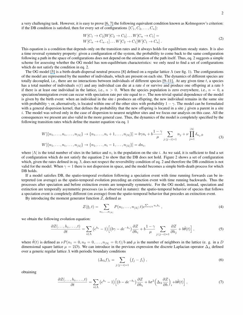
a very challenging task. However, it is easy to prove [6, 7] the following equivalent condition known as Kolmogorov’s criterion:if the DB condition is satisfied, then for every set of configurations {C1, C2, . . . , Cn}:

W [C1 → C2]W [C2 → C3] . . .W [Cn → C1] =

W [Cn → Cn−1] . . .W [C2 → C1]W [C1 → Cn] .(2)

This equation is a condition that depends only on the transition rates and it always holds for equilibrium steady states. It is alsoa time reversal symmetry property: given a configuration of the system, the probability to come back to the same configurationfollowing a path in the space of configurations does not depend on the orientation of the path itself. Thus, eq. 2 suggests a simplescheme for assessing whether the OG model has non-equilibrium characteristics: we only need to find a set of configurationswhich do not satisfy the condition in eq. 2.

The OG model [5] is a birth-death-dispersal neutral process [8] defined on a regular lattice Λ (see fig. 1). The configurationsof the model are represented by the number of individuals, which are present on each site. The dynamics of different species aretotally decoupled, i.e., there are no interactions between individuals of different species [9–11]. At any given time t, a specieshas a total number of individuals n(t) and any individual can die at a rate d or survive and produce one offspring at a rate bif there is at least one individual in the lattice, i.e., n > 0. When the species population is zero everywhere, i.e., n = 0, aspeciation/immigration event can occur with speciation rate per site equal to ν. The non-trivial spatial dependence of the modelis given by the birth event: when an individual in the site i produces an offspring, the new individual remains in the same sitewith probability γ or, alternatively, is located within one of the other sites with probability 1− γ. The model can be formulatedwith a general dispersion kernel, that defines the probability that the new offspring is located in a site j given a parent in a sitei. The model was solved only in the case of dispersion to nearest neighbor sites and we focus our analysis on this case. All theconsequences we present are also valid in the more general case. Thus, the dynamics of the model is completely specified by thefollowing transition rates which define the master equation via eq. 1

W [{n1, . . . , ni, . . . , n|Λ|} → {n1, . . . , ni + 1, . . . , n|Λ|}] = bγni + b1− γµ

∑j:|j−i|=1

nj + ν

|Λ|∏j=1

δnj ,0

W [{n1, . . . , ni, . . . , n|Λ|} → {n1, . . . , ni − 1, . . . , n|Λ|}] = dni,

(3)

where |Λ| is the total number of sites in the lattice and ni is the population on the site i. As we said, it is sufficient to find a setof configuration which do not satisfy the equation 2 to show that the DB does not hold. Figure 2 shows a set of configurationwhich, given the rates defined in eq. 3, does not respect the reversibility condition of eq. 2 and therefore the DB condition is notvalid for the model. When γ = 1 there is not dispersion in space, and the model becomes a simple birth-death process for whichDB holds.

If a model satisfies DB, the spatio-temporal evolution following a speciation event with time running forwards can be in-terpreted (on average) as the spatio-temporal evolution preceding an extinction event with time running backwards. Thus theprocesses after speciation and before extinction events are temporally symmetric. For the OG model, instead, speciation andextinction are temporally asymmetric processes (as is observed in nature): the spatio-temporal behavior of species that followsa speciation event is completely different (on average) from the spatio-temporal behavior that precedes an extinction event.

By introducing the moment generator function Z, defined as

Z(h, t) =∑

n1,...,n|Λ|

P (n1, . . . , n|Λ|; t)e∑

i∈Λ nihi , (4)

we obtain the following evolution equation:

∂Z(. . . , hi, . . . , t)

∂t=∑i∈Λ

(ehi − 1

)[(bγ − de−hi

) ∂Z∂hi

+ b1− γµ

∑j:|j−i|=1

∂Z

∂hj+ bθ(t)

], (5)

where θ(t) is defined as νP (n1 = 0, n2 = 0, . . . , n|Λ| = 0; t)/b and µ is the number of neighbors in the lattice (e. g. in a Ddimensional square lattice µ = 2D). We can introduce in the previous expression the discrete Laplacian operator ∆Λ definedover a generic regular lattice Λ with periodic boundary conditions

(∆Λf)i =∑

j:|j−i|=1

(fj − fi

), (6)

obtaining

∂Z(. . . , hi, . . . , t)

∂t=∑i∈Λ

(ehi − 1

)[(b− de−hi

) ∂Z∂hi

+ bσ2(

∆Λ∂Z

∂h

)i+bθ(t)

], (7)

3

where σ2 = (1 − γ)/µ. In the continuum limit (see the Supplementary Materials of [5]), the discrete Laplacian ∆Λ becomesthe Laplacian operator ∆ and thus we obtain

∂Z [H, t]

∂t=

∫A0

dDx(eH(x) − 1

)[bσ2∆

δZ [H, t]

δH(x)+(b− de−H(x)

)δZ [H, t]

δH(x)+ bθs(t)

], (8)

where A0 is the area (volume) of the entire system.One can show that the solution proposed by the authors in ref. [5] is equivalent to imposing DB. This condition for the OG

model (see fig. 1) can be written as

d(ni + 1)PDBs (. . . , ni + 1, . . . , nj , . . . ) =[bγni + b

1− γµ

∑j:|j−i|=1

nj + (∏j

δnj ,0)ν]PDBs (. . . , ni, . . . , nj , . . . )

(9)

for any choice of i. The notation PDBs stands for the stationary probability (i.e. the solution of the right hand side of masterequation set equal to zero) obtained by imposing the DB condition. By introducing into this expression the definition of Z, weobtain:

dehi∂Zdbs∂hi

= bγ∂Zdbs∂hi

+ bσ2∑

j:|j−i|=1

∂Zdbs∂hj

+ bθ , (10)

where θ is now equal to νPDBs (n1 = 0, . . . , n|Λ| = 0)/b. This expression, in the continuum limit, becomes

bσ2∆δZ db[H, t]

δH(x)+(b− de−H(x)

)δZ db[H, t]

δH(x)+ bθs = 0 . (11)

This is exactly the equation solved in ref. [5] . Thus we have shown that the solution obtained by the authors by consideringeq. 11 instead of the right side of eq 8 corresponds to imposing the detailed balance condition which is not valid for the OGmodel (as shown in fig. 2).

Assuming DB to hold when it is violated produces incorrect results. An example arises in the l-point correlation function.OG obtained an equation for the moment generating function Z defined in eq. 4: by expanding it, one can obtain the equationfor the l-points correlation function,

⟨ni1ni2 . . . nil

⟩:= Gl(i1, . . . , il). Because of its definition, the correlation function must

be symmetric under the exchange of its arguments, e.g., for the 3-point correlation function G3(i1, i2, i3) = G3(i2, i1, i3).We can show that applying DB to the OG model (i.e. by solving equation 11), one obtains asymmetric correlation functions.

Indeed the 3-point correlation function G3(i1, i2, i3) does not possess the required symmetry. To see this in an explicit way,a useful procedure to simplify and solve the involved differential equations is to apply the Fourier transform and consider thefunction G3(p

1, p

2, p

3). Because of the properties of the Fourier transform, we know that the function G3 is symmetric in

its arguments if and only if G3 is symmetric. By considering the first three correlation functions, we obtain the followingexpression:

G1(p1) =

bθ

b− dδ(p

1) =

⟨n⟩δ(p

1)

G2(p1, p

2) =

−dG1(p1

+ p2)

−bσ2p21

+ (b− d)=

−d⟨n⟩

−bσ2p21

+ (b− d)δ(p

1+ p

2)

G3(p1, p

2, p

3) =d

G1(p1

+ p2

+ p3)− G2(p

1+ p

2, p

3)− G2(p

1+ p

3, p

2)

−bσ2p21

+ (b− d)=

=2d⟨n⟩− bσ2p2

1+ (b− d)

(bσ2p21− b+ d)2

δ(p1

+ p2

+ p3) .

(12)

The three point correlation function is not symmetric in its arguments. It clearly shows that, on assuming DB in the OG model,we obtain inconsistencies in the solution. This inconsistence is valid for all the l-point correlation functions, except the 2-pointcorrelation function.

We have also simulated the model in a simple case: we show in fig. 3 that the analytical results do not match the numericalsimulations of the model. We consider the OG with just two sites. It is the simplest case in which DB is not valid (i.e. it ispossible to construct a cycle of configurations as in fig. 2). We find a stationary probability by applying DB and show that thiscondition produces inconsistencies.

4

Consider the generic configuration (n,m). The DB conditions can be expressed as{dPDB(1, 0) =

ν

2PDB(0, 0)

d(n+ 1)PDB(n+ 1,m) = b[γn+ (1− γ)m

]PDB(n,m) .

(13)

We can thus simply construct a solution by imposing DB. Specifically, we obtain for m and n bigger than zero

PDB(n,m) = θ(xγ)n+m

mn

[Γ(n+ 1−γ

γ m)

Γ(n)Γ(

1−γγ m

)] , (14)

where Γ(·) is the Gamma function and x = b/d. This expression is clearly inconsistent because it is not symmetric under theexchange of its arguments (n,m). We can see that this expression turns to be consistent for γ = 1 and γ = 1/2, exactly thechoices of parameters for which the reversal symmetry in fig. 2 is restored. This inconsistency is shown in fig. 3, where wecompare the analytical result with the numerical simulations. The case γ = 1 (which corresponds to σ = 0) is trivial becausein this case we are not considering diffusion in space and the sites are independent (see fig. 1) [9], and so the DB condition isvalid. In fact the 3-point correlation function in eq. 12 is symmetric in the case γ = 1. When we consider γ = 1/2 we expectthe DB not to be valid, because the 3-point correlation function is still non-symmetric. The fact that the DB seems to be valid inthe simulation of fig. 3 is simply due to the fact that we are considering a very simple case with only two sites.

We have shown that the solution obtained by applying the DB is not the real stationary solution of the model and that oneobtains incorrect results. It is not possible to treat that solution as an approximation to the correct one, because there is noparameter which is able to quantify the goodness of the approximation. In addition, the 3-point correlation function obtained onassuming DB is not symmetric and this leads to incorrect results, regardless of the nature of the approximation.

One may ask whether the formula obtained by applying the DB could provide a good fit to the data. Unfortunately this is notthe case. It is known that, at very small areas, the SAR grows linearly with the area [8, 12] and, in particular, it is equal to thenumber of sampled individuals. By expanding at small areas (r � σ) the solution obtained by imposing the DB, we obtain:

S(r) ∼ N(r) log( σ2

αr2

2

(1 + α)(log( 2σαr )− γE)

), (15)

where γE is the Euler-Mascheroni constant (γE ≈ 0.577 . . . ) andN(r) = θαπr

2 is the number of individuals sampled. Note thatthis expression is not close to the expected linear growth S(r) ∼ ρπr2 = N(r) (where ρ is the density of individuals), becausethe logarithm is much larger than one (σ/r � 1). Moreover, the expansion leads to the meaningless result that the number ofspecies sampled is larger than the number of individuals. This wrong prediction is one of the consequences of the use of the DBcondition.

The OG model was recently proposed [5] to describe the stationary properties of an ecosystem. This model appeared to bethe first solvable model able to predict the empirical Species-Area Relationship, which is one of the most important stationaryquantities in ecology. OG solved the model in an elegant manner via the moment generator functional. We have shown thatthe OG model is not an equilibrium model, as demonstrated in fig. 2. The OG model is a birth-death-migration process:a species changes its population and the individuals diffuse in space, a process which is not reversible. Furthermore, there areinconsistencies in the solution on wrongly assuming detailed balance such as the correlation functions no longer being symmetricin their arguments. The basic message is that the behaviors and the properties of the stationary state of equilibrium and non-equilibrium systems can be distinct. Life is not an equilibrium system nor it is reversible. Developing techniques for studyingthe behavior of models, which do not obey detailed balance, is a necessary but daunting step to understand the physics of non-equilibrium processes. An alternative to the OG model based on the Poisson cluster processes, which is solvable and leads to ananalytic expression for the SAR, has been recently developed [12].

Acknowledgments

JG and AM thank Cariparo foundation for financial support.

[1] R Durrett. Spatial Models for Species-Area Curves. Journal of Theoretical Biology, 179(2):119–127, March 1996.[2] Tommaso Zillio, Igor Volkov, Jayanth R. Banavar, Stephen P. Hubbell, and Amos Maritan. Spatial Scaling in Model Plant Communities.

Physical Review Letters, 95(9):1–4, August 2005.

5

[3] James Rosindell and Stephen J Cornell. Species-area relationships from a spatially explicit neutral model in an infinite landscape. Ecologyletters, 10(7):586–95, July 2007.

[4] Robert J. Wilson, Chris D. Thomas, Richard Fox, David B. Roy, and William E. Kunin. Spatial patterns in species distributions revealbiodiversity change. Nature, 432(7015):393–396, 2004. 10.1038/nature03031.

[5] James P O’Dwyer and Jessica L Green. Field theory for biogeography: a spatially explicit model for predicting patterns of biodiversity.Ecology letters, 13(1):87–95, January 2010.

[6] R K P Zia and B Schmittmann. Probability currents as principal characteristics in the statistical mechanics of non-equilibrium steadystates. Journal of Statistical Mechanics: Theory and Experiment, 2007(07):P07012–P07012, July 2007.

[7] A. Kolmogorov. Zur theorie der markoffschen ketten. Mathematische Annalen, 112:155–160, 1936. 10.1007/BF01565412.[8] Stephen P. Hubbell. The Unified Neutral Theory of Biodiversity and Biogeography. Princeton University Press, 2001.[9] Igor Volkov, Jayanth R. Banavar, Stephen P. Hubbell, and Amos Maritan. Neutral theory and relative species abundance in ecology.

Nature, 424(6952):1035–7, August 2003.[10] Igor Volkov, Jayanth R. Banavar, Stephen P. Hubbell, and Amos Maritan. Inferring species interactions in tropical forests. Proceedings

of the National Academy of Sciences of the United States of America, 106(33):13854–9, August 2009.[11] S. Azaele, R. Muneepeerakul, A. Rinaldo, and I. Rodriguez-Iturbe. Inferring plant ecosystem organization from species occurrences.

Journal of Theoretical Biology, 262(2):323–329, 2010.[12] J. Grilli, S. Azaele, J. Banavar, and A. Maritan. Spatial aggregation and the species area relationship across scales. Journal of Theoretical

Biology, 313(0):87 – 97, 2012.

6

independence

we can considerone species

at a time

no interactionbetween species

rate: d

death

rate: ν

speciation

rate: b(1-γ)

rate: bγ

birth

dynamics

FIG. 1: Definition of the OG model. The model is non-interacting (different species are totally decoupled) and neutral (theparameters of the model do not depend on the species we are considering). Because of these assumptions it is possible to

consider one species at a time. In the figure, a one dimensional lattice is shown for simplicity. A circle corresponds to a singleindividual and its color represents the species it belongs to. There is no limit to the number of individuals that can be placed ineach site. The dynamics is defined in terms of three possible main moves: birth, death and speciation. The per capita death rate

is equal to d, whereas the speciation rate (defined per unit of lattice spacing) is ν. The total birth rate is equal to b: with aprobability γ, the offspring is placed in the same site as the parent, while, with a probability 1− γ, it is placed in a different site

chosen uniformly among the neighboring sites (which corresponds to a dispersal move).

7

n

m

m

n

m+1

n+1

m+1

n+1

d(m+1) d(n+1)

d(n+1) d(m+1)

b[γm+(1-γ)n] b[γn+(1-γ)(m+1)]

b[γn+(1-γ)m]b[γm+(1-γ)(n+1)]

b2d2[γn+(1-γ)m][γm+(1-γ)(n+1)][m+1][n+1]

b2d2[γm+(1-γ)n][γn+(1-γ)(m+1)][m+1][n+1]

different!if γ≠½, γ≠1 or m≠n

FIG. 2: Detailed Balance in the OG model. In general, detailed balance is not satisfied if the probability to go along a closedpath in the space of configurations depends on the direction that one chooses (see eq. 2). Here we present the simplest

counterexample to eq. 2 for the OG model. The probability to find the system in any of the four configurations in red and linkedby the cycle depends on whether one follows the green or blue path. When γ = 1, detailed balance is valid, whereas, forγ = 1/2, it is generally not valid (i.e. even though the condition of eq. 2 is valid for this particular cycle, it is not valid

generally).

8

ɤ=0.25 ɤ=0.5

ɤ=0.75 ɤ=0.9

0 10 20 30 40 50n

1e-16

1e-12

1e-08

0.0001

1

Cum

ulat

ive

Pro

babi

lity

numerical simulationanalytical solution(detailed balance)

0 10 20 30 40 50n

1e-08

0.0001

1

Cum

ulat

ive

Pro

babi

lity

0 10 20 30 40 50n

1e-07

1e-06

1e-05

0.0001

0.001

0.01

0.1

1

Cum

ulat

ive

Pro

babi

lity

0 20 40n

1e-06

0.0001

0.01

1

Cum

ulat

ive

Pro

babi

lity

FIG. 3: Comparison between the simulations of the OG model and the analytical solution obtained by applying the DBcondition. The blue circles are simulations of the cumulative stationary probabilities P>1 (n) =

∑∞k=n

∑∞m=0 P (k,m). The red

triangles represents P>DB1 (n), obtained by summing over m eq. 14, which is calculated by imposing DB. As expected, thesolutions are different, except in the case γ = 1/2 (as expected from fig. 2). For this value of γ the DB is still not valid (3-pointcorrelation function is still non-symmetric). This special behavior of the model for γ = 0.5 is therefore caused by the smallness

of the system considered in this case, and not because DB is restored. The model is simulated with the following parameters:b = 0.9, d = 1. and ν = 0.1.