econstor www.econstor.eu

Der Open-Access-Publikationsserver der ZBW – Leibniz-Informationszentrum WirtschaftThe Open Access Publication Server of the ZBW – Leibniz Information Centre for Economics

Nutzungsbedingungen:Die ZBW räumt Ihnen als Nutzerin/Nutzer das unentgeltliche,räumlich unbeschränkte und zeitlich auf die Dauer des Schutzrechtsbeschränkte einfache Recht ein, das ausgewählte Werk im Rahmender unter→ http://www.econstor.eu/dspace/Nutzungsbedingungennachzulesenden vollständigen Nutzungsbedingungen zuvervielfältigen, mit denen die Nutzerin/der Nutzer sich durch dieerste Nutzung einverstanden erklärt.

Terms of use:The ZBW grants you, the user, the non-exclusive right to usethe selected work free of charge, territorially unrestricted andwithin the time limit of the term of the property rights accordingto the terms specified at→ http://www.econstor.eu/dspace/NutzungsbedingungenBy the first use of the selected work the user agrees anddeclares to comply with these terms of use.

zbw Leibniz-Informationszentrum WirtschaftLeibniz Information Centre for Economics

Dobos, Imre; Gobsch, Barbara; Pakhomova, Nadezhda; Pishchulov, Grigory;Richter, Knut

Working Paper

A vendor-purchaser economic lot size problem withremanufacturing and deposit

Discussion paper // European University Viadrina, Department of Business Administrationand Economics, No. 304

Provided in Cooperation with:European University Viadrina Frankfurt (Oder), Department of BusinessAdministration and Economics

Suggested Citation: Dobos, Imre; Gobsch, Barbara; Pakhomova, Nadezhda; Pishchulov,Grigory; Richter, Knut (2011) : A vendor-purchaser economic lot size problem withremanufacturing and deposit, Discussion paper // European University Viadrina, Department ofBusiness Administration and Economics, No. 304

This Version is available at:http://hdl.handle.net/10419/49533

A vendor-purchaser economic lot size problem with remanufacturing and deposit

Imre Dobos

Barbara Gobsch

Nadezhda Pakhomova

Grigory Pishchulov

Knut Richter

___________________________________________________________________

European University Viadrina Frankfurt (Oder)

Department of Business Administration and Economics

Discussion Paper No. 304

August 2011

ISSN 1860 0921

___________________________________________________________________

1

A vendor-purchaser economic lot size problem with remanufacturing and deposit

Imre Dobos1, Barbara Gobsch2, Nadezhda Pakhomova3, Grigory Pishchulov2, Knut Richter2

August 1, 2011

1 Corvinus University of Budapest, Institute of Business Economics, H-1093 Budapest, Fővám tér 8., Hungary, imre.dobos@uni-corvinus.hu 2 European University Viadrina Frankfurt (Oder), Chair of Industrial Management, D-15230 Frankfurt (Oder), Große Scharrnstr. 59, Germany, {Gobsch;Pishchulov;Richter}@europa-uni.de 3 St. Petersburg State University, Chair of Economic Theory, 62 Chaykovskogo str., 191123 St. Petersburg, Russia, pak-nadezda@yandex.ru Abstract. An economic lot size problem is studied in which a single vendor supplies a single purchaser with a homogeneous product and takes a certain fraction of the used items back for remanufacturing, in exchange for a deposit transferred to the purchaser. For the given demand, productivity, fixed ordering and setup costs, amount of the deposit, unit disposal, production and remanufacturing costs, and unit holding costs at the vendor and the purchaser, the cost-minimal order/lot sizes and remanufacturing rates are determined for the purchaser, the vendor, the whole system assuming partners’ cooperation, and for a bargaining scheme in which the vendor offers an amount of the deposit and a remanufacturing rate, and the purchaser responds by setting an order size.

Keywords: Joint economic lot size, Reverse logistics, Closed loop supply chain, Collection, Remanufacturing, EOQ

1. Introduction In the present paper, an economic lot size problem is studied in which a single vendor

supplies a single purchaser with a homogeneous product and takes a certain fraction of the

used items back for remanufacturing, in exchange for a deposit transferred to the purchaser.

For the given demand, productivity, remanufacturing rate, fixed ordering and setup costs,

amount of the deposit, unit disposal, production and remanufacturing costs, and unit holding

costs at the purchaser and the vendor, the cost-minimal order/lot sizes and remanufacturing

rates are determined for the purchaser, the vendor, the whole system assuming partners’

cooperation, and for a bargaining scheme in which the vendor offers the amount of the deposit

and the remanufacturing rate, and the purchaser reacts by setting the order size.

The problem of coordinating a supply chain with a single buyer demanding the product at a

constant rate and a single supplier operating in a lot-for-lot fashion has been addressed by

Monahan (1984) who considered quantity discounts as a coordination means. Subsequently

Banerjee (1986a,b) has put forward a more general model that accounts for the inventory

holding costs at the vendor, and coined the term joint economic lot size. Their work has

triggered a broad research interest in this and related supply chain coordination problems. In

particular, omission of the lot-for-lot assumption identifies a major research direction which

2

addressed different forms of production and shipment policy (see, among others, Lee and

Rosenblatt, 1986; Goyal, 1988; Hill, 1997, 1999; Eben-Chaime, 2004; Hill and Omar, 2006;

Zhou and Wang, 2007; Hoque, 2009; see also Goyal, 1976, for an earlier model); we refer the

reader to Sucky (2005) and Leng and Parlar (2005) for excellent reviews, as well. The work

by Affisco et al. (2002) and Liu and Çetinkaya (2007) takes imperfect product quality into

account and accommodates the opportunity of investing in quality improvement and setup

cost reduction at the supplier. Kohli and Park (1989) have addressed the question of benefit

sharing between the supply chain members from a game-theoretical standpoint. Sucky (2006)

has further analysed the Banerjee’s model in a setting with a privately informed buyer;

similarly, Voigt and Inderfurth (2011) study a problem with information asymmetry and

opportunity of investing in setup cost reduction. An approach to implement the joint

optimization by the supply chain members without explicit disclosure of one’s own sensitive

data has been recently addressed by Pibernik et al. (2011).

At the same time, closed-loop supply chain problems are receiving an increasing attention in

the literature. In the early work by Richter (1994, 1997) and Richter and Dobos (1999), an

EOQ-like system with manufacturing, remanufacturing and disposal has been analyzed and

the structure of optimal policies and cost functions established. More recently, Chung et al.

(2008), Gou et al. (2008), Mitra (2009) and Yuan and Gao (2010) address the inventory costs

minimization in a closed-loop supply chain context and offer an optimal

manufacturing/remanufacturing strategy throughout the planning horizon. Bonney and Jaber

(2011) extend the classical reverse logistics inventory models to environmentally related

manufacturing factors in order to involve further metrics in the cost functions of inventory

management — other than just the costs of operating the system. Grimes-Casey et al. (2007),

Lee et al. (2010) and Subramoniam et al. (2010) investigate the practical application of

reverse logistics models. In this context the models of Grimes-Casey et al. (2007) and Lee et

al. (2010) analyze the lifecycle aspects of the reuse systems. Ahn (2009) and Grimes-Casey et

al. (2007) suggest game-theoretical approaches for determining the best closed-loop supply

chain strategies.

In the present paper we study a family of problems that represent, on the one hand, an

extension of the basic model by Banerjee (1986a,b) to the case of reverse logistics flows —

which have not been addressed in his work. On the other hand, they generalize the

manufacturing and remanufacturing models of Richter (1994, 1997) and Richter and Dobos

(1999) by accommodating a purchaser into the analysis (see Fig. 1).

3

Fig. 1: Extending the models by Banerjee and Richter, Dobos

Furthermore, we investigate whether the reuse process helps to coordinate the vendor–

purchaser supply chain. The paper is organized as follows. In the second section we present

the models, classify them and construct the cost functions. In section 3 we determine the

optimal lot sizes and minimum cost functions for the purchaser, the vendor and the total

system for the case that the manufacturing process starts the production cycle. In the next

section an auxiliary function is introduced. The explicitly found minimum point of this

function helps to determine the optimal remanufacturing rates for the partners of the supply

chain. In section 5 the same problems will be solved for the case of starting the production

process with remanufacturing. In the sixth section, a bargaining scheme is considered in

which the vendor offers a deposit amount and a remanufacturing rate, and the purchaser reacts

by setting the order size. The final section concludes with a summary.

2. The model

2.1. General description

The model deals with the setting in which a single vendor (he) ships a homogeneous product

to a single purchaser (her) according to her deterministic constant demand of D units per time

unit. The vendor and the purchaser will have to agree on the regular shipment size q which

has also to be the production lot size of the vendor. This size can be determined by the

vendor, by the purchaser or jointly by both of them. The vendor manufactures new items and

can also produce as-good-as-new items by remanufacturing used ones. Both kinds of items —

which are shortly called serviceables — serve the demand of the purchaser. The end-of-use

items (nonserviceables) can be collected by the purchaser and taken back to the vendor for

remanufacturing. By assumption, the same vehicle that delivers the serviceables to the

purchaser, also picks up the nonserviceables accumulated by her and returns them back to the

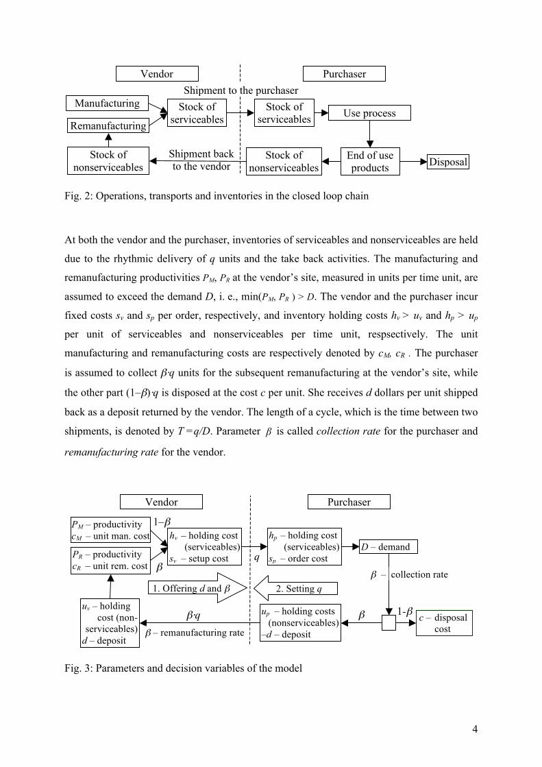
vendor when backhauling (see Fig. 2). The parameters and decision variables employed in the

model are presented in Fig. 3.

Banerjee

Richter, Dobos

Manufacturing, no remanufacturing

Manufacturing & remanufacturing

Manufacturer & purchaser

Manufacturer only, no purchaser

Manufacturer & purchaser,

manufacturing & remanufacturing

4

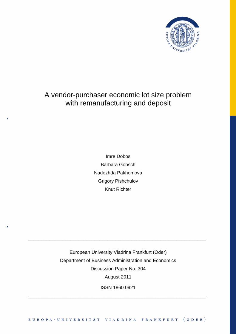
Fig. 2: Operations, transports and inventories in the closed loop chain

At both the vendor and the purchaser, inventories of serviceables and nonserviceables are held

due to the rhythmic delivery of q units and the take back activities. The manufacturing and

remanufacturing productivities PM, PR at the vendor’s site, measured in units per time unit, are

assumed to exceed the demand D, i. e., min(PM, PR ) > D. The vendor and the purchaser incur

fixed costs sv and sp per order, respectively, and inventory holding costs hv > uv and hp > up

per unit of serviceables and nonserviceables per time unit, respsectively. The unit

manufacturing and remanufacturing costs are respectively denoted by cM, cR . The purchaser

is assumed to collect β⋅q units for the subsequent remanufacturing at the vendor’s site, while

the other part (1–β)⋅q is disposed at the cost c per unit. She receives d dollars per unit shipped

back as a deposit returned by the vendor. The length of a cycle, which is the time between two

shipments, is denoted by T =q/D. Parameter β is called collection rate for the purchaser and

remanufacturing rate for the vendor.

Fig. 3: Parameters and decision variables of the model

β⋅q

q

1-β

1–β

β

Vendor

PM – productivity cM – unit man. cost

PR – productivity cR – unit rem. cost

uv – holding cost (non-

serviceables) d – deposit

hv – holding cost (serviceables)

sv – setup cost

Purchaser

D – demand

c – disposal cost

β – collection rate

up – holding costs (nonserviceables)

–d – deposit

hp – holding cost (serviceables)

sp – order cost

β

1. Offering d and β

β – remanufacturing rate

2. Setting q

Vendor

Manufacturing

Remanufacturing

Stock of nonserviceables

Stock of serviceables

Purchaser

Use process

End of use products

Stock of serviceables

Disposal Shipment back to the vendor

Stock of nonserviceables

Shipment to the purchaser

5

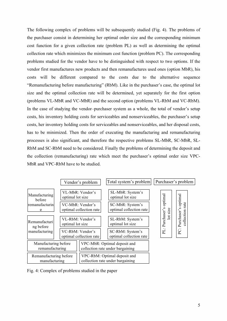
The following complex of problems will be subsequently studied (Fig. 4). The problems of

the purchaser consist in determining her optimal order size and the corresponding minimum

cost function for a given collection rate (problem PL) as well as determining the optimal

collection rate which minimizes the minimum cost function (problem PC). The corresponding

problems studied for the vendor have to be distinguished with respect to two options. If the

vendor first manufactures new products and then remanufactures used ones (option MbR), his

costs will be different compared to the costs due to the alternative sequence

“Remanufacturing before manufacturing” (RbM). Like in the purchaser’s case, the optimal lot

size and the optimal collection rate will be determined, yet separately for the first option

(problems VL-MbR and VC-MbR) and the second option (problems VL-RbM and VC-RbM).

In the case of studying the vendor–purchaser system as a whole, the total of vendor’s setup

costs, his inventory holding costs for serviceables and nonserviceables, the purchaser’s setup

costs, her inventory holding costs for serviceables and nonserviceables, and her disposal costs,

has to be minimized. Then the order of executing the manufacturing and remanufacturing

processes is also significant, and therefore the respective problems SL-MbR, SC-MbR, SL-

RbM and SC-RbM need to be considered. Finally the problems of determining the deposit and

the collection (remanufacturing) rate which meet the purchaser’s optimal order size VPC-

MbR and VPC-RbM have to be studied.

Fig. 4: Complex of problems studied in the paper

Vendor’s problem

Manufacturing before

remanufacturing

VL-MbR: Vendor’s optimal lot size

Purchaser’s problem Total system’s problem

VC-MbR: Vendor’s optimal collection rate

SL-MbR: System’s optimal lot size

SC-MbR: System’s optimal collection rate

PL: P

urch

aser

’s o

ptim

al

lot s

ize

PC: P

urch

aser

’s o

ptim

al

colle

ctio

n ra

te

Remanufacturing before

manufacturing

VL-RbM: Vendor’s optimal lot size

VC-RbM: Vendor’s optimal collection rate

SL-RbM: System’s optimal lot size

SC-RbM: System’s optimal collection rate

Remanufacturing before manufacturing

Manufacturing before remanufacturing

VPC-MbR: Optimal deposit and collection rate under bargaining

VPC-RbM: Optimal deposit and collection rate under bargaining

6

2.2. Purchaser’s cost function

Before the models can be formulated analytically some further assumptions have to be made.

The purchaser is supposed to sort out the items which are suitable for remanufacturing

continuously over time and at a constant rate. Hence the average inventory level of her

serviceables per order cycle is ( ) 2/qqI sp = and the inventory level of nonserviceables is

( ) 2/qββ,qI np ⋅= . Then the purchaser’s total costs per time unit are expressed by

€

TCp q,β( )= Cp q,β( )+ Rp β( ) (1)

where

( ) ( )ββ ⋅+⋅+⋅= pppp uhqqDsqC

2, and ( ) ( )( )DdccRp ββ +−= (2)

represent the cost components which respectively do and do not depend on the order size.

2.3. Vendor’s cost function for MbR

The inventory levels of serviceables and nonserviceables at the vendor depend obviously on

the order in which manufacturing and remanufacturing are executed. Consider first the MbR

option which assumes that in each order cycle, first (1-β)q items are manufactured and then

βq items are remanufactured. The RbM option will be studied subsequently in Section 5.

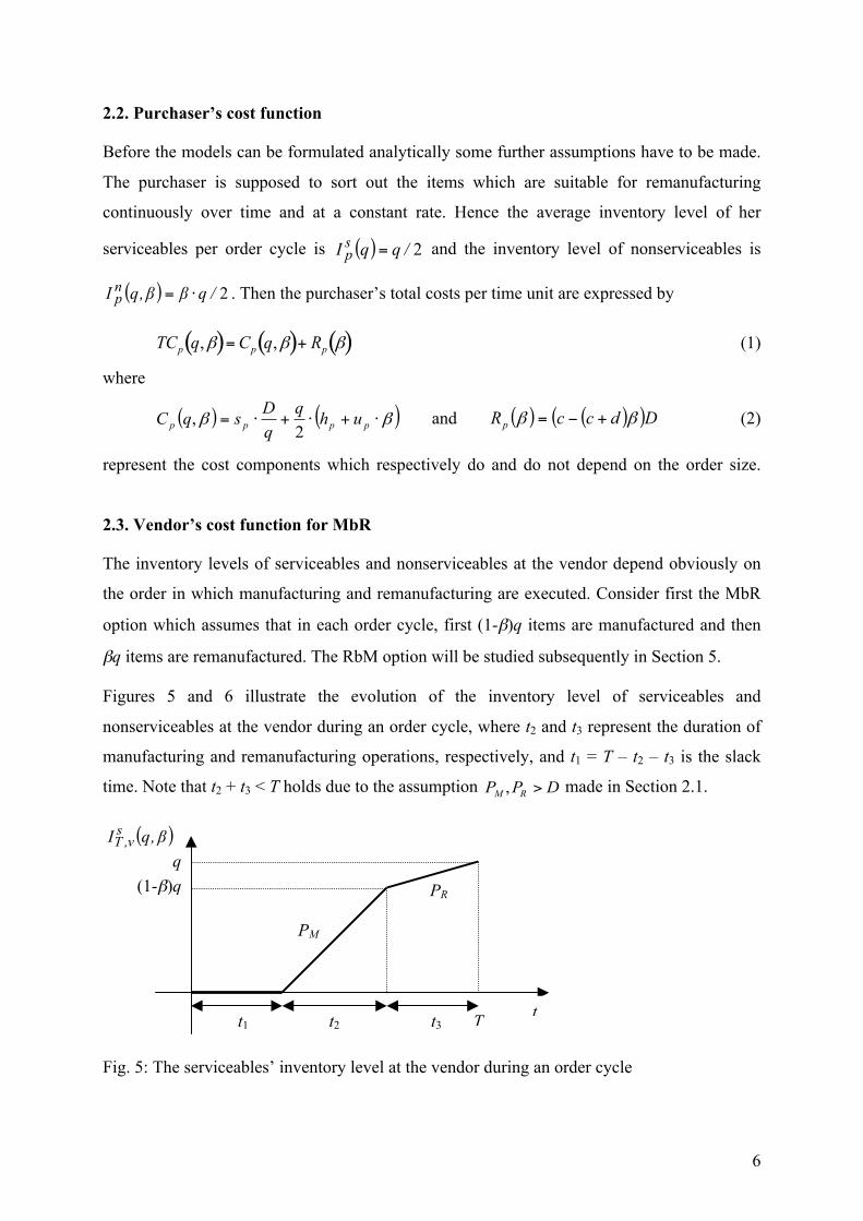
Figures 5 and 6 illustrate the evolution of the inventory level of serviceables and

nonserviceables at the vendor during an order cycle, where t2 and t3 represent the duration of

manufacturing and remanufacturing operations, respectively, and t1 = T – t2 – t3 is the slack

time. Note that t2 + t3 < T holds due to the assumption

€

PM ,PR > D made in Section 2.1.

Fig. 5: The serviceables’ inventory level at the vendor during an order cycle

(1-β)q PR

PM

t

q

T t1 t2 t3

( )β,qI s v,T

7

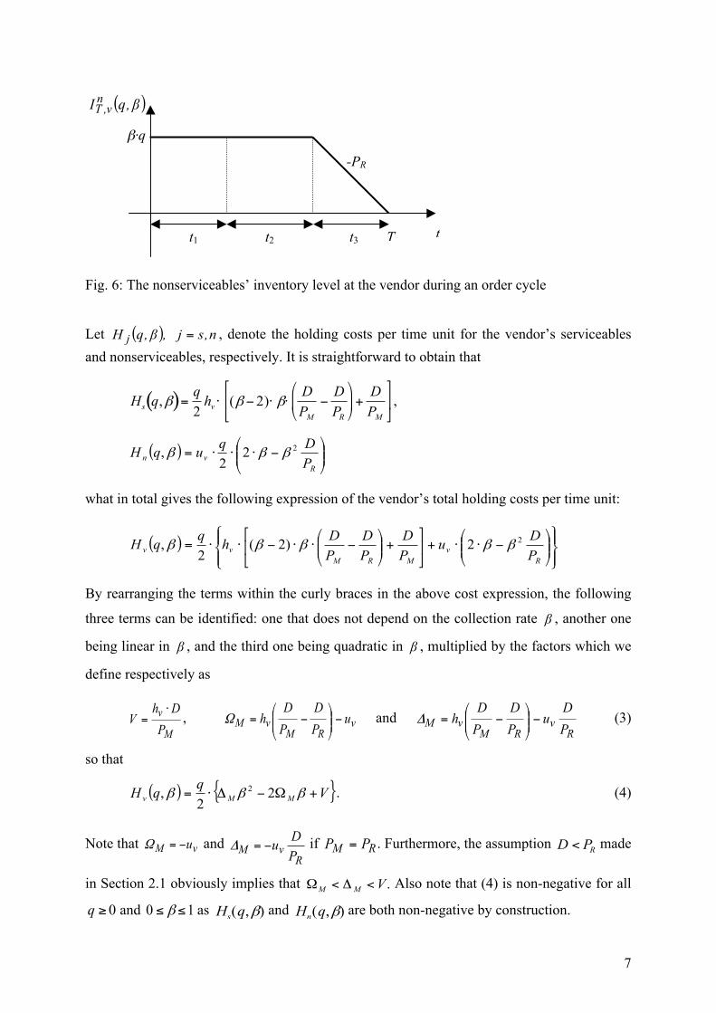
Fig. 6: The nonserviceables’ inventory level at the vendor during an order cycle

Let ( ) n,sj ,β,qH j = , denote the holding costs per time unit for the vendor’s serviceables and nonserviceables, respectively. It is straightforward to obtain that

€

Hs q,β( )=q2

hv ⋅ (β − 2)⋅ β⋅DPM

−DPR

⎛

⎝ ⎜

⎞

⎠ ⎟ +

DPM

⎡

⎣ ⎢

⎤

⎦ ⎥ ,

( ) ⎟⎟⎠

⎞⎜⎜⎝

⎛−⋅⋅⋅=

Rvn P

DquqH 222

, βββ

what in total gives the following expression of the vendor’s total holding costs per time unit:

( )⎪⎭

⎪⎬⎫

⎪⎩

⎪⎨⎧

⎟⎟⎠

⎞⎜⎜⎝

⎛−⋅⋅+⎥

⎦

⎤⎢⎣

⎡+⎟⎟⎠

⎞⎜⎜⎝

⎛−⋅⋅−⋅⋅=

Rv

MRMvv P

DuPD

PD

PDhqqH 22)2(

2, βββββ

By rearranging the terms within the curly braces in the above cost expression, the following

three terms can be identified: one that does not depend on the collection rate β , another one

being linear in β , and the third one being quadratic in β , multiplied by the factors which we

define respectively as

M

vPDh

V⋅

= , vRM

vM uPD

PD

h −⎟⎟⎠

⎞⎜⎜⎝

⎛−=Ω and

Rv

RMvM P

Du

PD

PD

h −⎟⎟⎠

⎞⎜⎜⎝

⎛−=Δ (3)

so that

( ) { }VqqH MMv +Ω−Δ⋅= βββ 22

, 2 . (4)

Note that vM u−=Ω and R

vM PDu−=Δ if RM PP = . Furthermore, the assumption

€

D < PR made

in Section 2.1 obviously implies that

€

ΩM < ΔM < V . Also note that (4) is non-negative for all

€

q ≥ 0 and

€

0 ≤ β ≤1 as

€

Hs(q,β) and

€

Hn(q,β) are both non-negative by construction.

( )β,qI n v,T

T t3

-PR

t

β·q

t1 t2

8

The vendor’s ordering and holding costs per time unit express consequently as

( ) { }MMvv VqqDsqC Ω⋅⋅−Δ⋅+⋅+= βββ 2

2, 2 . (5)

The vendor incurs also costs which do not depend on the lot size, amounting per time unit to

€

Rv β( )= cM + d + cR − cM( )β( )D .

Accordingly, the vendor’s total costs per time unit are expressed by

€

TCv q,β( )= Cv q,β( )+ Rv β( ). (6)

2.3. The total system costs

Now the costs of the vendor and the purchaser are considered jointly. The joint ordering and

holding costs per time unit are then expressed by

( ) ( ) ( ){ }pMpMpvT hVuqqDssqC ++Ω−+Δ⋅⋅++= 2

2, 2 βββ . (7)

Let

phVW += and MpuU Ω2−= . (8)

Then (7) can be rewritten as

( ) ( ) { }WUqqDssqC MpvT ++Δ⋅⋅++= βββ 2

2,

and the system-wide total costs per time unit expressed by

€

TCT q,β( )= CT q,β( )+ RT β( ) (9)

where

€

RT β( )= c + cM + β cR − c − cM( )( )D is the cost component that does not depend on the

lot size. Note that

( ) ( ) ( )00 ==

+=dpdvT RRR βββ . (10)

3. Analysis of the optimal lot sizes and minimal cost functions

Firstly, the cost functions of the purchaser, the vendor and the whole system are analyzed to

determine the optimal order and lot sizes, respectively.

9

The purchaser’s PL problem is merely a modification of the classical EOQ model. The

optimal order size for a given collection rate ! is then expressed as

€

qp∗ β( )=

2⋅ sp⋅ Dhp + β⋅ up

(11)

with the corresponding minimum total costs

€

TCp∗ β( )= 2⋅ D⋅ sp ⋅ hp + β⋅ up( )+ Rp β( ). (12)

In the same way, the vendor’s optimal lot size under MbR policy (i.e., the optimal solution to

the VL-MbR problem) is the one that minimizes (6) and expresses accordingly as

€

qv∗ β( )=

2⋅ D⋅ sv

β2 ⋅ ΔM − 2⋅ β⋅ ΩM +V. (13)

His resulting minimum total costs are then represented by the function

( ) ( ) ( )ββββ vMMvv RVsDTC ++Ω⋅⋅−Δ⋅⋅⋅⋅=∗ 22 2 . (14)

It is straightforward to see that the sign of this function’s 2nd derivative does not depend on

€

β,

therefore (14) is either convex or concave in β. Thus by analyzing its 1st derivative and the

function values at the borders, we can easily determine whether its minimum is attained at

β = 0, β = 1, or some point in between. In the latter case, the optimal collection rate will be

called non-trivial. Section 4.2 below provides a detailed analysis of the respective VC-MbR

problem.

Similarly, it follows from (7)–(9) that the system-wide optimal lot size (i.e., the solution to the

SL-MbR problem) is given by

q*(! ) =2 !D !(sv + sp )

W + ! 2 !"M + ! !U (15)

and implies the following minimum total costs for the system:

( ) ( ) ( ) ( )ββββ TMPv RUWssDTC +⋅+Δ⋅+⋅+⋅⋅=∗ 22 . (16)

It can be seen that in all of the above three cases, the classical EOQ formula is employed —

with merely straightforward modifications that reflect the composition of the cost function

coefficients in the purchaser’s, the vendor’s, and the system-wide problems, respectively.

10

4. The optimal collection and remanufacturing rates

Before we proceed with the analysis of the optimal collection and remanufacturing rates for

the purchaser, the vendor and the whole system, respectively, it makes sense to utilize the fact

that the respective minimum cost functions (12), (14), (16) have a similar form and to

introduce the following “omnibus” function:

( ) FECBAGK +⋅+−+= ββββ 22 (17)

for which we further assume that

€

A,G > 0 and that

€

A + Bβ2 − 2Cβ > 0 (18)

holds on the entire domain 10 ≤≤ β . It is straightforward to see that

€

K(β) is strictly convex

if and only if

€

AB > C2 , (19)

and otherwise concave. If strictly convex, the function has a minimum in the interior of its

domain whenever

€

ʹ′ K (0) < 0 and

€

ʹ′ K (1) > 0 — what, in turn, holds if and only if the

inequalities

€

C − BA + B − 2C

<EG

<CA

(20)

hold. In all other cases the minimum is found at one of the boundary points

€

β = 0,

€

β =1. This

provides us with the following

Lemma 1. Assume that

€

AB > C2 . If condition (20) is satisfied then

€

K(β) has a global minimum at

€

β* =CB−

EB

AB −C2

BG2 − E2 (21)

and otherwise at

€

β* = 0 whenever the right-hand inequality in (20) does not hold, and at

€

β* =1 whenever the left-hand one does not.

Proof: As discussed above, the assumption of the lemma implies that

€

K(β) is strictly convex.

Let (20) hold. Then the function is decreasing at 0=β due to

€

ʹ′ K (0) < 0 and increasing at

1=β due to

€

ʹ′ K (1) > 0. By the strict convexity, the global minimum is attained at the unique

interior point

€

β* ∈ (0,1) with

€

ʹ′ K (β* ) = 0 , which we accordingly determine by solving

€

ʹ′ K β( )= GBβ −C

A + Bβ2 − 2Cβ+ E = 0 (22)

11

what implies:

€

C2 − 2BCβ+ B2β2

A + Bβ2 − 2Cβ=

EG⎛

⎝ ⎜

⎞

⎠ ⎟

2

and gives the following quadratic equation after rearranging the terms:

€

B(BG2 − E2 )β2 − 2C(BG2 − E 2)β+ C2G2 − AE2 = 0.

Note that

€

B > 0 holds due to the assumption of the lemma. Also note that

€

BG2 − E2 ≠ 0 since

otherwise

€

C2G2 = AE2 what contradicts (20). Hence the above equation can be rewritten as

€

β2 − 2CBβ+

C2G2 − AE2

B(BG2 − E2 )= 0.

Its roots are given by

€

β1,2 =CB

±C2

B2 −C2G2 − AE2

B(BG2 − E2 )=

CB

±ABE2 −C2E2

B2(BG2 − E2 )=

CB

±| E |B

AB −C2

BG2 − E2 . (23)

Substituting both roots for ! in (22), one can see that ! * = !2 if E > 0 , otherwise ! * = !1 .

Thus the following applies:

€

β* =CB−

EB

AB −C2

BG2 − E2 .

Assume now that the right-hand inequality in (20) does not hold — what implies

€

ʹ′ K (0) ≥ 0.

By the strict convexity,

€

ʹ′ ʹ′ K > 0 and thus

€

ʹ′ K is growing at each point of the domain. Therefore

€

ʹ′ K (β) > 0 at all

€

0 < β ≤1, what proves

€

K(β) to grow on the right from

€

β = 0. Then obviously

€

β* = 0 is its global minimum. By a similar argument we obtain

€

β* =1 when the left-hand

inequality in (20) does not hold. Note that with

€

ʹ′ ʹ′ K > 0, both inequalities in (20) cannot be

violated simultaneously. �

It follows from the above proof that real-valued roots (23) which solve (22) exist under the

assumption of Lemma 1 if and only if

€

BG2 > E2 , otherwise there is no such interior point at

which

€

ʹ′ K (β) = 0. This provides us with the following

Corollary 1. The condition of Lemma 1 can only be satisfied if

€

B >E2

G2 holds. A sufficient

(but not necessary) condition for that is

€

C > 0,E ≥ 0, provided that the assumption and the

condition of Lemma 1 hold.

12

Proof: Indeed, assume that

€

C > 0 and

€

E ≥ 0 holds. The condition of Lemma 1 requires

€

EG

<CA

, what is then equivalent to requiring

€

E2

G2 <C2

A, given that

€

A,G > 0 holds for

€

K(β)

by assumption. At the same time, the assumption of the Lemma implies

€

C2

A< B. This gives

€

E2

G2 < B, as required. �

The following lemma treats the case of concave

€

K(β).

Lemma 2. If

€

AB ≤C2 then

€

K(β) has a global minimum at

€

β* = 0 whenever the inequality

€

A − A + B − 2C ≤EG

holds, and at

€

β* =1 whenever it holds in the opposite direction. The case of equality implies

that both

€

β = 0 and

€

β =1 deliver a global minimum to

€

K(β).

Proof: The condition

€

AB ≤C2 implies that the 2nd derivative

€

ʹ′ ʹ′ K is non-negative and constant

everywhere on the function’s domain, hence

€

K(β) is either strictly concave or linear. Hence

if a local optimum is found in the domain’s interior, it can only be a global maximum;

otherwise the function is monotonic on the entire domain and, in either case, it suffices to

compare its values at the boundary points to figure out a global minimum. This immediately

leads to the assertion of the lemma. �

We now proceed to the analysis of the respective optimal collection rates for the purchaser,

the vendor and the whole system.

4.1. Purchaser’s solution

It is straightforward to see that the purchaser’s minimum cost function (12) represents

K(!)

with

A = hp ,

B = 0,

C = !up / 2 ,

E = !(c + d )D ,

F = cD ,

G = 2Dsp and obviously

complies with the assumptions made for

K(!) at the beginning of Section 4. It is also obvious

to see that it satisfies the condition of Lemma 2, hence the purchaser is not interested in

collecting any used items (

!* = 0) if

(c + d ) D < hp + up ! hp( )" 2sp

and will collect all of them (

!* = 1) in the opposite case. He is indifferent between the two

policies if the above inequality be equality.

13

4.2. Vendor’s solution (VC-MbR)

The vendor’s minimum cost function (14) represents

K(!) with

A = V ,

B = !M ,

C = !M ,

E = (d + cR ! cM )D ,

F = cM D and

G = 2Dsv . There holds accordingly the following

Lemma 3. Under conditions (18)–(20), the vendor’s optimal remanufacturing rate is non-

trivial and given by

!* ="M

#M

$E#M

#M % V $"M2

#M % 2Dsv $ E2 . (24)

Corollary 2. Equation (24) can be used to determine the vendor’s optimal remanufacturing

rate whenever the following conditions simultaneously hold:

!M >"M

2

V (25)

!M >D" (d + cR # cM )2

2sv

(26)

uv ! (D / PR "1)(hv " uv )! D / PR + 2uv

<(d + cR " cM )! D

2Dsv

<#M

V (27)

In particular, either of conditions (25) and (26) imply:

PR

PM

> 1+uv

hv

. (28)

Hence PR must necessarily exceed PM for

!* being a non-trivial remanufacturing rate. If any

of conditions (25)–(27) is violated then the vendor’s optimal remanufacturing rate happens to

be either

!* = 0 or

!* = 1.

Proof: It can be easily seen that conditions (19) and (20) immediately translate to (25) and

(27), whereas (18) translates to:

!M"2 # 2$M" + V > 0 .

It is straightforward to see that the quadratic function on the left has no real-valued roots

whenever

!M2 < "MV — what is, in turn, required by (25). Also by the virtue of (25),

!M > 0

and the quadratic function has its branches directed upwards. This guarantees the required

positivity of the function for all feasible values of

!

"; thus, (25) implies (18) to hold. Further,

14

condition (26) is an immediate consequence of Corollary 1. Finally, either of (25) and (26)

imply

!M > 0. This together with the definition of

!M in (3) leads to (28). �

Example 1 (VC-MbR). Let D = 100, sv = 1000, hv = 100, uv = 5, cM = 35, cR = 20, d = 17,

PM = 200, PR = 250 (see Fig. 7). Then

A = V = 50, 8== MB Δ , 5== MC Ω , 200=E ,

F = 3500,

G ! 447.21. It is straightforward to see that conditions (25), (26), (27) respectively

hold:

!M = 8 >"M

2

V=

2550

= 0.5

!M = 8 >D" (d + cR # cM )2

2sv

=100" (17 + 20 # 35)2

2000= 0.2

uv ! (D / PR "1)(hv " uv )! D / PR + 2uv

# "0.433 <(d + cR " cM )! D

2Dsv

# 0.447 <$M

V# 0.707

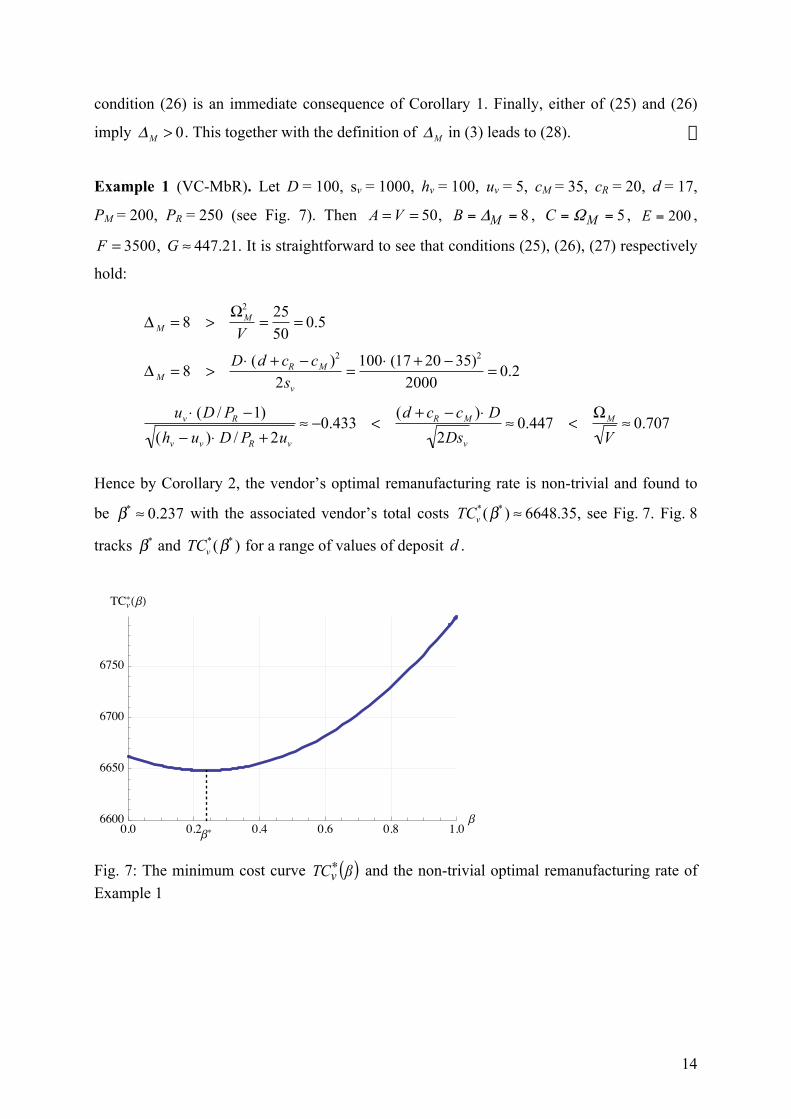
Hence by Corollary 2, the vendor’s optimal remanufacturing rate is non-trivial and found to

be

!* " 0.237 with the associated vendor’s total costs

TCv*(!* ) " 6648.35, see Fig. 7. Fig. 8

tracks

!* and

TCv*(!* ) for a range of values of deposit

d .

Β�0.0 0.2 0.4 0.6 0.8 1.0Β6600

6650

6700

6750

TCv���

Fig. 7: The minimum cost curve ( )βTCv

∗ and the non-trivial optimal remanufacturing rate of Example 1

15

10 12 14 16 18 20d0.0

0.2

0.4

0.6

0.8

1.0��d�

10 12 14 16 18 20d6100

6200

6300

6400

6500

6600

TCv����d��

Fig. 8: The optimal collection rate (left) and the vendor’s minimum total costs (right) as functions of the deposit in Example 1

4.3. The total system solution (SC-MbR)

The system-wide cost function (16) represents

K(!) with WA = , MB Δ= ,

22p

MuU

C −=−

= Ω ,

E = (cR ! c ! cM )D , ( )DccF M += and

G = 2D(sv + sp ) .

Lemma 4. Under conditions (18)–(20), the system-optimal collection and remanufacturing

rate is non-trivial and given by

!T* =

"M

#M

$E#M

#M %W $ ("M $ up / 2)2

#M % 2D(sv + sp ) $ E2 $up

2#M

. (29)

Corollary 3. Equation (29) can be used to determine the system-optimal collection and

remanufacturing rate whenever the following conditions simultaneously hold:

!M >("M # up / 2)2

V + hp

(30)

!M >D" (cR # c # cM )2

2(sv + sp ) (31)

uv ! (D / PR "1) " up / 2

(hv " uv )! D / PR + 2uv + hp + up

<(cR " c " cM )! D

2D(sv + sp )<#M " u p / 2

V + hp

(32)

In particular, either of conditions (30) and (31) imply (28) and, hence, PR must necessarily

exceed PM for

!T* being a non-trivial collection and remanufacturing rate. If any of (30)–(32)

is violated then the system-optimal collection and remanufacturing rate is either

!T* = 0 or

!T* = 1.

16

Proof: analogous to the proof of Corollary 2.

ΒT�0.0 0.2 0.4 0.6 0.8 1.0

Β10700

10720

10740

10760

10780

10800

10820

TCT� �Β�

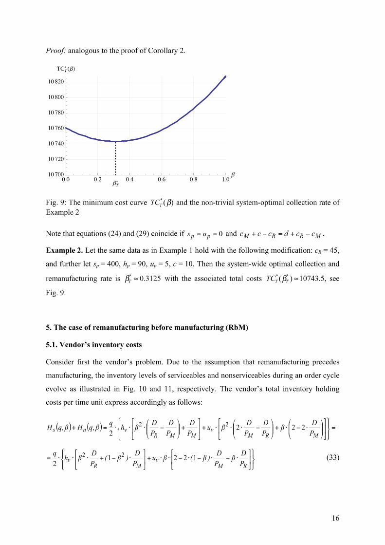
Fig. 9: The minimum cost curve

TCT* (!) and the non-trivial system-optimal collection rate of

Example 2

Note that equations (24) and (29) coincide if 0== pp us and MRRM ccdccc −+=−+ .

Example 2. Let the same data as in Example 1 hold with the following modification: cR = 45,

and further let sp = 400, hp = 90, up = 5, c = 10. Then the system-wide optimal collection and

remanufacturing rate is

!T* " 0.3125 with the associated total costs

TCT* (!T

* ) "10743.5, see

Fig. 9.

5. The case of remanufacturing before manufacturing (RbM)

5.1. Vendor’s inventory costs

Consider first the vendor’s problem. Due to the assumption that remanufacturing precedes

manufacturing, the inventory levels of serviceables and nonserviceables during an order cycle

evolve as illustrated in Fig. 10 and 11, respectively. The vendor’s total inventory holding

costs per time unit express accordingly as follows:

( ) ( ) =⎪⎭

⎪⎬⎫

⎪⎩

⎪⎨⎧

⎥⎦

⎤⎢⎣

⎡⎟⎟⎠

⎞⎜⎜⎝

⎛⋅−⋅+⎟⎟

⎠

⎞⎜⎜⎝

⎛−⋅⋅⋅+⎥

⎦

⎤⎢⎣

⎡+⎟⎟⎠

⎞⎜⎜⎝

⎛−⋅⋅⋅=+

MRMv

MMRvns P

DβPD

PDβu

PD

PD

PDβhqβ,qHβ,qH 222

222

⎭⎬⎫

⎩⎨⎧

⎥⎦

⎤⎢⎣

⎡⋅−⋅−⋅−⋅⋅+⎥

⎦

⎤⎢⎣

⎡⋅−+⋅⋅⋅=

RMv

MRv P

DβPD)β(βu

PD)β(

PDβhq 1221

222 (33)

17

Fig. 10: Evolution of the serviceables’ inventory level during an order cycle

Fig. 11: Evolution of the nonserviceables’ inventory level during an order cycle

By comparing vendor’s holding cost expressions (3)–(4) and (33) in MbR and RbM settings,

respectively, it is straightforward to obtain the following

Lemma 5. Let the same order size q and remanufacturing rate

!

" apply in MbR and RbM

settings. Then:

1. The vendor’s total holding costs in the MbR setting are strictly below those in the RbM

setting if and only if

PR

PM

> 1+uv

hv ! uv

(34)

2. They are equal if and only if (34) holds as equality or

!"{0,1}.

Corollary 4. The MbR setting outperforms the RbM one if the remanufacturing productivity

sufficiently exceeds the manufacturing one.

Corollary 5. Note that (34) represents a stronger condition than (28) which is necessary for a

non-trivial optimal remanufacturing rate in the MbR setting, from the vendor’s perspective.

βq

PM

PR

t

q

T t1 t3 t2

( )β,qI s v,T

T t2

–PR

t

β·q

t1 t3

( )β,qI n v,T

18

5.2. Vendor’s solution (VC-RbM)

As in Section 2, let us define

!R = (hv " uv )DPR

"DPM

#

$ %

&

' ( + uv

DPM

and

!R = 1"DPM

#

$ %

&

' ( ) uv . (35)

Then the vendor’s holding costs (33) can be rewritten as

( ) { }RRv ββVq

β,qH ΩΔ 22

2 ++⋅= , (36)

his total costs accordingly as

( ) { } ( )βRββVq

qDs

β,qTC vRRv

v +++⋅+= ΩΔ 22

2 ,

and his minimum total costs for a given remanufacturing rate as

( ) ( ) ( )βRββVsDβTC vRRvv ++⋅+⋅⋅⋅=∗ ΩΔ 22 2 , (37)

The latter expression represents function

K(!) as defined in (17), with VA = , RB Δ= ,

RC Ω−= , ( )DccdE MR −+= , DcF M= and vsDG ⋅⋅= 2 .

Lemma 6. Under conditions (18)–(20), the vendor’s optimal remanufacturing rate in the RbM

setting is non-trivial and given by

!RbM* = "

#R

$R

"E$R

$R % V "#R2

$R % 2Dsv " E2 . (38)

Corollary 6. Equation (38) can be used to determine the vendor’s optimal remanufacturing

rate whenever the following conditions simultaneously hold:

!R >"R

2

V (39)

!R >D" (d + cR # cM )2

2sv

(40)

(hv ! uv ) D / PR ! D / PM( ) + uv

(hv ! uv )D / PR + 2uv

>(cM ! d ! cR )D

2Dsv

>"R

V (41)

In particular, either of conditions (39) and (40) imply:

PM

PR

> 1!uv

hv ! uv

. (42)

19

Hence given a relatively low holding cost rate uv of nonserviceables, the manufacturing

productivity PM must necessarily be above a sufficiently large fraction of the remanufacturing

productivity PR for

!* being a non-trivial remanufacturing rate. Furthermore, condition (41)

implies:

cM > cR + d .

If any of conditions (39)–(41) is violated then the vendor’s optimal remanufacturing rate

happens to be either

!* = 0 or

!* = 1.

Proof: analogous to the proof of Corollary 2.

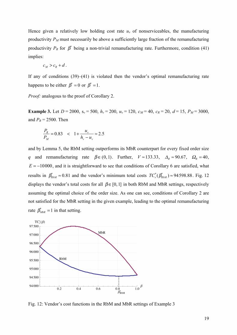
Example 3. Let D = 2000, sv = 500, hv = 200, uv = 120, cM = 40, cR = 20, d = 15, PM = 3000,

and PR = 2500. Then

PR

PM

= 0.83 < 1+uv

hv ! uv

" 2.5

and by Lemma 5, the RbM setting outperforms its MbR counterpart for every fixed order size

q and remanufacturing rate

!" (0, 1) . Further,

V !133.33,

!R " 90.67,

!R = 40,

E = !10000 , and it is straightforward to see that conditions of Corollary 6 are satisfied, what

results in

!RbM* " 0.81 and the vendor’s minimum total costs

TCv*(!RbM

* ) " 94598.88 . Fig. 12

displays the vendor’s total costs for all

!"[0, 1] in both RbM and MbR settings, respectively

assuming the optimal choice of the order size. As one can see, conditions of Corollary 2 are

not satisfied for the MbR setting in the given example, leading to the optimal remanufacturing

rate

!MbR* = 1 in that setting.

ΒRbM�

RbM

MbR

0.2 0.4 0.6 0.8 1.0Β94000

94500

95000

95500

96000

96500

97000

97500TCv���

Fig. 12: Vendor’s cost functions in the RbM and MbR settings of Example 3

20

5.3. The total system solution (SC-RbM)

It is straightforward to see that the system-wide costs in the RbM setting, assuming the

optimal choice of the order size, are expressed as

( ) ( ) ( )( ) ( )βRuββWssDβTC TpRRpvT +++⋅+⋅+⋅⋅=∗ ΩΔ 22 2 (43)

and represent

K(!) with WA = , RB Δ= ,

C = U = !"R ! up / 2 , ( )DcccE MR −−= ,

( )DccF M += and ( )pv ssDG +⋅⋅= 2 .

Lemma 7. Under conditions (18)–(20), the system-optimal collection and remanufacturing

rate in the RbM setting is non-trivial and given by

!T ,RbM* = "

#R

$R

"E$R

$R %W " (#R + u p / 2)2

$R % 2D(sv + sp ) " E2 "u p

2$R

. (44)

Corollary 7. Equation (44) can be used to determine the system-optimal collection and

remanufacturing rate whenever the following conditions simultaneously hold:

!R >("R + up / 2)2

V + hp

(45)

!R >D" (cR # c # cM )2

2(sv + sp ) (46)

!uv + up / 2 + (hv ! uv )(D / PR ! D / PM )

(hv ! uv )" D / PR + 2uv + hp + up

>(c + cM ! cR )" D

2D(sv + sp )>#M + up / 2

V + hp

(47)

In particular, either of conditions (45) and (46) imply:

PM

PR

> 1!uv

hv ! uv

(48)

what always holds if

uv ! hv / 2 , and is otherwise equivalent to

PR

PM

< 1+uv

hv ! uv

(49)

what is at the same time necessary and sufficient for RbM to outperform MbR for every fixed

order size q and remanufacturing rate

!" (0, 1) . Furthermore, condition (47) implies:

cR < c + cM .

21

If any of (45)–(47) is violated then the system-optimal collection and remanufacturing rate

!T ,RbM* is either 0 or 1.

Proof: analogous to the proof of Corollary 2 and by using Lemma 5.

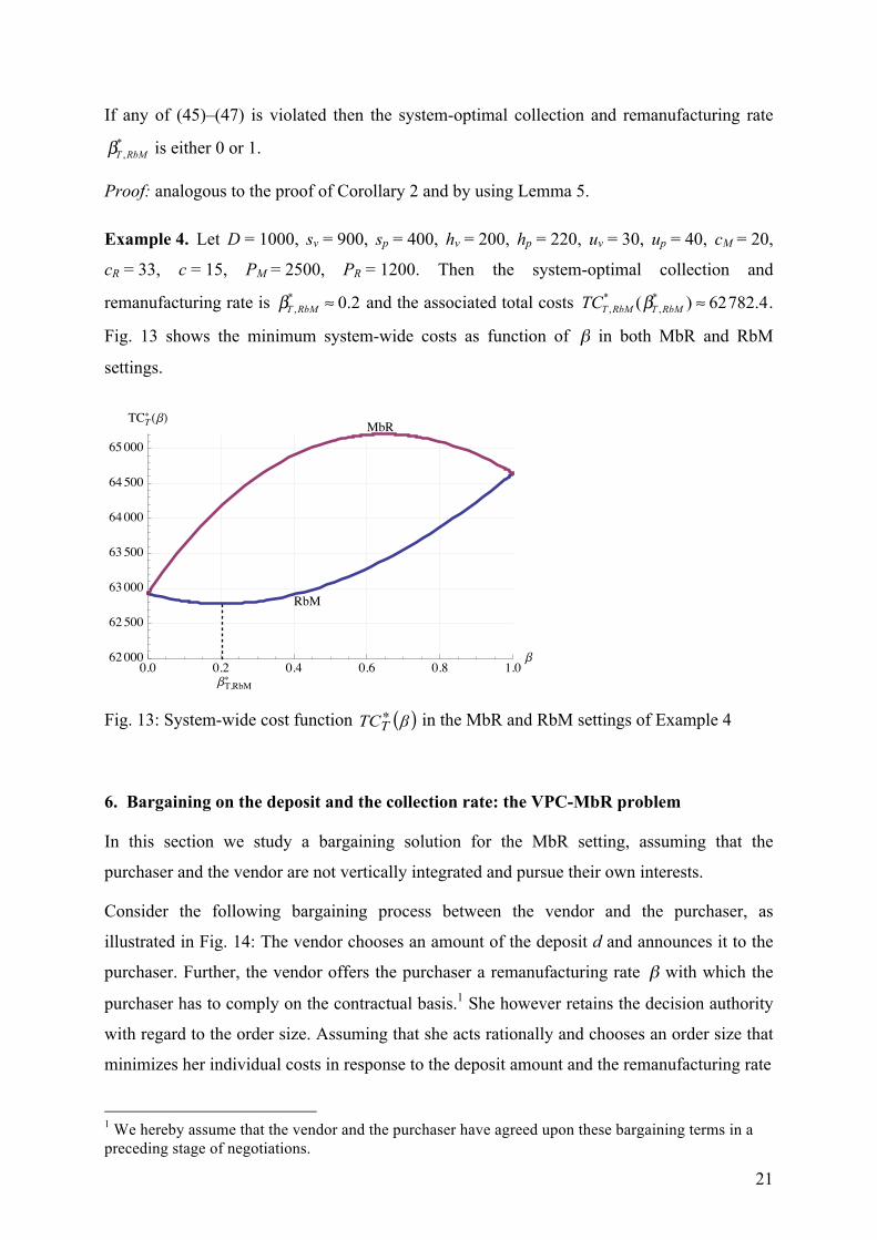
Example 4. Let D = 1000, sv = 900, sp = 400, hv = 200, hp = 220, uv = 30, up = 40, cM = 20,

cR = 33, c = 15, PM = 2500, PR = 1200. Then the system-optimal collection and

remanufacturing rate is

!T ,RbM* " 0.2 and the associated total costs

TCT ,RbM* (!T ,RbM

* ) " 62782.4.

Fig. 13 shows the minimum system-wide costs as function of

!

" in both MbR and RbM

settings.

ΒT,RbM�

RbM

MbR

0.0 0.2 0.4 0.6 0.8 1.0Β62000

62500

63000

63500

64000

64500

65000

TCT� �Β�

Fig. 13: System-wide cost function ( )βTCT∗ in the MbR and RbM settings of Example 4

6. Bargaining on the deposit and the collection rate: the VPC-MbR problem

In this section we study a bargaining solution for the MbR setting, assuming that the

purchaser and the vendor are not vertically integrated and pursue their own interests.

Consider the following bargaining process between the vendor and the purchaser, as

illustrated in Fig. 14: The vendor chooses an amount of the deposit d and announces it to the

purchaser. Further, the vendor offers the purchaser a remanufacturing rate

!

" with which the

purchaser has to comply on the contractual basis.1 She however retains the decision authority

with regard to the order size. Assuming that she acts rationally and chooses an order size that

minimizes her individual costs in response to the deposit amount and the remanufacturing rate

1 We hereby assume that the vendor and the purchaser have agreed upon these bargaining terms in a preceding stage of negotiations.

22

Fig. 14: The bargaining process

announced by the vendor, we henceforth address the following vendor’s problem: what choice

of the deposit and the remanufacturing rate is optimal for him? The problem under

consideration thus represents a Stackelberg game with the vendor being the leader and the

purchaser the follower; in more general terms, it represents a two-player extensive game with

perfect information (Osborne and Rubinstein, 1994), a solution to which can be determined as

a subgame perfect equilibrium by means of the backwards induction, as follows below.

By taking into account the purchaser’s optimal response, the vendor is able to foresee the

consequences of his decision (d,

!

") in terms of his resulting total costs — which we

accordingly define as

TC~

v (d,!) = Cv (qp* (!),!) + Rv (d,!) (50)

where Cv (q,! ) and Rv (d,! ) are vendor’s cost components as defined by (5)–(6), and qp* (! )

is the purchaser’s optimal order size as defined by (11). Note that we have now made

Rv (d,! ) explicitly depend on d; also note that qp* (! ) does not depend on d. By substituting

(5)–(6) and (11) in (50) we obtain:

TC~

v (d,!) = svD2spDhp +!up

+!M!

2 " 2#M! +V2

2spDhp +!up

+ (cM + (d + cR " cM )!)D (51)

The vendor’s optimal choice of (d,

!

") thus represents a solution to the following constrained

optimization problem:

min(d,! )

TC~

v (d,! ) s. t. d ! 0, 0 " ! "1 (52)

Vendor

Select deposit d

Determine optimal re-manufacturing rate βv(d)

Determine optimal lot size qv(β)

Purchaser

Determine optimal order size qp(β) if

qv(β)≠qp(β)

23

This problem must not necessarily be convex, therefore the Karush–Kuhn–Tucker (KKT)

conditions (Bazaraa et al., 2006, p. 204) alone are not sufficient for determining a point of

global optimum. However, they can be employed for determining potential local optima and

subsequently choosing a global minimum out of them. To implement this approach, consider

the Lagrange function of (52):

L(d,!,") = TC~

v (d,!) + " ! (! "1) (52)

whose arguments are nonnegative by assumption. The respective KKT conditions reduce to:

!L!d

= !D " 0 and d # !L!d

$ d!D = 0 (53)

!L!!

=!TC~

v

!!+" " 0 and ! #

!L!!

$ ! #!TC~

v

!!+"

%

&

'''

(

)

***= 0 (54)

!L!!

= " "1# 0 and ! $!L!!

% ! $ (" "1) = 0 (55)

An immediate consequence of condition (53) is the following

Lemma 8. There is no deposit refund as long as the vendor’s optimal choice is concerned.

Indeed, the second part of (53) requires that either d or ! or both is zero; if ! = 0 , no items

are returned and hence there is no refund, otherwise d = 0 and therefore no refund, as well.

The assertion of Lemma 8 is rather obvious: since the re-use rate is dictated by the vendor, the

deposit has no relevance as an incentive for the purchaser to return used items, and refunding

the deposit would represent just an unnecessary expenditure for the vendor.

Note that with ! = 0 , the choice of the deposit amount does not matter. We can therefore

require d = 0 as a necessary optimality condition for all ! ![0, 1] and separate the

subsequent analysis of (54)–(55) into three cases: ! = 0 , 0 < ! <1, and ! =1 , as follows.

a) ! = 0 . Then (55) implies ! = 0 , and (54) is accordingly fulfilled whenever the derivative

!TC~

v (0,! )!!

= (cR " cM )D +2Dsp

hp + !up"M! "#M +

up4

svsp

" "M!2 " 2#M! +Vhp + !up

#

$%&

'(#

$%

&

'( (56)

is nonnegative at ! = 0 , i.e., whenever

(cR ! cM )D+2Dsphp

up4

svsp!hvhp"DPM

#

$%%

&

'((!!M

#

$%%

&

'(( ) 0 . (57)

Note that the radical in (57) represents the purchaser’s classical economic order quantity.

24

b) 0 < ! <1 . As before, (55) implies ! = 0 , while (54) effectively requires ! to be a

stationary point of TC~

v (0, ! ) — i.e., a solution to the equation that sets (56) equal to 0.

The following examples show that such ! !(0, 1) must not necessarily exist, and when

exists, can be a local minimum or a local maximum, as well.

Example 5a. Let D = 400, sv = 2000, sp = 500, hv = hp = 50, uv = up = 25, cM = cR = 50,

PM = 500, PR = 2000. Then

TC~

v (0,!) ! 20000+1264.9 25! + 50 +316.2 25!2 "10! + 4025! + 50

does not have any stationary points on (0, 1) , as Fig. 15a demonstrates.

Example 5b. Let now hv = 100. Then

TC~

v (0,!) ! 20000+1264.9 25! + 50 +316.2 55!2 " 70! +8025! + 50

has a stationary point at ! ! 0.31 which is a global minimum, see Fig. 15b.

Example 5c. Let further PM = 1250 and cM = 57.5. Then

TC~

v (0,!) ! 23000"3000! +1264.9 25! + 50 +316.2 7!2 + 26! +3225! + 50

has a stationary point at ! ! 0.18 which is a global maximum, see Fig. 15c.

0.2 0.4 0.6 0.8 1.0Β

31500

32000

32500

33000TC�v�Β, 0�

0.2 0.4 0.6 0.8 1.0

Β

32600

32800

33000

33200

TC�v�Β, 0�

0.2 0.4 0.6 0.8 1.0Β

33340

33350

33360

33370

33380TC�v�Β, 0�

Fig. 15a–c: Vendor’s cost function TC~

v (0,!) in Examples 5a to 5c (left to right)

Although it is possible to obtain an analytic expression for a stationary point of TC~

v (0,!) , it

turns out to be bulky and impractical to use; therefore analyzing the function’s local extrema

in each particular case would be a more suitable approach. Higher derivatives can help to

reveal which stationary points represent local minima; however, this step is optional and can

25

be replaced by explicit evaluation of the function value at all stationary points for subsequent

comparison, as discussed below.

c) ! =1 . Then (54) and (55) essentially require the function’s derivative (56) to be no

positive at ! =1 , i.e.,

(cR ! cM )D+2Dsphp +up

uv 1!DPR

"

#$

%

&'+

up4

svsp!2uv + (hv !uv )D / PR

hp +up

"

#$$

%

&''

(

)**

+

,--

. 0 . (58)

It would suffice now to compare the function value at each of the points determined in a) – c)

to figure out a global minimum of TC~

v (d,!) .

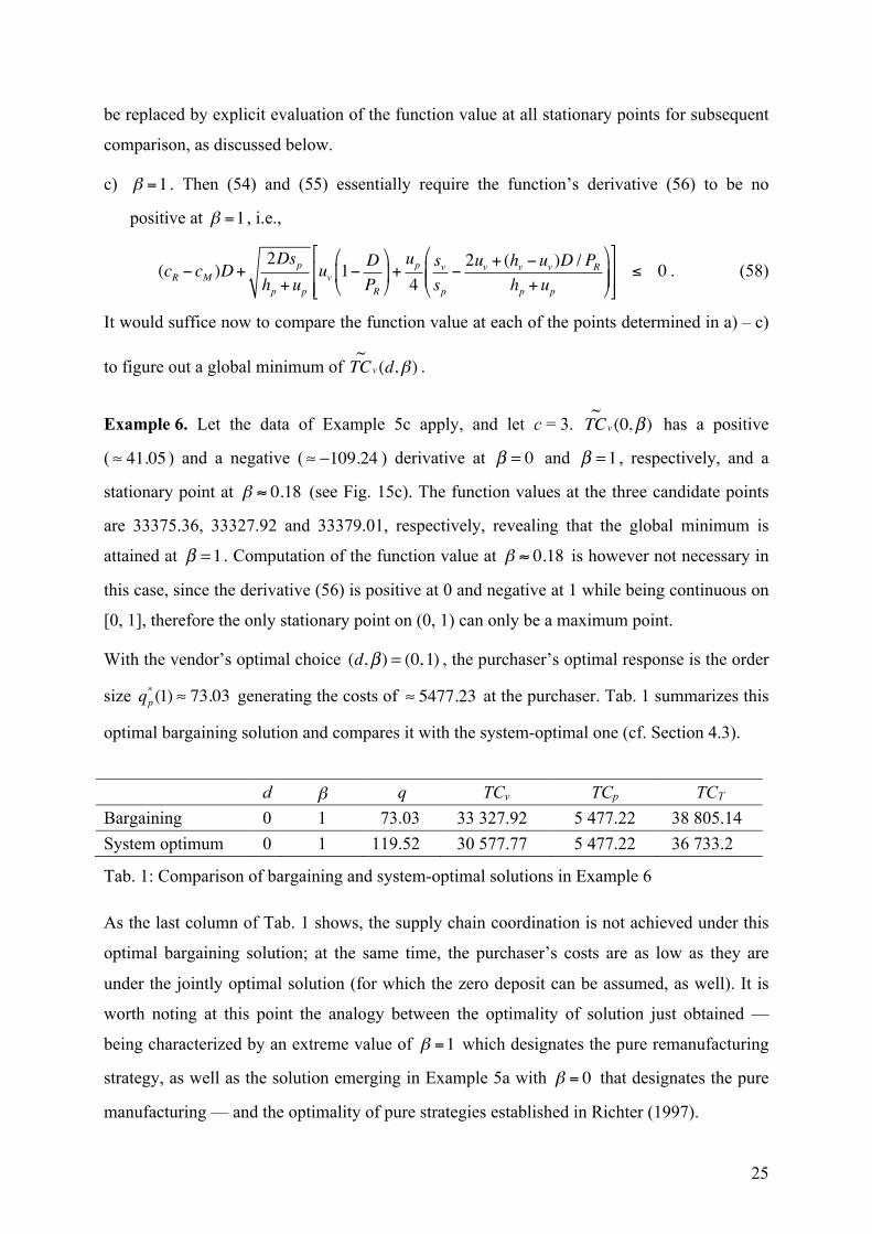
Example 6. Let the data of Example 5c apply, and let c = 3. TC~

v (0,! ) has a positive

(! 41.05 ) and a negative (! "109.24 ) derivative at ! = 0 and ! =1 , respectively, and a

stationary point at ! ! 0.18 (see Fig. 15c). The function values at the three candidate points

are 33375.36, 33327.92 and 33379.01, respectively, revealing that the global minimum is

attained at ! =1 . Computation of the function value at ! ! 0.18 is however not necessary in

this case, since the derivative (56) is positive at 0 and negative at 1 while being continuous on

[0, 1], therefore the only stationary point on (0, 1) can only be a maximum point.

With the vendor’s optimal choice (d,! ) = (0, 1) , the purchaser’s optimal response is the order

size qp* (1) ! 73.03 generating the costs of ! 5477.23 at the purchaser. Tab. 1 summarizes this

optimal bargaining solution and compares it with the system-optimal one (cf. Section 4.3).

d β q TCv TCp TCT

Bargaining 0 1 73.03 33 327.92 5 477.22 38 805.14 System optimum 0 1 119.52 30 577.77 5 477.22 36 733.2

Tab. 1: Comparison of bargaining and system-optimal solutions in Example 6

As the last column of Tab. 1 shows, the supply chain coordination is not achieved under this

optimal bargaining solution; at the same time, the purchaser’s costs are as low as they are

under the jointly optimal solution (for which the zero deposit can be assumed, as well). It is

worth noting at this point the analogy between the optimality of solution just obtained —

being characterized by an extreme value of ! =1 which designates the pure remanufacturing

strategy, as well as the solution emerging in Example 5a with ! = 0 that designates the pure

manufacturing — and the optimality of pure strategies established in Richter (1997).

26

As one can also see in the above example, the purchaser’s choice of the order size under

bargaining does not agree with the system-optimal order size. The vendor may attempt to

choose such a deposit amount d which would — together with the vendor’s respectively

optimal remanufacturing rate ! *(d) — induce the purchaser to choose an order size

qp* (! *(d)) equal to the order size qv

*(! *(d)) preferred by the vendor himself under this

deposit amount d and remanufacturing rate ! *(d) . The following example demonstrates that

when such vendor’s choice exists, either, it still must not represent an optimal strategy.

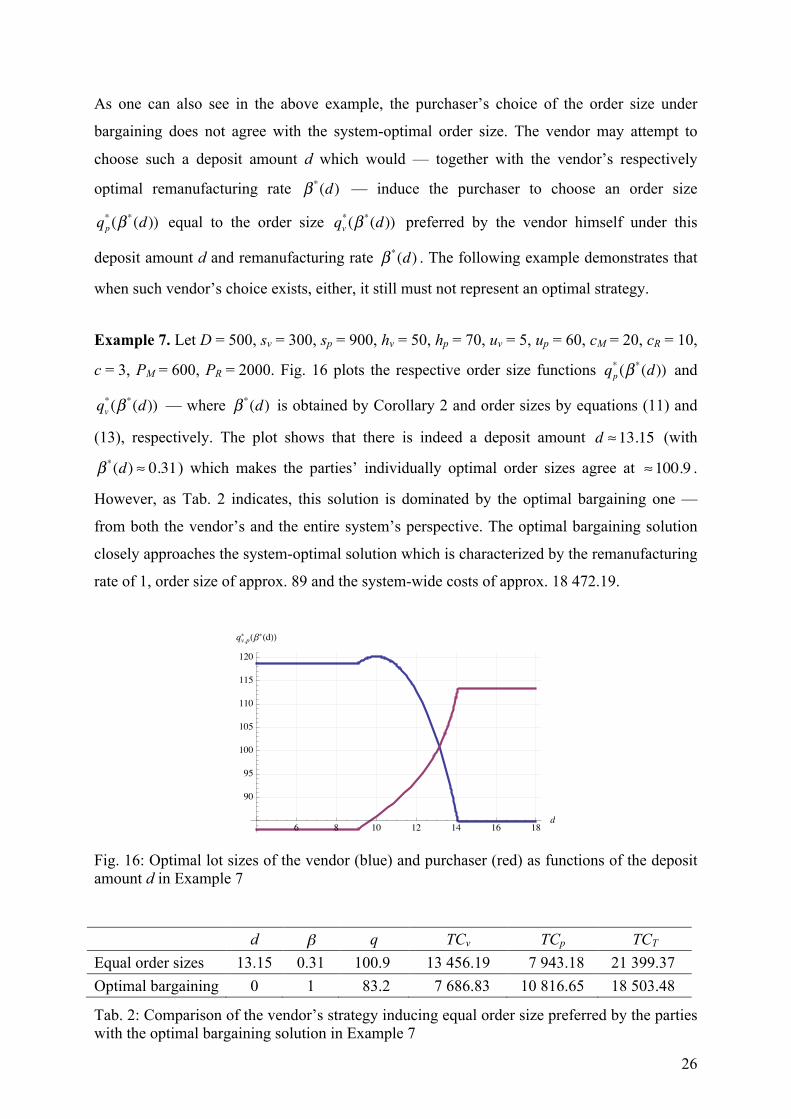
Example 7. Let D = 500, sv = 300, sp = 900, hv = 50, hp = 70, uv = 5, up = 60, cM = 20, cR = 10,

c = 3, PM = 600, PR = 2000. Fig. 16 plots the respective order size functions qp* (! *(d)) and

qv*(! *(d)) — where ! *(d) is obtained by Corollary 2 and order sizes by equations (11) and

(13), respectively. The plot shows that there is indeed a deposit amount d !13.15 (with

! *(d) ! 0.31) which makes the parties’ individually optimal order sizes agree at !100.9 .

However, as Tab. 2 indicates, this solution is dominated by the optimal bargaining one —

from both the vendor’s and the entire system’s perspective. The optimal bargaining solution

closely approaches the system-optimal solution which is characterized by the remanufacturing

rate of 1, order size of approx. 89 and the system-wide costs of approx. 18 472.19.

6 8 10 12 14 16 18d

90

95

100

105

110

115

120

qv,p� ���d��

Fig. 16: Optimal lot sizes of the vendor (blue) and purchaser (red) as functions of the deposit amount d in Example 7

d β q TCv TCp TCT

Equal order sizes 13.15 0.31 100.9 13 456.19 7 943.18 21 399.37 Optimal bargaining 0 1 83.2 7 686.83 10 816.65 18 503.48

Tab. 2: Comparison of the vendor’s strategy inducing equal order size preferred by the parties with the optimal bargaining solution in Example 7

27

The following example demonstrates that such vendor’s choice of the deposit amount d that

would make the order sizes of the parties agree may not exist, either.

Example 8. Let the demand and the vendor data of Example 1 apply: D = 100, sv = 1000,

hv = 100, uv = 5, cM = 35, cR = 20, PM = 200, PR = 250, as well as the purchaser data of

Example 4: sp = 400, hp = 220, up = 40, c = 15. Fig. 17 plots the respective order size

functions of the vendor and the purchaser. As the lower plot in the figure demonstrates, the

vendor has no way to entice the purchaser to choose the same order size he would himself

prefer by adopting a certain amount of the deposit and sticking to the respectively optimal

remanufacturing rate.

10 12 14 16 18 20d

63.5

64.0

64.5

65.0

qv��d�

10 12 14 16 18 20d

17.5

18.0

18.5

19.0

qp� �d�

10 12 14 16 18 20d

20

30

40

50

60

qv,p� �d�

Fig. 15: Optimal lot sizes of the vendor (left) and purchaser (right) as functions of the deposit amount d in Example 5. The lower plot displays both functions on a common scale.

Conclusion

A complex of problems for determining individual and jointly optimal lot (order) sizes,

remanufacturing (collection) rates and deposit amounts in a closed loop supply chain with a

28

single suppler and a single buyer has been studied in the paper. While no analytic expression

has been derived for the deposit amount under optimal bargaining, closed formulas have still

been obtained for all other quantities. It has been demonstrated on examples that supply chain

coordination must not necessarily be achieved in the bargaining game studied in the paper.

References

Affisco, J. F., Paknejad, M. J., Nasri, F., 2002. Quality improvement and setup reduction in the joint economic lot size model. European Journal of Operational Research 142(3), 497–508.

Ahn, H., 2009. On the profit gains of competing reverse channels for remanufacturing of refillable containers. Journal of Service Science 2009, 147–190.

Banerjee, A., 1986a. A joint economic lot-size model for purchaser and vendor. Decision Sciences 17, 292–311.

Banerjee, A., 1986b. On “A quantity discount model to increase vendor profits”. Management Science 32(11), 1513–1517.

Bazaraa, M. S., Sherali, H. D., Shetty, C. M., 2006. Nonlinear Programming: Theory and Algorithms. Wiley, 3rd ed.

Bonney, M., Jaber, M. Y., 2011. Environmentally responsible inventory models: Non-classical models for a non-classical era. International Journal of Production Economics 133(1), 43–53.

Chung, S.-L., Wee, H.-M., Yang, P.-C., 2008. Optimal policy for a closed-loop supply chain inventory system with remanufacturing. Mathematical and Computer Modelling 48, 867–881.

Eben-Chaime, M., 2004. The effect of discreteness in vendor-buyer relationships. IIE Transactions 36, 583–589.

Gou, Q., Liang, L., Huang, Z., Xu, C., 2008. A joint model for an open-loop reverse supply chain. International Journal of Production Economics 116, 28–42.

Goyal, S. K., 1976. An integrated inventory model for a single supplier–single customer problem. International Journal of Production Research 15, 107–111.

Goyal, S. K., 1988. “A joint economic-lot-size model for purchaser and vendor”: a comment. Decision Sciences 19, 236–241.

Grimes-Casey, H. G., Seager, T. P., Theis, T. L., Powers, S. E., 2007. A game theory framework for cooperative management of refillable and disposable bottle lifecycles. Journal of Cleaner Production 15, 1618–1627.

Hill, R. M., 1997. The single-vendor single-buyer integrated production-inventory model with a generalised policy. European Journal of Operational Research 97(3), 493–499.

Hill, R. M., 1999. The optimal production and shipment policy for the single-vendor single-buyer integrated production-inventory problem. International Journal of Production Research 37(11), 2463–2475.

Hill, R. M., Omar, M., 2006. Another look at the single-vendor single-buyer integrated production-inventory problem. International Journal of Production Research 44(4), 791–800.

Hoque, M. A., 2009. An alternative optimal solution technique for a single-vendor single-buyer integrated production inventory model. International Journal of Production Research 47(15), 4063–4076.

29

Kohli, R., Park, H., 1989. A cooperative game theory model of quantity discounts. Management Science 35(6), 693–707.

Lee, H. B., Cho, N. W., Hong, Y. S., 2010. A hierarchical end-of-life decision model for determining the economic levels of remanufacturing and disassembly under environmental regulations. Journal of Cleaner Production 18, 1276–1283.

Leng, M., Parlar, M., 2005. Game theoretic applications in supply chain management: A review. INFOR 43(3), 187–220.

Liu, X., Çetinkaya, S., 2007. A note on “quality improvement and setup reduction in the joint economic lot size model”. European Journal of Operational Research 182(1), 194–204.

Mitra, S., 2009. Analysis of a two-echelon inventory system with returns. Omega 37, 106–115.

Osborne, M. J., Rubinstein, A., 1994. A Course in Game Theory. MIT Press. Pibernik, R., Zhang, Y., Kerschbaum, F., Schröpfer, A., 2011. Secure collaborative supply

chain planning and inverse optimization – The JELS model. European Journal of Operational Research 208(1), 75–85.

Richter, K., 1994. An EOQ repair and waste disposal model. In: Proceedings of the Eighth International Working Seminar on Production Economics, Innsbruck, Vol. 3, 83–91.

Richter, K., 1997. Pure and mixed strategies for the EOQ repair and waste disposal problem. OR-Spektrum 19, 123–129.

Richter, K., Dobos, I., 1999. Analysis of the EOQ repair and waste disposal problem with integer setup numbers. International Journal of Production Economics 59, 463–467.

Subramoniam, R., Huisingh, D., Chinnam, R. B., 2010. Aftermarket remanufacturing strategic planning decision-making framework: theory & practice. Journal of Cleaner Production 18, 1575–1586.

Sucky, E., 2005. Inventory management in supply chains: A bargaining problem. International Journal of Production Economics 93–94, 253–262.

Sucky, E., 2006. A bargaining model with asymmetric information for a single supplier–single buyer problem. European Journal of Operational Research 171, 516–535.

Voigt, G., Inderfurth, K., 2011. Supply chain coordination and setup cost reduction in case of asymmetric information. OR Spectrum 33(1), 99–122.

Yuan, K. F., Gao, Y., 2010. Inventory decision-making models for a closed-loop supply chain system. International Journal of Production Economics 48, 6155–6187.

Zhou, Y.-W., Wang, S.-D., 2007. Optimal production and shipment models for a single-vendor–single-buyer integrated system. European Journal of Operational Research 180(1), 309–328.