ELSEVIER

An Intemational Journal Available online at www.sciencedirect.com computers &

.c ,E.c~ ~_~o..~cT. mathemat ics with applications

Computers and Mathematics with Applications 50 (2005) 1767 1790 www.elsevier.com/locate/camwa

A Jo int E c o n o m i c - L o t - S i z e M o d e l For P u r c h a s e r and V e n d o r

in F u z z y S e n s e

G, C, MAHATA, A. GOSWAMI* AND D. K. GUPTA D e p a r t m e n t of M a t h e m a t i c s

I .I .T. Kha. ragpur 721302, Ind ia

goswami~maths, iitkgp, ernet, in

(Received December 2003; revised and accepted October 2004)

A b s t r a c t - - T h i s paper investigates a group of computing schemas for joint economic lot size as fuzzy values of the economic lot size model for purchaser and vendor. We express the fuzzy order quant i ty/product ion lot size for the purchaser/vendor as the normal triangular fuzzy number (ql, q0, q2) and then we solve the aforementioned optimization problem under the condition 0 < ql < q0 < q2. We find that, after defuzzification, the joint total relevant cost is slightly higher than in the crisp model. @ 2005 Elsevier Ltd. All rights reserved.

K e y w o r d s - - F u z z y inventory, Purchaser, Vendor, Membership function, Extension principle, Fuz- zy order quanti ty/product ion lot size.

1. I N T R O D U C T I O N

In traditional inventory management systems, the economic-lot-size (ELS) for a vendor and a purchaser are managed independently, that is, the vendor finds their own optimal order quantity. As a result, the ELS of purchaser may not result in an optimal policy for the vendor and vice- versa. To overcome this problem, researchers have studied joint economic lot size (JELS) model where the joint total relevant cost (JTRC) for the purchaser as well as the vendor has been optimized. Ooyal [1] first introduced an integrated inventory policy for a single supplier and a single customer and derived the minimum joint variable cost for the supplier and the customer. Banerjee [2] introduced the JELS model for a single vendor and a single customer and obtained the mininmm joint total relevant cost for both buyer and vendor at the same time with the assumption that the vendor makes the production set up every time the buyer places an order and supplies on a lot for lot basis. Goyal [3] modified Banerjee's [2] paper on the assumption that vendor may possibly produce a lot size that rnay supply an integer number of orders to the buyer. Chatterjee and Ravi [4] further modified the paper of Ooyal [3] by assuming that production quantity of vendor will be supplied to the buyer in subbatches and there will be no

*Author to whom all correspondence should be addressed. We thank the anonymous referee for his valuable and constructive comments that have led to a significant im- provement in the original paper.

0898-1221/05/$ - see front matter @ 2005 Elsevier Ltd. All rights reserved. doi: 10.1016/j.camwa.2004.10.050

Typeset by A Az~S-~ID_X

1768 G . C . MAHATA et al.

break in production from vendor side. Lu [5] relaxed the assumption of Goyal [3] and developed a model with the assumption that the vendor can ship a subbatch to the supplier even before the entire batch is completed. Goyal [6] provided an alternative shipment policy where all the subbatches are not necessarily of same size. Agrawal and Raju [7] provided a model for subbatches of uniform size with a constant time allowance between any two consecutive supplies. In another paper, Hill [8] showed that the optimal solution lies in the interval [nl, n2], where nlis the number of equal-size subbatches provided by Lu [5] and n2 is that have provided by Goyal [6]. Goyal [9] suggested an alternative procedure by modifying the shipment sizes, which reduces the earlier total cost.

Recently, fuzzy concepts have been introduced in the EOQ models. Zadeh [10] showed the intention of accommodating uncertainty in the nonstochastic sense rather than the presence of random variables. Sommer [11] applied fuzzy dynamic progranmfing to an inventory and production-scheduling problem in which the management wishes to fulfill a contract for providing a product and then withdraw from the market. Kacprzyk and Staniewski [12] considered the determination of optimal of firms from a global viewpoint of top management with fuzzy constants imposed on replenishments and a fuzzy goal for preferable inventory levels to be attained. Instead of minimizing the average inventory cost, they reduced it to a multistage fuzzy decision making problem and used a/3/3 algorithm (branch and bound) in which a fuzzy optimal decision is the intersection of fuzzy constraints and fuzzy goal. Park [13] examined the EOQ model in the fiJzzy set theoretic perspective associating the fuzziness with the cost data. Here, the trapezoidal fuzzy numbers represented the inventory costs. Yao and Lee [14] used extension principle to solve EOQ model with shortages by fuzzifying order quantity. Later, Chang et al. [15] fuzzified the shortage quantity in the backorder model. Ray and Maiti [16] used FNLP to solve EOQ model of deteriorating items with stock-dependent demand under limited storage space. But, till now researchers have not investigated the JELS model for both purchaser and vendor in fuzzy sense.

In this paper, we have extended Banerjee's [2] JELS model with the assumption that the order quantity for the purchaser is a fuzzy variable. The general cost functions for the purchaser and vendor derived by Banerjee [2] are given, respectively, by

TRC~ (q) DA + qrc q 2 P

and

Dq T R C , , ( q ) : m J + - f - y C , , .

q

Thus, the JTRC for the purchaser and vendor for the lot-for-lot case is given by

D (S+A)+ q r ( D ) F (q) : q -fc + cp ,

where D is annual constant demand for the item, P is vendor's annual constant rate of production for the item, Cv is the unit production cost for the item, Cp is the unit purchase cost paid by the purchaser, A is the purchaser's ordering cost per order, S is the vendor's setup cost per setup cost per setup, r is the annual inventory carrying cost per dollar invested in stocks, q is the production lot size for the vendor (or order quantity for the purchaser), and F(q) is joint total relevant cost.

In developing our model, we have replaced the crisp order quantity or crisp production lot- size q by the fuzzy parameter (~ and obtained the solution procedure for the JELS model in fuzzy sense. In Section 2, we have derived tile JELS q** in tile fuzzy sense for the purchaser and vendor by considering the fuzzy order/production lot size ~) as the normal triangular fuzzy number (q~, q0, q2). From the fuzzy order/production lot size (~, we have induced the fuzzy joint total relevant cost F(~)) and by the process of defuzzification, we have generated a joint economic

A Joint Economic-Lot-Size Model 1769

lot size for bo th purchaser and vendor. Under the condit ion 0 < ql < q0 < q2, we have derived

the membership function of F((~) and its centroid. We have used the centroid of F(~)) as the

es t imat ion of the JTRC. Next, we have obta ined #F(Q) (Y) and its eentroid, which is the es t imated to ta l cost. This is ob ta ined in each of the following four cases,

Section 2.1: q. < ql < q0 < q2,

Section 2 . 2 : 0 < ql < q. < q0 < q2,

Section 2 . 3 : 0 < ql < q0 < q. < q2, and

Section 2 . 4 : 0 < q~ < q0 < q2 < q..

In Section 3, we have appl ied the Nelder and Mead me thod [17] to find the opt imal fuzzy

t r iangular number (q~,q~, q~), such tha t the centroid of the membersh ip function of the fuzzy J T R C of F ( Q ) is minimum. The classical centroid (q~ + q~ + q~)/3 is the op t imum JELS in the

fuzzy sense. The solution procedure is i l lus t ra ted with the help of numerical example.

In Section 4, we s tudy the sensi t ivi ty of the crisp JELS and the J T R C in the fuzzy sense.

2. M E M B E R S H I P F U N C T I O N O F T H E F U Z Z Y J T R C F U N C T I O N

The joint to ta l relevant cost ( JTRC) for the purchaser and the vendor for the lot-for-lot case is given by

) F (q) : ~ c ~ + c , . (1)

By setting the first derivative of the cost function F(q) with rcspect to q equal to zero at q : q,, we obta in the JELS,

2 D ( S + A )

q* = r ( ( D / P ) Cv + C p ) (2)

The min imum JTRC is given by

(3)

Suppose the membership function of fuzzy order quant i ty (or product ion lot size) 0 for the

purchaser (or for the vendor) is as follows,

x - q ~ i f q l < z < q o , qo - ql '

#Q(z) = q 2 - z , i f q o _ < x < q 2 , q2 - qo

0, otherwise,

(4)

where ql, q0, q2 are real variables and satis~" the condit ion, 0 < ql < q0 < q2. Then,

oo ql + q0 + q2 Mo (q,, qo, q',) = r ~ -- 3 (5)

L #~ (x) dx o ~

is the eentroid of #Q(x). We regard this value of Mo(ql, q0, q2) as the es t imat ion of 3ELS (joint

economic lot size) in the fuzzy sense.

From (1), we have

= - - + C p , 2£

1770 G.C. MAHATA et al.

where x > 0. By the extension principle, the membership function of the fuzzy total cost F ( 0 ) is

sup #Q(x), if F -I (y) • ¢, (6)

0, if F -1 (y) = ¢.

From F(x) = y, we obtain

D ) x2 r ~C,+Cp -2yx+2D(S+A)=O

and its discriminant, A y2 _ 2rD(S + A)((D/P)C, + C;). When

i y> 2Dr(S+A) Cv+Cp =(F(q,)),

f 1(~]) 7~ (~. T W O r o o t s o f (7) a r e

(7)

y+ /2 r((D/P) Cv+Cp) and X2=r((D/P) Cv+Cp)

Therefore, we have that if

then #F(Q)(Y) = 0 and if

then

i fY>_~2Dr(S÷A)(Dcv+Cp).

Y>- t 2 D r ( S + A ) ( D ) ~Cv + Cp ,

#F(Q) (Y) = sup {PC) ( x l ) , #Q (x2)} . (s)

T a b l e 1. S i t u a t i o n s o f Xl,X 2.

C a s c q2

(i) x ] , x2

(ii) x l x2

(iii) Xl

(iv) ~1

(v) ~I, x2

(v i ) x l

(vi i ) Xl

(vi i i )

(ix)

(x)

q0

Z2

X2

Xl~X2

Xl

q2 # F ( ~ ) (Y), Y ~ F ( q * )

0

x 2 - ql

qo - - ql

q2 - x 2

q2 - qo

x2 0

m2

x 2 - - ql

qo -- ql

Xl - - q l q2 - - x 2 ) m a x - - - - ~

qo -- ql q2 qo

Xl -- ql

qo -- ql

q2 -- Xl

q2 - - qo

q2 -- Xl x2

q2 qo

Xl , x2 0

A Joint Economic-Lot-Size Model 1771

In order to solve #F(Q)(Y), we show all possible situations of Xl and x2 in Table 1.

Obviously, we have xl _< x2. For convenience to solve the problem under the condition 0 <

ql < qo < q2, we consider the following four cases,

(1) 0 < q , < q l <qo <q2,

(2) 0 < ql < q, < qo < q2,

(3) O < q l < q 0 < q . <q2 ,

(4) 0 < q l <q0 <q2 < q , .

Assume a s = ( D / q j ) ( S + A) + ( q j / 2 ) ( ( D / A ) C v + Cp), for j - 1,0, 2.

Then, we obtain

qj > q, ,e~ aj < r + qj, (9)

qj > q. e* r + qj > 2Dr (S + A) Cv + Cp , (10)

Under the condition,

we have the following four inequalities.

(1) xl >_ qj, where j = 1, O, 2, i.e.,

( ( ; ) y2-2rD(S+A) Cv+Cp <y-r ~C~+Cp qj.

and

This inequali ty can be changed into the following simultaneous inequalities,

y > r + C p q j , y <_ aj

Therefore, we obtain

when (qj <_ xl) A (qj > q.) ~ there is 11o solution,

(2) x l < qj, j = 1 ,0 ,2 , i.e.,

y-r -fiC.+Cp qj< y2-2rD(S+g) Cv+Cp ,

(12)

(13)

1772

if

if

C-. C. MAHATA et al.

This inequality can be divided into the fbllowing two simultaneous inequalities,

{ (~ ) y > r Cv + Cp

y >_ aj,

qj, o r

D y <_ r ( ~ C v + Cp) qj,

Therefore, we have

(X 1 ~ qj) A (qj < q.) ~ aj <_ y,

(3) If qj < x2, j = 1, 0, 2, then

~(~ ) -~/ (~ ), 4- Cp qj - y < y2 _ 2rD (S + A) Cv + Cp

Similarly, we have

(qj < x~) A (qj < q.) ~ aj <_ y.

(14)

(la)

(16)

(17)

if

(4) When x2 <_ qj, j = 1,0,2, i.e.,

y 2 - 2 r D ( S + A ) C v + C p < r ~ C , + C p q j - y ,

(~ ) (x2 <_ qj)A(qj < q . ) ~ y < _ r -fiCv+Cp qj

and #F(C))(Y)= O, so we do not consider it.

In this case, we obtain

(is)

(19)

A Joint Economic-Lot-Size Model 1773

From the following relationship,

qi - qj ai - aj - 2qiqj

we obtain (20) and (21) as

[r ( D Cv + Cp) qiqj - 2D(S + A)] ,

i O, 2, { i = 2, for or ai > aj if qiqj >

j =1 , j =1,0 , i =0,1 , ( i =1 ,

for or / ai > aj if qiqj < j 2, j 2,0.

Let

P= f ~ PF(~) (Y) @

2D (S + A) r ((D/P) C~ + Cp)'

2D (S + A) r ((D/P) C~ + Cp)'

and

R = (~) (v) @,

then the centroid for #F(©)(Y) is given by RIP. For convenience, we denote

Vl ( c 1 , c 2 ) : ( 3 7 - - q l ) y C v ~-Cp 2g 2 1

= ~ yC.~,+Cp ( C ~ - C ~ ) - D ( S + A ) l n

2 c ~ + c ,

u~ (~1, ~2) = (q~ - ~) 1

r ( D y c ~ + c ~

r ( D Cp" +~ pco+

(1 1) q l ( c 2 - c l ) - D ( S + A ) q l ~ ~ ,

D ) D ( S + A ) ) d z yCv + c~ x2

(4 -4) + D(S + A)ln

q2 (C2 -- C,) -t- V ( S n [- A) q2

Ull (Cl,C2) = ~Cv @Cp x+ - (x qa) 1 X

x2 ) dx

=15 ycv+cp ( c~-~)+D~(S+A) ~

r2 ( D )2 D2(S+A)2 8 -'~Cv 4- Cp ql @2 _ C 2) 2

U21 (e l , c2) ----- -..~C v @ Cp z -r- -- (q2 - 29) 1 x

x z A) ) dx

12 yCv+Cp (4-c~)-D~(S+A) 2

r 2 ( D

D 2 (S + A) 2 1 1 ) -Jr- 2 q2 \ C 2 C21 •

1) ql C2

1)

(20)

(21)

(22)

(23)

(24)

(25)

1774 G.C. MAHATA et al.

2.1. lZF((2)(y) a n d I t s C e n t r o i d U n d e r C o n d i t i o n q, < ql < q0 < q2

Cons ide r

q, < ql < q0 < q2. (26)

F r o m (26), (9), (10), (11), and (20), we have

2Dr(S+A) y C v + C p < a j < r -~C~+Cp qj, f o r j 1 ,0 ,2 , (27)

a l < a0 < a2. (28)

Using Table 1, (26)- (28) , and (12) (19), we have the fol lowing cases.

(1) T h e m e m b e r s h i p degrees #F(C))(Y) of y for which the sa t i s fy ing Cases (i), (iv), and (x) in

Table 1 are 0, i.e., PF(c))(Y) = 0.

(2) F r o m Cases (v ) - ( ix ) in Table 1, we have qj _< Xl and q. < qj, for j = 1,0 and for (6),

t he re is no solut ion.

(3) F r o m Case (ii) in Table 1, we have x l _< ql _< x2 _< q. F r o m the inequal i t ies , we have

x , _< ql, ql _< x2, and x2 _< q0 and (15), (17), (19), and (26), we have

~ 2 D r ( S + A ) ( D c v + C p ) <_y, a~<_y,

and

F r o m (27) a n d (28) , we h a v e

~ F ( 0 ) (Y) - ~ - q~, qo - ql

f o r a l < y _ < a o .

(4) Case (iii): Xl _< ql and qo < x2 < q2. S imi la r to Case (ii) in Tab le 1, f rom (15), (17), (19),

and (26) (28), we have

#F(<)) (Y) - q2 - x2, for ao _ < y _ < a2. q2 qo

Therefore , we have the fol lowing T h e o r e m 2.1.

THEOREM 2.1. Under condition q, < ql < qo < q2, the membership function o f F ( 0 ) is

x 2 - q l if a, <_y_<ao, q0 -- ql '

~ F ( 0 ) ( Y ) = q ~ - x _ 2 q2 -- qo '

0,

if ao _< y _< a2,

o therwise .

Through defuzzification, we ca n /~n d the centroid of (29). Since

r (D ) D(S+A) ~ c . + cp qj > qJ

If

we have

for j = 1 ,0 ,2 .

y = a j = - - ( S + A) + - - r C~, + , qj

y2_2rD(S+A) Cv+Cp = ~ -fic~+ep qj

then x2 = qj, for j 1,0 ,2 .

(29)

D (S + A) q j '

A Joint Economic-Lot-Size Model 1775

Hence, from (29), #F(C))(ai) = 0, #F(Q)(a2) = 0, and #F(Q)(a0) 1. variable as follows,

X =

By (22) (25), we have

/ _ ~ #F(<))(Y) dy -- - - o o

i.e.,

and

y + x/y 2 - 2rD (S + A) ( (D/P) Cv + Cp)

r ( (D/P) Cv + Cp) : X 2 ) ,

~ ~ ~+G x+- - (S+A) .

Let us t ransform the

qo--1 ~qqo(m--ql) ( 2 ( ~ --~Cv 4-Cp) D ( S 4 - A ) )

+ - - (q2 - x) Cp x2 q2 qo o -fiC~ + dx (30)

1 1 - - U i ( q i , q o ) ÷ U2(qo,q2)=Pi (say) qo - qi q2 - qo

F 1 YPF(~) (Y) @ _ _ _ 1 UII (ql, qo) + U21 (qo, q2) = R~ (say) . (31)

oo q0 - ql q2 - q0

Therefore, we have the following theorem.

THEOREM 2.2. The centroid for #F(~))(Y) in (29) under the condition q, < ql < qo < q2 is

RI Mo (q~, qo, q2) = ~ , (32)

which is an estimate of JTRC.

2 .2 . t~F(~))(y) a n d I t s C e n t r o i d U n d e r C o n d i t i o n 0 < qi < q0 < q2 < q,

In the same manner as in Section 2.1, we have the membersh ip function of F((~) under condi-

t ion 0 < ql < qo < q2 < q, as follows.

Under the condition 0 < ql < qo < q2 < q., the membership function o f F ( 0 ) is THEOREM 2.3. given by

q 2 _ x 1 - - , i f a 2 _ < y _ < a o , q2 -- qo

#F(C)) (Y) = x i -- qi if ao < y < aa qo - ql

0, otherwise.

(33)

By defuzzification, we can obta in the centroid of/XF(Q)(y) for (33) as follows. In tegra t ion by

changing the variable by

y _ ~/y2 _ 2rD (S + A) ( ( D / P ) Cv + Cp) x = (= x l ) ,

r ( ( D / P ) Cv + C ; )

by method as in Theorem 2.2, yields Theorem 2.4.

TEtEOREM 2.4. The centroid of ttF(C))(Y) for (33) under the condition 0 < ql < qo < q2 < q. is

- R 1 M2 (ql, q0, q2) - - ~ 1 /~0 (ql, q0, q2). (34)

We regard tiffs value as the JTRC es t imat ion under the condit ion 0 < ql < qo < q2 < q.-

1776 G.C . ]VIAHATA at al.

2 . 3 . #F(C?)(Y) a n d I t s C e n t r o i d U n d e r t h e C o n d i t i o n 0 < ql < q, < qo < q2

Under the condition 0 < q~ < q, < qo < q2, we have

for j = 1,0,2. (35)

From (20), (21), and a0 _< a2, there are only the three pernmtations for 31, a0, and a2,

2D(S + A) a: < a0 < a2, if qoql >

r ( (D/P)C. + Cp) '

2D(S + A) ao < a : < a2, if qlq2 > and q:qo <

r((D/P)C~ + Cp)

2D(S + A) ao < a2 < al, if qlq2 < r((D/P)C~ + Cp)"

2D(S + A) r ( (D/P)Cv + Cp) '

(36)

(37)

(3s)

Using Table 1, (12)-(19) and (35)-(38), we have the following results. The membership degrees PF(<))(Y) of y satisfying Cases (i), (iv), and (x) in Table 1 are 0, i.e.,

(y) - 0.

(2) Case (ii) in Table 1: xl _< ql _< x2 < qo.

From (14), (16), and (19), we have

y ~ 31,

and

t 2 D r ( S + A ) ( D c v + C p ) < y < a o .

Therefore, we have fl'om (36),

t~'F(4)) (y) _ x2 -- qi, qo -- ql

2D (S + A) al _< y _< ao, if qoql > (39)

r ( (D/P) Cv + Cp)"

(3) Case (iii) in Table 1: Xl _< ql and qo _< x2 _< q2.

From (14), (17), and (19), we have the following inequalities,

y _> al, y _> ao, and 1 2 D r ( S + A) ( D c v + Cp) <_ y <_ a2.

Therefore, we obtain from (36) and (37),

~F(Q)(Y) -- q2 ~X_~2

q2 - q0 ' ao <_ y <_ a2,

2D (S + A) if qoql > (40)

7- ((D/P) C~ + Cp)'

#F(C)) (Y) -- q2 -- x2, q2 -- q0

2D (S + A) and r ((D/P) Cv + Cp)

al <<_y<_a2,

2D (S + A) (41)

if qoql < qlq2 > 7" ((D/P) C,v + Cp)"

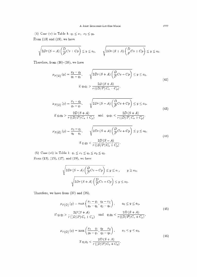
A Joint Economic-Lot-Size Model 1777

(4) Case (v) in Tab le 1: ql _< Xl, X2 ~ q0"

F r o m (13) and (19), we have

~2Dr(S-[-A) ( D c v + C p ) < Y < a l ,

Therefore , f rom (36)-(3s), we have

~F(o,) (y) - ~2 2q_1 qo - ql

if qoql >

~ / 2 D r ( S + A ) ( D c v + C p ) <_y<_ao.

~/2Dr(S + A) ( D cv + Cp) <_ Y ~ al,

2D (S + A) r ((D/P) C~ + Cp)'

(42)

#F(~)) (Y) -- x2 - - q l , qo -- ql

if qlq2 > 2D (S + A) and qoql < 2D (S + A) 7" ((D/P) C. + Cp) r ((D/P) C. + G)"

(43)

~F(~) (y) - x,~ - q l q0 ql

~ 2 D r ( S + A ) ( D c v + C p ) _<y_< a0,

if ql q2 < 2D (S + A)

r ((D/P) C. + Cv)"

(5) Case (vi) in Table 1: ql --~ Xl _< q0 < x2 < q2

From (13), (15), (17), and (19), we have

~ 2 D r ( S + A ) ( D c v + C p ) <_y<al, y>_ao,

Therefore , we have f rom (37) and (38),

( X~o ° - q l q2--2c2) ~ F ( ~ ) (y) = m a x - - - , - ql q2 qo

2D (S -F A) if qlq2 > and qlqo < r ((D/P) Cv + Cp)

ao < y < a l ,

2D (S + A)

r ((D/P) C. + G ) '

(44)

(45)

( X~o o - q l q 2 - x 2 I #F(<)) (Y) = m a x - - - , - - - , - ql q2 - q o

2D (S + A)

ao _< y _< 32,

(46)

if ql q2 < 'v ((D/P) C~ + Cp)"

1778 G . C . ~{AHATA et al.

(6) Case (vii) in Table 1: ql __ x2 < q0, q2 < x2,

F rom (13), (15), and (17), we have

y>_a2.

Therefore by (38), we have

~ F ( Q ) (Y) ~1 - - q l qo ql

2D (S + A) a2 < y < a l , if qlq2 < . (47)

- - r((D/P) C~ + Cp)

(7) Case (viii) a n d (ix) in Table 1 satisfy the inequa l i ty qo _< x l and qo > q.. Bu t from (12),

it has no solut ion.

We consider

m a x ql q2 -~

and s impli fy m a x in (45) for ao _< y _< a l or in (46) for ao < y <_ a2, respect ively as follows,

X l - - q l q2 - - x 2

qo - ql q2 - qo

equa t ion in y, we have

) 4(q2 q o ) ( q o - - q l ) y 2 - - 2 r q o ( q 2 - - q l ) 2 ~ C , , q - C p y

+ (q2 - ql) 2 r2q~ --tiC. + Cp + 2 r D (S + A) --tiC. + Cp (ql + q2 - 2qo) 2 = O.

( 4 8 )

Let D1 = rUq~(q2 - q l ) 4 ( ( D / P ) C . + Cp) 2 - 4(q2 - qo)(qo - ql). [rUq2o((D/P) C . + Cp) 2 + (q2 -

qx) 2 + 2 r D ( S + A ) ( ( D / P ) C , + C; ) (q l + q2 - 2qo)2].

If Dx > 0, t h e n equa t ion (48) has two roots, say s l and s2,

rqo (q2 - ql) 2 ( ( D / P ) C . + Cp) - x/-D7 rqo (q2 - ql) 2 ( ( D / P ) C . + Cp) + . / D 1

Sl : 4 (q2 - qo) (qo - ql) , s2 = 4 (q2 qo) (qo - ql) '

when Dt 0, t h e n equa t ion (48) has one root, say, s3

rqo (q2 - qx) 2 ( (D/ P) C~ + Cp) s3 : 4 (q2 - qo) (qo - q l )

Let

f ( y ) _ Xl - ql _ 1 y - x / y - 2 r D ( S + A ) ( ( D / P ) Cv + Cp) ]

qo - ql qo - ql r ( ( D / P ) Co ÷ C;) - ql] ,

[ Y+x/Y2-2rD(S+A)((D/P)C~+CP)] q2 -- ao < y < al ,

q2 -- qo q2 -- qo r ( ( D / P ) C . + Cp) ' - -

, ' ( ( D / P ) C v q- Cp) (q 0 - q l ) 1 - V / y 2 _ 2 r D ( S -[- A ) ( ( D / P ) Cv + Cp) < O,

2rD(S + A)((D/P) C~ + Cp) >0,

9 ( y ) _ q2 - z 2 _ 1

f ' (y ) =

f " (y ) = r ( ( D / P ) C~ + Cp)(qo - ql) {y2 _ 2 r D ( S + A ) ( ( D / P ) C , + Cp)} 3/2

A Joint Economic-Lot-Size Model 1779

lg

ao a 1

(a) D1 < 0.

Y

ao Sl se a I

(b) D1 > 0.

. y

=g(y )

a o s 3 ae

(c) D1 = 0.

Figure 1. Graphs of f and 9.

. Y

1780 G . C . MAHATA et al.

1 E 1 g'(Y) = r ( (D /P) C~ + Cp)(q2 - qo) 1 + v/Y 2 _ 2rD(S + A ) ( ( D / P ) C, + C;)

g,,(y) 2rD(S + A) ( (D /P) C. + Cp) = > 0 .

r ( (D /P) Cv + Cp)(q2 qo) {y2 _ 2rD(S + A) ( (D /P) Cv + Cp)} a/2

So, f and 9 are decreasing, concave upward , and con t inuous func t ions on the closed in terval

[ao, ax]. There fore , we have the fol lowing two cases.

(A) If

ql q2 >

and

q1 qo <

t h e n we ob t a in the following.

2D(S + A) ~((n/P)Cv + c,)

2D(S + A) r((D/P)Cv + Cp)'

(A-I ) If D1 < 0 or D1 = 0, and ao < sa < a l , t hen f (y) < g(y), y E [ao, a l l .

Therefore , we have

#F(©) (9) = m a x , -- , ql q2 q2 -- qo

(A-2) If D1 > 0 a n d a o < s l < s2 < a l , t hen

(2£~00 --ql q2 --X-~O0) { #F(O) (Y) = max , = ql q2

Similar to (A), under condi t ion

ao <Y<al .

q 2 - - x 2 , i f a o _ < y < s l , q2 -- q0

Xl - - q l , if Sl _~ y < 82, q0 -- qa

q 2 - - x 2 , i f s 2 _ < g < a l . q2 -- q0

(49)

(50)

2D(S + A) qlq2 < r((D/P)C~ + Up)

a n d 0 < q l < q . < q o < q 2 , we have if D , = 0 and a0 < s 3 < a 2 , t h e n

q2 -- x2 , i f a o _ < y _ < s a ,

. ~ ( ~ ) (y ) = m a x - - - , ( 51 ) -- ql q2 qo Xl - - q l , i f sa _< y _< a2.

qo -- ql

For convenience of express ion, we define the following sets unde r t he cond i t ion 0 < ql < q. <

2D(S + A) } E1 : (q,,qo,q2)/qoqs > r ( ( D ~ C . 7-Cp) '

2 D ( S + A ) l and qlqo < r ( (D/P)Cv -- Op) J '

qo < q2.

2 D ( S + A ) E2 = (qx ,qo ,q2) /q lq2 > r ( (D/P)Cv + Up)

{ 2 D ( S + A ) } E3 : (q l , qo, q2)/qlq2 < r ( ( D / P ) C , + Cp) '

E21 = {(ql,qo,q2)/D1 < 0 or (D1 : 0 and a0 < s3 < a l ) } ,

E22 : {(ql,qo, q2)/D1 > 0 and ao < s1 < $2 < a l} ,

]331 = {(ql ,qo, q2)/D1 0 and ao < s3 < a2)}.

A Joint Economic-Lot-Size Model 1781

F r o m (39) - (44) , (47), (49)- (51) , we ob t a in #F(C))(Y) in T h e o r e m 2.5.

THEOREM 2.5. Under condition 0 < ql < q. < qo < q2, the membership function #F(~)(Y) is as follows.

(1) If (ql, qo, q2) C El, (a l < ao < a2), then

[ x 2 - q ~ , 2 D r ( S + A ) C v + C p < y < a o , by (43),

#F(O,)(y) = q2 - z2 - - , ao <_ y <_ a2, by (45), (49) and (41), q2 - qo

0, o therwise .

(52)

(2a) f f (ql, qo, q2) E E2 N E21, then

X2--ql, q0 -- ql

#F(~)(Y) = q2 -- X2 q2 -- qo O,

~ 2 D r ( S + A) ( D c v + Cp) <_ y <_ ao, by (43),

ao _< y _< a2, by (45), (49), and (41),

o therwise .

(53)

(2b) / f (ql, qo, q2) E E2 n E22, then

x2 -- ql

qo--ql

q 2 - x 2

q2 -qo #F(~)(Y) = x l -- ql

q0 - q l

q2 - x2 - - , q2 - q o

0,

@2Dr ( S + A ) ( D cv + Cp) <_ y <_ ao, b y ( 4 3 ) ,

ao ~ y ~_ Sl~

sl _< y _< s~, by (45), (49), ~nd (41),

82 ~ Y _~ a2,

ot tmrwise.

(54)

(3) f f (ql, qo, q2) E E3 N/['31, ao < a2 < a l , then

x2 - ql

qo--ql

q2 - x2 #F(~)(Y) = q2 - - q o '

Xl -- q~

qo - q l

0,

~ 2 D r ( S + A ) ( D c v ÷ C p ) <_y<_ao, by (44),

ao _< y _< s3, by (48), (51), and (43),

s3 < y _< al~

o therwise .

(55)

Defuzzification of #F(©) (Y) in Theorem 2.5. We defuzzify •F((2)(y ) in (52) (55) by the centroid method as follows.

(A1) The centroid of #F(d~)(y ) for (52). There is x2 in the integration, then by changing variable

y + x/y ~ - 2rD (S + A) ((D/P) Cv + Cp) x = (= x2) ,

((D/P) Cv + cp)

1782 G . C . N~]AHATA et al.

we have that, for j = 0,2, i f y = aj, then x = qj and if

then x = q.. Therefore, by (22)-(25), we have

~ 1 m z oc IZF(Q) ( y ) d9 -- qo --1 ql U1 ( q . , qo) -4- q2 - qo U2 (qo, q2) P a l , say, (56)

j y#F(©)(y)dy U11(q.,qo) ÷ U21(qo,q2) = R31, say. (57) 1 1

q0 - ql q2 - q0

LEIVIMA 2.1. / f (ql, q0, q2) C E1 and 0 < ql < q. < qo < q2, then the centroid for PlffO)(Y) of (52) in Theorem 2.5 is

R31 M a l ( q l , qo,q2) - P31" (58)

We regard this value as the estimation of J T R C under this condition.

(A2) The centroid of PF(©)(y ) for (53),(54).

The centroid of #F(~)(y)for (53) and (54) is descriSed in two cases.

(A21) For (ql, qo, q2) E E2 A E21, we solve the centroid Of #F(Q ) (y) in (53).

Similar to L e m m a 2.1, we have the fol lowing L e m m a 2.2.

LEMMA 2.2. I f (ql,qo,q2) C F~2 A EZl and 0 < ql < q. < qo < q2, then the centroid for/~F(Q)(Y) of (53) in T h e o r e m 2.5 is

R31 (59) M321(ql,qo,q2) /)31'

which is an estimation of the J T R C under the given condition.

(A22) For (ql, q0, q2) E E2 71 E22, we a t t e m p t to solve the cen t ro id of I~F(Q)(y) in (54) as follows.

F r o m (54), if the re is x2 in the in tegra t ion , t h e n by changing the var iab le x = x2; if y = aj, t h e n x = qj for j = 0,2. If y = sj, t hen

sj + v/s~ - 2 r D ( S + A ) ( ( D / P ) C v + Cp)

x = r ( ( D / P ) C v + Cp) - t j , say,

for j = 1,2, 3. If the re is z l in the in tegra t ion , t h e n by changing the var iab le x = Xl; if

y = s j , t h e n x = pj (say), for j = 1, 2, 3.

2 > 2 r D ( S + A ) ( ( D / P ) C . + Up) for Since ao < s l < s2 < a l and ao < s3 < a l imply t h a t s j _

j = 1 ,2 ,3 .

There fore , we have

S octZF(Q) (y) dy = 1 [Ul (q . ,qo) + Ul (pl,P2)]-t- 1 qo - ql q2 -- qo

[0"2 (qo,t l) + U2 (t2,q2)] -~ P322, say,

, -o~ YttF(d2) (y) dy = lqo - ql [Ull (q., qo) -[- Ull (Pl, P2)] -[- q2 -1 qo [U21 (qo,t l) -[- [/21 (t2,q2)] = R322, say.

LEMMA 2.3. I f (ql,qo,q2) E E2 A E2~ and 0 < ql < q. < qo < q2, then the eentroid for l~F((~)(y)

of (54) in T h e o r e m 2.5 is R322

M 3 2 2 ( q l , q o , q 2 ) -- P322 ' (60)

which is an estimation of the joint total relevant cost ( JTRC) under the given condition.

A Joint, Economic-Lot-Size Model 1783

(A3) The centroid of ~F(Q) (5') for (55) in Theorem 2.5. In the same way as in (A22), we have

/ : ~ # F ( Q ) ( Y ) @ Ul(q.,qo) + U~(qo,t3)+ Ul(pa,ql) =- P33, say, 1 1 1

q o - q l q2 - qo q o - q l

f / y#F(Q)(y)dy _ 1 UH(q. q o ) + 1 U21(qo,t3) + 1 UH(P3,ql) ~ /{33, say. oo qo - - ql q2 - qo qo- -q l

I f (ql,qo,q2) E E3 A E31 and 0 < ql < q. < qo < q2, then the centroid for #F(Q)(Y)

(61)

LEMMA 2.4. of (55) in Theorem 2.5 is

R33 Ma3(q1, q0, q2) -- P33'

which is an estimation of the J T R C under the given condition.

Combining Lemmas 2.1 2.4, we have Theorem 2.6.

THEOREM 2.6. Under the condition 0 < ql < q, < qo < q2, the centroid for #F(Q)(Y) of(52) (55) in Theorem 2.5 is

A/Ia(ql,qo,q2) =M31(ql ,qo, q2)IE1

+M321(q1,qo,q2)IE2nE21 ÷M321(ql,qo,q2)IE2nE22 + M 3 ( q l , qo,q2)IEanEal (62)

where IA = ~ 1, if (ql,q0, q2) E A,

[ 0, if (ql,qo, q2) ~ A.

2.4. #F(Q,)(Y) a n d I t s C e n t r o i d U n d e r t h e C o n d i t i o n 0 < ql < q0 < q. < qz

Under the condition,

O < q l < q o < q , <q2 , (63)

we have

From (20), (21), and ao < al , there are only three permuta t ions of ao, al , a2,

(64)

2 D ( S + A) ao < a l < a 2 , i f q l q 2 > (65)

r ( ( D / P ) C~ + Cp)'

2D(S + A) 2D(S + A) a 0 < a 2 < al , if qoq2 > r ( ( D / P ) Cv + Cp) and qlq2 < r ( ( D / P ) C~ + Cp)' (66)

2D(S + A) a2 < a 0 < a l , ifqlq2 < (67)

r ( ( D / P ) Cv + Cp)"

Using (63)-(67), (12)-(19), Table 1 and Section 2.3, in a similar manner (Sections 2.3 and 2.4 being symmetrical) , we obtain the membership function #F(Q)(Y) of F (Q) under the condition 0 < ql < qo < q. < q2 in Theorem 2.7.

THEOREM 2.7.

as follows.

(1 °) I f

Under the condition, 0 < ql < qo < q. < q2, the membership function ItF(Q)(y) is

2D(S + A) qlq2 > ((D/P)Cv + cp)'

1784 G . C . ~VIAHATA et al.

D = O, a 0 < S 3 < al, and ao < az < a2, then

q2 - Xl }

q2 - qo

Xl - ql "F(Q) (Y) = qo ql'

q2 -- x2 - - }

q2 - qo

0, o therwise .

(20 ) If

i f I 2 D r ( S + A ) Q-~Cv-HCP) <-

if a0 _< y <_ s8,

i f s a < y < a z ,

2D(S + A) qoq2 > r ( (D/P)C, + Cp)' qlq2 <

and ao < a2 < al. (2%1) If D1 < 0 or (Dx = 0 and ao < sa < a2), then

I q 2 _ x l , q2 - qo

#F(d2)(Y) : x l - -q~ , i f a o _ < y < a l , qo - ql

0, o therwise .

(2%2) I f D1 > 0 and ao < sl < s2 < a2, then

q2-Xlq2_qo, i f I 2 D r ( S + A ) ( D c v

Xl - - q l , if ao _< y _< s l , qo -- qz

/ \

tZF(Q)< y) = q2 -- x2 i f 81 < y < 82, q2 -- qo

Xl ql i f S2 < y < a2 ,

q0 - ql

0, o therwise .

2D(S + A) ,-((D/P)C. + C,)'

i f ~ 2 D r ( S + A ) ( D c v + C p )

(3 °) ff

y ~ a o ,

< y < a o ,

+ Cp) < y < ao,

2D(S + A) qoq2 > r((D/P)C,, + Cp)'

q 2 - x l if 2 D r ( S + A ) C v + C p < y <

(y) IZF(Cg) Xl q-------21, if ao _< y < a l , qo - ql

O, o therwise .

Le t us define the fol lowing sets under the cond i t ion 0 < ql < qo < q. < q2.

$1 = (q l , qo ,q2 ) /q lq2 > r((D/P)Cv + Cp) '

2D(S + A) $2 : (q,,qo,q2)/qoq2 > r((D/P)Cv + Cp) and qlq2 <

2D(S+A) } S~ : (ql,qo,q~)/qoq~ < <((D~PTC%-a,) '

ao~

(68)

(69)

(70)

(71)

2D(S + A) I r ( (D /P)C . + CB) f '

$11 : { ( q l , qo, q2)/D1 = 0 and ao < s3 < a l ) } ,

A Jo in t Economic -Lo t -S i ze Mode l 1785

$21 = {(ql ,qo,q2)/D1 < 0 or (D1 -- 0 and ao < sa < a2)}, $22 - {(ql ,qo,q2)/D1 > 0 and

a0 < s t < s 2 < a l } . In the same m a n n e r as Sect ion 2.3, we have the cent ro id of #F(<))(Y) in T h e o r e m 2.7.

(B1) The cent ro id of tZF(6.)(y) in (68): there is z2 in the in tegra t ion , t h e n by changing the

var iable x = z2; if y = a2, t hen x = q2, and for x l chang ing the var iable z = Xl, t h e n if

y = a j , x = q j for j = 1 , 0 . We have

#F(d))(y)dy _ 1 Ul(q.,qo) + U2(qo,p3) -t- gl( t3,q2) = P41, say, oo q2 - qo qo - ql q2 - qo

/ y p f ( d 2 ) ( y ) d y _ 1 U l l (q . q0) ÷ 1 U21(qo,pa) ÷ 1 Uu(t3, q2) =- R41, say, oo q2 -- qo qo -- ql q2 -- qo

where tj an d pj are same as in Sect ion 2.3.

LEMMA 2.5. I f (ql, qo, q2) E $1 N S u and 0 < ql < qo < q. < q2, t hen the centroid for PF(~)(Y) of (68) i±1 Theorem 2.7 is

R41 M41(q1,q0,q2) -- P41 ' (72)

which is an estimation of the J T R C under the given condition.

(B2) The cent ro id of #F(O)(y ) for (68)-(70). We change var iable as in (B1).

(B21) The cent ro id of #F(c))(Y) for (q~, q0, q2) E $2 n $21. F rom (69), we have

and

/ #F(C))(Y) dy - oc q2 -- qo

/ / Y#F(~)(Y) dy -- c~ q2--q01

1 1 - - g 2 ( q . , q o ) -]- Ul(qo,ql) P421, say,

qo - ql

1 1 - - U 2 1 ( q . , q o ) + Ull(qo, ql) = R 4 2 1 , say.

q o - q l

Therefore, we have the following L e m m a 2.6.

LEMMA 2.6. I f (qt,qo,q2) E $2 A $21 and 0 < ql < qo < q. < qz, then the centroid Of PF(d2)(y )

in (69) is R421 ( 7 3 )

M421 (ql, qo, q2) = P421"

(B22) The cent ro id of #F((2)(Y) for (ql, q0, q2) E $2 A S2z. F rom (70), we have

]~ ~r(<)) (Y) dy = 1 [g2 (q., qo) + U2 (tl,t~)l + 1 [gl (qo,pl) d- U1 (P2, ql)] = P422, say, o~ q2 -- qo qo -- ql

. / • ¢ Y#F(O) (Y) dy = 1 [U21 (q.,qo) + U2: (tl,t2)] + 1 q2 q0 q0 -- ql

[Un ( q o , p l ) + g l l (p2 ,q l ) ] = R422, say.

Therefore, we have the following L e m m a 2.7.

LEMMA 2.7. I f (ql,qo,q2) E $2 A $22 and 0 < ql < qo < q. < q2, then the centroid of #F(d2)(y )

in (70) is R422 (74)

M422(q1,qo,q2) - P422'

LEMMA 2.8.

is

I f (ql,qo, q2) E Sa and 0 < ql < qo < q, < q2, then the centroid of gF((~)(y ) in (71)

R43 (75) M 4 3 ( q l , qo, q2) - - P 4 3 "

1786 G.C. ~IAHATA et al.

Combining Lemmas 2.5-2.8, we have the following Theorem 2.8.

THEOREM 2.8. is

Under the condition 0 < ql < qo < q. < q2, the centroid of#F(c)) (y) for (72)-(74)

M4(ql, qo, q2) = M41(q1,qo,q2)[&nsu -4-M421(q1, qo, q2)Is2ns21

+M422(ql,qo, q2)Is~ns= +M43(q l ,qo ,q2) I&. (76)

Let

(OR

3. OPTIMAL P R O D U C T I O N LOT SIZE FOR V E N D O R

ORDER Q U A N T I T Y FOR THE P U R C H A S E R )

['1 { (q t ,qo , q2)/q* < ql < q0 < q2},

['2 : { ( q l , q o , q 2 ) / O < ql < q0 < q2 < q * } ,

Fa = { ( q l , q o , q 2 ) / O < ql < q, < qo < q 2 } ,

and

[04 = {(ql ,qo,q2)/0 < ql < q0 < q* < q2}.

From Theorem 2.2, 2.4, 2.6, and 2.8, we have Theorem 3.1.

THEOREM 3.1. The joint total relevant cost est imate in the fuzzy sense is

4 M(ql ,qo,q2) = E M j ( q l , q o , q 2 ) I ~ ,

j=l for 0 < ql < q0 < q2,

where Mj(q l , qo, q2) are given in Section 2.

In order to minimize M(ql , qo, q2), we may use the Nelder-Mead method [17]. However, in our paper, ql,qo,q2 will satisfy 0 < ql < q0 < q2. Therefore, we apply the Nelder-Mead simplex algorithm [18], by transformations,

R : x + d ( X - C ) : (1 + d ) X - dG, 0 < d <_ 1,

E = X + e ( R - X ) = ( 1 - e ) X + e X , e>_ l ,

to revise this algorithm. In this paper, we denote qx for X(1) , G(1), R(1), and E(1); q0 for X(2) , G(2), R(2), and E(2); q2 for X(3) , G(3), R(3), and E(3). Given X(1) < X(2) < X(3) and G(1) < G(2) < G(3). We let [(x) = 1 if x > 0, else I ( x ) - O, then

(1) H ( k + 1, k) = X ( k ) - X ( k + 1) - G(k) + G(k + 1), k = 1,2 and choose d satisfying 0 < d < L , w h e r e L = l i f H ( k + l , k ) < 0 , V k = l , 2 , else

IX(2) - X(1) X(3) - X(2) I(H(3,2)), 1] . L : rain ~ ( ~ , ~ ) I ( H ( 2 , 1)), H(3, 2)

Hence, R(1) < R(2) </{(3).

(2) Let

and denote L. = oc, if

L(k + 1,k) = X(k + 1) - X(k ) + R(k) - R(k + 1),

L(k+l,k)<_O, V k = 1,2,

k = 1, 2,

R(k) : 2M(k) - V(k'), E(k) = 2R(k) - M(k) ,

else X(k + 1) - X(k)

L, = min I(L(k + 1, k)). ~=~,~ L(k +K,k )

If we take e satisfying 1 < e < L . , then i t is easy to show tha t E(1) < E(2) < E(3) . For

subrout ine in [17],

are replaced by

in the fuzzy sense.

R(k) : (1 - a)M(k) - aV(k), E(k) : bR(k) + (1 - b)M(k),

respectively, where a satisfies 0 < a < L and b satisfies 1 < b < L, . By this revised

algori thm, we find the opt imal value of qi, say q~, q~, q~, which minimize M(ql, qo, q2) and

obta in JELS, q~ + q~ + q~, q**

3

R

H

S

Figure 2. G is replaced by R.

G E

H

A Joint Economic-Lot-Size Model 1787

Figure 3. G is replaced by E.

4. N U M E R I C A L E X A M P L E

I M P L E M E N T A T I O N

In this section, we apply Theorem 3.1 for some numerical example to find the JELS q** in the

fuzzy sense such tha t the J T R C M(q~, q~, q~) is minimum. Let ql, q0, q2 be any initial points, q~,q~,q~, the coordinates of local minimum. Therefore, the centroid for the t r iangular fuzzy

number (q~, q~, q~) is given by q** _ q~ + q~ + q~

3

which is the JELS in the fuzzy sense.

2D(S+A) q* : , ' ( ( D / P ) C ~ + CV)

1788

(4.1.1)

(4.1.2)

(4.1.3)

(4.1.4)

ql q0 q2

401 407 412

403 408 415

400 407 411

402 409 414

C. C. MAHATA et al.

Table 2. Resu l t s for each case.

we have

q~ = 401.00, q; = 408.70, q~ = 413.71

q** = 4 0 7 . 8 , M ( q ~ , q ; , q ~ ) = 2 5 0 0 . 4 5 3

rq = 1.95%, r~ = .018%

0 < q, < q~ < q** < q~ < q~ (Case Sec t ion 2.1)

ql qo q2

390 395 398

385 394 399

387 393 397

391 396 400

we have

q~ = 384.9, q~ = 393.3, q~ = 398

q** =392.0667, M(q~,q~,q~)=2500.323

rq = -1.98%, 7"c = 0.013%

0 < q~ < q** < q; < q~ < q. (Case Sec t ion 2.2)

ql q0 q2

398 403 408 we have

399 405 409 q~ = 399.75, q~ = 402.2501, q~ = 404.5001

398 404 407 q** = 402.167, M(q~, qo, q2) -- 2500.058

397 405 410 rq = 0.542%, rc = 0.0023%.

0 < q{ < q, < q** < q(~ < q*2 (Case Sec t ion 2.3)

ql qo q2

392 397 403

393 398 402

391 395 401

394 396 403

we have

q~ = 392.0001, q~ = 394.2501, q~ = 400.2501

q*" = 395.5001, M(q~,q~,q~) : 2500.23

rq = 0.0113%, rc = 0.0092%

0 < q~ < q; < q** < q. < q~ (Case Sec t ion 2.4)

is the J E L S for crisp order q u a n t i t y and

is the co r re spond ing m i n i m u m J T R C .

Let q** _ q.

rq - - - - X 1 0 0 % q.

a n d

M(q'~, q~, q~) - .F(q,) x 100% = f ( q . )

be the re la t ive er ror of J E L S and the re la t ive er ror of J T R C , respect ively .

EXAMPLE 4.1. G iven D - 1000 un i t s / yea r , P = 3200 u n i t s / y e a r , A = $100 /o rde r , S = $400/se t -

up, Cp = $25 /un i t , C, = $20 /un i t , and r = 0.2, t hen we ob t a in q. - 4 0 0 u n i t s and F(q.) = $2500

as t he o p t i m a l so lu t ion for the crisp mode l which exac t ly m a t c h e s w i t h t he numer i ca l so lu t ion

ob t a ined by Bane I j ee [2].

A Joint Econoinic-Lot-Size Model 1789

For a g iven set of i n i t i a l p o i n t s qt , q0, q2, we have r e su l t s for e a c h case in T a b l e 2.

Since we cannot apply the analyt ica l method to solve the cri t ical point (q~, q~, q~), such tha t

M(q~, qo, q2) in Theorem 3.1 is mininmm, therefore, we have used the numerical method [17] to find the approximate cri t ical point (q{, q~, q~). From the above discussion, since there are three

variables ql, q0, q2, we have to assign four init ial points to run the compute r program. From the above (4.1.1)-(4.1.4), rc = 0.0023% in (4.L3) is less than in the other cases; therefore,

the min imum J T R C in the fuzzy sense is given by

M(ql, qo, q2) = 2500.058

and

is the corresponding JELS.

q** = 392.0667

5. C O N C L U S I O N

The y-range of the membership function, #F(O)(Y) of the fuzzy J T R C is y > F(q.). The

approx imate op t imal solution of 0 < ql < q0 < q2 is q~,q~,q~. Thus, in fuzzy sense, if the

es t imated cost, M(q l , q0,q2) is closer to F ( q . ) , the be t te r is the es t imate . From calculat ion of (4.1.1)-(4.1.4), the min imum of r~ is obta ined from (4.1.3). Therefore, in fuzzy sense best JELS q** = 392.0667 and M(q~, q~, q~) = 2500.058. In the crisp sense, bes t JELS q. -- 400, the relative error wi th tha t of fuzzy sense is rq -- 0.542%. In the crisp sense, the J T R C is F(q.) = 2500,

i t s r e l a t i ve e r ro r w i t h t h a t fuzzy sense is rc = 0 .0023%. Hence , if we t ake t h e va lues of qz, q0, q2

suf f ic ien t ly close to q, , t h e r e l a t ive e r ro r s are v e r y sma l l w h i c h shows t h a t ou r so lu t i on p r o c e d u r e

is eff icient a n d m a t c h e s w i t h t h e ex i s t i ng so lu t i on for t h e c o r r e s p o n d i n g cr i sp mode l .

R E F E R E N C E S

1. S.K. Goyal, An integrated inventory model for a single supplier-single customer problem, International Jour- nal of Production Research 15, 107 111, (1976).

2. A. Banerjee, A joint economic-lot-size model for purchaser and vendor, Decision Sciences 17 (3), 292-311, (1986).

3. S.K. Goyal, A joint economic lot-size model for the purchaser and vendor: A comment, Decision Sciences 19, 236 241, (1988).

4. A.K. Chatterjee and R. Ravi, Joint economic lot size inodel with delivery in sub-batches, Opsearch 28, 119-124, (1991).

5. L. Lu, A one-vendor multi-buyer integrated inventory model, European Journal of Operational Research 81, 209 210, (1995).

6. S.K. Goyal, A one-vendor multi-buyer integrated inventory model: A comment, European Journal of Oper- ational Research 82, 209-210, (1995).

7. A.K. Aggrawal and D.A. Raju, Improved joint economic lot size model for a purchaser and a vendor, Advanced Manufacturing Process, Systems, and Technologies 96, 579-585, (1997).

8. R.M. Hill, The single-vendor single-buyer integrated production-inventory model with a generalized policy, European Journal of Operational Research 97, 493 499, (1997).

9. S.K. Goyal, On improving the single-vendor single buyer integrated production inventory model with a generalized policy, Eu~vpean Journal of Operational Research 125, 429-430, (2000).

10. L.A. Zadeh, Fuzzy Sets, Information and Control 8, 338-353, (1965). 11. G. Sommer, Fuzzy inventory scheduling, In Applied Systems and Cybernetics, Volume VI, Edited by G.E.

Lasker, pp. 3052 3060, New York, (1981). 12. J. Kacpryzk and P. Staniewski, Long-term inventory policy-making through fuzzy-decision making models,

Fuzzy Sets and Systems 8, 117-132, (1982). 13. K.S. Park, Fuzzy-set theoretic interpretation of economic order quantity, IEEE Transactions on Systems,

Man, and Cybernetics SMC-17, 1082 1084, (1987). 14. J.S. Yao and H.M. Lee, Fuzzy inventory with backorder for fuzzy order quantity, Information Sciences 93,

283-319, (1996). 15. S.C. Chang, J.S. Yao and H.M. Lee, Economic reorder point for fuzzy backorder quantity, European Journal

of Operation Research 109, 183-202, (1998). 16. T.K. Roy and M. Maiti, A fuzzy EOQ model with demand-dependent unit cost under limited storage capacity,

European Journal of Operation Research 99, 425 432, (1997).

1790 G.C. MAHATA et al.

17. J.L. Buchanan and P.R. Turnur, Numerical Methods Analysis, McGraw-Hill, New York, (1992). 18. J.H. Mathews, Numerical Methods for Mathematics, Science, and Engineering, Prentice-Hall, London~

(1992).