A Variational Deduction of Second Gradient Poroelasticity II: An Application to the Consolidation...

JOURNAL OF MECHANICS OF MATERIALS AND STRUCTURESVol. 3, No. 4, 2008

A VARIATIONAL DEDUCTION OF SECOND GRADIENT POROELASTICITY II:AN APPLICATION TO THE CONSOLIDATION PROBLEM

ANGELA MADEO, FRANCESCO DELL’ISOLA, NICOLETTA IANIRO AND GIULIO SCIARRA

The second gradient model of poromechanics, introduced in Part I, is here linearized in the neighborhoodof a prestressed reference configuration to be applied to the one-dimensional consolidation problem orig-inally considered by Terzaghi and Biot. Second gradient models allow for the description of boundarylayer effects both in the vicinity of the external surface and the impermeable wall.

The formulated differential problem involves linear pencils of ordinary differential operators on afinite interval, with boundary conditions depending on the spectral parameter. Taking into account thedependence of the differential problem on initial stresses a linear stability analysis is carried out. Finally,numerical solutions are compared with the corresponding classical Terzaghi solutions.

1. Introduction

This paper addresses a geotechnical application of the macroscopic second gradient poroelasticity the-

ory presented in the first part; in particular we aim to treat the well known soil consolidation problem[Terzaghi 1943]. The consolidation of a soil layer of depth L can be schematically described as follows:when an external load p

ext. is applied on the surface of the layer, the fluid starts moving from the layertowards the surface, and it finally leaves the system. While the fluid keeps flowing, the external load isgradually distributed to the solid skeleton, which starts to deform.

Different theories which model consolidation have been developed in the literature [Biot 1941; Terza-ghi 1943; Heinrich and Desoyer 1961], however the two due to Terzaghi and Biot are surely the mostwidespread ones. Actually, as it was noted also by de Boer [1996], the derivation of the Terzaghidifferential equation [Terzaghi 1923] is obscure and essentially driven by the comparison between thephenomenon of soil consolidation and that of heat propagation, rather than from the statement of suitable

mechanical principles. On the other hand Biot’s theory seems to be well grounded from the mechanicalpoint of view, even if directly restricted to the case of linear elasticity, in its earliest presentation [Biot

1941]. The two models collapse one into the other when considering one-dimensional problems; how-ever, this is not the case when modeling, for instance, the behavior of a saturated porous slab [Mandel

1953] or a saturated porous sphere [Cryer 1963]. In both circumstances Biot’s three-dimensional modelprovides time increasing values of the water pressure (and fluid mass density) at the center of the slab (or

sphere) if the Lame constant µ of the skeleton is different from zero; on the other hand the solution forµ = 0 coincides with the one derived from Terzaghi’s three dimensional model. This localized pore-fluidsegregation is known in the literature as the Mandel–Cryer effect.

Keywords: poromechanics, second gradient materials, consolidation.

607

608 ANGELA MADEO, FRANCESCO DELL’ISOLA, NICOLETTA IANIRO AND GIULIO SCIARRA

The occurrence of compaction localization phenomena has recently been discovered by Mollema andAntonellini [1996], who presented evidence of so called “compaction bands” in outcrops of the JurassicNavajo sandstone in the Kaibab monocline, in Utah. These bands are characterized by volume loss dueto microfracturing, but essentially no grain crushing or comminution. Later on, laboratory experimentshave been developed [Olsson and Holcomb 2000; 2003] using triaxial compression tests to reproducethe formation of these bands. These tests proved that increasing axial stress σ11 initially determines onlyhomogeneous axial strain �11, however, when a suitable stress threshold has been overwhelmed, tabularzones associated with nonhomogeneous strain can be detected close to the axial borders of the specimen.Nonuniform compaction also affects fluid flow in the porous material, being detrimental if permeabilityof the compacted material is much reduced with respect to the uncompacted zone.

The second gradient poromechanical model presented in Part I [Sciarra et al. 2008] is capable ofdescribing fluid mass density boundary segregation even in the one dimensional model. Both in thevicinity of the external consolidating surface and the impermeable wall, suitable boundary layer effectscan be predicted by the second gradient model. Formation of segregation bands enhances high gradientsof density of the fluid entrapped in the pores of the solid skeleton. This can be explained by means ofnonvanishing hyperstresses at the boundary (see [Sciarra et al. 2008, Equations (32)2–(32)3]); these lastcause the pore pressure to differ from its reference initial value in a transient period, when dissipationdoes not yet dominate the evolution process.

Having in mind the classical Terzaghi’s consolidation problem, whose space-time evolution is gov-erned by the same equation as that of heat conduction, replacing temperature with pore-pressure, weclaim that the second gradient model, presented in [Sciarra et al. 2008], is capable of regularizing thebehavior of the Darcy flow inside the porous medium. Because of second gradient effects, the fluid massdensity diffusion is smoothed. It is self evident that Terzaghi’s theory does not model those phenomenaoccurring at the boundaries which oppose the fluid flow, for example, pore closure, solid-fluid capillarity,etc. The present model tries to macroscopically account for some of them and aims to establish thepreliminary theoretical framework necessary for conceiving and designing any kind of experimentalactivity. In this paper it is shown that the overpressure occurring at the impermeable boundary actuallydepends on second gradient coefficients; therefore a more detailed analysis of these effects is recognizedto be necessary.

Pore fluid segregation is probably the triggering effect for vertical drain or sand volcano formation,observed after liquefaction [Kolymbas 1998]; these last can indeed be interpreted as bifurcation modesof consolidation, which, in the case of the second gradient model should correspond to the boundarylayer detected close to the impermeable wall becoming larger and larger. As it is not possible to identifythis bifurcation mode in the case of linearized (small strain) theory, only the limit condition describingthe stability/instability limit is detected. Further developments will be devoted to study of the one-dimensional nonlinear problem.

From the mathematical point of view the present model, in which both second gradient conservative(relative to the behavior of the porous solid skeleton) and dissipative (relative to the flow of the saturating

fluid) contributions are taken into account, implies that the newly formulated initial boundary valueproblem of consolidation fits in the framework of the theory of linear pencils of ordinary differentialoperators on a finite interval with boundary conditions depending on the spectral parameter. We refer

A VARIATIONAL DEDUCTION OF SECOND GRADIENT POROELASTICITY: PART II 609

to the general results presented, for example, in [Shkalikov 1986; Shkalikov and Tretter 1996; Marlettaet al. 2003] for more details on this topic.

2. Linearization of the one-dimensional differential problem

We study here the aforementioned consolidation problem referring to the equations of motion for asecond gradient porous medium as obtained in [Sciarra et al. 2008, Equations (30) and (31)], restrictingour attention to the one-dimensional case. This will allow us to compare our results with the classical ones

due to Terzaghi [1923]. Of course, Equations (30)–(31) can also be applied to treat three-dimensionalproblems, so extending classical Biot’s equations.

Clearly, because of the one-dimensional hypothesis, all the gradient and divergence operations appear-ing in Equations (30) and (31) become simple derivatives with respect to the space variable x , and the

deformation tensor ε simply reduces to its only nonzero component εxx along the x axis. In the following

we will indicate the component εxx simply by ε.From now on we assume the hypothesis of small deformations in the neighborhood of a suitable solid

skeleton reference configuration. For the sake of simplicity we will therefore use the same notation as

used in [Sciarra et al. 2008] for ε and mf to indicate the corresponding incremental quantities with respect

to the considered small deformation parameter.In accordance with the aforementioned assumptions and the introduced nomenclature, the quadratic

expression for the Hemholtz free energy density �, in terms of the state parameters (ε, mf , εI , m

I

f) is

adopted as,

� = − pext.0 ε + µext.

0 mf + 12

�λ + 2µ + b

2M

�ε2 + 1

2M

�mf

m0f

�2

− bMεmf

m0f

+ 12

�Kss + �K

2s f

�(ε I )2 + �Ks f

mI

f

m0f

ε I + 12

��m

I

f

m0f

�2, (1)

where ε I and mI

findicate the first spatial derivatives of ε and mf , respectively.

The constant coefficients pext.0 , µext.

0 , and m0f

account for the state of stress of the solid skeleton, thechemical potential of the fluid, and the initial apparent density of the fluid before any external perturbation

is applied to the porous system. Moreover, λ and µ are the classical Lame coefficients, b and M the Biot

parameters, and �, Kss , and Ks f are the second gradient constitutive parameters.The nonstandard energetic contributions associated with (ε I )2, (m I

f)2, and ε I

mI

fare those responsible

for the presence of hyperstresses in the balance equations of the overall material and the pure fluid. Theyallow for describing the compaction/dilatancy localization effects arising in the fluid-filled porous mate-rial when the fluid remains entrapped in the solid skeleton. In particular Kss and � provide nonvanishing

hyperstress on the solid skeleton and the pure fluid if second gradient coupling is negligible. Followingthe interpretation of double forces given in [Sciarra et al. 2008, Section 2], these two constitutive pa-rameters allow for describing internal actions working on the rate of dilatancy along the outward unitnormal. The coupling coefficient Ks f is labeled as the cocapillarity coefficient in analogy to standardsecond gradient theories for capillarity models [Seppecher 1987]. It describes second gradient solid-fluidinteractions and can be assumed as vanishing in contrast with Kss and �, which will be proved to bepositive when positiveness of strain energy density is required (see Equation (2)).


Values of the Lame and Biot moduli can easily be recovered from the literature [Coussy 2004]; on theother hand no identification for the second gradient moduli is available up to now. It is not the purpose of

this paper to set up a constitutive identification based on experiments or mathematical homogenization;conversely, our aim is that of exhibiting the capability of the model presented in [Sciarra et al. 2008] tocatch compaction/dilatancy effects. Second gradient parameters therefore will be tuned so as to permitthe one-dimensional model to show boundary layer effects for the solid strain and the fluid mass densityin the vicinity of the external surfaces.

Requiring definite positiveness of the energy density � defined in Equation (1), the following condi-tions on the parameters must hold:

λ + 2µ > 0, M > 0, and Kss > 0, � > 0. (2)

The first two conditions are well known in the framework of the classical Biot poromechanics; the second

ones restrict the constitutive assumptions on the second gradient parameters.

2.1. Equations of motion. We will now deduce the linearized form of the equations of motion for the

second gradient consolidation problem. In order to do so, it is worthwhile to recall that in the one-dimensional, linearized problem the following chains of equalities hold:

Fs � I + ∇su = (1 + ε) I, (3)

u being the infinitesimal solid displacement field,

F−1s

� (1 − ε) I, (4)

andJs � det Fs = 1 + tr(∇0u) = 1 + ε, (5)

where we recall that all the considered fields in the right hand side of (3)–(5) have to be regarded asincremental quantities with respect to the small deformation parameter. Taking into account (1) for thestrain energy � and the one-dimensional form of (3) and (5) , the linearized governing equations givenin [Sciarra et al. 2008, Equations (30) and (31)], reduce to

��−p

ext.0 + λ + 2µ + b

2M

�ε − bM

mf

m0f

−�

Kss + �K2s f

�ε I I − �Ks f

mI I

f

m0f

�I

= 0, (6)

and

−m0f

�M

mI

f

�m

0f

�2 − bM

m0f

ε I − �Ks f

m0f

ε I I I − ��m

0f

�2 mI I I

f

�− D

�vf − vs

�+

�α�vf − vs

� I�I

= 0, (7)

for the solid skeleton and the pure fluid, respectively. We have denoted by D and α the only nonzerocomponent of the Darcy and Darcy-like tensors � and �, respectively (see [Sciarra et al. 2008, Equation(25)]), and by vf − vs the vertical component of the relative velocity. In the absence of inertia forces thesolid momentum conservation law, Equation (6), can be integrated in the form

�λ + 2µ + b

2M − p

ext.0

�ε − bM

mf

m0f

−�

Kss + �K2s f

�ε I I − �Ks f

mI I

f

m0f

= const. := c0. (8)


Moreover, considering that vf − vs is related to the apparent fluid density mf by means of the linearizedcontinuity equation mf + m

0f(vf − vs)

I = 0, (7) can be rewritten, performing a derivative with respect tothe space variable x , as

−m0f

M

mI I

f

�m

0f

�2 − bM

m0f

ε I I − �Ks f

m0f

ε I V − ��

m0f

�2 mI V

f

+ D

m0f

mf − α

m0f

mI I

f= 0, (9)

where we have indicated by mf the time derivative of mf .In order to write the linearized governing equations in a dimensionless form, the following quantities

are introduced:

ξ = x

L, mf = mf

m0f

, t = t

τ, with τ = DL

2

M,

where L is the depth of the solid layer.According to these definitions, (8) and (9) can be rewritten in their dimensionless form as

(λ + 2µ + b2M − p

ext.0 )

λ + 2µε − bM

λ + 2µmf −

(Kss + �K2s f

)

(λ + 2µ)L2 ε I I − �Ks f

(λ + 2µ) L2 mI I

f= c0

λ + 2µ, (10)

and�

M L2 mI V

f+ �

M L2 Ks f εI V − m

I I

f+ bε I I − α

DL2˙m I I

f+ ˙mf = 0, (11)

which represent the linearized equations of motion for the consolidation problem. For the sake of sim-

plicity, we will no longer distinguish between mf and mf , and, if not specified, mf will indicate thedimensionless quantity. Moreover, the dimensionless variables ξ and t will be also indicated by x and t

if no confusion can arise.

2.2. Boundary conditions. The constant c0 is deduced from the boundary condition (BC) in x = 0 given

in [Sciarra et al. 2008, Equation (32)1] which, in the linearized form, reads

�λ + 2µ + b

2M − p

ext.0

�

λ + 2µε − bM

λ + 2µmf −

�Kss + �K

2s f

�

(λ + 2µ)L2 ε I I − �Ks f

(λ + 2µ)L2 mI I

f= − �p

ext.

(λ + 2µ);

here �pext.

represents the incremental external pressure acting on the system, deriving from the lineariza-

tion process (pext. = p

ext.0 +�p

ext.). In other words, �p

ext.is the perturbation in the external load applied

on the surface of the soil layer. Comparing this BC with (10) it is easy to recognize that c0 = − �pext..

Equations (10) and (11) represent a differential system of the sixth order in the space variable x and of

the first order in time, the integration of which requires therefore six boundary conditions and one initialcondition. In classical poromechanics the Terzaghi consolidation problem does not take into accountsecond gradient effects, and indeed it can be obtained from (10) and (11) when the second gradientparameters �, Kss , Ks f , and α are vanishing. Clearly, the problem reduces in this case to a second order

system with respect to the space variable x .The boundary conditions for the consolidation problem are derived from the general ones deduced in

[Sciarra et al. 2008, Equation (32)]. In particular, since the given problem is one-dimensional, surface


divergence and surface gradient operations do not contribute to the BCs; moreover no edge Ek of theboundary exists. Extending the classical BCs stated in the Terzaghi consolidation problem we assume:

• Zero fluid traction in x = 0. This BC states that the surface of the solid layer is kept drained,meaning that the fluid reaching the surface is continuously removed from the surface itself. ThisBC corresponds to the one given in [Sciarra et al. 2008, Equation (32)1] which, in its linearized,dimensionless form, reduces to

mf − bε − �Ks f

M L2 ε I I − �

M L2 mI I

f+ α

DL2 mf =m

0f�µext.

M= 0, (12)

where �µext. represents the incremental chemical potential. In other words we have assumed thelinearization µext. = µext.

0 + �µext.. Assuming that the fluid is continuously removed from thesurface of the layer, this implies a restriction to the case �µext. = 0.

• Impermeable soil in x = L . With this BC we assume that the relative velocity is equal to zero inx = L , implying vf − vs = 0. Using Equation (7), which holds everywhere in the interval [0, L], the

impermeability of the layer x = L can be rewritten in its dimensionless form as

−mI

f+ bε I + �Ks f

M L2 ε I I I + �

M L2 mI I I

f− α

DL2 mI

f= 0. (13)

• Zero double force for the overall system in x = 0 and x = L . These BCs are those ones given in[Sciarra et al. 2008, Equation (32)2], and can be rewritten in their linearized dimensionless form as

mI

f+

(Kss + �K2s f

)

�Ks f

ε I = 0.

We remind that the overall double forces are the contact forces introduced in the second gradientmodel, which work on the rate of pore opening/pore shrinkage. With the assumption of vanishingdouble forces on the boundary of the porous material, we claim that no external source of double

force exists; internal double forces, on the contrary, allow for capturing the effects of pressuregradient concentration in the neighborhood of the external and impermeable surfaces [Holcomband Olsson 2003].

• Zero fluid double force in x = 0 and in x = L . These BCs are those ones given in [Sciarra et al.2008, Equation (32)3]. They can be rewritten in their linearized dimensionless form as

mI

f+ Ks f ε I = 0. (14)

The assumption on fluid double forces can be interpreted similarly to that considered for the overalldouble forces. In this case no external double forces are exerted on the fluid boundary, but internal dou-ble forces, associated with pressure gradient concentration, account for internal capillarity and wettingphenomena.


3. Initial boundary value problem

The differential Equations (10) and (11) can be reduced to a unique differential equation introducing anauxiliary function V (x, t) which satisfies the relationships

ε = Ks f �

(λ + 2µ) L2 VI I + bM

(λ + 2µ)V, (15)

and

mf =�λ + 2µ + b

2M − p

ext.0

�

(λ + 2µ)V −

Kss + �K2s f

(λ + 2µ) L2 VI I + �p

ext.

bM. (16)

In such a way, Equation (10) is identically satisfied, while (11) can be rewritten, after some straightfor-ward calculations, as

C1VV I − C2

�p

ext.0

�V

I V − C3VI V + C4

�p

ext.0

�V

I I + C5�

pext.0

�V

I I − C6�

pext.0

�V = 0; (17)

on the other hand, the boundary conditions given in (12)–(14) read

�1VI V − �2

�p

ext.0

�V

I I − �3VI I + �4

�p

ext.0

�V + �5

�p

ext.0

�V + �6 = 0 at x = 0, (18)

VI = 0 at x = 0, L , V

I I I = 0 at x = 0, L , VV = 0 at x = L . (19)

Finally, the initial condition (corresponding to the instant in which the external load is applied) isdeduced assuming that the apparent Lagrangian fluid density is vanishing for t = 0+. For instance,mf

�x, t = 0+�

= 0; this initial condition states, similarly to in classical consolidation, that, at the instantin which the external load is applied there is no instantaneous variation of the fluid density mf inside thesoil layer. In terms of the auxiliary function V the initial datum reads as

V (x, 0+) := Vin = − �pext.

bM

1C4 (π0) + k6

, (20)

where (16) with mf = 0 has been solved using BCs given in (19).All the coefficients appearing in the governing equation, (17), as well as in the initial and boundary

conditions, (20) and (19), depend on the constitutive parameters, the solid initial stress pext.0 , and the

increment of the external force �pext.; their expressions are listed in Appendix A.

It must be remarked that the expression for the energy density � assumed in (1) would not allowthe linearized differential problem to explicitly depend on the initial solid stress p

ext.0 and on the initial

chemical potential µext.0 . In fact, considering (1) we can write, in dimensionless form,

∂�

∂ε= 1

λ + 2µp

ext.0 + (1 + k6)ε − bk5mf ,

∂�

∂mf

=m

0f

λ + 2µµext.

0 + k5mf − bk5 ε, (21)

so that there are no linear terms (in ε and mf ) involving pext.0 and µext.

0 coming from ∂�/∂ε and ∂�/∂mf .

On the other hand the dependence of the differential system (17)–(19) on pext.0 is due to so called geomet-

rical nonlinearities; as matter of fact it is the presence of Fs in the balance of the total momentum (see[Sciarra et al. 2008]) which even in linearized problems implies a nontrivial dependence of the governing

equations on pext.0 (see the term εp

ext.0 in (10)).


Considering the linearity of the differential problem and the nonhomogeneity appearing in the BC,given in Equation (18), we will look for a solution V (x, t) in the form

V (x, t) = V (x) + W (x, t), (22)

where V (x) is the solution of the stationary problem

C1VV I − C2V

I V + C4VI I = 0, (23)

with nonhomogeneous BCs

�1VI V − �2V

I I + �4V = − �6 at x = 0, (24)

VI = 0 at x = 0, L , V

I I I = 0 at x = 0, L , VV = 0 at x = L , (25)

while the deviation W (x, t) is the solution of the initial boundary value problem (IBVP)

C1WV I − C2W

I V − C3WI V + C4W

I I + C5WI I − C6W = 0, (26)

with homogeneous BCs

�1WI V − �2W

I I − �3WI I + �4W + �5W = 0 at x = 0, (27)

WI = 0 at x = 0, L , W

I I I = 0 at x = 0, L , WV = 0 at x = L , (28)

and nontrivial initial condition

W (x, 0+) := Win = Vin − V (x) . (29)

For the sake of simplicity we will no longer specify the dependence of the coefficients Ci and �i on theprestress parameter p

ext.0 .

It is easy to prove that the solution of the stationary problem given by (23)–(25) when �4 �= 0 is given

by

V (x) = − �6

�4, �4 �= 0, (30)

while if �4 = 0 the stationary solution V (x) exists if and only if �6 = 0; in this case a family of constant

solutions of the stationary problem arises, so that we can write V (x) = K , and �4 = �6 = 0, where Kis an undetermined constant. On the basis of the preliminary study of the stationary solution V (x) wecan state that, according to the assumption (22), a solution of the given problem for the variable V existsif and only if �4 �= 0 or �4 = �6 = 0. We will now restrict our attention to the case �4 �= 0 and willanalyze the case �4 = 0 later.

4. Fourier series solution

The initial boundary value problem given by (26)–(29) is solved using the method of separation ofvariables; in other words we assume that W (x, t) = X (x)T (t). A straightforward calculation yields tothe definition of the real eigenparameter λ as λ = T /T, which leads to T (t) = T0 e

λt . Consequently, thefunction X (x) must satisfy the eigenvalue problem

C1 XV I − C2 X

I V + C4 XI I = λ

�C3 X

I V − C5 XI I + C6 X

�, (31)


endowed with the BCs

�1 XI V − �2 X

I I + �4 X = λ��3 X

I I − �5 X�, at x = 0, (32)

XI = 0 at x = 0, L , X

I I I = 0 at x = 0, L , XV = 0 at x = L . (33)

This is a nonclassical spectral problem since the BCs also depend on the spectral parameter λ; in theliterature this kind of spectral problem is referred to as a linear pencil �(X) = λ�(X). Many authorsinvestigate the spectral properties of the differential operators � and � in suitable function spaces inorder to guarantee completeness and orthonormality for the eigenfunction system and discreteness of thespectrum [Shkalikov 1986; Shkalikov and Tretter 1996; Marletta et al. 2003]. Here we rely on thesegeneral results and numerically determine a subset of the eigenfunction space so as to approach therequirements of the Parseval equality [Kolmogorov and Fomin 1975].

According to the aforementioned properties of the eigensystem, the solution of the considered IBVPcan be given in Fourier series form as

W (x, t) =+∞�

k=0

pk Xk(x)eλk t , (34)

where pk denotes the k-th Fourier coefficient, and, in particular, p0 the Fourier coefficient relative to thenull eigenvalue λ = 0 (if any). It is easy to prove that if �4 �= 0 the eigenfunction X0 relative to the nulleigenvalue is the trivial one X0 = 0, so that in Equation (34) k runs now from one to infinity.

The eigenfunctions (Xk)k∈� are orthogonal with respect to the following bilinear form defined, in theHilbert space H

3 ([0, L]) × H3 ([0, L]), as

�Xk, Xh� := α0

�L

0Xk Xhdx + α1

�L

0X

I

kX

I

hdx + α2

�L

0X

I I

kX

I I

hdx + α3

�L

0X

I I I

kX

I I I

hdx, (35)

where the coefficients αi are defined as

α0 = �4C6, α1 = �4C5 − C4�5 + �2C6,

α2 = �4C3 − �3C4 + �2C5 − C2�5 + �1C6, α3 = �2C3 − C2�3 + �1C5 − C1�5.

It must be noted that expression (35) is indeed an inner product over the aforementioned function spaceif and only if all the coefficients αi are positive definite.

We notice that when the initial stress pext.0 is vanishing the αi coefficients are all positive (assuming

positiveness of the energy �, see (2)), so that (35) always represents an inner product. On the other hand,

it is easy to verify that in the presence of prestress the positiveness of the aforementioned coefficients αi

is guaranteed if and only if pext.0 < λ + 2µ (⇔ �4 > 0).

The explicit form of the Fourier coefficients pk is determined by projecting the initial datum (29) onthe k-th element of the Fourier series according to the inner product (35); in particular we can find

�Win, Xk� = α0Win

�L

0Xk dx, (36)

�Win, Xk� =� +∞�

h=1

ph Xh, Xk

�

=+∞�

h=1

ph �Xh, Xk� = pk �Xk�2 , (37)


where we have noted by � · � = � · , · �1/2 the norm induced by the inner product � · , · �. ComparingEquation (36) with (37) it is easy to recognize that

pk = α0Win

�L

0 Xk dx

�Xk�2 ,

so that, recalling (34), the final form of the solution is

W (x, t) = α0Win

+∞�

k=1

�1

�Xk�2

�L

0Xk(ξ)dξ

�Xk(x)eλk t ,

and, according to (22) and (30), the solution for the variable V (x, t) is finally given by

V (x, t) = − �6

�4+ α0Win

+∞�

k=1

�1

�Xk�2

�L

0Xk(ξ)dξ

�Xk(x)eλk t . (38)

Finally, the fields ε and mf can be evaluated using (38) with (15) and (16) respectively.

4.1. The limit case �4 = 0. We have already mentioned that when �4 = 0 (pext.0 = λ+2µ) the stationary

solution V (x) exists if and only if �6 = 0 (⇔ �pext. = 0), and it is an undetermined constant K . This

means that, corresponding to a critical value of the prestress pext.0 , no solution can be found if perturbing

the porous system with an external load �pext.. The only possible solution is relative to the unloaded

configuration of the porous system (�pext. = 0). In this case the solution for V (x, t) is found by solving

the differential problem given by (17), (19), and (20) when �4 = �6 = 0. Separating the variables,V (x, t) = X (x)T (t), the solution can be found in Fourier series form as

V (x, t) =+∞�

k=0

pk Xk(x)eλk t . (39)

It must be noticed that when �4 = 0 the inner product (35) reduces to

�Xk, Xh��4=0 := α1

�L

0X

I

kX

I

hdx + α2

�L

0X

I I

kX

I I

hdx + α3

�L

0X

I I I

kX

I I I

hdx,

and it is still well defined over the quotient space of the H3 ([0, L]) functions, differing at most by a

constant. It follows that the Fourier coefficients pk are now determined on the basis of the reduced form� · , · ��4=0 of the inner product, according to the identities involving the initial condition Vin = constant,

0 = �Vin, X0��4=0 =�

p0 X0 ++∞�

k=1

pk Xk(x), X0

�

�4=0

= p0 �X0, X0��4=0 , (40)

0 = �Vin, Xk��4=0 =�

p0 X0 ++∞�

k=1

ph Xh(x), Xk

�

�4=0

= pk �Xk�2�4=0 , for all k ∈ �, (41)

where we have noted by � · ��4=0 = � · , · �1/2�4=0 the norm induced by the inner product � · , · ��4=0. Notice

that p0 and X0 = V = K are the Fourier coefficient and the constant eigenfunction corresponding to the


null eigenvalue λ0 = 0, respectively, while (Xk)k∈� are the remaining eigenfunctions. Since X0 =constant, Equation (40) reads p0 0 = 0 �⇒ p0 undetermined, moreover, (41) gives pk �Xk�2

�4=0 =0 �⇒ pk = 0, ∀k ∈ �. According to (39), the solution for V (x, t) is an undetermined constant, soV (x, t) = p0 X0 := p0 K = constant.

We want to remark that all the Fourier coefficients pk corresponding to nonvanishing eigenvalues turnto be zero only because the initial condition Vin has been assumed to be constant; if it was not the case,(41) would have stated the expression for the coefficients pk , and the solution for V (x, t) would havebeen known except for a constant K . The fact that a family of constant solutions for V (x, t) arises can be

seen as a sort of bifurcation phenomenon which is triggered when pext.0 reaches the critical value λ+ 2µ.

Finally, we underline that the null eigenvalue λ0 = 0 belongs to the spectrum of the differential problem

only when �4 = 0; in the following section we will show that when �4 > 0 only negative eigenvaluesexist, while if �4 < 0 some positive eigenvalues appear.

5. Numerical results

In this section we will show the numerical solution of the differential problem, given by (17)–(20), for aparticular set of values of the constitutive parameters, which are listed in Table 1. The first gradient pa-rameters are those relative to a water saturated clay, while the values of the second gradient dimensionless

numbers are chosen in order to let boundary layer effects arise.Fixing suitable values for the initial external pressure (p

ext.0 = 4.9 GPa) and for the increment of this

latter (�pext. = 1 MPa), so as to guarantee �4 > 0 and �6 �= 0, we look for a numerical solution V (x, t)

given by (38). In particular, we look for a numerical solution X (x) of the differential problem, given by(31)–(33), in the form

X (x) =6�

i=1

Ki eβi (λ)x , (42)

where Ki are the integration constants and βi (λ) are the solutions of the characteristic polynomial asso-ciated with the differential equation, (31). Consequently, BCs given by (32)–(33) yield

A(λ)v = 0, (43)

where A(λ) is a suitably defined 6 × 6 matrix and v := (K1, ..., K6). We notice that the matrix A(λ)

depends on the eigenparameter λ both because it appears in the differential equation, (31), and in theboundary condition, (32). It follows that the resulting eigenvalue problem cannot be classified as astandard eigenvalue problem. The system of algebraic equations, (43), has a nontrivial solution if andonly if det [A(λ)] = 0, which leads to the calculation of the eigenvalues λk (discrete spectrum). For

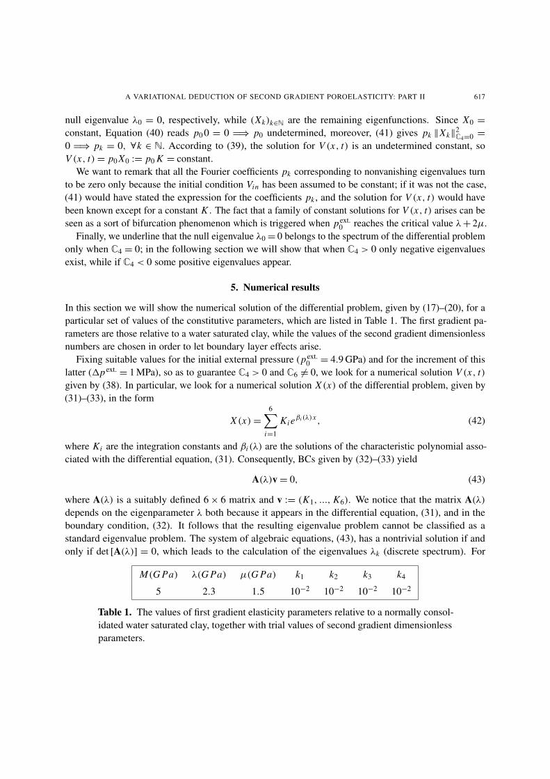
M(G Pa) λ(G Pa) µ(G Pa) k1 k2 k3 k4

5 2.3 1.5 10−2 10−2 10−2 10−2

Table 1. The values of first gradient elasticity parameters relative to a normally consol-idated water saturated clay, together with trial values of second gradient dimensionless

parameters.


0.0 0.2 0.4 0.6 0.8 1.0!0.0005

!0.0004

!0.0003

!0.0002

!0.0001

0.0000

x

mf

t"0

t"0.02

t"0.1

t"0.25

t"0.5

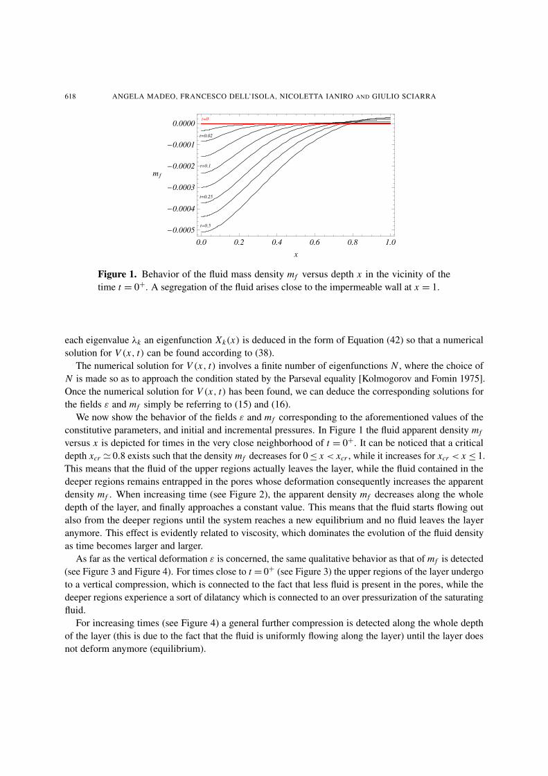
Figure 1. Behavior of the fluid mass density mf versus depth x in the vicinity of thetime t = 0+. A segregation of the fluid arises close to the impermeable wall at x = 1.

each eigenvalue λk an eigenfunction Xk(x) is deduced in the form of Equation (42) so that a numericalsolution for V (x, t) can be found according to (38).

The numerical solution for V (x, t) involves a finite number of eigenfunctions N , where the choice ofN is made so as to approach the condition stated by the Parseval equality [Kolmogorov and Fomin 1975].

Once the numerical solution for V (x, t) has been found, we can deduce the corresponding solutions forthe fields ε and mf simply be referring to (15) and (16).

We now show the behavior of the fields ε and mf corresponding to the aforementioned values of theconstitutive parameters, and initial and incremental pressures. In Figure 1 the fluid apparent density mf

versus x is depicted for times in the very close neighborhood of t = 0+. It can be noticed that a criticaldepth xcr � 0.8 exists such that the density mf decreases for 0 ≤ x < xcr , while it increases for xcr < x ≤ 1.

This means that the fluid of the upper regions actually leaves the layer, while the fluid contained in thedeeper regions remains entrapped in the pores whose deformation consequently increases the apparentdensity mf . When increasing time (see Figure 2), the apparent density mf decreases along the wholedepth of the layer, and finally approaches a constant value. This means that the fluid starts flowing outalso from the deeper regions until the system reaches a new equilibrium and no fluid leaves the layeranymore. This effect is evidently related to viscosity, which dominates the evolution of the fluid densityas time becomes larger and larger.

As far as the vertical deformation ε is concerned, the same qualitative behavior as that of mf is detected

(see Figure 3 and Figure 4). For times close to t = 0+

(see Figure 3) the upper regions of the layer undergo

to a vertical compression, which is connected to the fact that less fluid is present in the pores, while thedeeper regions experience a sort of dilatancy which is connected to an over pressurization of the saturating

fluid.For increasing times (see Figure 4) a general further compression is detected along the whole depth

of the layer (this is due to the fact that the fluid is uniformly flowing along the layer) until the layer doesnot deform anymore (equilibrium).


We remark that the chosen values of the prestress pext.0 are such that �4 > 0 so that the inner product

Equation (35) is well defined. Consequently the solution for V (x, t) (and thus for ε and mf ) can benumerically evaluated.

It is interesting to notice that when the initial stress pext.0 is such that p

ext.0 < λ + 2µ (�4 > 0) only

negative eigenvalues λk < 0 have been found, while in the region where �4 < 0 a finite number of positive

eigenvalues arise. In Figure 5 the behavior of the first eigenvalue λ1 is shown when varying pext.0 through

the threshold pext.0 = λ+ 2µ . It is worth noticing that when λ1 passes from negative to positive values,

the solution V (x, t) given in the form of Equation (38) blows up due to the presence of positive timeexponentials; the solution thus experiences an unstable behavior related to the fact that p

ext.0 reaches a

critical value. This kind of instability is known as geometrical instability since the presence of pext.0 in

the differential problem is due to the geometry of the problem (see Equation (21)).

0.0 0.2 0.4 0.6 0.8 1.0!0.0010

!0.0008

!0.0006

!0.0004

!0.0002

0.0000

x

mf

t"0

t"0.5

t"1

t"2

t"3

t"4

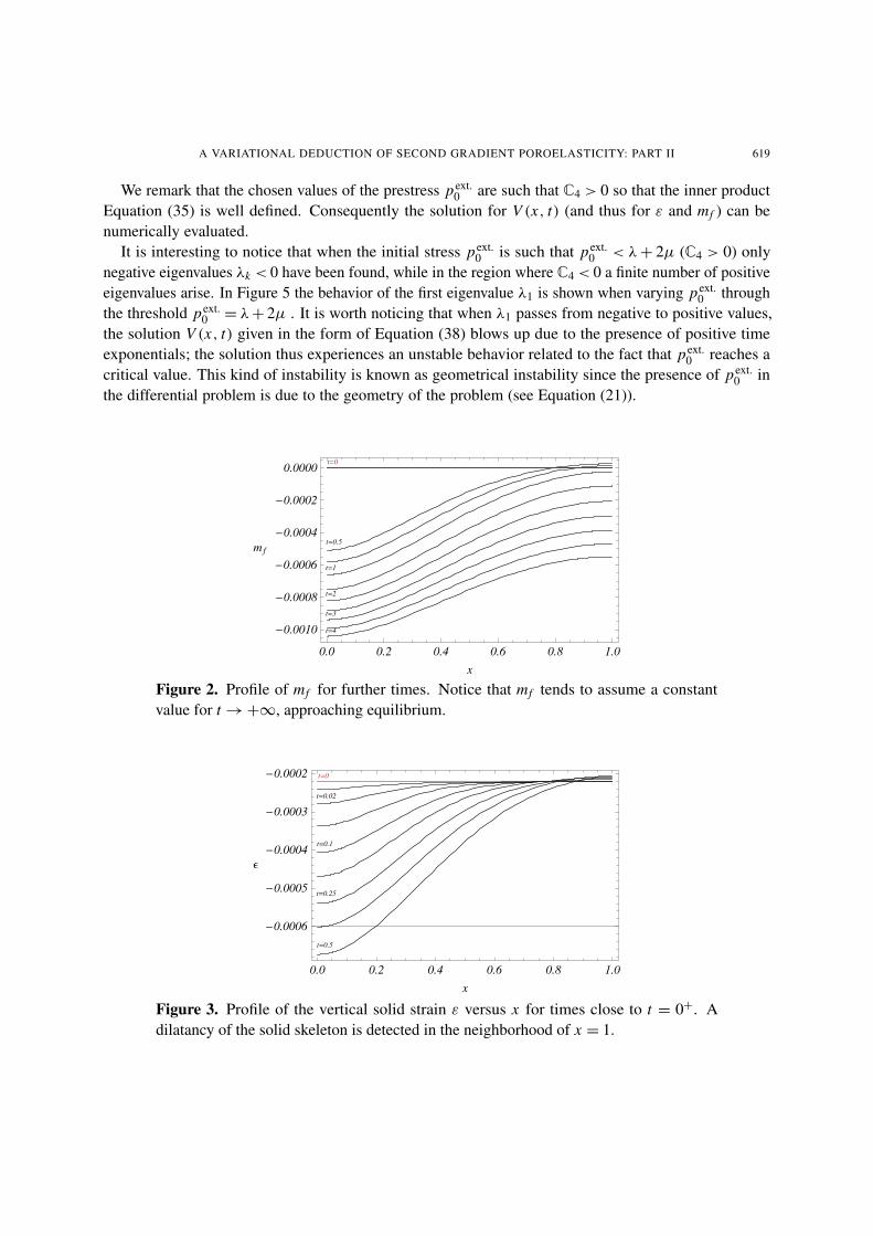
Figure 2. Profile of mf for further times. Notice that mf tends to assume a constantvalue for t → +∞, approaching equilibrium.

0.0 0.2 0.4 0.6 0.8 1.0

!0.0006

!0.0005

!0.0004

!0.0003

!0.0002

x

"

t#0

t#0.02

t#0.1

t#0.25

t#0.5

Figure 3. Profile of the vertical solid strain ε versus x for times close to t = 0+. Adilatancy of the solid skeleton is detected in the neighborhood of x = 1.


The linearity of the present model does not allow us to capture solutions associated with unstableconditions; this is evident when considering that the bilinear form given in (35) is no longer a welldefined inner product.

In order to show the influence of the solid prestress on the behavior of ε and mf we have found solutions

for different values of pext.0 and noticed changes in the solution when approaching the threshold �4 = 0.

Figure 6 shows the behavior of mf when pext.0 progressively approaches the critical value p

ext.0 = λ + 2µ.

When increasing the value of pext.0 the fluid density decreases in the superficial regions of the layer, while

increasing in the deeper ones. This means that the initial stress increases the capability of the fluid toflow out from the skeleton matrix close to the external surface, while pumping it in the deeper layers.

Let us now consider the second gradient constitutive parameters and the initial stresses to be vanish-ing. The resulting differential problem reduces to the classical Terzaghi consolidation problem. Moreparticularly, Equation (10) reduces to

ε = bM

λ + 2µ + b2 Mmf − �p

ext.

λ + 2µ + b2 M,

which, substituted in (11), gives

mf = amI I

f, a = (λ + 2µ)

λ + 2µ + b2 M. (44)

The Terzaghi consolidation problem thus reduces to the differential equation, Equation (44), togetherwith the initial datum mf

�x, 0+�

= 0 and the BCs, (12) and (13), which simplify into

mf = λ + 2µ + b2M

λ + 2µ

�b

�pext.

λ + 2µ

�:= c at x = 0. (45)

and mI

f= 0 at x = L , respectively.

It is easy to notice that the BC, (45), and the initial datum, mf

�x, 0+�

= 0, are not consistent, so theTerzaghi solution for mf exhibits the well known behavior of the classical unidimensional heat equation.

0.0 0.2 0.4 0.6 0.8 1.0!0.0012

!0.0010

!0.0008

!0.0006

!0.0004

!0.0002

x

"

t#0

t#0.5

t#1

t#2t#2

t#3

t#4

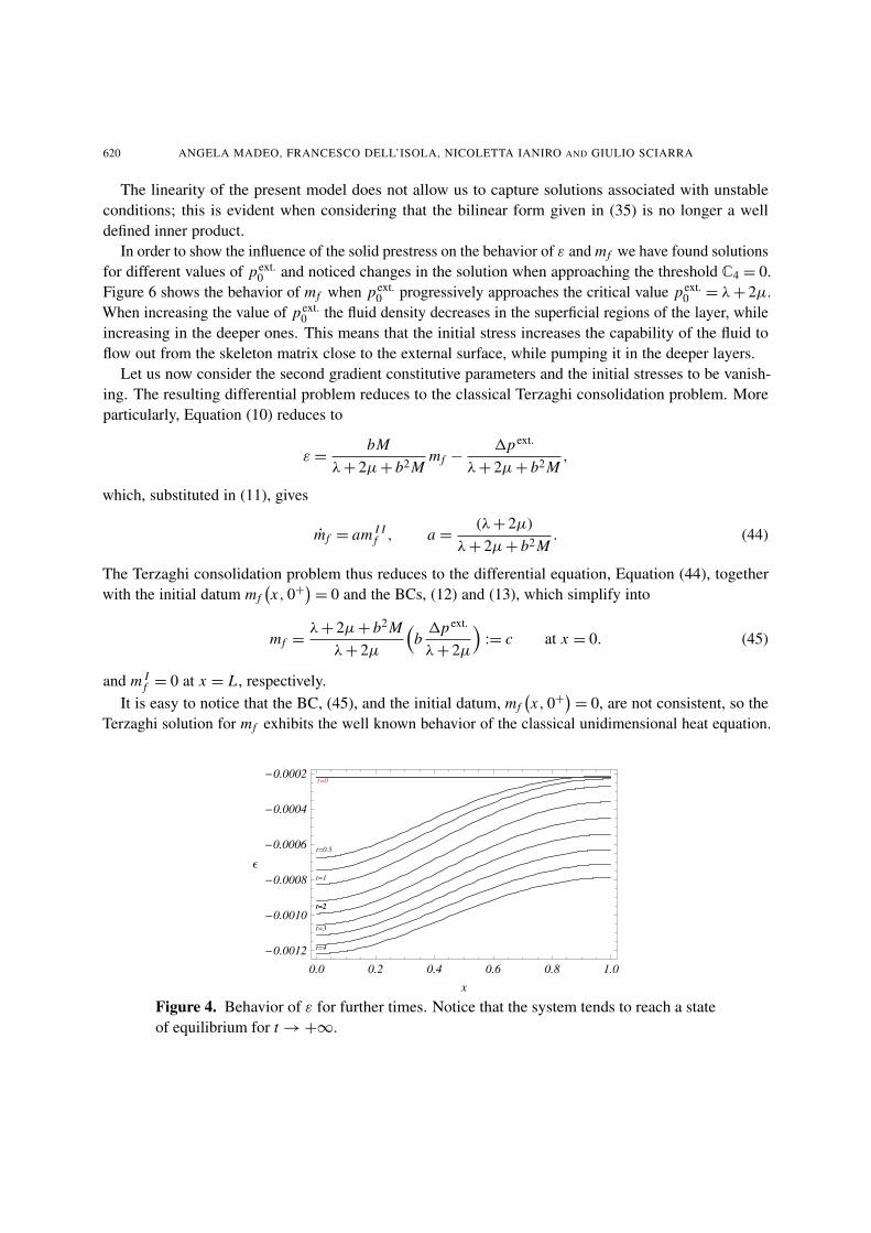
Figure 4. Behavior of ε for further times. Notice that the system tends to reach a state

of equilibrium for t → +∞.


!0.6 !0.4 !0.2 0.0 0.2 0.4 0.60

1."109

2."109

3."109

4."109

5."109

6."109

#1

p0ext

!4 $0

!4 %0p0ext&#'2(

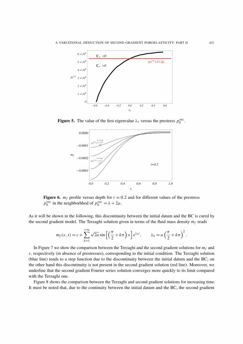
Figure 5. The value of the first eigenvalue λ1 versus the prestress pext.0 .

0.0 0.2 0.4 0.6 0.8 1.0

!0.0003

!0.0002

!0.0001

0.0000

x

mf

t"0.2

p0ext" ######################$ % 2&'

10

p0ext" ######################$ % 2&'

1.2

Figure 6. mf profile versus depth for t = 0.2 and for different values of the prestressp

ext.0 in the neighborhhod of p

ext.0 = λ + 2µ.

As it will be shown in the following, this discontinuity between the initial datum and the BC is cured bythe second gradient model. The Terzaghi solution given in terms of the fluid mass density mf reads

mf (x, t) = c ++∞�

k=1

√2a sin

��π

2+ kπ

�x

�eλk t , λk = a

�π

2+ kπ

�2.

In Figure 7 we show the comparison between the Terzaghi and the second gradient solutions for mf and

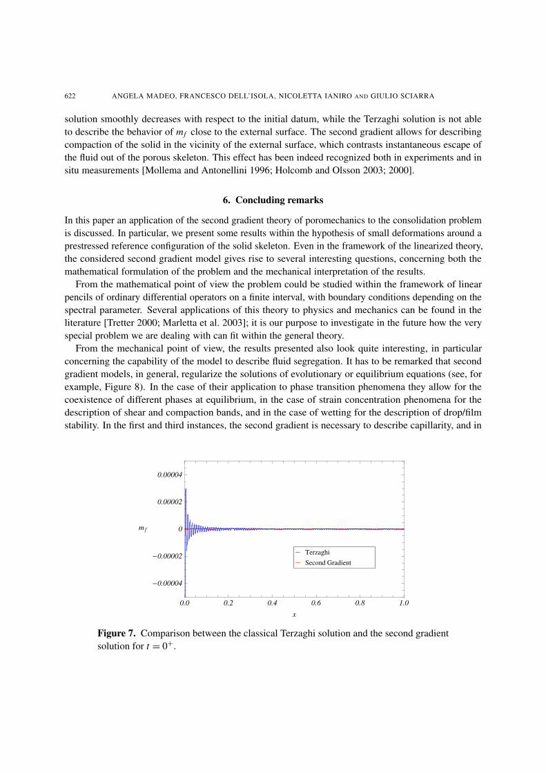
ε, respectively (in absence of prestresses), corresponding to the initial condition. The Terzaghi solution(blue line) tends to a step function due to the discontinuity between the initial datum and the BC; onthe other hand this discontinuity is not present in the second gradient solution (red line). Moreover, weunderline that the second gradient Fourier series solution converges more quickly to its limit comparedwith the Terzaghi one.

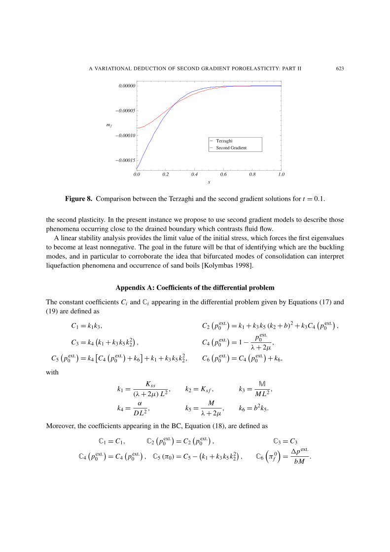
Figure 8 shows the comparison between the Terzaghi and second gradient solutions for increasing time.

It must be noted that, due to the continuity between the initial datum and the BC, the second gradient


solution smoothly decreases with respect to the initial datum, while the Terzaghi solution is not ableto describe the behavior of mf close to the external surface. The second gradient allows for describingcompaction of the solid in the vicinity of the external surface, which contrasts instantaneous escape ofthe fluid out of the porous skeleton. This effect has been indeed recognized both in experiments and insitu measurements [Mollema and Antonellini 1996; Holcomb and Olsson 2003; 2000].

6. Concluding remarks

In this paper an application of the second gradient theory of poromechanics to the consolidation problemis discussed. In particular, we present some results within the hypothesis of small deformations around aprestressed reference configuration of the solid skeleton. Even in the framework of the linearized theory,the considered second gradient model gives rise to several interesting questions, concerning both themathematical formulation of the problem and the mechanical interpretation of the results.

From the mathematical point of view the problem could be studied within the framework of linearpencils of ordinary differential operators on a finite interval, with boundary conditions depending on thespectral parameter. Several applications of this theory to physics and mechanics can be found in theliterature [Tretter 2000; Marletta et al. 2003]; it is our purpose to investigate in the future how the veryspecial problem we are dealing with can fit within the general theory.

From the mechanical point of view, the results presented also look quite interesting, in particularconcerning the capability of the model to describe fluid segregation. It has to be remarked that second

gradient models, in general, regularize the solutions of evolutionary or equilibrium equations (see, forexample, Figure 8). In the case of their application to phase transition phenomena they allow for thecoexistence of different phases at equilibrium, in the case of strain concentration phenomena for thedescription of shear and compaction bands, and in the case of wetting for the description of drop/filmstability. In the first and third instances, the second gradient is necessary to describe capillarity, and in

0.0 0.2 0.4 0.6 0.8 1.0

!0.00004

!0.00002

0

0.00002

0.00004

x

mf

Second GradientTerzaghi

Figure 7. Comparison between the classical Terzaghi solution and the second gradientsolution for t = 0+.


0.0 0.2 0.4 0.6 0.8 1.0

!0.00015

!0.00010

!0.00005

0.00000

x

mf

Second GradientTerzaghi

Figure 8. Comparison between the Terzaghi and the second gradient solutions for t = 0.1.

the second plasticity. In the present instance we propose to use second gradient models to describe thosephenomena occurring close to the drained boundary which contrasts fluid flow.

A linear stability analysis provides the limit value of the initial stress, which forces the first eigenvalues

to become at least nonnegative. The goal in the future will be that of identifying which are the bucklingmodes, and in particular to corroborate the idea that bifurcated modes of consolidation can interpretliquefaction phenomena and occurrence of sand boils [Kolymbas 1998].

Appendix A: Coefficients of the differential problem

The constant coefficients Ci and �i appearing in the differential problem given by Equations (17) and(19) are defined as

C1 = k1k3, C2�

pext.0

�= k1 + k3 k5 (k2 + b)2 + k3C4

�p

ext.0

�,

C3 = k4�k1 + k3 k5 k

22�, C4

�p

ext.0

�= 1 − p

ext.0

λ + 2µ,

C5�

pext.0

�= k4

�C4

�p

ext.0

�+ k6

�+ k1 + k3 k5 k

22, C6

�p

ext.0

�= C4

�p

ext.0

�+ k6,

with

k1 = Kss

(λ + 2µ) L2 , k2 = Ks f , k3 = �

M L2 ,

k4 = α

DL2 , k5 = M

λ + 2µ, k6 = b

2k5.

Moreover, the coefficients appearing in the BC, Equation (18), are defined as

�1 = C1, �2�

pext.0

�= C2

�p

ext.0

�, �3 = C3

�4�

pext.0

�= C4

�p

ext.0

�, �5 (π0) = C5 −

�k1 + k3 k5 k

22�, �6

�π 0

f

�= �p

ext.

bM.


It must be noticed that the constants k1, . . . , k4 are introduced by the second gradient model, while k5and k6 are related to the first gradient parameters M , λ, and µ, which represent the Biot bulk modulus

and the Lame coefficients of the considered material, respectively.

References

[Biot 1941] M. A. Biot, “General theory of three-dimensional consolidation”, J. Appl. Phys. 12:2 (1941), 155–164.[de Boer 1996] R. de Boer, “Highlights in the historical development of the porous media theory: toward a consistent macro-

scopic theory”, Appl. Mech. Rev. (Trans. ASME) 49:4 (1996), 201–262.[Coussy 2004] O. Coussy, Poromechanics, Wiley, Chichester, 2004.[Cryer 1963] C. W. Cryer, “A comparison of the three-dimensional consolidation theories of Biot and Terzaghi”, Q. J. Mech.Appl. Math. 16:4 (1963), 401–412.

[Heinrich and Desoyer 1961] G. Heinrich and K. Desoyer, “Theorie dreidimensionaler setznugsvorgänge in Tonschichten”,Ing. Arch. 30:4 (1961), 225–253.

[Holcomb and Olsson 2003] D. J. Holcomb and W. A. Olsson, “Compaction localization and fluid flow”, J. Geophys. Res.108:B6 (2003), 2290.

[Kolmogorov and Fomin 1975] A. N. Kolmogorov and S. V. Fomin, Introductory real analysis, Dover, New York, 1975.[Kolymbas 1998] D. Kolymbas, “Behaviour of liquified sand”, Phil. T. Roy. Soc. A 356:1747 (1998), 2609–2622.[Mandel 1953] J. Mandel, “Consolidation des sols (étude mathématique)”, Géothecnique 3 (1953), 287–299.[Marletta et al. 2003] M. Marletta, A. Shkalikov, and C. Tretter, “Pencils of differential operators containing the eigenvalue

parameter in the boundary conditions”, Proc. R. Soc. Edin. A-Ma 133 (2003), 893–917.[Mollema and Antonellini 1996] P. N. Mollema and M. A. Antonellini, “Compaction bands: a structural analog for anti-mode

I cracks in aeolian sandstone”, Tectonophysics 267:1-4 (1996), 209–228.[Olsson and Holcomb 2000] W. Olsson and D. Holcomb, “Compaction localization in porous rock”, Geophys. Res. Lett. 27:21(2000), 3537–3540.

[Sciarra et al. 2008] G. Sciarra, F. dell’Isola, N. Ianiro, and A. Madeo, “A variational deduction of second gradient poroelasticity

I: general theory”, J. Mech. Mater. Struct. 3 (2008), 507–526.[Seppecher 1987] P. Seppecher, Etude d’une modelisation des zones capillaires fluides: interfaces et lignes de contact, Ph.D.

thesis, Thèse Université PARIS VI, 1987.[Shkalikov 1986] A. A. Shkalikov, “Boundary problems for ordinary differential equations with parameter in the boundary

conditions”, J. Math. Sci. 33:6 (1986), 1311–1342.[Shkalikov and Tretter 1996] A. A. Shkalikov and C. Tretter, “Spectral analysis for linear pencils N −λP of ordinary differential

operators”, Math. Nachr. 179:1 (1996), 275–305.[Terzaghi 1923] K. v. Terzaghi, “Die Berechnung der Durchlässigkeitsziffer des tones aus dem verlauf der hydrodynamischen

spanunngserscheinnungen”, Technical report II a,132 N 3/4, 125,138, Akademie der Wissenschaften in Wien. SitzungsberichteMathnaturwiss Klasse Abt, 1923.

[Terzaghi 1943] K. v. Terzaghi, Theoretical soil mechanics, Wiley, New York, 1943.[Tretter 2000] C. Tretter, “On buckling problems”, ZAMM 80:9 (2000), 633–639.

Received 8 Mar 2007. Revised 27 Jul 2007. Accepted 25 Nov 2007.

ANGELA MADEO: [email protected] di Metodi e Modelli Matematici per le Scienze Applicate, Università di Roma “La Sapienza”, Via Scarpa 16,00161 Rome, Italy

FRANCESCO DELL’ISOLA: [email protected] di Ingegneria Strutturale e Geotecnica, Università di Roma “La Sapienza”, Via Eudossiana 18, 00184 Rome,Italy

and

Laboratorio di Strutture e Materiali Intelligenti, Palazzo Caetani (Ala Nord), 04012 Cisterna di Latina, Italy


NICOLETTA IANIRO: [email protected] di Metodi e Modelli Matematici per le Scienze Applicate, Università di Roma “La Sapienza”, Via Scarpa 16,00161 Rome, Italy

GIULIO SCIARRA: [email protected] di Ingegneria Chimica Materiali Ambiente, Università di Roma “La Sapienza”, Via Eudossiana 18, 00184 Rome,Italy

A Variational Deduction of Second Gradient Poroelasticity II: An Application to the Consolidation...

Documents

Transcript of A Variational Deduction of Second Gradient Poroelasticity II: An Application to the Consolidation...