A “Tortoise and the Hare” story - University of Surrey
163
A “Tortoise and the Hare” story: The relationship between induction time and polymorphism in glycine crystallisation. Laurie J. Little A thesis presented for the degree of Doctor of Philosophy Department of Physics Faculty of Engineering and Physical Sciences University of Surrey April 6, 2017
-
Upload
khangminh22 -
Category
Documents
-
view
0 -
download
0
Transcript of A “Tortoise and the Hare” story - University of Surrey
A “Tortoise and the Hare” story: The relationship
between induction time and polymorphism in glycine
crystallisation.
Laurie J. Little
A thesis presented for the degree of
Doctor of Philosophy
Department of Physics
Faculty of Engineering and Physical Sciences
University of Surrey
April 6, 2017
Abstract
Crystal polymorphism, where a molecule forms several different crystal lattices, is common, and
often needs to be controlled. For example, crystalline drugs must be manufactured as one specified
polymorph, so polymorph purity is essential to the pharmaceutical industry. This thesis is a
quantitative study of the crystallization of glycine from aqueous solution, which focuses particularly
on polymorphism. Crystallization is observed within a 96-well microplate, where each well is filled
with 0.1 mL of supersaturated solution.
We address the difficulty of obtaining reproducible nucleation data. This problem is difficult
because induction times are extremely sensitive to factors such as how the crystallizing system is
prepared, and small variations in the supersaturation. The appropriate statistical tests needed to
show reproducibility are discussed.
Glycine has two common polymorphs, alpha and gamma, the competition between these poly-
morphs is studied. We obtain data at multiple NaCl concentrations. Addition of NaCl is known to
favour nucleation of the gamma polymorph. The polymorph of crystals are individually identified
in-situ using Raman spectroscopy. At high salt concentrations, nucleation kinetics of the alpha
and gamma polymorphs are qualitatively different. The gamma polymorph behaves like the hare
in Aesop’s story of the tortoise and the hare: Nucleation start off rapidly, but slows, while for the
alpha polymorph, nucleation starts off slow but at later times almost overtakes that of the gamma
polymorph. The opposite time dependencies of the nucleation of the competing polymorphs, allows
optimisation of polymorph purity using time-dependent supersaturation.
Growth of the two polymorphs is analysed. The alpha polymorph is observed to grow faster
than the gamma polymorph. Growth rates were variable, so they were also analysed in relation to
induction times and crystal habits. We show that crystals with long induction times tend to be
needle-like, and needle-like morphologies tend to grow faster than non needle-like morphologies.

Acknowledgements
I would like to express my gratitude to a number of people, without whom this project would
not have gone nearly as well as it has. First and foremost, I would like to start by thanking my
supervisors Richard Sear and Joseph Keddie. My thanks for the countless ideas and suggestions,
both for possible experiments and for ways to analyse the experimental data, for useful discussions
of the theory, and for helping keep me on track throughout this project. Thanks to Alice King for
teaching me how to use our Raman spectrometer, as well as for extensive advice and assistance in
analysing the acquired spectra. Thanks to Daniel Driscoll for teaching me how to use our powder
X-ray diffraction equipment. I would like to thank Violeta Doukova for general help around the
lab. My thanks to EPSRC for funding the project. Finally, thanks to all my friends in the office,
Nicholas Howlett, James Mithen, Philip Richardson, David Makepeace and Mona Ibrahim for the
conversation and advice. In particular, thanks to Nick for persuading me to use Latex, to David
for helping me around the lab, and to James for introducing me to Python, without which I would
have had to use Fortran.
I

Contents
1 Introduction 1
1.1 Aims . . . . . . . . . . . . . . . . . . . . . . . . . . . . . . . . . . . . . . . . . . . . . 3
1.2 Overview . . . . . . . . . . . . . . . . . . . . . . . . . . . . . . . . . . . . . . . . . . 4
1.3 The tortoise and the hare . . . . . . . . . . . . . . . . . . . . . . . . . . . . . . . . . 5
2 Theory of nucleation from supersaturated solution 6
2.1 Creating supersaturated solutions . . . . . . . . . . . . . . . . . . . . . . . . . . . . . 6
2.2 Homogeneous and Heterogeneous nucleation . . . . . . . . . . . . . . . . . . . . . . . 8
2.2.1 Classical Nucleation Theory . . . . . . . . . . . . . . . . . . . . . . . . . . . . 8
2.2.2 Heterogeneous Nucleation . . . . . . . . . . . . . . . . . . . . . . . . . . . . . 10
2.3 Statistics of isothermal nucleation . . . . . . . . . . . . . . . . . . . . . . . . . . . . . 12
2.3.1 N(t) vs P (t) plots . . . . . . . . . . . . . . . . . . . . . . . . . . . . . . . . . 13
2.3.2 Kolmogorov Smirnov test . . . . . . . . . . . . . . . . . . . . . . . . . . . . . 13
2.3.3 Comparing N(t) Plots . . . . . . . . . . . . . . . . . . . . . . . . . . . . . . . 15
2.3.4 Heterogeneous Nucleation Models . . . . . . . . . . . . . . . . . . . . . . . . 16
2.4 Isothermal nucleation of competing polymorphs . . . . . . . . . . . . . . . . . . . . . 22
2.4.1 Formal definitions of the CIFs and CSHs . . . . . . . . . . . . . . . . . . . . 23
2.4.2 Models that include only observables . . . . . . . . . . . . . . . . . . . . . . . 24
2.4.3 Models of correlations between α and γ nucleation . . . . . . . . . . . . . . . 25
3 Literature Review 30
3.1 Analytical Techniques . . . . . . . . . . . . . . . . . . . . . . . . . . . . . . . . . . . 30
3.1.1 Analysing solutions and nucleation precursors . . . . . . . . . . . . . . . . . . 30
II
Contents
3.1.2 Morphology and crystal habit . . . . . . . . . . . . . . . . . . . . . . . . . . . 31
3.1.3 Polymorphism . . . . . . . . . . . . . . . . . . . . . . . . . . . . . . . . . . . 31
3.2 Nucleation Studies . . . . . . . . . . . . . . . . . . . . . . . . . . . . . . . . . . . . . 32
3.2.1 Ice nucleation . . . . . . . . . . . . . . . . . . . . . . . . . . . . . . . . . . . . 32
3.2.2 Nucleation Precursors . . . . . . . . . . . . . . . . . . . . . . . . . . . . . . . 33
3.2.3 Heterogeneous and homogeneous nucleation . . . . . . . . . . . . . . . . . . . 33
3.2.4 Isothermal experiments . . . . . . . . . . . . . . . . . . . . . . . . . . . . . . 34
3.3 Glycine Literature . . . . . . . . . . . . . . . . . . . . . . . . . . . . . . . . . . . . . 35
3.3.1 Glycine in solution . . . . . . . . . . . . . . . . . . . . . . . . . . . . . . . . . 35
3.3.2 Nucleation studies . . . . . . . . . . . . . . . . . . . . . . . . . . . . . . . . . 36
3.3.3 Crystal Growth . . . . . . . . . . . . . . . . . . . . . . . . . . . . . . . . . . . 42
3.3.4 Crystal growth in the presence of salt . . . . . . . . . . . . . . . . . . . . . . 45
3.4 Summary . . . . . . . . . . . . . . . . . . . . . . . . . . . . . . . . . . . . . . . . . . 46
4 Methods 47
4.1 Materials . . . . . . . . . . . . . . . . . . . . . . . . . . . . . . . . . . . . . . . . . . 47
4.2 Crystallisation experiments . . . . . . . . . . . . . . . . . . . . . . . . . . . . . . . . 47
4.2.1 Determination of induction times . . . . . . . . . . . . . . . . . . . . . . . . . 49
4.2.2 Crystal Growth Rates . . . . . . . . . . . . . . . . . . . . . . . . . . . . . . . 51
4.2.3 Temperature Control . . . . . . . . . . . . . . . . . . . . . . . . . . . . . . . . 52
4.2.4 Salt studies . . . . . . . . . . . . . . . . . . . . . . . . . . . . . . . . . . . . . 54
4.3 X-ray diffraction . . . . . . . . . . . . . . . . . . . . . . . . . . . . . . . . . . . . . . 54
4.3.1 Theory . . . . . . . . . . . . . . . . . . . . . . . . . . . . . . . . . . . . . . . 54
4.3.2 Experimental . . . . . . . . . . . . . . . . . . . . . . . . . . . . . . . . . . . . 55
4.4 Raman Spectroscopy . . . . . . . . . . . . . . . . . . . . . . . . . . . . . . . . . . . . 56
4.4.1 Theory . . . . . . . . . . . . . . . . . . . . . . . . . . . . . . . . . . . . . . . 56
4.4.2 Experimental . . . . . . . . . . . . . . . . . . . . . . . . . . . . . . . . . . . . 57
5 Results - Quantitative Glycine Nucleation Experiments 60
5.1 Experiments overview . . . . . . . . . . . . . . . . . . . . . . . . . . . . . . . . . . . 61
5.2 Well crystal populations . . . . . . . . . . . . . . . . . . . . . . . . . . . . . . . . . . 61
III
Contents
5.3 Measurement of crystal growth rates . . . . . . . . . . . . . . . . . . . . . . . . . . . 62
5.4 Studies on reproducibility of induction times . . . . . . . . . . . . . . . . . . . . . . 64
5.4.1 Varying heating times . . . . . . . . . . . . . . . . . . . . . . . . . . . . . . . 66
5.4.2 Pipette times . . . . . . . . . . . . . . . . . . . . . . . . . . . . . . . . . . . . 68
5.5 The effect of filtering impurities . . . . . . . . . . . . . . . . . . . . . . . . . . . . . . 69
5.6 Concentration . . . . . . . . . . . . . . . . . . . . . . . . . . . . . . . . . . . . . . . . 70
5.6.1 Comparison with classical nucleation theory . . . . . . . . . . . . . . . . . . . 72
5.7 Time of Day . . . . . . . . . . . . . . . . . . . . . . . . . . . . . . . . . . . . . . . . . 73
5.8 Polymorphism . . . . . . . . . . . . . . . . . . . . . . . . . . . . . . . . . . . . . . . . 75
5.9 Nucleation of the second crystal in samples where a crystal is already present . . . . 77
5.10 Summary . . . . . . . . . . . . . . . . . . . . . . . . . . . . . . . . . . . . . . . . . . 78
6 Results - competition between glycine’s polymorphs in the presence of sodium
chloride 80
6.1 Nucleation data . . . . . . . . . . . . . . . . . . . . . . . . . . . . . . . . . . . . . . . 81
6.1.1 Increasing salt concentration favours the γ polymorph . . . . . . . . . . . . . 81
6.1.2 Cumulative incident functions . . . . . . . . . . . . . . . . . . . . . . . . . . . 83
6.1.3 Modelling Data . . . . . . . . . . . . . . . . . . . . . . . . . . . . . . . . . . . 86
6.1.4 Reproducibility of total nucleation rates and relative nucleation rates . . . . . 90
6.1.5 Polymorph composition vs time . . . . . . . . . . . . . . . . . . . . . . . . . . 92
6.2 Growth rates and crystal habits . . . . . . . . . . . . . . . . . . . . . . . . . . . . . . 97
6.2.1 The effect of growth rates on the error in induction time measurements . . . 97
6.2.2 Variation in crystal size populations with time . . . . . . . . . . . . . . . . . 98
6.2.3 NaCl concentration and crystal growth . . . . . . . . . . . . . . . . . . . . . . 99
6.2.4 Polymorphism and crystal growth . . . . . . . . . . . . . . . . . . . . . . . . 99
6.2.5 Crystal habits . . . . . . . . . . . . . . . . . . . . . . . . . . . . . . . . . . . . 100
6.2.6 Induction time and crystal habit . . . . . . . . . . . . . . . . . . . . . . . . . 101
6.2.7 Growth rate and induction time . . . . . . . . . . . . . . . . . . . . . . . . . 102
6.3 Summary . . . . . . . . . . . . . . . . . . . . . . . . . . . . . . . . . . . . . . . . . . 103
IV

Contents
7 Conclusions and future work 105
7.1 Studies of crystal growth . . . . . . . . . . . . . . . . . . . . . . . . . . . . . . . . . . 106
7.2 Future work . . . . . . . . . . . . . . . . . . . . . . . . . . . . . . . . . . . . . . . . . 107
Appendices 109
A Additional material for Chapter 5 110
A.1 Classical nucleation theory’s prediction for the relationship between supersaturation
and nucleation rate . . . . . . . . . . . . . . . . . . . . . . . . . . . . . . . . . . . . . 110
A.2 Function fitting . . . . . . . . . . . . . . . . . . . . . . . . . . . . . . . . . . . . . . . 111
A.3 Additional XRD patterns . . . . . . . . . . . . . . . . . . . . . . . . . . . . . . . . . 111
B Additional material for Chapter 6 113
B.1 Individual runs of the 18 h heated dataset . . . . . . . . . . . . . . . . . . . . . . . . 113
B.2 Individual purity vs times . . . . . . . . . . . . . . . . . . . . . . . . . . . . . . . . . 113
B.3 Additional images . . . . . . . . . . . . . . . . . . . . . . . . . . . . . . . . . . . . . 115
C Python Programs 117
C.1 Competing Weibull functions . . . . . . . . . . . . . . . . . . . . . . . . . . . . . . . 117
C.2 Correlated polymorph induction times . . . . . . . . . . . . . . . . . . . . . . . . . . 120
C.3 Polymorphism vs time . . . . . . . . . . . . . . . . . . . . . . . . . . . . . . . . . . . 123
V
List of Figures
1.1 The crystal structure of diamond (left) and graphite (right). Carbon atoms are
shown in black. Distributed under Creative Commons Attribution-ShareAlike 3.0
Unported licence [1]. . . . . . . . . . . . . . . . . . . . . . . . . . . . . . . . . . . . . 2
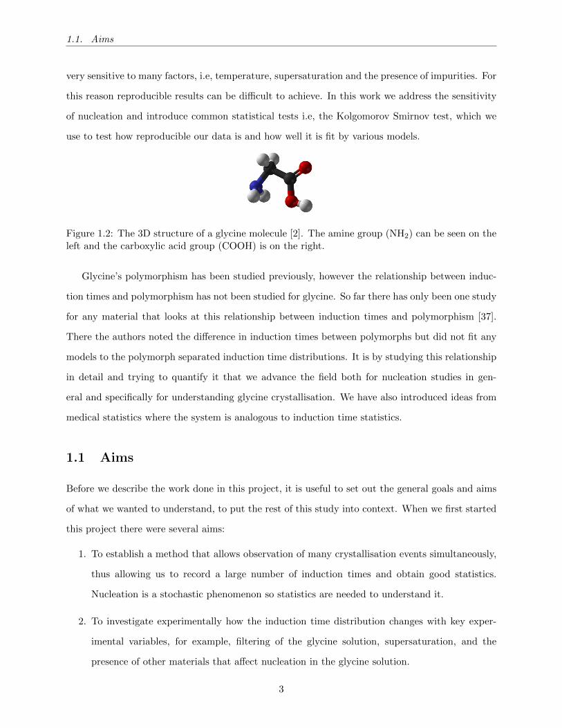
1.2 The 3D structure of a glycine molecule [2]. The amine group (NH2) can be seen on
the left and the carboxylic acid group (COOH) is on the right. . . . . . . . . . . . . 3
2.1 A typical solubility curve, where the black line shows the solubility as a function
temperature. . . . . . . . . . . . . . . . . . . . . . . . . . . . . . . . . . . . . . . . . 7
2.2 The free energy of a crystal nucleus in a superstarurated solution as a function of
the nucleus radius. . . . . . . . . . . . . . . . . . . . . . . . . . . . . . . . . . . . . . 9
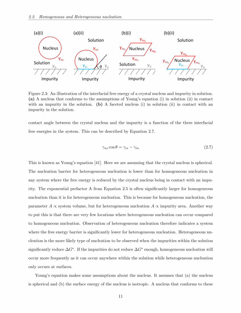
2.3 An illustration of the interfacial free energy of a crystal nucleus and impurity in
solution. (a) A nucleus that conforms to the assumptions of Young’s equation (i) in
solution (ii) in contact with an impurity in the solution. (b) A faceted nucleus (i)
in solution (ii) in contact with an impurity in the solution. . . . . . . . . . . . . . . . 11
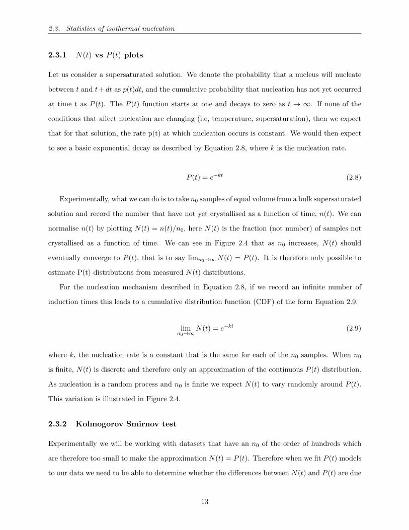
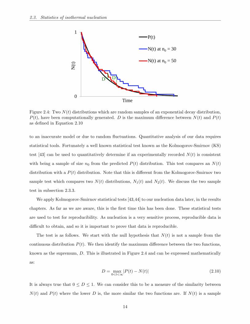
2.4 Two N(t) distributions which are random samples of an exponential decay distri-
bution, P (t), have been computationally generated. D is the maximum difference
between N(t) and P (t) as defined in Equation 2.10 . . . . . . . . . . . . . . . . . . . 14
2.5 An example of overfitting. A function f(x) has been fit with a linear function (red)
and a 6th order polynomial (blue) . . . . . . . . . . . . . . . . . . . . . . . . . . . . 20
VI
List of Figures
2.6 A graph illustrating the difference in the functional form of the Weibull, Gompertz
and exponential functions. We show one example of each function. For the expo-
nential function k = 0.05, for the Weibull function β = 0.5 and τ = 10 , and for the
Gompertz distribution m = 2 and ki = 0.1. . . . . . . . . . . . . . . . . . . . . . . . 21
3.1 (a) Solubility of the α and γ polymorphs of glycine as a function of temperature. Data
from Yang et al [3]. We have fit a second order polynomial (S = 0.0301T 2 + 2.96T +
109) so the solubility can be approximated between data points. (b) Solubility of γ
glycine from several sources [3–5]: Yang et al. [3], Dowling et al. [4], Han et al. [4]
and Yi et al. [5] . . . . . . . . . . . . . . . . . . . . . . . . . . . . . . . . . . . . . . . 35
3.2 The glycine molecule. Shown unchanged (left) and in zwitterion form (right) . . . . 36
3.3 The structures of (a) α glycine and (b) γ glycine. Reproduced from Ref. [6] with
permission from The Royal Society of Chemistry. The figure is colour coded as
follows: White - hydrogen, grey - carbon, red - oxygen and blue - nitrogen. . . . . . 37
3.4 Here we show several glycine growth rates measured from multiple sources: [Li] (Li
et al.) [7], (Han et al.) [Han-A] [4], [Han-B] (Han et al.) [8] and [Dow] (Dowling et
al.) [4]. These growth rates have been obtained from graphs, so are approximate.
Colour coding is as follows, α b-axis, α c-axis, γ b-axis and γ c-axis are pink, green,
gold and dark blue respectively. Experimental details e.g. temperature and cs are
displayed in Table 3.1. . . . . . . . . . . . . . . . . . . . . . . . . . . . . . . . . . . . 43
4.1 A diagram of the setup used to heat the glycine solution. . . . . . . . . . . . . . . . 48
4.2 A schematic illustrating the experimental setup. The light comes down vertically
from the ceiling. A translucent sheet of yellow tracing paper is fixed in position
above the microplate to increase the contrast of the crystals in the images recorded
by the camera. . . . . . . . . . . . . . . . . . . . . . . . . . . . . . . . . . . . . . . . 49
VII
List of Figures
4.3 (a) Images of the same well at times ranging from 5 min to 48 h after starting the
experiment. A crystal (circled in red) is first visible at 4 h which is taken to be its
induction time. (b) Images of another well at several times. Several crystals can
be seen forming, again circled in red. (c) The crystallisation observed in a 96-well
microplate at two different times: 5 min and 48 h. Crystallization has occurred in
many but not all wells. . . . . . . . . . . . . . . . . . . . . . . . . . . . . . . . . . . . 50
4.4 A crystal nucleating and growing over an hour long period. We show a zoomed-in
image of part of a single well in 7 successive images. Each image is labelled by the
elapsed time since the time of the last image in which no crystal was visible. The
size is measured by the greatest distance across the crystal. This is indicated by a
blue line marked on the crystal. . . . . . . . . . . . . . . . . . . . . . . . . . . . . . . 51
4.5 A plot of the temperature of the glycine solution in the wells as a function of time
for the hour after injecting the solution into the wells. . . . . . . . . . . . . . . . . . 52
4.6 (a) The room temperature recorded over a one week time period. The red dots
indicate 4:00am of each day which is consistently when the temperature is observed
to reach a minimum (b) Plot of the average room temperature plot as a function of
time of day. Each average temperature is the mean of 7 measurements taken across
a one week period. . . . . . . . . . . . . . . . . . . . . . . . . . . . . . . . . . . . . . 53
4.7 A schematic illustrating how X-ray diffraction occurs. Distributed under Creative
Commons Attribution-ShareAlike 3.0 Unported licence [10] . . . . . . . . . . . . . . 55
4.8 A schematic illustrating how the potential energy of an electron changes in Raman
scattering. . . . . . . . . . . . . . . . . . . . . . . . . . . . . . . . . . . . . . . . . . . 57
4.9 A schematic illustrating how our samples are analysed with Raman spectroscopy. . . 57
VIII
List of Figures
4.10 (a) XRD patterns of two powdered samples, one of α glycine and one of γ glycine
as identified with Raman spectroscopy. The glycine identified as α via Raman spec-
troscopy is shown in blue and glycine identified as γ is shown in green. The circles
represent known α XRD peaks while the triangles represent known γ XRD peaks.
(b)(i) Raman spectra for a typical α glycine crystal and a typical γ glycine crystal.
The spectra are normalised to the intensity of their highest peak at 886 cm−1 (b)(ii)
A magnified view of (b)(i) in the region 100 - 250 cm −1.(b)(iii) A magnified view of
(b)(i) in the region 450 - 550 cm −1. (c) and (d) Two additional α glycine spectra
where the characteristic peaks at 164 cm−1, 171 cm−1 and 203 cm−1 (which cannot
be eaily seen in (b)(ii)) can be more clearly seen. . . . . . . . . . . . . . . . . . . . . 59
5.1 Data for the first crystal to nucleate in each well of the population of wells where
nucleation occured after the first hour, for a single run. In total, 58 crystals were
observed, we show (a) The sizes of those crystals and (b) the growth rates of those
crystals. . . . . . . . . . . . . . . . . . . . . . . . . . . . . . . . . . . . . . . . . . . . 63
5.2 Plots of the fraction of samples where nucleation has not occurred, as a function of
time, for the three runs L1, L2 and L3 that make up dataset L. All runs are carried
out under identical conditions. In (a) we plot f(t), the fraction not crystallised, taken
from the complete set of 96 samples for each run. In (b) we plot f∗(t), the fraction
where nucleation has not occurred, taken only from the subset of these samples that
crystallised between 1 h and 48 h. . . . . . . . . . . . . . . . . . . . . . . . . . . . . 65
5.3 Plots of the fraction of samples not crystallised as a function of time. Each dataset
has a different tH . (a) The f(t) distributions, and (b) the f∗(t) distributions. . . . . 67
5.4 Plots of the fraction of samples where nucleation has not occurred, for runs with
different pipette holding times. In (a) and (b), we plot f(t) and f∗(t), respectively.
All runs are at c = 333.33 g/l. . . . . . . . . . . . . . . . . . . . . . . . . . . . . . . 69
5.5 The fraction of samples not crystallised as a function of time for filtered (dataset P)
and unfiltered solutions (dataset N). A 0.22 µm filter (Millex GP Merck Millipore)
was applied to the filtered solutions. In (a) and (b), we plot f∗(t) and f(t), respectively. 70
IX
List of Figures
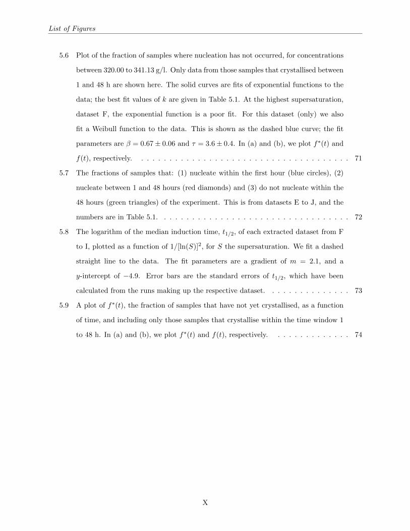
5.6 Plot of the fraction of samples where nucleation has not occurred, for concentrations
between 320.00 to 341.13 g/l. Only data from those samples that crystallised between
1 and 48 h are shown here. The solid curves are fits of exponential functions to the
data; the best fit values of k are given in Table 5.1. At the highest supersaturation,
dataset F, the exponential function is a poor fit. For this dataset (only) we also
fit a Weibull function to the data. This is shown as the dashed blue curve; the fit
parameters are β = 0.67± 0.06 and τ = 3.6± 0.4. In (a) and (b), we plot f∗(t) and
f(t), respectively. . . . . . . . . . . . . . . . . . . . . . . . . . . . . . . . . . . . . . 71
5.7 The fractions of samples that: (1) nucleate within the first hour (blue circles), (2)
nucleate between 1 and 48 hours (red diamonds) and (3) do not nucleate within the
48 hours (green triangles) of the experiment. This is from datasets E to J, and the
numbers are in Table 5.1. . . . . . . . . . . . . . . . . . . . . . . . . . . . . . . . . . 72
5.8 The logarithm of the median induction time, t1/2, of each extracted dataset from F
to I, plotted as a function of 1/[ln(S)]2, for S the supersaturation. We fit a dashed
straight line to the data. The fit parameters are a gradient of m = 2.1, and a
y-intercept of −4.9. Error bars are the standard errors of t1/2, which have been
calculated from the runs making up the respective dataset. . . . . . . . . . . . . . . 73
5.9 A plot of f∗(t), the fraction of samples that have not yet crystallised, as a function
of time, and including only those samples that crystallise within the time window 1
to 48 h. In (a) and (b), we plot f∗(t) and f(t), respectively. . . . . . . . . . . . . . 74
X

List of Figures
5.10 (a) X-ray diffraction patterns of the crystals generated from one 96-well plate. The
blue line (top) is the pattern for the samples that nucleated in the first hour, and
the red line (bottom) is the pattern for the samples that nucleated in the following
47 hours. The symbols identify diffraction peaks for the α and γ polymorphs. The
crystals were prepared using the same conditions as dataset G. See Appendix A.3
for the XRD pattern of a duplicate run. (b), (c), (d) and (e) are images of single
wells with crystals in them, obtained from a run at c = 333 g/l. (b) and (c) are
wells where the crystals formed in the first hour, while (d) and (e) are wells where
the crystals nucleated after the first hour of the experiment. Note that in (b) two
crystals have formed while in (c) many crystals have formed; for nucleation in the
first hour we frequently observe multiple crystals. There is only one crystal in (d)
and one in (e); (d) has the classic morphology of the α polymorph [11], while (e)
may be the γ polymorph. Each well is 6.8 mm across. . . . . . . . . . . . . . . . . . 76
5.11 A plot to compare nucleation of the first crystal, to nucleation of the second crystal
in the same well, from the five runs of dataset G. The blue circles are f∗23(t), the
fraction of samples that have not yet crystallised, as a function of time, including only
those samples that crystallise within the time window 1 to 23 h. The red diamonds
are f(2)23 (t), the fraction of samples in which one crystal has appeared but in which
a second crystal has not yet appeared. This is as a function of the time since the
first crystal nucleated, and it is calculated using only those samples that crystallise
within 23 h of the first nucleation event. In that time window, 256 samples formed
at least one crystal, of which 119 formed a second crystal. The green curve is a fit
of a Weibull function to f(2)23 ; the fit parameters are β = 0.25 and τ = 165 h. . . . . 78
XI
List of Figures
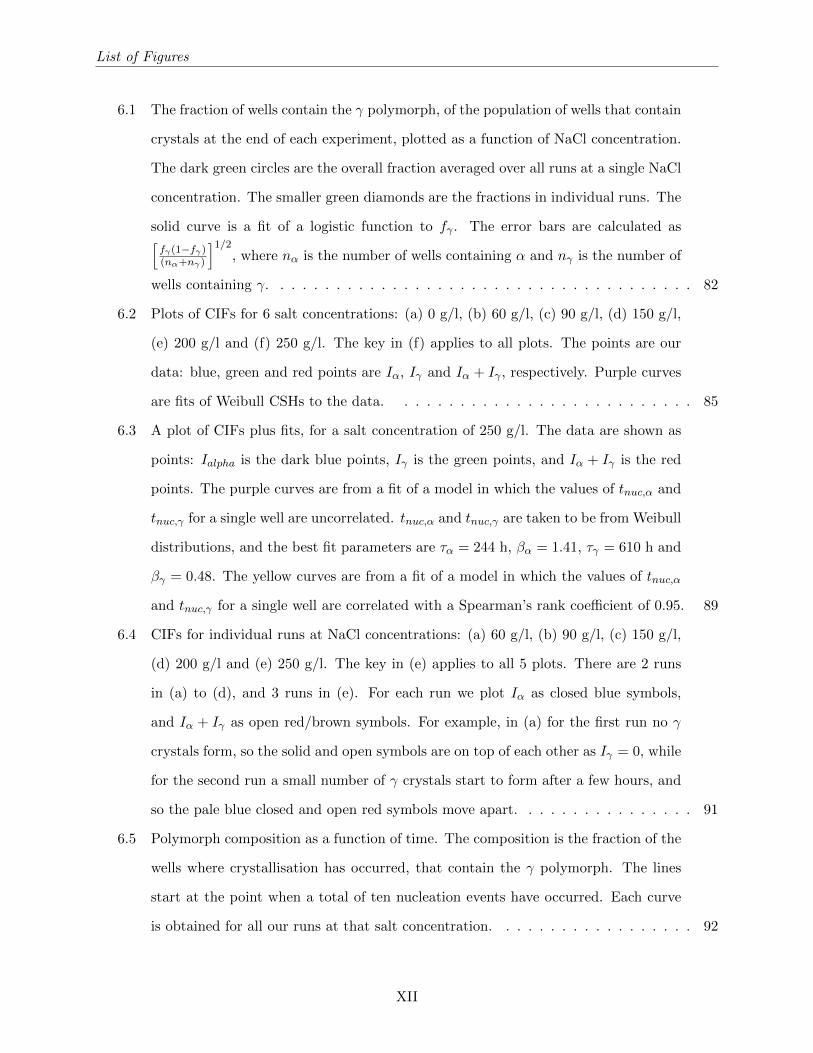
6.1 The fraction of wells contain the γ polymorph, of the population of wells that contain
crystals at the end of each experiment, plotted as a function of NaCl concentration.
The dark green circles are the overall fraction averaged over all runs at a single NaCl
concentration. The smaller green diamonds are the fractions in individual runs. The
solid curve is a fit of a logistic function to fγ . The error bars are calculated as[fγ(1−fγ)(nα+nγ)
]1/2, where nα is the number of wells containing α and nγ is the number of
wells containing γ. . . . . . . . . . . . . . . . . . . . . . . . . . . . . . . . . . . . . . 82
6.2 Plots of CIFs for 6 salt concentrations: (a) 0 g/l, (b) 60 g/l, (c) 90 g/l, (d) 150 g/l,
(e) 200 g/l and (f) 250 g/l. The key in (f) applies to all plots. The points are our
data: blue, green and red points are Iα, Iγ and Iα + Iγ , respectively. Purple curves
are fits of Weibull CSHs to the data. . . . . . . . . . . . . . . . . . . . . . . . . . . 85
6.3 A plot of CIFs plus fits, for a salt concentration of 250 g/l. The data are shown as
points: Ialpha is the dark blue points, Iγ is the green points, and Iα + Iγ is the red
points. The purple curves are from a fit of a model in which the values of tnuc,α and
tnuc,γ for a single well are uncorrelated. tnuc,α and tnuc,γ are taken to be from Weibull
distributions, and the best fit parameters are τα = 244 h, βα = 1.41, τγ = 610 h and
βγ = 0.48. The yellow curves are from a fit of a model in which the values of tnuc,α
and tnuc,γ for a single well are correlated with a Spearman’s rank coefficient of 0.95. 89
6.4 CIFs for individual runs at NaCl concentrations: (a) 60 g/l, (b) 90 g/l, (c) 150 g/l,
(d) 200 g/l and (e) 250 g/l. The key in (e) applies to all 5 plots. There are 2 runs
in (a) to (d), and 3 runs in (e). For each run we plot Iα as closed blue symbols,
and Iα + Iγ as open red/brown symbols. For example, in (a) for the first run no γ
crystals form, so the solid and open symbols are on top of each other as Iγ = 0, while
for the second run a small number of γ crystals start to form after a few hours, and
so the pale blue closed and open red symbols move apart. . . . . . . . . . . . . . . . 91
6.5 Polymorph composition as a function of time. The composition is the fraction of the
wells where crystallisation has occurred, that contain the γ polymorph. The lines
start at the point when a total of ten nucleation events have occurred. Each curve
is obtained for all our runs at that salt concentration. . . . . . . . . . . . . . . . . . 92
XII
List of Figures
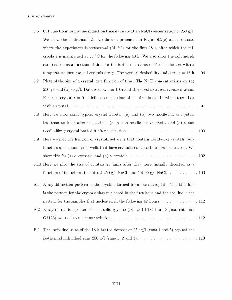
6.6 CIF functions for glycine induction time datasets at an NaCl concentration of 250 g/l.
We show the isothermal (21 C) dataset presented in Figure 6.2(e) and a dataset
where the experiment is isothermal (21 C) for the first 18 h after which the mi-
croplate is maintained at 30 C for the following 48 h. We also show the polymorph
composition as a function of time for the isothermal dataset. For the dataset with a
temperature increase, all crystals are γ. The vertical dashed line indicates t = 18 h. 96
6.7 Plots of the size of a crystal, as a function of time. The NaCl concentrations are (a)
250 g/l and (b) 90 g/l. Data is shown for 10 α and 10 γ crystals at each concentration.
For each crystal t = 0 is defined as the time of the first image in which there is a
visible crystal. . . . . . . . . . . . . . . . . . . . . . . . . . . . . . . . . . . . . . . . 97
6.8 Here we show some typical crystal habits. (a) and (b) two needle-like α crystals
less than an hour after nucleation. (c) A non needle-like α crystal and (d) a non
needle-like γ crystal both 5 h after nucleation. . . . . . . . . . . . . . . . . . . . . . . 100
6.9 Here we plot the fraction of crystallised wells that contain needle-like crystals, as a
function of the number of wells that have crystallised at each salt concentration. We
show this for (a) α crystals, and (b) γ crystals. . . . . . . . . . . . . . . . . . . . . . 102
6.10 Here we plot the size of crystals 20 mins after they were initially detected as a
function of induction time at (a) 250 g/l NaCl, and (b) 90 g/l NaCl. . . . . . . . . . 103
A.1 X-ray diffraction pattern of the crystals formed from one microplate. The blue line
is the pattern for the crystals that nucleated in the first hour and the red line is the
pattern for the samples that nucleated in the following 47 hours. . . . . . . . . . . . 112
A.2 X-ray diffraction pattern of the solid glycine (≥99% HPLC from Sigma, cat. no.
G7126) we used to make our solutions. . . . . . . . . . . . . . . . . . . . . . . . . . . 112
B.1 The individual runs of the 18 h heated dataset at 250 g/l (runs 4 and 5) against the
isothermal individual runs 250 g/l (runs 1, 2 and 3). . . . . . . . . . . . . . . . . . . 113
XIII
List of Figures
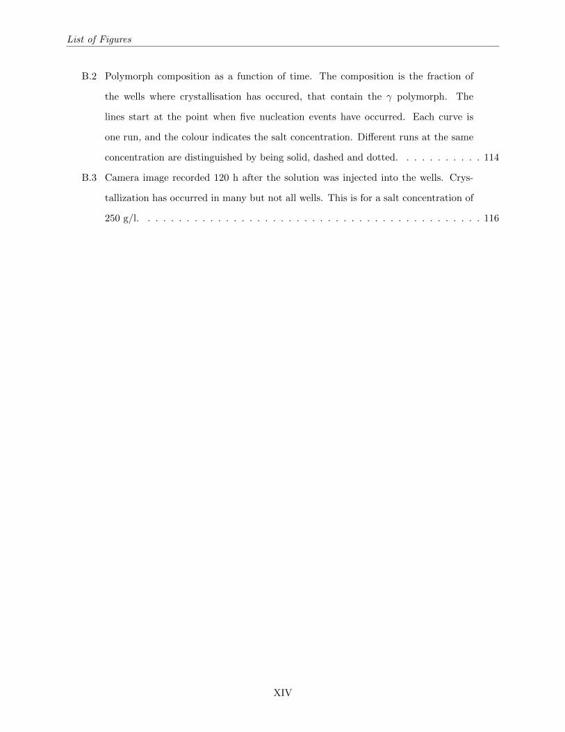
B.2 Polymorph composition as a function of time. The composition is the fraction of
the wells where crystallisation has occured, that contain the γ polymorph. The
lines start at the point when five nucleation events have occurred. Each curve is
one run, and the colour indicates the salt concentration. Different runs at the same
concentration are distinguished by being solid, dashed and dotted. . . . . . . . . . . 114
B.3 Camera image recorded 120 h after the solution was injected into the wells. Crys-
tallization has occurred in many but not all wells. This is for a salt concentration of
250 g/l. . . . . . . . . . . . . . . . . . . . . . . . . . . . . . . . . . . . . . . . . . . . 116
XIV

List of Tables
3.1 The experimental details of a number of studies on glycine growth. The growth rates
from these studies are shown in Figure 3.4. . . . . . . . . . . . . . . . . . . . . . . . 44
3.2 A table of γ glycine growth rates as a function of salt concentration, from a study
by Han et al [8]. Growth rates have been measured along the γ polymorph’s two
axes in aqueoues solution and 1.5m NaCl solution. The rates have been interpreted
from Figures 6 and 10 of thier study, so are approximate. . . . . . . . . . . . . . . . 45
5.1 A table of our datasets; each is identified by a letter in column one. . . . . . . . . . . 62
5.2 The KS numbers comparing the three datasets in Figure 5.2(a) and (b). The middle
and bottom rows are for the f(t) and f∗(t) functions, respectively. . . . . . . . . . . 66
5.3 The KS number comparing each of the different heating time datasets . . . . . . . . 67
5.4 KS numbers comparing f∗(t)s for the datasets A to D, for which theld is varied. . . . 68
5.5 The KS numbers comparing each of the datasets in Figure 5.6 to their respective
exponential fits. . . . . . . . . . . . . . . . . . . . . . . . . . . . . . . . . . . . . . . . 71
5.6 The KS numbers comparing datasets G, K and L. . . . . . . . . . . . . . . . . . . . 75
6.1 A table showing details of each dataset we recorded in this chapter, similar to Ta-
ble 5.1, but with details on the exact quantities of polymorphs. For all datasets
tH = 1 and tstart = 16:00. We show values of fγ the final fraction of wells with
crystals in them, where the crystals are of the γ polymorph, as a function of NaCl
concentration. Also shown are the total numbers of well with α and with γ crystals. 83
XV
List of Tables
6.2 Best-fit values for fits of Weibull CSHs to the CIFS for α and γ nucleation at 5 salt
concentrations. The first column is the salt concentration. Columns 2 to 5 give the
values of 4 fit parameters. Columns 6 and 7 give the R2 values for comparison of
the fit Iα and Iγ to the data. . . . . . . . . . . . . . . . . . . . . . . . . . . . . . . . 87
6.3 The best fit values of the parameters for fits of the data at 250 g/l NaCl. The first
column specifies the model, columns 2 to 5 contain the parameter values while the
last 2 columns give the values for the coefficients of determination (R2) for fits to
the Ii functions . . . . . . . . . . . . . . . . . . . . . . . . . . . . . . . . . . . . . . . 88
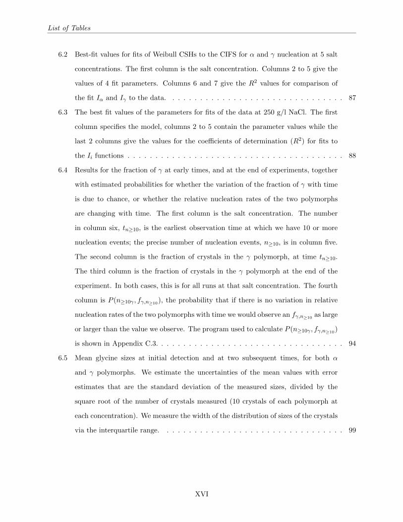
6.4 Results for the fraction of γ at early times, and at the end of experiments, together
with estimated probabilities for whether the variation of the fraction of γ with time
is due to chance, or whether the relative nucleation rates of the two polymorphs
are changing with time. The first column is the salt concentration. The number
in column six, tn≥10, is the earliest observation time at which we have 10 or more
nucleation events; the precise number of nucleation events, n≥10, is in column five.
The second column is the fraction of crystals in the γ polymorph, at time tn≥10.
The third column is the fraction of crystals in the γ polymorph at the end of the
experiment. In both cases, this is for all runs at that salt concentration. The fourth
column is P (n≥10γ , fγ,n≥10), the probability that if there is no variation in relative
nucleation rates of the two polymorphs with time we would observe an fγ,n≥10as large
or larger than the value we observe. The program used to calculate P (n≥10γ , fγ,n≥10)
is shown in Appendix C.3. . . . . . . . . . . . . . . . . . . . . . . . . . . . . . . . . . 94
6.5 Mean glycine sizes at initial detection and at two subsequent times, for both α
and γ polymorphs. We estimate the uncertainties of the mean values with error
estimates that are the standard deviation of the measured sizes, divided by the
square root of the number of crystals measured (10 crystals of each polymorph at
each concentration). We measure the width of the distribution of sizes of the crystals
via the interquartile range. . . . . . . . . . . . . . . . . . . . . . . . . . . . . . . . . 99
XVI
List of Tables
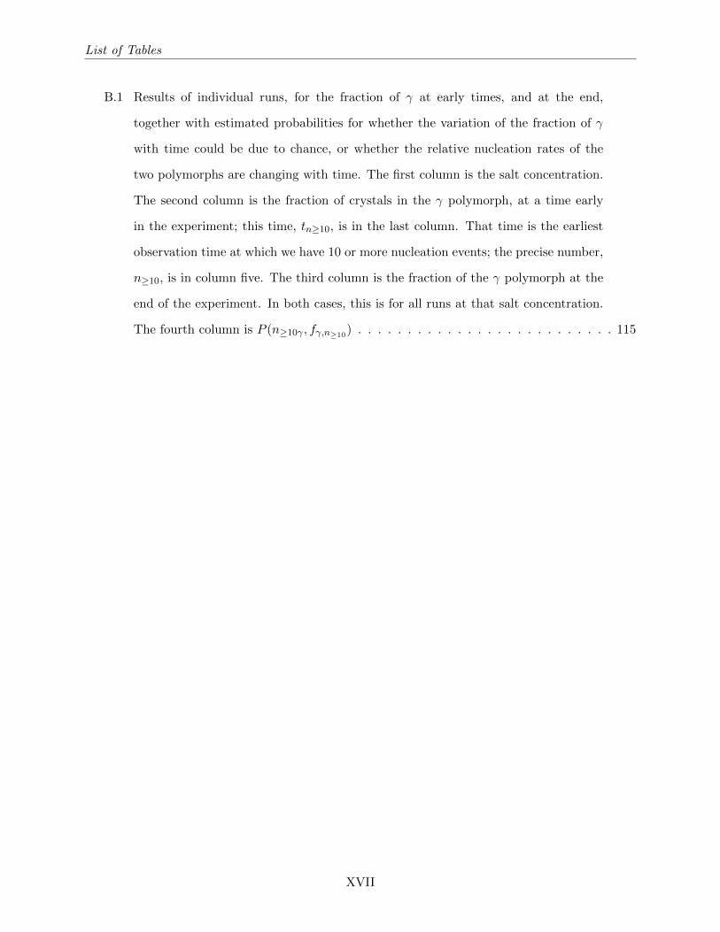
B.1 Results of individual runs, for the fraction of γ at early times, and at the end,
together with estimated probabilities for whether the variation of the fraction of γ
with time could be due to chance, or whether the relative nucleation rates of the
two polymorphs are changing with time. The first column is the salt concentration.
The second column is the fraction of crystals in the γ polymorph, at a time early
in the experiment; this time, tn≥10, is in the last column. That time is the earliest
observation time at which we have 10 or more nucleation events; the precise number,
n≥10, is in column five. The third column is the fraction of the γ polymorph at the
end of the experiment. In both cases, this is for all runs at that salt concentration.
The fourth column is P (n≥10γ , fγ,n≥10) . . . . . . . . . . . . . . . . . . . . . . . . . . 115
XVII

Abbreviations
AFM Atomic Force Microscopy
CDF Cumulative Distribution Function
CIF Cumulative Incident Function
CSH Cause Specific Hazard function
DLS Dynamic Light scattering
FTIR Fourier Transform Infra-Red
IQR Inter-quartile range
KS test Kolmogorov-Smirnov test
NTA Nanoparticle Tracking Analysis
PLM model Pound-La Mer model
SAXS Small Angle X-ray Scattering
SEM Scanning Electron Microscopy
TEM Transmission Electron Microscopy
XRD X-ray Diffraction
XVIII
1. Introduction
Crystals surround us in our everyday lives; there are ice crystals in the clouds above us, metals in
cars and trains, in the sand on beaches, in the drugs we buy at the pharmacy and in the chocolate
bars we eat. Crystallisation, the process by which crystals are formed, is still poorly understood. So
it is important to understand it better for a number of fields, from the production of pharmaceuticals
[12], to models of the contribution of clouds to climate change [13, 14]. Crystallisation begins via
nucleation: the formation of a small stable crystal nucleus. By stable we mean, a nucleus for which
it is favourable to grow, as oppose to dissolving back into the solution. There is often a significant
free energy barrier associated with nucleation [15] [16]. Nucleation can determine several important
details in crystallisation, for example, the time it takes for a crystal to form, the number of crystals
that form and the polymorph of those crystals. Polymorphism is the ability of a crystal to exist
as several possible crystal lattices, each different structure is referred to as a polymorph. After
nucleation, crystal growth occurs and the small nucleus grows into a larger, often macroscopic,
crystal.
Nucleation is relevant to many of the problems faced in the pharmaceutical industry. Specifi-
cally, it is often necessary to make crystals of a given size distribution and polymorph. Different
polymorphs have different crystal structures. Crystal structure is the way the atoms or molecules
that make up a crystal are arranged. When a material can crystallise into multiple crystal struc-
tures, those different structures can have very different properties. Consider the difference between
diamond and graphite, both made entirely of carbon, but have different structures as we can see
in Figure 1.1. The result of this is that diamond and graphite have very different properties, e.g.,
their electrical and mechanical properties.
The ability of carbon to exist in multiple structures is known as allotropy which is a term specific
to chemical elements. When we talk about organic materials, the ability of that material to exist in
several crystal structures is known as polymorphism. In the case of polymorphism, bonding within
1
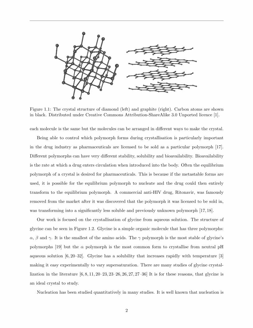
Figure 1.1: The crystal structure of diamond (left) and graphite (right). Carbon atoms are shownin black. Distributed under Creative Commons Attribution-ShareAlike 3.0 Unported licence [1].
each molecule is the same but the molecules can be arranged in different ways to make the crystal.
Being able to control which polymorph forms during crystallisation is particularly important
in the drug industry as pharmaceuticals are licensed to be sold as a particular polymorph [17].
Different polymorphs can have very different stability, solubility and bioavailability. Bioavailability
is the rate at which a drug enters circulation when introduced into the body. Often the equilibrium
polymorph of a crystal is desired for pharmaceuticals. This is because if the metastable forms are
used, it is possible for the equilibrium polymorph to nucleate and the drug could then entirely
transform to the equilibrium polymorph. A commercial anti-HIV drug, Ritonavir, was famously
removed from the market after it was discovered that the polymorph it was licensed to be sold in,
was transforming into a significantly less soluble and previously unknown polymorph [17,18].
Our work is focused on the crystallisation of glycine from aqueous solution. The structure of
glycine can be seen in Figure 1.2. Glycine is a simple organic molecule that has three polymorphs:
α, β and γ. It is the smallest of the amino acids. The γ polymorph is the most stable of glycine’s
polymorphs [19] but the α polymorph is the most common form to crystallise from neutral pH
aqueous solution [6, 20–32]. Glycine has a solubility that increases rapidly with temperature [3]
making it easy experimentally to vary supersaturation. There are many studies of glycine crystal-
lization in the literature [6, 8, 11, 20–23, 23–26, 26, 27, 27–36] It is for these reasons, that glycine is
an ideal crystal to study.
Nucleation has been studied quantitatively in many studies. It is well known that nucleation is
2
1.1. Aims
very sensitive to many factors, i.e, temperature, supersaturation and the presence of impurities. For
this reason reproducible results can be difficult to achieve. In this work we address the sensitivity
of nucleation and introduce common statistical tests i.e, the Kolgomorov Smirnov test, which we
use to test how reproducible our data is and how well it is fit by various models.
Figure 1.2: The 3D structure of a glycine molecule [2]. The amine group (NH2) can be seen on theleft and the carboxylic acid group (COOH) is on the right.
Glycine’s polymorphism has been studied previously, however the relationship between induc-
tion times and polymorphism has not been studied for glycine. So far there has only been one study
for any material that looks at this relationship between induction times and polymorphism [37].
There the authors noted the difference in induction times between polymorphs but did not fit any
models to the polymorph separated induction time distributions. It is by studying this relationship
in detail and trying to quantify it that we advance the field both for nucleation studies in gen-
eral and specifically for understanding glycine crystallisation. We have also introduced ideas from
medical statistics where the system is analogous to induction time statistics.
1.1 Aims
Before we describe the work done in this project, it is useful to set out the general goals and aims
of what we wanted to understand, to put the rest of this study into context. When we first started
this project there were several aims:
1. To establish a method that allows observation of many crystallisation events simultaneously,
thus allowing us to record a large number of induction times and obtain good statistics.
Nucleation is a stochastic phenomenon so statistics are needed to understand it.
2. To investigate experimentally how the induction time distribution changes with key exper-
imental variables, for example, filtering of the glycine solution, supersaturation, and the
presence of other materials that affect nucleation in the glycine solution.
3
1.2. Overview
3. To fit the induction time distributions observed in experiments with accurate models which
have sound physical bases.
As the project progressed we discovered that for glycine, polymorphism is related to induction
time. As is often the case in science, we let this interesting result steer the focus of our work. We
began to focus on the polymorphic outcome of nucleation; the project’s fourth objective can be
summarised as:
4. To quantify and model the difference between induction time distributions for the α and γ
polymorphs of glycine
These four aims cover the majority of the work presented here but the one all encompassing aim
of our work is simply to better understand the nucleation of crystals and be able to better predict
and control it. We believe that reproducible, quantitative experimental data on nucleation from
solution at constant supersaturation will take us toward this objective [16].
1.2 Overview
In the next chapter we discuss classical nucleation theory and the models used to describe induction
time distributions. In Chapter 3 we discuss the state of the art and specifics of literature on glycine
nucleation including how glycine nucleation is affected by the presence of sodium chloride. Then
in Chapter 4 we describe the methods used for our experiments. Our first results and analysis
chapter is Chapter 5. There we discuss the relationship between induction time and several factors
including: supersaturation, temperature, dissolution time and the time the supersaturated solution
is held in the pipette. We also discuss growth rates, some preliminary results on polymorphism
and data for second nucleation events. The results of Chapter 5 have been published in the journal
Crystal Growth & Design in 2015 [33]. The data collection and analysis for this paper was carried
out by me but the paper was co-written with Dr. Richard Sear and Prof. Joseph Keddie. In
Chapter 6 we present results on the influence of added sodium chloride on glycine nucleation. We
also present induction time distributions for individual polymorphs and discuss the competition
between glycine’s α and γ polymorphs. Again we also discuss growth rates. Finally in Chapter 7,
we conclude.
4
1.3. The tortoise and the hare
1.3 The tortoise and the hare
The tale of the Tortoise and the Hare is a popular fable originating from Aesop, a storyteller from
ancient Greece. In the tale, the tortoise and the hare agree to have a race. At the start of the
race, the hare is a lot faster than the tortoise and speeds away, but, confident of winning, the hare
decides to have a nap. While the hare sleeps, the tortoise gradually overtakes his competitor and
ends up winning the race.
In this thesis we record nucleation induction times for glycine’s polymorphs. With these, we are
able to observe effective nucleation rates. In Chapter 6 we find that α and γ glycine have effective
nucleation rates that vary with time. We show that much like the hare, γ nucleation is initially
fast, but slows down, allowing the α nucleation rate (the tortoise) to overtake the γ nucleation rate.
5
2. Theory of nucleation from
supersaturated solution
Here we discuss the theory of nucleation and statistical models for the distributions of induction
times. We can use the theory of nucleation to understand why nucleation occurs under certain
conditions and why the timescale associated with it can be highly variable. With nucleation theory,
we can also understand the usefulness of certain parameters that we can record from nucleation,
such as induction times. By looking at the predictions of classical nucleation theory we can see how
we expect certain factors, for example supersaturation, to affect experimental studies of nucleation.
It is therefore important to understand the underlying theory of nucleation. This chapter is split
into three sections:
1. Crystallisation from solution can only occur if the solution is supersaturated. We therefore
give a brief explanation in section 2.1 of how supersaturated solutions are created.
2. In section 2.2 we discuss the driving force behind nucleation and the microscopic mechanism
by which it occurs. We also discuss homogeneous and heterogeneous nucleation and classical
nucleation theory.
3. Nucleation is a stochastic process so we need statistical models to understand experimental
data. In section 2.3 we discuss the statistics of nucleation at constant supersaturation.
2.1 Creating supersaturated solutions
In a solution maintained at a constant temperature, there is a fixed amount of solute that can
be dissolved, at which point any further solute added to the solution will not dissolve. This fixed
amount is referred to as the solubility of the solution, and a solution exactly at solubility is said to
6
2.1. Creating supersaturated solutions
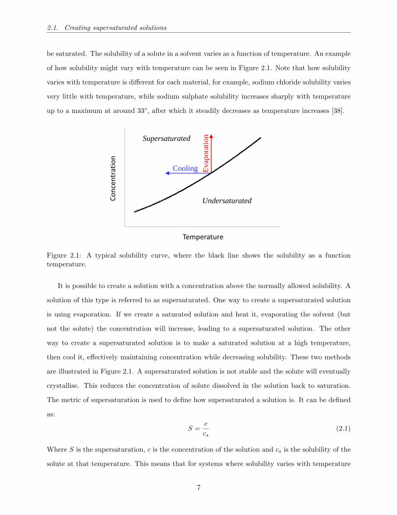
be saturated. The solubility of a solute in a solvent varies as a function of temperature. An example
of how solubility might vary with temperature can be seen in Figure 2.1. Note that how solubility
varies with temperature is different for each material, for example, sodium chloride solubility varies
very little with temperature, while sodium sulphate solubility increases sharply with temperature
up to a maximum at around 33, after which it steadily decreases as temperature increases [38].
Supersaturated
Evap
ora
tion
Cooling
50
8
Concentration
Temperature
Undersaturated
Figure 2.1: A typical solubility curve, where the black line shows the solubility as a functiontemperature.
It is possible to create a solution with a concentration above the normally allowed solubility. A
solution of this type is referred to as supersaturated. One way to create a supersaturated solution
is using evaporation. If we create a saturated solution and heat it, evaporating the solvent (but
not the solute) the concentration will increase, leading to a supersaturated solution. The other
way to create a supersaturated solution is to make a saturated solution at a high temperature,
then cool it, effectively maintaining concentration while decreasing solubility. These two methods
are illustrated in Figure 2.1. A supersaturated solution is not stable and the solute will eventually
crystallise. This reduces the concentration of solute dissolved in the solution back to saturation.
The metric of supersaturation is used to define how supersaturated a solution is. It can be defined
as:
S =c
cs(2.1)
Where S is the supersaturation, c is the concentration of the solution and cs is the solubility of the
solute at that temperature. This means that for systems where solubility varies with temperature
7
2.2. Homogeneous and Heterogeneous nucleation
(like glycine) supersaturation varies with temperature, at fixed c.
2.2 Homogeneous and Heterogeneous nucleation
There are two ways a nucleus can form in a solution: Homogeneously and heterogeneously. For
the former case the nucleus forms in the uniform solution. For the latter case, the nucleus forms
on a surface, the surface could be that of an impurity in the solution, the container that holds the
solution or any interface of the solution. Heterogeneous nucleation is often significantly quicker
than homogeneous nucleation [16, 39, 40], hence observation of homogeneous nucleation is rare. In
this section we discuss the free energy barrier associated with nucleation, then go on to discuss
heterogeneous nucleation in a little more detail.
2.2.1 Classical Nucleation Theory
We know that a supersaturated solution is thermodynamically less stable than a crystalline phase
in a saturated solution. With this in mind, the first logical question is: Why doesn’t the crystalline
phase immediately nucleate in a supersaturated solution? The reason is that a crystal starts off
microscopic and has to grow and when it forms, a solid-liquid interface is created which has a free
energy cost. The bulk of the crystal lowers its free energy when crystallising and so the free energy
of the system is determined by these competing effects. This can be described by Equation 2.2 [41]:
∆G = 4πr2γ − 4
3πr3∆GV (2.2)
Where γ is the interfacial free energy between the crystalline phase and the solution, ∆GV is the
free energy reduction per unit volume due to crystallisation and r is the nucleus radius. Note that
this assumes the crystal nucleus is spherical. The free energy of the nucleus therefore depends on
the surface area to volume ratio of the nucleus. When the nucleus is small the ratio is large such that
4πr2γ 43πr
3∆GV but as the nucleus increases in size the ratio decreases so 4πr2γ 43πr
3∆GV .
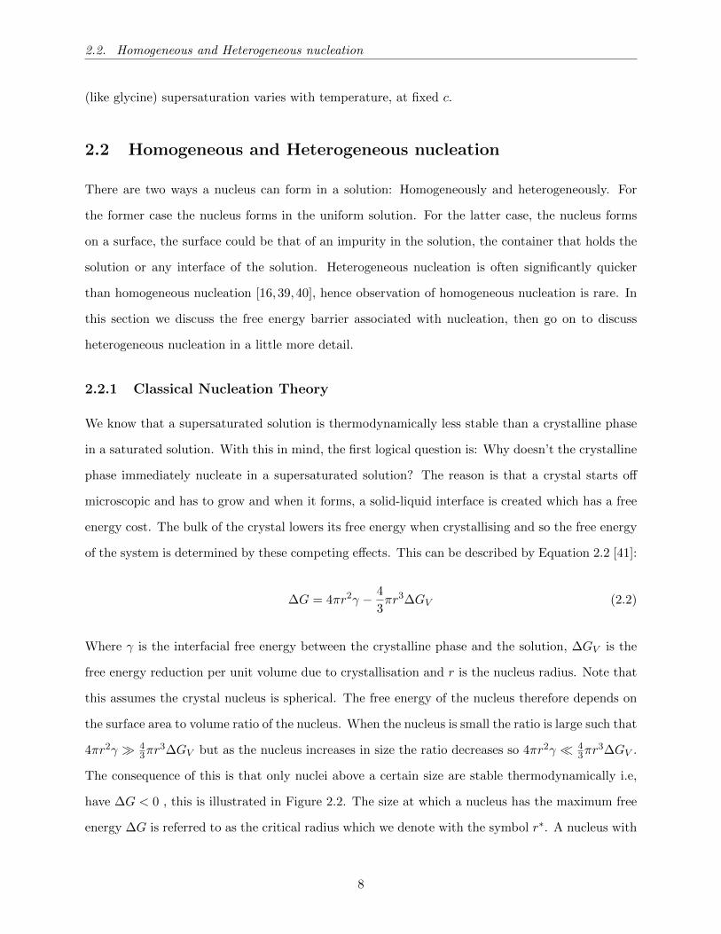
The consequence of this is that only nuclei above a certain size are stable thermodynamically i.e,
have ∆G < 0 , this is illustrated in Figure 2.2. The size at which a nucleus has the maximum free
energy ∆G is referred to as the critical radius which we denote with the symbol r∗. A nucleus with
8
2.2. Homogeneous and Heterogeneous nucleation
0
Nucleus radius
Fre
e E
nerg
y (Δ
G)
Interface free energy
Bulk free energy
Total free energyΔG*
r*
Figure 2.2: The free energy of a crystal nucleus in a superstarurated solution as a function of thenucleus radius.
a radius below r∗ will probably dissolve back into the solution. For a nucleus with a radius above
r∗ it is favourable for the nucleus to grow.
The height of the free energy barrier can be derived by setting the derivative of Equation 2.2
to equal zero. Rearranging that equation to make r the subject gives r∗ = 2γδGV
and substituting
that back into Equation 2.2 gives:
∆G∗ =16πγ3
3∆G2V
(2.3)
We can express ∆GV as ∆V where V is the nucleus volume and ∆µ is the difference between
the chemical potential of the solution and a solution at saturation or, to put it another way, the
bulk free energy reduction of the nucleus. For an ideal solution, ∆µ = kT ln(S), [42] where S
is supersaturation, k is Boltzmann’s constant and T is temperature. Equation 2.3 can then be
expressed as follows.
∆G∗ =16πV 2γ3
3(kT )2 ln2(S)(2.4)
The nucleus is formed via a fluctuation. The probability of a fluctuation reaching the top of
the free energy barrier, ∆G∗, is given by the Boltzmann factor, e−∆G∗/kT . The nucleation rate of
the system can therefore be given by the following equation.
rate = Ae−∆G∗/kT (2.5)
9
2.2. Homogeneous and Heterogeneous nucleation
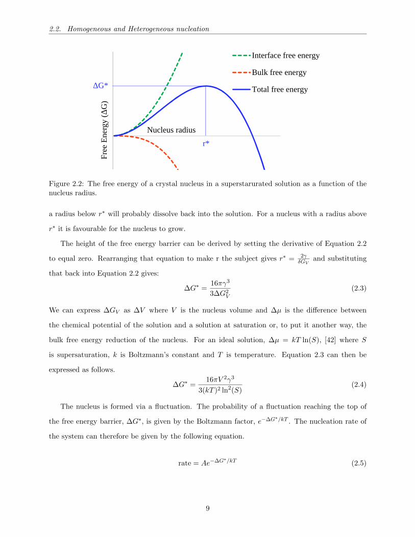
Here the prefactor A is determined by:
1. The rate at which molecules attach to the nucleus.
2. The volume of the system (in the case of homogeneous nucleation) or the number of nucleation
sites (in the case of heterogeneous nucleation).
3. The Zeldovich factor, this is a factor that determines the probability that a nucleus of size r∗
will grow into a stable nucleus as opposed to dissolving back into the solution.
This theory predicts that the nucleation rate does not vary as a function of time, so we therefore
expect a constant nucleation rate.
Experimentally we can measure induction times and supersaturation. As we can estimate the
nucleation rate at a range of supersaturations, it is useful to know the prediction for how the rate
varies with supersaturation according to CNT. Using Equation 2.4 and Equation 2.5 we know that
nucleation rate ∝ e−1
ln2(S) , if we take the natural log of each side of the equation we find.
ln(rate) ∝ −1
ln2(S)(2.6)
We can therefore test if our data are consistent with classical nucleation theory by plotting
the natural log of nucleation rate against one over the the natural log of supersaturation squared
(assuming solutions are ideal).
2.2.2 Heterogeneous Nucleation
In almost any solution, there are a number of impurities. These impurities often greatly reduce
the free energy barrier ∆G∗ which must be overcome for nucleation to occur. A crystal nucleus
has an interface with the solution which has an interfacial free energy γns. An impurity also has
an interface with the solution which has some interfacial free energy, γis. This is illustrated in
Figure 2.3 (a)(i). If the nucleus is in contact with the impurity both the nucleus and impurity have
reduced their respective surface areas in contact with the solution, this is illustrated in Figure 2.3
(a)(ii). The free energy of the system is therefore reduced by the nucleus being in contact with the
impurity unless the interfacial free energy between impurity and the nucleus, γin, is very large. The
10
2.2. Homogeneous and Heterogeneous nucleation
Nucleus
NucleusSolution
Impurity
Solution
Impurity
(a)(i) (a)(ii)
γin γis
γns
θγis
γns
Nucleus
Solution
Impurity
Solution
Impurity
(b)(i) (b)(ii)
γisγis
γns
Nucleusγin
1
γns2
γns3
γns4 γns1
γns2 γns3
Figure 2.3: An illustration of the interfacial free energy of a crystal nucleus and impurity in solution.(a) A nucleus that conforms to the assumptions of Young’s equation (i) in solution (ii) in contactwith an impurity in the solution. (b) A faceted nucleus (i) in solution (ii) in contact with animpurity in the solution.
contact angle between the crystal nucleus and the impurity is a function of the three interfacial
free energies in the system. This can be described by Equation 2.7.
γns cos θ = γis − γin (2.7)
This is known as Young’s equation [41]. Here we are assuming that the crystal nucleus is spherical.
The nucleation barrier for heterogeneous nucleation is lower than for homogeneous nucleation in
any system where the free energy is reduced by the crystal nucleus being in contact with an impu-
rity. The exponential prefactor A from Equation 2.5 is often significantly larger for homogeneous
nucleation than it is for heterogeneous nucleation. This is because for homogeneous nucleation, the
parameter A ∝ system volume, but for heterogeneous nucleation A ∝ impurity area. Another way
to put this is that there are very few locations where heterogeneous nucleation can occur compared
to homogeneous nucleation. Observation of heterogeneous nucleation therefore indicates a system
where the free energy barrier is significantly lower for heterogeneous nucleation. Heterogeneous nu-
cleation is the more likely type of nucleation to be observed when the impurities within the solution
significantly reduce ∆G∗. If the impurities do not reduce ∆G∗ enough, homogeneous nucleation will
occur more frequently as it can occur anywhere within the solution while heterogeneous nucleation
only occurs at surfaces.
Young’s equation makes some assumptions about the nucleus. It assumes that (a) the nucleus
is spherical and (b) the surface energy of the nucleus is isotropic. A nucleus that conforms to these
11

2.3. Statistics of isothermal nucleation
assumptions is shown in Figure 2.3(a). In reality a crystal nucleus will not be spherical because the
surface free energy of a crystal is anisotropic. Figure 2.3(b) shows how the surface energy might
vary for a faceted nucleus where different faces of the crystal nucleus can have different surface
free energies. In reality it is also unlikely that the crystal nucleus will have smooth faces with well
defined surface energies. An actual nucleus is likely to have some complex shape with a varying
interfacial energy across it’s surface. It is also possible that different nuclei in the same system
would have different shapes and interfacial energies. It is unclear how this would change Equations
2.5 and 2.4, therefore for crystal nucleation, CNT is best thought of as a way to understand why
nucleation can be so slow, not a theory to predict an exact rate in a given system.
2.3 Statistics of isothermal nucleation
Experimentally, studying nucleation is difficult. While the critical nucleus size r∗ varies depending
on the system, it is microscopic. The impurity on which it occurs (in the case of heterogeneous
nucleation) could also be too small to observe. There are often many impurities within a solution.
If we have no information about where these impurities are or the extent to which they reduce
the free energy barrier associated with nucleation we cannot be sure where nucleation might occur.
Hence, direct observation of nucleation is extremely difficult. As we cannot see nuclei or impurities,
we cannot predict the nucleation rate or even if it is well defined, so we need flexible statistical
models to describe nucleation.
Nucleation is a stochastic process. The time at which it occurs, the induction time, is highly
variable. It is experimentally ideal for the induction time to be much greater than the time it takes
for the nucleated crystal to grow to an observable size. In this case, the time at which a crystal
is observed during an experiment can be approximated as the induction time. The distribution of
induction times in a system can give us information about the microscopic mechanism of nucleation.
We discuss what induction times can tell us about nucleation, and the statistical tests we can apply
to them, in this section.
12
2.3. Statistics of isothermal nucleation
2.3.1 N(t) vs P (t) plots
Let us consider a supersaturated solution. We denote the probability that a nucleus will nucleate
between t and t+ dt as p(t)dt, and the cumulative probability that nucleation has not yet occurred
at time t as P (t). The P (t) function starts at one and decays to zero as t → ∞. If none of the
conditions that affect nucleation are changing (i.e, temperature, supersaturation), then we expect
that for that solution, the rate p(t) at which nucleation occurs is constant. We would then expect
to see a basic exponential decay as described by Equation 2.8, where k is the nucleation rate.
P (t) = e−kt (2.8)
Experimentally, what we can do is to take n0 samples of equal volume from a bulk supersaturated
solution and record the number that have not yet crystallised as a function of time, n(t). We can
normalise n(t) by plotting N(t) = n(t)/n0, here N(t) is the fraction (not number) of samples not
crystallised as a function of time. We can see in Figure 2.4 that as n0 increases, N(t) should
eventually converge to P (t), that is to say limn0→∞N(t) = P (t). It is therefore only possible to
estimate P(t) distributions from measured N(t) distributions.
For the nucleation mechanism described in Equation 2.8, if we record an infinite number of
induction times this leads to a cumulative distribution function (CDF) of the form Equation 2.9.
limn0→∞
N(t) = e−kt (2.9)
where k, the nucleation rate is a constant that is the same for each of the n0 samples. When n0
is finite, N(t) is discrete and therefore only an approximation of the continuous P (t) distribution.
As nucleation is a random process and n0 is finite we expect N(t) to vary randomly around P (t).
This variation is illustrated in Figure 2.4.
2.3.2 Kolmogorov Smirnov test
Experimentally we will be working with datasets that have an n0 of the order of hundreds which
are therefore too small to make the approximation N(t) = P (t). Therefore when we fit P (t) models
to our data we need to be able to determine whether the differences between N(t) and P (t) are due
13
2.3. Statistics of isothermal nucleation
0
1
0
N(t
)
Time
P(t)
N(t) at n0 =30
N(t) at n0=50
DD
P(t)
N(t) at n0 = 30
N(t) at n0 = 50
Figure 2.4: Two N(t) distributions which are random samples of an exponential decay distribution,P (t), have been computationally generated. D is the maximum difference between N(t) and P (t)as defined in Equation 2.10
to an inaccurate model or due to random fluctuations. Quantitative analysis of our data requires
statistical tools. Fortunately a well known statistical test known as the Kolmogorov-Smirnov (KS)
test [43] can be used to quantitatively determine if an experimentally recorded N(t) is consistent
with being a sample of size n0 from the predicted P (t) distribution. This test compares an N(t)
distribution with a P (t) distribution. Note that this is different from the Kolmogorov-Smirnov two
sample test which compares two N(t) distributions, N1(t) and N2(t). We discuss the two sample
test in subsection 2.3.3.
We apply Kolmogorov-Smirnov statistical tests [43,44] to our nucleation data later, in the results
chapters. As far as we are aware, this is the first time this has been done. These statistical tests
are used to test for reproducibility. As nucleation is a very sensitive process, reproducible data is
difficult to obtain, and so it is important to prove that data is reproducible.
The test is as follows. We start with the null hypothesis that N(t) is not a sample from the
continuous distribution P (t). We then identify the maximum difference between the two functions,
known as the supremum, D. This is illustrated in Figure 2.4 and can be expressed mathematically
as:
D = max0<t<∞
|P (t)−N(t)| (2.10)
It is always true that 0 ≤ D ≤ 1. We can consider this to be a measure of the similarity between
N(t) and P (t) where the lower D is, the more similar the two functions are. If N(t) is a sample
14
2.3. Statistics of isothermal nucleation
from P (t) we expect D to decrease as n0 increases, therefore if we multiply D by the square root
of n0, we obtain a measure of the similarity between the two functions that does not vary with the
number of samples, we refer to this measure as the KS number. Our null hypothesis that N(t) is
not a sample from P (t) could be correct when the following equation [43] is satisfied.
Dn120 = KS number ≥ C (2.11)
For a fixed value of C There is a known percentage of times we would expect the KS number to
be below that value if our null hypothesis is false. If N(t) is a sample from P (t) the KS number
should only exceed C = 1.36 5% of the time and C = 1.63 1% of the time. We can therefore say if
a KS number exceeds C, N(t) is very probably not a sample of size n0 from P (t). Note that this
test can only prove when N(t) is not a sample from P (t). If the KS number is lower than C then
it only implies that the difference between N(t) and the true distribution P (t) is so small that it is
consistent with random noise.
2.3.3 Comparing N(t) Plots
With the method we use for collecting data, the largest number of samples we are able to crystallise
in one experiment is 96. We do repeat experiments under the same conditions so we are able to
create a larger dataset i.e, n0 = 192, n0 = 288. The nucleation process is very sensitive to impurities
and small variations in temperature, supersaturation and other factors. It is therefore useful to
have a test we can apply to our N(t) distributions to see if they are random samples from the same
P (t) distribution. To put it another way, to have a test that shows any difference between two
N(t) distributions is consistent with the random nature of nucleation, and that the experimental
conditions are the same and hence the underlying P (t) has not changed. It is also useful to have this
test so that when we intentionally change a parameter and want to prove that two N(t) datasets
are from a different P (t) distribution, we can show that the difference between the two datasets is
not just due to the random nature of nucleation.
The test we use to determine if the difference between twoN(t) distributions is purely due to ran-
domness is the Kolmogorov-Smirnov two-sample test. The idea is very similar to the Kolmogorov-
Smirnov test described in subsection 2.3.1. We have two datasets, M(t) consisting of m0 samples
15
2.3. Statistics of isothermal nucleation
and N(t) consisting of n0 samples. We start with the null hypothesis that M(t) and N(t) are sam-
ples from two different P (t) distributions. We can take the supremum of the two datasets DMN
which we expect to decrease as m0 and n0 increase if our null hypothesis (that M(t) and N(t) are
samples from two different P (t) distributions) is incorrect. With this supremum we can say our
null hypothesis is likely to be correct when the following is true:
(m0n0
m0 + n0
) 12
DMN ≥ C (2.12)
Here, like in the previous section, we are interested in the percentage of times we expect the
left hand side of the equation to be below C if our null hypothesis is false. Conveniently the same
value of C applies for a given level of certainty as in the previous section. The left hand side of
Equation 2.12 should be above 1.36 only 5% of the time and above 1.63 only 1% of the time if our
null hypothesis is false.
2.3.4 Heterogeneous Nucleation Models
Here we look at some simple models of P (t) distributions, that we might expect to see when
there is heterogeneous nucleation and P (t) is non-exponential. We start by postulating that our
samples each contain some number of impurities. On these impurities there are ‘nucleation sites’,
microscopic areas where ∆G∗ is significantly reduced. In this situation each sample has a nucleation
rate that does not change with time and sample i can be described by P (t) = e−kit. The P (t)
distribution for the entire set of samples each with different impurities and rates is slightly more
complex and can be described by the following equation:
P (t) =1
n0
n0∑i
e−kit (2.13)
Where n0 is the number of samples, t is time and ki is the nucleation rate of the ith sample. When
the P (t) distribution of a set of samples can be described by this equation, we see an effective
nucleation rate that decreases over time [45].
Here each sample has a different nucleation rate so the system has no well defined rate. We
can talk about the effective nucleation rate of the system at a given time. We can define how
16

2.3. Statistics of isothermal nucleation
this rate varies with time as the hazard function. This function is frequently used in survival data
analysis [46]. We define the hazard function as:
h(t) =−1
P (t)
dP
dt=
p(t)
P (t)(2.14)
Here, h(t) is the effective nucleation rate for the remaining samples in a system which have not yet
crystallised after time t.
Extreme value statistics model
For our first model, we start by assuming the number of nucleation sites in a sample is very large
and does not vary significantly from sample to sample. We can therefore approximate the number
of nucleation sites in each sample to be equal but we assume each nucleation site is different and
therefore will reduce ∆G∗ by widely varying amounts. This means each nucleation site has a
different nucleation rate. If the distribution of site rates is very broad the highest site nucleation
rate in a sample is a good approximation of the total nucleation rate of the sample. We can express
this mathematically as ksample ≈ max(k1, k2, k3, ..., kimpurities). Here we are interested in the rate
of each sample, so what we need to know is the distribution of maxima.
A branch of mathematics known as Extreme Value Statistics can be used to describe the distri-
bution of these maxima [47]. The functional form of the CDF is known as the generalised extreme
value distribution and is given by:
P (t) = exp[−(1− ξ(t− u)/w)−1/ξ
](2.15)
For the derivation of this see [47]. This equation holds provided there are a large number of
impurities and the distribution of rates is smooth. Here w, u and ξ are parameters. By introducing
the boundary condition P (t = 0) = 1, we find u must equal −w/ξ and that ξ < 0. The equation
then simplifies to:
P (t) = exp[− (ξt/w)−1/ξ
](2.16)
This is a Weibull distribution. We can simplify further by substituting wξ = τ and −1
ξ = β. As
17

2.3. Statistics of isothermal nucleation
ξ < 0 it is true that β > 0. This leads to the functional form:
P (t) = exp[− (t/τ)β
](2.17)
Here β can be seen as a measure of how widely varying the nucleation rate [48] is from sample
to sample. τ can be seen as a characteristic time scale for nucleation in cases where β is close to
one. This becomes less true as β decreases and τ is no longer characteristic of the timescale for
nucleation in the system below β = 0.5 [48]. It is useful also to be able to assess visually whether
our N(t) data look similar to a Weibull distribution. If we take the natural log of each side of
Equation 2.17 and multiply by −1 we end up with Equation 2.18.
− ln[P (t)] = (t/τ)β (2.18)
If we then take the natural log of each side of Equation 2.18 and rearrange, we obtain Equation 2.19.
ln [− ln(P (t))] = β ln(t)− β ln(τ) (2.19)
When we have an experimental dataset, N(t), we can then plot ln[ln(N(t))] against ln(t) and we
expect an approximately linear relationship if N(t) is a sample from a P (t) which is a Weibull
distribution. We can therefore use this plot to visually verify whether a dataset follows Weibull
statistics.
The Pound-La Mer and simplified Pound-La Mer Model
The Pound La-Mer (PLM) model [49] makes different assumptions to the extreme value statistics
model. The PLM model is based on the idea that impurities are similar and therefore have equal
nucleation rates but it is the number of impurities that varies significantly from sample to sample.
The PLM model assumes that the number of impurities per sample are Poisson distributed, and
that each impurity has the same rate ki. Thus each sample has a rate nki + k0 where n is the
number of impurities in the solution and k0 is the rate in samples where there are no impurities.
18
2.3. Statistics of isothermal nucleation
This leads to a P (t) of the form:
P (t) = exp[−m(1− e−kit)
]+ exp[−m] exp
[e−k0t − 1
](2.20)
where m is the mean number of impurities in a sample. If we make the assumption that homoge-
neous nucleation is too slow to be observed on an experimental time scale then we can simplify by
setting k0 = 0. This leads to a two-parameter model of the form
P (t) = exp[−m(1− e−kit)
](2.21)
identifiable as the Gompertz function. The Gompertz function is a mathematical function com-
monly used in many other fields such as modelling tumour growth and modelling life expectancy
[50,51].
Model comparison
We have introduced a few models that can be used to model induction time distributions but there
are many functions that could be used to fit nucleation data. A two-exponential model for example,
of the functional form P (t) = fe−k1t+(1−f)e−k2t has been used to fit induction time distributions
in other studies [52]. A rationale for the model can be provided if we assume some significant
portion of samples contain a specific impurity that has a faster rate than those impurities in the
other wells.
The two-exponential model has three parameters. The more parameters a function has the more
easily it can fit a dataset, regardless of whether the model is correct or not. This phenomenon is
known as overfitting. The usefulness of a model is in it’s predictive power to generalise a trend to
parameter values for which data has not yet been recorded. While models with more parameters
usually fit recorded data better, they do not necessarily have better predictive power. An example
of this can be seen in Figure 2.5. This plot shows computationally generated data where f is a
linear function of x but Gaussian noise has been introduced. The 6th order polynomial (blue)
fits the recorded data very well but if further data points were to be recorded it would have poor
predictive power. Recording new data points and re-fitting would also lead to significantly different
19

2.3. Statistics of isothermal nucleation
0
10
20
30
40
50
60
70
80
0 2 4 6 8
f(x)
x
Figure 2.5: An example of overfitting. A function f(x) has been fit with a linear function (red) anda 6th order polynomial (blue)
parameter values, the model is therefore of little use. The linear fit (red) does not fit the recorded
data as well. It does however have a better predictive power for further data points, and refitting
with these data points would not significantly change the models parameter values. This model is
therefore useful. These are of course extreme examples but they help illustrate the importance of
the number of parameters in a model.
So far, we have introduced three nucleation models with two or less parameters: The exponential
decay (homogeneous), the simplified Pound La-Mer model or Gompertz function (heterogeneous)
and the extreme value statistics model or Weibull function (heterogeneous). These models have
significantly different functional forms. An example of each function is shown in Figure 2.6. We
note that the exponential has a constant effective nucleation rate, unlike the other two functions.
The exponential function almost always provides a worse fit than the other two models but only
has one fit parameter. As we have discussed, if we are able to fit data well with fewer parameters,
then this is generally preferable to using a model with more fit parameters. When analysing data,
if the exponential model does not provide a good fit for our data we should then test the Weibull
and Gompertz functions. The Weibull and Gompertz functions both have nucleation rates that
decrease over time and the differences between their functional forms is subtle. The Weibull function
is typically the better model for fitting data that have a large dynamic range of induction times
with the one caveat that it cannot fit a plateau. One advantage of using the gompertz function
20
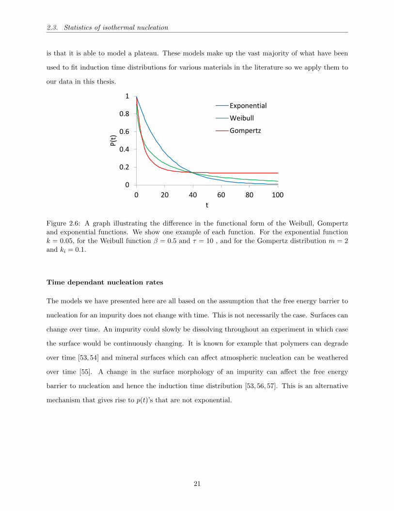
2.3. Statistics of isothermal nucleation
is that it is able to model a plateau. These models make up the vast majority of what have been
used to fit induction time distributions for various materials in the literature so we apply them to
our data in this thesis.
0
0.2
0.4
0.6
0.8
1
0 20 40 60 80 100
P(t)
t
Exponential
Weibull
Gompertz
Figure 2.6: A graph illustrating the difference in the functional form of the Weibull, Gompertzand exponential functions. We show one example of each function. For the exponential functionk = 0.05, for the Weibull function β = 0.5 and τ = 10 , and for the Gompertz distribution m = 2and ki = 0.1.
Time dependant nucleation rates
The models we have presented here are all based on the assumption that the free energy barrier to
nucleation for an impurity does not change with time. This is not necessarily the case. Surfaces can
change over time. An impurity could slowly be dissolving throughout an experiment in which case
the surface would be continuously changing. It is known for example that polymers can degrade
over time [53, 54] and mineral surfaces which can affect atmospheric nucleation can be weathered
over time [55]. A change in the surface morphology of an impurity can affect the free energy
barrier to nucleation and hence the induction time distribution [53, 56, 57]. This is an alternative
mechanism that gives rise to p(t)’s that are not exponential.
21

2.4. Isothermal nucleation of competing polymorphs
2.4 Isothermal nucleation of competing polymorphs
In the previous section we looked at modelling induction time distributions when polymorphism
is not considered. If we know the polymorph of each crystal formed in each nucleation event we
are able to apply other models to our data. These models allow us to compare and quantify the
nucleation behaviour of the polymorphs. Note that we could still apply the models in the previous
section, but they would not help us describe the competition between polymorphs.
In the results chapters we do not observe β glycine in any of our experiments, so in this section
we introduce models to describe the nucleation of two competing polymorphs (α and γ glycine). For
each of the wells where we observe nucleation, we have an induction time, tnuc, and the polymorph,
i = α or γ. We are only interested in the first nucleation event in each sample as after that event, the
supersaturation decreases. Experimentally we do not measure the nucleation of both polymorphs
in a single well; we have never identified both polymorphs the same well.
As we only observe one polymorph or the other in a single well, not both, nucleation of the
two polymorphs are mutually exclusive events in our system. Thus our data on the kinetics of
nucleation of single crystals of competing polymorphs consist of the pair of observations, (tnuc, i),
for each well where crystallisation occurred. We want to analyse this quantitative data to build the
most robust model with the greatest predictive power.
As we will see, the statistics of the nucleation of competing polymorphs is rather subtle, but
fortunately, analogous data sets occur in a number of other fields, in particular in medical statistics
[58–62]. Typically in mortality studies, there are competing illnesses or causes of death [61,63,64].
An example might be a study of, say, 100 patients at risk of dying of cancer or of heart disease,
where date and cause of death are recorded. As the two causes of death, like our competing
polymorphs, are mutually exclusive, the data is also of the form of a pair of observations: a time,
and one of a number of competing outcomes. We can use the results from medical statistics to
specify the limitations of what we can say about the relative behaviour of two polymorphs. The
study of competing processes such as death from heart disease and cancer is part of a subfield of
statistics, called survival data analysis [46,64,65].
We want to use our quantitative data to build quantitative models. This part of the chapter
introduces these models and has 3 parts. The first part formally defines the cause specific cumulative
22

2.4. Isothermal nucleation of competing polymorphs
incidence functions (CIFs), Ii(t), and cause specific hazard functions (CSHs), hi(t). The second
describes models based on the observables, the CSHs and CIFs, only. The third section gives details
of models based on latent induction times for each polymorph in each well: tnuc,α and tnuc,γ . These
are latent times as for each well we only observe one polymorph nucleating or the other, and so
for each well we only observe one of tnuc,α and tnuc,γ , the other is hidden. Thus the models of the
third section involve quantities that are not experimental observables.
2.4.1 Formal definitions of the CIFs and CSHs
Survival data in the presence of competing risks are typically plotted as what are called cumulative
incidence functions (CIFs) [61,64]. Experimentally, we record two CIFs, one for the α polymorph,
Iα, and one for the γ polymorph, Iγ . A CIF is defined as the probability that nucleation has
occurred at or before time t, and that polymorph i nucleated:
Ii(t) = Pr (induction time ≤ t,polymorph = i) (2.22)
The survival probability P (t) is the probability that nucleation has not occurred at or before time
t, so P (t) = 1− Iα(t)− Iγ(t).
The effective nucleation rates for the two polymorphs, hα(t) and hγ(t), are what are called
cause-specific hazard functions (CSHs) [61, 64], and are related to derivatives of the CIFs. The
CSH for the nucleation of each polymorph, hi, is [61, 63]
hi(t) =lim
∆t→ 0
Pr (t < induction time ≤ t+ ∆t,polymorph = i)
∆t(2.23)
So the effective nucleation rate hi is the slope of the cumulative incidence function Ii, divided by
the fraction of wells remaining uncrystallised, P (t). To put it another way, hi(t)dt is the probability
of obtaining a crystal of the ith polymorph between times t and t + dt. This means the normal
(non cause-specific) hazard function is the sum of all the cause specific hazard functions in the
system. Both CIFs and CSHs are observables, as CIFs are what we measure, and CSHs are then
obtained as time derivatives of the CIFs. It is important to note that although we refer to hα as
an effective nucleation rate for the α polymorph, hα depends on γ nucleation as well. We only
23

2.4. Isothermal nucleation of competing polymorphs
observe one polymorph in a well, so once a γ crystal has formed in a well α nucleation will not
occur. The two competing processes are entangled, we cannot separate them out, and so care is
needed in interpreting hα and Iα This is discussed by Geskus [64] and by Beyersmann et al. [61]
The same arguments of course apply in the other direction to hγ and Iγ .
2.4.2 Models that include only observables
Here the observables are the Ii, together with their derivatives hi, and P = 1 − Iα − Iγ . We
can construct models using only these functions. We can create a model by specifying the two
hazard functions. We have two types of model, in the first we set the hazard functions to both be
constant, here both polymorphs nucleate at constant rates, but these rates are in general different.
This model has two parameters. The second type is more general and has four parameters. It
models time-dependent hazard (or rate) functions as power laws, with exponents βα and βγ . These
CSHs have the form of the hazard function of a Weibull function. These models, are defined by
the CSHs:
hi(t) =
ki constant nucleation rate
βi
(tβi−1/τβii
)Weibull type
i = α, γ (2.24)
It is worth noting for the second type of model the Ii are not Weibulls, as the model has four
time scales. If you could cut off the nucleation of one polymorph then the CIF of the other would
become a Weibull function. When there are two polymorphs nucleating however, the nucleation of
one polymorph cuts off the nucleation of the other so while the hazard functions are ‘Weibull-like’
the CIFs are not Weibulls. In systems where multiple polymorphs nucleate, models have not been
fitted to polymorph separated induction time distributions in the literature. We use the models
above because we find the Weibull and exponential functions provide good fits for some of our
non-polymorph separated datasets in Chapter 5. It follows that these Weibull-like and constant
rate models are good candidates for fitting our polymorph separated data in Chapter 6.
24
2.4. Isothermal nucleation of competing polymorphs
Fitting procedure
The model we fit is defined by the definitions of Ii and of P :
dIi(t)
dt= P (t)hi(t) i = α, γ
P (t) = 1− Iα(t)− Iγ(t) (2.25)
with two boundary conditions Ii(t = 0) = 0. We can combine these to obtain a differential equation
for P , which we can integrate to get
P (t) = exp
[−∫ t
0dt′(hα(t′) + hγ(t′)
)](2.26)
which when the hi are Weibull CSHs, becomes
P (t) = exp[− (t/τα)βα − (t/τγ)βγ
](2.27)
Thus Eq. (2.25) is then
dIi(t)
dt= exp
[− (t/τα)βα − (t/τγ)βγ
]βi
(tβi−1/τβii
)i = α, γ (2.28)
For given values of the 4 (2 τi and 2 βi) parameters, we simply integrate the coupled ordinary
differential equations for the Ii, Eq. (2.28), to get the 2 Ii(t) functions. To fit this to data we simply
vary the 4 parameters, in order to minimize some quantity, for example, the least square difference
between the modelled Ii(t) and observed Ii(t). In Chapter 6, we fit this model to our experimental
data, the program we used to fit the model is shown in section C.1.
2.4.3 Models of correlations between α and γ nucleation
Models can also be constructed that rely on latent induction times, i.e., on hypothetical induction
times tnuc,α and tnuc,γ for each well. As we only observe one polymorph for a well, for those wells
where we observe nucleation we only measure the shorter one of these two times, the other one
is not observable. Thus in all cases one of these times is hidden, hence the name latent time.
See Beyersmann et al. [61] and Geskus [64] for discussion of the advantages and disadvantages of
25
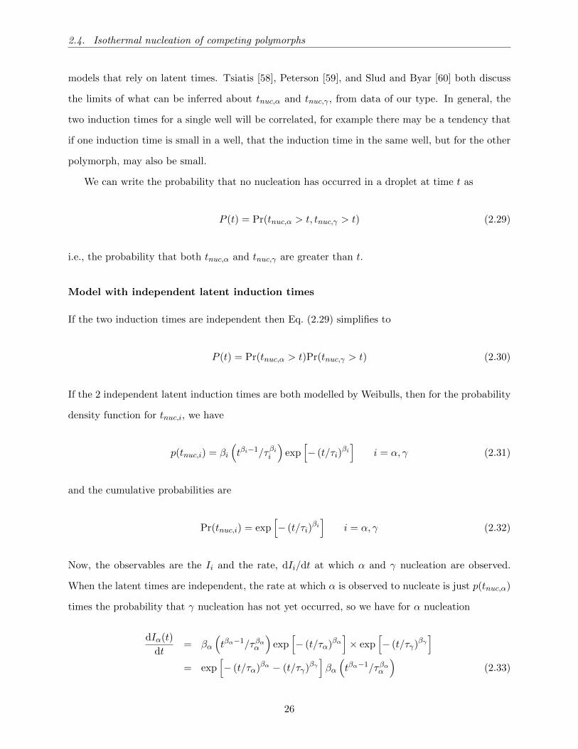
2.4. Isothermal nucleation of competing polymorphs
models that rely on latent times. Tsiatis [58], Peterson [59], and Slud and Byar [60] both discuss
the limits of what can be inferred about tnuc,α and tnuc,γ , from data of our type. In general, the
two induction times for a single well will be correlated, for example there may be a tendency that
if one induction time is small in a well, that the induction time in the same well, but for the other
polymorph, may also be small.
We can write the probability that no nucleation has occurred in a droplet at time t as
P (t) = Pr(tnuc,α > t, tnuc,γ > t) (2.29)
i.e., the probability that both tnuc,α and tnuc,γ are greater than t.
Model with independent latent induction times
If the two induction times are independent then Eq. (2.29) simplifies to
P (t) = Pr(tnuc,α > t)Pr(tnuc,γ > t) (2.30)
If the 2 independent latent induction times are both modelled by Weibulls, then for the probability
density function for tnuc,i, we have
p(tnuc,i) = βi
(tβi−1/τβii
)exp
[− (t/τi)
βi]
i = α, γ (2.31)
and the cumulative probabilities are
Pr(tnuc,i) = exp[− (t/τi)
βi]
i = α, γ (2.32)
Now, the observables are the Ii and the rate, dIi/dt at which α and γ nucleation are observed.
When the latent times are independent, the rate at which α is observed to nucleate is just p(tnuc,α)
times the probability that γ nucleation has not yet occurred, so we have for α nucleation
dIα(t)
dt= βα
(tβα−1/τβαα
)exp
[− (t/τα)βα
]× exp
[− (t/τγ)βγ
]= exp
[− (t/τα)βα − (t/τγ)βγ
]βα
(tβα−1/τβαα
)(2.33)
26
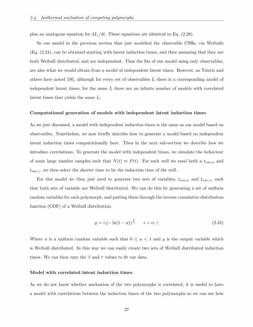
2.4. Isothermal nucleation of competing polymorphs
plus an analogous equation for dIγ/dt. These equations are identical to Eq. (2.28).
So our model in the previous section that just modelled the observable CSHs, via Weibulls
(Eq. (2.24), can be obtained starting with latent induction times, and then assuming that they are
both Weibull distributed, and are independent. Thus the fits of our model using only observables,
are also what we would obtain from a model of independent latent times. However, as Tsiatis and
others have noted [58], although for every set of observables Ii there is a corresponding model of
independent latent times, for the same Ii there are an infinite number of models with correlated
latent times that yields the same Ii.
Computational generation of models with independent latent induction times
As we just discussed, a model with independent induction times is the same as our model based on
observables. Nonetheless, we now briefly describe how to generate a model based on independent
latent induction times computationally here. Then in the next sub-section we describe how we
introduce correlations. To generate the model with independent times, we simulate the behaviour
of some large number samples such that N(t) ≈ P (t). For each well we need both a tnuc,α and
tnuc,γ , we then select the shorter time to be the induction time of the well.
For this model we then just need to generate two sets of variables, tnuc,α and tnuc,γ , such
that both sets of variable are Weibull distributed. We can do this by generating a set of uniform
random variables for each polymorph, and putting them through the inverse cumulative distribution
function (CDF) of a Weibull distribution.
y = τi(− ln(1− u))1βi i = α, γ (2.34)
Where u is a uniform random variable such that 0 ≤ u < 1 and y is the output variable which
is Weibull distributed. In this way we can easily create two sets of Weibull distributed induction
times. We can then vary the β and τ values to fit our data.
Model with correlated latent induction times
As we do not know whether nucleation of the two polymorphs is correlated, it is useful to have
a model with correlations between the induction times of the two polymorphs so we can see how
27
2.4. Isothermal nucleation of competing polymorphs
well the model fits. To generate the model, as in the previous section, we want two sets of Weibull
distributed numbers for tnuc,α and tnuc,γ . In this case however we want those two sets of numbers
to be correlated such that for a well with a short α induction time there is a high probability of a
short γ induction time
We set about generating these variables as follows. We generate two correlated sets of numbers,
both Gaussian distributed. We then put each number into a Gaussian CDF which transforms
them to uniformly distributed numbers between zero and one. After that, we put the uniformly
distributed numbers into an inverse Weibull CDF (Equation 2.34). At this point, we have two
Weibull distributed sets of numbers that are correlated. By generating a large number of induction
time pairs, we obtain Iα and Iγ pairs where the α and γ nucleation processes have the desired
correlation. So we can use these generated distributions to fit our data. In Chapter 6, we fit this
model to our experimental data, the program we used to fit the model is shown in section C.2.
Measuring correlation
We use Spearman’s rank coefficient [66] to measure correlation in this model. We briefly explain
how this metric works. For each sample we have two times: tnuc,α and tnuc,γ . We rank all the
tnuc,α, for all samples in order of increasing length. We do the same with the set of tnuc,γ . We
then measure for each pair of times the difference between the tnuc,α rank, rα and tnuc,γ rank, rγ .
For example, if we have 100 samples we take the induction times, (tnuc,α,tnuc,γ) and if for the pair,
tnuc,α is the 6th longest induction time (rα = 6) and tnuc,γ is the 11th longest induction time (rγ
= 11). The difference in ranks, rγ − rα is 5. Note that if tnuc,α and tnuc,γ are perfectly correlated
all their ranks will be the same, rγ = rα.
We measure the difference in rank for each pair of variables. The sum of the square rank
differences is the covariance of rα and rγ . The formula we use to calculate Spearman’s rank
correlation coefficient, Rs, is
Rs =cov(rα, rγ)
σrασrγ(2.35)
where σrα and σrγ are the standard deviations of all rα and rγ respectively and cov(rα, rγ) is the
covariance of rα and rγ . When data are strongly positively correlated Rs approaches 1, when data
are uncorrelated Rs is close to zero and when data are strongly negatively correlated Rs approaches
28

2.4. Isothermal nucleation of competing polymorphs
-1.
Spearman’s rank coefficient is a useful way of measuring correlation because it only looks at
the rank of numbers and not their absolute values. It makes no assumption about the functional
form of the correlation between α and γ nucleation. Spearman’s rank is also useful in that the
coefficient does not change when we change our correlated data from normally distributed data to
Weibull distributed data. This avoids any ambiguity.
29
3. Literature Review
In this chapter we review the relevant literature. We primarily focus on studies of glycine and
quantitative studies of nucleation. The chapter is split into three main sections. In the next
section we briefly discuss some of the techniques that have been used to analyse supersaturated
solutions and crystallisation. In the second section we look at quantitative studies of nucleation.
We primarily look at nucleation of crystals from solution with the exception of ice nucleation which
we discuss because it has been so extensively studied. Finally we look at studies of glycine. We
look at studies of glycine in solution, studies of glycine nucleation, and lastly, studies of glycine
crystal growth.
3.1 Analytical Techniques
A number of analytical techniques have been used to study crystallisation and nucleation. Here
we describe some of those techniques and how they have been used in the literature. There are
generally several types of use for these techniques: to analyse solutions before crystallisation, to
infer information about crystal structure (e.g., polymorphism), to infer information about crystal
habit and surface morphology, and finally to determine when phase transitions are occurring.
3.1.1 Analysing solutions and nucleation precursors
First we look at techniques that have been used to analyse solutions prior to crystallisation.
Nanoparticle Tracking Analysis (NTA) and Dynamic Light Scattering (DLS) are used to deter-
mine the size of species contained in a solution. They have been used to analyse the size and
concentration of any nucleation precursors that are present in solution [27,67]. Small Angle X-ray
Scattering (SAXS) is a technique that can be used to characterise the size of species in solution.
It has been used to determine emulsion droplet sizes [25], and also to analyse the proportion of
glycine that exists as dimers in solution [68]. Transmission electron microscopy (TEM) is an imag-
30

3.1. Analytical Techniques
ing technique that allows the user to image materials at a higher resolution than would be possible
with visible light. It has been used to record in real time the formation of pre-nucleation clusters
in solution. [69]
3.1.2 Morphology and crystal habit
Here we discuss techniques used to look at habit and morphology. The most common technique used
to look at habit and growth is basic optical microscopy. Growth rates can often be of the order of
µm/s so microscopy is accurate enough to detect the small changes in size. Atomic force microscopy
(AFM) can be used to analyse the surface morphology of a crystal up to sub-nm resolutions. [70,71].
Meirzadeh et al. [71] use this technique to observe the presence of thin hydrated layers on α glycine
crystals. Scanning Electron Microscopy (SEM) is another technique that has been used to look
at morphology. It has been used to image the impurity NX illite [72] which is known to aid ice-
nucleation in clouds. It has also been used to observe the crystal habit and morphology of glycine
crystals in high-resolution [23,26].
3.1.3 Polymorphism
X-ray Diffraction (XRD) is probably the most widespread technique to be used in crystallisation
studies. It is often used to determine the polymorphism of crystals [29, 33, 35, 73–75]. Raman
spectroscopy and Fourier Transform Infra-Red spectroscopy (FTIR) are also commonly used to
determine the polymorphism of crystals [76–79]. They can also be used to identify the presence of
functional groups when analysing a molecule of unknown composition.
Raman spectroscopy is dependant on light being scattered by electrons in a material while
FTIR is dependant on absorbance. Here, the Raman light scattering is dependant on the change
in polarizability of a molecule while the IR absorbance depends on a change in the dipole moment
when vibrating. The result of this is that the two techniques are suited to looking at different kinds
of bonds in materials. They are therefore often nice complementary techniques. Raman has the
advantage that it can analyse any type of sample, while powder XRD requires sample preparation.
In particular for powder XRD, it has to be used on dry samples, while Raman spectroscopy can be
used in-situ on crystals within the solution they have crystallised from [9].
31
3.2. Nucleation Studies
3.2 Nucleation Studies
Experimental studies of nucleation events can generally be assigned to two categories: Those in
which supersaturation is varying during the experiment and experiments at constant supersatu-
ration. We refer to the latter case as isothermal experiments because to keep supersaturation
constant, temperature and concentration must be kept constant throughout. In practice there
is usually some rapid cooling at the start of the experiment over a short timescale after which
the temperature remains constant. Many interesting results have been achieved with temperature
varying experiments [13, 80] and models describing nucleation as a function of temperature [81].
These experiments have certain advantages, for example, being able to observe the nucleation of
all samples within an experiment and also being able to carry out the experiment over a shorter
timescale than is possible with isothermal experiments [13]. The problem with these experiments
however is the nucleation rate of each sample changes throughout the experiment. Temperature
and therefore supersaturation change throughout the experiment and the nucleation rate depends
on both these quantities, see Equation 2.4 and Equation 2.5. This makes it harder to draw mean-
ingful conclusions from these experiments. For these reasons, and because they are more relevant
to our work, throughout this section we mainly focus on reviewing isothermal studies.
3.2.1 Ice nucleation
The most studied material in crystallisation studies to date is probably ice. Although ice crystalli-
sation is very different to glycine crystallisation i.e, glycine is crystallised from solution while ice is
crystallised from its liquid form, we can learn from these studies because some aspects of nucleation
are applicable to many systems. Crystal nucleation is a central process in atmospheric physics as it
determines the rate at which water droplets transform to ice crystals in clouds [13,14,82–85]. Due
to the large free energy barrier associated with the nucleation of ice from water droplets in clouds,
the clouds may have to cool to low temperatures, as low as around 240 K, [13] before crystallising.
It is known that the number of impurities in a water droplet can determine the number and size
of ice particles in the cloud, affecting the cloud lifespan [14]. There have been many studies of the
impurities upon which heterogeneous ice nucleation may occur in clouds [13,14,83]. Homogeneous
ice nucleation is rare to observe, but has also been studied [82, 84], where nucleation can occur at
32
3.2. Nucleation Studies
temperatures as low as ≈236 K. There have also been efforts to model ice nucleation computation-
ally [86, 87]. We see from studies of ice nucleation, that nucleation is usually heterogeneous, and
nucleation is very sensitive to impurities.
3.2.2 Nucleation Precursors
A nucleation precursor is a cluster or structure that appears in solution and that may play a role
in nucleation. A significant amount of literature focuses on nucleation precursors [88]: it has been
speculated that precursors represent an intermediate stage in nucleation, making nucleation a two-
step process [89]. Evidence of stable ‘pre-nucleation clusters’ existing in solution has been noted
in several different systems [90–93]. Gebauer et al. [92], looking at aqueous calcium carbonate,
found the existence of ion clusters several nanometres in size present in supersaturated solutions.
Gebauer et al. speculated that these clusters act as a precursor and hence play a role in nucleation.
Precursors have also been observed in protein solutions, although these are much larger with radii
of the order of hundreds of nanometres and are sometimes liquid-like in nature [27,94,95].
3.2.3 Heterogeneous and homogeneous nucleation
Observation of homogeneous nucleation is rare. Some experiments in the literature may have ob-
served homogeneous nucleation [39, 96], leading to a constant effective nucleation rate. Massa et
al. [39] study the polymer Poly(ethylene oxide) crystallisation in droplets. They provide evidence
of homogeneous nucleation in the form of a nucleation rate that is proportional to volume. Hetero-
geneous nucleation can also give a nucleation rate that is constant and scales with volume, provided
there are many nucleation sites in each sample and the distribution of rates is narrow. It is there-
fore challenging to prove that nucleation is occurring homogeneously. Conversely, heterogeneous
nucleation is commonly observed [73, 97–101]. It is also easy to prove heterogeneous nucleation
is occurring, in that, an effective nucleation rate that decreases over time indicates heterogeneous
nucleation. It is not possible for homogeneous nucleation to give an effective nucleation rate that
decreases over time [40]. 1-step homogeneous nucleation gives a constant nucleation rate.
While in most studies nucleation is happening heterogeneously on impurities, there has been
some work on adding specific nucleation inducing impurities or ‘nucleants’ to the system in the hope
of accelerating the crystallisation process and controlling features of the nucleated crystal [73, 97–
33
3.2. Nucleation Studies
101]. There have been many investigations into nucleants, species that will increase the nucleation
rate [13,73]. Diao et al [37,73] study the nucleation of ROY (5-methyl-2-[(2-nitrophenyl)amino]-3-
thiophenecarbonitrile) from solution. They managed to control nucleation rate, and to some extent,
polymorphic outcome, using polymer microgels with different nanoscale sized meshes. There has
been interest in both carbon based materials [98,99], i.e, carbon nanotubes and graphene as well as
metal nanoparticles [100,101]. There is also work on finding materials that inhibit nucleation [80].
This is useful for situations where nucleation is unwanted, e.g, gas hydrates crystallising in oil
pipelines [102].
3.2.4 Isothermal experiments
There are many quantitative studies of induction times of crystals in the literature [16,23,33,103–
105]. Systems where the effective nucleation rate increases over time have been observed [23, 104].
Kim et al. [104] observe an increasing nucleation rate for the crystallisation of RDX (Hexahydro-
1,3,5-trinitro-1,3,5-triazine). They speculate that this unusual result for an experiment at constant
supersaturation is due to a 2-step nucleation pathway where slow growing pre-nucleation clusters
act as an intermediate phase.
The majority of experimental studies find an effective nucleation rate that decreases over time
[106]. For a set of droplets that can be described by Equation 2.13, where each droplet has a
constant nucleation rate but the nucleation rate of each droplet is different, we always find a
decreasing nucleation rate [45]. Often a decreasing effective nucleation rate is well fit by a Weibull
function [103, 106]. In some cases two-exponential models have been used to fit data [52]. The
Pound La Mer model is another popular model [49,107] for fitting this type of data.
The set-up used by Laval et al [107] is an interesting one. They cover supersaturated solutions
with a layer of oil to prevent evaporation. After performing a nucleation experiment in each of
their samples, they heat them to dissolve the nucleated crystals before cooling again to record more
induction times. By performing these experiments they are able to record multiple induction times
for the same sample. This allows them to observe if a sample has similar length induction times
across several runs which shows the effects of impurities on induction times.
There are many studies that look at crystal polymorphism and many studies that look at
induction times. However, to our knowledge, there are few studies that identify the induction times
34
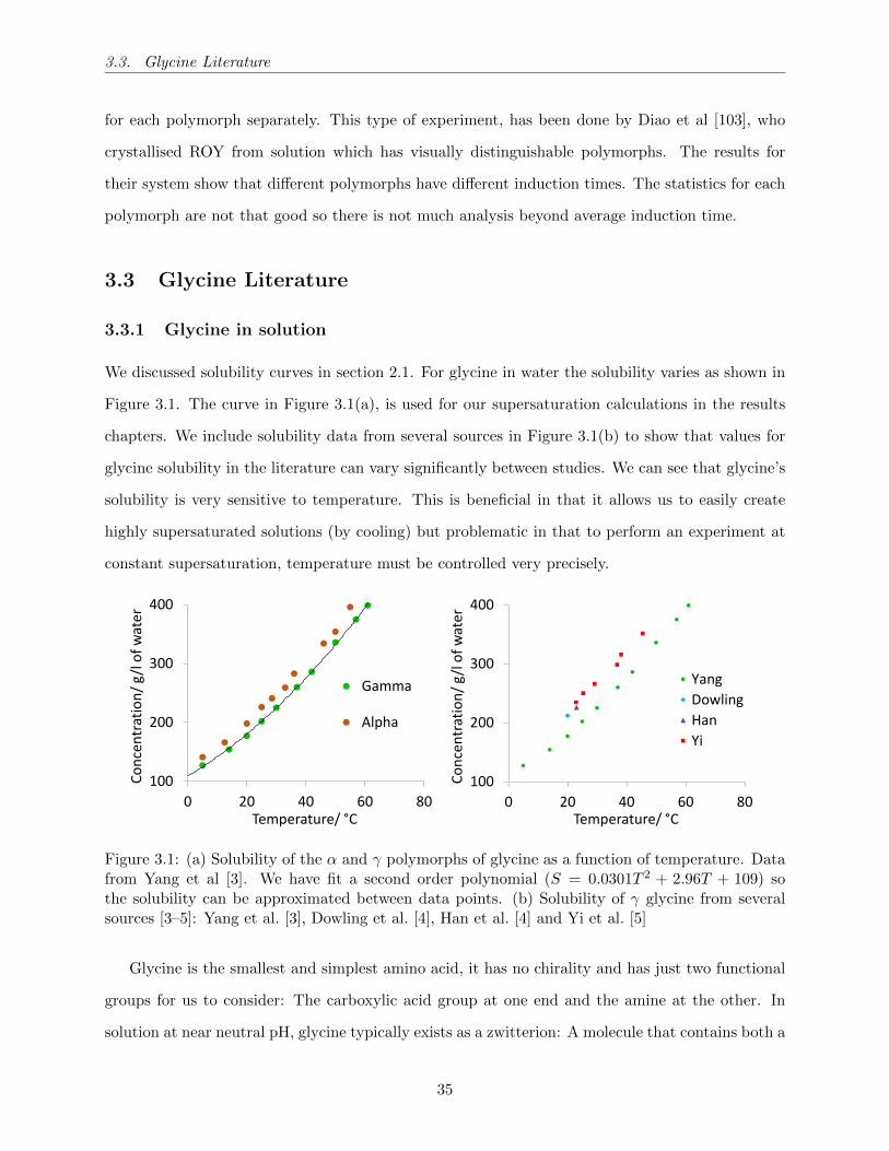
3.3. Glycine Literature
for each polymorph separately. This type of experiment, has been done by Diao et al [103], who
crystallised ROY from solution which has visually distinguishable polymorphs. The results for
their system show that different polymorphs have different induction times. The statistics for each
polymorph are not that good so there is not much analysis beyond average induction time.
3.3 Glycine Literature
3.3.1 Glycine in solution
We discussed solubility curves in section 2.1. For glycine in water the solubility varies as shown in
Figure 3.1. The curve in Figure 3.1(a), is used for our supersaturation calculations in the results
chapters. We include solubility data from several sources in Figure 3.1(b) to show that values for
glycine solubility in the literature can vary significantly between studies. We can see that glycine’s
solubility is very sensitive to temperature. This is beneficial in that it allows us to easily create
highly supersaturated solutions (by cooling) but problematic in that to perform an experiment at
constant supersaturation, temperature must be controlled very precisely.
100
200
300
400
0 20 40 60 80
Co
nce
ntr
atio
n/
g/l
of
wat
er
Temperature/ °C
Gamma
Alpha
100
200
300
400
0 20 40 60 80
Co
nce
ntr
atio
n/
g/l
of
wat
er
Temperature/ °C
Yang
Dowling
Han
Yi
Figure 3.1: (a) Solubility of the α and γ polymorphs of glycine as a function of temperature. Datafrom Yang et al [3]. We have fit a second order polynomial (S = 0.0301T 2 + 2.96T + 109) sothe solubility can be approximated between data points. (b) Solubility of γ glycine from severalsources [3–5]: Yang et al. [3], Dowling et al. [4], Han et al. [4] and Yi et al. [5]
Glycine is the smallest and simplest amino acid, it has no chirality and has just two functional
groups for us to consider: The carboxylic acid group at one end and the amine at the other. In
solution at near neutral pH, glycine typically exists as a zwitterion: A molecule that contains both a
35
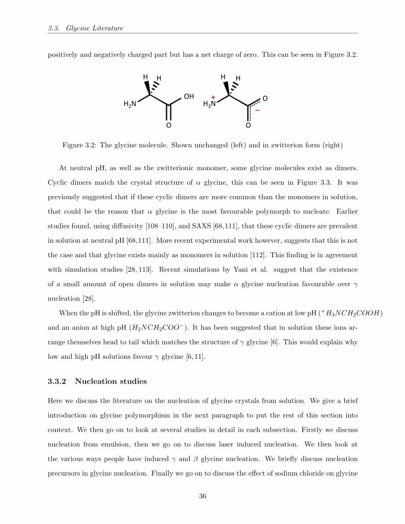
3.3. Glycine Literature
positively and negatively charged part but has a net charge of zero. This can be seen in Figure 3.2.
H H
OH
O
H2N
H H
O
O
H3N _+
Figure 3.2: The glycine molecule. Shown unchanged (left) and in zwitterion form (right)
At neutral pH, as well as the zwitterionic monomer, some glycine molecules exist as dimers.
Cyclic dimers match the crystal structure of α glycine, this can be seen in Figure 3.3. It was
previously suggested that if these cyclic dimers are more common than the monomers in solution,
that could be the reason that α glycine is the most favourable polymorph to nucleate. Earlier
studies found, using diffusivity [108–110], and SAXS [68,111], that these cyclic dimers are prevalent
in solution at neutral pH [68,111]. More recent experimental work however, suggests that this is not
the case and that glycine exists mainly as monomers in solution [112]. This finding is in agreement
with simulation studies [28, 113]. Recent simulations by Yani et al. suggest that the existence
of a small amount of open dimers in solution may make α glycine nucleation favourable over γ
nucleation [28].
When the pH is shifted, the glycine zwitterion changes to become a cation at low pH (+H3NCH2COOH)
and an anion at high pH (H2NCH2COO−). It has been suggested that in solution these ions ar-
range themselves head to tail which matches the structure of γ glycine [6]. This would explain why
low and high pH solutions favour γ glycine [6, 11].
3.3.2 Nucleation studies
Here we discuss the literature on the nucleation of glycine crystals from solution. We give a brief
introduction on glycine polymorphism in the next paragraph to put the rest of this section into
context. We then go on to look at several studies in detail in each subsection. Firstly we discuss
nucleation from emulsion, then we go on to discuss laser induced nucleation. We then look at
the various ways people have induced γ and β glycine nucleation. We briefly discuss nucleation
precursors in glycine nucleation. Finally we go on to discuss the effect of sodium chloride on glycine
36
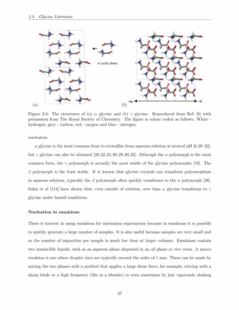
3.3. Glycine Literature
(a) (b)
Figure 3.3: The structures of (a) α glycine and (b) γ glycine. Reproduced from Ref. [6] withpermission from The Royal Society of Chemistry. The figure is colour coded as follows: White -hydrogen, grey - carbon, red - oxygen and blue - nitrogen.
nucleation.
α glycine is the most common form to crystallise from aqueous solution at neutral pH [6,20–32],
but γ glycine can also be obtained [20,22,25,26,29,30,32]. Although the α polymorph is the most
common form, the γ polymorph is actually the most stable of the glycine polymorphs [19]. The
β polymorph is the least stable. It is known that glycine crystals can transform polymorphism
in aqueous solution, typically the β polymorph often quickly transforms to the α polymorph [26].
Sakai et al [114] have shown that, even outside of solution, over time α glycine transforms to γ
glycine under humid conditions.
Nucleation in emulsions
There is interest in using emulsions for nucleation experiments because in emulsions it is possible
to quickly generate a large number of samples. It is also useful because samples are very small and
so the number of impurities per sample is much low than at larger volumes. Emulsions contain
two immiscible liquids, such as an aqueous phase dispersed in an oil phase or vice versa. A macro
emulsion is one where droplet sizes are typically around the order of 1 mm. These can be made by
mixing the two phases with a method that applies a large shear force, for example, stirring with a
sharp blade at a high frequency (like in a blender) or even sometimes by just vigorously shaking
37
3.3. Glycine Literature
the mixture. Microemulsions have droplet sizes of around the order of 10 nm. These are typically
made by mixing the oil and water phase with a surfactant and often a co-surfactant, which can
keep the emulsion stable by gathering at the water oil interfaces.
When crystallising from emulsion, the supersaturated solution is dispersed in an oil phase. The
size of crystals formed using this technique generally depends on the droplet size. The surfactant
used to stabilize the emulsion can affect the nucleation process. Toldy et al. [23] use a microfluidics
set-up to obtain significant nucleation statistics. By heating the emulsion they induce evaporation of
the aqueous phase from the emulsion after which their experiments are at constant supersaturation.
They observe nucleation over a timescale of hundreds of seconds. Surprisingly, they observe an
increasing effective nucleation rate but suggest adjacent samples may not be independent of one
another, i.e, nucleation in one droplet may trigger nucleation in nearby droplets. Chen et al. [25] also
use microemulsions but superstaurate their solutions by adding the anti-solvent, methanol. They
find that for emulsions stabilized with the surfactants span 80 and Brij 30 the glycine polymorph
produced is dependant on supersaturation. The γ polymorph is produced at lower supersaturation
S = 2.3, and α and β are produced at higher supersaturation S = 2.6. When the surfactant used is
changed to AOT (sodium bis-2-ethyl sulfosuccinate), they find nucleation occurs at a much lower
supersaturation of S = 1.2 and they obtain the γ polymorph. They observe nucleation over a
timescale of weeks. Allen et al. [26] find that for macroemulsions stabilized with span 80 and span
20 they obtain the β polymorph over a timescale of about 5 h. For microemulsions stabilized with
AOT, They observe nucleation over a timescale of weeks. They find that the γ polymorph nucleates
more frequently at lower supersaturations of S = 1.1 and almost entirely α nucleates at S = 1.5.
Laser induced nucleation
A number of studies have also been carried out on laser induced nucleation of glycine [75,115–117].
Zaccaro et al. [75] found that when glycine solution is subjected to pulses of laser light, at near
infra-red frequencies, nucleation occurs, and the γ polymorph forms. Rungsimanon et al. [117]
use a continuous IR laser beam in their setup. They suggest that the probability of getting the
γ polymorph of glycine increases with photon pressure but decreases with the localised heating
caused by the laser. They speculate that photon pressure is proportional to laser power but
that the localised heating increases nonlinearly with laser power. They therefore conclude that
38
3.3. Glycine Literature
there is some optimum laser power that can be used to obtain the highest γ glycine yield and
that below this power, less γ glycine is obtained due to the lower photon pressure but above this
optimum power, less γ glycine is obtained due to the supersaturation decrease from the localised
heating. Javid et al. [116] use a pulsed laser set up and carry out experiments at several different
supersaturations. They show that with their set up, the chance of obtaining the γ polymorph
increases as supersaturation increases. They also show that filtering solutions prior to irradiation
can suppress laser induced nucleation.
Nucleation of glycine’s polymorphs
Here we discuss studies that have obtained γ glycine. The γ polymorph of glycine has been obtained
using a number of different techniques. Han et al. have obtained γ glycine by varying pH [6, 11].
They worked with glycine solutions of around 100 ml, being constantly stirred in a glass beaker.
They found that α glycine was obtained at neutral pH but when various acids and bases were
present, i.e, KOH, HNO3, HCl and NaOH, the γ polymorph was obtained. Yogambal et al. [118]
have been able to obtain the γ polymorph by slowly evaporating glycine solution in the presence of
KCl. They performed their experiments in a petri dish and typically observed crystallisation over
a timescale of days. Other salts are also known to promote γ glycine. He et al. [29] crystallized by
slowly evaporating from a single droplet. Using this technique they are able to obtain γ glycine.
Here we discuss studies that have obtained β glycine. It is rare to observe the metastable β
polymorph of glycine but it has been obtained. Devi et al. [74] use a set-up where they rapidly
cool solutions to supersaturate them at the start of experiments, after which the remainder of
the experiment is isothermal. The samples are stirred throughout the experiments. They find at
low supersaturations, S = 1.2 - 1.4, they obtain the β polymorph. This is an unusual example
of the β polymorph nucleating without the use of anti-solvents or additives. Torbeev et al. [119]
have also observed β glycine. They add various amino acids to the supersaturated glycine solution
and find different amino acids can be used to induce each of glycine’s polymorphs. Kim et al.
[36], use a patterned substrate with hydrophilic islands on a hydrophobic substrate. They then
dip the substrate into glycine solution and when they remove it the hydrophilic islands act as
sample holders, keeping the droplets separated. They find that by cooling the solutions they obtain
almost entirely β glycine with small amounts of α present but with slow evaporation they obtain
39

3.3. Glycine Literature
a significant amount of all three polymorphs. They conclude that the polymorph that nucleates is
heavily influenced by the rate at which supersaturation is generated. Using the same set-up, Lee
et al. [78] showed that pH can also be used to influence the amount of each of glycine’s polymorphs
forming. They found that by making solution either more acidic or more basic they significantly
increased the probability of γ glycine forming.
Nucleation Precursors
There has been research into nucleation precursors for glycine. Jawor-Baczynska et al. [27, 67]
find the existence of both 1 nm molecular clusters and 250-750 nm amorphous mesospecies in
glycine solutions. They use DLS and NTA to observe pure water before adding glycine crystals.
These mesospecies are only detected upon the dissolution of the glycine crystals in the water
which shows these mesospecies must contain glycine and are not just impurities. They also show
these mesospecies have liquid like properties as applying a filter with a spacing smaller than the
mesospecies diameter does not remove them or even reduce the concentration of them in the
solution. They suggest that the larger 750 nm mesospecies may be nucleation precursors leading to a
2-step pathway for nucleation. They note that stirring the solution leads to an increased population
of the larger mesospecies which is a possible explanation for the increased nucleation rate when
stirring. Forsyth et al. [120, 121] show that the rate at which these mesospecies increase in size is
dependant on the shear rate and interfacial area of the solution. They also show that nucleation
rate is proportional to the product of the same two factors, shear rate and interfacial area. Thus
there is a correlation between these interesting structures and nucleation, but no direct evidence of
cause and effect. But it should be noted that as nucleation cannot be observed, establishing cause
and effect is very difficult.
Nucleation from Sodium Chloride Solution
In Chapter 6, we crystallise glycine from aqueous solution which also contains varying amounts
of sodium chloride (NaCl). We record induction times and the polymorph of the crystals formed.
There are several studies which look at the effect of salt on glycine crystallisation [8,34,35,122,123].
As we have discussed, when crystallising from neutral pH aqueous solution it is normal to obtain
the α polymorph. It is known that adding various salts, including NaCl, changes the polymorphic
40
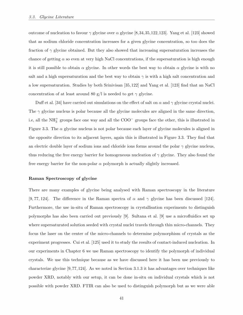
3.3. Glycine Literature
outcome of nucleation to favour γ glycine over α glycine [8,34,35,122,123]. Yang et al. [123] showed
that as sodium chloride concentration increases for a given glycine concentration, so too does the
fraction of γ glycine obtained. But they also showed that increasing supersaturation increases the
chance of getting α so even at very high NaCl concentrations, if the supersaturation is high enough
it is still possible to obtain α glycine. In other words the best way to obtain α glycine is with no
salt and a high supersaturation and the best way to obtain γ is with a high salt concentration and
a low supersaturation. Studies by both Srinivisan [35,122] and Yang et al. [123] find that an NaCl
concentration of at least around 80 g/l is needed to get γ glycine.
Duff et al. [34] have carried out simulations on the effect of salt on α and γ glycine crystal nuclei.
The γ glycine nucleus is polar because all the glycine molecules are aligned in the same direction,
i.e, all the NH+3 groups face one way and all the COO− groups face the other, this is illustrated in
Figure 3.3. The α glycine nucleus is not polar because each layer of glycine molecules is aligned in
the opposite direction to its adjacent layers, again this is illustrated in Figure 3.3. They find that
an electric double layer of sodium ions and chloride ions forms around the polar γ glycine nucleus,
thus reducing the free energy barrier for homogeneous nucleation of γ glycine. They also found the
free energy barrier for the non-polar α polymorph is actually slightly increased.
Raman Spectroscopy of glycine
There are many examples of glycine being analysed with Raman spectroscopy in the literature
[9, 77, 124]. The difference in the Raman spectra of α and γ glycine has been discussed [124].
Furthermore, the use in-situ of Raman spectroscopy in crystallisation experiments to distinguish
polymorphs has also been carried out previously [9]. Sultana et al. [9] use a microfluidics set up
where supersaturated solution seeded with crystal nuclei travels through thin micro-channels. They
focus the laser on the center of the micro-channels to determine polymorphism of crystals as the
experiment progresses. Cui et al. [125] used it to study the results of contact-induced nucleation. In
our experiments in Chapter 6 we use Raman spectroscopy to identify the polymorph of individual
crystals. We use this technique because as we have discussed here it has been use previously to
characterize glycine [9,77,124]. As we noted in Section 3.1.3 it has advantages over techniques like
powder XRD, notably with our setup, it can be done in-situ on individual crystals which is not
possible with powder XRD. FTIR can also be used to distinguish polymorph but as we were able
41

3.3. Glycine Literature
to do it with Raman spectroscopy alone and there are no drawbacks to using Raman spectroscopy
with our setup we were able to use just that one technique for determining polymorph.
3.3.3 Crystal Growth
There have been many studies in the literature on the growth rate of glycine crystals. Experimental
set-ups and supersaturations vary and measured growth rates for glycine vary from µm/h to mm/s,
a dynamic range of 106 [4, 7–9, 11, 23, 126]. Growth rates measured in several different studies are
plotted in Figure 3.4. We can see from Figure 3.4 that growth rates are strongly dependant on
supersaturation. We also see that there is a wide range of measured growth rates depending on
experimental set up. More details of the set ups of the data in Figure 3.4 are given in Table 3.1.
There was one growth rate, measured by Toldy et al. of ≈ 8× 104µm/min which was too large to
fit on our graph. Toldy et al. estimate the supersaturation in their experiments to be between 3.5
and 6.5 which varies between droplets. We can therefore say growth rate is heavily dependant on
supersaturation.
We can see in Figure 3.4 that for the α polymorph, growth along the c-axis (green) is generally
faster than growth along the b-axis (pink). This is found by all the studies shown here [4, 7, 9].
The shape of the α polymorph when grown in aqueous solution can be described as prismatic
bipyramidal [9,11]. There have been numerous studies looking at the effect of additives on crystal
habit. Weissbuch et al. [127, 128] observed that when crystallising α glycine, the crystal habit
changes when small amounts of other amino acids are added to the glycine solution. Dependent on
the chirality of those amino acids added the habit that forms can be pyramidal or even disk shaped
[9, 127, 128]. Simulations by Poornachary et al. [129, 130] suggest the effect on habit is dependant
on the solution speciation (by speciation we mean whether the additive exists as zwitterions or
anions etc. in solution) of the introduced additive and the preference of those species to interact
with certain crystal faces.
It is known that the α polymorph of glycine has a faster growth rate compared to the γ
polymorph [4,24], which can be seen in Figure 3.4. Han et al. [11] found that, at equal concentration,
α glycine growth is approximately 1.5 times faster than γ glycine.
In the growth of γ glycine, Dowling [131] suggests that growth along the b-axis of gamma
glycine is dependant on the c-axis growth rate. Below a supersaturation of ≈ 1.32 growth along
42
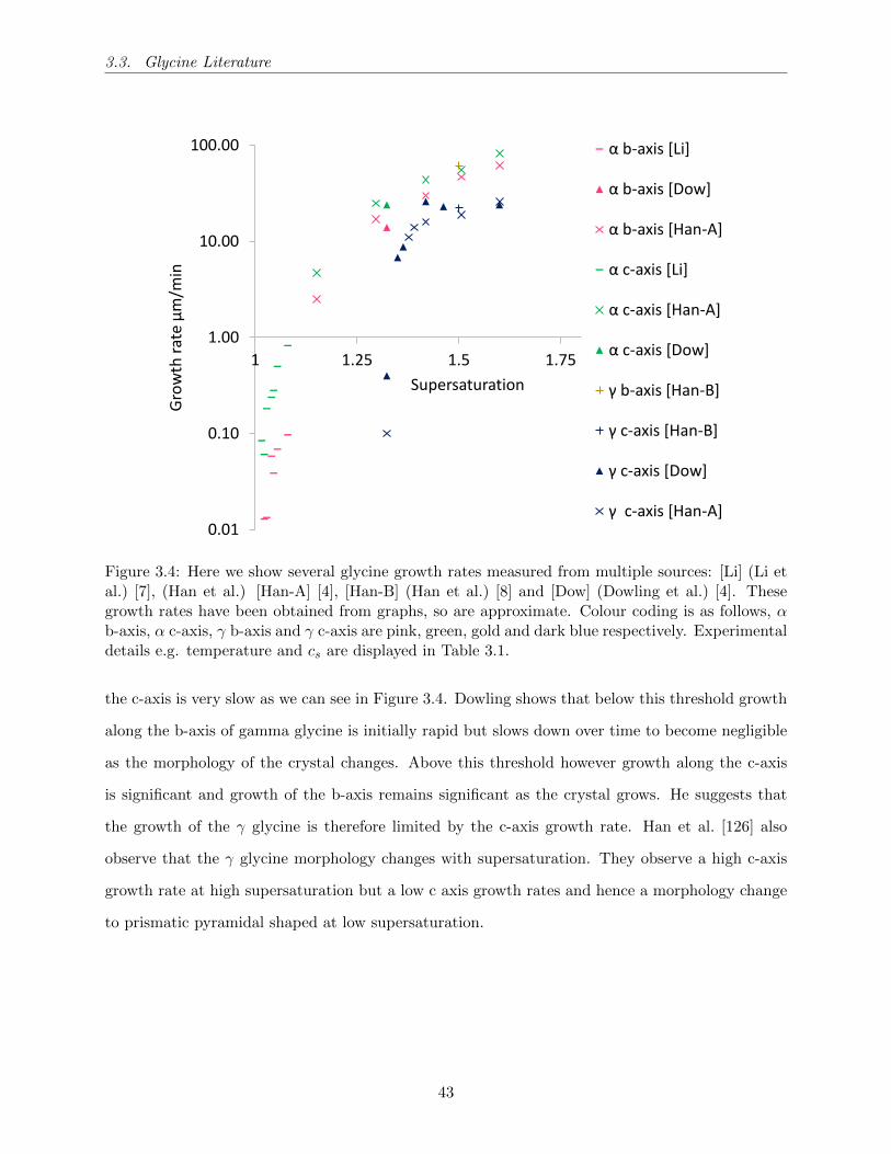
3.3. Glycine Literature
0.01
0.10
1.00
10.00
100.00
1 1.25 1.5 1.75
Gro
wth
rat
e μ
m/m
in
Supersaturation
α b-axis [Li]
α b-axis [Dow]
α b-axis [Han-A]
α c-axis [Li]
α c-axis [Han-A]
α c-axis [Dow]
γ b-axis [Han-B]
γ c-axis [Han-B]
γ c-axis [Dow]
γ c-axis [Han-A]
Figure 3.4: Here we show several glycine growth rates measured from multiple sources: [Li] (Li etal.) [7], (Han et al.) [Han-A] [4], [Han-B] (Han et al.) [8] and [Dow] (Dowling et al.) [4]. Thesegrowth rates have been obtained from graphs, so are approximate. Colour coding is as follows, αb-axis, α c-axis, γ b-axis and γ c-axis are pink, green, gold and dark blue respectively. Experimentaldetails e.g. temperature and cs are displayed in Table 3.1.
the c-axis is very slow as we can see in Figure 3.4. Dowling shows that below this threshold growth
along the b-axis of gamma glycine is initially rapid but slows down over time to become negligible
as the morphology of the crystal changes. Above this threshold however growth along the c-axis
is significant and growth of the b-axis remains significant as the crystal grows. He suggests that
the growth of the γ glycine is therefore limited by the c-axis growth rate. Han et al. [126] also
observe that the γ glycine morphology changes with supersaturation. They observe a high c-axis
growth rate at high supersaturation but a low c axis growth rates and hence a morphology change
to prismatic pyramidal shaped at low supersaturation.
43
3.3. Glycine Literature
Table 3.1: The experimental details of a number of studies on glycine growth. The growth ratesfrom these studies are shown in Figure 3.4.
Authors Supersaturation
range
Experimental set-up
Toldy et al. [23] 3.5− 6.5Crystals nucleate in supersaturated droplets within an emulsion
at 84C. Crystals sizes are of the order of tens of µm.
Dowling et al. [4] 1.3− 1.45
Individual crystals seeds are placed in supersaturated solution and
observed under a microscope at 20C. crystal sizes are of the order
of mm. cs is given as 212 g/l.
Han et al. [4] 1.15− 1.6
Individual crystals seeds are placed in supersaturated solution and
observed under a microscope at 23C. Crystal sizes are of the order
of mm. cs is given as 226 g/l.
Li et al. [7] 1.01− 1.08
Crystal seeds are placed in a glass cell at 23C while supersatu-
rated solution flows through the cell, seed sizes are of the order of
hundreds of µm.
Han et al. [8]
(2015)1.5
Set-up is same as in [4]
44

3.3. Glycine Literature
3.3.4 Crystal growth in the presence of salt
The effect of NaCl on γ glycine growth has been looked at by Han et al [8]. In that study [8], the γ
glycine growth rate in ultrapure water and 1.5 M (≈ 100 g/l of water) NaCl solution were compared.
The results from that study are shown in Table 3.2 The changes in growth rates along both axes
are small but they observe in the presence of NaCl, growth is slower along the c-axis and faster
along the b-axis changing the habit of the crystal to a less needle like shape. The α polymorph has
been studied in the presence of salt by Srinivasan and Arumugam [35], they do not present growth
rate as such but data on the final aspect ratio. When crystallised from aqueous solution glycine is
typically longest along its c-axis [35]. They find however, that as NaCl concentration increases, the
crystals become longer across the a-axis than the c-axis. This implies a shift in the relative growth
rates of the two axes.
Table 3.2: A table of γ glycine growth rates as a function of salt concentration, from a study by
Han et al [8]. Growth rates have been measured along the γ polymorph’s two axes in aqueoues
solution and 1.5m NaCl solution. The rates have been interpreted from Figures 6 and 10 of thier
study, so are approximate.
Solution conditions Growth rate/ µm/s
B-axis C-axis
aqueous solution 1.0 0.37
1.5m NaCl solution 1.1 0.32
In these last two sections we have looked at studies of glycine growth. The main finding of
the previous section was that growth rate is very sensitive to supersaturation. The literature also
showed that α glycine has similar growth rate along both axes, but γ glycine can have very different
growth rates along its axes. In this section we found that the effect of NaCl on glycine growth rate
was very small.
45
3.4. Summary
3.4 Summary
In this chapter we have discussed the relevant literature. Here we briefly discuss the gaps in the
literature that our work addresses. We introduce the well known KS test and KS two-sample test.
The former can be used to determine how well a model fits experimental data. The latter is a
useful tool to test for experimental reproducibility. Reproducibility problems are well known in
the field but rarely approached quantitatively. We hope introducing these tests will help address
these problems. As we have discussed there is only one set of polymorph-separated induction time
distributions for any material in the literature that we are aware of [37]. Our work is the first study
where these polymorph-separated induction time distributions are modelled. We introduce ideas
from medical statistics for analogous systems to specify the limitations of our model. This is also
the first study where these types of distributions have been recorded for glycine.
46

4. Methods
In this chapter we explain the methods used in our experiments. The experimental method is
largely the same for our two results chapters but with two notable differences. In Chapter 5 our
solutions contain just glycine in water, whereas in Chapter 6, sodium chloride is also present in
the aqueous glycine solution. The other difference is in Chapter 6, an additional technique, Raman
spectroscopy is used to identify polymorphism of individual glycine crystals.
4.1 Materials
Glycine solutions were made by adding solid glycine (99% HPLC from Sigma, cat. no. G7126) to
deionized water (Milli-Q, 18.2 MΩ cm) in a glass vial. This solid glycine consisted of mainly the γ
polymorph but had a small amount of the α polymorph; the XRD pattern is shown in Appendix
A.3. We fully dissolved the glycine during preparation of the solution. Experiments were carried
out at concentrations, c, in the range from 306.66 to 353.33 g/l of water. The solution was heated
to 70 C in a sealed vial and stirred at 1200 rpm for 1 h using a hot plate and magnetic stirrer bar.
The pH of a solution with c = 333.33 g/l of water was 6.2 ± 0.1, as obtained using a digital pH
meter. The set-up for sample preparation is shown in Figure 4.1.
4.2 Crystallisation experiments
Each experiment used a microplate (Nunclon Delta Surface) with 96 wells (arranged as 8 rows of 12
wells). For each run, a new microplate was used. Each well initially contained 100 µL of tridecane
(99% from Sigma-Aldrich, which has the chemical formula C13H28). We chose tridecane because
of its very low vapour pressure (0.056 mmHg at 25 C [38]) and very low miscibility with water.
At 25 C, the mole fraction solubility of water in tridecane is 6.1 × 10⁻⁴ [132]. The mole fraction
solubility of dodecane (C12H26), in water is 8.9× 10⁻¹⁰ [132]. Tridecane is a slightly larger alkane
47
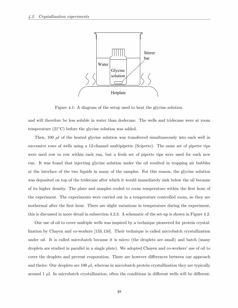
4.2. Crystallisation experiments
Hotplate
Water
Glycinesolution
Stirrerbar
Figure 4.1: A diagram of the setup used to heat the glycine solution.
and will therefore be less soluble in water than dodecane. The wells and tridecane were at room
temperature (21C) before the glycine solution was added.
Then, 100 µl of the heated glycine solution was transferred simultaneously into each well in
successive rows of wells using a 12-channel multipipette (Scipette). The same set of pipette tips
were used row to row within each run, but a fresh set of pipette tips were used for each new
run. It was found that injecting glycine solution under the oil resulted in trapping air bubbles
at the interface of the two liquids in many of the samples. For this reason, the glycine solution
was deposited on top of the tridecane after which it would immediately sink below the oil because
of its higher density. The plate and samples cooled to room temperature within the first hour of
the experiment. The experiments were carried out in a temperature controlled room, so they are
isothermal after the first hour. There are slight variations in temperature during the experiment,
this is discussed in more detail in subsection 4.2.3. A schematic of the set-up is shown in Figure 4.2.
Our use of oil to cover multiple wells was inspired by a technique pioneered for protein crystal-
lization by Chayen and co-workers [133, 134]. Their technique is called microbatch crystallization
under oil. It is called microbatch because it is micro (the droplets are small) and batch (many
droplets are studied in parallel in a single plate). We adopted Chayen and co-workers’ use of oil to
cover the droplets and prevent evaporation. There are however differences between our approach
and theirs: Our droplets are 100 µl, whereas in microbatch protein crystallization they are typically
around 1 µl. In microbatch crystallization, often the conditions in different wells will be different.
48
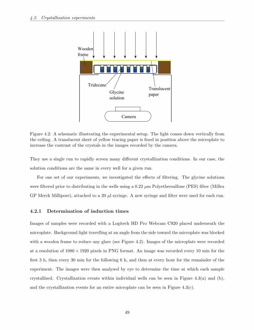
4.2. Crystallisation experiments
Camera
Tridecane
Glycine solution
Wooden frame
Translucent paper
Figure 4.2: A schematic illustrating the experimental setup. The light comes down vertically fromthe ceiling. A translucent sheet of yellow tracing paper is fixed in position above the microplate toincrease the contrast of the crystals in the images recorded by the camera.
They use a single run to rapidly screen many different crystallization conditions. In our case, the
solution conditions are the same in every well for a given run.
For one set of our experiments, we investigated the effects of filtering. The glycine solutions
were filtered prior to distributing in the wells using a 0.22 µm Polyethersulfone (PES) filter (Millex
GP Merck Millipore), attached to a 20 µl syringe. A new syringe and filter were used for each run.
4.2.1 Determination of induction times
Images of samples were recorded with a Logitech HD Pro Webcam C920 placed underneath the
microplate. Background light travelling at an angle from the side toward the microplate was blocked
with a wooden frame to reduce any glare (see Figure 4.2). Images of the microplate were recorded
at a resolution of 1080× 1920 pixels in PNG format. An image was recorded every 10 min for the
first 3 h, then every 30 min for the following 6 h, and then at every hour for the remainder of the
experiment. The images were then analysed by eye to determine the time at which each sample
crystallized. Crystallization events within individual wells can be seen in Figure 4.3(a) and (b),
and the crystallization events for an entire microplate can be seen in Figure 4.3(c).
49
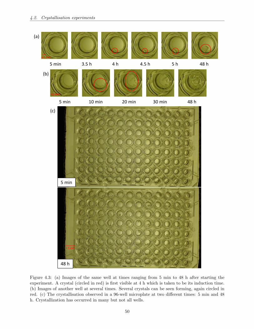
4.2. Crystallisation experiments
(a)
(b)
5 min 3.5 h 4 h 4.5 h 5 h 48 h
5 min 10 min 20 min 30 min 48 h
(c)
48 h
5 min
≈1 mm
≈1 mm
≈ 1 cm
Figure 4.3: (a) Images of the same well at times ranging from 5 min to 48 h after starting theexperiment. A crystal (circled in red) is first visible at 4 h which is taken to be its induction time.(b) Images of another well at several times. Several crystals can be seen forming, again circled inred. (c) The crystallisation observed in a 96-well microplate at two different times: 5 min and 48h. Crystallization has occurred in many but not all wells.
50
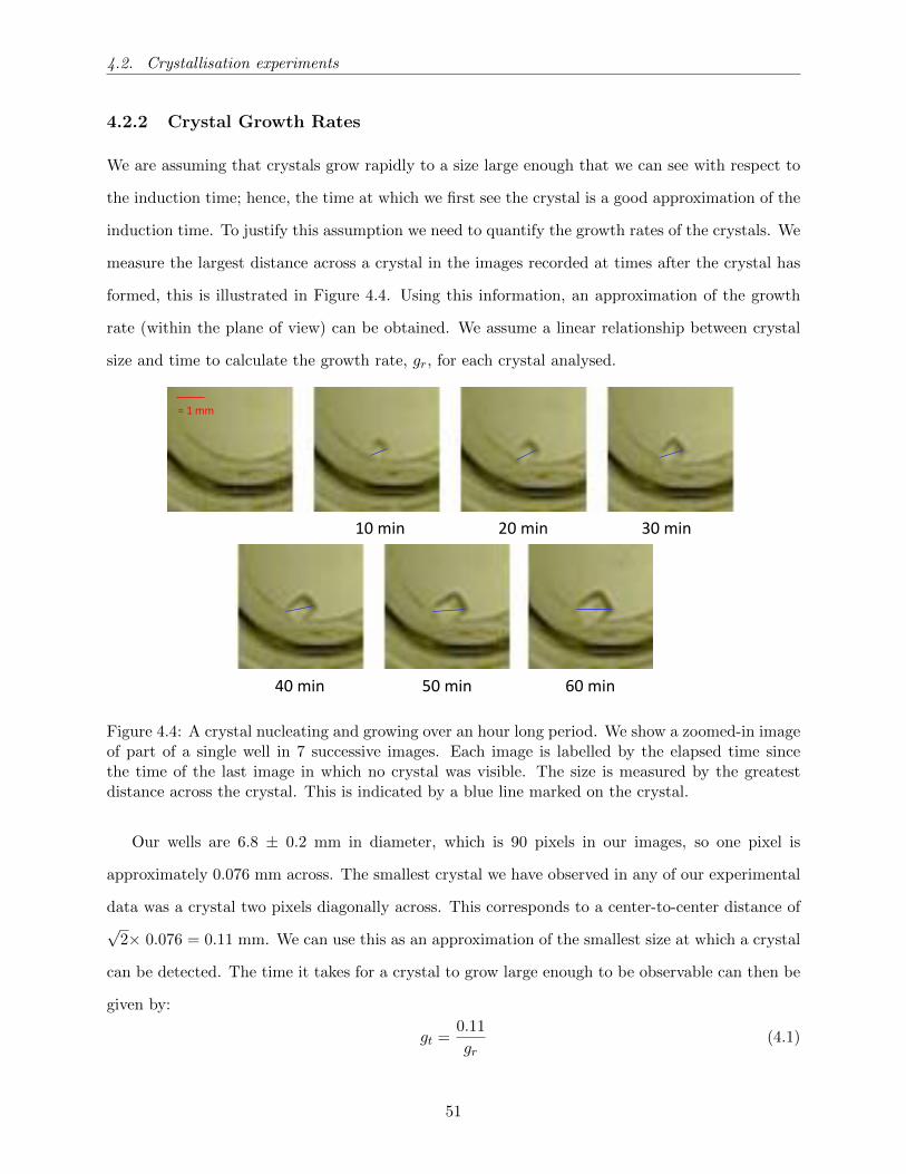
4.2. Crystallisation experiments
4.2.2 Crystal Growth Rates
We are assuming that crystals grow rapidly to a size large enough that we can see with respect to
the induction time; hence, the time at which we first see the crystal is a good approximation of the
induction time. To justify this assumption we need to quantify the growth rates of the crystals. We
measure the largest distance across a crystal in the images recorded at times after the crystal has
formed, this is illustrated in Figure 4.4. Using this information, an approximation of the growth
rate (within the plane of view) can be obtained. We assume a linear relationship between crystal
size and time to calculate the growth rate, gr, for each crystal analysed.
10 min 20 min 30 min
40 min 50 min 60 min
≈ 1 mm
Figure 4.4: A crystal nucleating and growing over an hour long period. We show a zoomed-in imageof part of a single well in 7 successive images. Each image is labelled by the elapsed time sincethe time of the last image in which no crystal was visible. The size is measured by the greatestdistance across the crystal. This is indicated by a blue line marked on the crystal.
Our wells are 6.8 ± 0.2 mm in diameter, which is 90 pixels in our images, so one pixel is
approximately 0.076 mm across. The smallest crystal we have observed in any of our experimental
data was a crystal two pixels diagonally across. This corresponds to a center-to-center distance of√
2× 0.076 = 0.11 mm. We can use this as an approximation of the smallest size at which a crystal
can be detected. The time it takes for a crystal to grow large enough to be observable can then be
given by:
gt =0.11
gr(4.1)
51

4.2. Crystallisation experiments
In this equation gt is growth time and 0.11 is the size in mm at which we approximate a crystal can
be observed. We discuss the growth rates and times for crystals to be observable in more detail in
the two results chapters, as the experiments are at different supersaturations, and we see different
growth rates and times.
4.2.3 Temperature Control
Cooling of the microplate to room temperature. The plate and samples cooled to room
temperature within the first hour of the experiment. The temperature of a well in the centre of
the plate and of a well in one of the corners of the plate are plotted in Figure 4.5. The corner well
took 20 minutes to cool to within 1 C of room temperature. The centre well took 30 minutes to
cool to within 1 C of room temperature. Both wells were within 0.1 C of room temperature after
1 hour.
20
25
30
35
40
0 20 40 60
T/ °
C
t/ minutes
Corner well
Centre well
Figure 4.5: A plot of the temperature of the glycine solution in the wells as a function of time forthe hour after injecting the solution into the wells.
Temperature Variation. In our system an increase in supersaturation of 1% is enough to
increase the nucleation rate by about 10%. The equation used to calculate this percentage can be
seen in section 5.7. This means that supersaturation variations during an experiment have to be
kept significantly below 1% in size to avoid them affecting the measured rate. For a substance such
as glycine, whose solubility varies strongly with temperature, this implies keeping the temperature
constant to about 0.1C.
52

4.2. Crystallisation experiments
To clarify whether temperature variation was significant, the room temperature was recorded
over a one week time period. The room in which experiments were carried out was temperature
controlled, however temperature was found to vary slightly throughout the duration of experiments.
The mean temperature as a function of time of day can be seen in Figure 4.6. On average, the
temperature ranged from a minimum of 20.7 C at 04:00 to a maximum of 21.4 C at 12:00. The
temperature was not found to vary throughout the year, just between day and night. The solubility
of glycine is very sensitive to temperature, which means that supersaturation varies during the
experiments. Using published solubility data, [3] it can be estimated that the temperature difference
between 21.4 C (solubility = 186 g/l of water) and 20.7 C (183 g/l of water) corresponds to a
supersaturation change of around 1.7% during an experiment.
(a)
20.4
20.6
20.8
21
21.2
21.4
21.6
18/7/14 20/7/14 22/7/14 24/7/14 26/7/14
Tem
per
atu
re/
°C
Date & Time (b)
20.6
20.8
21.0
21.2
21.4
04:00 10:00 16:00 22:00 04:00
Tem
per
atu
re /
°C
Time of day
Figure 4.6: (a) The room temperature recorded over a one week time period. The red dots indicate4:00am of each day which is consistently when the temperature is observed to reach a minimum (b)Plot of the average room temperature plot as a function of time of day. Each average temperatureis the mean of 7 measurements taken across a one week period.
Heating samples. For one set of experiments carried out in Chapter 6 we heated our samples
18 hours into each experiment. We did this to attempt to slow down nucleation as the supersat-
uration decreases as temperature increases. Here we just focus on the experimental details. The
microplates (containing the samples) were heated in a Sanyo Mov-112F oven. The temperature
within the oven was measured to be 30.4 C which remained constant to 0.1 of a degree. The
samples were kept at this temperature in the oven for 48 h. The mass of the samples was measured
before and after experiments to check for evaporation. The microplate was found to be 0.1 g lighter
after the samples had been in the oven for 48 h. This corresponds to evaporation of 1% of the total
53
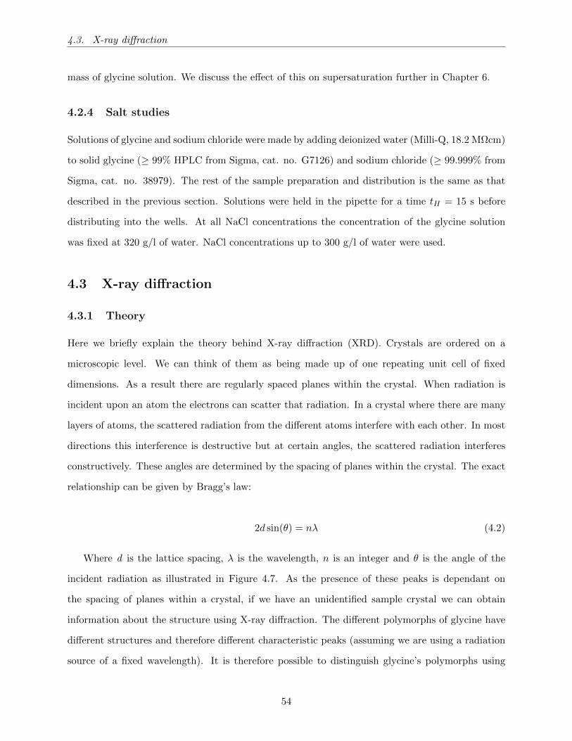
4.3. X-ray diffraction
mass of glycine solution. We discuss the effect of this on supersaturation further in Chapter 6.
4.2.4 Salt studies
Solutions of glycine and sodium chloride were made by adding deionized water (Milli-Q, 18.2 MΩcm)
to solid glycine (≥ 99% HPLC from Sigma, cat. no. G7126) and sodium chloride (≥ 99.999% from
Sigma, cat. no. 38979). The rest of the sample preparation and distribution is the same as that
described in the previous section. Solutions were held in the pipette for a time tH = 15 s before
distributing into the wells. At all NaCl concentrations the concentration of the glycine solution
was fixed at 320 g/l of water. NaCl concentrations up to 300 g/l of water were used.
4.3 X-ray diffraction
4.3.1 Theory
Here we briefly explain the theory behind X-ray diffraction (XRD). Crystals are ordered on a
microscopic level. We can think of them as being made up of one repeating unit cell of fixed
dimensions. As a result there are regularly spaced planes within the crystal. When radiation is
incident upon an atom the electrons can scatter that radiation. In a crystal where there are many
layers of atoms, the scattered radiation from the different atoms interfere with each other. In most
directions this interference is destructive but at certain angles, the scattered radiation interferes
constructively. These angles are determined by the spacing of planes within the crystal. The exact
relationship can be given by Bragg’s law:
2d sin(θ) = nλ (4.2)
Where d is the lattice spacing, λ is the wavelength, n is an integer and θ is the angle of the
incident radiation as illustrated in Figure 4.7. As the presence of these peaks is dependant on
the spacing of planes within a crystal, if we have an unidentified sample crystal we can obtain
information about the structure using X-ray diffraction. The different polymorphs of glycine have
different structures and therefore different characteristic peaks (assuming we are using a radiation
source of a fixed wavelength). It is therefore possible to distinguish glycine’s polymorphs using
54
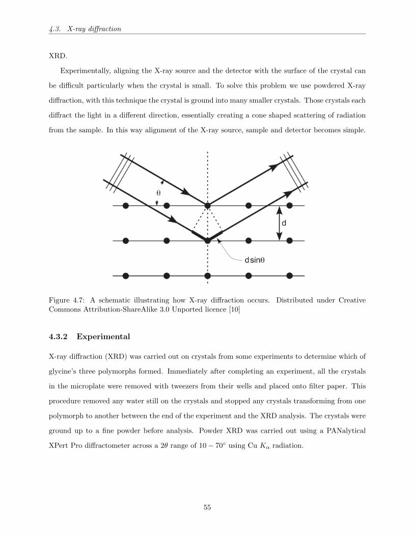
4.3. X-ray diffraction
XRD.
Experimentally, aligning the X-ray source and the detector with the surface of the crystal can
be difficult particularly when the crystal is small. To solve this problem we use powdered X-ray
diffraction, with this technique the crystal is ground into many smaller crystals. Those crystals each
diffract the light in a different direction, essentially creating a cone shaped scattering of radiation
from the sample. In this way alignment of the X-ray source, sample and detector becomes simple.
Figure 4.7: A schematic illustrating how X-ray diffraction occurs. Distributed under CreativeCommons Attribution-ShareAlike 3.0 Unported licence [10]
4.3.2 Experimental
X-ray diffraction (XRD) was carried out on crystals from some experiments to determine which of
glycine’s three polymorphs formed. Immediately after completing an experiment, all the crystals
in the microplate were removed with tweezers from their wells and placed onto filter paper. This
procedure removed any water still on the crystals and stopped any crystals transforming from one
polymorph to another between the end of the experiment and the XRD analysis. The crystals were
ground up to a fine powder before analysis. Powder XRD was carried out using a PANalytical
XPert Pro diffractometer across a 2θ range of 10− 70 using Cu Kα radiation.
55
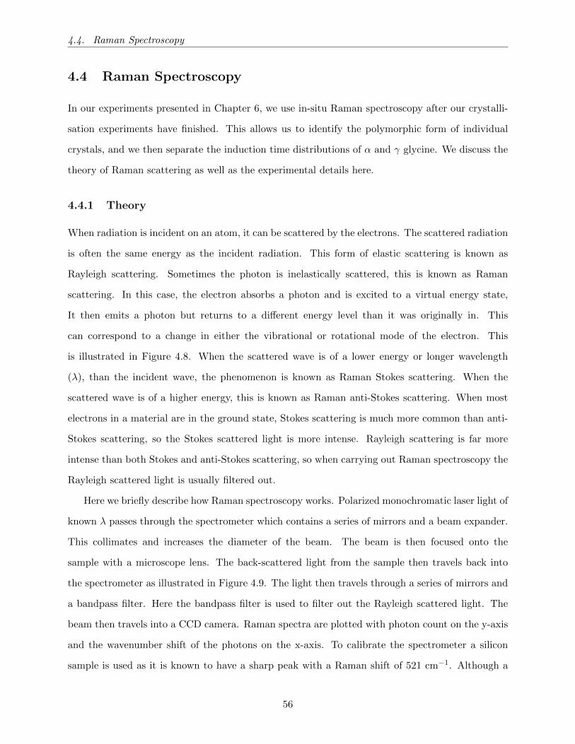
4.4. Raman Spectroscopy
4.4 Raman Spectroscopy
In our experiments presented in Chapter 6, we use in-situ Raman spectroscopy after our crystalli-
sation experiments have finished. This allows us to identify the polymorphic form of individual
crystals, and we then separate the induction time distributions of α and γ glycine. We discuss the
theory of Raman scattering as well as the experimental details here.
4.4.1 Theory
When radiation is incident on an atom, it can be scattered by the electrons. The scattered radiation
is often the same energy as the incident radiation. This form of elastic scattering is known as
Rayleigh scattering. Sometimes the photon is inelastically scattered, this is known as Raman
scattering. In this case, the electron absorbs a photon and is excited to a virtual energy state,
It then emits a photon but returns to a different energy level than it was originally in. This
can correspond to a change in either the vibrational or rotational mode of the electron. This
is illustrated in Figure 4.8. When the scattered wave is of a lower energy or longer wavelength
(λ), than the incident wave, the phenomenon is known as Raman Stokes scattering. When the
scattered wave is of a higher energy, this is known as Raman anti-Stokes scattering. When most
electrons in a material are in the ground state, Stokes scattering is much more common than anti-
Stokes scattering, so the Stokes scattered light is more intense. Rayleigh scattering is far more
intense than both Stokes and anti-Stokes scattering, so when carrying out Raman spectroscopy the
Rayleigh scattered light is usually filtered out.
Here we briefly describe how Raman spectroscopy works. Polarized monochromatic laser light of
known λ passes through the spectrometer which contains a series of mirrors and a beam expander.
This collimates and increases the diameter of the beam. The beam is then focused onto the
sample with a microscope lens. The back-scattered light from the sample then travels back into
the spectrometer as illustrated in Figure 4.9. The light then travels through a series of mirrors and
a bandpass filter. Here the bandpass filter is used to filter out the Rayleigh scattered light. The
beam then travels into a CCD camera. Raman spectra are plotted with photon count on the y-axis
and the wavenumber shift of the photons on the x-axis. To calibrate the spectrometer a silicon
sample is used as it is known to have a sharp peak with a Raman shift of 521 cm−1. Although a
56
4.4. Raman Spectroscopy
Virtual energy state
Excited states
Ground state
Rayleigh Stokes Anti-stokes
Figure 4.8: A schematic illustrating how the potential energy of an electron changes in Ramanscattering.
bandpass filter is applied to the Rayleigh scattered radiation a small amount of it still reaches the
detector. This peak at 0 cm−1 can be used in conjunction with the silicon peak to calibrate the
spectrometer.
Figure 4.9: A schematic illustrating how our samples are analysed with Raman spectroscopy.
4.4.2 Experimental
To identify the polymorphic form of each crystal, an NTEGRA Raman microscope (NT-MDT)
equipped with a 20x objective lens was used. Glycine crystals were excited with a 473 nm laser.
This technique has advantages over powder XRD for investigating polymorphism. Specifically,
57
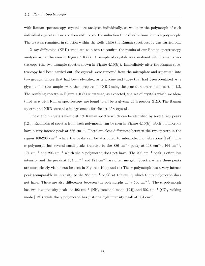
4.4. Raman Spectroscopy
with Raman spectroscopy, crystals are analysed individually, so we know the polymorph of each
individual crystal and we are then able to plot the induction time distributions for each polymorph.
The crystals remained in solution within the wells while the Raman spectroscopy was carried out.
X-ray diffraction (XRD) was used as a test to confirm the results of our Raman spectroscopy
analysis as can be seen in Figure 4.10(a). A sample of crystals was analysed with Raman spec-
troscopy (the two example spectra shown in Figure 4.10(b)). Immediately after the Raman spec-
troscopy had been carried out, the crystals were removed from the microplate and separated into
two groups: Those that had been identified as α glycine and those that had been identified as γ
glycine. The two samples were then prepared for XRD using the procedure described in section 4.3.
The resulting spectra in Figure 4.10(a) show that, as expected, the set of crystals which we iden-
tified as α with Raman spectroscopy are found to all be α glycine with powder XRD. The Raman
spectra and XRD were also in agreement for the set of γ crystals.
The α and γ crystals have distinct Raman spectra which can be identified by several key peaks
[124]. Examples of spectra from each polymorph can be seen in Figure 4.10(b). Both polymorphs
have a very intense peak at 886 cm−1. There are clear differences between the two spectra in the
region 100-200 cm−1 where the peaks can be attributed to intermolecular vibrations [124]. The
α polymorph has several small peaks (relative to the 886 cm−1 peak) at 118 cm−1, 164 cm−1,
171 cm−1 and 203 cm−1 which the γ polymorph does not have. The 203 cm−1 peak is often low
intensity and the peaks at 164 cm−1 and 171 cm−1 are often merged. Spectra where these peaks
are more clearly visible can be seen in Figure 4.10(c) and (d) The γ polymorph has a very intense
peak (comparable in intensity to the 886 cm−1 peak) at 157 cm−1, which the α polymorph does
not have. There are also differences between the polymorphs at ≈ 500 cm−1. The α polymorph
has two low intensity peaks at 492 cm−1 (NH3 torsional mode [124]) and 502 cm−1 (CO2 rocking
mode [124]) while the γ polymorph has just one high intensity peak at 504 cm−1.
58
4.4. Raman Spectroscopy
(a)
0
0.2
0.4
0.6
0.8
1
10 20 30 40
No
rmal
ised
co
un
ts
2θ/ degrees
α Crystals
α Peaks
γ Crystals
γ Peaks
(b)(i)
0
0 200 400 600 800 1000
Inte
nsi
ty (
arb
itra
ry)
Wavenumber/ cm-1
α
γ
(b)(ii)
0
100 150 200 250
Inte
nsi
ty (
arb
itra
ry)
Wavenumber/ cm-1(b)(iii)
0
450 475 500 525 550
Inte
nsi
ty (
arb
itra
ry)
Wavenumber/ cm-1
(c)
0
100 150 200 250
Inte
nsi
ty (
arb
itra
ry)
Wavenumber/ cm-1 (d)
0
100 150 200 250
Inte
nsi
ty (
arb
itra
ry)
Wavenumber/ cm-1
Figure 4.10: (a) XRD patterns of two powdered samples, one of α glycine and one of γ glycineas identified with Raman spectroscopy. The glycine identified as α via Raman spectroscopy isshown in blue and glycine identified as γ is shown in green. The circles represent known α XRDpeaks while the triangles represent known γ XRD peaks. (b)(i) Raman spectra for a typical αglycine crystal and a typical γ glycine crystal. The spectra are normalised to the intensity of theirhighest peak at 886 cm−1 (b)(ii) A magnified view of (b)(i) in the region 100 - 250 cm −1.(b)(iii)A magnified view of (b)(i) in the region 450 - 550 cm −1. (c) and (d) Two additional α glycinespectra where the characteristic peaks at 164 cm−1, 171 cm−1 and 203 cm−1 (which cannot be eailyseen in (b)(ii)) can be more clearly seen.
59
5. Results - Quantitative Glycine
Nucleation Experiments
Here, we look at the nucleation of glycine crystals from aqueous solution. We use the quantitative
technique described in the methods chapter to observe 96 nominally identical crystallisation exper-
iments over a 48 hour period. We record the induction time in each case which allows us to plot
N(t) curves. Nucleation is a very sensitive process so our initial experiments focused on the factors
affecting reproducibility.
In this chapter we look at how a number of factors affect induction time distributions, we also
look at crystal growth rates, the typical number of crystals that nucleate per well, and the time
between nucleation events. First, in the next section, we give a brief explanation of the way we
present induction time distributions in this chapter, and show the key parameters of all the datasets
recorded. Then we discuss the crystal populations in each well in section 5.2 followed by growth
rates in section 5.3. In section 5.4 we discuss the reproducibility of our induction time distributions
and how they are affected by: How long the solution is heated prior to pipetting into the wells
(subsection 5.4.1) and how long the solution is held in the pipette prior to distribution into the
wells (subsection 5.4.2). In section 5.5 we look at the effect of filtering our solutions. We look at
solution concentration/supersaturation in section 5.6, where we compare our data to the predictions
of classical nucleation theory. We look at the effect that changing the time of day at which the
experiment is started in section 5.7. We look at this because temperature varies slightly throughout
our experiments, as we discussed in the methods chapter. Finally we look at polymorphism using
XRD in section 5.8 and the time between first nucleation event and second nucleation event in each
well in section 5.9.
60
5.1. Experiments overview
5.1 Experiments overview
Our experimental data for glycine nucleation consists of 16 datasets. We list all the datasets
presented in this chapter in Table 5.1, each is identified by a letter. Here we define one run as being
induction times recorded for one 96-well microplate. For one experiment only, each two rows of the
microplate were under different experimental conditions, hence some of the datasets in Table 5.1
are made of 1.25 runs. We define a dataset as all runs carried out at the same concentration and
time of day. We performed experiments at a number of glycine concentrations, c. The solubility of
glycine at 21 C was calculated to be cs = 184 g/l of water by interpolating solubility data from
Yang et al [3], so the supersaturation S = c/184. We work at supersaturations of around 1.8.
For each dataset we give: the concentration, c, in g/l of water, the total number of wells, N , in
the dataset; tH , the time the solution had been heated and stirred for prior to distribution into the
wells; and tstart, the time of day at which each experiment starts. For datasets A through D (only),
we also controlled the time, theld, the solution was held in the pipette, before being injected into
the wells. For each dataset, we give the fraction of samples that nucleated within the first hour, the
fraction that nucleated after the first hour, and the fraction that did not nucleate within 48 hours,
respectively. We denote these quantities as F≤1, F ∗, and F>48 respectively. For some datasets we
have fitted an exponential to the extracted data where the extracted data are all nucleation events
that fall into the F ∗ region. Datasets E and J did not have enough induction times in the F ∗ region
to accurately fit an exponential function. For these we give the best fit values of k, with error bars
calculated from the standard deviation of k values fitted to each component run, divided by the
square root of the number of runs. The numbers in the rightmost column are the KS numbers
comparing pairs of f∗(t)s for runs in that line’s dataset. These KS numbers should be less than
1.36 when the runs are reproducible.
5.2 Well crystal populations
At the end of each experiment, some wells have more than one crystal in them. We studied this
phenomenon by counting the number of crystals in all five of the runs that made up dataset G (146
wells that crystallised in the first hour and 266 that crystallised in hours 2 to 48). For the samples
where the first nucleation event was within the first hour of starting the experiment, a mean of
61
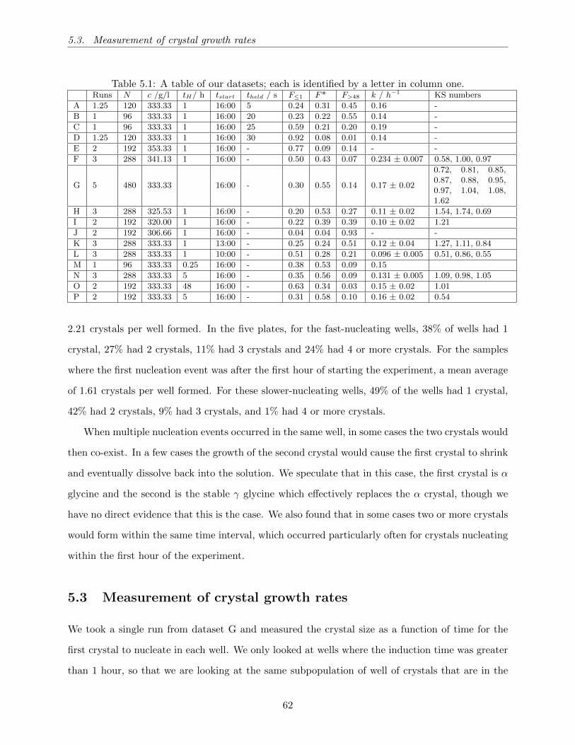
5.3. Measurement of crystal growth rates
Table 5.1: A table of our datasets; each is identified by a letter in column one.Runs N c /g/l tH/ h tstart theld / s F≤1 F* F>48 k / h−1 KS numbers
A 1.25 120 333.33 1 16:00 5 0.24 0.31 0.45 0.16 -
B 1 96 333.33 1 16:00 20 0.23 0.22 0.55 0.14 -
C 1 96 333.33 1 16:00 25 0.59 0.21 0.20 0.19 -
D 1.25 120 333.33 1 16:00 30 0.92 0.08 0.01 0.14 -
E 2 192 353.33 1 16:00 - 0.77 0.09 0.14 - -
F 3 288 341.13 1 16:00 - 0.50 0.43 0.07 0.234 ± 0.007 0.58, 1.00, 0.97
G 5 480 333.33 16:00 - 0.30 0.55 0.14 0.17 ± 0.02
0.72, 0.81, 0.85,0.87, 0.88, 0.95,0.97, 1.04, 1.08,1.62
H 3 288 325.53 1 16:00 - 0.20 0.53 0.27 0.11 ± 0.02 1.54, 1.74, 0.69
I 2 192 320.00 1 16:00 - 0.22 0.39 0.39 0.10 ± 0.02 1.21
J 2 192 306.66 1 16:00 - 0.04 0.04 0.93 - -
K 3 288 333.33 1 13:00 - 0.25 0.24 0.51 0.12 ± 0.04 1.27, 1.11, 0.84
L 3 288 333.33 1 10:00 - 0.51 0.28 0.21 0.096 ± 0.005 0.51, 0.86, 0.55
M 1 96 333.33 0.25 16:00 - 0.38 0.53 0.09 0.15
N 3 288 333.33 5 16:00 - 0.35 0.56 0.09 0.131 ± 0.005 1.09, 0.98, 1.05
O 2 192 333.33 48 16:00 - 0.63 0.34 0.03 0.15 ± 0.02 1.01
P 2 192 333.33 5 16:00 - 0.31 0.58 0.10 0.16 ± 0.02 0.54
2.21 crystals per well formed. In the five plates, for the fast-nucleating wells, 38% of wells had 1
crystal, 27% had 2 crystals, 11% had 3 crystals and 24% had 4 or more crystals. For the samples
where the first nucleation event was after the first hour of starting the experiment, a mean average
of 1.61 crystals per well formed. For these slower-nucleating wells, 49% of the wells had 1 crystal,
42% had 2 crystals, 9% had 3 crystals, and 1% had 4 or more crystals.
When multiple nucleation events occurred in the same well, in some cases the two crystals would
then co-exist. In a few cases the growth of the second crystal would cause the first crystal to shrink
and eventually dissolve back into the solution. We speculate that in this case, the first crystal is α
glycine and the second is the stable γ glycine which effectively replaces the α crystal, though we
have no direct evidence that this is the case. We also found that in some cases two or more crystals
would form within the same time interval, which occurred particularly often for crystals nucleating
within the first hour of the experiment.
5.3 Measurement of crystal growth rates
We took a single run from dataset G and measured the crystal size as a function of time for the
first crystal to nucleate in each well. We only looked at wells where the induction time was greater
than 1 hour, so that we are looking at the same subpopulation of well of crystals that are in the
62

5.3. Measurement of crystal growth rates
f∗(t) data for that run. A histogram of the crystal growth rates is plotted in Figure 5.1(a). The
growth rates were calculated by fitting a straight line to the plot of crystal size against time (see
Figure 5.1(b)), for points below the threshold size of 1.75 mm at which point growth often tended
to plateau.
(a)
0 10 20 30 40 50 60
0
1
2
3
4
5
t/ mins
Size
/ m
m
(b)
0
0.05
0.1
0.15
0.2
0.25
0.3
Growth rate/ mm/minN
orm
alis
ed F
req
uen
cy
Figure 5.1: Data for the first crystal to nucleate in each well of the population of wells wherenucleation occured after the first hour, for a single run. In total, 58 crystals were observed, weshow (a) The sizes of those crystals and (b) the growth rates of those crystals.
Here we compare our growth rates to those of Han et al. who work at a slightly lower concen-
tration than us (321 g/l of water in their work compared to 333 g/l of water in ours). Note they
define cs slightly differently to us so its easier to compare concentrations than supersaturations.
Our distribution of growth rates is very broad, but most crystals have growth rates around 0.02
mm/min. Our growth rates are slightly smaller than those measured by Han et al. [11] at lower
supersaturation/concentration and at the slightly higher temperature of T = 23 C. They find (at
our neutral pH) growth rates of approximately 0.08 ± 0.02 mm/min for the α polymorph and
0.05 ± 0.01 mm/min for the γ polymorph. Because we work at higher supersaturations, we would
expect our rates to be higher not lower than those of Han et al., but there are differences between
their system and our system. For example, they study larger crystals (approximately 5 mm and
larger) and study specific crystal faces.
Using our growth rates and Equation 4.1 we can calculate the time it takes for each crystal
to grow to an observable size. We estimate that, 98% of crystals are observable within 20 min
of nucleation, and 77% are observable within 10 min of nucleation. This means that there is an
63
5.4. Studies on reproducibility of induction times
uncertainty in our early induction time measurements, but the uncertainty becomes less significant
for longer induction times.
5.4 Studies on reproducibility of induction times
We first need to determine if our experiments are reproducible. Hence, we consider dataset L,
which consists of three runs: L1, L2 and L3. In Figure 5.2(a) we plot the fraction not crystallised,
f(t), for these three runs, which are all at the same conditions (concentration, and time of day
for the start of experiment). We see that there are large differences between the f(t) curves. The
corresponding KS numbers are presented in Table 5.2. The KS numbers in the second row of the
table are for the three possible pairwise comparisons between the runs. Two are greater than 1.36,
the value that is expected to be crossed only 5% of the time if data are reproducible. We conclude
that our f(t) distributions are not reproducible.
We can see in Figure 5.2(a) that the fractions that crystallise in the first hour vary between
runs. It appears that some factor causing immediate or almost immediate nucleation is changing
from one run to another. We note that it takes 30 minutes from the start of the experiment for
all wells to cool to within 1C of room temperature, and hence nucleation in the first hour is
not at constant supersaturation. The temperature in the wells as a function of time is plotted in
Figure 4.5. While there is a difference in the cooling rate between inner and outer wells, the cooling
curves are reproducible between runs; the cooling rate of a corner well in one run will be the same
as the cooling rate of a corner well in the next run, and similarly for the centre wells. Although
the cooling will affect nucleation in the first hour, variability in cooling rate is not the cause of the
variability in the amount of nucleation that we observe.
64
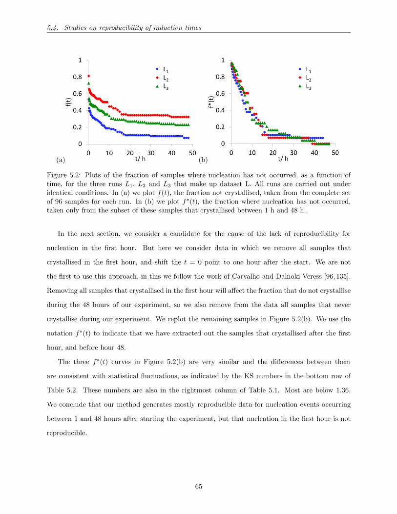
5.4. Studies on reproducibility of induction times
(a)
0
0.2
0.4
0.6
0.8
1
0 10 20 30 40 50
f(t)
t/ h
H1H2H3
L1
L2
L3
(b)
0
0.2
0.4
0.6
0.8
1
0 10 20 30 40 50
f*(t
)
t/ h
H1H2H3
L1
L2
L3
Figure 5.2: Plots of the fraction of samples where nucleation has not occurred, as a function oftime, for the three runs L1, L2 and L3 that make up dataset L. All runs are carried out underidentical conditions. In (a) we plot f(t), the fraction not crystallised, taken from the complete setof 96 samples for each run. In (b) we plot f∗(t), the fraction where nucleation has not occurred,taken only from the subset of these samples that crystallised between 1 h and 48 h.
In the next section, we consider a candidate for the cause of the lack of reproducibility for
nucleation in the first hour. But here we consider data in which we remove all samples that
crystallised in the first hour, and shift the t = 0 point to one hour after the start. We are not
the first to use this approach, in this we follow the work of Carvalho and Dalnoki-Veress [96, 135].
Removing all samples that crystallised in the first hour will affect the fraction that do not crystallise
during the 48 hours of our experiment, so we also remove from the data all samples that never
crystallise during our experiment. We replot the remaining samples in Figure 5.2(b). We use the
notation f∗(t) to indicate that we have extracted out the samples that crystallised after the first
hour, and before hour 48.
The three f∗(t) curves in Figure 5.2(b) are very similar and the differences between them
are consistent with statistical fluctuations, as indicated by the KS numbers in the bottom row of
Table 5.2. These numbers are also in the rightmost column of Table 5.1. Most are below 1.36.
We conclude that our method generates mostly reproducible data for nucleation events occurring
between 1 and 48 hours after starting the experiment, but that nucleation in the first hour is not
reproducible.
65
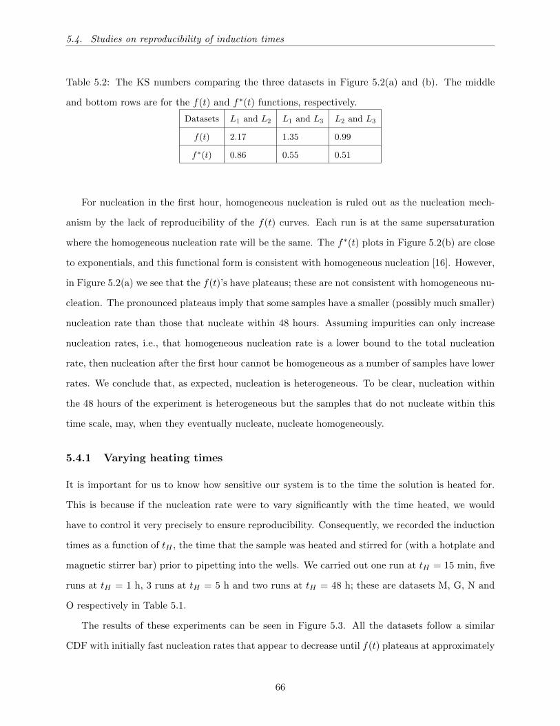
5.4. Studies on reproducibility of induction times
Table 5.2: The KS numbers comparing the three datasets in Figure 5.2(a) and (b). The middle
and bottom rows are for the f(t) and f∗(t) functions, respectively.
Datasets L1 and L2 L1 and L3 L2 and L3
f(t) 2.17 1.35 0.99
f∗(t) 0.86 0.55 0.51
For nucleation in the first hour, homogeneous nucleation is ruled out as the nucleation mech-
anism by the lack of reproducibility of the f(t) curves. Each run is at the same supersaturation
where the homogeneous nucleation rate will be the same. The f∗(t) plots in Figure 5.2(b) are close
to exponentials, and this functional form is consistent with homogeneous nucleation [16]. However,
in Figure 5.2(a) we see that the f(t)’s have plateaus; these are not consistent with homogeneous nu-
cleation. The pronounced plateaus imply that some samples have a smaller (possibly much smaller)
nucleation rate than those that nucleate within 48 hours. Assuming impurities can only increase
nucleation rates, i.e., that homogeneous nucleation rate is a lower bound to the total nucleation
rate, then nucleation after the first hour cannot be homogeneous as a number of samples have lower
rates. We conclude that, as expected, nucleation is heterogeneous. To be clear, nucleation within
the 48 hours of the experiment is heterogeneous but the samples that do not nucleate within this
time scale, may, when they eventually nucleate, nucleate homogeneously.
5.4.1 Varying heating times
It is important for us to know how sensitive our system is to the time the solution is heated for.
This is because if the nucleation rate were to vary significantly with the time heated, we would
have to control it very precisely to ensure reproducibility. Consequently, we recorded the induction
times as a function of tH , the time that the sample was heated and stirred for (with a hotplate and
magnetic stirrer bar) prior to pipetting into the wells. We carried out one run at tH = 15 min, five
runs at tH = 1 h, 3 runs at tH = 5 h and two runs at tH = 48 h; these are datasets M, G, N and
O respectively in Table 5.1.
The results of these experiments can be seen in Figure 5.3. All the datasets follow a similar
CDF with initially fast nucleation rates that appear to decrease until f(t) plateaus at approximately
66
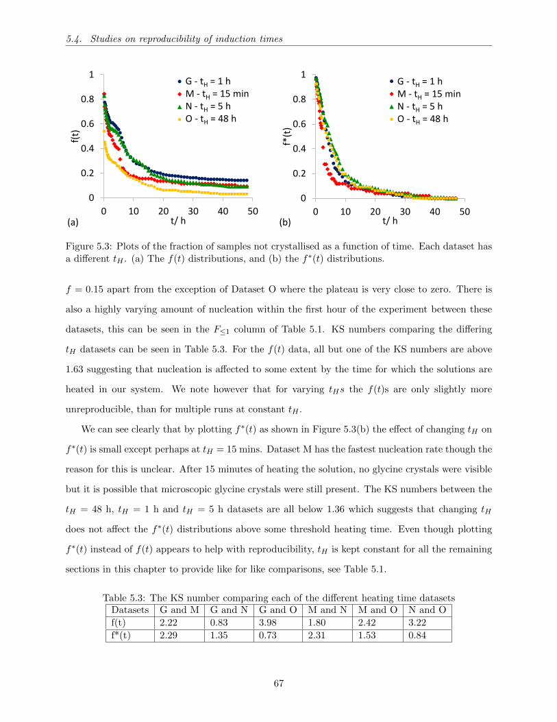
5.4. Studies on reproducibility of induction times
0
0.2
0.4
0.6
0.8
1
0 10 20 30 40 50
f(t)
t/ h
G - tH = 1 hM - tH = 15 minN - tH = 5 hO - tH = 48 h
G - tH = 1 hM - tH = 15 minN - tH = 5 hO - tH = 48 h
(a)
0
0.2
0.4
0.6
0.8
1
0 10 20 30 40 50
f*(t
)
t/ h
G - tH = 1 hM - tH = 15 minN - tH = 5 hO - tH = 48 h
G - tH = 1 hM - tH = 15 minN - tH = 5 hO - tH = 48 h
(b)
Figure 5.3: Plots of the fraction of samples not crystallised as a function of time. Each dataset hasa different tH . (a) The f(t) distributions, and (b) the f∗(t) distributions.
f = 0.15 apart from the exception of Dataset O where the plateau is very close to zero. There is
also a highly varying amount of nucleation within the first hour of the experiment between these
datasets, this can be seen in the F≤1 column of Table 5.1. KS numbers comparing the differing
tH datasets can be seen in Table 5.3. For the f(t) data, all but one of the KS numbers are above
1.63 suggesting that nucleation is affected to some extent by the time for which the solutions are
heated in our system. We note however that for varying tHs the f(t)s are only slightly more
unreproducible, than for multiple runs at constant tH .
We can see clearly that by plotting f∗(t) as shown in Figure 5.3(b) the effect of changing tH on
f∗(t) is small except perhaps at tH = 15 mins. Dataset M has the fastest nucleation rate though the
reason for this is unclear. After 15 minutes of heating the solution, no glycine crystals were visible
but it is possible that microscopic glycine crystals were still present. The KS numbers between the
tH = 48 h, tH = 1 h and tH = 5 h datasets are all below 1.36 which suggests that changing tH
does not affect the f∗(t) distributions above some threshold heating time. Even though plotting
f∗(t) instead of f(t) appears to help with reproducibility, tH is kept constant for all the remaining
sections in this chapter to provide like for like comparisons, see Table 5.1.
Table 5.3: The KS number comparing each of the different heating time datasetsDatasets G and M G and N G and O M and N M and O N and O
f(t) 2.22 0.83 3.98 1.80 2.42 3.22
f*(t) 2.29 1.35 0.73 2.31 1.53 0.84
67
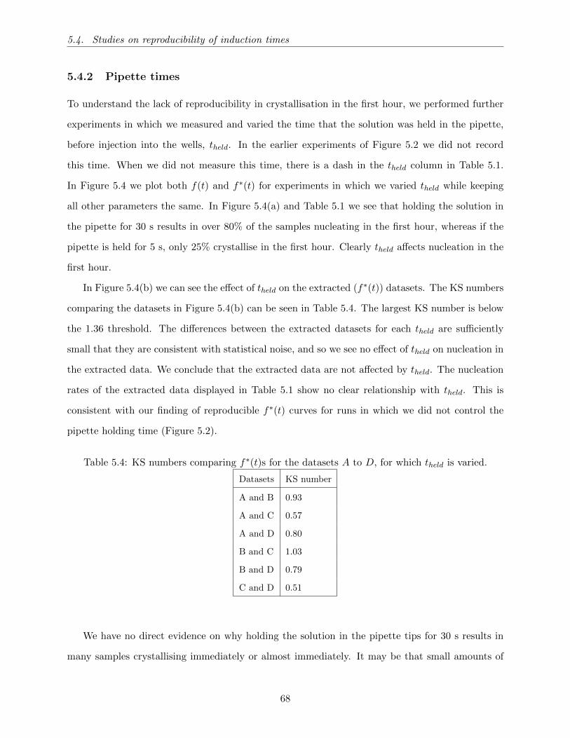
5.4. Studies on reproducibility of induction times
5.4.2 Pipette times
To understand the lack of reproducibility in crystallisation in the first hour, we performed further
experiments in which we measured and varied the time that the solution was held in the pipette,
before injection into the wells, theld. In the earlier experiments of Figure 5.2 we did not record
this time. When we did not measure this time, there is a dash in the theld column in Table 5.1.
In Figure 5.4 we plot both f(t) and f∗(t) for experiments in which we varied theld while keeping
all other parameters the same. In Figure 5.4(a) and Table 5.1 we see that holding the solution in
the pipette for 30 s results in over 80% of the samples nucleating in the first hour, whereas if the
pipette is held for 5 s, only 25% crystallise in the first hour. Clearly theld affects nucleation in the
first hour.
In Figure 5.4(b) we can see the effect of theld on the extracted (f∗(t)) datasets. The KS numbers
comparing the datasets in Figure 5.4(b) can be seen in Table 5.4. The largest KS number is below
the 1.36 threshold. The differences between the extracted datasets for each theld are sufficiently
small that they are consistent with statistical noise, and so we see no effect of theld on nucleation in
the extracted data. We conclude that the extracted data are not affected by theld. The nucleation
rates of the extracted data displayed in Table 5.1 show no clear relationship with theld. This is
consistent with our finding of reproducible f∗(t) curves for runs in which we did not control the
pipette holding time (Figure 5.2).
Table 5.4: KS numbers comparing f∗(t)s for the datasets A to D, for which theld is varied.
Datasets KS number
A and B 0.93
A and C 0.57
A and D 0.80
B and C 1.03
B and D 0.79
C and D 0.51
We have no direct evidence on why holding the solution in the pipette tips for 30 s results in
many samples crystallising immediately or almost immediately. It may be that small amounts of
68

5.5. The effect of filtering impurities
evaporation in the pipette tips locally raises the supersaturation enough to drive rapid nucleation,
creating seed crystals that are then pipetted into some wells. We note that a sub-micrometre volume
of solution is more than enough to allow nucleation, so only a microscopic volume of the solution
in the pipette needs to reach higher supersaturations to trigger nucleation. It is also possible that
cooling within the pipette tip is fast enough to induce nucleation. We do not know the effect of the
solution-air interface or the solution-pipette tip interface on nucleation but its possible that ∆G is
small at these interfaces and heterogeneous nucleation occurs. This is a speculative explanation.
Whether or not it is indeed the mechanism, future experiments using this methodology should
control theld to ensure reproducibility.
(a)0 10 20 30 40 50
0
0.2
0.4
0.6
0.8
1
t/ h
f(t)
JKLM
A - theld = 5sB - theld = 20sC - theld = 25sD - theld = 30s
(b)0 10 20 30 40 50
0
0.2
0.4
0.6
0.8
1
t/ h
f*(t
)
JKLM
A - theld = 5sB - theld = 20sC - theld = 25sD - theld = 30s
Figure 5.4: Plots of the fraction of samples where nucleation has not occurred, for runs withdifferent pipette holding times. In (a) and (b), we plot f(t) and f∗(t), respectively. All runs are atc = 333.33 g/l.
5.5 The effect of filtering impurities
We checked for a possible effect on nucleation of large impurities by filtering the glycine solution
prior to distributing into the wells. For dataset P, a 0.22 µm filter was applied to the solution
before transferring into the microplate wells (as described in section 4.2). Two runs were carried
out with filtered solutions. The conditions for dataset P are the same as those for dataset N with
the one exception that there was no filter applied to the solution for dataset N. A comparison of
the two datasets can be seen in Figure 5.5.
69
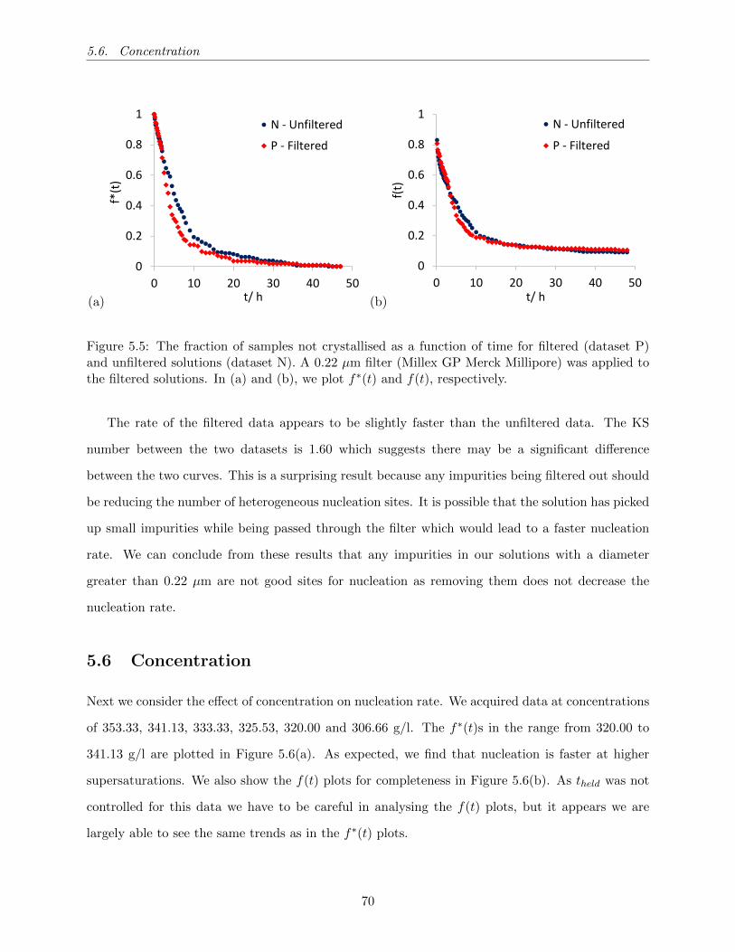
5.6. Concentration
(a)
0
0.2
0.4
0.6
0.8
1
0 10 20 30 40 50
f*(t
)
t/ h
N - Unfiltered
P - Filtered
(b)
0
0.2
0.4
0.6
0.8
1
0 10 20 30 40 50
f(t)
t/ h
N - Unfiltered
P - Filtered
Figure 5.5: The fraction of samples not crystallised as a function of time for filtered (dataset P)and unfiltered solutions (dataset N). A 0.22 µm filter (Millex GP Merck Millipore) was applied tothe filtered solutions. In (a) and (b), we plot f∗(t) and f(t), respectively.
The rate of the filtered data appears to be slightly faster than the unfiltered data. The KS
number between the two datasets is 1.60 which suggests there may be a significant difference
between the two curves. This is a surprising result because any impurities being filtered out should
be reducing the number of heterogeneous nucleation sites. It is possible that the solution has picked
up small impurities while being passed through the filter which would lead to a faster nucleation
rate. We can conclude from these results that any impurities in our solutions with a diameter
greater than 0.22 µm are not good sites for nucleation as removing them does not decrease the
nucleation rate.
5.6 Concentration
Next we consider the effect of concentration on nucleation rate. We acquired data at concentrations
of 353.33, 341.13, 333.33, 325.53, 320.00 and 306.66 g/l. The f∗(t)s in the range from 320.00 to
341.13 g/l are plotted in Figure 5.6(a). As expected, we find that nucleation is faster at higher
supersaturations. We also show the f(t) plots for completeness in Figure 5.6(b). As theld was not
controlled for this data we have to be careful in analysing the f(t) plots, but it appears we are
largely able to see the same trends as in the f∗(t) plots.
70
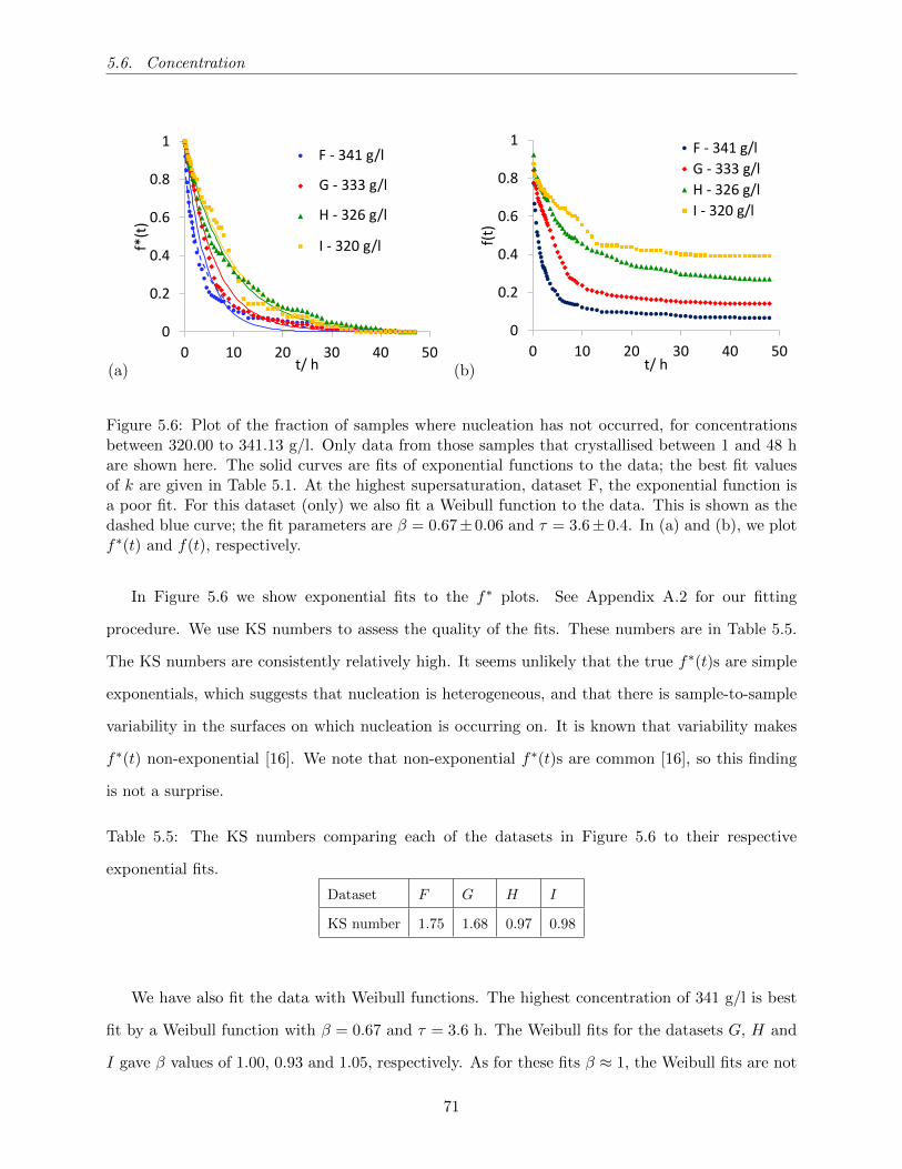
5.6. Concentration
(a)0 10 20 30 40 50
0
0.2
0.4
0.6
0.8
1
t/ h
f*(t
)F - 341 mg/ml
G - 333 mg/ml
H - 326 mg/ml
I - 320 mg/ml
F - 341 g/l
G - 333 g/l
H - 326 g/l
I - 320 g/l
(b)
0
0.2
0.4
0.6
0.8
1
0 10 20 30 40 50
f(t)
t/ h
F - 341 g/l
G - 333 g/l
H - 326 g/l
I - 320 g/l
Figure 5.6: Plot of the fraction of samples where nucleation has not occurred, for concentrationsbetween 320.00 to 341.13 g/l. Only data from those samples that crystallised between 1 and 48 hare shown here. The solid curves are fits of exponential functions to the data; the best fit valuesof k are given in Table 5.1. At the highest supersaturation, dataset F, the exponential function isa poor fit. For this dataset (only) we also fit a Weibull function to the data. This is shown as thedashed blue curve; the fit parameters are β = 0.67± 0.06 and τ = 3.6± 0.4. In (a) and (b), we plotf∗(t) and f(t), respectively.
In Figure 5.6 we show exponential fits to the f∗ plots. See Appendix A.2 for our fitting
procedure. We use KS numbers to assess the quality of the fits. These numbers are in Table 5.5.
The KS numbers are consistently relatively high. It seems unlikely that the true f∗(t)s are simple
exponentials, which suggests that nucleation is heterogeneous, and that there is sample-to-sample
variability in the surfaces on which nucleation is occurring on. It is known that variability makes
f∗(t) non-exponential [16]. We note that non-exponential f∗(t)s are common [16], so this finding
is not a surprise.
Table 5.5: The KS numbers comparing each of the datasets in Figure 5.6 to their respective
exponential fits.
Dataset F G H I
KS number 1.75 1.68 0.97 0.98
We have also fit the data with Weibull functions. The highest concentration of 341 g/l is best
fit by a Weibull function with β = 0.67 and τ = 3.6 h. The Weibull fits for the datasets G, H and
I gave β values of 1.00, 0.93 and 1.05, respectively. As for these fits β ≈ 1, the Weibull fits are not
71
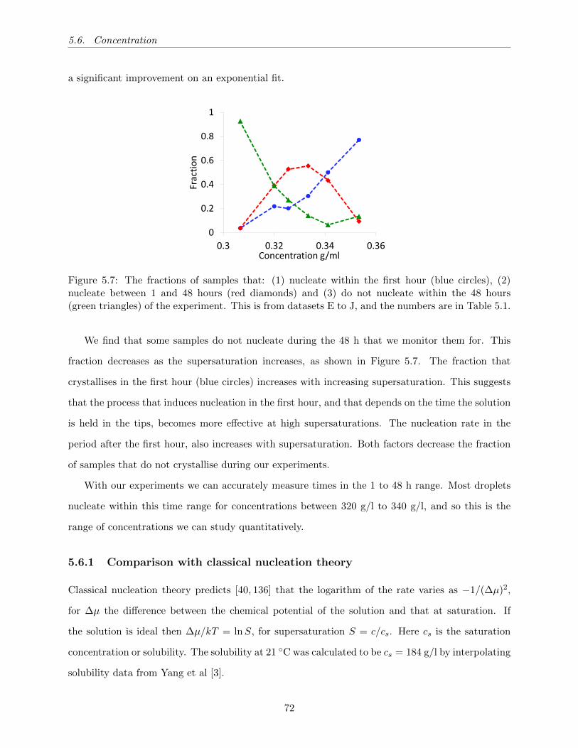
5.6. Concentration
a significant improvement on an exponential fit.
0
0.2
0.4
0.6
0.8
1
0.3 0.32 0.34 0.36
Frac
tio
n
Concentration g/ml
n < 1h1h < n < 48h48h < n
F≤1
F*F>48
Figure 5.7: The fractions of samples that: (1) nucleate within the first hour (blue circles), (2)nucleate between 1 and 48 hours (red diamonds) and (3) do not nucleate within the 48 hours(green triangles) of the experiment. This is from datasets E to J, and the numbers are in Table 5.1.
We find that some samples do not nucleate during the 48 h that we monitor them for. This
fraction decreases as the supersaturation increases, as shown in Figure 5.7. The fraction that
crystallises in the first hour (blue circles) increases with increasing supersaturation. This suggests
that the process that induces nucleation in the first hour, and that depends on the time the solution
is held in the tips, becomes more effective at high supersaturations. The nucleation rate in the
period after the first hour, also increases with supersaturation. Both factors decrease the fraction
of samples that do not crystallise during our experiments.
With our experiments we can accurately measure times in the 1 to 48 h range. Most droplets
nucleate within this time range for concentrations between 320 g/l to 340 g/l, and so this is the
range of concentrations we can study quantitatively.
5.6.1 Comparison with classical nucleation theory
Classical nucleation theory predicts [40, 136] that the logarithm of the rate varies as −1/(∆µ)2,
for ∆µ the difference between the chemical potential of the solution and that at saturation. If
the solution is ideal then ∆µ/kT = lnS, for supersaturation S = c/cs. Here cs is the saturation
concentration or solubility. The solubility at 21 C was calculated to be cs = 184 g/l by interpolating
solubility data from Yang et al [3].
72

5.7. Time of Day
As the datasets in Figure 5.6 are not all well fitted by an exponential P (t), we do not look at
how the fitted rate parameter k varies with supersaturation. Instead we look at how the median
induction time, t1/2, of each dataset, varies with lnS. This is plotted in Figure 5.8. The median
induction time is a better estimator of nucleation rate than k when the data is non-exponential.
The data is non-exponential for the higher supersaturation dataset F. Note that this is calculated
from the extracted data, i.e., the median time is defined by f∗(t1/2) = 1/2.
We see that our data are consistent with the natural log of t1/2 varying with 1/(lnS)2. However,
we note that the range of S values is not large, and also that as our concentrations are over 300 g/l,
the solution will not be ideal, and hence deviations of ∆µ from kT lnS are likely to be significant.
2.6 2.8 3 3.2 3.4
0
0.5
1
1.5
2
2.5
1/ ln(S)2
ln(t
1/2
)
Figure 5.8: The logarithm of the median induction time, t1/2, of each extracted dataset from F toI, plotted as a function of 1/[ln(S)]2, for S the supersaturation. We fit a dashed straight line to thedata. The fit parameters are a gradient of m = 2.1, and a y-intercept of −4.9. Error bars are thestandard errors of t1/2, which have been calculated from the runs making up the respective dataset.
5.7 Time of Day
Our samples are subject to a small temperature drop at night, see Figure 4.6. The temperature in
our temperature-controlled room varied from 20.7 to 21.4C. Using the solubility data of Yang et
al. [3], this corresponds to a solubility that varies from 183 to 186 g/l, and hence a supersaturation
S that varies from 1.82 to 1.79. This is a variation of 1.7% in the supersaturation between night
and day.
To estimate the effect of this change in S, we can use the fit in Figure 5.8 and write down an
expression for the ratio of median induction times at supersaturations S and S + ∆S, for small
73
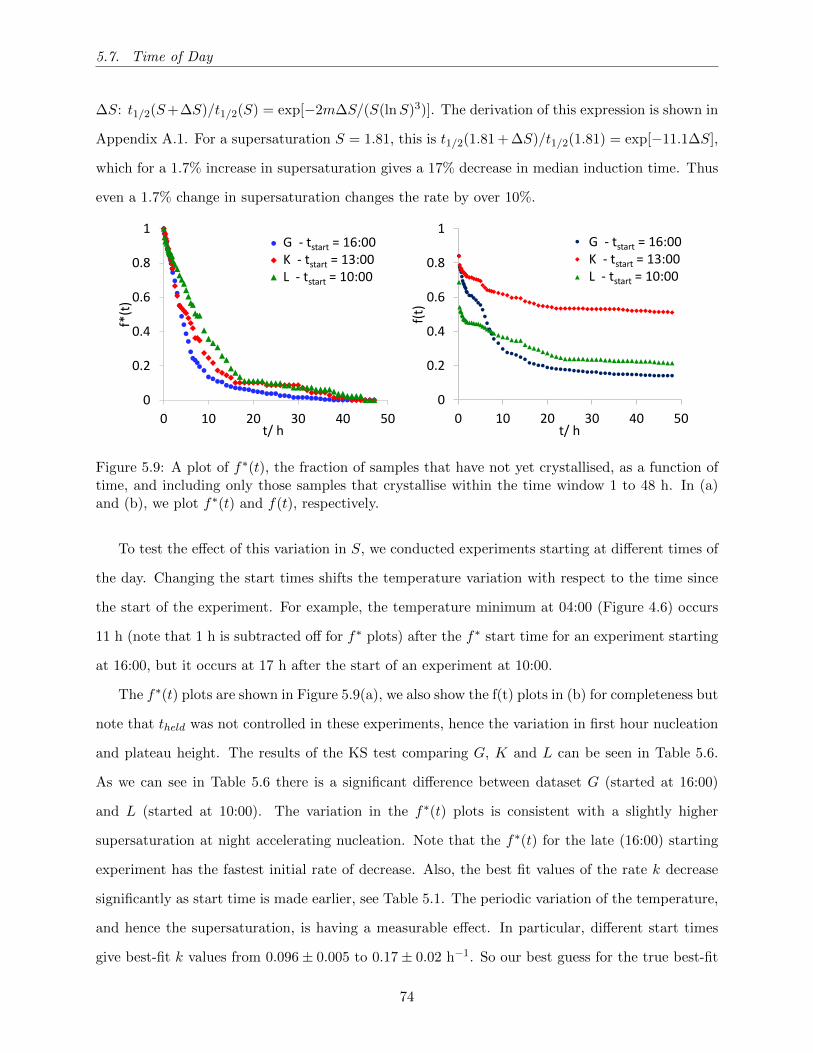
5.7. Time of Day
∆S: t1/2(S+∆S)/t1/2(S) = exp[−2m∆S/(S(lnS)3)]. The derivation of this expression is shown in
Appendix A.1. For a supersaturation S = 1.81, this is t1/2(1.81 + ∆S)/t1/2(1.81) = exp[−11.1∆S],
which for a 1.7% increase in supersaturation gives a 17% decrease in median induction time. Thus
even a 1.7% change in supersaturation changes the rate by over 10%.
0 10 20 30 40 50
0
0.2
0.4
0.6
0.8
1
t/ h
f*(t
)
Autumn evening1pm startearly
G - tstart = 16:00K - tstart = 13:00L - tstart = 10:00
0
0.2
0.4
0.6
0.8
1
0 10 20 30 40 50f(
t)t/ h
G - tstart = 16:00K - tstart = 13:00L - tstart = 10:00
G - tstart = 16:00K - tstart = 13:00L - tstart = 10:00
Figure 5.9: A plot of f∗(t), the fraction of samples that have not yet crystallised, as a function oftime, and including only those samples that crystallise within the time window 1 to 48 h. In (a)and (b), we plot f∗(t) and f(t), respectively.
To test the effect of this variation in S, we conducted experiments starting at different times of
the day. Changing the start times shifts the temperature variation with respect to the time since
the start of the experiment. For example, the temperature minimum at 04:00 (Figure 4.6) occurs
11 h (note that 1 h is subtracted off for f∗ plots) after the f∗ start time for an experiment starting
at 16:00, but it occurs at 17 h after the start of an experiment at 10:00.
The f∗(t) plots are shown in Figure 5.9(a), we also show the f(t) plots in (b) for completeness but
note that theld was not controlled in these experiments, hence the variation in first hour nucleation
and plateau height. The results of the KS test comparing G, K and L can be seen in Table 5.6.
As we can see in Table 5.6 there is a significant difference between dataset G (started at 16:00)
and L (started at 10:00). The variation in the f∗(t) plots is consistent with a slightly higher
supersaturation at night accelerating nucleation. Note that the f∗(t) for the late (16:00) starting
experiment has the fastest initial rate of decrease. Also, the best fit values of the rate k decrease
significantly as start time is made earlier, see Table 5.1. The periodic variation of the temperature,
and hence the supersaturation, is having a measurable effect. In particular, different start times
give best-fit k values from 0.096± 0.005 to 0.17± 0.02 h−1. So our best guess for the true best-fit
74
5.8. Polymorphism
rate, k, for nucleation at a truly fixed 21C (and c = 333 g/l) is approximately 0.14 ± 0.05 h−1.
With our data we cannot be more accurate than that. Reducing this uncertainty would require
better temperature control, as well as better statistics.
Table 5.6: The KS numbers comparing datasets G, K and L.
Dataset G and K K and L G and L
KS number 1.30 1.08 2.45
5.8 Polymorphism
In this section we examine which of glycine’s three polymorphs (α, β and γ) were formed in our
experiment. XRD samples were prepared using the same conditions as dataset G (c = 333 g/l,
and experiments started at 16:00). We obtained XRD patterns separately from those wells where
nucleation was rapid (< 1 h), blue curve in Figure 5.10, and where nucleation occurred between 1
and 48 hours, red curve in Figure 5.10. We needed to collect crystals from a number of wells in
order to obtain enough crystals for an XRD pattern.
For those wells where nucleation was effectively instantaneous, we see almost 100% α glycine.
There is a peak at 2θ = 25.1, which is characteristic of the equilibrium γ polymorph, but this peak
is very small in comparison to the α peaks. This result is expected. For crystallisation at neutral
pH for aqueous solution; the α polymorph is the expected polymorph [6, 20–32].
However, if we look at the XRD pattern (red curve) of the crystals that nucleated after 1 hour,
then we see that they are mostly the γ polymorph, although the α polymorph is present. A few
of the crystals that nucleated after the first hour have the classic distinctive morphology of the α
polymorph; we show one in Figure 5.10(d). The presence of the γ polymorph is surprising [6,20–32].
Although the ratio of the peak heights of the main γ and α peaks does not directly correspond to
the relative proportion of the two polymorphs, we can use it as a rough approximation. The ratio
of the height of the main γ peak (25.1) to the α peak (29.8), is 0.02 : 1 for the wells that nucleated
in the first hour, and 1 : 0.25 for the wells where crystallisation occurred later. A duplicate run
yielded very similar results, the patterns for this run are shown in Appendix A.3. Powder XRD
does not give us accurate quantitative data such that we can specify the relative amount of samples
75
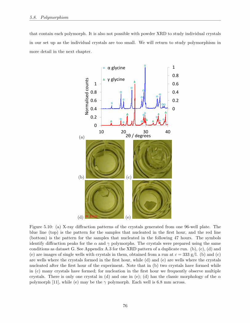
5.8. Polymorphism
that contain each polymorph. It is also not possible with powder XRD to study individual crystals
in our set up as the individual crystals are too small. We will return to study polymorphism in
more detail in the next chapter.
(a)
-0.4
-0.2
0
0.2
0.4
0.6
0.8
1
0
0.2
0.4
0.6
0.8
1
1.2
1.4
10 20 30 40
No
rmal
ised
co
un
ts
2θ / degrees
α glycine
γ glycine
(b) (c)
(d) (e)
Figure 5.10: (a) X-ray diffraction patterns of the crystals generated from one 96-well plate. Theblue line (top) is the pattern for the samples that nucleated in the first hour, and the red line(bottom) is the pattern for the samples that nucleated in the following 47 hours. The symbolsidentify diffraction peaks for the α and γ polymorphs. The crystals were prepared using the sameconditions as dataset G. See Appendix A.3 for the XRD pattern of a duplicate run. (b), (c), (d) and(e) are images of single wells with crystals in them, obtained from a run at c = 333 g/l. (b) and (c)are wells where the crystals formed in the first hour, while (d) and (e) are wells where the crystalsnucleated after the first hour of the experiment. Note that in (b) two crystals have formed whilein (c) many crystals have formed; for nucleation in the first hour we frequently observe multiplecrystals. There is only one crystal in (d) and one in (e); (d) has the classic morphology of the αpolymorph [11], while (e) may be the γ polymorph. Each well is 6.8 mm across.
76
5.9. Nucleation of the second crystal in samples where a crystal is already present
When we estimated the growth rates of crystals that nucleated after the first hour (see Fig-
ure 5.1) we found that a few crystals appeared to grow roughly 10 times faster than the most
common growth rate, which is near 0.02 mm/min. As we expect most of the crystals to be the γ
polymorph, with a few of the α polymorph, it is possible that the crystals near the peak of the
growth rate histogram of Figure 5.1 are of the γ polymorph while those in the fast-growth-rate
tail are of the α polymorph. In other words although there is variability in growth rate between
crystals of the same polymorph, some of the spread in growth rates seen in Figure 5.1 is because we
are following the growth of crystals of both polymorphs. We plotted the growth rates as a function
of induction time, to look for a correlation, but the data did not show a significant correlation.
5.9 Nucleation of the second crystal in samples where a crystal is
already present
In this work we focus on the formation of the first crystal in a solution that does not contain
pre-existing crystals. However, we do in fact have data on the times for the formation of additional
crystals in samples where there is already a crystal. This is plotted in Figure 5.11. To compare
formation of the first and second crystal on an equal footing, we compare nucleation data over a
period of 23 hours. We only have 48 h of data and so can only study both first and second nucleation
over 23 hours each. So in Figure 5.11 we have plotted f∗23(t), the fraction of samples that have not
yet crystallised, including only those samples that crystallise within the time window 1 to 23 h.
We compare this to f(2)23 (t), the fraction of the samples in which a second crystal has not nucleated,
as a function of the time since the first crystal nucleated. The fraction f(2)23 is calculated using the
same samples as used for f∗23. We give an example to be clear on exactly what we are plotting. If
in a given well the first crystal forms 9 h after the experiment begins and the second crystal forms
14 h after the experiment begins: f∗23(t) = 8h (as we remove the first hour) and f(2)23 = 5h.
We see that the effective nucleation rate for a second crystal starts off fast but rapidly slows
over a few hours. The observation that the rate decreases with time is not surprising, because the
supersaturation is decreasing with time as the first crystal grows. Note that as we saw in Figure 5.1,
there is substantial variability in the growth rates and so some crystals do take a few hours to grow.
Thus, we expect that at least in some cases the supersaturation takes a few hours to drop down to
77

5.10. Summary
the saturation concentration for the polymorph of the first crystal. This decreasing supersaturation
is an obvious explanation for the decreasing nucleation rate over the first few hours.
0
0.2
0.4
0.6
0.8
1
0 5 10 15 20 25t/ h
First nucleation events
Second nucleation eventsf 23∗an
df 23
(2)
Figure 5.11: A plot to compare nucleation of the first crystal, to nucleation of the second crystalin the same well, from the five runs of dataset G. The blue circles are f∗23(t), the fraction of samplesthat have not yet crystallised, as a function of time, including only those samples that crystallise
within the time window 1 to 23 h. The red diamonds are f(2)23 (t), the fraction of samples in which
one crystal has appeared but in which a second crystal has not yet appeared. This is as a functionof the time since the first crystal nucleated, and it is calculated using only those samples thatcrystallise within 23 h of the first nucleation event. In that time window, 256 samples formedat least one crystal, of which 119 formed a second crystal. The green curve is a fit of a Weibull
function to f(2)23 ; the fit parameters are β = 0.25 and τ = 165 h.
Secondary nucleation is, by definition [137], nucleation caused by a pre-existing crystal. For
example, if early in crystal growth a nanocrystallite broke off from an existing crystal and started
growing, we would see two crystals appear simultaneously or nearly simultaneously. It is possible
that the initial fast rate (steep decrease of f(2)23 ) is due to secondary nucleation. But as we cannot
observe nucleation directly, we do not know whether or not the second crystals we observe form
via secondary nucleation.
5.10 Summary
We have presented quantitative data on the nucleation of glycine from solution. Here we summarise
the key findings.
78
5.10. Summary
1. Our method can produce significant induction time statistics in a short period of time. We
believe that our approach, with its application of statistical tests for reproducibility, could be
useful in future work.
2. Growth rates vary from crystal to crystal. This is possibly due to different growth defects in
each crystal.
3. In our experiments nucleation is heterogeneous. Nucleation appears to be very sensitive to
the way a sample is prepared, e.g, to the time the solution is held in the pipette prior to
distribution and the time the solution is heated and stirred for.
4. The effective nucleation rate varies strongly with supersaturation. The way our induction
time distributions vary with supersaturation is consistent with the predictions of classical
nucleation theory.
5. Small fluctuations in temperature can significantly affect the effective nucleation rate. In the
case of our glycine experiments, even a 1% change in supersaturation can introduce a 10%
variation in the rate. With our data, we found a best-fit rate, k ≈ 0.14 ± 0.05 h−1, at a
concentration c = 333 g/l (S = 1.81), and at a nominal temperature of T = 21C.
6. Finally, we were surprised to find that although those crystals that nucleated immediately
or almost immediately were of the expected α polymorph [6, 20–32], those that nucleated
later were predominantly of the γ polymorph. This suggests that there is some relationship
between induction time and the probability of getting a given polymorph. We will study this
in detail in the next chapter.
79
6. Results - competition between
glycine’s polymorphs in the presence
of sodium chloride
In the previous chapter, one of our final results showed a relationship between induction time and
the polymorph that nucleates. The polymorph was determined via powder XRD. In this chapter our
objective is to explore this relationship further. To vary the amounts of the competing polymorphs,
we added sodium chloride to our solutions. Sodium chloride is known to change nucleation such
that it more frequently produces the γ polymorph. In the absence of salt we obtain mostly the α
polymorph.
We report the results of large-scale (hundreds of nucleation events) quantitative studies of the
nucleation of crystals of glycine. We vary the salt concentration in solution to control the relative
amounts of the α and γ polymorphs of glycine. Using Raman spectroscopy in situ on single crystals
we determine the polymorph of each crystal. As we discussed in Chapter 4, the difference between
the Raman spectra of α and γ glycine are well known. The quantitative data is then analysed in a
data-driven approach in which we directly model the experimental observables.
There is a growing literature that studies nucleation quantitatively [16,23,33,103–105,107,138,
139]. Earlier quantitative work, with the exception of that of Diao et al. [103], did not consider poly-
morphism. We benefit from the fact that the statistics of the nucleation of competing polymorphs
is analogous to problems faced in medical statistics, as we discussed in section 2.4. We employ
the ideas and techniques developed in medical statistics, to model the nucleation of competing
polymorphs. The combination of quantitative induction time data, identifying the polymorph of
each crystal and a modelling approach taken from medical statistics is new. We believe it advances
the state of the art.
80

6.1. Nucleation data
The layout of the chapter is as follows. There are two main sections, one is on nucleation and
polymorphism and one is on crystal growth. In the next section we start by quantifying the effect
of salt on the polymorphic outcome of nucleation in our experiments. We then discuss induction
time distributions of both polymorphs, and how those distributions vary with salt. We model
polymorph specific induction time distributions and consider the potential effect of correlation
between α nucleation and γ nucleation on our data. For the final part of the first section, we show
how reducing supersaturation at a specified time during an experiment can increase the % yield of
the γ polymorph.
In the second section we look at growth. We initially look at the effect of growth rate on the
uncertainty in induction time measurements. We then discuss the variation in our growth rates
and its relationship with crystal habit. After that we discuss how the growth rate varies between
salt concentrations and between the two polymorphs. We then discuss the relationship between
induction time and growth rate. The final section is a conclusion.
6.1 Nucleation data
6.1.1 Increasing salt concentration favours the γ polymorph
The glycine concentration for all experiments in this chapter is 320 g/l of water. Experiments
were carried out at NaCl concentrations cNaCl from 60 g/l of water to 300 g/l of water. All NaCl
concentrations in this chapter are given in the units g/l of water. At least two runs were carried
out at each salt concentration. We define a run as the set of induction times recorded from one
96-well microplate. An example image of the crystals of one of the runs is shown in Appendix B.3.
On completing each run, the fraction of wells containing each polymorph was determined.
In Figure 6.1 we have plotted the final fraction of crystallised samples that contain the γ
polymorph, fγ , as a function of NaCl concentration. To put it more simply, fγ =nγ
nα+nγwhere
nα and nγ are the number of wells containing α crystals and γ crystals respectively. We are just
looking at the relative amounts of each polymorph and not considering samples without crystals.
At low salt concentrations, there is little γ glycine present. We can see that as salt concentration
increases, the fraction of gamma crystals increases dramatically. It should be noted that statistics
are quite poor for the point at 300 mg/ml, see Table 6.1.
81
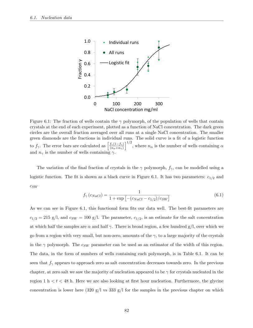
6.1. Nucleation data
0.0
0.2
0.4
0.6
0.8
1.0
0 100 200 300
Frac
tio
n γ
NaCl concentration mg/ml
Individual runs
All runs
Logistic fit
r2
r3
Figure 6.1: The fraction of wells contain the γ polymorph, of the population of wells that containcrystals at the end of each experiment, plotted as a function of NaCl concentration. The dark greencircles are the overall fraction averaged over all runs at a single NaCl concentration. The smallergreen diamonds are the fractions in individual runs. The solid curve is a fit of a logistic function
to fγ . The error bars are calculated as[fγ(1−fγ)(nα+nγ)
]1/2, where nα is the number of wells containing α
and nγ is the number of wells containing γ.
The variation of the final fraction of crystals in the γ polymorph, fγ , can be modelled using a
logistic function. The fit is shown as a black curve in Figure 6.1. It has two parameters: c1/2 and
cSW
fγ (cNaCl) =1
1 + exp[−(cNaCl − c1/2)/cSW
] (6.1)
As we can see in Figure 6.1, this functional form fits our data well. The best-fit parameters are
c1/2 = 215 g/l, and cSW = 100 g/l. The parameter, c1/2, is an estimate for the salt concentration
at which half the samples are α and half γ. There is broad region, a few hundred g/l, over which we
go from a region with very small, but non-zero, amounts of the γ, to a large majority of the crystals
in the γ polymorph. The cSW parameter can be used as an estimator of the width of this region.
The data, in the form of numbers of wells containing each polymorph, is in Table 6.1. It can be
seen that fγ appears to approach zero as salt concentration decreases towards zero. In the previous
chapter, at zero salt we saw the majority of nucleation appeared to be γ for crystals nucleated in the
region 1 h < t < 48 h. Here we are also looking at first hour nucleation. Furthermore, the glycine
concentration is lower here (320 g/l vs 333 g/l for the samples in the previous chapter on which
82
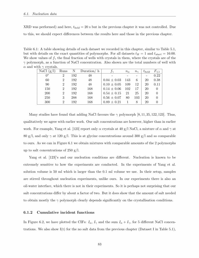
6.1. Nucleation data
XRD was performed) and here, theld = 20 s but in the previous chapter it was not controlled. Due
to this, we should expect differences between the results here and those in the previous chapter.
Table 6.1: A table showing details of each dataset we recorded in this chapter, similar to Table 5.1,but with details on the exact quantities of polymorphs. For all datasets tH = 1 and tstart = 16:00.We show values of fγ the final fraction of wells with crystals in them, where the crystals are of theγ polymorph, as a function of NaCl concentration. Also shown are the total numbers of well withα and with γ crystals.
NaCl (g/l) Runs N Duration/ h fγ nα nγ theld F≤1
0∗ 2 192 48 - - - - 0.2260 2 192 48 0.04 ± 0.03 143 6 20 0.3890 2 192 48 0.10 ± 0.05 109 12 20 0.11150 2 192 168 0.14 ± 0.06 102 17 20 0200 2 192 168 0.54 ± 0.15 21 25 20 0250 3 288 168 0.56 ± 0.07 80 103 20 0300 2 192 168 0.89 ± 0.21 1 8 20 0
Many studies have found that adding NaCl favours the γ polymorph [8, 11, 35, 122,123]. Thus,
qualitatively we agree with earlier work. Our salt concentrations are however, higher than in earlier
work. For example, Yang et al. [123] report only α crystals at 40 g/l NaCl, a mixture of α and γ at
80 g/l, and only γ at 120 g/l. This is at glycine concentrations around 300 g/l and so comparable
to ours. As we can in Figure 6.1 we obtain mixtures with comparable amounts of the 2 polymorphs
up to salt concentrations of 250 g/l.
Yang et al. [123]’s and our nucleation conditions are different. Nucleation is known to be
extremely sensitive to how the experiments are conducted. In the experiments of Yang et al.
solution volume is 50 ml which is larger than the 0.1 ml volume we use. In their setup, samples
are stirred throughout nucleation experiments, unlike ours. In our experiments there is also an
oil-water interface, which there is not in their experiments. So it is perhaps not surprising that our
salt concentrations differ by about a factor of two. But it does show that the amount of salt needed
to obtain mostly the γ polymorph clearly depends significantly on the crystallisation conditions.
6.1.2 Cumulative incident functions
In Figure 6.2, we have plotted the CIFs: Iα, Iγ and the sum Iα + Iγ , for 5 different NaCl concen-
trations. We also show I(t) for the no salt data from the previous chapter (Dataset I in Table 5.1),
83
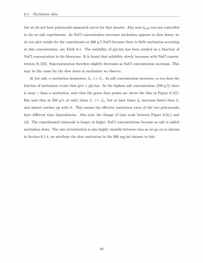
6.1. Nucleation data
but we do not have polymorph separated curves for that dataset. Also note theld was not controlled
in the no salt experiments. As NaCl concentration increases nucleation appears to slow down; we
do not plot results for the experiments at 300 g/l NaCl because there is little nucleation occurring
at this concentration, see Table 6.1. The solubility of glycine has been studied as a function of
NaCl concentration in the literature. It is found that solubility slowly increases with NaCl concen-
tration [8,123]. Supersaturation therefore slightly decreases as NaCl concentration increases. This
may be the cause for the slow down in nucleation we observe.
At low salt, α nucleation dominates, Iα >> Iγ . As salt concentration increases, so too does the
fraction of nucleation events that give γ glycine. At the highest salt concentration (250 g/l) there
is more γ than α nucleation, note that the green data points are above the blue in Figure 6.1(f).
But note that at 250 g/l, at early times Iγ >> Iα, but at later times Iα increases faster than Iγ
and almost catches up with it. This means the effective nucleation rates of the two polymorphs
have different time dependencies. Also note the change of time scale between Figure 6.2(c) and
(d). The experimental timescale is longer at higher NaCl concentrations because as salt is added
nucleation slows. The rate of nucleation is also highly variable between runs as we go on to discuss
in Section 6.1.4, we attribute the slow nucleation in the 200 mg/ml dataset to this.
84
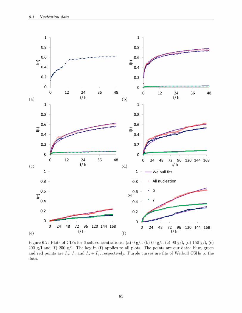
6.1. Nucleation data
(a)
0
0.2
0.4
0.6
0.8
1
0 12 24 36 48
I(t)
t/ h (b)
0
0.2
0.4
0.6
0.8
1
0 12 24 36 48
I(t)
t/ h
(c)
0
0.2
0.4
0.6
0.8
1
0 12 24 36 48
I(t)
t/ h (d)
0
0.2
0.4
0.6
0.8
1
0 24 48 72 96 120 144 168
I(t)
t/ h
(e)
0
0.2
0.4
0.6
0.8
1
0 24 48 72 96 120 144 168
I(t)
t/ h (f)
0
0.2
0.4
0.6
0.8
1
0 24 48 72 96 120 144 168
I(t)
t/ h
Weibull fits
All nucleation
α
γ
Figure 6.2: Plots of CIFs for 6 salt concentrations: (a) 0 g/l, (b) 60 g/l, (c) 90 g/l, (d) 150 g/l, (e)200 g/l and (f) 250 g/l. The key in (f) applies to all plots. The points are our data: blue, greenand red points are Iα, Iγ and Iα + Iγ , respectively. Purple curves are fits of Weibull CSHs to thedata.
85
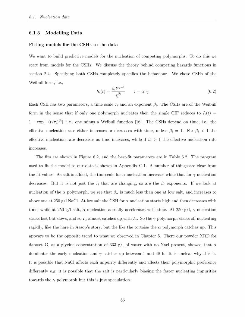
6.1. Nucleation data
6.1.3 Modelling Data
Fitting models for the CSHs to the data
We want to build predictive models for the nucleation of competing polymorphs. To do this we
start from models for the CSHs. We discuss the theory behind competing hazards functions in
section 2.4. Specifying both CSHs completely specifies the behaviour. We chose CSHs of the
Weibull form, i.e.,
hi(t) =βit
βi−1
τβiii = α, γ (6.2)
Each CSH has two parameters, a time scale τi and an exponent βi. The CSHs are of the Weibull
form in the sense that if only one polymorph nucleates then the single CIF reduces to Ii(t) =
1 − exp[−(t/τi)βi ], i.e., one minus a Weibull function [16]. The CSHs depend on time, i.e., the
effective nucleation rate either increases or decreases with time, unless βi = 1. For βi < 1 the
effective nucleation rate decreases as time increases, while if βi > 1 the effective nucleation rate
increases.
The fits are shown in Figure 6.2, and the best-fit parameters are in Table 6.2. The program
used to fit the model to our data is shown in Appendix C.1. A number of things are clear from
the fit values. As salt is added, the timescale for α nucleation increases while that for γ nucleation
decreases. But it is not just the τi that are changing, so are the βi exponents. If we look at
nucleation of the α polymorph, we see that βα is much less than one at low salt, and increases to
above one at 250 g/l NaCl. At low salt the CSH for α nucleation starts high and then decreases with
time, while at 250 g/l salt, α nucleation actually accelerates with time. At 250 g/l, γ nucleation
starts fast but slows, and so Iα almost catches up with Iγ . So the γ polymorph starts off nucleating
rapidly, like the hare in Aesop’s story, but the like the tortoise the α polymorph catches up. This
appears to be the opposite trend to what we observed in Chapter 5. There our powder XRD for
dataset G, at a glycine concentration of 333 g/l of water with no Nacl present, showed that α
dominates the early nucleation and γ catches up between 1 and 48 h. It is unclear why this is.
It is possible that NaCl affects each impurity differently and affects their polymorphic preference
differently e.g, it is possible that the salt is particularly biasing the faster nucleating impurities
towards the γ polymorph but this is just speculation.
86
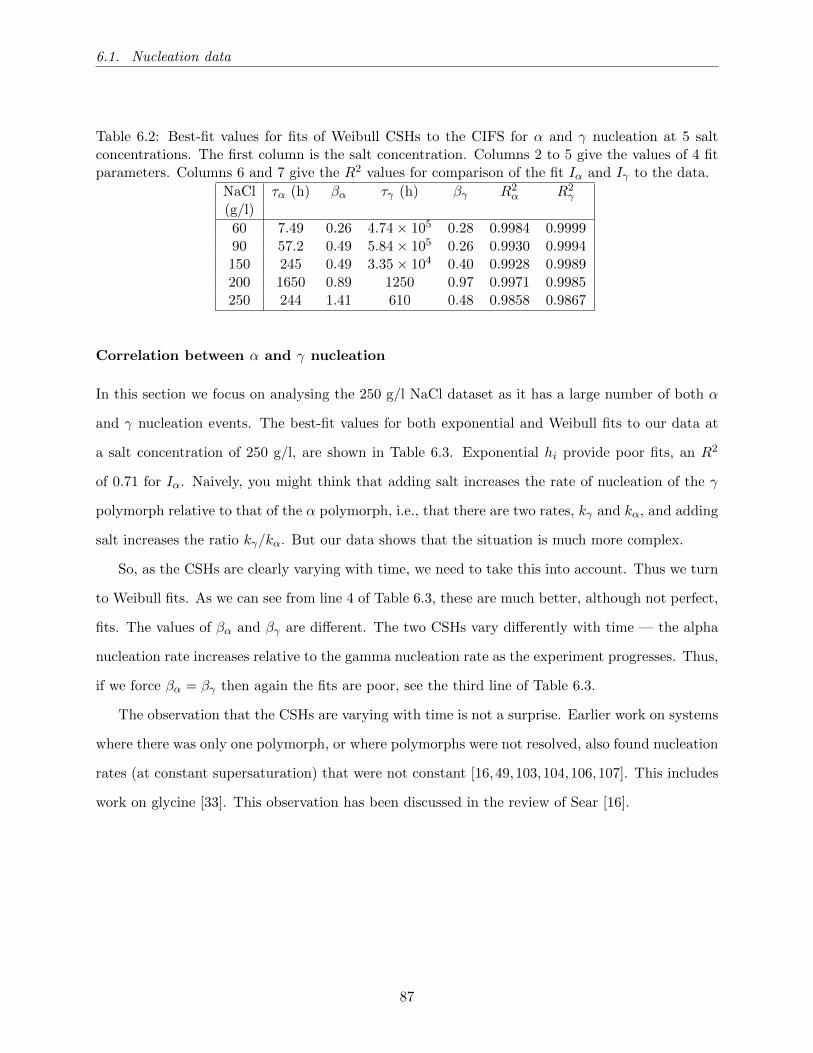
6.1. Nucleation data
Table 6.2: Best-fit values for fits of Weibull CSHs to the CIFS for α and γ nucleation at 5 saltconcentrations. The first column is the salt concentration. Columns 2 to 5 give the values of 4 fitparameters. Columns 6 and 7 give the R2 values for comparison of the fit Iα and Iγ to the data.
NaCl τα (h) βα τγ (h) βγ R2α R2
γ
(g/l)
60 7.49 0.26 4.74× 10⁵ 0.28 0.9984 0.999990 57.2 0.49 5.84× 10⁵ 0.26 0.9930 0.9994150 245 0.49 3.35× 10⁴ 0.40 0.9928 0.9989200 1650 0.89 1250 0.97 0.9971 0.9985250 244 1.41 610 0.48 0.9858 0.9867
Correlation between α and γ nucleation
In this section we focus on analysing the 250 g/l NaCl dataset as it has a large number of both α
and γ nucleation events. The best-fit values for both exponential and Weibull fits to our data at
a salt concentration of 250 g/l, are shown in Table 6.3. Exponential hi provide poor fits, an R2
of 0.71 for Iα. Naively, you might think that adding salt increases the rate of nucleation of the γ
polymorph relative to that of the α polymorph, i.e., that there are two rates, kγ and kα, and adding
salt increases the ratio kγ/kα. But our data shows that the situation is much more complex.
So, as the CSHs are clearly varying with time, we need to take this into account. Thus we turn
to Weibull fits. As we can see from line 4 of Table 6.3, these are much better, although not perfect,
fits. The values of βα and βγ are different. The two CSHs vary differently with time — the alpha
nucleation rate increases relative to the gamma nucleation rate as the experiment progresses. Thus,
if we force βα = βγ then again the fits are poor, see the third line of Table 6.3.
The observation that the CSHs are varying with time is not a surprise. Earlier work on systems
where there was only one polymorph, or where polymorphs were not resolved, also found nucleation
rates (at constant supersaturation) that were not constant [16,49,103,104,106,107]. This includes
work on glycine [33]. This observation has been discussed in the review of Sear [16].
87
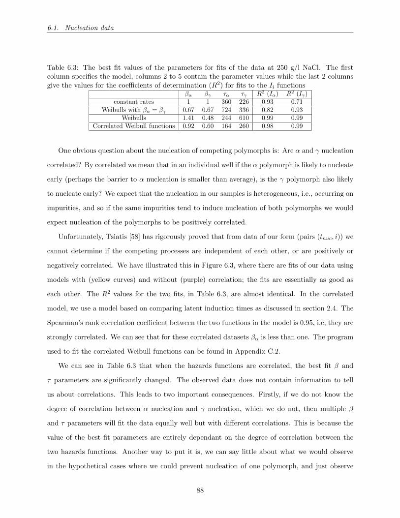
6.1. Nucleation data
Table 6.3: The best fit values of the parameters for fits of the data at 250 g/l NaCl. The firstcolumn specifies the model, columns 2 to 5 contain the parameter values while the last 2 columnsgive the values for the coefficients of determination (R2) for fits to the Ii functions
βα βγ τα τγ R2 (Iα) R2 (Iγ)constant rates 1 1 360 226 0.93 0.71
Weibulls with βα = βγ 0.67 0.67 724 336 0.82 0.93Weibulls 1.41 0.48 244 610 0.99 0.99
Correlated Weibull functions 0.92 0.60 164 260 0.98 0.99
One obvious question about the nucleation of competing polymorphs is: Are α and γ nucleation
correlated? By correlated we mean that in an individual well if the α polymorph is likely to nucleate
early (perhaps the barrier to α nucleation is smaller than average), is the γ polymorph also likely
to nucleate early? We expect that the nucleation in our samples is heterogeneous, i.e., occurring on
impurities, and so if the same impurities tend to induce nucleation of both polymorphs we would
expect nucleation of the polymorphs to be positively correlated.
Unfortunately, Tsiatis [58] has rigorously proved that from data of our form (pairs (tnuc, i)) we
cannot determine if the competing processes are independent of each other, or are positively or
negatively correlated. We have illustrated this in Figure 6.3, where there are fits of our data using
models with (yellow curves) and without (purple) correlation; the fits are essentially as good as
each other. The R2 values for the two fits, in Table 6.3, are almost identical. In the correlated
model, we use a model based on comparing latent induction times as discussed in section 2.4. The
Spearman’s rank correlation coefficient between the two functions in the model is 0.95, i.e, they are
strongly correlated. We can see that for these correlated datasets βα is less than one. The program
used to fit the correlated Weibull functions can be found in Appendix C.2.
We can see in Table 6.3 that when the hazards functions are correlated, the best fit β and
τ parameters are significantly changed. The observed data does not contain information to tell
us about correlations. This leads to two important consequences. Firstly, if we do not know the
degree of correlation between α nucleation and γ nucleation, which we do not, then multiple β
and τ parameters will fit the data equally well but with different correlations. This is because the
value of the best fit parameters are entirely dependant on the degree of correlation between the
two hazards functions. Another way to put it is, we can say little about what we would observe
in the hypothetical cases where we could prevent nucleation of one polymorph, and just observe
88
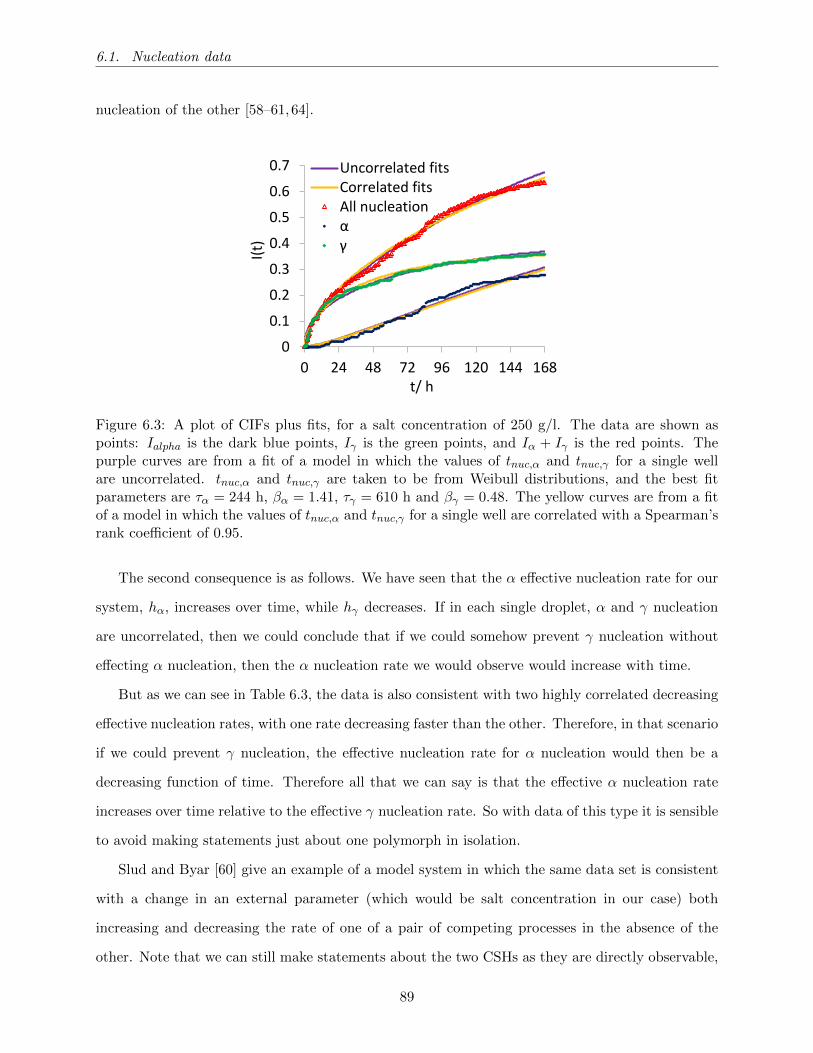
6.1. Nucleation data
nucleation of the other [58–61,64].
0
0.1
0.2
0.3
0.4
0.5
0.6
0.7
0 24 48 72 96 120 144 168
I(t)
t/ h
Uncorrelated fitsCorrelated fitsAll nucleationαγ
Figure 6.3: A plot of CIFs plus fits, for a salt concentration of 250 g/l. The data are shown aspoints: Ialpha is the dark blue points, Iγ is the green points, and Iα + Iγ is the red points. Thepurple curves are from a fit of a model in which the values of tnuc,α and tnuc,γ for a single wellare uncorrelated. tnuc,α and tnuc,γ are taken to be from Weibull distributions, and the best fitparameters are τα = 244 h, βα = 1.41, τγ = 610 h and βγ = 0.48. The yellow curves are from a fitof a model in which the values of tnuc,α and tnuc,γ for a single well are correlated with a Spearman’srank coefficient of 0.95.
The second consequence is as follows. We have seen that the α effective nucleation rate for our
system, hα, increases over time, while hγ decreases. If in each single droplet, α and γ nucleation
are uncorrelated, then we could conclude that if we could somehow prevent γ nucleation without
effecting α nucleation, then the α nucleation rate we would observe would increase with time.
But as we can see in Table 6.3, the data is also consistent with two highly correlated decreasing
effective nucleation rates, with one rate decreasing faster than the other. Therefore, in that scenario
if we could prevent γ nucleation, the effective nucleation rate for α nucleation would then be a
decreasing function of time. Therefore all that we can say is that the effective α nucleation rate
increases over time relative to the effective γ nucleation rate. So with data of this type it is sensible
to avoid making statements just about one polymorph in isolation.
Slud and Byar [60] give an example of a model system in which the same data set is consistent
with a change in an external parameter (which would be salt concentration in our case) both
increasing and decreasing the rate of one of a pair of competing processes in the absence of the
other. Note that we can still make statements about the two CSHs as they are directly observable,
89

6.1. Nucleation data
and are for nucleation of one polymorph in the presence of the other. This is a subtle point that
has been discussed extensively in the literature on competing risks [58–61,64].
6.1.4 Reproducibility of total nucleation rates and relative nucleation rates
The induction time cumulative incident functions (CIFs) can be seen for each individual run in
Figure 6.4. (By adding the individual runs together we obtain the CIFs in Figure 6.2). Repro-
ducibility, in terms of the amount of samples in which nucleation takes place on a run to run basis
is poor. What is reproducible however, is the fraction of nucleation events that correspond to each
polymorph. In Figure 6.4, γ nucleation corresponds to the difference between the all-nucleation
CIFs and the α nucleation CIFs for each run. We see at low NaCl concentrations nucleation is
dominated by the α polymorph and this phenomenon is reproducible between runs. Even when
two runs have a significantly different amount of nucleation occurring, the relative amount of the
nucleation of each polymorph is similar. For example at 150 g/l NaCl, see Figure 6.4(c), one run
(dark red) has about three times more nucleation events than the other (light red). However, for
both runs, about 15% of the total nucleation events give the γ polymorph.
It should also be noted that the distribution of induction times is reproducibly different for the
two polymorphs at the high salt concentration of 250 g/l NaCl, see Figure 6.4. The γ induction
time distribution initially has a very fast relative nucleation rate which slows down over time in
all of the runs, while the α induction time distribution initially has a very slow relative nucleation
rate which speeds up over time giving an ‘s-shaped’ curve. This is well illustrated by the median
induction times of the subpopulations of α nucleating wells and γ nucleating wells for each run.
The median α induction times for the three runs are 77 h, 102 h and 81 h, while median γ induction
times for those runs are 13.5 h, 14 h and 34 h respectively. We can therefore say, in addition to the
fraction of nucleation that corresponds to each polymorph being reproducible, the relative change
in the effective nucleation rates of the two polymorphs is also reproducible.
90

6.1. Nucleation data
(a)
0
0.2
0.4
0.6
0.8
1
0 12 24 36 48
I(t)
Time/ h (b)
0
0.2
0.4
0.6
0.8
1
0 12 24 36 48
I(t)
Time/ h
(c)
0
0.2
0.4
0.6
0.8
1
0 24 48 72 96 120 144 168
I(t)
Time/ h (d)
0
0.2
0.4
0.6
0.8
1
0 24 48 72 96 120 144 168
I(t)
Time/ h
(e)
0
0.2
0.4
0.6
0.8
1
0 24 48 72 96 120 144 168
I(t)
Time/ h
α1
α2
α3
α1 + γ1
α2 + γ2
α3 + γ3
α1
α2
α3
α1 + γ1
α2 + γ2
α3 + γ3
Figure 6.4: CIFs for individual runs at NaCl concentrations: (a) 60 g/l, (b) 90 g/l, (c) 150 g/l,(d) 200 g/l and (e) 250 g/l. The key in (e) applies to all 5 plots. There are 2 runs in (a) to (d),and 3 runs in (e). For each run we plot Iα as closed blue symbols, and Iα + Iγ as open red/brownsymbols. For example, in (a) for the first run no γ crystals form, so the solid and open symbols areon top of each other as Iγ = 0, while for the second run a small number of γ crystals start to formafter a few hours, and so the pale blue closed and open red symbols move apart.
91
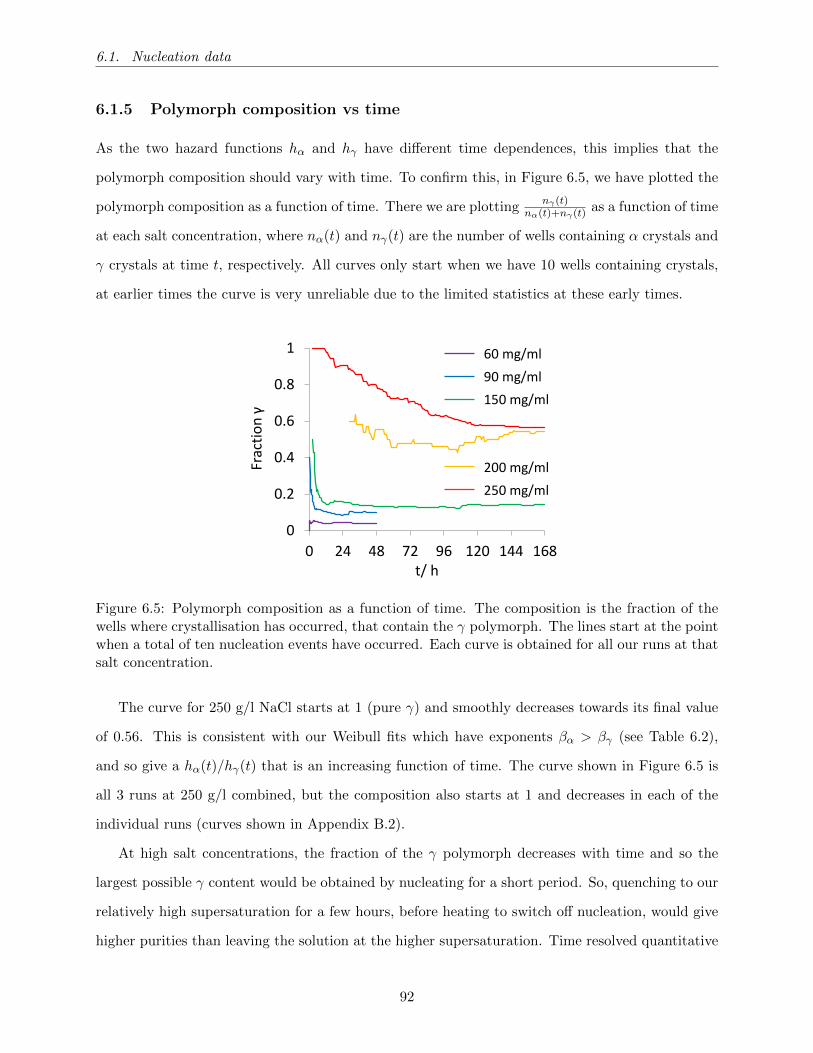
6.1. Nucleation data
6.1.5 Polymorph composition vs time
As the two hazard functions hα and hγ have different time dependences, this implies that the
polymorph composition should vary with time. To confirm this, in Figure 6.5, we have plotted the
polymorph composition as a function of time. There we are plottingnγ(t)
nα(t)+nγ(t) as a function of time
at each salt concentration, where nα(t) and nγ(t) are the number of wells containing α crystals and
γ crystals at time t, respectively. All curves only start when we have 10 wells containing crystals,
at earlier times the curve is very unreliable due to the limited statistics at these early times.
0
0.2
0.4
0.6
0.8
1
0 24 48 72 96 120 144 168
Frac
tio
n γ
t/ h
60 mg/ml
90 mg/ml
150 mg/ml
200 mg/ml
250 mg/ml
Figure 6.5: Polymorph composition as a function of time. The composition is the fraction of thewells where crystallisation has occurred, that contain the γ polymorph. The lines start at the pointwhen a total of ten nucleation events have occurred. Each curve is obtained for all our runs at thatsalt concentration.
The curve for 250 g/l NaCl starts at 1 (pure γ) and smoothly decreases towards its final value
of 0.56. This is consistent with our Weibull fits which have exponents βα > βγ (see Table 6.2),
and so give a hα(t)/hγ(t) that is an increasing function of time. The curve shown in Figure 6.5 is
all 3 runs at 250 g/l combined, but the composition also starts at 1 and decreases in each of the
individual runs (curves shown in Appendix B.2).
At high salt concentrations, the fraction of the γ polymorph decreases with time and so the
largest possible γ content would be obtained by nucleating for a short period. So, quenching to our
relatively high supersaturation for a few hours, before heating to switch off nucleation, would give
higher purities than leaving the solution at the higher supersaturation. Time resolved quantitative
92
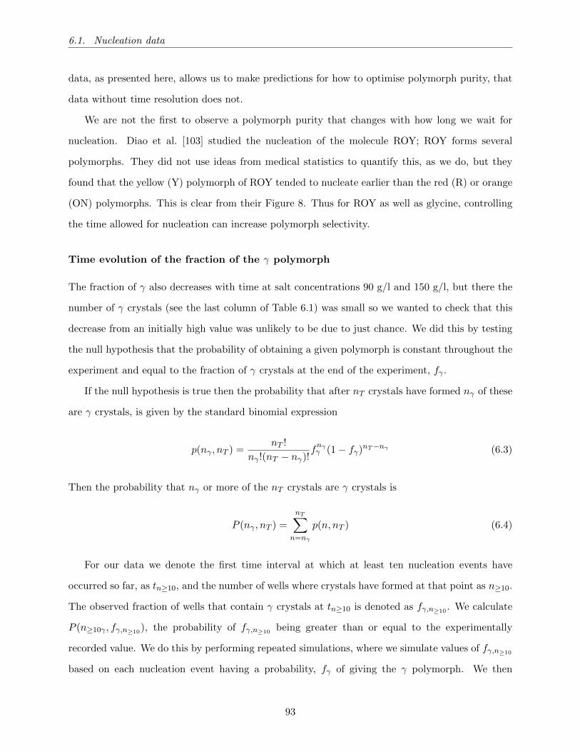
6.1. Nucleation data
data, as presented here, allows us to make predictions for how to optimise polymorph purity, that
data without time resolution does not.
We are not the first to observe a polymorph purity that changes with how long we wait for
nucleation. Diao et al. [103] studied the nucleation of the molecule ROY; ROY forms several
polymorphs. They did not use ideas from medical statistics to quantify this, as we do, but they
found that the yellow (Y) polymorph of ROY tended to nucleate earlier than the red (R) or orange
(ON) polymorphs. This is clear from their Figure 8. Thus for ROY as well as glycine, controlling
the time allowed for nucleation can increase polymorph selectivity.
Time evolution of the fraction of the γ polymorph
The fraction of γ also decreases with time at salt concentrations 90 g/l and 150 g/l, but there the
number of γ crystals (see the last column of Table 6.1) was small so we wanted to check that this
decrease from an initially high value was unlikely to be due to just chance. We did this by testing
the null hypothesis that the probability of obtaining a given polymorph is constant throughout the
experiment and equal to the fraction of γ crystals at the end of the experiment, fγ .
If the null hypothesis is true then the probability that after nT crystals have formed nγ of these
are γ crystals, is given by the standard binomial expression
p(nγ , nT ) =nT !
nγ !(nT − nγ)!fnγγ (1− fγ)nT−nγ (6.3)
Then the probability that nγ or more of the nT crystals are γ crystals is
P (nγ , nT ) =
nT∑n=nγ
p(n, nT ) (6.4)
For our data we denote the first time interval at which at least ten nucleation events have
occurred so far, as tn≥10, and the number of wells where crystals have formed at that point as n≥10.
The observed fraction of wells that contain γ crystals at tn≥10 is denoted as fγ,n≥10. We calculate
P (n≥10γ , fγ,n≥10), the probability of fγ,n≥10
being greater than or equal to the experimentally
recorded value. We do this by performing repeated simulations, where we simulate values of fγ,n≥10
based on each nucleation event having a probability, fγ of giving the γ polymorph. We then
93
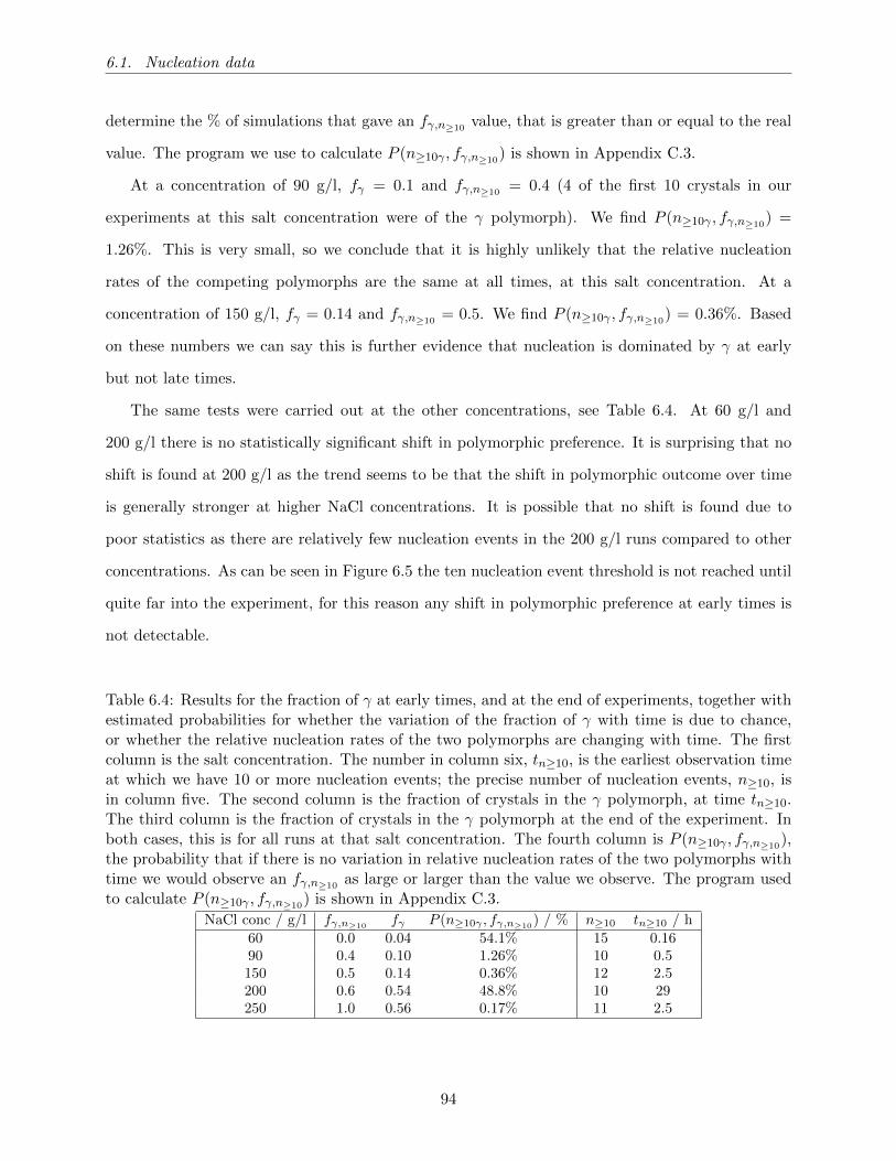
6.1. Nucleation data
determine the % of simulations that gave an fγ,n≥10value, that is greater than or equal to the real
value. The program we use to calculate P (n≥10γ , fγ,n≥10) is shown in Appendix C.3.
At a concentration of 90 g/l, fγ = 0.1 and fγ,n≥10= 0.4 (4 of the first 10 crystals in our
experiments at this salt concentration were of the γ polymorph). We find P (n≥10γ , fγ,n≥10) =
1.26%. This is very small, so we conclude that it is highly unlikely that the relative nucleation
rates of the competing polymorphs are the same at all times, at this salt concentration. At a
concentration of 150 g/l, fγ = 0.14 and fγ,n≥10= 0.5. We find P (n≥10γ , fγ,n≥10
) = 0.36%. Based
on these numbers we can say this is further evidence that nucleation is dominated by γ at early
but not late times.
The same tests were carried out at the other concentrations, see Table 6.4. At 60 g/l and
200 g/l there is no statistically significant shift in polymorphic preference. It is surprising that no
shift is found at 200 g/l as the trend seems to be that the shift in polymorphic outcome over time
is generally stronger at higher NaCl concentrations. It is possible that no shift is found due to
poor statistics as there are relatively few nucleation events in the 200 g/l runs compared to other
concentrations. As can be seen in Figure 6.5 the ten nucleation event threshold is not reached until
quite far into the experiment, for this reason any shift in polymorphic preference at early times is
not detectable.
Table 6.4: Results for the fraction of γ at early times, and at the end of experiments, together withestimated probabilities for whether the variation of the fraction of γ with time is due to chance,or whether the relative nucleation rates of the two polymorphs are changing with time. The firstcolumn is the salt concentration. The number in column six, tn≥10, is the earliest observation timeat which we have 10 or more nucleation events; the precise number of nucleation events, n≥10, isin column five. The second column is the fraction of crystals in the γ polymorph, at time tn≥10.The third column is the fraction of crystals in the γ polymorph at the end of the experiment. Inboth cases, this is for all runs at that salt concentration. The fourth column is P (n≥10γ , fγ,n≥10
),the probability that if there is no variation in relative nucleation rates of the two polymorphs withtime we would observe an fγ,n≥10
as large or larger than the value we observe. The program usedto calculate P (n≥10γ , fγ,n≥10
) is shown in Appendix C.3.
NaCl conc / g/l fγ,n≥10fγ P (n≥10γ , fγ,n≥10
) / % n≥10 tn≥10 / h
60 0.0 0.04 54.1% 15 0.1690 0.4 0.10 1.26% 10 0.5150 0.5 0.14 0.36% 12 2.5200 0.6 0.54 48.8% 10 29250 1.0 0.56 0.17% 11 2.5
94

6.1. Nucleation data
Isothermal and non-isothermal crystallisation
It is often the case that when producing crystals, the aim is to obtain a particular polymorph e.g.,
in the pharmaceutical industry for crystalline drugs a specific polymorph is required. We have
shown that the different polymorphs have different distributions of induction times. We observed
that at an NaCl concentration of 250 g/l, γ glycine nucleation dominated at early times, which
implies that cutting off nucleation early in the experiment would improve γ glycine polymorph
purity. To test this hypothesis we did additional experiments at 250 g/l NaCl, where we reduced
the supersaturation after 18 hours.
Here we present data for experiments where the first 18 h of the experiments are isothermal,
at a constant temperature of 21 C (the same as our other datasets), but after 18 hours the tem-
perature is increased to 30 C. It is then maintained at 30 C for the remainder of the experiment,
which is an additional 48 h (taking the total experiment time to 66 h). At 30 C the solution is
still supersaturated but the supersaturation is significantly lower than at 21 C, and therefore nu-
cleation should be significantly decreased. Here we aim to show that this technique of reducing the
supersaturation after some time period is an effective way of controlling the polymorphic outcome
of nucleation.
In Figure 6.6, we have data at 250 g/l NaCl, with and without a temperature increase at 18
h. We carried out two runs with the temperature increase at 18 h, between the two runs only one
crystal nucleated between 18 h and 66 h, the time period in which the samples were held at 30 C.
From Figure 6.6 we can clearly see that increasing the temperature at 18 h significantly reduces the
effective nucleation rate as compared to the normal isothermal data. For completeness, we show
the individual runs that make up these datasets in Appendix B.1.
95

6.1. Nucleation data
0
0.1
0.2
0.3
0.4
0
0.1
0.2
0.3
0.4
0.5
0.6
0 12 24 36 48 60 72
Frac
tio
n α
I(t)
t/ h
Heated to 30 °C after 18 hIsothermalHeated to 30 °C after 18 h frac αIsothermal frac α
Figure 6.6: CIF functions for glycine induction time datasets at an NaCl concentration of 250g/l. We show the isothermal (21 C) dataset presented in Figure 6.2(e) and a dataset where theexperiment is isothermal (21 C) for the first 18 h after which the microplate is maintained at 30C for the following 48 h. We also show the polymorph composition as a function of time for theisothermal dataset. For the dataset with a temperature increase, all crystals are γ. The verticaldashed line indicates t = 18 h.
We chose to heat the microplate after 18 h as it is the point at which the effective α nucleation
rate starts to become significant. For the isothermal dataset, only 9% of nucleation events before
18 h produce α glycine. For that same dataset after 18 h, the α nucleation rate sharply increases
while the γ nucleation rate sharply decreases. Almost 50% of the nucleation events between 18
h and 66 h give α glycine. The total % of crystallised wells containing α glycine approximately
triples between 18 h and 66 h.
For the dataset of two runs with the temperature increase at 18 h, none of the wells nucleating
in the first 18 h are α. For the isothermal dataset, one of the three runs of which it is composed
has no α nucleation events within the first 18 h (see Appendix B.2). We can therefore say any
differences between the two datasets presented here within the first 18 h are consistent with being
statistical fluctuations.
The results presented in this section give us some useful insights into controlling nucleation. By
reducing supersaturation mid-way through an experiment we can significantly decrease the effective
nucleation rate, there was only 1 nucleation event between 18 h and 66 h when we increased the
temperature to 30 C. By using a high NaCl concentration (250 g/l) in conjunction with controlling
96
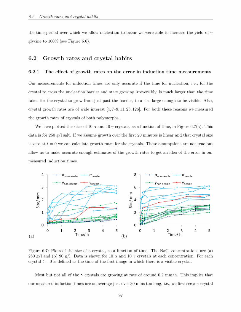
6.2. Growth rates and crystal habits
the time period over which we allow nucleation to occur we were able to increase the yield of γ
glycine to 100% (see Figure 6.6).
6.2 Growth rates and crystal habits
6.2.1 The effect of growth rates on the error in induction time measurements
Our measurements for induction times are only accurate if the time for nucleation, i.e., for the
crystal to cross the nucleation barrier and start growing irreversibly, is much larger than the time
taken for the crystal to grow from just past the barrier, to a size large enough to be visible. Also,
crystal growth rates are of wide interest [4, 7–9, 11, 23, 126]. For both these reasons we measured
the growth rates of crystals of both polymorphs.
We have plotted the sizes of 10 α and 10 γ crystals, as a function of time, in Figure 6.7(a). This
data is for 250 g/l salt. If we assume growth over the first 20 minutes is linear and that crystal size
is zero at t = 0 we can calculate growth rates for the crystals. These assumptions are not true but
allow us to make accurate enough estimates of the growth rates to get an idea of the error in our
measured induction times.
(a)
0
1
2
3
4
0 1 2 3 4 5
Size
/ m
m
Time/ h
αnon-needle
γnon-needle
αneedle
γneedle
(b)
0
2
4
6
8
0 1 2 3 4 5
Size
/ m
m
Time/ h
αnon-needle
γnon-needle
αneedle
γneedle
Figure 6.7: Plots of the size of a crystal, as a function of time. The NaCl concentrations are (a)250 g/l and (b) 90 g/l. Data is shown for 10 α and 10 γ crystals at each concentration. For eachcrystal t = 0 is defined as the time of the first image in which there is a visible crystal.
Most but not all of the γ crystals are growing at rate of around 0.2 mm/h. This implies that
our measured induction times are on average just over 30 mins too long, i.e., we first see a γ crystal
97

6.2. Growth rates and crystal habits
about 30 mins after it nucleated as a microscopic nucleus. A few α crystals are also growing at
around 0.2 mm/h, but most are initially growing of order 10 times faster. Our runs at 250 g/l salt
are of 168 h duration, so except for nucleation at early times, a 30 mins error is a relatively small
error.
We have also plotted the sizes of 10 α and 10 γ crystals, at 90 g/l NaCl in Figure 6.7(b). We
focus on the γ crystals for estimating induction time errors as their growth is slightly slower than
the α crystals. Here the growth rate for the γ crystals is around 2 mm/h. This means the error
in our induction time measurements should be less than 10 minutes in most cases. This is a small
error for all but the very shortest induction times.
6.2.2 Variation in crystal size populations with time
In Table 6.5, we present crystal sizes at three times from Figure 6.7. In this table, the interquartile
range (IQR) is Q3 −Q1, where Q1 is the first quartile of the distribution of crystal sizes, i.e., the
size at which 25% of the crystals are smaller and 75% are larger, and Q3 is the size where 75% are
smaller and 25% are larger. The IQR is a convenient measure of the spread in crystal sizes as it is
relatively insensitive to outliers (unlike the standard deviation), and we have outliers in the crystal
size, see Figure 6.7.
It is clear that the growth rates of both polymorphs vary widely between one crystal and another.
This is especially true for the α polymorph where at early times the IQR is larger than the mean.
This variability is related to crystal habit. As we can see in Figure 6.7, needle-like crystals tend to
have much faster growth rates than non needle-like crystals. Crystal growth is known to often rely
on defects and so different crystals grow at different rates due to having different defects [140]. It
may be that the crystals growing at different rates have different defects. This idea fits with habit
being related to growth rate. Ultimately, we have no knowledge of what defects are present and
affecting growth, so this is just speculation.
98

6.2. Growth rates and crystal habits
Table 6.5: Mean glycine sizes at initial detection and at two subsequent times, for both α and γpolymorphs. We estimate the uncertainties of the mean values with error estimates that are thestandard deviation of the measured sizes, divided by the square root of the number of crystalsmeasured (10 crystals of each polymorph at each concentration). We measure the width of thedistribution of sizes of the crystals via the interquartile range.
NaCl conc / g/l Time / mins Size/ mmmean Interquartile range
α γ α γ90 0 1.6 ± 0.5 0.6 ± 0.1 3.2 0.69
20 2.5 ± 0.7 1.2 ± 0.3 4.0 1.5300 4.3 ± 0.5 3.0 ± 0.2 3.0 0.56
250 0 0.5 ± 0.1 0.17 ± 0.02 0.74 0.1120 0.9 ± 0.2 0.23 ± 0.01 1.2 0.025300 1.8 ± 0.3 0.9 ± 0.1 2.3 0.23
6.2.3 NaCl concentration and crystal growth
If we compare Figure 6.7(a) and (b), we see that crystals grow faster at 90 g/l of salt than 250 g/l.
In the previous chapter we presented growth rates at the slightly higher glycine concentration of
333 g/l. Twenty minutes after first observing the crystal with that dataset, the mean crystal size
was 1.1± 0.1 mm, we did not have information on the polymorph of each crystal there but we do
know a majority were γ glycine. This is within error of our 90 mg/ml NaCl concentration γ growth
data of 1.2±0.3 mm. It is surprising that at this lower supersaturation of 320 g/l the growth is not
slower than at 333 g/l. We are unsure as to why this is. Adding more salt up to 250 g/l appears
to slow growth, but it is possible that the effect of salt on growth is non-linear.
Other work has looked at the effect of salt on glycine growth rate. In the work of Han et al. [8],
the γ glycine growth rate in ultrapure water is slightly faster than in ≈ 100 g/l of water NaCl
solution along the C-axis but slightly slower along the b-axis and the total shift in growth rate
is small. We appear to see a decrease in growth rate as salt concentration increases although it
should be noted that our experiments go to significantly higher salt concentrations than Han et
al. [8] worked at.
6.2.4 Polymorphism and crystal growth
We see in Table 6.5 the average size of each polymorph at each salt concentration. Due to crystal
growth plateauing at later times, especially for the 90 g/l NaCl data, our most reliable approx-
99
6.2. Growth rates and crystal habits
imation of growth rates are obtained by dividing the size 20 mins after nucleation, by 20 mins.
Growth of the α polymorph is generally faster than the γ polymorph. This is in agreement with
what has been observed in other studies [11]. As salt concentration increases the γ glycine growth
slows down more than α glycine growth.
6.2.5 Crystal habits
A significant number of alpha crystals grow in needle like shapes, parallel to the plane of view. We
show example crystals in the different habits in Figure 6.8. The way in which we measure the size
of crystals is in terms of a length as opposed to an area or volume. The consequence of this is that
a crystal with a large growth rate along one axis and a slow growth rate along the other axes will,
according to our metric, have a more rapid growth, than a crystal which has similar growth rates
across all of its axes. This may be true even if the second crystal’s volume is growing at a faster
rate.
(a) (b)
(c) (d)
Figure 6.8: Here we show some typical crystal habits. (a) and (b) two needle-like α crystals lessthan an hour after nucleation. (c) A non needle-like α crystal and (d) a non needle-like γ crystalboth 5 h after nucleation.
100

6.2. Growth rates and crystal habits
6.2.6 Induction time and crystal habit
As we have discussed, a number of the crystals formed were initially needle-like in shape. Here
we look at whether the shape of a crystal is related to its induction time. The aspect ratio of
crystals can change over time, and initially needle-like crystals may become less needle-like as time
progresses. Here, we define needle-like crystals as crystals which have an aspect ratio above 5:1
for the first 5 hours after nucleation occurs. To clarify we are interested only in the initial shape
of the crystal to categorise it and we do not quantitatively examine how the shape of each crystal
changes over time. We just look at the relationship between induction time and initial crystal habit.
The populations of needle-like and non needle-like crystals are quite distinct in that most of the
non needle-like crystals have an aspect ratio significantly lower than 5:1 and some of the needle-
like crystals have an aspect ratio significantly above 5:1. Although 5:1 is an arbitrary threshold
for categorizing needle-like crystals if we were to change it to say 6:1 or 4:1, the data plotted in
Figure 6.9 would only change very slightly.
In Figure 6.9 we plot the fraction of crystals that are needle-like as a function of the number of
wells crystallised for each salt concentration. We chose to compare the fraction of wells containing
needle-like crystals to the number of wells nucleated instead of time. The reason for this is by
plotting against time we would also be looking at the nucleation rate which varies between salt
concentrations. By plotting the number of crystallised wells on the x axis we are able to compare the
fraction of wells that contain need-like growths for each salt concentration without the comparison
being distorted by the varying nucleation rates at those salt concentrations.
101
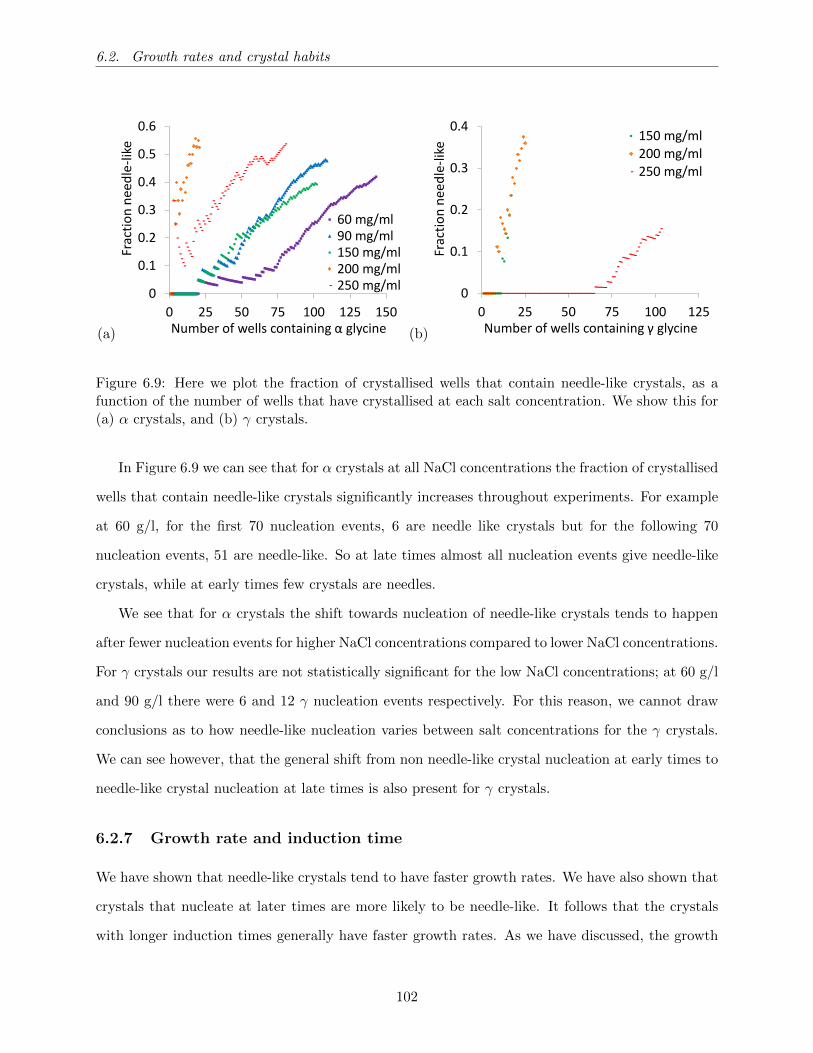
6.2. Growth rates and crystal habits
(a)
0
0.1
0.2
0.3
0.4
0.5
0.6
0 25 50 75 100 125 150
Frac
tio
n n
eed
le-l
ike
Number of wells containing α glycine
60 mg/ml90 mg/ml150 mg/ml200 mg/ml250 mg/ml
(b)
0
0.1
0.2
0.3
0.4
0 25 50 75 100 125
Frac
tio
n n
ee
dle
-lik
e
Number of wells containing γ glycine
150 mg/ml200 mg/ml250 mg/ml
Figure 6.9: Here we plot the fraction of crystallised wells that contain needle-like crystals, as afunction of the number of wells that have crystallised at each salt concentration. We show this for(a) α crystals, and (b) γ crystals.
In Figure 6.9 we can see that for α crystals at all NaCl concentrations the fraction of crystallised
wells that contain needle-like crystals significantly increases throughout experiments. For example
at 60 g/l, for the first 70 nucleation events, 6 are needle like crystals but for the following 70
nucleation events, 51 are needle-like. So at late times almost all nucleation events give needle-like
crystals, while at early times few crystals are needles.
We see that for α crystals the shift towards nucleation of needle-like crystals tends to happen
after fewer nucleation events for higher NaCl concentrations compared to lower NaCl concentrations.
For γ crystals our results are not statistically significant for the low NaCl concentrations; at 60 g/l
and 90 g/l there were 6 and 12 γ nucleation events respectively. For this reason, we cannot draw
conclusions as to how needle-like nucleation varies between salt concentrations for the γ crystals.
We can see however, that the general shift from non needle-like crystal nucleation at early times to
needle-like crystal nucleation at late times is also present for γ crystals.
6.2.7 Growth rate and induction time
We have shown that needle-like crystals tend to have faster growth rates. We have also shown that
crystals that nucleate at later times are more likely to be needle-like. It follows that the crystals
with longer induction times generally have faster growth rates. As we have discussed, the growth
102
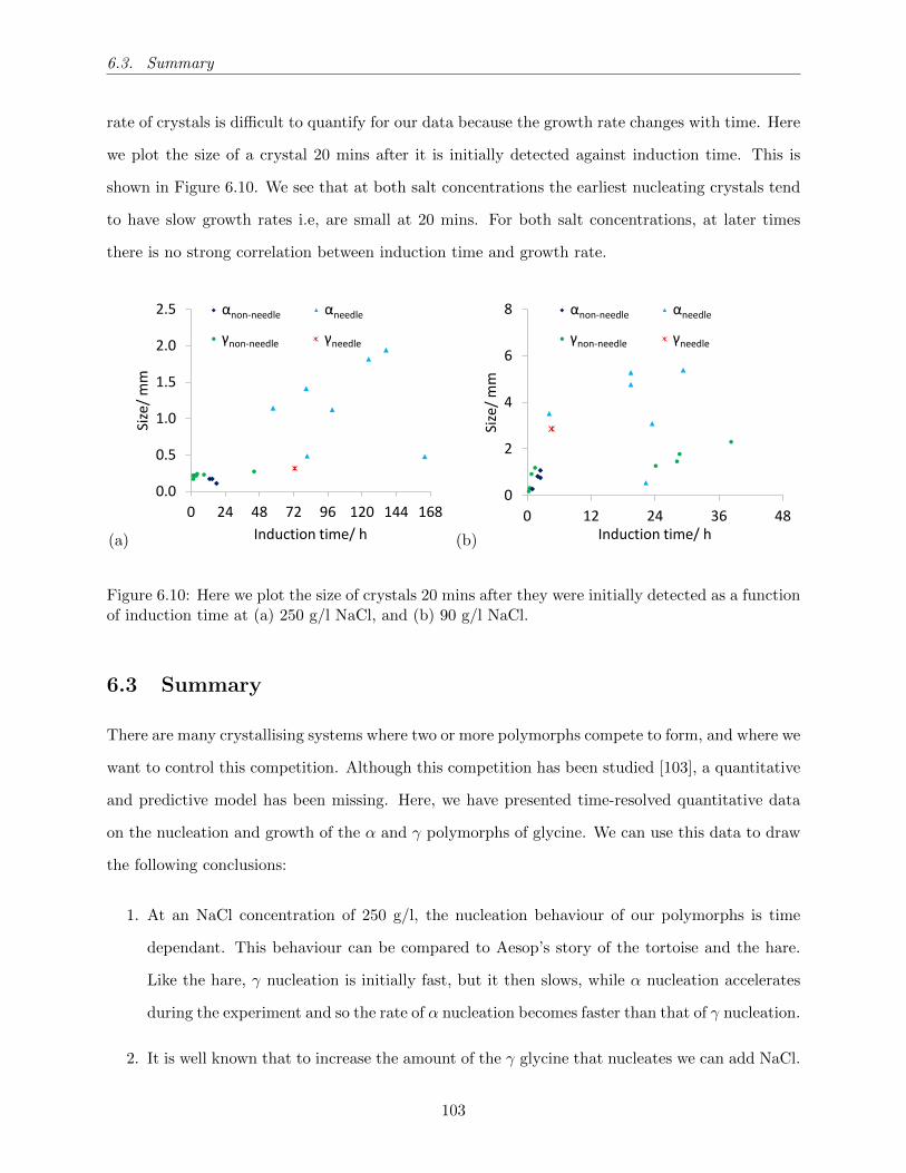
6.3. Summary
rate of crystals is difficult to quantify for our data because the growth rate changes with time. Here
we plot the size of a crystal 20 mins after it is initially detected against induction time. This is
shown in Figure 6.10. We see that at both salt concentrations the earliest nucleating crystals tend
to have slow growth rates i.e, are small at 20 mins. For both salt concentrations, at later times
there is no strong correlation between induction time and growth rate.
(a)
0.0
0.5
1.0
1.5
2.0
2.5
0 24 48 72 96 120 144 168
Size
/ m
m
Induction time/ h
αnon-needle
γnon-needle
αneedle
γneedle
(b)
0
2
4
6
8
0 12 24 36 48
Size
/ m
m
Induction time/ h
αnon-needle
γnon-needle
αneedle
γneedle
Figure 6.10: Here we plot the size of crystals 20 mins after they were initially detected as a functionof induction time at (a) 250 g/l NaCl, and (b) 90 g/l NaCl.
6.3 Summary
There are many crystallising systems where two or more polymorphs compete to form, and where we
want to control this competition. Although this competition has been studied [103], a quantitative
and predictive model has been missing. Here, we have presented time-resolved quantitative data
on the nucleation and growth of the α and γ polymorphs of glycine. We can use this data to draw
the following conclusions:
1. At an NaCl concentration of 250 g/l, the nucleation behaviour of our polymorphs is time
dependant. This behaviour can be compared to Aesop’s story of the tortoise and the hare.
Like the hare, γ nucleation is initially fast, but it then slows, while α nucleation accelerates
during the experiment and so the rate of α nucleation becomes faster than that of γ nucleation.
2. It is well known that to increase the amount of the γ glycine that nucleates we can add NaCl.
103

6.3. Summary
We have shown that to maximise this, we can also control the time period for which the
solution is at a high supersaturation. By keeping our solution at a high supersaturation for a
short period of time, before increasing temperature and so decreasing supersaturation, a 100
% yield of γ glycine was obtained.
3. We presented growth data for glycine’s α and γ polymorphs. We have also shown that α
growth is typically faster than γ growth across our range of NaCl concentrations.
4. Crystal growth was found to be slower as salt concentration increased. Growth rates were
observed to be highly variable from crystal to crystal, particularly for α crystals. We showed
that growth rates were linked to the crystal habit and that needle-like crystals tend to have
fast growth rates.
We end the chapter with a couple of speculations. The growth rate of crystals can be heavily
influenced by the presence of defects. The presence of defects affects the growth mechanism, and
therefore the growth rate along all axes and hence the habit of formed crystals. We speculate that
the presence of defects in some of our crystals is what simultaneously changes their growth rate
and hence habit.
As we have noted, previous work [58–61, 64] has shown that from data of our form we cannot
determine what the correlations are between α and γ nucleation, and so it is dangerous to assume the
two processes are independent as they may well be strongly correlated. Nevertheless, we would like
to make a final speculation, based on assuming independence (no correlation). It is known [16,141]
that disorder that makes the nucleation rate vary from one well to another acts to reduce the value
of the exponent β, while two or multistep processes act to increase its value. Thus the observed
increase in βα is consistent with added salt pushing nucleation of the α polymorph towards a two
or multi-step process.
104

7. Conclusions and future work
Here we discuss the main findings of the thesis and ideas for future work. The heart of the work
presented here has been in obtaining quantitative nucleation data and analysing it rigorously. We
have introduced well known statistical tests for determining reproducibility to the field. Modelling
techniques from medical statistics to analyse the competition between glycine’s polymorphs have
been introduced. We looked at how nucleation is affected by a wide range of factors. We have
analysed how nucleation is affected by: Supersaturation, filtering, and sample preparation (i.e,
heating time prior to the experiment and the time the supersaturated solution is held in the pipette
before distributing into wells). Finally, we have tried to get as much information out of the data
as possible. We have looked at the time between first and second nucleation events, crystal habit,
crystal growth rates and the crystal populations in each well. Some of the key points and findings
are discussed in more detail below.
The method introduced here, is able to measure of the order of a hundred induction times over
a single experiment. This is extremely useful for obtaining quantitative data which is often needed
for meaningful results. The set-up is inexpensive and simple. The only setback of this set-up is
ideally there would be more accurate control over temperature (to 0.1 C) to keep the nucleation
conditions constant.
We combined the quantitative experimental data with the Kolmogorov-Smirnov test and Kolmogorov-
Smirnov two sample test. These statistical tests enabled us to rigorously test the reproducibility
of the experiments. With these tests, we were also able to determine when changing some factor
e.g. the time of day at which the experiments were started, was affecting the data. Finally, they
allowed the testing of a model function’s ability to fit the data.
We have shown how the effective nucleation rate of glycine varies with supersaturation. It
has been shown that in our system, the relationship between these two factors is consistent with
the predictions of classical nucleation theory. We have also demonstrated that small changes in
105

7.1. Studies of crystal growth
temperature can strongly affect nucleation rate. This highlights the importance of temperature
control in experiments.
It has been demonstrated that the probability of nucleation being of a given polymorph is
dependant on the induction time of that crystal. We reported that sodium chloride affects the
polymorph produced by nucleation. Furthermore we have shown that in the presence of large
amounts of sodium chloride, the competition between glycine’s polymorphs is analogous to the
story of the tortoise and the hare. The nucleation of the γ polymorph is initially rapid like the
hare, but the nucleation slows as time goes on. Conversely, like the tortoise, the α polymorph starts
out slow but speeds up relative to the γ polymorph.
Well known ideas from medical statistics were used to specify the limitations of what can and
cannot be said about polymorph-induction time data. With data of this form we can only speak
about the behaviour of one polymorph relative to the other. Nonetheless we speculated on the
possibility that there is multi-step nucleation in our experiments.
Based on the relationship between polymorphism and induction time we decided to modify
the experimental procedure. We reduced the supersaturation of the samples part-way through an
experiment. We found that by doing this, nucleation stopped after the supersaturation was reduced,
so only the early nucleating crystals were left. These were all γ glycine. These experiments are an
example of how controlling the time period for which nucleation is allowed to occur can be used to
control the yield of a given polymorph from nucleation.
7.1 Studies of crystal growth
We obtained interesting results on the growth of glycine crystals from solution. Growth rates were
found to be very variable. Once we were able to identify the polymorphism of crystals, we found
that the polymorph of the crystal only partially accounted for this variation. In alignment with
the findings in the literature it was found that α glycine has a faster growth rate than γ glycine.
The growth rates of the crystals decreased with salt concentration.
We found that between crystals of the same polymorph there is significant variation in growth
rates. This variation is linked to crystal habit, needle-like crystals almost always grow faster than
non needle-like crystals. We went on to establish that growth rate, habit and induction time were
106

7.2. Future work
all linked. It was found that the crystal habit is strongly related to the induction time of the crystal.
It is possible that defects in the crystal are simultaneously affecting growth rates and hence the
habits of those crystals, which is why growth rate and habit are so strongly linked. It is also
possible that the process of nucleation affects the probability of certain defects forming via either
the mechanism of nucleation or the impurity on which nucleation occurs, which would explain the
relationship between induction time and habit. These ideas are just speculation.
7.2 Future work
We have acquired large amounts of quantitative data in this work which allowed us to apply
statistical tests. The approach of applying KS tests to determine the reproducibility of data could
be useful in future work. Nucleation is known to be a very sensitive process that can be strongly
affected by many factors such as temperature, supersaturation and impurities. The tests that have
been applied here can easily be used to test for the effects of small changes in any of these factors.
In this work we have established a link between induction time, crystal habit and growth rate.
The time resolution of our experiments allows accurate measurement of induction times but is a
little low for accurate growth rate measurements (see Figure 6.7). We have also only defined two
types of habit (needle-like and non needle-like). It would be possible to look at the relationship
between induction time, crystal habit and growth rate in more detail by doing the following. Using
a higher time resolution would allow for more accurate tracking of the crystal growth. Looking at
the growth rates of crystals across individual axes may also give more information than we have
obtained with our composite measures of crystal size. It would allow for more precisely defined
habit types. The habit of crystals is important as needle-like crystals are often difficult to process
into powders, as is necessary in the pharmaceutical industry. Understanding how habit changes as
a function of time could also give useful information on the fundamentals of crystal growth.
There is the potential for more work focusing on the relationship between induction time and
polymorphism. From our data we cannot determine if the nucleation of α and γ glycine are
correlated [58–61, 64]. However, in a different system in which polymorphism was not studied,
Laval et al. [107] were able to repeatedly induce crystallisation and dissolution of crystals, in
a set of droplets produced by microfluidics. If this can be done for a system with competing
107
7.2. Future work
polymorphs, without the droplets changing from one cycle to another, then the correlations between
the nucleation kinetics of competing polymorphs could be determined. The two competing processes
could then be disentangled. This could ultimately be a key step to understanding the relationship
between nucleation and polymorphism.
108

Appendices
109

A. Additional material for Chapter 5
A.1 Classical nucleation theory’s prediction for the relationship
between supersaturation and nucleation rate
In section 5.7 we estimate the effect of a small change in supersaturation on nucleation rate. We
explain the maths behind this calculation below.
We know from Equation 2.6 that CNT predicts that the log of nucleation rate is proportional
to 1lnS2 . We can rewrite this as:
ln(k) =−m
ln2(S)+ ln(A) (A.1)
Where A is the exponential prefactor described in Equation 2.5. When we plot nucleation rate
against the log of supersaturation squared, the gradient should equal m and the y-intercept should
equal ln(A).
If we know the nucleation rate at some supersaturation, S1, we can estimate the effect of a
small change in supersaturation using a Taylor series expansion, which is true when ∆S is small.
ln k(S1 + ∆S) ≈ ln k(S1) + ∆Sd ln k(S1)
dS(A.2)
The change in nucleation rate between S and ∆S is then given by:
ln k(S1 + ∆S)
ln k(S1)=
ln k(S1) + ∆S −2mS ln3 S
ln k(S1)(A.3)
or exponentiating:
k(S1 + ∆S)
k(S1)= exp
[−2m
S1 ln3(S1)∆S
](A.4)
which converted from k to t1/2 gives the equation in 5.7.
110
A.2. Function fitting
A.2 Function fitting
The datasets in Chapter 5 were fit with exponential and Weibull functions. Here we explain how
we fit these functions to our data.
For an exponential P (t) with rate k, plotting lnP (t) against t gives a straight line of slope −k.
So our exponential fits are fits of a straight line to lnP (t) as a function of t. However, we expect
the final few points to be noisy as there we have few samples remaining uncrystallised (P (t) is
then small), and so the statistics are poor there. So we use a weighted least squares fitting [142],
with point i weighted by Pi = P (ti), which is optimal assuming that the variance in lnPi scales
approximately as 1/Pi [142]. The function minimised is then
n∑i=1
Pi (ln Pi − kti)2 (S1)
For a Weibull distribution, P (t) can be written as
ln [− ln[P (t)]] = β ln(t)− β ln(τ) (S2)
This equation gives a simple linear relationship between the two variables. For our data we then
use the standard least squares method on a plot of ln[− ln[P (t)]] against ln(t) to determine values
of β and τ .
A.3 Additional XRD patterns
To confirm the reproducibility of the XRD patterns shown in section 5.8, we recorded a second
pair of XRD patterns. We performed an additional run and recorded XRD patterns of the crystals
formed in the first hour, and of the crystals formed in the following 47 hours of an experiment.
The results, shown in A.1, are very similar to those observed in Figure 5.10. In the XRD pattern
of the crystals formed in the first hour, no γ glycine is detectable. The main γ peak (25.1) to α
peak (29.8) ratio is 1 : 0.24 for the 1 < tN < 48h.
111
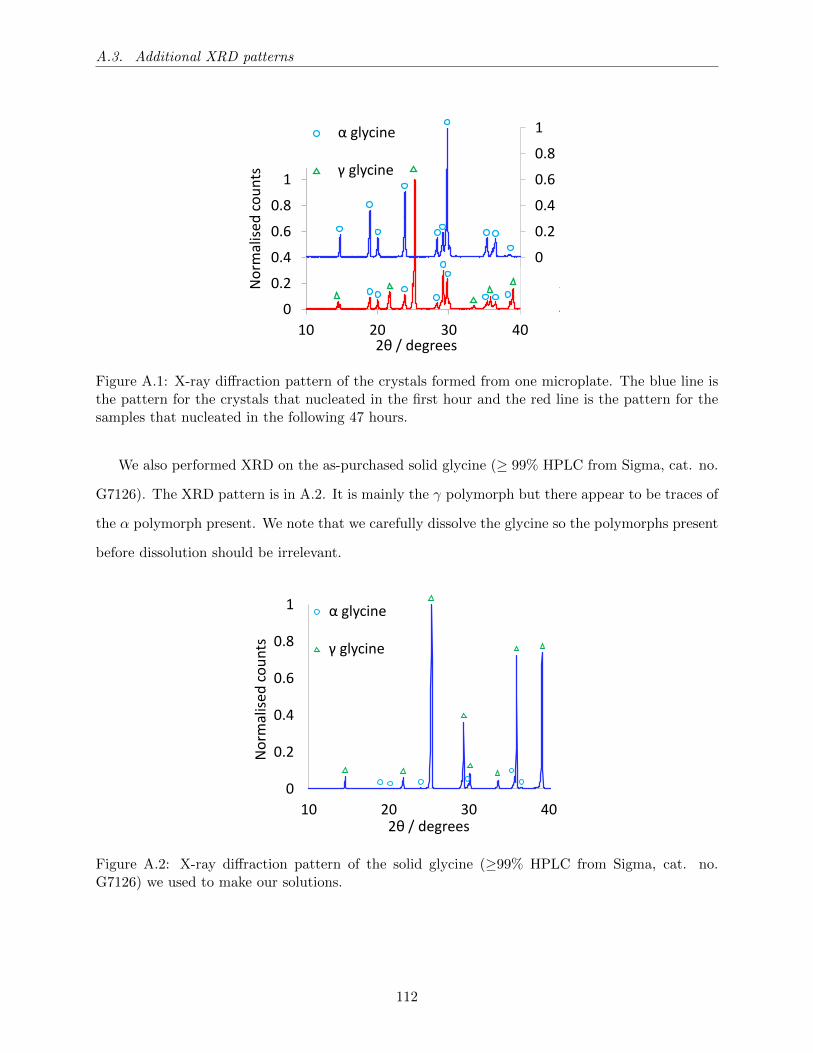
A.3. Additional XRD patterns
-0.4
-0.2
0
0.2
0.4
0.6
0.8
1
10 20 30 40
0
0.2
0.4
0.6
0.8
1
1.2
1.4
2θ / degrees
No
rmal
ised
co
un
ts
α glycine
γ glycine
Figure A.1: X-ray diffraction pattern of the crystals formed from one microplate. The blue line isthe pattern for the crystals that nucleated in the first hour and the red line is the pattern for thesamples that nucleated in the following 47 hours.
We also performed XRD on the as-purchased solid glycine (≥ 99% HPLC from Sigma, cat. no.
G7126). The XRD pattern is in A.2. It is mainly the γ polymorph but there appear to be traces of
the α polymorph present. We note that we carefully dissolve the glycine so the polymorphs present
before dissolution should be irrelevant.
10 20 30 40
0
0.2
0.4
0.6
0.8
1
2θ / degrees
No
rmal
ised
co
un
ts
α glycine
γ glycine
Figure A.2: X-ray diffraction pattern of the solid glycine (≥99% HPLC from Sigma, cat. no.G7126) we used to make our solutions.
112
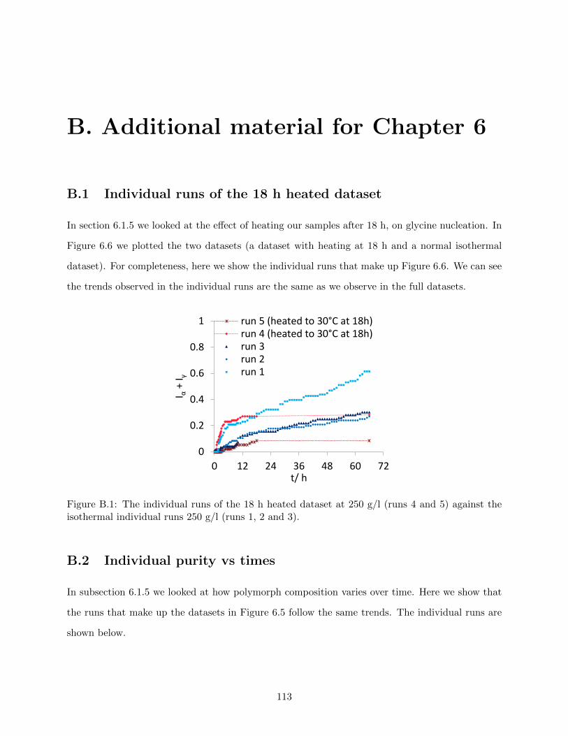
B. Additional material for Chapter 6
B.1 Individual runs of the 18 h heated dataset
In section 6.1.5 we looked at the effect of heating our samples after 18 h, on glycine nucleation. In
Figure 6.6 we plotted the two datasets (a dataset with heating at 18 h and a normal isothermal
dataset). For completeness, here we show the individual runs that make up Figure 6.6. We can see
the trends observed in the individual runs are the same as we observe in the full datasets.
0
0.2
0.4
0.6
0.8
1
0 12 24 36 48 60 72
I α+
I γ
t/ h
run 5 (heated to 30°C at 18h)run 4 (heated to 30°C at 18h)run 3run 2run 1
Figure B.1: The individual runs of the 18 h heated dataset at 250 g/l (runs 4 and 5) against theisothermal individual runs 250 g/l (runs 1, 2 and 3).
B.2 Individual purity vs times
In subsection 6.1.5 we looked at how polymorph composition varies over time. Here we show that
the runs that make up the datasets in Figure 6.5 follow the same trends. The individual runs are
shown below.
113
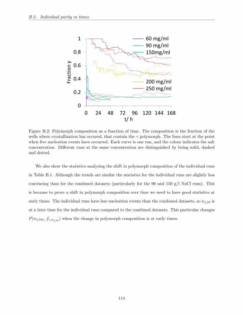
B.2. Individual purity vs times
0
0.2
0.4
0.6
0.8
1
0 24 48 72 96 120 144 168
Frac
tio
n γ
t/ h
60 mg/ml90 mg/ml150mg/ml
200 mg/ml250 mg/ml
Figure B.2: Polymorph composition as a function of time. The composition is the fraction of thewells where crystallisation has occured, that contain the γ polymorph. The lines start at the pointwhen five nucleation events have occurred. Each curve is one run, and the colour indicates the saltconcentration. Different runs at the same concentration are distinguished by being solid, dashedand dotted.
We also show the statistics analysing the shift in polymorph composition of the individual runs
in Table B.1. Although the trends are similar the statistics for the individual runs are slightly less
convincing than for the combined datasets (particularly for the 90 and 150 g/l NaCl runs). This
is because to prove a shift in polymorph composition over time we need to have good statistics at
early times. The individual runs have less nucleation events than the combined datasets, so n≥10 is
at a later time for the individual runs compared to the combined datasets. This particular changes
P (n≥10γ , fγ,n≥10) when the change in polymorph composition is at early times.
114
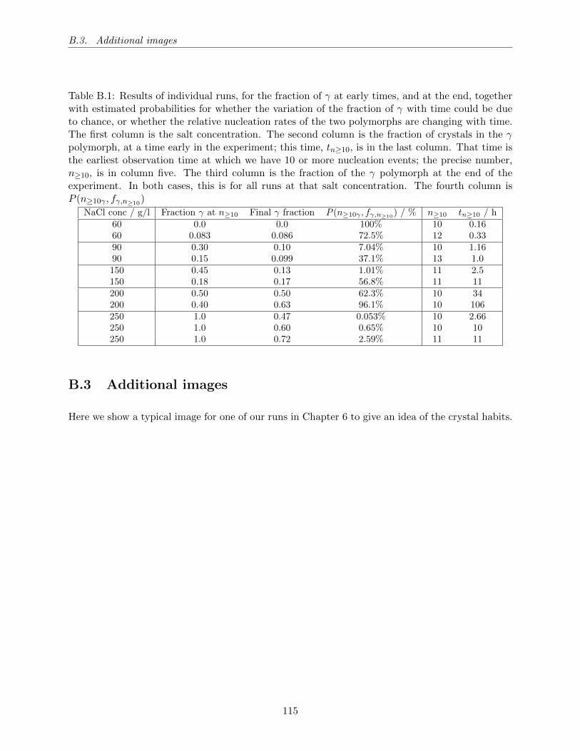
B.3. Additional images
Table B.1: Results of individual runs, for the fraction of γ at early times, and at the end, togetherwith estimated probabilities for whether the variation of the fraction of γ with time could be dueto chance, or whether the relative nucleation rates of the two polymorphs are changing with time.The first column is the salt concentration. The second column is the fraction of crystals in the γpolymorph, at a time early in the experiment; this time, tn≥10, is in the last column. That time isthe earliest observation time at which we have 10 or more nucleation events; the precise number,n≥10, is in column five. The third column is the fraction of the γ polymorph at the end of theexperiment. In both cases, this is for all runs at that salt concentration. The fourth column isP (n≥10γ , fγ,n≥10
)
NaCl conc / g/l Fraction γ at n≥10 Final γ fraction P (n≥10γ , fγ,n≥10) / % n≥10 tn≥10 / h
60 0.0 0.0 100% 10 0.1660 0.083 0.086 72.5% 12 0.3390 0.30 0.10 7.04% 10 1.1690 0.15 0.099 37.1% 13 1.0150 0.45 0.13 1.01% 11 2.5150 0.18 0.17 56.8% 11 11200 0.50 0.50 62.3% 10 34200 0.40 0.63 96.1% 10 106250 1.0 0.47 0.053% 10 2.66250 1.0 0.60 0.65% 10 10250 1.0 0.72 2.59% 11 11
B.3 Additional images
Here we show a typical image for one of our runs in Chapter 6 to give an idea of the crystal habits.
115
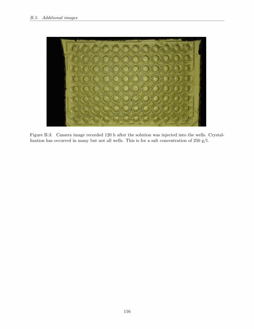
B.3. Additional images
Figure B.3: Camera image recorded 120 h after the solution was injected into the wells. Crystal-lization has occurred in many but not all wells. This is for a salt concentration of 250 g/l.
116
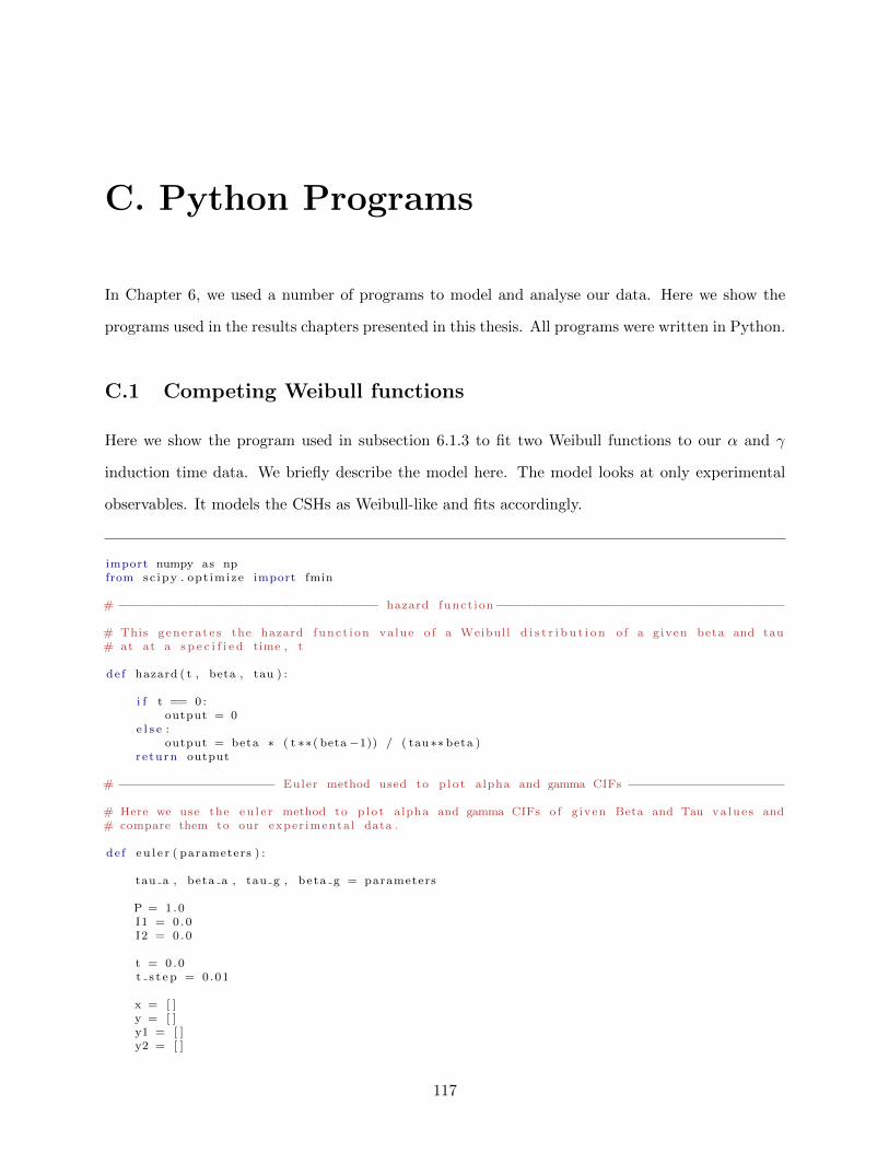
C. Python Programs
In Chapter 6, we used a number of programs to model and analyse our data. Here we show the
programs used in the results chapters presented in this thesis. All programs were written in Python.
C.1 Competing Weibull functions
Here we show the program used in subsection 6.1.3 to fit two Weibull functions to our α and γ
induction time data. We briefly describe the model here. The model looks at only experimental
observables. It models the CSHs as Weibull-like and fits accordingly.
import numpy as npfrom sc ipy . opt imize import fmin
# −−−−−−−−−−−−−−−−−−−−−−−−−−−−−−−−−−− hazard funct ion−−−−−−−−−−−−−−−−−−−−−−−−−−−−−−−−−−−−−−−
# This gene ra t e s the hazard func t i on value o f a Weibull d i s t r i b u t i o n o f a g iven beta and tau# at at a s p e c i f i e d time , t
de f hazard ( t , beta , tau ) :
i f t == 0 :output = 0
e l s e :output = beta ∗ ( t ∗∗( beta −1)) / ( tau ∗∗ beta )
re turn output
# −−−−−−−−−−−−−−−−−−−−− Euler method used to p l o t alpha and gamma CIFs −−−−−−−−−−−−−−−−−−−−−
# Here we use the e u l e r method to p l o t alpha and gamma CIFs o f g iven Beta and Tau va lue s and# compare them to our exper imenta l data .
de f e u l e r ( parameters ) :
tau a , beta a , tau g , beta g = parameters
P = 1 .0I1 = 0 .0I2 = 0 .0
t = 0 .0t s t e p = 0.01
x = [ ]y = [ ]y1 = [ ]y2 = [ ]
117
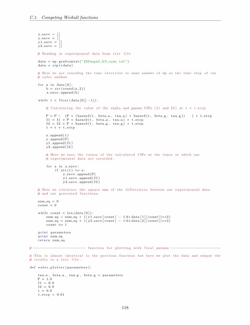
C.1. Competing Weibull functions
x save = [ ]y save = [ ]y1 save = [ ]y2 save = [ ]
# Reading in exper imenta l data from text f i l e
data = np . genfromtxt ( ”250 mgml All runs . txt ” )data = z ip (∗ data )
# Here we are rounding the time i n t e r v a l s to same number o f dp as the time step o f our# e u l e r method
f o r a in data [ 0 ] :b = s t r ( round (a , 2 ) )x save . append (b)
whi l e t < f l o a t ( data [ 0 ] [ − 1 ] ) :
# Ca l cu la t ing the value o f the alpha and gamma CIFs ( I1 and I2 ) at t + t s t e p
P = P − (P ∗ ( hazard ( t , beta a , tau a ) + hazard ( t , beta g , tau g ) ) ) ∗ t s t e pI1 = I1 + P ∗ hazard ( t , beta a , tau a ) ∗ t s t e pI2 = I2 + P ∗ hazard ( t , beta g , tau g ) ∗ t s t e pt = t + t s t e p
x . append ( t )y . append (P)y1 . append ( I1 )y2 . append ( I2 )
# Here we save the va lue s o f the c a l c u l a t e d CIFs at the t imes at which our# exper imenta l data are recorded .
f o r a in x save :i f s t r ( t ) == a :
y save . append (P)y1 save . append ( I1 )y2 save . append ( I2 )
# Here we c a l c u l a t e the square sum of the d i f f e r e n c e s between our exper imenta l data# and our generated f u n c t i o n s .
sum sq = 0count = 0
whi l e count < l en ( data [ 0 ] ) :sum sq = sum sq + ( ( y1 save [ count ] − 1.0+ data [ 1 ] [ count ] )∗∗2 )sum sq = sum sq + ( ( y2 save [ count ] − 1.0+ data [ 2 ] [ count ] )∗∗2 )count += 1
pr in t parametersp r i n t sum sqreturn sum sq
# −−−−−−−−−−−−−−−−−−−−−−−−− f unc t i on f o r p l o t t i n g with f i n a l params −−−−−−−−−−−−−−−−−−−−−−−−
# This i s almost i d e n t i c a l to the prev ious func t i on but here we p lo t the data and output the# r e s u l t s to a text f i l e .
de f e u l e r p l o t t e r ( parameters ) :
tau a , beta a , tau g , beta g = parametersP = 1 .0I1 = 0 .0I2 = 0 .0t = 0 .0t s t e p = 0.01
118
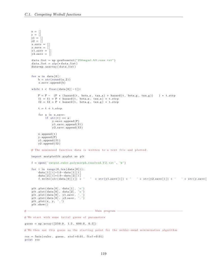
C.1. Competing Weibull functions
x = [ ]y = [ ]y1 = [ ]y2 = [ ]x save = [ ]y save = [ ]y1 save = [ ]y2 save = [ ]
d a t a l i s t = np . genfromtxt ( ”250 mgml All runs . txt ” )d a t a l i s t = z ip (∗ d a t a l i s t )data=np . asar ray ( d a t a l i s t )
f o r a in data [ 0 ] :b = s t r ( round (a , 2 ) )x save . append (b)
whi l e t < f l o a t ( data [ 0 ] [ − 1 ] ) :
P = P − (P ∗ ( hazard ( t , beta a , tau a ) + hazard ( t , beta g , tau g ) ) ) ∗ t s t e pI1 = I1 + P ∗ hazard ( t , beta a , tau a ) ∗ t s t e pI2 = I2 + P ∗ hazard ( t , beta g , tau g ) ∗ t s t e p
t = t + t s t e p
f o r a in x save :i f s t r ( t ) == a :
y save . append (P)y1 save . append ( I1 )y2 save . append ( I2 )
x . append ( t )y . append (P)y1 . append ( I1 )y2 . append ( I2 )
# The minimized func t i on data i s wr i t t en to a text f i l e and p l o t t ed .
import matp lo t l i b . pyplot as p l t
f = open ( ’ output eu l e r po lymorph reso lved V2 . txt ’ , ’w ’ )
f o r i in range (0 , l en ( data [ 0 ] ) ) :data [ 1 ] [ i ]=1.0−data [ 1 ] [ i ]data [ 2 ] [ i ]=1.0−data [ 2 ] [ i ]f . wr i t e ( s t r ( data [ 0 ] [ i ] ) + ’ ’ + s t r ( y1 save [ i ] ) + ’ ’ + s t r ( y2 save [ i ] ) + ’ ’ + s t r ( y save [ i ] ) + ’ \n ’ )
p l t . p l o t ( data [ 0 ] , data [ 1 ] , ’ o ’ )p l t . p l o t ( data [ 0 ] , data [ 2 ] , ’ o ’ )p l t . p l o t ( data [ 0 ] , y1 save , ’ . ’ )p l t . p l o t ( data [ 0 ] , y2 save , ’ . ’ )p l t . p l o t (x , y , ’ . ’ )p l t . show ( )
# −−−−−−−−−−−−−−−−−−−−−−−−−−−−−−−−−−−−−− Main program −−−−−−−−−−−−−−−−−−−−−−−−−−−−−−−−−−−−−−
# We s t a r t with some i n t i a l guess o f parameters
guess = np . array ( [ 2 5 0 . 0 , 1 . 5 , 600 .0 , 0 . 5 ] )
# We then use t h i s guess as the s t a r t i n g po int f o r the ne lder−mead minimizat ion a lgor i thm
r e s = fmin ( eu l e r , guess , x t o l =0.01 , f t o l =0.01)p r i n t r e s
119
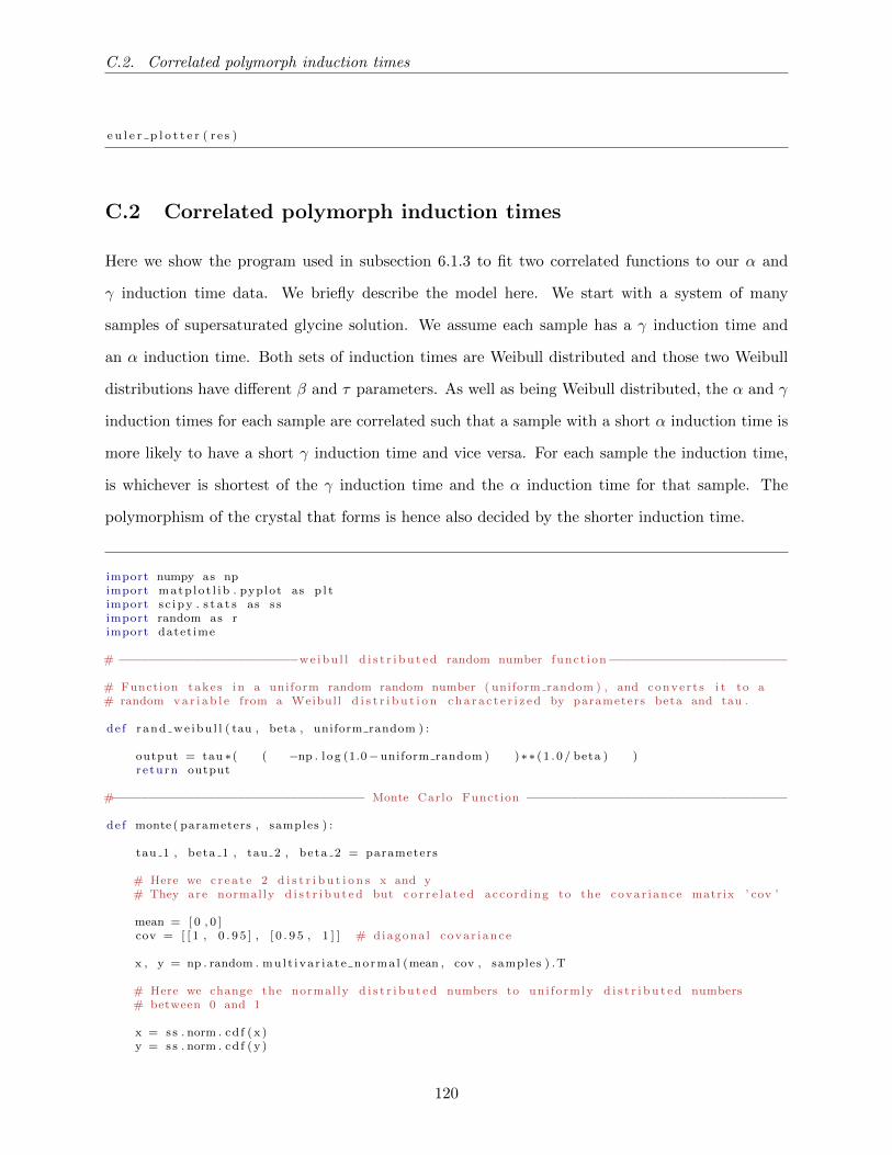
C.2. Correlated polymorph induction times
e u l e r p l o t t e r ( r e s )
C.2 Correlated polymorph induction times
Here we show the program used in subsection 6.1.3 to fit two correlated functions to our α and
γ induction time data. We briefly describe the model here. We start with a system of many
samples of supersaturated glycine solution. We assume each sample has a γ induction time and
an α induction time. Both sets of induction times are Weibull distributed and those two Weibull
distributions have different β and τ parameters. As well as being Weibull distributed, the α and γ
induction times for each sample are correlated such that a sample with a short α induction time is
more likely to have a short γ induction time and vice versa. For each sample the induction time,
is whichever is shortest of the γ induction time and the α induction time for that sample. The
polymorphism of the crystal that forms is hence also decided by the shorter induction time.
import numpy as npimport matp lo t l i b . pyplot as p l timport s c ipy . s t a t s as s simport random as rimport datet ime
# −−−−−−−−−−−−−−−−−−−−−−−−we ibu l l d i s t r i b u t e d random number funct ion−−−−−−−−−−−−−−−−−−−−−−−−
# Function takes in a uniform random random number ( uniform random ) , and conver t s i t to a# random v a r i a b l e from a Weibull d i s t r i b u t i o n c h a r a c t e r i z e d by parameters beta and tau .
de f rand we ibu l l ( tau , beta , uniform random ) :
output = tau ∗( ( −np . l og (1.0−uniform random ) )∗∗ ( 1 . 0/ beta ) )re turn output
#−−−−−−−−−−−−−−−−−−−−−−−−−−−−−−−−−− Monte Carlo Function −−−−−−−−−−−−−−−−−−−−−−−−−−−−−−−−−−−
de f monte ( parameters , samples ) :
tau 1 , beta 1 , tau 2 , beta 2 = parameters
# Here we c r e a t e 2 d i s t r i b u t i o n s x and y# They are normally d i s t r i b u t e d but c o r r e l a t e d accord ing to the covar iance matrix ’ cov ’
mean = [ 0 , 0 ]cov = [ [ 1 , 0 . 9 5 ] , [ 0 . 9 5 , 1 ] ] # diagona l covar iance
x , y = np . random . mul t iva r i a t e norma l (mean , cov , samples ) .T
# Here we change the normally d i s t r i b u t e d numbers to uni formly d i s t r i b u t e d numbers# between 0 and 1
x = ss . norm . cd f ( x )y = s s . norm . cd f ( y )
120
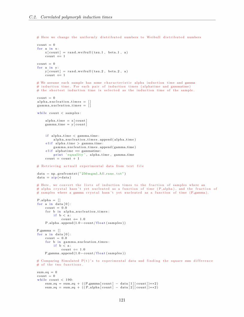
C.2. Correlated polymorph induction times
# Here we change the uni formly d i s t r i b u t e d numbers to Weibull d i s t r i b u t e d numbers
count = 0f o r a in x :
x [ count ] = rand we ibu l l ( tau 1 , beta 1 , a )count += 1
count = 0f o r a in y :
y [ count ] = rand we ibu l l ( tau 2 , beta 2 , a )count += 1
# We assume each sample has some c h a r a c t e r i s t i c alpha induct i on time and gamma# induct ion time . For each pa i r o f induct i on t imes ( alphatime and gammatime)# the s h o r t e s t induct i on time i s s e l e c t e d as the induct i on time o f the sample .
count = 0a l p h a n u c l e a t i o n t i m e s = [ ]gamma nucleat ion times = [ ]
whi l e count < samples :
a lpha t ime = x [ count ]gamma time = y [ count ]
i f a lpha t ime < gamma time :a l p h a n u c l e a t i o n t i m e s . append ( a lpha t ime )
e l i f a lpha t ime > gamma time :gamma nucleat ion times . append ( gamma time )
e l i f a lphatime == gammatime :p r i n t ’ e q u a l i t y ’ , a lpha t ime , gamma time
count = count + 1
# Ret r i ev ing a c t u a l l exper imenta l data from text f i l e
data = np . genfromtxt ( ”250 mgml All runs . txt ” )data = z ip (∗ data )
# Here , we convert the l i s t s o f induct i on t imes to the f r a c t i o n o f samples where an# alpha c r y s t a l hasn ’ t yet nuc leated as a func t i on o f time ( P alpha ) , and the f r a c t i o n o f# samples where a gamma c r y s t a l hasn ’ t yet nuc leated as a func t i on o f time (P gamma ) .
P alpha = [ ]f o r a in data [ 0 ] :
count = 0 .0f o r b in a l p h a n u c l e a t i o n t i m e s :
i f b < a :count += 1.0
P alpha . append (1.0− count / f l o a t ( samples ) )
P gamma = [ ]f o r a in data [ 0 ] :
count = 0 .0f o r b in gamma nucleat ion times :
i f b < a :count += 1.0
P gamma . append (1.0− count / f l o a t ( samples ) )
# Comparing Simulated P( t ) ’ s to exper imenta l data and f i n d i n g the square sum d i f f e r e n c e# o f the two f u n c t i o n s .
sum sq = 0count = 0whi l e count < 190 :
sum sq = sum sq + ( ( P gamma [ count ] − data [ 1 ] [ count ] )∗∗2 )sum sq = sum sq + ( ( P alpha [ count ] − data [ 2 ] [ count ] )∗∗2 )
121

C.2. Correlated polymorph induction times
count += 1
return sum sq
#−−−−−−−−−−−−−−−−−−−−−−−−−−−−− Simulated annea l ing func t i on −−−−−−−−−−−−−−−−−−−−−−−−−−−−−−−−
de f annea l ing ( parameters , samples , temperature , var iance , i t e r a t i o n t h r e s h o l d ) :
p r ev gues s = 1000000.0b e s t g u e s s = 1000000.0be s t gue s s pa ramete r s = 0count = 0 .0tau1 , b1 , tau2 , b2 = parameters
# In t h i s func t i on we try to f i n d the s e t o f beta and tau parameters f o r the we ibu l l# d i s t r i b u t i o n s , that minimizes the sum square d i f f e r e n c e between our s imulated func t i on# and exper imenta l data
whi l e True :
# I f a new minima has not been found f o r some number i t e r a t i o n s
i f count > i t e r a t i o n t h r e s h o l d :p r i n t ’ done ’p r i n t ’ bes t parameters ’ , be s t gues s paramete r s , ’ bes t guess sum sq ’ , b e s t g u e s sre turn be s t gue s s pa ramete r sbreak
count += 1.0
# Saving parameters from prev ious i t e r a t i o n o f loop
gue s s save = parameters
# Test ing new parameters which are s l i g h t l y d i f f e r e n t from thos t e s t e d in the# prev ious i t e r a t i o n .
tau1 = r . normalvar iate (1 , var i ance ) ∗ tau1tau2 = r . normalvar iate (1 , var i ance ) ∗ tau2b1 = r . normalvar iate (1 , var i ance ) ∗ b1b2 = r . normalvar iate (1 , var i ance ) ∗ b2parameters = np . array ( [ tau1 , b1 , tau2 , b2 ] )
# Putting new parameters i n to our monte c a r l o func t i on
new guess = monte ( parameters , samples )
# Here we t e s t i f the new parameters g ive a b e t t e r outcome than those in the# prev ious i t e r a t i o n .
i f new guess < prev gues s :
# I f the new parameters g ive a b e t t e r r e s u l t than the prev ious guess we use the# new parameters as the s t a r t po int f o r the next i t e r a t i o n .
p rev gues s = new guess
# Here i f the guess i s b e t t e r than the best guess so far , we a l s o re−as ign that .
i f new guess < b e s t g u e s s :b e s t g u e s s = new guessbe s t gue s s pa ramete r s = parameterscount = 0
# I f the new guess i s worse than the prev ious guess we e i t h e r go back to the# prev ious parameters or s t i c k with the new parameters . This depends on whether a# uniform random number i s g r e a t e r than the exponent i a l f unc t i on shown below# which l ooks at the d i f f e r e n c e o f the prev ious and new sum square d i f f e r e n c e s .
122
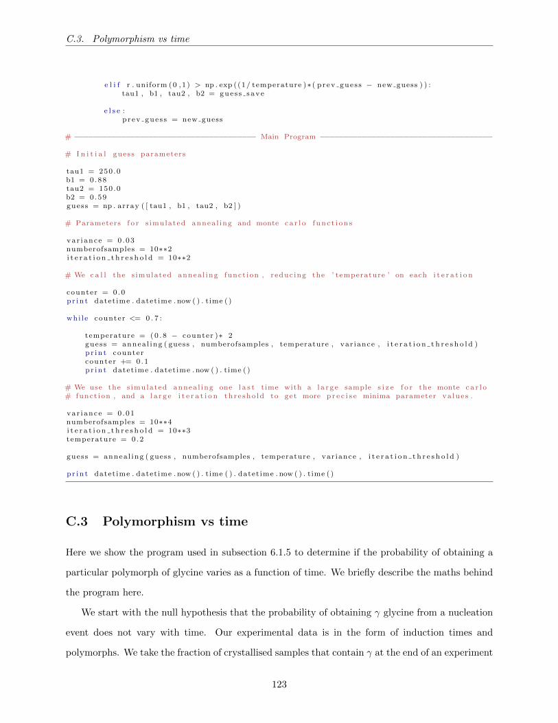
C.3. Polymorphism vs time
e l i f r . uniform (0 , 1 ) > np . exp ((1/ temperature )∗ ( p rev gues s − new guess ) ) :tau1 , b1 , tau2 , b2 = gue s s save
e l s e :p r ev gues s = new guess
# −−−−−−−−−−−−−−−−−−−−−−−−−−−−−−−−−−−−−−− Main Program −−−−−−−−−−−−−−−−−−−−−−−−−−−−−−−−−−−−−
# I n i t i a l guess parameters
tau1 = 250 .0b1 = 0.88tau2 = 150 .0b2 = 0.59guess = np . array ( [ tau1 , b1 , tau2 , b2 ] )
# Parameters f o r s imulated annea l ing and monte c a r l o f u n c t i o n s
var i ance = 0.03numberofsamples = 10∗∗2i t e r a t i o n t h r e s h o l d = 10∗∗2
# We c a l l the s imulated annea l ing funct ion , reduc ing the ’ temperature ’ on each i t e r a t i o n
counter = 0 .0p r i n t datet ime . datet ime . now ( ) . time ( )
whi l e counter <= 0 . 7 :
temperature = ( 0 . 8 − counter )∗ 2guess = annea l ing ( guess , numberofsamples , temperature , var iance , i t e r a t i o n t h r e s h o l d )p r i n t countercounter += 0.1p r i n t datet ime . datet ime . now ( ) . time ( )
# We use the s imulated annea l ing one l a s t time with a l a r g e sample s i z e f o r the monte c a r l o# funct ion , and a l a r g e i t e r a t i o n th r e sho ld to get more p r e c i s e minima parameter va lue s .
var i ance = 0.01numberofsamples = 10∗∗4i t e r a t i o n t h r e s h o l d = 10∗∗3temperature = 0 .2
guess = annea l ing ( guess , numberofsamples , temperature , var iance , i t e r a t i o n t h r e s h o l d )
p r i n t datet ime . datet ime . now ( ) . time ( ) . datet ime . now ( ) . time ( )
C.3 Polymorphism vs time
Here we show the program used in subsection 6.1.5 to determine if the probability of obtaining a
particular polymorph of glycine varies as a function of time. We briefly describe the maths behind
the program here.
We start with the null hypothesis that the probability of obtaining γ glycine from a nucleation
event does not vary with time. Our experimental data is in the form of induction times and
polymorphs. We take the fraction of crystallised samples that contain γ at the end of an experiment
123
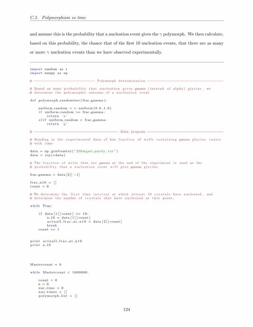
C.3. Polymorphism vs time
and assume this is the probability that a nucleation event gives the γ polymorph. We then calculate,
based on this probability, the chance that of the first 10 nucleation events, that there are as many
or more γ nucleation events than we have observed experimentally.
import random as rimport numpy as np
# −−−−−−−−−−−−−−−−−−−−−−−−−−−−− Polymorph determinat ion −−−−−−−−−−−−−−−−−−−−−−−−−−−−−−−−−−−−
# Based on some p r o b a b i l i t y that nuc l ea t i on g i v e s gamma ( in s t ead o f alpha ) g lyc ine , we# determine the polymorphic outcome o f a nuc l ea t i on event
de f polymorph randomiser ( frac gamma ) :
uniform random = r . uniform ( 0 . 0 , 1 . 0 )i f uniform random >= frac gamma :
re turn ’ a ’e l i f uniform random < frac gamma :
re turn ’ g ’
# −−−−−−−−−−−−−−−−−−−−−−−−−−−−−−−−−−−−−−−− Main program −−−−−−−−−−−−−−−−−−−−−−−−−−−−−−−−−−−−
# Reading in the exper imenta l data o f how f r a c t i o n o f w e l l s conta in ing gamma g l y c i n e v a r i e s# with time
data = np . genfromtxt ( ”250 mgml purity . txt ” )data = z ip (∗ data )
# The f r a c t i o n o f w e l l s that are gamma at the end o f the experiment i s used as the# p r o b a b i l i t y that a nuc l ea t i on event w i l l g ive gamma g l y c i n e
frac gamma = data [ 2 ] [ −1 ]
f r a c n10 = [ ]count = 0
# We determine the f i r s t time i n t e r v a l at which a t l e a s t 10 c r y s t a l s have nucleated , and# determine the number o f c r y s t a l s that have nuc leated at t h i s po int .
whi l e True :
i f data [ 1 ] [ count ] >= 10 :n 10 = data [ 1 ] [ count ]a c t u a l l f r a c a t n 1 0 = data [ 2 ] [ count ]break
count += 1
pr in t a c t u a l l f r a c a t n 1 0p r in t n 10
Mastercount = 0
whi l e Mastercount < 1000000:
count = 0n = 0nuc time = 0nuc t imes = [ ]po lymorph l i s t = [ ]
124
C.3. Polymorphism vs time
# Here we generate a s e r i e s o f nuc l ea t i on events where the induct i on t imes are the same# as our data but the polymorphism i s determined by the p r o b a b i l i t y determined by the# exper imenta l end f r a c t i o n o f gamma
whi le count < data [ 1 ] [ − 1 ] :
i f count < data [ 1 ] [ n ] :nuc time = data [ 0 ] [ n ]polymorph = polymorph randomiser ( frac gamma )
po lymorph l i s t . append ( polymorph )nuc t imes . append ( data [ 0 ] [ n ] )
count += 1
i f count == data [ 1 ] [ n ] :n += 1
count = 0num alphas = 0 .0num gammas = 0 .0
x = [ ]y = [ ]
# Here we determine how the f r a c t i o n o f w e l l s that are gamma f o r each po int up to n 10# ( n 10 i s the f i r s t po int at which the re are a t l e a s t 10 nuc l ea t i on events )
whi l e count < data [ 1 ] [ − 1 ] :
nuc time = nuc t imes [ count ]
# Here we add the next nuc l ea t i on event to the t o t a l number o f alpha or gamma# nuc l ea t i on events .
i f po lymorph l i s t [ count ] == ’ a ’ :num alphas += 1.0
e l i f po lymorph l i s t [ count ] == ’ g ’ :num gammas += 1.0
# This i s to count mu l i tp l e nuc l ea t i on events in a s i n g l e time i n t e r v a l
i f nuc t imes [ count ] == nuc t imes [ −1 ] :pass
e l i f nuc time == nuc t imes [ count + 1 ] :whi l e nuc time == nuc t imes [ count + 1 ] :
count += 1
nuc time = nuc t imes [ count ]
i f po lymorph l i s t [ count ] == ’ a ’ :num alphas += 1.0
e l i f po lymorph l i s t [ count ] == ’ g ’ :num gammas += 1.0
count += 1current frac gamma = num gammas / ( num alphas + num gammas)
# Once we have c a l c u l a t e d the f r a c t i o n o f w e l l s that are gamma at n 10 we e x i t the# loop .
i f count == n 10 :f r a c n10 . append ( current frac gamma )break
Mastercount += 1
125
C.3. Polymorphism vs time
# F i n a l l y we compare our s t a t i s t i c s f o r the s imulated numbers o f w e l l s that have# c r y s t a l l i s e d at n 10 to our exper imenta l data .
f r a c n10 . s o r t ( )
p r i n t ’ at n >10 f r a c t i o n o f gamma: ’ ’ mean ’ , round (np . average ( f r a c n10 ) , 3 ) , ’ median ’ , round (np . median ( f r a c n10 ) , 3 ) , ’s tdev ’ , round (np . std ( f r a c n10 ) , 3 )
count = 0f o r a in f r a c n10 :
i f round (a , 3 ) <= round ( a c t u a l l f r a c a t n 1 0 , 3 ) :count += 1
pr in t 100 ∗ f l o a t ( count )/ f l o a t ( l en ( f r a c n10 ) ) , ’% below or equal a c t u a l l f r a c a t n 1 0 ’p r i n t ’ a c t u a l l f r a c a t n 1 0 ’ , a c t u a l l f r a c a t n 1 0
126
Bibliography
[1] “Carbon allotropy schematic,” https://upload.wikimedia.org/wikipedia/commons/f/f9/
Diamond and graphite.jpg, accessed: 16-10-2016.
[2] “Glycine ball and stick image,” https://commons.wikimedia.org/wiki/File:Glycine-3D-balls.
png, accessed: 16-10-2016.
[3] X. Yang, X. Wang, and C. B. Ching, “Solubility of form α and form γ of glycine in aqueous
solutions,” Journal of Chemical & Engineering Data, vol. 53, no. 5, pp. 1133–1137, 2008.
[Online]. Available: http://pubs.acs.org/doi/abs/10.1021/je7006988
[4] R. Dowling, R. J. Davey, R. A. Curtis, G. Han, S. K. Poornachary, P. S. Chow,
and R. B. H. Tan, “Acceleration of crystal growth rates: an unexpected effect of
tailor-made additives,” Chem. Commun., vol. 46, pp. 5924–5926, 2010. [Online]. Available:
http://dx.doi.org/10.1039/C0CC00336K
[5] Y. Yi, D. Hatziavramidis, A. S. Myerson, M. Waldo, V. G. Beylin, and J. Mustakis,
“Development of a small-scale automated solubility measurement apparatus,” Industrial &
Engineering Chemistry Research, vol. 44, no. 15, pp. 5427–5433, 2005. [Online]. Available:
http://dx.doi.org/10.1021/ie049215y
[6] G. Han, S. Thirunahari, P. Shan Chow, and R. B. H. Tan, “Resolving the longstanding
riddle of ph-dependent outcome of glycine polymorphic nucleation,” CrystEngComm, vol. 15,
pp. 1218–1224, 2013. [Online]. Available: http://dx.doi.org/10.1039/C2CE26594J
127
Bibliography
[7] L. Li and N. Rodrguez-Hornedo, “Growth kinetics and mechanism of glycine crystals,”
Journal of Crystal Growth, vol. 121, no. 1, pp. 33 – 38, 1992. [Online]. Available:
http://www.sciencedirect.com/science/article/pii/002202489290172F
[8] G. Han, P. S. Chow, and R. B. H. Tan, “Growth behaviors of two similar crystals: The
great difference,” Crystal Growth & Design, vol. 15, no. 3, pp. 1082–1088, 2015. [Online].
Available: http://dx.doi.org/10.1021/cg501233w
[9] M. Sultana and K. F. Jensen, “Microfluidic continuous seeded crystallization: Extraction of
growth kinetics and impact of impurity on morphology,” Crystal Growth & Design, vol. 12,
no. 12, pp. 6260–6266, 2012. [Online]. Available: http://dx.doi.org/10.1021/cg301538y
[10] “XRD schematic,” https://commons.wikimedia.org/wiki/File:Bragg diffraction 2.svg, ac-
cessed: 16-10-2016.
[11] G. Han, P. S. Chow, and R. B. H. Tan, “Direct comparison of α- and γ-glycine
growth rates in acidic and basic solutions: New insights into glycine polymorphism,”
Crystal Growth & Design, vol. 12, no. 5, pp. 2213–2220, 2012. [Online]. Available:
http://dx.doi.org/10.1021/cg201321f
[12] J. Chen, B. Sarma, J. M. B. Evans, and A. S. Myerson, “Pharmaceutical crystallization,”
Crys. Growth Design, vol. 11, no. 4, p. 887, 2011.
[13] B. J. Murray, S. L. Broadley, T. W. Wilson, J. D. Atkinson, and R. H. Wills,
“Heterogeneous freezing of water droplets containing kaolinite particles,” Atmospheric
Chemistry and Physics, vol. 11, no. 9, pp. 4191–4207, 2011. [Online]. Available:
http://www.atmos-chem-phys.net/11/4191/2011/
[14] U. Lohmann and J. Feichter, “Global indirect aerosol effects: a review,” Atmospheric
Chemistry and Physics, vol. 5, no. 3, pp. 715–737, 2005. [Online]. Available:
http://www.atmos-chem-phys.net/5/715/2005/
[15] R. P. Sear, “Statistical theory of nucleation in the presence of uncharacterized
impurities,” Phys. Rev. E, vol. 70, p. 021605, 2004. [Online]. Available: http:
//link.aps.org/doi/10.1103/PhysRevE.70.021605
128
Bibliography
[16] R. P. Sear, “Quantitative studies of crystal nucleation at constant supersaturation:
experimental data and models,” CrystEngComm, vol. 16, pp. 6506–6522, 2014. [Online].
Available: http://dx.doi.org/10.1039/C4CE00344F
[17] S. L. Morissette, S. Soukasene, D. Levinson, M. J. Cima, and O. Almarsson, “Elucidation
of crystal form diversity of the HIV protease inhibitor ritonavir by high-throughput
crystallization,” Proceedings of the National Academy of Sciences, vol. 100, no. 5, pp.
2180–2184, 2003. [Online]. Available: http://www.pnas.org/content/100/5/2180.abstract
[18] J. Bauer, S. Spanton, R. Henry, J. Quick, W. Dziki, W. Porter, and J. Morris, “Ritonavir: An
extraordinary example of conformational polymorphism,” Pharmaceutical Research, vol. 18,
no. 6, pp. 859–866, 2001.
[19] S. A. Rivera, D. G. Allis, and B. S. Hudson, “Importance of vibrational zero-point
energy contribution to the relative polymorph energies of hydrogen-bonded species,”
Crystal Growth & Design, vol. 8, no. 11, pp. 3905–3907, 2008. [Online]. Available:
http://pubs.acs.org/doi/abs/10.1021/cg800524d
[20] C. S. Towler, R. J. Davey, R. W. Lancaster, and C. J. Price, “Impact of molecular speciation
on crystal nucleation in polymorphic systems: the conundrum of γ glycine and molecular self
poisoning’,” J. Am. Chem. Soc., vol. 126, no. 41, p. 13347, 2004.
[21] A. Dawson, D. R. Allan, S. A. Belmonte, S. J. Clark, W. I. F. David, P. A. McGregor,
S. Parsons, C. R. Pulham, and L. Sawyer, “Effect of high pressure on the crystal structures
of polymorphs of glycine,” Crys. Growth Design, vol. 5, no. 4, pp. 1415–1427, 2005.
[22] S. K. Poornachary, P. S. Chow, and R. B. H. Tan, “Influence of solution speciation of
impurities on polymorphic nucleation in glycine,” Crys. Growth Des., vol. 8, no. 1, pp.
179–185, 2008. [Online]. Available: http://pubs.acs.org/doi/abs/10.1021/cg060570w
[23] A. I. Toldy, A. Z. M. Badruddoza, L. Zheng, T. A. Hatton, R. Gunawan, R. Rajagopalan,
and S. A. Khan, “Spherical crystallization of glycine from monodisperse microfluidic
emulsions,” Crystal Growth & Design, vol. 12, no. 8, pp. 3977–3982, 2012. [Online].
Available: http://pubs.acs.org/doi/abs/10.1021/cg300413s
129
Bibliography
[24] J. W. Chew, S. N. Black, P. S. Chow, R. B. H. Tan, and K. J. Carpenter, “Stable
polymorphs: difficult to make and difficult to predict,” CrystEngComm, vol. 9, pp. 128–130,
2007. [Online]. Available: http://dx.doi.org/10.1039/B617321G
[25] C. Chen, O. Cook, C. E. Nicholson, and S. J. Cooper, “Leapfrogging ostwalds
rule of stages: Crystallization of stable γ-glycine directly from microemulsions,”
Crystal Growth & Design, vol. 11, no. 6, pp. 2228–2237, 2011. [Online]. Available:
http://pubs.acs.org/doi/abs/10.1021/cg101597q
[26] K. Allen, R. J. Davey, E. Ferrari, C. Towler, G. J. Tiddy, M. O. Jones, and R. G. Pritchard,
“The crystallization of glycine polymorphs from emulsions, microemulsions, and lamellar
phases,” Crystal Growth & Design, vol. 2, no. 6, pp. 523–527, 2002. [Online]. Available:
http://pubs.acs.org/doi/abs/10.1021/cg025568t
[27] A. Jawor-Baczynska, B. D. Moore, H. S. Lee, A. V. McCormick, and J. Sefcik,
“Population and size distribution of solute-rich mesospecies within mesostructured aqueous
amino acid solutions,” Faraday Discuss., vol. 167, pp. 425–440, 2013. [Online]. Available:
http://dx.doi.org/10.1039/C3FD00066D
[28] Y. Yani, P. S. Chow, and R. B. H. Tan, “Glycine open dimers in solution: New insights into
α-glycine nucleation and growth,” Crystal Growth & Design, vol. 12, no. 10, pp. 4771–4778,
2012. [Online]. Available: http://dx.doi.org/10.1021/cg300452n
[29] G. He, V. Bhamidi, S. R. Wilson, R. B. H. Tan, P. J. A. Kenis, and C. F. Zukoski, “Direct
growth of γ-glycine from neutral aqueous solutions by slow, evaporation-driven crystalliza-
tion,” Crys. Growth Design, vol. 6, no. 8, p. 1746, 2006.
[30] K. Kim, A. Centrone, T. A. Hatton, and A. S. Myerson, “Polymorphism control of nanosized
glycine crystals on engineered surfaces,” CrystEngComm, vol. 13, pp. 1127–, 2011.
[31] C. E. Nicholson, S. J. Cooper, C. Marcellin, and M. J. Jamieson, “The use of phase-inverting
emulsions to show the phenomenon of interfacial crystallization on both heating and cooling,”
J. Am. Chem. Soc., vol. 127, no. 34, p. 11894, 2005.
130
Bibliography
[32] C. E. Nicholson, C. Chen, B. Mendis, and S. J. Cooper, “Stable polymorphs crystallized
directly under thermodynamic control in three-dimensional nanoconfinement: A generic
methodology,” Crys. Growth Design, vol. 11, no. 2, p. 363, 2011.
[33] L. J. Little, R. P. Sear, and J. L. Keddie, “Does the γ polymorph of glycine nucleate faster?
a quantitative study of nucleation from aqueous solution,” Crystal Growth & Design, vol. 15,
no. 11, pp. 5345–5354, 2015. [Online]. Available: http://dx.doi.org/10.1021/acs.cgd.5b00938
[34] N. Duff, Y. R. Dahal, J. D. Schmit, and B. Peters, “Salting out the polar polymorph:
Analysis by alchemical solvent transformation,” The Journal of Chemical Physics, vol. 140,
no. 1, 2014. [Online]. Available: http://scitation.aip.org/content/aip/journal/jcp/140/1/10.
1063/1.4853775
[35] K. Srinivasan and J. Arumugam, “Growth of non-linear optical γ-glycine single
crystals and their characterization,” Optical Materials, vol. 30, no. 1, pp. 40
– 43, 2007, selected papers from the 4th International Symposium on Laser,
Scintillator and Nonlinear Optical Matetials: ISLNOM-44th International Symposium
on Laser, Scintillator and Nonlinear Optical Materials. [Online]. Available: http:
//www.sciencedirect.com/science/article/pii/S0925346706004101
[36] K. Kim, A. Centrone, T. A. Hatton, and A. S. Myerson, “Polymorphism control of nanosized
glycine crystals on engineered surfaces,” CrystEngComm, vol. 13, pp. 1127–1131, 2011.
[Online]. Available: http://dx.doi.org/10.1039/C0CE00394H
[37] Y. Diao, M. E. Helgeson, Z. A. Siam, P. S. Doyle, A. S. Myerson, T. A. Hatton, and B. L.
Trout, “Nucleation under soft confinement: Role of polymersolute interactions,” Crys. Growth
Des., vol. 12, no. 1, pp. 508–517, 2012.
[38] W. M. Haynes, Handbook of Chemistry and Physics, 97th ed. CRC, 2016.
[39] M. V. Massa and K. Dalnoki-Veress, “Homogeneous crystallization of poly(ethylene
oxide) confined to droplets: The dependence of the crystal nucleation rate on length
scale and temperature,” Phys. Rev. Lett., vol. 92, p. 255509, 2004. [Online]. Available:
http://link.aps.org/doi/10.1103/PhysRevLett.92.255509
131
Bibliography
[40] R. P. Sear, “The non-classical nucleation of crystals: Microscopic mechanisms and applica-
tions to molecular crystals, ice and calcium carbonate,” Int. Mat. Rev., vol. 57, pp. 328–356,
2012.
[41] R. A. L. Jones, Soft Condensed Matter. Oxford University Press, 2002.
[42] D. Kashchiev, Nulceation Basic Theory with Applications. Butterworth Heinemann, 2000.
[43] M. H. DeGroot and M. J. Schervish, Probability and Statistics, 3rd ed. Addison Wesley,
2002.
[44] R. L. Scheaffer and J. T. McClave, Probability and Statistics for Engineers, 4th ed. Duxbury
Press, 1995.
[45] F. Proschan, “Theoretical explanation of observed decreasing failure rate,” Technometrics,
p. 375, 1963.
[46] E. T. Lee, Statistical Methods for Survival Data Analysis, 2nd ed. Wiley, 1992.
[47] E. Castillo, Extreme Value Theory in Engineering. San Diego: Academic Press, 1988.
[48] D. C. Johnston, “Stretched exponential relaxation arising from a continuous sum of exponen-
tial decays,” Phys. Rev. B, vol. 74, no. 18, p. 184430, Nov 2006.
[49] G. M. Pound and V. K. L. Mer, “Kinetics of crystalline nucleus formation in supercooled
liquid Tin1,2,” Journal of the American Chemical Society, vol. 74, no. 9, pp. 2323–2332,
1952. [Online]. Available: http://pubs.acs.org/doi/abs/10.1021/ja01129a044
[50] E. T. Lee, Statistical Methods for Survival Data Analysis, 2nd ed. John Wiley & sons, 1992.
[51] L. D. Mueller, T. J. Nusbaum, and M. R. Rose, “The gompertz equation as a predictive tool
in demography,” Expt. Gerontology, vol. 30, no. 6, p. 553, 1995.
[52] P. Kabath, P. Stockel, A. Lindinger, and H. Baumgartel, “The nucleation of ice in supercooled
D2O and H2O,” Journal of Molecular Liquids, vol. 125, no. 23, pp. 204 – 211, 2006, complex
Liquids Fundamental Properties to Industrial Applications EMLG/JMLG Conference.
[Online]. Available: http://www.sciencedirect.com/science/article/pii/S0167732205001790
132
Bibliography
[53] R. P. Sear, “Nucleation of a new phase on a surface that is changing irreversibly
with time,” Phys. Rev. E, vol. 89, p. 022405, Feb 2014. [Online]. Available:
http://link.aps.org/doi/10.1103/PhysRevE.89.022405
[54] W. D. Callister, Materials Science and Engineering. John Wiley, 2010.
[55] A. F. White and S. L. Brantley, “The effect of time on the weathering of silicate minerals:
why do weathering rates differ in the laboratory and field?” Chemical Geology, vol.
202, no. 34, pp. 479 – 506, 2003, controls on Chemical Weathering. [Online]. Available:
http://www.sciencedirect.com/science/article/pii/S0009254103002560
[56] R. Sear, “What do crystals nucleate on? what is the microscopic mecha-
nism? how can we model nucleation?” MRS Bulletin, vol. 41, no. 5,
p. 363368, May 2016. [Online]. Available: https://www.cambridge.org/core/article/
what-do-crystals-nucleate-on-what-is-the-microscopic-mechanism-how-can-we-model-nucleation/
5C30D07B079738898B92BE0713C806FE
[57] L. Tan, R. M. Davis, A. S. Myerson, and B. L. Trout, “Control of heterogeneous
nucleation via rationally designed biocompatible polymer surfaces with nanoscale features,”
Crystal Growth & Design, vol. 15, no. 5, pp. 2176–2186, 2015. [Online]. Available:
http://dx.doi.org/10.1021/cg501823w
[58] A. Tsiatis, “A nonidentifiability aspect of the problem of competing risks,” Proc. Nat. Acad.
Sci., vol. 72, no. 1, pp. 20–22, 1975.
[59] A. V. Peterson, “Bounds for a joint distribution function with fixed sub-distribution
functions: Application to competing risks,” Proc. Nat. Acad. Sci., vol. 73, no. 1, pp. 11–13,
1976. [Online]. Available: http://www.pnas.org/content/73/1/11.abstract
[60] E. Slud and D. Byar, Biometrics, vol. 44, p. 265, 1988.
[61] J. Beyersmann, A. Latouche, A. Buchhol, and M. Schumacher, Statist. Med., vol. 28, p. 956,
2009.
133
Bibliography
[62] P. K. Andersen, R. B. Geskus, T. de Witte, and H. Putter, “Competing risks in epidemiology:
possibilities and pitfalls,” International Journal of Epidemiology, vol. 41, no. 3, pp. 861–870,
2012. [Online]. Available: http://ije.oxfordjournals.org/content/41/3/861.abstract
[63] J. J. Dignam, Q. Zhang, and M. N. Korcherginsky, “The use and interpretion of competing
risks regression models,” Clin Cancer Res, p. 2301, 2012.
[64] R. B. Geskus, Data Analysis with Competing Risks and Intermediate States. Chapman and
Hall / CRC, 2015.
[65] D. R. Cox and D. Oakes, Analysis of Survival Data. Chapman and Hall, 1984.
[66] J. I. Hoffman, “Chapter 29 - correlation,” in Biostatistics for Medical and Biomedical
Practitioners, J. I. Hoffman, Ed. Academic Press, 2015, pp. 513 – 536. [Online]. Available:
http://www.sciencedirect.com/science/article/pii/B9780128023877000299
[67] A. Jawor-Baczynska, J. Sefcik, and B. D. Moore, “250 nm glycine-rich nanodroplets are
formed on dissolution of glycine crystals but are too small to provide productive nucleation
sites,” Crystal Growth & Design, vol. 13, no. 2, pp. 470–478, 2013. [Online]. Available:
http://pubs.acs.org/doi/abs/10.1021/cg300150u
[68] S. Chattopadhyay, D. Erdemir, J. M. B. Evans, J. Ilavsky, H. Amenitsch, C. U. Segre, and
A. S. Myerson, “Saxs study of the nucleation of glycine crystals from a supersaturated solu-
tion,” Crys. Growth Des., vol. 5, no. 2, p. 523, 2005.
[69] K. Harano, T. Homma, Y. Niimi, M. Koshino, K. Suenaga, L. Leibler, and E. Nakamura,
“Heterogeneous nucleation of organic crystals mediated by single-molecule templates,” Nature
Materials, vol. 11, pp. 877 – 881, 2012.
[70] A. Ito, M. Yamanobe-Hada, and H. Shindo, “In situ AFM observation of polymorphic
transformation at crystal surface of glycine,” Journal of Crystal Growth, vol. 275, no. 12, pp.
e1691 – e1695, 2005, proceedings of the 14th International Conference on Crystal Growth
and the 12th International Conference on Vapor Growth and Epitaxy. [Online]. Available:
http://www.sciencedirect.com/science/article/pii/S0022024804017324
134
Bibliography
[71] E. Meirzadeh, L. Sapir, H. Cohen, S. R. Cohen, D. Ehre, D. Harries, M. Lahav, and
I. Lubomirsky.
[72] S. L. Broadley, B. J. Murray, R. J. Herbert, J. D. Atkinson, S. Dobbie, T. L. Malkin,
E. Condliffe, and L. Neve, “Immersion mode heterogeneous ice nucleation by an illite rich
powder representative of atmospheric mineral dust,” Atmos. Chem. Phys., vol. 12, p. 287,
2012.
[73] Y. Diao, M. E. Helgeson, A. S. Myerson, T. A. Hatton, P. S. Doyle, and B. L. Trout, “Con-
trolled nucleation from solution using polymer microgels,” J. Am. Chem. Soc., vol. 133, no. 11,
p. 3756, 2011.
[74] K. R. Devi, V. Gnanakamatchi, and K. Srinivasan, “Attainment of unstable β
nucleation of glycine through novel swift cooling crystallization process,” Journal
of Crystal Growth, vol. 400, pp. 34 – 42, 2014. [Online]. Available: http:
//www.sciencedirect.com/science/article/pii/S0022024814003200
[75] J. Zaccaro, J. Matic, A. S. Myerson, and B. A. Garetz, “Nonphotochemical, laser-
induced nucleation of supersaturated aqueous glycine produces unexpected γ-polymorph,”
Crystal Growth & Design, vol. 1, no. 1, pp. 5–8, 2001. [Online]. Available:
http://dx.doi.org/10.1021/cg0055171
[76] M. T. Rosado, M. L. T. Duarte, and R. Fausto, “Vibrational spectra of acid and alkaline
glycine salts,” Vibrational Spectroscopy, vol. 16, no. 1, pp. 35 – 54, 1998. [Online]. Available:
http://www.sciencedirect.com/science/article/pii/S0924203197000507
[77] J. Baran and H. Ratajczak, “Polarised IR and raman spectra of the γ-glycine
single crystal,” Spectrochimica Acta Part A: Molecular and Biomolecular Spectroscopy,
vol. 61, no. 7, pp. 1611 – 1626, 2005, honour Issue - Jim Durig. [Online]. Available:
http://www.sciencedirect.com/science/article/pii/S138614250400664X
[78] I. S. Lee, K. T. Kim, A. Y. Lee, and A. S. Myerson, “Concomitant crystallization
of glycine on patterned substrates: The effect of ph on the polymorphic outcome,”
135
Bibliography
Crystal Growth & Design, vol. 8, no. 1, pp. 108–113, 2008. [Online]. Available:
http://dx.doi.org/10.1021/cg700890m
[79] K. R. Devi and K. Srinivasan, “The role of charge compensation on the nucleation of α
and γ polymorphs of glycine from aqueous solution,” Journal of Crystal Growth, vol. 364,
pp. 88 – 94, 2013. [Online]. Available: http://www.sciencedirect.com/science/article/pii/
S0022024812008603
[80] T. Inada, T. Koyama, F. Goto, and T. Seto, “Ice nucleation in emulsified aqueous
solutions of antifreeze protein type iii and poly(vinyl alcohol),” The Journal of
Physical Chemistry B, vol. 115, no. 24, pp. 7914–7922, 2011. [Online]. Available:
http://pubs.acs.org/doi/abs/10.1021/jp111745v
[81] R. P. Sear, “Generalisation of levine’s prediction for the distribution of freezing
temperatures of droplets: a general singular model for ice nucleation,” Atmospheric
Chemistry and Physics, vol. 13, no. 14, pp. 7215–7223, 2013. [Online]. Available:
http://www.atmos-chem-phys.net/13/7215/2013/
[82] B. Riechers, F. Wittbracht, A. Hutten, and T. Koop, “The homogeneous ice nucleation
rate of water droplets produced in a microfluidic device and the role of temperature
uncertainty,” Phys. Chem. Chem. Phys., vol. 15, pp. 5873–5887, 2013. [Online]. Available:
http://dx.doi.org/10.1039/C3CP42437E
[83] D. J. Cziczo, K. D. Froyd, C. Hoose, E. J. Jensen, M. Diao, M. A. Zondlo, J. B. Smith,
C. H. Twohy, and D. M. Murphy, “Clarifying the dominant sources and mechanisms of
cirrus cloud formation,” Science, vol. 340, no. 6138, pp. 1320–1324, 2013. [Online]. Available:
http://science.sciencemag.org/content/340/6138/1320
[84] T. Kuhn, M. E. Earle, A. F. Khalizov, and J. J. Sloan, “Size dependence of volume
and surface nucleation rates for homogeneous freezing of supercooled water droplets,”
Atmospheric Chemistry and Physics, vol. 11, no. 6, pp. 2853–2861, 2011. [Online]. Available:
http://www.atmos-chem-phys.net/11/2853/2011/
136
Bibliography
[85] R. J. Herbert, B. J. Murray, T. F. Whale, S. J. Dobbie, and J. D. Atkinson, “Representing
time-dependent freezing behaviour in immersion mode ice nucleation,” Atmos. Chem. Phys.
Disc., vol. 14, pp. 1399–1442, 2014.
[86] T. Li, D. Donadio, G. Russo, and G. Galli, “Homogeneous ice nucleation from supercooled
water,” Phys. Chem. Chem. Phys., vol. 13, pp. 19 807–19 813, 2011. [Online]. Available:
http://dx.doi.org/10.1039/C1CP22167A
[87] A. Haji-Akbari and P. G. Debenedetti, “Direct calculation of ice homogeneous
nucleation rate for a molecular model of water,” Proceedings of the National
Academy of Sciences, vol. 112, no. 34, pp. 10 582–10 588, 2015. [Online]. Available:
http://www.pnas.org/content/112/34/10582.abstract
[88] D. Gebauer, M. Kellermeier, J. D. Gale, L. Bergstrom, and H. Colfen, “Pre-nucleation
clusters as solute precursors in crystallisation,” Chem. Soc. Rev., vol. 43, pp. 2348–2371,
2014. [Online]. Available: http://dx.doi.org/10.1039/C3CS60451A
[89] M. H. Nielsen, S. Aloni, and J. J. De Yoreo, “In situ tem imaging of CaCO3 nucleation reveals
coexistence of direct and indirect pathways,” Science, vol. 345, no. 6201, pp. 1158–1162,
2014. [Online]. Available: http://www.sciencemag.org/content/345/6201/1158.abstract
[90] P. G. Vekilov, “Nucleation,” Crystal Growth & Design, vol. 10, no. 12, pp. 5007–5019, 2010.
[Online]. Available: http://pubs.acs.org/doi/abs/10.1021/cg1011633
[91] K. Onuma and A. Ito, “Cluster growth model for hydroxyapatite,” Chemistry
of Materials, vol. 10, no. 11, pp. 3346–3351, 1998. [Online]. Available: http:
//dx.doi.org/10.1021/cm980062c
[92] D. Gebauer, A. Volkel, and H. Colfen, “Stable prenucleation calcium carbonate
clusters,” Science, vol. 322, no. 5909, pp. pp. 1819–1822, 2008. [Online]. Available:
http://www.jstor.org/stable/20177068
[93] N. Javid, S. Roy, M. Zelzer, Z. Yang, J. Sefcik, and R. V. Ulijn, “Cooperative self-assembly
of peptide gelators and proteins,” Biomacromolecules, vol. 14, no. 12, pp. 4368–4376, 2013,
pMID: 24256076. [Online]. Available: http://dx.doi.org/10.1021/bm401319c
137
Bibliography
[94] Y. Li, V. Lubchenko, and P. G. Vekilov, “The use of dynamic light scattering and brownian
microscopy to characterize protein aggregation,” Review of Scientific Instruments, vol. 82,
no. 5, 2011. [Online]. Available: http://scitation.aip.org/content/aip/journal/rsi/82/5/10.
1063/1.3592581
[95] K. Vogtt, N. Javid, E. Alvarez, J. Sefcik, and M.-C. Bellissent-Funel, “Tracing nucleation
pathways in protein aggregation by using small angle scattering methods,” Soft Matter,
vol. 7, pp. 3906–3914, 2011. [Online]. Available: http://dx.doi.org/10.1039/C0SM00978D
[96] J. L. Carvalho and K. Dalnoki-Veress, “Homogeneous bulk, surface, and edge nucleation in
crystalline nanodroplets,” Phys. Rev. Lett., vol. 105, p. 237801, Dec 2010.
[97] E. Saridakis and N. E. Chayen, “Towards a universal nucleant for protein crystallization,”
Trends Biotech., vol. 27, no. 2, pp. 99 – 106, 2009. [Online]. Available: http:
//www.sciencedirect.com/science/article/pii/S0167779908002886
[98] P. Asanithi, E. Saridakis, L. Govada, I. Jurewicz, E. W. Brunner, R. Ponnusamy, J. A. S.
Cleaver, A. B. Dalton, N. E. Chayen, and R. P. Sear, “Carbon-nanotube-based materials for
protein crystallization,” ACS App. Mat. Inter., vol. 1, no. 6, p. 1203, 2009.
[99] H. S. Leese, L. Govada, E. Saridakis, S. Khurshid, R. Menzel, T. Morishita, A. J.
Clancy, E. R. White, N. E. Chayen, and M. S. P. Shaffer, “Reductively pegylated
carbon nanomaterials and their use to nucleate 3d protein crystals: a comparison
of dimensionality,” Chem. Sci., vol. 7, pp. 2916–2923, 2016. [Online]. Available:
http://dx.doi.org/10.1039/C5SC03595C
[100] Y. Takeda and F. Mafun, “Induction of protein crystallization by platinum nanoparticles,”
Chemical Physics Letters, vol. 647, pp. 181 – 184, 2016. [Online]. Available:
http://www.sciencedirect.com/science/article/pii/S0009261416000828
[101] F. Hodzhaoglu, F. Kurniawan, V. Mirsky, and C. Nanev, “Gold nanoparticles induce protein
crystallization,” Crys. Res. Tech., vol. 43, no. 6, pp. 588–593, 2008. [Online]. Available:
http://dx.doi.org/10.1002/crat.200811125
138
Bibliography
[102] L. E. Zerpa, J.-L. Salager, C. A. Koh, E. D. Sloan, and A. K. Sum, “Surface chemistry and
gas hydrates in flow assurance,” Industrial & Engineering Chemistry Research, vol. 50, no. 1,
pp. 188–197, 2011. [Online]. Available: http://dx.doi.org/10.1021/ie100873k
[103] Y. Diao, K. E. Whaley, M. E. Helgeson, M. A. Woldeyes, P. S. Doyle, A. S. Myerson, T. A.
Hatton, and B. L. Trout, “Gel-induced selective crystallization of polymorphs,” J. Am. Chem.
Soc., vol. 134, no. 1, pp. 673–684, 2012.
[104] J.-W. Kim, J.-H. Park, H.-M. Shim, and K.-K. Koo, “Effect of amphiphilic additives
on nucleation of hexahydro-1,3,5-trinitro-1,3,5-triazine,” Crystal Growth & Design, vol. 13,
no. 11, pp. 4688–4694, 2013. [Online]. Available: http://pubs.acs.org/doi/abs/10.1021/
cg4006423
[105] C. Brandel and J. H. ter Horst, “Measuring induction times and crystal nucleation
rates,” Faraday Discuss., vol. 179, pp. 199–214, 2015. [Online]. Available: http:
//dx.doi.org/10.1039/C4FD00230J
[106] D. Knezic, J. Zaccaro, and A. S. Myerson, “Nucleation induction time in levitated droplets,”
J. Phys. Chem. B, vol. 108, no. 30, pp. 10 672–10 677, 2004.
[107] P. Laval, A. Crombez, and J.-B. Salmon, “Microfluidic droplet method for nucleation kinetics
measurements,” Langmuir, vol. 25, no. 3, pp. 1836–1841, 2009.
[108] R. M. Ginde and A. S. Myerson, “Cluster size estimation in binary supersaturated
solutions,” Journal of Crystal Growth, vol. 116, no. 1, pp. 41 – 47, 1992. [Online]. Available:
http://www.sciencedirect.com/science/article/pii/002202489290112V
[109] A. S. Myerson and P. Y. Lo, “Diffusion and cluster formation in supersaturated solutions,”
Journal of Crystal Growth, vol. 99, no. 1, pp. 1048 – 1052, 1990. [Online]. Available:
http://www.sciencedirect.com/science/article/pii/S0022024808800796
[110] A. S. Myerson and P. Y. Lo, “Cluster formation and diffusion in supersaturated binary and
ternary amino acid solutions,” Journal of crystal growth, vol. 110, no. 1-2, pp. 26–33, 1991.
139
Bibliography
[111] D. Erdemir, A. Y. Lee, and A. S. Myerson, “Nucleation of crystals from solution: Classical
and two-step models,” Acc. Chem. Res., vol. 42, no. 5, pp. 621–629, 2009, pMID: 19402623.
[Online]. Available: http://pubs.acs.org/doi/abs/10.1021/ar800217x
[112] J. Huang, T. C. Stringfellow, and L. Yu, “Glycine exists mainly as monomers, not dimers,
in supersaturated aqueous solutions: Implications for understanding its crystallization and
polymorphism,” J. Am. Chem. Soc., vol. 130, no. 42, p. 13973, 2008.
[113] S. Hamad, C. E. Hughes, C. R. A. Catlow, and K. D. M. Harris, “Clustering of glycine
molecules in aqueous solution studied by molecular dynamics simulation,” The Journal of
Physical Chemistry B, vol. 112, no. 24, pp. 7280–7288, 2008, pMID: 18503273. [Online].
Available: http://dx.doi.org/10.1021/jp711271z
[114] H. Sakai, H. Hosogai, T. Kawakita, K. Onuma, and K. Tsukamoto, “Transformation of
α-glycine to γ-glycine,” Journal of Crystal Growth, vol. 116, no. 34, pp. 421 – 426, 1992.
[Online]. Available: http://www.sciencedirect.com/science/article/pii/002202489290651X
[115] J. E. Aber, S. Arnold, B. A. Garetz, and A. S. Myerson, “Strong dc electric
field applied to supersaturated aqueous glycine solution induces nucleation of the γ
polymorph,” Phys. Rev. Lett., vol. 94, p. 145503, Apr 2005. [Online]. Available:
http://link.aps.org/doi/10.1103/PhysRevLett.94.145503
[116] N. Javid, T. Kendall, I. S. Burns, and J. Sefcik, “Filtration suppresses laser-induced
nucleation of glycine in aqueous solutions,” Crystal Growth & Design, vol. 16, no. 8, pp.
4196–4202, 2016. [Online]. Available: http://dx.doi.org/10.1021/acs.cgd.6b00046
[117] T. Rungsimanon, K.-i. Yuyama, T. Sugiyama, H. Masuhara, N. Tohnai, and M. Miyata,
“Control of crystal polymorph of glycine by photon pressure of a focused continuous wave
near-infrared laser beam,” The Journal of Physical Chemistry Letters, vol. 1, no. 3, pp.
599–603, 2010. [Online]. Available: http://dx.doi.org/10.1021/jz900370x
[118] C. Yogambal, D. R. Babu, and R. E. Vizhi, “Investigations on the nucleation kinetics of
γ-glycine single crystal,” Physica B: Cond. Matt., vol. 433, no. 0, p. 112, 2014. [Online].
Available: http://www.sciencedirect.com/science/article/pii/S0921452613006352
140
Bibliography
[119] V. Y. Torbeev, E. Shavit, I. Weissbuch, L. Leiserowitz, and M. Lahav, “Control of crystal
polymorphism by tuning the structure of auxiliary molecules as nucleation inhibitors. the
β-polymorph of glycine grown in aqueous solutions,” Crystal Growth & Design, vol. 5, no. 6,
pp. 2190–2196, 2005. [Online]. Available: http://dx.doi.org/10.1021/cg050200s
[120] C. Forsyth, I. S. Burns, P. A. Mulheran, and J. Sefcik, “Scaling of glycine nucleation kinetics
with shear rate and glassliquid interfacial area,” Crystal Growth & Design, vol. 16, no. 1,
pp. 136–144, 2016. [Online]. Available: http://dx.doi.org/10.1021/acs.cgd.5b01042
[121] C. Forsyth, P. A. Mulheran, C. Forsyth, M. D. Haw, I. S. Burns, and J. Sefcik,
“Influence of controlled fluid shear on nucleation rates in glycine aqueous solutions,”
Crystal Growth & Design, vol. 15, no. 1, pp. 94–102, 2015. [Online]. Available:
http://dx.doi.org/10.1021/cg5008878
[122] K. Srinivasan, “Crystal growth of α and γ glycine polymorphs and their polymorphic phase
transformations,” Journal of Crystal Growth, vol. 311, no. 1, pp. 156 – 162, 2008. [Online].
Available: http://www.sciencedirect.com/science/article/pii/S0022024808012013
[123] X. Yang, J. Lu, X.-J. Wang, and C.-B. Ching, “Effect of sodium chloride on the nucleation
and polymorphic transformation of glycine,” Journal of Crystal Growth, vol. 310, no. 3,
pp. 604 – 611, 2008. [Online]. Available: http://www.sciencedirect.com/science/article/pii/
S0022024807009748
[124] Y. Shi and L. Wang, “Collective vibrational spectra of α- and γ-glycine studied by terahertz
and raman spectroscopy,” Journal of Physics D: Applied Physics, vol. 38, no. 19, p. 3741,
2005. [Online]. Available: http://stacks.iop.org/0022-3727/38/i=19/a=024
[125] Y. Cui, J. Stojakovic, H. Kijima, and A. S. Myerson, “Mechanism of contact-induced
heterogeneous nucleation,” Crystal Growth & Design, vol. 16, no. 10, pp. 6131–6138, 2016.
[Online]. Available: http://dx.doi.org/10.1021/acs.cgd.6b01284
[126] G. Han, S. K. Poornachary, P. S. Chow, and R. B. H. Tan, “Understanding growth
morphology changes of γ-glycine and dl-alanine polar crystals in pure aqueous solutions,”
141
Bibliography
Crystal Growth & Design, vol. 10, no. 11, pp. 4883–4889, 2010. [Online]. Available:
http://dx.doi.org/10.1021/cg100934f
[127] I. Weissbuch, L. Addadi, M. Lahav, and L. Leiserowitz, “Molecular recognition at
crystal interfaces,” Science, vol. 253, no. 5020, pp. 637–645, 1991. [Online]. Available:
http://www.jstor.org/stable/2878835
[128] I. Weissbuch, L. Addadi, Z. Berkovitch-Yellin, E. Gati, S. Weinstein, M. Lahav, and
L. Leiserowitz, “Centrosymmetric crystals for the direct assignment of the absolute
configuration of chiral molecules. application to the .alpha.-amino acids by their effect on
glycine crystals,” Journal of the American Chemical Society, vol. 105, no. 22, pp. 6615–6621,
1983. [Online]. Available: http://dx.doi.org/10.1021/ja00360a012
[129] S. K. Poornachary, P. S. Chow, R. B. H. Tan, and R. J. Davey, “Molecular speciation
controlling stereoselectivity of additives: impact on the habit modification in -glycine
crystals,” Crys. Growth Des., vol. 7, no. 2, pp. 254–261, 2007. [Online]. Available:
http://pubs.acs.org/doi/abs/10.1021/cg060273r
[130] S. K. Poornachary, P. S. Chow, and R. B. Tan, “Effect of solution speciation
of impurities on α-glycine crystal habit: A molecular modeling study,” Journal
of Crystal Growth, vol. 310, no. 12, pp. 3034 – 3041, 2008. [Online]. Available:
http://www.sciencedirect.com/science/article/pii/S0022024808002133
[131] R. Dowling, A Study of the Nucleation and Growth of glycine and DL-alanine (PhD thesis).
The University of Manchester, 2012.
[132] A. Maczyski, M. Gral, B. Winiewska-Gocowska, A. Skrzecz, and D. Shaw, “Mutual
solubilities of water and alkanes,” Monatshefte fur Chemie / Chemical Monthly, vol. 134,
no. 5, pp. 633–653, 2003. [Online]. Available: http://dx.doi.org/10.1007/s00706-002-0561-0
[133] N. E. Chayen, P. D. S. Stewart, and D. M. Blow, “Microbatch crystallization
under oil a new technique allowing many small-volume crystallization trials,” Journal
of Crystal Growth, vol. 122, no. 14, pp. 176 – 180, 1992. [Online]. Available:
http://www.sciencedirect.com/science/article/pii/002202489290241A
142
Bibliography
[134] V. M. Bolanos-Garcia and N. E. Chayen, “New directions in conventional methods of
protein crystallization,” Progress in Biophysics and Molecular Biology, vol. 101, no. 13, pp. 3
– 12, 2009, novel Approaches to Protein Crystallization and Crystal Quality Enhancement.
[Online]. Available: http://www.sciencedirect.com/science/article/pii/S0079610709000868
[135] J. L. Carvalho and K. Dalnoki-Veress, Euro. Phys. J. E, vol. 34, p. 6, 2011.
[136] P. G. Debenedetti, Metastable Liquids. Princeton: Princeton University Press, 1996.
[137] G. Botsaris, “Secondary nucleation - a review,” in Industrial Crystallization, J. Mullin,
Ed. Springer US, 1976, pp. 3–22. [Online]. Available: http://dx.doi.org/10.1007/
978-1-4615-7258-9 1
[138] S. Akella, A. Mowitz, M. Heymann, and S. Fraden, Crys. Growth Design, vol. 14, p. 4487,
2014.
[139] D. Duft and T. Leisner, Atmos. Chem. Phys., vol. 4, p. 1997, 2004.
[140] R. Davey and J. Garside, From Molecules to Crystallizers. Oxford: Oxford University Press,
2000.
[141] R. P. Sear, “Estimation of the scaling of the nucleation time with volume when the
nucleation rate does not exist,” Crystal Growth & Design, vol. 13, no. 3, pp. 1329–1333,
2013. [Online]. Available: http://pubs.acs.org/doi/abs/10.1021/cg301849f
[142] W. T. Vettering, W. H. Press, S. A. Teukolsky, and B. P. Flannery, Numerical Recipes in
FORTRAN 77. Cambridge: Cambridge University Press, 1992.
143