J O U R N A L O F M A T E R I A L S S C I E N C E 3 8 (2 0 0 3 ) 35 – 49

A three dimensional model for direct laser metal

powder deposition and rapid prototyping

M. LABUDOVICCorning Lasertron, R & D, 11 Oak Park, M/S LZ-727, Bedford, MA 01730, USAE-mail: marko L@email.msn.com

D. HU, R. KOVACEVICDepartment of Mechanical Engineering, Southern Methodist University,P.O. Box 750337, Dallas, Texas, USA

A three-dimensional model for direct laser metal powder deposition process and rapidprototyping is developed. Both numerical and analytical models are addressed. In the caseof numerical modeling, the capabilities of ANSYS parametric design language wereemployed. The model calculates transient temperature profiles, dimensions of the fusionzone and residual stresses. Model simulations are compared with experimental resultsacquired on line using an ultra-high shutter speed camera which is able to acquirewell-contrasted images of the molten pool, and off-line using metallographical and x-raydiffraction analyses. The experiments showed good agreement with the modeling. Theresults are discussed to provide suggestions for feedback control and reduction of residualstresses. C© 2003 Kluwer Academic Publishers

NomenclatureA Heat absorptivity of laser beam

on metal surfaceC Specific heat (J/kg · K)d Diameter of the laser beam (m)dz , dx Length (width) of the laser beam in z (x)

direction (m)I Thermal flux density of laser beam (J/s · m2)E Elastic modulus (N/mm2)h Heat transfer coefficient (W/m2K)H Enthalphy (J/kg)H (.) Heaviside function (unit step function)k Boltzmann’s constant

(K = 1.38066 × 10−23 Ws/K)K Heat conductivity (J/m · s · K)L f Latent heat of fusion (J/kg)P Laser beam power (J/s)P Surface pressure vector (N/m2)q Rate of heat generation (J/s · m3)qii Tensor of heat flow derivatives (J/mm3s)Qv Volume-specific heat flow or source density

(J/mm3s)Q Body force vector (N/m3)r Distance from the center

of the laser beam (m)rb Effective laser beam radius (m)S Area (m2)Ssl Area of the solid-liquid interface (m)t Time (s)T Temperature (K)T Cooling rate (K/s)u, v, w Displacement components in the x, y, z

directions, respectively (m)

u Displacement vector (m)V Volume (m3)ym Molten pool depth (m)�t Incremental time (s)α Thermal expansion coefficient (1/K)ρ Density (kg/m3)ν Poisson’s ratioε Emissivityδ(.) Dirac delta functionε Strain tensor in updated Lagrange

configurationεii Tensor of elastic volumetric strain rates (1/s)εvpij Tensor of viscoplastic strain rates (1/s)ξ Inelastic heat fractionσ Stefan-Boltzmann constant

(σ = 5.670 × 10−8 W/m2 K4 σ )σdij Deviatoric stress tensor (N/mm2)σ Stress tensor in updated Lagrange

configuration (N/m2)ξ , ζ , χ Local coordinates

1. IntroductionThe direct laser metal powder deposition processis laser-assisted, direct metal manufacturing processfor rapid prototyping under development at SouthernMethodist University. The process is similar to thelaser-engineered net shaping (LENS)TM process de-veloped at Sandia National Laboratories [1]. It in-corporates features from stereolithography and lasercladding, that use computer-aided design (CAD) filecross sections (stl file) to control the forming process.Metal-powder particles are delivered in an argon gasstream into the focus of the laser beam to form a molten

0022–2461 C© 2003 Kluwer Academic Publishers 35

pool. The part is then driven by an xy positioning sys-tem to generate a three-dimensional part by layer-wise,additive processing.

In order to understand the thermal behavior of theprocess, an on-line high-shutter speed imaging wascoupled with a microstructural analysis, x-ray analy-sis, analytical and numerical modeling. Since the ther-mal behavior controls the morphology and properties ofthe specimen; thermal measurements, microstructuralanalysis, and modeling can be combined to develop theprocess parameters to control the microstructural devel-opment and tailor the properties of the specimens. As afirst step, a high-shutter speed imaging is employedin monitoring the deposition of 100 mesh MONEL400-alloy powder on AISI 1006 steel plate, at a varietyof laser powers and scanning speeds. The microstruc-ture of the deposits was investigated, and the dimen-sions of the fusion zone were correlated to the ther-mal conditions at solidification. Finally, both analyticaland numerical models were developed to determine thethermal history of the specimens both in the areas thatare accessible or not accessible to high-shutter speedimaging measurements. The results from heat trans-fer analysis were then used as loads for finite elementanalysis of residual stresses. Residual stresses were in-vestigated with an x-ray diffraction technique, and theresults were correlated with those obtained by the finiteelement modeling.

2. The Physical description of the phenomenaSince direct laser powder deposition is a thermal pro-cess, the well-known heat conduction equation playsa central role in the physical modeling of the process.The heat conduction equation follows from the energybalance of an appropriately chosen volume and consistsof the diffusive heat flows, the convective heat flows,and the possible sources of heat [2].

For the thermo-mechanical coupled system, the ther-mal equilibrium equation for analysis of heat transferin a domain D can be written as:

k

(∂2T

∂x2+ ∂2T

∂y2+ ∂2T

∂z2

)+ q = ρcT + ν

∂T

∂z(1)

To obtain the solution from the thermal equilibriumequation, the boundary conditions and the initial con-ditions are needed.

The initial condition is:

T (x, y, z, 0) = T0 for (x, y, z) ∈ D. (2)

The essential boundary condition is:

T (x, 0, z) = T0 (3)

on the boundary S1 for (x, z) ∈ S1 and t > 0. S1 repre-sents the bottom surface of the plate. The natural bound-ary conditions can be defined by:

kn∂T

∂n− q + h(T − T0) + σε

(T 4 − T 4

0

) = 0 (4)

on the boundary S2 for (x, y, z) ∈ S2 and t > 0. S2 rep-resents those surfaces that are subjected to radiation,convection and imposed heat fluxes.

The inclusion of the temperature-dependant thermo-physical and mechanical properties, and a radiationterm in the above boundary condition makes this typeof analysis highly nonlinear. Since the incorporation ofradiation effects are found to increase the solution timeby as much as three times, an empirical relationship asproposed by Vinokurov [3] was used:

H = 2.4 × 10−3εT 1.61 (5)

Equation 5 combines the effect of radiation and con-vection into a “lumped” heat transfer coefficient. Theassociated loss in accuracy using this relationship isestimated to be less than 5% [3].

The fundamental equation of thermomechanics ofelastic-viscoplastic continua follows according to [4]:

cρ T + qii = Qv − EαT

1 − 2vεii + ξσdijεvpij (6)

where ξ is the inelastic heat fraction; ξ ≤ 1.0, allowsfor the fact that all inelastic deformation energy is dis-sipated in the heat, but that part of it may appear in themicrostructural change.

The restriction to the plastic behavior without viscos-ity is adequate for the majority of laser surface treatmentresidual stress problems [4]. Therefore, the viscositybehavior in Equation 6 is neglected.

3. Simplified heat conduction equationFrom the above analysis of the physical phenomena,the following assumptions can be made:

1. The work piece is initially at 298 K. Both the workpiece and the coordinate mesh are fixed and the laserbeam moves in the positive z-direction with a constantvelocity, v.

2. All thermophysical, as well as mechanical proper-ties, are considered to be temperature-dependent. Theseproperties are given in [5] as well as the temperaturedependent stress-strain curves used in model.

3. The laser beam diameter is defined as the diameterin which the power density is reduced from the peakvalue by a factor of e2 [6].

4. During the simulation, the thermal load is givenin the form of the thermal flux density, which obeysnormal distribution as follows: [7]

I = 2AP

πr2b

exp

(−2r2

r2b

)(7)

giving the mean thermal flux density within the area ofthe laser beam scanning [7]

Im = 1

πr2b

∫ rb

0I (2πr ) dr

= 2π

πr2b

∫ rb

0

2AP

πr2b

exp

(−2r2

r2b

)r dr = 0.865AP

πr2b

(8)

5. The latent heat of fusion is simulated by an arti-ficial increase in the liquid specific heat according to

36

Brown and Song [8] and the relationship between theenthalpy (H ), density (ρ) and specific heat (c):

H =∫

ρc(T ) dT (9)

6. Since the direct laser metal powder deposition in-volves very rapid melting and solidification, convectiveredistribution of heat within the molten pool is not sig-nificant (whereas it is in other processes where a liquidpool is permanent). Convective flow of heat, therefore,is neglected.

4. Solution of the heat conduction equation4.1. The use of Green’s functionA well-known approach to solve the simplified heatconduction equation (1) given its boundary and ini-tial conditions is by the use of Green’s functions [2].Green’s function, for the problem under considera-tion, is the analytical solution of Equations 1–4 withI = δ(x)δ(y)H (t), where δ(.) is the Dirac delta func-tion and H (.) is the unit step function of Heavisidefunction. That is the Green’s function G (x , y, z, t , x ′,y′, z′, t ′, v, K , k) represent the temperature at (x , y, z)at time t due to a point source of unit strength generatedat (x ′, y′, z′) at time t ′, which is moving with velocityv. By integrating the product of the Green’s functionG with the actual absorbed power density Im , over thedimensions of the laser spot and time, the temperatureT (x , y, z, t), induced by the laser beam moving overthe surface (y′ = 0), is obtained:

T (x, y, z)=T0 +∫ t

0

∫ ∞

−∞

∫ ∞

−∞G(x, y, z, t, x ′, 0, z, t ′, v)

× AI(x ′, y′, t ′) dx ′ dy′ dt ′ (10)

Unfortunately, no explicit analytical solution ofEquation 10 for an arbitrary intensity profile I can befound. However, the equation can be solved in explicitfrom after introducing several approximations. To testvalidity, such an approximated analytical model wascompared to the numerical solution.

4.2. Analytical solution of the model4.2.1. Maximum surface temperature

induced by stationary laser beamFor stationary (v = 0) laser beam, analytical models forthe maximum surface temperature are available fromliterature, and these can be calculated from Equation 10.The maximum steady surface temperature induced bya stationary Gaussian intensity profile (TEM00), withdiameter d, equals [2]

T G0 {0, 0, 0) = APL

d K

√2

π(11)

4.2.2. Maximum surface temperatureinduced by fast moving laser beam

With the velocity of the laser beam approaching infin-ity, the heat flow in the solid can be approximated byone-dimensional flow perpendicular to the surface ofthe workpiece [2]. In addition, since the intensity pro-files under consideration are symmetric with respect to

the x-axis, then the maximum surface temperature forhigh laser beam velocities is reched at z = 0. Hence, themaximum surface temperature induced by the Gaussianintensity profile is [10]

T G∞ = 4C

√2

K (πd)32

APL

√k

v, C = maxx ∈ R

×{ ∫ χ

−∞

exp[−2η2]√χ − η

dη

}≈ 1.81 (12)

4.2.3. Maximum surface temperatureinduced at intermediate velocities

By combining the solutions for the stationary T0 andthe fast moving beam T∞, a following equation for theGaussian intensity profile is obtained [11]

T Gv = 4C

√2

d K√

πAPL

√k

π2dv + (4C)2k(13)

To evaluate the accuracy of this analytical expression,the Equation 13 is compared to the corresponding tem-peratures obtained by the numerical model.

4.3. Geometry of the molten poolThe geometry of the molten pool is determined by theenergy balance. In the case of direct laser metal powderdeposition, the energy balance consists of three terms:the absorbed laser energy QL , the energy QC trans-ported by heat conduction from the liquid-solid inter-face of the molten pool into the non-molten material,and the energy QF required to create a molten pool(latent heat of fusion). The energy balance reads:

QL − QF = QC (14)

4.3.1. Laser energyThe laser energy QL absorbed by the work piece, canbe approximated by:

QL = APLti (15)

Where ti denotes the interaction time of the laser beamwith a given point on the surface of the work piece. Thisinteraction time is approximated by [12]

ti = d

v(16)

where d denotes the diameter of the laser beam.

4.3.2. Heat conductionThe energy QC , which flows from the molten pool intothe solid material, can be calculated from the heat en-closed by the heat affected zone under consideration,and equals:

QC = ρcp

∫Vs

T (x, y, z, ti )dVs (17)

where Vs denotes the heat affected zone in the solidunder the molten pool, and T (x , y, z, ti ) denotes thecorresponding temperature field at time t = ti . It is as-sumed that the heat transfer under the molten pool may

37

be considered as one-dimensional. Then, according to[13]

T (z, ti ) = (Tm − T0)erfc

(y

2√

kti

)+ T0 (18)

The thickness of the heat affected zone Vs is assumed tobe equal to the heat penetration depth i.e. δh = 2

√kti .

Then the integral in Equation 18 can be evaluated if thearea Ssl of the solid-liquid interface is known. Assum-ing the parabolic shape of the solid-liquid interface:

QC = 4

3ymπ Rmρcp(Tm − T0)

∫ 2√

kd/v

0

×[

erfc

(yv

2√

kdv

)+ T0

]dy (19)

where ym is the depth of the molten pool, and Rm is theradius of the molten pool.

4.3.3. Latent heat of fusionThe energy QF , required to create a molten pool, fol-lows from the latent heat of fusion L f per unit mass ofthe material and the volume Vl of the molten pool:

QF = L f ρVl (20)

in which the volume Vl of the molten pool can be cal-culated as:

Vl =∫ 0

−ym

πr2 dy =∫ 0

−ym

πR2m

(y

ym+ 1

)dy = πym R2

m

2

(21)

4.3.4. Depth of the molten poolSubstitution of Equations 15, 16, 19–21 into the energybalance equation yields:

ym = 2APL

ρcpC2Tm

√kdv

(22)

This equation shows a linear dependence of the moltenpool depth on the ratio PL/(

√dv), which is some-

times referred as the specific energy [14]. Note thatthe similar relation holds for the maximum temperature(Equation 13).

5. Numerical solution of the modeland computer algorithm

In order to analyze the movement and deformation ofthe configuration in finite element method (FEM), sup-pose that the equilibrium states at all the time stepsfrom 0 to t have been obtained. Then, according to thevirtual work principle [15], the equilibrium equation attime t + �t can be expressed as follows:∫

Vσ · δεdV =

∫V

q · δudV +∫

Sp · δud S (23)

To account for the large deformation, the followingshape functions, with extra shape functions (ESF) for

element type of 8-node bricks, are used:

u = 18 [uI(1 − ξ )(1 − ζ )(1 − χ )

+ uJ(1 + ξ )(1 − ζ )(1 − χ )

+ uK(1 + ξ )(1 + ζ )(1 − χ )

+ uL(1 − ξ )(1 + ζ )(1 − χ )

+ uM(1 − ξ )(1 − ζ )(1 + χ )

+ uN(1 + ξ )(1 − ζ )(1 + χ )

+ uO(1 + ξ )(1 + ζ )(1 + χ )

+ uP(1 − ξ )(1 + ζ )(1 + χ )]

+ u1(1 − ξ 2) + u2(1 − ζ 2) + u3(1 − χ2)

v = 18 [vI(1 − ξ ) · · · (analogous to u)

w = 18 [wI(1 − ξ ) · · · (analogous to u) (24)

where uI (I = I, J, K, L, M, N, O, P) are nodal displace-ments.

Discretization of this problem is accomplished bymeans of the standard finite element procedure. Thus,the result of aggregation is a group of nonlinear equa-tions. The Newton-Raphson method is used to linearizethese equations:

[K ]{�u} = {Fa} − {Fnr } (25)

where [K ] = ∫V [B]T [Dep][B]dV is the tangential

stiffness matrix, [B] is the general geometric ma-trix, [Dep] is the elasto-plastic stress-strain matrix,{�u} is the displacement incremental at the ele-ment nodes, {Fa} is the applied force vector, and{Fnr } = ∫

V [B]T {σ }dV is Newton-Raphson restoredforce vector.

ANSYS provides a convenient means of numericallymodeling direct laser metal powder deposition pro-cess. This requires an integration of the heat conductionequation with respect to time. In the finite element for-mulation, this equation can be written for each elementas:

[CT ]{T } + [KT ]{T } = {Q} (26)

where [CT ][CT ] = ∫V ρc[N ][N ]T dV is the heat ca-

pacity matrix, [N ] is the shape function matrix,[KT ] = ∫

V k[B][B]T dV is the heat conduction matrix,{T } and {T } are nodal temperature vector and nodaltemperature rate vector, respectively, and {Q} is heatflux vector.

The moving laser beam is simulated using theANSYS Parametric Design Language (APDL) to pro-vide the heat boundary conditions at different positionsat different times. The first iteration in the solution pro-cedure solves the system equations at an assumed start-ing temperature (298 K), and subsequent iterations usetemperatures from previous iterations to calculate thethermal conductivity and specific heat matrices. Thefirst element was positioned onto the substrate witha set initial and boundary conditions. For subsequentelements, the model used the results from the previ-ous step as the initial condition for each new elementbirth. This was repeated for all birthing events until the

38

geometry was complete. The iterative process continuesfor time period T until a converged solution is achievedor until the dynamic equilibrium of heat exchange isestablished.

A study of the heat-transfer problem allows the deter-mination of the temperature distribution within a body.One can then determine the amount of heat moving intoor out of the body, and the residual stresses. Following,the basic equation for thermo-mechanical coupled cal-culation is as follows:

[[0] [0]

[0] [C]

] {{u}{T }

}+

[[K ] [0]

[0] [KT ]

] {{u}{T }

}=

{{F}{Q}

}

(27)

where {F} is the force vector including applied nodalforce and the force caused by the thermal strain.

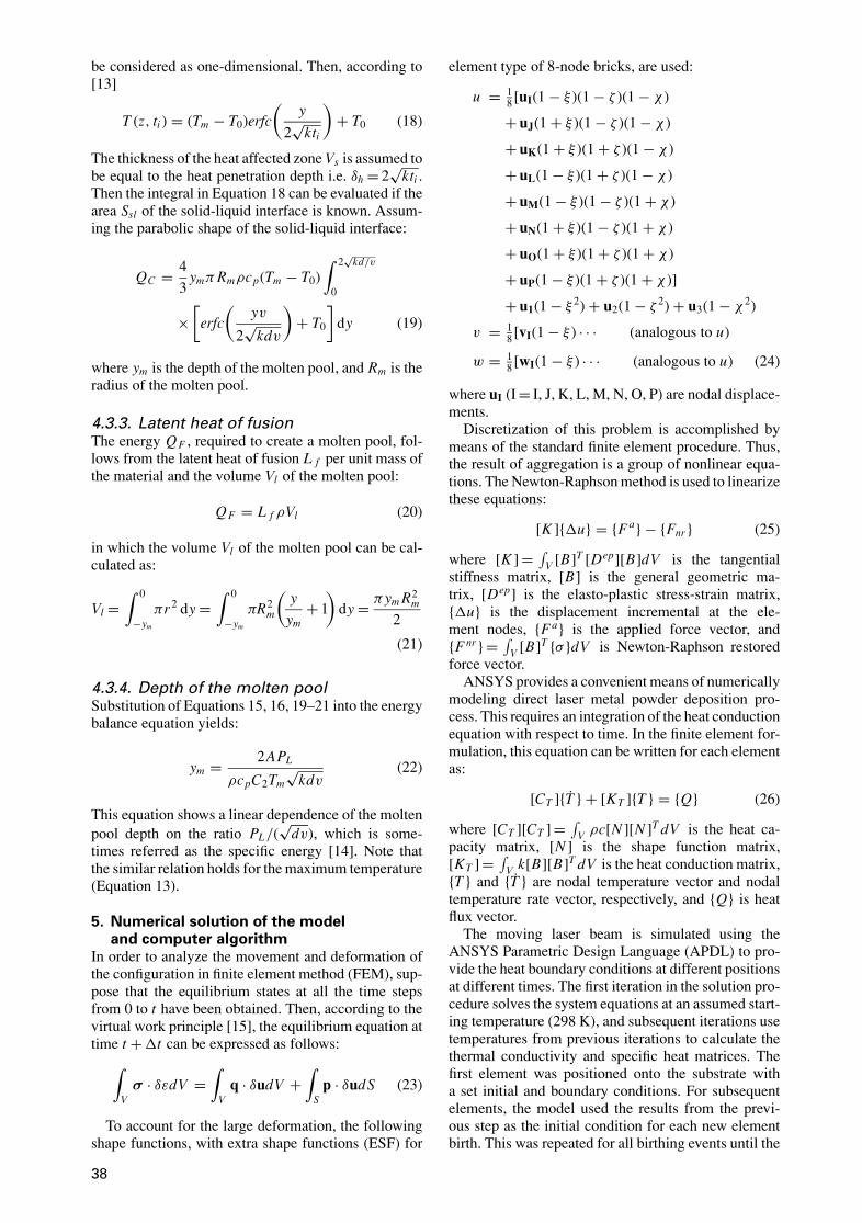
Figure 1 Computer algorithm.

Figure 2 Experimental set-up.

The residual stresses caused by inhomogeneous ther-mal expansion (or contraction) are termed “thermalstresses”. Elastic thermal stresses disappear after re-moving the inhomogeneous temperatures by whichthey have been caused. For this reason, many authorsdo not classify them as residual stresses. Where majordifferences in temperature exist, the thermal stressesgive rise to plastic deformations. After removal of thetemperature differences, residual stresses remain. Theplastic behavior is incorporated in the model by makinguse of the data given in [16].

ANSYS provides the performance of an IndirectCoupled-Field Analysis for implementing the aboveequations for calculating residual stresses. In thismethod, one performs two sequential analysis, usingresults from the first analysis as loads for the secondanalysis. Following, the algorithm for a residual-stressanalysis is summarized in Fig. 1.

39

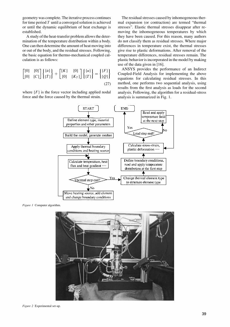
6. ExperimentThe experimental set-up of a Nd : YAG laser, threeaxis CNC positioning system, powder delivery system,laser-strobe vision system, shielding gas, and work-piece is shown in Fig. 2. The deposits were built byinjecting the 100 mesh MONEL 400—alloy powder

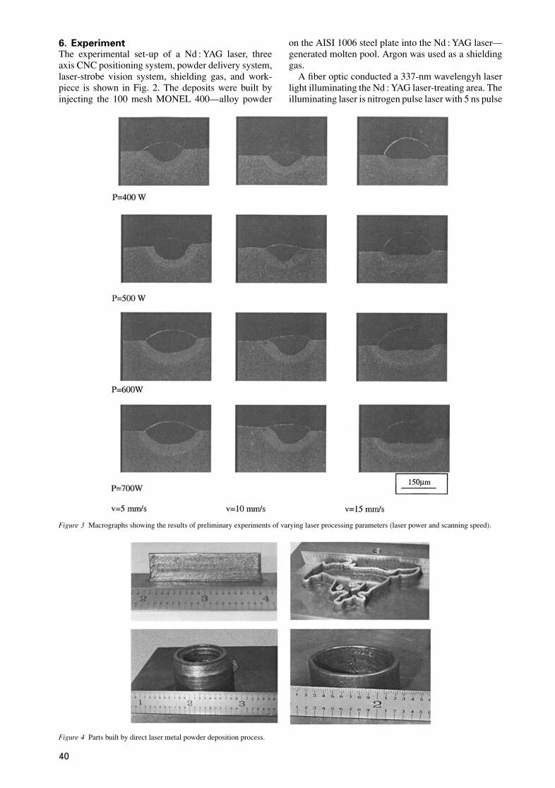
Figure 3 Macrographs showing the results of preliminary experiments of varying laser processing parameters (laser power and scanning speed).

Figure 4 Parts built by direct laser metal powder deposition process.

on the AISI 1006 steel plate into the Nd : YAG laser—generated molten pool. Argon was used as a shieldinggas.

A fiber optic conducted a 337-nm wavelengyh laserlight illuminating the Nd : YAG laser-treating area. Theilluminating laser is nitrogen pulse laser with 5 ns pulse

40

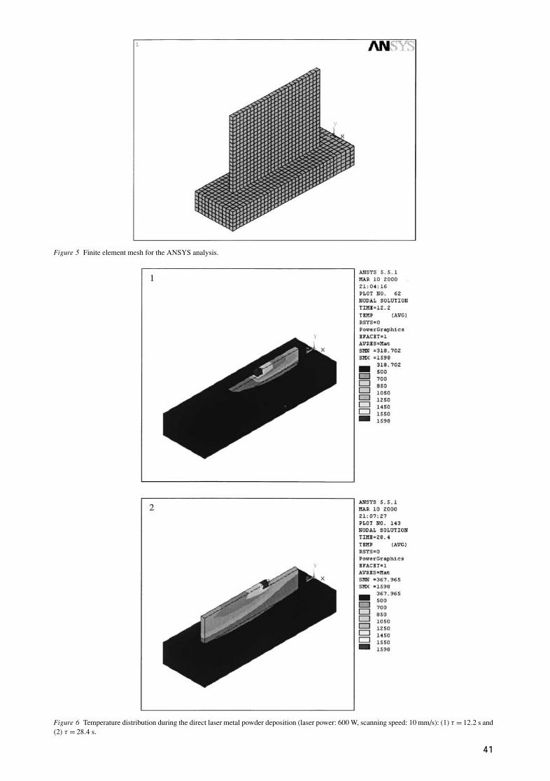
Figure 5 Finite element mesh for the ANSYS analysis.

Figure 6 Temperature distribution during the direct laser metal powder deposition (laser power: 600 W, scanning speed: 10 mm/s): (1) τ = 12.2 s and(2) τ = 28.4 s.

41

duration synchronizing with the high-speed shutter ofthe camera. The camera of the laser strobe vision systemis equipped with UV filter that only allows light near a337 nm wavelength to pass. During the illumination pe-riod, the intensity of the illuminating laser can suppressthe spatter and plasma light. Due to the reflection of themirror-like molten pool, a well-contrasted image of themolten pool was obtained. A frame grabber installedon a PII 350 PC computer acquired images from theultra-high shutter speed camera at 30 Hz. The imageprocessing and recognition was completed on the samecomputer.

Figure 7 Temperature distribution during the direct laser metal powder deposition (laser power: 600 W, scanning speed: 10 mm/s): (1) τ = 42.8 s and(2) τ = 90 s.

In preliminary experiments, laser-processing param-eters (laser power and scanning speed) were optimizedin order to achieve a good bonding of the depositedlayers and satisfactory depth of penetration without ex-cessive heat input (Fig. 3). The parts built with thisexperimental set-up, and after process parameter opti-mization, are shown in Fig. 4.

7. Modeling results and discussion7.1. The analysis of heat transferThe comparison of experimental with simulated resultsallows the estimation of the relative importance and role

42

of the complex physical interactions that govern directlaser metal powder deposition process. The comparisonof experiment and simulation were done on the AISI1006 steel plate with dimensions 50 × 20 × 10 mm. TheMONEL 400-alloy powder with 100 mesh was used tobuild 40 mm deposits (please see Fig. 4). The finiteelement mesh is shown in Fig. 5. The numerical modelwas run for both the duration of the laser heating and forthe subsequent cooling period using different powers(in the range of 300 to 1000 W) and scanning speeds(in the range of 5 to 15 mm/s). Figs 6 and 7 showthe typical analysis resulting from the use of 10 mm/sscanning speed and 600 W laser power.

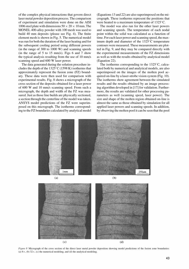
The data generated during the solution procedure in-cludes the depth of the 1325◦C (1598 K) isotherms thatapproximately represent the fusion zone (FZ) bound-ary. These data were then used for comparison withexperimental results. Fig. 8 shows a micrograph of thecross section of the deposits obtained for a laser powerof 600 W and 10 mm/s scanning speed. From such amicrograph, the depth and width of the FZ was mea-sured. Just as those line builds are physically sectioned,a section through the centerline of the model was taken.ANSYS model predictions of the FZ were superim-posed on this micrograph. The isotherms correspond-ing to the FZ boundaries calculated by analytical model

Figure 8 Micrograph of the cross section of the direct laser metal powder deposition showing model predictions of the fusion zone boundaries:(a) 8×, (b) 32×, (c) the numerical modeling, and (d) the analytical modeling.

(Equations 13 and 22) are also superimposed on the mi-crograph. These isotherms represent the positions thatwere heated to a maximum temperature of 1325◦C.

The model was also run for the other laser powersand scanning speeds. The temperature of each nodalpoint within the solid was calculated as a function oftime. For each laser power and scanning speed, the max-imum depth and diameter of the 1325◦C temperaturecontours were measured. These measurements are plot-ted in Fig. 9, and they may be compared directly withthe experimental measurements of the FZ dimensionsas well as with the results obtained by analytical model(Equation 22).

The isotherms corresponding to the 1325◦C, calcu-lated both by numerical and analytical models, are alsosuperimposed on the images of the molten pool ac-quired on-line by a laser-strobe vision system (Fig. 10).The isotherms show agreement between the simulatedresults and the results obtained by an image process-ing algorithm developed in [17] for validation. Further-more, the results are validated for other processing pa-rameters as well (scanning speed, laser power). Thesize and shape of the molten region obtained on-line isalmost the same as those obtained by simulation for allapplied laser powers and scanning speeds. In addition,by observing the molten pool it can be seen that the pool

43

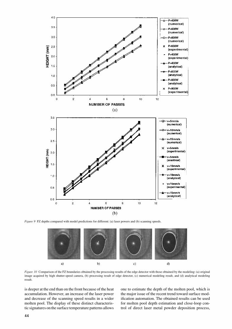
Figure 9 FZ depths compared with model predictions for different: (a) laser powers and (b) scanning speeds.

Figure 10 Comparison of the FZ boundaries obtained by the processing results of the edge detector with those obtained by the modeling: (a) originalimage acquired by high shutter-speed camera, (b) processing result of edge detector, (c) numerical modeling result, and (d) analytical modelingresult.

is deeper at the end than on the front because of the heataccumulation. However, an increase of the laser powerand decrease of the scanning speed results in a widermolten pool. The display of these distinct characteris-tic signatures on the surface temperature patterns allows

one to estimate the depth of the molten pool, which isthe major issue of the recent trend toward surface mod-ification automation. The obtained results can be usedfor molten pool depth estimation and close-loop con-trol of direct laser metal powder deposition process,

44

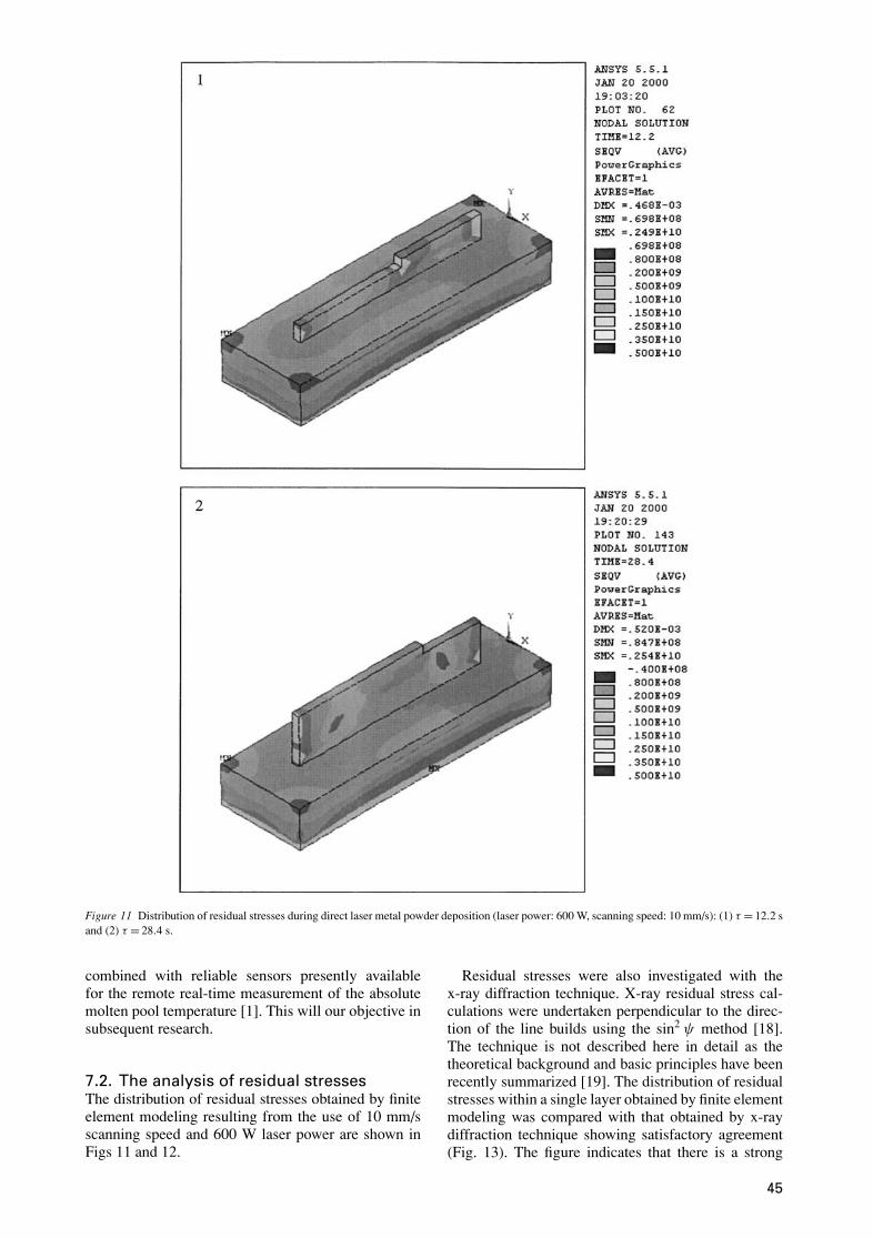
Figure 11 Distribution of residual stresses during direct laser metal powder deposition (laser power: 600 W, scanning speed: 10 mm/s): (1) τ = 12.2 sand (2) τ = 28.4 s.

combined with reliable sensors presently availablefor the remote real-time measurement of the absolutemolten pool temperature [1]. This will our objective insubsequent research.

7.2. The analysis of residual stressesThe distribution of residual stresses obtained by finiteelement modeling resulting from the use of 10 mm/sscanning speed and 600 W laser power are shown inFigs 11 and 12.

Residual stresses were also investigated with thex-ray diffraction technique. X-ray residual stress cal-culations were undertaken perpendicular to the direc-tion of the line builds using the sin2 ψ method [18].The technique is not described here in detail as thetheoretical background and basic principles have beenrecently summarized [19]. The distribution of residualstresses within a single layer obtained by finite elementmodeling was compared with that obtained by x-raydiffraction technique showing satisfactory agreement(Fig. 13). The figure indicates that there is a strong

45

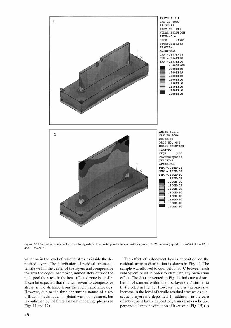
Figure 12 Distribution of residual stresses during a direct laser metal powder deposition (laser power: 600 W, scanning speed: 10 mm/s): (1) τ = 42.8 sand (2) τ = 90 s.

variation in the level of residual stresses inside the de-posited layers. The distribution of residual stresses istensile within the center of the layers and compressivetowards the edges. Moreover, immediately outside themelt-pool the stress in the heat-affected zone is tensile.It can be expected that this will revert to compressivestress as the distance from the melt track increases.However, due to the time-consuming nature of x-raydiffraction technique, this detail was not measured, butis confirmed by the finite element modeling (please seeFigs 11 and 12).

The effect of subsequent layers deposition on theresidual stresses distribution is shown in Fig. 14. Thesample was allowed to cool below 50◦C between eachsubsequent build in order to eliminate any preheatingeffect. The data presented in Fig. 14 indicate a distri-bution of stresses within the first layer (left) similar tothat plotted in Fig. 13. However, there is a progressiveincrease in the level of tensile residual stresses as sub-sequent layers are deposited. In addition, in the caseof subsequent layers deposition, transverse cracks (i.e.perpendicular to the direction of laser scan (Fig. 15)) as

46

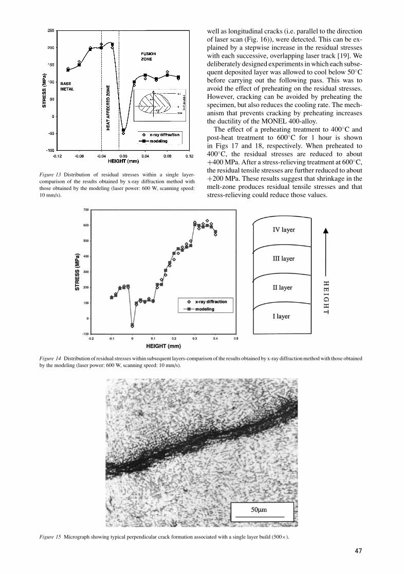
Figure 13 Distribution of residual stresses within a single layer-comparison of the results obtained by x-ray diffraction method withthose obtained by the modeling (laser power: 600 W, scanning speed:10 mm/s).

Figure 14 Distribution of residual stresses within subsequent layers-comparison of the results obtained by x-ray diffraction method with those obtainedby the modeling (laser power: 600 W, scanning speed: 10 mm/s).

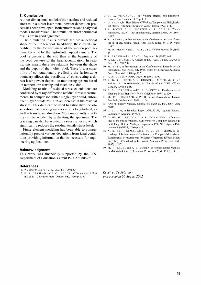
Figure 15 Micrograph showing typical perpendicular crack formation associated with a single layer build (500×).

well as longitudinal cracks (i.e. parallel to the directionof laser scan (Fig. 16)), were detected. This can be ex-plained by a stepwise increase in the residual stresseswith each successive, overlapping laser track [19]. Wedeliberately designed experiments in which each subse-quent deposited layer was allowed to cool below 50◦Cbefore carrying out the following pass. This was toavoid the effect of preheating on the residual stresses.However, cracking can be avoided by preheating thespecimen, but also reduces the cooling rate. The mech-anism that prevents cracking by preheating increasesthe ductility of the MONEL 400-alloy.

The effect of a preheating treatment to 400◦C andpost-heat treatment to 600◦C for 1 hour is shownin Figs 17 and 18, respectively. When preheated to400◦C, the residual stresses are reduced to about+400 MPa. After a stress-relieving treatment at 600◦C,the residual tensile stresses are further reduced to about+200 MPa. These results suggest that shrinkage in themelt-zone produces residual tensile stresses and thatstress-relieving could reduce those values.

47

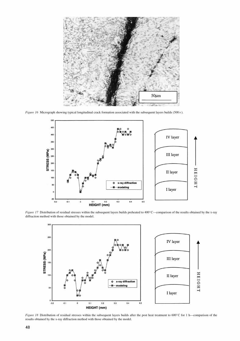
Figure 16 Micrograph showing typical longitudinal crack formation associated with the subsequent layers builds (500×).

Figure 17 Distribution of residual stresses within the subsequent layers builds preheated to 400◦C—comparison of the results obtained by the x-raydiffraction method with those obtained by the model.

Figure 18 Distribution of residual stresses within the subsequent layers builds after the post heat treatment to 600◦C for 1 h—comparison of theresults obtained by the x-ray diffraction method with those obtained by the model.

48

8. ConclusionA three-dimensional model of the heat flow and residualstresses in a direct laser metal powder deposition pro-cess has been developed. Both numerical and analyticalmodels are addressed. The simulation and experimentalresults are in good agreement.

The simulation results provide the cross-sectionalshape of the molten pool. In addition, these results arecertified by the topside image of the molten pool ac-quired on-line by the high-shutter-speed camera. Thepool is deeper at the end than at the beginning ofthe bead because of the heat accumulation. In real-ity, this means there are relations between the shapeand the depth of the molten pool. Therefore, a capa-bility of computationally predicting the fusion zoneboundary allows the possibility of constructing a di-rect laser powder deposition monitoring system basedon temperature-sensing and machine vision.

Modeling results of residual stress calculations areconfirmed by x-ray diffraction residual stress measure-ments. In comparison with a single layer build, subse-quent layer builds result in an increase in the residualstresses. This data can be used to rationalize the ob-servation that cracking may occur in a longitudinal, aswell as transversal, direction. More importantly, crack-ing can be avoided by preheating the specimen. Thecracking can also be avoided by stress relieving whichsignificantly reduces the residual tensile stress level.

Finite element modeling has been able to compu-tationally predict various deviations from ideal condi-tions providing information that is necessary for engi-neering applications.

AcknowledgmentThis work was financially supported by the U.S.Department of Education’s Grant P200A80806-98.

References1. W. H O F M E I S T E R et al., JOM 51 (1999) 274.2. H . S . C A R S L A W and J . C . J A E G E R , in “Conduction of Heat

in Solids” (Clarendon Press, Oxford, UK, 1959) p. 134.

3. V . A . V I N O K U R O V , in “Welding Stresses and Distortion”(Boston Spa, London, 1987) p. 118.

4. D . R A D A J , in “Heat Effects of Welding; Temperature Field, Resid-ual Stress, Distortion” (Springer-Verlag, Berlin, 1992) p. 1.

5. A . B O Y C E , P . H . M O R T E N and T . B E L L , in “MetalsHandbook, Vol. 5” (ASM International, Materials Park, OH, 1994)p. 835.

6. Y . N A M B A , in Proceedings of the Conference on Laser Form-ing in Space, Osaka, Japan, April 1986, edited by C. P. Wang,p. 403.

7. M. R . F R E W I N and D. A. S C O T T , Welding Journal 78 (1999)15.

8. S . B R O W N and H. S O N G , J. Eng. Ind. 114 (1992) 441.9. J . L I , J . M E R L I N , J . C H E N and Z . F A N , Chinese Journal of

Laser 3 (1997) 280.10. M. B A S S , in Proceedings of the Conference on Laser-Materials

Interactions, San Diego, July 1988, edited by T. Brown (AcademicPress, New York, 1998) p. 122.

11. J . A . G R E E N W O O D , Wear 150 (1991) 153.12. R . B . K U I L B O E R , P . K . K I R N E R , J . M E I E R , M. R U N D

and M. F . S C H N E I D E R , in “Annals of the CIRP” (Wiley,London, 1990) p. 585.

13. F . P . I N C R O P E R A and D. P . D E W I T T , in “Fundamentals ofHeat and Mass Transfer” (Wiley, Chichester, 1974) p. 120.

14. M. F . S C H N E I D E R , in Ph. D. thesis, University of Twente,Enschede, Netherlands, 1998, p. 104.

15. ANSYS Theory Manual, Release 6.0 (ANSYS Inc., USA, June2001).

16. C . S . K I M , in Technical Report ANL-75-55, Argonne NationalLaboratory, Argonne, 1975, p. 1.

17. D . H U , M. L A B U D O V I C and R. K O V A C E V I C , in Proceed-ings of the 9th International Conference on Computer Technologyin Welding, Detroit, Michigan, September 1999 NIST Special Pub-lication 949 (NIST, 2000) p. 417.

18. A . B . K L O S T E R M A N and J . T . M. D E H O S S O N , in Pro-ceedings of the International Conference on Computer Methods andExperimental Measurements for Surface Treatment Effects, Milan,Italy, July 1995, edited by G. Brown (Academic Press, New York,1995) p. 247.

19. M. R . J A M E S and J . B . C O H E N , in “Experimental Methodsin Materials Science” (Academic Press, New York, 1958) p. 30.

Received 21 Februaryand accepted 26 August 2002

49