A synapse-centric account of the free energy principle

David Kappel and Christian Tetzlaff

March 24, 2021

Abstract

The free energy principle (FEP) is a mathematical framework that describes how biological systems self-

organize and survive in their environment. This principle provides insights on multiple scales, from high-level

behavioral and cognitive functions such as attention or foraging, down to the dynamics of specialized cortical

microcircuits, suggesting that the FEP manifests on several levels of brain function. Here, we apply the FEP

to one of the smallest functional units of the brain: single excitatory synaptic connections. By focusing on

an experimentally well understood biological system we are able to derive learning rules from first principles

while keeping assumptions minimal. This synapse-centric account of the FEP predicts that synapses interact

with the soma of the post-synaptic neuron through stochastic synaptic releases to probe their behavior and use

back-propagating action potentials as feedback to update the synaptic weights. The emergent learning rules

are regulated triplet STDP rules that depend only on the timing of the pre- and post-synaptic spikes and the

internal states of the synapse. The parameters of the learning rules are fully determined by the parameters of

the post-synaptic neuron model, suggesting a close interplay between the synaptic and somatic compartment

and making precise predictions about the synaptic dynamics. The synapse-level uncertainties automatically

lead to representations of uncertainty on the network level that manifest in ambiguous situations. We show

that the FEP learning rules can be applied to spiking neural networks for supervised and unsupervised learning

and for a closed loop learning task where a behaving agent interacts with an environment.

1 Introduction

Synapses are inherently unreliable in transmitting their input to the post-synaptic neuron. For example, the

probability of neurotransmitter release, a major source of noise in the post-synaptic potential (PSP) is typically

around 0.5 [Katz, 1971, Oertner et al., 2002, Jensen et al., 2019], and can be as low as 0.2 in vivo [Borst, 2010],

suggesting that up to 80% of synaptic transmissions fail. This and other pre- and post-synaptic mechanisms result

in a large trial-by-trial variability in the PSP [Rusakov et al., 2020]. Several authors have suggested that noisy

synaptic transmission is a feature – not a bug – that enables the brain to reason about its own uncertainty [Maass,

2014, Aitchison et al., 2014, Neftci et al., 2016, Rusakov et al., 2020, Aitchison et al., 2021], but a definite answer

on the role of noise in synaptic transmission is still missing. Here, we show that synapses can exploit PSP noise

to encode uncertainty about the somatic membrane potential of the post-synaptic neuron. More precisely, we

show that synapses interact with the post-synaptic neuron by following the same principle of an organism that

interacts with the world that surrounds it and PSP variability expresses the uncertainty of the synapse about its

environment.

To establish this result we rely on a widely used model framework to describe biological systems that act

in uncertain environments: The free energy principle (FEP), which is based on the idea that biological systems

1

arX

iv:2

103.

1264

9v1

[q-

bio.

NC

] 2

3 M

ar 2

021

Figure 1: The free energy principle for single synapses. A: Illustration of the synapse model that interactswith its environment. Relevant variables are the post-synaptic current (action) the somatic membrane potentialof the efferent neuron (external state), the back-propagating action potential (feedback), and the synaptic weight(internal state). B: Three individual trials and estimated probability density of the membrane potential over 868trials of a post-synaptic spike interval of 100 ms (t1,t2). Solid blue line shows the mean, variance indicated byshaded area. The membrane potential is constraint to the firing threshold ϑ at spike times and then reset to uresetimmediately after every spike. C: Input current y(t) (green) and membrane potential u(t) (blue) to produce targetspiking behavior indicated (red). Spiking behavior over 20 trials is shown. D: Same as in (C) but for a brief firingburst as target activity.

instantiate an internal model of their environment that allows them to take actions to minimize surprise [Friston,

2010]. A mathematical formulation of surprise can be closely related to the physical notion of free energy, from

which the FEP inherits its name. The FEP is successful in explaining biological mechanisms on various spatial

and temporal scales, e.g. dendritic self-organization [Kiebel and Friston, 2011], network-level learning mechanism

[Isomura and Friston, 2018], human behavior [Ramstead et al., 2016] and even evolutionary processes [Ramstead

et al., 2018]. Here, we pursue a bottom-up approach that takes advantage of the excellent scaling abilities of the

FEP. Moreover, by virtue of this principle the whole network automatically follows the FEP through an emergent

effect of synapse-level FEP.

The intuition behind our model is illustrated in Fig. 2A. Despite its apparent simplicity a synapse has all

relevant components required by the FEP: (1.) actions in the form of post-synaptic current y that enable the

synapse to interact with (2.) the external states of the environment, given by the somatic membrane potential u,

(3.) feedback in the form of the back-propagating post-synaptic action potential (spike) that allow the synapse to

2

update the (4.) internal states in the form of the synaptic weight w.

We analyze a learning rule that is directly derived from minimizing the free energy for learning in single

synapses that interact with their environment. The FEP enables synapses to adapt their internal states to best

predict future stimuli. The synapse does so by probing the environment using its noisy post-synaptic current and

integrating the resulting feedback provided by the back-propagating action potential. Applied to a single neuron

the emergent synaptic plasticity rule reproduces a number of experimentally observed mechanisms of LTP/LTD

protocols. More precisely we show that the rule is well described by a regulated triplet STDP rule [Pfister

and Gerstner, 2006b, Gjorgjieva et al., 2011]. Applied to the network level we show that the rule leads to self-

organization and can be used to learn input-/output- dependencies of external stimuli.

Other than previous approaches (e.g. [Isomura et al., 2016]) that studied free energy minimization in the light

of reward mechanisms like the dopaminergic system, we focus here on self-organization that emerges from only

three local variables at the synapse: the pre-/post spike time and the current value of synaptic strength. We

show that these variables play together in the FEP to enable an efficient learning machinery. Through stochastic

synaptic currents synapses probe their environment and integrate the arriving feedback to update their internal

state. Therefore, every stochastic release event can be seen as a small experiment, that is based on previous

experience and the outcome of which shapes subsequent future activity. We show that this scheme gives rise to a

viable learning model that can be scaled up to network-level tasks.

2 Results

2.1 Synaptic free energy model

Here, we summarize the relevant steps to establish our model for free energy minimization on the synaptic level,

a detailed and more formal derivation can be found in Methods. We start by defining the relevant components

required by the FEP: (1.) the actions, (2.) the external states, (3.) the feedback and internal states (see [Friston,

2008] and Fig. 1A for an illustration).

1. The actions, that are utilized by the synapses to interact with the environment (the efferent neuron). In our

model this is done through stochastic synaptic currents y, where the mean and variance of y is governed by

the synaptic strength w.

2. The external states. From the perspective of a synapse the environment, it can immediately interact with,

is the post-synaptic neuron. Here, we model the external states as the membrane potential u(t) of a leaky

integrate and fire (LIF) neuron with firing threshold ϑ and resting potential u0.

3. The feedback. In our model, a synapse only receives the back-propagating action potential of the post-

synaptic neuron zpost as feedback to be informed about the somatic membrane potential. Formally, the

spike train zpost is denoted by the set of firing times t(n)post, t

(n+1)post , . . . of the post-synaptic neuron. This

feedback information about the external state u(t) is used by the synapse to update the internal model of

the environment.

4. The internal states summarizes all relevant internal variables that determine the behavior of the synapse.

Since we focus here on long term plasticity the internal state is given by the synaptic weight w. The

internal states can be augmented with additional variables to also include other mechanisms, e.g. short term

plasticity, but we neglect these here for the sake of simplicity.

3

The FEP provides a generic approach to solve the internal state → action → external state → feedback -loop

in Fig. 1A, by minimizing the variational free energy F(z, w) = surprise(z) + divergence(z∣w). The variational

free energy F(z, w) measures the surprise caused by the feedback z and the divergence between the internal model

and the estimated external state based on the internal state w. To this end the synapse maintains an internal

probabilistic model and uses stochastic synaptic currents to test this model against perception and in turn updates

the internal state w. In our model synaptic currents y are drawn from a Gaussian distribution parametrized by the

synaptic weight w. Whenever a pre-synaptic input spike arrives at time t synaptic currents are generated according

to y(t) ∼ N (y ∣ r0 w, s0 w), where r0 and s0 are scaling constants for the mean and variance, respectively. These

stochastic synaptic currents capture the combined effect of pre- and post-synaptic noise sources, such as stochastic

synaptic release.

The FEP explains the behavior of the synapse as the solution to a planning problem, where every synapse

strives to producing synaptic currents y that are consistent with the back-propagating action potentials. This

means that y should best match the evolution of u which leads to the spiking activity z, i.e. the action → external

state → feedback dependency. But the synapse does not have access to the true value of the somatic membrane

potential u and therefore it has to be inferred from the sparse information that is contained in the feedback z.

This is captured in a model p (u ∣ z) that expresses the probability density over membrane potential trajectories

for given spike trains z. The back-propagating action potential zpost only conveys the information that the post-

synaptic membrane potential has just reached the firing threshold u(t) = ϑ. This means that at any moment in

time zpost provides a single bit of information about u(t), which encodes whether the firing threshold ϑ has been

crossed at time t. Otherwise the membrane potential u(t) evolves according to some unobserved dynamics which

includes all synaptic input arriving at the somatic compartment, which leads to high trial-to-trial variability.

To illustrate the information that can be accessed by a synapse we simulated a single neuron that received

random input generated by noisy synaptic currents with constant mean and variance in Fig. 1B. This input

randomly drives the membrane to reach the firing threshold with different inter spike time intervals (∆t = t2− t1).

To analyze the trial-by-trial variability of the membrane voltage we show individual traces with a fixed ∆t=100 ms.

By taking averages over many traces we can recover the statistical properties of the membrane potential evolution

(mean µ(t) and variance σ2(t) over 868 trials indicated by blue shaded area). This setup provides us with an

empirical estimate of p (u ∣ z) for a given ∆t. In Appendix ?? we show that p (u ∣ z) can be expressed analytically

for arbitrary ∆t. All these solutions have in common that the uncertainty (σ2(t)) is minimal close to the firing

times and gradually increases reaching its maximum at around ∆t2

.

The FEP is a model-based approach that maintains p (u ∣ z) as an internal representation of the dynamics of

the external state. The FEP also explicitly expresses the uncertainty about the state of the environment, which

can be determined by time-varying mean and variance functions, µ(t) and σ2(t), respectively. This internal model

allows us to answer queries about the external world, i.e. what are synaptic currents y that most likely lead to

a spiking behavior z. Here we use a stochastic leaky integrate and fire (LIF) neuron with resting potential u0

and membrane time constant τm to describe the dynamics of the internal model. In Methods we show that for

any mean and variance function µ(t) and σ2(t) of the membrane potential u(t), we can infer a distribution over

synaptic currents y(t) that will lead to its realization. This is achieved by choosing y(t) ∼ N (y(t) ∣ a(t), b(t)),with a(t) = µ(t)′ + 1

τm(µ(t)− u0) and b(t) = (σ2(t))′ + 2

τmσ

2(t), where µ(t)′ and (σ2(t))′ denote time derivative.

Using this, arbitrary membrane potential dynamics and firing patterns can be realized.

Fig. 1C and D show two examples. In Fig. 1C we used a current y(t) that leads to a similar behavior to

the trial-averaged dynamics in Fig. 1B. The membrane potential reaches the threshold ϑ at a predetermined

4

firing time. The probabilistic model does not only allow us to define fixed firing times but also to create target

distributions of firing times as shown in Fig. 1D, given here by a brief burst of neural firing. We used this target

to infer distributions over synaptic current and membrane potential. Trial averages over 20 runs are shown.

2.2 Synaptic plasticity as free energy minimization

Figure 2: Regulated triplet STDP enables synapse-level FEP. A: Synapses cause stochastic post-synapticcurrents in response to pre-synaptic input spikes. B: Probability density of the membrane potential accordingto the stochastic process (µ(t), σ(t)). Solid blue line shows the mean µ(t), σ(t) indicated by shaded area. Themembrane potential is constraint to the firing threshold ϑ at spike times and then reset to ureset immediatelyafter every spike. C: The triplet STDP windows WLTP and WLTD that emerge from the FEP learning model.D: Mean synaptic weight changes (gray line) and individual trials (black dots) for an STDP pairing protocol. E:Synaptic weight changes as a function of pre- and post- rate. F: Weight dependence of the FEP learning rule.

In the previous section we have shown that the dynamics of u(t) can be expressed explicitly by a stochas-

tic process (µ(t), σ(t)), which denotes the solution of the LIF dynamics constraint to the (only) known values

u(t(n)post) = ϑ at the post-synaptic firing times t(n)post. Furthermore, the FEP allows us to provide solutions for the

synaptic current y that leads to an observed firing behavior z.

Here we show how the FEP can be used to derive learning rules for the synaptic weights w. Whenever an action

potential is triggered by pre-synaptic inputs the synapse produces a brief current pulse according to its learned

5

internal model represented by the synaptic weight w. As back-propagating action potentials invade the synapse

the synaptic weight is updated to more closely match the desired firing activity. This allows us to analytically

express the free energy and derive a learning rule that minimize F(z, w) with respect to w (see Methods for a

detailed derivation). Since the evolution of the membrane statistics µ(t) and σ2(t) only depend on the back-

propagating action potentials their dynamics can be fully determined by the relative firing times (see Fig. 2A,B

for an illustration). The synaptic weight updates therefore have the form

∆w = WLTP (∆t1,∆t2) − (1

2+ w)WLTD (∆t1,∆t2) +

1

2w. (1)

where WLTP (∆t1,∆t2) and WLTD(∆t1,∆t2) are triplet STDP learning windows that depend only on time dif-

ferences ∆t1 = tpost2 − tpre and ∆t2 = t

post2 − t

post1 of neighboring pre- and post-synaptic spikes, and w denotes the

current value of the synaptic efficacy.

The functional form of the triplet STDP windows is shown in Fig. 2C. WLTP has a potentiating effect which

is maximal close to tpost2 . This is a manifestation of Hebbian-type learning where close correlations of pre- before

post- firing leads to potentiation. WLTD has a depressing influence on the synaptic weight. It peaks on both

sides when close to a post-synaptic spike and is at its minimum around ∆t22

where the uncertainty about u(t) is

maximal. Both STDP windows show also a strong rate dependence (∆t2) as higher firing rates result in overall less

uncertainty about u(t). In addition the learning rule (1) shows a weight dependence that regulates the synaptic

strength. The two triplet STDP windows depend on the time differences ∆t1 and ∆t2 in a nonlinear manner [Pfister

and Gerstner, 2006a]. Fig. 2C shows the shape of the STDP windows WLTP (∆t1,∆t2) and WLTD(∆t1,∆t2).

2.3 Synapse-level FEP is compatible with STDP and Calcium-based plasticity

In this section we identify the most salient properties of the FEP learning rule Eq. (1). To test our learning rule

we put it in a synaptic environment. First, we applied an STDP pairing protocol where single pre-/post spike

pairs with different time lags ∆t were presented to a model synapse and synaptic changes were measured with

respect to ∆t [Pfister and Gerstner, 2006a]. The results after applying 10 pre-/post pairs are shown in (Fig. 2D).

The learning window closely matches experimentally measured STDP windows [Dan and Poo, 2004,Caporale and

Dan, 2008].

In Fig. 2E we further study the rate dependence of our learning rule. Random pre- and post-synaptic Poisson

spike trains where generated with different rates. The resulting synaptic weight changes after learning for 10

seconds were measured. For low pre- or post-synaptic rates synaptic weight changes were zero. Moderate post-

synaptic rates lead to LTD, whereas high post-synaptic rates manifested in LTP. This effect is consistent with

previous models of calcium-based plasticity [Graupner and Brunel, 2012].

In Fig. 2F we analyze the weight dependence of the learning rule. The learning rule Eq. (1) automatically

regulates the synaptic weight to not grow out of bounds. To show this we applied STDP protocols for synapses

with different initial synaptic weights. Small synaptic weights (w=1 pA) lead to learning windows that are positive

for all lags ∆t (LTP only). Large synaptic weights w=12 pA lead to pronounced LTD behavior.

In summary these results show that the FEP learning rule show features of classical Hebbian learning, spike-

timing-dependent plasticity (STDP) and rate dependent learning rules. More precisely, our learning rule can be

best described by an STDP triplet rule that depends on the pre-synaptic and the two neighboring post-synaptic

spike times (post-pre-post triplet STDP rule [Pfister and Gerstner, 2006a,Pfister and Gerstner, 2006b,Gjorgjieva

6

Figure 3: Synapse-level probability matching. A: A single neuron was presented with a frozen input spiketrain over 200 input neurons (top). The post-synaptic neuron was brought to fire according to a probabilitydistribution given by a single pulse (neuron #1) or a Gaussian distribution with different deviations σout (neu-ron #2-#4). Target spiking behavior after learning (solid gray line), individual output spikes over 20 runs (blackdots) and trial-averaged membrane potentials (blue) are shown. B: Histograms over emergent synaptic weightsafter learning output spikes with different input (σin) and output (σout) spike time deviations.

et al., 2011]). Our results suggests that a pre-synaptic spike that arrives briefly before a post-synaptic action

potential should cause long term potentiation (LTP), whereas spikes arriving shortly after should lead to depression

(LTD), much like in many other STDP or Hebbian learning rules that have been suggested. In addition our learning

rule amplifies post-synaptic high frequency events (see Fig. 2E) and it shows a strong weight dependence (Fig. 2F).

The strength of synaptic depression increases with the efficacy of the synapse w. This gives rise to a homeostatic

effect that prevents synapses from growing out of bounds.

2.4 Synapse-level probability matching of firing times

A prevailing feature of the FEP is that agents that follow this principle acquire an implicit probabilistic representa-

tion of their environment, that captures its typical behavior and its variability. After the model of the environment

has been acquired it can be used to reproduce state trajectories that match the learned probabilistic model.

To demonstrate this mechanism for our synaptic FEP model, we consider here a single neuron that receives

input from afferent neurons that fire according to a certain random input spike train, where every neuron emits a

sparse spike train in a time window of 300 ms. This input spike train is repeatedly presented to the neuron and

the neuron is driven externally to fire according to a defined target spike distribution (see Fig. 3). To demonstrate

7

the learning capabilities of the proposed model we applied different target distributions with different variances.

Neuron #1 in Fig. 3A was brought to fire a single spike at 150 ms after input onset. Neurons #2-#4 were brought

to fire according to a Gaussian distribution with mean at 150 ms and different spread σout of 20-100 ms. After

learning the neuron was able to reproduce the firing distribution (spike trains in Fig. 3 show spiking behavior of

20 individual trials). The membrane potential reflects the dynamics of the target spike trains. During the phase of

stochastic firing we observe a high trial-to-trial variability in the dynamics of the membrane potential (Fig. 3A).

Note that the input and the LIF neuron model are deterministic here, so the required trial-by-trial variability is

produced exclusively by the synapses. Hence, synapses have learned to utilize their intrinsic variability to drive

the deterministic neuron to fire according to a defined probability distribution.

In Fig. 3B we further analyze the learning behavior for synapse-level probability matching. Here we used in

addition to different output divergence σout also stochastic input spike times that were drawn from a Gaussian

with divergence σin. Weight histograms are shown over all synapses of 5 individually trained neurons for each

(σin, σout) pair. The weight histograms reflect the task that was to be learned. If high output precision is required

(e.g. σout = 0) few very strong synapses are formed and the overall spike distribution has a heavy-tailed shape.

With higher input and output variability the weight histogram approaches a uniform distribution.

2.5 Network-level learning using the synaptic FEP

The FEP lends itself very well to supervised and unsupervised learning. To demonstrate this for our synapse-

based FEP model we consider a pattern classification task. The network architecture is shown in Fig. 4A. The

network consists of input neurons that project to a set of output neurons. We generated five spike patterns of

200 ms duration (denoted in Fig. 4 by ,,, and ) which were used to control the activity of the input

neurons. Pattern presentations were interleaved with phases of 200 ms of zero spiking on all input channels. In

the supervised scenario for every output neuron one of the five patterns was selected as preferred stimulus. During

training the activity of the output neurons was clamped to fire during the presentation of the preferred stimulus

pattern. In the unsupervised case output neurons were simply allowed to run freely according to their intrinsic

dynamics. In the unsupervised case a rate adaptation was used to prevent the output neurons from becoming

silent (see Methods for details). The FEP learning rule was active for all synapses between input and output

neurons in both scenarios.

Fig. 4B shows the typical network activity after learning for 60 s for the supervised scenario. The output neurons

reliably responded to their preferred pattern. The output neurons had also learned a sparse representation of the

input patterns in the unsupervised case (Fig. 4C). Most neurons (46/50) were active during exactly one of the

input patterns (e.g. the -selective neuron in the top row of Fig. 4C). The remaining neurons showed mixed

selectivity and thus got activated by multiple stimulus patterns (see bottom rows of Fig. 4C).

Fig. 4D shows the evolution of the estimated mean free energy per synapse and the classification performance

throughout learning. The free energy decreased on average throughout the learning process in both scenarios.

After learning for 60 s the pattern identity could be recovered by a linear readout with 100% and 98.8% reliability

for the supervised and unsupervised case, respectively (see Fig. 4D bottom). These results demonstrate that

the FEP learning rule can be applied to supervised learning and also leads to self-organization of meaningful

representations in an unsupervised learning scenario.

The uncertainty encoded on the synapse level can also be read out from the neural activity. To demonstrate

this we created ambiguous patterns by mixing the spikes of two patterns ( and ) with different mixing rates.

8

Figure 4: The FEP for supervised and unsupervised learning. A: Illustration of the network structure.Five independent spike patterns (,,,,) are presented to the network by clamping the input neurons.Output neurons are either clamped to pattern-specific activity during learning (supervised) or allowed to runfreely (unsupervised). B: Learning result using the synapse-level FEP rule for the supervised scenario. Typicalspiking activity of the network after learning for 60 s. Black ticks show output spike times. C: Output activityafter learning for the unsupervised scenario. Traces of membrane potentials are shown for selected output neurons(matching color-coded arrows indicate neuron identities). D: Classification Performance and estimated free energyfor supervised and unsupervised learning scenario. The estimated free energy per synapse decreases with learningtime. Classification performance plateaus at near optimal value after about 20 s of learning time for both supervisedand unsupervised scenario. E: Spike patterns of two input symbols (, ) where mixed with different mixingrates. Uncertainty is reflected in output decoding (left) if inputs are ambiguous (around mixing rate of 1/2). Ifsynapse noise is disabled uncertainty is not represented in the output (right).

9

Figure 5: The FEP for supervised and unsupervised learning. A: Illustration of the behavior level FEPfor an agent that interacts with a dynamic environment (adapted from [Faisal et al., 2008]). B: A spiking neuralnetwork interacting with an environment using synapse-level FEP to learn a control policy. The activity of actionneurons controls the movement of an agent in a 3-dimensional environment. Feedback about the position of theagent is provided through feedback neurons. The policy to navigate the agent is learned through synapse-levelFEP between feedback and action neurons. Typical movement trajectories generated by the network are shown(blue). C: A typical spike train generated by the network after learning for 50 s. The network is here allowed tofreely interact with the environment after learning.

Mixing rates of 0 (1) corresponds to a pattern that is identical to () and intermediate values gave results of

different ambiguity. High levels of ambiguity were also encoded in the neural output (Fig. 4E, left). Noisy synapses

were necessary for encoding of uncertainty. To test this we trained a second network with noise turned off (Fig. 4E,

right). In this case the network uncertainty could not be decoded from the output activity, the decision between

and flipped around the maximum ambiguity at 1/2.

2.6 Behavioral-level learning using the synapse-level FEP in a closed loop

To further investigate the network effects of synapse level FEP, we implemented a closed loop setup where a

spiking neural network controls a behaving agent. Many previous models have focused on how the FEP enables a

behaving agent to interact with a dynamic environment [Friston, 2010]. We provide here a proof-of-concept study

how synapse-level FEP can be used as a building block to learn to interact with an environment on the behavior

level.

The behavioral level setup is illustrated in Figure 5A. The task here is to reach a fixed goal position xgoal

starting from xstart in a 3-dimensional task space. The network that was used to learn this task is shown in

Fig. 5B. It consists of a set of input neurons that receive encoded representations of the agents current position.

A set of action neurons encodes preferred directions that are applied to update the agents position. The weights

between feedback and action neurons were trained suing the synaptic FEP rule Eq. (1). During training actions

are given externally to provide a supervisor signal. Four typical trajectories after training for 50 seconds are

shown (40 repetitions of the target trajectory where performed previously during training). Fig. 5C shows typical

network activity of after training. The network has learned internal representations to reliably control the agent

in a closed loop setting.

10

3 Discussion

3.1 Previous spiking network models and experimental evidence for the FEP and

predictive coding

The FEP and the much related theory of predictive coding have been very successful in explaining animal behavior

and brain function [Rao and Ballard, 1999, Friston, 2005, Friston, 2010, Chalk et al., 2018]. On the neuron and

network level previous models utilized the FEP to derive learning rules for reward-based learning and models

of the dopaminergic system [Friston et al., 2014, Isomura et al., 2016]. In [Urbanczik and Senn, 2014] a model

for dendritic prediction of somatic spiking was proposed. This model utilizes a two-compartment neuron model

and learning depends on local membrane potential at the dendritic compartment which is updated to match

the spiking behavior at the soma. In contrast to our model uncertainty about the membrane potential is not

represented. The variational Bayesian inference method, which is at the core of the FEP, has been used to

learn auto-encoder network dynamics in spiking neural networks [Deneve, 2008, Brea et al., 2013, Rezende and

Gerstner, 2014, DJ Rezende, 2011, DJ Rezende, 2014]. There is also a close relationship between the FEP and

the information theoretic measure of Shannon entropy. Previous models have demonstrated that spiking neurons

can learn to minimize the loss of relevant information transmitted in the output spike train [Buesing and Maass,

2008,Buesing and Maass, 2010,Linsker, 1988].

A number of previous studies have approached the problem of deriving learning rules from the free energy

principle and other information-theoretic measures. [Isomura et al., 2016] used the FEP to derive synaptic weight

updates with third factor modulation using dopamine-like signals. In [Toyoizumi et al., 2005] it was shown that a

variant of the Bienenstock–Cooper–Munro (BCM) rule for synaptic plasticity maximizes the mutual information

between pre- and postsynaptic spike trains at single synapses. This result was generalized to show that a similar

rule [Buesing and Maass, 2008, Buesing and Maass, 2010] can perform information bottleneck optimization and

principal component analysis in feed-forward spiking networks. These results are a special case of the general free

energy minimization framework [Feinstein, 1986,Tishby et al., 2000,Friston and Ao, 2012].

Direct experimental evidence for the FEP acting in cultured neurons was provided by [Isomura et al., 2015]

where it was discovered that neurons could learn to represent particular sources while filtering out other signals.

Furthermore in [Isomura and Friston, 2018] a Bayes-optimal encoding model was formulated and shown that

these idealised responses could account for observed electrophysiological responses in vitro. Finally, evidence for

predictive coding is abundantly available in in-vivo recordings of neural activity and brain anatomy [Bastos et al.,

2012,Kanai et al., 2015,Barascud et al., 2016,Driscoll et al., 2017,Kostadinov et al., 2019].

While plasticity of synaptic transmission probability has been documented [Markram and Tsodyks, 1996,Yang

and Calakos, 2013,Monday et al., 2018] we focus here on a model where only the synaptic efficacy is plastic. The

FEP suggests that all parameters of a biological system should evolve to minimize the free energy. In future work

we will explore the role of plastic synaptic transmission probability to accurately learn complex spiking behavior.

3.2 STDP and triplet STDP

STDP is widely considered to provide a biological basis for the Hebbian postulate of correlation-based learning in

the brain [Caporale and Dan, 2008]. Therefore STDP learning is often employed in theoretical models of synaptic

plasticity. [Nessler et al., 2009,Nessler et al., 2013,Kappel et al., 2014] demonstrated Bayesian learning capabilities

of STDP in a cortical microcircuit motive. [Pecevski et al., 2014, Pecevski and Maass, 2016] have demonstrated

11

that STDP learning rules can learn arbitrary statistical dependencies between spike trains. [Pfister and Gerstner,

2006b] examined and formalized triplet STDP rules which considers sets of three spikes and compared them to

classical pair-based STDP learning rules. They showed that triplet rules provide an excellent fit of experimental

data from visual cortical slices as well as from hippocampal cultures. In [Gjorgjieva et al., 2011] triplet rules were

further analyzed and were found to be selective to higher-order spatio-temporal correlations, which exist in natural

stimuli and have been measured in the brain. [Clopath and Gerstner, 2010, Clopath et al., 2010] unifying STDP

and voltage-dependent learning rules into a single model.

3.3 Applications of the FEP in machine learning

The FEP and predictive coding has also strongly influenced machine learning research. Most prominently in the

literature on variational inference and auto-encoders (see e.g. [Mnih and Gregor, 2014] for a recap). These models

most often follow a top-down approach and are trained internally by the error back-propagation (Backprop)

algorithm. However, more recently it was shown that the FEP may also provide an interesting alternative to

Backprop. In [Whittington and Bogacz, 2017] it was demonstrated that a special case of the FEP emulates

the synaptic weight updates of Backprop with Hebbian-style learning rules. This work was recently generalized

to emulate Backprop in arbitrary deep learning networks [Millidge et al., 2020]. Following this line of research

could provide a definite answer on how the brain manages to achieve its remarkable performance at a minimum

communication overhead.

Another important property of the learning algorithm is that synaptic updates only depend on the timing of

pre- and post-synaptic spikes. The model is therefore very well suited for event-based neural simulation [Pecevski

et al., 2014, Peyser et al., 2017]. Since in most applications the neural firing rate is quite low (typically in the

range 0-5 Hz per neuron) the required processing power per synapse is also quite low. This property makes the

model also appealing for new brain-inspired hardware [Mayr et al., 2019,Davies et al., 2018].

3.4 Conclusion

In summary, we have presented a synapse-centric account of the FEP that views synapses as agents that interact

with their post-synaptic neuron much like an organism interacts with its environment. Using this principle we

derive a learning rule based on very few assumptions. This learning rule matches experimentally observed synaptic

mechanisms at a high level of detail. Our results complement previous applications of the FEP on the system

and network level [Friston, 2010, Isomura et al., 2016] and demonstrates that manifestations of the FEP can be

identified even on the smallest scales of brain function. In contrast to this prior work our model synapses use

only local information and yields triplet STDP dynamics which can be directly tested against experiments. The

emergent learning algorithm is fully event-based, i.e. computation only takes place when pre- and post-synaptic

spikes arrive at the synapses. The model is therefore very well suited for event-based neural simulation and

brain-inspired hardware.

12

4 Methods

4.1 Neuron model

We consider the leaky integrate and fire (LIF) neuron model [Gerstner et al., 2014]. The membrane potential u(t)at the soma at time t follows the dynamics

τmd u

d t= − (u(t) − u0) + Ry(t) , (2)

where τm is the membrane time constant, u0 is the resting potential, R the membrane resistance and y(t) is the

total external input current into the neuron at time t and denotes the summed effect of afferent synaptic inputs.

When the membrane potential reaches the threshold ϑ, the neuron emits an action potential, such that the spike

times tf are defined as the time points for which the criterion

tf ∶ u (tf) = ϑ , (3)

applies [Gerstner et al., 2014]. Immediately after each spike the membrane potential is reset to the reset potential

ureset.

4.2 Synapse model and Learning rule

We use a stochastic synapse model of input-dependent current, where the variability rate is proportional to the

synaptic efficacy w [Yang and Xu-Friedman, 2013]. The post-synaptic input current y(t) is given by

y(t) = zpre(t) (w r0 +√w s0 ε(t)) , (4)

where w ≥ 0 is the synaptic efficacy, zpre is a spike train given by Dirac delta pulses centered at pre-synaptic

spike times, and ε(t) is a source of independent unit variance zero mean Gaussian noise. The constant r0 and

s0 scale the mean and variance of the synaptic current. We used r0 =12

and s0 = r0 (1 − r0) if not stated

otherwise in accordance with previous models. The synapse model (4) is a simplified Gaussian approximation

to previous models of stochastic synaptic conductance that assumed a Binomial distribution over effective post-

synaptic currents [Gontier and Pfister, 2020, Katz, 1971]. The parameter r0 can therefore be linked to the pre-

synaptic release probability but captures here the combined effect of synaptic transmission noise. The Gaussian

approximation emerges in the limit of a large number of synaptic release quanta and was used here to simplify the

derivations.

The synaptic weights were updated using the learning rule (1). More precisely, we performed synaptic weight

updates wnew = wold+η∆w for every post-pre-post spike triplet, with tpost1 < t

pre< t

post2 , where t

post1 and t

post2 are

the spike times of two neighboring post-synaptic spikes, and tpre

is a pre-synaptic spike time. η is a small positive

constant learning rate. The weight changes ∆w were thus given by

∆w = W3 (∆t1,∆t2, w) = WLTP (∆t1,∆t2) − (1 − r0

2 r0+ w)WLTD (∆t1,∆t2) +

1

2w, (5)

with ∆t1 = tpost2 −tpre and ∆t2 = t

post2 −t

post1 . This is the general case for an arbitrary synaptic parameter r0. Eq. 1

shows the special case for r0 =12

which was used throughout this paper. WLTP (∆t1,∆t2) and WLTD (∆t1,∆t2)

13

are the triplet STDP windows as depicted in Fig. 2, given by

WLTP (∆t1,∆t2) = r0

µ′ (∆t1,∆t2) + 1

τ(µ (∆t1,∆t2) − u0)

(σ2 (∆t1,∆t2))′ + 2τσ2 (∆t1,∆t2)

, (6)

and

WLTD(∆t1,∆t2) = r20

1

(σ2 (∆t1,∆t2))′ + 2τσ2 (∆t1,∆t2)

, (7)

where µ (∆t1,∆t2) and σ2 (∆t1,∆t2), respectively, are the estimated mean and variance of the membrane potential

based on the back-propagating action potentials (see Section 4.4 for details), and µ′(t) = ∂

∂tµ(t) and (σ2(t))′ =

∂∂tσ

2(t) denote the time derivatives. In the following sections we will develop our main theoretical result to show

that the synaptic weight updates (5) minimize the free energy∂F(z,w)∂w

of the synaptic efficacy w with respect to

the back-propagating action potentials z.

4.3 Variational learning and free energy minimization

The FEP proposes a specific method to approaching a state of minimum surprise. This method rests on the idea

that a biological organism maintains an internal model, of its environment that allows it to reason about the

external states u. The internal model is composed of two parts, (1) the recognition density q (u ∣w), that describes

how the external state u interacts with the internal state w, and (2) the generative density p (u ∣ z), that describes

the dependency between external states u and feedback z [Buckley et al., 2017]. Using this internal model the

complexity of the learning problem can be approached by replacing the goal to minimize surprise directly by a

variational upper bound, that allows us to split the learning problem into two parts. The theory stems from the

observation that an upper bound on the surprise can be reached indirectly by employing the recognition density q

to guess external states u, and the generative density p evaluates how well the feedback z agrees with the guessed

external states u. The problem to minimize surprise is then augmented with a divergence term to also minimizing

the mismatch between q and p through learning.

We adopted this idea and suggested to minimize an upper bound on the surprise in every synapse, given by

the variational free energy F , which is defined as

F(z, w) = − log p (z) + DKL(q ∥ p) ≥ − log p (z) (8)

where DKL(q ∥ p) is the Kullback-Leibler (KL)-divergence between q and p. The inequality follows from DKL(q ∥ p) ≥0 for any two probability distributions q and p, given by

F (z, w) = − log p (z) +DKL(q ∥ p) = − log p (z) + ⟨ logq (u ∣w)p (u ∣ z) ⟩

q(u ∣w), (9)

where ⟨ f(u) ⟩q(u)

denotes the expectation of some function f(u) with respect to the probability density q (u).Learning is done in the FEP by minimizing F (z, w) with respect to w, which can be done by gradient decent

∆w = −∂

∂wF (z, w) , (10)

In the following sections we will derive the learning rule that solves this optimization problem for the case of our

14

synapse model step by step.

4.4 The generative density

In this section we formally define the generative density p (u ∣ z) which describes the dynamics of the membrane

potential u, given the observed post-synaptic spike train z back-propagating to the synapse, in Eq. 9. To arrive at

this result we first rewrite the dynamics of the membrane potential u(t), Eq. (2) in terms of a stochastic differential

equation, by replacing the deterministic input current y(t) with a stochastic one. This allows us to express the

uncertainty of the synapse about u(t)

d u =1τm

(u0 − u(t)) dt + σ0 dW(t) , (11)

with resting membrane potential u0 and where σ0 scales the contribution of the total stochstic input current and

W(t) is the Wiener process. Eq. (11) is an Ornstein-Uhlenbeck (OU)-process that describes the dynamics of the

LIF neuron model with stochastic inputs [Gerstner et al., 2014]. This model is convenient because it captures the

uncertainty of a synapse that is not able to observe all inputs to the post-synaptic neuron. The OU process can

be solved analytically using stochastic calculus, e.g. if the process (11) is fixed to u0 at time 0 it evolves according

to

u(t) = u0 + σ0 ∫t

0e− t−sτm dW(s) . (12)

For long observation times the OU process converges to a stationary distribution, given by a Gaussian with mean

u0 and variance σ20 , i.e. for t→∞, u(t) ∼ N (u(t) »»»»»u0, σ

20).

The information about the spike times z deflects the membrane potential from its resting state, which is

expressed in the generative density p (u ∣ z). We can express the dynamics of the membrane potential given the

information that the membrane potential is at the firing threshold ϑ at the firing times tpost

, i.e. the constraint

u(tpost1 ) = ureset and u(tpost2 ) = ϑ through a stochastic process with time varying mean µ(t) and variance σ2(t). For

our Ornstein-Uhlenbeck process model (11) the resulting constraint stochastic process has to fulfill the following

requirements

• The mean µ(t) obeys µ(tpost1 ) = ureset and µ(tpost2 ) = ϑ.

• For tpost1 < t ≤ t

post2 , µ(t) approaches the resting potential u0 asymptotically.

• The variance σ2(t) approaches 0 when close to the firing times t

post1 and t

post2 .

• For tpost1 < t ≤ t

post2 , σ

2(t) approaches the variance σ20 of the stationary distribution asymptotically.

• The functions µ(t) and σ2(t) are smooth and follow the LIF dynamics with time constant τm.

In Appendix A.2 we determine a stochastic dynamics that fulfills the above constraints. Using this result, for any

neighboring postsynaptic spike pair (tpost1 , tpost2 ) and time point t with t

post1 < t ≤ t

post2 we describe the dynamics

of u(t) using its mean µ(t) and variance function σ2(t), given by

µ(t) = ⟨u(t) ⟩ = u0 + (ureset − u0)e

∆t1τm − e−

∆t1τm

e∆t2τm − e−

∆t2τm

+ (ϑ − u0)e

∆t2−∆t1τm − e

∆t1−∆t2τm

e∆t2τm − e−

∆t2τm

(13)

15

and

σ2(t) = ⟨u2(t) ⟩ − ⟨u(t) ⟩ = σ

20

1

1 + γ (e∆t1−∆t2τm + e−

∆t1τm )

, (14)

where ∆t1 = tpost2 − t, ∆t2 = t

post2 − t

post1 and γ is a constant that scales the slope of the variance function. In other

words, the dynamics of the membrane potential subject to the constraint u(tpost1 ) = ureset and u(tpost2 ) = ϑ are

described by a stochastic process with mean µ(t) and variance σ2(t). The membrane potential mean and variance

functions (13) and (14) are piece-wise defined for all postsynaptic spike intervals (tpostn , tpostn+1 ). The membrane

dynamics during each interval are statistically independent of each other due to the resetting behavior of the

neuron model.

Using this result, we define the generative density for every time point t, as p (u(t) ∣ z) = N (u(t) »»»»»µ(t), σ2(t)).

Since the mean (13) and variance (14) functions only depend on the relative spike timing ∆t1 and ∆t2 the learning

rule Eq. 5 can be expressed through triplet STDP kernels, where µ (∆t1,∆t2) and σ2 (∆t1,∆t2), respectively,

denote µ and σ2

evaluated at the pre-synaptic spike time tpre

.

4.5 Derivation of the learning rule

Finally we make use of the result from Section A.1 to rewrite the free energy. We exploit here that that the OU

process model (11) suggests a one-to-one relation between synaptic inputs y(t) and somatic membrane potentials

u(t), that is, for a given y(t) we can determine u(t) through a deterministic function. Using this Eq. (10) becomes

∆w = −∂

∂wF (z, w) =

∂

∂w⟨ log

p (u(t) ∣ z)q (u(t) ∣w) ⟩

q(u(t) ∣w)=

∂

∂w⟨ log

p (y(t) ∣ z)q (y(t) ∣w) ⟩

q(y(t) ∣w). (15)

This last result is useful, because the generative model established in Section 4.4 allows us to express the

posterior distribution q (y(t) ∣w) in closed form. In Appendix A.1 we show in detail that a synaptic current

y(t) ∼ N (y(t) ∣ a(t), b(t)) enables a synapse to realize a somatic membrane potential u(t) that obeys the stochas-

tic processes with mean µ(t) and variance σ2(t), if

a(t) = µ′(t) + 1

τ (µ(t) − u0) ,

b(t) = (σ2(t))′ + 2τ σ

2(t) ,(16)

such that p (y(t) ∣ z) = N (y(t) ∣ a(t), b(t)), where µ(t) and σ2(t) are as defined for the constraint stochastic

process as defined above. This result is also the basis for the simulations presented in Fig. 1C,D. Furthermore,

the stochastic synapse model Eq. (4) suggests that at the time points of pre-synaptic firing tpre

the amplitudes of

synaptic currents follow a Gaussian distribution q (y ∣w) = N (y ∣ r0 w, s0 w).

16

Figure 6: Illustration of the rationale behind the learning rule Eq. (5). The weight updates can be splitinto two paths. The recognition path uses the recognition density q (y ∣w) to generate a synaptic current y. Inthe generative path this result is compared to the posterior distribution according to the stochastic bridge modelof the membrane potential.

To construct the term ∂∂w

⟨ logp(y(t) ∣ z)q(y(t) ∣w) ⟩q(y(t) ∣w)

of Eq. (15) we use the result from Section 4.4 to get

∂

∂w⟨ log

p (y(t) ∣ z)q (y(t) ∣w) ⟩

q(y(t) ∣w)

=∂

∂w⟨ − 1

2log (2π b(t)) − (y(t) − a(t))2

2b(t) ⟩q(y(t) ∣w)

+1

2

∂

∂wlog (2π e σ

2w(t))

=∂

∂w⟨ 2 y(t) a(t) − y

2(t)2 b(t) ⟩

q(y(t) ∣w)+

1

2

1

σ2w(t)

∂

∂wσ

2w(t)

= (a(t)b(t) )

∂

∂w⟨ y(t) ⟩

q(y(t) ∣w)−

1

2( 1

b(t))∂

∂w⟨ y2(t) ⟩

q(y(t) ∣w)+

1

2

1

σ2w(t)

∂

∂wσ

2w(t) . (17)

By plugging in Eq. (13) and (14) we recover the LTP and LTD term in Eq. (5). The rational underlying equation

(17) is illustrated in Fig. 6.

Using ⟨u(t) ⟩q(y(t) ∣w)

= µw(t) and ⟨u2(t) ⟩q(y(t) ∣w)

= µ2w(t) + σ2

w(t), we get

∂

∂w⟨ log

p (y(t) ∣ z)q (y(t) ∣w) ⟩

q(y(t) ∣w)= (a(t) − µw(t)

b(t) ) ∂

∂wµw(t) −

1

2( 1

b(t) −1

σ2w(t)

) ∂

∂wσ

2w(t) . (18)

Finally, using Eq. 4 we identify µw(t) and σ2w(t) get the final result for any t at the pre-synaptic firing times t

pre

∂

∂w⟨ log

p (y(t) ∣ z)q (y(t) ∣w) ⟩

q(y(t) ∣w)= (a(t) − r0 w

b(t) ) r0 −1

2( 1

b(t) −1

w r0 (1 − r0)) r0 (1 − r0) (19)

= r0a(t)b(t) − r0

1

b(t) (1 − r0

2+ r0 w) +

1

2w, (20)

which is identical to the result in Eq. (5).

17

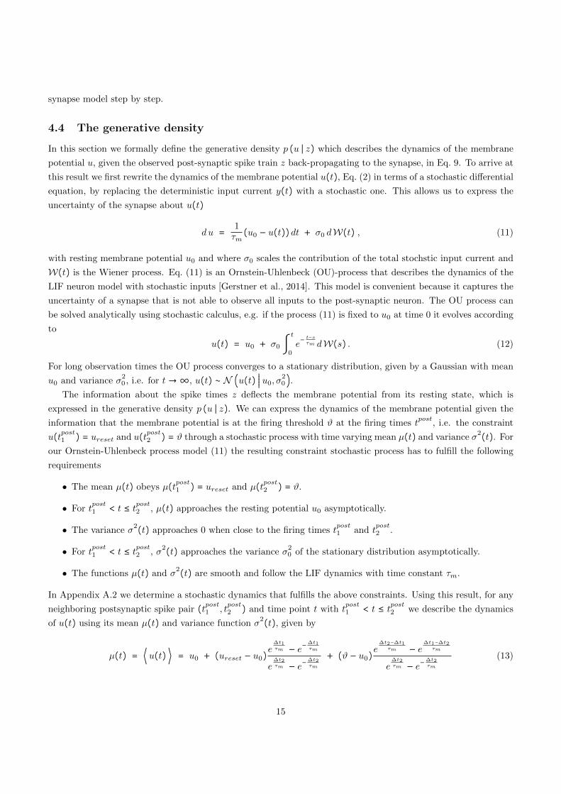
4.6 Numerical simulations

All simulations were performed in Python (3.8.5) using the Euler method to approximate the solution of the

stochastic differential equations with a fixed time step of 1 ms. Post-Synaptic currents were created as described

in Eq. (4) where Dirac delta pulses were approximated by 1 ms rectangular pulses and truncated at zero to

avoid negative currents. If not stated otherwise we used the following parameters. The synaptic current release

probability r0 was 12. In Eq. (2) the membrane time constant τm was 30 ms, the resting potential u0 was -70 mV

and the membrane resistance R was 10 MΩ. The firing threshold ϑ was -55 mV and ureset was -75 mV. For variance

function Eq. (14) we used γ = 10. The learning rate η was 10−5

.

4.6.1 Details to Figure 4

Rate patterns in Fig. 4 were generated by randomly drawing values from a beta distribution (α = 0.1, β = 0.8)

for each input channel and multiplying these values with the maximum rate of 50 Hz. From these rate patterns

individual Poisson spike trains were drawn for every pattern presentation. During the learning phase the output

neurons were clamped to fire at 50 Hz during presentation of the preferred stimulus and remain silent otherwise.

In Fig. 4C we used a simple threshold adaptation mechanism to control the output rate of the neurons for the

unsupervised case. Individual firing thresholds ϑ where used for every neuron. Thresholds were decreased by a

value of 10−5

mV in every millisecond and increased by 10−3

mV after every output spike. In Fig. 4E we set the

synaptic reliability parameter r0 in Eq. (4) to 1 to disable synaptic noise and trained a new network to create the

without noise results.

4.6.2 Details to Figure 5

In Fig. 5 we used a feed-forward network with 200 feedback neurons and 100 action neurons. Preferred positions

of the feedback neurons where scattered uniformly over the unit cube and firing rates were set scaled by the

euclidean distance between agent position and preferred position. Action neurons were randomly assigned to

preferred directions. Agent position were updated after every 50 ms time frame by adding the decoded position

offset provided by the action neurons.

References

Aitchison et al., 2021. Aitchison, L., Jegminat, J., Menendez, J. A., Pfister, J.-P., Pouget, A., and Latham,

P. E. (2021). Synaptic plasticity as bayesian inference. Nature Neuroscience, pages 1–7.

Aitchison et al., 2014. Aitchison, L., Pouget, A., and Latham, P. E. (2014). Probabilistic synapses. arXiv

preprint arXiv:1410.1029.

Barascud et al., 2016. Barascud, N., Pearce, M. T., Griffiths, T. D., Friston, K. J., and Chait, M. (2016). Brain

responses in humans reveal ideal observer-like sensitivity to complex acoustic patterns. Proceedings of the

National Academy of Sciences, 113(5):E616–E625.

Bastos et al., 2012. Bastos, A. M., Usrey, W. M., Adams, R. A., Mangun, G. R., Fries, P., and Friston, K. J.

(2012). Canonical microcircuits for predictive coding. Neuron, 76(4):695–711.

18

Borst, 2010. Borst, J. G. G. (2010). The low synaptic release probability in vivo. Trends in neurosciences,

33(6):259–266.

Brea et al., 2013. Brea, J., Senn, W., and Pfister, J.-P. (2013). Matching recall and storage in sequence learning

with spiking neural networks. The Journal of Neuroscience, 33(23):9565–9575.

Buckley et al., 2017. Buckley, C. L., Kim, C. S., McGregor, S., and Seth, A. K. (2017). The free energy principle

for action and perception: A mathematical review. Journal of Mathematical Psychology, 81:55–79.

Buesing and Maass, 2008. Buesing, L. and Maass, W. (2008). Simplified rules and theoretical analysis for infor-

mation bottleneck optimization and pca with spiking neurons. In Advances in Neural Information Processing

Systems, pages 193–200.

Buesing and Maass, 2010. Buesing, L. and Maass, W. (2010). A spiking neuron as information bottleneck.

Neural computation, 22(8):1961–1992.

Caporale and Dan, 2008. Caporale, N. and Dan, Y. (2008). Spike timing–dependent plasticity: a hebbian

learning rule. Annu. Rev. Neurosci., 31:25–46.

Chalk et al., 2018. Chalk, M., Marre, O., and Tkacik, G. (2018). Toward a unified theory of efficient, predictive,

and sparse coding. Proceedings of the National Academy of Sciences, 115(1):186–191.

Clopath et al., 2010. Clopath, C., Busing, L., Vasilaki, E., and Gerstner, W. (2010). Connectivity reflects

coding: a model of voltage-based stdp with homeostasis. Nature neuroscience, 13(3):344.

Clopath and Gerstner, 2010. Clopath, C. and Gerstner, W. (2010). Voltage and spike timing interact in stdp –

a unified model. Frontiers in synaptic neuroscience, 2:25.

Corlay, 2013. Corlay, S. (2013). Properties of the ornstein-uhlenbeck bridge. arXiv preprint arXiv:1310.5617.

Dan and Poo, 2004. Dan, Y. and Poo, M.-m. (2004). Spike timing-dependent plasticity of neural circuits.

Neuron, 44(1):23–30.

Davies et al., 2018. Davies, M., Srinivasa, N., Lin, T.-H., Chinya, G., Cao, Y., Choday, S. H., Dimou, G., Joshi,

P., Imam, N., Jain, S., et al. (2018). Loihi: A neuromorphic manycore processor with on-chip learning. Ieee

Micro, 38(1):82–99.

Deneve, 2008. Deneve, S. (2008). Bayesian spiking neurons ii: learning. Neural computation, 20(1):118–145.

DJ Rezende, 2014. DJ Rezende, S Mohamed, D. W. (2014). Stochastic backpropagation and approximate

inference in deep generative models. International Conference on Machine Learning.

DJ Rezende, 2011. DJ Rezende, D Wierstra, W. G. (2011). Variational learning for recurrent spiking networks.

Advances in Neural Information Processing Systems, pages 136–144.

Driscoll et al., 2017. Driscoll, L. N., Pettit, N. L., Minderer, M., Chettih, S. N., and Harvey, C. D. (2017).

Dynamic reorganization of neuronal activity patterns in parietal cortex. Cell, 170(5):986–999.

Faisal et al., 2008. Faisal, A. A., Selen, L. P., and Wolpert, D. M. (2008). Noise in the nervous system. Nature

reviews neuroscience, 9(4):292–303.

19

Feinstein, 1986. Feinstein, D. I. (1986). Relating thermodynamics to information theory: the equality of free

energy and mutual information. PhD thesis, California Institute of Technology.

Friston, 2005. Friston, K. (2005). A theory of cortical responses. Philosophical transactions of the Royal Society

B: Biological sciences, 360(1456):815–836.

Friston, 2008. Friston, K. (2008). Variational filtering. NeuroImage, 41(3):747–766.

Friston, 2010. Friston, K. (2010). The free-energy principle: a unified brain theory? Nature reviews neuro-

science, 11(2):127.

Friston and Ao, 2012. Friston, K. and Ao, P. (2012). Free energy, value, and attractors. Computational and

mathematical methods in medicine, 2012.

Friston et al., 2014. Friston, K., Schwartenbeck, P., FitzGerald, T., Moutoussis, M., Behrens, T., and Dolan,

R. J. (2014). The anatomy of choice: dopamine and decision-making. Philosophical Transactions of the Royal

Society B: Biological Sciences, 369(1655):20130481.

Gerstner et al., 2014. Gerstner, W., Kistler, W. M., Naud, R., and Paninski, L. (2014). Neuronal dynamics:

From single neurons to networks and models of cognition. Cambridge University Press.

Gjorgjieva et al., 2011. Gjorgjieva, J., Clopath, C., Audet, J., and Pfister, J.-P. (2011). A triplet spike-timing–

dependent plasticity model generalizes the bienenstock–cooper–munro rule to higher-order spatiotemporal

correlations. Proceedings of the National Academy of Sciences, 108(48):19383–19388.

Gontier and Pfister, 2020. Gontier, C. and Pfister, J.-P. (2020). Identifiability of a binomial synapse. Frontiers

in computational neuroscience, 14:86.

Graupner and Brunel, 2012. Graupner, M. and Brunel, N. (2012). Calcium-based plasticity model explains

sensitivity of synaptic changes to spike pattern, rate, and dendritic location. Proceedings of the National

Academy of Sciences, 109(10):3991–3996.

Isomura and Friston, 2018. Isomura, T. and Friston, K. (2018). In vitro neural networks minimise variational

free energy. Scientific reports, 8(1):16926.

Isomura et al., 2015. Isomura, T., Kotani, K., and Jimbo, Y. (2015). Cultured cortical neurons can perform

blind source separation according to the free-energy principle. PLoS computational biology, 11(12):e1004643.

Isomura et al., 2016. Isomura, T., Sakai, K., Kotani, K., and Jimbo, Y. (2016). Linking neuromodulated spike-

timing dependent plasticity with the free-energy principle. Neural computation, 28(9):1859–1888.

Jensen et al., 2019. Jensen, T. P., Zheng, K., Cole, N., Marvin, J. S., Looger, L. L., and Rusakov, D. A. (2019).

Multiplex imaging relates quantal glutamate release to presynaptic ca 2+ homeostasis at multiple synapses in

situ. Nature communications, 10(1):1–14.

Kanai et al., 2015. Kanai, R., Komura, Y., Shipp, S., and Friston, K. (2015). Cerebral hierarchies: predictive

processing, precision and the pulvinar. Philosophical Transactions of the Royal Society B: Biological Sciences,

370(1668):20140169.

20

Kappel et al., 2014. Kappel, D., Nessler, B., and Maass, W. (2014). Stdp installs in winner-take-all circuits an

online approximation to hidden markov model learning. PLoS Computational Biology, 10(3):e1003511.

Katz, 1971. Katz, B. (1971). Quantal mechanism of neural transmitter release. Science, 173(3992):123–126.

Kiebel and Friston, 2011. Kiebel, S. J. and Friston, K. J. (2011). Free energy and dendritic self-organization.

Frontiers in systems neuroscience, 5:80.

Kostadinov et al., 2019. Kostadinov, D., Beau, M., Pozo, M. B., and Hausser, M. (2019). Predictive and

reactive reward signals conveyed by climbing fiber inputs to cerebellar purkinje cells. Nature Neuroscience,

22(6):950–962.

Linsker, 1988. Linsker, R. (1988). Self-organization in a perceptual network. Computer, 21(3):105–117.

Maass, 2014. Maass, W. (2014). Noise as a resource for computation and learning in networks of spiking neurons.

Proceedings of the IEEE, 102(5):860–880.

Markram and Tsodyks, 1996. Markram, H. and Tsodyks, M. (1996). Redistribution of synaptic efficacy between

neocortical pyramidal neurons. Nature, 382(6594):807–810.

Mayr et al., 2019. Mayr, C., Hoeppner, S., and Furber, S. (2019). Spinnaker 2: A 10 million core processor

system for brain simulation and machine learning. arXiv preprint arXiv:1911.02385.

Millidge et al., 2020. Millidge, B., Tschantz, A., and Buckley, C. L. (2020). Predictive coding approximates

backprop along arbitrary computation graphs. arXiv preprint arXiv:2006.04182.

Mnih and Gregor, 2014. Mnih, A. and Gregor, K. (2014). Neural variational inference and learning in belief

networks. arXiv preprint arXiv:1402.0030.

Monday et al., 2018. Monday, H. R., Younts, T. J., and Castillo, P. E. (2018). Long-term plasticity of neuro-

transmitter release: emerging mechanisms and contributions to brain function and disease. Annual review of

neuroscience, 41:299–322.

Neftci et al., 2016. Neftci, E. O., Pedroni, B. U., Joshi, S., Al-Shedivat, M., and Cauwenberghs, G. (2016).

Stochastic synapses enable efficient brain-inspired learning machines. Frontiers in neuroscience, 10:241.

Nessler et al., 2013. Nessler, B., Pfeiffer, M., Buesing, L., and Maass, W. (2013). Bayesian computation emerges

in generic cortical microcircuits through spike-timing-dependent plasticity. PLoS Computational Biology,

9(4):e1003037.

Nessler et al., 2009. Nessler, B., Pfeiffer, M., and Maass, W. (2009). Hebbian learning of bayes optimal decisions.

Adv. Neura.l Inf. Process. Syst., 21:1169–1176.

Oertner et al., 2002. Oertner, T. G., Sabatini, B. L., Nimchinsky, E. A., and Svoboda, K. (2002). Facilitation

at single synapses probed with optical quantal analysis. Nature neuroscience, 5(7):657–664.

Pecevski et al., 2014. Pecevski, D., Kappel, D., and Jonke, Z. (2014). NEVESIM: Event-driven neural simulation

framework with a python interface. Frontiers in Neuroinformatics, 8:70.

21

Pecevski and Maass, 2016. Pecevski, D. and Maass, W. (2016). Learning probabilistic inference through spike-

timing-dependent plasticity. eNeuro, 3(2).

Peyser et al., 2017. Peyser, A., Deepu, R., Mitchell, J., Appukuttan, S., Schumann, T., Eppler, J. M., Kappel,

D., Hahne, J., Zajzon, B., Kitayama, I., et al. (2017). Nest 2.14. 0. Technical report, Julich Supercomputing

Center.

Pfister and Gerstner, 2006a. Pfister, J.-P. and Gerstner, W. (2006a). Beyond pair-based stdp: A phenomeno-

logical rule for spike triplet and frequency effects. In Advances in neural information processing systems, pages

1081–1088.

Pfister and Gerstner, 2006b. Pfister, J.-P. and Gerstner, W. (2006b). Triplets of spikes in a model of spike

timing-dependent plasticity. Journal of Neuroscience, 26(38):9673–9682.

Ramstead et al., 2016. Ramstead, M. J., Veissiere, S. P., and Kirmayer, L. J. (2016). Cultural affordances:

Scaffolding local worlds through shared intentionality and regimes of attention. Frontiers in psychology,

7:1090.

Ramstead et al., 2018. Ramstead, M. J. D., Badcock, P. B., and Friston, K. J. (2018). Answering schrodinger’s

question: A free-energy formulation. Physics of life reviews, 24:1–16.

Rao and Ballard, 1999. Rao, R. P. and Ballard, D. H. (1999). Predictive coding in the visual cortex: a functional

interpretation of some extra-classical receptive-field effects. Nature neuroscience, 2(1):79.

Rezende and Gerstner, 2014. Rezende, D. J. and Gerstner, W. (2014). Stochastic variational learning in recur-

rent spiking networks. Frontiers in Computational Neuroscience, 8:38.

Rusakov et al., 2020. Rusakov, D. A., Savtchenko, L. P., and Latham, P. E. (2020). Noisy synaptic conductance:

bug or a feature? Trends in Neurosciences.

Szavits-Nossan and Evans, 2015. Szavits-Nossan, J. and Evans, M. R. (2015). Inequivalence of nonequilibrium

path ensembles: the example of stochastic bridges. Journal of Statistical Mechanics: Theory and Experiment,

2015(12):P12008.

Tishby et al., 2000. Tishby, N., Pereira, F. C., and Bialek, W. (2000). The information bottleneck method.

arXiv preprint physics/0004057.

Toyoizumi et al., 2005. Toyoizumi, T., Pfister, J.-P., Aihara, K., and Gerstner, W. (2005). Generalized

bienenstock–cooper–munro rule for spiking neurons that maximizes information transmission. Proceedings

of the National Academy of Sciences, 102(14):5239–5244.

Urbanczik and Senn, 2014. Urbanczik, R. and Senn, W. (2014). Learning by the dendritic prediction of somatic

spiking. Neuron, 81(3):521–528.

Whittington and Bogacz, 2017. Whittington, J. C. and Bogacz, R. (2017). An approximation of the error

backpropagation algorithm in a predictive coding network with local hebbian synaptic plasticity. Neural

computation, 29(5):1229–1262.

22

Yang and Xu-Friedman, 2013. Yang, H. and Xu-Friedman, M. A. (2013). Stochastic properties of neurotrans-

mitter release expand the dynamic range of synapses. Journal of Neuroscience, 33(36):14406–14416.

Yang and Calakos, 2013. Yang, Y. and Calakos, N. (2013). Presynaptic long-term plasticity. Frontiers in

synaptic neuroscience, 5:8.

23

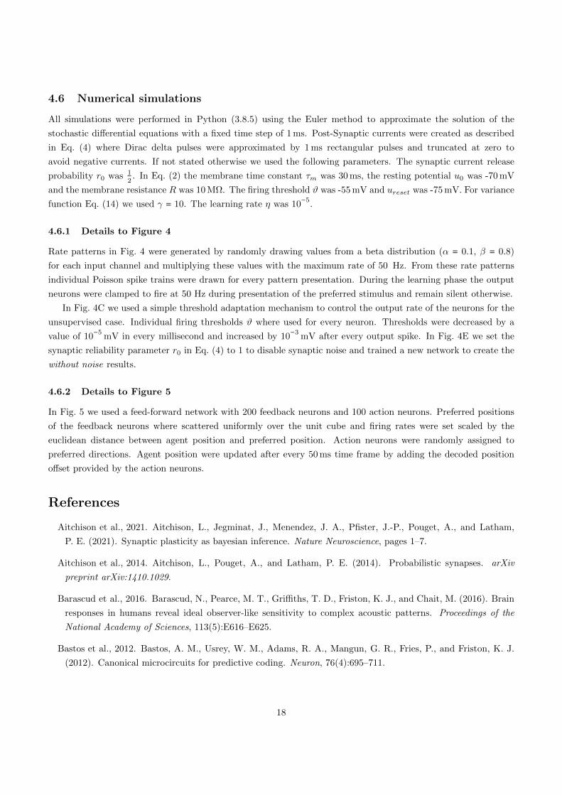
A Appendix

A.1 Derivation of the recognition density

Here we derive the recognition density q (u ∣w) for our synapse model. We will show that q (u ∣w) can be expressed

as a Gaussian distribution with time-varying mean and variance functions µw(t) and σ2w(t). This result can be

obtained by stochastic integration, but to keep this paper self-contained we provide a simple proof here. We start

by considering a general drift-diffusion process and then show the special case of the LIF neuron dynamics step

by step.

For the general case we consider the Fokker-Planck equation that governs the probability density function

p(x, t) of a stochastic process x at time t, with drift A(x, t) and diffusion B(x, t)

∂

∂tp(x, t) = −

∂

∂x(A(x, t) ⋅ p(x, t)) + 1

2

∂2

∂x2(B(x, t) ⋅ p(x, t)) . (A.1)

We treat here the case that p(x, t) is a Gaussian distribution with time-varying mean µ(t) and variance σ2(t)

functions, i.e.p(x, t) = N (x »»»»»µ(t), σ2(t)) at any time point t, to get

∂

∂tp(x, t) = p(x, t) (µ′(t)x − µ(t)

σ2(t) +1

2(σ2(t))′ ((x − µ(t))

2

σ4(t) −1

σ2(t))) ,

where µ′(t) = ∂

∂tµ(t) and (σ2(t))′ = ∂

∂tσ

2(t). Furthermore

∂

∂x(A(x, t) ⋅ p(x, t)) = p(x, t) ( ∂

∂xA(x, t) − A(x, t)x − µ(t)

σ2(t) )

and

∂2

∂x2(B(x, t) ⋅ p(x, t)) = p(x, t) ( ∂

2

∂x2B(x, t) − 2

∂

∂xB(x, t)x − µ(t)

σ2(t) + B(x, t) ((x − µ(t))2

σ4(t) −1

σ2(t))) .

Therefore, by plugging these results back into the Fokker-Planck equation (A.1), we find the condition that has

to be satisfied for functions A(x, t) and B(x, t) to be given by

µ′(t)x − µ(t)

σ2(t) +1

2(σ2(t))′ ((x − µ(t))

2

σ4(t) −1

σ2(t))!= (A.2)

A(x, t)x − µ(t)σ2(t) −

∂

∂xA(x, t) + 1

2

∂2

∂x2B(x, t) − ∂

∂xB(x, t)x − µ(t)

σ2(t) +1

2B(x, t) ((x − µ(t))

2

σ4(t) −1

σ2(t)) .

Clearly, the choice A(x, t) = µ′(t), B(x, t) = (σ2(t))′ satisfies this condition for any differentiable functions µ(t)

and σ2(t).

To arrive at the final result we replace the general drift-diffusion dynamics with the special case of a leaky

integrator with finite integration time constant τ using the ansatz A(x, t) = 1τ(x0 − x) + a(t) and B(x, t) = b(t).

In this case, we can make condition (A.2) satisfied if µ′(t) = 1

τ(x0 − µ(t)) + a(t) and (σ2(t))′ = b(t) − 2

τσ

2(t).

24

This can be verified by plugging this result back into Eq. (A.2)

(1τ (x0 − µ(t)) + a(t))

x − µ(t)σ2(t) +

1

2(b(t) − 2

τ σ2(t)) ((x − µ(t))

2

σ4(t) −1

σ2(t))!=

(1τ (x0 − x) + a(t))

x − µ(t)σ2(t) +

1τ +

1

2b(t) ((x − µ(t))

2

σ4(t) −1

σ2(t)) ,

from which the equality follows

↔1τ (x0 − µ(t))

x − µ(t)σ2(t) −

1τ ((x − µ(t))

2

σ2(t) − 1) !=

1τ (x0 − x)

x − µ(t)σ2(t) +

1τ

↔ (x0 − µ(t))x − µ(t)σ2(t) −

(x − µ(t))2

σ2(t)!= (x0 − x)

x − µ(t)σ2(t)

↔ (x0 − x)x − µ(t)σ2(t)

!= (x0 − x)

x − µ(t)σ2(t)

This proofs that a stochastic process x with p(x, t) = N (x »»»»»µ(t), σ2(t)), µ

′(t) = 1τ(x0 − µ(t))+a(t) and (σ2(t))′ =

b(t)− 2τσ

2(t) is realized by a drift A(x, t) = 1τ(x0 − x)+a(t) and diffusion B(x, t) = b(t). Equivalently, any process

x with mean µ(t) and variance σ2(t) can be realized if

a(t) = µ′(t) + 1

τ (µ(t) − x0) ,

b(t) = (σ2(t))′ + 2τ σ

2(t) ,(A.3)

and b(t) ≥ 0 can be satisfied for all t. This last result was used in the main text to derive the learning rule (5).

Furthermore, by integration of this last result we find that any integrable functions a(t) and b(t) > 0 yield the

following dynamics for the stochastic process x

µ(t) = x0 + e− tτ ∫

t

0esτ a(s) d s

σ2(t) = e

− 2tτ ∫

t

0e

2sτ b(s) d s .

(A.4)

For a(t) = 0 and b(t) = b (constant) we recover the Ornstein-Uhlenbeck process dynamics.

For our synapse model drift and diffusion are governed by the stochastic current release, which can be reflected

in the above model by using a(t) = r0Rw∑f δ(t− t(f)) and b(t) = r0 (1− r0)Rw∑f δ(t− t

(f)), where δ(t) is the

Dirac delta function. Using this we identify the recognition density qw(u(t)) = N (u(t) »»»»»µw(t), σ2w(t)), with

µw(t) = u0 + r0Rw ∑f

ε (t − t(f))

σ2w(t) = r0 (1 − r0)R2

w ∑f

ε (2 t − 2 t(f)) ,

(A.5)

25

where ε (t) = e−tτm Θ(t) and Θ(t) is the Heaviside step function.

A.2 Details to the generative density

The generative density p (u ∣ z) describes the evolution of the external world and the uncertainty of the synapse

based on the provided feedback information z. In our model the feedback is given by the back-propagating action

potentials which precisely determine the u at the spike times. At all other times the precise value of the membrane

potential is unknown and this uncertainty should be reflected in the generative density.

We use a Gaussian process model of the external world, such that the generative density is given by

p (u(t) ∣ z) = N (u(t) »»»»»µ(t), σ2(t)) . (A.6)

In principle we can assume any function µ(t) and σ2(t) and the learning rule Eq. 1 will strive to best approx-

imate its dynamics. However, a reasonable choice will obey the constraints imposed by the neuron and synapse

dynamics, e.g. the membrane time constant and the firing mechanism and resetting behavior of the neuron.

The LIF neuron implies OU process dynamics of the membrane potential. Given the information that the

membrane potential is at the firing threshold ϑ at the firing times tpost

, i.e. the constraint u(tpost1 ) = ureset and

u(tpost2 ) = ϑ, the OU process can be solved explicitly. The solution to this double constraint stochastic process

is the OU-bridge process [Corlay, 2013,Szavits-Nossan and Evans, 2015]. For any neighboring postsynaptic spike

pair (tpost1 , tpost2 ) and time point t with t

post1 < t ≤ t

post2 we can describe the dynamics of u(t) using its mean µ(t),

given by

µ(t) = ⟨u(t) ⟩ = u0 + (ureset − u0)sinh ( t

post2 −tτm

)

sinh ( tpost2 −t

post1

τm)+ (ϑ − u0)

sinh ( t−tpost1

τm)

sinh ( tpost2 −t

post1

τm), (A.7)

where sinh(t) = et−e−t

2is the hyperbolic sine function. This function describes the asymptotic approach to the

resting potential u0 and the slope towards the firing threshold ϑ. We used this function to determine the generative

density.

The OU-bridge process model also provides a solution for the variance function σ2(t), given by

σ2(t) = ⟨u2(t) ⟩ − ⟨u(t) ⟩ = σ

20

sinh ( tpost2 −tτm

) × sinh ( t−tpost1

τm)

sinh ( tpost2 −t

post1

τm)

. (A.8)

This variance function has a very steep slope to approach the firing threshold. It is so steep in fact that it would

require us to have negative variance for the synaptic current y close to the firing times to realize the process

Eq. (A.3). This has no meaningful physical interpretation and therefore we used the slower process that better

reflects the asymptotic behavior of a leaky integrator, given by

σ2(t) = σ

20

γ

γ + etpost1 −t

τm + et−tpost2τm

. (A.9)

26