A Study of Simulation of the Urban Space 3D Temperature ...

Citation: Huo, H.; Chen, F. A Study

of Simulation of the Urban Space 3D

Temperature Field at a Community

Scale Based on High-Resolution

Remote Sensing and CFD. Remote

Sens. 2022, 14, 3174. https://

doi.org/10.3390/rs14133174

Academic Editor: Constantinos

Cartalis

Received: 14 April 2022

Accepted: 28 June 2022

Published: 1 July 2022

Publisher’s Note: MDPI stays neutral

with regard to jurisdictional claims in

published maps and institutional affil-

iations.

Copyright: © 2022 by the authors.

Licensee MDPI, Basel, Switzerland.

This article is an open access article

distributed under the terms and

conditions of the Creative Commons

Attribution (CC BY) license (https://

creativecommons.org/licenses/by/

4.0/).

remote sensing

Article

A Study of Simulation of the Urban Space 3D TemperatureField at a Community Scale Based on High-Resolution RemoteSensing and CFDHongyuan Huo 1,2 and Fei Chen 1,*

1 Faculty of Architecture, Civil and Transportation Engineering, Beijing University of Technology,Beijing 100124, China; [email protected] or [email protected]

2 State Key Laboratory of Media Convergence Production Technology and Systems, Beijing 100803, China* Correspondence: [email protected]; Tel.: +86-152-7490-0298

Abstract: This study used high-resolution remote-sensing technology and CFD models to carry outa simulation study of a three-dimensional (3D) USTE for daytime and nighttime at a block scale.Firstly, the influence of vegetation with different spatial layouts on the 3D USTE was analyzed.Moreover, the heat transfer process and heat conduction process between urban surface componentsat the block scale were simulated, and in the meanwhile, the distribution and changes of the 3DUSTE and the regional wind pressure environment were monitored. The simulation results showedthat (1) vegetation has a relatively significant mitigation effect on the thermal environment near thesurface, (2) vegetation with different morphologies and layouts results in significant differences in themitigation efficiency of wind speed and canyon USTE, and (3) the seasonal spatial 3D temperaturecan be mitigated as well. In addition, this study analyzed the mitigation effect of vegetation on theurban wind–heat environment during both daytime and nighttime. The results indicated that (1) themitigation effect of vegetation is more significant during the daytime, while showing a small value atnight with an even temperature distribution, and (2) convection heat transfer is the primary cause, orone of the major causes, of differences in the USTE.

Keywords: remote sensing; computational fluid dynamics; simulation; urban spatial thermalenvironment

1. Introduction

The rapid expansion of urbanization has increased urban natural surfaces to be consid-erably replaced by impervious surfaces such as roads and buildings [1–3], which changesthe physical properties of the underlying surface of a city [4,5]. It has severely affectedthe urban microclimate, urban phenology, and the ecological environment and has led toa series of social, ecological, and environmental challenges [6]. Among them, the urbanthermal environment is one of the most significant problems [7]. Quantitative researchon urban spatial thermal environments has become one of the current hotspots in ur-ban ecological environment research to better understand thermal environment dynamiccharacteristics [8].

At present, the main methods for quantifying the thermal environment of a cityspace include site observation, remote-sensing technology, and numerical simulation.Remote-sensing methods can obtain large-area surface temperature information [9–13].The research methods for urban space thermal environments based on remote sensing andrelated models are relatively mature, and many key patterns have been revealed. However,remote sensing usually obtains surface temperature information, but it cannot directlyobtain the three-dimensional spatial air temperature and the side wall’s temperature ofa target simultaneously. Compared to remote-sensing methods, numerical simulation

Remote Sens. 2022, 14, 3174. https://doi.org/10.3390/rs14133174 https://www.mdpi.com/journal/remotesensing

https://doi.org/10.3390/rs14133174

https://doi.org/10.3390/rs14133174

https://creativecommons.org/

https://creativecommons.org/licenses/by/4.0/

https://creativecommons.org/licenses/by/4.0/

https://www.mdpi.com/journal/remotesensing

https://www.mdpi.com

https://orcid.org/0000-0001-5843-3106

https://doi.org/10.3390/rs14133174

https://www.mdpi.com/journal/remotesensing

https://www.mdpi.com/article/10.3390/rs14133174?type=check_update&version=2

Remote Sens. 2022, 14, 3174 2 of 29

methods can further simulate 3D surface and air temperature profiles simultaneously and,thus, make up for the shortcomings of remote-sensing technology [2,14–18].

CFD-based numerical simulation methods are mainly divided into three types: directnumerical simulation (DNS), Reynolds-averaged Navier–Stokes (RANS) method, and largeeddy simulation (LES). The DNS method has been applied in the field of aerodynamicssince earlier decades. LES is mainly aimed at solving problems of high Reynolds numberflow and wall turbulent flow. Both DNS and LES require massive computing power, and itis relatively difficult to conduct large-scale simulation research. In simulation studies ofurban thermal environments, the RANS method [19] is mostly used.

From the perspective of the spatial scale, CFD-based simulations of urban thermal envi-ronments can be divided into three categories, including micro-scale [20], block-scale [20,21]and macro-scale [1,17,22–25]. At the microscopic scale, there have been many studies onindoor thermal environments and ventilation performance based on CFD. Albatayneh [20]used CFD simulations to examine the distribution and change of the external surface tem-perature of a single building in Perth, Australia, during the Spring Festival and winter. vanHooff [26] conducted a comparative analysis and evaluated the turbulent kinetic energy ofone building based on LES, RANS, and experimental methods; the LES approach showed abetter performance than the other two methods.

At present, most studies on the simulation of urban thermal environments basedon CFD have been focused at the block scale. Concerning the study area, most of thestudy areas have been concentrated in streets, residential quarters, or a city’s centralbusiness district. The main research topics have included: (1) research on the influence andmitigation effects of buildings, vegetation, water bodies, and other factors, as well as theirmorphological changes and spatial layouts, on the thermal environments of urban localbuilding clusters [3,14,27,28]; (2) simulations of urban thermal environments to examine thelayout and design of urban ventilation corridors and their relationships with the thermalenvironment [29–31]; and (3) research on the relationship between the thermal environmentand the human thermal comfort index [24,28,32–36].

In recent years, significant progress has been achieved with CFD simulation studiesof urban thermal environments at a macro-scale. Li [1] combined CFD simulation withremote-sensing technology to analyze the heat environment of Wuhan, China, and thesimulation results contributed to the optimized planning of urban ventilation corridors.Antoniou [21] simulated the space thermal infrared temperature with an area of 0.247 km2

in Nicosia, Cyprus; the corresponding calculated area was 1700*1700*270 m3. Ashie [22]simulated the wind field and temperature of Tokyo Bay considering the influence of seabreeze based on CFD. Du [24] carried out a study on the effects of different layouts ofgreenspace on the urban thermal environment by simulating the space temperature fieldbased on CFD. The distribution of the temperature field of the entire Shanghai area underthe influence of water bodies was also simulated, and corresponding mitigation measuresto alleviate the thermal environment were proposed.

Regarding the study of methods and materials use to mitigate urban heat island effects,many scientists have developed quantitative analyses of the relationship between the land-scape and the canopy heat island. In addition, some materials have also been introduced tobe effectively used to alleviate heat island effects. Akbari (2016) summarized and analyzedmethods of mitigating urban climate change and urban heat island effects. Among them,the use of highly reflective materials, cool and green roofs, cool pavement, and urbangreening were very helpful in mitigating the heat island effect [37]. Chatzinikolaou (2018)performed a numerical simulation of the urban thermal environment at a block scale basedon GIS and ENVI-met to evaluate the influence of vegetation on the local air temperatureand thermal comfort of the urban environment. The results showed that roadside vegeta-tion could improve the thermal comfort conditions of the urban environment and alleviatethe heat island effect [38]. Liu (2020) used multitemporal remote-sensing data and GISmethods to analyze the dynamic relationship between land use–land cover ratio changesand urban heat islands and found that there was a significant positive correlation between

Remote Sens. 2022, 14, 3174 3 of 29

surface temperature and vegetation [39]. Zhang (2021) took Nanjing, China, as the researcharea and studied the temporal and spatial change trajectories and related characteristics ofthermal environment patterns based on Landsat8 remote-sensing image data simulation.The results showed that the spatial pattern of the heat island in Nanjing changed from ascattered distribution in the city periphery to a concentrated distribution in the city center,and the intensity of the heat island was increasing year by year. Changes in administrativedivisions, changes in the layout of traffic trunks, and the transfer of industrial centers wereimportant driving factors for the evolution of the surface thermal environment pattern [40].Combining remote-sensing spatial data and satellite imagery, Cocci (2022) used CFD tosimulate the wind–thermal environment in the suburbs of Ascoli Piceno, Italy. Based onthe simulation results, a dataset was obtained that defined the degree of vulnerability and,thus, the areas exposed to thermal risk [41].

With the development of space technology, the combination of RS, GIS, lidar, andother earth observation technologies is an important and difficult point in current CFDsimulations of urban space thermal environment research. Earth observation data canprovide important data source support for the optimization of CFD model parameters,the control of boundary input conditions, the accurate construction of 3D models, andthe verification of simulation results [1,17,21,22,24]. Li [1] and Du [24] both used groundsurface classification results and temperature inversion results combined with satelliteremote-sensing data to optimize CFD model parameters and boundary control conditionsand carried out simulation studies of urban space thermal environments at a macro-scale.Ashie [22] used GIS and lidar to obtain information on urban building elevations anddifferent land use types. On this basis, CFD was used to simulate the thermal environmentof 23 blocks with different land types in Tokyo, as well as the thermal environment dis-tribution of Tokyo Bay. Hedquist et al. [42] employed temperature and humidity sensorsand infrared cameras to acquire temperature, humidity, wind speed, and building surfacetemperatures and located and modeled real-time street views based on GPS and GoogleEarth. Based on CFD simulation, the impact of different building exterior materials anddifferent building layouts on the thermal environment in Phoenix, Arizona, USA, wasdepicted. Antoniou [21] utilized a thermometer, an ultrasonic anemometer, and an FLIR-P640 infrared thermal-imaging camera to collect information on the surface temperature,wind field, and air temperature, which provided initialization conditions and data sourcesupport for a CFD model to study the urban thermal environment of Nicosia, the capitalof Cyprus.

However, few studies have simulated the impact of vegetation morphology changesat both daytime and nighttime during different seasons on the urban thermal environmentusing CFD simulations. There is almost no research on simulations of seasonal air tempera-ture at a community scale, which is helpful to further analyze the urban canopy heat island.This research adopts CFD models combined with high-resolution remote-sensing technol-ogy and meteorological station observation data to (1) simulate the impact of vegetation indifferent spatial layouts on urban spatial temperature fields at both daytime and nighttimein different seasons and (2) simulate a seasonal urban spatial 3D temperature field. Theaim of the paper is to use a CFD model to (1) obtain an urban three-dimensional spatialtemperature field, including the surface temperature field and the vertical atmospherictemperature field, as well as the distribution and changes of the regional wind pressureenvironment; (2) explore the impact of vegetation morphology and layout on the thermalenvironment, as well as the distribution and changes of the spatial temperature field intypical residential quarters in Beijing during both day and night across four seasons; and(3) examine the difference in vegetation mitigation effects of different morphological lay-outs, the heat transfer process, and the heat conduction process between urban surfacecomponents at a block scale.

This study consists of five sections. Section 2 introduces the situation of the study areaand its geographic characteristics. Section 3 describes the methodology in detail, includingthe basic principles of CFD, model selection, and boundary condition settings. Section 4

Remote Sens. 2022, 14, 3174 4 of 29

presents the simulation results and findings. Section 5 concludes the paper by discussingthe limitations of this study and the implications for future research.

2. Study Area

The community of the Beijing University of Technology was selected as the studyarea. It is located in Chaoyang District, Beijing, China, covering the area of 116◦28′16′′–116◦28′57′′E, 39◦52′12′′–39◦52′41′′N. The study area has a typical temperate, semi-humid,continental monsoon climate, with hot and rainy summers, cold and dry winters, south-easterly winds prevailing in the summer, and northwesterly winds prevailing in the winter.The average annual temperature in 2019 was 13.8 ◦C; the average temperature in summerwas 28 ◦C during the day and 16 ◦C at night, and the average temperature in winter was5 ◦C during the day and 0 ◦C at night. The temperature peak generally occurs in Julyand was 38 ◦C in 2019. The average annual precipitation was 33.875 mm: 54.433 mm inthe summer and 2.567 mm in the winter. The average annual precipitation is typicallyconcentrated from July–September, with more rain in the spring and summer and lessrain in the winter. The statistics of the monthly average temperatures and precipitation inBeijing in 2019 are shown in Figure 1 (data from the National Meteorological Science DataCenter). The location of study area is shown in Figure 2a.

Remote Sens. 2022, 14, 3174 4 of 28

Section 4 presents the simulation results and findings. Section 5 concludes the paper by discussing the limitations of this study and the implications for future research.

2. Study Area The community of the Beijing University of Technology was selected as the study

area. It is located in Chaoyang District, Beijing, China, covering the area of 116°28′16″–116°28′57″E, 39°52′12″–39°52′41″N. The study area has a typical temperate, semi-humid, continental monsoon climate, with hot and rainy summers, cold and dry winters, south-easterly winds prevailing in the summer, and northwesterly winds prevailing in the win-ter. The average annual temperature in 2019 was 13.8 °C; the average temperature in sum-mer was 28 °C during the day and 16 °C at night, and the average temperature in winter was 5 °C during the day and 0 °C at night. The temperature peak generally occurs in July and was 38 °C in 2019. The average annual precipitation was 33.875 mm: 54.433 mm in the summer and 2.567 mm in the winter. The average annual precipitation is typically concentrated from July–September, with more rain in the spring and summer and less rain in the winter. The statistics of the monthly average temperatures and precipitation in Beijing in 2019 are shown in Figure 1 (data from the National Meteorological Science Data Center). The location of study area is shown in Figure 2a.

Figure 1. Statistical map of temperature and precipitation data for Beijing in 2019. Figure 1. Statistical map of temperature and precipitation data for Beijing in 2019.

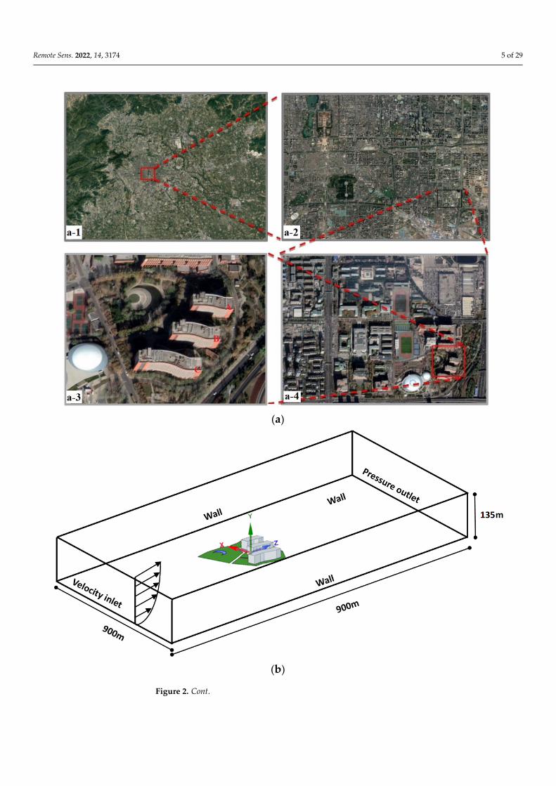
In this study, multispectral images from the GaoFen-2 satellite were combined withremote-sensing images from the Google Earth satellite to divide the urban underlyingsurface of the study area into four components, including buildings, grasslands, waterbodies, and roads. Based on the classification results, a 3D geometric model of eachcomponent was established using SpaceClaim 3D modeling software. In the study of theinfluence of changes in vegetation geometric characteristics on the thermal environment ofthe CFD simulation space, we chose three buildings, including the Ruanjian building (A inFigure 2(a-3)), the Chengjian building (B in Figure 2(a-3)), and the Shixun building (C inFigure 2(a-3)), of the university campus community as the CFD simulation objects, and webuilt the relevant geometric models (as shown in Figure 2b). In the research of simulating aspace thermal environment at a community scale, a three-dimensional geometric model ofthe community building of the Beijing University of Technology was established, as shownin Figure 2c.

Remote Sens. 2022, 14, 3174 5 of 29Remote Sens. 2022, 14, 3174 5 of 28

(a)

(b)

Figure 2. Cont.

Remote Sens. 2022, 14, 3174 6 of 29Remote Sens. 2022, 14, 3174 6 of 28

(c)

Figure 2. High-resolution remote-sensing satellite image of the study area: (a) the physical model of the CFD calculations in the study area, and the size of its computational domain, (b) the geometric model of the campus of the Beijing University of Technology, and (c) the geometric model of three buildings at the southeast of the campus of the Beijing University of Technology.

In this study, multispectral images from the GaoFen-2 satellite were combined with remote-sensing images from the Google Earth satellite to divide the urban underlying surface of the study area into four components, including buildings, grasslands, water bodies, and roads. Based on the classification results, a 3D geometric model of each com-ponent was established using SpaceClaim 3D modeling software. In the study of the in-fluence of changes in vegetation geometric characteristics on the thermal environment of the CFD simulation space, we chose three buildings, including the Ruanjian building (A in Figure 2(a-3)), the Chengjian building (B in Figure 2(a-3)), and the Shixun building (C in Figure 2(a-3)), of the university campus community as the CFD simulation objects, and we built the relevant geometric models (as shown in Figure 2b). In the research of simu-lating a space thermal environment at a community scale, a three-dimensional geometric model of the community building of the Beijing University of Technology was established, as shown in Figure 2c.

3. Materials and Methodology In this study, the dataset, including high-resolution, remotely sensed images and me-

teorological data, were preprocessed and used to build a three-dimensional (3D) geomet-ric model. The parameters of the materials and the conditions of boundary were set, and the turbulence model, radiation model, and computational method were selected. Then, the wind speed profile and its calculation method were defined. The porous media model for vegetation was simplified, and the parameters of the model were also set. The flowchart of the study is shown in Figure 3.

Figure 2. High-resolution remote-sensing satellite image of the study area: (a) the physical model ofthe CFD calculations in the study area, and the size of its computational domain, (b) the geometricmodel of the campus of the Beijing University of Technology, and (c) the geometric model of threebuildings at the southeast of the campus of the Beijing University of Technology.

3. Materials and Methodology

In this study, the dataset, including high-resolution, remotely sensed images and me-teorological data, were preprocessed and used to build a three-dimensional (3D) geometricmodel. The parameters of the materials and the conditions of boundary were set, and theturbulence model, radiation model, and computational method were selected. Then, thewind speed profile and its calculation method were defined. The porous media model forvegetation was simplified, and the parameters of the model were also set. The flowchart ofthe study is shown in Figure 3.

Remote Sens. 2022, 14, 3174 7 of 28

Figure 3. The flowchart of the study.

3.1. Materials and Their Processing 3.1.1. 3D Model Building Based on Remotely Sensed Dataset

According to GaoFen-2 multispectral images and Google Earth remote-sensing im-ages, a three-dimensional geometric model of the study area was established based on SpaceClaim, and a calculation area that met the relevant requirements of the CFD numer-ical simulation was set. According to the actual situation of the study area and the vege-tation distribution characteristics of the surrounding buildings, four morphological char-acteristics of vegetation distribution were designed as dotted wrapping, ribbon wrapping, polyline wrapping, and arc wrapping. The modeling of the specific morphological layouts is shown in Figure 4. Based on CFD, the wind and heat environments of the urban con-struction, software, and training buildings of the community of the Beijing University of Technology under layouts of different vegetation patterns were simulated. The simulation research process was set under the same meteorological conditions and boundary condi-tions for the four different vegetation arrangements. In order to reduce the computational workload and simplify the generation of grids, some details of the buildings’ three-di-mensional surfaces, such as balconies and shading components, were ignored in the sim-ulation process.

(a) (b)


Remote Sens. 2022, 14, 3174 7 of 29

3.1. Materials and Their Processing3.1.1. 3D Model Building Based on Remotely Sensed Dataset

According to GaoFen-2 multispectral images and Google Earth remote-sensing images,a three-dimensional geometric model of the study area was established based on Space-Claim, and a calculation area that met the relevant requirements of the CFD numericalsimulation was set. According to the actual situation of the study area and the vegetationdistribution characteristics of the surrounding buildings, four morphological characteristicsof vegetation distribution were designed as dotted wrapping, ribbon wrapping, polylinewrapping, and arc wrapping. The modeling of the specific morphological layouts is shownin Figure 4. Based on CFD, the wind and heat environments of the urban construction,software, and training buildings of the community of the Beijing University of Technologyunder layouts of different vegetation patterns were simulated. The simulation researchprocess was set under the same meteorological conditions and boundary conditions for thefour different vegetation arrangements. In order to reduce the computational workload andsimplify the generation of grids, some details of the buildings’ three-dimensional surfaces,such as balconies and shading components, were ignored in the simulation process.

Remote Sens. 2022, 14, 3174 7 of 28


3.1. Materials and Their Processing 3.1.1. 3D Model Building Based on Remotely Sensed Dataset

According to GaoFen-2 multispectral images and Google Earth remote-sensing im-ages, a three-dimensional geometric model of the study area was established based on SpaceClaim, and a calculation area that met the relevant requirements of the CFD numer-ical simulation was set. According to the actual situation of the study area and the vege-tation distribution characteristics of the surrounding buildings, four morphological char-acteristics of vegetation distribution were designed as dotted wrapping, ribbon wrapping, polyline wrapping, and arc wrapping. The modeling of the specific morphological layouts is shown in Figure 4. Based on CFD, the wind and heat environments of the urban con-struction, software, and training buildings of the community of the Beijing University of Technology under layouts of different vegetation patterns were simulated. The simulation research process was set under the same meteorological conditions and boundary condi-tions for the four different vegetation arrangements. In order to reduce the computational workload and simplify the generation of grids, some details of the buildings’ three-di-mensional surfaces, such as balconies and shading components, were ignored in the sim-ulation process.

(a) (b)

Remote Sens. 2022, 14, 3174 8 of 28

(c) (d)

Figure 4. Grass-building models with different geometric layouts: (a) dotted shape, (b) ribbon shape, (c) polyline shape, and (d) arc shape.

3.1.2. Definition of Materials According to the remote-sensing images combined with field research, the underly-

ing surface of the study area was divided into four elements, including trees, water bodies, buildings, and roads. Combining on-the-spot investigation and relevant architectural de-sign materials, the building materials were described mainly as concrete, and the roads were mainly asphalt pavement. During the process of this simulation research, the rele-vant material properties of the underlying surface were set as shown in Table 1.

Table 1. Physical properties of different underlying surface materials.

Material Type

Density kg/m3

Specific Heat Capacity J/kg*K

Thermal Conductivity W/(m2*k)

Absorption Coefficient

Albedo %

Building 400 837 1.056 0.5 0.5 Road 2300 924.9 2.3 0.8 0.2 Water 993.7 417.8 0.632 0.8 0.25

3.1.3. Meteorological Dataset This study selected relevant meteorological data (including temperature, humidity,

wind speed, wind direction, solar altitude, solar radiation, atmospheric visibility, etc.) that were used as the input conditions for the CFD space thermal environment simulation dur-ing both day and night in four seasons of spring, summer, autumn, and winter (data from the China Meteorological Administration; see Table 2). The solar radiation intensity could be obtained for a specific date by inputting the latitude and longitude information of the simulated area and the corresponding time zone into a solar calculator that came with the FLUENT software.

Table 2. Meteorological data used to simulate the seasonal daytime and nighttime space air temper-ature and wind field.

Date Time (Hours)

Air Temperature (°C)

Average Wind Direction at 1 m

Height in 10 min (°)

Average Wind Speed at 1 m Height in 10 min

(m/s)

19 January 01 0.1 46 2.6 13 3.9 306 1.9

19 April 01 14.9 201 1.7 13 14.6 234 1.0

18 July 01 25.8 38 0.8 13 29.2 126 1.4

20 October 01 15.6 27 0.9 13 12.8 211 0.8

Figure 4. Grass-building models with different geometric layouts: (a) dotted shape, (b) ribbon shape,(c) polyline shape, and (d) arc shape.

3.1.2. Definition of Materials

According to the remote-sensing images combined with field research, the underlyingsurface of the study area was divided into four elements, including trees, water bodies,buildings, and roads. Combining on-the-spot investigation and relevant architecturaldesign materials, the building materials were described mainly as concrete, and the roadswere mainly asphalt pavement. During the process of this simulation research, the relevantmaterial properties of the underlying surface were set as shown in Table 1.

Remote Sens. 2022, 14, 3174 8 of 29

Table 1. Physical properties of different underlying surface materials.

MaterialType

Densitykg/m3

Specific HeatCapacityJ/kg*K

ThermalConductivity

W/(m2*k)

AbsorptionCoefficient

Albedo%

Building 400 837 1.056 0.5 0.5

Road 2300 924.9 2.3 0.8 0.2

Water 993.7 417.8 0.632 0.8 0.25

3.1.3. Meteorological Dataset

This study selected relevant meteorological data (including temperature, humidity,wind speed, wind direction, solar altitude, solar radiation, atmospheric visibility, etc.) thatwere used as the input conditions for the CFD space thermal environment simulationduring both day and night in four seasons of spring, summer, autumn, and winter (datafrom the China Meteorological Administration; see Table 2). The solar radiation intensitycould be obtained for a specific date by inputting the latitude and longitude information ofthe simulated area and the corresponding time zone into a solar calculator that came withthe FLUENT software.

Table 2. Meteorological data used to simulate the seasonal daytime and nighttime space air tempera-ture and wind field.

Date Time(Hours)

Air Temperature(◦C)

Average WindDirection at 1 m

Height in10 min (◦)

Average WindSpeed at 1 m

Height in10 min (m/s)

19 January01 0.1 46 2.6

13 3.9 306 1.9

19 April01 14.9 201 1.7

13 14.6 234 1.0

18 July01 25.8 38 0.8

13 29.2 126 1.4

20 October01 15.6 27 0.9

13 12.8 211 0.8

3.2. CFD Modeling Principle3.2.1. CFD Turbulence Governing Equations

The k-ε two-equation model is the most commonly used CFD model to simulateturbulence. The two-equation model is further divided into the standard k-ε model [43],the RNG k-ε model [44], and the realizable k-ε model [45]. RANS and realizable k-ε modelscan quickly characterize flow properties. However, under the solution of the nondesignpoint, convergence is difficult, the flow field structure cannot be accurately simulated, anda large amount of calculation is required. They require not only high spatial resolution tocapture the flow structure, but also an accurate temporal description of the physical flow.Therefore, these two models are not suitable for simulating large separation flows. Thestandard k-ε turbulence model has high accuracy, a small fluctuation range, and requiresless computation than the other two methods, so it is widely used in simulation research ofurban thermal environments.

The governing equations of the standard k-ε turbulence model are as follows:Continuity Equation:

∂ρ

∂t+∇·(ρv) = 0 (1)

Remote Sens. 2022, 14, 3174 9 of 29

Momentum Equation:

∂(ρu)∂t

+ div·(ρuv) = − ∂ρ

∂x+

∂τxx

∂x+

∂τyx

∂y+

∂τzx

∂z+ Fx

∂(ρv)∂t

+ div·(ρvv) = −∂ρ

∂y+

∂τxx

∂x+

∂τyx

∂y+

∂τzx

∂z+ Fy (2)

∂(ρw)

∂t+ div·(ρwv) = −∂ρ

∂z+

∂τxx

∂x+

∂τyx

∂y+

∂τzx

∂z+ Fz

Turbulence Equation:

∂ρφ

∂t+ div·(ρvφ) = div(Γgradφ) +

[−∂(ρuφ)

∂x− ∂(ρvφ)

∂y− ∂(ρwφ)

∂z

]+ S (3)

Energy Equation:

∂(ρT)∂t

+∂(ρuT)

∂x+

∂(ρvT)∂y

+∂(ρwT)

∂z= − ∂

∂x

(kcp

∂T∂x

)+

∂

∂y

(kcp

∂T∂y

)+

∂

∂z

(kcp

∂T∂z

)+ ST (4)

in which:

ρ is the fluid density (unit is m3/s);t is time (unit is s);v is the speed vector (unit is m/s);p is the pressure on the infinite element (unit is N);τ is the viscous stress (unit is N);F is the volume (unit is m3);Cp is the thermal capacitance (unit is kJ·kg/◦C);T is the temperature (unit is ◦C);k is the coefficient of heat conductivity (unit is W·m2/K);ST is the viscous dissipation term;φ is the flux variant;Γ is the general diffusion coefficient;S is the general source term.

3.2.2. Mesh Division and Boundary Condition Parameter Settings

In the meshing part, the ANSYS FLUENT MESH module was used to divide thecomputational domain into unstructured meshes. The boundary conditions of the com-putational domain are shown in Table 3. For the radiation model, the P1 radiation modelwas used in this paper as referenced in [46]. In this study, in order to reduce the numberof grids and the amount of calculations, we simplified the real building into a wall with acertain thickness that participated in convective heat transfer and radiative heat transfer.

For simplicity, building walls, building roofs, and pavements were modeled as zero-thickness walls, where the heat conduction was calculated using a shell conduction model.Based on the solar radiation calculation module attached to the ANSYS FLUENT software,the total solar radiation, scattered solar radiation, and solar radiation vector were calculated.The P1 radiation model was used to solve for the radiative heat transfer, which is consideredto be less computationally demanding and is, thus, widely used [42,47–52].

Remote Sens. 2022, 14, 3174 10 of 29

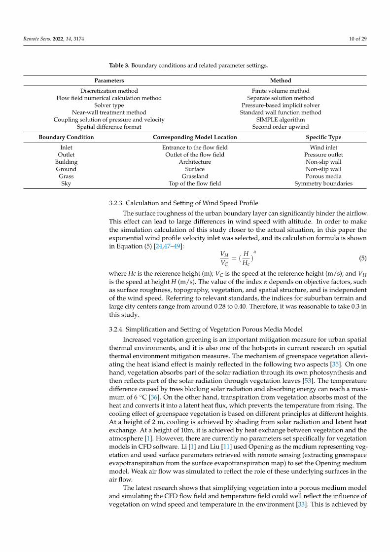
Table 3. Boundary conditions and related parameter settings.

Parameters Method

Discretization method Finite volume methodFlow field numerical calculation method Separate solution method

Solver type Pressure-based implicit solverNear-wall treatment method Standard wall function method

Coupling solution of pressure and velocity SIMPLE algorithmSpatial difference format Second order upwind

Boundary Condition Corresponding Model Location Specific Type

Inlet Entrance to the flow field Wind inletOutlet Outlet of the flow field Pressure outlet

Building Architecture Non-slip wallGround Surface Non-slip wallGrass Grassland Porous mediaSky Top of the flow field Symmetry boundaries

3.2.3. Calculation and Setting of Wind Speed Profile

The surface roughness of the urban boundary layer can significantly hinder the airflow.This effect can lead to large differences in wind speed with altitude. In order to makethe simulation calculation of this study closer to the actual situation, in this paper theexponential wind profile velocity inlet was selected, and its calculation formula is shownin Equation (5) [24,47–49]:

VHVC

= (HHc

)α

(5)

where Hc is the reference height (m); VC is the speed at the reference height (m/s); and VHis the speed at height H (m/s). The value of the index α depends on objective factors, suchas surface roughness, topography, vegetation, and spatial structure, and is independentof the wind speed. Referring to relevant standards, the indices for suburban terrain andlarge city centers range from around 0.28 to 0.40. Therefore, it was reasonable to take 0.3 inthis study.

3.2.4. Simplification and Setting of Vegetation Porous Media Model

Increased vegetation greening is an important mitigation measure for urban spatialthermal environments, and it is also one of the hotspots in current research on spatialthermal environment mitigation measures. The mechanism of greenspace vegetation allevi-ating the heat island effect is mainly reflected in the following two aspects [35]. On onehand, vegetation absorbs part of the solar radiation through its own photosynthesis andthen reflects part of the solar radiation through vegetation leaves [53]. The temperaturedifference caused by trees blocking solar radiation and absorbing energy can reach a maxi-mum of 6 ◦C [36]. On the other hand, transpiration from vegetation absorbs most of theheat and converts it into a latent heat flux, which prevents the temperature from rising. Thecooling effect of greenspace vegetation is based on different principles at different heights.At a height of 2 m, cooling is achieved by shading from solar radiation and latent heatexchange. At a height of 10m, it is achieved by heat exchange between vegetation and theatmosphere [1]. However, there are currently no parameters set specifically for vegetationmodels in CFD software. Li [1] and Liu [11] used Opening as the medium representing veg-etation and used surface parameters retrieved with remote sensing (extracting greenspaceevapotranspiration from the surface evapotranspiration map) to set the Opening mediummodel. Weak air flow was simulated to reflect the role of these underlying surfaces in theair flow.

The latest research shows that simplifying vegetation into a porous medium modeland simulating the CFD flow field and temperature field could well reflect the influence ofvegetation on wind speed and temperature in the environment [33]. This is achieved by

Remote Sens. 2022, 14, 3174 11 of 29

dividing the tree into solid walls in the trunk part and porous air domains in the canopypart and assuming that the air domains absorb heat by volume. The airflow part can berepresented by adding a source term to the CFD equation. The vegetation area is set as aporous medium, and the inertial drag coefficient and viscous drag coefficient are obtainedusing Darcy’s law [53].

The relevant formula is as follows:Momentum source term:

Sui = −12

ρacdLADµiµ (6)

Energy source terms absorbed by trees:

ST = Rn,vol − LAD(Qconv + LEv) (7)

Turbulent kinetic energy Sk and turbulent dissipation rate Sε:{Sk = ρacdLADµ3

iSε =

εk ρacdLADµ3

i(8)

in which:

ρa (kg/m3) is the density of air;Cd is the drag coefficient;LAD is the leaf area density;ui is the local speed in the i-direction;u is the magnitude of the local speed;Rn,vol (W/m3) is the volumetric net radiation;Qconv (W/m2) is the heat flux;LEv (J/kg) is the amount of latent heat released by leaves;Sk is the sink term of the turbulence kinetic energy equation;Sε is the sink term of the turbulent dissipation.

4. Results and Discussion

Regarding the aim of this study, the seasonal daytime and nighttime urban spatial 3Dsurface temperatures and air temperatures were simulated at a microscale, and the windfield information was also simulated based on meteorological datasets. Considering themitigation effects of vegetation for urban canopy heat island, as well as that vegetationis also an effective and inexpensive way to alleviate urban spatial thermal environments,we carried out a study on spatial air temperature field distribution and wind fields, aswell as the variation trends of different spatial layouts of vegetation, including dotted,ribbon, polyline, and arc layouts, designed based on real-area values. To further explorethe relationship between urban landscape and air temperature, especially the relationshipbetween the layout of construction buildings and the urban canopy heat island, we carriedout a simulation of 3D surface and air temperatures and analyzed their relationship withthe distribution and layout of buildings. We also analyzed the relationship between thespatial air temperature and the wind field distribution. Thus, the results are discussedbased on these two aspects.

4.1. Simulation of 3D Urban Spatial Surface and Air Temperatures4.1.1. Influence of Vegetation Morphology Layout on Temperature

Table 4 shows the air temperature field distribution and its variation trends underdifferent geometrical layouts of vegetation, including dotted, ribbon, polyline, and arclayouts of vegetation, simulated by CFD at heights of 0 m (land surface temperature), 2 m,5 m, 10 m, and 20 m. In Table 4, at the height of 0 m, namely at land surface, shows thetemperature distributions of buildings and ground surfaces under different vegetation

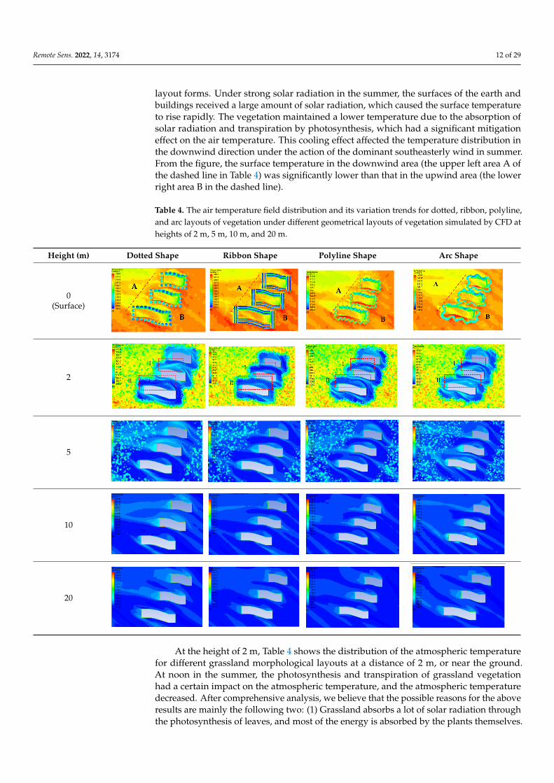
Remote Sens. 2022, 14, 3174 12 of 29

layout forms. Under strong solar radiation in the summer, the surfaces of the earth andbuildings received a large amount of solar radiation, which caused the surface temperatureto rise rapidly. The vegetation maintained a lower temperature due to the absorption ofsolar radiation and transpiration by photosynthesis, which had a significant mitigationeffect on the air temperature. This cooling effect affected the temperature distribution inthe downwind direction under the action of the dominant southeasterly wind in summer.From the figure, the surface temperature in the downwind area (the upper left area A ofthe dashed line in Table 4) was significantly lower than that in the upwind area (the lowerright area B in the dashed line).

Table 4. The air temperature field distribution and its variation trends for dotted, ribbon, polyline,and arc layouts of vegetation under different geometrical layouts of vegetation simulated by CFD atheights of 2 m, 5 m, 10 m, and 20 m.

Height (m) Dotted Shape Ribbon Shape Polyline Shape Arc Shape

0(Surface)

Remote Sens. 2022, 14, 3174 12 of 28

well as the variation trends of different spatial layouts of vegetation, including dotted, ribbon, polyline, and arc layouts, designed based on real-area values. To further explore the relationship between urban landscape and air temperature, especially the relationship between the layout of construction buildings and the urban canopy heat island, we carried out a simulation of 3D surface and air temperatures and analyzed their relationship with the distribution and layout of buildings. We also analyzed the relationship between the spatial air temperature and the wind field distribution. Thus, the results are discussed based on these two aspects.

4.1. Simulation of 3D Urban Spatial Surface and Air Temperatures 4.1.1. Influence of Vegetation Morphology Layout on Temperature

Table 4 shows the air temperature field distribution and its variation trends under different geometrical layouts of vegetation, including dotted, ribbon, polyline, and arc layouts of vegetation, simulated by CFD at heights of 0 m (land surface temperature), 2 m, 5 m, 10 m, and 20 m. In Table 4, at the height of 0 m, namely at land surface, shows the temperature distributions of buildings and ground surfaces under different vegetation layout forms. Under strong solar radiation in the summer, the surfaces of the earth and buildings received a large amount of solar radiation, which caused the surface tempera-ture to rise rapidly. The vegetation maintained a lower temperature due to the absorption of solar radiation and transpiration by photosynthesis, which had a significant mitigation effect on the air temperature. This cooling effect affected the temperature distribution in the downwind direction under the action of the dominant southeasterly wind in summer. From the figure, the surface temperature in the downwind area (the upper left area A of the dashed line in Table 4) was significantly lower than that in the upwind area (the lower right area B in the dashed line).

Table 4. The air temperature field distribution and its variation trends for dotted, ribbon, polyline, and arc layouts of vegetation under different geometrical layouts of vegetation simulated by CFD at heights of 2 m, 5 m, 10 m, and 20 m.


0 (Surface)

2

5

Remote Sens. 2022, 14, 3174 12 of 28






0 (Surface)

2

5

Remote Sens. 2022, 14, 3174 12 of 28






0 (Surface)

2

5

Remote Sens. 2022, 14, 3174 12 of 28






0 (Surface)

2

5

2

Remote Sens. 2022, 14, 3174 12 of 28






0 (Surface)

2

5

Remote Sens. 2022, 14, 3174 12 of 28






0 (Surface)

2

5

Remote Sens. 2022, 14, 3174 12 of 28






0 (Surface)

2

5

Remote Sens. 2022, 14, 3174 12 of 28






0 (Surface)

2

5

5

Remote Sens. 2022, 14, 3174 12 of 28






0 (Surface)

2

5

Remote Sens. 2022, 14, 3174 12 of 28






0 (Surface)

2

5

Remote Sens. 2022, 14, 3174 12 of 28






0 (Surface)

2

5

Remote Sens. 2022, 14, 3174 12 of 28






0 (Surface)

2

5

10

Remote Sens. 2022, 14, 3174 13 of 28

10

20

At the height of 2 m, Table 4 shows the distribution of the atmospheric temperature for different grassland morphological layouts at a distance of 2 m, or near the ground. At noon in the summer, the photosynthesis and transpiration of grassland vegetation had a certain impact on the atmospheric temperature, and the atmospheric temperature de-creased. After comprehensive analysis, we believe that the possible reasons for the above results are mainly the following two: (1) Grassland absorbs a lot of solar radiation through the photosynthesis of leaves, and most of the energy is absorbed by the plants themselves. (2) The heat of the near-surface soil exchanges energy with the atmosphere, and the waterin the soil is heated and vaporized into water vapor, which takes away a lot of energy.

Comparing the temperature distribution at a height of 2 m with different vegetation forms, it can be seen that the mitigation effects of different forms of vegetation on temper-ature in the downwind direction were significantly different. This difference was mainly reflected in the areas between the buildings (areas I and II). Comparing the temperatures in areas I and II under different layout forms, it was found that the folded-line grassland layout had the most obvious mitigation effect on the temperature, followed by the strip layout. It can be seen from the figure below that the mitigation capabilities of vegetation with different layouts were: polyline > strip > point > arc.

Table 4 also shows the air temperature distribution under different grassland layouts at heights of 5 m, 10 m, and 20 m. A comprehensive comparative analysis showed that, at heights of 5 m, 10 m, and 20 m, the mitigation effect of vegetation on the spatial thermal environment was very weak, or even negligible. Different grassland layouts did not cause significant temperature differences. We speculated that the main reason could be that grassland is mainly distributed near the surface, and its mitigation effect needs to rely on the medium of airflow and then rely on the flow of wind to transmit this mitigation effect to other areas to achieve temperature regulation. However, under nonquiet wind condi-tions, the flow of wind tended to move in the horizontal direction, and at the vertical height, the atmospheric temperature at higher altitudes was less affected by the mitigation effect of vegetation. Therefore, the mitigation effect of vegetation was only reflected near the ground and had no obvious effect at high altitudes.

4.1.2. Influence of Vegetation Morphology Layout on Wind Speed Different vegetation layouts have different blocking effects on airflow. The obstruc-

tion of airflow across vegetation surfaces increases with the surface roughness. When the surface is relatively smooth, there is less obstruction to the flow, and the air flow is smoother. This different degree of obstruction makes the airflow show characteristics of scattered distribution. Table 5 shows the wind speed distribution at the 2 m position under different vegetation layouts. It can be seen from the figure that, under the influence of the dominant southeast wind in the summer, there was a “narrow tube effect” between the buildings. This effect was more obvious on the north and south sides of the urban con-struction building, forming a local wind-speed-strengthening area. The maximum wind

Remote Sens. 2022, 14, 3174 13 of 28

10

20






Remote Sens. 2022, 14, 3174 13 of 28

10

20






Remote Sens. 2022, 14, 3174 13 of 28

10

20






20

Remote Sens. 2022, 14, 3174 13 of 28

10

20






Remote Sens. 2022, 14, 3174 13 of 28

10

20






Remote Sens. 2022, 14, 3174 13 of 28

10

20






Remote Sens. 2022, 14, 3174 13 of 28

10

20






At the height of 2 m, Table 4 shows the distribution of the atmospheric temperaturefor different grassland morphological layouts at a distance of 2 m, or near the ground.At noon in the summer, the photosynthesis and transpiration of grassland vegetationhad a certain impact on the atmospheric temperature, and the atmospheric temperaturedecreased. After comprehensive analysis, we believe that the possible reasons for the aboveresults are mainly the following two: (1) Grassland absorbs a lot of solar radiation throughthe photosynthesis of leaves, and most of the energy is absorbed by the plants themselves.

Remote Sens. 2022, 14, 3174 13 of 29

(2) The heat of the near-surface soil exchanges energy with the atmosphere, and the waterin the soil is heated and vaporized into water vapor, which takes away a lot of energy.

Comparing the temperature distribution at a height of 2 m with different vegetationforms, it can be seen that the mitigation effects of different forms of vegetation on tempera-ture in the downwind direction were significantly different. This difference was mainlyreflected in the areas between the buildings (areas I and II). Comparing the temperaturesin areas I and II under different layout forms, it was found that the folded-line grasslandlayout had the most obvious mitigation effect on the temperature, followed by the striplayout. It can be seen from the figure below that the mitigation capabilities of vegetationwith different layouts were: polyline > strip > point > arc.

Table 4 also shows the air temperature distribution under different grassland layoutsat heights of 5 m, 10 m, and 20 m. A comprehensive comparative analysis showed that, atheights of 5 m, 10 m, and 20 m, the mitigation effect of vegetation on the spatial thermalenvironment was very weak, or even negligible. Different grassland layouts did not causesignificant temperature differences. We speculated that the main reason could be thatgrassland is mainly distributed near the surface, and its mitigation effect needs to relyon the medium of airflow and then rely on the flow of wind to transmit this mitigationeffect to other areas to achieve temperature regulation. However, under nonquiet windconditions, the flow of wind tended to move in the horizontal direction, and at the verticalheight, the atmospheric temperature at higher altitudes was less affected by the mitigationeffect of vegetation. Therefore, the mitigation effect of vegetation was only reflected nearthe ground and had no obvious effect at high altitudes.

4.1.2. Influence of Vegetation Morphology Layout on Wind Speed

Different vegetation layouts have different blocking effects on airflow. The obstructionof airflow across vegetation surfaces increases with the surface roughness. When thesurface is relatively smooth, there is less obstruction to the flow, and the air flow is smoother.This different degree of obstruction makes the airflow show characteristics of scattereddistribution. Table 5 shows the wind speed distribution at the 2 m position under differentvegetation layouts. It can be seen from the figure that, under the influence of the dominantsoutheast wind in the summer, there was a “narrow tube effect” between the buildings. Thiseffect was more obvious on the north and south sides of the urban construction building,forming a local wind-speed-strengthening area. The maximum wind speed was close to5 m/s, and the maximum wind speed area was mainly distributed in the corridors betweenthe buildings (zones I and II).

Due to the blocking effect of the buildings on the airflow, in the northeast corner andthe west area of each building, the wind speed was lower than 1 m/s, and it was mainlydistributed in the downwind direction of the building with the dominant wind direction. Itcan be seen in Table 5 that the high-wind-speed area of zone I in the belt-like distributionwas the largest, followed by broken line > point > arc. The high wind speed in zone II wasthe largest, followed by point > arc > broken line.

Remote Sens. 2022, 14, 3174 14 of 29

Table 5. The wind field distribution and its variation trends with dotted, ribbon, polyline, and arclayouts of vegetation under different geometrical layouts of vegetation simulated by CFD at heightsof 2 m, 5 m, 10 m, and 20 m.


2

Remote Sens. 2022, 14, 3174 14 of 28

speed was close to 5 m/s, and the maximum wind speed area was mainly distributed in the corridors between the buildings (zones I and II).

Table 5. The wind field distribution and its variation trends with dotted, ribbon, polyline, and arc layouts of vegetation under different geometrical layouts of vegetation simulated by CFD at heights of 2 m, 5 m, 10 m, and 20 m.

Height (m)

Dotted Shape Ribbon Shape Polyline Shape Arc Shape

2

5

10

20

Due to the blocking effect of the buildings on the airflow, in the northeast corner and the west area of each building, the wind speed was lower than 1 m/s, and it was mainly distributed in the downwind direction of the building with the dominant wind direction. It can be seen in Table 5 that the high-wind-speed area of zone I in the belt-like distribution was the largest, followed by broken line > point > arc. The high wind speed in zone II was the largest, followed by point > arc > broken line.

4.1.3. Distribution Characteristics of Wind and Heat Environment during Daytime and Nighttime in Four Seasons (A) Distribution characteristics and analysis of wind and heat environment for day-

time in four seasonsTable 6 shows the distributions of surface temperature and building surface temper-

ature in different seasons based on different meteorological parameters. The results clearly show the difference that the vegetation and buildings made when they absorbed solar radiation during the day. Vegetation and water bodies kept the temperature at a low

Remote Sens. 2022, 14, 3174 14 of 28



Height (m)


2

5

10

20



time in four seasons Table 6 shows the distributions of surface temperature and building surface temper-


Remote Sens. 2022, 14, 3174 14 of 28



Height (m)


2

5

10

20





Remote Sens. 2022, 14, 3174 14 of 28



Height (m)


2

5

10

20





5

Remote Sens. 2022, 14, 3174 14 of 28



Height (m)


2

5

10

20





Remote Sens. 2022, 14, 3174 14 of 28



Height (m)


2

5

10

20





Remote Sens. 2022, 14, 3174 14 of 28



Height (m)


2

5

10

20





Remote Sens. 2022, 14, 3174 14 of 28



Height (m)


2

5

10

20





10

Remote Sens. 2022, 14, 3174 14 of 28



Height (m)


2

5

10

20





Remote Sens. 2022, 14, 3174 14 of 28



Height (m)


2

5

10

20





Remote Sens. 2022, 14, 3174 14 of 28



Height (m)


2

5

10

20





Remote Sens. 2022, 14, 3174 14 of 28



Height (m)


2

5

10

20





20

Remote Sens. 2022, 14, 3174 14 of 28



Height (m)


2

5

10

20





Remote Sens. 2022, 14, 3174 14 of 28



Height (m)


2

5

10

20





Remote Sens. 2022, 14, 3174 14 of 28



Height (m)


2

5

10

20





Remote Sens. 2022, 14, 3174 14 of 28



Height (m)


2

5

10

20





4.1.3. Distribution Characteristics of Wind and Heat Environment during Daytime andNighttime in Four Seasons

(A) Distribution characteristics and analysis of wind and heat environment for day-time in four seasons

Table 6 shows the distributions of surface temperature and building surface tempera-ture in different seasons based on different meteorological parameters. The results clearlyshow the difference that the vegetation and buildings made when they absorbed solarradiation during the day. Vegetation and water bodies kept the temperature at a low leveldue to their own physical properties, while the building surface absorbed solar radiationand increased its temperature rapidly. In addition, the temperature difference betweenbuilding walls exposed to solar radiation and those not exposed to the sun (within thedashed line in Table 6) is also well-shown in the figure, and the surface temperature in theshaded area was significantly lower than that of the direct solar area surface. In the figure,we can clearly see the changes in the shaded area of the buildings at different sun altitudesdue to the changes in the direct sunlight point in different seasons. In winter, the directsunlight point was located near the Tropic of Cancer. At this time, the sun elevation anglewas small, resulting in the largest shadow area in winter, followed by spring and autumn,and the smallest shadow area in summer.

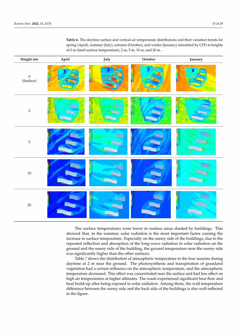
Remote Sens. 2022, 14, 3174 15 of 29

Table 6. The daytime surface and vertical air temperature distributions and their variation trends forspring (April), summer (July), autumn (October), and winter (January) simulated by CFD at heightsof 0 m (land surface temperature), 2 m, 5 m, 10 m, and 20 m.

Height (m) April July October January

0(Surface)

Remote Sens. 2022, 14, 3174 15 of 28

level due to their own physical properties, while the building surface absorbed solar ra-diation and increased its temperature rapidly. In addition, the temperature difference be-tween building walls exposed to solar radiation and those not exposed to the sun (within the dashed line in Table 6) is also well-shown in the figure, and the surface temperature in the shaded area was significantly lower than that of the direct solar area surface. In the figure, we can clearly see the changes in the shaded area of the buildings at different sun altitudes due to the changes in the direct sunlight point in different seasons. In winter, the direct sunlight point was located near the Tropic of Cancer. At this time, the sun elevation angle was small, resulting in the largest shadow area in winter, followed by spring and autumn, and the smallest shadow area in summer.

Table 6. The daytime surface and vertical air temperature distributions and their variation trends for spring (April), summer (July), autumn (October), and winter (January) simulated by CFD at heights of 0 m (land surface temperature), 2 m, 5 m, 10 m, and 20 m.


0 (Surface)

2

5

10

20

The surface temperatures were lower in sunless areas shaded by buildings. This showed that, in the summer, solar radiation is the most important factor causing the in-crease in surface temperature. Especially on the sunny side of the buildings, due to the

Remote Sens. 2022, 14, 3174 15 of 28




0 (Surface)

2

5

10

20


Remote Sens. 2022, 14, 3174 15 of 28




0 (Surface)

2

5

10

20


Remote Sens. 2022, 14, 3174 15 of 28




0 (Surface)

2

5

10

20


2

Remote Sens. 2022, 14, 3174 15 of 28




0 (Surface)

2

5

10

20


Remote Sens. 2022, 14, 3174 15 of 28




0 (Surface)

2

5

10

20


Remote Sens. 2022, 14, 3174 15 of 28




0 (Surface)

2

5

10

20


Remote Sens. 2022, 14, 3174 15 of 28




0 (Surface)

2

5

10

20


5

Remote Sens. 2022, 14, 3174 15 of 28




0 (Surface)

2

5

10

20


Remote Sens. 2022, 14, 3174 15 of 28




0 (Surface)

2

5

10

20


Remote Sens. 2022, 14, 3174 15 of 28




0 (Surface)

2

5

10

20


Remote Sens. 2022, 14, 3174 15 of 28




0 (Surface)

2

5

10

20


10

Remote Sens. 2022, 14, 3174 15 of 28




0 (Surface)

2

5

10

20


Remote Sens. 2022, 14, 3174 15 of 28




0 (Surface)

2

5

10

20


Remote Sens. 2022, 14, 3174 15 of 28




0 (Surface)

2

5

10

20


Remote Sens. 2022, 14, 3174 15 of 28




0 (Surface)

2

5

10

20


20

Remote Sens. 2022, 14, 3174 15 of 28




0 (Surface)

2

5

10

20


Remote Sens. 2022, 14, 3174 15 of 28




0 (Surface)

2

5

10

20


Remote Sens. 2022, 14, 3174 15 of 28




0 (Surface)

2

5

10

20


Remote Sens. 2022, 14, 3174 15 of 28




0 (Surface)

2

5

10

20


The surface temperatures were lower in sunless areas shaded by buildings. Thisshowed that, in the summer, solar radiation is the most important factor causing theincrease in surface temperature. Especially on the sunny side of the buildings, due to therepeated reflection and absorption of the long-wave radiation in solar radiation on theground and the sunny side of the building, the ground temperature near the sunny sidewas significantly higher than the other surfaces.

Table 7 shows the distribution of atmospheric temperature in the four seasons duringdaytime at 2 m near the ground. The photosynthesis and transpiration of grasslandvegetation had a certain influence on the atmospheric temperature, and the atmospherictemperature decreased. This effect was concentrated near the surface and had less effect onhigh air temperatures at higher altitudes. The roads experienced significant heat flow andheat build-up after being exposed to solar radiation. Among them, the wall temperaturedifference between the sunny side and the back side of the buildings is also well-reflectedin the figure.

Remote Sens. 2022, 14, 3174 16 of 29

Table 7. The daytime wind field distributions corresponding to temperature distributions (see Table 6)and their variation trends for spring (April), summer (July), autumn (October), and winter (January)simulated by CFD at heights of 2 m, 5 m, 10 m, and 20 m.


2

Remote Sens. 2022, 14, 3174 16 of 28

repeated reflection and absorption of the long-wave radiation in solar radiation on the ground and the sunny side of the building, the ground temperature near the sunny side was significantly higher than the other surfaces.

Table 7 shows the distribution of atmospheric temperature in the four seasons during daytime at 2m near the ground. The photosynthesis and transpiration of grassland vege-tation had a certain influence on the atmospheric temperature, and the atmospheric tem-perature decreased. This effect was concentrated near the surface and had less effect on high air temperatures at higher altitudes. The roads experienced significant heat flow and heat build-up after being exposed to solar radiation. Among them, the wall temperature difference between the sunny side and the back side of the buildings is also well-reflected in the figure.

Table 7. The daytime wind field distributions corresponding to temperature distributions (see Table 6) and their variation trends for spring (April), summer (July), autumn (October), and winter (Jan-uary) simulated by CFD at heights of 2 m, 5 m, 10 m, and 20 m.


2

5

10

20

(B) Distribution characteristics and analysis of wind and heat environment for nighttime in four seasonsIt can be seen from the nighttime surface temperature distribution diagram shown in

Table 8 that the surface temperature difference of different objects was smaller than that in the daytime, the temperature distribution was more stable, and the variation range was smaller. We believe that there were two main reasons for this result. On one hand, because

Remote Sens. 2022, 14, 3174 16 of 28





2

5

10

20

(B) Distribution characteristics and analysis of wind and heat environment for night time in four seasons It can be seen from the nighttime surface temperature distribution diagram shown in


Remote Sens. 2022, 14, 3174 16 of 28





2

5

10

20



Remote Sens. 2022, 14, 3174 16 of 28





2

5

10

20



5

Remote Sens. 2022, 14, 3174 16 of 28





2

5

10

20



Remote Sens. 2022, 14, 3174 16 of 28





2

5

10

20



Remote Sens. 2022, 14, 3174 16 of 28





2

5

10

20



Remote Sens. 2022, 14, 3174 16 of 28





2

5

10

20



10

Remote Sens. 2022, 14, 3174 16 of 28





2

5

10

20



Remote Sens. 2022, 14, 3174 16 of 28





2

5

10

20



Remote Sens. 2022, 14, 3174 16 of 28





2

5

10

20



Remote Sens. 2022, 14, 3174 16 of 28





2

5

10

20



20

Remote Sens. 2022, 14, 3174 16 of 28





2

5

10

20



Remote Sens. 2022, 14, 3174 16 of 28





2

5

10

20



Remote Sens. 2022, 14, 3174 16 of 28





2

5

10

20



Remote Sens. 2022, 14, 3174 16 of 28





2

5

10

20



(B) Distribution characteristics and analysis of wind and heat environment for nighttime in four seasons

It can be seen from the nighttime surface temperature distribution diagram shown inTable 8 that the surface temperature difference of different objects was smaller than that inthe daytime, the temperature distribution was more stable, and the variation range wassmaller. We believe that there were two main reasons for this result. On one hand, becausenight is not affected by solar radiation, the temperature difference mainly comes from heatconduction of the indoor temperature through building walls and air-layer heat convectionbetween building walls and near walls (Table 8). On the other hand, when vegetationenters the respiration stage at night, the effect of vegetation on air temperature is negligible.At this time, the main source of heat is the interior of buildings and artificial heat.

Remote Sens. 2022, 14, 3174 17 of 29

Table 8. The nighttime surface and vertical air temperature distributions and their variation trendsfor spring (April), summer (July), autumn (October), and winter (January) simulated by CFD atheights of 0 m (land surface temperature), 2 m, 5 m, 10 m, and 20 m.


0(Surface)

Remote Sens. 2022, 14, 3174 17 of 28

night is not affected by solar radiation, the temperature difference mainly comes from heat conduction of the indoor temperature through building walls and air-layer heat convec-tion between building walls and near walls (Table 8). On the other hand, when vegetation enters the respiration stage at night, the effect of vegetation on air temperature is negligi-ble. At this time, the main source of heat is the interior of buildings and artificial heat.

Table 8. The nighttime surface and vertical air temperature distributions and their variation trends for spring (April), summer (July), autumn (October), and winter (January) simulated by CFD at heights of 0 m (land surface temperature), 2 m, 5 m, 10 m, and 20 m.


0 (Surface)

2

5

10

20

In the downwind direction of the buildings, some heat on the building surfaces was convective heat transferred through the air near the walls. This phenomenon was more obvious in spring, summer, and autumn (Table 9; at the height of 0 m). However, it is worth mentioning that the efficiency of this heat exchange is relatively low, mainly be-cause most current building walls use thermal insulation materials. Therefore, even if there is an exchange of heat, it is difficult to make a significant difference in the air tem-perature. What is shown in the result graphs (Table 9; at heights of 2 m, 5 m, 10 m, and 20

Remote Sens. 2022, 14, 3174 17 of 28




0 (Surface)

2

5

10

20


Remote Sens. 2022, 14, 3174 17 of 28




0 (Surface)

2

5

10

20


Remote Sens. 2022, 14, 3174 17 of 28




0 (Surface)

2

5

10

20


2

Remote Sens. 2022, 14, 3174 17 of 28




0 (Surface)

2

5

10

20


Remote Sens. 2022, 14, 3174 17 of 28




0 (Surface)

2

5

10

20


Remote Sens. 2022, 14, 3174 17 of 28




0 (Surface)

2

5

10

20


Remote Sens. 2022, 14, 3174 17 of 28




0 (Surface)

2

5

10

20


5

Remote Sens. 2022, 14, 3174 17 of 28




0 (Surface)

2

5

10

20


Remote Sens. 2022, 14, 3174 17 of 28




0 (Surface)

2

5

10

20


Remote Sens. 2022, 14, 3174 17 of 28




0 (Surface)

2

5

10

20


Remote Sens. 2022, 14, 3174 17 of 28




0 (Surface)

2

5

10

20


10

Remote Sens. 2022, 14, 3174 17 of 28




0 (Surface)

2

5

10

20


Remote Sens. 2022, 14, 3174 17 of 28




0 (Surface)

2

5

10

20


Remote Sens. 2022, 14, 3174 17 of 28




0 (Surface)

2

5

10

20


Remote Sens. 2022, 14, 3174 17 of 28




0 (Surface)

2

5

10

20


20

Remote Sens. 2022, 14, 3174 17 of 28




0 (Surface)

2

5

10

20


Remote Sens. 2022, 14, 3174 17 of 28




0 (Surface)

2

5

10

20


Remote Sens. 2022, 14, 3174 17 of 28




0 (Surface)

2

5

10

20


Remote Sens. 2022, 14, 3174 17 of 28




0 (Surface)

2

5

10

20


In the downwind direction of the buildings, some heat on the building surfaces wasconvective heat transferred through the air near the walls. This phenomenon was moreobvious in spring, summer, and autumn (Table 9; at the height of 0 m). However, it isworth mentioning that the efficiency of this heat exchange is relatively low, mainly becausemost current building walls use thermal insulation materials. Therefore, even if there is anexchange of heat, it is difficult to make a significant difference in the air temperature. Whatis shown in the result graphs (Table 9; at heights of 2 m, 5 m, 10 m, and 20 m) is that the airtemperature distribution around the buildings was quite stable at different heights, andthe difference was not obvious, especially at night in the winter. Therefore, the regularityreflected in the temperature distribution map was not obvious.

Remote Sens. 2022, 14, 3174 18 of 29

Table 9. The nighttime wind field distributions and corresponding temperature distributions (seeTable 7) and their variation trends for spring (April), summer (July), autumn (October), and winter(January) simulated by CFD at heights of 2 m, 5 m, 10 m, and 20 m.


2

Remote Sens. 2022, 14, 3174 18 of 28

m) is that the air temperature distribution around the buildings was quite stable at differ-ent heights, and the difference was not obvious, especially at night in the winter. There-fore, the regularity reflected in the temperature distribution map was not obvious.

Table 9. The nighttime wind field distributions and corresponding temperature distributions (see Table 7) and their variation trends for spring (April), summer (July), autumn (October), and winter (January) simulated by CFD at heights of 2 m, 5 m, 10 m, and 20 m.


2

5

10

20

4.2. Simulation of Urban Wind and Heat Environment and Research on Its Distribution Characteristics at a Community Scale

The distribution of wind and thermal environments for different morphological ar-rangements of daytime and nighttime vegetation at a microscopic scale was discussed above. However, the community scale is the main activity area of residents, and the spatial air–heat environment and thermal comfort at the community scale are more closely re-lated to residents’ lives. Therefore, it is very necessary to simulate spatial wind and heat environments at the community scale. Urban structure layout greatly affects the urban heat island effect. Based on CFD and considering factors such as building layout, building number, building density, and building aspect ratio, simulating wind and heat environ-ments at both the micro-scale and the community scale is of great significance for opti-mizing comprehensive urban design, as well as improving the urban landscape and eco-logical environment. In urban planning, it is necessary to rationally arrange building in-terval and orientation in combination with meteorological conditions so that the building orientation conforms to the prevailing wind direction. This can increase the ventilation of buildings so that the urban heat distribution is more even and reasonable. It is of great

Remote Sens. 2022, 14, 3174 18 of 28




2

5

10

20



Remote Sens. 2022, 14, 3174 18 of 28




2

5

10

20



Remote Sens. 2022, 14, 3174 18 of 28




2

5

10

20



5

Remote Sens. 2022, 14, 3174 18 of 28




2

5

10

20



Remote Sens. 2022, 14, 3174 18 of 28




2

5

10

20



Remote Sens. 2022, 14, 3174 18 of 28




2

5

10

20



Remote Sens. 2022, 14, 3174 18 of 28




2

5

10

20



10

Remote Sens. 2022, 14, 3174 18 of 28




2

5

10

20



Remote Sens. 2022, 14, 3174 18 of 28




2

5

10

20



Remote Sens. 2022, 14, 3174 18 of 28




2

5

10

20



Remote Sens. 2022, 14, 3174 18 of 28




2

5

10

20



20

Remote Sens. 2022, 14, 3174 18 of 28




2

5

10

20



Remote Sens. 2022, 14, 3174 18 of 28




2

5

10

20



Remote Sens. 2022, 14, 3174 18 of 28




2

5

10

20



Remote Sens. 2022, 14, 3174 18 of 28




2

5

10

20



4.2. Simulation of Urban Wind and Heat Environment and Research on Its DistributionCharacteristics at a Community Scale

The distribution of wind and thermal environments for different morphological ar-rangements of daytime and nighttime vegetation at a microscopic scale was discussedabove. However, the community scale is the main activity area of residents, and the spatialair–heat environment and thermal comfort at the community scale are more closely relatedto residents’ lives. Therefore, it is very necessary to simulate spatial wind and heat environ-ments at the community scale. Urban structure layout greatly affects the urban heat islandeffect. Based on CFD and considering factors such as building layout, building number,building density, and building aspect ratio, simulating wind and heat environments at boththe micro-scale and the community scale is of great significance for optimizing comprehen-sive urban design, as well as improving the urban landscape and ecological environment.In urban planning, it is necessary to rationally arrange building interval and orientation incombination with meteorological conditions so that the building orientation conforms to theprevailing wind direction. This can increase the ventilation of buildings so that the urbanheat distribution is more even and reasonable. It is of great significance to alleviating theheat island effect. This section mainly analyzes the distribution and influence of buildinglayout at the community scale on urban spatial wind and heat environments at differentheights in different seasons. Figures 5 and 6 show the 3D urban spatial air temperatureprofiles simulated based on CFD. In Figure 5, some air temperature profiles are selectedas examples to illustrate that the 3D atmospheric temperature in the vertical direction of

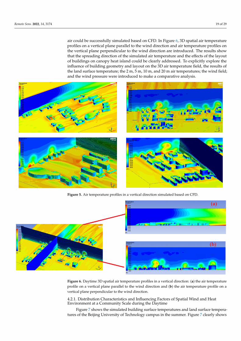
Remote Sens. 2022, 14, 3174 19 of 29

air could be successfully simulated based on CFD. In Figure 6, 3D spatial air temperatureprofiles on a vertical plane parallel to the wind direction and air temperature profiles onthe vertical plane perpendicular to the wind direction are introduced. The results showthat the spreading direction of the simulated air temperature and the effects of the layoutof buildings on canopy heat island could be clearly addressed. To explicitly explore theinfluence of building geometry and layout on the 3D air temperature field, the results ofthe land surface temperature; the 2 m, 5 m, 10 m, and 20 m air temperatures; the wind field;and the wind pressure were introduced to make a comparative analysis.

Remote Sens. 2022, 14, 3174 19 of 28

significance to alleviating the heat island effect. This section mainly analyzes the distribu-tion and influence of building layout at the community scale on urban spatial wind and heat environments at different heights in different seasons. Figures 5 and 6 show the 3D urban spatial air temperature profiles simulated based on CFD. In Figure 5, some air tem-perature profiles are selected as examples to illustrate that the 3D atmospheric tempera-ture in the vertical direction of air could be successfully simulated based on CFD. In Figure 6, 3D spatial air temperature profiles on a vertical plane parallel to the wind direction and air temperature profiles on the vertical plane perpendicular to the wind direction are in-troduced. The results show that the spreading direction of the simulated air temperature and the effects of the layout of buildings on canopy heat island could be clearly addressed. To explicitly explore the influence of building geometry and layout on the 3D air temper-ature field, the results of the land surface temperature; the 2 m, 5 m, 10 m, and 20 m air temperatures; the wind field; and the wind pressure were introduced to make a compar-ative analysis.

Figure 5. Air temperature profiles in a vertical direction simulated based on CFD.


Remote Sens. 2022, 14, 3174 19 of 28

significance to alleviating the heat island effect. This section mainly analyzes the distribu-tion and influence of building layout at the community scale on urban spatial wind and heat environments at different heights in different seasons. Figures 5 and 6 show the 3D urban spatial air temperature profiles simulated based on CFD. In Figure 5, some air tem-perature profiles are selected as examples to illustrate that the 3D atmospheric tempera-ture in the vertical direction of air could be successfully simulated based on CFD. In Figure 6, 3D spatial air temperature profiles on a vertical plane parallel to the wind direction and air temperature profiles on the vertical plane perpendicular to the wind direction are in-troduced. The results show that the spreading direction of the simulated air temperature and the effects of the layout of buildings on canopy heat island could be clearly addressed. To explicitly explore the influence of building geometry and layout on the 3D air temper-ature field, the results of the land surface temperature; the 2 m, 5 m, 10 m, and 20 m air temperatures; the wind field; and the wind pressure were introduced to make a compar-ative analysis.


Figure 6. Daytime 3D spatial air temperature profiles in a vertical direction: (a) the air temperatureprofile on a vertical plane parallel to the wind direction and (b) the air temperature profile on avertical plane perpendicular to the wind direction.

4.2.1. Distribution Characteristics and Influencing Factors of Spatial Wind and HeatEnvironment at a Community Scale during the Daytime

Figure 7 shows the simulated building surface temperatures and land surface tempera-tures of the Beijing University of Technology campus in the summer. Figure 7 clearly shows

Remote Sens. 2022, 14, 3174 20 of 29

that the buildings blocked the sun’s rays, resulting in temperature differences between theground surfaces. In addition, it can also be seen in Figure 6 that the temperature in theupwind direction was significantly lower than the temperature in the downwind directionon the building surfaces and the ground surface. This was mainly due to the obviousconvective heat transfer between the building surfaces and the atmosphere. Conversely,the surface temperature was higher in the downwind direction and in the area blocked bythe building (shown within the dashed line in Figure 7).

Remote Sens. 2022, 14, 3174 20 of 28

Figure 6. Daytime 3D spatial air temperature profiles in a vertical direction: (a) the air temperature profile on a vertical plane parallel to the wind direction and (b) the air temperature profile on a vertical plane perpendicular to the wind direction.

4.2.1. Distribution Characteristics and Influencing Factors of Spatial Wind and Heat En-vironment at a Community Scale during the Daytime

Figure 7 shows the simulated building surface temperatures and land surface tem-peratures of the Beijing University of Technology campus in the summer. Figure 7 clearly shows that the buildings blocked the sun’s rays, resulting in temperature differences be-tween the ground surfaces. In addition, it can also be seen in Figure 6 that the temperature in the upwind direction was significantly lower than the temperature in the downwind direction on the building surfaces and the ground surface. This was mainly due to the obvious convective heat transfer between the building surfaces and the atmosphere. Con-versely, the surface temperature was higher in the downwind direction and in the area blocked by the building (shown within the dashed line in Figure 7).

Figure 7. The daytime surface temperature field distribution and variation trend simulated by CFD.

Table 10 shows the temperature distribution, wind speed, and wind pressure distri-bution at 2 m, 5 m, 10 m, and 20 m of the Beijing University of Technology campus. Com-bining the results for the wind environment and thermal environment, it can be seen that the distribution of temperature had a great correlation with the direction of wind. Areas A and B for the daytime wind field results had lower wind speeds in the downwind di-rection due to the blocking of buildings, so the temperature in Table 10 is higher. The temperature was lower where the wind speed was higher, and the temperature was higher where the wind speed was lower. This was because the heat build-up in areas with lower wind speeds resulted in higher local temperatures, while areas with higher wind speeds could dissipate the accumulated heat well. This showed that convective heat trans-fer plays a leading role in the study of urban space thermal environments.

Figure 7. The daytime surface temperature field distribution and variation trend simulated by CFD.

Table 10 shows the temperature distribution, wind speed, and wind pressure distribu-tion at 2 m, 5 m, 10 m, and 20 m of the Beijing University of Technology campus. Combiningthe results for the wind environment and thermal environment, it can be seen that thedistribution of temperature had a great correlation with the direction of wind. Areas A andB for the daytime wind field results had lower wind speeds in the downwind direction dueto the blocking of buildings, so the temperature in Table 10 is higher. The temperature waslower where the wind speed was higher, and the temperature was higher where the windspeed was lower. This was because the heat build-up in areas with lower wind speedsresulted in higher local temperatures, while areas with higher wind speeds could dissipatethe accumulated heat well. This showed that convective heat transfer plays a leading rolein the study of urban space thermal environments.

In Table 10, under the action of the breeze, the building’s blocking effect on the windmade the wind speed on the leeward side of the building lower, and the wind speed valuewas below 1 m/s. However, the wind speed was not as large as possible. When the windspeed is greater than 5 m/s, the comfort of the human body in the wind environmentdecreases. It is worth mentioning that, in summer, an appropriate wind speed can dissipateheat very well, which can take away the heat accumulated around buildings and reducethe surrounding temperature significantly.

Remote Sens. 2022, 14, 3174 21 of 29

Table 10. The daytime 3D urban spatial air temperature, wind field distribution, and wind pressuredistribution with corresponding variation trends at heights of 2 m, 5 m, 10 m, and 20 m simulatedby CFD.

Height (m) Temperature(◦C)

Wind Field(m/s)

Wind Pressure(Pa)

2

Remote Sens. 2022, 14, 3174 21 of 28

Table 10. The daytime 3D urban spatial air temperature, wind field distribution, and wind pressure distribution with corresponding variation trends at heights of 2 m, 5 m, 10 m, and 20 m simulated by CFD.

Height (m) Temperature

(°C) Wind Field

(m/s) Wind Pressure

(Pa)

2

5

10

20

In Table 10, under the action of the breeze, the building’s blocking effect on the wind made the wind speed on the leeward side of the building lower, and the wind speed value was below 1 m/s. However, the wind speed was not as large as possible. When the wind speed is greater than 5 m/s, the comfort of the human body in the wind environment de-creases. It is worth mentioning that, in summer, an appropriate wind speed can dissipate heat very well, which can take away the heat accumulated around buildings and reduce the surrounding temperature significantly.

4.2.2. Distribution Characteristics and Influencing Factors of Spatial Wind and Heat En-vironment at the Community Scale at Nighttime

Figure 8 shows the simulation results of the surface temperature at nighttime on the campus of the Beijing University of Technology. It can be seen from the figure that the surface temperature map obtained by the simulation had a higher temperature on the building surfaces, while the other surface temperatures were lower. The surface temper-ature on the leeward side of the building was lower than on the other surface areas. Table 11 shows the nighttime temperature distributions at different heights on the campus of the Beijing University of Technology. In general, the temperature distributions at different

Remote Sens. 2022, 14, 3174 21 of 28



(°C) Wind Field

(m/s) Wind Pressure

(Pa)

2

5

10

20




Remote Sens. 2022, 14, 3174 21 of 28



(°C) Wind Field

(m/s) Wind Pressure

(Pa)

2

5

10

20




5

Remote Sens. 2022, 14, 3174 21 of 28



(°C) Wind Field

(m/s) Wind Pressure

(Pa)

2

5

10

20




Remote Sens. 2022, 14, 3174 21 of 28



(°C) Wind Field

(m/s) Wind Pressure

(Pa)

2

5

10

20




Remote Sens. 2022, 14, 3174 21 of 28



(°C) Wind Field

(m/s) Wind Pressure

(Pa)

2

5

10

20




10

Remote Sens. 2022, 14, 3174 21 of 28



(°C) Wind Field

(m/s) Wind Pressure

(Pa)

2

5

10

20




Remote Sens. 2022, 14, 3174 21 of 28



(°C) Wind Field

(m/s) Wind Pressure

(Pa)

2

5

10

20




Remote Sens. 2022, 14, 3174 21 of 28



(°C) Wind Field

(m/s) Wind Pressure

(Pa)

2

5

10

20




20

Remote Sens. 2022, 14, 3174 21 of 28



(°C) Wind Field

(m/s) Wind Pressure

(Pa)

2

5

10

20




Remote Sens. 2022, 14, 3174 21 of 28



(°C) Wind Field

(m/s) Wind Pressure

(Pa)

2

5

10

20




Remote Sens. 2022, 14, 3174 21 of 28



(°C) Wind Field

(m/s) Wind Pressure

(Pa)

2

5

10

20




4.2.2. Distribution Characteristics and Influencing Factors of Spatial Wind and HeatEnvironment at the Community Scale at Nighttime

Figure 8 shows the simulation results of the surface temperature at nighttime onthe campus of the Beijing University of Technology. It can be seen from the figure thatthe surface temperature map obtained by the simulation had a higher temperature onthe building surfaces, while the other surface temperatures were lower. The surfacetemperature on the leeward side of the building was lower than on the other surfaceareas. Table 11 shows the nighttime temperature distributions at different heights on thecampus of the Beijing University of Technology. In general, the temperature distributions atdifferent heights at night did not show obvious differences, and the temperature variationrange was small. Due to indoor heat transfer, the temperature in the densely built area washigher than that in the sparsely built area. Table 11 also shows the wind environment andwind pressure distribution at night on the campus of the Beijing University of Technology.The wind environment and wind pressure distribution were similar for night and day, andthere was no obvious difference.

Remote Sens. 2022, 14, 3174 22 of 29

Remote Sens. 2022, 14, 3174 22 of 28

heights at night did not show obvious differences, and the temperature variation range was small. Due to indoor heat transfer, the temperature in the densely built area was higher than that in the sparsely built area. Table 11 also shows the wind environment and wind pressure distribution at night on the campus of the Beijing University of Technology. The wind environment and wind pressure distribution were similar for night and day, and there was no obvious difference.

Figure 8. The nighttime surface temperature field distribution and variation trend simulated by CFD.

Table 11. The nighttime 3D urban spatial air temperature, wind field distribution, and wind pres-sure distribution with corresponding variation trends at heights of 2 m, 5 m, 10 m, and 20 m simu-lated by CFD.

Height (m) Temperature (°C)

Wind Field (m/s)

Wind Pressure (Pa)

2

5

10


Table 11. The nighttime 3D urban spatial air temperature, wind field distribution, and wind pressuredistribution with corresponding variation trends at heights of 2 m, 5 m, 10 m, and 20 m simulatedby CFD.

Height (m) Temperature(◦C)

Wind Field(m/s)

Wind Pressure(Pa)

2

Remote Sens. 2022, 14, 3174 22 of 28





Wind Field (m/s)

Wind Pressure (Pa)

2

5

10

Remote Sens. 2022, 14, 3174 22 of 28





Wind Field (m/s)

Wind Pressure (Pa)

2

5

10

Remote Sens. 2022, 14, 3174 22 of 28





Wind Field (m/s)

Wind Pressure (Pa)

2

5

10

5

Remote Sens. 2022, 14, 3174 22 of 28





Wind Field (m/s)

Wind Pressure (Pa)

2

5

10

Remote Sens. 2022, 14, 3174 22 of 28





Wind Field (m/s)

Wind Pressure (Pa)

2

5

10

Remote Sens. 2022, 14, 3174 22 of 28





Wind Field (m/s)

Wind Pressure (Pa)

2

5

10

10

Remote Sens. 2022, 14, 3174 22 of 28





Wind Field (m/s)

Wind Pressure (Pa)

2

5

10

Remote Sens. 2022, 14, 3174 22 of 28





Wind Field (m/s)

Wind Pressure (Pa)

2

5

10

Remote Sens. 2022, 14, 3174 22 of 28





Wind Field (m/s)

Wind Pressure (Pa)

2

5

10

20

Remote Sens. 2022, 14, 3174 23 of 28

20

Comparing the temperature maps in Tables 10 and 11, it was found that the daytime temperature difference in the building-intensive area was larger than the nighttime tem-perature difference, and the temperature diffusion rate in the local building-concentrated area was slow, which had a certain impact on the surrounding background features. This was mainly due to the fact that the wind speed in the concentrated building area was affected by the roughness of the underlying surface. Judging from the distance of the building layout, there was a certain distance between different buildings, which had a certain positive impact on the wind speed and temperature and accelerated the speed of heat dissipation. From the perspective of wind pressure, the wind pressure at night was more stable than the wind pressure during the day, but the wind pressure value at night was larger, and the pressure difference was larger. Analyzing the layout of the buildings from the perspective of ventilation performance, it can be found from Tables 10 and 11 that the staggered distribution of buildings affected the wind speed and wind pressure and had a certain blocking effect on the diffusion of building energy storage. The main wind direction and wind speed during the period when the heat island effect was the largest and the reasonable spacing and distribution of the buildings formed a ventilation corridor that was beneficial to heat dissipation.

In this study, through the analysis of the simulation results and data processing, it was found that there were still some problems that could affect the accuracy of the simu-lation results: (1) In the construction and simplification of the geometric physical model, subtle changes in the building surfaces, such as the arrangement of windows, doors, and roof structures, were ignored. We simplified the actual building as a building wall, intro-duced it into the CFD, and set it as concrete of a certain thickness to participate in the simulation calculation, ignoring the influence of the actual difference in the building sur-face on the results. (2) The CFD numerical simulation calculation ignored the wall tem-perature difference caused by the heat exchange inside the building. There were actually different types of underlying surfaces in the surface model, such as roads made of asphalt, squares made of concrete, and exposed soil, but these were reduced to a single underlying surface type. (3) There were also the limitations of the standard k-ε turbulence model and the P1 radiation model.

It is worth pointing out that, in the process of finite element simulation, the simplifi-cation processing and meshing of the model consume a lot of computation and time. Therefore, the work on model simplification and mesh division needs to be paid enough attention in the process of finite element simulation, including pre-processing, solver cal-culation, and post-processing. Unlike structural simulation, fluid mechanics simulation is characterized by a huge number of meshes. Therefore, it is necessary to make a trade-off in meshing the points of interest with a denser number of meshes to capture finer details, while the number of meshes for noninterest points can be smaller to reduce the computa-tional consumption. In model processing, according to the subject studied, the geometric features of the subject model are described in detail, and the geometric models in other areas can be simplified and modified appropriately.

Remote Sens. 2022, 14, 3174 23 of 28

20




Remote Sens. 2022, 14, 3174 23 of 28

20




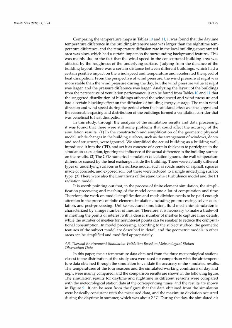
Remote Sens. 2022, 14, 3174 23 of 29

Comparing the temperature maps in Tables 10 and 11, it was found that the daytimetemperature difference in the building-intensive area was larger than the nighttime tem-perature difference, and the temperature diffusion rate in the local building-concentratedarea was slow, which had a certain impact on the surrounding background features. Thiswas mainly due to the fact that the wind speed in the concentrated building area wasaffected by the roughness of the underlying surface. Judging from the distance of thebuilding layout, there was a certain distance between different buildings, which had acertain positive impact on the wind speed and temperature and accelerated the speed ofheat dissipation. From the perspective of wind pressure, the wind pressure at night wasmore stable than the wind pressure during the day, but the wind pressure value at nightwas larger, and the pressure difference was larger. Analyzing the layout of the buildingsfrom the perspective of ventilation performance, it can be found from Tables 10 and 11 thatthe staggered distribution of buildings affected the wind speed and wind pressure andhad a certain blocking effect on the diffusion of building energy storage. The main winddirection and wind speed during the period when the heat island effect was the largest andthe reasonable spacing and distribution of the buildings formed a ventilation corridor thatwas beneficial to heat dissipation.

In this study, through the analysis of the simulation results and data processing,it was found that there were still some problems that could affect the accuracy of thesimulation results: (1) In the construction and simplification of the geometric physicalmodel, subtle changes in the building surfaces, such as the arrangement of windows, doors,and roof structures, were ignored. We simplified the actual building as a building wall,introduced it into the CFD, and set it as concrete of a certain thickness to participate in thesimulation calculation, ignoring the influence of the actual difference in the building surfaceon the results. (2) The CFD numerical simulation calculation ignored the wall temperaturedifference caused by the heat exchange inside the building. There were actually differenttypes of underlying surfaces in the surface model, such as roads made of asphalt, squaresmade of concrete, and exposed soil, but these were reduced to a single underlying surfacetype. (3) There were also the limitations of the standard k-ε turbulence model and the P1radiation model.

It is worth pointing out that, in the process of finite element simulation, the simpli-fication processing and meshing of the model consume a lot of computation and time.Therefore, the work on model simplification and mesh division needs to be paid enoughattention in the process of finite element simulation, including pre-processing, solver calcu-lation, and post-processing. Unlike structural simulation, fluid mechanics simulation ischaracterized by a huge number of meshes. Therefore, it is necessary to make a trade-offin meshing the points of interest with a denser number of meshes to capture finer details,while the number of meshes for noninterest points can be smaller to reduce the computa-tional consumption. In model processing, according to the subject studied, the geometricfeatures of the subject model are described in detail, and the geometric models in otherareas can be simplified and modified appropriately.

4.3. Thermal Environment Simulation Validation Based on Meteorological StationObservation Data

In this paper, the air temperature data obtained from the three meteorological stationsclosest to the distribution of the study area were used for comparison with the air tempera-ture data obtained through the simulation to validate the accuracy of the simulated results.The temperatures of the four seasons and the simulated working conditions of day andnight were mainly compared, and the comparison results are shown in the following figure.The simulation results for daytime and nighttime in different seasons were comparedwith the meteorological station data at the corresponding times, and the results are shownin Figure 9. It can be seen from the figure that the data obtained from the simulationwere basically consistent with the measured data, and the maximum deviation occurredduring the daytime in summer, which was about 2 ◦C. During the day, the simulated air

Remote Sens. 2022, 14, 3174 24 of 29

temperature was higher than the measured air temperature. At night, the simulated andmeasured data were not compared, and there was no obvious pattern.

Remote Sens. 2022, 14, 3174 24 of 28

4.3. Thermal Environment Simulation Validation Based on Meteorological Station Observation Data

In this paper, the air temperature data obtained from the three meteorological sta-tions closest to the distribution of the study area were used for comparison with the air temperature data obtained through the simulation to validate the accuracy of the simu-lated results. The temperatures of the four seasons and the simulated working conditions of day and night were mainly compared, and the comparison results are shown in the following figure. The simulation results for daytime and nighttime in different seasons were compared with the meteorological station data at the corresponding times, and the results are shown in Figure 9. It can be seen from the figure that the data obtained from the simulation were basically consistent with the measured data, and the maximum devi-ation occurred during the daytime in summer, which was about 2 °C. During the day, the simulated air temperature was higher than the measured air temperature. At night, the simulated and measured data were not compared, and there was no obvious pattern.

Figure 9. Validation for simulated results based on meteorological dataset.

In this study, the air temperature data collected from three meteorological stations near the study area were compared with the air temperature data obtained through the simulation. The temperatures in the four seasons and the simulated working conditions of day and night were mainly compared. The results showed that the CFD method had good applicability to simulate urban thermal environments in the four seasons and the daytime. The root mean square error (RMSE) of the measured data and simulated data was calculated, as shown in Table 12. A comprehensive analysis of the errors in the simu-lation results of the daytime and nighttime temperature fields showed that the RMSE in the daytime was greater than that at night, which was mainly due to the greater influence of solar radiation on temperature differences during the day. During the day, the temper-ature difference between the summer and spring was greater than that of the autumn and winter. At night, the difference was greatest in the autumn and smallest in the spring and winter. The reasons for the seasonal differences we analyzed could be caused by the fol-lowing aspects: (1) the different solar altitude angles and solar radiation intensities for different seasons, (2) the different influence of vegetation in different seasons (the influ-ence of leaves in autumn and winter), or (3) the emission of anthropogenic heat, especially the influence of indoor heating, in the winter.

Figure 9. Validation for simulated results based on meteorological dataset.

In this study, the air temperature data collected from three meteorological stationsnear the study area were compared with the air temperature data obtained through thesimulation. The temperatures in the four seasons and the simulated working conditionsof day and night were mainly compared. The results showed that the CFD method hadgood applicability to simulate urban thermal environments in the four seasons and thedaytime. The root mean square error (RMSE) of the measured data and simulated data wascalculated, as shown in Table 12. A comprehensive analysis of the errors in the simulationresults of the daytime and nighttime temperature fields showed that the RMSE in thedaytime was greater than that at night, which was mainly due to the greater influence ofsolar radiation on temperature differences during the day. During the day, the temperaturedifference between the summer and spring was greater than that of the autumn and winter.At night, the difference was greatest in the autumn and smallest in the spring and winter.The reasons for the seasonal differences we analyzed could be caused by the followingaspects: (1) the different solar altitude angles and solar radiation intensities for differentseasons, (2) the different influence of vegetation in different seasons (the influence of leavesin autumn and winter), or (3) the emission of anthropogenic heat, especially the influenceof indoor heating, in the winter.

Remote Sens. 2022, 14, 3174 25 of 29

Table 12. The validation for the simulated results based on three groups of meteorological datasets close to the study area.

Time Season1st Group 2nd Group 3rd Group

SeasonalRMSE

Day and NightRMSESimulation Meteorological

Data ∆t Simulation MeteorologicalData ∆t Simulation Meteorological

Data ∆t

Daytime

Spring 16.70 15.00 1.70 16.30 14.10 2.20 15.80 14.20 1.60 2.009

1.578Summer 30.60 29.20 1.40 31.10 28.90 2.20 30.90 28.50 2.40 2.396

Autumn 13.90 13.70 0.20 13.10 12.70 0.40 12.70 10.50 2.20 1.053

Winter 4.10 4.10 0.00 4.70 3.00 1.70 4.90 4.20 0.70 0.853

Nighttime

Spring 15.10 15.70 −0.60 14.30 14.70 −0.40 14.60 15.10 −0.50 0.399

0.872Summer 26.20 25.50 0.70 26.50 26.00 0.50 26.60 24.90 1.70 0.989

Autumn 15.20 13.80 1.40 15.50 14.70 0.80 15.80 13.30 2.50 1.781

Winter 0.50 −0.10 0.60 0.10 −0.20 0.30 0.20 0.20 0.00 0.321

Remote Sens. 2022, 14, 3174 26 of 29

5. Conclusions

Based on CFD, the numerical simulation results of an urban thermal environment atboth daytime and nighttime under different vegetation forms and different seasons hadhigh accuracy. Using the CFD method to study the urban space wind and heat environment,as well as to analyze its changing trend, had a better performance and a high accuracyfor exploring the heat conduction mechanism between different components of the urbanunderlying surface and the influence mechanism of different layout forms on the spatialthermal environment.

From the simulation results, the temperature in the upwind direction of the dominantwind was lower than that after passing through vegetation, indicating that vegetation playsan important role in the mitigation effect of the thermal environment. However, differentvegetation forms had different impacts on the urban thermal environment. The comparativeanalysis showed that the mitigation abilities from strong to weak of different forms ofvegetation to the spatial thermal environment were in the order of broken line, strip, point,and arc. Different forms of vegetation also had different effects on the wind environment.The comfort level of the wind environment from high to low was belt, point, arc, andpolyline. The characterization of the urban thermal environment in different seasons was inline with the climate conditions of the four seasons. The numerical simulations of the fourseasons during the day clearly reflected the temperature difference caused by the changeof the solar altitude angle with the seasons, as well as the temperature difference betweenthe direct solar surface and the shadow surface. In the thermal environment simulationsof the four seasons, it was found that the thermal environment performance at night wassmaller than that of the daytime temperature, and the overall temperature performance ofthe region was relatively stable.

In the simulation results of the spatial thermal environment of the campus of theBeijing University of Technology at the community scale, it was found that there was acertain correlation between the variation trends of air temperature and wind speed. Heattransfer was one of the important ways to cause differences in the thermal environmentof a space. By analyzing the simulation results at the community scale, it was found thatthe layout, number, and density of the buildings were closely related to the distribution ofthe thermal environment in the space. Areas with a large number of buildings and highdensity had large changes in wind speed and pressure and a high space temperature, whichwas not conducive to the diffusion of heat. The layout of the buildings also affected heatconduction and convection, so it is also extremely important to consider the relationship ofbuilding layouts to prevailing wind direction.

The results of this study showed that the integration of computational fluid dynamicsand remote-sensing technology could be used to simulate urban 3D spatial wind andheat environments at various scales. Through the comparison and verification of thetemperature data collected through meteorological data and the temperature data obtainedfrom the simulation, it was seen that CFD and remote sensing are becoming powerfultechnical means for the simulation of urban wind and heat environments with relativelyhigh accuracy. The simulation of urban wind and heat environments based on this methodis of great importance for reasonable urban planning, building layout, and the low-carbonconstruction of green buildings.

The essence of CFD simulations of urban space wind and heat environments is tosolve the partial differential governing equation of heat absorption and transfer by differentunderlying surface types under the action of solar radiation by each solution unit in thecalculation space. The accuracy of CFD technology based on a finite difference methodto simulate urban three-dimensional space wind and heat environments depends on thenumber of input parameters and their accuracy. These parameters include: (1) the under-lying surface data of different thermophysical properties that cause differences in solarradiation heat; (2) meteorological boundary condition data, such as the temperature andwind speed in a study area; and (3) high-quality grid data for the study area throughnumerical computing technology. It is the limitations of these data and grid techniques

Remote Sens. 2022, 14, 3174 27 of 29

that limit the application of this method to micro-scale and block-scale studies, with fewersimulations at the macro-scale. For the macroscopic scale, the research area is large: onone hand, the classification of the underlying surface and the geometric modeling of thethree-dimensional space are difficult; on the other hand, grid division is difficult, and thenumber of grids is large, which requires a huge amount of calculation. In view of theselimitations and difficulties, the following methods can also be used in macro-scale urban3D spatial wind and heat environment simulations: the comprehensive use of multisourceremote-sensing data to classify the underlying surfaces and to classify underlying surfaceswith the same heat transfer properties and the performance of clustering and mergingprocessing, which is beneficial to the simplification of the underlying surface and thethree-dimensional space modeling. Based on the similarity criterion of fluid mechanics, thescale modeling of a study area can significantly reduce the number of grids and reduce theneed for CFD calculation memory requirements, which can, in turn, significantly reducethe amount of computation.

Author Contributions: Conceptualization, H.H.; methodology, H.H. and F.C.; software, F.C.; valida-tion, H.H. and F.C.; formal analysis, H.H. and F.C.; investigation, H.H. and F.C.; resources, F.C.; datacuration, H.H. and F.C.; writing—original draft preparation, H.H. and F.C.; writing—review andediting, H.H.; visualization, F.C.; supervision, H.H.; project administration, H.H.; funding acquisition,H.H. All authors have read and agreed to the published version of the manuscript.

Funding: This research and the APC were funded by the Scientific Research Project of BeijingMunicipal Educational Commission (grant number KM202110005017) and by the National NaturalScience of Foundation of China (grant number 41701425).

Data Availability Statement: Not applicable.

Acknowledgments: Thanks for the funding from the State Key Laboratory of Media ConvergenceProduction Technology and Systems, Beijing 100803, China.

Conflicts of Interest: The authors declare no conflict of interest.

References1. Li, K.; Yu, Z. Comparative and Combinative Study of Urban Heat island in Wuhan City with Remote Sensing and CFD Simulation.

Sensors 2008, 8, 6692–6703. [CrossRef]2. Radhi, H.; Fikry, F.; Sharples, S. Impacts of urbanisation on the thermal behaviour of new built up environments: A scoping study

of the urban heat island in Bahrain. Landsc. Urban Plan. 2013, 113, 47–61. [CrossRef]3. Dimoudi, A.; Zoras, S.; Kantzioura, A.; Stogiannou, X.; Kosmopoulos, P.; Pallas, C. Use of cool materials and other bioclimatic

interventions in outdoor places in order to mitigate the urban heat island in a medium size city in Greece. Sustain. Cities Soc.2014, 13, 89–96. [CrossRef]

4. Takahashi, K.; Yoshida, H.; Tanaka, Y.; Aotake, N.; Wang, F. Measurement of thermal environment in Kyoto city and its predictionby CFD simulation. Energy Build. 2004, 36, 771–779. [CrossRef]

5. Huo, H.; Chen, F.; Geng, X.; Tao, J.; Liu, Z.; Zhang, W.; Leng, P. Simulation of the Urban Space Thermal Environment Based onComputational Fluid Dynamics: A Comprehensive Review. Sensors 2021, 21, 6898. [CrossRef]

6. Wong, K.; Paddon, A.; Jimenez, A. Review of World Urban Heat Islands: Many Linked to Increased Mortality. J. Energy Resour.Technol. 2013, 135, 022101. [CrossRef]

7. Fan, H.; Sailor, D. Modeling the impacts of anthropogenic heating on the urban climate of Philadelphia: A comparison ofimplementations in two PBL schemes. Atmos. Environ. 2005, 39, 73–84. [CrossRef]

8. Yao, Y.; Chen, X.; Qian, J. Research progress on the thermal environment of the urban surfaces. Acta Ecol. Sin. 2018, 38, 1134–1147.9. Sobrino, J.A.; Raissouni, N.; Li, Z.L. A comparative study of land surface emissivity retrieval from NOAA data. Remote Sens.

Environ. 2001, 75, 256–266. [CrossRef]10. Li, Z.L.; Tang, B.H.; Wu, H.; Ren, H.; Yan, G.; Wan, Z.; Trigo, I.F.; Sobrino, J.A. Satellite-derived land surface temperature: Current

status and perspectives. Remote Sens. Environ. 2013, 131, 14–37. [CrossRef]11. Liu, Z.; Wu, P.; Duan, S.; Zhan, W.; Ma, X.; Wu, Y. Spatiotemporal reconstruction of land surface temperature derived from

fengyun geostationary satellite data. IEEE J. Sel. Top. Appl. Earth Obs. Remote Sens. 2017, 10, 4531–4543. [CrossRef]12. Duan, S.B.; Li, Z.L.; Li, H.; Göttsche, F.M.; Wu, H.; Zhao, W.; Leng, P.; Zhang, X.; Coll, C. Validation of Collection 6 MODIS land

surface temperature product using in situ measurements. Remote Sens. Environ. 2019, 225, 16–29. [CrossRef]13. Qian, Y.; Wang, N.; Li, K.; Wu, H.; Duan, S.; Liu, Y.; Ma, L.; Gao, C.; Qiu, S.; Tang, L.; et al. Retrieval of surface temperature and

emissivity from ground-based time-series thermal infrared data. IEEE J. Sel. Top. Appl. Earth Obs. Remote Sens. 2020, 13, 284–292.[CrossRef]

http://doi.org/10.3390/s8106692

http://doi.org/10.1016/j.landurbplan.2013.01.013

http://doi.org/10.1016/j.scs.2014.04.003

http://doi.org/10.1016/j.enbuild.2004.01.033

http://doi.org/10.3390/s21206898

http://doi.org/10.1115/1.4023176

http://doi.org/10.1016/j.atmosenv.2004.09.031

http://doi.org/10.1016/S0034-4257(00)00171-1

http://doi.org/10.1016/j.rse.2012.12.008

http://doi.org/10.1109/JSTARS.2017.2716376

http://doi.org/10.1016/j.rse.2019.02.020

http://doi.org/10.1109/JSTARS.2019.2959794

Remote Sens. 2022, 14, 3174 28 of 29

14. Radhi, H.; Sharples, S.; Assem, E. Impact of urban heat islands on the thermal comfort and cooling energy demand of artificialislands—A case study of AMWAJ Islands in Bahrain. Sustain. Cities Soc. 2015, 19, 310–318. [CrossRef]

15. Huang, J.-M.; Chen, L.-C. A Numerical Study on Mitigation Strategies of Urban Heat Islands in a Tropical Megacity: A CaseStudy in Kaohsiung City, Taiwan. Sustainability 2020, 12, 3952. [CrossRef]

16. Kubilay, A.; Derome, D.; Carmeliet, J. Coupled numerical simulations of cooling potential due to evaporation in a street canyonand an urban public square. J. Phys. Conf. Ser. 2019, 1343, 012016. [CrossRef]

17. Hsieh, C.-M.; Huang, H.-C. Mitigating urban heat islands: A method to identify potential wind corridor for cooling andventilation. Comput. Environ. Urban Syst. 2016, 57, 130–143. [CrossRef]

18. Tominaga, Y.; Sato, Y.; Sadohara, S. CFD simulations of the effect of evaporative cooling from water bodies in a micro-scale urbanenvironment: Validation and application studies. Sustain. Cities Soc. 2015, 19, 259–270. [CrossRef]

19. Toparlar, Y.; Blocken, B.; Maiheu, B.; van Heijst, G. A review on the CFD analysis of urban microclimate. Renew. Sustain. EnergyRev. 2017, 80, 1613–1640. [CrossRef]

20. Albatayneh, A.; Alterman, D.; Page, A. Adaptation the use of CFD modelling for building thermal simulation. In Proceedings ofthe 2018 International Conference on Software Engineering and Information Management, Casablanca, Morocco, 4–6 January2018; pp. 68–72.

21. Antoniou, N.; Montazeri, H.; Neophytou, M.; Blocken, B. CFD simulation of urban microclimate: Validation using high-resolutionfield measurements. Sci. Total Environ. 2019, 695, 133743. [CrossRef]

22. Ashie, Y.; Kono, T. Urban-scale CFD analysis in support of a climate-sensitive design for the Tokyo Bay area. Int. J. Clim. 2010,31, 174–188. [CrossRef]

23. Chang, S.; Jiang, Q.; Zhao, Y. Integrating CFD and GIS into the development of urban ventilation corridors: A case study inChangchun City, China. Sustainability 2018, 10, 1814. [CrossRef]

24. Du, H.; Cai, Y.; Zhou, F.; Jiang, H.; Jiang, W.; Xu, Y. Urban blue-green space planning based on thermal environment simulation:A case study of Shanghai, China. Ecol. Indic. 2019, 106, 105501. [CrossRef]

25. Piroozmand, P.; Mussetti, G.; Allegrini, J.; Mohammadi, M.H.; Akrami, E.; Carmeliet, J. Coupled CFD framework with mesoscaleurban climate model: Application to microscale urban flows with weak synoptic forcing. J. Wind. Eng. Ind. Aerodyn. 2020,197, 104059. [CrossRef]

26. van Hooff, T.; Blocken, B.; Tominaga, Y. On the accuracy of CFD simulations of cross-ventilation flows for a generic isolatedbuilding: Comparison of RANS, LES and experiments. Build. Environ. 2017, 114, 148–165. [CrossRef]

27. Fatima, S.F.; Chaudhry, H.N. Steady-state CFD modelling and experimental analysis of the local microclimate in Dubai (UAE).Sustain. Build. 2017, 2, 5. [CrossRef]

28. Zhang, Y.; Zhan, Y.; Yu, T.; Ren, X. Urban green effects on land surface temperature caused by surface characteristics: A casestudy of summer Beijing metropolitan region. Infrared Phys. Technol. 2017, 86, 35–43. [CrossRef]

29. Tominaga, Y.; Mochida, A.; Okaze, T.; Sato, T.; Nemoto, M.; Motoyoshi, H.; Nakai, S.; Tsutsumi, T.; Otsuki, M.; Uamatsu, T.; et al.Development of a system for predicting snow distribution in built-up environments: Combining a mesoscale meteorologicalmodel and a CFD model. J. Wind. Eng. Ind. Aerodyn. 2011, 99, 460–468. [CrossRef]

30. Antoniou, N.; Montazeri, H.; Wigo, H.; Neophytou, M.K.-A.; Blocken, B.; Sandberg, M. CFD and wind-tunnel analysis ofoutdoor ventilation in a real compact heterogeneous urban area: Evaluation using “air delay”. Build. Environ. 2017, 126, 355–372.[CrossRef]

31. Mirzaei, P.A.; Haghighat, F. Approaches to study Urban Heat Island—Abilities and limitations. Build. Environ. 2010, 45, 2192–2201.[CrossRef]

32. Gülten, A.; Aksoy, U.T.; Öztop, H.F. Influence of trees on heat island potential in an urban canyon. Sustain. Cities Soc. 2016,26, 407–418. [CrossRef]

33. Weng, Q.; Lu, D.; Schubring, J. Estimation of land surface temperature–vegetation abundance relationship for urban heat islandstudies. Remote Sens. Environ. 2004, 89, 467–483. [CrossRef]

34. Hou, C.; Hou, J.; Kang, Q.; Meng, X.; Wei, D.; Liu, Z.; Zhang, L. Research on urban park design combined with the urbanventilation system. Energy Procedia 2018, 152, 1133–1138. [CrossRef]

35. Vuckovic, M.; Maleki, A.; Mahdavi, A. Strategies for Development and Improvement of the Urban Fabric: A Vienna Case Study.Climate 2018, 6, 7. [CrossRef]

36. Santamouris, M.; Haddad, S.; Saliari, M.; Vasilakopoulou, K.; Synnefa, A.; Paolini, R.; Ulpiani, G.; Garshasbi, S.; Fiorito, F. Onthe energy impact of urban heat island in Sydney: Climate and energy potential of mitigation technologies. Energy Build. 2018,166, 154–164. [CrossRef]

37. Akbari, H.; Cartalis, C.; Kolokotsa, D.; Muscio, A.; Pisello, A.L.; Rossi, F.; Santamouris, M.; Synnefa, A.; Wong, N.H.; Zinzi,M. Local climate change and urban heat island mitigation techniques—The state of the art. J. Civ. Eng. Manag. 2016, 22, 1–16.[CrossRef]

38. Chatzinikolaou, E.; Chalkias, C.; Dimopoulou, E. Urban microclimate improvement using ENVI-MET climate model. Int. Arch.Photogramm. Remote Sens. Spat. Inf. Sci. 2018, 42, 69–76. [CrossRef]

39. Liu, P.; Jia, S.; Han, R.; Liu, Y.; Lu, X.; Zhang, H. RS and GIS supported urban LULC and UHI change simulation and assessment.J. Sens. 2020, 2020, 5863164. [CrossRef]

http://doi.org/10.1016/j.scs.2015.07.017

http://doi.org/10.3390/su12103952

http://doi.org/10.1088/1742-6596/1343/1/012016

http://doi.org/10.1016/j.compenvurbsys.2016.02.005

http://doi.org/10.1016/j.scs.2015.03.011

http://doi.org/10.1016/j.rser.2017.05.248

http://doi.org/10.1016/j.scitotenv.2019.133743

http://doi.org/10.1002/joc.2226

http://doi.org/10.3390/su10061814

http://doi.org/10.1016/j.ecolind.2019.105501

http://doi.org/10.1016/j.jweia.2019.104059

http://doi.org/10.1016/j.buildenv.2016.12.019

http://doi.org/10.1051/sbuild/2017001

http://doi.org/10.1016/j.infrared.2017.08.008

http://doi.org/10.1016/j.jweia.2010.12.004



http://doi.org/10.1016/j.scs.2016.04.006

http://doi.org/10.1016/j.rse.2003.11.005

http://doi.org/10.1016/j.egypro.2018.09.139

http://doi.org/10.3390/cli6010007


http://doi.org/10.3846/13923730.2015.1111934

http://doi.org/10.5194/isprs-archives-XLII-4-69-2018

http://doi.org/10.1155/2020/5863164

Remote Sens. 2022, 14, 3174 29 of 29

40. Zhang, M.; Dong, S.; Cheng, H.; Li, F. Spatio-temporal evolution of urban thermal environment and its driving factors: Casestudy of Nanjing, China. PLoS ONE 2021, 16, e0246011. [CrossRef]

41. Grifoni, R.C.; Caprari, G.; Graziano, E.M. Combinative Study of Urban Heat Island in Ascoli Piceno City with Remote Sensingand CFD Simulation—Climate Change and Urban Health Resilience—CCUHRE Project. Sustainability 2022, 14, 688. [CrossRef]

42. Hedquist, B.C.; Di Sabatino, S.; Fernando, H.J.; Leo, L.S.; Brazel, A.J. Results from the Phoenix Arizona urban heat islandexperiment. In Proceedings of the Seventh International Conference on Urban Climate, Yokohama, Japan, 29 June–3 July 2009;Volume 29.

43. Jones, W.P.; Launder, B.E. The prediction of laminarization with a two-equation model of turbulence. Int. J. Heat Mass Transf.1972, 15, 301–314. [CrossRef]

44. Yakhot, V.; Orszag, S.A. Renormalization group analysis of turbulence. I. Basic theory. J. Sci. Comput. 1986, 1, 3–51. [CrossRef]45. Shih, T.-H.; Liou, W.W.; Shabbir, A.; Yang, Z.; Zhu, J. A new k-ε eddy viscosity model for high reynolds number turbulent flows.

Comput. Fluids 1995, 24, 227–238. [CrossRef]46. Krishnamoorthy, G. A computationally efficient P1 radiation model for modern combustion systems utilizing pre-conditioned

conjugate gradient methods. Appl. Therm. Eng. 2017, 119, 197–206. [CrossRef]47. Barbason, M.; Reiter, S. Coupling building energy simulation and computational fluid dynamics: Application to a two-storey

house in a temperate climate. Build. Environ. 2014, 75, 30–39. [CrossRef]48. Buratti, C.; Palladino, D.; Moretti, E.; Di Palma, R. Development and optimization of a new ventilated brick wall: CFD analysis

and experimental validation. Energy Build. 2018, 168, 284–297. [CrossRef]49. Gromke, C.; Blocken, B.; Janssen, W.; Merema, B.; van Hooff, T.; Timmermans, H. CFD analysis of transpirational cooling by

vegetation: Case study for specific meteorological conditions during a heat wave in Arnhem, Netherlands. Build. Environ. 2015,83, 11–26. [CrossRef]

50. Montazeri, H.; Blocken, B.; Derome, D.; Carmeliet, J.; Hensen, J.L. CFD analysis of forced convective heat transfer coefficients atwindward building facades: Influence of building geometry. J. Wind Eng. Ind. Aerodyn. 2015, 146, 102–116. [CrossRef]

51. Toparlar, Y.; Blocken, B.; Vos, P.; van Heijst, G.; Janssen, W.; van Hooff, T.; Montazeri, H.; Timmermans, H. CFD simulation andvalidation of urban microclimate: A case study for Bergpolder Zuid, Rotterdam. Build. Environ. 2015, 83, 79–90. [CrossRef]

52. Toparlar, Y.; Blocken, B.; Maiheu, B.; van Heijst, G. Impact of urban microclimate on summertime building cooling demand: Aparametric analysis for Antwerp, Belgium. Appl. Energy 2018, 228, 852–872. [CrossRef]

53. Dimitris, F.; Catherine, B.; Aris, T.; Thomas, B.; Constantinos, K. CFD study of thermal comfort in urban area. Energy Environ. Eng.2017, 5, 8–18. [CrossRef]

http://doi.org/10.1371/journal.pone.0246011

http://doi.org/10.3390/su14020688

http://doi.org/10.1016/0017-9310(72)90076-2

http://doi.org/10.1007/BF01061452

http://doi.org/10.1016/0045-7930(94)00032-T

http://doi.org/10.1016/j.applthermaleng.2017.03.055




http://doi.org/10.1016/j.jweia.2015.07.007


http://doi.org/10.1016/j.apenergy.2018.06.110

http://doi.org/10.13189/eee.2017.050102

A Study of Simulation of the Urban Space 3D Temperature ...

Documents

Transcript of A Study of Simulation of the Urban Space 3D Temperature ...