A STUDY OF CELLULOSIC BIOMASS SIZE REDUCTION

A STUDY OF CELLULOSIC BIOMASS SIZE REDUCTION

by

LADAN JAFARI NAIMI

B. Sc., Sharif University of Technology, 1992

M.A.Sc., The University of British Columbia, 2008

A THESIS SUBMITTED IN PARTIAL FULFILLMENT OF THE REQUIREMENTS FOR THE DEGREE OF

DOCTOR OF PHILOSOPHY

in

THE FACULTY OF GRADUATE AND POSTDOCTORAL STUDIES

(Chemical & Biological Engineering)

THE UNIVERSITY OF BRITISH COLUMBIA (Vancouver)

February 2016

© Ladan Jafari Naimi, 2016

ii

Abstract

Size reduction is an essential operation for preparing biomass for the production of pellets,

biofuels and bioproducts. Size reduction ranks second in terms of energy consumption after

drying in a pelleting operation. The major challenge in sizing and operating a grinder is the

difficulty in predicting the performance of a grinder and the quality of product due to the

variability in structure and composition of the biomass. As a result, grinders are often over-

designed to handle a wide range of biomass species, leading to disproportionate equipment size

and operating costs. This research investigated factors influencing the power requirement for

grinding biomass and developed mechanistic model equations to predict energy input to a

grinder to achieve a targeted particle size. Two softwood species and three hardwood species

were ground in a knife mill and/or a hammer mill. The experimental data consisted of power

inputs, mass flow rates, and particle size reduction ratios. The well-known mechanistic model

equations: Rittinger, Kick, and Bond, which relate energy input to particle size reduction, were

evaluated and the Rittinger equation was found to give the best prediction of the experimental

data. Douglas-fir consumed the least specific energy of grinding, 132-178 kJ kg-1, followed by

aspen, 197-232 kJ kg-1, pine, 201-263 kJ kg-1, and poplar, 252-297 kJ kg-1. Specific surface area

(m2 kg-1) created was largest for aspen and smallest for Douglas-fir. Correspondingly, Douglas-

fir consumed the least specific energy and aspen, with the largest specific surface area created,

required the highest specific energy. These data suggest that the specific energy has a direct

relation with the total surface area created as a result of size reduction, as captured by the

Rittinger equation. Ground Douglas-fir and willow were also pelletized in a single pelletization

unit. The combined grinding/densification energy input decreased with increasing particle size.

The properties most significantly affecting the grinding energy consumption based on the

comparison of the Rittinger’s constant, kR, were lignin content, particle density, and fibre length.

Woody biomass of a higher lignin content, lower particle density, and longer fibre length

requires more energy input to be ground to a targeted size.

iii

Preface

Preparation of the dissertation, literature review, experimental design and set-up, data

collection and analysis, and the interpretation of the results in this thesis have been performed by

Ladan Jafari Naimi under the supervision of Professors Shahab Sokhansanj, Xiaotao Bi, and Jim

Lim.

The manuscripts included in this dissertation are listed below. For the manuscripts with co-

authors, the contributions of Ladan Jafari Naimi have been described.

1. Results of the impact of wood properties on size reduction energy consumption were

presented in two presentations at the ASABE International Meeting held in Dallas, Texas

from July 29 to August 1, 2012, and at the ASABE International Meeting held in Kansas

City, Missouri from July 21-24, 2013. A manuscript on the influence of branch wood on

Rittinger’s constant was submitted and accepted for publication in the Journal of

Transactions of the ASABE. The experimental design, experiments, data collection, and

analysis were performed by Ladan Jafari Naimi under supervision of Professors Shahab

Sokhansanj, Xiaotao Bi, and Jim Lim.

2. The study on wood species vs. energy consumption for size reduction and pelletization is

from collaboration with Marius Woehler. Marius Woehler, a Master of Engineering

student at Rottenburg University, Germany spent 6 months of his training in Vancouver.

Marius conducted his assigned research under direct supervision of Ladan Jafari Naimi.

A manuscript is prepared and is under internal review. Ladan initiated the experimental

design, directed the experiments and performed analysis of the data under supervision of

Professors Shahab Sokhansanj, Xiaotao Bi, and Jim Lim.

3. A part of the results of development of relationship between energy consumption and

size reduction was published as: Naimi, L.J., S. Sokhansanj, X. Bi, C.J. Lim, A.R.

Womac, A. K. Lau, and S. Melin. 2013. Development of size reduction equations for

calculating energy input for grinding lignocellulosic particles. Applied Engineering in

Agriculture. 29(1): 93-100.

4. The part of Chapter 4 on modeling of grinding pine wood was the result of collaboration

with the student trainee Flavien Collard. Flavien was a Master student at INSA Lyon

iv

France. Flavien spent six months of his studies under direct supervision of Ladan Jafari

Naimi. A paper was presented at the Canadian Society of Chemical Engineers (CSChE,

2012) in Vancouver. A manuscript has been published in the Journal Biomass

Conversion and Biorefinery, available online January 2016. The experimental design,

experiments, data collection and analysis were performed under supervision of

Professors Shahab Sokhansanj, Xiaotao Bi, and Jim Lim.

5. The results of studying grinding characteristics of ten biomass samples collected from

fields are included in Appendix C. A paper was presented at the ASABE International

Meeting held in Kansas City, Missouri from July 21-24, 2013. A manuscript is in

preparation and will be submitted to a journal. The experimental design, experiments,

data collection and analysis were performed under supervision of Professors Shahab

Sokhansanj, Xiaotao Bi, and Jim Lim.

v

Table of Contents

Abstract ........................................................................................................................................... ii!

Preface ............................................................................................................................................ iii!

Table of Contents ............................................................................................................................ v!

List of Tables ................................................................................................................................. ix!

List of Figures ............................................................................................................................... xii!

Nomenclature ............................................................................................................................. xviii!

Acknowledgments ........................................................................................................................ xxi!

Chapter 1! Introduction ................................................................................................................. 1!

1.1! Background .................................................................................................................. 1!

1.2! Thesis hypothesis and objectives ................................................................................. 3!

1.3! Experimental ................................................................................................................ 4!

1.4! Scope and organization of the thesis ............................................................................ 5!

Chapter 2! Literature Review ........................................................................................................ 7!

2.1! Sensitivity of biomass conversion processes to particle size ....................................... 7!

2.2! Size reduction equipment ............................................................................................. 8!

2.2.1! Hammer mills ........................................................................................................ 9!

2.2.2! Tub grinders ........................................................................................................ 10!

2.2.3! Knife mills .......................................................................................................... 11!

2.2.4! Disk and drum chippers ...................................................................................... 11!

2.2.5! A prototype Crumbler™ machine to produce crumbles® .................................. 12!

2.3! Characterization of ground particle size .................................................................... 12!

2.4! Woody biomass sources ............................................................................................. 13!

2.5! Wood structure ........................................................................................................... 14!

2.6! Molecular structure and composition ......................................................................... 17!

2.7! Mechanical properties ................................................................................................ 20!

2.8! Modeling of energy/power input ............................................................................... 21!

2.8.1! Rittinger Theory .................................................................................................. 21!

vi

2.8.2! Kick’s Theory ..................................................................................................... 22!

2.8.3! Bond Theory ....................................................................................................... 22!

2.8.4! Empirical equations ............................................................................................ 23!

2.9! Biomass pelletization ................................................................................................. 25!

2.9.1! Energy input to make pellets ............................................................................... 26!

2.10! Concluding remarks ................................................................................................... 28!

Chapter 3! Experiments ............................................................................................................... 30!

3.1! Equipment .................................................................................................................. 31!

3.1.1! Knife mill ............................................................................................................ 31!

3.1.2! Hammer mill ....................................................................................................... 32!

3.1.3! Feeders ................................................................................................................ 32!

3.1.4! Tyler sieves ......................................................................................................... 33!

3.1.5! Gilson sieves ....................................................................................................... 33!

3.1.6! Data logging system ............................................................................................ 33!

3.1.7! Single pellet press ............................................................................................... 34!

3.2! Size reduction method ................................................................................................ 35!

3.2.1! Size reduction with knife mill ............................................................................. 35!

3.2.2! Size reduction with hammer mill ........................................................................ 37!

3.2.3! Power measurement ............................................................................................ 38!

3.3! Biomass properties ..................................................................................................... 39!

3.3.1! Particle density and solid density of wood pieces .............................................. 39!

3.3.2! Bulk density and tapped density of ground particles .......................................... 39!

3.3.3! Angle of repose ................................................................................................... 40!

3.3.4! Particle surface area ............................................................................................ 40!

3.4! Biomass composition ................................................................................................. 41!

3.4.1! Moisture content ................................................................................................. 41!

3.4.2! Ash content ......................................................................................................... 42!

3.4.3! Chemical composition ........................................................................................ 42!

3.5! Wood microstructure ................................................................................................. 42!

3.5.1! SilviScan analysis ............................................................................................... 42!

3.5.2! Fibre quality ........................................................................................................ 43!

vii

3.6! Pelletization ................................................................................................................ 44!

3.6.1! Pellet density ....................................................................................................... 45!

3.7! Statistical analysis ...................................................................................................... 45!


Chapter 4! Energy Input for Size Reduction ............................................................................... 47!

4.1! Input power measurement .......................................................................................... 48!

4.2! Energy input for size reduction .................................................................................. 49!

4.2.1! Experiment 1: Branches of Douglas-fir, pine, aspen, and poplar ....................... 49!

4.2.2! Experiment 2: Wood chips of Douglas-fir and willow ....................................... 50!

4.3! Experiment 3: Wood chips of pine ............................................................................ 52!

4.4! Estimating parameters for size reduction equations .................................................. 57!

4.4.1! Experiment 1: Branches of Douglas-fir, pine, poplar, and aspen ....................... 58!

4.4.2! Experiment 2: Wood chips of Douglas-fir and willow ....................................... 58!

4.4.3! Experiment 3: Wood chips of pine ..................................................................... 60!

4.4.4! Application of Rittinger equation to published grinding data ............................ 64!


Chapter 5! Integrated Size Reduction and Pelletization .............................................................. 67!

5.1! Pelletization ................................................................................................................ 67!

5.2! Total energy input for combined grinding and pelletization ..................................... 70!


Chapter 6! Effect of Wood Properties on the Energy Consumption of Size Reduction ............. 75!

6.1! Physical characteristics of raw wood samples ........................................................... 75!

6.2! Wood density before grinding ................................................................................... 77!

6.3! Microstructure of wood samples ................................................................................ 79!

6.4! Composition of wood samples ................................................................................... 81!

6.5! Size reduction of wood samples ................................................................................ 83!

6.6! Properties of ground particles .................................................................................... 86!

6.7! Correlation of Rittinger constant with biomass particles properties .......................... 92!

6.7.1! Single parameter regression analysis .................................................................. 93!

6.7.2! Multi-variable regression analysis ...................................................................... 94!

6.8! Discussion .................................................................................................................. 96!

viii

6.9! Conclusions .............................................................................................................. 101!

Chapter 7! Conclusions and Future Work ................................................................................. 102!

7.1! Summary of conclusions .......................................................................................... 102!

7.2! Proposed future work ............................................................................................... 103!

References ................................................................................................................................... 106!

Appendices .................................................................................................................................. 118!

Appendix A ImageJ Software Procedure to Use and Preliminary Tests .......................... 119!

Appendix B The Impact of Data Collection Rate ............................................................. 122!

Appendix C Results of Size Reduction ............................................................................. 126!

Appendix D Grinding Herbaceous Biomass ..................................................................... 128!

Appendix E Chemical Composition of Wood .................................................................. 147!

Appendix F SilviScan Analysis Results ........................................................................... 149!

ix

List of Tables

Table 2.1 Biomass distribution of a 400 mm diameter at breast height (DBH) of a Douglas-fir

tree (Briggs, 1994) ........................................................................................................................ 14!

Table 2.2 Composition (%) of softwood, hardwood, and bark ..................................................... 18!

Table 2.3 Summary of the previous studies on single pellet density of laboratory, semi industrial,

and single pellet presses. ............................................................................................................... 29!

Table 3.1 Summary of materials and grinders used to evaluate the generalized grinding equations30!

Table 4.1 An example of mean, standard deviation, maximum, minimum, and coefficient of

variation of power input (W) to grinder working empty .............................................................. 48!

Table 4.2 Summary of the results of ranges of energy consumptions of grinding four species by

knife mill (Experiment 1). Ranges of total energies while grinding, total energy deducting the

empty grinding, total mass, and feeding rate are listed. ................................................................ 50!

Table 4.3 Initial in-feed and ground geometric mean diameter (dgw) of particles ground in knife

mill and range of total (with empty working) energy (power) input (Experiment 2). Data in this

table were fitted to the Rittinger, Kick, and Bond equations. ....................................................... 52!

Table 4.4 Summary data of grinding pine in the hammer mill. Empty power (parasitic power) for

hammer mill= 435.5 W; Average flow rate=4.2 g s-1 (ranged from 4 to 5 g s-1) .......................... 54!

Table 4.5 Geometric mean diameter of PWC as received and ground particles from specified

screen size. .................................................................................................................................... 56!

Table 4.6 Results of fitting data to the generalized Rittinger, Kick, and Bond equations

(equations 4.1, 4.2, and 4.3) for grinding Douglas-fir, pine, aspen, and poplar using knife mill. 58!

Table 4.7 Constants and coefficients of determination for three grinding equations fitted to data

from knife mill. The second line for each species is for a line passed through origin (intercept

K2=0) ............................................................................................................................................. 60!

Table 4.8 Slopes and coefficients of determinations for fitting Equations 4.1, 4.2, and 4.3 to data

of grinding PWC by hammer mill on different screen sizes. Rittinger equation has a good fit for

feed from all sizes. Rittinger and Bond constants decrease as the feed particle size decreased.

Kick’s constant increases as the feed particle size decreased. ...................................................... 62!

x

Table 4.9 Slopes and coefficients of determination of the three grinding equations: Kick,

Rittinger, and Bond for grinding pine by hammer mill. Equations used in this table are in the

form of equations 2.7, 2.8 and 2.9. ............................................................................................... 62!

Table 5.1 Physical characteristics of pellets made from ground willow on the single pellet

device. ........................................................................................................................................... 68!

Table 5.2 Specific energy of pelletization for Douglas-fir (ground in knife mill) with 8-10% MC

and pellet die temperature of 80°C. Specific energy of pelletization increased as the screen size

in the grinder increased. ................................................................................................................ 70!

Table 5.3 Pellet density for three species ground in knife mill with three screen sizes. The

densities presented are the individual pellet densities determined by dividing mass by volume of

each pellet. .................................................................................................................................... 72!

Table 5.4 Pelletization energy of Douglas-fir mixed with different percentages of willow. ........ 73!

Table 6.1 Average and variations of moisture content, stem diameter, and bark content of

samples used in the experiments. .................................................................................................. 76!

Table 6.2 Particle and solid densities and estimated porosity of quarter-disk particles prior to

being ground in knife mill ............................................................................................................. 79!

Table 6.3 Density and microstructure of quarter-disk samples measured using SilviScan and

Fiber Quality Analyzer ................................................................................................................. 80!

Table 6.4 Chemical composition of feedstock species tested in this study .................................. 82!

Table 6.5 Specific energy consumption of grinding manually prepared pieces of Douglas-fir,

pine, aspen, and poplar by knife mill. Screen sizes of 2, 4, and 6 mm were used. Mean, SD, and

CV of the specific energy of size reduction are listed. ................................................................. 84!

Table 6.6 Summary of data for feeding quarter-disk pieces into the knife mill. The screen size

for these tests was 2 mm. .............................................................................................................. 85!

Table 6.7 Fraction of ground particles less than 0.6 mm. The data were extracted from

cumulative size distribution of ground particles from a knife mill with 2, 4, and 6 mm screen

sizes. .............................................................................................................................................. 89!

Table 6.8 Bulk density, tapped density, and porosity of the ground particles. The particles passed

through 2 mm screen in the knife mill. ......................................................................................... 90!

Table 6.9 Summary of kR, density and chemical properties of wood species ............................... 92!

xi

Table 6.10 Summary of kR, average density from SilviScan and fibre trait of the wood species . 92!

Table 6.11 Correlation matrix of nine wood properties measured in this research. ..................... 93!

Table 6.12 Regression coefficient and statistical information for multivariable regression of kR

with PD, FL, LC, and CC as independent variable. ...................................................................... 96!

Table B.1 Data acquisition rate, average recorded voltage, and the corresponding percentage

errors for knife mill when grinding willow wood chips. ............................................................ 125!

Table B.2 Parasitic power of hammer mill. ................................................................................ 125!

Table C.1 Data collected during grinding of Douglas-fir, pine, aspen, and poplar by knife mill

using 2 mm screen. ..................................................................................................................... 127!

Table D.1 Examples of standard deviations, maximums, minimums, and coefficients of

variations of power consumption (W) of continuous grinding of herbaceous biomass. ............ 141!

Table D.2 Summary of specific power (kWh t-1) required for grinding herbaceous biomass by

hammer mill on five screen sizes. ............................................................................................... 143!

Table D.3 Constants a and b of Equation D.1 for the data of the herbaceous biomass. The

equation fits fairly well to the data. ............................................................................................ 144!

Table D.4 Bulk density of hammer milled ground samples of ten herbaceous biomass ground on

four screen sizes by hammer mill. In most cases loose and tapped bulk density increased as the

screen size decreased. This trend did not happen for a few biomass when the screen size

decreased from 6.4 to 3.2 mm. Reorientation of the particles due to tapping caused tapped bulk

density to be higher than loose bulk density. .............................................................................. 145!

Table D.5 Slopes and coefficients of determinations for fitting Equations 4.9, 4.10, and 4.2 to the

data of grinding herbaceous biomass by hammer mill on different screen sizes. LP is replaced by

screen size inside the grinder. Rittinger equation has a good fit for feed from all sizes. ........... 146!

Table E.1 Chemical composition of four wood samples given as percentage oven-dry, extractive-

free wood meal. ........................................................................................................................... 148!

Table F.1 Density and MFA of tested woody feedstock using SilviScan method. .................... 150!

xii

List of Figures

Figure 1.1 Operations and equipment involved in preparing biomass from herbaceous biomass

(bales). The grey coloured boxes are equipment or processes that directly reduce feedstock

size. ................................................................................................................................................. 2!

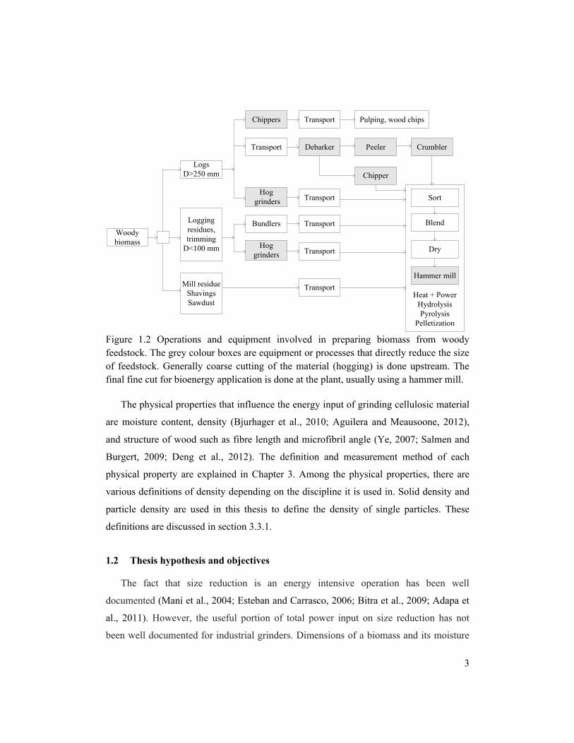
Figure 1.2 Operations and equipment involved in preparing biomass from woody feedstock.

The grey colour boxes are equipment or processes that directly reduce the size of feedstock.

Generally coarse cutting of the material (hogging) is done upstream. The final fine cut for

bioenergy application is done at the plant, usually using a hammer mill. ...................................... 3!

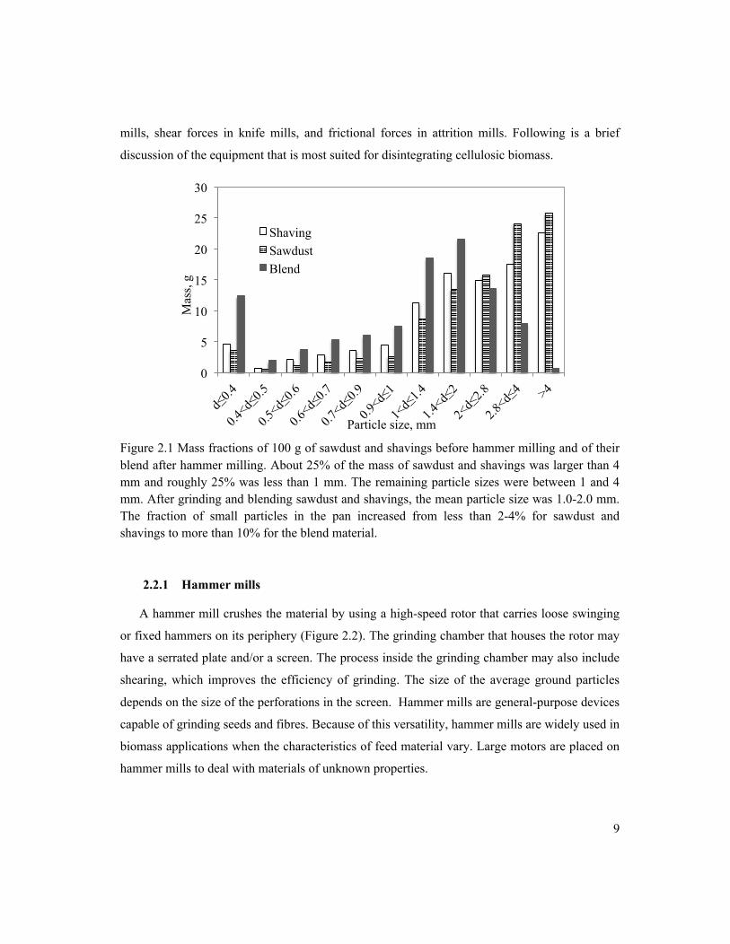
Figure 2.1 Mass fractions of 100 g of sawdust and shavings before hammer milling and of their

blend after hammer milling. About 25% of the mass of sawdust and shavings was larger than 4

mm and roughly 25% was less than 1 mm. The remaining particle sizes were between 1 and 4

mm. After grinding and blending sawdust and shavings, the mean particle size was 1.0-2.0

mm. The fraction of small particles in the pan increased from less than 2-4% for sawdust and

shavings to more than 10% for the blend material. ........................................................................ 9!

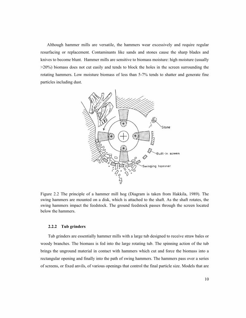
Figure 2.2 The principle of a hammer mill hog (Diagram is taken from Hakkila, 1989). The

swing hammers are mounted on a disk, which is attached to the shaft. As the shaft rotates, the

swing hammers impact the feedstock. The ground feedstock passes through the screen located

below the hammers. ...................................................................................................................... 10!

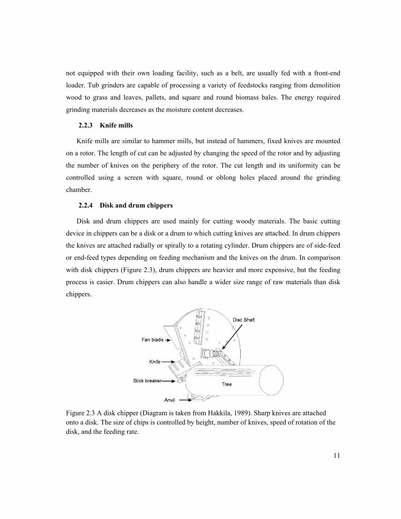
Figure 2.3 A disk chipper (Diagram is taken from Hakkila, 1989). Sharp knives are attached

onto a disk. The size of chips is controlled by height, number of knives, speed of rotation of

the disk, and the feeding rate. ....................................................................................................... 11!

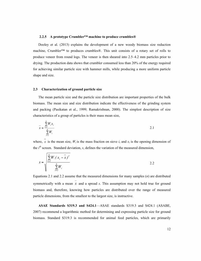
Figure 2.4 (a) Macrostructure of a softwood stem (Taken from Biermann, 1996). (b)

Transverse and longitudinal section of a hardwood (European beech), scanning electron

micrograph. (c) Transverse section of softwood (Scots pine) scanning electron micrograph

(Taken from Hofstetter et al., 2005). ............................................................................................ 15!

Figure 2.5 Physical properties of wood vary from the centre of the stem (pith) to the outside of

the stem (bark), depending on the age of the wood and the distribution of mature wood and

juvenile wood zones. The proportion of juvenile wood to mature wood increases from the base

of the wood stem to its top (Adapted from Green et al., 1999). ................................................... 17!

xiii

Figure 2.6 (a) Schematic definition of microfibril angle (MFA) in relation to a single cell. (b)

Stress-strain curves of wood samples with small and MFAs (Adapted from Salmen and

Burgurt, 2009). .............................................................................................................................. 18!

Figure 2.7 Pellet press mill. (a) Picture shows wood pellets compacted in pellet mill are

extruded from the die hole. (b) The diagram shows the internal roller arrangement that presses

the ground biomass through die holes. (Murray, 2014). ............................................................... 26!

Figure 3.1 (a) Inside the knife mill (Retsch grinder SM100). Three cutting blades are attached

to the rotor. There are four cutting strips attached to the periphery of the grinding chamber. A

curved perforated screen covering 120 degrees of the bottom portion of the housing is installed

below the grinding chamber to control the size of ground particles. (b) A number of these

screens are shown in the picture (Naimi, 2008). ........................................................................... 31!

Figure 3.2 (a) Glen Mill hammer mill. Twelve swing hammers are placed along a shaft in order

to have hammers every 90 degrees. The mill uses a removable perforated screen that extends

180 degrees around the lower section of the housing. (b) A number of these screens are shown

in the picture. ................................................................................................................................ 32!

Figure 3.3 Sieving system used to fractionate biomass samples. (a) RoTap sieve shaker holds

two stacks of five round sieves plus pan. The sieve motion was rotational with a tapping. (b)

Gilson sieve shaker holds five rectangular screens. The sieve motion was vertical shake. The

screen holes for both sieving systems were wire mesh. ................................................................ 34!

Figure 3.4 (a) A universal testing machine provides the compression force at a constant rate.

(b) The piston-cylinder assembly is used to form pellets. ............................................................ 35!

Figure 3.5 Branches of four species of wood as they were received in the lab. The leaves were

removed. The branches were cut in length for debarking, drying, and storage. ........................... 36!

Figure 3.6 (a) Wood samples were manually debarked, dried in 50oC air, and cut to lengths

ranging from 30 mm to 110 mm. (b) The samples were cut crosswise to quarter disks using a

band saw. ....................................................................................................................................... 37!

Figure 3.7 Hammer mill screen sizes (mm) used for grinding pine wood chips (PWC). Initially,

PWC was ground in hammer mill with screen sizes 25.4, 12.7, 10, 6.25, or 3.13 mm screens.

The ground particles were labelled with the screen size they were ground with. The five

labelled ground particles were then ground using all screen sizes smaller. For example the

particles labelled 10 were ground in the hammer mill with 6.25 and 3.13 mm screen sizes. ....... 38!

xiv

Figure 3.8 Device for measuring angle of repose (Geldart et al., 2006). The device consisted of

four main parts: a vibrator, a vibrating chute, a funnel, and a measuring baseboard. Particles

are loaded on the vibrating chute and pour down into the funnel. Particles form a semi-cone on

the measuring baseboard. Height and radius of the semi-cone can be read on the measuring

baseboard. ..................................................................................................................................... 41!

Figure 4.1 Block diagrams of experiments conducted to analyze the applicability of size

reduction equations to woody biomass ......................................................................................... 47!

Figure 4.2 Sample plot of power input to the knife mill with 6 mm screen running empty (No-

load) and grinding willow and Douglas-fir. All three curves have an initial perturbation

because of the sudden pull of electricity for the motor to start working. The curve for no-load

working defines a base line for the power needed for the knife mill working empty. The feed

wood chips had a variable size. ..................................................................................................... 49!

Figure 4.3 Size distribution of hammer-milled wood chips of willow and Douglas-fir on Gilson

sieve shaker and pine wood chips as-received (PWC). The screen size inside hammer mill is 25

mm. The ground wood chips are prepared for feeding to the knife mill and hammer mill. ......... 51!

Figure 4.4 A comparison between geometric mean diameter of the ground particles and the

mean length and mean width of ground particles of pine calculated by image analysis. Three

replicates of measurements are represented for each screen size. This figure shows that the

geometric mean diameter of the particles is very close to the width of the particles. .................. 57!

Figure 4.5 Specific energy vs. Kick’s size reduction parameters for grinding (a) Douglas-fir

and (b) willow. The lines for each species are one allowed having an intercept and one not

having an intercept. The regression coefficients R2 were low when the lines are forced through

origin ............................................................................................................................................. 59!

Figure 4.6 Specific energy of size reduction vs 1/LP. Data labelled with pine wood chips

represent the wood chips as received. Data labelled with 25.4, 12.7, and 10 mm represent pine

wood chips pre-ground with 25.4, 12.7, and 10 mm screens installed in the hammer mill. ........ 63!

Figure 4.7 Specific energy of size reduction vs LP-0.5. Data labelled with Pine wood chips



xv

Figure 4.8 Specific energy of size reduction vs ln (LP). Data labelled with Pine wood chips



Figure 4.9 Specific energy of size reduction vs LP-1-LF

-1. Data labelled with PWC represent the

wood chips as received. Data labelled with 25.4, 12.7,10.0, and 6.3 mm represent pine wood

chips pre-ground with 25.4, 12.7, 10, 6.3 mm screens installed in the hammer mill. .................. 64!

Figure 4.10 Specific energy vs. Rittinger’s size reduction ratio for the data from this study, and

those extracted from Mani et al. (2004), Bitra et al. (2009), and Adapa et al. (2011). The slopes

of the lines related to Douglas-fir, oat straw, switch grass and canola straw are similar and

highest among the slopes. The slopes were lower for willow, barley straw and wheat straw.

Corn stover had the lowest slope among all. ................................................................................ 65!

Figure 5.1 The plot of force vs displacement of single pellet of ground particles of Douglas-fir

and willow. Particles were ground in the knife mill with 6, 4, and 2 mm screens. The

maximum force was 5000 N, maintained for 30 s. ....................................................................... 69!

Figure 5.2 Specific energy consumption of size reduction and pelletization for willow and

Douglas-fir. Single pelletization was performed under a maximum force of 5000 N. ................. 71!

Figure 5.3 Integrated specific energy for size reduction and pelletization of Douglas-fir and

willow. .......................................................................................................................................... 71!

Figure 5.4 Density of pellets made from blends of willow and Douglas-fir. The population

means are not significantly different (ANOVA, p=0.05) among the percentages of willow in

the blend. ....................................................................................................................................... 73!

Figure 6.1 Bark fractions as a function of branch stem diameter. Aspen had the largest fraction

of bark followed by poplar and pine. Bark content decreases with increasing diameter of the

branch. ........................................................................................................................................... 77!

Figure 6.2 Effect of feeding rate on the specific energy of size reduction with a knife mill on a

2 mm screen. ................................................................................................................................. 86!

Figure 6.3 Cumulative size distribution of ground particles of the four biomass species of

Douglas-fir, pine, aspen, and poplar. The size distributions on 2, 4, and 6 mm screens are

shown in graphs (a), (b), and (c), respectively. The graph shows that the difference between

cumulative size distribution curves increases as the screen size decreases. The top graph shows

that the cumulative size distribution curves of aspen and poplar are fairly close and they are

xvi

located between the size distributions of softwoods with pine at the bottom and Douglas-fir at

the top. ........................................................................................................................................... 89!

Figure 6.4 Correlation of Rittinger constant with wood properties. The largest positive

correlation is with porosity of solid pieces and the largest negative correlation is with wood

density. .......................................................................................................................................... 94!

Figure A.1 (a) A test circle image with known dimension designed for understanding how

ImageJ software works. (b) The image of one particle wood chips with known dimension. (c)

The inverted image of the wood chips particle from image (b). ................................................. 120!

Figure A.2 A sample scanned image (a) of wood chips with known particle size and its

corresponding (b) inverted image used in ImageJ software. ...................................................... 120!

Figure A.3 A sample scanned image (a) of ground particles form 25.4 mm screen and its

corresponding inverted image (b) used in ImageJ software. ...................................................... 121!

Figure A.4 A piece of wood chips. The dimensions that are measured by ImageJ are shown on

the picture. ................................................................................................................................... 121!

Figure D.5 Herbaceous biomass collected from field. The ruler beside the pieces is for

estimating the size of pieces as received. The pictures also show the composition of samples. 133!

Figure D.6 Power consumption of grinding chipped willow in the hammer mill with 6.4 mm

(0.25 in) screen. The large variability of the data (SD=233) comparing to the variability of

power consumption working empty (SD=32) is due to variable size of input wood chips and

variable wood properties. ............................................................................................................ 138!

Figure D.7 Power consumption of grinding sorghum seeds in the hammer mill with 6.4 mm

(0.25 in) screen. The small variability of the data (SD=34) comparing to the variability of

power consumption working empty (SD=32) is due to uniform particle size and uniform

properties of sorghum seeds. ....................................................................................................... 138!

Figure D.8 Average energy input to grind herbaceous biomass. Four sizes of the screens 3.2

mm (1/8 in), 6.4 mm (1/4 in), 12.7 mm (1/2 in), and 25.4 mm (1 in) were used in the hammer

mill. Willow, corn stover, and bagasse have the highest energy input at 3.2 mm screen size. .. 139!

Figure D.9 Particle size distribution for straw and branches after grinding using the 6.4 mm

(1/4”) screen in the hammer mill. ............................................................................................... 139!

Figure D.10 Particle size distribution for seeds and olive residue after grinding using the 6.4

mm (1/4”) screen in the hammer mill. ........................................................................................ 140!

xvii

Figure D.11 Loose bulk density of bagasse, wheat straw, canola straw, sunflower seed husks,

corn stover and miscanthus ground at different screen sizes inside the hammer mill. Equation

D.1 is fitted and the trend of bulk density of each biomass are shown. ...................................... 140!

Figure F.12 Density profile for a Douglas-fir sample. ................................................................ 151!






Figure F.18 Density profile for a pine sample. ........................................................................... 154!






Figure F.24 Density profile for an aspen sample. ....................................................................... 157!






Figure F.30 Density profile for a poplar sample. ........................................................................ 160!






xviii

Nomenclature

Acronym

Avg Average

CC Cellulose Content

CV Coefficient of Variation

db dry basis

DBH Diameter at Breast Height, cm

EPS Events Per Second

FQA

FL

LC

Fibre Quality Analyzer

Fibre Length

Lignin Content

Max Maximum

MC Moisture Content

MFA Microfibril Angle

Min

PD

Minimum

Particle Density

PWC Pine Wood Chips

rpm Revolution per minute

SD Standard Deviation

Sol Soluble

W Mass fraction

wt Weight

wb wet basis

Symbols

a Constant;

A A variable representative

b Constant;

B A variable representative

d Particle size, mm

C Intercepts in Equations 4.1, 4.2, and 4.3

xix

dgw Geometric mean diameter of particles by mass, mm

E Specific energy, J g-1

F Feeding rate, g s-1

I Electric current, A

k Constant

K Constant

L Characteristic particle size equal to dgw, mm

m Constant

n Number of screens in Equations 2.1, 2.2, 2.3, and 2.4

n Constant

N Revolution per minute, rpm

Ns Number of stems

P Power consumption, W

R

R2

Electric resistance, Ω

Coefficient of determination

s Standard deviation, mm

S Screen size, mm

Slog Geometric standard deviation of log-normal distribution by mass, log mm

Sgw Geometric standard deviation of particle diameter by mass

Mean size, mm

V Electric potential difference, V

Greek letters

λ Shape factor

ϕ Porosity, dimensionless

ρbulk Bulk density, kg m-3

ρsolid

ρtapped

ρ

Solid density, kg m-3

Tapped density, kg m-3

Particle density, kg m-3

σ Scale factor

x

xx

Subscripts

B Bond

E Empty

F

g

Feed particles

Ground

i Sieve number

K Kick

P Product particles

R

sp

Rittinger

Solid pieces

0 Initial

1 Final

xxi

Acknowledgments

I have been privileged to work with wonderful people throughout the course of this study.

First of all, I would like to sincerely acknowledge my advisor Professor Shahab Sokhansanj,

for his invaluable guidance and generous support throughout my graduate studies. I wish to

thank my co-advisors Professor Xiaotao Bi and Professor Jim Lim for all their stimulating and

insightful discussions and comments. This thesis would have not been completed without their

guidance.

I am very grateful to Professor Peter Englezos and Professor Ezra Kwok for all their

support. I especially thank Professor Anthony Lau for his dedication and kind support. I am

honoured to have Professor James Fridley, Professor Farrokh Sassani, and Professor John

Grace as my examining committee. Their valuable questions and comments inspired me to

envision my future research.

I appreciate summer student assistant, Mohammad Emami’s help during the course of this

research. I thank Marius Woehler, Sebastian Fucks, and Flavien Collard for their

collaborations. Special thank to Dr Zahra Tooyserkani and Dr Fahimeh Yazdanpanah for their

friendship. I would like to thank all my friends and colleagues in Biomass and Bioenergy

Research Group at UBC, particularly Ehsan Oveisi, Bahman Ghiasi, and Maryam Tajilrou. I

also thank the staff of the Department of Chemical and Biological Engineering for their help.

I appreciate the financial support of the Natural Science and Engineering Research Council

of Canada (NSERC) Discovery Grant.

I feel very lucky to have a family that shares my enthusiasm to academic pursuits. I am

extremely grateful of my parents for all the love and encouragement. I sincerely thank my

husband who has been understanding and supportive of my studies. Finally to my daughters

Mahtab and Mahsa, who bring joy and happiness in my life every day.

1

Chapter 1 Introduction

1.1 Background

The increasing demands for energy and the negative impacts of fossil fuels on the

environment are shifting the focus of energy providers to alternative energy sources

including energy from biomass. Biomass comes from biological materials that can

reproduce in a short time and thus is considered renewable. Conversion processes,

whether they are simply converting biomass to heat and power or more complex gaseous

or liquid fuels, require high-quality and cost-competitive feedstocks. Simple combustion

may utilize a wide variety of feedstocks, with a wide range of moisture contents (MC),

mixtures of species, bark and wood, and a wide range of sizes. A complex chemical

conversion process requires feedstocks of strict specifications especially in particle size.

Size reduction is one of the most energy intensive and expensive operations in

transforming raw biomass to feedstock for biofuel production. Particle size and shape

have significant impact on the effectiveness of conversion processes, yet the

fundamentals of size reduction; specifically those applied to fibrous biomass, have not

been well understood or documented. Equipment operators use their experiences for

management and control of size reduction operations. Equipment designers do not have

adequate functional models/equations to guide them in the design or selection of the most

efficient grinding equipment.

Woody biomass collected from the field can be in several forms, depending on the

nature of the plant material. Logs and logging residues consists of branches, leaves, and

other anatomical parts of the plant. Sawdust, shavings, and leftovers from wood

processing operations are also available for bioenergy applications. Short rotation woody

biomass like willows and poplars can be harvested in chip form. The raw biomass

feedstock of varying size and format must then be processed to a desirable size for

handling and processing.

Figures 1.1 and 1.2 show the operations and equipment involved in preparing biomass

from herbaceous biomass (bales) and from woody biomass, respectively. The grey

coloured boxes are equipment or processes for directly reducing the size of feedstock. In

general, more than one step of size reduction is involved. First, a coarse grinding reduces

2

the material size to 25 mm size range. Depending upon the requirement of downstream

conversion process, the coarse ground biomass is further reduced in size to 1-3 mm for

pelletization and other conversion applications.

Baled biomass

Pelletization, d ~ 1 – 2 mm, moisture < 10%

Dryer

Pulping, d > 20 mm, any moistureRotary knives approx. size

20 mm

Hydrolysis – fermentation, d ~ 2 mm, any moisture

Hammer mill

Stationary knives size~ 150 mm

Undersize

Pyrolysis

Thermochemical, d ~ 0.1-0.2 mm, moisture <15%

Compact Pulp for paperSizer

Biochemical Bioethanol

Hammer millPellets

Figure 1.1 Operations and equipment involved in preparing biomass from herbaceous biomass (bales). The grey coloured boxes are equipment or processes that directly reduce feedstock size.

3

Woody biomass

Heat + PowerHydrolysisPyrolysis

Pelletization

LogsD>250 mm

Logging residues,trimming

D<100 mm

Chippers

Transport

Pulping, wood chips

Mill residueShavingsSawdust

Transport

Transport

Transport

Transport

Transport

Debarker

Chipper

Peeler Crumbler

Hog grinders

Bundlers

Hog grinders

Sort

Blend

Dry

Hammer mill

Figure 1.2 Operations and equipment involved in preparing biomass from woody feedstock. The grey colour boxes are equipment or processes that directly reduce the size of feedstock. Generally coarse cutting of the material (hogging) is done upstream. The final fine cut for bioenergy application is done at the plant, usually using a hammer mill.

The physical properties that influence the energy input of grinding cellulosic material

are moisture content, density (Bjurhager et al., 2010; Aguilera and Meausoone, 2012),

and structure of wood such as fibre length and microfibril angle (Ye, 2007; Salmen and

Burgert, 2009; Deng et al., 2012). The definition and measurement method of each

physical property are explained in Chapter 3. Among the physical properties, there are

various definitions of density depending on the discipline it is used in. Solid density and

particle density are used in this thesis to define the density of single particles. These

definitions are discussed in section 3.3.1.

1.2 Thesis hypothesis and objectives

The fact that size reduction is an energy intensive operation has been well

documented (Mani et al., 2004; Esteban and Carrasco, 2006; Bitra et al., 2009; Adapa et

al., 2011). However, the useful portion of total power input on size reduction has not

been well documented for industrial grinders. Dimensions of a biomass and its moisture

4

content can be measured and somewhat used for predicting the performance of a size

reduction operation. However, inherent structural properties like toughness or hardness of

a cellulosic biomass are not easily quantifiable or adjustable. As a result, size reduction

equipment is often designed to grind feedstock with unpredictable physical properties.

There have been limited attempts to develop correlations between energy

consumption and size reduction for cellulosic materials for a given biomass species, but

no report on the effect of biomass properties on size reduction performance. The lack of

knowledge on the influence of physical properties on size reduction is the main reason

that design and operation of size reduction processes have remained empirical, heavily

relying on the past experience gained by trial-and-error. Only highly skilled and

experienced operators are able to adjust the size reduction equipment to accommodate the

grinding of biomass of different properties. However an experienced operator’s

knowledge is limited to a few locally grown biomass species and specific size reduction

equipment. The knowledge is also qualitative in nature and not transferable from one

biomass species to another, from one grinder type to another grinder type, or from one

operator to the next.

The overall objective of this study is to establish a mechanistically-based

mathematical relation between energy consumption and the degree of size reduction for

cellulosic biomass materials of different properties so as to guide the design and optimum

operation of biomass grinders. The thesis is based on a hypothesis that biomass size

reduction follows fracturing mechanism(s) previously proposed for mineral materials.

Therefore, those established energy input vs. size reduction relationships can be applied

to grinding of cellulosic biomass. To test the hypothesis, extensive controlled grinding

tests have been carried out using two laboratory scale grinders: a knife mill grinder and a

hammer mill grinder. In addition to power input, selected physical characteristics and

compositional make-up of biomass samples are measured to elucidate the influence of

biomass properties on the performance of energy input vs. size reduction ratio

formulations.

1.3 Experimental

The experiments are designed mainly to develop experimental data with which to test

the applicability of the three fundamental size reduction equations, Rittinger, Kick, and

5

Bond, to cellulosic biomass. Among many candidate feedstock species, pine and

Douglas-fir are abundant and constitute the most common species found in British

Columbia. Samples of aspen and hybrid poplar are also included in the testing program to

expand the scope of experimental data and to examine the applicability of size reduction

equations to hardwood species. The starting form of the biomass is as pieces cut from tree

branches. The idea here is to test pieces of wood that might represent left-overs from

logging operations. The main independent variables in these tests are species of wood,

size of in-feed particles, and size of output particles. The dependent variable is power

input. Feeding rate is generally kept constant for a consistent grinder operation. Both

moisture content and feeding rate are carefully controlled. Particle sizes were those

typically used for pelleting. A number of herbaceous biomass material like wheat straw,

corn stover, switchgrass, miscanthus, bagasse, canola straw, sunflower seeds husks,

sorghum, and willows are tested as well. The experimental data for these crops are placed

in Appendix D for future analysis and reference.

1.4 Scope and organization of the thesis

This thesis is organized in seven chapters. Chapter 1 outlines the background of the

proposed research subject of biomass size reduction as a major operation in preparing

feedstock for downstream processing. Chapter 1 presents the formulation of the thesis

hypothesis and research objectives. Chapter 2 presents a critical review of relevant

literature on size reduction and a general introduction of pertinent properties of woody

and herbaceous biomass. The chapter briefly describes the mechanistic models developed

previously for predicting energy consumption of size reduction of mineral materials and

empirical correlations for biomass materials. The need for further research to evaluate the

applicability of the mechanistic models to biomass feedstock is discussed. Chapter 3

describes the biomass materials used in the experiments. This chapter provides details of

experimental equipment and methods used to measure mass flow rates and energy input

for grinding tests. Chapter 4 presents the systematic evaluation of the three mechanistic

grinding model equations using measured experimental data, including a discussion on

sources of uncertainty in the experimental data. Chapter 5 discusses the relations between

particle size and energy input for the combined size reduction and pelletization process,

in order to optimize the energy consumption of the whole pelletization process. Chapter 6

6

presents experimental data on biomass physical and compositional characteristics before

and after grinding, and the first attempt to develop a correlation to capture the effect of

biomass properties on the size reduction. Chapter 7 presents the overall conclusions and

recommends future research.

7

Chapter 2 Literature Review

Cellulosic biomass varies in size (dimensions) at the time of its harvest/collection. Like any

other solid feedstock, the size of raw biomass must be adjusted to fit to a specific conversion

process. This chapter first reviews the literature to identify the desired particle sizes suitable for

different conversion processes. The chapter briefly outlines the principal operations of size

reduction equipment and statistical models used to characterize the mean and the distribution of

ground particles. The structure of cellulosic biomass affects the power input and size

characteristics of a feedstock (ground particles as a feedstock for conversion processes); and to

this end, the chapter discusses relevant mechanical properties of woody biomass, including the

microstructure of wood. Finally, the chapter outlines available models to represent the

relationship between power consumption and size reduction ratios.

2.1 Sensitivity of biomass conversion processes to particle size

The desirable particle sizes for hydrolysis and subsequent fermentation are around 2 mm

(Van Draanen and Mello, 1997; Petersson et al., 2007; Wei et al., 2009). According to Smook

(1992), the ideal chip size for pulping is 4-5 mm thick and about 20 mm long in the grain

direction. In general, chips 10-30 mm in length and 3-6 mm in thickness are acceptable.

Bridgwater et al. (1999) reported that the maximum particle size for a circulating fluidized bed

gasifier is 6 mm. Bridgwater et al. (1999) also reported that particles less than 2 mm are suitable

for fast pyrolysis in a fluidized bed and entrained flow reactors. For slow pyrolysis, such as

torrefaction and charcoal making, where heat treatment is slow, the size of particles can be as

large as 50 mm. For efficient combustion, the content of very fine particles (smaller than 100

µm) should be higher than 10% by weight in order to achieve a short ignition time (Esteban and

Carrasco, 2006).

Particle size affects both the pressure drop across gasifiers and the required power to draw

air and gas through the gasifiers. Large pressure drops will lead to a reduction of the gas load in

downdraft gasifiers, resulting in a low bed temperature and high tar formation. Excessively large

size feedstocks give rise to reduced fuel reactivity, causing start-up problems and poor gas

8

quality. Acceptable fuel sizes depend on the design of the gasifiers. In general, fixed/moving bed

wood gasifiers work well using wood chips of 10 x 5 x 5 mm in size (Chandrakant, 1997).

Nexterra for example, requires particle sizes less than 75 mm for the optimum operation of its

updraft gasifier and specifies that the mass of particles with sizes less than 6 mm should not be

more than 25% of the total mass of the biofuel feedstock when fed into the gasifier (Nexterra,

2012).

In general, burners fuelled by biomass powders require particle sizes below 1 mm (Anderl et

al., 1999; Freeman et al., 2000; Kastberg and Nilsson, 2002), while particle sizes of coal in

pulverized coal burners are below 0.1 mm (Siegle et al., 1996; Freeman et al., 2000). Biomass

particles with sizes below 1.0 mm (Kastberg and Nilsson, 2002) have a residence time similar to

pulverized coal, and this is the reason for considering finely ground biomass as a pulverized

feedstock. Badger (2002) specified a particle size for biomass combustion boilers between 6 and

60 mm.

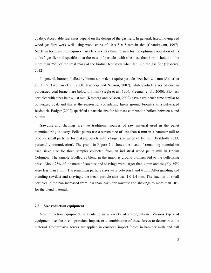
Sawdust and shavings are two traditional sources of raw material used in the pellet

manufacturing industry. Pellet plants use a screen size of less than 6 mm in a hammer mill to

produce small particles for making pellets with a target size range of 1-3 mm (Berkholtz 2013,

personal communication). The graph in Figure 2.1 shows the mass of remaining material on

each sieve size for three samples collected from an industrial wood pellet mill in British

Columbia. The sample labelled as blend in the graph is ground biomass fed to the pelletizing

press. About 25% of the mass of sawdust and shavings were larger than 4 mm and roughly 25%

were less than 1 mm. The remaining particle sizes were between 1 and 4 mm. After grinding and

blending sawdust and shavings, the mean particle size was 1.0-1.4 mm. The fraction of small

particles in the pan increased from less than 2-4% for sawdust and shavings to more than 10%

for the blend material.

2.2 Size reduction equipment

Size reduction equipment is available in a variety of configurations. Various types of

equipment use shear, compression, impact, or a combination of these forces to deconstruct the

material. Compressive forces are applied in crushers, impact forces in hammer mills and ball

9

mills, shear forces in knife mills, and frictional forces in attrition mills. Following is a brief

discussion of the equipment that is most suited for disintegrating cellulosic biomass.

Figure 2.1 Mass fractions of 100 g of sawdust and shavings before hammer milling and of their blend after hammer milling. About 25% of the mass of sawdust and shavings was larger than 4 mm and roughly 25% was less than 1 mm. The remaining particle sizes were between 1 and 4 mm. After grinding and blending sawdust and shavings, the mean particle size was 1.0-2.0 mm. The fraction of small particles in the pan increased from less than 2-4% for sawdust and shavings to more than 10% for the blend material.

2.2.1 Hammer mills

A hammer mill crushes the material by using a high-speed rotor that carries loose swinging

or fixed hammers on its periphery (Figure 2.2). The grinding chamber that houses the rotor may

have a serrated plate and/or a screen. The process inside the grinding chamber may also include

shearing, which improves the efficiency of grinding. The size of the average ground particles

depends on the size of the perforations in the screen. Hammer mills are general-purpose devices

capable of grinding seeds and fibres. Because of this versatility, hammer mills are widely used in

biomass applications when the characteristics of feed material vary. Large motors are placed on

hammer mills to deal with materials of unknown properties.

0

5

10

15

20

25

30 M

ass,

g

Particle size, mm

Shaving Sawdust Blend

10

Although hammer mills are versatile, the hammers wear excessively and require regular

resurfacing or replacement. Contaminants like sands and stones cause the sharp blades and

knives to become blunt. Hammer mills are sensitive to biomass moisture: high moisture (usually

>20%) biomass does not cut easily and tends to block the holes in the screen surrounding the

rotating hammers. Low moisture biomass of less than 5-7% tends to shatter and generate fine

particles including dust.

Figure 2.2 The principle of a hammer mill hog (Diagram is taken from Hakkila, 1989). The swing hammers are mounted on a disk, which is attached to the shaft. As the shaft rotates, the swing hammers impact the feedstock. The ground feedstock passes through the screen located below the hammers.

2.2.2 Tub grinders

Tub grinders are essentially hammer mills with a large tub designed to receive straw bales or

woody branches. The biomass is fed into the large rotating tub. The spinning action of the tub

brings the unground material in contact with hammers which cut and force the biomass into a

rectangular opening and finally into the path of swing hammers. The hammers pass over a series

of screens, or fixed anvils, of various openings that control the final particle size. Models that are

11

not equipped with their own loading facility, such as a belt, are usually fed with a front-end

loader. Tub grinders are capable of processing a variety of feedstocks ranging from demolition

wood to grass and leaves, pallets, and square and round biomass bales. The energy required

grinding materials decreases as the moisture content decreases.

2.2.3 Knife mills

Knife mills are similar to hammer mills, but instead of hammers, fixed knives are mounted

on a rotor. The length of cut can be adjusted by changing the speed of the rotor and by adjusting

the number of knives on the periphery of the rotor. The cut length and its uniformity can be

controlled using a screen with square, round or oblong holes placed around the grinding

chamber.

2.2.4 Disk and drum chippers

Disk and drum chippers are used mainly for cutting woody materials. The basic cutting

device in chippers can be a disk or a drum to which cutting knives are attached. In drum chippers

the knives are attached radially or spirally to a rotating cylinder. Drum chippers are of side-feed

or end-feed types depending on feeding mechanism and the knives on the drum. In comparison

with disk chippers (Figure 2.3), drum chippers are heavier and more expensive, but the feeding

process is easier. Drum chippers can also handle a wider size range of raw materials than disk

chippers.

Figure 2.3 A disk chipper (Diagram is taken from Hakkila, 1989). Sharp knives are attached onto a disk. The size of chips is controlled by height, number of knives, speed of rotation of the disk, and the feeding rate.

12

2.2.5 A prototype Crumbler™ machine to produce crumbles®

Dooley et al. (2013) explains the development of a new woody biomass size reduction

machine, Crumbler™ to produces crumbles®. This unit consists of a rotary set of rolls to

produce veneer from round logs. The veneer is then sheared into 2.5–4.2 mm particles prior to

drying. The production data shows that crumbler consumed less than 20% of the energy required

for achieving similar particle size with hammer mills, while producing a more uniform particle

shape and size.

2.3 Characterization of ground particle size

The mean particle size and the particle size distribution are important properties of the bulk

biomass. The mean size and size distribution indicate the effectiveness of the grinding system

and packing (Pasikatan et al., 1999; Ramakrishnan, 2000). The simplest description of size

characteristics of a group of particles is their mass mean size,

2.1

where, is the mean size, Wi is the mass fraction on sieve i, and xi is the opening dimension of

the ith screen. Standard deviation, s, defines the variation of the measured dimension,

2.2

Equations 2.1 and 2.2 assume that the measured dimensions for many samples (n) are distributed

symmetrically with a mean and a spread s. This assumption may not hold true for ground

biomass and, therefore, knowing how particles are distributed over the range of measured

particle dimensions, from the smallest to the largest size, is instructive.

ASAE Standards S319.3 and S424.1—ASAE standards S319.3 and S424.1 (ASABE,

2007) recommend a logarithmic method for determining and expressing particle size for ground

biomass. Standard S319.3 is recommended for animal feed particles, which are primarily

∑

∑=

=

=n

1ii

n

1iii

W

xWx

x

∑

−∑=

=

=n

1ii

2n

1ii

W

)xx(Ws

i

x

13

spherical or cubical, whereas Standard S424.1 is recommended for chopped forage. Standard

S319.3 defines geometric mean diameter or median size of particles by:

2.3

where dgw is the geometric mean diameter of particles by mass (dgw is in mm), Wi is the mass of

particles on ith sieve (sieves are numbered from large to small with the top sieve denoted with

number 1), N is the number of sieves plus pan, xi is nominal sieve opening size (mm), and log is

base 10 logarithm.

The geometric standard deviation of log-normal distribution by mass is defined by:

2.4

ANSI/ASAE S319.3 defines the geometric standard deviation of particle diameter by mass

Sgw (mm) as,

2.5

2.4 Woody biomass sources

Woody biomass comes from a wide range of sources including sawdust and shavings, whole

logs, debarked logs, mixed logging residues such as pieces of stems and branches, leaves,

municipal waste diversion materials, and sometimes roots. The diversity of biomass feedstock

and the diversity of forces required to break up a piece of woody biomass imply that size

reduction is a complex process. Harvesting whole trees will result in wood chips mixed with

bark and foliage, which have a weak market. It is assumed that a stem less than 10 cm (4 in) is

not made into lumber and can be used for biomass (Briggs, 1994).

Table 2.1 lists the mass fraction of an oven-dry Douglas-fir tree of 400 mm diameter at breast

height (DBH) harvested from Pacific Northwest. Out of the mass of 1145 kg (100%) for the

dgw = log−1

Wi log xi( )i=1

n

∑

Wii=1

n

∑

#

$

%%%%

&

'

((((

Slog =Wi (log xi − logdgw )

2

i=1

n

∑

Wii=1

n

∑

#

$

%%%%

&

'

((((

1/2

])(log[log21 1

log1

log1 −−− −≈ SSdS gwgw

14

entire tree, 828 kg (72.3%) is the bole or stem, 197 kg (17.2%) is the stump and 120 kg (10.5%)

is the stem and foliage. In terms of utilization of the tree, roughly 274 kg (27%) is sawn into

lumber, 295 kg (26%) is chipped for pulping, 219 kg (19%) is used for energy processes, and

357 kg (31%) remains in forest. The following sections review the characteristics of stem and

branches size reduction, excluding leaves, seeds, fruits, cones and fractions of wood like bark.

Table 2.1 Biomass distribution of a 400 mm diameter at breast height (DBH) of a Douglas-fir tree (Briggs, 1994) Oven dry weight, kg Percent Above ground: Crown:

Foliage 32 2.8 Live branches with bark 62 6.0 Dead branches with bark 19 1.7

Total 120 10.5 Stem or bole:

Wood 719 62.8 Bark 109 9.5

Total 828 72.3 Total above ground 948 82.8 Below ground:

Roots and stump 197 17.2 Total tree 1,145 100.0

2.5 Wood structure

Wood is a fibrous material that consists of a group of plant cells in which the wall of each cell

is made of a fibre-reinforced polymer (Kettunen, 2006). Under loading, the mechanical

properties of wood are dependent on the behaviour of the fibre-reinforced polymers that form

the edges of the cell walls (Gibson and Ashby, 1988, Brown et al., 1949). Wood properties result

from a combination of macroscopic morphology (distribution of different types of wood tissue),

anatomy (types of cells and their proportion), and chemical composition (Barnett and

Jeronimidis, 2003). The overall behaviour of wood strongly depends on its orthotropic material

properties (different properties in each orthogonal direction) and their distribution in space. The

heterogeneous microstructure of wood causes different properties in different directions. Hence,

15

at a macro level the material behaviour of wood is strongly influenced by the cellular structure at

a micro-level (Holmberg et al., 1999).

Figure 2.4 (a) shows cross-sections from a stem of softwood (coniferous) trees. The diagram

divides the stem into transverse, tangential, and radial sections. The transverse plane can be

further divided into bark and xylem. Xylem consists of sapwood, heartwood, and pith. There are

also stripes, called rays that sometimes start from pith and sometimes start from heartwood or

sapwood.

(a)

(b) (c)

Figure 2.4 (a) Macrostructure of a softwood stem (Taken from Biermann, 1996). (b) Transverse and longitudinal section of a hardwood (European beech), scanning electron micrograph. (c) Transverse section of softwood (Scots pine) scanning electron micrograph (Taken from Hofstetter et al., 2005).

K. Hofstetter et al. / European Journal of Mechanics A/Solids 24 (2005) 1030–1053 1033

Fig. 2. Hierarchical organization of wood: (a) Cross-section of a log (Ponderosa pine) (+); (b) Transverse and longitudinal section througha hardwood (European beech), Scanning electron micrograph (SEM) (o); (c) Transverse section through a softwood (Scots pine), Scanningelectron micrograph (SEM) (o); (d) Section through the cell wall, showing the cell wall layers, Transmission electron micrograph (TEM) (o);(e) Fibrillar structure of the S2 wall, Rapid freeze deep etching (RFDE) micrograph (x); (f) Chemical structure of cellulose chain (o); (g) Chem-ical structure of basic unit of lignin-polysaccharide complex (o); (+) . . . from (WHB, 1999), permission for reproduction requested from ForestProduct Society; (o) . . . from (Fengel and Wegener, 2003), permission for reproduction requested from Kessel Verlag; (x) . . . from (Hafren etal., 1999), permission for reproduction requested from Oxford University Press.

K. Hofstetter et al. / European Journal of Mechanics A/Solids 24 (2005) 1030–1053 1033

Fig. 2. Hierarchical organization of wood: (a) Cross-section of a log (Ponderosa pine) (+); (b) Transverse and longitudinal section througha hardwood (European beech), Scanning electron micrograph (SEM) (o); (c) Transverse section through a softwood (Scots pine), Scanningelectron micrograph (SEM) (o); (d) Section through the cell wall, showing the cell wall layers, Transmission electron micrograph (TEM) (o);(e) Fibrillar structure of the S2 wall, Rapid freeze deep etching (RFDE) micrograph (x); (f) Chemical structure of cellulose chain (o); (g) Chem-ical structure of basic unit of lignin-polysaccharide complex (o); (+) . . . from (WHB, 1999), permission for reproduction requested from ForestProduct Society; (o) . . . from (Fengel and Wegener, 2003), permission for reproduction requested from Kessel Verlag; (x) . . . from (Hafren etal., 1999), permission for reproduction requested from Oxford University Press.

16

Figures 2.4 (b) and (c) show the transverse section of softwood and hardwood under a

scanning microscope. Wood cells are like tubes having lengths of 2-10 mm (Hofstetter et al.,

2005). Cell diameters are normally 20-40 µm but in hardwoods a special type of cells called

vessels have a diameter of up to 500 µm. The vessels are shown in the transverse and

longitudinal section of hardwood in Figure 2.4 (b). Late wood and early wood cells are shown in

the transverse plane of softwood (Figure 2.4 (c)).

Softwood and hardwood have different ultra-structures in microstructure views (under an

optical microscope). Softwood cellular structure includes tracheid, parenchyma, and rays. A

tracheid consists of a single elongated cell. Softwoods consist of up to 95% tracheid cells, which

conduct water and sustain the tree mechanically. Hardwood cellular structure includes vessels,

fibres, parenchyma, and rays. In hardwoods and softwoods each specialized cell performs a

specific task (Lichtenegger et al., 1999). The term fibre length refers to the tracheid length in

softwoods and the fibre length in hardwoods. Fibre length and fibre coarseness (defined as the

weight of 1 m of fibre) have a major impact on the mechanical properties of wood (Young,

1994; Biermann, 1996).

Various parts of a tree have different structures depending upon the type and age of the tree.

The rings closest to the pith are called juvenile wood. The structure and mechanical properties of

juvenile wood is varying, changing from year two to year 20. In contrast, mature wood has a

relatively uniform structure and exhibits a stable physical behaviour. Juvenile wood cells are

shorter than those of mature wood. Figure 2.5 shows a gradual increase in the strength of a cell

from pith towards bark. In contrast, microfibril angle and moisture decrease from pith towards

bark. Mansfield et al. (2009) developed a statistical method to estimate the transition age from

juvenile to mature wood of lodgepole pine, using fibre traits like fibre length and MFA. They

found that fibre length showed a transition after 18+5 years whereas; the analysis of MFA

(discussed in the next section) indicated a transition after 15+7 years.

Wood also has characteristics that are related to wood species, health condition, stressed or

crooked wood, and stem wood or branch wood. Reaction wood represents the condition of the

wood as a response to leaning or crooked stems and branches. Reaction wood is divided into

tension wood and compression wood. Tension wood is formed on the upper sides of branches

and the upper, usually concave, side of leaning or crooked stems of hardwoods. Tension wood is

characterized anatomically by the lack of cell wall lignification and often by the presence of a

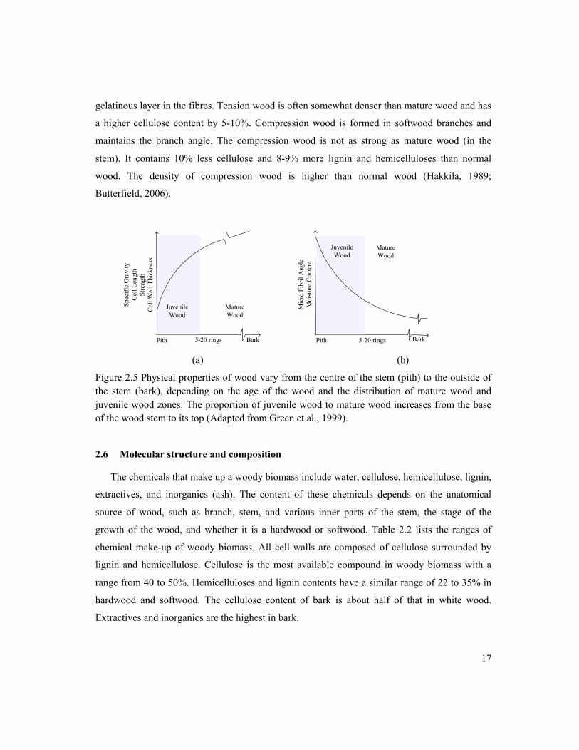
17

gelatinous layer in the fibres. Tension wood is often somewhat denser than mature wood and has

a higher cellulose content by 5-10%. Compression wood is formed in softwood branches and

maintains the branch angle. The compression wood is not as strong as mature wood (in the

stem). It contains 10% less cellulose and 8-9% more lignin and hemicelluloses than normal

wood. The density of compression wood is higher than normal wood (Hakkila, 1989;

Butterfield, 2006).

Juvenile Wood

Juvenile Wood

Mature Wood

Mature Wood

Mic

ro F

ibril

Ang

leM

oist

ure

Con

tent

Spec

ific

Gra

vity

Cel

l Len

gth

Stre

ngth

Cel

l Wal

l Thi

ckne

ss

Pith 5-20 rings BarkPith 5-20 rings Bark (a) (b)

Figure 2.5 Physical properties of wood vary from the centre of the stem (pith) to the outside of the stem (bark), depending on the age of the wood and the distribution of mature wood and juvenile wood zones. The proportion of juvenile wood to mature wood increases from the base of the wood stem to its top (Adapted from Green et al., 1999).

2.6 Molecular structure and composition

The chemicals that make up a woody biomass include water, cellulose, hemicellulose, lignin,

extractives, and inorganics (ash). The content of these chemicals depends on the anatomical

source of wood, such as branch, stem, and various inner parts of the stem, the stage of the

growth of the wood, and whether it is a hardwood or softwood. Table 2.2 lists the ranges of

chemical make-up of woody biomass. All cell walls are composed of cellulose surrounded by

lignin and hemicellulose. Cellulose is the most available compound in woody biomass with a

range from 40 to 50%. Hemicelluloses and lignin contents have a similar range of 22 to 35% in

hardwood and softwood. The cellulose content of bark is about half of that in white wood.

Extractives and inorganics are the highest in bark.

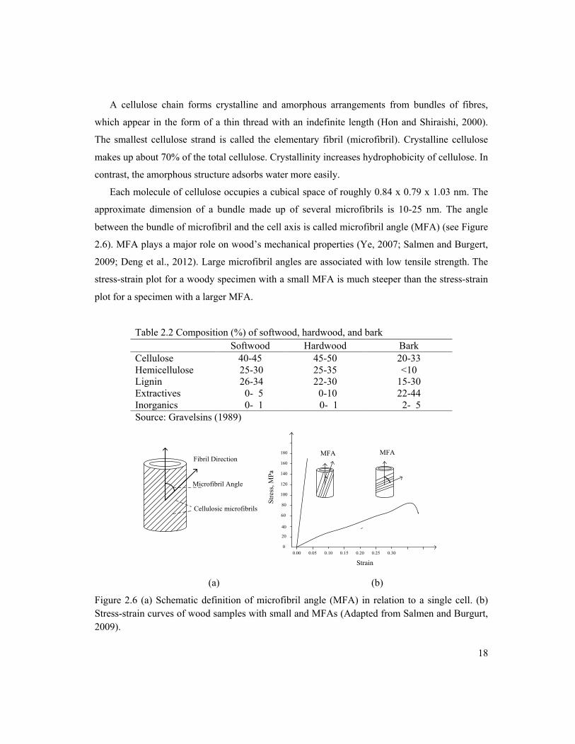
18

A cellulose chain forms crystalline and amorphous arrangements from bundles of fibres,

which appear in the form of a thin thread with an indefinite length (Hon and Shiraishi, 2000).

The smallest cellulose strand is called the elementary fibril (microfibril). Crystalline cellulose

makes up about 70% of the total cellulose. Crystallinity increases hydrophobicity of cellulose. In

contrast, the amorphous structure adsorbs water more easily.

Each molecule of cellulose occupies a cubical space of roughly 0.84 x 0.79 x 1.03 nm. The

approximate dimension of a bundle made up of several microfibrils is 10-25 nm. The angle

between the bundle of microfibril and the cell axis is called microfibril angle (MFA) (see Figure

2.6). MFA plays a major role on wood’s mechanical properties (Ye, 2007; Salmen and Burgert,

2009; Deng et al., 2012). Large microfibril angles are associated with low tensile strength. The

stress-strain plot for a woody specimen with a small MFA is much steeper than the stress-strain

plot for a specimen with a larger MFA.

Table 2.2 Composition (%) of softwood, hardwood, and bark Softwood Hardwood Bark

Cellulose 40-45 45-50 20-33 Hemicellulose 25-30 25-35 <10 Lignin 26-34 22-30 15-30 Extractives 0- 5 0-10 22-44 Inorganics 0- 1 0- 1 2- 5 Source: Gravelsins (1989)

Fibril Direction

Microfibril Angle

Cellulosic microfibrils

20

MFA MFA

40

60

80

100

120

140

160

180

Stre

ss, M

Pa

00.00 0.05 0.10 0.15 0.20 0.25 0.30

Strain (a) (b)

Figure 2.6 (a) Schematic definition of microfibril angle (MFA) in relation to a single cell. (b) Stress-strain curves of wood samples with small and MFAs (Adapted from Salmen and Burgurt, 2009).

19

Hemicelluloses are low molecular weight branched polysaccharides consisting of monomers

like xylose, mannose, glucose, galactose, arabinose, galacturonic acid, and 4-O-

methylglucutronic acid (Kettunen, 2006). Mannose (6 carbon sugar) is the most common sugar

monomer in softwood; xylose (5 carbon sugar) is more prevalent in hardwood. Hemicelluloses

have a larger fraction of amorphous structure than crystalline structure. Hemicelluloses also have

a lower degree of polymerization (DP=50-300) than celluloses (Kollmann and Cote, 1968;

Pettersen, 1984; Kettunen, 2006). Hemicelluloses help strengthen the cell wall through their

interaction with cellulose and lignin (Scheller and Ulvskov, 2010). Zhang et al. (2013) removed

hemicelluloses from a substrate of wood using successive treatments with NaOH and observed a

decreasing trend in the tensile strength of the wood fibres.

Lignin is a three-dimensional molecule composed of phenylpropane units, and is a

completely amorphous material. Lignin acts as glue between macrofibrils as well as between cell

walls, protects the cellulose and hemicelluloses from the detrimental influence of water (Pandey,

1999; Kettunen, 2006) and contributes to the mechanical strength of trees (Novaes et al., 2010).

Gindl and Teischinger (2002) showed that cell wall compression strength increases with the

increase in lignin content, and this relationship is strong in developing wood but weak in mature

wood.

Other components that are not considered as part of the structural backbone of wood are

proteins, starch, and pectins. Additionally, a series of low molecular substances can be extracted

from a cellulosic biomass that constitute up to 10% of the mass of the wood. These extractives

include phenolic compounds, terpenes, fatty acids and alcohols (Gravelsins, 1989). These

compounds, in the form of oils and resins, often interfere with size reduction. Inorganic elements

such as calcium, potassium, magnesium, and other elements make up the ash content of biomass.

The oxides of these salts, such as silicates, dull knives and sharp edges within the grinding

equipment.

The ash content of biomass is an important factor when the biomass is used as fuel for

combustion. Low ash biomass is preferred (Obernberger and Thek, 2010; Baxter et al., 2012) for

residential pellets because when such low ash pellets are used the ash box of wood stoves

require a less frequent emptying. High ash content also increases the possibility of slag and

deposit formation in combustion chambers and heat exchanger surfaces, and high ash content

20

fuels generate greater particulate matter emissions during combustion. The ash content level of

pellets determines the grade of the resulting wood pellets according to EN 14961-2 (2011),

which lists the ash content <0.7% for EN-Plus A1, ash content <1.5% for EN-Plus A2, and <3%

for EN-Plus B grades.

2.7 Mechanical properties

Density, MFA (microfibril angle) and chemical constituents are basic properties of the cell

wall that affects its mechanical strength. Aguilera and Meausoone (2012) listed density,

moisture content, fibre direction, and resin pockets as factors affecting the cutting energy of a

piece of wood. Mansfield et al. (2007) showed a strong dependency of modulus of elasticity on

density, moisture content, and MFA for western hemlock. Bjurhager et al. (2010) observed that

the stiffness of wood decreased due to a decrease in density. The changes in tensile properties of

wood are minor in the axial direction.

The most important mechanical properties that affect grinding performance are those

properties associated with the shear and fracture of the tissue. Because wood is orthotropic —i.e.

its properties are unique in three perpendicular directions— at least 12 constants are used to

describe the elastic properties of a wood specimen (Allen, 1988). Plastic properties are related

to conditions under which stretched or pressed wood does not regain its original shape or size.

The mechanical properties of wood are strongly linked to the orientation of its fibres, the angle

between the fibre orientation and the applied compression or tensile stress (Nielsen et al., 2009).

During plant development the long cells (tracheid) make enzymes that produce lignin, which

imparts rigidity to cell walls. The collenchyma cell, in contrast, makes enzymes that produce

pectins, which impart plastic properties to the cell wall (Raven et al., 2013).

Maiti et al. (1984) studied the mechanical properties of cellular solids such as wood, as a

function of density. Relative density, which is defined as the density of wood species divided by

the density of its cell wall material, is the most important feature of a cellular solid (Gibson and

Ashby, 1988). They concluded that the mechanical properties of a cellular solid are related to the

mechanics of buckling, bending, plastic collapse and brittle fracture of its cell walls. They also

showed that when wood was compressed, it showed a stress-strain curve with three parts: a

linear elastic part, a long plateau, and a regime of final densification.

21

According to Smith et al. (2003) fractures in wood are due to stresses before, during, and/or

after harvesting and processing. These stresses create cracks ranging from micro to macro scales.

Smith et al. (2003) believed that cracks or defects appear in all pieces of wood no matter how

clear they are. Cracks will eventually appear when magnification increases. Cracks grow in

length and create new surface areas by penetrating inside the particles (Recho, 2012). Menacho

(1985) described the size reduction of ores as a combination of fracture and abrasion. During

fracture a piece of ore breaks into smaller pieces of a wide distribution of sizes, whereas during

abrasion fine particles are broken from the surface with a narrow distribution of very small sizes.

These mechanisms of size reduction are the basis of models proposed to describe size reduction

in the following section.

2.8 Modeling of energy/power input

A size reduction operation subjects a solid material to an array of mechanical forces. The

resulting interactions can be shear, impact, compression, tension, flexural (twist), and friction, or

any combination that causes biomass to disintegrate. A number of well-regarded publications

and engineering practice handbooks (Earle and Earle, 1983, Perry et al., 1997) suggest Equation

2.6 as a general relationship for relating energy input to particle size reduction ratio:

2.6

In Equation 2.6, dE is the differential energy input in J g-1, L is a characteristic particle size,

K is the scale factor, and n is a constant whose value depends on the mode of particle

disintegration. The following paragraphs describe the three main theories that have been used to

assign a value to the constant n.

2.8.1 Rittinger Theory

The Rittinger theory was introduced in 1867 (Bond, 1952, 1961). This theory hypothesizes

that the work done for grinding and crushing is directly proportional to the new surface area

created. The theory assumes that the energy input is completely consumed for the creation of the

new surface area of the ground particles. According to Rittinger theory, n=2. Integration of

Equation 2.6 then yields:

ndLdE KL

= −

22

2.7

In Equation 2.7, Lp and LF are the representative size of product particles and feed particles in

mm, respectively. KR (J mm g-1) is the Rittinger constant. Tests performed by Austin and

Klimple (1964) showed that Rittinger’s assumptions are too simplified (Earle and Earle, 1983).

The fraction of energy consumed for the creation of new surface areas varies depending on

grinder configuration and operating conditions.

2.8.2 Kick’s Theory

Kick’s theory was introduced in 1885 (Bond, 1961). Kick assumed that the energy required

to reduce particles of the initial dimension LF, was directly proportional to the ratio dL/L. dL is

the change in a size (dimension) and n = 1. Integration of Equation 2.6 then yields:

2.8

KK (J g-1) is Kick’s constant; LP and LF are average product particle size and feed particle

sizes, respectively. The Kick theory assumes that compression or tension forces cause the

particle breakage (Bond, 1952).

2.8.3 Bond Theory

Bond (1952, 1961) introduced a third theory for which energy input was assumed to be

proportional to the new crack tip length produced in particles (cracks first appear on the surface

then penetrate into the volume). For Bond’s theory n=1.5 and the integration of Equation 2.6

yields:

2.9

For Equation 2.9, LP and LF are in mm. KB (J mm0.5 g-1) is the energy required to reduce the

unit mass of the solid material from an infinitely large particle down to a particle size of 100 µm

(Earle and Earle, 1983). In Bond’s equation, LF and LP refer to the screen size of the sieve

through which 80% of the particles pass.

E = KR1LP

−1LF

"

#$

%

&'

E = KK lnLFLP

E = KB1LP0.5 −

1LF0.5

"

#$

%

&'

23

Thomas and Filippov (1999) recommended Kick’s equation for particles with L > 50 mm,

Bond’s equation for particles of 50 mm >L> 0.05 mm and Rittinger’s equation for particles with

L< 0.05 mm. L is the size of particles after grinder.

2.8.4 Empirical equations

Mani et al. (2004) studied the energy consumption required to grind corn stover, switchgrass,

and wheat straw in a hammer mill with screen sizes of 3.2, 1.6, and 0.8 mm. The initial MC of

the test material was adjusted to 8% and 12% (wb). They fitted a straight line and a second order

polynomial to the data,

2.10

2.11

E is the specific energy (kWh t-1) and S is the hammer mill screen size (mm). The straight line

(Equation 2.10) fits the experimental data for 8% MC (wb) samples while the second order

Equation 2.11 fit the data for 12% MC samples.

Bitra et al. (2009) measured the energy consumption for grinding switchgrass, wheat straw,

and corn stover using a hammer mill equipped with a 3.2 mm screen. They distinguished

between the total and specific energy, with the difference being the parasitic energy for no-load

operation. The geometric mean diameter prior to grinding was 8.3, 7.1, and 5.3 mm for

switchgrass, wheat straw, and corn stover, respectively. Biomass was fed into the hammer mill

continuously with a feeding rate of 41.7 g s-1. Bitra et al. (2009) proposed the following equation

to fit their data,

; K=f(N) 2.12

where E is the specific energy (MJ Mg-1) consumption of the hammer mill. Δdgw is a unit size

reduction (mm) defined as the difference in geometric mean “diameter” caused by size

reduction. K is a function of the speed of rotation of the rotor, N (rpm).

Adapa et al. (2011) studied the grinding performance of barley straw, canola straw, oat

straw, and wheat straw. They prepared the chopped samples using a bale chopper. The chopped

biomass was ground in the first hammer mill with a 30 mm screen and the second hammer mill

with 6.4, 3.2, and 1.6 mm screen. They proposed the following equation,

E = k1 + k2S

E = k1 + k2S + k3S2

E = KΔdgw

24

2.13

where E is the specific energy (kWh t-1), S is the hammer mill screen size (mm), k1 and k2 are

constants. k2 is reported to have a range from 0.69 for oat straw (which is close to the Bond

theory) to 1.12 for canola straw (which is close to the Rittinger theory). It should be noted that

screen size is the independent variable in Equation 2.13 whereas in the three mechanistic

models, size reduction ratio is used as the independent variable.

Miao et al. (2011) experimented with a number of biomass species, biomass moisture

content, mill screen sizes, and particle geometric lengths. The biomass species included three-

year-old miscanthus, switchgrass, energy cane, and willow tree trunks harvested from 30-year-

old trees. The grinder was a knife mill (Retsch SK100, Retsch Inc., Newtown, Pa.) equipped

with screens ranging from 1 to 10 mm. They developed an equation describing the relationship

between energy input and a particle size parameter:

E = aSb 2.14

where E is defined as the specific comminution energy (J g-1), S is either the size of the opening

of the grinder screens (mm), or geometric mean diameter (mm). The constants a and b are

regression constants with b ranging from -1.10 to -1.33 when S is the opening of the grinder

screen (which is close to Rittinger theory). The coefficient of determination ranged from 0.96 to

0.99 among crops, size of screens, and moisture levels (15% and air dried 7%).

Dooley et al. (2011) described the fundamentals of failure for wood materials in order to

develop a mathematical model on crushing forces exerted by a round roller acting onto a round

log. Their hypothesis was that crushing or roller-splitting is a low-energy process to reduce the

thickness of round logs. Modes of failure during crushing suggest that a mathematical model

could be developed to estimate required crushing forces and energy for round logs. Their

(Dooley et al., 2011) crushing system was a roller pressing onto a log. They used an analogy

with a rotating wheel on soft soil to analyze the forces and compute the compression forces and

rolling resistance. The model was experimentally validated for a 400 mm roller crushing a 200

mm log.

Stokes et al. (1987) found that the power requirement for a chipper increases with an increase

in the diameter at breast height of the tree and number of stems fed to the chipper,

21kE k S−=

25

SN*DBH126.0DBH875.045.1P ++= 2.15

where P is power (kW), DBH is the stem diameter at breast height (cm), and NS is the number

of stems fed to the chipper (at once). Equation 2.15 is fitted to their data with a coefficient of

determination (R2) of 0.7.

The limited published literature shows that, to date, equations developed to predict energy

input to grind cellulosic biomass are simple, but entirely empirical. Little evidence is available to

show that the grinding of biomass has been studied from the perspective of fundamental

machine-plant interactions. The three grinding equations of Rittinger, Kick, and Bond have

built-in fundamental mechanisms, but the value of constant K for each of the three equations

depends on experimental data.

Temmerman et al. (2013) studied grinding wood chips of two softwoods (pine and spruce)

and two hardwoods (oak and beech) with five levels of moisture contents using a hammer mill.

They used the median size of particles as the representative mean size of particles and recorded

the grinding energy consumption. Their results showed that the Rittinger equation was the best

fitted equation to the data of size and specific energy consumption among the three equations of

Rittinger, Kick, and Bond.

2.9 Biomass pelletization

Wood pellet production in North America started in the mid-1970s, and later spread to

Europe and other parts of the world (Vinterback, 2004). Pelletization increases the bulk density

of biomass. Thek and Obernberger (2004) reported that the bulk density of sawdust increased

from 120 kg m-3 (db) to 610 kg m-3 (wb) when pelletized. The bulk density of wood pellets

produced in Canada routinely exceeds 750 kg m-3 (Tumuluru et al., 2010). The particle density

of individual pellets ranges from 1030-1300 kg m-3. Though denser pellets reduce the cost of

transport and storage, the increased density may increase the burn time during combustion

(Obernberger and Thek, 2004) or the breakup time during pellet hydrolysis (Tooyserkani et al.,

2012).

Recent years have seen a reduction in housing markets in North America. Meanwhile, the

capacity of wood pellet plants has been increasing. As a result, the source of raw material for

making pellets has been shifting from sawdust to logging and hog type residues. Unlike sawdust

and shavings, hogged residues contain considerable bark and other impurities. The physical and

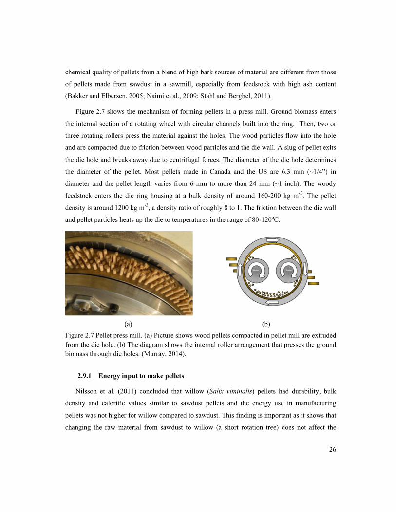
26

chemical quality of pellets from a blend of high bark sources of material are different from those

of pellets made from sawdust in a sawmill, especially from feedstock with high ash content

(Bakker and Elbersen, 2005; Naimi et al., 2009; Stahl and Berghel, 2011).

Figure 2.7 shows the mechanism of forming pellets in a press mill. Ground biomass enters

the internal section of a rotating wheel with circular channels built into the ring. Then, two or

three rotating rollers press the material against the holes. The wood particles flow into the hole

and are compacted due to friction between wood particles and the die wall. A slug of pellet exits

the die hole and breaks away due to centrifugal forces. The diameter of the die hole determines

the diameter of the pellet. Most pellets made in Canada and the US are 6.3 mm (~1/4”) in

diameter and the pellet length varies from 6 mm to more than 24 mm (~1 inch). The woody

feedstock enters the die ring housing at a bulk density of around 160-200 kg m-3. The pellet

density is around 1200 kg m-3, a density ratio of roughly 8 to 1. The friction between the die wall

and pellet particles heats up the die to temperatures in the range of 80-120oC.

(a) (b)

Figure 2.7 Pellet press mill. (a) Picture shows wood pellets compacted in pellet mill are extruded from the die hole. (b) The diagram shows the internal roller arrangement that presses the ground biomass through die holes. (Murray, 2014).

2.9.1 Energy input to make pellets

Nilsson et al. (2011) concluded that willow (Salix viminalis) pellets had durability, bulk

density and calorific values similar to sawdust pellets and the energy use in manufacturing

pellets was not higher for willow compared to sawdust. This finding is important as it shows that

changing the raw material from sawdust to willow (a short rotation tree) does not affect the

27

pellet characteristics and pelletization energy consumption. Stelte et al. (2011) studied the

pelletization characteristics of beech (hardwood) and spruce (softwood), with particle sizes,

between 1 to 3 mm and a MC of 10%. They used a single pellet press to produce pellets of 7.8

mm in diameter. The process was performed stepwise; the biomass was loaded portion by

portion in an amount of less than 0.25 g each time into the die, the compression rate was 2 mm s-

1, the maximum pressure was 200 MPa, and the hold time was 5 s. The biomass was loaded until

the pellet reached a length of 16 mm. Two die temperatures of 20oC and 100oC were tested. The

results showed that pellets made with a higher temperature had a higher mechanical strength. At

a temperature of 100°C, the pellets produced from beech needed a higher force to break in

comparison to pellets made from spruce. Kaliyan and Morey (2009) recommended that a

hammer mill screen size of 2.4-3.2 mm is suitable for the production of pellets with high

durability.

Table 2.3 summarizes the results of previous studies on individual pellet densities from

laboratory, semi industrial, and single pellet presses. The individual pellet density from the

single pellet press ranges from 0.8 to 1.5 g cm-3 (800 to 1500 kg m-3), while the pellet density

ranges from 0.6-1.38 g cm-3 (600 to 1380 kg m-3) for agricultural biomass. The wide range in

density for individual pellets is due to varying compressive forces, the rate of compression, die

temperature, and particle sizes that recur during industrial pelletization.

2.9.2 Measuring energy input to make pellets

Pelletization consists of packing ground biomass particles into a small channel. At high

pressures, the particles interlock and bond together to form a solid pellet. Mani et al. (2006),

Tooyserkani et al. (2012) and Lam et al. (2014) used a single pellet unit to measure the force

required to make wood pellets. A known mass of ground biomass is placed in the cylinder and

the force and position (displacement) of the piston are recorded as the piston compacts the

ground material. The area under the force-displacement curve gives the energy used to make the

single pellet. This integration can be done numerically if the force displacement data is

available.

28

2.10 Concluding remarks

The reviewed literature revealed that the topic of size reduction of biomass has not yet been well

researched. Mechanical size reduction is a complex combination of many types of mechanical

forces involving different material failure modes. The macro and microstructures of wood vary

with tree species, tree age, whether the wood is from stems or branches, moisture, and ash

content. Age is the primary factor in determining the strength of wood. It is not difficult for one

to determine the age of the tree based on the history of the stand. However factors such as

moisture content and density are more significant when predicting the strength of wood. The age

is not an indication of density and moisture content, which are dependent on the growth

conditions.

No relationships between the microstructure properties of wood and energy input for size

reduction have been published. The interaction of a size reduction operation with the material

properties of wood will have far reaching effects on predicting the scale and power input of the

size reduction equipment.

The equations developed to estimate power input for creating a given size reduction ratio are

all empirical and, thus, specific to a specific type of biomass and a specific type of grinder. The

three popular mechanistic equations of Rittinger, Kick and Bond have been used in the chemical

(mineral) industry. No literature was found on evaluating the applicability of these three

equations to fibrous lingo-cellulosic materials. These equations have been developed based on

observed and/or proposed cracking mechanisms of size reduction and, thus, have a potential to

be generalized for grinding of all biomass materials. The equations for estimating power input

for pelletization are empirical and semi-empirical, with constants being extracted from

regression of experimental data.

29

Table 2.3 Summary of the previous studies on single pellet density of laboratory, semi industrial, and single pellet presses.

Researchers Feedstock materials Approach – Test parameters Effects – Results Mani et al. (2006) Wheat straw, barley straw, corn

stover, and switchgrass Grinding screen: 3.2, 1.6, and 0.8 mm MC: 12 and 15% wb Compressive force: 1000, 2000, 3000, 4000, and 4400 N

Density of pellets: maximum for corn stover 1399 kg m-3 and minimum for barley straw 887.34 kg m-3

Rhen et al. (2007)

Norway spruce Stem wood, branch wood and bark had a MC range from 6.9, 8, and 10 wt%, respectively.

Grinding screen: 2 mm The pellet press was a small 50 kg h-1 laboratory press.

Density of pellets: From stem wood (no bark) 1500 kg m-3 From branches 940 kg m-3 From bark 1000 kg m-3 From saw dust similar to stem wood

Bergstrom et al. (2008)

Scot pine sawdust MC: 8.7%

Hammer milled Three narrow size distributions: fine, middle, and coarse prepared plus the original mixed particles as reference, The pellet press was 300 kg h-1 semi-industrial scale; Die preheat temperature: 90 °C;

MC of pellets were 5.8%, Pellet density was maximum for coarse particles, and minimum for middle particles.

Shaw et al. (2009) Poplar and wheat straw Grinding screen: 0.8 and 3.2 mm MC: 9 and 15% The single pellet press was used for pellet production. Force: 4000 N

Maximum pellet density was 1428 kg m-3for 9% MC. Ground on 0.8 mm screen. Minimum density was 1353.08 kg m-3 for 15% MC ground on 3.2 mm screen.

Carone et al. (2011)

Olive tree pruning residue. Grinding screen: 1, 2, and 4 mm; MC: 5, 10, 15, and 20 % wb; A single pellet press unit; Temperature: 60, 90, 120, and 150 °C; Load: 2000, 3000, 4000, and 5000 N.

Density of pellets increased when temperature increased and MC decreased. Particle size and load had minor impact on the pellet density

30

Chapter 3 Experiments

The goal of this research is to develop a mathematical equation for estimating the power

input required for size reduction of cellulosic biomass. To this end, the applicability of three size

reduction equations that are well known in the mineral industry are tested and analyzed for a

number of cellulosic biomass. The analysis requires a good understanding of biomass properties

and their interaction with size reduction equipment.

A series of laboratory grinding tests were planned. The experiments consisted of five

biomass samples, two softwoods (Douglas-fir, Pseudotsuga menziesii, and pine, Pinus contorta)

and three hardwoods (aspen, Populus tremuloides, hybrid poplar which is referred to as poplar

throughout this thesis, and willow). Two grinder types were used to grind the biomass samples: a

knife mill and a hammer mill. The remaining equipment was sieving devices for biomass

fractionation and particle size analysis.

Power input increases as the size of ground particles decreases. It is not clear whether particle

size has any major effect on pelletization. In this research we aimed at measuring the total power

input to a grinding operation followed by a pelletization operation. A single pellet press was used

to make wood pellets from pure and blends of several particle sizes of both softwood and

hardwood. The physical characteristics of raw feedstock and ground materials, as well as

compositional make-up of the material were measured. Table 3.1 summarizes the biomass types,

equipment, and instruments used for the experiments. Chapter 3 explains the details of material,

equipment and instrumentation.

Table 3.1 Summary of materials and grinders used to evaluate the generalized grinding equations Materials Douglas-fir, pine, aspen, poplar, willow Grinding equipment Knife mill, hammer mill Instruments Image processing Fractionation Gilson, Tyler mesh sieves

31

3.1 Equipment

Test equipment consisted of two types of grinders, sieving devices, imaging equipment for

particle size analysis, power transducers, and a data acquisition system. The size reduction

devices used were a knife mill and a hammer mill. Both grinders were of laboratory size located

in the laboratory in Chemical & Biological Engineering Department, University of British

Columbia. The following sections describe equipment and calibrations.

3.1.1 Knife mill

The knife mill was a Retsch mill Model SM100 (Retsch Inc. Newtown, PA) equipped with a

125 mm diameter rotor rotating at 1430 rpm. The cutting action was achieved with three blades

on the rotor and four stationary cutting strips embedded in the periphery of the housing (Figure

3.1 (a)). The internal volume within the mill was approximately 0.0012 m3 (1200 cm3). A

removable perforated screen covered 120 degrees around the lower section of the rotor housing.

Screens with circular perforations are available in the following sizes: 0.25, 0.5, 0.75, 1, 1.5, and

2 mm. Screens with square perforations are available in the following sizes: 2, 4, 6, 8, 10, and

20 mm where size is the side of the square (Figure 3.1 (b)).

(a) (b) Figure 3.1 (a) Inside the knife mill (Retsch grinder SM100). Three cutting blades are attached to the rotor. There are four cutting strips attached to the periphery of the grinding chamber. A curved perforated screen covering 120 degrees of the bottom portion of the housing is installed below the grinding chamber to control the size of ground particles. (b) A number of these screens are shown in the picture (Naimi, 2008).

32

3.1.2 Hammer mill

The hammer mill was a Model 10H MBL Glen mill (GlenMills Inc., Clifton, NJ) (Figure 3.2

(a)) equipped with swing hammers. The rotor is powered by a three phase induction motor

(Model C14ST34FB28D, Leeson Electric) at a speed of 3490 r/min. The rated nameplate power

was 3 hp (2.2 kW). Hammers (12 in total) were placed along a shaft in order to have a hammer at

every 90 degrees. The mill used a removable perforated screen that extended 180 degrees around

the lower section of the housing. Screens with circular perforation of 32, 25.4, 12.7, 10, 6.25,

3.13, 1.56, and 0.78 mm were available to be used in the hammer mill (Figure 3.2 (b)).

(a) (b) Figure 3.2 (a) Glen Mill hammer mill. Twelve swing hammers are placed along a shaft in order to have hammers every 90 degrees. The mill uses a removable perforated screen that extends 180 degrees around the lower section of the housing. (b) A number of these screens are shown in the picture.

3.1.3 Feeders

Each of the grinders was equipped with a vibratory feeder. The vibratory feeder for the

Retsch knife mill was ERIEZ model-15A (Eriez Manufacturing Co., Erie, PA) with a narrow flat

feeder trough, 406 mm long and 51 mm wide. The full load power input to the feeder was 15 W,

115 V, 60 Hz, single phase. The feeder speed was controlled by varying the applied voltage. The

voltage control could be set from 0 to 100%. Maximum vibration when set to 100% was 1000

cycles/s (1 kHz). The vibratory feeder used with hammer mill was also ERIEZ model-15A (Eriez

Manufacturing Co., Erie, PA). The feeder tray was 500 mm long and 110 mm wide. A circular

hopper with a short downspout was used to pour the material into the vibratory tray.

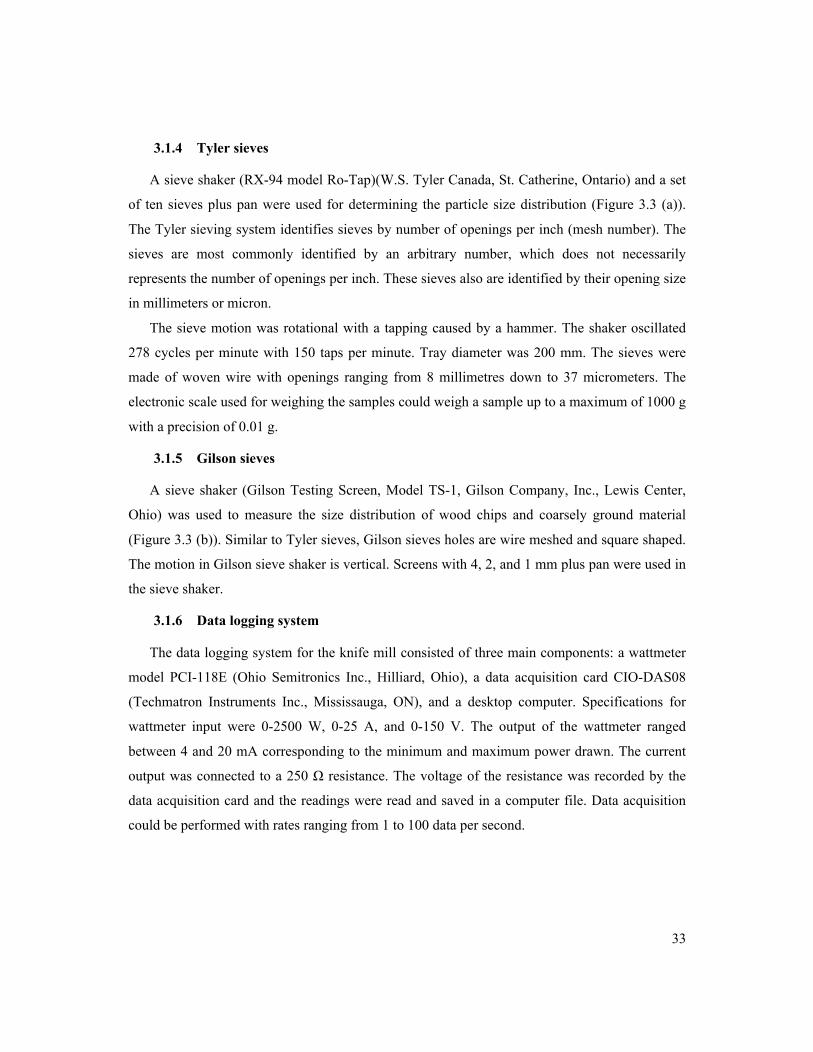
33

3.1.4 Tyler sieves

A sieve shaker (RX-94 model Ro-Tap)(W.S. Tyler Canada, St. Catherine, Ontario) and a set

of ten sieves plus pan were used for determining the particle size distribution (Figure 3.3 (a)).

The Tyler sieving system identifies sieves by number of openings per inch (mesh number). The

sieves are most commonly identified by an arbitrary number, which does not necessarily

represents the number of openings per inch. These sieves also are identified by their opening size

in millimeters or micron.

The sieve motion was rotational with a tapping caused by a hammer. The shaker oscillated

278 cycles per minute with 150 taps per minute. Tray diameter was 200 mm. The sieves were

made of woven wire with openings ranging from 8 millimetres down to 37 micrometers. The

electronic scale used for weighing the samples could weigh a sample up to a maximum of 1000 g

with a precision of 0.01 g.

3.1.5 Gilson sieves

A sieve shaker (Gilson Testing Screen, Model TS-1, Gilson Company, Inc., Lewis Center,

Ohio) was used to measure the size distribution of wood chips and coarsely ground material

(Figure 3.3 (b)). Similar to Tyler sieves, Gilson sieves holes are wire meshed and square shaped.

The motion in Gilson sieve shaker is vertical. Screens with 4, 2, and 1 mm plus pan were used in

the sieve shaker.

3.1.6 Data logging system

The data logging system for the knife mill consisted of three main components: a wattmeter

model PCI-118E (Ohio Semitronics Inc., Hilliard, Ohio), a data acquisition card CIO-DAS08

(Techmatron Instruments Inc., Mississauga, ON), and a desktop computer. Specifications for

wattmeter input were 0-2500 W, 0-25 A, and 0-150 V. The output of the wattmeter ranged

between 4 and 20 mA corresponding to the minimum and maximum power drawn. The current

output was connected to a 250 Ω resistance. The voltage of the resistance was recorded by the

data acquisition card and the readings were read and saved in a computer file. Data acquisition

could be performed with rates ranging from 1 to 100 data per second.

34

(a)

(b)

Figure 3.3 Sieving system used to fractionate biomass samples. (a) RoTap sieve shaker holds two stacks of five round sieves plus pan. The sieve motion was rotational with a tapping. (b) Gilson sieve shaker holds five rectangular screens. The sieve motion was vertical shake. The screen holes for both sieving systems were wire mesh.

The data logging system for the hammer mill consisted of a three-phase transducer to

transform alternate current and voltage into DC signals. A data acquisition card (PCI DAS-08)

received the instantaneous power consumption in W. Labview 8.2 software (National

Instruments, Austin, Texas, USA) and a desktop computer acquired, stored and displayed the

values. A delay knob on the front panel of the Labview screen controlled the data acquisition

rate. The delay knob could be set at 500, 1000, 1500, or 2000 ms, which meant that the data were

recorded at a rate of 2 Hz, 1 Hz, 0.67 Hz, or 0.5 Hz, respectively.

3.1.7 Single pellet press

Figure 3.4 shows the single pellet press device. It consisted of three parts: a universal testing

machine (MTI-10K, Measurement Technology Inc., Roswell, GA), a pellet press, and a desktop

computer. The single pellet press die system was designed and fabricated in Biomass and

Bioenergy Research Group at UBC. The universal testing machine provided the compressive

force at a constant speed. The upper section of the single pellet press was attached to the base

and the entire device centered under the crosshead of the universal testing machine. The die was

a 200 mm long steel cylinder with an inner diameter of 6.3 mm. A steel rod 150 mm long with

35

6.3 mm diameter compressed the ground biomass in the die. Software connected to the universal

testing machine controlled the force and the rate of force application. Force vs. displacement was

recorded.

(a)

(b)

Figure 3.4 (a) A universal testing machine provides the compression force at a constant rate. (b) The piston-cylinder assembly is used to form pellets.

3.2 Size reduction method

3.2.1 Size reduction with knife mill

Aspen, and poplar samples were in the form of branches. Pine and Douglas-fir samples were

both in chip form and branches (Figure 3.5). Willow samples were in chip form as received. All

branches were debarked by hand using a manual debarker. The debarked branch and the bark

were weighed separately. Bark content percentage (weight by weight percent) was calculated for

each branch. The debarked samples were dried in the oven at 50°C until the sample’s moisture

decreased to 8-10% wb. The debarked dried branches were cut perpendicular to grain direction

to pieces of 3.5 mm thickness using a band saw. Each piece was cut to quarter pieces. Figure 3.6

shows: (a) the debarked branches; and (b) quarter disk pieces.

To feed the quarter disk pieces to the knife mill, three 500 g lots were prepared. Each piece

was fed to the vibratory feeder manually in a way that always there were pieces lined up on the

tray when one piece was falling down into the knife mill.

36

To feed the wood chips to the knife mill, three 500 g lots were prepared. Each 500 g lot was

divided into five 100 g batches. Each 100 g batch was gradually fed to the vibratory feeder

manually through a funnel over 1 min until all five batches were exhausted. Each run took 5 min

to complete.

Douglas-fir Pine

Aspen Poplar

Figure 3.5 Branches of four species of wood as they were received in the lab. The leaves were removed. The branches were cut in length for debarking, drying, and storage.

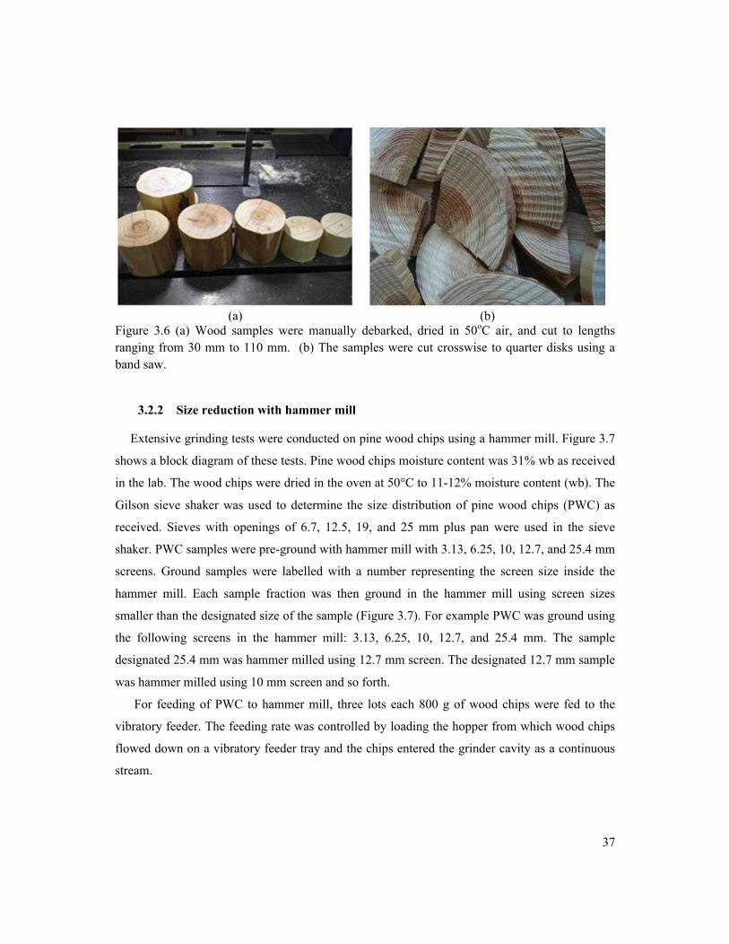
37

(a) (b)

Figure 3.6 (a) Wood samples were manually debarked, dried in 50oC air, and cut to lengths ranging from 30 mm to 110 mm. (b) The samples were cut crosswise to quarter disks using a band saw.

3.2.2 Size reduction with hammer mill

Extensive grinding tests were conducted on pine wood chips using a hammer mill. Figure 3.7

shows a block diagram of these tests. Pine wood chips moisture content was 31% wb as received

in the lab. The wood chips were dried in the oven at 50°C to 11-12% moisture content (wb). The

Gilson sieve shaker was used to determine the size distribution of pine wood chips (PWC) as

received. Sieves with openings of 6.7, 12.5, 19, and 25 mm plus pan were used in the sieve

shaker. PWC samples were pre-ground with hammer mill with 3.13, 6.25, 10, 12.7, and 25.4 mm

screens. Ground samples were labelled with a number representing the screen size inside the

hammer mill. Each sample fraction was then ground in the hammer mill using screen sizes

smaller than the designated size of the sample (Figure 3.7). For example PWC was ground using

the following screens in the hammer mill: 3.13, 6.25, 10, 12.7, and 25.4 mm. The sample

designated 25.4 mm was hammer milled using 12.7 mm screen. The designated 12.7 mm sample

was hammer milled using 10 mm screen and so forth.

For feeding of PWC to hammer mill, three lots each 800 g of wood chips were fed to the

vibratory feeder. The feeding rate was controlled by loading the hopper from which wood chips

flowed down on a vibratory feeder tray and the chips entered the grinder cavity as a continuous

stream.

38

3.2.3 Power measurement

Power consumption for each test run was recorded. The grinder’s power consumption was

calculated by deducting parasitic power input (power while running empty) from total recorded

power. Specific energy consumption was calculated by dividing power input by feeding rate. The

method of measuring power is outlined in Appendix B and in Naimi et al. (2013).

The measured power is used to calculate the specific energy, E, J g-1, for size reduction:

E = P − PEF 3.1

In Equation 3.1, PE, is parasitic power input to the grinder (power consumption of grinder

working empty), J s-1, P is total power consumption of grinding material, J s-1, and F is feeding

rate, g s-1.

Figure 3.7 Hammer mill screen sizes (mm) used for grinding pine wood chips (PWC). Initially, PWC was ground in hammer mill with screen sizes 25.4, 12.7, 10, 6.25, or 3.13 mm screens. The ground particles were labelled with the screen size they were ground with. The five labelled ground particles were then ground using all screen sizes smaller. For example the particles labelled 10 were ground in the hammer mill with 6.25 and 3.13 mm screen sizes.

Pine Wood Chips (PWC)

25.4

12.7

10

6.25

3.13

12.7

10

6.25

3.13

10

6.25

3.13

6.25

3.13

3.13

39

3.3 Biomass properties

3.3.1 Particle density and solid density of wood pieces

Multiple wood density definitions are used in wood science reference books (basic density,

true density, solid density, apparent density, bulk density, to list a few). The term ‘particle

density’ in this thesis refers to the density of a piece of wood calculated from the ratio of mass

over volume of a single piece of wood. In this thesis, height and diameter of each cylindrical

piece was measured using a calliper and the volume of the piece was calculated. Mass of the

particle was measured on a balance. According to Kollmann and Cote (1968), this density is

called physics density where mass and volume are measured at the same moisture content.

To determine solid density of wood pieces, volume of the pieces was measured in a

pycnometer (Quantachrome Instrument, Boynton Beach, FL). A pycnometer employs

Archimedes’ principle of gas displacement. Depending upon the applied gas pressure, the

displacing gas penetrates into the pore spaces of the material to measure the volume of the solid

fraction of material. The unit then gives a measure of the solid fraction of material. The density

is the ratio of mass of the wood to solid volume (as measured in pycnometer). The uncertainty in

solid density is associated with the fact that there would be pores to which the selected gas will

not be able to penetrate into. It should be noted that the solid density would be inherently less

than the term “wood substance density” which is estimated to be at 1500 kg m-3 (Kollmann &

Cote, 1968; Hakkila, 1989; Kettunen, 2006). Porosity of solid pieces is defined as the fraction of

void space in the material,

ϕ sp =1−ρ p

ρs 3.2

In Equation 3.2, ϕsp is porosity of solid pieces (dimensionless), ρp is the particle density (kg

m-3), and ρs is the solid density (kg m-3).

3.3.2 Bulk density and tapped density of ground particles

To determine bulk density, a container with a diameter of 77 mm and a height of 135 mm

was used. The particles were poured into the container until the container was full. The excess

particles on the top of the container were removed by a straight edge. The weight of the

container and particles was recorded on a balance. The weight of empty container was deducted

40

from total weight. Bulk density was calculated using the weight of ground particles divided by

the volume of container.

To determine tapped density, the filled container was tapped down from the height of 50 mm.

Each time the empty volume that was created due to tapping was filled with particles. The

tapping and filling sequence was repeated until there was no empty volume generated due to

tapping. The weight of container was recorded. The tapped density was calculated. Hausner ratio

is defined as the ratio of tapped density over bulk density. The ratio is a measure of the internal

friction condition of moving powder (Grey and Beddow, 1969). A Hausner ratio greater than

1.25 indicates high internal angle of friction and thus a poor flowability for the powder.

To determine solid density of ground particles, a procedure similar to that described in

Section 3.3.1 was used (Lam et al., 2008). The mass of ground sample in the pycnometer cell

was 4-5 grams. Porosity is defined as the fraction of void space in the ground particles,

ϕg=1− ρbulk

ρsolid 3.3

In Equation 3.3, ϕg is porosity (dimensionless), ρbulk is bulk density (kg m-3), and ρsolid is the

solid density (kg m-3).

3.3.3 Angle of repose

Angle of repose is the angle between the side of a pile of material and the horizontal base.

The present research used a device (Figure 3.8) attributed to Geldart et al. (2006) to create a pile

of ground biomass. A sample mass of 100 g of powder was weighed and put in a beaker. The

powder was poured on a vibrating sloped chute that guided the flow to a funnel. Once filled, the

contents of the funnel were released to pour on a graduated board to form a semi-cone. The

height and radius of the semi-cone was read on the unit’s vertical and horizontal scales.

3.3.4 Particle surface area

A scanner and a computer were used to capture images of the particles. Dimensions of the

projected surface area are used to calculate the external surface area of the particles. The external

surface area of the particles is referred to as particle surface area throughout this thesis. ImageJ

software (Rasband, 2004) was used to analyze the images (Appendix A). A representative

sample of approximately 50 g of ground particles was chosen. The particles were spread on an

A4 size transparent sheet on a scanner surface. Prior to scanning, the individual particles were

41

arranged so that they were not touching one another. The particles were arranged manually in

either vertical or horizontal directions using tweezers. The transparent sheet was covered with

black cardboard. The images of the samples were taken by a CanonScan 4400F high-resolution

scanner (Canon, Lake Success, NY) at 300 DPI resolutions. The resulting images were analyzed

by ImageJ software. The particles’ length and width were measured and stored in an Excel file.

The shape of the particles was assumed to be rectangular prism. The thickness of particles was

assumed to be equal to its smaller dimension. Total surface area was calculated by adding the

surface areas of all particles in a sample. Specific surface area was calculated by dividing total

surface area by total mass of sample (m2 kg-1).

Figure 3.8 Device for measuring angle of repose (Geldart et al., 2006). The device consisted of four main parts: a vibrator, a vibrating chute, a funnel, and a measuring baseboard. Particles are loaded on the vibrating chute and pour down into the funnel. Particles form a semi-cone on the measuring baseboard. Height and radius of the semi-cone can be read on the measuring baseboard.

3.4 Biomass composition

3.4.1 Moisture content

Moisture content of the wood was determined gravimetrically using a convection-drying oven

following the ASAE Standard S352.1 (ASAE Standard, 2012). The method consists of placing

pre-weighed sample in the oven. The temperature was set at 103±2ºC for 24 h. The dried sample

was weighed. The moisture content was calculated based on the weight loss of the sample.

Geldart, Abdullah, Hassanpour, Nwoke & Wouters: Characterisation of Powder Flowability

105

Fig. 1 Measurement of static and dynamic angle of repose.

In method I powder is poured into the funnel which is held at a fixed height above the flat base whereas in method II the funnel is filled with the test powder which is then raised gradually to allow the sample to flow out. Both these methods require that the powder should be able to flow through the small funnel, and cohesive powders may not do so. Moreover, the powders do not become aerated as they often do in production processes, unlike methods III and IV in which some ambient gas is entrained during the test. In none of these methods is it easy to measure the angle accurately. Methods III and IV require equipment that must be mounted on a shaft passing through a low friction bearing so that it can be tilted gradually until slipping oc-curs and the angle measured. The shaft and bearing often needs to be dismantled for thorough cleaning between tests, an inconvenience that slows down the testing pro-cedure.

By working closely with a large UK chemical company, Professor Geldart and his research students at the univer-sity of Bradford developed a piece of equipment in which the powder is made to flow so that it forms a semi-cone whose height and average radius are easy to measure and from which the dynamic AOR can be readily calculated or read from a table. The equipment has passed through several stages of development and comparison of ex-perimental values of AOR with practical experience on operating a large soda ash plant has confirmed it as a reliable device that is robust and easy to use even for co-hesive powders using quite small samples of powder. A picture of the Mark 4 (most recent version) of the tester is shown in Fig. 2. A representative sample of the powder to be tested (100 grams is the preferred mass) is weighed out +/- 1 g and put into a metal beaker. If the powder appears to be free-flowing, the 100 g sample is poured slowly and gently on to the upper converging chute, taking about 20 sec for the entire sample. If the powder shows signs of cohesiveness or reluctance to flow, the vibratory motor is switched on so that the powder flows down the upper chute, into the metal hopper and onto the lower sloping chute that directs the powder against the vertical wall. The powder should not be allowed to accumulate in the hopper, espe-

cially if it exhibits some cohesiveness. The semi-cone formed should have a well-defined, sharp apex, but some-times, if the pouring has been done too quickly, a distinct semi-cone may not be formed, because the apex may be ‘ragged’ making an accurate reading of the height of the semi-cone impossible, in which case that test should be repeated with the pouring done more slowly.

vibrating chute

funnel

chute

baseboard

backplate

vibrator

Fig. 2 Mark 4 Powder Research Ltd. AOR tester.

Another commonly used simple method for characteris-ing powders that are cohesive or semi-cohesive should be mentioned, the Hausner Ratio (Grey & Beddow, 1969) in which the tapped and aerated bulk densities are measured and the former is divided by the latter. It turns out that there is a good correlation between AOR and HR as shown later.

3. Materials Used Two types of powders have been used in some of our

recent work: spherical and porous Fluid Cracking Catalyst (FCC) (Fig. 3), and angular and non-porous aluminum oxide trihydrate (Fig. 4) used as a Fire Retardant Filler (FRF). Graded powder mixtures were tested for both powders. In order to form a series of powder samples having different mean particle sizes, small amounts of cohesive fine 7-micron particles were added in increments to a coarser 79-micron FCC and 63-micron FRF which were used as base materials to form mixtures having mass

Geldart, Abdullah, Hassanpour, Nwoke & Wouters: Characterisation of Powder Flowability

105

Fig. 1 Measurement of static and dynamic angle of repose.

In method I powder is poured into the funnel which is held at a fixed height above the flat base whereas in method II the funnel is filled with the test powder which is then raised gradually to allow the sample to flow out. Both these methods require that the powder should be able to flow through the small funnel, and cohesive powders may not do so. Moreover, the powders do not become aerated as they often do in production processes, unlike methods III and IV in which some ambient gas is entrained during the test. In none of these methods is it easy to measure the angle accurately. Methods III and IV require equipment that must be mounted on a shaft passing through a low friction bearing so that it can be tilted gradually until slipping oc-curs and the angle measured. The shaft and bearing often needs to be dismantled for thorough cleaning between tests, an inconvenience that slows down the testing pro-cedure.

By working closely with a large UK chemical company, Professor Geldart and his research students at the univer-sity of Bradford developed a piece of equipment in which the powder is made to flow so that it forms a semi-cone whose height and average radius are easy to measure and from which the dynamic AOR can be readily calculated or read from a table. The equipment has passed through several stages of development and comparison of ex-perimental values of AOR with practical experience on operating a large soda ash plant has confirmed it as a reliable device that is robust and easy to use even for co-hesive powders using quite small samples of powder. A picture of the Mark 4 (most recent version) of the tester is shown in Fig. 2. A representative sample of the powder to be tested (100 grams is the preferred mass) is weighed out +/- 1 g and put into a metal beaker. If the powder appears to be free-flowing, the 100 g sample is poured slowly and gently on to the upper converging chute, taking about 20 sec for the entire sample. If the powder shows signs of cohesiveness or reluctance to flow, the vibratory motor is switched on so that the powder flows down the upper chute, into the metal hopper and onto the lower sloping chute that directs the powder against the vertical wall. The powder should not be allowed to accumulate in the hopper, espe-

cially if it exhibits some cohesiveness. The semi-cone formed should have a well-defined, sharp apex, but some-times, if the pouring has been done too quickly, a distinct semi-cone may not be formed, because the apex may be ‘ragged’ making an accurate reading of the height of the semi-cone impossible, in which case that test should be repeated with the pouring done more slowly.

vibrating chute

funnel

chute

baseboard

backplate

vibrator

Fig. 2 Mark 4 Powder Research Ltd. AOR tester.

Another commonly used simple method for characteris-ing powders that are cohesive or semi-cohesive should be mentioned, the Hausner Ratio (Grey & Beddow, 1969) in which the tapped and aerated bulk densities are measured and the former is divided by the latter. It turns out that there is a good correlation between AOR and HR as shown later.

3. Materials Used Two types of powders have been used in some of our

recent work: spherical and porous Fluid Cracking Catalyst (FCC) (Fig. 3), and angular and non-porous aluminum oxide trihydrate (Fig. 4) used as a Fire Retardant Filler (FRF). Graded powder mixtures were tested for both powders. In order to form a series of powder samples having different mean particle sizes, small amounts of cohesive fine 7-micron particles were added in increments to a coarser 79-micron FCC and 63-micron FRF which were used as base materials to form mixtures having mass

42

3.4.2 Ash content

A representative sample of ground particles was dried 24 h in Precision Thelco oven (Mandel

Scientific Company Inc., Guelph, ON). Ash content was measured with a programmable oven

based on an oven setting procedure listed in NREL Standard NREL/TP-510-42622 (Sluiter et al.,

2008a). The oven temperature is set to 575°C. It is held at 575°C for 3 hours and then lowered to

105°C. Ash content measurements were repeated for each sample at least three times.

3.4.3 Chemical composition

A representative sample of 100 g was chosen from each species of wood. The sample was

ground using a Wiley mill (Thomas Model 4 Wiley Mill, Swedesboro, NJ) equipped with a 2

mm screen. Three replicates of 2 to 4 g of air-dried sample were weighed. The acetone-soluble

non-volatile material in the sample was removed by extraction using NREL (Sluiter et al.,

2008b) and TAPPI T 280 pm-99 (TAPPI, 1999). The extracted substrates were used for chemical

analysis. Acid insoluble residue was evaluated based on ASTM E1721-01 (2009). Chemical

analysis of the wood was performed based on Sluiter et al. (2011) and ASTM standard E1758-01

(2007).

3.5 Wood microstructure

SilviScan tests and Fibre Quality Analysis tests were performed at the PFInnovations

ValueTree Laboratory located on the campus of UBC in Vancouver. A FPInnovation technician

conducted the tests. The technician provided the text describing test procedures. It is assumed the

ValueTree program uses accepted and established procedures for evaluating the properties of

biomass samples.

3.5.1 SilviScan analysis

SilviScan comprises of a group of instruments used to measure the characteristics of wood

(Lawrence and Woo, 2005). The system was first developed by Evans et al. (1995) to investigate

differences among species and to identify genetic parameters (Evans et. al., 2000). SilviScan

combines three techniques: X-ray densitometry, X-ray diffraction, and image analysis (Chen and

Evans, 2010). Image analysis of fibre cross-sections is performed by X-ray absorption and X-ray

diffraction (Lundqvist et al., 2007). A cell scanner with a video microscope is used for collecting

43

information on the numbers and sizes of fibres and vessels, as well as orientations of annual

rings. X-ray absorption images provide information about wood density. X-ray diffraction

images provide information about the orientations of microfibrils in the wood matrix. MFA

measurement requires fibres to be perpendicular to the X-ray beam. In this system the sample

rotates around the beam direction and the diffraction pattern is recorded. As a result there is no

need for adjusting the orientation of the sample.

Jayawickrama (2001) and Lindstrom et al. (2004) studied the suitability of wood for sawn

products in relation to stiffness using SilviScan. SilviScan was also used to prove that properties

like wood density, MFA, fibre angle, and their variations within stems may have crucial role on

drying (Ball et al., 2005).

Pieces of 80 to 100 mm thickness were cut from the branches with a band saw. These pieces

were delivered to the SilviScan laboratory. The technical staff who conducted experiments

executed the following procedure. The pieces were cut to smaller sizes of 1 to 1.8 cm (10 to 18

mm) longitudinally and 1 to 1.8 cm (10 to 18 mm) tangentially. The cut pieces were pre-soaked

in water overnight. The soaked pieces of softwood were extracted with acetone; soaked pieces of

hardwood were dehydrated by alcohol. The extraction was continued for at least 6 hours in order

to remove extractives. The extracted pieces were cut in 2 mm thickness using a twin blade saw.

The cut pieces were polished and mounted on wooden sample holders using glue. The pieces

were exposed to X-ray for every 500 µm intervals and with a 30 s exposure time. Diffraction

patterns were recorded on a rotating copper anode. The output of this SilviScan analysis

provided data on local density and MFA from pith to bark.

3.5.2 Fibre quality

Fibre quality analysis consists of determining fibre length and fibre coarseness. For these

tests, biomass samples were shredded. A band saw was used to cut a piece of wood

approximately 15 mm thick, 15 mm wide, and 60-70 mm long. The pieces were oven dried. The

weights of oven-dried pieces were recorded. The dried pieces were placed in test tubes filled

with deionized water. The tubes were covered with aluminum foil and placed in a hot bath at

120°C. The tubes were boiled for 4 h or until the pieces sunk to the bottom of the tubes. The

water was let to cool down to 70oC.

44

Water was removed from tubes making sure that no solid material was lost. Maceration

consisted of removing extractives and pulping of wood. Maceration solution consisted of a 1:1

ratio of Glacial acetic acid and 35% hydrogen peroxide technical grade. The solution was added

to the tubes and covered with aluminum foil. The tubes were placed in a 70˚C bath for 48 h. The

tubes were checked occasionally to make sure that the pulping process was in progress. After 48

hours the chemicals were removed from the tubes. The fibres were washed with deionized water

2-3 times to make sure that the chemicals were completely removed.

The solid fraction was removed from the tube and poured into a tin blending-cup. Three-

quarter of the cup was filled with deionized water and samples were mixed for three minutes at a

slow to moderate speed until the fibres were completely separated. The mixture was poured on a

150-mesh screen, and then washed with deionized water by squeezing the hose and spraying the

pulp to remove any debris. The process of washing was repeated several times.

The water was squeezed out of the sample by a small screen vacuum. The pulp samples were

placed in aluminium weighing dishes to dry at room temperature for 1-2 days. The dried weight

was recorded. A sample of 30 mg for softwood or 15 mg for hardwood was weighed. A volume

of 5-10 ml of water was added to the pulp and let to soak for 4 h. The mixture was then diluted

by adding water to make 4 L in volume. The solution was mixed to reach to equal consistency.

Three samples of 600 ml of the mixed solution were separated and weighed. The FQA fibre

frequency of 20-40 EPS (Events Per Second) was used for hardwoods and 10-20 EPS for

softwoods (Woo, 2012). FQA software reports the length weighted fibre length and fibre

coarseness of the samples and their standard deviations. Length weighted average fibre length is

calculated as the sum of individual fibre lengths squared divided by the sum of the individual

fibre lengths. Fibre coarseness is a measure of milligrams of fibre per meter of fibre length.

3.6 Pelletization

Pelletization was carried in the single pellet press connected to the universal testing machine

as shown in Figure 3.4. The die of the single pellet unit was rinsed with acetone to remove any

possible contaminant (Woehler, 2011). The entire upper section consisting of the plate and the

piston was removed. The die temperature was set to 80°C by adjusting the current through the

electrical heater wrapped around the die. A metal piece that fitted underneath the die hole

blocked the bottom of the die. The die was filled with approximately 0.7 g of ground material.

45

The upper section of the pellet press was attached to the base of the upper plate and the entire

device centered under the crosshead of the universal testing machine. The crosshead moved

downward with a velocity of 10 mm min-1. The loading of the particles was stopped when the

maximum force of 5000 N was achieved. The force was held for 30 s. The load (force) vs.

displacement was recorded for the pelletization system working empty. The test with the die

filled with the sample was identical to the test with empty die. The test was repeated three times

on three sub lots from each batch. The formed pellet was placed in a sealed glass bottle for

further analysis.

3.6.1 Pellet density

The length and diameter of individual pellets were measured by calliper. The volume was

calculated by considering an individual pellet as a perfect cylinder. The weight of the individual

pellet was measured on a balance (ACCULAB Balance, Precision Weighing Balances, Bradford,

MA) with 0.001 g precision. The density of the individual pellets was calculated by dividing

measured mass over calculated volume.

3.7 Statistical analysis

Analysis of variance (ANOVA) and Tukey’s post-hoc test were performed (OriginLab,

Northampton, MA) for statistical analysis of the data. First an ANOVA test was performed to

show whether groups in the sample differed (p=0.05). If the results showed that there was a

significant difference among the groups, Tukey’s post-hoc test was performed to identify which

groups in the sample differ significantly.


This chapter described grinding and pelletization testing equipment and procedures. The

formats of raw feedstock prior to size reduction consisted of tree branches and wood chips. The

grinders were a knife mill and a hammer mill. The fractionation of particles was conducted either

on a Gilson or Tyler mesh sieves. Gilson was used on large particles; Tyler was used on small

particles. In all tests, attempts were made to feed the grinders as uniformly as possible. The

powers input to the grinders were measured using a Wattmeter. Physical and compositional

46

properties as well as microstructure of materials were measured. For most parts of this

experiment, the equipment and measuring instruments functioned property. However due to the

number of samples and grinding tests, there was not adequate time to conduct a complete

combination of materials and equipment test runs. An expert technician familiar with the

equipment at the FPInnovations laboratories performed SilviScan tests. The author of this thesis

did not have an opportunity to check equipment calibrations or the accuracy of measurements.

Chapters 4, 5, and 6 will present the experimental data and discuss the development of size

reduction equations.

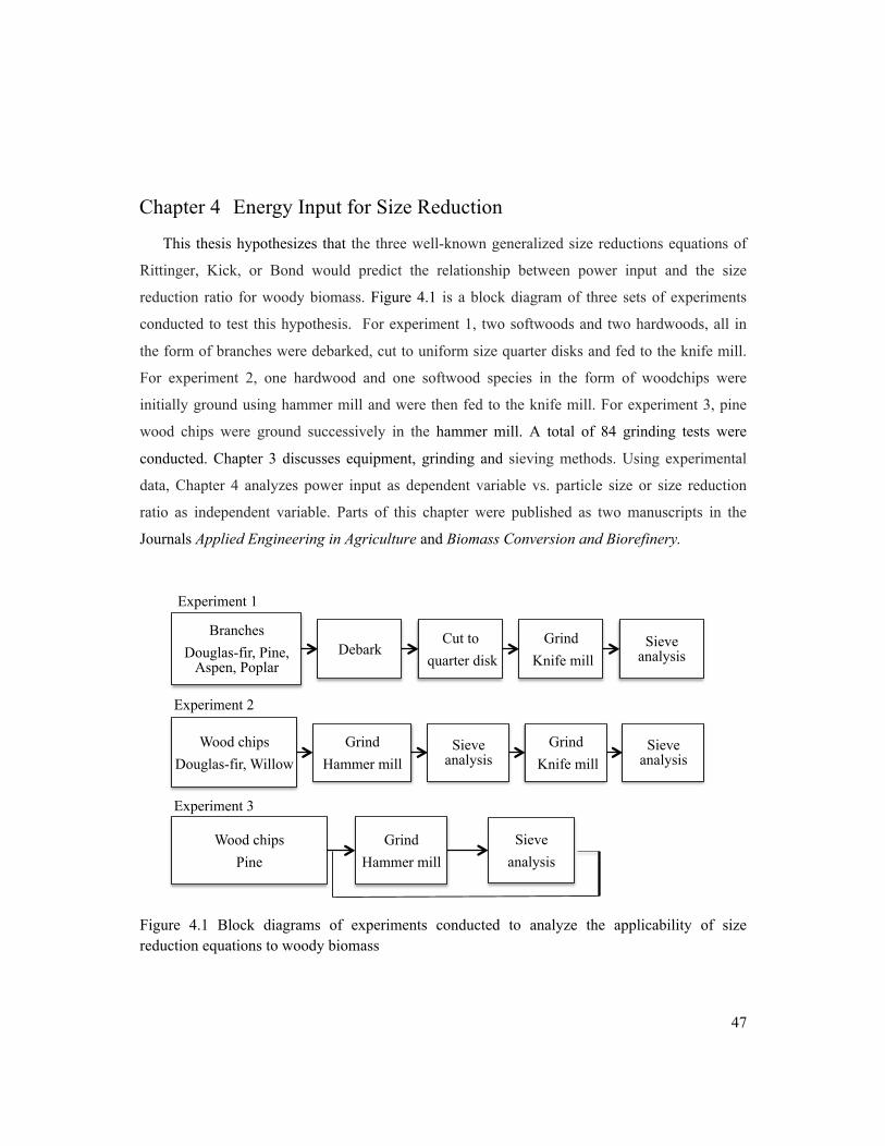
47

Chapter 4 Energy Input for Size Reduction

This thesis hypothesizes that the three well-known generalized size reductions equations of

Rittinger, Kick, or Bond would predict the relationship between power input and the size

reduction ratio for woody biomass. Figure 4.1 is a block diagram of three sets of experiments

conducted to test this hypothesis. For experiment 1, two softwoods and two hardwoods, all in

the form of branches were debarked, cut to uniform size quarter disks and fed to the knife mill.

For experiment 2, one hardwood and one softwood species in the form of woodchips were

initially ground using hammer mill and were then fed to the knife mill. For experiment 3, pine

wood chips were ground successively in the hammer mill. A total of 84 grinding tests were

conducted. Chapter 3 discusses equipment, grinding and sieving methods. Using experimental

data, Chapter 4 analyzes power input as dependent variable vs. particle size or size reduction

ratio as independent variable. Parts of this chapter were published as two manuscripts in the

Journals Applied Engineering in Agriculture and Biomass Conversion and Biorefinery.

Figure 4.1 Block diagrams of experiments conducted to analyze the applicability of size reduction equations to woody biomass

!!! Experiment 1

Experiment 2

Experiment 3

!!!!!!!!!!

!

Branches Douglas-fir, Pine,

Aspen, Poplar Debark

Cut to quarter disk

Grind Knife mill

Sieve analysis

Wood chips Douglas-fir, Willow

Grind Hammer mill

Sieve analysis

Grind Knife mill

Sieve analysis

Wood chips Pine

Grind Hammer mill

Sieve analysis

48

4.1 Input power measurement

Knife mill and hammer mill were equipped with a wattmeter to measure instantaneous power

input. The output was connected to a computer to record the data.

Figure 4.2 is a sample plot of power input to the knife mill with 6 mm screen running with

load (Douglas-fir and willow samples) and without load (empty run). Figure 4.2 plots the

recorded instantaneous power input when grinding willow and Douglas-fir (1.7 g s-1 feeding

rate). An initial perturbation was due to the sudden current draw when the motor was turned on.

Variations in the signal during grinding run are because of variations in feeding rate due to

variations in the feed particle size. These variations were significant when feeding quarter disk

pieces to the knife mill. Several tests were performed to determine whether a higher data

acquisition frequency than 1 Hz would have captured more details on measured signal and thus

an increased accuracy in recorded power. Table 4.1 lists the parasitic (no load) power recorded

for the four different data acquisition rates from 0.5 to 2 Hz. The recorded power increased from

an average of a mean of 385 to 393 W with an increased data acquisition rate of 0.5 to 2 Hz.

Standard deviations were constant at 32 W. It was deemed that data acquisition at a rate of 1 Hz

did not introduce a larger error than if the rate had been at 0.5 Hz. Nevertheless a larger

frequency rate is recommended for future measurements.

Table 4.1 An example of mean, standard deviation, maximum, minimum, and coefficient of variation of power input (W) to grinder working empty Data acquisition rate,

Hz Power, W

Mean S.D Max Min C.V 2.0 393 32 453 337 0.08

1.0 390 32 442 337 0.08

0.7 389 32 442 337 0.08

0.5 385 32 436 337 0.08

49

Figure 4.2 Sample plot of power input to the knife mill with 6 mm screen running empty (No-load) and grinding willow and Douglas-fir. All three curves have an initial perturbation because of the sudden pull of electricity for the motor to start working. The curve for no-load working defines a base line for the power needed for the knife mill working empty. The feed wood chips had a variable size.

4.2 Energy input for size reduction

4.2.1 Experiment 1: Branches of Douglas-fir, pine, aspen, and poplar

For these experiments as outlined in Figure 4.1, branches of Douglas-fir, pine, aspen, and

poplar were debarked, dried and cut to quarter disks. The disks were weighed and fed one by one

to the knife mill over a grinding cycle of 5 to 10 minutes. Meanwhile, the power input to the mill

was recorded. Table C.1 in Appendix C lists 14 grinding data sets from these runs including

moisture content, mass and number of pieces fed to the grinder, feeding time, and energy input.

Table 4.2 summarizes the data from Table C.1 showing the ranges of power and energy input to

the knife mill for each of the tested species. The energy input data show that a considerable

portion of the recorded power input was to power the grinder in no-load operation. The net

energy input ranged from a minimum of 66 kJ to grind Douglas-fir to a maximum of 149 kJ to

grind poplar. There were also considerable variations among the recorded energy both within

species and between species. Perhaps a portion of this variability can be attributed to non-

uniform feeding, variation in size of quarter disks, and variation in internal structure of the wood.

Data on energy input per unit mass shows that poplar and pine used the most energy, whereas

450

550

650

750

0 100 200 300

Pow

er, W

Time, s

Empty working Douglas-fir Willow

50

Douglas-fir used the least. Aspen used the least energy per unit area when energy was divided by

the total surface area of ground particles.

4.2.2 Experiment 2: Wood chips of Douglas-fir and willow

In this set of grinding tests, Douglas-fir and willow wood chips were ground first in the

hammer mill before being fed into the knife mill. Figure 4.3 is a plot of mass fraction of ground

particles of Douglas-fir and willow prepared from crushing wood chips in the hammer mill

equipped with a 25.4 mm screen. The hammer milled Douglas-fir particles, with a pan mass

fraction of 31%, were smaller than the hammer milled willow particles with a pan mass of 22%.

The fraction of large particles retained on 4-mm screen was 6% for Douglas-fir but 18% for

willow. The geometric mean diameter was 1.73 mm for Douglas-fir and 2.23 mm for willow

particles.

Table 4.2 Summary of the results of ranges of energy consumptions of grinding four species by knife mill (Experiment 1). Ranges of total energies while grinding, total energy deducting the empty grinding, total mass, and feeding rate are listed.

Species

Douglas-fir

Pine Aspen Poplar

Average measured power, W 693-1052 854-1046 854-968 841-851 Total mass, g 501- 505 500- 501 501-504 500-502 Total time, s 299- 699 388- 706 565-621 610-673 Calculated energy including knife mill empty energy, kJ

226- 459[a] 339- 481 415-431 466-509

Net calculated energy (after deducting knife mill empty energy), kJ

66 - 89 101- 132 99-117 126-149

Feeding rate, g s-1 Range[1] 1.1-4.0 1.8-3.0 1.1-3.1 1.1-1.3 SD 1.5 0.7 0.5 0.3 CV 0.52 0.31 0.53 0.28 Energy input per unit mass, J g-1

Range[2] 132-178 201-263 197-232 253-297 SD 20 33 20 23 CV 0.13 0.15 0.09 0.08

Energy input per unit area, kJ m-2

5,793 5,640 3,453 7,239

[a]Range of three to five tests. [1]At p=0.05 level, the population means are not significantly different. [2]At p=0.05 level, the population means are significantly different.

51

Figure 4.3 Size distribution of hammer-milled wood chips of willow and Douglas-fir on Gilson sieve shaker and pine wood chips as-received (PWC). The screen size inside hammer mill is 25 mm. The ground wood chips are prepared for feeding to the knife mill and hammer mill.

The size of screen was important for the uninterrupted operation of the knife mill. Douglas-

fir did not flow through 2 mm screen when feeding rate exceeded 2 g s-1. Similarly, willow did

not flow easily through 1 mm screen. In order to maintain a constant feeding rate for both

species on screens of 2, 4, and 6 mm, the feeding rate was maintained at 1.7 g s-1 in all

experiments.

Table 4.3 lists the result of power input for grinding Douglas-fir and willow (Experiment 2).

The knife mill was fitted with three sizes of screens: 2, 4, and 6 mm. The average particle size of

the feed material was 2.2-2.4 mm for willow and 1.7-2.4 mm for Douglas-fir. The average size

of material exiting the grinding ranged from 0.5 mm for 2 mm screen to 1.41 mm for the 6 mm

screen. The average ground particle size for Douglas-fir ranged from 0.54 to 1.30 mm when the

feeding rate was kept constant at 1.7 g s-1. Table 4.3 lists the size reduction ratios achieved. The

parasitic (no-load) power averaged 510 W, while the power recorded for the loaded grinder

ranged from 540 to 760 W, increased with increasing size reduction ratio. The power input

increased with decreasing screen size. For the same input particle size (2.38 mm), grinding

willow required an average power input of 600 to 650 W, whereas grinding Douglas-fir required

an average power input of 560 to 570 W. A parasitic power of 510 W was deducted to give the

net power consumption for grinding.

0 5

10 15 20 25 30 35 40

d≤1 1<d≤2 2<d≤4 4<d≤12.5 d>12.5

Mas

s per

cent

, %

Sieve opening, mm

Douglas-fir Willow Pine

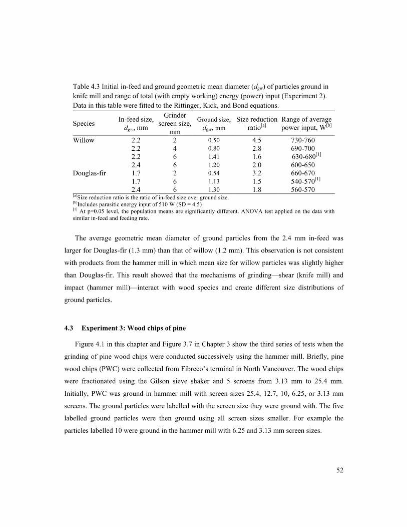
52

Table 4.3 Initial in-feed and ground geometric mean diameter (dgw) of particles ground in knife mill and range of total (with empty working) energy (power) input (Experiment 2). Data in this table were fitted to the Rittinger, Kick, and Bond equations.

Species In-feed size, dgw, mm

Grinder screen size,

mm

Ground size, dgw, mm

Size reduction ratio[a]

Range of average power input, W[b]

Willow 2.2 2 0.50 4.5 730-760 2.2 4 0.80 2.8 690-700 2.2 6 1.41 1.6 630-680[1] 2.4 6 1.20 2.0 600-650 Douglas-fir 1.7 2 0.54 3.2 660-670

1.7 6 1.13 1.5 540-570[1] 2.4 6 1.30 1.8 560-570

[a]Size reduction ratio is the ratio of in-feed size over ground size. [b]Includes parasitic energy input of 510 W (SD = 4.5) [1] At p=0.05 level, the population means are significantly different. ANOVA test applied on the data with similar in-feed and feeding rate.

The average geometric mean diameter of ground particles from the 2.4 mm in-feed was

larger for Douglas-fir (1.3 mm) than that of willow (1.2 mm). This observation is not consistent

with products from the hammer mill in which mean size for willow particles was slightly higher

than Douglas-fir. This result showed that the mechanisms of grinding—shear (knife mill) and

impact (hammer mill)—interact with wood species and create different size distributions of

ground particles.

4.3 Experiment 3: Wood chips of pine

Figure 4.1 in this chapter and Figure 3.7 in Chapter 3 show the third series of tests when the

grinding of pine wood chips were conducted successively using the hammer mill. Briefly, pine

wood chips (PWC) were collected from Fibreco’s terminal in North Vancouver. The wood chips

were fractionated using the Gilson sieve shaker and 5 screens from 3.13 mm to 25.4 mm.

Initially, PWC was ground in hammer mill with screen sizes 25.4, 12.7, 10, 6.25, or 3.13 mm

screens. The ground particles were labelled with the screen size they were ground with. The five

labelled ground particles were then ground using all screen sizes smaller. For example the

particles labelled 10 were ground in the hammer mill with 6.25 and 3.13 mm screen sizes.

53

Table 4.4 lists mean, standard deviation, and coefficient of variation of the data collected on

power consumption of each trial of grinding pine with hammer mill. Each trial repeated three

times. Grinding PWC on 3.1 mm screen has the maximum power consumption. Three trials of

grinding PWC on 3.1 mm screen have the highest coefficient of variations, representing the

greatest spreading in the data collected. Energy for grinding PWC on 3.1 mm screen is between

48-51 kWh t-1. Gil et al. (2004) ground pine wood chips by hammer mill with a 5 mm screen and

reported an energy consumption of 33 kWh t-1, which is similar to the result of this study where

grinding PWC on 6.3 mm screen consumed 39-41 kWh t-1.

Table 4.4 also lists the recorded mean specific energy input. The specific energy is calculated

without energy of empty working of the grinder. The specific energy increased as the screen size

inside the grinder decreased. The in-feed ranged from PWC to particles labelled as the 6.3 mm

screen. Grinding PWC particles had the lowest mean specific energy input when 25.4 mm screen

size was used. The specific energy increased from 5.2 J g-1 to 90.4 J g-1 when the screen size

decreased from 25.4 mm to 3.1 mm. The specific energy for grinding PWC using 25.4 mm

screen had a high standard deviation of 1.1 and a low mean of 5.2 J g-1. It results in the highest

coefficient of variation of 0.21. Coefficient of variations varies between 0.03 and 0.21 for the

grinding tests.

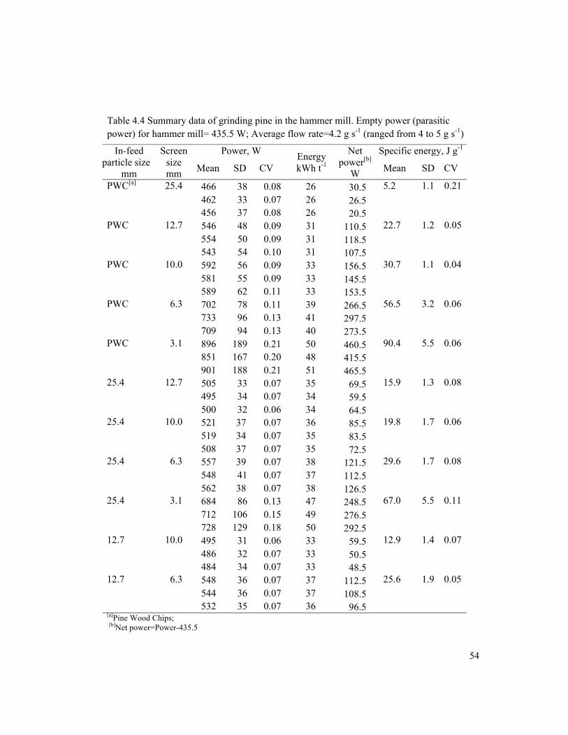
54

Table 4.4 Summary data of grinding pine in the hammer mill. Empty power (parasitic power) for hammer mill= 435.5 W; Average flow rate=4.2 g s-1 (ranged from 4 to 5 g s-1)

In-feed particle size

mm

Screen size mm

Power, W Energy kWh t-1

Net power[b]

W

Specific energy, J g-1

Mean SD CV Mean SD CV

PWC[a] 25.4 466 38 0.08 26 30.5 5.2 1.1 0.21 462 33 0.07 26 26.5

456 37 0.08 26 20.5 PWC 12.7 546 48 0.09 31 110.5 22.7 1.2 0.05 554 50 0.09 31 118.5 543 54 0.10 31 107.5 PWC 10.0 592 56 0.09 33 156.5 30.7 1.1 0.04 581 55 0.09 33 145.5 589 62 0.11 33 153.5 PWC 6.3 702 78 0.11 39 266.5 56.5 3.2 0.06 733 96 0.13 41 297.5 709 94 0.13 40 273.5 PWC 3.1 896 189 0.21 50 460.5 90.4 5.5 0.06 851 167 0.20 48 415.5 901 188 0.21 51 465.5 25.4 12.7 505 33 0.07 35 69.5 15.9 1.3 0.08 495 34 0.07 34 59.5 500 32 0.06 34 64.5 25.4 10.0 521 37 0.07 36 85.5 19.8 1.7 0.06 519 34 0.07 35 83.5 508 37 0.07 35 72.5 25.4 6.3 557 39 0.07 38 121.5 29.6 1.7 0.08 548 41 0.07 37 112.5 562 38 0.07 38 126.5 25.4 3.1 684 86 0.13 47 248.5 67.0 5.5 0.11 712 106 0.15 49 276.5 728 129 0.18 50 292.5 12.7 10.0 495 31 0.06 33 59.5 12.9 1.4 0.07 486 32 0.07 33 50.5 484 34 0.07 33 48.5 12.7 6.3 548 36 0.07 37 112.5 25.6 1.9 0.05 544 36 0.07 37 108.5 532 35 0.07 36 96.5 [a]Pine Wood Chips; [b]Net power=Power-435.5

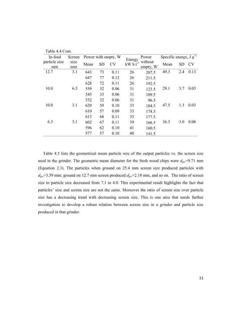
55

Table 4.4 Cont. In-feed

particle size mm

Screen size mm

Power with empty, W Energy kW h t-1

Power without empty, W

Specific energy, J g-1

Mean SD CV Mean SD CV

12.7 3.1 643 73 0.11 26 207.5 49.3 2.4 0.13 647 77 0.12 26 211.5

628 72 0.11 26 192.5 10.0 6.3 559 32 0.06 31 123.5 29.1 3.7 0.03 545 33 0.06 31 109.5 532 32 0.06 31 96.5 10.0 3.1 620 59 0.10 33 184.5 47.5 1.3 0.03 610 57 0.09 33 174.5 613 68 0.11 33 177.5 6.3 3.1 602 67 0.11 39 166.5 36.3 3.0 0.08 596 62 0.10 41 160.5 577 57 0.10 40 141.5

Table 4.5 lists the geometrical mean particle size of the output particles vs. the screen size

used in the grinder. The geometric mean diameter for the fresh wood chips were dgw=9.71 mm

(Equation 2.3). The particles when ground on 25.4 mm screen size produced particles with

dgw=3.59 mm; ground on 12.7 mm screen produced dgw=2.18 mm, and so on. The ratio of screen

size to particle size decreased from 7.1 to 4.0. This experimental result highlights the fact that

particles’ size and screen size are not the same. Moreover the ratio of screen size over particle

size has a decreasing trend with decreasing screen size. This is one area that needs further

investigation to develop a robust relation between screen size in a grinder and particle size

produced in that grinder.

56

Table 4.5 Geometric mean diameter of PWC as received and ground particles from specified screen size.

Screen size, mm Geometric mean diameter of particles, dgw mm

Ratio of screen size over diameter

PWC[a] 9.71 - 25.4 3.59 7.1 12.7 2.18 5.8

10.0 1.83 5.5 6.3 1.12 5.6 3.1 0.77 4.0

[a]Pine Wood Chips

The mean particle sizes of ground particles measured by image analysis were compared with

geometric mean diameter of particles. Figure 4.4 shows the average of three replicates of

measured mean length and mean width of ground particles from image analysis. The mean

geometric diameter of particles is also plotted on the graph. The geometric mean diameter of

particles dgw measured from sieving analysis is very close to the mean width of particles

measured from imaging. This is an evidence that the geometric mean diameter of the particles

which is calculated based on the results from sieving the particles is very close to the width of

the particles. This is expected as the particles pass the screen holes by their width not their

length.

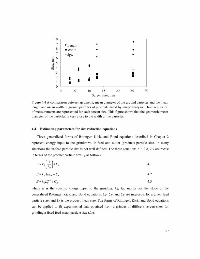
57

Figure 4.4 A comparison between geometric mean diameter of the ground particles and the mean length and mean width of ground particles of pine calculated by image analysis. Three replicates of measurements are represented for each screen size. This figure shows that the geometric mean diameter of the particles is very close to the width of the particles.

4.4 Estimating parameters for size reduction equations

Three generalized forms of Rittinger, Kick, and Bond equations described in Chapter 2

represent energy input to the grinder vs. in-feed and outlet (product) particle size. In many

situations the in-feed particle size is not well defined. The three equations 2.7, 2.8, 2.9 are recast

in terms of the product particle size Lp as follows,

4.1

4.2

4.3

where E is the specific energy input to the grinding; kR, kK, and kB are the slope of the

generalized Rittinger, Kick, and Bond equations; CR, CK, and CB are intercepts for a given feed

particle size; and LP is the product mean size. The forms of Rittinger, Kick, and Bond equations

can be applied to fit experimental data obtained from a grinder of different screen sizes for

grinding a fixed feed mean particle size (LF).

0 1 2 3 4 5 6 7 8 9

10

0 5 10 15 20 25 30

Size

, mm

Screen size, mm

Length Width dgw

E = kR1LP

!

"#

$

%&+CR

E = kK lnLP +CK

E = kBLP−0.5 +CB

58

4.4.1 Experiment 1: Branches of Douglas-fir, pine, poplar, and aspen

Table 4.6 lists the Rittinger constants, kR; the intercepts, CR; and regression coefficient, R2.

kR, ranged between 203 and 398 J mm g-1 with the maximum for pine and minimum for Douglas-

fir. The intercept, CR, ranged from -309 to -141 J g-1. The regression coefficient, R2, ranged from

0.93 to 0.96 indicating good linearity between E and kR. For aspen and poplar, the values for kR

were 299 and 277 J mm g-1 and for pine and Douglas-fir, the values were 398, and 203 J mm g-1.

The regression coefficients for other equations are also in the range of 0.93-0.97 indicating that

all three equations—Rittinger, Kick, and Bond—described the measured specific energy input

well.

Table 4.6 Results of fitting data to the generalized Rittinger, Kick, and Bond equations (equations 4.1, 4.2, and 4.3) for grinding Douglas-fir, pine, aspen, and poplar using knife mill.

Species Douglas-fir Pine Aspen Poplar

kR, J mm g-1 203 (16) 398 (38) 299 (19) 277 (30) CR -141 (19) -309 (41) -249 (24) -150 (36) R2 0.93 0.94 0.96 0.94 kK, J (ln mm)-1g-1 -239 (19) -443 (42) -376 (26) -342 (34) CK 65 (5) 95 (8) 47 (7) 131 (9) R2 0.95 0.94 0.96 0.94 kB, J mm0.5 g-1 441 (34) 841 (80) 674 (44) 597 (64) CB -378 (37) -749 (82) -625 (49) -462 (69) R2 0.95 0.94 0.97 0.93 1Numbers in parenthesis are standard errors.

4.4.2 Experiment 2: Wood chips of Douglas-fir and willow

Figure 4.5 (a) and (b) show two plots of the net specific energy input (parasitic energy input

is deducted) E vs. ln(LF LP-1) for the Kick’s equation applied to the size reduction data for

Douglas-fir and willow, respectively. LF and Lp represent the geometrical mean particle size of

in-feed particles and ground particles after the grinder, respectively. Plots of specific energy E

versus Rittinger and Bond parameters had a similar trend, indicating an increase in energy per

unit mass (specific energy) with increase in size reduction ratio.

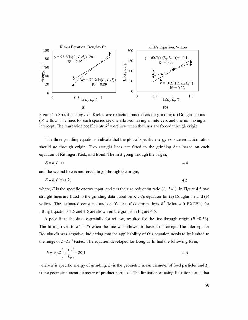
59

(a) (b)

Figure 4.5 Specific energy vs. Kick’s size reduction parameters for grinding (a) Douglas-fir and (b) willow. The lines for each species are one allowed having an intercept and one not having an intercept. The regression coefficients R2 were low when the lines are forced through origin

The three grinding equations indicate that the plot of specific energy vs. size reduction ratios

should go through origin. Two straight lines are fitted to the grinding data based on each

equation of Rittinger, Kick, and Bond. The first going through the origin,

4.4

and the second line is not forced to go through the origin,

4.5

where, E is the specific energy input, and x is the size reduction ratio (LF LP-1). In Figure 4.5 two

straight lines are fitted to the grinding data based on Kick’s equation for (a) Douglas-fir and (b)

willow. The estimated constants and coefficient of determinations R2 (Microsoft EXCEL) for

fitting Equations 4.5 and 4.6 are shown on the graphs in Figure 4.5.

A poor fit to the data, especially for willow, resulted for the line through origin (R2=0.33).

The fit improved to R2=0.75 when the line was allowed to have an intercept. The intercept for

Douglas-fir was negative, indicating that the applicability of this equation needs to be limited to

the range of LF LP-1 tested. The equation developed for Douglas-fir had the following form,

4.6

where E is specific energy of grinding, LF is the geometric mean diameter of feed particles and Lp

is the geometric mean diameter of product particles. The limitation of using Equation 4.6 is that

y = 70.9(ln(LF LP-1))

R² = 0.89

y = 93.2(ln(LF LP-1))- 20.1

R² = 0.95

0

20

40

60

80

100

0 0.5 1

Ener

gy, J

g-1

ln(LF LP-1)

Kick's Equation, Douglas-fir

y = 102.1(ln(LF LP-1))

R² = 0.33

y = 60.5(ln(LF LP-1))+ 46.1

R² = 0.75

0

50

100

150

200

0 0.5 1 1.5

Ener

gy, J

g-1

ln(LF LP-1)

Kick's Equation, Willow

E = k1 f (x)

E = k1 f (x)+ k2

E = 93.2 lnLf

LP

!

"#

$

%&− 20.1

60

grinding ratio (LF LP-1) should be more than 1.24 (i.e. 24% size reduction) in order to ensure that

the specific energy input calculation does not produce a negative number.

Table 4.7 shows the fit of the grinding equations to the data from Experiment 2 in which

hammer milled particles were fed to the knife mill. The values of coefficient of determination for

fitting a straight line through the intercept for Rittinger and Bond were small, with the intercepts

near zero. Only the Rittinger equation gave a positive intercept for Douglas-fir. Comparing R2

values, Rittinger’s equation had a better fit to the data than other two equations. The last two

rows in Table 4.7 represent grinding data when the combined data from willow and Douglas-fir

are used for the fitting. The R2 values were much smaller for the combined data than for the

individual species data.

Table 4.7 Constants and coefficients of determination for three grinding equations fitted to data from knife mill. The second line for each species is for a line passed through origin (intercept K2=0)

Kick Rittinger Bond Ln (LF/ LP) 1/LP-1/LF 1/LP

0.5-1/LF0.5

K1 K2 R2 K1 K2 R2 K1 K2 R2 Willow

60.5 (11.9)1

46.1 (12.1)

0.75 48.9 (8.5)

64.2 (8.0)

0.79 110.6 (20.0)

56.2 (9.5)

0.78

102.1 (19.4)

0.0 0.33 106.4 (12.4)

0.0 0.71 214.9 (19.3)

0.0 0.75

Douglas-fir

93.2 (8.5)

-20.1 (7.0)

0.95 67.2 (5.3)

3.9 (3.8)

0.97 159.0 (12.0)

-6.1 (4.9)

0.97

70.9 (4.8)

0.0 0.89 71.1 (3.0)

0.0 0.97 145.9 (6.0)

0.0 0.96

Composite of two species

83.4 (14.3)

8.9 (13.4)

0.66 60.5 (12.5)

35.7 (11.1)

0.57 143.7 (25.1)

24.2 (11.7)

0.62

92.0 (5.7)

0.0 0.65 93.6 (8.4)

0.0 0.33 191.2 (12.8)

0.0 0.53

1Numbers in parenthesis are standard errors.

4.4.3 Experiment 3: Wood chips of pine

Figures 4.6, 4.7 and 4.8 show the fitted lines to the data of specific energy vs product sizes

defined in Rittinger, Kick and Bond equations in the form of Equations 4.1, 4.2, and 4.3,

61

respectively. Each fitted line represents a specific feed particle size. The aim was to measure the

sensitivity of the slope of energy equations to feed particle size.

Table 4.8 lists the regression coefficients for three equations with hammer mill. The

regression coefficients ranged from 0.92-0.99 for Rittinger equation to 0.88-0.99 for the Bond

equation and 0.84-0.96 for Kick Equation. The Rittinger equation had the best fit. Table 4.8 also

lists the constants of Rittinger, Kick, and Bond to the grinding data. Rittinger constants, kR,

ranged 44.6-58.6 J mm g-1 for feed particle sizes of 10, 12.7, and 25.4 mm. This is a close range

as contrasted with the constant value of unground fresh wood chips at 81.45 J mm g-1. The slopes

are different for different feed particle sizes. It shows that feed particle size affects the slope of

the equations.

Table 4.9 lists the slopes and coefficient of determination for the three grinding equations

Rittinger, Kick and Bond for grinding pine with the hammer mill. The equations used were in the

form of Equations 2.7, 2.8, and 2.9. The fitted lines passed through the origin. The Rittinger

equation with a coefficient of determination of 0.91 is the best fitted equation among the three.

The results of fitting the lines having intercepts show a similar coefficient of determination as the

lines passing through the origin. Figure 4.9 shows the fitted line to the data of specific energy vs

LP-1-LF

-1. Data collected from different feed particle sizes are labelled with different markers.

The applicability of these models to grinding woody and herbaceous biomass as they are

collected from field was further explored in a separate project. The results are summarized in

Appendix D. In general the preliminary results showed that the relationship between energy

consumption and the size of ground particles was best fitted by Rittinger equation.

62

Table 4.8 Slopes and coefficients of determinations for fitting Equations 4.1, 4.2, and 4.3 to data of grinding PWC by hammer mill on different screen sizes. Rittinger equation has a good fit for feed from all sizes. Rittinger and Bond constants decrease as the feed particle size decreased. Kick’s constant increases as the feed particle size decreased.

Feed particle

size Rittinger Equation Bond Equation Kick Equation

kR J mm g-1

CR R2 kB

J mm0.5 g-1 CB R2 kK

J (ln mm)-1 g-1 CK R2

PWC[a] 81.5

(2.1)1 -15.6 (1.7)

0.99 138 (4.5)

-69.9 (3.8)

0.99 -54.4 (3.2)

68.4 (2.4)

0.96

25.4 mm 58.6 (5.5)

-13.8 (4.8)

0.92 105 (12.0)

-58.6 (10.7)

0.88 -45.5 (6.2)

47.1 (3.2)

0.84

12.7 mm 48.4 (3.0)

-15.0 (2.9)

0.97 90.2 (7.4)

-55.7 (7.0)

0.96 -41.1 (4.3)

35.5 (1.7)

0.93

10 mm 44.6 (5.4)

-10.6 (6.1)

0.94 93.1 (11.3)

-58.7 (11.9)

0.94 -48.4 (5.9)

34.6 (1.2)

0.94

[a]Pine Wood Chips 1Numbers in parenthesis are standard errors.

Table 4.9 Slopes and coefficients of determination of the three grinding equations: Kick, Rittinger, and Bond for grinding pine by hammer mill. Equations used in this table are in the form of equations 2.7, 2.8 and 2.9.

Kick’s Equation Rittinger’s Equation Bond’s Equation

KK, J g-1 R2 KR, J mm g-1 R2 KB, J mm0.5 g-1 R2

30.5 (1.9) 1 0.46 67.3 (1.6) 0.91 99.3 (3.4) 0.82 K1 K2 R2 K1 K2 R2 K1 K2 R2 24.0 (3.6)

9.7 (4.6)

0.51 65.9 (3.1)

1.0 (1.9)

0.91 99.1 (7.2)

0.08 (2.97)

0.82

1Numbers in parenthesis are standard errors.

p

fLL

lnfp L1

L1− 5.0

f5.0p L

1L1

−

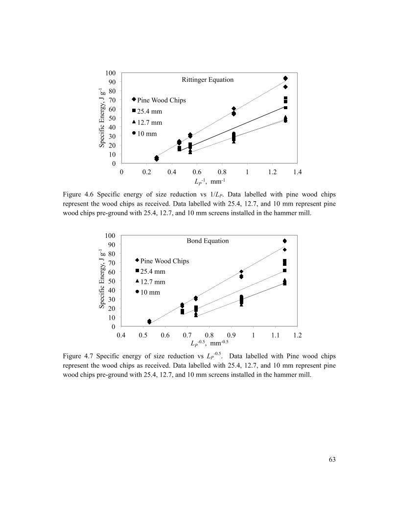
63

Figure 4.6 Specific energy of size reduction vs 1/LP. Data labelled with pine wood chips represent the wood chips as received. Data labelled with 25.4, 12.7, and 10 mm represent pine wood chips pre-ground with 25.4, 12.7, and 10 mm screens installed in the hammer mill.

Figure 4.7 Specific energy of size reduction vs LP

-0.5. Data labelled with Pine wood chips represent the wood chips as received. Data labelled with 25.4, 12.7, and 10 mm represent pine wood chips pre-ground with 25.4, 12.7, and 10 mm screens installed in the hammer mill.

0 10 20 30 40 50 60 70 80 90

100

0 0.2 0.4 0.6 0.8 1 1.2 1.4

Spec

ific

Ener

gy, J

g-1

LP-1, mm-1

Rittinger Equation

Pine Wood Chips 25.4 mm 12.7 mm 10 mm

0 10 20 30 40 50 60 70 80 90

100

0.4 0.5 0.6 0.7 0.8 0.9 1 1.1 1.2

Spec

ific

Ener

gy, J

g-1

LP-0.5, mm-0.5

Bond Equation


64

Figure 4.8 Specific energy of size reduction vs ln (LP). Data labelled with Pine wood chips represent the wood chips as received. Data labelled with 25.4, 12.7, and 10 mm represent pine wood chips pre-ground with 25.4, 12.7, and 10 mm screens installed in the hammer mill.

Figure 4.9 Specific energy of size reduction vs LP

-1-LF-1. Data labelled with PWC represent the

wood chips as received. Data labelled with 25.4, 12.7,10.0, and 6.3 mm represent pine wood chips pre-ground with 25.4, 12.7, 10, 6.3 mm screens installed in the hammer mill.

4.4.4 Application of Rittinger equation to published grinding data

Figure 4.10 plots specific energy versus Rittinger’s parameters for the data from this study,

and those extracted from Mani et al. (2004) for corn stover, wheat straw, switchgrass and barley

straw, from Bitra et al. (2009) for switchgrass, corn stover and wheat straw, and from Adapa et

0 10 20 30 40 50 60 70 80 90

100

-0.5 0 0.5 1 1.5

Spec

ific

Ener

gy, J

g-1

ln (LP), ln(mm)

Kick Equation


y = 67.3x R² = 0.9

0

20

40

60

80

100

0 0.2 0.4 0.6 0.8 1 1.2

Spec

ific

Ener

gy, J

g-1

LP-1-LF

-1, mm-1

Feed particle size: PWC Feed particle size: 25.4 mm Feed particle size: 12.7 mm Feed praticle size: 10.0 mm Feed particle size: 6.3 mm

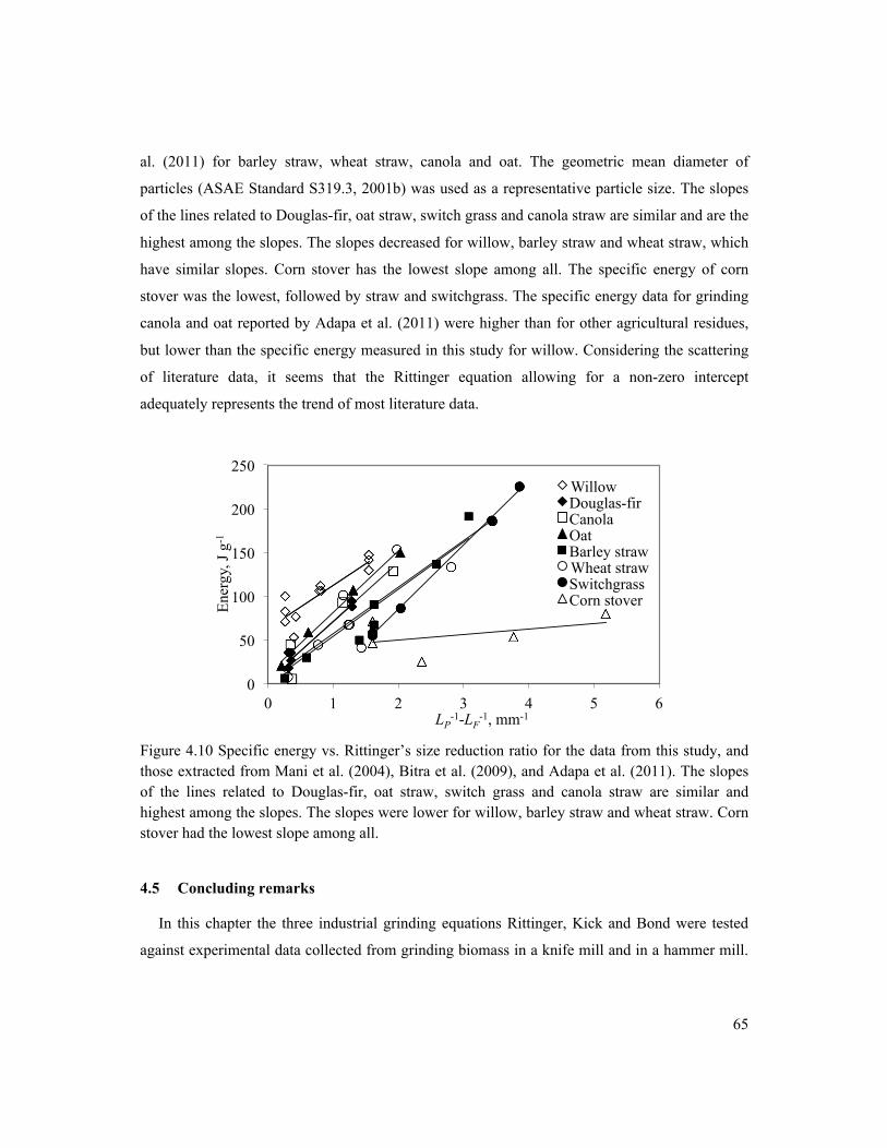
65

al. (2011) for barley straw, wheat straw, canola and oat. The geometric mean diameter of

particles (ASAE Standard S319.3, 2001b) was used as a representative particle size. The slopes

of the lines related to Douglas-fir, oat straw, switch grass and canola straw are similar and are the

highest among the slopes. The slopes decreased for willow, barley straw and wheat straw, which

have similar slopes. Corn stover has the lowest slope among all. The specific energy of corn

stover was the lowest, followed by straw and switchgrass. The specific energy data for grinding

canola and oat reported by Adapa et al. (2011) were higher than for other agricultural residues,

but lower than the specific energy measured in this study for willow. Considering the scattering

of literature data, it seems that the Rittinger equation allowing for a non-zero intercept

adequately represents the trend of most literature data.

Figure 4.10 Specific energy vs. Rittinger’s size reduction ratio for the data from this study, and those extracted from Mani et al. (2004), Bitra et al. (2009), and Adapa et al. (2011). The slopes of the lines related to Douglas-fir, oat straw, switch grass and canola straw are similar and highest among the slopes. The slopes were lower for willow, barley straw and wheat straw. Corn stover had the lowest slope among all.


In this chapter the three industrial grinding equations Rittinger, Kick and Bond were tested

against experimental data collected from grinding biomass in a knife mill and in a hammer mill.

0

50

100

150

200

250

0 1 2 3 4 5 6

Ener

gy, J

g-1

LP-1-LF

-1, mm-1

Willow Douglas-fir Canola Oat Barley straw Wheat straw Switchgrass Corn stover

66

The results of grinding the prepared quarter disk shaped pieces from branches of Douglas-fir,

pine, polar and aspen showed that all three equations fit the data quite well.

A second set of experiments was conducted to measure the specific energy for grinding wood

chips of willow and Douglas-fir in a two stage grinding process, namely hammer mill followed

by knife mill. The result of fitting the three equations to the experimental data showed that none

of the original equations fit the data well when these equations were forced through the origin

(0,0). When the equations were allowed to take slope and intercept, their performance in

predicting specific energy from particle size reductions improved substantially. Among the three,

the Rittinger equation had the best fit to the experimental data. Its good fit confirms the

hypothesis that grinding of fibrous biomass is likely dominated by the creation of new surface

areas (n=2 in Equation 2.6).

A final set of experiments was conducted to successively reduce the size of biomass

particles. Commercial pine pulp wood chips were size reduced in a hammer mill. The results

showed that Rittinger’s equation had the best-fit among the three equations (Rittinger, Kick, and

Bond). The successive tests revealed that the geometric mean diameter of particles was 4 to 7

times less than the screen size in the grinder. The measured length and thickness (diameter,

width) of particles using image analysis showed that the geometric mean diameter determined

from sieving analysis is close to the thickness of the particle.

67

Chapter 5 Integrated Size Reduction and Pelletization

Size reduction is an integral part of pelletization. Wood chips are dried to a low moisture

(~10%) and ground to a particle size of ~ 1 mm in order to produce durable pellets. Chapter 4

presented experimental data showing that grinding energy input increases as particles become

smaller. The size of particles has an effect on the density of pellets. This chapter presents data on

energy input for densification of Douglas-fir and willow for a number of particles sizes. The test

also includes pelletization of blends of Douglas-fir and willow to improve pellet density.

The results of previous studies on the impact of particle size on pellet density are summarized

in Table 2.3. Most of the studies used a single pellet press machine for producing pellets. Those

studies did not reveal a major impact of particle size on pellet density within the range of particle

sizes studied (Mani et al., 2006; Rhen et al., 2007; Shaw et al., 2009; Carone et al., 2011). The

only study performed on a semi-industrial scale unit prepared three categories of particle sizes by

sieving (Bergstrom et al., 2008). Although their results showed that pellet density was the

highest for coarse particles, they eliminated the presence of fine particles by sieving, which

might not represent what happens in the industrial operation where fines are present in the feed.

None of these studies looked at the effect of particle size on the energy consumption for size

reduction and pelletization.

5.1 Pelletization

Pelletization consists of three main operations drying, size reduction, and densification. Pellet

industries grind biomass on screens less than 6 mm perforations in order to prepare the material

for pelletization. The effect of particle size on pelletization energy is not well documented. As

shown in Chapter 4, ground particle size is inversely proportional to the energy consumption in

grinding. Particle size affects energy consumption for pelletization, though a clear relation has

not been shown experimentally or in the published literature. There is a debate over whether if

particle size is smaller, pellet density is higher and therefore the pellet durability improves. It is

thus important to investigate the impact of particle size on the overall energy consumption over

the two steps of size reduction and pelletization in order to identify an optimal or suitable

particle size. The aim in this chapter is to investigate the change of integrated energy

consumption for size reduction and pelletization and pellet density as the particle size decreases.

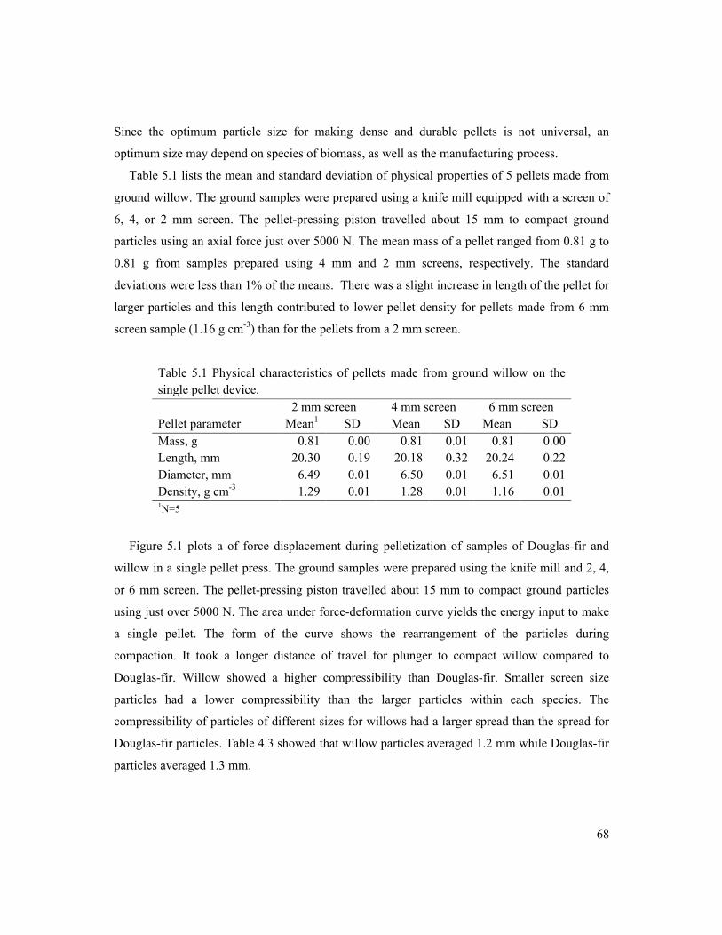
68

Since the optimum particle size for making dense and durable pellets is not universal, an

optimum size may depend on species of biomass, as well as the manufacturing process.

Table 5.1 lists the mean and standard deviation of physical properties of 5 pellets made from

ground willow. The ground samples were prepared using a knife mill equipped with a screen of

6, 4, or 2 mm screen. The pellet-pressing piston travelled about 15 mm to compact ground

particles using an axial force just over 5000 N. The mean mass of a pellet ranged from 0.81 g to

0.81 g from samples prepared using 4 mm and 2 mm screens, respectively. The standard

deviations were less than 1% of the means. There was a slight increase in length of the pellet for

larger particles and this length contributed to lower pellet density for pellets made from 6 mm

screen sample (1.16 g cm-3) than for the pellets from a 2 mm screen.

Table 5.1 Physical characteristics of pellets made from ground willow on the single pellet device.

Pellet parameter 2 mm screen 4 mm screen 6 mm screen Mean1 SD Mean SD Mean SD

Mass, g 0.81 0.00 0.81 0.01 0.81 0.00 Length, mm 20.30 0.19 20.18 0.32 20.24 0.22 Diameter, mm 6.49 0.01 6.50 0.01 6.51 0.01 Density, g cm-3 1.29 0.01 1.28 0.01 1.16 0.01 1N=5

Figure 5.1 plots a of force displacement during pelletization of samples of Douglas-fir and

willow in a single pellet press. The ground samples were prepared using the knife mill and 2, 4,

or 6 mm screen. The pellet-pressing piston travelled about 15 mm to compact ground particles

using just over 5000 N. The area under force-deformation curve yields the energy input to make

a single pellet. The form of the curve shows the rearrangement of the particles during

compaction. It took a longer distance of travel for plunger to compact willow compared to

Douglas-fir. Willow showed a higher compressibility than Douglas-fir. Smaller screen size

particles had a lower compressibility than the larger particles within each species. The

compressibility of particles of different sizes for willows had a larger spread than the spread for

Douglas-fir particles. Table 4.3 showed that willow particles averaged 1.2 mm while Douglas-fir

particles averaged 1.3 mm.

69

Figure 5.1 The plot of force vs displacement of single pellet of ground particles of Douglas-fir and willow. Particles were ground in the knife mill with 6, 4, and 2 mm screens. The maximum force was 5000 N, maintained for 30 s.

Table 5.2 lists the energy input for pelletization of Douglas-fir for three particles sizes from

knife mill (screen size of knife mill). Three to five pellets were made from each particle size.

Energy input for each pellet was calculated from integrating the area under the force-deformation

curve (Figure 5.1). Figure 5.1 shows the force-displacement curves of pellets made of willow

and Douglas-fir particles ground on 2, 4, and 6 mm screens. A longer gradual increase in force

vs displacement indicates that biomass particles are more flexible. These kinds of particles are

expected to have a larger spring back after the compression cycle. Figure 5.1 shows that willow

particles are more flexible than Douglas-fir particles. As expected the larger size particles show a

larger flexibility than the smaller particles.

The energy input recorded per pellet decreased slightly for making pellets from ground

particles of 2 mm screen vs making pellets from ground particles of 4 mm screen. The energy

input increased from 25 J to around 31 J per pellet. The variation in energy input per gram of

pellets was similar to the variation of energy input per pellet. The energy input per gram ranged

from 36.2 J g-1 to 45.0 J g-1. Statistical analysis of the data of specific energy of pelletization

showed that at the p=0.05 level, the population means are significantly different. Table 5.2 lists

the result of Tukey’s post-hoc paired test to show the means that are significantly different. The

Tukey test showed that the pelletization energy for pressing ground sample for 4 mm particles

0

1000

2000

3000

4000

5000

6000

0 10 20 30 40 50

Forc

e, N

Displacement, mm Willow 6 mm Willow 4 mm Willow 2 mm Douglas-fir 6 mm Douglas-fir 2 mm Douglas-fir 4 mm

70

(grinder screen size) did not differ much from the energy input to make pellets from 2 mm

screens. But the input energy to pelletize 6 mm was different from the 2 and 4 mm screens.

Table 5.2 Specific energy of pelletization for Douglas-fir (ground in knife mill) with 8-10% MC and pellet die temperature of 80°C. Specific energy of pelletization increased as the screen size in the grinder increased. Screen size,

mm Sample

no. Energy, J/Pellet

Pellet mass, g

Specific Energy of pelletization, J g-1[1]

2 1 26.19 0.704 37.18 2 26.30 0.703 37.44 3 25.81 0.701 36.81

4 1 25.41 0.702 36.22 2 25.86 0.701 36.88 3 25.88 0.702 36.89*

6 1 28.05 0.703 39.87 2 31.37 0.701 44.77 3 31.65 0.704 44.97♦+

[1] At p=0.05 level, the population means are significantly different. * Tukey’s post-hoc test indicates no difference compared to 2 mm screen size. ♦ Tukey’s post-hoc test indicates difference compared to 2 mm screen size. + Tukey’s post-hoc test indicates difference compared to 4 mm screen size.

5.2 Total energy input for combined grinding and pelletization

Figure 5.2 shows the specific energy consumption of grinding and pelletization for willow

and Douglas-fir. Specific energy for grinding varied from 71 J g-1 to 148 J g-1 for willow and 27

J g-1 to 135 J g-1 for Douglas-fir as the screen size increased from 2 to 4 mm. Figure 5.3 also

shows the energy consumption of the pelletization of ground willow and Douglas-fir with 2, 4

and 6 mm screen sizes. The specific energy of pelletization increased as the screen size

increased. As shown in Table 5.2 and Figure 5.2, specific energy consumption for pelletization

ranged from 39 to 46 J g-1 for willow 37 to 43 J g-1 for Douglas-fir, and a minimum specific

energy consumption of pelletization occurred at 4 mm screen for the two species studied. Figure

5.2 shows that energy consumption for size reduction is more (ranges from 27-148 J g-1) than the

energy consumption for pelletization (ranges from 37- 44 J g-1).

71

Figure 5.2 Specific energy consumption of size reduction and pelletization for willow and Douglas-fir. Single pelletization was performed under a maximum force of 5000 N.

Figure 5.3 shows the integrated specific energy consumption of pelletization and size

reduction of Douglas-fir and willow. The data show that as the screen size increased the

integrated energy consumption of grinding and pelletization decreased. The results also show

that the integrated energy consumption of size reduction and pelletization is lower for Douglas-

fir than for willow.

Figure 5.3 Integrated specific energy for size reduction and pelletization of Douglas-fir and willow.

0 20 40 60 80

100 120 140

1 2 3 4 5 6 7

Spec

ific

ener

gy, J

g-1

Screen size, mm Pelletization-Douglas-fir Pelletization-Willow Size reduction-Douglas-fir Size reduction-Willow

50

70

90

110

130

150

170

190

1 2 3 4 5 6

Size

redu

ctio

n an

d pe

lletiz

atio

n en

ergy

, J g

-1

Screen size, mm

Douglas-fir

Willow

72

Table 5.3 lists the density of individual pellets of Douglas-fir and willow. The table also

shows the influence of grinding screen size on pellet density. Douglas-fir pellets have lower

density than willow pellets across the screen sizes; however, the density of pellets for the two

species changed slightly as the screen size increased. ANOVA analysis on the pellet density of

each species for different screens was performed. The results showed that the population means

of pellet density is significantly different for Douglas-fir and willow pellets. Previous studies

showed that at similar process temperature and moisture content, as the screen size inside the

hammer mill increased, the individual pellet density decreased (Samson and Duxbury, 2000;

Jannasch et al., 2001; Mani et al., 2006; Shaw et al., 2009).

Table 5.3 Pellet density for three species ground in knife mill with three screen sizes. The densities presented are the individual pellet densities determined by dividing mass by volume of each pellet.

Species Screen size, mm Pellet density, g cm-3

Douglas-fir 2 1.31(0.01) 4 1.35(0.03) ∞ 6 1.27(0.01)[1]*∞◊

Willow 2 1.29(0.01) 4 1.28(0.01) ∞ 6 1.16(0.01) [2]*∞◊

[1]n=3; [2] n=5 *At p=0.05 level, the population means are significantly different. ∞ Tukey’s post-hoc test indicates no difference compared to 2 mm screen size. ◊ Tukey’s post-hoc test indicates difference compared to 4 mm screen size.

Table 5.4 shows the specific energy consumption (J g-1) of pellets made from various

mixtures of Douglas-fir and willow. As the percentage of willow content increased, the energy

consumption of pelletization decreased. The energy consumption dropped from 49 J g-1 for

pellets made from Douglas-fir to 44 J g-1 for pellets made from willow. The results from

ANOVA analysis shows that at p=0.05 level, the population means of specific energy

consumption of pelletization change as the percentage of willow increases in the mixture of

Douglas-fir and willow.

73

Table 5.4 Pelletization energy of Douglas-fir mixed with different percentages of willow.

Percentage of willow mixed with Douglas-fir

Pelletization energy, J g-1[1] *

0 48.6(2.1) 25 47.8(2.5) ∞ 50 45.1(2.0)+*◊

75 44.1(1.9) +♦^# 100 44.2(2.3) +♦^ [1] n=10 ; *At p=0.05 level, the population means are significantly different. + Tukey’s post-hoc test indicates difference compared to 0% willow. ∞ Tukey’s post-hoc test indicates no difference compared to 0% of willow. ♦ Tukey’s post-hoc test indicates difference compared to 25% willow. ◊ Tukey’s post-hoc test indicates no difference compared to 25% willow. ^ Tukey’s post-hoc test indicates no difference compared to 50% willow. # Tukey’s post-hoc test indicates no difference compared to 100% willow.

Figure 5.4 shows the density of pellets made from a mixture of willow and Douglas-fir. The

mean of individual pellet densities did not vary substantially (1.12 to 1.13 g cm-3) as the

percentage of willow increased from 0 to 100 percent in the mixture of Douglas-fir and willow.

The result of ANOVA analysis showed that population means do not differ significantly. The

pellet densities measured in previous studies are listed in Table 2.3, these spread over a range of

0.94-1.5 g cm-3.

Figure 5.4 Density of pellets made from blends of willow and Douglas-fir. The population means are not significantly different (ANOVA, p=0.05) among the percentages of willow in the blend.

1.08

1.09

1.10

1.11

1.12

1.13

1.14

1.15

1.16

0 20 40 60 80 100

Pelle

t den

sity

, g c

m-3

Willow, %

74


The impact of particle size on combined energy consumption of size reduction and

pelletization was investigated. The results show that as the particle size increases, the energy

consumption of size reduction decreased, but the energy consumption of pelletization increased.

The combined energy consumption of size reduction and pelletization decreased as the particle

size increased, suggesting that too fine particles should not be used in pelletization in order to

reduce overall electrical energy consumption in the pellet plant provided that the pelleting

machine can handle coarse particles. Screens with 2, 4, and 6 mm opening are used in this study.

Future study should therefore be focused on testing pelletization of particles prepared using

grinder screen sizes above 6 mm to identify the maximum acceptable particle size for

pelletization without sacrificing pellet quality. In commercial pellet mills, pellets flow into the

die hole as the roller press inside die ring presses the material. Too large particles tend not to

flow easily in the die hole.

To the knowledge of the author, there was no study available on pelletization characteristics

of a mixture of hardwood and softwood. The test results showed that mixing fractions of

Douglas-fir white wood with willow increased the energy consumption of pelletization.

However, the pellet density did not change as the percentage of willow increased.

75

Chapter 6 Effect of Wood Properties on the Energy Consumption of

Size Reduction

The data presented in Chapter 4 show that the energy consumption for grinding is strongly

related to the size reduction ratio according to the Rittinger’s equation, for each specific biomass

species. The energy consumption input was also found to vary significantly between different

biomass species. This chapter attempts to examine the potential relationship between size

reduction and the physical and compositional properties of both raw biomass samples and

ground samples. The chapter begins by presenting measured properties of the branches of

Douglas-fir, pine, aspen, and poplar, as received. The bulk properties of ground samples, and the

size distribution of ground samples, are discussed, and possible correlations between grinder

performance (i.e. specific energy consumption and size distribution) and measured physical,

chemical, and mechanical properties are then explored. A part of this chapter was prepared as a

manuscript, submitted, and accepted for publication in the Journal of Transactions of the ASABE.

6.1 Physical characteristics of raw wood samples

Chapter 3 described the detailed equipment and procedures for sample preparation. Briefly,

the branches of Douglas-fir, pine, aspen, and poplar were collected from forests or from tree

plantations in Western Canada. The branches were saw-cut to lengths ranging from 200 to 400

mm. The diameter of cut stems ranged from 35 to 112 mm. Figure 3.5 show the branch stem

samples prior to grinding. The stems that were initially at 30-60% moisture content were dried

to about 10% moisture content in a 50oC oven. The diameter and mass of each stem was

measured before drying and the bark was peeled off using a manual bark peeler. The mass and

the thickness of the removed bark were then measured and recorded.

Table 6.1 lists averages, standard deviation, and coefficients of variations of moisture

content, diameter of stems, bark thickness, and mass percent of bark. Bark thickness and bark

mass percent of Douglas-fir branches are not reported because the branches of Douglas-fir were

collected from under the trees and were fairly dry. It is not thus possible to properly peel off the

barks and measure bark thickness and bark mass fraction for Douglas-fir branch stems. It is

noted that the moisture content of stems is higher than 50%, which is usually the accepted

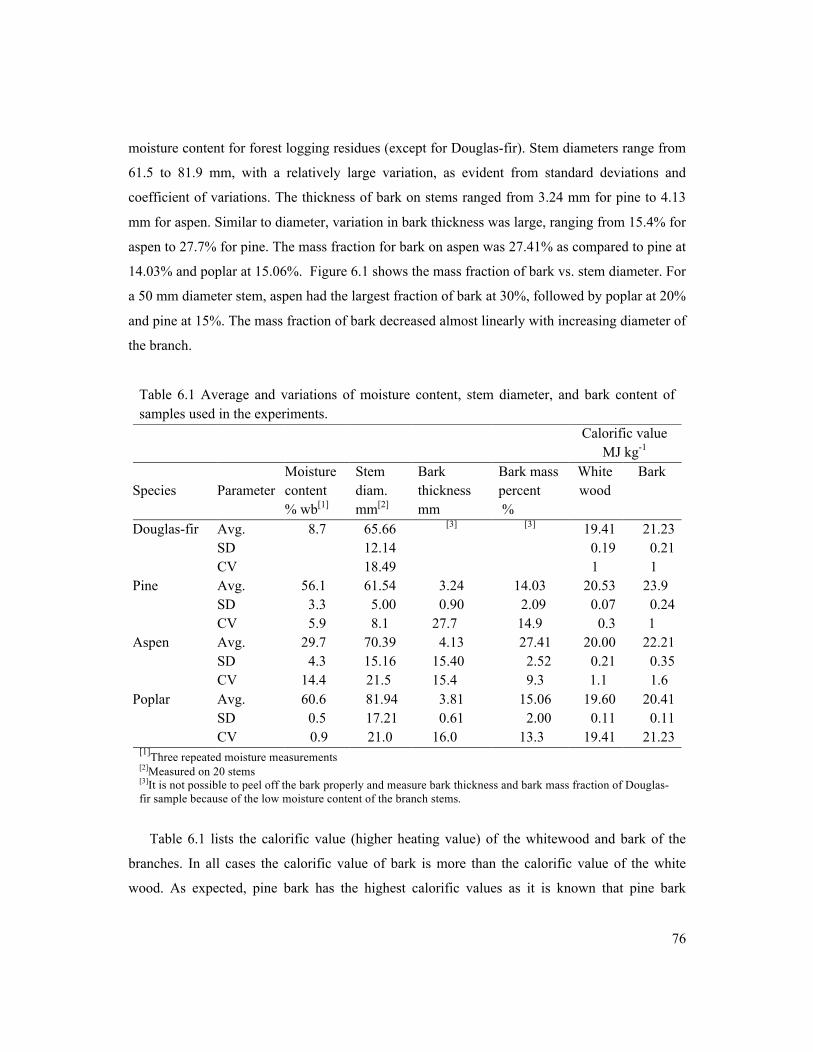
76

moisture content for forest logging residues (except for Douglas-fir). Stem diameters range from

61.5 to 81.9 mm, with a relatively large variation, as evident from standard deviations and

coefficient of variations. The thickness of bark on stems ranged from 3.24 mm for pine to 4.13

mm for aspen. Similar to diameter, variation in bark thickness was large, ranging from 15.4% for

aspen to 27.7% for pine. The mass fraction for bark on aspen was 27.41% as compared to pine at

14.03% and poplar at 15.06%. Figure 6.1 shows the mass fraction of bark vs. stem diameter. For

a 50 mm diameter stem, aspen had the largest fraction of bark at 30%, followed by poplar at 20%

and pine at 15%. The mass fraction of bark decreased almost linearly with increasing diameter of

the branch.

Table 6.1 Average and variations of moisture content, stem diameter, and bark content of samples used in the experiments. Calorific value

MJ kg-1

Species Parameter Moisture content % wb[1]

Stem diam. mm[2]

Bark thickness mm

Bark mass percent %

White wood

Bark

Douglas-fir Avg. 8.7 65.66 [3] [3] 19.41 21.23 SD 12.14 0.19 0.21 CV 18.49 1 1 Pine Avg. 56.1 61.54 3.24 14.03 20.53 23.9

SD 3.3 5.00 0.90 2.09 0.07 0.24

CV 5.9 8.1 27.7 14.9 0.3 1

Aspen Avg. 29.7 70.39 4.13 27.41 20.00 22.21

SD 4.3 15.16 15.40 2.52 0.21 0.35

CV 14.4 21.5 15.4 9.3 1.1 1.6

Poplar Avg. 60.6 81.94 3.81 15.06 19.60 20.41

SD 0.5 17.21 0.61 2.00 0.11 0.11

CV 0.9 21.0 16.0 13.3 19.41 21.23

[1]Three repeated moisture measurements [2]Measured on 20 stems [3]It is not possible to peel off the bark properly and measure bark thickness and bark mass fraction of Douglas-fir sample because of the low moisture content of the branch stems.

Table 6.1 lists the calorific value (higher heating value) of the whitewood and bark of the

branches. In all cases the calorific value of bark is more than the calorific value of the white

wood. As expected, pine bark has the highest calorific values as it is known that pine bark

77

contains extractives (e.g. turpentine) that have high heating values (Moya and Tenorio, 2013).

The heating values of the whitewoods of these species are quite similar, except for that of pine,

which is slightly higher than the other three species.

The bark mass percentages of whole trees of Douglas-fir, pine, and aspen grown in British

Columbia were measured by Standish et al. (1985). The bark content of pine and aspen were 7

and 18%, respectively. This trend is consistent with the results from this study, which found bark

contents of 14 and 27.7% for pine and aspen, respectively. It should be noted that branch wood

was tested in this study, whereas Standish et al. (1985) measured the bark content of a whole

tree. Branch wood is expected to have a higher fraction of bark because of its smaller diameter

compared to tree trunks.

Figure 6.1 Bark fractions as a function of branch stem diameter. Aspen had the largest fraction of bark followed by poplar and pine. Bark content decreases with increasing diameter of the branch.

6.2 Wood density before grinding

Each debarked stem was first dried to about 10% moisture content in a 50oC oven. Then the

stems were sliced into 35 mm disks. The volume Vp of each individual disk was calculated from

the diameter and thickness of these pieces. The mass of each disk m was measured using an

electronic balance accurate to 0.01 g. Particle density of the disk, ρp was estimated from the ratio

of mass of a disk divided by its volume,

0

0.05

0.1

0.15

0.2

0.25

0.3

0.35

40 60 80 100 120

Bar

k fr

actio

n, w

/w

Diameter, mm

Pine

Aspen

Poplar

78

6.1

The solid density of a quarter-disk ρs was calculated by replacing Vp in equation 6.1 with the

volume Vs measured using a gas comparison pycnometer (Quantachrome Instrument, Boynton

Beach, FL). The pycnometer measured and recorded the solid volume of a quarter-disk placed in

a nitrogen gas pressurized cell. The ratio of a piece’s particle density (PD) over solid density was

a measure of the porosity ϕ of a cut piece.

Table 6.2 lists the average and standard deviation of PD and the solid density of samples. The

average PD (Equation 6.1) ranged from 474 kg m-3 for poplar to 708 kg m-3 for Douglas-fir.

Standard deviations between samples tested were high as shown with CV. There was a high PD

variation within Douglas-fir and pine specimens with the CV ranging from 0.12 to 0.15; there

was a low PD variation for aspen and poplar, where the CV ranged 0.04-0.07. It seems that

variations for solid density values were less than variations for values for PD. Volumes measured

by the pycnometer must have been more consistent than volumes calculated from disk

dimensions. Softwoods, Douglas-fir and pine, were denser than hardwoods, aspen or poplar. This

difference in density is evident from the porosity values of 38.4-56% for Douglas-fir and pine

and 47.1-61.6% for aspen and poplar. The result of the ANOVA test (p=0.05) on samples’ PD

showed that the population means were significantly different. Simpson and TenWolde (1999)

reported a CV of 10%, best describing the variability of density within the U.S. wood species.

The pycnometer was used to obtain the volume, which was then used to calculate the solid

density of pieces. Porosity of pieces was calculated using Equation 3.2. Pine and poplar had the

highest solid density of 1242 and 1234 kg m-3, respectively. The solid density of Douglas-fir and

aspen was lower at 1150 and 905 kg m-3, respectively. The CV of solid density ranged from 0.06

to 0.13, which was lower than the CV of particle density—which was between 0.04 and 0.15.

Later on, it will be shown (Table 6.6) that the values for the solid density of ground wood

particles were higher than those in Table 6.2. The results of the ANOVA test (p=0.05) on

samples’ solid densities show that the population means differ significantly.

pp V

m=ρ

79

Table 6.2 Particle and solid densities and estimated porosity of quarter-disk particles prior to being ground in knife mill

Species Parameter Particle density (PD)

kg m-3

Solid density kg m-3

Porosity of solid pieces

% Douglas-fir Avg[1] 708 1150 38 SD[a] 108 129[b] CV, % 15 11 Pine Avg 547 1242 56 SD 68 79[d] CV, % 12 6 Aspen Mean 479 905 47 SD 18 121[b] CV, % 4 13 Poplar Mean 474 1234 62 SD 35 70[c] CV, % 7 6 [a]n=6 ; [b]n=5 ; [c]n=4 ; [d]n=3 [1]At p=0.05 level, the population means are significantly different.

6.3 Microstructure of wood samples

A SilviScan instrument at the FPInnovations Laboratory, located on the campus of the

University of British Columbia, was used to analyze the microstructure of the samples (Evans et

al., 1995). This instrument scans across a cut (sawed) section of a wood sample. The output

consists of values of local density and microfibril angle (MFA). Appendix F shows the density

profiles for six samples of each of the four species of Douglas-fir, pine, aspen and poplar. Table

F.1 lists the results of maximum, minimum, Avg, and SD of the density profile for all of the six

samples from the four species. The prominent frequencies of the density profiles are also located

and summarized in Appendix F. The average density of wood samples using SilviScan (Table

6.3) is in agreement with the density calculated from measured mass and volume (Table 6.2). It

appears that the SilviScan density includes the airspace within the wood. Douglas-fir has the

highest density at 716 kg m-3, followed by pine at 550 kg m-3, aspen at 482 kg m-3 and poplar at

473 kg m-3. The density of wood is directly related to its modulus of elasticity (Evans and Ilic,

2001).

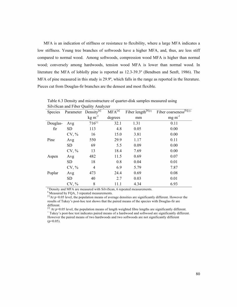
80

MFA is an indication of stiffness or resistance to flexibility, where a large MFA indicates a

low stiffness. Young tree branches of softwoods have a higher MFA, and, thus, are less stiff

compared to normal wood. Among softwoods, compression wood MFA is higher than normal

wood; conversely among hardwoods, tension wood MFA is lower than normal wood. In

literature the MFA of loblolly pine is reported as 12.3-39.3º (Bendtsen and Senft, 1986). The

MFA of pine measured in this study is 29.9º, which falls in the range as reported in the literature.

Pieces cut from Douglas-fir branches are the densest and most flexible.

Table 6.3 Density and microstructure of quarter-disk samples measured using SilviScan and Fiber Quality Analyzer Species Parameter Density[a]

kg m-3 MFA[a] degrees

Fiber length[b][2]

mm Fiber coarseness[b][2]+

mg m-1 Douglas-

fir Avg 716[1] 32.1 1.31 0.11 SD 113 4.8 0.05 0.00

CV, % 16 15.0 3.81 0.00

Pine Avg 550 29.9 1.17 0.11

SD 69 5.5 0.09 0.00

CV, % 13 18.4 7.69 0.00

Aspen Avg 482 11.5 0.69 0.07

SD 18 0.8 0.04 0.01

CV, % 4 6.9 5.79 7.87

Poplar Avg 473 24.4 0.69 0.08

SD 40 2.7 0.03 0.01

CV, % 8 11.1 4.34 6.93

a Density and MFA are measured with SilviScan, 6 repeated measurements. b Measured by FQA, 3 repeated measurements. [1]At p=0.05 level, the population means of average densities are significantly different. However the results of Tukey’s post-hoc test shows that the paired means of the species with Douglas-fir are different. [2] At p=0.05 level, the population means of length weighted fibre lengths are significantly different. + Tukey’s post-hoc test indicates paired means of a hardwood and softwood are significantly different. However the paired means of two hardwoods and two softwoods are not significantly different (p=0.05).

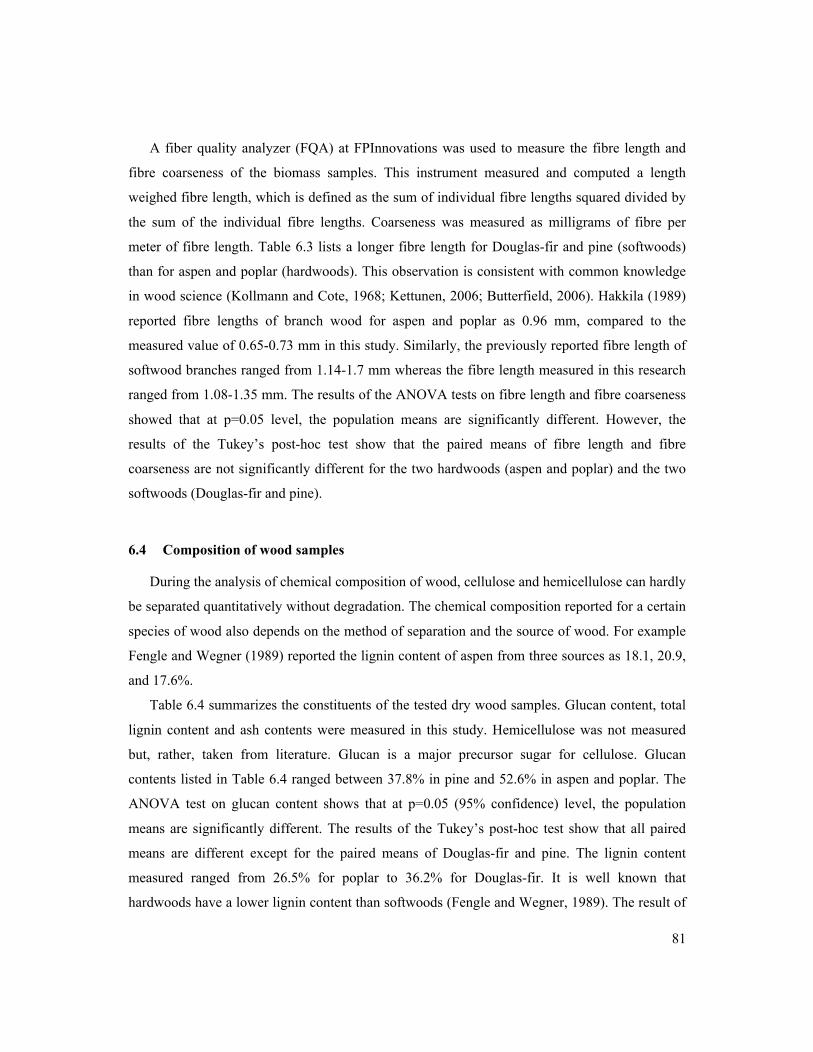
81

A fiber quality analyzer (FQA) at FPInnovations was used to measure the fibre length and

fibre coarseness of the biomass samples. This instrument measured and computed a length

weighed fibre length, which is defined as the sum of individual fibre lengths squared divided by

the sum of the individual fibre lengths. Coarseness was measured as milligrams of fibre per

meter of fibre length. Table 6.3 lists a longer fibre length for Douglas-fir and pine (softwoods)

than for aspen and poplar (hardwoods). This observation is consistent with common knowledge

in wood science (Kollmann and Cote, 1968; Kettunen, 2006; Butterfield, 2006). Hakkila (1989)

reported fibre lengths of branch wood for aspen and poplar as 0.96 mm, compared to the

measured value of 0.65-0.73 mm in this study. Similarly, the previously reported fibre length of

softwood branches ranged from 1.14-1.7 mm whereas the fibre length measured in this research

ranged from 1.08-1.35 mm. The results of the ANOVA tests on fibre length and fibre coarseness

showed that at p=0.05 level, the population means are significantly different. However, the

results of the Tukey’s post-hoc test show that the paired means of fibre length and fibre

coarseness are not significantly different for the two hardwoods (aspen and poplar) and the two

softwoods (Douglas-fir and pine).

6.4 Composition of wood samples

During the analysis of chemical composition of wood, cellulose and hemicellulose can hardly

be separated quantitatively without degradation. The chemical composition reported for a certain

species of wood also depends on the method of separation and the source of wood. For example

Fengle and Wegner (1989) reported the lignin content of aspen from three sources as 18.1, 20.9,

and 17.6%.

Table 6.4 summarizes the constituents of the tested dry wood samples. Glucan content, total

lignin content and ash contents were measured in this study. Hemicellulose was not measured

but, rather, taken from literature. Glucan is a major precursor sugar for cellulose. Glucan

contents listed in Table 6.4 ranged between 37.8% in pine and 52.6% in aspen and poplar. The

ANOVA test on glucan content shows that at p=0.05 (95% confidence) level, the population

means are significantly different. The results of the Tukey’s post-hoc test show that all paired

means are different except for the paired means of Douglas-fir and pine. The lignin content

measured ranged from 26.5% for poplar to 36.2% for Douglas-fir. It is well known that

hardwoods have a lower lignin content than softwoods (Fengle and Wegner, 1989). The result of

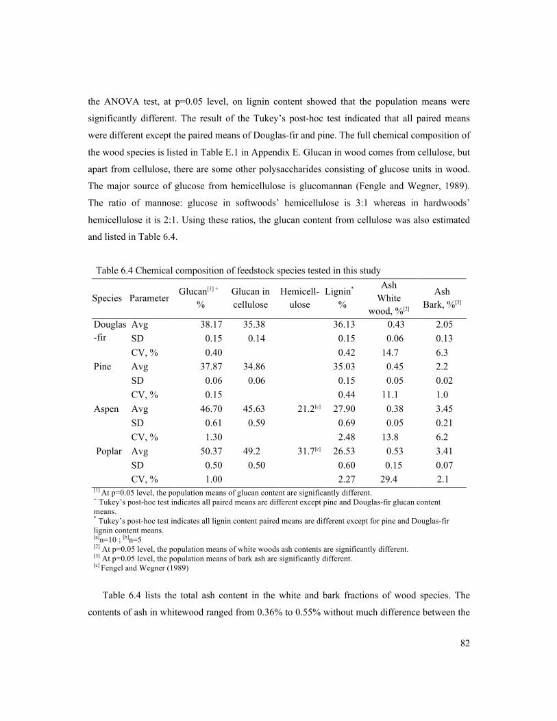
82

the ANOVA test, at p=0.05 level, on lignin content showed that the population means were

significantly different. The result of the Tukey’s post-hoc test indicated that all paired means

were different except the paired means of Douglas-fir and pine. The full chemical composition of

the wood species is listed in Table E.1 in Appendix E. Glucan in wood comes from cellulose, but

apart from cellulose, there are some other polysaccharides consisting of glucose units in wood.

The major source of glucose from hemicellulose is glucomannan (Fengle and Wegner, 1989).

The ratio of mannose: glucose in softwoods’ hemicellulose is 3:1 whereas in hardwoods’

hemicellulose it is 2:1. Using these ratios, the glucan content from cellulose was also estimated

and listed in Table 6.4.

Table 6.4 Chemical composition of feedstock species tested in this study

Species Parameter Glucan[1] +

% Glucan in cellulose

Hemicell-ulose

Lignin* %

Ash White

wood, %[2]

Ash Bark, %[3]

Douglas-fir

Avg 38.17 35.38 36.13 0.43 2.05 SD 0.15 0.14 0.15 0.06 0.13 CV, % 0.40 0.42 14.7 6.3

Pine Avg 37.87 34.86 35.03 0.45 2.2 SD 0.06 0.06 0.15 0.05 0.02 CV, % 0.15 0.44 11.1 1.0

Aspen Avg 46.70 45.63 21.2[c] 27.90 0.38 3.45 SD 0.61 0.59 0.69 0.05 0.21 CV, % 1.30 2.48 13.8 6.2

Poplar Avg 50.37 49.2 31.7[c] 26.53 0.53 3.41 SD 0.50 0.50 0.60 0.15 0.07 CV, % 1.00 2.27 29.4 2.1

[1] At p=0.05 level, the population means of glucan content are significantly different. + Tukey’s post-hoc test indicates all paired means are different except pine and Douglas-fir glucan content means. * Tukey’s post-hoc test indicates all lignin content paired means are different except for pine and Douglas-fir lignin content means. [a]n=10 ; [b]n=5 [2] At p=0.05 level, the population means of white woods ash contents are significantly different. [3] At p=0.05 level, the population means of bark ash are significantly different. [c] Fengel and Wegner (1989)

Table 6.4 lists the total ash content in the white and bark fractions of wood species. The

contents of ash in whitewood ranged from 0.36% to 0.55% without much difference between the

83

species. The ash content of the bark was 3.41-3.43% in aspen and poplar compared to 2.05-

2.21% in Douglas-fir and pine. The results of the ANOVA test on the ash content of whitewood

and bark, at p=0.05 level, showed that the population means were significantly different.

6.5 Size reduction of wood samples

The quarter-disk pieces were fed uniformly into the knife mill equipped with 2, 4, or 6 mm

screens. Table C.1 in Appendix C lists the detailed measured data for grinding the four species in

the grinder with a 2 mm screen. In total, 14 grinding runs, using more than 7 kg of sample (2261

pieces of quarter-disk pieces, Figure 3.2), were completed for grinding on a 2 mm screen. A test

run consisted of about ~500 g sample with the number of pieces ranging from 86 to 239

depending upon the size and mass of each piece. It took 125 to 476 seconds to feed the wood

into the grinder, while the cutter rotor operated 299 to 706 seconds to complete a grinding run.

The average feeding rate was calculated from dividing the total feed by the grinding time and

was expressed in g s-1. During the operation, the power input (W) of the mill was recorded for

each second using a wattmeter. Prior to a test run, the power input to the grinder was recorded

for a minimum of 600 seconds. The difference between power input with load and power input

without load was calculated as the net power input over each grinding run.

Table 6.5 lists the results of specific energy and the geometric mean diameter of ground

particles from 2, 4, and 6 mm screens. The average of the specific energies of three to four trials

and the standard deviation of the trials are listed. Both the specific energy and its standard

deviation decreased as the screen size increased. The coefficients of variation of the tests are also

listed, which decreased as the screen size increased. Douglas-fir (a softwood) and poplar (a

hardwood) have the lowest and highest specific energy consumptions of grinding, respectively.

However, pine (a softwood) has a higher specific energy of grinding compared to aspen, which is

a hardwood. These results suggest that there is no clear-cut difference in energy consumption

between grinding hardwood and grinding softwood.

84

Table 6.5 Specific energy consumption of grinding manually prepared pieces of Douglas-fir, pine, aspen, and poplar by knife mill. Screen sizes of 2, 4, and 6 mm were used. Mean, SD, and CV of the specific energy of size reduction are listed.

Species Screen size

mm Specific energy, J g-1 Geometric size of

particles, dgw, mm Mean SD CV Douglas-fir 2[1] x 156 20 0.1 0.68

4[1] + 56 4 0.1 1.05 6[1]* 42 2 0.0 1.09

Pine 2 226 33 0.2 0.74 4 71 3 0.0 1.10 6 31 3 0.1 1.11

Aspen 2 209 20 0.1 0.65 4 103 11 0.1 0.85 6 52 7 0.1 1.00

Poplar 2 276 23 0.1 0.65 4 153 8 0.1 1.00 6 87 3 0.0 1.08

[1] At p=0.05 level, the population means of specific energies of grinding using the screen size are significantly different. xTukey’s post-hoc test indicates all paired means are different except the specific energy of grinding means of pine and aspen, and poplar and aspen on a 2 mm screen. + Tukey’s post-hoc test indicates all paired means are different except the specific energy of grinding means of pine and Douglas-fir on a 4 mm screen. *Tukey’s post-hoc test indicates all paired means are different except the specific energy of grinding means of aspen and Douglas-fir on a 6 mm screen.

Table 6.6 summarizes detailed results for the grinding test operation using a 2 mm size

screen. The average mass of the quarter-disk pieces was 2.6-2.7 g, except for Douglas-fir, which

had heavier pieces, averaging 4.1 g. Feeding rate was controlled by feeder tray vibration which

was set to 20% of full scale. The mass of the samples prepared for each grinding trial was 500 g.

The pieces size was controlled by two factors: choosing branch stems with diameters of 50 to

100 mm and cutting the quarter-disc shaped pieces with a thickness of 3 to 4 mm (Figure 3.6

(b)). The pieces were aligned on the feeder tray to make sure that they were continuously falling

into the grinder. Diameter and density of each piece affected the feeding rate, making it vary for

different species. Pine and aspen took the least amount of time, 1.28 to 1.43 s, for a piece to be

fed into the grinder. Poplar took 2.41 s/piece to be fed to the grinder because its branches had

larger diameters compared to the branches from other species (Table 6.1). In terms of feeding

rates, poplar showed the lowest feeding rate at 0.77 g s-1 compared to Douglas-fir at 1.1 g s-1.

85

Figure 6.2 shows that the specific energy consumption increased for pine, poplar, and aspen,

but not for Douglas-fir, when the feeding rate increased. The greatest variability in feeding rate

was observed for Douglas-fir, while variabilities in feeding rates for aspen and poplar were the

least among the species. The variability of a branch’s density (particle density) from which

quarter-disk pieces were taken was higher for Douglas-fir compared to the branches from the

other three species (see Table 6.3). Goswami and Singh (2003) studied the impact of feeding rate

on the specific size reduction energy for grinding cumin in an attrition mill. They concluded that

the specific energy consumption decreased as the feeding rate increased, reached a minimum

value before increasing with further increase in the feeding rate. It is hard to compare our results

with the literature because of a limited range of feeding rate tested in this study and a different

type of grinding mill used in this study (knife mill).

Table 6.6 Summary of data for feeding quarter-disk pieces into the knife mill. The screen size for these tests was 2 mm. Species of

tested biomass

Parameter Average mass of quarter-disk

g

Time to feed a quarter-disk,

s/Disk

Feeding rate g s-1[1]

Energy J g-1

Douglas-fir Avg 4.13 2.4 1.10 156 SD 0.99 1.4 0.51 20

Pine Avg 2.74 1.3 0.84 226 SD 0.22 0.5 0.33 33

Aspen Avg 2.78 1.4 0.85 209 SD 1.15 0.1 0.04 20

Poplar Avg 2.67 2.4 0.77 276 SD 0.58 0.5 0.04 23

[1] At p=0.05 level, the population means of feeding rates are not significantly different.

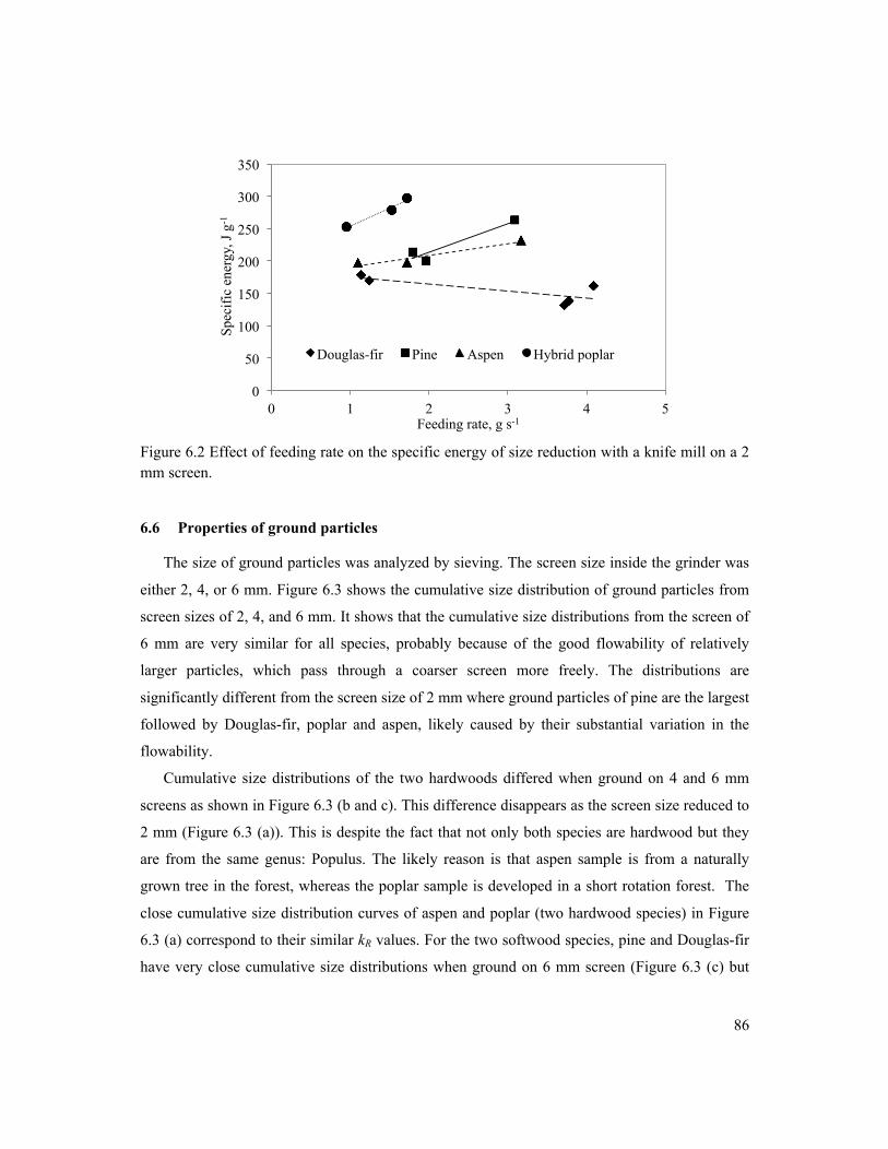
86

Figure 6.2 Effect of feeding rate on the specific energy of size reduction with a knife mill on a 2 mm screen.

6.6 Properties of ground particles

The size of ground particles was analyzed by sieving. The screen size inside the grinder was

either 2, 4, or 6 mm. Figure 6.3 shows the cumulative size distribution of ground particles from

screen sizes of 2, 4, and 6 mm. It shows that the cumulative size distributions from the screen of

6 mm are very similar for all species, probably because of the good flowability of relatively

larger particles, which pass through a coarser screen more freely. The distributions are

significantly different from the screen size of 2 mm where ground particles of pine are the largest

followed by Douglas-fir, poplar and aspen, likely caused by their substantial variation in the

flowability.

Cumulative size distributions of the two hardwoods differed when ground on 4 and 6 mm

screens as shown in Figure 6.3 (b and c). This difference disappears as the screen size reduced to

2 mm (Figure 6.3 (a)). This is despite the fact that not only both species are hardwood but they

are from the same genus: Populus. The likely reason is that aspen sample is from a naturally

grown tree in the forest, whereas the poplar sample is developed in a short rotation forest. The

close cumulative size distribution curves of aspen and poplar (two hardwood species) in Figure

6.3 (a) correspond to their similar kR values. For the two softwood species, pine and Douglas-fir

have very close cumulative size distributions when ground on 6 mm screen (Figure 6.3 (c) but

0

50

100

150

200

250

300

350

0 1 2 3 4 5

Spec

ific

ener

gy, J

g-1

Feeding rate, g s-1

Douglas-fir Pine Aspen Hybrid poplar

87

their cumulative size distribution curves become significantly different as the screen size

decreases to 2 mm (Figure 6.3 (a)). In general, the higher the kR value the coarser ground

particles are expected from grinding operation. The softwoods have significantly different kR

values, and are expected to have different size distribution of ground particles. One possible

reason is the presence of resin canal complexes in pine wood structure.

Similar trend was reported by Repellin et al. (2010). They ground spruce (a softwood) and

beech (a hardwood) by a knife mill with a 8 mm screen. They showed the same percentage of

ground particles below 2 mm sieve for both species in the coarse grinding. The size of the feed

wood chips was not reported in their paper. In the further fine ground in an ultra centrifugal mill

equipped with 500 µm grid, the particles collected between 2 mm and 4 mm sieve from the

coarse grinding were used as the feed. The results showed that 90% (vol%) of ground spruce

particles were under 500 µm, while 90% (vol%) of beech particles were under 620 µm, showing

a noticeable difference.

88

(a)

(b)!

!(c)

0

0.2

0.4

0.6

0.8

1

0 0.2 0.4 0.6 0.8

Cum

ulat

ive

wei

ght f

ract

ion

Sieve opening, mm

Knife mill screen 2 mm

Douglas-fir Pine Aspen Poplar

0 0.1 0.2 0.3 0.4 0.5 0.6 0.7 0.8 0.9

1

0 0.2 0.4 0.6 0.8 1 1.2 1.4

Cum

ulat

ive

wei

ght f

ract

ion

Sieve opening, mm

Knife mill screen 4 mm

Douglas-fir Pine Aspen Poplar

0 0.1 0.2 0.3 0.4 0.5 0.6 0.7 0.8 0.9

1

0 0.5 1 1.5 2

Cum

ulat

ive

wei

ght f

ract

ion

Sieve opening, mm

Knife mill screen 6 mm Douglas-fir

Pine

Aspen

Poplar

89

Figure 6.3 Cumulative size distribution of ground particles of the four biomass species of Douglas-fir, pine, aspen, and poplar. The size distributions on 2, 4, and 6 mm screens are shown in graphs (a), (b), and (c), respectively. The graph shows that the difference between cumulative size distribution curves increases as the screen size decreases. The top graph shows that the cumulative size distribution curves of aspen and poplar are fairly close and they are located between the size distributions of softwoods with pine at the bottom and Douglas-fir at the top.

Table 6.7 lists the fraction of particles less than 0.6 mm with data extracted from the

cumulative size distribution curve (Figure 6.3). The species are arranged from top to bottom

based on their particle size: pine having the largest particles at the top, followed by Douglas-fir,

poplar, and aspen. Table 6.7 shows that pine and Douglas-fir (the two softwoods) have a similar

fraction of ground particles below 0.6 mm sieve size when ground on a 6 mm screen. However,

this fraction is very different when the two softwoods are ground on 2 mm screen. This shows

that pine and Douglas-fir behave similarly on big screens but they behave differently when the

screen size is decreased to 2 mm. Table 6.7 shows the fraction of ground particles below 0.6 mm

sieve size are different for poplar and aspen (the two hardwoods) when ground on a 6 mm

screen. This difference disappeared when the two hardwoods were ground on a 2 mm screen.

This demonstrates that the softwoods and hardwoods show different performances depending on

the screen size.

Table 6.7 Fraction of ground particles less than 0.6 mm. The data were extracted from cumulative size distribution of ground particles from a knife mill with 2, 4, and 6 mm screen sizes.

Species Knife mill screen size, mm

2 4 6 Pine 0.38 0.27 0.16 Douglas-fir 0.57 0.34 0.16 Poplar 0.66 0.35 0.17 Aspen 0.67 0.57 0.22

Particle surface area was measured by a scanner and by a publicly available software

(Rasband, 2004). The procedure is explained in Appendix A. Table 6.8 lists the results of the

specific surface area of particles produced with a 2 mm screen. The mass of each sample was all

within 45 g to 50 g with an average of 47 g. The specific surface area (surface area over mass)

90

for ground particles was calculated as 41.4 mm2 g-1 with SD of 16.0 and CV of 38%. These large

variations were due to the differences in the surface area of the particles, although their mass did

not change very much. The results of the ANOVA (p=0.05) test showed that population means

of specific areas of the four species were different.

Table 6.8 Bulk density, tapped density, and porosity of the ground particles. The particles passed through 2 mm screen in the knife mill.

Species Parameter Specific surface

area mm2 g-1

Loose density kg m-3

Tapped density kg m-3

Hausner ratio

Solid density of

ground particles kg m-3

Porosity of ground particles (fraction)

Angle of repose

(degrees)

Douglas-fir Avg 26.93 343 396 1.16 1408 0.76 37.1 SD[a] 9.07 3 3 30 0.7 CV, % 34 1.9

Pine Avg 40.13 285 331 1.16 1350 0.79 39.6 SD 4.25 3 3 46 0.6 CV, % 11 1.4

Aspen Avg 60.57 245 294 1.20 1335 0.82 42.4 SD 17.95 2 1 68 1.4 CV, % 30 3.2

Poplar Avg 38.20 175 213 1.22 1461 0.88 41.8 SD 7.36 1 1 12 0.6 CV, % 19 1.3

[a]3 runs for each species

Table 6.8 lists the loose bulk density, tapped density, Hausner ratio, solid density, porosity,

and angle of repose of particles ground in the knife mill with a 2 mm screen. The ground

particles were less than 0.841 mm (Figure 6.3). Douglas-fir particles had the largest loose bulk

density of 343 kg m-3. Poplar had the least loose bulk density at 175 kg m-3. The increased bulk

density due to tapping was in the range of 15 to 22%. The Hausner ratio, which is a measure of

the friction condition of moving powders (Grey and Beddow, 1969), of ground poplar was larger

than ground Douglas-fir, indicating that poplar has a poorer flowability. This may indicate that

poplar particles were interlocked to give a lower flowability. The angle of repose, another

measure of the flowability of powders which defines the cohesiveness of a bulk of ground

particles (Geldart et al., 2006), shows a consistent trend as the Hausner ratio, higher for the two

91

hardwood species than the two softwood species. As speculated before, the poor flowability of

hardwood species may cause particles to stay a longer time in the grinder with a screen installed,

leading to an increase in fine fraction of ground particles. This proposed mechanism seems to be

supported by the fine fraction data in Table 6.7 where the fine fraction less then 0.6 mm is

generally higher for the hardwood samples than for the softwood samples for the operation with

installed screens of different sizes. Lower bulk density may also result in a lower rate of pellet

formation.

Table 6.8 also lists the angle of repose of the ground particles. A smaller angle of repose for

Douglas-fir is an indication of low specific energy input for grinding (J g-1) because the particles

with a small angle of repose flow easily and leave the grinding chamber as soon as they are

created and have passed through the screen holes. By comparison, the low flowability of poplar

particles, which have the highest angle of repose provides an explanation for the highest specific

energy consumption of grinding in J g-1. The lower flowability caused the particles to remain in

the grinding chamber longer and, thus, consumed more energy over a longer residence time and

generated more fine particles.

Volumes of ground particles were also measured by a pycnometer to calculate the solid

density. The porosity (void space in ground particles) of the bulk ground particles was calculated

using Equation 3.3. The trend of porosity was similar to the trend of the Hausner ratio. Porosity

values range from 0.76 for Douglas-fir to 0.88 for poplar. An increase in porosity indicates that

the material is fluffy and difficult to flow.

As shown in this section, the grinding performance of a knife mill is strongly correlated with

the properties of the wood species. Even for a grinder with a fixed screen installed, different

specific energy consumption and ground particle size and size distribution could result when

grinding different biomass species of the same particle size and feeding rate, because of the

difference in the wood properties. For example, sticky particles may stay longer inside the

grinder chamber, increasing the grinding energy consumption for creating more fine ground

particles. To investigate the effect of wood properties on the grinder performance, the Rittinger

coefficient kR, which is independent of the particle size changes through the grinder, will be

correlated with measured biomass properties in this study.

92

6.7 Correlation of Rittinger constant with biomass particles properties

kR is a constant which is developed based on specific energy consumption over size reduction

ratio of feed and product particles through the grinder. Therefore, it is a parameter representative

of energy consumption, but independent of feed and product particles sizes, and it can be used to

quantify the influence of biomass properties on the grinding performance. Tables 6.9 and 6.10

summarize the measured properties of the four wood species, and their kR values.

It is seen that the only substantial differences between the two hardwoods are in the pieces

solid density, MFA, and the fibre coarseness, lower for the aspen sample. Since the kR values and

ground particle size distributions are almost the same for aspen and poplar, it seems to suggest

that pieces solid density, MFA, and fibre coarseness are not important in determining the

grinding energy consumption, at least for the hardwoods.

kR is quite different for the two softwoods. Examining the properties of the two samples, it is

apparent that both the particle density and density determined from SilviScan (Table 6.3)

consistently show a lower value for pine than Douglas-fir. The fact that Douglas-fir has a lower

kR value and a higher particle density suggests that it is easier to grind softwood of higher

particle density.

Table 6.9 Summary of kR, density and chemical properties of wood species

Species kR Particle density

(PD) Pieces solid

density Porosity

Lignin content

Cellulose glucan

J mm g-1 kg m-3 kg m-3 % % % Douglas-fir 203 708 1151 38 36 35 Pine 398 547 1243 56 35 35 Aspen 299 479 905 47 28 46 Poplar 277 474 1234 62 27 49

Table 6.10 Summary of kR, average density from SilviScan and fibre trait of the wood species

Species kR Density MFA Length weighted

fibre length Fibre coarseness

J mm g-1 kg m-3 degrees mm mg m-1 Douglas-fir 202 716 32 1.3 0.11 Pine 398 550 30 1.2 0.11 Aspen 299 482 12 0.7 0.07 Poplar 277 473 24 0.7 0.08

93

6.7.1 Single parameter regression analysis

The nine properties of woody samples listed in Tables 6.9 and 6.10 are highly

interdependent. Table 6.11 lists the correlation matrix for the nine properties. The correlations

range from 0 to +1. A value close to +1 indicates strong positive correlation. A smaller value

near 0 indicates a poor correlation. Some of the correlations can be easily explained like those

related to density and porosity. The relationship between fiber length and MFA is less obvious.

Table 6.11 lists the strongest correlation between particle density measured manually and the

particle density measured using SilviScan method. Among physical features, MFA has a strong

correlation with density and fiber length, but a weak correlation with porosity. Most of the

measured properties using SilviScan have positive correlation with lignin, but negative

correlation with cellulose content (glucan).

Table 6.11 Correlation matrix of nine wood properties measured in this research. Property Particle

density Solid

density Porosity Lignin content

Cellulose glucan

Density (SilviScan) MFA Fibre

length Fibre

coarseness Particle density 1.00

Solid density 0.21 1.00

Porosity -0.76 0.47 1.00 Lignin

content 0.85 0.37 -0.52 1.00

Cellulose glucan -0.79 -0.32 0.50 -0.99 1.00

Density (SilviScan) 1.00 0.20 -0.77 0.85 -0.79 1.00

MFA 0.71 0.83 -0.09 0.79 -0.73 0.70 1.00 Fibre length 0.87 0.43 -0.50 1.00 -0.98 0.87 0.84 1.00

Fibre coarseness 0.78 0.63 -0.29 0.96 -0.93 0.78 0.93 0.97 1.00

Figure 6.4 shows the correlation of Rittinger’s constant with the nine measured properties of

the wood samples. The strongest positive correlation was with porosity, solid density, and fiber

coarseness. On the negative side, the strongest correlation was between kR and particle density

and density from silviscan. The relationship between kR and particle density can be explained

with a second order polynomial with a high degree of coefficient of determination (R2=0.99):

94

kR = −0.01ρ2 +13.9ρ −3594.9 6.2

Particle density, ρ, is in kg m-3 and kR is in J mm g-1. More data on density vs. power input is

needed to develop a more robust relation. The validity of Equation 6.2 is limited to the range of

particle density measured in this research.

Figure 6.4 Correlation of Rittinger constant with wood properties. The largest positive correlation is with porosity of solid pieces and the largest negative correlation is with wood density.

6.7.2 Multi-variable regression analysis

The two softwood species have kR values either higher or lower than the two hardwood

species. The mean particle sizes of softwood are generally coarser than hardwood, as shown in

Figure 6.3. We may speculate that it is generally harder to grind softwood than the hardwood, i.e.

kR should be higher for softwood. Examining those properties of softwood and hardwood, which

are similar in hardwood (because those properties which are different within the two hardwood

species are unlikely to affect the grinding in view of the similar performance of the two

hardwood species) but different in softwood, 5 properties are identified as having potentially

created the difference in grinding operation: particle density, lignin content, cellulose content,

length weighted fibre length and fibre coarseness. However, because only 4 species of wood

-0.6

-0.4

-0.2

0

0.2

0.4

0.6

Porosity Solid density

Fibre coarseness

Lignin content

Fibre length

MFA Cellulose glucan

Density (SilviScan)

Particle density

Cor

rela

tion

Coe

ffici

ent w

ith k

R

95

were tested in this study, it is not possible to conduct a multivariable analysis involving more

than two independent variables (5 variables are identified in Tables 6.9 and 6.10). Considering

the literature review, the four variables of particle density (PD), fibre length (FL), glucan in

cellulose, which is considered as a representative of cellulose content, (CC), and lignin content

(LC) are analyzed pair-wise to identify the most important properties that affect kR.

A multivariable regression is developed for kR and any two of the four variables as

independent variables using Origin software (OriginLab, Northampton, MA). The following

equation represents this relationship:

kR = a.Am.Bn

6.3

where kR is the Rittinger constant (J mm g-1). A and B represent two of the selected four

independent variables. a, m, and n are constants. Table 6.12 lists the regression coefficients and

their statistical standard errors. The highest R2 values for PD and CC, and PD and LC as

independent variables suggest that PD, CC, and LC have the most significant effects on kR. It

should also be noted that cellulose content and lignin content are inter-related because a higher

lignin content generally corresponds to a lower cellulose content. In view of the uncertainty in

cellulose content (represented by glucan) measurement in this study, it is more appropriate to

state that particle density (PD), lignin content (LC), and fibre length (FL) are the three most

important biomass properties influencing the biomass grinding performance, which will be

discussed in the next section.

96

Table 6.12 Regression coefficient and statistical information for multivariable regression of kR with PD, FL, LC, and CC as independent variable.

Constants Value Standard error Equation R2 A=PD B=FL

ln(a) 26.1 3.9 kR = 2.2×10

11PD−3.2FL1.5 0.96 m -3.2 0.6 n 1.5 0.3

A=PD B=CC

ln(a) 29.5 1.5 kR = 6.5×10

12PD−2.5CC −2.2

1.00 m -2.5 0.2 n -2.2 0.2

A=PD B=LC

ln(a) 14.4 0.4 kR =1.8×10

6PD−3.0LC3 1.00 m -3.0 0.1

n 3.0 0.1 A=FL B=CC

ln(a) 25.1 15.7 kR = 7.9×10

10FL−2.7CC−5.3 0.61 m -5.3 4.3 n -2.7 2.2

A=FL B= LC

ln(a) 24.4 9.3 kR = 3.9×10

10LC−5.1FL−2.4 0.80 m -2.4 2.5 n -5.1 1.2

A=CC B= LC

ln(a) 99.0 15.7 kR = 9.9×10

42CC −12.4LC −13.8

0.97 m -12.4 2.1 n -13.8 2.3

6.8 Discussion

Wood species: One noticeable difference between the softwood and hardwood is their

density profile in the scale of 2-4 mm (Hofstetter et al., 2004). The second noticeable difference

is the presence of vessels in the structure of hardwoods in the scale of 20-500 µm. Figure 2.4 (b)

and (c) shows the difference between the scanning electron micrograph of the transverse sections

of softwoods and hardwoods. Vessel elements in hardwoods create pores inside the wood

structure, whereas there is no vessel element in softwoods. When a crack happens in hardwoods,

there is a high chance that the crack ends up in a pore and creates a small particle. The

probability of this failure in softwood is smaller and therefore softwood particles are larger than

hardwood particles. Comparison of the scale of the two phenomena shows that the latter is more

dominant when smaller screens are installed in the grinder.

Structurally, leaning tree branches are classified as reaction wood, which forms when wood

is under stress and develops differently in softwoods and hardwoods. In hardwoods, reaction

97

wood is developed as tension wood on the upper side of the branch. It has a higher density and

tensile strength compared to the normal wood. In softwoods, reaction wood is developed as

compression wood on the lower side of the branch. Compression wood also has a higher density

than normal wood (Hakkila, 1989; Kettunen, 2006). Although it is higher in density but it has a

lower tensile strength, modulus of elasticity and impact strength than normal wood (Butterfield

and Meylan, 1980).

Nati et al. (2010) studied grinding of branches and logs of poplar and pine using a drum

chipper. They installed two screens of medium and large sizes on the chipper. The overall results

showed that branch wood had less accept particles and more fines and oversize particles

compared to logs, which was undesirable. Their results showed that chipping poplar and pine on

the same screen consumed the same level of specific energy but created smaller ground particles

for pine compared to poplar.

Many studies have reported the change of specific energy consumptions with species of

wood. Repelline et al. (2010) reported a specific energy of 750 kWh t-1 for grinding spruce (a

softwood), which is lower than energy input for grinding beech (a hardwood) at 850 kWh t-1.

They used a laboratory size ultra centrifugal Retsch mill equipped with a 500 µm screen that is

why a high input power was recorded in their experiments. Esteban and Carrasco (2006) reported

that the specific energies for grinding poplar (hardwood) and pine (softwood) chips by a hammer

mill were 82.6 and 119.1 kWh o.d t-1, respectively. However, their studies did not report the

distribution of ground particle sizes on all screens used, and thus their findings cannot be directly

compared with the current study on the grinding performance based on kR.

Recently, Temmerman et al. (2013) studied grinding wood chips of two softwoods (pine and

spruce) and two hardwoods (oak and beech) with five levels of moisture contents using hammer

mill (1.1 kW). They pre-ground wood chips using an industrial hammer mill. The ground wood

chips were then screened using a 16 mm diameter round mesh screen to eliminate the fraction of

wood chips larger than 16 mm. They used the median size of particles as the representative mean

size of particles and recorded the grinding energy consumption. Their results confirmed that the

Rittinger equation was the best fitted equation to the data of size and specific energy

consumption among the three equations of Rittinger, Kick, and Bond. KR was reported to be in

the range of 55.5-126.3 W h mm kg (od)-1 (199.8-454.7 J mm g (db)-1) for pine with MC of 9-

13.5%. The estimated KR is in dry basis and is higher than 67.3 J mm g (wb)-1 obtained in this

98

study for pine with a MC of 11-12% (see Figure 4.9). This difference may be due to the smaller

hammer mill or in the definition of the mean size of particles in this thesis. Temmerman et al.

(2013) showed that as the MC increased the KR increased and the estimated KR is smaller for

softwoods than hardwoods. Our results show that kR is smaller for Douglas-fir (softwood) than

hardwoods, but pine had the highest kR among all the four species tested. This might be because

the wood samples we studied are branch wood, as well as the specific properties of the two

softwood species. For example, looking at the structure of pine and Douglas-fir, resin canal

complexes are often visible on the transverse section in pine but they are much smaller in

Douglas-fir (Wiedenhoeft and Miller, 2005).

Particle Density (PD): Simpson and TenWolde (1999) reported the specific gravity of

Douglas-fir, pine, and aspen as 0.51, 0.43, and 0.40, respectively, where the basic density (the

oven dry mass divided by the green volume) is used for calculating the specific gravity. The

particle densities in this thesis follow the same order as the specific gravities from Simpson and

TenWolde’s. The solid densities of the ground wood particles shown in Table 6.8 are higher than

those reported in Table 6.2. The difference may be due to the method of measuring pore volumes

and estimating density. Nitrogen gas at a pressure of 103 kPa (15 psi) was used to penetrate the

open pores of the piece in the pycnometer to measure solid density. This pressure was probably

not adequate for nitrogen gas to penetrate into all the enclosed pores within the internal wood

structure.

As listed in Tables 6.2 and 6.3, the particle density (PD) and average density from

microstructure analysis are similar. A negative exponent predicts that as the PD increases kR will

decrease leading to a larger drop in specific energy consumption. This seems to be contradictory

to what have reported by other researchers (e.g. Hakkila, 1989) that higher energy is required to

grind wood with a higher basic density. Hakkila (1989) referred to two previous studies by Arola

et al. (1983) and Papworth and Erickson (1966) who ground tree trunks of green softwoods and

hardwoods with an average MC of 38% using a disk chipper. Arola et al. (1983) reported that

wood species with specific gravities of 0.36, 0.39, 0.39, 0.51, 0.53, and 0.54 required a low

specific power input of 0.64, 0.77, 0.88, 1.10, 0.82, and 1.18 kW h t-1, respectively. The first

noticeable difference is the low power input. Arola et al. (1983) did not use a screen in their disk

chipper. The generated particles immediately leave the chipper, whereas in the grinder with a

screen the particles stay in the grinder chamber until the particles become small enough to pass

99

through the screen. The smaller the screen size the longer is the residence time of the particles

inside the grinding chamber. Secondly, they did not report the chip size and whether there is a

variation in the ground chip sizes among the different samples. Similar to what we found in this

work, Twaddle (1997) reported that the length to thickness ratio for chips made from the same

chipper were 3.4, 2.7, 3.6, and 3.6 for loblolly pine, Southern red oak, sweetgum and shagbark

hickory, respectively. Dubois et al. (1992) showed that with similar log diameter and grinder

mechanism, hickory, sweetgum, and oak gave 79%, 90%, and 92.5% acceptable size chips,

respectively. Therefore, the result from Arola et al. (1983) could not be directly compared with

our finding, which is based on kR rather than the specific energy consumption, unless the feed

and output particle sizes were maintained the same for different samples in their study, which

was unlikely based on our experience and other previous studies.

The effect of particle density can also be explained by examining the density profiles of

softwoods and hardwoods from SilviScan analysis (Figures F.1 and F.13). Figure F.1 shows the

density profile of Douglas-fir from pith to bark where sharp changes of density are observed.

Marchal et al. (2009) explained a similar process for peeling softwoods. They observed that for

heterogeneous woods such as softwoods, as they called it, the density profile tends to reduce the

veneer thickness. In softwoods, the wood around the touching knife tip is crushed, then torn

through the area with low density that reduces the ground piece thickness. As a result although

softwoods have a higher density they are ground much faster, pass the screens earlier and

consume less energy. Table F.1 lists the frequencies in density profiles in softwoods and

hardwoods. The frequencies are in the range of 0.6-0.8 cycle mm-1 for softwoods and 0.1 cycle

mm-1 for hardwoods, reflecting the heterogeneity of softwoods. The results show that the wood

density profile could be an important factor to be considered in understanding the impact of

particle density on kR instead of only the average density.

Chemical composition: It has been well documented in the literature that lignin and

cellulose are the constituents in providing the strength of wood (Kollmann and Cote, 1968;

Gindl, 2002). Horvath et al. (2010) showed that as the lignin content decreased, the modulus of

elasticity and compression strength parallel to the grain decreased in genetically modified aspen

species. Kollmann and Cote (1968) showed that as the lignin content increases the quality factor,

which is defined as the ratio of crushing strength over specific gravity, increases. One can thus

expect an increase of kR for grinding wood of high lignin content, consistent with what we found

100

from regression in Table 6.11. Such trend also seems to be supported by the reported moisture

effect on grinding operation. Temmerman et al. (2013) showed that kR increased as the moisture

content of wood increased. This can be attributed to the increased binding forces and stickiness

of moist particles (softened lignin), which require more energy to crush them. In the

densification operation, which is opposite to grinding operation, higher biomass lignin content

can create a strong bond for making strong pellets, and the presence of certain moisture content

helps improving the lignin bonding.

de Borst et al. (2012) studied the mechanical properties of ten hardwood species and showed

that at similar MFA the indentation modulus increases as the cellulose content increases. There is

also a wide range of studies on the impact of cellulose content on wood strength (Kollmann and

Cote, 1968; Keckes et al., 2003; Kettunen, 2006; Deng et al., 2012). Because of the uncertainty

in the measured cellulose (glucan in this study), we will only focus on the effect of lignin in this

section.

Fibre length (FL): The fibre length of softwood measured in this research ranged between

1.08-1.35 mm, which is approximately in the range of fibre length reported in the literature. The

fibre length of loblolly pine was reported as 1.57-4.03 mm with CV (Coefficient of Variation) of

5.5-19.1% (Bendtsen and Senft, 1986) and the fibre length of pine measured in this study is in

the range of 1.08-1.25 mm. This difference may be because the samples studied in the literature

were from wood stems, whereas the samples in this study were from branch woods. The fibre

length of poplar was reported to be between 0.9-1.1 mm from 10 clones with a standard

deviation of 0.02-0.3 mm (Koubaa et al., 1997), while the fibre length of poplar in this study was

measured as 0.66-0.71 mm. This difference might be due to the tree genus, age, location, and/or

soil conditions. The results of multivariable regression show that the fibre length has a major

impact on kR whereas fibre coarseness does not show a major impact on kR (Table 6.12). Our

regression predicts that as the fibre length increases kR increases. As the dominant grinding

mechanism of knife mill is shear, it can be explained that as the fibre length increases more

cutting steps are needed to reach a specific length of particles of a dimension similar to the fibre

length (mm) in fine grinding. Aspen and poplar have a similar fibre length of 0.7 mm and similar

kR, Douglas-fir and pine also have a similar fibre length but the they have quite a different kR,

because of the difference in particle density. Further studies are needed to elucidate the impact of

fibre length on kR.

101

MFA- There is no specific relationship between kR and MFA. MFA influences the fracture

properties of cell walls (Donaldson, 2008), and previous studies on the impact of MFA on wood

strength (Shupe et al., 1996; Lichtenegger et al., 1999; Gindl and Schoberal, 2004; Fratzl, 2003;

Via et al., 2009) show that wood with low MFA is stiffer than wood with high MFA. Douglas-fir

with the highest MFA has the lowest kR whereas pine with the second highest MFA has the

highest kR. The results show that combinations of MFA and other properties of wood might have

impact on kR. The relationship presented in Equation 6.3 is used to analyse the relationship

between PD and MFA as independent variables and kR:

kR = 2.9×1012PD−1.2MFA0.21 6.4

The R2 is 0.38. Further studies needed to understand the impact of MFA on kR.

6.9 Conclusions

The present study investigated the effects of wood properties on kR, the Rittinger equation

constant. Wood branches were chosen from softwoods and hardwoods. The branches were

debarked to reduce the variability of the samples’ properties.

Chemical composition, microstructural characteristics, fibre qualities, and mechanical

properties of the samples were measured. The four species were ground in a laboratory knife

mill. The energy consumption of grinding was measured. kR was calculated based on the results

of specific energy consumption and particle size ratio for each species. Multivariable regressions

were performed to identify the wood properties with the highest impact on kR. The results

showed that particle density, lignin content and fibre length have the most significant impacts on

kR. The ground hardwood particles were smaller than ground softwood particles using the same

screen size inside the grinder. A large variability in energy consumption and wood properties

was observed even in the branch wood of one species. This variability causes an uncertainty on

the selection of optimum grinding mechanism and screen size.

102

Chapter 7 Conclusions and Future Work

7.1 Summary of conclusions

This research studied grinding performance of wood branches in laboratory-grinders. The

experimental data was used to evaluate the applicability of a set of mechanistic size reduction

equations for the grinding of lignocellulose biomass. Douglas-fir and willow wood chips, and

Douglas-fir, pine, aspen, and poplar wood chips from tree branches were ground in a knife mill.

Pine wood chips were ground in a hammer mill. Input and output particle sizes and the level of

electrical energy used to grind the material were acquired electronically and recorded. Specific

grinding energy (J g-1) was correlated with input and output mean sizes according to three

popular model equations: Rittinger, Kick, and Bond. The results of the first set of tests on

grinding Douglas-fir and willow wood chips showed that all three equations fitted to the

experimental data linearly but the best-fitted lines did not go through the origin, i.e., the fitted

lines had a slope and intercept. The Rittinger equation had the best fit, followed by the Bond

equation and the Kick equation. Grinding pine with a hammer mill was performed for a wide

range of input and output particle sizes. The results showed that the Rittinger equation had the

best fit.

The Rittinger equation also showed the best fit to the data of grinding wood chips from

branches of Douglas-fir, pine, aspen and poplar. kR, the Rittnger equation constant was obtained

based on fitting the specific energy consumption over the size reduction ratio of the feed and

ground particles. Therefore, it is a unique character representing the energy performance of a

grinder, independent of feed and product particles sizes. Chemical composition, microstructural

characteristics and mechanical properties were measured for Douglas-fir, pine, aspen, and poplar

branch samples used in this study. The correlation between wood properties and kR showed that

particle density has the highest correlation with kR. Multivariable regression of the kR against any

two of measured wood properties was conducted and three wood properties: particle density,

lignin content, and fibre length, were identified as having the most significant influence on kR.

The ground hardwood particles were generally smaller in size than ground softwood particles

and correspondingly more energy was consumed for grinding hardwood than for grinding

softwood in a grinder with a given screen installed. A large variability in energy consumption

103

and wood properties was observed even for the branch wood of one species. This variability

causes uncertainty on the selection of optimum grinding mechanism and screen size.

The impact of particle size on integrated energy consumption of size reduction and

pelletization was investigated. The results showed that as the particle size increased, the energy

consumption for size reduction decreased, but the energy consumption for pelletization

increased. The integrated energy consumption of size reduction and pelletization decreased as

the particle size increased, suggesting that too fine particles should not be used in pelletization in

order to reduce overall electrical energy consumption in the pellet plant, provided that the

pelleting machine can handle coarse particles.

7.2 Proposed future work

Grinding Douglas-fir, willow, pine, aspen, and poplar with a knife mill and pine with a

hammer mill is studied in this research. It is recommended to extend the number of species, part

of the tree (stem wood or branch wood with or without bark), and grinder mechanisms to further

examine and validate the applicability of the proposed model equation. Especially it is important

to note the stage of wood maturity to understand the age effect on energy input. Comparing the

results from grinding pine with a hammer mill with grinding Douglas-fir and willow with a knife

mill reveals that the accuracy of fitted model parameters can be improved by extending the range

of feed particle sizes. It should be noted that some preliminary tests need to be performed to

identify the optimum feeding rate for a specific biomass and grinder for designing the

experiments. The proposed future study can be classified into three categories:

Small laboratory grinders with clean, clear, pieces of stem wood: As shown in Chapter 6,

the wood properties studied vary from species to species and even within one species. In order to

understand the impact of each property on kR, small pieces with uniform and known properties

from one species should be prepared and then ground in a small grinder. The energy

consumption of grinding is then monitored and compared for all pieces. The same procedure can

be repeated for pieces from different species. Using grinders with different mechanisms of

grinding such as hammer mills (impact grinding) and knife mills (shear grinding) will help to

understand the impact of grinding mechanism on the energy consumption of grinding and

characteristics of ground particles.

In this study the focus was on the impact of wood properties on energy consumption of

biomass size reduction so in Equation 2.6 n was considered as a constant. Therefore, Equations

104

2.7, 2.8, and 2.9 were followed as each of them is based on a physical hypothesis and is well

established in size reduction of mineral and pharmaceutical particles. It is recommended to

estimate the optimum value of n using experimental size reduction tests for each species. The

impact of biomass properties on n then can be investigated.

Semi-industrial grinders with specific parts of a tree: The next step of study is to choose

one species of tree as a reference. One whole tree should be chosen from the species and then

fractionated into its parts such as stems, branches, bark, and leaves. The big fractions like stem

and branches should be subdivided into sub fractions. Extensive property measurements and

grinding energy consumption measurements should be carried out on each fraction. The

applicability of the Rittinger equation should be tested on the collected data. kR can be calculated

for each fraction and, if for the same species, compared to the results of this study. The data from

these measurements will show the variability in properties and grinding energy consumption of

the fractions of a tree. The data also can be used as a reference for comparing other trees from

the same species and trees from other species.

Industrial grinders working in the field: Both grinders used in this study are equipped with

screens. The modelling should be extended to grinders that do not have screens like chippers to

examine the applicability of the model equation for such grinders. Woody biomass such as stems

with bark can also be studied in either semi industrial or industrial grinders.

Integrated size reduction and pelletization: The optimum particle size corresponding to the

minimum integrated energy consumption of grinding and pelletization is determined using knife

mill and a single pellet press. The particle size should be extended to a wider range. The result of

such a study can identify the particle size that corresponds to the minimum energy consumption

for grinding and pelletization. However, the pellet density and durability should be included in

determining the optimum particle size. Only pellet density is measured in this study as few

pellets were made in each particle size category. The future work should use an industrial scale

grinder and industrial pellet mill to identify the optimum particle size. The bulk of the pellets

produced from such experiments can be used to measure other pellet properties such as pellet

strength, pellet breakability (important for handling), particles surface area after pellet grinding

(important when using pellets as raw material for bioethanol production), and pellets

combustibility (important when pellets are used for thermal conversions). An optimum particle

size then can be chosen, not only based on minimum energy consumption, but also considering

105

the optimum pellet property depending on the final conversion process. In summary the future

study requires to answer the following questions:

1. The range of applicability of Rittinger equation. Is the Rittinger equation valid for

predicting the energy consumption of grinding based on particle size ratio for a wide

range of feed and product particle sizes, grinders with different mechanisms (with or

without screen), and different species?

2. What is the optimum particle size for the combined process of size reduction and

pelletization that would result in minimum energy consumption and improved pellet

quality with respect to efficient transportation and final conversion process?

3. How the wood properties of pieces of clean stem wood from different species affect kR

when ground in small laboratory grinders? Using clear pieces of stem wood could

eliminate the impact of variable wood properties in branch wood.

4. How particle size is characterized for a size reduction operation? Is it length, width,

aspect ratio, or a combination of a number of physical properties?

106

References

Adapa, P., Tabil, L. & Schoenau, G. (2011). Grinding performance and physical properties of

non-treated and steam exploded barley, canola, oat and wheat straw. Biomass and Bioenergy,

35, 549-561. http://dx.doi:10.1016/j.biombioe.2010.10.004

Aguilera, A. & Meausoone, P.J. (2012). Cutting energy on wood and wood products machining.

In J. P. Davim (Ed.), Wood and Wood Products. (pp. 57-86). Nova Science Publishers, Inc.

New York.

Allen, L.H. (1988). Pitch control during the production of aspen kraft pulp. Pulp and Paper

Canada. 89(10), 87-91.

Anderl, H., Mory, A. & Zotter, T. (1999). Gasification of biomass and co-combustion of the gas

in a pulverized-coal burner. Proceeding of the 15th International Conference on Fluidized

Bed Combustion. Savannah, Georgia. May 16-19, 1999. ASME.

Arola, R.A., Winsauer, S.A., Radcliffe, R.C., & Smith, M.R. (1983). Chunkwood production: A

new concept. Forest Products Research Society. 33(7/8), 43-51.

ASAE Standards. (2007a). S424.1 –Method of determining and expressing particle size of

chopped forage materials by screening. 576-578. St. Joseph, MI.:ASAE.

ASAE Standards. (2007b). S319.3 – Method of determining and expressing fineness of feed

materials by sieving. 573-576. St. Joseph, MI.: ASAE.

ASAE Standards. (1989). S352.1: Moisture measurement - Grain and seeds. St. Joseph, Mich.:

ASABE.

ASTM Standard. (2009). E1721-01. Standard test method for determination of acid-insoluble

residue in biomass. ASTM International. West Conshohocken, PA. ASTM.

ASTM Standard. (2007). E1758-01. Standard test method for determination of carbohydrates in

biomass by high performance liquid chromatography. ASTM International. West

Conshohocken, PA. ASTM.

Austin, L. G. & Klimple, R. R. (1964). The theory of grinding. Industrial and Engineering

Chemistry. 56(11), 19-29.

107

Badger, P.C. (2002). Processing cost analysis for biomass feedstocks. Reprot No. ORNL/TM-

2002/199. U.S. Department of Energy. Office of Energy Efficiency and Renewable Energy.

Biomass Program.

Bakker, R.R., & Elbersen, H.W. (2005). Managing ash content and Quality in herbaceous

biomass: An analysis from plant to product. Online report. Unpublished Lecture. Accessed

on: September 2012.

Ball, R.D., McConchie, M.S., & Cown, D.J. (2005). Evidence for associations between

SilviScan-measured wood properties and intra ring checking in a study of twenty-nine 6-yea-

old Pinusradiata. Canadian Journal of Forest Research. 35, 1156-1172.

Barnett, J.R., & Jeronimidis, G. (2003). Wood Quality and its Biological Basics. Blackwell

Publishing. CRC Press LLC, Canada.

Baxter, X.C., Darvell, L.I., Jones, J.M., Barraclough, T., Yates, N.E., & Shield, I. (2012). Study

of Miscanthus x giganteusash composition-Variation with agronomy and assessment method.

Fuel. 95, 50-62.

Bendtsen, B.A. & Senft, J. (1986). Mechanical and anatomical properties in individual growth

rings of plantation-grown eastern cottonwood and loblolly pine. Wood and Fiber Science.

18(1), 23-38.

Bergstrom, D., Israelsson, S., Ohman, M., Dahlqvist, S., Gref, R., Boman, C., & Wasterlund, I.

(2008). Effects of raw material particle size distribution on the characteristics of Scots pine

sawdust fuel pellets. Fuel Processing Technology. 89(12), 1324-1329.

Biermann, C.J. (1996). Handbook of Pulping and Papermaking. 2nd Edition. Academic Press.

San Diego. California.

Bitra, V. S. P., Womac, A.R., Chevanan, N., Miu, P.I., Igathinathane, C., Sokhansanj, S., &

Smith, D. R. (2009). Direct mechanical energy measures of hammer mill comminution of

switchgrass, wheat straw, and corn stover and analysis of their particle size distributions.

Powder Technology. 193, 32-45.

Bjurhager, I., Olsson, A., Zhang, B., Gerger, L. Kumar, M., Berglund, L.A., Burgert, I.,

Sundberg, B. & Salmen, L. (2010). Ultrastructure and Mechanical Properties of Populus

Wood with Reduced Lignin Content Caused by Transgenic Down-Regulation of Cinnamate

4-Hydroxylase. Biomacromolecules, 11, 2359-2365.

Bond, F.C. (1952). The third theory of comminution. Mining Engineering. 484-494.

108

Bond, F.C. (1961). Crushing and grinding Calculations Part I. British Chemical Engineering.

6(6), 378-385.

Bridgwater, A.V., Meier, D. & Radlein, D. (1999). An overview of fast pyrolysis of biomass.

Organic Geochemistry. 30, 1479-1493.

Briggs, D.G. (1994). Forest Products Measurements and Conversion Factors: With special

Emphasis on the U.S. Pacific Northwest. Retrieved from

http://www.ruraltech.org/projects/conversions/briggs_conversions/briggs_book.asp.

September 2014.

Brown, H.P., Panshin, A.J. & Forsaith, C.C. (1949). Textbook of Wood Technology. 1st Ed.

McGraw-Hill Book Company, INC. Toronto, Canada.

Butterfield, B. G. & Meylan, B. A. (1980). Three-dimensional structure of wood. An

Ultrastructural Approach. Chapman and Hall. New York. USA.

Butterfield, B., (2006). The Structure of Wood: Form and Function. Primary Wood Processing

Principles and Practice. 2nd Ed. Edited by: J.C.F. Walker. Springer. Dordrecht. The

Netherlands.

Chandrakant, T. (1997). Biomass gasification. Technology and Utilization. ARTES Institute,

University of Flensburg, Flensburg, Germany. Retrieved from

http://members.tripod.com/~cturare/bio.htm. January 2008.

Carone, M.T., Pantaleo, A., & Pellerano, A. (2011). Influence of process parameters and biomass

characteristics on the durability of pellets from the pruning residues of Oleaeuropaea L.

Biomass and Bioenergy. 35, 402-410.

Chen, F.F., & Evans, R. (2010). Automated measurement of vessel properties in birch and poplar

wood. Holzforschung. 64(3), 369–374.

de Borst, K., Bader, T.K., & Wikete, C. (2012). Microstructure-stiffness relationships of ten

European and tropical hardwood species. Journal of Structural Biology. 177, 532-542.

Deng, Q., Li, S. & Chen, Y. (2012). Mechanical properties and failure mechanism of wood cell

wall layers. Computational Materials Science. 62, 221-226.

Devasahayam, S.R. (2013). Signals and Systems in Biomedical Engineering. 2nd Ed. Springer.

NewYork.

109

Dooley, J. H., Lanning, C. J. & Lanning, D. N. (2011). Modeling energy consumption for

crushing of roundwood as a first stage of feedstock preparation. ASABE Paper 111085.

ASABE Annual International Meeting, Louisville, Kentucky August 7 – 10, 2011.

Dooley, J. H., Lanning, D. N., & Lanning, C. J. (2013). Woody biomass size reduction with

selective material orientation. Future science. Retrieved from

http://www.forestconcepts.com/media/Pubs/Pub.Dooley.2013.WoodyBiomassSizeReductio

n.pdf. February 2014.

Dubois M.R., Watson, W.F. & Stokes, B.J. (1992). Utilization of Southern hardwood logs for

chips by species and size. Tappi Pulping Conference Proceedings.

Earle, R.L., & Earle, M.D. (1983). Unit Operations in Food Processing. NZIFST(Inc). Retrieved

from http://www.nzifst.org.nz/unitoperations/index.htm. January 2008.

Esteban, L.S. & Carrasco, J.E. (2006). Evaluation of different strategies for pulverization of

forest biomasses. Powder Technology. 166, 139-151.

EN 14961 (2011). Solid biofuels – Fuel Specification and classes, Part 2-General requirements.

CEN (European Committee for Standardization).

Evans, R., Gartside, G., & Downes, G. (1995). Present and prospective use of SilviScan for

wood microstructure analysis. Appita ’95. 91-96.

Evans, R., Stringer, S., & Kibblewhite, R.P. (2000). Variation of microfibril angle, density and

fibre orientation in twenty-nine Eucalyptus nitens trees. Appita Journal. 53(5): 450-457.

Evans, J., & Ilic, J. (2001). Rapid prediction of wood stiffness from microfibril angle and

density. Forest Products Journal. 51(3), 53-57.

Fengel, D., & Wegener, G. (1989). Wood Chemistry, Ultrastructure, Reactions. Walter de

Gruyter & Co. Berlin.

Fratzl, P. (2003). Cellulose and collagen: from fibres to tissues. Current opinion in colloid and

interface science. 8(1), 32-39.

Freeman, M.C., O’Dowd, W.J., Brown, T.D., Hargis, R.A., James, R.A., Plasynski, S.I.,

Walbert, G.F., Lowe, A.F., & Battista, J.J. (2000). Pilot-scale air toxics R&D assessment of

creosote-treated and PCP-treated wood cofiring for pulverized coal utility boiler applications.

Biomass and Bioenergy.19, 447-456.

110

Geldart, D., Abdullah, E.C., Hassanpour, A., Nwoke, L.C., & Wouters, I. (2006).

Characterization of powder flowability using measurement of angle of repose. China

Particuology. 4(3-4), 104-107.

Gibson, L. J., & Ashby, M. F. (1988). Cellular Solids. Structures and properties.

Pergamon Press, New York.

Gil, M., Gonzalez, A., & Gil, A. (2004). Evaluation of milling energy requirements of biomass

residues in a semi-industrial pilot plant for co-firing. Retrieved from

http://www.bioscale.es/wp-content/uploads/downloads/2014/04/Evaluation-of-milling-

energy-requirements-of-biomass-residues-for-cofiring.pdf. March 2014.

Gindl, W., (2002). Comparing mechanical properties of normal and compression wood in

Norway spruce: The role of lignin in compression parallel to the grain. Holzforschung. 56(4),

395-401.

Gindl, W., & Teischinger, A. (2002). Axial compression strength of Norway spruce related to

structural variability and lignin content. Composites: Part A. 33(12), 1623-1628.

Gindl, W., & Schoberl, T. (2004). The significance of the elastic modulus of wood cell walls

obtained from nanoindentation measurements. Composites: Part A. 35, 1345-1349.

Goswami, T.K., & Singh, M. (2003). Role of feed rate and temperature in attrition grinding of

cumin. Journal of Food Engineering. 59, 285-290.

Gravelsins, R.J. (1998). Studies of grinding of wood and bark-wood mixtures with the Szego

mill. (Doctoral dissertation). Retrieved from

https://tspace.library.utoronto.ca/bitstream/1807/12007/1/NQ33903.pdf. November 2008.

Green, D.W., Winandy, J.E., & Kretschmann, D.E. (1999). Mechanical Properties of Wood.

Forest Products Laboratory. Wood handbook-Wood as an engineering material. Gen. Tech.

Rep. FPL-GTR-113. Madison, WI: U.S. Department of Agriculture, Forest Service.

Grey, R.O., & Beddow, J.K. (1968-69). On the Hausner Ratio and its relationship to some

properties of metal powder. Powder Technology. 2(6), 323-326.

Hakkila, P. (1989). Utilization of Residual Forest Biomass. Heidelberg, Berlin: Springer-Verlag.

Hofstetter, K., Hellmich, C., & Eberhardsteiner, J. (2005). Development and experimental

validation of a continuum micromechanics model for the elasticity of wood. European

Journal of Mechanics A/Solids. 24, 1030-1053.

111

Holmberg, S., Persson, K., & Petersson, H. (1999). Nonlinear mechanical behaviour and analysis

of wood and fibre materials. Computers and Structures. 72(4-5), 459-480.

Hon, D.N.S., & Shiraishi, N. (2000). Wood and Cellulosic Chemistry. 2nd Edition. CRC Press.

NewYork. NY. USA.

Horvath, L., Ilona, P., Peralta, P., Kasal, B., & Li, L. (2010). Mechanical properties of

genetically engineered young aspen with modified lignin content and/or structure. Wood and

Fiber Science. 42(3), 310-317.

Jannasch, R., Quan, Y., & Samson, R. (2001). A process and energy analysis of pelletizing

switchgrass. Retrieved from

http://www.reap-canada.com/online_library/feedstock_biomass/11%20A%20Process.pdf.

November 2008.

Jayawickrama, K.J.S. (2001). Breeding radiate pine for wood stiffness: review and analysis.

Australian Forestry. 64(1), 51-56

Kaliyan, N. & Morey, V. (2009). Factors affecting strength and durability of densified biomass

products. Biomass and Bioenergy.33, 337-359.

Kastberg, S., & Nilsson, C. (2002). Combustion Oprimization Study of Biomass Powder. SLU

Keckes, J., Burgert, I., Fruhmann, K., Muller, M., Kolln, K., Hamilton, M., Burghammer, M.,

Roth, S. V., Stanzl-Tschegg, S., & Fratzl, P. (2003). Cell-wall recovery after irreversible

deformation of wood. Nature Materials. 2, 810-814.

Kettunen, P.O., (2006). Wood, Structure and Properties. Trans Tech Publications Ltd., Zuerich,

Switzerland.

Kollmann, F.F.P., & Cote, W.A. (1968). Principles of Wood Science and Technology. Springer-

Verlag New York. Berlin. Heidelberg.

Koubaa, A., Hernandez, R.E., Beaudoin, M. & Poliquin, J. (1997). Interclonal, intraclonal, and

within-tree variation in fiber length of poplar hybrid clones. Wood and Fiber Science. 30(1),

40-47.

Lam, P. Y., Lam, P.S., Sokhansanj, S., Bi, X., Lim, C.J., & Melin, S. (2014). Effects of

pelletization conditions on breaking strength and dimensional stability of Douglas fir Pellet.

Fuel. 117(Part B), 1085-1092.

112

Lam, P.S., Sokhansanj, S., Bi, X., Lim, C.J., Naimi, L.J., Hoque, M., Mani, S., Womac, A.R.,

Ye, X.P., & Narayan, S. (2008). Bulk density of wet and dry wheat straw and switchgrass

particles. Applied Engineering in Agriculture. 24(3), 351-358.

Lawrence, V., & Woo, K. (2005). Silviscan: An Instrument for Measuring Wood Quality.

Paprican Special Report: PSR 550. Paprican. Vancouver, BC.

Lichtenegger, H., Reiterer, A., Stanzl-Tschegg, S.E., & Fratzl, P. (1999). Variation of cellulose

microfibril angles in softwoods and hardwoods—A possible strategy of mechanical

optimization. Journal of Structural Biology. 128, 257-269.

Lindstrom, H., Harris, P., & Sorensson, C.T. (2004). Stiffness and wood variation of 3-year old

Pinus radiate clones. Wood Science Technology. 38, 579-597.

Lundqvist, S., Hansson, A., & Olsson, R. (2007). SilviScan measurements on Maritime pine.

French samples cut perpendicular to the fibres. STFI-Packforsk report no.: 326. Retrieved

from http://www.innventia.com/Documents/Rapporter/STFI-

Packforsk%20report%20326.pdf. August 2013.

Marchal, R., Mothe, F., Denaud, L. E., Thibaut, B., & Bleron, L. (2009). Cutting forces in wood

machining-Basics and applications in industrial processes. A review. Holzforshung. 63, 157-

167.

Maiti, S. K., Gibson, L. J., & Ashby, M. F. (1984). Deformation and energy absorption diagrams

for cellular solids. Acta Metallurgica. 32(11), 1963-1975.

Mani, S, Tabil, L.G., & Sokhansanj, S. (2004). Grinding performance and physical properties of

wheat and barley straws, corn stover, and switchgrass. Biomass and Bioenergy.27, 339-352.

Mani, S, Tabil, L.G., & Sokhansanj, S. (2006). Effects of compressive force, particle size, and

moisture content on mechanical properties of biomass pellets from grasses. Biomass and

Bioenergy. 30, 648-654.

Mansfield, S.D., Iliadis, L. & Avramidis, P. (2007). Neural network prediction of bending

strength and stiffness in western hemlock (Tsuga heterophylla Raf.). Holzforschung. 61(6),

449-456.

Mansfield, S.D., Parish, R., Di Lucca, C.M., Goudie, J., Kang, K.Y. & Ott, P. (2009). Revisiting

the transition between juvenile and mature wood: a comparison of fibre length, microfibril

angle and relative wood density in lodgepole pine. Holzforschung. 63, 449-456.

113

Menacho, J.M. (1986). Some solutions for the kinetics of combined fracture and abrasion

breakage. Powder Technology. 49, 87-96.

Miao, Z., Grift, T. E., Hansen, A. C. & Ting, K. C. (2011). Energy requirement for comminution

of biomass in relation to particle physical properties. Industrial Crops and Products 33(2),

504-513.

Moya, R., & Tenorio, C. (2013). Fuelwood characteristics and its relation with extractives and

chemical properties of ten fast-growth species in Costa Rica. Biomass and Bioenergy. 56: 14-

21.

Murray, G. (2014). Status update: Canadian Wood pellet Industry. Presentation to natural

Resources Canada. Retrieved from: http://www.pellet.org/ December 2014.

Naimi, L.J. (2008). Experiments and modeling of size reduction of switchgrass in a laboratory

rotary knife mill. MASc dissertation. Vancouver, Canada: The University of British

Columbia, Chemical and Biological Engineering.

Naimi, L.J., Oveisi, E., Sokhansanj, S., Sowlati, T., Lau, A. K., Bi, X., Lim, C. J., Melin, S.,

Igathinathane, C., Skea, D., Day, K., MacDonald, J., Sauder, T., & Womac, A. (2009). The

performance (quality) of size reduction of woody biomass. ASAE Paper No. 097957. St.

Joseph, Mich.: ASAE.

Naimi, L.J., Sokhansanj, S., Bi, X., Lim, C.J., Womac, A.R., Lau, A.K., & Melin, S. (2013).

Development of Size Reduction Equations for calculating Energy Input for Grinding

Lignocellulosic Particles. Applied Engineering in Agriculture. 29(1), 93-100.

Nati, C., Spinelli, R., & Fabbri, P. (2010). Wood chips size distribution in relation to blade wear

and screen use. Biomass and Bioenergy. 34, 583-587.

Nexterra. (2012). UBC biomass fuel specification for i.c. engine systems. Nexterra Corp.

Vancouver, Canada.

Nielsen, N.P.K., Holm, J.K. & Felby, C. (2009). Effect of fiber orientation on compression and

frictional properties of sawdust particles in fuel pellet production. Energy & Fuels. 23, 3211-

3216.

Nilsson, D., Bernesson, S. & Hansson, P. (2011). Pellet production form agricultural raw

materials-A systems study. Biomass and Bioenergy. 35, 679-689.

114

Novaes, E., Kirst, M., Chiang, V., Winter-Sederoff, H., & Sederoff, R. (2010). Lignin and

Biomass: A negative correlation for wood formation and lignin content in trees. Future

Perspectives in Plant Biology. 154, 555-561.

Obernberger, I., & Teck, G. (2004). Physical characterization and chemical composition of

densified biomass fuels with regard to their combustion behaviour. Biomass and Bioenergy

27, 653-669.

Obernberger, I., & Thek, G. (2010). The Pellet Hanndbook. The Production and Thermal

Utilisation of Pellets. Earthscan Ltd, London, UK.

Papworth, R.L. & Erickson, J.R. (1966). Power Requirements for Producing Wood Chips. Forest

Products Journal. 16(10), 31-36.

Pandey, K. K., (1999). A study of chemical structure of soft and hardwood and wood polymers

by FTIR spectroscopy. Journal of Applied Polymer Science. 71: 1969-1975.

Pasikatan, M.C., Steele, J.L., Milliken, G.A., Spillman, C.K. & Haque, E. (1999). Particle size

distribution and sieving characteristics of first-break ground wheat. ASABE paper MC99-

129. St. Joseph, Mich.: ASABE.

Perry, R.H. & Green, D.W., (1997). Perry's Chemical Engineers' Handbook (7th Edition)

McGraw-hill.

Pettersen, R.G. (1984). The chemical composition of wood. In Rowell, R.M. (Ed.), The

chemical composition of wood. Retrieved from

www.fpl.fs.us/documnts/pdf1984/pette84a.pdf. June 2009.

Petersson, A., Thomsen, M.H., Hauggaard-Nielsen, H., & Thomsen, A.B. (2007). Potential

bioethanol and biogas production using lignocellulosic biomass form winter rye, oilseed rape

and fababean. Biomass and Bioenergy. 31(11-12), 812-819.

Ramakrishnan, K.N., (2000). Modified Rosin Rammler equation for describing particle size

distribution of milled powders. Journal of Materials Science Letters.19, 1903-1906.

Rasband, W. (2004). ImageJ. (Version V1.45) [Computer software]. Retrieved from

http://rsbweb.nih.gov/ij/index.html. June 2012.

Raven, P., Johnson, G., Mason, K., Losos, J., & Singer, S. (2013). Biology. McGraw-Hill.

London.

Recho, N. (2012). Fracture Mechanics and Crack Growth. Wiley & Sons, Inc., London, England.

115

Repellin, V., Govin, A., Rolland, M., & Guyonnet, R. (2010). Energy requirement for fine

grinding of torrefied wood. Biomass and Bioenergy. 34, 923-930.

Rhen, C., Ohman, M., Gref, R., & Wasterlund, I. (2007). Effect of raw material composition in

woody biomass pellets on combustion characteristics. Biomass and Bioenergy. 31(1): 66-72.

Salmen, L., & Burgert, I. (2009). Cell wall features with regard to mechanical performance. A

review. Holzforschung. 63, 121-129.

Samson R. & Duxbury, P. (2000). Assessment of pelletized biofuels. Retrieved from

http://www.reap

canada.com/online_library/feedstock_biomass/15%20Assessment%20of.PDF. May 2009.

Scheller, H.V., & Ulvskov, P. (2010). Hemicelluloses. Annual Reviews. 61: 263-289.

Shaw, M.D., Karunakaran, C. & Tabil, L.G. (2009). Physicochemical characteristics of densified

untreated and steam exploded poplar wood and wheat straw grinds. Biosystems Engineering.

103, 198-207.

Shupe, T.F., Choong, E.T. & Gibson, M.D. (1996). Variation in cell dimensions and fibril angle

for two fertilized even-aged loblolly pine plantations. Wood and Fiber Science. 28(2), 268-

275.

Siegle, V., Schweitzer, B., Splethoff, H., & Hein, K.R.G. (1996). Preparation and co-combustion

of cereals with hard coal in a 500 kW pulverized-fuel test unit. Proceedings of the 9th

European Bioenergy Conference, Vol. II, Elsevier Oxford, UK, 1027-1032.

Simpson, W., & TenWolde, A. (1999). Physical Properties and Moisture Relations of Wood.

Forest Products Laboratory. Wood handbook-Wood as an engineering material. Gen. Tech.

Rep. FPL-GTR-113. Madison, WI: U.S. Department of Agriculture, Forest Service.

Sluiter, A., Hames, B., Ruiz, R., Scarlata, C., Sluiter, J. & Temleton, D. (2008a). Determination

of Ash in Biomass. Technical Report. NREL/TP-510-42622. Retrieved from www.nrel.gov.

January 2012.

Sluiter, B., Ruiz, R., Scarlata, C., Sluiter, J. & Temleton, D. (2008b). Determination of

Extractives in Biomass. Technical Report. NREL/TP-510-42619. Retrieved from

www.nrel.gov. January 2012.

Sluiter, A., Hames, B., Ruiz, R., Scarlata, C., Sluiter, J., Temleton, D., & Crocker, D. (2011).

Determination of Structural Carbohydrate and Lignin in Biomass. Technical Report.

NREL/TP-510-42618. Retrieved from www.nrel.gov. January 2012.

116

Smith, I., Landis, E. & Gong, M. (2003). Fracture and Fatigue in Wood. John Wiley & Sons

Ltd. Chichester, England.

Smook, G.A. (1992). Handbook for Pulp and Paper Technologists. Vancouver, BC: Angus

Wilde Publication.

Stahl, M., & Berghel, J. (2011). Energy efficient pilot-scale production of wood fuel pellets

made from a raw material mix including sawdust and rapeseed cake. Biomass and Bioenergy.

35, 4849-4854.

Standish, J.T., Manning, G.H. & Demaerschalk, J.P. (1985). Development of biomass equations

for British Columbia tree species. Canadian Forestry Service. Information Report BC-X-264

Pacific Research Centre.

Stelte, W., Holm, J.K., Sanadi, A.R., Barsberg, S., Ahrenfeldt, J., & Henriksen, U.B. (2011). A

study of bonding and failure mechanisms in fuel pellets from different biomass resources.

Biomass and Bioenergy. 35(2), 910-918.

Stokes, B.J., Watson, W.F., & Sirois, D.L. (1987). Factors affecting power requirements for

chipping whole trees. Paper No. 87-6012. American Society of Agricultural Engineers

Summer Meeting, Baltimore, Maryland, June 28-July 1, 1987.

TAPPI Standard. T 280 pm-99. (1999). Acetone Extractives of Wood and Pulp, Test Method.

Technical Association of the Pulp and Paper Industry.Process and Product Quality.

Temmerman, M., Jensen, P. D., & Hebert, J. (2013). Von Rittinger theory adapted to wood chip

and pellet milling, in laboratory scale hammermill. Biomass and Bioenergy. 56, 70-81.

Thek, G., and I. Obernberger. 2004. Wood pellet production costs under Austrian and in

comparison to Swedish framework conditions. Biomass and Bioenergy.27, 671-673.

Thomas, A., & Filippov, L.O. (1999). Fractures, fractals and breakage energy of mineral

particles. International Journal of Mineral Processing. 57(4), 285-301.

Tooyserkani, Z., Sokhansanj, S., Bi, X., Lim, C.J., Saddler, J., Lau, A.K., Melin, S., Lam, P., &

Kumar, L. (2012). Effect of steam treatment on pellet strength and the energy input in

pelleting of softwood particles. Transactions of ASABE. 55(6), 2265-2272

Tumuluru, J. S., Wright, C. T., Kenny, K. L., & Hess, J. R. (2010). A review on biomass

densification technologies for energy application. Retrieved from

www.inl.gov/technicalpublications/documents/4886679.pdf. March 2011.

Twaddle, A., (1997). The influence of species chip length, and ring orientation on chip thickness.

117

Tappi Journal. 80(6), 123-131.

Van Dranen, A., & Mello, S. (1997). Production of ethanol from biomass. U.S. Patent No.

5677154.

Via, B.K., So, C.L., Shupe, T.F., Groom, L.H., & Wikaira, J. (2009). Mechanical response of

longleaf pine to variation in microfibril angle, chemistry associated wavelengths, density,

and radial position. Composites: Part A. 40(1), 60-66.

Vinterback, J., (2004). Pellets 2002: the first world conference on pellets. Biomass and

Bioenergy.27, 513-520.

Wei, L., Pordesimo, L.O., Igathinathane, C., & Batchelor, W.D. (2009). Process engineering

evaluation of ethanol production from wood through bioprocessing and chemical catalysis.

Bimass and Bioenergy. 2009. 33, 255-266.

Wiedenhoeft, A. C. & Miller, R.B. (2005). Structure and Function of Wood. In R.M Rowell

(Ed.), The chemical composition of wood. Retrieved from

www.fpl.fs.us/documnts/pdf1984/pette84a.pdf. February 2014.

Woehler, M. (2011). Investigation of pretreatment and pelletization of Douglas-fir and SRC

willow. Master Thesis. University of Applied Forest Sciences. Rottenburg. Germany.

Woo, K. (2012). FQA Preparation Procedure. FPInnovation Resource Evaluation. Personal

Communication.

Ye, C. (2007). Spectroscopic transmission ellipsometry enables quick measurement of pulp fiber.

Sensing and Measurement. Retrieved from spie.org. December, 2013.

Young, R. A., (1994). Comparison of the properties of chemical cellulose pulps. Cellulose. 1,

107-130.

Zhang, S., Wang, C., Fei, B., Yu, Y., Cheng, H., & Tiang. G. (2013). Mechanical function of

lignin and hemicelluloses in wood cell wall revealed with microtension of single fibre.

BioResources. 8(2), 2376-2385.

118

Appendices

119

Appendix A ImageJ Software Procedure to Use and Preliminary Tests

ImageJ software (Rasband, 2004) was used to measure the surface area of ground particles.

The software measured the width and length of particles. The projected surface area is

calculated. An assumption was made that the width of each particle is equal to its height. The

total surface area of each particle was calculated following this assumption.

Procedure

Procedure of using scanned image and ImageJ software to measure the particle size:

1) Clean as much as possible the scanner’s screen and the transparent sheet in order

to avoid any interfering particles in sample;

2) Draw a line of 30 mm on a sheet of paper that will be used as a scale for the

measures;

3) Take a representative sample of the particles and spread them on the transparent

sheet. Don’t forget to put your scale on a corner of the transparent sheet;

4) Align the particles on the vertical or horizontal axis of the scanner with a sharp

tool;

5) Scan the particles with the scanner (grey scale);

6) Open ImageJ;

7) Open the image that you want to analyse;

8) Set the scale: Select the straight line cursor. Draw a line over the scale’s line with

the same dimension. Set a scale. Enter the known distance (30 mm in that case) and the

unit (mm).

9) Invert the black and white of the image;

10) Analyse Particles: choose the limits of size and circularity that you want to

measure (you can let the default settings run).

11) Save the file Results as an Excel Sheet;

12) Process the results to obtain the length and width of particles with Excel: Max

(width; length) will give the length and Min (width; length) will give the width of

particles;

Preliminary tests

120

Preliminary tests were designed to understand how to work with ImageJ software. The first

image (Figure A.1 (a)) was a circle with known dimension. It was scanned and analyzed to make

sure the procedure of using the software. The tests continued with one piece of wood chips with

known sizes (Figure A.1 (b)). Figure A.1 (c) shows the invert of the image of one wood chip of

Figure A.1 (b). In both Figures of A.1 (b) and A.1 (c) a piece of paper is shown beside the wood

chips with a known size line. The line size is used for calibrating the size in ImageJ.

(a) (b) (c)

Figure A.1 (a) A test circle image with known dimension designed for understanding how ImageJ software works. (b) The image of one particle wood chips with known dimension. (c) The inverted image of the wood chips particle from image (b).

Figure A.2 (a) shows the image of wood chips with different known sizes. The picture was

inverted, analyzed for threshold, and filtered to create the final image shown in Figure A.2 (b).

The final image then analyzed for the size of particles.

(a) (b)

Figure A.2 A sample scanned image (a) of wood chips with known particle size and its corresponding (b) inverted image used in ImageJ software.

121

Figure A.3 (a) shows the image of particles ground with screen size 25.4 mm. It shows how

the particles are aligned either in vertical or horizontal direction. Figure A.3 (b) shows the

filtered image analyzed by ImageJ software. Figure A.4 shows the length and width of one wood

chips that are measured by the ImageJ software.

(a) (b) Figure A.3 A sample scanned image (a) of ground particles form 25.4 mm screen and its corresponding inverted image (b) used in ImageJ software.

Figure A.4 A piece of wood chips. The dimensions that are measured by ImageJ are shown on the picture.

122

Appendix B The Impact of Data Collection Rate

B.1 No-load energy of knife mill

Data acquisition system reads the voltage output of the knife mill. Figure B.1 shows a sample

plot of instantaneous voltage versus time for duration of 6 min with no-load (no mass in the

grinder). Voltage change is converted to current by:

B.1

where, I is current (A), V is electric potential difference (V), and R is resistance (Ω). The range in

current I was 4-20 mA, which corresponds to 0-2.5 kW power of the knife mill. Each point

(voltage) that was read by the data acquisition system was converted to its corresponding power

point, kW. Figure B.2 is the conversion of the same plot as Figure B.1 to power versus time. The

signal had an initial perturbation but quickly became steady. The average of the data at steady-

state was reported as the power input of the grinder. The mean power input for no-load operation

of the knife mill varied little with a value at about 510 W (SD = 5 W). CV for the parasitic power

was 0.009.

The sampling theorem states that if a signal containing maximum frequency of fmax is

sampled at a rate of f which is bigger than twice of fmax then all the information in the continuous

time signal will be retained in the sample signal (Devasahayam, 2013). Data collection of no-

load was repeated with the rates of 100, 50, 25, 12, 6, 3, and 1 Hz, and the average of voltage

was recorded. Fast Fourier transform of the data showed the frequencies were in the range of

0.03 to 0.1 Hz.

An analysis was conducted to determine the effects the rate of data collection may have on

recorded power input to the grinder when grinding wood. Grinding of willow was repeated and

the data acquisition was performed with a rate of 100 Hz. Average voltage input was calculated

during several continuous runs. The data-reading rate was reduced to 50, 25, and 1 Hz and the

average voltage was recorded. Table B.1 summarizes the average values of voltage

corresponding to each data sampling rate and its error in comparison with the reading rate of 1

Hz. The average voltage shows that data recording at 1 Hz or above is adequate for capturing the

average power consumption.

RVI =

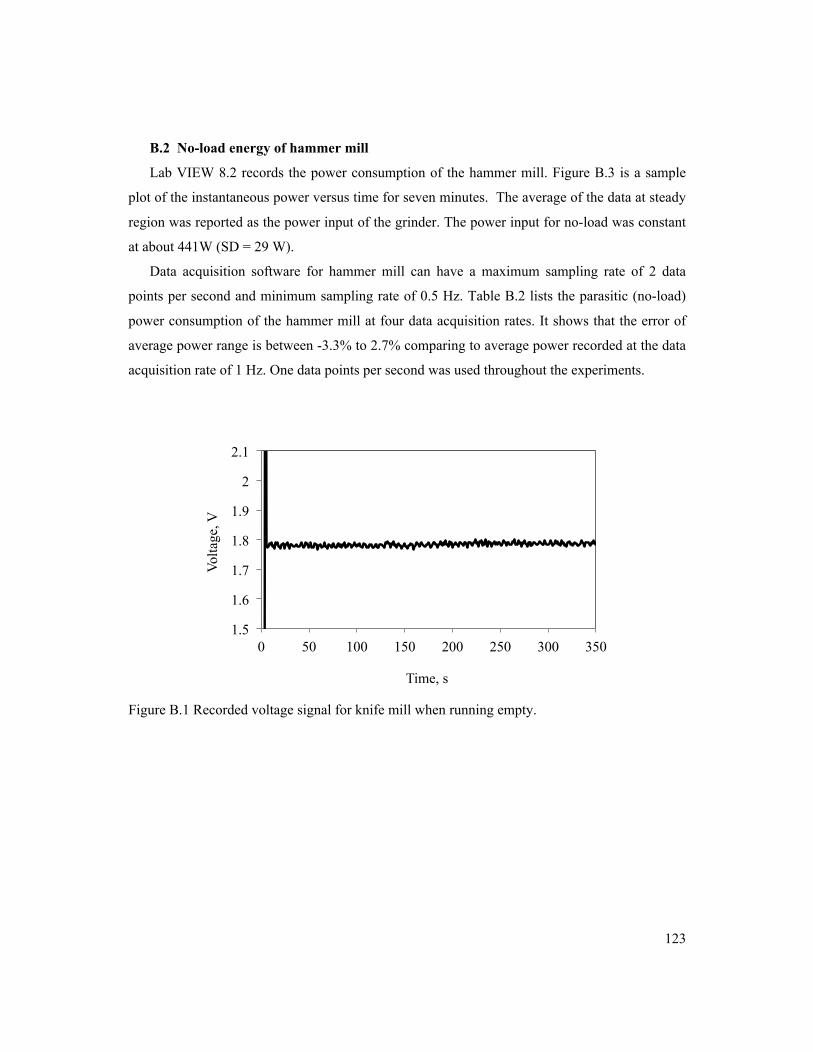
123

B.2 No-load energy of hammer mill

Lab VIEW 8.2 records the power consumption of the hammer mill. Figure B.3 is a sample

plot of the instantaneous power versus time for seven minutes. The average of the data at steady

region was reported as the power input of the grinder. The power input for no-load was constant

at about 441W (SD = 29 W).

Data acquisition software for hammer mill can have a maximum sampling rate of 2 data

points per second and minimum sampling rate of 0.5 Hz. Table B.2 lists the parasitic (no-load)

power consumption of the hammer mill at four data acquisition rates. It shows that the error of

average power range is between -3.3% to 2.7% comparing to average power recorded at the data

acquisition rate of 1 Hz. One data points per second was used throughout the experiments.

Figure B.1 Recorded voltage signal for knife mill when running empty.

1.5

1.6

1.7

1.8

1.9

2

2.1

0 50 100 150 200 250 300 350

Volta

ge, V

Time, s

124

Figure B.2 Power input vs. time for knife mill when running empty. The signal has a sudden pick which is due to the sudden pull of power to start up the grinder. The signal continues with a uniform wave pattern.

Figure B.3 Power input vs time for hammer mill when running empty. The signal has a sudden pick, which is due to the sudden pull of power to start up the grinder. The signal continues with a uniform wave pattern, which has an average of 442 W.

400

450

500

550

600

0 50 100 150 200 250 300 350

Pow

er, W

Time, s

300

350

400

450

500

550

600

0 50 100 150 200 250 300 350 400 450

Pow

er, W

Time, s

Average: 442 W

125

Table B.1 Data acquisition rate, average recorded voltage, and the corresponding percentage errors for knife mill when grinding willow wood chips. Data acquisition rate, Hz Avg voltage, V % Error

100 1.9866 0.0151 50 1.9867 0.0101 25 1.9872 -0.0151 12 1.9870 -0.0050 6 1.9874 -0.0252 3 1.9878 -0.0453 1 1.9869 -0.0000

Table B.2 Parasitic power of hammer mill. Data acquisition rate,

Hz Avg power,

W % Error SD

2.0 441 + 2.3 29 1.0 436 0.0 30 0.7 437 - 3.3 26 0.5 440 + 2.7 29

126

Appendix C Results of Size Reduction

Table C.3 lists the raw data collected during grinding of the four wood species: Douglas-

fir, pine, aspen, and poplar by knife mill on 2 mm screen. Moisture contents of the samples

were between 8.5-10%. The mass of material fed to the grinder was almost constant at 500-

505 g. Feeder vibration was kept at 25%. The vibration of 25% was the minimum vibration at

which the quarter disk shape pieces from all species move smoothly on the feeder tray. The

aim was to provide a uniform flow of materials to the grinder. The number of quarter shape

pieces in each charge of the feed to the grinder is listed in Table C.3. The number of quarter

shape pieces depends on the density of the wood and the branch radius the pieces are cut

from. The pieces were lined up on the feeder tray and fell inside the grinder one by one. The

feeding time was varied for the 500 g total feed for each run. The feeding time was depended

on the density of the particles although the total mass was kept constant. The total energy

consumption and the time of grinding are listed in Table C.3.

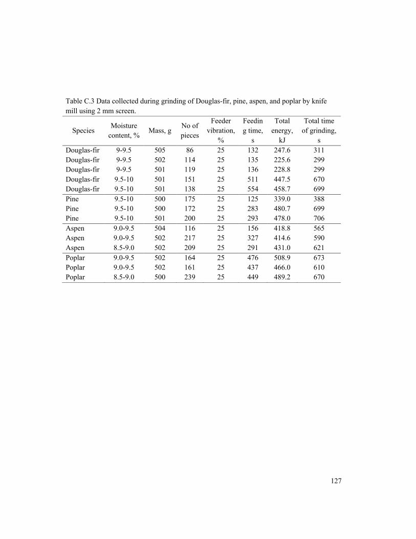
127

Table C.3 Data collected during grinding of Douglas-fir, pine, aspen, and poplar by knife mill using 2 mm screen.

Species Moisture

content, % Mass, g

No of pieces

Feeder vibration,

%

Feeding time,

s

Total energy,

kJ

Total time of grinding,

s Douglas-fir 9-9.5 505 86 25 132 247.6 311 Douglas-fir 9-9.5 502 114 25 135 225.6 299 Douglas-fir 9-9.5 501 119 25 136 228.8 299 Douglas-fir 9.5-10 501 151 25 511 447.5 670 Douglas-fir 9.5-10 501 138 25 554 458.7 699 Pine 9.5-10 500 175 25 125 339.0 388 Pine 9.5-10 500 172 25 283 480.7 699 Pine 9.5-10 501 200 25 293 478.0 706 Aspen 9.0-9.5 504 116 25 156 418.8 565 Aspen 9.0-9.5 502 217 25 327 414.6 590 Aspen 8.5-9.0 502 209 25 291 431.0 621 Poplar 9.0-9.5 502 164 25 476 508.9 673 Poplar 9.0-9.5 502 161 25 437 466.0 610 Poplar 8.5-9.0 500 239 25 449 489.2 670

128

Appendix D Grinding Herbaceous Biomass

Seven samples: wheat straw, switchgrass, sunflower seed husks, sorghum seeds,

miscanthus, olive residue, corn stover were received from Ottawa on September 26, 2012.

Two samples: canola straw and willow were received from Alberta on October 8, 2012.

Bagasse sample was received on January 9, 2012. Upon receiving the samples, they were

labelled from 1 to 9. The information that was provided on each species was recorded. In

addition, further observations on the nature of each sample were noted. Figure D.5 shows the

samples as-received.

Herbaceous biomass samples were either dried or moisturized to a controlled moisture

content of 10-11% wb. Canola straw, willow, and corn stover samples consisted of big pieces.

Since these big pieces could not be fed to the hammer mill directly, they were first shredded

in a Model 80, Crary Bear Cat Chipper/Shredder, West Fargo, ND with screen size of 38.1

mm.

A representative sample of 2 kg was prepared. The sample was divided into ten portions

of 200 g each. The portions were fed into the grinder in a way to maintain a consistent input

of material. It was tried to feed the prepared ten portions in 2 minutes. The grinding was

repeated on three replicates for each species. The feeding rate was adjusted depending on the

material characteristics or screen size inside the hammer mill to maintain a continuous

grinding.

Power consumption for grinding each species by hammer mill was recorded. Specific

power consumption of grinding was calculated as power consumption of grinding minus

parasitic power input. The range of power input with a 6.4 mm screen was recorded. Willow

branches were hardest to grind. Wheat straw, canola straw, bagasse, and miscanthus required

similar levels of energy input. Small particles like sorghum seed, olive residue, and sunflower

seed husk required the least energy input. There were flow issues with some samples such as

corn stover, which produced strings of fibre that did not flow easily. Specific energy

consumption of grinding was calculated by dividing specific power input by feeding rate.

Specific energy consumption of grinding was the energy for grinding one kilogram of

biomass.

129

The results of grinding ten herbaceous biomass samples are summarized in Table D.4.

Table D.4 lists the average, standard deviation, maximum, minimum, and coefficient of

variation of the power consumptions of grinding tests. The standard deviation or the

variability of power consumption increased as the screen size decreased for all feedstock.

Figure D.6 shows the power consumption of grinding chipped willow on 6.4 mm screen.

The figure shows the power consumption increased when the feeding starts. The power

consumption reached a constant region when the grinder chamber was filled with material

and the feeding rate was equal to production rate. Power consumption decreased when the

feeding rate stopped. The decrease continued until the grinder chamber was emptied of the

material. The variability of power consumption was high in the constant region (SD=233).

Figure D.7 shows the power consumption of grinding sorghum seeds. The figure shows that

there was a small variability in power consumption during continuous grinding (SD=34)

compared to the variability of power consumption of hammer mill working empty (SD=32).

Figure D.8 represents the average energy inputs measured using screens of 3.2, 6.4, 12.7,

and 25.4 mm. As expected, energy input increased with decreasing screen size. Screens of

12.7 mm and 25.4 mm were not used for sorghum seeds and olive residue, whose particles

were smaller than the opening sizes of these screens. The other eight herbaceous biomass

were passed through all the four screens. The largest energy input for the 3.2 mm (1/8”)

screen was for grinding corn stover followed by bagasse and willow. Willow consumed the

largest amount of energy to pass through 6.4 mm (1/4”) screen. Figure D.8 highlights the fact

that a wide range of power input is required to meet the differences in grindability of the

biomass species tested.

Figure D.9 shows the size distributions for straw and branches after grinding using the 6.4

mm (1/4”) screen in the hammer mill. The vertical axis is the percent fraction remaining on

the sieve size. Corn stover had the largest fraction of small particles in the pan. Most particles

were collected in the 0.85 mm sieve. Ground willow had the largest size particles remaining

on the top 2 mm sieve.

Figure D.10 shows the particle size distribution for seeds and olive residue after grinding

using the 6.4 mm (1/4”) screen in the hammer mill. The vertical axis is the percent fraction

remaining on the sieve. Olive residue had the largest fraction of small particles in the pan.

130

Most particles were in 0.85-1.4 mm range. Ground olive residue had the largest size particles

remaining on the top 2 mm screen.

Table D.7 lists the results of loose bulk density, tapped bulk density, percent of density

increase due to tapping, and Hausner ratio of ground materials. Loose density and tapped

density increased as the screen size increased in all biomass except sunflower seed husk.

There was a small amount of sunflower seeds mixed with the sunflower seed husk sample.

The sunflower seeds had a chance to be ground when the screen size was 3.2 mm. The ground

sunflower seeds released oil and made the surface of the particles sticky which prevented the

particles from moving freely and caused the decrease in loose and tapped density when the

screen size decreased from 6.4 to 3.2 mm. The Hausner ratio less than 1.25 means the ground

particles are easy to flow. Among the ground particles, only olive residue has a Hausner ratio

of 1.12 (less than 1.25).

Figure D.11 shows the loose bulk densities of the ground materials based on the grinder

screen sizes. The ground sunflower seed husks sample has the highest loose bulk density.

Ground wheat straw has the lowest bulk density. Loose bulk density decreased for all ground

feedstocks as the screen sizes increased. Equation D.1 (Lam et al., 2008) is used to fit the

data.

ρbulk = ax−b D.2

where a and b are constants, x is the screen size, and ρbulk is the bulk density. Table D.3 lists

the constants of a and b for the biomass tested.

Herbaceous biomass has significant size and form variation. A method needs to be

identified to give a size factor to a collected feedstock. This size factor can then be used as the

initial size to test the applicability of Rittinger’s equation on grinding feedstock collected

from field.

An analysis was conducted to evaluate the validity of Rittinger’s, Kick’s and Bond’s

equations on the results of grinding ten herbaceous biomass. Two assumptions were made to

simplify the analysis:

1. The feed particle size (LF) is large. It makes LF-1 in Rittinger equation and LF

-0.5 in

Bond equation small number that can be ignored. Equation:

131

2.7

is modified to:

D.3

and Equation:

2.9

is modified to:

D.4

Kick equation in the form of Equation 4.2 is used for fitting the data.

2. The size of the screen installed in the grinder is used as the final particles size (LP) to

simplify the analysis.

Equations D.2, D.3 and 4.2 are fitted to the data of specific energy consumption and its

corresponding screen size. The results of fitting are summarized in Table D.8. The

coefficients of determination show that overall Rittinger equation fits well to the data. There

are a few exceptions such as corn stover whose data have a higher coefficient of

determination when fitted to Bond equation. Also willow and switchgrass have higher

coefficients of determinations when Kick equation is used.

The biomass can be divided into three categories based on its kR value. The first category

is willow, which is a woody biomass, and has the highest kR, which is equal to 378 J mm g-1.

The kR value for the second category has a range of 66-267 J mm g-1. It includes corn stover,

bagasse, wheat straw, miscanthus, switchgrass, canola straw, and sunflower seed husks.

The third category is olive residue and sorghum seeds which have the lowest kR ranged

between 18-56 J mm g-1. Olive residue is a biomass, which already went through a

physical/mechanical process. Sorghum seed has the structure of agricultural seeds.

The statistical analysis of the instantaneous power consumption signals for grinding

herbaceous biomass collected from field as-it-is shows that the standard deviation (Table D.4)

E = KR1LP

−1LF

"

#$

%

&'

E = KR1LP

!

"#

$

%&

E = KB1LP0.5 −

1LF0.5

"

#$

%

&'

E = KB1LP0.5

!

"#

$

%&

132

of the signal increases as the kR increases. The first biomass category has a low standard

deviation such as sorghum seeds and olive residue (low kR). The second biomass category has

a medium standard deviation such as corn stover, bagasse, wheat straw, miscanthus,

switchgrass, canola straw, and sunflower seed husks (medium kR). The third biomass category

has the highest standard deviation such as willow (high kR). Standard deviation of power

consumption increased as the screen size installed inside the grinder decreased.

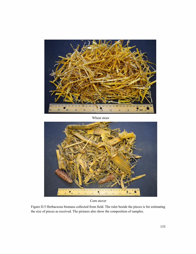
133

Wheat straw

Corn stover

Figure D.5 Herbaceous biomass collected from field. The ruler beside the pieces is for estimating the size of pieces as received. The pictures also show the composition of samples.

134

Switch grass

Sunflower seed husk

Figure D.1 Cont.

135

Sorghum seeds

Olive residue

Figure D.1 Cont.

136

Miscanthus

Canola straw

Figure D.1 Cont.

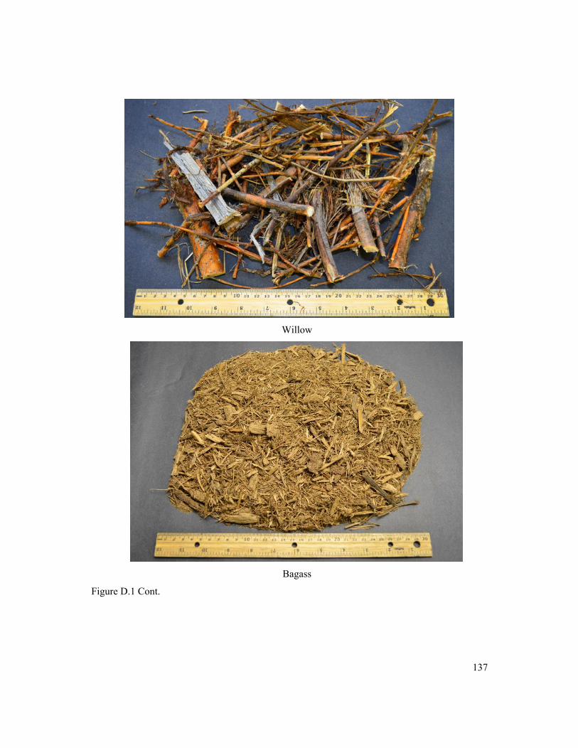
137

Willow

Bagass

Figure D.1 Cont.

138

Figure D.6 Power consumption of grinding chipped willow in the hammer mill with 6.4 mm (0.25 in) screen. The large variability of the data (SD=233) comparing to the variability of power consumption working empty (SD=32) is due to variable size of input wood chips and variable wood properties.

Figure D.7 Power consumption of grinding sorghum seeds in the hammer mill with 6.4 mm (0.25 in) screen. The small variability of the data (SD=34) comparing to the variability of power consumption working empty (SD=32) is due to uniform particle size and uniform properties of sorghum seeds.

0

500

1000

1500

2000

25 75 125 175 225

Pow

er, W

Time, s

0

200

400

600

800

1000

0 20 40 60 80 100 120 140 160

Pow

er, W

Time, s

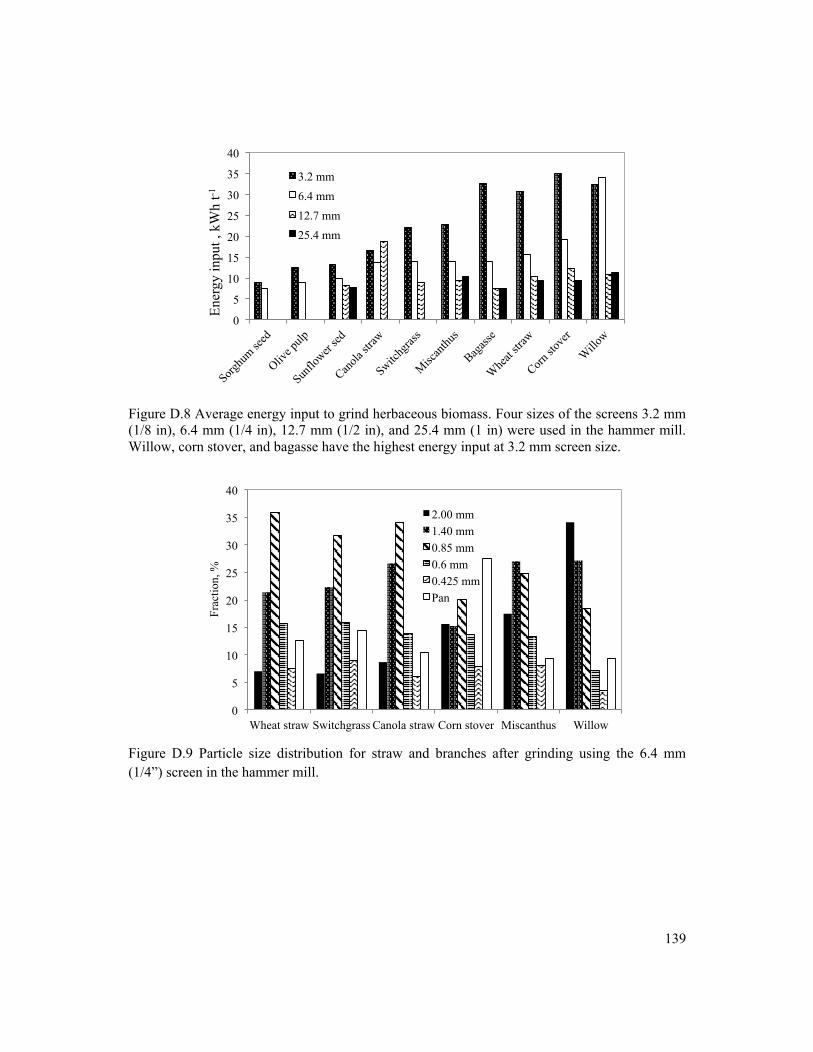
139

Figure D.8 Average energy input to grind herbaceous biomass. Four sizes of the screens 3.2 mm (1/8 in), 6.4 mm (1/4 in), 12.7 mm (1/2 in), and 25.4 mm (1 in) were used in the hammer mill. Willow, corn stover, and bagasse have the highest energy input at 3.2 mm screen size.

Figure D.9 Particle size distribution for straw and branches after grinding using the 6.4 mm (1/4”) screen in the hammer mill.

0

5

10

15

20

25

30

35

40

Ener

gy in

put ,

kW

h t-1

3.2 mm 6.4 mm 12.7 mm 25.4 mm

0

5

10

15

20

25

30

35

40

Wheat straw Switchgrass Canola straw Corn stover Miscanthus Willow

Frac

tion,

%

2.00 mm 1.40 mm 0.85 mm 0.6 mm 0.425 mm Pan

140

Figure D.10 Particle size distribution for seeds and olive residue after grinding using the 6.4 mm (1/4”) screen in the hammer mill.

Figure D.11 Loose bulk density of bagasse, wheat straw, canola straw, sunflower seed husks, corn stover and miscanthus ground at different screen sizes inside the hammer mill. Equation D.1 is fitted and the trend of bulk density of each biomass are shown.

0

5

10

15

20

25

30

35

40

Sunflower seed Olive residue Sorghum seed

Frac

tion,

%

2.00 mm 1.40 mm 0.85 mm 0.6 mm 0.425 mm Pan

0 20 40 60 80

100 120 140 160 180 200

0 5 10 15 20 25 30

Loos

e bu

lk d

ensi

ty, k

g m

-3

Grinder screen size, mm Bagasse Sunflower seed husks

Wheat Straw Corn Stover

Canola Straw Miscanthus

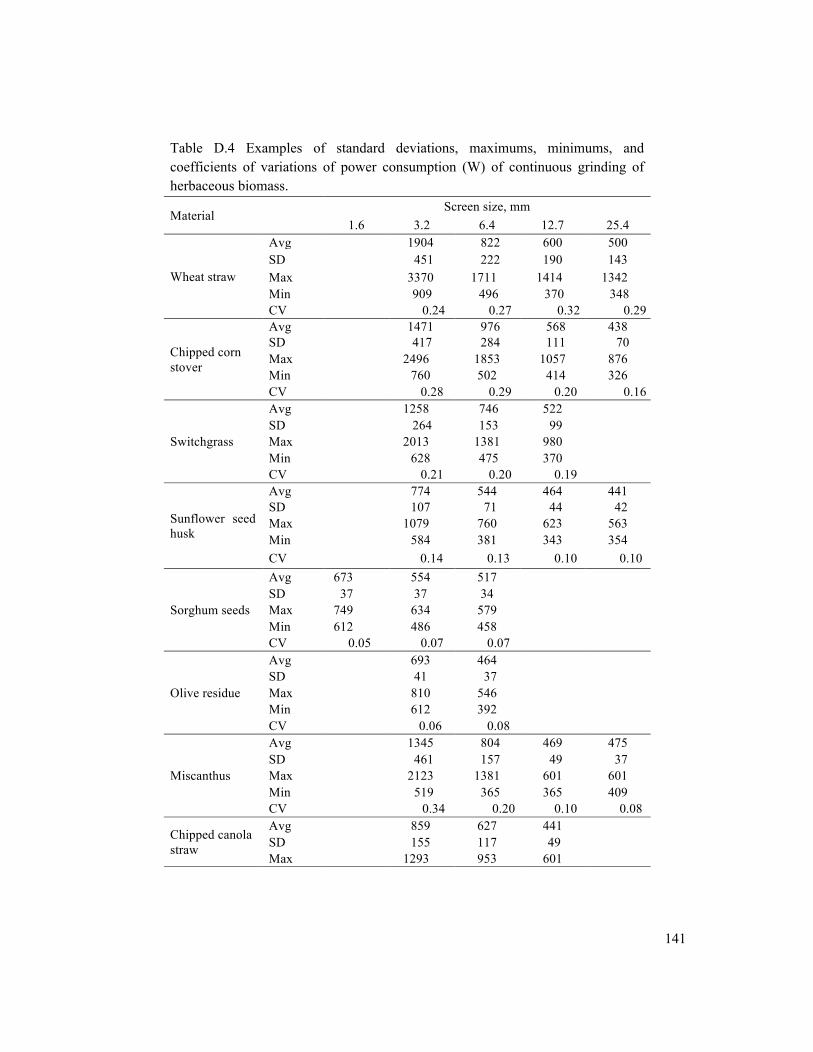
141

Table D.4 Examples of standard deviations, maximums, minimums, and coefficients of variations of power consumption (W) of continuous grinding of herbaceous biomass.

Material Screen size, mm 1.6 3.2 6.4 12.7 25.4

Wheat straw

Avg 1904 822 600 500 SD 451 222 190 143 Max 3370 1711 1414 1342 Min 909 496 370 348 CV 0.24 0.27 0.32 0.29

Chipped corn stover

Avg 1471 976 568 438 SD 417 284 111 70 Max 2496 1853 1057 876 Min 760 502 414 326 CV 0.28 0.29 0.20 0.16

Switchgrass

Avg 1258 746 522 SD 264 153 99 Max 2013 1381 980 Min 628 475 370 CV 0.21 0.20 0.19

Sunflower seed husk

Avg 774 544 464 441 SD 107 71 44 42 Max 1079 760 623 563 Min 584 381 343 354 CV 0.14 0.13 0.10 0.10

Sorghum seeds

Avg 673 554 517 SD 37 37 34 Max 749 634 579 Min 612 486 458 CV 0.05 0.07 0.07

Olive residue

Avg 693 464 SD 41 37 Max 810 546 Min 612 392 CV 0.06 0.08

Miscanthus

Avg 1345 804 469 475 SD 461 157 49 37 Max 2123 1381 601 601 Min 519 365 365 409 CV 0.34 0.20 0.10 0.08

Chipped canola straw

Avg 859 627 441 SD 155 117 49 Max 1293 953 601

142

Table D.1 Cont.

Material Screen size, mm 1.6 3.2 6.4 12.7 25.4

Chipped canola straw

Min 584 453 343 CV 0.18 0.19 0.11

Chipped willow

Mean 1537 1050 548 433 SD 522 233 142 67 Max 2853 1826 1310 799 Min 612 574 310 310 CV 0.34 0.22 0.26 0.16

Bagasse

Mean 1764 646 443 417 SD 675 113 46 38 Max 4660 991 634 590 Min 1255 464 343 337 CV 0.38 0.17 0.10 0.10

143

Table D.5 Summary of specific power (kWh t-1) required for grinding herbaceous biomass by hammer mill on five screen sizes.

Material MC Screen size, mm

1.6 3.2 6.4 12.7 25.4

Wheat straw 11 26.4 14.9 10.5 9.3 11 32.6 17.0 10.5 11 33.4 14.8 10.1

Corn stover 10 18.2 10 17.4 11 35.0 21.9 12.3 9.5

Switchgrass 11 21.3 12.4 8.9 11 9.0

Sunflower seed husk

10 13.8 9.3 7.9 7.5 10 12.2 9.5 8.0 7.6 10 13.4 9.4 7.9 7.5

Sorghum seeds 5 10.9 9.0 8.6 5 11.1 6.6

Olive residue 10 11.7 9.0 10 13.2

Miscanthus 11 23.5 13.9 10.9 9.9 11 22.4 15.1 8.2 11.3 11 22.4 12.9 9.0 9.6

Canola straw 11 16.7 12.0 18.7 11 11.3

Willow 11 32.3 32.5 10.7 11.2 11 21.2

Bagasse 10 34.2 11.2 7.2 7.4 10 32.1 12.8 7.7 7.0 10 31.5 18.0 7.6 7.7

144

Table D.6 Constants a and b of Equation D.1 for the data of the herbaceous biomass. The equation fits fairly well to the data. Material a b R2 Bagasse 110.9 0.1 0.72 Canola straw 153.8 0.3 0.97 Corn stover 112.6 0.1 1 Miscanthus 153.9 0.2 0.74 Sunflower seed husk 200.1 0.1 0.63 Wheat straw 156.9 0.5 0.96 (113.8)[1] (0.39) (0.98)

[1]Lam et al. (2008) tested the equation on clean stems that were cut to exact lengths of wheat straw. The constants provided in parenthesis are extracted from his study.

145

Table D.7 Bulk density of hammer milled ground samples of ten herbaceous biomass ground on four screen sizes by hammer mill. In most cases loose and tapped bulk density increased as the screen size decreased. This trend did not happen for a few biomass when the screen size decreased from 6.4 to 3.2 mm. Reorientation of the particles due to tapping caused tapped bulk density to be higher than loose bulk density.

Material Screen size, mm

Loose bulk density, kg m-3

Tapped bulk density, kg m-3

Density increase due to

tapping, %

Hausner ratio

Wheat straw

25.4 29.8 51.4 73 1.70 12.7 39.9 65.6 65 1.60 6.4 68.6 102.5 49 1.50 3.2 81.1 120.6 49 1.50

Corn stover

25.4 70.5 95.0 35 1.35 12.7 76.8 98.5 28 1.28 6.4 98.0 137.1 40 1.40 3.2 95.3 130.5 37 1.40

Switchgrass 6.4 97.6 148.1 52 1.52

Sunflower seed husk

25.4 160.5 206.7 29 1.29 12.7 159.4 227.9 43 1.43 6.4 236.7 303.8 28 1.28 3.2 189.4 277.8 47 1.47

Sorghum seed 6.4 649.7 811.6 25 1.25 Olive residue 6.4 611.8 686.8 12 1.12

Miscanthus 12.7 95.6 134.1 40 1.40 6.4 121.5 162.9 34 1.34 3.2 121.1 170.7 41 1.40

Canola straw

25.4 61.5 90.5 47 1.47 12.7 69.8 101.6 46 1.46 6.4 95.1 140.6 48 1.48 3.2 107.9 150.2 39 1.39

Willow 6.4 131.7 212.9 62 1.62

146

Table D.8 Slopes and coefficients of determinations for fitting Equations 4.9, 4.10, and 4.2 to the data of grinding herbaceous biomass by hammer mill on different screen sizes. LP is replaced by screen size inside the grinder. Rittinger equation has a good fit for feed from all sizes.

Biomass

Rittinger Equation

Bond Equation Kick Equation

kR J mm g-1

R2 kB

J mm0.5 g-1 R2 kK

J (ln mm)-1 g-1 CK R2

Willow 378 0.44 378 0.43 -51 166 0.61 Corn stover 267 0.94 112 0.95 -40 121 0.86 Bagasse 246 0.84 246 0.84 -45 125 0.80 Wheat straw 240 0.88 108 0.59 -42 120 0.80 Miscanthus 164 0.91 164 0.91 -27 80 0.86 Switchgrass 154 0.95 108 0.59 -33 87 0.96 Canola straw 96 0.97 96 0.97 -19 52 0.96 Sun flower seed husks 66 0.96 29 0.68 -10 30 0.85 Olive residue 56 0.86 56 0.86 -20 41 1 Sorghum seeds 18 0.92 13 0.78 -6 14 0.86

147

Appendix E Chemical Composition of Wood

Table E.1 lists the result of chemical composition of wood samples. The chemical

components are given as percentages oven-dry, extractive-free wood meal. Lignin, acid insoluble

and acid soluble content were determined in triplicate with a modified standard method (Sluiter

et al., 2011).

Table E.1 provides the data for the chemical composition, as percentages of oven-dry,

extractive-free wood meal, of the samples evaluated. The mass balance is as expected for the

combined methodologies employed. The mass balance for the aspen sample is somewhat lower

than was obtained for the other samples. This result suggests that the inclusion of extractives,

which would comprise between 2 - 4% (Allen, 1988, Davis et al., 1995) and uronic acids (~5%)

(Isenberg, 1981), would close the mass balance for this aspen sample.

148

Table E.9 Chemical composition of four wood samples given as percentage oven-dry, extractive-free wood meal.

Species Sample

no. Glucan

% Xylan

% Galactan

% Arabinan

% Mannan

% Insol. Lignin

% Sol. Lignin

%

Douglas-fir

1 38.8 7.5 8.0 2.0 8.5 32.1 4.5 2 38.3 7.5 8.0 1.9 8.4 32.4 4.2 3 39.2 7.7 8.1 2.0 8.6 32.5 4.4

Pine 1 37.8 8.6 7.3 2.3 8.9 30.3 4.7 2 38.2 8.6 7.4 2.3 9.1 30.7 4.9 3 38.1 8.7 7.3 2.3 9.1 30.4 4.6

Aspen 1 42.8 20.1 0.8 0.7 1.9 20.1 5.9 2 42.9 20.0 0.8 0.7 1.9 20.7 5.5 3 45.1 20.7 0.8 0.7 2.1 20.8 4.9

Poplar 1 52.6 20.4 0.7 0.5 2.5 20.8 5.9 2 51.1 20.2 0.7 0.4 2.3 21.6 6.1 3 50.1 19.7 0.6 0.4 2.3 20.3 6.2

149

Appendix F SilviScan Analysis Results

Density profiles of samples of wood species from pith to bark are depicted in Figures F.1

to F.24. Three branches of the four species are randomly picked. Samples are identified by

their species followed by branch number, and sample number. Prominent frequency of the

density profile is located by Fast Fourier Transform using OriginPro (OriginLab,

Northampton, MA). Avg and SD and prominent frequency are listed in each graph.

Table F.10 lists the results of maximum, minimum, average, and standard deviation of the

density profile for all the six samples from the four species. The prominent frequency of each

density profile is located by Fast Fourier Transform using Origin software (OriginLab,

Northampton, MA). The dominant frequencies are listed in Table F.10. Table F.10 also lists

the maximum, minimum and average MFA of the samples. Douglas-fir has the highest

dominant frequency followed by pine. Aspen and poplar have the lowest dominant

frequencies.

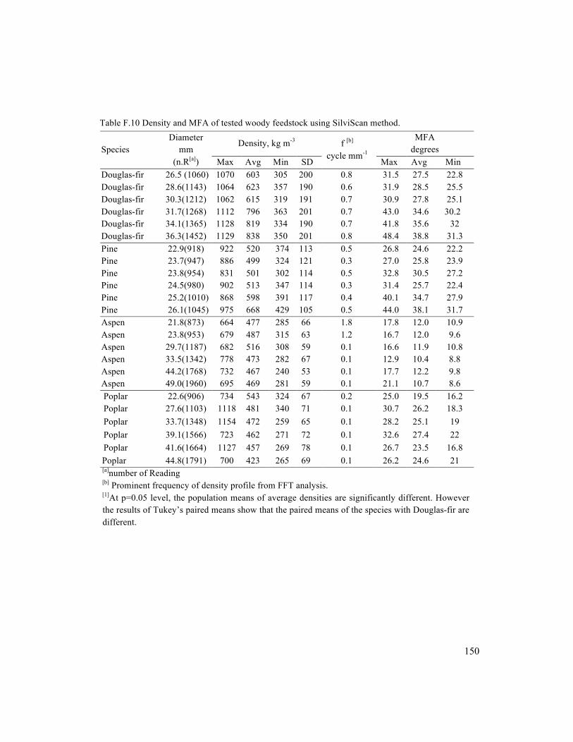
150

Table F.10 Density and MFA of tested woody feedstock using SilviScan method.

Species Diameter

mm (n.R[a])

Density, kg m-3 f [b]

cycle mm-1

MFA degrees

Max Avg Min SD Max Avg Min Douglas-fir 26.5 (1060) 1070 603 305 200 0.8 31.5 27.5 22.8 Douglas-fir 28.6(1143) 1064 623 357 190 0.6 31.9 28.5 25.5 Douglas-fir 30.3(1212) 1062 615 319 191 0.7 30.9 27.8 25.1 Douglas-fir 31.7(1268) 1112 796 363 201 0.7 43.0 34.6 30.2 Douglas-fir 34.1(1365) 1128 819 334 190 0.7 41.8 35.6 32 Douglas-fir 36.3(1452) 1129 838 350 201 0.8 48.4 38.8 31.3 Pine 22.9(918) 922 520 374 113 0.5 26.8 24.6 22.2 Pine 23.7(947) 886 499 324 121 0.3 27.0 25.8 23.9 Pine 23.8(954) 831 501 302 114 0.5 32.8 30.5 27.2 Pine 24.5(980) 902 513 347 114 0.3 31.4 25.7 22.4 Pine 25.2(1010) 868 598 391 117 0.4 40.1 34.7 27.9 Pine 26.1(1045) 975 668 429 105 0.5 44.0 38.1 31.7 Aspen 21.8(873) 664 477 285 66 1.8 17.8 12.0 10.9 Aspen 23.8(953) 679 487 315 63 1.2 16.7 12.0 9.6 Aspen 29.7(1187) 682 516 308 59 0.1 16.6 11.9 10.8 Aspen 33.5(1342) 778 473 282 67 0.1 12.9 10.4 8.8 Aspen 44.2(1768) 732 467 240 53 0.1 17.7 12.2 9.8 Aspen 49.0(1960) 695 469 281 59 0.1 21.1 10.7 8.6 Poplar 22.6(906) 734 543 324 67 0.2 25.0 19.5 16.2 Poplar 27.6(1103) 1118 481 340 71 0.1 30.7 26.2 18.3 Poplar 33.7(1348) 1154 472 259 65 0.1 28.2 25.1 19 Poplar 39.1(1566) 723 462 271 72 0.1 32.6 27.4 22 Poplar 41.6(1664) 1127 457 269 78 0.1 26.7 23.5 16.8 Poplar 44.8(1791) 700 423 265 69 0.1 26.2 24.6 21 [a]number of Reading [b] Prominent frequency of density profile from FFT analysis. [1]At p=0.05 level, the population means of average densities are significantly different. However the results of Tukey’s paired means show that the paired means of the species with Douglas-fir are different.

151

Figure F.12 Density profile for a Douglas-fir sample.


0

200

400

600

800

1000

1200

0 5 10 15 20 25 30 35

Den

sity

, kg

m-3

Distance from pith, mm

Douglas-fir 1-1 Avg=838 kg m-3 SD=201 kg m-3 f= 0.8 cycle mm-1

0

200

400

600

800

1000

1200

0 5 10 15 20 25 30

Den

sity

, kg

m-3


Douglas-fir 1-2 Avg=623 kg m-3 SD=190 kg m-3 f= 0.6 cycle mm-1

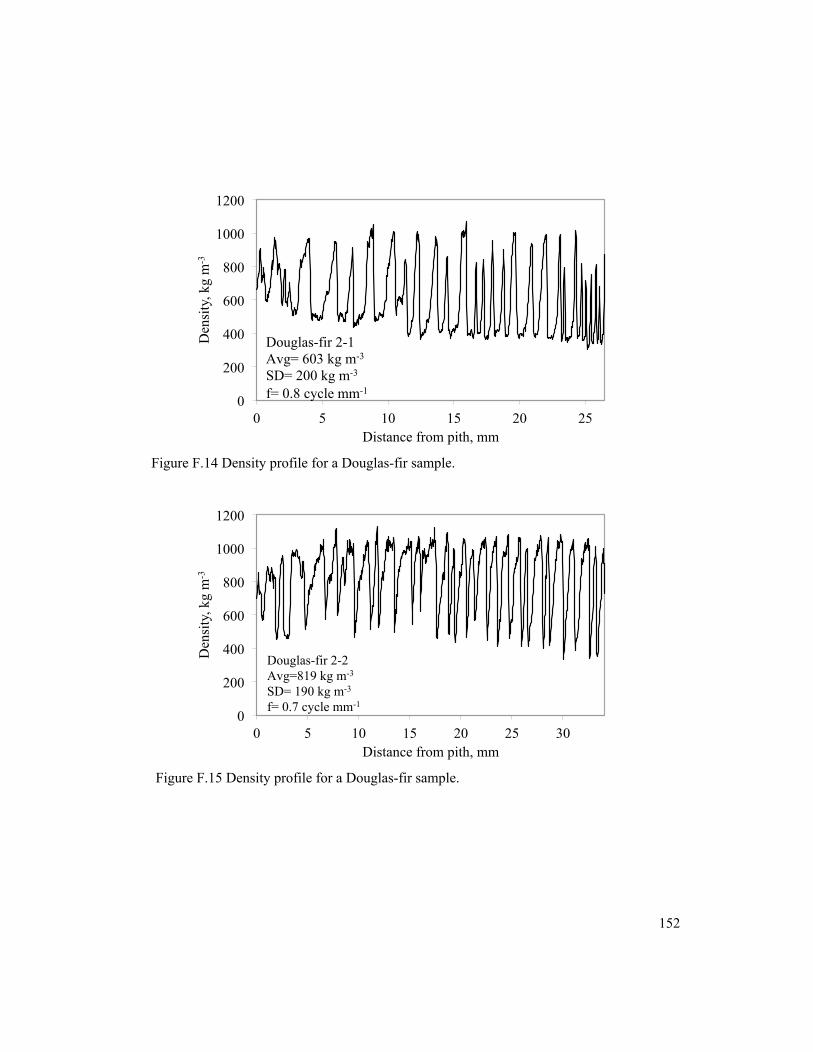
152



0

200

400

600

800

1000

1200

0 5 10 15 20 25

Den

sity

, kg

m-3


Douglas-fir 2-1 Avg= 603 kg m-3

SD= 200 kg m-3

f= 0.8 cycle mm-1

0

200

400

600

800

1000

1200

0 5 10 15 20 25 30

Den

sity

, kg

m-3


Douglas-fir 2-2 Avg=819 kg m-3 SD= 190 kg m-3 f= 0.7 cycle mm-1

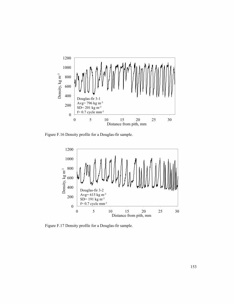
153



0

200

400

600

800

1000

1200

0 5 10 15 20 25 30

Den

sity

, kg

m-3



SD= 201 kg m-3 f= 0.7 cycle mm-1

0

200

400

600

800

1000

1200

0 5 10 15 20 25 30

Den

sity

, kg

m-3




154

Figure F.18 Density profile for a pine sample.


0

200

400

600

800

1000

1200

0 5 10 15 20 25

Den

sity

, kg

m-3


Pine 1-1 Avg= 598 kg m-3

SD = 117 kg m-3

f= 0.4 cycle mm-1

0

200

400

600

800

1000

1200

0 5 10 15 20

Den

sity

, kg

m-3


Pine 1-2 Avg= 499 kg m-3 SD= 121 kg m-3

f= 0.3 cycle mm-1

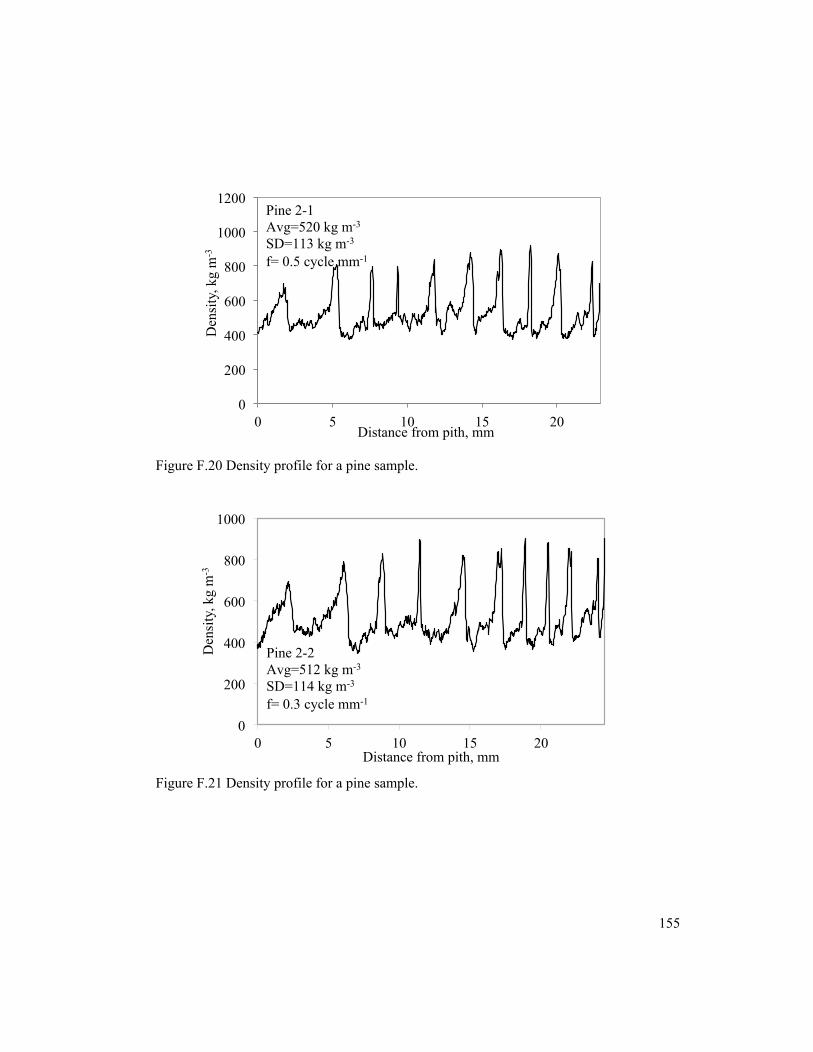
155



0

200

400

600

800

1000

1200

0 5 10 15 20

Den

sity

, kg

m-3


Pine 2-1 Avg=520 kg m-3

SD=113 kg m-3

f= 0.5 cycle mm-1

!

0

200

400

600

800

1000

0 5 10 15 20

Den

sity

, kg

m-3



SD=114 kg m-3

f= 0.3 cycle mm-1

156



0

200

400

600

800

1000

1200

0 5 10 15 20 25

Den

sity

, kg

m-3



SD=105 kg m-3

f= 0.5 cycle mm-1

0 100 200 300 400 500 600 700 800 900

0 5 10 15 20

Den

sity

, kg

m-3

Distance form pith, mm

Pine 3-2 Avg= 501 kg m-3

SD=114 kg m-3

f= 0.5 cycle mm-1

!

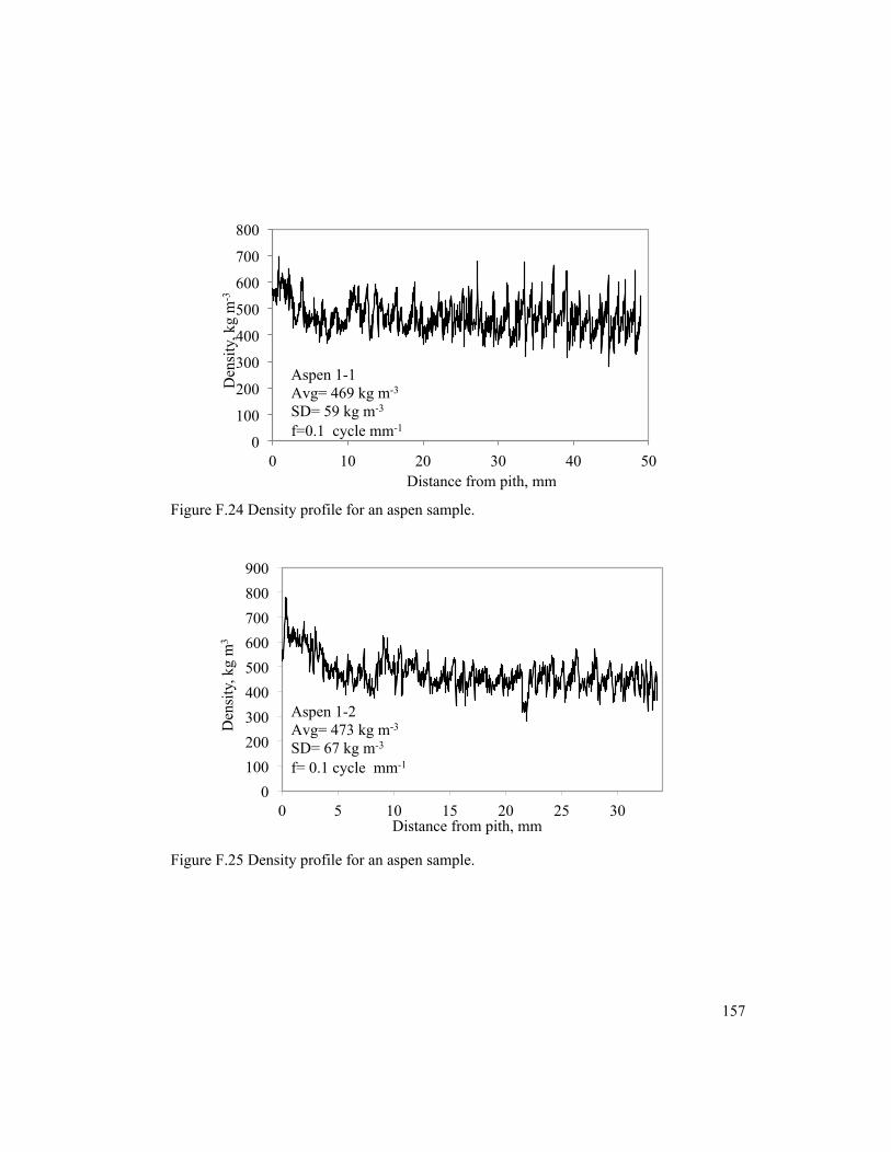
157

Figure F.24 Density profile for an aspen sample.


0

100

200

300

400

500

600

700

800

0 10 20 30 40 50

Den

sity

, kg

m-3


Aspen 1-1 Avg= 469 kg m-3

SD= 59 kg m-3 f=0.1 cycle mm-1

0 100 200 300 400 500 600 700 800 900

0 5 10 15 20 25 30

Den

sity

, kg

m3




!

158



0

100

200

300

400

500

600

700

800

0 10 20 30 40

Den

stiy

, kg

m-3



SD= 53 kg m-3 f=0.1 cycle mm-1 !

0

100

200

300

400

500

600

700

800

0 5 10 15 20 25

Den

sity

, kg

m-3



SD= 59 kg m-3 f= 0.1 cycle mm-1 !!

159



0

100

200

300

400

500

600

700

800

0 5 10 15 20

Den

sity

, kg

m-3



SD= 63 kg m-3 f= 1.2 cycle mm-1 !

0

100

200

300

400

500

600

700

0 5 10 15 20

Den

sity

, kg

m-3



SD= 66 kg m-3 f= 1.8 cycle mm-1 !!

160

Figure F.30 Density profile for a poplar sample.


0

100

200

300

400

500

600

700

800

0 5 10 15 20 25 30 35 40

Den

sity

, kg

m-3

Distance from pith , mm

Poplar 1-1 Avg= 423 kg m-3 SD= 69 kg m-3 f= 0.1 cycle mm-1

0

200

400

600

800

1000

1200

0 5 10 15 20 25 30 35 40

Den

sity

, kg

m-3


Poplar 1-2 Avg= 457 kg m-3 SD= 78 kg m-3 f= 0.1 cycle mm-1 !

161

!



0

200

400

600

800

1000

1200

0 5 10 15 20 25 30

Den

sity

, kg

m-3


Poplar 2-1 Avg= 472 kg m-3 SD= 65 kg m-3

f= 0.1cycle mm-1

0

100

200

300

400

500

600

700

800

0 5 10 15 20 25 30 35

Den

sity

, kg

m3



f= 0.1 cycle mm-1

162



0

200

400

600

800

1000

1200

0 5 10 15 20 25

Den

sity

, kg

m 3



f= 0.1 cycle mm-1

0

100

200

300

400

500

600

700

800

0 5 10 15 20

Den

sity

, kg

m-3

Distance form pith, mm


f= 0.2 cycle mm-1

A STUDY OF CELLULOSIC BIOMASS SIZE REDUCTION

Documents

Transcript of A STUDY OF CELLULOSIC BIOMASS SIZE REDUCTION