
A structured approach for the engineering of biochemical network models, illustrated for signalling...
43
A structured approach for the engineering of biochemical network models, illustrated for signalling pathways * Rainer Breitling 1 , David Gilbert 2 , Monika Heiner 3 , Richard Orton 2 1 Groningen Bioinformatics Centre University of Groningen 9751 NN Haren, The Netherlands 2 Bioinformatics Research Centre University of Glasgow Glasgow G12 8QQ, Scotland, UK 3 Department of Computer Science Brandenburg University of Technology 03013 Cottbus, Germany [email protected], {drg,rorton}@brc.dcs.gla.ac.uk, [email protected] April 11, 2008 Abstract Quantitative models of biochemical networks (signal transduction cas- cades, metabolic pathways, gene regulatory circuits) are a central com- ponent of modern systems biology. Building and managing these complex models is a major challenge that can benefit from the application of formal methods adopted from theoretical computing science. Here we provide a general introduction to the field of formal modelling, which emphasizes the intuitive biochemical basis of the modelling process, but is also accessible for an audience with a background in computing science and/or model engineering. We show how signal transduction cascades can be modelled in a mod- ular fashion, using both a qualitative approach – Qualitative Petri nets, and quantitative approaches – Continuous Petri Nets and Ordinary Dif- ferential Equations. We review the major elementary building blocks of a cellular signalling model, discuss which critical design decisions have to be made during model building, and present a number of novel computa- tional tools that can help to explore alternative modular models in an easy * Accepted for publication in Briefings in Bioinformatics 1
Transcript of A structured approach for the engineering of biochemical network models, illustrated for signalling...

A structured approach for the engineering of
biochemical network models,
illustrated for signalling pathways∗
Rainer Breitling1, David Gilbert2, Monika Heiner3, Richard Orton2
1 Groningen Bioinformatics Centre
University of Groningen
9751 NN Haren, The Netherlands
2 Bioinformatics Research Centre
University of Glasgow
Glasgow G12 8QQ, Scotland, UK
3 Department of Computer Science
Brandenburg University of Technology
03013 Cottbus, Germany
[email protected], {drg,rorton}@brc.dcs.gla.ac.uk,[email protected]
April 11, 2008
Abstract
Quantitative models of biochemical networks (signal transduction cas-cades, metabolic pathways, gene regulatory circuits) are a central com-ponent of modern systems biology. Building and managing these complexmodels is a major challenge that can benefit from the application of formalmethods adopted from theoretical computing science. Here we provide ageneral introduction to the field of formal modelling, which emphasizes theintuitive biochemical basis of the modelling process, but is also accessiblefor an audience with a background in computing science and/or modelengineering.
We show how signal transduction cascades can be modelled in a mod-ular fashion, using both a qualitative approach – Qualitative Petri nets,and quantitative approaches – Continuous Petri Nets and Ordinary Dif-ferential Equations. We review the major elementary building blocks ofa cellular signalling model, discuss which critical design decisions have tobe made during model building, and present a number of novel computa-tional tools that can help to explore alternative modular models in an easy
∗Accepted for publication in Briefings in Bioinformatics
1
CONTENTS 2
and intuitive manner. These tools, which are based on Petri net theory,offer convenient ways of composing hierarchical ODE models, and permita qualitative analysis of their behaviour.
We illustrate the central concepts using signal transduction as our mainexample. The ultimate aim is to introduce a general approach that providesthe foundations for a structured formal engineering of large-scale modelsof biochemical networks.
Contents
1 Motivation 2
2 Modelling enzymatic reactions 4
3 Signal transduction cascades 9
4 Modelling one step in the cascade 11
5 Composing kinase cascades using building blocks 15
6 Analysing the behaviour of the models 21
7 Tools 23
8 Summary 24
1 Motivation
Quantitative modelling of biological systems ranging from metabolic networksto signalling pathways has experienced a renaissance in recent years. Biologistshave come to realize that to fully understand (and successfully manipulate) com-plex interacting systems a quantitative description of their dynamic behaviouris all but essential. However, they have also noted that a successful model notonly has to reproduce the system behaviour correctly, but also must reflect itsphysical structure in a meaningful way. The most popular way to achieve thisis by modelling with ordinary differential equations (ODEs), which have a well-established biophysical basis and straightforward molecular interpretation (see[SSP06] for a detailed review). Petri nets are a well established formal descrip-tive technique from Computer Science for modelling dynamic systems whichhave recently been applied to biological networks (see Chaouiya [Cha07] for anexcellent review).
This paper aims to lay the foundations for a more structured approach forthe engineering of large-scale models of biochemical networks, illustrated forsignalling pathways. Our approach exploits both Ordinary Differential Equa-tions and the method of Petri nets. The integrated discussion of differentialequation modeling, which is familiar to most biologists, and the corresponding

1 MOTIVATION 3
structured approach enabled by continuous Petri nets, opens new perspectivesthat should be of broad relevance for system modelers in many areas of cell andmolecular biology. The illustration of the central concepts are based on familiarsignal transduction pathways and classical enzyme kinetics, in order to ensurethat the relevant concepts are immediately accessible to the widest possibleaudience.
Appendix A gives a short explanation of continuous Petri nets in mathe-matical terms, but for the following discussion only an intuitive understandingof the main concepts is needed. Basically, Petri nets are bipartite graphs (net-works) with two types of nodes, one corresponding to molecules (“places”), theother corresponding to reactions (“transitions”). This structure is very simi-lar to the familiar representation of biochemical networks, such as the mapsof the Kyoto Encyclopedia of Genes and Genomes (KEGG). The arcs (edges)connecting the nodes encode information about reaction stoichiometry, and theplaces encode the molecular concentration. In the continuous version of Petrinets, each transition node contains detailed information about the kinetics ofthe associated chemical reaction (“firing rate function”). Consequently, eachcontinuous Petri net corresponds in a unique and well-defined way to a systemof ODEs describing the biological system dynamics. The advantages of this andother features of Petri nets will be discussed in more detail in the rest of thetutorial.
When building an ODE model with, e.g., a model building tool such asGepasi [Men93], model complexity can rapidly increase to a level that is difficultto manipulate. Computational tools that allow the modular construction andvisualization of ODE models would be very helpful, see e.g. [GH04]. In addition,one usually faces a number of non-trivial design choices during model building.Even for a relatively simple model there may be many ways to describe itsdynamic behaviour. In the present paper we introduce the major elementarybuilding blocks of a cellular signalling model, discuss some exemplary designdecisions that have to be made during model building, and present a number ofnovel computational tools that can help to explore alternative modular modelsin an easy and intuitive manner. These tools, which are based on Petri nettheory, offer convenient ways of composing hierarchical ODE models, using agraphical user interface, and we will discuss their application in some detail.
The basic building block of any biological dynamic system is the enzymaticreaction: the conversion of a substrate into a product catalysed by an enzyme.Such enzymatic reactions can be used to describe metabolic conversions, theactivation of signalling molecules and even transport reactions between varioussubcellular compartments. The simple enzymatic reaction can be represented invarious ways, and we will use this fundamental example to illustrate our paper.Modular tools, like the Petri net approach described below, will help to explorethe consequences of alternative designs.

2 MODELLING ENZYMATIC REACTIONS 4
2 Modelling enzymatic reactions
The simplest chemical reaction in a biochemical system is spontaneous decay,whereby a substance A decays to produce a substance B:
A → B . (1)
In general, biochemical reactions are reversible (i.e. they have forward andreverse reaction rates which may be quite similar), and can be illustrated by
A B . (2)
Besides the spontaneous reaction, there is the enzymatic reaction, in whichan enzyme catalyses the conversion of one or more biochemical entities (thesubstrates) into others (the products). We can illustrate a simple enzymaticreaction involving one substrate A, one product B, and an enzyme E by
AE−→ B . (3)
Enzymes greatly accelerate reactions in one direction (often by factors of atleast 106), and most reactions in biological systems do not occur at perceptiblerates in the absence of enzymes.
To support the graphical construction of larger models by instantiation andcomposition of graph components, we also provide the continuous Petri netrepresentations for all building blocks. In the Petri net notation, each reactionis modelled by a transition, where the pre-places are all its substrates and thepost-places all its products. An enzyme establishes a side-condition at the givenabstraction level; therefore its place is connected to the catalysed reaction bytwo opposite arcs. Compare Figure 1 for the Petri net representation of the threebasic building blocks according Equations 1–3 as well as for the combination ofEquations 2 and 3, the enzymatic reversible reaction.
A B A B BA
BA
E
A B
E E
BA
k1
k1
k2
k1
k1
k2
(1) (2)
(3)
k1, k2
k1, k2
Figure 1: Building blocks corresponding to Equations 1–3 as Petri net componentsfor irreversible (first column) and reversible (remaining columns) reactions, without(upper row) and with (lower row) explicitly modelled enzyme places. In the lastcolumn, the macro transitions, represented by two centric squares, stand for hier-archical nodes, hiding the two transitions of a reversible reaction on the next lowerhierarchy level. In other words, the last column is just an abbreviation of the middleone. The labels k1 and k2 may be read as transition (reaction) identifiers, but theywill also be interpreted as the kinetic parameters in the mass-action approach.

2 MODELLING ENZYMATIC REACTIONS 5
The Michaelis-Menten approach (MM)
In structural terms the reaction described by Equation 3 is particularly simple,because it does not require a detailed molecular understanding of the enzymaticreaction mechanism itself. Any kinetics that are just a function of the concen-trations of A, B and E and some constant parameters will be compatible withthis description. In practice, the Michaelis-Menten equation is commonly usedwhen modelling enzymatic reactions. It is given in Equation MM
V = Vmax ×[A]
KM + [A](MM)
where V is the reaction velocity, Vmax is the maximum reaction velocity, andKM , the Michaelis constant , is the concentration of the substrate at which thereaction rate is half its maximum value. The concentration of the substrate A isrepresented by [A] in this rate equation. With the total enzyme concentration[ET ] and the equation
kcat =Vmax[ET ]
(4)
we are able to write the differential equations describing the consumption ofthe substrate and production of the product as:
d[A]
dt= −
d[B]
dt= −kcat× [ET ]×
[A]
(KM + [A])(5)
That is exactly the result we get by assigning the Michaelis-Menten kineticsto the continuous transition labelled with k1 in subfigure (3) of Figure 1.
It is critical to note that the Michaelis-Menten equation only holds at theinitial stage of a reaction before the concentration of the product is appreciable,and makes the following assumptions:
1. The concentration of product is (close to) zero.
2. No product reverts to the initial substrate.
3. The concentration of the enzyme is much less than the concentration ofthe substrate, i.e. [E]� [A].
These are reasonable assumptions for enzyme assays in a test tube. However,assumptions 1 and 2 do not hold for most metabolic pathways in vivo, and noneof the assumptions is correct for cellular signalling pathways. For instance,the concentration of kinases in a signalling cascade is about the same as theconcentration of its downstream target, which usually is also a kinase. Also,reversibility and broad changes in substrate, enzyme and product concentrationplay an important role in cellular signalling pathways, requiring more detaileddescriptions.
2 MODELLING ENZYMATIC REACTIONS 6
The mass-action approach (MA1)
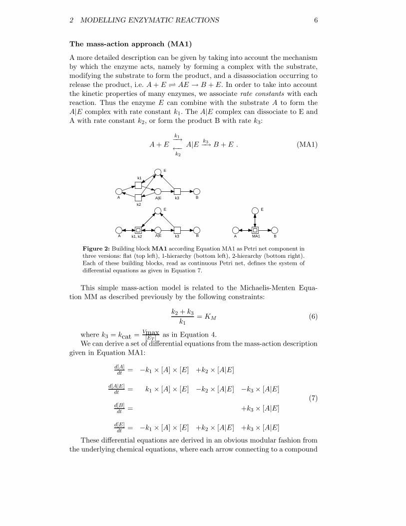
A more detailed description can be given by taking into account the mechanismby which the enzyme acts, namely by forming a complex with the substrate,modifying the substrate to form the product, and a disassociation occurring torelease the product, i.e. A + E AE → B + E. In order to take into accountthe kinetic properties of many enzymes, we associate rate constants with eachreaction. Thus the enzyme E can combine with the substrate A to form theA|E complex with rate constant k1. The A|E complex can dissociate to E andA with rate constant k2, or form the product B with rate k3:
A + E
k1−→←−k2
A|Ek3−→ B + E . (MA1)
E
BA|EA
A A|E B
E
A B
E
k3
k2
k1
k3k1, k2 MA1
Figure 2: Building block MA1 according Equation MA1 as Petri net component inthree versions: flat (top left), 1-hierarchy (bottom left), 2-hierarchy (bottom right).Each of these building blocks, read as continuous Petri net, defines the system ofdifferential equations as given in Equation 7.
This simple mass-action model is related to the Michaelis-Menten Equa-tion MM as described previously by the following constraints:
k2 + k3
k1= KM (6)
where k3 = kcat = Vmax[ET ] as in Equation 4.
We can derive a set of differential equations from the mass-action descriptiongiven in Equation MA1:
d[A]dt
= −k1 × [A]× [E] +k2 × [A|E]
d[A|E]dt
= k1 × [A]× [E] −k2 × [A|E] −k3 × [A|E]
d[B]dt
= +k3 × [A|E]
d[E]dt
= −k1 × [A]× [E] +k2 × [A|E] +k3 × [A|E]
(7)
These differential equations are derived in an obvious modular fashion fromthe underlying chemical equations, where each arrow connecting to a compound

2 MODELLING ENZYMATIC REACTIONS 7
corresponds to one term in the sum of the associated differential equation. Like-wise, these differential equations are uniquely defined by the Petri net structureas given in Figure 2, if read as a continuous Petri net, compare Appendix. Obvi-ously, the Petri net notation provides visualisation of the structure (topology),which is hidden in the ODEs.
The mass-action model described in Equation MA1 and Figure 2 assumesthat almost none of the product reverts back to the original substrate, a con-dition that holds at the initial stage of a reaction before the concentration ofthe product is appreciable. This means that this type of mass-action model isa direct equivalent of the Michaelis-Menten equation, and will face the samelimitations when applied to in vivo signalling systems. However, as we will showbelow, the mass-action description offers much more flexibility and thus can beeasily expanded to cover more general situations.
More detailed mass-action descriptions of enzyme kinetics
The Michaelis-Menten equation and the corresponding mass-action model hasbeen derived under the explicit assumption that there is no product present. Itonly holds for the initial rate of any enzymatic reaction. But almost all dynam-ical system models are concerned primarily with time-courses and/or steady-state behaviour. Both of these are clearly outside the range of the Michaelis-Menten approach and its corresponding mass-action model.
We can address this problem by formulating more detailed descriptions ofenzymatic reactions using mass-action kinetics. Given that both substrate(s)and product(s) of an enzymatic reaction will bind to the same binding site,which often has the highest affinity for the transition state that is intermediatebetween substrate and product, it is reasonable to assume that the followingextended version MA2 of the reaction equations is a good approximation, seeFigure 3 for the Petri net representation of this building block:
A + E
k1−→←−k2
A|Ek′3−→ B|E
k′2−→←−k′1
B + E (MA2)
E
B|EA|EA B
BA A|E B|E
E
BA
E
k’3
k2
k1 k’2
k’1
k’3k1, k2 k’2, k’1 MA2
Figure 3: Building block MA2 according Equation MA2 as Petri net component inthree versions: flat (top left), 1-hierarchy (bottom left), 2-hierarchy (bottom right).Each of these building blocks, read as continuous Petri net, defines the same systemof differential equations (not given).

2 MODELLING ENZYMATIC REACTIONS 8
The rate constants for the association and disassociation of the complex B|Eto B + E are related to those for the association and disassociation of A|E, i.e.k1 ' k′
1 and k2 ' k′2 because in general there will be only one bond change
between the substrate A and the product B, while the overall conformationof the complexes A|E and B|E is maintained. Of course this assumption is asimplification, but it is made here without loss of generality. The only challengethen is to estimate k1 and k2, so that they fulfill the constraints in Equations 6and 4 above, with the additional constraint that
k3 = kcat =k2 ∗ k′
3
(k2 + k′3)
(8)
assuming that the concentration of the enzyme-metabolite complexes is insteady state.
An even more complete mass-action model is given in Equation MA3, seeFigure 4 for the corresponding Petri net representation of this building block.In this case the model describes in more detail the way in which the substrateis modified to form the product. The substrate first associates with the en-zyme, and is then modified to form the product which is still associated withthe enzyme. Finally the product and enzyme disassociate. All of the stages inthe reaction are modelled as being reversible. An enzymatic reaction that isdescribed by a certain set of Km/kcat values implies most strongly that itsbehaviour is governed in fact by equations MA2 and MA3 above. Any exten-sion of Michaelis-Menten beyond time point 0 will be fraught with problems,as discussed earlier.
A + E
k1−→←−k2
A|E
k′3−→←−k′4
B|E
k′2−→←−k′1
B + E (MA3)
E
B|EA|EA B
BA A|E B|E
E
BA
E
k’3
k2
k1 k’2
k’1k’4
k1, k2 k’2, k’1 MA3k’3, k’4
Figure 4: Building block MA3 according Equation MA3 as Petri net component inthree versions: flat (top left), 1-hierarchy (bottom left), 2-hierarchy (bottom right).Each of these building blocks, read as continuous Petri net, defines the system ofdifferential equations (not given).
The differential equations for Equation MA2 and Equation MA3 can againbe derived in an obvious modular fashion as demonstrated above for the mass-action pattern MA1, or – likewise – be generated out of the continuous interpre-
3 SIGNAL TRANSDUCTION CASCADES 9
tation of the Petri net structures given in Figures 3 and 4 (compare Section 7for a description of the tools used in our technology).
In Equation 9, based on Equation MA1, we give one description for thetransformation of two substrates A1 and A2 into two corresponding productsby the association first of A1 with the enzyme and then the association of A2
with the the complex formed by the first substrate and the enzyme. We modelthe disassociation and conversion into the two products in one step.
A1 + A2 + E
k1A1−−−→←−−−k2A1
A1|E + A2
k1A2−−−→←−−−k2A2
A1|A2|Ek3−→ B1 + B2 + E (9)
Basic building blocks give us the ability to construct quite complex models,on a textual level by composing equations, or in a graphical way by composingPetri net components. Thus, for example the description of the RKIP influencedERK signalling pathway is described by Cho et al. [CSK+03] employing anODE description based on Equation 9 and two equations of the form given inEquation MA1. A corresponding Petri net representation is given in [GH04].
The decision of what granularity should be used to describe biochemicalequations will largely be driven by the availability of kinetic data – the highgranularity of mass-action descriptions will often require data on rate constantswhich cannot be obtained from the literature or experiments. A Michaelis-Menten description is often the most pragmatic choice even though it mayyield misleading results in terms of simulation and analysis.
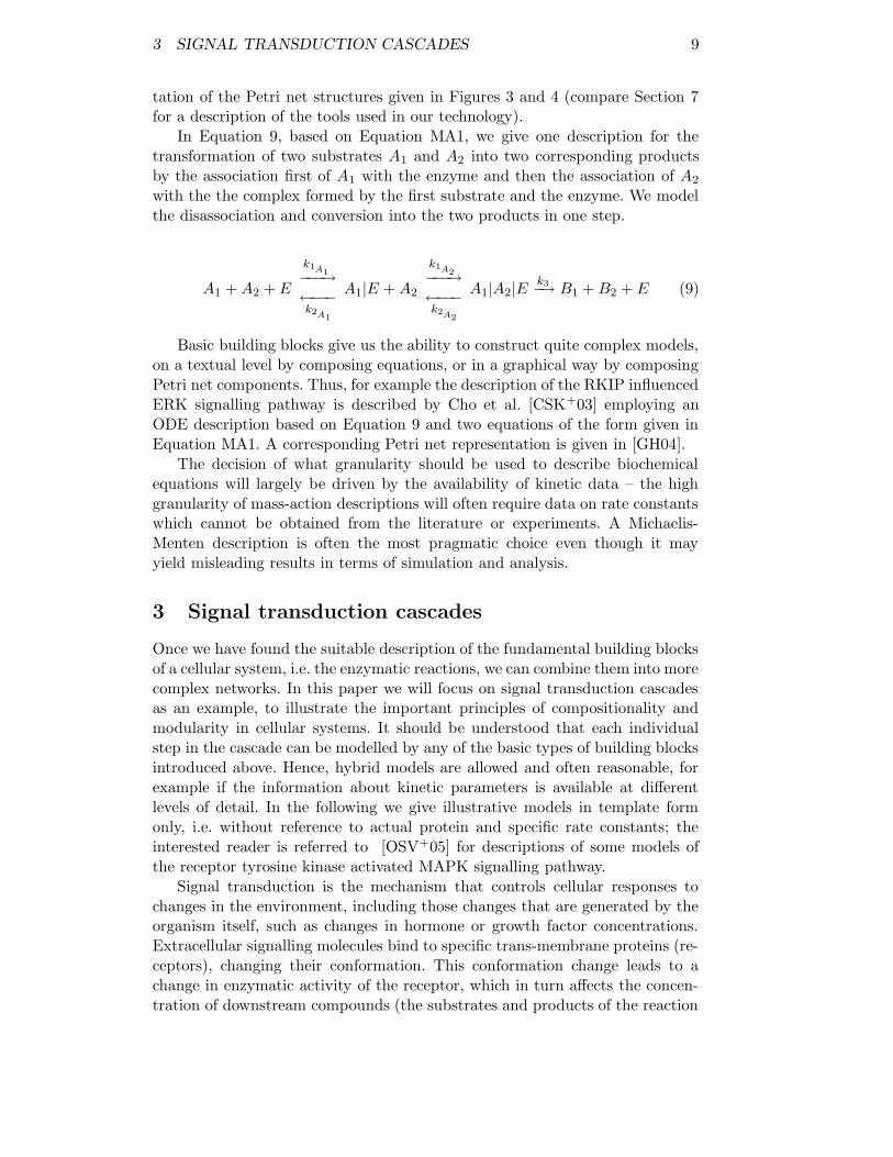
3 Signal transduction cascades
Once we have found the suitable description of the fundamental building blocksof a cellular system, i.e. the enzymatic reactions, we can combine them into morecomplex networks. In this paper we will focus on signal transduction cascadesas an example, to illustrate the important principles of compositionality andmodularity in cellular systems. It should be understood that each individualstep in the cascade can be modelled by any of the basic types of building blocksintroduced above. Hence, hybrid models are allowed and often reasonable, forexample if the information about kinetic parameters is available at differentlevels of detail. In the following we give illustrative models in template formonly, i.e. without reference to actual protein and specific rate constants; theinterested reader is referred to [OSV+05] for descriptions of some models ofthe receptor tyrosine kinase activated MAPK signalling pathway.
Signal transduction is the mechanism that controls cellular responses tochanges in the environment, including those changes that are generated by theorganism itself, such as changes in hormone or growth factor concentrations.Extracellular signalling molecules bind to specific trans-membrane proteins (re-ceptors), changing their conformation. This conformation change leads to achange in enzymatic activity of the receptor, which in turn affects the concen-tration of downstream compounds (the substrates and products of the reaction

3 SIGNAL TRANSDUCTION CASCADES 10
enzyme_1 enzyme_2 enzyme_3 enzyme_2
enzyme_1
enzyme_3
k1 k2 k3
k1
k2
k3
Figure 5: The essential structural difference between metabolic networks (left) andsignal transduction networks (right) in terms of Petri net structures.
catalysed by the receptor). The downstream compounds may themselves be en-zymes that in a cascade of enzymatic reactions ultimately lead to a change ingene expression or some other major adjustment of cellular physiology. Theseevents, and the molecules that they involve, are referred to as (intracellular)“signalling pathways”; they are central to processes such as proliferation, cellgrowth, movement, apoptosis, and inter-cellular communication. The effect of“signalling cascades” which comprise a series of enzymatic reactions in whichthe product of one reaction acts as the catalytic enzyme for the next can beamplification of the original signal. However, in some cases, for example theMAP kinase cascade, the signal gain is modest [SEJGM02], suggesting that amain purpose, over and above relaying the signal, is regulation [KCG05] whichmay be achieved by positive and negative feedback loops (see below).
The main factor which distinguishes signal transduction pathways frommetabolic networks is that in the former the product of an enzymatic reactionbecomes the enzyme for the next step in the pathway, whereas in the latter theproduct of one reaction becomes the substrate for the next, see Figure 5. Ingeneral, it is transient behaviour which is of interest in a signalling pathway,as opposed to the steady state in a metabolic network. In gene regulatory net-works, on the other hand, the inputs are proteins such as transcription factors(produced from signal transduction or metabolic activity), which then influencethe expression of genes – enzymatic activity plays no direct role here. However,the products of gene regulatory networks can play a part in the transcriptionof other proteins, or can act as enzymes in signalling or metabolic pathways.
The first model of the ERK signalling cascade (the prototypical eukaryoticsignal transduction pathway [BH05, WSL03]) was published in 1996 and utilisedstandard mass action kinetics (MA1) to represent the activation (phosphoryla-tion) and deactivation (dephosphorylation) of the protein kinases [HF96]. Al-though relatively small (11 reactions and 18 species), the model was effectivelyused to investigate if the cascade exhibited ultrasensitivity. However, the nextmodel of the ERK cascade utilised purely Michaelis-Menten type kinetics (MM)and was used to investigate whether the activation of ERK by MEK was pro-cessive or distributive [BS97]. Therefore, this shows that the different kineticmodelling approaches have both been employed from the very beginning ofsignal transduction modelling.
Over the past decade, an ever increasing number of models of the ERK

4 MODELLING ONE STEP IN THE CASCADE 11
cascade have been developed, growing in both size and complexity throughthe years. Models now routinely incorporate growth factor receptors and theplethora of adaptor proteins that can bind to them and subsequently acti-vate the core ERK cascade. However, like their predecessors, these models stillutilise the standard mass action or Michaelis-Menten type kinetics (or a mix-ture of both) to represent the biochemical reactions of a system. One of theearliest models of the Epidermal Growth Factor Receptor (EGFR), which ac-tivates the downstream ERK cascade, utilised a mixture of both kinetic mod-elling approaches to represent ligand/receptor and receptor/adaptor bindingand activation [KDGH99]; in general, MM kinetics were used to represent de-phosphorylation reactions whilst MA1 kinetics were used to represent bind-ing/dissociation and phosphorylation reactions in this model. Similarly, themodel of the EGFR-ERK system developed by [BF03] also utilised both ki-netic modelling approaches. However, this time MM kinetics were more ex-tensively employed, representing both phosphorylation and dephosphorylationreactions, whilst MA1 kinetics were used primarily for binding/dissociation re-actions. In addition, models composed entirely of mass action kinetics [LBS00,CSK+03, SEJGM02, IBG+04] or entirely [Koh00] and almost entirely [BHC+04]of Michaelis-Menten kinetics have also been constructed and successfully appliedto signalling pathways. In some cases, the choice of kinetic modelling approachis explained [YTY03] and tends to favour the mass action approach due to someof the assumptions used to derive the Michaelis-Menten equation. However, inmost cases the choice of kinetic modelling approach and its implications isnot discussed, and alternatives are not systematically explored. Exploiting themodular approach advocated here, such an exploration of model space wouldbe much easier to implement and could become a natural step of model analysisstrategies.
4 Modelling one step in the cascade
One step in a classical signal transduction cascade comprises the phosphory-lation of a protein by an enzyme S which is termed a kinase, see Figure 6.It is the phosphorylated form Rp which can act as an enzyme to catalyse thephosphorylation of a further component in the cascades, see Figure 9(a).
�
����
Figure 6: Basic enzymatic step; R – signalling protein; Rp – phosphorylated form;S1 – kinase
We can model this reaction using any of the kinetic patterns introducedin Section 2; e.g., the Mass Action MA1 pattern as follows, straightforwardlyadapted from Equation MA1 or equally its Petri net component given in Fig-ure 2, by renaming in Equation 10, where R is a protein and Rp its phospho-

4 MODELLING ONE STEP IN THE CASCADE 12
rylated form, S is a signal enzyme and R|S the complex formed from R andS:
R + S
k1−→←−k2
R|Sk3−→ Rp + S (10)
In order to ensure that such a single step is not a ‘one shot’ affair (i.e. toensure that the substrate in the non-phosphorylated form is replenished andnot exhausted), and hence that the signal can be deactivated where necessary,biological systems employ a phosphatase which is an enzyme promoting thede-phosphorylation of a phosphorylated protein. This is depicted in Figure 7,which we are going to model by all four introduced kinetic patterns.
�
�
����
Figure 7: Basic phosphorylation–dephosphorylation step; R – signalling protein;Rp – phosphorylated form; S1 – kinase; P1 – phosphatase
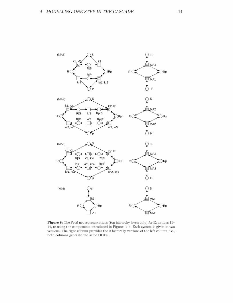
We start with the mass-action patterns. Using the MA1 pattern (Mass Ac-tion kinetics 1) we get Equation 11, where P is a phosphatase and kn, krn arerate constants for the forward and reverse reactions respectively. In many casesit would also be justified to model the dephosphorylation as an un-catalysedfirst-order decay reaction, because detailed knowledge of phosphatase concen-trations, specificities, and kinetic parameters is still lagging behind our under-standing of the kinase enzymes.
R + S
k1−→←−k2
R|Sk3−→ Rp + S
R + Pkr3←−− R|P
kr1←−−−−→kr2
Rp + P
(11)
We can construct a more complex description of the cascade step by utilisingthe more detailed formulation in Equation MA2 to give Equation 12 using MA2(Mass Action kinetics 2):

4 MODELLING ONE STEP IN THE CASCADE 13
R + S
k1−→←−k2
R|Sk′3−→ Rp|S
k′2−→←−k′1
Rp + S
R + P
kr1←−−−−→kr2
R|Pkr′3←−− Rp|P
kr′2←−−−−→kr′1
Rp + P
(12)
A complete description in mass-action kinetics can be given by adaptingEquation MA3 to give Equation 13 using MA3 (Mass Action kinetics 3):
R + S
k1−→←−k2
R|S
k′3−→←−k′4
Rp|S
k′2−→←−k′1
Rp + S
R + P
kr1←−−−−→kr2
R|P
kr′3←−−−−→kr′4
Rp|P
kr′2←−−−−→kr′1
Rp + P
(13)
The Michaelis-Menten description MM for this reaction usually omits ex-plicit reference to the phosphatase concentration because it is hard to measure;moreover because it is constant and not involved in any other reaction the term−kcat×[ET ] can be replaced by a single constant. Thus Equation 14 is modifiedfor the reverse (dephosphorylation) reaction in Equation 14 to treat [P ] as aconstant that is implicit in the kinetic constant k ′
3:
V = k3 × [S]×[R]
(KM1 + [R])− k′
3 ×[Rp]
(KM2 + [Rp])(14)
where
• d[Rp]dt
is the reaction rate V,
• k3 × [S] is Vmax for the forward reaction,
• k′3 is Vmax for the reverse reaction, and
• KM1 = (k2+k3)k1
with values from Equation 11.
Figure 8 summarizes the corresponding Petri net models for these four ver-sions of the basic phosphorylation-dephosphorylation step.
4 MODELLING ONE STEP IN THE CASCADE 14
RpRR|S Rp|S
S
RpR
S
PP
Rp|PR|P
RpR
P
RpR|P
R
P
SS
R|S
Rp|PR|P
P P
S
R Rp
S
Rp|SR|SR Rp
S
R Rp RpR
S
kr3
k3
kr'3
k'3
k3
k'3
(MA1)
(MA2)
(MM)
(MA3)
k1, k2 k'2, k'1MA3
k'3, k'4
kr1, kr2 kr'2, kr'1MA3
kr'3, kr'4
k1, k2MA1
kr1, kr2MA1
k1, k2 k'2, k'1MA2
kr'1, kr'2kr2, kr1MA2
MM
MM
Figure 8: The Petri net representations (top hierarchy levels only) for Equations 11–14, re-using the components introduced in Figures 1–4. Each system is given in twoversions. The right column provides the 2-hierarchy versions of the left column; i.e.,both columns generate the same ODEs.
5 COMPOSING KINASE CASCADES USING BUILDING BLOCKS 15
5 Composing kinase cascades using building blocks
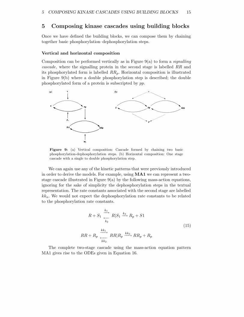
Once we have defined the building blocks, we can compose them by chainingtogether basic phosphorylation–dephosphorylation steps.
Vertical and horizontal composition
Composition can be performed vertically as in Figure 9(a) to form a signallingcascade, where the signalling protein in the second stage is labelled RR andits phosphorylated form is labelled RRp. Horizontal composition is illustratedin Figure 9(b) where a double phosphorylation step is described; the doublephosphorylated form of a protein is subscripted by pp.
�� ���
�� ���� ��� ���
��
�
� ���
����
����
�
��
���� ���
Figure 9: (a) Vertical composition: Cascade formed by chaining two basicphosphorylation-dephosphorylation steps. (b) Horizontal composition: One stagecascade with a single to double phosphorylation step.
We can again use any of the kinetic patterns that were previously introducedin order to derive the models. For example, using MA1 we can represent a two-stage cascade illustrated in Figure 9(a) by the following mass-action equations,ignoring for the sake of simplicity the dephosphorylation steps in the textualrepresentation. The rate constants associated with the second stage are labelledkkn. We would not expect the dephosphorylation rate constants to be relatedto the phosphorylation rate constants.
R + S1
k1−→←−k2
R|S1k3−→ Rp + S1
RR + Rp
kk1−−→←−−kk2
RR|Rpkk3−−→ RRp + Rp
(15)
The complete two-stage cascade using the mass-action equation patternMA1 gives rise to the ODEs given in Equation 16.

5 COMPOSING KINASE CASCADES USING BUILDING BLOCKS 16
d[R]dt
= −k1 × [R]× [S1] + k2 × [R|S1]
d[R|S1]dt
= k1 × [R]× [S1]− k2 × [R|S1]− k3 × [R|S1]
d[Rp]dt
= k3 × [R|S1]
d[S1]dt
= −k1 × [R]× [S1] + k2 × [R|S1] + k3 × [R|S1]
d[RR]dt
= −kk1 × [RR]× [Rp] + kk2 × [RR|Rp]
d[RR|Rp]dt
= kk1 × [RR]× [Rp]− kk2 × [RR|Rp]− kk3 × [RR|Rp]
d[RRp]dt
= kk3 × [RR|Rp]
d[Rp]dt
= −kk1 × [RR]× [Rp] + kk2 × [RR|Rp] + kk3 × [RR|Rp]
(16)
The Michaelis-Menten description for this two-stage cascade is more com-pact than the ODE version above, and is given by Equation 17:
d[Rp]dt
= k3 × [S1]×[R]
(KM1+[R]) − k′3 ×
[Rp](KM2+[Rp])
d[RRp]dt
= kk3 × [Rp]×[RR]
(KMM1+[RR]) − kk′3 ×
[RRp](KMM2+[RRp])
(17)
The ODEs given in Equations 16 and 17 are defined by the continuous Petrinets given in Figure 10(b), using appropriately chosen kinetic patterns for themacro transitions.
The addition of a double phosphorylation step to a cascade layer is givenin Figure 9(b), where both the single and double phosphorylation steps arecatalysed by the same enzyme S; likewise, the two dephosphorylation steps areusually catalysed by the same phosphatase P . This system component can bedescribed by Equation 18, if we apply the mass-action kinetics MA1 and ignoreagain for the sake of simplicity the dephosphorylation steps in the textual rep-resentation. The rate constants associated with the double phosphorylation arelabelled kpn. Often, we can assume that the rate constants for the two steps ofthe double phosphorylation are similar to those for the single phosphorylation.
R + S
k1−→←−k2
R|Sk3−→ Rp + S
Rp + S
kp1−−→←−−kp2
Rp|Skp3−−→ Rpp + S
(18)
The ODEs for the double phosphorylation can be generated by the contin-uous Petri net given in Figure 10(c), where the kinetic patterns for the macrotransitions have to be adjusted appropriately.

5 COMPOSING KINASE CASCADES USING BUILDING BLOCKS 17
RpR
S
Rpp
S1
P1
R Rp
P2
RR RRp
Rpp
S1
P1
R
Rp
RRppRR
RRp
RpR
P
S
P
P2
(a) (b)
(c)
(d)
Figure 10: Starting from the building block (a) for the basic phosphorylation-dephosphorylation step (as defined in four versions in Figure 8), we can do verticalcomposition forming signalling cascades, as given in (b), and horizontal composi-tion, resulting in the structure (c) for the double phosphorylation. Applying bothcomposition principles yields the two-stage double phosphorylation cascade as givenin (d).
5 COMPOSING KINASE CASCADES USING BUILDING BLOCKS 18
Negative and positive feedback
Feedback in a signalling network can be achieved in several ways. For example,negative feedback can be implemented at the molecular level by sequestrationof the input signal S1 by the product of the second stage RRp. This systemis sketched in Figure 11(a), and can be achieved by combining equations 15and 19. See Figure 12(a) for the continuous Petri net, from which the ODEscan be derived; of course, these need to be completed by the dephosphorylationequations (this is equally true for all the structures discussed in the following).
Similarly, positive feedback can also be achieved by the sequestration ofthe input signal S1 by the product of the second stage, under the additionalcondition that the resulting S1|RRp complex is a more active enzyme than S1
alone. In this case we add Equation 20 to equations 15 and 19. The system issketched in Figure 11(b), and the continuous Petri net is given in Figure 12(b),from which the ODEs can be derived.
S1 + RRp
i1−→←−i2
S1|RRp (19)
R + S1|RRp
kp1−−→←−−kp2
R|S1|RRpkp3−−→ Rp + S1|RRp (20)
Many other molecular mechanisms can be envisaged and are in fact observedin biological systems. All of these can be represented using the same basicformalism. For example, we can model an influence of RRp on the phosphataseP1, in which case the effects of positive and negative feedback are reversed,i.e. sequestration of P1 by RRp can cause positive feedback – see Figure 11(c).This can be achieved with Equations 15 and 21. Alternatively the situationwhere the P1|RRp complex is more active than P1 will cause negative feedback,Figure 11(d), and can be described by adding Equation 22 to Equations 15 and21.
P1 + RRp
i1−→←−i2
P1|RRp (21)
Rp + P1|RRp
kr′1−−→←−−kr′2
Rp|P1|RRp
kr′3−−→ R + P1|RRp (22)

5 COMPOSING KINASE CASCADES USING BUILDING BLOCKS 19
(b)
R Rp
P1
RR RRp
P2
S1(a)
R Rp
P1
RR RRp
P2
S1
(d)
R Rp
P1
RR RRp
P2
S1
R Rp
P1
RR RRp
P2
S1(c)
Figure 11: Two-stage cascade with (a) negative feedback, (b) positive feedback;alternative two-stage cascade with (c) negative feedback, (d) positive feedback.

5 COMPOSING KINASE CASCADES USING BUILDING BLOCKS 20
S1|RRp
RRp
P2
Rp
RR
R
S1
P1
R|S1|RRp S1|RRp
RRp
P2
Rp
RR
R
S1
P1
Rp|P1|RRp
P1|RRp
RRp
P2
Rp
RR
R
S1
P1
P1|RRp
RRp
P2
Rp
RR
R
S1
P1
kp3
kr'3
(a) (b)
(c) (d)
i1, i2 i1, i2
kp1, kp2
kr'1, kr'2
i1, i2 i1, i2
Figure 12: Petri nets, corresponding to Figure 11, for a two-stage cascade with(a) negative feedback, (b) positive feedback (the reaction sequence i1, kp1, kp3
contributes to the phosphorylation); alternative two-stage cascade with (c) negativefeedback (the reaction sequence i1, kr′1, kr′3 contributes to the dephosphorylation),(d) positive feedback.

6 ANALYSING THE BEHAVIOUR OF THE MODELS 21
6 Analysing the behaviour of the models
Clearly the construction of models of a biochemical system has to be done withsome purpose in mind. Overall, the main motivation will often be to providesome guidance to biochemists regarding the way in which they could carryout the exploration, modification or (re-)construction of a biological system ofinterest. Such advice could contribute towards the optimisation of resources(human, fiscal) and time in terms of the choice and temporal ordering of whatassays to perform. The usefulness of the models will depend on their ability toprovide an unambiguous representation of the knowledge about the biochemicalsystem, obtained from interviewing the biologists, searching the literature aswell as experimental data from biochemical experiments. Thus a major taskin model construction is interaction with biologists in order to ensure that thecorrect model is built.
Models should be able to provide biochemists with a foil against whichto test their understanding of a biological system – initially the componentsand how they interact (network topology), and then regarding aspects of thebehaviour of the system. In the first instance, the explanatory power of a modelis related to its ability to represent and explain everything that is known aboutthe biological system, under various conditions. Furthermore, the usefulness ofthe explanatory power of a model is often linked to its capability to correctlypredict the behaviour of a system under new (as yet unseen) conditions whichwill be achieved by new biological assays.
The first check that should be carried out on a model of a biochemical net-work is whether it correctly describes the components and their relationshipsat an adequate level of detail. This should be done with biochemists who willoften represent the system of interest in some diagram with more or less for-mality and internal consistency. The initial task for the modeller is thus tocreate an abstract, qualitative representation of a biochemical network, mini-mally described by its topology, usually as a bipartite directed graph with nodesrepresenting biochemical entities or reactions, or in Petri net terminology placesand transitions. Arcs can be annotated with stoichiometric information.
The qualitative description can be further enhanced by the abstract repre-sentation of discrete quantities of species, achieved in Petri nets by the use oftokens at places. These can represent the number of molecules, or the discretelevel of concentration, of a species. A particular arrangement of tokens overa network is called a marking . The firing rule brings the tokens to life. Theirmotion through the network (token animation) can be visualized by playingthe token game, which allows to experience model behaviour. The standard se-mantics for these qualitative Petri nets (QPN) does not associate a time withtransitions or the sojourn of tokens at places, and thus these descriptions aretime-free. The qualitative analysis considers, however, all possible types of be-haviour of the system under any timing. The behaviour of such a net forms adiscrete state space, which can be analysed in the bounded case, for example,by a branching time temporal logic, one instance of which is ComputationalTree Logic (CTL); see [CGP01] and the Model Checking Kit [SSE03] for collec-tions of suitable model checkers. Qualitative analyses may also be made using

6 ANALYSING THE BEHAVIOUR OF THE MODELS 22
classical Petri net theory, as provided, e.g., by the Integrated Net Analyser INA[SR99]. The partial order behaviour as provided by qualitative Petri nets cancontribute to deeper insights into the signal-response behaviour of signallingnetworks, as demonstrated in [GHL07].
Timed information can be added to the qualitative description in two ways– stochastic and continuous. [GH04], [GHL07] provide case studies, demonstrat-ing the complementary application of qualitative as well as quantitative modelsto a common biological system. It should be borne in mind that time assump-tions generally impose constraints on behaviour. Thus qualitative models con-sider all possible behaviours under any timing, whereas continuous models areconstrained by their inherent determinism to consider a subset. This may betoo restrictive when modelling biochemical systems, which by their very natureexhibit variability in their behaviour and a stochastic approach may be moresuitable. However, in this paper for reasons of space we ignore the stochasticview, and refer the reader to [GHL07] for a description of stochastic Petri netsand their relationship to qualitative and continuous models.
The continuous model replaces the discrete values of species with continuousvalues, and hence is not able to describe the behaviour of species at the levelof individual molecules, but only the overall behaviour via concentrations. Wecan regard the discrete description of concentration levels as abstracting overthe continuous description of concentrations. Timed information is introducedby the association of a particular deterministic rate information with each tran-sition, permitting the continuous (Petri net) model to be represented as a setof ordinary differential equations (ODEs). The concentration of a particularspecies in such a deterministic model will have the same value at each point oftime for repeated computational simulations.
(Qualitative) Petri nets and ODEs do share some concepts, as e.g. the no-tions of P-invariants and T-invariants, see [Mur89], which are known in thecontinuous world under the terms mass conservation or stationary flux, ele-mentary mode, extreme pathway, respectively, see [Pal06]. Because qualitativeand quantitative models share the structure, it is likely that they share somebehaviour, too. Thus, [ADLS07] presents a qualitative Petri net approach topersistence analysis in (continuous) chemical reaction networks.
Systems of ODEs are often non-linear, and not amenable to analytical solu-tion methods, thus numerical methods must be used. In addition, the ODEs candescribe a stiff system and stiff ODE solvers need to be used. Such solutionsgive traces of the deterministic behaviour of the concentrations of biochemicalspecies over time, from which for example input–output (signal–response) be-haviour can be computed. One common task is to fit the behaviour of a modelto the observed data, essentially undertaking system identification which can bedone both in terms of the qualitative as well as quantitative aspects. The lattercan be achieved in a semi-manual manner by parameter scanning or by moreautomatic methods based on optimisation. However, laboratory data is oftensparse in terms of time points, does not contain the results of many repeatedexperiments, and is highly variable. This presents a particular challenge to mod-elling, and it is an ongoing area of research to develop appropriate data-fittingtechniques. The automated performance of qualitative model identification (i.e.

7 TOOLS 23
the choice of suitable topologies to describe a system), in conjunction with thederivation of kinetic data is a difficult task.
The state space of such models is continuous and linear and can be analysed,for example, by Linear Temporal Logic with constraints (LTLc) as provided bythe Biocham tool [CCRFS06]. Besides the numerical evaluation of ODEs, thequalitative analysis of their solutions are often of interest, as analysis of (theexistence of) equilibria and stability, oscillation, persistency, sensitivity andbifurcation [Gle94]. ODEs are also commonly used in the classical metaboliccontrol analysis [HS96], which aims at a quantification in terms of control coef-ficients to determine the extent to which different enzymes limit the flux underparticular conditions.
7 Tools
Several tools are available which permit the construction of qualitative biochem-ical pathway models using kinetic descriptions and their simulation and analy-sis; these often read and write in SBML [HFS+03] format which is one de-factostandard for the description of quantitative models of biochemical pathways.Such tools include BioNessie [Bio], and Copasi [HSG+06]. MATLAB [SR97] isa high-level language and interactive environment which contains a large num-ber of ODE solvers which can be used to numerically solve and analyse ODEs.The SimBiology toolbox extends MATLAB with tools for modelling, simulat-ing, and analyzing biochemical pathways, and has an interface which can readand write SBML. The Systems Biology Workbench (SBW) [BS06], is a soft-ware framework that includes Jarnac, a fast simulator of reaction networks,permitting time course simulation (ODE or stochastic), steady state analysis,basic structural properties of networks, dynamic properties like the Jacobian,elasticities, sensitivities, and eigenvalues, and JDesigner, a friendly GUI frontend to an SBW compatible simulator. Bifurcation analysis can be performedconveniently using Xppaut [Erm02].
In this paper, the (continuous) Petri net models have been designed usingSnoopy [Sno], a tool to design and animate hierarchical graphs, especially Petrinets. Snoopy supports qualitative as well as quantitative Petri nets, among themcontinuous Petri nets. Snoopy’s export feature opens the door to various analysistools, comprising tools devoted to standard Petri net theory, e.g. INA [SR99],as well as a variety of model checkers, e.g. the Model Checking Kit [SSE03].There is also an export to SBML [HFS+03], allowing access to other tools formore detailed evaluations of continuous Petri nets in addition to the standardalgorithms of ODE solvers provided by Snoopy. Moreover, the ODEs definedby a continuous Petri net can be generated in LATEX style, see Appendix Bfor examples.
All the continuous Petri nets introduced in this paper, and by this way allthe ODEs defined by them, are available at
www-dssz.informatik.tu-cottbus.de/examples/ode tutorial .

8 SUMMARY 24
8 Summary
In this paper we have shown how signal transduction cascades can be modelledin a modular fashion, using Qualitative and Continuous Petri Nets, and Ordi-nary Differential Equations. We have reviewed the major elementary buildingblocks of a cellular signalling model, described some basic network topologies,and discussed which critical design decisions have to be made during modelbuilding. We have also presented a number of novel computational tools thatcan help to explore alternative modular models in an easy and intuitive man-ner. These tools, which are based on Petri net theory, offer convenient ways ofcomposing hierarchical ODE models, and permit a qualitative analysis of theirbehaviour.
With these tools and the concepts introduced in this paper, readers shouldbe able to start their journey into the exciting area of formal computational sys-tems biology. We hope to have shown that there are many interesting challengesyet to be solved, and that a structured principled approach will be essential fortackling them.
Our longer-term goal is that the concepts described in this paper will con-tribute to a general approach that provides the foundations for a structuredformal engineering of large-scale models of biochemical networks.
Acknowledgements
This work has been partially supported by the Beacons Post Genomics grantQCBB/C.012/00010 from the Department of Trade and Industry (UK) andEuropean Union FP6 STREP project 027265.
References
[ADLS07] D. Angeli, P. De Leenheer, and E.D. Sontag. A petri net approachto persistence analysis in chemical reaction networks. In G. Gar-cia I. Queinnec, S. Tarbouriech and (eds.) S.-I. Niculescu, editors,Biology and Control Theory: Current Challenges, Lecture Notes inControl and Information Sciences, pages 181–216. Springer, 2007.
[BF03] F.A. Brightman and D.A. Fell. Differential feedback regulation ofthe MAPK cascade underlies the quantitative differences in EGFand NGF signalling in PC12 cells. FEBS Lett, 482(3):169–174,2003.
[BH05] R. Breitling and D. Hoeller. Current challenges in quantita-tive modeling of epidermal growth factor signaling. FEBS Lett,579(28):6289–94, 2005.
[BHC+04] K.S. Brown, C.C. Hill, G.A. Calero, C.R. Myers, K.H. Lee, J.P.Sethna, and R.A. Cerione. The statistical mechanics of complexsignaling networks: nerve growth factor signaling. Phys Biol, 1(3–4):184–195, 2004.

REFERENCES 25
[Bio] BioNessie. A biochemical pathway simulation and analysis tool.University of Glasgow, www.bionessie.org.
[BS97] W.R. Burack and T.W. Sturgill. The activating dual phos-phorylation of MAPK by MEK is nonprocessive. Biochemistry,36(20):5929–33, 1997.
[BS06] F. T. Bergmann and H. M. Sauro. SBW - a modular frameworkfor systems biology. In L. F. Perrone, B. Lawson, J. Liu, and F. P.Wieland, editors, Winter Simulation Conference, pages 1637–1645.WSC, 2006.
[CCRFS06] L. Calzone, N. Chabrier-Rivier, F. Fages, and S. Soliman. Machinelearning biochemical networks from temporal logic properties. InT. Comp. Sys. Biology VI, LNCS 4220. Springer, 2006.
[CGP01] E.M. Clarke, O. Grumberg, and D.A. Peled. Model checking. MITPress 1999, third printing, 2001.
[Cha07] Claudine Chaouiya. Petri net modelling of biological networks.Briefings in Bioinformatics, 8(4):210–219, 2007.
[CSK+03] K.-H. Cho, S.-Y. Shin, H.-W. Kim, O. Wolkenhauer, B. McFerran,and W. Kolch. Mathematical modeling of the influence of RKIP onthe ERK signaling pathway. Lecture Notes in Computer Science,2602:127–141, 2003.
[DA05] R. David and H. Alla. Discrete, Continuous, and Hybrid PetriNets. Springer, 2005.
[Erm02] B. Ermentrout. Simulating, Analyzing, and Animating DynamicalSystems: A Guide to Xppaut for Researchers and Students (Soft-ware, Environments, Tools). SIAM, 2002.
[GH04] D. Gilbert and M. Heiner. From Petri Nets to Differential Equa-tions - an Integrative Approach for Biochemical Network Analysis;.In Proc. 27th ICATPN 2006, LNCS 4024, pages 181–200. Springer,2004.
[GHL07] D. Gilbert, M. Heiner, and S. Lehrack. A unifying framework formodelling and analysing biochemical pathways using Petri nets.In Proc. CMSB 2007, LNCS/LNBI 4695, pages 200–216. Springer,2007.
[Gle94] P. Glendinning. Stability, Instability, and Chaos: an Introductionto the Theory of Nonlinear Differential Equations. Cambridge Uni-versity Press, 1994.
[HF96] C.Y. Huang and J.E. Ferrell. Ultrasensitivity in the mitogen-activated protein kinase cascade. Proc Natl Acad Sci U S A,93(19):10078–83, 1996.
REFERENCES 26
[HFS+03] M. Hucka, A. Finney, H. M. Sauro, H. Bolouri, J. C. Doyle, H. Ki-tano, and et al. The systems biology markup language (SBML):A medium for representation and exchange of biochemical networkmodels. Bioinformatics, 19:524–531, 2003.
[HS96] R. Heinrich and S. Schuster. The Regulation Of Cellular Systems.Springer, 1996.
[HSG+06] S. Hoops, S. Sahle, R. Gauges, C. Lee, J. Pahle, N. Simus, M. Sing-hal, L. Xu, P. Mendes, and U. Kummer. COPASI - a COmplexPAthway SImulator. Bioinformatics, 22(24):3067–3074, 2006.
[IBG+04] A.E. Ihekwaba, D.S. Broomhead, R.L. Grimley, N. Benson, andDB. Kell. Sensitivity analysis of parameters controlling oscilla-tory signalling in the NF-kappaB pathway: the roles of IKK andIkappaBalpha. Syst Biol (Stevenage), 1(1):93–103, 2004.
[KCG05] W. Kolch, M. Calder, and D. Gilbert. When kinases meet math-ematics: the systems biology of MAPK signalling. FEBS Lett.,579(8):1891–5, 2005.
[KDGH99] B.N. Kholodenko, O.V. Demin, Moehren G., and J.B. Hoek. Quan-tification of short term signaling by the epidermal growth factorreceptor. J Biol Chem, 274(42):30169–81, 1999.
[Koh00] B.N. Koholodenko. Negative feedback and ultrasensitivity canbring about oscillations in the mitogen-activated protein kinasecascades. Eur J Biochem, 267(6):1583–1588, 2000.
[LBS00] A. Levchenko, J. Bruck, and P.W. Sternberg. Scaffold proteins maybiphasically affect the levels of mitogen-activated protein kinasesignaling and reduce its threshold properties. Proc Natl Acad SciU S A, 97(11):5818–23, 2000.
[Men93] P. Mendes. GEPASI: A software package for modelling the dynam-ics, steady states and control of biochemical and other systems.Comput Applic Biosci, 9:563–571, 1993.
[Mur89] T. Murata. Petri Nets: Properties, Analysis ans Applications.Proc.of the IEEE 77, 4:541–580, 1989.
[OSV+05] R. Orton, O. Sturm, V. Vyshemirsky, M. Calder, D. Gilbert, andW. Kolch. Computational Modelling of the Tyrosine ReceptorKinase Activated MAPK Pathway. Biochem J, 392:249–261, 2005.
[Pal06] B. Ø. Palsson. Systems Biology, Properties of Reconstructed Net-works. Cambridge University Press, 2006.
[SEJGM02] B. Schoeberl, C. Eichler-Jonsson, E.D. Gilles, and G. Muller. Com-putational modeling of the dynamics of the MAP kinase cascade ac-tivated by surface and internalized EGF receptors. Nature Biotech,20:370–375, 2002.

REFERENCES 27
[Sno] Snoopy. A tool to design and animate hierarchical graphs. BTUCottbus, CS Dep., www-dssz.informatik.tu-cottbus.de.
[SR97] L. F. Shampine and M. W. Reichelt. The MATLAB ODE Suite.SIAM Journal on Scientific Computing, 18:1–22, 1997.
[SR99] P.H. Starke and S. Roch. Ina - The Intergrated NetAnalyzer. Technical report, Humboldt University Berlin,http://www.informatik.hu-berlin.de/∼starke/ina.html, 1999.
[SSE03] C. Schroter, S. Schwoon, and J. Esparza. The Model Checking Kit.In Proc. ICATPN, LNCS 2679, pages 463–472. Springer, 2003.
[SSP06] Z. Szallasi, J. Stelling, and V. Periwal. System Modeling In CellularBiology. From Concepts to Nuts and Bolts. MIT Press, 2006.
[WSL03] H. S Wiley, S. Y. Shvartsman, and D. A. Lauffenburger. Com-putational modeling of the EGF-receptor system: a paradigm forsystems biology. Trends Cell Biol, 13(1):43–50, 2003.
[YTY03] S. Yamada, T. Taketomi, and A. Yoshimura. Model analysis ofdifference between EGF pathway and FGF pathway. Biochem Bio-phys Res Commun, 314(4):1113–1120, 2003.

REFERENCES 28
Appendix A: Continuous Petri Nets
Continuous Petri nets are a quantified version of the standard notion of qualita-tive Petri nets, see e.g. [Mur89]. Like their ancestor, they are weighted, directed,bipartite graphs with the following basic ingredients.
• There are two types of nodes, which are called (continuous) places P ={p1, . . . , pm}, in the figures represented by circles, and (continuous) tran-sitions T = {t1, . . . , tn}, in the figures represented by rectangles. Placesusually model passive system components like species, while transitionsstand for active system components like reactions.
• The directed arcs connect always nodes of different type.
• Arcs are weighted by non-negative real numbers, whereby the arc weightmay be read as the multiplicity of the arc. The arc weight 1 is the defaultvalue and is usually not given explicitly.
• Each place gets a non-negative real number, called token value, which weinterpret as the concentration of a given species. The token values of allplaces establish the marking of the net, which represents the current stateof the system.
To be precise we give the following definition.
Definition 8.1 (Continuous Petri net ) A continuous Petri net is a quin-tuple CON = 〈P, T, f, v,m0〉, where
• P and T are finite, non empty, and disjoint sets. P is the set of continuousplaces. T is the set of continuous transitions.
• f : ((P × T ) ∪ (T × P )) → R+0 defines the set of directed arcs, weighted
by non-negative real numbers.
• v : T → H assigns to each transition a firing rate function, wherebyH :=
⋃
t∈T
{
ht|ht : R|•t| → R}
is the set of all firing rate functions, andv(t) = ht for all transitions t ∈ T .
• m0 : P → R+0 gives the initial marking.
The function v(t) defines the marking-dependent transition rate for thetransition t. The domain of v(t) is restricted to the set of pre-places of t, i.e.•t := {p ∈ P |f (p, t) 6= 0}, to enforce a close relation between network struc-ture and transition rate functions. Therefore v(t) actually depends only on asub-marking. Technically, any mathematical function in compliance with thisrestriction is allowed for v(t). However, often special kinetic patterns are ap-plied, whereby Michaelis-Menten and mass-action kinetics seem to be the mostpopular ones.
The behaviour of a continuous Petri net is defined by the following. A con-tinuous transition t is enabled at m, iff ∀p ∈ •t : m(p) > 0. Due to the influence
REFERENCES 29
of time, a continuous transition is forced to fire as soon as possible. The instan-taneous firing of a transition is carried out like a continuous flow, whereby thestrength of the flow is determined by the firing rate function.
Altogether, the semantics of a continuous Petri net is defined by a systemof ordinary differential equations (ODEs), where one equation describes thecontinuous change over time on the token value of a given place by the con-tinuous increase of its pre-transitions’ flow and the continuous decrease of itspost-transitions’ flow, i.e., each place p subject to changes gets its own equation:
m (p)
dt=
∑
t∈ •p
f (t, p) v (t)−∑
t∈ p •
f (p, t) v (t) .
The notation •p specifies the set of pre-transitions of p, i.e. all reactionsproducing the species p: •p := {t ∈ T |f (t, p) 6= 0},and p• specifies the set of post-transitions of p, i.e. all reactions consuming thespecies p: p• := {t ∈ T |f (p, t) 6= 0}.
The notation m(p) refers to the current token value of place p, and corre-sponds to the more popular notation [p]. To simplify the notation in the gen-erated ODEs, places are usually interpreted as (non-negative) real variables,which allows to write, e.g., v(A,B) instead of v(m(A),m(B)) or v([A], [B]).
Each equation corresponds basically to a line in the incidence matrix (stoi-chiometric matrix), whereby now the matrix elements consist of the rate func-tions multiplied by the arc weight, if any. Moreover, as soon as there are transi-tions with more than one pre-place, we get typically a non-linear system, whichcalls for a numerical treatment of the system on hand.
With other words, the continuous Petri net becomes the structured descrip-tion of the corresponding ODEs. Due to the explicit structure we expect to getdescriptions which are less error prone compared to those ones created manu-ally in a textual notation from the scratch. For more details see [GH04], andfor a family of related models see [DA05].

REFERENCES 30
Appendix B: Complete Example Nets
In the following we give six models of a three-stage signalling cascade, demon-strating the composition principle using building blocks. First, the basic modelsfor in vivo and in vitro cascades are given, each extended afterwards by negativefeedback (according to the pattern given in Figure 12(a)) and drug inhibition.
The given Petri nets may be read as discrete as well as continuous ones. Theessential analysis results of the discrete Petri nets are given directly below thenet in the style of the two-column result vector as produced by the IntegratedNet Analyser INA [SR99]. By assigning rate functions, the Petri nets turn intocontinuous ones, describing ODEs. Please note, here we read the place namesas real variables, which allows to skip the bracket notation, which is usuallyused to indicate that the species’ concentration is meant and not the speciesitself. All ODEs are given as produced by Snoopy [Sno], a tool to design andanimate hierarchical graphs, especially Petri nets.

REFERENCES 31

REFERENCES 32
R|S1
S11
R 1Rp|P1
P11
P21
RRp|P2RRpRR 1
RR|Rp
P31
RRRp|P3RRRpRRR 1
RRR|RRp
Rp
k3
kr3
kkr3
kk3
kkkr3
kkk3
����������� ��!"�$#"%�� &�'"($'�&�) &��"�$'�& )�*�+ *�)�+ )",�+�,�)�+���- '"� )�& .�)�& .�'/ / / / � � / / � � � � � � � � /��0�# '"�1& '"��� '"��2$&�#�3 &�0�3 ! '�! ��."($��'�* !�'�* ��0�4 ��&�) 5 5"($5�6�'/ / / / / / / / / � 7 � � / / /8�8�8�8�8�898�8�8�8�8�8�8�8�8�8�8�8�8�8�8�8�8�8�8�8�8�8�8�8�898�8�8�8�8�8�8�8�8�8�8�8: , 8�;"<9=�> 4 ;�>"< *�?@ * 8�;"<9=�> 4 ;�>"< *�?BADC *�4 ;"=�;�>�E�F�G�<�H�<�8 *�4 ;"=�;�>�E�I4�JLKNM G ?�* > *�O�? F�P�Q C > 4�R�? F�P ?�R�R
k1, k2
kr1, kr2
kk1, kk2
kkr1, kkr2
kkk1, kkk2
kkkr1, kkkr2
Figure 13: Three-stage in vivo cascade (MA1).
REFERENCES 33
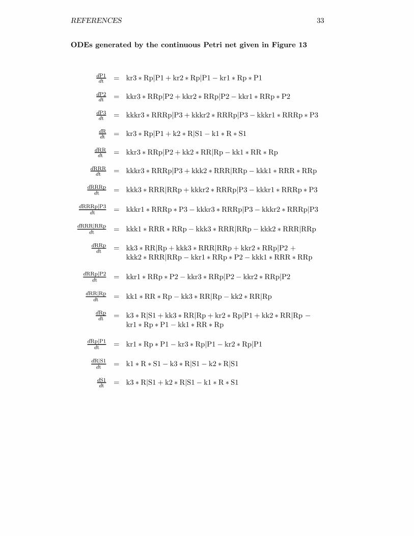
ODEs generated by the continuous Petri net given in Figure 13
dP1dt = kr3 ∗ Rp|P1 + kr2 ∗ Rp|P1− kr1 ∗ Rp ∗ P1
dP2dt = kkr3 ∗ RRp|P2 + kkr2 ∗ RRp|P2− kkr1 ∗ RRp ∗ P2
dP3dt = kkkr3 ∗ RRRp|P3 + kkkr2 ∗ RRRp|P3− kkkr1 ∗ RRRp ∗ P3
dRdt = kr3 ∗ Rp|P1 + k2 ∗ R|S1− k1 ∗ R ∗ S1
dRRdt = kkr3 ∗ RRp|P2 + kk2 ∗RR|Rp− kk1 ∗RR ∗ Rp
dRRRdt = kkkr3 ∗ RRRp|P3 + kkk2 ∗RRR|RRp− kkk1 ∗ RRR ∗ RRp
dRRRpdt = kkk3 ∗RRR|RRp + kkkr2 ∗ RRRp|P3− kkkr1 ∗ RRRp ∗ P3
dRRRp|P3dt = kkkr1 ∗ RRRp ∗ P3− kkkr3 ∗RRRp|P3− kkkr2 ∗RRRp|P3
dRRR|RRpdt = kkk1 ∗RRR ∗ RRp− kkk3 ∗ RRR|RRp− kkk2 ∗ RRR|RRp
dRRpdt = kk3 ∗RR|Rp + kkk3 ∗RRR|RRp + kkr2 ∗ RRp|P2 +
kkk2 ∗RRR|RRp− kkr1 ∗ RRp ∗ P2− kkk1 ∗ RRR ∗RRp
dRRp|P2dt = kkr1 ∗ RRp ∗ P2− kkr3 ∗ RRp|P2− kkr2 ∗ RRp|P2
dRR|Rpdt = kk1 ∗RR ∗Rp− kk3 ∗ RR|Rp− kk2 ∗ RR|Rp
dRpdt = k3 ∗ R|S1 + kk3 ∗ RR|Rp + kr2 ∗ Rp|P1 + kk2 ∗ RR|Rp −
kr1 ∗ Rp ∗ P1− kk1 ∗ RR ∗ Rp
dRp|P1dt = kr1 ∗ Rp ∗ P1− kr3 ∗ Rp|P1− kr2 ∗ Rp|P1
dR|S1dt = k1 ∗ R ∗ S1− k3 ∗ R|S1− k2 ∗R|S1
dS1dt = k3 ∗ R|S1 + k2 ∗ R|S1− k1 ∗ R ∗ S1

REFERENCES 34
R|S1
S11
R 1
RRpRR 1RR|Rp
RRRpRRR 1RRR|RRp
Rp
k3
kk3
kkk3
S�T�U�V�S�W X�Y"W$Z"[�T \�]"^$]�\�_ \�S"X$]�\ _�`�a `�_�a _"b�a�b�_�a�W�c ]"W _�\ d�_�\ d�]e e e e X X e X X X X e X X e e eU�f�Z ]"W1\ ]"W�U ]"W�g$\�Z�h \�f�h Y ]�Y T�d"^$U�]�` Y�]�` U�f�i U�\�_ j j"^$j�k�]X e X X e X e e X e l X X X X Xm�m�m�m�m�m9m�m�m�m�m�m�m�m�m�m�m�m�m�m�m�m�m�m�m�m�m�m�m�m9m�m�m�m�m�m�m�m�m�m�m�m�mn b m�o"p9q�r i o�r"p `�st `�i o"q1o�r�u ` m�o"p�q�r i o�r"p `�si�vLwNxys�` r `�z�s�{�| r i�}�s�{ n s�}�}L~Ds
k1, k2
kk1, kk2
kkk1, kkk2
Figure 14: Three-stage in vitro cascade (MA1).

REFERENCES 35
ODEs generated by the continuous Petri net given in Figure 14
dRdt = k2 ∗ R|S1− k1 ∗ R ∗ S1
dRRdt = kk2 ∗ RR|Rp− kk1 ∗ RR ∗ Rp
dRRRdt = kkk2 ∗ RRR|RRp− kkk1 ∗ RRR ∗RRp
dRRRpdt = kkk3 ∗ RRR|RRp
dRRR|RRpdt = kkk1 ∗ RRR ∗ RRp− kkk3 ∗RRR|RRp− kkk2 ∗ RRR|RRp
dRRpdt = kk3 ∗ RR|Rp + kkk3 ∗ RRR|RRp + kkk2 ∗ RRR|RRp −
kkk1 ∗ RRR ∗ RRp
dRR|Rpdt = kk1 ∗ RR ∗ Rp− kk3 ∗ RR|Rp− kk2 ∗ RR|Rp
dRpdt = k3 ∗ R|S1 + kk3 ∗ RR|Rp + kk2 ∗ RR|Rp− kk1 ∗RR ∗ Rp
dR|S1dt = k1 ∗ R ∗ S1− k3 ∗R|S1− k2 ∗ R|S1
dS1dt = k3 ∗ R|S1 + k2 ∗ R|S1− k1 ∗R ∗ S1

REFERENCES 36
R|S1
S11
R 1Rp|P1
P11
P21
RRp|P2RRpRR 1
RR|Rp
P31
RRRp|P3RRRpRRR 1
RRR|RRp
S1|RRRp
Rp
k3
kr3
kkr3
kk3
kkkr3
kkk3
i1
i2
����������� ���"�$�"��� ���"�$����� ���"�$��� ����� ����� �"������������� �"� ��� ����� ���� � � � � � � � � � � � � � � � ������ �"�1� �"��� �"���$����� ����� � ��� ���"�$����� ����� ����� ����� � �"�$������ � � � � � � � � � � � � � � ������������9�������������������������������������������������9������������������ � ���"�9��� � ���"� ��� � � ��������� � ���"� ���B¡ � ��� �"������¢�£�¤��1¥"��� ��� �"������¢�¦��§L¨N© ¤ ��� � ��ª�� £ �« � � ��¬�� £ ��¬�¬
k1, k2
kr1, kr2
kk1, kk2
kkr1, kkr2
kkk1, kkk2
kkkr1, kkkr2
Figure 15: Three-stage in vivo cascade with negative feedback (MA1).

REFERENCES 37
ODEs generated by the continuous Petri net given in Figure 15
dP1dt = kr3 ∗ Rp|P1 + kr2 ∗ Rp|P1− kr1 ∗ Rp ∗ P1
dP2dt = kkr3 ∗ RRp|P2 + kkr2 ∗ RRp|P2− kkr1 ∗ RRp ∗ P2
dP3dt = kkkr3 ∗ RRRp|P3 + kkkr2 ∗ RRRp|P3− kkkr1 ∗ RRRp ∗ P3
dRdt = kr3 ∗ Rp|P1 + k2 ∗ R|S1− k1 ∗ R ∗ S1
dRRdt = kkr3 ∗ RRp|P2 + kk2 ∗RR|Rp− kk1 ∗RR ∗ Rp
dRRRdt = kkkr3 ∗ RRRp|P3 + kkk2 ∗RRR|RRp− kkk1 ∗ RRR ∗ RRp
dRRRpdt = kkk3 ∗RRR|RRp + kkkr2 ∗ RRRp|P3 + i2 ∗ S1|RRRp −
kkkr1 ∗ RRRp ∗ P3− i1 ∗ S1 ∗ RRRp
dRRRp|P3dt = kkkr1 ∗ RRRp ∗ P3− kkkr3 ∗RRRp|P3− kkkr2 ∗RRRp|P3
dRRR|RRpdt = kkk1 ∗RRR ∗ RRp− kkk3 ∗ RRR|RRp− kkk2 ∗ RRR|RRp
dRRpdt = kk3 ∗RR|Rp + kkk3 ∗RRR|RRp + kkr2 ∗ RRp|P2 +
kkk2 ∗RRR|RRp− kkr1 ∗ RRp ∗ P2− kkk1 ∗ RRR ∗RRp
dRRp|P2dt = kkr1 ∗ RRp ∗ P2− kkr3 ∗ RRp|P2− kkr2 ∗ RRp|P2
dRR|Rpdt = kk1 ∗RR ∗Rp− kk3 ∗ RR|Rp− kk2 ∗ RR|Rp
dRpdt = k3 ∗ R|S1 + kk3 ∗ RR|Rp + kr2 ∗ Rp|P1 + kk2 ∗ RR|Rp −
kr1 ∗ Rp ∗ P1− kk1 ∗ RR ∗ Rp
dRp|P1dt = kr1 ∗ Rp ∗ P1− kr3 ∗ Rp|P1− kr2 ∗ Rp|P1
dR|S1dt = k1 ∗ R ∗ S1− k3 ∗ R|S1− k2 ∗R|S1
dS1dt = k3 ∗ R|S1 + k2 ∗ R|S1 + i2 ∗ S1|RRRp− k1 ∗ R ∗ S1 −
i1 ∗ S1 ∗ RRRp
dS1|RRRpdt = i1 ∗ S1 ∗ RRRp− i2 ∗ S1|RRRp

REFERENCES 38
R|S1
S11
R 1
RRpRR 1RR|Rp
RRRpRRR 1RRR|RRp
S1|RRRp
Rpk3
kk3
kkk3
i1
i2
�®�¯�°��± ²�³"±$´"µ�® ¶�·"¸$·�¶�¹ ¶�"²$·�¶ ¹�º�» º�¹�» ¹"¼�»�¼�¹�»�±�½ ·"± ¹�¶ ¾�¹�¶ ¾�·¿ ¿ ¿ ¿ ² ² ¿ ¿ ² ² ² ² ² ² ² ² ¿¯�À�´ ·"±1¶ ·"±�¯ ·"±�Á$¶�´� ¶�À� ³ ·�³ ®�¾"¸$¯�·�º ³�·�º ¯�À�à ¯�¶�¹ Ä Ä"¸$Ä�Å�·² Æ ² ² ¿ ² ¿ ¿ ² ² Æ ² ² ² ² ²Ç�Ç�Ç�Ç�Ç�Ç9Ç�Ç�Ç�Ç�Ç�Ç�Ç�Ç�Ç�Ç�Ç�Ç�Ç�Ç�Ç�Ç�Ç�Ç�Ç�Ç�Ç�Ç�Ç�Ç9Ç�Ç�Ç�Ç�Ç�Ç�Ç�Ç�Ç�Ç�Ç�Ç�ÇÈ ¼ Ç�É"Ê9Ë�Ì Ã É�Ì"Ê º�ÍÈ º�à É"Ë1É�Ì�Î º Ç�É"Ê�Ë�Ì Ã É�Ì"Ê º�ÍÃ�ÏLÐNÑyÍ�º Ì º�Ò�Í�Ó�Ô�Ô Ì Ã�Õ�Í�Ó È Í�Õ�ÕLÖDÍ
k1, k2
kk1, kk2
kkk1, kkk2
Figure 16: Three-stage in vitro cascade with negative feedback (MA1).

REFERENCES 39
ODEs generated by the continuous Petri net given in Figure 16
dRdt = k2 ∗ R|S1− k1 ∗ R ∗ S1
dRRdt = kk2 ∗ RR|Rp− kk1 ∗ RR ∗ Rp
dRRRdt = kkk2 ∗ RRR|RRp− kkk1 ∗ RRR ∗RRp
dRRRpdt = kkk3 ∗ RRR|RRp + i2 ∗ S1|RRRp− i1 ∗ S1 ∗ RRRp
dRRR|RRpdt = kkk1 ∗ RRR ∗ RRp− kkk3 ∗RRR|RRp− kkk2 ∗ RRR|RRp
dRRpdt = kk3 ∗ RR|Rp + kkk3 ∗ RRR|RRp + kkk2 ∗ RRR|RRp −
kkk1 ∗ RRR ∗ RRp
dRR|Rpdt = kk1 ∗ RR ∗ Rp− kk3 ∗ RR|Rp− kk2 ∗ RR|Rp
dRpdt = k3 ∗ R|S1 + kk3 ∗ RR|Rp + kk2 ∗ RR|Rp− kk1 ∗RR ∗ Rp
dR|S1dt = k1 ∗ R ∗ S1− k3 ∗R|S1− k2 ∗ R|S1
dS1dt = k3 ∗ R|S1 + k2 ∗ R|S1 + i2 ∗ S1|RRRp− k1 ∗R ∗ S1 −
i1 ∗ S1 ∗RRRp
dS1|RRRpdt = i1 ∗ S1 ∗RRRp− i2 ∗ S1|RRRp

REFERENCES 40
R|S1
S11
R 1Rp|P1
P11
P21
P21
RRp|P2
RRpRR 1
RR|Rp
P31
RRRp|P3RRRpRRR 1
RRR|RRp
S1|RRRp
RR|U
U 1 U1
RR|Rp|URRp|U
RRp|P2|U
Rp
Rp
k3
kr3
kkr3
kk3
kkkr3
kkk3
i1
i2
b1u
u1u u2ub2u
kk3u
kkr3u
×ÙØÙÚÜÛÝ×ßÞáàÝâßÞäãßåÝØçæÙèßéêèÙæÙëçæÙ×ßàäèÙæ ëíìÙîçìÙëÙîçëßïÝîÜïðëÙîÜÞÙñ èßÞ ëíæ òÙëÙæçòÙèó ó ó ó à à ó ó à à à à à à à à àÚÙôÙãçèßÞÝæáèßÞÝÚçèßÞÙõäæÙãÙöáæÙôÙö â èÙâ ØíòßéäÚÙèÙìçâÙèÙìçÚíôÙ÷çÚÙæÙë ø øßéäøÙùÙèó ó ó à ó ó ó ó ó à ú à à ó ó óûÙûÙûÙûÙûÙûÙûÙûíûÙûÙûÙûÙûÙûÙûÙûÙûÙûÙûÙûíûÙûÙûÙûÙûÙûÙûÙûÙûÙûÙûÙûÙûíûÙûÙûÙûÙûü ï ûÙýßþÙÿ�� ÷ ý��ßþ ì����� ì ûÙýßþÙÿ�� ÷ ý��ßþ ì���� ��� ìÙ÷ ýßÿÝý������Üþ� þÝû ìÙ÷ ýßÿÝý�����÷���� � î����Ùì � ì���� �������� ÷���� � �����
k1, k2
kr1, kr2
kk1, kk2
kkr1, kkr2
kkk1, kkk2
kkkr1, kkkr2
kk1u, kk2u
kkr1u, kkr2u
Figure 17: Three-stage in vivo cascade with negative feedback and drug inhibition(MA1). The nodes given in gray indicate logical nodes (also called fusion nodes).Logical nodes with identical names are from a structural point of view identical;they are used to increase readability in larger net structures by connecting logicallyremote net parts.

REFERENCES 41
ODEs generated by the continuous Petri net given in Figure 17
dP1
dt= kr3 ∗ Rp|P1 + kr2 ∗ Rp|P1 − kr1 ∗ Rp ∗ P1
dP2
dt= kkr3 ∗ RRp|P2 + kkr2 ∗ RRp|P2 + kkr3u ∗ RRp|P2|U +
kkr2u ∗ RRp|P2|U − kkr1 ∗ RRp ∗ P2 − kkr1u ∗ RRp|U ∗ P2
dP3
dt= kkkr3 ∗ RRRp|P3 + kkkr2 ∗ RRRp|P3 − kkkr1 ∗ RRRp ∗ P3
dR
dt= kr3 ∗ Rp|P1 + k2 ∗ R|S1 − k1 ∗ R ∗ S1
dRR
dt= kkr3 ∗ RRp|P2 + kk2 ∗ RR|Rp + u1u ∗ RR|U− kk1 ∗ RR ∗ Rp −
b1u ∗ RR ∗ U
dRRR
dt= kkkr3 ∗ RRRp|P3 + kkk2 ∗ RRR|RRp− kkk1 ∗ RRR ∗ RRp
dRRRp
dt= kkk3 ∗ RRR|RRp + kkkr2 ∗ RRRp|P3 + i2 ∗ S1|RRRp −
kkkr1 ∗ RRRp ∗ P3 − i1 ∗ S1 ∗ RRRp
dRRRp|P3
dt= kkkr1 ∗ RRRp ∗ P3 − kkkr3 ∗ RRRp|P3− kkkr2 ∗ RRRp|P3
dRRR|RRp
dt= kkk1 ∗ RRR ∗ RRp− kkk3 ∗ RRR|RRp− kkk2 ∗ RRR|RRp
dRRp
dt= kk3 ∗ RR|Rp + kkk3 ∗ RRR|RRp + kkr2 ∗ RRp|P2 + kkk2 ∗ RRR|RRp +
u2u ∗ RRp|U− kkr1 ∗ RRp ∗ P2 − kkk1 ∗ RRR ∗ RRp− b2u ∗ RRp ∗ U
dRRp|P2
dt= kkr1 ∗ RRp ∗ P2 − kkr3 ∗ RRp|P2 − kkr2 ∗ RRp|P2
dRRp|P2|Udt
= kkr1u ∗ RRp|U ∗ P2 − kkr3u ∗ RRp|P2|U − kkr2u ∗ RRp|P2|U
dRRp|Udt
= kk3u ∗ RR|Rp|U + b2u ∗ RRp ∗ U + kkr2u ∗ RRp|P2|U − u2u ∗ RRp|U −kkr1u ∗ RRp|U ∗ P2
dRR|Rp
dt= kk1 ∗ RR ∗ Rp− kk3 ∗ RR|Rp− kk2 ∗ RR|Rp
dRR|Rp|Udt
= kk1u ∗ RR|U ∗ Rp − kk3u ∗ RR|Rp|U− kk2u ∗ RR|Rp|U
dRR|Udt
= b1u ∗ RR ∗ U + kkr3u ∗ RRp|P2|U + kk2u ∗ RR|Rp|U− u1u ∗ RR|U −kk1u ∗ RR|U ∗ Rp
dRp
dt= k3 ∗ R|S1 + kk3 ∗ RR|Rp + kr2 ∗ Rp|P1 + kk2 ∗ RR|Rp +
kk2u ∗ RR|Rp|U + kk3u ∗ RR|Rp|U− kr1 ∗ Rp ∗ P1 − kk1 ∗ RR ∗ Rp −kk1u ∗ RR|U ∗ Rp
dRp|P1
dt= kr1 ∗ Rp ∗ P1 − kr3 ∗ Rp|P1 − kr2 ∗ Rp|P1
dR|S1
dt= k1 ∗ R ∗ S1 − k3 ∗ R|S1 − k2 ∗ R|S1
dS1
dt= k3 ∗ R|S1 + k2 ∗ R|S1 + i2 ∗ S1|RRRp− k1 ∗ R ∗ S1 − i1 ∗ S1 ∗ RRRp
dS1|RRRp
dt= i1 ∗ S1 ∗ RRRp− i2 ∗ S1|RRRp
dU
dt= u1u ∗ RR|U + u2u ∗ RRp|U− b1u ∗ RR ∗ U − b2u ∗ RRp ∗ U

REFERENCES 42
R|S1
S11
R 1
RRpRR 1
RR|Rp
RRRpRRR 1RRR|RRp
S1|RRRp
RR|U
U 1 U1
RR|Rp|URRp|U
Rp
Rp
k3
kk3
kkk3
i1
i2
b1u
u1u u2ub2u
kk3u
�������������� ��"!�#���$�%�&'%�$�(�$����'%�$ (�)�*�)�(�*�(�+�*�+�(�*,��- %�� (�$ .�(�$�.�%/ / / / � � / / � � � � � � � � ���0�!�%���$�%�����%���1'$�!�2�$�0�2 %� ��.�&"��%�)� �%�)���0�3���$�( 4 4�&"4�5�%� / � � / � / / � � 6 � � � � �7�7�7�7�7�7�7�7�7�7�787�7�7�7�7�7�7�7�7�7�7�787�7�7�7�7�7�7�7�7�7�7�7�787�7�7�7�7�7�79 + 7�:�;�<�= 3 :�=>; )�?@ )�3 :�<�:�=�A ) 7�:�;�<�= 3 :�=�; )�?3�B�CED 9 ?�) = )8F�?�G�H�D = 3�I�?�G,J�?�I�I�KL?
k1, k2
kk1, kk2
kkk1, kkk2
kk1u, kk2u
Figure 18: Three-stage in vitro cascade with negative feedback and drug inhibition(MA1).
REFERENCES 43
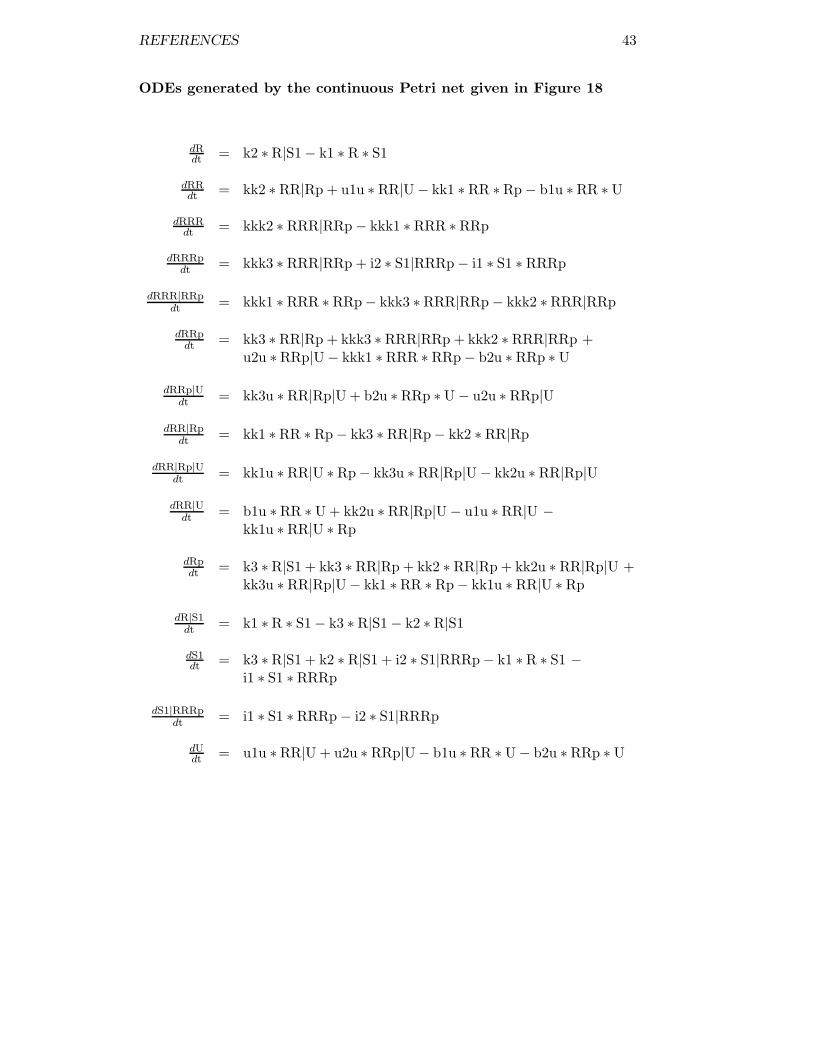
ODEs generated by the continuous Petri net given in Figure 18
dRdt = k2 ∗R|S1− k1 ∗ R ∗ S1
dRRdt = kk2 ∗ RR|Rp + u1u ∗ RR|U− kk1 ∗ RR ∗Rp− b1u ∗RR ∗ U
dRRRdt = kkk2 ∗ RRR|RRp− kkk1 ∗ RRR ∗RRp
dRRRpdt = kkk3 ∗ RRR|RRp + i2 ∗ S1|RRRp− i1 ∗ S1 ∗ RRRp
dRRR|RRpdt = kkk1 ∗ RRR ∗ RRp− kkk3 ∗RRR|RRp− kkk2 ∗RRR|RRp
dRRpdt = kk3 ∗ RR|Rp + kkk3 ∗ RRR|RRp + kkk2 ∗ RRR|RRp +
u2u ∗RRp|U− kkk1 ∗RRR ∗ RRp− b2u ∗ RRp ∗ U
dRRp|Udt = kk3u ∗ RR|Rp|U + b2u ∗ RRp ∗U− u2u ∗ RRp|U
dRR|Rpdt = kk1 ∗ RR ∗ Rp− kk3 ∗ RR|Rp− kk2 ∗ RR|Rp
dRR|Rp|Udt = kk1u ∗ RR|U ∗ Rp− kk3u ∗ RR|Rp|U− kk2u ∗ RR|Rp|U
dRR|Udt = b1u ∗RR ∗ U + kk2u ∗ RR|Rp|U− u1u ∗RR|U −
kk1u ∗ RR|U ∗ Rp
dRpdt = k3 ∗R|S1 + kk3 ∗ RR|Rp + kk2 ∗ RR|Rp + kk2u ∗ RR|Rp|U +
kk3u ∗ RR|Rp|U− kk1 ∗ RR ∗ Rp− kk1u ∗ RR|U ∗ Rp
dR|S1dt = k1 ∗R ∗ S1− k3 ∗R|S1− k2 ∗ R|S1
dS1dt = k3 ∗R|S1 + k2 ∗ R|S1 + i2 ∗ S1|RRRp− k1 ∗R ∗ S1 −
i1 ∗ S1 ∗RRRp
dS1|RRRpdt = i1 ∗ S1 ∗RRRp− i2 ∗ S1|RRRp
dUdt = u1u ∗RR|U + u2u ∗ RRp|U− b1u ∗ RR ∗ U− b2u ∗RRp ∗ U