A Stochastic Population Dynamics Model for Aedes Aegypti : Formulation and Application to a City...

Bulletin of Mathematical Biology (2006) 68: 1945–1974DOI 10.1007/s11538-006-9067-y

ORIGINAL ARTICLE

A Stochastic Population Dynamics Model for AedesAegypti: Formulation and Application to a City withTemperate Climate

Marcelo Oteroa, Hernan G. Solaria,∗, Nicolas Schweigmannb

aDepartment of Physics, Facultad de Ciencias Exactas y Naturales, Universidad deBuenos Aires, Buenos Aires, Argentina

bDepartment of Genetics and Ecology, Facultad de Ciencias Exactas y Naturales,Universidad de Buenos Aires, Buenos Aires, Argentina

Received: 6 December 2004 / Accepted: 25 November 2005 / Published online: 11 July 2006C© Society for Mathematical Biology 2006

Abstract Aedes aegypti is the main vector for dengue and urban yellow fever. It isextended around the world not only in the tropical regions but also beyond them,reaching temperate climates. Because of its importance as a vector of deadly dis-eases, the significance of its distribution in urban areas and the possibility of breed-ing in laboratory facilities, Aedes aegypti is one of the best-known mosquitoes. Inthis work the biology of Aedes aegypti is incorporated into the framework of astochastic population dynamics model able to handle seasonal and total extinctionas well as endemic situations. The model incorporates explicitly the dependencewith temperature. The ecological parameters of the model are tuned to the presentpopulations of Aedes aegypti in Buenos Aires city, which is at the border of thepresent day geographical distribution in South America. Temperature thresholdsfor the mosquito survival are computed as a function of average yearly tempera-ture and seasonal variation as well as breeding site availability. The stochastic anal-ysis suggests that the southern limit of Aedes aegypti distribution in South Americais close to the 15◦C average yearly isotherm, which accounts for the historical andcurrent distribution better than the traditional criterion of the winter (July) 10◦Cisotherm.

Keywords Mathematical ecology · Population dynamics · Aedes aegypti ·Stochastic model · Temperate climate

1. Introduction

Aedes aegypti is mostly a domestic mosquito and the primary vector for urban yel-low fever and dengue. It is the most important vector for dengue in the Americas,

∗Corresponding author.E-mail address: [email protected] (Hernan G. Solari).

1946 Bulletin of Mathematical Biology (2006) 68: 1945–1974

and it can be found in tropical and subtropical regions such as Florida, CentralAmerica, the Caribbean Islands and Brazil. It is estimated that about 2500–3000millions of people live in areas where the transmission of the dengue virus is en-demic.

The limits for the geographical distribution of Aedes aegypti tentatively adoptedby Christophers (1960), and reproduced by several authors (FUNCEI, 1999a;WHO, 1998), are the winter isotherms of 10◦C (corresponding to July in the south-ern hemisphere and to January in the northern hemisphere). This criterion is farfrom being perfect as Christophers showed (we will come back to the discussion ofthe geographical distribution and its relation with climate later in this work). TheJuly 10◦C isotherm is indicated in Fig. 1 as a thick solid line.1

Aedes aegypti has been reported, in the decade of the 1930s, in Bahıa Blanca (onthe Atlantic coast 38◦44′S, 62◦16′W, average yearly temperature 15.4◦C, July meantemperature 7.6◦C) before the Aedes aegypti eradication program in the Americas,and is currently a permanent inhabitant of Buenos Aires city (34◦38′S, 58◦28′W,average yearly temperature 18.0◦C, July mean temperature 11.0◦C) (Carbajo et al.,2001; de Garın et al., 2000; Schweigmann and Boffi, 1998).

Historical records show that an epidemic of dengue in 1916 affected the citiesof Concordia (31◦22′S, 58◦09′W, average yearly temperature 18.9◦C, July meantemperature 12.3◦C) and Parana (31◦44′S, 60◦32′W, average yearly temperature18.2◦C, July mean temperature 11.2◦C), and yellow fever epidemics decimatedBuenos Aires city in 1852, 1857, 1870, 1871, 1896, 1899 and 1905. Nowadays,dengue is present in tropical regions of Argentina, i.e. in the northern provinces ofSalta, Jujuy and Misiones (FUNCEI, 1998, 1999a,b).

In order to study the possible evolution of a dengue epidemic in any city witha temperate climate, such as Buenos Aires city, the seasonal variation of adultmosquito populations has to be taken into account since the abundance of adultfemales is the key factor for the transmission of the disease. Adult mosquitoesare close to extinction during the winter months and re-emerge in the spring. Incontrast eggs are present all year long. The studies performed in Buenos Aires(Carbajo et al., 2001) suggest that extinctions of all forms of the mosquito as wellas repopulation processes are common in localised areas of the city.

The Aedes aegypti eradication program carried out in Argentina (1954–1963), aspart of the eradication program in the Americas was based on the use of insecticide(DDT) and the systematic destruction of breeding sites (Ministerio de AsistenciaSocial y Salud Publica, 1964). As an application of the model we will be discussinghow the number of available breeding sites affects the survival of the species.

The description of mosquito populations (as well as other insects) has beenaddressed using Dynamic Life Table Models (Depinay et al., 2004; Focks et al.,1993a,b; Powell and Jenkis, 2000). These models are deterministic in nature and

1The temperature maps were produced by D. R. Legates and C. J. Willmott using terrestrial obser-vations of shelter-height air temperature and shipboard measurements. The combined databaseof the world consisted of 17986 independent terrestrial station records and 6955 oceanic grid-pointrecords. The data were interpolated to a 0.5◦ of latitude by 0.5◦ of longitude lattice. Most of theland station records are for the years between 1920 and 1980. Median air temperatures over theoceans are taken from the Comprehensive Ocean-Atmosphere Data Set (COADS) for the years1950–1979. COADS data are 2-degree latitude-longitude resolution (Legates and Willmott, 1990).

Bulletin of Mathematical Biology (2006) 68: 1945–1974 1947

Fig. 1 July temperature in South America. The thick solid line represents the July 10◦Cisotherm. The cities of (South to North) Bahıa Blanca, Buenos Aires, Parana and Concordiaare indicated on the map. Adapted from Legates and Willmott (1990).

their stochasticity depends solely on the stochastic components of the climate data.Intrinsic stochasticity is not present and fixed rules are used in place of stochasticphenomena. For example, in Focks et al. (1993a,b) egg hatching cannot occur be-low an arbitrary temperature (an adjustable parameter, taken to be 22◦C in theoriginal work). However, experimental reports present several different minimalhatching temperatures varying from 20 to 13◦C (Christophers, 1960) (hatching of


eggs at a temperature as low as 1◦C has been reported, although the larvae werefound dead). Indirect evidence of egg hatching below 17◦C is provided by the ob-served sharp rise in the population of adults when the average daily temperaturereaches approximately 18◦C (field studies performed at Buenos Aires (Camposand Macia, 1996)). Reports of a sharp rise at 17◦C in the northern city of Cordoba(Domınguez et al., 2000) suggest that this value depends on additional factors andnot only on the instantaneous temperature.

Moreover, Dynamic Life Table models are computationally demanding, pre-venting their use beyond homogeneous situations and do not allow for a simplemathematical analysis (Powell and Jenkis, 2000).

In the present work we develop a model for the evolution of Aedes aegypti asa (nonlinear or state dependent) Markov chain (Ethier and Kurtz, 1986) consid-ering the four life stages of a mosquito: egg, larva, pupa and adult. For every lifestage, the relevant changes are modelled in terms of random events with rates de-termined from the biological data available for Aedes aegypti. The rates dependon time through weather parameters. The relation with the deterministic models,emerging in the infinite populations limit, will also be addressed and their resultscompared with the stochastic model.

A minimalist stochastic model has several advantages over deterministic mod-els. It shares much of the computational efficiency of models based upon dif-ferential equations but can deal properly with extinction processes. It is alsoconsiderably less computationally demanding than following cohorts in dynam-ical table models and has the additional advantage that stochastic processes,such as development, are described in stochastic terms without resorting to ad-ditional (ad hoc) parameters to simulate them with deterministic methods. Ad-ditionally, the stochastic process has been approximated in this work with aPoisson method (see Appendix A) that represents a substantial saving of com-puter time compared to a direct Monte Carlo implementation of the stochasticprocess.

We will show in this work that the technical advantages allow for deeper scrutinyof the biological problem. In particular, they allow us to reconsider the habitatlimits for Aedes aegypti.

In what follows we shall describe the basic biology of Aedes aegypti (Section 2),the formulation of the model (Section 3) and the evaluation of parameters basedon the biological data (Section 4). Section 5 discusses the limitations of the modelwhile Section 6 presents some results and issues of biological interest. The geo-graphical limits for Aedes aegypti are discussed in Section 7 as a function of av-erage yearly temperature, amplitude of the seasonal variation of the temperatureand availability of breeding sites. The last section is dedicated to the summary,discussion and conclusions.

2. Biological notes on Aedes aegypti

The life cycle of a mosquito presents four distinct stages: egg, larva, pupa and adult(see Fig. 2). In the case of Aedes aegypti the first three stages take place in or nearwater while air is the medium for the adult stage.


Fig. 2 Life cycle of Aedes aegypti.

The eggs are laid on wet surfaces just above the water level (egg deposition).Aedes aegypti prefers small containers such as cans, buckets, flower pots, bottles,jars, urns and rain-water containers. Used car tires provide an ideal larval habitatand an adult resting site. In tropical climates larvae can also be found in naturalcavities such as tree holes. The eggs of Aedes aegypti can resist desiccation andlow temperatures for up to one year. Under the weather conditions considered inthis work, desiccation is not a relevant mortality factor and has not been furtherconsidered. Although hatching of mature eggs may spontaneously occur at anytime, it is greatly stimulated by flooding. Hence, hatching is more likely to occurafter rainfall (Christophers, 1960).

The larva moult four times in a period of a few days (depending on the tempera-ture) which culminates in the pupal stage (pupation). Both the larva and pupa areactive stages, but only the larvae eat.

The pupal stage lasts from one day to a few weeks (depending on the tem-perature). At the end of the stage the adult emerges from the pupal skin (adultemergence).

The adult stage of the mosquito is considered to last an average of eleven days inthe urban environment. Dengue and yellow fever are spread only by adult females.Mosquito females require blood to complete oogenesis. Aedes females are mainlyanthropophagic, they prefer human blood to other mammals’, although they canalso bite other vertebrates. In this process, the female ingests human viruses withthe blood meal. The viruses develop within the mosquito and are reinjected intothe blood stream with the saliva of the mosquito in later blood meals.

Adult females lay an average of 63 eggs at each oviposition. The number changesaccording to the weight of the female and other factors. The gonotrophic cycle isregulated by the temperature and is longer for the first oviposition than for thesubsequent ones (Christophers, 1960). We will later distinguish between adult fe-males in their first gonotrophic cycle, (A1 females), and in subsequent gonotrophiccycles (A2 females).

The natural regulation of Aedes aegypti populations has been discussed insome depth in the literature. In general terms, mosquito populations may display


intra-specific competition for food and other resources within the same develop-mental cycle (Dye, 1982; Gleiser et al., 2000; Southwood et al., 1972; Subra andMouchet, 1984). In the present work we will only consider competition within thelarval stage, which is the only one well documented for Aedes aegypti. Predationmay also be a factor in controlling the population of Aedes aegypti (Focks et al.,1993a).

In practical terms many of these mechanisms may be indistinguishable, as all ofthem will increase, in a first approximation, the mortality rate of the larvae as afunction of larval density in the breeding site. In other words, each breeding sitewill be characterised by a carrying capacity.

Other mechanisms of population control have been reported for mosquitoes. Inparticular, inhibition of egg hatching due to a large density of larvae has been re-ported for Ochlerotatus triseriatus (formerly Aedes triseriatus) and may also affectAedes aegypti populations (Livdahl et al., 1984).

3. Mathematical model of the life cycle

The model considers five different populations: eggs (E), larvae (L), pupae (P),female adults not having laid eggs (A1), and female adults having laid eggs (A2).The population of adult male mosquitoes is not considered explicitly except thatevery time a female adult emerges, we will discount two pupae from the pool of pu-pae since about one half of the emerging adults are females. Actually, Arrivillagaand Barrera (2004) report a ratio of 1.02:1 male:female. Since we lack statisticalinformation regarding oviposition, we will consider that each female lays a fixednumber of eggs (63) at every oviposition.

The evolution of the five populations is affected by ten different possible events:death of eggs, egg hatching, death of larvae, pupation, death of pupae, adult emer-gence, death of young adults (A1), death of A2 adults, oviposition by A1 femalesand oviposition by A2 females. Table 1 summarises this information.

Events occur at rates that depend not only on population values but also on tem-perature, which in turn is a function of time since it changes over the course of theyear. Hence, the dependence on the temperature introduces a time dependence inthe event rates.

The inhibitory effect of larvae density on egg hatching, γ (L), is modelled with a(negative) step function and its relevance will be later discussed in this work.

The evolution of the populations is modelled by a (state dependent) Poissonprocess (Andersson and Britton, 2000; Ethier and Kurtz, 1986) where the proba-bility of the state (E, L, P, A1, A2) evolves in time following a Kolmogorov for-ward equation (also known as master equation) that can be constructed directlyfrom the information collected in Table 1.

The associated deterministic differential equation model (Ethier and Kurtz,1986; Kurtz, 1970, 1971) reads

dE/dt = egn(ovr1 × A1 + ovr2 × A2) − me × E − elr(1 − γ (L))E

dL/dt = elr(1 − γ (L))E − ml × L− α × L2 − lpr × L


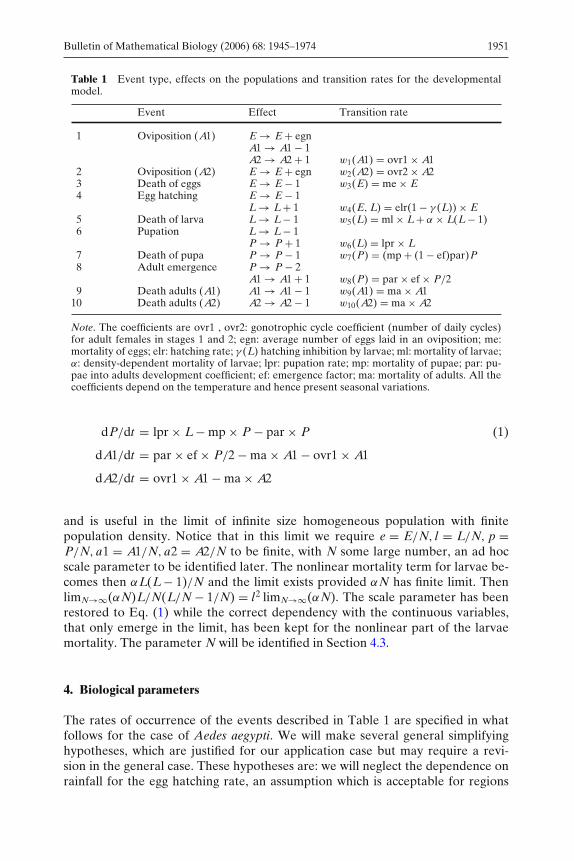
Table 1 Event type, effects on the populations and transition rates for the developmentalmodel.

Event Effect Transition rate

1 Oviposition (A1) E → E + egnA1 → A1 − 1A2 → A2 + 1 w1(A1) = ovr1 × A1

2 Oviposition (A2) E → E + egn w2(A2) = ovr2 × A23 Death of eggs E → E − 1 w3(E) = me × E4 Egg hatching E → E − 1

L → L+ 1 w4(E, L) = elr(1 − γ (L)) × E5 Death of larva L → L− 1 w5(L) = ml × L+ α × L(L− 1)6 Pupation L → L− 1

P → P + 1 w6(L) = lpr × L7 Death of pupa P → P − 1 w7(P) = (mp + (1 − ef)par)P8 Adult emergence P → P − 2

A1 → A1 + 1 w8(P) = par × ef × P/29 Death adults (A1) A1 → A1 − 1 w9(A1) = ma × A1

10 Death adults (A2) A2 → A2 − 1 w10(A2) = ma × A2

Note. The coefficients are ovr1 , ovr2: gonotrophic cycle coefficient (number of daily cycles)for adult females in stages 1 and 2; egn: average number of eggs laid in an oviposition; me:mortality of eggs; elr: hatching rate; γ (L) hatching inhibition by larvae; ml: mortality of larvae;α: density-dependent mortality of larvae; lpr: pupation rate; mp: mortality of pupae; par: pu-pae into adults development coefficient; ef: emergence factor; ma: mortality of adults. All thecoefficients depend on the temperature and hence present seasonal variations.

dP/dt = lpr × L− mp × P − par × P (1)

dA1/dt = par × ef × P/2 − ma × A1 − ovr1 × A1

dA2/dt = ovr1 × A1 − ma × A2

and is useful in the limit of infinite size homogeneous population with finitepopulation density. Notice that in this limit we require e = E/N, l = L/N, p =P/N, a1 = A1/N, a2 = A2/N to be finite, with N some large number, an ad hocscale parameter to be identified later. The nonlinear mortality term for larvae be-comes then αL(L− 1)/N and the limit exists provided αN has finite limit. ThenlimN→∞(αN)L/N(L/N − 1/N) = l2 limN→∞(αN). The scale parameter has beenrestored to Eq. (1) while the correct dependency with the continuous variables,that only emerge in the limit, has been kept for the nonlinear part of the larvaemortality. The parameter N will be identified in Section 4.3.

4. Biological parameters

The rates of occurrence of the events described in Table 1 are specified in whatfollows for the case of Aedes aegypti. We will make several general simplifyinghypotheses, which are justified for our application case but may require a revi-sion in the general case. These hypotheses are: we will neglect the dependence onrainfall for the egg hatching rate, an assumption which is acceptable for regions


where there is no dry season. We will also consider the mean daily temperature ofbreeding sites equal to the mean daily temperature of the air.

We shall make here the important distinction between breeding sites and watercontainers. While every breeding site is, by the biological nature of the mosquito,a water container, not every water container is a breeding site. For example, watercontainers with high exposure to the sun or in places infested by predators will notbe effective as breeding sites and will not be considered as such in this work. Weavoid in this form the accumulation of uncertainties produced by indirect calcula-tions of breeding sites.

Since Buenos Aires is a city with temperate climate, we will neglect in thismanuscript the often deadly effect of high temperatures. Adult Aedes aegypti seekcover under bushes and trees during hot weather and also choose their breedingsites in protected places. In temperate climates, containers under tree or bush pro-tection reach temperatures substantially below the upper limits for development.

The different parameters appearing in the stochastic process described byTable 1 characterise Aedes aegypti. The stochastic population dynamic modelmakes no attempt to follow individual cohorts of mosquitoes but considers thefull population as a homogeneous set. More detail could be incorporated into de-velopmental stages in the four populations following more closely in this form thebiology of the Aedes aegypti.

4.1. Developmental rates

There are four developmental rates in our model, and they correspond to egghatching, pupation, adult emergence and gonotrophic cycle. Each of these ratesis evaluated using the results of the thermodynamic model developed by Sharpeand DeMichele (1977). According to this model for poikilothermal developmentthe maturation process is controlled by one enzyme which is active in a given tem-perature range, the enzyme is deactivated at low, TL, and high, TH, temperatures.The development is stochastic in nature and is controlled by a Poisson process withrate RD(T). In general terms RD(T) takes the form

RD(T) = RD(298◦K)

× (T/298◦K) exp((�HA/R)(1/298◦K − 1/T)1 + exp((�HH/R)(1/TH − 1/T)) + exp((�HL/R)(1/TL − 1/T))

(2)

Here TH, TL are absolute temperatures (◦Kelvin) while �HA, �HH and �HL

are thermodynamic enthalpies characteristic of the organism, in particular, �HL

is negative in general while �HH is positive. R is the universal gas constant.Schoofield et al. introduced a simplified model with only high temperature de-

activation (Schoofield et al., 1981). The model reads

RD(T) = RD(298◦K)(T/298◦K) exp((�HA/R)(1/298◦K − 1/T))

1 + exp(�HH/R)(1/T1/2 − 1/T))(3)


Table 2 Coefficients for the enzymatic model of maturation (Eq.( 3)).

Develop. cycle (3) RD(T) RD(298◦K) �HA �HH T1/2

Egg hatching elr 0.24 10798 100000 14184Larval develop. lpr 0.2088 26018 55990 304.6Pupal develop. par 0.384 14931 −472379 148Gonotrophic cycle (A1) ovr1 0.216 15725 1756481 447.2Gonotrophic cycle (A2) ovr2 0.372 15725 1756481 447.2

Note. RD is measured in day−1, enthalpies are measured in (cal/mol) and the temperature ismeasured in absolute (Kelvin) degrees.

where T1/2 is the temperature when half of the enzyme is deactivated because ofhigh temperature. We adopt Schoofield’s model since it is flexible enough for fit-ting the available biological data.

In Table 2 we present the values for the different coefficients involved in theevents: egg hatching, pupation, adult emergence and gonotrophic cycle. The valuesare taken from Focks et al. (1993a). We will later discuss this particular applicationof the enzymatic model.

The resulting developmental rates are displayed in Fig. 3 as a function of tem-perature.

Fig. 3 Developmental rates according to Table 2 as a function of the temperature. elr: hatchingrate; lpr: pupation rate; par: pupae into adults development coefficient; ovr1, ovr2: gonotrophiccycle coefficient (number of daily cycles) for adult females in stages 1 and 2.


4.2. Mortality, emergence and oviposition rates

The different mortality rates as well as the emergence rate and average depositionrate have been taken from Focks et al. (1993a), Christophers (1960) and are asfollows.

Oviposition. Females lay a number of eggs that is roughly proportional to theirbody weight (46.5 eggs/mg) (Bar-Zeev, 1957; Nayar and Sauerman, 1975). Themean weight of a three-day-old female is 1.35 mg (Christophers, 1960), hence weestimate the average number of eggs laid in one oviposition as egn = 63. Thegonotrophic cycle for the first oviposition takes longer than in subsequent oviposi-tions, a fact reflected in the parameters of Table 2. The number of ovipositions foran adult female estimated from the parameters of the model are: one at 20◦C, fouror five at 25◦C and six at 30◦C.

Egg mortality. The mortality of the eggs is chosen to be me = 0.01 1/day and isindependent of the temperature in the range 278◦K ≤ T ≤ 303◦K (Trpis, 1972).

Larva mortality. The death of the larvae is divided in two contributions as ex-plained above. One contribution accounts for natural mortality under optimalconditions and depends only on the temperature. Its rate is approximated byml = 0.01 + 0.9725 exp(−(T − 278)/2.7035) and is valid in the range 278◦K ≤ T ≤303◦K (Bar-Zeev, 1958; Horsfall, 1955; Rueda et al., 1990). The other contri-bution is the density-dependent (regulatory) mortality, due to the accumulationof adverse factors. This contribution will be considered separately in the nextsubsection.

Death of Pupae. The intrinsic mortality of a pupa has been considered as mp =0.01 + 0.9725 exp(−(T − 278)/2.7035) (Bar-Zeev, 1958; Horsfall, 1955; Ruedaet al., 1990).

Emergence. Besides the daily mortality in the pupal stage, there is an importantadditional mortality associated with the sometimes unsuccessful emergence of theadult individual. We assume a mortality of 17% of the pupae at this event, whichis added to the mortality rate of pupae. Some 83% of the pupae that reach mat-uration will emerge as adult mosquitoes, hence the emergence factor is ef = 0.83and multiplies the developmental rate of the pupa already described (Southwoodet al., 1972).

Adult death. The mortality of adults is taken to be independent of the temperature.The mortality rate for an adult is ma = 0.09 1/day in the range 278◦K ≤ T ≤ 303◦K(Christophers, 1960; Fay, 1964; Horsfall, 1955).

4.3. State-dependent rates

From a mathematical point of view, state dependent rates (also calleddensity-dependent rates in the mathematical literature) introduce the necessary


nonlinearities that prevent an exponential growth (on average) of the populations.Density-dependent transition probabilities reflect the regulatory processes that af-fect the populations.

We have introduced two regulatory process: density-dependent mortality of lar-vae and egg-hatching inhibition by larvae.

Density-dependent mortality of larvae. This regulatory mechanism may be due toseveral concurrent processes such as food limitations, chemical interactions, pres-ence of specialised predators at the breeding site, and more. It reflects not only acharacteristic of the species but also a characteristic of the environment. As such,it is expected to take different values at different locations.

Crowding effects for larvae have been reported for Aedes aegypti (Dye,1982). Other Aedes mosquitoes such as Aedes albopictus are more exposedto predation as a consequence of being able to use breeding sites in thewilderness.

Predation is believed to be an important factor in the control of Aedes aegyptiin South America where Aedes aegypti is a domestic mosquito unable to survive inunprotected places such as large parks. Aedes aegypti can live in the wilderness atother locations such as in North America and Central America.

In the present work this effect is taken into account as the simplest nonlinearcorrection to the larvae mortality, i.e.:

ω5(L) = ml × L+ αL(L− 1) (4)

the value of α can be further decomposed as

α = α0/BS (5)

with α0 being associated with the carrying capacity of a single (standardised)breeding site and BS being the number of breeding sites grouped as a single-site-equivalent in the homogeneous model. The value of α0 can be fitted to ob-served values in the region being simulated. Recalling the deterministic model(1), the requirement for αN to have a finite limit when N goes to infinity canbe rephrased as limN→∞ N/BS = 1. In this way BS becomes the internal param-eter of the stochastic model that controls the approximation to the deterministicmodel for population fractions. In the deterministic model BS will only be a scaleparameter.

Hatching inhibition by larvae. The possibility of a complex regulatory process, inwhich the high density of larvae inhibits egg hatching, inducing the eggs to enterdiapause, was unearthed by Livdahl et al. (1984). We have introduced this effectthrough a factor lowering the hatching rate when the larvae exceed a predeter-mined density. The hatching rate becomes then

w4(L) = elr(1 − γ (L)) (6)


with

γ (L) ={

0 if L/BS < a0

0.63 if L/BS ≥ a0(7)

where a0 is the critical value resulting from the product of the critical density timesthe estimated average volume of the breeding sites.

According to Livdahl et al. (1984) the hatching fraction changes somewhere be-tween 10 and 70 larvae per litre. The region between these values has not beenexplored, hence we have considered that the inhibition effect takes place for densi-ties above a given value named the critical density. Critical density values between10 and 70 larvae per litre have been considered as well as an average size of thebreeding site of 1/2 l.

5. Discussion of the biological model

As in any phenomenological model, there are several compromises that have to beaddressed. They emerge between the precision of the description and the analyti-cal, as well as numerical, difficulties introduced.

The philosophy of our model is minimalist, i.e. we have attempted to producethe simplest model for the dynamics of Aedes aegypti populations compatible withexistent data. It may be later necessary to introduce age structure (for example,introducing the different instars in larvae development), adult male populations orother details in the description. It may also be necessary to improve the weatherdata incorporating humidity and rainfall for example.

The incorporation of the spatial extension of the model seems to be the mosturgent need. Dispersal strategies of mosquitoes might be a determining factor intheir survival in temperate climates as well as in environments with a low densityof breeding sites.

A second source of deficiencies of the model has its origin in the quality of thebiological data we have been able to collect.

Measurements of developmental rates at temperatures in a range larger than278–303◦K are needed if the parameters of the enzymatic model are going to beretrieved in a realistic form. The parameters listed in Table 2 make little biologi-cal sense in several cases. Temperatures as high as 14184◦K or as low as 148◦K aswell as negative deactivation enthalpies (ruled out by hypothesis in the model) areeasily explained as artifacts of a nonlinear fit based on data within a range insuffi-cient to display the behaviour associated with the enzymatic model. Actually, it ispossible to fit the same data with equivalent accuracy with a substantially smallernumber of parameters.

Statistics for egg deposition would also help to improve the quality of the modelby removing the hypothesis of a fixed number of eggs laid by deposition. Noticethat egg deposition is influenced by environmental variables since it depends onbody weight of the females which, in turn, depends on feeding conditions in the lar-val stage. Arrivillaga and Barrera (2004) report body weights of females from 0.554to 2.338 mg under laboratory conditions, however, females collected in field stud-ies in tropical Venezuela show different weights at different seasons with weightaverages from 0.74 to 0.94 mg.


The inhibitory effect produced by larval population density on egg hatching re-ported in Livdahl et al. (1984) presents hatching fractions for low densities and forhigh densities while there are no measurements in the density range 10–70 larvaeper litre where the transition from low to high density occurs. Hence, there is roomfor improving the description of the inhibitory effect.

Other effects regulating the dynamics of the population such as inhibition ofoviposition in larvae saturated breeding sites may be also in action but very littleis known about them, and their present status is closer to “conjecture” than toanything else.

The effects of food deprivation and starvation of larvae have not been explicitlyincorporated in the model although they might be a relevant mechanism for theregulation of the mosquito populations (Arrivillaga and Barrera, 2004).

6. Results

6.1. Analysis of the deterministic model

We shall explore the elementary solutions of the deterministic model (1) usingstandard methods of nonlinear analysis (Solari et al., 1996; Wiggins, 1990).

The fixed points of (1) satisfy

E0 = L0egn(ovr2 + ma)ovr1 × par × ef × lpr

2 × ma(me + elr × µ)(mp × ma + mp × ovr1 + par × ma + ovr1 × par)

P0 = L0lpr

mp + par

A10 = L0par × ef × lpr

2 × (mp × ma + mp × ovr1 + par × ma + ovr1 × par)

A20 = L0ovr1 × par × ef × lpr

2 × ma(mp × ma + mp × ovr1 + par × ma + ovr1 × par)

0 = elr × µ × E0 − ml × L0 − α × L20 − lpr × L0 (8)

with µ = 1 − γ (L0).There are at most three solutions of (8). The trivial state, with all the populations

zero and two non trivial solutions, one corresponding to γ (L0) = 0 and the secondone corresponding to γ (L0) = 0 (in both cases they are the root of a homogeneouspolynomial of order two).

The non trivial solutions are biologically significant only when the populationsare positive, a condition that is written as

L0 × α = elr × µ

(E0

L0

)− (lpr + ml) ≥ 0 (9)


where equality in the last term corresponds to the condition for the transcriticalbifurcation that signals, in parameter space, the point at which the population isviable under constant temperature conditions. This case corresponds to consid-ering µ = 1 since the density of larvae is zero. The bifurcation occurs, using theparameter values given in the previous sections, at 10 ≤ T ≤ 10.5◦C.

We further notice that the equilibrium point is always proportional to 1/α andby (5) it is proportional to BS/α0, i.e. the environmental variable BS determinesthe size of the equilibrium population in the deterministic model (to obtain theresult, notice that γ (L) depends only on the quotient L/BS in (7)). Further noticethat the occurrence of BS in (1) can be suppressed by a change of scale, rescalingall the population variables by 1/BS. Hence, the occurrence of BS in (1) is some-what artificial, the deterministic model is actually a model for population densities(Kurtz, 1971).

It is important to realize, at this point in the discussion, that the condition for thebifurcation is independent of the number of breeding sites, BS. This result is ex-pected since the deterministic equations are, in essence, equations for the variables(A1, A2, E, L, P)/BS valid in the limit BS → ∞ with ||(A1, A2, E, L, P)/BS|| fi-nite (Ethier and Kurtz, 1986), such a population has an indefinitely large numberof available breeding sites.

The third solution of (8) is not associated with a bifurcation since the functionγ (L) is not smooth. We will not discuss it further since the discussion does notcarry significant contributions to the understanding of the biological problem.

6.2. Seasonal variation

The discussion of the viability of the mosquito under constant weather conditionsis relevant only for laboratory studies, but in any urban area the mosquito will besubject to seasonal changes in the temperature. In what follows we have adopteda simple model for mean daily temperature variation that contains only the deter-ministic component of the temperatures. The model is taken after Kiraly and Jnosi(2002) and takes the form:

T = a + b cos(

2π t365.25 days

+ c)

(10)

with the time measured in days beginning on the first of July. The values for theparameters a, b and c fitted from temperature records in the period 1980–1990(when Aedes aegypti reappeared in Buenos Aires) are: a = 18.0◦C; b = 6.7◦C andc = 9.2. The temperature variation during the day has not been taken into accountin the model, keeping the model simple. This simplification is not expected to in-troduce important distortions in the population dynamics (de Garın et al., 2000;Focks et al., 1993a) at this level of the description since the characteristic times ofall the processes involved are of several days and their probabilities are ruled bytime-integrals of the rates. Hourly temperature fluctuations are then smoothed bythe dynamics.

The adjusted parameters for the observations corresponding to Buenos Airescity (Ezeiza station of the Servicio Meteorolgico Nacional, Argentina) are


Fig. 4 Fit of Buenos Aires mean daily temperatures using Eq. (10). The data corresponds toEzeiza (Buenos Aires airport) station of the Servicio Meteorolgico Nacional, Argentina.

presented in Fig. 4, for which the fit was performed using a Levenberg-Marquardtalgorithm.

6.3. Deterministic stability analysis of the trivial solution

Once again, the viability of the mosquito population corresponds to the loss ofstability of the trivial solution (absence of the mosquito). The stability analysisusing Floquet’s method requires finding the monodromy matrix after a one yearperiod. Notice once again that the transition rates in (1) depend indirectly on timebecause of their dependence on the temperature which by (10) is periodic.

The equation for the monodromy matrix around the trivial fixed point reads:

dMdt

=

⎛⎜⎜⎜⎜⎝

−elr − me 0 0 egn × ovr1 egn × ovr2elr −ml − lpr 0 0 00 lpr −(mp + par) 0 00 0 par × ef/2 −ma ovr10 0 0 ovr1 −ma

⎞⎟⎟⎟⎟⎠ M

(11)

with the initial condition M(0) being the identity matrix.The extinction solution is stable when all the eigenvalues of the monodromy

matrix M(1 year) are less than one in modulus. When the first eigenvalue crossesthe unit circle the extinction solution loses stability and a (stable) periodic solutionemerges in a transcritical bifurcation. The bifurcation set obtained numerically ispresented in Fig. 8 (solid green curve). Technical details on the application of sta-bility theory to the present case are presented in Appendix B.

6.4. Numerical explorations of the stochastic model

Simulations for the homogeneous model (1) were carried out using the Pois-son Approximation for fixed time intervals (Solari and Natiello, 2003a,b) (seeAppendix A).


Fig. 5 Dependence of the egg population with initial value. Different values for the egg subpop-ulation were arbitrarily specified at the coldest day of the winter. The populations presented noobservable sensitivity to the initial conditions when the next favourable cycle (spring–summer)developed. The example corresponds to the egg population for BS = 50.

The characteristic volume of a breeding site was estimated to be about half alitre and an average of seven larvae per breeding site are found during the mostfavourable week of the year.

The time evolution of the population was considered with initial conditions inthe winter time, when all the subpopulations are presumably extinct or near ex-tinction except the subpopulation of eggs.

Runs with different initial values presented no significant differences in anypopulation numbers provided the mosquito survived until the following (spring–summer) favourable season (see Fig. 5). These results show a strong regulatorycapability of the environment. The carrying capacity of the environment, as re-flected by the parameter BS, regulates the mosquito populations which, addition-ally, show little to no memory of the population situation one year before. It couldbe said in this regard that the reproductive potential of Aedes aegypti promotesthe populations found at the beginning of the favourable period (spring) up to thelimits set by the environment.

6.5. Biological checkpoints

The homogeneous model introduces a representation of the individual biologicalprocesses involved in the life cycle of Aedes aegypti. It also allows for the calcula-tion of some observed quantities not used in the construction of the model.


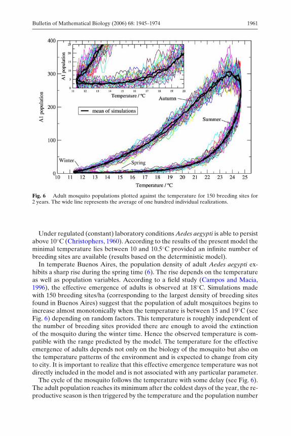
Fig. 6 Adult mosquito populations plotted against the temperature for 150 breeding sites for2 years. The wide line represents the average of one hundred individual realizations.

Under regulated (constant) laboratory conditions Aedes aegypti is able to persistabove 10◦C (Christophers, 1960). According to the results of the present model theminimal temperature lies between 10 and 10.5◦C provided an infinite number ofbreeding sites are available (results based on the deterministic model).

In temperate Buenos Aires, the population density of adult Aedes aegypti ex-hibits a sharp rise during the spring time (6). The rise depends on the temperatureas well as population variables. According to a field study (Campos and Macia,1996), the effective emergence of adults is observed at 18◦C. Simulations madewith 150 breeding sites/ha (corresponding to the largest density of breeding sitesfound in Buenos Aires) suggest that the population of adult mosquitoes begins toincrease almost monotonically when the temperature is between 15 and 19◦C (seeFig. 6) depending on random factors. This temperature is roughly independent ofthe number of breeding sites provided there are enough to avoid the extinctionof the mosquito during the winter time. Hence the observed temperature is com-patible with the range predicted by the model. The temperature for the effectiveemergence of adults depends not only on the biology of the mosquito but also onthe temperature patterns of the environment and is expected to change from cityto city. It is important to realize that this effective emergence temperature was notdirectly included in the model and is not associated with any particular parameter.

The cycle of the mosquito follows the temperature with some delay (see Fig. 6).The adult population reaches its minimum after the coldest days of the year, the re-productive season is then triggered by the temperature and the population number


reaches a maximum (controlled by the carrying capacity of the environment) afterthe hottest days of the year.

7. Extinction/survival thresholds

What is the world wide potential habitat for Aedes aegypti? What percentage ofbreeding sites has to be destroyed to eradicate the mosquito from a given city?These two questions might appear, in a first inspection, unrelated but we will showthey are closely related.

Christophers considered the first question (Christophers, 1960). Given the factthat Aedes aegypti cannot proliferate (develop) under laboratory experiments attemperatures below 10◦C, it was then argued that, if mosquitoes were to survivethe winter in larval or adult form, the 10◦C winter (July in the South or Januaryin the North) isotherm would then give an idea of their potential habitat. Noticethat with the temperature profile adopted in Eq. (10) the average July temperatureresults from averaging the temperature profile during the 31 days of the month ofJuly, resulting in TJuly = a − b 0.98732, hence Christopher’s criterion is representedby a = 10◦C + b 0.98732 (Christophers’ criterion is illustrated in Fig. 8 -straightline-).

A serious problem with Christophers’ criterion is that the hypothesis of larvaor adult winter survival does not hold. Mosquitoes can survive the winter in theegg form as it is verified in Buenos Aires (Schuster, 1984). Christophers realizedthat there were abundant exceptions to his criterion, he mentioned in particularthe case of Bahıa Blanca (South America) as well as records of the presence of themosquito at several cities on the East coast of North America (the northernmostone being Boston) as well as many other cities around the world.

The importance and relevance of egg winter survival was advanced beforeChristophers’ criterion by Carter (1931) where the occurrence of Aedes aegyptiin ports is discussed in the following terms:

If breeding places were available and the temperature on landing highenough for the full functional activity of the insects, a colony could beestablished and would be permanent or not, according to the wintertemperature of the locality, and the colony would last until the species(eggs) were destroyed by the cold, which might be the first winter; or, inborder-line places, the species might live several years, to be destroyedeventually by some winter of unusual length or severity. Such seems tohave been the case in Philadelphia and possibly New York in the latterpart of the eighteenth century.

Carter’s survival criterion (based on egg winter survival) acknowledges not onlywinter temperature as a factor but also the duration of the winter. We will show inthis section that our simulations are fully compatible with Carter’s considerations.

If the potential habitat of the mosquito is going to be discussed, some additionalspecifications are needed. We will consider in this section the influence of thetemperature in terms of average yearly temperature and the seasonal amplitudeas presented in Eq. (10). We will also specify different environmental conditions


Fig. 7 Probability for the next year extinction as a function of average yearly temperature. Thethermal amplitude is 6.7◦C and the number of breeding sites is BS = 50. The probabilities wereestimated as the number of extinctions in 200 simulations.

represented by different values of the parameter BS. Additionally, we will see thatthe deterministic limit is achieved for unrealistically large numbers of breedingsites.

By a continuity argument, the transition between a region where the mosquitoescan live permanently and another region where they cannot live at all must be me-diated by a transition region where both the presence of the mosquito for severalyears and its extinction are likely to occur. The definition of this region has a cer-tain degree of arbitrariness. After all, the Markov process describing the problemhas the extinction state as an absorbing one.

We arbitrarily defined a region to be at the border of the potential habitat whenan already established population (i.e. a population that has survived at least oneyear in the habitat) has a survival probability for the next year of 1/2. A systemwith parameter values satisfying this condition will be said to be at threshold. InFig. 7 we show the dependence of the next year survival probability as a functionof average yearly temperature. The transition from 0.99 to 0.01 probability takesplace with an approximate change from 20.8 to 14.5◦C in the average temperaturefor a seasonal amplitude of 6.7◦C considering 50 breeding sites (see Fig. 7).

The threshold is then a hypersurface in parameter space, in our case a curverelating the values of the parameters a, b in Eq. (10) controlling the temperatureand the number of breeding sites assigned to the homogeneous region.

For infinitely many breeding sites available, the threshold corresponds to thelost of stability of the extinction solution in the deterministic model (1). The deter-ministic threshold begins at around 10.5◦C when there are no seasonal variationsand is lower for higher seasonal variations (see Fig. 8).


Fig. 8 Threshold parameters for the Aedes aegypti populations in the parameter space (meantemperature, thermal amplitude), i.e. parameters (a, b) of Eq. (10). The points correspond to es-timations using the stochastic model for several different carrying capacities of the environment.Dotted lines are a guide for the eye relating points corresponding to the same number of breedingsites. The straight line corresponds to Christophers’ criterion, while the curved line correspondsto unlimited resources (deterministic model).

Infinitely many available breeding sites are, clearly, unrealistic. We tentativelyestimated the extinction thresholds for a homogeneous place having a number ofbreeding sites between the highest (BS = 150) and the lowest number of breedingsites (BS = 15) found in a (100 m)2 patch in field studies at Buenos Aires. Alsodisplayed in Fig. 8 are calculations performed for unrealistically large number ofbreeding sites for illustrative purposes.

The parameter α0 in Eq. (5) was fitted to reproduce the number of larvaeper breeding site found during the most favourable week of the year (in termsof number of larvae) in field studies performed at Buenos Aires cemeteries(Vezzani et al., 2004) and was given the value α0 = 1.5. Since α0 is the only ad-justable parameter of the model, we produced simulations with various choices ofα0 under the conditions corresponding to cemeteries in Buenos Aires, adjustingthe α0 value to match the average number of larvae per breeding site during thesummer week with the largest number of larvae. This value is only a rough esti-mation, and it is not worth refining the value of this parameter considering theaccuracy of the available data. Each container was considered to have an averageof half a litre of water producing an estimated 14 larvae per litre (7 larvae per half


litre breeding site), a number that is relevant only when considering egg hatchinginhibition.

The results of the simulations are displayed in Fig. 8 (dots). Notice that thestochastic thresholds show an average temperature higher than in the determin-istic case as one would have expected, but also, that an increase in the thermalamplitude (seasonal variation) renders the settlement of Aedes aegypti more dif-ficult. Figure 8 also shows the temperature values corresponding to Buenos Airescity in the period 1960–1991 (squares), a period of time that includes the end ofthe eradication program as well as the years of the reinfestation. It is interestingto notice that with the highest values for BS the populations can survive even inisolation, however, with the lower values local extinctions are expected, hence em-phasising the roles as reservoirs of places with high density of breeding sites.

There are different aspects of Fig. 8 worth mentioning. On the mathematicalside, the slow convergence of the stochastic results towards the deterministic curveis noticeable. As many as 106 breeding sites are needed to get close to it, a numbersharply contrasting the estimation of no more than 150 breeding sites within a(100 m)2 patch.

On the biological side it is interesting to notice that, for relatively high seasonalthermal amplitude, the effects of the favourable weather are less relevant than theeffects of the not favourable weather, i.e. higher average yearly temperatures arerequired for higher amplitudes. Actually, the population is regulated in spring–summer by the environment and its carrying capacity. Even when the weather ismore favourable, the mosquito populations cannot increase because of the satura-tion of the breeding sites. Hence, egg populations at the beginning of the winterare expected to be roughly independent of the high temperatures of the summer.

The mosquito spends parts of the winter in the egg stage suffering a daily mor-tality of eggs, which is roughly independent of the temperature. It is then the du-ration of the unfavourable period that makes a difference for the survival of themosquito population. Hence, the mortality increases with the thermal amplitude(for the same average temperature). The lines of equal unfavourable (winter) timeare straight lines with positive slopes in Fig. 8 (not shown) and this is the apparentform that the threshold curves take for large amplitudes.

The biology encoded in the model is then fully compatible with the qualitativediscussion given in Carter (1931).

According to the present results, a map of South America with the cities likely tosupport domestic populations of Aedes aegypti can roughly be based on the 15◦Cisotherm (yearly average), see Figure 9. This criterion corresponds to the aver-age yearly temperature of the threshold with seasonal amplitudes and maximumnumber of breeding sites as those found in Buenos Aires.

Of the 661 towns and cities of Argentina with present or historical records ofAedes aegypti populations, we have displayed on the map of average yearly tem-peratures those lying below the July 10◦C isotherm (data extracted from Moraleset al. (2004)). Notice that the 15◦C average yearly temperature isotherm gives areasonable idea of the habitat limits for Aedes Aegypti.


Fig. 9 Average temperature (yearly) in South America. Dark grey for regions with average tem-perature above 25◦C, grey for temperatures between 20 and 25◦C, light grey for temperaturesbetween 15 and 20◦C and white for temperatures lower than 10◦C. The dots represent towns andcities of Argentina below the 10◦C July isotherm where the mosquito has been detected. Theblack contour line represents the 15◦C average yearly isotherm.

7.1. Egg hatching inhibition

The effects of egg hatching inhibition by high larvae density on the threshold areminimal in this study. We repeated the threshold calculations changing the criti-cal density (7) from 10 to 70 larvae per litre. The resulting threshold values are


Fig. 10 Differences in egg and larva populations for the two extreme values of the egg hatchinginhibition effect, simulated for 50 breeding sites. The shoulders in the population data are anartifact of the step function (7) used to simulate the effect in the absence of better experimentaldata determining the function.

almost identical, with the threshold slightly lower in mean temperature for thelower critical density. This result was in part expected since egg-hatching inhibi-tion by larvae will produce a higher reserve of eggs for the winter period and then,a larger probability of surviving the unfavourable season. However, in the environ-mental conditions considered, the effect is only evident in the peak of the breedingseason and most of the produced eggs will not reach the larva stage (see Fig. 10).

7.2. Extinction probabilities as a function of initial conditions

As another example of the information that the model can provide, we studiedthe changes in the probability of extinction during the first year as a function ofthe number of eggs remaining in the winter. The study is motivated by a possiblestrategy against the mosquito that consists of removing as many eggs as possible inthe winter time, thereby trying to drive the population into extinction.

We considered the case of 150BS in Buenos Aires climate and produced ex-tinction statistics based on 1000 runs for each initial condition. All runs began thecoldest day of the year with a population consisting only of eggs.

The results of the simulations are presented in Fig. 11. Two solid lines havebeen drawn in the plot. The first one connects the results for initial number ofeggs below 100 and is a straight line in the logarithmic scale of the plot. It clearly


Fig. 11 The extinction probability after one year of evolution as a function of the initial condi-tion. The population at the beginning of the runs was in the form of eggs. The probabilities ofextinctions are computed as the number of runs that produced total extinction in 1000 runs. Thenumber of breeding sites is BS = 150.

represents the fate of small numbers of eggs and is accounted for the probabilityof one egg (or its biological evolution) to die. The processes are independentwhen the population is small (where “small” is relative to the carrying capacityof the patch) and hence, the exponential dependence with the number of eggsfollows from statistical independence (Pext = ((0.9926 ± 0.03%)eggs) are the fittedvalues).

However, for initial conditions larger than 100 eggs, the extinction probabilityfollows a law of the form: 5.81(eggs)0.49±0.04 (the uncertainty corresponds to thestandard deviation of the fitted coefficient). The point corresponding to 100 eggsis at border of the region with this dependence and far from the exponential de-pendence.

It is interesting to notice that the probability of extinction decreases more slowlywhen there are interactions than in the independent case. A result that can beattributed to the fact that the only interaction among individuals corresponds toan increase of mortality in the larval stage.

The number of eggs estimated on July 1st for BS = 150 and temperatures cor-responding to Buenos Aires for an established population of mosquitoes is ap-proximately 1000 according to our numeric simulations. Hence, nine of every teneggs should be removed to achieve an extinction probability of 0.6. Furthermore,to achieve a probability of 0.8 less than 30 eggs should remain, this is, half theaverage number of eggs laid by a female, requiring a very efficient eradicationcampaign.


8. Summary and conclusions

We have developed a stochastic model for Aedes aegypti populations based on thelife cycle of the mosquito. The number of eggs, larvae, pupae, young female adultsand female adults after the first oviposition are the five stages of the mosquito lifeincluded in the description.

The evolution of the subpopulations is considered in terms of ten random eventswith transition probabilities prescribed in terms of the biology of Aedes aegypti andthe environment.

The model is able to deal with extinction processes and is ready for extensions tospatially heterogeneous environments and as such is particularly appropriated tostudy the potential evolution of Aedes aegypti populations in temperate climates.

The construction of the model has led us to a critical revision of the availabledata and modelling of the different biological events and several opportunities forimprovements have been detected (see Section 5).

The model is based on realistic parameter values and we have shown that it isable to produce results that correspond well with field data not used as input forthe model.

Based on our results we have discussed the temperature and environmental con-ditions that are needed for the survival of a local population of Aedes aegypti. Suchdata are critical for the design of eradication campaigns as well as for the evalua-tion of the effects of global weather changes in the distribution of the mosquito.The results indicate that average yearly temperature, seasonal temperature varia-tion and numbers of breeding sites are relevant parameters required to evaluatethe potential of a city to host a local population of Aedes aegypti.

The criterion introduced tentatively by Christophers resulting in a distributionlimit based on the 10◦C winter (July in the South, January in the North) isothermwas discussed concluding that the most relevant effect for temperate climatesemerge from the number of breeding sites available for reproduction and the du-ration of the winter, rather than winter temperatures. The model fully supports anearlier criterion proposed by Carter (1931) through the critical observation thatAedes aegypti can survive the winter in egg form.

The stochastic nature of the model allows for the maintenance of Aedes aegyptipopulations for a (random) number of years until extinction eventually occurs.A situation already envisioned by Carter as the likely case for the populations inPhiladelphia and New York by the end of the eighteenth century. Such a possibilitycontrasts with the conjecture that Aedes aegypti populations in ports were linked tosummer infestations by mosquitoes landing from the boats that could not survivethe first winter (Ministerio de Asistencia Social y Salud Publica, 1964).

The model also shows an important dependency of thresholds with the environ-ment represented by the breeding site parameter. This feature explains the obser-vations made during the eradication campaign in Argentina (Ministerio de Asis-tencia Social y Salud Publica, 1964) where the environment (where the mosquitothrived) changes from North to South following the general rule that the colderthe site the higher the concentration of breeding sites required for finding Aedesaegypti.


While the stochastic model has a deterministic limit in terms of large population(as large as needed) we have shown numerically that such populations are severalorders of magnitude larger than realistic homogeneous populations.

The criterion for the persistence of Aedes aegypti populations, discussed in thiswork, depends on the average yearly temperature, the seasonal variation and thecarrying capacity of the environment. These data will change from city to city. Con-sidering the maximum carrying capacity found at Buenos Aires cemeteries and theseasonal temperature amplitudes characteristic of Buenos Aires, the threshold forthe persistence of the mosquito was roughly estimated to be the 15◦C isotherm(average yearly temperature). This rough criterion is the result of a number ofcompromises with the data readily available. Temperature choices are then 10,15 and 20◦C; carrying capacity represented by breeding sites and thermal ampli-tude corresponding to estimated values for Buenos Aires. Historical records of thepresence of Aedes aegypti in Argentina below the 10◦C July isotherm are consis-tent with this criterion, these latter records are also affected by uncertainties: werethey just summer infestations or did the population persist, detected or undetected,at least one year? Infestations depend not only on favourable conditions but alsoon the probability of the mosquito reaching the city.

The introduced criterion helps to understand, and potentially explains, whyAedes aegypti has not been found in the Atlantic region below Buenos Aires (be-tween approximately 38.5◦S to 38.0◦S on the Atlantic coast) in coincidence witha region with average yearly temperatures below 15◦C but has been historicallyreported in Bahıa Blanca (average yearly temperature 15.4◦C) just south of thisregion on the Atlantic coast.2

Finally, the fact that a large part of Buenos Aires city presents a density of breed-ing sites that cannot support populations of Aedes aegypti is in concordance withfield results that suggest that repopulation processes are taking place every yearduring the warm season. The dynamics of such re-population processes in hetero-geneous habitats requires the explicit inclusion of the space in the model as well asthe biological and environmental data associated with the dispersal of mosquitoes.

A. Appendix: The Poisson approximation

We shall briefly describe in this appendix the main ideas involved in the Poissonapproximation for a density-dependent Markov process.

Let X be an integer vector having as entries the populations under considera-tion, and eα, α = 1, . . . , κ the events at which the populations change by a fixedamount �α in a Poisson process with density-dependent rates. Then, a theorem byKurtz (1986) allows us to rewrite the stochastic process as:

X(t) = X(0) +κ∑

α=1

�αY(∫ t

0(ωα(X(s)))

)ds (A.1)

2The climate in Bahıa Blanca is greatly affected by the large amplitude of the ocean tides and thevery shallow estuary that extends from Bahıa Blanca to the north for a few hundred kilometres(Perillo and Piccolo, 2004).


where ωα(X(s)) is the transition rate associated with the event α and Y(x) is arandom Poisson process of rate x.

This expression is the starting point for several approximations. In particular, thedeterministic limit is obtained for transition rates of the form ωα(X) = N�α(X/N)(a relation known as the mass-action law) and considering the stochastic variableX/N in the limit N → ∞ for fixed t (Kurtz, 1970) (in this approximation only themean values of the Poisson variables are relevant).

The deviations from the deterministic limit scaled by a factor 1/√

N correspondin the same limit to a Brownian process (Andersson and Britton, 2000; Kurtz, 1971)(in this case, the Poisson variables are approximated by Gaussian variables).

The Poisson approximation to the stochastic process represented by Eq. (A.1)consists in introducing a self-consistent deterministic approximation for the argu-ments of the Poisson variables Y(x) in Eq. (A.1) (Aparicio and Solari, 2001; Solariand Natiello, 2003b). The rationale under such a proposal is that the transitionrates change at a slower rate than the populations. The number of each kind ofevent is then approximated as independent Poisson processes with deterministicarguments satisfying a differential equation.

The probability of nα events of type α having occurred after a time dt is approx-imated by a Poisson distribution with parameter λα . Hence, the probability of thepopulation taking the value

X = X0 +κ∑

α=1

�αnα (A.2)

at a time interval dt after being in the state X0 is approximated by a product ofindependent Poisson distributions of the form

Probability(n1, . . . , nκ , dt/X0) =κ∏

α=1

P(λα) (A.3)

Finally,

dλα/dt = 〈ωα(X)〉 (A.4)

where the averages are taken (self-consistently) with the proposed distribution(λα(0) = 0). Actually, there are some small (O(dt2)) corrections to this presenta-tion when one of the populations is one event away from extinction (Solari andNatiello, 2003b). Such correction has not been implemented in the present casebecause the extinction processes are very slow.

From the Poisson approximation it is possible to recover the deterministic equa-tion and the Brownian approximation of the fluctuations in the proper limit. Theapproximation is accurate not only in the N → ∞ (with fixed t) limit, but also inthe infinitesimal time limit when the average number of events is small. It is thislatter property what makes it specially suitable for the study of a process involvingextinction.


The use of the Poisson approximation represents a substantial saving of com-puter time compared to direct (Monte Carlo) implementations of the stochasticprocess.

The details of the particular implementation for the population dynamics of theAedes aegypti are tedious. The computer code, written in C, can be requested fromthe corresponding author.

B. Stability analysis of the trivial solution

We refresh stability theory in this appendix, further details can be read in Hill(1877), Wiggins (1988), and Solari et al. (1996).

The deterministic model (1) presents coefficients that depend periodically ontime through the temperature, Eq. (10). The phase space of the problem isthen (R+)5S1 with R+ the non-negative real numbers and S1 the one dimen-sional circle corresponding to the time of the year. The trivial solution is then(L, P, A1, A2, H, t) = (0, 0, 0, 0, 0, t).

Small perturbations of the trivial solution will evolve according to the linearEq. (11). Notice that the fate of a perturbation, for example the introduction ofa few adults, will not only depend on the type of the perturbation but also thetime of the year in which it was produced, since it is not the same to introducethe adults under unfavourable winter conditions as during the favourable summertime. If the perturbation performed at t0 is x0 its time evolution is x(t) = M(t, t0)x0.The evolution up to a time t + s consists in further integrating the problem by atime s with initial condition x(t), hence M(t + s, t0) = M(t + s, t)M(t, t0) which isnothing but the semi-group property for the flow.

The long time evolution of a perturbation of the trivial state, say after a time t −t0 = kyears + s, with k integer, will be given by M(t, t0) = M(s + t0, t0)M(1 year +t0, t0)k where we have used that M(t + n year, n year + t0) = M(t, t0) for n integer.

Hence, any perturbation will have the trivial solution as time-infinite limit ifall of the eigenvalues of M(1 year + t0, t0) are smaller than one in absolute value(asymptotic stability). Further notice that the eigenvalues of M(1 year + t0, t0) areexactly the same than those for M(1 year, 0) since both matrices are conjugated byM(t0, 0)

M(1 year + t0, t0)M(t0, 0) = M(t0, 0)M(1 year, 0) = M(1 year + t0, 0)

meaning that the stability does not depend of the time of the year chosen as t0.

Acknowledgments

The authors thank Daniel Barrera and Pablo Orellano for providing importantinformation. We thank Mario Natiello and Joan Aron for carefully reading themanuscript. The authors acknowledge support by the University of Buenos Airesunder grant X308 and by the Agencia Nacional de Promocin Cientıfica y Tec-nologica (Argentina) under grant PICTR 87/2002.


References

Andersson, H., Britton, T., 2000. Stochastic epidemic models and their statistical analysis. Volume151 of Lecture Notes in Statistics. Springer-Verlag, Berlin.

Aparicio, J.P., Solari, H.G., 2001. Population dynamics: A poissonian approximation and its rela-tion to the langevin process. Phys. Rev. Lett. 86, 4183–4186.

Arrivillaga, J., Barrera, R., 2004. Food as a limiting factor for aedes aegypti in water-storage con-tainers. J. Vector Ecol. 29, 11–20.

Bar-Zeev, M., 1957. The effect of density on the larvae of a mosquito and its influence on fecun-dity. Bull. Res. Council Israel 6B, 220–228.

Bar-Zeev, M., 1958. The effect of temperature on the growth rate and survival of the immaturestages of aedes aegypti. Bull. Entomol. Res. 49, 157–163.

Campos, R.E., Macia, A., 1996. Observaciones biologicas de una poblacion natural de aedes ae-gypti (diptera: culicidae) en la provincia de buenos aires, argentina. Rev. Soc. Entomol. Ar-gent. 55(1–4), 67–72.

Carbajo, A.E., Schweigmann, N., Curto, S.I., de Garın, A., Bejaran, R., 2001. Dengue transmissionrisk maps of argentina. Trop. Med. Int. Health 6(3), 170–183.

Carter, H.R., 1931. Yellow Fever: An Epidemiological and Historical Study of Its Place of Origin.The Williams & Wilkins Company, Baltimore.

Christophers, R., 1960. Aedes aegypti (L.), The Yellow Fever Mosquito. Cambridge Univ. Press.,Cambridge.

de Garın, A.B., Bejaran, R.A., Carbajo, A.E., de Casas, S.C., Schweigmann, N.J., 2000. Atmo-spheric control of aedes aegypti populations in buenos aires (argentina) and its variability.Int. J. Biometerol. 44, 148–156.

Depinay, J.-M.O., Mbogo, C.M., Killeen, G., Knols, B., Beier, J., Carlson, J., Dushoff, J., Billings-ley, P., Mwambi, H., Githure, J., Toure, A.M., McKenzie, F.E., 2004. A simulation model ofafrican anopheles ecology and population dynamics for the analysis of malaria transmision.Malaria J. 3(29), 1–21.

Domınguez, C., Almeida, F.F.L., Almiron, W., 2000. Dinamica poblacional de aedes aegypti(diptera: Culicidae) en cordoba capital. Revista de la Sociedad Entomologica de Argentina59, 41–50.

Dye, C., 1982. Intraspecific competition amongst larval aedes aegypti: Food exploitation or chem-ical interference. Ecol. Entomol. 7, 39–46.

Ethier, S.N., Kurtz, T.G., 1986. Markov Processes. John Wiley and Sons, New York.Fay, R.W., 1964. The biology and bionomics of aedes aegypti in the laboratory. Mosq. News. 24,

300–308.Focks, D.A., Haile, D.C., Daniels, E., Moun, G.A., 1993a. Dynamics life table model for aedes

aegypti: Analysis of the literature and model development. J. Med. Entomol. 30, 1003–1018.Focks, D.A., Haile, D.C., Daniels, E., Mount, G.A., 1993b. Dynamic life table model for aedes

aegypti: Simulations results. J. Med. Entomol. 30, 1019–1029.FUNCEI, 1998. Dengue enfermedad emergente. Fundacion de estudios infectologicos 1(1), 1–6,

http://www.funcei.org.ar.FUNCEI, 1999a. Dengue enfermedad emergente. Fundacion de estudios infectologicos 2(2), 1–8,

http://www.funcei.org.ar.FUNCEI, 1999b. Dengue enfermedad emergente. Fundacion de estudios infectologicos 2(1), 1–

12, http://www.funcei.org.ar.Gleiser, R.M., Urrutia, J., Gorla, D.E., 2000. Effects of crowding on populations of aedes albi-

fasciatus larvae under laboratory conditions. Entomologia Experimentalis et Applicata 95,135–140.

Hill, G.W., 1877. On the part of motion of the lunar perigee which is function of the mean motionsof the sun and moon. Acta Math. 8, 1.

Horsfall, W.R., 1955. Mosquitoes: Their Bionomics and Relation to Disease. Ronald, New York,USA.

Kiraly, A., Janosi, I. M., 2002. Stochastic modelling of daily temperature fluctuations. Phys. Rev.E 65, 051102.

Kurtz, T.G., 1970. Solutions of ordinary differential equations as limits of pure jump markov pro-cesses. J. Appl. Prob. 7, 49–58.

Kurtz, T.G., 1971. Limit theorems for sequences of jump processes approximating ordinary dif-ferential equations. J. Appl. Prob. 8, 344–356.


Legates, D.R., Willmott, C.J., 1990. Mean seasonal and spatial variability in global surface airtemperature. Theor. Appl. Climatology 41, 11–21.

Livdahl, T.P., Koenekoop, R.K., Futterweit, S.G., 1984. The complex hatching response of aedeseggs to larval density. Ecol. Entomol. 9, 437–442.

Ministerio de Asistencia Social y Salud Publica, A., 1964. Campana de erradicacion del Aedesaegypti en la Repblica Argentina. Informe final. Buenos Aires.

Morales, M.A., Monteros, M., Fabbri, C.M., Garay, M.E., Introini, V., Ubeid, M.C., Baroni, P.G.,Rodriguez, C., Ranaivoarisoa, M.I., Lanfri, M., Scavuzzo, M., Gentile, A., Zaidemberg, M.,Ripoll, C. M., Fernandez, H., Blanco, S., Enria, D.A., 2004. Riesgo de aparicin de denguehemorragico en la argentina. In: II Congreso Internacional Dengue y Fiebre Amarilla. LaHabana, Cuba, http://www.cidfa2004.sld.cu.

Nayar, J.K., Sauerman, D.M., 1975. The effects of nutrition on survival and fecundity in floridamosquitoes. part 3. utilization of bood and sugar for fecundity. J. Med. Entomol. 12, 220–225.

Perillo, G.M.E., Piccolo, M.C., 2004. que es el estuario de bahıa blanca? Ciencia Hoy 14(81), 8–15,on line at http://www.ciencia-hoy.retina.ar.

Powell, J.A., Jenkis, J.L., 2000. Seasonal temperature alone can synchronize life cycles. Bull. Math.Biol. 62, 977–998.

Rueda, L.M., Patel, K.J., Axtell, R.C., Stinner, R.E., 1990. Temperature-dependent developmentand survival rates of culex quinquefasciatus and aedes aegypti (diptera: Culicidae). J. Med.Entomol. 27, 892–898.

Schoofield, R.M., Sharpe, P.J.H., Magnuson, C.E., 1981. Non-linear regression of biologicaltemperature-dependent rate models based on absolute reaction-rate theory. J. Theor. Biol.88, 719–731.

Schuster, H.G., 1984. Deterministic Chaos. Physik Verlag, Weinheim.Schweigmann, N., Boffi, R., 1998. Aedes aegypti y aedes albopictus: Situacion entomologica en

la region. In: Temas de Zoonosis y Enfermedades Emergentes, Segundo Cong. Argent. deZoonosis y Primer Cong. Argent. y Lationoamer. de Enf. Emerg. y Asociacion Argentina deZoonosis. Buenos Aires, pp. 259–263.

Sharpe, P.J.H., DeMichele, D.W., 1977. Reaction kinetics of poikilotherm development. J. Theor.Biol. 64, 649–670.

Solari, H., Natiello, M., Mindlin, B., 1996. Nonlinear Dynamics: A Two-way Trip from Physics toMath. Institute of Physics, Bristol.

Solari, H., Natiello, M., 2003a. Poisson approximation to density dependent stochastic processes:A numerical implementation and test. In: Khrennikov, A. (Ed.), Mathematical Modellingin Physics, Engineering and Cognitive Sciences. Proceedings of the Workshop DynamicalSystems from Number Theory to Probability–2, vol. 6.Vaxjo University Press, Vaxjo, pp.79–94.

Solari, H.G., Natiello, M.A., 2003b. Stochastic population dynamics: the poisson approximation.Phys. Rev. E 67, 031918.

Southwood, T.R.E., Murdie, G., Yasuno, M., Tonn, R.J., Reader, P.M., 1972. Studies on the lifebudget of aedes aegypti in wat samphaya bangkok thailand. Bull. W.H.O. 46, 211–226.

Subra, R., Mouchet, J., 1984. The regulation of preimaginal populations of aedes aegypti (l.)(diptera: Culicidae) on the kenya coast. ii. food as a main regulatory fa ctor. Ann. Trop.Med. Parasitol. 78, 63–70.

Trpis, M., 1972. Dry season survival of aedes aegypti eggs in various breeding sites in the darsalaam area, tanzania. Bull. WHO 47, 433–437.

Vezzani, C., Velazquez, S.T., Schweigmann, N., 2004. Seasonal pattern of abundance of aedesaegypti (diptera: Culicidae) in buenos aires city, argentina. Memor Inst Oswaldo Cruz 99,351–356.

WHO, 1998. Dengue Hemorrhagic Fever. Diagnosis, Treatment, Prevention and Control. WorldHealth Organization, Ginebra, Suiza.

Wiggins, S., 1988. Global Bifurcations and Chaos. No. 73. Applied Mathematical Science.Wiggins, S., 1990. Introduction to Applied Nonlinear Dynamical Systems and Chaos. Springer,

New York.

A Stochastic Population Dynamics Model for Aedes Aegypti : Formulation and Application to a City...

Documents

Transcript of A Stochastic Population Dynamics Model for Aedes Aegypti : Formulation and Application to a City...