arX

iv:0

810.

2788

v1 [

astr

o-ph

] 1

5 O

ct 2

008

Received 2008 July 15; Accepted 2008 October 10Preprint typeset using LATEX style emulateapj v. 03/07/07

A STEEP FAINT-END SLOPE OF THE UV LUMINOSITY FUNCTION AT Z ∼ 2 − 3: IMPLICATIONS FORTHE GLOBAL STELLAR MASS DENSITY AND STAR FORMATION IN LOW MASS HALOS1

Naveen A. Reddy2,3 & Charles C. Steidel4

Received 2008 July 15; Accepted 2008 October 10

ABSTRACT

We use the deep ground-based optical photometry of the Lyman Break Galaxy (LBG) Survey toderive robust measurements of the faint-end slope (α) of the UV luminosity function (LF) at redshifts1.9 ≤ z ≤ 3.4. Our sample includes > 2000 spectroscopic redshifts and ≈ 31000 LBGs in 31 spatially-independent fields over a total area of 3261 arcmin2. These data allow us to select galaxies to 0.07L∗

and 0.10L∗ at z ∼ 2 and z ∼ 3, respectively. A maximum-likelihood analysis indicates steep values ofα(z = 2) = −1.73± 0.07 and α(z = 3) = −1.73 ± 0.13. This result is robust to luminosity-dependentsystematics in the Lyα equivalent width and reddening distributions, is similar to the steep valuesadvocated at z & 4, and implies that ≈ 93% of the unobscured UV luminosity density at z ∼ 2 − 3arises from sub-L∗ galaxies. With a realistic luminosity-dependent reddening distribution, faint tomoderately luminous galaxies account for & 70% and & 25% of the bolometric luminosity density andpresent-day stellar mass density, respectively, when integrated over 1.9 ≤ z < 3.4. We find a factor of8 − 9 increase in the star formation rate density between z ∼ 6 and z ∼ 2, due to both a brighteningof L∗ and an increasing dust correction proceeding to lower redshifts. Combining the UV LF withstellar mass estimates suggests a relatively steep low mass slope of the stellar mass function at highredshift. The previously observed discrepancy between the integral of the star formation history andstellar mass density measurements at z ∼ 2 may be reconciled by invoking a luminosity-dependentreddening correction to the star formation history combined with an accounting for the stellar masscontributed by UV-faint galaxies. The steep and relatively constant faint-end slope of the UV LF atz & 2 contrasts with the shallower slope inferred locally, suggesting that the evolution in the faint-endslope may be dictated simply by the availability of low mass halos capable of supporting star formationat z . 2.

Subject headings: galaxies: evolution — galaxies: formation — galaxies: high redshift — galaxies:luminosity function

1. INTRODUCTION

The last decade has seen significant advances in our un-derstanding of the history of star formation and stellarmass assembly. Today, one can find several hundred de-terminations of the star formation rate density (SFRD)estimated from observations at many wavelengths acrossa large range of lookback time. Taken together, these ob-servations suggest a rapid increase in the SFRD from theepoch of reionization to z ∼ 1 − 2, after which time theSFRD steadily decreased over the last ∼ 10 billion years.This picture is generally understood in the context of hi-erarchical buildup at early times and gas exhaustion orheating at late times. While this characterization of thestar formation history is broadly accepted, there are sev-eral key details that are missing from this interpretation,including the potentially important contribution of UV-faint (sub-L∗) galaxies to the census of star formationand baryon budget. If rest-UV/optical light is a biasedtracer of galaxy formation — particularly at high red-

1 Based, in part, on data obtained at the W.M. Keck Observa-tory, which is operated as a scientific partnership among the Cal-ifornia Institute of Technology, the University of California, andNASA, and was made possible by the generous financial supportof the W.M. Keck Foundation.

2 National Optical Astronomy Observatory, 950 N. Cherry Ave,Tucson, AZ 85719

3 Hubble Fellow.4 California Institute of Technology, MS 105–24, Pasadena, CA

91125

shift where most of the baryons in galaxies are likely toreside in cold gas (Prochaska & Tumlinson 2008) — thenfaint galaxies may constitute an important population forstudying the process of star formation and feedback. Fur-ther, the number density of both bright and faint galax-ies departs significantly from expectations based on theΛCDM model, suggesting a regulation of star formationin both luminosity regimes. In this paper, we presentan extension of our previous work on the UV luminosityfunction at z ∼ 2 − 3 in order to provide robust con-straints on the prevalence of UV-faint galaxies at epochswhen galaxies were forming most of their stars.

The luminosity function (LF) is a fundamental probeof galaxy formation and evolution, and can be used toaddress the relative importance of bright and faint galax-ies to the energy budget at a given epoch. Furthermore,comparison with the dark matter halo distribution in-forms us of the efficiency of star formation and effects offeedback at different mass scales (Rees & Ostriker 1977;Silk & Rees 1998; Dekel & Birnboim 2006). Therefore,constraining accurately the shape of the LF is a necessarystep in acquiring a more complete census of galaxies andelucidating the relationship between the baryonic pro-cesses that govern galaxy evolution and the dark matterhalos that host them.

The UV LF is relevant in several respects. Rest-frame UV emission is a direct tracer of massive starformation, modulo the effects of dust. Rest-frame UVobservations of high redshift galaxies are generally not

2 Reddy & Steidel

limited by spatial resolution and the deepest observa-tions are up to a factor of ≈ 2000 times more sensi-tive than those in the infrared and longer wavelengths.The combination of resolution, sensitivity, and the ac-cessibility of UV wavelengths over almost the entire ageof the Universe makes the UV LF a unique tool in as-sessing the star formation history. The relative effi-ciency of UV-dropout selection has enabled a numberof investigations of the UV LF at high redshifts basedon photometrically-selected samples (Steidel et al. 1999;Adelberger & Steidel 2000; Yan & Windhorst 2004;Bunker et al. 2004; Dickinson et al. 2004; Bouwens et al.2007; Sawicki & Thompson 2006; Reddy et al. 2008;Ouchi et al. 2004; Beckwith et al. 2006; Yoshida et al.2006; Iwata et al. 2007).

Apart from the uncertainties that can be constrainedfrom photometry alone, such as photometric errors andfield-to-field variations, spectroscopy is a critical meansof quantifying several important systematics that can af-fect the LF. These include contamination from low red-shift objects and high redshift AGN/QSOs, attenuationof UV emission due to the opacity of the intergalacticmedium (IGM), and perturbation of galaxy colors due toLyα, reddening, and stellar population ages of galaxies.The relevance of these systematic effects is underscoredby the fact that while there are numerous studies of theUV LF, the results have been inconsistent, both at low(z . 3; e.g., Reddy et al. 2008; Le Fevre et al. 2005) andat high (z & 4; e.g., Beckwith et al. 2006; Bouwens et al.2007) redshifts.

Unfortunately, spectroscopic surveys have been limitedto UV-bright (R . 25.5) galaxies at relatively low red-shifts (z . 4) and spectroscopic constraints on the num-ber density of faint sources at z & 2 are still lacking.Deeper spectroscopy is expensive and will remain so un-til the next generation of large (& 10 m) ground-basedtelescopes come online. Given the present practical lim-itations and the complexity of systematics involved incomputing LFs, it seems prudent to revisit and extendour initial estimate of the UV LF (Reddy et al. 2008,hereafter R08) by evaluating the impact of these system-atics on the inferred number density of faint galaxies atz ∼ 2 − 3. We go beyond the initial analysis of R08by quantifying several important effects relevant in thecomputation of star formation rate and stellar mass den-sities, including the effects of luminosity-dependent dustcorrections and the integrated stellar mass of low massgalaxies.

To this end, we combine what we know about the spec-troscopic properties of LBGs at z ∼ 2 − 3 with deepground-based optical data in 31 spatially independentfields to determine the faint-end slope with greater preci-sion. A brief description of the LBG survey, photometry,and followup spectroscopy is given in § 2. Our methodfor computing the UV LF is presented in § 3, and re-sults are discussed in § 4. Our results are compared withthose in the literature and analyzed in the context of theearly Hubble Deep Field (HDF) results, and we assessthe impact of sample variance in § 5. The evolution ofthe UV LF is quantified in § 6. The contribution to thefaint-end population from dusty, star-forming galaxiesas well as quiescently-evolving galaxies with large stel-lar masses is discussed in § 7. § 8 and 9 present con-straints on the star formation rate density (SFRD) and

its evolution. We also reassess the stellar mass densityat z ∼ 2 and compare it to inferences from integrat-ing the star formation history. Finally, the evolution ofthe faint-end slope of the UV LF is discussed briefly in§ 10. All magnitudes are expressed in AB units, un-less stated otherwise. Unless indicated, a Kroupa (2001)IMF is assumed. A flat ΛCDM cosmology is assumedwith H0 = 70 km s−1 Mpc−1, ΩΛ = 0.7, and Ωm = 0.3.

2. DATA: SAMPLE SELECTION AND SPECTROSCOPY

2.1. Fields and Photometry

The Lyman Break Galaxy (LBG) survey is be-ing conducted in fields chosen primarily for hav-ing relatively bright background QSOs with which tostudy the interface between the IGM and galaxiesat z ∼ 2 − 3 (Adelberger et al. 2003, 2004, 2005b;Steidel et al. 2003, 2004). Additionally, the survey wasextended to include fields that are the focus of multi-wavelength campaigns, including the Groth-Westphal(Steidel et al. 2003; Groth et al. 1994) and GOODS-North fields (Dickinson et al. 2003; Giavalisco et al.2004b). Presently, the survey includes 31 fields, 29 ofwhich have been targeted spectroscopically (see R08 forfurther details). As emphasized throughout this paper,the large number of spatially independent fields providesa precise handle on the magnitude of sample variance,an effect that has limited the conclusions that couldbe drawn from previous determinations of the LF. Forthis analysis, we have included two additional fields be-yond the 29 that were presented in R08, “Q1603” and“Q2240”. Instruments used and dates of observation arepresented in Steidel et al. (2003, 2004). For ease of refer-ence, the fields are listed in Table 1; together they includean area of 3261 arcmin2, or 0.91 square degrees.

Excepting Q1603, a modified version of FOCAS(Valdes 1982) was used to extract photometry from theoptical (UnGR) images of the survey fields. Source Ex-tractor (Bertin & Arnouts 1996) was used for photom-etry in Q1603. We took care to minimize systematicsbetween the FOCAS and Source Extractor results forQ1603 from an examination of the color distribution ofrecovered LBG candidates. Object detection was done atR band, and G−R and Un−G colors were computed byapplying the isophotal aperture from the R band imageto the Un and G images. Further details on the photome-try are discussed in Steidel et al. (2003) and Steidel et al.(2004). The images have a 5 σ depth of 27.5 − 29.5 ABas measured through a ∼ 3′′ diameter aperture.

2.2. Color Selection

We used the BX and LBG criteria which are basedon the rest-frame UV colors expected of galaxies at red-shifts 1.9 . z . 2.7 and 2.7 . z . 3.4, respectively(Steidel et al. 2004, 2003). For spectroscopic followup,the sample of candidates was limited to R = 25.5. How-ever, because we are interested in using the entire pho-tometric sample to constrain the LF at 1.9 . z . 3.4,we did not impose this restriction. Rather, the detectionsignificance and color distribution of candidates were ex-amined to establish a faint limit. The limits applied toeach field and numbers of candidates are listed in Table 1.Fields with the deepest imaging in the survey allow usto select candidates to R ∼ 26.5 with a detection com-pleteness of ≈ 60%, based on the simulations described

A Steep Faint-End Slope at z ∼ 2 − 3 3

TABLE 1Survey Fields

αa δb Field SizeField Name (J2000.0) (J2000.0) (arcmin2) Rlim NBX

c NLBGd

Q0000 00 03 25 -26 03 37 18.9 25.5 78 29CDFa 00 53 23 12 33 46 78.4 26.0 490 192CDFb 00 53 42 12 25 11 82.4 25.5 347 123Q0100 01 03 11 13 16 18 42.9 26.5 579 230Q0142 01 45 17 -09 45 09 40.1 26.0 379 158Q0201 02 03 47 11 34 22 75.7 26.0 289 114Q0256 02 59 05 00 11 07 72.2 25.5 325 105Q0302 03 04 23 -00 14 32 244.9 25.5 2113 1025Q0449 04 52 14 -16 40 12 32.1 26.5 287 138B20902 09 05 31 34 08 02 41.8 25.5 229 72Q0933 09 33 36 28 45 35 82.9 26.0 723 313Q1009 10 11 54 29 41 34 38.3 26.5 512 305Q1217 12 19 31 49 40 50 35.3 26.0 311 83GOODS-N 12 36 51 62 13 14 155.3 26.0 496 154Q1307 13 07 45 29 12 51 258.7 26.0 2011 718Westphal 14 17 43 52 28 49 226.9 25.5 783 289Q1422 14 24 37 22 53 50 113.0 26.0 1041 5183C324 15 49 50 21 28 48 44.1 25.5 187 56Q1549 15 51 52 19 11 03 37.3 26.0 329 153Q1603 16 04 56 38 12 09 38.8 26.5 396 160Q1623 16 25 45 26 47 23 290.0 26.0 1878 735Q1700 17 01 01 64 11 58 235.3 26.0 2263 609Q2206 22 08 53 -19 44 10 40.5 26.0 257 70SSA22a 22 17 34 00 15 04 77.7 25.5 274 183SSA22b 22 17 34 00 06 22 77.6 26.0 435 217Q2233 22 36 09 13 56 22 85.6 26.0 420 173DSF2237b 22 39 34 11 51 39 81.7 26.5 1004 474Q2240 22 40 02 03 17 50 35.9 26.0 421 176DSF2237a 22 40 08 11 52 41 83.4 26.5 553 183Q2343 23 46 05 12 49 12 212.8 25.5 1209 436Q2346 23 48 23 00 27 15 280.3 26.0 1547 472

TOTAL ... ... 3260.8 ... 22166 8663

a Right ascension in hours, minutes, and seconds.b Declination in degrees, arcminutes, and arcseconds.c Number of BX candidates to the limiting magnitude given in column (5).d Number of LBG candidates to the limiting magnitude given in column (5).

below. Our maximum-likelihood method for computingthe LF allows us to extend the absolute magnitude limit≈ 0.5 mag fainter given the broadness of the redshiftdistribution, N(z), of the sample as constrained fromextensive spectroscopic followup. Even at these depths,galaxies are detected with typically & 5 σ significancein the R-band. The photometric sample used here in-cludes BX candidates in the original LBG survey fieldswhere no spectroscopic followup of BX candidates wasundertaken.

2.3. Spectroscopy

The spectroscopy of UV-selected candidates includ-ing LBGs and BXs is discussed in Steidel et al. (2003,2004). To date, roughly 24% and 35% of BX and LBGcandidates, respectively, with R < 25.5 have been tar-geted spectroscopically. The resulting sample includes2023 star-forming galaxies with 1.9 ≤ zspec < 3.4, thelargest spectroscopic sample of star-forming galaxies atthese redshifts. The spectroscopic statistics, includingthe number of spectroscopic redshifts, for each field ofthe LBG survey are given in R08.

The spectroscopic sample is used to estimate the over-all contamination rate in the photometric sample. Thiscontamination can arise from stars, low redshift galaxiesand AGN, as well as QSOs and AGN at 1.9 ≤ z < 3.4.The contamination statistics and the extent to which

they can be applied to determine the number of contam-inants in the photometric sample are discussed in R08.Note that the contamination rate is a strong functionof magnitude (being largest at bright magnitudes) andquantifying it is a crucial step in computing the bright-end of the LF.

3. INCOMPLETENESS CORRECTIONS

3.1. Method

The approach that we adopted to correct the LBGsample for incompleteness and compute the UV LF isdescribed in detail by R08. For convenience, here wesummarize a few of the key features of our method. Theprimary goal is to construct a set of transformations thatrelate the observed properties of galaxies (e.g., observedluminosity, rest-frame UV slope, and redshift) to theirtrue properties (e.g., intrinsic luminosity, reddening, andredshift). Using X-ray and mid-IR data for a sample ofLBGs at z ∼ 2 − 3, Reddy et al. (2006b) demonstratethat the rest-frame UV slope can be used to measure theamount of dust reddening for typical LBGs, and we willassume this for the subsequent discussion.

We first used a Monte Carlo simulation to add galax-ies of varying sizes and colors to our UnGR images.The distribution of colors reflects that expected for star-forming galaxies at z ∼ 2−3 with constant star formationfor > 100 Myr and varying amounts of dust reddening.

4 Reddy & Steidel

Specifically, we added objects with redshifts 1 < z < 4and reddening of 0.0 < E(B − V ) < 0.6. The simulatedredshift is used to apply an IGM opacity to the colorsusing the Madau (1995) prescription. To make the sim-ulation as realistic as possible, we forced the simulatedgalaxies to abide by a Schechter (1976) luminosity dis-tribution and added just 100 − 200 of them at a timeto the images. The latter restriction maintains the de-blending statistics which in turn affect the photometricerrors. Photometry was performed in the same man-ner as was used on the real data and the detection rateand recovered magnitudes and colors of the simulatedgalaxies were recorded. We repeated this procedure un-til ≈ 2 × 105 galaxies were added to the images in eachfield of the survey.

It is common to use such simulations to determine whatfraction of galaxies with a given magnitude will be de-tected with colors that satisfy the LBG selection crite-ria. However, strictly speaking, the simulation will onlytell us the probability that galaxies with a given simu-lated magnitude will be detected with a given recoveredmagnitude, and there may not be a monotonic corre-spondence between simulated and recovered magnitude.More generally, it is not necessarily true that the av-erage simulated properties of galaxies are equivalent totheir average observed properties. This is particularlytrue if photometric errors have significant biases and arecomparable to the bin sizes used to compute the LF andthe selection window spans a region of color space notmuch larger than the typical photometric errors. Othersystematic effects, such as the Lyα equivalent width dis-tribution (WLyα) of the population, may scatter galaxiesin certain directions of color space. Also, some galax-ies with simulated colors that do not initially satisfy thecolor criteria may have recovered colors that do: by def-inition, these galaxies’ simulated properties will not, onaverage, reflect their observed properties. Because ofthese systematic effects, the number of galaxies that liein a particular bin of observed properties will be someweighted combination of the number of galaxies in anynumber of bins of simulated properties.

Because of these systematic effects, we approach theproblem of incompleteness by using the maximum like-lihood method described in R08. Using this formalism,our goal is to maximize the likelihood of a given set of lu-minosity, reddening, and redshift distributions, denotedby L, according to the following expression:

− lnL ∝∑ijk

nijk −∑ijk

nijk ln nijk, (1)

where nijk is the expected number of galaxies in theith bin of luminosity, jth bin of reddening, and kth binof redshift that the values of the luminosity, reddening,and redshift distributions imply and nijk is the observednumber of galaxies in that bin. The Monte Carlo sim-ulations give the probability that a galaxy in the i′j′k′

bin of simulated properties will lie in the ijk bin of re-covered properties. The set of probabilities, defined asthe transitional probability function,

ξ ≡ pi′,j′,k′→ijk, (2)

is used to compute nijk. The basic procedure is to thenvary the input distributions of luminosity, reddening, and

Fig. 1.— Intrinsic rest-frame Lyα equivalent width (WLyα) dis-tribution for R ≤ 25.5 star-forming galaxies at 1.9 ≤ z < 2.7and 2.7 ≤ z < 3.4, from R08. Lyα in emission is represented asWLyα > 0. Error bars are determined from simulations and reflectthe variance in the distributions allowed by the errors in the UVLF and reddening distribution (see R08 for discussion).

redshift until the differences between the expected andobserved numbers of galaxies in each ijk bin are mini-mized.

3.2. Lyα Equivalent Width (WLyα) Distribution

An important systematic effect to consider is the scat-tering of colors due to the presence of Lyα emission andabsorption: the Lyα line falls within the Un and G bandsat redshifts that are targeted with the BX and LBG cri-teria, the same bands that are used to select the galaxies.Rather than adding the WLyα distribution as another freeparameter in the maximum-likelihood analysis — thuscomplicating our ability to determine the LF — we per-formed simulations where we made various assumptionsregarding the intrinsic WLyα distribution at z ∼ 2−3 andobserved the effects on the best-fit LF (R08). We did thisby adding a random WLyα drawn from a distribution ofWLyα to each galaxy, and then recomputing the colors ofeach galaxy. Effectively, the addition of Lyα will perturbthe colors and thus modulate the transitional probabilityfunction, ξ. R08 showed that the BX and LBG color cri-teria did little to alter the intrinsic WLyα distribution atz ∼ 2 and z ∼ 3. Therefore, we assume the WLyα distri-bution observed for BXs and LBGs (Figure 1). Here, werepeat the simulations of R08, but also allow for changesin the shape of the WLyα distribution proceeding fromUV-bright to UV-faint galaxies (see Appendix).

4. RESULTS: THE UV LF AT 1.9 ≤ Z < 3.4

4.1. Computation of the LF and Errors

The value of the luminosity distribution that maxi-mizes the likelihood of observing our data (Eq. 1) is com-puted using the method discussed in the previous sec-tion. Initially, we assumed that the intrinsic distributionof (1) rest-frame UV slopes, (2) redshifts, and (3) WLyα

remain constant as a function of apparent magnitude.In R08, we justified these assumptions when computingthe LF to our spectroscopic limit of R = 25.5. How-ever, it is not unreasonable to suspect that, for example,

A Steep Faint-End Slope at z ∼ 2 − 3 5

the reddening and WLyα distributions of galaxies fainterthan our spectroscopic limit may be different than thosefor galaxies where we are able to directly measure thedistributions with spectroscopy (“spectroscopic distribu-tions”). Such differences will change ξ and thus affect ourincompleteness corrections. First, we first made the sim-plified assumptions that all of these distributions remainunchanged as a function of apparent magnitude. LFs de-rived in this case are referred to as the “fiducial” LFs.In the appendix, we discuss how the LF would changeif we adopt more realistic assumptions for the propertiesof UV-faint galaxies. In our analysis, the effect of in-creasing photometric error for fainter galaxies is alreadyincorporated in the calculation of ξ.

LFs were computed separately for star-forming galax-ies in the redshift ranges 1.9 ≤ z < 2.7 and 2.7 ≤ z < 3.4using the photometric BX and LBG samples, respec-tively. For the lower redshift range, the LF is computedin terms of a (composite) absolute magnitude that is theaverage of the G and R-band fluxes. For the higher red-shift range, the LF is computed using the R-band mag-nitude. This method provides the closest match betweenrest-frame wavelengths, roughly 1700 A.

The total error in the LF is computed using the follow-ing method. The observed number counts of galaxies ineach field were adjusted randomly in accordance with aPoisson distribution and the maximum-likelihood LF wascomputed for each field. This procedure was repeatedmany times for all the fields. The dispersion in the LFvalues for each bin in absolute magnitude is taken as thetotal error which, as a consequence of the way in whichit is computed, includes both Poisson and field-to-fieldvariations.

4.2. Summary of Systematic Effects and Final Results

The details of the systematic tests performed to judgethe effects of luminosity-dependent WLyα and reddeningdistributions on the LF are presented in the Appendix.To summarize, we analyzed the influence of galaxies with(1) strong Lyα emission and (2) zero or declining redden-ing with apparent UV magnitude. Employing currentestimates of the mean stellar population, reddening, andnumber density of galaxies with strong Lyα emission as afunction of UV luminosity at high redshifts, we find thatthe inferred number density of galaxies on the faint-endof the UV LF increases by . 3% at 1.9 ≤ z < 2.7 and de-creases by . 4% at 2.7 ≤ z < 3.4. Because these changesare not negligible compared to the Poisson and field-to-field errors on the faint-end number densities, theyshould be included in any proper assessment of the LF.Nonetheless, these changes in number density can be ac-commodated by Schechter parameterizations that varywithin the uncertainties of the individual parameters, α,M∗, and φ∗.

We have also examined how changes in the mean red-dening of galaxies as function of UV luminosity affectsour measurement of the UV LF. We considered two sce-narios, one in which the extinction drops to zero forgalaxies fainter than R = 25.5 and one in which theextinction decreases monotonically with UV luminosity,and approaches zero in the faintest luminosity bin con-sidered here. The latter scenario is more realistic thanthe former, and is parameterized as a linear relation be-tween E(B − V ) and magnitude (see the appendix; we

TABLE 2Rest-Frame UV Luminosity Functions of 1.9 . z . 3.4 Galaxies

φRedshift Range MAB(1700A) (×10−3 h3

0.7 Mpc−3 mag−1)

1.9 ≤ z < 2.7 −22.83 — −22.33 0.004 ± 0.003−22.33 — −21.83 0.035 ± 0.007−21.83 — −21.33 0.142 ± 0.016−21.33 — −20.83 0.341 ± 0.058−20.83 — −20.33 1.246 ± 0.083−20.33 — −19.83 2.030 ± 0.196−19.83 — −19.33 3.583 ± 0.319−19.33 — −18.83 7.171 ± 0.552−18.83 — −18.33 8.188 ± 0.777−18.33 — −17.83 12.62 ± 1.778

2.7 ≤ z < 3.4 −23.02 — −22.52 0.003 ± 0.001−22.52 — −22.02 0.030 ± 0.013−22.02 — −21.52 0.085 ± 0.032−21.52 — −21.02 0.240 ± 0.104−21.02 — −20.52 0.686 ± 0.249−20.52 — −20.02 1.530 ± 0.273−20.02 — −19.52 2.934 ± 0.333−19.52 — −19.02 4.296 ± 0.432−19.02 — −18.52 5.536 ± 0.601

TABLE 3Best-fit Schechter Parameters for UV LFs of 1.9 . z . 3.4

Galaxies

Redshift Range α M∗AB(1700A) φ∗ (×10−3 Mpc−3)

1.9 ≤ z < 2.7 −1.73 ± 0.07 −20.70 ± 0.11 2.75 ± 0.542.7 ≤ z < 3.4 −1.73 ± 0.13 −20.97 ± 0.14 1.71 ± 0.53

refer to this latter scenario as the “luminosity-dependentreddening model”). In this case, we find appreciableincreases of ≈ 10% in the inferred number density be-tween 1.9 ≤ z < 2.7. In the higher redshift range2.7 ≤ z < 3.4, there is little change in the inferred num-ber densities. Our final determinations of the LF andthe corresponding Schechter fits are shown by the datapoints and solid lines, respectively, in Figure 2, with thevalues and Schechter parameterization listed in Tables 2and 3.

Our determinations of the bright-end of the UV LFsto M(1700A) = −18.83 and −19.52 at z ∼ 2 and z ∼ 3,respectively, incorporate data over 3261 arcmin2 in 31independent fields. Data from 22 fields and 2239 arcmin2

are used to constrain the LFs at −18.83 ≤ M(1700A) <−18.33 and −19.52 ≤ M(1700A) < −19.02 at z ∼ 2and z ∼ 3, respectively. Finally, data from 6 spatiallyindependent fields and 317 arcmin2 are used to constrainthe LF in the faintest magnitude bin to M(1700A) =−17.83 and −18.52 at z ∼ 2 and z ∼ 3, respectively. Toensure that spatial variance in these 6 deep fields are notdriving the observed faint-end slope, we recalculated αby fitting Schechter functions to the LFs excluding thefaintest bin. Allowing φ∗ and M∗ to vary, we calculateα = −1.75 ± 0.09 and −1.94 ± 0.18 at z ∼ 2 and z ∼ 3,respectively, still significantly steeper than the shallowerα > −1.6 found in previous studies. The similarity in αobtained with or without data from the faintest bin is notsurprising given that the uncertainty in the LF includesthe sample variance from the 6 fields used to constrain

6 Reddy & Steidel

-2 -1.5-21.5

-21

-20.5

-20

Fig. 2.— Rest-frame UV luminosity functions of star-forming galaxies at 1.9 ≤ z < 2.7 (circles) and 2.7 ≤ z < 3.4 (squares), along withthe best-fit Schechter (1976) functions. The 68% and 95% likelihood contours between M∗ and α for our final determinations of the LFsare shown in the inset panel.

the number density in this bin.The degeneracy between the faint-end slope (α) and

characteristic magnitude (M∗) — illustrated by the like-lihood contours in Figure 2 (inset) — is reduced signifi-cantly compared to that computed in R08. Our analysisextends to luminosities that are 4 times fainter than thelimit dictated by efficient spectroscopy, and ≈ 14 and 10times fainter, respectively, than the characteristic lumi-nosity L∗ at z ∼ 2 and 3. Our sample is large enough sothat the error in the LF at all magnitudes is dominatedby field-to-field variations (Figure 3). Within the totalerrors, the UV LFs at z ∼ 2 and z ∼ 3 are virtually in-distinguishable, indicating little change between the twoin the number density of both UV-bright and UV-faintgalaxies.

5. DISCUSSION: LARGE-SCALE CONTEXT

In the following sections, we discuss our results inthe context of previous determinations of the UV LF(§ 5.1) and its evolution with redshift (§ 6). To gainfurther insight into the nature of sub-L∗ galaxies, we as-sess the contribution to the faint-end population fromdusty, star-forming galaxies and those with large stel-lar masses (§ 7). In § 8, we discuss the implications ofa luminosity-dependent reddening distribution and the

Fig. 3.— Poisson (dashed line) and total (solid line) error in theUV LF at z ∼ 2. The Poisson error increases to fainter magnitudesgiven the smaller survey area used to constrain the faint-end. Atall magnitudes, however, the error in the LF is dominated by field-to-field variations. Similar results are obtained for the z ∼ 3 UVLF.

average corrections required to recover the bolometric

A Steep Faint-End Slope at z ∼ 2 − 3 7

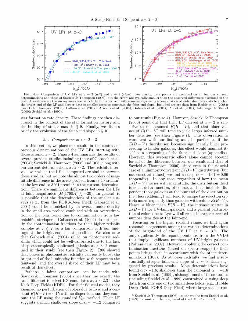
Fig. 4.— Comparison of UV LFs at z ∼ 2 (left) and z ∼ 3 (right). For clarity, data points are excluded on all but our currentdeterminations and those of Sawicki & Thompson (2006), but the errors are typically smaller than the observed differences discussed in thetext. Also shown are the survey areas over which the LF is derived, with some surveys using a combination of wider shallower data to anchorthe bright-end of the LF and deeper data in smaller areas to constrain the faint-end slope. Included are are data from Reddy et al. (2008);Sawicki & Thompson (2006); Paltani et al. (2007); Arnouts et al. (2005); Gabasch et al. (2004); Poli et al. (2001); Adelberger & Steidel(2000); Steidel et al. (1999).

star formation rate density. These findings are then dis-cussed in the context of the star formation history andthe buildup of stellar mass in § 9. Finally, we discussbriefly the evolution of the faint-end slope in § 10.

5.1. Comparisons at z ∼ 2 − 3

In this section, we place our results in the context ofprevious determinations of the UV LFs, starting withthose around z ∼ 2. Figure 4 summarizes the results ofseveral previous studies including those of Gabasch et al.(2004); Sawicki & Thompson (2006) and R08, along withour current determination, at z ∼ 2. The redshift inter-vals over which the LF is computed are similar betweenthese studies, but we note the almost two orders of mag-nitude difference in the areas probed, from ≈ 40 arcmin2

at the low end to 3261 arcmin2 in the current determina-tion. There are significant differences between the LFsat faint magnitudes (M(1700A) & −20). In general, itis possible that the determinations of the smaller sur-veys (e.g., from the FORS-Deep Field; Gabasch et al.2004) could be mimicked by an overall under-densityin the small area probed combined with an overestima-tion of the bright-end due to contamination from lowredshift interlopers. Gabasch et al. (2004) do not spec-ify the contamination fractions for their higher redshiftsamples at z & 2, so a fair comparison with our find-ings at the bright-end is not possible. We also notethat Gabasch et al. (2004) relied on photometric red-shifts which could not be well-calibrated due to the lackof spectroscopically-confirmed galaxies at z ∼ 2 exam-ined in their study (see their Figure 2). R08 showedthat biases in photometric redshifts can easily boost thebright-end of the luminosity function with respect to thefaint-end, and the overall shape of their LF may be aresult of this effect.

Perhaps a fairer comparison can be made withSawicki & Thompson (2006) since they use exactly thesame filter set to select BX candidates at z ∼ 2.3 in theKeck Deep Fields (KDFs). For their fiducial model, theyassumed no perturbation of colors due to Lyα and a con-stant E(B−V ) = 0.15 with no dispersion, and they com-pute the LF using the standard Veff method. Their LFsuggests a much shallower slope of α ∼ −1.2 compared

to our result (Figure 4). However, Sawicki & Thompson(2006) point out that their LF derived at z ∼ 2 is sen-sitive to the assumed E(B − V ), and that bluer val-ues of E(B − V ) will tend to yield larger inferred num-ber densities (see their Figure 7). This observation isconsistent with our finding and, in particular, if theE(B − V ) distribution becomes significantly bluer pro-ceeding to fainter galaxies, this effect would manifest it-self as a steepening of the faint-end slope (appendix).However, this systematic effect alone cannot accountfor all of the difference between our result and that ofSawicki & Thompson (2006), since even in the fiducialcase of a luminosity-invariant E(B−V ) distribution (butnot constant-valued) we find a steep α = −1.67 ± 0.06(appendix). In any case, regardless of how the meanE(B − V ) varies with magnitude, the distribution itselfis not a delta function, of course, and has intrinsic dis-persion; those galaxies at the blue end of the distribution(i.e., less reddening) will tend to escape the selection cri-teria more frequently than galaxies with redder E(B−V ).Hence, a bluer mean E(B − V ), the intrinsic scatter inE(B −V ) for UV-faint galaxies, and a general perturba-tion of colors due to Lyα will all result in larger correctednumber densities at the faint-end.

Focusing on the higher redshift range, we find againreasonable agreement among the various determinationsof the bright-end of the UV LF at z ∼ 3.5 Theonly significantly discrepant points are from the VVDSthat imply significant numbers of UV-bright galaxies(Paltani et al. 2007). However, applying the correct con-tamination fractions (based on spectroscopy) to theirpoints brings them in accordance with the other deter-minations (R08). As at lower redshifts, we find a sub-stantially steeper faint-end slope at z ∼ 3 than sug-gested by previous results. Most determinations havefound α > −1.6, shallower than the canonical α = −1.6from Steidel et al. (1999), although most of these studies(including Steidel et al. 1999) constrained α using deepdata from only one or two small deep fields (e.g., HubbleDeep Field, FORS Deep Field) where large-scale struc-

5 Sawicki & Thompson (2006) use the results from Steidel et al.(1999) to constrain the bright-end of the UV LF at z ∼ 3.

8 Reddy & Steidel

ture may be an issue. Sawicki & Thompson (2006) findα = −1.43+0.17

−0.09 based on the Keck Deep Field data over

an area of 169 arcmin2.

5.2. Differences in LF Computation

What could be the reason for the disparity in thefaint-end number densities between our study and pre-vious determinations? Without a more detailed com-parative analysis incorporating the data used in theseother studies, it is difficult to pinpoint a single causefor the discrepancy. There are, however, a number ofdifferences between our analysis and others that maylead to the observed variance in α. Our analysis (1)uses over 2000 spectroscopic redshifts to evaluate andcorrect for contamination as a function of luminosity;(2) models the systematic effects of a luminosity depen-dence in the intrinsic Lyα equivalent width and redden-ing distribution of galaxies, likely to be the two domi-nant sources of systematic error in the LF; (3) employsa maximum-likelihood method that is more robust thanthe Veff method against biases in photometry and othernon-uniform sources of scatter; and (4) takes advantageof data in 31 spatially uncorrelated fields over a total areaof close to a square degree. Even at the faint-end, ourdeterminations are based on 6 independent fields with atotal area of 317 arcmin2, a roughly 88% larger area thanused in the previous faint-end determination at z ∼ 2−3(but see next section). For all of these reasons, we believeour LFs to be the most robust determinations to date.

The differences in faint-end slope derived betweenstudies with similar depth is not particularly significantwithin the marginalized errors on α. For example, theα = −1.43+0.17

−0.09 of Sawicki & Thompson (2006) is stillconsistent within the 1 σ (marginalized) error of our de-termination of α = −1.73 ± 0.13 at z ∼ 3. Yet, thedifference in the actual number density of faint galax-ies is significant at the 2 − 3 σ level. This emphasizeswhy comparisons between α derived in different stud-ies should perhaps not be taken too seriously withoutplacing them in the context of the errors on the actualnumber density of UV-faint galaxies.

5.3. Cosmic Variance

In spite of the care used in the present sample, even317 arcmin2 is a relatively small area over which to con-strain α. As noted above, the uncertainties in the LF aredominated by field-to-field variance at all magnitudes.We can assess how the empirically-constrained errors onthe UV LF compare to expectations based on the cor-relation function. Following the procedure outlined byTrenti & Stiavelli (2008), we can estimate the combineduncertainty due to cosmic variance and Poisson statis-tics by integrating the two point correlation function fordark matter halos with some average galaxy bias. Thebasic premise is that the spatial correlation function ofhalos gives information on the variance in the spatial dis-tribution of galaxies along different lines of sight givenvarious assumptions for the cosmology and halo fillingfactor. For this calculation, we assumed a number den-sity of objects as implied by the maximum-likelihood LFat z ∼ 2 and a sample “completeness” fraction of 0.47.This number is the ratio of star-forming galaxies thatsatisfy the color selection criteria to the total number of

star-forming galaxies as determined from the LF (see R08for a discussion of this fraction). The cosmology is set asfollows: Ωλ = 0.74, Ωm = 0.26, Ho = 70 km s−1 Mpc−1,a spectral index ns = 1, and σ8 = 0.9 (Spergel et al.2007). We must also make some assumption for thehalo filling factor. Star-forming galaxies are scatteredout of the LBG selection window due to primarily ran-dom processes such as photometric scatter (Reddy et al.2005), and must therefore cluster in the same way asgalaxies that do satisfy the LBG criteria (Conroy et al.2008). Further, the comoving number density of LBGsis similar to the number density of halos that have simi-lar clustering strength, suggesting a halo filling factor of≈ 1 (Conroy et al. 2008). Assuming this remains validfor UV-faint galaxies, we find a fractional error in num-ber counts of ≈ 9% over a survey area of 317 arcmin2.In general, we would expect this calculation to yield alower limit to the uncertainty since other effects (e.g.,uncertainties in zeropoints and systematics in the colordistributions from field to field) contribute to the errorin the LF, and indeed our empirically-derived error inthe faintest bin of the z ∼ 2 UV LF is ≈ 50% largerthan the value obtained from the two point correlationfunction. For comparison, this calculation implies thatthe field-to-field variance is ≈ 17% lower than what wewould have obtained over the area probed by the KDFsof 169 arcmin2 (Sawicki & Thompson 2006). This dif-ference is not large enough to explain the apparent dis-crepancy at the faint-end, and some of the systematicsdiscussed above are also likely to play a role. Deep UVimaging over areas of close to a square degree (similarto that used to estimate the bright-end of the LF) willbe required to constrain the fractional error in numbercounts to . 5%.

5.4. Hubble Deep Field (HDF)

A comparison between the present work and thoseof the early HDF-based studies of the UV LF is use-ful, particularly in light of the often-used argumentthat the HDF presents a biased view of the Uni-verse, and one that is invoked to explain the diver-gent results on the UV LF at z ∼ 3 (Steidel et al.1999; Dickinson et al. 2003; Giavalisco et al. 2004a;Gabasch et al. 2004; Sawicki & Thompson 2006). Thebright-end of the LFs computed here and by Steidel et al.(1999) are in excellent agreement. Within the 1 σmarginalized errors, the faint-end slope derived at z ∼ 3agrees with the slope found by Steidel et al. (1999) andAdelberger & Steidel (2000), and there is essentially nosignificant difference in φ∗ and M∗. However, given thewidespread use of the Steidel et al. (1999) results, it isimportant to note that their determination of α — con-strained from a U -dropout sample in the HDF — doesnot take into account incompleteness from photometricscatter. As discussed in § 3, the effect of such scatteris to make the incompleteness corrections larger at thefaint-end, thus steepening the faint-end slope. In sum-mary, contrary to the suggestion that the HDF containedan over-density of faint galaxies relative to bright oneswhen compared with other fields, our results imply thatthe HDF is reasonably representative of the z ∼ 2 − 3universe.

6. DISCUSSION: EVOLUTION OF THE UV LF

A Steep Faint-End Slope at z ∼ 2 − 3 9

Fig. 5.— (Left) Evolution of the UV LFs from z ∼ 7 to z ∼ 2. For clarity and consistency, we show only LFs at z & 4 from Bouwens et al.(2007, 2008) since they are calculated using a maximum-likelihood technique similar to the one used here. For comparison, the local UVLF from Wyder et al. (2005) is also shown. (Right) Evolution of the characteristic UV luminosity or magnitude, M∗, with redshift. Pointsare from Wyder et al. (2005) at z ∼ 0 (open triangle), Arnouts et al. (2005) at 0 . z . 3.0 (filled triangles), Bouwens et al. (2008) at z & 4(squares), and our determinations at z ∼ 2 − 3 (circles).

Fig. 6.— (Left) dN/dz as a function of redshift, assuming our determinations of the UV LF at z ∼ 2 − 3 and those of (Bouwens et al.2007) at z & 4, integrated to 0.1L∗

z=3 (blue) and 0.1L∗z (red). The shaded regions indicate approximately the uncertainty based on the

errors in the Schechter parameters. (Right) Total dL/dz as a function of redshift (green) and dL/dz brighter and fainter than 0.1L∗z=3 (red

and blue, respectively).

Figure 5 summarizes our UV LFs at z ∼ 2 − 3along with higher redshift determinations. For clar-ity and consistency, we included the findings fromBouwens et al. (2007) only since those authors use amaximum-likelihood method for determining the LF thatis similar to the method we use. These authors providea detailed comparison of UV LFs at z & 4 from differentstudies.

6.1. Evolution in M∗

Despite the large number of investigations at z & 4,there is still a fair amount of uncertainty regarding theparameterization of the evolution in the UV LF. Somehave claimed that the evolution occurs primarily in L∗

(Bouwens et al. 2007), while others find an evolutionin φ∗ (Beckwith et al. 2006) or the faint-end slope α(Iwata et al. 2007). Some have also suggested an evo-lution in both L∗ and φ∗ (e.g., Dickinson et al. 2004;Giavalisco et al. 2004a) such that the total luminositydensity could remain constant from z ∼ 3−6. Of course,the reach of some of these conclusions is limited by thedepth of data used to derive the LF. Because the LFsat z & 2 shown in Figure 5 are derived using data ofcomparable depth and analyzed in a similar manner —

although we note that our LFs at z ∼ 2−3 are anchoredby spectroscopy and photometry in an area roughly anorder of magnitude larger than used at z & 4 — here-after we will assume that the evolution of the LF atz & 4 can be accommodated by a change in L∗ as ad-vocated by Bouwens et al. (2007). Given the observedfading of galaxies at z . 2 (e.g., Dickinson et al. 2003;Madau et al. 1996; Lilly et al. 1995, 1996; Steidel et al.1999), it is useful to examine our results in the context ofthis evolution in L∗ (Figure 5). In particular, we find thatL∗ is brightest at z ∼ 2−3, with this average unobscuredUV luminosity decreasing at z & 4 (earlier cosmic time)and decreasing by a factor of ≈ 16 between z ∼ 2 andthe present-day. Quantitatively, Bouwens et al. (2008)found a linear parameterization between M∗ and z atz & 4 that appears to follow that generally expected forthe growth of the halo mass function — assuming an evo-lution in the mass-to-light ratio for halos of ∼ (1+z)−1 —given standard assumptions for the matter power spec-trum, indicating that hierarchical assembly of halos maybe dominating the evolution in M∗, or equivalently L∗.In the context of this study, the linear parameterizationcan be ruled out at the 8 σ level at z = 2.3 (in thesense that it would predict a significantly larger L∗ at

10 Reddy & Steidel

Fig. 7.— Faint-end slope α as a function of redshift. At z & 2, weinclude our results (filled circles), that of Steidel et al. (1999) (opencircle), and those of Bouwens et al. (2007) (squares). At lower red-shifts, we included only points in the Ryan et al. (2007) compila-tion that were derived from the rest-UV LF and that relied ondata extending at least two magnitudes fainter than M∗, includingresults from Budavari et al. (2005) and Wyder et al. (2005) (tri-angles). Also shown are points from Sawicki & Thompson (2006),Iwata et al. (2003) (errors in α are not provided by these authors;crosses), and Yan & Windhorst (2004) (range of likely α indicatedby hashed box). The dashed line marks the mean value of αfound at z & 2 from our study and that of Bouwens et al. (2007)(〈α〉 ∼ −1.73).

z = 2.3 than is observed), indicating that by these red-shifts, some other effect(s) modulate L∗ away from thevalue expected from pure hierarchical assembly.

These observations are illustrated more clearly by ex-amining dN/dz as a function of redshift (Figure 6), whichis extrapolated based upon linearly fitting the relation-ship between L∗ and z and φ∗ and z, and assuming afixed α = −1.73 as indicated by the Schechter fits (Ta-ble 3). Integrating the number counts to a fixed luminos-ity shows that bright galaxies with L > 0.1L∗

z=3 increasein number density by an order of magnitude with cosmictime from z ∼ 7 to z ∼ 2. Alternatively, the numbercounts are flatter at z & 4 when integrating to 0.1L∗(z)(i.e., L∗ appropriate at the redshift z where dN/dz iscalculated) suggesting that φ∗ is relatively constant atthese redshifts (e.g., Bouwens et al. 2007). There maybe a slight increase in φ∗ between z ∼ 2 − 3, though themagnitude of the errors on φ∗ are large enough that wecannot rule out non-evolution in the number density.

Also shown is dL/dz, both above and below a fixedluminosity, in this case 0.1L∗

z=3, along with the total lu-minosity density. The evolution implied by our LFs sug-gests that the approximately order of magnitude increasein luminosity density between z ∼ 7 and z ∼ 4 is followedby a flattening between z ∼ 2 − 3. This result itself ishardly surprising (see Giavalisco et al. 2004a, R08), butits significance is constrained robustly given that our LFsare determined over two orders of magnitude in luminos-ity. We will return to a discussion of these findings inthe context of the cosmic star formation history (§ 8).

6.2. Evolution in α

Perhaps the most striking result of our analysis — andone that is possible to address with confidence given thedepth of data considered here — is a very steep faint-end slope of α ∼ −1.73 at z ∼ 2− 3 that is robust to theluminosity-dependent systematics discussed in the Ap-pendix. The α we derive at z = 2.30 is virtually identicalto that derived at z = 3.05, and is remarkably similar to

the steep faint-end slopes favored at z & 4 (Figure 7).Given the rapid evolution in L∗ and the luminosity den-sity at z & 2, the invariance of α over the same ∼ 3 Gyrtimespan and the shallow α found locally (Wyder et al.2005; Budavari et al. 2005) pose interesting constraintson models of galaxy formation. We revisit this issue in§ 10.

7. DISCUSSION: NATURE OF GALAXIES ON THEFAINT-END OF THE UV LF

Before proceeding to discuss the implications of ourresults, it is useful to assess the contribution of galax-ies selected with different methods to the UV LF. R08demonstrate that the BX and LBG criteria to R = 25.5select the majority of galaxies on the bright-end of theUV LF, namely those with LUV & 0.1L∗. We show inthe appendix that these criteria recover the majority ofstar-forming galaxies fainter than 0.1L∗. The tests dis-cussed in the Appendix assume that the vast majorityof galaxies on the faint-end of the UV LF are relativelyunreddened, young galaxies. The aim of this section is toquantify the fraction of galaxies on the faint-end that are(1) UV-faint simply because they are heavily-reddened or(2) older galaxies that have passed their major phase ofstar formation. The latter investigation is relevant if weare to make inferences on the connection between thedark matter halo mass distribution and the luminosityfunction.

7.1. Bolometrically-Luminous Galaxies

Deep mid-to-far IR surveys have uncovered a siz-able population of dusty and infrared luminousgalaxies at z ∼ 2 − 3 (e.g., Yan et al. 2007;Caputi et al. 2007; Papovich et al. 2007; Reddy et al.2005; Chapman et al. 2005; van Dokkum et al. 2004;Smail et al. 1997; Barger et al. 1998). The first suchgalaxies were discovered via their submillimeter emis-sion (Smail et al. 1997; Barger et al. 1998; Hughes et al.1998), and are now commonly referred to as submillime-ter galaxies (SMGs). Chapman et al. (2005) estimatedthat ≈ 65% of such spectroscopically-confirmed brightSMGs (e.g., with S850µm & 5 mJy) at z ∼ 2 − 3 haverest-frame UV colors similar to those of BXs and LBGs,yet are on average a factor of ≈ 10 times more luminous.There is some uncertainty in the luminosities relatedboth to the conversion between mid and IR luminosi-ties to total bolometric luminosities and the fraction ofthe luminosity that arises from an AGN (Alexander et al.2005). Taking the far-IR estimates of the SFRs of SMGsat face value then suggests that SMGs are examples ofgalaxies whose UV slopes typically under-predict theirtotal attenuation and hence total bolometric luminosi-ties (Reddy et al. 2006b).

Measuring the frequency of such dusty galaxies amongUV-faint sources requires that we estimate the former’sspace density. Coppin et al. (2006) determine a surfacedensity of SMGs with S850µm > 5 mJy of 0.139 arcmin−2.The spectroscopic study of Chapman et al. (2005) foundthat 50% of bright SMGs lie at redshifts 1.9 ≤ z < 2.7,implying a space density at these redshifts of 2.63 ×10−5 Mpc−3. These authors also found 30−50% of themhave 25.5 < R < 28.0, corresponding to LUV . 0.34L∗

at the mean redshift of the BX sample (z = 2.30).According to our UV LF, the total number density of

A Steep Faint-End Slope at z ∼ 2 − 3 11

galaxies over this same apparent magnitude range is3.28 × 10−2 Mpc−3, implying that UV-faint SMGs withR > 25.5 constitute 0.02−0.04% of sources on the faint-end. Even in the most conservative case where we assumethat all SMGs with S850µm > 5 mJy lie at 1.9 ≤ z < 2.7and all have R > 25.5, we find a fractional contributionof only 0.16%. The results of Chapman et al. (2005) in-dicate that this SMG fraction would be even lower amongz > 2.7 galaxies, although we note that their adoptionof a radio-preselection may have biased the distributionof their sources to lower redshifts. We make note of thefact that the exact contribution will depend on the limitof what we consider to be “bright” SMGs, and extend-ing the limit to fainter submillimeter fluxes will undoubt-edly include galaxies that are less attenuated, on average,and more likely to be recovered via their UV colors (e.g.,Reddy et al. 2005; Adelberger & Steidel 2000). In anycase, the current best estimates for SMGs that are ob-served routinely in the first generation of submm surveysimply that by number they make a very small contribu-tion to the number density of sub-L∗ galaxies.

Reddy et al. (2006b) demonstrate that the vast major-ity of luminous infrared galaxies (LIRGs) at z & 2 willhave rest-frame UV colors that satisfy the BX/LBG cri-teria. While such criteria also pick up a non-negligiblenumber of ultraluminous infrared galaxies (ULIRGs),the best method of accounting for these galaxies is viatheir infrared emission. The launch of Spitzer enabledobservations that are sensitive to the warmer dust inhigh redshift starburst galaxies. Such galaxies are lu-minous in the infrared and appear to account for an in-creasing fraction of galaxies at z & 1 (e.g., Dey et al.2008; Caputi et al. 2007; Le Floc’h et al. 2005). Basedon such studies, there have been a few estimates ofthe number density of ultraluminous infrared galaxies atz ∼ 2 − 3. For instance, Caputi et al. (2007) find a den-sity of (1.5±0.2)×10−4 Mpc−3 for 24µm-selected galax-ies with Lbol & 1012 L⊙ (excluding AGN) in the GOODSfields. Similarly, 24µm-bright galaxies (f24µm ≥ 0.3 mJy)with red optical to mid-IR colors (R − [24] ≥ 14) havea space density in the redshift range 0.5 ≤ z ≤ 3.5 of(2.82 ± 0.05) × 10−5 Mpc−3 (Dey et al. 2008), almostall of which lie below L∗, the characteristic unobscuredUV luminosity. Assuming conservatively that all of theULIRGs of Caputi et al. (2007) are fainter than R = 25.5and as faint as R ∼ 28.0, we find a ULIRG fraction on theUV faint-end of 0.46%. In terms of the Dey et al. (2008)objects, assuming their space density does not evolve be-tween 0.5 ≤ z ≤ 3.5, this fraction is 0.086%. Hence,while such dusty, star-forming galaxies contribute signif-icantly to the total IR luminosity density, they must bevastly outnumbered by galaxies with fainter bolometricluminosities. This result is not surprising given the close-to-exponential drop-off in number counts of such infraredluminous galaxies according to the Schechter function,combined with the steep faint-end slope of the UV LF.

Taken another way, if we make the supposition thata large fraction of galaxies on the faint-end of the UVLF are indeed very dusty star-forming ULIRGs, thenby virtue of the sheer numbers of UV-faint galaxies, wewould predict a number density of ULIRGs significantlyin excess of the measured value. These calculations indi-cate that rapidly star-forming, dusty galaxies constitutea very small fraction of the total number density of star-

forming galaxies on the faint-end of UV LF. Moreover,they support our premise that the E(B − V ) distribu-tion is unlikely to be redder for UV-faint galaxies thanfor UV-bright ones (appendix).

7.2. Galaxies with Large Stellar Masses

Another population of galaxies at z & 2 charac-terized by their faint UV luminosities are those thathave undergone their major episode(s) of star forma-tion and are evolving quiescently (Franx et al. 2003),commonly referred to as “Distant Red Galaxies,” orDRGs. Such galaxies have low specific star formationrates (Papovich et al. 2006; Reddy et al. 2006b) and areinferred to have low gas fractions (Reddy et al. 2006b)relative to UV-selected galaxies. The bulk of BX/LBGshave stellar masses in the range 109−1011 M⊙ (Erb et al.2006; Reddy et al. 2006a; Shapley et al. 2005), whileK < 20 DRGs have typical stellar masses of & 1011 M⊙

(e.g., van Dokkum et al. 2004, 2006), although thereis some small overlap in the stellar mass distribu-tion between BX/LBGs and DRGs (Shapley et al. 2005;van Dokkum et al. 2006), particularly at fainter K-bandmagnitude (Reddy et al. 2005).

van Dokkum et al. (2006) find that galaxies with stel-lar masses > 1011 M⊙ are also typically faint in the op-tical, with > 2/3 fainter than R = 25.5. Conservativelyassuming that all such galaxies are fainter than R = 25.5and as faint as R ∼ 28.0, and have an estimated spacedensity of (2.2± 0.6)× 10−4 Mpc−3 (van Dokkum et al.2006), then we compute a fractional contribution to thefaint-end of the UV LF in the same magnitude range of0.67%. van Dokkum et al. (2006) noted that only 1/3 ofthese massive galaxies had the colors of BX/LBGs. How-ever, examination of their UnGR color distribution showsthat a large fraction of the “missing” 2/3 have colorsthat hug the BX/LBG selection boundaries. Our incom-pleteness corrections will take into account objects thatscatter into the BX/LBG samples because of stochasticeffects like photometric errors, but conservatively assum-ing that 2/3 of massive galaxies are missed even afterthese corrections would imply a massive galaxy fractionamong UV-faint sources of ≈ 2%.

These estimates imply that like dusty star-forminggalaxies, those with large stellar masses (> 1011 M⊙)comprise a very small fraction (. 2%) of all UV-faintgalaxies. Hence, virtually all sub-L∗ galaxies havesmaller stellar masses and are less dusty than the typesof galaxies considered above. From a broader perspec-tive, several studies have shown that galaxies with largestellar masses tend to cluster more strongly than lessmassive galaxies (Quadri et al. 2007; Adelberger et al.2005a). This is consistent with the expectation thatgalaxies with large stellar masses formed stars earlierin more massive potential wells which are expected tobe the most clustered. Furthermore, Adelberger et al.(2005c) demonstrated that UV-bright galaxies clustermore strongly than UV-faint ones, at least at z & 2.Given the sheer number of UV-faint galaxies, these ob-servations suggest that galaxies on the faint-end of theUV LF are likely to be less clustered than their brightercounterparts, and hence associated with lower mass ha-los.

12 Reddy & Steidel

8. DISCUSSION: CONSTRAINTS ON THE STARFORMATION RATE DENSITY

Fig. 8.— Unobscured UV luminosity density, ρUV, per 0.5magnitude interval (dashed lines) and integrated (solid lines) at1.9 ≤ z < 2.7 (cyan, blue) and 2.7 ≤ z < 3.4 (magenta, red),respectively. Dotted lines indicate M∗ at z ∼ 2 and z ∼ 3.The equivalent star formation rate density assuming the Kennicutt(1998) relation and a Kroupa IMF is shown on the right-hand axis.

As is customary, the Kennicutt (1998) relation is usedto convert UV luminosity to star formation rate (SFR),adopting a Kroupa IMF from 0.1 to 100 M⊙ (Figure 8,Table 4, Table 5). This results in factor of ∼ 1.7 de-crease in SFR for a given luminosity owing to the largerfractional contribution of high-mass stars to the Krouparelative to the Salpeter (1955) IMF. For consistency withprevious investigations, the luminosity density is calcu-lated to a limiting luminosity of 0.04L∗

z=3 unless statedotherwise. The differential and cumulative unobscuredUV luminosity densities to 0.04L∗

z=3, ρUV(> 0.04L∗z=3),

are ≈ 6% and 42% larger at z ∼ 2 and 3, respectively,than reported by R08. This difference is attributable tothe steeper faint-end slope and slightly brighter L∗ de-rived in this study. Below, we consider the effects of aluminosity-dependent dust correction, the bolometric lu-minosity functions at z ∼ 2− 3, and implications for thestar formation history.

8.1. Luminosity-Dependent Dust Corrections

As a consequence of the steep faint-end slopes atz ∼ 2 − 3, ≈ 93% of the unobscured UV luminositydensity (integrated to zero luminosity) is contributed bygalaxies fainter than L∗ (Figure 8). The abundance ofUV-faint galaxies and their cumulative luminosity makesthem ideal candidates for the sources responsible for mostof the ionizing flux at z & 3. However, the luminositydependence of reddening implies that their contributionto the bolometric luminosity is likely to be diminishedcompared to their contribution to the unobscured lumi-nosity density. The bolometric luminosity density can beexpressed simply as

ρbolUV =

∫L

Lφ(L)10[0.4k′(λ)A(L)]dL, (3)

where A(L) is the reddening, parameterized by E(B−V ),as a function of luminosity and k′(λ) is the starburstattenuation relation defined in Calzetti et al. (2000).For this calculation, we have assumed that the bolo-metric luminosity can be recovered from the rest-frame

UV colors — as motivated by Spitzer mid-IR observa-tions of UV-selected galaxies (Reddy et al. 2006b) —via the Calzetti et al. (2000) relation. This has beenshown to be valid for moderately luminous galaxies (i.e.,LIRGs; Reddy et al. 2005, 2006b). We will considershortly the contribution from high redshift galaxies thatdo not follow the local starburst attenuation relations(Meurer et al. 1999; Calzetti et al. 2000).

Defining N(E(B − V ), L) ≡ N(E(B − V )) will ofcourse leave the relative contribution of UV-faint galaxiesto ρbol

UV unchanged from their contribution to the unob-scured UV luminosity density. The bolometric luminos-ity density is calculated under the more realistic case of adeclining average reddening with unobscured luminosity(appendix), with the results tabulated in Tables 4 and 5.In this case, we find that galaxies fainter than L∗ — de-fined as the characteristic unobscured UV luminosity —contribute 0.62 and 0.78 at z ∼ 2 and 3, respectively, toρbolUV integrated to 0.04L∗

z=3. These fractions are likely tobe lower limits since there is a non-negligible number ofvery dusty and bolometrically luminous UV-faint galax-ies at these redshifts (§ 7). Below, we revisit our estimateof the bolometric luminosity density after incorporatingthe effect of the most luminous galaxies at z ∼ 2 − 3.

8.2. Bolometric Luminosity Functions

Although so far we have defined L∗ in terms of theknee of the UV LF uncorrected for extinction, we canalso examine the fractional contributions as a functionof luminosity to the bolometric luminosity density. Thisis accomplished by reconstructing the UV LF correctedfor extinction using a method similar to that presentedin R08. Briefly, a large number of galaxies are simu-lated with magnitudes and E(B − V ) drawn randomlyfrom the LF and luminosity-dependent E(B −V ) distri-bution. The Calzetti et al. (2000) relation is used to re-cover the bolometric luminosities, which are then binnedto produce a luminosity function (Figure 9). We allowfor the LF to vary within the errors and add a 0.3 dexscatter to the dust correction implied by E(B − V ), re-flecting the approximate scatter in both the local rela-tions (Meurer et al. 1999; Calzetti et al. 2000) and thosefound at z ∼ 2 (Reddy et al. 2006b). This scatter resultsin a 5% random error in the faint-end of the bolometricLF, significantly smaller than the systematic errors thatresult from assuming different relations between dusti-ness and UV luminosity (Figure 9).

Note that we use only the E(B−V ) distribution foundfor UV-selected galaxies to reconstruct the bolometric lu-minosity functions. The range in attenuation factors ob-tained for such galaxies will be smaller than the intrinsicrange of reddening among all galaxies at z ∼ 2 − 3. Oneobvious reason for this bias is the incompleteness for ob-jects that never scatter into our sample because of theirred colors. Another reason is that even if such red, dustygalaxies do satisfy the LBG color criteria, their bolomet-ric luminosities may be underestimated severely basedon the UV colors alone. Hence, the method for recover-ing bolometric LFs based on the E(B − V ) distributionof galaxies that scatter into the BX/LBG windows willunderestimate the contribution of galaxies to the bright-end of the bolometric luminosity function. Because ofthis, the contribution of these dusty galaxies is based onresults published elsewhere. Specifically, we adopt the

A Steep Faint-End Slope at z ∼ 2 − 3 13

TABLE 4Total UV Luminosity Densities at 1.9 ≤ z < 3.4

Unobscureda Dust-Correctedb

Redshift Range (ergs s−1 Hz−1 Mpc−3) (ergs s−1 Hz−1 Mpc−3)

1.9 ≤ z < 2.7 (3.89 ± 0.24) × 1026 (1.36 ± 0.30) × 1027

2.7 ≤ z < 3.4 (3.28 ± 0.24) × 1026 (8.74 ± 2.55) × 1026

a Uncorrected for extinction, integrated to 0.04 L∗z=3.

b Corrected for luminosity-dependent extinction, including both ob-scured and unobscured UV luminosity, integrated to 0.04 L∗

z=3.

TABLE 5SFRD Estimates and Dust Correction Factors

z ∼ 2 z ∼ 3Llim = 0.04L∗ a Llim = 0 Llim = 0.04L∗ a Llim = 0

(1) UV SFRDuncorb 0.032 ± 0.002 0.064 ± 0.003 0.027 ± 0.002 0.055 ± 0.003

(2) UV SFRDcor (LDR)bc 0.112 ± 0.025 0.122 ± 0.027 0.072 ± 0.021 0.080 ± 0.023(3) UV Dust Correction (LDR)c 3.50 ± 0.78 1.91 ± 0.42 2.67 ± 0.78 1.45 ± 0.42(4) UV SFRDcor (CR)bd 0.144 ± 0.009 0.288 ± 0.014 0.122 ± 0.009 0.248 ± 0.014(5) UV Dust Correction (CR)d 4.5 4.5 4.5 4.5(6) Total SFRDcor

be 0.142 ± 0.036 0.152 ± 0.038 0.102 ± 0.032 0.110 ± 0.034(7) Total Dust Correctionf 4.44 ± 1.13 2.38 ± 0.59 3.78 ± 1.19 2.00 ± 0.62

a Integrated to include all galaxies with unobscured UV luminosities brighter than 0.04L∗z=3, or M(1700A) ≈ −17.48.

b In M⊙ yr−1 assuming a Kroupa IMF.c Invokes luminosity-dependent reddening (LDR).d Invokes luminosity-invariant reddening (CR).e Sum of LDR-corrected star formation rate density from row(2) and the contribution of Lbol > 1012 L⊙ galaxies fromCaputi et al. (2007).f Dust correction required to recover total star formation rate density in row (6) from the unobscured star formation ratedensity in row (1).

Fig. 9.— Bolometric luminosity functions at z ∼ 2 (blue) andz ∼ 3 (red), computed by combining the measurement of the UVluminosity function with a luminosity-dependent E(B − V ) dis-tribution (see text). The upper limits of the shaded regions indi-cate the LF derived assuming a constant E(B − V ) distribution.The lower limits indicate the LF derived assuming that all galaxieswith apparent magnitude fainter than R = 25.5 have zero redden-ing. These limits encompass the range of likely LFs and give anindication as to the systematic uncertainty in the bolometric LF.The solid lines denote the bolometric LF obtained using our modelof the luminosity-dependent E(B − V ) distribution that gradu-ally falls to zero reddening for the faintest galaxies. At z ∼ 2,the higher luminosity points (circles) from Caputi et al. (2007) areshown, along with their Schechter extrapolation to fainter lumi-nosities (long-dashed line).

value of the bright-end of the infrared LF at z ∼ 2 (af-ter exclusion of bright AGN) presented by Caputi et al.(2007) since the bright-end of the bolometric LF should

track the bright-end of the IR LF. The results are sum-marized in Figure 9 assuming no evolution in the bright-end of the LF (Lbol & 1012 L⊙) in the redshift range1.9 ≤ z < 3.4. It is important to keep in mind thatνLν at 1700 A scales with SFR in a different way thanthe infrared luminosity (LIR ≡ L(8 − 1000µ)). Hence,the bolometric luminosity — the sum of the UV and IRluminosities as defined in this paper — will scale in anon-linear way with SFR. In the present context, starformation rate densities are computed separately for (1)galaxies where Lbol is determined from the UV-correctedvalues and (2) galaxies with Lbol & 1012 L⊙ where thebolometric luminosity is determined purely from the in-frared luminosity (Caputi et al. 2007). The star forma-tion rate densities from the two contributions are thenadded to estimate the total. With the appropriate scal-ings, this calculation implies that ≈ 70 − 80% of thebolometric luminosity density arises from galaxies withLbol . 1012 L⊙, consistent with findings of R08.

Taken together, these findings can be summarized asfollows. Including ULIRGs — those galaxies whose UVslopes tend to under-predict their bolometric luminosi-ties (e.g., Papovich et al. 2006, 2007; Reddy et al. 2006b)— does not change the fact that a large portion of thebolometric luminosity density arises from faint galax-ies, either those that are fainter than the characteris-tic unobscured UV luminosity or those that are fainterthan the characteristic bolometric luminosity. Placingthese results in a wider context will require more preciseestimates of the bright-end of the bolometric luminos-

14 Reddy & Steidel

ity function that (1) take into account the luminosity-dependent conversion between mid-IR luminosity (uponwhich most estimates are based) and the total infraredluminosity and (2) the potential contamination fromAGN that are prevalent among galaxies with such highIR luminosities. Nonetheless, combining the most re-cent estimate of the bright-end of the bolometric lumi-nosity function (Caputi et al. 2007) with our results atthe faint-end points to a luminosity density that is dom-inated by bolometrically faint to moderately luminousgalaxies. The implications for a luminosity-dependentreddening distribution on the average dust correction fac-tors applied to high redshift samples and the evolutionof the star formation rate density are discussed in thefollowing sections.

8.3. Average Dust Correction Factors

A luminosity dependent dust correction and the largeratio of UV-faint to UV-bright galaxies implies an aver-age UV dust correction that is sensitive to the limit ofintegration used to compute the luminosity density. Itseems prudent to consider such a systematic effect giventhat estimates of the star formation rate density implystellar mass densities in excess of what are actually mea-sured (Wilkins et al. 2008). This effect is mentioned inR08; here, we proceed to quantify the average dust cor-rection factors relevant for luminosity densities computedto different limits based on our new determination of thefaint-end slope.

The calculated dust corrections and star formation ratedensities are listed in Table 5. We have assumed a contri-bution of Lbol > 1012 L⊙ galaxies to the star formationrate density at z ∼ 2 as computed from Caputi et al.(2007). We also assume this same contribution at z ∼ 3,though it has not been measured directly at these higherredshifts, in order to place conservative estimates on theeffect of a luminosity-dependent dust correction on theaverage dust correction factors required to convert UVluminosity densities to star formation rate densities.

The luminosity-dependent reddening model impliesdust corrections of a factor of 3.5 and 2.7 at z ∼ 2 and 3,respectively, integrated to 0.04L∗ (Table 5), which are upto a factor of two smaller than the typical 4.5− 5.0 dustcorrections found for R ≤ 25.5 galaxies (Steidel et al.1999; Reddy & Steidel 2004). Aside from differences inthe luminosity range probed, this difference in averageextinction is mitigated somewhat by the fact that a sig-nificant fraction (∼ 0.2 − 0.3) of the bolometric lumi-nosity density arises from ULIRGs, where the usual dustconversions do not apply (see discussion above). Theexpectation is that the lower dust-corrected luminositydensities inferred in the luminosity-dependent reddeningcase are compensated by the inclusion of galaxies whereE(B−V ) tends to under-predict the reddening. The to-tal dust corrections required to recover the bolometric lu-minosity density, including that contributed by ULIRGs,are 4.4 and 3.8, somewhat larger than the values quotedabove. While the differences between these dust correc-tions may seem small at z ∼ 2 − 3, they do result inup to a factor of two in systematic scatter in star for-mation rate density measurements, comparable to thedispersion in the local calibrations between luminosityand star formation rate, and so should be taken into ac-count. The dependency of the average dust correction

on the integration limit will be even greater for steeperfaint-end slopes given the larger fractional contributionof less-reddened faint galaxies to the luminosity density.The average dust correction factors stated above are rel-evant when integrating the UV luminosity function to0.04L∗

z=3. Integrating to zero luminosity alters the cor-rections to be a factor of 2.4 and 2.0 at z ∼ 2 and 3,respectively. To reiterate, these extinction correctionsaccount for not only the dust-obscuration among moder-ately luminous galaxies prone to UV-selection, but alsofor those ultraluminous galaxies that may either escapeUV-selection or simply have rest-UV slopes that under-predict their bolometric luminosities. These effects un-derscore the various subtleties that can affect extinctioncorrections for UV-selected samples.

Of course, these dust corrections are equally impor-tant at higher redshifts z & 3 where the only constraintson the star formation rate density come from UV ob-servations. Evidence suggests that UV-selected galaxiesbecome bluer at redshifts z & 3, relative to galaxies atlower redshifts (Yan & Windhorst 2004; Bouwens et al.2007).6 This trend may be attributable to two effects.First, as noted above, L∗ evolves strongly as a func-tion of redshift at z & 3, such that the average UV lu-minosity of galaxies decreases with increasing redshift.If sub-L∗ galaxies have lower dust reddening than UV-bright ones, the trend in UV color may be interpretedas a decrease in dust reddening. A consequence of theluminosity-dependent reddening model is that, when ex-amined over a large dynamic range of luminosity, theunobscured UV luminosity must track the bolometric lu-minosity, or SFR. This leads to the second effect whichis tied to the observation that high redshift galaxies areless attenuated than lower redshift galaxies of the samebolometric luminosity, resulting in a trend of decreas-ing extinction per unit SFR proceeding to higher red-shifts (Reddy et al. 2006b, R08). Stated another way,extrapolating the results of Reddy et al. (2006b) to red-shifts z & 4 implies that higher redshift galaxies are lessopaque at UV wavelengths than lower redshift galaxiesof the same bolometric luminosity. Hence, the combinedeffect of a lower L∗ and lower average dust attenuation toa given bolometric luminosity implies lower dust correc-tions at higher z (R08, Bouwens et al. 2007). The impli-cations for this evolution in the average dust correctionare discussed in the next section.

There have been several explanations put forth to ex-plain the discrepancy between the integrated star for-mation history and stellar mass density measurements,including missing stellar mass, an evolution of the IMF(Dave 2008; van Dokkum 2008), or more generally anevolving conversion between luminosity and star forma-tion rate. In light of these effects, we consider the po-tential impact of an evolving dust correction on the starformation history, as described below.

9. DISCUSSION: STAR FORMATION HISTORY ANDBUILDUP OF STELLAR MASS

6 It is generally accepted that the highest redshift star-formingpopulations exhibit bluer UV colors on average than similarlyselected galaxies at lower redshifts, although the result has notbeen verified independently with longer wavelength observations.Bouwens et al. (2007) present a discussion of why there may notbe a strong bias against dusty galaxies with the higher redshiftdropout criteria.

A Steep Faint-End Slope at z ∼ 2 − 3 15

We have already touched upon a few of the implica-tions of a steep faint-end slope on the star formation ratedensity. In particular, we noted that a very large frac-tion of the unobscured UV luminosity density (& 90%)arises from galaxies fainter than the characteristic unob-scured UV luminosity. Similarly, our results suggest thateven assuming a lower reddening among UV-faint galax-ies relative to UV-bright ones implies a bolometric, ordust-corrected, luminosity density dominated by galax-ies fainter than the characteristic bolometric luminosity.There are several important consequences of these resultsthat we discuss in the next few sections.

9.1. Contributions at z ∼ 2 − 3 to the Global StellarMass Density

A significant fraction of the stellar mass density thatformed between z = 1.9 and z = 3.4 (the redshift limitsof our analysis) — corresponding roughly to the epochwhen galaxies were forming most of their stars (§ 1) —occurs in galaxies with Lbol . 1012 L⊙. Using a linearinterpolation of the contributions of galaxies with dif-ferent luminosities to the bolometric luminosity densitybetween z ∼ 3 and z ∼ 2 and multiplying by the timebetween z = 3.4 and z = 1.9, yields a total SMD ofΩ∗(1.9 ≤ z < 3.4) = 0.0014 ± 0.0003 in units of thecritical density. This value is already 0.57 times that ofthe present-day value reported in Cole et al. (2001). Asmentioned above, there is still a fair amount of uncer-tainty regarding the bright-end of the bolometric lumi-nosity function. Irrespective of the number density ofbolometrically-luminous galaxies, our calculations sug-gest that 43± 9% of the present-day stellar mass densitywas formed in galaxies with 6×108 < Lbol < 1012 L⊙ be-tween redshifts z = 3.4 and 1.9.7 While much attentionrecently has been focused on the stellar mass buildupassociated with luminous galaxies at high redshift, it isclear that fainter galaxies, those that are routinely pickedup in UV surveys but may be missing from rest-opticaland far-IR ones, also play an important role. It suggeststhat much of the stellar mass assembly at a time whengalaxies where forming most of their stars occurred inthe typical and more numerous galaxies that populatethese redshifts.

9.2. Evolution of the Star Formation Rate Density

A luminosity-dependent dust correction not only hasconsequences for the total star formation rate densitymeasured at a given redshift, but the strong evolution ofL∗ suggests that it will induce a systematic effect withredshift. Figure 10 summarizes the star formation ratedensities inferred with the luminosity-dependent redden-ing model from this study and those of Bouwens et al.(2007) at z & 3.8, compared with the star formationhistory assuming a constant dust-correction of 4.5 (redline), along with lower redshift determinations compiledin Hopkins (2004). For consistency with the latter study,we have integrated to zero luminosity (see § 9.4 for a dis-cussion of the systematic effects associated with the lim-its of integration). The luminosity-dependent reddening-corrected star formation history points to a factor of 8−9

7 The limit of 6 × 108 L⊙ is adopted for consistency with R08.The bolometric LF exhibits a slope that is somewhat shallower thanthe UV LF, so changing the limit of integration to zero bolometricluminosity will add roughly 10% to the luminosity density.

increase in the star formation rate density between z ∼ 6and z ∼ 2 (e.g., see also R08, Bouwens et al. 2007), sig-nificantly steeper than the factor of 4 that we would haveinferred in the case of a luminosity-invariant (constant)dust correction. As discussed in § 6.1, the evolution inthe unobscured star formation rate density is connectedto the increase in number, and hence luminosity, densityof galaxies brighter than L∗. Figure 10 demonstratesthat the comparable evolution in the bolometric star for-mation rate density is driven both by an increase in thenumber density of bright galaxies and an evolving dustcorrection.

The elevated star formation rate densities predictedin the luminosity-invariant reddening model result in astellar mass growth of Ω∗ = 0.0026 ± 0.0007 between2.3 ≤ z ≤ 5.9, compared to Ω∗ = 0.0013 ± 0.0003for the luminosity-dependent reddening model over thesame redshifts, a factor of two difference between the twodust correction scenarios. More importantly, a constantdust correction model predicts stellar mass buildup be-tween 2.3 ≤ z ≤ 5.9 that exceeds the local measurement.Notwithstanding the noted disagreement between stel-lar mass density measurements and the integral of thestar formation history (Figure 10 and discussion below),these results suggest that we may be able to rule out theelevated star formation rates predicted by constant dustcorrection models, although we caution that the differ-ences in total stellar mass accumulated by z ∼ 2.3 basedon a constant versus declining star formation history aresmall compared to the uncertainties in the star forma-tion rate and stellar mass density measurements. In thenext section, we discuss this disparity between the in-tegrated star formation history and stellar mass densitymeasurements and possible resolutions.

9.3. Reconciling the Star Formation History withStellar Mass Density Measurements:

Luminosity-Dependent Dust Corrections andMissing Stellar Mass

Figure 10 shows the star formation history inferredby differentiating measurements of the stellar mass den-sity (integrated to zero) as a function of redshift (purplehashed region). The results imply that there is a max-imum disparity of ≈ 0.5 dex in this inference and ac-tual observations of the star formation rate density atz ∼ 2 − 3. It is of general interest to determine whetherthis discord is due to some lack of understanding of thefundamental physical processes that govern star forma-tion and/or to the mundane nature of the uncertaintiesthat seemingly plague SFR and stellar mass estimates,including sample incompleteness and the limits to whichone integrates to obtain the star formation rate and stel-lar mass densities.

In light of the steep faint-end slopes of the UV LFadvocated at z & 2, it is worthwhile to consider the pos-sibility that the stellar mass density measurements atthese redshifts are too low, primarily because they donot account for low mass galaxies that may escape stel-lar mass selected samples but, even with their low stellarmasses, are sufficiently numerous to add appreciably tothe total budget of stellar mass. The comparison drawnin Figure 10 implicitly assumes that all the galaxies con-tributing to the estimate of the star formation rate den-sity are in some way also represented in the estimate

16 Reddy & Steidel

Fig. 10.— Cosmic star formation history, including theluminosity-dependent dust-corrected determinations at z ∼ 2 − 3from this analysis (large pentagons) and those of Bouwens et al.(2007) at z & 3.8 (open circles at high z), and the compilation fromHopkins (2004) (open squares) at low z. Note that our estimatesinclude the directly-measured contribution to the star formationrate density from ultraluminous infrared galaxies and assume thatthis contribution is non-evolving between z ∼ 3 and z ∼ 2. Also,for consistency with the Hopkins (2004) compilation, our pointsand those of Bouwens et al. (2007) are computed by integratingthe UV LF to zero luminosity. The solid red line shows the starformation history assuming a constant dust correction of 4.5 tothe unobscured UV luminosity densities at z ∼ 2 − 6. The short-dashed line shows the fit to the star formation history including thisconstant dust correction model. The solid blue line indicates thebest-fit star formation history assuming a luminosity-dependentdust correction to the z & 2 measurements. The solid hatched pur-ple region indicates the ±1 σ star formation history inferred fromthe evolution of the stellar mass density (Wilkins et al. 2008), withan extrapolation at z & 4.5 based on stellar mass density measure-ments at z ∼ 5 − 6 from McLure et al. (2008); Eyles et al. (2007);Stark et al. (2007); Verma et al. (2007); Yan et al. (2006) (dashedpurple region). As discussed in the text, much of the discrepancybetween the stellar mass density measurements and the integral ofthe star formation history may be due to incompleteness of lowmass objects in the stellar mass estimates. A Kroupa IMF is as-sumed throughout.

of the stellar mass density. In practice, the problem isthat unlike SFR-limited samples, mass-selected samplesat high redshift do not probe far enough down the stel-lar mass function due to the significant amount of timerequired to assemble the requisite near-IR data. Hence,such studies may underestimate the low-mass slope ofthe stellar mass function.

9.3.1. Stellar Mass Density in UV-Bright (R ≤ 25.5)Galaxies

The slope of the stellar mass function at z ∼ 2 − 3is not well-constrained. However, if we are able to es-timate the average stellar mass of LBGs, then knowingtheir number density from the UV LF will enable us toestimate their contribution to the stellar mass density.We compiled stellar mass estimates for BXs and LBGsin the GOODS-N and Q1700 fields (Reddy et al. 2006a;Shapley et al. 2005). Briefly, stellar masses are com-puted for spectroscopically-confirmed BXs and LBGs byfitting Bruzual & Charlot (2003) model templates to theobserved UnGR+JKs+IRAC photometry, and allowingthe star formation history τ and E(B−V ) to vary freely.The star formation rate and stellar mass are determinedby the normalization of the model SED to the broad-band photometry (Shapley et al. 2005; Erb et al. 2006;Reddy et al. 2006a).

Excluding spectroscopically identified AGN, the distri-butions of stellar mass for 208 BXs and 42 LBGs from

the 2 aforementioned fields are shown in Figure 11. Sincemost moderately star-forming galaxies escape BX/LBGselection due to stochastic effects (e.g., photometric scat-ter; § 3), we adopt the reasonable premise that galaxiesto R = 25.5 that do not satisfy the BX/LBG criteriahave a similar distribution in stellar masses to those thatdo. Note that, as discussed previously, this may not bethe case for the most massive galaxies at these redshifts(e.g., van Dokkum et al. 2006). However, in the presentcontext we are interested primarily in the contributionof typical star-forming galaxies — which outnumber byfar the most massive galaxies at these redshifts (§ 7) —to the stellar mass density. Further, we show in the ap-pendix that adopting a young stellar population does notaffect appreciably the incompleteness corrections to theBX/LBG samples. Consequently, it is unlikely that largenumbers of young galaxies with low stellar masses arescattered out the sample relative to the frequency withwhich more massive galaxies are scattered out of the sam-ple, particularly among UV-bright galaxies. Therefore,we make the reasonable assumption that the stellar massdistributions for UV-bright BX/LBGs are representativeof UV-bright star-forming galaxies in general. Figure 11also shows the distribution in absolute UV magnitudefor galaxies with stellar mass estimates, spanning thefull range of magnitudes represented in the spectroscopicsample. As first shown by Shapley et al. (2005), we findno significant correlation between unobscured UV mag-nitude and stellar mass, perhaps not surprising since thetwo quantities are related only peripherally. We will re-visit this issue below.

Based on these distributions, let us proceed to esti-mate the stellar mass density contributed by UV-brightgalaxies. To do this, we generated many random re-alizations of the UV LF as allowed by the errors, anddrew random absolute magnitudes from each of these re-alizations. We assigned a stellar mass drawn randomlyfrom the observed distribution (Figure 11), which is thenperturbed by 0.3 dex to account for random uncertain-ties (Shapley et al. 2005). The masses are then binnedto produce a rough proxy for the stellar mass func-tion. The resulting Gaussian distributions for R ≤ 25.5galaxies at z ∼ 2 and 3 – corresponding to galaxieswith MAB(1700A) ≤ −19.53 and −20.05 and z = 2.3and z = 3.05, respectively — are shown in Figure 12.Integrating these distributions for those galaxies withM∗ < 1011 M⊙ yields:

Ω∗(MAB(1700A) ≤ −19.53; < 1011 M⊙; z ∼ 2.3) =(4)

(3.72 ± 0.28)× 10−4

Ω∗(MAB(1700A) ≤ −20.05; < 1011 M⊙; z ∼ 3.05) =

(1.53 ± 0.15)× 10−4(5)

in units of the critical density (Table 6). These estimatesare meant to reflect the stellar mass densities contributedby UV-bright star-forming galaxies. Note that the stellarmass densities computed here differ from those derived in§ 9.1; the latter are based on integrating the star forma-tion rate density, whereas the former are based on massesdetermined from broadband fitting of galaxy SEDs, andso are subject to somewhat different systematics. Theimportant result of this section is that even without cor-rections for (1) the most massive and dusty galaxies atthese redshifts for which the BX/LBG criteria are incom-

A Steep Faint-End Slope at z ∼ 2 − 3 17

Fig. 11.— (Left): Distribution of stellar mass for spectroscopically-confirmed BX/LBG galaxies, excluding AGN, with mean valuesindicated in the panel and by the vertical lines. (Right): Stellar mass as a function of unobscured absolute UV magnitude for BX galaxies(filled squares) and LBGs (open circles).

TABLE 6Stellar Mass Density Budget at 1.9 ≤ z < 3.4

1.9 ≤ z < 2.7 2.7 ≤ z < 3.4

Ω∗(R ≤ 25.5; < 1011 M⊙)a 3.72 ± 0.28 1.53 ± 0.15Ω∗(R > 25.5; < 1011 M⊙)b 2.06 ± 0.26 1.86 ± 0.21Ω∗(> 1011 M⊙)c 1.64 ± 0.45 ...Ω∗(Total)d 7.42 ± 0.59 > 3.39 ± 0.26

a Stellar mass density, in units of the critical density ×10−4,in galaxies with R ≤ 25.5 and stellar masses < 1011 M⊙

assuming a Kroupa IMF.b Same as (a), but includes the contribution inferred forR > 25.5 galaxies based on the correlation between SFRand stellar mass for UV-selected galaxies (see text).c Stellar mass density in galaxies with stellar masses >1011 M⊙, based on the data of van Dokkum et al. (2006).d Total stellar mass density, computed by adding the num-bers from the first three rows, including the contribution ofUV-bright and faint galaxies, as well as those with stellarmasses > 1011 M⊙.

plete (§ 7) and (2) UV-faint galaxies with R > 25.5, wealready find a stellar mass density at z ∼ 2 comparableto estimates from rest-frame optically-selected samples(Figure 12; Fontana et al. 2003; Dickinson et al. 2003;Rudnick et al. 2003; Drory et al. 2005). Of course, di-rect comparisons between our measurements and thosefrom optically-selected samples are fraught with signifi-cant biases, both random (e.g., field-to-field variations inthe optical samples) and systematic (adopted rest-frameoptical limits, underestimates of stellar mass by assuminga single component SF model, or more generally system-atics in the assumed M/L ratio and differences in stellarpopulation models). Some of the random uncertaintiesare constrained by taking values from different surveysconducted in spatially disjoint fields, and at face value,the results above suggest that typical star-forming galax-ies already contain an amount of stellar mass comparableto that detected in rest-frame optically-selected surveys.

9.3.2. Massive Galaxies

From the survey results of van Dokkum et al. (2004),after converting to a common IMF, the mass density con-tributed by galaxies with stellar masses > 1011 M⊙ at

2.0 < z < 3.0 is Ω∗(> 1011 M⊙) = (1.64 ± 0.45) × 10−4

(Table 6), where the uncertainty does not include po-tentially large systematic errors in photometric redshifts(e.g., R08, Shapley et al. 2005). For this calculation, wehave assumed that the mass density does not evolve overredshifts 2.0 < z < 3.0, although it most likely does,and have assumed the aforementioned value is valid atz ∼ 2.3. Adding this to the contribution from UV-bright galaxies yields a mass density of Ω∗(z ∼ 2.3) =(5.36±0.53)×10−4. Do UV-faint galaxies contain enoughstellar mass to add appreciably to this number? We ex-plore this question in the next section.

9.3.3. Stellar Mass in UV-faint Galaxies

How might the stellar mass distribution be expectedto change for UV-faint sub-L∗ galaxies? Shapley et al.(2005) and Reddy et al. (2006b) highlight the biases in-herent in photometric redshift estimates for star-forminggalaxies at z ∼ 2, perhaps even more so for UV-faintgalaxies. We are at present targeting UV-faint galaxieswith deep spectroscopy to remedy this situation. Suchspectroscopy, combined with deep multi-wavelength datain several of our survey fields, should allow us to con-strain the stellar populations and masses of sub-L∗ to asmuch confidence as one can obtain with such an analy-sis. A full SED analysis of such galaxies is beyond thescope of this paper, yet we can make some progress indetermining the stellar mass content of sub-L∗ galaxiesbased on observations of UV-bright galaxies.

To do this, we exploited the log-linear relation be-tween SFR and stellar mass found at z ∼ 2.3 froman analysis of deep HDF data by Sawicki et al. (2007):log(Mstars/M⊙) = 9.0 + 0.86 log[SFR/(M⊙yr−1)]. Theypresent evidence that this correlation remains validfor galaxies with SFRs of ≈ 1 M⊙ yr−1, correspond-ing to unobscured UV magnitudes of MAB(1700A) ∼−18.0. Several other correlations between SFR and stel-lar mass have been published, including most recently byReddy et al. (2006b) and Daddi et al. (2007). Adoptingthese latter relations results in a slightly larger contri-bution of stellar mass from UV-faint galaxies. There-fore, as a conservative estimate, we have adopted the

18 Reddy & Steidel

Fig. 12.— (Left): Stellar mass functions for R ≤ 25.5 star-forming galaxies at 1.9 ≤ z < 2.7 (filled circles) and 2.7 ≤ z < 3.4 (opensquares), based on combining the number density computed from the UV LF and the stellar mass distribution measured for BXs and LBGs(Figure 11). The dotted lines indicate the inferred contribution from galaxies fainter than R = 25.5, based on the trend between SFR andstellar mass for UV-selected galaxies (see text). The dashed lines indicate the total contribution from both UV-bright and faint galaxies.For comparison, the GOODS and FDF results at 2.25 < z < 3.00 from Drory et al. (2005) are denoted by the open triangles. (Right):Stellar mass density measurements at 1.9 < z < 2.7 (open triangles) from the following sources: Rudnick et al. (2003); Drory et al. (2005);Pozzetti et al. (2007); Fontana et al. (2003); Dickinson et al. (2003); Fontana et al. (2006). All of these studies constrain the SMD overareas that are significantly smaller than the almost 1 square degree probed in this study, and most rely on photometric redshifts. Ourestimates at z ∼ 2.3 are shown by the large circles: dotted shows the estimate for UV-bright (R ≤ 25.5) galaxies with M∗ < 1011 M⊙;dashed shows the estimate including UV-faint galaxies with M∗ < 1011 M⊙ to a faint limit of MAB(1700A) = −18.0; and solid denotes thetotal contribution including massive (M∗ > 1011 M⊙) galaxies. The stellar mass density inferred by integrating the star formation history(Figure 10) to a limit of 0.083L∗ (same as that used to compute the stellar mass density) is denoted by the solid line. For comparison, thedashed line shows the result when integrating the star formation history to zero luminosity.

Sawicki et al. (2007) correlation in the subsequent dis-cussion.8 Although we do not observe a significant cor-relation between unobscured UV luminosity and stellarmass for UV-bright (R ≤ 25.5) galaxies, the log-linearbehavior of SFR with stellar mass implies that such acorrelation must exist when examined over a large dy-namic range in unobscured UV luminosity. In particular,since UV-faint galaxies are likely to have lower reddeningthan their brighter counterparts (§ 7), the UV luminos-ity for these galaxies is expected to track the bolometricluminosity given the tight relation between SFR and red-dening (e.g., Reddy et al. 2006a). This, combined withthe trend between SFR and M∗, implies a correlationbetween UV luminosity and stellar mass when examinedover a large range in luminosity. Using the procedureoutlined above, we recomputed the stellar mass densityby integrating the UV LF to MAB(1700A) = −18.00and allowing the stellar mass to adjust according tothe empirical relation between SFR and M∗. The SFRis determined by combining the absolute magnitude ofgalaxies with the luminosity-dependent reddening model.The resulting stellar mass densities (Table 6) suggestthat roughly as much stellar mass is contained in UV-faint galaxies as is contained in UV-bright ones, imply-ing a relatively steep low mass slope of the stellar massfunction, a conclusion that appears to be a generic re-sult of most cosmological simulations (Nagamine et al.2004; Finlator et al. 2007). Note that this computa-tion includes only those galaxies that are brighter thanMAB(1700A) = −18.00, since it is down to this limit thatthe correlation between SFR and M∗ has been verified

8 The zeropoint of the SFR-stellar mass relation appears toevolve with redshift (Noeske et al. 2007). For our analysis, we haveassumed the correlation found at z ∼ 2.3.

empirically. Assuming the correlation is valid at faintermagnitudes results in a 64% larger stellar mass densitycontribution from UV-faint galaxies when integrated toMAB(1700A) = −16.00. For the subsequent discussion,however, we assume the numbers that result from in-tegrating to the brighter limit. More importantly, thisdiscussion highlights the considerable leeway in adjust-ing the stellar mass density estimates upwards even withconservative assumptions of the stellar mass distributionfor UV-faint galaxies.

9.3.4. Comparisons with the Integrated Star FormationHistory

Can our revised estimate of the stellar mass density atz ∼ 2.3 account for the star formation that has occurreduntil then? Figure 12 shows a compilation of stellar massdensity estimates from the literature, along with our de-terminations and the stellar mass density inferred by in-tegrating the luminosity-dependent reddening-correctedstar formation history. Recall that our calculation ofthe stellar mass density includes galaxies brighter thanMAB(1700A) = −18.0 at z = 2.3, corresponding to a lu-minosity of 0.083L∗, where L∗ is the unobscured charac-teristic luminosity at z = 2.3. When integrating the starformation history, we must keep track of how these galax-ies evolved with time. We have already shown that L∗

evolves strongly with redshift, such that > 0.083L∗z=2.3

galaxies at z = 2.3 would have been fainter on averageat higher z. To account for this fading with increasingredshift, we adopt a lower limit to the integral of theUV LF that evolves in the same way as L∗. Specifically,to find the star formation rate density, we integrate theUV LF to a limit of 0.083L∗ where, in the integral, L∗

varies with redshift. By doing this, we are in effect keep-ing track of these galaxies’ location on the UV LF as

A Steep Faint-End Slope at z ∼ 2 − 3 19

a function of time. Note that there may be individualgalaxies that contribute to the stellar mass density priorto z = 2.3, but then fall below a luminosity of 0.083L∗ atsome later epoch. However, galaxies will of course accu-mulate most of their stellar mass when they are formingstars at higher rather than lower rate. Further, virtu-ally all of the evolution of the UV LF at z > 2.3 canbe accommodated by a brightening of L∗ with increas-ing cosmic time (§ 6.1) and, therefore, it is unlikely thatthere are large numbers of galaxies fading beyond a fixedfraction of L∗. We noted in § 6 that there is little evo-lution in the UV LF between z ∼ 4 and z ∼ 2.3, butpresumably most of the galaxies that are fading are des-tined to become massive galaxies by z ∼ 2.3, and recallthat our estimate of the stellar mass density at z ∼ 2.3includes that from massive galaxies with M∗ > 1011 M⊙.Given these reasons, it is reasonable to assume that in-tegrating to 0.083L∗(z) should approximate the stellarmass accumulated by galaxies brighter than this limit atall previous epochs.

With this premise, we show the integrated star forma-tion history in Figure 12. Accounting for the stellar masscontent of both UV-bright and faint galaxies results in astellar mass density at z = 2.3 that agrees well with ourinference from integrating the star formation history. Infact, it is perhaps remarkable that with a simple calcu-lation where we account for the fading of galaxies withincreasing cosmic time, we are able to resolve the inte-grated star formation history with the global stellar massdensity at the very epoch where their supposed dispar-ity reaches its greatest amplitude (Figure 10). A carefulanalysis of the stellar mass density contributed by galax-ies over the bulk of the LF, combined with an integrationof the luminosity-dependent reddening-corrected star for-mation history to an appropriate limit, may obviate theneed to invoke some other mechanism, such as an evolv-ing IMF, to explain the discrepancy. Of course, with thepresent analysis we cannot rule out that there may besome redshift evolution of the IMF, and there are theo-retical arguments as to why this may be the case (Larson1998, 2005). Indeed, such an evolution may plausibly ex-plain the shift in zeropoint of the trend between SFR andstellar mass as a function of redshift (Dave 2008). All wehave shown here is that there is a simpler explanation forthe discrepancy between the integrated star formationhistory and stellar mass measurements at z ∼ 2, namelythat the former must take into account an evolving dustcorrection and the latter are likely to be incomplete forgalaxies with low stellar masses. In point of fact, incom-pleteness of stellar mass density measurements and anevolving dust correction are physically well-motivated byobservations of high redshift galaxies, as we have shownhere and elsewhere (Reddy et al. 2006b, R08), whereasIMF evolution has yet to be verified observationally. Theresults of the last few sections highlight the subtletiesthat without proper accounting may lead to the typesof discrepancies reported in the past. Our findings fa-vor a more nuanced view of the purported discrepancybetween the integral of the star formation history andstellar mass density measurements.

Note that we have not measured directly the stellarmass function at z ∼ 2, but have inferred it by combin-ing our knowledge of the UV LF (which gives the numberdensity of galaxies) with stellar masses determined from

broadband SED fitting. Our analysis suggests that anappreciable fraction of stellar mass is hosted by sub-L∗

galaxies and that the steepness of the slope of stellarmass function may have been underestimated in previ-ous studies based on near-IR data. The robustness ofour conclusions should be verified by significantly deeperrest-frame near-IR observations that constrain the lowmass end of the stellar mass function. A more directsampling of the stellar masses of UV-faint galaxies is re-quired.

9.4. Concluding Remarks

We conclude this section with a few cautionary re-marks. As stated previously, we have adopted thez & 4 measurements of the UV LF that are based ona maximum-likelihood analysis that is most analogousto the method we have used, and that are based on datathat extend to comparable depths as achieved here, al-beit over an area an order of magnitude smaller, in orderto make the most consistent comparison between starformation rate density estimates. Obvious effects thatcan contribute to both random and systematic error inthe star formation history include cosmic variance andthe limit to which the UV LF is measured. Large-scalemulti-field surveys at z & 4 analogous to the present sur-vey at z ∼ 2 − 3 will provide better constraints on therandom errors associated with cosmic variance. Further,it may be of interest to determine if the similarity in theUV LF from the HDF studies versus the universal onemeasured at z ∼ 2−3 (§ 5.4) extends to higher redshifts.

Another point of consideration is the expected turnoverin the faint-end slope at very faint luminosities. Thisturnover is likely dictated by the threshold of cold gassurface density in halos required to trigger star forma-tion (Schmidt 1959; Kennicutt 1998). In the context ofthe present analysis, the magnitude of the systematiceffect that results from integrating the LF to zero lumi-nosity will depend on the steepness of the faint-end slope.For a fixed φ∗, the difference between integrating the LFto 0.04L∗ versus zero luminosity is a factor of 1.85 forα = −1.73, 1.44 for α = −1.6, and 1.19 for α = −1.4.However, at present there are no empirical constraintson the turnover of the faint-end slope of the LF. Evenlocally, where surveys can probe to luminosities signifi-cantly fainter than L∗, there is no evidence for a fall-off innumber density of dwarf galaxies. The local u-band LFfrom the SDSS, for instance, appears to abide by a log-linear relationship between number density and magni-tude down to ≈ 0.02L∗ (Baldry et al. 2005) and, in fact,surveys of the local group of star-forming dwarf galaxiessuggest an increasing slope to 0.0001L∗ (Mateo 1998).Of course, there is no reason why the local rest-frameoptical LFs should have the same slope as the rest-frameUV LF, particularly if the LF represents a sequence inmass-to-light ratio. Recall that we have adopted a zeroluminosity limit for consistency with the SFRD compila-tion of Wilkins et al. (2008) and Hopkins (2004). Giventhe steep faint-end slopes found at z & 2 and the ac-commodation of a significant fraction of the luminositydensity by faint galaxies, we should bear in mind thepossible systematic effects of integrating to zero lumi-nosity, both in terms of the unobscured UV luminositydensity and the average dust corrections in the case ofluminosity-dependent reddening. A further systematic in

20 Reddy & Steidel

the star formation history may be caused by a redshift-dependency in the turnover of the faint-end slope of theUV LF. We note, however, that these systematics willnot affect our comparison of the integrated star forma-tion history and stellar mass density measurements atz ∼ 2 given that we restricted our analysis to luminosi-ties (> 0.083L∗) where we do have empirical constraintson the LF.

It is also worthwhile to mention that the Kennicutt(1998) relation for converting UV luminosity to star for-mation rate is valid only for a stellar population age thatis & 100 Myr, since it is after this time that the mix ofO and B stars stabilizes assuming a constant star forma-tion history. For galaxies much younger than this, theUV luminosity will underpredict the SFR based on thisrelation. Hence, discerning trends in the stellar popula-tion age as a function of unobscured UV luminosity is anecessary step in computing accurately the star forma-tion rate density, particularly since the UV luminositydensity appears to be dominated by UV-faint galaxies, ifsuch UV-faint galaxies are systematically younger thantheir brighter counterparts.

Finally, we note that because the stellar mass densityis an integrated quantity, we cannot add arbitrarily largeamounts of stellar mass at high redshift without violatingthe local constraints, assuming the latter are completein stellar mass. Given that the local measurements canbe systematically uncertain by up to 30% (Bell 2003),and the additional contribution from faint galaxies toMAB(1700A) = −18.0 at z & 2 is only ≈ 9% of the localvalue, then our finding of significant stellar mass in UV-faint galaxies at z > 2 does not pose a problem in termsof the budget of stellar mass in the local universe. Inpractice, our preliminary estimates of the number den-sity of galaxies with low stellar masses (M∗ . 1010 M⊙)may be used to constrain cosmological models that cur-rently predict low-mass slopes of the stellar mass functionat z & 3 that are comparably steep as the slope of thehalo mass function (Nagamine et al. 2008). Ultimately,this issue may be resolved through detailed clusteringanalysis of sub-L∗ galaxies and inferences as to their lo-cal descendants. Alternatively, if LAEs represent a shortphase in the lifetimes of UV-faint galaxies but are other-wise unremarkable sub-L∗ galaxies, then the clustering ofLAEs may provide clues to the descendants of UV-faintgalaxies (e.g., Kovac et al. 2007; Gawiser et al. 2007).

10. DISCUSSION: EVOLUTION OF THE FAINT-END SLOPE

So far, the discussion has focused on what the UVLFs can tell us about the star formation rate den-sity and buildup of stellar mass. The modulationof the LF with respect to the underlying halo massdistribution also yields important information regard-ing the processes that regulate star formation, such assupernovae-driven or radiative winds, and energy in-jection from AGN, mechanisms generically referred toas “feedback.” For example, the sharp cutoff at thebright-end of the UV LF may be partly attributableto AGN feedback suppressing star formation in highmass halos (Croton et al. 2006; Scannapieco et al. 2005;Granato et al. 2004), even after taking into accountthe saturation of UV light with respect to the to-tal star formation rates of galaxies with large SFRs(Adelberger & Steidel 2000; Reddy et al. 2006b). Sim-

ilarly, the shallowness of the faint-end slope of the LFrelative to that of the halo mass function suggests someregulating mechanism associated with star formation it-self, such as through reionization (Kravtsov et al. 2004;Gnedin 2000), supernovae winds, or radiatively-drivenwinds (Martin 1999; Springel & Hernquist 2003).

One important conclusion from our analysis is that thefaint-end slope of the UV LF is relatively constant andsteep between z ∼ 2 and the highest redshifts where αcan be measured well, around z ∼ 6 (Figure 7). At thesame time, L∗ evolves strongly between these redshifts(§ 6.1). Because the average galaxy is brightening, theinvariance of α over these redshifts is not likely reflectiveof an equilibrium between fading and brightening galax-ies. Rather, whatever sub-L∗ galaxies at z ∼ 6 brightento become L∗ galaxies by z ∼ 2 are made up in numberby halos in which gas has newly condensed to form starsby z ∼ 2.

The steep α ∼ −1.7 at z & 2 stands in contrastwith the shallower values of α ∼ −1.1 measured locally(Wyder et al. 2005; Budavari et al. 2005). The redshiftevolution of α(z) is summarized in Figure 7 and suggeststhat most of the change in α occurs mainly below z ∼ 2.What may be the cause of this change? It has been sug-gested recently that the evolution in α(z), such that α isshallower at lower redshifts, may reflect the delayed on-set of feedback from Type Ia SN (Khochfar et al. 2007).However, even if such feedback is energetically impor-tant, it is unclear whether it would have any perceivableeffect on α(z) given that the faint-end population evolvesstrongly between the redshifts in question. A more likelyexplanation is that the evolution in α(z) is dictated sim-ply by the availability of low mass halos with cold gasat redshifts z . 2. Perhaps it is not surprising that theapparent shift from steep to shallow faint-end slopes oc-curs at an epoch (z ∼ 2) that is marked by a confluenceof other important transitions, including the reversal inthe evolution of the cosmic star formation density.

11. CONCLUSIONS

We have used the spectroscopic redshifts and pho-tometric data in all of the fields of the Lyman BreakGalaxy (LBG) survey to make the most robust determi-nation of the UV luminosity functions (LFs) at 1.9 ≤z < 2.7 and 2.7 ≤ z < 3.4. Our sample includes over2000 spectroscopic redshifts, and ≈ 31000 LBGs spreadacross 31 spatially-independent fields over a total area of3261 arcmin2. The depth of these data allow us to selectLBGs to 0.07L∗ and 0.1L∗ at redshift z ∼ 2 and 3, re-spectively. The LFs are constrained using a maximum-likelihood procedure that includes the effects of photo-metric errors, contaminants, and perturbation of galaxycolors due to Lyα. The principle conclusions of this workare as follows:

1. We have quantified the effects of a luminosity depen-dent reddening and Lyα equivalent width (WLyα) distri-bution on the incompleteness corrections to our sample.Allowing for a larger fraction of galaxies with large WLyα

among UV-faint galaxies results in a 3 − 4% increase inthe faint-end number densities relative to those obtainedby assuming a luminosity-invariant WLyα distribution asconstrained from our spectroscopic sample. Similarly,adopting a luminosity-dependent reddening distributionwhere the mean reddening of galaxies decreases to fainter

A Steep Faint-End Slope at z ∼ 2 − 3 21

UV magnitudes results in an up to 10% increase in theinferred number density of UV-faint galaxies. Whilethese differences in the number density are not negligi-ble, accounting for these luminosity-dependent system-atics does little to alter the Schechter parameters, inparticular the faint-end slope (α), and it suggests thatthe UV-color criteria are robust to such systematics andthat our derived LF must be reasonably complete forUV-faint galaxies. Adopting reasonable assumptions forthe luminosity dependence of WLyα and reddening, wederive faint-end slopes of α(z = 2) = −1.73 ± 0.07 andα(z = 3) = −1.73 ± 0.13.

2. A comparison indicates that our determinationyields sub-L∗ number densities that are significantlylarger, and faint-end slopes that are somewhat steeper,than those published previously. We believe our resultsare robust given (a) the large number of spectroscopicredshifts used to constrain the bright-end of the UV LF,(b) photometry over a large area spread across manyspatially-independent fields to mitigate cosmic variance,and (c) a careful analysis of the systematics (Lyα lineperturbations and luminosity-dependent reddening) thatare important for computing the faint-end slope. Ouranalysis suggests that LFs based on HDF-N data aloneare not biased significantly from the universal value ofthe LF determined here, at least at redshifts z ∼ 2 − 3.

3. There is very little evolution in the UV LF in theredshift range 1.9 ≤ z < 3.4. However, examined overa larger baseline in redshift and using the published re-sults at z ∼ 6, we find a brightening of the characteristicunobscured UV magnitude of ∼ 1.2 mag between z ∼ 6and z ∼ 2. The faint-end slope remains relatively con-stant and steep between these redshifts, with a value ofα ∼ −1.7 to −1.8.

4. To examine the frequency of atypical galaxies on thefaint-end of the UV LF, we compared the number den-sity of sub-L∗ galaxies to those of dusty ultraluminousinfrared galaxies and galaxies with large stellar masses> 1011 M⊙. With conservative assumptions regardingtheir UV-magnitude distributions, we find that galax-ies with large stellar masses and bolometrically-luminousgalaxies comprise . 2% of the total space density ofgalaxies fainter than R = 25.5. This small fraction un-derscores not only the rarity of these objects, but also thelarge number of UV-faint galaxies implied by the steepfaint-end slope.

5. Integrating the UV LFs at z ∼ 2− 3 to zero impliesthat 93% of the unobscured luminosity density residesin galaxies fainter than L∗. Adopting our prescriptionfor the luminosity-dependence of reddening, we constructbolometric luminosity functions to estimate that > 70%of the bolometric luminosity density arises from galax-ies fainter than the characteristic bolometric luminosityat these redshifts. The luminosity-dependent reddeningmodel combined with a steep α imply that the averagedust corrections needed to recover the bolometric lumi-nosity density from the unobscured UV luminosity den-sity will depend sensitively on the limit of integrationused to compute the luminosity density. Of course, thesecorrections will depend also on whether they include onlythe reddening corrections for galaxies routinely selectedby their rest-UV colors or if they also include correctionsfor galaxies that escape UV selection altogether.

6. Assuming a constant reddening correction of 4.5

to the UV-determined star formation history results ina factor of two overestimate of star formation rates andstellar mass densities accumulated at z ∼ 2 − 3 rela-tive to the values obtained by assuming a luminosity-dependent reddening correction to the star formation his-tory. Integrating the latter indicates that at least 25%of the present-day stellar mass density was formed insub-ultraluminous galaxies between redshifts z = 3.4 andz = 1.9.

7. The luminosity-dependent reddening-corrected starformation history points to a factor of 8−9 increase in thestar formation rate density (integrated to zero luminos-ity) between z ∼ 6 and z ∼ 2, significantly steeper thanthe factor of 4 that we would have inferred in the caseof constant dust reddening. The evolution in the bolo-metric star formation rate density is driven equally byan evolution in the unobscured characteristic luminosityand an evolving (luminosity-dependent) dust correction.

8. We have examined the offset between the integralof the star formation history and previously publisheddeterminations of the stellar mass densities at z ∼ 2,the epoch where this discrepancy appears to peak in am-plitude and where our data are most sensitive. Giventhe steep faint-end slopes observed at z ∼ 2, we haveexplored whether UV-faint galaxies could plausibly ac-count for the observed differences. By summing the stel-lar mass from all galaxies brighter than 0.083L∗

z=2, wefind a stellar mass density that is in remarkable agree-ment with the luminosity-dependent reddening-correctedstar formation history when the latter is integrated to thesame 0.083L∗ limit that accounts for the fading of galax-ies with increasing cosmic time. This exercise highlightsthe importance of UV-faint galaxies in the total budgetof stellar mass, and suggests that computing the inte-gral of the star formation history in a way that reflectshow galaxies evolve may obviate the need to invoke othermechanisms (e.g., an evolution of the IMF) to reconcilethe integrated star formation history and the global stel-lar mass density at z ∼ 2.

9. Finally, while the faint-end slope at any given red-shift is likely to be regulated by feedback, discerning thesignatures of delayed feedback (e.g., from Type Ia SN)in the redshift evolution of α is not trivial, particularlygiven the strong evolution of the UV LF at z & 2. Ourresults suggest that α is roughly constant at z & 2, con-trasting with the shallower values found locally. Thisevolution may be dictated simply by the availability oflow mass halos capable of supporting star formation atz . 2.

This work benefited from discussions with Arjun Deyand Max Pettini. We thank Max Pettini for useful sug-gestions regarding the organization of the paper. N. A.R. thanks Romeel Dave for sending the data includedin Figure 10, and Pieter van Dokkum for an electronicversion of the stellar mass data from van Dokkum et al.(2006). We thank the staff of the Keck Observatory fortheir help in obtaining the data presented here. Supportfor N. A. R. was provided by NASA through Hubble Fel-lowship grant HST-HF-01223.01 awarded by the SpaceTelescope Science Institute, which is operated by theAssociation of Universities for Research in Astronomy,Inc., for NASA, under contract NAS 5-26555. Additional

22 Reddy & Steidel

support has been provided by research funding for theSpitzer Space Telescope Legacy Science Program, pro-vided by NASA through contracts 1224666 and 1287778,issued by the Jet Propulsion Laboratory, California In-

stitute of Technology. C. C. S. has been supported bygrants AST 03-07263 and AST 06-06912 from the Na-tional Science Foundation and by the David and LucilePackard Foundation.

REFERENCES

Adelberger, K. L., Erb, D. K., Steidel, C. C., Reddy, N. A., Pettini,M., & Shapley, A. E. 2005a, ApJ, 620, L75

Adelberger, K. L., Shapley, A. E., Steidel, C. C., Pettini, M., Erb,D. K., & Reddy, N. A. 2005b, ApJ, 629, 636

Adelberger, K. L. & Steidel, C. C. 2000, ApJ, 544, 218Adelberger, K. L., Steidel, C. C., Pettini, M., Shapley, A. E.,

Reddy, N. A., & Erb, D. K. 2005c, ApJ, 619, 697Adelberger, K. L., Steidel, C. C., Shapley, A. E., Hunt, M. P., Erb,

D. K., Reddy, N. A., & Pettini, M. 2004, ApJ, 607, 226Adelberger, K. L., Steidel, C. C., Shapley, A. E., & Pettini, M.

2003, ApJ, 584, 45Alexander, D. M., Bauer, F. E., Chapman, S. C., Smail, I., Blain,

A. W., Brandt, W. N., & Ivison, R. J. 2005, ApJ, 632, 736Arnouts, S., et al. 2005, ApJ, 619, L43Baldry, I. K., et al. 2005, MNRAS, 358, 441Barger, A. J., et al. 1998, Nature, 394, 248Beckwith, S. V. W., et al. 2006, AJ, 132, 1729Bell, E. F. 2003, ApJ, 586, 794Bertin, E. & Arnouts, S. 1996, A&AS, 117, 393Bouwens, R. J., Illingworth, G. D., Blakeslee, J. P., & Franx, M.

2006, ApJ, 653, 53Bouwens, R. J., Illingworth, G. D., Franx, M., & Ford, H. 2007,

ApJ, 670, 928—. 2008, ArXiv e-prints, 803Bruzual, G. & Charlot, S. 2003, MNRAS, 344, 1000Budavari, T., et al. 2005, ApJ, 619, L31Bunker, A. J., Stanway, E. R., Ellis, R. S., & McMahon, R. G.

2004, MNRAS, 355, 374Calzetti, D., Armus, L., Bohlin, R. C., Kinney, . A. L., Koornneef,

J., & Storchi-Bergmann, T. 2000, ApJ, 533, 682Caputi, K. I., et al. 2007, ApJ, 660, 97Chapman, S. C., Blain, A. W., Smail, I., & Ivison, R. J. 2005, ApJ,

622, 772Charlot, S. & Fall, S. M. 1993, ApJ, 415, 580Cole, S., et al. 2001, MNRAS, 326, 255Conroy, C., Shapley, A. E., Tinker, J. L., Santos, M. R., & Lemson,

G. 2008, ApJ, 679, 1192Coppin, K., et al. 2006, MNRAS, 372, 1621Croton, D. J., et al. 2006, MNRAS, 365, 11Daddi, E., et al. 2007, ApJ, 670, 156Dave, R. 2008, MNRAS, 385, 147Dekel, A. & Birnboim, Y. 2006, MNRAS, 368, 2Dey, A., et al. 2008, ApJ, 677, 943Dickinson, M., Papovich, C., Ferguson, H. C., & Budavari, T. 2003,

ApJ, 587, 25Dickinson, M., et al. 2004, ApJ, 600, L99Drory, N., Salvato, M., Gabasch, A., Bender, R., Hopp, U., Feulner,

G., & Pannella, M. 2005, ApJ, 619, L131Erb, D. K., Steidel, C. C., Shapley, A. E., Pettini, M., Reddy,

N. A., & Adelberger, K. L. 2006, ApJ, 646, 107Eyles, L. P., Bunker, A. J., Ellis, R. S., Lacy, M., Stanway, E. R.,

Stark, D. P., & Chiu, K. 2007, MNRAS, 374, 910Finlator, K., Dave, R., & Oppenheimer, B. D. 2007, MNRAS, 376,

1861Fontana, A., et al. 2003, ApJ, 594, L9Fontana, A., et al. 2006, A&A, 459, 745Franx, M., et al. 2003, ApJ, 587, L79Gabasch, A., et al. 2004, ApJ, 616, L83Gawiser, E., et al. 2007, ApJ, 671, 278Giavalisco, M., et al. 2004a, ApJ, 600, L103Giavalisco, M., et al. 2004b, ApJ, 600, L93Gnedin, N. Y. 2000, ApJ, 542, 535Granato, G. L., De Zotti, G., Silva, L., Bressan, A., & Danese, L.

2004, ApJ, 600, 580Gronwall, C., et al. 2007, ApJ, 667, 79Groth, E. J., Kristian, J. A., Lynds, R., O’Neil, Jr., E. J.,

Balsano, R., Rhodes, J., & WFPC-1 IDT. 1994, in Bulletinof the American Astronomical Society, Vol. 26, Bulletin of theAmerican Astronomical Society, 1403–+

Hopkins, A. M. 2004, ApJ, 615, 209

Hughes, D. H., et al. 1998, Nature, 394, 241Iwata, I., et al. 2007, MNRAS, 376, 1557Iwata, I., et al. 2003, PASJ, 55, 415Kennicutt, R. C. 1998, ARA&A, 36, 189Khochfar, S., Silk, J., Windhorst, R. A., & Ryan, Jr., R. E. 2007,

ApJ, 668, L115Kovac, K., Somerville, R. S., Rhoads, J. E., Malhotra, S., & Wang,

J. 2007, ApJ, 668, 15Kravtsov, A. V., Berlind, A. A., Wechsler, R. H., Klypin, A. A.,

Gottlober, S., Allgood, B., & Primack, J. R. 2004, ApJ, 609, 35Kroupa, P. 2001, MNRAS, 322, 231Larson, R. B. 1998, MNRAS, 301, 569—. 2005, MNRAS, 359, 211Le Fevre, O., et al. 2005, Nature, 437, 519Le Floc’h, E., et al. 2005, ApJ, 632, 169Lilly, S. J., Le Fevre, O., Hammer, F., & Crampton, D. 1996, ApJ,

460, L1+Lilly, S. J., Tresse, L., Hammer, F., Crampton, D., & Le Fevre, O.

1995, ApJ, 455, 108Madau, P. 1995, ApJ, 441, 18Madau, P., Ferguson, H. C., Dickinson, M. E., Giavalisco, M.,

Steidel, C. C., & Fruchter, A. 1996, MNRAS, 283, 1388Martin, C. L. 1999, ApJ, 513, 156Mateo, M. L. 1998, ARA&A, 36, 435McLure, R. J., Cirasuolo, M., Dunlop, J. S., Foucaud, S., &

Almaini, O. 2008, ArXiv e-prints, 805Meurer, G. R., Heckman, T. M., & Calzetti, D. 1999, ApJ, 521, 64Nagamine, K., Ouchi, M., Springel, V., & Hernquist, L. 2008,

ArXiv e-prints, 802Nagamine, K., Springel, V., Hernquist, L., & Machacek, M. 2004,

MNRAS, 350, 385Noeske, K. G., et al. 2007, ApJ, 660, L43Ouchi, M., et al. 2008, ApJS, 176, 301Ouchi, M., et al. 2004, ApJ, 611, 660Paltani, S., et al. 2007, A&A, 463, 873Papovich, C., et al. 2006, ApJ, 640, 92Papovich, C., et al. 2007, ApJ, 668, 45Poli, F., Menci, N., Giallongo, E., Fontana, A., Cristiani, S., &

D’Odorico, S. 2001, ApJ, 551, L45Pozzetti, L., et al. 2007, A&A, 474, 443Prochaska, J. X. & Tumlinson, J. 2008, ArXiv e-prints, 805Quadri, R., et al. 2007, ApJ, 654, 138Reddy, N. A., Erb, D. K., Steidel, C. C., Shapley, A. E., Adelberger,

K. L., & Pettini, M. 2005, ApJ, 633, 748Reddy, N. A. & Steidel, C. C. 2004, ApJ, 603, L13Reddy, N. A., Steidel, C. C., Erb, D. K., Shapley, A. E., & Pettini,

M. 2006a, ApJ, 653, 1004Reddy, N. A., et al. 2006b, ApJ, 644, 792Reddy, N. A., Steidel, C. C., Pettini, M., Adelberger, K. L.,

Shapley, A. E., Erb, D. K., & Dickinson, M. 2008, ApJS, 175, 48Rees, M. J. & Ostriker, J. P. 1977, MNRAS, 179, 541Rudnick, G., et al. 2003, ApJ, 599, 847Ryan, Jr., R. E., et al. 2007, ApJ, 668, 839Salpeter, E. E. 1955, ApJ, 121, 161Sawicki, M., et al. 2007, in Astronomical Society of the Pacific

Conference Series, Vol. 380, Deepest Astronomical Surveys, ed.J. Afonso, H. C. Ferguson, B. Mobasher, & R. Norris, 433–+

Sawicki, M. & Thompson, D. 2006, ApJ, 642, 653Scannapieco, E., Silk, J., & Bouwens, R. 2005, ApJ, 635, L13Schechter, P. 1976, ApJ, 203, 297Schmidt, M. 1959, ApJ, 129, 243Shapley, A. E., et al. 2005, ApJ, 626, 698Shapley, A. E., Steidel, C. C., Pettini, M., & Adelberger, K. L.

2003, ApJ, 588, 65Silk, J. & Rees, M. J. 1998, A&A, 331, L1Smail, I., Ivison, R. J., & Blain, A. W. 1997, ApJ, 490, L5+Spergel, D. N., et al. 2007, ApJS, 170, 377Springel, V. & Hernquist, L. 2003, MNRAS, 339, 312Stark, D. P., Bunker, A. J., Ellis, R. S., Eyles, L. P., & Lacy, M.

2007, ApJ, 659, 84

A Steep Faint-End Slope at z ∼ 2 − 3 23

Steidel, C. C., Adelberger, K. L., Giavalisco, M., Dickinson, M., &Pettini, M. 1999, ApJ, 519, 1

Steidel, C. C., Adelberger, K. L., Shapley, A. E., Pettini, M.,Dickinson, M., & Giavalisco, M. 2003, ApJ, 592, 728

Steidel, C. C., Shapley, A. E., Pettini, M., Adelberger, K. L., Erb,D. K., Reddy, N. A., & Hunt, M. P. 2004, ApJ, 604, 534

Trenti, M. & Stiavelli, M. 2008, ApJ, 676, 767Valdes, F. 1982, FOCAS User’s Manual (NOAO, Tucson).van Dokkum, P. G. 2008, ApJ, 674, 29van Dokkum, P. G., et al. 2004, ApJ, 611, 703van Dokkum, P. G., et al. 2006, ApJ, 638, L59Verhamme, A., Schaerer, D., Atek, H., & Tapken, C. 2008, ArXiv

e-prints, 805

Verma, A., Lehnert, M. D., Forster Schreiber, N. M., Bremer,M. N., & Douglas, L. 2007, MNRAS, 377, 1024

Wilkins, S. M., Trentham, N., & Hopkins, A. M. 2008, MNRAS,385, 687

Wyder, T. K., et al. 2005, ApJ, 619, L15Yan, H., Dickinson, M., Giavalisco, M., Stern, D., Eisenhardt,

P. R. M., & Ferguson, H. C. 2006, ApJ, 651, 24Yan, H. & Windhorst, R. A. 2004, ApJ, 612, L93Yan, L., et al. 2007, ApJ, 658, 778Yoshida, M., et al. 2006, ApJ, 653, 988

APPENDIX

TESTING FOR SYSTEMATIC EFFECTS

As discussed in § 3, the transitional probability function ξ (Eq. 2) is sensitive to changes in the intrinsic propertiesof galaxies. Our goal is to determine if the resulting modulation of ξ is significant enough to induce a noticeabledifference in the maximum-likelihood LF. Since we are interested primarily in computing the UV luminosity distributionof galaxies at these redshifts, we will concentrate on how the reddening, N(E[B − V ]), and Lyα equivalent width,N(WLyα), distributions might change with luminosity. More generally, the distributions may also be a function ofredshift, but for this analysis we ignore such redshift evolution since there is little published evidence for it over theredshifts considered here (see below). We conclude by discussing the fraction of stellar objects and galaxies outsidethe redshift ranges of interest.

The most direct approach for testing systematic changes in N(E[B − V ]) and N(WLyα) is to examine the LBGcolor distribution. However, it is difficult from an analysis of the candidates’ colors alone to separate the selectioneffects imposed by the color criteria from those induced by other systematics, such as real changes in the reddeningand/or WLyα distributions. A different approach takes advantage of the fact that the transitional probability functionξ encapsulates all of the information regarding the selection biases imposed by the color criteria. Therefore, ratherthan examine directly the color distribution of BXs and LBGs, we chose to make various assumptions of how thereddening and WLyα distributions vary as a function of magnitude. Then, based on these assumptions, we recalculatedξ using Monte Carlo simulations and repeated the maximum-likelihood procedure to find the best-fit LF.

A. WLyα Distribution

There is an increasing body of work that indicates that Lyα emitters (LAEs), those objects selected by narrowbandtechniques, exhibit significantly larger rest-frame WLyα, but are much fainter in the continuum, on average, thantraditional color-selected galaxies that are restricted to R . 25.5. Most of these LAEs will lie on the faint-end of theUV LF. Adding Lyα emission to a star-forming galaxy’s spectrum will tend to scatter such a galaxy out of the BXselection window (Figure 13).9 Therefore, for a fixed observed number of faint BX candidates, the incompletenesscorrections will be larger if they have a distribution skewed towards high WLyα, thus increasing the inferred numberdensity of faint galaxies. The degree to which the faint-end slope α changes will depend on the WLyα distribution,the stellar population distribution, and the number density of high WLyα systems. For example, there may be littledifference in the faint-end slope derived assuming a high WLyα (LAE) population relative to that derived assuminga constant WLyα distribution (§ 4) if LAEs constitute a small and constant percentage of galaxies as a function ofmagnitude on the faint-end of the UV LF. We will now consider in detail how a luminosity-dependent WLyα distributionaffects our analysis.

A.1. Assumptions

Here we quantify the effects of a luminosity dependent WLyα distribution by making the following assumptions.

First, for ease of discussion, we assume that an “LAE” is any star-forming galaxy with rest-frame WLyα ≥ 50 A,corresponding roughly to the observational lower limits of typical LAE surveys (e.g., Ouchi et al. 2008) and upper. 10% of continuum-selected galaxies to R = 25.5 (e.g., Steidel et al. 2003; Shapley et al. 2003, R08). In a strictsense, an LAE is any galaxy with WLyα > 0, but here we limit ourselves to those that are easily identified usingnarrowband techniques, to distinguish them from emission line galaxies that are routinely identified from spectroscopyof continuum-selected galaxies. The adoption of the WLyα = 50 A cutoff is for reference purposes only, and does notaffect the subsequent analysis since a separate assumption is made regarding the median value of WLyα for LAEs. In

particular, the simulations are performed using different values of WLyα ranging from 50 A to 250 A (rest-frame),the latter being a canonical upper limit for standard assumptions of the IMF (Salpeter 1955) and solar metallicity(Charlot & Fall 1993).

Second, we adopt an average stellar population consistent with the most recent analyses of LAEs at high redshift.The range of ages found for LAEs is ∼ 10 Myr at the low end to ∼ 1 Gyr at the high end, with typical ages of∼ 100− 200 Myr, and low metallicity and reddening (e.g., Gronwall et al. 2007; Ouchi et al. 2008). We conservatively

9 For galaxies at z > 2.48, where Lyα lies in the G-band, the presence of emission will scatter them out of the BX window and into theLBG window (see also Figure 4 of R08).

24 Reddy & Steidel

Fig. 13.— Color tracks for a typical LBG with constant star formation for 100 Myr and E(B − V ) = 0.15 (solid line) and our model forLyα emitters (LAEs) with constant star formation for 50 Myr and E(B − V ) = 0 (no reddening; dashed line). The attenuation of colorsdue to the IGM has been accounted for following Madau (1995). The labels along each track indicate particular redshifts as follows: (1)z = 1.00, (2) z = 1.68, (3) z = 2.17, (4) z = 2.48, (5) z = 2.65, and (6) z = 2.91. The Lyα line falls in the Un band at 1.68 ≤ z < 2.17(between points 2 and 3) and in the G-band at z > 2.48 (above point 4), as indicated by the thicker lines. The effect of adding Lyα emissionto the spectrum is shown by the arrows, tending to scatter galaxies out of the BX selection window (trapezoid).assume an average LAE age of 50 Myr, metallicity of 1/20 Z⊙, and zero dust reddening for the purposes of oursimulation. For illustrative purposes, Figure 13 shows the colors as a function of redshift for such a stellar populationcompared to a model that represents the typical LBG with age > 100 Myr and E(B − V ) ∼ 0.15 (assuming the BC06model). As discussed above, irrespective of whether Lyα lies in the Un or G band, the effect of adding emission is toscatter galaxies at 1.9 ≤ z < 2.7 out of the BX selection window.

Third, we must determine the frequency of LAEs among the general star-forming population as a function ofcontinuum magnitude. Ouchi et al. (2008) determine the UV LF of LAEs with WLyα & 50 A at z ≈ 3.1 and find it

to be fit adequately with a Schechter form of the LF with φ∗ = (5.6+6.7−3.1) × 10−4 Mpc−3 and M∗

1500A= −19.8 ± 0.4

with a fixed faint-end slope of αLAE = −1.6. Integrating the continuum-UV LF of LAEs and comparing with the UVLF determined above for all star-forming galaxies implies an LAE fraction (ǫ) that is a strong function of magnitude,ranging from less than 0.02% in the brightest magnitude bin (−22.83 ≤ M(1700A) < −22.33) to ≈ 9.3% in the faintestbin (−18.33 ≤ M(1700A) < −17.83). Note that the fraction of LAEs on the faint-end is based on an extrapolation ofthe UV LF of LAEs assuming α = −1.6 (Ouchi et al. 2008). Further, the fractions will go up (or down) dependingon whether we decrease (or increase) the limiting WLyα that segregates LAEs from other galaxies (e.g., using a limit

of WLyα = 20 A instead of 50 A). In our simulations, we assume (1) no evolution in the UV LF of LAEs betweenz ∼ 2− 3 and (2) a fraction of LAEs that varies with absolute magnitude in accordance with our findings above, witha fraction of 10% for WLyα > 50 A in the faintest bin considered here.

To recap, the main assumptions going forward are that LAEs are described by a 50 Myr stellar population with noreddening and comprise anywhere from < 0.02% to 10%, respectively, of galaxies within the bright and faint magnitudebins of our analysis. In the next section, we consider how different values of WLyα among LAEs affects the faint-endof the UV LF of all star-forming galaxies.

A.2. Effect of a Changing WLyα Distribution

With the aforementioned premises, the UV LF is computed for varying amounts of emission among the LAEs, withequivalent widths from 50 A to 250 A. In our simple model, the luminosity dependent WLyα distribution can beexpressed as:

N(WLyα,R) = [1 − ǫ(R)]No(WLyα) + ǫ(R)δ(ω), (A1)

where No(WLyα) is the distribution for R ≤ 25.5 galaxies (Figure 1), ǫ(R) is the WLyα > 50 A fraction as a function

of magnitude as determined above, and δ(ω) is a delta function with center at ω = 50, 100, 150, 200, and 250 A.10

The results at z ∼ 2 and z ∼ 3 (Figure 14) are presented in terms of the ratio of the number density (η∗) fordifferent values of WLyα for LAEs to the number density (η) derived using the fiducial WLyα distribution for R ≤ 25.5continuum-selected galaxies (e.g., Figure 1),

f =η∗

η, (A2)

10 The intrinsic distribution for UV-bright galaxies (Figure 1) also includes a small fraction of continuum-selected galaxies with WLyα ≥

50 A. We ignore this small overlap between the continuum and LAE WLyα distributions, with the obvious consequence of slightly increasing

the total fraction of galaxies with WLyα ≥ 50 A.

A Steep Faint-End Slope at z ∼ 2 − 3 25

Fig. 14.— Comparison of maximum-likelihood number density of galaxies as a function of magnitude for (1) our fiducial UV LFs assumingthat all galaxies abide by the WLyα distribution seen for bright (R ≤ 25.5) continuum-selected galaxies (Figure 1) and (2) the UV LFsderived assuming a population of Lyα emitters (LAEs) with high WLyα at faint magnitudes. The different lines show the ratio of the LFsdetermined from (2) to that determined from (1), and correspond to differing amounts of Lyα emission attributed to the LAE population.The typical error in this ratio (σf ) is shown by the vertical errorbar. In all cases, we find that such a population of high WLyα systemsdoes little to alter the faint-end slope of the UV LF.

with error given by

σf =[η2σ2

η∗ + (η∗)2σ2η]1/2

η2. (A3)

The error in number density ση∗ is determined in exactly the same manner as the error in the LF (ση; § 4). Even with

the most conservative assumption for the WLyα attributed to LAEs (an assumed value of WLyα = 250 A), we findthat inclusion of such a population alters the faint-end number densities at a 2 − 4% level depending on the redshift.Not surprisingly, at lower redshifts, 1.9 ≤ z < 2.7, the inclusion of LAEs increases the inferred number densities atthe faint-end by . 3%, since such galaxies would be preferentially scattered out of the BX selection window. Theopposite is found at higher redshifts (2.7 ≤ z < 3.4), where the number density is systematically lower by up to 4%,primarily because there are more LAEs scattered from z < 2.7 into the LBG selection window than are (at any redshift2.7 ≤ z < 3.4) scattered out of the window, assuming no evolution of the UV LF of LAEs at the redshifts of concern.Hence, for a fixed number of z ∼ 3 LBG candidates, the tendency would be to over-estimate the number density hadwe not accounted for the LAE population.

The expectation of a steepening α for the universal UV LF (i.e., for all star-forming galaxies) at z ∼ 2 when includingLAEs is not borne out with our simulations for several reasons. First, the overall fraction of LAEs, even at the faint-end of the UV LF, is small (. 10%). Their effect on the LF is further diminished because they will only affect the

26 Reddy & Steidel

TABLE 7Best-fit Schechter Parameters for UV LFs of 1.9 . z . 3.4 Galaxies

Redshift Range Systematic Effect α M∗AB(1700A) φ∗ (×10−3 Mpc−3)

1.9 ≤ z < 2.7 Fiduciala −1.67 ± 0.06 −20.65 ± 0.08 2.84 ± 0.42WLyα = 150 Ab −1.68 ± 0.06 −20.68 ± 0.08 2.83 ± 0.42[E(B − V )]grad

c −1.72 ± 0.06 −20.71 ± 0.09 2.64 ± 0.46)Combined

d −1.73 ± 0.07 −20.70 ± 0.11 2.75 ± 0.54

2.7 ≤ z < 3.4 Fiduciala −1.77 ± 0.12 −20.98 ± 0.13 1.54 ± 0.43WLyα = 150 Ab −1.80 ± 0.12 −21.06 ± 0.13 1.34 ± 0.42[E(B − V )]grad

c −1.78 ± 0.12 −20.97 ± 0.13 1.55 ± 0.43Combined

d −1.73 ± 0.13 −20.97 ± 0.14 1.71 ± 0.53

a Fiducial LF assumes no change in the WLyα and E(B − V ) distributions as a function ofUV apparent magnitude.b LF derived assuming an LAE population at the faint-end with WLyα = 150 A (see text).c LF derived assuming a linearly declining mean E(B − V ) for galaxies with R > 25.5 (seetext).d LF derived combining the effects of a changing WLyα and E(B − V ) distribution as afunction of UV apparent magnitude.

broadband colors if they are at particular redshifts (Figure 13). Second, the current determination of the UV LF ofLAEs assumed a fixed αLAE = −1.6 (Ouchi et al. 2008), which is not too different from the fiducial α (§ 4). Thus,while the fraction of LAEs among the general population is a strong function of magnitude between our brightest andfaintest magnitude bin, it is in fact a relatively constant ≈ 8 − 9% for bins fainter than M(1700A) ≈ −20. Adoptinga steeper faint-end slope of the UV LF of LAEs of αLAELF = −1.9 still results in a universal faint-end slope (αUVLF)that is consistent with the fiducial value (Figure 14).

Future studies that constrain more robustly αLAELF over the entire redshift range probed here will be useful forassessing the overall impact of high WLyα systems on the faint-end slope inferred for all star-forming galaxies. It is alsonot unreasonable to suspect disparate absorption properties between UV bright versus faint galaxies, so spectroscopicstudies, while difficult to carry out at present, are crucial for assessing the variation of WLyα with luminosity (e.g.,Shapley et al. 2003).

Nonetheless, while the inclusion of high WLyα systems among the UV continuum-faint population may be a smallsystematic effect (3− 4%), it is not negligible compared to the error in number density at the faint-end of the UV LF(10 − 15%), and so should be included in any proper assessment of the UV LF. The critical point, and one that isdemonstrated unambiguously with our simulations (Figure 14), is that such a systematic effect does little to alter thefaint-end slope of the universal LF.11 In our final determination of the LF, we have made the conservative assumptionof a median value of WLyα = 150 A for the LAE population with WLyα > 50 A (although, as noted above, the exactvalue does little to alter the LF). The resulting best-fit Schechter parameters are listed in Table 7.

B. REDDENING DISTRIBUTION

B.1. Test Cases

In the prior section, we assumed a young stellar population and no reddening when modeling LAEs. In this section,we test for modulation in the LF if all UV-faint galaxies are characterized with a young stellar population and lowerreddening than UV-bright galaxies. In this case, the LAEs would simply represent a phase of UV-faint galaxies with ashort duty cycle of . 10%, based on the number density of LAEs compared to the general continuum population (e.g.,Kovac et al. 2007; Nagamine et al. 2008; Verhamme et al. 2008; Gawiser et al. 2007). Note that here we are concernedwith the changing distribution of reddening of galaxies as a function UV magnitude at a given epoch. A somewhatrelated issue is how the reddening distribution in general shifts to lower values at higher redshift for galaxies of a givenstar formation rate (R08; see also § 8).

The first case under consideration is if the average E(B−V ) of galaxies with R > 25.5 is zero. This scenario would bethe most conservative one we can make for two reasons. First, R08 demonstrate using UV continuum-slopes and SpitzerMIPS data that the reddening distribution of UV-selected galaxies does not vary significantly to the spectroscopiclimit of R ∼ 25.5. Because this limit is arbitrary with respect to galaxy properties, we would not expect the reddeningto change so suddenly for galaxies fainter than this limit and indeed it would be unphysical. A more meaningful modelis one in which the average reddening asymptotes to zero proceeding to fainter luminosities (R08). Second, there is anon-negligible fraction of galaxies at z ∼ 2 − 3 on the faint-end of the UV LF that are bolometrically-luminous anddusty (e.g., Chapman et al. 2005; van Dokkum et al. 2004). Yet, a large fraction of these galaxies have colors and UVopacity that do not differ significantly from those of UV continuum-bright objects (Chapman et al. 2005; Reddy et al.2005, 2006b, R08). By assuming an average reddening that falls to zero for galaxies fainter than R = 25.5, we areeffectively seeking the maximal change in the LF under such a scenario. We also consider a more physical reddening

11 While the small change in the WLyα distribution brought on by the inclusion of LAEs does little to alter the faint-end slope, significantdiscrepancies in the faint-end of the UV LF arise when not accounting at all for the WLyα distribution of galaxies at these redshifts (R08).

A Steep Faint-End Slope at z ∼ 2 − 3 27

distribution whose mean 〈E(B − V )〉 decreases monotonically from a value of 〈E(B − V )〉 ∼ 0.13 at R = 25.5 tozero at the faintest apparent magnitude bin of our analysis (case 2). With this model, galaxies at the faint-end of theUV LF (M(1700A) ≈ −18.00) will have close to zero reddening, similar to the mean reddening (as inferred from therest-UV slopes) of dropout galaxies at z ∼ 6 with comparable unobscured UV luminosities (Bouwens et al. 2006). Ifwe define the N(E(B − V )) distribution for galaxies brighter than R = 25.5 as

N [E(B − V ),R ≤ 25.5] ≡ No, (B1)

then our model for the luminosity dependence of N(E(B − V ),R) can be written as

N(E(B − V ),R)=No, R ≤ 25.5

= f(〈E(B − V )〉, σ(No)),

R > 25.5, (B2)

where the function f(〈E(B − V )〉, σ(No)) is a Gaussian with mean 〈E(B − V )〉 = 0 (Case 1) and 〈E(B − V )〉 =−0.09R+ 2.43 (Case 2) and dispersion equivalent to that observed for No (i.e., σ(No)). Note that while No is not infact distributed normally, the differences that arise by assuming a Gaussian are negligible. Further, for simplicity wehave assumed that the dispersion of the E(B−V ) distribution is independent of magnitude. R08 argue for an increaseddispersion at faint magnitudes due to the mixing of galaxies with intrinsically low star formation rates and those thatare UV-faint because of high extinction. The effect of such an increasing dispersion is to reduce the effective volumeof the survey and thus the incompleteness corrections will be larger at the faint-end. In general, however, because thenumber density of UV-faint galaxies with little reddening is inferred to be much larger than that of heavily reddenedUV-faint galaxies (§ 7), the increase in dispersion attributable to the latter is likely to be negligible. In addition, at thefaintest magnitudes where 〈E(B −V )〉 approaches zero, the dispersion will be dominated not by reddening but by theintrinsic variation in SEDs of galaxies. Consequentially, the dispersion will likely be smaller than the σ(N0) measuredat brighter magnitudes. Note that there is a non-negligible number of galaxies in the spectroscopic sample that havemeasured E(B − V ) < 0. Since we use E(B − V ) as an indicator of dust, we set a lower limit of E(B − V ) = 0 forany galaxies that happen to be assigned a negative value. Finally, R08 demonstrate that the mean extinction amonggalaxies above a particular unobscured luminosity is roughly constant with redshift between 1.9 ≤ z < 3.4. Motivatedby this, we adopt non-evolution of reddening in the simulations; i.e., N(E(B−V ),R, z) ≈ N(E(B−V ),R). For brevityin the subsequent discussion, the abbreviation ZR refers to the case of a discontinuous reddening distribution such thatgalaxies with R > 25.5 have E(B−V ) = 0. Similarly, LDR refers to our analytical model for the luminosity-dependentreddening distribution that has reddening decreasing monotonically with UV magnitude.

B.2. Results

The results are summarized in Figure 15 for both case 1 (ZR), where all galaxies with R > 25.5 have E(B −V ) = 0,and case 2 (LDR), where the mean reddening decreases with magnitude. There are several conclusions of import.Focusing on the lower redshift galaxies, in the ZR case we find a significant increase of up to 70% in the inferrednumber density of galaxies with M(1700A) > −20 relative to that inferred from the fiducial model. This can beunderstood by examining Figure 13. Galaxies with no reddening (e.g., as in the case of the LAE model) have bluercolors that approach the boundary of the BX color selection window. Thus, photometric errors preferentially scattergalaxies out of the selection window compared to typical BXs. The net effect is that for a fixed number of observed BXcandidates, the incompleteness corrections will be larger, leading to larger number densities. We find a statisticallyinsignificant difference between the fiducial and ZR faint-end slopes, attributable to the fact that the reddeningdistribution is fixed to have 〈E(B − V )〉 = 0. A gradually declining distribution (case 2; LDR), results in numberdensities that are up to ≈ 10% larger and a slightly steeper faint-end slope, although the parameters of the Schechterfunction are still consistent with those of the fiducial case within their respective marginalized errors.

The luminosity-dependent variation of the E(B − V ) distribution has less of an effect on the faint-end numberdensities in the higher redshift range 2.7 ≤ z < 3.4, primarily because the LBG criteria include colors that are muchbluer than those expected for even a young and unreddened stellar population. However, because we account also forthe intrinsic scatter in N(E(B − V )), the differences in faint-end number densities are still somewhat larger than wewould have obtained had we modeled the N(E(B − V )) distribution as a δ function at a given R-band magnitude(i.e., assuming all galaxies at a given R have the same reddening). In any case, the LBG criteria are somewhat morerobust to extreme assumptions regarding the E(B−V ) distribution of UV-faint galaxies compared to the BX criteria.Simply altering the BX criteria to include candidates with bluer G −R colors could alleviate some of this difference,but we note that our deep photometry indicates that galaxies with such blue colors (G−R . −0.2) are rare. For thepurposes of our present analysis, the exact placement of the color criteria is not important as long as the effect of thecriteria is modeled appropriately and incompleteness is accounted for using a likelihood analysis.

Deep spectroscopy combined with multi-wavelength indicators of the extinction of sub-L∗ galaxies is required tomore robustly constrain the E(B − V ) distribution as a function of unobscured UV luminosity. For the time being,however, we have shown that adopting simple scenarios for how the distribution changes with UV luminosity resultsin a faint-end slope that can be potentially steeper at z ∼ 2 than we would have obtained by assuming a constantE(B−V ) distribution. For our final determination of the UV LF, we have adopted our prescription for the luminositydependence of reddening, namely one in which the reddening declines linearly with apparent magnitude, as discussedabove. The resulting best-fit Schechter parameters are listed in Table 7.

28 Reddy & Steidel

Fig. 15.— Change in faint-end slope of the UV luminosity function assuming that galaxies with R > 25.5 have (1) 〈E(B − V )〉 = 0(αE(B−V)=0) and (2) 〈E(B − V )〉 that falls off linearly with magnitude (αsys

E(B−V)), compared to the fiducial value that assumes galaxies

have the same 〈E(B − V )〉 ≈ 0.13 irrespective of apparent magnitude (α0). For clarity, data points are shown only for case (2) in bothpanels and the Schechter fit for case (2) is excluded from the right panel.

C. Objects Outside the Redshift Ranges of Interest

Intrinsic variations in the SEDs of star-forming galaxies and photometric errors lead to significant wings of theredshift selection functions, N(z, L), for color-selected samples. Here, the selection function is parameterized in termsof both redshift and luminosity. In this analysis, we have computed the LFs specifically over the redshift ranges1.9 ≤ z < 2.7 and 2.7 ≤ z < 3.4, although the exact redshift interval used is unimportant since the LF does not evolveover these redshifts (see R08 and § 6). More importantly, we estimate the fraction of photometric candidates that fallin the redshift ranges over which the LFs are computed, information that is provided directly from the spectroscopicsample.

In the faintest apparent magnitude bin of the spectroscopic sample, 25.0 ≤ R < 25.5, the observed fractions ofgalaxies (excluding AGN/QSOs) that fall in the ranges 1.9 ≤ z < 2.7 and 2.7 ≤ z < 3.4 are 77% and 72%, respectively(virtually all of the objects that are outside these redshift ranges still have z > 1 since the contamination due to z ≤ 1objects is very small at these faint magnitudes — see R08). In the previous analysis, the fractions of 77% and 72% areassumed to remain constant for galaxies fainter than R = 25.5. There are at least a couple of reasons why this is likelyto be a reasonable assumption. First, the contamination from z < 1 objects to the photometric sample is a strongfunction of magnitude. If this trend continues to fainter magnitudes, then we would expect the z < 1 contaminationrate to be less than 1% for objects fainter than R = 25.5. Adopting zero contamination from z < 1 objects at R > 25.5results in number densities at the faint-end that are ≈ 1% larger. This is an insignificant change given the magnitudeof the other systematics discussed above. In theory, the larger photometric errors for UV-faint objects may resultin an increase of the contamination rate at the faint-end. A small sample of 15 spectroscopically-confirmed galaxieswith 25.0 < R < 26.0 in the Q1422 field (Steidel et al. 2003; R08) implies a zero contamination fraction. Largerspectroscopic samples of UV-faint objects will be required to obtain a statistically-robust estimate of contaminationat the faint-end. However, all of the previous studies that have attempted to constrain the faint-end of the UV LF(Steidel et al. 1999; Sawicki & Thompson 2006) also assume negligible contamination at the faint-end. Hence, thedifference between our determination of a steep-faint end slope and the shallower values found elsewhere (see § 5.1)cannot be attributable to differences in the assumed contamination rate as a function of UV luminosity.

Second, the redshift distribution for UV-selected galaxies will be modulated primarily by systematics that affectthe overall colors of galaxies at these redshifts, namely Lyα perturbations and the E(B − V ) distribution, such thatN(z, L) = f(N [WLyα], N [E(B − V )]). From this discussion, we conclude that the redshift distribution likely remainssimilar between UV-bright and faint galaxies (i.e., N(z, L) ≈ N(z)). It is easy to see, however, the potential dangerof assuming that N(z) is insensitive to luminosity: even gradual changes in the stellar population and reddening ofgalaxies as a function of magnitude may result in an artificial suppression of the faint-end of the UV LF with respectto the bright-end. This motivates the need for selection criteria that are efficient at targeting galaxies with a widerange of intrinsic properties at the desired redshifts (see next section).

For the selection criteria adopted here, the presence of high WLyα systems and/or a bluer population of UV-faintgalaxies does little to alter the parameterization of the maximum-likelihood LF under reasonable assumptions for LAEnumber densities and the reddening distribution. In other words, the modulation of N(z, L), and more generally ξ,the transitional probability function, due to these systematic effects do not affect appreciably our LF determination.Substantial changes in the redshift distribution can arise from a rapid evolution of the LAE number density andE(B − V ) distributions over the redshifts of concern. However, lacking evidence that such evolution is occurring —and, as discussed above, there is little evolution in the E(B − V ) distribution over these redshifts; R08) — it is likelythat the redshift distributions of BXs and LBGs with R > 25.5 is similar to those of R < 25.5 galaxies.

A Steep Faint-End Slope at z ∼ 2 − 3 29

D. Implications for Color Selection at High Redshift

It is instructive to take a broader view and examine the significance of the tests described here in the context ofthe color selection criteria. The primary result of this section is that the systematics brought about by reasonableassumptions for the unobscured UV luminosity dependence of the WLyα and reddening distributions do little to alterour inference of the UV LF for the selection criteria used here. We emphasize the latter part since obviously some setsof criterion will be more susceptible to modulations of N(WLyα) and N(E[B−V ]) than others. As has been discussedelsewhere (Steidel et al. 2003, 2004; Adelberger et al. 2004), the goal of observing efficiency dictates that a balance bestruck between the inclusion of as many galaxies at the redshifts of interest as possible and the exclusion of as manyforeground or background contaminants. In the context of the present analysis, luminosity-dependent properties ofgalaxies should also be taken into account when designing color criteria. UV-dropout criteria are in general the mostefficient method for selecting high-redshift galaxies. Because they target preferentially bluer galaxies, the luminosity-dependent systematics expected for UV-faint galaxies works in favor of their selection via rest-frame UV emission. Incontrast, near-IR selections that target redder galaxies (either because they are dusty, have large stellar masses, orboth), may potentially miss an appreciable fraction of galaxies that populate the faint-end of the UV LF (§ 7). Hence,the aggregate of these selection methods provides a complementary view and are necessary for obtaining an unbiasedcensus of star formation.

Obviously, incompleteness corrections for criteria that target blue galaxies are not completely immune to extremeluminosity-dependent gradients in N(E[B − V ],R), for example (Figure 15). The power of our simulations andmaximum-likelihood method is that they can be used to quantify and correct for even severe biases (e.g., in the faint-end slope) imposed by high redshift galaxy selection in a way that is not possible with the traditional methods ofcomputing luminosity functions (see discussion in R08). The keystone of our entire method is the spectroscopy: whilenot extending fainter than the typical ground-based magnitude limit, spectroscopy for UV-bright galaxies does providea critical foundation, or “zero-point,” for assessing how luminosity dependent systematics may affect our inferences ofthe faint-end. Using these techniques, we showed in R08 that, after correcting for low redshift objects and AGN/QSOsbased on extensive spectroscopy, the UV LF inferred by magnitude limited surveys is similar to that derived fromcolor-selected surveys. Hence, we argued that we must be complete for UV-bright galaxies. The slight modificationsof the Schechter parameterization of the LF after taking into account N(WLyα,R) and N(E[B − V ],R) implies thatour determination must also be reasonably complete for UV-faint galaxies.