DOCUMENT RESUME

ED 197 941 SE 033 396

TITLE Resource Development of Watershed Lands: A Six WeekShort Course.

INSTITUTION Arizona Univ., Tucson.SPONS AGENCY Dephrtmnnt of Agriculture, Washington, D.C.PUB DATE BONOTE -359p.: Not available in hard copy due to marginal

legibility of original document.

EDRS PRICE MF01 Plus Pcstage. PC Not Available from EDRS.DESCRIPTORS Administration: Ecological Factors; Economic Factors:

Instructional Material:: *Land Use: NaturalResources: Postseconda.:y Education: *TechnicalEducation: *Water Resources

IDENTIFIERS Hvdrolooy: *Fatural Rerources Management: WaterQuality: *Watersheds

ABSTRACTThis course was designed to provide the water

resource technician or manager with information which will aid in theimplementation of improvements of present land use practices and toillustrate alternative concepts and tochnigues in land and water usefor increasing and improving the multtple products of watershedlands. (Author/CO)

************************************t*******************************A*** Reproductions supplied by EDRS Ire the best that can be made ** from the origilal document. ********4*****************A**********1**********************************

Developof

Watershed LandsA Six Week Short Course

Sponsored -b

U S OEPARTMENT OF HEALTH,EOUCATION & WELFARENATIONAL INSTITUTE OF

EOUCATION

THIS DOCUMENT HAS BEEN REPRO-DUCED EXACTLY AS RECEIVED FROMTHE PERSON OR ORGANIZATION ORIGINATING IT POINTS OF VIEW OR OPINIONSSTATED DO NOT NECESSARILY REPRE-SENT OFFICIAL NATIONAL INSTITUTE OFEDUCATION POSITION OR POLICY

The International Training Office,U.S. Department of Agriculture

Presented

School of Renewable Natural Resources 1.

University of Arizona

FOREWORD

This course has been developed for medium level technicians andprofessionals engage' in the management and development of watershed lands indeveloping nations. A major aim of this syllabus is to provide the waterresource technician or manager with information which wi' aid him in theimplementation of improvements of present land use piactices and to inform himof alternative concepts and techniques in land and water use that might beapplied to increasing and improving the multiple 'products of the watershed landsof his or her country.

It should be understood that because of the large scope of thissyllabus, exact solutions to each specific problem of watershed lands as theymay exist under the physical, social and economic conditions in each of thedeveloping nations cannot be given.

Watershed lands are defined broadly as habitable areas of the earth, butwhich do not include well defined agricultural lands, urban areas, or specialreserve areas. Because the production from these lands is inextriceoly linkedwith water, a basic portion of the course will deal with fundarrentaN ofhydrology; and, because most of the problems in developing the multiple productsof watershed lands are of social and economic origin, the course will emphasizethis aspect of development.

3

1

Contents

CONTENTS

Development and Management of Watershed Lands

Water and Energy Budgets

Hydrologic Processes

Measurement of Precipitation

Stream Flow Measurement Stream Gauging

Stream Flow Measurement Precalibrated Structures

Stream Flow Estimation Simple Field Methods

Stream Flow Estimation SCS Method

Economic Analysis of Projects

A Simplified Approach to Agricultural Systems

Estimation of Return Periods for Extreme Events

Predicting Soil Loss

Landslides Mass Soil Movement

Runoff Agriculture Water Harvesting and Water Spreading

Water Yield Improvement

Water Quality on Upland Watersheds

Integrating Water Management with the Multiple Use Concept

Erosion Processes and Control

Inventory and Evaluation of Rangeland

Range Condition

Livestock Grazing Management to Improve Watersheds

Vegetation Manipulation on Rangelands

Biomass for Fuel Wood and other Energy Applications

Social Alternatives for Range Management

Developmental Planning and Environment

Evapotranspiration

WIRF1/Develorrrent and Management of Watershed Lands /Thames

Development and Management of Watershed Lands

Introduction

Beyond the limits of welldefined agricultural lands and urban areas lies a major portion ofthe earth's habitable land surface, a residual often classed as forest or rangeland, wild lands,marginal lands or simply undeveloped lands. For lack of a more specific generic term, these

residual lands will be termed watershed lands. They include more than 80 percent of the 25 billionacres of land on earth. It is to these watershed lands that we must look for increased productivityof food, fiber, energy, and living space for our burgeoning population, and it is these lands thatcurrently stand in great jeopardy all over the world.

This course is directed toward the understanding, planning, development, and management ofthe land and water resources of watershed lands. It is aimed particularly at some of the majorproblems that concern the use of these lands in the developing countries.

Problems of Watershed LandsThe problems of watershed lands in the developing countries most often are deeply entwined

in social and economic patterns which are incompatable with environmental limitations. 'At present,three billion human beings inhabit the earth. Each day, 200,000 more individuals are added to ourplanet's population. By the year 2000, which is only 21 years away, these 3 billion may hay..increased to 6 billion. As the growing population places increasing pressures upon globalresources, our fragile planet will need increasingly r-areful management if the survival of mankindis to be assured. However, human survival alone is not now and has never been an acceptable goal

for any nation; this is true today more than ever before. The world's developed nations have becomeaccustomed to increasingly high living standards based upon :he consumption of a far greater thanproportionate share of the world's resources. The developing nations are aspiring to equal economicand social standards that would require a more equitable share of these resources. It is these

aspirations, in the face of ever increasing doubts about our planet's capability to even feed itspopulation, that place mankind in a most vulnerabie world situation.

Worldwide, the ratio of land to population is dwir.dling: in a number of countries, the

amount of cultivated land per person is less than a single acre. Only a few decades ago, foodproduction could be increased in most countries by bring:ng additional acres under cultivation or byextending grazing areas; now that option is disappearing in many regions:

At present, between 50 and 80 percent of the population of the developing nations live onwatershed lands. For these millions of people it is a fact of life that the harder they work, thepoorer they get. Their land is either too steep or too dry or the soil is too poor to support morethan a mean level of existence for a few people. Because of increasing population and intractablepatterns of intensive land use and tenure, fragile environments are being subjected to mistreatmentwhich they cannot much longer sustain.

As populations increas the only alternative is for rural peoples to migrate into

increasingly fragile areas. In the more humid regions, forested slopes are cleared for fuel, fodder

and primitive cultivation. Fires are allowed to escape from fields and burn indiscriminately;forests are being grazed to an extent that prevents their reproduction; networks of trails are

established with Lo concern for the erosion hazard they create. The consequenes are acceleratedsoil loss and land deterioration, environmental degradation and further impoverishment of the rural

TRF1/Deve I orment and Management of Watershed Lands/Thames

inhabitants themselves. In more arid areas where cultivation or wood harvesting is not possible,overgrazing is practiced to the extent that more than 1.5 million square miles of the earth havebeen converted to unproductive deserts during the past fifty years.

Of at least equal importance to the loss of the productivity of watershed lands, in bothhumid and arid areas, is the loss of the protective cover of the soil and the subsequent reductionof the soil reservoir the principal means by which water and erosion are controlled on watershedlands. The results have been increased flooding of valleys and the shifting of stream bedsaccompanied by damage from water and silt to prime agricultural land, irrigation structures,reservoirs, settlements, and communications. Stream flow during dry periods becomes unreliable andinsufficient for the dilution of disease carrying pollutants, the maintenance of irrigation works,and for urban and industrial needs. Ground water levels decline, resulting in the failure ofsprings and wells.

Examples of Watershed Lands and Their Problems

Steep and Mountainous Watershed LandsSteep and mountainous watershed lands make up nearly one quarter of the earth's land

surface, and are occupied by 10 percent of the total world's population. A great proportion ofthese lands have mesic or humid climates, vegetative cover (often forest) with little arable soiland low population densities. Some of the most severe problems of steep land watersheds are seen in

Nepal where erosion, accelerated by man's activities, is contributing 250 million cubic meters ofsilt to the Ganetic Plain each year. According to Napli observers, the beds of the rivers in theTerai Plain of southern Nepal are rising by 15 to 30 centimeters annually which leads to floodingand shifts in river courses. The Kosi River, for example, has shifted its course 115 kilometerswestward within the past 150 years, leaving 15,000 square kilometers of once fertile land buriedunder a mass of sand and rubble. This process has displaced 6.5 million persons.

The ever increasing populations of Nepal and other countries in the region are pushing everfurther into the mountains and higher up the slopes in order to seek a means of livelihood. Evenwith the aid of terracing, which the farmers of Nepal have been practicing for centuriei; theseslopes are too steep and the soils too thin for intense cultivation. Nevertheless, a single acre ofcultivated land must now support four people. The demands of increasing population result in lesssuitable soils and steeper lands being brought into cultivation, leading to a reduction of overallproductivity in the country. In the densely populated eastern hills of Nepal, as much as 40 percentof what once was farm land has been abandoned and allowed to revert to bush because it is no longerfertile enough to support crops. These lands are severely eroding and are the sites and sources ofmassive land slides and severe,gully erosion. However, cultivation is responsible only in part forthe rapid deterioration of the watersheds. Nepal's forest lands stand in much greater jeopardy.The demands made by increasing numbers of livestock (over 15 million at present) are taking theirtoll on the forests of the steep hillslopet by fodder harvesting and overgrazing. Forest and rangefires also present a serious problem.

The annual per capita energy consumption in Nepal is small compared to that of developedcountries (e.g., only 2.5 Geal as compared with 30 Geal for Switzerland). Nevertheless, 6.6 millioncubic meters of wood are consumed annually. In some regions of the country it is estimated that 90percent or more of wood extraction from the forests is for fuel purposes.

In many of the steep and mountainous watershed lands of the world, the effects of timber andfirewood extraction, forest clearance for cultivation, grazing, looping for fodder and burning ofthe undergrowth, combined with inefficient timber utilization are causing a general degradation ofthe forests by thinning, overaging and finally destruction. It is evident that the destruction ofthe forests of these steep and mountainous watersheds is progressing every year. In Nepal, forexample, These lands (over 80 percent of the country) are likely to be all but totally denuded bythe end of the century.

62

WTRF1/Deve I orment and Management of Watershed Lands/Thames

This calamity has already taken place over ;Huth of the East African highlands. In Ethiopia,erosion from the mountain studded 6,000 foot high Amhara Plateau produced the silt carried by theNile that fertilized the agricultural flood plain of Egypt for centuries. Now, the high dam atAswan traps the silt and helps control the Nile's floods. The darn has created a lake of over 5,000square kilometers which extends from Aswan to the border of Somalia, and which receives an estimated90 million tons of sediment each year, giving the lake a life expectancy of only 500 years in a landa cultural history of more than 5,000 years. The rate of sedimentation may increase in the future.At one time 75 percent of Ethiopia was covered with forests which moderated the process of soilloss. However, recent surveys indicate that substantial forest cover has diminished to only 4percent of that nation's total land area. Deforestation is still proceeding at an estimated rate of1,000 square kilometers per year.

In great portions of the Andes mountain range of South America, deforestation is almostcomplete, particularly in Peru. In Peru's mountainous region, which covers more than 1/3 of thecountry, the population has doubled and redoubled in this t:,entury. The mountain farmers have beenforced into large scale deforestation, overgrazing, overcropping, and drastic crop reduction duringthe fallow periods of shifting agriculture. In some areas the hill people have been driven todigging up even the roots of trees and shrubs 'co burn for fertilizer, thereby greatly increasing thealready depleted soil's susceptibility to severe erosion. As in the Andes, devegetation of steepand mountainous watershed lands is also being accelerated in Eastern India, Pakistan, Thailand, thePhilippines, Indonesia, Malaysia, Nigeria, Tanzania, and many other countries.

Dry Watershed LandsArid and semi-arid regions are not often thought of as watershed lands. However, the water

relationships of these regions are p -haps more critical to a greater number of people on earth thanthose of more humid regions. Water is always in critical balance with arid ecosystems and thisbalance is presently being upset by man and his animals at alarming rates over vast acreages of theear th.

Dry regions cover more than one-third of the earth's land surface, and slightly over half oftheir area is inhabited by 630 million people. The remainder is climatically so arid andunprOductive that it cannot support human life. But the degradation of land and water resources byhuman activities is turning potentially productive dry lands into unproductive deserts in Asia,Africa and Latin America. This process is calid desertification. It has been estimated that acollective -z-ea larger than Brazil, with rainfall above the level classified as semi-arid, has beendegraded to desert-like conditions. This does not take into account the far greater degradationthat is taking place within the potentially productive semi-arid zones.

About 60 million people in the developing countries live on the semi-arid into' lace betweendeserts and more humid areas. Desert encroachment in West Africa has received the greatestinternational attention recently. Although some reports from the Sahara seem wildly overdrawn,reliable estimates indicate that 250,000 square miles (650,000 square kilometers) of land suitablefor agriculture or intensive grazing have been forfeited to that desert over the past 50 years alongits southern edge.

One of the most outstanding examples of the problems of dry watershed lands is typified bythe arid lands of India which include the sandy wastes of the Thor Desert of Western Rajasthan, alarger inhabited but desolate area surrounding it that is often called the Rajasthan Desert, andother dry areas further south and east. An average of 61 people now occupy each square kilometer ofthese lands. The practical consequence of the pressure this population exerts has been theextension of cropping to submarginal lands which are fit only for forest or range, helping make thisperhaps the world's dustiest area. Meanwhile, as the land available for forage shrinks, the numberof grazing animals swells. The area available exclusively for grazing in Western Rajasthan droppedfrom 13 to 11 million hectares between 1951 and 1961, while the population of goats, sheep and

'7

WI1T1/Deve I oprnent and Management of Watershed Lands /Thames

cattle jumped from 9.4 to 14.4 million. The livestock population is still growing. During thedecade of the 1960's the cropped area expanded from 26 percent to 38 percent of the total area,squeezing the grazing area even more.

As long as current land use patterns continue, the livelihood of tens of millions living in

the arid lands of India will, at best, remain at its current dismal level. At worst, and mostprobably, a prolonged drought in the future will mercilessly rebalance the number of people with theavailable resources. As it is, relief programs for the arid zones are seriously draining thegovernments' funds, and food stores.

Present land use patterns in desert environments must be reshaped in order that delicatewater -relations are not pushed beyond their limits. As the number of people and animals living inthe arid zones climbs and the quality of the land on which they must live simultaneously declines,the impact will be globa3 unless solutions are implemented.

Humid Tropical Wa:ershul LandsThere is a common fallacy that however much steep and mountainous lands might loose their

production potential by erosion or how much marginal land is degraded into desert, the world canfall back on its tropical watershed basin lands. One quarter of the Asian, African and LatinAmerican tropics are occupied by these lands. The Amazon Basin, for example, includes nearly 3million square miles, 40 percent of the South American continelt, yet it is inhabited by less than 3percent of its population.

Another common fallacy is that these lands, because they support a rich and diverse plantcover, ,-nuit also be highly suited to intensive agriculture. Unfortunately, tropical rain forestsare closed systems with most of the available nutrients tied up in the vegetative canopy. The

nutrients are easily released to the soil if the canopy is burned. Thus, these lands are wellsuited to slash and burn agriculture which has been practiced in tropical regions for thousands ofyears. !t only becomes a serious threat when production pressures become too great tc allow asufficiently ieng recovery period between slash and burn cycles. There is good evidence that thesepressures were largely responsible for the collapse of several jungle civilizations, notably theMayan civilization of Central, America and the ancient Khmer Empire of Cambodia whose agriculturalpractices led to cementation and loss of fertility of the lateritic soils they farmed.

Increasing demands for food and fiber are now placing pressure upon tropical watershed landson a global scale. In eastern Nigeria, for instance, the most densely populateri part of Africasouth of the Sahara, shifting agriculture has been forced into shorter and shorter rotation cyclesto the point that it has become continuous cropping. The result is an almost universal progressionin the loss of nutrients and breakdown of soil structure. This decline has been severe in Africa-where per capita food production has actually declined over the past twenty years.

One of the best examples of the problems of tropical watershed lands are those developing in

the Amazon basin. By any account, the soils of most of the Amazon basin are poor and could perhapsbest be exploited through forestry or nonagricultural practices. Only about 4 percent of theBrazilian portion of the Amazon have soils with medium to high fertility. Most of -the better soilsare in narrow plains along the banks of rivers, and their development for large scale agriculturewill require large expenditures for drainage and flood control. Nevertheless, the Amazoniangovernments have programs to help new farmers from other regions settle in the basin. Since 1971,fifty thousand families have settled along a proposed highway between Peru and the Atlantic. Withfew financial and administrative resources, and less knowledge of tropical farming techniques, eventhe most successful 'barely attain production at subsistence levels. It is probable that many morecolonists will find it impossible to make a living and will abandon their plots after the soil hasbeen severely degraded by averintense, inappropriate cultivation.

84

WW1/Development and Management of Watershed Lands/Thames

The Watershed or a Unit for. DevelopmentThe fundamental unit of water resource management is the watershed basin. It may be a

catchment area for the precipitation provided to stream channels or a larger basin which contributeswater to a particular river channel or set of river channels. Biologists, ecologists, and

biogeographers have turned to the watershed as an ideal unit in which to develop the ecosystemapproach. Systems engineers and economists view the watershed as the basis for study anddevelopment in terms of river basin planning for economic development. Hydrologists and engineersconsider the watershed to be a system within which a balance can be struck between inflow andoutflow of water and energy.

The term watershed implies a domain or system within boundaries. The boundaries may bephysical ones, such as watershed divides, or they may be defined by processes such as runoff. Thewatershed domain may be further divided into subcomponents c,f smaller watersheds or intosubprocesses such as ov'riand flow. Watersheds may be controlled with physical structures such asthe series of dams ,operated by the Tennessee Valley Authority in the United States or uncontrolledas are most watersheds in developing countries.

In a social science context, th'; watershed has emerged rather recently as a logical unit ofundstanding and policy making. This emergence is closely connected, in the course of generaleconomic development, with technological change and shifting demands for the main products of awatershed: hydroelectric power; water; timber; livestock; agricultural crops and the amenities.

The Role of the Water Resource ManagerThe water resource manager may be called upon to exercise control over a watershed to meet

some objective through the application of upstream treatments. His objectives may be to: increasewater yields; provide a dependable supply of water for downstream use; improve forest, range andsmall farm production on the watershed; 'maintain a specified standard of water qualilty; reduceerosion and flood hazard; or enhance recreation and wildlife on the watershed. These tasks mightinvolve the selection of appropriate cover types, harvesting methods,. and plant cover or cropmanagement systems. The water resource manager may have to consider the feasibility of reservoirsin combination with upstream watershed structures and land treatments. The development of surfaceor ground water :'or human and/or animal use or small scale irrigation may also be one of his or herresponsibilities. The water resource manager must be versed in hydrology 'and he must also be everaware of the needs, customs and traditions of the people who live within and depend directly uponthe watershed areas for their livelihoods. The lives of those people living downstream from awatershed are also affected by its multiple and integrated products. Perhaps the most importanttask of the water resource manager is to apply his skills toward solving, in ways which will be ofgreatest benefit to mankind, the numerous problems assoc' ,ted with land use which currently threatenlarge areas' of tl,e earth.

It is the task of the water resource manager to reduce this impact, but simply creating newsources of water will not solve the problem. In fact, the development of water in dry environmentsis often a major cause OT desertification. With water, livestock numbers inevitably increase, andeach new watering spot becomes a nucleus for further expanding the desert. The water resourcemanager in dry environments must not only know the techniques of water development, but mustconfront the dilemma of what is essential to the survival of society over the long term is usuallyat cross purposes with what is essential to the survival of the individual over the short term.

The watershed manager in humid, tropical watershed lands must be versed in small farmingpractices and alternatives to these practices, knowledgeable in transport systems and economicmarketing, in addition to being an expert in the hydrology and soils of humid tropical regions. Insteep or mountainous regions, he must be familiar with the techniques of erosion control,reforestation and forest management. He must deal with the problems of shifting cultivation, fuelwood harvesting, and forest grazing. Groundwater development and stream control may be an importantpart of his job.

s

W1RF1 /Development and Management of Watershed Lands/Thames

The Development of Water ResourcesThere is clear evidence that the physical potential exists on earth to feed ia much larger

population than now lives here. Despite this encouragement, it must be remembered that theresources of individual countries vary widely. Even India, which is often cited as hopeless byprofessional pessimists, is capable, with its abundant sunlight and deep soils, of producing manytimes over the amount of food presently being grown.

Water resource development has a long gestation time before it yields benefits. Politicalleaders in both the rich and poor countries have short term horizons. They focus on immediate andpopular concerns. Yet the conservation and production of the resources of watershed lands depend onlong term and expensive commitments. Both the developed and developing countries must be ready tomake this commitment to the development of the world's watershed lands if future worldwide disasteris to be avoided.

It is important to recognize that the problems of watershed lands do not necessarily arisefrom physical limitations nor from lack of technical knowledge. The limitations on production andabundance are found in the political and social structures of nations and the economic relationsamong them. The resources are there, and their successful development depends upon the will of men.The water resource manager can help strengthen this will by presenting and implemenling sound,practical solutions for developing the productivity of watershed lands which will provide thegreatest benefit to man over the long term.

It must be pointed out that, despite a prevailing pessimism, solutions do exist. Much isknown and much more remains to be learned. The problems are complex and touch sensitive areas ofthe political, economic and technological structures of nations. Solutions will not be easy tofind. They will require knowledge, imagination and courage, but they can be obtained when the bestminds endeavor to develop wise operational policies that will also be acceptable to the public.

1

ViEBAL/Water and Energy Budgets/Brooks

Quantifying the Hydrologic Cycle:%ter and Energy Budgets

The Hydrologic BalanceThe hydrologic balance or water budget is both a fundamental concept of hydrology and a

useful method for the study of the hydrologic cycle. The hydrologic cycle represents the processesand pathways involved in the circulation of water from land and water bodies, to the atmosphere and

back again (Figure 1). The cycle is complex and dynamic but can be simplified if we categorizecomponents into input, output or storages as illustrated in Figure 2. Input such as rainfall,snowmelt and condensation must balance with changes in storage and with outputs which includestreamflow, groundwater, and evapottanspiration. The water budget. is essentially an accountingprocedure ,which quantifies and balances these components.

The quantities of water in the atmosphere, soils, groundwater, surface water and othercomponents are constantly changing because of the dynamic nature of the hydrologic cycle. At anyone point in time, however quantities of water in each component can be approximated. If weconsider the total water resource on the earth, only about 3 percent is fresh water. About 77percent of this fresh water is tied up in the polar ice caps and glaciers, and 1.1 percent is storedin deep groundwater aquifers, leaving 11.6 percent for active circulation. Of this 11.6 percent,only 0.55 percent exists in the atmosphere and biosphere (from the top of trees to the lowestroots). The atmosphere redistributes evaporated water by precipitation and condensation-Components of the biosphere partition this water into runoff, soil water storage, groundwater orback to the atmosphere.

The hydrologic processes of the biosphere and the effects of vegetation and soils on these

processes are of particular interest to watershed managers. Processes such as interception,evaporation, transpiration, infiltration, percolation, surfacerunoff, subsurface flow andgroundwater flow can all be affected by land management activities. Likewise, man can alter themagnitude of various storage components including soil water, snowpacks, lakes, reservoirs andrivers. With a water budget we can examine existing watershed systems, quantify the effects ofmanagement impacts on the hydrologic cycle and in some cases predict or estimate the hydrologicconsequences of proposed or future activities.

Water Budget ConceptThe water budget is simply an application of the conservation of mass principle to the

hydrologic cycle. That is, for a given watershed and a certain time interval:I 0 = delta S

where:

I = inflow of water to the system0 = outflow of water from the system

del to S = change in storage of the volume of water in the system.

Substituting with the hydrologic components of a watershed or river basin, the aboverelationship for a given time interval becomes:

1NEBAL/Water and Energy Budgets/Brooks

where:

where:

P (Q + ET) + L = delta S

P = total precipitationQ = total runoff or streamflow, including measured groundwater

flowET = total evaporation and transpiration lossesL = leakage out of the system by deep seepage () or leakage

into the system ( +) from an adjacent watersheddel ta S = change in storage in the system which is determined by:

delta S = St St-1

St = storage at the end of the time period

St-1 = storage at the beginning of the time period

If adequate time and manpower were available, each of. these terms could be either measured directlyor estimated by a variety of techniques which will be discussed later. Units for water budgetcomponents are typically in areal inches or cm of water depth for the watershed being studied. Bycombining many processes and components together this method simplifies the analysis of thehydrologic cycle.

Water budgets can be determined for small plots, headwater drainages, large river 6asins oreven continents. If a water budget was to be determined over one year for all land and water areas,the total change in storage would usually be negligible. The annual budget could then beapproximated by using the following data from Todd (1970):

P = 9.86 x 1 01 3 cubic meters of water falling on land surfaces= 36.98 x 1013 cubic meters falling on the ocean

E = 40.3 x 1 013 cubic meters of evaporation from the oceanET = 6.54 x 1013 cubic meters of evapotranspiration from land

areasQ = 3.32 x 1 013 cubic meters of streamflow and runoff from land

surfaces and groundwater to the ocean

For land areas the budget would be, in units of 101 3 cubic meters:P = ET + Q or 9.86 = 6.54 + 3.32

For the ocean, streamflow and runoff are inputs so that the budget in 1013 cubic meters is changedto:

P + Q E = 0, or 36.98 + 132 40.3 = 0During periods of glaciation, however, a net increase in storage of water in the form of ice wouldoccur in the polar regions and would be followed by periods with a net reduction in storage.

Water budgets for the different continents indicate the abundance of precipitation andstreamflow for each continent as a whole (Table 2). By looking at the ratio ET/P we can also makerelative comparisons of the abundance of water. A high ratio indicates a more arid climate(Australia), a lower ratio a more wet climate (Europe). Water budgets for such large areas do nottell us anything about the distribution of precipitation and streamflow within the continents. Theunequal distribution of water supplies over continental areas and with respect to season results inmany of our water resource problems. Thus, water budget studies are typically performed on riverbasins or individual watersheds, and often for time periods shorter than one year.

12

IAEBALPhter and Energy Budgets/Brooks

The Water Budget as a Hydrologic MethodThe application of a water budget as a llydrologic tool is relatively simple; if all but one

component of a system can either be measured or estimated, then a can solve directly for theunknown part. !n the examples previously discussed, all components were known; in practice weusually not have measurements for all budget components.

The annual water budget for a watershed or drainage basin is often used because of thesimplifying assumption that changes in storage over a year period are negligible in many instances.Computations for the water budget could be made, beginning and ending with wet months (A A') or

dry months (B B') as illustrated in Figure 3. In either case the difference in soil water content(storage) between the beginning and ending of the period is negligible. By measuring the totalprecipitation and streamflow for the year, the annual evapotranspiration (ET) can be estimated fromthe following:

ET =P QProvided that a reasonable estimate of precipitation on the watershed is obtained, the next majorassumption is that the total outflow of liquid water from the watershed has been measured. Thisimplies that there is no loss of water by deep seepage to underground strata and that allgroundwater flow from the watershed is measured at the gaging site. If certain kinds of geologicstrata such als limestone underlie a watershed, the surface watershed boundaries may not coincidewith the boundaries governing the flow of groundwater. In such cases there are two unknowns in thewater budget, ET and groundwater seepage (L), which result in:

ET+L=P QIf losses to groundwater are suspected, they can sometimes be estimated by specialists in

hydrogeology who have knowledge of geologic strata and respective hydraulic conductivities.

The change in storage can sometimes be difficult to quantify when we cannot assume thatchange in storage is negligible over the time interval.. Estimates of change in storage become moredifficult as computational interval diminishes and as the size of the area under investigationincreases. The change of storage for a small vegetated plot may involve only periodic measurementsof soil water content. Such measurements can be made gravimetrically (weighing a known volume ofsoil, drying the soil in an oven and reweighing), with neutron attenuation probes or other methods.As the size of the area increases, the storage changes of surface reservoirs, lakes and groundwatermust also be considered. Stageelevationoutflow data are needed to evaluate changes in lake orreservoir storage, and are not particularly difficult to analyze when compared with storage changesin surface soils and geologic strata.

The soilwaterstorage component is usually distinguished from geologic strata in waterbudget computations, as that part which can be depleted by evapotranspiration. Diurnal as well asseasonal changes in storage of the soil mantle can be significant. The underlying geologic strata,on the other hand, represents a zone in which changes in storage are slow. Recharge and drainageaccount for changes in storage within strata below the soil mantle. These strata along withunconsc 'dated sand and gravel deposits are the sources of sustained streamflow (baseflow)from many watersheds.

Energy BudgetSolar energy is the driving force of the hydrologic cycle. As with the water budget, the

components of the energy cycle can be identified and partitioned. Some of these components can thenbe related to parts of the water budget. The linkage between the water and energy budgets isdirect; net energy available at the earth's surface is apportioned largely as a result of quantitiesof water in the. various storage components. The primary purposes for studying the energy budget,like the water budget, are to develop a better understanding of the hydrologic cycle and to be ableto quantify or estimate certain parts of the cycle. The energy budget has been widely used toestimate evaporation from bodies of water, the potential evapotranspiration for terrestrial systems,

We3AL/Water and Energy Budgets/Brooks

and has also been used to estimate snowmelt.

The earthts surface n:ither gains nor loses significant quantities of energy over long periodsof time, but there may be a net gain or a net loss for any given time interval as determined by:

wfier e

(S + s) (1 a). + I I = Rn

S = direct solar radiation (shortwave) in langleys

s = diffuse or scattered solar radiation (shortwave) in langleys

a = albedo or reflectivity to shortwave radiation (a decimal)

I = incoming longwave radiation in langleys

I = outgoing longwave radiation in langleys

Rn = net radiation in langleys

The net radiation is therefore the residual of incoming and outgoing shortwave and longwaveradiation. The albedo or reflectivity of the terrestrial system determines the proportion of totalincoming shortwave radiation which is reflected back into the atmosphere. The albedos of severalnatural surfaces are listed in Table 3.

The apportionment of solar radiation is also affected by weather conditions. On theaverage, about 85 percent of the total downward stream of solar radiation is direct solar, butduring cloudy days the diffuse or scattered shortwave radiation is the only shortwave input.Likewise, the longwave radiation components are affected by atmospheric conditions. A cloudy orhazy atmosphere essentially traps longwave radiation which would otherwise be lost from the earth,resulting in a larger incoming component (I ) than an outgoing component (I ). The emittingconstituents of longwave radiation in the atmosphere are primarily CO2, 03 and the liquid and vaporforms of water. Terrestrial objects absorb and radiate longwave radiation very efficiently,approaching 100 percent. Therefore, reflectivity of longwave radiation by terrestrial objects isconsidered negligible.

The net radiation (Rn) available at a surface is important from a hydrologic standpointbecause it is usually the primary source of energy for evaporation, transpiration and snowmelt:

Rn = LE + H +G +Pn + Sn

Where

LE = latent heat of vaporization multiplied by the totalwater evaporated (langleys)

H = sensible heat (langleys)G = heat of storage, to the soil or underlying strata (langleys)

Pn = energy utilized in photosynthesis (langleys)Sn = heat of fusion, energy used to melt snow (langleys)

Typically when snow is present, the majority of net radiation is apportioned to snowmelt (80cal g-1). In snowfree systems, the allocation of net radiation is highly dependent upon the

Ar*

4

WSINLPhhter and Energy Bud3ets/Brooks

presence or absence of water. If water is abundant and is readily available for evaporation and

transpiration, then large amounts of energy are consumed in the evaporation process (about 585 cal

g-1 at common rerrestrial temperature). Little energy is left to heat the air (H) or ground (G).On the other hand, if water is limiting, LE is small and a greater amount of energy is available toheat the air, the ground surface and other terrestrial objects. Losses (or gains) of energy to theinterior earth do not change rapidly with time and are usually negligible when compared to LE and H.Similarly, energy consumed in photosynthesis, although of unmeasurable importance to life on earth,

is a very small quantity in hydrologic terms and is usually not considered.

The energy budget may be used to estimate evapotranspiration for conditions where water in

the soil and plant system is abundant (not limiting), when horizontal advection is negligible and

when Rn can be measured. In essence then, the energy budget estimates potential evapotranspiration

which is governed only by available energy. For example, if we measured the energy budget componentsover a vegetated surface and soil water was not limiting to the plants the following estimate ofevapotranspiration could be obtained:

If R = 470 ly day-1n

then,

and

H = 90 ly day

G= 48 ly day

LE = 470 90 48 = 332 ly day-1

E = 332 ly day-1 / 585 cal gm-1 = .57 cm day-1

Components of the energy budget are difficult to measure and as a result, several empiricalrelationships have evolved which allow one to estimate ET with more limited climatic measurements.Penman's (1948) equation is perhaps the most widely known approach used to estimate potential

evapotranspiration (PET):

where

PET = delta Rn + Ea / delta + gamma

delta = slope of the saturation vapor pressure temperature

curve at the air temperatureRn = net radiation in langleysEa = a function of wind speed and vapor pressure gradient

and

gamma = constant

Measuremerts of wind speed, vapor pressure gradient, air temperature and net radiation requirerather extensive instrumentation and are time consuming and costly. For most practical hydrologystudies we do not have such climatic dat available. Other methods require less extensive data,

such as Thornthwaite's, which use only air temperature data. Monthly pan evaporation data may also

be used to estimate PET with appropriate pan coefficients. With any of these methods we can onlyequate PET to actual ET when the soils have adequate water.

Water Budget Examples

Each watershed is a unique system which responds to precipitation and energy inputsaccording to its biological and physical characteristics. The following examples cover a variety ofecosystems and applications to provide the reader with some insight into the usefulness of the water

budget method.

5

W33AL/Water and Energy Budgets /Brooks

Tropical EcosystemsThe characteristics of tropical forests and watersheds require special considerations for

water budget applications. High temperatures and abundant annual rainfall (usually more than 1500mm) which is evenly distributed throughout the year, characterize the rainy tropics or tropical rainforests. Some tropical areas such as the northern Philippines, Burma and the east coast of Vietnamhave distinct dry seasons, typical of the monsoon tropics. High altitude tropics likewise havestrongly contrasting wet and dry seasons with distinct soil water changes and streamflow recessions.Soils are typically deep (usually more than 2 meters), stonefree. of uniform texture and structure,and well drained. Vegetation is dense and multilayered with he result that only about onethirdof all rainfall penetrates the forest canopy.

Streamflow yield and other components of the hydrologic cycle can be obtained for tropicalecosystems by using a water budget to couple climatological records with knowledge of the watershedsystem. Average soil texture and r!epth, and the rooting depth or extent to which the existingforest community can deplete soil water should be known. Generalized relationships of soil textureand "plant available water" (Figure 4) can then be used with estimates of soil depth to obtainvalues of the total soil water holding capacity and the total water available forevapotranspiration. For most tropical forest ecosystems, roots are assumed to fully occupy the soilsystem and evapotranspiration is considered to occur at or near the potential rate. Estimates ofpotential ET and rainfall are then coupled with the above soilplant characteristics to provide anaccounting of water surplus or deficit for given time increments.

An example of mean month!) water budgets based on climatological data from two differentareas in Thailand is presented in Table 4. The mean monthly rainfall (item 1) is the input item ofthe accounting method. Potential ET for each month is listed as item 4. Actual ET (item 5) iseither the total available moisture (item 3) or the potential ET (item 4), whichever is smallest.The available soil water is determined as the difference between field capacity and permanentwilting point. The quantity of -soil water available to plants when soils are fully recharged forChanthaburi and Chiang Mai are 279 mm and 124 mm, respectively. The first month's calculation,without actual soilwater content data, would appear to be somewhat of a guess. Errors associatedwith unknown antecedent soil water status can be minimized, however, if the accounting begins with amonth in which the soil is typically recharged with water. The month which ends the rainy season,in these examples October, is a good starting month. The total available moisture (item 3) is

determined from the sum of the rainfall and the initial soil moisture content (item 2). The

remaining available moisture (item 6) is determined as the difference between total availablemoisture and actual ET. Any amount in item 6 which is in excess of the soilwater capacity iscalculated as runoff in item 8.

Historical data rather than mean monthly values can be analyzed in a similar manner as Table4, if we were interested in evaluating the water yield associated with some observed sequence ofrainfall, perhaps a drought period. Water budget analyses of drought sequences are useful fordetermining storage requirements for water supply or hydroelectric reservoirs. Likewise, sequentialmonthly values for several years could be analyzed "beffTe and after" some management activity whichaffects the actual ET. For example, the effect of clearcutting on water yield can be estimated bychanging the effective rooting zone in the soil system after clearcutting and recomputing the waterbudget. Approximate effects on water yield may then be obtained as the results of a modified"effective soil water storage capacity."

A water budget analysis is only as good as the input data and the assumptions which havebeen made. Such assumptions include: (1) there are no deep seepage losses or "leakage" from or tothe system, (2) transpiration responses are linearly related to available soil water content (unlessbetter knowledge of physiological responses is available), and (3) rainfall intensities do notaffect the volume of runoff, i.e., runoff only occurs when field capacity is exceeded. Theassumption on leakage is always difficult to evaluate. Likewise,. the manner in which the communityof forest species respond to diminishing soil water content is unknown. The third assumption for

6 16

NEBAL/Mter and Energy Budgets/Brooks

tropical forest ecosystems is likely valid because of the extremely high infiltration capacities ofsoils.

Plot Studies

Small plots may be useful for water budget studies in remote areas. Plot studies haveseveral advantages: (1) they are relatively easy and inexpensive to establish, (2) with propercare, all factors affecting the budget can either be measured or estimated, and (3) they can beuseful to compare the effects of different soil and vegetation characteristics on water budgetcomponents. The major difficulty with plot studies is that their results or relationships aredifficult to extrapolate to a larger watershed system or river basin. An example of a plot study isgiven below.

Pereira (1973) compared the actual evapotranspiration of three different tropical species onthe basis of soil water sampling on plots. A natural bamboo thicket (Arundinaria alpina), Monterreycypress (C.. macrocarpa) and radiata pine P. radiata) plantation were compared. Gypsum block

electrical resistance gauges were used to measure soil water content in the root zone (upper 3.2 m).

No surface runoff occurred and soil water measurements were taken after free water drainage.Rainfall and soil water changes were then used to estimate water use by trees. These plot studiesindicated that the ratio of actual ET to free water evaporation (E0) were quite uniform, i.e., .86,repeated tests for a given cover type in a region, then such ratios can be used to estimate ETdirectly from PET ;stimates instead of the more laborious soil water. sampling.

In a similar study, but on a warmer and drier site, Pereira (1973) estimated actual ET of abamboo thicket to be approximately 0.85 Ea The excess water available to recharge groundwater wasof interest in this case and was estimated with an annual water budget (Table 5). Five out of theeight years showed excess water available for groundwater recharge.

Such an approach is quick, but the validity of using ET = 0.85 EO may not be valid for allyears, particularly years which contain long dry periods. If more accurate estimates are desired,soil water content should be sampled periodically.

Watershed Studies

Although plot studies are useful for comparative purposes, they cannot be used directly toquantify the hydrologic response of a watershed. Likewise, plot studies cannot be used to representthe total watershed response to landuse changes which may include numerous activities spatiallydistributed over the area. It is often necessary, therefore, to instrument and determine a waterbudget of a control and a "treated" watershed in order to quantify the integrated hydrologic effects

of some "treatment" or management activity. The following is an example of such a study.

Much of the densely forested hills south of Lake Victoria, Kenya has been cleared andplanted to tea. Pereira (1973) and Blackie (1972) used a water budget to estimate the effects ofsuch clearing on the seasonal pattern of streamflow and total yield. Two parallel forestedwatersheds were instrumented, one 700 ha and the other 540 ha. After one year of measurements, 120

ha of the 700 ha Sambert watershed was cleared and tea was planted; within four years, 350 ha of teawere planted. This planting was also accompanied by the development of roads, housing and a

factory.

The following data were collected: daily streamflow, daily rainfall, Penman estimates ofpotential evapotranspiration, soil water content changes in the root zone, and changes in storagebelow the root zone as estimated from baseflow recession curves. Actual ET for both watersheds wasdetermined from:

7

1 rY

AEBAL/Whter and Energy Budgets/Brooks

ET = P Q delta S delta G Lwhere ET, P, Q, and #5 are as previously defined and

delta G = changes in storage below the root zoneL = any possible net loss of groundwater other than by streamflow.

The ET estimates from above were compared with Penman's potential ET. The initial clearing reducedET by 11 percent, but over the first eleven years the average annual ET values were the same forcleared and control watersheds. Both watersheds exhibited an ET/PET ratio of 0.8. Therefore, themodifications to the watershed did not have any major effect on water yield except for the initialclearing.

Checks for leakage in this study consisted of comparing apparent water loss (P Q) withPemman's PET. If P Q had exceeded PET substantially, leakage would have been suspected.

Such watershed studies, if performed on representative sites, may be used as indicators ofthe total hydrologic response to some form of land use. Just as with plot studies, however, theextrapolation of results to other areas must be done with caution.

Brushland WatershedsChaparral vegetation covers extensive mountainous watersheds in the southwestern United

States, watersheds which have hydrologic characteristics typical of semiarid climates in othercontinents. Vegetation is shrublike and includes Quercus and Ceanothus species. Potentialevapotranspiration demands are high when compared to annual precipitation resulting in low annualstreamflow yield. Flash floods, however, are not uncommon and result from high intensity summerrainstorms. Serious erosion and sedimentation problems are also common. Frontaltype precipitationin the winter months provides the majority of annual precipitation with some snow in the higherelevations. Winter precipitation may be followed by several months with little or no rain-fall untillate summer convective storms occur. Thus, soil water storage becomes substantially depleted overthe growing season.

Mean annual precipitation in the Arizona chaparral varies from 400 to 635 mm. Annual waterbudgets for three chaparral watersheds in Arizona are presented in Table 6.

An interest in increasing water yield in Arizona led to several studies which considered thereplacement of deep rooted chaparral shrubs with shallow rooted grasses. Such changes in vegetationtype effectively reduce the magnitude of soil water storage which can be depleted by plant roots.Convc-sion to grasses took place on one of the Three Bar watersheds resulting in a reduction inevapot .nspiration losses and a subsequent increase in water yield for ten years followingconversion, For the tenyear period, mean annual streamflow was 216 mm as compared to 39 mm thatwould have been expected under chaparral vegetation. Contrasting annual estimates of ET before andafter conversion tell us that ET was reduced from 614 mm (653 39) to 437 mm (653 216). Inaddition to the annual increase in water yield, streams which were intermittent began to flowthroughout the year.

Boreal Forest Peatland EcosystemsPeatlands cover large areas in the boreal forests of North America, Europe and the Soviet

Union as well as in many other locations throughout the world. In general they occur wheretopography is flat and where precipitation exceeds potential evapotranspiration. Peatlands laveshallow water tables and consequently the evapotranspiration losses approach potential rates.Because these peatlands are integrally tied to regional and perched groundwater systems, theharvesting of forest products, including the peat itself, can affect the hydrologic response of suchareas. The water budget can be used to gain a better understanding of these hydrologic systemsunder undisturbed and managed conditions.

This example was taken from work by Bay (1967) in which two perched peatlands in northernMinnesota were instrumented and water budgets developed. The watersheds were 3.2 and 2 hectares,

.1.88

..EBAL/Water and Energy Budgets/Brooks

contained peat bogs with soils of from 1 to 3.5 meters deep and were isolated from the regionalwater table with minimal seepage losses. Upland mineral soils supported aspen (Populus tremuloides)and peat soils supported black spruce (Picea friariana). Changes in soil water storage of uplandsoils were not measured; however, these soils are typically fully recharged at spring and again atlate fall. Thus, a water budget could be computed between spring and late fall with the assumptionth4,1 #S = 0. For the peat soils, differences in water storage over a period of time were determinedfrom records of recording wells. Changes in the elevation of the water table were converted towater storage by determining water yield coefficients for the horizons within the peat soil. The

following water budget was then used to estimate evapotranspiration losses (ET) from the watersheds:

ET =P Q Sb

where Sb = change in water storage within the peat soil, based

on wat. table changesThe water budget, computed for the growing season of six individual years, characterized thehydrologic response of these watersheds (Table 7). Actual ET values, as determined from the waterbudget, were compared to the potential ET as calculated by the Thornthwaite method. Estimates of ETwere reasonably close to potential ET for half the years. High air temperatures and dry conditionsduring 1961 and 1963 were explanations for actual ET being much tower than potential ET.

During 1 965 actual ET exceeded potential ET for both watersheds. This discrepancy wasexplained by excessive rainfall in September which probably resulted in deep percolation throughmineral soils in the upland areas but was included in the water budget estimate of ET. Measurements

of deep water tables in the area verified this explanation. Also, potential ET estimates were quitelow because of cold air temperatures in August and September.

Water Budget ExerciseOne hundred ninety hectares of mixed hardwoods are to be clearcut on a watershed which

drains into a water supply reservoir. The city which received water from this reservoir is

interested in determining how much of an increase in water yield might be expected as a result ofthis cut. In order to provide a conservative estimate of possible increases, a dry 21month periodwas selected for analysis with a water budget. A water budget has been calculated for this dryperiod under precut conditions (Table 8).

1. Using the following information and the same rainfall and potential ET data in Table 8,estimate the change in water yield in cubic meters for the 21month period.

a. Soils are clayloam with an average depth of about 1.7 m; plant available water (fieldcapacity minus permanent wilting point) averages 164 mm per meter of soil depth.

b. The root,systems of the mature hardwood stand fully occupy the soil; therefore, the totalsoil water which can be depleted by ET is 279 mm (1.7 m x 164 mm/m) as indicated in Table &c. Studies have shown that under light herbaceous plant cover, a condition similar to aclearcut area, soil water is depleted by ET only to a depth of about 0.6 m.

2. Discussion questionsa. What assumptions were made in applying the water budget in this study?

b. What factors would be important in determining the quantities of increased water yieldwhich would be available at the reservoir site?

VEBAL/Water and Energy Budgets/Brooks

REFERENCES

Anderson, H. W, M. D. Hoover, and K. G. Reinhart. 1976. Forests and water. USDA Forest Service

General Tech. Report PSW-18. 115 pp.

Bay, R. R. 1967. Evapotranspiration from two peatland watersheds. From "Geochemistry

Precipitation, Evaporation, SoilMoisture, Hydrometry," General Assembly of Bern. pp. 300-307.

Blackie, J. R. 1972. Hydrologic effects of a Chang; in land use from rain forest to tea p:antatio:

in Kenya. Symp. Rep. .nd Exp. Basins. Wellington, N.Z. Bull. Int. Assoc. Sci. Hydrol.

Chow, V. T. (editor). 1964. Handbook of Applied Hydrology. McGrawHill Book Company.

Critchfield, H. J. 1974. General Climatology. PrenticeHall, Inc. Englewood Cliffs, New Jersey

446 pp.

Dunne, T. and L. B.Leopold. 1978. Water in Environmental Planning. W. H. Freeman and Company, Sal

Francisco. 818 pp.

Eagleson, P. S. 1970. Dynamic Hydrology. McGrawHill Book Company. 462 pp.

Gray, D. M. (editor). 1970. Handbook on the Principles of Hydrology. Water Information Center

Inc., Port Washington, N.Y.

Hewlett, J. D. and W. L. Nutter. 1969. An Outline of Forest Hydrology. University of Georgi

Press, Athens. 1 37 pp.

Hibbert, A. R. and P. A. Ingebo. 1971. Chaparral treatment effects on streamflow. In: 1St

Annual Arizona Watershed Symposium Proc. pp. 25-34.

Longman, K. A. and J. Jenik. 1976. Tropical Forest and Its Environment. Longman Group Unlimitec

London. 196 pp.

Nace, R. L. 1964. Water of the World. Nat. Hist., Vol. 73, No. 1.

Pereira, H. C. 1973. Land Use and Water Resources. Cambridge University Press. 246 pp.

Reifsnyder, W. E. and H. W. Lull. 1965. Radiant energy in relation to forests. Tech. Bull. NI(

1344, U.S. Department of Agriculture, Forest Service. 111 pp.

Satterland, D. R. 1972. Wildland Watershed Management. The Ronald Press Co., New York. 370 pp.

Todd, D. K. 1971. The Water Encyclopedia. Water Information Center, Port Washington, N.Y. 5!

PP-

U.S.D.A. 1961. Handbook of Soils. Forest Service. Roosevelt National Forest, Ft. Collin

Colorado.

Viesman,. W., T. E. Harbaugh, and J. W. Knapp. 1972. Introduction to Hydrology. Intext Education,

Publishers, N.Y. 41 5 pp.

1

10

WEBAL/Water and Energy Budgets /Brooks

Table 1. Approximate distribution of the earth's fresh waterresources

(from Nace, 1964).

Hydrologic Storage Component

Polar ice and glaciersDeep groundwater (>800 m)Shallow groundwater (<800 m)Freshwater lakes /streamsSoilAtmosphere

Percent of totalfresh water

77.3511.0511.05

.34

.18.03

Table 2. Water budgets of the continents (from Todd, 1970).

P ET cm/yr ET/PContinents cm/yr cm/yr

Africa 67 51 16 .76Asia 61 39 22 .64Australia 47 41 6 .87Europe 60 36 24 .60

North America 67 40 27 .60

South America 135 86 49 .64

Table 3. Albedos of natural surfaces (Budti< 3, 1956 as presented byReifsnyder and Lull, 1965).

Sur face

Dry light sandy soils

Al bedo

0.25 - .45Moist, grey soils 0.10 - .20Dark soils 0.05 - .15Meadows 0.15 - .25Deciduous forests 0.15 - .20Coniferous forests 0.10 - .15

11

WEBAL/Water and Energy Budgets/Brooks

Table 4. Average monthly water budgets for two stations in Thailand1971).

taken from Holdridge et al.

Station: Chanthaburi, Thailand OCT NOV DEC JAN FEE MAR APR MAY JUN JUL AUG SEP YR

ran

1. Average rainfall 231 74 15 48 46 76 117 325, 498 444 439 478 2791

2. Initial soil moisture 275 279 238 136 75 18 0 9

'334

215 279 279 279

3. Total available moisture 510 353 253 184 121 94 117 713 723 718 757

4. Potential. ET 123 115 117 109 103 110 108 119 123 128 129 124 1408

5. Actual ET 173 115 117 109 103 94 108 119 123 128 129 1.24 1392

6. Fanaining available moisture 387 233 136 75 18 0 9 215 590 595 589 633 --

7. Final soil moisture 279 233 136 75 18 0 9 215 279 279 279 279

S. Runoff 103 0 0 .0 0 0 0 0 311 316 310 354 1399

Station: Clain/Nal, Thailand

1. Average rainfall 130 46 10 5 10 13 51 127 132 198 -722 290 1244 tig

2. Initial soil moisture 124 124 63 0 0 0 0 0. 24 46 124 124

3. Total available moisture 254 170 73 5 10 13 51 127 156 244 356 414

4. Potential ET 114 107 1U2 99 85 87 87 103 110 117 120 112 1243

5. Actual ET . 114 107 73 5 10 13 51 103 110 117 120 112 935

6. Ramaining available moisture 140 63 0 Q 0 0 0 24 46 127 236 302 --

7. Final soil moisture 124 63 0 0 0 0 0 24 46 124 124 124 --

8. Runoff 16 0 Q 0 0 0 0 0 0 3 112 178 309

Table 5. Water budget for a bamboo thicket (taken from Pereira, 1973).

YearWater Budget 1 953 1954 1955 1956 1957 1958 1959 1960

Canponent mm per year

Rainfall 787 1295 940 1143 1372 1448 940 813

ET = 0.85 E 965 839 940 839 864 864 889 9650

Balance available 178 +456 0 +304 +508 +584 +51 152for recharge

Table 6. Water budgets of three watersheds in Arizona (from Hibbert

and Ingebo, 1971).

Mean Mean Annual Mean Annual Estimated Annual

Watershed Elevation Precip. Q ET

(ft) (mm) (rnmi) _pm)

Naturaldrainage 4600 467 30 437

Mingus 6300 503 5 498

Three Bar 3500 653 53 600

12

1

MEBALfAhter and Energy Budgets/Brooks

Table 7, Water budgets of two peatland watersheds in northern Minnesota

over the growing season May 1 to November 1 (taken from Bay,1967).

Watershed Year P

(mm)

Q

(mm)

S

b

(mm)

ET

(mm)

PotentialET*

(mm)

S-2 1961 513 89 54 478 537

1 962 578 152 71 497 488

1 963 509 81 37 465 527

1 964 597 165 61 493 525

1965 579 132 66 513 443

1 966 572 141 75 506 511

S-6 1965 575 104 56 527 4341966 545 134 89 500 511

* As calculated by the Thornthwaite method.

Table 8. Water budget exercise for a hardwoodcovered watershed, before clearcutting.

'Marl laar2

a7 DEC mw nm Kul APR tVY M.`1 Mx AUG STP MT MN MC JAN rm A114 teW MMrat

1.11 Average rainfall sa 103 133 98 100 48 27 4 31 42 36 12 50 120 140 105 90 95 65 20 46

2-3/ burial soil moisture 56 57 140 273 277 277 277 246 161 65 0 0 0 0 100 240 277 277 277 277 208

3. 7bud Available moisture 114 160 273 371 377 325 304 250 192 107 36 12 50 120 240 145 367 372 342 297 254

4.2/ Potential ET 57 20 0 . 3 13 58 89 127 173 157 107 57 20 0 0 3 13 58 89 127

5.11 Actual E7

a fereuzu.re awailable=wince

57

57

20

140

0

273

0 3

371 374

13

312

58

246

89

161

127

65

107

0

36

0

12

0

SO

0

20

100

0

240

0

345

3

364

13

359

58

284

89

208

127

127

7,1/ Final soil moisture 57 140 273 279 279 279 246 161 65 0 0 0 0 100 240 279 279 279 279 208 127

Pteloff 0 0 0 92 95 33 0 0 0 0 0 0 0 0 0 66 85 80 5 0 0

I/ Average over the watershed for each sonth of r000rd.

2/ At start of each month. Sao as 'final soil moisture' of previous month.

2( average ardwa valuta for the month, as estimated by Thernawaite's method.

1/ Tbtal available moisture, or potential C7, whichever is smaller.

1( At and of month. Sam as "initial soil moisture' for next month. This value cannot be Larger than the soil-wnter holdLno capacity determined for

the watersooO for this watershcc1279 mm-

6/ Ruoff =mars when the reaming available moisture exceeds the water holding capacity for the watcrshmd mg me),

13

VEAL/Water and Energy Budgets/Brooks

Figure 1. The hydrologic cycle.

EVAPOTRANSP RATION

STREAP1 FL 0 W

HEBAL/Water and Energy Budgets/Brooks

Figure 2. Hydrologic components of a watershed system (taken from Anderson et al. 1976)

WATER STORAGE IN ATMOSPHERE

drab..I I

OUTPUT(Gaseous)

711" 11'Evaaotranscuration

III \\EvCporatiOn

(Inteception)

\\\\Loss\\

Tronsoiration

ST0RAGE

IN

LANT

I I

INPUT

II I

Rain, Snow.Conaensation(EnergY)

INTERCEPTIONSTORAGE(On ;lams)

IISemfIcw,

CanooydrioWind clown snow

To Plants

ThrOughtoll

SURFACE STORAGE(litter and soil)

I

Infiltration

C rerlc-cl -Flow

SOIL-WATER STORAGE I Subsurface(Above .orer table)

Flow

SeeoageI I

GROUNDWATER STORAGE(Scow wow 'awe )

I I

Seeooge

11

OUTPUT(Liquid)

Total Water Yield

CHANNEL

ST0RAG

EGroundwater

Flow

osito*

Figure 3. Hypothetical fluctuation of soil moisture on an annual basis.

i 10IAiI

i `''''

ISoil LIS -PO

Water 1 I

,...

Content / \ -7r \' /\ \ // \ / N. \ 0/ /in / 5 // /

I // LTITO .. ,...-I 1

3FMAMJJASONDJFMAMJJASONDJFMAMJJtime

VIEBAL/Water and Energy Budgets/Brooks

Figure 4. Typical water characteristics of differenttextural soils (adapted from USDA, 1961)

-100.

%O

3

GRAVITATIONAL WA TER

Sand Fine Sar.d y

Sqnd

C.

LIN A VA IL AS LE. WATER

Fine Lo am Silt tvikt Clay Heavy Clay

Sandy Loci., cloy Loot,. .7.1 t./

Lao rn LOCIM LOG KA

1-fRA1/1-Ydrologic Processes/Brooks

Hydrologic Processes

The hydrologic and energy budget concepts discussed in the previous section provide thebasis for a more detailed look at the various hydrologic processes. Before we can truly understandhydrology and be able to predict the hydrologic consequences of land management activities, we mustunderstand the processes which govern the flow and storage of water within the soilplantatmospheresystem

PrecipitationPrecipitation is the component of the hydrologic cycle with which most people are familiar.

We read about precipitation amounts and forecasts on a daily basis. As a process, however, mostpeople. have a cursory understanding of why precipitation occurs and why it occurs where it does.Hydrologists view precipitation as one of the major input components of a hydrologic study orwatershed system analysis. Although its importance to any hydrologic study is readily acknowledged,we seldom have adequate precipitation data. Precipitation data networks need to be designed and putinto the field so that we can get the information where we need it, and when we need it. It is

essential that we understand the precipitation process and the factors which influence the amountand distribution of precipitation over an area before such networks can be developed.

Precipitation occurs when three conditions in the atmospere are met: (1) the atmospherebecomes saturated, (2) small particles or nuclei are present in the atmosphere upon whichcondensation or sublimation can take place, and (3) water or ice particles must coalesce and growlarge enough to fall under the influence of gravity. Saturation results when either the air mass iscooled until the saturated vapor pressure is reached or when moisture is added to the air mass(Figure 1). Rarely does the direct introduction of moist air cause precipitation. More commonlyprecipitation occurs when an air mass is lifted, becomes cooled, and reaches its saturated vaporpressure. Air masses are lifted as a result of (1) frontal systems, (2) orographic effects, or (3)

convection. Different storm and precipitation characteristics result from ,nach of these liftingprocesses.

Frontal precipitation occurs when two air masses of different temperature and moisturecontent are brought together by general circulation and air becomes lifted at the frontal surface.A, cold front results from a cold air mass replacing and lifting a warm air mass. Conversely, a warmfront results when warm air rides up.and over a cold air mass. Cold fronts are characterized by highintensity rainfall of relatively short duration and usually have less areal extent than warm fronts.Widespread, gentle rainfall is more characteristic of warm fronts.

Orographic precipitation occurs when an air mass is forced up and over mountain ranges as aresult of general circulation. As the air mass' becomes lifted, a greater volume of the air massreaches saturation vapor pressure resulting in a general increase in precipitation with increasing

elevation. Once the air mass passes over mountains a lowering and warming of the air occurs. This

results in a rain shadow effect on the leeward side of mountain ranges.

Convective precipitation, as characterized by suL mer thunderstorms, is the result ofexcessive heating of the earth's surface. When the air adjacent to the surface becomes warmer thanthe air mass above, lifting occurs. As the air rises and condensation takes place, the latent heatof vaporization is released, mot, energy is added to the air mass and consequently more liftingoccurs. Rapidly uplifted air can reach high altitudes where water droplets become frozen and hail

6)7ti1

HPRAWHYdrologic Processes/Brooks

forms or becomes intermixed with rainfall. Such rain or hail storms are of the most sevenprecipitation events anywhere. High intensity, short duration rainfall over rather limited areacharacterize convective storms. Numerous thunderstorms can occur over a widespread area, howeverand can cause flash flooding.

Interception Net Precipitation

Once: rainfall or snowfall has occurred, the type, extent and ccndition of vegetation carstrongly influence the disposition and amount of precipitation reaching the soil surface. Densconiferous forests in northern latitudes and the multistoried canopies of the tropics can catch ancstore large quantities of precipitation which ultimately evaporate and are lost from the watershedIn the tropics, over 70 percent of the annual precipitation may be lost via interception. As weproceed to more arid or semiarid environments, and more sparse vegetation, the interception losse!become less important. Table 1 summarizes interception losses of different vegetation typesAlthough we generally consider forests to have the highest interception losses, grasses .nayintercept 10 to 20 percent of gross precipitation during periods when maximum growth has beerattained.

Not all the precipitation which is caught by a forest canopy is lost to the atmosphere,Much may drip off the foliage or run down the stems and thereby reach the )uil surface. Conversely,not all the precipitation that penetrates the forest canopy becomes available for either soil wateror runoff. The litter which accumulates on the forest floor can store large quantities ofprecipitation which ultimately evaporate.

The amount of intercepted precipitation which is not available at the soil sur face is

defined as:

I = Pg Th Sf

where: I = interception loss in mm or inches

Tg= gross precipitation in mm or inches= throughfall in nci or inches

Sf = stemflow in mm or inches

The partioning of a given quantity of rainfall into the above pathways is determined by the kind andamount of vegetative cover. If we were to observe the interception process of a growing forest fromseedling stage to mature forest we would see that (1) Th would diminish over time as the canopycover increases, (2) Sf would increase over time, but would be rather small, and (3) the storagecapacity of vegetation and litter, as related primarily to leaf surface area, would increasesubstantially. In general, conifer forests have a greater storage capacity (2mm) than hardwoods (1ram). We must recognize, however, that the total interception loss from a forest stand is the resultof not only canopy interception, but also that of understory shrubs, grasses and forest floormaterials.

If interception losses were determined fcr individual storms, we would see that theprecipitation and associated storm characteristics influence the interception process as well asvegetation characteristics. The type of precipitation, whether rain or snow, the intensity andduration of rainfall, wind velocity and evaporative demand affect interception losses associatedwith individual storms. The interception of snow, although clearly visible for a conifer forestimmediately after snowfall, is usually not considered to be a significant loss. Much of the snowcaught by foliage reaches the soil surface by the mechanical action of wind or by melt and drip.The process of interception during a rainstorm usually results' in greater losses than with snowfalland can be visualized as in rigure 2. The total interception loss is determined by both theevaporative demand during the storm and the storage capacity of the vegetation. .1f a storm were tolast over a long period of time under windy conditions, we would expect the interception loss to

N.,

2

HPRA1/11ydrologic Processes/Brooks

exceed that from a storm of equal duration but with calm conditions. Conversely, a high intensity,short duration thunderstorm with high wind speeds may have the least amount of interception loss.This would be explained by the action of wind which could mechanically remove water from the canopyand, therefore, not allow the storage capacity of the canopy to be reached. With the shortduration, the effects of wind on evaporative loss would be minimal.

The hydrologic importance of interception as a loss component of the water budget of awatershed is dependent upon several climatic, physical and vegetative characteristics. Because boththe evaporation of intercepted water and transpiration are energy dependent processes, the totalevapotranspiration (ET) loss for a period of time may be about the same for either process under thesame climatic conditions. Therefore, the evaporation of intercepted water woud not be a total"loss" if balanced by a reduction in transpiration which would have ocurred had the canopy been dry.This reasoning is valid only if rainstorms occur during periods when active transpiration would haveotherwise been taking place.

In most water budget studies, interception loss is considered to be an important storageterm which should be subtracted from gross precipitation. The result is net precipitation, or thatamount of precipitation that is available to either replenish soil water deficits or become surface,subsurface or groundwater flow out of the system. Net precipitation can be determined from

Pn = Pg I

where: Pn = net precipitation in mmPg = gross precipitation measured by rain gauges in openings,

in mm, and= intercepticin loss in mm.

For simple plot studies, the above terms can be measured rather easily. An evaluation of netprecipitation over a watershed can, however, be quite complex. The spatial variability of canopycover type and 'extent, canopy stratification or layering and the storage capacity of plant litterall affect the total interception loss for a watershed. Under certain climatic conditions,the interception storage differences between species can result in water yield differences. Inregions where annual precipitation exceeds potential evapotranspiration (ET) and soil water rarelylimits transpiration, differences in water yield may be observed between say conifers and hardwoods.Converting from hardwoods to conifers in the humid southeastern United States, for example, hasresulted in significant reductions in annual streamflow volume (Swank and Miner, 1968). Suchdifferences would not likely be observed in semiarid regions because of the higher ratio of annualpotential ET to annual precipitation. The reasoning is that the difference in precipitationreaching the soil surface, due to differences in interception, will on the average satisfy soilwater deficits. Thus, these differences in net precipitation will simply be transpired at somelater time.

The effects of forest canopies on the disposition of precipitation, particularly snow, alsohave management implications for water yield improvement. Snow has a high surface area to massratio and consequently is highly affected by wind patterns. Small openings within a conifer stand,for example, experience eddies which deposit more snow than the adjacent forest. Also, much of thesnow intercepted by surrounding trees becomes mechanically deposited into these openings by wind.Studies have indicated that by clearcuttng strips in conifer stands and orienting them perpendicularto wind, the deposition of snow can be increased within the strips. Ins ne cases this increasedaccumulation results in an increase in water yield.

Up to this point in our discussion, interception has been considered a loss from awatershed. In some coastal areas, however, fog may be intercepted by vegetation foliage and by .

means of coalescence and ,drip, may be added to the soil. In such cases, the greater the surfacearea, the greater the inercepton Input to thewater budge.

N.

HPRAl/Hydrologic Processes/Brooks

Movement of Water Into and Through the SoilThe rate of net precipitation, once it reaches the forest floor or soil surface, depends

upon the soil surface conditions and the physical, characteristics of the soil itself. Of primaryinterest are those factors which affect the rate at which water can enter the soil and thesubsequent rate of movement through the soil.

Plant material or litter on the soil surface influences the amount and rate of movement ofwater into the soil surface. Litter can be viewed as two hydrologically distinct layers: (1) anupper horizon composed of leaves, stems and other undecomposed plant material, and (2) a lowerhorizon of decomposed plant material which behaves much like mineril soil. The upper horizonprotects the soil surface from the energy of raindrop impact which could displace smaller soilparticles into voids and effectively seal the soil surface. Plant debris als^ acts to detain anysurface runoff which might occur and in effect minimizes overland flow. The !ower horizon has asubstantial storage capacity, over 200 percent by weight in some instances. Thus plant litter is

important as both a storage component and as a protective cover which maintains an "open" soilsurface condition favorable for high rates of water entry into the surface.

The process by which water enters the soil surface is called infiltration. Infiltrationresults from the combined forces of capillarity and gravity. If we applied water to a dry, mediumtextured soil, a very rapid initial infiltration rate would be observed (Figure 31. This highinitial rate is due to the strong physical attraction of soil particles to water (capillarity). As

time proceeds and the soil water content increases, the rate of infiltration eventually becomes aconstant. At this time, infiltration, is only as rapid as the rate, which the soil can drain underthe influence of gravity. The process of saturated flow through the soil mantle under gravitationalforces is called percolation.

The flow of water through unsaturated or saturated soils can be described by Darcy's lawwhich states:

Q = k A (delta H /L)

where Q = flow per unit time (cm 3 sec-1)k = coefficient, of permeability for saturated flow or hydraulic conductivity for insaturated

flow (cm3 cm-2 se c-1)

A = crosssectional area through which flow occurs (cm2)delta H/L = hydraulic head gradient (delta H) across the length (L) of flow path (cm cm-1)

In the case of saturated flow, the coefficient of permeability (k) is a constant. For unsaturatedflow, the hydraulic conductivity (K) is used instead of k and varies with the water content in thesoil.

The infiltration capacity of a soil (fm) is the n-iaximum rate at which water can enter thesoil surface, At a:-,y point in time, the infiltration capacity of a soil depends on soil watercontent and other physical conditions such as the presence of soil frost. Actual infiltration ratesequal fm only when rainfall or snowmelt intensity equals or exceeds fm (t2 t3 in Figure 4). In

this case, the soil water content was high and rainfall intensity (Ri) exceeded infiltrationcapacity resulting in surface runoff or ponding. The same rainfall intensity at a time of driersoil (t0 t 1) would result in no surface runoff because the infiltration capacity is greater thanthe rainfall rate, thus actual infiltration rate equals rainfall rate.

Forest soils are characterized by high infiltration capacities which are rarely exceeded byrainfall intensity. Forest soils have rough surfaces and contain many large channels or pores inaddition to the interpore spaces associated with soil texture and structure. Soils associated withother types of vegetation, in general, have lower infiltration capacities than forest soils. A

comparison of net infiltration rates (that part of 415, infiltration curve which becomes constant)C.! U

HPRAl/Hydrologic Processes/Brooks

for various vegetation and soil characteristics are ,illustrated in Table 2. The importance of thestorage capacity of a soil is clearly evidEnt, e.g., even sandy soils with forest cover have lowinfiltration rates if the soil is shallow and underlain by bedrock.

EvapotranspirationEvaporation from soils, plant surfaces and water bodies, and transpiration through plant

stomata are often considered collectively as evapotranspiration (ET). Evapotranspiration is ofparticular interest to watershed managers because it strongly affects the water yieldcharacteristics of an area and is often influenced by forest and range management practices.

The evaporation process is simply the net loss of water from a surface by means of a changein state of water from liquid to vapor. The requirements for evaporatioh or transpiration are:

(1.1 a flow of energy to the evaporating or transpiridg surface;(2) a flow of vapor away from these surfaces; and(3) a flow 'of liquid water to these surfaces.

If one or more of these flows are changed, there is a corresponding change in the total ET loss froma surface. Conditions that control the net flow of energy by radiation, convection, and conductionto evaporating surfaces determine the amount of energy available for the latent heat ofvaporization. The albedo or reflectivity of the evaporating surface determines the proportion ofincident solar radiation that is absorbed by the surface. This absorbed solar radiation plus thenet longwave radiation constitutes the net allwave radiation which is available to evaporate water,heat the air, or heat the soil system. When water is readily available, most of this net radiationis utilized in the ET process. Some studies have shown that over 80 percent of net radiation isutilized in ET for wellwatered soils with a dense vegetative cover. As water becomes limiting agreater proportion of the net radiation goes into heating the air and soil surfaces.

The ways in which net radiation becomes allocated to ET or other processes can be clearlyillustrated if we consider the "oasis effect." Oases are islands of vegetation which have adequatewater supplies (usually artesian springs) but are surro,mded by desert. The net radiation in thebarren desert is largely allocated to heating the soil surface and the air above, because water isnot available. Very high soil and air temperatures result. Net radiation available at the oasis,however, may be entirely allocated to ET. In some cases, ET rates in oases exceed the potentialEP'', which is determined only by the net radiation. Such extremely high ET rates are caused by theaddition of advected sensible heat from the surrounding desert area. The surface area of thefoliage thus becomes important as a receptor of sensible heat which is added to the evaporatingsurface.

The flow of vapor away from a surface is initially a diffusion process from a region of highwater concentration to a region of lower water concentration. The zone immediately above theevaporating su7face through which only diffusion occurs is called the boundary layer. Above theboundary layer, water vapor is more rapidly transported away from the evaporating surface by massmovement due to turbulent eddy movement or wind. As wind and turbulence increase, the thickness ofthis boundary layer diminishes which increases the rate of vapor flow away from the surface. Thisexplains the rapid evaporation rates observed during windy conditions.

Differences in the concentration of water in the atmosphere and the evaporating surface are

measured as vapor pressure differences. The vapor pressure of a wet surface is a function of itstemperature. The vapor pressure of the atmosphere is a function of its temperature and its relativehumidity. Vapor flow occurs only when the vapor pressure of the evaporating surface exceeds that ofthe atmosphere. Thus, the vapor pressure gradient is the driving force of the evaporation process.

The flow of water, both liquid and vapor, through the soilplantatmosphere system is

analogous to Ohm's Law. For a freewater surface the flow (current) is proportional to the vaporpressure gradient (voltage) and inversely related to resistance as follows:

HPRAMHYdrologic Processes/Brooks

where'

E = V.P.D./rbi

E = evaporation fluxV.P.D. = vapor pressure gradient

rbl = resistance to flow (boundary layer).

The major resistance to evaporation from a freewater surface is related to the thickness of thboundary layer. Under still air conditions, this resistance is large.

When we consider the flow of water through a soilplant system the processes become morcomplicated. The flow of liquid water to the evaporating surface must equa! the flow of vapor awafrom the surface for the evaporation or transpiration rate to be sustained. If water were readilavailable, the transpiration flux would equal:

T = * * / * ri

where T = transpiration flux* * = water potential gradientr. = resistances within the soilplant system.

Flow is always from a region of high water potential (high energy status) to low water potentia(low energy status) as ilIustrated in Figure 5. The total water potential gradient, rather thastrictly the vapor pressure gradient, is the driving force of water flow. The total flux iinversely related, however, to several resistances including the soil (r51) and those within thplant. As the soil dries, the area through which water can flow diminishes and consequently th,resistance to flow increases. Within the plant, most resistances remain relatively constant, suclas the root cortex (re.), xylem (rx), and the cuticle (rcu) of plant leaves. The major "variablyresistor" component of a plant system is the stomata (r s). The stomata of plant leaves open anyclose in response to environmental factors such as light, CO2 concentration, and soilwater contentGenerally during daylight, stomata are open and plants transpire at rates proportional to the soil.water content. As soil water beomes limiting, stomata close (rs becomes large) and transpiratioiceases. When soil water is abundant and plant stomata are open, the flux of water again becomedominated by the boundary layer (rbl) only this time at the leafatmosphere interface.

The effects of different vegetation types on the water budget are apparent when. we comparethe evaporation of a bare soil with the transpiration of both a herbaceousgrass cover and a matureforest (Figure 6). As long as soil water is abundant in all three cover types, evaporation anctranspiration will occur at rates primarily dependent upon the net energy available, the vaporpressure gradient and wind conditions:. Once the soil begins to dry, however, the resistance to flowwithin the soil becomes large enough to reduce the flow of liquid water to the evaporating soilsurface. Soil water depletion may only occur to depth "a" after a given period of time. Except forvery coarse soils, evaporation seldom depletes soil water below 0.6 0.7 meter depth. Withherbaceous vegetation the flow of water to the evaporating (transpiring) surface can continue for alonger time period because plant roots grow and extend into greater depths (b) and extract waterwhich would otherwise not evaporate from the soil in the given time period. The deep rooted forestvegetation can extract water to depth "c" and will transpire until resistances to flow become large.Obviously, a greater volume of water can be extracted by the deeper rooted vegetation. Thesedifferences in soilwater depletion result in differences in water yield. Given a rain or snowmeltevent, more water will be required to recharge the soil under forest vegetation than the soil withherbaceous cover. The least amount of water would be needed to recharge the bare soil.Consequently, the proportion of rainfall or snowmelt that will be yielded as streamflow will begreatest for the bare soil and least for the forested area. By removing forest vegetation or byconverting from a deeprooted species to a shallowrooted species, annual ET losses can be reducedand water yield increased. The maximum changes in water yield for such conversions will be observedin areas with deep soils.

6

HPRA1/1-11ydrologic Processes/Brooks

An example of the effects of thinning a forest stand on soil water content over an activeperiod of transpiration is illustrated in Figure 7.. For clearcutting operations, such differencesin soil water storage would be over a larger area with a greater potential for increased wateryield. As vegetation grows back onto the site, soilwater depletion will increase and water yieldwill be diminished.

Differences in transpiration rates and annual transpiration losses among different speciesof vegetation can be attributed to factors other than rooting depth. The albedo or reflectivity ofa plant surface with respect to solar radiation can affect the energy available for transpiration.The length of the growing season or the period of active transpiration can differ among species andalso result in water yield differences. For example, annual grasses typically have a very shortgrowing season and become dormant quickly as soil water becomes limited. Some coniferous forests onthe other hand may transpire over much longer periods of time even during winter months whentemperatures are warm and soil water is available.

RunoffRunoff refers to the various processes and pathways by which excess water becomes

streamflow. Excess water represents that part of total precipitation which runs off the landsurface and that which drains from the soil and is thus not consumed by ET. Some water flows ratherquickly to produce streamflow yet other pathways have a detention storage time which may take weeksor months for excess precipitation to show up as streamflow. If we were to identify the majorpathways of flow and compare these with a streamflow hydrograph2 from a watershed, the runoffprocess can be somewhat simplified (Figure 8).

A perennial stream, i.e., one which flows throughout the year, is most likely being fed bygroundwater, pathway tIDII in Figure 8. This component sustains streamflow between periods ofprecipitation or snowmelt and represents the relatively constant baseflow part of a hydrograph.Because of the long and tortuous pathways involved, groundwater flow, hence baseflow does notrespond quickly to moisture input.

Once rainfall or snowmelt occurs, several additional pathways of flow feed streamflow. The

most direct pathway from precipitation to streamflow is that part which falls directly into thestream channel, called channel interception (A in Figure 8). This component causes the initial risein the streamflow hydrograph and ceases soon after precipitation stops. Surface runoff or overlandflow occurs from impervious areas or areas in which the rainfall rate exceeds the infiltrationcapacity of the soil (B). Some surface runoff is detained by the roughness of the soil surface, butnevertheless represents a quick flow response to moisture input, second only to 'channelinterception. During a rainstorm, this component of the hydrograph would be relatively large forurban areas but typically insignificant for forested areas with deep soils.

Subsurface flow or interflow is that part of precipitation which infiltrates, yet arrives atthe stream channel over a short enough time period to be considered a part of the storm hydrograph,illustrated as pathway "C" in Figure 8. This is considered to be the major contributing pathway ofstorm hydrographs from forested watersheds.

The sum of channel interception, surface and subsurface flow is called direct runoff orstormflow. Direct runoff is the part of the hydrograph of interest when we look at the floodproducing characteristics of most watersheds.

Although we can conceptually visualize the four major pathways of flow, subsurface flow isparticularly difficult to quantify or separate from the others. Also, the actual pathway fromrainfall to streamflow may in reality involve surface and subsurface flow. Water may infiltrate inone area and exfiltrate downslope and run over the land surface for some distance. Conversely, some

surface runoff may collect in depressions in the land surface to be evaporated or infiltrated at

HPRA1/Hydrologic Processes/Brooks

some later time. By viewing the total streamflow hvdrograph, therefore, we are seeing the totalintegrated response of a watershed to some quantity of moisture input.

In forested areas with deep soils, the primary source of stormflow is from subsurface flow.The mechanisms by which subsurface flow produces stormflow hydrographs have been explained by thevariable source area concept. This concept states that direct runoff is the result of slope watermovement and channel expansion (Figure 9). Slope water movement occurs by percolation and by thedisplacement of stored water. Thus, areas in depressions and areas adjacent to perennial,intermittent and ephemeral channels usually have higher soil water contents than upslope areas, andare the initial sources of stormflow. As rainfall continues a larger portion of the basincontributes. Some areas in the ridgetops of mountainous watersheds may never contribute tostormflow and would be considered recharge areas. As a rainstorm progresses, soils along streamchannels become saturated and surface flow results. This surface flow typically "collects in drawsto form intermittent and ephemeral channels which in turn increase the channel length during a largestorm to perhaps ten or twenty times the perennial length" (Hewlett and Nutter, 1969). This channelexpansion can reach areas upslope quickly which would otherwise not contribute to stormflow for amuch longer time period.

The variable contributing area in forested watersheds has important implications withrespect to the impacts of land use activities on water quality.. Areas adjacent to stream channels,for example, would be the first areas to contribute dissolved and particulate material tostreamflow. If we are concerned with the delivery of nutrients, chemicals, and sediments tostreamflow, our management guidelines should focus on those areas which most likely contribute torunoff.

Notes

1. Potential. ET is generally defined as the rate of evaporation and transpiration whichwould take place from a completely vegetated area and one in which soil water was not limiting.

2. A streamflow hydrograph is the graphical relationship of streamflow discharge (m3/secplotted against time.

HPRA1 /1-tydr o I ogic Processes/Brooks

References

American Society of Civil Engineers. 1975. Watershed Management, Proc. Symposium,. Utah StateUniversity, Logan. 781 pp.

Chow, V. T. (editor). 1964. Handbook of Applier! Hydrology. McGrawHill Book Company.

Douglas, J. E. 1966. Effects of species and arrangement of forests on evapotranspiration. In:International Symposium on Forest Hydrology. Pergamon Press, New York. pp. 451-461.

Dunne, T. and L. B. Leopold. 1978. Water in Environmental Planning. W. H. Freeman and Company, SanFrancisco. ' 818 pp.

Eagleson, P. S. 1970. Dynamic Hydrology. McGrawHill Book Company. 462 pp.

Gray, D. M. (editor). 1570. Handbook on the Principles of Hydrology. Water information Center,Inc., Port Washington, New York.

Hewlett, J. D. and W. L. Nutter. 1969. An Outline of Forest Hydrology. Univ. Georgia Press,Athens. 137 pp.

Leonard, R. E. 1961. Inxerception of precipitation by northern hardwoods. U.S. Forest Service,Northeastern Forest Exp. Sta., Paper 159, 16 pp.

Rose, C. W. 1966. Agricultural Physics. Pergamon Press, New York.

Satterlund, D. R. 1971. Wildland Watershed Management. The Ronald Press Co., New York. 370 pp.

Sopper, W. E. and H. W. LA (eds.). 1966. International Symposium on Forest Hydrology. PergamonPress, New "ork.

Swank, W. T. ano N. h. Miner. 1968. Conversion of hardwoodcovered watersheds to white pinereduces water yield. Water Resources Res. 4:947-954.

9

HPRAl/Hydrologic Processes/Brooks

Figure 1. Processes by which an air mass becomes saturated; (a) the

moisture content of the air increases or (131 temperaturedecreases.

VAPORPAtzscheS

Tem Peed4 -toga OF 774e

Table 1. Selected interception losses from different vegetation typesas a percent of gross precipitation (taken from Dunne andLeopold, 19781.

Median InterceptionVegetation (% of gross precipitation)

Deciduous forests 13

Coniferous forestsNorth America 27

Europe 35

Alfalfa 36Oats 7*

Spring wheat 10-35*

* During growing season only.

10

I-FRA1/1-Vdrologic Processes/Brooks

Figure 2. Interception loss during a rainstorm (from Leonard, 1961 ).

fi

INTERCEPTION

LC 53

?A:A.:FALL N Mr.1

zisireecePri

SroRA6E OFV CGCTA T1 cA1

-1/APORATtoN

Figure 3. Infiltration capacity for an unfrozen mineral soil,illustrating the initial rapid infiltration due to capillarity(I) and the constant rate caused by gravity flow (II).

INFILTRATIONRATE

(rrrn/hr)

11

TIME (HRS)OR

SOIL WATER CONTENT

O r,

IPRA1 /Hydrologic Processes/Brooks

Figure 4. Relationships between infiltration capacity, rainfallintensity ano actual infiltration rates.

INFILTRATIONRATE

ORRAINFALL

RATE

(mm/hr)

IN;71.7;e477 0AI CAPACITY

4 tI f2

SOIL WATER CONTENT

13

SuRFAce.-Rutgoer-

Table 2. Net infiltration rates in mm/hour for unfrozen soils (taken from!Gray, 1970).

Soil Bare Row Poor Small GoodCategory Soil Crops Pasture Grains Pasture Forested

I 8 13 15 18 25 76

II 3 5 8 10 13 15

HI 1 2 3 4 5 6

IV <1 <1 <1 <1 <1 <1

=, Coarsemedium text. soils over sand or gravel outwashII = Medium text. soils over medium text. till.

III Medium and fine text. soils over fine text. till.IV = Soil over shallow bedrock.

3812

HPRA1/1-ydrologic Processes/Brooks

Figure 5. A diagrammatic representation of soil-plant-atmosphereresistances to water flow and the corresponding water

Slonlgt

Water sink

(atmosphere)

External' air

Boundarylayer c rbi

Xylem

Rootcortex rc

CutIclit

Soilrsi

cU

Water source(soil )

flux =r

0 +Total water

p oterifi of 44

Figure 6. Canparison of soil-water depletion (cross-hatched area) ofbare soil, herbaceous cover and forest cover.

a.

0In

0 b

OC.

Bare Soil

Herbaceouscover

ForestCover

11

1 3 39

Figure 7. Comparison of soil-water distribution beneath a thinned andunthinned stand of loblolly pine (from Douglas, 1965).

E

PINeLIN 1HINNE D

'PINE

tWeI tsiatNtik 01 SThR

t.vrE is01(15-40

4c--VIM) imick

Mo tsCoo TENTOm/ SO

1 2.7 I.y 0 O I.y 2.1 1 . Z1

D1STAVCG Cr .6P5)

401 4

HPRA1 /Hydro I og I c Processes/Brooks

Figure 3. Relationship between pathways of flow from a watershed andthe resultant streamflow hydrograph.

RAINFALL(re/hr)

STREMOWDISCHARGE

(m /sec)

--1SUBSURFACE C

GROUNDWATER D -111:"

RAINFALL

CHANNELSURFACE INTERCEPTION

FLOWS I A4

Total StreamflowHydrograph

BASErLOW (0)

. 1.11. WOO

TIME

Figure 9. Variable-source-area concept; cross-hatched area representscontributing areas early (A) and late (B) in a rainstorm.Note the channel expansion over time.

A

15

pptnmeas/Nbasurament of ?recipitation/Thames

Measurement of Precipitation

John Thames

Purpose: to acquaint the participants with:1. Factors affecting the accuracy of precipitation meaasurements2. Methods of gauging precipitation3. Techniques of estimating average precipitation for a watershed4. Analyses of rainfall records.

Input (precipitation)The measurement of precipitation is an integral part of most hydrologic projects.

Information on precipitation amount, intensity, type, frequency, duration is essential to muchof the research and to the development of operational programs in the management of watershed lands.Although a wide variety of gauges have been developed, the basic method of making measurements hasremained unchanged since 1400, when rain gauges similar to those now in use were first used in

Korea. The major problems have usually been to make point measurements accurately acid toextrapolate point values to estimates for areas.

Types of Gauges (Point Measurements)Three types of precipitation gauges are now in general use: (1) the standard gauge -- size

varies with standards established in individual countries (usually re_d after each storm e4:nt orrelatively short predetermined time intervals); (2) the storage gauge (manufactured in several

sizes and read only periodically); and (3) the recording gauge (records rate of precipitation aswell as depth).

It has been shown that over a 1,6 year period the difference in rainfall catch between astandard gauge and a weighingrecording gauge was less than 0.05 percent. Properly exposed,calibrated, and evaluated, the 8in. diameter weighing rain gauge yields hourly precipitation valueswith standard error of about 0.01 in. so that reliability within 0.02 may be assumed.

Gauges with several different orifice diameters seem to measure rainfall with about the samedegree of accuracy. It has been found that rain gauges with orifices 2 to 24 inches in diameter donot vary by more than 1 or 2 percent in accuracy of measurement.

Errors in Point Measurement of PrecipitationThe effects of wind are due primarily to an increase in pressure on the windward ide of the

gauge, a decrease in pressure and a marked acceleration of wind over the top of the gauge, and eddycurrents over and within the orifice. As wind speed normally increases with height, the higher thecollector is placed above the ground the greater will be the error due to wind effect.

The catch of an unshielded 8in. gauge, even when only moderately exposed to the wind, isabout 5 percent less than the true precipitation.

Improving the Accuracy of Point MeasurementsTo correct the errors due to wind turbulence, several types of windshields have been

developed. The most notable of these are the Nipher and Alter shields. Windshields are designed todivert the flow of air down and around the rain gauge to eliminate updraft in the region of theorifice, thus placing it in an undisturbed flow of air.

421

pptnmeas/Measurament of Precipitation/lharres

The relative effectiveness of the Alter and Nipher shields has been investigated on a totalcatch basis. The general consensus is that the Nipher shield was superior for reducing wind errors.

The pit gauge probably gives the most accurate measurements of rainfall at a point. Whenthe rain gauge is placed in a pit with its orifice level with the land surface, any deleterious windeffects on the gauge are diminished. However, pit gauges are inadequate for snow measurement. And

for extensive rain gauge networks, the increased accuracy may not warrant the additional cost ofinstalling and maintaining pit gauges.

Selection of Raingauge SitesThree general types of natural parameters which affect the variation in amounts of

precipitation over an area are: (1) weather itself, in terms of area distribution of condensationprocesses and types of circulation of and within storms; (2) topoography of a scale large enough toaffect the weather; (3) smaller scale terrain effects which influence the performance of the gauge.The selection of a gauge site, which is representative of the surrounding area. will be influencedprimarily by factor (3).

Local anomalies in the rainfall pattern may be produced by smallscale topographicinfluences or by obstructions which distort the wind pattern in the immediate vicinity of the gauge.This distortion may make the particular gauge site nonrepresentative of the general region,introducing an error in the determination for the area. In, regions of flat topography, this factoris usually of minor importance. In mountainous terrain, it may account for much of the variation inprecipitation measurements. Variation in precipitation may be attributed in some cases tovariations in the local exposure of gauge sites rather than in ar. fa! differences in thedistribution of precipitation.

An ideal exposure would eliminate all turbulence and eddy currents near the gauge.Individual obstructions, whether a building or a tree, may set up serious eddy currents and, as ageneral rule, should not be closer to the gauge than twice (preferably four times) the height of tteobject above the gauge. When objects are numerous and uniform, such as in a forest opening, theirheight above the gauge should not exceed about twice their distance from the gauge.

At exposed sites, compensate for the lack of natural protection by shielding or by using pitgauges. The Nipher shield is recommended if the prei.;ipitation is primarily rain, the Alter shieldif a substantial portion of the precipitation is snow.

Measurements for AreasFairly wide variations in precipitation exist in areas of level terrain as well as in those

of considerable relief. Most of these variations are due to storm type, elevation, aspect, landslope, wind direction, and wind speed.

Assuming that individual records used are reliable, the accuracy of an estimate of arearainfall seems to depend primarily on the actual range of rainfall within the area, and on thenumber of records used. For a even number of stations the accuracy of the average is proportionalto the range of variation between the amounts for the different stations.

The fairly wide variations in precipitation, due to storm type or terrain, point out thefallacy of taking the records of one station as representative or typical of large areas. It shouldalso be kept in mind that the sampling area of a standard 8in. rain gauge is only 8 x.10-6 acre insize.

How accurately a point rainfall measurement represents the mean rainfall for areas ofvarying sizes in the vicinity of the point observation is .pertinent to the design of rain gaugenetworks and to the interpretation of data.

432

pptnmeas/Measurement of Precipitation/Thames

Number of Gauges RequiredAn example for locating rain gauges in agricultural watersheds ranging in size from 23 to

330 acres is given in Table 4. Considered here are both area distribution and site exposurerequirements for areas with a continental type of climate, where heavy precipitation often occurs as

a result of thunderstorms.

The use of random sammpling as a means of excldding bias in the selection of gauge sites andfor estimating the number of gauges needed is suggested. Random sampling also lends itself tostandardized statistical methods of analyses. However, in areas of dense brush or forest, this typeof rainfall sampling may not be practical owing to the difficulty of obtaining adequate samplingsites.

Rainfall variability on a watershed for monthly, seasonal, or annual periods can beestimated at much lower operating cost by using a regular network which is read after each stormevent. By reading storage gauges monthly' or seasonally, the effects of storm types on variabilitymay be lost, but systematic differences in precipitation between parts of the watersheds for theselonger periods can be estimated.

Methods of Calculating Mean Watershed PrecipitationThe mean depth of precipitation over a watershed is required in most hydrologic

investigations. Several procedures are used in deriving this value. The three most common are thearithmetic, the Thiessen, and the isohyetal methods.

Arithmetic Method A straight arithmetic average is the simplest of all methods for estimating themean rainfall on a watershed. This method yields good estimates in level terrain if the gauges arenumerous and uniformly distributed. Even in mountainous country with a dense rain gauge network,arithmetic averages will yield fairly accurate results if the orographic influences on precipitationare considered in the selection of gauge sites. However, ,. gauges are relatively few andirregularly spaced and precipitation over the area varies considerably, the arithmetic mean is

likely to differ greatly from the results derived by other methods.

Thiessen Method This method involves determination of an area of influence for each station.Polygons are formed from the perpendicular bisectors of lines joining nearby stations. The area ofeach polygon is determined and is used to weigh the rainfall amount of the station in the center ofthe polygon. The entire area within any polygon is nearer to the rainfall stations containedtherein than to any other, and it is, therefore, assumed that the rainfall recorded at that stationshould apply to that area. The results are usually more accurate than the arithmetic average unlessa large number of gauges are used. The Thiessen method allows for nonuniform distribution ofgauges by providing the weighting factor for each gauge.

The method assumes linear variation of precipitation between stations and makes no attemptto allow for orographic influences.

isohyetal Method In the isohyetal method, station location and amounts are plotted on a suitablemap, and contours of equal precipitation (isohyets) are drawn. The average depth is then determinedby computing and dividing by the total area. Many investigators indicate this as theoretically themost accurate method of determining mean watershed precipitation. But it is also by far the mostlaborious.

The accuracy of the isohyetal method depends upon the skill of the analyst. An improperanalysis may lead to serious error. If linear interpolation between stations is used, the resultswill be essentially the same as those obtained with the Thiessen method.

44

3

pptnmmas/Measurement of Precipitation/Thames

Summary

In evaluating the accuracy of precipitation measurements on watersheds, consideration mustbe given to errors due to (I) failure of the rain gauge to represent actual point rainfall and (2)extrapolation of point rainfall to area values.

The accuracy with which a gauge measures precipitation at a point is influenced by manyfactors, the most important of which is wind (exposure). Under exposed conditions, wind action onthe gauge tends to reduce the catch. The precision of point rainfall measurements may be increasedby using a Nipher windshield on the gauge or by placing the gauge In a pit with its orifice parallel,

to the slope of the ground. Tilted gauges have improved the catch at exposed mountain sites,especially when precipitation falls at large inclinations from the vertical. However, they are notrecommended unless considerable study is made beforehand.

Fairly wide variations in precipitation have been shown to exist in areas of level terrainas well as those of considerable relief. Most of these variations are accounted for by storm type,elevation, aspect, lard slope, wind direction, and wind speed. Enough gauges must be used to sampleadequately the variations to obtain reliable estimates of area. The average difference betweenpoint and area mean rainfall increases as the storm size increases, and it decreases as samplingtime increases. The relative variability tends to decrease as storm mean rainfall increases and asthe totalizing period is increased. Standards of accuracy for area averages should be modified ininverse r:lation to the size and importance of storms to avoid using an impractically large numberof rain gauges.

For areas of relatively flat terrain, a uniform distribution of gauges is best fordetermining amount and variability of precipitation. In mountainous areas, however, altitude andaspect as well as area must be fully sampled to derive accurate estimates of precipitation over awater shed.

The fairly wide variation in precipitation, owing to storm type or terrain, points out thefallacy of taking the records of one station, as representative of large areas. Whether 'a gauge siteis representative of an area can be determined only by sampling the immediate vicinity with severalgauges to obtain a measure of existing variation. To calculate mean basin precipitation onwatersheds having welldesigned rain gauge networks, t)-t Thiessen method is the most expedient touse.

References

International Symposium of Forest. 1965. Edited by W. E, Sopper and H. W. Lull. Pergamon

Field Manual for Research in Agricultural Hydrology. 1961. Agriculture Handbook No. 224. A.R.S.

15

4

pptnmeas/Nbasurement of Precipitation/Thames

Table 1. Approximate errors in precipitation measurement.(from Kurtyka, 1953)

Factors Percent Error

Evaporation -1.0Adhesion -0.5Color , -0.5Inclination -0.5Splash +1.0

Subtotal -1.5

Exposure -5.0 to -80.0

Table 2. Effect of gauge height on rainfall catch

Height aboveground (cm)

2 4 6 8

Rainfall (mm) 105 103 102 101

100 500 2000

100 95 90

46

ppinmeas/Mkasurement of Precipitation/Thames

Table 3. Effect of shielding.

Wind velocity(m.p.h.)

Percent increase inshielded gauge catch

Rain Snow

0-30 4 34

30-75 40 69

> 75 42 300

Table 4. Measurement of precipitation on experimental agriculturalwatersheds.

Size of drainage area Minimum number of(acres) rainfall stations

0 to 30 1

30 to 100 2100 to 200 3200 to 500 1 per 100 acres500 to 2500 1 per 250 acres

2500 to 5000 1 per square mileover 5000 1 per each 3 square miles

This recommendation will often be impractical in watersheds of more than 20 square miles. Forlarger areas, strive for good distribution with as many rainfall stations as can be properlymaintained and serviced.

Rain gauge chart.

47

strergaugiStr eam Gauging/Thames

Stream Flow Measurements Stream Gauging

John Thames

Purpose

1. To define some of the principal terms used 'to describe the discharge from a watershed.

2. To acquaint the student with methods used for gauging stream flow.

Measuring Stream FlowStream flow data is perhaps the most important information needed by both the engineer and

the water resource manager. Peak flow data are needed in planning for flood control or engineering

structure's (e.g., bridges, culverts, etc.). Minimum flow data are required for estimating thedependability of water supplies. Total runoff and its variation must be known for design purposes(e.g., investigation works, storage reservoir, etc.).

The stream hydrograph is a record of the discharge of a watershed as it changes with time.It provides a record that shows the integrated effects of the hydrologic processes which occur in awatershed and, therefore, the hydrologic condition of the watershed.

Analyses of single storm hydrographs (the reaction of a stream to a rainstorm event orperiod of snowmelt) can indicate the condition of a watershed and provide information on the effects

of land use and management practices (see Fig. 1). Storm hydrographs can be separated intocomponents of quick return flow (primarily surface runoff) and subsurface runoff (base flow andinterf low)

The stage of water in a stream is readily measured at some point on a stream reach with astaff gauge a a clockdriven water level recorder. The problem is to convert a record of the stageof a stream to discharge or quantity of flow per unit of time. This is accomplished either bystream gauging or with precalibrated structures such as flumes or weirs constructed in the stream.

Stream gaugingIn stream gauging, this requires the development of a rating curve or rating table which

indicates the relationship between stream discharge and stream stage (see Fig. 2).

Discharge can be computed if the velocity and cross sectional area of the stream are known.The stage can be measured from a reference level (usually some point in the stream bed) to thesurface of the water. When a sufficient number of stages and their associated discharges have beenmeasured a rating curve can be constructed similar to the one shown in Fig. 2.

One of the simplest ways of measuring discharge is to observe how far some floating objecttossed into the stream travels in a given length of time. A measurement of the cross sectional areaof the stream should be made simultaneously; the two should then be multiplied together:

481

strrreaugiStream Gauging /Thames

VA=Q

where V = the velocity in feet per secondA = the cross section in square feetQ =.the discharge in cubic feet per second.

However, a simple measurement such as this would not. be very accurate, particularly for a largestream because velocity varies from point to point with depth and width over the cross section of astream.

Ideally, the velocity profile of a longitudinal section of a stream would appear as shown in

Fig. 3.

The velocity at the surface is greater than the mean velocity of the stream; thus, a

reduction factor is needed if the velocity is measured at the surface. Generally it is assumed to

be about 85 percent.

From the preceding, the velocity profile of a stream would appear as shown in Fig. 4.However, because of the roughness, configuration, and turbulence of natural streams such idealprofiles would seldom exist. Since the discharge of a stream is the product of its cross sectional

area and the mean velocity, accurate measurement of both these quantities are needed to construct

an accurate rating curve.

If the cross section of a stream is divided into finite vertical sections, the velocity

profile can be estimated by measuring individually the mean velocity of each section. The area ofeach section can be determined and the average discharge of the entire stream is then computed asthe sum of the product of area and velocity of each section as follows:

Z A. V.1

where n = the number of sections.

The greater the number of sections, the closer the approximation. However, for practical purposes,

10 sections are usually sufficient under ideal conditions, but 20 are commonly used. The actualnumber then depends upon the stream's channel and the rate of change in the stage. The following

rules should be observed: (1) depth and velocity should not vary greatly between verticals, and (2)the measurements should be completed before the stage changes too much (a 0.5 foot change is too

much for most cases).

There are two ways of, approximating areas. They are: (1) the midsection method where each

vertical is considered the midpoint of a rectangular subsection extending halfway to the midsection

of the other vertical, and (2) the mean section method where each section is considered a trapezoid.

The midsection method is most commonly used (Fig. 5).

Velocity and depth of verticals can be taken by wading into the stream, from cable car, boat

or bridge. Velocity is usually measured with a current meter. There are several ways of performing

a velocity measurement. Consider again the longitudinal velocity profile (Fig. 3). For depths

greater than 1.5 feet, two measurement are made for each section at 20 and 80 percent of the total

depth. For example, if the depth of water at a station is 1.8 feet, the current meter is set at .2x 1.8 = .36 foot and at .8 x 1.8 feet = 1.44 feet below the water surface. For depths less than 1.5

492

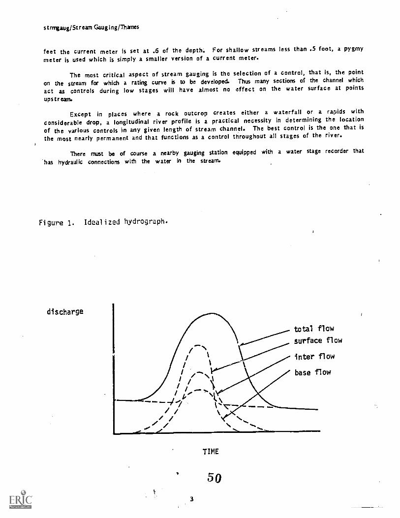
strrtgaug/Strearn Gauging/Thames

feet the current meter is set at .6 of the depth. For shallow streams less than .5 foot, a pygmymeter is used which is simply a smaller version of a current meter.

The most critical aspect of stream gauging is the selection of a control, that is, the pointon the stream for which a rating curve is to be developed. Thus many sections of the channel which

act as controls during low stages will have almost no effect on the water surface at pointsupstream

Except in places where a rock outcrop creates either a waterfall or a rapids with

considerable drop, a longitudinal river profile is a practical necessity in determining the locationof the various controls in any given length of stream channel. The best control is the one that isthe most nearly permanent and that functions as a control throughout all stages of the river.

There must be of course a nearby gauging station equipped with a water stage recorder that

has hydraulic connections with the water in the stream.

Figure 1. Idealized hydrograph.

discharge

total flow

surface flow

/--\I inter flow

base flow

OMEN. 111=Ii

.00

TIME

50

strrrga.ug/Stream Gauging/Than-es

4,

wrn

tr,

6

Figure 2. Rating curve.

10 20 30 40 50 60 70

Discharge - cfs

Figure 3. Longitudinal section of a stream.

0.2 depth velocity ______ Water surface

Flow ----..

0.6 depth velocity

0.8 depth

. .""

r*.

Bottom

51

stmgaug/Strearn Gauging /Thames

Figure 4. Vertical velocity profile of a stream.

Figure 5. Measurements needed to record channel cross section and

velocity.

CROSS SECTION

O (y0)

Wi W2 W3

W T W.VID1+ W2

W.1V D etc

Q22

52

W = width, feetD = depth, feetV = velocity, feet per secondQ = discharge, cubic feet per

second

precal ib/Stream Flow Meas. Precal i b. Struct/Thames

Precalibrated Structures for Stream Flow Measurement

Purpose1. To acquaint the participant with the common structural devices used to measure streamflow.2. To provide design and construction criteria for flumes and weirs.3. To give the student practice in analyzing stream flow records.

Weirs and FlumesOn small watersheds, particularly experimental watersheds, precalibrated structures are

often used because of their convenience and accuracy.

Small watersheds include those of a few to about 1,500 acres. Such watersheds are smallenough so that construction of an artificial control is not impractical. On larger streams, gaugingis usually done by using natural controls as discussed in the preceding section.

The most common types of precallbrated structures are weirs and flumes. The variousobjectives for which streamgauging stations have been built have resulted in many different designsfor weirs and flumes. Weirs are often preferred for gauging small watersheds particularly thosewith perennial flows. Where heavy sedimentladen flows are common, flumes are often moreconvenient. A flume is a stabilized channel (without an impoundment) with access to a stillingwell. Flumes also must be used where the gradient of the stream is particularly low.

Weirs or flumes can be constructed of a great many materials. Concrete, because of itsstrength and permanence, probably is used the most. Treated wood, concrete blocks, metal, and manyother materials are also used. The notch of a weir is often a steel blade set into concrete, andflumes are often lined with steel for permanence.'

WeirsAs used here, weir includes all components of a streamgauging station that incorporates a

notch control (Figures 1 and 2). An impr 'ctment of water (the weir basin) is formed upstream fromthe wall or dam containing the notch. I-. Ailing well with waterlevel recorder is connected to theweir basin. A gaugehouse or some other type of shelter is provided to protect the recorder.

The cutoff wall or dam is used to divert through the notch all water (above or below thestreambed) moving down the channel. Where possible, the cutoff wall is tied into bedrock or otherimpermeable material so that no water can flow under or around it. But where leakage is apt tooccur, the weir basin is sometimes constructed as a watertight box.

The edge or surface over which the water flows is called the crest. Weirs can be eithersharp crested a broad crested. A sharpcrested weir has a blade with a sharp upstream edge so thatthe passing water touches only a thin edge and springs clear of the rest of the crest.

A broadcrested weir has a flat or broad surface over which the discharge flows. Broadcrested weirs are generally used where sensitivity to low flows is not critical and where sharpcrests would be dulled a damaged by sediment or debris.

The sheet of water flowing over the weir is the nappe. The weir has free discharge if thenappe discharges into the air: air circulates freely on all sides of the flow issuing from the weirnotch.

1

tit)

precalib/Stream Flow Meas. Precalib. Structahames

As the nappe flows through the notch, the velocity of flow iicreases and the nappe ci-osssection is reduced or contracted. The contraction is affected by the shape of the notch and basin'characteristics immediately upstream from the notch.

Where the depth of water from the crest to the basin flow is less than 2.5 times the head ofwater over the crest, the crest contraction of the nappe is partially suppressed. Velocr:; ofapproach will increase, and actual discharge will be greater than that shown by the normally :rsedformulas and tables (Fig. 1).

If the basin is the same width as the crest, the weir has its end contractions suppress;;.For complete end contractions, the distance from the edge of the notch to the side of the weir basinor channel should be at least 2.5 times the head being measured. A narrower weir basin or channelresults in increased velocity of approach and increased flow for a given head.

For best results, the velocity of approach should be held to a maximum of 0.5 foot persecond. Where velocities of approach are appreciable, the discharge should be corrected.

Water discharging over the crest of a weir drops slightly in elevation immediately upstr ;amfrom the crest. Th4 decrease is caused by the water's acceleration in velocity as it approa;hesthe crest. Such a drop is called surface contraction or drop-down. In sharp-crested weirs, theeffect of this surface contraction extends upstream from the crest a distance twice the head ofwater flowing over the crest. Therefore, the intake to the stilling well should be located upstreamfrom the crest a distance equal to or greater than twice the head of the maximum anticipated flow(Fig. 2). Fully contracted weirs are generally preferred in research.

The rectangular weir has vertical sides and horizontal crest. Its major advantage is itscapacity to handle high flows. However, the rectangular weir does not provide for precisemeasurement of the low flows of small experimental watersheds a small increase in head will give

only a slightly increased discharge.

The trapezoidal weir is similar to the rectangular weir. Its sides, of course, are slopedfrom the vertical. It has a smaller capacity than a rectangular weir of the same crest length; thedischarge is approximately the sum of discharges from the rectangular and triangular sections.

Sharp-crested V-notch er triangular weirs are often used where accurate measurements of lowflows are important. The V-notch weir may have a rectangular section above to accommodateinfrequent high flows.

The two most common sharp-crested V-notch weirs are the 90° notch and the 120° notch, with

metal blades ground to a sharp edge and built into a concrete cutoff wall. The 90° type givesgreater sensitivity at low flows; the 120° type covers a wider range of flows. V-notch weirs areusually constructed to accommodate heads up to 2 feet; however, both in the United States andelsewhere V-notch weirs capable of handling gauge heights in excess of 2 feet are in use (seeAppendix A).

Broad-crested triangular weirs with 2:1, 3:1, and 5:1 side slopes (with notchesapproximately 127°, 143°, and 157°, respectively) were developed and rated by the Soil Conservation

Service for measuring flows up to about 1,000 cfs. The shape and thickness of the crest permitscomparatively free passage of debris and minimizes the effect on the stage-discharge relationship ofsmall irregularities of the crest. and of trash temporarily lodged on the crest. A reasonablystraight and practically level channel for 50 feet above the weir, with the notch 6 inches above thebottom of the approach channel, is essential for accuracy (see Appendix B).>

542

precalib/Stream FlowlMeas. Precalib. Struct/Thames

FlumeA flume is an artificial open channel built to contain flow within a designed crosssection

ark* length. The types of flumes that have been used on small watersheds are described here.

HS, H, and HL flumes developed and rated by the Soil Conservation Service have convergingvertical sidewalls cut back on a slope at the outlet to give them a trapezoidal projection. Thesehave been used largely to measure intermittent runoff. Maximum depths of waterflow are 1 foot forthe HS type, 4,5 feet for the H type, and 4 feet for On HL type. Maximum flows are 0.8, 84, and117 cfs, respectively. These flumes are in use at many Agricultural Research Service installationsand a number of other locations (See Appendix A).

The Venturi flume (Fig. 3) has a gradually contractingthroat and an expanding section immediately downstream. The floorgrade as the stream channel, whereas that of the Parshall flumethe throat section. Stilling wells for measuring the head are atthe difference in head at the two wells is related to discharge.trapezoidal, triangular, or any other regular shape. They areirrigation water.

section leading to a constrictedof the Venturi flume is the same(described below) is depressed inthe entrance and at the throat;Venturi flumes are rectangular,

widely used in measurement of

The Parshall flume, a modification of the Venturi flume, measures water in open conduits andis widely used, especially for measuring irrigation water. It consists essentially of a contractinginlet, a parallelsided throat, and an expanding outlet, all of which have vertical sidewalls. Itcan measure flows under submerged conditions. Two waterlevel recorders are used when measuringsubmerged flow, one in the sidewall of the contracting inlet and the other slightly upstream fromthe lowest point of the flow in the throat. When measuring free flow, only the upper measuringpoint is used.

The San Dimas flume (Fig. 4) was designed on the San Dimas Experimental Forest of the U.S.Forest Service to measure debrisladen flows in mountain streams. It is rectangular and has asloping floor ( 3 percent gradient) that functions as a broadcrested weir except that the

contraction is from the sides rather than the bottom; therefore, there is no barrier to causesediment depositon. Depth measurements are made in the parallelwalled section at about themidpoint. Rapid flow keeps the flume scoured clean.

The types of weirs and flumes that have been discussed are these most used in research. In

some cases, structures have been built to incorporate features of more than one type for example,a 90° Vnotch recently built into a Trentontype weir at the Pennsyvania State University. When awide range in flow or sediment load is anticipated, it may be advantageous to instO more than onedevice at the same site.

StatuaryThe type of flume or weir to be used depends upon several factors: maximum and minimum

flows; accuracy needed in determining total discharge, high flows, and low flows; amount of sedimentor debris that is expected, and whether it is suspended or bedlcad; channel gradient; channel crosssection; underlying material; accessibility of site; financial limitations; and length of study.

Maximum and minimum flows likely to be encountered must be estimated before construction.Such estimates can be made from observation of high and low flews and high watermarks and frominformation given by local residents, or they might be based on the area of the watershed andrecords from other gauging stations in the region. Maximum expected flood peaks can also beestimated from rainfall, soil, and cover data, using a method developed by the U.S. Soil

Conservation Service. Assistance should be sought from the U.S. Geoological Survey and U.S. SoilConservation Service, if this approach is needed.

55

precal ib/Stream Flow Meas. -- Precal ib. St ruct/Thames

The maximum and minimum flow to be measured at any degree of precision depend upon the

objectives of the study and the extremes that might occur. In some cases, a gauge will be adequate

if it will measure, with acceptable accuracy, 80 to 10 percent of the flow. These limits exclude

extreme peaks and very low flows. However, the structure must be strong enough to withstand the

highest flow expected.

Once maximum and minimum estimazes are made, reference to rating tables for various

structures or to formulas for competing flow will show the types and sizes of installations that can

be used. Maximum and minimum discharges for several types of weirs and flumes are given in Table 1.

Rating tables will also show the relationship between the increase in discharge and the

corresponding rise in head at various stage heights. This association indicates the sensitivty ofthe gauging station at different levels of discharge.

Rating can be simplified by choosing a design for which a statedischarge relationship hasbeen determined in the laboratory. After construction, the laboratory rating should be checked at

various gauge heights by direct measurement with current meter, velocity head rod, or another

instrument for determining velocity, or by volumetric measurements.

Where excessive amounts of suspended sediment, bedload, and floating debris are encountered,

flumes are preferable. Weis would be unsatisfactory because the basin would trap this material,

which would alter the weir rating, and debris would clog the crest of the weir, giving grossly

inaccurate measurements. Broadcrested weirs are often used on agricultural watersheds where grass

and other debris would lodge on a sharpcrested weir and invalidate the rating curve.

The gradient of the stream channel may affect choice of design. If the gradient is too low,

it may be impossible to install a weir that will meet the requirements of a standard rating (depth

of water below crest equal to at least 2.5 times the maximum head to be measured). A control with

less evaluation may have to be built, and the station will then have to be rated by current meter or

other means.

The channel cros, section and strea.-abanks may dictate design. Under some conditions, a

cutoff wall high enough to satisfy rating requirements would have to be of considerable length to

tie into solid material at the sides. The cost of such a wall might rule out this type of

installation.

Underlying marterial must be considered. If permeability is a problem, either a watertightbox weir design, which can support an artificial head of water, or a flume will be necessary.

With weirs, sharp crests give greater accuracy than broad crests. Blades of sharpcrested

weirs are constructed of angle iron or steelpiate, ground to a sharp edge or to a flat edge onesixteenth inch wide, and set into concrete cutoff walls or dams. Blades may be dented, bent,

rusted, and clogged with debris. In many locations they must be screened to prevent clogging, and

care should be exercised when working near them; some maintenance, such as annual painting, is

rew i red.

Flumes are often satisfactory where weirs are impracticable. They can handle debrisladen

flows better; even so, such flows may be difficult to measure. With flumes, velocity of approach is

less of a problem than with weirs. There is less loss in head with flumes than with weirs; thus,

they can be used in channels with low gradients. This is one of the main reasons why flumes are

used in measurement of water for irrigation. And flumes, requiring no excavation for ponding, may

be easier and cheaper to install.

Details of construction of an Hflume ar;c1 Vnotch and sharpcrested weirs are given in

Appendixes A and B. Methods for computing rainfall intensity from recording rainauge charts and

far computing runoff from a stage recorder chart are given in Appendix D.

56

precalib/StrearnFlow Meas. -- Precalib. Struct/Thames

Literature

Much of this section was taken directly from the following publications:

Internatimtal Symposium of Forest. 1965. Edited by W. E.Sopper and H. W. Lull. Pergamon Press.

Field Manual for Research in Agricultural Hydrology. 1961

Agriculture Handbook No. 224, A.R.S.U.&D.A.

Streamgauging Stations for Research on Small Watersheds.

1964. K. G. Reinhart and R. S. Pierce.

Table 1.

Maximum and minimum discharges for several types of weirs and flumes incubic feet per second (approximate).

WEIRS

TypeMini-mum

Maxi-mum

Sharp-crested weirs:2 feet high, 90° V-notch <0.001 14

2 feet high, 120' V-notch <.001 24

2 feet high, 6 feet wide rectaneular 1.24 56

2.75 feet high, 8 feet wide Cipolletti 1.30 123

4 feet high, 12 feet wide Cipolletti 1.46 323

Broad-crested weirs:Triangular 2:1 side slopes 22.017 '510

Triangular 3:1 side stones 2.025 3803

Triangular 5:1 side slopes 2.037 '1,440

2 feet high Columbus deep notch .026 62

FLUMES

HS type:0.4 foot high 10.001 0.1

1.0 foot high 1.002 .8

H type:1.0 foot high 1.004 2

2.0 feet high 1.007 11

4.5 feet hi'h 1;015 84

HL type:4.0 feet high 1.03 117

San Dimas:1 foot wide .1 6

3 feet wide 2 77

6 feet wide 10 318

10 feet wide 36 1,000

Trapezoidal:1- foot -wide throat, 4 feet high,

30 side slopes. 1.15 350

Parshall:1 foot wide, 2.5 feet high .4 16

2 feet wide, 2.5 feet high .7 33

4 feet wide, 2.5 feet high 1.3 68

8 feet wide, 2.5 fee' high. 4.6 140

'Flow at 0.05-foot head.2Flow at 0.1-foot head.'Flow at 6-foot head with cross-sectional area of 300 square feetin the channel of approach 10 feat upstream from center of crest.

5 7

precal lb/Stream Hoy/meas. rrecalto. Mructimarrms

WELL

1:1Pd''r;..:.1.

t

-L__ "LL___

' I

a

I

CPINfafL 411CliCNTC

0.CCTION OF 'Low

Fig. 3. Schematic diagram of Venturi flume, which requires r.ecsurorntof stage at two points. Flume is sale gr,.de as stre6r. cF.JonQl.A, Plan view of Venturi flume; B, cross-stction 0 Venturiflume.

/ ! ,TRANSITION, PARALLEL WALLR .2W ,-- SECTION -- SECTION .-:

I e -UPSTREAM !

ENOi

----.. -SLOT

.0

7t ..

-; ;-- I AI

1

.,__.A::IL-.. --4 - ENODOWNSTREAM

201 1 . w

wLp 2 W

L.3iWPLAN

H corm or FLUME

L * LE'.4 To OF PARALL FL FLUME SECTIONL folAL LE.'GTM OF FLUMER qAu.us 0; TRANSITION

SILT TRAP

LEVEL 34

SILT TRAP - L,

SECTION A-A

SECTION S-8

wTEOL

Fig. 4. Generalized drawing of San Dimas flume. This design has beenused for flumes with widths of 0.5, 1.0, 2.0, 3.0, 4.0,6.0, and 10.0 feet.

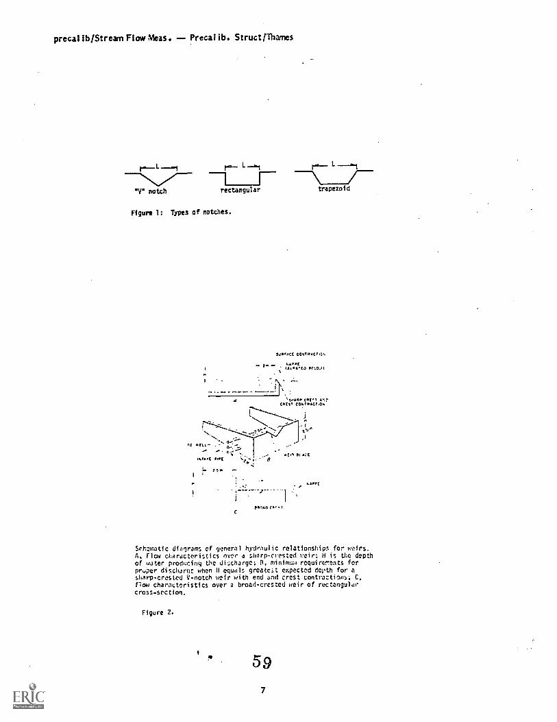
precalib/StreamFlowNleas. Precalib. Struct/ThaTes

L L

"Ir notch rectangular trapezoid

Figure 1: Types of notches.

Cr 0.4.CCD PrL031

A 4.1,11a CINITC*CS, CDO.TNACT014

,

- 4

TO ELL .

mTs.0

-,'5.1,11.1

aC.0

e.nAn CA/C

Schematic diagrams of general hydraulic relationships for weirs.A, Flew characteristics nver a sharp-crested weir; H is the depthof water prodheing the discharge; 1, minimvia requirements forprvper discharge when II equdls greatest expected depth for asharp-crdslcd V-notch weir with end and crest contractions; C,flow characteristics over a broad-crested weir of rectangularcross-section.

Figure 2.

4

stf loest /Stream Flow Estn. Field Methods/Thames)

Stream Flow Estimations Simple Field Methods

John Thames

Purpose: To acquaint the participant with simple field methods of estimating streamdischarge.

Flood flows and high peak flows are often of primary interest, particularly in determiningdownstream effects of land use, and for the design of engineering structures. Although it is rarefor a field survey to coincide with a peak flow event, a measurement at any stage of flow can bevery useful.

Surface floats are the simplest method of measuring the velocity of a stream and therebyestimating the volume of streamflow. A float is thrown into the center of the stream and the timeit takes to travel a measured distance of stream reach is observed. Velocity is calculated as:

V = L/t

where V = velocityL = length of stream reach, andt = time

The volume of flow (discharge) is determined by

Q=A V

where Q = discharge in volume per unit of time andA = crosssection at the midpoint of the stream reach.

The crosssection area of the stream is best determined by summing a series of crosssectionsegments across the channel as shown in the section on stream gauging. The accuracy of surface

floats is rather poor, since they only indicate the velocity at the water surface and also can beinfluenced by the wind. The mean velocity of nonturbulent streams is generally about 0.85 x thesurface velocity, so a correction factor should be applied. Accuracy can be improved, particularlyfor deep, slow flows, by using a cannister or rod float, so as to avoid wind effects. These can be

improvised from materials at hand and are designed to float with their bulk below the water surface.

Where it is difficult to recover floats, it may be better to release a series of surface floatsacross the stream, timing the velocity of each and letting them represent crosssection segments.Water discharge is then calculated as described in the section on stream gauging.

Empirical Estimations of Stream FlowIt must be emphasized that estimates, no matter how sophisticated, are never as good as

direct measurements. However, in many developing countries: *ream gauging networks are few or data

may be completely lacking. An estimation of streamflow, no matter how rough, is often essential for

appraising the condition of catchments. Most often, a main interest is in flood flows. Of course,

reasonable estimates can often be made by extrapolating information from a similar baSin. However,

this must be done cautiously and by an experienced individual.

60

stiloest/Stream Flow Estn. Field Methods/Tharnes

Flow, equationsSeveral empirical methods are available. Two in common use for estimating stream discharge

at known stages (depths) of flow are the Manning and the Chezy equations.

The Manning Equation is:

V = 1/n R2/3 S2/3

where V = the average velocity in the stream crosssection in meters per second,R = the hydraulic radius in meters, and R = A/P (i.e., crosssection area of flow divided bywetted perimeter)S = the water surface slope in meters per meter, or hf/L, where hf = friction head loss orfall per reach of stream L,n = a roughness coefficient.

The Chezy Equation is:

V =C /RS (2)

where C = the Cher/ roughness coefficient.

Equations (1) and (2) are similar, and the relationship between the roughness coefficientsis:

C = 1.81/n R1/6 (metric) or

C = 1.5/n R1/6 (English)

The equations are used in similar fashion: the hydraulic radius and water surface slope areobtained from crosssection and bed slope data in the field (Figure 1). The roughness coefficientis estimated from Table 1 and the average discharge Q is calculated by multiplying the velocitytimes the crosssection area (A in Figure 1). Since the Chezy and Manning equations are related byequation (3), it is only necessary to consider one of the coefficients (Gray 1970).

In practice, since the interest is in some previous peak flow, highwater marks must belocated to estimate the depth of flow. Sometimes this can be obtained by measuring the height ofdebris caught up along the stream channel (Figure 2) or by interviews with local inhabitants. Thisshould be obtained for a reach of channel where the crosssection of the flow of interest can bemeasured with reasonable accuracy. The slope of the water surface can be approximated by the slope

of the stream channel along the reach. The wetted perimeter can be measured by laying a tape on thechannel bottom and sides between the high water marks. The crosssection area should be measured bysumming several segments.

Frequently, it is not possible to obtain the measurements needed for equations 1 or 2,particularly where there is no welldefined channel or where the flow spreads over an adjacent plainor where evidence of high flows cannot be obtained from interviews. In these cases, it is necessaryto resort to empirical methods such as the SCS method described in another section. There are alsoseveral simpler methods that can be used for small catchments which require easily obtainedmeasurements. The Rational Method is one of the most common.

61

stfloest/Stream Flow Estn. -- Field Methods/Thames

pe channel and dr.:option

Table 1: Values of roughness coefficient en"

Minimum Normal MaAirnum* I Pe n( channel and 513.11mmil

Var 33re:1) rook. Of.1 u heo C ind rim-

orldunkrbr.011111,,ntafr streams. no in

hanks ustaa!!!: steep. Itt.es3.. ! ',01t along hanks vihmergetl 311 <hr..

3..; els..,131.1-0es. and fewfat

2 1+-r:^..., Cohlles tat '.rge boulder,

11 2 11 I roJo' ad.

I:..r.2

1.. "hat. I or-asI1. .?12 ru;. crors3 '0.0m, 11-1d ...of

C

2 I t rr5 a:,4 3,...ner

5 !' 41.00 13 dens" s-11. in MITMC:4, 11 .

j It ,j A 111..V. 1113:;...no

r.r....I.1.,: .. alm3e Int ..111, 11.'3,3I '' .. t!, of Trw.ii

.n.1.!tir I. f.na .1..wn. lOile und-r"r311..11..":1 gar

c ' 0....313.1arx

No ...v.

Is `A. :3 r . ,r !loud001 1, . do i

11, l' .1 I, ...! o f1

,01 114'01

1 'IrnTi ... lion

0.075 0,100 0.150

0 030 0.040 0.0500.040 0.050 0 070

0 025 0 050 0 0350(13(1 0.C.15 0.050

011:0 0 010 01)4')01125 0 0 IS 00)50.' 4(1 0.010 f) 050

f435 0 0531 0 0700015 11 050 0 0,110 010 0 0..1 0.0900 ' 15 0O0 0 1100.!.70 0 100 0.1141

U 111) 015(1 0.200

0.010 040 0.0 +0

0 050 0.0"n Q(0I)

0 '0.'0 0 100 0.12(1

0 100 1.1,120 U.169

0.0250 035

A. I 3.n...1,1 .,r 11..a 1Jr111, .11:,,;111 and

I. (1:an. r.-, ':444) compkted2 Cluati...31er neaillerina3 14 manr.n CI an4 V. Iti. 7ra..3.. fee. 4.'

h fart!, a and sluitei%13I 5.0 .:. har.331,2.

3. D,.. r 3quarf;r3knnd.

4 I ill I. 41.1111 rtot,h. .1...5 St,.:;3 1,..torn ai .....3431 1.o11.3.

6 I ...101: !tt,.nli 3)444 ;

.irI Y.:" %.; !.01,112 1.1 11, 4!;1 hatik

d 11-.1. 03.I ",,a2 J ...!

au,. 3 . I

1). 30. ,fat2 (I.,. I.l4 14411,43 (44) '

3 Sam..1 11,!.. host,. high

11. Sife.ro11 1. \I....3r ..1,13. lCp

lCL ?(''Ii 3a 5.:, AP. j'Lill

I %Lie.. nn o11.133 II.. 1..3o17.

2 S,,i, hut ne..tyand

3 3 put!. 111:* joc

11..11.

..1):1

5 S.-, .1,., 1%f .1..Tv.. :Intl ...I,

511.1 1, .....11,3te -too.7 Sinerhh vomly..1. 13-01:.

. 0.9'6 01.4k00?'(.1

'1'.It

0 02.1 01r.:025 4)0313 ri.;11.

010

W

1.11.3r.

ri.z5

0.1,

I

1;

0

0 1: 1

150

0.2.7101.11-

(1 ro

0 O..,U 0."

4.' ,1 ! ;

:1

0 (I no lo .

1.1 (o.lot

(s 4 lo "o

414,1'. II 111,

h :1. 1)11

11 I, j. o

03(1 (I

stf loest/Stream Flow Estn. Field Methods/Thames

Rational MethodOften, for purposes of designing small dams, water diversions or culverts, the peak flow

estimation most generally employed for small watersheds is the socalled Rational Method. It issummarized in the equation:

q = C i A/36 (3)

where qp = peak rate of flow in cubic meters per secondc = coefficient of runoff,i = design rainfall intensity in centimeters per hour for a given frequency and a duration

equal to the time of concentration of the basinA = area in hectares

Values for the coefficient of runoff are given in Table 2. The time of concentration, Tc,is the time it takes for water to travel from the most distant point on the watershed to thewatershed outlet. An equation for estimating this watershed characteristic is:

Tc = L1.15/15 H0.38 (4)

where Tc = time of concentration in hoursL = length of the watershed along the main stream from the outlet to the most distant ridgein kilometers, andH = the difference in elevation between the watershed outlet and the most distant ridge inki laneters.

In areas where rainfall records are lacking, the time of concentration can be calculated toarrive at the duration of the design storm. Intensity can then be estimated either from what localinformation is available or obtained from adjacent areas where there are data.

Values of C for Rational Formula 2

Soil type Watershed coverCultivated Pasture Woodlands

With aboveaverage infiltration rates;usually sandy or gravelly

0.20 0.15 0.10

With average infiltration rates; noclay pans; foams and similar soils

0.40 0.35 0.30

With belowaverage infiltration rates;heavy clay soils or soils with a claypan near the surface; shallow soils

0.50 0.45 0.40

above impervious rock

Other InformationFor more information on runoff evaluation and on instrumentation, the reader may wish to

request lists of available studies and reports in hydrology from the International HydrologicalProgramme, UNESCO, Place de Fontency, 75 Paris 7eme, France, particularly their book "Representativeand Experimental Basis." WMO also has a Series of "Technical Notes" on hydrology, produced by theworking group of the Commission for Hydrology, World Meteorological Organization, CH 1211, Geneva20, Switzerland. They also produce a "Guide to hydrological practices."

63

stfloest/Strearn Flow Es tn. Field Methods/Thames

The FAO Land and Water Development Division issues hydrological reports in its "Irrigationand Drainage Paper" series, FAO, via delle Terme di Caracalla, Rome.

Much useful information also is available from "Technical Bulletins" released by the InlandWaters Branch, Department of the Environment, Ottawa, Canada. The U.S. Geological Survey has aseries "Techniques of waterresource investigations of the U.S.G.S.," available from theSuperintendent of Documents, U.S. Government Printing Office, Washington, D.C. 20402. Their series

of "Water supply papers" also is useful.

In the French language, a hydrological series is offered by the Office de la RechercheScientifique et Technique Outremer, 19, rue Eugene Carriere, Paris, 18eme.

A good summary of hydrology produced in conjunction with the International HydrologicalDecade (UNESCO) is "Handbook on the principles of hydrology" (D. M. Gray,' ed.) by the NationalResearch Council of Canada, available from Water Information Center, Inc., Water Research Building,Manhasset Isle, Port Washington, N.Y. 11050, U.S.A. A useful reference also is the "Handbook ofapplied hydrology" by Chow (ed.), McGrawHill Book Company, N.Y. Of course many individual texts

are available in various specialized topics of the field of hydrology.

References

Chow, Ven Te. Handbook of Applied Hydrology. McGrawHill Book Co., New York. 1964

Gray, D. NI. (ed.). Handbook on the Principles of Hydrology. National Research Council of Canada.

1970.

64

stfloest/Stream Flow Estn. Field Methods/Thanes

a

A

V ap:

b

e S

1.

C

Figure 1. Stream channel section showing slope or gradient ofstreambed, wetted perimeter P (which is line a-b-c) and cross-section

area A. R = A/P.

1

undisturbed

estimated high water level

`--, debris evidence

signs .

of cutting.

debris

sedimentdeposits

water levelduring visit

Figure 2: L000king for evidence of high water level in the field.

656

scs/Strean Flow Estimation: SCS Method /Thames

Stream Flow Estimation: SCS Method

John Thanes

IntroductionIn many areas of the world there is little or no information pertaining to the quantity and

timing of runoff from watershed lands. This presentation discusses the U.S. Soil ConservationService method for estimating water and sediment yields from small ungaged watersheds. While its

initial use was intended for the more humid regions, this procedure is now also used in aridregions. Although runoff data for small watersheds is generally lacking, information on

precipitation is generally available for the site in question or can be obtained by extrapolationfrom areas where data is known. Some means is needed, therefore, to transform precipitation into

runoff volume and peak flow rates.

Storm runoff volumeFor ungaged watersheds, the Soil Conservation Service (SCS) uses the following basic

rainfall runoff equation for estimating the runoff volume from a given storm:

Q = (P 0.25)2 / P + 0.8S

where Q = storm runoff, in mmP = storm rain:,..C, in mmS = a watershed `:actor which reflects the infiltration characteristics of the

area under 4:t.nsideration, also expressed in mm.

A watershed index W, sometimes called a runoff curve number is related to S by the equation

W = 1,000/10 + S

The watershed index depends on soil type, the general hydrologic condition of the area, thenature and extent of cover and the antecedent moisture condition at the start of the storm period

which produces runoff.

Soil types are classified into four groups, the details of which are given in Table 1.

Table 1. Soil Groups for Estimation of Watershed Index W

Soil Group Description of soil characteristics

A Soil having very low runoff potential. For example, deep sands with vey little silt orclay.

ti Light soils and/or well structured soils having aboveaverage infiltration when thoroughlywetted. For example, light sandy loams, silty loams.

C Medium soils and shallow soils having below average infiltration when thoroughly wetted.

For example, clay loams.

D Soils having high runoff potential. For example, heavy soils, particularly clays of highswelling capacity, and very shallow soils underlain by dense clay horizons.

66

scs/Stream Flow Estimation: SCS Method/Thanes

Three antecedent moisture conditions are allowed for, depending on the amount of rainfallreceived 5 days prior to the runoff. Details of these conditions are given in Table 2.

Table 2. Antecedent Moisture Conditions for Estimation of Watershed Index W

Antecedent Moisture Condition (AMC) Rain in previous 5 days

I < 15 mm15 to 40 mm> 40 mm

Figure 1, which is more applicable to semiarid regionsiand Table 3 both give values for thewatershed index for various soil-hydrologic-cover combinations, assuming antecedent moisturecondition II. For other antecedent moisture conditions, the value of W obtained from Table 3 mustbe adjusted as shown in Table 4.

The meanings of the terms listed in Table 3 under the heading "Hydrologic Condition" are as

follows :

a. Native pastures: Pasture in poor condition is sparse, heavily grazed pasture with lessthan half the total watershed area under plant cover. Pasture in fair condition is moderatelygrazed and with between half and three-quarters of the catchment under plant cover. Pasture in goodcondition is lightly grazed and with more than three-quarters of the catchmen area under plantcover.

b. Timbered areas: Poor areas are sparsely timbered and heavily grazed with no

undergrowth. Fair areas are moderately grazed, with some undergrowth. Good areas are denselytimbered and ungrazed, with considerale undergrowth.

c. Improved permanent pastures: Densely sown permanent legume pastures with proper grazingmanagement are said to be in good hydrologic condition.

d. Rotation pastures: Dense, moderately grazed pasturs used as part of a well-planned,crop-pasture-fallow rotation are considered to be in good hydrologic condition. Sparse, overgrazedOr "opportunity" pastures are considered to be in poor condition.

e. Crops: Good hydrologic condition refers to crops which form part of a well-planned andmanaged crop, pasture, fallow rotation. Poor hydrologic condition refers to crops managed accordingto a simple crop fallow rotation.

Peak flow rate

With the aid of Figure 2, a synthetic traingular hydrograph of storm runoff is developedwhich can be used to derive the estimated peak flow rate. The general equation is:

qp =1<AQ/Tp

where q = peak runoff rate in cfs= watershed area in km

Q = storm runoff volume in mmT = time in hours from start of runoff to peak rate2n = is a constant dependent on shape of hydrograph. A value of K = 484 is

frequently assumed.

67

scs/Strearn Flow Estimation: XS Method /Thames

Time to peak, T , is estimated from a consideration of both rainfall and watershedcharacteristics. A relatioPnship often used is:

T = .5D + .6T.

where D = duration of excess rainfall in hours (for convective storms, this can be equalto the duration of rainfall).

Tc = time of concentration in hours, which is estimated from the following equation:

Tc = .0078 L'77 S'385

where L = length of the watershed along the main stream from the outlet to most distantridge in km.

S = average slope of the main stream, a dimensionless ration of difference in

elevation between outlet and most remote point to length of watershed L.

For most cases, the constant K has a value of 0.75 if the units are similar for both sidesof the peak flow equation.

Literature

Flaxrnan E. M. 1972. Predicting sediment yield in western United States. Journal Hydraulics 1.);:,ASCE 96 (HY 12): 2073-2085.

Fogel, M. M. 1969. The effect of storm variability on runoff from small semiarid watersheds.Transactions ASAE 12(6): 808-812.

Kern:, K. M. 1968. A method for estimating volume and rate of runoff in small watersheds. USDA

SC5 TP-149. 40 pp.

Soil Conservation Service. 1972:' National Engineering Handbook. Section 4 Hydrology. U.S.

Department of Agriculture. Washington, D.C.

Williams, J. R. and R. W. Hann, Jr. 1973. Hymo: Problemoriented computer language for hydrologic

modeling. Agriculture ARSS-9. 76 pp.

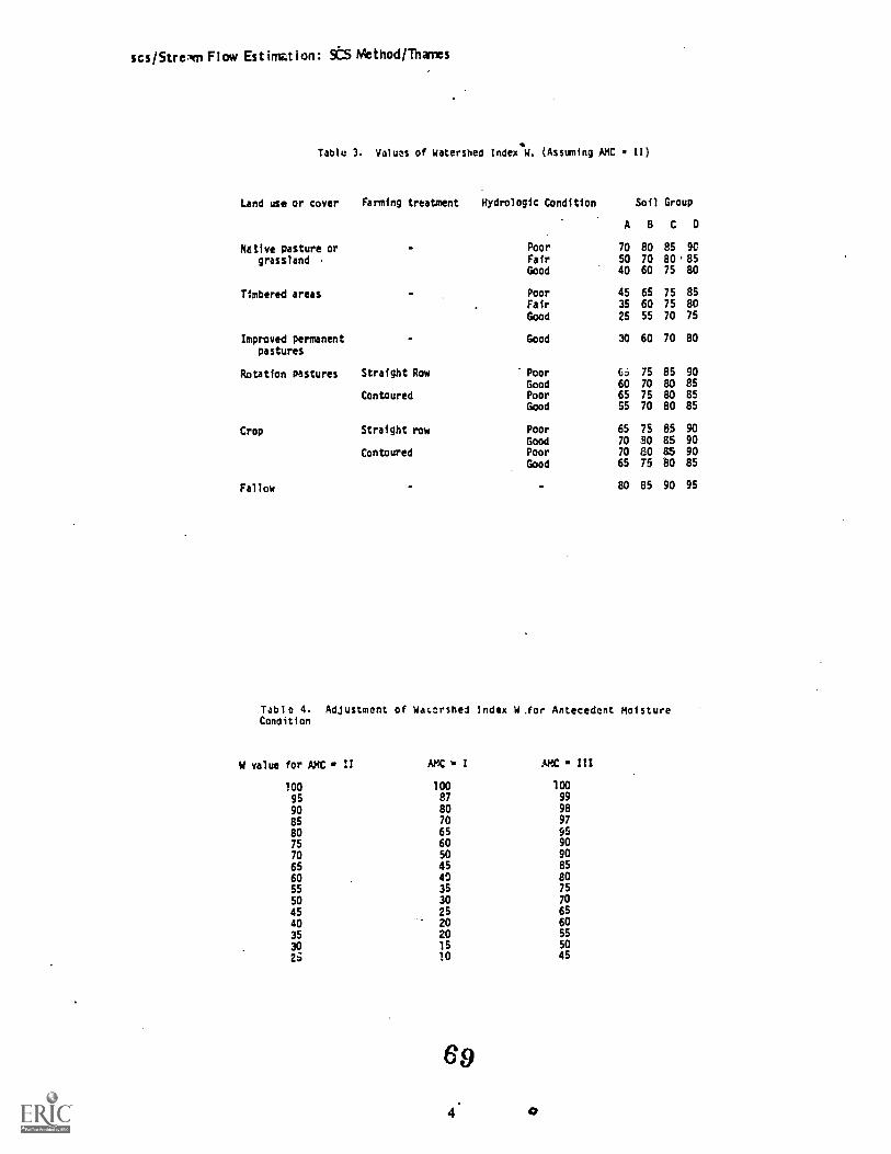
scs/StreAm Flow Est irtmtion: 9t5 Method/Thames

Table 3. Values of Watershed Index W. (Assuming AMC II)

Land use or cover Farming treatment Hydrologic Condition

ABCOSoil Group

Native pasture or Poor 70 80 85 90

grassland Fair 50 70 80 85Good 40 60 75 80

Timbered areas Poor 45 65 75 85

Fair 35 60 75 80

Good 25 55 70 75

Improved permanentpastures

Good 30 60 70 BO

Rotation Pastures Straight Row Poor 66 75 85 90

Good 60 70 80 85

Contoured Poor 65 75 80 85

Good 55 70 80 85

Crop Straight row Poor 65 75 15 90

Good 70 30 85 90

Contoured Poor 70 80 85 90

Good 65 75 tO 85

Fallow 80 85 90 95

Table 4. Adjustment of Watershed Index W .for Antecedent MoistureCondition

W value for AMC 1.1 AMC I AMC 0 III

100 100 100

95 87 99

90 80 98

85 70 97

80 65 95

75 60 90

70 50 90

65 45 85

60 40 BO

55 35 75

50 30 70

45 25 65

40 20 60

35 20 55

302i

1510

5045

69

scs/Stream Flow Estimation: SCS Method/Thames

Cover Density as Percent

Fig. 1

HYDROLOGIC SOIL COVER COMPLEXESAND ASSOCIATED CURVE NUMBERS

so

SO.--

70

SO

SO

--1desert

!

brush4r r

herbaceous

!

moutatn brush1

0)

1

sotjuniper -gross

ro e

so-- ... 'gm

sa IIto t- -

I

10

ponderosa pine.I*,

1D--1Tv

Tb

74.2

orreLeouvrr OP TAIAPIOULAR ITTIMOITA01

Figure 2

7o

econanal/Econcmic Analysis of Projects/Gregersen

Economic Analysis of Watershed Projects

byHans M. Gregersen

College of ForestryUniversity of Minnesota

March 1979

IntroductionFor the hydrologist or watershed manager concerned with action programs and gettin

technically sound project proposals implemented, economics is of central concern as are politics

social pressures, etc. This is the basic rationale for including an economic perspective in thi

course. While the academic hydrologist at times can quite justifiably ignore economics and politic

in his search for the "best" technical approach to a watershed problem, the practitioner who i

of central concern to this course cannot ignore the broader picture, i.e., the conditions whitdetermine the commitment and capacity to implement hydrology projects.

The present paper presents a descriptive outline of some essential economic consideration!

as discussed in a forthcoming guide to economic analysis of forestry projects (Gregersen an

Contreras, in press). It also summarizes some "lessons learned" from a recent review of a number c

studies which have attempted to apply economic analysis to watershed projects (Gregersen and Brook!

1978).

Watershed objectives and project planningMost landuse related projects involve implications in terms of changes in water qualit

and/or quantity. Thus, most such projects should include explicit consideration of water relateimpacts and of potential activities to achieve acceptable watershed protection standards. In som

cases the major oojectives of a project maybe water related and constitute the reason why th

project is being considered and proposed. In other cases, water related concerns may merely ente

the project analysis in the form of constraints on other project activities.

Different waterrelated objectives and/or constraints apply in different situations. Thu!

for example, project objectives will vary widely with climatic and landform conditions as well aother factors. Appendix I presents a schematic overview of objectives which tend to dominate i

different climatic regions. Regardless of objectives, constraints and other conditions,consistent approach to project planning is needed.

The overall nature of project planning is described in several documents (FAO, 1974; Wati

1973; references cited in both these documents). Basically, project planning involves a) definitio

of objectives, b) identification of alternatives to meet objectives, c) design of alternatives i

terms of specific required inputs and outputs, d) analysis or appraisal of alternatives, and e

choice among alternatives. It is a dynamic and iterative process whi:h uses feedback from past an

ongoing operations to imprIve future project planning activities.

econanal/Econcmic Analysis of Projects/Gregersen

The focus of this paper is on one of the elements in the overall planning process, namelyanalysis or appraisal. We limit ourselves to the economic analysis and appraisal process,recognizing full well that most projects invoke other appraisals, including: a) technicalappraisal (a main subject covered in the present course), b) commercial appraisal, or theconsideration of the availability of inputs when needed and the actual uses or requirements foroutputs, c) institutional and organizational appraisal, which deals with the consistency of a givenproject alternative in terms of the institutional structure existing and the organizations ,apacityto undertake a project; d) managerial appraisal, or the consideration of whether or not in factthere is the managerial capacity available to implement and execute a given project; and e)financial appraisal, or the consideration of budget implications and financial profitability. Someof these types of appraisals have been discussed already in this seminar. Others will be covered ata later stage. Some will not be discussed, since they are outside the scope of this seminar and itsobjectives.

The basic framework for an economic analysisAn economic analysis is carried out to provide information for decisionmaking on the costs

and benefits or economic impacts associated with a project and the relationship between costs andbenefits, e.g., whether the benefits exceed the costs for a given project alternative.

The emphasis here is on economic analysis from a national, public point of view, as distinctfrom the closely related financial analysis, which is of central concern to private entities. Thepublic sector is also interested in financial considerations, since a project cannot be undertakenunless it is financially viable, i.e., within the budget limits of the public sector or agencyconsidering the project. A financial or budget analysis for a watershed project is fairlystraightforward and involves consideration of financial (money) outflows and inflows for a givenentity or group of entities.

There are two main applications of economics in project planning. First, we are interestedin the economics of alternative designs (or project opportunities) to achieve the same objective(s).This involves analysis of "mutually exclusive" project alternatives. Second, once the "best" designfor meeting a given objective has been chosen, i.e., the economically "optimum" design, ezonsmics is

relevant in terms of deciding whether or not in fact the project will be undertaken, when otherknown uses for scarce resources are considered.

Economic analyses of watershed projects are no different in principle or concept thaneconomic analyses for any other type of project. Basically, in an economic analysis we areconcerned with economic efficiency associated with alternative allocations of resources, i.e., howto achieve the greatest benefits with given resources, or how to minimize the expenditure ofresources in achieving given benefits. Thus, the general concepts and guidelines presented in FAO'sEconomic Analysis of Forestry Projects (EAFP) are valid also for watershed related projects.However, some analytical issue and empirical problems are particularly important for such projects.Some of these issues and problems retate to economic factors, and they are the main subject of thispaper. Others relate primarily to technical factors and their treatment is properly the task ofhydrologists; many of these have been discussed in earlier sessions of the course. Thus, we do notdiscuss them further here, other than in terms of how the economist can interact with thehydrologist in determining what physical inputoutput information is needed in order to carry out aneconomic analysis. A basic point is that the physical relationships must be quantified before aneconomic analysis can be carried out. Thus, the present discussion proceeds under the assumptionthat such information can be generated. Given the fact that the lack of such information is inpractice the major bottleneck encountered in most watershed project appraisals, it may seem thatthis assumption is made here to avoid a major problem. in fact, it is made to emphasize the pointthat the economist cannot solve the information and data problems associated with watershedprojects. What he can do is to a) suggest a systematic approach to identifying direct and indirectnegative and positive impacts associated with a project, and b) point out what information and dataare needed for him to be able to value these various impacts.

scs/Stream Flow Estimation: 9:5 Method/Thames

Time to peak, T , is estimated from a consideration of both rainfall and watershedcharacteristics. A relationship often used is:

Tp = .50 + .6Tc

where D = duration excess rainfall in hours (for convective storms, this can be equalto the notation of rainfall).

Tc = time of concentration in hours, which is estimated from the following equation:

Tc = .0078 L'77 5'385

where L = length of the watershed along the main stream from the outlet to most distantridge in km.

S = average slope of the main stream, a dimensionless ration of difference in

elevation between outlet and most remote point to length of watershed L.

For most cases, the constant K has a value of 0.75 if the units are similar for both sides

of the peak flow equation.

Literature

Flaxman E. M. 1972. Predicting sediment yield in western United States. Journal Hydraulics Div.

ASCE 98 (I-1Y 12): 2073-2085.

Fogel, M. M. 1969. The effect of storm variability on runoff from small semiarid watersheds.Transactions ASAE 12(6): 808-812.

Kent, K. M. 1968. A method for estimating volume and rate of runoff in small watersheds. USDA

SCSTP-149. 40 pp.

Soil Conservation Service. 1972. National Engineering Handbook. Section 4 Hydrology. U.S.

Department of Agriculture. Washington, D.C.

Williams, J. R. and R. W. Hann, Jr. 1973. Hymo: Problemoriented computer language for hydrologic

modeling. Agriculture ARJS-9. 76 pp.

73

3

econana I /Econcmic Analysis of Projects /Gregersen

Particular issues of concern in hydrology projects.Based on review of a number of hydrology/watershed management projects in developing

countries, it appears that there are some specific analytical and empirical issues which areparticularly common for watershed projects. These are discussed in the remainder of the paper. The

discussion is in most cases taken directly from an earlier study (Gregersen and Brooks, 1978).

The specific points selected for further treatment are the following:

1. Consideration of alternative means for achieving goals.

2. Determination of project scope and context.

3. Identifying costs for watershed projects.

4. Identifying benefits for watershed projects.

5. Treatment of benefits and costs in multipI2 purpose projects.

6. Presenting cost and benefit information in an appropriate form.

The fact that there are only six points listed does not mean that they are the only ones of concernto the analyst of a watershed related project. For a more systematic discussion of the entire rangeof issues enceumered, the reader is referred to EAFP and FAO (1974).

In order to provide common empirical reference points during the discussion of each ofthese, two case study analyses of projects involving watershed considerations are summarized inSection 6. These two examples are then referred to in Section 7, which provides a discussion of thesix points listed above.

ExarrplesThe first of the examples is an economic analysis of alternative logging systems. The

objective of the analysis is to find that system that maximizes net revenue subject to a constrainton maximum allowable sediment discharge. It is an example of an economic analysis to provideinformation for an operational decision where water related concerns are entered as a constraint.

The second example illustrates in summary form an economic analysis of a major watershedproject designed to reduce the rate of sedimentation in a reservoir, thereby extending the usefullife of the reservoir and producing additional downstream benefits. The project also involvesseveral other elements, including wood production in combination with watershed protection, pastureimprovement, and general improvement of upstream agriculture.

Example No. 1: Watershed Considerations as a Constraint .in a ProjectThe growing worldwide concern for environmental protection makes this type of example

relevant.

A 20 ha woodlot is to be harvested. The lot occupies land along a river with an averageslope of 20-3096. In order to prevent erosion and decrease resulting sediment flows, a clearcut willnot be allowed by regulatory agencies. For this reason a selective cut will be made. However, itis anticipated that with standard logging techniques about 4 tons of sediment per hectare will enterthe river the first year after the harvest. This amount of sediment is considered unacceptable byauthorities and they will not issue the harvesting permit unless measures arc taken to reducesediment to no more than 2 tons per hectare. Thus, the forest manager must find an alternative thatwill reduce sedimentation of the river by at least 2 tons/ha/yr at the lowest cost possible, i.e.,he is searching for the least cost alternative for logging the area that will meet the constraint.

P74

econana I /Econcrac Analysis of Proj ects/Gregersen

Harvestable volume on the tPoodlot is 300 cubic meters/ha wh;ch can be sold for $10/cubicmeter.

If all 20 ha had been harvested using standard methods, it is estimated that the followingcosts and returns would have obtained:Returns:

300 cubic meters/ha x $10/cubic meter x 20 ha equals $60,00C'

Costs:

Net revenue:

labour: 1000 man hours x $2.00/hr equals ;2000tractor: 250 hours x $25/hr equals $6250loading/transport: 120 hours x $20/hr equals $2400total cost: $10,650

$60,000 minus $10,650 equals $49,350.

However, as mentioned the standard method is not acceptable because of the high sedimentdischarge associated with it. Two alternatives are proposed that would meet the maximum dischargerestriction.

The first feasible alternative consists of leaving a 25 m wide buffer strip (no cutting)along the river. The woodlot has a shoreline of 1600 m, therefore, cutting would be reduced to atotal of 16 ha instead of 20 ha. This means a loss of 4 ha of timber or 300 cubic meters x 4 ha x$10/cubic meter which ecuals $12,000 of revenue foregone. This is considered a cost for thisalternative. It is assumed that other costs would be reduced by 20 percent since only 16 ha couldbe harvested. Thus, costs other than revenue foregone would decrease to $8520 (20 percent less than

$10,650). Total cost of this alternative would be $20,520 ($8520 plus $12,000).

The second alternative which meets the sediment discharge requirements consists ofestablishment of 40 m filter strip in which no machines are aliowed. All commercial timber (i.e.,300 cubic meters/ha) on this 6.4 ha filter strip can be cut but must be winched out at a highercost. On the 6.4 ha of the filter strip costs are estimated to be $8,094. For the remaining 13.6ha costs will drop to an estimated $7,242 to reflect reduction in area logged. Thus, total cost ofthis alternative will be $15,336.

Assuming that these are the only two alternatives considered that meet the sedimentdischarge restriction, we would choose the lowest cost alternative or the filter strip approach.Revenue would be $60,000 as before and cost would be $15,336, for a net return of $44,664, whichcompares with a net return of $29,480 in the buffer strip alternative. The information generated inthis analysis further indicates that the cost of the sediment discharge restriction would be $49,350minus $44,664 or $4,686.

Example No. 2: Economic Analysis of a Watershed Protection and Managennt Project*1

Background on Project

Project title:Watershed protection for the Sierra Reservoir.

Project situation:Some years ago, a reservoir was built along the Sierra River to provide storage of water for

downstream use during periods of low flow. Downstream uses include irrigation on some 9500 ha anddomestic water use by the local population. It has been found after five years of operation thatthe reservoir is silting in at a much faster rate than initially anticipated, thus reducing

'7

econanal/Econanic Analysis of Projects/Gregersen

effective capacity and ability to meet water requirements downstream. Siltation is occurring at arate of 4 million cubic meters per year. Present reservoir capacity is down to 100 million cubicmeters. At the present rate of siltation, it will only be four years before capacity is reduced toa point where it can no longer meet estimated water requIrem.ents of downstream users. (Domesticwater use is increasing at a rate of about 6.19 percent per year, while irrigation use is fairlycons tant )

Project goal:To prevent the reduction (or loss) of water related downstream benefits (those that would be

lest without the project include crop values and health and,satisfaction associated with domesticwater use), the project would extend the effective capacity and life of the reservoir by reducingthe rate of siltation from 4 million cubic meters/year to 1 million cubic meters/year. Since therewas apparently no problem of flood damage with or without the project, flood prevention was notincluded as a goal. It could be added in as a goal and treated in exactly the same way, if it was aproblem.

Project points of view:(a) Downstream users of water have a direct interest in maintainingthe capacity of the reservoir so that they can continue to receivewater during the dry periods when river flow is inadequate to meetrequirements;

(b) Upstream users of the land which would be affected by the variousconservation measures proposed for the project are interested in howsuch measures would affect them. If effects are negative, some form ofcompensation may be included in the project plan;

(c) The nation at large is concerned with increased crop consumption,improved welfare of domestic water users, and losses or gains incurredby upstream land users.

The point of view adopted in the analysis is primarily that of the nation, although theother two viewpoints are also considered.

Identification and Valuation of Project CostsTo accomplish the project goal, the following project components have been proposed in the

technical design and analysis:

(1) Establish protection forest on the most critical areas where noother activity should take place because of slope or critical nature ofsoil protection.

(2) Establish protection/production forests on areas that needpermanent protection but which are less critical so that some forestutilization can take place on a controlled basis.

(3) Build terraces on some of the most critical areas with veryunstable soils.

(4) Manage and maintain pasture lands on a rotation, based on theircarrying capacity and ability to regenerate. This will primarilyinvolve control and policing actittes together with technicalassistance.

econanal/EConanic Analysis of Projects/Gregersen

(5) Establish forest management on existing natural forest areas. Thiswould include control on harvest and other activities, watershedprotection inputs into access road establishment, inventory and otherinformation gathering activities.

(6) Establish an overall watershed management and administration unitwithin the regional government to supervise and control implementationof an integrated watershed management programme for the wholewatershed, including the above elements. Include extension servicesfor local farmers.

In the project documentation, appropriate technology, input requirements and timing for eachof the project components were analyzed. Based on an initial survey of the total watershed of17,500 ha, the scale of each of the project components was determined, as shown in Table 1. Average

input requirements per ha were estimated and applied to the total areas to arrive at total labour,equipment, and other input requirements. These input requirements together with unit valueestimates were then used by the economist in valuing the project costs, which are summarized onlines 4 through 8 of Table 4.

In developing economic values for inputs, only unskilled labour was shadow priced. Otherinputs were valued in the economic analysis at their financial or market price values.

A project period of 26 years was considered appropriate, considering the relevant socialdiscount rate of 12 percent. For discussion of choice of project period and discount rate, see

&VP.

Identification of benefitsReservoir demand (i.e., the demand on water from the reservoir which would not be available

without it)*2 is estimated at 86 million cubic meters in the first year (year 0) of the project asshown on the first line of columns 5 or 6 of Table 2. The capacity of the reservoir is 100 millioncubic meters at present (start of project) and is decreasing by about 4 million cubic meters peryear due to siltation. (See Col. 2 of Table 2). Thus, in about four years from the present theestimated capacity of the reservoir without the project would just be equal to demand. From thenon, the reservoir would not meet the requirements for water from it.

With the project, it is estimated that the rate of siltation can be reduced to about 1million cubic meters per year. Thus, the reservoir will be able to meet requirements for a longerperiod of time, although eventually, even with the project, demand for water will outstrip thecapacity of the reservoir. (This will occur in year 10. Compare Cols. 3 and 6.)

A first reaction might be to use the difference between the without and with projectcapacities as shown in Col. 4 as a measure of benefits. However, this would overstate benefits,since even without the project, the reservoir could satisfy demand for four more years. With orwithout the project, the benefits would be the same during those first four years and, thus, thebenefits due to the project would be zero during that period (years 0-3). For the next six years(years 4-9) capacity with the project would stilt be above demand. Thus, with the project, thebenefits due to the project for this period would be the difference between estimated demand andsupply without the project, or the demand deficit which would start to be felt in year 4 if theproject were not undertaken. (This is the difference between raw items in Cols. 5 and 6). In year10 demand would start to outstrip supply even with the project. Thus, from year 10 and on to theend of the project, the appropriate benefit figures would be the differences in capacity with andwithout the project (i.e., the difference between cols. 2 and 3). Using the above approach, the

77

econanal/Econanic Analysis of Projects/Gregersen

increased water use due to the project is identified and shown for each year in Col. 7 of Table 3.2.

The figures shown in Cols. 5 and 6 are gross figures which include evaporation from thereservoir, estimated to average about 54 million cubic meters per year. Since the evaporation wouldbe approximately the same with and without the project, there is no need to adjust the figures shownin Col. 7. They represent net increases in effective water use.

In addition to the direct benefits associated with increased reservoir capacity, there willbe some timber related benefits from the combined production/protection plantings. Based onexperience elsewhere, these are expected to be as shown in Table 3. In years 6 through 10 therewill be some minor thinning volurnes available and in years 17 through 21 there will be final harvestvolumes available.

In addition to the water and timber related benefits, the following indirect benefits wereidentified but not quantified in the study:

(a) Eventual increases in livestock production due to regulation ofgrazing on watershA lands. (At present, many of the pastures aremarginal due to overrazing). The project would restore these lands.

(b) Aesthetic values will increase as the land is rehabilitated.

(c) Access roads required for protection and other watershed managementactivities will permit faster and cheaper access by farmers to marketsand increased mobility for extension personnel so they can reach morefanners.

(d) The project is expected to result in an increase in water qualityin addition to quantity. A reduction in suspended loads carried overthe reservoir dam will decrease the need for maintenance on individualirrigation installations.

Valuation of benefitsBased on studies of crop increases made possible by irrigation, it was estimated that

irrigation water flowing out of the reservoir would return a net of P2 per cubic meter of water.*3Since (1) the major portion of the water is used for irrigation, (2) there was no feasible way ofplacing a value on the water used for domestic purposes, and (3) there is no feasible way ofallocating the increased water made possible by the project to irrigation and domestic use, it wasdecided to value the domestic water at the rate used for irrigation, namely P2 per cubic meter.This was recognized to be a conservative estimate. Using this value per cubic meter and the waterincrease figures in Col. 7 of Table Z the corresponding annual water related benefits from theproject were determined as shown in row 1 of Table 4.

The wood production benefits were valued at P290 per cubic meter on the stump. This valuewas a parity price based on the value of imported wood. The parity price war; adjusted down by 10percent to reflect the lower quality of project wood. Total wood production benefits are shown online 2 of Table 4.

Other benefits were not valued due to inadequate data or to the inappropriateness ofattempting to quantify values, e.g., for the aesthetic benefits.

Comparing costs and benefitsAs indicated on line 9 of Table 4, there is a net cost involved in the project for the first

four years, after which the value flow turns positive and increases steadily over the life of theproject. Using a uslte of discount of 12 percent, we arrive at a Net Present Worth (NPW) for the

7R

econanal /Econcmic Analysis of Prof ects/Gregersen

project of some P292 million.*4 The rate of return (ERR) of the project would be well in excess of50 percent.

The high returns to this project can be explained quite easily. Since the reservoir wasalready in place and its cost represented "sunk costs," they were not included in the analysis ofthe project. Thus, the small amount of additional expenditure required for the watershed protectionactivities (the project) were compared with the returns which actually include the total incrementalbenefits from the reservoir, O'oviously, if one were analyzing a new reservoir project, thesituation woudld be quite different, since the substantial expenditure for the reservoir would haveto be added into the cost stream for the project, while the benefits would remain approximately the

Me.

Discussion of IssuesThe two examples presented are representative of the types of economic analyses one

encounters for watershed related projects. The following discussion outlines some of the majorissues which arise concerning these examples and points to watch when apr: Ing the guidelinespresented in EAFP to watershed related projects.

Considering alternative means for achieving project goalsOne of the basic points made in EAFP is that project planners should explore alternative

means for achieving given project goals. If only one alternative is presented to the deck 71

maker, his only decision is whether to accept or reject it. On the other hand, if information ispresented which permits him to look at a range of alternative means for achieving a goal, then hecan more thoroughly consider and weigh the implications of different courses of action.

In Example 1 two alternatives to the standard logging approach were considered explicitly in

tha analysis. If other known alternatives had bean available then they should also have beenconsidered. In this case, the objective was to find the lowest cost alternative that met themaximum allowable sediment discharge restriction or constraint. Thus, one should note that costsand benefits for the standard logging approach were used only as a. basis for comparison since itwas, by definition, an unacceptable alternative due to the fact that it did not meet the constraint.Thus, actually only two alternatives were compared, the buffer strip one and the filter strip one.If others had been available (technically defined) they could very easily be included in theanalysis.

The appraisal did not consider alternatives in the case of Example 2. However, there appearto be two which might have been considered. The first is the use of dredging at some future date tomaintain reservoir capacity equal to demand. The second is the expansion of the reservoir toincrease capacity so it can meet demand even when siltation occurs. In addition, the report onwhich this example is based did not discuss alternative technologies and scales for projectcomponents, nor did it go into the relative advantages of alternative timings of project activitiesto more efficiently achieve the goal of the project. Finally, although some of the projectcomponents were separable in terms of costs, the analysts did not have information on which to base

a seaparation in terms of benefits. Thus components were not analyzed separately and it was notpossible to evaluate alternative combinations of project activities to find a more efficient overallsolution for meeting the goals.

Determining project scope and contextA major question facing project planners is what to include and what not to include within

the scope of a given project.

From a practical point of view, it boils down to a question of where to cut off the endlesschain of effects or impacts associated with a given project. The theoretical answer is: "Includeall the imp- acts." The practical answer is: "Include all those impacts which you can identify andwhich appear to be lage enough relative to the direct and immediate impacts to make a difference in

7 9

econanal /Economic Analysis of Proj ects/Gregersen

the cost and benefit flows." The object of a project evaluation is to generate the informationneeded to make a sound decision as to whether or not the project has benefits exceeding costs and,if so, whether the benefits exceed the costs by a large enough margin to make it worthwhile tocommit scarce resources to the project rather than to some alternative use. If the direct benefitsassociated with a project are large enough relative to costs to make the project worth undertakingfrom an economic point of view, then spending a large amount of effort and funds on further analysis

of all the various indirect impacts will not be worthwhile. However, if the project is marginallyunacceptable, then there is a much stronger case for detailed analysis of indirect impacts. Nogeneral guidelines can be put forth here on how to determine the appropiate cutoff for consideringindirect impacts. That will depend on each project situation, the knowledge of the project plannersand staff specialists, the cost and time involved in generating information on indirect impacts, andthe objectives of the institution sponsoring the analysis.

In the case of Example 1, the scope was very narrow, mainly due to the fact that the projectinvolved a very small area and probably had insignificant indirect impacts. The example illustrateswell the type of brief, uncomplicated analysis associated with operational decisions. Once thisparticular situation had been analyzed and the best logging method chosen (the lowest cost methodthat met the constraint) it is likely that that method was accepted and used for other similarlogging situations without further analysis, i.e., this simple analysis served as the basis fordeveloping an operational guideline for logging that says: nIn situations of riverside logging, a

filter strip system is the cheapest alternative logging system which meets the specified maximumallowable sediment discharge constraint."

In the case of Example 2, the project scope included the major impact elements, with theexception that there was no consideration given to how the project would affect the farmers upstreamon the watershed lands who would have to change their operations due to conversion of land to forestor due to curtailment of grazing on critical watershed lands. Similarly, there was no quantitativeanalysis of the positive impacts on farm economies associated with the improved road network and the

increased mobility and availability of extension services. Ideally, these should have been includedin the analysis, and one would expect even without having information on the project backgroundand area that it would have been possible to provide some more explicit treatment of theseimpacts.

The question of project scope is closely related to other aspects of project definition:(1) project points of view, and (2) cost aft(' benefit identification.

Concerning project points of view, Example 1 can be identified with two: the loggingoperator (or company involved with logging the area), and the public point of view concerningsediment discharge. In this case, the public point of view has been expressed in terms of themaximum allowable discharge regulation and thus does not need to receive further consideration inthe analysis. s5 The logging nperator or company point of view (assuming that this is a privateentity involved) is really the point of view from which the analysis is carried out, i.e., thequestion is: "What is the minimum cost we have to incur to achieve the constraint?" If the publicsector is doing the logging, the question remains the same from an economic efficiency point ofview.

Example 2 is somewhat nvirc complex in terms of points of view. As stated in the text, thereare three points of view identified, namely the downstream water users, the upstream land users andthe national point of view which incorporates the other two points of view within an overallobjective function.6 The downstream users' point of view defines the scope of the project at thatend: the project should be defined broadly enough to include the necessary downstream costs toachieve the benefits accruing to the downstream users. Ori the other hand, the upstream land users'

point of view defines the scope of the project at that end: the project should be defined broadlyenough to include those costs and benefits for that group that occur because of the project. As

mentioned earlier, there did not appear to be adequate consideration given to this point of view and

416

econanal /Econcrnic Analysis of Projects/Gregersen

the associated costs and benefits.

Consideration of points of view helps the analyst in identifying the appropriate scope andin identifying relevant costs and benefits for use in the economic, financial and social analysisfor the project. The following two sections discuss cost and benefit identification in terms ofeconomic efficiency analysis.

Identifying costsOne can specify three main categories of costs involved in watershed projects. These are.

Structures and work costs: These include costs of dams, gully plugs, construction ofcontour furrows or terraces, channel construction or improvement, road relocation, retainer walls,etc., and maintenance of these structures and facilities.

Vegetation manipulation costs: These mainly include costs of removal of vegetation andplanting and management costs associated with the establishment of new vegetation.

Value of outputs foregone: Even eroded or deteriorated lands may be producing valuesthrough grazing, subsistence farming, et'. These activities may have to be curtailed for a periodof time in order to restore land to some higher level of productivity. The value of such productionforegone should be included as a project cost. In the case of a protection project, timberharvested per unit area may be reduced due to the introduction of buffer strips along rivers,streams, roads, etc. Selective harvest may have to be imposed on steep hillsides which may in turnreduce the present value of harvests. This reduction is a cost.

The first two categories of costs are quite obvious, and both examples in Section 6 treatedthese in an adequate fashion. The third category value of outputs foregone -- is also relevantto both cases. In Example 1, it can be noted that the analyst treated the value of timber foregone

through creation of a buffer strip as a cost. He could also have merely reduced the total benefitfigure by this amount, thus treating this value foregone in terms of benefits. Either way 'wouldhave produced the same result, siice the objective was to arrive at the alternative with the highest

net return.

In the second example, there were values of outputs foregone from changes in land use thatshould have been considered but were not, as explained in the previous section. This supports thepoint made earlier that project scope points of view and cost and benefit identification are closelyinterrelated. Since the upstream land users' point of view was not adequately defined the analystalso missed identifying explicitly changes in value of output associated with upstream land use dueto restriction of grazing on some lands and shift in land use from agriculture to forestry on otherI ands.

Identifying benefits using the "with and without" testThe basic approach suggested for identifying costs and benefits involves use of the "with

and without" test. Basically, this means that the analyst asks and answers the question: "Whatwould the situation likely be without the project over the pay iod of years contemplated for theproject and what would the situation likely be with the project?"

The particular point to emphasize here is that the "without" project situation is not thesame as the present situation for most types of watershed projects. Thus, over time, without theproposed watershed project, soil conditions might deteriorate, erosion might increase, etc. The

analyst has to make sure that these changes are taken into account. Figure 1 illustrates a typicalsituation. As noted, at time 0, production is at level X. Without the project, conditions woulddeteriorate until in year n production would have decreased to Y. With the project, it is estimatedthat production will increase to Z. The point to note lore is that both Z minus X and X minus Y arelegitin.Ate benefits to be attributed to the project. Ttitis, the analyst will not only need to

81

econana I /Econcrnic Ana! ys s of Proj ects /Gr eger sen

estimate the increase in production which will be possible (i.e., Z-X) but he will also have to makean estimate of the losses which will be avoided (i.e., X-Y). Example 2 illustrates this point.

Application of the "with and without" test also brings out another point related to benefitidentification and valuation (which is also illustrated by Example 2). The point is that merelybecause a project changes some physical dimension in a positive way, this does not necessarily meanthat there is a benefit involved. In Example 2, the project starts immediately to reduce the levelof siltation in the Sierra reservoir and thereby increases the effective capacity of the reservoir.However, even without the project the level of capacity of the reservoir is in excess of demand andwill continue to be so for the next 4 years. Applying the "with and without?' test, the analyst cansee that consumption of water (the relevant benefit parameter) will remain the same with or withoutthe project for this period. Thus, the benefit (losses avoided) due to the project will be zeroduring the first four years, or until the capacity of the reservoir without the project would havefallen below requirements for water. This point applies more broadly to many different types ofwatershed projects.

The above point relates to the fact that in an economic efficiency analysis, benefits shouldbe measured in terms of human consumption. Thus, for example, the hydrologist may provide anestimate of tons or cubic feet of soil loss that can be avoided by undertaking a given project. Butthis information is not enough for an economic analysis. In order to value the benefits from theproject, such losses avoided have to be translated into a schedule of crop or other consumptionlosses avoided. Thus, agricultural experts have to come up with a relationship between soil lossand crop production or soil loss and production of some other consumption item. This consumptionloss can then be valued and used as the benefit in the economic efficiency analysis.

Treatment of. Benefits and Costs in Multiple Purpose ProjectsA point worth mentioning here is the need to use care and caution in identifying costs and

benefits associated with multiple purpose projects which include a watershed management element.For example, in some cases, trees planted on denuded lands as part of a watershed protection orrestoration project will also be managed for controlled harvest for fuel or other products. In suchcases, both types of benefits will have to be included in the analysis. Of course, any associatedcosts involved in harvest will have to be subtracted, if roadside value for the harvest is usedinstead of stumpage value. Proper allocation of tree planting costs to the watershed benefits andthe wood output benefits is difficult. If timber production is the main objective of the projectwith watershed protection or restoration as a secondary purpose, then one practical approach wouldbe to allocate the basic costs to the timber objective. Any additional costs of vegetationmanagement to achieve the constraint or watershed objective would be allocated to the watershedcomponent of the project. Similarly, in the case of logging road redesign to meet certain watershedconstraints or objectives, the equivalent of the minimum road cost to get the timber out would beattributed to the timber element, while the additional costs associated with higher standards tomeet the watershed objectives would be allocated to the watershed element.

In the case of a primary purpose watershed project, the cost of tree planting or otheractivities would be associated with the primary purpose and benefits, while timber benefits would betreated as secondary benefits. As mentioned earlier, it is important in such cases to remember tosubtract any secondary costs associated with the timber production up to the point of valuation ofthe timber (e.g., stumpage level, delivered log level, etc.).

Timing of Costs and Benefits -- Presenting cost and benefit informationMost watershed projects tend to be longer term projects in the sense that the inputs occur

over a considerable period of time and the benefits accrue over an even longer period of time.Further, benefits and costs are constantly changing over time.

A main problem is to develop a sound estimate of the timing of the benefits. Restorationprojects generally take time to implement. Full productivity is restored slowly in most cases. For

1 2 82

econanal /Eco'im:c Analysis of Projects/Gregersen

example, if trees are planted on a deteriorated watershed, the full protective effect on erosioncontrol will take some time to achieve.

In order to keep track of the project assumptions regarding the buildup to project benefitsand costs over time, it is essential to use appropriate physical flow tables ar.j, ultimately,properly designed value flow tables. (Such tables are shown as Tables 3 and 4 in Example 2 in thispaper.)

Treatment of uncertaintyWatershed related project are particularly subject to great uncertainty in terms of the

values of costs and benefits used. Thus, it is important that project appraisals include explicittreatment of uncertainty. Neither of the two examples presented earlier did so, and that is perhapsa typical situation found in most economic appraisals.

There some simple techniques, such as sensitivity analysis and breakeven analysis,which can be applied rather easily and cheaply in most cases. Basically, sensitivity analysis

invol 'as varying assumptions concerning the values of key parameters and then testing .thesensitivity of the chosen measures of project worth to such changes. A breakeven analysis is aimed

at identifying values of key parameters which would switch the profitability of a project fromacceptable to unacceptable levels (see EAFP, chapter 10).

Summary and ConclusionsThe present paper presents an overview of some special problems associated with economic

analyses of watershed projects. No attempt is made to provide systematic, detailed guidelines forproject analysis, since these are covered in FAO,s Economic Analysis of Forestry Projects (EAFP).The paper presents some exarn,oe.s and case studies of economic analyses of watershed projects andprovides insights into how the analyst car. consider watershed elements when they are imposed asconstraints on projects that have other ocials (e.g., wood production).

A question remains: What lessons and conclusions can be drawn in terms of how the economistcan work more effectively with hydrologists, foresters, agronomists and other technical specialistsin attempting to provide improved analyses of watershed projects? Based on the discussion in thispaper and a review of a number of watershed project appraisals, the following points are relevant inanswering this question:

(1) In general, it would appear that the weakest link or themajor problem in carrying out zn appraisal of a watershed projectrelates to the identification and quantification of the physical inputoutput relationships and the costs and benefits involved. Once costsand benefits have been appropriately identified and quantified in

physical terms, there do not appear to be any special problems inve!vedin valuing them and comparing them in terms of the measures of projectworth commonly used. With regard to this point, it would appear thatthere are a lot more data available on inputoutput relationships thanis generally thougnt and used in projects. The problem is that verylittle has been done to bring this information together in a practicalform that can be used by the general project planner. Thus there is aneed to spend a lot more time and effort in developing comparativestudies. and translating highly technical information into practic-alguidelines that can be used by project planners.

We fully recognize that the technical specialist and researcher mayargue that each case is a different one and that it is impossible totransfer the experience from one situation to another" situation. While

we agree that there is seldom a siRNion v,:,ere experience from one

econanal/Econcrnic Analysis of Projects/Gregersen

project fits perfectly the conditions for another project, we alsosuggest that most analysts are dealing with averages and orders ofmagoltricle in their attempts to analyze new projects, particularly indeg countries. They have no choice.

Iconomists and the other technical specialists have to

inter, at all stages in the project planning process, for theeconomist cannot carry out an economic analysis unless he has the basicphysical inputoutput information on which to base his analysis. The

economist has to make known at an early stage his information needs.If he does not, then he can rightly be criticized. However, the

primary responsibility for generating the needed information lies

squarely on The shoulders of the hydrologist and other technicalspecialists. This is not within the economist's area of competence.His main responsibility starts when the appropriate information hasbeen generated. We stress the word napor>.oriaten since in a number ofcases it has been observed that a great ckai of information has beenaccumulated for a project, but it is not the right information for thepurposes of quantifying and valuing costs and benefits. Thus, forexample, it is not enough to have informat:::1 on average per ha soil

losses under various conditions. The agronomist and soil experts mustmake a specific link between soil loss and crop loss, for benefits inthis case have to ;:e specified in terms of consumption losses avoided.We do not "cons', tie" soil, we consume the products grown on it. In

order to value such product losses avoided through implementation of awatershed project, we will need to link soil loss to crop productionchanges. The same argument holds for other types of relationships.

Kith the above in mind, we strongly recommend Mac if an economic analysis is to be carried

a watershed project then the economist should be included in the planning process at ane.7111, stage so he can make his information needs known. It may well be that the information heneeds cannot readily be generated with available time and funds. In such cases, it will not bapossible to carry out an economic analysis that considers both costs aid benefits. Rather, theeconomist will have to stick to a costeffectiveness analysis or some other types of partialanalysis. Or, at the extreme, he will have to state that an economic analysis is not possible,given the present state of knowledge and data availability. However, at this point we should stressagain that, ;n many cases, more information is available than is generally thought and used Itwould be well worthwhile to spend some time and effort on bringing :ogether such information in aform that is readily understood by general project planners and decisionmakers.

econana I /Econanin Analysis of Projects /Gregersen

obtes

'1 Adapted from a project in the Andean foothills of a South American country.

'2 I.e., release of water in dry season to meet requirements during that period. It does

not include the water used that would have been available without the reservoir, i.e., the

requirements which would have been met from normal precipitation and river flow without it.

'3 I.e., after subtracting from final crop value all costs back to the reservoir, e.g.,farming costs, marketing, water distribution, etc., but excluding any sunk costs.

'4 The rate of discount was given to the project planners by the national planning officeand represents the rate used for evaluating all public projects in the countr..,

'5 Unless, of course, the analyst is also asked to look explicitly at the costs andbenefits associated with different levels of sedimentation. This, however, is separate question.

'6 As mentioned in EAFP this objective function relates to project impact on aggregateconsurpt ion.

Appendix 1

Wtttershed Management Objectives Relevant for Different Climatic Regions

The following table (Gregersen and Brooks, 1978) presents a general view of the variety ofwatershed management objectives which may be relevant for different climatic regions. Obviously,

there are exceptions to such a generalized ranking. But it does indicate some general

considerations. Specific site characteristics and other factors such as proximity to populationcenters and level of economic development may in some situations reorder the watershed management

priorities listed. For example in a midlatitude mixed forest with abundant rainfall and watersupplies, the management of municipal watersheds for maintaining or perhaps increasing the quantityof water .yield to satisfy the demands of an increasing population may be a major objective.Conversely, the goal of increasing the quantity of water in many desert ecosystems may be

unrealistic from a watershed man:gement viewpoint because of the lack of opportunities to do so.

References

FAO of the United Nations. 1974. An Introduction to Planning Forestr, Development.

Gregers,cn, H. M. and Brooks, K. N. 1978. "Economic Analysis of Watershed Projects; SpecialProblems axl Examples. Rome: FAO, FO:MISC/78/18.

Gregersen, H. M. and C_itreras, A. 1979. Economic Analysis of Forestry Projects. Rome: FAO.

Watt, G. R. 1973. "The Planning and Evaluation of Forestry Projects," Institute Paper No. 45,Commonwealth Forestry Institute, University of Oxford.

8515

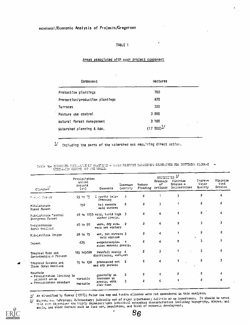
ecnnana jEconcrnic Ana I ys is of Projec ts/Gr eger sen

TABLE 1

Areas associated with each project component

Component Hectares

Protection plantings

Protection/production plantings

Terraces

Pasture use control

Natural forest managenent

Watershed planning & Adm.

760

870

320

3 850

3 160

(17 500)1/

1/ Including the parts of the ,catershed not requiring direct actior.

C" - nEZ0===/.;72:E; 0EJEcz:7Es i -

"""- CF

PrecipitationknnualAmounts

(cc)

Incresze

Commenta quantity

2/Drainace Nizinizo

Reduce of Erosion

Flooding Wetlands Eedimentation

Improve MinimiteWater Windquality Erosion

25 to 75 months be:owfreezing

hot summers 2

cold winteroYid-Latitude 750

Mixed Foreot

Mad-Latitzte rotate..Evergreen Forect

3

40 to 7250 mild, humid high 3

winter ;:rectp.

Mediterranean 40 to 90

Scrub -,;:c.iiand

Mid-Latitude Itcppe 30 to 75

2coert 425

Tropical Rain andEmi-docidua.a To.. .

Tropical itsvanna and:nom: ;crud Wood:and

warm, dry ezm- 2

rera wet winters

wet, hot zerocold winters

3

evapotranapir- 1

ation exceeds precip.

165 to>760 rainfall evenly 4

distributed, warm,wct

75 to 130 pronounced wet 2

and dry periods

Maintain- Precipitation limiting in

ad!aecnt ar",n variable

- Fretipitaticn abundant variable

generally an 2

increase inprocip. with 3

elevation

2 3

2 3 1

2 4 1

2 4 2

2 4 1

2 4 2

2 3 1

2 4 1

2 4 2

2 4 1

2 4

2 4

2 4

3 3

2 2

3 2

3 4

2 3

2 4

2 4

jJ Ac classified by Rumney (19C1); Polar ice cap and tundra climatea were not conoiderod in thin analysis.

ij Ob:cati?ea: 1.PrImv-y; 2.2acondary; 3.Uoually not oz major importance; 4..Littlo or no importance. :t should be noted

t!7,...t c00% ob:ettiveo are highly dependent,upcn i1da1 waterched characterictico including topoev..phy, olopco, and

solia, and other factoro mush as land ume, population, and level of econoTic development.

86

econanal/Economic Analysis of Projects/Gregersen

Table 2 - Weterrhed Protest: :Centifitaticn of Water 2enefito

(1)

Year

(2) (3)rnervoir Carnaitv

(4)Differencewith 1c with-out pro:set

(millions of

(5)7enorNoir 11z.:

r3/yr)(7)

Difference;La .aze with 1.

2/w11:.set

pro:ect

witn

pro:ect

wathoztproject

with

projectl/without

0 100 1C0 0 86.0 66.0 0

1 95... 99 3 26.4 86.4 0

2 92 93 6 66.3 86.3 0

3 53 97 9 87.2 37.2 C

4 9.4 56 12 64 87.7 3.7

5 .83 95 15 80 63.2 3.2

6 76 54 le 76 38.7 12.7

7 72 53 21 72 69.: 17.2

8 53 92 24 63 69.a 22 .:.

9 64 91 27 64 93.4 26.4

10 60 iC 30 60 90 30.0

56 89 33 56 69 33

12 52 28 36 52 85 35

13 43 67 39 43 87 39

14 44 .86 42 44 85 42

15 40 65 45 40 65 45

16 34 64 48 36 24 42

17 32 63 51 32 83 51

13 23 62 54 28 82 54

19 ;%-: 81 57 24 61 57

20 23 EC 60 20 20 60

21 16 79 63 15 79 63

22 12 76 66 12 73 66

23.......

F.

4,

77

76

6972

a4

7776

6972

25 3 0 75 0 75 75

2/ Conotrained by derrad. forwater durine first 4 years themconolraired by capacity azdomand outatripo eepp:y

2/ Coentrained by dettand forfirst 10 yearu then conotrLnee.by capacity az d.-and outstrip°c.4.crit; ewa wi:n the p-azect

2 Thin in tho meszure Cue tothe project, i.e. tho difforencein use with and without theproject

:nblo 3 Input° and Cato::t.: - ?redaction roreat Comronent

0 1 2 3 4 j 6 7 8 9 10 11 -16 17 18 19 20 21

Ha slanted 174 174 174 174 174 174 174 174 174 174

7hirnini: harvestha 174 174 17., 174 174

C 3/ha 20 20 20 20 20

total m 3480 3480 3420 3480 3480

Tlmal 1:arvnt

ha '14 774 174 174 174

:n3jh 3:5 525 525 525 325

total r.3( 1;00)91.3 91.3 91.3

17

econanal/Economic Analysis of Projects /Gregersen

Table A Value F1o. Table

(mmtlione of ;cepa)

0 1 2 3 4 5 6 7 8 9 10 11 12 13 14 15 16 17

sr.cryrrs

1 /rriention&emetic es, 0 0 0 0 7.4 16.4 25.4 M.4 45.6 52.8 60 66 72 78 84 90 96 102

2 Wood vrodue-lion 1.0 1.0 1.0 1.0 1.0 26

3 Total 0 0 0 0 7.4 16.4 26.4 35.4 46.6 53.8 61 66 72 78 84 90 96 125

CA S9

4 Plan:Inc pr,teetton foryet 3.4 4.5 1.1

5 Plantine Imro-dJetmon forest 1.3 1.6 1.6 1.6 1.6 0.3 1.3

6 Terrsze con-strue:mon 0.8

7 Mano.lneent

costa 2/ '.0 1.0 1.0 1.0 1.0 1.0 1.0 1.0 1.0 1.0 1.0 1.q 1.0 1.0 1.0 1.0 1.0 1.0

8 Tmtal 6.5 7.1 3.7 2.6 2.6 1.3 1.0 1.0 1.0 1.0 1.0 1.0 1.0 1.0 1.0 1.0 2.3

9 In Br:) -IT(0091) (6.; 7.1 3.7 2.6)4.8 15.1 25.4 34.4 45.6 52.8 60 65 71 77 83 89 95 125.4

10 Present Valueat 13% (6.5 6.3 2.9 1.8)3.0 12.9 12.9 15.6 18.4 19.0 19.3 19.7 19.2 17.6 17 16.3 15.5 18.3

YPu at 12%11 rPV at 12% P292 million

2/ ineludinc protactioo and crtenoion sersteeo, maintenmumee and admnmotration

Figure 1

levelof

production

present level

0

(present) > (end of project)

A - losses avoided

B production increases over presentevel

18 88

18 19 20 21 22 23 24 25

108 114 120 126 132 138 144 156

26 26 26 26

134 140 146 152 132 138 144 150

1.6 1.6 1.6 1.6 0.3

1.0 1.0 1.0 1.0 1.0 1.0 1.:

2.6 2.6 2.6 2.6 1.3 1.0 1.0 1.0

131.4 137.4 143.4 149.4 130.7 137 :43 149

17.1 19.9 14.9 13.8 10.8 "3.1 9.4 2.8

-gsyst/Agr icu I tura I Systems /Cox

A Simi f i ed Approach to Agricultural Sys tems

by

Milo L. Cox

Deputy Directoi, Office of Agriculture, Technical Assistance Bureau, Agency forInternational Development.

Reprinted from a revised paper prepared for the 1972 Conference of the SoutheastAsia Development Advisory Group Singapore, Septclioer 1972.

IssuesAgriculture directly controls the economic and social life of about 70% of the world's

people. The present state of this agriculture, although improving slowly, still inhibits economicprogress, frustrates the improvement of rural life and encourages urban migra*ion. Acceleratedlevels of economic development, political stability and human well-being depend strongly upon therate at which the LDCs adopt measures for solving four primary agricultural issues, namely:

A- Materially enhance political response to the rural sector.B. Significantly increase the production, distribution and utilization of food and fiber.C. Greatly improve effective rural income levels.D Substantially ;;crease the wise utilization of agricultural resources.

Performance to DateSporadic progress has been attained in each of the above basic issues facing the LDCs, but

this progress has been slow and erratic. Rural per capita incomes have remained below one-third of

urban incomes and generally have failed to increase proportionately with rises in the GNP. Farmproduction in absolute terms has grown, but per capita food production has remained relativelystatic on a world basis. Gov ernment response to the needs of the rural sector, in terms of priceincentives, infrastructure, agricultural research, credit availability, marketing functions, and

Ministry of Agriculture budgets has been inadequate and vast areas of potentially productive lands

stir remain idle.

These consraints, among others, have resulted in production levels that have aboutmaintained the status quo These levels are too low to satisfy the nutritional needs of growingpopulations, too low to allow the agricultural sector to contribute substantially to overalleconomic growth, and too low to offer hope for an improved future to the millions of subsistencefarmers saddled with present inequities.

Progress towards the attainment of acceptable rural living levels for the mass of theworld's farm population i. grossly unsatisfactory. Failure to substantially improve these levels ofliving tends to increase migration to the cities, creating new influxes of the discontented uponalready smoldering urban frustration and preventing the settlement of new lands and the acceptanceof modern techniques of -agriculture production on the farm.

Early U.S. efforts in attempting to impr8enagriculture in the LDCs were directed primarily

agsyst/Agricultural Systans/Cox

towards the transfer of the techniques of production. These techniques resulted in increased yieldsbut markets were unreliable, inputs often expensive, credit limited and farm prices low, thusexpected profits did not generally accrue. Recent improved analyses of the total economic andsocial environment offer much broader understanding., more viable approaches and new mechanisms bywhich an economic environment can be established in which agricultural progress is possible and thetechnology truly useful.

Constraints and OpportunitiesThe physical character of the agriculture of any country is largely shaped by the character

of the land forms, soils and climate of the region, but what happens within the constraints imposedby physical charcteristics is closely related to economic, social and political as well as agronomicforces and the relative balance between these forces. It is the first premise of technical,assistance that these forces as well as some of the physical features are alterable, that bydeliberate but careful adjusment, both the direction and pace of agricultural development can bealtered, and that the economic, social and political costs of such alterations need not beexcessive.

Changeable though these factors are, there remain the constraints imposed by the very natureof the typical agricultural system -- which is large, ponderous, geared to biological and seasonalclimatic forces, made up of thousands of widely dispersed units and controlled by the mostconservative and least literate segment of the population. Because of the nature of these systems,little that is positive can be accomplished by force, quotas, penalties or other such uses ofgovernment authority. Even under the most carefully controlled conditions of a police state, thesemeasures have resulted in disappointing output, and sometimes in agricultural chaos and governmentalfrustration. The second premise of technical assistance in agriculture then, is that the systemmust be led or pulled, not forced nor driven. There exists a diversity of tools that can be usedfor leading or pulling the agricultural sector towards desirable change, some of which can be usedor influenced by technical assistance. Others require political actioi en;;ghtened by adequateknowledge of how the agricultural system works.

Farmers' DecisionsThe farmer's choices, among alternative production activities, are influenced not only by

customs and habits carried over from the past, but by the incentives and opportunities to improvehis income and social situation and by the risks associated with these opportunities, as he seesthem. As stated in the first premise above, many of these factors are alterable. Thus, technicalassistance in seeking to foster constructive change, should concern itself with the environment ofincentives and opportunities for productive activity and the concommitant risks that face theindividual farmer. Improvements in incentives and reductions in risks exert the pull on which thesecond premise is based.

The adjustable components of this environment are primarily the set of government policiesaffecting agriculture and the set of institutions providing services to agriculture. For example, aprice policy change can provide the farmer with an incentive to produce, but he may not be able torespond to this incentive without access to adequate credit, technical, marketing, risk bearing orother services that he needs.

In any case, what happens in agriculture in nearly any country, is the sum or total of theeffects of hundreds of thousands of individual farmers' decisions. The farmer hopes that thedecisions he makes will be to his greatest economic and/or social advantage. His government andA.I.D. hope that the decisions he makes will be to the advantage of the country's economic andsocial development. Our role is to foster the selection of choices in such a way that when thefarmer makes the decision that is best for him, it is also likely to be best for the development ofthe country in which he lives. This is the essence of helping the agriculture sector to adequatelyfeed a growing population, contribute significantly to overall economic development and hopefullyresult in a better life for the peor.:e of the LDCs.

90

agsys t/Agr i cu I tura I Sys terns/Cox

Agriculture Sector AnalysisAn agriculture sector analysis is essentially a detailec, study of agricultural production,

distribution anci .itilization systems, the major components of such systems and the many factorsinfluencing these systems. A thorough understanding of the components of an agricultural sector isnecessary for the setting of realistic goals, the formulation of acceptable strategy, the

development of workable plms and the structuring of implementing activities. A sector analysis,systematically applied to reasonable accurate dea, should describe the main components of theagricultural sector, the relative health of the components, how these pieces fit together, how theyinterface with and influence each other and the sensitivity of agricultural systems to intentionalor naturally occurring changes in components or factors. Also, the analysis should indicate thedegree, timing and location of changes required to achieve selected goals.

Strategy formulation and planning, if they are to be truly meaningful, ought to be based onrather comprehensive in depth analysis of the sector one hopes to influence. Detailed analysis ofthe agricultural sector and the relationship of this sector with all other sectors in the economyare universal needs in developing countries. Interaction among and interfaces between the variouscomponents of the agricultural sector need to be evaluated by interdisciplinary groups that canbring to bear broader understanding than that provided by specialists in the many componcn:sinvolved in the flow of events from original inputs, through production to eventual marketing andutilization. Although such sector analyses must be closely oriented to the specific countryinvolved, there is a universal need for this type of approach in all developing countries.HistoricaVy, where assistance groups have Failed to effectively promote continuous improyt;nent inagriculture over time, there has often beer. a failure to do enough analytical work to be able topredict the probable rate of development or response and to plan and decide what to do when certainprogress levels have been achieved and then follwoed by a decline and demise are usually based onincomplete systems.

Institution or subsector analyses do not appear to be adequate bases for selection amongvarious program alternatives within or among sectors. Criteria and measures which are broadlymeaningful and which allow comparison of relative projects and programs must be developed.Intersectoral and sectoral analyses and planning should provide a fairly complete staging of inputsand outputs which permit tracing of actions and responsibilities through the system for rapidisolation of lagging elements and provision for timely remedial action. The full application ofevaluation as a management tool is only possible within such a complete system. Effectivemanagement also requires that at each management level, the manager be able to view his own stage inrelation to the stages that feed him inputs and those which are consumers of his outputs and tounderstand the overall relationships and implications of his actions. Flexibility must be builtinto the system to permit the manager to detect probable lags and shift resources intelligently toobtain essential outputs within the time limitations and to request am' obtain additional resourcesor to alert managers at the appropriate levels of an anticipated lag so they can modify theirtargets or take other appropriate action.

This whole process then depends heavily upon a thorough understanding of the way theagricultural sector works, the internal and external mechanisms involved, the state of developmentand general healt' of the many interrelated romponents and the effects of policies and practicesexercised by the government. A thorough sector analysis should provide this fundamentalunderstanding upon which strategy and planning depend. Of all the functions carried out byassisting agencies in the developing countries, this one has received the least attention, yet nobetter method has been found for placing in perspective the entire complex of agricultural systems,to identify problems and plan corrective action at important points in the economy.

The general principles of how to conduct such analyses so as to achieve an unbiased and

91

agsys t/Agr isul tura' Systems/Cox

factual evaluation of the agricultural sector are now generally known and the techniques, met: odsand procedures for carrying out a sector analysis are now being better defined and more adequatelystructured.

The level of sophistication of a sector analysis can vary from quickie type studies of a fewweeks' duration through more comprehensive analyses lasting a few months at least through onecropping and marketing season to one or twoyear very thorough and detailed studies made by amultidisciplinary team of experts assisting host country analysis teams. Th..; ultimate is a neverceasing study that continuously upgrades and improves the analytical work, based on a constantstream of new data. Thr, type analysis decided upon for any one study depends largely upon 1) the

kinds of infc 'nation needed for the level of strategy and planning contemplated, 2) the nature ofcommitments I be made based on the study, 3) the time available for the study or the degree ofurgency, 4) the number and competence of analysts that can be supplied by the host country, 5) theorganizational structures from which these analysts are drawn, and 6) the funds available for thestudy. A very special problem exists particularly for small countries having inadequate numbers oftrained analysts, no organized analytical institution, very little available funding and an urgentneed for a sound planning base.

The developing countries ordinarily do not have adequate members of trained agriculturaleconomists to carry ou sector analyses, identify the most useful development strategies, provideadequate planning, encourage helpful policy formulation, structure improved m sketing systems andeconomic reseearch and to work with production specialists in improving efficiencies and

profitability in farming systems. The problem of a low agricultural economics capability oftenprevents adequate analysis of ADC problems, allows poor choices among alternatives to go unnoticed,

creates distortions in programs where interactions are critical and may make the selection ofconditions precedent to sector loans difficult or awkward.

Simplified SystemsMany countries do not have the resources for, and may not really have the need for, highly

sophisticated detailed studies and simulation models in order to do adequate planning. Yet failureto understand the agricultural system or the inability to adequately estimate the sensitivity of thesystem to specific changes in any of its parts, usually results in a hodgepodge of more or lessunrelated projects, each in itself a good thing, but not adding up to an integrated program. Othersuch projects fails to achieve their individual goals because of other more limiting but undetectedfactors elsewhere in the system that prevented the expression of success in an otherwise goodproject. What is needed then is some kind of a simplified systems approach that is admittedly lessthan perfect but that would allow the planners to view the whole system at once so that a largenumber of variables and their interactions can be considered simultaneously. By such a systembottlenecks can be more readily identified, knowledge and -action gaps surfaced, interactionsestimated, institutional or organizational deficiencies pinpointed and alternate pathwaysconsidered. A very simple and highly generalized flow chart of such a system is included here, asFigure 1, that shoWs the central components of an agricultural system. This chart is a bareskeleton in that each block on the chart could be enlarged into a system of its own and other blocksadded as required in specific cases, but -a simplified form is adequate for this discussion.

Starting in the lower righthand corner with the block labeled food needs (for thisdiscussion, phrases or words underlined refer to items on the chart), we h' 'e a block that is easilycalculated for any given country. All the data needed are the number of people in the population,the rate of pupulation growth and the amount of food considered to be an adequate diet for theregion, and food needs can be readily determined. This number, arrived at in this way, is oftenfrighteningly large and this is the number that has people and governments worried because it is

larger than food production in many coutnries. It is often large enough to make most governmentofficials reassess their doubts about Malthus. Now let's look at the next block labeled effectivedemand, This block represents the amount of food the population can afford to purchase or it's ameasure of the size of the market. Effective demand, particularly in a hungry country, is much

92

agsyst/Agricultural Systems /Cox

smaller than food needs. Therefore, if farmers produce up to the need level and throw thisproduction on a market (effective) that cannot absorb then this "overproduction" works its wayback through the system to farm prices. Farm prices fall, the incentive to produce is reduced andthe farmer tends to retreat into subsistence agriculture because he has no other alternatives and

this is precisely what we are trying to get him out of. If consumer costs are held down bygovernment policy (often done to maintain peace in the urban areas) the same thing happens to thefarmer. That is, sooner or later, farm prices and farmers' profits decline and his productionincentive goes down with it. If attempts are made to get farm prices up in order to increaseproduction then this is eventually reflected in higher consumer prices which are politicallyexplosive but worse than that, high consumer prices lower effective demand. This sets a ceiling onproduction more effectively than a lack of production technology. So we have a seesaw effect:trying to help the farmer and his incentives we hurt the consumer and demand.. Trying to holdconsumer costs down to get demand up we hurt the farmers' incentive. And we must have both i.e.,

there must be a strong incentive to produce and a demand for the product, else production will notincrease above subsistence levels.

One of the most workable ways to break his impasse is through the marketing process. There

is usually a large spread between farm prices and consumer prices. If efficiencies can be achievedin the marketing process then large savings can be achieved in the price spread. If policies aresuch that a part of _these savings can be ai:ocated to the farmer and part to the consumer thenincentive to produce and effective demand can be increased simultaneously. In the market block or.the chart there is a list (illustrative but not all inclusive) of factors that can usually be

improved. If market news can be made available to the farmer so that he knows the value of hiscommodity before he barters, if storage facilities are available for that production which cannot besold immediately, if items can be processed for sale later, if distribution is faster and cheaper,if spoilage can be reduced, then the spread can be reduced. Middlemen, multiple transfers and salestaxes on transactions contribute to large price spreads and much can be gained by efforts to

increase efficiency in this area. Paradoxically the middlemen -- shippers, warehousemen,wholesalers, retailers, etc. are the only organized group in the marketing process. Farmersrarely know what prices the ultimate consumer pays and the consumer is usually not aware of what thefarmer receives. The people who work in the price spread area are wonderfully adept at soaking upefficiencies achieved at either end of the marketing chain, i.e. if production costs are reduced,making lower commodity prices- possible, this is rarely reflected in decreased consumer costs.Conversely, when consumers must pay higher prices to farmers, this almost never results in higherprices to farmers. Government intervention that would increase competition in the marketing areausually pays big dividends in farmer incentive and consumer demand, both prime requisites fc

increased production.

The Government block has been divided arbitrarily into a national government that setspolicies and a local government that is more involved in local planning and organization. On thenational government side, a single policy, guaranteed minimum prices, is used as an example only.Any one or group of policies could be included or substituted for this one. Guaranteed prices donot mean a subsidized nor necessarily a very high price. It is intended as a floor or minimumprice. This reduces the farmer's marketing risks and gives him confidence to purchase the inputsrequired to get high yiIds. The problem with this procedure is that it is difficult to decide onwhich policies would give the best results and it is often difficult to get traditional policieschanged even when they have become disincentives to investment in the agricultural sector. Many

times policy changes are politically difficult for governments to make. Lending agencies usuallywrite policy changes into loan requirements but often write in too many conditions or insist onpolicy changes that really do not have much effect. That is to say that until the lending agencyhas gained competence in estimating the sensitivity of the production system to various policychanges made to different degrees and at different times, they are not yet prepared to wisely writethe conditions precedent to the loan. A systems approach should minimize this difficulty.

agsyst/Agricultural Systems /Cox

On the local government side, the most important factor assisting farm income is whereprivate sector processors offer farmers contracts for their production, at prices agreed to prior toplanting, if the farmers will meet processors' requirements for variety, quality, etc. This isalready working well in many countries for certain products. The difficulty here is that theprocess usually is helpful only to those farmers near the processing plant. But the basic principleis no different than the government backed guaranteed minimum price program. Both of these shouldtend to raise farm income and production incentive.

The production block is where most assistance agencies have put major emphasis. Here weexpect the private sector to provide cheaper inputs to farmers. This added to the productiontechnology coming from the experiment stations give higher yieles at lower per unit cost ofproduction. This gives increased farm profits without price changes. This process is a powerfultool in getting production incentives up without increasing consumer prices. The whole system thenis geared to getting consumer demand up without reducing farmers' prices or getting farm prices upwithout killing off the demand, or some desirable mix of the two.

If the private sector earns profits selling inputs to farmers, and they must, then this isreflected in somebody's increased income which is a major factor in demand. Farm profits increasedemand also, mainly for commodities other than food, but it is surprising how much processed food isnow sold in many rural communities. So we have come full cycle on the chart. Now the problem ishow do we get all of these blocks on stream at the same time. This is the basic strategy and whenthe system is working fairly well we expect:

1. Farm prices to improve2. The incentive to produce to grow and production to increase3. The price spread to decline4. Consumer costs to decline or remain stable or at least to

increase slower than income5. Effective demand to get closer and closer to food needs

the basic goal.

Now, we come to a seeming paradox. Almost everywhere in the LDCs we encounter markets fullof food. In the face of real hunger much food is for sale and it is mostly food of local productionand it is almost never all sold. This means essentially that the farmer has always traditionallyproduced up to effective demand and he is still doing so today. Actually, because there is a largespoilage component in storzge and in the wholesale and retail markets, the farmer is producing aboveeffective demand, by the amount of this spoilage, minus imports. Anywhere you travel, even inremote villages, if you have some money you can buy food. It is very true, however, that if all ofthe people had enough money to buy all the food they wanted, the local markets would run outquickly, but there is nearly always enough food to satisfy effective demand. Farmers know that theyonly drive markets down when they produce more than they can sell, so any program that pushesincreased production without getting demand up is likely to fail.

If the farmer has always met effective demand, how was this possible? Generally it has beenpossible because demand has always gone up slowly. Population growth and increased incomes bothtend to make demand go up (and they are both occurring all over the world) but spiraling consumerprices depress it. The resultant vector is a very slow rise in demand and a primitive agriculturecan change fast enough to meet this slow demand rise. Farmers have traditionally done this byincreasing the land cultivated or, in their own limited way, increased the intensity of theiragriculture. They have not generally gone the route of purchased inputs and high level technologywhere quantum jumps in production are possible basically because it has not been profitable. Butthey have about used up these two ways of increasing product in. There may be more land but it is

remote and not economically available to the farmers and they cannot intensify much more withoutresorting to high cost inputs of fertilizers, new varieties, pesticides, etc. Therefore, ifeffective demand for food should take off undelle impetus of population growth and increased

6

agsyst/Agricultural System /Cox

incomes, then a primitive agriculture would no longer be adequate and means would have to be foundto make new lands available to the farmers or increase his profits to the point where he couldafford technical inputs or some mix of the two.

The system then is like a heating system that pumps hot water to ail the rooms in a house.It's a continuous system and any restriction anywhere in the house reduces the flow. The problemmay be upstairs, downstairs, in front of the pump, behind the pump or in the furnace, but arestriction slows down the whole system. If it was a complete stoppage the limiting factor couldreadily be located, but it is rarely so in agricultural systems. Different parts of the system maywork well or poorly at different times so a mechanism for locating bottlenecks that are not

obviously apparent is necessary.

There is nothing really new in this system. All of the items have been discussed for years.This approach is simply an attempt to organize the major factors in such a way that the effects ofeach part and the possible interaction between parts becomes apparent. Analysis of the agriculturalsector along these lines should show where major effort is required and should tend to concentrateresources on the most limiting factor. This is particularly important because usually there are notenough funds to work on all the various parts at once. As soon as the most limiting factor has beenidentified and progress is being made 'towards a solution to this particular problem, then attentioncan be directed at deciding which factor will become the most limiting once the first one has beensolved. By this process an order of priority can be established.

Of copurse this chart must be altered to fit corditions in any specific country. In its

present form it is so generalized that it may omit factors peculiar to a given country. For

simplicity many factors have been omitted but are implied. Research must be applied at severalpoints, particularly to production and marketing, extension activities fit between the productionblock and the farmer, land tenure problems could be attached as a policy problem, etc., until thechart fits the country of concern to the planner. This approach is simply a plea for orderlythinking about a food problem. It is no panacea nor is it a substitute for careful analysis,thoughtful strategy formulation and detailed planning. Rather it is a tool that should facilitate

7

agsys t /Agr icu I tura I Systems /Cox

A Proposed Development Sequence

A. Data (What do we know? What are orders of magnitude? How are data collected?How reliable? Are there gaps?)

B. Analysis (Where are we? What is the data trying to tell us? What does it reallymean to people? What do we have to work with? What can we do?)

C. Goals, Objectives (Where do we want to go? What are we trying to achieve? What is thepurpose of outside help?)

D. Assessment (Is C realistic? Overstated? Understated? Are there reasonable ways toget from B to C? Can they be financed? Administered?)

E. Essential Steps (What are the major things needed to be done to reach C?)(Strategy)

F. Planning (What are workable methods and means? What kind of a plan is needed toaccomplish E?

1. Is it technically possible?2. Is it economically feasible?3. Is it politically acceptable?4. Is it administratively practical?5. Is it socially desirable?)

G. Organization (How do we set up a system to make A through F a continuous operation and toaccomplish E by carrying out F?)

H. Implementation (Put F in motion, administered by G)

I. Evaluation

J. Feedback

(Is H going ahead? Are G and F working? Are we headed towards E? Will

this lead us to C in a reasonable time frame?)

(Have I revealed errors or indicated a waste of resources which we do notwant to repeat? Or success we do want to repeat? Feed back I informationto A through H to upgrade system)

8

96

extreme/Estirating Return Extreme Events/Vogler

Estimating Return Periods for Extreme Events

Ken Vogler

Watershed management often involves the design and construction of flood control structuresand soil and water conservation works. The size of structures or works must be economicallyfeasible and should be designed to handle safely extreme events. Thus, it is necessary to estimatethe magnitude of a hydrologic event, such as runoff volume or peak flow, that can be expected toequal or exceed the design of the structure at least once during its projected lifetime.

These extreme events are analyzed using probability distributions as models and are oftenclassified in terms of a return period. The return period has been defined as the average intervalin years between events which equal or exceed the considered magnitude of the event. Return periodsare determined for many hydrologic processes including rainfall depth, rainfall intensity, runoffvolume and peak flow.

Extreme event data is often considered in two ways, as an annual series acid as a partialseries. The annual ceries are those data which consist of the peak value for any particular year.The partial series consists of those data which exceed a certain base value, regardless of thenumber of times that base is exceeded in a year. The annual series is advantageous because mosthydrologic data is processed in a way which makes it easy to get peak annual events and a goodtheoretical basis has been established for extrap3lation of peak annual events. A principleargument against annual series is that it does not consider large events which are not peak annual

events. On the other hand partial series considers all events above a base level. Because of thelack of independence that can occur between events, good statistical theory has not yet beendeveloped for partial series. Partial series does give larger values for lower return periods thandoes annual series; however, both give essentially the same values for return periods greater than

ten years.

In this paper, the annual series will be considered for which the Gumbel Extreme ValueDistribution has been found to fit observed data very well. Often extreme value data will not fit aGumbel distribution and other distributions such as the Log Pearson Type III should be consids-ad.

A graphical technique is used in which observed data are plotted on Gumbel graph paper andthe magnitude of the event is simply read off the graph for the desired return period. If the meanand mode of the data are known, then these points can be plotted on Gumbel paper and used to draw astraight line which also represents the relationship between magnitude and return period. Opinion

is currently divided as to which of these two methods is preferable.

ProcedureAnnual peak values are chosen for a given hydrologic process, i.e., rainfall depth/event,

daily rainfall depth, average daily discharge or instantaneous peak discharge, for a data record of

at least thirty years. Peak values are ranked in increasing order and assigried a number startingwith one for the smallest event. The relative frequency is estimated as:

where f = frequency of occurrencem = rank assigned to the peak valuen = number of years of record.

f = m/(n +1)

I

9 7

extreme /Estimating Return Extreme Events/Vogl er

The relative frequency is then plotted with the corresponding peak annual value on Gumbel

paper. A straight line is fitted to the plotted points by "eyeballing" and the values for peakannual events are then read for a given return period or probability of occurrence.

Exarp I eThis example compares peak annual instantaneous runoff values fitted to the Gumbel and the

Log Pearson Type Ill distributions. Thirtysix years of data from the Sabino Creek Basin nearTucson, Arizona are used. In this case, the Log Pearson distribution gives a better fit. A

discharge of 4690 cfs is expected for a return period of 25 years using this distribution. On the

other hand it is difficult to determine what the discharge will be from the Gumbel distributionbecause of the wide variation between the eyeballed line and the statistical line (3,150 and 3,600cfs respectively).

Sabina Creek

To determine the number of intervals in a hist4gram

K 1 + 3.3 log n

where n = number of years of record

K = 6

interval no. of

in cfs occurences

0 - 1000 18

1001 - 2000 8

2001 - 3000 5

3001 - 400 2

4001 - 500Z

5001 - 6000 2

Mode 500

mean 1527.0

Var. 1977804

SO. 1406

Sabino Creek

Statistical Parameters for Log Pe. son Type III

log mean = 2.999log s = 0.435log coef.'skew s-0.556105log Q = log Ma + K (log a ;

Recurrenceyears

a

chance

K

interpolated

log Q

2 50 0.092 3.03902 1,094

5 20 0.857 3.371795 2,354

10 10 1.207 3.524045 3,342

25 4 1.545 3.671075 4,689

50 2 1.745 3.758075 5,729

100 1 1.913 3.831155 6,779

200 0.5 2.056 3.89336 7,823

1000 0.1 2.330 4.01255 10,293

Formulas used

1 N 1 N - I

mean a -7.1 z Xi S = 47371 z (xi - x).-imi 1 =1

1 N

Coefficient of Skew (g) N : (Xi - ;)3i=i

S3

Values for K are determined from Tables of Skew Curve Factors forthe Log Pearson Type. III distribution using g.

3 90

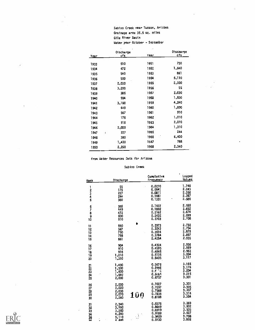
Sabino Creek near Tucson, Arizona

Orainage area 35.5 sq. miles

Gila River Basin

Water year October - September

YearOischarge

cfs YearOischarge

cfs

1933 510 1951 750

1934 472 1952 1,640

1935 540 1953 861

1936 500 1954 5,110

1937 2,020 1955 2,000

1938 3,200 1956 55

1939 385 1957 2,030

1940 904 1958 1,500

1941 3,180 1959 4,240

1942 449 1960 1,600

1943 567 1961 910

1944 175 1962 1,010

1945 916 1963 2,070

1946 2,000 1964 1,310

1947 1 227 1965 244

1948 380 1966 6,400

1949 1,430 1567 788

1950 2,260 1968 2,340

from Water Resources Data for Arizona

Sabino Creek

Rank Discharge

1 55

2 175

3 227

4 244

5 380

6 385

7 4498 472

9 500

10 510

11 540

12 567

13 750

14 788

15 861

16 904

17 910

18 916

19 1,010

20 1,310

21 1,430

22 1,500

23 1,600

24 1,640

25 2,000

26 2,000

27 2,020

28 2,030

29 2,070

30 2,260

31 2,34032 3,180

33 3,200

34 4,240

35 5,110lc A AtIA

IP

109

CumulativeFrequency

LoggedValues

0.0270 1.740

0.0541 2,243

0.0811 2.356

0.1081 2.387

0.1351 2.580

0.1622 2.585

0.1892 2.652

0.2162 2.674

0.2432 2.699

0.2703 2.708

0.2973 2.732

0.3243 2.754

0.3514 2.875

0.3784 2.897

0.4054 2.935

0.4324 2.956

0.4595 2.959

0.4865 2.962

0.5135 3.004

0.5405 3.117

0.5676 3.155

0.5946 3.176

0.f "S 3.204

0.6464 3.2150.6757 3.301

0.7027 3.301

0.7297 3.305

0.7568 3.307

0.7838 3.316

0.8108 3.354

0.8378 3.369

0.8649 3.502

0.8919 3.5050.9189 3.627

0.9459 3.7080.9730 3.806

soiloseq/Soil Loss Equation/Thames

Predicting Soil Loss

J. L Thames and J. M. Kramer

At present the Universal Soil Loss Equation (USLE) is the model most often used to predictsoil losses. Especially in the U.S., the equation has been adopted by the Soil Conservation Service(SCS) for via* concerned with areal erosion. For many years the equation, developed by Wischmeierand his associates from 1957 onwards (i.e, Wischmeier and Smith, 1965; Wischmeier and Smith, 1978),has been used on agricultural lands, from 1 971 on construction sites and from 1 972 onwards also forrange and forest lands. Correlations have been satisfactory for conditions in North America, butthe equation may not always apply in other environments. For instance, the rainfall factor (R) hasa high correlation with soil loss on Java, Indonesia, but a poor correlation with soil loss inBenin. Therefore, the equations may need- to be adapted to local conditions, especially thesignificance of the rainfall fa,,:or (R) and the croppingmanagement factor (C). Also, although theUSLE equation is a simple steadystate model, it requires a rather sophisticated data set,especially with respect to rainfall (daily records over a number of years), vegetation, and, to alesser extent, soil conditions. Even when sufficient data are available some caution is neededbecause little experience has been gained on slopes over 20° or longer than 150 m (500 ft).

This section is mainly based upon Wischmeier and Smith, Agriculture Handbook No. 282,Arnoldus, 1977.

The Basic Equation

The basic equation is

and is written as

A=RxK xLSxCxP

A=RKLSCP (1)

In which

A = computed soil loss per unit area; obtained by multiplication of the remaining factors.

R = rainfall factor; the number of erosion index units (El units) in the period of consideration.The erosion index is a measure of the erosive force of raindrop impact.

K = soil erodibility factor; the erosion rate per unit of erosion index for a specific soil, in a

cultivated continuous fallow on a 9 percent slope, 22.1 m (72.6 ft) long.

L = slope length factor; the ratio of soil loss from the field slope length to that from a 22.1 m(72.6 ft) length on the same soil type and gradient.

S = slope gradient factor; the ratio of soil loss from the field gradient to that from a 9 percentslope, on the same soil type and slope length.

C = croppingmanagement factor; the ratio of soil loss from a field with specific cropping andmanagement to that from the fallow condition on which the factor K is evaluated.

P = erosioncontrol practice factor; the ratio of soil loss with contouring, striperopping or

terracing etc., to that with straightrow farming, upanddown slope.

11)

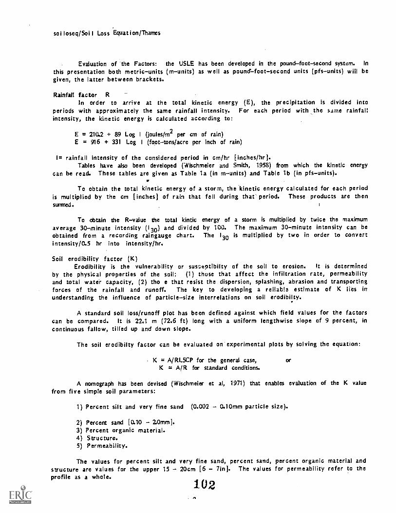
soiloseq/Soil Loss Equation/Thames

Evaluation of the Factors: the USLE has been developed in the poundfootsecond system. In

this presentation both metricunits (munits) as well as poundfootsecond units (pfsunits) will begiven, the latter between brackets.

Rainfall factor R

In order to arrive at the total kinetic energy (E), the precipitation is divided intoperiods with approximately the same rainfall intensity. For each period with the slate rainfallintensity, the kinetic energy is calculated according to:

E = 210.2 + 89 Log I (joules/m2 per cm of rain)E = 916 + 331 Log I (foottons/acre per inch of rain)

1= rainfall intensity of the considered period in cm/hr [inches/hr].Tables have also been developed (Wischmeier and Smith, 1958) from which the kinetic energy

can be read. These tables are given as Table la (in munits) and Table lb (in pfsunits).

To obtain the total kinetic energy of a storm, the kinetic energy calculated for each periodis multiplied by the cm [inches] of rain that fell during that period. These products are thensunned.

To obtain the Rvalue the total kintic energy of a storm is multiplied by twice the maximumaverage 30minute intensity (130) and divided by 100. The maximum 30minute intensity can beobtained from a recording raingauge chart. The 130 is multiplied by two in order to convertintensity/0.5 hr into intensity/hr.

Soil erodibility factor (K)Erodibility is the vulnerability or sus,.;totibilty of the soil to erosion. It is determined

by the physical properties of the soil: (1) those that affect the infiltration rate, permeabilityand total water capacity, (2) tho e that resist the dispersion, splashing, abrasion and transportingforces of the rainfall and runoff. The key to developing a reliabizt estimate of K lies inunderstanding the influence of particlesize interrelations on soil erodibilty.

A standard soil loss/runoff plot has been defined against which field values for the factorscan be compared. It is 22.1 m (72.6 ft) long with a uniform lengthwise slope of 9 percent, in

continuous fallow, tilled up and down slope.

The soil erodibilty factor can be evaluated on experimental plots by solving the equation:

K = A/RLSCP for the general case, orK = A/R for standard conditions.

A nomograph has been devised (Wischmeier et al, 1971) that enables evaluation of the K valuefrom five simple soil parameters:

1) Percent silt and very fine sand (0.002 0.10mm particle size).

2) Percent sand [0.10 2.0mm].3) Percent organic material.4) Structure.5) Permeability.

The values for percent silt and very fine sand, percent sand, percent organic material andstructure are values for the upper 15 20cm [6 7in]. The values for permeability refer to theprofile as a whole.

102

soiloseq/Soil Loss Equation/Thames

Particle sizeParticle size is a major determinate of soil erodibilty. To improve the predictive value of

the two parameters they have been slightly redefined. Silt is considered to include very fine sandand the sand size range is somewhat reduced. The particlesize parameter is then defined as theproduct of percent silt and percent sand and silt.

Organic materialIt has been found that organic material in the range 0-4 percent is inversely related to

erodibilty and that the magnitude of this effect is related to texture (Wischmeier et al., 1971).The curve that relates percent organic material to erodibility is included in the nomograph. Inpart it explains the difference between topsoil and subsoil erodibilty, the latter having a reducedOM fraction.

Soil structureStructure type and size, but not grade, are important in determining erodibility. Structure

is coded as:

1) Very fine granular and very fine crumb (<1mm,).2) Fine granular and fine crumb (1-2mm).3) Medium granular, medium crumb (2-5mm).4) Platy prismatic, columnar, blocky and very coarse granular.

Soil permeabilitySoil permeability classes are designed to be deduced from routine soil profile descriptionL

A certain amount of flexibility in the system allows for experienced interpretations of specificsoil profiles. The basic classes, however, are sufficient for most field uses. They are coded as:

1) Rapid to very rapid.2) Moderately rapid.3) Moderate.4) Moderately slow.5) Slow.6) Very slow.

General permeablity classes guides are given in the USDA Soil Survey Manual (Soil SurveyStaff, 1 951), but laboratory determinations are not necessary in general. They supplemented theguides wi.h the following rules of thumb for codes 4, 5 and 6:

fragipan soils are coded 6;more permeable surface soils underlain by massive clay or silty day are :oded 5;moderately permeable surface soils underlain by a silty day or silty clay loam having aweak subangular or angular blocky structure are coded 4;if the subsoil structure grade remains moderate or strong, or the texture remains coarser

than silty clay loam, the code is 3.

Cakulation of KfactorThe procedure for evaluating the Kfactor with the use of the nomograph (Figure 1) is as

follows:

1) Enter the nomograph on the vertical scale at the left with the appropriate percentagesilt + very fine sand (0.002 mm 0.10 mm).

2) Proceed horizontally to intersect the correct percentsand curve (0.10 mm 2.0 mm),interpolating to the nearest percent.

103

soiloseq/Soil Loss Equation/Thaffes

3) Proceed vertically to the correct organic matter content.

4) Proceed horizontally to the right.

5) For soils with a fine granular or fine crumb structure and moderate permeability thevalue of K can be read directly from the first-approximation of K scale on the righthand edge of the first section of the nomograph (only in metric units).

6) For all other soils: continue horizontally to intersect the correct structure curve.

7) Proceed vertically to the correct permeability curve.

8) i',-4eed horizontally to the soil-erodibility \scale on the left hand edge of the secondse,Ition of the nomograph to read the value of K.

Experience with the nomograph in the U.S. led to the following additional recommendations(SCS, 1973):

1) K-values derived from the nomograph range from 0.93 [0.02 in pfs units] to 1.10 [0.69 inpfs units]. For practical purposes it suffices to use K-value classes, namely: 0.13; 0.19; 0.22;0.26; 0.31; 0.36; 0.41; 0.48; 0.56; 0.63; 0.71; 0.83; [in pfs units: 0.10; 0.15; 0.17; 0.20; 0.24;0.28; 0.32; 0.37; 0.43; 0.49; 0.55; 0.64.

2) K-values must be adjusted for coarse fragments if present. K-values for soils high incoarse fragments (gravelly, channery, shaly, slaty, cherty, cobbly, stony, or flaggy for thedefinitions see USDA Soil Survey Manual, 1951, pp. 215, 216.) are reduced by one or two classes. K-values for soils that are very high in these coarse fragments are reduced by two ar three classes.

3) In arid or semi-arid areas where erosion pavement is a significant factor in reducingsoil loss the K value should be reduced by 33 percent if the soli is stony and by 50 percent if itis very stony.

Slope length factor (L) and slope gradient factor (5)Slope length is defined as "The distance from the point of origin of overland flow to either

of the following, whichever is limiting for the major part of the area under considerations: (i)the point where the slope decreases to the extent that deposition begins, or (ii) the point whererunoff enters a well defined channel that may be part of a drainzo,-e network or a constructed channelsuch as a terrace of diversion" (Wischmeier, 1965).

The slope length factor is defined as:

L = (g/22.1)m (m)L = (t/72.6)m (pfs)

or-as

where: g = field slope length (meters, feet)m = exponent, influenced by the interaction of slope length with gradient and may

Also be influenced by soil properties, type of vegetation, etc.

The exponent value ranges from 0.3 for very long slopes with a gradient Of less than 0.5% to0.6 for slopes over 10%. The average value, app':cable to most cases is 0.5, the value used for thedevelopment of the slope-effect chart (Figure 2). The slope-effect chart allows one to read a valuefor the combined effect of slopa lengthand slope gradient. Figure 3 allows one to use this chart in cases where values for the exponentother than 0.5 are more appropriate. The figure translates the field slope length for slopes withexponents in = 0.3, m = 0.4 and m = 0.6 into equivalent slope length with exponent m = 0.5.

1 0 a

soiloseq/Soil Loss Equation[Thames

The slope gradient factor is defined as:

S = (0.43 + 0.30s + 0.043s2)/6.613

where: s = slope gradient (in %)

For slopes up to 20% and 350 m [1,148 ft] long the combined effect for slope length andslope gradient can be read from Figure 4 Far slopes from 10% up to 50% and up to 800 m [2,625 ft]long, a rough estimation may be obtained from Figure 5, but the relationship has not beensufficiently tested to indicate the reliability of the prediction.

Foster and Wischmeier (1974) have adapted the LS factor f..,r use on irregular slopes. Thisis especially useful on wildland sites which rarely have uniform slopes. They describe the combinedfactor as:

(s al'LS

s1=1 j1

4(72.6) 0.5

where: X . = distance in feet from the top of the slope to the lower end ofthe jth segment.

X = the slope Length above segmentj-1= overall slope length.

Si= S factor for segment j.

The graph in Figure 6 can be used in place of the equation. The graph is a family of curves, forspecified slopes ranging from 2% to 20%. The quantity (SX

1.5/72.60.5)is designated by the symbol

and is plotted on LogLog paper against *.he values of X. The graph is entered on the horizontalaxis with the value of 11 ir Moving upwards to the curve fa the percent slope fa the segment j, thevalue of 11 1j is read on the vertical scale. The graph is then entered with the value of X j toobtain the corresponding value of 11.,. The diff;rence then equals the quantity,

This procedure is repeated for each of the slope segments, and the n values of (ii2jii1j) aresummed. Dividing the sum by the overall slope length x gives the effective LS value determined bythis procedure is a function of all the segment lengths and slope steepnesses and also of theirparticular sequence on the slope.

P f s

j.

The percentage of the total sediment yield that comes from each of the n segments is alsoobtained by this computational procedure. The relative sediment contribution of any segment j is:

P2j Plj / E (P2j

P )

lj

Cropping management factor (C)This factor describes the total effect ,of vegetation, residua, soil surface and land

management on soil loss. The value of the factor is in most casen not constant over the year.Although treated as an independent vnriable in the eqnation, the "true" value of this factor is

probably dependent upon all other factors. Therefore, the value of the Cfactor needs to beestabnished experimentally in many rases.

105

soiloseq/Soil Loss Equation/Thames

For crops: Cvalues need to be established for each of the following stages for all cropsof the rotation (11):

period F: rough fallow (turn ploughing to seeding);

period 1: seeding (seedbed preparation to 1 month after planting);

period 2: establishment (from 1 to 2 months after spring or summer seeding; for fall seededgrain this period includes the winter months);

per iod 3: growing and maturing crops from the end of period 2 to crop harvest;

period 4 residue or, stubble.

It should pointed out that the value found for a period F in the rotation cannot beextrapolated to any other fallow periods within the rotation, because the value is influenced by thecropping history of the. soil, the nature and quantity of residue turned under and other factors.

In order to arrive at a proper value for a crop rotation the soil loss ratio (i.e. the ratioof soil loss from the field with the particular cropping and management to that of bare soil) has tobe adjusted according to the distribution of the erosionindex for each period, because fieldconditions are immaterial when there is no rain and most important when there is much rain.Therefore the soil loss ratio for each period is multiplied with the percentage of El 30index

applicable to that period. This percentage of El .30 index can easily be read from an erosionindexdistribution curve (see Arnoldus, 1977). Tables have been developed from which the soil loss ratiosfor the different periods of the common rotations can be read. In combination with the appropriateerosionindex distribution curve, zne Cvalue for any part of the rotation can be established. Thistable and the distribution curves are presented in Agriculture Handbook No. 537 (Wischmeier andSmith, 1978).

In areas of the world for which no guidelines for the establishment of Cvalues for fieldcrop exist, it is probably easiest to try to correlate soil loss ratio with amount of dry organicmatter pt.: unit area or with percent ground cover.

For permanent pasture, range lands and idle lands and for woodlands, tables have beenpublished (SCS, 1 975) from which the averge annual Cvalues can be read. These tables arereproduced as Tables 2 and 3.

Nonagricultural C factorsThe Cfactor portion of the equation is currently being modified to better express forest

management conditions. Nine elements have been selected that should be considered when developingthis factor for woodlands. The following is a summary of the elements based on that of Dissmeyer(1978).

Eight of the nine elements have been used in the development of the agricultural CFactors,only a few of which have been published. One new element has been developed for forest land thatdoes not occur in the agricultural environment namely the step element.,

The nine elements are soil consolidation, surface residue, canopy, fine roots, residualeffect of fine roots after tillage, contour effect, roughness, weeds and grasses, and steps.Surface residue is the effect of the area covered by litter, slash and live vegetation, which is thepredominant factor. The other eight factors are evaluation or modification of the influence of bareground.

106

soiloseq/Soil Loss Equation /Thames

Soil consolidation can be viewed as a modifier of the basic erosion factor (K -F actor). TheK-factor as published is for continuously tilled soil, in fallow condition with tillage up and downthe slope. Tillage breaks down soil structure, aggregates, bonds, etc., which leaves the soil moreerodible than unfilled soils. Research has found that if fallow plots are left unfilled, theerosion rate reduces over time until seven years have past where no further erosion reductionoccurs. At this point, the erosion rate is 45% of that of the original fallow conditions. Forforest soils the soil consolidation modifier of 0.45 is used. If the soil is tilled by bedding,discing, etc., the K-Fa:: tor is modified by a soil consolidation factor which is a function of timesince tillage.

Surface residue (that is, Jitter, slash, logs, rock, live vegetation, etc.) in directcontact with the soil surface is the first element to evaluate. The percent area occupied bysurface residue is projected into a chart to derive the factor.

The following elements plus soil consolidation apply to the bare ground only, so we focusour attention now to the exposed soil and its condition.

Canopy ever (litter, slash, logs, rock, live vegetation, etc.) in direct contact with thesoil surface is the first el ement to evaluate. The percent area occupied by surface residue is

projected into a chart to derive the factor.

Fine roots in the top one or two inches of soil are very important in tying soil par ticlestogether. These fine roots are the feeding roots of trees, grasses etc. The element is evaluatedby inspecting the bare area and estimating the percent area with fine roots and projecting onto agraph. Fine roots usually have to be physically removed by scalping or pushing the soil with adozer or tractor. This element is only used for non-till ed areas. If the area has been tilled thuscutting up this mat of fine roots, another element is used residual effects of fine roots aftertillage. This is read from a chart with a correction for time elapsed since last till ed.

If an area has been tilled, invading weeds and grasses, and sprouting are assumed tocompensate for decaying fine roots, thus avoiding double counting.

Contour tillage can reduce erosion and this element is used on disced and bedded areas. Thecontour element is a function of slope and alignment of the furrow within the contour. As slopeincreases the effect from this element decreases and as the alignment increasingly departs from thecontour, the effect decreases. This el ement is estimated by using a table, a chart and a simpleequation.

Roughness expresses the influence of surface depression storage available to trap on-sitesoil movement. This factor is estimated in the field.

Finally, the step element expresses the influence of small steps that form on hillsides as aresult of on-site erosion and deposition process. Close examination of the soil surface will oftenreveal a fairly large percent of the area in small steps. The element is a function of slope and ofthe percent area in steps. It is evaluated with the use of a chart.

The computation of the C-Factor is the simple multiplication of pertinent element factorsfor the disturbance.

Erosio-.-control practice factor (P)The effect of erosion-control measures is considered an independent variable, therefore it

has not been included in the cropping management factor. The soil loss ratios for erosion-controlpractices vary according to slope gradient. Soil loss ratios for contouring, contour strip croppingand terracing are given in Table 4. In the table, two values are presented for terracing: the

107

soiloseq/Soil Loss Equation/Thames

higher one describes the soil loss from the field, the lower one the effect on sedimment yield, thedifference being the sediment lost from the field but trapped in the terrace channel.

Soil Loss and Conservation PlanningFor conservation planning the soil loss tolerance (T)(i.e., the maximum soil loss that can

be tolerated) needs to be established. The following guidelines are used in the U.S.A. (SCS, 1974).

Soil loss tolerance (T), sometimes called permissible soil loss, is the maximum rate of soilerosion that will permit a high level of crop productivity to be sustained economically andindefinitely.

Soil loss tolerance values (T) of 2.3 thy:nigh 11.2 tons per hectare per year (I to 5

tons/acre per year) are used. The numbers represent the permissible soli loss where food, feed andfiber plants are to be grown. "T" values are not applicable to construction sites but can be usedon forest and wildland sites.

A single T value is normally assigned to each soil series. A second Tvalue may be assignedto certain kinds of soil where erosion has significantly reduced the thickness of the effective rootzone, thus reducing the potential of the soil to produce plants. over an extended period of time.For example, eroded phases of soil series that are shallow to moderately deep to a soil layer thatrestricts roots are commonly given a Tvalue one class lower than the uneroded phase of the samesoil. The following criteria are used by soil scientists and other specialists for assigning soilloss tolerance values (T) to soil series:

(1) An adequate rooting depth must be maintained in the soil for plant growth. For soilsthat are shallow over hard rock or other restrictive layers, it is important to retainthe remaining soil; therefore, not much soil loss is tolerated. The soil loss toleranceshould be less on shallow soils or those with impervious layers than for soils with goodsoil depth or for soils with favorable underlying soil materials that can be renewed bymanagement practices (Table 5).

(1) Soils that have significant yield reductions when the surface layer is removed by erosionare given lower soil loss tolerance values than those where erosion effects yield verylittle.

A maximum of 11.2 tons of soil loss per ha per year has been selected for use with theuniversal soil loss equation. This maximum value has been used for the following reasons:

I) Soil losses in excess of 11.2 tons per ha per year affect the maintenance, cost andeffectiveness of watercontrol structures such as open ditches, ponds, and other structures affectedby sediment.

2) Excessive sheet erosion is accompanied by gully formation in many places causing addedproblems to tillage operations and to sedimentation of ditches, streams and waterways.

3) Loss of plant nutrients. The average value of nitrogen and phosphorus in a ton of soilis about two to three dollars. Plant nutrient losses of more than twenty five dollars per ha peryear is considered to be excessive. (Monetary values are estimates from 1973.)

4) Numerous pnctices are known that can be used successfully to keep soil losses belowmaximum tolerable levels.

After having established the soil lass tolerance we can rewrite the USLE as:

CP T / RKLS1

solloseq/Soil Loss Equation/hames

By choosing the right cropping management system and appropriate conservation practices, avalue for the combined effect oi C and P can be established that fits the equation. In order to doso it will be helpful to consult the erosiorindex distribution curve of the area in order to singleout thc, most critical stages as far as rainfall agressivity is conceror=d, because these are thestages where improvements result in the greatest reduction in the Cvalue.

References Cited

Arnoldus, H. M. J., 1977. Predicting soil losses due to sheet and rill erosion. In: Guidelines forWatershed Management. FAO, Rome. 293 pp.

Dissmeyer, G. 1978. Soil loss prediction for forest lands. Personal communication.

Foster, G. R. and W. H. Wischmeier. 1974. Evaluating irregular slopes for soil loss prediction.Trans. American Association for Agricultural Engineers. 17(2) pp. 305-309.

Soil Conservation Service 1973. Advisory Soils 6: Soil erodibility and soil loss tolerancefactors in the Universal Soil Loss Equation. USDA, Washington, D.C.

Soil Conservation Service. 1975. .Tech. Release No. 51, Geology Procedure for computing sheet andrill erosion on project areas. SCS, USDA, Washington, D.C. 13 pp.

Soil Survey Staff. 1951. Soil Survey Manual. Ag. Handbook No. 18. Ag. Res. Service. USDA,Washington, D.C. 503pp.

Wischmeier, W. H. and D. D. Smith. 1958. Rainfall energy and its relationship to soil loss.American Geophysical Union Transactions. 39 pp. 285-291.

Wischmeier, W. H. and D. D. Smith. 1965. Predicting rainfall erosion losses from cropland east ofthe Rocky Mountains; guide for the selection of practices for soil and water conservation. Ag.Handbook No. 282. Agr. Res. Serv. in Coop. with Purdue Agr. Exp. Station. U.S.D.A. Washington,D.C. 47pp.

Wischmeier, W. H., Johnson, C. B. and B. V. Cross. 1971. Soil erodibility nomograph for farmlandand construction sites. J. Soil and Water Conservation. 26 pp. 189 -193.

Wischmeier, W. H. and D. D. Smith. 1978. Predicting rainfall erosion losses -- a guide toconservation planning. U.S.D.A. Ag. Hamdbook 537. 58 pp.

1O9

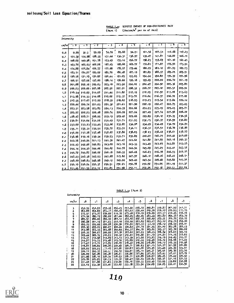
solloseq/Soil Loss Equation/Thames

TABLE 1.a: KINETIC EMMY OP HON.-OW:RAP= RAIN

(Part 1) (Joules /m2 per cm of rain)

Intensity

cm/hr . 0 . 1 . 2 . 3 ] I. 4 . 5 . 6 . 7 . 8 . 9

0.0 0.00 32.3 59.09 74.76. 85.e8 94.51 101.56 107.51 112.68 117.23

0.1 121.10 124.98 128.35 131.44 134.31 136.97 139.47 141.81 144.02 146.11

0.2 148.09 149.981 151.78 153.49 155.14 156.72 158.23 159.69 161.10 162.45

0.3 163.76 165.03 166.26 167.45 168.60 169.72 170.81 171.87 172.90 173.91

0.4 174.88 175.84. 176.77 177.68 178.57 179.44 180.29 181.12 181.93 182.73

C.5 183.51 184.27 185.02 185.76 186.48 187.19 187.89 188.57 189.25 189.91

0.6 190.56 191.19 191.82 192.44 191.05 193.65 194.24 194.82 195.39 195.96

0.7 196.51 197.06 197.60 198.14 198.66 199.18 199.69 200.20 200.70 201.19

0.8 201.68 202.16 202.63 203.10 203.56 204.02 204.47 204.92 205.36 205.80

0.9 206.23 206.661 207.08 207.50 207.91 208.32 208.72 709.12 209.52 209.91

1.0 210.30 210.69 211.07 211.44 211.82 212.19 212.55 212.92 213.78 213.63

1.1 213.98 214.33 214.68 215.02 215.37 215.70 216.04 216.37 216.70 217.02

1.2 217.35 217.67 217.99 218.30 218.62 218.93 219.23 219.54 217.84 220.14

1.3 220.44 220.74 221.03 221.32 221.61 221.90 222.19 222.47 222.75 223.03

1.4 223.31 223.58 223.85 224.13 224.39 224.66 224.93 225.19 225.45 225.71

1.5 225.97 226.23 226.48 226.74 226.99 227.24 227.49 227.74 227.98 228.22

1.6 c28.47 228.71 228.95 229.19 229.42 229.66 229.89 230.12 230.35 230.58

1.7 230.81 231.04 231.26 231.49 231.71 231.93 232.15 232.37 232.59 232.80

1.8 233.02 233.23 233.45 233.66 233.87 234.08 234.29 234.49 234.70 234.91

1.9 235.11 235.31 235.51 235.72 235.91 246.11 236.31 236.51 236.70 236.90

7.0 237.09 237.28 237.48 237.67 237.86 238.05 238 23 238.42 238.61 238.77

2.1 238.98 239.16 239.34 239.53 239.71 239.89 240.07 740.25 240.42 260.60

2.2 240.78 .240.95 241.13 241.30 241.47 241.64 241.82 241.99 242.16 242.33

2.3 242.49 242.66 242.83 243.00 243.16 243.33 243.49 243.65 243.82 243.93

2.4 244.14 244.30 244.46 244.62 264.78 244.94 245.09 245.25 245.41 243.56

2.5 245.72 245.97 246.02 246.18 246.33 246.48 246.63 246.78 246.93 247.01

2.6 247.23 247.38 247.53 247.68 247.82 247.97 248.12 248.26 248.40 248.5%

2.7 248.69 248.83 248.99 249.12 249.26 249.40 249.54 249.68 249.82 249.96

7.8 250.10 250.24 250.37 250.51 250.65 250.78 250.92 251.05 251.19 251.32

2.9 251.45 251.59 251.72 251.85 251.98 2x2.11 252.23 252.38 252.'1 259.44

TABU: 1.at (Part 2)

Intensity

cm/hr .0 .1 .2 .3 .4 .5 .6 .r .3 .9 .

3 252.76 254.03 255.26 256.45 257.60 258.72 259.81 260.87 261.90 2e7.91

4 263.88 264.84 265.37 766.68 267.57 268.44 269.29 2/0.12 210.93 771.73

5 272.51 273.27 274.02 214.76 275.48 276.19 276.89 271.57 278.25 279.91

6 279.56 780.19 280.82 281.44 282.05 282.65 283.24 283.62 284.39 284.36

7 285.51 286.06 286.60 287.14 287.66 288.19 288.69 289.26 289.70 220.19

8 290.68 791.16 291.63 292.10 292.56 293.02 293.47 293.92 294.36 294.30

9 295.23 295.66 296.08 296.50 226.91 297.32 :;1.72 298.12 228.52 293.91

10 299.30 299.69 300.07 300.44 300.82 301.19 301.55 201.92 302.28 302.63

11 302.98 303.33. 303.68 304.02 304.37 304.70 205.04 305.37 305.70 306.02

t2 336.35 306.67 306.99 307.30 307.62 307.93 308.23, 308.54 30.64 309.14

13 309.44 309.74. 310.03 310.32 310.61 310.90 311.19 311.47 311.75 312.03

14 312.31 312458 312.85 313.13 313.39 313.66 313.93 314.19 314.45 314.71

15 314.97 315.23 315.43 315.74 315.99 316.24 316.49 316.74 316.98 317.22

16 317.47 317.71 317.95 318.19 318.42 318.66 318.89 319.12 319.35 319.58

17 319.81 320.04 320.26 320.49 320.71 320.93 321.15 321.37 321.59 321.80

18 322.02 322.23 ;22.45 372.66 322.87 323.08 323.29 323.49 323.70 323.91

19 324.11 324.31 324.51 324.72 324.91 325.11 325.31 325.51 325.70 325.20

20 326.09 326.28 326.48 326.67 326.86 327.05 327.23 327.42 327.61 327.79

21 321.98 328.16 328.34 328.53 328.71 328.89 329.07 329.25 329.42 329.60

22 329.78 329.95 330.13 330.10 330.47 330.64 330.82 330.97 331.16 331.33

23 331.49 331.66 331.83 332.00 332.16 332.33 332.49 332.65 422.82 332.98

24 333.14 334.30 333.46 333.62 333.78 333.94 334.09 334.25 334.41 334.56

110

soiloseq/Soil Loss Equation/Thames

TABLE 1.b: KIHETTC 3ItRCY CF NM-CMCCFAPHIC RAIN(Foot-tone/acre per inch of rain)

Intensity

in/hr 0.0 0.1 0.2 0.3 0.4 0.5 0.6 0.7 0.8 0.9

0 0 254 354 412 453 485 512 534 553 570

0.1 585 599 611 623 633 643 653 661 669 677

0.2 685 692 698 705 711 717 722 728 733 738

0.3 743 748 752 757 761 755 769 773 777 781

0.4 784 788 791 .795 798 301 804 207 810 814

0.5 816 b19 822 825 827 630 833 835 838 840

843 245 847 850 852 854 656 858 861 853I0.60.7 865 867 869 871 873 675 877 873 630 632

0.8! 0.9

884901

"886902

887904

289906

691

907

893

909

894

910895912

696913

699915

0 0.1 0.2 0.3 0.4 0.5 0.6 0.7 0.8 0.9

1 916 930 942 954 964 974 984 992 1000 1003

2 1016 1023 1029 1016 1042 1048 1051 1059 1064 1069

3 1074 1079 1053 1056 1092 1096 1100 1104 1708 1112

4 1115 1119 1122 1126 1129 1132 1135 1138 1141 1144

5 '147 1150 1153 1156 1158 1161 1164 116 1159 1171

6 1174 1176 1178 1181 1183 1185 1194

7 1196 1198 1200 1202 1204 1226 1208 1209 1211 1213

8 1215 1217 1218 1220 1222 1224 1225 1227 1229 1230

9 1232 1233 1235 1237 1233 1240 1241 1243 1244 1245

TABLE t: PC" Values for Permanent Pasture, Rangeland, and :dle Larteril

Vegetal Canopy Cover That Contact, the Surfane

Type and Heightof Raised Canopy k/

Canopy,CoverE/ Typod/ Pcre..rt Grouri Cover

0 20 40 60 60 95-120

Coil= No.: 2 3 /. 5 6 7 8 9

No appreciable canopy G .45 .20 .10 .042 .013 .003W .45 .24 .15 .090 .043 .011

Canopy of tail weeds 25 G .36 .17 .09 .038 .012 .003

Or short brush W .36 .22 .13 .092 .041 .011

(0.5 n fall ht.) 50 G .26 .13 .07 .035 .012 .003

W .26 .16 .11 .075 .039 .011

75 G .17 .10 .06 .031 .011 .003

W .17 .12 .09 .C67 .038 .C11

Appreciable brush 25 G .40 .18 .09 .040 .013 .003

or bushes W .40 .22 .14 .C95 .042 .011

(2 m fall ht.) 50 G .34 .16 .085 .038 .012 .003

W .34 .19 .13 .281 .042 .011

75 G .28 .14' .08 .036 .012 .00)

W .28 .17 .12 .077 .040 .011

Trees but no appre- 25 G .42 .19 .10 .041 .013 .003

ciable low brush W .42 .23 .14 .CS7 .042 .011

(La fall ht.) 50 G. .39 .18 .09 .040 .013 .003

W .39 .21 .14 .C85 .042 .011

75 G .17 .09 .039 .012 .003

V .36 .20 .13 .083 .041 .011

1/ All values shown assume: (1) random distribution of nulcb or vegetation,and (2) mulch of appreciable depth where it exists.

ki Average fall height of waterdrops frOm canopy.to soil surface: n = meters.

ej Portion of total-area surface that would be hidden from, view by canopy ina vertical projection, (a bird's-eye view).

J G: Cover at surface is grass, grasslike 'plant., decaying compacted duff,or litter at least 5ca (2 inches) deep.

W: Cover at surface is mostly broadleaf herbaceous ple,nts (as weeds) withlittle lateral-root network near the surface. and/or tu,lecayrd residue.

(This Table appeared as Table 1 in sCS111).

1-1

soiloseq/Soil Loss Equation/Thames

Table 3 -"C" Factor. for Woodland

(This Table appeared as Table 2 in SCB,IVr2, p.3)

StandCondition

Tree Canopy I/

% of AreaForest Litter 1/

% of Area Undergrowth "C" Factor

Well stocked 100-75 100-90 Managed AlUnmanaged 11/

Medium stocked 70-40 85-75 Managed.110;11134Unmanaged

Poorly stocked 35 -20 70-40 Managed .0O3 -.009

Unmanaged .02-.09 I/

!../ When tree canopy is leas than 20%, the area will be considered as grassland, orcropland for estimating soil lams. See Table 2

Forest litter is assumed to be at least two inches deep over the percent groundsurface area covered.

Undorgrowth is defined as shrubs, weeds, gr vino., etc. on the surface :acenot protected by forest litter. Usually found under canopy openings.

Managed - grazing and fire are controlled.Unmanaged - stands that are overgrazed or subjected to repeated burning.

21 For unmanaged woodland with litter cover of less than 40%, C values should betaken from table 2.

TABLE 4: "P" Factors for Contouring, Contour Striperoppingand Terracing

Land Slope P Values

ContouringContour Terracing

a/ 12/Striperopping

2.0 to 7 0.50 '0.25 0.50 0.10

8.o to 12 0.60 0.3o 0.60 0.12

13.0 to 18 0.80 0.40 0.80 0.16

19.0 to 24 0.90 0.45 0.90 0.18

pi For erosion-control planning on farmland.

For prediction of contribution to off-field sediment load.

(This Table appeared in SCS,IVT2 p. 9).

TABLE St Guide for Assigning Soil Loss Tolerance Value. (T)to Soils having Different Rooting Depths

RootingDepth

Soil Loss Tolerance ValuesAnnual Soil Loss - Tons/ha (Tons/acre)

on (inches)

0 - 25 0-10)25 - 50 10-20)50 - 100 20-40

100 - 150 40-60150 60

RenewableSoil

2.24.56.7 3

9.o 4

11.2 5

Non-RenewableSoil

2.2 (I)2.2 (1

4.5 i26.7 3

11.2 5

'Soils with favourable substrata that can be renewed by tillage, fertilizer,

organic matter, and other management practices.

ki Soils with unfavourable substrata such as rock or soft rock that can not he

renewed by economical means.

(This Table appeared inSCS,1112 p. 4).

12

112

soiloseq/Soil Loss Equation/Thames

SOIL-ERODIBILITY NOMOGRAPH(METRIC SYSTEM)

. .

n ti 1. Sail credibility nonograoh. For codification an! prozadure pea text. Fire. mpproxttation of K in S2.antts

only; fi N1 rensl: of toil credibility factor, K both in S.1%..uaif.m and pfe-units, with to latter it tracmats.

(Admptod :ram Wisandolor et 4,1,71 Figur* 1, p. 190).

111.. 111., Car 4.10.1,4111.% 0 SA' S/(72.61° S. where S dupend A tiso....ur fr.ro top of Jape 1010.11.dr .1 00010.6

Forty. tt7q)

11.3

13

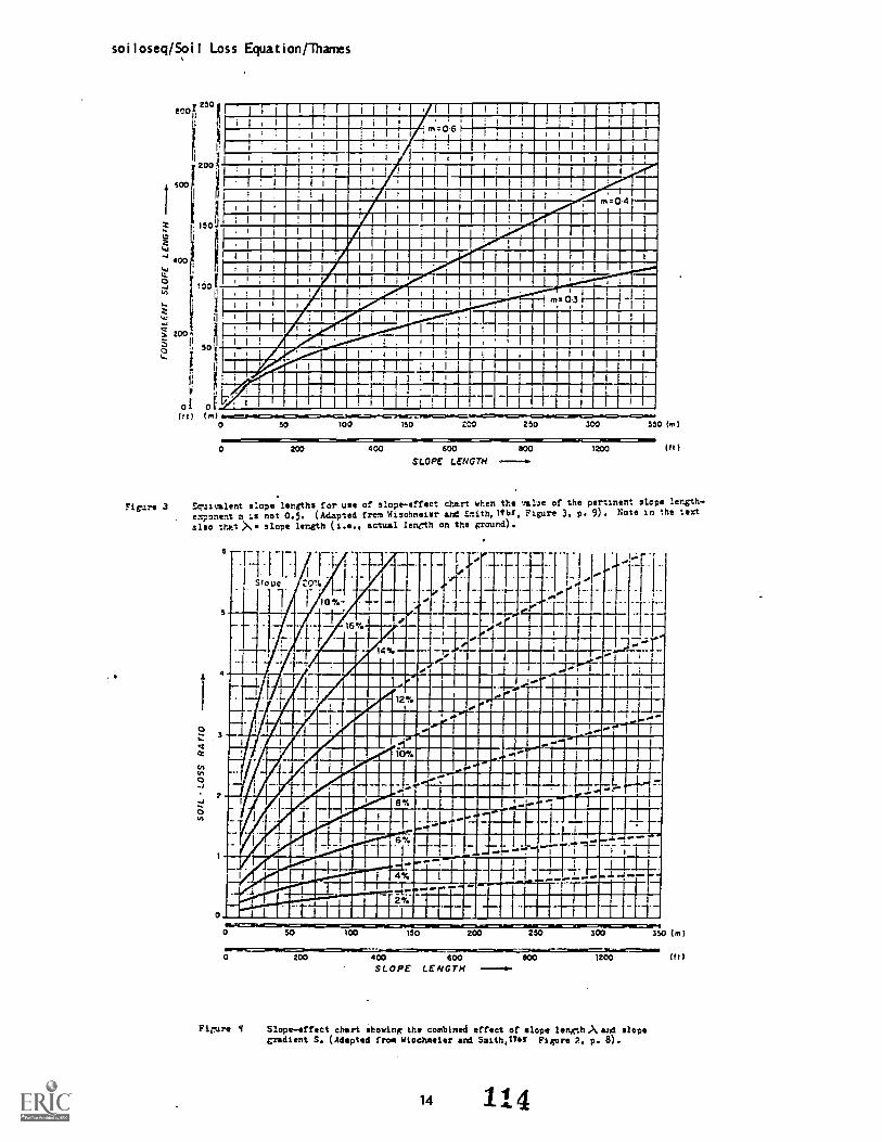
soiloseq/Soil Loss Equation/Thames

9250600.

200,

tWOi

. 150u

400

r,o.II

II

N 200,I

o '

01t ft,

50

Ot(m)

0

1I 1 , I II

, I ENE , i 1 Illi I I,-06m

I I' 1 1 III, 1

i 1 1 I 1 I ' I 1

1 ! 1 1 ! : 1 1 ,

,

, I i III, mr,.....ida m.04,,

, , MIIMMEWAI11 i 1 1

1 1

t

i FrAMION21111111 i1 1 EMIT4 ME AlliMiiiiii.Winniiiii

MIENMEMMIM EPP" , 1111171 :

1

AM1111111111111 I

m-c"[MIMI gag11:111111

1 :

I I Mr"MrAir" -AMIE

1/1111141iMMEIE

I I 1 !MU= I IIMMEM

IRE111111 1 I I 1

. 1 -r IN50 100 150 CO 250 300 350 (m)

0 200 400 600

SLOPE LENGTH1200 (H)

Figure 3 Equivalent slope lengths for use of slope-effect chart when the value of the pertinent slope length-

emponemt m e not 0.5. (Adapted from Wischmeter and Smith, 1ebe, Figure 3, P. 9). Note lo the text

also that X.. slope length (i.e., actual length on the ground).

3

2

0

.1111 ._-_-4 _-_ v._

-...

MI516:

NI_;--r:

Am il is -T-..a.r....... min ...2.......r,A: neni........mai.. .r..laitrou....- w

Adipuunia:paria-o% MIERMIII11 IIMmu=14032uni !111,i-i-r --r.

.m. ...4.0m 40. /...Oliege,1111%111151rininirallin

OM.MI I Mil=

0 100 150 200 250 300 350 ( rn )

O 200 400 600SLOPE LENGTH

1200

Firure 9 Slope-effect chart showing the combined effect of elope lengthAmmi elopeGradient S. (Adapted from Wiechmeier and South,176T Figure 2, p. 8).

(ft)

soiloseq/Soil Loss Equation /Thames

100C 100.1

SLOPE LENGTH 4.Z500 (ft)

%gars E 5:e:ifeffete cccrt for :lope lengths). and slope gradients S exceeding those in Figure 6. Srtrapolatedtxe rIrge of the data; uce on.4 as cpeculative estimates. (Adapted fro: SCS,1470 Figure 3, p. 8).

landslid/Soil Mass Ubverrent/Swanston & Swanson

Landslides or Soi! Mass Movement

Adapted from: Swanston, D.H. , Swanson, F.J., and Rosgen, D., in press, Soil Mas

Movement, Chapter V., in AN APPROACH TO WATER RESOURCES EVALUATION, NONPOINT

SOURCES SILVICULTURE (a procedural handbook). -USDA Forest Service.

Principal Soil Mass Movement ProcessesDownslope soil mass movements result primarily from gravitational stress. It may cake the

form of (1) failure, both along planar and conc.', ,e surfaces, of finite masses of soil and forest

debris which move rapidly (debris avalanchesdebris flows) or slowly (slumpearthflows) (fig. 1);(2) pure rheological flow with minor mechanical shifting of mantle materials (creep) (fig 2); and

(3) rapid movement of watercharged organic a .d inorganic matter down stream channels (debris

torrents) (fig.3).

Slope gradient, soil depth, soil water conteA and physical soil properties, such as

cohesion and coefficient of friction, control the mechanics alai rates of soil mass movement.

Geological, hydrological, and vegetative factors determine occurrence and relative importance ofsuch processes in a particular area.

Slurp- EarthflowsWhere creep displacement has exceeded the shear strength of soil, discrete failure occurs

and slumpearthflow features are formed (Varnes 1958). Simple slumping takes place as a rotational

movement of a block of earth over a broadly concave slip surface and involves little breakup of the

moving material. Where the moving material slips downslope and is broken up and transported either

by a flowage mechanism or by gliding displacement of a series of blocks, the movement is termed slow

earthflow (Varnes 1958). Geologic vegetative, and hydrologic factors have primary control over

slumpearthflow failure, particularly where these materials are overlain by hard, competent rock(Wilson 1970, Swanson and James 1975), Earthflow movement also appears to be sensitive to longterm

fluctuations in soil water content (Wilson 1970, Swanston 1976).

Because earthflows are slowly moving, deepseated, poorly drained features, individual

storms probably have much less influence on their movement than on the likelihood of occurrence of

debris avalanchesdebris flows. Where planes of slumpearthflow are more than several meters deep,

wieght of vegetation and vertical root anchoring effects are insignificant.

Earthflows can move imperceptibly slowly to more than 1 m/day in extreme cases. In parts of

northwestern North America, many slumpearthflow areas appear to be inactive (Colman, 1973; Swanson

and James, 1 975). Where they are active, rates of movement have been monitored directly by repeated

surveying of marked points and inclinometers and by measuring deflection of roadways and other

inadvertent reference systems. These methods have been used to estimate the rates of earthflow

movement shown in table 1 (Swanston and Swanson 1976, Kelsey 1977).

The area of occurrence of slumpearthfolows is mainly determined by bedrock geology. For

example,in the Redwood Creek basin, northern California, Colman (1973) observed that of the 27.4

percent of the drainage which is in slumps, earthflows, and older or questionable soil mass

movements, as very high percentage of the unstable areas are located in clayrock and pervasively

sheared sedimentary rocks. Areas underlain by schists and other more highly metamorphosed rock are

much less prone to deepseated soil mass movement. The area of occurrence of slumpearthflows in

volcanic terrains has also been closely linked to bedrock (Swanston and Swanson 1976). There are

numerous examples of accelerated or reactivated slumpearthflow movement after forest road

construction in the western United States (Wilson 1970). Undercutting the toes of earthflows andpiling rock and soil debris on slump blocks are common practices which influence slumpearthflow

movement. Stability of such areas, is also affcted by modification of drainage systems, particularly

where road drainage systems route additional water into the slumpearthflow areas. These

Pis

landslid/Soil Nhss.NbveTent/Swanston & Swanson

disturbances may increase movement rates from a few millimeters per year to many centimeters. On

such areas have been destabilized, they may continue to move at accelerated rates for several year

Although the impact of deforestation alone on slumpearthflow movement has not bedemonstrated quantitativoy, evidence suggests that it may be significant. In massive, deep seatsfailures, lateral and vertical anchoring by tree root systems is negligible. Hydrologic impactsdeforestation, however, appear to be important. Reduced evapotranspiration will increase sc

moisture availability. This water is, therefore, free to pass through the rooting zone to deepslevels of the earthflow.

Debris AvalanchesDebris FlowsDebris avalanchesdebris flows are rapid, shallow soil mass movements from hillslope area

Here the term "debris avalanchedebris flow" is used in a general sense encompassing debris slideavalanches, and flows which have been distinguished by Varnes (1958) and others on the basis c

increasing water content and type of included material. From a land management standpoint, there

little purpose to differentiating amoung the types of shallow hilislope failures, since th

mechanics and th.! controlling and contributing factors are the same. Areas prone to debravalanchesdebris flows are typified by shallow, noncohesive soils on steep slopes where subsurfacwater may be concentrated by subtle topography on bedrock or glacial till surfaces. Because debravalanchesdebris flows are shallow failures, factors such as root strength, anchoring effects, arthe transfer of wind stress to the soil mantle are potentially important influence. Factors whitinfluence antecedent soil moisture conditions and the rate of water supply to the soil durirsnowmelt and rainfall also have significant control over the time and place of debris avalanchesdebris flows.

The rate of occurrence of debris avalanchesdebris flows is controlled by the stability c

the landscape and the frequency of storm events severe enough to trigger them. Therefore, the ratof erosion by debris- avalanches debris flows will vary from one geomoephicclimatic setting I

another. Table 2 (Swanston and Swanson 1976) shows that annual rates of debris avalanche erosic

from forested study site in Oregon and Washington in the United States, and British Columbia i

Canada, range from 11 to 72m3/km2/yr. These estimates are based on surveys and measurements cdebris avalanche erosion during a particular time period (15 to over 32 years) over a large area (1km2 or larger).

An analysis of harvesting impacts in the western United States (Swanston and Swanso1 976)(table 2) reveals that timber harvesting commonly results in an acceleration of soil ma!

movement activity by a fctor of 2 .to 4 times relative to forested areas. In the four study arealisted in table 2, roadrelated debris avaianche erosion was increased by factors ranging from 25 t340 times the rate of debris aval:riche erosion forested areas. The great variability in the impacof roads reflects not only differen;tes in the mature stability of the landscape, but also, and morimportantly from an engineering standpoint, differences in site location, design, and constructioof roads.

Soil CreepSoil creep is defined as the slow, downslope movement of soil mantle materials as the resul

of longterm applicationof gravitational stress. The mechanics of soil creep have been investigateexperimentally and theoretically (Terzaghi 1953, Goldstein and TerStepanian 1957, Saito and Uezaw1961, Culling 1963, Haefeli 1965, Bjerrum 1967, Carson and Kirkby 1972). Movement is quasiviscou

it occurs under shear stresses sufficient to produce permanent deformation, but too small to resulin discrete failure. Mobilization of the soil mass is primarily by deformation at grain boundarieand within clay mineral structures. Both interstitial and absorbed water appear to contribute tcreep movement by opening the structure within and between mineral grains thereby reducing frictio

within the soil mass. Creeping terrain can be reccognized by characteristic rolling, hummocktopography with frequent sag ponds, springs, and occasional benching due to local rotation;

117

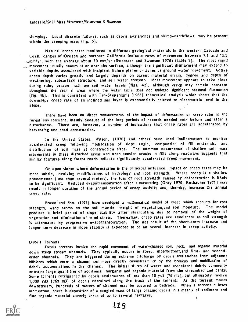
landslid/Soil Mass Moverrent/Sv,inston & Swanson

slumping. Local discrete failures, such as debris avalanches and slumpearthflows, may be presentwithin the creeping mass (fig. 5).

Natural creep rates monitored in different geological 'materials in the western Cascade andCoast Ranges of ,Oregon and northern California indicate rates of movement between 7.1 and 15.2

,.mm/yr, with the average about 10 mm/yr (Swanston and Swanson 1976) (table 3). The most rapidmovement usually occurs at or near the surface, although the significant displacment may extend tovariable depths associated with incipient fialure planes or zones of ground water ,-,-.ovement. Activecreep depth varies greatly and largely depends on parent material origin, degree and depth ofweathering, subsurface structure, and soil water content. Most movement appears to take placeduring rainy season maximum soil water levels (figs. 4a), although creep may remain constantthroughout the year in areas where the water table does not undergo significant seasonal fluctuation

4b). This is consistent with TerStepanian's (1963) theoretical analysis which show that thedownsk,pe creep rate of an inclined soil layer is exponentially related to p:ezometric level in thes lope.

There have been no direct measurements of the impact of deforestation on creep rates in the

forest environment, mainly because of the long periods of records needed both before and after adisturbance. There are, however, a number of indications that creep rates are accelerated byharvesting and road construction.

In the United States, Wilson, (1970) and others have used inclinometers to monitoraccelerated creep following modifcation of slope angle, compaction of fill materials, and

distribution of soil mass at construction sites. The common occurrence of shallow soil mass

movements in these disturbed areas and open tension cracks in fills along roadways suggests thatsimilar features along forest roads indicate significantly accelerated creep movement.

On open slopes where deforestation is the principal influence, impact on creep rates may bemore subtle, involving modifications of hydrology and root strength. Where creep is a shallowphenomenon (less than several meters), the loss of root strength caused by deforestation is likelyto be significant. Reduced evapotranspiration after clearcutting (Gray 1970, Rothacher 1971) mayresult in longer duration of the annual period of creep activity and, thereby, increase the annualcreep rate.

Brown and Sheu (1975) have developed a mathematical model of creep which accounts for rootstrength, wind stress on the soil mantle weight of vegetation,and soil moisture. The modelpredicts a brief period of slope stability after clearcutting due to removal of the weight ofvegetation and elimination of wind stress. The'reafter, creep rates are accelerted as soil strengthis attenuated by progressive evapotranspiration. The net result of the shortterm increase andlonger term decrease in slope stablity is expected to be an overall increase in creep activity.

Debris TorrentsDebris torrents involve the rapid movement of watercharged soil, rock, arid organic material

down steep stream channels. They typically occure in steep, intermittent,and first and secondorder channels. They are triggered during extreme discharge by debris avalanches from adjacenthillslopes which enter a channel and move directly downstream or by the breakup and mobilization ofdebris accumulations in the channel. The initial slurry of water and associated debris commonlyentrains large quantities of additional inorganic and organic material from the streambed and banks.Some torrents retriggered by debris avalanaches of less than 10 yd3 (76 m3), but ultimately involve1,000 yd3 (760 m3) of debris entrained along the track of the torrent. As the torrent movesdownstream, hundreds of meters of channel may be scoured to bedrock. When a torrent n losesmomentum, there is deposition of a tangled mass of large organic debris in a matrix of sediment andfine organic material coverig areas of up to several hectares.

118

landslid/Soil Mass Movernent/Swanston & Swanson

The main factors zontrolling the occurrence: of debris torrents are the quantity andstability of adjacent hillslopes,and peak discharge: characteristics of the channel. Theconcentration and stability of debris in channels reflect the history of stream flushing and thehealth and stage of development of the surrounding timber stand (Froehlick 1973). The stability ofadjacent slopes depends on factors described in previous sections. The history of storm flows has acontrolling influence over the stability of both soils on hillslopes and debris in stream channels.Velocities of debris torrents, estimated to be up to several tens of meters/second, are known onlyfrom a few verbal and written accounts.

Deforestation appears to dramatically accelerate the occurrence of debris torrents byini;reasing the freqency of debris avalanches. Although it has not been demonstrated, it is alsopossible that increased concentratior.s of unstable debris in channels during forest harvesting(Rothacher 1 959, Froehlich 1)73, Swanson and others 1976) and possible increased peak dischages(Rothacher 1973, Harr and others 1975) may accelerate the frequency of debris torrents.

The impact of clearcutting and road construction on frequency of deris torrents(events/km"2/yr) may be compared to debris torrent occurrence under natural conditions. In the H. j.Andrews Experimental forest and Mhe Alder Creek study sites in Oregon,Mtimber havesting appeared toincrease occurrence )f debris torrents by 4.5 and 8.8 times; and roads were responsible forincreases of 42.5 and 13) tMmes relative to forested areas.

Although the quantitative reliability of these estimates of harvesting impacts is limited bythe small number of events analyzed, there is clear evidence of mared acceleration in the frequencyof debris avalanchesdebris flows as a result of forest harvesing and road building. The historiesof debris avalanchesdebris flows as a result of forest harvesing and road building. The historiesof debris avalanchesdebris flows in the two study areas clearly indicate that increased deristorrent occurrence is primarily a result of two conditions: debris avalanches trigger most debris

'torrents (table 4) and the occurrence of deris avalanchesdebris flows is temporarily celerated bydeforestation and road construction (table 2).

Mechanics of MovementDirect application of soil mechanics theory to analysis of soil mass movement porcesses is

difficult because of the heterogeneous nature of soil materials, the extreme variability of soilwater conditions, aid the related variations in stressstrain relationships with time. However, thetheory provides a convenient framework for disussing the mineral mechanism and the complexinterrelationships of the various factors active in development of soil mass movements on mountains lopes .

In terms of factor of safety analysis, the stability of soils on a slope can be expressed asa ration between shear strength, or resistance of the soil to sliding, and the downslope pull ofgravity or gravitational stress. As long as shear strength exceeds the pull of gravity, the soilwill remains in a stable state (Terzaghi 1950, Zaruba and Mend 1969).

It is important to remember that soil mass movements result from changes in the soil shearstrengthgravitational stress relationship in the vicinity of failure. This may involve a

mechanical readjustment among individual particles or a more complex interaction between bothinternal and external factors acting on the slope.

Figure 5 shows the geometrical relationship of factors acting on a small portion of the soilmass. Any increases in gravitational. stress will increase the tendency for the soil to movedownslope. Increases in gravitational stress result from increasing inclination of the slidingsurface or increasing unit weight of the soil mass. Stress can also be augmented by: (1) thepresence of zones of weaknesses in the soil or underlying bedrock produced by bedding planes andfractures, (2) application of wind stresses transferred to the soil through the stems and root

Iandslid /Soil Nhss Nbvement/Swanston & Swanson

systems of trees, (3) strain or deformation in the soil produced by progressive creep, (4)fractional "drag" produced by seepage pressure, (5) horizontal accelerations due to earthquakes andblasting, and (6) removal of downslope support by undercutting.

Shear strength is governed by a more complex interrelationship between the soil and slopecharcteristics. Two principal forces are active in resisting downslope movement. These are: (1)cohesion or the capacity of the soil particles to adhere together, a soil property produced bycementation, capillary tension, or weak electrical bonding of organic colloids and clay particles;and (2) the frictional .resistance between individual particles and between the soil mass and thesliding surface. Frictional resistance is controlled by the angle of internal friction of the soil

the degree of interlocking of individual grains and the effective weight of the soil whichincludes both the weight of the soil mass and any surface loading plus the ,effect of slope gradientand excess soil water.

Pore water pressure pressure produced by the head of water in saturated soil and

transferred to the base of the soil through the pore water acts to reduce the frictionalresistance of the soil by reducing its effctive weight. In effect, its action causes the soil to"float" above the sliding surface.

Controlling and Contributing FactorsParticle size distribution or "texture" (which governs cohesion), angle of internal

friction, soil moisture content, and angle of sliding surface are the controlling factors in

determining stability of a steepland soil. For example. shallow coarsegrained soils low in claysize particles have little or no cohesion, and frictional resistance determines the strength of thesoil mass. Frictional resistance is, in turn, strongly dependent on the angle of internal frictionof the soil and pore water pressure. A low angle of internal friction relative to slope angle orhigh pore water pressure can reduce soil shear strength to negligible values.

Slope angle is a major indicator of the stability of low cohesion soils. Slopes at or above

the angle of internal friction of the soil indicate a highly unstable natural state.

Soils of moderate to high clay content exhibit more complex behavior because resistance tosliding is deterrmined by both cohesion and frictional resistance. These factors are controlled toa large extent by clay mineralogy and soil moisture. In a dry state, clayey soils have a high shearstrength with the internal angle of friction quite high (>300). Increasing water content mobilizesthe clay through absorption of water onto the clay structure. The angle of internal friction is

reduced by the addition of water to the clay lattices (in effect reducing "intragranular" friction)and may approach zero in saturated conditions. In addition, water between grains interstitialwater may open the structure of the soil mass. This permits a "remolding', of clayfriction,transforming it into a slurry, which then lubricates the remaining soil mass. Some claysare more susceptible to defrmation than others, making clay mineralogy an important conideration inareas charcterized by quasiviscous flow deformation of "creep." Swelling clays of the smectitegroup (montmorillenite) are particularly unstable because of their tendency to absorb largequantities of water and to experience alternate expansion and contraction during periods of wettingand drying which may resultin progressive failure of a slope. Thus, clayrich soils have a highpotential for failure given excess soil moisture content. Under these conditions, failures are notdirectly dependent on sliding surface gradient as in cohesionless soils, but may develop on slopeswith gradients as low as 2° or 3°.

Parent material type has a major effct on the particle size distribution, depth ofweathering, and relative cohesiveness of a steepland soil. It frequently can be used as an

indicator of relative stability or potential stability problems. In humid regions where chemicalweathering predominates, transformation of easily weathered primary minerals to clays and claysizeparticles may be extensive. Siltstones, clay st9nres, shales, nonsiliceous sandstones, pyroclastics,

1-40

landslid/Soil Mass Nbvement/Swanston & Swanson

and serpentinerick rocks are the most easily altered and are prime candidates for sol mass movementof the creep and slumpearthflow types. Conversely, in arid or semiarid regions, slopes underlainby these rocks may remain stale for many years due to slow chemical weathering processes and lack ofenough soil moisture to mobilize existing clay minerals. On steep lands underlain by resistantrocks, especially where mechanical weathering prevails, soils are usually coarse and lose in claysize particles. Such areas are more likely to develop soil mass movements of the debris avalanchedebris flow type.

Parent material structure is a critical factor in stabiity of many shallow soils. Highlyjointed bedrock slopes with principal joint planes parallel to the slope provide little mechanicalsupport to the slope and create avenues for concentrated subsurface flow and active pre waterpressure development, as well as readymade zones of weakness and potental failure surfaces for the

overrlying material. Sedimentary rocks with bedding planes parallel to the slope, function in

essentially the same way, with the uppermost bedding plane forming an impermeable boundary to

subsurface water movement, a layer restricting the penetration and development of tree roots, and a

potential failure surface. Vegetation cover generally helps control the amount of water reaching the

soil and the amount held as stored water against gravity, largely through a combination ofinterception and evapotranspiration. The direct 'effect of interception on the soil water budget isprobably not large, especially in areas of high total rainfall or during large storms, where

interception is effective, probably have little influence on total soil water available for

activating mass movements.

In areas of low rainfall, the effect of evapotranspiration is much more pronounced, but itis particularly dependent on region and rainfall. In areas charcterized by warm, dry summers,evapotranspiration significantly reduces the degree of saturation resulting from the first storms of

the fall recharge period. This effect diminishes as soil water deficit is satisfied. Once the soilis recharged, the effects of previous evapotranspirational losses become negligible. Conversely, in

areas of continuous high rainfall or those with an arid or semiarid climate, evapotranspirational

effects are probably negligible. Depth of evapotranspirational withdrawals is important also. Deep

withdrawals may require substantial recharge to satisfy the soil water deficit, delaying or reducing

the possibility of saturated soil conditions necessary for major slideproducing events. Shallow

sosls, however, recharge rapidly, possibly becoming saturated and most unstable during the firstmajor storm.

Root systems of trees and other vegetation may increase shear strength in unstable soils byanchoring through the soil mass into fractures in bedrock, providing continuous long fiberousbinders within the soil mass, an tying the slope together across zones of weakness or instability.

In shallow soils, all three effects may ,be important. In deep soils, the anchoring effectof roots becomes negligeable but the other paramoters will remain important. In one extremely steep

area in western North America, root anchoring may be the dominant factor in maintaining slopeequilibrium of an otherwise unstable area (Swanston and Swanson 1975).

Snow cover increases soil unit weight by surface loading and affects delivery of water tothe soil by retaining rainfall and delaying release of much water. Delayed release of melt water,coupled with usually heavy storms during a midwinter or early spring warming trend, has been

identified as the principal initiating factor in recent major landslide activity on forest lands incentral Washingron (Klock and Helvey 1976).

Characterizing Unstable Slopes in Forested Watersheds

The following guidelines are designed to help delineate the hazards of unstable slopes on I

forested lands.121

landslid/Soil Mass Nbvement/Swanston & Swanson

There are six environmental qualities that should be carefully considered when judgingstability of natural slopes in terms of surface erosion and soil mass movement. They are:

A. landform featuresB. soil characteristicsC. bedrock lithology and structureD. vegetative coverE. hydrologic characteristics of siteF. climate

Each of these qualities encompasses a group of factors which control stability conditions onthe slope and determine or identify the type of processes and movements which are most likely tooccur.

Key factors identifying potentially unstable slopes on any mountainous terrain include slopegradient (a landform quality) and concentration of precipitation (both intensity and duration).Soil properties, including soil depth and such diagnostic characteristics as texture, permeability,angle of internal friction, and cohesion determine the types of processes that will dominate and, tosome degree, determine the stable slope gradient within a particular soil type. Bedrock structure,especially attitude of beds and degree of fracturing or jointing, are important contributing factorscontrolling local stability conditions. Many of these factors are identifiable on the ground or inreadily available support documentation (climatological records, etc.).

The following outline discusses the six environmental qualities important for judgingstability of natural slopes and the key factors associated with each.

Landform features1. Landforms on which subject area occurs. A qualitative indicator of potentially

unstable landform types. Obtainable from air photos and topographic maps., For example, alpineglaciated terrain characteristically exhibits Ushaped valleys with extensive areas of very steepslopes. Fracturing parallel to the slope is common, and soils, either of colluvial or glacialorigin, are usually shallow and cohesionless. The underlying impermeable surface may be eitherbedrock or compact glacial till. Such terrain is frequently subject to debris avalanchedebris flowprocesses.

Areas formed by continental glaciation commonly exhibit rolling terrain consisting of lowhills and ridges composed of bedrock, glacial till, and stratified drift separated by areas ofground moraine and glacial outwash. Glaciolacustrine deposits may be present locally, consisting ofthick deposits of silt and clay which may be particularly subject to slumpearthflow processes ifdisturbed.

Fluvially formed landscapes underlain by bedded sedimentary and metasedimentary rocks mayhave slope steepness controlled by jointing, fracturing, and faulting; by orientation of bedding;and by differential resistance of alterating rock layers. Debris avalanchedebris flow failuresfrequently occur in shallows colluvial soils along these structurally controlled surfaces. Slumpearthflow failures may occur in clayrock or deeply weathered units, in deeply weathered soils andcolluvial debris on the low er slopes, and in valley fills adjacent to active stream channels.

Volcanic terrain consisting of units of easily weathered volcaniclastic rocks and hard,resistant flow rock commonly exhibit slumpearthflow failures in deeply weathered volcanisclasticmaterials. Such failures usually occur just below a capping flow or just above an underlying flowdue to concentration of ground water. Debris avalanchedebris flow failures are common in shallowresidual or colluvial soils developed on the resistant flow rock units.

Because of the large variability in Intypirn processes and the modifying influcence ofN.,

landslid/Soil Mass Nbvement/Swanston & Swanson

climatic conditions on weathering rates and products, geologists with some knowledge of the areashould be consulted.

2. Slope configuration. Shape of the slope in the area of consideration. A qualitativeindicator of location and extent of most highly unstable areas on a slope. Obtainable from air

photos and topographic maps. On both concave and convex slopes, usually the steepest portions have

the greatest stability hazard. Convex slopes may have oversteep gradients in lower portions of the

slope. Concave slopes have oversteep gradients .1 their upper elevations.

3. Slope gradient. A key factor controlling soil stablity in steep mountain watersheds.

Slope gradient may be quantiftdci on the ground or from topographic maps. It deter-rah-di-

effectiveness of gravity acting to move a soil mass downslope. For debris avalnchedebris flowfailures, this is a major indicator of the natural soil mass movement hazard. For slumpearthflowfailures, this is not as important since, given the right conditions of soil moisture content, soil

texture, and clay mineral content, failures can occur on slope gadients as low as 2° or 3°. Slope

gradient also has a major effect on subsurface water flow in terms of drainage rate and susequentsusceptibility to temporary water table buildup during high intensity storms.

B. Soil Characteristics1. Present soil mass movement type and rate. Obtainable from air photos and field checks.

This is a qualitative indicator of size and location of potential stability problems, type of recentlandsliding, and kinds of soil mass movement processes operative on the slope. These, in turn,

suggest probable soil depth and certain dominant soil characteristics. For example, debris

avalanchesdebris flows most frequently develop in shallow, coarsegrained soils which have a lowclay content or in deeply weathered pelitic sediments, serpentinite, and volcanic ash and breccia.

2. Parent material. A qualitative indicator of probable shape of soil particles, bulk

density (or weight), degree of cohesion or clay mineral content, soil depth, permeability, and

presence or absence of impermeable layers in the soil. These, in turn, suggest types of soil massmovement prpcesses operative within an area. This information is obtainable from existing geologic

and soil survey maps, by air photo inerpretation, and by field check.

Soils developed from colluvial or residual materials and some tills and pumice soils

commonly possess little or np cohesion. Failures in such soils are usually of the deris avalanche-.debris flow type.

Soils developed from weathered fine grained sedimentary rocks (mudstones, claystones,

nonsiliceous sandstone chales), volcaniclastics, and glaciolacustrine clays and silts possess a

high degree of cohesion and characteristically develop failures of the slumpearthflow type.

The mica content also has a major influence on soil strength. Ten to twenty percent micawill produce results similar to high clay content.

3. Occurrence of compacted, cemented, or impermeable layer. A qualitative indicator ofthe depth of potentially unstable soil and probable principal planes of failure on the slope. This

information is obtanable from borings, soil pits, and inspection of slope failure scars in the

field.

4. Evidence of concentrated subsurface drainage (including evidence of seasonal

saturation). A qualitative indicator of local zones of periodic high soil moisture content

including saturation and potentially active pore water pressure during high rainfall periods. These

identify potential areas of slope failure. This information is obtainable by air photo

interpretation and ground observation. Diagnostic features include broad linear depressions

perpendicular to slope contour, representing old landslide site and areas on the slope, representingsprings and areas of concentrated ground water movement.

landslid/Soil Mass Yovenent/Swanston & Swanson

5. Diagnostic soil characteristics. Key factors in determining dominant types of soilmass movement process mechanics of motion and probable maximum and minimum stable slope gradients

for a particular soil. This is identifiable through field testing, sampling, and laboratory

analysis. Data on benchmark soils also may be obtained from soil surveys and engineering analyses

for road construction in or adjacent to the proposed silvicultural activity.

a. Soil depth. Principal component of the weight of the soil mass and an importantfactor in determining soil strength and gravitational stress acting on an unstable soil.

b. Texture (Particle size distribution) the relative proportions of sand (2.0 0.5 mm),

silt (0.5 .002 mm), and clay (<.002 mm) in a soil. Texture, along with clay mineral content, areimportant factors in controlling cohesion, angle of internal friction, and hydraulic conductivity ofan unstable soil.

c. Clay mineralogy. An indicator of sensitivity to deformation. Some clays are moresusceptible to deformation than others, making clay mineralogy an important consideration in areaswhere creep occurs. "Swelling" clays of the smectite group (rnontmorillonite) are particularlyunstable.

d. Angle of internal friction An indicator of the internal frictional resistance of asoil caused by intergranular friction and interlocking of individual grains, an important factor indetermining soil shear strength or resistance to gravitational stress. The tangent of the angle ofinernal friction times the weight of the soil constitute a mathematical expression of frictionalresistance. For shallow, cohesionless soils, a slope gradient at or above the angle of internalfriction times the weight of the soil constitute a mathematical expression of frictional resistance.For shallow, cohesionless soils, a slope gradient at or above the angle of internal friction is a

good indicator of a highly unstable site.

e. Cohesior. The capacity of soil particles to stick or adhere together. This is a

distinct soil property produced by ..:cementatiol., capillary tension, and weak electrical bonding oforganic colloids and clay particles. Cohesion is usually the direct result of high (20 perc:nt orgreater) clay particle content and is an important contributor to shear strength of a fine grainedsoil.

C. Bedrock Lithology and Structure1. Rock type. A qualitative indicator of overlying silt texture, clay mineral content,

and relative cohesiveness. It provides a regional guide to probable areas of soil mass movementproblems and dominant porcesses. For example, in the Cascades and Coast Range of Oregon andWashington, areas underlain by volcanic ash and breccias and silty sandstone are particularlysusceptible to slumpearthflows. Where hard, resistant volcanic flow rock is present, shallowplanar failures dominate. Slopes underlain by granites and diorites are also more susceptible toshallow planar failures although where extensive chemical weathering has occurred, such rocks mayexhibit slumpearthflow features. The slope stability characteristics of a particular rock type offormation largely depend on mineralogy, climate, and degree of weathering, and must be determined

for each particular area.

2. Degree of weathering. A qualitative indicator of soil depth and type of siol massmovement ae:tivities. In some rock types, it is also an indicator of degree of clay mineralformat ion.

3. Attitude of beds. Quantifiable on the ground, from geologic maps, and occasionallyfrom air photos. This is an important contributing factor to unstable slopes, especially whereattitude of bedding parallels or dips in the same direction as the slope. Under these conditions,the beddig planes form zones of weakness along which slope failures can occur due to high pore water

' 4

landslid/Soil Miss Nbverent/Swanston & Swanson

pressures and decreases in frictional resistance. Conversely, bedding planes dipping into the slopefrequently produce natural buttresse and increase slope stability. Care must be taken in assessingthe stabilizing influence of horizonta! or indepping bedding planes particularly where weldeveloped jointing is present (see no. 4).

4. Degree of jointing and fracturing Quantifiable on the ground and occasionally fromgeologic maps as dip and strike of faults, fractures, and joint systems. Joints in particular areimportant contributing factors to slope instabilty, especially on slopes underlain by igneousmaterials. Joints parallel to or dipping in the same directions as the slope, create local zones ofweakness along which failures occur. Jointing also provides avenues for deep penetratin ofgroundwater with subsequent active pore water pressure development along downslope dipping jointplanes.

Valleys developed along high angle faults in mountainous terrain may have exceptionallysteep slopes. Deep penetratin of ground water into uneroded fault and shear zones can result inextensive weathering and alteration of zone materials, resulting in generation of slumpearthflowfailures. Such zones can also form barriers to ground water movement cauing redirection and

concentration of water into adjacent potentially unstable sites.

D. Vegetative Characteristics1. Root distribution and degree of root anchoring in the subsoil. An indicator of

effectiveness of tree roots as a stabilizing factor in shallow steep slope soils. Quantifiable onthe ground by observing the degree of penetration of roots through the soil and into a moreresistant substratum and by measuring the biomass of the roots contained in a potentially unstablesoil. High biomass of contained roots is an expression of the binding capacity of "reinforcing" ofroots to the soil mass.

2. Vegetation type and distribution. Cover density, vegetation type, and stand age arequalitative indicators of the history of soil mass movement on a site and soil and ground water

conditions. This information is obtainable by air photo interpretation and ground checking.

E. Hydrologic Characteristics1. Hydraulic conductivity. A measure of water movement in and through soil material.

This is quantifiable in the field and in the laboratory using pumping tests and permeameters. Low

hydraulic conuctivities mean rapid storm generated saturation and a high probability of active porewater pressure, which produces highly unstable conditions in steep slope soils.

2. Pore water pressure. A measure of the pressure produced by the head of water in asaturated soil and transferred to the base of the soil through the pore water. Ths is quantifiablein the field through measurement of free water surface level in the soil. Pore water pressure is akey factor in failure of a steep slope soil, and operates primarily by reducing the weight componentof soil shear strength.

F. aimate1. Precipitation occurrence and distribution. A key factor in predicting regional soil

mass movement occurrences. Most soil mass movements are triggered by soil saturation and actve pore

water pressures produced by rainfall of high intensity and long duration. lsohyetal maps of

rainfall occurrences and distribution, constructed from data obtainable from local monitoring

stations or from the Weather Bureau, can be used to pinpoint local areas of high rainfall

concentration. It is advisable to develop a simple relationshir between rainfall intensity and purewater pressure development for a particular soil type or area of interest so that magnitude andreturn period of damaging storms can be identified. This can be done simply by locating a rain gage

at the site or using near by rainfall data and correlating this with piezomtric data obtained fromopenended tubes installed to the probable depth of failure at the site. Each storm should bemonitored. 125

landslid/Soil Mass Nbvement/Swanston & Swanson

Estimating Soil Mass Movement Hazard and Sediment Delivered to Channels

This section delineates a procedure to be used on potentially unstable areas to analyze thehazard of soil mass movement associated with silvicultural activities and to determine the potentialvolume and delivery of inorganic material to the closest drainageway. This is a broad levelanalysis designed to determine where specific controls or management treatment variations arerequired because of possible water quality changes resulting from soil mass movement. Thisprocedure will not substitute for site specific analysis of road design, maintenance, and

rehabilitation as may be required under current management procedures.

To assess soil mass movement hazards that might deliver inorganic material to a streamcourse, a basic qualitative evaluation is undertaken based on the following information:

1. A delineation of hazard areas and dominant soil mass movement types using aerial photo andtopographic map interpretation with minimum ground reconnaissance.

2. An estimate of the likelihood of failure or "sensitivity" of an area caused by both natural andmaninduced events, using subjective analysis of controlling and ocntributing factors within definedhazard areas.

3. An estimate of the volume of material released by soil mass movements during storm events with a10year return inerval or less.

4. An estimate of the volume of sediment released by soil mass movements which actually reach awater course based on slope position, gradient, and shape and type of movement.

Although soil mass movements are too infrequent for effective direct annual evaluation,delivery volumes can be expressed on an average annual basis for purposes of comparison between preand postsilvicultural activity conditions.

A broad delineation of potentially unstable terrain by slope characterisVcs and soil massmovement types is an essential part of the hazard analysis. A detailed flow chart (fig. 6) shows thesequence of analysis cnce the delineation of unstable terrain is accomplished.

The limits placed on variable ranges for high, medium and low hazard indices are

approximating professionals. The weighted values for hazard indices reguides only, and they weredetermined from consultation with practicing professionals as well as a limited analysis of severalunstable areas in Colorado and western Oregon. However, they do reflect the relatve importance ofthe idividua; factors and their effects on likelihood of failure by the major soil mass movementtypes. These weightings and the ranges of hazard index should be adjusted to reflect the conditionsprevalent within a given area.

Procedural DescriptionThe following information decribes each step of the procedural flow chart, fig. 6. Data

from the Horse Creek example are used to illustrate the following procedure. This complete example

is presented in "Chapter VIII: Procedural Example."

Broad Delineation of Potentially Unstable AreasGuidelines have been presented that provide a qualitative characterization of unstable or

potentially unstable slopes on forested lands. Using these guidelines, evaluate the area of theproposed silvicultural activity to ascertain the stability of the site.

1 gn

landslid/Soil Mass Movement/Swanston & Swanson

Identify and Map Areas by Soil Mass Movement TypeIf the area is generally unstable or potentially unstable, delineate the hazard areas and

dominant soil mass movement types (debris avalanchesdebris flows and slumpearthflows) using aerialphotos and topographic map interpretation. Potentially unstble areas are those that may becomeunstable due to the proposed silvicultural activity. Unstable areas are those that have or

presently are undergoing a soil mass movement.

Characterize Soil Mass Movement TypeSoil mass movements have been classified into two major types; debris valanchesdebris flows

and slumpearthflows. Several site parameters and management activities can be used to evaluate thepossibility of soil mass movement. Although both movement types hve similar facts that can be usedto evaluate the hazad of a failure, the relative importance of these factors may be differentbetween the two movement types. In addition, each kind of soil mass movement has some site ormanagement activity parameters that are specific for that movement. Therefore, to evauate thehazard of a soil mass movement, each type must be evaluated separately using the factors that havebeen found to be significant in characterizing that particular kind of failure.

Debris Avalanchedebris FlowAreas prone to debris avalanchesdebris flows are typified by shallow, noncohesive soils on

steep slopes where subsurface water may be concentrated by subtle topography on bedrock or glacial

till surfaces.

Natural Hazard Site CharacteristicsFor debris avalanchesderis flows, the following site characteristics have been found'to be

critic) in evaluating the potential hazard of a natural soil mass movement slope gradirgit, soildepth, subsurface drainage characteristics, soil texture, bedding structure and orientation, surfaceslope configuration, and precipitation input. This information can be obtained from geologic andsoils maps, pertinent literature, field knowledge of local experts, etc. The relative importance ofeach site ,charcteritic is indicated in table I: and worksheet 1 by the weighting value assigned.

Management Induced Hazard CharacteristicsFor debris avalanchesdebris flows, the following management activities have been found to

be critical in evaluating the; potential hazard for initiation or acceleration of a soil mass

movement; vegetative cover removal, roads and skidways, and harvest systems. This information canbe obtained from past records of silvicultural activities from proposed silvicultural activityplans. The relative importance of each management activity is indicated in table 5 and worksheet 2by the weighting value assigned.

Hazard IndexThe hazard index analysis procedure places weighted values on the factors affecting

different types of soil mass movement. A threepart hazard index is used: high, medium, and low.The numerical ratings are subjective and depend on who is considered acceptable for a particularsilvicultural activity. Assumptions 1 and 2 in the procedure detail and define a high, medium, andlow hazard.

The natural hazard index for debris avalanchesdebris flows is determined by summing theweighted values from worksheet 1 and comparing this value to the ranges of values fr high, medium,and low hazard indices. For example, if the sum of the weighted values for the natural hazard index(worksheet 1) was 31, the hazard index would be medium. The value 31 falls within the range ofvalues (22-44) for the medium hazard.

The relative hazard for debris avalanchesdebris flows caused by silvicultural activities isdetermined by summing the weighted values from worksheet 2. The overall hazard index caused bynatural plus existing proposed silvicultural acitvities is determiled by adding the total weightedvalue for he natural hazard. This overall weighted value is compared with the range of values given

127

landslid/Soil Mass Nbverent/Swanston & Swanson

for a high, medium, or low hazard index. For example, if the silvicultural activities resulted in atotal weighted value of 31, the overall wieghted va:ue of both the natural (31) plus thesilvicultural activity (31) would be equal to 62 and the overall hazard index would be high.

Si trrpEar thf lowSlumpearthflow prone areas are typified by deep. cohesive soils and clayrock bedrock

overlying hard, competent rock. Slumpearthflow soil mass movement also appears to be sensitive tolongterm fluctuations.

Natural Hazard Site CharacteristicsFor slumpearthflows, the following site characteristics have been found to be critical in

evaluating the potential hazard of a natural soil mass movement: slope gradient, subsurfacedrainage characteristics, soil texture, surface slope configuration, vegetative indicators, beddingstructure and orientation, and precipitation input. This information can be obtained from soilsmaps, vegetative cover maps, pertinent literature, field knowledge of local experts, etc. Therelative importance of each site characteristic is indicated in table 7 and worksheet 3 by theweighting value assigned.

Management Induced Hazard CharacteristicsFor slumpearthflows, the following management activities have been found to be critical in

evaluating the potential hazard for initiation or acceleration of a soil mass movement: vegetativecover removal, roads and skidways, and harvest systems. This information can be obtained from pastrecords of silviculture' activities or from proposed silvicultural activity plans. The relativeimportance of each management activity is indicated in table 8' and worksheet 4 by the weightingvalue assigned.

Hazard IndexThe hazard index analysis procedure places weighted values on the factors affecting

different types of soil mass movement. A threepart hazard index is used: high, medium, and low.The numberical ratings are subjective and depend on what is considered acceptable for a particularsilviculture! activity. Assumptions 1 and 2 in the procedure detail and define a high, medium, andlow hazard.

The natural hazard index for slumpearthflows is determined by summing the weighted values

from: worksheet 3 and comparing this value to the ranges of values for high, medium, and low hazardindex. For example, if the sum of the wighted values for the natural hazard index (wkslit. 3) was38, the hazard index would be medium. The value 38 falls within the range of values (22-44) for themedium hazard.

The relative hazard for slumpearthflows caused by silvicultural activities is determined bysumming the weighted .values form worksheet 4. The overall hazard index resulting from natural plus

existing or proposed silvicultural activities is determined by adding the total weighted value fromsilvicultral activites to the total weighted value for the natural hazard. This overall weightedvalue is compared with the range of values given for a high, medium, or low hazard index.example, if the silvicultural activities resulted in a total weighted value of 8, the overallweighted value of both the natural (38) plus the silvicultural activity (8) would be equal to 46,and the overall hazard index would be high.

Bibliography not available at time of printing.

129

!ands 1 id/Soi I iiiass tlovanent/Swanston & Swanson

we.eAers4lotbecx.k see\

est I

f3e.21iNsck.

T)QN,Ins

ill/ 1

0 o

A4o.kcww_\-, e_

Vtry roc)1114 kb

eykrrne rc.?A

Dezrs s I\ Qeryraf,I6

Pic\

Table 1. Observations of movement rates of active earthflowsin the western Cascade Range. Oregon (Swanston and Swanson 1978)and Van Duzen River Basin, northern California (Kelsey 1977)

Location Period of Movement Method ofrecord years rate cm/yr obesrvation

Landes Creek)(Sec. 21 T.22S,R.4E.)

15

Boone Creek) 2

(Sec.17 T.17S,R.5E.)

Cougar Resevoirl 2

(Sec.29 T.17S,R.5E.)

Lookout Creek) 1

(Sec.30 T.15S,R.3E.)

Donaker Earthflow2

(Sec.10 T.1N,R.3E.)

Chimney Rock Earthflows2(Sec.60 T.1N,R.4E.)

Halloween earthflow2(Sec.6 T.1N,R.5E.)

12 Deflection ofroad

25 .

2.5

Deflection ofroad

Deflection ofroad

7 Strain rhombusmeasurements acrossactive ground break.Resurvey of stakeline

1 60

1 530

3 2,720

Resurvey of stakeline

Resurvey of stakeline

1Swanston and Swanson 1978

2Kelsey 1977 12914

,0q- 7, ``.

landslid/Soil Mass Nbvement/Swanston & Swanson

ave..nck..? :r):-'1c !I in ;..r10 and 175,'

Ciza PC:lit:li el 0'..44*:.::7..1 l:t :4.7cr:.-. 17.;'.: ze : ! : 3 ',,,:!.."7.7.. 7rczveti Por. i ------ of ree0_!::,:::::;-.-- ::::..:. ., 4 r;::r:417:-.

:::!-:= 3 4:7.). :7, i t:'.....,'--)s-r..:-,p.irc.-,nt km2 rn'IK:-..'iy:

5:cc.i...r.,!::-;o :".:r-i-i..':t. C.1.-yrnp:::'.-ctf.r:,,..f.3, r.nton. L.I.:3A. (Fi'-.p.-.... 1974);Forest e4 7:;.0Clszr.:1..!. 6 1!.0P0J3r.1 0 3.r.;

9.5 25 71.1, 1.04.4 0 0.0 0.r.c. 11.1::::--...Tt 1,.1 .;.,

1 24.4

Al.:i:r 1...:-.-...-.. ..4:-.47,:4-Fil ...7n,::!.:!'e R'-in.f.,.. C.;r..-:.-.1 U.F1.".. ()r,:: nr: 11;7!)..For-....::: 23 7.:4'.; 12.3 7

1 4:51:31

1 0C::::::'.r..7ut 15 23.1) 4.5 11;no,.ct 15 3.::: 0.3 344.0

17.4 11.0J

Sr.!:::::!..:.f.: ^r7.:(1:4;4:7:i. Co-'! '....'".1:.:-":!. `I". F.5r*:'^!. r....`:':::::1'-':-:. .71!!-.:.:;:'PCIrt.:::4 32 E......q 2:-. ').1 '47, 1 '..°

22 i:i.5 n /L.:- .-. 1:1 24.5 "::.:.T.-.)....' 2.2 1..5 /.2 11 ''..-..;:-., 2.'...7....i..._

275.7 5E;

H. J. Andrews Experiment Forest, western Cascade Range, Oregon, USA(Swanson and Dyrness 1975)

.2.1 ,,... 1.'.3'5 1?:...2 2

63 1:i ,-...'....; 4-...,0

'fr.:7 d;:,..:,Cf. ,'rc.....: . 20 r.:i -O..'Pc::: 2, 2.t..,

:: . : .

.9 1 5 pr L.. 0.1:0T:;:. 0:Sr.rv!ce.

UPSLOPEI I

DOWNSLOPEo

SPRING a

o FALL

P

I 1 I .1

9.0 5.0 0 5.0DEFLECTION (mm)

-3 E

9.09

UPSLOPE4

DOWNSLOPE0

5.0 2.5 0 2.5DEFLECTION (mm)

Figure i . Deformation of inclinometer taLf:,s at tal si tnt in

southern Cascade ;tinge and Coast 9anoe of nreion. U.S.A.

a) Coyote Creek in the southern Cascade range shnwinn seasnoal variationin movement rate as the result nf charging soil watnr lenls. Nnte

that ton difference in readings hetripPn snring and Lill of each year

(dry months) is very small.h) Baker Creek, Coquille nivpr, nrpnnn Cnast ranne, sbowinn constant rate

of creen as a result of continual high water levels.

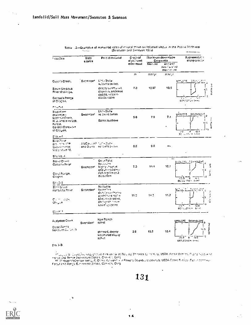
landslid/Soil Mass Nbvernent/Swanston & Swanson

Tahla .2.E..x.imph.rs of mrod ra;e: of r,;ur31 rcia.sted ;n fne fq7.:in.vestrt j.r,ncji

Dot, Pres.:It zn,-1)/101 C-nr..:1 of 7.1:::r!rnurn down-,40.::'3 R..-pre3en!.if .:

e.lUrt9 e.:-'''Llpnt Cr..sr, rata cre:lp pre...;triSv,mant Sur;., ZC:., ci

t .:C.-....,;,'rJrilD7 --.7. .li

rn mmiyr

Cray Cree:.c.sei

Sou:n UrrpNa -I. 7.3 13.97 10.9Ri7c;

daciftc. vc.:c.:E.71-

Castada Psnce r,:cks

BILIS kivI;qCreIf.P;IS

H.FurcA.

CI Cr.son.

Swan.:on'

rRicer

Swartz:on'

For.ge.

e.7'4

S..?sm5fon'

Butevc :.--i;.;c7orres

5.6Same 25 boys

;-, 0.5

,r r.",-;;:t

and 41'.-:-.1rfsh an.]

7.3

15 22trld

1.0" . . : .

L;

7.9

9.0

L;PSV:=Z7.1 r--. 1°

I

L

16.4 10.7

143 11.7 I

CrI Kerr Fil-er.:11.1 dyroo0Swenstcn, sr.Mst

Csftc,::;-..n '..t.':.s

5! e. 3-3

hr 'red. cleanly 2.6 15.2 10.4wi.:.thered CIyscrw:t

UPSLSPE '00VitISLOPEI e

1-11 ...... 5

1 1

GEFL E7.fl.:N I^".:

.; fl s'..t1 in : .hy .F.",,OCTS Sf.n z.1.1d F7r..f171:::1!thief Crc.n L. F. C.:, cr: cnres'). ;:c,enci..:1:..1c4;.,...ry. USDA

E. r- C:r. 1.

131

C.

landslid/Soil Mass Movement/Swanston & Swanson

Table 4 Characteristics of debris torrents with respect to debris avalanches' and lard use status ofiniation in the H. J. Andrews Experimental Forest'. and Alder Creek Drainage (Morrison 1975)

Site Areas of Period of Debris torrents Debris torrents Total Rate of debriswatershed record triggerred by with no associated torrent occurrence

debris avalanche debris avalanche relative toforested areas

km2_ yr number km2 /yr

H. J. Andrews Experimental Forest, western cascades, OregonForest 49.8 25 9 1 10 0.008 1.0Clearcut 12.4 25 5 6 11 0.036 4.5Road 2.0 25 17 17 0.340 42.0

32f72' '7

Alder Creek drainage, western Cascade Range, OregonForest 12.3 90 5 1 6 0.005 1.0Clearcut 4.5 15 2 1 3 0.044 8.8Road 0.6 15 6 6 0.667 133.4

774-

17Tarick J. Swanson,unpuOlished data on file at Forestry Sciences laboratory,USDA Forest Service, PacificNorthwest Forest and Range Experiment Station, Corvallis, Oregon.

Figure 5.- Simplified diagram of forces acting on a massof soil on a slope (Swanston 1974a)

On

landslid/Soi 1 Miss Way ernent/Swanston & Swanson

BROAD DELINEATION OF POTENTIALLYUNSTABLE AREAS

IDENTIFY AND MAP AREAS BYSOIL MASS MOVEMENT TYPE

DEBRIS AVALANCHEDEBRIS FLOW

[HAZARD.. INDEX

ARACTERI E\SOIL MASS

MOVEMENT TYPE \

NATURAL HAD:D-1SITE

CHARACTERIS11C.3SLOPE GRADIENT

SOIL DEPTHSUBSURFACE

DRAINAGECHARACTERISTICS

SOIL TEXTUREBEDDING STRUCTURE

AND ORIENTATIONSURFACE SLOPECONFIGURATION

PRECIPITATION INPUT

MANAGEMENTINDUCED HAZARDCHARACTERISTICS

VEGETATIVECOVER REMOVAL

ROADS AND SKIDWAYSHARVEST SYSTEMS

SLUMPEARTHFLOW

NATURAL HAZARDSITE

CHARACTERISTICSSLOPE GRADIENT

VEGETATIVEINDICATORS

SUBSURFACEDRAINAGE

CHARACTERISTICSSOIL TEXTURE

BEDDING STRUCTUREAND ORIENTATION

SURFACESLOPECONFIGURATION

PRECIPITATION INPUT

MANAGEMENTINDUCED HAZARDCHARACTERISTICS

VEGETATIVECOVER REMOVAL

ROADS AND SKIDWAYS\ HARVEST SYSTEMS

HAZARDINDEX

FOR THE TWO SOIL MASS MOVEMENT TYPES,EVALUATE NATURAL VS. MAN INDUCED MASS MOVEMENT I

Figure 6 - Flow chart of the soil mass movement procedure

133

landslid/Soil Mass Nbvement/Swanston & Swanson

Table .5. Weighting factors for determination of natural hazard of debris avalanche-debris flow failures

Factor Hazard Index and fang,

Slope gradient

Soil depth

High>34°

Medium29° -34°

Low<29°

Weight

30

15

5

High 3

Shallow soils, <5 ftMedium 2

Moderately deep soils, 5-10 ftLow 1

Deep soils, >10 ft

Subsurface drainage Highcharacteristics High density, closely spaced incipient drainage depressions

Presence of bedrock or Impervious material at shallow depth whichrestricts vertical water movement and concentrates subsurface flowPresence of permeable low density zones above the restricting layerIndlcatiVe of saturated flow parallel to the slopeEvidence of springs on the slope

MediumPresence of incipient drainage depressions, but widely spacedPresence of Impervious material at shallow depths, but no low densityzones presentSprings are absent

Soil texture

Bedding structureand orientation

3

2

Low 1

Incipient drainage depressions rare to absentNo shallow restricting layers presentNo Indications of near-surface flow

High 3

Unconsolidated, non-cohesive soils and colluvial debris Includingsands and gravels, rock fragments, weathered granites, pumice andnoncompacted glacial this with low silt content (<10%) and no clay

Medium 2

Unconsolidated, non-cohesive soils and colluvial debrif, with moderateslit content (10-20%) and minor clay (<10%)

Low 0

Fine grained, cohesive soils with greater than 20% clay sized particlesor mica

High 3

Extensive Jointing and fracturing parallel to the slopeBedding planes parallel to the slopeFaulting or shearing parallel to the slope (the stability Influence of bed-ding planes horizontal or dipping into the slope is offset by extensiveparallel Jointing and fracturing)

Medium 2

Bedding planes are horizontal or dipping into the slope with minorjointing at angles less than the natural slope gradientMinor surface fracturing no faulting or shearing evident

Low 1

Bedding planes are horizontal or dipping into the slopeJointing and fracturing Is minor no faulting or shearing evident

1 .% 4

19

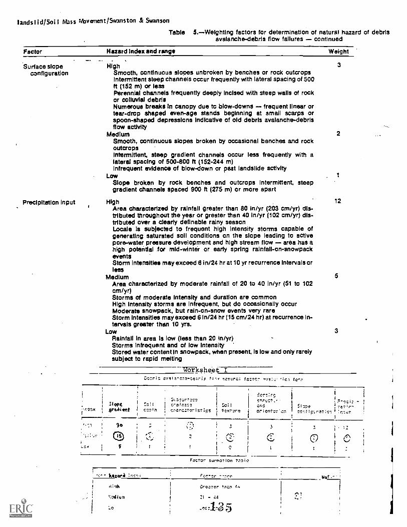
lands I id/Soil Mass tirbvement/Swanston & Swanson

Table 5.Weighting factors for determination of natural hazard of debrisavalanche-debris flow failures continued

Factor Hazard Index and range Weight

Surface slopeconfiguration

Precipitation Input

HighSmooth, continuous slopes unbroken by benches or rock outcropsintermittent steep channels occur frequently with lateral spacing of 500ft (152 m) or lessPerennial channels frequently deeply Incised with steep walls of rockor colluvial debrisNumerous breaks In canopy due to blow-downs frequent linear ortear-drop shaped even-age stands beginning at small scarps orspoon-shaped depressions Indicative of old debris avalanche-debrisflow activity

MediumSmooth, continuous slopes broken by occasional benches and rockoutcropsIntermittent, steep gradient channels occur less frequently with alateral spacing of 500400 ft (152-244 m)Infrequent evidence of blow-down or past landslide activity

LowSlope broken by rock benches and outcrops intermittent. steepgradient channels spaced 900 ft (275 m) or more apart

HighArea characterized by rainfall greater than 80 in/yr (203 cm/yr) dis-tributed throughout the year or greater than 40 in/yr (102 cm/yr) dis-tributed over a clearly definable rainy seasonLocale Is subjected to frequent high Intensity storms capable ofgenerating saturated soli conditions on the slope leading to activepore-water pressure development and high stream flow area has ahigh potential for mid-winter or early spring rainfall-on-snowpackeventsStorm intensities may exceed 8 in/24 hr at 10 yr recurrence Intervals orless

MediumArea characterized by moderate rainfall of 20 to 40 In/yr (51 to 102cm/yr)Storms of moderate intensity and duration are commonHigh intensity storms are Infrequent, but do occasionally occurModerate snowpack, but rain-on-snow events very rareStorm intensities may exceed 61n/24 hr (15 cm/24 hr) at recurrence In-tervals greater than 10 yrs.

LowRainfall in area Is low (less than 20 In/yr)Storms infrequent and of low IntensityStored water content in snowpack, when present, is low and only rarelysubject to rapid melting

Worksheet I

3

2

12

5

3

ate1.1 _e,. iF naTurei feetcr 'iCA for:r.

5 t ope91 se1i int

IS

5

C=!1e=111

crafracacnereeTorist:ps

Sol!

texrure

STruCt.,endoricnteT'cn

7d7I *.r,77.;j1.

3 3

..---,.t,

C 1 1

Factor surmatlon t:ta10

GreeTer ?nen 44

21 - 44

-1'9 5

landslid/Soil Mass Niovarrent/Svanston & Swanso

Table .6.Weighting factors for determination of management-induced hazard of debris avalanche-debris flow failuresFactor Hazard index and range Weight

Vegetation cover Highremoval Total removal of cover large clearcuts with openings continuous

dovmsiope such removal is sufficient to increase soli moisture levelsand reduce strengthBroadcast burning of slash

MediumCover partially removed with slope sections >34° left undisturbedclearcuts in small patches or strips less than 20 ac (8 ha) and discon-tinuous on slopes

LowCover density altered through partial cutting no ciearcutting nobroadcast burning. of sites with >34° slope

Roads and Highskidways High density (>15°/. of area in roads) on potentially unstable slopes

(>28°) cut and fill constructionRoads and skidways located on steep, unstable portions of the slope(>34°)Uncontrolled fille-with poor compaction produced by side-casting overorganic debrisInadequate cross drainage (poor location; improper spacing andmaintenance, size too small for 10 yr storm flow)Lack of fill slope protection of drainage outletsConcentrations of drainage water directed into Identifiable unstableareas

MediumMixed road types, both fully benched and cut-and-fill (balanced)moderate road density (8-15% of area)Areas with slopes >340 or with identifiable landslide activity have beenavoided or fully benchedOn potentially unstable slopes >29° skidways and cut-and-fill typeconstruction are limitedRldgetop roads have large this In saddlesFills, where present, are constructed by sidecasting over organicdebris with little controlled compactionRoads generally have adequate cross drains for normal runoff condi-tions (number and location) but are undersized for the 10 yr storm flowFill slopes below culvert outfalis protected by rip-rap dissipation struc-tures at potentially unstable sitesMajor concentrations of water Into identifiable unstable areas avoided

LowVery few roads on slopes above 28° low road density (less than 8%of area) with roads on potentially unstable terrain (slopes between 29°and 34°) predominantly of full bench type most road locations orconstruction limited to ridgetops with minimum fills In saddles andlower slopes adequate cross drains with major water coursesbridged and culverts designed for 10 yr storm flow or larger

HighOperation of tractor yarding, jammer yarding and other ground leadsystems on slopes >29° (53%)

MediumNo tractor logging high lead with partial suspension on slopes >29°(53%)

LowHelicopter and balloon yarding full suspension of logs by anymethod yarding by any method on slopes <29° (53%)

Harvest systems

cove- rt.l'ov41

C:

5

Worksheet 2

L-toods

2

0

Fe:tor sum

8

5

2

20

8

2

3

2

0

1

1.Greater ti.m

Arun 21 - 44

Less thim 21

landslid/Soil Mass Movanent/Swanston & Swanson

Table .7. Weighting factors for determination of natural hazard of slump-earthflow failures

Factor Hazard Index and range Weight

Slope gradient High 6

greater than 30° (58%)Medium 4

15 -30° (27%48%)Low 2

under 15° (27)

Subsurface drainage - High 6

characteristics Area exhibits abundant evidence of impaired groundwater movementresulting In local zones of saturation within the soil mass short, Ir.regular surface drainages which begin and end on the slopeimpaired drainage, indicated at the surface by numerous sag pondswith standing water, springs and patches of wet groundimpaired drainage involves more than 20% of the area

Medium 4Some Indications of In "aired drainage, but generally Involving lessthan 10% of the areaActive springs are uncommon, Infrequent, or contain no standingwater

Low 2No evidence of impaired drainage

Soil texture High 15Predominantly fine grained cohesive soils derived from weatheredsedimentary rocks, voicanic;s, aeollan and alluvial silts andgiacioiacustrine slits and claysClay sized particle content generally greater than 20%Clay minerals predominantly of the smectite group (montmorillonite),exhibiting swelling characteristics upon wetting

Medium . . 10Soils of variable texture including both fine and coarse grained compo-nents in layers and lensesThe fine grained, cohesive component may contain a clay sized parti-cle content greater than 20%, but clay minerals are predominantly ofthe Hilts and kaolinite groups. exhibiting lower sensitivity to changes Instress

LowSolis of variable textureSome clayey soils present but widely dispersed In small layers orlenses

Slope configuration High40% or more of the area is characterized by hummocky topographyconsisting of roiling, bumpy ground, frequent benches and depres-Vona locally enclosing sag pondsTension cracks and headwall scarps indicating slumping are un-vegetated and clearly visibleSlopes are Irregular and may be slightly concave In the vnoer 1/2 andconvex in the lower 1/2 as a result of the downsiope redistribution ofsoil materialsZones of active movement are abundant

Medium5% to 40% of the area ,ft characterized by hummocky topographyOccasional sag ponds occur. but slump depressions are generally dryHeadwall scarps are revegetated and no open tension cracks are visi-bleActive slump-earthflow features are abseni

LowLess than 5% of the area Is characterized by hummocky topographyOld siump-earthflow features are absent or subdued by weatheringand erosionNo %live slump earthflow feature Present. slopes are generallysmooth and continuous from Alley floor

5

2

Table .1.Weighting factors for determination of natrual hazard of slump-earthflow continued

Factor Hazard Index and range Weight

Vegetative High 5Indicators Phreatophytic (wet site) vegetation widespread

Tipped Uackstrawed) and spilt trees are commonPistol -butted trees occur In areas of obvious hummocky topography(note: pistol-butted trees should be used as indicators of active slump-earthflow activity only in the presence of other Indicators pistol-butting can also occur In areas of high snowfall and Is often the resultof snow creep and glide)

Medium 3Phreatophytic vegetation limited to occasional moist areas on the openslope and within sag pondsTipped trees absent

Low 0Phreatophytic vegetation absent

Precipitation High 18Input Area characterized by high rainfall of greater than 80 In/yr (203 cm/yr)

distributed throughout the year or greater than 40 in/yr (102 cm/yr)distributed over a clearly definable rainy seasonLocale is subjected to frequent high Intensity, long duration stormscapable of generating continuing saturated conditions within the solimass leading to active pore water pressure development and mobiliza-tion of the clay fractionArea has a high potential for rain-on-snow events

Medium -10Area characterized by moderate rainfall of 20 to 40 in/yr (51 cm/yr to102 cm/yr)Storms of moderate Intensity and duration are commonSnowpack is moderate, but rain-on-snow es ants are rare

Low 2Rainfall In the area Is low (less than 20 In/yr) storms are Infrequent andof low intensity and duration -Stored water content in the snowpack, when present. Is low throughoutthe winter with no mid-winter or early spring releases due toclimatological events

Worksheet 3 - -

5IU'^-Tn^'A4104 t2C7rr :aluz':=1 ..^r

S:

lent

Supsurtaccr-cincr.r.clv_ract:ri:t:CS

Soli Slone Ye^ztztivs!lx-urc con:ic!!;r:Tion

(i)!f.

i 7,5

;14ctio:r. ! 4 0 0 2 $ 11-/'..

!

I

!

I 0i

I

1. 2 5oi 1

Factcr su=atIon t:bIe

'Sr' hazard (nee*

--- -risk*24idit

Greater trIzn !4

21 - 44

4 Lcs! VI= 21

%:urall

23

lands! id/Soi I Mass Niavement/Swanston A Swanson

Table A.Weighting factors for determination of management induced hazard Jump-earthflow failures

Factor Hazard Index and range Weight

Vegetation Highcover removal Total removal of cover or large deercuts with openings continuous

downslope such removal would be sufficient to Increase soil. moisture levels and reduce root strength

MediumCover partially removed clearcuts In small patches or strips lessthan 20 acres (8 ha) is size and discontinuous downslope

LowCover density altered through partial cutting, no ciearcutting evident

Roads and Highskidways High density (>15% of area in roads) cut-and-fill type (balanced) con-

structionRoads and skidways located or planned across 4.kinttflable unstablegroundRoads crossing active or dormant slump-earthflow featuresMassive fills or spoil piles on slump benchesInadequate drainage creating concentrations of water at the surfacewith diversion of surface drainage into unstable areas

MediumMixed road types, both fully benched and cut-and-fill (balanced)moderate road density (8-15% of area In roads), unstable areasfeatures avoidedRoads generally have adequate cross drains': mr,mal runoff condi-tions but are undersized for 10 yr storm flow..Diversions of concentrations of water into unstable sites avoided

LowNo roads present if present, predominantly fully benchedRoad density less than 8%Most road location and construction on ridgetops or In alluvial valleyfloorsAdequate cross drainage with dispersal 'rather than heavily con-centrated surface flow

Harvest systems HighOperation of tractor yarding, Jammer yarding or other ground leadsystems causing excessive ground disturbance

MediumHigh Wed yarding with partial suspension and skyline with partialsuspensionNo tractor yarding

LowHelicopter and balloon yardingFull suspension of logs by any method

3

2

1

7

4

2

3

2

1

Worksheet 4

Slueb-earthflow managementrelated factor evaluation form

tridrx

Vegetationcover removal

Roads andsladdays

Harvestmethods

illgn (i)7

Medium 2 4 2

low 1 0 I

.._

139

Factor suematIon table

Irnv. h.arid Inds

1

Range

Ilyh Greater then 44

401um 21 44

.0. Lots than 21

tiOuralmanagement

3C+ 111.*

wtrsprd/Runoff Agriculture and Water Harvesting/

Runoff Agriculture: Water Harvesting and Water Spreading

Gerald Harwood

(Partially adapted from Fogel, 1975 and Cluff and Dutt, 1975)

Runoff Agriculture

The term runoff agriculture implies the direct use of water that has been collected on awatershed and transported to an irrigation site through streams or channels. Taking advantage ofnatural processes, it was developed simultaneously with early Middle Eastern civilizations. Runoffagriculture Incorporates two important techniques, water spreading and water harvesting. Waterspreading involves the direct diversion of rain water from a natural watershed through systems ofdikes and channels to an irrigation site. Water harvesting is a further refinement of the processin which precipitation water is derived from a specially treated collection surface. In eithersituation, the water may be used immediately or stored for the future. While water harvesting andwater spreading will be discussed separately in this unit, the reader should be aware of their closerelationship. Water harvesting refers to a method of ztter collection whereas water spreadingconcerns its distribution. Water harvesting sysr-rn .:sed for agriculture must incorporate waterspreading techniques.

Early Runoff Agriculture Systems

Irrigation is basically the process of artificially applying water to land for agriculturaluse. While it was burn of early cultures in arid and semi-arid lands, the practice has spread tomost parts of the world and has become absolutely essential for the feeding of the earth'sburgeoning population. Since rivers and lakes were the major freshwater sources, the earliestirrigation efforts probably consisted of systems of canals for the transport of river water tonearby fields. Natural water channels were enhanced for purposes of drainage and irrigation, givingrise to the development of canals and levees; dams were also constructed for water control andstorage.

Biswas (1972) has noted that the earliest of the earth's major civilizations were foundedalong river banks: the Sumerians of Mesopotamia on Me Tigris and Euphates rivers; in India, theHarappans on the banks of the Indus; the the Egyptians on the Nile; and the Chinese on the Huang-Horiver. These civilizations had certain geographical conditions in common: they were located onmajor rivers, rainfall was scarce, summer temperatures were high and, in each case, they had to dealwith problems arising from fluctuations in flow of the rivers upon which they were dependent. TheChinese civilization on the Huang-Ho river developed after Ii o B.C.; the other three societies dateback some 4,000 years.

Gulhati (1955) and Biswas (1972) have described several early irrigation projects, some ofwhich are more than 4,000 years otd. In the valley of the Euphrates and Tigris rivers, the remainsof two irrigation canals can be found which are thought to have been used circa 2300 B. C.; onecanal, estimated to hare been between 30 and 50 feet deep and 400 feet wide, is now part of a modernIrrigation system. King Menes, the first Pharoh of the First Egyptian Dynasty, ca 3000 B.C., dammedthe Nile and dir,zrted its course through 'a 12 mile long channel into a lake which stored flood

141

wtrsprd/RUnoff Agriculture and Water Harvesting/

waters for release into irrigation basins during periods of drought. Irrigation systems in Chinadate back to at least 300 B.C. The Imperial Canal, constructed in China around 700 A.D., was 700miles long and used for both irrigation and navigation.

Ancient irrigation, however, was not restricted to river valleys and lands that could beserved by diversion canal systems. Runoff agriculture systems incorporating water harvestingtechniques were developed in the Middle East almost simultaneously with river diversion. Waterharvesting is extremely simple in concept, involving the collection, conveyance and storage ofsurface water derived from precipitation runoff. Water harvesting can be done on a large scale suchas a watershed or on areas as small as a rooftop. Watersheds may be left in their natural conditionor specially treated to enhance surface water runoff.

Water harvesting systems were used by the peoples of the Negev Desert perhaps 4,000 yearsago (Evenari, Shanan, Tadmar and Aharoni, 1961). Hillsides were cleared of vegetation and smoothedin order to provide as much precipitation runoff as possible; the water was then channeled in

contour ditches to agricultural fields at lower elevations. By the time the Roman Empire extendedinto the region, this method of farming encompassed more than 700,000 acres and had become quitesophisticated. After the conquest of this land by the Arabs in 630 AD, these farms declined and thetechnique was gradually forgotten. In the New World, approximately 400 700 years ago, peopleliving in what is now the Mesa Verde region of Colorado employed relatively simple methods of waterharvesting for irrigation (O'Bryan, Cooley and Winter, 1969).

The use of water harvesting in recent times is reflected in the term "rain barrel" which isstill a common phrase language even though such barrels are rarely seen today in the continentalUnited States. The collection and use of runoff from roof tops is a widespread practice in manyparts of the world. In the U.S. Virgin Islands, water harvesting is mandated for domestic use.Building codes require that 10 gallons of water storage capacity be provided in cisterns for eachsquare foot of roof surface area. Even the smallest buildings have collection and storage systems;very large catchments have been constructed on hillsides to provide water for hotels and schools.At one time, water so collected was sold to passing ships. The harvesting of rain water for modernagricultural use was pioneered in Australia during the 1920's. Galvanized rooflike structures werebuilt without houses beneath them, solely for 0:e purpose of water harvesting. Alternatively,sections of sheet metal were spiked to the ground for water collection (Kenyon, 1929).

Modern Runoff Agriculture Systems

Requisite Conditions for Runoff Agriculture SystemsBefore planning a runoff agriculture system, certain essential conditions must be met by the

proposed site. First, there rr...ist be a sufficient quantity of surface runoff water available in theproper seasons for crop production. Accordingly, the topography, geology, soil, vegetation andclimate must combine each year to give at least a few sudden water flows of usable quantity withoutthe production of flood damage. Secondly, the land on which the runoff water is used must be bothsuitable for crop production and conveniently located to the runoff area.

The type of farming practiced must make the best use of the water. In general, perennialcrops with deep. root systems adapt well to runoff agriculture because they can use water stored deepin the soil where it is safe from evaporation.

While there are several variations to runoff agricultural systems, three basic elements are

common to all: (1) a water supply produced by a runoff area or a water harvestng system; (2) a waterspreading site where the crops are to be grown; and (3) a water distribution system.

141

wtrsprd/Runoff Agriculture and Water Harvesting/

The Water SupplyThe water supply for runoff agriculture will generally came from a stream channel which is

dry most of the time but which flows for short perk...is following heavy rains or snow melt.Alternatively, the supply source could be a water harvesting catchment. First, It is important todetermine whether the watershed area above the spreading site will be capable of furninshing anadequate supply of water. Ideally, the source should be able to provide a prolonged flow at a ratethat is large enough to spread well while remaining manageable.

When planning runoff agriculture systems, the first task is to determine whether or not thewatershed above the site will be able to furnish an adequate supply of water. It is desirable tohave a flow large enough to spread over the irrigation site but not so large as to exceed thecapacity of the water spreading system. Accordingly, information is necessary with respect to: (1)the rate of peak flow per second; (2) the total volume of available water In a given period ofstreamflow; and (3) whether or not such flows will be frequent enough to justify building thesystem.

Watershed characteristics that Influence runoffWatershed conditions are seldom uniform; instead, they present a great variety of slopes,

soils, vegetation, stream patterns and other variables which can affect runoff. It Is important toexamine the watershed with the following points In mind:

Topography. Observe the slopes and exposed rock formations. If the rock layers or strataare tipped or inclined into the drainage area, conditions should be favorable for good runoff. Ifthe reverse is true, runoff may be very low. On the other hand, a level bedded formation mayprovide an excellent site.

Note which slopes have the most vegetation. In dry regions, vegetation and water supply areclosely interrelated. Where there is more vegetation, there is more soil moisture. Rainfall usuallyincreases with elevation above the surrounding country. The higher the drainage area, the betterare the chances for abundant runoff. Great differences in rainfall may occur within shortdistances. Other things being equal, In the northern hemisphere, northern slopes usually yield themost water, as they are protected from the drying influence of the sun; in the southern hemisphere,this effect will be observed on the southern slopes. Streams with steep gradients tend to carrylarge amounts of bed load or heavy material ranging from very fine particles to coarse gravel andboulders which roll or slide along stream bottoms during periods of flow.

Close observations of small rills or depressions will indicate whether 'hey carry waterfrequently. If flows are frequent, the chznnels will be swept clean excepting for drift materialwhich is plainly water deposited. As a rule, the steeper the slope, the greater the runoff.

If the drainage area consists of many small, narrow valleys with steep slopes at rightangles to the streams, the runoff will probably be rapid and of short duration. Terrain consistingof broad, flat valleys, will produce significantly longer runoff periods. Another factor affectingrunoff periods and peak flows Is the grade of a stream. Long narrow drainages produce longer runoffperiods with lower peaks than do relatively wide and short ones.

Rainfall. It is Important to study all available rainfall records that may berepresentative of the drainage area. The distribution of the rainfall, not only by months but alsoby days, is very Important. The frequency of maximum intensity storms is also important. Runoff is

usually produced by heavy rains falling within a short period of time. For example, if the averageannual precipitation is 8 inches, and half of it usually occurs during June and July, it is

desirable to know whether there are 15 days with rain during this period or only 5 in the averageyear.

142

wtrsprd/Runoff Agriculture and Water Harvesting/

Soils. The soils of the runoff area should be carefully examined. Most clay soils absorbwater slowly. Shallow soils over clay or impervious rock yield high runoff after the permeablelayers become filled with water. Deep sandy soils and soils with good structure will absorb waterrapidly and release it slowly. Sandy or silty soils are likely to be erodible, especially on steepslopes. Sometimes soils can be examined in the sides of gullies or cut banks.

Vegetation. Vegetation is an important factor affecting water yield and type of streamflow. Watersheds with a heavy _cover of grass, shrubs, or trees seldom produce sudden heavy runoff.Vegetation affects most soils in such a manner as to cause the soil to act as a sponge, in taking upmoisture as it falls and then releasing it slowly. This condition is favorable for sustained streamflow.

Vegetation Is the most desirable medium of erosion control. Runoff from a drainage areawith good vegetation cover will not usually contain enough sediment to overburden a water

distribution system. Grass is the best vegetative cover for a watershed used in runoff agriculture;improving existing grass cover will not greatly reduce water yield. Runoff from vegetated drainageareas may carry considerable drift comprised of grass blades, leaves, twigs, and sticks; such debrismay be a nuisance to water distribution systems but it is preferable to large volumes of sediment.

Estimation of precipitation runoffAvailable runoff records. Runoff records, when available, are the best source of

information on water supply, particularly records which are continuous for a 20year period orlonger. The records from gauging stations on reservoirs and streams are sometimes available. Here

again, the records are not likely to be reliable unless they cover a period of at least 20 years.It is important to be aware of the fact that many gauging stations are so distant from the drainagearea that considerable care must be exercised in using the records. Sometimes, however, ifconditions are reasonably similar, records from drainage areas as much as 50 to 100 miles away may

be useful.

Determination of peak runoff by the slope area method. If no runoff measurements areavailable, the slope area formula is commonly used to compute peak discharge. The computation isbased upon water marks and drI;t lines left by high flows observed at several points in a streamchannel. A sufficient number cf highwater marks must be located along a reasonably straight,smooth portion of the stream channel in order to permit determination of the surface slope at thetime of peak runoff. Cross sections of the channel are then determined, usually by leveling. With

an estimate of the channel roughness, the peak flow is computed by either the Chezy or the Manning

form,ilas. Accurate estimations of flow are difficult to obtain by this method, as the flowdurations are not known. If flow durations can be estimated from available runoff data, a simple

triangular hydrograph can be used to estimate the volume of flow.

Collection of Precipitation by Water Harvesting

Elements of Water Harvesting SystemsWater harvesting systems may be defined as artificial methods whereby precipitation can be

collected and stored until it is beneficially used. The system consists of a catchment made moreimpervious by artificial means than it was in its natural state and, unless the water is to beimmediately used, a storage facility for the harvested water.

Water Collection. There is no single method of treating catchments to increase runoff thatis universally applicable. Each site must be individually evaluated in order to determine theoptimum treatment that will produce water from a given site for a particular use.

Numerous factors must be considered in the design of a water harvesting system, including

the amount of runoff to be expected fromislpr3 ms of various magnitudes, the ratio of runoff toj.f

wtrsprd/Runoff Agriculture and Water Harvesting/

precipitation or runoff efficiency, and the effect of the selected treatment on the quality if thewater. The runoff efficiency is highly variable, depending upon storm intensity, the permeabilityof the surface of the watershed, the degree of saturation of soil of the watershed, etc.Precipitation is a random variable; the selection of a particular treatment to induce runoff and thesize of the catchment should reflect the uncertainty of precipitation and runoff.

For almost all treatments, there is a minimum threshold amount of precipitation required tosaturate the catchment surface; below this amount, virtually no runoff occurs. However, once thisthreshold has been exceeded, the relationship between storm precipitation and runoff will beessentially linear. The Soil Conservation procedure is one method that can be used to relate runoffto rainfall.

A catchment can be made more impervious using the following methods: (1) and surfacealteration, (2) chemical treatments, (3) soil cementation treatments, and (4) ground covermodification. In land alteration, runoff can be increased by (1) clearing and smoothing, (2)shaping, and (3) compaction. The two basic types of chemical treatment are the use of waterrepellents such as silicones and clay dispersants such as sodium salts. Soil cementation treatmentsinclude the mixing of asphalt, cement, resins, and polymers into the soil. Ground covers that havebeen used for catchment construction can be classified as (1) exposed membranes including butyl,plastic, and asphalt, (2) covered membranes, generally utilizing gravel to cover plastic sheeting,(3) reinforced cementmortar coated plastic, (4) sheet metal, (5) concrete, (6) reinforced asphalt,and (7) asphalt planking.

Water Storage. Various methods of storage have been used with the above methods ofcatchment construction. These methods include (1) aboveground tanks and (2) lined reservoirs.

The aboveground tanks have been constructed from (1) steel, (2) reinforced concrete, (3)metal grain bins with flexible liners, (4) .butyl bags, (5) wire reinforced stucco, and (6) railraodtank cars and other types of surplus tanks.

The earth reservoirs have been sealed with various types of membrane liners and bymechanical and chemical treatment. The membranes that have been used include (1) plastic and butylrubber sheeting, (2) unreinforced and reinforced asphalt membranes, and (3) reinforced cementmortarcoated plastic. Mechanical and chemical treatments include (1) mechanical compaction with andwithout the use of a compacting agent such as enzymes, (2) clay dispersants which are also sometimescompacted, (3) water repellants, (3) polymers sucel as SS-13, and (5) bentonite (Boyer and Cluff1972).

Evaporation and Seepage Control. Evaporation and seepage control are needed in order tosuccessfully store harvested water. . The methods used in achieving this control are generallydependent on the size and function of the storage facility. Frequently, the same materials are usedfor both the catchment and the reservoir because seep2;e control and runoff inducement must bothfunction so as to reduce the entry of water into the soil. Like Vie catchment, the size of thereservoir must anticipate the precipitation and runoff variability of the particular site. In someinstances, evaporation has been controlled by use of chemicals such as long chain alcohols, by useof floating and suspended covers of butyl rubber ::id plastic sheeting on small tanks, and bycompletely filling the tank with rock.

Integration of Water Harvesting and Water SpreadingIntegrated water harvesting systems can be designed. In these systems, storage of the water

may be less important than catchment and distribution. The method chosen for treatment of thewatershed must be one that will provide water of a quality that will permit growth of the plantedseedlings. Strip planting and water spreading may also be important elements of the system. Waterspreading systems can be integrated with strip planting and water harvesting in desert farming; forexample, a series of terraces can be used to shed water onto a neighboring strip of productive soil.

144

wtrsprd/Runoff Agriculture and Water Harvesting/

These may be tiered up a hillslope, but on level terrain, an artificial slope can be made bymounding the soil between the strips. The watershed section can, alternatively, be left in a

natural state, cleared of vegetation, planted with range grasses or treated by some water harvestingtechnique that will induce runoff. These systems have been discussed in some detail by Fogel(1975).

Development of Modern Water Harvesting Techniques

Since the 1950's,- the technology of water harvesting has developed variety andsophistication. In Australia, " roaded" catchments, based upon the concept of compacted earth, wereconstructed over thousands of acres in order to collect water for agricultural purposes. In a

roaded catchment, the soil is graded into a series of parallel ridges, having gentle slopes thatpermit water flow into the ditches that separate them. The ditches then channel the water tostorage areas, or the water may be used directly at the site (see Myers, 1975). Detaileddiscussions of roaded catchments- may be found in Firth (1975).

In the United States, catchments were built in the 1950's out of sheet metal for wateringlivestock. Also during this period, experimentation was undertaken with plastic and artificialrubber membranes, for the construction of both catchments and of reservoirs (Lauritzen, 1960).Since then, butyl rubber catchments have been installed in many areas. More than 300 catchments inthe state of Hawaii have been constructed of this material (Myers, 1975). Chiarella and Beck (1975)have reviewed the use of water harvesting techniques on Indian reservations in the western UnitedStates. A number of experiments have been attempted over the years, not all have been successful,but some have worked well. One catchment at Shongotiovi, on the Hopi reservation, has providedsupplemental domestic water since the early 1 930's; this catchment was constructed with very littledisruption of the natural topography. On the Navajo reservation, butyl rubber catchments andstorage bags are successfully used by stockmen. A concrete catchment is being constructed on coalmine spoils on the Black Mesa to test the feasibility of water harvesting for agricultural purposeson the spoils McBride and Shiflet (1 975) have described the construction, placement and use oflarger catchments in the Safford district of southern Arizona.

In 1961, Myers (1961) suggested the waterproofing of the soil itself to serve as a catchmentstructure. His group tested materials that imparted hydrophobic properties to the soil, thus

decreasing its permeability to water. Materials tested included sprayable asphaltic compounds,plastic and metal films bonded to the soil, soil compaction and dispersion, andi field fabricatedasphalt and fiberglass membranes (Myers, 1975). In Israel, Hillel has investigated the potential ofoil and other water repellants for soil treatment, but most of his research has been along the linesof soil smoothing and crusting (Cooley, Dedrick, and Frasier, 1975).

Aldon and Springfield (1975) have tested the applicability of water harvesting techniquesfor the growing of shrubs on coal strip mine soils in New Mexico. They found that treatment of theground with paraffin increased water runoff and the growth. of two month old saltbush and Siberianpeashrub transplants; the soil moisture content of treated plots was increased by about twentypercent. A number of studies have been done on the use and suitability of water harvesting as anagricultural technique. Fogel (1975) has discussed various aspects of runoff agriculture, includingtechniques for computing runoff, and water spreading systems. Morin and Matlock (1975) havecomputer modeled a system of water harvesting and strip farming, based upon data collected in theTucson area. Their results suggest that while conventional irrigation techniques produce greatercrop yields, tgnificant short season grain sorghum crops could be produced from harvested water in4 out of 5 years. Further discussion of agricultural applications of water harvesting may be foundin Fangmeier (1975), Jones and Hauser (1975), Luebs and Laag (1975) and Rawitz and Hillel (1975).

There is considerable variation in the cost longevity and efficiency of the above methods ofcatchment and storage construction. The above systems would need to be evaluated for each site in

order to select the optimum system. Some of the systems to be discussed in the following section

14

wtrsprd/Runoff Agriculture and Water Harvesting/

have been developed and/or tested at the Water Resources Research Center, University of Arizona,over the past fifteen years. In general, these systems are among the most economical of thosementioned above. These water harvesting systems were designed to (1) provide a dependable supply ,of,-,stock water, (2) provide a high quality water for domestic and industrial supplies, and (3) extendagriculture into lands presently uncultivated due to lack of water.

Water Harvesting Catchments Tested at the University of ArizonaSome of the more economical materials mentioned in earlier sections of this chapter have

been tested in the Water Harvesting Program at the University of Arizona; however, the mostexpensive materials, such as sheet metal, concrete, asphalt panels, and asphaltic pavements, werenot tested. The results from small plots using exposed unreinforced asphalt membranes have shownthat, although relatively inexpensive, this method is undesirable due to cracking caused byoxidation, plant germination, and swelling and shrinking of the soil subgrade. Myers, Frasier, andGriggs (1967) have experienced these difficulties in their work with exposed, unreinforcedmembranes. Based on the results of small plot tests, economics, and 'experience of otherresearchers, large scale testing at the University of Arizona has been limited to the followingtreatments: (1) compacted earth, (2) sodium, (3) gravel covered plastic, and (4) reinforced chipcoated asphalt catchments. A discussion of these catchments follows. [Note: All cost estimationspresented in the following section are in 1 972 U.S. dollars, and unless otherwise noted, are based

upon construction methods used in Arizona.]

Compacted Earth Catchments (CE)The Public Works Department of Western Australia initiated in 1948 a program of construction

of Roaded Catchments (Carder 1970). These catchments consisted of clearing, shaping, and contouring

to control length and degree of slope and compacting with the aid of pneumatic rollers. An

estimated 2500 roaded catchments have been installed principally to supply water for livestock use(Hollick 1973). These average approximately two acres in size. There are also 21 roaded catchments

totaling 1 745 acres (706 hectares) and ranging in size from 30 to 175 acres (12.1 to 70.8 hectares)presently being used to furnish domestic water for small towns in Western Australia.

This relatively large scale use in Australia of the compacted earth catchment attests totheir utility. A one acre (0.4 hectare) compacted earth catchment was constructed in the spring of1970 at Atterbury Experimental Watershed located near Tucson, Arizona. A design similar to those in

Australia was used. Two 300 foot (121.9 meters) long drains spaced 50 feet (15.2 meters) apartcollected water from 25 foot (7.6 meters) long slopes. The drainage channels were covered withplastic and gravel to prevent erosion and water loss. The catchment was shaped by a graderfollowing a onehalf inch (1.27 centimeters) rainfall. The plot was then smoothed using a tractordrawn rotary rock rake (Cluff et al. 1972). This proved to be an excellent method of smoothing.Following an additional onehalf inch (1.27 centimeters) of precipitation, the plot was compacted

using a 26 ton (23.6 metric tons) vibratory drum roller. The drainage channels were also lined atthis time. The total cost of the catchment was approximately $250 including wages at $3.50 perhour. The cost would be more if the catchment site were more remote, unless several catchments wereinstalled at one time. For large catchments, the cost should be less than $150 per acre ($370.60per hectare), the cost being primarily dependent on the cost of clearing and shaping. The smoothing

and compaction costs on a large plot would be relatively low. There has been little maintenancesince the plot was installed. Carder (1970) indicated that maintenance would consist primarily ofweed control, and if care were taken not to disturb the surface while controlling weeds, the road

surface should improve with age.

During the 18month project period, a total rainfall of 19.73 inches (50.11 centimeters)occurred. The compacted plot yielded 6.96 inches (17.68 centimeters) or 35.3 percent of the totalrainfall. This represented an increase of 4.86 inches (12.34 centimeters) over the water yield froma control plot. The amount of precipitation required to initiate runoff was about 0.20 inches (0.51

cent irreter s ). 1. d 6

wtrsprd /Iino.ff Agriculture and Water Harvesting/

Assuming a life of 20 years, an interest rate of six percent, and an efficiency of 35percent in a 12inch (30.48 centimeters) rainfall area, the cost of water harvested from thecompacted plot would be approximately 18 cents per thousand gallons ($0.48 per cubic meter). Thisprice does not include weed control costs. Economy of scale would reduce this cost even further onlarger catchments.

Sodium treated catchmentsResults from previous research (Kemper and Noonan 1970; Cluff et al. 1971) indicate that

small amounts of sodium, when applied to the surface of desert soils where there is little or novegetation, will cause a dramatic reduction in infiltration rate. The effect, however, has beenfound to be temporary. Sodium does cause a clay migration from the surface. Clay lenses have beencreated in the laboratory and the field through the use of a relatively heavy treatment of sodiumchloride. These clay lenses have been found to be migratory in the sandy loam soil (clay content =11 percent) at Atterbury Experimental Watershed. When the lenses are close to the surface, theyhave a large effect on runoff. As the lenses move down in the soil profile, the effect becomesnegligible.

The application of a relatively light treatment of sodium (up to 15 percent exchangeablesodium in the surface inch) to a grasscovered soil does not result in a significant change ininfiltration rate. The maintenance of a grass cover seems to be incompatible with the use of alight treatment of sodium chloride to increase runoff.

Results have indicated that sodium chloride can be uses) si ..,,f.9asing runoff where the soilis bare. Periodic disking and smoothing of the soil surface may be needed along with retreatment ofsodium chloride in order to maintain a low infiltration rate. The disking may also be required toreturn the clays to the surface. This method of treatment would require shaped catchment areas tominimize the length and degree of slopes so that erosion would not he excessive.

Perhaps the most effective use of sodium chloride is in conjunction with the compacted earthcatchment. The sodium not only renders the catchment more impervious but is an effective way tocontrol weeds. Weeds are the major maintenance problem in compacted earth catchments. TheCompactedEarth SodiumTreated (CEST) Catchment has been field tested on a one acre site at PageExperimental Ranch. The catchment was prepared in the spring of 1971 in the same way as the CECatchment at Atterbury Experimental Watershed. After shaping, the plot was rototilled to destroysoil structure. Five tons of granulated salt were then added using a fertilizer spreader. Thegranulated salt was mixed into the upper two inches of soil and the soil surface smoothed using therotating tractordrawn rock rake. Following a 0.4 inch (1.01 centimeters) rainfall, the catchmentwas compacted with a drum roller. The total cost of the CEST Catchment was approximately $450.Economy of scale should reduce the cost of this catchment to less than $350 per acre. Thiscatchment was constructed to serve a dual purpose. Grapes and deciduous fruit trees have beenplanted in the drainageways. Water is stored both in the soil and in a 150,000 gallon storage tankwhere it is available for use during dry periods. Thus, the catchment can produce both food andwater. This type of dual system 'should be more acceptable to the general public than bare catchmentareas. The efficiency of this system neglecting soilstored water has been greater than 50 percentof the total rainfall.

The Page CEST Catchment is located in a 16inch (40.64 centimeters) rainfall area. Based ona 25year amortization period and an interest rate of six percent, the cost of excess water producedat this catchment is $0.16 per thousand gallons ($0.42) per cubic meter) or $0.20 per thousandgallons ($0.0529 per cubic meter) in a 12inch (30.48 centimeters) rainfall area. Economy of scaleshould reduce this cost still further on large size catchments. The above cost figures do notreflect the value of crops produced from the soil stored water. These costs are similar to thosegiven for the CE Catchment at the Atterbury Experimental Watershed. It should be noted that the CECatchment would be impractical at Page Ranch due to weed and grass problems.

1 17

wtrsprd/RUnoff Agriculture and MAT,. Hkrvesting/

Gravel covered plastic (GCP)The use of exposed plastic for water harvesting has been unsuccessful (Cluff 1971) due to

ultraviolet induced oxidation, wind, and mechanical damage. The use of gravel protects the plasticfrom sunlight and wind. Gravel covered plastic catchments were first installed at the University ofArizona in December of 1965. The sixmil (0.015 millimeters) polyethylene plastic in early

installations is still in excellent shape.

In order to reduce costs of the gravel covered plastic catchment, two different types ofautomated installation were developed. One type was a plastic laying gravel chute that fits on theback of a dump truck. By means of the chute, plastic could be laid down and covered in oneinstallation (Cluff 1968).

A more controlled method of installation of GCP catchments can be attained through the use

of a selfpropelled chip spreader modified in the manner shown in Figure 1. Where specializedgravel spreading equipment is not available, the catchment has been installed at a rate of 2000 ft2(185.8 square meters) per hour using a frontend loader and a crew of five.

Large areas of the world have sufficient gravel in the upper soil profile to cover theplastic. Because of this, a machine was developed that would extract the gravel from the soil, layplastic, and cover the plastic with the extracted rock. Considerable research effort was expendedin the successful testing of this type of machine which was called the Gravel Extracting Soil Sifter(GESS) (Cluff et al. 1971).

A schematic of the GESS is given in Figure 2. In areas where the GESS is not available orfor remote sites, hand labor can be utilized.

The efficiency of a graveled plastic catchment is given by:

n n m

E = 100 Z (Pi L)/(Z Pi + Si )1 1 1

where L = amount of water trapped by the gravel cover

m = total number of storms which have a rainfall total less than L

n = total number of storms which have a rainfall total greater than L

E = efficiency of the plastic catchment for period when n + m storms occur

Pi = precipitation total of ith storm whose total is greater than L

SIp= recipitatioo total of jth storm whose total is less than L.

The loss L has been found to stabilize at approximately 0.11 inches (0.28 centimeters) for aproperly constructed catchment. In a rainfall regime similar to Tucson, the efficiency would beapproximately 70 percent.

A catchment is properly constructed if the plastic is covered with the minimum size anddepth of gravel needed to provide a complete cover and resist erosion. Figure 3 contains theresults of a study which indicates what this minirmun cover would be for different slopes (Cluff etal. 1971). This figure shows that on a 10 percent slope 100 feet (30.48 meters) long, a onehalfinch cover of 3/16 to 3/8 inch (0.48 to 0.95 centimeters) gravel will withstand an 18inch (45.7centimeters) per hour intensity rainfall. In contrast with the CE and CEST catchments, the GCPCatchment produces sediment free water, a primary consideration in domestic, supplies. The cost'

1 F?

wqrsprd/RUnoff Agriculture and Water Harvesting/

depends on the method of installation. In general, it would be approximately $1000 per acre ($2475per hectare) for large catchments installed with an improved version of the GESS using ten mil(0.0254 millimeters) polyethylene plastic. The use of imported gravel would increase the cost toover $1500 per acre ($3713 per hectare). The projected life of a properly constructed andmaintained GCP catchment is twentyfive years. With a 70 percent efficiency and a 6 percentamortization rate, the cost of water would be $0.34 per thousand gallons ($0.089 per cubic meter) in

a 12inch (30.48 centimeters) rainfall zone.

Chipcoated reinforcedasphalt catchmentsFrasier, Myers, and Griggs (1970) have developed the fiberglass reinforced asphalt

catchment. Several of these catchments have been field tested in Arizona. Work at the Universityof Arizona in the area of reinforced asphalt catchments have centered around the use of plastic,both polyethylene and polypropylene, as the reinforcement material. The treatment consists of aprime coat of emulsified asphalt followed by a layer of four mil (0.0102 millimeter) polyethylenesheeting or polypropylene matting, which is then immediately covered with a top coat of emulsifiedasphalt and 1/8 to 3/16 inch (0.32 to 0.48 centimeters) chips. This AsphaltPlastic AsphaltChipcoated (APAC) catchment has many good features. It requires approximately onethird the amount ofgravel as a GCP Catchment. The treatment should work on any toil type since the plasticreinforcement prevents cracking. Treatment can be completed at one time. No curing time is needed

during construction. The plastic should last at least 25-30 years if the catchment is properlymaintained. Retreatment would be made by sweeping loose chips from the surface and laying down anew asphalt and chip protective coating. Based on the use of similar treatments in the roofingindustry, retreatment would probably be needed every 10 to 15 years. Results from small plotsindicate the catchment will cost at least twice as much as the GCP Catchment but will have anefficiency from 90 to 95 percent. This treatment has sufficient merit, and large scale testing is

planned.

Water Storage Methods Compatible with Water Harvesting

Catchments Tested at the University of ArizonaIn general, the water storage techniques tested at the University of Arizona have been

related to stock water supplies and consequently are limited in size. The basic treatment wouldalso be suitable for lar mr reservoirs, with the possible exception of the rockfilled tank or thosetanks utilizing the suss, ded cover for evaporation control. The seepage and evaporation controlmethods outlined here can also be used on existing or new reservoirs that are filled from othersources of water.

Plasticlined rockfilled reservoirThe construction of this tank was prompted by the availability of commercial rock pickers

which make the collection of rock for small tanks economical. Although decreasing storage by over50 percent, the rock greatly reduces evaporation loss and practically eliminates any chance ofmechanical damage including vandalism.

The tank is first excavated, then the surface is raked smooth. Two or three layers of tenmil (0.0254 millimeters) polyethylene plastic is then laid down and covered with used rubber tires.The tires are filled with silty clay cover material to reduce the significance of any holes that mayinadvertently occur in the plastic. The tires protect the plastic liner as rocks are added to thetank. In the United States, used rubber tires can be easily obtained at no cost. In areas whereused tires are difficult to obtain, a 12-18 inch (30.48 to 45.72 centimeter) layer of soil on slopesless than 1:3 or a reinforced coat of cementmortar could be used on the tank to protect theplastic. Three rockfilled tanks have been constructed in Arizona using a rotary drum commercial

rock picker in areas containing sufficient rock to make the system economical. The cost is

dependent upon the site and method of collection of the rock (Cluff et al. 1972). The tanks wereconstructed for a cost of appreNirnately $2300 for 25,000 gallons (94.6 cubic meters) net storage

wtrsprd/Runoff Agriculture and Water Harvesting/

with $1600 expended for the filling of the tank with rock. A reeltype rock picker was tested inconnection with the construction of the above tanks. These tests indicated that the use of thistype of picker should reduce costs by 50 percent.

The rockfilled tank is very compatible with the GCP Catchment. The larger rock can' go intothe tank with the smaller rock being used to cover the plastic on the catchment. A sciqematic of ,a

water harvesting system of this type is shown in Figure 4.

Plasticlined concretecoated or earthcoveredThe various methods of seepage control were outlined in the introduction. Plastic lining,

if properly covered, offers a positive method of seepage control that is very competitive with othermethods. Tests have indicated that a layer of silty soil, or a threequarter inch (1.90 centimeter)layer of wire mesh reinforced cementmortar will greatly reduce the seepage loss through holes thatmay inadvertently be placed in the plastic liner (Boyer and Cluff 1972). The reinforced mortarcoating is placed directly on the plastic and has proven to be an effective cover to use on steepslopes. This coating may either be placed using gunnite equipment or can be hand plastered. The

cost of this cover is less than twenty cents per square foot ($2.15 per square meter).

In order to reduce the cost of installation on larger reservoirs, the same equipmentdeveloped for laying graveled plastic catchments can be used for laying and covering of plasticliners with soil (Cluff 1968). On smaller tanks, of the size used for stock purposes, the soil

covering is generally installed using hand labor. A tank using a covering of soil in the bottom andreinforced mortar on the sides is shown in Figure 5. The economy and strength of the reinforcedmortar covered plastic makes it practical to construct a walkthrough cattle trough that is directlyconnected to the tank. This design avoids the need for a float valve which is subject tomalfunction and vandalism. The use of the mortar covering also makes it possible to run waterdirectly from the catchment into the tank, thus avoiding any chance of stoppage.

A CoupledExpandedPolystyrene AsphaltChipcoated (CEPAC) Raft can be used for evaporation

control (Cluff 1972). This system, first tested in the spring of 1972, is essentially 100 percenteffective in preventing evaporation loss for the area covered. Any size of polystyrene sheets canbe coupled together. Those tested at the University of Arizona have been primarily one inch (2.54

centimeters) thick, four by four foot (1.62 x L62 meters) sheets. These sheets are coated withemulsified asphalt and immediately covered with 1/16 to 1/8 inch (0.16 to 0.32 centimeters) chips.The sheets are coupled together using a coupler made out of two short lengths of slotted 1-1/2 inch(3.81 centimeters) PVC pipe. An outer frame of 1 -1/4 inch (3.17 centimeters) PVC pipe filled wih

water provides a protective bumper for the rafts which have been constructed up to 1600 square feet

(148.6 square meters). These rafts can be coupled together to cover as large a body of water asdesired. The cost of this system is less than ten cents per square foot ($1.07 per square meter).

A suspended cover of butyl or reinforced plastic would be recommended (Cluff et al. 1:r2)for smaller tanks used for domestic control in which it is desirable to keep out foreign material oreliminate algae growth.

Sodium treated reservoirsWhen there is sufficient clay in the soil and the incoming water is higher in sodium than

calcium, the use of sodium salt is the most economical treatment for seepage control. The 150,000gallon (567.8 cubic meters) tank at Page Ranch, constructed in connection with the salt treatedcatchment, was sealed in 1971 with sodium chloride at the rate of five tons (11.20 metric tons perhectare) per acre. The seepage loss at the tank appears to be insignificant, and due to the factthat the incoming water has more sodium than calcium, the life of the seal is indefinite.Evaporation is controlled at the Page Ranch tank through the use of CEPAC Rafts.

wtrsprd/Rainoff Agriculture and Water Harvesting/

Discussion of the Economics of Water Harvesting Systems

Table 1 gives a summary of the costs and estimated life of the catchments developed at theUniversity of Arizona. Each site and potential water use snould be examined in order to determinewhich catchment and method of storage to use.

The use of the CE and CEST Catchments are limited to areas where soil conditions arefavorable. Both the CE and CEST Catchments should not be built where soils are difficult tocompact. Tests to date have indicated that clay content should not be less than five nor greaterthan 35 percent. For soils with the higher clay 'content, it would also be important to have moresand than silt, otherwise erosion problems would be unsolvable.

Water produced from a CE or CEST Catchment contains considerable sediment. In the case ofthe CEST Catchment, this sediment is finely dispersed and will remain in suspension. Although salttreated, the water from a CEST Catchment has less than 500 parts per million total salinity and canbe used for most purposes including agriculture. Although more expensive, the CEST Catchment isgenerally preferred over the CE Catchment since the sodium not only increases the efficiency of thecatchment but also serves as an herbicide which reduces maintenance costs.

A sodium treated tank would probably be the best to use in conjunction with a CE or CEST'Catchment. Periodic retreatment of the tank may be necessary with a CE Catchment.

A graveled plastic catchment should be considered r.I.ere gravel is economically aviailatle,the soil condition is not suitable for a CE or CEST Catchment, and/or a sedimentfree water Isdesired. Generally, a plasticlined reservoir would be used in conjunction with the GCP Catchment.A rock filled tank should be considered with the GCP Catchment if there is sufficient rock in thearea and vandalism is a problem. Otherwise, a CEPAC raft covering would be recommended forevaporation control, unless the water were to be used directly for domestic use. In the 'altercase, a suspended cover would be recommended.

The APAC system would be used in areas where (1) soil or gravel conditions are such as tomake the CE, CEST or GCP Catchments impractical and/or (2) rainfal' and/or storage considerationswere such that a high efficiency would be needed to maintain a firm water supply. In general, thesame type of storage system used for the GCP Catchment could be used for the APAC system. The sizeof the storage reservoir could be reduced due to the higher efficiency of the APAC system.

Although more research is needed, costs of installation of water harvesting systems havebeen greatly reduced through application of modern techniques and methods described in this paper.Water harvesting should be considered whenever new water supplies for domestic and livestock use in

developing arid and semiarid lands are needed. If the cost is low enough or the value of the cropis high enough, the water harvesting systems described in this paper can also be used to develop newagricultural lands where water is presently unavailable.

The Wzaerspreading Site

A: stated earlier, the basic requirements for runoff agriculture are (1) a watershed thatprovides enough water to mature a crop and (2) a site suitable for crop production. Numerousfavorable and adverse factors must be weighed against each other to determ:ne whether a site isfeas!ble, or to compare one site with another. An evaluation of these factors is also needed todetermine the design of the distribution system. Some of the principal factors are discussed in thesection: tlat follow.

151

wtrsprd/Runoff Agriculture and Water litrvesting/

Water supply factors to considerBoth volume and frequency of flow are important. While one flow per year may put sufficient

moisture into the soil to produce a satisfactory crop, frequent floodings will naturally producemore yield. A small volume (especially if combined with infrequent flow) may not be worth the cost

of diversion. A large volume may be too difficult to handle or too much for the size of theavailable spreading area. In this area, prevision must be made to bypass the excess water.

The proper depth of water on the cropgrowing area or rate of water application is also animportant factor in planning the system. The decision will depend on the water supply, theinfiltration and penetration characteristics of the soil, the tolerance of the plants to inundationand the normal season of available water.

For agricultural crop production, the distribution of rainfall events throughout the growingseason is crucial to a successful harvest, particplarly :for the shallowrooted crops. These cropsrequire water more frequently than those having deep roots. The depth of application per runoffevent can be balanced against the relative sizes of the runoffproducing and the cropgrowing area.There is no alternative, however, to a scarcity of rainfall events.

For forage production, where surface and internal drainage on the spreading area are goodand the water supply abundant, applications up tb 300 mm in depth over the area are not too much, ifa flow can be expected only once or twice during the growing season. If water is scarce and thearea suitable for spreading is greater than the water supply (as is frequently the case), theapplication of 75 to 150 mm when available may produce more feed than heavier applications on asmaller area.

In connection with water supply, water quality is a factor that must be considered. If thewater contains excessiveamounts of dissolved solids, it may be unfit for spreading, and in a fewyears may ruin the soil on the spreading area. If the water supply is suspected of containingharmful salts, analyses should be made to determine if the quantity exceeds allowable tolerances.

Sedimentation factors to considerFrequent and heavy deposits of sediment may interfere with the effective operation of the

system. Such deposits will retard plant growth and may kill the younger plants. Even if the

sediment is not excessive in amount, it may be made up of fine materials that will clog the soilpores on the cultivated area and in time reduce the water intake.

If the water coming to the proposed cropgrowing site is on a steep gradient and flowing athigh velocity, it may be carrying a large quantity of sediment. Most of this load will be droppedwhen the velocity is checked. Such a quick and heavy deposit of sediment in one place is a distinctdisadvantage and must be avoided.

If sediment of high silt content is deposited slowly, it may be beneficial rather thanhumful. The spreading water tends to deposit the sediments in a gently sloping plane which fillsthe low spots and small gullies and other irregularities. Silt deposited in such a manner actuallyimproves the site for spreading purposes. The silt also adds to the soil depth and thus generallyImproves growing conditions.

Unlike most types of sediment basins, a waterspreading system can function indefinitelywithout the loss of expensive storage capacity. As sediment accumulates, the height of the dikescan be increased and the storage capacity restored and enlarged. Rapid and heavy sedimentaccumulation, however, is usually indicative of serious :soil erosion conditions in the drainage areaupstream, and no time should be lost in applying corrective measures.

152

wtrsprd/Runoff Agriculture and Water Hkrvesting/

Site factors to considerThe ideal site on which to spread runoff water for crop production is a broad, smooth gtly

sloping plain whose soil is a deep fertile loam.

Runoff agriculture requires a deep soil that can store water between rains. It works bestfor deeprooted crops such as trees and shrubs, which can tap stored water and depend less onfrequent rainfall. In contrast, annual crops need rain at the beginning of the growing season andusually at intervals thereafter. The method is enhanced by plant varieties able to withstandintermittently wet and dry soil.

Environmental prerequisites include:

1. A minimum mean precipitation of 80 mm per rainy season if the rainyseason coincides with the cold period of the year, more if it occursduring summer when evaporation is greater.

2. Soils in the cropgrowing areas with high waterstoring capacity.

3. Not more than 2 to 3 percent salinity in the cultivated soil.

4. A minimum of 1.5 m of soil depth in the cultivated area (unlesswaterstorage facilities are available).

The Water Distribution System

Several runoff water distribution systems exist from simple terraces to complex diversions.The selection of a particular one will depend on the site factors encountered and on the crops to beirrigated with the harvested water. Usually range and pasture lands use a system in which water isdiverted from a ratura! course onto the land by a system of diversion dams and spreader dikes.Other crops, such as fruits, barley, sorghum and millet, can use a similar waterspreading system ora technique known as desertstrip farming.

Water spreadingIn arid regions, the limited rainfall usually falls during short, intense storms. The water

swiftly drains away into washes and gullies and is lost to the region. Sometimes floods occur oftento areas untouched by the storm. Waterspreading is a practice of deliberately diverting thefloodwaters from their natural courses and 'preading them over adjacent floodplains or detainingthem on valley floors. The wet floodplains or valley floors are then used to grow forage orcultivated crops (Figures 1 and 2).

The simplest waterspreading system is a small earth dam that may be less than one meter highand five meters long across a minor water course. If the land slopes away from such streams oneither side, a number of these simple structures may spread water on a considerable area, This typeof structure, but with slightly larger dams, may be effective on areas where the water diverted atany one point reaches 0.5 cubic meters/s. The next step or refinement is the conveyance dikes orditches which transport the water from the diversion point on a natural water course to the cropgrowing areas. This may be some distance, up to several kilometers, in which case the dikes areactually ditches or canals. They can be built with earth taken from above or below .tie dikealignment. If the ground on which they are constructed has little slope, a strip up to 150 meterswide above the dike will be covered with water and irrigated whenever the system is in operation.

Spreading dikes are often found at the end of a conveyance dike. These dikes are usually acontinuation of the conveyance dike with outlets for water. At appropriate intervals, part of thewater is turned onto the land below the dike by means of outlets through the dike. For fairly clear

wtrsprd/Runoff Agriculture and Water Harvesting/

water, outlets should be at the bottom of the flow channel at an elevation as the land on the lowerside, thereby reducing erosion.

Waterspreading systems need a careful design and engineering layout to withstandfloodwaters. While potential sites are found on many arid and semiarid ranges, they must beselected with full consideration for topography, soil type, and vegetation.

Desert strip farmingIn arid and semiarid regions, although only a very small percentage of the rainfall reaches

major stream channels, considerable runoff occurs on the gently sloping upland watershed areas.Desert strip farming makes use of this water by employing a series of terraces that shed water ontoa neighboring strip of productive soil. They are often tiered up a hillslope, but on level terrain,an artificial slope for the catchment can be made by mounding the soil between the strips. Thewatershed section can be left in a natural state, cleared of vegetation, planted with range grassesor treated by some waterharvesting technique to induce runoff. (Figures 8 and 9)

Improvement and Maintenance

The discussion that follows pertains mainly to the operation, improvement, and maintenanceof waterspreading systems for forage production. The principles, however, are similar for usingthis method on other crops and for other methods of runoff agriculture.

Common design defectsIt is difficult to design a waterspreading system which is free of flaws when first

constructed. The flow of water is seldom the same in any two storms. Nevertheless, the system musthandle these variable flows by one automatic plan. Incomplete and inaccurate basic data arefrequently a further handicap.

Usually the first flow of water through the system will reveal the flaws in design. If thedesigner can be on hand to vatch the water flow through the system, he will be able to recognize the

defects of his plan much more quickly than if he has to study the effects of the flow after it haspassed by. Following are some of the effects that may appear of r the system receives a flow ofwater:

1. Too great a concentration of water hitting certain section!, of adike with too high velocity. This may cause the water to overtop thedike or to break through. The solution of this problem may require therelocation or widening of a spillway from the dike above. The

difficulty might be solved by a diversion dike or ditch above toincrease the spread of the water. Possibly the dike may have to beraised in height or reinforced.

2. Dry areas not receiving water. Often a short ditch leading waterto the dry spot will solve the problem, or a dike may be required todivert water to the dry area. A pipe may have to be put through a diketo let water come through to the dry spot. Sometimes partial dike orspillway, relocation is necessary. The designer should not expect toirrigate all of the spreader area in each run. If 65 to 85 percent ofthe area can be given a good wetting in the average water run, a

successful design has been attained.

3. Too much or too little water coming through the openings in floodspreaders. This fault can be corrected by reducing or increasing thesize of the opening.

1541 S

wtrsprd/Runoff Agriculture and Water Harvesting/

4. Too rapid concentration of flowing water in the system. This flowmay require more small plugs or dikes in natural drainage ways, in oldroad ruts and trails, in low spots, in basin lips, in the borrow pits,etc., to turn out the water frequently and keep it in a sheet. Oftenin wild flooding systems, only the primary dikes are constructed at thebeginning and the secondary dike construction is delayed until a flowof water has gone through the system, thus indicating where thesecondary dikes will do the most good.

5. Improper division of water flowing into the borrow pit and thatmoving directly towards the next dike in flood spreaders. Correctionscan be made with ditches or wing dikes.

Common maintenance problemsMaintenance of waterspreading systems should be given prompt and careful attention to avoid

much heavier costs later. If sediment accumulation is slow, the maintenance costs usually declineto a fairly kw figure after about the third year. By this time, the weak spots have beenstrengthened and the flaws in design have been corrected in connection with maintenance work. Inaddition, the dikes have settled and have in some cases become partially covered with soilbindingvegetation. On the other hand, if sediment accumulation continues to be great, there may be heavyannual maintenance work to raise the dikes and adjust dike design as needed.

In some cases, channels behind diversion dikes may have to be cleared of sediment. Theelevation of the floor of the diversion may have to be raised to provide sufficient flow in channelsmade inadequite by sedimentation.

Very often heavy maintenance costs on a waterspreading system can be reduced by improvingvegetation on the upper watershed to help prevent the runoff from coming down in one . big flash floodof terrific force but short duration. Delayed runoff may save dikes from being overtopped andbreached. It will also reduce the amount of sediment carried from the watershed and stream channelinto the spreading system.

Some of the more common maintenance problems are as follows:

1. Gullying at the spillways. Slight gullying at thespillways is frequent and nothing to cause grave concern. If thegullies spread or entrench quickly it may be necessary to make thespillway wider by tearing down some of the dike at the spillway end inorder to give the water more spread space. More openings or pipes mayhave to be put through the dike in order to cut down the amount ofwater going to the spillway.

2. Excessive widening or plugging of the spreader dike

spillway. Excessive widening may occur as a result of erosion at theend of the dike. It can usually be stopped by building a riprap faceon the. end of the dike. Plugging is usually caused by deposits ofsediment or debris which may have to be removed or smoothed out fromtime to time.

3. In straight channels paralleling dikes, obstructions, suchas rocks, drift, shrubs, or earth projections, may deflect the currentagainst the loose dike fur causing the dike to wash or cave. Removesuch obstructions to permit free flow.

1;5

wtrsprd/Runoff Agriculture and Water Harvesting/

4. Gullying in the return or excess water channel. It is wellto note the tail or excess water area particularly after a big flow.If head cuts are developing, direct the water to a more favorablelocation if possible. At least keep it in a thin sheet where it movesover areas likely to erode. It is sometimes impossible to avoid someerosion for a few years while an artificially sloped and vegetated areadevelops. art adequate cover which will take the flow without eroding.The maintenance of the excess channel may require protection fromgrazing by fencing.

Note: Much of the material on water harvesting was excerpted from Cluff and Dutt, 1975 and muchof the information on runoff agriculture was obtained from Fogel, 1975.

Li terature Cited

Aldon, E. F. and Springfield, H. W. 1975. Using paraffin and poly-ethylene to harvest water forgrowing shrubs. 1975. In Proc. Water Harvesting Symposium. Phoenix, March 1974. pp. 251-257.

Biswas, A K. 1972. History of Hydrology. Amsterdam: North-Holland Publishing Company, 336 pp.

Boyer, D. G. and C. B. Cluff. May 1968. An Evaluation of Current Practices in Seepage Control.Hydrology and Water Resources in Arizona and the Southwest. Volume 2. Proceedings of the 1 972Meetings of the Arizona Section of the American Water Resources Association and the HydrologySection of the Arizona Academy of Science. Prescott, Arizona.

Carder, D. J. May 1970. Roaded Catchments A Method of Increasing Runoff into Dams andReservoirs. Technical Bulletin No. 5. Western Australian Department of Agriculture.

Chiarella, J. V., and Beck, W. H. 1975. Water harvesting catchments on Indian lands in theSouthwest. In Proc. Water Harvesting Symposium. Phoenix, March 1974. pp. 104-114.

Cluff, C. B. March 1968. A New Method of Installing Plastic Membranes. Proceedings of the SecondSeepage Symposium. ARS 41-147. Agricultural Research Service. Phoenix, Arizona.

Cluff, C. B. November 1971. Plastic Catchments for Economical Harvesting of Rainfall. Proceedings

of the Tenth National Agricultural Plastes Conference. Chicago, Illinois.

Cluff, C. B. July 1972. Low-Cost Evaporation Control to Save Precious Stock Water. ArizonaFarmer-Ranchman. Phoenix, Arizona.

Cluff, C. B. 1973. Plastic reinforced membranes for precipitation harvesting and seepage control.In Proc. Eleventh National Agricultural Plastics Conference. San Antonio, Texas.

Cluff, C. B., G. R. Dutt, P. R. Ogden, and J. k. Kuykendall. July 1972. Development of EconomicWater Harvesting Systems for Increasing Water Supply. OWRR Project No. B. -015 -ARIL CompletionReport. The University of Arizona, Tucson.

Cluff, C. B., G. R. Dutt, P. R. Ogden, and J. I. Stroehlein. September 1971. Development ofEconomic Water Harvesting Systems for Increasing Water Supply. OWRR Project No. B-005-AR iZ.Completion Report. The University of Arizona, Tucson.

1 56

wqrsprd/Plimoff Agriculture and Water Harvesting

Cluff, C. B. and G. R. Dutt. Economic Waterharvesting Systems for Increasing Water Supply in Arid

Lands. In: Watershed Management in Arid Zones: A Prototype Short Course. Saltillo, Mexico, March

1975. School of Renewable Natural Resources, Univ. of Arizona, Tucson. pp. 130-146.

Cooley, K., Brazell, L., Frazier, G., Fink, D. 1976. Water harvesting on the Arizona strip calledeconomically feasible. Arizona Farmer Ranchman, May 1976, Vol. 55, No. 5.

Cooley, K. R., Dedrick, A. R. and Frasier, G. W. 1975. Water harvesting: State of the art. In

Proc. Symposium on Water Management. Irrigation Division, ASCE, Logan, Utah, August 1975. pp. 1-21.

Evenari, M. L., Shanan, L., Tadmar, N., and Aharoni, Y. 1961. Ancient agriculture in the Negev.Science 133: 979-996.

Fangmeier, D. D. 1975. Crop production by water harvesting. In Proc. Water Harvesting Symposium.Phoenix, March 1974. ARS W-22, February 1975. pp. 269-276.

Firth, J. L. 1975. Design and construction of roaded catchments. In: Proc. Water HarvestingSymposium. Phoenix, March 1974. ARS W-22, February 1975. pp. 122 -125.

Fogel, M. M. 1975. Runoff agriculture: Efficient use of rainfall. In Watershed Management inArid Zones: A Prototype Short Course. Saltillo, Mexico, March 1975. School of Renewable Natural

Resources, Univ. of Arizona, Tucson. pp. 130-146.

Frasier, G. W., L. E. Myers, and J. R. Griggs. June 1970. Installation of Asphalt-FiberglassLinings for Reservoirs and Catchments. Agricultural Research Service. United States WaterConservation Laboratory Report No. 8. Phoenix, Arizona.

Gulhati, N. D. 1955. Irrigation in the World: A Global Review. International Commission on

Irrigation and Drainage. New Delhi.

Hillel, D. 1967. Runoff inducement in arid lands. Final technical report submitted to U.S. Dept.of Agriculture. Volcani Inst. of Agri. Res. and Hebrew Univ. of Jerusalem. Rehovolt, Israel. 142

PP.

Hollick, M. Personal communication dated Mas, 23, 1973. Department of Civil Engineering. The

University of Western Australia.

Hollick, M. A. 1974. A technical and economic review of water harvesting methods. Civil

Engineering Transactions, Paper No. 3316. Australia.

Jones, 0. R. and Hauser, V. L. 1975. Runoff utilization for grain production. In Proc. WaterHarvesting Symposium. Phoenix, March 1974. ARS W-22, February 1975. pp. 277-283.

Kemper, W. D. and L. Noonan. 1970. Runoff as Affected by Salt Treatments and Soil Texture. Soil

Sci. Soc. Am. Proceedings 34:126-130.

Kenyon, A. S. 1 92 9. The "ironclad" or artificial catchment. Victoria Dept. Agr. Jour. 27:86-91.

Kirkland, L. A. 1969. The Gravel Cover and Catchment Efficiency in the Plastic-Lined Catchment.

Master of Science Thesis. Department of Hydrology. The University of Arizona.

Lauritzen, C. W. 1960 Ground covers for collecting precipitation. Farm and Home Science 2:66-67,

87.

18 157

wtrsprd/Runoff Agriculture and Water Harvesting

Luebs, R. E. and Laag, A. E. 1975. Water harvesting for barley in a 30cm winter rainfall area.In Proc. Water Harvesting Symposium. Phoenix, March 1 974 ARS W-22, February 1975. pp. 284-291.

McBride, M. W. and Shiflet,, L. W. 1975. Water harvesting catchments in the Safford district,southeastern Arizona. In Proc. Water Harvesting Symposium. Phoenix, March 1974. ARS W-22,

February 1975. pp. 115-121.

Morin, G. C. A. and Matlock, G. 1975. Desert strip farming computer simulation of an ancientwater harvesting technique. In Proc. Water Harvesting Symposium. March 1974. ARS W-22, February

1975. pp. 141-150.

Myers, L. E. 1961. Waterproofing soil to collect precipitation. Soil and Water ConservationJournal 1 6:2 81-282.

Myers, L. E. 1975. Water harvesting 2000 B.C. to 1 974 A.D. In: Proc. Water HarvestingSymposium. Phoenix, March 1974. ARS W-22, February 1975. pp. 1-7.

Myers, L E., G. W. Frasier, and J. R. Griggs. September 1967. Sprayed Asphalt Pavements for Water

Harvesting. Jour. of the Irrigation and Drainage Division. Proceedings of the American Society ofCivil Engineers.

National Academy of Sciences. 1974. More water for arid lands promising technologies andresearch opportunities. Board of Science and Technology for International Development, National

Academy of Sciences. Washington, D.C. 153 pp.

O'Bryan, D., Colley, M. E., and Winter, T. C. 1969. Water, population pressure, and ancient Indianmigrations. Bulletin 10, International Hydrologic Decade. June 1 96 9. pp. 438 -442.

Rawitz, E. and Hillel, D. Water harvesting by runoff inducement for irrigation of an almond orchardin a semiarid climate. In Water Harvesting Symposium, Phoenix, March 1974 ARS W-22, 1975. pp.

223-231.

Stokes, C. M., R. D. Larson and C. K. Pearse. 1954. Range improvement through waterspreading.Foreign Operations Administration, Washington, D.C. 36 pp.'

wqrsprd/Rtinoff Agriculture and Water Harvesting

TABLE 1

RELATIVE COST AND EFFICIENCY OF CATCHMENTS

DEVELOPED AT THE UNIVERSITY OF ARIZONA

December, 1972

Approx. Cost per Approx. Cost Efficiency Est.

Catchment Methods Square Yard per Acre in Percent Life

Compacted Earth (CE)* $0.03-0.05 $150-250 30-50 Indefinite

Compacted EarthSodium Treated (CEST)* $0.06-0.10 $300-500. 40-70 Indefinite

Graveled Plastic (GCP)** $0.20-0.50 $1000-2400 60-80 20-25 years

Asphalt-PlasticAsphalt-Chip-Coated (APAC)***

Polyethylene Reinforced $0.50-0.60 $2400-2900 85-95 10-15 years

Polypropylene Reinforced $0.90-1.00 $4400 -4900 85-95 10-15 years

*

* *

* * *

Prices and efficiency of CE and CEST Catchments are dependent on soil type, cost ofclearing and shaping. Maintenance consists of weed removal and recompaction as needed.

.-ocuirad pEricdically pr:., `cc .:c11:97once of

the CEST Catchment.

The variation in price of the GP Catchment is primarily dependent on the cost of the

gravel and to a lesser extent the cost of clearing and shaping. The cast of the 10 mil

black polyethylene plastic to be used is relatively stable. Maintenance consists ofadding gravel if necessary on exposed portions of the catchment.

Prices of the APAC systems are based on projection of small plots. Larger installations

neea to be made to firm up prices. Maintenance consists of recoating with asphalt and

chips every 10-15 years.(*Foe ccur f D'erf, /72.1j

Figure 1 (Cluff and Dutt, 1975)

Figure 2 (Cluff et a1,1972)

:

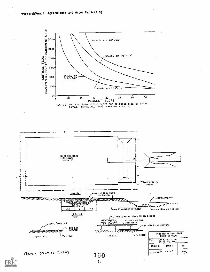
wtrsprd /Runoff Agriculture and Water Hhrvesting

/2 30.0Li2U 25 0-Q

LLc 0 20 0-- J

0 15.0-C-) 0I-E 10.0-

rn

U

C ,

6

GRAVEL DIA3/16.-3/8"

GRAVEL DIA. 3/IV-I/2

10

F:G'..:RE 3. CRI7'.CALCOVER.

18 22PERCENT SLOPE

FLOW VERSUS SLOPE FOR ", c'''TED SIZE(KIRKLAND, 19591 (.0:.

26 30

I:1.111:' :UM C:111(3/WM tlIf101(

SGIf:I

34

OF GRAVEL

Ptit tttM 21111 012102 WWI!IOU 1111(3 Tllt

Ilft- A:41M

RCMStu: r r

121101 ififfl COW

III. Ill:ttitizarm

77774777777".0"..re.0...-////-'

fInMff Wig SI::113(

Fioure 4 (ocurr ,Dc.171 /In)

40NiiitNONmasiamasts

14"Patentug tin

Galt s

DIMM 11:::1 KITY 11:11 YILYI

HMO MITI 1111 CHM TM la II :WM

III LIM Cr ilSte TIMMID MITI Ha

/,-11V0 111113 Of I7 KIL /011(11!IIII

/%7Y"./.77777/77%717Z/t:7.7--.Tiff Zttill SCIEtigt

Muff f(frif:IS fflf1111 1(11(1if Min

16021

Ind: clan mIsr:rim In hull len

MO II Ill it

C 3 Ci.ver tr.-% ;

Slll

wtrsprd /Runoff Agricultureand Water Harvesting

I ......... ....... I ......... .......... i ..m................. I

Ir

100 X i!t)' ASPHALT -PLASTIC- CHIPCATCHMENT

SCALE I.: 20'

NOTE:4:TH AN EPPICIENCY OF 90%THIS SYSTEM YLL PRODUCEWATER AT RATE OF :0,000GALLONS PER ONE INCH OFplitc:P:TATION

I.

I I I

PLAN VIEW

1..,._.FOUR STRAW+BARB WIRE Wet

WATERSURFACE

_z24' X 9C EXPANDED POLY STYRENE COUPLED RAFT

50.000 GALLON TANK

i / / /- / , / , ,24 0'

/EARTH CORrItiOPULYCTHLLNE

APINZOx TJA TELT I/4' AVHALT CHIP-COVER,-4 MIL GLAcx PCLYETHLENE

Pt.DED TO V.:BORAH WITHEKIULSIFIED ASPHALT

,5U8GRAOE

CATCuodEIT DETAIL

Figure 5 C ceorr otar, 1921)

SCCTION AAAPPNUX SCALE. I :

Went P:IUFORCED ES:4EyiWO/TAR COVERED C

1-12' 6 ,--- :2' 4SECTION 13-9

SCALE I'

/-FENCE

Y4E-RE:UPC/CEO CCSCRETE-_------71AORTAN LIMPED PLASTIC

5 1,1!.att Gqn

A"Il 1W:4 '110;Cti

I / I 4.0' 1,-R-1.1.75' LTs /ob.. 0

PLASTIC ON SIOES COVERED WITIICONCRETE VOIOAll trEttifoRCED WWII20 GAGE WIRE MESH WITH r OrENINGS

PLASTIC.ON BOTTOM COVERED/-WITH 2 EARTH BALLAST

TWO LAYERS OF10 NIL POLYETHLENE

`..SUBORADE

TANK DETAI

.42.1-.: A j.

. ,4. 4..:

am.

0

0 .%LI

Fig. 6-. Schematic of a waterspreading system.Comet, /7,$)161

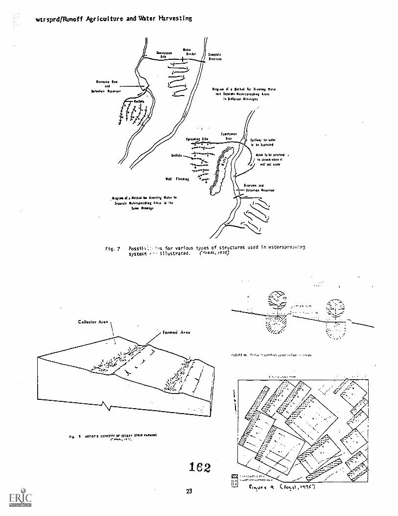
wtrsprd/Runoff Agriculture and Water Harvesting

Ismsissaid

Is Italia Inn..,

Wales

Di OOOO ito

lisps. it s &MIS Ier Disorient ReinuU Upstate VI din tttt

is Odln,tl Oraialps

Coss

Sproodiai °s Solly/y 10 watt

IS 1.11111114

Wilet IS he 'shooed ./ Is %trim

WI se Hats

Magma st a NOW Ists Mantis, Wain IsSeurat. Nall OOOOOO hog AIM is the

Saw Wasp

...miss aidDelentiss lnnnir

Fig, 7 Possif,r.;].:.Ft,s for various types of structures used in waterspreuotho

systerA illustrated. (":,4ei.,,,,$)

Collector Area

i Farmed Area

I.e. I ARTIST'S COSICr PT Of 5(55S1 STRIP OARIONG"V, et

1 C 2

23

FIGLIAE 44. Pr 4, :! ,j,11-or r,.11.

wtryield/Water Yield lirprovement/Ffol I kat

Water Yield Inprovement

IntroductionDemands for surface and round water in much of the world require that all potential sources

of water be evaluated for possible development. To this end, several approaches to wateraugmentation and methods for better water management have been explored. Water harvesting, reuse,

salvage (by removal of riparian plant communities), and vegetation management on upstream catchmentsare some of these approaches.

Of specific interest here is the management of vegetation on upstream catchments to increasethe yield of usable water. It appears that water yield can be increased through vegetativetreatments that benefit, or are at least compatible with, other natural resource objectives. Tofurnish an assessment of these possibilities, underlying concepts of vegetation management for wateryield improvement will be presented, along with a brief summary of several worldwide studies on theeffects of altering vegetative cover on water yield.

Vegetation Management for Water .Yield Concepts

Many studies conducted throughout the world have demonstrated that annual water yields can

be increased following the implementation of vegetation management practices. In general, theincreased runoff is often attributed to decreased evapotranspiration on the watersheds. That is,following treatment, less precipitation input is converted to vapor as a result of rainfall andsnowfall interception and transpiration, and more is made available for streamflow runoff.Presumably, the reduced evapotranspiration is due to changes in the structure and composition ofvegetation on the watershed.

Evaporation processes generally account for a significant proportion of the annualprecipitation input on most watersheds. Consequently, the potential to increase water yield bydecreasing evapotranspiration is attractive. For example, 85 to 95 percent of the annualprecipitation is evaporated or used by plants on many watersheds in arid and semiarid regions,leaving only 5 to 15 percent available for streamflow runoff. On high elevation mountain watershedsin the snow zones of the world, the annual water yield may be as high as 50 'percent of theprecipitation input, but the evapotranspiration component is still significant and potentiallysubject to reduction through vegetation management.

Perhaps the above concepts may best be illustrated with a hypothetical but realistic waterbudget for a forested watershed (Table 1). Prior to treatment, average annual precipitation andevapotranspiration were 635 and 560 millimeters (mm), respectively, leaving 75 mm for streamflowrunoff. After the implementation of a vegetation management practice, perhaps a partial harvestingof the forest overstory in a timber management operation, the annual streamflow runoff is increasedby 25 mm (from 75 to 100 mm) due to a reduction in evapotranspiration of 25 mm (from 560 to 535 mm).The annual precipitation input of 635 mm remained the same, as basic precipitation patterns areusually not affected by modifications In the structure and composition of vegetation cover.

In the case illustrated, annual water yield increased by 33 percent, while annualevapotranspiration decreased by 5 percent. It should be noted that, no matter what vegetationmanagement practice is imposed on watersheds, the annual evapotranspiration may only change butlittle. However, as demonstrated above, even a small reduction in evapotranspiration may causesignificantly increased streamflow runoff.

163

wtryie I d/Water Yield Irrprovement/Ffo I I iott

Indications are that, for appropriate conditions and situations, water yields can beaugmented by vegetation management p-actices without denuding watersheds of plant cover and withoutunacceptable changes in erosion and sedimentation. Evidence also suggests that vegetationmanagement designed for water yield improvement can be developed to be compatible with other naturalresource uses and values, and in some cases even to be complementary.

If the structure and composition of vegetation at the interface of earth and atmosphere canbe modified by management practices, evapotranspiration may be reduced with the result that more ofthe annual precipitation input will be released from watersheds as usable water. This concept isthe primary basis for .the belief that vegetation can be managed for water yield improvement as wellas for other natural resource products and amenities.

Summary of Water Yield Improvement Experiments

Experime nal catchments, often supplemented by plot studies and computer modeling, have beenused on numerous occasions to demonstrate that the hydrologic relationships of a river basin may besignificantly affected by the implementation of A vegetation management practice on upstreamcatchments. These management practices, often imposed as a water yield improvement practice,include various types of forest cutting or removal, or changes of forest cover from one tree type toanother, or more drastic changes in which a forest cover is replaced by another type of vegetation.

As an overview of the potentials far water yield improvement through vegetation 'nanagement,a brief summary of several worldwide studies on the effects of altering vegetative cover on wateryield, and the significance of the resulting conclusions, follow.

Emmenthal MountainsIn 1900, an early study of the effects of forest treatments on water yield was carried out

in the Emmenthal Mountains of Switzerland. Here, measurements of climate, precipitation, andstreamflow were made on two small catchments, one forested and the other pastureland, to determinethe influence of forests on water production. Despite attention to detail, there was no way toascertain that the observed differences in streamflow between the two catchments were caused only bydifferences in vegetation cover.

Wagon Wheel GapA second attempt to quantitatively analyze the influence of forests on water yield was made

in the Wagon Wheel Gap investigation of 1911. The control watershed approach (in which streamflowfrom two similar catchments are compared during a period of "calibration," and then treating onecatchment while leaving the other untreated as a control) was first used in this study of twoforested catchments in the Colorado Rockies of the western United States. After eight years ofcalibration, one of the catchments was denuded by removing the scrub aspen and coniferousvegetation. Then, for seven additional years, streamflow from the denuded a eas was compared withflow from the control catchment. This investigation conclusively demonstrated that clearing forestcover did increase streamflow. This study also demonstrated that changes in water yield could bequantitatively assessed.

Coweeta Hydrologic LaboratoryIn 1934, the Coweeta Hydrologic Laboratory was established by the USDA Forest Service to

analyze the effects of various forest cutting and vegetative conversion treatments on water yield inthe humid mountains of the eastern United States. Mixed hardwoods with basal area densities of 20-25 square meters per hectare characterized the original forest conditions on the twelve experimentalcatchments at Coweeta. Treatments implemented and then evaluated included clearcutting with andwithout control of regrowth, poisoning of forest overstories on portions of catchments with regrowthrestricted, and thinning above and below by selective logging.

641

wtryleld/W-.ter Yield Irrierovement/Ffol I iott

With the exception of limited thinning (25 percent of the basal area remcied), thetreatments evaluated increased water yield by varying amounts. In general, these increases weregreatest immediately after treatment, and the duration of effect was dependent, in part, upon theseverity of treatment. One of the catchment studies is the cite of the only cutting expeiirrientreplicated in time.

Kamabut i

Coniferous and deciduous fort:,' overstories on a small mountainous catchment in Kamabuti,Japan were cleared in 1948, with sus_ sequent annual recutting on sprouts. Significant water yieldincreases were observed following treatment, although these increases were restricted to the growingseason.

Fernow Experimental ForestIn 1951, the USDA Forest Service began gauging on several small catchments at the Fernow

Experimental Forest in the Allegheny Mountains of West Virginia in the eastern United States.Original forest conditions on these catchments were mixed hardwoods at 20-25 square meters of basal

area per hectare. After calibration, water yield improvement studies were designeJ and implementedto determine effects of logging on strearnflow. Treatments evaluated consisted, for the most part,of thinning by alternative silvicultural practices.

As was found at Coweeta, with the exception of limited thinning (in this case, approximately

15 percent of the basal area removed), the treatmentsevaluated increased water yield by varying

amounts. Also, these increases wets- greatest immediately after treatment.Fraser Experimental ForestTo assess effects of forest cutting on snow pack dynamics and subsequent streamfiow, the

USDA Forst Service logged mature lodgepole pine and sprucefir in strips and blocks on an

experimental catchment in the Colorado Rockies of the western United States. As a result of thistreatment, in which about 40 percent of the catchment was clearcut from 1 954 to 1956, streamflowincreased during the snowmelt period (essentially May and June). This increase in water yield was

attributed, primarily, to redistributions in snerpacks brought about by a restructuring of thefor est overstories.

Kimak la

In 1956, the high montane and bamboo forests on an experimental catchment at Kimakia itKenya, East Africa, was cleared and planted to patuia pint. Vegetables were grown among the pinesuntil the third posttreatment year (when the pines were 3 to 5 meter; high). A large increase inwater yield was observed following cutting, with the greatest increases immediately after treatment,No change in seasonal patterns of streamfiow

occurred.San Dimas Experimental Forest

At San Dimas, located in the semiarid region of California in the western United States, theUSDA Forest Service selectively treated chaparral vegetation thought to use proportionally largequantities of water. In 1958-59, riparian vegetation was cut and regrowth controlled on oneexperimental catchment (less than 2 percent of the area -rested), while chaparral on moist siteswith deep soils was sprayed with herbicides on another catchment (about 40 percent of the areatreated). Both treatments increased water yield, with dryseason streamflov: affected moresignificantly.

A disastrous wildfire swept San Dimas in 1960, destroying all existing vegetation. Dryse:on streamfiow increased appreciably following the wildfire on the two catchments treated, whilestreamfiow from untreated (control) but burned catchments did not.

wtryieldNster Yield Improvement/Ffol I iott

H. J. Andrews Experimental Forest

To determine how logging activities affect streamflow on the western slope of the Cascade

Range in Oregon, United States, two experimentalcatchments were subjected to staged treatments

(road construction,cutting of the coniferous overstories, and burning) during the period of 1959 to

1963. Significantincreases in water yield occurred in the low flow season after each treatment,

but they were small in actual volume (less than 0.1 mm per day).

Jonkershoek Forest Reserve

Analysis of streamflow from an experimental catchment on the Jankershoek Forest Reserve,

South Africa, has shown a 50 percent increase in water yield after onethird of the radiata pine

forest cover wasremoved 16 years following planting. Presumably, most of the increase in -flow was

due to less transpiration losses. This effect of increased streamflow was maintained for three

years after the thinning treatment.

Junquillar BasinTo evaluate effects el established land use patterns on the western slope of Chile's coastal

mountains, three experimentalcatchments (two burned and an unburned control) were gauged in he

Junquillar Basin during 1970. Native vegetation on the area included small trees (roble maulino,

white boldo, and litre), shrubs, and a few grasses. Radiata pine had been planted on the burned

catchments, a common practice in the region.

While still exploratory, preliminary results have indicated that streamflow from the

catchments did not differ noticeably. However, peak flows, which are more sensitive to treatment

and may be more important in a region of high rainfall, were higher on the burned areas.

North MaroondahMeasurements of effects of thinning radiata pine plantations and regrowth

mountain ash on

streamflow volumes are the stfuject of major experimental catchment studies conducted by the

Melbourne and Metropolitan Board of Works in the North Maroondah area of Australia. Preliminary

results suggest that forest manipulationsinvolving thinning of these forest cover types may be a

feasible approach to increasing Melbourne's water supplies.

Arizona Watershed Program

Watershed managers in the southwesternUnited States, a semiarid region with short water

supplies, have been particularly interested in evaluating possibilities of water yield improvement

by vegetation management.As a result, the Arizona Watershed Program (involving federal, state, and

private interests) was formulated to study the influence of vegetation managementpractices on the

hydrologic processesaffecting water yield improvement. While many vegetation types have been

investigated, results of experiment:0 r.,atchment studies to date indicate that the greatest

opportunities for water yield improverriait by vegetation management are found in chaparral shrub

communities, pinyonjuniper woodlands, ponderosa pine forests, and mixed conifer (including aspen)

forests..

It appears that water yield from chaparral shrub communities can be increased by removing

shrub overstories and establishing a cover of grasses and forbs. Although experimental catchments

have been established by the USDA Forest Service at several locations in chaparral, only the Three

Bar Watersheds,located in eastcentral Arizona, will be considered here.

In 1956, four small catchments (B, C, D, and F) were established on Three Bar. All were

burned over by wildfire three year's later. Wirh the exception of Catchment C, all of the catchments

were seeded with grass shortly after the fire; Catchment B was reseeded and Catchment C seeded for

the first time in 1960. After calibration, control of chaparral shrub regrowth with herbicides was

attempted on Catchments C and and changes in water yield were observed. On Catchment C, the

1 e 6

wtryie I d/Water Yield Irrprovanent/Ffol I iott

shrubs were controlled through aerial applications and hand treatments with herbicide:). Aonual

water yield following treatment increased over 325 percent. Hand application of herbicides to theshrubs on the northfacing slopes, comprising 40 percent of Catchment B, increased annual wateryield by 320 percent. Complete conversion on Catchment F resulted in an annual water yield increase

of approximately 700 percent.

Originally thought to have potential, improving water yield by manipulating pinyonjuniperwoodlands does not appear promising at this time. On Beaver Creek and Corduroy Creek, experimental

catchments located in northcentral and eastcentral Arizona, respectively, removal of pinyonjuniper overstories by mechanical techniques (chaining, cabling; and hand clearing) has not

increased water yield. However, water yield was improved on one experimental catchment by killingpinyon and juniper trees with herbicides and leaving them stand. The increase on. Beaver CreekCatchment 3 after aerial spraying of herbicides was 65 percent annually. However, this study wastoo limited to make general statements about chemical conversion treatments for increasing wateryield.

Opportunities for and estimates of water yield improvemnt through vegetation management in

ponderosa pine forests are synthesized from the results of experiments on Castle Creek, located ineastcentral Arizona, and Beaver Creek. For purposes of discussion, vegetation management optionsin ponderosa pine forests may be placed into two categories: clearing of forest overstories andthinning of forest overstories. Various alternatives are possible within these categories, however.For instance, clearings can be arranged and oriented in various patterns, and intensity of thinningcan be varied.

Clearing of ponderosa pine from onesixth of the West Fork of Castle Creek and thinning theremaining fivesixths increased annual water yield by over 25 percent. On Beaver Creek Catchment12, an increase of approximately 30 percent has .occurred annually since the complete clearing of theforest overstory. Clearing forest overstories from 20 meter side strips and leaving alternatinguncut strips 60 meters wide increased annual water yield by nearly 15 percent on Beaver CreekCatchment 9. Thinning the forest overstory by group selection on Beaver Creek Catchment 17

increased annual water yield by about 20 percent.

Estimates of water yield improvement through the manipulation of mixed conifer forestoverstories are based, in part, upon partial conversion experiments on the Workman Creek Water ineastcentral Arizona. On the North Fork of Workman Creek, deciduous riparian vegetation wasremoved, and twothirds of the moistsite and drysite forests w ere converted to grass. The

resulting increase in water yield was approximately 85 percent. On the South Fork of Workman Creek,annual water yield increased nearly 115 percent after an individual tree selection cut was follow ed

by a conversion cut.

Discussion of Water Yield Improvement Experiments

A review of worldwide studies of the effects of altering vegetative cover on water yieldsuggests that several generalizations can be made:

1. reduction in densities of forest overstories increase water yield:2. establishment of forest overstories on sparsely vegetated land decreases water yield; and3. response of water yield to treatment is highly variable and, for the most part, unpredictable.

The above generalizations must be qualified when specific experiments are considered but, in

most instances, they are accurate. With few exceptions, the worldwide studies have shown a definiteresponse to vegetative cover alteration. However, the magnitude of treatment response has variedconsiderably. For example, removal of scat aspen and coniferous vegetation in the Colorado Rockies

of the western United States caused streamflow to increase only 35 mm during the first year after

1e

wtryield/Water Yield Irrproverrent/Ffol I iott

treatment; while complete cutting and reinoval of high montane and bamboo forests in the mountains ofEast Africa increased water yield in excets of 450 mm during the first year. These extremes reflectthe diverse nature of the results and suggest the complexity of the causative factors.

To summarize, the results of experimental catchment studies suggest that vegetationmanagement may save potential for increasing water yield on many drainages throughout the world.Furthermore, if desired, many of these management practices can be designed to ml:itain or enhancethe production and use of associated natural resources, including timber, dc,,,estic livestock,wildlife, aesthetics, and soils. Such possibilities are not surprising, as many of the vegetationmanagement practices tested in various: parts of the world are employed to benefit other naturalresources. Therefore, it seems possible that vegetation management can satisfy increasing demandsfor other natural resources while it is increasing water yield.

It must be emphasized, however, that the results presented in this overview are based, forthe most part, on research tests and not operational programs. Hopefully, these research findingscan be coupled with economic and social considerations to develop operational practices that will

References

DeBano, L. F. 1977. Influence of forest practices on water yield, channel stability, erosion, andsedimentation. In: Proceedings, Society of American Foresters National Convention, Albuquerque, New

Mexico, United States, October 2-6, 1977, pp. 74-78.

Ffolliott, Peter F., and David B. Thorud. 1978. Water yield improvement by vegetation managementin the southwestern United States. In: Proceedings, Eighth World Forestry Congress, Jakarta,

Indonesia, October 16-18, 1978, pp. 1-9.

Hewlett, John D., and Aldren R. Hibbert. 1961. Increases in water yield after several types offorest cutting. International Association of Scientific Hydrology, Quarterly Bulletin, pp. 5-1 7.

Hibbert, Aldren R. 1966. Forest treatment effects on water yield. In: Proceedings, InternationalSymposium on Forest Hydrology, Pennsylvania State University, Pennsylvania, United States, August29September 10, 1965, pp. 527-543.

Pereira, H. C. 1973. Land use and water resources. Cambridge University Press, London, GreatBritain, 246 pr_

Reinhart, K. G. 1965. Increasing water production through manipulation of vegetation. In:Proceedings, Municipal Watershed Management Symposium, University of Massachusetts, Amherst,Massachusetts, United States, pp. 17-21.

Ward, R. C. 1971. Small watershed experiments an appraisal of concepts and researchdevelopment. Occasional Papers in Geography No. 18, University of Hull, London, Great Britain, 254

PP-

1E8

WTQAL/Water Qiality of Lpland Watersheds/Ffolliott

Water Quality on Upland Watersheds

Dissolved Chemical ConsituentsThe hydrologic cycle depicts the movement of water through a forest ecosystem. Water flow

is a major component of the environment, linking together the atmosphere, soil, biotic, and streamcompartments of the system. Since water is the carrier of materials and energy between theatmospheric and terrestrial portion of the system and the stream, an understanding of the 'processeswhich affect water quality in forest streams has as its basis an understanding of the hydrologicprocess.

To understand various impacts, one must realize that forest streams are not separate anddistinct from the area they drain, but are an intregal part of the ecosystem. As water comes intocontact with each part of the system, the chemical characteristics adjust accordingly. Chemicalreactions and physical processes occur as the water contacts the atmosphere, soil and biota. It is

these processes and the condition of each compartment that determine the amount and kind of chemicalspecies in solution.

The major sources of dissolved constituents in water draining upland watersheds are:geologic weathering of parent rock; meteorological inputs; and biological inputs. Chemical andphysical weathering converts rock minerals into soluble or transportable form. Dissolved matter,including organic compounds and mineral ions, are added to the forest ecosystem in precipitation,dust, and other aerosols. The biological inputs are mainly materials gathered elsewhere anddeposited in the forest by animals, including man, and also the photosynthetic production of organicmaterial from inorganic substances followed by the subsequent breakdown of the organic back to the

inorganic compounds.

In undisturbed ecosystems, the rock substrate and soil generally control the relativeconcentrations of metallic ions (cations such as Ca+ , Mg++, K+, and Na+), while the relationship ofbiological and biochemical processes in the soil to precipitation rarely governs the anionic (HCO3,NO3, and PO4) yield. Anions, such as chloride (CI), nitrate (NO3), and sulfate (504), at leastin the absence of abundant sulfide minerals, originate from the atmosphere; the output of these ionsis regulated by soil processes.

Although appreciable quantities of nitrogen, sulfur and other elements are often found inprecipitation and in dust and dry fallout between rains, the soil under natural forest conditions isconsidered the greatest contributor of dissolved elements to runoff. Other components of theecosystem (biologic, atmospheric, rock substrate), through their influence on soil processes andproperties, play an important role in determining the chemistry of outflow.

Such dissolved compounds can leave a system by water transport over and through the soil or

forest floor to either groundwater or surface flow.

The above processes are often lumped wider the term nutrient cycling, which consists ofinputs, outputs, and the movement of dissolved solids within the system. This is chiefly concernedwith outputs, that is, the streamfiow from upland basins and the various factors influencing thechemical components in this runoff.

The movement of water through thi rib along with biological activity controls the ionic

Wit:A./Water CUal ity of Upland Watersheds/Ffo I I iott

composition of water leaving upland watersheds as streamflow. The most chemically active components

of a forest soil are the cl?y and organic colloids. Soil colloids have a large capacity to cxchangions in solution for those absorbed on their surfaces. Clays have high exchange capacities comparewith most other minerals because of their large surface area per unit volume and their negativeelectrical charge.

A simplified picture of the exchange process would be tha: cations absorbed on soil colloidsare selectively exchanged for hydrogen ions from the soil water. The hydrogen ions come principally

from the solution of carbon dioxide in water and dissociation of the resulting H2CO3 molecule intohydrogen ion and a bicarbonate ion. The dissolved carbon dioxide originates chiefly in thmetabolism of microorganisms and plant roots in th' soil. Based on the above assumptions, only thewater remaining for some time in interstices between soil particles is likely to pick up alappreciable load of dissolved carbon dioxide and consequently be effective in leaching mineral ions

Studies have shown that the ionic concentrations and their relationships to discharge arquite variable. For example, a direct relationship exists between H+, Nor concentrations andischarge, but no relationship between discharge and the concentrations of Mg++, Ca++, SOC, and Khas been found in streams on an experimental forest in New Hampshire. Elsewhere, individual catio

concentration, when considered throughout the year, appeared to be independent of discharge rate o

four experimental watersheds in the southern Appalachians. An inverse relationship to catioconcentrations and discharge of selected streams has been reported in Colorado. Also, an inverserelationship between on concentrations and discharge was observed from a stream in California. I

large streams, general ionic concentrations are commonly lower at times of high flow than at loflow due to the long residence time of water in the soil during the dry weather, which gives moreopportunity for chemical reactions.

]Concentrations at a given flow rate are often greater when a stream is falling than when it

is rising. This phenomenon might be explained by noting that during periods of rising hydrograp

following rain or rapid snowmelt, most water movement occurs as subsurface flow. Also, some wate

enters root channels, worm holes, and other crevices and flows through these openings without coming

1into direct contact with the soil's chemically active compartment. On the falling hydrographmoisture is confined to soil pores for longer periods, where it comes into intimate contact withactive colloids.

It is thought that thin films of water moving slowly through unsaturated soil make a majocontribution to base flow of streams during dry periods. This unsaturated flow is particular!important in forest drainage basins that are relatively steep with deep soil profiles.

Just how the mechanism of mass flow works thrcugh unsaturated soil is still not completelyknown, but active water films are in close contact with soil particles for long periods. It mightbe well to point out that more research is needed in the area of the removal and transportmechanisms of ions in unsaturated flow and the role of this flow in determining the ioniccomposition of streams draining forested lands.

With respect to the mechanisms of ion transport involved during short periods of rapid fluxsuch as those associated with a wetting front through a forest soil, it has been hypothesized thatone probable factor controlling cation leaching in a mineral forest soil is the anion level of thesoil solution. As previously mentioned, the soil has a large component of immobile negative chargesin the form of the exchange complex, and cation mobility is dependent on the production of a mobileanion. The bicarbonate ion, which comprises a large portion of the total anions present in the soilsolution, is formed from carbon dioxide dissolved in percolating water. Microbial action in theforest floor is the primary source of such carbon dioxide. It is proposed that hydrogen ionsassociated with the bicarbonate ions replace exchangeable cations from the soil complex. These

cations are transported along with mobile bicarbonate ions during periods of soil water flow.

1 70

WTONL/Ahter Quality of Lifland WaZersheds/Ffolliott

Land management practices can significantly influence ionic balances. For example, if thecationanion balance of the soil solution is changed temporarily by the addition or subtraction ofan ionic species due to logging or fire, the equilibrium is restored by an equivalent change in theconcentrations of oppositely charged ions. This will be considered in more detail later.

Once water has reached an effluent stream, it is oft..:n considered to consist of a base flowfraction made up of ground water that infiltrates into the channel and a direct runoff fraction,which in turn enters the drainage system during and soon after precipitation periods. The directrunoff presumably has no residence time in the ground water reservoir and only a short contact withsoil or vegetation. As mentioned earlier, reactions in the soil zone are commonly extensive enoughthat the direct runoff has a considerably higher dissolvedsolids content than the original rain orsnow. Usually the base flow, when present, has a still greater dissolved load. Based on theassumptions outlined above, the solute concentration of river water would be inversely related toflow rate. This would not necessarily be the case if the stream were influent with base flownonexistent.

Other natural factors in the stream itself that influence ionic composition include:reactions of water with mineral solids in the streambed and in suspension, reactions among solutes,losses by evaporation and by transpiration from plants growing in and near the stream, and effectsof organic matter and aquatic organisms. This latter set of natural factors results in fluctuationsof composition that bear little relation to discharge rates.

Chemical equilibria probably control a few properties of water in flowing streams. Forexample, the ionexchange reactions of solutes with suspended sediment probably are rapid enoughthat they usually are at equilibrium. Certain oxidations, such as ferrous to ferric ion, alsonormally reach equilibrium. For biological processes such as the utilization and production ofcarbon dioxide and oxygen, the equilibrium approach is not necessarily appropriate. If the streamis to be considered a dynamic system, which it is, kinetics would better describe its chemistryrather than using a steadystate equilibrium approach. For example, the processes wherebybiological organisms consume organic loads of the stream can often be better studied and understoodby applying rates of reactions and processes.

When a forest is harvested (especially clearcut), trees no longer take up nutrients, and thenonmerchantable parts of trees increase forest litter. The removal of the forest canopy changes themicroclimate, making it warmer and reducing evapotranspiration, the latter resulting in an increasedsoil water content. This increased temperature and water content of the soil accelerates theactivity of microorganisms that break down organic matter. The greatly increased respiration ofthese organisms raises the carbn dioxide partial pressure of the soil atmosphere, which in turnincreases the bicarbonate anion level and leaching loss of cations from the system.

Nitrogen losses as nitrate may also occur, when it is produced by the oxidation of organicmatter (nitrification) and not utilized by the forest vegetation which has been removed.

Recent studies throughout the United States do show that following clearcutting, there is anincreased loss of nutrients (cations and nitrate) from the logged area along with an increasedrunoff volume. This increased, ionic loss along with increased runoff would possibly tend to giveconcentrations of ions a less noticeable increase, but total losses should be quite outstanding.

Studies have also shown that slash burning following logging produces an even greaterincrease in the release of ions from the forest floor litter and mineral soil. This increase in therelease of ions is due to the breakdown of the organic debris to a soluble form, making it easilyremoved from the soil by leaching water. Generally, this process can lead to an increase in thetotal loss of nutrients in streamflow. However, the above may not always happen. For example, amoderately severe fire in a conifer stand had no specific effect on the concentrations of Ca +,Mg', Nat, K+, or H03 in the stream. It was postulated in this study that ash constituents were

1 1,4

WTO6L/Water ity of goland Watersheds/Ffol I iott

dissolved by light rainfall and latched into the permeable forest soil before the first snow.Because of the acidic nature of the soil, the dissolved cations were absorbed on the exchangecomplex instead of being washed directly into the stream. Of course, rains of high intensityfollowing a severe fire could move large quantities of soluble ash compound into flowing streams.

As the forest regenerates following a perturbation, the dissolved load of the stream alsoreturns to levels experienced before the disturbance.

In summary, the dissolved load of streams after various forest activities, such asclearcutting or burning, is a function of the several soil, vegetation, and climatic characteristicsthat describe a forest ecosystem. Soil characteristics, such as porosity and texture, determine thepathway and rate of water movement in or over soil, soil erodibility, and how strongly nutrientswill be held within the soil matrix. Vegetation characteristics, such as species composition,influence the rate of nutrient uptake. The rate of revegetation controls the rapidity with whichrecycling begins after system disruption. The leaching rate is influenced by form, chemistry,amount and intensity of precipitation. Generalization of effects of forest management in widelydiffering upland ecosystems is precluded by the intricate interaction amoung these many variables.

Suspended SedimentUndisturbed upland watersheds generally have low suspended sediment concentrations (10 to 20

ppm mean concentration). Higher concentrations are usually the result of a perturbation to thedrainage area such as roads, logging or ..atural catastrophes which can cause accelerated erosion.

Erosion of soils produces sediment in waters draining forest lands. Three major erosionprocesses are of concern: surface erosion, mass soil movement and channel erosion.

Surface erosion is the direct result of rain striking unprotected soil surfaces. Soilparticles are detached and transported by overland flow across the soil surface. This process isrelatively nonexistent in the nondisturbed, well protected forest floor which has a highinfiltration rate. Accelerated erosion can be expected in cases where the protective forest floorlitter has been removed exposing mineral soil along with soil compaction.

Mass soil movement is the process by which large volumes of soil and rock materials movedownslope under the influence of gravity. This movement is usually prevalent in areas where thegeologic substrate is naturally unstable.

Channel erosion is the result of abrasion by water or debris on the stream bank and bed.This erosion process can contribute heavily to suspended sediment. It has been found, for instance,that 25 percent of the sediment yields in the Willamette River in western Oregon could be attributedto logging activity, 23 percent to agricutlure, and 50 percent to bank cutting in the main river.

In general, increased velocity of streamflow will give an increased concentration ofsuspended sediment. Also, any practice that reduces the stability of the streambank or otherwatershed surfaces will cause suspended sediment to increase.

Roads and road building are considered to be the principle sources of suspended sediment.Studies and observations have shown that as much as 90 percent of the sediment produced from timbersale areas in the northern regions of the United States comes from roads.

There have been numerous studies relating forestry activities to accelerated erosion andsedimentation. Generally,it has been found that-in most cases, watershed damage from felling,limbing and bucking of trees during timber harvesting is probably negligible.

Skidding and yarding activities can cause accelerated erosion, however, but the greatvariety of techniques and machines used in this operation provide alternatives for minimizing damage

1 72

WIC)41./Ahter cOality of Upland Watersheds/Ffolliott

on many sites, A major rule here is, the less compactive and disturbing the contact with the forestfloor the less will watershed damage result from skidding and yarding.

Balloon logging probably results in the least compaction and disturbance because the logsare transported free in the air over most of the cut area. Grapple and yarding systems are

intermediate between skyline and high lead, as they combine features of each. The most destructive

technique of all is tractor logging.

Harvest areas on upland watersheds are subject to erosion until new vegetative cover isestablished, since it is the exposed mineral soil that is a major source of suspended sediment.Furthermore, varying degrees of damage to the forest floor result from the several combinations ofharvesting and log transport systems.

Clearcutting and removal of trees by the balloon system resulted in the lowest soil sedimentdeposited in streams and also had the smallest exposure of bare soil. Clearcutting by tractor, asexpected, exposed the most mineral soil (over 29 percent).

Once an area is logged, slash is frequently eliminated by controlled burning. Intense firesoften lead to accelerated erosion. Extremely hot fires consume vegetation, litter and duffmaterials and leave the soil unprotected. Such fires may also reduce the organic content of thesoil and alter the stability of surface soil aggregates. Infiltration rates are often reduced andsurface runoff can be increased by the production of a nonwettable surface layer.

Controlled burns are usually not intense enough to cause erosion problems.

Fire can also be a contributor to accelerated mass wasting. This is due largely to the

destruction of the natural mechanical supports of soils. In northern Utah, logging and burningproduced increases in mass soil movements due to the loss of mechanical support of the root systemsof trees and plants. Many other studies support the relationship of fire, logging and road buildingto accelerated mass movements and resulting stream sedimentation.

Bacteriological QualityQuite often, bacteriological indicators are employed to gain knowledge of the biological

quality of streamflow. An estimate of these organisms is a relatively simple, fast and inexpensiveindex of pollution, especially when the membrane filter technique is used. Knowledge of cycles andvariability of bacteria in natural waters and the relationships of bacteria to physicalenvironmental factors is sparse.

There have been some studies of relatively undisturbed watersheds describing bacteriaenvironment relationships.

Seasonal coliform trends have been studied and evidence for relationships between coliformcounts and certain physical environmental factors (streamflow and air temperature) has been found.Great increases in logging and stream turbidity over a period of years d:d :tot affect coliformdensities, but it should be noted that the logging was on municipal watersheds and disturbance wasprobably minimal.

An assessment of the causes of variation in bacterial numbers of a small, unpolluted streamin Colorado indicated that the most important cause of bacteria population fluctuations '..as summerrainstorms of short duration, producing overland flow. When streamflow is stable during periods ofno precipitation, bacterial numbers can be related to the size of the waterstreambed contactsurface. As streamflow increases after precipitation, bacteria are deposited in the ground waterassociated with the stream and are later released into the stream as it recedes. Bacterial numbersfluctuate during the winter even when temperatures are as low os 0° 5.5°C. It has also been foundthat when cattle graze in marshy areas adjacent to the stream, the bacterial density of the stream

1735

WICIAL/Water Quality of Lifland Watersheds/Ffolliott

rises. The bacteria counted were coliform and total bacteria.

in a measurement of bacterial groups in streamflow from mountain watersheds in Colorado,total coliform, fecal streptococcus and fecal coliform bacterial groups were closely related to thephysical parameters of the stream, and they were especially dependent on the "flushing effect" ofrunoff from snowmelt and rain, summer storms, or irrigation. The seasonal trend for all bacterialgroups was similar: low counts prevailed while the water was at C°C; high counts appeared during

rising and peak flows caused by June snowmelt and rain; a short "postflush" decrease in bacterialcounts took place as the runoff receded in early July; high bacterial counts were again found in the

JulyAugust period of warmer temperatures and low flows; and counts declined in September.

Concerning evidence that h forest floor can act as a bacterial filter, it has been foundthat snowmelt water that had percoiated through a strip of forest on the bank of a reservoircontained fewer bacteria than water that had not passed through the forested strip.

The major sources of fluctuations in bacterial content (especially fecal coliform) that canlead to pollution levels in stream water are concentrations of any warm blooded animals on th\twatershed including man, livestock or big game animals. If bacterial content of stream water is tobe kept below pollutional levels, strict attention must be given to all sources of potentialcontamination by living urganisms

WW1 /Watershed Management Mi I ti pie Use/Ffol I iott

Integrating Watershed Management with the Multiple Us 1' C.--incepc

Watershed management is simply a component of the overall management plan and system to the

wildland administrator actively pursuing a multiple use land management. Similarly, timber

management, range management, and wildlife management are components of the management scheme. In

many instances and situations, one or two of the wildland resource prr ,r,ts may prevail due to local

demands. However, even when one tree or a stand of timber is cut for sawtimber to attempt anincrease in water production, herbage production and esthetic and recreational values will almostcertainly be affected. Therefore, to effectively and efficiently practice one component of multipleuse management, such as watershed management, the wildland administrator must be aware of the

associated wildland resource management implications.

The Multiple Use ConceptIn almost any discussion of wildland management problems, multiple use management is cited

as a guiding principle. At times one gets the impression that multiple use is a panacea for all the

problems of wildland administration. However, while there has been little difficulty in gaininggeneral acceptance of the multiple use c:,;:cept, it has had far less success as a working tool ofmanagement. Most people concede that timber or water production is not necessarily the soleproduction function of wildlands, and that forage, wildlife, and recreation should be considered in

management decisions. But how much managerial effort should be allocated to each potential land use

is a problem that wildland administrators have not always been able to resolve. Reconciliation ofconflicting interests continue s to be an important responsibility of wildland management agencies.

Meaning and Objective of Multiple UseThe term multiple use may be applied either to areas of land or to particular wildland

resource products. When applied to land areas, multiple we refers to the production and managemeN

of various resource products or resource product combinations on a particular land management unit.The r elation of several resource products on a management unit to one another may be competitive,complementary, or supplementary. A competitive relation exists between resource products when one

must be sacrificed to gain more of another, as may occur between timber and water or between timber

and forage. In complementary relations, both resource products ine: ease together, as may occurbetween forage and water once the timber has been removed. A supplementary relation is one such

that changes in one resource product have no influence on another, as may take place with livestockand wildlife within limited ranges or changes in forage production.

Conceivably, the relation of several resource products to one another on a particular andmanagement unit may be competitive, complementary, and supplementary, depending on the area of

management concern. In this situation, it is important for the wildland administrator to know what

area of management concern confronts him. For example, if working with a supplementary relationship

between timber and water, the administrator may not be able to influence water production by

altering timber production, as illustrated in Figure 1.

When applied to a particular wildland resource, multiple use refers to the utilization ofthe resource products for various purposes. Water may be utilized for irrigation, industry, or

recreation. Timber may be used for lumber, pulpwood, or Christmas trees. Forage may have value as

feed for livestock and wildlife, or for watershed stabilization. Here again, the utilization ofresource products may be,, competitive, compIr tary, or supplementary.

5

INTF1/Watershed Management Multiple Use/Ffol I iott

In practice, multiple use management involves both the multiple use of land areas and ofparticular wildland resource products. Demands on particular resource products (water) for specificuses (irrigation) places demands on the land areas where the resources are produced (watersheds).

The basic objective of multiple use management is to manage the wildland resource productcomplex for the most beneficial combination of present and future uses. The idea of maximizing thebenefits from a given resource product base is not new, but it has become more important ascompetition for limited and interrelated resource products increases. These increased pressuresforced Congress to enact the legislation necessary to establish multiple use as a policy on publicwildlands. The multiple use policy for the National Forests was laid down by Public Law 86-517 ofJune 12, 1960, while Public Law 88-607 of September 19, 1964 outlines authority for multiple usemanagement of land in the custody of the Bureau of Land Management.

The multiple use concept as described by law does not flecessarily demand that every landunit in question should be utilized for all possible uses and resources products simultaneously.Instead, most public wildlands are utilized, to varying degrees, for a wide array of uses, as

dictated by productivity and demand.

Multiple use land management of wildlands may be accomplished by any one of the followingoptions, or by combinations of the three:

1. Concurrent and continuous use of the several wildland resource products obtainable on aparticular land management unit, requiring the production of several goods and servicesfrom the same area.

2. Alternating or rotating the uses of the various resource products or resource productcombinations on a unit.

3. Geographical separation of uses or use combinations so that multiple use is accomplished

across a mosaic of units, any specific unit area being put to the single use to which it is

most suited.

All of these options are legitimate multiple use management practices and should be applied

in the most suitable combinations.

From society's point of view, regardless of the land management unit in question, multiple

use involves a broader set of parameters that concerns the private investor. Generally, society is

more interested in preserving wildland benefits for future generations, requiring investments beyond

the dictates of limited business economics. On the other hand, the private investor makes decisions

based upon rPlatively shortterm profit motives commonly related to lim?:ed resource product uses.

Effective multiple rise management should accommodate the full spectrum of today's needs and provide

for tomorrow's requirements.

Types of Multiple Us. ManagementThere are two fundamental types of multiple use, land management resourceoriented and area

oriented. Resourceoriented multiple use management is dependent upon knowledge ofinterrelationships describing how the management of one resource affects the production of others,

or hc.., one use of a particular resource affects other uses of the same resource. Essentially,

substitution; between resource products or resource uses, and the associated benefitcost

comparisons of ziternative production combinations are taken into account. Resourceoriented

management may deal with a single resource product with alternate uses, or with two or more resource

products with alternative uses for each.

Resourceoriented multiple use management requires the understanding of wildland resource

production capacities. However, to accomplish effective and efficient multiple use management,

1'6

INTF1 /Watershed Management ililtiple Use/Ffol I iott

resources must not only be related to each other but also to the needs and wants of people. Areaoriented multiple use. management meets this general objective through consideration of the physical,biological, economic, and social factors relating to wildland resource product development in a

particular place. This type of management provides a framework in which information concerning theadministration of land management units can be arranged, analyzed, and evaluated for the purpose ofmaking sound management decisions. Areaoriented management draws that information needed todescribe wildland resource product potentials from resourceoriented management, and then relatesthis to the dynamics of local and regional demands. Areaoriented management is not necessarilyintended to replace, other forms of management, but rather to complement it. Hopefully, this willhelp to close the gap between resource management and problems on the ground.

Integrating Watershed Management With Multiple Use

The problems of integrating watershed management within the multiple use concept, a

necessity in effective and efficient wildland management, are not always fully realized by thewildland administrators. While these problems may often be structured in resourceorientedmanagement objectives during the initial phases of management implementation, wildlandadministrators must continually be aware of areaoriented management implications, especially whenmanagement plans and systems are developed for application over large land areas. Numerous landmanagement considerations, policy formulations, and institutional conflicts confront the wildlandadministrator attempting to integrate the component parts of multiple use land management. Although

many of these issues are common to all components, several problems unique to watershed management

implementation must be considered.

Land Management ConsiderationsOften, watershed management involves the development, evaluation, and application of land

management systems designed to alter water production. The impact of management systems on a river

basin may extend beyond simple attempts to alter the flow of water into downstream reservoirs. Many

wildland resource products in addition to water are in demand from upstream lands, and these

resource products must be a. lcated to maximize total benefits to society.

Land management systems designed to alter water production are commonly recommended by

various interests groups. These systems often require sweeping modifications of vegetation on lands

where the potential to alter water production is the highest. Some of these systems could

jeopardize other land values, and some are irrevocable, at least in the short run, in that they caneasily be made but cannot be undone if they turn out to be mistakes. Furthermore, in many cases,

technological and economic guidelines have not been sufficiently developed to carry out theimplementation of the system effectively and efficient'y.

The implications of land management systems designed to alter water production are ofparticular interest to upstream land management agencies, such as the U.S. Forest Service, since

these agencies are charged with administering a large portion of the potentially better wateryielding areas. But, because management agencies like the U.S. Forest Service are committed to the

concept of multiple use management, the implications of these land management systems extend beyond

considerations of water production-alone.

The problem is to determine advantages and disadvantages of land management systems designed

to altar water production before the systems become operational.

Estimates of Wildland Resource ProductsMeasurements of the yields of all wildland resource products are necessary to determine

their responses to land management systems. -these products include water, timber, range for

livestock and wildlife, and recreation. Consequently, estimates of water yield and quality before

and after a management system has been imposed are desirable. Timber growth and quality

1 77

IN1F1 /Watershed Management Mul tip! e Use/Ffol I iott

measurements should also be obtained on a before and after basis. Likewise, records of foraproduction and utilization can subsequently be translated into beef gains and wildlife habit

potential. Records of game and hunter use can be used to assess recreational values.

The measurements of wildland resource products on a management unit can be summarizedtabular form as a pioduct mix. This table describes multiple use by quantitatively presentingresource products derived from a particular area or class of land. Product mixes developed beforeland management system is implemented will form a reference for comparison with product mixdeveloped after implementation. These comparisons will show what is gained and sacrificedmultiple use terms, assuming that a resource product response to a system can be determined wibefore and after measurements. Such comparisons form a basis for deciding among land managermsystems in terms of an appraisal of the advantages and disadvantages in resource product response

as shown in Table 1.

On one acre, if things remain as they are, T0, the annual output will be 0.5 acre feetwater, 60.0 cubic feet of timber growth, enough forage for 1.5 pounds of beef gain, and 0.02 delNo timber will be cut. With conversion of moist sites to grass, T0, 0.75 acre feet of water willproduced, 36.0 cubic feet of timber growth, enough forage for 10.5 pounds of beef gain, and 0.deer. One thousand one hundred board feet of timber will be cut. Columns T2 and 73 contain telements of unevenaged and evenaged management, respectively. The multiple use management probliis to determine what combination of these is the best. If To is the best, as judged by an apprai!of the advantages and disadvantages in resource product responses, the existing management systt

should be continued.

Direct Costs and BenefitsDetermining the costs of implementing and maintaining a land management system, as well

the direct returns associated with the management system, is prerequisite to efficient multiple uland management.

A large body of information on costs is available in the literature. Unfortunately, thedata normally reflect a particular economic situation and time, and cannot easily be adjustedlocal conditions. Consequently, gross job time costs data in terms of physic-al inputoutpvariables characterizing the management system and land area may be required. Inputs collectinclude labor time, equipment time, direct supervision time, and materials. Outputs specify totproduction as units thinned, cleared, etc. Costs are then determined by multiplying inputscurrent wage rates,- machine rates, and material costs. The sum of costs divided by the numberproduction units accomplished gives an estimate of the average unit costs for a management system.

Direct returns to the land management unit may largely be dependent on the sale of timeremoved in the initial establishment of the management system. Remember, calculations based on"sawtimberonly" market, as currently exists within many market areas, could become obsolete ifpulpwood or veneer mill is installed. The presence of these additional outlets could alter texpected dollar returns by making previously unmerchantable material salable. Therefore, sinmarket conditions can change quickly, and since they'-affect returns so significantly, the Limbresource should be described in terms of multiproduct potentials, providing timber quality ayield information for management and utilization decisions on a continuing basis.

Direct returns derived from other resource products, i.e., forage for livestock a

wildlife, recreation, etc., could conceivably be determined by comparable objective analystalthough these markets may be more poorly defined than timber.

The flexibility derived from the collection of objective costbenefit data will allow la

management systems to be reevaluated as economic conditions change through time. Consequently,

178

INTF1/1/.-!ershed nagerrent Use/Ffolliott

system initially considered economically impractical could become ^perational with a change in wagenr machine rates, or with increased market outlets.

Economic EvaluationsTo make an economic evaluation of a recommended land management system designed to alter

water production, the following criteria could be selected to form a basis of choice:

1. Maximize benefits.2. Maximize the returns on an investmet.3. Achieve a specified production goal at leastcost.

Data required to satisfy the first two criteria include estimates of resource product values andphysical responses resulting from land management redirection, and costs of implementing the

managern:At system. To satisfy the third criterion, goals often derived through the political

process, must be established for various levels of production.

Economic evaluations essentially consist of an array of pertinent economic analyses designed

to help wildland administrators make a better decision. Individual analysis may yield a oneanswer

solution to the prottlem of selecting a land management system that maximizes the returns to the

land. A group of such analyses, based on different criteria, will result in an array of items for

decision makers. Such an array may include:

1. Estimates of multiple use production associated with different land management systems.

2. Estimates of ,..osts of management alternatives.

3. Least cost solutions for different goals of multiple use production.

4. Gross and net benefits associated with a range of management alternatives.

5. Investment returns and costbenefit ratios associated with different management

systems.

Policy Formulations and Institutional ConflictsGiven the above array of economic relationships, the watershed manager, acting as a wildland

administrator, should be able to choose the best course of action in terms of implementing a land

management system. However, it is anticipated that there may be policy issues and institutional

cnflicts that must be resolved before a land management system becomes operational within the

multiple use concept.

The question of who will pay for the establishment of a new land management system

specifically designed to alter water production must be answered. The group of people that executes

the system may not derive direct benefits from all of the multiple uses affected. For instance, it

is questionable whether the U.S. Forest Service, who will carry out many of the operational programs

necessary to implement a management system, will receive benefits rommensurate with their costs.

The role of downstream groups benefiting from increased water production from upstream lands will

have to be established regarding costs.

The costs and benefits of a land management system designed to alter water production to

society needs to be ascertained. Various viewpoints will need to be adopted so people can determine

how a management system is going to affect them individually and collectively.

Local groups on or near the land area directly affected by a land management system will

want to know how a program may affect them personally. Their viewpoint can be developed by the

4.

INMF1fAhtershed Management Miltiple Use/Ffolliott

valuation of raw multiple use products on site or by the value added through manufacturing stages in

the econn-T,- stream from resource to consumer within the local area. A single economic solution may

not be , but analyses reflecting the various viewpoints may yield the required answer.

.1 interests will probably bear a large portion of the investment in a land management

system, a, they will want to know how a program will affect them. A determination of the effects

of a management system on a state's economy seems appropriate to this viewpoint. Finally, the

national viewpoint must be the basis for some evaluation, primarily because most of the land that

may be subjected to a management system wili be federally managed, and the federal government will

make at least a portion of the investment.

Perhaps the greatest problem facing the watershed manager pursuing multiple use land

management is that of the development of an efficient institutional framework through which land

areas subjected to the multiple use concept can be managed. A realistic mu' tiple use management

plan, such as that outlining a land managemcnt system designed to alter water production, mus

either work within the existing institutional svucture, or modify it in order to be effective. A

evaluation of the portical and social organizations through which wildland resources are currently

administered may suggest a necessity for institutional reform.

Refe:ences

Amidon, Eliot L. 1964. A computeroriented system for assembling and displaying land

information. U.S. Forest Serv., Res. Paper PSW-1 7, 34 pp., illus.

roana, S. T. 1943. Multiple use, biology, and economics (Editorial). Jour.- Forestry 41:625 -626.

Gregory, G. Robinson 1955, An economic approach to multiple use. Forest Sci. 1:6-13.

Hopkin, John A. 1956. Use of economics in making decisions relating to range use. Jour. Far

Econ. 38:1594-1603.

McArdle, Richard E. 1955. Multiple use -- multiple benefits. Jour. Forestry 51:323-325.

McConnon, Richard J. 1967. The use and development of American's forest resources. Econ. Bota

21:2-14.

McConnon, R. J., Navon, D. I., and Amidon, E. L. 1965. Efficient development and use of fere

lands: An outline of a prototype computeroriented system for operational planning. Pro

Mathematical Models in Forest Management, Edinburgh, Scotland, pp. 18-32.

Navon, Daniel I. 1967. Computeroriented systems of wildland management. Jour. Forestry 67:47

479.

Pearson, G. A. 1944. Multiple use in forestry. Jour. Forestry 42:243-249.

Ridd, Merrill K. 1965. Areaoriented multiple use analysis. U.S. Forest Serv., Res. Paper ;NT-

14 pp., illus.

Worley, David P. 165. The Beaver Creek watershed for evaluating multiple use effects of watershe

treatments. U.S. i-orest Serv., Res. Paper RM-13, 12 pp., illus.

Worley, David P. i966. Economic evaluations of watershed management alternatives the Beav

Creek watersheds. N. Mex. Water Conf. Proc. 11:58-65.

180

INTI-lAiltershea managerrent multiple useir 10111U1.1.

:igUre 1. A hypothetical relationship between water and timber production on a land managementunit, illustrating competitive, complementary, and supplementary relations. It is

imperative that the w ildl and administrator ascertain which relation confronts him beforeimplementing a land management redirection. Here, for example, the administrator willno t be able to influence water production by al tering timber production if operating inarea a or b.

Table 1. Product mix vectors Arizona ponderosa pine.*

ItemT0

As lc

T1

ConvIrt

T2

Uneven-aged

T3

Even-aged

Water (ac.ft.) 0.5 0.75 0.54 .6

Timber growth (cu.ft.) 60.0 36.0 79.0 75.0

Livestock (lbs. gain) 1.5 10.5 0.3 6.0

W lid,: te (no. deer) 0.02 0.03 0.03 0.03

Timber :ut ( Wit.) 0.0 17 00.0 600.0 400.0

Adapted from Mc Connen (1967) to represent ponderosa pine crt the "high productivity sites" in

An i zona.

7

intfla/Watershed Management Multiple Use: isppendix/Ffol I iott

Appendix A

Ecosystem Ccnponent S irru I a t i onA project is currently under way to develop a prototype family of computer simulation moth

to aid natural resource managers in estimating the impacts of land management practices 'c

ecosystems impacted by human activity. This farrilly, called ECOSIM (Ecosystem COmponent SlmulatiiModels), inc;udes three general modules: (1) FLORA for estimating responses fo vegetation (e.gforest overstay, herbaceous understory, organic material and opeis areas), (2) FAUNA for evaluatirwildlife habitats, carrying capacities (wild and domestic), and population dynamics, and (3) WATEfor assessing streamflow yield, sedimentation, and chemical quality. A command system enables use

to operate all modules through a common language written in straightforward user terminology. Th

design provides flexibility in representing management activities by operating selected moduliinteractively on an appropriate data base.

EOCSIM is designed so that resource management professionals at remote locations can readilearn its use to obtain reliable predictions with readily available data and modest computrequipment. To date, ECOSIM has been developed to evaluate the effects of silvicuttural ;:racties c

forest ecosystems. The methodology is readily adaptable to the severe problems of shiftiragriculture, fuelwood harvesting and forest grazing practices which prevail on the upland watersheiin most of the developing nations. This project will modify and adapt the procedure to thlsproblems. This appendix highlights ECOSIM and outlines the direction of future development.

Fl ora ModuleAt present, the FLORA rrcdule consists of computer simulators that predict the growth, yieli

and diversity of forest overstories, the production and (to some extent) composition of herbaceoLunderstories, and the development and accumulation of organic material on the forest floor.

Forest OverstoriesThe component simulators designed to estimate the growth and yield of foreit overstorie

gererally fall into two categories: first, models that are broadly structured to represent a widvariety of tree species (or tree species groups); and second, models that are spec ificallstructured to represent a particular tree species (or tree species group).

Within the first category, three simulators have been developed, or are presently undedevelopment. These simulators, called TREE, STAND, and FOREST, will estimate the growth and yielof an individual tree, a forest stand (by definition, a community of trees possessing sufficienuniformity as regards composition, age, spatial arrangement, or condition to be distinguishable froradjacent communities), and an entire forest property, respectively.

TREE is an interactive modification of a computer model that simulates the growth of aindividual tree from knowledge of diameter, height, and volume (Pierce 1976). In addition, one caeasily see how individual tree growth is influenced by tree size and age. While this is not a nel,concept in forestry, the approach exemplified by TREE differs from that of others (Beck 1974, Lii1974, Burkhart and Strub 1974) who have employed mathematical formulas to simulate tree gro w tlphenomena.

The primary reason for including TREE in the ECOSIM family of models is to analyze changein tree growth as influenced by alternative silvicultural management practices. Such assessmentfurnish direct insight to the understanding of the dynamics of evenaged and unevenaged foresstand developments.

152

intfla/Water shed Management Multiple Use: Append ix/Ffol I iott

STAND, is structured to estimate the growth and yield of forest stands comprised of singletree species (ponderosa pine, slash pine, aspen, etc.) or a mixture of tree species (southwesternmixed conifers, shortleafloblolly pine, balsam firblack spruce, etc,). In essence, themensurational input to STAND to date has involved the simplification of prior stand projectionmethods applicable to unevenaged forest stands (Hasel 1961, Larson and Gogorth 1970). Subsequent

work will be directed toward considerations of growth and yield predictions in evenageo forest

stands.

The simulation objective of STAND is to predict the growth (both gross and net) and yield offorest stands prior to and, if appropriate, following the implementation of various silviculturalmanagemment practices. Inputs to this modular component include a listing of trees per acre by sizeclass, and associated diameter growth rates and volume expressions. As management is prescribed tochange these inputs, posttreatment growth and yield are interactively generated. Silviculturalmanagement practices that can be simulated within STAND represent an array of viable options for the

different forest stand compositions being considered.

Outputs derived from STAND, including summaries of basal area levels through time prior toand following a management redirection, are readily used by other modular components in FLORA and byother modules in ECOSIM. As the manipulation of forest overstories is a primary management activityaffecting many aspects of an ecosystem, such interfaceCamong modular components are critical torealistic simulation of an ecosystem's overall behavior.

FOREST is being assembled as an interactive version of other general computer models thathave been structured to simulate the growth and yield of single or mixed tree species, and evenagedor unevenaged forest properties (Botkin, Janek, and Wallis 1970, Ek and Monserud 1974). This

modular component addresses topics of forest growth and yield such as seed production, dispersal,and germination, as well as competition, mortality, and stocking manipulation by man.

In concept, inputs to FOREST include a set of real or generated tree locations andassociated tree characteristics. Each tree is then grown for a specified number of projectionperiods, based on potential growth functions modified by competition measures synthesized fromrelative tree size, crowding, and shade tolerance. Mortality is generated stochastically anddepends, in part, upon the competitive status of the individual trees. Reproduction is representedby simulating seed production and germination and, if appropriate, sprout production from the forestoverstory. Numerous site alterations and harvesting options can be specified as the forest develops

over time. Outputs from FOREST wi I be in the form of periodic tables displaying data on stocking,mortality, and yield for an array of primary wood products and total biomass.

FOREST is initially being written as a set of individual computer subroutines, each of whichcorrespond to particular stages or processes in the develocient of a tree, forest stand, or forestproperty. Each subroutine is being designed to facilitate inp..its by noncomputeroriented users notnecessarily familiar with computer technology or the operational details of the original computermodels.

An excellent example of a simulator designed to estimate the growth and yield of aparticular tree species (or tree species group) within the ECOSIM family of models is PIPO (Larson

1975, Larson 1978). This modular component is an interactive management simulator for ponderosapine stands. Users can initialize the model by selecting prestored stand tables, by enteringtallies from point sample inventories, or by entering the number of trees per acre by size class.Then, harvests can be specified at intervals through a sequence of questions and answers to meet aparticular management objective. PIPO can be used to determine stand density levels or cuttingpractices for desired volume production, rotation lengths, and sustained yields.

In addition to computer simulators that predict growth and yield, a modular component is

under development !n FLORA to estimate the diversity of (and within) forest overstories. This

1 S3

intfla/Watershed Management Multiple Use: Append ix/Ffol I iott

component, called DIVER, has two primary options with respect to manipulations of forest overstoriesclearing and thinning. The clearing option derives a diversity index that represents the edge

irregularity of a clearing (or other type of forest opening). The thinning option calculates adiversity index that represents the proportion of an area that is stocked to different forestdensity lev els.

The diversity index derived by the clearing option is based on a previously reportedanalytic model that quantifies wildlife habitat (Patton 1975). The geometric shape with thegreatest area and the least perimeter or edge is a circle. If the ratio of circumference to area ofa circle is arbitrarily given an index of 1, a formula can be used to compute an index forcomparison of any area with a circle. The higher index value is above 1, the greater theirregularity, and by definition within DIVER, this value is an expression of diversity.

In the thinning option, the calculated diversity index is obtained through solutions offorest stocking equations that are developed for the particular forest type and size classdistribution being evaluated. Stocking equations define exceedance curves which describe theproportion of a forest area (the dependent variable, expressed in percent) that is stocked tominimum basal area levels (the independent variable). Val ues that represent minimum basal arealevels for alternative silvicultural management practices are the required inputs to the simulator.To date, the set of stocking equations in the DIVER thinning option only character ze southwesternponderosa pine forest conditions (Ffolliott and Worley 1973). Work is now under way to expand thisoption for use in other ecosystems.

Herbaceous UnderstoriesA compute simulator has been structured with the FLORA module to estimate herbage production

from knowledge of forest overstory parameters, precipitation amount, and if appropriate, time sincethe implementation of a silvicultural management practice. (As used in ECOSIM, herbage refers toall understory species, while forage refers to that component of the understory that is consi4eredpalatable for a given animal species.) Depending upon the particular simulation objective, a usermay operate this component, called UNDER, individually or as part of an interfaced package. In thelatter instance, outputs from other modular components in FLORA and other modules in ECOSIM areutilized as inputs. An interactive language is used in either case.

Many of the previous attempts at developing computer simulation techniques to estimateherbage production have been dependent, primarily, on input variables depicting forest densityconditions (Myers and Currie 1970, for example). While this approach remains viable and has beenutilized in several UNDER subroutines, the herbage production simulator will eventually also utilizeknowledge o' forest overstory growth. Estimates of herbage production that are based on knowledgeof this variable apoear consistently of higher precision than those based on knowledge of forestdensity alone.

Subsequent additions to UNDER will- facilitate partitioning of simulated herbage productioninto (at least) three categories: grasses and grasslike plants, forbs and half shrubs, aid shrubs.

Organic MaterialTwo modular components describe the development, accumulation, rnd distribution of organic

material on a forest floor. One component, referred to as FLOOR, estimates the accumulation of treeneedles and leaves (by layer of decomposition) on a forest floor at a pointintime, the rate ofaccumulation with respect to time, and the spatial distribution in -pace. Another component, calledCROWN, predicts the magnitude of tree crown and branchwood accumulation associated with alternativesilvicultural management practices being simulated. These models are designed such that they may beexecuted individually or as an interfaced package.

FLOOR is an interactive component which outputs parameters that describe the development,accumulation, and distribution of tree nced_les and leaves as a function of forest density levels

1.1S4

intfla/Watershed Managerrent Multiple Use: Appendix/Ffol I iott

(usually expressed as basal area) for different management practices. In terms of accumulation at a

pointintime, the following individual layers are considered: litter, fermentation, humus, andtotal. To date, the rate of litter accumulation is the only FLOOR simulation output that provides atime dimension. Regarding spatial distribution, only the total forest floor (all layers) is

represented.

While in the early stages of development, CROWN is intended to present knowledge of adjusteocrown volumes by area for a given forest stand prior to the implementation of a silviculturalmanagement practice. This will, hopefully, provide a reference point to assess the quantity of treecrowns and branchwood that will occur as logging residues on the forest floor after implementation.

Fauna ModulePresently, the FAUNA module includes interactive computer simulators that describe the

habitat quality for a variety of animal species, the potential animal carrying capacity of an area,and the dynamics of selected animal populations within specific ecosystem situations.

Habitat AssessmentSimulators that assess habitat quality fall .ato two categories models broadly structured

to represent a variety of animal species (including game, nongame, and domestic) and modelsspecifically structured to represent a particular animal species.

The primary example of a modular component in the first category is HABRAN (HABitatRANking). In essence, this component involves the synthesis of ranked response predictions which,in turn, can be summarized and arrayed as pattern recognition model-. Within HABRAN, animalhabitats are assigned numerical values ranging from 0 to 10, with habitat quality in an ecosystemincreasing with numerical value. The specific assignment of these values is achieved throughanalyses of functions that relate habitat preference to readily available inventorypredictionparameters, the magnitude of which are altered by alternative silvicultural management practices.By comparing numerical habitat quality values for existing conditions with those predicted forhabitats modified by management redirection, either an increase (+), a decrease (), or no change(0) is detern,mtzl., Then, a matrix of pluses and minuses, and zeros arrayed for all animal habitatsand management alternatives of interest (by definition, a pattern recognition model) can be

displayed to provide insight as to comparative management impacts.

Initial efforts in the development of HABRAN, centered in the southwestern ponderosa pineforest ecosystem, have been directed toward: big game (specifically deer and elk); small game(including tree squirrels and cottontails); small rodents (such as mice, chipmunks, and groundsquirrels); nongame birds species (as grouped by feeding categories); and domestic livestock(including cattle and sheep).

The HABRAN component of the FAUNA module is, in a sense, a firstlevelofinterestassessment of the impacts of alternative silvicultural management practices. In many instances,this sort of analysis may be all that is required. However, if estimates of carrying capacities andanimal distributions are needed, other modular components may be called into play.

Other habitat quality simulators broadly structured to represent a variety of animal speciesin ECOSIM that are in the early stages of development include: FEATUR, which is evolving from the

feature species concept of timer and wildlife management (Holbrook 1975); and LIFE, which is based

on the nntion of life forms as related community and successional stage of habitat dynamics(Thomas et al. 976). These two components, along with HABRAN, will provide users with a choice Prapproaches to the simulation of habitat quality.

Within the category of FAUNA simulators designed to represent a particular animal species,perhaps the best present example is SCAB, an interactive version of a system for rating habitatquality for Abert Squirrel in southwestyn_ponderosa pine forests (Patton 1977). This system bringsr

intf ia/Watershed Management Miltiple Use: Appendix/Ffol I iott

together information of food, cover, and diversity to produce a simple rating of habitat from poorto excellent. In brief, ratings are based upon: food the occurrence of cone producing ponderosapine and acorn producing Gambel oak (often found intermixed in southwestern ponderosa pine forests);

cover forest density and tree size criteria; and diversity combinations of tree groups,

dominance, and spacing. Changes in food, cover, and diversity resulting from the implementation ofa silvicultural management practice are reflected by changes in the rating of habitat quality.

Animal Carrying CapacityIn the modular component that has been structured to predict animal carrying capacity,

referred to as CARRY, herbage production (entered as a direct input by the user or obtained from the

herbage production simulator) is partitioned into usable forage for deer, elk, cattle, and sheep.Appropriate plant species to include in each forage component was ascertained from existing

literature relevant to the preferred foods for these animals, along with information about

appropriate or proper utiliz;tion percentages.

It has been assumed that the proper use factors to be applied in CARRY will be introduced bythe use in an attempt to meet specific management objectives. It may be necessary, for example, to

reduce a proper use factor on a particular range that has been sujbected to prolonged overgrazing

pressures. As baseline information relating to proper use factors for deer, elk, cattle, and sheepincreases, the ability to predict carrying capacities will improve accordingly.

The amount of usable forage required per animal unit month (AUM) for the animal species

being considered in the prototype model was derived from a base value of 1.0 for cattle.Specifically, animal unit equivalents for deer, elk, and sheep, as determined from existing

literature, were: 0.19 for deer, 0.50 for elk, and 0.15 for sheep. Assuming 750 pound of forageper cattle unit month (again, as determined from available information), approximately 140, 375, and112 pounds of forage are required per AUM for deer, elk, and sheep, respectively.

As an alternative to the abovementioned approach to obtaining AUM values, the user canexplicitly (and directly) input AUM values, assuming that knowledge is available to do so.

With respect to the number of months that deer, elk, cattle, and sheep will actually beconsuming forage on any tract of rangeland, this value is quite variable depending, in part, uponweather factors that characterize the particular ecosystem and year of simulation (time 'f snowfallin the autumn, time of snowpack disappearance in the spring, etc.). At best, only estimates basedon local knowledge of average situations in the longrun can be made. However, to provide a pointofdeparture in utilizing CARRY, specific forage consumption time durations have been selected. Itshould be emphasized that the user can readily override these default duration values to moreaccurately reflect local conditions if better information is available.

At this time, relatively little can be said about possible constraints that may affect thedistribution of animals that are considered by CARRY. While it is known that various factors mayrestrict (or at least modify) animal movements, explicit identification and subsequentquantification are currently difficult. Conceivably, portions of a tract may be eliminated from usebecause of movement constraints (physiography, fences, etc.), which may necessitate appropriatereductions in animal stocking rates.

The effects of alternative silvicultural management practices on animal carrying capacitiesof a given area are primarily evaluated through predictions of changes in the level of herbageproduction. As forest overstories are reduced in density, a corresponding increase in herbage

production commonly occurs. The increased production of herbage is then partitioned into forage

which, in turn, is converted into AUM values that are distributed over the range.

Population DynamicsAlthough still in the formulation stage, an interactive population dynamics model, called

1 S 6

intflaPhhtershed Management -- Multiple Use: Appendix/Ffolliott

DYNAM, is intended to predict the impacts of silvicultural management practices on the reproduction,

growth, mortality, and structure of selected animal populations. More specifically, this modular

component is to predict the manner by which a given population, specified by the user as reflectingexisting conditions within an ecosystem, will respond to changes food, cover, and diversity thatare attributed to management redirection.

The initial effort is to synthesize a branch of DYNAM to estimate the effects on mule deerpopulation of silvicultural management practices imposed in southwestern ponderosa pine forests.

The subject forest types are essentially summer range, therefore, the model will emphasize thatsegment in the life of a defined mule deer population. Hopefully, once developed, the generalizedstructure of this model can be utilized to represent other animal populations in other ecosystems.

Water Module

At this time, the WATER module is comprised of generalized components to predict streamflow

yield, as well as suspended sediment and chemical quality of streamflow.

Streamflow YieldThe requirement for a small model with simple data needs to represent streamflow yield has

led to the development of YIELD. Within YIELD are several water yield prediction components which

may be inserted in the ECOSIM package to handle the prediction of water yield.

One modular component, wnich in essence is a modification of a previously developed computer

model that describes hydrologic behavior on forested watersheds (Rogerson 1976), simulates a water

balance on a daily basis. It is designed such that data inputs required from the user are few and

commonly available.

Another component is a water balance model developed to handle various depths and textures

of soil, and either coniferous or deciduous forests.

Coupled with these water yield components may be other models which predict the accumulation

and melt of snow. There are currently two models which may be utiiized to predict water yield from

snow. One is a model based on degree day concept of snowmelt. Another is a routine developed from

a modification of a documented computer model of snowmelt (Leaf and Brink 1973, Solomon et al.

19761. This routine, which provides for modeling intermittent snowpacks, is dependent on four daily

input variables: maximum and minimum temperatures, precipitation, and shortwave radiation.Initializing requires only limited knowledge of watershed and snowpack parameters.

The assemblage of the water yield model, to predict yield in the nonsnow setting, and oneof the snow handling models, for snow conditions, produces a general model which predicts wateryield from an area for all times of the year.

The primary "driving variable" within YIELD is daily precipitation. The primary

initialization variable is a measure of forest density conditions, expressed here in terms of basal

area. Outputs from the model a'e values representing daily runoff, change in soil moisture,

evapotranspiration, melt and deep seepage. Linkages to other components in ECOSIM are used to

obtain basal area, while the outputs of daily runoff are, in turn, inputs to the components used topredict sediment and chemical quality.

SedimentationOne modular component in WATER, called SED, predicts the amount of suspended sediment in

streamflow. While structured to facilitate extrapolation to other ecosystems, the present version

of this interactive simulator relies on relationships developed in an assessment of suspended

sediment data collected from several watersheds in the ponderosa pine forests of central Arizona.

intflaPhhtershed Management -- MLItiple Use: Appendix/Ffolliutt

The model is structured to offer a choice between two alternative sets of input datarequirements. As based on the data which a user may have available, he will select one set to beused. Input data, which either represents forest density conditions or spatial distributions oforganic materials on a forest floor, are entered directly by the user or generated by STAND orFLOOR, respectively. The other data input needed, streamflow yield, may be obtained from YIELD. Thprogram outputs" the maximum concentration of suspended sediment each day, the maximum streamflowdischarge, and the total weight of suspended sediment produced under alternative silviculturalmanagement practices simulated.

Chemical lualityA. an intial attempt at developing a modular component to predict the chemical quality of

streamflow, a simulator has been devised to estimate maximum concentrations and daily volumes ofselected dissolved chemical constituents. This component of WATER, called CHEM, is specificallyaimed at providing descriptions of the chemical quality of lowvolume, winter (snowmelt runoff)discharges from watersheds characterized by southwestern ponderosa pine forests and southwesternmixed conifer forests. The i.rimary "driving variable" is streamflow quantity, the magnitude ofwhich will often vary with alternative silvicultural management practices. This input variable canbe entered directly by the user or obtained from outputs from YIELD.

Presently, thirteen constituents are estimated within the CHEM framework: calcium (Ca++),magnesium (Mg++), sodium (Na++), choride (CI-1, sulfl (504), carbonate (CO3), bicarbonate (HCO3), fluoride (F), nitrate (NO3), phosphate (PO4 ), total soluble salts, hydrogen ion (ph), andconductivity. Efforts are under way to include other water quality parameters, such as heavy metals(Zn, Fe, Cu, Pd, Cd, etc.) and dissolved oxygen.

The Command SystemThe command system of ECOSIM is largely dispersed into the respective modules. In fact,

there is little evidence of a main command system in the overall operation of the ECOSIM family ofmodels. Initial selection of which modules and components are to be used and subsequent assignmentof default values needed in the operation are handled by the command system. Also, timing andsequencing of operation of individual modular components are carried out by the system.Additionally, summary displays (tables, graphs, maps, etc.) of the simulation results are achievedthrough the command system.

All of the modules in ECOSIM have been structured to have three modes of operation:initialization, cycling in time, and summary. In the initialization mode, all needed input data areeither introduced directly by the user or entered from stored files. The second mode of operationis a cycling in time of the processes being simulated (daily streamflow, yearly forest growth,etc.). Finally, the third mode of operation is summary and, if appropriate, other activities at theend of a simulation problem.

When a user informs the command system which modular components are to be operated, he alsostates when they are to be used in the simulation problem. For example, the component CHEM may berequired to operate only in the fifth year of simulation, while all other components may be operatedevery year. The command system stores this directive and acts accord;Igly.

The entire system is designed to operate with minimal input data. Default values areoffered with nearly all of the interactive questions posed so that, whether or not the user has therequired data or reason for overriding the default values, simulation can still proceed. Similarly,if a module or component is not directly included in a simulation problem, default values are loadedinto the system to provide estimates of needed parameters normally obtained as output from theunused modular components. te8

After the system cycles through the specified number of simulation years, individual modelsare entered into the summary mode of operation. Any needed computations to allow -display summaries

intfla/Watershed Management Multiple Use: Appendix/Ffol I iott

of the operation to be output are carried out at this point. Output summaries may be obtained

either on a local computer terminal or at a central computer location. These summaries may be brief

or detailed, depending upon the user need. In general, the parameters shown are representative of

the various modules and components used in the problem. If a component is not used and default data

are utilized, the parameters for the unused component will not alter the display.

Future DirectionsAs currently conceived, future work in the development of ECOSIM will follow two directions:

synthesis of other modules and components, and extrapolation of the interactive system into of :-.

forest and range ecosystems.

While in various stages of development, several other modules and components are recognized

as part of the ECOSIM family of computer :71odels. For example, to facilitate overall planning withrespect to a particular simulation problem, a module called PLAN is being structured to generate aPERT network of activities necessary to reach an objective. Another module, referred to as AREA,calculates the adjusted surface area of management units within an ecosystem, correcting for sloping

or broken terrain.

As knowledge of site quality -is required as input to some modular components in ECOSIM, amodule called SITE is under development to generate site quality directly (through estimation ofsite indices) or indirectly (through analyses of plant indicators, physiography, soil surreys,

etc.). Outputs from this module will describe productivity potentials for both forest overstoriesand herbaceous understories.

To evaluate depth and quality of view within an ecosystem in terms of current and, ifappropriate, anticipated conditions, a module named SEEN is being evaluated as part of ECOSIM.Another module, called FIRE, predicts the probability occurrence of wildfires of given intensitiesfrom knowledge of fuel properties and sequencing of meteorological events; this module also

estimates the impacts of fire on an ecosystem.

SNOW is a module that interactively simulates the dynamics of snowpack accumulation and melt

within forests comprised of trees in varying spatial arrangements. ROAD allows for predictions ofsediment loads resulting from the construction of roads with alternative design criteria.

To further aid managers and planners in analyzing land use alternatives, a module thatfacilitates the development and subsequent display of basic production economics models (productionfunctions, productproduct relationships, etc.) has been synthesized. This module, referred to asECON, also includes components that represent various LP and Goal programming techniques. Other

modules and components will be considered within ECOSIM to more completely provide socioeconomicsimulation capabilities.

The primary emphasis in the intial developmental work on ECOSIM has been placed onsimulation within iree specific forest ecosystems: southwestern ponderosa pine, southwestern mixed

conifer, and southeastern loblolly and slash pine. Current plans are to extend this work in toother .forests and, as the need arises, into range and arid ecosystems.

Extrapolation of the ECOSIM concept into other ecosystems is often made easier by thegeneralized structure commonly followed in much of the initial development. In fact, many of themodular components that have been synthesized only require "localization" of coefficients forextrapolation. Others, particularly those structured to represent an explicit plant or animal

species, are only appropriate for use in simulating those ecosystems in which they occur and must be

replaced by other species specific models that characterize other ecosystems under consideration.

However, even here, replacement is relatively easy within the overall structure of the command

system.

1 F, 9

intfla/Whtershed Management -- Multiple Use: Appendix/Ffolliott

Literature Cited

Beck, D.E. 1974. Predicting growth of individual trees in thinred stands of yellow poplar. Growthmodel for tree and stand simulation. Skegshoyekolan, Royal College of Forestry, Stockholm, Sweden,pp. 47-55.

Botkin, D.B., J.F. Janak, and J.R. Wallis. 1970. A simulator for northeastern forest growth: Acontribution of the Hubbard Brook ecosystem study and IBM research. IBM Research, RC 3140, 20 p.

Burkhart, H.E., and M.R. Strub. 1974. A model for simulation of planted loblolly pine stands.Growth models for tree and stand simulation. Skegshoyekolan, Royal College of Forestry, Stockholm,Sweden, pp. 128-135.

Ek, A.R., and R.A. Monserud. 1974. FOREST: A computer model for simulating the growth andreproduction of mixed conifer forest stands. School of Forestry, College of Agricultural and LifeSciences, University of Wisconsin, 18 p. appendix.

Ffolliott, P.F., and D.P. Worley. 1973. Forest stocking equations: Their development andapplication. USDA Forest Service, Research Paper RM-102, 8 p.

Holbrook, H.L. 1974. A system for wildlife habitat management on southern national forests.Wildlife Society Bulletin 2:11 9-1 23.

Hasel, A.A. 1961. A design for multipurpose forest surveys. USDA Forest Service, Unpublishedreport, 51 p.

Larson, F.F. 1975. Simulating growth and management of ponderosa pine stands. Ph.D Dissertation,Colorado State University, 118 p.

Larson, F.R. 1978. PIPO: a simulator for the growth and management of ponderosa pine stands. USDA

Forest Service, Manuscript in preparation.

Larson, R.W., and M.H. Goforth. 1970. TRAS: A computer program for the projection of timbervolume. USDA Forest Service, Agricultural Handbook 377, 24 p.

Leaf, Charles F., and Glwne E. Brink. 1973. Computer simulation of snowmelt within a Coloradosubalpine watershed. USDA Forest Service, Research Paper RM-99, 22 p.

Lin, J.Y. 1974. Stand growth simulation models for Douglas fir and western hemlock in thenorthwestern United States. Growth models for tree and stand simulation. Skegshoyekolan, RoyalCollege of Forestry, Stockholm, Sweden, pp. 102-118.

Mawson, J.C., J.W. Thomas, and R.M. DeGraaf. 1976. Program HTVOL: The determination of tree crownvolume by layers. USDA Forest Service, Research Paper NE-354, 9 p.

Myers, C.A., and P.O. Currie. 1970. Simulation techniques in forestrange management. Modellingand systems analysis in range science. Range Science Department, Colorado State University, pp. 17-

22.

Patton, D.R. 1975. A diversity index fOr quantifying habitat "edge". Wildlife Society Bulletin3:;7;;73.

Patton, D.R. 1977. Managing southwestern ponderosa pine for the Abert squirrel. Journal ofForestry 75:264-267.

intflatAatershed Management -- Multiple Use: Appendix/Ffolliott

Pierce, W.R. 1976. Simulating tree growth by computer: A direct approach. Western Wildlands3:27-32.

Rogerson, T.L. 1976. Simulating hydrologic behavior on Quachita Mountain drainages. USDA Forest

Service, Research Paper S)-119, 9 p.

Solomon, Rhey M., Peter F. Ffolliott, Malchus B. Baker, Jr., and J.R. Thompson. 1976. Computersimulation of snowmelt. USDA Forest Service, Research Paper RM-174, 8 p.

Thomas, J.W., R.J. Miller, H. Black, J.E. Rodiek, and C. Maser. 1976. Guidelines for maintainingand enhancing wildlife habitat in forest management in the Blue Mountains of Oregon and Washington.

Transactions, North American Wildlife and Natural Resources Conference 41:452-476.

191

...osion/Erosion Processes and Control/Heede

Erosion Processes and Control

byB. Heede

Gully Development and Control

Historical BackgroundEarly man was less mobile and more dependent on the surrounding land than his modern

descendant. In many desert and semidesert regions, he not only learned to live with gullies, but

utilized them for the collection of water and the production of food. Such, desert agriculture was

practiced in North Africa, Syria, Transjordan, southern Arabia, and North and South America. Thus,

many areas in the world once supported more people than today. The Sierra Madre Occidental, Mexico,

had a much higher population density 1,000 years ago than at present (Dennis and Griffin 1971), as

did the Negev Desert in Israel (Evenari 1974).

Gully control on these ancient farms was not an end in itself, but a means for food

production. Ev enari et al. (1951) found welldefined "runoff farms" in the Negev Desert of Israel

dating back to the Iron Age, 3,000 years ago. The climate, undoubtedly not different today, is

characterized by an average yearly precipitation of 95 mm (3.7 inches), most of which falls in

relatively small showers. Precipitation exceeds 10 mm (0.39 inch) on an average of only 2 days pe:

year. Still, runoff farms, using check dams anu water spreaders in wadis, gullies, and on

hillsides, were able to support dense populations until the Negev was occupied by nomadic Bedouins

after the Arab conquest in the 7th century A.D.

At lest 900 years ago, the aborigines of the northern Sierra Madre Mountains of Chihuahua

and Sonora, Mexico, developed an intensive field system by altering the natural environment with the

help of trincheras (Herold 1965). Trricheras of the Sierran type -- check dams built from loose

rock created field and gardea plots within gullies and valleys by sediment accumulation,

increased water storage within the deposits, and spread the flows on the deposits during storms.

Similar but less developed systems were built sporadically in Arizona, New Mexico, and southwestern

Colorado. About 1450 A.D. this flourishing agriculture disappeared.

With the ago. of industrialization, man lost his close dependence on the land. Population

densities increased, land was fenced, and roads and communication systems mushroomed. Ths rapid

change caused a different philosophy in the approach to gullies. Gullies were visualied as

destroyers of lives and property, and as barriers to speedy communication. It is not surprising,

therefore, that the first textbook on gullies or torrents, published in the 1860's in France, dealt

with control only. Others followed quickly in Austria, Italy, Germany, and later in Japan.

It is not surprising that our knowledge on thy mechanics of gullying is meager if we

consider that, during the last 100 years, torrent and gully control were emphasized. Gully control

research focused on engineering aspects structural dimensions, types of structures, and

adaptation of advances in civil engineering elsewhere. When in the middle 1950's interest was

awakened in gully processes, efforts concentrated on mathematical and statistical, rather than

physical, relationships.

erosion/Erosion Processes and Control/Heede

The time has come to concentrate our efforts on understanding gully mechanics, and to

reassess our philosophy on gully control. The objectives must be broadened beyond those of defense,

and incorporate those of agricultural production, water yield, and environmental values. This task

will not be easy, and in many cases tradeoffs will be required.

In areas of food shortage, the most pressing objective in gully control may be agriculturalproduction. Foodshort areas are often arid or semiarid, where gullies are the only streambeds

supporting flow at times, and gully bottoms are closest to the lowlying water table. Gully flows

as well as moisture storage both were utilized for plant growth by ancient man. Modern man may have

to relearn the forgotten art of gully management in desert farming. This possibility is better for

many developing countries; in highly industrialized countries, the present costprice structure will

seldom permit successful gully management for food production in deserts and mountain lands.

In the United States, however, gully manageMent has been successfully practiced on

agricultural lowlands at least since the 1930's, when conservation farming was introduced on a large

scale. Farmers converted gullies into grassed waterways to serve the dual purpose of safe

conveyance of surplus irrigation water and forage production. Often the federal governmentsubsidized this work by extending technical and monetary help.

In contrast to agricultural lowlands, we know very little about sully management on mountain

lands, where we have been mainly concerned with control. In the United States, a first approach to

gully management on mountain slopes was Heede's (1968a) installation of vegetationlined waterways

in the Colorado Rocky Mountains. Converted areas lost 91 percent less soil than untreated gullies,

and the unpalatable plant cover, consisting mainly of sagebrush, was changed to a palatabe one,

adding to the grazing resource.

In Italy intensive hand tabor, plowing, and manmade torrent streams reshaped gullied

mountain slopes of the Apennines into gentle hillsides that could support pastures, vineyards, and

orchards. The reshaping, called hydraulic reclamation (Heede 1965a), was justified by efforts to

place Italian agriculture on a competitive basis when it would join the Common Market Community in

the late 1960's (Heede, 1962).

Modern check dam systems can also benefit water yield. Brown (1963) reported on the

conversion of ephemeral flows to perennial streams below check dams. Heyde (1977) obtained

perennial flow 7 years after installation of a check dam system where only ephemeral flow had

occurred during the previous 50 years. It is postulated that this change is due to water storage in

the sediment accumulations above the dams. Considerable vegetation develops within the gullies as

well as on the watershed. Although this additional vegetation undoubtedly uses water, the

evapotranspiration loss is more than offset by increased soil infiltration rates, resulting from

vegetation cover improvement, which benefit soil water storage at times of high flows. The duration

of significant flows increased, but total water yield did ;lot.

The environmental value of gullies is assessed differently ay different people. To some,

gullies may represent a typical landform of the Old West, a dear sentiment, adding to environmental

quality. To them, gully contra should be attempted only if needed to meet pressing land management

objectives. To others, gullies may offer only an unsightly scene, and the conversion of raw gully

walls into green stable slopes is a desirable goal. Our approaches to gully management must

therefore remain flexible.

It is the objective of this paper to show progress and limits in our knowledge of gullies

and their control, and thus to help the land manager achieve his galls.

t x3

sion/Erosion Processes and Control/Heede

ScopeThis paper attempts to summarize the available body of knowledge and hypotheses on gully

ation and control. As illustrated by the historical development of gully management, gullytrol currently comprises the larger body of knowledge. Of necessity, the discussion of gullytrol will be based mainly on works in the Colorado Rocky Mountains, where considerable effort hasn invested since the work of the Civilian Conservation Corps in the 1930's.

Gully Formation

Processes and Morphologycontinuous Gullies

Leopold and Miller (1956) classified gullies as discontinous or continuous. Discontinuous

lies may be found at any location on a hillslope. Their start is signified by an abrupt headcut.orally, gully depth decreases rapidly downstream. A fan forms where the gully intersects theley. Discontinuous gullies may occur singly or in a system of chains (Heede 196" in which one

y follows the next downslope. These gullies may be incorporated into a continuous system eitherfusion with a tributary, or may become a tributary to the continuous stream net themselves by a

cess similar to stream "capture.0 In the latter case, shifts on the alluvial fan cause the flow-n a discontinuous gully to be diverted into a gully, falling over the gully bank. At this point,ieadcut will develop that proceeds upstream into the discontinuous channel where it will form acpotot. Headward advance of. the nickpoint will lead to gully deepening.

A chain of discontinuous gullies can be expected to fuse into a single continuous channel.ede (1967) described the case history of such a fusion. Within three storm events of less thaneptional magnitude, the headcut of the downhill gully advanced 13 m to the next uphill channel,loving 70 m3 of soil and forming one gully.

Vegetation types on the eastern and western flanks of the Colorado Rocky Mountains have not

'trolled the advance of htadcuts of discontinuous gullies. Ponderosa pine and Douglas fir types,h with understory of grasses and other herbaceous vegetation, grew on the eastern flank; grass

I sagebrush dominated the western flank. Since dense root mats of all these species c---,ur at a1th below ground surface of only 0.3 to 0.6 m, undercutting by the waterfall over the headcut lipders the mats ineffective.

Investigation of valley fill profiles arid discontinuous gullies in Wyoming and New Mexicowed that discontinuous gullies formed on ,..ur-hts of steeper gradient within a valley (Schumm and

iley 1957). The authors postulated that overly steep gradients within alluviated valleys could belained by deficiency of water in relation to sediment. In arid and semiarid areas, water lossesrig stream 'courses are well known (Murphey et al. 1972). The maintenance of stable alluvial:ambeds is related to the Quantity of water and the quantity and type of sediment moving through

system (Schumm 1969).

On the Alkali Creek watershed, evidence suggests that discontinuous gullies began to form at

ations on the mountain slopes that were characterized by a break in slope gradient. This

ervation coincides with Schumm and Hadley's (1957) survey on valley floor and discontinuous gully

files on Wyoming and New Mexico, and with Patton and Schumm's (1975) investigations of gullies in

oilshale mountains of western Colorado. There, the breaks in valley gradients constituted atical oversteepening of the valley slope. The oversteepening was the product of tributary:ams that deposited large alluvial fans on the valley floor; Since flow data were not available,ton and Schumm related the valley slope to drainage area. Discriminant'function analysis showed

t, for areas larger than 10 km`, a highly significant relationship existed between slope

dient, drainage area, and gullying. Discontinuous gullies occurred only above a critical slope

1 4

erosion/Erosion Processes and Control/Heede

value for a given area. The authors suggested that the results may be applicable only for the study

region, since climate, vegetation and geology were considered constants. Yet for this particularregion, the land manager obtained a valuable tO0e that tells him where discontinuous gullies may

form.

The initiation of a discontinuous gully may also be explained by piping collapse (Hamilton

1970). Leopold et al. 5 '.964) reported soil pipes to be an important element in the headward

extension of this gully type. Since soil piping may be rebated to soil sodium, soil chemistry must

also be regarded as a factor in gully formation, as demonstrated or the Alkali Creek watershed

(Heede 1971). Piping soils, which caused gully, widening and the formation of tributary gullies, had

a significantly higher exchangeable sodium percentage (ESP) than nonpiping soils. The sodium

decreased the layer permeability of the soils by 88 to 98 percent. Other prerequsites for the

occurrence of pipes were low gypsum content, finetextured soils with montmorillonite clay, andhydraulic head.

Older soil piping areas showed that extensive presence of pipes leads to a karstlike

topography. The mechanical breakdown of the soils under such conditions facilitates leaching of the

sodium from the soils, which in turn benefits plants. The new topography, characterized by more

gentle gully side slopes compared with the former vertical walls of sodium soils, a :rmits increased

water infiltration, and natural rehabilitation of the gully by vegetation.

Dontinuous GulliesThe continuous gully begins with many fingerlike ex,:ensions into the headwater area. It

gains depth rapidly in the downstream direction, and maintains approximately this depth to the gully

mouth. Continuous gullies nearly always form systems tstream nets). They are found in different

vegetation types, but are prominent in the semiarid and arid regions. It appears that localized orregional depletion of any vegetation cover can lead to gully formation and gully stream nets, ifother factors such as topography and soils are conducive to gully initiation. Several studies have

demonstrated, however, that vegetation and soil type predominantly influence the morphology of

gm I I i es .

Schumm (1960) found that, in western channels, the type of material in banks and bottoms

controls the cross sectional channel shape. When the mechanical .v,ialysis of the soils was related

to the widthdepth ratio (upper width versus mean depth), linear re cession indicated that increases

in the ratio conformed with the increases of the average percent sand in the measured load. This

relationship was also established by the Soil Conservation Service at Chickasha, Oklahoma

(unpublished report). On Alkali Creek, where extensive sampling showed no significant differences

in the texture of the soils, meaningful correlations between the widthdepth ratio and thalweg

length could not be established (Heede 1970).

7 uan (1966) reported, in a critical review of literature on gullies in New Mexico, thatchannels developed in a semiarid upland environment were of moderate depth, and cut into sandy

alluvium. Deep trenches were rare. The influence of sand in gully bank material on sediment

production was shown when upland gullies were studied in the loess hills of Mississippi (Miller et

al. 1952): They found that the annual volume of sediment produced ranged from 0.091 to 0425 m3 per

hectare of exposed gully surface. The lower rate was associated with an average 6m vertical gully

wall having a low percentage of uncemented sager, whi' the higher rate was found in gullies with 12

m vertical walls and a high percentage of uncemented sand. As illustrated by gully erosion on the

Alkali Creek watershed, sediment production may also be related to the chemical composition o. the

soils (Heede 1971).

That vegetation surrounding a gully may exert stronger influences on the channel morphology

than the soils was shown for small streams in northern Vermont (Zimmermes et al. 1967), and also for

a large gully in California (Orme and Bailey 1 971). The California gully occupied a 354ha

watershed in the San Gabriel Mountains. In an experiment to increase water yield, the riparian

5

erosion/Erosion Processes and Control /Heede

woodland was removed and replaced by grasses. Two years later, a wildfire destroyed all vegetation

on the watershed, and 57 ha of side slopes (16 percent of total area) were seeded to grass. The

vegetative conversion was maintained by aerial sprays with selective herbicides. When high-

intensity storms hit the watershed 6 and 9 years after conversion, stream discharge rites and

sediment loads increased to previously unknown magnitudes. Changes in longitudinal profile and

channel cross sections were spectacular. The gully "survived" as a relict feature partially ciogged

with storm debris, but had not regained its hydraulic efficiency by mid -1971.

In the Vermont streams, encroachment and disturbance by vegetation eliminated the geomorphic

effect of channel width increase in the downstrem direction, a normal .stream behavior. In contrast,

on the Alkali Creek watershed where gullies did not experience severe encroachment or disturbance by

the sagebrush-grass cover, this geomorphic effect was eliminated by local rock outcrops and soils

with low permeability due to high sodium (Heede 1970).

To establish gully morphology and possible stages of gully development, Heede (1974)

analyzed the hydraulic geometry of 17 Alkali Creek gullies. Stream order analysis showed that 57

percent of the area of a fourth-order basin was drained by first-order streams. This is contrasted

to 1 percent, the average for similar river basins in the United States (Leopold et al. 1964).

Since the Alkali Creek gully system is still in the process of enlargement toward headwaters the

drainage area of the first-order streams will decrease with time. The longitudinal profiles of the

gullies exhibited weak concavities, and it was argued that concavity would increase with future

gully development.

The shape factor of the gullies, relating maximum to mean depth and expressing channel

stape, had relatively high values (average 2.0). These, values represent cross sections with large

wetted perimeters that in turn indicate hydraulic ine.fficienc%! of the gullies.

The tested hydraulic parameters drainage net, profile, and shape factor -- wereinterpreted as indicating juvenile stages of gully development (termed youthful and early mature).

Thus it can be argued that gully development should be recognized in terms of landform evolution,

proceeding from young to old age stages. If stages of development could be expressed in terms of

erosion rates and sediment yields, a useful tod would be provided for the watershed manager.

When the hydraulic geometry of the gullies was compared with that of rivers, 'it wassuggested that the mature gully stage should be characterized by dynamic equilibrium. 1 he condition

of dynamic equilibrium does not represent a true balance between the opposing forces, but includes

the capability to adjust to changes in short timespans, and thus regain: equilibrium (Heece. 1975b).

Although some gullies of the Alkali Creek watershed approached this condition, it must be realized

that in ephemeral gullies, a mature stage may not be defined by stream equilibrium alone, but may

include other aspec-s of stability such as channel vegetation (Heede 1975a). Invasion of vegetation

into the gully is stimulated during dry channel periods.

During the youthful stage, gully processes proceed toward the attainment of dynamic

equilibrium, while in the old age stage, a gully loses the characteristics for which it is named,

and resembles a river or "normal" stream. Gully development may not end with old age, however.

Environmental changes such as induced by new land use (Nir and Klein 1974) and climatic fluctuatior.

or uplift, may lead to rejuvenation, throwing the gully back ii LC, youthful stage.

The condition of steady state, representing true equilibrium, is a theoretical one and can

hardly be conceived to apply to gully systems, with the possible exception of very short timespans.

Schurn-n and Lichty (1965) expressed a similar view when they stated that only certain components of a

drainage basin may be in steady state.

We must also recognize that gully development is not necessarily an "orderly" process,proceeding from one condition to the next "advanced" one. Erosion processes accelerate at certain

...

erosion/Erosion Processes and Control /Heede

times, and at others apparently stand still.' For example, Harris (1959) established four epicyclesof erosion during the last 8,000 years for Boxelder Creek in northern Colorado. During theinterims, the stream was in dynamic equilibrium most of the time. In a case study on ephemeralgullies, it was demonstrated that flows alter the channel, at times leaving a more stable, at othersa very unstable, condition (Heede 1967). The tatter internal condition leads to the wellknownexplosive behavior of geomorphic systems (Thornes 1974). Exte-lal events, however, such as floodingin natural streams, may also lead to rapid, drastic changes (Schumm and Lichty 1953).

Objectives in Gully Control

Main Processes of Gully Erosion as Related to ControlThe mechanics of gully erosion can be reduced to two main processes: downcutting and

headcutting. Downcutting of the gully bottom leads to gully deepening and widening. Headcuttingextends the channel into ungullied headwater areas, and increases the stream net and its density bydeveloping tributaries. Thus, effective gully control must stabilize both the channel gradient andchannel headcuts.

LongTerm Objective of Controls VegetationIn gully control, it is of benefit to recognize longand shortterm objectives because often

it is very difficult or impossible to reach the longterm goal -- vegetation -- directly; gullyconditions must be altered first. Required alterations are the immediate objectives.

Where an effective vegetation cover will grow, gradients may be controlled by theestablishment of plants without supplemental mechanical measures. Only rarely can vegetation alonestabilize headcuts, however, because of the concentrated forces of flow at these locations. The

most effective cover in gullies is characterized by great plant density, deep and dense rootsystems, and low plant height. Long, flexible plants, on the other hand, such as certain tallgrasses, lie down on the gully bottom under impact of flow. They provide a smooth interface betweenflow and original bed, and may substantially increase flow velocities. These higher velocities mayendanger meandering gully banks and, in spite of bottom protection, widen the gully. Trees,especially if grown beyond sapling stage, may restrict the flow and cause diversion against thebank. Where such restrictions are concentrated, the flows may leave the gully. This is veryundesirable because, in many cases, new gullies develop and new headcuts form where the flowreenters the original channel.

Enginners' Measures An Aid to Vegetation RecoveryIf growing conditions do not permit the direct establishment of vegetation (due to climatic

or site restrictions, or to severity of gully erosion), engineering measures will be required (Heede1968b). These measures are nearly alway: required at the critical locations where channel changesinvariably take place. Examples are nickpoints en the gully bed, headcuts, and gully reaches closeto the gully mouth where deepening, widening, and deposition alternate frequently with differentflows. Nickpoints signify longitudinal gradient changes; a gentler gradient is being extendedtoward headwaters by headcutting on the bed. Normally, critical locations are easily definablesince the active stage of erosion at these sites leaves bed and banks in a raw, disturbed condition.,

The designer must keep in mind that wellestablished vegetation perpetuates itself and thusrepresents a permanent type of control. In contrast, engineering measures always require somedegree of maintenance. Because maintenance costs time and money, projects should be planned so thatmaintenance is not required indefinitely.

An effective engineering design must help establish and rehabilitate vegetation.Revegetation of a site can be aided in different ways. If the gully gradient is stabilized,vegetation can become established on the bed. Stabilized gully bottoms will make possible thestabilization of banks, since the toe of the gully side slopes is at rest. This process can be

1 :2 76

erosion/Erosion Processes and Control/Heede

speeded up mechanically by sloughing gully banks where steep banks would prevent vegetation

establishment. Banks should be sloughed only after the bottom is stable, however.

Vegetation rehabilitation is also speeded if large and deep deposits of sediment accumulate

in the gully above engineering works. Such alluvial deposits make excellent aquifers, increase

channel storage capacity, decrease channel gradients, and thus, decrease peak flows. Channel

deposits may also raise the water table on the land outside the gully. They may reactivate driedup

springs, or may convert ephemeral springs to perennial flow. All these results create conditions

much more favorable to plant growth than those existing before control.

Watershed Restoration Aids Gully Control Measures

Measures taken outside the channel can also aid revegetation processes in the gully.

Improvements on the watershed that (1) increase infiltration and decrease overland flow, and (2)

spread instead of concentrate this flow, will benefit gully healing processes. A study on sediment

control measures showed that sediment yields were reduced 25 to 50 percent by land treatment and

land use adjustments, as surveyed at 15 to 20yearold flood water retarding structures in the

southern Great Plains (Renfro 1972). But when combined land treatment and structural measures were

applied, sediment yields were reduced 60 to 75 percent.

Normally, however, gully improvements can be attained quicker within the gully than outside,

because of concentration of treatment and availability of higher soil moisture in the defined

channel.

Since watershed restoration measures are only supplemental to gully control, some examples

will suffice here: seeding and planting with and without land preparation and fertilization;

vegetation cover conversions; and engineering works such as reservoirs, water diversions, benches,

terraces, trenches, and furrows.

Immediate Objectives of ControlDifferent types of measures benefit plants in different ways. It is therefore important to

clarify the type of help vegetation establishment requires most. Questions should be answered such

as: Is the present moisture regime of the gully bottom sufficient to support plants, or should the

bottom be raised to increase moisture availability? One must recognize that a continuous, even

raising of the bottom is not possible. Due to the processes of sedimentation above check dams,

deposits have a wedgeshaped cross section if plotted along the thalweg.

The immediate objectives of a gully treatment must consider other aspects in additiOn to

plant cover. Usually, these considerations involve hydraulics, sedimentations, soils, and sometimes

the logistics required for the management of the watershed. For instance, management may call for

deposits of maximum possible depth at strategic locations to provide shallow gully crossings. Thus,

if sediment catch is a desirable objective, large dams should be built. But if esthetic

considerations make check dams undesirable (and watershed logistics and revegetation offer no

problems), the gully bottom may be stabilized with dams submerged into the bed, and thus invisible

to the casual observer.

These examples illustrate how important it is to clarify the immediate and overall

objectives of a planned treatment before deciding on approaches and measures. The objectives

determine the measures; the measures, the type of result.

Gully Control Structures and SystemsTypes of Porous Check Dams

The most commonly applied engineering measure is the check dam. Forces acting on a check

dam depend on design and type of construction material. Nonporous dams with no weep holes, such as

those built from concrete (Poncet 1963, lieede 1965b, KronfellnerKraus 1971), sheet steel, wet

masonry, and fiberglass, receive a strong impaEittrom the dynamic and hydrostatic forces of theI.; 66

erosion/Erosion Processes and Control/Heede

flow. These forces require strong anchoring of the dam into the gully banks, to which most of thepressure is transmitted. In contrast, porous dams release part of the flow through the structure,and thereby decrease the head of flow over the spillway and the. dynamic and hydrostatic forces'against the dam. Much less pressure is received at the banks than with nonporous dams. Since

gullies generally are eroded from relatively soft soils, it is easier to design effective porouscheck dams than nonporous ones. Once the catch basin of either porous or nonporous dams is filledby sediment deposits, however, structural stability is less critical because the dam crest hasbecome a new level of the upstream gully floor.

Loose rock can be used in different types of check dams. Darns may be built of loose rockonly, or the rock may be reinforced by wire mesh, steel posts, or other materials. The

reinforcements may influence rock size requirements. If wire mesh with small openings is used,rocks may be smaller than otherwise required by the design flow.

Some different types of check dams will be described, but the field of check darn design iswide open. Many variations are possible. The torrentcontrol engineers of Europe have beenespecially successful with filter or open darr4s. Most of their designs are for large torrents wherestresses on the structures are much greater than those ir; gullies,, generally. Clauzei and P.,.icet(1963) developed a concrete dam whose spillway is a concrete chute with a steel grid as the chutebottom. This grid acts as a filter for the bedload. Periodic cleaning of the darn is required,however.

Other types of filter dams have vertical grids, or grids installed at an angle to the

vertical. Such dams are described by Puglisi (1967), KronfellnerKraus (1970), and Fattorelli(1971).

All the torrent control dams are quite sophisticated, and thus costly. Such high costs areoften justified in Europe, however, since population densities require the most effective and

lasting control measures. These qualities are especially important if the basic geologicinstability of the alpine torrents is considered. In contrast, most gullies in the western UnitedStates are caused by soil failure, and life and highcost property are not usually endangered.Simpler, lowcost structures will therefore be preferable. Some of the most effective and

inexpensive darns are built mainly from loose rock. They will, therefore, be emphasized in thedescriptions that follow.

Loose RockThe basic design of a lonserock check dam is illustrated in Fig. 1. If facilities are not

availble to use the computer program developed by Heede and Mufich (1974), volumes, of excavation andof rocks required in the construction can be calculated from the drawings. Rock volumes can also beobtained from an equation discussed in the section on Equations for i'olume Calculations. In a

Colorado project, the drawings also served well in the field as construction plans (Heede 1956).

Since looserock dams are not reinforced, the angle of rest of the rock should determine theslopes of the dam sidrc. This angle depends on the type of rock, the weight, size, and shape of theindividual rocks, and their size distribution. If the dam sides are constructed at an angle steeperthai that of rest, the structure will be unstable and may lose its shape during the first heavyrunoff. For the design of check dams, the following rule of thumb can be used: the angle of restfor angular rock corresponds to a slope ratio of 1.25 to 1.00; for round rock, 1.50 to 1.00. Fig. 1illustrates a dam built from angular loose rock.

WireBound Loose RockA wirebound check dam is identical in shape to that of a looserock dam, but the loose rock

is enclosed in wire mesh to reinforce the structure. The flexibility within the wire mesh is

sufficient to permit adjustments in the structural shape, if the dam sides are not initially sloped

109

erosion/Erosion Processes and Control/Heede

to the angle of rest. Therefore, the same rock design criteria are required for a wirebound darn as

for a looserock structure.

The wire mesh should: (1) be resistant to corrosion, (2) be of sufficient strength towithstand the pressure exerted by flow and rocks, and (3) have openings not larger than the average

rock size in the dam. Wire mesh may not be effective in bc..ulderstrewn gullies supporting flows

with heavy, coarse loads.

Single FenceSingle fence rock check dams (Fig. 2) differ greatly in shape and requirements of

construction :laterials from the looserock and wirebound dams. These structures consist of (1) awiremesh fence, fastened to steel fenceposts and strung at right angles across the gully, and (2) aloosere-A fill, piled from upstream against the fence. The rock fill can be constructed at anangle steeper than that of rest for two reasons:

1. The impact of flows will tend to push the individual rock into the fill and against the dam.

2. Sediment deposits will add stability to the fill and will eventually cover it.

The design of this type of check darn should emphasize specifications for the wire mesh, andthe setting, spacing, and securing of the steel fenceposts. The wire mesh. specifications will bethe same as those for the wirebound darns.

The steel fenceposts should be sufficiently strong to resist the pressure of the rock filland the flows, and must be driven into the gully bottom and side slopes to a depth that insurestheir stability in saturated soil. If it is impractical to drive posts to sufficient depths, thestability of the posts should be enhanced by guys. These guys should be anchored to other poststhat will be covered and thus held in place by the rock flli.

In general, spacing between the fenceposts should not be more than 1.2 m to preventexcessive pouching (stretching) of the wire mesh. Where conditions do not alloW this spacing, amaximum of 1.5 m can be used but the fende must be reinforced by steel posts fastened horizontallybetween the vertical pasts. Excessive pouching of the wire mesh redu;e,s the structural height andimpairs the stability of the dam.

Double FenceThe doublefence rock check dam has two wire mesh fences, strung at a distance from each

other across the channel (Fig. 3). In this type of dam, a wellgraded supply ofrocks is essential,

otherwise the relative thinness of the structure would permit rapid throughflow, resulting in waterjets. Doublefence dams should only be built if an effective rock gradation can be obtained.

In Colorado, parallel fences were spaced 0.6 m (Heede 1955). Peak flows did not exceed 0.7

m3/s, and loads consisted mainly of finer material. Dams were no taller than 1.8 m. At many dam

sites, maintenance and repairs were required because excessive water jetting through the structurescaused bank damage. The percentage of small rock sizes was too low.

When flow; of large magnitude, say 2 m3/s, or gullies on steep hillsides are encountered,the base of the doublefence dam should be wider than the crest. This will add structural stabilityand increase the length of the slow through the lower part of the dam.

Gab ionA gabion check darn consists of prefabOcated wire cages that are filled with loose rock.

Individual cages are placed beside and onto each other to obtain the dam shape. Normally, this dam

is more esthetically pleasing, but it is more costly than looserock or wirebound rock check dams.

9200

erosion/Erosion Processes and Control/Heede

Headcut ControlHeadcuts can be stabilized by different types of structures, but all have two important

requirements: (1) porosity in crder to avoid excessive pressures and thus eliminate the need forlarge, heavy structural foundations; and (2) some type of inverted filter that leads the seepagegradually from smaller to the larger openings in the structure. Otherwise, the soils will be

carried through the control, resulting in erosion. An inverted filter can be obtained if theheadcut wall is sloughed to such an angle that material can be placed in layers of increasingparticle size, from fine to coarse sand and on to fine and coarse gravel. Good results may also beobtained by use of erosion cloth, a plastic sheet available in two degrees of porosity.

If rock walls reinforced by wire mesh and steel posts are used, site preparation can beminimized. ;_oose rock can be an effective headcut control (Heede 1956) if the flow through thestructure is controlled also. As in looserock check dams, the size, shape, and size distributionof the rock are of special importance to the success of the structure. The wall of the headcut mustbe sloped back so the rock :an be placed against it.

If the toe of the rock fill should be eroded away, the fill would be lost. Therefore,stabilization of this toe must be emphasized in the design. A looserock dam can be de-Sig-bed todissipate energy from the chuting flows, and to catch sediment (Fig. 4). Sediment depositions willfurther stabilize the toe of the rock fill by encouraging vegetation during periods with no or lowchannel flow.

Genera; Design CriteriaLoose Rock

Loose rock has proved to be a very suitable construction material if used correctly. Oftenit is found on the land and thus eliminates expenditures for long hauls. Machine and/or hand labormay be used The quality, shape, size, and size distribution of the rock used in construction of acheck dam affect the success and lifespan of the structure.

Obviously, rock that disintegrates rapidly when exposed to water and atmosphere will have ashort structural life. Further, if only small rocks are used in a dam, they may be moved by theimpact of the first large water flow, and the dam quickly destroyed. In contrast, a check damconstructed of only large rocks that leave large voids in the structure will offer resistance to theflow, but may create water jets through the voids. These jets can be h%ghly destructive if directedtoward openings in the bank protection work u. other unprotected parts of the chr.nnel. Large voidsin check dams also prevent the accumulation of sediment above the structures. In general, thisaccumulation is desirable because it increases the stability of structures and enhances'stabilization of the gully.

Large voids will be avoided if the rock is well graded. Well grad .d rock will permit someflow through the structure. The majority of the rock shouid be large enough to resist the flow.

Since reuired size and gradation of rock depend on size. of dam and magnitude of flow, strictrates for effective rock gradation cannot be given. The recommendations given below are empiricalvalues derived from gully treatments in the Colorado Rocky Mountains, and should be evaluatedaccordingly. The designer should use these values only as a guide for his decision.

As a general rule, rock diameters should not be less than 10 cm, and 25 percent of all rocksshould fall into the 10 to 14cm size class. The upper size limit will be determined by the sizeof the dam; large dams can include larger rock than small ones. Flat and round rock, such as rivermaterial, should be. avoided. Both types slip out of a structure more easily than broken rocks,which anchor well with each Itiaer.

201

erosion/Erosion Processes and .Control /Heede

In general, large design peak flows will require larger rock sizes than small flows. As an

example, assume that the designed total dam height ranges between 7 and 2 m, where total height is

measured from the bottom of the darn to the crest of the freeboard. Type of darn is loose rockwithout reinforcement. Design peak flow is estimated not to exceed 1 m3/s. An effective rockgradation would call for a distribution of size classes as follows:

Size Percent10-14 cm 25

15-19 cm 20

20-30 cm 25

31-45 cm 30

If, on the other hand, darn height would be increased to 3 m, rock up to 1 rn diameter, constituting15 percent of the volume, could e placed into the base of the dam and the second size class

decreased by this portion. If peak flow was estimated not to exceed 0.75 m3/s, the 31 to 45cmsize class could be eliminated and 55 percent of the volume could be in the 20 to 30cm class.

SpacingThe location of a check dam will be determined primarily by the required spacing of the

structures. Requirements for spacing depend on the gradients of the sediment deposits expected to

accumulate above the dams, the effective heights of the dams, the available funds, and the objective

of the gully treatment. If, for instance, the objective is to achieve the greatest possible

deposition of sediment, high, widely spaced dams would be constructed. On the other hand, if theobje,,:tive is mainly to stabilize the gully gradient, the spacing would be relatively close and thedams low.

In general, the most efficient and most economical spacing is obtained if a check dan isplaced at the upstream toe of the final sediment deposits of the next dam downstream. This ideal

spacing can only be estimated, of course, to obtain guidelines for construction plans.

Normally, objectives of gully control require spacings of check dams great enough to allow

the full utilization of the sedimentholding capacity of the structures. Determination of thisspacing requires definite knowledge of the relationship between the original gradient of the gullychannel and that of sediment deposits above check dams placed in the gully.

In Colorado, earth dams were examined for guidance in determining the spacing of dams (Heede

1965). Data indicated that, in gullies of less than 20 percent gradient, the dams would notinterfere with sediment catch if their spacing was based on the expected slope of the deposits being

0.7 of the original gully gradient. For gully gradients exceeding 20 percent, expected sediment

deposits would have a gradient of 0.5 that If the gully. Heede and Mufich (1 9 73) developed an

equation to simplify the calculation of spacing as follows:

S = HE /K G cos & , (1)

where S is the spacing, HE is effective dam height as measured from gully bottom to spillway crest,G represents the gully gradient as a ratio, & is the angle 'corresponding to the gully gradient (G =

tan &), and K is a constant. The equation is based on the assumption that the gradient of the

sediment deposits is (1 K)G. In the Colorado example, values for K were:

K = 0.3 for S <= 0.20K = 0.5 for G > 0.20

(2)

(3)

The generalized equation (1) can be used by the designer, after the applicable K value hasbeen determined for the treatment area. Works older than 10 years should be inspected for this

determination. Fig. 5 illustrates the relationship between dam spacing, height, and gully gradient.

2 02

erosion/Erosion Processes and Contro:/Heede

For a given gully, the required number of dams O'ecreases with increasing spacing or increasing

effective dam height, and increases with increasing gully gradient. An example for a 600 m gully

segment is given in Fig. 6.

KeysKeying a check dam into the side slopes and bottom of the gully greatly enhances the

stability of the structure. Such keying is important in gullies where expected peak flow is large

and where sods are highly erosive (such as soils with high sand content). Looserock check dams

without keys were successfully installed in soils derived from Pikes Peak granite, but estimated

peak flows did not exceed 0.2 m3/s (Heede 1960).

The objective of extending the key into the gully side slopes is to prevent destructive

flows of water around the dam and consequent scouring of the banks. Scouring could lead to gaps

between dam and bank -;that_, would render the structure ineffective. The keys minimize the danger of

scouring and tunneling around check dams because the route of seepage is considerably lengthened.

As voids in the keys bc'ome plugged, the length of the seepage route increases. This increase

causes a decrease in the flow velocity of the seepage water and, in turn, a decrease of the erosion

energy.

The part of the key placed into the gully bottom is designed to safeguard the check dam

against undercutting at the downstream side. Therefore, the base of the key, which constitutes the

footing of the dam, must be designed to be below the surface of the apron. This is of particular

importance for fencetype and impervious structures because of the greater danger of scouring at the

foot of these dams. The water flowing over the spillway forms a chute that creates a main critical

area of impact where the hydraulic jump strikes the gully bottom. This location is away from the

structure. The sides of looserock and wirebound check damf, slope onto the apron, on the other

hand, and no freefall of water occurs.

The design of the keys calls for a trench, usually 0.6 m deep and wide, dug across the

channel. Where excessive instability is demonstrated by large amounts of loose materials on the

lower part of the channel side slopes or by large cracks and fissures in the bank walls, the depth

of the trench should be increased to 1.2 or 1.8 m.

Dam construction starts with the filling of the key with loose rock. Then the darn is

erected on the rock fill. Rock size distribution in the key should be watched carefully. If voids

in the key are large, velocities of flow within the key may lead to washouts of the bank materials.

Since the rock of the keys is embedded in the trench and therefore cannot be easily moved, it is

advantageous to use smaller materials, such as a mixture with 80 percent smaller than 14 crrt.

HeightThe effective height of a check darn_ (HE) is the elevation of the crest of the spillway above

the original gully bottom. The height not only influences structural spacing but also volume of

sediment deposits.

Heede and Mufich (1973) developed an equation that relates the volume of sediment depo,its

to spacing and effective height of dam:

VS = 1/2 HE S cos & L HE (4)

where Vs is the sediment volume, S represents the spacing, and LHE is the average length of dam,

considered for effective darn height and calculated by the equation:

LHE =LB + (Lu LB /2D) HE

2O3

(5)

erosion/Erosion Processes and Control /Heede

where LB is the bottom width and L 'Uthe bank width of the gully, measured from brink to brink, and

is the depth of the gully. If S in equation (4) is substituted, then

2Vs = (HE /2K..,) LHE (6)

where the constant K has the values found to be applicable to the treatment area. Equation

indicates that sediment deposits increase as the square of effective daim height (Fig. 7).(6)

For practical purposes, based on the sediment deposit model, the sediment curve in Fig. 7 is

valid for treatments in gullies with identical cross sections and gradients ranging from 1 to 30

percent. At this range, the difference is 4.5 percent with smaller deposits on the steeper

gradients, a negligible fraction in such estimates. The volume of deposits, compared with that on a

1 percent gradient, decreases by 10 percent on a gradient of 45 percent, if the cross sections areconstant. Magnitudes of cross sections, of course, exert strong influences on sediment deposition.

In most cases, dam height will be restricted by one or all of the following criteria: (1)

costs, (2) stability, and (3) channel geometry in relation to spillway requirements. Cost relations

between different types of rock check dams will be discussed later. Stability of impervious check

dams should be calculated where life and/or property would be endangered by failure. Heede (1965b)

presented an example for these calculations which can be easily follow ed. Pervious dams such as

rock check dams cannot be easily analyzed for stability, ho wever, because of unknowns such as the

porosity of a structure.

Severely tested check darns in Colorado (Heede 1966) had maximum heights as follows: loose

rock and wirebound dams, 2.2 m; and fencetype dams (thickness of 0.5 m), 1.8 m.

In gullies with small widths and depths but large magnitudes of flow, the effective heightof dams may be greatly restricted by the spillway requirements. This restriction may result from

the spillway depth necessary to accommodate expected debrisladen flows.

SpillwaySince spillways of rock check dams may be considered broadcrested weirs, the discharge

equation for that type of weir is applicable:

Q = CLH3/2 (7)

where Q = discharge m3/s, C = coefficient of the weir, L = effective length of the weir in m; and

H = head of flow above the weir crest in m.

The value of C varies. The exact value depends on the roughness as well as the breadth and

shape of the weir and the depth of flow. Since in rock check dams, breadth of weir changes within a

structure from one spillway side to the other, and shape and roughness of thc rocks lining thespillway also change, C would have to be determined experimentally for each dam. This, of course,

is not practical and it is recommended, therefore, to use a mean value of 1.65. This value appears

reasonable in the light of other inaccuracies that are introduced in calculating the design storm

and its expected peak flow. For this reason also, the discharge calculations would not be

significantly improved if they were corrected for the velocity of approach above a dam. Such a

correction would amount to an increase of 5 percent of the calculated discharge at a head of flow of

0.5 m over a dam 0.75 m high, or 8 percent if the flow had a 0.9 m head.

Most gullies have either trapezoidal, rectangular, or Vshaped cross sections. Heede and

Mufich (1 973) developed equations for the calculation of spillway dim ensions for check dams placed

in these gully shapes. In trapezoidal gullies, the equation for length of spillway can be adjusted2 (Lel

erosion/Erosion Processes and Control/Heede

I

to prevent the water overfall from hitting the gully side slopes, thus eliminating the need for

extensive bank protection. In V shaped gullies this is not possible, generally. In rectangular

ones, aujustment of the equation is not required becau::::: the freeboard requirement prevents the

water from falling directly on the banks. One equation was established, therefore, for Vshaped and

rectangular gullies as follows:

HSV (Q/CLAs)2/3 (8)

where Hsv is spillway depth, the constant C is taken as 1.65, and LAS, the effective length of

spillway, was derived from the equation

L = LU

/D(HE

f) (9)

in which f is a constant, referring to the length of the freeboard. In gullies with a depth of 1.5

m or less, the f value should not be less than 0.15 m; in gullies deeper than 1.5 m, the minimum

value should be at least 0.3 m.

For structural gully control, design storms should be of 25 years magnitude, and, as a

minimum, spillways should accommodate the expected peak flow from such a storm. In mountainous

watersheds, however, where forests and brushlands often contribute large amounts of debris to the

flow, the size and the shape of spillways should be determined by this expected organic material.

As a result, required spillway sizes will be much larger than if the flow could be considered alone.

Spillways designed with great lengths relative to their depths are very important here. Yet,

spillway length can be extended only within limits because a sufficient contraction of the flow over

the spillway is needed to form larger depths of flows to float larger loads over the crest. The

obstruction of a spillway by debris is undesirable since it may cause the flow to overtop the

freeboard of the check dam and lead to its destruction.

The characteristics of the sides of a spillway are also important for the release of debris

over the structure. Spillways with perpendicular sides will retain debris much easier than those

with sloping sides; in other words, trapezoidal cross sections are preferable to rectangular ones. A

trapezoidal shape introduces another benefit by increasing the effective length of the spillway with

increasing magnitudes of flow.

The length of the spillway relative to the width of the gully bottom is important for the

protection of the channel and the structure. Normally, it is desirable to design spillways with a

length not greater than the available gully bottom width so that the waterfall from the dam will

strike the gully bottom. There, due to the stillingbasin effects of the dam apron, the turbulence

of the flow is better controlled than if the water first strikes against the banks. Splashing of

water against the channel side slopes should be kept at a minimum to prevent new erosion.

Generally, spillway length will exceed gully bottom width in gullies with Vshaped cross sections,

or where large flows of water and debris are expected relative to the available bottom width. In

such cases, intensive protection of the gully side slopes below the structures is required.

Equation (8) includes a safety margin, because the effective length of the spillway is

calculated with reference to the width of the gully at the elevation of the spillway bottom, instead

of that at half the depth of the spillway. At spillway bottom elevation, gullies are generally

narrower than at the location of the effective spi'lway length. This results in somewhat smaller

spillway lengths, which will benefit the fit of the spillway into the dam and the gully.

If the spillway sides are sloped 1:1, it follows that in Vshaped and rectangular gullies,

the bottom length of the spillway 0..eso is derived from the equation

20 5

erosion/Erosion Processes and Control/Heede

L =L HBSV AS SV

(10)

and the length between the brinks of the spillway (Lusv) is given by the equation

L =L + i-IUSV AS SV

In trapezoidal gullies, the effective length of the spillway equals the bottom width of the

gully. From the discharge equation for broadcrested weirs, it follows that the depth of spillway

(Hs) in these gullies is given by the equation

Hs = (Q/CLB )2/3

in which the coefficient of the weir (C) is taken as 1.65.

(12)

Lengths at the bottom (L85) and between the brinks of the spillway (Lus) are calculated by

the equations

L =L HBS 8 5

and

L =L HUS B 5

respectively.

(13)

(14)

ApronAprons must be installed on the gully bottom and protective works on the gully side slopes

below the check dams, otherwise flows may easily undercut the structures from downstream and destroy

them.

Apron length below a looserock check darn cannot be calculated without field and laboratory

investigations on prototypes. Different structure may have different roughness coefficients of the

darn side slope that forms a chute to the flow if tailwater depth is low. Differences in rock

gradation may be mainly responsible for the different roughness values.

The design procedures for the looserock aprons were therefore simplified and a rule of

thumb adopted: the length of the apron was taken as 1.5 times the height of the structure in

channels where the gradient did not exceed 15 percent, and 1.75 times where the gradient was steeper

than 15 percent. The resulting apron lengths included a sufficient margin of safety prevent the

waterfall from hitting the unprotected gully bottom. The design provided for embedding the apron

into the channel floor so that its surface would be roughly level and about 0.3 m below the original

bottom elevation.

At the downstream end of the apron, a looserock still should be built 0.15 m high, measured

from channel bottom elevation to the crest of the still. This end sill creates a pool in which the

water will cushion the impact of the waterfall.

The installation of an end silt provides another benefit for the structure. Generally,

aprons are endangered by the socalled ground roller that develops where the hydraulic jump of the

20n

erosion/Erosion Processes and Control/Heede

water hits the gully bottom. These vertical ground rollers of the flow rotate upstream, and where

they strike the gully floor, scouring takes place. Thus, if the hydraulic jump is close to the

apron, the ground roller may undermine the apron and destroy it (Vanoni and Pollak 1959). The end

sill will shift the hydraulic jump farther downstream, and with it the dangerous ground roller. The

higher the end sill, the farther downstream the jump will occur. Since data on sediment and flow

are not usually available, a uniform height of sill may be used for all structures.

Ephemeral gullies carry frequent flows of small magnitudes. Therefore, it is advisable notto raise the crest of the end sills more than 0.15 to 0.25 m above the gully bottom. End sills, ifnot submerged by the water, are dams and create waterfalls that may scour the ground below the sill.

At higher flows, some tailwater usually exists below a sill and cushions to some extent the impact

from the waterfall over the sill.

Where the downstream nature of the gully is such that appreciable depth of tailwater isexpected, the installation of end sills is not critically important. The hydraulic jump will strike

the water surface and ground rollers will be weak.

Bank ProtectionInvestigations have shown (Heede 1960) that check dams may be destroyed if flows scour the

gully side slopes below the structures and produce a gap between the dam and the bank. Since water

below a check dam is turbulent, eddies develop that flow upstream along each gully side slope.

These eddies are the cutting forces.

Several types of material are suitable for bank protection. Loose rock is effective, butshould be reinforced with wiremesh fence, secured to steel posts, on all slopes steeper than 1.25

to 1.00. The design should provide for excavation of the side slopes to a depth of about 0.3' m so

that the rock can be placed flush with the surrounding side slope surface to increase stability of

the protection. Excavation of, surface materials also assures that the rock would not be set on

vegetation. Banks should be protected for the full length of the apron.

The height of the bank protection depends on the characteristics of channel, flow, and

structure. Where gullies have wide bottoms and spillways are designed to shed the water only on the

channel floor, the height should equal total dam height at the structure, but can rapidly decrease

with distance from the structure. In contrast, where the waterfall from a check dam will strikeagainst the gully bank;, the height of the bank protection should not decrease with distance from

darn to prevent the water from splashing against unprotected banks.

In gullies with Vshaped cross sections, the height of the bank protection should be equalto the elevation of the upper edges of the freeboards of the dam. In general, the height of thebank protection can decrease with increasing distance from the dam.

Equations for Volume CalculationsAfter the dam locatHns have been determined in the field, based on spacing requirements and

suitability of the site for, a dam, gully cross sections at these locations should be surveyed and

plotted. If possible, use the computer program developed by Heede and Mufich (1974) to design the

dams. Otherwise the dams must be designed from the plotted gully cross sections. Structural and

gully dimensions can be used in equations developed by the above authors.

LooseRock and WireBound DamsThe volume equation for the dam proper of looserock and wirebound dams considers either

angular or round rock, because the angle of repose varies with rock shape and influences the side

slopes of the dam. The generalized equation is

207

erosion/Erosion Processes and Control/Heede

v2R

= (HD /tan AR + 0.6 HD) LA V5, (15)"L

where VLR is the volume of the dam proper, HD represents darn height, 0.6 is a constant that refers

to the breadth of dam, LA is the average length of the dam, tan AR is the tangent of the angle of

repose of the rock type, and Vsp is the volume of the spillway. It is assumed that the angle of

repose for angular rock is represented by a slope of 1.25:1.00, corresponding to a tangent of

0.8002; for round rock, the slope is 1.50:1.00 with a tangent of 0.6590. LA is given by the

equation

LA = L$ + (Lu LB /2D)HD (16)

where LB is the length of darn at the bottom, Lu represents bank to bank width of gully, and D is the

depth of the gully. Vsp is calculated by the equation

Vsp = HsLAsBA (17)

where Hs is the depth and LAS is the effective length of the spillway; BA is the breadth of the dam,

measured at half the depth of the spillway and derived from the equation

BA = H5 ''tan AR + 0.6

where 0.5 is the breadth of dam.

(18)

Angular rock is preferable to round rock because less is required, and it enhances dam

stability.

The equation for volumes of looserock and wirebound looserock dams ( eq. 15) was

simplified by assuming a zero gully gradient. This assumption results in an underestimate of

volumes in gullies with steep gradients. To offset this underestimate on gradients larger than 15

percent, 10 percent should be added to the calcualted volume.

If the design peak flow is larger than 0.3 m3/s, all types of check dams must be keyed into

the gully banks and bottom. Under varied conditions in Colorado, it was found that a bottom key of

3.6 m depth and width was sufficient for check dams up to 2 m high. 4 width of 3.5 m was also

adequate for the bank keys. The depth of the keys, however, must be adjusted according to

characteristics of the soils. Thus, the equation for the volume of the key is generalized as

follows:

VK = (LA + 2R) (0.6HD + 0.36) 0.6HDL (19)

where R represents the depth of key and 0.6 m and 0.35 m2 are constants, referring to depth and

width of bottom key and width of bank key, respectively.

In the construction plan, the volume VK should be kept separate from that of the dam proper

because, generally, a finer rock gradation is required for the keys.

Apron and bank protection below the structure are always required at check dams. The

equation developed for the volume calculations is:

VA = (cHDLB + dHEi )0.3 (20)

208

erosion/Erosion Processes and Control/Heede

in which VA is the rock volume of the apron and bank protection, and c and d are constants whosevalues depend on gully gradient. For gradients <= 15 percent, c = 1.5 and d = 3.0; for gradients >15 percent, c = 1.75 and d = 3.5.

The total rock volume required for a looserock dam with keys is the sum of equations (15),(19), and (20).

Besides rock, wire mesh and steel fenceposts are used in most of the dams. If darn height isequal to or larger than 1.2 m, reinforcement of the bank protection work by wire mesh and fencepostswill generally be required. The equation for amount of wire mesh and number of posts includes amargin of safety to offset unforeseen additional needs. To assist in construction, dimensions ofthe mesh are given in length and width. The length measured along the thalweg is

1.3 = 150 HO (21)

where MLB is the length of the wire mesh for the bank protection, and 3.50 is a constant. The widthof the wire mesh, measured from the apron to the top of the bank protection at the darn, equals thetotal darn height.

The number of fenceposts is calculated by the equation

NB = 3HD + 2 (22)

where N3 is the number of fenceposts for the bank protection, rounded up to a whole number divisibleby 4, and 2 and 3 are constants, the latter derived from a 1.2 m spacing. Of the total number ofposts, half should be 0.75 m taller than the dam; the other half are of darn height.

For wirebound dams, the length of the wire mesh is taken as that of the darn crest, whichincludes a safety margin and is calculated by the equation

=1-13 + (1-u LB/D) HD (23)

where Mt. is the length of the wire mesh. The width of the mesh, measured parallel to the thalweg,depends not only on darn height but also on rock shape. The equation for the width of the wire meshis

Mw = 2HD/tan AR + 2HD/sin AR + 3 (24)

where Mw is the width and AR the angle of repose of the rock. For angular rock, this angle is

assumed to be 38° 40', corresponding to a dam side slope of 1.25:1.00, and for round rocks 33° 25',representing a slope of 1.50:1.00. The term 3 is a constant, in meter units. Equation (24)provides for an overlapping of the mesh by 1.8 m.

SingleFence DamsA zero gully gradient was assumed for calculating rock volume for the dam proper of single

fence dams. This results in overestimates that compensate for simplification of the equation forvolume calculation. If the construction plan calls for a dam with a 0.6 m breadth, for ease ofcalculation, the cross section of the darn parallel to the thalweg is taken as a right triangle witha dam side slope of 1.25:1.00 in the equation:

VSF D A= [H2 /2(180020M. VSSF (25)

where VSF 4 the rock volume of the dam proper, 2 4 constant, and 0.80020 represents the tangent ofa slope of 1.25:1.00. VSSF is the volume of the spillway, calculated by the equation

209

erosion/Erosion Processes and Control / Heede

VSSF(26)

where B SFis the breadth of the dam, measured at half the depth of the spillway and given by the

equation \-

BSF

= H /2(0.80020) (27)

The length of wire mesh for a singlefence dam is given by equyation (23), while the widthequals dam height. The number of fenceposts is calculated by the equation

NSF = LB/1.2 + (Lu LB/1.2D)H0 + 1 (23)

where NSF is the number of posts of the dam proper of a singlefence darn, rounded up to a whole

number: 1.2 signifies a distance of 1.2 m between the posts; and 1 is a constant. Of the totalnumber of posts, half are 0.75 m taller than the dam; the other half are darn height.

doubleFence DamsThe equation for rock volume of a doublefence dam with vertical fences, 0.5 m apart, is:

DF 0*611)1A VSDF(29)

where V DFis the volume, 0.6 is a constant, and VSDF is the volume of the spillway, computed by the

equation

VSDF= 0.61-LAs (30)

where 0.6 represents the standard breadth of the dam, in meters.

The length of wire mesh is given by

= 21.8 + (1.0 1,3/0 )2Fb (31)

where MLD is the length, of the mesh. The width of the wire mesh equals darn height. The number of

fenceposts is computed by the equation

NDF = LB/0.6 + (Lu LB/0.60)HD + 2 (32)

where NDF is the number of posts of the dam proper of a doublefence dam, rounded up to a whole even

number, and 0.6 and 2 are constants. The equation is based on a post spacing of 1.2 m. Half, of the

posts are darn height, while the other half are 0.75 m taller than the darn.

Headcut ControlThe volume requirements for a headcut control structure are given by the equation

VHC [D2 /2(0.33333)] [Lu + 3LB/4) (33)

where VHCis the rock volume, D is the depth of the gully at the headcut, and 0.33333 is the tangent

of the angle that refers to a structure with a slope gradient of 3:1. If a slope gradient differentfrom 3:1 is selected, the value of the tangent in the equation should be changed to correspond to

that gradient.

Rock Volume Relations Among Dam TypesIn the Colorado project (Heede and Mufich 1973), rock volumes required for the various types

of check dams were expressed graphically (Fig. 8). If this graph is used for decisionmaking, it

must be recognized that doublefence dams had parallel faces 0.5 m apart. Where double fence

21.0

erosion/Erosion Processes and Control/Heede

structures with bases wider than ',.he breadth of dam are required, rock volume requirements will be

larger. The graph shows that a looserock or wirebound dam with effective height of 1.8 m requiresabout 3 times more rock than a douoiefence dam.

Construction ProceduresBefore construction starts, the following design features should be staked and flagged

conspicuous ly:

1. Mark the centerline of the dam and the key trenches, respectively, on each bank. Set

the stakes away from the gully edge to protect them during construction.

2. Designate the crest of the spillway by a temporary benchmark in the gully side slopesufficiently close to be of value for the installation of the dam.

3. Mark the downstream end of the apron.

4. For looserock and wirebound dams, flag the upstream and downstream toes of the darn

proper.

Caution is required during excavation to avoid destroying the stakes before the main work of

installation begins.

The construction of all dams should start with the excavation for the structural key, theapron, and the bank protection. This very important work can be performed by a backhoe or hand

labor. Vegetation and loose material should be cleaned 'from the site at the same time.

The trenches for the structural keys will usually have a- width of 0.6 m, therefore a 0.5mwide bucket can be used on the backhoe. If the construction plan calls for motorized equipment, two

types of backhoes can be used. One, mounted on a rubberwheeled vehicle and operating from a

turntable, permits the backhoe to rotate 350°. This machine travels rapidly between locations where

the ground surfaces are not rough, and works very efficiently in gullies whose side slopes and

bottoms can be excavated from one or both channel banks. The other type can be attached to a

crawler tractor. This type 'proves to be advantageous at gullies that are difficult to reach, andwith widths and depths so large that the backhoe has to descend into the channel to excavate. In

deep gullies with Vshaped cross sections, temporary benches on the side, slopes may be necessary.

Often, the bench can be constructed by a tractor with blade before the backhoe arrives.

The excavated material should be placed upstream from the dam site in the gully. The

excavated trench and apron should then be filled with rock. Since a special graded rock is requiredfor the keys, rock piles for keys must be separate from those used in the apron and dam proper.Excavations can be filled by dumping from a dump truck or by hand labor. During dumping operations,

the fill must be checked for voids, which should be eliminated.

If dump trucks are loaded by a bucket loader, some soil may be scooped up along with the

rock. Soil is undesirable in a rock structure because of the danger of washouts. To avoid soil

additions, use a bucket with a grilled bott'm that can be shaken before the truck is loaded. Other

devices such as a grilled loading chute would also be appropriate.slr

Dumping rock into the dam proper has two advantages: The structure will attain greater

density, and rocks will be closer to their angle of repose than if placed by hand. Hand labor can

never be completely avoided, however, since plugging larger voids and the final dam shape require

hand placement. Where gullies are deep and dumping is impractical, rock chutes may be used.

Often, gully control projects are planned to provide employment for numbers of people. This

objective can easily be accomplished if sufficient supervision is available for the individual steps

211,

erosion/Erosion Processes and Control/Heede

in the construction. Special attention is needed at the spillway and freeboard. In loose roc'{ and

wirebound structures, where the shape of the dam is not outlined by a fence as in the other types,experience shows there is a tendency to construct the spillways smaller than designed.

In wirebound dams, a commercial, galvanized stock fence, usually about 1.2 m wide, can be

used. The stay and line wires should not be less than 12-1/2 gage lowcarbon steel, the top and

bottom wires 10 gage lowcarbon steel, and the f.penings in the mesh 0.15 m. To conne'.t ends of the

fence or to attach the fence to steel posts, a galvanized 12-1/2 gage coil wire is sufficiently

strong.

The wire mesh of required length and width should be placed over the gully bottom and side

slopes after the trench and apron have been filled with rock. Generally, several widths of mesh

will be needed to cover the surface from bank to bank.. If several widths are required, they should

be wired together with coil wire where they will be covered with rocks. The parts not to be covered

should be left unattached to facilitate the fencestringing operations around the structure.

Before the rock is placed on the wire mesh for the installation of the darn proper, the mesh

should be temporarily attached to the gully banks. Otherwise, the wire mesh lying on the gully side

slopes will be pushed into the gully bottom by the falling rock and buried. Usually, stakes are

used to hold the wire mesh on the banks.

After the darn proper is placed and shaped, the fence can be bound around the structure.

Fence stretchers should be applied to pull the upstream ends of the fence material down tightly over

the downstream ends, where they will be fastened together with coil wire. Then the bank protection

below the darn shobld be installed.

The installation of single- and doublefence dams begins with the construction of the fences

after excavation is completed. Construction drawings should be followed closely here, because the

final shape of the dams will be determined by the fences. Conventional steel fenceposts can be

used. In some locations, the great height of posts may offer difficulties for the operator of the'

driving equipment, and scaffolds should be improvised. A pneumatically driven pavement breaker with

an attachment designed by Heede (1964) can be used to ease the job of driving. Since relatively

great lengths of hose may be attached, this tool may be used in deep gullies and on sites with

difficult access.

At singlefence darns, dumping of rock is practical if the gully is not excessively deep or

wide. At doublefence structures, hand labor or a backhoe or clamshell will be required. The rock

should be placed in layers and each layer inspected for large voids, which should be closed manually

by rearranging rocks.

Much time and effort can be saved during construction if a realistic equipment plan is

established beforehand. Such a plan requires an intimate knowledge of the crosssectional

dimensions of the gullies and their accessibility to motorized equipment. Pioneer roads that might

be needed because of lack of access are not only important for equipment considerations, but will

also enter into the cost of the construction.

If equipment is to be used, as a general rule, it appears to be advantageous to use heavier

and larger machines if their mobility is adequate. Although hourly costs for heavier machines are

usually greater, the total cost for a job is reduced.

With few exceptions, conventional construction equipment is not sufficiently mobile to

operate in rough topography without pioneer roads. In watershed rehabilitation projects such as

gully control, road construction is undesirable because it disturbs the ground surface and may lead

to new erosion. It is therefore desirabj to consider crawlertype equipment only.

12

erosion/Erosion Processes and Control/Heede

Cost RelationsRelationships ')etween the installation costs of the four different types of :ock.check dams

described here are bas;scl on research in Colorado (Heede 1966). The relationships are expressed byratios (Fig. 9) to avoid specqic dollar comparisons. When considering the cost ratio, one mustkeep in mind that differential inflation may have offset some finer differences in cost. It is

advisable, therefore, to test the cost of individual structures by using material and volumerequirements as given by the equations. The cost ratios in Fig. 9 can then be adjusted, ifnecessary.

n a given gully, for example, a double-fence dam with an effective heIght of 1.3 m 'costsonly about four times as much as a 0.3 m loose-rock dam, while a wire-bound dam 1.8 m higti costs 8.5

times as much. Costs will change with different sizes and gradients of gullies, but the generalrelationships will not change.

It is obvious that the cost of installing a complete gully treatment increases with gullygradient because the required number of dams increases. Figure 10 indicates there is one effectivedam height at w4ch the cost is lowest. In the sample gully, this optimum height for loose-rockdams is about 0.5 m, for single-fence dams 0.7 m, and for double-fence dams 1.1 m. A constant gully

cross section was assumed. In reality, of course, gully cross sections usually change between darn

sites. The optimum height for lowest treatment costs is not a constant, but changes betweengullies, depending on shape and magnitude of the gully cross sections at the dam sites.

Since the cost of the dam is directly proportional to the rock volume, Fig. 10 also

expresses the relationship between rock requirement and effective darn height. This means that, in a

given gully, there is one dam height at which rock requirements for a treatment are smallest.

A treatment cannot be evaluated on the basis of cost of installation alone, because

recognition of benefits is part of the decision-making process. Sediment deposits retained by checkdams can be incorporated into a cost ratio that brings one tangible benefit into perspective.Sediment has been cited as the nation's most serious pollutant (Allen and Welch 1971). The

sediment-cost ratio increases (treatment is increasingly beneficial) with dam height and decreaseswith increasing gradient (Fig. 11). The example in Fig. 11 shows that a treatment consisting ofloose-rock dams on a 2 percent gradient has a sediment-cost ratio larger than 1.0 for effective darnheights of 0.75 m and above. The large ratio is explained by the fact that a gully with a 2 percentgradient requires only a small number of dams (see Fig. 6), while volumes of sediment deposits do

not decrease significantly with number of dams or with gradient.

Since single-fence and dothie-fence dams cost less than loose-rock and wire-bound loose-rockdams for an effective height greater than 0.3 m, the sediment-cost ratio is more favorable for thefence-type structure. The ratios remain smaller than 1.0 on all gradients larger than 5 percent fortreatments with loose-rock and wire-bound loose-rock dams, and on gradients larger than 7 and 9percent for treatments with single-fence and double-fence dams, respectively.

The importance of sediment-cost ratios in relation to gully gradient and effective damheight becomes apparent in situations where not all gullies of a watershed can be treated. Gullies

with the smallest gradient and largest depth, and highest possible fence-type dams should be chosenif other aspects such as access or esthetic value are not dominant.

Other Gully Control Structures and Systems

Nonporous Check DamsRock can be used for the construction of wet masonry darns. Limitations in available masonry

skills, however, may not permit this approach. A prefabricated concrete dam was designed (Heede

1965b) and a prototype installed in Colorado. It required very little time and no special skills for

installation. The capital investment for this dam is larger than for a rock structure, however. A

213

erosion/Erosion Processes and Control/Heede

prestressed concrete manufacturer must be available reasonably close to the project area, and theconstruction sites must be accessible to motorized equipment. Where esthetic considerations andland values are high recreational sites and parks, for example -- a prestressed, prefabricatedconcrete check dam may be the answer.

Check dams may also be built from corrugated sheet steel. For successful application, a

pile driver is required to assure proper fit of the sheets. Excavating trenches for the sheets

jeopardizes dam stability if the refill is not compacted sufficiently. Quite often, insufficient

depth of soil above the bedrock does not permit this darn type.

Earth Check DamsEarth check dams should be used for gully control only in exceptional cases. Basically, it

was the failure of the contruction material, soil, that in combination with concentrated surfacerunoff -- caused the gully. Gullies with very little flow may be an exception if the emergencyspillway safely releases the flow onto the land outside the gully. The released flow should notconcentrate, but should spread out on an area stabilized by an effective vegetation cover or by some

other type of protection such as a gravel field. Most gullied watersheds do not support areas forsafe water discharge.

Standpipes or culverts in earth check dams generally create problems, because of the danger

of clogging the pipe or culveit inlet, and the difficult in estimating peak flows. Therefore,

additional spillways are required.

If soil is the only darn material available, additional watershed restoration measures (such

as vegetation cover improvement work and contour trenches) should be installed to improve soilinfiltration rates, to enhance water retention and storage, and thus decrease magnitude and peak of

gully flows.

VegetationLined WaterwaysWith the exception of earth check dams, gully control measures described previously treat

the flow where it is in the gully. In contrast, treatments by waterways take the water out of

the gully by changing the topography. Check dams and waterways both modify the regimen of the flow

by decreasing the erosive forces of the flow to a level that permits vegetation to grow. In

waterways, however, flow is modified compared with the original gully, in two ways (Heede 1963a):(1) lengthening the watercourse results in a gentler bed gradient; and (2) widening the cross

section of flow provides very gentle channel side slopes. This latter measure leads to shallowflows with a large wetted perimeter (increase in roughness parameter). Both measures substantially

decrease flow velocities, which in turn decrease the erosive forces.

Contrasted with check dam control, waterway projects strive to establish a vegetation coverwhen land reshaping is finished. Indeed, a quick establishment of an effective vegetation lining is

the key to successful waterways. It follows that the prime requisites for a successful application

are precipitation, temperature, and fertility of soils, all favorable to plant growth. Other

requisites are:

1. Size of gully should not be larger than the available fill volumes;

2. Width of valley bottom must be sufficient for the placement of a waterway with greaterlength than that of the gully;

3. Depth of soil mantle adequate to permit shaping of the topography; and

4. Depth of topsoil sufficient to permit later spreading on all disturbed areas.

Design criteria or prerequisites in terms of hydraulic geometry are not yet available.

21 423

erosion/Erosion Processes and Control/Heede

Vegetationlined waterways require exact construction and therefore close construction

supervision, and frequent inspections during the first treatment years. The risk, inherent to

nearly all types of erosion control work, is greater for waterways at the beginning of treatmentthan for check dam systems. To offset this risk, in Colorado 19 percent of the original cost ofinstallation was expended for maintenance, while for the same period of time, only 4 percent wasrequired at check dams (Heede 1968b).

Eight percent less funds were expended per linear meter of gully for construction andmaintenance of grassed waterways than for check darns. This cost difference is not significant,especially if the greater involvement in waterway maintenance is recognized. In deciding on the

type of gully control, one should consider not only construction costs but also risk of andprerequisites for vegetationlined waterways.

Summary of Design Criteria and RecommendationsSpacing decreases with increasing gully gradient and increases with effective dam height

(see Fig. 5).. Number of check darns increases with gully gradient and detreases with increasingeffective dam height (see Fig. 6). Expected volumes of sediment deposits increases with effective

height (see Fig. 7).

For practical purposes, gully gradients ranging from 1 to 30 percent do not influencevolumes of sediment deposits in a treatment. On gradients larger than 30%, sediment catch decreases

more distinctly with increasing gradient.

Rock volume requirements are much larger for looserock and wirebound looserock dams than

for fencetype dais. At effective dam heights larger than 0.6 m, treatments with doublefence dams require smallest amounts of rock (see Fig. 8).

At effective dam heights larger than about 0.5 m, looserock and wirebound looserock damsare more expensive than fencetype - dams. The difference in cost increases with height (see Fig. 9).

Singlefence dams are less expensive than doublefence dams at effective heigiu. up to 1.0 m.

Regardless of gradient, in a given gully, there is one effective darn height for each type ofstructure at which the cost of treatment is lowest (see Fig. 10). For each type of treatment, rockrequirements are smallest at the optimum effective dam heights for least costs (see Fig. 10). The

sediment cost ratio (the value of expected sediment deposits divided by the cost of treatment)increases with effective darn height and decreases with increasing gully gradient (see Fig. 11). At

effective dam heights of about 0.6 m and larger, singlefence dams have a more pronounced beneficial

sedimentcost ratio than looserock or wirebound looserock dams. At effective dam heights of 1.1

m and larger, treatments with doublefence dams have the largest sedimentcost ratios (see Fig. 11).

erosion/Erosion Processes and Control /Heede

References

Allen, Paul B. and Norman H. Welch. 1971. Sediment yield reductions on watersheds treated with

floodretarding structures. Trans. ASCE 14(5):814-817.

Brown, J. B. 1963. The role of geology in a unified conservation program, Flat Top Ranch, Bosque

County, Texas. Baylor Geol. Stud. Bull. 5, 29 pp. Baylor Univ., Waco, Tex.

Clauzel, L. and A. Poncet. 1963. Barrages filtrants et correction torrentielle par segregation desmateriaux charries. [Filter dams and torrent control by bed load retention.] Rev. For. Fr. (Nancy)

15(4):280-292.

Tennis, Howard W. and Ernest C. Griffin. 1971. Some effects of trincher as on small river basin

hydrology. J. Soil Water Conserv. 25(6):240-242.

Evenari, Michael. 1974. Desert farmers: Ancient and modern. Nat. Hist. 83(7):42-49.

Evenari, M, L. Shana, N. Tadmor, and Y. Aharoni. 1961. Ancient agriculture in the Negev. Science

133 (3457 ) : 979-995 .

Fattorelli, Sergio. 1971. Opere per la correzione dei torrenti nelle Alpi francesi. [Torrent

control structures in the French Alps.] Monte e Boschi 22(5):33-44.

Hamilton, Thomas M. 1970. Channelscarp formation in western North Dakota. U.S. e o I Surv. Prof.

Pap. 700C, p. C229C232.

Harris, David Vernon. 1959. Late quaternary alluviation and erosion in Boxelder Creek valley,

Larimer County, Colorado. Ph.D. Diss., Univ. Colo., Boulder. 104 pp.

Heede, Burchard H. 1950. A study of early gullycontrol structures in the Colorado Front Range.

U.S. Dep. Agric., For. Serv., Rocky Mt. For. and Range Exp. Stn., Stn. Pap. 55, 42 pp. Ft. Collins,

Colo.

Heede, Burchard H. 1964. A pavement breaker attachment to drive steel fenceposts. J. Soil Water

Conserv. 19 (5 ):1 81-1 82.

Heede, Burchard H. 1955a. Hydraulic reclamation: A unique Italian method in watershed

rehabilitation. J. Soil Water Conserv. 20:216 -219.

Heede, Burchard H. 1955b. Multipurpose prefabricated concrete check darn. U.S. For. Serv. Res.

Pap. RM-12, 16 pp. Rocky Mt. For. and Range Exp. Stn., Fort Collins, Colo.

Heede, Burchard H. 1966. Design, construction and cost of rock check dams. U.S. For. Serv. Res.

Pap. RM-20, 24 pp. Rocky Mt. For. and Range Exp. Stn., Fort Collins, Colo.

Heede, Burchard H. 1967. The fusion of discontinuous gullies -- a case study. Bull. Int. Assoc.

Sci. Hydrol. 12:42-50.

Heede, Burchard H. 1968a. Conversion of gullies to vegetation lined waterways on mountain slopes.

USDA For. Serv. Res. Pap. RM-40, 11 pp. Rocky Mt. For. and Range Exp. Stn., Fort Collins, Colo.

Heede,, Burchard H. 1968b. Engineering techniques and principles applied to soil erosion control.

U.S. For. Serv. Res. Note RM-102, 7 pp. Rocky Mt. For. and Range Exp. Stn, Fort Collins, Colo.

21 6

erosion/Erosion Processes and Control / Heede

Heede, Burchard H. 1970. Morphology of gullies in the Colorado Rocky Mountains. Bull. Int. Assoc.

Sci. Hydrol. 15:79 -89.

Heede, Burchard H. 1 971

Res. Pap. RM-68, 15 pp.

Heede, Burchard H. 1974.

Geomorphol. 18(3):260-271.

. Characteristics and processes of soil piping in gullies. USDA For. Serv.Rocky Mt. For. and Range Exp. Stn., Fort Collins, Colo.

Stages of development of gullies in western United States of America. 7.

Heede, Burchard H. 1975a. Stages of development of gullies in the West. In Present andprospective technology for predicting sediment yields and sources. U.S. Dep. Agric., Agric. Res.Serv., ARS-S-40, p. 155-161.

Heede, Burchard H. 1975b. Mountain watersheds and dynamic equilibrium. Watershed Manage. Symp.,

ASCE, Irrig. Drain. Div. [Logan, Utah, Aug. 1975] Proc. 1975:407-420.

Heede, Burchard H. 1977. Case study of a watershed rehabilitation project: Alkali Creek,Colorado. USDA For. Serv. Res. Pap. RM-1 89, 18 pp. Rocky Mt. For. and Range Exp. Stn., FortCollins, Colo.

Heede, Burchard H. and John G. Mufich. 1973. Functional relationships and a computer program forstructural gully control. J. Environ. Manage. 1:321-344.

Heede, Burchard H. and John G. Mufich. 1974. Field and computer procedures for gully control bycheck dams. J. Environ. Manage. 2:1-49.

Herold, Laurance C. 191;5. Trincheras and physical environment along the Rio Gavilan, Chihuahua,Mexico. Publ. Geogr., Tech. Pap. 55-1, 233 pp. Dep. Geogr., Univ. Denver.

Kronfellner-Kraus, Gottfried. 1970. Uber offene Wildbachsperren. (Open torrent control dams.)Mitt. Forst., Bundes-Versuchsanst. Wien, Austria. (88):7-76.

Kronfellner-Kraus, Gottfried. 1971. Untersuchungen and Messungen an Wildbachsperren. [Studies and

measurements on torrent check dams.] Forst!. Bundes-Versuchsanst. Wien, Austria. Pap. presented at

Int. Union For. Res. Organ., 15th Congr. [Gainesville, Fla., Mar. 1971.] 63 pp.

Leopold, Luna B. and J. P. Miller. 1956. Ephemeral streams hydraulic factorsto the drainage net. U.S. Geol. Surv. Prof. Pap. 282-A, 37 pp.

Leopold, Luna B., M. Gordon Wolman and John P. Miller. 1954. Fluvial processes522 pp. W. H. Freeman and Co., San Francisco, London.

and their relation -

in geomorphology.

Miller, Carl R., Russel Woodburn and Herschel R. Turner. 1952. Upland gully sediment production.Symp. of Bari, Comm. of Land Erosion. Int. Assoc. Sci. Hydrol. Publ. 59, p. 84 -104.

Murphey, J. B., L. J. Lane and M. H. Diskin. 1972. Bed material characteristics and transmissionlosses in an ephemeral stream. In Hydrology and Water Resources in Arizona and the Southwest, Proc.Ariz., Sect. Amer. Water. Resour. Assoc., Hydrol. Sect. Ariz. Acad. Sci. 2:455-472.

Nir, D. and M. Klein. 1974. Gully erosion induced in land use in a semi-arid terrain (Naha!Shigrna, Israel). Z. Geomorphol. Suppl. 21:191-201.

Orme, Antony R. and Robert G. Bailey. 1971. Vegetation conversion and channel geometry in Monroe

Canyon, southern California. Assoc. Pac. Coast Geogr. Yearb. 33:65-82.

21,

erosion/Erosion Processes and Control/Heede

Patton, Peter C. and Stanley .4 Schumrn. 1975. Gully erosion, north western Colorado: A threshold

phenomenon. Geology 3(2):38-90.

Poncet, A. 1963. Tendances autrichiennes en matiere de calcul de barrages de correction

torrentielle. [Austrian approaches to stability calculations of torrent control dams.] Rev. For.

Fr. (Nancy) 15(3) :203 -216.

Puglisi, Salvatore. 1 96 7. L'impiego di dispositivi filtranti nefla correzione dei torrenti. [The

use of filter dams in torrent control.] L'Italia Forestale e Montana 22(1 ) :12 -24.

Renfro, Graham W. 1972. Sediment control measures and effects, southern Great Plains. In Control

of agriculturerelated pollution in the Great Plains. Water Resour'. Comm., Semin., [Lincoln, Nebr.,July 1972] Great Plains Agric. Counc. Publ. 60, pp. 41-48.

Schumm, S. A. 1960. The shape of alluvial channels in relation to sediment type. U.S. Geol. Surv.

Prof. Pap. 352B:16-30.

Schumm, Stanley A. 1959. River metamorphosis. Proc. ,ASCE, J. Hydraul. Div., 95(HY1):255-273.

Schumm, S. A. and R. F. Hadley. 1957. Arroyos and the semiarid cycle of erosion. Am. J. Sci.

255:161-174.

Schumm, S. A. and R. F. Lichty. 1963. Channel widening and flood plain construction along the

Cimarron River in southwestern Kansas. U.S. Geol. Surv. Prof. Pap. 352D:71-88.

Schumm, S. A. and R. W. Lichty. 1965. Time, space and causality in geomorphology. Am. J. Sci.

263:110-119.

Thornes, John B. 1974. Speculations on the behavior of stream channel width. Discuss. Pap. 49, 17

pp. Grad. School Geogr, London School Econm, Engl. (mimeogr.).

Tuan, YiFu. 1966. New Mexican gullies: A critical review and some recent observations. Ann.

Assoc. Am. Geogr. 56(4):573-597.

Vanoni, Vito A. and Robert E. Pollak. 1959. Experimental design of low rectangular drops for

alluvial flood channels. Calif. Inst. Technol. Tech. Rep. E-82, 122 pp.

Zimmerman, R. C., J. C. Goodlett, and G. H. Corner. 1967. The influence of vegetation on channel

form of small streams. Symp. River Morphol., Int. Assoc. Sci. Hydro!. Publ. 75, p. 255-275.

218

erosion/Erosion Processes and Cbntrol/Heede

Srbols

= angle corresponding to the gully gradient.

= angle of repose of rock.

BA = breadth of loose rock or wirebound looserock dams, measured at onehalf of the depth ofthe spillway.

3SF

= breadth of singlefence dams, measured at onehalf of the depth of the spillway.

C = discharge coefficient, taken at 1.55.

= constant whose value depends on the watershed configuration.

c = constant whose value changes with groups of gully gradients.

D = depth of gully.

d = constant whose value changes with groups of gully gradients.

f = constant whose value changes with groupi of gully gradients.

= gully gradient in percent.

H = head of flow above we crest.

HJ = total height of darn.

H = effective height of dam, the elevation of the crest of the spillway above the originalgully bottom.

HS= depth of spillway of a dam installed in a rectangular or trapezoidal gully.

HSV= depth of spillway for a dam installed in a Vshaped gully.

K = constant, referring to tho expected sediment gradient.

L = effective length of the weir.

LA = average length of dam.

LAS = effective length of spillway.

LB= bottom width of the gully.

LBS= bottom length of the spillway of a dam installed in a rectangular or trapezoidal gully.

Law = bottom length of the spillway of a dam installed in a V shaped gully.

219

erosion/Erosion Processes and Control /Heede

1--HE= average length of dam.

1-1J= width of the gully between the gully brinks.

Lt.6 = length between the brinks of the spillway of a darn installed in a rectangular or

trapezoidal gully.

LUSV= length between the brinks of the spillway of a dam installed in a Vshaped gully.

= length of the wire mesh of a wirebound dam.

NLg = length of the wire mesh of the bank protection, measured parallel to the thalweg.

PAD= length of the wire mesh for a doublefence dam.

= width of the wire mesh of a wirebound darn, measured parallel to the thalweg.

= number of fenceposts of the bank protection work.

= number of fenceposts of the dam proper of a doublefence darn.

NSF= number of ferleposts of the dam proper of a singlefence dam.

Q = rate of the peak flow in m3 Is, based on the design storm.

= constant, representing the depth of key.

5 = spacing of check darns.

VA = volume of i zk for the apron and bank protection.

VIC = volume of a headcut control structure.

V1 = volume of the dam proper of a doublefence dam.

VK= volume of the key.

V = volume of the darn proper of a looserock darn.

V5 = ...7lurne of sediment deposits above check dams.

Vsc = volume of the darn proper of a singlefence dam.

VSP

= volume of the spillway of 'noose rock and wirebound loose rock dams.

VSDF= volume of the spillway of a doublefence darn.

V55F= volume of the spillway of a singlefence dam.

yr = flow width.

220

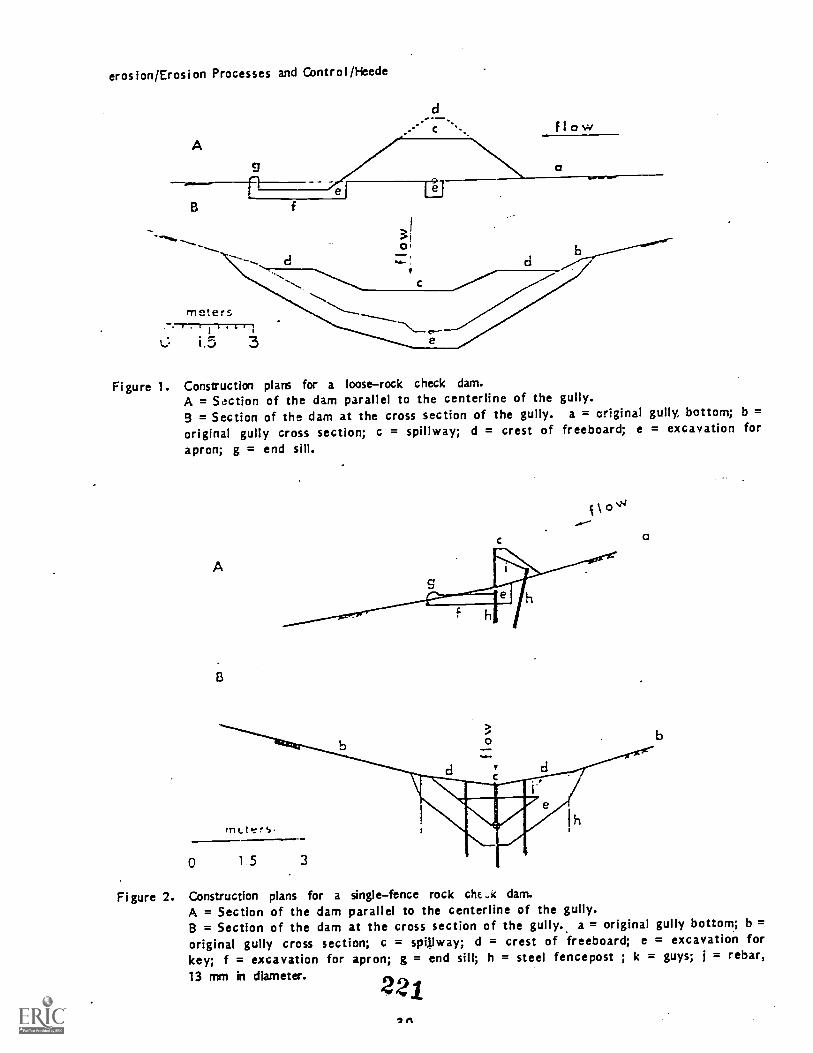
erosion/Erosion Processes and Control /Heede

d

flow

B f

Figure 1. Construction plans for a looserock check dam.A = Section of the dam parallel to the centerline of the gully.9 = Section of the dam at the cross section of the gully. a = original gully, bottom; b =original gully cross section; c = spillway; d = crest of freeboard; e = excavation forapron; g = end sill.

A

Figure 2. Construction plans for a singlefence rock cht..x dam.A = Section of the dam parallel to the centerline of the gully.B = Section of the dam at the cross section of the gully.. a = original gully bottom; b =original gully cross section; c = spillway; d = crest of freeboard; e = excavation forkey; f = excavation for apron; g = end sill; h = steel fencepost ; k = guys; j = rebar,13 mm in diameter. 221

A

erosion/Erosion Processes and Control/Heede

Figure 3. Construction plans for a doublefence rock check dam.A = Section of the dam parallel to the centerline of the gully.B = Section of the dam at the cross section of the gully. a = original gully bottom; b =original gully cross section; c = spillway; d = crest of freeboard; e = excavation forkey; f = excavation for apron; g = end sill; h = steel fencepost; i = rebar, 13 mm ind lame t er

f

rrie!ers

0 15

Figure 4. Construction plan for a gully headcut control with a looserock check dam. The section

of the structure is parallel to the centerline of the gully. a = original gully bottom;b = excavated area of headcut wall; c = spillway; d = crest of freeboard; e = excavationfor key; f = excavation for apron; g = end sill; h = rock fill.

2'

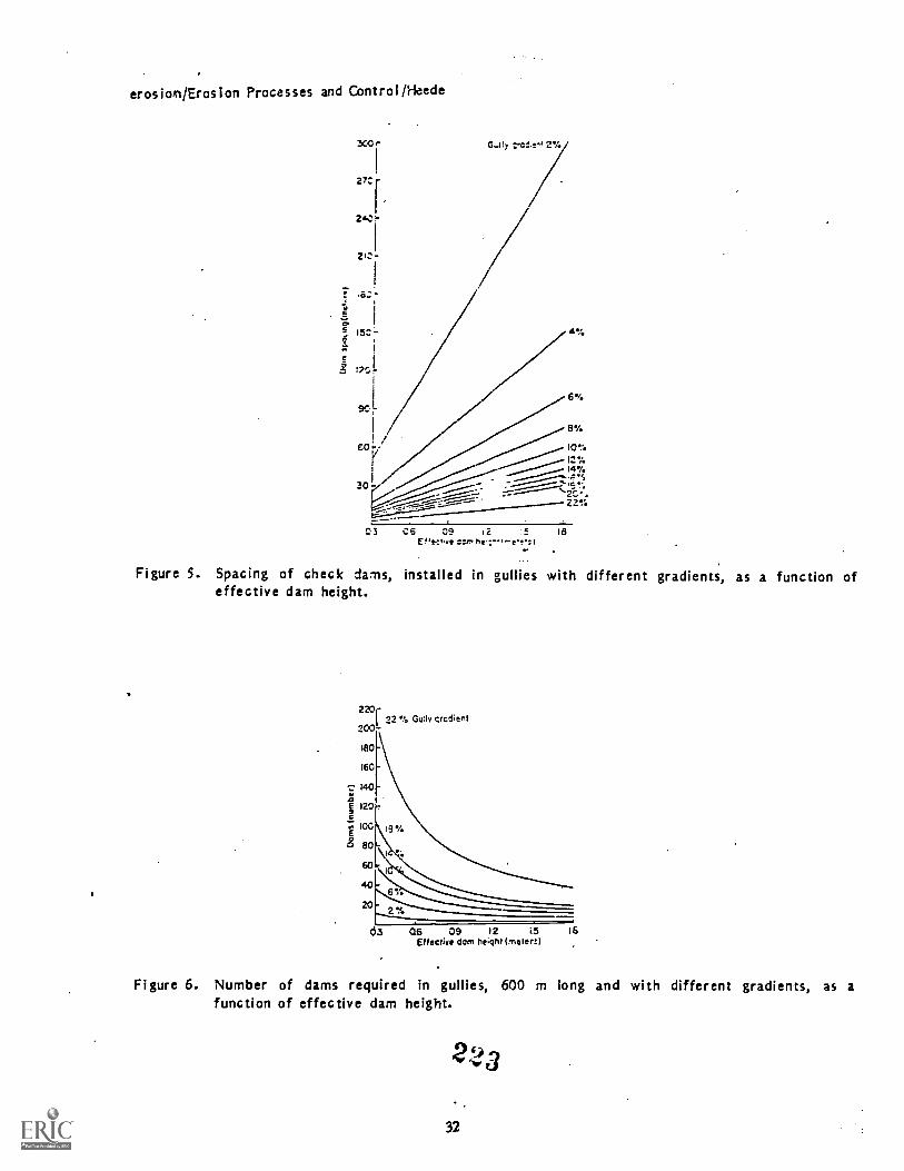
erosion/Erosion Processes and Control/Heede

300,

27:

24C-

212-

!eo

V10%

1

re...tro 2%

4%

6%

8%

12%

i -,-,.">14%

30 - ....,a..

'''..."---.:---,,.."---rx------

-- ,

03 C6 09 12 :5Effe-,trve :::r hirr'r,e.e,:l

22!:

18

Figure 5. Spacing of check darns, installed in gullies with different gradients, as a function ofeffective dam height.

220i

200.-

180

160

140

g 120.5

10G

8 80

22 % Gu:1Y Crcdient

d3 Q6 09 12 15Effective dam he;g111(meien)

16

Figure 6. Number of darns required in gullies, 600 m long and with different gradients, as afunction of effective dam height.

223

32

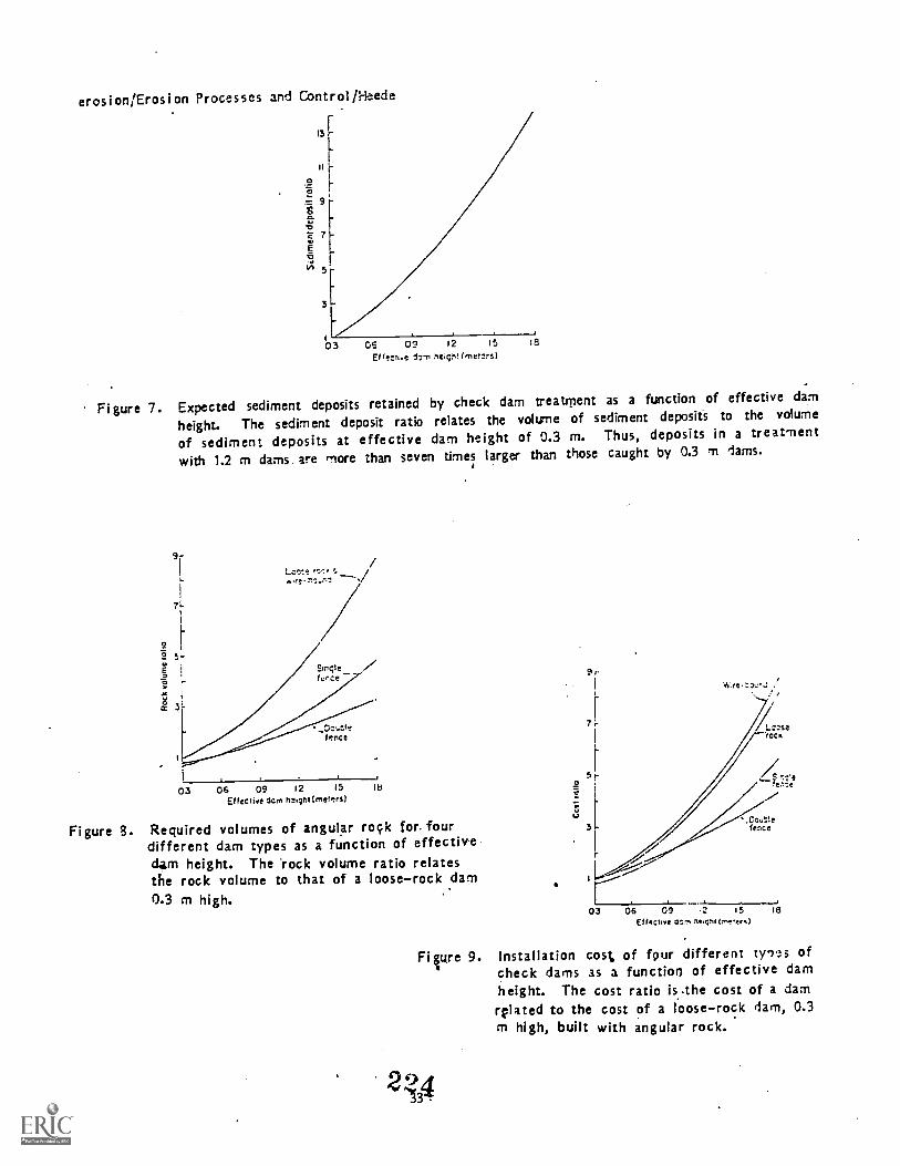
erosionlErosion Processes and ControlMeede

13

9

7

GS 09 t2 15

Et Fen.e trn heic.ro melcrsl

Figure 7. Expected sediment deposits retained by check darn treatment as a function of effective darn

height. The sediment deposit ratio relates the volume of sediment deposits to the volume

of sediment deposits at effective darn height of 0.3 m. Thus, deposits in a treatment

with 1.2 m dams. are more than seven times larger than those caught by 0.3 m dams.

wIre ns_ell

03 06 09 12 15

Et fects.e Ocm (meters)Ifs

Figure 8. Required volumes of angular rock for. fourdifferent dam types as a function of effectivedarn height. The 'rock volume ratio relatesthe rock volume to that of a looserock darn0.3 m high.

9 rW.re

Elleove ocm ne,cnt(m...u.,r)

Fi tire 9. Installation cost of four different trs ofcheck darns as a function of effective dam

height. The cost ratio is .the cost of a darnrelated to the cost of a looserock dam, 0.3m high, built with angular rock.

2;4

0'1 1ion/EroSion Processes and Control/Heede

23;

Op

.,r,

.,}

Co.,.11.**?:**.

3

S

54.

'9' S-.;. v- re.1*

4 4,. is-1,7 :..... ...* IN

is.....,... \\,......1"...17._.__......--.-wia.

5 ' -,----,",........._____------------ '......"--....._____

..3 :'"-- _-------------- 7..."----- "-

1

03 :4 9i .2 15 1d -04 09 .5 l0

t:.4Figure 11. Relative cost of installation of check-dam treatments and relative angular rock volume

requirements in gullies with different gradients as a function of effective dam height.

The cost and rock volume ratios relate the cost and rock volume of a treatment to those

of a treatment with loose-rock dams 0.3 m high installed on a 2 percent gradient.

244 r-al

Vo..4110...4 rc,s

2

044 v14...0 2%,Do..:.r.:10.:-s

2.5

2

/.5

05

03 G6

4%.

09 1.2 1.5 1.9 Or, 09Wool.. darn Pole/ (rr I.

$2 $5 18

Figure 11. The sediment-cost ratio relates the value of the expected sediment deposits to the cost

of treatment. The graphs show this ratio as a function of effective dam height on gullygradients ranging from 2 to 22 percent. The base cost was taken as $20/cubic meter of

A..v. rho v2Inot of 1 cubic meter of sediment deposits was assumed to be one-

evaluate/Range Inventory & Eval uat i on/S-ni th

Inventory and Evaluation of RangelandL. Snith

IntroductionPurpose of Range Inventory

Any resource manager needs information on which to base planning and make management

decisions. Such information includes data on climate, soils, geology, topography, animal

populations, hydrology, location of natural water, and cultural, features such as fences, roads,

wells, land ownership status, etc. The range specialist may collect this information himself orrely on collaboration of specialists in various areas. The range specialist usually has primaryresponsibility for evaluating the status of the vegetation and degree of soil protection on therange. This involves measuring the kind and/or amount of vegetation and soil cover to documentchanges over time or to make comparisons between areas managed in different ways. The information

may be used for such purposes as determining carrying capacity for livestock, estimating rangecondition, evaluating reseeding or brush control projects, describing patterns of distribution of

grazing. animals and many other purposes.

Problems of Range InventoryMany of the principles and techniques used in range inventory are identical or similar to

those used in other fields of agriculture such as forestry and agronomy. However there are two mainconsiderations which make range inventory more difficult than measurement of intensive pastures orproductive forests. One is cost. Rangelands are usually less productive on an acre (or hectare)basis than other lands and the areas involved are often large, remote and difficult of access.3ecause of their low productivity the costs of inventory per acre must be kept low.

The second, and most important, problem is variability. Rangelands typically are composedof native, plant communities composed of a great variety of species. These species vary widely ingrow th habit (annualperennial, bunch grasssodform er, herbaceousshrubby, tallprostrate, etc.) andin seasonal growth pattern. Measurement techniques which work well on some species are poorlysuited or impossible to use on others. Results may differ greatly if measurements are made atdifferent seasons of the year. Another source of variability is due to the variety of soils,

elevations, topographic position, slopes and exposures often found within a fairly small area.These lead to differences in species composition and production. Even where these factors arerelatively uniform vegetation is often very "patchy" in occurrence due to plant competition andreproductive method. Another important source of variability is caused by high variation in

rainfall within short distances and high yeartoyear variation typical of rangelands. This meansthat measurements collected in one place may not apply even a short distance away and it may benecessary to collect data for several years in succession to appropriate a "normal" situation.Finally, variability ..lay be introduced by differing historical use by grazing animals.

Therefore the range manager must continually seek to control variability to the extentpossible in his measurement techniques and be continually aware of the variability in his data whenmaking interpretations of it.

There are no simple or standard solutions to the problems of evaluating vegetationespecially on rangelands. Different kinds of information are needed in different situations and thetype or variability of vegetation may determine the appropriate techniques to be used. Carefulthought, especially when embarking on large scale or longterm projects, should be given to thefollowing questions:

1. What attributes of vegetation or soil are most likely to give the information requiredfor decision making and how will the data be interpreted, i.e. What do I really need to know andwhat must I measure to find out the answer? 226

evaluate /Range Inventory & Eval uat ion/Snith

2. What are the possible techniques that can be used, modified or developed to givereliable and interpretable results for the kind of vegetation involved?

3. What are the possibilities for controlling ariability to increase sampling efficiency?

4. How precisely must atrrioutes be measured to detect the differences expected in, time orspace?

5. Is an absolute roeasure needed, or will a relative difference (e.g. trend over time) bejust as useful?

6. What kind of preliminary testing and training is necessary to insure that the methodsused give repeatable and unbiased results?

Sarrp I ing and MeasurementsAccuracy and Precision

In any natural resource inventory it is usually impossible or impractical to measure theentire resource. Therefore a sample is taken to represent the whole population. There are twoaspects of this sample which are of concern: accuracy and precision.

Accuracy refers to how nearly the sample value approaches the true value for the population,i.e. is it a truly representative sample or is it biased in some way? There are several ways aninaccurate or biased sample may result. Malfunctioning or improperly used equipment may give abias. For instance, scales that are not properly adjusted may consistently read high or low.Another possibility is technique or personal bias of the data collector. Another is that the samplewas not selected properly. For example if all samples were taken near roads the results may notapply to the whole area since roads may tend to avoid steeper or rockier areas. Every effort mustbe made to eliminate bias or at least to recognize when unavoidable bias exists. Unfortunately, itis usually not possible to measure the amount of bias since the true population value is usually notknown.

Precision refers to the repeatability of the measurement. Precision is determined mainly bythe natural variability in the material being measured, consistency in technique of the datacollector and capability of the equipment used. Precision can be improved by controlling variationin the sampling, improving the technique or equipment used or just by taking more samples.Statistical analysis can be used to estimate precision. A sample may be precise but inaccurate oraccurate and imprecise.

Compatibility of MeasurementsThere are two kinds of error in measurements: absolute error and relative error. Absolute

error is expressed in units of measurement, e.g. grams, degrees, while relative error is expressedin percent. If a scale is graduated in one gram increments then it can only be read to the nearestgram, i.e. a weight recorded as lOg may actually be anywhere from 9.5 to 10.5. The absolute errorin this case is ± .5g. The relative error is .5g/10g = ± 5%. If the object weighs 100g theabsolute error remains the same, t .5g, but the relative error is now .5g/100g = .5%, a much moreprecise measurement. Thus, it is important to match the precison of equipment to the precision ofmeasurement required.

Whenever two different kinds of measurements are combined by multiplying or dividing it isimportant that the relative precision of each be approximately the same. The relative precision ofthe result is only as good as the [east precise component. For example, if you wished to estimatethe kilos of crude protein per hectare you need to measure the kilos of. plant material per hectareand multiply it times the percent of crude protein in the material. If crude protein content may bemeasured in the lab to a precision of 2% of the average value, but plant material per hectare is

2` 7

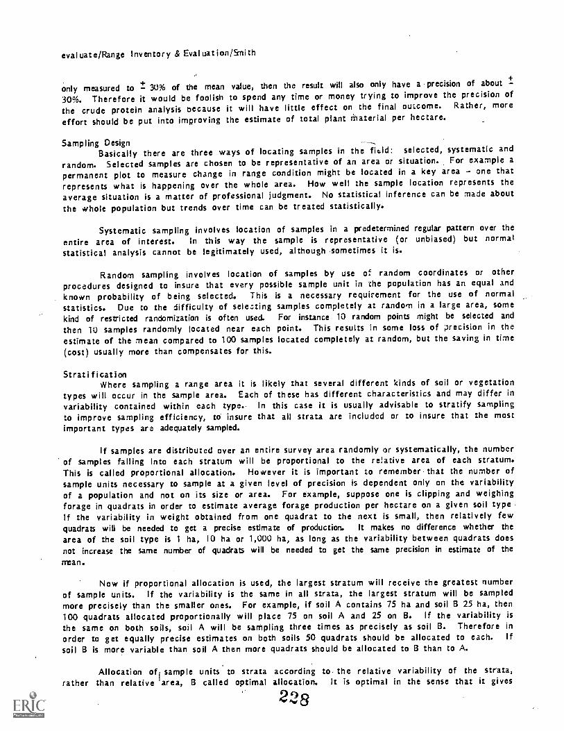
evaluate /Range Inventory & Evaluation /Smith

only measured to 30% of the mean value, then the result will also only have a precision of about +

30%. Therefore it would be foolish to spend any time or money trying to improve the precision of

the crude protein analysis because it will have little effect on the final outcome. Rather, more

effort should be put into improving the estimate of total plant Material per hectare.

Sampling DesignBasically there are three ways of locating samples in the fibld: selected, systematic and

random. Selected samples are chosen to be representative of an area or situation. For example apermanent plot to measure change in range condition might be located in a key area one thatrepresents what is happening over the whole area. How well the sample location represents theaverage situation is a matter of professional judgment. No statistical inference can be made aboutthe whole population but trends over time can be treated statistically.

Systematic sampling involves location of samples in a predetermined regular pattern over the

entire area of interest. In this way the sample is representative (or unbiased) but normalstatistical analysis cannot be legitimately used, although 'sometimes it is.

Random sampling involves location of samples by use of random coordinates or otherprocedures designed to insure that every possible sample unit in The population has an equal andknown probability of being selected. This is a necessary requirement for the use of normalstatistics. Due to the difficulty of selecting samples completely at random in a large area, somekind of restricted randomization is often used. For instance 10 random points might be selected and

then 10 samples randomly located near each point. This results in some loss of precision in theestimate of the mean compared to 100 samples located completely at random, but the saving in time(cost) usually more than compensates for this.

StratificationWhere sampling a range area it is likely that se veral different kinds of soil or vegetation

types will occur in the sample area. Each of these has different characteristics and may differ invariability contained within each type. In this case it is usually advisable to stratify samplingto improve sampling efficiency, to insure that all strata are included or to insure that the mostimportant types are adequately sampled.

If samples are distributed over an entire survey area randomly or systematically, the numberof samples falling into each stratum will be proportional to the relative area of each stratum.This is called proportional allocation. Ho wever it is important to remember that the number ofsample units necessary to sample at a given level of precision is dependent only on the variabilityof a population and not on its size or area. For example, suppose one is clipping and weighingforage in quadrats in order to estimate average forage production per hectare on a given soil type -If the variability in weight obtained from one quadrat to the next is small, then relatively fewquadrats will be needed to get a precise estimate of production. It makes no difference whether thearea of the soil type is 1 ha, 10 ha or 1,000 ha, as long as the variability between quadrats doesnot increase the same number of quadrats will be needed to get the same precision in estimate of themean.

Now if proportional allocation is used, the largest stratum will receive the greatest numberof sample units. If the variability is the same in all strata, the largest stratum will be sampledmore precisely than the smaller ones. For example, if soil A contains 75 ha and soil B 25 ha, then100 quadrats allocated proportionally will place 75 on soil A and 25 on B. If the variability is

the same on both soils, soil A will be sampling three times as precisely as soil B. Therefore inorder to g et equally precise estimates on both soils 50 quadrats should be allocated to each. Ifsoil B is more variable than soil A then more quadrats should be allocated to B than to A.

Allocation of'

sample units to strata according to, the relative variability of the strata,rather than relative area, B called optimal allocation. It is optimal in the sense that it gives

228

evaluate /Range Inventory & Eval uat ion/9ni th

equal sampling precision for all strata and the maximum amount of information from a given level ofsampling effort.

Number of Sampling Units NecessarySample units are the units in which a population is divideL for purposes of selecting

samples. If metersquare quadrats are used for sampling forage production then each quadrat is asample unit and represents a sample from all possible metersquare quadrats in the area. How manyare necessary to obtain a given level of precision depends only on the variability among them, asshown by the following equation:

n = t 2s2 /E2 ,

where n = number of units required, t = value of "t" statistic for desired level of probability, s =standard error, and E is onehalf the desired confidence interval around the mean.

If you have an estimate of the variability (S) from previous experience or a preliminarytest, you can calulate about how many sampling units (n) you need to estimate the mean withincertain limits (E) with a known chance of being wrong (t).

A less sophisticated but efffective way to estimate adequate sample size is simply to plot arunning mean as sampling progresses. For instance, when clipping quadrats you would average theresults of the first two quadrats, clip another and average all three and so on. The means obtainedwill vary considerably at first but, eventually will not change much as you add more quadrats. Atthis point the sample is adequate to give a good estimate of the true mean.

The variability among sampling units is partly due to inherent variability in the soil orvegetation being sampled and partly due to size, shape or arrangement of sample units. Therefore the

objective in sampling is to minimize the difference among sample units by including as muchvariability as feasible within sample units.

Size of Sample UnitsSuppose you were estimating the percent of ground covered by a shrub which averaged 4 sq. m

in crown area. Assume the actual percent ground cover is 50%, i.e. the size of the bare areasbetween plants also averages 4 sq. m. If you were using a square quadrat with an area of 1/10 m2

what would happen? Most of the quadrats would either land completely in a bare spot or within the

crown of a shrub; giving cover values of 0% and 100% respectively. Only a few plots would belocated overlapping the edge of the shrub to give intermediate values closer to the real coverpercentage. The coefficient of variation is very high meaning a large number of plots would benecessary to estimate cover precisely. In fact, the data obtained in this example are not normallydistributed and a valid confidence interval could not be calculated using normal statistics.

Now if the plot size is increased more and more plots will overlap the edge of the shrubsand the proportion of plots with 0% or 100% will decline. If the plots are larger than 4m2 thenvery few plots will have these extreme values. Increasing the plot size has reduced the coefficientof variation and fewer would be required to sample at a given loss of precision. The data have alsobecome normally distributed.

If the cover percentage remained at 50% but the average size of shrubs was only 2m2, i.e.there are twice as many of them, then the same number of smaller plots or a lower number of largeplots could be used. If the shrubs remained at 4m2 but cover was only 10%, then using a 4m2 quadrat

would still result in a very high proportion of zero values (a skewed distribution) and the plotsize should be increased. Thus the plot size should be larger than the average size of bare areasbetween plants and this is a function of both the size and the number of plants.

2 29

evaluate /Range Inventory & Evaluation /Smith

The preceeding discussion is based on the assumption that individual plants are randomly orregularly distributed over the sample area. However, plants very commonly grow in patches orclumps. This is called a contagious distribution. In this situation, once the size of plot is largeenough to overlap more than one plant, a further increase will increase the coefficient of variationbecause values for plots located inside dense patches increase more rapidly than those in sparsepatches. This process would continue until the plot size is bigger than the average size ofpatches, just as occurred with individual plants. In this kind of situation, one can either samplethe patches separately (stratify) or use a plot bigger than the average size of the patches.

The optimum plot size indicated by vegetation characteristics and statistics must bebalanced against costs and errors which may occur. Very large plots can be cumbersome to carry ortime consuming to lay out on the ground. Therefore it may be more efficient to use smaller plotsand take more of them. It is also more difficult to observe large plots and this may result inerrors or bias in collecting data. On the other hand large plots have less border effect for agiven area than small plots and thus bias may be reduced.

Experience has shown that it is usually best to use the smallest plots possible which do notresult in skewed distributions.

Shape of Sample UnitsShape of the sample unit also affects the variability of the sample, and consequently, the

number of sampling units required. Shape and size of sampling units are interrelated.

Go back to the example used for plot size, wh,4re shrub cover was 50% and average shrub sizAwas 4m 2. It was concluded that a square plot of 1/10m was too small and a square plot of about 4rti`was required. Now instead of being square, suppose the 1/10m2 plot was 1/100 wide and 10m long.Since the average diameter of shrubs and bare spaces is only about 2m, it is likely that a plot lOmlong will intersect several plants and several bare spaces. This means that cover values of 0 or100% would be rare, the distribution would be nearnormal, and coefficient of variation much lowerthan that obtained by square plots of the same size. Therefore a long narrow plot will samplevegetation more efficiently than a square or circular plot.

There are some disadvantages to the long plots however. It may be more difficult to see thewhole plot at once or to collect data from it, leading to errors or increased tin.:r per plot. An

important source of bias in using quadrats arises in making decisions whether a plant is inside oroutside the plot. This decision has to be made at the edge of the plot. 'since long, narrow plotshave a greater perimeter per unit area the chance for bias due to edge effect is greater forrectangular plots than for square or circular plots of the same size.

Rectangular plots should always be laid out with the long axis running across the gradientpatterns of the vegetation. Far example, on a slope the vegetation usually changes more from top to

bottom than along the contour. Therefore long narrow plots should be laid out with the long axisrunning up and down the slope since this will cut across the changes in vegetation and reducevariability from one plot to another.

Permanent or Paired PlotsOften the variability on rangelands is so great that it is impossible to measure attributes

precisely enough, within the limit of time and money available, to detect change over time or among

treatments. One way to get around this problem is to use permanent or paired plots to measuretrends.

If you wished to monitor changes in vegetation over time you could select a number ofrepresentative locations and mark them. By going back and remeasuring the same plots you couldmeasure trend over time. If the relative change is consistent on these plots the relative changecan be stated with confidence. However the absolute change in the true mean over the whole area

254

evaluate/Range Inventory & Evaluation/Shith

cannot be determined with much precision because the total number of plots is too low. The use of LI

permanent plots is not possible of course if the method of sampling influences the results obtained,

as it would if destructive sampling were used.

When destructive sampling is used or where different treatments are imposed, paired plots

can be used. In this procedure pairs of plots are chosen to be as much alike as possible to startwith. Treatment is applied to one of the paired plots and not to the other. If the relative change

on each pair of plots is similar the relative effects of the treatment can be expressed with

confidence, but again the absolute change in the whole area is not precisely known.

Botanical AnalysisGeneral

Many measurements used in range inventory involve measurement of various attributes of the

vegetation. There are many different attributes which can be measured and many different techniques

for doing so. Most of the attributes however involve some measure of weight, number or cover and

most of the techniques are variations on the use of points, lines, quadrats or plotless methods.Some of the most basic and commonly used are discussed below. First, there are some generalconsiderations which apply to all or most of them.

Range plant communities usually contain a variety of different plant species which may varyin size, spacing or growth habit (shrubs, trees, grasses, cactus, etc.). Because of differences insize, number or spacing optimum number, size or shape of sampling unit may be different for each

species. In addition, the interpretation of different attributes may vary among species, as well as

the most feasible technique for measuring these attributes. For instance, leaf area has no meaning

for cactus; stem diameter of shrubs may be difficult to measure on multiplestemmed shrubs.

Careful consideration must be given to the most appropriate techniques and how the results

will be interpreted. It is necessary to specify the "ground rules" on how the data will be

recorded; e.g. Will a plant be measured only if it is rooted inside the plot or if a portion hangs

over the plot? Preliminary testing of techniques and training of observers is necessary to assure

that data will be free from bias.

Most measurements involving several species can be expressed in either relative or absolute

terms. Production of species A can be expressed as kilos/hectare or as a percentage of the totalproduction of all species in the community. The relative measure is called composition. Which way

the results are expressed depends partly on how the data are collected and partly on how they are to

be interpreted.

If the most desired or useful measurement is very difficult or time consuming to obtain then

regression (or doublesampling) techniques are often used. This procedure involves the use of a

characteristic which is easy to measure and highly correlated with the desired characteristic to

estimate the desired characteristic. For instance if height and cover of grasses is found to be

highly correlated to production these characteristics may be used as an index to production or to

estimate production by regression equations. Although some error is introduced in making the

estimate it is more than offset by the increased number of measurements possible since cover and

height are much easier and faster to measure directly than production. It is often better to

sacrifice some precision on each measurement in order to obtain a greater number of observations.

DensityDensity is the number of plants per unit of area, such as trees/hectare. In some cases

density is a useful measurement as, for example, in evaluating seedling establishment and mortality,

the effects of brush control, age structure of stands, etc. Two problems are often encountered in

measuring or interpreting density:231

evaluate/Range Inventory & Eviluation/Snith

1. Density is not well correlated with other attributes if the size of the plants variesconsiderably. Ten trees per hectare may have more biomass, annual production, or area than 1,000

grass plants per hectare.

2. It is difficult to distinguish individual plants of some species. Imagine trying to

count the number ofbermuda grass plants in a lawn. There is no way to tell where one plant startsand the other stops. In this case the only solution would be to count individual stems.

Ranking Density may be simply estimated into classes, e.g. very abundant, abundant,

occasional, rare, very rare. The classes may be defined in terms of numbers or in descriptive

terms. A qualitative rating of density is called abundance.

Plots Density is usually measured by counting the number of plants in quadrats. This

is very straightforward if individual plants can be identified. The number and size of plots

required for efficient sampling usually varies quite a bit among different species. Since the

estimate of density for a given unit of area is independent of plot size, different numbers and/or

size of plots can be used for each species without affecting the mean estimate. A good rule ofthumb for plot size is that average number of plants/plot should be about four.

Distance Measures (Plotless) Plots may be difficult to lay out in shrub or forest type

vegetation. For this reason distance measures have been proposed. They are easier to use because

no plots are required. These methods are based on the concept that density (plants/unit area) is

the reciprocal of mean area (area/plant). Area can be calculated by measuring the dimensions of a

square, triangle or other polygon having a plant at each corner. Therefore the mean distance

between plants is related to the mean area per plant and density can be calculated from mean area as

follows: density = 1/mean area. There are four commonly used methods of distance measures, each

differing somewhat in the lengths measured and therefore the calculation of mean area.

1. Closest individual Sample points are located randomly or along a compass line. At

each point the distance to the nearest plant is measured. Mean area = (2d)2, where d = the distance

measured.

2. Nearest neighbor Sample points are located as before. The plant nearest the samplepoint is identified and the distance measured between that plant and its nearest neighbor. Mean

area = (1.67d)2.

3. Random pairs Sample points located as before. At each point, the observer faces the

nearest plant. The distance is measured to the nearest plant on the opposite side of a line running

througi the sample point perpendicular to the direction the observer is facing. Mean area =

.(0.8d)`.

4. Point centered quarter method At each sample point the area around the point is

divided into quadrants. The distance to the nearest plant in each quadrant is measured and the four

distances averaged. Mean area = (d)2.

All of these methods are based on the assumption that plants are randomly distributed. If

they are not, the estimate of density obtained will be biased. If the data are recorded on a

species basis the relative density of each species can be calculated whether distribution is random

or not.

FrequencyFrequency is the number of quadrats in which a species occurs divided by the total number of

quadrats, usually expressed as a percentage. For each quadrat, each species is recorded simply as

present or absent. The number of plants of each species is not counted.

232

evaluate /Range Inventory & Evaluation /Smith

Frequency of a species is dependent o the size of quadrat used. As quadrat size increasesthe chance of finding a given species in any one quadrat also increases. If plants are randomlydistributed over an area frequency is related to dens; ty; as density increases, so does frequency.If plants are not randomly distributed, i.e. they, occur in patches or clumps, then there is no fixedrelationship be t.v een density and frequency. For example if a sample of 100 meter-square quadrats in

taken and one plant occurs in each the density is 1 /m and the frequency is 100%. However if all ofthe 100 plants occur in one quadrat and nothing in the other 99, the density is still 1 /m2 but thefrequency is 1%.

Very high (>95%) or very low (+-5%) frequency is difficult to intepret or analyze becausedistributions' are highly skewed at extreme values. A desirable quadrat size is one which willmeasure the most species within these limits. A general rule is that if the most frequent speciesare in the range of 65-85% the quadrat site is about right. Some times two or more quadrat sizesmust be used in order to get information on an adequate number of species. Fr equency percentagesmeasured by different quadrat sizes are not comparable however.

Frequency data are analyzed using statistics based on the binomial distribution since onlypresence or absence is recorded. The variance is es timated as follows:

s2 = pq/n-1 ,

where p = the o frequency, q = 1-p, and n = the number of quadrats. About 200-300 quadrats usuallygive an adequate sample.

For ease of location, frequency quadrat.; are sometimes located in transects. About h)transects with 25 quadrats per transect have been recommended.

The principal advantages of frequency samplint are:

1. Data collection is rapid and objective. The observer only has to know the species anddecide if they are in or out of the quadrats.

2. Data is quantitative, subject to statistical analyses.

3. Mor complete information on species is usually obtained since the amount of area lookedat is large compared to most other types of sampling.

Disadvantages are:

1. Results obtained depend on quadrat size, therefore data c.:lected with different sizequadrats is not easily compared.

.. Frequency is difficult to interpret since it measures both number and dispersion ofplants. It is not necessarily correl at ' with density, cover, or production especially for

interspecific comparisons.

3. Frequency is an independent measure for each species. This means that data for eachspecies must be analyzed separately, i.e. a total value for all species has no measuring as it doesfor cover, density or production.

CoverVegetation coy-. and ground cover are n measured in range inventories because (1 )

vegetation cover is a good indicator of ecologic? tance of species in a community since it is

related both to size and number of individuals .;nd (2) ground cover gives a good measure ofprotection. Also-, cover measurement is relatively easy and can be consistently measured.

233

evaluate/Range Inventory & Eval uat ion/9ni th

Vegetation cover is a measure of the area of aboveground vegetation in relation to groundarea, usually expressed as percentage. There are several ways it can be approached:

Leaf area index (LAI) is the total area of leaves by species measured as a percent ofground area. Both inter specific and in traspecific overlap are included. LAI is widely used inagronomic studies on intensive pastures or forage crops because it is related to phtotsynthetic area(i.e. productivity). On denser vegetation LAI usually exceeds 100Vo, often reaching 500-1000%. Itis less used in sparse range vegetation' because leaf area and shading are not usually the limitingfactors to production.

Foliar projection is a measure of leaf (and sometimes stem) cover which is best thoughtof as the area of shadow which would be produced on the ground if a strong light shone vertically onthe vegetation. Overlap of leaves is ignored, therefore this measure is always less that LAI.

Canopy area is the toal area included within the perimeter of the plant canopy, i.e. itignores both leaf overlap on the same plant and the small holes or discontinuities within thecanopy. it would always be greater than foliar projection.

Basal area or cover is a measure of stem area at the ground surface (or some standarddistance above it). Foresters use basal area extensively because it is easy to measure on trees andrlates well to growth and production. Range managers have found it useful for herbaceous plants,especially bunchgrasses, because it is less dependent on current year's growing conditions and lessaffected by current utilitzation by grazing animals than < anopy cover is. Rasdi area is harder tomeasure on multiplestemmed shrubs and generally less meaningful on shrubs because of their variaolegrowth forms.

One decision that nearly always has to be made when measuring vegetation cover is how todeal with ovelapping canopies of different species. If cover is being measured to express speciescomposition related to relative ecological importance or forage production, then overlap shouldusually be included i.e. total crown cover could exceed 100%. However if an inde'x to soilprotec tin or rainfall interception is the objective, canopy overlap is generally best ignored. Inother words the interest may be more :n how much ground is uncovered rather than how much iscovered.

Ground cover includes vegetation cover and also the amount of litter, rock, gravel and baresoil. Thes'e classes are usually defined so that the total adds to 100%.

Visual EstimationWith experience, cover percentage can be estimated visually either by just walking through

the area or by using quadrats. Without careful training considerable personal bias can beintroduced. An example of the use of quadrats is Daubenmire's canopy cover method. A number ofquadrats, usually .25 to 1 m2 are used. Canopy cover by species is ranked in each quadrat asfol lows:

Rank Cover %1

2 5-253 25-504 50-755 75-956 95-100

2 tr-3 4

evaluate /Range Inventory & Evaluati on/SmitN

Ranks are used because it is much faster to decide if a species falls in a certain classthan to estimate the exact cover percentage. After a number of quadrats are taken the ranks aremultiplied times the midpoint of the class cover percent (e.g. for rank 1 it is 2-1/2)c) andaveraged. Unequal cover class sizes are used because this gives more sensitivity to species ,vithvery high or very low cover percentages.

Point MethodsIf frequency quadrats are reduced in size to a dimensionless point, then the percentage or

frequency of hits on a plant is an unbiased measure of cover. Points are used in various ways suchas linepoints, pointquadrat, or steppoint methods.

The pointquadrat or pointframe techniques involve the use of a metal or wooden framedesigned to hold metal pins in a vertical or oblique position. Usually there are 10 pins to a

frame. The pins are lowered slowly to the ground one by one and it is recorded what the point ofthe pin touches. It may touch leaves, stems, litter, bare ground, etc. Multiple hits on leaves maybe recorded if LAI is to b, measured. Each 10point frame is considered an observation or samplingunit. The use of the frame is only a convenience which allows a more objective placement of the pinsthan would be possible if they were handheld. The optimum number of pins used per frame and thedistance between them depends on size and spacing of plants (as discussed under size of samplingunits). The number of frames (or total points) necessary depends on the variability between framesand the sparseness of the vegetation. Points may be spread out along a tape or line at longerintervals than would be practical using a frame. This is called a linepoint transect.

Another variation of the point method is the steppoint transect commonly used by rangemanagers. In this case, a point is marked, or a notch cut, on the toe of the shoe. The observerthen paces a straight line across the szmple area and at regLilar intervals records hits under thepoint. A pin may be used or merely a visual sighting.

Point methods are fairly rapid to use and give unbiased and objective data if properly done.Some important advantages and disadvantages are:

1. In sparse vegetation, a very targa number of points is required to get good estimates onindividual species, e.g. when total cover is only 5%, 1000 points will only give 50 hits onvegetation. This is a small sample to base composition on. On the other hand 100-500 points givesa very reliable estimate of bare ground in sparse vegetation.

2. Point methods are best suited to lowgrowing vegetation. To record "hits" on tallspecies requires that the observer project the point upward, which is difficult to do in an unbiased:canner.

3. Recording foliar hits on windy days is difficult.

4. Bias is introduced (cover over estimated) as the size of th:: point is increased.

5. In the steppoint procedure, bias may be introduced if the observer deliberately orsubconsciously lengthens or shortens his pace or deviates from a straight line to miss obstacles inhis path.

One way range managers attempt to improve on the estimates of composition in sparsevegetation is to use the nearestplant technique. At each point location where no plant is hit, thenearest plant to the point is recorded in a "composition tally" in addition to recording bare groundor whatever else the point hits. Thus the number of Observations on plant species composition isincreased.

2`'10

evaluate /Range Inventory & Evaluat ion/Snity

Line InterceptionIn this method a line of known length is stretched between two stakes. The intersection of

plant canopies or basal area is measured by species. The total length of intercept dividq by thelength of the line is an unbiased estimate of percent cover. Each line (transect) is a sampling

unit. For efficient sampling, the length of line is usually greater in sparse vegetation than in

dense. Lines of 15-50 m length are usually used on rangelands.

Line interception is particularly useful for canopy cover of lowgrowing shrubs and basalarea of bunchgrasses. Basal area on sodforming grasses or single stemmed herbs is hard to measure.Density is sometimes measured along the transect by counting all plants within a certain distance of

the line.

Other TechniquesThere are a variety of other techniques used for cover. Foresters have made extensive use

of the "variable plot" or Bitterlich method for basal using a prism or anglegage. It has hadlimited use for range vegetation however because the margins of plant canopies are less distinctthan tree trunks.

Cover of shrubs or trees is sometimes figured by measuring average canopy area of a numberof shrubs and multiplying this times the number per hectare.

Various techniques involving mapping or charting of quadrats have been used. These involve

a scale drawing of the outline of each plant on a sheet of paper. This is done with a pantograph orby visual estimated or measured coordinates. These are good methods for recorded changes over time

and for plant demographic studies. However char!:Ag methods are very time consuming.

Vertical photographs can also be used to record cover. Quantification of data by species isnot simple however due to difficulty of identification and distortion in the photographs.

Production (Weight)Weight of plant material is measured for a variety of reasons. It is a good measure of site

productivity and ecological importance of species, it is related to carrying capacity, it may beused as a measure of fuel for controlled burns, etc. The actual techniques of measuring weight arefairly simple, although laborious. The most important considerations are what to measure and whento measure.

First, it is necessary to consider the various components of vegetation that can be measuredand the terms used to describe them. Biomass is the total amount of plant and animal materialpresent. Abovearound plant biomass excludes animal material and plant roots. Aboveground plantbiomass may be divided into living (or green) biomass and dead (or dry). The dead portion can beseparated into standing dead (still attached to the plant) and litter or mulch (detached or fallenmaterial). Standing crop usually refers to the living and dead material still attached to the plantat any given time. Production is the total weight of plant material produced over a period of time,whereas productivity is the rate of production over a specified period of time.

Range managers are usually most interested in measuring weight as an indication of siteProductivity or of carrying capacity. To measure production in a given season or year, it is

necessary to separate the material produced prior to that time and only weigh the current year'sgrowth or current season's growth. For example, on a shrub which was several years old we wouldmeasure only the leaves and young sterns produced this year, which might be only a small portion ofthe total standing crop. Even grasses and forbs may still have standing growth produced in earlierperiods. In some cases, on evergreen shrubs or cactus, for example, it is very difficult to

identify current year's growth. Separation may be done in the field or in the laboratory.

In order to use information on production for estimating animal carrying capacity a

distinction must be made between total plant growth and forage production. Forage is that portion

2 9ri

evaluate /Range Inventory & Eval uati on/Sni t,

In order to use information on production for estimating animal carrying capacity adistinction must be -made between total plant growth and forage production. Forage is that portionof the plant growth which animals can and will eat.. The proportion of the total production which isconsidered forage depends on the palatabilty of the plant or plant part (which depends on the kindof animal and season of use), the proper level of utilization which can be made of the plant, andaccessibility of the plant material (e.g. leaves growing too high for an animal to reach cannot beconsidered forage).

Production is usually measured at the end of the growing season since this is when the peaktotal production for the y ear occurs. After this time there is a decrease in plant material presentbecause of decomposition, consumption by insects or wild animals, etc. However, even when plants

are growing, these losses occur so that production measured at any one time never represents thetrue total production for the year. This is especially true where two growing seasons occur in one

year or where. plant species in the community have very different phenological patterns. The

underestimate of total production may be slight or range up to about 5096 of the true value.

If the range has been or is being grazed by livestock or other animals when production is

measured, then the areas used for measurement must be protected from grazing or the amount of forage

eaten estimated and added to the production measured. There are techniques available for measuring

utilization which will not be discussed here. Regrowth of plants after grazing is another possiblesource of error.

Production measured for one year may not indicate the average annual rate of production. On

many ranges the production per year varies greatly from one year to another due to weather,

especially rainfall. Production in good years may be 2-10 times the production in poor years.Therefore measurement of forage production may not mean much unless repeated over several years or

adjusted for growing conditions.

Finally moisture content of plants, especially green portions, varies widely depending on

the plant part (leaves, stems, seeds) season of year, current soil moisture and even the time of

day. For this reason plant weight is almc74 always reported on a dry weight basis. This means that

samples should be or en dried or air dried before weighing or a subsample taken to determine amoisture correction factor.

Harvest MethodThe most straightforward way of measuring production is to clip and weigh in quadrats.

Separation of different species or of current vs. old growth may be done in the field or in the lab.

On sparse range ;etation it is usually easier in the field. Samples may be weighed moist in the

field and subsamples taken for moisture correction or the w hole sample taken in and dried before

weighing.

Clipping plots is a very time consuming procedure and the high variability of rangevegetation often requires a large numb er of samples for reasonable precision. If the number of

samples required is large it may take days or weeks to collect them unless a large crew is

available. This may introduce additional error because the vegetation may mature or disappear over

the sampling period. Thus anything which can increase the sampling efficiency is justified. One

way to increase efficiency is to low er the variability between sampling units. This has already

been discussed. Another is to decrease the time spent per sampling units even at the expense of

some precision on each observation, in order to increase the sample size possible for a given amount

of time and money. The following techniques are aimed at the latter alternative.

2') 7WeightEstimate

Weight may be estimated in quadrats rather than clipped. Estimation is much faster than

clipping but highly subject to bias or error on the part of the estimator. For this reason,

extensive training and rechecking is necessary. Estimatim is best done by weightunits. The

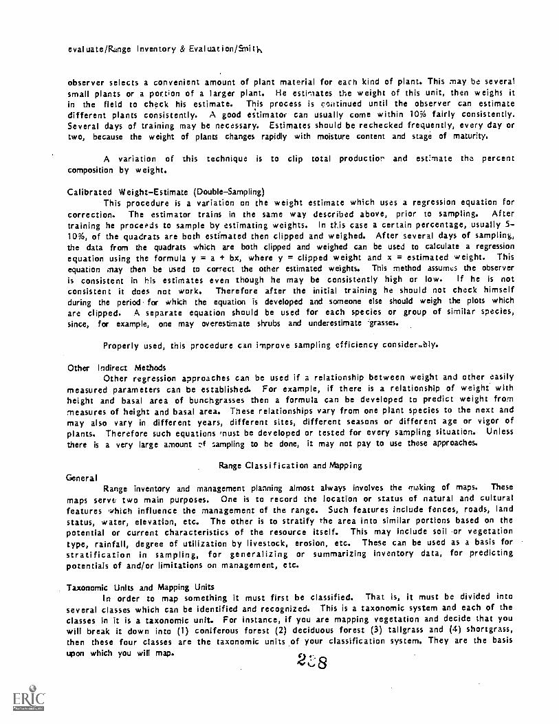
evaluate /Runge Inventory & Evaluation /Snit},

observer selects a convenient amount of plant material for each kind of plant. This may be severalsmall plants or a portion of a larger plant. He estimates the weight of this unit, then weighs itin the field to check his estimate. This process is continued until the observer can estimatedifferent plants consistently. A good estimator can usually come within 10% fairly consistently.Several days of training may be necessary. Estimates should be rechecked frequently, every day ortwo, because the weight of plants changes rapidly with moisture content and stage of maturity.

A variation of this technique is to clip total production and est:mate the percentcomposition by weight.

Calibrated WeightEstimate (DoubleSampling)This procedure is a variation on the weight estimate which uses a regression equation for

correction. The estimator trains in the same way described above, prior to sampling. Aftertraining he procePds to sample by estimating weights. In this case a certain percentage, usually 5-10%, of the quadrats are both estimated then clipped and weighed. After several days of sampling,the data from the quadrats which are both clipped and weighed can be used to calculate a regressionequation using the formula y = a + bx, where y = clipped weight and x = estimated weight. Thisequation may then be used to correct the other estimated weights. This method assumes the observeris consistent in his estimates even though he may be consistently high or low. If he is not

consistent it does not work. Therefore after the initial training he should not check himselfduring the period for which the equation is developed and someone else should weigh the plots which

are clipped. A separate equation should be used for each species or group of similar species,since, for example, one may overestimate shrubs and underestimate grasses.

Properly used, this procedure can improve sampling efficiency considerably.

Other Indirect MethodsOther regression approaches can be used if a relationship between weight and other easily

measured parameters can be established. For example, if there is a relationship of weight withheight and basal area of bunchgrasses then a formula can be developed to predict weight frommeasures of height and basal area. These relationships vary from one plant species to the next andmay also vary in different years, different sites, different seasons or different age or vigor ofplants. Therefore such equations must be developed or tested for every sampling situation. Unless

there is a very large amount sampling to be done, it may not pay to use these approaches.

Range Classification and MappingGeneral

Range inventory and management planning almost always involves the making of maps. These

maps serve two main purposes. One is to record the location or status of natural and culturalfeatures which influence the management of the range. Such features include fences, roads, landstatus, water, elevation, etc. The other is to stratify the area into similar portions based on thepotential or current characteristics of the resource itself. This may include soil or vegetationtype, rainfall, degree of utilization by livestock, erosion, etc. These can be used as a basis forstratification in sampling, for generalizing or summarizing inventory data, for predictingpotentials of and/or limitations on management, etc.

Taxonomic Units and Mapping UnitsIn order to map something it must first be classified. That is, it must be divided into

several classes which can be identified and recognized. This is a taxonomic system and each of theclasses in it is a taxonomic unit. For instance, if you are mapping vegetation and decide that youwill break it down into (1) coniferous forest (2) deciduous forest (3) tallgrass and (4) shortgrass,then these four classes are the taxonomic units of your classification system. They are the basisupon which you will map.

evaluate/Range Inventory & Evaluation/SmireT

Mapping units are the areas delineated on a map and given a name or number. A simple

mapping unit is one where all or most of the area within the unit is composed of one taxonomic unit.

It may have minor inclusions of other taxonomic units within it but these do not usually amount tomore than about 10% of the total area. For instance, if you drew a line around an area and called

it "coniferous forest", it would contain all or mostly coniferous forest with only minor inclusionsof other classes, such as deciduous forest or tallgrass.

It may happen however that two or more taxonomic units are so intermixed that it is

impossible to draw a line around an area which is predominantly one or the other. In this case

about the best you can do is to map areas with similar proportions or patterns of the different

taxonomic units. For instance you might map one area which contained about 60% coniferous forestand 40% deciduous forest, another might have 75% deciduous forest and 2596 coniferous forest; still

another might have 60% deciduous forest and 40% tallgrass with minor inclusions of shortgrass.

These are called complex mapping units. They are patterns of taxonomic units rather than uniform

areas of one taxonomic unit.

Whether you can map simple or complex units depends on the scale of the map and thecomplexity of the pattern of taxonomic units in the area. The more finely divided the differentsoil or vegetation types and/or the smaller the scale of mapping the more likely it is that complex

units will be mapped.

The important point is if mapping units are complex, sampling for inventory purposes should

be carried out separately on each taxonomic unit within the mapping unit. This will increase

sampling efficiency and make the resulting data much more useful and interpretable. Data collected

on each taxonomic unit can be weighted by the estimated area of each taxonomic unit to give an

overall average for the mapping unit.

Aerial PhotosRange mapping can be and has been done without aerial photos. The use of aerial photos

increases the accuracy and efficiency of field work so greatly that it is foolish to attempt

inventory of any sizeable area without them. Aerial photos are available now for almost any area in

the world, often several different dates and scales are available. Black and white, natural color

or color infrared photos may be used.

Aerial photos always contain some distortion of scale caused by differences in distance to

the lens of the camera. However, unless the photography was very poorly done or elevational

differences are great in relation to photo scale, these distortions are not enough to affect

accuracy of most range surveys greatly.

The first step is to obtain the photos. Black and white are adequate for most range work.

Photos are usually flown in strips with each photo overlapping the next about 60% to allow

stereoscopic viewing. The strips overlap 10-20% on the sides.

The second step is to delineate effective mapping areas on the photos. Points about midway

in the zone of overlap of adjacent photos are selected and located on each photo. Two or three of

these points on each side of the photo are connected with lines. The area within the lines is the

area mapped on each photo; when you get to the boundary of the effective area you switch to the

adjacent photo. These effective areas make it easier to avoid skipping areas and facilitate

transfer of information to maps. Delineating effective area on alternate photos within a strip is

usually satisfactory and reduces the number of photos needed in the field.

The third step is to pretype the photos. This should be done under stereo if possible.Many features can be mapped in the office, especially if you know the area well. Pretyping should

be erasable so it can be changed if field checking shows it to be in error.

cVell1.10.1./ tcalsbs. sa v...."

The fourth step is to go to the field and complete the mapping. This may be done directly

on the photo (with soft pencil) or on a transparent overlay. Exact locations of sample points,

fence corners, benchworks, etc. may be pinpricked through the photo and identified on the back.

The fifth step is to ink on the completed mapping on the photo or transfer it to a

planimetric base map. To determine area or distance on the photo or, transfer information to a map

you need to know the scale of each photo. This can be determined by measuring the distance between

two points both on the ground and on the photo and calculating the ratio between them.

24015

rangecon/Range Condition /Ogden

Range Condition

Phil OgdenProfessor of Range Mangement, University of Arizona

IntroductionAs researchers and resource managers consider data collection and techniques for management

of watersheds to improve soil stability and/or water yield, they are immediately faced with thecomplexity of the watershed resources with which they must work. These complexities are not only in

vegetation, soils, topography, and climate but also in differences in uses such as livestock and

wildlife grazing. The watershed manager must recognize that grazing influences differ among soils

and vegetation communities on watersheds. An initial step in reducing the soil a,.d vegetation

complexity is to identify management units which are sufficiently homogeneous so that research data

may be extrapolated from one unit to another and to which similar management techniques apply.

Range Si tes

A basic unit of land classification which has been utilized in range evaluation, especially

by the U.S. Soil Conservation Service, has been the range site. A range site as defined by the

Range Term Glossary Committee (1964) is:

An area of land having a combination of edaphic, climatic, topographic and natural biotic factors

that is significantly different from adjacent areas. These environmental areas are considered as

units for purposes of discussion, investigation, and management. Changes from one site to another

represent significant differences in potential forage production and/or differences in management

requirements for proper land use.

Within a specified precipitation zone, topographical position (bottomland, upland,

ridge, etc.), slope, aspect, and soil factors combine to create range sites. Each site

has a potential to produce specific plant and animal communities and sediment and water

yields within a watershed. Sometimes range sites within the watershed are sufficiently

large so that they may be mapped and managed as separate entities, but often they occur in

patterns where only complexes of sites can be mapped. Sampling, however, should be

accomplished at the site level. It is at the range site level that the researcher andmanager can correlate treatments and results and, thus, begin to understand apparently

unrelated data. Aerial photography is an excellent aid in identification and delineation

of range sites within a watershed.

Range Condition and TrendEach range site has a potential to grow specific plants with a level of vigor, ground cover,

and erosion protection which can be called excellent for the site. This potential, or excellent

condition, for each range site can be determined by observing wellmanaged areas. Range condition

is defined as the current status of vegetation and soil compared to the potential for the site.

Thus, range condition is excellent, good, fair, or poor depending on characteristics of the site at

the present compared to what it is capable of producing.

The concept of range condition requires that some potential characteristics of vegetation

and soil be established for each site against which current characteristics can be compared. In the

United States, ungrazed portions of sites have often been used to establish the potentials. This

has been criticized on the basis that ungrazed conditions are not a reasonable management goal. The

researcher or manager has two ways by which he may avoid this criticism. One way is to define the

potential as the vegetation and soil characteristics which can be attained under what is considered

good management. The second alternative is to define potential in terms of ecological climax

vegetation without livestock grazing but set the management goal for the condition level which

241

rangecon/Range Condition /Ogden

maximizes returns and proves stability to the watershed. This later approach is preferred ifungraz ed areas can be found as a basis for establishing potential.

Plant species composition (relative abundance of different species in the plant community)is one of the most important characteristics related to range condition. There is a dynamicrelationship which exists between soils and plant communities on each range site. As plantcommunities occupy a range site, they in turn modify the site by changing the soil nutrients, waterholding capacity, and other factors. These new conditions enable other plant communities to replacethe existing communities on the site. This succession of one plant community replacing anothercontinues until a plant community exists which maintains itself on the site (climax community).Figure 1 represents plant community development on a site with fluctuations created by weathercycles. Note that there is a general development toward a climax plant community (Cn) for the sitebut periods of dry we ather cause fluctuations in this development. Vegetational succession on asite may also be reversed by excessive grazing, fire, plant diseases, or mechanical disturbance ofthe site (Cn). This will level off (C

P) when the disturbance is removed and development again turns

upward. ?figure 2 shows the relationship bet ween ecological climax and range condition classes.Correct management decisions require the knowledge of the condition of the vegetation of each site,

whether the trend is toward succession or retrogression, and the cause for the current situation,Heady (1973).

Dyksterhuis (1 949) developed a quantitative method of evaluating range condition based onplant composition which has been widely used by the U.S. Soil Conservation Service. His methodclasses plants as de creasers, in creasers, and invaders. Decreaser plants are those which decreasein abundance, at least initially, with heavy use. Increaser plants are those which initiallyreplace the decreasers in early stages of heavy grazing use but they also decline in abundance asgrazing pressure continues and the grazing load shifts to them. Invaders are not present on a sitein excellent condition but they move in when decreasers and increasers no longer fully occupy thesite. For evaluation of condition, site locations are selected which are producing what is

considered to be the potential vegetation for the site. Guides are established for the range sitein this excellent condition, listing the plants as decreasers, increasers, or invaders for the site.Increaser plants are given a maximum percentage composition value at which they would occur(percentage allow able toward condition score) on the site in excellent condition. Table 1 shows ahypothetical guide for a range site. The evaluation of condition in the field is made by estimatingplant composition on the site under evaluation and comparing with the guide. Composition must bebased on the same criteria as the guide but may be based on cover or weight.

Table I

Range condition guide for a sandy upland range site receiving 300 mmof annual precipitation. Plant composition based on percentage by weight.

Decr easers

(Count all of percentagecompositon toward condition score)

Increasers(Count only percentage

allowable toward condition score)

Invaders(Count none toward

the condition score)

Percentage Allowable

SpeciesA

C

SpeciesD 30

E 10

F 5

SpeciesG

rangecon/Range Condition/Ogden

CI AT u FSOIL.

ti

tGt

r.

c.0

r cLzm.ixL VEG ETAT:ION

ExcELLEN1

GOOD1:70/),Icr*rf:.12.v

1.?c

POO'?

IZE7F.1?.10 R/17 IRAN 6E1_4147)

1 tam 41?'/31.E,e3

:1,.. `" a C: vr43,vc

ver.:::i re dsteri:ratec

Fretipitraion- causedtluctunt.ons

0 Time

Figure 2. FLAIIT RICCI SS WU, P.EGUESSI(.1;:, SOIL ilEt/LLOPIVIT MO MCC CONIIIII:t;

CLASSES, 'mom (1970)

213

Tr;

rangecon/Range Condition/Ogden

Table 2 shows field data for a sandy upland range site and calculation of range conditionsocre. Scores of- 0-25 are poor condition, 26-50 fair, 51-75 good, and 76-100 as excellentcondition. Plant cover, litter accumulation, plant vigor, current erosion and other factors mayalso be utilized to evaluate site condition estimates.

Table I I

Field data as percentage plant species composition by weight fromsandy upland range site and calculation of a range condition socre.

Percentage Compo Contribution toSpecies sition by Weight Condition Score

A 10 10

B 10 10

D 60 30

F 10 5

H 10 0

Total 100 55

Condition Score is 55, which is Good condition.

Change in range condition over time is known as range trend. Range trend may be upward(improving), downward (kenning), or static. Evaluation of trend helps to monitor use influenceson range sites on a watershed.

Plant Growth INfluenced by GrazingFor an understanding of why overgrazing causes vegetation retrogression, it is appropriate

to review a few basic plant growth requirements. Each plant growing on the range functions as aconverter of solar energy to chemical energy stored in organic compounds. The process by which this

is accomplished is photosynthesis which takes place in the green leaves of plants. The chemicalenergy formed by the plant is utilized by the plant to make root growth and herbage growth, produce

seed, and develop winter or drought hardness. Also, it may be stored in roots and stem bases to beused to. initiate growth following winter or drought dormancy. Without adequate leaf material lefton a plant, it is unable to convert adequate energy to meet its needs for survival. This chemicalenergy converted by plants is also the source of energy for animal populations 'which obtain foragefrom rangelands.

The energy reserves stored in the roots and stem bases of plants is reduced to its lowestlevels at the time a plant first initiates growth after a period of winter drought dormancy. Figure3 shows the accumulation and depletion of carbohydrate reserves in sideoats grama (Boutelouacurtipendula) growing in southern Arizona. Close and continued grazing when reserves are low, sothere is no opportunity to replenish reserves, is extremely harmful to plant vigor. After, growthhas been well started, however, most plants can function effectively and continue to carry onadequate photosynthesis if no more than NA of their herbage weight is removed.

With close and continued overgrazing, growth is reduced, seeds are not developed, and theplant is reduced in vigor to the extend it is unable to withstand drought or cold or to makeregrowth after dormancy. In addition, if grass plants are grazed too closely, the growth buds atthe base of the plant are exposed to the temperature extremes of hot in the daytime and cold atnight and to extreme drying. Adequate plant material left at the base of plant protects the tendernew buds which produce the next crops of herbage. r.

414

range-con/Range Condition/Ogden

!4n

120

100

0 t t I I I I 1 t t1

J J A S 0 N 0 J F ?.1 A t.I

107 3 1974

3. 7.z.-::-:s."ate -3;erves 25 c:'vale-ts in rcc c sicna:s ;-a-ar2 E';Ir. ,7.-.:zs.13. ;5 .7?'":2-:

Individual plants vary greatly as their sensitivity to closeness of grazing and season ofgrazing. This variability and their different abilities to withstand droughty sites accounts,partly, for the fact that some plants decrease, and some increase in abundance with close grazing.Combined with this is the difference in preference of livestock for different plants. Grazing putsa stress on palatable plants which is not given to unpalatable plants.

Site Characteristics Influenced by GrazingIn addition to the influences of overgrazing on individual plants, there are general

influences on the soil and ant community. Probably the greatest influence caused by overgrazingis the reduction in vegeta,, v e cover, thus increasing compaction of the soil from rain drop impactand increasing water movement over the soil surface. Removal of vegetation by grazing also mayreduce organic matter added to the soil which influences soil structure. Removal of vegetation mayalso al ter the microclimate at the soil level leading to an increase of the soil temperature and,thus, moisture lo,ss by evaporation. Added to these influences are animal influences through soilcompaction by trampling and creating trails along which water may flow. The effect of theseinfluehces is that overgrazing may create a situation of less available water for plant growth andthe retrogression caused by the overgrazing is expressed similarly to, and difficult to distinguishfrom, a downward trend associated with drought.

The watershed manager, then, must recognize that grazingwhether by domestic livestock orwild herbivoresdoes influence sites within watersheds and he should work with livestock producersand wildlife managers to develop grazing levels and systems which are of mutual benefit. For mostwatersheds, there are levels and systems of grazing which are compatible with watershed stability.

5215

rangecon/Range Condition /Ogden

Literature Cited

Dyksterhuis, E.J. 1949. Condition and management of range land based on qu .ntitative ecology. J.Range Manage. 2:104-115, illus.

Heady, Harold F. 1973. Structure and function of climax. In D.N. Ryder (eq.), Arid shrublands.Proc. of the Third Workshop of the United States/Australia Rangelands Panel. Tucson, Arizona.

Range Term Glossary Committee. 1964. A glossary of terms used in range management. American Societyof Range Management. Portland, Oregon. 32 pp.

Sule, Bello. 1974. Growth, development and carbohydrate reserves of sideoats grama (Boutelouacurtipendula) and plains lovegrass (Eragrostis intermedia). M.S. Thesis, University of Arizona. 36pp.

Thomas, G.W. 1970. The Western Range and the livestock industry it supports. Crop Science Soc. ofAmerica. Spec. Pub. No. 3 pp. 1-17.

grazing/Grazing Management/Ogden

Livestock Grazing Management to Improve Witersheds

Phil R. OgdenProfessor of Range Management, University of Arizona

IntroductionThe intensity and amount of rainfall are the major factors influencing runoff and sediment

yield from a watershed. The watershed manager cannot control these factors directly, but he caninfluence their effects by managing the vegetation on the watershed. Livestock exert a majorinfluence on vegetation. Thus, if grazing is a use of the watershed, then watershed managementplans must include provisions for grazing management. This paper discusses some of the generalconsiderations which must be the basis for all grazing management programs.

Considerations as a Basis for Grazing ManagementThe quantity of forage produced, the season or seasons it is produced, and dependability of

the production is a first consideration. A cow and calf (considered an an animal unit or roughly1,000 pounds of live animal weight) require about 900 pounds of range forage per month. This

requirement must be met with less than half of the herbage and browse production on each range site,because at least half of the production should be left on the watershed to maintain vigofr of plantsgrowing there .and provide for ground cover, organic matter return to the soil and maintainfavorable microclimate on range sites on the watershed.

If the major furage production occurs during a single growing season, then forage must beutilized both to provide forage for livestock and to maintain a protective soil cover on the rangethr.-dughout the year. Livestock grazing capacity may be limited by the number of animals which can

be carried during the dormant periods of vegetation. Herbage and browse production S.nould bemanaged so that there is adequate provision for watershed protection at the end of dormant periodsand prior to major growing seasons. Drought is common in dry climates, and plants may not haveenough vigor to recover full production after dry periods, especially if the period extends overmore than one season. Stocking, therefore, should be flexi,,le to adjust to a variable foragesupply.

The variability of the physiological and morphological growth characteristics of individualplants also influences management. Plants on the same range site may differ in growthcharacteristics and respond differently to grazing pressure in different seasons. When planning

grazing management systems, it is important to know, at least for the major plant species, theperiods of new shoot development, carbohydrate depletion and accumulation curves, periods of majornew root growth, time of seed production, etc. These characteristics influence the capability ofdifferent plants to benefit from periods of rest from grazing and their susceptibility to damage byclose grazing at specific seasons.

In addition to the variability in response of individual plants to grazing ;, there is

variability in livestock preference. Yhe preference may be for particular species at any season orthere may be a seasonal preference for different species. A major objective of any grazingmanagement system should be to even out the use among plants on the range, so that forage productioncomes from niany plants and not just a few selected species which receive all of the grazingpressure. if one or more major species tend to receive a greater perticn of the grazing pressureand are heavily razed before other species are used, then some management scheme must be used to

give these plants a rest. If use cannot be shifted to associated species, the total grazing

capacity must be based on the level of use which' can be tolerated by the most preferred species.

If topography, veg'tation and soils are variable on a watershed, distribution of live:,ockuse over the range may be poor. Livestock tend to use some areas more heavily than others,2 (4 ry

Of

grazing/Grazing Management/Ogden

especially near water, along level bottomlands, ridges, and certain range sites. They may avoidsteep slopes, some soils, and dense brush. An attempt to attain uniform livestock use over therange also should be a major objective of any management plan.

The requirements of the livestock must also be considered in any management system. Besides

the total intake requirement for forage discussed above, this forage must be of a quality to meettheir nutritional needs. We are usually concerned with meeting nutritional requirements in, fourcategories when dealing with range forage: protein, energy, phosphorus, and carotene. All of thesenutrients are generally at a satisfactory level when adequate green forage is available. Browsespecies, however, usually do not contain adequate energy, ant; dry grass after maturity is low inprotein, phosphorus, and carotene. If palatable browse species are present on the range along withgrass, nutritional requirements can often be met from range forage alone. If not, some

supplementation is necessary. A high nutrition, plane is especially important at the time oflivestock breeding if a high percentage of the cows are to breed, especially while they aremaintaining a calf.

Livestock grazing management programs may also require that additional care be taken ofyoung replacement heifers to provide them with the special attention and feed required for theirmaximum growth and production. It may also be necessary to maintain bulls separately from the cowsfor some parts of the year. Cows should be available for observation and for branding and handlingcalves at time of calving and convenient for rounding up at time of weaning calves and shipping.The livestock grazing management program should not emphasize these livestock care requirements tothe detriment of the watershed rsource, but the overall plan, to be effective, must also take intoaccount these livestock handling needs.

Establish Specific Management ObjectivesIn ger'ral, the livestock grazing plan :nay be directed toward providing maximum livestock

production, .c maintaining or improving watershed stability. For any specific watershed, however,the goals should be outlined in more detail, identifying the range sites and even the particularspecies which are used as the key plants for which management is directed. If a specific area ofthe watershed is in need of improvement in vegetation cover, specify this as an objective of thegrazing management system. Design management to fit the specific objectives.

Implementation of Grazing ManagementAn inventory of forage available on the watershed is necessary to determine the livestock

grazing capacity. Then regulation of livestock numbers so that they are in balance with the foragesupply at a level of use which maintains plant vigor and watershed stability is often the majorproblem which must be solved in implementation of proper grazing management. The level of forage

use which will maintain range condition is very dependent on the specific range site, season of useand plants being grazed. A general estimate is to utilize 50% and leave 50%. A proper level ofgrazing is usually consistent with longterm goals of sustained production for a livestock operationbut is not always consistent with shortterm economic goals of private livestock producers.Educational programs aimed at showing longterm goals in terms of society needs and presented tolivestock producers and the general public are necessary parts of this implementation of properlivestock numbers grazing a range. Ideally, livestock producers should participate in plans forproper stocking if it is to be successful, for they are the persons responsible for the success orfailure of grazing management programs. Polilicai and social pressures, however, may be necessaryto accomplish proper levels of livestock grazing on watersheds.

Balancing livestock numbers with the forage supply should include procedures to provideflexibility to these numbers to adjust to good and bad forage years with provisions in themanagement plan for heavy culling and sale of extra animals in drought years. The alternative is tostock at a conservative level so that the .watershed is protected even in drought years. This,

however, does net utilize forage to optin :m levels every year. The provision for flexibility sothat numbers can be adjusted upward or downward is a better alternative if it can be accomplished.

grazing /Grazing Nianagernent/Ogden

Livestock use distribution on ranges usually can be improved by wellplanned waterdevelopments, because lives to -A can be attracted to are:,s where they would not use the foragebecause of a lack of water. In dry climates, controlling livestock access to water and riding tomove livestock from one area to another is a means of regulating areas of livestock concentration.Fencing may be used to regulate where livestock may graze, and trails may be constructed in rough orbrushy country to help move livestock from one area to another to obtain more even distribution.Salt also may be used to some extent to attract livestock to areas which would other wise be littleused.

Fencing and water developments may also be utilized to plan a system of grazing so livestock

use is regulated at specific seasons to specific areas of the range while resting plant species onother portions of the range. The periods of rest should be designed to enable certain plant speciesto improve plant vigor by allowing them to make. root growth, to seed, replenish carbohydratereserves, initiate new shoots or to meet a combination of these growth requirements which could nc,t

be met under a yearlong grazing period. There are numerous systems of grazing recommended aroundthe world, but any successful system must fit the local conditions if it is to be of any value. Toooften grazing systems have been instituted which were not based on local needs and they have Trotbeen an improvement over yearlong grazing.

Good livestock husbandry and correct management practices combine to provide efficientconversion of the range forage to marketable protein. The test of an efficient range livestockoperation could well be the pounds of range forage consumed to produce a pound of marketable meat.In today's world of protein and energy shortages this is an important contribution of w ellmanagedrange lands.

M3 ni tor Results of Grazing PlanAfter a grazing plan is put into effect on a watershed, a monitoring program should be

established to constantly measure results in terms of range condition on the watershed, on livestock

productivity, and other aspects of the watershed which would show influence of the grazing

management program. Set up the monitoring program to specifically test whether the objectives ofthe plan, as initially established, are being met. If the objectives are not being met, determinethe causes and make appropriate changes. No management should be static. As more information is

gained and objectives change, the plan should be flexible to the changes. But be careful thatchanges are consistent with the objectives of the watershed management and are not changes tosat. -fy temporary pressures which may not be in accord with the primary longrange objectives ases tabi :shed.

21.9

vegTenip/Rangeland Vegetation Manipulation/Ogden

Vegetation Manipulation on Rangelands

Phil R. Ogden.Professor of Range Management, University of Arizona

IntroductionAny decision to manipulate vegetation on a watershed must be based on an understanding of

precipitation patterns, range sites, potential productivity of each range site on which vegetationchanges are to be made, and an estimate of successional or retrogressional trends which may resultfrom different management strategies. Previous discussions concerning range sites, range condition,precipitation dependability, and livestock grazing influences provide the basic informationnecessary to make decisions with regard to vegetation manipulation. Much of the information

necessary for making proper decisions r t be provided by research.

Manipulating Vegetation with Grazing AnimalsWith proper grazing management, vegetation condition on sites within a watershed may be

improved to provide both improved cover and an increase in desirable plant species. In addition tothis general improvement which can be accomplished by good management, there are cases wherelivestock may be utilized to influence changes in plant species. Cattle, sheep, and goats haveforage preference differences and these differences may be further accentuated by seasonal forage

preference differences among livestock classes. If research data are available on livestockpreference by different seasons and pl-ent growth requirements are known, grazing systems sometimes

can be designed to benefit preferred plant species or reduce the vigor of undesirable ones. There

are limitations, however. If the undesirable plants are longlived, suchas woody species, and are

not palatable to livestock, grazing animals will not eliminate these plants once they have becomeestablished. Other methods for changing the kind of vegetation may then be needed.

Manipulating Vegetation with Fire _

Plant species are extremely variable as to their esponse to fire, and there is a seasonal

variability in fire damage to plants For instance, creosotebush (Larrea tridentata) in southernArizona showed higher mortality from burning in June and July than when burned at other seasons

(White 1968). Creosotebush mortality was influenced most by the more intense and longer burning

fires in June and July compared to other seasons.

In general, shrubby species are more damaged by fire than herbaceous species, but some

shrubs may sprout after being burned so that followup treatment may be necessary to obtain control.

Research data, or management experience over time, must provide the information on how individualspec': respond to fire in order to plan efficient use of fire in vegetation manipulation.

A major cost of burning is the herbage which must be conserved for use as fuel rather than

as forage. This cost must be included in economic evaluations of burning. Also, any recommended

burning treatment must be coordinated with grazing management programs so that fuel is provided for

the fire, and forage is provided for livestock. Burning must also be coordinated with precipitationpatterns so that burned watershed areas are not devoid of cover when the probability is great for

high intensity storms.

Chemical Control of Undesirable PlantsIn southern Alizona, diesel oil applied to the base of individual mesquite trees (Prosopis

juliflora) killed 90% of the plants (Martin 1957). This is an effective method of shrubby plant

control if the shrub species to be controlled is susceptible, and if the plants are scattered.

Foliar application of herbicides nay also be used to eradicate undesirable species. Low

rates of 2,4,5T sprayed twice in successive years has been effective in controlling mesquite (Cable

vegranip/Rangeland Vegetation Manipulation /Ogden

and Tshirley 1961). Success with foliar herbicides is very seasonal dependent, as the leaves mustbe at a growth state so that they have adequate surface area, yet have not developed a cuticle layerwhich reduces absorption of the chemical. For the best plant kill, the herbicide must then betranslocated to the roots of the plant. Type of herbicide, rates, and season of application studiesare necessary to determine the most effective and economical control conditions. Granularherbicides applied to the ground at the base of plants to be killed are less sensitive to time ofapplication but are dependent on moisture conditions. Effective amounts are dependent on species tobe controlled, soil conditions, and moisture. Intensive research programs are needed to makecorrect recommendations on herbicidal control of undesirable plants on a watershed, Scifres (1977).These research programs should also include monitoring of herbicides in water from a watershed andthe effects of the herbicide on plants other than the ones to be controlled.

Chemical control of undesirable plants has the greatest chance of being a useful method ofvegetation manipulation when one or more species can be reduced in abundance to allow other, more

valuable, native species to increase. If reseeding is necessary because there is a lack ofdesirable species, then mechanical control which will also provide a seedbed may be the mostdesirable control method.

Mechanical Treatments to Remove Undesirable PlantsThere are numerous methods of mechanical control of undesirable plants which may be utilized

to manipulate vegetation. The selection of a method is dependent on species to be removed, soil,labor and equipment available, costs, and the kind of seedbed which is prepared if seeding is to

follow mechanical control.

Chopping or grubbing individual plants by hand is effective if plants to be controlled arenot too numerous and if relatively cheap labor is available. These methods are not effective inpreparing a seedbed if reseeding of the area is necessary.

Cabling or chaining is accomplished by dragging a heavy chain or cable between two crawlertype tractors. This method is good for large trees or shrubs which will either be uprooted by thechain or break off and not sprout. Small, limber shrubs or trees are not well controlled by thismethod. Soil is disturbed but may not be loosened enough to be a good seedbed on some soils.

Bulldozing individual trees is a method which may be used on nearly all sites except steepslopes. It is best used on large shrubs or small trees. This method may be utilized where plantsare scattered or where plants are dense. The cost is greater with denser vegetation.

Rootplowing is an effective control of woody plants. A rootplow can be adjusted for depthto cut below the bud zone. The tilt can be adjusted to lift plants out of the soil and to prepare agood seedbed. For small brush on soils wnich are not too rocky, discing may provide effectivecontrol of vegetation and preparation of a seedbed. Pitting may also be accomplished along with, or

following plowing, to improve seeding success on certain range sites.

Many mechanical treatment research studies and trials have been conducted throughout the

world. The application of results from one area to another depends on characteristics of species to

be controlled, soils, and local economic and technical considerations. Any research program onmechanical control treatments, as with any research program, should be based on a critical review ofresearch which has been accompiised in view of possible adaptation to local situations. Then selectthe most promising methods for trial studies on local range sites.

ReseedingOn areas or sites where high value plant species are in such low numbers that recovery by

natural r,ears under proper management is not possible then one should consider reseeding. However,

range reseeding is expensive and success is by no means assured, particularly in drier climates.Reseeding success is dependent upon many factors, d research should be aimed at identifying the

Q

yes-run p/Range I and Vegetation Man pu I at ion/Ogden

combination of these factors which contribute to the greatest probability of success for various

range sites. There are sites with low rainfall and/or soil conditions which provide a very lo w

chance of successful reseeding. These sites should be identified as well as those sites which can

be successfully seeded.

Successful seeding requires that the following conditions be me t:

I. A suitable site with soil and precipitation conditions which provide a reasonable

probability for success. In general, higher precipitation is required to establish plants on clay

soils than on more sandy soils.

2. The plan t species to be seeded must be adapted to the site. Selecting adapted ecotypes

within a species may also provide an extra measure of success on some sites. Wright and Streetm an

(1960) discussed methods of selecting for drought tolerance, and Wright has selected seedlings ofLehmann lovegrass (Eragrostis Iehrnanniana) for drought tolerance which has provided higher seedling

survival in southern Arizona trials.

3. Preparation of a seedbed which adequately con trols existing vegetation and provides for

rapid infiltration of moisture in to the soil. A loose, irregular seedbed is often desirable on

range seeding operations.

4. Sow adequate seed to insure a successful stand but not to the point of being wasteful.Seeding approximately one million viable seeds per acre is a rough estimate of seeding intensity.

For smallseeded species, like Lehmann lovegrass, the seeding rate is less than one pound per acre,

and this pound per acre rate increases as seed becomes larger.

5. Provide for proper depth of seed coverage. The smaller the seed, the shallower it

should be seeded. Broadcasting of small seed on loose seedbeds is often adequate, but drilling is

recommended for large seeds and on crusted seedbeds.

6. Seed at the season when favorable moisture and temperature combine for the longest

possible favorable germination and seedling grow th period.

7. Provide for protection of seedlings until they have become well established. In very

dry sites, this may be for three or more growing seasons.

8. Provide for proper grazing after the reseeded area is grazed again. Reseeding is

expensive and can only be justified if it provides returns in forage and for watershed protection

over many years.

Vegetation manipulation may be accomplished by many methods or combination of methods. Each

method has some advantages and disadvantages for any given situation. The researcher is usually

faced with the task of selecting some alternatives which appear best for his area and then

conducting trials to determine which are the best for his specific conditions.

252

vegmanip/Rangeland Vegetation Manipulation/Ogden

Literature Cited

Cable, Dwight R. and Tschirley, F.H. 1961. Responses of native and introduced grasses followingaerial spraying of velvet mesquite in southern Arizona. J. Range Manage. 14:155-159, illus.

Martin, S. Clark. 1957. To control mesquite economically start early and keep at it. Ariz.Cattle log 12(6):22-26, illus.

Scifres, C.J. 1977. Herbicides and the range ecosystem: residues, research, and the role ofrangement. Jour. of kange Manage. 30(2):86-90, March.

White, Larry D. 1968. Factors affecting susceptibility of creosotebush (Larrea tridentata (D.C.)Cov.) to burning. Ph.D. Dissertation, Univ. of Arizona. 96 pp., illus.

Wright, Neal and Streetman, L.J. 1960. Grass improvement for the Southwest relative to droughtevaluation. Arizona Agric. Expt. Sta. Tech. Bull. 143. 16 pp.

253

laFl/Bianass for Energy Applications/Ffolliott

Biomass for Fuelwood and other Energy Applications

IntroductionForests and associated vegetative communities are among the most important accumulators of

energy. Storage of this energy provides a variety of timber, fuels, and organics that are usefulfor synthetic fibers, plastics, industrial acids, medicines, carbohydrates, and many other

substances. Conventional silviculture provides many ways to increase forest growth for timber andto modify forests for wildlife habitats, recreation, and aesthetic values.

Concern for finding new energy sources is increasing interest in converting forests to fuelsthroughout the world. The phrase "energy forests" implies a special kind of forest management forenergy. Unfortunately, past experience has demonstrated that the culture of plantations for timberproduction requires large investments in fossil fuels. Further, the demand for woodbased energycomes at a time when analyses suggest increased demands for timber and fiber. A number of timberrelated industries are making large investments to increase production and are searching the worldfor opportunities to exploit the remaining natural forests. Further, the people in many countriesdepend on a rapidly shrinking wood supply for fuel. Clearly, the world faces a variety of competingdemands for forest production. Yet, our experience has shown that exploitation of forests can haveimportant ecological, sociological, and economic implications. The problem is how to interrelatethe biological potentials for production with the sociological, environmental, and economic valuesof forests.

Decisions for the rational use of forests are complex because demands for forest benefitsare expanding rapidly to include a wide variety of physical goods and nonconsumptive services.Methods are needed to match an increasing variety of benefits with an increasing variety ofmanagement without creating insoluble conflicts in actions. .Examrles of different kinds of

management are the maintenance of a place to live for all endemic species; the production of lumber,firewood, food and fiber; the regulation of flows of water and nutrients; and management forrecreation, aesthetics, hunting and fishing, and maintenance of living space for man.

For centuries, fuelwood and timber for construction and fiber have been removed fromforests. Yet, the biological potentials for production have not been interrelated with studies ofthe longterm sociological and economic consequences. The increasing cost and scarcity of fossilfuels suggests that forest resources may become a primary, relatively inexpensive source of supply.The question is nolonger one of forest exploitation for timber or fuelwood, but a question of thelongterm survival of people and .civilizations.

Forest Use and Energy FlowForests and associated vegetative communities make a major contribution to energy use.

Approximately onesixth of the world's annual fuel supplies are wood fuel and about half of all

trees harvested are used for cooking and heating purposes. In countries where excessivedeforestation has occurred, such as Nepal and Papua New Guinea, village women and children dailyhave to walk long distances in search of fuelwood. While forest utilization in such situations isintensive, the energy cost of the daily search is high and wasteful of human resources. Agroforestry in which landuse systems are being developed to provide closer integration betweenagricultural and forest production seems to offer hope for the future; in India, Egypt and China, ithas reached an advanced stage and farmers include trees as one of their crops.

254

BICFI/Biurass for Energy Applications/Ffolliott

Despite major research efforts mounted over the last few decades, knowledge of thefunctioning of forest ecosystems unfortunately is incomplete. For a few forests, not necessarilyrepresentative of the world's forests, estimates of energy capture as above ground plant netproduction and of the major pathways of organic turnover have been made. But for most forests, and

especially commercial forests, knowledge of productivity is limited to estimates of millable timber.

World maps of global productivity patterns have illustrated the importance of environmentalfactors and of differences between ecosystem types. Tentative estimates of the earth's primaryproduction indicate that forests and woodlands produce about 45 percent of the annual production oforganic matter. The carbon contained in their biomass (estimated as 400-700 x 109 tons) is not muchless than carbon present as carbon dioxide in the atmosphere (700 x 109 tons).

If balance sheets of energy and organic flow for different forest types and vegetativecommunities are prepared as guidelines for more rational use of forest resources or to assess thepotential of forests as a source of photobiological fuels, several different organic and energypathways need be quantified. In addition to the natural flows of energy into (mainly captured byphotosynthesis) and out of (mainly by respiration and decomposition) forest ecosystems, and theresultant changes in the amounts of energy contained in the forest biomass, it is necessary todetermine energy removal in the variety of products harvested, the energy required to sustain andharvest the forest, and energy used to transport and process forest products.

The world's annual use of energy is only about onetenth of the annual photosyntheticstorage, so there appears to be considerable potential to harvest plant organic matter for energy.Consideration is being given in some countries to energy forests as a means of capturing solarenergy for human use. The, advantages of using such an energy source are that it is based on arenewable resource, is less ecologically offensive than some other sources of energy, and is withinthe capacity of known technology. To achieve high levels of efficiency, such schemes may have to bebased on forest monoculture over large areas, mechanical silviculture, and more rapid rotations thanformerly. Considerable doubt exists about the validity of such schemes, however. Inevitably, largeareas of land are needed and must be set aside against the needs of other rural and urban uses.Intensive forestry can be demanding of labor, capital, water, and fertilizers. The cost oftransporting forest produce to processing plants is expensive. Environmental problems arise withthe heavy and widespread use of fertilizers and severe effluent disposal problems result from woodhydrolysis processes, and in obtaining petrochyemical substitutes and gaseous fuels from trees.Monocultures and intensively used forests may prove costly to protect against the ravages of fire,pests, or disease organisms, and they have adverse effects on the -soil.

Synthetic fuel available for use in internal combustion engines can be produced fromcellulose and other plant material via processes such as enzyme hydrolysis of starch and

fermentation of organic material to methane and pyrolysis of wood to produce pyrolytic oil. Itappears a significant part of the world's liquid fuel might be derived from cellulose by growingtrees and other plants specifically for conversion to liquid fuel.

As an example, studies have been conducted to examine the consequences of meeting onehalfof Australia's liquid fuel requirements in the year 2000 by producing "energy crops" and convertingthem to alcohol for use as fuel. In the case of eucalyptus, the cost would be $1.60 (U.S.) pergallon requiring 13 million hectares of land; the comparative figures are $0.80 (U.S.) per gallonand 4.5 million hectares for cassava. Alcohol contains only about 62 percent as much energy aspetrol which costs $0.42 (U.S.) per gallon without tax. The availability of land and otherresources to grow these energy crops and the social and environmental consequences may presentserious practical problems, however.

Energy forestry could be more profitable if the annual yield per hectare could be increasedwithout a disproportionate rise in costs. The main possibilities of improving energy yield appear

2552

to be improved management practices including the introduction of trees bred for high photosyntheticefficiency and better utilization of all kinds of forest organic matter.

Various claims have been made by some researchers based on the study of open grown treesthat there is a large potential to increase organic production. These claims seem overlyoptimistic. In considering native forest production, it is essential to think in terms ofphotosynthesis of the forest as a unit on an area basis.

Studies of production in forest age sequences suggest that the greatest levels of organicproduction tend to occur relatively early, usually just after the forest canopy closes, when thereis the maximum amount of leaf. It seems that, where soil nutrients and water are not limiting,native forest production can equal that of other high producing plant communities provided that thetree species used have a high photosynthetic efficiency, the forest rotation is relatively short,and the initial stocking is high to make full use of the site when the trees are young. Economicproduction can also be increased by using species which divert a greater proportion of thephotosynthate into harvestable wood material. It has also been thought that coppice woodlands arecapable of high levels of net production because less photosynthate goes into root ',reduction andstem growth from the coppice shoots is rapid after harvesting.

However, the scope to increase organic production by native forest stands is limited sincethe photosynthetic process is relatively inefficient in capturing incident solar energy. There arealso problems of maintaining forest production over several rotations. In Australia, for example,there is evidence of a falloff in production in second rotation stands although the reasons forthis are not fully understood. While energy forests are probably not the only answer to the energycrisis they do provide an opportunity to lessen its impact.

Environmental ConsequencesThe harvest of forests for wood products and energy, particularly wholetree harvesting,

disturbs the water, air, and soil. Existing knowledge about environmental consequences comesprimarily from analyses of the removal of -timber from large areas and the clearing of land foragriculture. In general, extractions by people living on or near forests cause little disturbanceE o long as the number of people is small. However, extraction from large contiguous areas is mostdestruct ive.

Frequent harvesting, intensive and repeated cultural treatments (such as cultivation andirrigation) pose dangers of soil erosion, compaction, and nutrient and organic matter depletion.Chemical contamination of the soil can occur following the application of fertilizers and

pesticides. And, any or all of these factors may induce detrimental microbiological changes. Theseintensive forms of forestry are being used in many parts of the world, especially in the tropics.In Latin America, for example, exploitation of patches of forests for agriculture reducesproductivity of the land for both food and fuels.

Potentially, energy plantations have problems similar to other forms of agriculture. Theseproblems may often be acute, since energy plantations are typically thought to be appropriate formarginal landscapes unfit for regular agriculture. If the soil is to be artificially created, as in

mature agricultural districts, refertilization, recycling of organic matter, and the development ofgenetic ally adapted trees must be done by man; this will entail a cost and will require considerableresearch as we44. Generally, people do not know how to fit fertilization, manuring, recycling oforganic wastes, and genetically modified trees to forest soils so that the maximum amount of diffusesolar energy is fixed for harvesting.

Energy plantations will affect recreation and scenic values as well as the livelihood formany plants and animals. Plant and animal populations will change depending upon changes in

habitats. Wildlife habitat may be impaired by reducing the proportion of most producing and oldgrowth forests and by frequent disturbance of the forest. Herbivores, insects and diseases may

3 25

BICF1 /Biomass for Energy App I icati ons/Ffo I I iott

become problems in energy plantations, especially if these are evenaged stands of a single species.

It has been pointed out that, in Indonesia, in situ conservation is a most effective way toprevent the loss of productivity and the loss of genetic materials in native tropical forests.Specifically, solutions to the problems caused by shifting cultivation and poor logging operationsare needed. Both of these actions have transformed productive forests into unproductive secondaryforests and unproductive grasslands, which total many millions of hectares. In addition, plant andanimal communities may be dislocated, soils are frequently degraded, and genetic diversity of nativespecies is often reduced. There is also a risk of actually losing some species by inappropriate useof the forest.

At the recent Eighth World Forestry Congress, many people expressed concerns over theenvironmental consequences of using forests for energy. These concerns include the lack ofecological basis for t, a presently used cutting methods, the indiscriminate use of selection andclearcutting methods for regeneration, and the lack of knowledge' about species composition, growth,and yield of the second crop. It is already known that certain practices must be implemented, suchas minimizing the width of extraction paths, refraining from making unnecessary tractor paths,avoiding excessive wetweather yarding, and the use of winching techniques to avoid the use oftractors on small hills.

Another important point to be made is that, white rates of wood production in the tropicsare roughly equal to that in the temperate zone on a yearly basis, environmental costs may behigher. High environmental costs result from nutrient losses, soil erosion, and increased numbersof parasitic species. Except for specific cases (such as Puerto Rico, where nutrients and water arenot limiting), the immediate prospects for energy plantations in Latin America, Africa, and Asia arenot thought to be bright.

Over time it is likely that people will become more and more dependent on using woodymaterial for energy and organics. This increased use of woody materials depends, in large part,upon improved technological developments for the culture of woody plants. One of the importantchallenges is to find ways to direct the flows of diffuse, solar energy through natural andartificial ecosystems in such a way that biological diversity and productivity of the Earth ispreserved. In the words of Rene DuBos, "...the Earth is to be seen neither as an ecosystem to bepreserved unchanged, not as a quarry to be exploited for selfish and shortrange economic reasons,but as a garden to be cultivated for development of its own potentialities...."

Environmental consequences do not stand alone. Each consequence is an holistic probleminvolving political, social, biological and physical elements. Concern with any one of theseelements alone only creates more problems which lead to more problems which lead to more problems.

SocioEconomic Issues. The use of forests and associated vegetative communities for energy may become ecologically

more acceptable than many other energy sources mainly because of the limited associated populationproblems. However, such use is fraught with many socioeconomic cons':quences and constraints whichdeserve urgent attention and action if optimum results are to be obtair.ed.

Emphasis and priorities may vary from country to country. Worldwide, people strive tomaintain or improve their standard of living. However, some developing countries emphasize suchconcepts as life abundance for all, or selfreliar,ce of people's participation as part of theirstrategy for development. These varying viewpoints on development goals put different shades ofemphasis on socioeconomic determinants of the use of any resource and could lead to differing pathsof development even though the overall goal of any strategy adopted will still be geared towardshuman welfare and development.

Energy exploitation and utilization are issues of global concern, in spite of obvious

2457

BICF1/Biamass for Energy Applications/Ffolliott

differences among nations in terms of their varying socioeconomic development. The use of forestresources for energy production will play a significant part in the alleviation of recent and

current energy crises. A worldwide approach to planning and development of forest energy stockswill not only promote multinational cooperation but will also yield definite benefits, such as

pointing the way for expansion of world trade, for transfer of technology and management skills, and

for decreasing dependence on the use of fossil fuels.

Even though global approaches to the exploitation and utilization of forest energy resourcesare feasible, it is obvious that different areas of the world could develop particular and distinct,though possibly complementary, approaches which become necessary in view of the peculiarities of thesocio-economic circumstances of each of these areas. Clearly, the approaches adopted by the world'sdeveloping and developed countries probably will be different, in degree if not in kind, because ofthe varying levels of their industrial needs and technological development. For example, approachesof the developed countries are determined to a considerable extent by the fact that the commonsource of energy is fossil fuels. The approaches of most developing countries, however, seem to befocusing on the important use of fuelwood for cooking and heating purposes.

There is a difference between the degree of socioeconomic significance forest energyresources play in the developed and developing countries. In the former, energy from wood tosustain the existing level of economic development is unlikely in the immediate future and, at best,may be only a supplementary source of energy. Developed countries will continue to use wood forother purposes, but these uses probably will be small when compared with energy use. On the otherhand, fuelwood remains the primary, if not the total, source of energy for cooking and heating inmost developing countries; in some cases fuelwood constitutes more than 90 percent of the totalenergy needs. In general, changes affecting forest energy resources will probably have more farreaching effects in the socioeconomic milieu of developing countries than in that of the developed.The differences portrr, 'ay developed and developing countries in terms of the relative importanceof fuelwood are simile!, those between urban and rural areas of many countries of the world.Fuelwood, for instance, ;s not as important in the energy requirements of people in the urban areasof developing countries as it is in those of rural inhabitants. Socioeconomic consequences andconstraints of the use of land and forests for energy are also less dramatic in the urban than rural

-eas.

Socioeconomic circumstances of development in general, and that of the use r.1 forestdevelopment for energy in particular, constantly are being affected by demographic c anges in

different parts of the world. As the population increases, pressure on land and other resourcesincluding forests increases. As a result, land and forests which were available for use at one timemight become inadequate later simply because of rising population. The population in manydeveloping countries has been increasing in recent decades out of proportion to other resources suchas food and energy. Furthermore, the skills of the population have been upgraded through increasingeducational input in the last few decades; this has resulted in increased income for workers whonormally tend to give up using fuelwood for electricity or gas. There seems to be a strongcorrelation between income and upliftment status visavis the type of energy sources beingutilized, although the conclusion seems irresistible.

Various technologies have been transferred consciously or inadvertently from the developedto developing countries, and the use of some of these have led to environmental damage. Forexample, power saws have become readily available property for the citizens of many countries.Mechanical equipment has conferred an unusual power advantage on the users, most of whom have usedthe power to humiliate the environment. In terms of the consumption of goods to which standards ofliving are equated, it often depends upon abundant supplies of energy.

Use of forest resources for energy has obvious advantages and disadvantages depending on howthe socioeconomic parameters of the use are handled. The advantages include a more or lesspermanent or dependable supply of energy based oiri 411 e renewability of forest resources, an even

t.)85

BICF1 /Bicmass for Energy Appl icat ions/Ffol I iott

spread of developmental activities through the afforestation of remote and/or economically orecologically marginal lands, a generation of employment opportunities particularly in rural areaswhich are invariably closer to forest plantations, and so on. The disadvantages mainly areenvironmental or ecological. On balance, the world economy stands to gain significantly from theuse of land and forests for energy.

6

socalt/Social Alternatives/Bartlet et al

Social Alternatives for Range Management

E. T. Bartlett, D. W. Ford, Gregory B. Greenwood & Jorge G. Medina T.

Department of Range Science, Colorado State University, Fort Collins, Colorado

Contents

Rangeland Production and Hunan PopulationModel of Range Use

StructureFunction

The Role of the Technical ExpertKlow I edgeInterventions

Strnnary

Range Problems and SolutionsAlternative SolutionsDirection of Solutions

Information GatheringBehaviorist InnovationsEducationInstitutional Change

Samar y

Case ExamplesThe Sahel

Description of MilieuInterventions in the SahelAnalysis of Herder Perceptions and Values

Current Projects in ChadStranary

The Chihuahuan DesertDescription of MilieuInterventionsAnalysis of Perceptions and ValuesCurrent Approaches

yThe Navajo

Description of MilieuInterventionsAnalysis of Navajo ValuesSurinary

Reasons for FailureCritical Factors in Exchange and Development

Project DesignProject ImplementationThe Foreign Technical Expert

Social Change and Experimentation

1

260

socalt/Social Alternatives/Bartlet et al

Rangeland Production and Human Population

Grazing lands, or more simply range, comprise a large portion of the t:arth's land area where

climate, physiography and soils constrain vegetative development to herbaceous and shrubby types.The highest use of these lands for human welfari is often animal grazing for the production ofproducts such as meat, fiber, milk and hides. Man and his animals have long been an integral part

of ecosystems determining ,o a great degree the evolution of those ecosystems. Man's activitieshave been oriented towar,J the extraction of the harvestable portion of the ecosyste:, with littleregard to longterm transformations of the ecosystems.

The situation might be summarized as one of man's actions transforming other components of

the ecosystem, and those changes transforming man's havior and activities"Man's impact on man ".Thus the problem is not new but has accompanied mail throughout history. However, with greaterdemographic pressures from increasing human populations, the severity of the problem is greater, and

consequently the effort to find solutions is intensified.

In the past several decades, the developing world has seen a great proliferation of projects

and proposals that fall under the general heading of range and livestock development. These projects

have attempted, directly or indirectly, to increase the welfare of mankind. They have not always

resulted in success, and it is hypothesized that project failures have resulted from one or more

components of the system. The purposes of this paper are: 1) to propose a framework whichidentifies components and actors of the general system, 2) to review activities that have been or

might be used to benefit man, 3) to introduce several case examples which demonstrate how components

and actors interact, and 4) to summarize concerns and recommendations for future actions.

Model of Range UseThe framework that facilitates the discussion of the system, the associated problems and

solutions is a model of range use. A model can be defined as an abstraction of reality in which

some phenomenon is to be highlighted. Clark and Cole (1975) identify four categories of models, two

of which are symbolic and mental. Both are concerned with formal assertions made in logical terms;

these assertions are in verbal terms in mental models and in mathematical terms in symbolic models.

The model of range use is a mental model in which no mathematical relationships are given, although

the mental assertions could be formed mathematically.

StructureThe model of range use includes the natural ecosyBtem, man and man's animals but is not

limited to these components (Figure 1). Other comn:dnents are included in the system s-,ch as

society, political institutions, economic markets and so on. These components are at leasl,

as important as the first three and may be more important.

The primary actor in the system is the decision maker who plays the pivotal role in the

model. It is he who must decide what actions will best satisfy his goals, and it is he who willreap the rewards or suffer the consequences of those actions. In the range situation, the decision

maker is the pastoralist who interacts directly with the ecosystem. In most societies, the

pastoralist appears to be the main decisior; maker. If the model was applied to a developed areasuch as the United States, the resource manager would need to be included as a decision maker and

the interaction between the manager and pastoralist would need to be examined. The assumption

making the pastoralist the major decision maker has an interesting implication in that the resourcemanager can only manage the resource through an intermediarythe pastoralist. Other disciplines

would center the model on different partsthe economist on the market system, the anthropologist on

society and its cultural system, the ecologist on the ecological interactions.

The model has been drawn such that similar components are located in the same general area.

The upper components of the model are socioeconomic, and the lower are ealogical; these

interactions are specified and labeled witirespect to the nature of the interactions. Thus, the

61

11

11

MARKET \EXTERNAL

ENVIRONMENT

14 44

WirtilifIi: colpiOnlY o

01

CE11111AL COyEllUMF.Ni

4.4414.144roo0,Li

1

IJOICCII SOCIETY

.11N. . 4 LA

''S IL\ 1 ay

\ ', o\ I':

1

"'J'LOCI,

SOCIf. I YLOCAL

WV( IIHMINI

Of SICIAL5

0

ExPrur

0

t ric IHN AND

rictiNicAl P000045

V4

104

04'

A

Vk L

a

lit s runt

2 C 2

414.44re

LIVES roc,

1.010/.1111011*444444 4444444

/11

0 I 'to;

t H if

tii F 4 V

1 ki

L niloh CIWITIn SYSTEM

05Or

fluman oclor ,

actions flqpelid heavily on his coati,

and aracqpiien al iy;lem 10ncriOn

Coals, 1 rrception

Time IlAm00

0

JV

VI0

Nonlamon co:flagon, 17tay melode

6MM 111111109 IllllyrIL ConSCirmi

RI

noilnirreaccillioonn:), woos eml;colo 110-0.

11)

4M1

Imer0c1lons preitimrttl, nul C9NOrlr VI

14nown, Or 1701 y11 0 Iemirlf0

t

rf

SOCIOCCONNIC CO4r0NorTs

COMMON rICIOuNCtSECOLOOICAt CLAINOENTS

it' 44%

!li11111111 vrra. InlION S011. II wilt! ii[

N

3.O

1/1

4

101

I

NN

CI WAIT,

Figure 1, 'The !Wel of range use.

AI ot11't

C.

2C3

0

socalt/Social ,:,iternatives/E3artlet et al

pastoralistlivestock interaction involves: 1) the livestock conferring dairy products, meat and

social status on the pastoralist; and 2) the pastoralist who. returns labor in the form of husbandry

and protection. Similarly, the pastoralist both conforms to and, in a small way, alters the social

norms of this community.

Interactions between components usually (and in the long run, almost ,:ways) result in the

establishment of feedback loops. An initial change in one component reverters:es through the system

of interactions changing other components until the original componenet is itself changed. Certain

interactions may involve direct and immediate feedback: the pastoralist and his livestock might be

a good example. Other interactioris lack direct feedback and may appear to be unidirectional; but in

the long run, feedback does occur through an indirect route. A particularly interesting example isthe climatesoilvegetation interaction. Climate has long been known to be the major influence in

soil development, but recently evidence indicates that regional denudation of the soil may intensify

aridity (Hare 1977).

Feedback loops may be positive or negative, and because they are often only partiallyperceived, provide the mechanism for dysfunctions. A dysfunction is defined as an action thatappears to cause the desired direct response on a component but through feedback results in the

opposite response and failure.

In terms of structure, then, we have a model of a system involving both human actors and

nonhuman components, linked by interactions. In the short run the interaction may appear to be

uni or bidirectional, but in the long run they always give rise to feedback mechanisms, involving

variable time lags.

FunctionTwo characteristics broaden the utility of this model: its inclusive nature and its

adaptability. The basic premise of the model is that interactions do exist. Exactly what those

interactions are (their nature, direction, the lag times of the feedback loops they create, and the

very bounds of the system itself) will depend on the particular environment to which the model is

applied. In attempting to specify the interactions, the researcher can learn more about the system

than he could in any other way.

System DynamicsOnce the structure of the system is specified, its temporal nature must be considered.

Figure 1 might be considered as a crosssection of the system at a particular time. Through time,

the feedback mechanisms can change the character of the components, e.g., the livestock population.

th welfare of the pastoralist, the elaboration of social norms, etc. One would hope that over thelone, run these feedback mechanisms lead to some equilibrium, that is, that the system maintains its

integrity (United Nations, 1977).

Equilibrivm of a system does riot always evolve. The system can also transform itself or betransformed by mechanisms only vaguely described such as politics, social change, or cultural change

(Friedmann 1969). The overlay of the modern nationstate on the existing socioeconomic structure of

precolonial Africa might be an example. In this case, a component that never existed within the

system was added quickly, causing reverberations that continue today as central governments attempt

to spread their control over vast hinterlands.

Component Operation and PerceptionThere are two major types of components in the model: the human and the nonhuman. In

Figure 1, the nonhuman components are shown as boxes, and the human are identified by circles. Itis assumed that the nonhuman components and their interactions are knowable and predictable in acomparative sense. For example, a great deal is known in range science involving the mutual effects

of livestock, vegetation and soil. In fact, mathematical models have been constructed of temperate 1

ecosystems. However, understanding of tropical ecology is far less developed (MAB, 1974); there is

26414

socal t/Social AI ternatives/Bar tl et et al

considerable uncertainty about the operation of the ecological components in the context of thedeveloping wor10. It may be assumed that, through similar rnethodologies, the knowledge of theseecosystems is attainable.

More cliff' ult to specify but perhaps of greater importance in the lo.-igrun operation of themodel are the ir-Her ,workings of the human components or actors. Behaviorists might argue that theactors act just as mechanistically or predictably as the nonhuman components. This assertion mightbe valid if there were trme to run the experiments necessary to determine what the mechanisms are.Howe'Ver, the time is se Born available, and the actors' exact actions are unknown before they occur.Of course, one c,,_; ;peculate on the nature of the mechanisms that determine the actors' behavior.

A basic premise of economics is that people act to maximize utility. Exactly what utilitymeans obviously differs between people and peoples. In maximizing utility each actor pursues goals.In terms of the model, goals might mean certain "quantities" attained in other system componentswithin a given time period. Decisions are made, and actions are taken to reach established goals.This implies that all actors have some perception of system function, essentially their own model.This perception of the system provides the means to evaluate the proposed actions in terms of thedesired goals. If the actors are frustrated in the pursuit of their goals, they perceive that theyhave a problem. It is important to note that such problems are the property of particular actors inthe system, and not of the system itself. Thus, it might be expected that since all the actors inthe system, including technical experts, may have different goals and different perceptions, therecan be as many perceived problems as actors.

An illustration of different goals is provided by one important problem: desertification.In terms of the model, desertification has resulted from decisions by the pastoralist which weatherconditions have led to a less productive system. An outsider's goal might be to manipulate whatevervariables his knowledge indicates are pertinent to prevent a continued downward cycle. Depending onthe degree of understanding of the system, action might be taken through the market, the governmentor some technical innovation.

A local government official might have a completely different goal and perception of thesystem evolution as he pursues his goal. His utility function might be described as maintenance oftne existing political order through maximum tax revenues from production by the ecosystem. He mayonly dimly see how his tax policy affects the natural vegetation, but affect it he does, through theintermediary of the herder.

How does the pastoralist react to project personnel who talk about a deteriorating resourcebase, while the governor hounds him for taxes? He continues to maximize his utility according tohis definition, he affects the ecosystem in ways unforeseen and perhaps not all desired by otheractors.

Several important observations evolve from this example. The particular perception of thesystem that each actor uses to evaluate the efficacy of his alternative actions has all the hazardsthat are encountered in building a model. He may encounter difficulty in specifying all thepertinent components of the system, as well as all their interactions. He must also attempt topredict what other actors will do, particularly difficult whenever he does not understand theirperceptions of the system. His model may be very general in some areas, very specific in others.And, in the end, it may or may not serve the actor very well.

For example, good rainfall combined with technical innovations during the 1950's and 1960'sallowed Sahelian pastoralists to greatly expand their herds, presumably increasing their welfare(Bernus 1 975a). This expansion of livestock Populations severely taxed the range's ability tosupport the herds and maintain itself at the sane time. Thus, when the great drought of the early1 97U's hit the region, the system virtually collapsed. It seems likely that both the range and theherds would have suffered much less in that tlrought if the herd expansion of the previous two

5 2C5

socalt/Social Alternatives/Barnet et al

decades had not occurred. Thus the pastoralists' attempt to maximize their welfare led

paradoxically but inevitably to a general deterioration of their welfare.

It is difficult for technicians from developed countries to determine whether the

pastoralist's perception of the system was deficient or if he had no alternative course of action.It might be argued that he did not account for the possibility of the drought, nor did he considerthe results of all pastoralists acting exactly as he did. Another possibility is that he increasedhis herds during favorable periods essentially as stored wealth. The market and financialstructures and, in fact, the culture itself may not provide a structure to store wealth. In

addition, the pastoralist may have perceived that the method to best survive a drought would be toobtain as many animals as possible so that if a fixed percentage die, he still has more animals thanif he had not increased his herds. (Glantz, 1976a, cited a Fulani herder: "I had 100 head ofcattle and lost 50 in the drought. Next time I will have 200.") Thus he sees the inevitability ofa drought but has no alternative. One of the current authors observed that many people in refugeecamps in the Sahel did not seem to expect to be helped, although they did accept help when it wasoffered.

An important question to pose is how does the pastoralist react when he does not reach his

goals--when, in fact, he may be getting worse off? Does he suppose that he was wrong in his

perception or does he attribute the dysfunction to bad luck, fate, or the will of God? The same

questions might be asked of the technical experts. The technical expert might recommend a bettermarket system to remove animals from the range, increasing income to the pastoralist and providinggreater tax revenues to the government. Yet the outcome Is not clearthe pastoralist might reactto higher prices by selling fewer cattle for the same amount of money since his utility function ismaximized by cattle, not money (Khalifa and Simpson, cited by Glantz, 1977). Does the expertsuppose that he perceived the problem incorrectly or does he perceive that the other actors hadmisperceptions?

A corollary to the perception that each actor uses to evaluate his effectiveness is thateach actor's goals may eventually be shown to be internally inconsistent. Thus, the pastoralistwhose set of goals may include having many head of cattle, lots of green grass, and no governmentofficials may find that by pursuing one goal (more cattle) he may not only frustrate other goals(reducing forage) but may also bring about frustration of all his goals. His cattle die fromstarvation, and there is an influx of officials to determine what is happening and why.

Depending on uncertain knowledge of the ecosystem and the actor's goals, it might bepossible to determine the relative imcompatibilities within a goal set. Yet ascertaining theoptimum level of goal satisfaction both within one actor's goal set and between goal sets of allactors depends on actors realizing that they are co:)strained, i.e., that a gain on one front

requires a loss on another. It seems quite likely that these tradeoffs can almost never bedetermined beforehand, even by the actors themselves, but must be played out to be realized

(Lindblom 1959). However, these conflicting goals must be identified and included in a model ofrange use if any progress is to be made.

The Role of the Technical ExpertHow does the technical expert become involved in this system? Usually he becomes involved

at the behest of * government. The government has a problem; it may be one of insufficientproduction, of desertification, or of difficulty in making itself felt throughout the territory.For the sake of discussion let us choose desertification as the problem to be addressed here. The

problem of desertification has received much attention recently and, in fact, has been mentionedpreviously in this paper. Examples in the sections that follow will not be confined to this

problem; however, it serves here to delineate the role of the technical expert. While an expertfrom a developed country may feel that desertification is the "real" problem, it is crucial to

2e6

socalt/Social Alternatives/Bartlet et al

understand that his perception is but one of the many inf.eracting perceptions of the direct resourceuse (Glantz and Katz 1977). The model which includes the expert as one of the many actors suggestsseveral ways in which the problem can be solved.

KnowledgeAny expert's goal must be operationally defined. It must specify a system state that is

measurable and ecologically feasible and which indicates that the problem is being resolved. Thismeans that there must be a fairly complete understanding of the ecosystem and what it could beexpected to produce.

It would be helpful to understand the goals, perceptions and problems of all actors so as tobetter anticipate their reactions to interventions. For the pastoralist such research might coversuch topics as: 1) his selfperception as herder/farmer, 2) the functions that livestock and cropsserve, 3) the relative importance of social structures, and 4) his likelihood of reacting to marketincentives. For a government official, interest might be centered on: 1) his sense of service, 2)his identification with the present regime, and 3) his selfperception (functionary vs. change

agent). Given such understanding it might be possible to determine certain points of potentialconflict where some goals of different actors, again the experts included, are incompatible.

If the above tasks were accomplished, the model would be fairly welldeveloped. Such

research, though, cannot h considered in a vacuum. To illustrate, local government officials oftenstate that enough reser ach has been done and that what is needed is action. The model explainstheir behavior as follows. They perceive a problem, largely one of acting like an effectivegovernment and not a university. They feel compelled to do something for their nation. Their goalis to act to use the pow er. What their acts are designed to accomplish may not be clear to other

actors. It is very possible that what they would do is not ecologic ally sound and may in factexacerbate desertification and the pastoralist's problem of maximizing his welfare; it may even bepolitic ally counterproductive. Yet their problem is a very real one; their desires are very

corn-lendable.

Communication between actors is necessary to define the problem and to select possiblesolutions. One action that could conceivably contribute to the solution of several problems is thatof involving the local population in the ecological research in order to obtain a betterunderstanding of the system (MAB, 1974; United Nations, 1977).

InterventionsAssuming that the model could be specified, the impact of different interventions on the

system could be evaluated. It could be determined whether a technical innovation such as a newpricing system or new legislation would move toward or away from the operationally defined goal. In

a way this implies a behavioristic 'approach toward other actors; parameters are changed and theactors react differently yet consistently in light of their own utility functions. Such an approachmight lead to several actors agreeing on a particular intervention but for different, and possiblyfundamentally different, reasons. Many of the projects to date have been of this type and theirresults have seldom been good, usually because of dysfunctions arising from a lack of understandingof other actors' modes of operation. At least in range management one wonders if any technicalsolutions exist that further everyone's goals while requiring that none of them be changed.

Through understanding of the system it may be found that no interventions of this

manipulative type would move toward the desired system state. That is, the desired state cannot beattained except by altering in some way the perceptions and goals of the other actors. Action mightbe taken to coopt other actors, or actions could be initiated that change the institutional systemor culture of the actors.

Educational programs may have ve the greatest chance of longterm success. Such programsinvolve developing interpersonal skills, and promo ting an understanding of other actors'

2C7

socalt/Social Al ternati ves/Bar tlet et al

perceptions. They may even use technical innovations that are in the short run inimical to thegoal, but that create trust and cooperation which may be more important in the long run (Arensbergand Niehoff 1964).

Samar yMost decision makers or technical experts can recall projects of the various types discussed

above. The purpose of this section is to stress that all -; these projects are related; they allseek to solve problems perceived by the project formui as. The success or failure of suchprojects can be explained by the accuracy of the formulators' understanding of the ecosystem and ofthe other actors and their goals. Projects and proposals fall into four basic categories:

1. Information gathering.

2. Behaviorist innovations, usually technical, which change some of the parameters of thesystem, but not the actors' perceptions.

3, Educational programs, which seek to alter the perception or goals of acto alter theperception or goals of actors.

4. Institution building, which seeks to transform the system.

Solutions that are curt ently being attempted and solutions that are available but littleused are discussed in following sections. These alternatives will be discussed with respect to theabove classifications and the context of the model of range use.

Range Problems and SolutionsProblems encountered on rangelands in developing regions of the world can take on many forms

and are often quite difficult to identify. Practical solutions to these problems may be even morecomplex. Comprehension of and the solutions to range problems begin with a detailed evaluation ofthe system involved. The inde 1) should be considered bothindividually and as parts of the whole so that the consequences of any future actions might betraced. Thus, the transformation of the range into a productive unit for the benefit of maninvolves the identification of the most critical variables constraining the productivity and an

understanding of the functioning of the entire system.

The present molding and deterioration of rangelands can be attributed to some combinationof: 1) the pastoralist's management and exploitation practices and 2) the limiting factors andnatural fluctuations of the physical and biological environment. In arid areas the onlyenvironmental change due to natural causes has been due to periodic droughts with the resultantshortterm effects (Warren and Maizels 1976). However, those processes of change induced by man andhis available technology tend to persist for much longer periods of time.

Even though range problems can adopt a multiplicity of forms, the main indicator of rangedegradation is the sustained decline in yield of both vegetation and livestock. The net impact ofovergrazing is low production per animal and per hectare, a symptom of suboptimal utilization offorage and low rangeland productivity (Mott 1960). A procedure for evaluating desertification andthe actual state of pastoral areas has been proposed by Warren and Maizels (1976). Their syntheticapproach includes the following steps:

1. Selection of homogeneous land units.

2. Selection of key ecological factors. 2cs3. Assessment of the condition and trend of key factors.

socal t/Soci al Al ternatives/Bar t I et et al

4. Identification of threshold and critical conditions to identify ecological constraints.

5. Develop: nt of an integrated scale of degradation on a land unit basis.

6. Determination of constraints amenable to treatment.

7. Recommendation of a management strategy for maximum longterm production to haltdeterioration and restore stability.

This methodology only focuses on the natural resource component and does not account forhuman influences. It provides a guide to evaluate the vegetationsoilanimal subsystem of the rangeas though it were independent of or isolated from man,, The solutions provided by this methodologyare dependent on information gathered from the productionrelated sybsystem; however, differentanswers are obtained from the point of view of anthropic optimization (Riveros and Gasto 197E). Inorder to overcome this problem, Nava et al. (1979) conceptualized the ecosystem as the unity of manand nature; its state at any given point in time and space is bound to an interrelated set ofsocial, economic, physical and ecological variables. In this form, any methodology for studying andevaluating the range resources to generate management alternatives of social interest must includebiogeostructure, sociostructure, technostructure, and internal and incident systems. Thesecomponents correspond to the natural resource, human organization, infrastructure (material,economic and technical), surrounding environment, and exogeneous variables, respectively.

Tne development of an approach to study such components was undertaken by Maynez and otners(1975). Their methodology considers the ecosystem as a patient whose state may be normal orabnormal depending on whether or not the functioning characteristics correspond to a given level ofmanchanneled productivity. It consists of five successive and coordinated steps: clinicexamination, diagnosis, treatment, strategy, and verification. The approach is based on twoassumptions: 1) the existence of an optimum state which may be defined by anthropic criteria, and2) the feasibility for directing the process of change of the whole ecosystem towards this optimumstate. The range resources constitute only one component interacting with several elements of adiversified nature, of which the most important are man and his socioeconomic structure (Riveros etal. I 979a).

Once the range components have been identified and analyzed, the next consideration is thedefinition of transformation alternatives or management activities aimed at the optimum utilizationand productivity of the range for the benefit of man.

Alternative SolutionsIn seeking solutions to the development of pastoral areas one must be concerned with

specific objectives of the planned change. Development can be seen in terms of: 1) the aims, and2) the means employed. In the first case, the development process is viewed as a dynamic endstatehaving as its fundamental goal the achievement of better styles of life. In other words, itprovides a whole set of opportunities for the fulfillment of the physical, mental, social andeconomic development of the human personality (Streeten 1977; Goulet 1977; McGranahan 1972; Leneroand Trueba 1972). In the second case, development concerns specific ways in which the overallpurpose of the project will be accomplished. This involves material needs, capital, persons ororganizations, services, and actions oriented to give specific solutions to particular problems(Armijo et al. 1 976; Seers 1977).

Consideration of shortterm vs. longterm solutions must be taken into account. Heavygrazing could result in higher monetary returns per hectare in the short run than could strategiesinvolving medium and light grazing. However, in the long run such solutions often result in widefluctuations and a sustained decline in return. Therefore, shortrun solutions can result in longterm system instability. This is a matter of, choosing present vs. future use of the resources.

0 2P n

socalt/Social Alternatives/Bartlet et al

In this context the recognition of a need by the people, who are both the subject and objectof development, has an extremely high priority in the adoption of technology. The behavior of thepastoralist as imposed by the widely fluctuating environmental conditions is highly indicative ofthe r elu c tan ce of the people to accept the introduction of new technologies. Thus for a degradedrange, general destocking and developments such as fencing and watering points could be helpful inreversing the negative trend of the range. However, the local population might be against riskyinvestments; they may be more willing to accept management alternatives which would be less capital

intensive even though they may take longer to be beneficial.

For the pastoralist solutions to range problems would appear to fit into the frameworkpresented in Figure 2. Complex interactions between physical, ecological, social and economicfactors constrain and limit the applicability of any given technological strategy (Nava et al.

1979). Alternatives selected fr-,-- 7ossible range improvement and management techniques need to meetthe particular physical requirements of the area. Appropriate questions are: what will be thelong and shortterm ecological consequences, what kinds of treatment are more appropriate for theflood plains vs. Lhe sandy hills or slopes, what species are more adapted for reseeding in the Xrea,what grazing system and what kind of animals are best suited for proper forage utilization in termsof intensity, frequency, season and distribution of the grazing.

PhysicalLevel

EcologicalLevel

Social

Level

EconomicLevel

Domain of Technical Alternatives

High

Low

Figure 2. Levels for decision-rraking in natural resources problems (Nava et al, 1979).

2

socalt/Social Alternatives/Bartlet et al

Solutions must also fit into the social structure and cultural context of the region. It P.

necessary to properly evaluate whether an alternative solution addresses the needs, perceivedproblems and goals of people. For example, the implementation of watering points may make itpossible to run additional cattle on the range, but this may not be what local people need. Theremay be alternative solutions that more genuinely reflect the people's perceptions of the problem.Approaches should encourage participation in the proposed projects and strategies that can besuccessfully used for organizing the people identified.

Finally, before implementing ar,i project an economic and financial analysis is need- ' toestimate its profitability and incentives. Funding for productir., and maintenance must beavailable, and the local labor force must be sufficient to handle the required work. Also, if a

part of the project requires specific training of unskilled labor, provisions have to be made toimplement such training.

From the above considerations it is fairly obvious than n-t all proposed solutions will meetthe preceding criteria. Nevertheless some sort of action must be taken. In practice theeradication of all felt problems at any given time is almost impossible because it implies theutilization of resources that are not always available. For this reason a given development policymust allow for a prioritization of problems and goals. If the questions of who and how to establishpriorities are answered, the management activities can be implemented so that i: sequential formthey .vill tend to reduce problems witnout creating additional conflicts (Jameson and 'Medina 1978).

Direction of Solutions

The technological progress ?cnieved in recent decades has been a direct result of theenormous contribution of science for extending our domain of the world. However, this progress isnot automatically converted into development. Cultural diversity, social and economicheterogeneity, and ethnic variations produce a heavy load of ethical and moral values from whichdevelopment projects cannot be disassociated. For instance, the conception of man as master ofnature has influenced western modem science and technology changing man's, attitudes from reverenceto the exploitation and utilization of nature for human goals (White 1967; Richter 1972). ;Ilan hasbeen compelled to intensively transform his surrounding environment in order to meet hip, increasingfood demands and/or his needs for open space recreation. Rangelands have not escaped from thistrend; at the present time, they constitute one of the more extensively used resources in arid andsemi-arid regions of the world.

Two types of solutions to range management problems are com nonly used: 1) the molding ofsocial-economic structure of a region to a particular technology; and 2) the adaptation of a

technique to a region. This is viewed as the difference between "soft" and "ha; d" technology. Thefirst type emphasizes the use of improved operations, procedures, and management methods, whereasthe latter involves new equipment or new or improved material infrastructures. As the model ofrange use suggests, the problem of improving a rural community cannot be reduced to a simplisticview. However, to facilitate the analysis of proposals and projects for solving range problems,technologies have been grouped into four basic categories: information gathering, behavioristinnovations, education and institutional change.

Information GatheringIn the identification, design and implementation of a project, the process of information

gathering and analysis helps the project manager to make better decisions in terms of (Morse et al.1976):

1. Collecting data which allows for the selection of the most promising project,

2. Collecting data which will allow for the specification of project parameters, and

9

socalt/Social Alternatives/Bar tlet et al

3. Collecting data to be used in monitoring project activities, evaluating project success,and analytically diagnosing the strengths and limitations of the project.

The information collected may be used directly or may provide a data base for use with othertechniques. Table 1 presents some data requirements for range development projects. Thisinformation is used to determine whether a proposed technology can be tailored to the localenvironment. If this is feasible, the information serves in the specification of existing productionand sociocultural patterns, and in the determination of changes which must take place if thealternative technology is to benefit project participants (Morse et al. 1975).

Behaviorist InnovationsBehaviorist innovations are used whenever the manager decides that changes are necessary in

order to alter the way an operation is run. These solutions carry the basic assumption that theproblem itself can be isolated and that some existing techniques can be selected so as to solve thatproblem without creating any others. If proper range use is not adhered to or if the land is pushedbeyond its normal carrying capacity, it is often necessary to utilize behaviorist techniques toreverse undesirable range trends. In these cases an approach involving a natural recovery of therange is thought to be economically prohibitive. It follows that range improvements ,,ivolve theapplication of special treatments and strategies, i.e., the building of certain water developmentsor fencing facilities, which allow for or facilitate increased use of the range (Vallentine 1971).Techniques can be divided into two categories: 1) those having shortterm effects, and 2) thosehaving longterm effects. In the first case, the vegetation is manipulated through pyric,mechanical, manual, chemical, or biological 'treatments as well as reseeding and fertilizationpractices, contour furrowing, water harvesting and other special treatments to improve theinfiltration of water in situ or reduce soil erosion (Heady 1975; Stoddart et al. 1975). Animalscan be managed by controlling their number, kind, and distribution on the range by fencing, waterdevelopment, salting, herding, construction of livestock trails, corrals and roads, and by thedevelopment of specialpurpose pastures.

The main objective of range management is to increase the productivity and stability ofrangelands. However, the rate of the change will be determined by factors such as the particularkind of range ecosystem and its degree of depletion, the climatic conditions or fluctuations, theplan of improvement, and the overall management efficiency of the project.

EducationThis category of projects includes formal and informal educational programs which seek to

support the development of a selfreliant process among pastoralists. The educational perspectivewould allow people to perceive their problems more clearly, to dIfine and examine them, and todecide on specific solutions (Lassen 1979). S.ich education attempts to provide people with theappropriate information needed to make decisions. Agricultural extension represents one of the mostwidely used approaches oriented towards this task. On the other hand, the "consciousnessraising"approach of Freire (1970; 1974) is representative of the conflict methodologies; it emphasizes theprocess of building up the selfdignity and decisionmaking capacities of the oppressed rural poorin the less developed countries. That is, rather than accepting the existing practices orauthority, people are encouraged to perceive themselves as active, creative subjects capable ofexamining critically, interacting with, and transforming their naturalsocial complex.

12

socaltlSocial Alternatives/Bartlet et al

Fable I. Information requirements to siipport rural devolopment projects

(Adapted from hkirse et al, 197b).

Phase System 1%1EL! Category Data Needed Data To Be Used To:

1 dent i float Ion

lies I ill

Production-related

Lo,ial/Cot-Loral

Related

Goals

Production Environment

Production Techniques

Possible TechnologiesApplicable to the area

Site, dispersement oftarget population

Obvious buttleneeksand constraints

Determine potential ofpastoral environment

Determine most e H. 1 C 1 clit

local technolugies now beingused which will affect speedand magnitude of new change

to be introduced

Determine how long it mighttake to develop idwrovedtechnological package

Determine size of overallprogram the magnitude l

Determint major obstaclesto be overcome

ProduLtion- 'technology tor

related herders

(within aiea)

Transferring know-ledge to herders

Services availableto small herders

try3

Existing productionpatternPast livestock history

,;uil/ouather/h111411e/

drought/special condition

Livestock calendar

Availability of adapta-

live research institu-tions

Alternative tech-nology used bylarge herders

Spread pattern ofnew technology

Impact of existinge:tensionists

Willingness to trynew productionmethods

lholding, tenan-cy, improvement re-capture, rent orpurchase arrange-ments

Variance in land-holding, land used

Land used in rela-tion to land heldor available

Labor use calendar

Labor requirementsby skill level

Livestock suppliesused, their availa-bility 6 price

Determine degree ut changefur new technologyDetermine appropriatenes-, utalternative technology

Determine special constraintsCu alternative tedinology

Determine Clme constraints ellnew endeavors

Determine mechanisms furtailoring technology to local

conditions

Determine if othercould be adapted forsmall herders

Determine the rapidity ofexisting extension and .now-ledge transfer channe:s

Determine the existing extens:at.and knowledge transfer charthe:s

Determine degree of extensiuhservices retiLired for

technology

Determine the obstacles toproduction change resultingfrom landholdings and us:..e

patterns

Determine the relarive 1.e:11:ndisp-:rsion in tne area

Determine the potential forexpansion of land under uti!i-

cation

Determine labor constraints to

new technology

Determine alternative labor

sources

Determine the requirements forthe project to provide supplies

socalt/Social Alternatives/Bartlet et al

Phase

Table 1. 'continued)

System Data Category Data Needed Data To lie Used To:

Production/related(outside area)

Social/Cultural-Related

Credit fursmall herders

MarketingProdocriun

Profitabtlityand Risk

Local leadershippattern

Local Organization

Cash/credit availa-bility by source forinnovation

Credit use by Sup-plier

Credit rates, bysource

Credit repaymenthistory, bysource

Percent of presentoutput sold forcash, by animaltype

Marketing networks;local, regional,national prices

Relative prices titinputs and outputs

Cash requirements ofpresent productiontechniques

Cash.regnirement ofalternative produc-tion tech.

Surplus above sub-sistence

Local assistance ininstances of failures

Alternative technolo-gies developed else-where, other developmentprojects which mightfit the Ioca1 produc-tion environment

Influence pattern oflocal leaders overchange

Small-group leaders

Extent of leadershipinfluence

Leadership cohesionwith the targetpopulation

Herders' associationsor other functional

organizations

274

Determine if credit will heu necessary part of projectdesign

Determine if local mechanismscould tic used to supply in-stitutional credit

Determine the constraints tonew technology from interestpayments

Determine how institutionalcredit, if needed, can bedistributed and recovered

Determine present involvementin cash market (may affectsubsistence and .risk)

Determine whether project mustassist in the marketing uinew output

Determine profit margin ofpresent technology

Determine the return to cashfrom present technology

Determine risk on upfront casb,return CO cash from alternativetechnology

Determine level or disasterif new technology fails

Determine if mutual assistancemechanisms help take some riskout of innovation

Determine largest posnihle setof options for technologicalinnovations which might heaPPlicable to the project area

Determine who must be convincedof the need to innovate

Determine who should he selectedfor more extensive demonstration.

Determine whether local leadershCan resolve disputes, enforcecontracts, etc.

Determine whether existing localleadership can be expected tu.support income benefits fur thetarget group

Determine whether existibg organ'zations could he used n5 developcount intermediaries

socalt/Social Alternatives/Bartlet et al

Phase

fable I. (contiouud)

mplementation

System Data Category Data Needed Data To Be Used lo:

1.uc.41 Swcial/

cultural system

Local PoliticalSystem

tither traditiuoalor community or-ganizations orgroups

Past history ofeouperatiun inthe locale

Social cohesionin production andexchange of goods

Constraints to per-sonal accumulationul wealth

Constraints tocummaluity endeavors

ronstralots tocuopurate withothers in the tar-get population

Perceptions of out- DetermineSRL:1.s, own pupti- wedge furlotion, govit., etc.

Determine if these organizatiooscould he transformed tu complementthe project

Determine if there are Lion:solvableproblems or potential fu: positivelocal or district associations

Determine if the society Can acceptmutual responsibilities 4 obligations

Dutermilw Jkleqw.icy of income in the

incentive system

Determine division of public andprivate development efforts

homogeneity of Largetpupulattun

who shoul0 t,e the cateringthe project

hasis of local Determine the likely commitment of

gov't., power and governing her), to the Large( group

Ability of localgov't. to drawnpon outside support

Monitoring System

;:vulnation System

Analysis, Feedbackand RevisionSystem

15

Determine the 7 vie ov't.should /eau play in proieLt

Detenuine if project is operating efficiently within estatelisped guidelines

Determine results of project,total effects of project andidentifi and diagnose prohlems

Provide a quantitative andqualitative analysis of theresults and thn reasons forthe results

socalt/Social Alternatives/Bartlet et al

The educational strategy should include some ways of increasing the participation of aprofr -''c beneficiaries. Possible participation opportunities for local people are (Lassen 1979):

I. Participation in the decisionmaking phase of a project,

1. Participation in the implementation of a project,

3. Participation in the evaluation of the performance of project administrators, and

4. Participation in control of how a project is directed in the long run.

From 2nother perspective the formal university training of the project manager, technicalexpert, or change agent can provide him with a highly sophisticated ahility to identify technicalproblems that local people may not identify or perceive as threatening to rtir survival. For thisreason, local. people will react skepti:, y to most technological innovations unless theirperception of the problem is altered. Mist crosscultural projects are characterized by markeddifferences between local people and techni-al experts in the perceptions and prioritization ofproblemS. Therefore, the training of change agents ". . .must be based on a knowledge both ofscientific research and of field knowledge and problems of active pastoralists. . (Warren andMaizels 1976).

Institutional ChangeThis catt.,-;ory calls for varying degrees of reorganization and transformation of existing

organizational structures in order to shape sustained group action within and among ruralcommunities. Grazing systems fall here, as well as pastoralist cooperatives, human developmentprograms, insurance plans, land ownership patterns, project management committees, agriculturalresearch and oxtension, and government rural development agency coordination. Often t .e

implementation of a needed solution to a range use problem does not result in the expected hene itsunless a concurrent change is instituted inside or outside the pastoralist community. A particulargrazing plan, for example, may be necessary to implement certain range improvement procedures; yet,

legal land tenure aspects could prevent proper management. This is the case of the common rangelandused by many rural societies in developing countries. Here, .he rangeland is owned by the communityand any member has the right to use it without a special provision rr commitment for its furtherdevelopment or improvement. In addition, only a few members of the community own most of theii;estock. Therefore, the-e few benefit at the expense of the rest of the community (Guzman et al.1978; Fernandez 1975). Such situations call for changes in the traditional utilization of commonrangeland for successful project implementation and for increased distribution of benefits.

Strriar y

The cumulative experiences in range development projects for agropastoral societies in theless dev eloped nations of the world make manifest the need for fresher approaches for the

fulfillment of the fundamental goal of improving people's condition. A particular project may beoriented in four different directions: information gathering, behaviorist innovations, educationand institutional changes, which individually and as a whoie affect all the components of the moielof range use. This provides a basic framework for the evaluation of specific a;tions within eachcategory of project proposals, past, ongoing or future, and their impact on the range producti "ity,herder's welfare and social status, and the perception of the change agent.

Case Exarpl es

Three cPse exar,7ples of rangeland use are presented and represent situations where rangelandshave been degraded -in different areas of the world. The first example is the Sahelian region ofAfrica with particular emphasis on Chad. The second is the Chihuahuan Desert region in M..xico, and

the third is the Navajo Reservation in Southwestern United States.

276

socalt/Social Alternatives/Bartlet et al

The purpose of the case examples is to demonstrate how compener,s and actor, of the rangeuse model interact, and to discuss specific range development projects. For each case example adescription of the ecological and social systems is presented, followed by a history ofinterventions in each area. The values and perceptions of the pastoralists are emphasized andrelated to current projects.

The SahelDescription of MilieuAbi o tic

The Sahel is the part of Africa stretching east to west across the continent just south ofthe Sahara Desert. The region's name is derived from the Arabic word for edge; thus, edge of thedesert. It has a generally dry climate, with precipitation increasing from 100 mm in the north to500-600 mm in the south (Bernus 1 975a). North of the 103 mm isohyte lies the desert with its

permanent aridity. Toward the south the Sahel grades into the sa 'Ana, the Sudan.

The rainfall in the Sahel comes with the high sun between June and September. The Sahel

receives virtually all of the annual rainfall during this fourmonth period. `',/eather records also

show a very high degree of variability in precipitation, both spatially within a season and

temporally between seasons. Following the summer rainy season, cool dry air blows out of the desertand dominates the weather for the next four months. In March as the sun moves north, the cool wind

stops and the region begins to heat up, reaching highs of 45° to 47°C in April and May before northmoving clouds reduce the insol.,ion prior to t; advent of the rains.

Several plateaus occur in the Sahel and have furnished sediments in the basins laid down byrivers of the region, notably in the Lake Chad Basin and the basin of the Send of the Niger. Lakes

of continents' scale occupied the basins in the Quaternary Period; Lake Chad is a remnant of such a

lake. Drought periods druing the Pleistocene Epoch allowed for the reworking of the fluvialsediments and the creation of ergs, sand seas, that remain today, often stabilized by grass andtrees (INTSH 1972). The soils of the Sahel follow the general climatic regime as modified by thelocal topography, leading to heavy lacustrine clays, the sandy soils of the ergs and river valleysgrading up to the southern laterized sands and gravel of the plateaus. Some areas, particularly thehigher parts of the plateaus, show very little soil development (INTSH 1972).

BioticThe and vegetation of the Sahel display behavior adapted to the long dry period.

The herbaceous plants have dormant stages, and most of the trees have deciduous leave; and long tap

roots as well as broad surface root systems.

The northern Sahel has an herbaceous steppe, often formed on the fluvial or aeolian sands.Wadis (beds of intermittent rivers) often interrupt the steppe. The wadis carry water only duringthe short rainy season, while th.. steppes are generally dry with the water table usually 50 m belowthe surface. As such, herders use these steppes only during the wet season. The steppes form thenorthernmost point of the trcnshumant circuit.

The plant community of the southern Sahel is floris..cally different but also serves as weseason pasture. Trees and shrubs become more important toward the south, but the availability of

livestock water still limits the grazing season.

ihe southern Sahel also has numerous clay lowlands and floodplains which are often inundated

during the rainy season and avoided by herders. As the water recedes from the iuwlands, herdersmove their cattle onto thzse pastures ciurhig the dry season. Tall growing perennials cover these

pastures. Herders often burn off the wet season growth to trigger new green growth during the dry

season. As the dry season progresses and the herbaceous forage is consumed, trees and shrubs become

more important forage sources.2".

1 7

socalt/Social Alternatives/Bartlet et al

Econcmi cTne vast majority of Sahelian Africans are employed in traditional occupations. These

occupations include farming of millet, sorghum and beans, herding of cattle, sheep, goats and camels

as well as traditional urban occupations such as traders, Koranic teachers and blacksmiths.Development in its various forms has created new job categories such as school teachers,administrators, nurses and mechanics for bicycles, kerosene lamps and radios.

Traditionally, the distinction between farmers and herders has not always been clear.Certainly some are strictly farmers or herders; yct 't is quite common to find farmers that owncattle or sheep and herders that plant and harvest millet. Thus, each group divides their labor invarious proportions between farming and herding. Others have only recently been to experiment withthe opposite technology. Herding or at least owning cattle is a relatively recent innovation in

southern Chad, just as millet cultivation is for some groups in the north.

It is important to realize that both traditional transhumant (transhumance is a system ofseasonal herd migration following a welldefined route reflecting seasonal aridity vs. nomadismwhich reflects erratic search for pasture and occurs under a desert regime) livestock raising andtraditional shifting agriculture were relatively well adapted systems of resource use (Bernus 1975a;

Johnson 1975). It is not at all surprising to find an intergradation of farming and herding sincesouthern Sahel presents opportunities for both activities. Horowitz (1972) explained thesegregation of the two activities on the basis of social mores, not ecology.

Though rural Africans, particularly pastoralists, are essentially traditional, they are opento innovations that correspond with their value systems.

I know of no group, not even those very isolated, who do not have somenotion of improvement, of modernization, if only the wish to be less the victimof inequality in the face of sickness and death (Tubiana 1975).

In the realm of livestock,

where some development was clearly and immediately "beneficial", such as

water development, then it was accepted without hesitation, but where it was notobviously beneficial then some form of demonstration was necessary. The secretof success in such cases was to make the demonstration in a context as familiaras possible to the pastoralist, otherwise it would be thought of as another"government scheme", born of incomprehensible technology and endless funds(Baker. R. 1975).

Many articles of African resource use give the impression that land use was traditionallychaotic and unorganized. Yet, the current state of land use control may not reflect African

traditions. There are several examples of traditional land use controls, particuiarly where there

was a fairly homogeneous population and a clear power structure. Gallais (1975) describes the types

of pastures recognized by the Fulani in the Niger Delta in Mali and theii. pastoral code (diva)which restricted access to dry season pasture. Paul Baker (1975) and Bernus (1975a) both discussthe rising tensions between pastoral groups as a result of the breakdown of traditional regionalhegemony.

Another mistaken impression of African livestock production is that of a poorly developedmarketing system. In fact, the movement of cattle for sale can often cover hundreds of kilometersand involve a fairly elaborate system of intermediaries, buyers and drivers all commissioned by one

cattle merchant. The major movement is from north to south toward the more populous and red meatdeficient zones of the humid savanna and forest with lateral movements toward centers of population,

particularly Nigeria. Considerable profits accrue tenfencattle merchants because of the regional0

18

socal t/Social AI ternati ves/Bartl et et al

price differential. The price for cattle in Maiduguri, Nigeria (300 k from Chad) is three to five

times higher than in Chad.

Social

Most Sahelian societies are deeply influenced by Islam. While the effects of Islam are

manifold, certair, practices such as the pilgrimage to Mecca I.(.21D, the fast month of Ramadan and

the two major feast days have strong economic overtones. For example, the price of sheep can triple

in the weeks preceding id al adha, a feast day that requires the sacrifice of a sheep. Also a

certain fatalism can be attributed to the influence of Islam. Disasters are often explained away as

mugaddarl Arabic for fated.

The societies are not always homogeneous; minorities exist in many areas. Haddads in Chad

and Bororos throughout the Sahel are good examples. Haddads whose name derives from the Arabic word

for iron were originally blacksmiths, but now do a wide variety of jobs. They are often excellent

farmers of millet and gardeners in the wadi gardens, but are generally viewed as social inferiors by

their neighbors.

Bororos are racially related to the Fulani, but have resisted the urbanizing influence of

Islam. (Fulani is the Arabic name -for these people, also called Teulh, Fulata and Mbororo--they

have traditionally been regarded as foreigners.) They herd livestock in the bush. They are

strikingly different from the surrounding peoples, and are viewed as bizarre, occasionally

dangerous, but useful for some household tasks (pounding of millet to flour) and for raising cattle.

Cultural shatter zones exist throughout the Sahel, i.e., areas that, while generally 'iloslern,

are inhabited by many different groups. For example, within the sousprefecture of Massakory, east

of Lake Chad, eight different groups live and speak four different languages although one, Arabic,

is generally understood. Such intermingling reflects a turbulent past, with different groups vying

for power throughout history. Such a heterogeneous area will present problems and opportunities

very different from those of a homogeneous zone (Gallais 1975).

Interventions in the SahelIn reviewing the history of intervention in the Sahel, it is helpful to remember that

interventions in Africa have a long and checkered history. In particular, the effect of domination

and colonization by the Europear powers, superseded by the independent governments, must not be

over looked.

AdministrationThere is evidence in some areas that effective land use control existed prior to

colonization but was destroyed by colonization.

Historically, it is hardly po5..:ible to avoid the question of theconsequences of administrative action in the colonial period, oriented toward the

establishment of political domil,ation based on force and when necessary on the

physical liquidation of opponents (Monad 1975).

Political actions aimed at reducing local power also reduced or destroyed the land use

controls exercised as part of the tribal power: an excellent example of a dysfunction arising from

an attempt to transform the system.

RanchingOne of the earliest developments in the realm of livestock and range resource use was the

establishment of ranches in the Sahel. In Chad, these ranches were run by private companies and

were models of rational range use, complete with fences and deep water wells. Neither of the

ranches in Chad are presently operating. The most common reasons for their failure are isolation

1 9 2

so :alt /Social Al ternati ves/Bartlet et al

and marketing difficulties. In any event, the ranches did not parallel the means of production usedby local pastoral peoples and surely could not have been expanded to cover large areas of the Sahelwithout causing serious problems for other resource users. Ranches are examples of extractivetechnical colonial enterprises that use local natural resources but only involve local people as

salaried workers. In terms of the model, the ranches were new institutions that competed with local

pastoralists for range resources.

Water and Veterinary ServicesThe interventions that directly touched most of the livestock owners in the Sahel are the

establishment of: 1) a veterinary system, and 2) a network of. water developments. Both arebehaviorist interventions that sought to and did change parameters of the system. Both provideexamples of interventions that led to great ecological disturbance even though most agreed that they

were "good".

In essence both interventions removed two major limiting factors on livestock population.The vaccination allowed for a more rapid increase in livestock population, while the establishmentof water wells changed the usual migration routes converting previous dry season pasture to yearround pasture and concentrating the increasing livestock populations around wells.

It is interesting to speculate on the perceptions of the pastoralist. Herders t..) this daystill maintain, that what they need most are more wells, probably because water is not developed in

unexploited areas. Digging wells and watering stock are very difficult tasks, and any technologicalimprovement is welcome (Bernus 1 975a). Yet, herders are aware of the effects wells have, thetradeoffs that are to be made between their labor and the condition of the range. At least onesurvey in Niger in 1 972 showed that the pastoralist preferred cement wells to mechanical pumpingstations because open wells were easier to use and open wells reduce the threat of overstocking,possibly because fewer cattle can be watered by hand than by pump (Monad 1975).

What the project formulators foresaw is less clear. Certainly they must have understoodthat they were removing two major factors limiting the expansion of livestock in the Sahel. One

wonders if they went so far as to ponder the nature of the new limiting faCtor or to imagine thatincreased herd size automatically meant greater offtake in the market sense. The goals of theformulators had nothing to do with perception of ecological limiting factors, but were political.Most of the vaccination programs and water development programs were financed by colonial

governments and foreign aid organizations. These projects were relatively easy to implement, hadresults measurable within a politically expedient time frame, and demonstrated geld will, both onthe ;.art of the foreign governments and developing nations' governments.

The effects of these two interventions, compounded by the natural increase in the herderpopulation, have been documented elsewhere (Glantz 1976b; Bernus 1975a), but they resulted 'n rapirgrowth of livestock populations during the relatively wet years of the 50's and 60's. This growthwas followed by decimation of the herds during the early 70's when a 50 to 100 year droughtdrastically reduced forage levels. Forage beCame the new limiting factor and equilibrium was reestablished, but at a much lower livestock population.

These interventions not only contributed to the disaster but also may have made futuredisasters even more likely. Bernus (1975a) noted that wells not only concentrated livestock butalso led to deterioration in land use control:

These new constructions have often led to a certain anarchy in the exploitationof pasture lands and in the use of space. Once the watering points are put atthe disposal of everyone, it becomes impossible for a group of nomads to exercise

surveillance over the region it used to control. . ,[the policy of water point

260

socal t/Soc jai Al ternati ves/Bartl et et at

development] has. . .deprived the original occupants- -often the owners of wellswhich they themselves have dugof the exc.usive grazing rights of neighboringpastures.

Thus, this intervention exacerbated the already difficult problem of and use.

__Analysis of Herder Perceptions and ValuesThe physical and socioeconomic environment of the resource user has been described as well

as the outcomes of some institutional and behaviorist interventions. Before enumerating recentprojects, it would be helpful to look more closely at the herder's perception of the system, sinceresults show that evidently project formulators have not understood their "client populations".

Pastoral Type"(he nature of the pastoralists' perception of the system depends largely on which pastoral

group is considered. Livestock owning and rearing exist in a multitude of different economies asmeans to exploit local resources more fully. Thus, livestock are found in many different systems:1) transhumant herds that follow an annual -oute according to forage and water availability, and

that form the major livelihood of their owners, 2) herds owned by villagers and pastured in theimmediate vicinity of the village throughout the year, and 3) herds owned by villagers but whichmove seasonally great distances from the village. In Chad, certain Arab tribes follow long (600 km)transhumant routes in the east, while near Lake Chad and in the Chari and Logone River Basins,Kanembou, Ylassa and Arab cattle owned by villagers move much shorter distances throughout the year

(INTSH 1972).

Within one pastoral group, not all people are equally wealthy in livestock. In fact, theherds in most groups seem to be concentrated in very few hands. Bonte (cited by Bernus 1975b) foundthat in one Touareg tribe (transhumants in Niger) 76 percent of the sheep were owned by 6.3 percentof the families. Other studies such as the socioeconomic study for the AssaleSerbewel Project(Reyna 1972) show similar concentrations of cattle ownership among villagebased livestock owners.Apparently, concentrated individual ownership of livestock was not always the case (Baker, P.,

1975), !..,,!t presently it is clear that within cattle owning groups there are at least two distinctclasses of livestock. owners.

Herd ValuesThe rise of livestock ownership among villagers and the apparent division of herd wealth

within groups leads to the crucial notion of the utility of livestock. If the functions thatlivestock perform for their owner could be determined, the resource manager would be more able tosuggest substitutes that would be less damaging ecologically or more productive economically.

A great deal has been written on the motivations of pastoralists and their perceptions oflivestock. Most of the studies referenced below concentrate on the "pure" pastor alist.Comparatively little is available on the sedentary, mixed herding/farming peoples. This lack ofinformation is unfortunate since the adoption of the livestock innovation by villagers is a majorcause of the growth of African livestock populations (Frantz 1975). Since the villagers are not asdependent on their animals as are the "pure" pastoral peoples, they may be more inclined' to risksome of the innovations suggested by the resource manager.

Production. A cursory review of the literature shows that livestock are owned for severalreasons. Most obvious among these is that livestock produce useful products, milk, butter and to alesser extent red meat, from otherwise unproductive resources, range fodder plants. The varioustypes of livestock common to the Sahel, camels, cattle, sheep and goats, allow exploitation ofdifferent types of forage available at different seasons of the year. The seasonal availability ofthe forage and water and seasonal risks of livestock disease account for the transhumance of many

Sahelian peoples.

socal t/Social ternati ves/Bartl et et al

Security. Considered in a longer time frame, herds serve as insurance against thevariability of rainfall and forage production in the Sahel. During years of good forage productionand good harvest, the herds grow rapidly. When bad years occur, the animals can be sold in order tobuy the food necessary to insure survival. This adaptation helps explain the widely fluctuatingmarket conditions.

Cattle are an obvious source of investment, since cattle breed cattle and theanimals are readily convertible into almost all other values. All people in the

area measure wealth in cows (Horowitz 1972).

It is via the investment in, and the occasional sale of, livestock that the herders pay thebride price and head taxes, the costs of the had and the religious feasts of the Moslem year. On

sheerly economic grounds, investment in cattle herds which grow much faster than any bank accountseems to have the greatest survival value.

While herds cm provide a measure of security against the vagarities of the environment, somepastoral peoples have substituted other activities that yield more security.

Employment in the government supported segment of the economy eliminates the needto herd camels as an insurance policy against drought...In a very real sense, amarginal niche has been abandoned and a more productive niche developed in themodern sector of the economy (Monad 1975).

Thus, it appears that security is a major motivation of the herder that could move him

towards alternative strategies of livelihood.

Social Value. Livestock are the currency so to speak of many social transactions. The

payment of livestock to the bride's parents is probably the most obvious example, but loans ofcattle to less wealthy relatives and friends serve an important social function. The loans obligate

the recipients to the donor and serve to elaborate the social network. Perhaps this too is an

adaption to the variability of the environment: he who is rich today may be destitute tomorrow butwill be able to collect his debts in order to survive (Baxter 1975; Horowitz 1972). In many cases

the value of the social function exceeds the monetary value of the livestock.

Like the Kababish (transhumant herders of Sudan) what East African pastoralistsseek from their herds is "the maximum rate of increase in animal nun 5ers forenhancing social advantage, rather than the optimum rate of offtake formaximizing financial advantage" (Asad, cited by Baxter, 1975).

In some pastoral groups, the role of livestcick is not only economic and social, but may also

be psychological. Dognin (1975) explains that the Peulh (Fulani) consider their herd as an

expression of self. Thomas (1965) gives a moving description of the Dodoth's (Uganda) perception of

their herds as wealth itself.

Relationships Between Values. It is usually these descriptions of cattle as wealth thatauthors seize upon as proof of the impossibility of destocking programs or market incentives in

Africa. While it is probably true that destocking as an isolated intervention is not feasible, itis important to realize that its infeasibility stems from its contradictions of a pro....n existing

system of survival. If interventions are to be accepted by pastoralists, it must be demonstratedthat the interventions provide a more secure alternative than that of traditional herding with itseconomic and social security functions.

The tradeoffs between different goals and the risks of innovaticn might he crucial for themajority of livestock owners who own but a few head. Although they would value a large herd asinsurance and social status, they are constrained to a smaller herd that tias value as a subsistence

2S2

socalt/Social AlternativesiBartlet et al

economic unit. An interesting possibility is t,?.t in Chad women handle the production of dairy

oroducts and reap the rewards accruing to the production (Pfister and Rauch 1977). Thus, it seems

tnat there is at least one group within that pastoral society that would be interes.ed in maximizing

dairy production. Projects aimed at demonstrating different herd management strategies to those

poorer herders and providing some form of insurance if the herders chose to try an innovation, would

allow herders the opportunity to assess tradeoffs between their goals.

Recent Entrants to the 1 ivestock Sector. The pure pastoralists are no longer the sole

users of the range.

A major. ..development, often overlooked in discussions of animal husbandry, ha:

been the introduction or expansion of cattlerearing among horticultural peoples,

. . .In addition, cattle ownership has noticeably increased among merchants,

contractors, administrators and other business or professional persons, most ofwhom are town dwellers. Some of this rew category of cattle owners have acquired

cows. . .as a source of income, since incomes generally can be augmented more

quickly than through expanded farming. More frequently; however, this group ofcattleowners build up their stock mainly as a form of social secuii:y or a

reserve investment (Frantz 1975).

The breakdown in traditional grazing control has allowed exploitation of the rang,: resources by non

pastoral peoples. These peoples' perceptions of livestock may be largel., economic. If so, the

resource manager might want to concentrate his efforts on this group.

Land Use ControlWorking with more production oriented peoples, simply because they are more amenable to

livestuLJ: interventions that yield monetary results, may lead to a worse resource condition. Recall

that at least in some environments, grazing was not always as anarchistic as today. Access to

pasture was controlled by ownership of water wells by pastoral groups. Human and animal populations

were held in check by natural limiting factors. The concurrent release of limiting factors with the

destruction or neutralization of traditional land use control, and the entrance of new resource

users had a drastic effect on range condition. The destruction of land use controls allowed the

entrance of these new resource users; yet, the establishment of a new and favorable equilibrium

requires the reinstitution of land use control.

The difficulty in range use control is one of a "common good". Everyone realizes the worth

of the good (or the costs of not providing it) but no one is willing to pay for it.

Fulani herders. . .fully understand the degradation that results fromovergrazing, but feel that their own system of land use, among other reasonsdissuades them from reducing herd size, since nothing could prevent anotherherder from moving his cattle on to the improved pasture (Forowitz 1972).

Thus the major difficulty in land use controls is the conversion of a relatively free good to a

relatively exclusive good whether that good is land or water. Several factors are involved in this

conversion.

Water Points. As many people have noted, forage is indeed free in Africa. Questions

posed to herders in terms of land or forage will invariably yield results that indicate that land

use controls are infeasible. Yet rangelands can only generally be overexploited if a permanent

water source is available. Wells are quite clearly owned by those who dig them. Public wells, such

as those dug with foreign aid monies, belong to no one in particular; hence, the overuse of the

range occurs around them. The'efore, the desire for new wells might best be handled in a selfhelp

manner so that new wells beloit to a particular group. Consequently, they would in essence own the

right to use the surrounding range.

soca' t/Soc ia I AI ternat i ves/Bar t I et et al

Size of Pastoral Unit. If there exists some vestige of traditional land use control thatcould be reactivated with government support, the populations must be sufficiently integrated sothat overuse by one user could be immediately detected by his peers.

Common Action. In a fragmented area such as described around Massakory, where no previous

land use control seems to have existed, the institution of land use control would be very difficultsince it involves changing the perceptions of all users who have no history of common action. In

this Case a demonstration of the value of common action is necessary, i.e., the solution is a

social, rather than a technical innovation. Such a demonstration is political; yet, to exclude such

a project on the basis of involving politics is to ignore the true dimensions of resource use.

Current Projects in ChadMost livestock projects in Chad are administered through the central government's Ministry

of Agricultural and Pastoral Development. The projects fall into each of the four categoriessuggested by the range use model : information gathering, behaviorist, educational and

institutional.

Information gatheringMost of the scientific information pertaining to pastures and livestock in Chad has been

gathered and analyzed by the Farcha Labor?tory, run by the Institute of Tropical Livestock andVeterinary Medicine (France). While funds are usually available for additional research, the

general consensus among Chadian administrators is that sufficient information exists to facilitate

project implementation.

BehavioristVaccination programs and the maintenance of the rural veterinary service are the major

components of the Livestock Service's funds and personnel are used to support these components.

Several marketoriented interventions are currently being tried. The dairy of the Centerfor the Modernization of Animal Production is the oldest operating facility. Milk is collected fromherd owners in the vicinity of the dairy, processed into pasteurized milk, yogurt and cheese, and

sold though the Center's commercial outlet. The Center is strictly productionoriented, .and

although a study has been made of the effects of the dairy on the lifestyle of the livestock owners(Pfister and Rauch 1977), little is known about the dairy's effect on herd composition and land use.

A second market intervention is the incorporation of all cattle merchants within a nationalmarketing corporation (SOTE RAChadian Corporation for the Exploitation of Animal Resources) in

order to take advantage of economies of scale. The company combines the traditional purchasing

system of merchants with a central office that negotiates large supply contracts with neighboring

countries. They intend to buy during periods of market glut and hold the animals at one of theformer ranches until better mark et conditions prevail. The increased efficiency is to accrue inpart to the herders in the form of better prices for their animals. Yet, the goals of profitableproduction make it unlikely that a -higher price will be offered to the herder by the company,

particularly if herders can only deal with a monopolistic firm. This marketing venture onlyrecently began operations, and no studies of its effects are available.

Educational and InstitutionalTwo projects in Chad and neighboring Northern Cameroon fall into this categorythe Assale

Serbew el Project and the Massakory Herder Training Center.

The AssaleSerbewel Project, administered by the Lake Chad Basin Commission, involves themodernization and reorganization of the livestock sector in the Assale Canton of Chad and theadjacent Serbewel Canton of Cameroon. It was begun in the early 70's with the provision of complete

veterinary services. The mode of the project w as to introduce those innovations most valued by the

2'4

socait/Social Alternatives/Bartlet et al

local people in order to establish a rappc,rt. Once this rapport was established, the project began

introducing other innovations: first, a village pharmacy system, a registration of ail residents,

exclusion of all nonresident cattle and the formation of marketing cooperatives. A projectevaluation was written after the first five y ears of operation, but has not been made available.

The Herder Training Center at Massakory, Chad, had a similar goal, but a different origin.The Ministry of Agriculture established a chain of Agricultural Training Centers throughout the

cotton zone of southern Chad. These Centers initially offered technical training and access to

agricultural implements. The Centers soon found additional functions, essentially those of

animation as mentioned above. The farmers who chose to attend the Centers became cat tts for

social change when they returned to their villages.

Project formulators hoped that a similar approach could be used in the northern livestock

sector. The Center did not have control of all the pertinent factors in the region; it had no

jurisdiction over water wells or veterinary programs as did the AssaleSerbewel project. It did,

however, have a greater educational impact. It was not only to offer courses in herd management and

heal th measures but also was to actively solicit the advice of the herders in defining areas of

interest. The Center also has land on which to demonstrate the value of range improvements and land

use control. The Center only recently began operation, and no evaluation of results is y.:t

available.

Surrmar yIt appears that interventions in the livestockrange sector of the Sahel have largely failed

because project formulators did not consider all the impacts of their projects. In future projects,

the benefits of the proposed interventions must be clearly demonstrated, and they must be conceived

in a fashion that ',would allow their presentation to the pastoralist as a coherent alternative to his

present system of range and livestock use. The nonpecuniary functions of livestock which serve the

security needs of the herder and the risks that the herder must take with innovations must not be

ignored. Projects with the best chance of success will require a holistic approach, touching not

only on technical and economic issues, but also on social structures and the political process.

The Chihuahuan Desert

Description of MilieuThe arid and semiarid lands of Mexico occupy 41 percent of the country's total surface.

The Chihuahuan Desert covers half this area including major portions of the states of Chihuahua,

Coahuila, Nuevo Leon, Durango, Zacatecas, and San Luis Potosi, and minor areas of Sonora,

Tamaulipas, and Guanajuato (Henrickson and Straw 1976). This region occupies the plateau between

the Sierra Madre Occidental and the Sierra Madre Oriental in north central Mexico and extends into

the United States occurring in Arizona, New Mexico and Texas.

AbioticThe Chihuahuan Desert has two general climatic zones, the steppe and the desert which define

the semiarid and arid zones, respectively (Garcia 1978). Annual precipitation is 350 mm or less

and occu, . mainly in the mid and late summer months as isolated storms or as a consequence of

cyclonic disturbances in the Pacific or Gulf of Mexico. The majority of rainfall occurs in the

summer, and a drought period occurs between November and April (Marroquin et al. 1964). The summer

rains dev elop from w arm, moist air masses which originate in the Gulf of Mexico (Tamayo 1976).

Precipitation is highly variable in time and space. The mean maximum temperature of July, the

hottest month, ranges from 32 to 34 °C in the southernmost part and increases to 40°C in the north

(CETENAL 1970). January, the coldest month, has mean minimum temperatures ranging from 2 to 4°C.

The soil order most common in the region is the aridisol. This represents :mineral soils

that have no water available to plants for long periods, and soil layers dry throughout the rest of

the year. A common feature of these soils is the presence of a layer of carbonate accumulation orcaliche resulting from a lack of or very light leaching (Buol et al. 1973).

socalt/Social Alternatives/Bartlet et al

BioticThe vegetation of the area is highly diverse. Twelve different vegetation types were

classified for Coahuila alone (Hernandez 1970). However, the more extensive grazing landcorresponds to the Desert Scrub (microphyllous inerm) dominated by the species Larrea tridentata(creosotebush) and Flourensia cernua (tarbush). According to Gonzalez (1972) this vegetation unit,found in the open valleys and mesas, occupies approximately 10 million hectares. The most commonforageproducing species are annual grasses such as Aristida adscencionis, Chloris virgata,Bouteloua barbata and Enneapogon desvauxii. and. some perennial grasses like Hilaria mutica,Muhlenbergia repent and Muhlenbergia porteri. The last are observed in the bottomlands whereadditional moisture comes from upslope runoff. An inv;:ntory carried out in the early 1960's showedthat 86 percent of this vegetation type is grazed yearlong while the rest is used for seasonalgrazing of steers and heifers.

Above this vegetation type, in the attitudinal gradient, is the Desert Scrub (rosetteforming leaves) characterized by several shrubby species of the genuses Agave and Yucca. Theproduction of foi age is higher and comes mainly from the following perennial grasses: Boutelouabreviseta, B. gracifis, B. curtipendula, and Heteropogon contortus. Because of the lack of wateringpoints, this community is used seasonally.

In the playas, halophytic shrubs and grasses are found. An important halophyte associationis the AtriplexProsopisSporobolus association (Gonzalez 1972). Major species are Atriplexcanescens, A. nuttelli, Prosopis "uliflora, Sporobolus airoides, Panicum havardii, and S. plexuosus.

The area supports a scarce population of big game including deer, cougar and lynx. Otheranimals of regional interest are hares, rabbits, rattlesnakes, pigeons, racoons and coyotes. Gamespecies provide limited sources of income but provide a recreational activity for urban people.

Econcmi cExcept for welldefined irrigation districts, the rural population has three main

occupations: 1) rainfed farming of staplefood crops, 2) gathering and extraction of native plantproducts, and 3) openrange livestock husbandry. The subsistence agricultural activities, as aresult of low and erratic rainfall, are highly risky operations; on the average, crops are lost inthree out of five years. Farming is carried out with low levels of mechanization with most workbeing doge by animal traction implements and hand labor. Cultivation and harvest of crops arealmost entirely dependent on hand labor, except for the early plant growing period when it is

possible to utilize draft animals. Maize and beans comprise the majority of the crops, but wheat,barley, and vegetables are also planted.

During the nonfarming period some seasonal parttime activities exist such as thegathering, extracting, and selling of native plant products including fruits, fibre, wax, and otherproducts. The most important plants are lechugilla (Agave lecheguilla) and palmas (Yucca filiferaand Y. carnerosana) for extracting ixtle fibre, and candelilla (Euphorbia anvisiphyliitica) forextracting wax. This activity often provides the sole source of income during annual dry periods.

Cattle, goats and sheep use the shrubgrass communities in the region. Three forms oflivestock raising can be distinguished: 1) patio or small livestock, 2) mixed nomadic livestock,and 3) range livestock. The patio livestock comprises all of domestic animals specieshogs,chickens, turkey, rabbits, ducks, etc., that are raised in the yards or patios of the individualhouseholders. Housewives and children normally take care of the animals and feed them with foodwaste, wild vegetables, hay and gains produced by the householders.

26

socal t/Soc i al Al ternat i yes/Bart I et et al

The mixed nomadic livestock includes the family herds of ca ttle, sheep, goats and horsesthat graze near villages, fallow farms, and aftermath crops. These animals are also provided withhay and silage in the patios.

Range livestock raising consists mainly of ca ttle grazing permanently and freely in therangelands of the community. Herds are generally owned by a small group of peasants who each pay agrazing fee to the community's authorities. El:mients basic for complete use of the rangeresources--such as fences, watering points, salt troughs, and othersare lacking.

About 90 percent of the active population is engaged in primary activities generally forlocal consumption (Fernandez 1975). As a consequence, the tenants are very much restricted in theiraccumulation of working capital for improvements or to finance modernization projects.

SocialThe average social and economic conditions of peasants in the arid and semiarid zones of

Mexico are the poorest among the country's population. W het ten (1948) stated that the livingconditions of rural people in Mexico were just as their anc estoe had lived with inadequatenutrition and educational levels and without any faith in government officials.

The rural communities are widely scattered, and a high proportion have low populations.Access to these small communities is through unpaved roads which are almost impassable during therainy season. In 197J the total population resided in 21,230 towns or villages, distributed as

follows: 62 percent had less than 100 inhabitants, 27 percent had 100-500 people and 11 percent hadmore than 500 people. This situation has limited the introduction of the basic public services atreasonable costs. De Vries (1962) notes that: ". . .the fact that ejidatarios live in scatteredhamlets has hampered the development of any social facilities."

In most instances the local villages present an internal duality with respect to theownership of production factors. On one hand, a small number of landholders monopolize most of thelocal resources, and by exerting economic pressure on the less affluent tenants, control the localeconomy (Guzman et al. 1978). On the other hand, most people have little choice of farming systemsand are customarily engaged in operations that produce low outputs per hectare, such as livestockraising and gathering native plants.

In general the region suffers from a highly pernicious phenomenon that is detrimental tosocial and economic development: the "minifundia" (Manzanilla 1969). This problem is closelyassociated with the land tenure system in Mexico. The legal forms of land tenure for nonurbanareas are the Private Property and the Ejido. The first is a type of land subject to limits in

size. For irrigated agriculture or its equivalent, 100 hectares is the limit; for cotton and fruitorchards the limits are 150 and 300 acres, respectively. For livestock raising, the limit is

dependent on the carrying capacity of the range, but no more than an area sufficient to support 500animal units is allow ed.

The Ejido institution of land ownership refers to an agrarian community which holds land inaccordance with the agrarian laws resulting from the revolution of 1910. The law provides that each

ejidatario (a member of the Ejido) is to receive a parcel no larger than eight hectares for farming.The rangeland is commonly used by the Ejido's members without any special restrictions on the extent

of use. Presently the Ejido structure allows for communityowned projects which are generallysupported in part by government institutions. De Landa (1976) considers that the present landtenure system inhibits livestock development projects. He affirms that the Ejido lands compriseapproximately 43 percent of the land, and that they are inadequate for profitable livestock raising.The private sector owns the remaining 57 percent but the land is in the hands of a few people.

2(17

27

socal t/Social Al ternat i yes/Bar t I et et al

InterventionsThe communal land tenure system in Mexico is not a new institution, having been held by the

native indian tribes of ancient Mexico. A brief description of tha: situation is given by Blanco

(1955):

. . .pre-hispanic codices and the narratives of the Spanish missionaries reveal

that among the native tribesspecially the Aztecsoccupying the central plateau

before the Spanish conquistadores arrived, the land was distributed in five

groups. The best were the lands owned by the royal family. Next best were the

properties of the nobility, then those that belonged to the temples, then the

army lands. Those of the rest of population were, of course, the poorest andsmallest.. .title [of the communal lands] was vested in the community, althoughthe families that worked them controlled the produce.. .

After the Spanish army conquered the Indian tribes, the land tenure system showed a radical

change. Under the Spanish domination, the ownership of colonial lands was divided into three major

categories. These major groups were: 1) the private property of high government officials and the

soldiers of the conquering army, 2) the property of the native communities, granted by special royal

decrees (Blanco 1955). The last category is the origin of the Ejido. The word "Ejido" is derived

from the Latin "exitus" which means located out of town. Some characteristics of landholding during

the Spanish domination in Mexico are outlined by Humphreys (1946):

.in feudal Spain the great estate was the normal landholding, but villagesand towns held title to common land--the ejido--without their gates. . .villages

and towns were to have the Ejidos, and the Ejidoes were not, as in Spain, simply

the waste lands at the exit of the village, but the whole of the [traditionallyindian] communal agricultural land. ..

Brand (1961), in his historical review of the range cattle industry in northern Mexico,

emphasizes the prosperous existence of many latifundio (large estates) chiefly dedicated to cattle

raising activities. This industry had its rise and fall. From 1832 to 1 884 cattle ranching

declined because of the frequent India- raids. From 1884 to 1910, the cattle industry increased;

finally, the revolution period from 1910 to 1 923 brought the range cattle business to an end.

According-to McBride (1923), the war for independence (1810 -1821) did not affect The land

tenure pattern itself because the large estates formerly owned by Spaniards had now passed into

possession of native-born Mexicans, either creoles or mestizos. Land monopoly steadily increased

the following years, and by 1910, 95 percent of the people who worked the land did not own it.

This situation czused a revolution which was mainly directed against the latifundia system,

and the most popular battle cry was that of Zapata: "the land belongs to those who work it." After

the triumph ofthe revolution, several plans were made to reorganize and redistribute the land. An

Ejido could be organized when a group of at least twenty peasants asked the government for land. If

they were able to prove that their community owned the land either during the time of the Aztecs or

under the Spanish domination, the government returned it at once. If they had never owned land, the

government allocated land from the neighboring large estates.

area.Presently the Ejidos play a very important role in the agro-pastoral development of the

.today the better use of the ejirio, either in modernized communal farming, orby subdivision to peasant small-holdings run as family farms, has been described

as "Mexico's way out", and the country's main hope of raising rural standards of

. .(Watson 1967).

25'8

28

socalt/Social Alternatives/Bartlet et at

However, land tenure reform was essentially social in nature, which amounted to an almost

entire neglect of the technical aspects related to the planning, management, and proper _utilization

of the land. Rangelands were subjected to immoderate exploitation which impaired their

productivity. Further deterioration resulted from the plowing of extensive shrubgrass communities

for rainfed farming (Aguirre 1973).

Livestock, as a Spanish legacy, brought several cultural elements:

1. The Mesta, a social system of investments' monopoly, lawful rights, and exclusiveness of

i nher i tage.

2. A concept of extensive livestock exploitation.

3. Exclusive attention to domestic animals and an attitude of indifference to the rangeland

resources.

4. The use of the number of animals as .a yardstick of the wealth of th., range livestock(Reyna 1953).The present situation in the arid and semiarid rangelands is summarized by Hernandez (1970): 1)

low levels of technology, 2) low 'ley els of productivity, 3) overstocking, 4) incipient efforts at

range and livestock improvement, and 5) slight attempts at range management research.

The overexploitation of the rangelands can be analyzed from two perspectives, dividing the

pastoralist in private owners and ejid itarios. ',lost of private ranchers tend to overgraze the rangebecause normally their land is unlawfully ow ned and disguised under different names of ,relatives,

friend:,, subordinates, and others (Roldan and Treuba 1978). Fur this reason they are constantlyintimidated by landless peasants petitioners of land before government authorities. The Ejidorangelands are collectively owned by the entire community, but livestock are individually owned.Few owners try to obtain the rnaxim:im possible return from the land pushing the range resourcesbeyond their carrying capacity.

Analysis of Perceptions and ValuesImplementors of range development projects in the Chihuahuan Desert have not been concerned

with equity of benefits. It is suggested that projects include some societal alternVives to

distribute benefits more evenly among the people. This aspect was clearly pointed out by '.4anzanilla

(1969) when discussing the role of sociologists in agrarian reform:

. . .the sociologists's task, that analyzes the process of specialization,

integration and adoption of man in the new agrarian structure, has been

underestimated. It seems that specialists, politicians and economists only

consider the land, capital, production and marketing as essentials in the

agricultural process, forgetting that bet ween land and the other factors is

situated the man and his organization.

Moreover, the previous knowledge of the people's peculiar patterns of social organization

must be matched with the development of efficient agricultural extension activities for the

fusion of new technology, and planning of development projects in rural areas.

. . .this bespeakes the necessity for effective technical guidance so that he

[ the peasant I may acquire the more efficient agricultural practices. Much of

this guidance, to be effective, must be of a demonstrative nature. It is

necessary to demonstrate to him the superiority of the more efficient tuchniquewith concre'e illustrations that he can readily understand. . .the challenge willbe to devise programs that will fit the needs of the local inhabitants; that willgradually lead them to accept more efficient techniques . . . (Whetten 1948).

2S9

socalt/Social Alternatives/Bartlet et al

The major prerequisite for a range improvement program is obtaining the basic information on

the people's standards and means of living, social customs and relationships, traditions, attitudes,beliefs, and main occupations. And as it was stated by Dickson (1957), extreme care must be kept ".effort from the beginning. . ."

It is evident that to succeed in a particular development strategy, it is necessary todemonstrate first that the local pattern can be improved. For that purpose, it is of primeimportance to design a scheme to genuinely identify the felt needs, articulate them as a problem,search for solutions, determine alternatives, and implement them to reduce their effects (Havelock1969). The process of technology adoption will be facilitated, in a large measure, by theidentification and the recognition of the needs and problems of the people.

Current ApproachesInformation Gathering

In 1965, the federal government through the Secretary of Agriculture and Livestock created atechnical commission to determine the carrying capacity of the country's rangelands. Thefundamental goal was to formulate a technical basis to define the area of land sufficient to support500 animal units. By 1975, 33 vegetation types and 1400 range sites had been classified (.Martinez1975). This important data base constitutes an essential element for the planning and developmentof the range resources of the country.

A preliminary analysis of the inventory showed that approximately 37.5 million hectares ofarid and semiarid rangelands were degraded and that 17 to 53 hectares were required per animal unityear (Martinez and MaIdonado 1973). An earlier survey conducted in the northcentral statesindicated that only 25 percent of the range was in good to excellent range condition (CFANCID1965).

Recently, a more integrative approach has been applied in a region of the Chihuahuan Desertin northeast Zacatecas (Riveros et al. 1979b). In addition to the evaluation of the land resources,the social structure, infrastructure, and exogenous variables have been included the analysis.This information base along with the analysis of research results on land usT. mznzgementalternatives and potential productiv,ty of the resources was used to elaborate a theoreticalapproximation of the productive potential of the area and an organizational alternative of resourceutilization that supposedly can result in a more optimal state of the region.

BehavioristMany attempts have been made to e the critical economic conditions of the area's people.

Unfortunately, few have been recorded iil the available literature. A recent major effort wasconducted in the Candelillera Zone, a region embracing all the waxproducing Ejidos. A special fundfrom the National Association of Importers and Distributors of Parafin was created to promote thediversification of production activities among the ejidos. Such a diversification was important toreduce the economic depen-ieicy of Ejidos on the gathering of candelilla native plants for theextraction of wax.

A technical committee was organized for the allocation of funds among the Ejidos andincluded representatives of the Association of Importers and Distributors of Parafin, governmentofficials, and ejidatarios. The projects varied according to the Ejidos' particular needs butusually included livestock and domestic water developments, land clearing and deep tillage,environmental sanitation planning, range reseeding, introduction of poultry yards, and improvementsin the rural housing.

Guzman et al. (1978) analyzed four of the 39 waxproducing Ejidos in centralorientalCoahuila. A great proportion of the livestock, trade, vehicles and machinery was controlled by ahandful of individuals who obtained the grsatest benefit from the projects. It is evident that

26' 07 A

socait/Social Alternatives/Bartlet et al

benefit distribution is still a problem.

From these experiences, all the projects camed out during the period from 1975 to 1977 1the support of previous surveys which helped to seduce ongoing project improvisations. Projec:were oriented to alleviate the needs of ejidatarios az:cording to the results of the surveys. Tractivities started only after several meetings with Ejido assemblies in which the projects terfully discussed.

Sumnar yFrom the present analysis it may be concluded that the Ejido as an organizational unit ryas

contain a socialcultural status and technological level in accord to the natural resource system:The large estates of the prerevolution era have been converted into "miniestates". The Ejidcbeen assisted by a bureaucratic structure with little understanding of V-ieproblems of theTemporal and impromptu solutions have often contributed to less efficient patterns of produzzl.:-and resulted in less orgIn7ation of the people. it seems of greater value to work withpopulation's .intermediate strata, because they seem to represent more truly the interests of tr.welltodo and the less affluent sectors of the Ejidos. Generally, the Ejido leaders originate frr.--the intermediate strata and they foster change in the community.

The NavajoThe Navajo consititute a society somewhat different from the others mentioned in this paPe:

for they are a nation fighting to survive within and to inte.nrate into a society which is basica::very unlike their own.

In order to study rangeland problems on the Navajo reservation it is important to havegeneral understanding of factors that have helped to form their society. The Navajo have integrate.bits and pieces of many peoples cultures into their own, so that although strictly Navajo they ar:strongly affected by outside influences.

Since they first encountered white men, the Navajo have been fighting to retain the:identity as well as to survive. Downs (1964) discussed in depth the proolerns of integrating, :-acculturating, the Navajo into American society and cites House Report Number 2503 (1953) in wni:acculturation was defined as the gradual change of indians into 'Acriricans" with the disappearanc:of Indian culture being the expected outcome of the process.

At present the Navajo people are in serious trouble both physically and financially. T.land is greatly overcrowded, and their soils and vegetation have been depleted. l''owever, tna

cannot be held completely responsible for these conditions since the imposition of white waystheir own and their confinement to a limited space may have created a majority of their curre:-..

problems.

To date, very few documented rangerelated projects have been undertaken on Navajothose projects available for reference will be discussed here. General themes which have been winto the description of each of these projects is that the Navajo are a people very differentthe white people surrounding them, and that it is difficult for them to accept white pope:answerrs to their proolerns. The Navajo are a very proud people. In their language the orthemselves, dine, means "the people". Historii:ally one of the basic problems confronting them nabeen that they have not been treated as such.

Abiotic"The Navajo Reservation is located on the Colorado River Plateau of the Intermonta-

Division of the United States and covers portions of three states: northeastern Arizonanorthwestern New Mexico, and southwestern Utah," (Leviness and Ogden 1974). Although the Nava:

were originally allocated only 3,500,00u acres, the size of their reservation rapidly increasedits present size of approximately 15,000,000 acres, of which 6!.'k percent are in Arizona, 27 percer.

...

31O'J.

socalt/Social Alternatives /Sartlet et al

are in New Mexico, and g percent are in Utah.

There are four general types of topography on the Navajo Reservation: 1) flat alluvialvalleys, 2) broad rolling upland plains, 3) rugged tablelands, and 4) mountains. Valleys are oftenwide and flat and tend to be broken by flattopped mesas, buttes, and steep spires (Leviness and

Ogden 1974). Elevations range from 1,200 meters in the valleys and 1,800 meters in the plains to as

high as 3,000 meters in the mountains.

Precipitation normally follows a splitseason distribution pattern as is characteristic ofmost of the Southwestern United States (Leviness and Ogden 1974). During the summer months about 50

percent of the precipitation falls in heavy thunderstorms; during the rest of the year gentleprecipitation is the rule.

Three distinct climates are characteristic of the area. A warm desert climate prevails onapproximately 50 percent of the area, the middle elevation has a "steppe" climate, and the higherelevations have a cold, mountainous climate. Rainfall averages only 20 cm over the entire area, soagriculture is not really favorable anywhere except where irrigation water is available. Because

"high temperature during the summer and subzero weather during the winter, high winds, frequentsand storms, and high evaporation rates are characteristic," (Kluckholm 1 962) the Navajo live in anarea in which successful agricultural existence is extremely difficult.

The soils of the area were formed primarily from sandstone and limestone parent material(Leviness and Ogden 1974). It is generally believed that the productivity of the soils has

decreased by as much as 50 percent since 1E68. Kluckholm (1962) states that in 1961 15 percent ofthe total area was worthless for plant production, 23 percent ,vas in poor condition, 29 percent wasin fair condition, 22 percent was in good condition, anci 11 percent was in excellent condition.

Upland soils are sandy to sandy loams and variable in depth with sand dunes and clay"badlands" common. Floodplain soils are deep foams and clay loams which are often highly productive

but may be high in salts making plant reestablishment difficult (Leviness and Ogden 1974).

BioticA wide variety of vegetation types occur on the Navajo grazing lands. Leviness and Ogden

(1974) mention the following plant association: sagebrush, blackbrush, shadscale, shortgrass,

pinyonjuniper, and ponderosa pine woodlands. Under good conditions these vegetation types are allcapable of supporting healthy livestock herds; however, limiting climatic and topographic

characteristics create a fragile balance between anirnzl numbers and vegetative productivty on Navajo

land.

SocioeconomicThe Navajo live on some of the poorest lands in the United States and most can barely

survive as herders and farmers; yet, they are very closely tied to both their land and theiranimals. Many young people are now educated enough to make a living off of the reservation butlarge numbers of them choose to stay behind because "I was born here and I like it here" (Downs1964).

The Navajo are Apachean indians who migrated from Canada to the southwestern portion of what

is now the United States sometime between 100) and 1500 A.D. There they established a society based

upon skills as hunters and gatherers. Shortly thereafter they came in contact with other peoples of

the area and acquired the farming and weaving skills which would eventually lead to their strongbond with the land and with the area in which they lived. in fact, in their own tongue the word"Navajo" means "large areas of cultivated land" (Kluckholm 1962). 2 u 2

The first known written reference to "the people" was in the report of a Franciscan

missionary in 1626. By that time the Navajo had become accomplished agriculturalists and no longer

3Z

.socalt/Social Alternatives/Bartlet et al

were a migratory society (Kluckholrn 1962). Agriculture was then the basic economic pursuit but theintroduction of sheep, goats, horses, and cattle by the Spaniards soon changed that. Livestockopened up totally new avenues for the Navajo people and allowed them to advance above and beyondother Apachean peoples. Their economy soon came to be based upon animals, with wool, mohair, hidesand woolen textiles providing a steady source of exchangeable income for the first time in Navajohistory. "Livestock formed the basis for a transition to a capitalistic economy, with new goals forindividuals and for family groups, a new system of social stratification and prestige hierarchy, analtered set of values," (Kluckholrn 1 962).

With the introduction of horses the Navajo became more mobile; they were able to controllarger areas and to raid other tribes for stock and slaves (Aberle 1978).

During the years 1626 -1346 major alterations in the lives of the people occurred. Withouttheir knowledge the entire Navajo lifestyle was being changed, and they were beginning to becomealiens on their own land.

Beginning in 1846 the Navajo were under American rule. American troops continuously ravagedthe Navajo people destroying their pride and homes as they cleared the way for settlers moving west.Years of tragedy climaxed with the long imposed walk to and imprisonment at Fort Sumner in 1364.The Navajo had been defeated, and 8000 of them would spend the next four years in captivity (Aberle1978). When it became apparent that the Navajo could be kept in captivity no longer, they wereallowed to return to a small portion of their original land holdings and were given a minimal numberof livestock to raise.

On returning to the reservation the Navajo were allotted only 15,000 sheep, 2,CtYJ goats, and30,000 horses. However, livestock were still used as the primary measure of Navajo wealth and sothey enthusiastically attacked the problem of increasing livestock numbers. "When the Navajoculture is examined. . .we see that the acceptance of livestock as a subsistence base in theseventeenth century was a crucial aid shaping all subsequent Navajo history and culture.. .(Dcwns1 964). By 1930, herds had increased to approximately 1,300,000 sheep and goats and 75,000 horses,and the human population nad increased to the extent that all of the people could no longer besupported by the land. In the 1930's the Phelps Stokes .Fund (1939) sponsored a study whichestimated that the carrying capacity of the land was only 600,000 sheep. Many of the people wereliving off government funds, and the quality of life was very poor:

Interactions between the Arrierican government and the Navajo people are officially channeledthrough the Bureau of Indian Affiars, also known as the Navajo Agency. The BIA is responsible forall aspects of reservation life from the economic and social welfare of the people to :heir health;as such, it is unique among governmental agencies in that it is concerned with a broad range ofareas.

In actuality, however, it has historically been the trader who has ben responsible for theintroduction of new elements into Navajo life. The wants of the people used to be very few, butwith more and more intermingling with white society the Navajo have come to require many nonreservation articles. "The trader allowed the Navajo to remain onreservation and yet obtain thoseitems of white culture that :hey desired (Downs 1964).

InterventionsIn the 1930's the federal government instituted a number of programs aimeJ a: improving the

condition of Navajo rangeland, which were aimed at increasing the quality of Navajo life.

At that time nearly 12 percent of their total land area could have been considered completewaste. Thirty percent of the land would support less than one sheep per 50 acres. Seventeenpercent of the land would support only one sheep on every 17-25 acres, and a mere 29 percent of the

332..13

socalt/Social Alternatives/Bartlet et al

land would support a sheep on less than 16 acres. The range had deteriorated to the point wheremore than 75 percent of the productive topsoil had been removed from 10 percent of the area(Kluckholm 1962).

Resource and Social ProgramsBetter breeding stock were pruchased and offered for individual use in an attempt to

increase the quality of the herds. Soil programs were initiated in an attempt to control erosionbut failed because of the Navajo belief that nature is the Supreme Power and that is is thereforepresumptuous of man to try to control her. Health programs also were initiated, but they too failedbecause of the Navajo belief that the body should be treated a whole and that individual partsshould not be treated separately (Kluckholm 1 962).

Educational ProgramsThe educational advancement program began at the same time as the stock reduction program.

This program was aimed at educating both the young and the old in order to prepare :hem for nonlievstock oriented livestyles and to introduce them to "better" livestock handling techniques.

Like many other federal programs, the schooling began without Navajo consent. Children were

sent to boarding schools away from the reservation where they were broken of many Navajo habits, and

thus they were prepared neither for life on the reservation nor away from it. Soon governmentofficials realized that they must educate the Navajo to be Navajo. Schools were built on thereservation, Navajo teachers were used, and the program began to be accepted. This made educationalprograms one of the few to be successful in the long run.

Stock ReductionThe most consequential programs were the stock reductions begun in 1933. The reduction was

voluntary in 1933, 1 934 and 1935; a planned and imposed reduction began in 1 937 (Aberle 1 978).

Federal funds were made available for the purchase of surplus stock, and for the employMent ofNavajos in conservation work so as to supplement their loss of livestockrelated income.

There was a minimum of community involvement in the reduction prograM (,?berle 1973). The

tribal council was asked to carry out the reduction but was not asked to participate in its

form I at i on .

Beginning in 1933, range surveys laid the basis for systematic reduction. The

reservation was divided into land management units, or districts, their carryingcapacity estimated, and a permit system devised that required reduction ofthedistricts herds to carrying capacity by reducing large herds and freezing smallerones at current herd size (Aberle 1978).

Although the program was originally aimed at reducing the size of large herds, all herds were

reduced by similar percentages. This gave large livestock holders the opportunity to call theirherds vihile driving many smaller herders out of business.

By 1945 livestock reduction to below carrying capacity had been accomplished and per cacfca

livestock income rose by 7 percent. However, the Navajos were not in the livestock business in thesame way that nearby white ranchers were. Navajos ran a household economy, using livestock forexchange at the trading post, for food, and for social purposes; livestock reduction destroyed rn:?:economy. Navajos had less protein overall, and they had fewer livestock to give away at soota:

occasions. More and more Navajo were forced to become wageworkers, which involved changingentire way of life. Few Navajo gave up owning livestock altogether:

2 ,9 4

socal t/Social AI ternatives,'Bar fl et et al

Reasons for FailureWith regard to the model proposed in riection I, most of the failures of range projects can

be attributed to misunderstanding of: 1) the system components, or 2) interactions between

components of the range resource use system.

Proj ect formulators have often misunderstood or ignored goals and perceptions of livestock

owners; they have designed projects that would increase livestock quality or production, while the

pastoralist has generally been interested in animal numbers and the security that big herds afford.

The smaller herd usually envisioned in range management plans to provide for proper range use would

be a better survival strategy only if land use controls existed--an innovation that would require

the ccoperation of all resource users and the implementation of institutional changes.

The need to account for the social dimension of cooperation between actors has often been

ignor ed, typifying the second general source of system failure: misunderstanding the interactions

between system components. Within this category falls one wellknown example: the failure of water

point installation to increase pastoral welfare. In this case, technology has altered ecologicalinteractions to the point that only food supplythe 'ultimate limiting factor--is important. Social

considerations often hinder any treatment of this limiting factor; therefore, attempts to deal with

these considerations simply by the use of technology leaves the. system vulnerable to further

dysfunctions and future disasters.

Critical Factors in Exchange and Development

Project DesignOrientation

Since our analysis has highlighted the present importance of social factors, range projectsshould explicitly recognize an,4 deal with those factors. Often it would seem that social factorsare much more critical than technical considerations. Of course, technology serves an importantfunction in that its quick results and visibility facilitate the establishment of a rapport with the

local population. However in the long run, emphasizing land use practices, interactions bet ween

groups arxi control within groups may be more important aspects related to the transfer and diffusion

of technology.

DurationSince social interactions are considerably more difficult to determine and alter than are

technical means of production, project formulators should conceive of projects as longterm

commitments to the local society. Permanent results cannot be expected in less than 10 to 15 years,

and a more realistic figure might be that of a generation. Social change is a lengthy process and

project formulators, as well as funding agencies, should recognize this. However, shortterm

incentives must be considered so that the project may be attractive and more easily accepted by the

beneficiaries.

Local ConditionsSince our analysis has defined local practices as selected means of exploiting local

resources, projects should attempt to specify and use the particular ecological and sociological

conditions characteristic of the project zone. Rather than viewing the region merely as a site with

varying suitability for given technologies, project formulators should allow regional conditions to

suggest directions to be taken. For instance where a form of land use control does exist, projects

might consider strengthening that control structure while providing some means o'f insuring

distributive justice. A diverse region such as a mountainous or plateau province might provide a

better mix of resources throughout the course of the year than would a plains environment, thus

allowing for a more sedentary population and easier regulation of land use. Therefore, regional

characteristics rather than possible innovations should be the project's point of departure.

'35 2"'5

socal t/Social Al ternat i yes/Bar tl et et al

Project ImplementationPublic Involvement

It is a truism, often forgotten, that people are a region's most important resource. Socialchange is a means by which the "human capital" of a region can be more fully developed. If theorientation of a project is that of social change, the local population must be involved iivirtually all aspects of operation. It is particularly important that the local public be given theopportunity to suggest or modify innovations, whether technical or social. The true feasibility ofsuch innovations can then be quickly determined and, more importantly, the nature of the localevaluating and decisionmaking process can be seen in action.

Project PersonnelCritical to the success of any project are the people that staff it. Since our analysis

points to social change as the predominant factor in the improvement of range resource use,personnel must concern themselves with this dimension even if their professional specialty istecilnical. In all cases project personnel should consider themselves to be change agents, ratherthan mere conduits for technical transfer. Factors such as personal comportment, attitudes towardlocal people, and the ability to adapt to and integrate experiences from a new environment may bemore important than technical skills.

Local Power StructuresMuch extension literature recognizes the importance of leaders in the acceptai ce of

innovations. Whenever the innovation is in fact a change in the social structure, it is necessaryto identify what Friedmann (1959) calls the "societal guidance system"--those individuals andinstitutions that guide the evolution of a society. The societal guidance system might includetraditional chiefs and their councils, religious leaders, important merchants and so on. Workingwith this traditional power structure increases the likelihood of a significant social change, sincepersonnel will be seen as supportive of, rather than antagonistic toward, traditional more.

E.)emonstration and RiskReturning to the characterization of traditional resource use as a survival strategy, local

people are not likely to accept an innovation unless it can be clearly demonstrated as superior totradition4I means. While demonstrating 'the value of a technical innovation may be relatively easy,the demonstration of the value of a social change may be considerably more difficult, requiringtime, ingenuity in design, appropriate documentation and frequent consultation w:th the localpeople.

It is also important to remember that an innovation successful in one region may not besuccessful in anothlr. Preliminary studies, can tell us only approximate prooabilities of success.An onthesite trial is necessary to show the value of the innovation in any particular region;however, it is unreasonable to expect local people to risk their meager personal resources for suchexperimentation. Therefore, a project manager should assume this risktaking experimentation orprovide some means of insurance to those who are likely to participate in any experimtra.

The Foregin Technical ExpertThe above recom,nendations also apply to the technician of the foreign aid agenc,... except

that he should view as this target population his host country counteroarts. In this case thesocialfecotogical conception of resource use may be the appropriate innovation he ,vishes to impartto his counterpart. Thui,, he must orient his activities around the transfer of this concept. Hemust deal seriously with the experiences and attitudes of his counterparts, integrating these withhis own experiences, while remaining aware of his own basic role of change agent within theprofessional community to wnich tie and his host country counterparts belong.

The foreign technical expert should consider his host country counterparts as the legitimateinterpreters ot ;he local populations. Attempts to bypass the local professional power structurizcan Quickly eliminate any possibilities of future cooperation. Ackr"tfcVample, although veterinary

34,

socaltiSocial Al ternatives/Bartlet et al

programs may in fact be inimical to the solution of a long tern problem, shortterm funding of these

projects may help establish importint professional rapport with the lOCaf agency.

On the other hand, even if the foreign expert does have enough influence, he must still seek

ways to demonstrate that the projects he proposes can yield significant results. Furthermore, he

must be willing to commit the funds necessary to demonstrate the value of his project. Few local

governments have resources so vast that they can allocate their funds to projects of unknown value.

Social Change and ExperimentationChange is inherent in human societies if only because of natural increases, in population.

The rate of change in some traditional societies has been accelerated due to a cultural differential

created by colonialism or other forms of exposure to the West. In some cases the traditional

equilibrium has been drastically altered if not destroyed. A new equilibrium will eventually be

established, but it may not necessarily be one which would be considered beneficial.

Development can be vieted as a more or less conscious search for a new dynamic equilibrium,

one tnat will yield higher retui ns over the long run than could the traditional system. Development

is more or less directed social change. Yet in terms of the present model, it is nearly impossible

to determine whether a conscious social change will bring us close to the desired state of affairs.

This, along with the limited number of howtodo prescriptions, places rural development actions in

z noman'sland in the research arena. A range development project must, therefore, be viewed as a

learning process which should be subjected to critical scientific analysis in which the actions are

inserted in a theoretical framework.

Experimentation should be done with procedures and results visible to the local population

whereby social or teciinical innovations could be tested for their effects. Projects designed and

implemented using this sense of experimentation and aiaptation would provide one method for peaceful

and positive rural change. In addition, such projects would constitute an invaluable v2'licle for

the promotion of knowledge concerning applied strategies for directed social change.

Literature Cited

Aber le., David F. 1978. The lessons of the Navajo livestock reduction. In: Proc. of 1st

International Rangeland Congress, D. N. Hyder, ed. pp. 62-66.

Aguirre, E. L. 1973. Manejo de pastizales en la education superior en Mexico. Rangeman's News

5(3):1,8,9.

Arensberg, C. M. and Niehoff, A. H. 1964. Introducing Social Change. .Aldine Publ. Co., Chicago.

214 p.

Armijo, T. R., R. Nava C., J. G. Medina T. and H. Davila H. 1976. Ecodesarrollo como un proceso de

transformation de ecosistemas. In: Leff, E. (Ed.] Memories del primer simposio sobre

ecodesarrollo. Asociacion Mexicana de Epistemologia. Mexico, D. F. pp. 143-170.

Baker, P. 1975. "Some human science background and methods for the study of North African arid

grasslands", Regional Meeting on the Establishment of Cooperative Programs of Interdisciplinary

Ecological Research, Training and Rangeland Manazement for Arid and Semiarid Zones of Northern

Afriza (M A3 30) UNESCO, Paris, 1975. rp. 51-54.

2,"7

socalt/Social AI ternatives;Bartlet et al

Baker, Randall. 1975. "Development" and the Pastoral People of Karam*, North-East2rn Uganda: an

example of the treatment of symptoms. In: Monad, T., Pastoralism in Tropical Africa. OxfordUniversity Press, London. pp. 137-205.

Baxter, P. T. W. 1973. Some consequences of sedentarization for social relationships. In: Monad,

T., Pastoralism in Tropical Africa, Oxford University Press, London. pp. 206-228.

Bernus, Edmond. 1975a. Human geography in the Sahelian Zone. In: The Sahel: EcologicalApproaches to Land Use. UNESCO, MA3 Technical Notes. pp. 67-74.

Bernus, Edmond. 1975b. Les composantes geographiques et socia!es des types d'elevage en milieutouareg. In: Monad, T., Pastoralism in Tropical Africa, Oxford University Press, London. pp. 229-244.

Blanco, G. 1955. 3ig far-ns or small? Americas 7(4):3-8.

Brand, 0. D. 1961. The early history of the range cattle industry in northern Mexico.

Agricultural History 35(3):132-139.

Buol, S. 'N., F. D. Hole and R. J. McCracken. 1973. Soil Genesis and Classification. The IowaState University Press, Ames. 360 p.

CETENAL. 197.). Carta de clim as a esc al a 1: 500,000. Comision de Estudios del Terri torioNacional- Institute de Geografia de Ia UNAM. Tallares Graficos de Ia Nacion. Mexico, D. F.

CFAN-CID. 1965. Estudio preliminar sobre la ganaderia de la zona norte de Ia republica mexicana.

Vol. 1V. Comite de Fomento Agropecuario del Norte-Centro de investigaf:iones del Desarrollc.

COPARME X. Mexico.

Clark, John and Sam Cole. 1975. Glooal Simulation Models. John Wiley and Sons, New York. 135 p.

p. 33.

De Landa, De Los R. S. 1976. Planteamie.nto de Ia problematica ganadera. In: Institute deEstudios Politicos; Economicos y Sociales. Reunion Nacional Zonas Aridas. San Luis Potosi, April,1976. 5 p.

De Vries, E. 1966. :social Research and Rural Life in Central America, Mexico, and the Caribbean

Region. UNESCO, Paris. 257 p.

Dickson, B. T. [Eci.] 1937. Guide Book to Research Data for Arid Zone Development. UNESCO, Paris.

191 p.

Dognin, Rene. 1973. Sur trois ressorts du comportement peul. In: Monad, T., Pastoralism HTropical Africa, Oxford University Press, London. pp. 298-321.

Downs, James. F. 1964. Animal Husbandry in Navajo Society and Culture. Univ. of Calif. Press,Berkeley. 104 p.

.Downs, James F. 1972. The Navajo. Holt, Rinehart and Ninston, Inc., New York. 135 p.

Fernandez, A. B. 1975. Las zonas aridas de mexico. Conference presented at the Institute deEstudios Politicos, Economicos y Sociales. PRI. April 3. Mexico, D. F. 23 p.

Frantz, C. 1975. Contraction and expansion in Nigerian bovine pastoralism. In: Monad, T.,

Pastoralism in Tropical Africa, Oxford University Press, London. pp. 338-353.

-38 2 0R

socalt/Social Alternatives/Bartlet et al

Horowitz, M H. 1972. Ethnic boundary maintenance among pastoralists and farmers in the ,kitestern

Sudan. In: Dyson-Hudson and I rors, Perspectives on Nomadism, E. J. Brill. pp. 105-114.

Horowitz, M. H. 1975. Hardman and husbandman in Niger: values and strategies. In: Monad, T.,

Pastoralism in Tropical Africa, Oxford University Press, London. pp. 387-405.

Humphreys, R. A 1945. The Evolution of Modern Latin America. Oxford Univef-stri7- Press, New York.

1 76 p.

INTS1-1. 1972. Atlas Practique du Tchad. Institut National Tchadien pour les Sciences Hurnaines,

I G N. Paris.

Jameson, D. A. and J. G. Medina T. 1978. Metas, evaluation de recursos, selection de actividades yplaneacion de sisternas de recursos naturales. Conference presented at the Universidad AutanomaAntonio Narro, June 12. Sal till o, Mexico. 23 p.

Johnson, D. L. 1975. The status of pastoral nomadism in the Sahelian zone. In: The Sahel:

Ecological Approaches to Lard Use. UNESCO, MA3 Technical Notes. pp. 75-87.

Kluckholrn, Clyde and 0. Leighton. 1962. The Navajo. Doubleday and Company, Inc., New York. 355

Lassen, Ch...s. 1979. Reaching the assetless rural poor. Development Digest 27(1):3-26. AID, U.S.

Department of State.

Lenero, 0. L.. and J. Trueba. 1972. De sarrollo Social: La Participation del Pueblo en el

Desarrollo. Institute exican° de Es cudios Sociales. Mexico, D. F.

Leviness, Edward A. and._..P. R. Ogden. 1974. Range improvements potentials on Navajo lands.Univei'sity of Arizona, School of Renewable Natural Resources. (mimeo).

Lindblom, Charles E. 1959. The science of muddling :hrough. Publ. Admin. Rev. 19:79-99.

Man and the 3 iosphere. 1974. Regional meeting on integrated ecological research and trai,iing nees

in the Sahelian region. UNESCO, MA3 Rept. No. 18. 44 p.

Manzanilla, S. V.. 1969. La reforma agraria Mexicana. Comunidades 12:31.

Marroquin, J., G. Borj a, R. Velazquez and J. A. De La Cruz C. 1964. Estudio ecolo-gico-dasonomico

las zonal aridas del nor te de Mexico. IN IF pub. Esp. No. 2. SAG. Mexico. 166 .- p.

de

Martinez, M. L. 1975. Opening speech at the 27th Annual e ring of the Society for RangeManagement. February, 1975. Mexico City. 7 p.

Martinez, M. L. and L. J. Maldonado. 1973. Zonas A-idas. Recursos vege tales. 301. Div. PROi'4ASE-

SAG. Mexico, D. F. 30 p.

Mayne z, Del R. F., R. Armijo T. and J. Gasto C. 1975. Clinic a ecosistemica sil voagrooecuaria.

Furdamentos y metodologia. Univ. Aut. Agr. Antonio Narro Monogr a fia T ecnico-Cienti fiza I: 72-135.

Sal ti 11c, Mexico.

McBride, G. M. 1923. The land system of Mexico. American Geographical Society. New York. 24 p.

McGr anahan, D. 1972. Development indicators and development models. The Journal of Development

Studies 8(3 ): 91-102. 3 2 9

socal t/Soci al AI ternat i yes/Bar tl et et al

Tubiana, MarieJose and Joseph. 1975. Tradition de developpement au Soudan oriental: Peke:notezaghuawa. In: Monad, T., Pastoralism in Tropical Africa, Oxford University Press, London. pp.468-486.

United Nations. 1977. Sahel Green Sett Transnational Project. United Nations Conference onDesertification Document A/CONF/74/29. 32 p.

Vallentine, J. F. 1971. Range Development and Improvements. Brigham Young University Press.Provo, Utah. 516 p.

Warren, A. and J. K. Maize's. 1976. Ecologica! change and desertification. First Draft Reportprepared for the Desertification Secretariat, United Nations Environment Programme. 129 p.

Watson, J. W. 1967. North America, Its Countries and Regions. F. A. Praeger Press, New York. 381

P

Whetten, N. L. 1947. Rural Mexico. University of Chicago' Press, Chicago. 671 p.

White, L. Jr. 1967. The historical roots of our ecological crisis. Science 155:1203-1207.

DEVF1/Developmental Planning and Environment/Saunier PAGE 1

DEVELOPMENTAL PLANNING AND THE ENVIRONMENT

by Richard E. Saunier

I. Introduction

The purpose of this unit is to present a justification and a methodology for

including "environmental" work in development planning efforts. First, this requires a

look at the foundation upon which development and planning exist because the f)undetioe'

for including environmental work is DO different. Second, it requires a few definitions

in order to rid ourselves of some misconceptions. In addition, we will take a rapid look

at some general guidelines for planning, and then outline a methodology itself.

Development has been defined as tno "application of human, financial, living and

non-living resources, in order to satisfy human needs and improve the quality of life."

To make this definition a bit more useful, one must have some idea of 'Mat is meant ey the

phrase "to satisfy human needs and improve the quality of life." What are those hemen

needs? Table 1 iists several categories related to human needs and life quality.

Both the needs and their satisfaction will vary between and within populations 3S

well as between individuals and even in the same individual over time. The items in this

list appear to be basie; a minimum of each is needed for anything like human life to

continue; improvement on them is to improve the quality of life. Successful effort at

improvement is what we should mean by development and this in turn indicates some

guidelines as to how one should so about development planning. Explicit in the definition

of development is that the "quality of life" should be improved. That leaves aside el./

number of projects that have been called developmental which, in fact, ha;.te net been

deyelopmental. We ought to be very jealous of the weed development and make sure that it

moans " change to improve quality of life" and not just "change."

But where does "environment" fit in? The question asked by many, in developed and

developing countries elika, is "why don't the environmentalists leave us alone so that we

can get on with the process of development?" Although perhaps once valid, it is now 3

non-question because it has been defined out of existence. That is, the

environmental /developmental debate was raised as an issue because a large number of people

vegan using words not clearly understood by the hearer nor for that matter by the speaker.

_ne of these, of course, is development. Others are: environme-t, environmentel impact

and environmentalist. Also, because it will appear in one -ty or another in these

definitions, we need to define ecosystem.

An ecosystem is a geographic unit or organization which comprises an interacting

community of living organisms and its non-living environment. Since each ecosystem is

somewhat arbitrarily defined, there,are innumerable ecosystems in the world. A large

ecosystem, such as a river basin, contains many other ecosystems (forests, lakes, rivers,

farms, pastures and cities). There is a physical portion which influences and is

influenced by the activities of the biological portion; and there are a large number of

processes which condition the interaction between components.

It is important to remember at this point that ecosystems are characterized by

both "structure" and "function." The structure of an ecosystem includes, for example, the

301

socalt/Social Alternatives/Bartlet et at

Freire, P. 1970. Pedagogy of the Oppressed. The Seabury Press, New York. 186 p.

Freire, P. 1974. Education for Critical Consciousness. The Seabury Press, New York. 164 p.

FriBdmann, John. 1969. Notes on societal action. Jour. of the Amer. Inst. of Planners.

35(5):311-318.

Gallais, Jean. 1975. Traditions pastorales et developpement: problernes actuels clans la region de

Mopti. In: Monad, T., Pastoralism in Tropical Africa, Oxford University Press, London. pp. 354-

368.

Garcia, C. F. 1978. Marco geografico de la desertification en Mexico. In: Medellin, L. F. [Ed.]

La Desertification en mexico. Secretaria de Eduz:acion Publica-Universidad Aiirtonoma de San Luis

Potosi, Mexico. pp. 35-54.

Glantz, M. H. 1976a. Nine fallacies of a natural disaster: The case of the Sahel. In: Politics

of a Natural Disaster: The Case of the Sahel Drought, M. H. Glantz [Ed). Praeger Publ., Nero York.

pp. 3-24.

Glantz, M. H. 1976b. Water and inappropriate technology: deep wells in the Sahel. J. of

Internatl. Law and Policy 6:527.

Glantz, M. H. 1977. The value of a long range weather forecast for the 'Nest African Sahel.

Bulletin of the Amer. Meteor. Soc. 53(2):150-158.

Glantz, M. H. and Richard W. Katz. 1977. When is a drought a drought? Nature 267(5603):192 -193.

Gonzalez, M. H. 1972. Manipulating shrub-grass plant communities in arid zones for increased

animal production. In: Mc Kell, C. M., J. P. Blaisdell and J. R. Goodin j Ed. J Wildland shrubs- -

their biology and utilization. USDA For. Serv. Gen. Tech. Rep. INT-1. pp. 429-434.

Goulet, D. 1977. The Uncertain Promise: Value conflicts in technology transfer. IDOC/North

America, Inc. New York. 320 p.

Guzman, M. E., R. Nava C. and H. Davila H. 1978. Desarrollo rural en las zonas aridas del norte de

Mexico. Cuatro Ejidos candelilleros. Univ. Aut. Agr. Antonio Narro Monografia Tecnico-Cientifica4:290-373. Saltillo, Mexico.

Hare, F. Kenneth. 1977. Climate and desertification, background document. United Nations Conf. on

Desertification. A/Conf. 74/5. 14 p.

Havelock, R. G. 1969. Planning for innovation: A comparative study of the literature ondissemination and utilization of knowledge. Center for Research on Utilization of Scientific

Knowledge. Institute for Social Research. The Univ. of Michigan, Ann Arbor.

Heady, H. F. 1975. Rangeland Managein,,7t. McGraw-Hill 3ook Co., New York. 460 p.

Henrickson, J. and R. M. Straw. 1976. A gazetteer of the chihuahuan desert region. A supplement

to the chihuahuan desert flora. California State University, Los Angeles. 272 p.

Hernandez, X. E. 1970. Mexican experience. In: Dregne, H. E. [Ed.] Arid lands in transition.Amer. Assn. Advance. Sci. Publ. No. 90. Washington, D. C. pp. 317-343.

oc32

DEVFliDevelopmenta! Planning and Environment/Saunier DAGE 3

protection by making an ecological reserve. Table 3 gives some of these. alternatives.

Note that the impacts may occur both in the present and in the future and on the

"resource" being developed as well as on the other resources. They also may be positive

or negative.

Since These goods and services are eventually translated into human welfare they

can be assigned to socio-economic sectors. This gives a second important definition of

environmental impact which is the net change in man's well-being brought about by man's

activities in those ecosystems that surround and support him. Tho impact may be positive

or negative and is generally described by the affected poulation or sector. In negative

terms, it is one sector or subsector (or even the some sector) playing havoc with another

sector or subsector. Fcr example, following the Table of Economic Sectors as defined by

the United Nations (Table 4), a declining fisheries production caused by erosion andsedimentation as a result of timber harvesting activities is Sector 1.2 against Sector

1.3; air contamination from a petrochemical complex that causes health prob;ems in the

surrounding population is Sector 3.5 against Section 9.3.3; the problem of water

allocation between hydroelectricity and irrigation is a problem between Sectors 1.1 and

4.2. Nearly any negative environmental impact can be defined as a problem between and

within sectors.

that is common to the vast majority of the negative environmental impacts is that

the quality of the affected human population hes been, in some significant way, decreased

-- the very antithesis of what development is about. Given the above definitions, tee

debate is indeed between development and nondevelopment but not in the context of

development verses onviromnent.

This then brings us to a definition of enviromentalist. It is a word replete w:th

misconception. No doubt, many who call themselves environmentalists are not, and many who

do not call themselves environmentalists very much fit that category. To begin with, an

environmentalist is someone who has a broad view. That does not necessarily mad!, broad

knowledge. A specialist may or may not be an environmentalist. There are foresters and

ornithologists who are not environmentalists; there are engineers and economists who are.

What makes en environmentalist is an understanding that the environment extends eei !

beyond the contents of any one sector or discipline, and that the whole is at least

different from, if not greater than, the sum of its parts. An environmentalist is one wno

acknowiedges that important interactions and interrelationship; exist in the environment

and who therefore works and acts in an integrated and integrative fashion. What this

means is that any member of a planning team can be an environmentalist be he wildlife

biologist, agronomist, hydrologist, engineer, geologist, planner or economist.

II. General Recommendations for Planning

All of this, then, forms a background for a methodology of planning that includes

environmental considerations. Mind you, the problem is not necessarily That an

environmental clearance is or is not given. We have been giving clearances of en economic

nature on projects since the beginning and our record of cost overruns and economic

failure is terribly discomforting. Thera is no assurance that an environmental check --

simple or otherwise -- at the end, middle or beginning of the planning exercise will or

much better. This has some fairly important ramifications for the planning exercise which

include 1) the mandate of the planning mission; 2) the design of the work by individual

disciplines and sectors, and 3) how the planning team is managed and coordinated,

Several recommendations can be enumerated.

'. Environmental quality objective. The mandate of the specific planning

exercise must include an environmental quality objective alongside of and generally equal

to the economic or social development objective. The reason for including en

environmental quality objective is that environmental quality then becomes an integral

303

socalt/Social Alternatives/Bartlet et at

Monad, 1. 1975. Introduction to Pastoralism in Tropical Africa. Oxford University Press, London.pp. 99-183.

Morse, E. R., John K. Hatch, D. R. Mickelwait and Ch. F. Sweer. 1976. Strategies for Small FarmerDevelopment Vol. I. Westview Press, Inc. Boulder, Colorado. 347 p.

Mott, G. 0. 1960. Grazing pressure and the measurement of pasture production. In: Proceedings of

the Eighth International Grassland Congress. pp. 605-611.

Nava, C. R., R. Armijo T. and J. Gasto a 1979. Ecosistema. La unidad de la .naturaleza y el

hombre. Universidad Autoncrna Agraria Antonio Narro. In press.

Pfister and Rauch. 1977. Les effets induits par le laiterie de Farcha sur la mode de vie desEleveurs au nord de N'Djarnena/Tchad, report produced for Swissaid. 130 p.

PhelpsStokes Fund. 1929. The Navajo Indian Problem. PhelpsStokes Fund, New York. 127 p.

Reyna, C. A 195& La industria ganader. lexico. (mimeo).

Reyna, S. 1972. Socioecono:nic study for the AssaleSerbewel Project. Report produced for US

Richter, M. N. Jr. 1972. Science as a Cultural Process. Schenkrnart Publishing Co., Inc.Cambridge, Mass. 130 p.

Riveros, V. E., and J. Gasto C. 1973. Planteamiento de econdesarrollo predial en ecosisternaspecuarios. Estudio un case de rninifundio chileno. Paper presented at the IV Conferencia 'olundial

de Production Animal. Buenos Aires, Argentina. 36 p.

Riveros, V. E., L. Perez R., J. R. Reynaga V. and J. J. Lopez G. 1 979a. Metodologia de anaiisis yestudio de ecosistemas silvoagropecuarios aridos de Mexico. Univ. Aut. Agr. Antonio NarroMonografia TecnicoCientifica 5(1)1-48. Saltillo, Mexico.

Riveros, V. E., R. Reynaga V., L. Perez R., J. J. Lopez R., R. De Luna V., R. Nava C., \l. MartinezA. and H. Gonzalez M. 1979b. Organization de los recursos naturales para plantear ecodesarrollo en

ecosisternas aridos del norte de Mexico. Univ. Aut. Agr. Antonio Narro Mongrafia TecnicoCientific35(2):49. Saltillo, Mexico.

Roldan, P. A. and J. Treuba D. 1978. Factores ecologicos y sociales de las desertification. In:Medellin, L. F. [Ed.] La desertification en Mexico. Secretaria de Education PublicUniversidadAutonorna de San Luis Potosi. Mexico. pp. 55-80.

Seers, D. 1977. The new meaning of development. International Development Review 19(2):2-7.

Stoddart, A. L., D. A. Smith and T. 'N. Box. 1975. Range 'Management, 2nd Ed. McGrawHill t3ook Co.,New York. 460 p.

Streeten, P. 1977. The distinctive features of a basic needs approach to development.

International Development Review 19(3):8-16.

Tamayo, J. 1976. Geografia moderns de Mexico. Editorial Trillas. Mexico.

Thomas, Elizabeth. 1965. Warrior 1-1ffdsnlgrandc-n x House, New York. 245 p.

;104 1

OEVF1/Developmental Planning and Environment/Saunier PAGE 5

made to protect public interest and a mechanism should be provided so that public interest

is considered when fixing and adjusting objectives, and when the decision on a development

project is made.

5. Generation of alternatives. Almost any use of any resource, in any place, at

any time will create conflicts between competing interest groups. Use of one resource may

mean the destruction of another. Because planning looks toward the development and use cf

resources, the planning activity is not immune to these conflicts. And clearly their

rational resolution is called for before projects are initiated; rational resolution of

these conflicts necessitates the generation of alternative plans for development. The

number of alternatives, of course, depends upon the number and nature of tne stated

objectives and their complementarity.

The selection of alternatives as far as possible should not foreclose other

developmental options. Methods of identifying a problem of option foreclosure include

evaluating the uniqueness of the affected resources and considering the irreversibility of

the impacts of a given development project. Altliough difficult to evaluate

quantitatively, these two methods give rise to a preservation value for unique

environmental components and processes. This value can be termed the option value or the

option demand and is characterized by a willingness on the part of individuals to pay for

the option to preserve an area possessing important or potentially important resources and

processes that could be irreversibly altered by a development action.

6. Assignment and display of economic and other value to adverse and beneficial

impacts. Certainly, a large number of impacts are not quantifiable. at all, not to mention

quantifiable in economic terms. Others, which are easily assigned to sectors, are

included in an economic analysis. For example, commercial forestry and fisheries losses

are commonly inciJded as a cost of hydroelectric poser project. Additionally, hwover,

attempts have been made to further calculate costs on the basis of. a distinction between

commodity and amenity resources and the concept can be useful in assigning values to costs

and benefits at the early planning levels.

Commodity resources are those that require the intervention of some form of

production technology between the resource in its natural state and its use by man; they

are those resources that are allocated on the basis of some focus of market mechanism.

Examples are the use of forests for lumber, mining of ore for production of metals, and

harnessing of a river flow for production of power. Others are given in Table 2.

Amenity resources are used without production technology. Examples are he scenic

value of a rare landscape or other values associated with the maintenance free services

offered by natural ecosystems (Table 2).

These effects can be expressed as economic values but, 1; tnis is not possible,

other quantitative and qualitative factors can be used and defined in other Terms: taeir

influence on man, the uniqueness of the component (expressed on a simple scale) and the

significance of any effect that is irreversible.

In any case this information should be displayed for the decision maker because

the consequences of development cannot, without severe distortion, be reduced to a single

term such on the benefit/cost ratio. To do so vastly increases the potential for error,

and the use of only one term can obscure more information than it reveals. In 3n attempt

to circumvent this danger, both the potentially adverse and beneficial affects of a

project should be displayed as completely and as quantitatively as posslele. These

effects can often be expressed as economic values but, if this is not possible, other

quantitative and qualitative factors can be used.

7. Consideration of dynamics and interaction. The world in which we live is one

of action ana interaction, of cause and effect, of movement and change in both time and

space and the planning team must pay attention to the nature and meaning of these

Interrelationships. To be sure, it Is more difficult to measure the properties of dynamic

305

DE7F2/Developmental Planning end Environment/Saunier PAGE 7

fiag areas of potential significance and to suggest areas requiring further study.

The model represents the flow of energy, materials and information (lines) between

components (symbols) within the system and therefore relationships can be visually

described. At each Interaction there is a loss, change of direction or change of intensity

of energy, material or information. Major interactions can be highlighted by a small

black dot. These represent major interactions which can be considered as impacts. They

are specific points where further study will be required to elucidate the kind and degree

of impact.

The model is a visual representation; it can never be complete and is not The

final product. It is a tool not unlike a base map. In many ways, it can be considered a

base map. It is used to analyze and verify, and, through the interactive process of

planning, it can be modified and quantified to the limits of the existing resources and

needs.

The symbols which describe the basic elements of the system are:

1) Forcing function -- any input force originating from an energy source outside

the predetermined boundaries of the system being analyzed. The symbol used is a circle

with one energy flow line coming out (Fig. 4a). At the biosphere scale, the only forcing

functions operating on the earth are the sun and tne gravitational pull of the moon.

Tnese two examples illustrate the great variability in what can constitute a forcing

function, yet which have analogous effects from an energy flow perspective. The sun's

input is 3 flow of light energy driving the great air and 'water circulation patterns by

differential heating and providing the basis for photosynthesis by plants. The noon's

gravitational pull acts more circuitously, causing the tides to flow in and out of +he

coastal estuaries twice daily. The tides in turn multiply productivity by irrigation and

transiocation of food and nutrients. In modern agriculture, sun and rain are supplemented

by such man-controlled forcing functions as irrigation, biocides, fertilizers and fossil

fuels. While agriculture can exist without any external subsidy save sun, rain and hand

labor, man cannot augment crop production per farmer and per acre without some auxiliary

fossil fuel inputs. A forcing function may be, or become (if applied at 3 ra+e in excess

of the optimum), a negative force on a system's productivity. Unseasonal cold or heavy

rainfall, excessive pesticide or fertilizer use, or in a resort community, :,..:cessive

numbers of tourists, are examples of conditionally negative inputs. The basic difference

between natural forcing functions such as sun and tide and man-controlled ones is that the

former are free while the latter require a fossil fuel energy output to sustain input

flow.

2) Component -- a part of z system with a distinct, functional role, depending on

the scale and level of detail desired in analysis. A component may be an entire trophic

level such as primary producers, herbivores, an industrial sector, or a paper mill. Three

basic symbols are used. A bullet shaped symbol (Figura 4b) represents a solar energy

dependent photosynthesizing plant species population or cultivated or natural community --

the primary producer trophic level. Only plants are represented by this symbol; there are

no manmade analogies. The arrow to ground represents the energy cost of self-maintenance,

the pumping out of entropy increase, as required by the second law of thermodynamics. A

hexagonal symbol (Figure 4c) is used for any self - maintaining cnsumer component such as

the herbivore, carnivore and organic matter reducing and recycling detritivore Trophic

levels. A power plant, Individual or family, or a city are examples from a developed

system. A tank-shaped symbol (Figure 4d) Is used as a more general term for any energy

storage in a system, regardless of trophic level.

All three representations of a component have in common input flows, energy stored

as structure (i.e., plant biomass or store inventory), and output flows to other trophic

levels and for self-maintenance,

3) Interaction workgates or multipliers, shown with an arrownhead-shaped

306

DEVF1/Developmental Planning and Fnvironment/Saunier PAGE 2

density and distribution of plant and animal populations, the physical and chemical

characteristics of the soil, the d!stributions of soil and parent rock, and the amounts of

precipitation and runoff. The functioning of ecosystems includes such Things as nutrient

cycling and energy flow; the processes of infiltrations interception, runoff, and

evapotranspiration; successional phenomena; phenology; predator/prey relationships;

population dynamics and migration; and photosynthesis and respiration.

Environment, as defined in the dictionary, is "something that surrounds." To be

useful to us, however,, portions of this definition need, to be clarified. The question

"surrounds what?" needs to be answered and "something" needs to be explained. In the

context of economic development, environment is man centered and consists of the stucture

and the function of those natural and manmade ecosystems that surround and support human

life. Development, then, becomes the manipulation of ecosystems so that human quality of

life is improved. This definition of development is somewhat different that the one given

above in that it makes concerns for development and concerns for the environment one and

the same thing.

Planning is the analysis of resources and demands and the formulation of projects

and strategies that utilize those resources to resolve problems and meet needs. All too

often planning is narrowly focused in that it looks at the structure of the environment

but not at the function. Developmental planners must look at both if ecosystems are to be

safely and successfully manipulated.

Both nature! and manmade (rural and urban) ecosystems are manipulated in

development. Development is not just the manipulation of economics, it is not just the

manipulation of the water resource or the forest resource or the soil resource; it is not

the manipulation of human populations nor the imposition of modern agriculturalTechnology. it is the manipulation of interactions and relationships between present and

future components (structure) and processes (function) of natural and manmade ecosystems.

Ecosystems support human life. That is, the structure and function of these

ecosystems support life and it is these that are manipulated. One can make a list of the

specific ecosystem components and functions. However, to emphasize their support value in

the context of development we can call them "goods and services" without doing too much

damage to the economic usage of those terms. Table 2 is such a list.

All ecosystems of course do not contain all of these characteristics. And the

value of each changes over space and time. But given the fact of their presence,

development is the enhancement, the use, exploitation and/cr protection/conservation of

these goods and services. The problem is that the use of one often eliminates the uses of

others. This then becomes one definition of negative environmental impact. That is, it

is the loss or impairment of an ecosystem's goods (structure, form) and services (process,

function) due to man's activities in that or allied ecosystems.

For example, Figure 1 represents a forest ecosystem offering serveral goods and

services. These are:

1. Tree species having high quality wood

2. Erosion control

3. Scenic recreation

4. Water for downstream navigation

5. Habitat for an endangered species of fauna

6. Habitat for several narrow endemic species of plants

7. Nutrient storage

8. Ornamental plants

9. Sediment control

10. Nonmetallic minerals

Given these "resources" a number of development projects could be planned from

complete ecosystem destruction to extract the mineral resource, to complete ecosystem

307

DPVF2/Developmental Planning and Environment/Seunier PAGE 9

Table 1. Categories identified with the satif.11ection of human needs and

the human quality of life.

Heal 1-h -- Adequate nutrHion

-- Freedom from disease

-- Freedom from physic,: trauma

Shelter Protection from the elements

-- Adequate clothing

Protection from

Agression

Security

Spiritual needs

-- Territory

-- Personal

-- Work

-- Personal liberty

-- Religion (find his place in the Universe)

-- Self-confidence (find his place among men)

3O

CEVFI/Developmental Planning and Environment/Saunier PAGE 4

part of the wlole planning process to be treated at each of the planning stages. Further

it helps to insfre that each member of the planning team has a concern for environmental

quality when formulating and evaluating strategies and projects.

2. Explicit treatment of environmental quality throughout the planning process.

Explicit treatment of environmental quality is necessary because the planning process

increases in rigidity from the statement of the objectives to execution of the program.

Therefore, insertion of concerns for environmental quality after initiation of the

planning process becorra increasingly more difficult. To place them at the beginning

helps assure that they will be considered during the entire process at li'7tle extra cost,

that later environmental/development disputes will be circumvented and :'rat information

for the formulation and evaluation of specific environmental projects wi'l be sought.

In this regard the makup of the team and the terms of reference for the

individual special ists and sectors becomes important. This means the use of

interdisciplinary teams. In the past, much of planning was undartaken by engineers,

economists and hydrologists for narrowly prescribed purposes, However, the ramifications

of development are too broad, and the chance for error too great, for planning to be left

to one more or less homogeneous group. Indeed, the problem with the word "intangibles" is

that what may be intangible to an engineer or economist may be well understood by a

sociologist, anthropologist, epidemiologist, and ecologist. Because the reverse is also

true, interdisciplinary planning teams become necessary. Incentives and opportunities for

intersectoral and interdisciplinary interaction should be included in the terms of

reference for each member of the planning team. That is, discussion and information flow

should be mandatary.

3. Coordination of planning efforts with other planning entities. Tne,boundaries

of planning units may be defined in many ways: political, social, economic, natural and

even arbitrarily. The planning unit may be a state, province, river basin, watershed,

air shed, vegetation type, biome, ecosystem, city or neighborhood. What is common to all

of these, other than being a unit of space, is that what goes on within the boundaries

influences and is influenced by what goes on outside those boundaries. Water runs

downhill, winds blow, populations migrate, commerce takes place, traffic moves, money

flows and decisions are made (or not made). Because of this, the success of planning

efforts depends on the close coordination of planning entities whose work will somehow

influence what goes on within the planning area. These may be entities having

geographical jurisdictions as well as those that have sectoraf jurisdictions. Whatever

mechanisms, arrangements or nierarchical structures fo- coordination are required to

consider and resolve issues of non-compatibility of plans, they should be developed.

4. Public particivfon. In addition to the economic sectors given in Table 4

there is what is called he Public Sector, which can be divided into two subsectors: the

"target" )6Culation and the "affected" population. Both should be involved in planning

decisions. However, the participation of the public in planning is, at the same time,

both necessary and problematical. It is necessary because development involves life

qual ity values which vary over time as well as between and within cultures and

individuals. Likewise, much of the data on which planning decisions are made are of the

most subjective kind. These decisions not only try to predict the future but also, to an

even larger degree, attempt to guide the future. Since these can involve the "quality of

life" of thousands or even millions of people, it is best that they themselves have the

opportunity to say what they want for their future.

It is problematical because, for public participation to be of value,

participation must be informed and based on a certain degree of self-understanding.

Furthermore, it Is problematical because cultures differ In the manner in which political

decisions are made, and these vary from the completely democratic to the completely

autocratic. Whatever the socio-political-cultural realities, however, efforts should be

309

DEVF2/0evelopmental Planning and Environment/Saunier PAGE 11

Table 2. (continued)

47. Gene pool (fauna)

48. Gene pool (plants)

49. Riverine,, lacustrina, marine transportation

50. Metallic minerals

51. Non-metallic minerals

52. Construction materials (sand, clay, cin'ers, cement, gravel, ro:k6, oarble;

53. Food materials (salt)

54. Mineral nutrient (phosphorus)

55. Space

56. Air-shed (dilution of air contaminants)

57. Population control (pests)

58. Hides, leather, skin

59. Other animal materials (bones, feathers, tusks, teeth, claws)

60. Other vegetative materials (seeds)

61. Energy sources (wind, tides, sun)

62. Fossil fuels (oil, gas, coal)

63. Sport hunting

64. Pet and zoo trade

65. Mineral dyes, glazes

66. Ornamental fish

67. Early warning system

68. Moisture modification

59. Irrigation water

70. Physical support for plants

71. Agricultural production

72. Water fcr ecosystem maintenance downstream

Table 3. Possible development projects in a forest ecosystem and potential impacts.

(-) = negative impact; (+). = positive impact; and (0) = no known sianificant

impact,

Projects-

Present

0

Impacts

+ -

Future

0 +

Mining 1-9 - 10 1-10 - -

Ecologic Reserve 1,10 2-9 1-10

Clearance for

Agriculture 1-10 1-9 10

Selective CLtting 2,3,5

(Forestry) 6,7,9 10 1,4,8 1-9 10

31. 0

DEVF2/Developmental Planning and Environment/Samier PAGE 6

system than it is to measure a stationary state, but it takes only a few well chosen

observations on a system to provide useful information. The number and size of the trees

in a forest may be important for planning purposes, but a knowledge of the role of the

forest in erosion control, water supply, as a food source, the value of its gene pool as

well as its replacement pcential, successional stages, and position and role in the

cycling of nutrients is important for these same planning purposes.

A number of fairly reliable techniques have been developed in systems analysis

which can be and are used in planning. Fortunately, they can be used at almost any level

of sophistication and can play an important role in organizing a study as well as in

analyzing the ecosystems involved. At the early stages of planning, which is where the

Program of Regional Development of the OAS works, these involve primarily the use of

matrices and conceptual modeling.

III. Planning Methodology

Three things condition the following methodology: 1) an environment characterized

by interaction and interrelationships; 2) the resource base is of primary value for the

betterment of human life quality; and 3) the planning exercise more often than not is

resi-icted by lack of time, finances and information. To do the job of making efficient,

effective, longterm use of the available natural resources through planning, an awareness

of interrelationships and interdependency is essential. To make the best use of the

available time, finances and information each task throughout the planning exercise must

be guided to gain the maximum at minimum cost and time; it requires specific targeting of

the terms of reference for the technical team members and, at the same time, a flexible

strategy which allows the formulation of viable project alternativs.

This methodology requires:

a. A spatial definition of the major ecosystems or "ecological units" in the

region. These may be such things as "life zone" maps but:vegetation maps or even general

physiographic maps may be used.

b. A list of the ecosystem goods and services for each of the units. Fang of

these have been given in Table 2.

c. Available information on the "environmental units" including energy sources,

food chains, linkages and interactions in order to construct a conceptual modal of the

region. This model should show the major interactions within the regional system (Figure

2). When a development activity is added to the regional model (Figure 3), specific

points of in-eraction can be located and described according to available information and

project objectives. If there is little or no information available, specific points

requiring treatment in the planning exercise can be identified. The model will also help

identify the processes and structures which offer possibilities for economic development

as well as indicating points where impacts would occur.

d. Once the impact points are located, the particular disciplines involved can be

identified and terms of reference developed to maintain and orient communication between

sectors and disciplines.

e. Once specific projects are identified, an impact matrix or table can be

constructed placing project against ecosystem goods and services. The body of the matrix.

indicates likely changes from a no plan alternative. These then can be evaluated against

the criteria of a) quantity; b) quality; c) singularity; d) deterioration; e)

reversibility and f) importance.

Conceptual Model

The purpose of the conceptual model is as an aid to the systematic review of

relationships within the regional system including those brought on by development

activities. It serves to help define the important interactions within the system, to

311

DE` /F2/Developmental Planning and Environment/Saunier PAGE 13

931. Education

932. Investigation

933. Medicine

934. Welfare

9.4. Recreaticn

9.5. Personal services

9.6. International organization

0.0 Nonspecific activities

Figure 1.

1

Forest ecosystem offering goods and services and five differlInt potential

development projects and their impacts.

312

DEVF2/Developmental Planning and Environment/Saunier PAGE 8

symbol, represent the interaction of a major energy flow essential to sane process such as

crop production. The inputs and outputs are shown in Figure 4e. The control flow

entering a multiplier may be a whole number or a fraction. In the latter case, a division

or decrease takes place in the energy output flow. A vary important consideration in

interpreting workgate functions is that the energy multiplier value of a control flow is

measured by the magnitude of change in the output flow relative to the input flow over a

range of control flow magnitudes, including zero. The cost of creating the control flow is

reflected in the maintenance drain. For example, a flood represents an energy flow, the

destructive power of which is measured by the crest height. The value of a flood control

project (a fractional control multiplier) is measured by the reduction in crest height it

produces and the resultant decrease in damage to potentially affected property. The

maintenance cost of the project is reflected in the energies expended in creating and

maintaining water control structures, floodplain excavation and resettlement, or other

action. Secondary and tertiary effects of a project result from additional interactions

between the project and other energy flows in the system.

Each symbol in the energy language described above can be expressed

mathematically. A procesg can be modeled, expressed as a series of differential

equations, and simulated using an analog computer. Impact assessment involves qualitative

conceptual modeling, quantification of significant energy flows and storages fcr analysis

and, if needed, computer simulation.

3 1 3

NATURAL

ENERGIES

Sun

Rain

Tides

etc.

, Increased

Demand

314

Management

and Labor

Extraction etc

MANAGED SUBSTEM A

NATURAL SUBSYSTEM

Aquatic and Terrestrial\

IStruct4

ric !lure

Forestry

etc.

Food etc.

Weals/Assimilation

Recreation etc.

Increased .

Demand on

Nature

11)0

Benefit(

I s"-6.

ACTION

Power Plant

Highway

Mining

Now towns

etc,

%Wastes,etc.

\ (may be negative if in excess)

Land \D slornent

eople

New jobs

'Lost of

I Natural and Agri-

cultural land.

MAN-0 MINATED

SUBSY TENS

) Cities

induitries etc

Figure 3. The rev lond I ecosystem model of Figure 2 with d typical irspdct act ion imposed,

DashiAl I Ines I rid !cat° processes which must be oval ua tea.

315"

0m

0

0

03

DEVF2/Developmental Planning and Environment/Saunier PAGE 10

Table 2. Ecosystem goods and services

1. Nutrient cycling

2. Nutrient storage

3. Nutrient distribution

4. Lumber

5. Firewood

6. Construction materials from wood (posts, vigas, etc.)

7. Vegetation fibers

8. Medicinal plants

9. Food for human consumption (fruits, chicle, honey, sap)

10. Plant chemical substance (dyes, stains, waxes, latex, gums, tannin, syrup, sugar)

11. Food for wildlife

12. Ornamental plants (indoor, outdoor, dry)

13. Habitat for wildlife

14. Windbreaks

15. Shade

16. Potable water

17. Hydroelectric power

13. Industrial water

19. Recreational use of water

20. Dilution of contaminants

21. Decomposition of contaminants

22. Erosion control

23. Sediment control

24. Flood control

25. Habitat for aquatic life

26. Food for aquatic life

27. Food fish (crustaceans, fin-fish, mollusks)

28. Food for livestock (fish meal)

29. Fertilizer (fish meal)

30. Fertilizer (guano, other dung)

31. Fuel (dung, peat, charcoal)

32. Aquatic plants for food (algae)

33. Aquatic precious-semiprecious materials (pearl, coral, conches, mother of pearl)

34. Sport fishing

35. Ecosystem regulation (faunal)

36. Ecosystem regulation (vegetative)

37. Forage for livestock

38. Scenic tourism

39. Recreation tourism

40. Scientific tourism

41. Scientific values

42. Spiritual values

43. Historical values

44. Cultural values

45. Endangered species (fauna)

46. Endangered species (plants)

6

devlapp I /Devel Applications Water Resources /Roberts

DevelopTent Applications of Water ResourcesUpstream/Watershed Management

U.S. A.I.D. in ASIA

by

John E. RobertsAgency for International Development

Office for Project Development, Asia Bureau1979

IntroductionThe Agency for International Devlopment, under a variety of pseudonyms, has provided U.S.

economic foreign assistance since the late 1940's. Today, AID provides economic assistance to 75developing nations of the world. U.S. bilateral assistance is provided under annual appropriationauthority of the U nited States Congress and is provided relative to country needs, country

commitments, absorbtive capacity, and U.S. interests. This assistance is appropriated , in the

following functional categories: Agriculture/Rural Development, Health, Population, Education /HumanResource Development, Science/Technology/Energy, Special Development Problems, and Food for Peace.

Over the past few years, the United States Congress has provided an average of $750 millionannually to A.I.D. for projects related to Agriculture/Rural Development; roughly 2/3 of the annual

totals. For the nine country programs administered by the Asia Bureau, annual appropriations haverecently averaged $5 0 0 million, of which, about $3 2 5 million are designated for Agriculture/RuralDevelopment activities. These nine countries (Bangladesh, Burma, India, Indonesia, Nepal, Pakistan,Philippines, Sri Lanka, and Thailand) have a total population well in excess of one billion people.Since 1 973 almost every Asian A.I.D.recipient nation has been implementing water management and/orupper watershed projects with U.S. financing. This, of course, reflects the critical needs no wfully recognized for better conservation and applications of water resources, worldwide. As we moveinto the new decade of the 1980's, and the United Nations declared "Water Decade," the emphasis onwater resources will expand even further.

More than $171 million of A.I.D. assistance to the above nine countries is presently being

utilized to implement a variety of water and watershed managementrelated projects. The objectives,intended impacts, and specific foci of these projects, naturally, differ from one country to

another. Some examples are as follows:

Bangladesh: Integrated Land & Water UseWater Management/Rural Irrigation

Indonesia: Provincial Area Development Program(Several components are directly applicable)Sederhana Irrigation & Land DevelopmentCitanduy Basin Development(including $1 7 million A.I.D. and Government of Indonesiacontributions for 12,000 ha of upper watershedrestoration, development and water control)

Nepal: t Resource Conservation & Utilization(focused on 6 specific and representative watershed areas)

Pakistan: t BaraniRainfed Land & Water ManagementWater Management Research

DEVF2/Developmental Planning and Environment/Saunier PAGE 12

Table 4. Economic sectors. (Adapted from Uniform International Industrial

Classifications of All Economic Activities: Statistical Report N. 42, 1969.

Department of Economic and Social Affairs -- U.N.)

1. Agriculture, hunting, silviculture and fisheries

1.1. Agriculture and hunting

1.2. Silviculture and timber harvesting

1.3. Fisheries

2. Mining

2.1. Coal

2.2. Petroleum and natural gas

2.3. Metallic minerals

2.4. Other minerals

3. Industry

3.1. Food, drink and tobacco

3.2. Textiles, leather goods, furs

3.3. Wood products

3.4. Paper

3.5. Chemical

3.6. Mon-metallic minerals

3.7. Metallic minerals

3.8. Metallic products

4. Energy

4.1. Gas and steam electric energy

4.2. Hydroelectric energy

5. Construction

6. Commerce

6.1. Wholesale

6.2. Retail

6.3. Hotel and restaurants

7. Transportation, storage, communication

7.1. Land

7.2. Water

7.3. Air

7.4. Communications

8, Financial

8.1. Financial establishments

8.2. Insurance

8.3. Real estate

9. Services

9.1. Public administration

9.2. Sanitation

9.3. Social services

318

devlapp I /Devel . Applications Water Resources /Roberts

(a) Decreasing soil erosion by 80-PS to no more than 5 tons per acre annually,

(b) Reducing runoff by 5O-80':; during the monsoon season (Kharif) and in the

winter - season (Raton,

(c) Significant reductions in sedimentation, and

(d) Generally increasing the areas and magnitudes of agricultural production.

Planned project objectives or outputs include:

(a) An effective system of agency/departmental coordination,

(b) Specialized training of soil and water management teams,

(c) Organization of and assistance to farmers, and

(d) Putting into practice vegetative cover erosion control measures.

NepalUpper watershed problems in mountainous Nepal are even more difficult. The problem here

affects a majority of the country where more than 10,000 square kilometers are totally devoid ofvegetation and are entering a period of actual desertification. It has been estimated that morethan 240,000,000 cubic meters of soil are annually being carried out of Nepal (to India) by thenation's four major rivers, fed by some 6,000 tributaries. These figures translate into an annualloss of 50 to 75 tons of soil per hectare of potentially productive land. (A comparable U.S. figure

is 2.5 to 12.5 tons of soil per hectare.) Much of Nepal's forest resources have been destroyed for

timber, fuelwood, and grazing. As a res'ilt, valuable nutrients have been leached out of what soil

is left and serious landslides are becoming the rule rather than the exception.

USAID and the Government of Nepal are beginning a $6 million project entitled Resource.

Conservation and Utilization (RCU) to attempt rectification of these major problems in six

experimental pilot areas of the Terra', middlehills, and mountain regions. The Nepalese national

counterpart is semiautonomous Agricultural Projects Services Center (APROSC), but includes design

and implementation committees from various geographic /administrative/development zones and

Panchayats (districts). The U.S. counterparts under the U.S. Foreign Assistance Act, Title XII, are

the universities and institutions linked to SECID (Southeast Consortium for InternationalDevelopment).

The RCU project includes detailed design/application efforts, training of po.licylevel andmanagement personnel, nationalregionallocal workshops and seminars, and ongoing demonstration

activities in the six pilot areas to introduce seedlings, forage crops, and to undertake small

construction schemes such as drains, ditches, checkdams, and water diversions.

As a complement, a recent joint study by the FAO, ODA (U.K.) and A.I.D. recommended theestablishment in Nepal of threeyear B.Sc. courses in watershed management /forestry at Khairenitarh,

oney-ar certificate courses, onthejob local training courses, and a concentrated national

Institute of Renewable Resources".

If the objectives and targets of the Resource Conservation and Utilization project are to be

met, the results must be seen both promptly and in the longterm. This new project hopes to

3'9

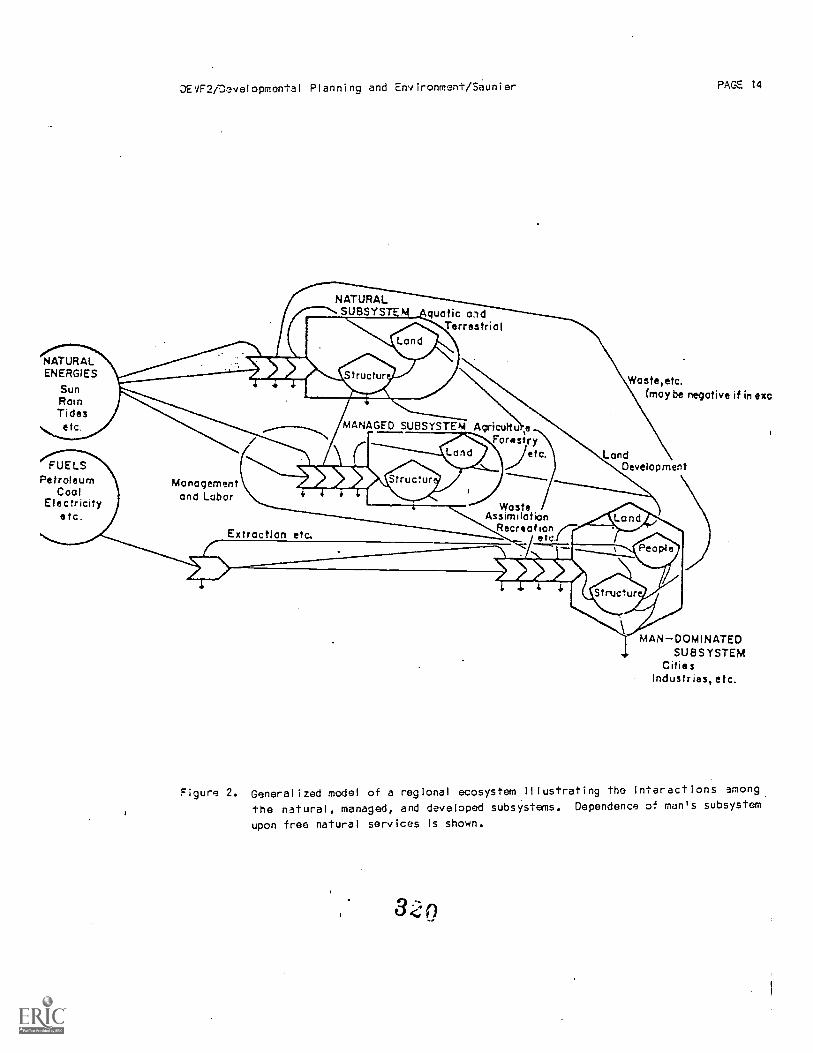
NATURALENERGIES

SunRainTidesetc.

FUELSPetroleum

Cool.Electricity

etc.

DEVF2jils.evel opmontal Planning and Env ironment/Saunier PAGE 14

Managementand Labor

NATURALSUBSYST

Structure

Extraction etc.

(vatic aidTerrestrial

MANAGED SUBSYSTEM' AgricuttuForestry

Land )etc.

AssimilationRecreation

etc.

Figure 2.

Waste,etc.(may be negative if in exc

LandDevelopment

StrUCtur

MANDOMINATEDSUBSYSTEM

CitiesIndustries, etc.

Generalized model of a regional ecosystem Illustrating the interactions amongthe natural, managed, and developed subsystems. Dependence of man's subsystem

upon free natural services is shown.

devlappl/Devel. Applications Water Resources/Roberts

(d) Increase village communal woodlots, hedgerows, etc., by 400,000 acres, and

(e) Establish three or four national nurseries providing annualforest seedling production of 3 to 3.5 million.

The Sri Lankans are fully aware of the value and need for their forest reserves,

particularly in the upper basins. They are convinced that forests and appropriate vegetative coverare the solution to their massive planned development and resettlement programs for some 1.2 million

people in the lower basin areas which are so dependent upon the status of soil erosion and waterflow control.

IndonesiaThe case study of Indonesia, at least focused on the core island of Java with 87 million

people, represents one of the most critical and important examples of the need for effectivedevelopment application of water resources. Population pressures have resulted in intensive andextensive methods of agriculture (primarily rice cultivation) being applied on every type ofavailable land, both lowland and highland. It has been estimated that more than 1/3 of the familieson rural Java are landless and, for those haying any access to production assets, the average farm

unit is less than .3 ha.

In 1975, the Government of Indonesia in cooperation with USAID began a major development

project of flood control and irrigation rehabilitation/extension in the lower basin of the CitanduyRiver. The area of this basin, which is subject to increasingly severe annual flooding and

inundation, is over 100,000 hectares, under the administration of 4 Kabupaten (districts) within 2provinces (West and Central Java), and contains over 2.8 million people, of which 1.2 million aredirectly engaged in agricultural production. The Citanduy River Basin Development Project is

administered as a central government project by the Directorate of Water Resources, Ministry ofPublic Works with initial investment of $19.5 million from USAID and the Government of Indonesia.Primary objectives of the project were to provide for new and rehabilitated irrigation for more than13,000 hectares of paddy land, construct and rehabilitate 200 kilometers of flood levees, therebyproviding flood protection for more than 60,000 hectares of paddy land. The project also providedfor long and shortterm training in watershed management, 0 & M, and flood control.

A few months ago, the project was assessed and formally evaluated. A.I.D. evaluationregulations, as mandated by the U.S. Congress in Section 102(d) of the Foreign Assistance Act, wasintensively applied to the project and its goals and objectives. For illustrative purposes,

portions of the nonquantitative evaluation results for the Citanduy project (which are applicableto all A.I.D.assisted development activities) are shown below:

I. General Project Impacts:

A. Demonstrate Increases of Agricultural Productivity:

Flood damage protection.Water provided by irrigation.Farmer risks reduced, agricultural inputs encouraged,yields consequently raised.

Concurrently, improved practices in the upperwatershed increased production.

B. Reduction of Infant Mortality:Prevention/reduction of flooding has reduced waterborne diseases.

32 1

DEVF2/Developmental Planning and Environmen-1-/Saunier PAGE 16

FORCING FUNCTION

a

CONSUMER

MAJORENERGY

INPUT

C

AUXILIARY ORFEEDBACK INPUT

WORK OUTPUT

ENTROPY

S

Figure 4. Basic energy flow modeling symbols.

GREEN PLANT

b

STORAGE

dev I appl /Devel Applications Water Resources /Roberts

(Flood control contributes to all objectives, which protects crops,which encourages greater investment, which increases yields.)

V. Important ExtraConsequences of Project:Increased the wellbeing of even poorer upland mixedcrop farmers.Upper watershed subproject evolved in Panawangan which is

increasing upland food production and employment.Assistance is being provided in backsloped terracing and vegetativepractices. Agricultural production and labor opportunities areincreasing. Both upper and low er basins are receiving protection.

Project has encountered a widespread phenomenon of developing a

"project constituency" and is rapidly creating a "climate of opinion"in both West and Central Java.Regional and local public officials (Planning Boards, Public Works,Agriculture, Universities, Technical Schools, etc.) are all takingactive and operational interest in project, far and above rolesas envisaged by the Directorate of Water Resources.

Local leaders and spokespersons hay,: added to the innovation andcontinuity of the project's integrity. This condition is developingwithout direction of any central comprehensive authority, and itappears to be selfsustaining and growing.

Auxiliary agricultural inputs agencies, formerly ignoring the project,have voluntarily returned. The Department of Fores tries isassuming a major role in the upper watershed. The momentum isgrowing from the voluntary and evolving coordination of existinginsti tutions.

VI. General ProblemsProblems continue with local currency budget cycles and

constructionyear opportunities.Topographic mapping and design/feasibility studies are inadequateor unavailable. There are no aerial photographic maps.

Project expenditures are slow. Deadlines are being missed.

In reviewing the various aspects of this evaluation and being generally familiar with theproject area, both in the upper watershed area and the lower basin, it is impossible not to beimpressed by the "unplanned successes" in the upper watershed. In fact, the most surprising aspectof the initial project itself is absence of any formal attention to the upper watershed and thesingular focus on the 100,000, or so, hectares of the lower river basin. The source of the waterresources for the primary project area, and, not so surprisingly, the cause of the increasingflooding problems, emanates in the upper watershed.

The upper watershed and the successful complementary pilot project area of Panawangan is no

longer being ignored. The enthusiasm of the people in Panawangan for the addon pilot project ismatched by the enthusiasm of the local and regional government officials and by both neighboring andfarflung upland farmers from all over Java. It has become a showpiece for local leadership,farmer participation and interagency coordination. Other upper watershed management projects arenow beginning to use the model and momentum of Panawangan as their guide. The farmers of Panawanganare even providing "exportable technical assistance" to nearby upland areas. The Javanes:' havecultivated rice on terraces for generations, but the steeper the slope, the greater the chance forproblems. Although they built "bunds" or lips on the terraces, they do not withstand heavy,prolonged rain. Now terraces are being sloped backward into the hillside, and excess water is

carried away by rear ditches, then carried downward through bamboo or rocklined trenches withdescending trenches intersecting with other laterals to allow controlled drainage of excess water.

3?

devlappl /Devel Applications Water Resources /Roberts

Philippines: AgroForestation

Sri Lanka: t Reforestation and Watershed ManagementWater ManagementMahaweli Basin De9elopment (Design and Supervisiun)

Thailand: Highland Integrated Rural Development(Mae Chaem Watershed)

t Various aspects of these four projects are discussed in greater detail and relationship to the

development applications of water resources in other sections of this paper.

Development Applications of Water Resources in AsiaPakistan

The Barati highlands are found in the Punjab Province, Rawalpindi District of Pakistan.More than 14 million people live in this geographic watershed, known in Pakistan as the regionalexporter of the nation's water and power. Much of this water export has undesirable effects, bothfor the Barani (Which loses more than 3,000,000 acre feet of water annually through runoff, thuscausing high degrees of nitrogen depletion in the soils) and for the downstream basin areas ofPakistan which are presently incapable of using or controlling so much excess water. Due to thesewater losses, the region is also unwillingly exporting from 8 to 27 tons of soil annually from eachacre! (The disastrous results of this soil erosion are not recognized by the people of the Barani,

but are well known throughout South Asia for their cause; effect on the Tarbela Dam Project.)

As long ago as 1968-69, the United States Department of Agriculture (USDA) and A.I.D.conducted a study entitled "Resource Management for Rainfed Regions of West Pakistan." The

recommendations made within the study called for:

(a) Improved provincial administration,

(b) Long range national policies,

(c) Recognition of various socioeconomic problems within the region,

(d) Development of localized strategies,

(e) Encouragement of local participation,

(f) Increase of effective water resource personnel through training opportunities,

(g) Expanded research, and

(h) Development of pilot demonstration projects.

These types of approaches are not extraordinary given the degrees of the problem and they

were, no doubt, needed. They are even more needed today.

An action project entitled Rainfed Land and Water Management estimated to cost up to $52million has been proposed for implementation in many of the subproject areas of the Barani. The

project is proposed for various pilot activities in sites ranging from 30 to 3,000 acres. It

relates directly to Pakistanis Fifth Development Plan J1977-83) and calls for integration and

coordination within the disciplines of soil and water conservation, forestry, range management,watershed management, anu agricultural extension. Project targets call for:

324

devl app I /Devel . App I icat ions Water Resources /Roberts

B. Village Cooperation/CoordinationThe efforts to save the upper basins and make them proriuc tive requiresjoint and communal efforts, sacrifices, and benefits. Suchactivities are incorporated in the terraces, spillways, catchments,reforestation, etc.

C. Multicrop FocusSingle crop production is most difficult in saving and revitalizing theupper watersheds. Most successes have occurred with the integrationof agricultural production beyond paddy with livestock, fish, fruit,legumes, grains, tree crops, etc.

D. Local LeadersLocal projects because they are small in implementation andbenefits are focused almost totally on the involved local are?.Local leaders must be allowed to have primary and major roles in the

proj ect, and have endresult responsibility. Centralized bureaucraciesand visiting officials from the capital cannot be ultimately responsible.

E. Delayed Synergistic BenefitsBenefits from such projects cannot be seen immediately nor canthey be separated or isolated. These joint benefits accruing fromproject activities include runoff rates/siltation and flood controlswhich are not con trollable or measurable until full vegeative coveris restored and control infrastructures are operational. Improvedfiltration and improved water tables may not be quantifiable forseveral years.

Upper watershed development projects must be selfsustaining and selfbeneficial. Whilethey are necessary to protect the lower basins, they must be successful entities in and ofthemselves, since there is no easy way for measuring compensation to highlanders from lowlanders for

improving the upper watershed. The highlanders must be able to compensate themselves.

In contemplating the "lessons learned," it should be stated that informal projectmanagership, both by host country and foreign technician counterparts, have proven most successful.While planning and implementing a project must be formal and as precise as possible, the informalityrefers to the outside approaches of proj ect managers. These approaches are in making andmaintaining connections among and between the official participants and the people. Personal

linkages and direct access should be applied to various horizontal levels within the projectcommunity, and, if possible, up and down the vertical lines of government organization. Suchliaison approaches will serve to remind all concerned of the overall project concept, maintain aconcentration on the goals, targets and objectives of the project, and tend to prevent bureaucraticor technical fragmentation .of ,the participants.

NOTE: This paper only represents the research and compilation of ideas by the writer. It doesnot represent in any way an official position or attitude of the Agency for InternationalDevelopment or the United States Government.

devl app I /Devel i cat ions Water Resources /Roberts

concentrate on the replanting of Nepal's steep slopes with fastmaturing, dual purpose fodder andfuelwood.

It plans to improve livestock management on the less steeply sloped pastureland, and itintends to introduce new varieties of agricultural production on the upland terraces above 9,000feet in altitude. The very future of Nepal may depend upon its success.

Sri LankaThe situation in Sri Lanka, the island nation off the southeast tip of the Indian

subcontinent, while not as immediately critical as that found in Nepal, is nevertheless as

important. One of the most encouraging aspects of the overall water resource issue is the priorityattention it is now receiving throughout the world and in every nation. This issue is also not

being viewed in isolation, but is being addressed in terms of its impact on and relationship to theenvironment and to development.

Like much of the world, upper watersheds in Sri Lanka have been rapidly and drasticallydepleted. As late as 1960, 44% of the entire island was forested. Today, only 21% (3 million

acres) has forest cover. Another 260,000 acres are in forest plantations. There is presently animmediate and critical need to reforest 100,000 acres in Sri Lanka's upper watershed basins. The

Gov ernment of Sri Lanka has recognized this need. Their national development plans provide a highpriority for the maintenance of adequate and suitable forest reserves on behalf of the nationalenvironment, the applied practice of soil and water resource conservation, and the preservation ofthe national ecosystems.

Sri Lanka's Forestry Department contains more than 450 fulltime employees. Using their own

resources, they have raised their capability for the general reforesting of reclaimed lands from200 acres per year in 1940 to nearly 20,000 acres annually today. At the same time, as pointed outearlier, forest resources are dwindling and the misuse of watersheds is growing.

With USAID, the government has proposed a $7 million project entitled Reforestation andWatershed Management. This project proposes to begin by replanting 15,000 acres in the Upper.1f1aha.veli Catchment Basins (the minimum start required to ensure adequate resources for downstream,and resettlement programs) and 70,000 acres of new fu elwood plantations. Targets of this projectinclude:

(a) Establishment of a national upper watershed policy,

(b) Strengthening the capabilities of the Forestry Department,

(c) Conducting a land use/suitability study incorporating aerial surveys,

(d) Development of a forest/watershedi extension service, and

(e) The conducting of an effective public publicity campaign.

This proj ect, as view ed by Sri Lanka, is seen as the first component of a longrange policyand plan. The broadscope targets are to :

(a) Reforest 100,000 acres of the 1.34 million acres in the upper watershed

of the Mahaw eli (which sinc.e 1956 has seen 114,000 acres denuded),

(b) Reforest at least 400,000 acres of Sri Lanka for commerical timbering,

( c) Establish fu elwood plantations covering 250,000 acres,

3Y 64

pet/Evapotranspiration Notes/ Gay

Evapotranspiration Notes

compiled byLloyd Gay

Outline

Introduct ion

Evaporation Principles

Evaporation from LakesCalculations: mass transfer approachCalculations: evaporation pan approach

Potential EvapotranspirationPan evaporation modelsEmpirical models

A Temperature ModelA Radiation and Temperature ModelA Net Radiation ModelThe Combination Model

Comparison of modelsPET examples

Actual EvapotranspirationAdjustments to PETThe Water balanceThe energy balance

Literature cited

Introduction

These notes on evapotranspiration are an informal compilation from a variety of sources.Their purpose is to assist shortcourse students in covering certain aspects of this important topicin the hydrologic cycle. These notes have been greatly influenced by the following:

Doorenbos, J., and W. 0. Pruitt, 1975 Crop Water Requirements. Irrigation and Drainage Paper 24.FAO, Rome. 179p.

Dunne, T., and L. B. Leopold. 1978. Water in Environmental Planning. W. H. Freeman and Company.San Francisco. 818p.

Gay, L. U. 19 . Potential Evapotranspiration in Deserts. (in press).

Hounam, C. E. 1973. Comparison Between Pan and Lake Evaporation. Tech. Note 1216, WMD, Geneva.52p.

devl app I /Devel . Applications Water Resources /Roberts

C. Population Growth Controlled:Not applicable.

D. Broadened & Equitable Income Distribution Promoted:Poorer populations in floodprone areas were benefited.Irrigation availabilities enhanced and better water distributionprovided to endofthe system poorest farmers.

E. Under & Unemployment Reduced:Protection against flooding has produced higher yields,thus more work.

Antiflood and irrigation infrastructure constructionhas been labor intensive.

F. Related Project Imparts1. Creation or strengthening of institutions which assist socio/economic

development:Training has promoted better water resource utilization and bettercoordination/application of agricultural development agencies.

2. Improvement in Social/Political/Economic. Conditions of Women:Primary agricultural roles for women have expanded through theagricultural extension program.

II. Profile of Beneficiaries

A. Direct1. Income: Farmers in area (appx. 1.2 million).2. Labor Provision: Construction laborers (5,000).3. Agricultural Production: 900,000 people from improved irrigation

and agricultural practices.4. Education/Training/Management: Government officials, engineers,

and farm ers.5. Medical Treatment: Not applicable.6. General Living Conditions Improved: Water, housing, sanitation, nutrition.

B. Indirect1. Area Population:

Food Increases YesIncreased Mobility N/AGent: al Health Improvement YesOverall Economic. Improvement Yes

Number: Approximately 2.8 million2. People NOT affected and why:3. People adversely affeided and why:

Project/Sec tor GoalDecrease dependency on food imports.Improve wellbeing of area's poor majority.

3-8IV. Project Purpose

Reduce flood damage.Increase rice and other foodcrop production.

Further integrat,u basin development.Irrigation, systems and upper waters.' Aanagernent.

pet/Evapotranspiration Notes/Gay

Water molecules moving out of the liquid produce a vapor pressure, which is a function ofthe rate at which water molecules leave the surface, and therefore of the temperature (energy) ofthe surface. Some molecules of water vapor move from the atmosphere into the liquid and condense.The rate at which they do so is directly proportional to the vapor pressure of water in theatmosphere, which in turn is controlled by its water vapor content. Evaporation is the net rate ofmovement out of the liquid and is therefore directly proportional to the difference in vaporpressure between the water surface and the atmosphere. This difference is called the vapor pr:ssuredeficit.

if the aft' above an evaporating surface were still, the addition of water vapor to the lo werlayer or air would soon raise the atmospheric vapor pressure to that of the evaporating body and the

air would be saturated with water vapor. If this condition is to be avoided and evaporation is tocontinue, the surface layer must be removed and continually replaced by unsaturated air. The majormechanism for replacing the surface layer of air is wind, which creates the turbulence responsiblefor moving saturated air away fran the evaporating surface.

Four conditions are necessary, therefore, for continued evaporation: a source of water,energy, a difference in vapor pressure between the water and the atmosphere, and a method ofexchanging surface air for air capable of holding more water vapor.

The energy requirement for vaporizing water is precisely defined (L 585 cal'g at T =21.8°C). There is a slight dependence upon temperature, but 535 calig is an adequate working valuefor latent energy of water. ,There is full equivalence between energy and mass of water vapor, soevaporation can be referred to in terms of energy or of depth equivalent.

Recall that 1 cm depth of water is really a volume per unit area (1 cm = 1 cm 31 cm-).

Thus 1 cm depth of water evaporated is the same as '1 g/ cm-, which utilizes 585 cal/cm- in thevaporization process. The exchange could be viewed as either 535 cal/ cm 2 of latent energy or as 1

cm depth of water; the two sets of units are equivalent. Using the symbols L for latent heat offusion (L = 585 cal/g = 585 call cm3), E( glom 2) for evaporaion, and LE for laten'. energy, we seethat E = LE/L and LE = E x L. The convertability ter ween energy and mass of evaporated water will

prove exceedingly useful in evaluating evaporation later in this discussion.

It will also be possible to evaluate evaporation through the "mass balance" approach, basedupon the Principle of Conservation of Mass. For our purpose, we shall state that the change II, mass

(or volume) of water during a specified time in a specified volume will be equal to the gains inwater mints any losses of water. This can be a very pow erful tool.

Consider the simple case of a pond with no surface inflow or outflow, and no seepage. The

only gain is oy precipitation (P) and the only loss is by evaporation (E). Then the mass balance iss irrp I y

Change in Volume = P - E.

The evaporation can be measured v ery simply by measuring P and observing any changes in depth inorder to estimate changes in volume.

The mass balance technique can be applied to ponds, lakes, glaciers, the soil volumes andentire watersheds. The concept can also be used with the energy equivalent of evaporation in an"energy balance" evaluation. Both methods will prove useful in estimating evaporation.

The availability of water plays a major role in the rapidity of the evaporation takingplace. While a supply of liquid water (cloud droplets, lakes, e!(-) is necessary in order forevaporation to proceed, the supply need not be on the surface if it is available within the rootingzone of vegetation. The evaporating surface is within the stomata of the leaves when vegetation is

devlappl /Devel App I ications Water Resources /Roberts

Economic development for the villages and businesses in the upper watershed is growing rapidly and

agricultural ac tivities are diversifying and expanding into livestock, forage planting, fish

breeding, multicropping, etc.

General Approaches and Lessons Learned for DevelopmentApplications

It may be strenuously argued that successful development applications for upper watershedareas, like those for any area or sec tor, cannot be generalized. What might work in one nation (orregion, or province, or village) will not automatically or systematically work in every other or inany other. Physical and visual progress in the construction, rehabilitation, or revitalization of

requisite infrastructure or public works, despite unplanned delays or problems, are always theeasiest aspect of a project to plan and implement. Nevertheless, the more critical and difficultproject components necessary for success involve roles of farmers and local leaders, the integrationof technologies employed, the administrative/budgetary methodolo.., the coordination apparatusestablished and applied, etc. It is also always best to begin small, with manageable pilot areas ordemonstrations. Limiting the ..ize and scope of projects allows for indepth attention to the

necessary elements of site coordination, intensive training, etc. Successful water management

projects, particularly in upper watersheds, require long beginnings and nurturing. This period

should usually occur over a one to two year period, then be followed by another two yearconsolidation period. If after this three year period of start/consolidation the project(s) haveestablished good and relatively successful foundations, expansion and replication with the necessarymodifications to meet the new or changed situations have high probabilities for success. Premature

expansion before a reasonable period of time which is necessa, to evaluate and assess the pilotdemonstration endangers the entire activity. The history of "developmen,. processes" is replete withfailures which have been caused by impatience. This is all very difficult because no re can argue

that the critical need or crisis situation requiring attention does not exist, particularly in most

upper watersheds. The tendency is to expand and push those activities which "appear" successful.

Most bureaucrats, technocrats, planners, and common people are all alike in exhibiting their

impatience and their interest to "do something." Certainly "something" must be done, but the

problem is so severe, that the doing something must be correct; it must work; and it must besustained and longterm. Nothing will serve to embitter farmers or local leaders as much as an

abandoned or unsuccessful project. Nothing so certain to have a disastrous impact on the alreadyprecarious ecological system (and the mental outlook of the project advocates) as an unnecessary

project failure. This does not mean that starting "small" automatically will be successful or thatit rules out speedy or massive programs. On the contrary, while the small starts must succeed in

the initial and consolidation phases, the geometric growth of replication can be widespread and

sustaining thereafter.

If nothing else, the past experiences and a pocketful of "failures" in upper watershed

applications of development have provided some valuable lessons. The following appraisal

"ch,..cklist" was suggested by the former (for 3 years) USA, D ::ounterpart Project Manager (from 1975 -

7j,) of the Indonesia Citanduy Project. Under his influence, the pilot upper watershed subproject

tt Panawangan evolved 'nd was made an unseparable, integra part of the lower basin development

program.

Success ful Upper Watershed Management Projects require the following:

A. Grassroots ParticipationSince over 9036 of the project is by and far the local people, oftenunlike major downstream irrigation infrastructure, this local participationtrust control the identification, planning design, implementationand evaluation of the project.

3 tA

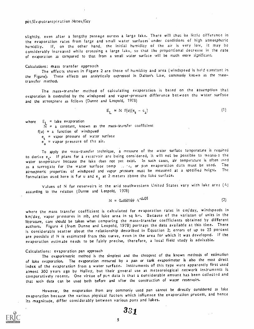
pet/Evapotranspiration Notes/Gay

slightly, even after a lengthy passage across a large lake. There will thus be little difference inthe evaporation rates from large and small water surfaces' under condi dons of high atmospherichumidity. If, on the other hand, the initial humidity of the air is very low, it may beconsiderably increased while crossing a large lake, so that the proportional decrease in the rateof evaporation as compared to that from a small water surface will be much more significant.

Calculations: mass transfer approachThe effects shown in Figure 2 are those of humidity and area (windspeed is held constant in

the Figure). These effects are analytically expressed in Dalton's Law, commonly known as the masstransfer method.

The masstransfer method of calculating evaporation is based on the assumption thatevaporation is controlled by the windspeed and vaporpressure difference between the water surface

and the atrnospnere as fcllo.vs (Dunne and Leopold, 1978)

EL = N f(u)(es ca)

where EL = lake evaporationN = a constant, known as the masstransfer coefficient

f(u) = a function of windspeedes = vapor pressure of water surfaceea = vapor pressure of the air.

(1)

To apply the masstransfer technique, a measure of the water surface temperature is required

to derive es. If plans for a reservoir are being considered, it will not be possible to measul e the

water temperature because the lake does not yet exist. In such cases, air temperature is often osed

as a surrogate for the water surface temp . -4, or pan evaporation data must be used. The

atmospheric properties of windspeed and vapor pressure must be measured at a specified height. The

formulation used. here is for u and ea at 2 meters above the lake surface.

Values of N for reservoirs in the arid southwestern United States vary with lake area (A)according to the relation (Dunne and Leopold, 1978)

N = 0.000169 A-105 (2)

where the mass transfer coefficient is calculated for evaporation rates in cm/day, windspeeds inkm/day, vapor pressures in mb, and lake area in sq kn. Because of the variaton of units in theliterature, care should be taken when comparing the masstransfer coefficients obtained by differentauthors. Figure 4 (from Dunne and Leopold, 1978) portrays the data available at this time. There

is considerable scatter about the relationship described in Equation 2; errors of up to 25 percentare possible if N is estimated from this curve, even in the area for which it was developed. If the

evaporation estimate needs to be fairly precise, therefore, a local field study is advisable.

Calculations: evaporation pan approachThe evaporimetric method is the simplest and the cheapest of the known methods of estimation

of lake evaporation. The evaporation mesured by a pan or tank evaporimeter is also the most direct

index of the evaporation from a water surface. Instruments of this type were apparently first usedalmost 300 years ago by Halley, but their general use as meteorological network instruments is

comparatively recent. One virtue of pz.r: data is that a considerable amount has been collected and

that such data can be used both before and after the construction of water reservoirs.

However, the evaporation from any commonly used pan cannot be directly considered as lake

evaporation because the various physical factors which influence the evaporation process, and henceits magnitude, differ considerably between various pans and lakes.

3,315

dev I app I /Devel . Applications Water Resources /Roberts

References/ResourcesAgency for International Development Congressional Presentations Fiscal Year 1979 and Fiscal Year1980.

A.I.D. Project Papers and documentation for:Barani Rainfed Land and Water Management PAKISTANResource Conservation and Utilization NEPALReforestation and Watershed Management SRI LANKACitanduy River Basin Development INDONESIA

"Resource Management for Rained Regions of West Pakistan", USDA/USAID, 1969.

A.I.D. Project Evaluation System (PES) April 1979 Project Assessment of the Citanduy River BasinDevelopment Project INDONESIA

USAID /Indonesia Memorandum "An Indonesian Watershed Program and USAID Involvement," Dr. Gerrit H.Argento, September, 1978.

pet/Evapotranspiration Nbtes/Gay

The accurate value of evaporation for such an interval of time can only be obtained by means of aspecial survey to evaluate changes in heat storage and aclv ected energy.

Seasonal variations in the lake to Class A pan coefficients are usually large enough topreclude the use of a constant value. The annual coefficients depend on climate and lake depth andrange fro.n 0.60 to 0.30. The average annual value of the Class A pan coeffficient to 0.73. The

range for Australian sunk en tank coefficient appears to be equally large.

The spatial variation in the lake to Class A pan coefficient is real and appears to be

related to climate. In the U.S.A. the variation' of the annual coefficient is from 0.60 in arid

zones to near 0.30 over the moist east and west coast states. Geographic corrections of this nature

could be used when applying U.S.A. results to other countries.

Annual evaporation from tanks with diameters greater than about 3.0 m and depth about 2.0 m

approximates lake evaporation. Their data, without any considerable corrections, may be extended to

small reservoirs 5-10 hectares in area and up to 5 m deep, when the tank and reservoir are locatedin open land under similar environmental conditions."

Potential EvapotranspirationEvapotranspiration (ET) is the term that applies to the total water vapor exchange as a

result of evaporation from surface of soil and vegetation (as for intercepted water) and fromtranspiration through the plant. The ET rate thus depends upon both the availability of water tothe plant and the climatic demand for water. The evaluation could be simplified if calculations w eremade only of the rate to be expected from wellwatered plants, i.e. "potential evapotranspiration."

The potential evapotranspiration (PET) concept was first proposed by hornthwaite(1944,1943; in an effort to simplify calculation of water use by irrigated crops. After some minorrevisions, the currently accepted definition is; "The rate of evaporation from an extended surfaceof a short green crop actively growing, completely shading the ground of uniform height, and notshort of water".

The PET concept has been widely accepted, and it has stimulated a vast amount of researchinto evaporation from natural sur facei. There have been many applications in classification of

climate, but the greatest interest has been in the development of PET estimates as a first step inestimating actual evapotranspiration. For this application, the initial PET estimates are adjusted

to account for lack of water or failure of the surface conditions to meet the requirements of thedefinition.

The basic conditions that are required for PET are given in the definition. Specifying thatthe vegetation be low in height, actively growing and with complete canopy closure reduces thevariability in the plant component of the hydrologic cycle. Variability in soil water is minimizedby specifying that the soil be plentifully supplied with water. These conditions are preciselythose to be encountered in virtually any arid zone irrigation project, once the crop canopies haveclosed, leading to Thornthwaite's (1944) original concept was that PET would be equal to consumptive

use in irrigated agriculture.

The PET concept has also been severely criticized. W. C. Swinbank's (1965) discussion of

Stanhill's paper on this topic is an example: "I would suggest to Dr. Stanhill tha the concept ofpotential evaporation is a useless one, in that it cannot be defined and cannot be measured, andthat ail he has said this afternoon reinforces this view." Stanhill (1973) concluded "Despite themanifold uses to which the concept of potential evapotranspiration has been put in the past,

inherent contradictions in the multiplicity of definitions that have been put forward, make it onewhose current necessity is ,open to considerable doubt."

3 `. 37

pet/Evapotranspiration Notes /Gay

Ward, R. C.. 1975. Principles. of Hydrology. Second Edition. McGrawHill. 367p.

These provide excellent summaries of a rich and varied literature on evaporation, and theyare good sources for further reference and for applications.

The role of evaporation in the hydrologic cycle has held the interest of water managers for

many years, as this process generates a direct loss of water that might otherwise be placed to ahigher, more beneficial use.

The magnitudes of this loss can be considerable, especially in arid regions. The ArizonaWater Commission (1975) places the annul evaporation from Lake Mead at 813,000 acre feet (1.003 x10m3). This volume is about 10 percent of the 1959-73 average annual flow of the Colorado River atHoover Dam (7,989,000 acre feet. pr 9.354 x 109m3). This volume is equivalent to a depth of 82inches (2.1m) over the surface of Lake Mead. The annual evaporation from Lake Nasser, in contrast,has been estimated to be 24 x109 m3, equivalent to 3m depth. This amounts to 25 percent of theannual flow of the Nile at Aswan Dam.

Further data on various annual evaporation totals are tabulated in Table 1. Note that onlyone of the reservoirs included in the list loses more water than the annual total of 84 inches(2.13m) lost by the Atlantic Ocean of Cape Hatteras, North Carolina.

The losses from free water in reservoirs are large, but the areas are not too great. Theamount of water evaporated from various types of natural plant communities is also considerable.Data tabulated in Table 2 range from a depth equivalent of 10.5 inches in semiarid grasslands up to

33 inches in moist coniferous forests.

The urge to put these "losses" to beneficial- use in agriculture has been great. The variouscrops grown in the southwestern USA are tabulated in the Table 3, with regard to annual waterrequirements. Tnese vary from somewhat less than 1 ft. up to 5 ft. per year. Much of the emphasis

in watershed management research has been to develop ways to reduce the evaporation loss fromnatural plant communities in order to provide additional water for irrigation.

The magnitude of possible savings can be examined in Table 4, which summarizes the waterlosses from phreatophytes in various areas of the USA. Phreatophytes florish along streams,shorelines, and in floodplains where their roots have ready access to shallow groundwater. Thehe ,vy water consumption and limited value of phreatophytes have made them prime candidates forvegetation conversion schemes.

Our purpose is to examine the processes and measurement techniques for evaluatingevaporation, now that we have reviewed data that illustrate the mgnitude involved. The application

of the evaporation data to watershed management problems will be carried out in a subsequent portionof the shortcourse.

Evaporation PrinciplesEvaporation of water in the hydrologic cycle consists of the change of state from liquid to

vapor and the net transfer of this vapor into the atmosphere. The process occurs when somemolecules of the liquid attain sufficient kinetic energy to overcome the forces of surface tensionand escape from the surface of the liquid. To do so, the molecules must obtain energy from anoutside source. This energy comes from solar radiation, sensible heat transfer from the atmosphere, or from heat advected into the water body by infloing warm water. Because radiation is usuallythe dominant source of energy, evaporation is a function of latitude, season, time of day, andcloudiness.

3,42

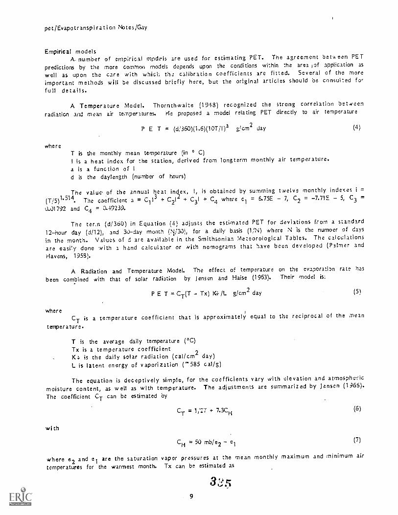
pet/Evapotranspiration Notes/Clay

Empirical modelsA. number of empirical co.ndrls are used for estimating PET. The agreement bet .; een PET

predictions by the more common models depends upon the conditions within the area ,of application as

well as upon the care with which tha calibration coefficients are fitted. Several of the moreimportant methods will be discussed briefly here, but the original articles should be consulted forfull details.

A Temperature Model. Thornthwaite (1948) recognized the strong correlation between

radiation and mean air temperatures. He proposed a model relating PET directly to air temperature

where

P E T = (d:360)(1.6)(10T/I)a g!cm2 day (4)

T is the monthly mean temperature (in ° C)I is a heat index for the station, derived from longterm monthly air temperature.a is a function of I

d is the daylength (number of hours)

The value of the annual heat index, I, is obtained by summing twelve monthly indexes i =

(T/5)1.514. The coefficient a = C1 I3 + C2I 2 + C31 + C4 where c1 = 6.75E 7, C2 = 7.71E 5, C3 =

0.J1792 and C4 = 3.49239.

The tern (d/360) in Equation (4) adjusts the estimated PET for deviations from a standard

12hour day (d/12), and 3iday month (N/30), for a daily basis (1/N) where N is the numoer of days

in the month. Values of d are available in the Smithsonian Meteorological Tables. The calculations

are easi!y done with a hand calculator or with nomograms that have been developed (Palmer andHavens, 1955).

A Radiation and Temperature Model. The effect of temperature on the evaporation rate has

been combined with that of solar radiation by Jensen and Haise (1963). Their model is:

where

P E T = CT(T Tx) K4. /L g/cm2 day (5)

CT is a temperature coefficient that is approximately equal to the reciprocal of the mean

temperature.

T is the average daily temperature (°C)Tx is a temperature coefficientK4, is the daily solar radiation (cal/cm2 day)L is latent energy of vaporization ("' 585 cal/g)

The equation is deceptively simple, for the coefficients vary with elevation and atmospheric

moisture content, as well as with temperature. The adjustments are summarized by Jensen (1965).The coefficient CT can be estimated by

with

CT = 1 /27 + 7.3CH (6)

CH = 50 mb /e2 (7)

where e2 and e1 are the saturation vapor pressures at the mean monthly maximum and minimum air

temperatures for the warmest month. Tx can be estimated as

9

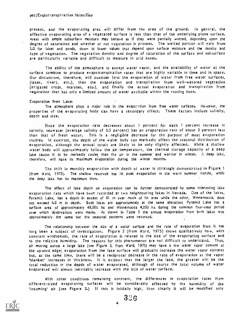
pet/Evapotranspiration Nbtes/Gay

present, and the evaporating area will differ from the area of the ground. In general, theeffective evaporating area of a vegetated surface is less than that of the underlying plane surface.Areas with ample subsurface moisture may behave as if they were partially wetted, depending upon thedegree of saturation and whether or not vegetation is present. The wetted portion will vary from1.0 for lakes and ponds, down to lower values that depend upon surface moisture and the density andtype of vegetation. The vegetation density and degree of saturation of the surface and subsurfaceare particularly variable and difficult to measure in arid zones.

The ability of the atmosphere to accept water vapor, and the availability of water at thesurface combine to produce evapotranspiration rates that are highly variable in time and in space.Our discussions, therefore, will consider first the evaporation of water from free water surfaces,(lakes, rivers, etc.), then the evaporation and transpiration from wellwatered vegetation(irrigated crops, marshes, etc.), and finally the actual evaporation and transpiration fromvegetation that has only a limited amount of water available within the rooting zone.

Evaporation from LakesThe atmosphere plays a major role in the evaperition from free water surfaces. However, the

properties of the evaporating body can have a secondary effect. These factors include salinity,depth and size.

Since the evaporation rate decreases about 1 percent for each 1 percent increase in

salinity, seawater (average salinity of 3.5 percent) has an evaporation rate of about 3 percent lessthan that of fresh water. This is a negligible decrease for the purpose of most evaporationstudies. In contrast, the depth of the water body can markedly affect the seasonal distribution ofevaporation, although the annual totals are likely to be only slightly affected. While a shallowwater body will approximately follow the air temperature, the thermal storage capacity of a deeplake causes it to be markedly cooler than the air in the summer and warmer in winter. A deep lake,therefore, will have its maximum evaporation during the winter months.

The shift in monthly evaporation with depth of water is strikingly demonstrated in Figure 1(from Ward, 1975). The shallow reservoir has its peak evaporation in the warm summer months, while

the deep lake has its maximum then.

The effect of lake depth on evaporation can be further demonstrated by some interesting lakeevaporation data which have been recorded at two neighbouring lakes in Nevada. One of the lakes,Pyramid Lake, has a depth in excess of 61 rn over much of its area while the other, 'Winnemucca, does

not exceed 4.6 m in depth. Both lakes are approxiamtely at the same elevation; Pyramid Lake has a

surface area of approximately 48,000 ha and Winnemucca 4,050 ha during the common fouryear periodover which observatiors were made. As shown in Table 5 the annual evaporation from both lakes wasapproximately the same but the seasonal patterns were reversed.

The relationship between the size of a water surface and the rate of evaporation from it has

long been a subject of investigation. Figure 2 (from Ward, 1975) shows qualitatively how, withconstant windspeeds, the rate of evaporation is related to the size of the evaporating surface andto the relative humidity. The reasons for this phenomenon are not difficult to understand. Thus,

air moving across a large lake (see Figure 3, from Ward, 1975) may have a low water vapor content atthe upwind edge; evaporation from the lake surface will gradually increase the water vapor contentbut, at the same time, there will be a reciprocal decrease in the rate of evaporation as the vapor'blanket' increases in thickness. It is evident that the larger the lake, the greater will be thetotal reduction in the depth of water evaporated, although of course the total volume of waterevaporated almost inevitably increase with the size of water surface.

With other conditions remaining constant, the differences in evaporation rates fromdifferentsized evaporating surfaces will be considerably affected by the huimidity of the'incoming' air (see Figure 2.) If this is initially high, then clearly it will be modified only

3 3 G4

pet/Evapotranspiration Notes/Gay

The Penman model predicts the evaporation expected from an open water surface (E,,), rather

than that from vegetation (PET). Penman related the two by an experimentally det:trrnin-ed

coefficient, k, (PET = kE0) that varied under English conditions from 0,6 in winter to 0.3 in

sinner.

The weighting coefficient (W =A/(A +y )) is the same as in the PriestleyTaylor model(Equation 8). The coefficient expresses the relative importance of the two terms that comprise thecombination equation. The first term is primarily of radiation, and the second of aerodynamicprocesses. The temperature effect was illustrated previously in Figure 10 at both sea level and 2000

m elevation over a range of temperatures. At sea levei, the relative weights of the radiative andthe aerodynamic terms are approximately equal at 7°C. As temperatures rise above 30°C, the weight

of the radiative term becomes greater than that of the aerodynamic term by a factor of 4 or more.

The model can be applied over any desired time period. With units above, and for inputvariables averaged over the period of a day (24hours), the evaporation estimates will have units ofg /cm day, which is equivalent to evaporation in cm/day. The model is intended to yield mean dailyestimates of evaporation, with the daily input variables being averaged from weekly or monthlymeteorological records.

The wind function is an important component of the second term in Equation (9). The windfunction depends upon the units specified, as well as upon the time period over which the estimatesare being made. The original function was developed to estimate evapora:ion over daylong periods.Penman's (1943) wind function (adjusted to g/cm2 day mb) was f(u) = 0.035 (1 + 0.0098 U2), with 1.)2

being the total wind run (miles; day) at a height of 2m. This was revised slightly (Penman, 1956) tof(u) = 0.035(0.5 + 0.01 U). The coefficients are scaled for vapor pressure deficits in mm Hg,rather than mb. With U expressed in uits of km/day and vapor pressure in mb, Penman's original windfunction becomes f(u) = 0.02262(1 + 0.0061 U2) gicm2 day /mb.

Wind values are often measured at a height other than 2 m; these can be adjusted to theequivalent value, at 2 m by multiplication with an adjustment factor. The approximate adjustmentfactor is (2/za) i where as is the actual measurement height (in meters).

Comparison of modelsInability to identify and develop a standard reference surface has limited tests and

verification of the various PET models. There have, however, been quantitative comparisons ofvarious methods against meaxurements from irrigated vegetation, and additional, more qualitative,comparisons among a number of methods without comparison against a standard.

Many of these studies have been carried out in humid areas with ample precipitation. Some

0' the studiess have been affected by selection of the model, or the size of the coefficients used.Not all of they experiments have proven useful in identifying the most general or most accurate PETestimators. We shall examine results from several studies that were carried out in arid areas.

Stanhill (1 961) reported a test of eight methods of calculating potentialevapotranspiration, with reference to actual losses from three lysimeters in an irrigated alfalfacrop. The data used covered 12 months (49 weeks) while the crop was fully developed. The methods

used included measurements from a Class A evaporation pan, the temperature method of Thornthwaite, a

solar radiation and air temperature method described by Makkink (1957), and the combinations method

of Penman.

The monthly comparisions indicated that the adjusted estimates (E0) from the Penman equation

gave the smallest coefficient of error, the highest correlation coefficient (r -= 0.96) and thepredictions nearest unity (dEo/dE = 1.03). The Makkink and Thornthwaite methods gave similarresults in that the correlation coefficients were high (r = 0.95, 0.94, respectively), but the model

11 3 t/k,

pet/Evapotranspiration Notes /Gay

The basic calculation of EL is

EL = kp x Ep (3)

where Ep is the measured pan evaporation and kp is a pan coefficient where kp = EL/Ep. Thedevelopment of coefficients for various environments and for various types of evaporation pans hasbeen discussed thoroughly by Hounarn (1973). 73). He concludes that simple pan coefficients (EL /Ep)can be used for annual totals of evaporation, but more thorough considerations are required forestimating seasonal EL values.

The basic evaporation pan that we shall consider is the USA Class A pan. The pan is

circuiar, 121.0 cm (47.5 in.) in diameter and 25.4 cm (10 in.) deep, mounted on a wooden open frameplatform so chat the pan base is about 5 -10 cm (2-4 in.) above the ground. it is normallyconstructed of galvanized iron, but other more durable metals or fibreglass have been used(presently monel metal is recommended). The pan is filled to within 5.1 cm (2 in.) of the rim, andmeasurements may be made by hook or fixed point gauge. There are a variety of evaporation pandesigns that are in routine use around the world. The more common ones are listed in Table 5.

The factors that affect the evaporation rate of the pan include radiation exchangecharacteristics (albedo, temperature), wind exposure, size of evaporating pan surface, and nature ofsurroundings. In addition, the relationship to a given lake will be influenced by the site and thedepth of the lake.

The Class A pan is freely exposed to the environme) r consequently evaporates morewater than lakes, especially in warm dry climates. Hounam (1>-)4 nap summarized available data on

Class A pan coefficients in Table 7. His analysis can be consulted for details and for the primaryreferences. The coefficients range from 0.60 at Lake Mead in Western Arizona up to 0.82 at LakeMendota in +Visconsin and 0.86 at Lake Eucumbene in New South Wales, Australia.

The annual lake evaporation totals in Arizona can be estimated using evaporation pan data.The pan evaporation totals are shown in Figure 6; they range from 380 cm in the extreme west to less

than 190 cm in the northeast. The limited number of observation pans requires considerableconjecture to interpolate the results. The pan coefficients used by the U.S. Weather Bureau aremapped in Figure 7 (U.S. Dept. Commerce, 1968). The coefficients are associated with exposure; theyrange from 0.60 in the hot dry west to 0,70 in the cool, more humid central mountain region.

The estimated lake evaporation across the state is shown in Figure 8, based upon the panevaporation in Figure 6 and the pan coefficients in Figure 7. The annual values range from 230 cmin the west down to 127 cm in the northeast. The maximum values are in the arid western lowlands,and the minimum values are in the higher, cooler northeast.

Although Hounam (1 9 73) should be consulted for detailed applications, his followingconclusions apply to the pan method:

The simple lake to pan coefficients, determined as (EL/Ep), can only provide estimates oflake evaporation with reasonable accuracy on an annual basis.

When pan measurements are used to compute lake evaporation for a particular year or seasonor to provide a mean monthly estimate, corrections have to be introduced to account for thoseparameters which have an important influence on lake and pan evaporation, such as net heatadvection, change in heat stored and the surface area. This must be done for all types of pan atpresent in use for measuring evaporation.

No general technique has as yet been developed for accurately estimating the lakeevaporation from pan evaporation data for short periods of time such as a week lor a 1 0day period.

36

pet/Evapotranspiration Notes /Gay

occurring in midsummer. The adjusted pan evaporation rate of 8.8 mm/day fell midway between the t vo

highest formula estimates at the summer peak.

Both the PriestleyTaylor and the Thornthwaite estimates were low in comparison with theabove three. The Thornthwaite method also shifted peak evaporation rates from June into July. Thisphase shift, noted many times by other authors, is associated with heat storage in the soil duringthe warming season (spring arxd early summer).

The monthly and annual means by the various methods are tabulated in Table 8 with totals in

cm for month or for year. The Penman estimatees exceed adjusted pan evaporation slightly on anannual basis. Other wise, the order is the same as for the midsummer period. The largest estimatefrom a formula method (J ensenHaise) is about twice that of the lowest (Thornthwaite).

Considerable variability is evident among the selected methods in Figure 11 and Table 3.The Penman method, as pointed out by Doorenbos and Pruitt (1975), varies with such fac tors as

distribution of wind between day and night, and with choice of wind function. The Thornthwaiteestimates demonstrate the empirical temperature m ethod's shortcomings in arid climates. Rates fromthe Jensen Liaise method are higher than the adjusted pan evaporation (open water) which itself isdirectly affected by the selection of a pan coefficient.

The lack of a reference standard makes comparison of methods difficult. Even whenevaporation data is available from research plots, the evapotranspiration rate is influenced by thephysiological condition of the vegetation as well as by the size of the plot. These factors tend tosupport the v ie w that the evaporation pan is the best possibility for a standardized estimate ofpotential evapotranspiration. The configuration of the pan and condition of exposure can becarefully defined, and the development of reasonable procedures for evaluating pan coefficients i5

well along (Door enbos and Pruitt, 1975). The pan method holds great promise fir obtainingevaporation estimates that can be compared from one place to another.

The annual PET totals for a specific site such as Tucson, Arizona, are of general interest,but they are not necessarily indicative of actual evapotranspiration, even from irrigated crops thatmeat the conditions of the PET definition. The period during which the plants meet the PETconditions is one reason for discrepancy. Most irrigated crops do not maintain closed canopies andfull growth throughout the year, even in warm regions. Grains, for example, cease growth atmaturity, and a considerable period may elapse in the spring before crown closure occurs in somecrops. This was clearly illustrated earlier in Figure 9. Further, belowfreezing temperatureseffectively limit transpiration. Tucson, Arizona, for example, has a season from Feb. 16 to Nov. 28between the normal occurrence of the last severe frost (-2.2°C, or 28°F) in the spring, and thefirst in the fall. Yuma, in the southwest corner of Arizona, is normally frost free throughout theyear, while Flagstaff, in the central mountains, normally goes only from May 22 to Oct. 10 between2.2 °C (28°F) frosts. Regional evapotranspiration estimates should be adjusted to predict totals forthe frostfree season.

Actual Evapotranspiration.Actual evapotranspiration (ET) obviously could originate from either of the previously

discussed situations: lake evaporation and potential evapotranspiration. This discussion willgeneralize the solutions for evaluating water losses to include the conditions when the supply ofwater is limited. This condition makes the problem much more difficult. The methods to be

described are also applicable for use in measuring EL or PET. The methods will be consider ed inorder of increasing precision and complexity. The first will be adjustment of PET estimates, nextthe application of the water balance, and finally evaluation of the energy balance.

Adjustments to PETThe most popular method of computing actual evapotranspiration is through the calculation of

potential evapotranspiration. if there is abundant moistlec.phthe soil, the two rates are equal.to

13

pet /Evapotranspiration Notes/Gay

Problems in utilizing the PET concept are related to the imprecise nature of the definition,leading to errors in application and misplaced expectations. There have also been failures to fullyappreciate shortcomings inherent in the many different models that have been proposed for

estimating PET. The extreme climatic conditions of arid environments have contributed to these

pr,oblems. However, when vegetation is irrigated, essentially all variability associated withavailability of water is eliminated. Also the effects of vegetation upon the evaporation rate fromwellwatered surfaces are essentially similar. This has led to a vast amount of experimental workdesigned to estimate evaporation solely from properties of the atmosphere.

As the PET concept has become accepted, a variety of methods have evolved to provide thedesired estimates. These models are based almost entirely upon atmospheric variables, since the PETdefinition removes the greater scurce of variability associated with the availability of water.

The wide variety of models proposed for evaluating PET will not be reviewed in detail here.Doorenbos and Pruitt (1975), for example, identify 31 formulas that estimate evapotranspiration fromirrigated crops; nine of the formulas estimate PET. Nearly all of these formUlas are empirical, anddepend upon a known correlation between evapotranspiration and one or more climate variables such as

temperature, radiation, humidity, and wind speed. Other formulas have related evapotranspiration todirect observations from evaporation pans. Almost all of the formulas contain empiricalcoefficients that calibrate the models for conditions of the regions in which they are used.

There have been many comparisons of different methods for estimating PET, but there is noreference standard to determine the "true" PET value. The lack of a suitable reference has made itdifficult to test the various approaches to estimating PET.

Pan evaporation modelsA possible standard for PET is the evaporation rate (E ) that is measured directly with an

evaporation pan. As in the application to lake evaporation, the basic model is simple: PET = K E

with the constant K to be determined empirically. Note that the coefficient K differs from they kP

used in Equation (3) to relate E and EL.

Stanhill (1965) recommends the Class A evaporation pan as the best method of estimatingpotential evapotranspiration, given consideration of accuracy, simplicity and cost. Pruitt (1966)

reviewed many studies and concluded that pan evaporation could give an excellent estimate ofevapotranspiration from irriga grass. He emphasized the necessity to standardize the exposure of

the pans, because rates in Jicultural areas may differ as much as 40 percent between dryland sites

and irrigated field sites. He further suggested a reduction in the order of 0.75 would bring lossesfrom dryland Class A pans down to the levels of those located within irrigated fields.

The pan design also influences the evaporation rate. The exposed Class A pan of the U. S.Neather Bureau evaporates at a higher rate than do various sunken or insulated models. Guidelines

for choice of an appropriate reduction coefficient are given by Doorenbos and Pruitt (1975) for avariety of climatic and site conditions.

The relation between the adjusted 'evaporation rates and the evapotranspiration fromirrigated crops is quite good in temperate regions. The ratio of PET to Epan for Class A pans overa range of sites was about 0.8 for grass and grassclover mixtures, and 1.0 for alfalfa (Pruitt,

1966). Doorenbos and Pruitt (1975) point out that pan exposure errors increase in arid climates,especially in windy regions, and suggest that other methods, such as those based upon radiation, may

be preferable for truly desert areas. They give excellent application guidelines for the pan method

in many types of climates. Note that the coefficient can vary markedly with stage of vegetation.

This is shown in Figure 9 far corn (from Dunne and Leopold, 1978).

8

pet /Evapotranspiration Notes/Gay

The water balanceA water balance can be developed for large basins by measurements or estimates of t'e gains

and losses. More accurate results are possible using small experimental catchments in which

detailed measurements are made of hydrological variables. If the water balance equation I' Q E

= 0 (where P is precipitation, Q is streamflow, E is actual evapotranspiration, ands S andare changes in soil moisture and groundwater storage respectively) can be solved, then it is

probable that the values of the individual components of that balance are accurate.

Clearly, this may not be so if discrepancies in the assessment of individual variables -refortuitously corn- plernentary, although this source of error can usually be guarded against by mal,:ngspecimen water balance calculations for different time periods within the same run of data Since

precipitation, streamflow, soil moisture, and groundwater measurements can-be made with a greateraccuracy than the corresponding estimations of evaporative loss, the value of E which consistentlygives the best result in the water balance equation is the most 'suitable'.

The water balance approach need not be restricted to use only on watersheds. Indeed, the

basic observations with the evaporation pan are specialized water balance measurements. An estimate

of evapotranspiration can also be obtained by calculating the partial water balance for the soil

profile, often within the context of an experimental plot study. The important work done byThornthwaite on the climatic water balance substantiated the close relationship between f', E, and

An approach through soil moisture measurement, and particularly the determination of successive

soil moisture profiles, is attractive because, within the soil profile one can obtain a directmeasure of the amount of water withdrawn by the vegetation cover. The repeated soil moisturemeasurements that are needed to obtain an estimate of 2- S are now routinely and accurately obtained

with neutron probes that can be repeatedly returned to the same sampling point.

The c;mcept of the soil moisture balance and the evaporation pan are combined in the

lysimeter. Lysimeters are confined blocks of soil that, facilitate measurements of moisture change.Vegetation can be grown within the confined soil volurne so a precise measurement can be made of

moisture changes.

Two main types exist: the earliest designs, called "evapotranspireters", maintained moist

PET conditions within the soilfilled container. The moisture losses could be evaluated bymeasuring the water added to restore the water level, or by measuring the amount needed to bring the

soil profile back to field capacity by subtracting drainage out the bottom from the input quantity.The more recent designs are essentially sealed except at the top, and the weight change is monitored

continuously by weighing.

In order to extrapolate lysimeter measurements to the surrounding vegetation, the soil

profile, root development, and moisture conditions should be the same within and without the tank.The type, height and density of the vegetation growing on the lysimeter must likewise match that ofthe surroundings. The weighing lysimeter is suited to a range of conditions and some designs pec:,:t

precise measurements.

The neutron probe and the weighing lysimeter were used by Sammis and Gay (1979) in a study

of yearlong transpiration in a creosotebush community near Tucson. Primary measurements were made

with a weighing lysimeter containing a large creosotebush. The water budget method was used toevalute evaporation from bare soil plots and evapotranspiration from a creosotebush community.Creosotebush was the dominant shrub, with paloverde (Cercidium microphyllum) and bursage (Ambrosia

del toidea) also present on the site.

A monolith lysimeter was constructed beneath a creosotebush, selected for its typical size,shape, condition and relative proximity to neighboring shrubs. The lysimeter was 4 m in diameterand 1 m deep. Lysimeter weight changes were measured by a commercially available straingaug5capable of detecting a w eight change of 2.36 kg, equivalent to 0.19 mm of water over the 12.57 rn"

15 24

pet/Evapotranspiration Notes/Gay

- -Tx = 23 + CH + 750 CT

for those areas with CH < 2.8. For actual calculations,refer to Jensen and Haise (1963). As anexample, the coefficients at Tucson, Arizona (elevation 788m, July maximums of 36.9 °C and minimumsof 23.3 °C) are CT = 0.0271°C, Tx = 3.59 L'C.

A Net Radiation Model. The ?riestley and Taylor (1975) model focuses upon available energy

(Q* + G) as the primary factor conti oiling potential evapotranspiration from wellwateredvegetation. Net radiation (Q*) is used to represent available energy because the storage term (G)is relatively small at any time, and it is generally negligible when averaged over a 24hour period.Net radiation is now being measured at a number of locations; it can also be estimated rather easilyfor those areas where measurements are lacking.

The PriestleyTaylor model is

P E T =a WQ*/L (8)

where cy. is an empirical constant (ct = 1.25), L is the latent heat of vaporization and "V is a

temperature dependent weighting factor. The flux density of net radiation (Q*) is expressedcallcrn2day.

The weighting factor W is equal to LIR LI+ y), where is the slope of the saturation vaporcirve (in mb/°C) at air temperature Ta, and Yis the psychrometric constant (mb/°C). ;,an bereadily calculated from tabulated values of saturated vapor pressure (es, in mb) as a furnction oftemperature (see, for example, the Smithsonian Meteorologic?! Tables). The psychrometric con-tans,y, has a nominal value of about 0.66 mb1°C. This varies with air pressure, p, in the ratio pip°where Po is sea level pressure (po = 1013.25 mb). W thus varies with both temperature and withpressure (Figure 10). Typical sea level values of W are 0.55, 0.68, and 0.73 at temperatures of10°, 20°, 30°C, respectively.

It is interesting to note that since Q* is linearly related to K.I. (Q* = a + bK4-, Gay, 1 971),both the Priestley Taylor and the JensenHaise models have the same basic form: PET = b K 4- where (t)

represents the fraction of solar radiation transformed to net radiation, and ultimately, intoevapotranspiration.

The Combination Model. The combination model of Penman (1948) is probably the most widelyknown PET estimator. la contrast to the pan observations and the. empirical models, the Penman modelis based upon a simplified radiation budget that i'as been combined wim an aerodynamic analysis. Thefundamental basis of the model gives it some generality in application. It has been applied in a

wide range of conditions.

where

Penman's model can be writzen (after Doorenbos and Pruitt, 1975) as

E0 = W*(Q* + G)/L + (1 W f(u) (es e) g/cm2 day (9)

E0 is flux density of potential evaporation based upon open water (g/cm2 day).W is a dimensionless weighting factor that accounts for effects of temperature and pressure

(see Figure 10).Q* is the flux density of net radiation (cal/cm2 day).G is the change in stored thermal energy, expressed as a flux density (cal/cm2 day).L is latent heat of vaporization (585 cal/g at 21.8°C).f(u) is a wind function that approximates the diffusivity of the atmosphere near the ground

(g/cm2 day), and

cs e is the vapor pressure deficit of the atmosphere at 2 m height (in mb).

34 4,(14

10

pet/Evapotranspiration Nbtes/Gay

In practice, two psychrometers are used to measure Ta and e at two levels in the air above

but near the evaporating surface (which, by substraction, yield z2Ta and e). Direct measurements

are made of net radiation and changes in storuJ energy, and then Equations (12, 13) are solved for

LE.

A recent report by Gay and Fritschen (1979) compares Bowen ratio estimates against constant

let/el lysimeter estim;:es of evapotranspiration from saltcedar.

The Bernardo lysimeter site was selected for the energy budget measurements. Six constant

level lysimeters had been established in 1 961 by the U. S. Bureau of Reclamation in an expanse of

saltcedar on the floodplain of the Rio Grande, about 50 miles south of Albuquerque. The Bureau

operated the lysimeters continuously from 1 962-1 968 (U. S. Bureau Reclamation, 1973), and has

maintained them for intermittant measurements since that date. The lysirneters are equipped with

pumps that maintain the water level at a constant setting. The mean depth to water was 154 cm

during the period of our measurements, both within and without the lysirneters. Meteorological

instrumentation was established above the sal tcedar in the vicinity of the lysimeters. The

saltcedar was about 115 rn. tall. Though the stand was extensive, the canopy was sparse.

Instrumentation was similar to that used elsewhere for energy budget measurements (see Gay,

1973, among others). Net radiation was measured above the canopy with two net radimeters, and a

soil heat flux plate within 3 cm of the surface provided an estimte of the changes in stored energy

in the soil. Differential psychrometers were used to measure drybulb temperature and vapor

pressure differences between two levels above the canopy. The psychrometer employed a reversing

mechanism to exchange the sensors between levels in order to eliminate small biases that might

otherwise affect the results. Hind velocities w ere measured above the canopy. The instruments were

recorded periodically on a digital data system. The article should be consulted for a full

description of the instrumentation and experimental design.

The diurnal energy balance for a single day is shown in Figure 13 ;...t two different points

over the saltcedar. The components of the energy balance, Equation 11, are identified in the Figure

and plotted as ra 2s of energy transfer (cal/cm" min). The daily sums of the energy budgetcomponents at the two sal tcedar sample points are tabulated in Table 9. The latent energy totals

can be converted to depth equivalent of evaporated water by division with the latent heat of

vaporization E = LE/L). The daily LE totals (in mm) are compared with the direct measurements from

the four lysimeters in Table 10. The paper should be consulted for full analyses, but for our

purpose it is sufficient to note that the fiveday energy balance mean evaporation of 8.2 mm/day

compares closely with the lysimeter mean of 7.9 mm /day.

Given the difference in conditions at the Bowen ratio sites and on the lysimeters, the

agreement between the two methods was excellent. This reassuring agreement between the energy

budget analysis and lysimeter mesurernents adds confidence to the long (1 5 year) record obtained by

the U. S. Bureau of Reclamation at the Bernardo experimental site. The agreement also substantiates

the usefulness of the mobile, although more tedious, energy budget method for estimating

evapotranspiration from riparian sites in arid zones.

313

17

pet/Evapotranspiration (Vbtes/Gay

estimates were considerably lower than actual evapotranspiration PET/dE = 0.67, 0.68,respectively). The direct measurement of open water evaporation with the Class A evaporation panhad a similar degree of suitability but with an overestimate (dE /dE = 1.43, r = 0.95). Stanhillconcluded that the Penman method was the most satisfactory of the ones tested.

Cruff and Thompson (1967) compared a number of methods for estimating potentialevapotranspiration in the Southwest, using mean monthly data (10 years of record) from U. S. WeatherBureau. Their standard of comparison was lake evaporation, which was estimated from evaporation panmeasurements that were adjusted for exposure (the adjustment coefficients ranged from 0.60 to 0.78).The methods tested included the temperature methods of Thornthwaite, the temperature plus solarradiation method of Lane (1 964) for estimating lake evaporation (EL) and the U. S. Weather Bureaumethod. The Lane method is of the basic form of the JensenHaise model, and the U. S. WeatherBureau method is a minor variant of the Penman combination method.

The combination method gave the best results of the ones tested. The agreement between meanmonthly EL and lake (adjusted pan) evaporation was quite close, being 1.06 for the 7 sites that hadadequate data. Other methods with smaller data requirements were tested at as many as 25 sites.Results from the Thornthwaite method were much lower (0.61) than the adjusted pan evaporation at 25sites; results at 22 sites from the temperature plus solar radiation method of Lane were markedlyhigher (1.15).

Van Bavel (1966) compared Penman's method with lysimeter measurements of evaporation fromopen water, saturated soil, and irrigated alfalfa at Phoenix, Arizona. He used a revised windfunction to estimate hourly and daily evaporation rates. For 13 days, the ratio of Ecs to measuredevaporation was 1.04, leading Van Bavel to conclude that irrigated alfalfa exhibited essentially nostomata) resistance since it transpired near the potential rate. Further, he concluded that thePenman method satisfactorily evaluated the advective conditions that commonly occur in irrigatedfield within arid areas.

PET Examples.The variability between methods of estimating PET at a single po,nt can be examined with

referencz to T icson, Arizona.

The published temperature, wind, humidity and pan evaporation data at Tucson, Arizona,augmented by solar radiation data, were used to estimate PET by the various methods for the 10yearmean 1966-1975.

The net radiation values needed for the Penman and the PriestleyTaylor models wereestimated from incoming solar radiation usi^z the procedures of Doorenbos and Pruitt (1975). Theyfirst reduce the incoming solar for an assumed albedo of the hypothetical crop canopy (here, c =

0.25). They next estimate the longwave component of net radiation with reference to percentpossible sunshine and the temperature and the moisture content of the air. The percent possiblesunshine was evaluated from average sky cover. Refer to Doorenbos and Pruitt (1975) for the detailsof the computations..

The Penman estimates were based on Equation 9, with Doorenbos and Pruitt's (1 975) windfunction: f(u) = 0.027 (1 + 0:01 U2) g/cm 2 day. The other methods used the formulas as definedearlier; the adjusted pan evaporation is based upon a pan coefficient of 0.67 for the Tucson area(see Figure 7).

The mean monthly rates (mm/day) are plotted in Figure 11. Several methods (JensenHaise,adjusted pan, Penman) appeared reasonably consistent. The unadjusted pan evaporation rates were in

the order of 150 of the PET values predicted by this group. The JensenHaise method predictedmaximum values of 9.9 mm/day during the midsummer months. The Penman estimates were the nexthighest of the formula methods; this method predicted 8.0 mm/day, with the evaporation peak also

3112

evapotrn/Evanotranspi rat i on/Gay

TABLE 3. VARIATIONS IN CONSUMPTIVE USE BY CROPS

(from The Water Encyclopedia, 1970,

D. K. Todd, Editor)Crop No. cf tests

Range inwater

requirements, ft.

A. FARM CROPS IN THE SOUTHWESTAlfalfa 369 3.47.5.03Rhodes grass 12 3.49.4 47Sudan grass 25 2.88-3.13Barley 3 1.24-1.33

Oats 2 1.902.09

Wheat 46 1.45.2.24Corn 42 1A4-1.9,9

Kafir 16 1.32-1.54Flax 3 1.23.1.59Broomcorn 9 0.97-1.15

Emmer 6 1.19-1.87Feterita 8 0.97-1.10Millet 5 0.91-1.09Milo 35 0.96-L67Sorghum 34 1.69-2.09

Coon 103 2.35.3.51Potatoes 12 1.59-2.04

Soybeans 36 1.66-2.31Sugar bi>es 5 1.77.2.72Sugar cane' 41 3.48-4..56

B. VEGETABLE CROPS IN THE SOUTHWEST

Beans. snag 9 0.87-1.44Beats. tab'. 29.. 0.87.1.37Cabbage 21 0.94-1 49

Carrots 6 1.27-1 60

Caunflower a 1.43.1.77

Lenuce 49 0.72.1.35Onions 4 0.731.52Peas 8 1.21.1.E.6

Melons 3 2.48.3 40Spinach 12 0.80-1.07

Sweet potatoes 3 1.77_25Tomatoes 17 0.95.1 42

-Nor cwrmonhi poduced in the Scut, Ai:it.

TABLE 4. pHREATOPHYTE AREAS AND THEIR CONSUMPTIVE USEIN SELECTED WESTERN STATES

(from The Water Encyclopedia, 1970,

fl :1 Togdd Editor)mtb

Area Annual use(Acres) (Acrefeet)

A rizona 405.000 1,280.000California! 317,000 1,150,000Coloeadol 737,060 1,056.000idsho 500.000 1.000,010Montana 1,600,000 3,200.000

Nebraska' 515,000 709,000Nevada 2,801,000 1,500,000New Met,,7'u 300,000 900 COONorth O.Jk Dtd 1,035,000 1,650.000Oregon I 40,800 21,200

South Oak ota 850.000 1,240,000Texas' 262,000 436,600Utah 1,200,000 1,500,000Wyoming 527,000 1,100,000

Total fapproximate12 11,000,000 16,750.000

I Portial data, from published reports on orals within the State.Partial data.

31 519

pet/Evapotranspiration Nbtes/Cray

When moisture supply becomes limiting, the computed potential rate is modulated by a factor thatdepends upon the amount of water in the soil. The relationship can be expressed as (Dunne andLeopold, 1978)

AET = PET x f (AW/AWC) (10)

where AET and PET = the actual and potential rates of evapotranspiration

f( ) = some function of the term inside the parentheses= the available soil moisture = (soil moisture content permanent wilting point)x rooting depth of vegetation (cm)= the available water capacity of the soil = (field capacity permanent wiltingpoint) x rooting depth of vegetation (cm).

The form of the function that modu:atcs PET in response to limiting water has received muchstudy. Veihmeyer and his coworkers conducted a series of experiments in California and concludedthat evapotranspiration proceeds at the potential rate until soil moisture is depleted to the

permanent wilting point. Plants then wilt and evapotranspiration rates fall sharply to near zero.Thornthwaite and M-ather, working on a loam in Nebraska, found that the ratio of actual to potentialevapotranspiration decreases as a linear function of the amount of available water (see Figure 12).Other workers have proposed various compromises between these two extremes, most of them suggestingthat evapotranspiration occurs at close to the potential rate until a considerable proportion of theavailable water is depleted, after which the actual evapotranspiration rate falls rapidly. One such

example (Pierce) is incorporated in Figure 12(a) (from Dunne and Leopold, 1978).

The accuracy of these approximations will vary with soil type and rooting characteristics.In a sandy soil, for example, plants with a dense root system can withdraw water rapidly from thepores, and evapotranspiration may proceed at close to the potential rate until soil moisture contentis close to the wilting point. In a clayrich, loamy soil, water is held more tightly at a givensoil moisture content, and movement of water to the roots is slow. Under such circumstancesmoisture supply to the roots will not keep up with potential rates of loss, and actualevapotranspiration rates will decline throughout most of the range of available water. Holmes (see

Figure 12(b)) presented a schematic relationship between actual and potential rates ofevapotranspiration over the range of available water capacity for three soil textures. This

relationship can be compared with the results of previously mentioned workers in Figure 12(a). The

comparison sho..-.'s that the Veihmeyer and Thornthwaite models should be adequate approximations for

sandy and clayrich soils, respectively. In the ab,ence of detailed measurements, an estimation ofthe appropriate relationship for intermediate .sn;ls involves a good deal of guesswork. The

situation is further complicated by the intensity of tne evaporative demand. Under low demand, soil

moisture may be able to move to the root system rapidly enough to maintain transpiration at thepotential rate. If the demand increases, the soil moisture movement may not be rapid enough to dothis.

In view of the difficulties of applying the previously mentioned results to soils for thesolution of particular problems, several simpler relationships have been used with some success.Ideally they should be checked under the field conditions to which they are to be applied by makingmeasurements of actual soil moisture losses, but in practice this is not usually done. Often thehydrologist will use two extreme estimates and calculate the actual water loss under bothconditions. Frequently, the results do not differ by a large amount.

The application of the method is simple. The PET estimates are used to reduce the amount ofwater remaining in the soil. Eventually, a point is reached, (based on the function used) when

actual ET falls below PET. The ET becomes reduced further and further below PET as more and more ofthe soil water is extracted. Eventually, precipitation should recharge the soil profile and actualET, given that soil water is freely available, will again equal PET.

evapotrniEv.votrarispi rat ion/Gay

. I ------- -H; ; ;I

).aF7...---:;74,...-...7,-..-.1.--:.-s-----;.;--: 7:" 7 ." _. _ ".",.7, .?..,7.,.%,7,77,7:"'77775/,77774/7t7;7;;..!

W.n1 Olf eCti,jr1

Figure 3 A simple illustration of the increase in humidity and decrease in evaporation as air movesacross a large water surface (Ward, 1975).

-"-:"---

'.. -;.-,:

------ ,F ....-3

.....___.z

-7,

,i-ol

.C:01

.0405

.0001.C.)01

I

',,I.------)-I

___!-

c

i

.....).

1

° _ I 0

._

.01

....:__7

.1 1 10 100

Area of I2.ketsquare kilorr..:t.trs)

Figure 4. Masstransfer coefficient, N, as a function of lake area. Open circles are data fromlakes in the southwestern U.S.; solid circles are for Indiana and western Canada; dashed line is

I-Earbeck's mean relationship.

11..4000q.1 s%,090ar

4,:,qcvI0 1-SAL

--771,//,./h7//rir //////fc //Ow/ . /1/ I/ ff 'ft /WO

Figure 5 Side view of Class A pan (Hounam, 1973).

"1

pet/Evapotranspiration Motes/Gay

surface area. The lysimeter weight change was recorded weekly. Water loss on the bare soil and the

vegetated plots was determined by a water balance where:

Evapotranspiration = Precipitation ÷ Change in soil moisture.

This simple formulation applies where deep drainage and runoff are negligable. At this experimental

site, all changes in soil moisture during the study period were confined to the top meter of soil.Further, no measurable runoff occurred through flumes on the watershed.

The neutron probe was used to measure changes in soil moisture content at the experimental

site. One set of four access tubes was located in a bare soil plot in an open area that wasisolated from shrub roots by a plastic barrier. Four additional sets, each containing four accesstubes, were located within the surounding creosotebush stand. The soil moisture content at eachaccess tube was determined at 25 cm intervals t3 a depth of 2 m, and meaurements were normally made

every 2 weeks.

The oneyear water loss from the weighing lysimeter was 259mm, compared to neutron probe

estimates of 242 mm from an adjacent stand of creosotebush, and 231 mm from bare soil plots. The

three loss estimates were in good agreement with measured annual precipitation of 234 mm. There was

no deep percolation or surface runoff during the year, and all losses were by evapotranspiration.

This study is one of the few applications of lysimeter to measurements of wildland ET.There are numerous reports of their use in irrigated agriculture, however.

The energy balanceThe balance of energy gains and losses to an area can be measured more easily than the

moisture fluxes in certain experimental situations, thus providing a means for evaluating

evaporation from energy measurements. This provides a powerful tool that can be used forexperimental work on evaporation and to crosscheck evaporation estimates derived from other

techniques.

The basic energy budget model is di,scribed in many different texts. It sums the energy

available from net exchange of radiation (Q ), changes in stored energy (G), convection (H) and

latent energy (LE):

Q*+ G + H 4- LE = 0 (11)

The energy budget expressed in flux density units (e.g., cal/cm2 min or W/m2) applies to periods of

any length. The flux polarities may be either positive or negative, and we use the common

convention that fluxes directed to the surface are positive, and those away from the surface are

negati ye.

The basic Bowen ratio model is :

LE = (Q* + G) / (1 )

where f3 = H/LE. B was estimated from measurements of drybulb temperature differences

vapor pressure differences (Q E) at two levels above the vegetation with the model

= y( 8..Ta/A e) (13)

(12)

( A'Ta) and

where y is the psychrometric constant ( y is approximately equal to 0.66 mb/°C) at sea level pressure

(P = Po). y varies with air pressure in the ratio P/Po, and so le may drop to values near 0.55 at

higher elevations.

31816

evapotrniEvapotranspiration/Cray

Table 7

Annual coefficients for lake to Class A pan evaporation (EL/Ep) (Pounan, 1973).

Location

Surfacearea insquarekilo-metres

Averagedolt:h.

inmetres

Fancoe:-ricieni

ince:-7atior.

periodm ethod

arra:en: a

Lake Eleinore California 22.27 3.05 0.77 1232-41 Vater 'cudgel.. Young' (19.:!

ae4.31uffRear,

Texas - 0.6E 1953-47 Water tutget Kahle: ;1954)

lake0kaeohotea

Florida 1313.0 3.05 0.51 1940-46 Water tudget Kohlar (:954)

Lake Nermsr 0k1ahoma 3.E2 7.)3 C.25 :95:-.5: Water 'cudgel: Sellers ..,....o.;;

Felt Lake California 0.24 6.40 3.77 19!.5 Water tudget Kohler

lake ColoradoCity

Texas e.29 4.92 0.72 1954-59 7......er67 tot Xshler (1932)

Lake Mead Arizons 512.22 53.59 0.E.0 1952-i3 Energy tutget Kohler (1932)

Lake Mendota Wisconoin 39.:: 12.20 0.22 27 yesre aCnerri tudgot Sellers (17:65:

Salton Sea California 777.01 7.32 0.52 1:-62 Sellsrs (1965:.

21:ver Lake California 51.50 0.91 0.61 191E-19 Water tudget Kohler (..-.7.1

Tort Molntoot Texas - - 0.79 1950-51 Kohler *.2ii:

Kirtton 2ark 1.onion 0.16 7.:: 0.70 1956.-42 Water tudat Latuortn *..7'5:i

Litz Pee F.Z.W. 90. :4 23.77 0.24 1962-44 Sulkaerodynamic

Snovy rounloin....;

EFro-clez. I

v..nout . ished!

LOCATION OFEVAPORATION PANS

AVERAGE ANNUAL PAN EVAPORATIONG6nometpes

FLgure 6 Average annual pan evaporation in Arizona (adapted fran U.S. Dept. Cairn. 1968).

23

evapotrn/Evapotranspiration/Gay

TABLE 1. RESERVOIR EVAPORATION AT SELECTED STATIONS INTHE UNITED STATES

(from D. K. Todd, Editor, The Water Encyclopedia. 1970)[Mean monthly computed values in inches]

Station MonthJan. Feb. Mar. Apr. May June July Aug. Sept. Oct. Nov. Dec.

Ariz., Yuma 3 9 4.6 6.5 8.0 9.8 11.5 13,4 12.9 10.7 8.0 6.1 4.5Calif., Sacramento 1.4 2.5 3.6 5.0 7.1 8.9 8.6 7.1 :1.8 2.6 1.2Colo., Cenver 1 6 1.3 2.5 3.7 5.0 7.4 8.8 8.4 6.7 4.6 3.0 1.9Fla., M'arri 3 0 3.4 4.1 4.9 5.0 4.8 5.3 5.1 4.3 4.1 4.3 2.7Ga., Macon 1 7 2.2 3.1 4.3 5.1 6.2 6.3 5.8 5.2 4.2 2.8 1.8

Me., Eastport 0 8 0.7 0.9 1.1 1.4 1.7 2,0 2.1 2.0 1.6 1.1 03Minn., Minneapolis 0.3 0.4 0.9 1.7 3.2 4.4 6.0 5.8 4.6 3.0 1.3 0.4Miss., Vicksburg 1 3 1.9 2.9 4.2 5.0 5.7 5.8 5.5 5.2 4.4 2,9 1.6Mo., Kansas City 0 9 1.1 1.7 3.1 4.4 6.1 8.0 7.8 6.0 4.5 2.5 1,0Mont., Havre 0 5 0.5 1.1 2.5 4,5 6.1 8.2 8.3 5.6 3.3 1.5 0.7

Nebr., North Platte 0.8 1.1 2.2 3.7 5.0 6.5 8.6 8.4 6.9 4.6 2.6 1.1N. Mex.;Roswell 2 1 3.2 4.9 6.8 8.3 9.8 9.4 8.3 6.9 5.5 3.5 2.5N. Y., Albany 0 6 0.7 1.1 2.0 3.2 4.3 5.2 4.7 3.4 2.4 1.4 0.8N. Oak., Bismarck 0 4 0.5 1.0 2.3 4.0 5.3 7.3 7.7 5.8 3.3 1.3 0.5Ohio, Columbus 0 6 0.8 1.1 2.3 3.5 4.6 5.6 5.1 4.1 3.0 1.6 0.6

Okla., Oklahoma City . 1.5 1.9 3.1 4.7 5.5 7.8 10.2 10.7 8.8 6.3 3.5 2.0Ore., Baker 0 5 0,7 1.4 2.5 3.4 4.4 6.9 7.3 4.9 2.9 1.5 0.6S.C., Columbia 1 6 2.4 3.2 4,5 5.4 6.3 6.6 6.0 5.5 4.4 3,0 1.9Tenn., Nashville 0 9 1.3 1.9 3.3 4.1 5.1 5.8 5.4 4,9 3.7 2.1 1.1Tex., Galveston 0 9 1.3 1.6 2.6 4.1 5.6 6.2 6.1 5.7 4.6 2.7 1.3

Tex., San Antonio . . . 2.2 3.1 4.5 5.6 6.5 8.4 9.4 9,4 7.6 5,8 3.7 2.4Utan, Salt Lake City . 0.8 1.0 2.0 3.5 5.1 7.9 10.6 10.4 7.3 3.9 2.0 1.0Va., Richmond 1 3 1.7 2.2 3.5 4.1 5.0 5.6 4.9 4.1 3.2 2.4 1.5Wash., Seattle 0 8 0.8 1.4 2.1 2.7 3.4 3.9 3.4 2.6 1.6 1.1 0.7Wis., Milwaukee 0 6 0.7 0.9 1.3 2.1 3.2 5.0 5.4 4.7 3.2 1.6 0.6

Gulf off Texas Cdas: . . 4.0 4.0 3.5. 3.5 4.0 4.5 5.0 5.5 6.5 6.5 6.0 5.0Gulf Stream off Cape

Hatteras, N.C. . . . .' 9.0 9.5 8.5 7.0 5.5 3.5 3.5 3.5 5.5 9.0 9.5 10.0Ocezn off Massachusetts . 3.0 2.5 2.0 1.5 1.0 1.5 1.5 2.0 2.5 3.0 3.5 .1.3

TABLE 2. ESTIMATED EVAPOTRANSPIRATION FOR TYPESOF VEGETATION IN THE WESTERN UNITED STATES

(Source: Select Committee on National Water Resources, U.S. Senate, 19601

(from The Water Encyclopedia, 1970,D. K. Todd, Editor)

Vegetation type

AnnualEvapotranspiration,

inches

Forest:Lodgepole pineEngeimann sprucefirWhite pinelarchfirMixed coniferTrue fir

1915222224

Aspen 23Pacific Douglasfirhemlockredwoud 30Interior ponderosa pine .17Interior Douglas -fir 21

Chaparral and woodland: 3i) ()Southern California chaparral e 20California woodlandgrass 18Arizona chaparral 17,5Pirionjuntper 14.5

Semiarid grass and shrub 10.6Alpine 20

A

10

.8

.6

4

.2

0

evapotrn/Evapotranspi rat ion/Gay

Figure 9 The ratio of evapotranspiration fromcorn to open-pan evaporation as a function of timeduring the growing season. (Fran Dunne and Leopold, 1978). -

Rela tive Weight ofAerodynamic Term

5 I-

5.: 4

$

3!-

5 l 25 5 1 :sNI.11

4

Relative We.0 t ofRadiative Term

8 12 16 20 24 28

(°C)

14

12

10

32 36

- .2

15 :5 5

Vorith

! :5

Aug

4 Figure 10 The dependence of weighting

terms (w, 1-w) on terperature and pressure..6

.3

' 1.040

.N.

Priestly-TaylorJensen -NoiseModified PenmanThornthwoiteAdjusted PonPon Evaporation

8 /. -\..

.44. .\.../.

6 ..........''... s".... .\.... /.. .....

-... \.... ..- .... ./4 .0. .....0 \ .

... .. /..../

.., .......

2 ... .

...--.,,,..- ---0 f-- i , , , , , , , ,

...

,

JAN FEB MAR APR MAY .JUN JUL AUG 'SEP OCT NOV DEC

TIME (Months)

Figure 11 Estimates of potential evapotranspiration by several methods at Tucson, Arizona, for the

period 1966 - 1975. The methods are describedin the text.

35125

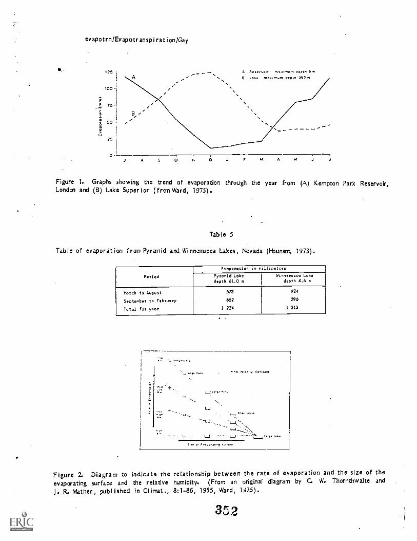
evapotrn/Evapotranspi rat ion/Gay

125 A peeery 0. cx,rm,mt Ce0t0 gm8 Lose rn0x.murn tiepin 397m

100

EE 75

0

50Oaa

25

J A S A

Figure 1. Graphs showing the trend of evaporation through the year from (A) Kempton Park Reservoir,London and (B) Lake Super ior (frcrn Ward, 1975).

Table 5

Table of evaporat ion fran Pyramid and Winnerrucca Lakes, Nevada (1- bunam, 1973).

Evaporation in millimetres

Period Pyramid Lake Winnemucca Lake

depth 61.0 m depth 4.6 n

March to August 573 924

September to February 652 290

Total for year 1 224 1 213

J Ste. 1,

L_J

U

w 0 wee.iv CoMtsol

S.S. pr cvaa2 s.ta,

Figure 2. Diagram to indicate the relationship between the rate of evaporation and the size of theevaporating surface and the relative humidity. (From an original diagram by C. W. Thornthwaite and

J. R. Mather, published in CI imat 8:1-86, 1955, Ward, 1975).

352

evapotrn/EvapotranspirationiGay

Table 9

Energy Budget arponants at Bernardo (Gay and Fri tschen, 1979)

Q,' G LE, H X! Q2' C.; LE2_

June 14, 1977 451 -33 -513 100 730 461 -33 -450 22

June 15, 1977 436 -29 -554 127 736 464 -29 -435 0

June !6. 1977 452 -30 -493 75 765 470 -30 -429 -IIJure 17, 1977 439 -30 -493 84 738 452 -30 -429 7

June 18, 1977 439 -33 -502 91 690 443 -23 -424 9

Daily totals in calories per square centimeter per 24 hours.

Table 10

Evapotranspiration Totals at Bernardo.

LE, LE2 lys5 lys, lys5 lyso

Jure 14, 1977 8.8 7.7 6.4 6.5 S.S 9.0

June 15, 1977 9.5 7.4 6.3 6.9 9.3 9.1

Jure 16.1977 9.5 7.4 6.2 6.5 9.0 9.0

June 17. 1977 8.4 7.3 6.6 6.R 9.2 9.3

June IS, 1977 E. 7.2 6.2 6.3 9.4 9.4

Mean 9.0 7.4 6.4 6.7 9.2 9.2

Means S.2 7.9

In millimeters per 24 hours.

.6

- 1 2t 1

6 8 10 12 IA 16 18 20 22 00 2 4 6

TIME (HIS)

Figure 13 Energy transfer rates over saltcedar at two sites near Bernardo, N.M., June 14-15, 1977.

The time axis is Mountain Daylight Time (MDT). Symbols are K *, solar radiation; Q*, net radiation;

G, soil heat flux; H, cogvection; and LE, latent energy. Subscript 1 is the site with the taller,more vigorous vegetation. (Gay and Fritschen, 1979.)

353

pet/Evapotranspiration dotes /Gay

Table 6

Evaporation pans in use in national weather networks (iiounarn, 1973).

area IrraiColorado sunken pan, 3 ft2, 18 in deep CUM 0.84

CGI 20 dia. 5 m, depth 2 m (USSR) 20

Sunken pan, dia. 12 ft, depth 3.3 ft (Israel) 10.5

Synirons pan 6 ft2, depth 2 ft (LK) 3.3

BPI dia. 6ft, depth 2 ft (US=N) 2.6

Kenya pan dia. 4 ft, depth 14 in 1.2

Australian pan, dia. 3 ft, depth 3 ft 0.7

Aslyng pan, 0.33 m2, depth 1 m (Den-nark) 0.3

CGI 30(X) dia. 61.3 an, depth 60-83 an 0.3

Sunken pan dia. 50 an, depth 25 cm (Netherlands) 0.2

Table 7

Annual coefficients for lake to Class !, pan evaporation (ELIF) (}bun, 1973).

S»rfl:eare:. l'n

me::or

,

47traFedo-t!.

=etre.

F.:.

c.:1:*-

::,,nt

nrer-vLI:ct;tr:od

r. otn:c.7..efe:tnze

:a::2:r7:e 22.2' !.:::. :. :?!:-.:2

.,".1,.. .2 Texas - :.%! 15:2-27 1:.-.4.1- 1:%::.ret E.::.,..r

I:,:1;h,:tee,i:2:ta 183.0 3..2! C.4: 194:-tE

1 :A..*1 21efr.sr Ck2a.nt7.2. E.22 ?.?: 2.:1 :7.,..:.!,: '..L:tr 1::e..i.c: st::er5

re:: 2..z.k. CL:Iftrnts :.2i 6.2: C. 2.?!! ',.:L:t: ":%:::E.: Ecn:tr :::5t)

I::.:74:A2 E.29 4.88 c.72 li;G-55 2...-r.f.:.,;: 1,a,:f,e: Zchler (19 ;

17.ii C.f: 2.!!=-!: EMC.r:Y 1:::!ie: Keh:cr

:

t2' :.rarE Ene%7 2e::er,

SA::er2

C. Va:er Xch:er

I 7c:1 n:rtcst 7azacE:h1er .`"'

Lon!= c.:i 7.:: VC:FT La;v:rtt 1:Sd

53.:a :3.77 c.aE 19.C2-64terziymes=ic

I

LC:AT:ON OPEVAPCPA7ION PANS

AYE;AC,E ANNUA:. EvAPORAT ION

ICen:,metprs

Figure 6 Axer,ze annu41 pan evaporation in Arizona (adaptedfro-71 U.S. Dept. Csrm. 1963).

23 355'

evapotrn/Evapotranspiration/Gay

PAN CGEFFIC!ENT(Percent)

Figure 8 Annual lake evaporation in

Arizona (adapted frcm U.S. Dept. Cannerce, 1968)

24

Figure 7 Coefficients to adjust evaporation pan

;.tasure-nents for microclimate variations (U.S.

AVgRAGC ANNUAL :AKE EVAPCgArION(Centimert)

VTGe.Pul.

Figure 9 The ratio cf evapotransriration from

cern to open-pan evaporation as a funr;tion of timedu"irtg tat- C vir..2; season. (FroT, and Leopold, 1978).

f e WeJ`n ofAero..4focrr.::: Term.

3 12 16

ti

14

12

10

8

6

A

2

0

Relative V.'e,;:ht cf

Rocitotie Term I .8

, t t

70 24 28 32 36 40

I (C)

/-*

\../ . .s . .

... 4*.I. \.....,/../ ... "..", -' "`... . --#: -

.. -- ',/. `.. ,

.. A \.. .0* / : .,. ...-

.0*.0*/ \ ..... \

...,.....

/ /......

. ../

i.

\

' . !

IJ-e A4 5,7

Figure 10 The deperc.:enc.:. of weigh.: ing

terms ;tv., 1-4,:.; en te-rperature arrd pressur::.

Priestly-TaylorJensen-HoisetAodified PenmonThornlhwoiteAdjusted PonPon E,,cporatfon

--

IAN Hi; MAR APR MAY JUN Ji'l AUG SEP OCT NOv DEC

TIME iMonths)

Figure 11 Estimates of potential evapntranspiratibn by several methods at Tucson, Arizona, for the

pz:r :bd 1956 - 1975. The T.ethvis are desc.rib,N1 in the text.

32, 7

evapotrniEvapotranspi rat ion,'Gay

Table 8

Mean evapor a : i on at Tucson, Arizona ;1965 - 1975). ATounts are totals (anjrnan th, or an/year )

!,ethod J F M A M J J A S 0 t. D Total

Evap. pan 9.5 12.9 19.1 25.9 36.0 40.0 35.5 30.7 27.5 21.0 12.; 7.; 273.4.

Adjusted pan 6.4 8.5 12.3 17.4 24.1 26.8 24.1 20.6 12.5 14.1 8.5 5.3 187.3

Jensen 5.9 7.6 12.4 17.1 23.6 29.7 29.5 26.7 20.. 14.3 6.7 5.3 201.2

Penman 8.4 10.1 14.3 18.3 22.5 24.0 23.3 20.5 18.3 14.0 10.5 7.4 191.7

Priestly 4.2 5.0 10.0 13.1 15.7 17.1 19.9 17.4 12.0 3.9 4.9 3.5 132.7

Thornth.aite 1.5 2.2 3.7 5.1 10.5 13.0 22.0 18.6 12.6 7.4 3.5 1.6 106.3

ial

.6 10 0 1.0

Rat,'' of ay.:i!..lble soil moiture ..nuilable water capacit) (b)

Figure 12 Relation of ac tual evapotranspiration to available soil moisture. (a) Actualevapotranspiration as a ratio to potential plotted against the ratio of available soil moisture toavailable water capacity according to models of three investigators. (After Holmes and Robertson,1959.) (b) Ratio of actual to potential evapotranspiration a.. a function of soil moisture for threesoil textures. The ratio of available soil moisture to the available water capacity varies from Uat the permanent wilting point to 1.0 at fiele capacity. (After Holmes, 196%) (From Dunne andLeopold, 1976.)

ea2otrri 'Evapotr ansp r a t ion/Gay

Table 9

Energy Cudset aTponents at 2ernardo !ay an:: Fri tscne::, 1979)

Q C LE, 9'-1/.

14. 1977 45! -33 -5:5 10-.! 730 4:I -33 -450 221,1:.e !:. !'..77 4:..;6 -2', -554 127 7:': 4...4 -2.", -435 0

hre 16. 1'177 452 -30 -493 75 765 471: -3., -429 -11hr.= 17. 1977 439 -30 -493 54 735 4.:' -30 -4'4 7

hre :F. 1977 439 -35 -502 91 692 443 -25 -424 9

cz.!....;rtes per s;...:are cent:...netrr per 2-1 hours.

iable 10

Evapotra7spiratich Tctals at 3ernardo.

LE, LE2 Iys, 1:o, 1.s, lys,.

Jure 14.1977 8.5 7 7 6.4 6.5 E. S 9.0hr.c 15,1977 9.5 7.4 6.5 6.9 9.3 9.1

16, 1977 9.5 74 6.2 6.5 90 9.0hr.: 17. 1977 8 4 73 6 6 6 S 92 9.3Jr IS, 1977 5.6, .2 ó S S4 94Nitan 9.0 6.4 6.7 92 9.2Means S.2 7,9

1.-. mi:11rneters per 24 hours

K

.

hoe 11 - 15. 1977

C\ /..., ....

... . HI -- ...../ _\...,.\-7 : \,...:-:.--C.:;%---,-t.tz:4",z... ,.-- --....,.V.,77,..,.......... '....-..............--,., --e-*"..-"N.

--7---;:----,----- --f:--\------;'::".'"-- .. ' ---"--,----;----_s---

- t 2

LE2

4_12 14 to 16 23 22 0: 2 4 6

TINE (),Rs)

El

, I

Fivre 13 Enersy tran:ifer ratts over saltced3r at two sites near Bernardo, N.M., June 14-15, 1977.

The time axi-, Mountail Dayhgn: Time (MDT). Symbols are K *, solar radiation; C)*, net radiation;

G, he;:: f;ux; H, colvection; znd LE, latent energy. Subscript 1 is the site with the taller,

rIcre vi;o;-% vesetation. (14 and Fritschcn, 1979.)

27