A simulation tool for designing nutrient monitoring programmes for eutrophication assessments

ENVIRONMETRICSEnvironmetrics 2010; 21: 3–20Published online 3 April 2009 in Wiley InterScience(www.interscience.wiley.com) DOI: 10.1002/env.980

A simulation tool for designing nutrient monitoring programmes foreutrophication assessments‡

Janet Heffernan1∗,†, Jon Barry2, Michelle Devlin3 and Rob Fryer4

1J. Heffernan Consulting, 60 Monument Way, Ulverston, LA12 9SY, U.K.2CEFAS, Pakefield Road, Lowestoft, NR33 OHT, U.K.

3ACTFR - Catchment to Reef Research Group, James Cook University, Townsville QLD 4811, Austrialia4Fisheries Research Services, Marine Laboratory, Victoria Road, Aberdeen, AB11 9DB, U.K.

SUMMARY

This paper describes a simulation tool to aid the design of nutrient monitoring programmes in coastal waters. Thetool is developed by using time series of water quality data from a Smart Buoy, an in situ monitoring device.The tool models the seasonality and temporal dependence in the data and then filters out these features to leave awhite noise series. New data sets are then simulated by sampling from the white noise series and re-introducingthe modelled seasonality and temporal dependence. Simulating many independent realisations allows us to studythe performance of different monitoring designs and assessment methods. We illustrate the approach using totaloxidised nitrogen (TOxN) and chlorophyll data from Liverpool Bay, U.K. We consider assessments of whetherthe underlying mean concentrations of these water quality variables are sufficiently low; i.e. below specifiedassessment concentrations. We show that for TOxN, even when mean concentrations are at background, daily datafrom a Smart Buoy or multi-annual sampling from a research vessel would be needed to obtain adequate power.Copyright © 2009 Crown Copyright

key words: nutrient monitoring; eutrophication assessments; TOxN; chlorophyll; seasonality; semiparametricmodelling; Smart Buoy data; statistical power; temporal dependence; Generalised Pareto distribution

1. INTRODUCTION

Coastal water monitoring is required by the EU Urban Wastewater Treatment Directive (CEC, 1991;CSTT, 1994, 1997) and Water Framework Directive (CEC, 2000). Such monitoring aims to increaseour knowledge of risks and to improve the targeting of measures to manage these risks. One such riskis eutrophication–deleterious effects that can arise due to high concentrations of nutrients in the water.The Urban Wastewater Treatment Directive (CEC, 1991) defines eutrophication as

∗Correspondence to: J. Heffernan, J. Heffernan Consulting, 60 Monument Way, Ulverston, LA 12 9SY, U.K.†E-mail: [email protected]‡This article “A simulation tool for designing nutrient monitoring programmes for eutrophication assessments” was written byJ. Heffernan, J. Barry, M. Develin and R. Fryer of J. Hefferman Consulting, CEFAS, ACTFR–Catchment to Reef Research Group,and Fisheries Research Services respectively. It is published with the permission of the Controller of HMSO and the Queen’sPrinter for Scotland.

Received 25 September 2007Copyright © 2009 Crown Copyright Accepted 19 October 2008

4 J. HEFFERNAN ET AL.

The enrichment of water by nutrients especially compounds of nitrogen and phosphorus, causingan accelerated growth of algae and higher forms of plant life to produce an undesirable disturbanceto the balance of organisms and the quality of the water concerned.

Eutrophic conditions are triggered by increased nutrient input which can lead to the rapid growth ofopportunistic, fast-growing primary producers and the accumulation of extra biomass (Gillbricht, 1988).Negative effects include blooms of planktonic algae, increased growth of epiphytic algae, the growth ofnuisance macroalgae, the loss of submerged vegetation due to shading, the development of hypoxic (andanoxic) conditions due to decomposition of the accumulated biomass, and changes in the communitystructure of benthic animals (see Bricker et al., 2003; Tett, 1986; Smayda and Reynolds, 2001).

Throughout the last decade, most nutrient monitoring in coastal waters around the U.K. has involvedtaking spot water samples from research vessels. This approach can provide reasonable spatial coverage,but temporal coverage is severely limited by cost. The lack of temporal data has made it difficult toassess the performance of nutrient monitoring progammes in the context of eutrophication assessments.Recently, however, technological advances have led to the introduction of Smart Buoys, automated insitu instruments that monitor a range of chemical and environmental variables as frequently as every15 min. Few Smart Buoys are currently in use and most monitoring will continue to be ship-based inthe forseeable future. However, here we show how the temporal resolution of Smart Buoy data can beused to inform the design of ship-based nutrient monitoring programmes.

1.1. Water quality variables

We consider two water quality variables: total oxidised nitrogen (TOxN) and chlorophyll. TOxN is theconcentration of nitrate and nitrite, two of the three types of dissolved inorganic nitrogen (DIN) that canbe taken up by phytoplankton. The third type is ammonia but this is difficult to measure using a SmartBuoy. Eutrophication assessments focus on DIN concentrations in winter (November to February). DINconcentrations are highest at this time of year, falling in spring when primary production increases, andtypically remaining low until the autumn. Here we use TOxN as a proxy for DIN, since ammonia usuallycomprises less than 5% of winter DIN concentrations in coastal waters. TOxN concentrations can varywith salinity, the relationship arising through the mixing of fresh and marine waters (Chester, 1990).

Chlorophyll also follows a seasonal cycle, with highest concentrations in the summer (March toSeptember), particularly during the spring bloom. Assessments are based on summer concentrations.Elevated chlorophyll concentrations can result from, but are not necessarily due to, nutrient enrichment,since chlorophyll is also influenced by environmental factors such as light availability and phytoplanktonspecies composition, physiological state and grazing pressure (Cloern, 1999, 2001; Harding, 1994;Painting et al., 2005, 2007).

1.2. Eutrophication assessments

The Oslo and Paris (OSPAR) Convention for the Protection of the Marine Environment of the North-EastAtlantic was entered into in 1998. OSPAR aims to achieve and maintain a healthy marine environmentwhere eutrophication does not occur (OSPAR, 2003). The precautionary principle is an integral part ofthis strategy and requires signatory countries to the convention to demonstrate that mean winter DINand summer chlorophyll concentrations are suitably low; i.e. below assessment concentrations definedas percentage deviations, not exceeding 50%, above justified area-specific background concentrations(OSPAR, 2003). For example, in its 2001 eutrophication assessment (Malcolm et al., 2002; OSPAR,

Copyright © 2009 Crown Copyright Environmetrics 2010; 21: 3–20DOI: 10.1002/env

EUTROPHICATION IMPACT 5

2003), the U.K. used assessment concentrations of 20 �M and 15 �gl−1, corresponding to backgroundconcentrations of 13 �M and 10 �gl−1, for winter DIN and summer chlorophyll respectively in coastalwaters. One way of incorporating the precautionary principle in assessments is to use ‘Green’ tests ofthe form

H0 : µ ≥ µ0

H1 : µ < µ0

where µ is the mean concentration in the environment and µ0 is the assessment concentration. Theenvironment is declared ‘healthy’ only if the null hypothesis is rejected.

In its 2007 eutrophication assessment, the U.K. also stipulated that the 90th percentile of summerchlorophyll concentrations must lie below some specified threshold. This was to bring procedures inline with those developed for the Water Framework Directive (Vincent et al., 2002) and to provide someprotection against the very high chlorophyll concentrations that can occur during the spring bloom.Eutrophication assessments thus consider a range of statistics, including means and percentiles.

1.3. Simulation tool for monitoring design

In this paper, we use data from a Smart Buoy in Liverpool Bay, off the North-West coast of England, todevelop a tool to simulate the behaviour of TOxN and chlorophyll concentrations. The tool filters out theseasonality and short-term temporal dependence of the original data to leave a stationary independent(or white noise) series. We then simulate from the white noise series and re-introduce the seasonalityand short-term temporal dependence to provide independent replicate series with the same propertiesas the original data. These replicate series can be used to test different monitoring designs and assess-ment methods for areas such as Liverpool Bay. For simplicity, we illustrate the tool using the Greentest of whether mean winter DIN and summer chlorophyll concentrations are below the assessmentconcentrations given in Section 1.2.

The paper is set out as follows. Section 2 examines the data in more detail. Section 3 describes themodelling techniques used to build our simulation tool. Section 4 shows how the power of the Greentest varies with sample size when samples are taken at equally spaced intervals throughout the samplingwindow. We discuss our findings in Section 5.

2. THE DATA

The Smart Buoy in Liverpool Bay is in a region of freshwater influence close to the major riverinenutrient sources of the Mersey, the Dee and the Conwy. We have data from November 2002 through toFebruary 2006 for TOxN and through to June 2006 for chlorophyll and salinity. Unfortunately, there aremany gaps in the time series due to bio-fouling on the censors, bad weather and instrument failure, withonly 63 and 38% of days having data for TOxN and chlorophyll, respectively. Chlorophyll and salinitymeasurements were taken up to every 20 min and TOxN measurements up to every 2 h. The numberof observations each day varied and observations collected on the same day were highly dependent.We therefore used only the last four observations each day (those closest to midnight) to standardisethe number of observations, whilst still providing information on very short-term variability includingmeasurement error.



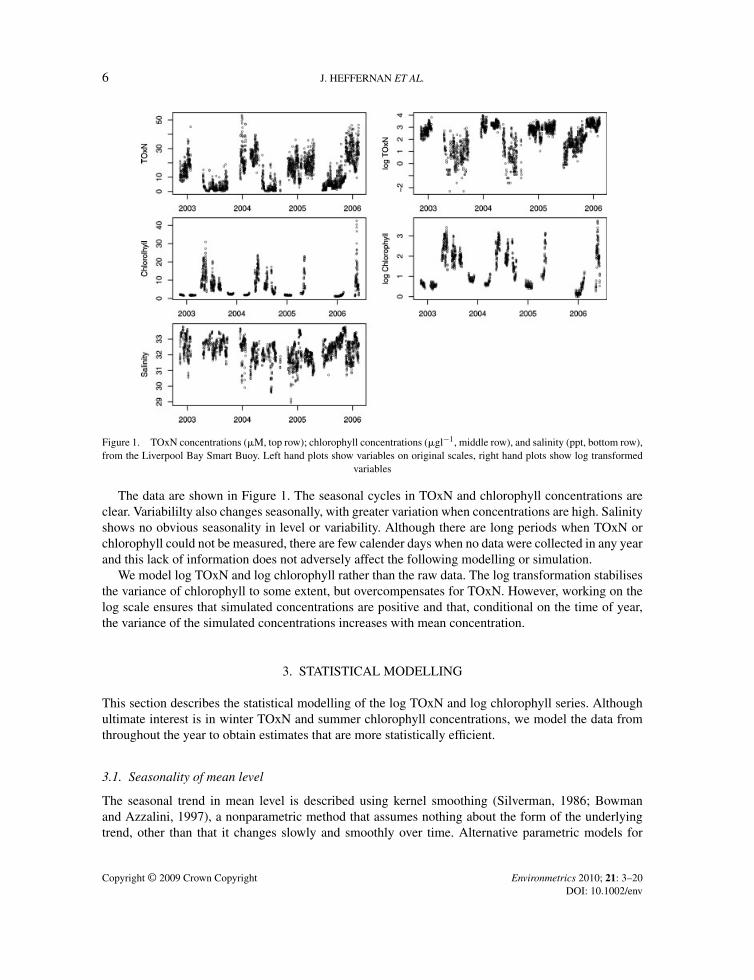
Figure 1. TOxN concentrations (�M, top row); chlorophyll concentrations (�gl−1, middle row), and salinity (ppt, bottom row),from the Liverpool Bay Smart Buoy. Left hand plots show variables on original scales, right hand plots show log transformed

variables

The data are shown in Figure 1. The seasonal cycles in TOxN and chlorophyll concentrations areclear. Variabililty also changes seasonally, with greater variation when concentrations are high. Salinityshows no obvious seasonality in level or variability. Although there are long periods when TOxN orchlorophyll could not be measured, there are few calender days when no data were collected in any yearand this lack of information does not adversely affect the following modelling or simulation.

We model log TOxN and log chlorophyll rather than the raw data. The log transformation stabilisesthe variance of chlorophyll to some extent, but overcompensates for TOxN. However, working on thelog scale ensures that simulated concentrations are positive and that, conditional on the time of year,the variance of the simulated concentrations increases with mean concentration.

3. STATISTICAL MODELLING

This section describes the statistical modelling of the log TOxN and log chlorophyll series. Althoughultimate interest is in winter TOxN and summer chlorophyll concentrations, we model the data fromthroughout the year to obtain estimates that are more statistically efficient.

3.1. Seasonality of mean level

The seasonal trend in mean level is described using kernel smoothing (Silverman, 1986; Bowmanand Azzalini, 1997), a nonparametric method that assumes nothing about the form of the underlyingtrend, other than that it changes slowly and smoothly over time. Alternative parametric models for



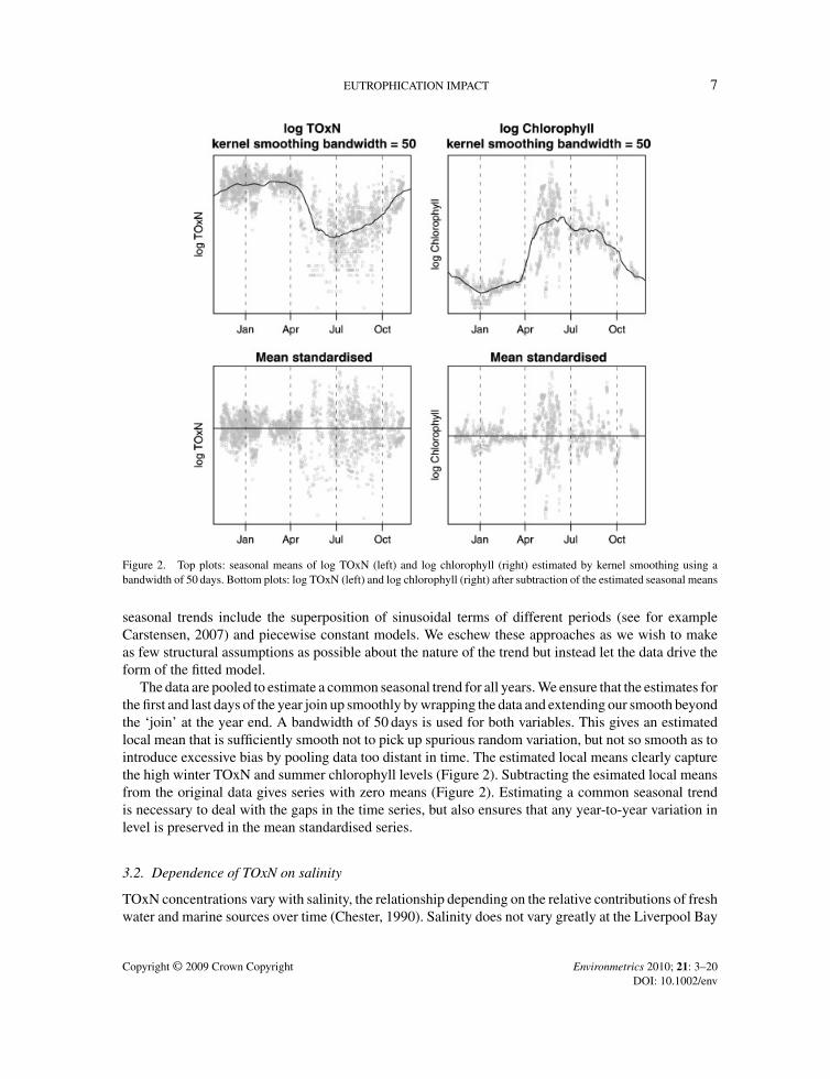
Figure 2. Top plots: seasonal means of log TOxN (left) and log chlorophyll (right) estimated by kernel smoothing using abandwidth of 50 days. Bottom plots: log TOxN (left) and log chlorophyll (right) after subtraction of the estimated seasonal means

seasonal trends include the superposition of sinusoidal terms of different periods (see for exampleCarstensen, 2007) and piecewise constant models. We eschew these approaches as we wish to makeas few structural assumptions as possible about the nature of the trend but instead let the data drive theform of the fitted model.

The data are pooled to estimate a common seasonal trend for all years. We ensure that the estimates forthe first and last days of the year join up smoothly by wrapping the data and extending our smooth beyondthe ‘join’ at the year end. A bandwidth of 50 days is used for both variables. This gives an estimatedlocal mean that is sufficiently smooth not to pick up spurious random variation, but not so smooth as tointroduce excessive bias by pooling data too distant in time. The estimated local means clearly capturethe high winter TOxN and summer chlorophyll levels (Figure 2). Subtracting the esimated local meansfrom the original data gives series with zero means (Figure 2). Estimating a common seasonal trendis necessary to deal with the gaps in the time series, but also ensures that any year-to-year variation inlevel is preserved in the mean standardised series.

3.2. Dependence of TOxN on salinity

TOxN concentrations vary with salinity, the relationship depending on the relative contributions of freshwater and marine sources over time (Chester, 1990). Salinity does not vary greatly at the Liverpool Bay



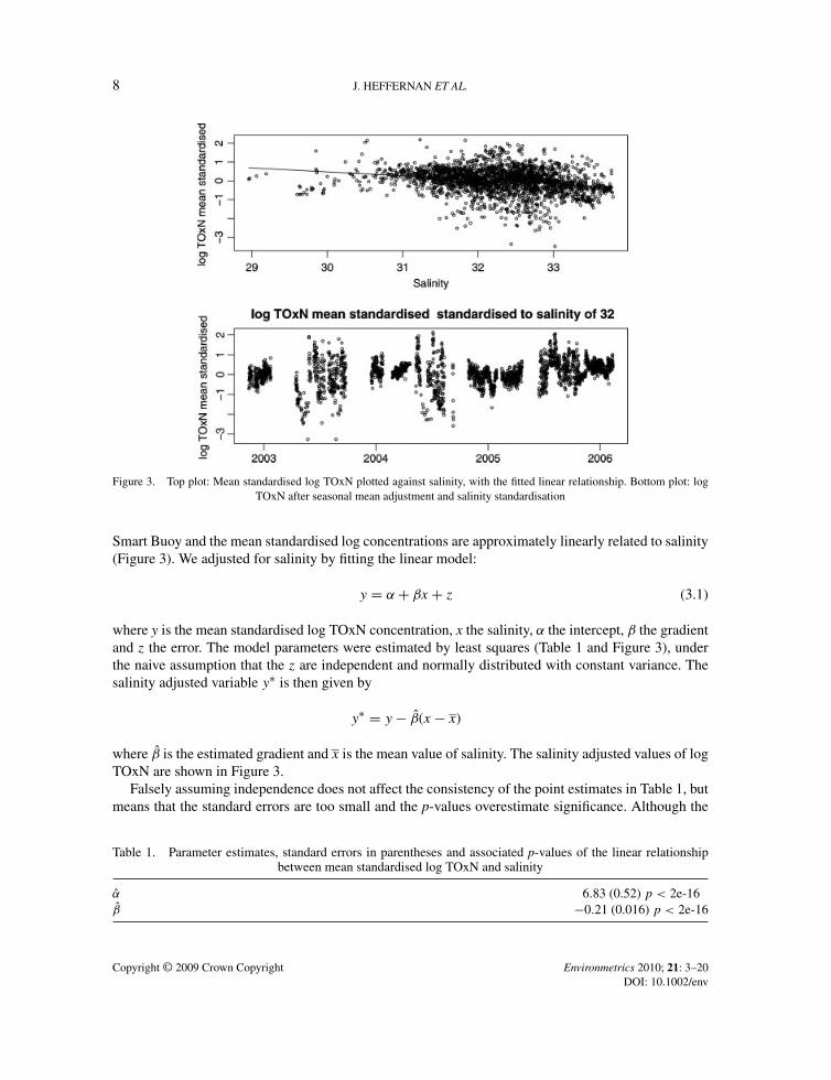
Figure 3. Top plot: Mean standardised log TOxN plotted against salinity, with the fitted linear relationship. Bottom plot: logTOxN after seasonal mean adjustment and salinity standardisation

Smart Buoy and the mean standardised log concentrations are approximately linearly related to salinity(Figure 3). We adjusted for salinity by fitting the linear model:

y = α + βx + z (3.1)

where y is the mean standardised log TOxN concentration, x the salinity, α the intercept, β the gradientand z the error. The model parameters were estimated by least squares (Table 1 and Figure 3), underthe naive assumption that the z are independent and normally distributed with constant variance. Thesalinity adjusted variable y∗ is then given by

y∗ = y − β(x − x)

where β is the estimated gradient and x is the mean value of salinity. The salinity adjusted values of logTOxN are shown in Figure 3.

Falsely assuming independence does not affect the consistency of the point estimates in Table 1, butmeans that the standard errors are too small and the p-values overestimate significance. Although the

Table 1. Parameter estimates, standard errors in parentheses and associated p-values of the linear relationshipbetween mean standardised log TOxN and salinity

α 6.83 (0.52) p < 2e-16β −0.21 (0.016) p < 2e-16



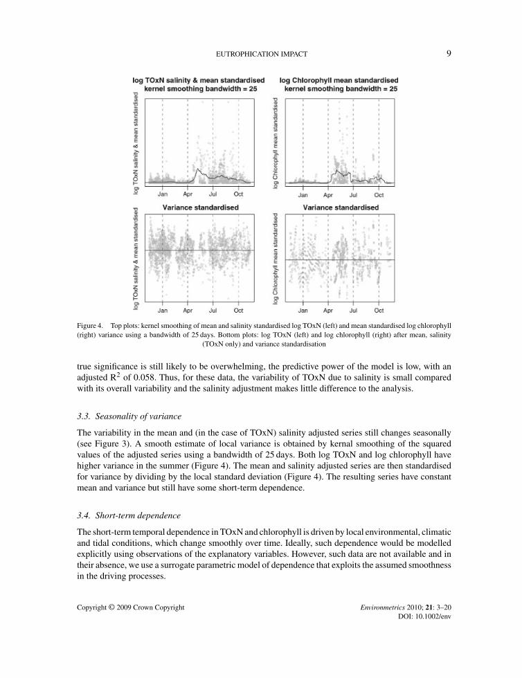
Figure 4. Top plots: kernel smoothing of mean and salinity standardised log TOxN (left) and mean standardised log chlorophyll(right) variance using a bandwidth of 25 days. Bottom plots: log TOxN (left) and log chlorophyll (right) after mean, salinity

(TOxN only) and variance standardisation

true significance is still likely to be overwhelming, the predictive power of the model is low, with anadjusted R2 of 0.058. Thus, for these data, the variability of TOxN due to salinity is small comparedwith its overall variability and the salinity adjustment makes little difference to the analysis.

3.3. Seasonality of variance

The variability in the mean and (in the case of TOxN) salinity adjusted series still changes seasonally(see Figure 3). A smooth estimate of local variance is obtained by kernal smoothing of the squaredvalues of the adjusted series using a bandwidth of 25 days. Both log TOxN and log chlorophyll havehigher variance in the summer (Figure 4). The mean and salinity adjusted series are then standardisedfor variance by dividing by the local standard deviation (Figure 4). The resulting series have constantmean and variance but still have some short-term dependence.

3.4. Short-term dependence

The short-term temporal dependence in TOxN and chlorophyll is driven by local environmental, climaticand tidal conditions, which change smoothly over time. Ideally, such dependence would be modelledexplicitly using observations of the explanatory variables. However, such data are not available and intheir absence, we use a surrogate parametric model of dependence that exploits the assumed smoothnessin the driving processes.



We use variograms to characterise the temporal dependence of the mean, salinity and varianceadjusted series. The variogram γ(t) describes how the variability of the data increases as a functionof separation t between data points. We assume that points closer together in time are more highlydependent and hence more similar and that the dependence structure does not change over time; i.e.intrinsic stationarity. In fact, we assume second order stationarity, since we use the covariance matrixassociated with the variogram. Variogram models and their properties are described in detail in Cressie(1991) and Myers (1997).

We used the powered exponential variogram, a flexible but parsimonious model for temporal depen-dence. The variogram has four parameters as follows:

γ(t) = τ2 + σ2{1 − exp(−αtκ)} : τ, σ, α, κ > 0 (3.2)

The parameter τ2 is the nugget of the process and represents the local variability of individualobservations including sampling variability and measurement error. The parameter σ2 describes theremaining variability of the process. The range of temporal dependence is controlled by the scaleparameter α and the rate of decay of this dependence is controlled by the shape parameter κ.

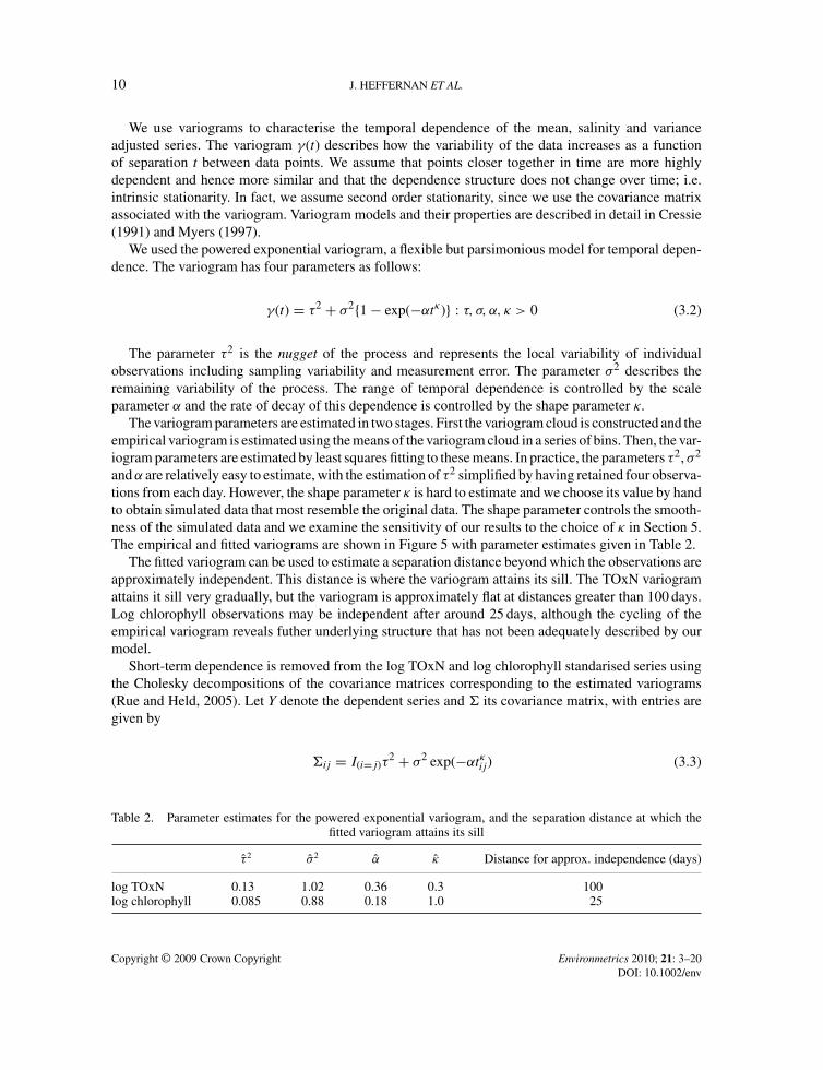
The variogram parameters are estimated in two stages. First the variogram cloud is constructed and theempirical variogram is estimated using the means of the variogram cloud in a series of bins. Then, the var-iogram parameters are estimated by least squares fitting to these means. In practice, the parameters τ2, σ2

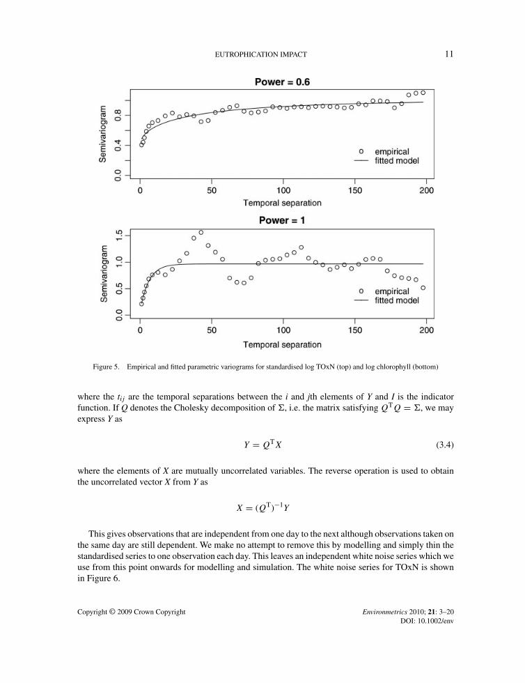
and α are relatively easy to estimate, with the estimation of τ2 simplified by having retained four observa-tions from each day. However, the shape parameter κ is hard to estimate and we choose its value by handto obtain simulated data that most resemble the original data. The shape parameter controls the smooth-ness of the simulated data and we examine the sensitivity of our results to the choice of κ in Section 5.The empirical and fitted variograms are shown in Figure 5 with parameter estimates given in Table 2.

The fitted variogram can be used to estimate a separation distance beyond which the observations areapproximately independent. This distance is where the variogram attains its sill. The TOxN variogramattains it sill very gradually, but the variogram is approximately flat at distances greater than 100 days.Log chlorophyll observations may be independent after around 25 days, although the cycling of theempirical variogram reveals futher underlying structure that has not been adequately described by ourmodel.

Short-term dependence is removed from the log TOxN and log chlorophyll standarised series usingthe Cholesky decompositions of the covariance matrices corresponding to the estimated variograms(Rue and Held, 2005). Let Y denote the dependent series and � its covariance matrix, with entries aregiven by

�ij = I(i=j)τ2 + σ2 exp(−αtκij) (3.3)

Table 2. Parameter estimates for the powered exponential variogram, and the separation distance at which thefitted variogram attains its sill

τ2 σ2 α κ Distance for approx. independence (days)

log TOxN 0.13 1.02 0.36 0.3 100log chlorophyll 0.085 0.88 0.18 1.0 25



Figure 5. Empirical and fitted parametric variograms for standardised log TOxN (top) and log chlorophyll (bottom)

where the tij are the temporal separations between the i and jth elements of Y and I is the indicatorfunction. If Q denotes the Cholesky decomposition of �, i.e. the matrix satisfying QTQ = �, we mayexpress Y as

Y = QTX (3.4)

where the elements of X are mutually uncorrelated variables. The reverse operation is used to obtainthe uncorrelated vector X from Y as

X = (QT)−1Y

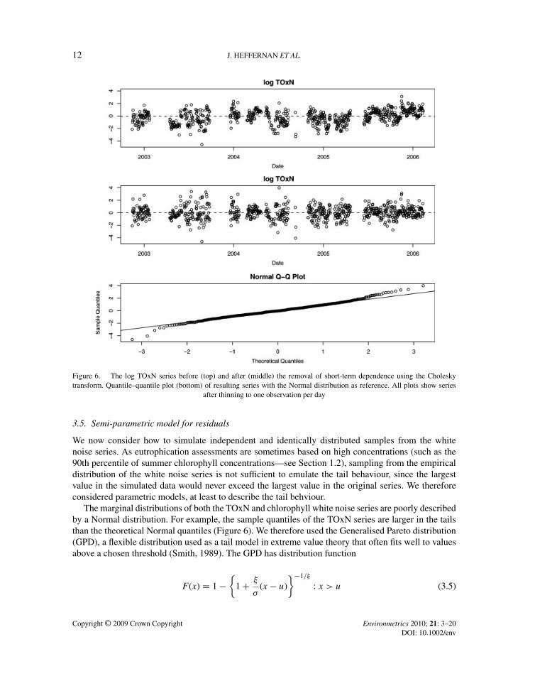
This gives observations that are independent from one day to the next although observations taken onthe same day are still dependent. We make no attempt to remove this by modelling and simply thin thestandardised series to one observation each day. This leaves an independent white noise series which weuse from this point onwards for modelling and simulation. The white noise series for TOxN is shownin Figure 6.



Figure 6. The log TOxN series before (top) and after (middle) the removal of short-term dependence using the Choleskytransform. Quantile–quantile plot (bottom) of resulting series with the Normal distribution as reference. All plots show series

after thinning to one observation per day

3.5. Semi-parametric model for residuals

We now consider how to simulate independent and identically distributed samples from the whitenoise series. As eutrophication assessments are sometimes based on high concentrations (such as the90th percentile of summer chlorophyll concentrations—see Section 1.2), sampling from the empiricaldistribution of the white noise series is not sufficient to emulate the tail behaviour, since the largestvalue in the simulated data would never exceed the largest value in the original series. We thereforeconsidered parametric models, at least to describe the tail behviour.

The marginal distributions of both the TOxN and chlorophyll white noise series are poorly describedby a Normal distribution. For example, the sample quantiles of the TOxN series are larger in the tailsthan the theoretical Normal quantiles (Figure 6). We therefore used the Generalised Pareto distribution(GPD), a flexible distribution used as a tail model in extreme value theory that often fits well to valuesabove a chosen threshold (Smith, 1989). The GPD has distribution function

F (x) = 1 −{

1 + ξ

σ(x − u)

}−1/ξ

: x > u (3.5)



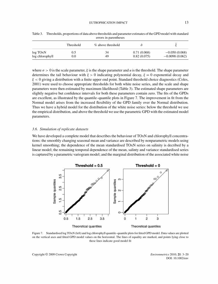
Table 3. Thresholds, proportions of data above thresholds and parameter estimates of the GPD model with standarderrors in parentheses

Threshold % above threshold σ ξ

log TOxN 0.5 34 0.71 (0.068) −0.050 (0.068)log chlorophyll 0.0 49 0.82 (0.075) −0.0098 (0.062)

where σ > 0 is the scale parameter, ξ is the shape parameter and u is the threshold. The shape parameterdetermines the tail behaviour with ξ > 0 indicating polynomial decay, ξ = 0 exponential decay andξ < 0 giving a distribution with a finite upper end point. Standard threshold choice diagnostics (Coles,2001) were used to choose appropriate thresholds for both white noise series, and the scale and shapeparameters were then estimated by maximum likelihood (Table 3). The estimated shape parameters areslightly negative but confidence intervals for both these parameters contain zero. The fits of the GPDsare excellent, as illustrated by the quantile–quantile plots in Figure 7. The improvement in fit from theNormal model arises from the increased flexibility of the GPD family over the Normal distribution.Thus we have a hybrid model for the distribution of the white noise series: below the threshold we usethe empirical distribution, and above the threshold we use the parametric GPD with the estimated modelparameters.

3.6. Simulation of replicate datasets

We have developed a complete model that describes the behaviour of TOxN and chlorophyll concentra-tions: the smoothly changing seasonal mean and variance are described by nonparametric models usingkernel smoothing; the dependence of the mean standardised TOxN series on salinity is decribed by alinear model; the remaining temporal dependence of the mean, salinty and variance standardised seriesis captured by a parametric variogram model; and the marginal distribution of the associated white noise

Figure 7. Standardised log TOxN (left) and log chlorophyll quantile–quantile plots for fitted GPD model. Data values are plottedon the vertical axes and fitted GPD model values on the horizontal. The lines of equality are marked, and points lying close to

these lines indicate good model fit



series is described by a semiparametric model with a GPD tail. We can now use this model to generatemultiple independent realisations of TOxN and chlorophyll concentrations on dates t1, . . . , tn, with oneobservation each day. Each realisation is obtained as follows:

(1) Generate a vector X = (x1, . . . , xn) of n independent random samples, with replacement, from thewhite noise series obtained in Section 3.4. The samples are treated as observations taken on datest1, . . . , tn.

(2) Replace the values xi : i = 1, . . . , n exceeding the GPD threshold u by independent samples fromthe fitted GPD conditional on being above this threshold, using the parameter estimates (σ, ξ) inTable 3. We sample x from the fitted GPD by first simulating a value of p from the Uniform[0, 1]distribution, then applying the inverse probability integral transform given by inverting the GPDdistribution function given in Equation (3.5) so that

x = u + σ

ξ

{(1 − p)−ξ − 1

}

(3) Compute the covariance matrix � corresponding to time points t1, . . . , tn using Equation (3.3) andthe parameter estimates in Table 2 and then find the Cholesky decomposition Q of this matrix.Transform vector X into a dependent vector Y by applying Equation (3.4).

(4) Multiply the elements of Y by the estimated local standard deviations (Section 3.3) at times t1, . . . , tn.(5) Add the estimated local means (Section 3.1) at times t1, . . . , tn.(6) Exponentiate, to obtain data on the concentration scale.

For simplicity, we do not re-introduce variability in TOxN due to salinity, since this would requirethe modelling of the salinity time series.

4. POWER CALCULATIONS

We now show how the simulation tool can be used to investigate the power of assessment tests andhow they depends on the sampling design. For simplicity, we focus on the Green test, described inSection 1.2, of whether mean winter TOxN and summer chlorophyll concentrations are below theassessment concentration (AC), and consider sampling in a single year with samples taken at equallyspaced intervals through the sampling window. However, the methodology is general and can be appliedto more complicated tests (e.g. based on percentiles) and designs.

4.1. Simulations and monitoring designs

Each power calculation is based on 5000 independent realisations of TOxN or chlorophyll concen-trations, each realisation having 1 year of daily observations. A (common) constant is added to eachrealisation, between stages 5 and 6, so that the underlying mean winter TOxN or summer chlorophyllconcentration (i.e. the mean concentration over all realisations within the season of interest) equals aspecified value. The mean concentration of each realisation will thus vary about the underlying seasonalmean, emulating random year to year variation. We consider underlying mean concentrations runningfrom background through to the assessment concentration (13 to 20 �M for winter TOxN and 10 to15 �gl−1 for summer chlorophyll).



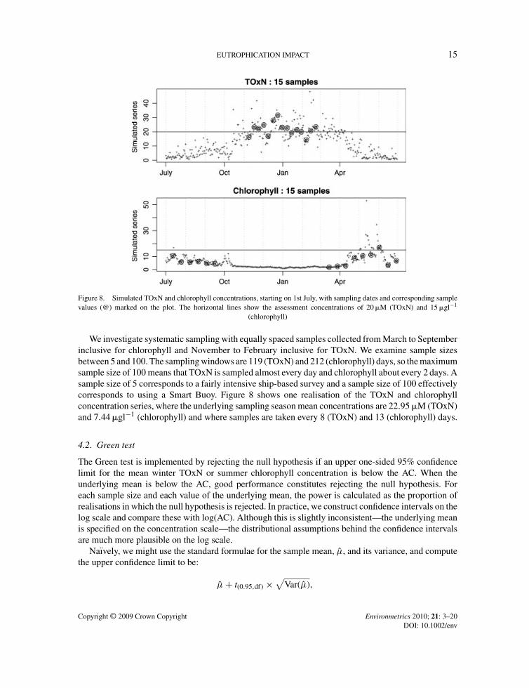
Figure 8. Simulated TOxN and chlorophyll concentrations, starting on 1st July, with sampling dates and corresponding samplevalues (@) marked on the plot. The horizontal lines show the assessment concentrations of 20 �M (TOxN) and 15 �gl−1

(chlorophyll)

We investigate systematic sampling with equally spaced samples collected from March to Septemberinclusive for chlorophyll and November to February inclusive for TOxN. We examine sample sizesbetween 5 and 100. The sampling windows are 119 (TOxN) and 212 (chlorophyll) days, so the maximumsample size of 100 means that TOxN is sampled almost every day and chlorophyll about every 2 days. Asample size of 5 corresponds to a fairly intensive ship-based survey and a sample size of 100 effectivelycorresponds to using a Smart Buoy. Figure 8 shows one realisation of the TOxN and chlorophyllconcentration series, where the underlying sampling season mean concentrations are 22.95 �M (TOxN)and 7.44 �gl−1 (chlorophyll) and where samples are taken every 8 (TOxN) and 13 (chlorophyll) days.

4.2. Green test

The Green test is implemented by rejecting the null hypothesis if an upper one-sided 95% confidencelimit for the mean winter TOxN or summer chlorophyll concentration is below the AC. When theunderlying mean is below the AC, good performance constitutes rejecting the null hypothesis. Foreach sample size and each value of the underlying mean, the power is calculated as the proportion ofrealisations in which the null hypothesis is rejected. In practice, we construct confidence intervals on thelog scale and compare these with log(AC). Although this is slightly inconsistent—the underlying meanis specified on the concentration scale—the distributional assumptions behind the confidence intervalsare much more plausible on the log scale.

Naıvely, we might use the standard formulae for the sample mean, µ, and its variance, and computethe upper confidence limit to be:

µ + t(0.95,df) ×√

Var(µ),



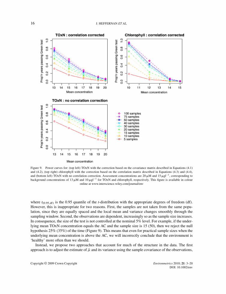
Figure 9. Power curves for: (top left) TOxN with the correction based on the covariance matrix described in Equations (4.1)and (4.2), (top right) chlorophyll with the correction based on the correlation matrix described in Equations (4.3) and (4.4),and (bottom left) TOxN with no correlation correction. Assessment concentrations are 20 �M and 15 �gl−1, corresponding tobackground concentrations of 13 �M and 10 �gl−1 for TOxN and chlorophyll, respectively. This figure is available in colour

online at www.interscience.wiley.com/journal/env

where t(0.95,df) is the 0.95 quantile of the t-distribution with the appropriate degrees of freedom (df).However, this is inappropriate for two reasons. First, the samples are not taken from the same popu-lation, since they are equally spaced and the local mean and variance changes smoothly through thesampling window. Second, the observations are dependent, increasingly so as the sample size increases.In consequence, the size of the test is not controlled at the nominal 5% level. For example, if the under-lying mean TOxN concentration equals the AC and the sample size is 15 (50), then we reject the nullhypothesis 25% (35%) of the time (Figure 9). This means that even for practical sample sizes when theunderlying mean concentration is above the AC, we will incorrectly conclude that the environment is‘healthy’ more often than we should.

Instead, we propose two approaches that account for much of the structure in the data. The firstapproach is to adjust the estimate of µ and its variance using the sample covariance of the observations,



estimated from all 5000 simulated time series. This leads to genearlised least squares estimates:

µ = (1′�−11)−11′�−1y (4.1)

Var(µ) = (1′�−11)−1 (4.2)

where 1 is a vector of ones, � is the covariance matrix (corresponding to the sampling times in the survey)and y is the vector of observations. The second approach, instead of the covariance matrix, uses thecorrelation matrix corresponding to the fitted variogram (Equation (3.2)) and assumes constant varianceof the observations about their local mean throughout the sampling window. This gives estimates:

µ = (1′ϒ−11)−11′ϒ−1y (4.3)

Var(µ) = s2(1′ϒ−11)−1 (4.4)

where ϒ is the correlation matrix of the observations and s2 is the usual estimate of variance (assumingcommon variance and independence). The first approach uses the correct covariance structure but stillignores any seasonality in mean through the sampling window. The second approach uses the correctcorrelation structure but ignores any seasonality in mean and variance. In most practical situations, boththe covariance and correlation matrices are unavailable; we return to this in Section 5.

4.3. Performance of different sampling schemes

Power curves for TOxN and chlorophyll are shown in Figure 9. The curves for TOxN are based onthe correction using the covariance matrix (using Equations (4.1) and (4.2)). The size of the test hasbeen correctly controlled at about 5%. However, the power of the test is limited, since even whenthe underlying mean equals the background concentration, daily sampling only gives a power of about80%. Increasing the sample size does not have a big effect on power, since the relatively large separationdistance for TOxN (i.e. the range of the variogram) means that taking more samples gives only limitedextra information. The power curves for TOxN using the correction based on the correlation matrix(using Equations (4.3) and (4.4), not shown) gave a similar picture with only a small reduction in power.

For chlorophyll, the covariance matrix was close to singular due to near-zero variances of the sim-ulated observations at the start of the sampling window, resulting in numerical instabilities when cal-culating µ and Var(µ). Therefore, the power curves for chlorophyll are based on the correction usingthe correlation matrix (Equations (4.3) and (4.4)). The size of the test is less than the nonimal 5%, butat least this is compatible with the precautionary approach since it makes it harder to demonstrate thatthe environment is ‘healthy’. Sample size has a much greater effect on power than for TOxN, probablybecause the separation distance for chlorophyll is smaller. When the underlying mean equals the back-ground concentration, taking 100 samples (i.e. every 2 days) gives nearly 100% power and 23 samples(i.e. every 9 days) gives 80% power.

5. DISCUSSION

We have developed a hybrid semiparametric model to describe the seasonal, covariate and temporaldependence of two water quality variables used to assess eutrophication. The model can be used to sim-ulate independent realisations with properties similar to the original data, and provides the opportunity,



hitherto unavailable, to study the performance of monitoring designs and assessment methods used ineutrophication assessments.

We have shown how sample size affects the performance of a test to assess whether mean winterTOxN and summer chlorophyll concentrations are below the assessment concentrations. For TOxN wewould need about 100 samples (i.e. daily sampling) and for chlorophyll about 23 samples, to obtain 80%power when the underlying mean equals the background concentration. Daily sampling is unrealisticusing research vessels and implies that a Smart Buoy would be required. The large sample sizes arisebecause, with strong temporal dependence, there are some years when the realised mean TOxN andchlorophyll concentrations are well above the background concentration (even though the underlyingmean equals the background concentration). A more promising approach would be to base assessmentson the data from several years, a 5 year monitoring window aligning naturally with the timing of OSPARand Water Framework Directive assessments. The required sample size would then drop because thedata from different years would be independent. The effect might be quite marked for TOxN which hasa much larger separation distance than chlorophyll. Future work will consider the design and analysisof multi-year monitoring programmes.

The results shown here are based on the data from a single Smart Buoy, in Liverpool Bay. However,we have also studied TOxN and chlorophyll data from a Smart Buoy at Gabbard, a coastal site in theThames Estuary. Our modelling approach also worked well with these data and provided broadly similarparameter estimates and conclusions. This suggests that monitoring designs and assessment methodsappropriate for Liverpool Bay may be more generally applicable to other coastal sites.

More data will be required to study estuarine sites where freshwater influences are more important.The levels and patterns of variation may differ and the relationship with salinity will be much stronger.Here, the seasonal mean and the relationship with salinity might be more effectively modelled using aGeneralised Additive Model (Wood, 2006). Also, ship-based monitoring in estuaries tends to involvesampling along transects down the salinity gradient, so different designs and assessment methods wouldneed to be considered.

It is important to incorporate the serial correlation in the data when carrying out the Green Tests. Wecould do so because we had already modelled the correlation structure in our analysis of the Smart Buoydata. For locations without a Smart Buoy, an alternative approach would be necessary. One possibilitywould be to replace ϒ in Equations (4.3) and (4.4) by an estimate of the correlation matrix from thevariogram of the observations. This estimate is liable to be poor, especially for small sample sizes,but could be improved by pooling data from several years. An alternative would be to assume that thecorrelation structure for Liverpool Bay is valid elsewhere, and to use the parameter estimates in Table 2to estimate ϒ. This is a strong assumption that would need to be verified. Future work will investigatethe performance of tests at the Gabbard site using the Liverpool Bay variogram, and vice versa.

The short term temporal dependence in our model is characterised by the variogram. As mentionedin Section 3.4, the shape parameter κ is difficult to identify and we chose the value of κ by hand to giverealisations of the process most similar in appearance to the original series. For TOxN, values of κ in therange 0.3–0.5 were plausible with smaller and larger values giving processes that were too rough and toosmooth, respectively. For chlorophyll, values of κ in the range 0.9–1.4 all giving plausible realisations.However, the estimates of power were not sensitive to the choice of κ. For TOxN, increasing κ from 0.3(used in the power calculations reported above) to 0.5 reduced the power by at most 3% for any samplesize and underlying mean. Similarly, for chlorophyll, increasing κ from 0.9 to 1.4 reduced power by atmost 2%.

We worked on the logarithmic scale throughout. This ensured that simulated concentrations werepositive and that, when we adjusted the underlying mean concentration in the power study, the local



variability would change accordingly. In particular, conditional on the time of year, concentrations wouldbe distributed with constant coefficient of variation. This relationship between mean and variance isdifficult to verify without more years of data in which the mean concentration varies systematically,but it is plausible and consistent with the analysis of spot water samples from research vessels and thebehaviour of concentration data in other marine monitoring programmes (e.g. ICES, 1989).

The aim of our modelling has been to understand the temporal behaviour of concentrations ofTOxN and chlorophyll, and to consider the implications for designing surveys to detect whether meanconcentrations at a particular location are below specified thresholds. Of course, this is only one step indesigning a monitoring programme. Further steps include selecting a network of monitoring locationsthat gives an adequate geographical coverage and integrating spot sampling from research vessels withmore intensive sampling from Smart Buoys to provide suitable data to inform eutrophication assessmentsat a more regional level.

ACKNOWLEDGEMENT

Much of the work for this project was funded from DEFRA contract E2202.

REFERENCES

Bricker SB, Ferreira JG, Simas T. 2003. An integrated methodology for assessment of estuarine trophic status. EcologicalModelling 169: 39–60.

Bowman AW, Azzalini A. 1997. Applied Smoothing Techniques for Data Analysis. Oxford University Press : New York.Carstensen J. 2007. Statistical principles for ecological status classification of Water Framework Directive monitoring data.

Marine Pollution Bulletin 55(1–6): 3–15.C.E.C. 1991. Council Directive of 21 May 1991 concerning urban waste water treatment (91/271/EEC). Official Journal of the

European Communities L135: 40–52.C.E.C. 2000. Directive 2000/60/EC of the European Parliament and of the Council of 23 October 2000 establishing a framework

for Community action in the field of water policy. Official Journal of the European Communities L327: 1–73.Chester R. 1990. Marine Geochemistry. Unwin Hyman: London.Cloern JE. 1999. The relative importance of light and nutrient limitation of phytoplankton growth: a simple index of coastal

ecosystem sensitivity to nutrient enrichment. Aquatic Ecology 33: 3–16.Cloern JE. 2001. Our evolving conceptual model of the coastal eutrophication problem. Marine Ecology Progress Series 210:

223–253.Coles SG. 2001. An Introduction to Statistical Modeling of Extreme Values. Springer–Verlag: London.Cressie N. 1991. Statistics for Spatial Data. John Wiley and Sons: New York.CSTT. 1994. Comprehensive studies for the purposes of Article 6 of DIR 91/271 EEC, the Urban Waste Water Treatment

Directive. Published for the Comprehensive Studies Task Team of Group Coordinating Sea Disposal Monitoring by the 4thRiver Purification Board, Edinburgh.

CSTT. 1997. Comprehensive studies for the purposes of Article 6 & 8.5 of DIR 91/271 EEC, the Urban Waste Water TreatmentDirective, 2nd edition. Published for the Comprehensive Studies Task Team of Group Coordinating Sea Disposal Monitoringby the Department of the Environment for Northern Ireland, the Environment Agency, 2002 Scottish Environmental ProtectionAgency and the Water Services Association, Edinburgh.

Gillbricht M. 1988. Phytoplankton and nutrients in the Helgoland region. Helgolander Meeresuntersuchungen 42: 435–467.Harding L. 1994. Long term trends in the distribution of phytoplankton in Chesapeake Bay: roles of light, nutrients and streamflow.

Marine Ecology Progress Series 104: 267–291.ICES. 1989. Statistical analysis of the ICES co-operative monitoring programme data on contaminants in fish muscle tissue

(1975–1985) for determination of temporal trends. ICES Co-operative Research Report No. 162.Malcom S, Nedwell D, Devlin M, Hanlon A, Dare S, Parker R and Mills D. (2002). First application of the OSPAR comprehensive

procedure to waters around England and Wales, Cefas report, Cefas, Pakefield Road, Lowestoft, NR33 OHT, UK.Myers J. 1997. Geostatistical Error Management. International Thompson Publishing Co.: New York, NY, U.S.A.OSPAR Commission 2003. The OSPAR Integrated Report 2003 on the Eutrophication Status of the OSPAR Maritime Area based

upon the first application of the Comprehensive Procedure. MMC 2003/2/4, OSPAR Publication 2003, ISBN: 1-904426-25-5.



Painting S, Devlin MJ, Rogers S, Mills DK, Parker ER, Rees HL. 2005. Assessing the suitability of OSPAR EcoQOs foreutrophication vs ICES criteria for England and Wales. Marine Pollution Bulletin 50: 1569–1584.

Painting SJ, Devlin MJ, Malcolm SJ, Mills C, Mills DK, Parker ER, Tett P, Wither A, Burt J, Jones R, Winpenny K. 2007.Assessing the impact of nutrient enrichment in estuaries: susceptibility to eutrophication. Marine Pollution Bulletin 55: 74–90.

Rue H, Held L. 2005. Gaussian Markov Random Fields: Theory and Applications. Chapman and Hall: Boca Raton, FL.Silverman B. 1986. Density Estimation for Statistics and Data Analysis. Chapman and Hall: London.Smayda TJ, Reynolds CS. 2001. Community assembly in marine phytoplankton: application of recent models to harmful di-

noflagellate blooms. Journal of Plankton Research 23: 447–461.Smith RL. 1989. Extreme value analysis of environmental time series: an application to trend detection in ground level ozone

(with discussion). Statistical Science 4: 367–393.Tett P, Gowen R, Grantham B, Jones K, Miller BS. 1986. The phytoplankton ecology of the Firth of Clyde sea-lochs Striven and

Fyne. Proceedings of the Royal Society of Edinburgh, 90B, 223–238.Vincent C, Heinrich H, Edwards A, Nygaard K, Haythornthwaite K. 2002. Guidance on typology, reference conditions and classi-

fication systems for transitional and coastal waters. Produced by: CIS Working Group 2.4 (COAST), Common ImplementationStrategy of the Water Framework Directive, European Commission; 119.

Wood SN. 2006. Generalized Additive Models: An Introduction with R. Chapman and Hall, CRC: Boca Raton, FL.


A simulation tool for designing nutrient monitoring programmes for eutrophication assessments

Documents

Transcript of A simulation tool for designing nutrient monitoring programmes for eutrophication assessments