194 Int. J. Sensor Networks, Vol. 4, No. 3, 2008

Copyright © 2008 Inderscience Enterprises Ltd.

A simple performance analysis of RFID networks with binary tree collision arbitration

Gianluigi Ferrari* Information Engineering Department, University of Parma, Italy E-mail: gianluigi.ferrari@unipr.it *Corresponding author

Fabio Cappelletti Selta SpA, Cadeo (PC), Italy E-mail: f.cappelletti@selta.it

Riccardo Raheli Information Engineering Department, University of Parma, Italy E-mail: raheli@tlc.unipr.it

Abstract: Radio Frequency Identification (RFID) networks are becoming a widespread technology in industry and commerce. In this paper, we propose a simple performance analysis of RFID networks, based on the binary tree collision arbitration protocol. We evaluate various network performance metrics such as throughput, delay and average number of packets needed to take a census of the RFID tags. In order to validate our analytical results, we develop a simple, yet accurate, simulator and show that the predicted analytical performance is in good agreement with the simulation results. While the analytical approach does not take into account the communication channel characteristics, we evaluate, through simulations, the impact of fading and topology (in terms of tag spatial density) on the network performance.

Keywords: Radio Frequency Identification networks; RFID networks; binary tree protocol; delay; throughput; fading; tag spatial density; simulations.

Reference to this paper should be made as follows: Ferrari, G., Cappelletti, F. and Raheli, R. (2008) ‘A simple performance analysis of RFID networks with binary tree collision arbitration’, Int. J. Sensor Networks, Vol. 4, No. 3, pp.194–208.

Biographical notes: Gianluigi Ferrari received the ‘Laurea’ (a five-year programme) (summa cum laude) and the PhD degrees in electrical engineering from the University of Parma, Italy, in 1998 and 2002, respectively. Since 2002, he has been a Research Professor at the Department of Information Engineering, University of Parma, Italy, where he is now the Coordinator of the Wireless Ad-hoc and Sensor Networks (WASN) lab. He also visited, between 2000 and 2004, the University of Southern California, USA, and Carnegie Mellon University, USA. He is a corecipient of best student paper award at the 2006 International Workshop on Wireless Ad hoc Networks (IWWAN’06).

Fabio Cappelletti was born in Piacenza, Italy, in 1978. He received the ‘Laurea’ degree (five-year programme) in electrical engineering from the University of Parma, Italy, in December 2004 discussing a thesis with title ‘Information rates of multidimensional front-ends for digital storage channels with data-dependent transition noise’ (in Italian). From January 2005 to November 2005 he was a Research Assistant at the Department of Information Engineering of the University of Parma. From November 2005 to April 2007 he was in WellNetwork spa, Piacenza, Italy. Since April 2005, he has been with Selta spa, Roveleto di Cadeo, Piacenza, Italy.

Riccardo Raheli was educated in electrical engineering at the University of Pisa, Italy, and the University of Massachusetts at Amherst, USA. He held positions at Siemens Telecomunicazioni, Milan, Italy, the Scuola Superiore S. Anna, Pisa, Italy, and the University of Southern California, Los Angeles, USA. Since 1991, he has been with the University of Parma, Italy, currently as Professor of communications engineering. He served on the Editorial Boards of the IEEE Transactions on Communications, the IEEE Journal on Selected Areas in Communications (JSAC), the European Transactions on Telecommunications (ETT) and on the Technical Program Committees of several leading international conferences.

A simple performance analysis of RFID networks 195

1 Introduction

In recent years, Radio Frequency Identification (RFID) systems are found in increasing applications in several business areas such as service, purchasing and distribution logistics, manufacturing, ticketing, animal identification and material flow systems (Finkenzeller, 2003). In fact, nowadays several of these businesses are based on the use of barcodes, which, although inexpensive (a desirable characteristic), have several limits, among which are an insufficient information storage space and the impossibility of being reprogrammed. A technically optimal solution to these problems would be the storage of data in a silicon chip. However, this solution requires mechanical contacts, which are often unfeasible. A contact-less transfer of data between the data-carrying device and its reader is far more flexible. Ideally, the power required to operate the electronic data-carrying device would also be transferred from the reader using the contact-less technology.

A practical form of contact-less identification (ID) systems is given by RFID systems, and the large number of companies involved in the development of this technology is a clear sign of its tremendous potential. The RFID market is a fast-growing sector of the radio technology industry, including mobile phones and cordless telephones. RFID systems are now available in the market, and developers need more and more to be able to optimise these systems for specific applications. Therefore, it is very important for them to have efficient tools to evaluate the performance of the systems under design.

In the literature, the study of RFID networks is somewhat immature, especially in terms of the evaluation of performance metrics such as throughput and delay. Several RFID systems are based on the use of the binary tree collision arbitration protocol. In Capetenakis (1979), the author shows that the number of collisions in packet broadcast channels is reduced by using the binary tree protocol. In the same paper, the author proposes a thorough statistical analysis for the evaluation of the delay performance of the system. In Hush and Wood (1998), the applicability of the binary tree collision arbitration protocol for RFID arbitration is considered. In Myung and Lee (2005), a new collision arbitration protocol based on the well-known query tree protocol, characterised by the fact that the reader can remember tags which have collided, is proposed. Moreover, in Myung and Lee (2005) and Myung et al. (2006a), the authors compute the average number of time slots necessary to detect the entire tag population in the interrogator field and they also show that their new method significantly reduces the number of collisions for the successive reading operation. This approach is further extended in Myung and Lee (2006) and Myung et al. (2006b), where adaptive splitting protocols for RFID tag collision arbitration are proposed. In Simplot-Ryl et al. (2006), a hybrid randomised protocol for RFID tag identification is proposed, and its performance is analytically evaluated. A survey of collision resolution protocols between the tags and the tag reader is proposed in Abraham et al. (2004), and realistic performance benchmarks, as well as experimental results, for

passive Ultra-High Frequency (UHF) RFID tags are presented in Ramakrishnan and Deavours (2006). In Zhou et al. (2004), the power consumption of a multiple access scheme for RFID systems with query tree protocol is analysed. In Siden et al. (2001) and Zhou and Wang (2004), the impact of the antenna radiation pattern on the performance of RFID networks is evaluated.

The goal of this paper is to propose a simple analytical framework for the evaluation of RFID network performance metrics such as average delay and throughput. The key idea of our approach consists in analysing an RFID network as a deterministic system. In other words, the evolution of the tag census process is somehow ‘idealised’, and the analytical derivation becomes significantly simpler. Our results show that during an n-tag network census process (1) the average number of transmitted packets per node is 2(log ),nΘ where the notation ( )Θ ⋅ means ‘on the order of’ and will be clearly defined later, (2) the network throughput is 2(1 log )nΘ / and (3) the delay is 2( log ).n nΘ In order to validate our simplified analytical approach, we build a reliable and scalable RFID network simulator. Our simulator is developed with OPNET 11.0 (Opnet Technologies, 2006) and implements the binary tree collision arbitration protocol. In particular, we consider an RFID system based on the ISO 18000 standard (ISO IEC, 2004). The simulation results agree with results recently appeared in the literature (Glidden et al., 2004) and they are also in good agreement with our analysis. This confirms the applicability of our analytical framework. Moreover, using the OPNET simulator, we investigate aspects which are not taken into account by our analytical framework, namely the impact of fading and network topology on the system performance.

This paper is structured as follows. In Section 2, we provide the reader with preliminaries on RFID networks and on the binary tree protocol. In Section 3, we propose a simple analytical approach for performance evaluation of RFID systems using the binary tree collision arbitration protocol. In Section 4, the structure of our OPNET simulator is described. In Section 5, we use the analytical framework introduced in Section 3 to compute the throughput and delay performance of the considered RFID systems, and we validate our analysis through simulations, evaluating also the impact of fading and network topology on the system performance. Section 6 concludes the paper.

2 Preliminaries

RFID systems are closely related to smart cards, i.e. bank and telephone cards (Finkenzeller, 2003). In fact, as in smart card systems, data is stored in an electromagnetic data-carrying device (the tag). However, unlike the smart card, the power supply to the data-carrying device and the date exchange between the data-carrying device and the interrogator are achieved without the use of electrical contacts, but using electromagnetic fields. The underlying technology is drawn from the fields of radio and radar engineering.

196 G. Ferrari, F. Cappelletti and R. Raheli

An RFID system needs to be optimised for each specific application, and it is difficult to give general guidelines. However, there are some key points which should be considered in the selection of the best RFID system for the application at hand.

• Carrier frequency: RFID systems based on inductive coupling operate in the frequency range between 100 kHz and 30 MHz, whereas microwave radio systems employ UHF domain.

• Maximum distance between the tags and the reader: this has an impact on the required transmit power at the reader.

• Memory capacity at the tags (the reader’s memory capacity is usually not an issue): this is relevant when more advanced versions of the binary tree protocol need to be developed, such as in Myung and Lee (2005).

• Choice of the proper standard: this depends on the particular project at hand.

In the following, we first present a brief overview on the existing standards, giving more details on the standard which will be considered in this work. Then, we describe the binary tree protocol, used to take a census of the tags.

2.1 RFID system standards

Due to the increasing application of RFID technology in the last years, several organisations have proposed various standards such as ISO/IEC 18000 international standard (ISO IEC, 2004), the AUTO ID center standard (Auto ID Center, 2003) and the GEN2 standard (which is the new generation ISO standard; EPC Global, 2005). All the documents define key values for the air interface of an RFID tag: in particular, they propose a set of values for the physical layer parameters such as coding, modulation, frequency rate and a set of possible values for identification parameters such as the number of bits used to define the identification codes and so on. All the standards also characterise exactly the so-called collision arbitration procedure, i.e. the multiple access scheme, since this is a fundamental network aspect. Another important system characteristic described by each standard is the quantity of memory that the tags are equipped with. As briefly mentioned at the beginning of this section, this is very important since if tags can store more information, then the arbitration protocol can be made more effective and the network performance can be improved. The main difference between the above standards resides in the multiple access schemes. In fact, these protocols can be classified into two main categories: (1) the first category is based on the slotted Aloha Medium Access Control (MAC) protocol (ISO 18000 Type A) (Bertsekas and Gallager, 1992), whereas (2) the second one is based on the binary tree protocol (ISO 18000 Type B, GEN2 and AUTO ID) (Capetenakis, 1979). The slotted Aloha MAC protocol is simple to implement but its performance is ‘intrinsically’ limited. On the other hand, a binary tree collision arbitration protocol is an efficient solution to reduce the number of collisions.

We now provide the reader with a quick overview on the characteristics of tags and interrogator in the various standards. The ISO standard proposes two different kinds of tags, denoted as Type A and Type B. They have different features in terms of channel encoding, modulation index and data rate of forward (from interrogator to tag) and backward (from tag to interrogator) links. The AUTO ID standard introduces a modified version of the binary tree protocol denoted as query tree protocol. The latter protocol is based on the ability of the interrogator to detect, after a collision has occurred, the position of the bits that were different in the ID number of the tags (ISO IEC, 2004). This is possible through the use of Miller coding.

In this paper, we consider the Type B ISO 18000 standard, with binary tree collision arbitration protocol. To the best of our knowledge, no simulation-based study of this system has appeared so far. Moreover, our novel analytical framework allows one to evaluate the network performance with good accuracy in a relatively simple fashion.

2.2 Binary tree protocol

The binary tree protocol is a census protocol which efficiently reduces the number of collisions in multi-access networks (Capetenakis, 1979; Wu and Li, 1991; Hush and Wood, 1998). The reader (or interrogator) illuminates the tags, which, through small (but sufficient) absorbed energy, can transmit their IDs to the reader. Obviously, several tags can simultaneously transmit and, therefore, collide. In order to reduce efficiently the number of collisions, the key idea of the binary tree protocol consists in assuming that a set of colliding tags can be divided into two subgroups: the tags belonging to one of the subgroups will not transmit until re-interrogated, whereas the tags belonging to the other group will try to retransmit (ISO IEC, 2004). The same procedure can be used recursively to take a census on the latter group of tags. Eventually, only one tag will transmit, and the reader will correctly receive its ID information. The process which leads to correct identification of a single tag will be referred to as round. Taking a census of all tags in the network requires a number of rounds equal to the number of tags.

We now describe the evolution of the tag state during a census operation. The complete state diagram of a single tag is shown in Figure 1. After being turned on, the tag is initially in the ‘READY’ state. The interrogator can use some (radio) commands to define the subset of tags which participate to the collision arbitration. Initially, upon reception of a group select command sent by the reader, a group of tags move to the ‘ID’ state. Once the interrogator has selected the subset of tags which participate into the collision arbitration, the round can start. Each tag has a counter, which is initialised to 0 at the beginning of the round and changes during the round. The reading process in a round can be described as follows.

• All tags in the ID state with their counters set to 0 transmit their ID numbers. This step is performed by all selected tags.

A simple performance analysis of RFID networks 197

• If more than a single tag reply to the transmitter, the interrogator receives an erroneous response and sends the tags a failed command.

• Each tag with the counter set to 0 receiving a failed command by the interrogator ‘tosses a coin:’ with probability ½, it retransmits its ID (leaving the counter set to 0), while with probability 1/2, it increases the counter by 1 and does not retransmit. Each tag with the counter set to a value larger than 0 increases the counter and does not transmit its ID.

Figure 1 Tag state diagram

From the above process, one can conclude that only tags with the counter set to 0 have a chance to transmit their IDs. At the end of this period, there can be four possible scenarios.

1 If more than one tag retransmit its ID, then the interrogator does not receive a correct frame and resends a failed command.

2 If all tags with counter set to 0 randomly choose not to retransmit, the interrogator does not receive anything and, after a guard time, transmits a success command. This will cause all tags to decrease their counter by 1.

3 If only one tag retransmits, the interrogator receives a good frame and can detect that tag. The interrogator then sends to that tag a read command. Upon reception of this command, the tag enters into the ‘DATA EXCHANGE’ state, as shown in Figure 1, and transfers its information to the interrogator. At the end of this operation, the interrogator sends a success command, the tag moves to the READY state and a new round can start. Obviously, the number of tags which ‘play’ in the new round is equal to the number in the previous round reduced by 1.

4 If only one tag transmits its ID but this message is not correctly received by the reader, then the reader sends a retransmit command and the same tag will retransmit its ID.

3 A simple analytical approach

In this section, a novel analytical approach for evaluating the performance of RFID networks is presented. Rather than considering a complicated statistical approach as in Capetenakis (1979) and Hush and Wood (1998), we propose a simple analysis based on a deterministic characterisation of the binary tree protocol proposed in ISO IEC (2004). While our approach is a priori suboptimal (since the stochastic nature of the collision-based resolution algorithm is neglected), it allows to derive simple, yet very accurate, performance bounds. Moreover, our analysis is in good agreement with realistic simulation results. In the following subsections, we evaluate the network throughput and the delay incurred in a census operation.

3.1 Network throughput Let us preliminarily define a time slot as the interval of time during which a tag transmits a packet with its ID information. Denoting the packet length by L (dimension: [b/pkt]) and the data rate by Rb (dimension: [b/s]), the duration of a time slot is slot bD L R/ (dimension: [s]). We first compute the total number of packets sent by the tags during a census of the entire tag population in the RFID network. In order to do this, it is not necessary to take into account the number of idle time slots, i.e. time slots where no tag is transmitting. The idle time slots, however, have a strong impact on the delay required to take the census, and they will be taken into account in the following subsection. We assume that if n tags transmit (and then collide) in a time slot, the number of tags that will retransmit their IDs in the following time slot is n/2. This is the key difference between our simplified analysis and more sophisticated statistical analyses, based on the approach originally proposed in Capetenakis (1979). Since, on average, each tag has probability 1 2/ of retransmitting, it is reasonable to assume that, on average, half of the colliding nodes will try to retransmit. Note that the validity of this simplifying assumption reduces when the binary tree characterising the evolution of the tags becomes unbalanced, i.e. upon a collision the tags do not split in equal subgroups (Capetenakis, 1979). In other words, in reality it might happen that if there is a collision between a generic number k (where k ≤ n) nodes, in the following time slot a number of nodes either much higher or much lower than k/2 will retransmit. This phenomenon is exacerbated when the number of tags n is large, since during the census of the tag population there are many collisions and the probability of tree unbalancing increases significantly. The intuition behind this observation will be confirmed in the following, where the number of transmitted packets predicted by the analysis will be lower than that predicted by the simulator. We are currently working on an extension of our approach to take into account the tree unbalancing phenomenon. On average, however, the proposed analytical framework is correct.

In order to clearly describe our approach, we consider the evolution of the binary tree protocol in a simple RFID network with four tags. The evolution of the binary tree, according to

198 G. Ferrari, F. Cappelletti and R. Raheli

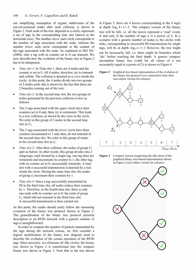
our simplifying assumption of regular subdivision of the not-yet-censused nodes after each collision, is shown in Figure 2. Each node of the tree, depicted as a circle, represents a set of tags in the corresponding time slot (shown in the horizontal axis). The number above each circle corresponds to the number of tags associated with the node, whereas the number below each circle corresponds to the counter of the tags associated with the node. As explained in ISO IEC (2004), only a tag with its counter set to 0 can transmit. We now describe how the evolution of the binary tree in Figure 2 has to be interpreted.

• Time slot 1: In Time slot 1, there are 4 nodes and the counter is set to 0. All 4 nodes, therefore, try to transmit and collide. The collision is denoted as a cross inside the circle. At this point, the 4 nodes divide into two groups of 2 nodes each: this is shown by the fact that there are 2 branches coming out of the root.

• Time slot 2: In the second time slot, the two groups of nodes generated by the previous collision evolve as follows.

• The 2 tags associated with the upper circle have their counters set to 0 and, then, try to retransmit. This leads to a new collision, as shown by the cross in the circle. We refer to this group of 2 nodes in the second time slot as C2.

• The 2 tags associated with the lower circle have their counters incremented to 1 and, then, do not transmit in the second time slot. We refer to this group of nodes in the second time slot as I2.

• Time slot 3: After their collision, the nodes of group C2 split as before. In other words, this group divides into 2 subgroups, each formed by a single tag: one tag does not retransmit and increments its counter to 1; the other tag, with its counter set to 0, successfully transmits. A time slot with a successful transmission is denoted by a tick inside the circle. During the same time slot, the nodes of group I2 increment their counters by 1.

• Time slot 4: Since a tag successfully transmitted its ID in the third time slot, all nodes reduce their counters by 1. Therefore, in the fourth time slot, there is only one node with its counter set to 0: the node of group C2 which did not transmit in the third time slot. A successful transmission is then carried out.

At this point, the reader should easily follow the remaining evolution of the binary tree protocol shown in Figure 2. The generalisation of the binary tree protocol pictorial description to an RFID network with a generic number of tags is straightforward.

In order to compute the number of packets transmitted by the tags during the network census, we first consider a logical modification of the binary tree diagram used to describe the evolution of the census operation of the RFID tags. More precisely, we eliminate all idle circles: the binary tree shown in Figure 2 is transformed into the compact binary tree shown in Figure 3. Note that in the tree shown

in Figure 3, there are 4 leaves (corresponding to the 4 tags) at depth 2log 4 1 3.+ = The compact version of the binary tree will be full, i.e. all the leaves represent a ‘read’ event, if and only if the number of tags n is a power of 2. In a scenario with a generic number of nodes n, the circles with ticks, corresponding to successful ID transmissions by single tags, will be at depth 2log 1.n + 1 However, the tree might not be necessarily full, i.e. there might be branches which ‘die’ before reaching the final depth. A generic compact incomplete binary tree (valid for all values of n not necessarily equal to a power of 2) is shown in Figure 4.

Figure 2 Graphical tree-based representation of the evolution of the binary tree protocol over consecutive time slots (see online version for colours)

Figure 3 Compact version (neglecting the idle slots) of the graphical binary tree-based representation shown in Figure 2 (see online version for colours)

A simple performance analysis of RFID networks 199

Figure 4 Compact version of a binary tree protocol in a scenario where n is not equal to a power of 2 (see online version for colours)

Suppose that there are n tags and consider the compact version of the binary tree describing the evolution of the census operation. For the sake of analytical simplicity, we assume that n is a power of 2, i.e. 2 ,kn k N= , ∈ but we will also comment on how the obtained results should be modified for values of n which are not powers of 2. In a scenario with a full compact binary tree, all the nodes at each intermediate level of the tree (i.e. at depth lower than

2log 1n + ) correspond to the transmission of a packet for all n tags. Therefore, the total number of transmitted packets is

2lo g

20

[ ] ( lo g 1).n

iP n n n n

=

= = +∑ (1)

For sufficiently large number of tags, equation (1) can be approximated as

2[ ] log .P n n n

In a generic scenario where n is not a power of 2, the compact binary tree is incomplete. In this case, the number of transmitted packets can be bounded as follows:

( )( )( )

2

2

log2

log2

[ ] 2 log 1

[ ] 2 1 log 2 .

n

n

P n n

P n n

⎢ ⎥⎣ ⎦

⎢ ⎥⎣ ⎦

> +⎢ ⎥⎣ ⎦

< + +⎢ ⎥⎣ ⎦

Obviously, for sufficiently large values of n , one can conclude that

( ) ( )( )2 2log log2 22 log 1 2 1 log 2n nn n⎢ ⎥ ⎢ ⎥⎣ ⎦ ⎣ ⎦+ + +⎢ ⎥ ⎢ ⎥⎣ ⎦ ⎣ ⎦

and, therefore, 2log

2[ ] 2 log .nP n n⎢ ⎥⎣ ⎦ ⎢ ⎥⎣ ⎦

Since for large values of n, 2log

2 22 log logn n n n⎢ ⎥⎣ ⎦ ⎢ ⎥⎣ ⎦

it follows that the higher the number of tags, the more accurate is the analysis carried out assuming that n is exactly a power of 2. Therefore, in the following we will limit ourselves to the case of a full binary tree, i.e. 2 .kn = From equation (1), it follows that the average number of packets sent by a single tag during the census is

node2 2

[ ][ ] log 1 logP nP n n nn

= = +

where the last approximation holds for sufficiently large values of n.

Network throughput can be defined as the ratio between the number of successfully transmitted packets (equal, obviously, to the number of tags) and the total number of packets sent by the tags during the census:

2 2

1 1[ ] .[ ] log 1 lognS n

P n n n=

+

The throughput per node can be written as

node

2 2

[ ] 1 1 1[ ] .[ ] (log 1) log

S nS nn P n n n n n

= =+

3.2 Census delay

At this point, we extend the previous analysis in order to compute the delay necessary to take a census of the entire RFID network tag population. The main difference with respect to the previous analysis is that in this case idle time slots, i.e. time slots where no tag transmits, have to be taken into account. To this end, we assume that after a collision, when the colliding tags have split into two subgroups (one subgroup with half of the initial number of nodes will not transmit, since they increase their counters), there is a sequence of idle time slots where no tag, among the subgroup of tags with their counters set to 0, is transmitting. With reference to the example with 4 tags considered before, the binary tree shown in Figure 2 modifies to that shown in Figure 5. Note that as opposed to throughput evaluation, in this case the binary tree in Figure 2 cannot be compacted as in Figure 3, since the entire evolution, including the idle time slots, is essential to perform a correct delay analysis.

The key point for the delay evaluation is then the computation of the number of idle time slots which follow a collision. In order to make an average analysis, we simply assume that the number of idle time slots is the average value associated with the number of tags of the subgroup of tags which do not increment their counters. Let us denote this number of tags by nc – note that the number of tags associated with the immediately previous collision (denoted as a circle with a cross in the binary tree) is 2nc. The probability that the next time slot is idle can be expressed as

cc1(idle time slot tags) .

2np n| =

200 G. Ferrari, F. Cappelletti and R. Raheli

Therefore, denoting by I the number of consecutive idle time slots, the average number of idle time slots after a collision among cn tags can be computed as follows:

c

c cc 20

1 2[ ] .2 (1 2 )

i n

n ni

I n i−∞

−=

⎛ ⎞= =⎜ ⎟ −⎝ ⎠∑ (2)

We remark that the considered approach for the computation of the average number of idle time slots after a collision is approximated. In fact, we are implicitly assuming that after an idle time slot the same number cn of nodes will have their counters set to 0. However, in the ISO 18000 standard Type B, after an idle time slot all tags decrease their counters

(ISO IEC, 2004). Therefore, it might happen that after an idle time slot more than the initial cn tags have their counters set to 0 and, therefore, might transmit. Our assumption of keeping the value of cn constant is valid for sufficiently large values of cn , since the probability of more than one idle time slot is very low – from equation (2), one can easily conclude that c[ ]I n is a decreasing function of c .n As will be shown in Section 5, the delay predicted by our simple analysis is in good agreement with the delay predicted through simulations and with recent results appeared in the literature.

Figure 5 Binary tree protocol, with idle time slots, for the computation of the delay (see online version for colours)

The normalised total census delay (in terms of time slots), denoted as [ ],T n can be expressed as follows:2

[ ] [ ] [ ]T n n C n I n= + +

where n is the number of time slots where single tags correctly transmit their IDs (i.e. n is the number of tags),

[ ]C n is the number of time slots with collisions and [ ]I n is the number of idle time slots. We first evaluate the number of time slots with collisions. This can easily be done considering the compact binary tree used in the previous subsection for the computation of the network throughput (see Figure 3). In fact, under the assumption that n is a power of 2, the number of time slots with collisions is equal to the number of intermediate nodes in the compact binary tree:

2log 1

0

[ ] 2 .n

i

i

C n n−

=

= =∑

The number of idle time slots [ ]I n can be computed extending the approach used above for evaluating [ ].C n In fact, considering the compact binary tree used for throughput evaluation, each collision node at a generic depth

21 log 1k … n= , , − ( 0k = corresponds to the tree root) in the binary tree is such that 2kn/ nodes collide. Therefore, before each of these collisions, there will be an average number of time slots equal to [ 2 ]kI n/ (see Figure 5). Since the number of collision nodes at depth k in the compact binary tree is 2 ,k the total number of idle time slots can be expressed as

2 2 2log log

221 1

idle[ ]

2[ ] 2 [ 2 ] 2 .

1 2

k

k

nn nk k k

nk k

k

I n I n⎛ ⎞⎜ ⎟⎜ ⎟⎜ ⎟⎝ ⎠

− /

− /= =

= / =−

∑ ∑ (3)

Therefore, the total delay [ ]T n can be written as follows:

2log 2

221

2[ ] 2 2 .1 2

k

k

n nk

nkT n n

⎛ ⎞⎜ ⎟⎜ ⎟⎜ ⎟⎝ ⎠

− /

− /=

= +−

∑ (4)

In order to simplify equation (4), one can derive upper and lower bounds on [ ].I n Observing that c[ ]I n is a decreasing function of c ,n one can conclude that the generic term idle[ ]k in the summation at the right-hand side of equation (3) is an increasing function of k. In particular, the following lower and upper bounds for idle[ ]k in equation (3) can be obtained:

2

2

1

2

2

2idle[ ] idle[1]1 2

idle[ ] idle[log ] 2 .

n

nk

k n n

−

⎛ ⎞−⎜ ⎟⎜ ⎟⎝ ⎠

≥ =−

≤ =

From these bounds, it is possible to find the following lower and upper bounds for the number of idle time slots:

2

2

1

22

2[ ] log

1 2

n

nI n n

−

−⎛ ⎞⎜ ⎟⎜ ⎟⎝ ⎠

≥−

(5)

A simple performance analysis of RFID networks 201

2[ ] 2 log .I n n n≤ (6)

Using equations (5) and (6) for the number of idle time slots, the total number of time slots [ ]T n in equation (4) can be bounded as follows:

12

12

1

2 LB2

2 2 UB

2[ ] 2 log 2 [ ]1 2

[ ] 2 [log 1] 2 log [ ].

T n n n n T n

T n n n n n T n

−

⎛ ⎞−⎜ ⎟⎜ ⎟⎝ ⎠

≥ +−

≤ +

4 Simulator structure

In order to evaluate the performance of RFID networks, it is important to have a versatile simulation tool, able to characterise several aspects of these networks. A network simulator must be reliable and model accurately the reality. We now derive a novel simulator, based on the use of OPNET 11.0 (Opnet Technologies, 2006), which is relatively simple, yet very powerful. OPNET offers a hierarchical approach to network planning, which allows to describe several scenarios. In particular, the utiliser can draw the topology of the network and set all relevant network parameters. Each node of the network can be designed at three different depths of accuracy: (1) network topology, (2) node and (3) process. We now summarise the main characteristics of our RFID network simulator at these three levels of descriptions.

4.1 Network topology level

At the network topology level, one can simply place the nodes according to the network topology which is needed. An example of RFID network topology is shown in Figure 6, with 15 tags randomly distributed over a rectangular surface and 1 reader. In most of the following simulation results, unless stated otherwise, the simulation results will be obtained by averaging over a sufficiently large number of randomly generated network topologies.

Figure 6 An example of RFID network topology (see online version for colours)

4.2 Node level At the node level, one can define the basic functions to be performed by the node as a series of black boxes connected together: each box manages a portion of the overall function. The link between two boxes can be either a physical link, traversed by data information, or a logical link, traversed only by control information. The node models for a tag and the interrogator are shown in Figure 7(a) and 7(b), respectively.

• The tag node model in Figure 7(a) is composed by (1) a ‘tag’ box, which performs the operations carried out at the tag, (2) a ‘receiver’ (RX) box, which is devoted to the operations regarding the reception of the packets sent by the interrogator, (3) a ‘transmitter’ (TX) box, which implements the transmission side of the tag and (iv) an ‘antenna’ box, where the physical description of the antenna used by the tag is considered.

• The interrogator node model in Figure 7(b) is composed by a (1) ‘packet generator’ box, which generates packets according to a uniform distribution with mean equal to 1 s, (2) a ‘code’ box, which processes the packets coming from the generator and those coming from the channel (i.e. from the tags), (3) a ‘receiver’ box, (4) a ‘transmitter’ box and (5) an ‘antenna’ box (the last three boxes are similar to those in the tag node model). As one can imagine, the key block of the interrogator is the ‘code’ box, where the intelligence is concentrated. In particular, the binary tree collision arbitration protocol is implemented inside this block.

Figure 7 Node models: (a) tag and (b) interrogator (or reader)

4.3 Process level

The black boxes used at the node level can be predefined or (as in our case) created for the specific simulation scenario at hand. In order to create new black boxes, one must resort to the second level of depth, i.e. to the process

202 G. Ferrari, F. Cappelletti and R. Raheli

level. At this level, the black box is modelled as a Finite State Machine (FSM), whose evolution is determined by discrete events. Each discrete event triggers the evolution of the FSM from one state to another. In our RFID network simulator, the discrete events are packet transmissions or collisions. The FSM states are divided between forced and unforced states. When the FSM evolves into a forced state, it executes the operations associated with that state and, immediately afterwards, evolves to a new state. Vice versa, when the FSM evolves into an unforced state, it executes the operations associated with it and waits for a new event in order to exit from the unforced state. Finally, the states of the FSM node model can be characterised accurately. In fact, each state can be assigned a set of instructions to be executed every time the FSM evolves into this state.

• The FSM model of the tag, shown in Figure 8(a), is associated with the processor block ‘tag’ in Figure 7(a). The tag FSM is relatively simple, since the tag is batteryless and, therefore, its signal processing capabilities are limited. There are only two states: a forced state (INIT) and an unforced state (Idle). The tag must have on-board only an 8-bit counter and a random number generator. Every time the tag is illuminated by the interrogator, it must detect the associated command and execute the corresponding operation. If a failed command is detected, the tag generates a random number, from which a binary decision is taken. If the decision is ‘0’ and its counter is 0, then it transmits its ID information; otherwise, it increases its counter by 1.

• The interrogator FSM is shown in Figure 8(b). It is composed of four states: three forced states (INIT, Collision and Idle) and one unforced state (start). When a round starts, the FSM evolves from the INIT state into the start state. When the FSM is the INIT state, the counter and the system variables are reset, and the statistics are initialised. In the start state, the interrogator waits for an input, i.e. a packet generation. Every time a packet is generated, the interrogator checks what kind of packet has been received: if the packet comes from the channel (PCK_ARR_TAG), the collision check is initiated (collision state); if the packet is good, i.e. no collision has occurred, a success message and a read message are sent to that tag, and the read message forces the tag to move into the ‘data exchange’ state (see Figure 1). Otherwise, a failed message is sent to all tags. A time counter is reset every time a packet is sent, and if no packet arrives after a time-off period (TIME_OUT), a success message is sent and the tag moves to the ‘Idle’ state. The round finishes when all tags are detected and the simulation terminates.

4.4 Other simulator settings

In order to completely characterise the simulator scenario, it is important to define the structure of the packets that will be sent by the interrogator and the tags. The packet structures,

for both tag and interrogator, considered in the rest of this paper, are shown in Figure 9. These packet structures are similar to those described in the ISO 18000 standard (ISO IEC, 2004). However, we do not consider the CRC-16 field, associated with the error detection code. This simplifies the simulation, since a packet is either received perfectly or not received.

Figure 8 FSM models: (a) node and (b) interrogator (see online version for colours)

Figure 9 Packet fields for (a) tag packet and (b) interrogator packet

The propagation scenario is simply characterised as a free space loss propagation environment (Rappaport, 2002). In this case, the received power Pr is related to the transmit power Pt through the following relation (assuming no loss other than that due to propagation):

A simple performance analysis of RFID networks 203

t rr t

l

g gP P

f= ⋅

where tg and rg are the transmitter and receiver antenna gains, and the parameter lf is defined as

2c

l4 f d

fc

π⎛ ⎞⎜ ⎟⎝ ⎠

where cf is the carrier frequency, d is the distance between transmitter and receiver and c is the speed of light. The carrier frequency used in our simulations is fc = 869.25 MHz.

In order to take into account the presence of multipath, we also consider the presence of Ricean fading (Rappaport, 2002). In particular, the Rice fading model used in our simulator is proposed in Punnoose et al. (2000) and also available on the OPNET website (Opnet Technologies, 2006). More precisely, in Punnoose et al. (2000), the authors propose a simulation model to characterise the effects of small-scale fading. Small-scale fading is caused by movements of the transmitter and/or receiver, and/or also by the movement of objects in the nearby environment – the latter movement can be characterised in terms of Doppler spreading. In Punnoose et al. (2000), the Doppler power spectral density is modelled according to the approach proposed in Clarke (1968) and Gans (1972).

In most of the packet simulators, the fading is generated as a random process with the appropriate statistics. However, the time correlation between consecutive fading realisations, required to simulate accurately burst errors, is often overlooked. In order to simulate the time correlation, we resort to a simple method based on a lookup table, where the discretised version of the fading envelope is stored. This lookup table is used to take into account several parameters describing the fading process, among which are the Ricean K factor and the maximum Doppler frequency. Another important parameter used in our network model is the power threshold at the tags, defined as the minimum received power required by a tag to turn on. We show that the census time is strictly related to this parameter, which, in reality, depends on the electronic technology used to develop the tag’s microchip. In our simulations, we consider various values of this threshold, which is an adimensional gain with reference transmit power Pt = 0.5 W from the reader. For instance, a power threshold equal to – 30 dB corresponds to a minimum required received power equal to 0.5 mW, whereas a threshold equal to –40 dB corresponds to a minimum required received power equal to 0.05 mW.

5 Performance evaluation

In this section, we evaluate the RFID network performance using the analytical framework proposed in Section 3 and the simulator described in Section 4. In the simulation

results presented in Figures 10–13, the power threshold at the tags is assumed to be very low (lower than –40 dB). In this case, the fading has no influence on the network performance, since the power received at the tags, even though fluctuating, is always sufficient to turn the tags on. At the end of this section, we will investigate the impact of fading in scenarios where the power threshold is not sufficiently low.

In Figure 10, the average number of packets transmitted by a single tag during a census is shown as function of the number n of tags. As one can see, the trends of simulation and analytical results are quite similar. In particular, the average number of packets predicted by the analysis, i.e. Pnode[n] = log2n, is lower than the (realistic) value predicted by the simulation. As mentioned in Subsection 3.1, the analysis underestimates the number of transmitted packets, since no unbalancing of the binary tree is considered. In a realistic scenario, however, the presence of collisions where nodes split in significantly different subgroups leads to a higher number of collisions in the following time slots, and, therefore, to a higher number of unsuccessful packet transmissions. From the results in Figure 10, one can conclude, however, that the average number of transmitted packets per node is Θ(log2n), where the notation Θ(·) is used, in the realm of algorithms, to describe the asymptotic functional relationship between functions of time (Cormen et al., 2002). More precisely, the notation f(n) = Θ(g(n)) means that there exists an n0 such that for n ≥ n0, ∃c1 ∈(0, 1), c2 > 1 such that c1g(n) ≤ f(n) ≤ c2g(n).

In Figure 11, the network throughput and the throughput per node are shown as functions of the number of tags n. As one can see, there is good agreement between simulation and analytical results. In particular, the network throughput is Θ(1/log2n). One can conclude that the throughput decreases ‘slowly’ to zero. This confirms the fact that the binary tree protocol is a robust census protocol, in the sense that for increasing number of tags the throughput decreases much less than inverse linearly.

Figure 10 Average number of packet per tag during a census process as a function of the total number n of tags in the network (see online version for colours)

204 G. Ferrari, F. Cappelletti and R. Raheli

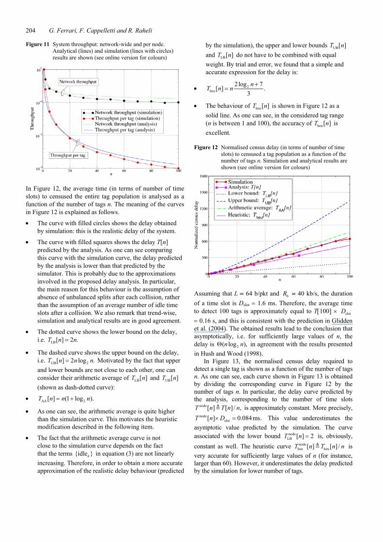
Figure 11 System throughput: network-wide and per node. Analytical (lines) and simulation (lines with circles) results are shown (see online version for colours)

In Figure 12, the average time (in terms of number of time slots) to censused the entire tag population is analysed as a function of the number of tags n. The meaning of the curves in Figure 12 is explained as follows.

• The curve with filled circles shows the delay obtained by simulation: this is the realistic delay of the system.

• The curve with filled squares shows the delay T[n] predicted by the analysis. As one can see comparing this curve with the simulation curve, the delay predicted by the analysis is lower than that predicted by the simulator. This is probably due to the approximations involved in the proposed delay analysis. In particular, the main reason for this behaviour is the assumption of absence of unbalanced splits after each collision, rather than the assumption of an average number of idle time slots after a collision. We also remark that trend-wise, simulation and analytical results are in good agreement.

• The dotted curve shows the lower bound on the delay, i.e. LB[ ] 2 .T n n=

• The dashed curve shows the upper bound on the delay, i.e. UB 2[ ] 2 log .T n n n= Motivated by the fact that upper and lower bounds are not close to each other, one can consider their arithmetic average of LB[ ]T n and UB[ ]T n (shown as dash-dotted curve):

• AA 2[ ] (1 log ).T n n n= +

• As one can see, the arithmetic average is quite higher than the simulation curve. This motivates the heuristic modification described in the following item.

• The fact that the arithmetic average curve is not close to the simulation curve depends on the fact that the terms {idle }k in equation (3) are not linearly increasing. Therefore, in order to obtain a more accurate approximation of the realistic delay behaviour (predicted

by the simulation), the upper and lower bounds UB[ ]T n and LB[ ]T n do not have to be combined with equal weight. By trial and error, we found that a simple and accurate expression for the delay is:

• 2heu

2 log 7[ ] .

3n

T n n+

=

• The behaviour of heu [ ]T n is shown in Figure 12 as a solid line. As one can see, in the considered tag range (n is between 1 and 100), the accuracy of heu [ ]T n is excellent.

Figure 12 Normalised census delay (in terms of number of time slots) to censused a tag population as a function of the number of tags n. Simulation and analytical results are shown (see online version for colours)

Assuming that L = 64 b/pkt and bR = 40 kb/s, the duration of a time slot is Dslot = 1.6 ms. Therefore, the average time to detect 100 tags is approximately equal to T[100] × slotD = 0.16 s, and this is consistent with the prediction in Glidden et al. (2004). The obtained results lead to the conclusion that asymptotically, i.e. for sufficiently large values of n, the delay is 2( log ),n nΘ in agreement with the results presented in Hush and Wood (1998).

In Figure 13, the normalised census delay required to detect a single tag is shown as a function of the number of tags n. As one can see, each curve shown in Figure 13 is obtained by dividing the corresponding curve in Figure 12 by the number of tags n. In particular, the delay curve predicted by the analysis, corresponding to the number of time slots

node[ ] [ ] / ,T n T n n is approximately constant. More precisely, node

slot[ ] 0.084ms.T n D× This value underestimates the asymptotic value predicted by the simulation. The curve associated with the lower bound node

LB [ ] 2T n = is, obviously, constant as well. The heuristic curve node

heu heu[ ] [ ] /T n T n n is very accurate for sufficiently large values of n (for instance, larger than 60). However, it underestimates the delay predicted by the simulation for lower number of tags.

A simple performance analysis of RFID networks 205

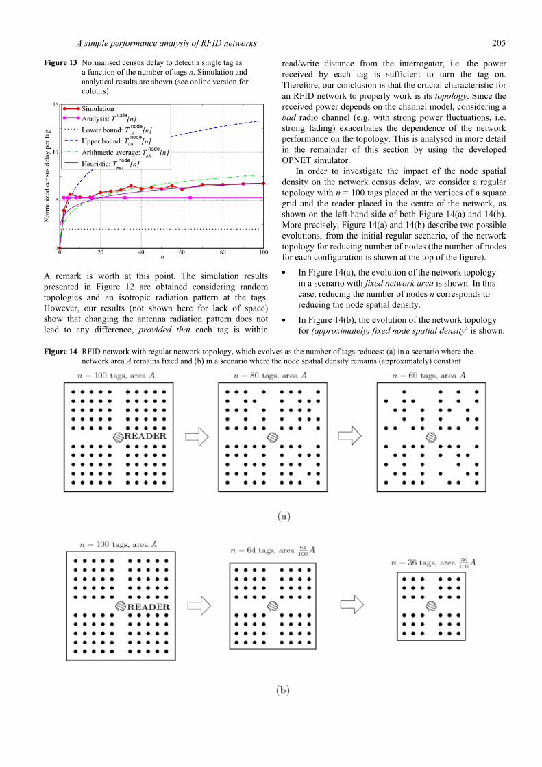
Figure 13 Normalised census delay to detect a single tag as a function of the number of tags n. Simulation and analytical results are shown (see online version for colours)

A remark is worth at this point. The simulation results presented in Figure 12 are obtained considering random topologies and an isotropic radiation pattern at the tags. However, our results (not shown here for lack of space) show that changing the antenna radiation pattern does not lead to any difference, provided that each tag is within

read/write distance from the interrogator, i.e. the power received by each tag is sufficient to turn the tag on. Therefore, our conclusion is that the crucial characteristic for an RFID network to properly work is its topology. Since the received power depends on the channel model, considering a bad radio channel (e.g. with strong power fluctuations, i.e. strong fading) exacerbates the dependence of the network performance on the topology. This is analysed in more detail in the remainder of this section by using the developed OPNET simulator.

In order to investigate the impact of the node spatial density on the network census delay, we consider a regular topology with n = 100 tags placed at the vertices of a square grid and the reader placed in the centre of the network, as shown on the left-hand side of both Figure 14(a) and 14(b). More precisely, Figure 14(a) and 14(b) describe two possible evolutions, from the initial regular scenario, of the network topology for reducing number of nodes (the number of nodes for each configuration is shown at the top of the figure).

• In Figure 14(a), the evolution of the network topology in a scenario with fixed network area is shown. In this case, reducing the number of nodes n corresponds to reducing the node spatial density.

• In Figure 14(b), the evolution of the network topology for (approximately) fixed node spatial density3 is shown.

Figure 14 RFID network with regular network topology, which evolves as the number of tags reduces: (a) in a scenario where the network area A remains fixed and (b) in a scenario where the node spatial density remains (approximately) constant

206 G. Ferrari, F. Cappelletti and R. Raheli

In the following, we analyse the network census delay, as a function of the number of nodes n, in the two scenarios described above. As it will be shown, these two topology evolution scenarios lead to very different behaviours in terms of network census delay.

We first consider the evolution of the network when the area remains fixed, i.e. as described in Figure 14(a). In particular, the area is set to A = 4 m2. In Figure 15, the network census delay (computed with the simulator) is shown as a function of the number of nodes n, which ranges from 10 to 100, for various values of the power threshold at the tags. The communication channel between each tag and the reader is affected by Rice fading with K = 10 dB. The transmission data rate and the packet length are set as before (Rb = 40 kb/s and L = 64 b/pkt), and the duration of a time slot is Dslot = 1.6 ms. As one can see, the power threshold at the tags has a strong bearing on the census delay. More precisely, two different cases are shown in Figure 15.

• If the power threshold is very low (–40 dB), then the network census delay increases as Θ (n log2n), as previously observed in a scenario where fading had no effect. In other words, if the power threshold is sufficiently low, the fluctuations caused by fading are negligible and even the farthest tags (with respect to the reader) are regularly turned on when illuminated.

• If the power threshold is very high (–30 dB), then the network census delay increases significantly for values of n between 10 and 20, and then it almost remains constant. This regime value is much higher than in the case with very low power threshold. This behaviour can be explained as follows. When the number of nodes is low (n = 10), all nodes are likely to be relatively close to the reader. Therefore, fading has no effect on the tags. However, as the number of nodes increases, it is very likely that some of them will be relatively far from the reader and fading significantly affects these nodes. Therefore, even if only a single node is far, this has a large impact on the overall census delay, since the reader might need several census rounds to detect this single tag. The network census delay then remains stable, since other nodes (closer to the reader) have a limited impact. This behaviour can be given an alternative explanation. If the received power is around the critical threshold, the presence of fading generates instability in the network: there could be intervals during which the tags are not turned on and, therefore, time is wasted since no tag tries to transmit; suddenly, several tags could be on, causing a large number of collisions.

Note that the fact that the critical threshold value is between –30 and –40 dB depends on the specific network area A. More precisely, while a critical power threshold at the tags exist in any scenario with fading, the specific value of this threshold depends on the network topology and, more precisely, on the distance of the farthest tags.

Finally, we turn our attention to a scenario where the network evolves with (approximately) fixed tag spatial density, i.e. as described in Figure 14(b). In Figure 16, the network census delay is shown as a function of the number of nodes n, which ranges from 10 to 100, for various values of the power threshold at the tags. Comparing the results shown in Figure 16 with those in Figure 15, the following comments can be made.

Figure 15 The network census delay is shown as a function of the number of nodes, for various values of the power threshold at the tags. The network area is kept fixed (A = 4 m2) and communication between tags and reader is power affected by Rice fading with K = 10 dB. The results are obtained through simulations (see online version for colours)

Figure 16 Network census delay is shown as a function of the number of nodes, for various values of the power threshold at the tags. The tag spatial density is kept fixed (approximately equal to n/A = 100/4 = 25 tags/m2) and communication between tags and reader is power affected by Rice fading with K = 10 dB (see online version for colours)

• For a number of nodes lower than or equal to 80, the network census delay is not affected by the power threshold. This is due to the fact that if the number of tags is sufficiently low, then all tags are relatively close to the reader and, therefore, the received power is sufficiently high that fading has a negligible impact on the performance.

A simple performance analysis of RFID networks 207

• When the number of tags increases beyond 80, then the ‘new’ tags are those placed on the edges, i.e. the farthest from the reader. The identification time required by these tags depends heavily on the power threshold, because of the presence of fading. For low values of the power threshold (–40 dB), the network census delay behaves as in Figure 15. On the other hand, if the power threshold is high (–30 dB), then the network census delay increases dramatically.

6 Conclusions

In this paper, we have developed a novel and simplified analytical approach for evaluating the throughput and delay of RFID networks based on the binary tree multi-access protocol, such as those compliant with the ISO/IEC 18000 RFID standard. In order to validate our simple analytical framework, we have developed a simulator and we have shown that the performance predicted by the analysis is in good agreement with the realistic simulation performance. This underlines the validity of our analytical framework for the design of RFID networks. Moreover, through the simulator, we have evaluated the impact of fading and network topology (in terms of tag spatial density) on the network performance. One of the key results consists of the fact that if the power threshold at the tags is not sufficiently low, then the presence of fading might significantly increase the census delay. Since the power threshold is technology-dependent, our findings suggest that a careful study of the network topology is fundamental to guarantee a good performance.

References Abraham, C., Ahuja, V., Ghosh, A.K. and Pakanati, P. (2004)

Inventory Management Using Passive RFID Tags: A Survey, Technical report, Department of Computer Science, The University of Texas at Dallas, Richardson, TX, USA (white paper).

Auto ID Center (2003) 860 MHz 930 MHz Class 0 Radio Frequency Identification Tag Protocol Specification Candidate Recommendation, Technical report, MIT. v. 1.0.0. Available online at: http://www.epcglobalinc.org/standards_ technologies/secure/v.1.0/UHF class0.pdf

Bertsekas, D. and Gallager, R. (1992) Data Networks, 2nd ed., Prentice-Hall, Upper Saddle River, NJ.

Capetenakis, J. (1979) ‘Tree algorithms for packet broadcast channels’, IEEE Transactions on Information Theory, Vol. 25, No. 5, pp.505–515.

Clarke, R.H. (1968) ‘A statistical theory of mobile radio reception’, Bell System Technical Journal, Vol. 47, pp.957–1000.

Cormen, T.H., Leiserson, C.E., Rivest, R.L. and Stein, C. (2002) Introduction to Algorithms, 2nd ed., MIT Press, Cambridge, MA.

EPC Global (2005) EPC Radio-Frequency Identity Protocols Class-1 Generation 2 UHF RFID. Available online at: http://www.epcglobal.com

Finkenzeller, K. (2003) RFID Handbook: Fundamentals and Applications in Contactless Smart Cards and Identification, 2nd ed., John Wiley & Sons, New York.

Gans, M.J. (1972) ‘A power spectral theory of propagation in the mobile radio environment’, IEEE Transactions on Vehicular Technology, Vol. 21, No. 1, pp.27–38.

Glidden, R., Bockorick, C., Cooper, S., Diorio, C., Dressler, D., Gutnik, V., Hagen, C., Hara, D., Hass, T., Humes, T., Hyde, J., Oliver, R., Onen, O., Pesavento, A., Sundstrom, K. and Thomas, M. (2004) ‘Design of ultra-low-cost UHF RFID tags for supply chain applications’, IEEE Communications Magazine, Vol. 42, No. 8, pp.140–151.

Hush, D.R. and Wood, C. (1998) ‘Analysis of tree algorithms for RFID arbitration’, In Proceedings of IEEE Symposium on Information Theory (ISIT), Cambridge, MA, USA, p.107.

ISO IEC (2004) ISO IEC 18000-6: Parameters for air interface communications at 860 MHz to 960 MHz. Available upon subscription.

Myung, J. and Lee, W. (2005) ‘An adaptive memory-less tag anti-collision protocol for RFID networks’, In Proceedings of IEEE Conference on Computer Communications (INFOCOM), Miami, FL , USA (Poster session).

Myung, J. and Lee, W. (2006) ‘Adaptive splitting protocols for RFID tag collision arbitration’, In Proceedings of the ACM International Symposium on Mobile Ad Hoc Networking and Computing (MOBIHOC), Florence, Italy, pp.202–213.

Myung, J., Lee, W. and Shih, T. K. (2006a) ‘An adaptive memoryless protocol for RFID tag collision arbitration’, IEEE Transactions on Multimedia, Vol. 8, No. 5, pp.1096–1101.

Myung, J., Lee, W. and Srivastava, J. (2006b) ‘Adaptive binary splitting for efficient RFID tag anti-collision’, IEEE Communications Letters, Vol. 10, No. 3, pp.144–146.

Opnet Technologies (2006) OPNET 11.0. Available online at: http://www.opnet.com

Punnoose, R.J., Nikitin, P.V. and Stancil, D.D. (2000) ‘Efficient simulation of Ricean fading within a packet simulator’, In Proceedings of IEEE Vehicular Technology Conference (VTC), Boston, MA, pp.764–767.

Ramakrishnan, K.M. and Deavours, D.D. (2006) ‘Performance benchmarks for passive UHF RFID tags’, In Proceedings of the 13th GI/ITG Conference on Measurement, Modeling, and Evaluation of Computer and Communication Systems, Nurenberg, Germany.

Rappaport, T.S. (2002) Wireless Communications. Principles & Practice, 2nd ed., Prentice-Hall, Upper Saddle River, NJ.

Siden, J., Jonsson, P., Olsson, T. and Wang, G. (2001) ‘Performance degradation of RFID system due to the distortion in RFID tag antenna’, Proceedings of International Conference Microwave & Telecommunication Technology (CriMiCo), Sevastopol, Crimea, Ukraine, pp.371–373.

Simplot-Ryl, D., Stojmenovic, I., Micic, A. and Nayak, A. (2006) ‘A hybrid randomized protocol for RFID tag identification’, Sensor Review, Vol. 26, No. 2, pp.147–154.

Wu, C-S. and Li, V.O.K. (1991) ‘Delay analysis of tree conflict resolution algorithm with and without broadcast reservation using random or pseudo random addressing’, In Proceedings of IEEE International Conference on Communications (ICC), Denver, CO.

Zhou, F., Chen, C., Jin, D., Huang, C. and Min, H. (2004) ‘Evaluating and optimizing power consumption of anti-collision protocols for applications in RFID systems’, Proceedings of ACM International Symposium on Low Power Electronics and Design (ISLPED), Newport Beach, CA, pp.357–362.

208 G. Ferrari, F. Cappelletti and R. Raheli

Zhou, X. and Wang, G. (2004) ‘Study on the influence of curving of tag antennas on performance of RFID system’, Proceedings of International Conference on Microwave and Millimeter Wave Technology, Newport Beach, CA, pp.122–125.

Notes 1 We remark that this will not necessarily be the case in a

scenario with unbalanced tree decomposition. However, as mentioned above, in this paper we are considering scenarios with perfectly balanced tree decomposition.

2 Note that the normalised delay refers to the number of time slots. In order to derive the effective delay (in seconds), one should consider slot[ ] .T n D×

3 Note that in the evolution of the network topology in Figure 14(b) the node spatial density does not exactly remain fixed, since there are four clusters of tags and reducing the number of tags in each cluster leads to an overall node spatial density reduction. However, the node spatial density can be considered almost constant with respect to the network evolution described in Figure 14(a).