A Simple Fusion Method for Image Time Series Based on the ...
21
Remote Sens. 2015, 7, 704-724; doi:10.3390/rs70100704 remote sensing ISSN 2072-4292 www.mdpi.com/journal/remotesensing Article A Simple Fusion Method for Image Time Series Based on the Estimation of Image Temporal Validity Mar Bisquert 1,2, *, Gloria Bordogna 3 , Agnès Bégué 4 , Gabriele Candiani 3 , Maguelonne Teisseire 2 and Pascal Poncelet 1 1 Laboratoire d’Informatique, de Robotique et de Microélectronique de Montpellier, 161 Rue Ada, 34090 Montpellier, France; E-Mail: [email protected] 2 Institute de Recherche en Sciences et Technologies pour l’Environnement et l’Agriculture, Unité Mixte de Recherche Territoires, Environnement, Télédétection et Information Spatiale, 500 Rue Jean François Breton, 34093 Montpellier, France; E-Mail: [email protected] 3 Consiglio Nazionale delle Ricerhe, Istituto per il Rilevamento Elettromagnetico dell’Ambiente, Via Bassini 15, 20133 Milano, Italy; E-Mails: [email protected] (G.B.); [email protected] (G.C.) 4 Centre de Coopération Internationale en Recherche Agronomique pour le Développement, Unité Mixte de Recherche Territoires, Environnement, Télédétection et Information Spatiale, 500 Rue Jean François Breton, 34093 Montpellier, France; E-Mail: [email protected] * Author to whom correspondence should be addressed; E-Mail: [email protected]; Tel.: +34-926-264-007 (ext. 6039). Academic Editors: Clement Atzberger and Prasad S. Thenkabail Received: 29 August 2014 / Accepted: 5 January 2015 / Published: 12 January 2015 Abstract: High-spatial-resolution satellites usually have the constraint of a low temporal frequency, which leads to long periods without information in cloudy areas. Furthermore, low-spatial-resolution satellites have higher revisit cycles. Combining information from high- and low- spatial-resolution satellites is thought a key factor for studies that require dense time series of high-resolution images, e.g., crop monitoring. There are several fusion methods in the bibliography, but they are time-consuming and complicated to implement. Moreover, the local evaluation of the fused images is rarely analyzed. In this paper, we present a simple and fast fusion method based on a weighted average of two input images (H and L), which are weighted by their temporal validity to the image to be fused. The method was applied to two years (2009–2010) of Landsat and MODIS (MODerate Imaging Spectroradiometer) images that were acquired over a cropped area in Brazil. The fusion OPEN ACCESS
-
Upload
khangminh22 -
Category
Documents
-
view
1 -
download
0
Transcript of A Simple Fusion Method for Image Time Series Based on the ...
Remote Sens. 2015, 7, 704-724; doi:10.3390/rs70100704
remote sensing ISSN 2072-4292
www.mdpi.com/journal/remotesensing
Article
A Simple Fusion Method for Image Time Series Based on the Estimation of Image Temporal Validity
Mar Bisquert 1,2,*, Gloria Bordogna 3, Agnès Bégué 4, Gabriele Candiani 3, Maguelonne Teisseire 2
and Pascal Poncelet 1
1 Laboratoire d’Informatique, de Robotique et de Microélectronique de Montpellier, 161 Rue Ada,
34090 Montpellier, France; E-Mail: [email protected] 2 Institute de Recherche en Sciences et Technologies pour l’Environnement et l’Agriculture, Unité
Mixte de Recherche Territoires, Environnement, Télédétection et Information Spatiale, 500 Rue
Jean François Breton, 34093 Montpellier, France; E-Mail: [email protected] 3 Consiglio Nazionale delle Ricerhe, Istituto per il Rilevamento Elettromagnetico dell’Ambiente, Via
Bassini 15, 20133 Milano, Italy; E-Mails: [email protected] (G.B.);
[email protected] (G.C.) 4 Centre de Coopération Internationale en Recherche Agronomique pour le Développement, Unité
Mixte de Recherche Territoires, Environnement, Télédétection et Information Spatiale, 500 Rue
Jean François Breton, 34093 Montpellier, France; E-Mail: [email protected]
* Author to whom correspondence should be addressed; E-Mail: [email protected];
Tel.: +34-926-264-007 (ext. 6039).
Academic Editors: Clement Atzberger and Prasad S. Thenkabail
Received: 29 August 2014 / Accepted: 5 January 2015 / Published: 12 January 2015
Abstract: High-spatial-resolution satellites usually have the constraint of a low temporal
frequency, which leads to long periods without information in cloudy areas. Furthermore,
low-spatial-resolution satellites have higher revisit cycles. Combining information from
high- and low- spatial-resolution satellites is thought a key factor for studies that require
dense time series of high-resolution images, e.g., crop monitoring. There are several fusion
methods in the bibliography, but they are time-consuming and complicated to implement.
Moreover, the local evaluation of the fused images is rarely analyzed. In this paper, we
present a simple and fast fusion method based on a weighted average of two input images
(H and L), which are weighted by their temporal validity to the image to be fused. The
method was applied to two years (2009–2010) of Landsat and MODIS (MODerate Imaging
Spectroradiometer) images that were acquired over a cropped area in Brazil. The fusion
OPEN ACCESS
Remote Sens. 2015, 7 705
method was evaluated at global and local scales. The results show that the fused images
reproduced reliable crop temporal profiles and correctly delineated the boundaries between
two neighboring fields. The greatest advantages of the proposed method are the execution
time and ease of use, which allow us to obtain a fused image in less than five minutes.
Keywords: MODIS; Landsat; validation; remote sensing
1. Introduction
Time series of satellite images allow the extraction of vegetation phenology and are thought a key
factor in many studies, including vegetation monitoring (crops, forests, etc.) [1], biomass production
study [2] and land cover classification [3]. Monitoring agricultural activities is crucial for the assessment
of productivity and food supplies, and it requires information that highly varies in space and time [4].
Historically, the crop yield estimation was assessed by local experts and/or statistics. Currently, remote
sensing offers spatial information with high spatial and temporal coverage, and though it can be exploited
to provide decisive information in agricultural applications.
Natural vegetation and forests phenology is also required for mapping and studying forests
ecosystems, the effect of climate changes on forests and the effect of greenhouse gasses and carbon
sequestration [5–9]. The use of image time series is also highly valuable for land cover classification
purposes because it allows capturing information of the vegetation at different growth stages, which
leads to more accurate classifications than by using single images [1,3].
However, in each study case, different spatial resolution images may be required. For forest studies,
images with a low spatial resolution (250 m–1 km) may be suitable for obtaining the phenology. For
land cover classification and agricultural purposes, higher-spatial-resolution images are desired. In the
latter cases, the required spatial resolution depends on the heterogeneity and size of the agricultural
parcels in the study area. Generally, spatial resolutions of 10–250 m can be used for land cover
classification. Images with spatial resolution of 5–30 m may be more suitable for crop monitoring.
Nevertheless, times series of high-spatial-resolution (HR) images have a coarse temporal resolution,
whereas low-spatial-resolution (LR) satellites may offer daily information. For example, the MODIS
(MODerate Resolution Image Spectroradiometer) sensor offers daily images with a spatial resolution of
250 m–1 km (depending on the spectral band), whereas the Landsat satellite offers information at
30 m spatial resolution with a temporal frequency of 16 days. Moreover, the drawback of low temporal
frequency time series is much more evident in areas with important cloud coverage because the presence
of clouds can determine missing or inaccurate information for long time periods. Additionally, when
using HR image time series one may need to cope with missing data at specific dates (when an
observation is necessary), since an image might not to be acquired at the desired time, and with the high
economic costs, which are an important constraint, particularly when many images are required.
Fusion or blending methods of image time series allow simulating HR images in dates where only
LR images are available; thus, they can be a solution to cope with the above problems. These methods
are usually based on rules to combine the information of HR and LR images at different dates. Many
existing methods have been defined and applied for the combination of Landsat and MODIS images.
Remote Sens. 2015, 7 706
A widely used fusion method is the Spatial and Temporal Adaptive Reflectance Fusion Model
(STARFM) [10]. This method can be applied using one or two pairs of HR and LR images, and a
low-resolution image at the target date (the date of the image that we pretend to obtain). The STARFM
has been used to evaluate the gross primary productivity of crops in India by combining Landsat and
MODIS images to simulate 46 images in 2009 [11]. In [12], the STARFM was used to complete a time
series that allowed improving the classification of tillage/no tillage fields. In [13], it was used to construct
a Landsat image time series (2003–2008) to monitor changes in vegetation phenology in Australia.
A modification of the STARFM was developed by [14] and named the Enhanced Spatial and
Temporal Adaptive Reflectance Fusion Method (ESTARFM). The ESTARFM requires two pairs of HR
and LR images. In [15], the two algorithms (STARFM and ESTARFM) were compared at two different
sites. The authors concluded that the ESTARFM outperformed the STARFM in one site, and the
STARFM outperformed the ESTARFM in the other site. The main difference between the two sites is
the predominance of temporal or spatial variance: the ESTARFM is better for a site where spatial
variance is dominant, whereas the STARFM is preferred when temporal variance is dominant.
Fusion methods are usually validated using global statistics, such as the correlation between real
images acquired at the same dates when the fused images were simulated, Root Mean Square Error
(RMSE), Mean Absolute Deviation (MAD) and Average Absolute Difference (AAD). These statistic
parameters provide an indication of the global accuracy; however, the performance at the local scale
should also be analyzed.
The objective of this work was to refine and validate a fusion method introduced in [16], in order to
have a simple and fast image fusion method that only uses two input images and fuzzy operators.
“Simple” indicates that it does not require much input in terms of both data and parameters, and “fast”
indicates that it substantially reduces the computational time required to generate a fused image with
respect to concurrent methods by achieving at least comparable results to those methods, as described in
the validation analysis section. The method was tested in an agricultural area in Brazil, which was mainly
covered with Eucalyptus plantations, with MODIS and Landsat images. The method validation and
comparison to the ESTARFM were performed at global and local scales.
2. Theoretical Bases
The fusion method was developed based on several desired properties and conditions as defined in
our previous work [16]. In the present paper, we refine this method and evaluate its potentialities by
emphasizing the settings for its application. The desired condition was to develop a simple method that
requires only two input images, one high-resolution image (H) available at any unspecified date and one
low-resolution image (L) on the target date when we want to generate a fused high-resolution image
(H’). This method should be applied to pairs of satellite images (H and L) with similar spectral
configurations (i.e., same spectral bands, atmospheric corrections and viewing angles). In the case the
two images have a distinct spectral configuration, first one has to decide which one of the two images
has the configuration to be maintained in the fused image, and then one has to normalize the other image
before applying the fusion.
The desired property of the fusion method was to generate the fused image by considering an inverse
function of the temporal distances (hereafter called “validity”) between the input images and the target

Remote Sens. 2015, 7 707
date t. The rationale of using the time validity to weight the contribution of an input image to the fused
image is based on the assumption that vegetation covers are affected by gradual changes with time: the
closer the date of acquisition of the input image to the target date, the higher should be its “similarity”
to the image at the target date. Thus, we weight the input image contribution by an inverse function of
its time distance from the target date.
Figure 1 shows a schema of this idea, which includes the graphic representation of the validity
degrees (μ). We have two time series: one of high-resolution images (H) taken at dates tH and one of
low/coarse-resolution images (L), which are composite images of several days within a temporal range
[tLmin, tLmax] (tLmin and tLmax represent the first and last days of the compositing image). The unimodal
function of the temporal distances between the input images H and L is a triangular membership function
of a fuzzy set defined on the temporal domain of the time series; the central vertex is t and the other two
vertices t0 and tE are placed before and after t. Therefore, the validity of a timestamp tH is computed
as follows:
If t0 ≤ tH < t then t ⁄
If t ≤ tH < tE then ⁄ (1)
Figure 1. Representation of two time series of High- (H2, H4) and Low- (L1, L2, L3, L4)
resolution images with distinct timestamps (tH, t) and temporal density. The black bars
represent the membership degrees that define the time validities (µt(tH), µt(tLmin), µt(tLmax)) of
the images with respect to the target timestamp t. t0 and tE are determined from a user-defined
parameter tx.
The temporal range [t0, tE] can be established based on previous or heuristic data or by training the
method using different values. For example, if we know that the scene in the images is almost entirely
covered by a Eucalyptus forest with two main seasons, because we know that eucalyptus lose their leaves
at the end of the dry season, we can define the time validity of the images that model this variation. In
the present case, the temporal range is modulated using a user-defined parameter tx as follows:
min , ,
max , , (2)
In the experiment reported in this paper, since our objective was to find the best settings of [t0, tE] by
a training phase, we tested the method with different settings of tx for a specific region.
Coarse resolution images (L)
L1
L2
L3
L4
tE
High resolution images (H)
ttH
µt(tH) µt(tLmin) µt(tLmax)
t0
t0=th-tx
tE=tLmax+tx
tx tx
Remote Sens. 2015, 7 708
For low-resolution composite images, the validity degrees and of their time
limits tLmin and tLmax were computed by replacing tH with tLmin and tLmax in Equation (1). Then, the
maximum validity is chosen as the validity degree of image L (Equation (3)), which implies that the best
validity of the two extremes of the time range of the L image is chosen.
max , (3)
A simple and intuitive fusion function that satisfies the previously stated desired property is a
weighted average (Equation (4)) between the L and H images, where the weights are a function that
depend on the validities as computed using Equation (2).
∗ ∗
(4)
The choice of the function f can be modified based on either a sensitivity analysis that exploits the
training data or by stating some hypothesis.
The first simple method is to set the function f as an identity: ; thus, the equation
is directly the weighted average (WA, Equation (5)), which implies that each pixel of the fused image is
the weighted average between the pixel at H and the downscaled pixel of the L image. Notice that this
weighted average differs from the weighted average where the weights are inversely proportional to the
absolute time difference between t and tH, and t and tL.
, ∗ ∗
(5)
A hypothesis can be made if we know a priori that one of the two time series is preferred to the other
one. For example, in the present study case, the L image always has a higher validity than the H image;
however, because our intention is to obtain an H image, we may want to enhance the weight of the input
H image by placing a preference on it. The enhanced weight is defined by a parameter p > 0, representing
the preference, which serves to modulate the WA so as to obtain a weighted average with preference
(WP, Equation (6)):
, , ∗
/∗
/ in which p > 0 (6)
In this function, f(.)p is a concentrator modifier, i.e., it decreases the weight of the argument when p
increases above 1; conversely, when p > 1, f(.)1/p increases the weight of the argument of the function.
Thus, when p > 1 the weight of image H is increased with respect to the weight of image L, which is
decreased. The contrary occurs when 0 < p < 1.
The second hypothesis can be made if we want to avoid overestimating or underestimating the pixel
values. For example, if our time series correspond to a growing season, we do not want to underestimate
the fused values, whereas if we are in a decreasing season, we do not want to overestimate. This is
because in the growing season the pixel values representing an indication of the vegetation vigor in a
given area are likely to increase, and conversely in a decreasing season. These hypotheses are considered
in the method hereafter called WP, whose formulation is as follows (Equations (7) and (8)):
Not overestimating NOVER (H, L, p): ,, ,
(7)
Remote Sens. 2015, 7 709
Not underestimating NUNDER (H, L, p): ,, ,, (8)
The selection between applying NOVER or NUNDER depends on the season identification: growing or
decreasing. The season is automatically identified from the date and average NDVI values of each image.
Growing season (NUNDER): tL < tH and av.(H) < av.(L) or tL > th and av.(L) > av.(H)
Decreasing season (NOVER): tL < tH and av.(H) > av.(L) or tL > th and av.(L) < av.(H)
3. Study Area and Data Used
The study area is located in the Sao Paulo state, southeastern Brazil. In this region, there are an
important number of Eucalyptus plantations, which have been studied in [17]. Eucalyptus is a fast-growing
crop with rotation cycles of five to seven years. The growth rate is affected by seasonal changes,
particularly in the dry season, when the trees are water-limited [17,18].
MODIS and Landsat images were downloaded for 2009 and 2010 to be used in this study. The
vegetation indices MODIS product (MOD13Q1) was selected because of the usefulness of vegetation
indices for monitoring purposes. MOD13Q1 product offers 16-day composite images with 250 m spatial
resolution. As high-resolution images, the Landsat product Surface Reflectance Climate Data Record
(CDR) was selected. Landsat CDR provides surface reflectance from Landsat 5 satellite with 30 m
spatial resolution and 16 days revisit cycle.
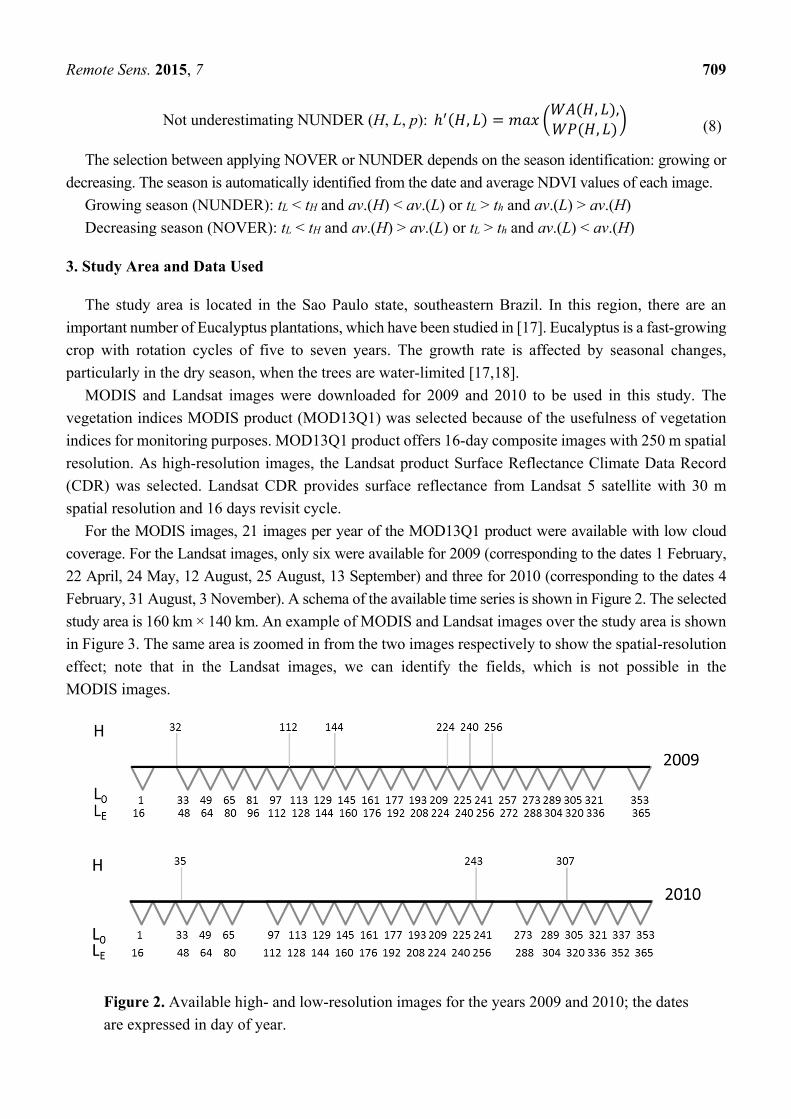
For the MODIS images, 21 images per year of the MOD13Q1 product were available with low cloud
coverage. For the Landsat images, only six were available for 2009 (corresponding to the dates 1 February,
22 April, 24 May, 12 August, 25 August, 13 September) and three for 2010 (corresponding to the dates 4
February, 31 August, 3 November). A schema of the available time series is shown in Figure 2. The selected
study area is 160 km × 140 km. An example of MODIS and Landsat images over the study area is shown
in Figure 3. The same area is zoomed in from the two images respectively to show the spatial-resolution
effect; note that in the Landsat images, we can identify the fields, which is not possible in the
MODIS images.
Figure 2. Available high- and low-resolution images for the years 2009 and 2010; the dates
are expressed in day of year.

Remote Sens. 2015, 7 710
(a) (b)
Figure 3. NDVI images of the study area: (a) Landsat (acquisition date on 22 April 2009)
and (b) MODIS image (composition period: 7 April 2009–22 April 2009). The images are
radiometrically normalized.
4. Methodology
4.1. Preparation of the Time Series
The first preprocessing step consisted of masking pixels with low quality information because of
clouds, shadows or other factors. Both products (MOD13Q1 and CDR) are provided with a quality band,
which was used to mask the poor-quality pixels in all images.
Afterwards, to assure the spectral comparability of the images, a normalization procedure was
applied. In this case, the Landsat time series was normalized to the MODIS one using the method
described in [17]. The normalization method requires that the high-spatial-resolution image is first
degraded to the low-spatial-resolution of the MODIS image in order to compute a linear regression
between the co-referent pixels of both images, i.e., pixels covering the same area. The degradation was
performed using the pixel aggregate method of ENVI software (Exelis Visual Information Solutions,
Boulder, CO, USA): this method averages all values of the pixels in the Landsat image which cover a
subpart of the area of a MODIS pixel by taking into account their distinct contributions to the area. The
NDVI

Remote Sens. 2015, 7 711
equation obtained from the linear regression adjustment between MODIS and Landsat-degraded pixels
is the normalization equation, and it relates the pixel radiances of Landsat to MODIS. Therefore, the
normalization equation is applied to the Landsat image at its original spatial resolution. The
normalization was applied to the red and NIR bands of the Landsat and MOD13Q1 images, and the
NDVI was computed from the normalized bands. Successively, the MODIS images were rescaled to the
Landsat spatial resolution using a bilinear interpolation method, thus yielding the MODIS and Landsat
pixels with the same size. Finally, a subset (Figure 3) was extracted for both time series.
4.2. Fusion Methods
4.2.1. Fusion Methods Based on Temporal Validity
The methods described in section two (WA and WP including NOVER/UNDER) were applied to the
available NDVI time series. These methods can be applied with different parameterizations by changing
the combination of input images and the temporal range (tx) in both cases (WA and WP) and by changing
the preference (p) in the WP. Preference values greater than 1 will give a larger effect of the input H
image on the fused image. Therefore, two experiments were carried on to analyze the effect of the
parameters and the combination of input images.
In the first experiment, the temporal range was fixed at tx = 50, whereas several values of p were
examined. Additionally, different combinations of input images were used for each target date.
In the second experiment, a unique combination of input images per target date was used, and the
preference value was also set to a fixed value (the input images and preference value that were identified
in the previous experiment as leading to the best results). In this case, the temporal range was changed
with tx values varying in 5–200.
These two experiments were performed on the 2009 time series to simulate H images at the dates
when we had a Landsat image: 112 (22 April), 144 (25 May), 224 (12 August), 240 (28 August) and 256
(13 September). The existing Landsat image, which was not used in the fusion method, was used for
validation. These experiments allowed us to choose the best combination of input images, the best
parameter values and the best method. Landsat image 1 January 2009 (32) was not used in experiments
1 and 2 because the MODIS image with timestamp at this date was lacking; therefore, the normalization
of the Landsat image was not possible. However, the Landsat image (32) was normalized using the next
MODIS image and used in the evaluation at the local scale.
Afterwards, the best method was used to fuse all lacking images over the entire time series
(2009–2010). A complete enriched time series was built using the true Landsat images on the dates when
they were available and completed with the fused images.
4.2.2. ESTARFM
The ESTARFM method uses two pairs of input images, H and L, which are taken on the same date
and one L on the target date. The L images are downscaled to the high spatial resolution. Then, the two
pairs of images are independently used to identify similar pixels in a predefined window. Afterwards, a
conversion coefficient is obtained between the H and L images from the two pairs of images. The
conversion coefficient corresponds to the gain obtained using regression analysis of the previously
Remote Sens. 2015, 7 712
identified similar pixels. Then, a reflectance value is obtained from each pair of input images and the L
image at the target date. Finally, a weighted average is applied by considering three factors: the spectral
differences between H and L images on the same date, the temporal differences between the two L images
and the spatial distance between similar pixels in the moving window and its central pixel.
The default ESTARFM parameters were used (window size of 51 and 4 classes). The requirement of
two pairs of input images limits the possible input combinations. Moreover, because the processing time
of this method is long, only one combination of input dates per target was tested. The method was used,
as the methods based on the weighted average, to obtain H images on the dates when we had a Landsat
image. In this case, the red and NIR band were fused, and the NDVI was subsequently calculated. The
validation results were compared to those obtained using the WA and WP methods.
Then, the H time-series 2009–2010 was enriched by simulating the lacking images.
4.3. Validation Analysis
Different fusion methods were compared in terms of the quality of the fused images based on the
validation results at global and local scales and in terms of ease of applicability and processing time.
4.3.1. Validation at Global Scale
Since the objective of a fusion method is to simulate a target image at a given date, in order to perform
the validation it was necessary to generate fused images at target dates when we had available real
images, i.e., true images, acquired at the same dates and with the same spatial resolution of the fused
images. The quality of fusion methods is usually assessed on the basis of a pair-wise cross comparison
technique, in which the single values of the co-referent pixels in the fused image and in the true image
(a real image acquired at the same date of the fused one) are matched so as to allow the computation of
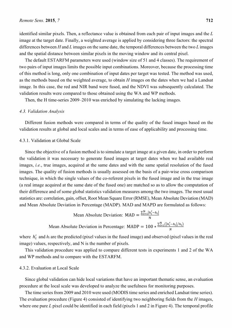
their difference and of some global statistics validation measures among the two images. The most usual
statistics are: correlation, gain, offset, Root Mean Square Error (RMSE), Mean Absolute Deviation (MAD)
and Mean Absolute Deviation in Percentage (MADP). MAD and MAPD are formulated as follows:
Mean Absolute Deviation: MAD∑
Mean Absolute Deviation in Percentage: MADP 100 ∗∑
where and hi are the predicted (pixel values in the fused image) and observed (pixel values in the real
image) values, respectively, and N is the number of pixels.
This validation procedure was applied to compare different tests in experiments 1 and 2 of the WA
and WP methods and to compare with the ESTARFM.
4.3.2. Evaluation at Local Scale
Since global validation can hide local variations that have an important thematic sense, an evaluation
procedure at the local scale was developed to analyze the usefulness for monitoring purposes.
The time series from 2009 and 2010 were used (MODIS time series and enriched Landsat time series).
The evaluation procedure (Figure 4) consisted of identifying two neighboring fields from the H images,
where one pure L pixel could be identified in each field (pixels 1 and 2 in Figure 4). The temporal profile
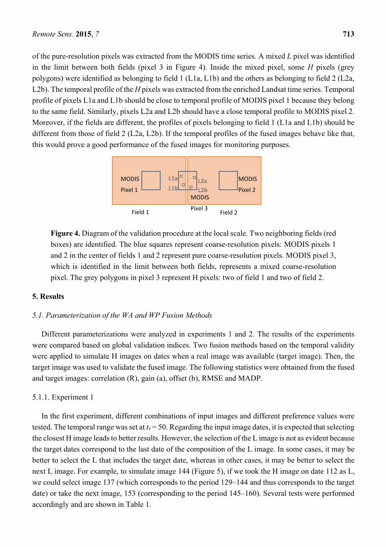
Remote Sens. 2015, 7 713
of the pure-resolution pixels was extracted from the MODIS time series. A mixed L pixel was identified
in the limit between both fields (pixel 3 in Figure 4). Inside the mixed pixel, some H pixels (grey
polygons) were identified as belonging to field 1 (L1a, L1b) and the others as belonging to field 2 (L2a,
L2b). The temporal profile of the H pixels was extracted from the enriched Landsat time series. Temporal
profile of pixels L1a and L1b should be close to temporal profile of MODIS pixel 1 because they belong
to the same field. Similarly, pixels L2a and L2b should have a close temporal profile to MODIS pixel 2.
Moreover, if the fields are different, the profiles of pixels belonging to field 1 (L1a and L1b) should be
different from those of field 2 (L2a, L2b). If the temporal profiles of the fused images behave like that,
this would prove a good performance of the fused images for monitoring purposes.
Figure 4. Diagram of the validation procedure at the local scale. Two neighboring fields (red
boxes) are identified. The blue squares represent coarse-resolution pixels: MODIS pixels 1
and 2 in the center of fields 1 and 2 represent pure coarse-resolution pixels. MODIS pixel 3,
which is identified in the limit between both fields, represents a mixed coarse-resolution
pixel. The grey polygons in pixel 3 represent H pixels: two of field 1 and two of field 2.
5. Results
5.1. Parameterization of the WA and WP Fusion Methods
Different parameterizations were analyzed in experiments 1 and 2. The results of the experiments
were compared based on global validation indices. Two fusion methods based on the temporal validity
were applied to simulate H images on dates when a real image was available (target image). Then, the
target image was used to validate the fused image. The following statistics were obtained from the fused
and target images: correlation (R), gain (a), offset (b), RMSE and MADP.
5.1.1. Experiment 1
In the first experiment, different combinations of input images and different preference values were
tested. The temporal range was set at tx = 50. Regarding the input image dates, it is expected that selecting
the closest H image leads to better results. However, the selection of the L image is not as evident because
the target dates correspond to the last date of the composition of the L image. In some cases, it may be
better to select the L that includes the target date, whereas in other cases, it may be better to select the
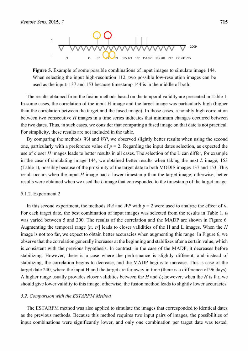
next L image. For example, to simulate image 144 (Figure 5), if we took the H image on date 112 as L,
we could select image 137 (which corresponds to the period 129–144 and thus corresponds to the target
date) or take the next image, 153 (corresponding to the period 145–160). Several tests were performed
accordingly and are shown in Table 1.
MODIS
Pixel 1 MODIS
Pixel 3
MODIS
Pixel 2
Field 1 Field 2
L1a L1b L2b
L2a

Remote Sens. 2015, 7 714
Table 1. Results of the validation of the WA and WP fusion methods for six target images using different input images and preferences for
2009. The image dates are expressed as day of year (DoY). The following statistics where obtained from the fused and target images: correlation
(R), gain (a), offset (b), RMSE and MADP. The results that correspond to the best combination of input images and the best method are marked
in bold.
Target 112 144 224 240 256
H 32 32 144 32 32 112 112 224 240 256 144 144 256 144 144 144 144 224 224
L 97–112 113–128 97–112 129–255 145–160 129–144 145–160 129–144 129–144 129–144 209–224 225–240 209–224 225–240 241–256 241–256 257–272 241–256 257–272
Dist(t-th) 80 80 −32 112 112 32 32 −80 −96 −112 80 80 −32 96 96 112 112 32 32
Dist(t-tLmin) 15 −1 15 15 −1 15 −1 15 15 15 15 −1 15 15 −1 15 −1 15 −1
R (H,Target) 0.63 0.63 0.79 0.59 0.59 0.79 0.79 0.64 0.62 0.58 0.64 0.64 0.84 0.62 0.62 0.58 0.58 0.84 0.84
R(L,Target) 0.75 0.76 0.75 0.75 0.78 0.75 0.77 0.75 0.75 0.75 0.78 0.79 0.78 0.78 0.79 0.77 0.73 0.77 0.73
WA
R(H’,Target) 0.79 0.80 0.86 0.78 0.80 0.84 0.87 0.80 0.80 0.79 0.82 0.83 0.88 0.81 0.83 0.79 0.78 0.86 0.87
a 0.66 0.68 0.82 0.59 0.63 0.70 0.74 0.66 0.67 0.63 0.72 0.73 0.79 0.74 0.74 0.68 0.66 0.80 0.78
b 0.26 0.23 0.12 0.31 0.27 0.23 0.19 0.21 0.20 0.24 0.19 0.19 0.13 0.19 0.20 0.22 0.25 0.13 0.15
RMSE 0.08 0.07 0.06 0.09 0.08 0.08 0.07 0.08 0.08 0.08 0.08 0.08 0.07 0.09 0.09 0.09 0.10 0.07 0.07
MAPD 8.84 8.65 7.41 11.37 10.43 9.45 8.50 10.33 10.54 10.87 12.66 12.27 9.70 13.41 13.63 13.16 14.73 9.97 10.37
WP, p = 1.5
R( H’,Target) 0.79 0.80 0.86 0.78 0.81 0.84 0.87 0.80 0.79 0.78 0.81 0.82 0.89 0.81 0.82 0.79 0.78 0.86 0.87
a 0.66 0.68 0.82 0.58 0.63 0.70 0.74 0.66 0.67 0.63 0.72 0.72 0.79 0.73 0.73 0.68 0.66 0.80 0.79
b 0.26 0.23 0.12 0.31 0.27 0.23 0.19 0.20 0.20 0.23 0.20 0.19 0.13 0.19 0.20 0.22 0.25 0.13 0.15
RMSE 0.08 0.07 0.06 0.09 0.08 0.08 0.07 0.08 0.08 0.09 0.09 0.08 0.07 0.09 0.09 0.09 0.09 0.07 0.07
MAPD 8.80 8.65 7.38 11.34 10.43 9.41 8.47 10.39 10.65 11.00 12.75 12.38 9.58 13.48 13.66 13.17 14.59 9.86 10.18
WP, p = 2
R( H’,Target) 0.79 0.80 0.86 0.78 0.81 0.84 0.87 0.80 0.79 0.78 0.81 0.82 0.89 0.81 0.82 0.79 0.78 0.86 0.87
a 0.66 0.67 0.82 0.58 0.62 0.70 0.74 0.67 0.67 0.63 0.71 0.71 0.79 0.73 0.73 0.68 0.66 0.80 0.79
b 0.26 0.23 0.12 0.31 0.27 0.23 0.19 0.20 0.19 0.23 0.20 0.19 0.13 0.19 0.20 0.22 0.24 0.12 0.14
RMSE 0.08 0.07 0.06 0.09 0.08 0.08 0.07 0.08 0.09 0.09 0.09 0.08 0.07 0.09 0.09 0.09 0.09 0.07 0.07
MAPD 8.79 8.65 7.36 11.33 10.43 9.40 8.45 10.43 10.73 11.09 12.79 12.44 9.53 13.51 13.67 13.16 14.51 9.81 10.08
Remote Sens. 2015, 7 715
Figure 5. Example of some possible combinations of input images to simulate image 144.
When selecting the input high-resolution 112, two possible low-resolution images can be
used as the input: 137 and 153 because timestamp 144 is in the middle of both.
The results obtained from the fusion methods based on the temporal validity are presented in Table 1.
In some cases, the correlation of the input H image and the target image was particularly high (higher
than the correlation between the target and the fused image). In those cases, a notably high correlation
between two consecutive H images in a time series indicates that minimum changes occurred between
the two dates. Thus, in such cases, we consider that computing a fused image on that date is not practical.
For simplicity, these results are not included in the table.
By comparing the methods WA and WP, we observed slightly better results when using the second
one, particularly with a preference value of p = 2. Regarding the input dates selection, as expected the
use of closer H images leads to better results in all cases. The selection of the L can differ, for example
in the case of simulating image 144, we obtained better results when taking the next L image, 153
(Table 1), possibly because of the proximity of the target date to both MODIS images 137 and 153. This
result occurs when the input H image had a lower timestamp than the target image; otherwise, better
results were obtained when we used the L image that corresponded to the timestamp of the target image.
5.1.2. Experiment 2
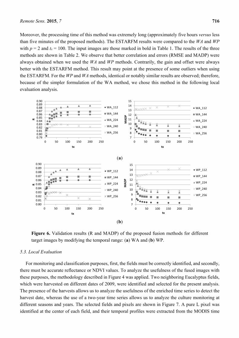
In this second experiment, the methods WA and WP with p = 2 were used to analyze the effect of tx.
For each target date, the best combination of input images was selected from the results in Table 1. tx
was varied between 5 and 200. The results of the correlation and the MADP are shown in Figure 6.
Augmenting the temporal range [t0, tE] leads to closer validities of the H and L images. When the H
image is not too far, we expect to obtain better accuracies when augmenting this range. In Figure 6, we
observe that the correlation generally increases at the beginning and stabilizes after a certain value, which
is consistent with the previous hypothesis. In contrast, in the case of the MADP, it decreases before
stabilizing. However, there is a case where the performance is slightly different, and instead of
stabilizing, the correlation begins to decrease, and the MADP begins to increase. This is case of the
target date 240, where the input H and the target are far away in time (there is a difference of 96 days).
A higher range usually provides closer validities between the H and L; however, when the H is far, we
should give lower validity to this image; otherwise, the fusion method leads to slightly lower accuracies.
5.2. Comparison with the ESTARFM Method
The ESTARFM method was also applied to simulate the images that corresponded to identical dates
as the previous methods. Because this method requires two input pairs of images, the possibilities of
input combinations were significantly lower, and only one combination per target date was tested.
9 41 57 73 89 105 121 137 153 169 185 201 217 233 249 265
H
L
2009
Remote Sens. 2015, 7 716
Moreover, the processing time of this method was extremely long (approximately five hours versus less
than five minutes of the proposed methods). The ESTARFM results were compared to the WA and WP
with p = 2 and tx = 100. The input images are those marked in bold in Table 1. The results of the three
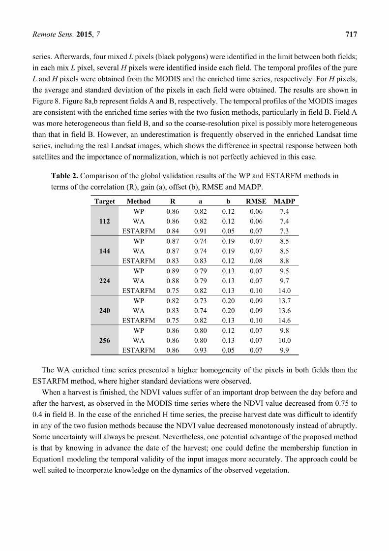
methods are shown in Table 2. We observe that better correlation and errors (RMSE and MADP) were
always obtained when we used the WA and WP methods. Contrarily, the gain and offset were always
better with the ESTARFM method. This result may point at the presence of some outliers when using
the ESTARFM. For the WP and WA methods, identical or notably similar results are observed; therefore,
because of the simpler formulation of the WA method, we chose this method in the following local
evaluation analysis.
(a)
(b)
Figure 6. Validation results (R and MADP) of the proposed fusion methods for different
target images by modifying the temporal range: (a) WA and (b) WP.
5.3. Local Evaluation
For monitoring and classification purposes, first, the fields must be correctly identified, and secondly,
there must be accurate reflectance or NDVI values. To analyze the usefulness of the fused images with
these purposes, the methodology described in Figure 4 was applied. Two neighboring Eucalyptus fields,
which were harvested on different dates of 2009, were identified and selected for the present analysis.
The presence of the harvests allows us to analyze the usefulness of the enriched time series to detect the
harvest date, whereas the use of a two-year time series allows us to analyze the culture monitoring at
different seasons and years. The selected fields and pixels are shown in Figure 7. A pure L pixel was
identified at the center of each field, and their temporal profiles were extracted from the MODIS time
0.790.800.810.820.830.840.850.860.870.880.890.90
0 50 100 150 200 250
R
tx
WA_112
WA_144
WA_224
WA_240
WA_256
7
8
9
10
11
12
13
14
15
0 50 100 150 200 250
MADP
tx
WA_112
WA_144
WA_224
WA_240
WA_256
0.80
0.81
0.82
0.83
0.84
0.85
0.86
0.87
0.88
0.89
0.90
0 50 100 150 200 250
R
tx
WP_112
WP_144
WP_224
WP_240
WP_256
7
8
9
10
11
12
13
14
15
0 50 100 150 200 250
MADP
tx
WP_112
WP_144
WP_224
WP_240
WP_256
Remote Sens. 2015, 7 717
series. Afterwards, four mixed L pixels (black polygons) were identified in the limit between both fields;
in each mix L pixel, several H pixels were identified inside each field. The temporal profiles of the pure
L and H pixels were obtained from the MODIS and the enriched time series, respectively. For H pixels,
the average and standard deviation of the pixels in each field were obtained. The results are shown in
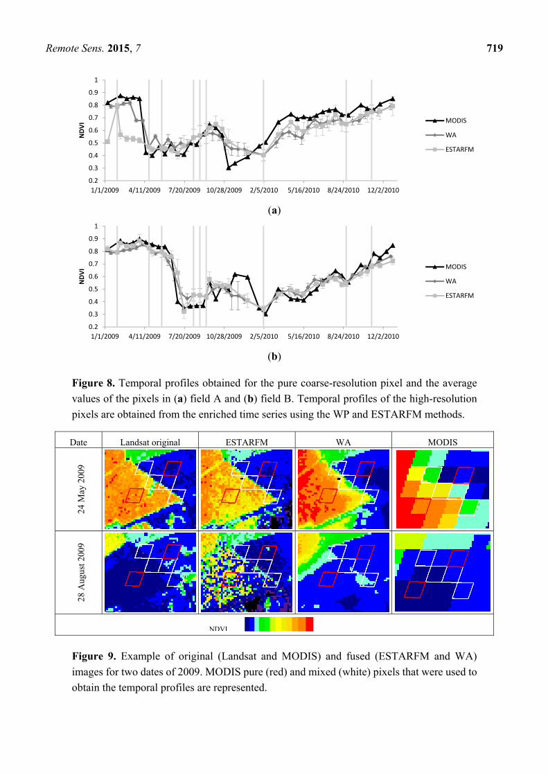
Figure 8. Figure 8a,b represent fields A and B, respectively. The temporal profiles of the MODIS images
are consistent with the enriched time series with the two fusion methods, particularly in field B. Field A
was more heterogeneous than field B, and so the coarse-resolution pixel is possibly more heterogeneous
than that in field B. However, an underestimation is frequently observed in the enriched Landsat time
series, including the real Landsat images, which shows the difference in spectral response between both
satellites and the importance of normalization, which is not perfectly achieved in this case.
Table 2. Comparison of the global validation results of the WP and ESTARFM methods in
terms of the correlation (R), gain (a), offset (b), RMSE and MADP.
Target Method R a b RMSE MADP
112 WP 0.86 0.82 0.12 0.06 7.4 WA 0.86 0.82 0.12 0.06 7.4
ESTARFM 0.84 0.91 0.05 0.07 7.3
144 WP 0.87 0.74 0.19 0.07 8.5 WA 0.87 0.74 0.19 0.07 8.5
ESTARFM 0.83 0.83 0.12 0.08 8.8
224 WP 0.89 0.79 0.13 0.07 9.5 WA 0.88 0.79 0.13 0.07 9.7
ESTARFM 0.75 0.82 0.13 0.10 14.0
240 WP 0.82 0.73 0.20 0.09 13.7 WA 0.83 0.74 0.20 0.09 13.6
ESTARFM 0.75 0.82 0.13 0.10 14.6
256 WP 0.86 0.80 0.12 0.07 9.8 WA 0.86 0.80 0.13 0.07 10.0
ESTARFM 0.86 0.93 0.05 0.07 9.9
The WA enriched time series presented a higher homogeneity of the pixels in both fields than the
ESTARFM method, where higher standard deviations were observed.
When a harvest is finished, the NDVI values suffer of an important drop between the day before and
after the harvest, as observed in the MODIS time series where the NDVI value decreased from 0.75 to
0.4 in field B. In the case of the enriched H time series, the precise harvest date was difficult to identify
in any of the two fusion methods because the NDVI value decreased monotonously instead of abruptly.
Some uncertainty will always be present. Nevertheless, one potential advantage of the proposed method
is that by knowing in advance the date of the harvest; one could define the membership function in
Equation1 modeling the temporal validity of the input images more accurately. The approach could be
well suited to incorporate knowledge on the dynamics of the observed vegetation.
Remote Sens. 2015, 7 718
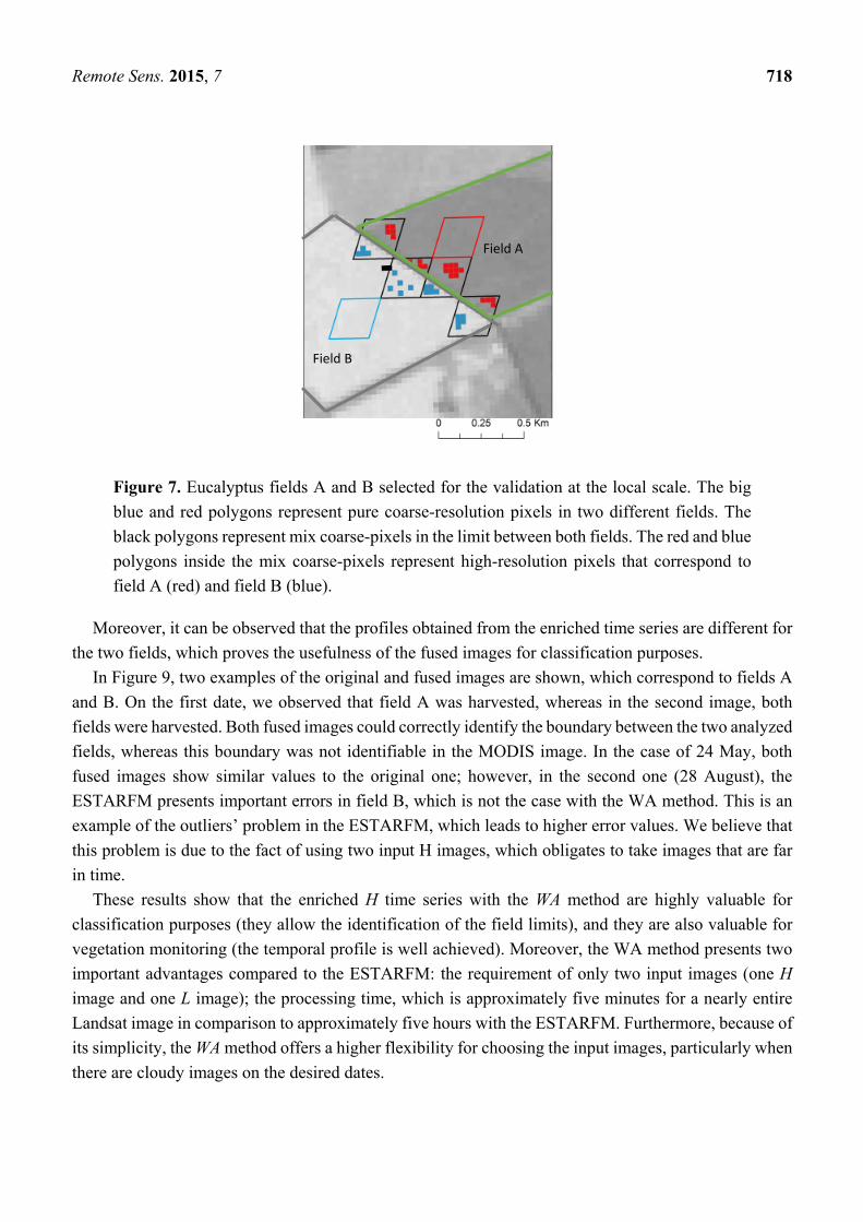
Figure 7. Eucalyptus fields A and B selected for the validation at the local scale. The big
blue and red polygons represent pure coarse-resolution pixels in two different fields. The
black polygons represent mix coarse-pixels in the limit between both fields. The red and blue
polygons inside the mix coarse-pixels represent high-resolution pixels that correspond to
field A (red) and field B (blue).
Moreover, it can be observed that the profiles obtained from the enriched time series are different for
the two fields, which proves the usefulness of the fused images for classification purposes.
In Figure 9, two examples of the original and fused images are shown, which correspond to fields A
and B. On the first date, we observed that field A was harvested, whereas in the second image, both
fields were harvested. Both fused images could correctly identify the boundary between the two analyzed
fields, whereas this boundary was not identifiable in the MODIS image. In the case of 24 May, both
fused images show similar values to the original one; however, in the second one (28 August), the
ESTARFM presents important errors in field B, which is not the case with the WA method. This is an
example of the outliers’ problem in the ESTARFM, which leads to higher error values. We believe that
this problem is due to the fact of using two input H images, which obligates to take images that are far
in time.
These results show that the enriched H time series with the WA method are highly valuable for
classification purposes (they allow the identification of the field limits), and they are also valuable for
vegetation monitoring (the temporal profile is well achieved). Moreover, the WA method presents two
important advantages compared to the ESTARFM: the requirement of only two input images (one H
image and one L image); the processing time, which is approximately five minutes for a nearly entire
Landsat image in comparison to approximately five hours with the ESTARFM. Furthermore, because of
its simplicity, the WA method offers a higher flexibility for choosing the input images, particularly when
there are cloudy images on the desired dates.
Field B
Field A
Remote Sens. 2015, 7 719
(a)
(b)
Figure 8. Temporal profiles obtained for the pure coarse-resolution pixel and the average
values of the pixels in (a) field A and (b) field B. Temporal profiles of the high-resolution
pixels are obtained from the enriched time series using the WP and ESTARFM methods.
Date Landsat original ESTARFM WA MODIS
24 M
ay 2
009
28 A
ugus
t 200
9
Figure 9. Example of original (Landsat and MODIS) and fused (ESTARFM and WA)
images for two dates of 2009. MODIS pure (red) and mixed (white) pixels that were used to
obtain the temporal profiles are represented.
0.2
0.3
0.4
0.5
0.6
0.7
0.8
0.9
1
1/1/2009 4/11/2009 7/20/2009 10/28/2009 2/5/2010 5/16/2010 8/24/2010 12/2/2010
NDVI MODIS
WA
ESTARFM
0.2
0.3
0.4
0.5
0.6
0.7
0.8
0.9
1
1/1/2009 4/11/2009 7/20/2009 10/28/2009 2/5/2010 5/16/2010 8/24/2010 12/2/2010
NDVI MODIS
WA
ESTARFM
NDVI
Remote Sens. 2015, 7 720
In the case of study, the H images were simulated using the closest Landsat image as the
high-resolution input; however, when this image is taken after the target date, the identification of
harvests will be difficult. Using an input Landsat image before the target date will minimize this problem;
however, if the input and target dates are far away, the global results will worsen. This result should be
considered when selecting the input images depending on the objectives of the study.
6. Discussion
Fusion methods are very useful for completing time series of high-resolution images. Several methods
already exist but are complicated and time consuming. We have presented here a simple and fast fusion
method; simple because it only needs two input images and a simple formulation that makes it a fast
method. Its main characteristics is the ability to model the heuristic knowledge of the crop modeling
dynamics by defining a time validity degree for each input image at a target date when one wants to
generate a fused image. The time validity is obtained in a temporal range that is user-selected. Although
in this case we have performed a test for selecting the temporal range, this approach may be suitable for
classified images in order to obtained enriched time series where the crop stages can be monitored. In
this case an expert could define the time validity of each pixel in the image depending on the crop type
present in the area. Further work will be performed to analyze the usefulness of the enriched time series
for crop-monitoring purposes such as crop stage identification, on the line of the initial experiments done
by the authors in [19].
Moreover the method has certain limitations. The major limitation may be the need of a normalization
procedure between the high- and low-resolution images being used. This procedure is needed because
the spectral bands of both satellites may differ, also the atmospheric correction performed to the images
from both satellites could be different and have an influence in the reflectivities captured by them. In
order to correct these perturbations, we have applied here a simple normalization procedure, which
relates the spectral reflectivities (in the red and NIR bands) of the Landsat images to the MODIS ones
by linear regression; though we apply the normalization equation to the Landsat images to obtain
comparable reflectivities to MODIS. The evaluation at local scale has shown that there are still some
differences between the Landsat (normalized) and the MODIS reflectivities, so one perspective of this
work will be enhancing the normalization procedure and we expect this will enhance the results of the
fusion method. Moreover, although the ESTARFM does not require this normalization procedure, we
have checked that better results are obtained when the input images are normalized.
The comparison between ESTARFM and WA lead to similar results, lower errors were generally
obtained with WA, but visual inspection showed that in ESTARFM structures seemed better defined;
however there were important local errors using ESTARFM, probably due to the need of two high
resolution images as input, this force to use images that are far away in time. Because WA was applied
to fuse NDVI images and ESTARFM to fuse red and NIR bands, some tentative experiments have been
carried out to compare the WA method with ESTARFM method where both are directly applied to the
spectral bands as input pixel values. A validation on the 5 Landsat images of 2009 (see Table 3) lead to
similar results to those presented previously by applying the proposed fusion to the NDVI images, thus
providing promising results which deserve confirmation by consistent and thorough experiments.

Remote Sens. 2015, 7 721
A major problem when applying fusion methods is the perfect co-registration of the Landsat and
MODIS images, in this work we have paid attention to that problem, but only by visual inspection,
although the high correlation values obtained from the normalization equation makes us think that they
are well co-register. However we will consider in future works analyzing this problem in detail.
Also, in the future we intend to apply the WA method to other combinations of satellite images, and
also consider adapting the method to thermal bands.
Table 3. Comparison of the NDVI global validation results of the WA applied to NDVI
pixels and the WA applied to red and NIR in terms of the correlation (R), gain (a), offset (b),
RMSE and MADP.
Target Method R a b RMSE MADP
112 WA_NDVI 0.86 0.82 0.12 0.06 7.4 WA_reflect 0.86 0.82 0.12 0.06 7.4
144 WA_NDVI 0.87 0.74 0.19 0.07 8.5 WA_reflect 0.86 0.73 0.19 0.07 8.6
224 WA_NDVI 0.88 0.79 0.13 0.07 9.7 WA_reflect 0.89 0.80 0.12 0.07 9.5
240 WA_NDVI 0.83 0.74 0.20 0.09 13.6 WA_reflect 0.82 0.73 0.20 0.09 13.8
256 WA_NDVI 0.86 0.80 0.13 0.07 10.0 WA_reflect 0.86 0.80 0.13 0.07 10.0
7. Conclusions
The purpose of this paper was to refine a simple and fast fusion method. This method was designed
to fuse Landsat and MODIS images, although it can be applied to other pairs of high- and low-resolution
images. For this method, only two input images are required. The resulting fused image is based on the
weighted average (WA) of the two input images. The weight assigned to each image depends on its
temporal distance to the target date.
A global validation of the results (fused images) obtained by the simple fusion WA-method was
performed using five Landsat images acquired in 2009 over the Sao Paulo region of Brazil. The global
validation consists in computing statistical indices between NDVI estimated from target and fused
images. The validation results of our simple fusion method were compared to those obtained using a
more complex fusion method, the ESTARFM (Enhanced Spatio Temporal Fusion Method). The global
validation of the two fusion methods showed good performance, with higher correlations and lower
errors (RMSE and MADP) between the target image and the fused image obtained using the proposed
WA-method. The RMSE varied between 0.07 and 0.1, and the MADP between 7% and 15% in terms of
NDVI. Global validation procedures can hide local errors due to disagreements between fused and
reference images. Therefore, in addition to the global validation, an evaluation at local scale was
performed using a two-year time series of Landsat and MODIS images. The evaluation at local scale
aimed to check the usefulness of the fused images for field delineation and vegetation monitoring. This
local evaluation was based on temporal profiles of NDVI. Good results were obtained by comparing
temporal profiles extracted from fused images with both methods to a reference temporal profile.
Remote Sens. 2015, 7 722
However, the WA method led to cleaner results with lower deviations and lower aberrant pixels. Local
evaluation is not usually analyzed when validating fusion methods. We have performed a simple
evaluation procedure, however this evaluation is limited and further work should be performed for
evaluating fusion methods at local scale.
The constraint of the WA method is that a normalization of the input images has to be performed
before applying the fusion in order to have radiometrically comparable high and low resolution images.
The normalization is not a necessary step in the ESTARFM method although we verified that better
results were also obtained when the input images were normalized. However, the evaluation at local
scale showed that the normalization procedure applied did not lead to perfect agreement between the
high and low resolution images. Though, further work will focus on normalization procedures, since an
enhancement of this step would enhance the results of the fusion methods.
To summarize the main achievements, the main advantage of the WA method is its ease of use (only
two input images are required), low processing time (less than 5 minutes), and good results.
Acknowledgments
This work was supported by public funds received in the framework of GEOSUD, a project
(ANR-10-EQPX-20) of the program “Investissements d’Avenir” managed by the French National
Research Agency, the Italian CNR short term mobility program, the Space4Agri project of CNR and
Regione Lombardia and the project CGL2013-46862-C2-1/2-P form the Spanish Ministry of Economy
and Competitiveness.
Author Contributions
Mar Bisquert and Gloria Bordogna defined and developed the method presented in the paper and
wrote the manuscript. Mar Bisquert was responsible for the data processing and application of the
methodology. Agnès Bégué, Maguelonne Teisseire, Pascal Poncelet and Gloria Bordogna revised the
analyses performed and the manuscript.
Conflicts of Interest
The authors declare no conflict of interest.
References
1. Le Maire, G.; Dupuy, S.; Nouvellon, Y.; Loos, R.A.; Hakamada, R. Mapping short-rotation
plantations at regional scale using MODIS time series: Case of eucalypt plantations in Brazil.
Remote Sens. Environ. 2014, 152, 136–149.
2. Meroni, M.; Rembold, F.; Verstraete, M.; Gommes, R.; Schucknecht, A.; Beye, G. Investigating
the relationship between the inter-annual variability of satellite-derived vegetation phenology and
a proxy of biomass production in the Sahel. Remote Sens. 2014, 6, 5868–5884.
3. Zhou, F.; Zhang, A.; Townley-Smith, L. A data mining approach for evaluation of optimal time-series
of MODIS data for land cover mapping at a regional level. ISPRS J. Photogramm. Remote Sens.
2013, 84, 114–129.
Remote Sens. 2015, 7 723
4. Atzberger, C. Advances in remote sensing of agriculture: Context description, existing operational
monitoring systems and major information needs. Remote Sens. 2013, 5, 949–981.
5. Clerici, N.; Weissteiner, C.J.; Gerard, F. Exploring the use of MODIS NDVI-based phenology
indicators for classifying forest general habitat categories. Remote Sens. 2012, 4, 1781–1803.
6. Han, Q.; Luo, G.; Li, C. Remote sensing-based quantification of spatial variation in canopy
phenology of four dominant tree species in Europe. J. Appl. Remote Sens. 2013, 7, 073485–073485.
7. Chuine, I.; Beaubien, E.G. Phenology is a major determinant of tree species range. Ecol. Lett. 2001,
4, 500–510.
8. Alley, R.B.; Marotzke, J.; Nordhaus, W.D.; Overpeck, J.T.; Peteet, D.M.; Pielke, R.A.;
Pierrehumbert, R.T.; Rhines, P.B.; Stocker, T.F.; Talley, L.D.; et al. Abrupt climate change. Science
2003, 299, 2005–2010.
9. Jandl, R.; Lindner, M.; Vesterdal, L.; Bauwens, B.; Baritz, R.; Hagedorn, F.; Johnson, D.W.;
Minkkinen, K.; Byrne, K.A. How strongly can forest management influence soil carbon
sequestration? Geoderma 2007, 137, 253–268.
10. Gao, F.; Masek, J.; Schwaller, M.; Hall, F. On the blending of the Landsat and MODIS surface
reflectance: Predicting daily Landsat surface reflectance. IEEE Trans. Geosci. Remote Sens. 2006,
44, 2207–2218.
11. Singh, D. Generation and evaluation of gross primary productivity using Landsat data through
blending with MODIS data. Int. J. Appl. Earth Obs. Geoinf. 2011, 13, 59–69.
12. Watts, J.D.; Powell, S.L.; Lawrence, R.L.; Hilker, T. Improved classification of conservation tillage
adoption using high temporal and synthetic satellite imagery. Remote Sens. Environ. 2011, 115,
66–75.
13. Bhandari, S.; Phinn, S.; Gill, T. Preparing Landsat Image Time Series (LITS) for monitoring
changes in vegetation phenology in Queensland, Australia. Remote Sens. 2012, 4, 1856–1886.
14. Zhu, X.; Chen, J.; Gao, F.; Chen, X.; Masek, J.G. An enhanced spatial and temporal adaptive
reflectance fusion model for complex heterogeneous regions. Remote Sens. Environ. 2010, 114,
2610–2623.
15. Emelyanova, I.V.; McVicar, T.R.; van Niel, T.G.; Li, L.T.; van Dijk, A.I.J.M. Assessing the
accuracy of blending Landsat-MODIS surface reflectances in two landscapes with contrasting
spatial and temporal dynamics: A framework for algorithm selection. Remote Sens. Environ. 2013,
133, 193–209.
16. Bisquert, M.; Bordogna, G.; Boschetti, M.; Poncelet, P.; Teisseire, M. Soft Fusion of heterogeneous
image time series. In Proceedings of the 15th International Conference on Information Processing and
Management of Uncertainty in Knowledge-Based Systems, Montpellier, France, 15–19 July 2014.
17. Le Maire, G.; Marsden, C.; Verhoef, W.; Ponzoni, F.J.; Lo Seen, D.; Bégué, A.; Stape, J.-L.;
Nouvellon, Y. Leaf area index estimation with MODIS reflectance time series and model inversion
during full rotations of Eucalyptus plantations. Remote Sens. Environ. 2011, 115, 586–599.
18. Almeida, A.C.; Soares, J.V.; Landsberg, J.J.; Rezende, G.D. Growth and water balance of Eucalyptus
grandis hybrid plantations in Brazil during a rotation for pulp production. For. Ecol. Manag. 2007,
251, 10–21.

Remote Sens. 2015, 7 724
19. Candiani, G.; Manfron, G.; Boschetti, M.; Busetto, L.; Nutini, F.; Crema, A.; Pepe, M; Bordogna, G.
Fusione di immagini telerilevate provenienti da dataset eterogenei: Ricostruzione di serie temporali
ad alta risoluzione spazio-temporale. In Proceedings of the 18th Conferenza Nazionale ASITA,
Firenze, Italy, 14–16 October 2014.
© 2015 by the authors; licensee MDPI, Basel, Switzerland. This article is an open access article
distributed under the terms and conditions of the Creative Commons Attribution license
(http://creativecommons.org/licenses/by/4.0/).